Isochrones and the dynamics of kicked oscillators

Physica A 155 (1989) X2-584

North-Holland, Amsterdam

ISOCHRONES AND THE DYNAMICS OF KICKED OSCILLATORS

A. CAMPBELL and A. GONZALEZ

Universidad Nucional de Mar de1 Plats, Facultad de Ciencias Exactaas, Funes 3350. (7600) Mar de1 Plats, Argentina

D.L. GONZALEZ* and 0. PIRO**

Universidad National de la Plats, Laboratorio de Fisica Tedrica, CC 67, (1900) La Plata. Argentina

H.A. LARRONDO

Univrrsidad National de Mar de1 Plata, Facultad de Ingenieria, Juan B. Just0 Y Pampa, (7600) Mar de1 Plata, Argentina

Received 16 March 1988

Revised manuscript received 8 July 1988

The interest in studying the isochrone portrait of relaxation oscillators with a stable limit

cycle is that knowledge of this portrait implies knowledge of the Phase Transition Curve

(PTC) and the PTC allows one to obtain, in the case of impulsive forces, a one-dimensional

approximation of the Poincark (stroboscopic) map of the system.

In this paper a simple and effective method for finding the isochrone portrait is shown. The

effectiveness of our method was tested in the reconstruction of an isochrone of the

BonhGffer-Van der Pol model, studied by A.T. Winfree.

Using the isochrone portrait and simple geometric arguments. important properties of the

PTC, such as its topological degree and the presence of cubic singularities, can be predicted

without calculation.

The method is applied to two models: Van der Pol and Brusellas. We also compute

explicitly the PTCs to show how the geometric analysis works.

The analysis is valid for a large class of impulsive forces.

1. Introduction

Non-linear oscillators driven by periodic forces appear in many problems of

physics and other sciences [l-lo]. Equilibrium oscillators, chemical reactions

*On leave of absence, present address: Riparto di Cinematografia Scientifica (C.N.R.),

University of Bologna, Via de1 Inferno 5, Bologna, Italy.

** On leave of absence, present address: Brookhaven National Laboratory, Physics Department. Building 5104, UPPOM, New York 11973, USA.

0378-4371 I89 /$03.50 0 Elsevier Science Publishers B .V.

(North-Holland Physics Publishing Division)

566 A. Campbell c’t al. 1 lsochrones und the dynamics of kicked osci1lator.v

periodically fed with reactants [l, 61, externally synchronized electronic oscil-

lators [7, lo], biological rythms [3,8,9], etc., are a few examples.

Very often the external perturbation consists of very short pulses and can be

approximated by a periodic delta function [3,6-171. In this case, the connec-

tion between the system of ordinary differential equations defining the appro-

priate model and maps on the circle becomes extremely clear.

Knowledge of the isochrone portrait is equivalent to knowledge of the

one-dimensional map associated with the oscillator.

The study of the isochrone portrait allows one to predict the forced

oscillator’s behaviour using simple geometric reasoning.

The organization of this paper is as follows:

In section 2 we give definitions of isochrones and PTCs and relations

between them. In section 3 numerical results are obtained for typical models:

Bonhoffer-Van der Pol, Van der Pol and Brusellas. Section 4 are the conclu-

sions. In the Appendix the numerical

portrait are described in some detail.

2. Isochrones and maps on the circle

methods used for finding the isochrone

Relaxation oscillators with exactly one attracting limit cycle are modelled (in

their autonomous regime) by a system of two first order, non-linear differential

equations,

i

dx,idt=j-,(x,.x2),

dx,idt = j;(x,, x2) , f,(o,o)=f~(o.o)=(),

where the fixed point is at the origin. For example the two models studied here

are:

a) Van der Pol (V),

dlxldt’ + /L(x’ - 1) dxldt + x = 0, @.>O.

whose equivalent system in the phase plane representation is

dx,ldt = x, . dx,ldt = -p(xf - 1)x, - x, >

b) Brusellas (B),

dxldt=a-(b+I)x+x’y,

dyldt = bx - A$.

(2)

(3)

(4)

A. Campbell et al. I Isochrones and the dynamics of kicked oscillators 561

which through a change in coordinates becomes

i

dx,ldt = a - (b + 1)(x, + a) + (x, + @(x2 + b/a),

dx,ldt = b(x, + a) - (x, + a)*(~, f b/a) (5)

The limit cycle, being a closed curve, can be parameterized like the unit circle

by one variable which we will call its phase (4). Thus, for points on the limit

cycle (C) we have the correspondence:

c-+&s’ )

(6)

(Xl> -4-f Q, = 4(x,, $13 # E P, 4,,,) *

The limit cycle’s domain of attraction is the whole phase space except for the

origin. We can therefore extend the correspondence (6) to

Iw* - (0,0)-t s’ )

(7)

(x,2 x2)+ 4 = Qr_m @H T~,(X,, x2)) 3 nEN,

where QT is the flow of the system at time T, T,, is the period of the autonomous

oscillator, and (x, , x2) is any point on the phase space.

Definition. An isophase curve is the preimage of 4, where 4 is an element of

s’.

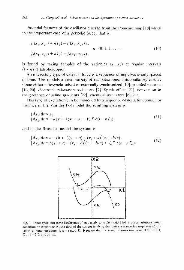
Each isophase meets the limit cycle exactly once, that is, a parametrization

of the limit cycle is equivalent to a numbering of isophases. As a curve in IR’

the limit cycle can be parameterized in various ways. In particular taking

4 “lRX = T, in (6) and + = t mod T,, in (7) the isophases are called isochrones

[8], due to the fact that in this case from an arbitrary initial condition the how

of the system tends to the limit cycle, meeting isophases at unit velocity (see

fig. 1).

When the oscillator is driven by a term purely dependent on time the system

of equations (1) becomes

dx,/dt=f,(x,,x?, t),

Wdt = f,(x,, ~2, t> , 03)

equivalent to the three-dimensional autonomous system

dx,/dt = f,(x,, x2,7> , dx,ldt = f&, , x2, 7) , dTldt = 1

(9)

568 A. Campbell et al. I Isochrones and the dynamics of kicked oscillators

Essential features of the oscillator emerge from the PoincarL map [IS] which

in the important case of a periodic force, that is:

f,(Xl~ x2. j+ nT,) =f1(x,, xj, t) 1 n=0,1,2,.. , (10)

f&l > X2? t + nT,) = f&x, > x2, t> ,

is found by taking samples of the variables (x,. x2) at regular intervals

(t = nT,) (stroboscopic).

An interesting type of external force is a sequence of impulses evenly spaced

in time. This models a great variety of real situations: autooscillatory cardiac

tissue either autosynchronised or externally synchronized [ 191, coupled neurons

[ 10,201, electronic relaxation oscillators [7], Spark effect [21], convection in

the presence of saline gradients [22], chemical oscillators [6], etc.

This type of excitation can be modelled by a sequence of delta functions. For

instance in the Van der Pol model the resulting system is

1

dx,ldt = x2 ,

dx,/dt = -/..~(x; - 1)x, - x, + V, C 6(r - nT,) ,

and in the Brusellas model the system is

(1’)

dx,ldt = a - (b + 1)(x, + a) + (x, + &x2 + b/a),

dx,/dr = h(x, + U) - (x, + u)‘(xz + b/u) + V, I: s(t - nT,) . (12)

Fig. 1. Limit cycle and some isochrones of an exactly solvable model [ 161. From an arbitrary initial

condition on isochrone A, the flow of the system tends to the limit cycle meeting isophases at unit velocity. Parametrization is 4 = t mod T,,. It means that the system crosses isochrone B at t = 114.

C at t = 112 and so on.


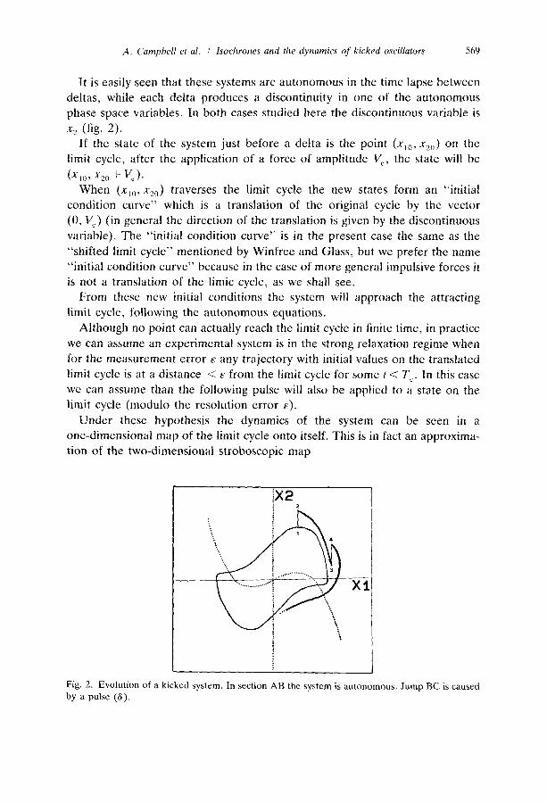
It is easily seen that these systems are autonomous in the time lapse between

deltas, while each delta produces a discontinuity in one of the autonomous

phase space variables. In both cases studied here the discontinuous variable is

x2 (fig. 2). If the state of the system just before a delta is the point (x,,,, x2,,) on the

limit cycle, after the application of a force of amplitude V,, the state will be

(x10, x20 + K). When (x,,), x2”) traverses the limit cycle the new states form an “initial

condition curve” which is a translation of the original cycle by the vector

(0, V,) (in general the direction of the translation is given by the discontinuous

variable). The “initial condition curve” is in the present case the same as the

“shifted limit cycle” mentioned by Winfree and Glass, but we prefer the name

“initial condition curve” because in the case of more general impulsive forces it

is not a translation of the limit cycle, as we shall see.

From these new initial conditions the system will approach the attracting

limit cycle, following the autonomous equations.

Although no point can actually reach the limit cycle in finite time, in practice

we can assume an experimental system is in the strong relaxation regime when

for the measurement error E any trajectory with initial values on the translated

limit cycle is at a distance < E from the limit cycle for some t < T,. In this case

we can assume than the following pulse will also be applied to a state on the

limit cycle (modulo the resolution error E).

Under these hypothesis the dynamics of the system can be seen in a

one-dimensional map of the limit cycle onto itself. This is in fact an approxima-

tion of the two-dimensional stroboscopic map

Fig. 2. Evolution of a kicked system. In section AB the system is autonomous. Jump BC is caused

by a pulse (6).

570 A. Campbell et rd. I Isochrotw und the dynamics of kicked oscillurors

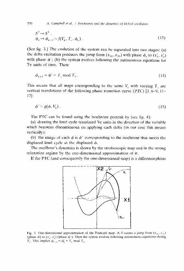
(See fig. 3.) The evolution of the system can be separated into two stages: (a)

the delta excitation produces the jump from (x,,), x,,) with phase 4,z to (xi, x;)

with phase 4’; (b) the system evolves following the autonomous equations for

Te units of time. Then:

4 ,!+, = 4’ + T, mod T,, . (14)

This means that all maps corresponding to the same V, with varying T, arc

vertical translations of the following phase transition curve (PTC) [3,6-9, ll-

171:

4’=g(AV,). (15)

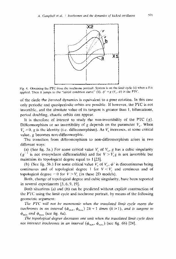
The PTC can be found using the isochrone portrait by (see fig. 4):

(a) drawing the limit cycle translated Ve units in the direction of the variable

which becomes discontinuous on applying each delta (in our case this means

vertically);

(b) the image of each 4 is 4’ corresponding to the isochrone that meets the

displaced limit cycle at the displaced 4.

The oscillator’s dynamics is shown by the stroboscopic map and in the strong

relaxation regime by the one-dimensional approximation of it.

If the PTC (and consequently the one-dimensional map) is a diffeomorphism

Fig. 3. One-dimensional approximation of the Poincari: map. A 6 causes a jump from (x,,,, x2,,)

(phase 4) to (x;. xi) (phase 4’). Then the system evolves following autonomous equations during

T,. This implies +,, , , = qb:, + T, mod ‘F,,.


Fig. 4. Obtaining the PTC from the isochrone portrait. System is on the limit cycle (a) when applied. Then it jumps to the “initial condition curve” (b). 4’ = R (V,, 4) is the PTC.

a 6 is

of the circle the iterated dynamics is equivalent to a pure rotation. In this case only periodic and quasiperiodic orbits are possible. If however, the PTC is not invertible, and the absolute value of its tangent is greater than 1, bifurcations, period doubling, chaotic orbits can appear.

It is therefore of interest to study the non-invertibility of the PTC (g). Diffeomorphism or no invertibility of g depends on the parameter V,. When V, = 0, g is the identity (i.e. diffeomorphism). As V, increases, at some critical value, g becomes non-diffeomorphic.

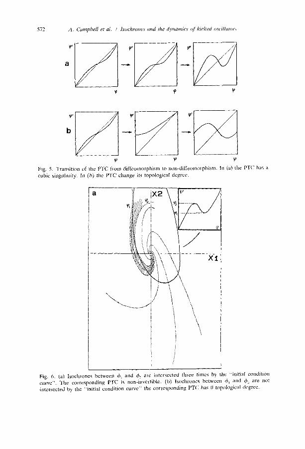
The transition from diffeomorphism to non-diffeomorphism arises in two different ways:

(a) (See fig. 5a.) For some critical value V, of V,, g has a cubic singularity (g-’ is not everywhere differentiable) and for V > V,g is not invertible but maintains its topological degree equal to 1 [23].

(b) (See fig. Sb.) For some critical value V, of V,, 4’ is discontinuous being continuous and of topological degree 1 for V <V, and continous and of topological degree = 0 for V > V, (in these 2D models).

Both, change of topological degree and cubic singularity, have been reported in several experiments [3,6,9, 191.

Both situations (a) and (b) can be predicted without explicit construction of the PTC using the limit cycle and isochrone portrait, by means of the following geometric argument:

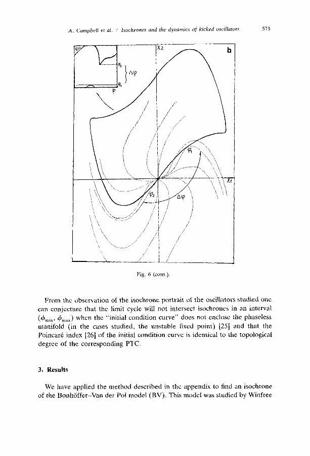
The PTC will not be monotonic when the translated limit cycle meets the

isochrones in an interval (&“, &,,,) 2k + 1 times (k 3 l), and is tangent to

4mi, and &,,,, (see fig. 64. The topological degree decreases one unit when the translated limit cycle does

not intersect isochrones in an interval (&,,in, &,,,,) (see fig. 6b) [24].

572 A. Campbell et al. I Isochrones and the dynamics of kicked oscillcrtor.~

Q P Q

Fig. 5. Transition of the PTC from diffeomorphism to non-diffeomorphism. In (a) the PTC has a

cubic singularity. In (b) the PTC change its topological degree.

Fig. 6. (a) Isochrones between 6, and & are intersected three times by the “initial condition

curve”. The corresponding PTC is non-invertible. (b) Isochrones between 4, and 4b, are not

intersected by the “initial condition curve ” the corresponding PTC has 0 topological degree.

A. Cumpbell et al. / Isochrones and the dynamics of kicked oscillators 573

L

\. . . ‘..,, ,: ..: ,.!

‘. ‘.

., “‘.. ..,,,,,,.... .” ,:’ ;: ,.:

,.; .:’ .:’

X, .:’ ; ,..’ /

Fig. 6 (cont.).

From the observation of the isochrone portrait of the oscillators studied one

can conjecture that the limit cycle will not intersect isochrones in an interval

(4minr &,,,,) when the “initial condition curve” does not enclose the phaseless

manifold (in the cases studied, the unstable fixed point) [25] and that the

PoincarC index [26] of the initial condition curve is identical to the topological

degree of the corresponding PTC.

3. Results

We have applied the method described in the appendix to find an isochrone

of the BonhGffer-Van der Pol model (BV). This model was studied by Winfree

574 A. Campbell et al. i Isochrones and the dynamics of‘ kicked oscilluiors

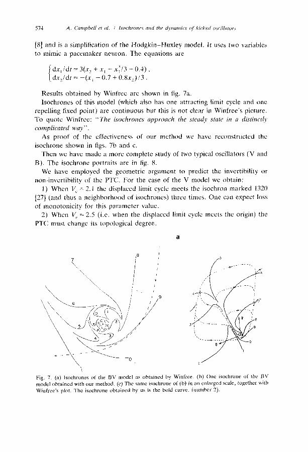
[8] and is a simplification of the Hodgkin-Huxley model. It uses two variables

to mimic a pacemaker neuron. The equations are

dx,idt = 3(x2 + x, - 413 - 0.4) ,

dx,ldt = -(x, - 0.7 + 0.8x,)/3.

Results obtained by Winfree are shown in fig. 7a.

Isochrones of this model (which also has one attracting limit cycle and one

repelling fixed point) are continuous but this is not clear in Winfree’s picture.

To quote Winfree: “The isochrones approach the steady state in a distinctly

complicated way”.

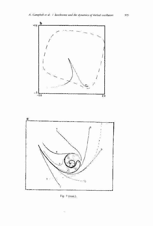
As proof of the effectiveness of our method we have reconstructed the

isochrone shown in figs. 7b and c.

Then we have made a more complete study of two typical oscillators (V and

B). The isochrone portraits are in fig. 8.

We have employed the geometric argument to predict the invertibility or

non-invertibility of the PTC. For the case of the V model we obtain:

1) When V, = 2.1 the displaced limit cycle meets the isochron marked 1320

[27] (and thus a neighborhood of isochrones) three times. One can expect loss

of monotonicity for this parameter value.

2) When V, = 2.5 (i.e. when the displaced limit cycle meets the origin) the

PTC must change its topological degree.

a

Fig. 7. (a) lsochrones of the BV model as obtained by Winfree. (b) One isochrone of the BV

model obtained with our method. (c) The same isochrone of (b) in an enlarged scale, together with

Winfree’s plot. The isochrone obtained by us is the bold curve. (number 2).

A. CampbeN ef al. I Isochrones and fhe dynamics of kicked oscillators 575

_.E

C

I

1

,

/

/

,

I

/

I 9 /

/ j:’

Fig. 7 (cont.).

576 A. Campbell et al. I Isochrones and the dynamics of kicked oscilluton

In fig. 9 the explicitly obtained PTCs are shown confirming these facts.

Repeating for the model we obtain similar results.

Other theoretical models recently studied [?I, 1517,261 show different be-

haviour: only the second transition is present (i.e. change of degree). It is

interesting that both are differential equations with analytical solution. This is

not our case.

The same method can be extended to more general external forces:

c f(x,, X,P(t - nT,) ? (1fd

modifying the “initial conditions curve” which now will be obtained by means

of the following transformation of the limit cycle:

For example we have also studied the parametric excitation

L

-2.i 12.5

Fig. 8. (a) lsochrone portrait of the Van der Pal oscillator with p = 2. (b) Isochrone portrait of the

Brusellas oscillator with a = 0.4 and h = 1.2.

A. Campbell et al. / lsochrones and the dynamics of kicked oscillators 577

Fig. 8 (cont.).

dx,idt = -I”(x~ - 1)x, - x, + Vex, C 8(t - nT,> . (1%

In this case the intersection of the isochrones with a deformed limit cycle

must be considered. As in the non-parametric case this curve is an “initial

condition curve” (after a delta is applied) and coordinates of points on it are

found by applying the following transformation to the original limit cycle:

(x1, XZ)++,‘X2 + vex,>

For any value of V, points of the limit cycle with x1 = 0 are also in the “initial

condition curve”. This fact prevents a change of topological degree of the PTC,

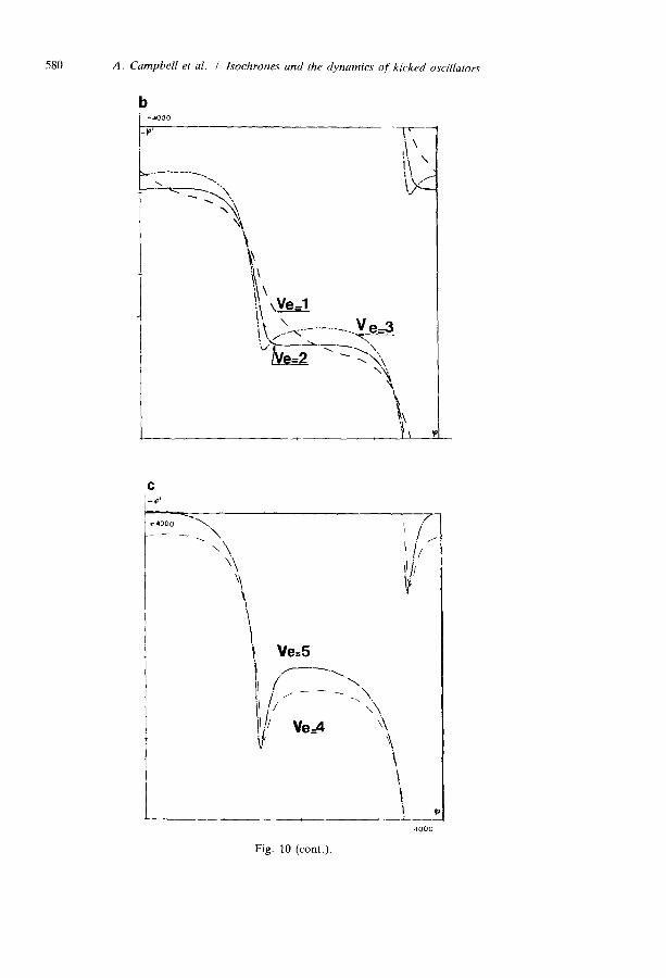
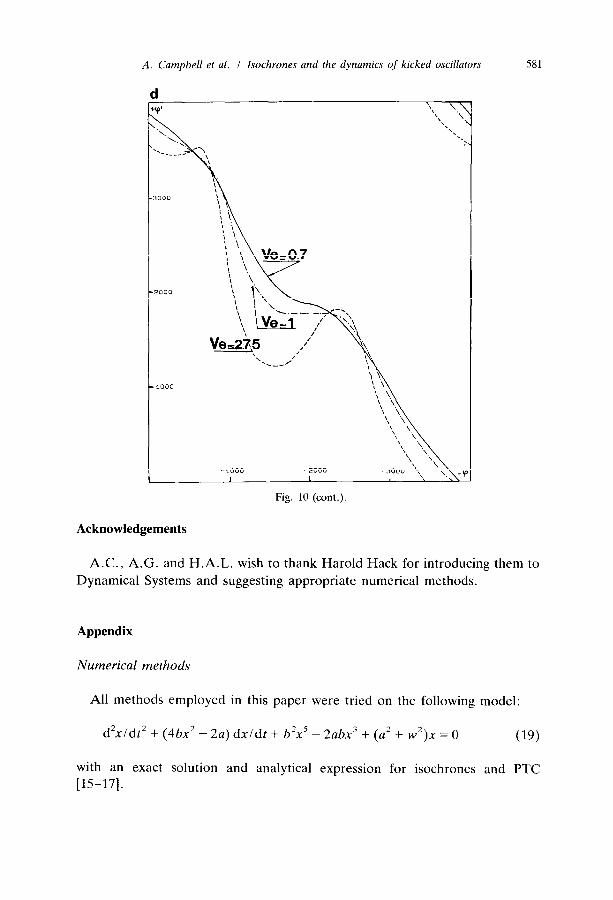
but cubic singularity transition is still possible. Applying the same geometrical

argument as in the non-parametric case we predict (see fig. 10) non-invertibility

of the PTC for V, > 2 in the V model.

578 A. Campbell et al. / Isochrones and the dynamics of kicked osci1lator.t

a I

b

Fig. 9. (a) PTC’s of the Van der Pal oscillator with p = 2. (b) PTC‘s of the Brusellas oscillator with rr=O.4 and b=J.Z.


4. Conclusions

The calculus of the isochrone portrait has fundamental advantages over

calculus of the PTC’s. In the first place, using the methods described in the

appendix, the time required for calculating the entire isochrone portrait is the

same as that required for obtaining one PTC. Secondly the isochrone portrait is

equivalent to knowledge of the PTCs for any value V, of the deltas (whether

these are of constant amplitude or modulated by f(x,, x,)). Using simple

geometric reasoning one can predict without calculation the presence of cubic

singularities and the degree of the PTC.

+a. 14

Fig. 10. (a) Isochrones and “initial condition curve” in the parametric case for Van der Pol oscillator with CL = 2 and Ve = 2. Note that “initial condition curve” passes through points A and B

which are on the limit cycle; then a change of topological degree is avoided. (b) and (c) PTC’s of

the Van der Pol oscillator (p = 2) for the parametric case. (d) PTC’s of the Brusellas oscillator

(a = 0.4, b = 1.2) for parametric excitation.

580 A. Campbell et al. I lsochrones and the dynamics of kicked oscillators

c

I

L

P’ .

-4300 .\ /

-- .\ ’ i

\\ ’ I,’

\ Ve=5

Y

‘1000

Fig. 10 (cont.).

A. Campbell et al. I Isochrones and the dynamics of kicked oscillators

7 \ 4

d +v

581

Fig. 10 (cont.).

Acknowledgements

A.C., A.G. and H.A.L. wish to thank Harold Hack for introducing them to

Dynamical Systems and suggesting appropriate numerical methods.

Appendix

Numerical methods

All methods employed in this paper were tried on the following

d2xldt’ + (46x2 - 2~) dxldt + b2x5 - 2abx3 + (a2 + w’)x = 0

with an exact solution and analytical expression for isochrones

[15-171.

model:

(19)

and PTC

582 A. Campbell et al. I lsochrones and the dynamics of kicked oscillators

a) Integration method

A fourth order Runge Kutta method was used. The choice was made based

on the results obtained for (19) and comparison with the analytical solution for

this model. Simpler methods (i.e. Euler) were not precise enough.

The equation is normalized so that for the integration step chosen (h =

0.001) the discrete limit cycle stored has 4000 points. This number of steps

parametrizes the limit cycle and is the variable we have called phase (i.e. this

phase is a number between 0 and 4000).

The integration step chosen (h = 0.001) gave 7 correct significant figures. A

smaller h does not significantly change the precision in results and means using

far more CPU.

b) Finding the limit cycle

From an arbitrary point in the phase space as the initial condition, the

differential equation is integrated for N,,,,, steps for sufficiently large N,,,,,.

After verifying that the solution is on the limit cycle (modulo machine zero) its

period T,, can be found (modulo the error of the integration method used).

Finally, starting from this final point, which is assumed to be on the limit cycle,

the states (x,, x2) are stored in a file after each integration step for the

duration of the period.

For the oscillator V an approximation of the period (TX) as a function of Al. is

known [29]. In this case we took N,,,,, = lOT:lh = 10 OOOTE.

For B we took 1000 000 9 N,,,,, % 500 000.

c) Finding the PTC’s

From an initial condition (x,(,, x2,,) on the limit cycle whose phase is $,,, a

perturbation (6) is applied, which takes the system to the state (x,,,, x2(, +

V,xf,), where k = 0 for constant amplitude and k = 1 for the parametric case.

From this state the autonomous differential equation (V or B) is integrated,

and after each step the new state of the system is compared with a fixed state

on the limit cycle chosen as a reference. If N is the number of steps needed in

order to reach this fixed state, &r is the phase of the reference point, and NC, is

the number of points of the limit cycle, then

g = const. - N mod N,, ,

where const. = 4reI - 4, and N, = 4000.

The values +,, and g(Ve, 4,) are stored in a file.

d) Finding the isophase curves

We found the following steps useful:


(1) The system of equations is normalized so that the limit cycle has period 4 and 4000 points using the change of variables

t* = 4tlP,

where P is the original period of the system. This means that only minor changes are needed in the program for different

relaxation oscillators. (2) The autonomous system of differential equations is integrated with

h = -0.001 from a very slightly modified state on the limit cycle which has phase 4 (this means we go back in time). The states after each m integration steps are stored in the corresponding isophases 4 - m, d, - 2m, . . . etc. The number m is selected as follows: let h be the integration step used for obtaining the limit cycle (in our case O.OOl), and let A’,, be the number of points of one period of the limit cycle (in our case 4000); then N,,lm is the number of isochrones equally spaced in phase that one want to obtain. We have used m = 20 and our isochrone’s portraits contain 200 isophases (we show only a few of them in the figures).

(3) Complementing (2) initial conditions on a grid in the phase plane are integrated (forward) and each mth integration step is stored in a matrix. The results are stored for half a period (2000 steps). Then integration is continued for sufficient periods in order to have reached the limit cycle (within an error E) at phase 4. For E we have used the criterion of coincidence of at least the first three significant figures.

The states (x,, y,) stored in the matrix are now stored in the isophases ++m, ++2m,... etc, where m is the same as above.

Method (3) (forward integration) has the disadvantage that there is no way of knowing beforehand if the initial conditions used correspond to one of the No/m chosen isophases. We have used this method mainly in order to complete isochrones in parts of the phase space where by method (2) we have obtained few points. The original grid covers a rectangle in this zone and is found by rule of thumb; then if necessary it is refined until sufficient points of the chosen isophases are obtained in order to continuously complete these isochrones.

With these methods it is possible to construct 200 isophases in approximately 6 hours of CPU using a HP 1000 computer.

References

[l] K. Tomita, Phys. Rep. 86 (1982) 115. [2] B.A. Huberman, Phys. Rep. 92 (1982) 45

584 A. CumpbelI el al. i Isochrones md the dynamics of kicked oscillators

[3] M.R. Guevara and L. Glass, J. Math. Biology 14 (1982) 1.

J.P. Keener and L. Glass. J. Math. Biology 21 (1984) 175.

[4] P.S. Linsay, Phys. Rev. Lett. 47 (1981) 1349.

[5] R.H.G. Helleman, Fundamental Problems in Statistical Mechanics, vol. 5, E.D.G. Cohen.

cd. (North-Holland, Amsterdam, 1980), p. 165.

(61 M. Dolnik, I. Schreiber and M. Marek. Phys. Lett. A 100 (1984) 316.

(71 M. Van Exter and A. Lagendijk, Phys. Lett. A 99 (1983) I.

[8] A.T. Winfree, The Geometry of Biological Time (Springer Berlin, 1980).

[9] L. Glass, M.R. Guevara. J. Belair and A. Shrier, Phys. Rev. A 29 (1984) 1348.

[lo] T. Allen, Physica D 6 (19X3) 305.

[II] L. Glass and R. Perez, Phys. Rev. Lett. 48 (lY82) 1772.

[12] R. Perez and L. Glass, Phys. Lett. A 90 (1982) 441.

[13] J. Belair and L. Glass, Phys. Lett. A 96 (1984) 117.

[14] Z.A. Slavsky, Phys. Lett. A 69 (1978) 145.

1151 D.L. Gonzalez and 0. Piro, Phys. Lett. A 101 (1984) 455.

[16] D.L. Gonzalez and 0. Piro, Phys. Rev. Lctt. SO (1983) 870.

(171 D.L. Gonzalez and 0. Piro. Phys. Rev. A 30 (1984) 2788.

[ 181 J. Guckenheimcr and P. Holmes, Nonlinear Oscillators, Dynamical Systems and Bifurcations

of Vector Fields (Springer, Berlin, 1983).

[19] M.R. Guevara, L. Glass and A. Shrier, Science 214 (1981) 1350.

(201 A. T. Winfree, Science lY7 (1977) 761.

[21] B.R. Hardas and S.Scheeline, Anal. Chem. 56 (1984) 169.

[22] E. Knobloch and N.O. Weiss, Phys. Lett. A 85 (lY81) 127.

[23] Let f : S’ - S’ be differentiable. _v is a regular value off if no x in the preimage of y has its

derivative equal to zero. The topological degree of f at a regular value y is deg(f, y) =

C sgn (df(x) idx) for all x such that f(x) = y where sgn is the sign function. It is known that

deg( f, y) is independent of y. If f is a diffcomorphism its topological degree is 1 or - 1; the

converse is not true in general. (See: J.W. Milnor, Topology from the Differentiable

Viewpoint (Univ. Press of Virginia, Charlottesville, 1965).)

1241 The change of topological degree is one of the central ideas in Winfree’s book [8]. Other

important papers arc:

M. Kawato and R. Suzuki, Biol. Cyb. 30 (1978) 241. L. Glass and A.T. Winfree, Am. J. Physiol (1984).

J. Guckenhcimer. J. Math. Biol. 1 (1975) 259. 1251 A.T. Winfrec, in: Lecture Notes in Mathematics, vol. 17 (Am. Math. Sot., Providence, RI.

1979).

[26] Given a planar flow as in (1) and C a simple closed curve not passing through any equilibrium

points we consider the orientation of the vector field at the point p = (x,, x~) E C. Letting ,LI

traverse C counterclockwise the vector (f;(~, y). fi(x, y)) rotates continuously and upon

returning to the original position has rotated through an angle 2kn for some integer k. We call

k the index of the closed curve C (see also ref. [18]).

1271 lsochrones are numbered from 0 to 4000. See appendix.

[28] E.J. Ding, Phys. Rev. A 35 (1987) 2669. [2Y] E. Roxin and V. Spinadel, Ecuaciones Diferenciales Ordinarias (Eudeba, Argentina. 1976).

p. 307.

Isochrones and the dynamics of kicked oscillators

Documents