GHENT UNIVERSITY FACULTY OF ECONOMICS AND BUSINESS ADMINISTRATION ACADEMIC YEAR 2015 – 2016 Is the stock-bond return correlation in the BRIC countries affected by their economic expansion? Master’s Dissertation submitted to obtain the degree of Master of Science in Business Engineering Eron Durnez Under the guidance of Prof. Koen Inghelbrecht

Welcome message from author
This document is posted to help you gain knowledge. Please leave a comment to let me know what you think about it! Share it to your friends and learn new things together.
Transcript
GHENT UNIVERSITY
FACULTY OF ECONOMICS AND BUSINESS
ADMINISTRATION
ACADEMIC YEAR 2015 – 2016
Is the stock-bond return correlation in
the BRIC countries affected by their
economic expansion?
Master’s Dissertation submitted to obtain the degree of
Master of Science in Business Engineering
Eron Durnez
Under the guidance of
Prof. Koen Inghelbrecht

i
PERMISSION
I declare that the content of this Master’s Dissertation can be consulted and/or reproduced if the
sources are mentioned.
Name
student:…………………………………………………………………………………………………………………………………..
Signature:

ii
Acknowledgements
I would like to express my deepest appreciation to my promoter Prof. Koen Inghelbrecht for the
necessary guidance and the demonstration of DataStream®. Furthermore, I would like to thank my
friends and family for the emotional support.

iii
Nederlandse samenvatting
In deze thesis wordt onderzoek gedaan naar de determinanten van de correlatie tussen aandelen- en
obligatierendementen in de BRIC landen en of hoe deze geëvolueerd zijn over tijd. De Verenigde
Staten worden betrokken in de analyse als referentie voor de ontwikkelde landen. Het model bestaat
uit macro-economische grootheden aangevuld met twee variabelen die een beeld geven van de
stabiliteit van het desbetreffende land. Deze thesis maakt gebruik van driemaandelijkse data, die de
periode 1998-2015 omvat voor de Verenigde Staten, 2002-2015 voor Brazilië, 2005-2014 voor
Rusland, 2002-2015 voor India en 2004-2015 voor China. De resultaten worden bekomen door
middel van regressie. Als uitbreiding op de bestaande literatuur wordt de impact van de
determinanten eerst geschat met constante bèta's voor de gehele onderzoeksperiode. Ten tweede,
wordt de data aan een Chow test onderworpen met de financiële crisis als breekpunt. Indien de
Chow test een structurele verandering aangeeft worden de determinanten geïdentificeerd door de
toevoeging van interactietermen met een dummy variabele aan het originele model.
Algemeen kan worden gesteld dat de correlatie tussen de aandelen- en obligatie rendementen in de
BRIC landen overwegend positief is terwijl in de Verenigde Staten een overwegend negatieve
correlatie wordt waargenomen. Verder, vind ik dat het model met constante bèta's geen significant
deel van de variantie in de aandeel-obligatie rendementscorrelatie in India en China kan verklaren.
In Brazilië wordt een significante link met de credit rating teruggevonden. De correlatie in Rusland
wordt positief beïnvloed door de economische groei en de VIX terwijl de rentevoet en het geld
aanbod een negatief effect hebben.
Ik vind significant verschillende resultaten voor en achter de financiële crisis voor Brazilië, Rusland en
India. Terwijl de rentevoet in Brazilië een negatieve invloed had voor de crisis, wordt een positieve
invloed waargenomen na de crisis. In Rusland zijn zes van de zeven variabelen van teken verandert
na de financiële crisis. Tot slot, is er een significant verschil tussen de invloed van inflatie voor en na
de financiële crisis in India.

iv
Content
PERMISSION ............................................................................................................................................. i
Acknowledgements ..................................................................................................................................ii
Nederlandse samenvatting ..................................................................................................................... iii
Content .................................................................................................................................................... iv
List of Figures ........................................................................................................................................... vi
List of tables ........................................................................................................................................... vii
1 Introduction ..................................................................................................................................... 1
2 Literature review ............................................................................................................................. 2
2.1 Stylized facts of the stock-bond return correlation ................................................................ 2
2.2 Determinants of the stock-bond return correlation ............................................................... 3
2.2.1 A simple present value model ......................................................................................... 3
2.2.2 Real interest rate ............................................................................................................. 4
2.2.3 Inflation ........................................................................................................................... 5
2.2.4 Stock market uncertainty ................................................................................................ 6
2.2.5 Economic growth ............................................................................................................. 7
2.2.6 Bond market uncertainty ................................................................................................ 8
2.3 Flight-to-Quality Phenomenon ................................................................................................ 8
2.4 Stock-bond correlation in emerging countries ........................................................................ 9
3 Relevance ...................................................................................................................................... 13
4 Purpose .......................................................................................................................................... 13
5 Data ............................................................................................................................................... 14
5.1 Data Collection ...................................................................................................................... 14
5.2 Descriptive statistics .............................................................................................................. 15
6 Methodology ................................................................................................................................. 21
6.1 Regression model .................................................................................................................. 21
6.1.1 Corrections .................................................................................................................... 22
6.1.1.1 Multicollinearity ........................................................................................................ 22

v
6.1.1.2 Heteroscedasticity ..................................................................................................... 22
6.1.1.3 Autocorrelation ......................................................................................................... 22
6.2 Structural break in regression results ................................................................................... 22
7 Empirical result .............................................................................................................................. 23
7.1 Results of the entire time sample regressions ...................................................................... 24
7.2 Structural break results ......................................................................................................... 25
8 Conclusion ..................................................................................................................................... 28
9 Recommendations for further research ........................................................................................ 29
References ............................................................................................................................................. 31
Appendix 1 ............................................................................................................................................. 33
Descriptive statistics .......................................................................................................................... 33
Returns .......................................................................................................................................... 33
Explanatory variables .................................................................................................................... 33

vi
List of Figures
Figure 1: Relationship credit quality and investment value .................................................................. 10
Figure 2: Stock-bond return correlations .............................................................................................. 17
Figure 3: GDP per Capita ....................................................................................................................... 18
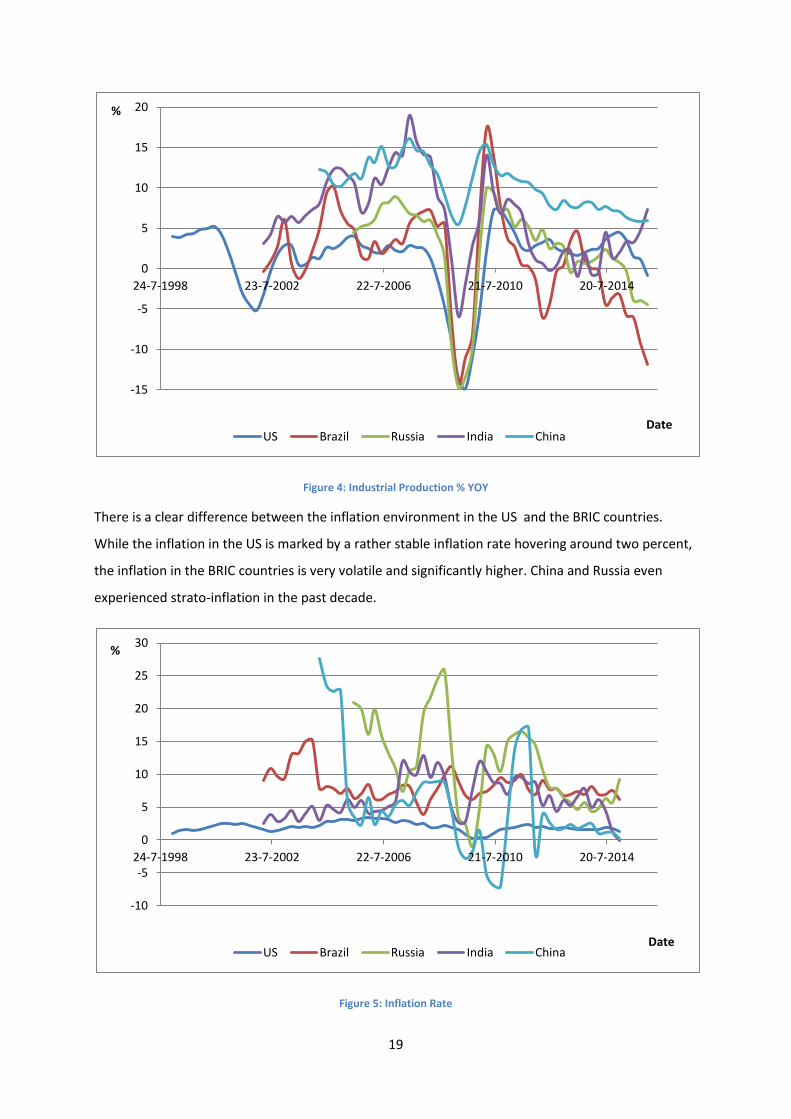
Figure 4: Industrial Production % YOY ................................................................................................... 19
Figure 5: Inflation Rate .......................................................................................................................... 19
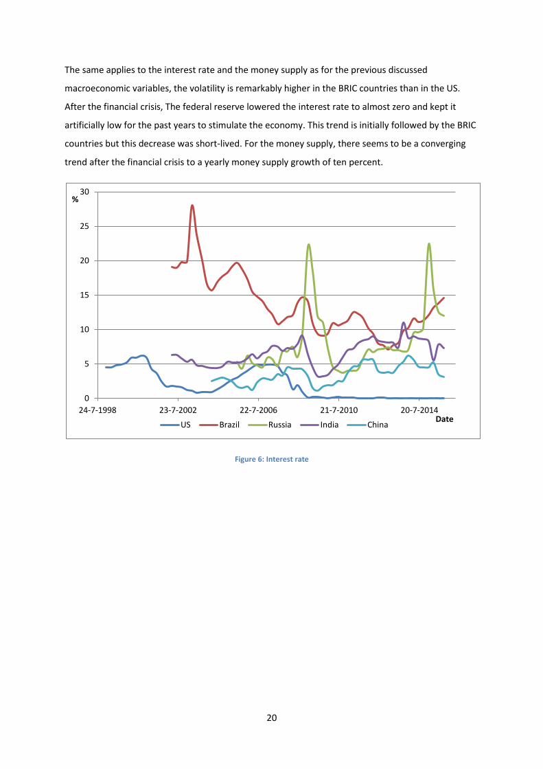
Figure 6: Interest rate ............................................................................................................................ 20
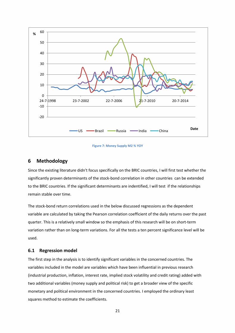
Figure 7: Money Supply M2 % YOY ....................................................................................................... 21

vii
List of tables
Table 1: Full time sample regression results ......................................................................................... 25
Table 2: Chow test results ..................................................................................................................... 26
Table 3: Breakpoint analysis regression results .................................................................................... 27

1
1 Introduction
Everyone who followed an introductory course investment analysis knows the first principle you are
taught is diversification. This principle basically means that a portfolio with a combination of
investments will have a lower risk than the weighted average risk while the return equals the
weighted average return of the individual investments. Diversification becomes more advantageous
when the correlation between the investments declines. As stocks and bonds are two of the main
asset classes, it should be clear that the stock-bond return correlation is a determining factor for the
risk of a portfolio.
So why concentrate on the BRIC countries? This has three reasons. The BRIC countries have
experienced a tremendous economic growth in the past decades. And this has had its influence on
the bond and stock returns in the countries. In the time sample used in this master's thesis all four
stock indices of the BRIC countries have outperformed the stock index of the US and three out of
four bond indices have outperformed the bond index of the US. This illustrated the attractiveness of
the investment environment in the BRIC countries. Second, the unusual economic growth is
translated in the increased contribution to the worldwide gross domestic product. China has even
surpassed the US as largest contributor. Despite this increased importance of the BRIC countries, not
much is known about the stock-bond return correlation in these countries. The literature is mainly
focussed on the G7 countries, in particular the US. Lastly, the result of the BRIC countries can serve as
a predictor for emerging countries who will follow the same economical trajectory. This three
reasons make the BRIC countries highly interesting to investigate.
The remainder of this master's thesis is organized as follows. Section 2 gives an overview of the
stock-bond return correlation related literature in the developed and emerging countries. Section 3
explains how this research can add value to the existing literature. Section 4 elaborates more on the
research question of this master's thesis. Section 5 gives more information about the data collection
and the descriptive statistics of the data. Section 6 outlines the used methodology. Section 7
discusses the result of the research. Section 8 summarizes the main finding. Lastly, in section 9 I
conclude with the recommendations for further research.

2
2 Literature review
2.1 Stylized facts of the stock-bond return correlation
In the literature a couple of reoccurring conclusions are made about the course of the stock-bond
return correlation which will be shortly mentioned below. In the early 1990 several authors stated
the stock-bond return correlation is rather stable en positive over time. They claim this result is
caused by a common discount rate effect ( Campbell & Ammer, 1993; Shiller & Beltratti, 1992). But
more recent research contradicts this result. Almost stated in every paper about this topic is the
large time-varying character of the stock-bond return correlation. Although the stock-bond return
correlation is positive on average, there is considerable time variation and several periods of
extended negative correlation. These changes can occur within short periods of time. There are
several examples of consecutive months with changing signs of the stock-bond return correlation
(Jammazi, Tiwari, Ferrer & Moya, 2015; Baker and Wurgler 2012; Baele, Bekaert & Inghelbrecht,
2010; Li 2002; Connolly, Strivers & Sun, 2005; Andersson, Krylova & Vähämaa, 2008).
Li (2002) has put forward two trends in his research conducted in the G7 countries from 1958 till
2001. First, He observed a enduring upward trend in the stock-bond return correlation until 1995. In
1995 the trend reversed and stock-bond return correlation evolved to values around zero. This is
called the reverting trend. Harumi (2015) came to the same result when searching for trends in the
stock-bond return correlation. Some authors put the increasing market integration and introduction
of the European Monetary Union forward as the cause of the reverting trend in the European
countries. There would have been uncertainty among investors about the future of the European
Monetary Union and how this would impact the macroeconomic fundamentals. This uncertainty
would have led to investors shifting their portfolios to safer assets, from stocks to bonds. On the
contrary of the other G7 countries, the stock-bond correlation in Italy has had an upward trend from
2000 onwards. Investors welcomed the euro in Italy because it could reduce the volatile financial
markets and macroeconomic uncertainty the country faced in the past (Kim, Moshirian & Wu 2006).
The weakening relationship between bond and stock returns in the past decade can also be
explained by the increased financial integration. The bonds and stocks of many countries comove
more strongly with the dominant American bond and stock markets. This means the benefits of
cross-country diversifications have decreased substantially. Thereby investors reallocate their
portfolio more frequent. This induces a more random walk in the stock-bond return correlation (Baur
2010).
The second trend is called the converging trend. It seems as the stock-bond return correlations from
the G7 countries excluding Japan are moving closer to each other. The results of Kim and In (2007)

3
show Japan has a substantial higher stock-bond return correlation than the other G7 countries. These
two trends are both visible in research conducted with a 60-month moving average and a one-month
moving average stock-bond return correlation. This can be interpreted as a result of the increasing
market integration between these countries. There also seems to be a converging trend among the
EU countries. But the opinions on the cause of this observation are divided. Garcia and Tjafack (2011)
argue that the stock-bond return correlations of the EU countries act more homogeneous after the
introduction of the euro. Cappiello, Engle and Sheppard (2006) share the same opinion. They
observed a structural brake in the cross-country bond-bond and stock-stock return correlations after
the introduction. Both were significantly higher which indirectly leads to more homogenous stock-
bond return correlations in the EU countries. On the contrary Baur and Lucey (2006) stated this
converging trend takes place after the Asian crisis.
2.2 Determinants of the stock-bond return correlation
2.2.1 A simple present value model
To get a better understanding of the underlying mechanisms of the co-movements between stocks
and bonds, it will be useful to first take a closer look at the valuations of the asset classes. Factors
who move the price of both assets in the same direction will drive the stock-bond return correlation
up. On the contrary, factors who move the asset prices in opposite directions or only affect one of
the two asset classes will have a negative influence on the stock-bond return correlation. The
statements mentioned above hold as long as cross-market pricing influences are left aside.
The valuation formulas of both assets come down to the same principle. The future incomes are
discounted back to today. Which means the price of both assets is the present value of the income
generated over the maturity of the bond or holding period of the stock.
From the formula of the stock valuation it can be derived that the price is dependent on the future
dividends and the discount rate.
D
D
n n
n
i
i
P=stock price
D=dividend
r=discount rate
4
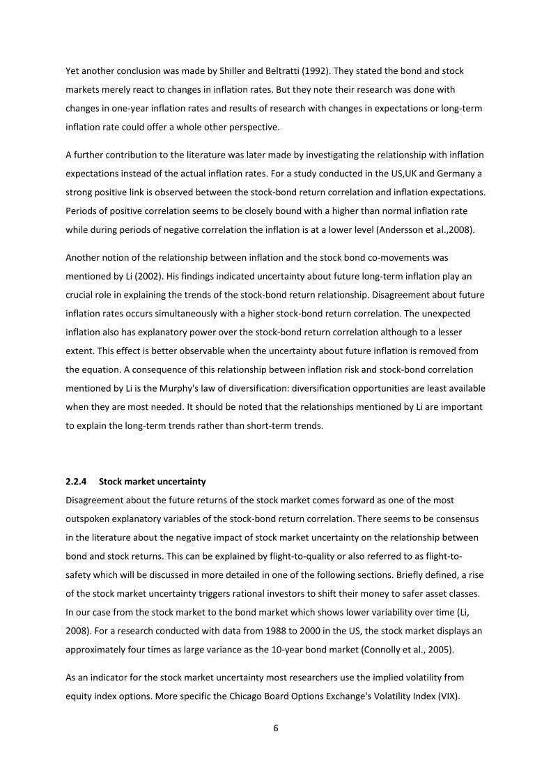
In the case of bonds, the price is only determined by changes in the discount rate. It is assumed that
the bonds have a fixed interest rate which makes the coupon payment constant over time.
n
n
P=bond price
C=coupon payment
M=par value
r=discount rate
With these formulas in mind, it should be clear that determinants who have influence on the
discount rate will have a positive effect on the stock-bond return correlation. Both the stock and
bond prices increase (decrease) with falling (rising) discount rates. The determinants who lead to a
change in expected dividends will normally drive the correlation down as it only affects the stock
price.
These formulas are off course a simplified representation of the reality. The stock-bond return
correlation is subject to more complex influences. Although researchers were already able to
indentify significant parameters of the stock-bond return correlation, Their regressions could only
explain about forty percent of the variations. Next, the most mentioned determinants of the stock-
bond return correlation will be discussed.
2.2.2 Real interest rate
The real interest rate is an important determinant because it is an indicator of the monetary policy
conducted in the country. As the real interest rate has an direct impact on the discount rate of both
stocks and bonds, it should be expected that the real interest rate is an important factor in explaining
periods with a high stock-bond return correlation. Campell and Ammer (1993) found that the stock-
bond return correlation tends to move in the same direction when the real interest rate changes,
however, the effect on the returns remains modest. The real interest rate is responsible for changes
in the short-term nominal interest rate and slope of the term structure but it seems that these
effects doesn't translate in significant stock and bond price changes. Although the positive effect
from real interest rate on the stock-bond return correlation, this result is of minor importance
because the real interest rate has relatively little variability over time. These findings could help
explain why they came to the conclusion that the stock-bond correlation is only slightly positive.

5
For a study conducted between 1953 and 2001 Li (2002) found a significant relationship with the
stock-bond return correlation. The stock-bond correlation exhibits a higher level during economic
expansion than during recession periods in the US. This is caused by higher interest rate during
expansion. the opposite is true for the UK. Related to the real interest rate, results indicate that
higher short rates are typically followed by a more elevated stock-bond correlation (Yang, Zhou &
Wang, 2009; D'Addona and Kind 2006).
2.2.3 Inflation
There is no unanimity about the effect of inflation on the stock-bond return correlation in the related
literature. Although the various authors agree on the effect inflation has on bonds, there is no
common agreement about the reaction of stock prices to inflation changes. Inflation changes have
an equal effect on the discount rate of both asset classes. An increase (decrease) will lead to a higher
(lower)nominal interest rate which means a higher (lower) discount rate and lower (higher) asset
prices. But inflation changes also influence the dividends paid by stocks. Higher inflation mostly
comes together with elevated dividends because higher inflation rates typically occur during
economic upturns. Because of this reasons the effect of inflation is negative for bonds and
ambiguous for stock. Campbell and Ammer (1993) therefore argue inflation changes promote a
negative correlation. This hypothesis is reinforced by their result over a time sample from 1952 till
1987.
The fundamental approach of Campbell and Ammer (1993) had three basic determinants. Both real
interest rates and common movements in expected returns are responsible for a positive stock-bond
correlation while inflation changes are the only factor who could induce a negative stock-bond return
correlation. Connolly et al. (2005) rejected this hypothesis by testing it over a different time sample
period. They observed the period from 1986 till 2000. The inflation in this period was rather stable
and at a relatively low level while the stock-bond correlation was characterized by considerable time
variation and extended periods of negative correlation. This result indicated that there are other
factors which drive the correlation down. They introduce stock market uncertainty and the related
flight-to-quality, which will be discussed later, as another determinant which influences the stock-
bond return relationship in a negative sense.
Ilmanen (2003) also contradicts the hypothesis of Campbell and Ammer. According to his finding, the
effect on the discount rate of stocks is of greater importance than the effect on the future cash flows
in times of high inflation. Consequently, Ilmanen predicts a higher inflation rate leads to a positive
stock-bond correlation. Yang (2009) confirms the positive relationship between inflation and the
stock-bond return correlation but to a lesser extent.
6
Yet another conclusion was made by Shiller and Beltratti (1992). They stated the bond and stock
markets merely react to changes in inflation rates. But they note their research was done with
changes in one-year inflation rates and results of research with changes in expectations or long-term
inflation rate could offer a whole other perspective.
A further contribution to the literature was later made by investigating the relationship with inflation
expectations instead of the actual inflation rates. For a study conducted in the US,UK and Germany a
strong positive link is observed between the stock-bond return correlation and inflation expectations.
Periods of positive correlation seems to be closely bound with a higher than normal inflation rate
while during periods of negative correlation the inflation is at a lower level (Andersson et al.,2008).
Another notion of the relationship between inflation and the stock bond co-movements was
mentioned by Li (2002). His findings indicated uncertainty about future long-term inflation play an
crucial role in explaining the trends of the stock-bond return relationship. Disagreement about future
inflation rates occurs simultaneously with a higher stock-bond return correlation. The unexpected
inflation also has explanatory power over the stock-bond return correlation although to a lesser
extent. This effect is better observable when the uncertainty about future inflation is removed from
the equation. A consequence of this relationship between inflation risk and stock-bond correlation
mentioned by Li is the Murphy's law of diversification: diversification opportunities are least available
when they are most needed. It should be noted that the relationships mentioned by Li are important
to explain the long-term trends rather than short-term trends.
2.2.4 Stock market uncertainty
Disagreement about the future returns of the stock market comes forward as one of the most
outspoken explanatory variables of the stock-bond return correlation. There seems to be consensus
in the literature about the negative impact of stock market uncertainty on the relationship between
bond and stock returns. This can be explained by flight-to-quality or also referred to as flight-to-
safety which will be discussed in more detailed in one of the following sections. Briefly defined, a rise
of the stock market uncertainty triggers rational investors to shift their money to safer asset classes.
In our case from the stock market to the bond market which shows lower variability over time (Li,
2008). For a research conducted with data from 1988 to 2000 in the US, the stock market displays an
approximately four times as large variance as the 10-year bond market (Connolly et al., 2005).
As an indicator for the stock market uncertainty most researchers use the implied volatility from
equity index options. More specific the Chicago Board Options Exchange's Volatility Index (VIX).

7
When the bond returns are high in comparison with the stock return, typically a increase in implied
volatility is observed. This results were consistent over the several tested time period. This indicates
that stock market uncertainty has considerable cross-market pricing influences. Although stock news
uncertainty isn't perceived as good news by investors, the decline of the stock-bond return
correlation means investors can better diversify their risk (Connolly et al 2005). Connolly et al.(2005)
introduced also a second measure for the stock market uncertainty namely stock turnover. A change
in stock turnover could be a sign of divergent beliefs among investors or may be linked with a
modification in the investment opportunity. Both of these options are associated with stock market
uncertainty. Their result indicated that the chance of a lower stock-bond return correlation over the
next days is higher when higher values for the implied stock volatility and stock turnover are noted.
Baele, Bekaert and Inghelbrecht (2010) regressed the VIX on the residuals of their fundamental 8
factor model (with output gap, inflation, expected future output gap, output uncertainty, expected
inflation, inflation uncertainty, nominal interest rate, cash flow growth as factors) and found a
significant negative relationship on the stock-bond return correlation confirming the result of
Connolly et al.(2005). Further evidence for the negative relationship between stock market
uncertainty and the stock-bond return correlation is the switch from a positive stock-bond return
correlation during the 1990s to a negative stock-bond return correlation in early 2000s in a wide
range of developed countries. This can be explained by the collapse of the dot-com bubble which led
to uncertainty on the stock markets. This was another conformation of the flight-to-quality
phenomenon (Jammazi et al. 2015). Chou and Liao (2008) even attribute the remarkable lower stock-
bond return correlation in the past decade to above average stock market uncertainty.
Another interesting view on the relationship between the stock market uncertainty and the stock-
bond return correlation is cited in a paper by Baker and Wurgler (2012). In this paper, they
investigate if there are differences in the correlation between bonds and the cross-section of stocks.
They found that government bonds have a higher correlation with bond-like stocks. They define bond
like stocks as follows: stock of large, mature, low-volatility, profitable, dividend-paying firms that are
neither high growth nor distressed. Their results indicated that bond-like stocks are less sensitive to
periodic flights-to-quality. Even when bonds and stocks become decoupled (the stock-bond return
correlation turns from positive to negative), the correlation with bond-like stocks remains
approximately at the same level.
2.2.5 Economic growth
Several researchers have included a variable for economic growth in their model. Andersson et al.
(2008) incorporated expectations about the economic growth but were unable to find a significant
8
link with the stock-bond return correlation. Yang et al.(2009) made use of a dummy variable which is
one for recession and zero otherwise. Their research was conducted in the United Kingdom and the
United States. The UK and US showed opposite resulst. In the US, they observe a higher stock-bond
return correlation during expansions than during recessions. On the contrary, in the UK the stock-
bond return correlation is higher during recessions than during expansions.
Other authors argue the bonds and stocks react different to macroeconomic news during expansion
than during recessions. More particularly, in times of economic expansion the discount effect of
stocks may be dominant over the cash flow effect. This should result in a positive stock-bond return
correlation. The contrary should be true for recessions which would lead to lower or even negatively
correlated stock and bond returns (Boyd et al. 2005; Andersen et al. 2007).
2.2.6 Bond market uncertainty
Similarly as for stock market uncertainty, there is research into the impact of bond market
uncertainty on the stock-bond return correlation but with lesser and inconsistent results. The
volatility of the bond returns influences the stock-bond return correlation in a negative but
insignificant way in the US but in a positive and significant way in Germany and the UK (Baur & Lucey,
2006).
2.3 Flight-to-Quality Phenomenon
Many authors had difficulties with explaining the occasionally negative periods in the stock-bond
return correlation. They argued common effect of macroeconomic variables induces positively
correlated stock and bond returns but the cause of periods with a negative stock-bond return
correlation was uncertain until later research introduced stock market uncertainty. When there is
increased uncertainty about the future direction of the stock market, investors tend to shift their
portfolio from riskier to safer assets. In our case from stocks to bonds. This leads to numerous lows in
the stock-bond return correlation graph. This strong negative relationship between the stock market
uncertainty and the stock-bond return correlation is the flight-to-quality phenomenon. Before we
can speak of flight-to-quality, two conditions need to be met: (1) change in sign of the stock-bond
return correlation (from positive to negative) (2) it occurs in tumbling stock markets (Baur & Lucey
2006).
Baur and Lucey (2006) argue there are two regimes in the stock-bond returns correlation which we
can differentiate. A regime with positively correlated stock and bond returns caused by the similar
effect of the macroeconomic variables on the returns and a regime with negatively correlated stock
and bond returns caused by the flight-to-quality phenomenon. There isn't one regime dominant over

9
the other. Quite the reverse, regime changes are very common. As discussed in the previous section,
the relationship between the bond volatility and the stock-bond returns correlation isn't consistent
over different countries but this changes when the relationship is tested separately in both regime.
The bond volatility exhibits a significantly positive coefficient in both the negative and positive
regime. These results indicate that an increased bond volatility can be partly responsible for a return
from the negative to the positive regime.
Baur and Lucey (2009) expended their research about the flight-to-quality phenomenon. They
compared the occurrence in different countries and revealed flight-to-quality occurs simultaneously
in many countries. They further refer to the positive implication of the phenomenon. As flight-to-
quality leads to a negative stock-bond return correlation it provides investors with better
diversification opportunities in crisis periods.
Flight-to-quality induces a negative stock-bond return correlation. So this means opposed to a falling
stock market there is a rising bond market. Durand, Junker and Szimayer (2010) went a step further
and investigated what the chance is to observe a rising bond market when the stock market plunges.
Their result indicate that in approximately one out of seven times increasing bond markets are
associated with falling stock markets (for a time sample from 1952 till 2003 in the US).
Another phenomenon which leads to remarkable changes in the stock-bond return correlation is
contagion. There is talk of (negative) contagion when there is a simultaneously fall of both the stock
and bond markets. Contagion is typically witnessed in crisis period. So, as opposed to flight-to-quality
contagion leads to positively correlated stock and bond returns. An example of contagion in the US is
the period after the terroristic attacks on 11 September 2001 (Baur & Lucey, 2006).
2.4 Stock-bond correlation in emerging countries
Emerging countries went through a completely different economical and political trajectory as
developed countries over the last decades. As a result, findings of research conducted in developed
countries can't be extended to emerging countries, in our case the BRIC countries. Although the
literature about the stock-bond return correlation in emerging countries isn't very extended, the
main findings will be discussed below.
Kelly, Martins and Carlson (1998) were one of the first to address the relationship between stocks
and bonds in emerging countries. In their paper, they have special attention for the link between
sovereign risk and the stock-bond return correlation. In their conceptual framework they state that in
countries with a high level of sovereign risk, bond and stock returns are closely linked. They first
discuss the relationship between sovereign risk and the value of equity. Their assumption describes
10
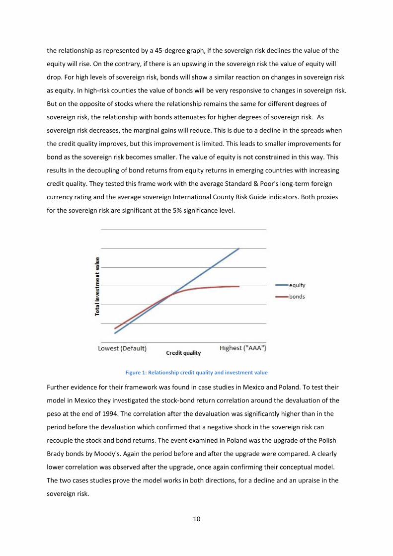
the relationship as represented by a 45-degree graph, if the sovereign risk declines the value of the
equity will rise. On the contrary, if there is an upswing in the sovereign risk the value of equity will
drop. For high levels of sovereign risk, bonds will show a similar reaction on changes in sovereign risk
as equity. In high-risk counties the value of bonds will be very responsive to changes in sovereign risk.
But on the opposite of stocks where the relationship remains the same for different degrees of
sovereign risk, the relationship with bonds attenuates for higher degrees of sovereign risk. As
sovereign risk decreases, the marginal gains will reduce. This is due to a decline in the spreads when
the credit quality improves, but this improvement is limited. This leads to smaller improvements for
bond as the sovereign risk becomes smaller. The value of equity is not constrained in this way. This
results in the decoupling of bond returns from equity returns in emerging countries with increasing
credit quality. They tested this frame work with the average Standard & Poor's long-term foreign
currency rating and the average sovereign International County Risk Guide indicators. Both proxies
for the sovereign risk are significant at the 5% significance level.
Figure 1: Relationship credit quality and investment value
Further evidence for their framework was found in case studies in Mexico and Poland. To test their
model in Mexico they investigated the stock-bond return correlation around the devaluation of the
peso at the end of 1994. The correlation after the devaluation was significantly higher than in the
period before the devaluation which confirmed that a negative shock in the sovereign risk can
recouple the stock and bond returns. The event examined in Poland was the upgrade of the Polish
Brady bonds by Moody's. Again the period before and after the upgrade were compared. A clearly
lower correlation was observed after the upgrade, once again confirming their conceptual model.
The two cases studies prove the model works in both directions, for a decline and an upraise in the
sovereign risk.
11
Another parameter who could lead to a potential lower stock-bond return correlation is the
increasing market integration of emerging countries. As emerging stock markets become more
integrated with the rest of the world, the segmentation risk premia on stocks reduces and the
demand for stocks increases. This effect on stocks can even lead to a declining demand for bonds.
This results in lower correlated stock and bond returns. The opening up of stock markets is good
news for investors because it gives them better diversification opportunities (Panchenko & Wu,
2009).
Dimic, Kiviaho, Piljak and Äijö (2016) were among the first to investigate the determinants of the
stock-bond return correlation in emerging countries. First of all, they observed a difference in the
level of the stock-bond return correlation between the US and emerging countries in their time
sample (January 2001 till December 2013). The stock-bond return correlation in the emerging
countries is positive most of the time which is clearly different from the mostly negative correlation
in the US. Another eye-catching observation in their descriptive statistics is the higher volatilities of
the bond and stock returns in the emerging countries. The higher volatility of the bond market
emphasises the higher risk of investing in bonds of emerging countries.
They went even a step further and tested the impact of the determinants over different time
horizons. Fluctuations ranging between two to four months are considered short term while
fluctuation between one to three years are considered long term. Several differences between the
short and long time horizon emerged. The first differences are noticed in sign and magnitude. The
stock-bond return correlation at short-term horizons exhibit large variations. Changes in sign and
magnitude can occur very rapidly. Within their time sample the stock-bond correlation changes
numerous times from positive to negative episodes and vice-versa. This result is a confirmation that
the flight-to-quality phenomenon can be extended to emerging countries. This indicates short-term
investors shift their means from stocks to bonds in crisis periods as they perceive the emerging bond
markets as a good hedge for the emerging stock markets over a short time horizon. The flight-to-
quality is clearly observed after the Dotcom market crash and during the financial crisis of 2008 in all
surveyed emerging countries. Over the long-term horizon a different pattern is observed. As the
stock-bond return correlation at the short-term horizon is characterized by a large volatility and
alternating periods of positive and negative correlation, the stock-bond return correlation at the
long-term is characterized by less volatility and a remaining positive sign. The rather stable positive
stock-bond correlation at the long-term horizon implies the flight-to-quality phenomenon only
occurs over a short time horizon which indicates the bonds of emerging countries aren't perceived as
safe assets in comparison with to emerging market stocks. Variations in the long-term can be
12
explained easier than variations in the short-term as their explanatory power of their model is
significantly higher at the long-term horizon than at the short-term horizon.
Dimic, Kiviaho, Piljak and Äijö(2016) tested a model with business cycle fluctuation, inflation
environment, monetary policy stance and global uncertainty factors(VIX for stocks and MOVE for
bonds) in 10 emerging countries. Domestic monetary policy included in the model with the three-
month interbank interest rate is the most influential factor at the short term-horizon. Although the
monetary policy stance is significant in seven out of the ten countries, the coefficient sign varies
across the countries. This indicates the monetary measures haven't the same impact on bond and
stock prices in the surveyed countries. The global uncertainty measures have a modest impact on the
stock-bond return correlation. The VIX index is only significant in 5 countries and the MOVE index in
3 countries at the short-term horizon. The results of Bianconi, Yoshino and De Sousa in 2013 showed
that the correlation between the bond returns, stock returns and the US financial stress measures
increased after the collapse of the Lehman Brothers. As many papers on the stock-bond return
correlation in developed countries, Dimic, Kiviaho, Piljak and Äijö(2016) also have difficulty finding a
consistent link between the business cycle and the stock-bond return correlation. The industrial
production (their proxy for the business cycle ) is only significant in two countries.
In general, the factors have an higher impact on the long-term horizon than on the short-term
horizon. Where the R-squared for their model at the short term horizon varied between 22% and
65%, their model has a significantly higher R-squared at the long-term horizon (ranging between 74%
to 96%). Inflation seems to be the most important factor in explaining long-term fluctuation as it is
significant in all surveyed countries. The coefficient of inflation is positive in 8 out of the 10 countries
which is consistent with previous research in developed countries. This indicates that the increased
cash flow effect on stocks is dominated by the discount effect for high inflation rates. An surprising
result is found for the global stock market uncertainty. Although the VIX is significant in 9 out of the
10 countries, the coefficient is positive in seven countries which is in contrast to previous research
conducted in developed countries. This implies that in times of the elevated stock market uncertainty
bonds and stock will commove tightly. Another positive relationship is observed between the
economic growth and the stock-bond return correlation. Economic growth seems to have a similar
effect on bonds and stocks in the long run. The conclusion for the monetary policy stance is
comparable with the results at short-term horizon. There doesn't seems to be a consistent link over
the countries.
13
3 Relevance
A better understanding about the impact of determinants on the stock-bond return correlation is
beneficiary for different parties.
The first and most important reason is the impact of the stock-bond return correlation on the
portfolio risk. As the stock-bond return correlation is one of the main inputs, a better prediction of
the stock-bond return correlation would enable investors to drastically improve their dynamic asset
allocation strategy.
Second, the stock-bond return correlation can be a source of information for policymakers. A
changing stock-bond return correlation can be an indication of changing expectations of economic
variables among the market participants. But this can also be looked at from another viewpoint. If
research is able to quantify the relationships of the determinants on the stock-bond return
correlation, policymakers would be able anticipate the possible impact of their policies on the asset
markets(Li & Zou 2008).
Furthermore, there is an increased interest in emerging market assets by international investors.
Dimic et al.(2016) cite two reasons why investing in government bonds of emerging markets gained
attention over the past years. First of all, The bond markets have evolved. They have become more
transparent and liquid which makes it safer to invest. Second, the government bonds are the second
largest source of financing in these fast growing countries. This increased interest make the BRIC
countries a highly interesting study subject.
4 Purpose
The literature about the topic of the stock-bond return correlation isn't that broad and mainly
focused on developed countries, especially the G7 countries. Little is known about the determinant
of the stock-bond return correlation in emerging countries, let alone why and how they differ from
the determinants in the developed countries. Furthermore, the literature is mainly focused on
identifying determinants or validate the existing result with new data. I notice there is a lack of
research which investigates if these relationships remain stable over time. The BRIC countries went
from developing countries to engines of the world economy, with China even as the largest
contributor to the worldwide GDP, at a swift pace. This makes these countries highly interesting to
test the time variance of the determinants. Moreover, the BRIC countries are very diverse in many
aspects. First of all, they are geographically diverse. Second, the control over the capital markets by
the state differs between the BRIC countries. The capital market in India and China are relatively
14
closed and controlled by the state while the capital markets in Russia and Brazil are more open.
Third, the timing, economic growth rate and expansion source are difficult to compare. All four BRIC
countries are export driven. Although, Brazil and Russia owe their economic expansion to commodity
export while India and China experienced a substantial growth in export of goods & services
(Bianconi et al. 2013).
The main purpose of this research is to get an answer to the following questions:
Is there also a conversing trend noticeable between the BRIC countries and the US?
Do the determinants have the same impact on the stock-bond return correlations of the BRIC
countries as in the US?
Was the impact of the determinants on stock-bond returns influenced by the exceptional
economic growth the BRIC countries went through in the past decades?
5 Data
5.1 Data Collection
In order to include as much as possible of the economic expansion the BRIC countries underwent and
still undergo, the aim was to collect data for a as large as possible time sample. Unfortunately,
qualitative data is only published since the early 2000 for this countries. The US will also be
concluded in this research to expose the differences between the US and the BRIC countries. The
time frames for this research are from the beginning of 2002 till the third quarter of 2015 for Brazil,
from the second quarter of 2005 till the end of 2014 for Russia, from the beginning of 2002 till the
second quarter of 2015 for India, from the beginning of 2004 till the third quarter of 2015 for China
and finally from the last quarter of 1998 till the third quarter of 2015 for the USA. All the data has
been collected via Thomas Reuters DataStream® except for the stock market uncertainty which is the
VIX from the Chicago Board Options Exchange. Because the majority of the macroeconomic factors is
only announced on a quarterly basis, this research will preserve the same frequency in the overall
data.
To get to the stock returns, comprehensive stock price indices of the concerning countries where
collected. Subsequently, the stock returns where calculated out of these stock price indices. The
following stock price indices were collected: the Bovespa index for Brazil, the RTS index for Russia,
The Nifty 500 price index for India, The FTSE B35 index for China and lastly the Nasdaq composite
price index for the US.

15
The same method was used to calculate the bond returns as for the stock returns. I opted for bonds
with a 10-year maturity because the long-term bond have a maturity closer to the infinite maturity of
stocks. The indices used are government bond indices published by JP Morgan for all the concerning
countries.
The literature doesn't have an outspoken opinion about the effect of economic growth on the stock-
bond return correlation but I nevertheless decided to conclude a variable in my research. As a proxy
for the economic growth I incorporated the year on year industrial production. To give a indication of
the prosperity of the countries the evolution of the GDP per capita was gathered. They are all
expressed in the same currency, namely the American dollar.
Other important aspects of the economic climate are the inflation rate and the monetary policy
stance. To include the inflationary environment the GDP deflator of the countries is used. The
monetary policy stance is incorporated with two variables. First of all a short-term interest rate. The
3-month treasury bill rate is used for all countries except Russia. Due to insufficient data about the
Russian treasury bills the 3-month prime rate is used. The second variable is the money supply. I used
the year on year change in money supply of M2. This variable is included because it better represents
the quantitative easing policies of the central banks.
As mentioned above the stock market uncertainty is incorporated with the VIX of the CBOE. The
CBOE also produces the VIX measure for emerging countries but these only started in 2011.
Incorporating the VIX measures of the concerned countries in the model would substantially shorten
the time samples. Thereby the VIX of the US will be used in the BRIC countries as a proxy for the
global stock market uncertainty.
As Kelly et al. (1998) argued credit rating could be a possible determinant of the stock-bond return
correlation. A credit rating is incorporated as a numeric variable where the average credit rating over
the quarter is converted on a zero to twenty scale. On this scale zero equals the default rating and
twenty the AAA rating. Furthermore, the political stability of the countries will be taken into account.
This will be done by a numeric variable where zero stands for total instability and seven for highly
stable political system.
5.2 Descriptive statistics
In the following section remarkable observations about the data will be discussed.
I first going to scrutinize the stock and bond returns. In general the normal assumptions about bonds
and stocks hold. More specific, in all countries we observe that the stock returns have a higher
16
average return and a higher average standard deviation than the bond returns. When we compare
the stock returns over the countries, there is a remarkable result for India. India has by far the
highest average return and also has the lowest average standard deviation even lower than the US.
There doesn't seem to be a one size fit all if it comes down to the skewness of the stock returns. India
and China are skewed to the left while Brazil, Russia and the US are skewed to the right. All the bond
return series are skewed to the left which means there are frequent small positive returns and
extreme negative returns from time to time. The stock and bond return series all have a positive
kurtosis. Some series even exceed the extreme value of hundred. These leptokurtic distributions
mean there is a too high frequency of realizations clustered around the mean (in our case slightly
positive returns) in comparison with the normal distribution. This also means the variance originate
from infrequent extreme deviations.
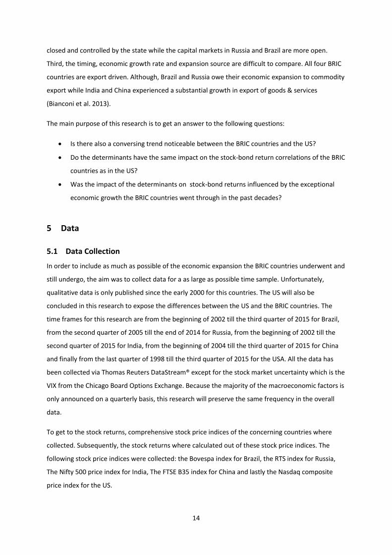
As we take a look at the stock-bond return correlations of the countries, there are some observations
worth mentioning. The stock-bond return correlations displayed in the graph are the 30-days moving
averages. Firstly, we can reject the assumption of Campbell & Ammer (1993) and Shiller & Beltratti
(1992) who stated the stock-bond return correlation remains slightly positive and rather stable over
time. The correlation estimates have a very large time-varying character and positive periods are
frequently alternated with negative periods. Second, the stock-bond return correlation in the US is
lower than the correlations in the emerging countries. It seems like the bond and stock returns in the
US are negatively correlated most of the time. This means the benefits of cross-asset diversification
are the largest in the US. The Asian crisis, Russian crisis, collapse of the dotcom bubble and the
financial crisis could have induces flights-to-quality and periods negative stock-bond return
correlation linked to this. Second, Brazil shows a higher stock-bond correlation until 2008. From 2008
onwards it coincides more with the stock-bond return correlations of China and India. The opposite is
the case for Russia, the stock-bond return correlation seems to coincide with the correlations of India
and China until 2008. Between 2008 and 2012 Russia has a substantially higher stock-bond return
correlation than the other countries. Moreover, there doesn't seem to be a converging trends
between the stock-bond return correlations of the BRIC countries and the US. This could possibly
indicate there hasn't been a substantial increase in market integration between the BRIC countries
and the US.
17
Figure 2: Stock-bond return correlations
The macroeconomic variables will be discussed briefly to highlight the differences between the BRIC
countries mutually and the US as an example of a developed country.
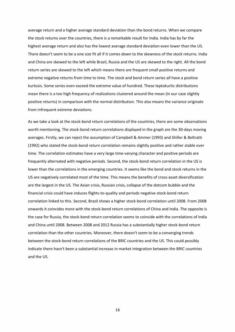
As expected, The US has by far the highest GDP/capita, followed by Russia, Brazil, China and India. In
our time sample, the GDP/capita has doubled for China, who has a considerably higher growth rate
than the other BRIC countries. The financial crisis has had an impact on the prosperity of Russia and
the US, who exhibit a slight decrease in 2008. On the opposite, the prosperity growth in Brazil, India
and China seems to be unaffected by the financial crisis.
-0,8
-0,6
-0,4
-0,2
0
0,2
0,4
0,6
0,8
24-7-1998 23-7-2002 22-7-2006 21-7-2010 20-7-2014
ρ
Date US Brazil Russia India China
18
Figure 3: GDP per Capita
The economic expansion the BRIC countries have experienced in the previous years is clearly visible.
The average GDP growth is considerably higher in the BRIC countries than in the US, with China as an
outlier with an average GDP growth of approximately 10%. As indicated by the trough in 2009, the
financial crisis also influenced the economies in the BRIC countries. After the financial crisis the GPD
growth of the BRIC countries exhibits a downwards trend. At the end of the time sample the growth
rate of Brazil and Russia even plummet. This sharply contrasts with the upward trend before the
financial crisis.
0
2000
4000
6000
8000
10000
12000
14000
24-7-1998 23-7-2002 22-7-2006 21-7-2010 20-7-2014
$
Date US Brazil Russia India China
19
Figure 4: Industrial Production % YOY
There is a clear difference between the inflation environment in the US and the BRIC countries.
While the inflation in the US is marked by a rather stable inflation rate hovering around two percent,
the inflation in the BRIC countries is very volatile and significantly higher. China and Russia even
experienced strato-inflation in the past decade.
Figure 5: Inflation Rate
-15
-10
-5
0
5
10
15
20
24-7-1998 23-7-2002 22-7-2006 21-7-2010 20-7-2014
%
Date US Brazil Russia India China
-10
-5
0
5
10
15
20
25
30
24-7-1998 23-7-2002 22-7-2006 21-7-2010 20-7-2014
%
Date US Brazil Russia India China
20
The same applies to the interest rate and the money supply as for the previous discussed
macroeconomic variables, the volatility is remarkably higher in the BRIC countries than in the US.
After the financial crisis, The federal reserve lowered the interest rate to almost zero and kept it
artificially low for the past years to stimulate the economy. This trend is initially followed by the BRIC
countries but this decrease was short-lived. For the money supply, there seems to be a converging
trend after the financial crisis to a yearly money supply growth of ten percent.
Figure 6: Interest rate
0
5
10
15
20
25
30
24-7-1998 23-7-2002 22-7-2006 21-7-2010 20-7-2014
%
Date US Brazil Russia India China
21
Figure 7: Money Supply M2 % YOY
6 Methodology
Since the existing literature didn't focus specifically on the BRIC countries, I will first test whether the
significantly proven determinants of the stock-bond correlation in other countries can be extended
to the BRIC countries. If the significant determinants are indentified, I will test if the relationships
remain stable over time.
The stock-bond return correlations used in the below discussed regressions as the dependent
variable are calculated by taking the Pearson correlation coefficient of the daily returns over the past
quarter. This is a relatively small window so the emphasis of this research will be on short-term
variation rather than on long-term variations. For all the tests a ten percent significance level will be
used.
6.1 Regression model
The first step in the analysis is to identify significant variables in the concerned countries. The
variables included in the model are variables which have been influential in previous research
(industrial production, inflation, interest rate, implied stock volatility and credit rating) added with
two additional variables (money supply and political risk) to get a broader view of the specific
monetary and political environment in the concerned countries. I employed the ordinary least
squares method to estimate the coefficients.
-20
-10
0
10
20
30
40
50
60
24-7-1998 23-7-2002 22-7-2006 21-7-2010 20-7-2014
%
Date US Brazil Russia India China

22
ρ= stock-bond return correlation
%IP= industrial production YOY (%)
INF= inflation
IR= interest rate
MS= money supply YOY (%)
VIX= volatility S&P 500
CR= credit rating
PR= political risk
6.1.1 Corrections
Some patters in the data can cause biased result of the OLS estimators. The detection method and
the corrections for multicollinearity, heteroscedasticity and autocorrelation are briefly discussed
below.
6.1.1.1 Multicollinearity
Multicollinearity can cause serious problems for the statistical significance of parameters. When
there is a high level of multicollinearity between the explanatory variables the confidence intervals
tend to be much wider which could lead to the acceptance of the zero null hypothesis more readily.
In the initial model the GDP/capita was included as a proxy of the prosperity of the country. This
variable had a high degree of multicollinearity with the credit rating and a transformation to yearly
change was excluded because this is already largely capture by the yearly change in the industrial
production. Because of this reasons the GDP/capita was removed from the model. There are still
some variables with a high degree of multicollinearity especially in Russia but this could not be solved
without detracting the model.
6.1.1.2 Heteroscedasticity
When we neglect the presence of heteroskedasticity when using the OLS method, the result could be
misleading because the estimator of the variances of the variables is biased. Heteroscedasticity will
be detected with the White's general heteroscedasticity test . When there is a question of
heteroscedasticity, the White's heteroscedasticity-consistent standard errors will be used.
6.1.1.3 Autocorrelation
Using the OLS estimation and disregarding the presence of autocorrelation will result in misleading
results. Typically the R2 will be overestimated and the usual t and F tests of significance will no longer
be valid. The occurrence of autocorrelation will be tested with the Breusch-Godfrey test. If the test
rejects the null hypothesis of no autocorrelation, the OLS standard errors will be corrected with the
Newey-West method.
6.2 Structural break in regression results

23
To assess whether the regression results have changed within the time sample a chow test will be
executed. The Chow test, however, has two major drawbacks. First of all, it doesn't propose a
particular point in time when the structural break could have happened. As these research aims at
identifying the impact of economic growth on the determinant of the stock-bond return correlation,
the financial crisis (quarter 1, 2009)is chosen as the break point in the Chow tests. Besides the sharp
decline in economic growth during the financial crisis, it can also be seen that the upward trend in
the economic growth before the crisis has been replaced by a downward trend after the financial
crisis. This makes the financial crisis the exquisite moment in these time samples for the break point
in the Chow tests. The second drawback is the lack of information the Chow test generates.
Although, the test expresses whether there is a structural break in the regression result or not, it
doesn't give any information about the change in the individual variable coefficients. This problem
can be resolved with an additional regression. A dummy variable needs to be create with the value
zero before the breakpoint and the value one after the breakpoint. This regression model starts from
the model that is used for the entire time sample regressions. To identify which variables have a
different impact before and after the financial crisis, there are interaction terms of each variable
with the dummy variable added to the model. If the interaction term of the concerned variable with
the dummy variable has a significant influence on the stock-bond correlation, we can state that the
impact of this variable is different before and after the break point.
ρ= stock-bond return correlation
%IP= industrial production YOY (%)
INF= inflation
IR= interest rate
MS= money supply YOY (%)
VIX= volatility S&P 500
CR= credit rating
PR= political risk
D= dummy variable
If the Chow test indicates that the regression result are actual different before and after the
breakpoint, this model will be applied to the data of the concerned country. The same corrections as
discussed for the entire time sample regressions have been applied to these regressions.
7 Empirical result
24
This section is subdivided in two parts. First the result of the entire time sample regressions are
presented followed by the results of the Chow tests.
7.1 Results of the entire time sample regressions
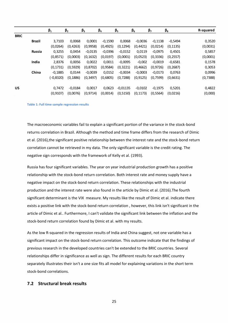
The results of the regressions are reported in table 1. The betas and R-squared are displayed with the
corresponding p-values below them. When we first take a look at the explanatory power of the
model, the large variation between the countries jumps out. While the R-squared of the US, Brazil
and Russia indicates that the model predicts a significant level of the variance in the stock-bond
return correlation, the model doesn't predict significantly more than the intercept-only model in
China and India.
The model has three significant variables in the US: the year on year change in industrial production,
the 3-month t-bill rate and the political risk variable. The negative industrial production coefficient
implies we should observe a higher stock-bond return correlation during economic recession than
during economic expansion. This result doesn't corresponds with previous research which argues
that the discount effect dominates the cash flow effect during expansion and vice versa during
recessions leading to a positive relationship between economic growth and the stock-bond return
correlation (Ilmanen, 2003; Yang, 2009). The impact of the interest rate is consistent with previous
research, the discount effect leads to co-movements between the bond and stock returns (Campell &
Ammer, 1993; Li, 2002; Yang et al., 2009; D'Addona & Kind, 2006). The third significant variable is the
political risk which was added to the model to include an extra dimension of stability for the BRIC
countries. The fact that the political risk variable is only significant in the US and in none of the BRIC
countries comes unexpected. The highly insignificant inflation coefficient suggests the rather stable
inflation rate in the US is unable to predict the large short-term variations in the stock-bond return
correlations. The VIX measure doesn't have a significant influence on the stock-bond return
correlation. This surprising result could be partly caused by the quarterly frequency of the regression.
25
Table 1: Full time sample regression results
The macroeconomic variables fail to explain a significant portion of the variance in the stock-bond
returns correlation in Brazil. Although the method and time frame differs from the research of Dimic
et al. (2016),the significant positive relationship between the interest rate and the stock-bond return
correlation cannot be retrieved in my data. The only significant variable is the credit rating. The
negative sign corresponds with the framework of Kelly et al. (1993).
Russia has four significant variables. The year on year industrial production growth has a positive
relationship with the stock-bond return correlation. Both interest rate and money supply have a
negative impact on the stock-bond return correlation. These relationships with the industrial
production and the interest rate were also found in the article by Dimic et al. (2016).The fourth
significant determinant is the VIX measure. My results like the result of Dimic et al. indicate there
exists a positive link with the stock-bond return correlation , however, this link isn't significant in the
article of Dimic et al.. Furthermore, I can't validate the significant link between the inflation and the
stock-bond return correlation found by Dimic et al. with my results.
As the low R-squared in the regression results of India and China suggest, not one variable has a
significant impact on the stock-bond return correlation. This outcome indicate that the findings of
previous research in the developed countries can't be extended to the BRIC countries. Several
relationships differ in significance as well as sign. The different results for each BRIC country
separately illustrates their isn't a one size fits all model for explaining variations in the short term
stock-bond correlations.
7.2 Structural break results
β1 β2 β3 β4 β5 β6 β7 β8 R-squared
BRIC
Brazil 3,7103 0,0068 0,0001 -0,1590 0,0068 -0,0036 -0,1138 -0,5494 0,3520
(0,0264) (0,4263) (0,9958) (0,4925) (0,1294) (0,4421) (0,0214) (0,1135) (0,0031)
Russia 0,3255 0,0454 -0,0135 -0,0396 -0,0152 0,0119 -0,0975 0,4501 0,5857
(0,8571) (0,0003) (0,1632) (0,0197) (0,0001) (0,0523) (0,3336) (0,2557) (0,0001)
India 2,8376 0,0056 0,0022 0,0011 -0,0095 -0,002 -0,0019 -0,6581 0,1578
(0,1731) (0,5929) (0,8702) (0,9584) (0,3221) (0,4662) (0,9726) (0,2687) 0,3053
China -0,1885 0,0144 -0,0039 0,0152 -0,0034 -0,0003 -0,0173 0,0763 0,0996
(-0,8320) (0,1886) (0,3497) (0,6805) (0,7288) (0,9125) (0,7599) (0,6631) (0,7388)
US 0,7472 -0,0184 0,0017 0,0623 -0,01135 -0,0102 -0,1975 0,5201 0,4822
(0,9107) (0,0076) (0,9714) (0,0014) (0,5150) (0,1173) (0,5564) (0,0216) (0,000)
26
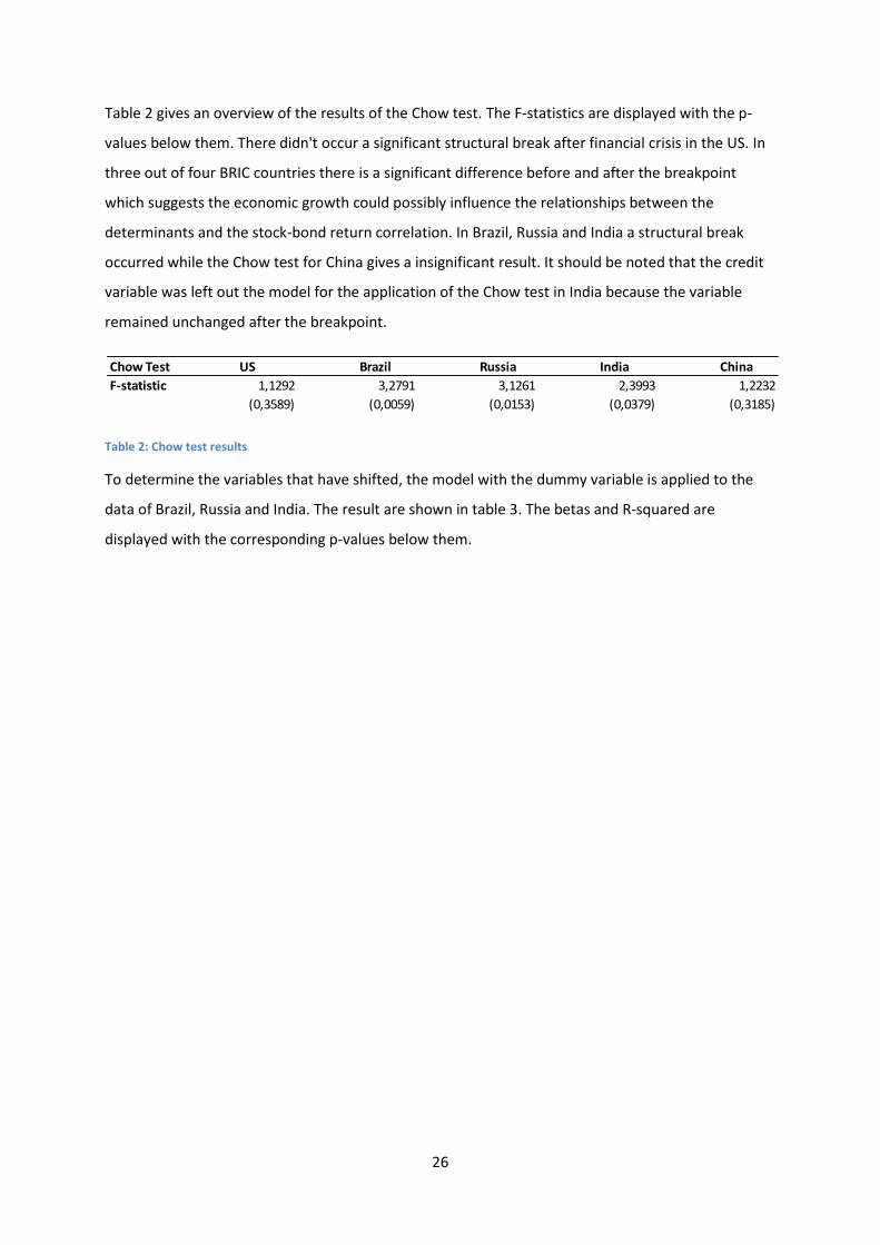
Table 2 gives an overview of the results of the Chow test. The F-statistics are displayed with the p-
values below them. There didn't occur a significant structural break after financial crisis in the US. In
three out of four BRIC countries there is a significant difference before and after the breakpoint
which suggests the economic growth could possibly influence the relationships between the
determinants and the stock-bond return correlation. In Brazil, Russia and India a structural break
occurred while the Chow test for China gives a insignificant result. It should be noted that the credit
variable was left out the model for the application of the Chow test in India because the variable
remained unchanged after the breakpoint.
Table 2: Chow test results
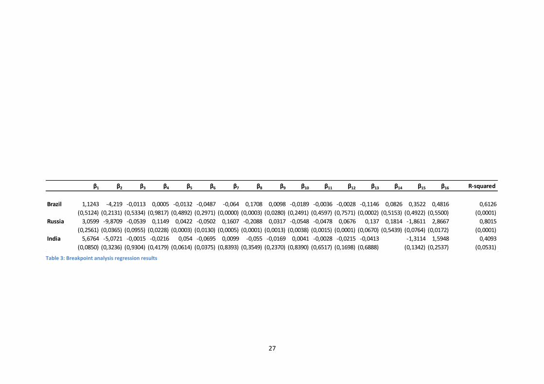
To determine the variables that have shifted, the model with the dummy variable is applied to the
data of Brazil, Russia and India. The result are shown in table 3. The betas and R-squared are
displayed with the corresponding p-values below them.
Chow Test US Brazil Russia India China
F-statistic 1,1292 3,2791 3,1261 2,3993 1,2232
(0,3589) (0,0059) (0,0153) (0,0379) (0,3185)
27
β1 β2 β3 β4 β5 β6 β7 β8 β9 β10 β11 β12 β13 β14 β15 β16 R-squared
Brazil 1,1243 -4,219 -0,0113 0,0005 -0,0132 -0,0487 -0,064 0,1708 0,0098 -0,0189 -0,0036 -0,0028 -0,1146 0,0826 0,3522 0,4816 0,6126
(0,5124) (0,2131) (0,5334) (0,9817) (0,4892) (0,2971) (0,0000) (0,0003) (0,0280) (0,2491) (0,4597) (0,7571) (0,0002) (0,5153) (0,4922) (0,5500) (0,0001)
Russia 3,0599 -9,8709 -0,0539 0,1149 0,0422 -0,0502 0,1607 -0,2088 0,0317 -0,0548 -0,0478 0,0676 0,137 0,1814 -1,8611 2,8667 0,8015
(0,2561) (0,0365) (0,0955) (0,0228) (0,0003) (0,0130) (0,0005) (0,0001) (0,0013) (0,0038) (0,0015) (0,0001) (0,0670) (0,5439) (0,0764) (0,0172) (0,0001)
India 5,6764 -5,0721 -0,0015 -0,0216 0,054 -0,0695 0,0099 -0,055 -0,0169 0,0041 -0,0028 -0,0215 -0,0413 -1,3114 1,5948 0,4093
(0,0850) (0,3236) (0,9304) (0,4179) (0,0614) (0,0375) (0,8393) (0,3549) (0,2370) (0,8390) (0,6517) (0,1698) (0,6888) (0,1342) (0,2537) (0,0531)
Table 3: Breakpoint analysis regression results
28
Concerning Brazil, the credit rating variable remains significantly negative and stable as seen in the
full time sample regression. However, the monetary policy variables have also become significant.
The interest rate and the interaction term of the interest rate and the dummy variable are both
significant, meaning the impact of the interest rate on the stock-bond return correlation changed
substantially. Notable, the interest rate variable in negative while the interaction term is positive and
larger in magnitude. This result implies a increase in the interest rate pushed the stock and bond
returns in the opposite direction before the financial crisis whereas after the financial crisis the
interest rate influences the stock-bond correlation in the same way. The money supply has a
constant positive impact on the stock-bond return correlation.
The addition of the interaction terms has huge implication for the result in Russia. All seven
explanatory variable and six out of seven interaction terms are significant. All the significant
interaction terms are the opposite sign of the corresponding variable and larger in magnitude. These
results suggest the financial crisis have largely impacted the relationships between the determinants
and the stock-bond return correlation. More specifically, the financial crisis has inverted the impact
of all variables excluding the credit rating variable. The credit rating influences the stock-bond return
correlation in a positive sense. This result doesn't correspond with Kelly et al. (1993). The industrial
production, VIX and political risk have a negative impact on the co-movements of the stock and bond
returns before the financial crisis and invert to a negative sign after. The opposite can be said about
the inflation rate, interest rate and money supply.
India has no significant determinants in the model for the full time sample regressions. After adding
the dummy variables, a significant link with the inflation rate emerges. Before the financial crisis, the
result indicate a positive relationship between the inflation rate and the stock-bond return
correlation. After the financial crisis the link becomes slightly negative.
8 Conclusion
This master's thesis investigates the influential factors of the large variations the stock-bond return
correlation. More specifically, a model is composed out of determinants which have proven to be
significant in previous stock-bond return correlation related research in develop countries as well as
emerging countries. The results are obtained by means of regression.
This master's thesis contributes to the existing literature in two ways. First, by testing the model on
the full time sample I want to provide new evidence to the little existing literature about stock-bond
return correlation in emerging countries. Second, as the majority of the related research assumes
constant relationships over time, I want to examine the possibility of time-varying relationships
29
induced by the unusual high economic growth witnessed in the BRIC countries. Furthermore, this
research discussed the course of the stock-bond return correlations of the BRIC countries in
perspective with the stock-bond return correlation in the US
The stock-bond return correlations in the BRIC countries exhibits large time variations. The stock-
bond return correlation of China hovers around zero while the stock-bond return correlation of
Brazil, Russia and India is positive for the majority of time. This is in stark contrast with the stock-
bond return correlation in the US which is negative for the majority of time. There is no converging
trend observed between the stock-bond return correlation in the US and the BRIC countries.
The empirical findings of the full time sample regressions show there doesn't exist a one size fits all
model for explaining the short-term variations in the stock-bond return correlations of the BRIC
countries. The model captures a significant part of the variation in Brazil and Russia but fails in
explaining a significant part in China and India. The credit rating has a negative impact on the stock-
bond return correlation in Brazil. In Russia, there are significant links found between the economic
growth, interest rate, money supply and VIX. None of the result found in the BRIC countries can be
compared with the result of the US.
To test the time-variance of the relationships a Chow test was applied with the financial crisis as
breakpoint. This point was chosen because a structural break in the economic growth is observed at
that moment. There are significant differences in the regression result before and after the financial
crisis for Brazil, Russia and India. The Chow test is has a insignificant result for China. The negative
link between the interest rate and stock-bond return correlation observed before the breakpoint
becomes negative in Brazil. Furthermore, the constant effect of the money supply and the credit
rating persist. Six out of the seven determinant have changed sign after the breakpoint in Russia
while a positive link the credit rating remained unchanged. Concerning India, the positive
relationship observed before the breakpoint is replaced by a negative relationship afterwards. These
larger differences before and after the financial crisis could indicate that the economic growth has an
impact on the relationships between the determinants and the stock-bond return correlation.
9 Recommendations for further research
In the process of putting together this master's thesis I stumbled upon two limitations while
collecting the data.
When gathering qualitative data about emerging countries the time sample narrows very quickly.
Due to this fact, the BRIC countries already experienced a large expansion of their economy before

30
the start date of the time samples. Access to larger databank or incorporating a larger part of the
transformation in research of other emerging countries could possibly lead to more accurate results.
The VIX measure of the concerned BRIC countries is purposely not used because this would limit the
time sample too much. As this measure is highly significant in the US in numerous researches,
including this measure could be very enriching for future research.
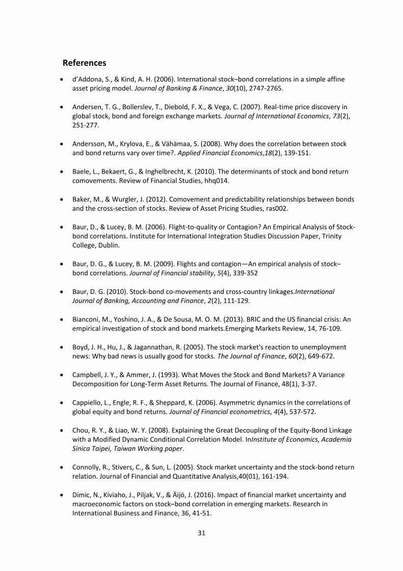
31
References
d’Addona, S., & Kind, A. H. (2006). International stock–bond correlations in a simple affine asset pricing model. Journal of Banking & Finance, 30(10), 2747-2765.
Andersen, T. G., Bollerslev, T., Diebold, F. X., & Vega, C. (2007). Real-time price discovery in global stock, bond and foreign exchange markets. Journal of International Economics, 73(2), 251-277.
Andersson, M., Krylova, E., & Vähämaa, S. (2008). Why does the correlation between stock and bond returns vary over time?. Applied Financial Economics,18(2), 139-151.
Baele, L., Bekaert, G., & Inghelbrecht, K. (2010). The determinants of stock and bond return comovements. Review of Financial Studies, hhq014.
Baker, M., & Wurgler, J. (2012). Comovement and predictability relationships between bonds and the cross-section of stocks. Review of Asset Pricing Studies, ras002.
Baur, D., & Lucey, B. M. (2006). Flight-to-quality or Contagion? An Empirical Analysis of Stock-bond correlations. Institute for International Integration Studies Discussion Paper, Trinity College, Dublin.
Baur, D. G., & Lucey, B. M. (2009). Flights and contagion—An empirical analysis of stock–bond correlations. Journal of Financial stability, 5(4), 339-352
Baur, D. G. (2010). Stock-bond co-movements and cross-country linkages.International Journal of Banking, Accounting and Finance, 2(2), 111-129.
Bianconi, M., Yoshino, J. A., & De Sousa, M. O. M. (2013). BRIC and the US financial crisis: An empirical investigation of stock and bond markets.Emerging Markets Review, 14, 76-109.
Boyd, J. H., Hu, J., & Jagannathan, R. (2005). The stock market's reaction to unemployment news: Why bad news is usually good for stocks. The Journal of Finance, 60(2), 649-672.
Campbell, J. Y., & Ammer, J. (1993). What Moves the Stock and Bond Markets? A Variance Decomposition for Long‐Term Asset Returns. The Journal of Finance, 48(1), 3-37.
Cappiello, L., Engle, R. F., & Sheppard, K. (2006). Asymmetric dynamics in the correlations of global equity and bond returns. Journal of Financial econometrics, 4(4), 537-572.
Chou, R. Y., & Liao, W. Y. (2008). Explaining the Great Decoupling of the Equity-Bond Linkage with a Modified Dynamic Conditional Correlation Model. InInstitute of Economics, Academia Sinica Taipei, Taiwan Working paper.
Connolly, R., Stivers, C., & Sun, L. (2005). Stock market uncertainty and the stock-bond return relation. Journal of Financial and Quantitative Analysis,40(01), 161-194.
Dimic, N., Kiviaho, J., Piljak, V., & Äijö, J. (2016). Impact of financial market uncertainty and macroeconomic factors on stock–bond correlation in emerging markets. Research in International Business and Finance, 36, 41-51.

32
Durand, R. B., Junker, M., & Szimayer, A. (2010). The flight‐to‐quality effect: a copula‐based analysis. Accounting & Finance, 50(2), 281-299.
Harumi, O. H. M. I., & Tatsuyoshi, O. K. I. M. O. T. O. (2015). Trends in Stock-Bond Correlations (No. 15115).
Ilmanen, A. (2003). Stock-bond correlations. The Journal of Fixed Income,13(2), 55-66.
Jammazi R. , Kr. Tiwari A. , Ferrer R. , Moya P. (2015). Time-varying dependence between stock and government bond returns: International evidence with dynamic copulas. The North American Journal of Economics and Finance, 33(3), 74-93
Garcia, R., & Tsafack, G. (2011). Dependence structure and extreme comovements in international equity and bond markets. Journal of Banking & Finance, 35(8), 1954-1970.
Kelly, J. M., Martins, L. F., & Carlson, J. H. (1998). The relationship between bonds and stocks in emerging countries. The Journal of Portfolio Management,24(3), 110-122.
Kim, S. J., Moshirian, F., & Wu, E. (2006). Evolution of international stock and bond market integration: Influence of the European Monetary Union. Journal of Banking & Finance, 30(5), 1507-1534.
Kim, S., & In, F. (2007). On the relationship between changes in stock prices and bond yields in the G7 countries: Wavelet analysis. Journal of International Financial Markets, Institutions and Money, 17(2), 167-179.
Li, L, (2002). Macroeconomic Factors and the Correlation of Stock and Bond Returns, Yale ICF Working Paper 02-46
Li, X. M., & Zou, L. P. (2008). How do policy and information shocks impact co-movements of China’s T-bond and stock markets?. Journal of Banking & Finance, 32(3), 347-359.
Panchenko, V., & Wu, E. (2009). Time-varying market integration and stock and bond return concordance in emerging markets. Journal of Banking & Finance, 33(6), 1014-1021.
Shiller, R. J., & Beltratti, A. E. (1992). Stock prices and bond yields: Can their comovements be explained in terms of present value models?. Journal of Monetary Economics, 30(1), 25-46.
Yang, J., Zhou, Y., & Wang, Z. (2009). The stock–bond correlation and macroeconomic conditions: one and a half centuries of evidence. Journal of Banking & Finance, 33(4), 670-680.
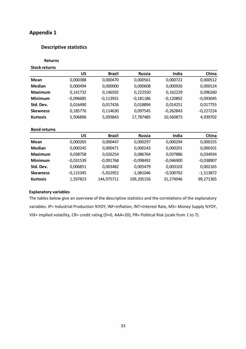
33
Appendix 1
Descriptive statistics
Returns
Explanatory variables
The tables below give an overview of the descriptive statistics and the correlations of the explanatory
variables. IP= Industrial Production %YOY, INF=Inflation, INT=Interest Rate, MS= Money Supply %YOY,
VIX= implied volatility, CR= credit rating (D=0, AAA=20), PR= Political Risk (scale from 1 to 7).
US Brazil Russia India China
Mean 0,000388 0,000470 0,000561 0,000722 0,000512
Median 0,000494 0,000000 0,000608 0,000926 0,000124
Maximum 0,141732 0,146592 0,222550 0,162229 0,096260
Minimum -0,096685 -0,113931 -0,181186 -0,120892 -0,093045
Std. Dev. 0,016490 0,017426 0,018894 0,014251 0,017755
Skewness 0,185776 0,114630 0,097545 -0,262843 -0,227224
Kurtosis 5,506896 5,093843 17,787485 10,560873 4,939702
Bond returns
US Brazil Russia India China
Mean 0,000265 0,000447 0,000297 0,000294 0,000155
Median 0,000245 0,000471 0,000243 0,000201 0,000101
Maximum 0,038758 0,026254 0,086764 0,037886 0,034934
Minimum -0,031539 -0,091768 -0,098492 -0,046900 -0,038907
Std. Dev. 0,006851 0,003482 0,005479 0,003103 0,002165
Skewness -0,115345 -5,652952 -1,081046 -0,500702 -1,513872
Kurtosis 1,597823 144,975711 109,205156 31,274946 99,271365
Stock returns

34
US
IP INF INT MS VIX CR PR
Mean 1,27 1,97 1,90 6,44 21,01 19,84 5,94
Median 2,45 1,93 1,09 6,21 19,34 19,89 5,92
Maximum 7,23 3,39 6,21 10,14 58,61 20,00 6,21
Minimum -14,90 0,20 -0,01 1,96 11,05 19,67 5,75
Std. Dev. 4,24 0,72 2,04 1,81 8,05 0,11 0,15
Skewness -2,09 -0,02 0,70 -0,06 1,94 -0,81 0,59
Kurtosis 4,88 -0,07 -1,03 0,16 6,44 -0,75 -1,05
IP 1
INF 0,25 1
INT 0,23 0,51 1
MS -0,49 -0,19 -0,09 1
VIX -0,52 -0,34 -0,10 0,44 1
CR -0,09 0,22 0,42 -0,35 0,24 1
PR 0,12 0,27 0,72 0,05 0,18 0,49 1
Descriptive Statistics
Correlations
Brazil
IP INF INT MS VIX CR PR
Mean 1,55 8,21 13,69 15,76 20,18 9,81 3,88
Median 1,82 7,78 12,29 14,91 17,49 10,67 3,89
Maximum 17,39 15,11 27,97 38,90 58,61 12,00 4,22
Minimum -14,14 3,93 7,14 3,25 11,05 6,33 3,33
Std. Dev. 5,88 2,11 4,37 7,73 8,69 2,00 0,18
Skewness -0,19 1,58 0,92 1,10 2,21 -0,52 -1,02
Kurtosis 0,80 3,24 0,84 1,59 6,70 -1,26 3,03
IP 1
INF -0,08 1
INT 0,14 0,53 1
MS -0,11 0,04 0,16 1
VIX -0,27 0,27 0,04 0,63 1
CR -0,29 -0,45 -0,87 -0,08 0,02 1
PR 0,34 0,57 0,42 0,14 0,20 -0,55 1
Descriptive Statistics
Correlations
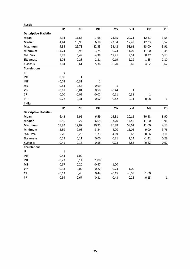
35
Russia
IP INF INT MS VIX CR PR
Mean 2,94 11,66 7,68 24,35 20,21 12,31 3,55
Median 4,44 10,96 6,78 22,54 17,49 12,33 3,52
Maximum 9,88 25,73 22,33 53,42 58,61 13,00 3,91
Minimum -14,74 -0,98 3,75 -10,73 11,05 11,00 3,45
Std. Dev. 5,77 6,49 4,39 17,21 9,51 0,37 0,13
Skewness -1,76 0,28 2,31 -0,19 2,29 -1,55 2,10
Kurtosis 3,04 -0,61 5,36 -0,70 6,69 4,02 3,62
IP 1
INF 0,50 1
INT -0,74 -0,31 1
MS 0,84 0,56 -0,69 1
VIX -0,61 -0,01 0,58 -0,44 1
CR 0,00 -0,02 -0,02 0,11 0,31 1
PR -0,22 -0,31 0,52 -0,42 -0,11 -0,08 1
Correlations
Descriptive Statistics
India
IP INF INT MS VIX CR PR
Mean 6,42 5,95 6,59 13,81 20,12 10,58 3,90
Median 6,56 5,27 6,65 13,20 17,46 11,00 3,91
Maximum 18,92 12,87 10,95 26,78 58,61 11,00 4,13
Minimum -5,89 -2,03 3,24 4,20 11,05 9,00 3,76
Std. Dev. 5,20 3,25 1,73 4,69 8,62 0,66 0,11
Skewness 0,13 0,11 0,00 0,31 2,24 -1,41 0,29
Kurtosis -0,41 -0,16 -0,58 -0,23 6,88 0,62 -0,67
IP 1
INF 0,44 1,00
INT -0,23 0,14 1,00
MS 0,67 0,20 -0,47 1,00
VIX -0,33 0,02 -0,22 -0,24 1,00
CR -0,13 0,40 0,44 -0,15 -0,05 1,00
PR 0,59 0,67 -0,31 0,43 0,28 0,15 1
Descriptive Statistics
Correlations
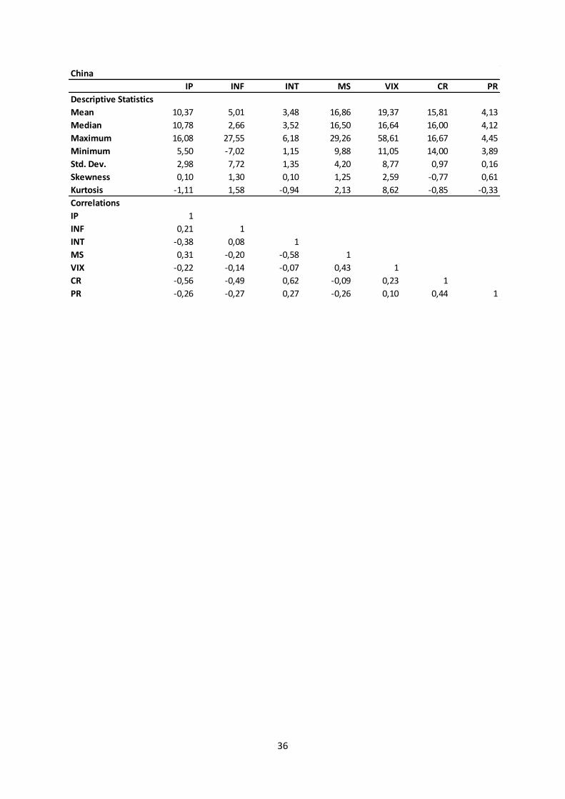
36
China
IP INF INT MS VIX CR PR
Descriptive Statistics
Mean 10,37 5,01 3,48 16,86 19,37 15,81 4,13
Median 10,78 2,66 3,52 16,50 16,64 16,00 4,12
Maximum 16,08 27,55 6,18 29,26 58,61 16,67 4,45
Minimum 5,50 -7,02 1,15 9,88 11,05 14,00 3,89
Std. Dev. 2,98 7,72 1,35 4,20 8,77 0,97 0,16
Skewness 0,10 1,30 0,10 1,25 2,59 -0,77 0,61
Kurtosis -1,11 1,58 -0,94 2,13 8,62 -0,85 -0,33
IP 1
INF 0,21 1
INT -0,38 0,08 1
MS 0,31 -0,20 -0,58 1
VIX -0,22 -0,14 -0,07 0,43 1
CR -0,56 -0,49 0,62 -0,09 0,23 1
PR -0,26 -0,27 0,27 -0,26 0,10 0,44 1
Correlations
Related Documents