IS PROTEIN FOLDING PROBLEM REALLY A NP-COMPLETE ONE? FIRST INVESTIGATIONS

arX

iv:1

306.

1372

v1 [

q-bi

o.B

M]

6 J

un 2

013

Is protein folding problem really a NP-complete one ?

First investigations

Jacques M. Bahia, Wojciech Bieniac, Nathalie Coteb, Christophe Guyeuxa,1,∗

aFEMTO-ST Institute, UMR 6174 CNRS, University of Franche-Comte, Besancon, FrancebLaboratoire de Biologie du Developpement, UMR 7622, Universite Pierre et Marie Curie,

Paris, FrancecG-SCOP Laboratory, ENSIMAG, 46 av. Felix Viallet, F-38031 Grenoble Cedex 1, France

Abstract

To determine the 3D conformation of proteins is a necessity to understand their

functions or interactions with other molecules. It is commonly admitted that,

when proteins fold from their primary linear structures to their final 3D confor-

mations, they tend to choose the ones that minimize their free energy. To find

the 3D conformation of a protein knowing its amino acid sequence, bioinfor-

maticians use various models of different resolutions and artificial intelligence

tools, as the protein folding prediction problem is a NP complete one. More

precisely, to determine the backbone structure of the protein using the low

resolution models (2D HP square and 3D HP cubic), by finding the conforma-

tion that minimize free energy, is intractable exactly [6]. Both the proof of

NP-completeness and the 2D prediction consider that acceptable conformations

have to satisfy a self-avoiding walk (SAW) requirement, as two different amino

acids cannot occupy a same position in the lattice. It is shown in this document

that the SAW requirement considered when proving NP-completeness is differ-

ent from the SAW requirement used in various prediction programs, and that

they are different from the real biological requirement. Indeed, the proof of NP

completeness and the predictions in silico consider conformations that are not

possible in practice. Consequences of this fact are investigated in this research

∗Corresponding author1Authors in alphabetic order

Preprint submitted to Elsevier June 7, 2013

work.

Keywords: Protein folding problem, Self-Avoiding Walk requirement,

NP-completeness, Graph theory, Pivot moves

1. Introduction

Proteins are polymers formed by different kinds of amino acids. During or

after proteins have been synthesized by ribosomes, they fold to form a specific

tridimensional shape. This 3D geometric pattern defines their biological func-

tionality, properties, and so on. For instance, the hemoglobin is able to carry

oxygen to the blood stream thanks to its 3D conformation. However, contrary

to the mapping from DNA to the amino acids sequence, the complex folding

of this sequence is not yet understood. In fact, Anfinsen’s “Thermodynamic

Hypothesis” claims that the chosen 3D conformation corresponds to the lowest

free energy minimum of the considered protein [2]. Efficient constraint pro-

gramming methods can solve the problem for reasonably sized sequences [14].

But the conformation that minimizes this free energy is most of the time im-

possible to find in practice, at least for large proteins, due to the number of

possible conformations. Indeed the Protein Structure Prediction (PSP) prob-

lem is a NP-complete one [11, 6]. This is why conformations of proteins are

predicted : the 3D structures that minimize the free energy of the protein under

consideration are found by using computational intelligence tools like genetic

algorithms [16], ant colonies [26], particle swarm [23], memetic algorithms [19],

constraint programming [14, 22], or neural networks [15], etc. These computa-

tional intelligence tools are coupled with protein energy models (like AMBER,

DISCOVER, or ECEPP/3) to find a conformation that approximately minimize

the free energy of a given protein. Furthermore, to face the complexity of the

PSP problem, authors who try to predict the protein folding process use mod-

els of various resolutions. For instance, in coarse grain, single-bead models, an

amino acid is considered as a single bead, or point. These low resolution models

are often used as the first stage of the 3D structure prediction: the backbone

2

of the 3D conformation is determined. Then, high resolution models come next

for further exploration. Such a prediction strategy is commonly used in PSP

softwares like ROSETTA [7, 10] or TASSER [28].

In this paper, which is a supplement of [4, 5], we investigate the 2D HP square

lattice model. Let us recall that this popular model is used to test methods

and as a first 2D HP lattice folding stage in some protein folding prediction

algorithms [16, 9, 20, 27, 18]. It focuses only on hydrophobicity by separating

the amino acids into two sets: hydrophobic (H) and hydrophilic (or polar P) [13].

These amino acids occupy vertices of a square lattice, and the 2D low resolution

conformation of the given protein is thus represented by a self avoiding walk

(SAW) on this lattice. Variations of this model are frequently investigated:

2D or 3D lattices, with square, cubic, triangular, or face-centered-cube shapes.

However, at each time, a SAW requirement for the targeted conformation is

required. The PSP problem takes place in that context: given a sequence of

hydrophobic and hydrophilic amino acids, to find the self avoiding walk on the

lattice that maximizes the number of hydrophobic neighbors is a NP complete

problem [11].

We will show in this document that this SAW requirement can be under-

stood in various different ways, even in the 2D square lattice model. The first

understanding of this requirement in the 2D model, called SAW1 in the remain-

der of this paper, has been chosen by authors of [11] when they have established

the proof of NP-completeness for the PSP problem. It corresponds to the fa-

mous “excluded volume” requirement, and it has been already well-studied by

the discrete mathematics community (see, for instance, the book of Madras and

Slade [21]). It possesses a dynamical formulation we call it SAW2 in this doc-

ument. The SAW3 set is frequently chosen by bioinformaticians when they try

to predict the backbone conformation of proteins using a low resolution model.

Finally, the last one proposed here is perhaps the most realistic one, even if

it still remains far from the biological folding operation. We will demonstrate

that these four sets are not equal. In particular, we will establish that SAW4

is strictly included into SAW3, which is strictly included into SAW1 = SAW2.

3

So the NP-completeness proof has been realized in a strictly larger set than

the one used for prediction, which is strictly larger than the set of biologically

possible conformations. Concrete examples of 2D conformations that are in a

SAWi without being in another SAWj will be given, and characterizations of

these sets, in terms of graphs, will finally be proposed.

The remainder of this paper is structured as follows. In the next section

we recall some notations and terminologies on the 2D HP square lattice model,

chosen here to simplify explanations. In Section 3, the dynamical system used

to describe the folding process in the 2D model, initially presented in [4, 5], is

recalled. In Sect. 4, various ways to understand the so-called self-avoiding walk

(SAW) requirement are detailed. Their relations and inclusions are investigated

in the next section. Section 6 presents a graph approach to determine the size

ratios between the four SAW requirements defined previously, and the conse-

quences of their strict inclusions are discussed. This paper ends by a conclusion

section, in which our contribution is summarized and intended future work is

presented.

2. Background

In the sequel Sn denotes the nth term of a sequence S and Vi the ith com-

ponent of a vector V . The kth composition of a single function f is repre-

sented by fk = f ◦ ... ◦ f . The set of congruence classes modulo 4 is denoted

as Z/4Z. Finally, given two integers a < b, the following notation is used:

Ja; bK = {a, a+ 1, . . . , b}.

2.1. 2D Hydrophilic-Hydrophobic (HP) Model

In the HP model, hydrophobic interactions are supposed to dominate pro-

tein folding. This model was formerly introduced by Dill, who consider in [13]

that the protein core freeing up energy is formed by hydrophobic amino acids,

whereas hydrophilic amino acids tend to move in the outer surface due to their

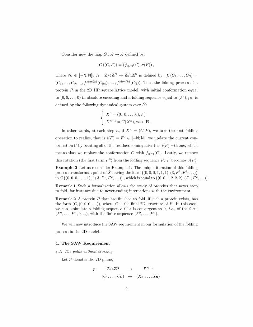
affinity with the solvent (see Fig. 1).

4

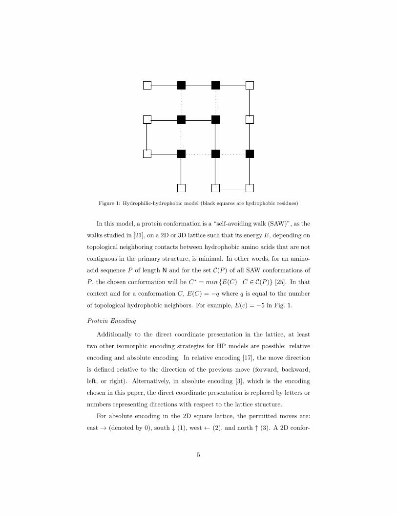
Figure 1: Hydrophilic-hydrophobic model (black squares are hydrophobic residues)

In this model, a protein conformation is a “self-avoiding walk (SAW)”, as the

walks studied in [21], on a 2D or 3D lattice such that its energy E, depending on

topological neighboring contacts between hydrophobic amino acids that are not

contiguous in the primary structure, is minimal. In other words, for an amino-

acid sequence P of length N and for the set C(P ) of all SAW conformations of

P , the chosen conformation will be C∗ = min {E(C) | C ∈ C(P )} [25]. In that

context and for a conformation C, E(C) = −q where q is equal to the number

of topological hydrophobic neighbors. For example, E(c) = −5 in Fig. 1.

Protein Encoding

Additionally to the direct coordinate presentation in the lattice, at least

two other isomorphic encoding strategies for HP models are possible: relative

encoding and absolute encoding. In relative encoding [17], the move direction

is defined relative to the direction of the previous move (forward, backward,

left, or right). Alternatively, in absolute encoding [3], which is the encoding

chosen in this paper, the direct coordinate presentation is replaced by letters or

numbers representing directions with respect to the lattice structure.

For absolute encoding in the 2D square lattice, the permitted moves are:

east → (denoted by 0), south ↓ (1), west ← (2), and north ↑ (3). A 2D confor-

5

mation C of N+1 residues for a protein P is then an element C of Z/4ZN, with

a first component equal to 0 (east) [17]. For instance, in Fig. 1, the 2D abso-

lute encoding is 00011123322101 (starting from the upper left corner), whereas

001232 corresponds to the following path in the square lattice: (0,0), (1,0),

(2,0), (2,-1), (1,-1), (1,0), (0,0). In that situation, at most 4N conformations are

possible when considering N + 1 residues, even if some of them invalidate the

SAW requirement as defined in [21].

3. A Dynamical System for the 2D HP Square Lattice Model

Protein minimum energy structure can be considered statistically or dynam-

ically. In the latter case, one speaks in this article of “protein folding”. We recall

here how to model the folding process in the 2D model, or pivot moves, as a

dynamical system. Readers are referred to [4, 5] for further explanations and to

investigate the dynamical behavior of the proteins pivot moves in this 2D model

(it is indeed proven to be chaotic, as defined by Devaney [12]).

3.1. Initial Premises

Let us start with preliminaries introducing some concepts that will be useful

in our approach.

The primary structure of a given protein P with N+ 1 residues is coded by

00 . . .0 (N times) in absolute encoding. Its final 2D conformation has an absolute

encoding equal to 0C∗1 . . . C

∗N−1, where ∀i, C

∗i ∈ Z/4Z, is such that E(C∗) =

min{

E(C)/

C ∈ C(P )}

. This final conformation depends on the repartition of

hydrophilic and hydrophobic amino acids in the initial sequence.

Moreover, we suppose that, if the residue number n+ 1 is at the east of the

residue number n in absolute encoding (→) and if a fold (pivot move) occurs

after n, then the east move can only by changed into north (↑) or south (↓).

That means, in our simplistic model, only rotations or pivot moves of +π2 or

−π2 are possible.

Consequently, for a given residue that has to be updated, only one of the two

possibilities below can appear for its absolute encoding during a pivot move:

6

• 0 7−→ 1 (that is, east becomes north), 1 7−→ 2, 2 7−→ 3, or 3 7−→ 0 for a

pivot move in the clockwise direction, or

• 1 7−→ 0, 2 7−→ 1, 3 7−→ 2, or 0 7−→ 3 for an anticlockwise.

This fact leads to the following definition:

Definition 1 The clockwise fold function is the function f : Z/4Z −→ Z/4Zdefined by f(x) = x+ 1 (mod 4).

Obviously the anticlockwise fold function is f−1(x) = x− 1 (mod 4).

Thus at the nth folding time, a residue k is chosen and its absolute move is

changed by using either f or f−1. As a consequence, all of the absolute moves

must be updated from the coordinate k until the last one N by using the same

folding function.

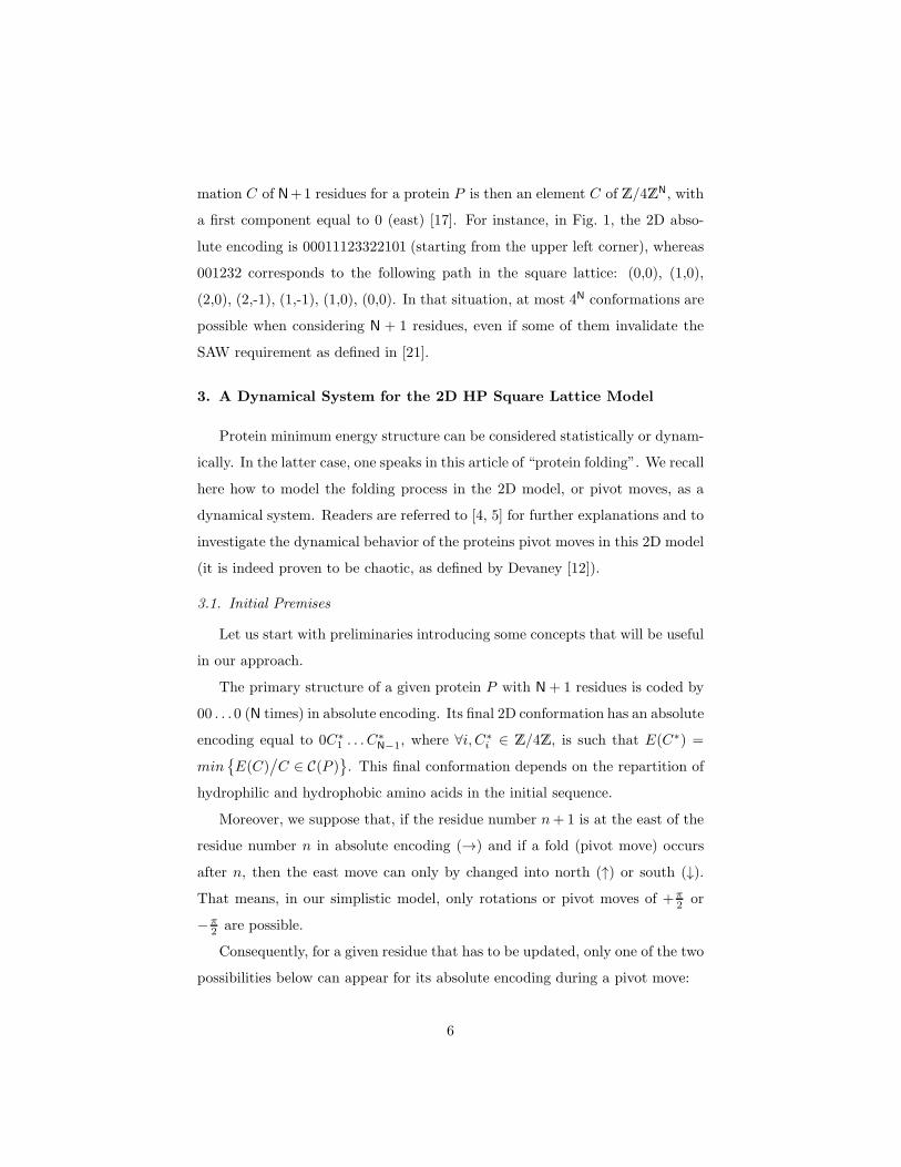
Example 1 If the current conformation is C = 000111, i.e.,

and if the third residue is chosen to fold (pivot move) by a rotation of −π2

(mapping f), the new conformation will be (C1, C2, f(C3), f(C4), f(C5), f(C6)),which is (0, 0, 1, 2, 2, 2). That is,

These considerations lead to the formalization described thereafter.

3.2. Formalization and Notations

Let N + 1 be a fixed number of amino acids, where N ∈ N∗ = {1, 2, 3, . . .}.

We define

X = Z/4ZN × J−N;NKN

7

as the phase space of all possible folding processes. An element X = (C,F ) of

this dynamical folding space is constituted by:

• A conformation of the N+1 residues in absolute encoding: C = (C1, . . . , CN) ∈

Z/4ZN. Note that we do not require self-avoiding walks here.

• A sequence F ∈ J−N;NKN of future pivot moves such that, when Fi ∈

J−N;NK is k, it means that it occurs:

– a pivot move after the k−th residue by a rotation of −π2 (mapping

f) at the i−th step, if k = Fi > 0,

– no fold at time i if k = 0,

– a pivot move after the |k|−th residue by a rotation of π2 (i.e., f−1)

at the i−th time, if k < 0.

On this phase space, the protein folding dynamic in the 2D model can be for-

malized as follows.

Denote by i the map that transforms a folding sequence in its first term (i.e.,

in the first folding operation):

i : J−N;NKN −→ J−N;NK

F 7−→ F 0,

by σ the shift function over J−N;NKN, that is to say,

σ : J−N;NKN −→ J−N;NKN

(

F k)

k∈N7−→

(

F k+1)

k∈N,

and by sign the function:

sign(x) =

1 if x > 0,

0 if x = 0,

−1 else.

Remark that the shift function removes the first folding operation (a pivot move)

from the folding sequence F once it has been achieved.

8

Consider now the map G : X → X defined by:

G ((C,F )) =(

fi(F )(C), σ(F ))

,

where ∀k ∈ J−N;NK, fk : Z/4ZN → Z/4ZN is defined by: fk(C1, . . . , CN) =

(C1, . . . , C|k|−1, fsign(k)(C|k|), . . . , f

sign(k)(CN)). Thus the folding process of a

protein P in the 2D HP square lattice model, with initial conformation equal

to (0, 0, . . . , 0) in absolute encoding and a folding sequence equal to (F i)i∈N, is

defined by the following dynamical system over X :

X0 = ((0, 0, . . . , 0), F )

Xn+1 = G(Xn), ∀n ∈ N.

In other words, at each step n, if Xn = (C,F ), we take the first folding

operation to realize, that is i(F ) = F 0 ∈ J−N;NK, we update the current con-

formation C by rotating all of the residues coming after the |i(F )|−th one, which

means that we replace the conformation C with fi(F )(C). Lastly, we remove

this rotation (the first term F 0) from the folding sequence F : F becomes σ(F ).

Example 2 Let us reconsider Example 1. The unique iteration of this foldingprocess transforms a point of X having the form

(

(0, 0, 0, 1, 1, 1); (3, F 1, F 2, . . .))

inG(

(0, 0, 0, 1, 1, 1), (+3, F 1, F 2, . . .))

, which is equal to(

(0, 0, 1, 2, 2, 2), (F 1, F 2, . . .))

.

Remark 1 Such a formalization allows the study of proteins that never stopto fold, for instance due to never-ending interactions with the environment.

Remark 2 A protein P that has finished to fold, if such a protein exists, hasthe form (C, (0, 0, 0, . . .)), where C is the final 2D structure of P . In this case,we can assimilate a folding sequence that is convergent to 0, i.e., of the form(F 0, . . . , Fn, 0 . . .), with the finite sequence (F 0, . . . , Fn).

We will now introduce the SAW requirement in our formulation of the folding

process in the 2D model.

4. The SAW Requirement

4.1. The paths without crossing

Let P denotes the 2D plane,

p : Z/4ZN → PN+1

(C1, . . . , CN) 7→ (X0, . . . , XN)

9

where X0 = (0, 0), and

Xi+1 =

Xi + (1, 0) if ci = 0,

Xi + (0,−1) if ci = 1,

Xi + (−1, 0) if ci = 2,

Xi + (0, 1) if ci = 3.

The map p transforms an absolute encoding in its 2D representation. For

instance, p((0, 0, 0, 1, 1, 1)) is ((0,0);(1,0);(2,0);(3,0);(3,-1);(3,-2);(3,-3)), that is,

the first figure of Example 1.

Now, for each (P0, . . . , PN) of PN+1, we denote by

support((P0, . . . , PN))

the set (without repetition): {P0, . . . , PN}. For instance,

support ((0, 0); (0, 1); (0, 0); (0, 1)) = {(0, 0); (0, 1)} .

Then,

Definition 2 A conformation (C1, . . . , CN) ∈ Z/4ZN is a path without crossingiff the cardinality of support(p((C1, . . . , CN))) is N+ 1.

This path without crossing is sometimes referred as “excluded volume” re-

quirement in the literature. It only means that no vertex can be occupied by

more than one protein monomer. We can finally remark that Definition 2 con-

cerns only one conformation, and not a sequence of conformations that occurs

in a folding process.

4.2. Defining the SAW Requirements in the 2D model

The next stage in the formalization of the protein folding process in the

2D model as a dynamical system is to take into account the self-avoiding walk

(SAW) requirement, by restricting the set Z/4ZN of all possible conformations

to one of its subset. That is, to define precisely the set C(P ) of acceptable

conformations of a protein P having N + 1 residues. This stage needs a clear

definition of the SAW requirement. However, as stated above, Definition 2 only

10

focus on a given conformation, but not on a complete folding process. In our

opinion, this requirement applied to the whole folding process can be understood

at least in four ways.

In the first and least restrictive approach, we call it “SAW1”, we only require

that the studied conformation satisfies the Definition 2.

Definition 3 (SAW1) A conformation c ofZ/4ZN satisfies the first self-avoidingwalk requirement (c ∈ SAW1(N)) if this conformation is a path without cross-ing.

It is not regarded whether this conformation is the result of a folding process

that has started from (0, 0, . . . , 0). Such a SAW requirement has been chosen by

authors of [11] when they have proven the NP-completeness of the PSP problem.

It is usually the SAW requirement of biomathematicians, corresponding to the

self-avoiding walks studied in the book of Madras and Slade [21]. It is easy to

convince ourselves that conformations of SAW1 are the conformations that can

be obtained by any chain growth algorithm, like in [8].

As stated before, protein minimum energy structure can be considered stati-

cally or dynamically. In the latter case, we speak here of “protein folding”, since

this concerns the dynamic process of folding. When folding on a lattice model,

there is an underlying algorithm, such as Monte Carlo or genetic algorithm,

and an allowed move set. In the following, for the sake of simplicity, only pivot

moves are investigated, but the corner and crankshaft moves should be further

investigated [24].

Basically, in the protein folding literature, there are methods that require the

“excluded volume” condition during the dynamic folding procedure, and those

that do not require this condition. This is why the second proposed approach

called SAW2 requires that, starting from the initial condition (0, 0, . . . , 0), we

obtain by a succession of pivot moves a final conformation being a path without

crossing. In other words, we want that the final tree corresponding to the true

2D conformation has 2 vertices with 1 edge and N − 2 vertices with 2 edges.

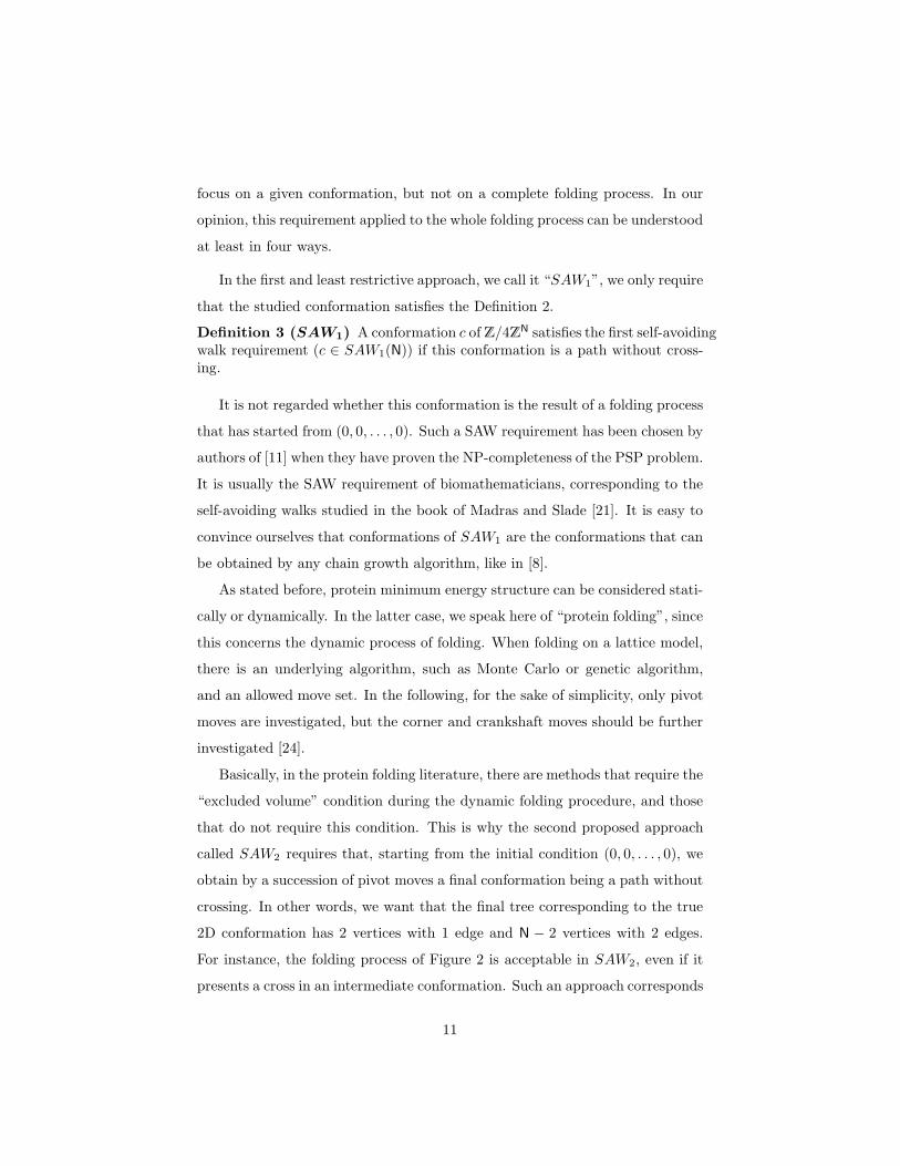
For instance, the folding process of Figure 2 is acceptable in SAW2, even if it

presents a cross in an intermediate conformation. Such an approach corresponds

11

Figure 2: Folding process acceptable in SAW2 but not in SAW3. The folding sequence (-4,-3,-2,+4), having 3 anticlockwise and 1 clockwise pivot moves, is applied here on the conformation0000 represented as the upper line.

to programs that start from the initial conformation (0, 0, . . . , 0), fold it several

times according to their embedding functions, and then obtain a final confor-

mation on which the SAW property is checked: only the last conformation has

to satisfy the Definition 2. More precisely,

Definition 4 (SAW2) A conformation c of Z/4ZN satisfies the second self-avoiding walk requirement SAW2 if c ∈ SAW1(N) and a finite sequence (F 1, F 2, . . . , Fn)of J−N,NK can be found such that

(c, (0, 0, . . .)) = Gn(

(0, 0, . . . , 0),(

F 1, F 2, . . . , Fn, 0, . . .))

.

SAW2(N) will denote the set of all conformations satisfying this requirement.

In the next approach, namely the SAW3 requirement, it is demanded that

each intermediate conformation, between the initial one and the returned (final)

one, satisfies the Definition 2. It restricts the set of all conformations Z/4ZN, for

a given N, to the subset CN of conformations (C1, . . . , CN) such that ∃n ∈ N∗,

∃k1, . . . , kn ∈ J−N;NK,

(C1, . . . , CN) = Gn ((0, 0, . . . , 0); (k1, . . . , kn))

and ∀i 6 n, the conformation Gi ((0, . . . , 0); (k1, . . . , kn)) is a path without

crossing. Let us define it,

12

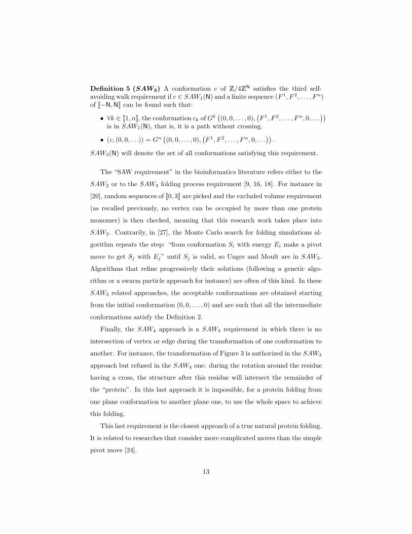
Definition 5 (SAW3) A conformation c of Z/4ZN satisfies the third self-avoiding walk requirement if c ∈ SAW1(N) and a finite sequence (F 1, F 2, . . . , Fn)of J−N,NK can be found such that:

• ∀k ∈ J1, nK, the conformation ck ofGk(

(0, 0, . . . , 0),(

F 1, F 2, . . . , Fn, 0, . . .))

is in SAW1(N), that is, it is a path without crossing.

• (c, (0, 0, . . .)) = Gn(

(0, 0, . . . , 0),(

F 1, F 2, . . . , Fn, 0, . . .))

.

SAW3(N) will denote the set of all conformations satisfying this requirement.

The “SAW requirement” in the bioinformatics literature refers either to the

SAW2 or to the SAW3 folding process requirement [9, 16, 18]. For instance in

[20], random sequences of J0, 3K are picked and the excluded volume requirement

(as recalled previously, no vertex can be occupied by more than one protein

monomer) is then checked, meaning that this research work takes place into

SAW2. Contrarily, in [27], the Monte Carlo search for folding simulations al-

gorithm repeats the step: “from conformation Si with energy Ei make a pivot

move to get Sj with Ej” until Sj is valid, so Unger and Moult are in SAW3.

Algorithms that refine progressively their solutions (following a genetic algo-

rithm or a swarm particle approach for instance) are often of this kind. In these

SAW3 related approaches, the acceptable conformations are obtained starting

from the initial conformation (0, 0, . . . , 0) and are such that all the intermediate

conformations satisfy the Definition 2.

Finally, the SAW4 approach is a SAW3 requirement in which there is no

intersection of vertex or edge during the transformation of one conformation to

another. For instance, the transformation of Figure 3 is authorized in the SAW3

approach but refused in the SAW4 one: during the rotation around the residue

having a cross, the structure after this residue will intersect the remainder of

the “protein”. In this last approach it is impossible, for a protein folding from

one plane conformation to another plane one, to use the whole space to achieve

this folding.

This last requirement is the closest approach of a true natural protein folding.

It is related to researches that consider more complicated moves than the simple

pivot move [24].

13

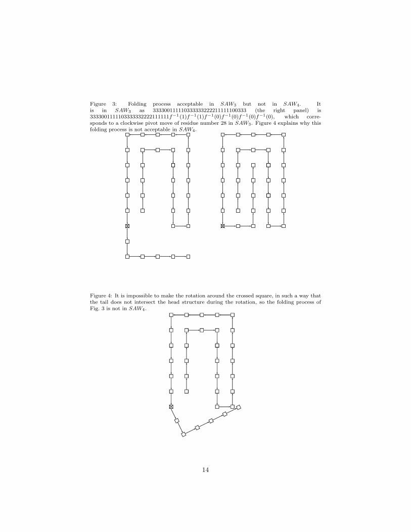
Figure 3: Folding process acceptable in SAW3 but not in SAW4. Itis in SAW3 as 333300111110333333222211111100333 (the right panel) is3333001111103333332222111111f−1 (1)f−1(1)f−1(0)f−1(0)f−1(0)f−1(0), which corre-sponds to a clockwise pivot move of residue number 28 in SAW3. Figure 4 explains why thisfolding process is not acceptable in SAW4.

Figure 4: It is impossible to make the rotation around the crossed square, in such a way thatthe tail does not intersect the head structure during the rotation, so the folding process ofFig. 3 is not in SAW4.

14

5. Relations between the SAW requirements

For i ∈ {1, 2, 3, 4}, the set⋃

n∈N∗

SAWi(n) will be simply written SAWi. The

following inclusions hold obviously:

SAW4 ⊆ SAW3 ⊆ SAW2 ⊆ SAW1

due to the definitions of the SAW requirements presented in the previous section.

Additionally, Figure 3 shows that SAW4 6= SAW3, thus we have,

Proposition 1 SAW4 ( SAW3 ⊆ SAW2 ⊆ SAW1.

Let us investigate more precisely the links between SAW1, SAW2, and SAW3.

5.1. SAW1 is SAW2

Let us now prove that,

Proposition 2 ∀n ∈ N, SAW1(n) = SAW2(n).

Proof We need to prove that SAW1(n) ⊂ SAW2(n), i.e., that any conforma-tion of SAW1(n) can be obtained from (0, 0, .., 0) by operating a sequence of(anti)clockwise pivot moves.

Obviously, to start from the conformation (0, 0, .., 0) is equivalent than tostart with the conformation (c, c, ..., c), where c ∈ {0, 1, 2, 3}. Thus the initialconfiguration is characterized by the absence of a change in the values (theinitial sequence is a constant one).

We will now prove the result by a mathematical induction on the number kof changes in the sequence.

• The base case is obvious, as the 4 conformations with no change are inSAW1(n) ∩ SAW2(n).

• Let us suppose that the statement holds for some k > 1. Let c =(c1, c2, ..., cn) be a conformation having exactly k changes, that is, thecardinality of the set D(c) =

{

i ∈ J1, n− 1K/

ci+1 6= ci}

is k. Let us de-note by p(c) the first change in this sequence: p(c) = min {D(c)}. Wecan apply the folding operation that suppress the difference between cp(c)and cp(c)+1. For instance, if cp(c)+1 = cp(c) − 1 (mod 4), then a clockwisepivot move on position cp(c)+1 will remove this difference. So the con-

formation c′ =(

c1, c2, . . . , cp(c), f(

cp(c)+1

)

, . . . , f(cn))

has k − 1 changes.By the induction hypothesis, c′ can be obtained from (j, j, j, . . . , j), wherej ∈ {0, 1, 2, 3} by a succession of clockwise and anticlockwise pivot move.We can conclude that it is the case for c too.

15

Indeed the notion of “pivot moves” is well-known in the literature on protein

folding. It was already supposed that pivot moves provide an ergodic move set,

meaning that by a sequence of pivot moves one can transform any conformation

into any other conformation, when only requiring that the ending conformation

satisfies the excluded volume requirement. The contribution of this section is

simply a rigorous proof of such an assumption.

5.2. SAW2 is not SAW3

To determine whether SAW2 is equal to SAW3, we have firstly followed a

computational approach, by using the Python language. A first function (the

function conformations of Listing 1 in the appendix) has been written to re-

turn the list of all possible conformations, even if they are not paths without

crossing. In other words, this function produces all sequences of compass di-

rections of length n (thus conformations(n) = Z/4Zn). Then a generator

saw1 conformations(n) has been constructed, making it possible to obtain all

the SAW1 conformations (see Listing 2). It is based on the fact that such a

conformation of length n must have a support of cardinality equal to n.

Finally, a program (Algorithm 3) has been written to check experimentally

whether an element of SAW1 = SAW2 is in SAW3. This is a systematic

approach: for each residue of the candidate conformation, we try to make a

clockwise pivot move and an anticlockwise one. If the obtained conformation is

a path without crossing then the candidate is rejected. On the contrary, if it is

never possible to unfold the protein, whatever the considered residue, then the

candidate is in SAW2 without being in SAW3.

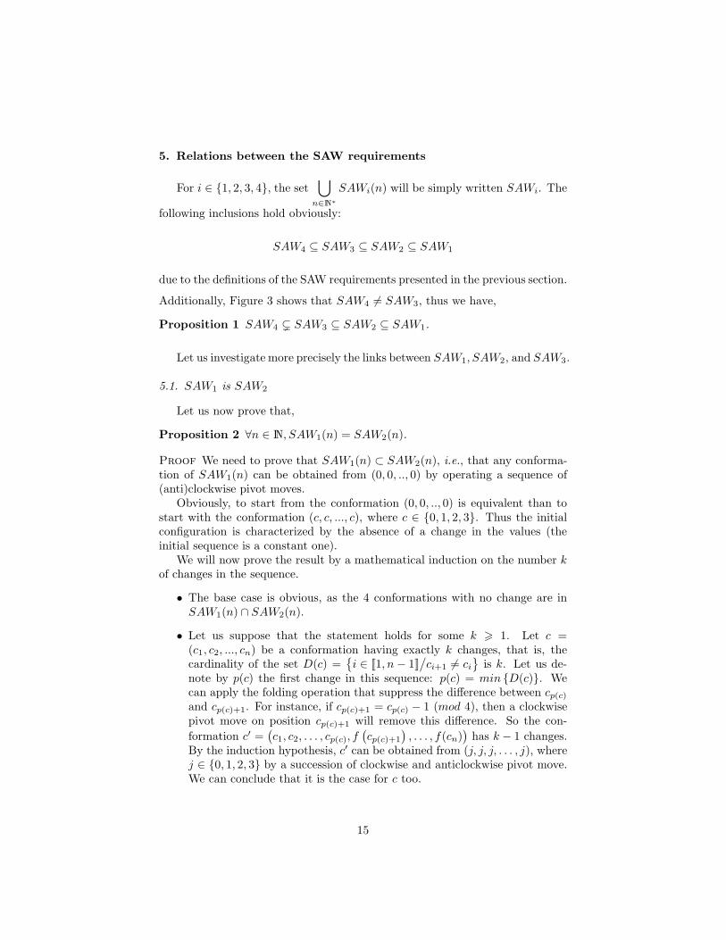
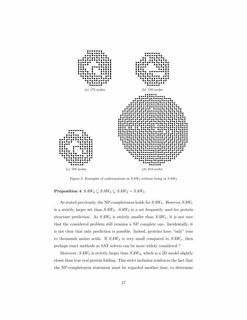
Figure 5 gives four examples of conformations that are in SAW2 without

being in SAW3 (the unique ones authors have found via the programs given in

the appendix). These counterexamples prove that,

Proposition 3 ∃n ∈ N∗, SAW2(n) 6= SAW3(n).

5.2.1. Consequences of the strict inclusion

Proposition 1 can be rewritten as follows,

16

(a) 175 nodes (b) 159 nodes

(c) 169 nodes (d) 914 nodes

Figure 5: Examples of conformations in SAW2 without being in SAW3

Proposition 4 SAW4 ( SAW3 ( SAW2 = SAW1.

As stated previously, the NP-completeness holds for SAW1. However SAW1

is a strictly larger set than SAW3. SAW3 is a set frequently used for protein

structure prediction. As SAW3 is strictly smaller than SAW1, it is not sure

that the considered problem still remains a NP complete one. Incidentally, it

is not clear that only prediction is possible. Indeed, proteins have “only” tens

to thousands amino acids. If SAW3 is very small compared to SAW1, then

perhaps exact methods as SAT solvers can be more widely considered ?

Moreover, SAW3 is strictly larger than SAW4, which is a 2D model slightly

closer than true real protein folding. This strict inclusion reinforces the fact that

the NP-completeness statement must be regarded another time, to determine

17

if this prediction problem is indeed a NP-complete one or not. Furthermore,

prediction tools could reduce the set of all possibilities by taking place into

SAW4 instead of SAW3, thus improving the confidence put in the returned

conformations.

All of these questionings are strongly linked to the size ratio between each

SAWi: the probability the NP-completeness proof remains valid in SAW3 or

SAW4 decreases when these ratios increase. This is why we will investigate

more deeply, in the next section, the relation between SAW2 and SAW3

6. A Graph Approach of the SAWi Ratios Problem

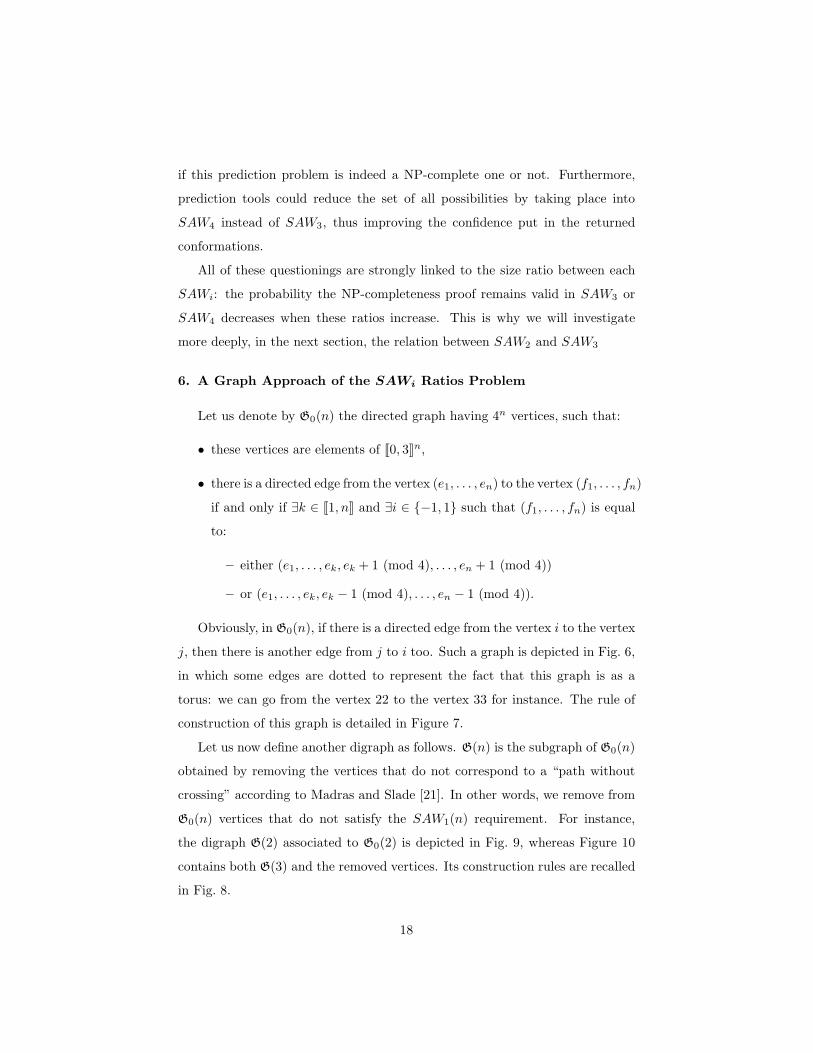
Let us denote by G0(n) the directed graph having 4n vertices, such that:

• these vertices are elements of J0, 3Kn,

• there is a directed edge from the vertex (e1, . . . , en) to the vertex (f1, . . . , fn)

if and only if ∃k ∈ J1, nK and ∃i ∈ {−1, 1} such that (f1, . . . , fn) is equal

to:

– either (e1, . . . , ek, ek + 1 (mod 4), . . . , en + 1 (mod 4))

– or (e1, . . . , ek, ek − 1 (mod 4), . . . , en − 1 (mod 4)).

Obviously, in G0(n), if there is a directed edge from the vertex i to the vertex

j, then there is another edge from j to i too. Such a graph is depicted in Fig. 6,

in which some edges are dotted to represent the fact that this graph is as a

torus: we can go from the vertex 22 to the vertex 33 for instance. The rule of

construction of this graph is detailed in Figure 7.

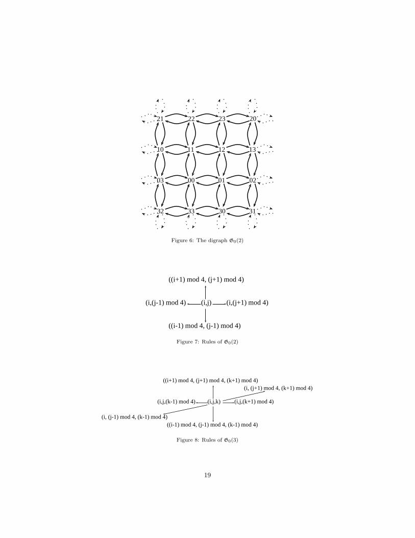
Let us now define another digraph as follows. G(n) is the subgraph of G0(n)

obtained by removing the vertices that do not correspond to a “path without

crossing” according to Madras and Slade [21]. In other words, we remove from

G0(n) vertices that do not satisfy the SAW1(n) requirement. For instance,

the digraph G(2) associated to G0(2) is depicted in Fig. 9, whereas Figure 10

contains both G(3) and the removed vertices. Its construction rules are recalled

in Fig. 8.

18

21 22 23 20

10 11 12 13

03 00 01 02

32 33 30 31

Figure 6: The digraph G0(2)

(i,j)

((i+1) mod 4, (j+1) mod 4)

(i,(j+1) mod 4)(i,(j-1) mod 4)

((i-1) mod 4, (j-1) mod 4)

Figure 7: Rules of G0(2)

(i,j,k)

((i+1) mod 4, (j+1) mod 4, (k+1) mod 4)

(i,j,(k+1) mod 4)(i,j,(k-1) mod 4)

((i-1) mod 4, (j-1) mod 4, (k-1) mod 4)

(i, (j+1) mod 4, (k+1) mod 4)

(i, (j-1) mod 4, (k-1) mod 4)

Figure 8: Rules of G0(3)

19

21 22 23

10 11 12

03 00 01

32 33 30

Figure 9: The digraph G(2)

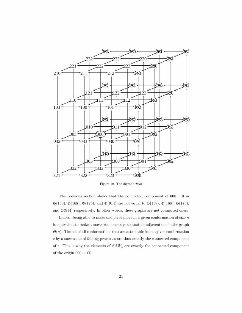
The links between G(n) and the SAW requirements can be summarized as

follows:

• The vertices of the graph G0(n) represent all the possible walks of length

n in the 2D square lattice.

• The vertices that are preserved inG(n) are the conformations of SAW1(n) =

SAW2(n).

• Two adjacent vertices i and j in G(n) are such that it is possible to change

the conformation i in j in only one pivot move.

• Finally, a conformation of SAW3(n) is a vertex of G(n) that is reachable

from the vertex 000 . . .0 by following a path in G(n).

For instance, the conformation (2, 2, 3) is in SAW3(3) because we can find

a walk from 000 to 223 in G(n). The following result is obvious,

Theorem 1 SAW3(n) corresponds to the connected component of 000 . . .0 inG(n), whereas SAW2(n) is the set of vertices of G(n). Thus we have:

SAW2(n) = SAW3(n)⇐⇒ G(n) is (strongly) connected.

20

203 200 201 202

232 233 230 231

221 222 223 220

210 211 212 213

132 133 130 131

121 122 123 120

110 111 112 113

103 100 101 102

021 022 023 020

010 011 012 013

003 000 001 002

032 033 030 031

310 311 312 313

303 300 301 302

332 333 330 331

321 322 323 320

Figure 10: The digraph G(3)

The previous section shows that the connected component of 000 . . .0 in

G(158), G(168), G(175), and G(914) are not equal to G(158), G(168), G(175),

and G(914) respectively. In other words, these graphs are not connected ones.

Indeed, being able to make one pivot move in a given conformation of size n

is equivalent to make a move from one edge to another adjacent one in the graph

G(n). The set of all conformations that are attainable from a given conformation

c by a succession of folding processes are thus exactly the connected component

of c. This is why the elements of SAW3 are exactly the connected component

of the origin 000 . . .00.

21

Furthermore, the program described in Section 5.2 is only able to find con-

nected components reduced to one vertex. Obviously, it should be possible to

find larger connected components that have not the origin in their set of con-

nected vertices. These vertices are the conformations that are in SAW2\SAW3.

In other words, if c is the connected component of c,

SAW2(n) \ SAW3(n) = {c ∈ S(n) s.t. 000 . . .00 /∈ c} (1)

Such components are composed by conformations that can be folded several

times, but that are not able to be transformed into the line 0000 . . .00. These

programs presented previously are thus only able to determine conformations

in the set

{c ∈ S(n) s.t. 000 . . .00 /∈ c and cardinality of c is 1} (2)

which is certainly strictly included into SAW2(n) \ SAW3(n). The authors’

intention is to improve these programs in a future work, in order to determine

if the connected component of a given vertex contains the origin or not. The

problem making it difficult to obtain such components is the construction of

S(n). Until now, we:

• list the 4n possible walks;

• define nodes of the graph from this list, by testing if the walk is a path

without crossing;

• for each node of the graph, we obtain the list of its 2×n possible neighbors;

• an edge between the considered vertex and one of its possible neighbors is

added if and only if this neighbor is a path without crossing.

Then we compare the size of the connected component of the origin to the

number of vertices into the graph (this latter is indeed the number of n-step

self-avoiding walks on square lattice as defined in Madras and Slane, that cor-

responds to the Sloane’s A001411 highly non-trival sequence; it is known that

there are αn self avoiding walks, with upper and lower bounds on the value α).

22

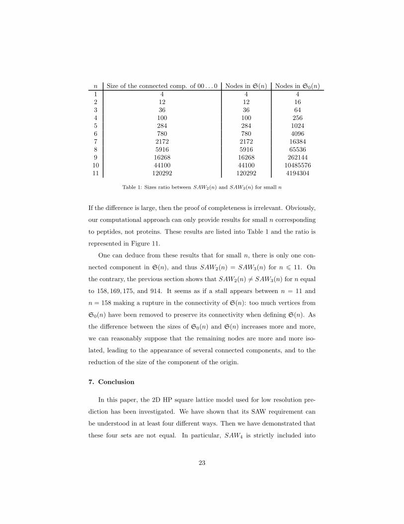
n Size of the connected comp. of 00 . . . 0 Nodes in S(n) Nodes in S0(n)1 4 4 42 12 12 163 36 36 644 100 100 2565 284 284 10246 780 780 40967 2172 2172 163848 5916 5916 655369 16268 16268 26214410 44100 44100 1048557611 120292 120292 4194304

Table 1: Sizes ratio between SAW2(n) and SAW3(n) for small n

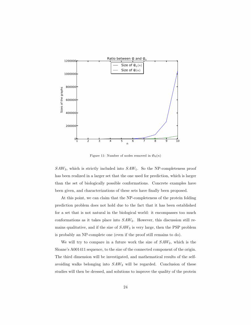
If the difference is large, then the proof of completeness is irrelevant. Obviously,

our computational approach can only provide results for small n corresponding

to peptides, not proteins. These results are listed into Table 1 and the ratio is

represented in Figure 11.

One can deduce from these results that for small n, there is only one con-

nected component in S(n), and thus SAW2(n) = SAW3(n) for n 6 11. On

the contrary, the previous section shows that SAW2(n) 6= SAW3(n) for n equal

to 158, 169, 175, and 914. It seems as if a stall appears between n = 11 and

n = 158 making a rupture in the connectivity of S(n): too much vertices from

S0(n) have been removed to preserve its connectivity when defining S(n). As

the difference between the sizes of S0(n) and S(n) increases more and more,

we can reasonably suppose that the remaining nodes are more and more iso-

lated, leading to the appearance of several connected components, and to the

reduction of the size of the component of the origin.

7. Conclusion

In this paper, the 2D HP square lattice model used for low resolution pre-

diction has been investigated. We have shown that its SAW requirement can

be understood in at least four different ways. Then we have demonstrated that

these four sets are not equal. In particular, SAW4 is strictly included into

23

1 2 3 4 5 6 7 8 9 10n

0

200000

400000

600000

800000

1000000

1200000Sizes of the graphs

Ratio between � and �0

Size of �0 (n)

Size of �(n)

Figure 11: Number of nodes removed in S0(n)

SAW3, which is strictly included into SAW1. So the NP-completeness proof

has been realized in a larger set that the one used for prediction, which is larger

than the set of biologically possible conformations. Concrete examples have

been given, and characterizations of these sets have finally been proposed.

At this point, we can claim that the NP-completeness of the protein folding

prediction problem does not hold due to the fact that it has been established

for a set that is not natural in the biological world: it encompasses too much

conformations as it takes place into SAW2. However, this discussion still re-

mains qualitative, and if the size of SAW3 is very large, then the PSP problem

is probably an NP-complete one (even if the proof still remains to do).

We will try to compare in a future work the size of SAW2, which is the

Sloane’s A001411 sequence, to the size of the connected component of the origin.

The third dimension will be investigated, and mathematical results of the self-

avoiding walks belonging into SAW3 will be regarded. Conclusion of these

studies will then be dressed, and solutions to improve the quality of the protein

24

structure prediction will finally be investigated.

References

[1] Proceedings of the IEEE Congress on Evolutionary Computation, CEC

2010, Barcelona, Spain, 18-23 July 2010. IEEE, 2010.

[2] Christian B. Anfinsen. Principles that govern the folding of protein chains.

Science, 181(4096):223–230, 1973.

[3] R. Backofen, S. Will, and P. Clote. Algorithmic approach to quantifying

the hydrophobic force contribution in protein folding, 1999.

[4] Jacques Bahi, Nathalie Cote, and Christophe Guyeux. Chaos of protein

folding. In IJCNN 2011, Int. Joint Conf. on Neural Networks, pages 1948–

1954, San Jose, California, United States, July 2011.

[5] Jacques Bahi, Nathalie Cote, Christophe Guyeux, and Michel Salomon.

Protein folding in the 2D hydrophobic-hydrophilic (HP) square lattice

model is chaotic. Cognitive Computation, 4(1):98–114, 2012.

[6] Bonnie Berger and Tom Leighton. Protein folding in the hydrophobic-

hydrophilic (hp) is np-complete. In Proceedings of the second annual in-

ternational conference on Computational molecular biology, RECOMB ’98,

pages 30–39, New York, NY, USA, 1998. ACM.

[7] Richard Bonneau and David Baker. Ab initio protein structure prediction:

Progress and prospects. Annual Review of Biophysics and Biomolecular

Structure, 30(1):173–189, 2001.

[8] Erich Bornberg-Bauer. Chain growth algorithms for hp-type lattice pro-

teins. In Proceedings of the first annual international conference on Com-

putational molecular biology, RECOMB ’97, pages 47–55, New York, NY,

USA, 1997. ACM.

25

[9] Michael Braxenthaler, R. Ron Unger, Ditza Auerbach, and John Moult.

Chaos in protein dynamics. Proteins-structure Function and Bioinformat-

ics, 29:417–425, 1997.

[10] Dylan Chivian, David E. Kim, Lars Malmstrm, Jack Schonbrun, Carol A.

Rohl, and David Baker. Prediction of casp6 structures using automated

robetta protocols. Proteins, 61(S7):157–166, 2005.

[11] Pierluigi Crescenzi, Deborah Goldman, Christos Papadimitriou, Antonio

Piccolboni, and Mihalis Yannakakis. On the complexity of protein folding

(extended abstract). In Proceedings of the thirtieth annual ACM symposium

on Theory of computing, STOC ’98, pages 597–603, New York, NY, USA,

1998. ACM.

[12] Robert L. Devaney. An Introduction to Chaotic Dynamical Systems.

Addison-Wesley, Redwood City, CA, 2nd edition, 1989.

[13] KA Dill. Theory for the folding and stability of globular proteins. Bio-

chemistry, 24(6):1501–9–, March 1985.

[14] I. Dotu, M Cebrian, P. Van Hentenryck, and P.Clote. On lattice protein

structure prediction revisited. IEEE/ACM Transactions on Computational

Biology and Bioinformatics, 8(6):1620–32, Nov–Dec 2011.

[15] I. Dubchak, I. Muchnik, S. R. Holbrook, and S. H. Kim. Prediction of

protein folding class using global description of amino acid sequence. Proc

Natl Acad Sci U S A, 92(19):8700–8704, Sep 1995.

[16] Trent Higgs, Bela Stantic, Tamjidul Hoque, and Abdul Sattar. Genetic

algorithm feature-based resampling for protein structure prediction. In

IEEE Congress on Evolutionary Computation [1], pages 1–8.

[17] Md. Hoque, Madhu Chetty, and Abdul Sattar. Genetic algorithm in ab

initio protein structure prediction using low resolution model: A review. In

26

Amandeep Sidhu and Tharam Dillon, editors, Biomedical Data and Appli-

cations, volume 224 of Studies in Computational Intelligence, pages 317–

342. Springer Berlin Heidelberg, 2009.

[18] Dragos Horvath and Camelia Chira. Simplified chain folding models as

metaheuristic benchmark for tuning real protein folding algorithms? In

IEEE Congress on Evolutionary Computation [1], pages 1–8.

[19] Md. Kamrul Islam and Madhu Chetty. Novel memetic algorithm for pro-

tein structure prediction. In Proceedings of the 22nd Australasian Joint

Conference on Advances in Artificial Intelligence, AI ’09, pages 412–421,

Berlin, Heidelberg, 2009. Springer-Verlag.

[20] Md. Kamrul Islam and Madhu Chetty. Clustered memetic algorithm for

protein structure prediction. In IEEE Congress on Evolutionary Compu-

tation [1], pages 1–8.

[21] Neal Madras and Gordon Slade. The Self-avoiding walk. Probability and

its applications. Birkhauser, 1993.

[22] M. Mann, S. Will, and R. Backofen. Cpsp-tools–exact and complete algo-

rithms for high-throughput 3d lattice protein studies. BMC Bioinformatics,

7:9:230, May 2008.

[23] Luis German Perez-Hernandez, Katya Rodrıguez-Vazquez, and Ramon

Garduno-Juarez. Estimation of 3d protein structure by means of parallel

particle swarm optimization. In IEEE Congress on Evolutionary Compu-

tation [1], pages 1–8.

[24] Andrej S[breve]ali, Eugene Shakhnovich, and Martin Karplus. How does a

protein fold? Nature, 369(6477):248–251, May 1994.

[25] Alena Shmygelska and Holger Hoos. An ant colony optimisation algorithm

for the 2d and 3d hydrophobic polar protein folding problem. BMC Bioin-

formatics, 6(1):30, 2005.

27

[26] Alena Shmygelska and Holger H Hoos. An ant colony optimisation algo-

rithm for the 2d and 3d hydrophobic polar protein folding problem, 2005

Feb.

[27] Ron Unger and John Moult. Genetic algorithm for 3d protein folding sim-

ulations. In Proceedings of the 5th International Conference on Genetic

Algorithms, pages 581–588, San Francisco, CA, USA, 1993. Morgan Kauf-

mann Publishers Inc.

[28] Yang Zhang, Adrian K. Arakaki, and Jeffrey Skolnick. Tasser: An auto-

mated method for the prediction of protein tertiary structures in casp6.

Proteins, 61(S7):91–98, 2005.

28

Appendix

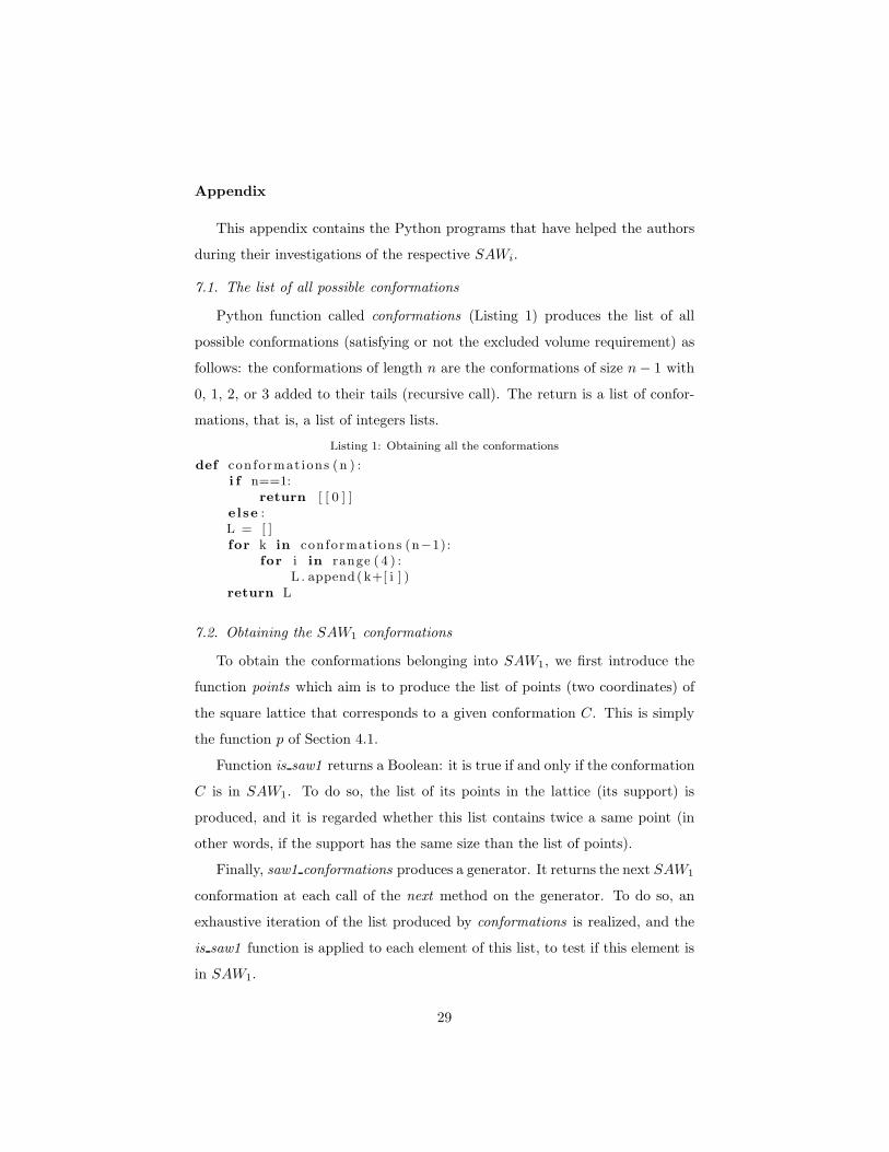
This appendix contains the Python programs that have helped the authors

during their investigations of the respective SAWi.

7.1. The list of all possible conformations

Python function called conformations (Listing 1) produces the list of all

possible conformations (satisfying or not the excluded volume requirement) as

follows: the conformations of length n are the conformations of size n− 1 with

0, 1, 2, or 3 added to their tails (recursive call). The return is a list of confor-

mations, that is, a list of integers lists.

Listing 1: Obtaining all the conformations

def conformat ions (n ) :i f n==1:

return [ [ 0 ] ]else :L = [ ]for k in conformat ions (n−1):

for i in range ( 4 ) :L . append(k+[ i ] )

return L

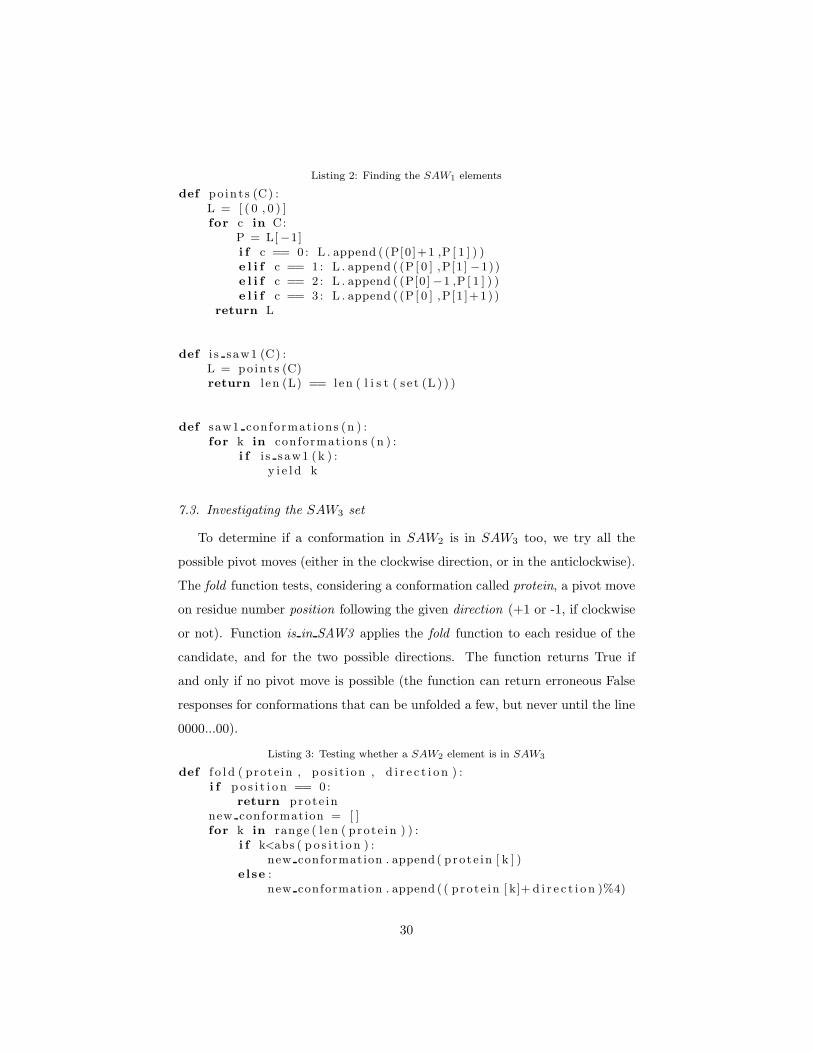
7.2. Obtaining the SAW1 conformations

To obtain the conformations belonging into SAW1, we first introduce the

function points which aim is to produce the list of points (two coordinates) of

the square lattice that corresponds to a given conformation C. This is simply

the function p of Section 4.1.

Function is saw1 returns a Boolean: it is true if and only if the conformation

C is in SAW1. To do so, the list of its points in the lattice (its support) is

produced, and it is regarded whether this list contains twice a same point (in

other words, if the support has the same size than the list of points).

Finally, saw1 conformations produces a generator. It returns the next SAW1

conformation at each call of the next method on the generator. To do so, an

exhaustive iteration of the list produced by conformations is realized, and the

is saw1 function is applied to each element of this list, to test if this element is

in SAW1.

29

Listing 2: Finding the SAW1 elements

def po in t s (C) :L = [ ( 0 , 0 ) ]for c in C:

P = L[−1]i f c == 0 : L . append ( (P[0 ]+1 ,P [ 1 ] ) )e l i f c == 1 : L . append ( (P [ 0 ] ,P[1 ] −1))e l i f c == 2 : L . append ( (P[0]−1 ,P [ 1 ] ) )e l i f c == 3 : L . append ( (P [ 0 ] ,P[1 ]+1) )

return L

def i s saw1 (C) :L = po in t s (C)return l en (L) == len ( l i s t ( s e t (L ) ) )

def saw1 conformat ions (n ) :for k in conformat ions (n ) :

i f i s saw1 (k ) :y i e l d k

7.3. Investigating the SAW3 set

To determine if a conformation in SAW2 is in SAW3 too, we try all the

possible pivot moves (either in the clockwise direction, or in the anticlockwise).

The fold function tests, considering a conformation called protein, a pivot move

on residue number position following the given direction (+1 or -1, if clockwise

or not). Function is in SAW3 applies the fold function to each residue of the

candidate, and for the two possible directions. The function returns True if

and only if no pivot move is possible (the function can return erroneous False

responses for conformations that can be unfolded a few, but never until the line

0000...00).

Listing 3: Testing whether a SAW2 element is in SAW3

def f o l d ( prote in , pos i t i on , d i r e c t i o n ) :i f p o s i t i o n == 0 :

return prot e innew conformation = [ ]for k in range ( l en ( p rot e in ) ) :

i f k<abs ( p o s i t i o n ) :new conformation . append ( p rot e in [ k ] )

else :new conformation . append ( ( p rot e in [ k]+ d i r e c t i o n )%4)

30

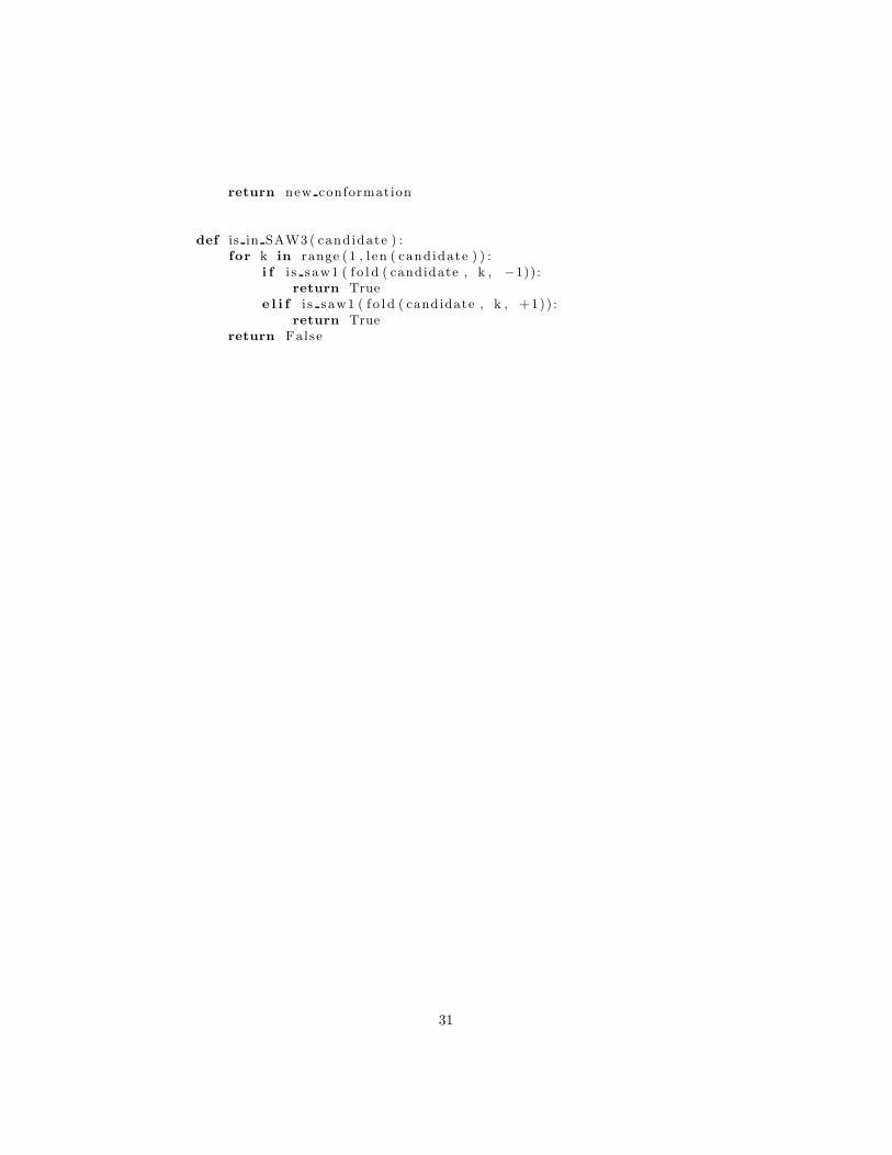
return new conformation

def is in SAW3 ( cand idate ) :for k in range (1 , l en ( cand idate ) ) :

i f i s saw1 ( f o l d ( candidate , k , −1)):return True

e l i f i s saw1 ( f o l d ( candidate , k , +1)) :return True

return False

31