Is possible to constrain models climate sensitivity using paleo proxy-data ? Hugues Goosse, Marie-France Loutre, Thierry Fichefet, Université catholique de Louvain, Belgium Jesus Fidel Gonzalez-Rouco, Universidad Complutense de Madrid, Spain Hugo Beltrami, Environmental Sciences Research Centre, Nova Scotia,

Is possible to constrain models climate sensitivity using paleo proxy-data ? Hugues Goosse, Marie-France Loutre, Thierry Fichefet, Université catholique.
Dec 14, 2015
Welcome message from author
This document is posted to help you gain knowledge. Please leave a comment to let me know what you think about it! Share it to your friends and learn new things together.
Transcript

Is possible to constrain models climate sensitivity using paleo
proxy-data ?
Hugues Goosse, Marie-France Loutre, Thierry Fichefet,
Université catholique de Louvain, Belgium
Jesus Fidel Gonzalez-Rouco, Universidad Complutense de Madrid, Spain
Hugo Beltrami, Environmental Sciences Research Centre, Nova Scotia, Canada

Description of LOVECLIM
LOVECLIM (3D)
ECBilt(atmosphere)
AGISM(ice sheets)
CLIO(sea ice-ocean)
VECODE(terr. biosphere)
LOCH(oceanic carbon cycle)
ECBilt (Opsteegh et al., 1998)Quasi-geostrophic atmospheric model (prescribed cloudiness; T21, L3).
CLIO (Goosse and Fichefet, 1999)Ocean general circulation model coupled to a thermodynamic-dynamic sea ice model (3 x 3, L20).
VECODE (Brovkin et al., 2002)Reduced-form model of the vegetation dynamics and of the terrestrial carbon cycle (same resolution as ECBilt).
LOCH (Mouchet and François, 1996)Comprehensive oceanic carbon cycle model (same resolution as CLIO).
AGISM (Huybrechts, 2002)Thermomechanical model of the ice sheet flow + visco-elastic bedrock model + model of the mass balance at the ice-atmosphere and ice-ocean interfaces (10 km x 10 km, L31).
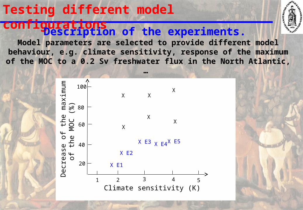
Testing different model configurations
Description of the experiments. Model parameters are selected to provide different model behaviour, e.g. climate
sensitivity, response of the maximum of the MOC to a 0.2 Sv freshwater flux in the North Atlantic, …
Climate sensitivity (K)
Dec
reas
e of
the
max
imum
of
the
MO
C (
%)
1 2 3 4 5
20
40
60
80
100
X E1
X E2
X E3 X E5X E4
X
X
XX
XX

Annual mean temperature anomaly averaged over the northern Hemisphere during the last 1000 years
E2E3
E4
E5
E1
Time
Tem
pera
ture
ano
mal
yTesting different model configurations

Annual mean temperature anomaly averaged over the northern Hemisphere during the last 8000 years
E2E3
E4
E5
E1
Time
Tem
pera
ture
ano
mal
yTesting different model configurations

Model-data comparison of underground temperatures
Borehole reconstructions Concept
Geothermalgradient
Summer Winter

Model-data comparison of underground temperatures
Borehole reconstructionsConcept

Model-data comparison of underground temperatures
Gonzalez-Rouco et al. 2006
ForwardForward modelmodel
894 grid points894 grid points
Inversion + Lat weighted avg.Inversion + Lat weighted avg.
Replicating the borehole method using ECHO-G GCM as surrogate reality
Model SATReconstruction

Model-data comparison of underground temperatures
Stevens et al. 2007
Forward-modeled profiles produced from a simulation performed using ECHO-G compared to observations (in black). The various grey, red and green cruves are computed from model results suing various reference level.
We need an adequate reference to compute anomalies !

E2E3
E4
E5
E1
Changes in sea-ice extent in the Arctic
Location of the September ice edge in the 5 experiments
Pre-industrial conditions 1980-2000 averages
Goosse et al. 2007
E2E3
E4
E5
E1
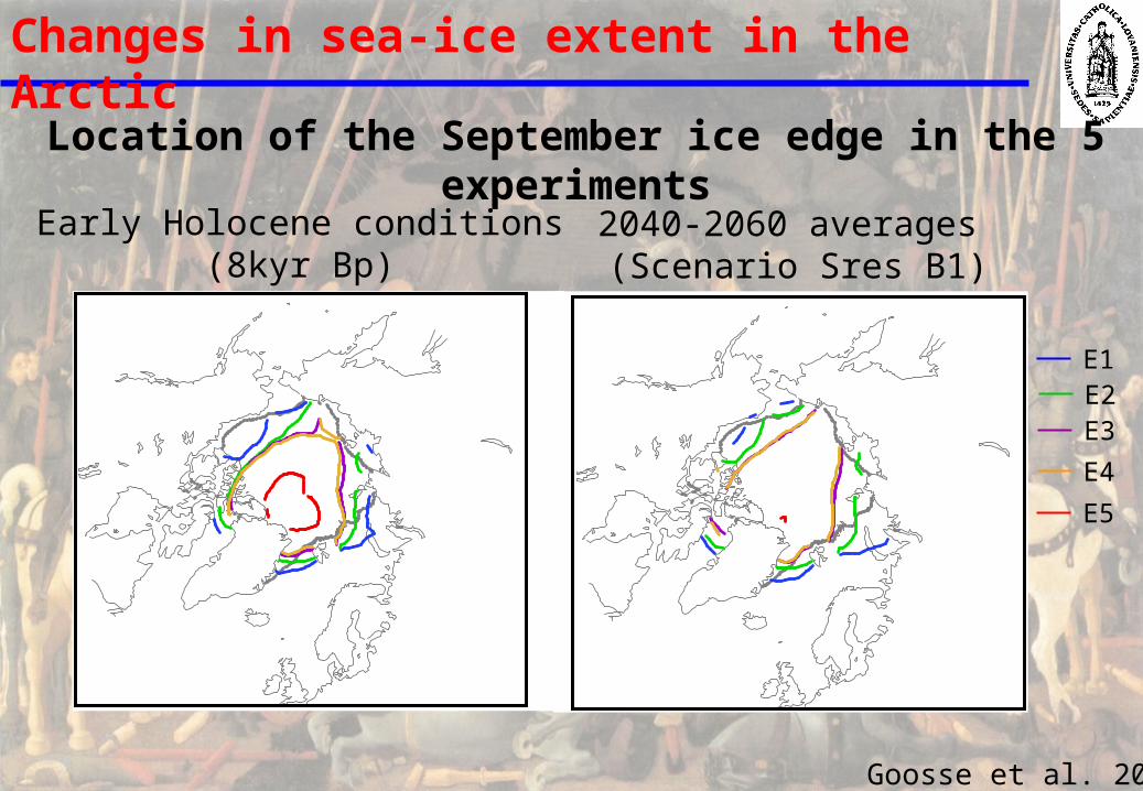
Changes in sea-ice extent in the Arctic
Location of the September ice edge in the 5 experiments
Early Holocene conditions(8kyr Bp)
2040-2060 averages (Scenario Sres B1)
Goosse et al. 2007

Goosse et al. 2007
Link between the minimum Arctic sea ice extent (in 106 km2) for the early Holocene and the period 2040-2060 AD (scenario SRES B1)
Changes in sea-ice extent in the Arctic
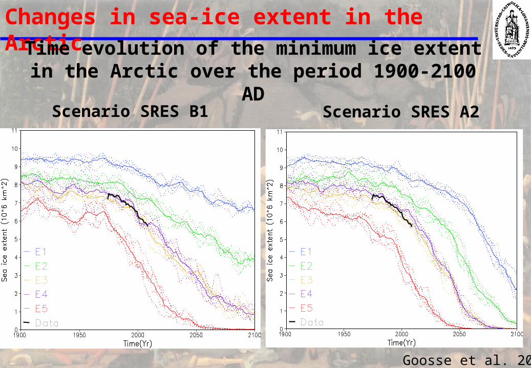
Changes in sea-ice extent in the Arctic
Time evolution of the minimum ice extent in the Arctic over the period 1900-2100 AD
Scenario SRES B1 Scenario SRES A2
Goosse et al. 2007

Conclusions
Paleo-proxy data could efficiently be used to constrain model behavior.
They could provide complementary information compared to the one obtained from the recent past.
Accurate data are required, with a good spatial sampling and one should take care of the methodology used for model-data comparison.
Related Documents


