Is it the climate or the weather? Differential economic ... · Is it the climate or the weather? Differential economic impacts of climatic factors in Ethiopia Mintewab Bezabih, Salvatore

Is it the climate or the weather? Differential

economic impacts of climatic factors in

Ethiopia

Mintewab Bezabih, Salvatore Di Falco and

Alemu Mekonnen

February 2014

Centre for Climate Change Economics and Policy Working Paper No. 165

Grantham Research Institute on Climate Change and the Environment

Working Paper No. 148

ii

The Centre for Climate Change Economics and Policy (CCCEP) was established by the University of Leeds and the London School of Economics and Political Science in 2008 to advance public and private action on climate change through innovative, rigorous research. The Centre is funded by the UK Economic and Social Research Council and has five inter-linked research programmes:

1. Developing climate science and economics 2. Climate change governance for a new global deal 3. Adaptation to climate change and human development 4. Governments, markets and climate change mitigation 5. The Munich Re Programme - Evaluating the economics of climate risks and

opportunities in the insurance sector

More information about the Centre for Climate Change Economics and Policy can be found at: http://www.cccep.ac.uk.

The Grantham Research Institute on Climate Change and the Environment was established by the London School of Economics and Political Science in 2008 to bring together international expertise on economics, finance, geography, the environment, international development and political economy to create a world-leading centre for policy-relevant research and training in climate change and the environment. The Institute is funded by the Grantham Foundation for the Protection of the Environment and the Global Green Growth Institute, and has five research programmes:

1. Global response strategies 2. Green growth 3. Practical aspects of climate policy 4. Adaptation and development 5. Resource security

More information about the Grantham Research Institute on Climate Change and the Environment can be found at: http://www.lse.ac.uk/grantham.

iii

This working paper is intended to stimulate discussion within the research community and among users of research, and its content may have been submitted for publication in academic journals. It has been reviewed by at least one internal referee before publication. The views expressed in this paper represent those of the author(s) and do not necessarily represent those of the host institutions or funders.

iv

Is it the Climate or the Weather? Differential Economic Impacts of Climatic Factors in Ethiopia

Mintewab Bezabih, Salvatore Di Falco, and Alemu Mekonnen∗

Abstract

This paper assesses the distinct impacts of weather and climate change measures on agricultural revenue of farm households in the Amhara region of Ethiopia. This distinction is highlighted by observations in the temperature data, which show that the pattern of temperature for both short term and long values follows a bell-shaped distribution, with the striking feature that the extreme ends of the distribution have fatter tails for the long term values. The analysis employs monthly rainfall and 14 temperature categories related to weather measures and four categories corresponding with the extreme ends of the long term temperature distribution. The analysis also distinguishes between summer and spring seasons and different crops in recognition of Ethiopia’s is a multi-cropping and multi-season agriculture. The major findings show that temperature effects are distinctly non-linear but only when the weather measures are combined with the extreme ends of the distribution of the climate measures. In addition, rainfall generally has less important role to play than temperature, contrary to expectations in rain-fed agriculture.

Key Words: crop revenue; climate change; weather variability; Mundlak’s Fixed Effects method; Ricardian analysis; Ethiopia

JEL Codes: D2, Q12, Q15

∗ Mintewab Bezabih (corresponding author), the Grantham Institute on Climate Change and the Environment, London School of Economics and Political Science. Tower 3 | Clements Inn Passage | London WC2A 2AZ. [email protected]; Salvatore Difalco, Department of Economics, University of Geneva, UniMail 40, Bd du Pont D'Arve 1211. [email protected]; Alemu Mekonnen, Department of Economics, Addis Ababa University, P.O. Box 150167, Addis Ababa, Ethiopia. [email protected]. The authors gratefully acknowledge the Environmental Economics forum for Ethiopia for access to data and financial support for the study. The authors would also like to thank the Global Green Growth Institute, the Grantham Foundation for the Protection of the Environment and the Economic and Social Research Council (ESRC) through the Centre for Climate Change Economics and Policy for financial support. Comments from participants at the 20th Annual Conference of the European Association of Environmental and Resource Economists, 26-29 June 2013, Toulouse, France; the 6th Annual Meeting of the Environment for Development Initiative, 25-29 October 2012, La Fortuna, Costa Rica, and Peter Berck, are appreciated. The usual disclaimer applies.

1

Introduction

Agriculture is the economic sector that is most directly linked to climate and climatic change. The empirical estimation of the role of climatic factor on agricultural outcomes is however, subject to considerable controversy (Mendelsohn et al., 1994; Deschênes and Greenstone, 2007; Fisher et al. 2012). The controversy is (mostly) based on two important related issues: the choice of the model and the choice of climatic factors metrics. Since the pioneering contribution of Mendelsohn et al. (1994), the use of the Ricardian model has been adopted widely. This is a hedonic approach that uses cross-sectional analysis where farmland values or farm net revenues are regressed on long term average climate variables. This approach has the key advantage that it can take account for all the range of different adaptation measures that farmers may put in place (Lang, 2007). It has, however, been criticized on the ground of potential inconsistency of parameters estimated by cross sectional analysis. There may be unobservable confounding factors (e.g., soil quality) that affect the outcome variable. The use of the Ricardian approach can therefore suffer by omitted variables bias. To circumvent this problem random year-to-year weather variation in a panel can be used to estimate the relationships between agricultural profits or yields and weather (Deschênes and Greenstone; 2007; Schlenker and Roberts; 2009).1 While, this strategy has clear econometric benefits it does use short - term variation (annual weather)2 to estimate the impact of a long -term phenomena (climate). The difference matters as using inter-annual changes in weather can only capture a limited set of adaptation measures implemented by farmers (Massetti and Mendelsohn, 2011). The use of year-to-year weather fluctuation is, thus, likely to produce larger estimates of the impact of climate change in agriculture (Deschênes and Greenstone, 2007).3 The contribution of this paper is twofold. First, we contribute to the literature and try to solve the controversy by using a simple but comprehensive empirical strategy. We use a panel data model where the inclusion of time-invariant (e.g., climate) variables along with time variant (weather) is accommodated and that allows for correlation between time invariant variables and the fixed effect. We therefore use the Mundlak-Krishnakumar estimator (Mundlak, 1978; Krishnakumar, 2006).4 This is the first paper

1 Schlenker and Roberts (2009) argue that estimating the correct relationship between weather and yields is a critical first step before assessing structural shifts in response to climate change.

2 Assessing the impacts of weather-related measureson agricultural yields has been a commonplace in the agronomic literature (e.g. Black, 1978; Adams, 1995;Brown and Rosenberg, 1999; Cassman, 1999; Merns et al., 2001;Dai et al.2004;Murthy, 2004; Yu, 2011)

3 The readers interested in the identification of the adaptation strategies should refer to Kurukulasuriya and Mendelsohn, 2008; Seo and Mendelsohn, 2008a; Seo and Mendelsohn, 2008b; Di Falco and Veronesi, 2013.

4 For an application in the education sector see Chatelain and Rolf (2010).

2

that attempts to estimate the role of both weather and climate on economic outcomes. The inclusion of both climate and weather allows capturing the full extent of underlying adaptation decisions. Farmers may indeed respond to both long run changes as well as weather shocks. Indeed, there is a wealth of evidence, particularly from developing countries, showing that weather variability could lead to non-negligible changes in farming practices, as a form of adaptation. In line with this, Burgess et al. (2013) show that weather fluctuations have a profound effect on the health and mortality of India’s rural population, through its effect on agricultural production. As adaptation is implicitly an important feature of the Ricardian approach (Massetti and Mendelsohn, 2011), omission of the short- term impacts – such as weather shocks that trigger an adaptive response - implies that the approach would produce biased estimates.5 We use information on both temperature and rainfall.6 Secondly, this paper focuses on assessing the impacts of weather and climate on agriculture in Ethiopia by incorporating the different features of short term (weather) and long term (climate) measures and emphasizing on extreme values corresponding to the measures.7 We follow Schlenker and Roberts (2006; 2009) and use the full information on the distribution of both long run and short run temperature. As Hodges (1991) and Grierson (2002) show, plant growth depends on the cumulative exposure to heat and precipitation during the growing season. Specifically, as plants cannot absorb heat above or below a specific threshold, the effect of heat accumulation tends to be nonlinear. As a result, the standard agronomic approach involves converting daily temperatures into degree days, which represent heating units accounting for such non-linarites. Rosenzweig et al. (2009) argue that due consideration should be given to disproportionately large changes in the frequency of extreme events that are associated with, and not captured by, small changes in long term mean temperatures. Indeed, the

5 This distinction between short term and long term climate measures is highly relevant in a setting like Ethiopia, where both seasonal and yearly variations in rainfall are significant, rainfall is hugely erratic and weather insurance mechanisms are virtually nonexistent (Dercon et al., 2009; Adnew, 2006), leaving considerable rooms for weather related adaptations.

6 Furthermore, unlike many climate change studies that have focused on estimating the impact of either temperature or precipitation in isolation, we combine both measures in our analysis. As argued in Auffhammer et al. (2013) such an approach is crucial to in order obtain unbiased estimates of the effects of changes in precipitation and temperatures, which are historically correlated, both variables must be included in the regression equation, especially if the correlation is predicted to change in the future.

7The difference between weather and climate is a measure of time. While weather is the day-to-day state of the atmosphere, and its variation over minutes to weeks, climate is defined as statistical weather information that describes the variation of weather at a given place for a specified interval. To determine climate, the weather of a locality is usually averaged over a 30-year period (Gutro, 2005). Weather and climate are expected to have different economic implications, as they represent essentially different phenomena (Fischer et al, 2012). It should also be noted that to the extent that the distributions of weather and climate are identical, the distinction between the two is irrelevant. The essence of such distinction becomes relevant when the two are distributionally different.

3

effects of such variations and extremes are likely to be captured through measures that account for changes in patterns of temperature in a more detailed manner, as opposed to average climatic parameters (De Salvo et al., 2013). In addition, Maraun et al. (2010) show that extreme events and temporal-spatial variations tend to be poorly represented by average climate change measures. We use panel data from Ethiopia (four rounds from 1999 to 2007) combined with 30-year monthly rainfall and temperature data. Moreover, the country provides a large extent of variation in climatic factors. We distinguish between summer and spring seasons and different crops in recognition of Ethiopia’s multi-season agriculture.

Long term mean measures are used as climate variables, while the weather variables were constructed as averages for the years corresponding to the survey years. Ethiopia is a prime area to study the impact of climatic factors on agriculture. The country heavily relies on the agricultural sector and like many other sub Saharan countries is expected to suffer large part of the impact of climate change (Mendelsohn et al. 2006). Developing countries and their economic progress are likely to suffer tremendously from climate change, given their extremely nature-dependent agrarian economies (Mendelsohn and Dinar, 2009). As a result, accurate quantification of the economic impact of climate change on the agricultural sector is of paramount importance in guiding appropriate adaptation measures (Sachs et al., 1999; Stage, 2010) and ensuring genuine participation of developing countries in climate change agreements (Cao, 2008; Timmins, 2006).

We find that the distribution of weather temperature and climate temperature, measured in terms of number of days spent in each degree range over a growing season, indicates that both follow a bell-shaped distribution across the -5 to +40 degree range. However, both ends of the extreme values exhibit a fatter tail for the distribution of climate temperature to the weather temperature distribution. We also find that long- term impacts are larger than short term. This may indicate that farmers, contrary to what is assumed by the Ricardian framework, are not adapting optimally to climate change. While, they may have better capacity to cope with weather variability.

The rest of the paper is organized as follows. The next section presents an overview of the importance of climate change and weather uncertainty in Ethiopia. Next, the data employed in the empirical analysis is presented. The econometric methodology employed is discussed in the section that follows. The empirical findings are then discussed, and the last section concludes the paper.

Weather variability, climate change and agricultural productivity in Ethiopia: a Background

Agriculture remains one of the most important sectors in the Ethiopian economy for the following reasons: (i) it directly supports about 83% of the population in terms of employment and livelihood; (ii) it contributes over 40% of the country’s gross domestic

4

product (GDP); (iii) it generates about 85% of export earnings; and (iv) it supplies around 73% of the raw material requirements of agro-based domestic industries, such as biofuels (MEDaC 1999; AfDB 2011). It is also the major source of food for the population and hence the most important sector for food security. In addition, agriculture is expected to play a key role in generating surplus capital to speed up the country’s overall socio-economic development (MEDaC 1999). Ethiopia has a population of over 80 million with a population growth rate of about 2.6% (AfDB 2011). The country has a total land area of about 112.3 million hectares. Of this, about 16.4 million hectares are suitable for producing annual and perennial crops. Of the estimated arable land, about eight million hectares is used annually for rain-fed crops. Small-scale farmers who are dependent on rain-fed mixed farming dominate the agricultural sector; they use traditional technologies with low inputs and get low output. The present government of Ethiopia has given top priority to this sector and has taken steps to increase its productivity. However, various problems are holding this back. Some causes of poor crop production are declining farm size; subsistence farming partly due to population growth; land degradation due to inappropriate land use such as cultivation of steep slopes; over cultivation and overgrazing; and inappropriate policies. Other causes are tenure insecurity; weak agricultural research and extension services; lack of appropriate agricultural marketing; an inadequate transport network; low use of fertilizers, improved seeds and pesticides; and the use of traditional farm implements. However, the major causes of low levels of production are drought, which often causes famine, and floods. This climate related disasters make the nation dependent on food aid.

With agriculture almost completely dependent on rainfall, rain rules the lives and well-being of many rural Ethiopians. It determines whether they will have enough to eat and whether they will be able to provide basic necessities and earn a living. Indeed, the dependence on rainfall and its erratic pattern has largely contributed to the food shortages and crop crises that farmers are constantly faced with. Even in good years, the one-time harvest or crop may be too little to meet the yearly household needs; as a result, the majority of Ethiopia’s rural people remain food insecure (Devereux 2000)8.

Rainfall contributes to poverty both directly, through actual losses from rainfall shocks, and indirectly, through responses to the threat of crisis. The direct impacts most often occur when a drought destroys a smallholder farmer’s crops. Under such circumstances, not only will the farmers and their families go hungry, but they also will

8Ethiopia has experienced at least five major national droughts since 1980, along with literally dozens of localized ones (World Bank 2008b). These cycles of drought create poverty traps for many households, constantly consuming any build-up of assets or increase in income. Evidence shows that about half of all rural households in the country experienced at least one major drought during the five years preceding 2004 (Dercon, 2009). The evidence also suggests that these shocks are a major cause of transient poverty. That is, had Ethiopian households been able to smooth consumption, then poverty in 2004 would have been at least 14 percent lower, which translates into 11 million fewer people falling below the poverty line.

5

be forced to sell or consume their plough animals in order to survive. They are then significantly worse off than before because they can no longer farm effectively when the rains return (Barrett et al., 2007).

Data and variables

Data used in the analysis were collected through four waves of rural household surveys conducted in the years 2000, 2002, 2005 and 2007 with the same households. The surveys were conducted by the Ethiopian Development Research Institute and Addis Ababa University in collaboration with Gothenburg University, and through financial support from the Swedish International Development Cooperation Agency (Sida). The survey sites include households in two Zones (South Wollo and East Gojjam) of the Amhara National Regional State, a region that encompasses part of the Northern and Central Highlands of Ethiopia. Monthly rainfall and daily temperature data were obtained from the Ethiopian Meteorology Authority, in eight stations close to the study villages (kebeles) for the years 1976 to 2006. In order to impute farm specific information from station level observations, an inverse distance weighting interpolation method was employed. This method combines latitude, longitude, and station level rainfall and temperature observations. The climate change and weather measures used in the analysis are then constructed from these rainfall and temperature data9.

Temperature and rainfall variables

Following Schlenker and Roberts (2006; 2009), we construct the distribution of temperature by first fitting a sinusoidal curve between predicted minimum and predicted maximum temperatures. This sinusoidal interpolation gives the time spent in each 1◦C-degree temperature interval between −5◦C and +40◦C within each day10. Each of the one degree Celsius in the -5 to 40 degree Celsius range is then converted into a more aggregate distribution by summing together each three-degree temperature interval. The length of time spent on each three-degree Celsius temperature interval in each day is then summed across all days of the month, for each farm household.

9There are two instances where the assessment of weather as a separate variable may not be important. First, to the extent that weather variability is stable over time, it may also mimic climate change, making the impact of climate change on agricultural productivity akin to that of weather variability. Second, if mechanisms are in place to ensure against weather risks, then farmers are unlikely to incorporate much of the impact of weather variability into their decision making.

10 The determination of the maximum and minium values of the range is based on our observed data.

6

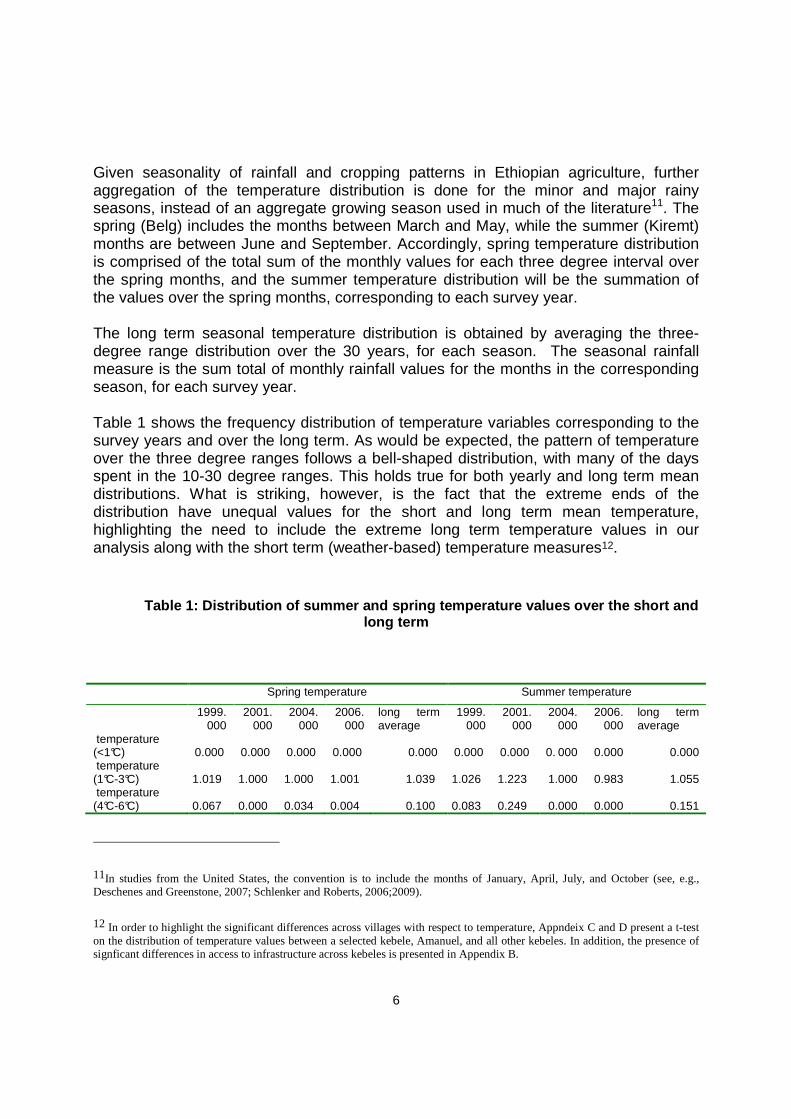
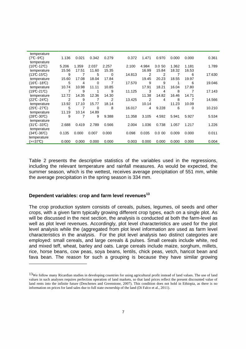
Given seasonality of rainfall and cropping patterns in Ethiopian agriculture, further aggregation of the temperature distribution is done for the minor and major rainy seasons, instead of an aggregate growing season used in much of the literature11. The spring (Belg) includes the months between March and May, while the summer (Kiremt) months are between June and September. Accordingly, spring temperature distribution is comprised of the total sum of the monthly values for each three degree interval over the spring months, and the summer temperature distribution will be the summation of the values over the spring months, corresponding to each survey year. The long term seasonal temperature distribution is obtained by averaging the three-degree range distribution over the 30 years, for each season. The seasonal rainfall measure is the sum total of monthly rainfall values for the months in the corresponding season, for each survey year. Table 1 shows the frequency distribution of temperature variables corresponding to the survey years and over the long term. As would be expected, the pattern of temperature over the three degree ranges follows a bell-shaped distribution, with many of the days spent in the 10-30 degree ranges. This holds true for both yearly and long term mean distributions. What is striking, however, is the fact that the extreme ends of the distribution have unequal values for the short and long term mean temperature, highlighting the need to include the extreme long term temperature values in our analysis along with the short term (weather-based) temperature measures12.

Table 1: Distribution of summer and spring temperature values over the short and long term

Spring temperature Summer temperature

1999.000

2001.000

2004.000

2006.000

long term average

1999.000

2001.000

2004.000

2006.000

long term average

temperature (<1°C) 0.000 0.000 0.000 0.000 0.000 0.000 0.000 0. 000 0.000 0.000 temperature (1°C-3°C) 1.019 1.000 1.000 1.001 1.039 1.026 1.223 1.000 0.983 1.055 temperature (4°C-6°C) 0.067 0.000 0.034 0.004 0.100 0.083 0.249 0.000 0.000 0.151

11In studies from the United States, the convention is to include the months of January, April, July, and October (see, e.g., Deschenes and Greenstone, 2007; Schlenker and Roberts, 2006;2009).

12 In order to highlight the significant differences across villages with respect to temperature, Appndeix C and D present a t-test on the distribution of temperature values between a selected kebele, Amanuel, and all other kebeles. In addition, the presence of signficant differences in access to infrastructure across kebeles is presented in Appendix B.

7

temperature (7°C -9°C) 1.136 0.021 0.342 0.279 0.372 1.471 0.970 0.000 0.000 0.361 temperature (10°C-12°C) 5.206 1.359 2.037 2.257 2.100 4.984 3.0 50 1.362 1.181 1.789 temperature (13°C-15°C)

15.569

17.517

11.605

15.350 14.813

16.992

15.842

18.327

16.536 17.630

temperature (16°C -18°C)

15.605

17.084

18.040

17.847 17.570

19.459

20.239

18.551

19.976 19.046

temperature (19°C-21°C)

10.747

10.989

11.111

10.859 11.125

17.913

18.214

16.048

17.807 17.143


12.722

14.359

12.367

14.302 13.425

11.382

14.824

16.468

14.717 14.566


13.925

17.107

15.770

18.148 16.017

10.144 9.228

11.236

10.090 10.210

temperature (28°C-30°C)

11.199

10.147

14.899 9.388 11.358 3.105 4.592 5.941 5.927 5.534

temperature (31°C -33°C) 2.688 0.419 2.789 0.566 2.004 1.036 0.738 1.057 1.217 1.226 temperature (34°C-36°C) 0.135 0.000 0.007 0.000 0.098 0.035 0.0 00 0.009 0.000 0.011 temperature (>=37°C) 0.000 0.000 0.000 0.000 0.003 0.000 0.000 0.000 0.000 0.004

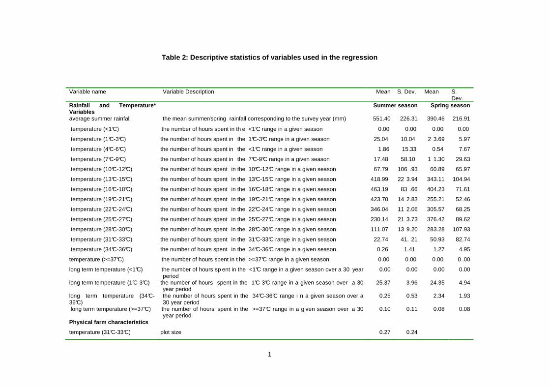
Table 2 presents the descriptive statistics of the variables used in the regressions, including the relevant temperature and rainfall measures. As would be expected, the summer season, which is the wettest, receives average precipitation of 551 mm, while the average precipitation in the spring season is 334 mm.

Dependent variables: crop and farm level revenues13

The crop production system consists of cereals, pulses, legumes, oil seeds and other crops, with a given farm typically growing different crop types, each on a single plot. As will be discussed in the next section, the analysis is conducted at both the farm-level as well as plot level revenues. Accordingly, plot level characteristics are used for the plot level analysis while the (aggregated from plot level information are used as farm level characteristics in the analysis. For the plot level analysis two distinct categories are employed: small cereals, and large cereals & pulses. Small cereals include white, red and mixed teff, wheat, barley and oats. Large cereals include maize, sorghum, millets, rice, horse beans, cow peas, soya beans, lentils, chick peas, vetch, haricot bean and fava bean. The reason for such a grouping is because they have similar growing

13We follow many Ricardian studies in developing countries for using agricultural profit instead of land values. The use of land values in such analyses requires perfection operation of land markets, so that land prices reflect the present discounted value of land rents into the infinite future (Deschenes and Greenstone, 2007). This condition does not hold in Ethiopia, as there is no information on prices for land sales due to full state ownership of the land (Di Falco et al., 2011).

8

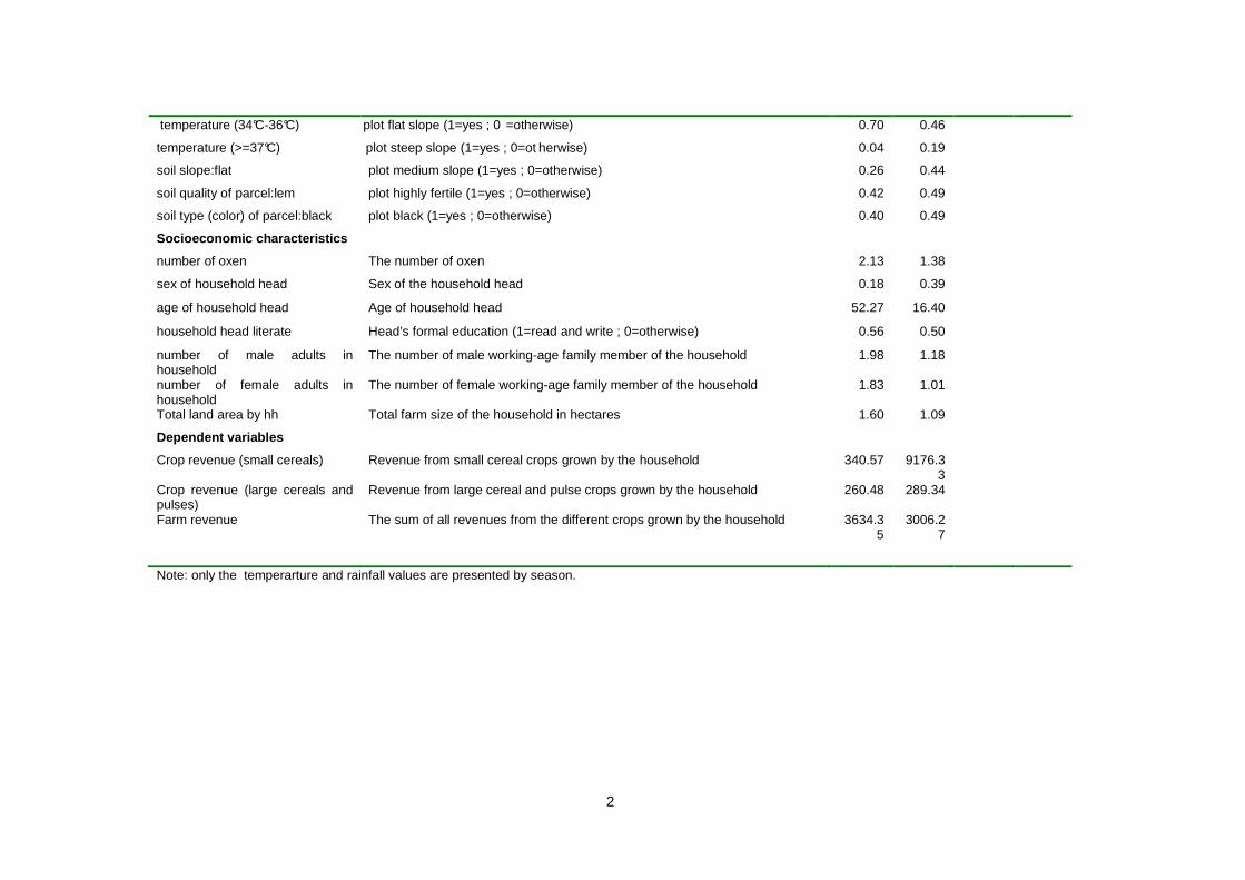
temperature range and they also have similar soil quality and land preparation requirements. As per Table 2, the overall farm revenue averages at around Br. 3634 while that of small cereals and large cereals are Br. 340 and 260, respectively.

Socio-economic and physical farm characteristics

Around 18% of the surveyed households have a female head. The average age of the household head is 52.The proportion of household heads that are able to read and write is 56%. An average household has1.98 and 1.83 male and female adults of working age, respectively, indicating a gender balance between male and female labour availability. Livestock ownership, measured in tropical livestock units14, is around 6 per household, while the number of oxen owned by an average household is around 2. The average farm size is 1.60 ha, slightly higher than the national average of 1.1 ha. On average, 69% of the plots are flat, with moderately steep and steep plots making up the rest of the plots. In addition to topographic features, plots are defined by their soil colour, which is also a rough representation of other features such as water retention capacity and texture. An average of 40 percent of the plots per farm have black soil colour, while an average of 56% have red soil colour. The average proportion of fertile plots per household is 40%, while the average number of plots with moderately fertile and infertile soil types is 40% and 20%, respectively.

14 Tropical livestock unit is a common unit to describe livestock numbers of various species as a single figure that expresses the total amount of livestock present – irrespective of the specific composition (FAO, 2010). http://www.fao.org/ag/againfo/programmes/en/lead/toolbox/Mixed1-/TLU.htm

1

Table 2: Descriptive statistics of variables used in the regression

Variable name Variable Description Mean S. Dev. Mean S. Dev.

Rainfall and Temperature* Variables

Summer season Spring season

average summer rainfall the mean summer/spring rainfall corresponding to the survey year (mm) 551.40 226.31 390.46 216.91

temperature (<1°C) the number of hours spent in th e <1°C range in a given season 0.00 0.00 0.00 0.00

temperature (1°C-3°C) the number of hours spent in the 1°C-3°C range in a given season 25.04 10.04 2 3.69 5.97

temperature (4°C-6°C) the number of hours spent in the <1°C range in a given season 1.86 15.33 0.54 7.67

temperature (7°C-9°C) the number of hours spent in the 7°C-9°C range in a given season 17.48 58.10 1 1.30 29.63

temperature (10°C-12°C) the number of hours spent in the 10°C-12°C range in a given season 67.79 106 .93 60.89 65.97

temperature (13°C-15°C) the number of hours spent in the 13°C-15°C range in a given season 418.99 22 3.94 343.11 104.94

temperature (16°C-18°C) the number of hours spent in the 16°C-18°C range in a given season 463.19 83 .66 404.23 71.61





temperature (31°C-33°C) the number of hours spent in the 31°C-33°C range in a given season 22.74 41. 21 50.93 82.74

temperature (34°C-36°C) the number of hours spent in the 34°C-36°C range in a given season 0.26 1.41 1.27 4.95

temperature (>=37°C) the number of hours spent in t he >=37°C range in a given season 0.00 0.00 0.00 0 .00

long term temperature (<1°C) the number of hours sp ent in the <1°C range in a given season over a 30 year period

0.00 0.00 0.00 0.00

long term temperature (1°C-3°C) the number of hours spent in the 1°C-3°C range in a given season over a 30 year period

25.37 3.96 24.35 4.94

long term temperature (34°C-36°C)

the number of hours spent in the 34°C-36°C range i n a given season over a 30 year period

0.25 0.53 2.34 1.93

long term temperature (>=37°C) the number of hours spent in the >=37°C range in a given season over a 30 year period

0.10 0.11 0.08 0.08

Physical farm characteristics

temperature (31°C-33°C) plot size 0.27 0.24

2

temperature (34°C-36°C) plot flat slope (1=yes ; 0 =otherwise) 0.70 0.46

temperature (>=37°C) plot steep slope (1=yes ; 0=ot herwise) 0.04 0.19

soil slope:flat plot medium slope (1=yes ; 0=otherwise) 0.26 0.44

soil quality of parcel:lem plot highly fertile (1=yes ; 0=otherwise) 0.42 0.49

soil type (color) of parcel:black plot black (1=yes ; 0=otherwise) 0.40 0.49

Socioeconomic characteristics

number of oxen The number of oxen 2.13 1.38

sex of household head Sex of the household head 0.18 0.39

age of household head Age of household head 52.27 16.40

household head literate Head’s formal education (1=read and write ; 0=otherwise) 0.56 0.50

number of male adults in household

The number of male working-age family member of the household 1.98 1.18

number of female adults in household

The number of female working-age family member of the household 1.83 1.01

Total land area by hh Total farm size of the household in hectares 1.60 1.09

Dependent variables

Crop revenue (small cereals) Revenue from small cereal crops grown by the household 340.57 9176.33

Crop revenue (large cereals and pulses)

Revenue from large cereal and pulse crops grown by the household 260.48 289.34

Farm revenue The sum of all revenues from the different crops grown by the household 3634.35

3006.27

Note: only the temperarture and rainfall values are presented by season.

1

Estimation Procedure

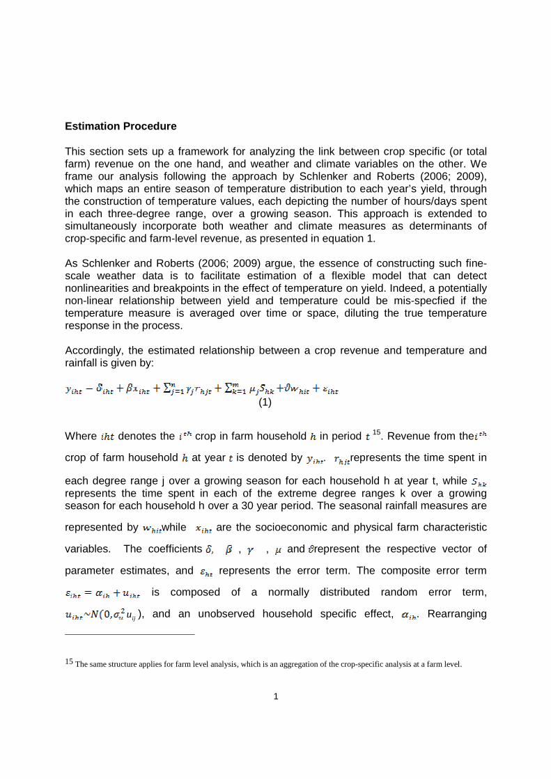
This section sets up a framework for analyzing the link between crop specific (or total farm) revenue on the one hand, and weather and climate variables on the other. We frame our analysis following the approach by Schlenker and Roberts (2006; 2009), which maps an entire season of temperature distribution to each year’s yield, through the construction of temperature values, each depicting the number of hours/days spent in each three-degree range, over a growing season. This approach is extended to simultaneously incorporate both weather and climate measures as determinants of crop-specific and farm-level revenue, as presented in equation 1. As Schlenker and Roberts (2006; 2009) argue, the essence of constructing such fine-scale weather data is to facilitate estimation of a flexible model that can detect nonlinearities and breakpoints in the effect of temperature on yield. Indeed, a potentially non-linear relationship between yield and temperature could be mis-specfied if the temperature measure is averaged over time or space, diluting the true temperature response in the process. Accordingly, the estimated relationship between a crop revenue and temperature and rainfall is given by:

(1)

Where denotes the crop in farm household in period 15. Revenue from the

crop of farm household at year is denoted by . represents the time spent in

each degree range j over a growing season for each household h at year t, while represents the time spent in each of the extreme degree ranges k over a growing season for each household h over a 30 year period. The seasonal rainfall measures are

represented by while are the socioeconomic and physical farm characteristic

variables. The coefficients , , and represent the respective vector of

parameter estimates, and represents the error term. The composite error term

is composed of a normally distributed random error term,

iju ), and an unobserved household specific effect, . Rearranging

15 The same structure applies for farm level analysis, which is an aggregation of the crop-specific analysis at a farm level.

2

equation (1) by grouping time-variant and time invariant variables together, and introducing the fixed effect gives:

(2)

Under the assumption that is orthogonal to the observable covariates, a random effects estimator can be employed as an effective estimator (Baltagi 2001; Wooldridge

2002). However, allowing arbitrary correlation between and the regressors/observed

covariates requires a fixed effect, as it takes to be a group-specific constant term and uses a transformation to remove this effect prior to estimation (Wooldridge 2002). The alternative approach of the random effects estimator has a specification similar to the fixed effects estimator, with the additional requirement of no correlation between the

fixed effect and the regressors/observed covariates (Baltagi, 2001). Despite this shortcoming, however, the random effects estimator does not rely on the data transformation in the fixed effects estimator and thus is not affected by the associated shortcoming of removing any time-constant explanatory variables along with

(Wooldridge, 2002). However, the random effects specification assumes exogeneity of all the regressors and the random individual effects. As long as the assumption of no correlation of the regressors and individual effects is satisfied, the random effects estimator guarantees a consistent and efficient estimator (Baltagi, 2001; Mundlak, 1978)16. To remedy the major drawback of removing the household specific effects of the fixed effects estimator, we employ the Mundlak-Krishnakumar fixed effects estimation approach. The approach involves explicitly modeling the relationship between time varying regressors and the unobservable effect in an auxiliary regression (Chatlain and Ralf, 2010).

In particular, can be approximated by its linear projection onto the observed explanatory variables:

(3)

Where represents the random error term and and are vector of all the average over time of time-varying and time invariant regressors in equation (3), respectively. Combining the auxiliary regression with the original equation (2) gives:

16The standard test for this is the Hausman test with the null hypothesis that there is no significant difference between the coefficients of the fixed and random effects estimators (Wooldridge, 2002).

3

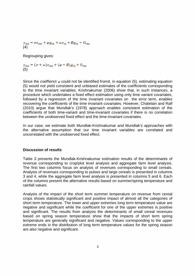
(4)

Regrouping gives:

(5)

Since the coeffienct could not be identified from , in equation (5), estimating equation (5) would not yield consistent and unbiased estimates of the coefficients corresponding to the time invariant variables. Krishnakumar (2006) show that, in such instances, a procedure which undertakes a fixed effect estimation using only time variant covariates, followed by a regression of the time invariant covariates on the error term, enables recovering the coefficients of the time invariant covariates. However, Chatelain and Ralf (2010) argue that Mundlak’s (1978) approach enables consistent estimation of the coefficients of both time-variant and time-invariant covariates if there is no correlation between the unobserved fixed effect and the time-invariant covariates. In our case, we estimate both Mundlak-Krishnakumar and Mundlak’s approaches with the alternative assumption that our time invariant variables are correlated and uncorrelated with the unobserved fixed effect.

Discussion of results

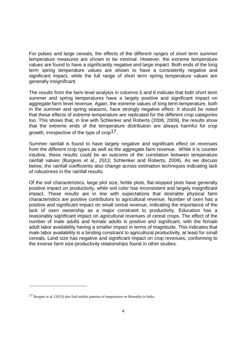
Table 3 presents the Mundlak-Krishnakumar estimation results of the determinants of revenue corresponding to crop/plot level analysis and aggregate farm level analysis. The first two columns focus on analysis of revenues corresponding to small cereals. Analysis of revenues corresponding to pulses and large cereals is presented in columns 3 and 4, while the aggregate farm level analysis is presented in columns 5 and 6. Each of the columns present the alternative results based on summer/spring temperature and rainfall values. Analysis of the impact of the short term summer temperature on revenue from cereal crops shows statistically significant and positive impact of almost all the categories of short term temperature. The lower and upper extremes long term temperature value are negative and significant while the coefficient for one of the upper extremes is positive and significant. The results from analysis the determinants of small cereal revenues based on spring season temperature show that the impacts of short term spring temperature are generally significant and negative. Values corresponding to the upper extreme ends in the distribution of long term temperature values for the spring season are also negative and significant.

4

For pulses and large cereals, the effects of the different ranges of short term summer temperature measures are shown to be minimal. However, the extreme temperature values are found to have a significantly negative and large impact. Both ends of the long term spring temperature values are shown to have a consistently negative and significant impact, while the full range of short term spring temperature values are generally insignificant. The results from the farm level analysis in columns 5 and 6 indicate that both short term summer and spring temperatures have a largely positive and significant impact on aggregate farm level revenue. Again, the extreme values of long term temperature, both in the summer and spring seasons, have strongly negative effect. It should be noted that these effects of extreme temperature are replicated for the different crop categories too. This shows that, in line with Schlenker and Roberts (2006; 2009), the results show that the extreme ends of the temperature distribution are always harmful for crop growth, irrespective of the type of crop17. Summer rainfall is found to have largely negative and significant effect on revenues from the different crop types as well as the aggregate farm revenue. While it is counter intuitive, these results could be an outcome of the correlation between temperature rainfall values (Burgess et al., 2013; Schlenker and Roberts, 2009). As we discuss below, the rainfall coefficients also change across estimation techniques indicating lack of robustness in the rainfall results. Of the soil characteristics, large plot size, fertile plots, flat-slopped plots have generally positive impact on productivity, while soil color has inconsistent and largely insignificant impact. These results are in line with expectations that desirable physical farm characteristics are positive contributors to agricultural revenue. Number of oxen has a positive and significant impact on small cereal revenue, indicating the importance of the lack of oxen ownership as a major constraint to productivity. Education has a reasonably significant impact on agricultural revenues of cereal crops. The effect of the number of male adults and female adults is positive and significant, with the female adult labor availability having a smaller impact in terms of magnitude. This indicates that male labor availability is a binding constraint to agricultural productivity, at least for small cereals. Land size has negative and significant impact on crop revenues, conforming to the inverse farm size-productivity relationships found in other studies.

17 Burgess et al. (2013) also find similar patterns of temperature on Mortality in India.

1

Table 3: Mundlak-Krishnakumar Fixed Effects Estimation of the Impacts of Climate Change and Weather on crop/farm level revenue

Small cereals Pulses and large cereals All crops/farm level

Summer Spring Summer Spring Summer Spring

temperature (1°C-3°C) -0.979 13.212*** 0.79 5.056 4.918 18.854***

(1.290) (3.495) (1.316) (3.320) (5.428) (5.334)

temperature (4°C-6°C) 4.320** -10.708*** 0.838 -4. 327* 17.049** -10.177***

(1.781) (2.435) (2.145) (2.389) (7.292) (3.709)

temperature (7°C-9°C) 4.011* 1.19 1.117 -0.215 20.304** 5.312***

(2.198) (0.933) (2.561) (1.142) (9.155) (1.374)

temperature (10°C-12°C) 3.625* -2.146** 1.205 -1.5 77 19.050** 2.527*

(2.181) (1.041) (2.537) (1.230) (9.071) (1.531)

temperature (13°C-15°C) 4.537** -1.906* 1.167 -0.7 91 21.517** 3.273**

(2.193) (1.010) (2.542) (1.209) (9.125) (1.482)

temperature (16°C-18°C) 3.579 -0.862 0.129 -0.103 18.512** 3.916**

(2.236) (1.065) (2.573) (1.253) (9.284) (1.554)

temperature (19°C-21°C) 2.766 -1.386 1.39 -1.189 16.976* 3.043**

(2.143) (0.945) (2.529) (1.147) (8.937) (1.416)

temperature (22°C-24°C) 3.653* -2.006** 1.12 -0.97 18.452** 2.924**

(2.176) (0.990) (2.539) (1.180) (9.057) (1.450)

temperature (25°C-27°C) 3.821* -2.363** 1.571 -1.8 33 19.087** 2.525*

(2.160) (0.993) (2.530) (1.194) (9.003) (1.478)

temperature (28°C-30°C) 2.797 -2.009** 0.756 -1.22 9 16.575* 2.669*

(2.172) (0.977) (2.535) (1.181) (9.043) (1.441)

temperature (31°C-33°C) 6.224*** -1.634 0.705 -1.1 55 25.089*** 3.446**

2

(2.240) (1.032) (2.577) (1.227) (9.297) (1.515)

temperature (34°C-36°C) 2.856 . 6.824* . -0.921 .

(3.304) . (3.542) . (13.194) .

long term temperature (1°C-3°C) -4.567*** -4.086*** -0.452 -2.386*** -18.462*** -0.905***

(0.331) (0.299) (0.440) (0.330) (2.320) (0.186)

long term temperature (34°C-36°C) 16.325*** 27.168* ** 0.75 26.465*** 21.210* 4.361***

(1.945) (1.054) (2.062) (1.143) (11.602) (0.585)

long term temperature (>=37°C) -126.942***

-465.606*** -80.851*** -608.903*** -123.299* -98.030***

(9.951) (26.587) (11.400) (27.342) (63.613) (14.169)

Summer/spring rainfall 0.016 -0.062** -0.119*** -0.067** -0.216** -0.108***

(0.222) (0.028) (0.023) (0.028) (0.090) (0.036)

Plot size in hectars: calculated 394.554*** 429.420*** 337.017*** 346.734*** 72.704 333.583***

(14.312) (14.542) (13.172) (13.464) (72.398) (26.691)

slope of parcel:meda -5.222 -10.233 -2.678 -5.395 71.984* 12.975

(7.387) (7.507) (7.120) (7.257) (41.797) (15.216)

soil quality of parcel:lem 36.882*** 14.151** -6.206 -11.765* 70.617** -6.32

7.104 7.201 6.553 6.667 35.689 13.34

soil type (color) of parcel:black 13.662* -11.502 -25.069*** -38.937*** -135.528***

-75.004***

(7.144) (7.202) (6.600) (6.693) (39.774) (14.388)

Constant 150.615*** 97.912*** 18.364 47.078*** 490.252*** 26.741***

(9.006) (8.291) (11.716) (9.087) (62.886) (5.025)

N 9810 9810 6293 6293 4844 4799

Year Dummy YES YES YES YES YES YES

Wald Chi2 1904.82 1481.79 1306.88 935.29 1288.30 384.01

Prob>chi2 0.0000 0.0000 0.0000 0.0000 0.0000 0.0000

Socioeconomic characteristics YES YES YES YES YES YES

* P<0.1, **p<0.05, ***p<0.001

Note: 1) The farm level analysis in the last two columns aggregates the revenues from all crops/plots at a farm level. Hence, the analysis is at a farm household level, instead of at a plot level, unlike the first four columns.

3

2) The socioeconomic characteristics controlled for include total land area, illiteracy, age of the household head, gender of the household head, number of oxen and livestock, number of male adult members, number of female adult members.

1

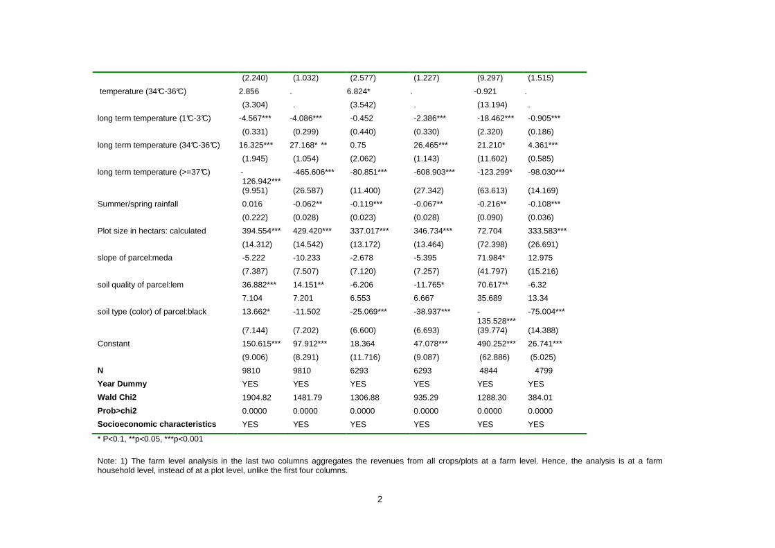
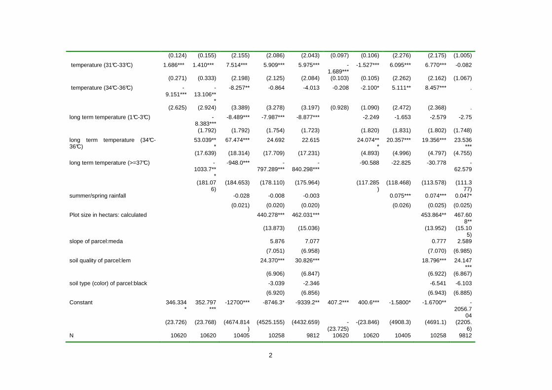
Tables 4 presents the Mundlak’s pseudo fixed effects estimation results corresponding to the determinants of revenues from small cereal crops. In the first panel of Table 4, the results based on summer temperature measures are presented. In the second panel, the results from the spring temperature measures are presented. In each of the panels, the first column presents the regression results based on short term temperature measures. The succeeding columns gradually add long term temperature measures, rainfall measures, physical farm characteristics, and finally socioeconomic characteristics. While the results reported in the earlier columns are added as robustness checks, discussion of the results is based on the last column in each panel where all these variables are controlled for. The results corresponding to short term temperature are positive and significant while the results for short term spring temperature are negative and signficant. Similarly, for long term temperature measures, both the lower (<3 degree Celsius) and upper (>37 degree Celsius) coefficients show strongly significant and negative impacts on the small cereal revenue. In comparison with the impacts of both short and term temperature based on the Mundlak-Krishnakumar estimator (Table 3), this indicates that that temperature has consistent impact on revenue from small cereals. Spring rainfall (short term) has a positive and significant impact, while summer rainfall is insignificant. The impacts of the physical farm and socioeconomic characteristics are similar to the results in the Mundlak-Krishnakumar analysis. In addition, these results are also shown to generally hold when using (dropping) other controls, such as physical farm characteristics, socioeconomic characteristics and rainfall, indicating the robustness the temperature results-the main focus of our analysis.

1

Table 4: Pseudo-Fixed Effects Estimation of the Impacts of Climate Change and Weather on crop level revenue (small cereals)**

Analysis based on summer temperature Analysis based on spring temperature

teff1 teff2 teff3 teff4 teff5 teff1 teff2 teff3 teff4 teff5

temperature (1°C-3°C) 0.478 0.451 2.606** 1.987* 2 .816** 9.911*** 9.482*** 9.324*** 10.243*** 6.821**

(0.920) (0.972) (1.241) (1.189) (1.170) (3.474) (3.543) (3.537) (3.381) (3.282)

temperature (4°C-6°C) -0.125 0.436 5.374*** 3.843* * 3.623** -7.410***

-7.837*** . . -4.905*

* (0.556) (0.589) (1.852) (1.799) (1.757) (2.287) (2.302) . . (2.308)

temperature (7°C-9°C) 0.307*** 0.293*** 6.449*** 4 .669** 4.814** 2.230*** 0.785*** 8.356*** 9.307*** 2.497***

(0.085) (0.086) (2.197) (2.126) (2.083) (0.196) (0.280) (2.303) (2.202) (0.941)

temperature (10°C-12°C) -0.138** 0.023 6.121*** 4. 289** 4.526** -2.407***

-1.413*** 6.189*** 6.766*** -0.31

(0.065) (0.073) (2.178) (2.108) (2.064) (0.135) (0.193) (2.288) (2.187) (1.089)

temperature (13°C-15°C) 0.386*** 0.453*** 6.603*** 4.625** 4.856** 1.131*** 1.108*** 8.697*** 9.039*** 2.101**

(0.067) (0.074) (2.191) (2.120) (2.077) (0.107) (0.109) (2.244) (2.145) (1.051)

temperature (16°C-18°C) 0.359** 0.364** 6.649*** 4 .437** 4.676** -1.592***

-0.934*** 6.728*** 7.770*** 0.839

(0.145) (0.152) (2.245) (2.173) (2.129) (0.287) (0.301) (2.210) (2.113) (1.126)

temperature (19°C-21°C) -0.591***

-0.345***

5.616*** 3.846* 4.110** 5.055*** 4.014*** 11.368*** 10.862*** 4.191***

(0.101) (0.105) (2.136) (2.069) (2.026) (0.283) (0.322) (2.309) (2.207) (0.974)

temperature (22°C-24°C) 0.049 0.073 6.157*** 4.366 ** 4.706** -3.448***

-3.567*** 4.007* 4.778** -1.970*

(0.066) (0.066) (2.169) (2.100) (2.057) (0.252) (0.258) (2.289) (2.188) (1.018)

temperature (25°C-27°C) -0.253***

0.204** 6.218*** 4.377** 4.519** 0.18 0.299* 7.848*** 7.916*** 0.988

(0.074) (0.097) (2.149) (2.081) (2.037) (0.147) (0.153) (2.304) (2.202) (1.047)

temperature (28°C-30°C) -0.884***

-0.383** 5.638*** 3.797* 4.225** -0.244** -0.387*** 7.136*** 7.448*** 0.621

2

(0.124) (0.155) (2.155) (2.086) (2.043) (0.097) (0.106) (2.276) (2.175) (1.005)

temperature (31°C-33°C) 1.686*** 1.410*** 7.514*** 5.909*** 5.975*** -1.689***

-1.527*** 6.095*** 6.770*** -0.082

(0.271) (0.333) (2.198) (2.125) (2.084) (0.103) (0.105) (2.262) (2.162) (1.067)

temperature (34°C-36°C) -9.151***

-13.106**

*

-8.257** -0.864 -4.013 -0.208 -2.100* 5.111** 8.457*** .

(2.625) (2.924) (3.389) (3.278) (3.197) (0.928) (1.090) (2.472) (2.368) .

long term temperature (1°C-3°C) -8.383***

-8.489*** -7.987*** -8.877*** -2.249 -1.653 -2.579 -2.75

(1.792) (1.792) (1.754) (1.723) (1.820) (1.831) (1.802) (1.748)


53.039***

67.474*** 24.692 22.615 24.074***

20.357*** 19.356*** 23.536***

(17.639) (18.314) (17.709) (17.231) (4.893) (4.996) (4.797) (4.755)

long term temperature (>=37°C) -1033.7**

*

-948.0*** -797.289***

-840.298***

-90.588 -22.825 -30.778 -62.579

(181.076)

(184.653) (178.110) (175.964) (117.285)

(118.468) (113.578) (111.377)

summer/spring rainfall -0.028 -0.008 -0.003 0.075*** 0.074*** 0.047*

(0.021) (0.020) (0.020) (0.026) (0.025) (0.025)

Plot size in hectars: calculated 440.278*** 462.031*** 453.864** 467.608**

(13.873) (15.036) (13.952) (15.105)

slope of parcel:meda 5.876 7.077 0.777 2.589

(7.051) (6.958) (7.070) (6.985)

soil quality of parcel:lem 24.370*** 30.826*** 18.796*** 24.147***

(6.906) (6.847) (6.922) (6.867)

soil type (color) of parcel:black -3.039 -2.346 -6.541 -6.103

(6.920) (6.856) (6.943) (6.885)

Constant 346.334*

352.797***

-12700*** -8746.3* -9339.2** 407.2*** 400.6*** -1.5800* -1.6700** -2056.7

04 (23.726) (23.768) (4674.814

) (4525.155) (4432.659) -

(23.725) -(23.846) (4908.3) (4691.1) (2205.

6) N 10620 10620 10405 10258 9812 10620 10620 10405 10258 9812

3

Year Dummy YES YES YES YES YES YES YES YES YES YES

Mundlak's fixed effects NO NO NO NO YES NO NO NO NO YES

Adjusted R-sq 0.1446 0.15 0.153 0.2342 0.2642 0.135 0.1394 0.1425 0.2281 0.2568

Socioeconomic characteristics NO NO NO NO YES NO NO NO NO YES

* P<0.1, **p<0.05, ***p<0.001



1

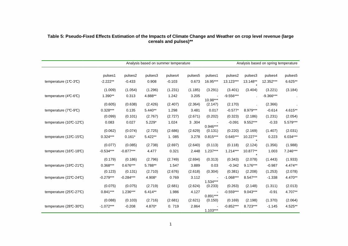
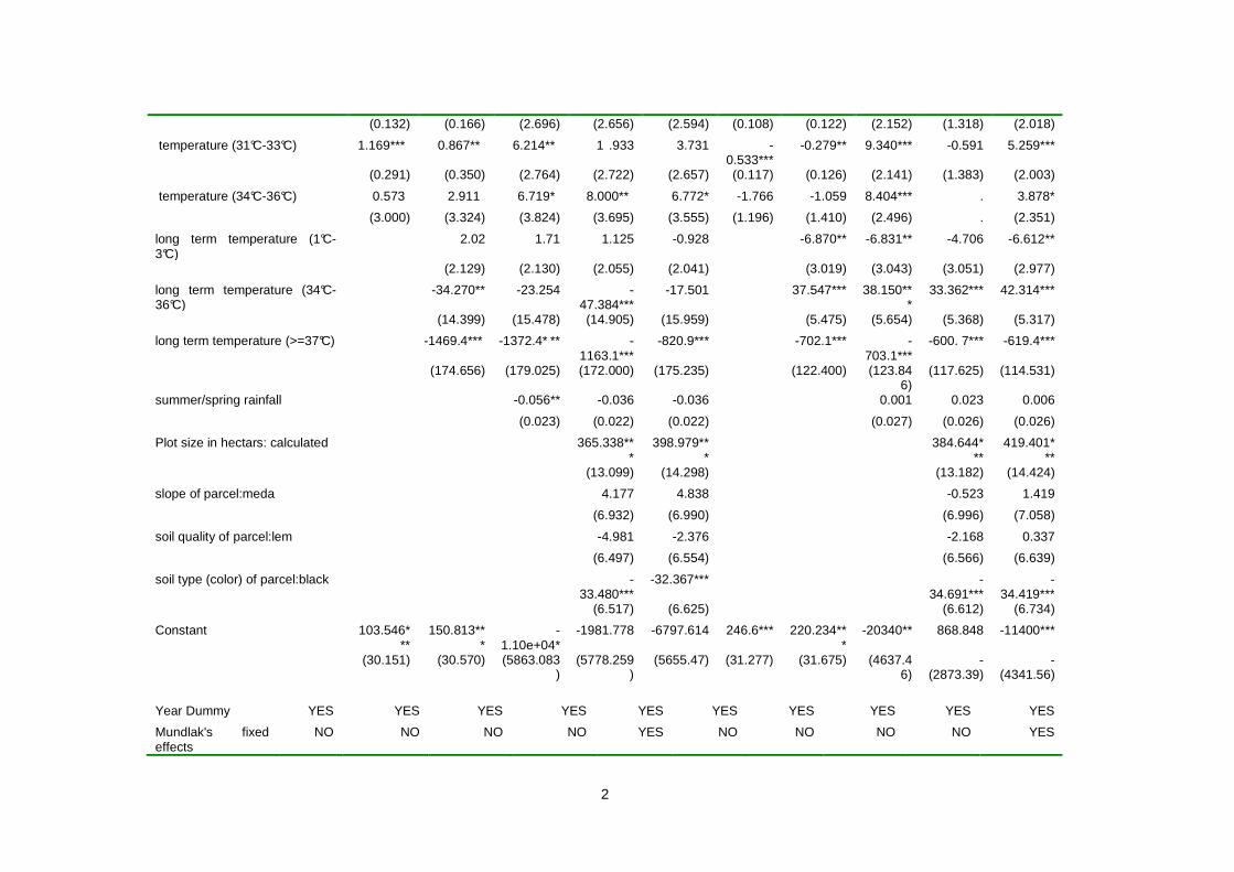
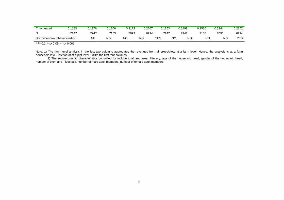
Table 5 presents Mundlak’s pseudo fixed effects estimation results for pulses and large cereals. Short term summer temperature is shown to have a generally insignificant on the revenue from this category of crops, but short term spring temperature has a positive and significant effect. The extreme ends of the long term temperature value are consistently negative for both spring and summer measures. The major (summer) season rainfall and minor (spring season rainfall are also largely insignificant. The impact of physical farm characteristics is largely insignificant, except plots with black soil colour showing negative impact on revenues from pulses and large cereals. Comparing Tables 4 and 5 shows that the patterns of the impact of socioeconomic characteristics is largely identical across the two crop categories, the impact of adult female labour is not significant in the large cereal and pulses category. This could be due to the fact that the small cereals are susceptible to weeds, a largely female labour task, making the availability of female labour more critical in the case of small cereal crops.

1

Table 5: Pseudo-Fixed Effects Estimation of the Impacts of Climate Change and Weather on crop level revenue (large cereals and pulses)**


pulses1 pulses2 pulses3 pulses4 pulses5 pulses1 pulses2 pulses3 pulses4 pulses5

temperature (1°C-3°C) -2.222** -0.433 0.908 -0.103 0.673 16.95*** 13.123*** 13.148***

12.352*** 6.625**

(1.009) (1.054) (1.296) (1.231) (1.185) (3.291) (3.401) (3.404) (3.221) (3.184)

temperature (4°C-6°C) 1.390** 0.313 4.888** 1.242 3.205 -10.98***

-9.556*** . -9.366*** .

(0.605) (0.638) (2.426) (2.407) (2.364) (2.147) (2.170) . (2.366) .

temperature (7°C-9°C) 0.328*** 0.135 5.440** 1.298 3.481 0.017 -0.577* 8.979*** -0.614 4.615**

(0.099) (0.101) (2.767) (2.727) (2.671) (0.202) (0.323) (2.186) (1.231) (2.054)

temperature (10°C-12°C) 0.083 0.027 5.229* 1.024 3 .304 -0.946***

-0.091 9.552*** -0.33 5.579***

(0.062) (0.074) (2.725) (2.686) (2.629) (0.131) (0.220) (2.169) (1.407) (2.031)

temperature (13°C-15°C) 0.324*** 0.161* 5.422** 1. 085 3.278 0.815*** 0.645*** 10.227***

0.223 6.034***

(0.077) (0.085) (2.738) (2.697) (2.640) (0.113) (0.118) (2.124) (1.356) (1.988)

temperature (16°C-18°C) -0.534*** -0.877*** 4.477 0.321 2.448 1.237*** 1.214*** 10.877***

1.003 7.246***

(0.179) (0.186) (2.796) (2.749) (2.694) (0.313) (0.343) (2.078) (1.443) (1.933)

temperature (19°C-21°C) 0.368*** 0.676*** 5.788** 1.547 3.889 0.03 -0.342 9.176*** -0.987 4.474**

(0.123) (0.131) (2.710) (2.676) (2.618) (0.304) (0.381) (2.208) (1.253) (2.078)

temperature (22°C-24°C) -0.279*** -0.284*** 4.908* 0.769 3.112 -1.534***

-1.068*** 8.547*** -1.338 4.470**

(0.075) (0.075) (2.719) (2.681) (2.624) (0.233) (0.263) (2.148) (1.311) (2.013)

temperature (25°C-27°C) 0.841*** 1.236*** 6.414** 1.986 4.127 -0.891***

-0.559*** 9.043*** -0.91 4.707**

(0.088) (0.103) (2.716) (2.681) (2.621) (0.150) (0.169) (2.198) (1.370) (2.064)

temperature (28°C-30°C) -1.072*** -0.208 4.870* 0. 719 2.864 -1.103***

-0.852*** 8.723*** -1.145 4.525**

2

(0.132) (0.166) (2.696) (2.656) (2.594) (0.108) (0.122) (2.152) (1.318) (2.018)

temperature (31°C-33°C) 1.169*** 0.867** 6.214** 1 .933 3.731 -0.533***

-0.279** 9.340*** -0.591 5.259***

(0.291) (0.350) (2.764) (2.722) (2.657) (0.117) (0.126) (2.141) (1.383) (2.003)

temperature (34°C-36°C) 0.573 2.911 6.719* 8.000** 6.772* -1.766 -1.059 8.404*** . 3.878*

(3.000) (3.324) (3.824) (3.695) (3.555) (1.196) (1.410) (2.496) . (2.351)


2.02 1.71 1.125 -0.928 -6.870** -6.831** -4.706 -6.612**

(2.129) (2.130) (2.055) (2.041) (3.019) (3.043) (3.051) (2.977)


-34.270** -23.254 -47.384***

-17.501 37.547*** 38.150***

33.362*** 42.314***

(14.399) (15.478) (14.905) (15.959) (5.475) (5.654) (5.368) (5.317)

long term temperature (>=37°C) -1469.4*** -1372.4* ** -1163.1***

-820.9*** -702.1*** -703.1***

-600. 7*** -619.4***

(174.656) (179.025) (172.000) (175.235) (122.400) (123.846)

(117.625) (114.531)

summer/spring rainfall -0.056** -0.036 -0.036 0.001 0.023 0.006

(0.023) (0.022) (0.022) (0.027) (0.026) (0.026)

Plot size in hectars: calculated 365.338***

398.979***

384.644***

419.401***

(13.099) (14.298) (13.182) (14.424)

slope of parcel:meda 4.177 4.838 -0.523 1.419

(6.932) (6.990) (6.996) (7.058)

soil quality of parcel:lem -4.981 -2.376 -2.168 0.337

(6.497) (6.554) (6.566) (6.639)

soil type (color) of parcel:black -33.480***

-32.367*** -34.691***

-34.419***

(6.517) (6.625) (6.612) (6.734)

Constant 103.546***

150.813***

-1.10e+04*

-1981.778 -6797.614 246.6*** 220.234***

-20340** 868.848 -11400***

(30.151) (30.570) (5863.083)

(5778.259)

(5655.47) (31.277) (31.675) (4637.46)

-(2873.39)

-(4341.56)

Year Dummy YES YES YES YES YES YES YES YES YES YES

Mundlak's fixed effects

NO NO NO NO YES NO NO NO NO YES

3

Chi-squared 0.1183 0.1276 0.1306 0.2172 0.2667 0.1353 0.1498 0.1536 0.2244 0.2252

N 7247 7247 7153 7093 6294 7247 7247 7153 7093 6294


* P<0.1, **p<0.05, ***p<0.001



1

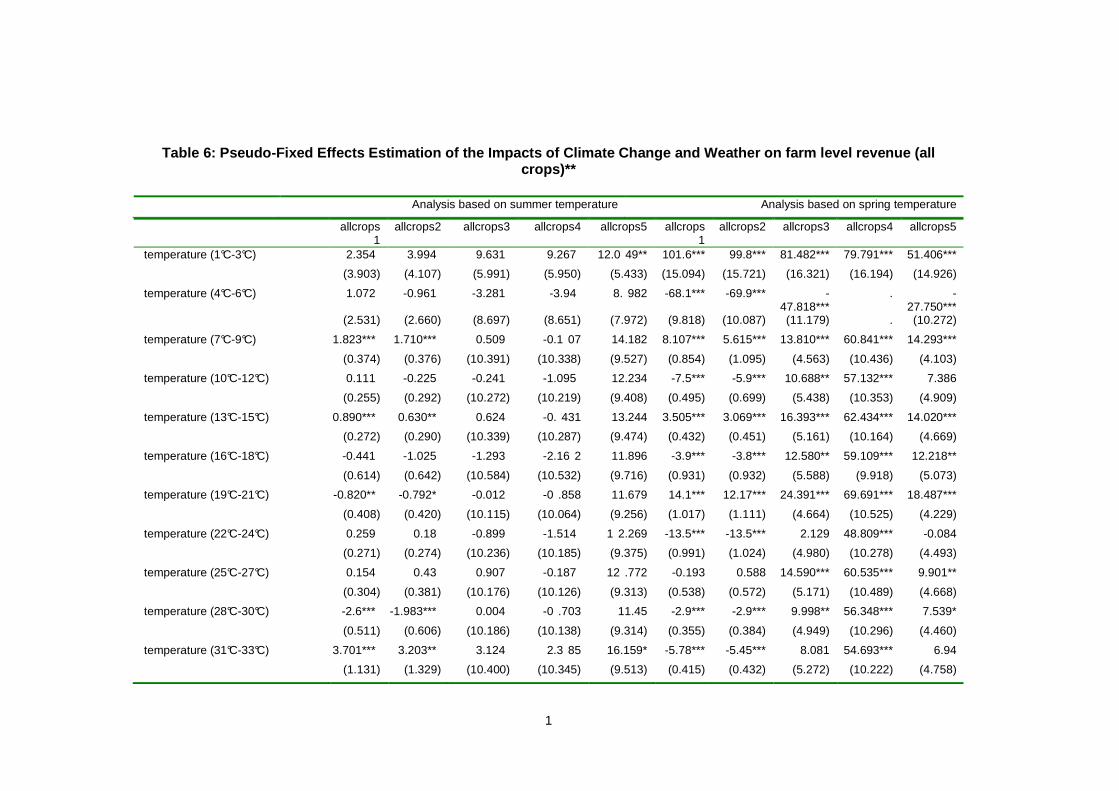
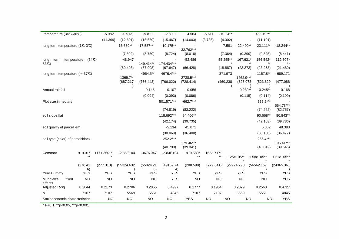
For farm level revenue, comparison of the results from Table 6 (Mundlak’s pseudo fixed effects estimator) and Table 3 (Mundlak-Krishnakumar estimator) show that both short term summer and spring temperatures have generally positive and significant effects. Summer and spring precipitation has no significant effect, based on the results from Table 6. Flat-slopped plots, having one of the desirable physical farm characteristics are associated with plots with significantly higher revenue. The effects of the physical farm characteristics and socioeconomic characteristics remain similar to those of the crop-specific analyses.

1

Table 6: Pseudo-Fixed Effects Estimation of the Impacts of Climate Change and Weather on farm level revenue (all crops)**


allcrops1

allcrops2 allcrops3 allcrops4 allcrops5 allcrops1

allcrops2 allcrops3 allcrops4 allcrops5

temperature (1°C-3°C) 2.354 3.994 9.631 9.267 12.0 49** 101.6*** 99.8*** 81.482*** 79.791*** 51.406***

(3.903) (4.107) (5.991) (5.950) (5.433) (15.094) (15.721) (16.321) (16.194) (14.926)

temperature (4°C-6°C) 1.072 -0.961 -3.281 -3.94 8. 982 -68.1*** -69.9*** -47.818***

. -27.750***

(2.531) (2.660) (8.697) (8.651) (7.972) (9.818) (10.087) (11.179) . (10.272)

temperature (7°C-9°C) 1.823*** 1.710*** 0.509 -0.1 07 14.182 8.107*** 5.615*** 13.810*** 60.841*** 14.293***

(0.374) (0.376) (10.391) (10.338) (9.527) (0.854) (1.095) (4.563) (10.436) (4.103)

temperature (10°C-12°C) 0.111 -0.225 -0.241 -1.095 12.234 -7.5*** -5.9*** 10.688** 57.132*** 7.386

(0.255) (0.292) (10.272) (10.219) (9.408) (0.495) (0.699) (5.438) (10.353) (4.909)

temperature (13°C-15°C) 0.890*** 0.630** 0.624 -0. 431 13.244 3.505*** 3.069*** 16.393*** 62.434*** 14.020***

(0.272) (0.290) (10.339) (10.287) (9.474) (0.432) (0.451) (5.161) (10.164) (4.669)

temperature (16°C-18°C) -0.441 -1.025 -1.293 -2.16 2 11.896 -3.9*** -3.8*** 12.580** 59.109*** 12.218**

(0.614) (0.642) (10.584) (10.532) (9.716) (0.931) (0.932) (5.588) (9.918) (5.073)

temperature (19°C-21°C) -0.820** -0.792* -0.012 -0 .858 11.679 14.1*** 12.17*** 24.391*** 69.691*** 18.487***

(0.408) (0.420) (10.115) (10.064) (9.256) (1.017) (1.111) (4.664) (10.525) (4.229)

temperature (22°C-24°C) 0.259 0.18 -0.899 -1.514 1 2.269 -13.5*** -13.5*** 2.129 48.809*** -0.084

(0.271) (0.274) (10.236) (10.185) (9.375) (0.991) (1.024) (4.980) (10.278) (4.493)

temperature (25°C-27°C) 0.154 0.43 0.907 -0.187 12 .772 -0.193 0.588 14.590*** 60.535*** 9.901**

(0.304) (0.381) (10.176) (10.126) (9.313) (0.538) (0.572) (5.171) (10.489) (4.668)

temperature (28°C-30°C) -2.6*** -1.983*** 0.004 -0 .703 11.45 -2.9*** -2.9*** 9.998** 56.348*** 7.539*

(0.511) (0.606) (10.186) (10.138) (9.314) (0.355) (0.384) (4.949) (10.296) (4.460)

temperature (31°C-33°C) 3.701*** 3.203** 3.124 2.3 85 16.159* -5.78*** -5.45*** 8.081 54.693*** 6.94

(1.131) (1.329) (10.400) (10.345) (9.513) (0.415) (0.432) (5.272) (10.222) (4.758)

2

temperature (34°C-36°C) -5.982 -0.913 -9.811 -2.80 1 4.564 -5.611 -10.24** . 48.919*** .

(11.369) (12.601) (15.559) (15.467) (14.003) (3.785) (4.302) . (11.101) .

long term temperature (1°C-3°C) 16.669** -17.587** -19.175** -32.762***

7.591 -22.490** -23.111** -18.244**

(7.502) (8.750) (8.724) (8.018) (7.364) (9.399) (9.325) (8.441)


-48.947 -149.414**

-174.434***

-52.486 55.255***

167.631***

156.542***

112.507***

(60.493) (67.908) (67.647) (66.428) (18.887) (23.373) (23.258) (21.480)

long term temperature (>=37°C) -1369.7**

-4954.5** -4676.4*** -2738.5***

-371.973 -1462.9***

-1157.8** -689.171

(687.217)

(766.443) (766.020) (728.414) (460.238)

(526.073)

(523.629)

(477.088)

Annual rainfall -0.148 -0.107 -0.056 0.239** 0.245** 0.168

(0.094) (0.093) (0.086) (0.115) (0.114) (0.109)

Plot size in hectars 501.571*** -662.7*** 555.2*** -564.78***

(74.819) (83.222) (74.262) (82.757)

soil slope:flat 118.692*** 94.406** 90.668** 80.843**

(42.174) (39.735) (42.103) (39.736)

soil quality of parcel:lem -5.134 45.071 5.052 48.383

(38.060) (36.400) (38.100) (36.477)

soil type (color) of parcel:black -252.2*** -179.46***

-256.4*** -195.41***

(40.790) (39.341) (40.842) (39.545)

Constant 919.01***

1171.360***

-2.88E+04 -3676.047 -2.84E+04 1819.589***

1653.717***

-1.25e+05**

*

-1.58e+05**

*

-1.21e+05**

* (278.41

6) (277.313) (55324.632

) (55024.21

6) (49162.74

4) (280.590) (279.841) (27774.790

) (56562.157

) (24365.361

) Year Dummy YES YES YES YES YES YES YES YES YES YES

Mundlak's fixed effects

NO NO NO NO YES NO NO NO NO YES

Adjusted R-sq 0.2044 0.2173 0.2706 0.2855 0.4997 0.1777 0.1964 0.2379 0.2568 0.4727

N 7107 7107 5569 5551 4845 7107 7107 5569 5551 4845


* P<0.1, **p<0.05, ***p<0.001

3



1

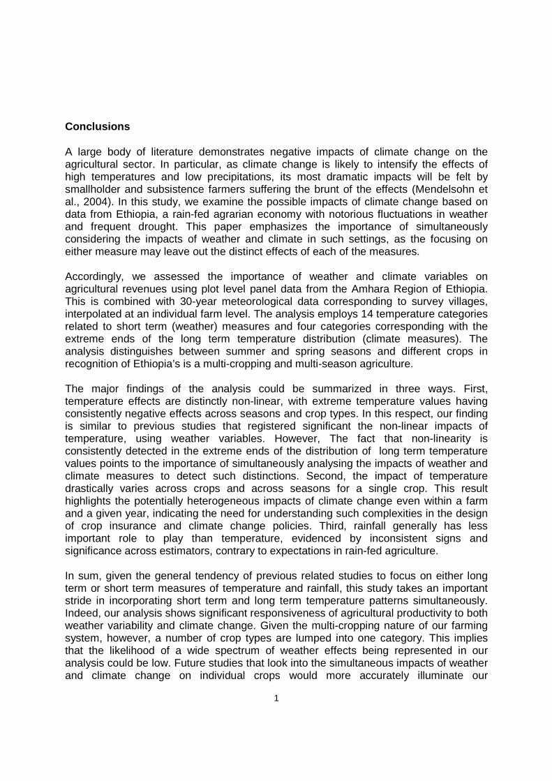
Conclusions

A large body of literature demonstrates negative impacts of climate change on the agricultural sector. In particular, as climate change is likely to intensify the effects of high temperatures and low precipitations, its most dramatic impacts will be felt by smallholder and subsistence farmers suffering the brunt of the effects (Mendelsohn et al., 2004). In this study, we examine the possible impacts of climate change based on data from Ethiopia, a rain-fed agrarian economy with notorious fluctuations in weather and frequent drought. This paper emphasizes the importance of simultaneously considering the impacts of weather and climate in such settings, as the focusing on either measure may leave out the distinct effects of each of the measures. Accordingly, we assessed the importance of weather and climate variables on agricultural revenues using plot level panel data from the Amhara Region of Ethiopia. This is combined with 30-year meteorological data corresponding to survey villages, interpolated at an individual farm level. The analysis employs 14 temperature categories related to short term (weather) measures and four categories corresponding with the extreme ends of the long term temperature distribution (climate measures). The analysis distinguishes between summer and spring seasons and different crops in recognition of Ethiopia’s is a multi-cropping and multi-season agriculture. The major findings of the analysis could be summarized in three ways. First, temperature effects are distinctly non-linear, with extreme temperature values having consistently negative effects across seasons and crop types. In this respect, our finding is similar to previous studies that registered significant the non-linear impacts of temperature, using weather variables. However, The fact that non-linearity is consistently detected in the extreme ends of the distribution of long term temperature values points to the importance of simultaneously analysing the impacts of weather and climate measures to detect such distinctions. Second, the impact of temperature drastically varies across crops and across seasons for a single crop. This result highlights the potentially heterogeneous impacts of climate change even within a farm and a given year, indicating the need for understanding such complexities in the design of crop insurance and climate change policies. Third, rainfall generally has less important role to play than temperature, evidenced by inconsistent signs and significance across estimators, contrary to expectations in rain-fed agriculture. In sum, given the general tendency of previous related studies to focus on either long term or short term measures of temperature and rainfall, this study takes an important stride in incorporating short term and long term temperature patterns simultaneously. Indeed, our analysis shows significant responsiveness of agricultural productivity to both weather variability and climate change. Given the multi-cropping nature of our farming system, however, a number of crop types are lumped into one category. This implies that the likelihood of a wide spectrum of weather effects being represented in our analysis could be low. Future studies that look into the simultaneous impacts of weather and climate change on individual crops would more accurately illuminate our

2

understanding of the underlying relationships. We may note, however, that to the extent that the pattern of climate change mimics weather uncertainty, policy measures aimed at mitigating the impacts of climate change could also serve the same purpose as those for weather uncertainty. From policy perspective, the results highlight the need to factor in the distinction between crops and seasons in designing yield insurance measures. In addition, insurance schemes also need to look into specific measures that target extreme values.

References

Adams RM, Flemming RA, Chang CC, McCarl B, Rosenzweig C (1995) A reassessment of the

economic effects of global climate change on U.S. agriculture. Climatic Change 30:147–

167.

Adenew, B. 2006. Effective Aid for Small Farmers in Sub-Saharan Africa: Southern Civil Society Perspectives—Ethiopia Case Study. Addis Ababa, Ethiopia: Canadian Food Security Policy Group. http://www.ccic.ca/_files/en/working_groups/003_food_2007-01_small_farmers_research_report_ethiopia.pdf. Accessed 23 February 2010.

AfDB (African Development Bank) (2011). Federal Democratic Republic of Ethiopia: Country

Strategy Paper 2011-15, April.

Auffhammer, M., S. Hsiang, W. Schlenker, A. Sobel (2013) Using weather data and climate

model output in economic analyses of climate change. Rev. Environ. Econ. Policy 7,

181–198

Barrett, C.B., ,B.J. Barnett, M.R. Carter, S. Chantarat;, J.W. Hansen;, A.G. Mude , D.E. Osgood,

J.R. Skees, C.G. Turvey, M.N. Ward, 2007. Poverty Traps and Climate Risk: Limitations

and Opportunities of Index-Based Risk Financing, IRI Technical Report 07-03 Working

Paper, Columbia University.

Batagi, B.H. (2001). Econometric Analysis of Panel Data (Second Edition), New York, Wiley.

Black JR, Thompson SR (1978) Some evidence on weather-crop-yield interaction. American

Journal of Agricultural Econ 60:540–543.

3

Brown RA, Rosenberg NJ (1999) Climate change impacts on the potential productivity of corn

and winter wheat in their primary United States growing regions. Climatic Change

41:73–107.

Burgess, R., O. Deschenes, D. Donaldson, M. Greenestone (2013) The Unequal Effects of

Weather and Climate Change: Evidence from Mortality in India.

Cao, J. 2008. Reconciling Human Development and Climate Protection: Perspectives from

Developing Countries on Post-2012, International Climate Change Policy. Discussion

Paper 08-25. The Harvard Project on International Climate Agreements, Kennedy School

of Government, Harvard University.

Chatelain, J and K. Ralf (2010) Inference on Time invariant variables using Panel Data: A pre-

Test Estimator with an Application to the Returns to Schooling. PSE Working Paper.

Available at http://hal-paris1.archives-

ouvertes.fr/docs/00/49/20/39/PDF/Chatelain_Ralf_Time_Invariant_Panel.pdf

Cassman, Kenneth G. (1999) Ecological intensification of cereal production systems: Yield

potential, soil quality, and precision agriculture. Proceedings of the National Academy of

Science of the United States of America, 96(11):5952-5959, 1999.

Dai, A., K. E. Trenberth, and T. Qian (2004). A global data set of Palmer Drought Severity Index

for 1870-2002: Relationship with soil moisture and effects of surface warming. J.

Hydrometeorology, 5:1117-1130, 2004.

Dercon, S., 2009 Risk, poverty and insurance, IFPRI Focus 17(3), International Food Policy

Research Institute (IFPRI), Washington DC.

Devereux, S. 2000. Food Insecurity in Ethiopia: A Discussion Paper for DFID. Sussex, UK:

IDS. http://cramforum.jrc.it/Shared%20Documents/Food%20Insecurity%20in%20-

Ethiopia.pdf. Accessed 23 February 2010.

De Salvo, M., R. Roberta and M. Riccarda (2013). The impact of climate change on permanent

crops in an Alpine region: A Ricardian analysis. Agricultural Systems 118: 23-32.

4

Deschênes, Olivier, and Michael Greenstone (2007). The Economic Impacts of Climate Change:

Evidence from Agricultural Output and Random Fluctuations in Weather. American

Economic Review, 97(1): 354–385.

Salvatore Di Falco and Marcella Veronesi (2013). How African Agriculture Can Adapt to

Climate Change? Countefactual Analysis from Ethiopia. Land Economics. 89 (4): 743-

766.

Di Falco, Salvatore, Marcella Veronesi and Mahmud Yesuf (2011) Does Adaptation To Climate

Change Provide Food Security? A Micro-Perspective from Ethiopia, American Journal of

Agricultural Economics, 93(3): 829-846.

Fezzi, Carlo. I. Bateman, and W. Schlenker (2010) The Ricardian Approach with Panel Data and

Flexible Functional Forms: An Additive Mixed Model applied to England and Wales

farmland.

values.http://www.webmeets.com/files/papers/WCERE/2010/1528/paper%20CC-

%20%20_%20conference%20version.pdf

Fisher, A., W. M. Hanemann, M.J. Roberts, and W. Schlenker (2012) The Economic Impacts of

Climate Change: Evidence from Agricultural Output and Random Fluctuations in

Weather: Comment. American Economic Review. 102:3749-3760.

Gutro, Rob (2005). NASA's Earth-Sun Science News Team/SSAINASA Goddard Space Flight

Center, Greenbelt, Md., and excerpts from NOAA's CPC web page, and the U.S. EPA

web page. 2/2005Edits: Dr. J. Marshall Shepherd, NASA/GSFC, Drew Shindell,

NASA/GISS, Cynthia M. O'Carroll, NASA/GSFC.

Grierson, W. (2002) Role of Temperature in the Physiology of Crop Plants: Pre- and Post-

Harvest, in Mohammed Pessarakli (editor), Handbook of Plant and Crop Physiology,

New York: MarcelDekker.

Hodges, T, ed. (1991): Predicting Crop Phenology, Boca Raton: CRC Press, 1991.

Krishnakumar, Jaya (2006) Time invriant variables and panel data models: a generalised Frisch-

Waugh theorem and its implications. Chap. 5 In ‘Panel data econometrics: theoretical

5

contributions and empirical applications’, edited by Badi H. Baltagi. 119-32. Amsterdam:

Elsevier.

Kurukulasuriya, P., and Mendelsohn, R. (2008) Crop switching as a strategy for adapting to

climate change, African Journal of Agricultural and Resource Economics, Volume 2, No.

1 (March), Pretoria.

Lang, G (2007) Where are Germany’s gains from Kyoto? Estimating the effects of global

warming on agriculture. Climate Change 84: 423-439

Lobell, David B. and Gregory P. Asner (2003) Climate and Management Contributions to Recent

Trends in U.S. Agricultural Yields. Science 299:1032, 2003.

Maraun, D., F. Wetterhall, A. M. Ireson, R. E. Chandler, E. J. Kendon, M. Widmann. S.

Brienen, H. W. Rust, T. Sauter, M. Theme V. K. C. Venema, K. P. Chun, C. M. Goodess,

R. G. Jones, C. Onof, M. Vrac, and I. Thiele (2010). Precipitation downscaling under

climate change: Recent developments to bridge the gap between dynamical models and

the end user. Review of Geophysics 48(3): 1-34.

Massetti, E.and R. Mendelsohn (2011) Estimating Ricardian Models With Panel Data, Climate

Change Economics, Vol. 2(4): 301-319.

Mearns, LO, Easterling W, Hays C, Marx D (2001) Comparison of agricultural impacts of

climate change calculated from high and low resolution climate change scenarios: Part I.

The uncertainty due to spatial scale. Climatic Change51:131–172.

Mendelsohn, R. and A. Dinar (2009) Climate change and agriculture.An economic analysis of

global impact, adaptation and distributional effects, Elgar, Cheltenham.

Mendelsohn RO, Nordhaus WD, Shaw D (1994): The Impact of Global Warming on

Agriculture: ARicardian Analysis. American Economic Review, 84(4): 753-771.

Mendelsohn, R., A. Dinar, and L. Williams. 2006. “The Distributional Impact of Climate Change

On Rich and Poor Countries” Environment and Development Economics 11: 1-20

Mundlak, Y. 1978. On the Pooling of Time Series and Cross Section Data. Econometrica 46: 69-85.

6

Radha, V. Krishna Murthy (2004) Ecological intensification of cereal production systems: Yield

potential, soil quality, and precision agriculture. In Satellite Remote Sensing and GIS

Applications in Agricultural Meteorology, volume AGM-8, 2004.

Rosenzweig, C., A. Iglesias, X.B. Yang, P. R. Epstein and E. Chivian (2009) Climate Change

and Extreme Weather Events; Implications for Food Production, Plant Diseases, and

Pests Global Change & Human Health. 2(2): 90-104.

Sachs, J., T. Panatayou, and A. Peterson (1999) Developing Countries and the Control of

Climate Change: A Theoretical Perspective and Policy Implications. CAER II Discussion

Paper, no. 44. Cambridge, MA, USA: Harvard Institute for International Development

HII D.

Stage, J. (2010) Economic valuation of climate change adaptationin developing countries.

Annals of the New York Academy of Sciences.1185 150–163 c_ 2010 New York

Academy of Sciences.

Schlenker, Wolfram, and Michael J. Roberts.2009. Nonlinear Temperature Effects Indicate

SevereDamages to US Crop Yields under Climate Change. Proceedings of the

NationalAcademy of Sciences106 (37): 15594–8.

Schlenker, Hanemann, and Fisher (2006).The Impact of Global Warming on U.S.Agriculture: An

Econometric Analysis of Optimal Growing Conditions. Review of Economics and

Statistics, 88(1): 113-125, February 2006.

Schlenker, W. and M. Roberts (2006). Non Linear Effects of Weather on Corn Yields. Review of

Agricultural Economics. 28: 391-398.

Seo, S.N., and R. Mendelsohn ( 2008a) Measuring Impacts and Adaptations to Climate Change:

A Structural Ricardian Model of African Livestock Management. Agricultural

Economics 38(2): 151-165.

Seo, S. N., and R. Mendelsohn (2008b) A Ricardian Analysis of The Impact of Climate Change

Impacts on South American Farms. Chilean Journal of Agricultural Research 68: 69-79.

7

Stockle CO, Donatelli M, Nelson R (2003) CropSyst: a cropping systems simulation model. Eur

J Agron18:289–307.

Timmins, C. (2006) Endogenous Land use and the Ricardian Valuation of Climate Change

Environmental& Resource Economics, 33(1): 119-142.

Wooldridge, J.M. 2002. Econometric Analysis of Cross Section and Panel Data. MIT

Press, Cambridge, MA.

World Bank (2008a) Ethiopia: Climate Factsheet, Washington DC: World Bank,

http://siteresources.worldbank.org/INTAFRICA/Resources/Ethiopia_Country_Note.pdf.

Accessed 29 April 2010.

World Bank (2008b) Rural Households and Their Pathways Out of Poverty.In World

Development Report 2008.http://siteresources.worldbank.org/INTWDR2008/-Resources-

/2795087-1192112387976/WDR08_06_ch03.pdf. Accessed 23 February 2010.

Yu, Tian. Three Essays on Weather and Crop Yield.PhD thesis, Iowa State Univeristy, 2011.

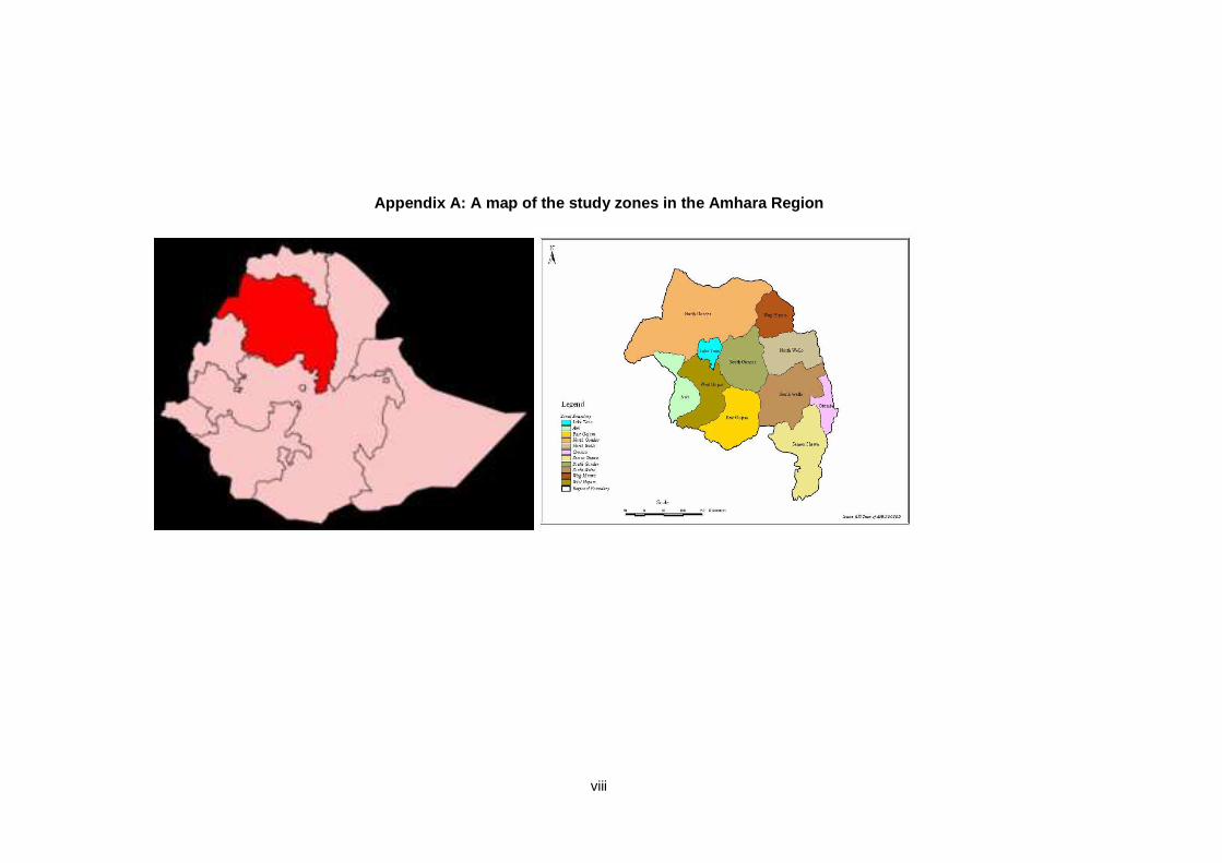
viii

Appendix A: A map of the study zones in the Amhara Region

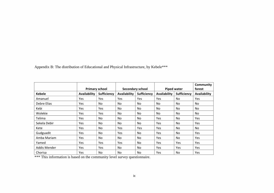
ix

Appendix B: The distribution of Educational and Physical Infrastructure, by Kebele***

Primary school Secondary school Piped water

Community

forest

Kebele Availability Sufficiency Availability Sufficiency Availability Sufficiency Availability

Amanuel Yes Yes Yes Yes Yes No Yes

Debre Elias Yes No No No No No No

Kebi Yes Yes No No No No No

Wolekie Yes Yes No No No No No

Telima Yes No No No Yes No Yes

Sekela Debir Yes No No No Yes No Yes

Kete Yes No Yes Yes Yes No No

Gudguadit Yes No Yes No Yes No Yes

Amba Mariam Yes No No No Yes No Yes

Yamed Yes Yes Yes No Yes Yes Yes

Addis Mender Yes Yes No No Yes Yes Yes

Chorisa Yes No No No Yes No Yes

*** This information is based on the community level survey questionnaire.

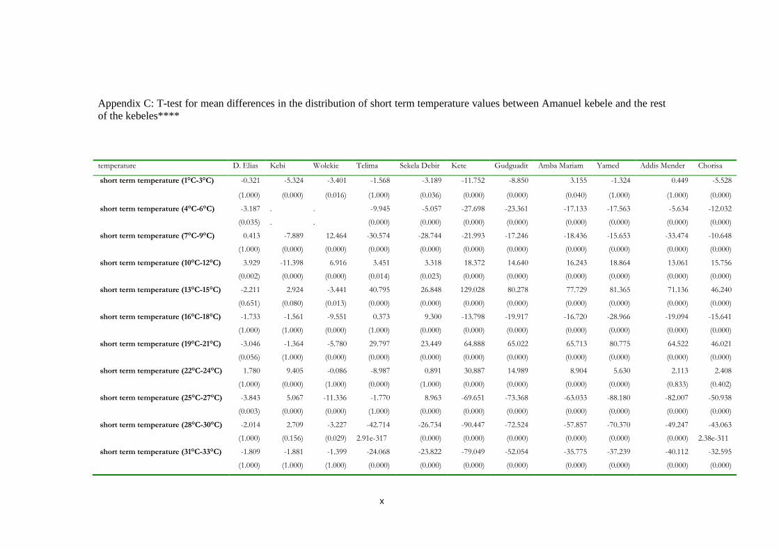
x

Appendix C: T-test for mean differences in the distribution of short term temperature values between Amanuel kebele and the rest of the kebeles****

temperature D. Elias Kebi Wolekie Telima Sekela Debir Kete Gudguadit Amba Mariam Yamed Addis Mender Chorisa

short term temperature (1°C-3°C) -0.321 -5.324 -3.401 -1.568 -3.189 -11.752 -8.850 3.155 -1.324 0.449 -5.528

(1.000) (0.000) (0.016) (1.000) (0.036) (0.000) (0.000) (0.040) (1.000) (1.000) (0.000)

short term temperature (4°C-6°C) -3.187 . . -9.945 -5.057 -27.698 -23.361 -17.133 -17.563 -5.634 -12.032

(0.035) . . (0.000) (0.000) (0.000) (0.000) (0.000) (0.000) (0.000) (0.000)

short term temperature (7°C-9°C) 0.413 -7.889 12.464 -30.574 -28.744 -21.993 -17.246 -18.436 -15.653 -33.474 -10.648

(1.000) (0.000) (0.000) (0.000) (0.000) (0.000) (0.000) (0.000) (0.000) (0.000) (0.000)

short term temperature (10°C-12°C) 3.929 -11.398 6.916 3.451 3.318 18.372 14.640 16.243 18.864 13.061 15.756

(0.002) (0.000) (0.000) (0.014) (0.023) (0.000) (0.000) (0.000) (0.000) (0.000) (0.000)

short term temperature (13°C-15°C) -2.211 2.924 -3.441 40.795 26.848 129.028 80.278 77.729 81.365 71.136 46.240

(0.651) (0.080) (0.013) (0.000) (0.000) (0.000) (0.000) (0.000) (0.000) (0.000) (0.000)

short term temperature (16°C-18°C) -1.733 -1.561 -9.551 0.373 9.300 -13.798 -19.917 -16.720 -28.966 -19.094 -15.641

(1.000) (1.000) (0.000) (1.000) (0.000) (0.000) (0.000) (0.000) (0.000) (0.000) (0.000)

short term temperature (19°C-21°C) -3.046 -1.364 -5.780 29.797 23.449 64.888 65.022 65.713 80.775 64.522 46.021

(0.056) (1.000) (0.000) (0.000) (0.000) (0.000) (0.000) (0.000) (0.000) (0.000) (0.000)

short term temperature (22°C-24°C) 1.780 9.405 -0.086 -8.987 0.891 30.887 14.989 8.904 5.630 2.113 2.408

(1.000) (0.000) (1.000) (0.000) (1.000) (0.000) (0.000) (0.000) (0.000) (0.833) (0.402)

short term temperature (25°C-27°C) -3.843 5.067 -11.336 -1.770 8.963 -69.651 -73.368 -63.033 -88.180 -82.007 -50.938

(0.003) (0.000) (0.000) (1.000) (0.000) (0.000) (0.000) (0.000) (0.000) (0.000) (0.000)

short term temperature (28°C-30°C) -2.014 2.709 -3.227 -42.714 -26.734 -90.447 -72.524 -57.857 -70.370 -49.247 -43.063

(1.000) (0.156) (0.029) 2.91e-317 (0.000) (0.000) (0.000) (0.000) (0.000) (0.000) 2.38e-311

short term temperature (31°C-33°C) -1.809 -1.881 -1.399 -24.068 -23.822 -79.049 -52.054 -35.775 -37.239 -40.112 -32.595

(1.000) (1.000) (1.000) (0.000) (0.000) (0.000) (0.000) (0.000) (0.000) (0.000) (0.000)

xi

short term temperature (34°C-36°C) . . . -2.538 -3.279 -21.341 -16.712 -17.539 -20.398 . -10.656

. . . (0.280) (0.026) (0.000) (0.000) (0.000) (0.000) . (0.000)

**** Figures in parenthesis are p-values

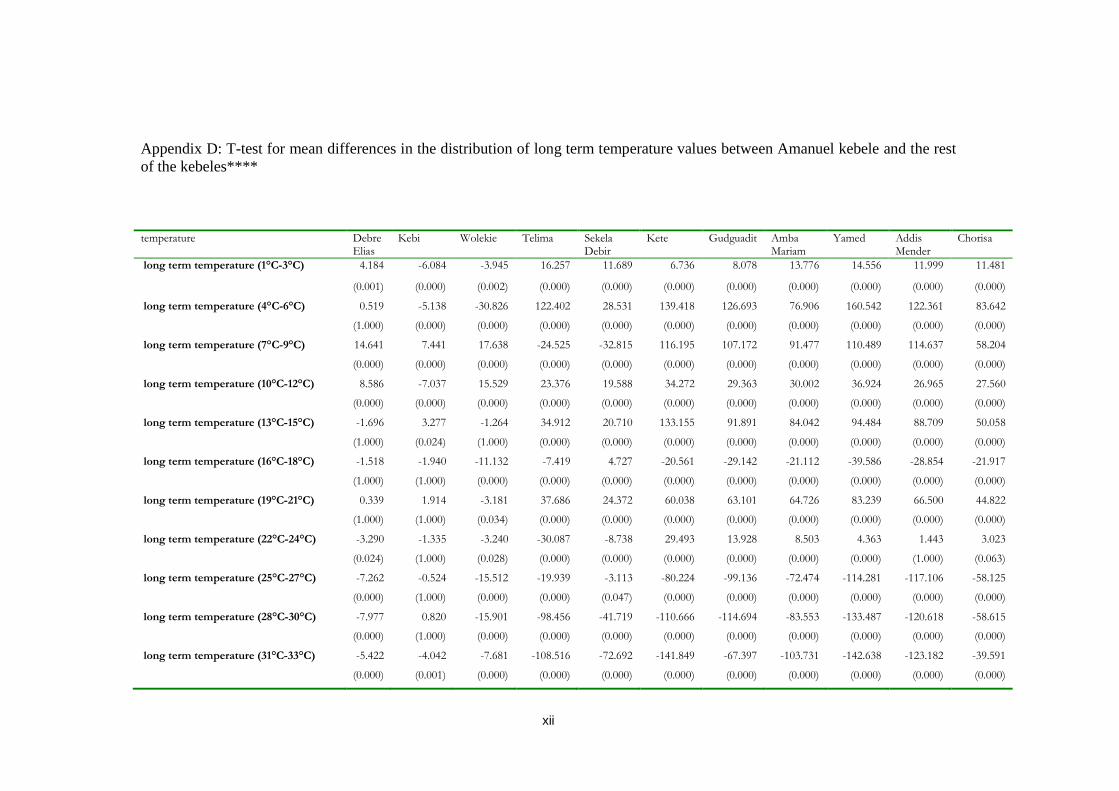
xii

Appendix D: T-test for mean differences in the distribution of long term temperature values between Amanuel kebele and the rest of the kebeles****

temperature Debre Elias

Kebi Wolekie Telima Sekela Debir

Kete Gudguadit Amba Mariam

Yamed Addis Mender

Chorisa

long term temperature (1°C-3°C) 4.184 -6.084 -3.945 16.257 11.689 6.736 8.078 13.776 14.556 11.999 11.481

(0.001) (0.000) (0.002) (0.000) (0.000) (0.000) (0.000) (0.000) (0.000) (0.000) (0.000)

long term temperature (4°C-6°C) 0.519 -5.138 -30.826 122.402 28.531 139.418 126.693 76.906 160.542 122.361 83.642

(1.000) (0.000) (0.000) (0.000) (0.000) (0.000) (0.000) (0.000) (0.000) (0.000) (0.000)

long term temperature (7°C-9°C) 14.641 7.441 17.638 -24.525 -32.815 116.195 107.172 91.477 110.489 114.637 58.204

(0.000) (0.000) (0.000) (0.000) (0.000) (0.000) (0.000) (0.000) (0.000) (0.000) (0.000)

long term temperature (10°C-12°C) 8.586 -7.037 15.529 23.376 19.588 34.272 29.363 30.002 36.924 26.965 27.560

(0.000) (0.000) (0.000) (0.000) (0.000) (0.000) (0.000) (0.000) (0.000) (0.000) (0.000)

long term temperature (13°C-15°C) -1.696 3.277 -1.264 34.912 20.710 133.155 91.891 84.042 94.484 88.709 50.058

(1.000) (0.024) (1.000) (0.000) (0.000) (0.000) (0.000) (0.000) (0.000) (0.000) (0.000)

long term temperature (16°C-18°C) -1.518 -1.940 -11.132 -7.419 4.727 -20.561 -29.142 -21.112 -39.586 -28.854 -21.917

(1.000) (1.000) (0.000) (0.000) (0.000) (0.000) (0.000) (0.000) (0.000) (0.000) (0.000)

long term temperature (19°C-21°C) 0.339 1.914 -3.181 37.686 24.372 60.038 63.101 64.726 83.239 66.500 44.822

(1.000) (1.000) (0.034) (0.000) (0.000) (0.000) (0.000) (0.000) (0.000) (0.000) (0.000)

long term temperature (22°C-24°C) -3.290 -1.335 -3.240 -30.087 -8.738 29.493 13.928 8.503 4.363 1.443 3.023

(0.024) (1.000) (0.028) (0.000) (0.000) (0.000) (0.000) (0.000) (0.000) (1.000) (0.063)

long term temperature (25°C-27°C) -7.262 -0.524 -15.512 -19.939 -3.113 -80.224 -99.136 -72.474 -114.281 -117.106 -58.125

(0.000) (1.000) (0.000) (0.000) (0.047) (0.000) (0.000) (0.000) (0.000) (0.000) (0.000)

long term temperature (28°C-30°C) -7.977 0.820 -15.901 -98.456 -41.719 -110.666 -114.694 -83.553 -133.487 -120.618 -58.615

(0.000) (1.000) (0.000) (0.000) (0.000) (0.000) (0.000) (0.000) (0.000) (0.000) (0.000)

long term temperature (31°C-33°C) -5.422 -4.042 -7.681 -108.516 -72.692 -141.849 -67.397 -103.731 -142.638 -123.182 -39.591

(0.000) (0.001) (0.000) (0.000) (0.000) (0.000) (0.000) (0.000) (0.000) (0.000) (0.000)

xiii

long term temperature (34°C-36°C) 2.254 5.262 -0.691 -41.510 -35.407 -23.726 9.287 85.430 102.263 147.284 39.083

(0.582) (0.000) (1.000) (0.000) (0.000) (0.000) (0.000) (0.000) (0.000) (0.000) (0.000)

long term temperature (>=37°C) 2.628 4.523 -6.331 -52.227 -59.935 -133.043 -67.885 -82.325 -85.675 -93.442 -33.984

(0.207) (0.000) (0.000) (0.000) (0.000) (0.000) (0.000) (0.000) (0.000) (0.000) (0.000)