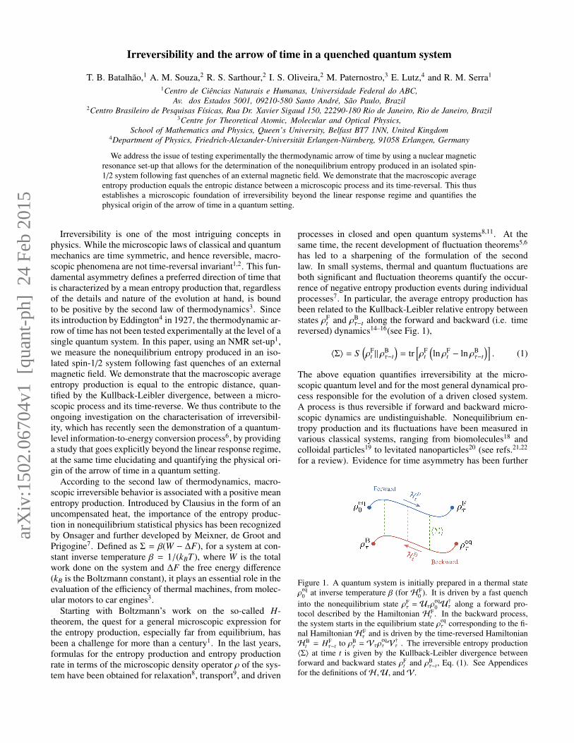
Irreversibility and the arrow of time in a quenched quantum system

Irreversibility and the arrow of time in a quenched quantum system

T. B. Batalhão,1 A. M. Souza,2 R. S. Sarthour,2 I. S. Oliveira,2 M. Paternostro,3 E. Lutz,4 and R. M. Serra1

1Centro de Ciências Naturais e Humanas, Universidade Federal do ABC,Av. dos Estados 5001, 09210-580 Santo André, São Paulo, Brazil

2Centro Brasileiro de Pesquisas Físicas, Rua Dr. Xavier Sigaud 150, 22290-180 Rio de Janeiro, Rio de Janeiro, Brazil3Centre for Theoretical Atomic, Molecular and Optical Physics,

School of Mathematics and Physics, Queen’s University, Belfast BT7 1NN, United Kingdom4Department of Physics, Friedrich-Alexander-Universität Erlangen-Nürnberg, 91058 Erlangen, Germany

We address the issue of testing experimentally the thermodynamic arrow of time by using a nuclear magneticresonance set-up that allows for the determination of the nonequilibrium entropy produced in an isolated spin-1/2 system following fast quenches of an external magnetic field. We demonstrate that the macroscopic averageentropy production equals the entropic distance between a microscopic process and its time-reversal. This thusestablishes a microscopic foundation of irreversibility beyond the linear response regime and quantifies thephysical origin of the arrow of time in a quantum setting.

Irreversibility is one of the most intriguing concepts inphysics. While the microscopic laws of classical and quantummechanics are time symmetric, and hence reversible, macro-scopic phenomena are not time-reversal invariant1,2. This fun-damental asymmetry defines a preferred direction of time thatis characterized by a mean entropy production that, regardlessof the details and nature of the evolution at hand, is boundto be positive by the second law of thermodynamics3. Sinceits introduction by Eddington4 in 1927, the thermodynamic ar-row of time has not been tested experimentally at the level of asingle quantum system. In this paper, using an NMR set-up1,we measure the nonequilibrium entropy produced in an iso-lated spin-1/2 system following fast quenches of an externalmagnetic field. We demonstrate that the macroscopic averageentropy production is equal to the entropic distance, quan-tified by the Kullback-Leibler divergence, between a micro-scopic process and its time-reverse. We thus contribute to theongoing investigation on the characterisation of irreversibil-ity, which has recently seen the demonstration of a quantum-level information-to-energy conversion process6, by providinga study that goes explicitly beyond the linear response regime,at the same time elucidating and quantifying the physical ori-gin of the arrow of time in a quantum setting.

According to the second law of thermodynamics, macro-scopic irreversible behavior is associated with a positive meanentropy production. Introduced by Clausius in the form of anuncompensated heat, the importance of the entropy produc-tion in nonequilibrium statistical physics has been recognizedby Onsager and further developed by Meixner, de Groot andPrigogine7. Defined as Σ = β(W − ∆F), for a system at con-stant inverse temperature β = 1/(kBT ), where W is the totalwork done on the system and ∆F the free energy difference(kB is the Boltzmann constant), it plays an essential role in theevaluation of the efficiency of thermal machines, from molec-ular motors to car engines3.

Starting with Boltzmann’s work on the so-called H-theorem, the quest for a general microscopic expression forthe entropy production, especially far from equilibrium, hasbeen a challenge for more than a century1. In the last years,formulas for the entropy production and entropy productionrate in terms of the microscopic density operator ρ of the sys-tem have been obtained for relaxation8, transport9, and driven

processes in closed and open quantum systems8,11. At thesame time, the recent development of fluctuation theorems5,6

has led to a sharpening of the formulation of the secondlaw. In small systems, thermal and quantum fluctuations areboth significant and fluctuation theorems quantify the occur-rence of negative entropy production events during individualprocesses7. In particular, the average entropy production hasbeen related to the Kullback-Leibler relative entropy betweenstates ρF

t and ρBτ−t along the forward and backward (i.e. time

reversed) dynamics14–16(see Fig. 1),

〈Σ〉 = S(ρF

t ‖ ρBτ−t

)= tr

[ρF

t

(ln ρF

t − ln ρBτ−t

)]. (1)

The above equation quantifies irreversibility at the micro-scopic quantum level and for the most general dynamical pro-cess responsible for the evolution of a driven closed system.A process is thus reversible if forward and backward micro-scopic dynamics are undistinguishable. Nonequilibrium en-tropy production and its fluctuations have been measured invarious classical systems, ranging from biomolecules18 andcolloidal particles19 to levitated nanoparticles20 (see refs.21,22

for a review). Evidence for time asymmetry has been further

Figure 1. A quantum system is initially prepared in a thermal stateρ

eq0 at inverse temperature β (for HF

0 ). It is driven by a fast quenchinto the nonequilibrium state ρF

τ = Uτρeq0 U

†τ along a forward pro-

tocol described by the Hamiltonian HFt . In the backward process,

the system starts in the equilibrium state ρeqτ corresponding to the fi-

nal Hamiltonian HFτ and is driven by the time-reversed Hamiltonian

HBt = HF

τ−t to ρBτ = Vτρ

eqτ V

†τ . The irreversible entropy production

〈Σ〉 at time t is given by the Kullback-Leibler divergence betweenforward and backward states ρF

t and ρBτ−t, Eq. (1). See Appendices

for the definitions ofH ,U, andV.

arX

iv:1

502.

0670

4v1

[qu

ant-

ph]

24

Feb

2015

2

observed for a driven classical Brownian particle and its elec-trical counterpart23. However, quantum experiments have re-mained elusive so far, owing to the difficulty to measure ther-modynamic quantities in the quantum regime. To date, Eq. (1)has thus never been tested.

In order to investigate the physical origin of irreversibil-ity, we consider a nuclear spin-1/2 system (13C in a chloro-form molecule liquid sample), initially prepared in a thermalstate ρeq

0 at inverse temperature β. The system is driven outof equilibrium to the state ρF

τ by a fast quench of its Hamil-tonian (denoted as HF

t in this forward process) lasting a timeτ. We experimentally realize this quench by a transverse time-modulated radio-frequency (rf) field set at the frequency of thenuclear spin (see Appendices). We study processes of maxi-mal duration τ ∼ 10−4s, which is much shorter than any rele-vant decoherence time of the system (a few seconds). The dy-namics of the spin is therefore unitary to a very good degree ofaccuracy. We implement the backward process, shown in Fig.1, by driving the system with the time-reversed Hamiltonian,HB

t = HFτ−t, from the equilibrium state, ρeq

τ = exp(−βHFτ )/Zτ,

that corresponds to the final HamiltonianHFτ (Zt here denotes

the partition function at time t). Work is performed on thesystem during forward and backward processes. The corre-sponding probability distributions, PF,B(W), are related via theTasaki-Crooks fluctuation relation25–27

PF (W) /PB (−W) = eβ(W−∆F). (2)

Equation (2) characterizes the positive and negative fluctua-tions of the quantum work W along single realizations. Itholds for any driving protocol, even beyond the linear re-sponse regime, and is a generalization of the second law towhich it reduces on average, β(〈W〉 − ∆F) ≥ 0.

We experimentally verify the arrow of time expressed byEq. (1) by determining both sides of the equation indepen-dently. We first evaluate the Kullback-Leibler relative entropybetween forward and backward dynamics by tracking the stateof the spin-1/2 at any time t with the help of quantum statetomography1. Figure 2 shows reconstructed trajectories fol-lowed by the Bloch vector, for both forward and backwardprocesses, for different quench times. As a second step, wemeasure the probability distribution P(Σ) of the irreversibleentropy production using the Tasaki-Crooks relation (2). Em-ploying NMR spectroscopy1 and the method described inrefs.9–11 (see Supplementary Information), we determine theforward and backward work distributions, PF,B(W), fromwhich we extract β, W and ∆F, and hence the entropy pro-duced during each process. The measured nonequilibrium en-tropy distribution is shown in Fig. 3. It is discrete as expectedfor a quantum system. We further observe that both positiveand negative values occur owing to the stochastic nature ofthe problem. However, the mean entropy production is posi-tive (red line) in full agreement with the Clausius inequality,〈Σ〉 ≥ 0, for an isolated system. We have thus directly veri-fied one of the fundamental expressions of the second law ofthermodynamics at the level of an isolated quantum system3.

A comparison of the mean entropy production with theKullback-Leibler relative entropy between forward and back-ward states is displayed in Fig. 4 as a function of the quench

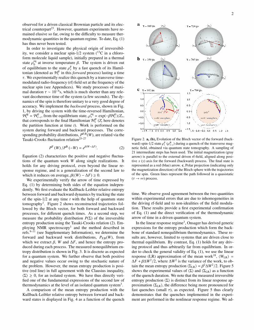
Figure 2. a, (b), Evolution of the Bloch vector of the forward (back-ward) spin-1/2 state ρF

t (ρBτ−t) during a quench of the transverse mag-

netic field, obtained via quantum state tomography. A sampling of21 intermediate steps has been used. The initial magnetization (grayarrow) is parallel to the external driven rf-field, aligned along posi-tive x (y) axis for the forward (backward) process. The final state isrepresented as a red (blue) arrow. c, Polar projection (indicating onlythe magnetization direction) of the Bloch sphere with the trajectoriesof the spin. Green lines represent the path followed in a quasistatic(τ→ ∞) process.

time. We observe good agreement between the two quantitieswithin experimental errors that are due to inhomogeneities inthe driving rf-field and to non-idealities of the field modula-tion. These results provide a first experimental confirmationof Eq. (1) and the direct verification of the thermodynamicarrow of time in a driven quantum system.

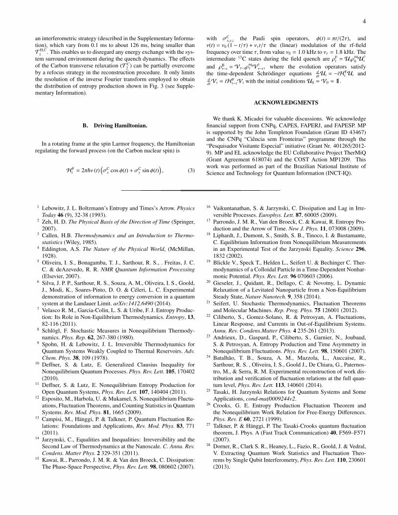
In the linear response regime3, Onsager has derived genericexpressions for the entropy production which form the back-bone of standard nonequilibrium thermodynamics. These re-sults are, however, limited to systems that are driven close tothermal equilibrium. By contrast, Eq. (1) holds for any driv-ing protocol and thus arbitrarily far from equilibrium. In or-der to check the general validity of Eq. (1), we use the linearresponse (LR) approximation of the mean work18, 〈WLR〉 =

∆F + β∆W2/2, where ∆W2 is the variance of the work, to ob-tain the mean entropy production 〈ΣLR〉 = β2∆W2/2. Figure 5shows the experimental values of 〈Σ〉 and 〈ΣLR〉 as a functionof the quench duration. We note that the measured irreversibleentropy production 〈Σ〉 is distinct from its linear response ap-proximation 〈ΣLR〉, the difference being more pronounced forfast quenches (small τ), as expected. Figure 5 thus clearlydemonstrates that the quenches implemented in the experi-ment are performed in the nonlinear response regime. We ad-

3

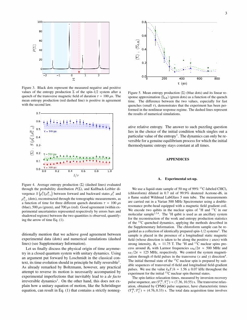
Figure 3. Black dots represent the measured negative and positivevalues of the entropy production Σ of the spin-1/2 system after aquench of the transverse magnetic field of duration τ = 100 µs. Themean entropy production (red dashed line) is positive in agreementwith the second law.

Figure 4. Average entropy production 〈Σ〉 (dashed lines) evaluatedthrough the probability distribution P(Σ), and Kullback-Leibler di-vergence S

(ρF

t ‖ ρBτ−t

)between forward and backward states ρF

t andρBτ−t (dots), reconstructed through the tomographic measurements, as

a function of time for three different quench durations τ = 100 µs(blue), 500 µs (green), and 700 µs (red). Good agreement (within ex-perimental uncertainties represented respectively by errors bars andshadowed regions) between the two quantities is observed, quantify-ing the arrow of time Eq. (1).

ditionally mention that we achieve good agreement betweenexperimental data (dots) and numerical simulations (dashedlines) (see Supplementary Information).

Let us finally discuss the physical origin of time asymme-try in a closed quantum system with unitary dynamics. Usingan argument put forward by Loschmidt in the classical con-text, its time evolution should in principle be fully reversible1.As already remarked by Boltzmann, however, any practicalattempt to reverse its motion is necessarily accompanied byexperimental imperfections that inevitably lead to a de factoirreversible dynamics1. On the other hand, this does not ex-plain how a unitary equation of motion, like the Schrödingerequation, can result in Eq. (1) that contains a strictly nonneg-

Figure 5. Mean entropy production 〈Σ〉 (blue dots) and its linear re-sponse approximation 〈ΣLR〉 (green dots) as a function of the quenchtime. The difference between the two values, especially for fastquenches (small τ), demonstrates that the experiment has been per-formed in the nonlinear response regime. The dashed lines representthe results of numerical simulations.

ative relative entropy. The answer to such puzzling questionlies in the choice of the initial condition which singles out aparticular value of the entropy1. The dynamics can only be re-versible for a genuine equilibrium process for which the initialthermodynamic entropy stays constant at all times.

APPENDICES

A. Experimental set-up.

We use a liquid-state sample of 50 mg of 99% 13C-labeled CHCl3

(chloroform) diluted in 0.7 ml of 99.9% deutered Acetone-d6, ina flame sealed Wildmad LabGlass 5 mm tube. The measurementsare carried out in a Varian 500 MHz Spectrometer using a double-resonance probe-head equipped with a magnetic field gradient coil.We encode two qubits in the nuclear spins of 1H and 13C in ourmolecular sample1,3,4. The 1H qubit is used as an ancillary systemfor the reconstruction of the work and entropy production statisticsof the 13C quenched dynamics, applying the methods described inthe Supplementary Information. The chloroform sample can be re-garded as a collection of identically prepared spin-1/2 systems3. Thesample is placed in the presence of a longitudinal static magneticfield (whose direction is taken to be along the positive z axes) withstrong intensity, B0 ≈ 11.75 T. The 1H and 13C nuclear spins pre-cess around B0 with Larmor frequencies ωH/2π ≈ 500 MHz andωC/2π ≈ 125 MHz, respectively. We control the system magneti-zation through rf-field pulses in the transverse (x and y) direction4.The initial thermal state of the 13C nuclear spin is prepared by suit-able sequences of transversal rf-field and longitudinal field-gradientpulses. We use the value kBT/h = 1.56 ± 0.07 kHz throughout theexperiment for the initial 13C nuclear spin thermal states.

The spin-lattice relaxation times, measured by inversion recoverypulse sequence, are (T H

1 ,TC1 ) ≈ (7.36, 10.55) s. The transverse relax-

ation, obtained by CPMG pulse sequence, have characteristic times(T H

2 ,TC2 ) ≈ (4.76, 0.33) s. The total data acquisition time involves

4

an interferometric strategy (described in the Supplementary Informa-tion), which vary from 0.1 ms to about 126 ms, being smaller thanT

H,C1 . This enables us to disregard any energy exchange with the sys-

tem surround environment during the quench dynamics. The effectsof the Carbon transverse relaxation (T C

2 ) can be partially overcomeby a refocus strategy in the reconstruction procedure. It only limitsthe resolution of the inverse Fourier transform employed to obtainthe distribution of entropy production shown in Fig. 3 (see Supple-mentary Information).

B. Driving Hamiltonian.

In a rotating frame at the spin Larmor frequency, the Hamiltonianregulating the forward process (on the Carbon nuclear spin) is

HFt = 2π~ν (t)

(σC

x cos φ(t) + σCy sin φ(t)

), (3)

with σCx,y,z the Pauli spin operators, φ(t) = πt/(2τ), and

ν(t) = ν0 (1 − t/τ) + ντt/τ the (linear) modulation of the rf-fieldfrequency over time τ, from value ν0 = 1.0 kHz to ντ = 1.8 kHz. Theintermediate 13C states during the field quench are ρF

t = Utρeq0 U

†t

and ρBτ−t = Vτ−tρ

eqτ V

†τ−t, where the evolution operators satisfy

the time-dependent Schrödinger equations ddtUt = −iHF

t Ut andddtVt = iHF

τ−tVt with the initial conditionsU0 = V0 = 11.

ACKNOWLEDGMENTS

We thank K. Micadei for valuable discussions. We acknowledgefinancial support from CNPq, CAPES, FAPERJ, and FAPESP. MPis supported by the John Templeton Foundation (Grant ID 43467)and the CNPq “Ciência sem Fronteiras” programme through the“Pesquisador Visitante Especial” initiative (Grant Nr. 401265/2012-9). MP and EL acknowledge the EU Collaborative Project TherMiQ(Grant Agreement 618074) and the COST Action MP1209. Thiswork was performed as part of the Brazilian National Institute ofScience and Technology for Quantum Information (INCT-IQ).

1 Lebowitz, J. L. Boltzmann’s Entropy and Times’s Arrow. PhysicsToday 46 (9), 32-38 (1993).

2 Zeh, H. D. The Physical Basis of the Direction of Time (Springer,2007).

3 Callen, H.B. Thermodynamics and an Introduction to Thermo-statistics (Wiley, 1985).

4 Eddington, A.S. The Nature of the Physical World, (McMillan,1928).

5 Oliveira, I. S., Bonagamba, T. J., Sarthour, R. S., . Freitas, J. C.C. & deAzevedo, R. R. NMR Quantum Information Processing(Elsevier, 2007).

6 Silva, J. P. P., Sarthour, R. S., Souza, A. M., Oliveira, I. S., Goold,J., Modi, K., Soares-Pinto, D. O. & Céleri, L. C. Experimentaldemonstration of information to energy conversion in a quantumsystem at the Landauer Limit. arXiv:1412.6490 (2014).

7 Velasco R. M., Garcia-Colin, L. S. & Uribe, F. J. Entropy Produc-tion: Its Role in Non-Equilibrium Thermodynamics. Entropy, 13,82-116 (2011).

8 Schlögl, F. Stochastic Measures in Nonequilibrium Thermody-namics. Phys. Rep. 62, 267-380 (1980).

9 Spohn, H. & Lebowitz, J. L. Irreversible Thermodynamics forQuantum Systems Weakly Coupled to Thermal Reservoirs. Adv.Chem. Phys. 38, 109 (1978).

10 Deffner, S. & Lutz, E. Generalized Clausius Inequality forNonequilibrium Quantum Processes. Phys. Rev. Lett. 105, 170402(2010).

11 Deffner, S. & Lutz, E. Nonequilibrium Entropy Production forOpen Quantum Systems, Phys. Rev. Lett. 107, 140404 (2011).

12 Esposito, M., Harbola, U. & Mukamel, S. Nonequilibrium Fluctu-ations, Fluctuation Theorems, and Counting Statistics in QuantumSystems. Rev. Mod. Phys. 81, 1665 (2009).

13 Campisi, M., Hänggi, P. & Talkner, P. Quantum Fluctuation Re-lations: Foundations and Applications, Rev. Mod. Phys. 83, 771(2011).

14 Jarzynski, C., Equalities and Inequalities: Irreversibility and theSecond Law of Thermodynamics at the Nanoscale. C. Annu. Rev.Condens. Matter Phys. 2 329-351 (2011).

15 Kawai, R., Parrondo, J. M. R. & Van den Broeck, C. Dissipation:The Phase-Space Perspective, Phys. Rev. Lett. 98, 080602 (2007).

16 Vaikuntanathan, S. & Jarzynski, C. Dissipation and Lag in Irre-versible Processes. Europhys. Lett. 87, 60005 (2009).

17 Parrondo, J. M. R., Van den Broeck, C. & Kawai, R. Entropy Pro-duction and the Arrow of Time. New J. Phys. 11, 073008 (2009).

18 Liphardt, J., Dumont, S., Smith, S. B., Tinoco, I. & Bustamante,C. Equilibrium Information from Nonequilibrium Measurementsin an Experimental Test of the Jarzynski Equality. Science 296,1832 (2002).

19 Blickle V., Speck T., Helden L., Seifert U. & Bechinger C. Ther-modynamics of a Colloidal Particle in a Time-Dependent Nonhar-monic Potential. Phys. Rev. Lett. 96 070603 (2006).

20 Gieseler, J., Quidant, R., Dellago, C. & Novotny, L. DynamicRelaxation of a Levitated Nanoparticle from a Non-EquilibriumSteady State, Nature Nanotech. 9, 358 (2014).

21 Seifert, U. Stochastic Thermodynamics, Fluctuation Theoremsand Molecular Machines. Rep. Prog. Phys. 75 126001 (2012).

22 Ciliberto, S., Gomez-Solano, R. & Petrosyan, A. Fluctuations,Linear Response, and Currents in Out-of-Equilibrium Systems.Annu. Rev. Condens.Matter Phys. 4 235-261 (2013).

23 Andrieux, D., Gaspard, P., Ciliberto, S., Garnier, N., Joubaud,S. & Petrosyan, A. Entropy Production and Time Asymmetry inNonequilibrium Fluctuations. Phys. Rev. Lett. 98, 150601 (2007).

24 Batalhão, T. B., Souza, A. M., Mazzola, L., Auccaise, R.,Sarthour, R. S. , Oliveira, I. S., Goold J., De Chiara, G., Paternos-tro, M., & Serra, R. M. Experimental reconstruction of work dis-tribution and verification of fluctuation relations at the full quan-tum level, Phys. Rev. Lett. 113, 140601 (2014).

25 Tasaki, H. Jarzynski Relations for Quantum Systems and SomeApplications, cond-mat/0009244v2.

26 Crooks, G. E. Entropy Production Fluctuation Theorem andthe Nonequilibrium Work Relation for Free-Energy Differences.Phys. Rev. E 60, 2721 (1999).

27 Talkner, P. & Hänggi, P. The Tasaki-Crooks quantum fluctuationtheorem, J. Phys. A (Fast Track Communication) 40, F569–F571(2007).

28 Dorner, R., Clark S. R., Heaney, L., Fazio, R., Goold, J. & Vedral,V. Extracting Quantum Work Statistics and Fluctuation Theo-rems by Single Qubit Interferometry, Phys. Rev. Lett. 110, 230601(2013).

5

29 Mazzola, L., De Chiara, G., & Paternostro, M. Measuring theCharacteristic Function of the Work Distribution, Phys. Rev. Lett.110, 230602 (2013).

30 Vandersypen, L. M. K. & Chuang, I. L. NMR Techniques forQuantum Control and Computation. Rev. Mod. Phys. 76, 1037(2004).

31 Cory, D. G., Fahmy, A. F. & Havel, T. F. Ensemble QuantumComputing by NMR Spectroscopy, PNAS 94, 1634 (1997).

6

I. SUPPLEMENTARY INFORMATION

In this Supplementary Information we provide some details of theexperiment and theory to support the main text.We employ a 13C labelled liquid-state chloroform sample to en-code a two qubit system in the nuclear spins of 1H and 13C,through the framework of nuclear magnetic resonance (NMR)spectroscopy1–4. The 1H nuclear spin will be instrumental for ourpurposes, as the subsystem to be employed to monitor the energyfluctuations in the dynamics of the 13C nuclear spin driven by afast field quench. The driving protocol is implemented by a suit-able modulation of a radio frequency (rf) transverse field, set atthe resonance of 13C nuclei, being described by the Hamiltonian(for the forward dynamics):

HFt = 2π~ν (t)

(σC

x cos φ(t) + σCy sin φ(t)

), (4)

with σCx,y,z the Pauli spin operators (for the Carbon nuclei), φ(t) =

πt/(2τ), and ν(t) = ν0 (1 − t/τ) + ντt/τ the (linear) modulation ofthe rf field over time τ, from value ν0 = 1.0 kHz to ντ = 1.8 kHz.This forward dynamics will be associated with the propagatorUt (defined in the Appendices of the main text). In the back-ward protocol the rf field is modulated in order to produce thetime-reversed interaction Hamiltonian, HB

t = HFτ−t and the time-

reversed evolutionVt.

Initial thermal state preparation

Preparation of the initial state can be done employing spatial av-eraging techniques, i.e., a combination of transverse rf pulses andlongitudinal field gradients1,2. Through this standard method, weprepared a joint pseudo pure state equivalent to |0〉H〈0| ⊗ ρ

eqα for

the Hydrogen and the Carbon nuclear spins, with α = 0, τ for theforward and backward protocols, respectively. We are using thelogical representation of the ground (|0〉) and excited (|1〉) spinstates. The Hydrogen nuclear spin is prepared in the ground statewhile the Carbon is effectively prepared in a thermal diagonalstate ρeq

α = e−βHFα /Zα, where Zα = tr e−βH

Fα is the partition func-

tion for HFα . The initial populations of ρeq

α in the HFα basis fol-

low the Gibbs distribution associated with inverse spin (pseudo-)temperature β = (kBT )−1.In all experiments we fixed the spin temperature of theCarbon in the initial Gibbs thermal distribution, such thatkBT/h = 1.56 ± 0.07 kHz. The uncertainty in this value is ob-tained through a comparison of Carbon populations in a se-ries of independent state preparation and quantum state tomog-raphy. The trace distance between the experimentally preparedinitial state (ρexp) and the ideal Gibbs state (ρideal), defined asδ ≡ tr |ρexp − ρideal|1/2, is smaller than 0.03 for all prepared states,in other words a less than 3% chance to discriminate them.

Work and irreversible entropy distributions

The work performed on or by a closed quantum system undergo-ing a protocol (dictated by HF,B

t ) is a stochastic variable5,6. For aquasi-static and isothermal process, the average work equals thevariation in free energy. On the other hand, in a scenario involvinga non-quasistatic and driven closed system dynamics (as in our ex-periment), an amount of work may be done on the system abovethe variation in free energy. This introduces a dissipated work,〈Wdiss〉 = 〈W〉 − ∆F ≥ 0, inherently linked to the irreversible na-ture of the process. Such irreversibility is associated to an entropyproduction7,8,

Σ = β (W − ∆F) . (5)

which is also a stochastic variable that depends on the work dis-tribution, the net change in the system free energy, and the inversetemperature. So the entropy production probability distribution,P(Σ), is built upon the experimental assessment of all the men-tioned variables.An important step in our experiment is the characterization of theprobability distribution of work fluctuations during the quencheddynamics. Such a distribution is obtained using a Ramsey-like in-terferometric method9–11. This approach is based on the interfer-ometric measurement of the characteristic function of the workdistribution12, which can be written for the forward process (F) as

χF(u) =∑m,n

peq,0n pF,τ

m|neiu(εm−εn) , (6)

where peq,0n = e−βεn/Z0 is the initial occupation probability for

the n-th eigenstate (|n0〉) of HF0 with energy εn, while pF,τ

m|n =

|〈mτ|Uτ|n0〉 |2 is the conditional transition probability to find the

system in the m-th eigenstate (|mτ〉) of HFτ (with energy εm) if it

was previously in |n0〉 at t = 0.The characteristic function can also be written as

χF(u) = tr[(Uτe−iuHF0 )ρeq

0 (e−iuHFτUτ)†] . (7)

The main idea of the protocol to reconstruct χF (u) is to esti-mate the trace in Eq. (7) via an ancillary system, the Hydro-gen nuclear spin in the present experiment. The NMR pulse se-quence employed to perform such a task is depicted in fig. 6.The ancillary system, initially prepared in the ground pseudo-purestate, is rotated to an equal-weighted superposition (equivalent to(|0〉H + |1〉H) /

√2) in the grey box of fig. 6. The Carbon nuclear

spin is the driven system of our interest. For technical reasons(which will be clarified in what follows), the 13C spin starts froma mixture of computational-basis (σC

z -basis) states, with occupa-tion probabilities given by peq,0

n (or by peq,τn in backward mode).

In fact the state basis will be further rotated to the initial Hamil-tonian one. Controlled-unitary operations are performed using thenatural scalar coupling interactionHJ = 2πJσH

z σCz , which is pro-

portional to σCz , while the initial and final Hamiltonians HF

0 andHF

τ in the forward protocol are proportional to σCy and σC

x , re-spectively. This is compensated by the rotations inside the greenboxes of fig. 6. Such rotations also account for the fact that theinitial state was prepared in the σC

z -basis. The same reasoning isapplied in the backward case. The purple boxes in fig. 6 are a re-focus strategy to mitigate the effects of the transverse relaxation.The quenched dynamics is a consequence of a suitable modula-tion (amplitude and phase) of a transverse rf field, which can bedescribed by the Hamiltonian in Eq. (4) for the forward proto-col. The final step of the algorithm is the measurement of the freeinduced decay (FID) signal of the Hydrogen nuclear spin. Fromthis signal one can obtain the transverse magnetization, where thecharacteristic function is encoded as χF,B (u) = 2

⟨σH

x

⟩+ 2i

⟨σH

y

⟩.

Application of an inverse Fourier transform allows us to obtainthe work distribution for the quenched dynamics.We have measured several experimental configurations, keepingfixed the initial spin temperature (given by the weights peq,0(τ)

n ofthe initial Carbon population), and varying the quench type (for-ward or backward) and the quench time-length. For each configu-ration, the interaction time s of the free evolution under the scalarcoupling in fig. 6 was varied through 360 equally-spaced values;each realisation corresponds to an independent experiment withan average over a set of identical and independent molecules.A typical output of the characteristic function reconstruction al-gorithm is shown in fig. 7a, where each data point corresponds

7

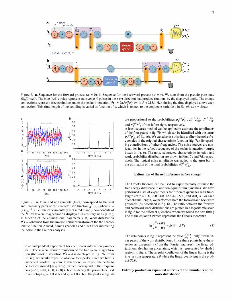
Figure 6. a, Sequence for the forward process (α = 0). b, Sequence for the backward process (α = τ). We start from the pseudo-pure state|0〉H〈0|⊗ρ

eqα . The blue (red) circles represent transverse rf-pulses in the x (y) direction that produce rotations by the displayed angle. The orange

connections represent free evolutions under the scalar interaction,HJ = 2πJσHz σ

Cz (with J ≈ 215.1 Hz), during the time displayed above each

connection. This time-length of the coupling is varied as function of s, which is related to the conjugate variable u in Eq. (6) as s = 2πν0u.

Figure 7. a, Blue and red symbols (lines) correspond to the realand imaginary parts of the characteristic function χF (u) (where u =

(2πν0)−1 s), i.e., the experimentally measured x and y components ofthe 1H transverse magnetization displayed in arbitrary units (a. u.),as function of the adimensional parameter s. b, Work distributionPF(W) obtained from the inverse Fourier transform of the the charac-teristic function. c and d, Same as panels a and b, but after subtractingthe noise in the Fourier analyses.

to an independent experiment for each scalar interaction parame-ter s. The inverse Fourier transform of the transverse magnetiza-tion (the work distribution PF(W)) is displayed in fig. 7b. FromEq. (6), we would expect to observe four peaks, since we have aquenched two-level system. Furthermore, we expect the peaks tobe located around {±(ν0 ± ντ)}, which correspond to the frequen-cies {−2.8,−0.8,+0.8,+2.8} kHz considering the parameters usedin our setup (ν0 = 1.0 kHz and ντ = 1.8 kHz). The peaks in fig. 7b

are proportional to the probabilities peq,01 pF,τ

0|1 , peq,00 pF,τ

0|0 , peq,01 pF,τ

1|1 ,and peq,0

0 pF,τ1|0 , from left to right, respectively.

A least-squares method can be applied to estimate the amplitudesof the four peaks in fig. 7b, which can be identified with the termspeq,0

n pF,τm|n of Eq. (6). We can also use this data to filter the noise fre-

quencies in the original characteristic function (fig. 7a) disregard-ing contributions of other frequencies. The noise sources are non-idealities in the refocus sequence of the scalar interaction (purpleboxes in fig. 6). The noise-subtracted characteristic function andwork probability distribution are shown in Figs. 7c and 7d, respec-tively. The typical noise amplitude was added to the error bar inthe estimation of the total probabilities peq,0

n pF,τm|n.

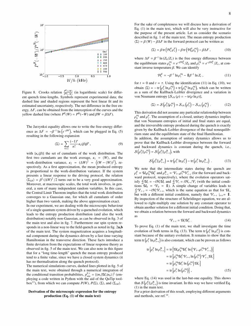
Estimation of the net difference in free energy

The Crooks theorem can be used to experimentally estimate thefree energy difference in our non-equilibrium dynamics. We haveperformed a set of experiments for different quenches with time-lengths of τ = 100, 200, 260, 320, 420, 500, and 700 µs. For eachquench time-length, we performed both the forward and backwardprotocols (as described in fig. 6). The ratio between the forwardand backward work distributions are plotted in a logarithmic scalein fig. 8 for the different quenches, where we found the best fittingline to the equation (which represents the Crooks theorem):

lnPF (+W)PB (−W)

= β(W − ∆F) . (8)

The data points in fig. 8 represent the ratio PF(+W)PB(−W) only for the in-

ner peaks of the work distributions. Since these points have them-selves an uncertainty (from the Fourier analyses), the linear ad-justment also has an uncertainty, which is represented by shadedregions in fig. 8. The angular coefficient of the linear fitting is theinverse spin temperature β while the linear coefficient is the prod-uct β∆F.

Entropy production expanded in terms of the cumulants of thework distribution

8

Figure 8. Crooks relation PF(+W)PB(−W) (in logarithmic scale) for differ-

ent quench time-lengths. Symbols represent experimental data; thedashed line and shaded regions represent the best linear fit and itsestimated uncertainty, respectively. The net difference in the free en-ergy, ∆F, can be obtained from the interception of the curves and theyellow dashed line (where PF(W) = PB(−W) and βW = β∆F).

The Jarzynksi equality allows one to write the free-energy differ-ence as ∆F = −β−1 ln

⟨e−βW

⟩, which can be plugged in Eq. (5)

resulting in the following expansion

〈Σ〉 =∑n≥2

(−1)n

n!κn(β)βn , (9)

with {κn(β)} the set of cumulants of the work distribution. Thefirst two cumulants are the work average, κ1 = 〈W〉, and thework-distribution variance, κ2 = (∆W)2 =

⟨(W − 〈W〉)2

⟩, re-

spectively. As a first approximation, the mean produced entropyis proportional to the work-distribution variance. If the systempresents a linear response to the driving protocol, the relation〈ΣLR〉 = β2 (∆W)2 /2 turns out to be a very good approximation.Moreover, at macroscopic scales, the total work involves, in gen-eral, a sum of many independent random variables. In this case,the Central Limit Theorem implies that the total work distributionconverges to a Gaussian one, for which all cumulants of orderhigher than two vanish, making the above approximation exact.In our experiment, we are dealing with the microscopic behaviourof a single quantum system driven by a quenched evolution, whichleads to the entropy production distribution (and also the workdistribution) notably non-Gaussian, as can be observed in fig. 3 ofthe main text and also in fig. 7. Furthermore our spin system re-sponds in a non-linear way to the field quench as noted in fig. 2a,bof the main text. The system magnetization acquires a longitudi-nal component during the dynamics driven by a fast time-varyingHamiltonian in the transverse direction. These facts introduce afinite deviation from the expectations of linear response theory asobserved in fig. 5 of the main text. We can also note in this figurethat for a “long time-length” quench the mean entropy producedtend to a finite value, since we have a closed system dynamics (ithas no thermalisation along the quench protocol).The numerical simulations curves, dashed lines plotted in fig. 5 ofthe main text, were obtained through a numerical integration ofthe conditional transition probabilities, pF,τ

m|n = |〈mτ|Uτ|n0〉 |2 (em-

ploying a code written in Python with the aid of the QuTip tool-box13), from which we can compute P(W), P(Σ), 〈Σ〉, and 〈ΣLR〉.

Derivation of the microscopic expression for the entropyproduction (Eq. (1) of the main text)

For the sake of completeness we will discuss here a derivation ofEq. (1) in the main text, which will also be very instructive forthe purpose of the present article. Let us consider the scenariodescribed in fig. 1 of the main text. The mean entropy production〈Σ〉 = β 〈W〉 − β∆F in the forward protocol can be written as

〈Σ〉 = β tr(HF

τ ρFτ

)− β tr

(HF

0 ρeq0

)− β∆F , (10)

where ∆F = β−1 ln (Z0/Zτ) is the free energy difference betweenthe equilibrium states ρeq

0 = e−βHF0 /Z0 and ρeq

τ = e−βHFτ /Zτ, at con-

stant inverse temperature β. We can identify

HFt = −β−1 ln ρeq

t − 11β−1 ln Zt , (11)

for t = 0 and t = τ. Using the identification (11) in Eq. (10), weobtain 〈Σ〉 = − tr

(ρFτ ln ρeq

τ

)+ tr

(ρ

eq0 ln ρeq

0

), which can be written

as a sum of the Kullback-Leibler divergence and a variation invon Neumann entropy [SvN (ρ) = − tr(ρ ln ρ)],

〈Σ〉 = S(ρFτ‖ρ

eqτ

)+ SvN

(ρFτ

)− SvN

(ρ

eq0

). (12)

This derivation did not assume any particular relationship betweenρ

eq0 and ρF

τ . The assumption of a closed, unitary dynamics impliesthat von Neumann entropies of initial and final states are equal,and the irreversible entropy produced during the quench is exactlygiven by the Kullback-Leibler divergence of the final nonequilib-rium state and the equilibrium state of the final Hamiltonian.In addition, the assumption of unitary dynamics allows us toprove that the Kullback-Leibler divergence between the forwardand backward dynamics is constant during the quench, i.e.,S

(ρFτ‖ ρ

eqτ

)= S

(ρF

t ‖ ρBτ−t

), with

S(ρF

t ‖ ρBτ−t

)= tr

(ρF

t ln ρFt

)− tr

(ρF

t ln ρBτ−t

). (13)

We note that the intermediate states during the quench areρF

t = Utρeq0 U

†t and ρB

τ−t = Vτ−tρeqτ V

†τ−t (for the forward and back-

ward protocol, respectively), where the evolution operators sat-isfy d

dtUt = −iHtUt and ddtVt = iHτ−tVt (with the initial condi-

tions U0 = V0 = 11). A simple change of variables leads toddtVτ−t = −iHtVτ−t, which is the same equation as that for Ut,but with a different initial condition, namely that Vτ−t |t=τ= 11.By inspection of the structure of Schrödinger equation, we are al-lowed to right-multiply one solution by any constant operator toobtain another solution for a different initial condition. Doing that,we obtain a relation between the forward and backward dynamicsas

Vτ−t = UtU†τ . (14)

To prove Eq. (1) of the main text, we shall investigate the timeevolution of both terms in Eq. (13). The term tr

(ρF

t ln ρFt

)is con-

stant because of the unitary evolution. It remains to show that theterm tr

(ρF

t ln ρBτ−t

)is also constant, which can be proven as follows

tr[ρF

t ln ρBτ−t

]= tr

[Utρ

eq0 U

†t ln

(Vτ−tρ

eqτ V

†τ−t

)]= tr

[ρ

eq0 U

†tVτ−t ln

(ρ

eqτ

)V†τ−tUt

]= tr

[ρ

eq0 U

†τ ln

(ρ

eqτ

)Uτ

]= tr

[ρFτ ln

(ρ

eqτ

)], (15)

where Eq. (14) was used in the last-but-one equality. This showsthat S

(ρF

t ‖ ρBτ−t

)is time invariant. In this way we have verified Eq.

(1) in the main text.For a prior derivation of this result, employing different argumentsand methods, see ref.14.

9

1 Oliveira, I. S., Bonagamba, T. J., Sarthour, R. S., . Freitas, J. C.C. & deAzevedo, R. R. NMR Quantum Information Processing(Elsevier, Amsterdam, 2007).

2 Jones, J. A., Quantum computing with NMR, Prog. NMR Spec-trosc. 59, 91 (2011).

3 Vandersypen, L. M. K. & Chuang, I. L. NMR Techniques forQuantum Control and Computation. Rev. Mod. Phys. 76, 1037(2004).

4 Cory, D. G., Fahmy, A. F. & Havel, T. F. Ensemble QuantumComputing by NMR Spectroscopy, PNAS 94, 1634 (1997).

5 Esposito, M., Harbola, U. & Mukamel, S. NonequilibriumFluctuations, Fluctuation Theorems, and Counting Statistics inQuantum Systems. Rev. Mod. Phys. 81, 1665 (2009).

6 Campisi, M., Hänggi, P. & Talkner, P. Quantum FluctuationRelations: Foundations and Applications, Rev. Mod. Phys. 83,771 (2011).

7 Jarzynski, C., Equalities and Inequalities: Irreversibility andthe Second Law of Thermodynamics at the Nanoscale. C.Annu. Rev. Condens.Matter Phys.2 329-351 (2011).

8 Deffner, S. & Lutz, E. Generalized Clausius Inequality forNonequilibrium Quantum Processes. Phys. Rev. Lett. 105,170402 (2010).

9 Dorner, R. , Clark S. R., Heaney, L., Fazio, R., Goold, J. &Vedral, V. Extracting Quantum Work Statistics and FluctuationTheorems by Single Qubit Interferometry, Phys. Rev. Lett. 110,230601 (2013).

10 Mazzola, L., De Chiara, G. , & Paternostro, M. Measuring theCharacteristic Function of the Work Distribution, Phys. Rev.Lett. 110, 230602 (2013).

11 Batalhão, T. , Souza, A. M. , Mazzola, L., Auccaise, R.,Sarthour, R. S. , Oliveira, I. S. , Goold J.,De Chiara, G. , Pa-ternostro, M., & Serra, R. M. Experimental reconstruction ofwork distribution and verification of fluctuation relations at thefull quantum level, Phys. Rev. Lett. 113, 140601 (2014).

12 Talkner, P., E. Lutz, E., & Hänggi, P., Fluctuation theorems:Work is not an observable, Phys. Rev. E 75, 050102(R) (2007).

13 Johansson, J. R., Nation, P. D.,&, Nori, F., QuTiP: An open-source Python framework for the dynamics of open quantumsystems, Comput. Phys. Comm. 183, 1760 (2012).

14 Parrondo, J. M. R., Van den Broeck, C. & Kawai, R. EntropyProduction and the Arrow of Time. New J. Phys. 11 073008(2009).