ir.lib.hiroshima-u.ac.jp · Acknowledgements It is my pleasure to acknowledge the role of several individuals who helped me to complete my Ph.D. research. Firstly, I would like to

Essays on the Whittaker–Henderson

Method of Graduation

September 2019

Fatima Tuj Jahra

D166772

Graduate School of Social Sciences

Hiroshima University

In Partial Fulfillment of the Requirements for the Degree of

Doctor of Philosophy

Acknowledgements

It is my pleasure to acknowledge the role of several individuals who helpedme to complete my Ph.D. research.

Firstly, I would like to express my special appreciation and thanks to myacademic supervisor Professor Dr. Hiroshi Yamada, you have been a greatmentor for me. I would like to thank you for encouraging my research andguiding me to grow as a researcher. You opened a window of econometrics tome. Professor Yamada gave me not only valuable time but also good adviceand a mentor that I will always be grateful for. Overall, Professor Yamada is avery kind person and I feel very proud and lucky to have him as my supervisor.

I would like to acknowledge the Japanese Government for its financial supportthrough the MEXT scholarship.

Last but not the least, I would like to thank my family: my parents and to mydaughters and to my husband Dr. Mostak Ahmed for supporting me spirituallythroughout writing this thesis and my life in general.

Contents

1 Introduction 11.1 Introductory survey . . . . . . . . . . . . . . . . . . . . . . . . . . . . . . 11.2 Some preliminary definitions and basic properties: . . . . . . . . . . . . . . 6

1.2.1 Whittaker (1923) . . . . . . . . . . . . . . . . . . . . . . . . . . . 151.3 Objectives and Outlines . . . . . . . . . . . . . . . . . . . . . . . . . . . . 201.4 Appendix . . . . . . . . . . . . . . . . . . . . . . . . . . . . . . . . . . . 221.5 References . . . . . . . . . . . . . . . . . . . . . . . . . . . . . . . . . . . 23

2 Explicit Formulas for the Smoother Weights of the Whittaker–HendersonGraduation of Order 1 262.1 Introduction . . . . . . . . . . . . . . . . . . . . . . . . . . . . . . . . . . 262.2 The main results . . . . . . . . . . . . . . . . . . . . . . . . . . . . . . . . 282.3 Formulas based on Cornea-Madeira’s (2017) approach . . . . . . . . . . . 322.4 Concluding remarks . . . . . . . . . . . . . . . . . . . . . . . . . . . . . . 342.5 Numerical example . . . . . . . . . . . . . . . . . . . . . . . . . . . . . . 352.6 Appendix . . . . . . . . . . . . . . . . . . . . . . . . . . . . . . . . . . . 382.7 References . . . . . . . . . . . . . . . . . . . . . . . . . . . . . . . . . . . 41

3 An Explicit Formula for the Smoother Weights of the Hodrick–Prescott Filter 423.1 Introduction . . . . . . . . . . . . . . . . . . . . . . . . . . . . . . . . . . 423.2 A literature review . . . . . . . . . . . . . . . . . . . . . . . . . . . . . . 43

3.2.1 De Jong and Sakarya (2016) . . . . . . . . . . . . . . . . . . . . . 443.2.2 Cornea-Madeira (2017) . . . . . . . . . . . . . . . . . . . . . . . 45

3.3 Another explicit formula for the smoother weights of the HP filter . . . . . 463.4 Concluding remarks . . . . . . . . . . . . . . . . . . . . . . . . . . . . . . 503.5 Numerical example . . . . . . . . . . . . . . . . . . . . . . . . . . . . . . 513.6 Appendix . . . . . . . . . . . . . . . . . . . . . . . . . . . . . . . . . . . 54

i

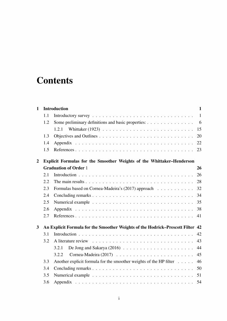
3.7 References . . . . . . . . . . . . . . . . . . . . . . . . . . . . . . . . . . . 59

4 A Discussion on the Whittaker–Henderson Graduation and Bisymmetry of theRelated Smoother Matrices 614.1 Introduction . . . . . . . . . . . . . . . . . . . . . . . . . . . . . . . . . . 614.2 A literature review . . . . . . . . . . . . . . . . . . . . . . . . . . . . . . 65

4.2.1 Yamada (2019) . . . . . . . . . . . . . . . . . . . . . . . . . . . . 654.2.2 El-Mikkawy and Atlan (2013) . . . . . . . . . . . . . . . . . . . . 66

4.2.2.1 An algorithm for solving centrosymmetric linear systemof even order: . . . . . . . . . . . . . . . . . . . . . . . 66

4.2.2.2 An algorithm for solving centrosymmetric linear systemof odd order: . . . . . . . . . . . . . . . . . . . . . . . . 68

4.3 Formulas for calculating xxx in (4.1) . . . . . . . . . . . . . . . . . . . . . . 714.4 Bisymmetry of the smoother matrices in (4.3) and (4.4) . . . . . . . . . . . 764.5 Concluding remarks . . . . . . . . . . . . . . . . . . . . . . . . . . . . . . 774.6 Appendix . . . . . . . . . . . . . . . . . . . . . . . . . . . . . . . . . . . 78

4.6.1 A MATLAB/GNU Octave function to calculate (IIIn + λDDD′pDDDp)−1

based on (4.14)–(4.19) . . . . . . . . . . . . . . . . . . . . . . . . 784.6.2 Proof of (4.22) and (4.23) . . . . . . . . . . . . . . . . . . . . . . 794.6.3 Proof of (4.24)–(4.26) . . . . . . . . . . . . . . . . . . . . . . . . 81

4.7 References . . . . . . . . . . . . . . . . . . . . . . . . . . . . . . . . . . . 83

ii

Chapter 1

Introduction

1.1 Introductory survey

The Whittaker–Henderson(WH) method of graduation is a frequently used smoothing toolin econometric time series analysis. The main purpose of this thesis is to analyze the specialcases of the Whittaker–Henderson method of graduation. There are two popular cases ofWhittaker–Henderson method of graduation, first one is called exponential smoothing (ES)filter (King and Rebelo, 1993) or WH method of order 1 and the second one is popularlyknown as Hodrick-Prescott (HP) filter (Hodrick and Prescott, 1997) or WH method of order2. Though we called it the Whittaker–Henderson method of graduation but the method wasfirst introduced by a German scholar George Bohlman (1899). Later, the method was welldeveloped by Whittaker (1923) and Henderson (1924) separately and now it is popularlyknown as the Whittaker–Henderson method of graduation.

Bohlman suggested a method for graduating data where he used the first-order dif-ferences for graduation. His proposed method is described as the minimization problem ofthe following function with respect to x1, . . . ,xT is:

T

∑t=1

(yt− xt)2 +λ

2T−1

∑t=1

(∇xt)2, (1.1)

where yyy = [y1, . . . ,yT ]′ denotes univariate time series of T observations, xxx = [x1, . . . ,xT ]

′,λ 2 ≥ 0 is a parameter. Here, ∇xt = xt+1− xt is called the first-order difference and theoperator ∇ represents the forward difference operator. The first term, the square of thedeviations and the second term represents the smoothing term. The parameter λ 2 is used

1

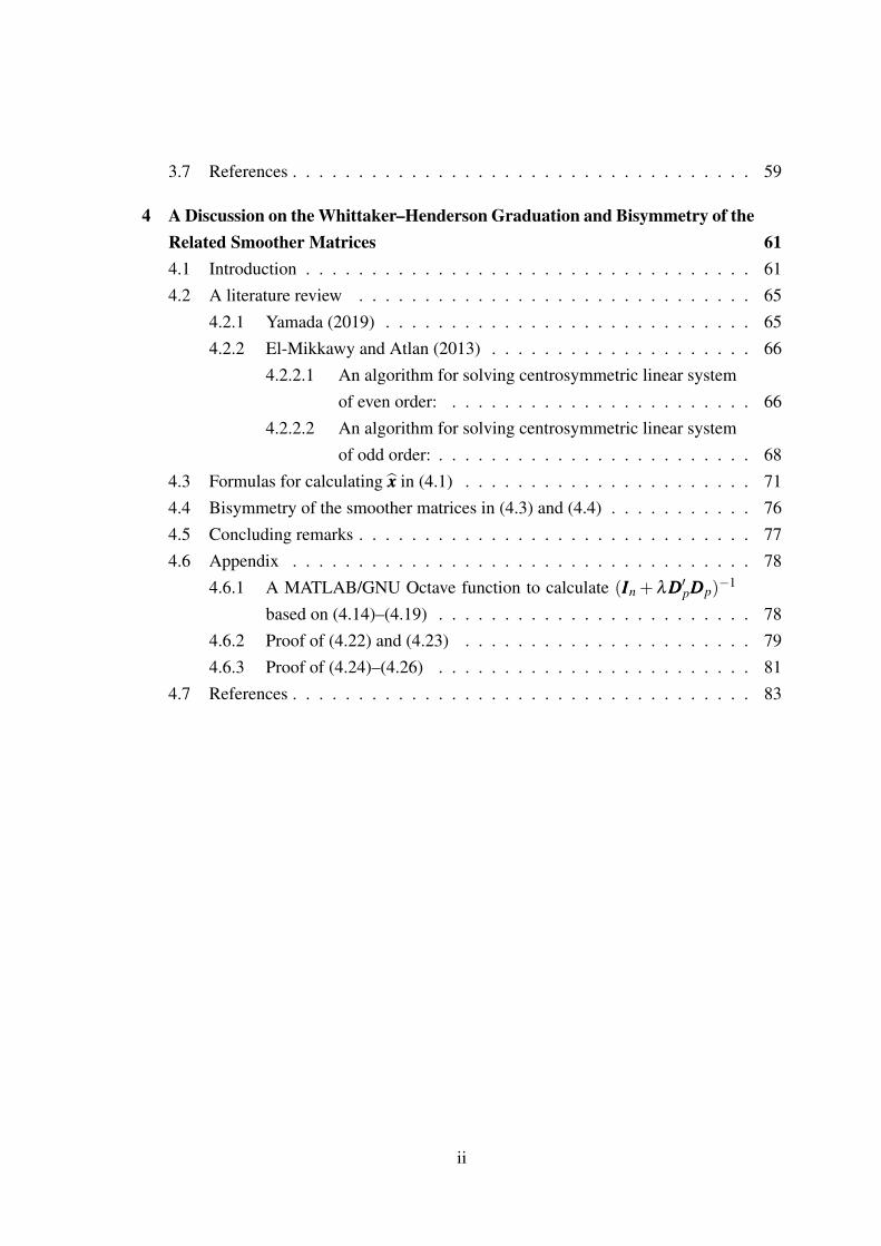
to control the trade-off between the smoothness of the graduated data and the size of thedeviation. If the value of λ 2 increases, the solution becomes smoother.

Whittaker (1923), without knowing about Bohlman’s work, published a papernamed as “On a New Method of Graduation”, where he suggested a method for datasmoothing using third-order differences that is ∇3xt = (xt+3 − 3xt+2 + 3xt+1 − xt). Heconsidered the following penalized least squares problem:

minx1,...,xT∈R

f (x1, . . . ,xT ) =T

∑t=1

h2t (yt− xt)

2 +λ2

T−3

∑t=1

(∇3xt)2, (1.2)

where ∇xt = xt+1− xt and derived the following optimality condition:

h21y1 = h2

1x1 +λ2(−1)∇3x1, (1.3)

h22y2 = h2

2x2 +λ23∇

3x1 +λ2(−1)∇3x2, (1.4)

h23y3 = h2

3x3 +λ2(−3)∇3x1 +λ

23∇3x2 +λ

2(−1)∇3x3, (1.5)

h24y4 = h2

4x4 +λ2∇

3x1 +λ2(−3)∇3x2 +λ

23∇3x3 +λ

2(−1)∇3x4, (1.6)

...

For proof of the above condition see section 1.2.1 of this chapter.

On the other hand, Henderson(1924) published an article about the data smoothingmethod named as “A New Method of Graduation”, where he discovered a factorizationformula to calculate Whittaker’s method in a more simpler way. Later, the method is knownas the Whittaker–Henderson’s method of graduation.

An important contribution was made by Greville (1957) about Whittaker–Henderson’s smoothing process is to express objective function in matrix notation and tosolve the system. Greville minimized expression of the form

(xxx− yyy)′WWW (xxx− yyy)+ xxx′GGGxxx. (1.7)

Here WWW = III is positive definite matrix and GGG is a positive semi-definite matrix. Here asmall value of the first term is taken to indicate a close approach to the original data, whilea small value of the second is considered to reflect a high degree of smoothness. This is the

2

first attempt of minimizing the expression (1.7) for a given yyy leads to the equation

xxx = (III +WWW−1GGG)−1yyy. (1.8)

For proof of equation (1.8), see the appendix of this chapter.Hodrick and Prescott (1997) introduced a method, which is known as Hodrick-

Prescott (HP) filtering in econometrics and it is also regarded as the Whittaker–Hendersonmethod of graduation of order 2. Hodrick and Prescott (1997) popularized the Whittaker–Henderson method of graduation in modern economics. According to HP (1997), a giventime series yt is the sum of a growth component xt and a cyclical component ct ,i.e.,

yt = xt + ct , for t = 1,2, ...,T. (1.9)

For determining the growth components, HP filter is

argminx1,...,xT∈R

[T

∑t=1

(yt− xt)2 +λ

T

∑t=3

[(xt+1− xt)− (xt− xt−1)]2

], (1.10)

where, the parameter λ > 0 is a tuning/smoothing parameter. Here, the first term measuresthe fidelity to the datum and the second term measures the smoothness.

Weinert (2006) introduced some algorithms to compute the estimates and the GCV(generalized cross-validation) score for the Whittaker–Henderson smoothing problem. Ac-cording to him, a known sequence yt for T measurements and positive real number λ

and a positive integer p < T , and the solution sequence is xxxt which minimizes

λ

T

∑t=1

(yt− xt)2 +

T−p

∑t=1

(∇pxt)2, (1.11)

where, ∇ is a forward difference operator. The minimizer of (1.11) is

AAAxxx = λyyy, (1.12)

whereAAA = λ III +MMM′MMM. (1.13)

Here, MMM is a (T − p)×T difference matrix. To solve (1.12) he factorized the coefficient

3

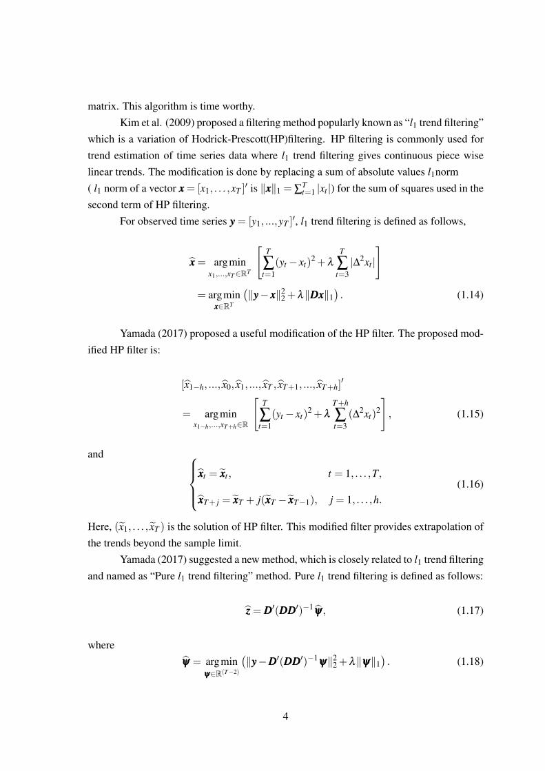
matrix. This algorithm is time worthy.Kim et al. (2009) proposed a filtering method popularly known as “l1 trend filtering”

which is a variation of Hodrick-Prescott(HP)filtering. HP filtering is commonly used fortrend estimation of time series data where l1 trend filtering gives continuous piece wiselinear trends. The modification is done by replacing a sum of absolute values l1norm( l1 norm of a vector xxx = [x1, . . . ,xT ]

′ is ‖xxx‖1 = ∑Tt=1 |xt |) for the sum of squares used in the

second term of HP filtering.For observed time series yyy = [y1, ...,yT ]

′, l1 trend filtering is defined as follows,

xxx = argminx1,...,xT∈RT

[T

∑t=1

(yt− xt)2 +λ

T

∑t=3|∆2xt |

]

= argminxxx∈RT

(‖yyy− xxx‖2

2 +λ‖DDDxxx‖1). (1.14)

Yamada (2017) proposed a useful modification of the HP filter. The proposed mod-ified HP filter is:

[x1−h, ..., x0, x1, ..., xT , xT+1, ..., xT+h]′

= argminx1−h,...,xT+h∈R

[T

∑t=1

(yt− xt)2 +λ

T+h

∑t=3

(∆2xt)2

], (1.15)

and xxxt = xxxt , t = 1, . . . ,T,

xxxT+ j = xxxT + j(xxxT − xxxT−1), j = 1, . . . ,h.(1.16)

Here, (x1, . . . , xT ) is the solution of HP filter. This modified filter provides extrapolation ofthe trends beyond the sample limit.

Yamada (2017) suggested a new method, which is closely related to l1 trend filteringand named as “Pure l1 trend filtering” method. Pure l1 trend filtering is defined as follows:

zzz = DDD′(DDDDDD′)−1ψψψ, (1.17)

whereψψψ = argmin

ψψψ∈R(T−2)

(‖yyy−DDD′(DDDDDD′)−1

ψψψ‖22 +λ‖ψψψ‖1

). (1.18)

4

Note that, DDD is a tridiagonal Toeplitz matrix of which the first row is [1,−2,1,0, . . . ,0] andDDDDDD′ is a banded Toeplitz matrix. Since DDD is of full row rank, DDDDDD′ is positive definite,which indicates DDDDDD′ is non-singular.

De Jong and Sakarya (2016) recently derived an explicit formula for the smootherweights of the WH graduation of order 2 which is popularly known as the Hodrick–Prescottfilter. It’s worth to mention that the T × T matrix (IIIT + λDDD′DDD)−1 is referred to as thesmoother matrix of the HP filter. More recently, by applying the SMW formula and thespectral decomposition of a symmetric tridiagonal Toeplitz matrix, Cornea-Madeira (2017)provided a simpler formula of it. We note here that to derive the explicit formula, we applya different approach to that of Cornea-Madeira (2017). In this thesis, we derived explicitformulas for the Whittaker–Henderson graduation of orders 1 and 2 and also prove thatthese two smoother matrices are bisymmetric.

5

1.2 Some preliminary definitions and basic properties:

Suppose BBB is a K × K symmetric matrix having K distinct characteristic vectorsvvv1,vvv2, . . . ,vvvk and the corresponding characteristic roots are λ1,λ2, . . . ,λk. The character-istic vectors of a symmetric matrix are orthogonal. Now, the matrix VVV is the eigenvectormatrix i.e. VVV = [vvv1,vvv2, . . . ,vvvk] and ΛΛΛ = diag(λ1,λ2, . . . ,λk) is a eigenvalue matrix. Here wediscuss some basic properties of linear algebra which are particularly related to this thesis.

Definition:[K. M. Abadir and J. R. Magnus (Matrix Algebra)] The trace of a squaresymmetric matrix BBB is the sum of its diagonal elements:

trace(BBB) =K

∑i=1

bii,

where bii are the diagonal elements of BBB.

Definition:[K. M. Abadir and J. R. Magnus (Matrix Algebra)] The transpose of amatrix is an operator which flips a matrix over its diagonal. Transpose of a matrix BBB isoften denoted by BBB′ or BBBT . If BBB is an m×n matrix, then BBB′ is an n×m matrix, that is, thei-th row, j-th column element of BBB′ is the j-th row, i-th column element of BBB: [BBB′]i j = [BBB] ji .

If AAA is another matrix then (AAABBB)′ = BBB′AAA′.An example of the transpose of a matrix is:

1 2 3

4 0 6

′

=

1 4

2 0

3 6

.

Definition:[K. M. Abadir and J. R. Magnus (Matrix Algebra)] The diagonalizationof a symmetric matrix BBB is

VVV ′BBBVVV = ΛΛΛ.

Definition:[K. M. Abadir and J. R. Magnus (Matrix Algebra)] The spectraldecomposition of a symmetric matrix BBB is defined as

6

BBB =VVV ΛΛΛVVV ′ =K

∑k=1

λkvvvkvvv′k.

This is also called the eigenvalue decomposition of matrix BBB.

Definition:[K. M. Abadir and J. R. Magnus (Matrix Algebra)] A matrix is calledidempotent if it is equal to it’s square, that is, BBB2 =BBBBBB=BBB. If BBB is symmetric then BBB′BBB=BBB.

Definition:[K. M. Abadir and J. R. Magnus (Matrix Algebra)] The rank of asymmetric matrix is the number of non-zero characteristic roots/eigenvalues it contains.

Definition:[K. M. Abadir and J. R. Magnus (Matrix Algebra)] A square matrix BBB iscalled a permutation matrix if every row and every column of BBB contains only one element1 and the other elements are 0. For order 2 there exist 2 permutation matrices, they are:

0 1

1 0

,1 0

0 1

.For order 3 there are 6 permutation matrices. In this way, for order n there are n!permutation matrices.

Definition:[K. M. Abadir and J. R. Magnus (Matrix Algebra)] For any square matrixBBB, the quadratic form can be written as:

xxx′BBBxxx.

Now, if xxx′BBBxxx > 0 for all real xxx 6= 000, then BBB is positive definite,if xxx′BBBxxx < 0 for all real xxx 6= 000, then BBB is negative definite,if xxx′BBBxxx≥ 0 for all real xxx, then BBB is positive semi-definite,if xxx′BBBxxx≤ 0 for all real xxx, then BBB is negative semi-definite.

Definition:[K. M. Abadir and J. R. Magnus (Matrix Algebra)] If BBBxxx = xxx for all xxx

then particularly for the unit vectors xxx= eee j implies that BBBeee j = eee j so that bi, j = eee′iBBBeee j = eee′ieee j,which is 0 when i 6= j and 1 when i= j, then BBB= III is called the identity matrix of a specifiedorder. Conversely, if BBB = III, then BBBxxx = xxx holds for all xxx. An n×n identity matrix is written

7

as IIIn and III′n = III2n = III−1

n = IIIn holds.For example,

III3 =

1 0 0

0 1 0

0 0 1

.

Definition:[K. M. Abadir and J. R. Magnus (Matrix Algebra)] A matrix BBB = [bi, j]

is diagonal if all the entries outside the principal diagonal (that is, for i 6= j) are zero. Thediagonal entries themselves may be or may not be zero. Matrix BBB can also be written asBBB := diag(b1,b2, ...,bn).An example of a diagonal matrix is:

3 0 0

0 5 0

0 0 2

.

Definition:[K. M. Abadir and J. R. Magnus (Matrix Algebra)] A real square matrixBBB is orthogonal if BBB′BBB = BBBBBB′ = III. If a matrix is orthogonal, then its rows form an orthonor-mal set and its columns also form an orthonormal set.An example of an orthogonal matrix is:

23

13

23

−23

23

13

13

23 −2

3

.

8

Definition:[K. M. Abadir and J. R. Magnus (Matrix Algebra)] A tridiagonalToeplitz matrix is a special (square) Toeplitz matrix where the major and minor diagonalentries are constant and others are zero. Example of a tridiagonal Toeplitz matrix is:

−2 1

1 −2 1

. . .. . .

. . .

1 −2 1

1 −2

,

where the empty spaces are filled with zeroes.

Definition:[K. M. Abadir and J. R. Magnus (Matrix Algebra)] PentadiagonalToeplitz matrix is a square matrix of five major and minor diagonal elements are constant.An example of a pentadiagonal Toeplitz matrix is

DDD′ =

6 −4 1

−4 6 −4 1

1 −4 6 −4 1

. . .. . .

. . .. . .

. . .

1 −4 6 −4 1

1 −4 6 −4

1 −4 6

,


Definition:[K. M. Abadir and J. R. Magnus (Matrix Algebra)] Let, xxx = [x1, ...,xn]′

be an n× 1 column vector. A sequence of differences ∆xi = xi− xi−1, where i = 2, ...,nis called the linear first order differences, which can be expressed in matrix form as D1x,

9

where DDD1 the (n− 1)× n matrix is called a linear first-order difference matrix of the fol-lowing form:

−1 1

−1 1

. . .. . .

−1 1

,


Definition:[K. M. Abadir and J. R. Magnus (Matrix Algebra)] A PPPth orderdifference matrix is expressed as DDDp, whose dimension is (n− p)×n for n, p ∈ R, is

DDDp = (−1)p

1 −(p

1

) (p2

)−(p

3

)· · · 1

1 −(p

1

) (p2

)−(p

3

)· · · 1

. . .. . .

. . .. . .

. . .

1 −(p

1

) (p2

)−(p

3

)· · · 1

,


Definition:[K. M. Abadir and J. R. Magnus (Matrix Algebra)] l1 norm of a vectorxxx = [x1, . . . ,xn]

′ is defined as

‖xxx‖1 =n

∑t=1|xt |.

Definition:[K. M. Abadir and J. R. Magnus (Matrix Algebra)] l2 norm of a vectorxxx = [x1, . . . ,xn]

′ is defined as

10

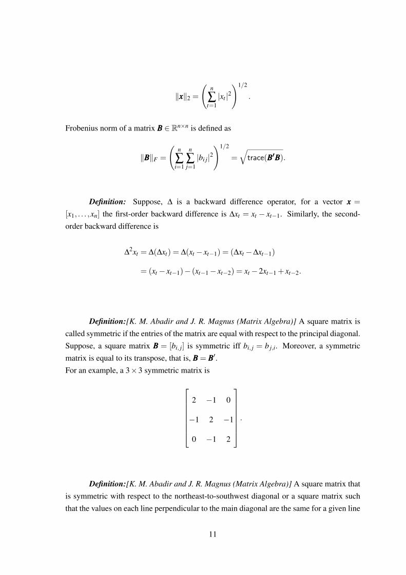
‖xxx‖2 =

(n

∑t=1|xt |2

)1/2

.

Frobenius norm of a matrix BBB ∈ Rn×n is defined as

‖BBB‖F =

(n

∑i=1

n

∑j=1|bi j|2

)1/2

=√trace(BBB′′′BBB).

Definition: Suppose, ∆ is a backward difference operator, for a vector xxx =

[x1, . . . ,xn] the first-order backward difference is ∆xt = xt − xt−1. Similarly, the second-order backward difference is

∆2xt = ∆(∆xt) = ∆(xt− xt−1) = (∆xt−∆xt−1)

= (xt− xt−1)− (xt−1− xt−2) = xt−2xt−1 + xt−2.

Definition:[K. M. Abadir and J. R. Magnus (Matrix Algebra)] A square matrix iscalled symmetric if the entries of the matrix are equal with respect to the principal diagonal.Suppose, a square matrix BBB = [bi, j] is symmetric iff bi, j = b j,i. Moreover, a symmetricmatrix is equal to its transpose, that is, BBB = BBB′.For an example, a 3×3 symmetric matrix is

2 −1 0

−1 2 −1

0 −1 2

.

Definition:[K. M. Abadir and J. R. Magnus (Matrix Algebra)] A square matrix thatis symmetric with respect to the northeast-to-southwest diagonal or a square matrix suchthat the values on each line perpendicular to the main diagonal are the same for a given line

11

is called a persymmetric matrix.Suppose, a square matrix of order n is BBB = [bi, j], will be a persymmetric matrix if and onlyif it satisfies

bi, j = bn− j+1,n−i+1 for 1≤ i, j ≤ n.

For an exchange matrix, TTT persymmetric matrix BBB satisfies the relation, BBBTTT = TTT BBB′′′.An example of a 3×3 persymmetric matrix is:

2 −1 0

−1 5 −1

0 −1 2

.

Definition:[K. M. Abadir and J. R. Magnus (Matrix Algebra)] A square matrix iscalled a centrosymmetric matrix if it is symmetric about its center. A matrix of order n,BBB = [bi, j] is centrosymmetric if and only if it satisfies

BBBi, j = BBBn−i+1,n− j+1 for 1≤ i, j ≤ n.

A centrosymmetric matrix also satisfies BBBTTT = TTT BBB relation with the exchange matrix. Thegeneral form of a 3×3 centrosymmetric matrix is

b11 b12 b13

b21 b22 b21

b13 b12 b11

.

Definition:[K. M. Abadir and J. R. Magnus (Matrix Algebra)] A matrix BBB ∈ Rn×n

12

is said to be a skew-symmetric matrix if and only if its entries satisfy the relation

BBBi, j =−BBBn−i+1,n− j+1 for 1≤ i, j ≤ n.

For any real xxx, a skew-symmetric matrix also satisfies the relation xxx′BBBxxx = 0 andBBBTTT =−TTT BBB for an exchange matrix TTT .

Definition:[K. M. Abadir and J. R. Magnus (Matrix Algebra)] Bisymmetric ma-trices are both symmetric centrosymmetric and symmetric persymmetric matrices. Moreprecisely, a bisymmetric matrix is a square matrix that is symmetric about both of its maindiagonals. An n× n matrix BBB is bisymmetric if it satisfies both BBB = BBBTTT and BBBTTT = TTT BBB

where TTT is the n×n exchange matrix. An example is

2 −1 0 1

−1 5 4 0

0 4 5 −1

1 0 −1 2

.

Discrete cosine transformation (Type-II): The discrete cosine transformation ma-trix of type 2 is an invertible n×n square matrix where the n real numbers x0, ...,xn−1 aretransformed into the N real numbers X0, ...,Xn−1 according to the following formula:

Xk =n−1

∑t=0

xt cos[

π

n

(t +

12

)k], k = 0, . . . ,n−1.

Woodbury matrix identity: Woodbury matrix identity was originated by Max A.Woodbury. It is also known as matrix inversion lemma. The lemma states that if BBB and CCC

are respectively n×n and k×k square invertible matrices and XXX and YYY are matrices so that

13

and XXXCCCYYY have the same dimensions), then

(BBB+XXXCCCYYY )−1 = BBB−1−BBB−1XXX(CCC−1 +YYY BBB−1XXX)−1YYY BBB−1.

The main purpose of this lemma is to perform numerical computations easily where BBB−1

is known and it is desired to compute (BBB+XXXCCCYYY )−1. This lemma is a special case of theBinomial inversion theorem.

Sherman-Morrison formula: Sherman-Morrison formula is a special case of theWoodbury matrix identity. Let BBB ∈ Rn×n be a square matrix and it’s inverse exist. Ifuuu,vvv ∈ Rn are two column vectors then,

(BBB+uuuvvv′)−1 = BBB−1− BBB−1uuuvvv′BBB−1

1+ vvv′BBB−1uuu.

Here, uuuvvv′ is the outer product of two vectors. The above equation is applicable if and onlyif 1+ vvv′BBB−1uuu 6= 0.

14

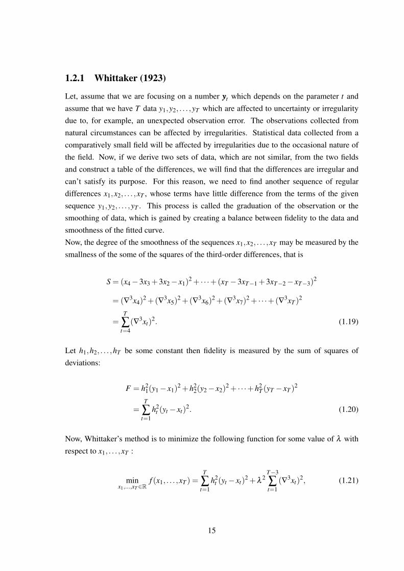
1.2.1 Whittaker (1923)

Let, assume that we are focusing on a number yyyt which depends on the parameter t andassume that we have T data y1,y2, . . . ,yT which are affected to uncertainty or irregularitydue to, for example, an unexpected observation error. The observations collected fromnatural circumstances can be affected by irregularities. Statistical data collected from acomparatively small field will be affected by irregularities due to the occasional nature ofthe field. Now, if we derive two sets of data, which are not similar, from the two fieldsand construct a table of the differences, we will find that the differences are irregular andcan’t satisfy its purpose. For this reason, we need to find another sequence of regulardifferences x1,x2, . . . ,xT , whose terms have little difference from the terms of the givensequence y1,y2, . . . ,yT . This process is called the graduation of the observation or thesmoothing of data, which is gained by creating a balance between fidelity to the data andsmoothness of the fitted curve.Now, the degree of the smoothness of the sequences x1,x2, . . . ,xT may be measured by thesmallness of the some of the squares of the third-order differences, that is

S = (x4−3x3 +3x2− x1)2 + · · ·+(xT −3xT−1 +3xT−2− xT−3)

2

= (∇3x4)2 +(∇3x5)

2 +(∇3x6)2 +(∇3x7)

2 + · · ·+(∇3xT )2

=T

∑t=4

(∇3xt)2. (1.19)

Let h1,h2, . . . ,hT be some constant then fidelity is measured by the sum of squares ofdeviations:

F = h21(y1− x1)

2 +h22(y2− x2)

2 + · · ·+h2T (yT − xT )

2

=T

∑t=1

h2t (yt− xt)

2. (1.20)

Now, Whittaker’s method is to minimize the following function for some value of λ withrespect to x1, . . . ,xT :

minx1,...,xT∈R

f (x1, . . . ,xT ) =T

∑t=1

h2t (yt− xt)

2 +λ2

T−3

∑t=1

(∇3xt)2, (1.21)

15

where ∇xt = xt+1− xt . Let yyy = [y1, . . . ,yT ]′, xxx = [x1, . . . ,xT ]

′, HHH = diag(h21, . . . ,h

2T ), and

DDD ∈ R(T−3)×T be a matrix such that

DDDxxx = [∇3x1, . . . ,∇3xT−3]

′.

Then, (1.21) can be expressed in matrix notation as follows:

minxxx∈RT

f (xxx) = (yyy− xxx)′HHH(yyy− xxx)+λ2(DDDxxx)′(DDDxxx). (1.22)

From

∂ f (xxx)∂xxx

=−2HHH(yyy− xxx)+2λ2DDD′DDDxxx, (1.23)

letting xxx denote the solution of (1.21)/(1.22), the optimality condition for (1.21)/(1.22) canbe expressed as

−HHH(yyy− xxx)+λ2DDD′DDDxxx = 000. (1.24)

Equivalently,

HHHyyy = HHHxxx+λ2DDD′DDDxxx. (1.25)

Given that

DDDxxx = [∇3x1, . . . ,∇3xT−3]

′ (1.26)

16

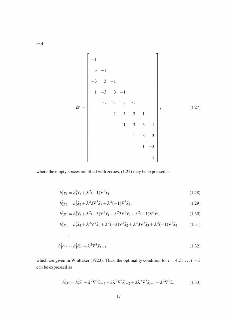
and

DDD′ =

−1

3 −1

−3 3 −1

1 −3 3 −1

. . .. . .

. . .. . .

1 −3 3 −1

1 −3 3 −1

1 −3 3

1 −3

1

, (1.27)

where the empty spaces are filled with zeroes, (1.25) may be expressed as

h21y1 = h2

1x1 +λ2(−1)∇3x1, (1.28)

h22y2 = h2

2x2 +λ23∇

3x1 +λ2(−1)∇3x2, (1.29)

h23y3 = h2

3x3 +λ2(−3)∇3x1 +λ

23∇3x2 +λ

2(−1)∇3x3, (1.30)

h24y4 = h2

4x4 +λ2∇

3x1 +λ2(−3)∇3x2 +λ

23∇3x3 +λ

2(−1)∇3x4, (1.31)

...

h2T yT = h2

T xT +λ2∇

3xT−3, (1.32)

which are given in Whittaker (1923). Thus, the optimality condition for t = 4,5, . . . ,T −3can be expressed as

h2t yt = h2

t xt +λ2∇

3xt−3−3λ2∇

3xt−2 +3λ2∇

3xt−1−λ2∇

3xt . (1.33)

17

For simplification we assume that, h1 = h2 = · · ·= hT .Now, if we consider h2

1 = h22 = · · · = h2

T = ελ 2 ,where ε is a non-negative constant, thenthe above system of equations can be written as:

εy1 = ε x1−∇3x1,

εy2 = ε x2 +3∇3x1−∇

3x2,

εy3 = ε x3−3∇3x1 +3∇

3x2−∇3x3,

εy4 = ε x4 +∇3x1−3∇

3x2 +3∇3x3−∇

3x4,

...

εyT = ε xT +∇3xT−3.

So, the above system is equivalent to the following expression

εyt = ε xt +∇3xt−3−3∇

3xt−2 +3∇3xt−1−∇

3xt . (1.34)

Let Fxt = xt+1. Then, we obtain

∇3xt−3−3∇

3xt−2 +3∇3xt−1−∇

3xt = ∇3(xt−3−3xt−2 +3xt−1− xt)

= ∇3(xt−3−3Fxt−3 +3F2xt−3−F3xt−3)

= ∇3(1−3F +3F2−F3)xt−3

=−∇3(F−1)3xt−3

=−∇6xt−3. (1.35)

Substituting (1.35) into (1.34) yields

εyt = ε xt−∇6xt−3. (1.36)

18

For finding the optimal solution xxx = [x1, ..., xT ]′ of the above function (1.21), now all the

equations except the three first and the three last are of the form

xt− yt =1ε

∇6xt−3, for t = 4,5, . . . ,T −3. (1.37)

Similarly, the first three and the last three equations can also be brought to the same formby introducing new quantities of xt . The quantities are ∇3x−1,∇

3x−2,∇3x0,∇

3xT+1,

∇3xT+2,∇3xT+3 for which

∇3x−1 = 0,∇3x−2 = 0,∇3x0 = 0,∇3xT+1 = 0,∇3xT+2 = 0,∇3xT+3 = 0. (1.38)

Thus the graduated values xt satisfy the linear difference equation

ε xt−∇6xt−3 = εyt t = 1,2, . . . ,T, (1.39)

and the solution has to satisfy the terminal conditions ∇3xt = 0 for t =−2,−1,0,T +1,T +

2,T + 3. After that Whittaker expanded the equation in powers of ε , which he assumedwould be small and solve the linear equations.

19

1.3 Objectives and Outlines

The main goal of this research is to analyze the special cases of the Whittaker–Hendersonmethod of graduation, which originates in the work of Bohlmann (1899), which is a widelyused graduating method. The WH method of graduation has been used for the mortalitytable construction, in the Actuarial literature. At the beginning of this thesis, some prelim-inary definitions and relevance methods are discussed. The primary objective of this thesisis to establish alternative methods to gain simpler formulas.This thesis dissertation consists of four chapters. In chapter 1, the introductory survey ofresearch, some preliminary definitions, examples and relevance methods are discussed.

Chapter 2, we provide an explicit formula for the smoother weights of theWhittaker–Henderson (WH) graduation of order 1 along with some related results, whichleads to a richer understanding of the filter. (IIIn + λDDD′pDDDp)

−1 in is the smoother matrixof the WH graduation and its elements are the smoother weights of the smoothing. Themain motivation of this thesis comes from De Jong and Sakarya (2016). They providedan explicit formula for the smoother weights of the WH graduation of order 2, followingwhich Cornea-Madeira (2017) gave a simpler explicit formula. In econometrics, the WHgraduation of order 2 is referred to as the Hodrick–Prescott (1997) filter. We note herethat to derive the explicit formula, we apply a different approach to that of Cornea-Madeira(2017). This is mainly because the approach given in Chapter 2 leads to a simpler formula.In the last part of this chapter, for comparison, we show another formula based on Cornea-Madeira’s (2017) approach. A MATLAB code is included which visualizes the efficiencyof the proposed method.

In Chapter 3, we provide an alternative simpler formula for the Hodrick–Prescott(HP) (1997) filter and explains the reason why our approach leads to a simpler formula.The Hodrick–Prescott (HP) filter is a popular method to estimate the trend componentof the univariate time series. It is described as a penalized least squares problem and aspecial case of the Whittaker–Henderson (WH) method of graduation. By implementingthe Sherman–Morrison–Woodbury (SMW) formula and a discrete cosine transformationmatrix, De Jong and Sakarya (2016) recently derived an explicit formula for the smootherweights of the Hodrick–Prescott filter. In recent times, by applying the SMW formula andthe spectral decomposition of a symmetric tridiagonal Toeplitz matrix, Cornea-Madeira(2017) provided a simpler formula. In this chapter, we provide a simpler alternative formulafor the smoother weights of the HP filter. A MATLAB code to find the smoother weightsof the popular HP filter is included in the last part of the chapter which guaranteed theefficiency of the proposed method.

20

In Chapter 4, based on the result of Yamada (2019), simple formulas for calculatingthe smoother matrix of the WH method is provided. In addition, we show some results,which include that two other smoother matrices related to the WH graduation are alsobisymmetric.

21

1.4 Appendix

Proof of Equation (1.8)

Differentiating equation (1.7) we get

WWW (xxx− yyy)+GGGxxx = 000,

following which we obtain

(WWW +GGG)xxx =WWWyyy.

WWW +GGG is a positive definite matrix and thus it is invertible. Then, it follows that

xxx = (III +WWW−1GGG)−1yyy.

22

1.5 References

1. Abadir, K. M. and J. R. Magnus, 2005, Matrix Algebra, Cambridge University Press,Cambridge.

2. Ahmed, N., T. Natarajan, and K. R. Rao, 1974, Discrete cosine transform, IEEE

Transactions on Computers, C-23, 1, 90–93.

3. Baxter, M. and R. G. King, 1999, Measuring business cycles: Approximate band-pass filters for economic time series, Review of Economics and Statistics, 81, 4, 575–593.

4. Bierens, H., 1997, Testing the unit root with drift hypothesis against nonlinear trendstationarity, with an application to the U.S. price level and interest rate, Journal of

Econometrics, 81, 29–64.

5. Bohlmann, G., 1899, Ein Ausgleichungsproblem, Nachrichten von der Gesellschaft

der Wissenschaften zu Gottingen, Mathematisch-Physikalische Klasse, 260–271.

6. Cornea-Madeira, A., 2017, The explicit formula for the Hodrick–Prescott filter infinite sample, Review of Economics and Statistics, 99, 2, 314–318.

7. De Jong, R. M. and N. Sakarya, 2016, The econometrics of the Hodrick–Prescottfilter, Review of Economics and Statistics, 98, 2, 310–317.

8. Diele, F. and L. Lopez, 1998, The use of the factorization of five-diagonal matricesby tridiagonal Toeplitz matrices, Applied Mathematics Letters, 11, 3, 61–69.

9. Gomez, V., 2001, The use of Butterworth filters for trend and cycle estimation ineconomic time series, Journal of Business and Economic Statistics, 19, 3, 365–373.

10. Greville,T.N.E., 1948, Recent Development in Graduation and Interpolation, Ameri-

can Statistical Association , Vol. 43, No. 243, 428-441.

11. Henderson, R., 1924, A New Method of Graduation, Transactions, Actuarial Society

of America, Vol. 25, Part I, No. 71, 29-40.

12. Hodrick, R. J. and E. C. Prescott, 1997, Postwar U.S. business cycles: An empiricalinvestigation, Journal of Money, Credit and Banking, 29, 1, 1–16.

13. Hoerl, A. E. and R. W. Kennard, 1970, Ridge regression: Biased estimation fornonorthogonal problems, Technometrics, 12, 1, 55–67.

23

14. Kim, S., K. Koh, S. Boyd, and D. Gorinevsky, 2009, `1 trend filtering, SIAM Review,51, 2, 339–360.

15. King, R. G. and S. T. Rebelo, 1993, Low frequency filtering and real business cycles,Journal of Economic Dynamics and Control, 17, 1–2, 207–231.

16. Marr, R. B. and G. H. Vineyard, 1988, Five-diagonal Toeplitz determinants and theirrelation to Chebyshev polynomials, SIAM Journal on Matrix Analysis and Applica-

tions, 9, 4, 579–586.

17. Montaner, J. M. and M. Alfaro, 1995, On five-diagonal Toeplitz matrices and orthog-onal polynomials on the unit circle, Numerical Algorithms, 10, 1, 137–153.

18. Nocon, A. S. and W. F. Scott, 2012, An extension of the Whittaker–Hendersonmethod of graduation, Scandinavian Actuarial Journal, 2012, 1, 70–79.

19. Paige, R. L. and A. A. Trindade, 2010, The Hodrick–Prescott filter: A special caseof penalized spline smoothing, Electronic Journal of Statistics, 4, 856–874.

20. Pesaran, M. H., 1973, Exact maximum likelihood estimation of a regression equationwith a first-order moving-average error, Review of Economic Studies, 40, 4, 529–535.

21. Phillips P. C. B., 2010, Two New Zealand pioneer econometricians, New Zealand

Economic Papers, 44, 1, 1–26.

22. Ravn, M. O. and H. Uhlig, 2002, On adjusting the Hodrick–Prescott filter for thefrequency of observations, Review of Economics and Statistics, 84, 2, 371–380.

23. Strang, G., 1999, The discrete cosine transform, SIAM Review, 41, 1, 135–147.

24. Strang, G. and S. MacNamara, 2014, Functions of difference matrices are Toeplitzplus Hankel, SIAM Review, 56, 3, 525–546.

25. Tibshirani, R., 1996, Regression shrinkage and selection via the lasso, Journal of the

Royal Statistical Society Series B 58, 267–288.

26. Wang, C., H. Li, and D. Zhao, 2015, An explicit formula for the inverse of a penta-diagonal Toeplitz matrix, Journal of Computational and Applied Mathematics, 278,15, 12–18.

27. Weinert, H. L., 2007, Efficient computation for Whittaker–Henderson smoothing,Computational Statistics and Data Analysis, 52, 959–974.

24

28. Yamada, H., 2015, Ridge regression representations of the generalized Hodrick–Prescott filter, Journal of the Japan Statistical Society, 45, 2, 121–128.

29. Yamada, H., 2018, Several least squares problems related to the Hodrick–Prescottfiltering, Communications in Statistics – Theory and Methods, 47, 5, 1022–1027.

30. Yamada, H. and F. T. Jahra, 2018, Explicit formulas for the smoother weights of theWhittaker–Henderson graduation of order 1, Communications in Statistics – Theory

and Methods, 48, 12, 3153–3161.

31. Yamada, H, 2019, A note on Whittaker–Henderson graduation: Bisymmetry of thesmoother matrix, Communications in Statistics – Theory and Methods, DOI: 10.1080/03610926.2018.1563183.

25

Chapter 2

Explicit Formulas for the Smoother

Weights of the Whittaker–Henderson

Graduation of Order 1

This chapter basically based on a previously published article [Yamada, H. and F. T. Jahra,2018].

2.1 Introduction

The Whittaker–Henderson (WH) graduation, which originates in the work of Bohlmann(1899), is a widely applied smoothing method. The WH graduation (of order p) is definedas

minx1,...,xn∈R

n

∑t=1

(yt− xt)2 +λ

n

∑t=p+1

(∆pxt)2, (2.1)

where y1, . . . ,yn represent a sequence of n observations, λ > 0 is a smoothing parameter,and ∆xt = xt − xt−1. For historical remarks on the filter, see Weinert (2007).1 It may also

1See also Phillips (2010) and Nocon and Scott (2012).

26

be represented in matrix notation as

minxxx∈Rn

(yyy− xxx)′(yyy− xxx)+λ (DDDpxxx)′(DDDpxxx), (2.2)

where yyy = [y1, . . . ,yn]′, xxx = [x1, . . . ,xn]

′, and DDDp ∈ R(n−p)×n is the pth-order differencematrix such that DDDpxxx = [∆pxp+1, . . . ,∆

pxn]′. For example,

DDD1 =

−1 1 0 · · · 0

0 −1 1. . .

...

.... . .

. . .. . . 0

0 · · · 0 −1 1

∈ R(n−1)×n.

Since the objective function of the WH graduation is quadratic and its Hessian matrix ispositive definite, it has a unique global minimizer, which is expressed explicitly as

xxxp = (IIIn +λDDD′pDDDp)−1yyy, (2.3)

where IIIn is the identity matrix of order n.(IIIn +λDDD′pDDDp)

−1 in (2.3) is the smoother matrix of the WH graduation and its ele-ments are the smoother weights of the smoothing. Recently, De Jong and Sakarya (2016)provided an explicit formula for the smoother weights of the WH graduation of order 2,following which Cornea-Madeira (2017) gave a simpler explicit formula.2 In this paper,we contribute to the literature by providing an explicit formula for the smoother weightsof the graduation of order 1 along with some related results, which enables us to gain aricher understanding of the filter. We note here that to derive the explicit formula, we ap-ply a different approach to that of Cornea-Madeira (2017). This is mainly because, in thecase under consideration, the approach given in the present paper leads to a simpler for-mula. Later, for comparison, we show another formula based on Cornea-Madeira’s (2017)approach.

This chapter is organized as follows. In Section 2.2, we provide the main results.In Section 2.3, we show the formula based on Cornea-Madeira’s (2017) approach. Section2.4 concludes the paper.

2In econometrics, the WH graduation of order 2 is referred to as the Hodrick–Prescott (1997) filter.

27

2.2 The main results

Recall that DDD1DDD′1 = QQQn−1, where

QQQr =

2 −1 0 · · · 0

−1 2 −1. . .

...

0. . .

. . .. . . 0

.... . . −1 2 −1

0 · · · 0 −1 2

∈ Rr×r,

which is a well-known symmetric tridiagonal Toeplitz matrix (Strang and MacNamara,2014). From the three-term recurrence relation of multiple angles in sine function, thespectral decomposition of QQQr is:3 QQQr =VVV rΛΛΛrVVV ′r, where ΛΛΛr = diag(λr,1, . . . ,λr,r) and VVV r =

[vr,i, j]i, j=1,...,r with

λr,k = 2−2cos(

kπ

r+1

), k = 1, . . . ,r, (2.4)

vr,i, j =

√2

r+1sin(

i jπr+1

), i, j = 1, . . . ,r. (2.5)

Hence the spectral decomposition for DDD1DDD′1 is

DDD1DDD′1 =VVV n−1ΛΛΛn−1VVV ′n−1. (2.6)

We note that (i) 0 < λn−1,1 < · · ·< λn−1,n−1 < 4 and (ii) VVV n−1 is an orthogonal matrix.4 Weapply (2.6) to derive an explicit formula for the smoother weights of the WH graduation oforder 1.

Theorem 2.1.

xxx1 = yyy−DDD′1VVV n−1(λ−1IIIn−1 +ΛΛΛn−1)

−1VVV ′n−1DDD1yyy. (2.7)3Pesaran (1973) used the spectral decomposition of a more general matrix.4Also, from trace(DDD1DDD′1) = 2(n− 1) and |DDD1DDD′1| = n, it follows that ∑

n−1k=1 λn−1,k = 2(n− 1) and

∏n−1k=1 λn−1,k = n.

28

Proof. Applying the Woodbury matrix identity to (IIIn +λDDD′1DDD1)−1, it follows that

(IIIn +λDDD′1DDD1)−1 = IIIn−DDD′1(λ

−1IIIn−1 +DDD1DDD′1)−1DDD1. (2.8)

Moreover, from (2.6), the right-hand side of (2.8) may be rewritten as

IIIn−DDD′1(λ−1IIIn−1 +DDD1DDD′1)

−1DDD1 = IIIn−DDD′1(λ−1IIIn−1 +VVV n−1ΛΛΛn−1VVV ′n−1)

−1DDD1

= IIIn−DDD′1VVV n−1(λ−1IIIn−1 +ΛΛΛn−1)

−1VVV ′n−1DDD1, (2.9)

which proves (2.7).

Denote the (i, j) entry of (IIIn +λDDD′1DDD1)−1 by qi, j and the Kronecker delta by δi, j.

Let xxx1 = [x1,1, . . . , x1,n]′.

Corollary 2.1. Denote the (i, j) entry of DDD′1VVV n−1(λ−1IIIn−1 +ΛΛΛn−1)

−1VVV ′n−1DDD1 by pi, j.

qi, j = δi, j− pi, j = δi, j−n−1

∑k=1

(vn−1,i,k− vn−1,i−1,k)(vn−1, j,k− vn−1, j−1,k)

λ−1 +λn−1,k(2.10)

= δi, j−2n

n−1

∑k=1

sin( iπk

n

)− sin

((i−1)πk

n

)sin(

jπkn

)− sin

(( j−1)πk

n

)λ−1 +2−2cos

(πkn

)(2.11)

for i, j = 1, . . . ,n.

Proof. Firstly, (λ−1IIIn−1 +ΛΛΛn−1)−1 in (2.7) may be represented as

(λ−1IIIn−1 +ΛΛΛn−1)−1

= diag(λ−1 +λn−1,1)

−1, . . . ,(λ−1 +λn−1,n−1)−1

= diag

[λ−1 +2−2cos

(1π

n

)−1

, . . . ,

λ−1 +2−2cos

((n−1)π

n

)−1].

Secondly, because

vn−1,0, j =

√2n

sin(

0 · jπn

)= 0, vn−1,n, j =

√2n

sin(

n · jπn

)= 0,

29

for j = 1, . . . ,n−1, DDD′1VVV n−1 in (2.7) is expressed by

DDD′1VVV n−1

=

vn−1,0,1− vn−1,1,1 · · · vn−1,0,n−1− vn−1,1,n−1

......

vn−1,n−1,1− vn−1,n,1 · · · vn−1,n−1,n−1− vn−1,n,n−1

=

√2n

sin(0·1π

n

)− sin

(1·1π

n

)· · ·

√2n

sin(

0·(n−1)πn

)− sin

(1·(n−1)π

n

)...

...√2n

sin((n−1)·1π

n

)− sin

(n·1π

n

)· · ·

√2n

sin((n−1)·(n−1)π

n

)− sin

(n·(n−1)π

n

)

.

Using this result, (2.10) and (2.11) immediately follow from Theorem 2.1.

Let ιιι = [1, . . . ,1]′ ∈ Rn.

Corollary 2.2. For given i, j = 1,2, . . .,

qi, j→ δi, j−2λ

∫ 1

0

sin(iπr)− sin((i−1)πr)sin( jπr)− sin(( j−1)πr)1+4λ sin2(0.5πr)

dr, (n→ ∞).

(2.12)

For i, j = 1, . . . ,n,

qi, j→1n, (λ → ∞), (2.13)

and

qi, j→ δi, j, (λ → 0). (2.14)

Proof. (2.12) immediately follows from (2.11). Recalling that IIIn−DDD′1(DDD1DDD′1)−1DDD1 =

1n ιιιιιι ′,

(2.13) follows from (2.7). Finally, (2.14) is evident from (2.10).

Proposition 2.1. (IIIn +λDDD′1DDD1)−1 is a symmetric centrosymmetric matrix.

30

Proof. We only prove that (IIIn + λDDD′1DDD1)−1 is centrosymmetric. Let JJJn ∈ Rn×n be the

exchange/permutation matrix:

JJJn =

0 · · · 0 1

... . ..

. ..

0

0 . ..

. .. ...

1 0 · · · 0

.

Because

DDD′1DDD1 =

1 −1 0 · · · 0

−1 2 −1. . .

...

0. . .

. . .. . . 0

.... . . −1 2 −1

0 · · · 0 −1 1

∈ Rn×n (2.15)

is a centrosymmetric matrix, (IIIn+λDDD′1DDD1) is also a centrosymmetric matrix. Accordingly,it follows that (IIIn +λDDD′1DDD1) = JJJn(IIIn +λDDD′1DDD1)JJJn. Recalling that JJJ−1

n = JJJn, we obtain

(IIIn +λDDD′1DDD1)−1 = JJJn(IIIn +λDDD′1DDD1)

−1JJJn,

which proves that (IIIn +λDDD′1DDD1)−1 is a centrosymmetric matrix.

Remarks. From Proposition 2.1, we immediately obtain qn−i+1,n− j+1 = qi, j for i, j =

1, . . . ,n. For example, qn,n−2 = q1,3, qn,n−1 = q1,2 and qn,n = q1,1. Thus, for large n,qn−i+1,n− j+1 approximately equals the right-hand side of (2.12).

We also remark that it follows immediately from (2.8) and DDD1ιιι = 000 that

n

∑j=1

qi, j = 1, i = 1, . . . ,n, (2.16)

31

and 1n ∑

ni=1 x1,i =

1n ∑

ni=1 yi.5

2.3 Formulas based on Cornea-Madeira’s (2017) ap-

proach

From (2.15), it follows that DDD′1DDD1 = QQQn− eee1eee′1− eeeneee′n, where eee1 = [1,0, . . . ,0]′ ∈ Rn andeeen = [0, . . . ,0,1]′ ∈ Rn. Accordingly, we obtain

(IIIn +λDDD′1DDD1)−1 = (AAA−λeee1eee′1−λeeeneee′n)

−1, (2.17)

where AAA = IIIn +λQQQn. In the same way as Cornea-Madeira (2017), we apply the Sherman–Morrison formula twice to (2.17), we obtain the following results:

(IIIn +λDDD′1DDD1)−1 = (AAA−λeee1eee′1)

−1 +λ(AAA−λeee1eee′1)

−1eeeneee′n(AAA−λeee1eee′1)−1

1−λeee′n(AAA−λeee1eee′1)−1eeen

,

where

(AAA−λeee1eee′1)−1 = AAA−1 +λ

AAA−1eee1eee′1AAA−1

1−λeee′1AAA−1eee1.

Let AAA−1 = [bi, j]i, j=1,...,n and denote the first and last column of AAA−1 by βββ 1 and βββ n,respectively. We obtain the following results:

Theorem 2.2.

(IIIn +λDDD′1DDD1)−1 = AAA−1 +

2λ (κ11βββ 1βββ′1 +κ1nβββ 1βββ

′n +κn1βββ nβββ

′1 +κnnβββ nβββ

′n)

κ211−κ2

1n−κ2n1 +κ2

nn, (2.18)

where κ11 = 1−λb1,1, κ1n = λb1,n, κn1 = λbn,1, and κnn = 1−λbn,n.

Proof. See the Appendix.

5Some related discussion may be found in Yamada (2015, 2018).

32

Since AAA−1 =

VVV n(IIIn +λΛΛΛn)VVV ′n−1

=VVV n(IIIn +λΛΛΛn)−1VVV ′n, we obtain

bi, j =n

∑k=1

(vn,i,kvn, j,k

1+λλn,k

)=

2n+1

n

∑k=1

sin( iπk

n+1

)sin(

jπkn+1

)1+λ

2−2cos

(πk

n+1

) , i, j = 1, . . . ,n. (2.19)

Corollary 2.3. Let (IIIn +λDDD′1DDD1)−1 = [qi, j]i, j=1,...,n. We have

qi, j = bi, j +2λ (κ11bi,1b j,1 +κ1nbi,1b j,n +κn1bi,nb j,1 +κnnbi,nb j,n)

κ211−κ2

1n−κ2n1 +κ2

nn, (2.20)

where κ11 = 1−λb1,1, κ1n = λb1,n, κn1 = λbn,1, and κnn = 1−λbn,n.

Let nnn1 = 1,3, . . . ,n if n is odd, nnn1 = 1,3, . . . ,n − 1 if n is even, nnn2 =

2,4, . . . ,n−1 if n is odd, and nnn2 = 2,4, . . . ,n if n is even. The following result corre-sponds to Cornea-Madeira’s (2017) Theorem 1:

Corollary 2.4. Let φi = 2λ

(1−2λ ∑k∈nnni v2

n,1,kγ−1k

)−1for i = 1,2, where γk = 1+λλn,k

for k = 1, . . . ,n. Then, it follows that

(IIIn +λDDD′1DDD1)−1 =VVV n(IIIn +λΛΛΛn)

−1VVV ′n +φ1VVV nKKK1VVV ′n +φ2VVV nKKK2VVV ′n, (2.21)

where KKKr = [kr,i, j]i, j=1,...,n for r = 1,2 is such that

k1,i, j =

vn,i,1vn, j,1

γiγ j, i+ j : even, j : odd

0, otherwise; k2,i, j =

vn,i,1vn, j,1

γiγ j, i+ j : even, j : even

0, otherwise.

Proof. See the Appendix.

Finally, concerning bi, j in Corollary 2.3, it follows from (2.19) that, for given i, j =

1,2, . . .,

bi, j→ 2∫ 1

0

sin(iπr)sin( jπr)1+4λ sin2(0.5πr)

dr, (n→ ∞). (2.22)

33

2.4 Concluding remarks

In this chapter, we provided explicit formulas for the smoother weights of the WH gradua-tion of order 1 and some related results. The results obtained in the chapter are summarizedin Theorems 2.1 and 2.2, in Corollaries 2.1, 2.2, 2.3, and 2.4, and in Proposition 2.1.

We note that although we may consider algorithms based on the explicit formulasderived in the paper, they are not necessarily recommended for practical use when n islarge, because they may not be numerically efficient even though the smoother matrix is asymmetric centrosymmetric matrix. An efficient algorithm that reduces execution time andmemory use is obtainable by performing a Cholesky decomposition of (IIIn +λDDD′1DDD1) andthen solving the resulting triangular systems. See Weinert (2007) for further details.

34

2.5 Numerical example

As an example, we are going to find the inverse of (III5+λDDD′1DDD1)−1 ∈R5×5 , where λ = 1.

We know that, the first-order difference matrix

DDD1 =

−1 1 0 0 0

0 −1 1 0 0

0 0 −1 1 0

0 0 0 −1 1

∈ R4×5,

and

DDD′1DDD1 =

1 −1 0 0 0

−1 2 −1 0 0

0 −1 2 −1 0

0 0 −1 2 −1

0 0 0 −1 1

∈ R5×5. (2.23)

A 5×5 tridiagonal Toeplitz matrix QQQ5 is as follows

QQQ5 =

2 −1 0 0 0

−1 2 −1 0 0

0 −1 2 −1 0

0 0 −1 2 −1

0 0 0 −1 2

. (2.24)

Now, from equations (2.23) and (2.24) we get the following relation:

DDD′1DDD1 = QQQ5− eee1eee′1− eee5eee′5, (2.25)

35

where

eee1 =

1

0

0

0

0

and eee5 =

0

0

0

0

1

,

are unit vectors.Note that QQQ5 has distinct eigenvalues

γ j = 2−2cos(

π j6

), j = 1, ...,5,

and corresponding eigenvector xxx j = [x1, j, ...,x5, j]′ with

xi, j =

(13

)1/2

sin(

πi j6

), i, j = 1, ...,5.

Let, AAA = III5 +λQQQ5. Now we consider the eigenvalue matrix of (III5 +λQQQ5) is

ΛΛΛ = diag(λ1, ...,λ5),

withλ j = 1+λγ j,

36

We have

AAA−1 = (III5 +λQQQ5)−1 =

0.3819444 0.1458333 0.0555556 0.0208333 0.0069444

0.1458333 0.4375000 0.1666667 0.0625000 0.0208333

0.0555556 0.1666667 0.4444444 0.1666667 0.0555556

0.0208333 0.0625000 0.1666667 0.4375000 0.1458333

0.0069444 0.0208333 0.0555556 0.1458333 0.3819444

,

and let AAA−1 = [bi, j]i, j=1,...,5 and denote the first and last column of AAA−1 by βββ 1 and βββ 5

respectively.

Now, according to the Theorem 2.2, the explicit inverse is:

(III5 +λDDD′1DDD1)−1 = (III5 +λQQQ5−λeee1eee′1−λeee5eee′5)

−1

= (AAA−λeee1eee′1−λeee5eee′5)−1

= AAA−1 +2λ (κ1,1βββ 1βββ

′1 +κ1,5βββ 1βββ



′5)

κ21,1−κ2

1,5−κ25,1 +κ2

5,5. (2.26)

Here, κ1,1 = 1−λb1,1, κ1,5 = λb1,5,κ5,1 = λb5,1, and κ5,5 = 1−λb5,5.So, now we get

(III5 +λDDD′1DDD1)−1 =

0.618182 0.236364 0.090909 0.036364 0.018182

0.236364 0.472727 0.181818 0.072727 0.036364

0.090909 0.181818 0.454545 0.181818 0.090909

0.036364 0.072727 0.181818 0.472727 0.236364

0.018182 0.036364 0.090909 0.236364 0.618182

.

37

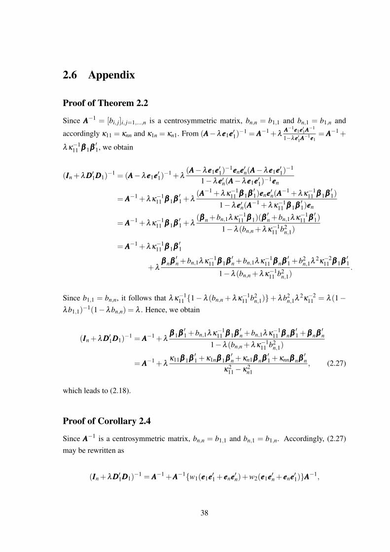
2.6 Appendix

Proof of Theorem 2.2

Since AAA−1 = [bi, j]i, j=1,...,n is a centrosymmetric matrix, bn,n = b1,1 and bn,1 = b1,n and

accordingly κ11 = κnn and κ1n = κn1. From (AAA−λeee1eee′1)−1 = AAA−1+λ

AAA−1eee1eee′1AAA−1

1−λeee′1AAA−1eee1= AAA−1+

λκ−111 βββ 1βββ

′1, we obtain

(IIIn +λDDD′1DDD1)−1 = (AAA−λeee1eee′1)

−1 +λ(AAA−λeee1eee′1)

−1eeeneee′n(AAA−λeee1eee′1)−1

1−λeee′n(AAA−λeee1eee′1)−1eeen

= AAA−1 +λκ−111 βββ 1βββ

′1 +λ

(AAA−1 +λκ−111 βββ 1βββ

′1)eeeneee′n(AAA

−1 +λκ−111 βββ 1βββ

′1)

1−λeee′n(AAA−1 +λκ

−111 βββ 1βββ

′1)eeen


′1 +λ

(βββ n +bn,1λκ−111 βββ 1)(βββ

′n +bn,1λκ

−111 βββ

′1)

1−λ (bn,n +λκ−111 b2

n,1)


′1

+λβββ nβββ

′n +bn,1λκ


′n +bn,1λκ

−111 βββ nβββ

′1 +b2

n,1λ 2κ−211 βββ 1βββ

′1

1−λ (bn,n +λκ−111 b2

n,1).

Since b1,1 = bn,n, it follows that λκ−111 1− λ (bn,n + λκ

−111 b2

n,1)+ λb2n,1λ 2κ

−211 = λ (1−

λb1,1)−1(1−λbn,n) = λ . Hence, we obtain

(IIIn +λDDD′1DDD1)−1 = AAA−1 +λ

βββ 1βββ′1 +bn,1λκ


′n +bn,1λκ

−111 βββ nβββ

′1 +βββ nβββ

′n

1−λ (bn,n +λκ−111 b2

n,1)

= AAA−1 +λκ11βββ 1βββ

′1 +κ1nβββ 1βββ

′n +κn1βββ nβββ

′1 +κnnβββ nβββ

′n

κ211−κ2

n1, (2.27)

which leads to (2.18).

Proof of Corollary 2.4

Since AAA−1 is a centrosymmetric matrix, bn,n = b1,1 and bn,1 = b1,n. Accordingly, (2.27)may be rewritten as

(IIIn +λDDD′1DDD1)−1 = AAA−1 +AAA−1w1(eee1eee′1 + eeeneee′n)+w2(eee1eee′n + eeeneee′1)AAA−1,

38

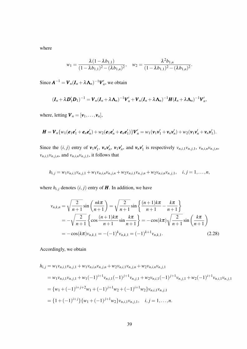
where

w1 =λ (1−λb1,1)

(1−λb1,1)2− (λb1,n)2 , w2 =λ 2b1,n

(1−λb1,1)2− (λb1,n)2 .

Since AAA−1 =VVV n(IIIn +λΛΛΛn)−1VVV ′n, we obtain

(IIIn +λDDD′1DDD1)−1 =VVV n(IIIn +λΛΛΛn)

−1VVV ′n +VVV n(IIIn +λΛΛΛn)−1HHH(IIIn +λΛΛΛn)

−1VVV ′n,

where, letting VVV n = [vvv1, . . . ,vvvn],

HHH =VVV nw1(eee1eee′1 + eeeneee′n)+w2(eee1eee′n + eeeneee′1)VVV ′n = w1(vvv1vvv′1 + vvvnvvv′n)+w2(vvv1vvv′n + vvvnvvv′1).

Since the (i, j) entry of vvv1vvv′1, vvvnvvv′n, vvv1vvv′n, and vvvnvvv′1 is respectively vn,i,1vn, j,1, vn,i,nvn, j,n,vn,i,1vn, j,n, and vn,i,nvn, j,1, it follows that

hi, j = w1vn,i,1vn, j,1 +w1vn,i,nvn, j,n +w2vn,i,1vn, j,n +w2vn,i,nvn, j,1, i, j = 1, . . . ,n,

where hi, j denotes (i, j) entry of HHH. In addition, we have

vn,k,n =

√2

n+1sin(

nkπ

n+1

)=

√2

n+1sin(n+1)kπ

n+1− kπ

n+1

=−

√2

n+1

cos

(n+1)kπ

n+1sin

kπ

n+1

=−cos(kπ)

√2

n+1sin(

kπ

n+1

)=−cos(kπ)vn,k,1 =−(−1)kvn,k,1 = (−1)k+1vn,k,1. (2.28)

Accordingly, we obtain

hi, j = w1vn,i,1vn, j,1 +w1vn,i,nvn, j,n +w2vn,i,1vn, j,n +w2vn,i,nvn, j,1

= w1vn,i,1vn, j,1 +w1(−1)i+1vn,i,1(−1) j+1vn, j,1 +w2vn,i,1(−1) j+1vn, j,1 +w2(−1)i+1vn,i,1vn, j,1

= w1 +(−1)i+ j+2w1 +(−1) j+1w2 +(−1)i+1w2vn,i,1vn, j,1

= 1+(−1)i+ jw1 +(−1) j+1w2vn,i,1vn, j,1, i, j = 1, . . . ,n.

39

Thus, we have

hi, j =

0 (i+ j : odd)

2(w1 +w2)vn,i,1vn, j,1 (i+ j : even, j : odd)

2(w1−w2)vn,i,1vn, j,1 (i+ j : even, j : even)

for i, j = 1, . . . ,n. From (2.5), it follows that vn,i, j = vn, j,i for i, j = 1, . . . ,n. Then, from(2.28), we obtain vn,n,k = (−1)k+1vn,1,k. Thus, we have

b1,n =n

∑k=1

(vn,1,kvn,n,k

γk

)=

n

∑k=1

(−1)k+1v2n,1,kγ

−1k .

In addition, b1,1 = ∑nk=1 v2

n,1,kγ−1k . Then, using these results yields

w1 +w2 =λ (1−λb1,1)+λ 2b1,n

(1−λb1,1)2− (λb1,n)2 =λ (1−λb1,1 +λb1,n)

(1−λb1,1−λb1,n)(1−λb1,1 +λb1,n)

=λ

1−λb1,1−λb1,n= λ

(1−2λ ∑

k∈nnn1

v2n,1,kγ

−1k

)−1

.

Likewise, we obtain

w1−w2 ==λ (1−λb1,1)−λ 2b1,n

(1−λb1,1)2− (λb1,n)2 =λ (1−λb1,1−λb1,n)

(1−λb1,1−λb1,n)(1−λb1,1 +λb1,n)

=λ

1−λb1,1 +λb1,n= λ

(1−2λ ∑

k∈nnn2

v2n,1,kγ

−1k

)−1

.

40

2.7 References

1. Bohlmann, G., 1899, Ein Ausgleichungsproblem, Nachrichten von der Gesellschaft

der Wissenschaften zu Gottingen, Mathematisch-Physikalische Klasse, 260–271.





6. Pesaran, M. H., 1973, Exact maximum likelihood estimation of a regression equationwith a first-order moving-average error, Review of Economic Studies, 40, 4, 529–535.




9. Weinert, H. L., 2007, Efficient computation for Whittaker–Henderson smoothing,Computational Statistics and Data Analysis, 52, 2, 959–974.




and Methods, 48, 12, 3153–3161.

41

Chapter 3

An Explicit Formula for the Smoother

Weights of the Hodrick–Prescott Filter

This chapter basically based on a previously published article [Yamada, H. and F. T. Jahra,2019].

3.1 Introduction

The Hodrick–Prescott (HP) (1997) filter is a popular method to estimate the trend compo-nent of univariate time series. It is described as a penalized least squares problem and aspecial case of the Whittaker–Henderson (WH) method of graduation:1

xxx = argminx1,...,xT∈R

[T

∑t=1

(yt− xt)2 +λ

T

∑t=3

(∆2xt)2

]

= argminxxx∈RT

(‖yyy− xxx‖2 +λ‖DDDxxx‖2)

= (IIIT +λDDD′DDD)−1yyy, (3.1)

where yyy= [y1, . . . ,yT ]′ denotes univariate time series T observations, xxx= [x1, . . . ,xT ]

′, λ > 0is a smoothing parameter, IIIT is the T ×T identity matrix, and DDD denotes the (T − 2)×T

second-order difference matrix such that DDDxxx = [∆2x3, . . . ,∆2xT ]

′ with ∆2xt = ∆xt−∆xt−1 =

1In the actuarial sciences, the WH method of graduation has been used for mortality table construction.For historical remarks on the filter, see Weinert (2007).

42

xt−2xt−1 +xt−2 for t = 3, . . . ,T . Explicitly, DDD is the (T −2)×T Toeplitz matrix of whichthe first and last rows are [1,−2,1,0, . . . ,0] and [0, . . . ,0,1,−2,1], respectively. The T ×T

matrix (IIIT +λDDD′DDD)−1 in (3.1) is referred to as the smoother matrix of the HP filter.De Jong and Sakarya (2016, Theorem 1) provided an explicit formula for the

smoother weights of the HP filter, following which, Cornea-Madeira (2017, Theorem 1)provided a simpler explicit formula. Both of these works applied the Sherman–Morrison–Woodbury (SMW) formula to the following form of matrix:

(ΩΩΩ+λζζζ 1ζζζ′1 +λζζζ 2ζζζ

′2)−1, (3.2)

where ΩΩΩ is a nonsingular matrix whose inverse is easily obtainable, and both ζζζ 1 and ζζζ 2 arecolumn vectors. In this paper, we provide a simpler alternative formula for the smootherweights of the HP filter. The reason such a simpler formula is obtainable is that in ourapproach both ζζζ 1 and ζζζ 2 in (3.2) are unit vectors.

In addition to the above papers, we list two other papers related to this paper. Thefirst one is Wang et al. (2015), which developed a method for deriving the explicit inverseof a pentadiagonal (five-diagonal) Toeplitz matrix. Our approach may be regarded as anapplication of Wang et al. (2015). The second one is Yamada and Jahra (2018), which de-rived explicit formulas for the smoother weights of the exponential smoothing filter (Kingand Rebelo, 1993), which is also a special case of the WH method of graduation.

The chapter is organized as follows. In Section 3.2, we provide a literature review.In Section 3.3, we show another explicit formula for the smoother weights of the HP filter.Section 3.4 concludes.

3.2 A literature review

In this section, we briefly review two closely related papers: De Jong and Sakarya (2016)and Cornea-Madeira (2017).

43

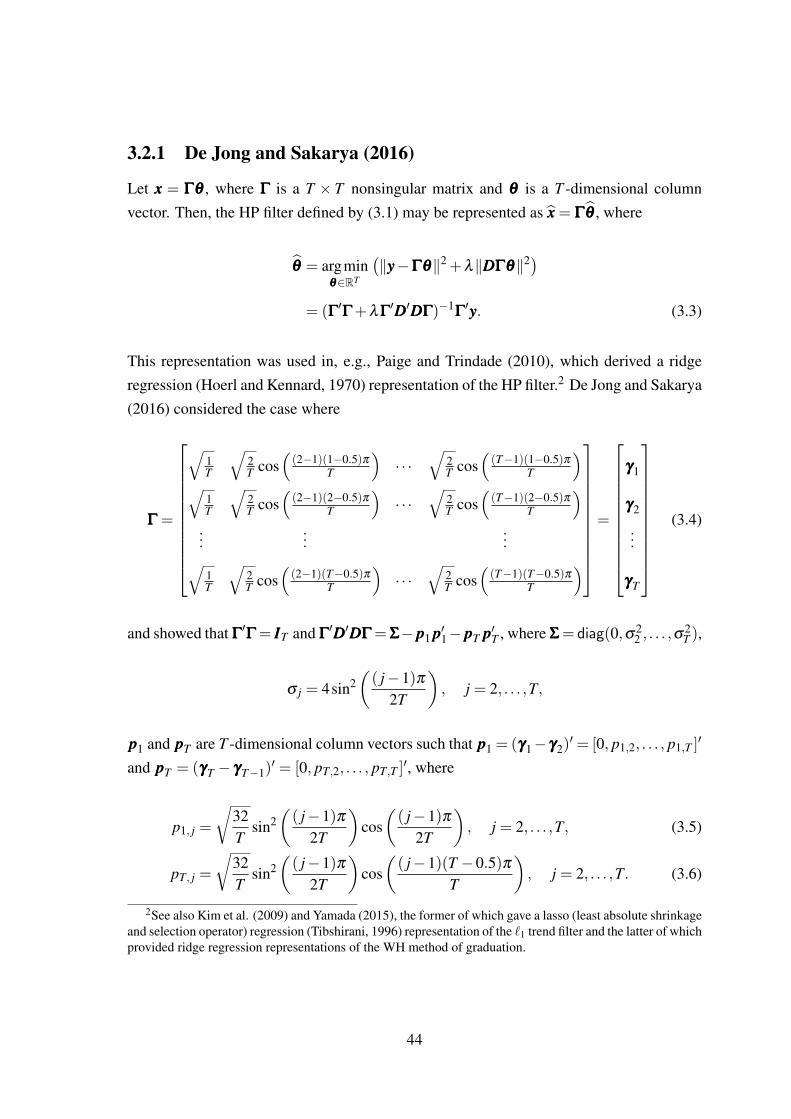
3.2.1 De Jong and Sakarya (2016)

Let xxx = ΓΓΓθθθ , where ΓΓΓ is a T × T nonsingular matrix and θθθ is a T -dimensional columnvector. Then, the HP filter defined by (3.1) may be represented as xxx = ΓΓΓθθθ , where

θθθ = argminθθθ∈RT

(‖yyy−ΓΓΓθθθ‖2 +λ‖DDDΓΓΓθθθ‖2)

= (ΓΓΓ′ΓΓΓ+λΓΓΓ′DDD′DDDΓΓΓ)−1

ΓΓΓ′yyy. (3.3)

This representation was used in, e.g., Paige and Trindade (2010), which derived a ridgeregression (Hoerl and Kennard, 1970) representation of the HP filter.2 De Jong and Sakarya(2016) considered the case where

ΓΓΓ =

√1T

√2T cos

((2−1)(1−0.5)π

T

)· · ·

√2T cos

((T−1)(1−0.5)π

T

)√

1T

√2T cos

((2−1)(2−0.5)π

T

)· · ·

√2T cos

((T−1)(2−0.5)π

T

)...

......√

1T

√2T cos

((2−1)(T−0.5)π

T

)· · ·

√2T cos

((T−1)(T−0.5)π

T

)

=

γγγ1

γγγ2

...

γγγT

(3.4)

and showed that ΓΓΓ′ΓΓΓ= IIIT and ΓΓΓ

′DDD′DDDΓΓΓ=ΣΣΣ− ppp1 ppp′1− pppT ppp′T , where ΣΣΣ= diag(0,σ22 , . . . ,σ

2T ),

σ j = 4sin2(( j−1)π

2T

), j = 2, . . . ,T,

ppp1 and pppT are T -dimensional column vectors such that ppp1 = (γγγ1−γγγ2)′= [0, p1,2, . . . , p1,T ]

′

and pppT = (γγγT − γγγT−1)′ = [0, pT,2, . . . , pT,T ]

′, where

p1, j =

√32T

sin2(( j−1)π

2T

)cos(( j−1)π

2T

), j = 2, . . . ,T, (3.5)

pT, j =

√32T

sin2(( j−1)π

2T

)cos(( j−1)(T −0.5)π

T

), j = 2, . . . ,T. (3.6)

2See also Kim et al. (2009) and Yamada (2015), the former of which gave a lasso (least absolute shrinkageand selection operator) regression (Tibshirani, 1996) representation of the `1 trend filter and the latter of whichprovided ridge regression representations of the WH method of graduation.

44

For the proofs of (3.5) and (3.6), see the Appendix. It is noteworthy that ΓΓΓ is an orthogonalmatrix that represents a discrete cosine transformation (DCT-II) (Ahmed et al., 1974).3

Accordingly, it follows that

θθθ = (AAA−λ ppp1 ppp′1−λ pppT ppp′T )−1

ΓΓΓ′yyy, (3.7)

where AAA= IIIT +λΣΣΣ. Since AAA is a diagonal matrix, AAA−1 is easily obtainable. By applying theSMW formula to (AAA−λ ppp1 ppp′1−λ pppT ppp′T )

−1 in (3.7), De Jong and Sakarya (2016) derivedan explicit formula for the smoother weights of the HP filter.

3.2.2 Cornea-Madeira (2017)

Let QQQT denote the T × T symmetric tridiagonal Toeplitz matrix where the first rowis [2,−1,0, . . . ,0], which is a well-known matrix (Strang and MacNamara, 2014), andQQQm = GGGT ΛΛΛT GGG′T denotes its spectral decomposition.4 Letting qqq1 = [−2,1,0, . . . ,0]′ be aT -dimensional column vector and qqqT = JJJT qqq1, where JJJT is the T ×T exchange matrix, itfollows that

DDD′DDD = QQQ2T −qqq1qqq′1−qqqT qqq′T , (3.8)

which indicates

xxx = (BBB−λqqq1qqq′1−λqqqT qqq′T )−1yyy, (3.9)

where BBB = (IIIT + λQQQ2T ) = GGGT (IIIT + λΛΛΛ

2T )GGG

′T . Since IIIT + λΛΛΛ

2T is a diagonal matrix and

GGGT is an orthogonal matrix, BBB−1 = GGGT (IIIT +λΛΛΛ2T )−1GGG′T , which is easy to calculate. By

applying the SMW formula to (BBB−λqqq1qqq′1−λqqqT qqq′T )−1 in (3.9), Cornea-Madeira (2017)

derived an explicit formula.

3See also Hamming (1973), Bierens (1997), and Strang (1999).4For the explicit forms of ΛΛΛT and GGGT , see (3.16) and (3.17).

45

3.3 Another explicit formula for the smoother weights of

the HP filter

The product of any two tridiagonal Toeplitz matrices is not a pentadiagonal Toeplitz matrixbecause the first and the last entries in the principal diagonal are different to the other ones(Marr and Vineyard, 1988; Montaner and Alfaro, 1995; Diele and Lopez, 1998; Wang etal., 2015). Accordingly, QQQ2

T−2 is not a pentadiagonal Toeplitz matrix. Explicitly, it is

QQQ2T−2 =

5 −4 1 0 · · · 0

−4 6. . .

. . .. . .

...

1. . .

. . .. . .

. . . 0

0. . .

. . .. . .

. . . 1

.... . .

. . .. . . 6 −4

0 · · · 0 1 −4 5

. (3.10)

Interestingly, the corresponding pentadiagonal Toeplitz matrix to QQQ2T−2 is DDDDDD′ and their

relationship may be expressed as

DDDDDD′ = QQQ2T−2 +UUUUUU ′, (3.11)

where

UUU = [eee1,eeeT−2]. (3.12)

Here, IIIT−2 = [eee1, . . . ,eeeT−2]. Note that (3.11) corresponds to (3.16) of Wang et al. (2015).By applying the SMW formula to (IIIT + λDDD′DDD)−1 in (3.1), the HP filter may be

46

alternatively expressed as5

xxx = yyy−DDD′(λ−1IIIT−2 +DDDDDD′)−1DDDyyy = yyy−DDD′ΨΨΨ−1DDDyyy, (3.13)

where ΨΨΨ= λ−1IIIT−2+DDDDDD′, which is a pentadiagonal Toeplitz matrix. From (3.11), ΨΨΨ maybe represented as ΨΨΨ = CCC+UUUUUU ′, where CCC = λ−1IIIT−2 +QQQ2

T−2. As in Wang et al. (2015),applying the SMW formula to (CCC+UUUUUU ′)−1, it follows that

ΨΨΨ−1 = (CCC+UUUUUU ′)−1 =CCC−1−CCC−1UUU(III2 +UUU ′CCC−1UUU)−1UUU ′CCC−1. (3.14)

It is noteworthy that III2 +UUU ′CCC−1UUU in (3.14) is a 2×2 matrix and hence its inverse is easilyobtainable.6 In addition, for obtaining the explicit formula for CCC−1, it is possible to applythe spectral decomposition of QQQT−2 as in Cornea-Madeira (2017):

CCC−1 = GGGT−2(λ−1IIIT−2 +ΛΛΛ

2T−2)

−1GGG′T−2, (3.15)

where (λ−1IIIT−2 +ΛΛΛ2T−2)

−1 in CCC−1 = GGGT−2(λ−1IIIT−2 +ΛΛΛ

2T−2)

−1GGG′T−2 is a diagonal ma-trix, where ΛΛΛT−2 = diag(λ1, . . . ,λT−2) is

λ j = 4sin2(

jπ2(T −1)

), j = 1, . . . ,T −2, (3.16)

and (i, j)-entry of GGGT−2, denoted by gi, j, is

gi, j =

√2

T −1sin(

i jπT −1

), i, j = 1, . . . ,T −2. (3.17)

See, e.g., Strang and MacNamara (2014).We may summarize the above results as follows:

5It is of interest that a ridge regression exists in (3.13): xxx = yyy−DDD′φφφ , where

φφφ = argminφφφ∈R(T−2)

(‖yyy−DDD′φφφ‖2 +λ

−1‖φφφ‖2)= (DDDDDD′+λ−1IIIT−2)

−1DDDyyy.

Yamada (2018) listed several penalized/unpenalized least squares problems related to the HP filter.6Likewise, letting VVV = [qqq1,qqqT ], it follows that VVVVVV ′ = qqq1qqq′1 + qqqT qqq′T , and accordingly, (3.9) becomes xxx =

(BBB−λVVVVVV ′)−1yyy. The proof of Cornea-Madeira (2017) may become simpler by applying the SMW formulato (BBB−λVVVVVV ′)−1. See the Appendix for details.

47

Theorem 3.1. xxx in (3.1) may be expressed as

xxx = (IIIT +λDDD′DDD)−1yyy

=[IIIT −DDD′CCC−1DDD+DDD′CCC−1UUU(III2 +UUU ′CCC−1UUU)−1UUU ′CCC−1DDD

]yyy (3.18)

= yyy−DDD′CCC−1DDDyyy+DDD′CCC−1UUU(III2 +UUU ′CCC−1UUU)−1UUU ′CCC−1DDDyyy, (3.19)

where UUU and CCC−1 are defined by (3.12) and (3.15), respectively.

Proof. (3.18) immediately follows from (3.13) and (3.14).

Remarks. Since UUUUUU ′ = eee1eee′1 + eeeT−2eee′T−2, the trend extracted by the HP filter may berewritten as xxx = yyy−DDD′(CCC+eee1eee′1+eeeT−2eee′T−2)

−1DDDyyy. Then, it is possible to obtain the resultin Theorem 3.1 by applying the SMW formula to (CCC+eee1eee′1 +eeeT−2eee′T−2)

−1. Nevertheless,in this case, its derivation becomes longer.

Denote (i, j)-entry of CCC−1 in (3.15) by ci, j. In addition, let ccc1 and cccT−2 denote thefirst and last column of CCC−1, respectively. Then, since eee′iCCC

−1eee j = ci, j for i, j = 1,T −2 andCCC−1UUU = [CCC−1eee1,CCC−1eeeT−2] = [ccc1,cccT−2], it follows that

(III2 +UUU ′CCC−1UUU)−1 =1

(1+ c1,1)(1+ cT−2,T−2)− c1,T−2cT−2,1

1+ cT−2,T−2 −c1,T−2

−cT−2,1 1+ c1,1

and we accordingly obtain

CCC−1UUU(III2 +UUU ′CCC−1UUU)−1UUU ′CCC−1

=(1+ cT−2,T−2)ccc1ccc′1− c1,T−2ccc1ccc′T−2− cT−2,1cccT−2ccc′1 +(1+ c1,1)cccT−2ccc′T−2

(1+ c1,1)(1+ cT−2,T−2)− c1,T−2cT−2,1, (3.20)

where CCC−1 = [ccc1, . . . ,cccT−2] = [ci, j]i, j=1,...,T−2 is calculated by

ci, j =T−2

∑k=1

gi,kg j,k

λ−1 +λ 2k, i, j = 1, . . . ,T −2. (3.21)

From (3.10), QQQ2T−2 is a centrosymmetric matrix and accordingly CCC = λ−1IIIT−2 +QQQ2

T−2 isalso a centrosymmetric matrix. Since the inverse of a nonsingular centrosymmetric matrix

48

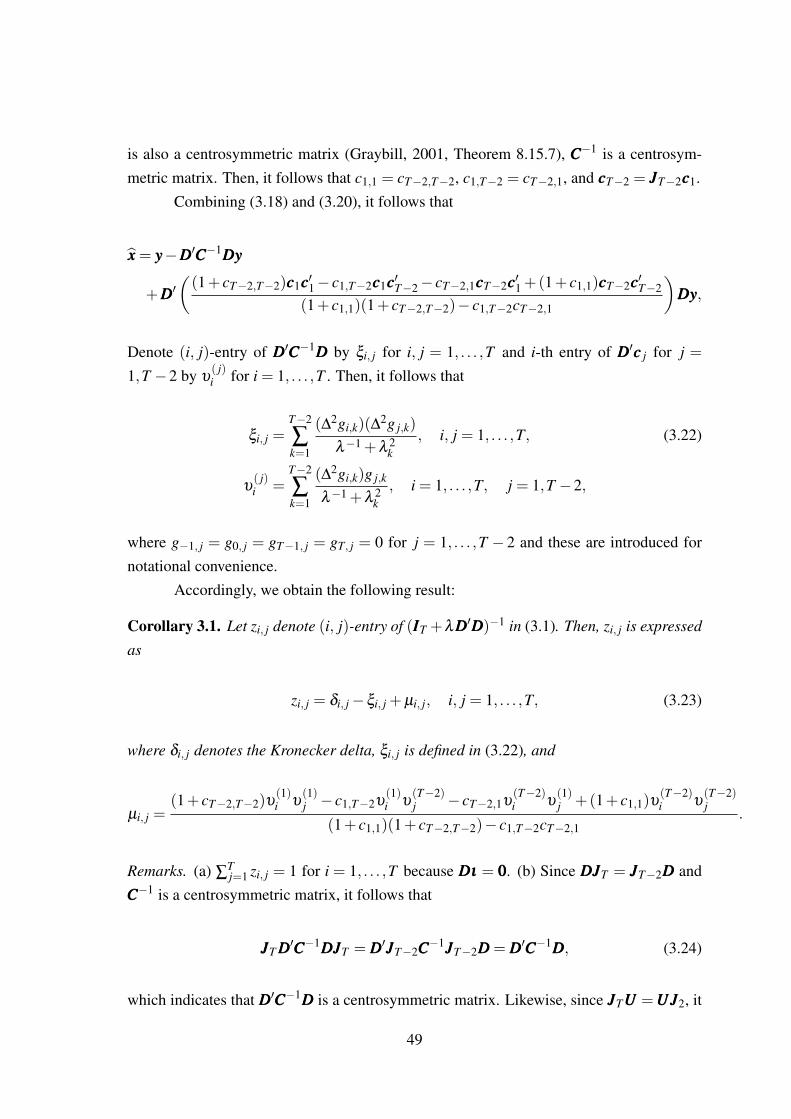
is also a centrosymmetric matrix (Graybill, 2001, Theorem 8.15.7), CCC−1 is a centrosym-metric matrix. Then, it follows that c1,1 = cT−2,T−2, c1,T−2 = cT−2,1, and cccT−2 = JJJT−2ccc1.

Combining (3.18) and (3.20), it follows that

xxx = yyy−DDD′CCC−1DDDyyy

+DDD′((1+ cT−2,T−2)ccc1ccc′1− c1,T−2ccc1ccc′T−2− cT−2,1cccT−2ccc′1 +(1+ c1,1)cccT−2ccc′T−2

(1+ c1,1)(1+ cT−2,T−2)− c1,T−2cT−2,1

)DDDyyy,

Denote (i, j)-entry of DDD′CCC−1DDD by ξi, j for i, j = 1, . . . ,T and i-th entry of DDD′ccc j for j =

1,T −2 by υ( j)i for i = 1, . . . ,T . Then, it follows that

ξi, j =T−2

∑k=1

(∆2gi,k)(∆2g j,k)

λ−1 +λ 2k

, i, j = 1, . . . ,T, (3.22)

υ( j)i =

T−2

∑k=1

(∆2gi,k)g j,k

λ−1 +λ 2k

, i = 1, . . . ,T, j = 1,T −2,

where g−1, j = g0, j = gT−1, j = gT, j = 0 for j = 1, . . . ,T − 2 and these are introduced fornotational convenience.

Accordingly, we obtain the following result:

Corollary 3.1. Let zi, j denote (i, j)-entry of (IIIT +λDDD′DDD)−1 in (3.1). Then, zi, j is expressed

as

zi, j = δi, j−ξi, j +µi, j, i, j = 1, . . . ,T, (3.23)

where δi, j denotes the Kronecker delta, ξi, j is defined in (3.22), and

µi, j =(1+ cT−2,T−2)υ

(1)i υ

(1)j − c1,T−2υ

(1)i υ

(T−2)j − cT−2,1υ

(T−2)i υ

(1)j +(1+ c1,1)υ

(T−2)i υ

(T−2)j

(1+ c1,1)(1+ cT−2,T−2)− c1,T−2cT−2,1.

Remarks. (a) ∑Tj=1 zi, j = 1 for i = 1, . . . ,T because DDDιιι = 000. (b) Since DDDJJJT = JJJT−2DDD and

CCC−1 is a centrosymmetric matrix, it follows that

JJJT DDD′CCC−1DDDJJJT = DDD′JJJT−2CCC−1JJJT−2DDD = DDD′CCC−1DDD, (3.24)

which indicates that DDD′CCC−1DDD is a centrosymmetric matrix. Likewise, since JJJTUUU =UUUJJJ2, it

49

follows that JJJ2UUU ′CCC−1UUUJJJ2 =UUU ′JJJTCCC−1JJJTUUU =UUU ′CCC−1UUU , which indicates (III2+UUU ′CCC−1UUU)−1

is a centrosymmetric matrix. Accordingly, it follows that

CCC−1UUU(III2 +UUU ′CCC−1UUU)−1UUU ′CCC−1 = JJJTCCC−1JJJTUUU(III2 +UUU ′CCC−1UUU)−1UUU ′JJJTCCC−1JJJT

= JJJTCCC−1UUUJJJ2(III2 +UUU ′CCC−1UUU)−1JJJ2UUU ′CCC−1JJJT

= JJJTCCC−1UUU(III2 +UUU ′CCC−1UUU)−1UUU ′CCC−1JJJT ,

which indicates that CCC−1UUU(III2 + UUU ′CCC−1UUU)−1UUU ′CCC−1 is a centrosymmetric matrix.From these results, we obtain, e.g., ξ1,1 = ξT,T and µ1,1 = µT,T in (3.23). (c)calc_HP_hat_matrix in the Appendix is a MATLAB/GNU Octave function to cal-culate (IIIT +λDDD′DDD)−1 in (3.1) based on (3.23).

Finally, we emphasize that our approach leads to a simpler formula because weapply the SMW formula to (CCC+UUUUUU ′)−1 = (CCC+ eee1eee′1 + eeeT−2eee′T−2)

−1, where both eee1 andeeeT−2 are unit vectors. Observe that pppi in (3.7) and qqqi in (3.9), where i = 1,T , are not unitvectors.


By applying the SMW formula and a discrete cosine transformation matrix, De Jong andSakarya (2016) derived an explicit formula for the smoother weights of the HP filter. Then,by applying the SMW formula and the spectral decomposition of a symmetric tridiagonalToeplitz matrix, Cornea-Madeira (2017) provided a simper formula. In this chapter, weprovided an alternative simpler formula and explained why our approach leads to a simplerformula. The main result of this chapter is summarized in Theorem 3.1 and Corollary 3.1.

50

3.5 Numerical example

Consider, we are going to find the inverse of the smoother matrix of the HP filter, (IIIT +

λDDD′2DDD2)−1 ∈RT×T where T = 7 and λ = 7. Here, DDD2 is the second-order difference matrix

DDD222 =

1 −2 1 0 0 0 0

0 1 −2 1 0 0 0

0 0 1 −2 1 0 0

0 0 0 1 −2 1 0

0 0 0 0 1 −2 1

∈ R5×7,

and

DDD2DDD′2 =

6 −4 1 0 0

−4 6 −4 1 0

1 −4 6 −4 1

0 1 −4 6 −4

0 0 1 −4 6

∈ R5×5. (3.25)

Suppose QQQ5 denotes the 5×5 symmetric tridiagonal toeplitz matrix where the firstrow is [2,−1,0, ...,0] and accordingly, QQQ2

5 is not a pentadiagonal toeplitz matrix because ofthe first and last elements of the diagonal entries. Explicitly, it is

QQQ25 =

5 −4 1 0 0

−4 6 −4 1 0

1 −4 6 −4 1

0 1 −4 6 −4

0 0 1 −4 5

∈ R5×5. (3.26)

Now, from equation (3.25) and (3.26) we get the following expression:

DDD2DDD′2 = QQQ25 +UUUUUU ′, (3.27)

51

where UUU = [eee1,eee5] and eee1, eee5 are two unit vectors of the form:

eee1 =

1

0

0

0

0

, eee5 =

0

0

0

0

1

.

Suppose, the spectral decomposition of QQQ25 is GGG5ΛΛΛ

25GGG′5. Where, ΛΛΛ

25 denotes the eigenvector

matrix of QQQ25 and its distinct eigenvalues are

λ j = 4sin2(

jπ12

), j = 1, ...,5, (3.28)

and the (i, j) th entry of the corresponding eigenvector matrix GGG5 is

gi, j =

(13

)1/2

sin(

πi j6

), i, j = 1, ...,5. (3.29)

From the Woodbury matrix identity and later using equation (3.27), we have

(III7 +7DDD′2DDD2)−1 = III7−DDD′2(

17

III5 +DDD2DDD′2)−1DDD2

= III7−DDD′2(17

III5 +QQQ25 +UUUUUU ′)−1DDD2

= III7−DDD′2(CCC+ eee1eee′1 + eee5eee′5)−1DDD2

= III7−DDD′2ΨΨΨ−1DDD2. (3.30)

Suppose,

CCC =17

III5 +QQQ25, (3.31)

ΨΨΨ−1 = (CCC+ eee1eee′1 + eee5eee′5)

−1. (3.32)

52

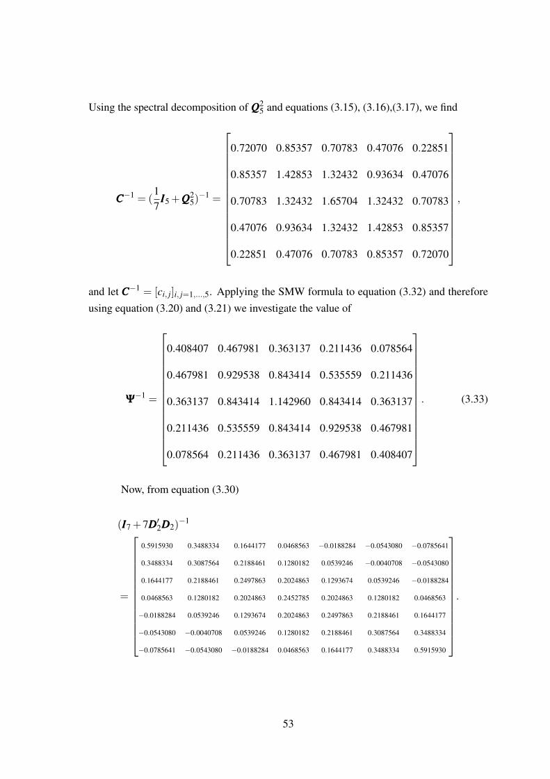
Using the spectral decomposition of QQQ25 and equations (3.15), (3.16),(3.17), we find

CCC−1 = (17

III5 +QQQ25)−1 =

0.72070 0.85357 0.70783 0.47076 0.22851

0.85357 1.42853 1.32432 0.93634 0.47076

0.70783 1.32432 1.65704 1.32432 0.70783

0.47076 0.93634 1.32432 1.42853 0.85357

0.22851 0.47076 0.70783 0.85357 0.72070

,

and let CCC−1 = [ci, j]i, j=1,...,5. Applying the SMW formula to equation (3.32) and thereforeusing equation (3.20) and (3.21) we investigate the value of

ΨΨΨ−1 =

0.408407 0.467981 0.363137 0.211436 0.078564

0.467981 0.929538 0.843414 0.535559 0.211436

0.363137 0.843414 1.142960 0.843414 0.363137

0.211436 0.535559 0.843414 0.929538 0.467981

0.078564 0.211436 0.363137 0.467981 0.408407

. (3.33)

Now, from equation (3.30)

(III7 +7DDD′2DDD2)−1

=

0.5915930 0.3488334 0.1644177 0.0468563 −0.0188284 −0.0543080 −0.0785641

0.3488334 0.3087564 0.2188461 0.1280182 0.0539246 −0.0040708 −0.0543080

0.1644177 0.2188461 0.2497863 0.2024863 0.1293674 0.0539246 −0.0188284

0.0468563 0.1280182 0.2024863 0.2452785 0.2024863 0.1280182 0.0468563

−0.0188284 0.0539246 0.1293674 0.2024863 0.2497863 0.2188461 0.1644177

−0.0543080 −0.0040708 0.0539246 0.1280182 0.2188461 0.3087564 0.3488334

−0.0785641 −0.0543080 −0.0188284 0.0468563 0.1644177 0.3488334 0.5915930

.

53

3.6 Appendix

Proof of (3.5)

From (3.4), γγγ1− γγγ2 is

γγγ1− γγγ2 =

[√1T

√2T cos

((2−1)(1−0.5)π

T

)· · ·

√2T cos

((T−1)(1−0.5)π

T

)]−[√

1T

√2T cos

((2−1)(2−0.5)π

T

)· · ·

√2T cos

((T−1)(2−0.5)π

T

)].

Let β j = π( j−1)/(2T ) for j = 2, . . . ,T . Then, it follows that

√2T

cos(( j−1)(1−0.5)π

T

)−√

2T

cos(( j−1)(2−0.5)π

T

)=

√2T[cos(β j)− cos(3β j)] =

√32T

sin2(β j)cos(β j).

The last equality follows from cos(β j)− cos(3β j) = 4sin2(β j)cos(β j).

Proof of (3.6)

From (3.4), γγγT − γγγT−1 is

γγγT − γγγT−1 =

[√1T

√2T cos

((2−1)(T−0.5)π

T

)· · ·

√2T cos

((T−1)(T−0.5)π

T

)]−[√

1T

√2T cos

((2−1)(T−1−0.5)π

T

)· · ·

√2T cos

((T−1)(T−1−0.5)π

T

)]

Let β j = π( j−1)/(2T ) and κ j = 2T β j = π( j−1) for j = 2, . . . ,T . Then, it follows that

√2T

cos(( j−1)(T −0.5)π

T

)−√

2T

cos(( j−1)(T −1−0.5)π

T

)=

√2T[cos(β j(2T −1))− cos(β j(2T −3))] =

√2T[cos(κ j−β j)− cos(κ j−3β j)].

54

Here, since sin(κ j) = 0, it follows that

cos(κ j−β j)− cos(κ j−3β j)

= cos(κ j)cos(β j)+ sin(κ j)sin(β j)− cos(κ j)cos(3β j)− sin(κ j)sin(3β j)

= cos(κ j)[cos(β j)− cos(3β j)]+ sin(κ j)[sin(β j)− sin(3β j)]

= cos(κ j)[4sin2(β j)cos(β j)]+ sin(κ j)[4sin3(β j)−2sin(β j)]

= 4sin2(β j)[cos(κ j)cos(β j)+ sin(κ j)sin(β j)]−2sin(κ j)sin(β j)

= 4sin2(β j)cos(κ j−β j),

where

κ j−β j = 2T β j−β j = β j(2T −1) =π( j−1)(2T −1)

2T=

π( j−1)(T −0.5)T

.

Application of the SMW formula to (BBB−λVVVVVV ′)−1

As in Cornea-Madeira (2017), by applying the SMW formula to (BBB−λqqq1qqq′1−λqqqT qqq′T )−1,

we obtain the following results:

(BBB−λqqq1qqq′1−λqqqT qqq′T )−1

= (BBB−λqqq1qqq′1)−1 +λ

(BBB−λqqq1qqq′1)−1qqqT qqq′T (BBB−λqqq1qqq′1)

−1

1−λqqq′T (BBB−λqqq1qqq′1)−1qqqT

, (3.34)

where

(BBB−λqqq1qqq′1)−1 = BBB−1 +λ

BBB−1qqq1qqq′1BBB−1

1−λqqq′1BBB−1qqq1. (3.35)

On the other hand, by applying the SMW formula to (BBB−λVVVVVV ′)−1, we obtain

(BBB−λVVVVVV ′)−1

= BBB−1−BBB−1VVV (VVV ′BBB−1VVV −λ−1III2)

−1VVV ′BBB−1

55

= BBB−1− [BBB−1qqq1,BBB−1qqqT ]

qqq′1BBB−1qqq1−λ−1 qqq′1BBB−1qqqT

qqq′T BBB−1qqq1 qqq′T BBB−1qqqT −λ−1

−1qqq′1BBB−1

qqq′T BBB−1

. (3.36)

By comparing (3.36) with (3.34) and (3.35), it is observable that (3.36) is preferable to(3.34), mainly because (3.36) is symmetric with respect to qqq1 and qqqT .

A MATLAB/GNU Octave function to calculate (IIIT +λDDD′DDD)−1 in (3.1)

based on (3.23)

function HP_hat_matrix = calc_HP_hat_matrix(T, lambda)

% T: sample size

% lambda: smoothing parameter

Lam = diag( 4*(sin((1:T-2)*pi/(2*(T-1))).ˆ2) );

G = zeros(T-2,T-2);

for i = 1:T-2

for j = 1:T-2

G(i,j) = sqrt(2/(T-1))*sin(i*j*pi/(T-1));

end

end

invC = zeros(T-2,T-2);

for i = 1:T-2

for j = 1:T-2

s = 0;

for k = 1:T-2

s = s + G(i,k)*G(j,k)/( (1/lambda)+Lam(k,k)ˆ2 );

end

invC(i,j) = s;

end

end

Xi = zeros(T,T);

56

DG = diff([zeros(2,T-2);G;zeros(2,T-2)],2);

for i = 1:T

for j = 1:T

s = 0;

for k = 1:T-2

s = s+DG(i,k)*DG(j,k)/((1/lambda)+Lam(k,k)ˆ2);

end

Xi(i,j) = s;

end

end

Up1 = zeros(T,1); Up2 = zeros(T,1);

for i=1:T

s1 = 0; s2 = 0;

for k = 1:T-2

s1 = s1+DG(i,k)*G(1,k)/((1/lambda)+Lam(k,k)ˆ2);

s2 = s2+DG(i,k)*G(end,k)/((1/lambda)+Lam(k,k)ˆ2);

end

Up1(i) = s1; Up2(i) = s2;

end

c11 = invC(1,1);

c22 = invC(end,end);

c12 = invC(1,end);

c21 = invC(end,1);

den = (1+c11)*(1+c22)-c12*c21;

Tau = zeros(T,T);

for i=1:T

for j=1:T

num = (1+c22)*Up1(i)*Up1(j)-c12*Up1(i)*Up2(j)- ...

c21*Up2(i)*Up1(j)+(1+c11)*Up2(i)*Up2(j);

Tau(i,j) = num/den;

end

end

Z = zeros(T,T);

57

I = eye(T);

for i=1:T

for j=1:T

Z(i,j) = I(i,j)-Xi(i,j)+Tau(i,j);

end

end

HP_hat_matrix = Z;

end

58

3.7 References

1. Ahmed, N., T. Natarajan, and K. R. Rao, 1974, Discrete cosine transform, IEEE

Transactions on Computers, C-23, 1, 90–93.

2. Bierens, H., 1997, Testing the unit root with drift hypothesis against nonlinear trendstationarity, with an application to the U.S. price level and interest rate, Journal of

Econometrics, 81, 29–64.



5. Diele, F. and L. Lopez, 1998, The use of the factorization of five-diagonal matricesby tridiagonal Toeplitz matrices, Applied Mathematics Letters, 11, 3, 61–69.

6. Graybill, F. A., 2001, Matrices with Applications in Statistics, 2nd ed., CengageLearning, Belmont.

7. Hamming, R. W., 1973, Numerical Methods for Scientists and Engineers, 2nd ed.,McGraw-Hill, New York.


9. Hoerl, A. E. and R. W. Kennard, 1970, Ridge regression: Biased estimation fornonorthogonal problems, Technometrics, 12, 1, 55–67.

10. Kim, S., K. Koh, S. Boyd, and D. Gorinevsky, 2009, `1 trend filtering, SIAM Review,51, 2, 339–360.


12. Marr, R. B. and G. H. Vineyard, 1988, Five-diagonal Toeplitz determinants and theirrelation to Chebyshev polynomials, SIAM Journal on Matrix Analysis and Applica-

tions, 9, 4, 579–586.

13. Montaner, J. M. and M. Alfaro, 1995, On five-diagonal Toeplitz matrices and orthog-onal polynomials on the unit circle, Numerical Algorithms, 10, 1, 137–153.

59

14. Paige, R. L. and A. A. Trindade, 2010, The Hodrick–Prescott filter: A special caseof penalized spline smoothing, Electronic Journal of Statistics, 4, 856–874.

15. Ravn, M. O. and H. Uhlig, 2002, On adjusting the Hodrick–Prescott filter for thefrequency of observations, Review of Economics and Statistics, 84, 2, 371–380.

16. Strang, G., 1999, The discrete cosine transform, SIAM Review, 41, 1, 135–147.


18. Tibshirani, R., 1996, Regression shrinkage and selection via the lasso, Journal of the

Royal Statistical Society Series B 58, 267–288.

19. Wang, C., H. Li, and D. Zhao, 2015, An explicit formula for the inverse of a penta-diagonal Toeplitz matrix, Journal of Computational and Applied Mathematics, 278,15, 12–18.

20. Weinert, H. L., 2007, Efficient computation for Whittaker–Henderson smoothing,Computational Statistics and Data Analysis, 52, 959–974.




and Methods, 48, 12, 3153–3161.

24. Yamada, H. and F. T. Jahra, 2019, An explicit formula for the smoother weights ofthe Hodrick–Prescott filter, Studies in Nonlinear Dynamics and Econometrics, DOI:10.1515/snde-2018-0035.

60

Chapter 4

A Discussion on the

Whittaker–Henderson Graduation and

Bisymmetry of the Related Smoother

Matrices

4.1 Introduction

The Whittaker–Henderson (WH) method of graduation is a comprehensive smoothing toolwhich is widely used in the actuarial literature and in the macroeconomic time seriesanalysis. Although we call WH’s graduation method, the method was originally intro-duced by German scholar George Bohlman in 1899. Whittaker (1923), without know-ing about Bohlman’s work, published a paper named as “On a New Mehtod of Grad-

uation”, where he proposed a method for data smoothing using third order differences(∆3xt = xt−3xt−1 +3xt−2− xt−3). On the other hand, Henderson (1924), published an ar-ticle about the data smoothing method named as “A New Mehtod of Graduation”. Accord-ing to Joseph (1952), Henderson discovered a factorization formula to calculate the Whit-taker’s method in a simpler way. Later, the method is known as the Whittaker–Henderson’smethod of graduation. For the archival assessment of the WH method of graduation, see

61

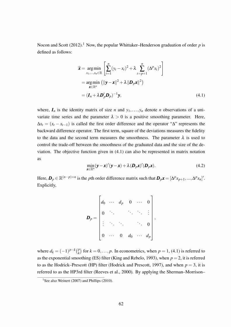
Nocon and Scott (2012).1 Now, the popular Whittaker–Henderson graduation of order p isdefined as follows:

xxx = argminx1,...,xn∈R

[n

∑t=1

(yt− xt)2 +λ

n

∑t=p+1

(∆pxt)2

]

= argminxxx∈Rn

(‖yyy− xxx‖2 +λ‖DDDpxxx‖2)

= (IIIn +λDDD′pDDDp)−1yyy, (4.1)

where, IIIn is the identity matrix of size n and y1, . . . ,yn denote n observations of a uni-variate time series and the parameter λ > 0 is a positive smoothing parameter. Here,∆xt = (xt − xt−1) is called the first order difference and the operator “∆” represents thebackward difference operator. The first term, square of the deviations measures the fidelityto the data and the second term measures the smoothness. The parameter λ is used tocontrol the trade-off between the smoothness of the graduated data and the size of the de-viation. The objective function given in (4.1) can also be represented in matrix notationas

minxxx∈Rn

(yyy− xxx)′(yyy− xxx)+λ (DDDpxxx)′(DDDpxxx). (4.2)

Here, DDDp ∈R(n−p)×n is the pth order difference matrix such that DDDpxxx = [∆pxp+1, ...,∆pxn]

′.Explicitly,

DDDp =

d0 · · · dp 0 · · · 0

0. . .

. . .. . .

...

.... . .

. . .. . . 0

0 · · · 0 d0 · · · dp

,

where dk = (−1)p−k(pk

)for k = 0, . . . , p. In econometrics, when p = 1, (4.1) is referred to

as the exponential smoothing (ES) filter (King and Rebelo, 1993), when p = 2, it is referredto as the Hodrick–Prescott (HP) filter (Hodrick and Prescott, 1997), and when p = 3, it isreferred to as the HP3rd filter (Reeves et al., 2000). By applying the Sherman–Morrison–

1See also Weinert (2007) and Phillips (2010).

62

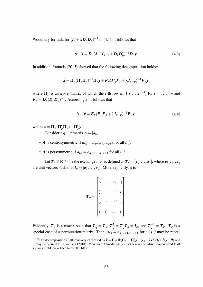
Woodbury formula for (IIIn +λDDD′pDDDp)−1 in (4.1), it follows that

yyy− xxx = DDD′p(λ−1IIIn−p +DDDpDDD′p)

−1DDDpyyy. (4.3)

In addition, Yamada (2015) showed that the following decomposition holds:2

xxx = ΠΠΠp(ΠΠΠ′pΠΠΠp)

−1ΠΠΠ′pyyy+FFF p(FFF ′pFFF p +λ IIIn−p)

−1FFF ′pyyy,

where ΠΠΠp is an n× p matrix of which the t-th row is [1, t, . . . , t p−1] for t = 1, . . . ,n andFFF p = DDD′p(DDDpDDD′p)

−1. Accordingly, it follows that

xxx− τττ = FFF p(FFF ′pFFF p +λ IIIn−p)−1FFF ′pyyy, (4.4)

where τττ = ΠΠΠp(ΠΠΠ′pΠΠΠp)

−1ΠΠΠ′pyyy.

Consider a q×q matrix AAA = [ai, j].

• AAA is centrosymmetric if ai, j = aq−i+1,q− j+1 for all i, j,

• AAA is persymmetric if ai, j = aq− j+1,q−i+1 for all i, j.

Let TTT q ∈Rq×q be the exchange matrix defined as TTT q = [eeeq, . . . ,eee1], where eee1, . . . ,eeeq

are unit vectors such that IIIq = [eee1, . . . ,eeeq]. More explicitly, it is

TTT q =

0 · · · 0 1

... . ..

. ..

0

0 . ..

. .. ...

1 0 · · · 0

.

Evidently, TTT q is a matrix such that TTT ′q = TTT q, TTT 2q = TTT ′qTTT q = IIIq, and TTT−1

q = TTT q. TTT q is aspecial case of a permutation matrix. Then, ai, j = aq−i+1,q− j+1 for all i, j may be repre-

2The decomposition is alternatively expressed as xxx = ΠΠΠp(ΠΠΠ′pΠΠΠp)

−1ΠΠΠ′pyyy+(IIIn +λDDD′pDDDp)

−1(yyy− τττ) andit may be derived as in Yamada (2018). Moreover, Yamada (2017) lists several penalized/unpenalized leastsquares problems related to the HP filter.

63

sented by AAA = TTT qAAATTT q.3 Likewise, ai, j = aq− j+1,q−i+1 for all i, j may be represented byAAA = (TTT qAAATTT q)

′. Accordingly, it immediately follows that if AAA is a symmetric centrosym-metric matrix, it is also a persymmetric matrix. Similarly if AAA is a symmetric persymmetricmatrix, it is also a centrosymmetric matrix. If AAA is a symmetric centrosymmetric matrix, itis referred to as a bisymmetric matrix. For example,

5 1 2

1 −3 1

2 1 5

is a bisymmetric matrix. As shown above, since it is a bisymmetric matrix, it may be madefrom the bold-faced 4 entries even though there are 9 entries in it.

Cornea-Madeira (2017) noted that the smoother matrix of the HP filter, (IIIn +

λDDD′2DDD2)−1, is a bisymmetric matrix and Yamada (2019) for generalizing this proved that

this is true for any p ∈ N such that (n− p)> 0.The chapter is organized as follows. In Section 4.2, a literature review is discussed

and in Section 4.3 using the result of Yamada (2019) we provide formulas for calculatingxxx in (4.1). In Section 4.4, we show that the smoother matrices in (4.3) and in (4.4) are alsobisymmetric matrices. Section 4.5 concludes.

3Dagum and Luati (2004) referred to the transformation from BBB to TTT rBBBTTT s: t(BBB) = TTT rBBBTTT s as t-transformation, where BBB is a r× s matrix.

64

4.2 A literature review

In this section, we briefly review two closely related papers: Yamada (2019) and El-Mikkawy and Atlan (2013).

4.2.1 Yamada (2019)

For proving that the smooother matrix (IIIn+λDDD′pDDDp)−1 of WH graduation is a bisymmetric

matrix Yamada (2019) first provided the following lemma:

Lemma 4.1. TTT n−pDDDp = (−1)pDDDpTTT n.

Proof. For j = 1, . . . , p, let

DDD( j) =

−1 1 0 · · · 0

0 −1 1. . .

...

.... . .

. . .. . . 0

0 · · · 0 −1 1

∈ R(n− j)×(n− j+1),

which is a first order difference matrix. Then, since premultiplication (postmultiplication)by an exchange matrix exchanges rows (columns) in reverse order, it follows that

TTT n− jDDD( j) =

0 · · · 0 −1 1

... . ..

. ..

. ..

0

0 −1 1 . .. ...

−1 1 0 · · · 0

=−

0 · · · 0 1 −1

... . ..

. ..

. ..

0

0 1 −1 . .. ...

1 −1 0 · · · 0

=−DDD( j)TTT n− j+1.

In addition, by definition of DDDp, DDDp may be represented as follows:

DDDp = DDD(p)DDD(p−1)×·· ·×DDD(1).

65

Combining these equations yields

TTT n−pDDDp = TTT n−pDDD(p)DDD(p−1)×·· ·×DDD(1) = (−1)DDD(p)TTT n−p+1DDD(p−1)×·· ·×DDD(1)

= (−1)pDDD(p)DDD(p−1)×·· ·×DDD(1)TTT n = (−1)pDDDpTTT n.

Now using the above result Yamada provided that, (IIIn + λDDD′pDDDp)−1 in (4.1) is a

bisymmetric matrix. Since it is evident that (IIIn +λDDD′pDDDp)−1 is a symmetric matrix, Ya-

mada showed that it is a centrosymmetric matrix. Using TTT n−pDDDp = (−1)pDDDpTTT n, it followsthat

TTT nDDD′pDDDpTTT n = TTT nDDD′p(−1)p(−1)pDDDpTTT n = DDD′pTTT n−pTTT n−pDDDp = DDD′pDDDp,

which indicates that DDD′pDDDp is a centrosymmetric matrix and consequently (IIIn+λDDD′pDDDp) isalso a centrosymmetric matrix. Accordingly, it follows that

TTT n(IIIn +λDDD′pDDDp)−1TTT n = [TTT n(IIIn +λDDD′pDDDp)TTT n]

−1 = (IIIn +λDDD′pDDDp)−1.

4.2.2 El-Mikkawy and Atlan (2013)

El-Mikkawy (2013), in their paper, constructed two algorithm for solving centrosymmetriclinear system of even and odd order. These two algorithms are described briefly in here.

4.2.2.1 An algorithm for solving centrosymmetric linear system of even order:

Let, an even, n=2m order centrosymmetric partitioned matrix form be as follows:

AAA TTT BBBTTT

BBB TTT AAATTT

xxx1

xxx2

=

bbb1

bbb2

(4.5)

Here, AAA is an m×m matrix of the form AAA = [ai j] where i, j = 1,2, ...,m and another matrixBBB = [ai, j] where i = m,m−1, ...,1 and j = 2m,2m−1, ...,m+1.xxx1 = [x1,x2, ...,xm]

′, xxx2 = [xm+1,xm+2, ...,x2m]′

66

bbb1 = [b1,b2, ...,bm]′, bbb2 = [bm+1,bm+2, ...,b2m]

′

The system in (4.5) can be written in matrix form as follows:

RRRxxx = bbb, (4.6)

where RRR = [ai j]i, j=1,...,2m is the coefficient matrix of the system (4.5), xxx = [x1,x2, ...,x2m]′

and bbb = [b1,b2, ...,b2m]′ is the constant vector. Now, let, QQQ1 = 1√

2

IIIm IIIm

TTT m −TTT m

be an

orthogonal matrix such that

RRR =

AAA TTT BBBTTT

BBB TTT AAATTT

= QQQ1

AAA+TTT BBB 000

000 AAA−TTT BBB

QQQ′1.

Now,

| RRR |=| QQQ1 |

∣∣∣∣∣∣∣∣AAA+TTT BBB 000

000 AAA−TTT BBB

∣∣∣∣∣∣∣∣ | QQQ′1 |

=| QQQ1 || AAA+TTT BBB || AAA−TTT BBB || QQQ′1 |

=| AAA+TTT BBB || AAA−TTT BBB || QQQ′1QQQ1 |

=| AAA+TTT BBB || AAA−TTT BBB | .

Step 1: Construc the m×m matrices PPP, QQQ and the m-vectors bbb and bbb as follows:

PPP = AAA+TTT BBB = [ai j +ai,2m+1− j]i, j=1,...,m,

QQQ = AAA−TTT BBB = [ai j−ai,2m+1− j]i, j=1,...,m,

bbb = [b1 +b2m,b2 +b2m−1, ...,bm +bm+1]′,

bbb = [b1−b2m,b2−b2m−1, ...,bm−bm+1]′.

67

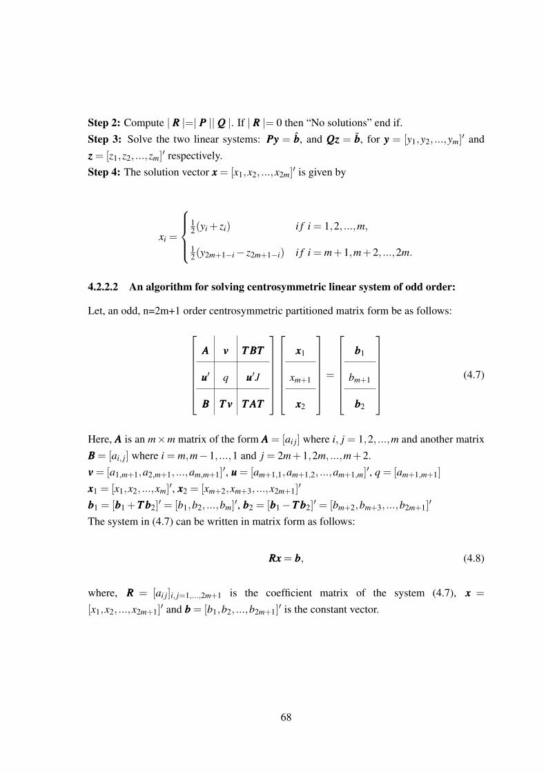
Step 2: Compute | RRR |=| PPP || QQQ |. If | RRR |= 0 then “No solutions” end if.Step 3: Solve the two linear systems: PPPyyy = bbb, and QQQzzz = bbb, for yyy = [y1,y2, ...,ym]

′ andzzz = [z1,z2, ...,zm]

′ respectively.Step 4: The solution vector xxx = [x1,x2, ...,x2m]

′ is given by

xi =

12(yi + zi) i f i = 1,2, ...,m,

12(y2m+1−i− z2m+1−i) i f i = m+1,m+2, ...,2m.

4.2.2.2 An algorithm for solving centrosymmetric linear system of odd order:

Let, an odd, n=2m+1 order centrosymmetric partitioned matrix form be as follows:

AAA vvv TTT BBBTTT

uuu′ q uuu′J

BBB TTT vvv TTT AAATTT

xxx1

xm+1

xxx2

=

bbb1

bm+1

bbb2

(4.7)

Here, AAA is an m×m matrix of the form AAA = [ai j] where i, j = 1,2, ...,m and another matrixBBB = [ai, j] where i = m,m−1, ...,1 and j = 2m+1,2m, ...,m+2.vvv = [a1,m+1,a2,m+1, ...,am,m+1]

′, uuu = [am+1,1,am+1,2, ...,am+1,m]′, q = [am+1,m+1]

xxx1 = [x1,x2, ...,xm]′, xxx2 = [xm+2,xm+3, ...,x2m+1]

′

bbb1 = [bbb1 +TTT bbb2]′ = [b1,b2, ...,bm]

′, bbb2 = [bbb1−TTT bbb2]′ = [bm+2,bm+3, ...,b2m+1]

′

The system in (4.7) can be written in matrix form as follows:

RRRxxx = bbb, (4.8)

where, RRR = [ai j]i, j=1,...,2m+1 is the coefficient matrix of the system (4.7), xxx =

[x1,x2, ...,x2m+1]′ and bbb = [b1,b2, ...,b2m+1]

′ is the constant vector.

68

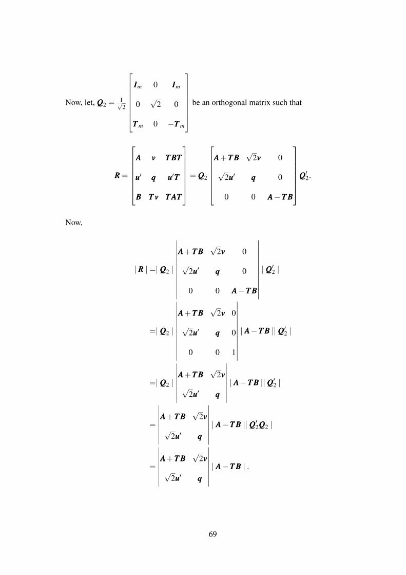
Now, let, QQQ2 =1√2

IIIm 0 IIIm

0√

2 0

TTT m 0 −TTT m

be an orthogonal matrix such that

RRR =

AAA vvv TTT BBBTTT

uuu′ qqq uuu′TTT

BBB TTT vvv TTT AAATTT

= QQQ2

AAA+TTT BBB

√2vvv 0

√2uuu′ qqq 0

0 0 AAA−TTT BBB

QQQ′2.

Now,

| RRR |=| QQQ2 |

∣∣∣∣∣∣∣∣∣∣∣∣

AAA+TTT BBB√

2vvv 0

√2uuu′ qqq 0

0 0 AAA−TTT BBB

∣∣∣∣∣∣∣∣∣∣∣∣| QQQ′2 |

=| QQQ2 |

∣∣∣∣∣∣∣∣∣∣∣∣

AAA+TTT BBB√

2vvv 0

√2uuu′ qqq 0

0 0 1

∣∣∣∣∣∣∣∣∣∣∣∣| AAA−TTT BBB || QQQ′2 |

=| QQQ2 |

∣∣∣∣∣∣∣∣AAA+TTT BBB

√2vvv

√2uuu′ qqq

∣∣∣∣∣∣∣∣ | AAA−TTT BBB || QQQ′2 |

=


√2vvv

√2uuu′ qqq

∣∣∣∣∣∣∣∣ | AAA−TTT BBB || QQQ′2QQQ2 |

=


√2vvv

√2uuu′ qqq

∣∣∣∣∣∣∣∣ | AAA−TTT BBB | .

69

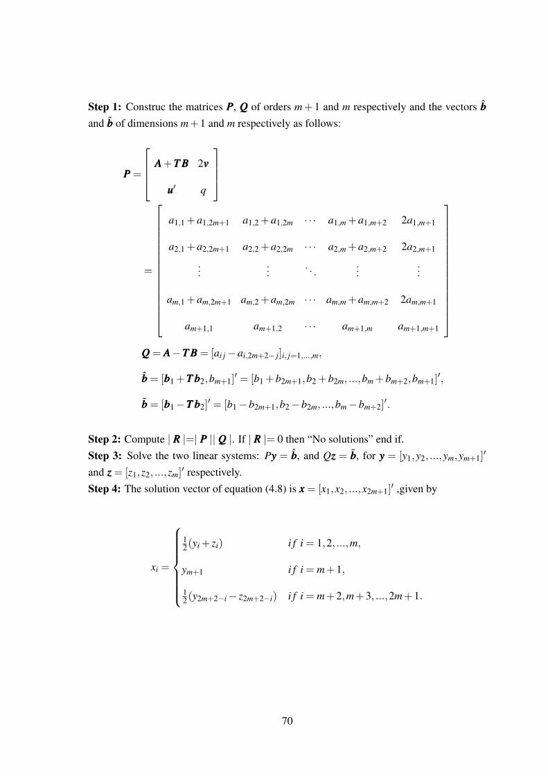
Step 1: Construc the matrices PPP, QQQ of orders m+ 1 and m respectively and the vectors bbb

and bbb of dimensions m+1 and m respectively as follows:

PPP =

AAA+TTT BBB 2vvv

uuu′ q

=

a1,1 +a1,2m+1 a1,2 +a1,2m · · · a1,m +a1,m+2 2a1,m+1

a2,1 +a2,2m+1 a2,2 +a2,2m · · · a2,m +a2,m+2 2a2,m+1

......

. . ....

...

am,1 +am,2m+1 am,2 +am,2m · · · am,m +am,m+2 2am,m+1

am+1,1 am+1,2 · · · am+1,m am+1,m+1

QQQ = AAA−TTT BBB = [ai j−ai,2m+2− j]i, j=1,...,m,

bbb = [bbb1 +TTT bbb2,bm+1]′ = [b1 +b2m+1,b2 +b2m, ...,bm +bm+2,bm+1]

′,

bbb = [bbb1−TTT bbb2]′ = [b1−b2m+1,b2−b2m, ...,bm−bm+2]

′.

Step 2: Compute | RRR |=| PPP || QQQ |. If | RRR |= 0 then “No solutions” end if.Step 3: Solve the two linear systems: Pyyy = bbb, and Qzzz = bbb, for yyy = [y1,y2, ...,ym,ym+1]

′

and zzz = [z1,z2, ...,zm]′ respectively.

Step 4: The solution vector of equation (4.8) is xxx = [x1,x2, ...,x2m+1]′ ,given by

xi =

12(yi + zi) i f i = 1,2, ...,m,

ym+1 i f i = m+1,

12(y2m+2−i− z2m+2−i) i f i = m+2,m+3, ...,2m+1.

70

4.3 Formulas for calculating xxx in (4.1)

Let m = bn/2c, both HHH11 and HHH21 be m×m matrices, both www and vvv be m-dimensionalcolumn vectors, and q be a scalar. Then, since (IIIn + λDDD′pDDDp)

−1 is a centrosymmetricmatrix, if n is even,

(IIIn +λDDD′pDDDp)−1 =

HHH11 TTT mHHH21TTT m


,and if n is odd,


HHH11 www TTT mHHH21TTT m

vvv′ q vvv′TTT m

HHH21 TTT mwww TTT mHHH11TTT m

.

For example, see Abu-Jeib (2002, Lemma 2.3). Moreover, (IIIn+λDDD′pDDDp)−1 is a symmetric

persymmetric matrix, HHH11 = HHH ′11, TTT mHHH21TTT m = HHH ′21, and vvv = www. Accordingly, if n is even,


HHH11 HHH ′21


, (4.9)

and if n is odd,


HHH11 www HHH ′21

www′ q www′TTT m


. (4.10)

For example, when n = 7, p = 3, and λ = 1, the smoother matrix is

(IIIn +λDDD′pDDDp)−1

71

=

HHH11 www HHH ′21

www′ v www′TTT m


=

0.8718 0.2393 −0.0342 −0.0769 −0.0342 0.0085 0.0256

0.2393 0.4302 0.3048 0.1026 −0.0285 −0.0570 0.0085

−0.0342 0.3048 0.4217 0.2821 0.0883 −0.0285 −0.0342

−0.0769 0.1026 0.2821 0.3846 0.2821 0.1026 −0.0769

−0.0342 −0.0285 0.0883 0.2821 0.4217 0.3048 −0.0342

0.0085 −0.0570 −0.0285 0.1026 0.3048 0.4302 0.2393

0.0256 0.0085 −0.0342 −0.0769 −0.0342 0.2393 0.8718

.

(4.11)

Since (IIIn +λDDD′pDDDp) is bisymmetric, when n is even, it may be expressed as

(IIIn +λDDD′pDDDp) =

GGG11 GGG′21

GGG21 TTT mGGG11TTT m

, (4.12)

where GGG11 is an m×m matrix. Likewise, when n is odd, it is


GGG11 ααα GGG′21

ααα ′ r ααα ′TTT m

GGG21 TTT mααα TTT mGGG11TTT m

, (4.13)

where GGG11 is an m×m matrix.

72

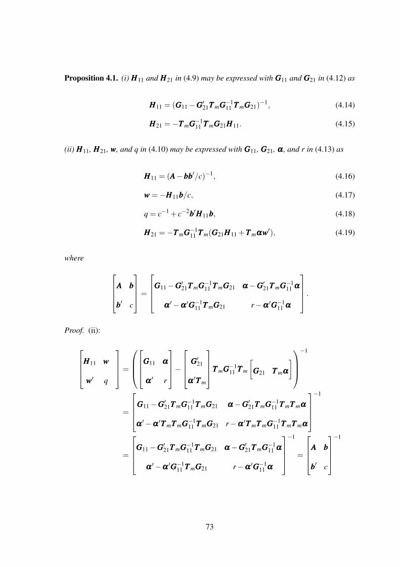
Proposition 4.1. (i) HHH11 and HHH21 in (4.9) may be expressed with GGG11 and GGG21 in (4.12) as

HHH11 = (GGG11−GGG′21TTT mGGG−111 TTT mGGG21)

−1, (4.14)

HHH21 =−TTT mGGG−111 TTT mGGG21HHH11. (4.15)

(ii) HHH11, HHH21, www, and q in (4.10) may be expressed with GGG11, GGG21, ααα , and r in (4.13) as

HHH11 = (AAA−bbbbbb′/c)−1, (4.16)

www =−HHH11bbb/c, (4.17)

q = c−1 + c−2bbb′HHH11bbb, (4.18)

HHH21 =−TTT mGGG−111 TTT m(GGG21HHH11 +TTT mαααwww′), (4.19)

where AAA bbb

bbb′ c

=

GGG11−GGG′21TTT mGGG−111 TTT mGGG21 ααα−GGG′21TTT mGGG−1

11 ααα

ααα ′−ααα ′GGG−111 TTT mGGG21 r−ααα ′GGG−1

11 ααα

.Proof. (ii):

HHH11 www

www′ q

=

GGG11 ααα

ααα ′ r

− GGG′21

ααα ′TTT m

TTT mGGG−111 TTT m

[GGG21 TTT mααα

]−1

=


11 TTT mTTT mααα

ααα ′−ααα ′TTT mTTT mGGG−111 TTT mGGG21 r−ααα ′TTT mTTT mGGG−1

11 TTT mTTT mααα

−1

=


11 ααα

ααα ′−ααα ′GGG−111 TTT mGGG21 r−ααα ′GGG−1

11 ααα

−1

=

AAA bbb

bbb′ c

−1

73

Then, it follows that

HHH11 = (AAA−bbbbbb′/c)−1, www =−HHH11bbb/c, q = c−1 + c−1bbb′HHH11bbbc−1.

In addition,

[HHH21 TTT mwww

]=−TTT mGGG−1

11 TTT m

[GGG21 TTT mααα

]HHH11 www

www′ q

=−TTT mGGG−1

11 TTT m

[GGG21HHH11 +TTT mαααwww′ GGG21www+TTT mαααq

]=

[−TTT mGGG−1

11 TTT m(GGG21HHH11 +TTT mαααwww′) −TTT mGGG−111 TTT m(GGG21www+TTT mαααq)

].

Remarks. (a) A MATLAB/GNU Octave function to calculate (IIIn +λDDD′pDDDp)−1 based on

(4.14)–(4.19) is provided in the Appendix. It is noteworthy here that (i) even though (IIIn +

λDDD′pDDDp) is a n× n matrix, its inverse is obtainable by inverting m×m matrices and (ii)since (IIIn +λDDD′pDDDp) is a (2p+1)-diagonal matrix, it follows that GGG21 is generally a sparsematrix but GGG21 6= 000. For example, when n = 7, p = 3, and λ = 1,


GGG11 ααα GGG′21

ααα ′ r ααα ′TTT m

GGG21 TTT mααα GGG22

=

2 −3 3 −1 0 0 0

−3 11 −12 6 −1 0 0

3 −12 20 −15 6 −1 0

−1 6 −15 21 −15 6 −1

0 −1 6 −15 20 −12 3

0 0 −1 6 −12 11 −3

0 0 0 −1 3 −3 2

.

Corollary 4.1. (i) When n is even, letting yyy = [yyy′1,yyy′2]′, where yyy1 is a m-dimensional column

74

vector, it follows that

xxx =

xxx1

xxx2

=

HHH11yyy1 +HHH ′21yyy2

HHH21yyy1 +TTT mHHH11TTT myyy2

, (4.20)

where HHH11 and HHH21 are defined in (4.14) and (4.15), respectively. (ii) When n is odd,

letting yyy = [yyy′1,ym+1,yyy′2]′, where yyy1 is a m-dimensional column vector and ym+1 is a scalar,

it follows that

xxx =

xxx1

xm+1

xxx2

=

HHH11yyy1 +wwwym+1 +HHH ′21yyy2

www′yyy1 +qym+1 +www′TTT myyy2

HHH21yyy1 +TTT mwwwym+1 +TTT mHHH11TTT myyy2

, (4.21)

where HHH11, HHH21, www, and q are defined in (4.16), (4.17), (4.18), and (4.19), respectively.

Remarks. From the centrosymmetry of (IIIn + λDDD′pDDDp), we may obtain an alternative in-version formula to (4.20) by applying El-Mikkawy and Atlan’s (2013) CENTROSYMM-Ialgorithm:

xxx1 =12(ξξξ 1 +ξξξ 2), (4.22)

xxx2 =12

TTT m(ξξξ 1−ξξξ 2), (4.23)

where ξξξ 1 = (GGG11 + TTT mGGG21)−1(yyy1 + TTT myyy2) and ξξξ 2 = (GGG11− TTT mGGG21)

−1(yyy1− TTT myyy2). Itis notable that similarly to (4.20), xxxi for i = 1,2 are obtainable by inverting not n× n

matrices but m×m matrices. Likewise, by applying El-Mikkawy and Atlan’s (2013)CENTROSYMM-II algorithm, we may obtain an alternative inversion formula to (4.21)as follows:

xxx1 =12(ζζζ 1 +ζζζ 2), (4.24)

xm+1 = ζm+1, (4.25)

xxx2 =12

TTT m(ζζζ 1−ζζζ 2), (4.26)

75

where

ζζζ 1

ζm+1

=

GGG11 +TTT mGGG21 2ααα

βββ′ r

−1yyy1 +TTT myyy2

ym+1

and ζζζ 2 = (GGG11−TTT mGGG21)

−1(yyy1−TTT myyy2). Here, ααα , βββ , and r are defined as follows.


GGG11 ααα TTT mGGG21TTT m

βββ′ r βββ

′TTT m


,

The proofs of (4.22)–(4.23) and (4.24)–(4.26) are provided in the Appendix.

4.4 Bisymmetry of the smoother matrices in (4.3) and

(4.4)

We show that similar properties hold for DDD′p(λ−1IIIn−p + DDDpDDD′p)

−1DDDp in (4.3) andFFF p(FFF ′pFFF p +λ IIIn−p)

−1FFF ′p in (4.4).

Corollary 4.2. DDD′p(λ−1IIIn−p +DDDpDDD′p)

−1DDDp in (4.3) is a bisymmetric matrix.

Proof. From Yamada (2019) we know that,

TTT n(IIIn +λDDD′pDDDp)−1TTT n = [TTT n(IIIn +λDDD′pDDDp)TTT n]

−1 = (IIIn +λDDD′pDDDp)−1.

It follows that

TTT pDDD′p(λ−1IIIn−p +DDDpDDD′p)

−1DDDpTTT p = IIIn−TTT p(IIIn +λDDD′pDDDp)−1TTT p

= IIIn− (IIIn +λDDD′pDDDp)−1

= DDD′p(λ−1IIIn−p +DDDpDDD′p)

−1DDDp,

76

which indicates that DDD′p(λ−1IIIn−p +DDDpDDD′p)

−1DDDp is a centrosymmetric matrix. In addition,it is also a symmetric matrix. Thus, it is a bisymmetric matrix.

Yamada (2019) proved that, TTT n−pDDDp = (−1)pDDDpTTT n. Similarly, we obtain the fol-lowing result:

Lemma 4.2. TTT nFFF p = (−1)pFFF pTTT n−p.

Proof. From Yamada (2019) we know that, TTT n−pDDDp = (−1)pDDDpTTT n, it follows that

TTT nFFF p = TTT nDDD′p(DDDpDDD′p)−1 = ((−1)p(−1)pDDDpTTT n)

′TTT n−p(TTT n−pDDDpDDD′pTTT n−p)−1TTT n−p

= (−1)p(TTT n−pDDDp)′TTT n−p(TTT n−pDDDpDDD′pTTT n−p)

−1TTT n−p

= (−1)pDDD′p(DDDpDDD′p)−1TTT n−p = (−1)pFFF pTTT n−p.

Proposition 4.2. FFF p(FFF ′pFFF p +λ IIIn−p)−1FFF ′p in (4.4) is a bisymmetric matrix.

Proof. From Lemma 4.2, it follows that

FFF p(FFF ′pFFF p +λ IIIn−p)−1FFF ′p = FFF pTTT n−pTTT n−p(FFF ′pFFF p +λ IIIn−p)

−1TTT n−pTTT n−pFFF ′p

= FFF pTTT n−p(TTT n−pFFF ′pFFF pTTT n−p +λ IIIn−p)−1TTT n−pFFF ′p

= TTT nFFF p(FFF ′pTTT nTTT nFFF p +λ IIIn−p)−1FFF ′pTTT n

= TTT nFFF p(FFF ′pFFF p +λ IIIn−p)−1FFF ′pTTT n,

which indicates that FFF p(FFF ′pFFF p +λ IIIn−p)−1FFF ′p is a centrosymmetric matrix. In addition, it

is also a symmetric matrix. Thus, it is a bisymmetric matrix.


In this chapter, based on the result of Yamada (2019), we presented simple formulas forcalculating the smoother matrix of the WH graduation. In addition, we showed some re-sults, which include that two other smoother matrices related with the WH graduation arealso bisymmetric. The results obtained in the paper are summarized in Propositions 4.1,and 4.2 and in Corollaries 4.1 and 4.2.

77

4.6 Appendix

4.6.1 A MATLAB/GNU Octave function to calculate (IIIn +λDDD′pDDDp)−1

based on (4.14)–(4.19)

function invP = Calc_Hat_WK_Graduation(n, p, lambda)

D = diff(eye(n), p);

P = eye(n)+lambda*D’*D;

m = floor(n/2);

I = eye(m);

T = I(:, m:-1:1);

if mod(n, 2) == 0 % even

G11 = P(1:m, 1:m);

G21 = P(m+1:n, 1:m);

invG11 = inv(G11);

H11 = inv(G11-G21’*T*invG11*T*G21);

H21 = -T*invG11*T*G21*H11;

invP = [H11, H21’; H21, T*H11*T];

else % odd

G11 = P(1:m, 1:m);

alpha = P(1:m, m+1);

r = P(m+1, m+1);

G21 = P(m+2:n, 1:m);

invG11 = inv(G11);

A = G11-G21’*T*invG11*T*G21;

b = alpha-G21’*T*invG11*alpha;

c = r-alpha’*invG11*alpha;

H11 = inv(A-b*b’/c);

w = -H11*b/c;

q = 1/c+(1/cˆ2)*(b’*H11*b);

H21 = -T*invG11*T*(G21*H11+T*alpha*w’);

invP = [H11, w, H21’; w’, q, w’*T; H21, T*w, T*H11*T];

end

78

end

4.6.2 Proof of (4.22) and (4.23)

When n is even, (IIIn +λDDD′pDDDp)xxx = yyy may be expressed as



xxx1

xxx2

=

yyy1

yyy2

. (4.27)

Premultiplying (4.27) by diag(IIIm,TTT m), we obtain

GGG11 TTT mGGG21

TTT mGGG21 GGG11

xxx1

TTT mxxx2

=

yyy1

TTT myyy2

, (4.28)

SinceIIIm IIIm

IIIm −IIIm

GGG11 TTT mGGG21

TTT mGGG21 GGG11

=

GGG11 +TTT mGGG21 TTT mGGG21 +GGG11

GGG11−TTT mGGG21 TTT mGGG21−GGG11

=

GGG11 +TTT mGGG21 000

000 GGG11−TTT mGGG21

IIIm IIIm

IIIm −IIIm

,premultiplying (4.28) by IIIm IIIm

IIIm −IIIm

,it follows thatGGG11 +TTT mGGG21 000

000 GGG11−TTT mGGG21

xxx1 +TTT mxxx2

xxx1−TTT mxxx2

=

yyy1 +TTT myyy2

yyy1−TTT myyy2

,

79

which leads toxxx1 +TTT mxxx2

xxx1−TTT mxxx2

=

(GGG11 +TTT mGGG21)−1(yyy1 +TTT myyy2)

(GGG11−TTT mGGG21)−1(yyy1−TTT myyy2)

=

ξξξ 1

ξξξ 2

.By solving the above simultaneous equations, we obtain (4.22) and (4.23).

Here, we remark that we may apply the inversion formula of centrosymmetric ma-trix given in Good (1970):



−1

=

KKK11 KKK21TTT m

TTT mKKK21 TTT mKKK11TTT m

,where

KKK11 =12[(GGG11 +TTT mGGG21)

−1 +(GGG11−TTT mGGG21)−1],

KKK21 =12[(GGG11 +TTT mGGG21)

−1− (GGG11−TTT mGGG21)−1],

Accordingly, it follows that

xxx1 = KKK11yyy1 +KKK21TTT myyy2

=12[(GGG11 +TTT mGGG21)

−1 +(GGG11−TTT mGGG21)−1]yyy1

+12[(GGG11 +TTT mGGG21)

−1− (GGG11−TTT mGGG21)−1]TTT myyy2

=12(ξξξ 1 +ξξξ 2).

Likewise, we may obtain

xxx2 = TTT mKKK21yyy1 +TTT mKKK11TTT myyy2

=12

TTT m[(GGG11 +TTT mGGG21)−1− (GGG11−TTT mGGG21)

−1]yyy1

+12

TTT m[(GGG11 +TTT mGGG21)−1 +(GGG11−TTT mGGG21)

−1]TTT myyy2

80

=12

TTT m(ξξξ 1−ξξξ 2).

4.6.3 Proof of (4.24)–(4.26)

When n is odd, (IIIn +λDDD′pDDDp)xxx = yyy may be expressed as

GGG11 ααα TTT mGGG21TTT m

βββ′ r βββ

′TTT m


xxx1

xm+1

xxx2

=

yyy1

ym+1

yyy2

(4.29)

Premultiplying (4.29) by diag(IIIm,1,TTT m), we obtain

GGG11 ααα TTT mGGG21

βββ′ r βββ

′

TTT mGGG21 ααα GGG11

xxx1

xm+1

TTT mxxx2

=

yyy1

ym+1

TTT myyy2

(4.30)

SinceIIIm 0 IIIm

000 1 000

IIIm 0 −IIIm

GGG11 ααα TTT mGGG21

βββ′ r βββ

′

TTT mGGG21 ααα GGG11

=

GGG11 +TTT mGGG21 2ααα TTT mGGG21 +GGG11

βββ′ r βββ

′

GGG11−TTT mGGG21 000 TTT mGGG21−GGG11

=

GGG11 +TTT mGGG21 2ααα 000

βββ′ r 000

000 000 GGG11−TTT mGGG21

IIIm 0 IIIm

000 1 000

IIIm 0 −IIIm

,

81

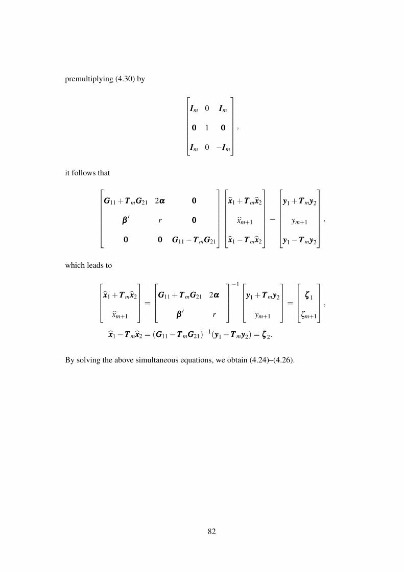
premultiplying (4.30) by

IIIm 0 IIIm

000 1 000

IIIm 0 −IIIm

,

it follows thatGGG11 +TTT mGGG21 2ααα 000

βββ′ r 000

000 000 GGG11−TTT mGGG21

xxx1 +TTT mxxx2

xm+1

xxx1−TTT mxxx2

=

yyy1 +TTT myyy2

ym+1

yyy1−TTT myyy2

,

which leads to

xxx1 +TTT mxxx2

xm+1

=

GGG11 +TTT mGGG21 2ααα

βββ′ r

−1yyy1 +TTT myyy2

ym+1

=

ζζζ 1

ζm+1

,xxx1−TTT mxxx2 = (GGG11−TTT mGGG21)

−1(yyy1−TTT myyy2) = ζζζ 2.

By solving the above simultaneous equations, we obtain (4.24)–(4.26).

82

4.7 References

1. Abu-Jeib, I. T., 2002, Centrosymmetric matrices: Properties and an alternative ap-proach, Canadian Mathematical Quarterly, 10, 4, 429–445.


3. Dagum, E. B. and A. Luati, 2004, A linear transformation and its properties withspecial applications in time series filtering, Linear Algebra and its Applications, 388,107–117.

4. El-Mikkawy, M. and F. Atlan, 2013, On solving centrosymmetric linear systems,Applied Mathematics, 4, 21–32.

5. Fassbender, H. and Ikramov,K. D., 2003, Computing matrix vector products withcentrosymmetric and centrohermitian matrics, Linear Algebra and its Application,364, 235-241.

6. Good, I. J., 1970, The inverse of a centrosymmetric matrix, Technometrics, 12, 4,925–928.






11. Reeves, J. J., C. A. Blyth, C. M. Triggs, and J. P. Small, 2000, The Hodrick–Prescottfilter, a generalization, and a new procedure for extracting an empirical cycle from aseries, Studies in Nonlinear Dynamics and Econometrics, 4, 1, 1–16.

12. Weinert, H. L., 2007, Efficient computation for Whittaker–Henderson smoothing,Computational Statistics and Data Analysis, 52, 2, 959–974.

83


14. Yamada, H., 2018, Why does the trend extracted by the Hodrick–Prescott filteringseem to be more plausible than the linear trend?, Applied Economics Letters, 25, 2,102–105.



and Methods, 48, 12, 3153–3161.

17. Yamada, H. and F. T. Jahra, 2019, An explicit formula for the smoother weights ofthe Hodrick–Prescott filter, Studies in Nonlinear Dynamics and Econometrics, DOI:10.1515/snde-2018-0035.

18. Yamada, H., 2019, A note on Whittaker–Henderson graduation: Bisymmetry of thesmoother matrix, Communications in Statistics – Theory and Methods, DOI: 10.1080/03610926.2018.1563183.

84

ir.lib.hiroshima-u.ac.jp · Acknowledgements It is my pleasure to acknowledge the role of several individuals who helped me to complete my Ph.D. research. Firstly, I would like to

Documents