IRJET-Real-Time Damage Detection in Laminated Composite Beams Using Dynamic Strain Response and Modular Neural Arrays for Aerospace Applications

International Research Journal of Engineering and Technology (IRJET) e-ISSN: 2395 -0056

Volume: 02 Issue: 03 | June-2015 www.irjet.net p-ISSN: 2395-0072

© 2015, IRJET.NET- All Rights Reserved Page 2060

Real-Time Damage Detection in Laminated Composite Beams Using

Dynamic Strain Response and Modular Neural Arrays for Aerospace

Applications

Sanjay Goswami1, 2 and Partha Bhattacharya2

1 Assistant Professor, Department of Computer Applications, Narula Institute of Technology, Agarpara, Kolkata-109, India

2 Associate Professor, Department of Civil Engineering, Jadavpur University, Kolkata-32, India

---------------------------------------------------------------------***---------------------------------------------------------------------Abstract Damage detection in multi-layer laminated “Glass Fiber

– Epoxy Resin” composite beams have been studied for

Structural Health Monitoring applications. A numerical

model of the beam is developed using Finite Element

Method (FEM). The FEM model is used to simulate

damages in the structure, and also mechanical

vibrations, actuated at one end of it. Strain responses

corresponding to the vibrations are picked up at a

different location and are studied to identify the

location and severity of the damage. Since multiple

parameters like Location, Layer and Severity of the

damage are to be identified a single array of multiple

neural network units (termed neural-array) is initially

proposed which fell short of producing desired

identification success rates. To address this short

coming, a collaborative group of parameter-specific

multiple neural arrays is proposed, which finally

produced fairly impressive damage identification

results.

Keywords: Structural Health Monitoring; Glass Fiber – Epoxy Resin Composite; Strain Response; Finite Element Method; Modular Neural Network Array.

1. INTRODUCTION

Structural Health Monitoring (SHM), an emerging interdisciplinary field, incorporates techniques from computer science, electronics and electrical engineering to solve structural problems related to monitoring of in-service civil structures such as bridges, buildings, aerospace vehicles, etc. The objective is to detect and identify damages that may occur in these structures while in operation. If some levels of damages are detected early, suitable disaster prevention mechanism can be initiated to save public lives. In that sense, it is a mission critical technology. The field of SHM involves study of several individual structural components, such as beams, plates,

shells, etc., and integrating them to provide a holistic damage/failure detection mechanism. Several approaches have been proposed in the open literature by different researchers, ranging from tap testing to modern day acoustics, x-rays, ultrasound and vibration signal processing based techniques. Among them vibration based techniques have been found to be most effective in addressing aerospace domain problems (Farrar et al [01], Carden et al [02], Raghavan et al [03]). Qiao [04] presented some of the most relevant signal processing techniques suitable for vibration based damage analysis. Staszewsky et al [05] elaborated the utility of signal processing based techniques in detecting damage especially in aerospace structures. Sohn et al [06] and Taha et al [07] emphasized the effectiveness of wavelet transform in delamination detection of composite structures. The problem of structural damage detection is essentially a statistical pattern recognition problem, which is supported by the works of Carden et al [02], Raghavan et al [03] and Fan et al [08]. Modern pattern recognition approaches ranging from genetic algorithms, neural networks and support vector machines, suitable for damage detection problems have been discussed in the studies by Bakhary et al [09] and Liu et al [10]. The concept of neural network arrays in pattern recognition has been discussed in Sharkey [11].

Goswami et al [12] investigated the detection of single damages in a structure made of isotropic material (steel). Only two damage parameters, namely Zone and Extent, were identified. In another related work Goswami et al [13] extended the study of [12] to detect multiple damages in a similar type of structure. In the manufacturing of modern day aircrafts and automobiles, laminated composite structures are being increasingly used as they are light weight and have a very high strength-to-weight ratio. Hence, there is a need to extend further the study of damage identification in laminated structures. The laminated structure consists of




orthotropic layers arranged in a certain configuration. However, because of its complex manufacturing process and being exposed to challenging environments during its operations, structural degradation can take place. Using normal damage identification methods, certain damages such as laminar failure, may not always be identified. The focus of the current work is to detect damages in laminated composite beams, with identification of an additional parameter, the Layer at which the damage occurs, along with the other two parameters namely, Zone and Extent.

2. NUMERICAL PROBLEM FORMULATION In the present research study a laminated glass – epoxy composite cantilever beam is considered wherein various extents of damages are simulated at different locations along the length and thickness of the beam. The detailed model of the beam is presented in the next few sections. 2.1 Description of the Structure 1) Geometry and Boundary Condition The beam structure considered for the present study is having the following dimensions: 1.5m length, 0.2m width and 0.00175m thickness (Figure 1). One end of the structure is mechanically fixed to prevent any displacement while the other end is kept free, giving it a cantilever class. A load (force) is applied at the free end and vibration signal is picked and studied at the other end.

2) Material Modeling The composite structure is chosen to be composed of 7 layers (say), each layer composed of Glass Fibers embedded in Epoxy Resin. When the orientation of fibers (X’ axis), is along the X-axis of the structure (Figure 2), the properties of the material are as described in Table 1.

Table 1: Material Properties for the Fiber-Epoxy Composite Structure

Modulus of Elasticity (E) Shear Modulus (G)

Ex Ey Ez Gxy Gyz Gzx

140 GPa 9 Gpa 9 Gpa 6 Gpa 6 Gpa 6 Gpa

Changing the orientation of fibers in the epoxy material gives rise to different material properties, and with that we can produce several such structures, known as Orthotropic Composite structures. A typical orientation scenario is shown in Figure 3.

In a multi-layered laminated composite beam, different layers are characterized by the orientation of its fibers with respect to the X-axis, and the scheme for different orientations in each layer is summarized in Table 2.

Table 2: Fiber Orientations at Different Layers

Layer Fiber Orientation, θ Orientation Pattern

1 0 ͦ

2 45 ͦ

3 -45 ͦ

4 90 ͦ

5 -45 ͦ

6 45 ͦ

7 0 ͦ

Fig.2 Glass Fiber Orientation along X-Axis

(top view)

Y

X

X

’

Y

’

Fig.3 Glass Fiber Orientation along direction θ from X-axis (top view)

Y

X

θ

X

’ Y

’

Load (f)

Vibration pickup

Fig. 1 Dimensions of the Beam Structure.

Right end is the fixed end.

0.00175 m

1.5m

0.2m

X

Y

Vibration

Waves




Each layer is 0.25mm thick, thus making the total thickness of the cross-section of the entire structure to be 1.75mm. The sectional view of the structure is shown in Figure 4. To localize the damages, the structure is divided into seven logical segments along the X-axis. Segment 1 is meant for applying the force, segment 7 for sensing the vibrations and rest of the segments 2 to 6 are for studying the damage locations. The typical scheme is shown in Figure 5, where shaded regions represent prospective damage zones. The structure discussed above is simulated using Finite Element Method (FEM) on ANSYS ver. 11.0 platform. The FE Model for this structure is discussed in the next section. 2.2 Finite Element Model of the Structure A 4-node isoparameteric finite element model (Shell181, ANSYS ver. 11.0), with 5 displacement degrees of freedom is used to discretize the structure. It is discretized using 110 elements in the length direction and 8 elements in the width direction (Figure 6).

Damages are simulated at various sections of the structure by numerically varying the Modulus of Elasticity and Shear Modulus. A load is applied at the free end of the beam, at node number 53, while the strain data collected from the

other end, at 982-989-996 span, and are analyzed subsequently. The details are discussed in the next section.

3. NUMERICAL SIMULATION 3.1 Simulating Load Actuation The actuating load is simulated numerically by applying a Moment of 100 N-m for a period of 0.0005s about the Y-axis at coordinates (0.0, 0.1, 0.0). The applied actuation is expected to generate transverse bending oscillations and eventually picked up by the strain sensors bonded near the fixed end of the beam. 3.2 Damage simulation schemes By varying the Modulus of Elasticity E and Shear Modulus G numerically, from 1% to 100% of absolute values, various severities of damages are simulated. However, the Location at which the severity is to be created is done by selecting the appropriate element area of the FE model that represents a certain Layer and a Zone. For example, Figure 7 shows a pictorial idea of a typical damage scenario being simulated at Layer 4 of Zone 3.

3.3 Dynamic Strain Response Simulation Based on the FE model of Figure 6, strain response corresponding to the vibrations is computed from a point near the fixed end of the structure. It has been observed from several random simulations that the strain response near the fixed end is highest and most sensitive to damages. The location (x,y,z) = ( 1.4733,0.1,0.0) (in the present FE model) is thus selected for the purpose. Surface Strain at a given node is computed from the relative displacement between two nodes adjacent to that node along the x-direction. In the FE model as defined in ANSYS, the deformation at particular layer along the x- direction is given by

(1)

Where u0 is the displacement along the middle layer of the structure, roty defines the rotation about Y-axis of the normal to the mid-layer and z defines the location of any layer from the neutral axis (zero strain axis) along the thickness (e.g. z=d/2 for the layer at the surface).

Fig.4 Sectional visualization of the 7-Layer Model of the Laminated Composite Structure

1.7

5 m

m 0

.25

mm

Fig.5 The 7-Segment Model of the Structure

1 2 3 4 5 6 7

Fig.7 Simulated damage scenario at Zone 3, Layer 4

Zones

1 2 3 4 5 6 7

Layers

1

2

3

4

Fig.6 The Finite Element Model with node numbers and

xyz coordinates. Produced by Ansys 11.0

X

Y

∆x

982

989

996

Loa

d (

Nod

e 5

3)

(0.0

, 0.1

, 0.0

)

7 6 5 4 3 2 1

(0.0,0.2,0.0) (1.1,0.2,0.0) (0.5,0.2,0.0) (0.7,0.2,0.0) (0.9,0.2,0.0) (0.3,0.2,0.0) (1.3,0.2,0.0)

(0.0,0.0,0.0) (1.1,0.0,0.0) (0.5,0.0,0.0) (0.7,0.0,0.0) (0.9,0.0,0.0) (0.3,0.0,0.0) (1.3,0.0,0.0)

(1.5

,0.2

,0.0

) (1

.5,0

.0,0

.0)

Strain Measurement Point

1

4

19 0

32 5

46 0

59 5

73 0

86 5

30

48

20

5

34

0

47

5

61

0

74

5

88

0




Structurally, strain in the x-direction is defined by the differential ∂u/∂x. By applying first principle of calculus, the strain at a given location can be computed by the following formula (e.g., node 989 in Figure 6):

Where, strain989 is the strain at node 989, roty996 and roty982 are Rotational Degrees of Freedom about Y-axis at nodes 996 and 982 respectively, ∆x is the distance between nodes 996 and 982, and d is the thickness of the beam. Following Eq. (2), several strain response signals are generated for all possible damage cases, each being 500 time steps long. The response signals are generated using the following dynamic equilibrium equation (Goswami et al [12]),

where, [M] is the Mass Matrix, [C] is the Damping Matrix, [K] is the Stiffness Matrix and {F} is the Dynamic Load Vector. The mass matrix is a function of the density of the material and the stiffness matrix is a function of the elasticity modulus, E and the shear modulus, G. The vectors are the displacement, velocity and

acceleration vectors, respectively. The strain response signals for various damage cases are then used in the pattern recognition scheme to detect damages, as described in the next section.

3.4 The Pattern Recognition Scheme adopted Various damage scenarios are represented by the strain response signals obtained from the previous step. These damage scenarios can be identified by a suitable pattern recognition scheme. Figure 8 describes the pattern recognition scheme followed in the current work. The steps involve Signal Acquisition, Filtering, Feature Extraction, Feature Selection and Neural-Array Pattern Recognition.

Referring to the figure, it can be understood that the strain response produced by strain sensors are, in real life, to be acquired by a signal acquisition system, which may contain noise. However, in the present work signals are simulated numerically and hence to add realistic features in the obtained response signals, synthetic noise is added. The signals generated are made noisy (5% Gaussian white noise, equivalent to SNR=20:1) and then cleansed by a digital signal filter named Butterworth filter (Oppenheim et al [14]). Filtered signals are then subjected to Continuous Wavelet Transform (CWT) (Walker [15] ,Graps [16] and Mallat [17]) for extraction of features in the form of Wavelet Coefficient Matrix (or Wavelet Scalogram). Subsequently, Principal Component Analysis (PCA) (Haykin [18]) is applied to reduce the dimension of the feature matrix and extraction of principal features. The extracted principal features are then used to train a Modular Neural Network Array (Goswami et al [12], Sharkey [11]) to classify the damage parameters. The following sub-section (3.5) gives the description of a general neural network modular array structure for real time pattern recognition. 3.5 Structure of a Neural Network Modular Array for

real-time multi-parameter pattern recognition. A Modular Neural Array (Sharkey [11]), or simply a Neural Array, is a conglomeration of several independent specialist neural network classifier units that work in collaboration with each other, in divide-and-conquer strategy, to solve a bigger identification problem. Figure 9 shows the structure of a typical neural array adopted for the present work.

Strain Response

Fig.8 The Pattern Recognition Scheme followed

Noisy

Signal

Continuous Wavelet

Transform

Filtered Signal

Principal

Features

Wavelet Scalogram

Trained Neural Array

Neural Array

Training (CWT)

Principal Component

Analysis (CWT)

Signal Acquisition

Low Pass Filter

Fig.9 The Structure of the Modular Neural Array. Each unit being an independent MLP Neural Network

A Typical Neural Unit

Pri

nci

pa

l

Fea

ture

Vec

tor

Individual MLP Neural Units with

Parameter Specific Training

Indiv

idu

al

Pa

ram

eter

Valu

e C

lass

es

Neural Unit 1

Neural Unit 2

Neural Unit n

P1

P2

Pn




It consists of several neural units, called Multi Layer Perceptrons (MLP). MLPs are specific multi-layer neural networks which follow Back Propagation class of learning algorithms to classify patterns (Haykin [18] and Konar [19]). Each MLP is individually trained to identify a specific parameter linked with the feature pattern. All the MLPs are fed with the same input feature vector in parallel, and different parameters are identified almost simultaneously, in near real time. Modularization is also suitable for designing embedded applications.

3.6 Structural description of the Neural Network Units

(MLP Units) used in a Neural Array Specifications of the individual MLP units such as number of input layer nodes, number of neurons in hidden and output layers, etc. are summarized in Table 3.

Table 3: The MLP Neural Network Unit Specifications for Damage Severity, Zone and Layer Classification.

Input Layer

Hidden Layer Output Layer Training Algorithm

Maximum Training

Iterations

500 nodes

20 neurons

2 to 6 neurons

(based on application)

Scaled Conjugate Gradient

Back Propagation

(memory efficient,

fast convergence)

1000

Transfer Function = Tan

Sigmoid Output [-

1,+1] (provides

balanced input to output layer

neurons)

Transfer Function =

Log Sigmoid Output [0,1]

(output needs to be +ve)

The input layer of the MLP Neural Network unit is taken to be 500 nodes long. This is owing to the fact that the size of the input feature vector is 500 elements long, produced by CWT and PCA from the 500 time step long input signal. Damage severities are categorized into 6 classes, while damage locations into 5 classes. Thus the size of the output layer is taken as 6 in case of Severity, while 5 in case of Zone classification. In case of Layer classification, only four layers are examined. This is because the fiber orientations in the layers above and below the central layer (layer 4) are symmetrical. Damage occurring in any corresponding symmetric layers, i.e. 1 or 7, 2 or 6, etc., will have the same effect on the strain response. Thus the output layer for Layer classification is taken to be 4 neurons long. The transfer function for the hidden layer neurons is taken to be Tan-Sigmoid. This is because the output of this function varies from -1 to +1 with x from -∞ to +∞, and helps in providing a balanced input to the output layer neurons (Konar [19]). The Transfer function for the output layer neurons is taken to be Log-Sigmoid,

ensuring the output to be positive between 0 and 1, specifying some positive class (Konar [19]). The training algorithm used is the Scaled Conjugate Gradient (SCG), a variant of the Back Propagation (BP) Algorithm. As per Moller [20], the SCG-BP algorithm is more memory efficient and faster in convergence.

3.7 Damage Simulation Cases In the current work, single damage cases are simulated and identified. Parameters that are identified about the damages are – Zone, Layer and Extent (Severity). Various damage cases are simulated by varying the Zone, Layer and, Elasticity and Strain Modulus values, as briefed in the Table 4.

Table 4: Damage Simulation Cases Generation Parameter 1

Severity (Extent) Parameter 2

Zone Parameter

3 Layer

Varying the Extent parameter value from 1% to 100% of

absolute Moduli of

Elasticity (E) and Strain (G)

Varying Zone parameter from 2 to 6

Varying Layer

parameter from 1 to

4

A total of 100 x 5 x 4 = 2000 damage cases are created, which are used to train respective neural units to identify corresponding Extent, Zone and Layer parameters. 3.8 Pattern Recognition Cases Case 1: Use of Single Neural-Array When a single Neural Array is used, one neural unit each is employed to identify the individual damage parameters. Such as, MLP1 is employed to identify the Severity of the damage; MLP2 is employed for identification of Zone of occurrence, while MLP3 is employed for identification of Layer of occurrence of the damage. The output vector obtained from a given neural unit indicates a specific class of the value of the parameter it is identifying. An interpretive description of the output vectors of the individual neural units are summarized in Table 5a. Table 5a: Interpretation of the Vectors from Output Layer

of the Neural Units. MLP 1 MLP 2 MLP 2

Parameter 1 Extent (%)

Ranges

Output Vector

Parameter 2

Zone

Output Vector

Parameter 3

Layer

Output Vector

1 – 20 100000 2 100000 1 10000 21 – 40 010000 3 010000 2 01000 41 – 60 001000 4 001000 3 00100 61 – 80 000100 5 000100 4 00010 81 - 99 000010 6 000010 No Layer 00001

100 000001 No Zone 000001 - -

Case 2: Use of Multiple Neural-Arrays When multiple neural arrays are used, each is employed wholly to identify a particular damage parameter. The individual neural units of each array focus on a particular




sub-class of the damage parameter. The array pattern recognizer scheme is briefly summarized in Table 5b (appendix). Though Suresh et al [21] have proposed a modular neural array architecture, but the current proposed architecture is different in its approach to monitor exact locations of the damage more accurately. Each array is composed of several neural units. A neural unit of a particular array is dedicated for identifying a specific parameter value class. For example, the neural unit A1MLP1 of Array1 is dedicated for detecting whether the severity of the damage falls into the 99 – 80% class or not. Similarly neural units of the Array2 are dedicated for detecting the Zone of the damage occurrence, and so on. The output vectors of all these neural-arrays are taken to be two elements long only, viz. 10 or 01, indicating whether the parameter value falls in a particular class or not, respectively. This scheme actually reduces the overhead on individual neurons to remember large number of classes and improves the accuracy of prediction. Pictorially the scheme is described in Figure 10.

3.9 Strain Response Plots and Corresponding CWT Scalograms

Some sample response signals are taken and their corresponding wavelet scalograms are created. Figure 11(appendix) shows the strain response plot and its corresponding CWT Scalogram in case of an undamaged structure.

Fig.11 (a) Strain Response Signal and (b)

Corresponding Scalogram for Undamaged Structure

(a) Array 1

Fig.10. (a)-(c) Neural Arrays 1, 2 and 3. Each Neural

Unit of an Array is dedicated to identify a specific

parameter value class.

Zone 2

Zone 6

Zone 5

Zone 4

Zone 3

Signal Features

A2MLP1

A2MLP2

A2MLP3

A2MLP4

A2MLP5

99 – 80%

19 – 1%

39 – 20%

0%

59 – 40%

79 – 60%

A1MLP1

A1MLP2

A1MLP3

A1MLP4

A1MLP5

A1MLP6

Signal Features

(c) Array 3

Layer 1

Layer 4

Layer 3

Layer 2

Signal

Feature

A3MLP1

A3MLP2

A3MLP3

A3MLP4

(b) Array 2




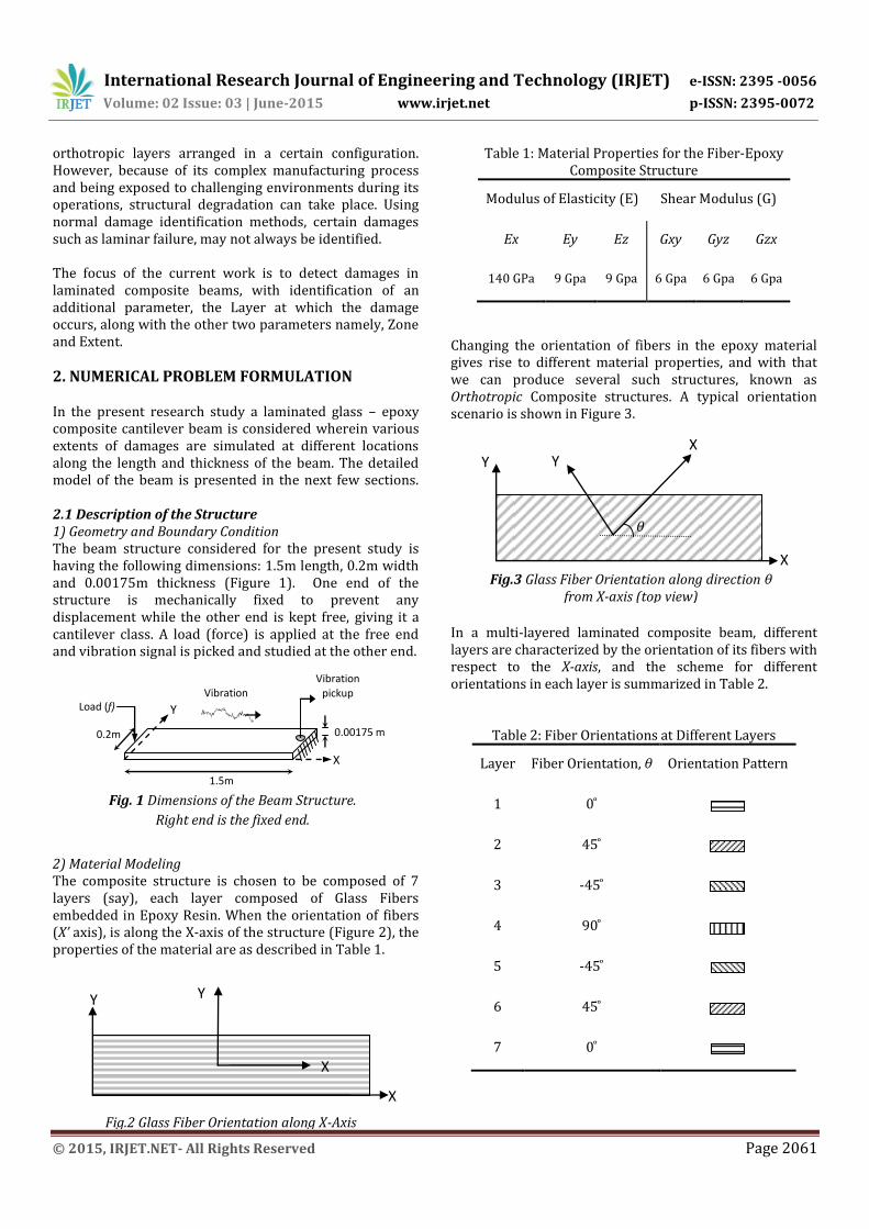
Figure 12 shows typical response plots and their scalograms corresponding to 50% and 99% damages at the Layer 1 of the Zone 2.

Similarly Figures 13 through 14 show response plots and Scalograms corresponding to the similar extents of damages at the Layer 2 of Zone 4, and Layer 4 of Zone 6, respectively.




4. RESULTS AND ANALYSIS Case-1: Single Damage, Single Neural-Array In the first case, an attempt is made to identify single damage in a particular layer of a particular zone. For that purpose, a single neural array is used. The constituent neural units of the array are trained individually to identify a specific damage parameter, e.g., Neural Unit 1 is trained for identifying Extent, Neural Unit 2 for Zone, and Neural Unit 3 for Layer. The success rates in identifying these parameters are summarized in Table 6a. It is seen that success rates in case of Zone and Layer are fairly good, but that in case of Extent is not very promising, as compared to results in Goswami et al [12].

Table 6a: Single damage success rates: Single array

Strain Pickup Location

Neural Unit 1 Extent

Identification

Neural Unit 2 Zone

identification

Neural Unit 3 Layer

identification 989 78.45% 85.4% 91.5%

The reason for poorer performance in identifying Extent may be that the damage is occurring at a certain layer of a certain zone. Dimensionally, the size of the damage is small, thus and hence less sensitive to be identified by a single neural unit. Case-2: Single Damage, Multiple Neural-Arrays

Fig.13 (a)-(d)Strain Response Signals and Corresponding

Scalograms for Damage at Zone4 and Layer2

Fig.14 (a)-(d)Strain Response Signals and Corresponding


Fig. 12 (a)-(d) Strain Response Signals and Corresponding





To address the limitation in case 1, a distributed neural monitoring approach is proposed based on the findings of Goswami et al [13]. In the current approach, separate neural arrays are employed to monitor each parameter type, where each constituent neural unit monitors a particular parameter value or range (Figure 10, Table 5b). The success rates of each neural unit in identifying its corresponding parameter value/range are summarized in Table 6b(appendix). It can be seen from the table that identification success rates have fairly improved with the introduction of distributed monitoring scheme for the given model. It is because the individual MLP units now have a lesser number of damage parameter classes to identify which enables them to be more accurate in classifying signal patterns to their respective damage parameter classes. 5. CONCLUSIONS It has been observed in the current work that the damages occurring in multi-layer laminated composites can be identified by vibration based signal processing method. A special case has been taken for the study where a composite beam is subjected to laminar damage at a certain layer and signal processing based method is applied for detection of the damage. Two types of neural array schemes are employed for identification of damages. In the first scheme, a single neural array has been proposed, where each single neural-unit is assigned the job of identifying entire value-classes of the designated damage parameter, and yielded fairly poor classification success rates. However, with the use of separate arrays for different damage parameters, with each neural unit of an array being trained to identify a particular value-class, better success rates were obtained. It can thus be concluded that the use of higher levels of distributed monitoring can improve damage identification results in laminated composite beams. This work can viably be extended in future to explore multiple damage detection possibilities, in laminated composite plates, with different signal processing and pattern recognition approaches. REFERENCES [01] Farrar Charles R., Doebling Scott W. and Nix David A.

(2001), Vibration-Based Structural Damage Identification. Philosophical Transactions of Royal Society London, 359, pp.131–149.

[02] Carden E. Peter and Fanning Paul (2004), Vibration Based Condition Monitoring: A Review. Structural Health Monitoring, 3(4), pp. 355-377.

[03] Raghavan Ajay and Cesnik Carlos E. S. (2007), Review of Guided-Wave Structural Health Monitoring. The Shock and Vibration Digest, 39, pp. 91-115.

[04] Qiao Long (2009), Structural Damage Detection Using Signal-Based Pattern Recognition. Ph.D. Dissertation, Kansas State University.

[05] Staszewski W.J. and Worden K. (2004), Signal Processing for Damage Detection. In: Staszewski W.J., Boller C. and Tomlinson G.R. (ed.) Health Monitoring of Aerospace Structures – Smart Sensor Technologies and Signal Processing, John Wiley & Sons, Sussex, pp. 163-206.

[06] Sohn H., Park G., Wait J. R., Limback N. P., and Farrar C. R. (2004), Wavelet-Based Active Sensing for Delamination Detection in Composite Structures, Smart Materials and Structures, 13(1), pp. 153–160.

[07] Taha M. M. Reda, Noureldin A., Lucero J. L. and Baca T. J. (2006), Wavelet Transform for Structural Health Monitoring: A Compendium of Uses and Features. Structural Health Monitoring, 5(3), pp. 0267-0296.

[08] Fan Wei and Qiao Pizhong (2011), Vibration Based Damage Identification Methods: A Review and Comparative Study. Structural Health Monitoring, 10(1), pp. 83-111.

[09] Bakhary N., Hao H. and Deeks Andrew J. (2010), Structure Damage Detection Using Neural Network with Multi-Stage Substructuring. Advances in Structural Engineering, 13(1), pp.95-110.

[10] Liu Han-Bing and Jiao Yu-Bo (2011), Application of Genetic Algorithm-Support Vector Machine (GA-SVM) for Damage Identification of Bridge. International Journal of Computational Intelligence and Applications, 10(4), pp. 383-397.

[11] Sharkey Amanda J.C. (1999), Multi-Net Systems. In: Sharkey Amanda J. C. (ed.) Combining Artificial Neural Nets – Ensemble and Modular Multi-Net Systems, Springer, New York, pp. 1-30.

[12] Goswami Sanjay and Bhattacharya Partha (2012a), A Scalable Neural-Network Modular-Array Architecture for Real-Time Multi-Parameter Damage Detection in Plate Structures Using Single Sensor Output. International Journal of Computational Intelligence and Applications, Vol. 11(4), pp. 1250024-1250045.

[13] Goswami Sanjay and Bhattacharya Partha (2012b), Pattern Recognition for damage detection in Aerospace Vehicle Structures. In Proceedings of the 2012 Third International Conference on Emerging Applications of Information Technology (EAIT2012), pp. 178 – 182, Nov. 30 - Dec. 1, 2012, Kolkata, IEEE Xplore.

[14] Oppenheim Alan V., Schafer Ronald W. and Buck John R. (1999), Discrete-Time Signal Processing, 2nd ed. Prentice-Hall Inc., New Jersey.

[15] Walker James S. (2008), A Primer on Wavelets and their Scientific Applications, 3rd ed., Chapman & Hall/CRC, USA.

[16] Graps Amara (1995), An Introduction to Wavelets, IEEE Computational Science and Engineering, 2(2), pp. 50 – 61.




[17] Mallat S. (1989), A Theory for Multiresolution Signal Decomposition: The Wavelet Representation. IEEE Pattern Analysis and Machine Intelligence, vol. 11(7), pp. 674-693.

[18] Haykin Simon (1999), Neural Networks – A Comprehensive Foundation, 2nd ed., Pearson, New Delhi.

[19] Konar Amit (2005), Computational Intelligence – Principles, Techniques and Applications, Springer, New Delhi.

[20] Moller M.F. (1993), A Scaled Conjugate Gradient Algorithm for Fast Supervised Learning, Neural Networks, 6, pp. 525-533.

[21] S. Suresh, S.N. Omkar, R. Ganguli and V. Mani (2004), Identification of crack location and depth in a cantilever beam using a modular neural network approach, Smart Materials and Structures, 13(4), 907-915.

BIOGRAPHIES

Sanjay Goswami obtained B.Sc. from

Kanpur University, India and M.C.A.

from Indira Gandhi National Open

University, India. Presently he is an

assistant professor in the Department

of Computer Applications, Narula

Institute of Technology, Kolkata and

working towards his Ph.D. degree from

Civil Engineering Department,

Jadavpur University, Kolkata. His area

of interest includes soft computing

applications in core engineering areas.

Partha Bhattacharya obtained his B.E. in Civil Engineering from Jadavpur University, Kolkata. Then M.Tech. and Ph.D. in Aerospace Engineering from IIT Kharagpur. Held positions as scientist at National Aerospace Laboratory, Bangalore and post-doctoral fellow at German Aerospace Center (DLR), Germany. Currently he is an Associate Professor in the Civil Engineering Department, Jadavpur University, and his area of interest includes structural health monitoring, acoustics and applications in the aerospace domain.

APPENDIX

Table 5b: Multi-Array Pattern Recognizer Scheme (Refer Figure 10) Array 1 Array 2 Array 3

Severity Identification Zone Identification Layer Identification

% age of E & G values

Actual %age of Damage

Neural Unit No.

Output Vectors

Zone No. Neural Unit

No. Output Vectors

Layer No.

Neural Unit No.

Output Vectors

1 – 20 % 99 – 80% A1MLP1 10 or 01 2 A2MLP1 10 or 01 1 A3MLP1 10 or 01 21 – 40 % 79 – 60% A1MLP2 10 or 01 3 A2MLP2 10 or 01 2 A3MLP2 10 or 01 41 – 60% 59 – 40% A1MLP3 10 or 01 4 A2MLP3 10 or 01 3 A3MLP3 10 or 01 61 – 80% 39 – 20% A1MLP4 10 or 01 5 A2MLP4 10 or 01 4 A3MLP4 10 or 01 81 – 99% 19 – 1% A1MLP5 10 or 01 6 A2MLP5 10 or 01 - -

100% 0% A1MLP6 10 or 01 - - - - -

Table 6b: Multi-array pattern recognizer scheme results (refer figure 10) Array 1 Array 2 Array 3

Severity Identification Zone Identification Layer Identification

% age of E & G values

Actual %age of Damage

Neural Unit No.

Success Rate

Zone No.

Neural Unit No.

Success Rate

Layer No.

Neural Unit No.

Success Rate

1 – 20 % 99 – 80% A1MLP1 96.4% 2 A2MLP1 92.6% 1 A3MLP1 98.1% 21 – 40 % 79 – 60% A1MLP2 84.5% 3 A2MLP2 94.5% 2 A3MLP2 90.7% 41 – 60% 59 – 40% A1MLP3 84.3% 4 A2MLP3 94.6% 3 A3MLP3 91.3% 61 – 80% 39 – 20% A1MLP4 84.5% 5 A2MLP4 95.3% 4 A3MLP4 97.5% 81 – 99% 19 – 1% A1MLP5 88.6% 6 A2MLP5 90.5% - -

100% 0% A1MLP6 99.0% - - - - -

IRJET-Real-Time Damage Detection in Laminated Composite Beams Using Dynamic Strain Response and Modular Neural Arrays for Aerospace Applications

Documents