Corso di Dottorato in Ingegneria Elettrica, Elettronica e delle Telecomunicazioni, Matematica e Automatica – Indirizzo in Ingegneria Elettronica e delle Telecomunicazioni DIPARTIMENTO DI ENERGIA, INGEGNERIA DELL’INFORMAZIONE E MODELLI MATEMATICI Settore Scientifico Disciplinare: ING-INF/03 Opportunistic traffic Offloadings Mechanisms for Mobile/4G Networks IL DOTTORE IL COORDINATORE Ing. Antonino Masaracchia Prof. Ing. Alessandro Busacca IL TUTOR CO TUTOR Ing. Stefano Mangione Ing. Andrea Passarella Ing. Raffaele Bruno CICLO XXVI ANNO CONSEGUIMENTO TITOLO 2016

Welcome message from author
This document is posted to help you gain knowledge. Please leave a comment to let me know what you think about it! Share it to your friends and learn new things together.
Transcript

Corso di Dottorato in Ingegneria Elettrica, Elettronica e delle Telecomunicazioni, Matematica e Automatica – Indirizzo in Ingegneria Elettronica e delle Telecomunicazioni
DIPARTIMENTO DI ENERGIA, INGEGNERIA DELL’INFORMAZIONE E MODELLI MATEMATICI
Settore Scientifico Disciplinare: ING-INF/03
Opportunistic traffic Offloadings Mechanisms forMobile/4G Networks
IL DOTTORE IL COORDINATORE Ing. Antonino Masaracchia Prof. Ing. Alessandro Busacca
IL TUTOR CO TUTOR Ing. Stefano Mangione Ing. Andrea Passarella
Ing. Raffaele Bruno
CICLO XXVIANNO CONSEGUIMENTO TITOLO 2016


Abstract
In the last few years, it has been observed a drastic surge of data traffic demand from
mobile personal devices (smartphones and tablets) over cellular networks [1]. Even
though a significant improvement in cellular bandwidth provisioning is expected with
LTE-Advanced systems, the overall situation is not expected to change significantly. In
fact, the diffusion of M2M and IoT devices is expected to increase at an exponential pace
(the share of M2M devices is predicted to increase 5x by 2018 [1]) while the capacity of
the cellular network is expected to increase linearly [1]. In order to meet such a high
demand and to increase the capacity of the channel, multiple offloading techniques are
currently under investigation, from modifications inside the cellular network architec-
ture, to integration of multiple wireless broadband infrastructures, to exploiting direct
communications between mobile devices. All these approaches can be diveded in two
main classes:
• To develop more sophisticated physical layer technologies (e.g. massive MIMO,
higher-order modulation schemes, cooperative multi-period transmission/recep-
tion)
• To offload part of the traffic from the cellular to another complementary network.
From this perspective the thesis contributes on both areas. On the one hand we discuss
our investigations about the performance of the LTE channel capacity through the de-
velopment of a unified modelling framework of the MAC-level downlink throughput of
a sigle LTE cell, which caters for wideband CQI feedback schemes, AMC and HARQ
protocols as defined in the LTE standard. Furthemore we also propose a solution, based
on reinforcement learning, to improve the LTE Adaptive Modulation and coding Scheme
(MCS).
On the other hand we have proposed and validated offloading mechanisms which are
minimally invasive for users’ mobile devices, as they use only minimally their resources.
Furthemore, as opposed to most of the literature, we consider the case where requests
for content are non-synchronised, i.e. users request content at random points in time.

Acknowledgements
This work was partly funded by the EC under the EINS (FP7- FIRE 288021),MOTO
(FP7 317959), and EIT Digital MOSES (Business Plan 2014-15) projects in wich the
National Resarch Council of Pisa is a Partner.
I really thank all my supervisors, Ing. Stefano Mangione from University of Palermo,
which has given me many advices and technical support, Ing. Andrea Passarella and Ing.
Raffaele Bruno from the CNR of Pisa , which have given me insights in the opportunistic
Network context.
iv

Contents
Abstract iii
Acknowledgements iv
Contents v
List of Figures vii
List of Tables ix
1 Introduction 1
1.1 Thesis contributions in the area of LTE throughput modelling and im-provement . . . . . . . . . . . . . . . . . . . . . . . . . . . . . . . . . . . . 3
1.1.1 LTE Channel Modelling . . . . . . . . . . . . . . . . . . . . . . . . 4
1.1.2 Reinforcement Learning in LTE-AMC scheme . . . . . . . . . . . . 4
1.2 Thesis contribution in the area of Mobile Data Offloading . . . . . . . . . 5
1.2.1 Mobile Opportunisitc Traffic Offloading . . . . . . . . . . . . . . . 7
2 State of the Art 11
2.1 LTE Related Works . . . . . . . . . . . . . . . . . . . . . . . . . . . . . . 11
2.2 Opportunistic Offloading Related Works . . . . . . . . . . . . . . . . . . . 12
3 3GPP LTE Standard 15
3.1 Introduction . . . . . . . . . . . . . . . . . . . . . . . . . . . . . . . . . . . 15
3.2 System Architecture . . . . . . . . . . . . . . . . . . . . . . . . . . . . . . 16
3.2.1 Core Network . . . . . . . . . . . . . . . . . . . . . . . . . . . . . . 16
3.2.2 Radio-Access Network . . . . . . . . . . . . . . . . . . . . . . . . . 18
3.3 Radio Protocol Architecture . . . . . . . . . . . . . . . . . . . . . . . . . . 19
3.3.1 Radio-Link Control . . . . . . . . . . . . . . . . . . . . . . . . . . . 21
3.3.2 Medium-Access Control . . . . . . . . . . . . . . . . . . . . . . . . 22
3.3.3 Logical Channels and Transport Channels . . . . . . . . . . . . . . 22
3.4 Scheduling . . . . . . . . . . . . . . . . . . . . . . . . . . . . . . . . . . . . 25
3.4.1 Downlink Scheduling . . . . . . . . . . . . . . . . . . . . . . . . . . 26
3.4.2 Uplink Scheduling . . . . . . . . . . . . . . . . . . . . . . . . . . . 27
3.4.3 Channel-State Reporting . . . . . . . . . . . . . . . . . . . . . . . 29
3.5 HYBRID ARQ WITH SOFT COMBINING . . . . . . . . . . . . . . . . . 30
3.6 Physical Layer Organizzation . . . . . . . . . . . . . . . . . . . . . . . . . 31
v

Contents vi
4 Analysis of MAC-level Throughput in LTE Systems 35
4.1 Introduction . . . . . . . . . . . . . . . . . . . . . . . . . . . . . . . . . . . 35
4.2 LTE MAC Protocol Specification . . . . . . . . . . . . . . . . . . . . . . . 36
4.3 MAC-level Throughput Analysis . . . . . . . . . . . . . . . . . . . . . . . 39
4.3.1 CQI feedback scheme and AMC strategy . . . . . . . . . . . . . . 41
4.3.2 Physical layer error model . . . . . . . . . . . . . . . . . . . . . . . 43
4.4 Model Performance Evaluation . . . . . . . . . . . . . . . . . . . . . . . . 46
4.4.1 Simulation setup . . . . . . . . . . . . . . . . . . . . . . . . . . . . 47
4.4.2 Results with fixed CQI . . . . . . . . . . . . . . . . . . . . . . . . . 49
4.5 Summary . . . . . . . . . . . . . . . . . . . . . . . . . . . . . . . . . . . . 49
5 Robust Adaptive Modulation and Coding (AMC) Selection 51
5.1 Introduction . . . . . . . . . . . . . . . . . . . . . . . . . . . . . . . . . . . 51
5.2 AMC in LTE . . . . . . . . . . . . . . . . . . . . . . . . . . . . . . . . . . 53
5.3 Background on Reinforcement Learning (RL) . . . . . . . . . . . . . . . . 54
5.4 An RL-based AMC Scheme (RL-AMC) . . . . . . . . . . . . . . . . . . . 56
5.5 Performance Evaluation . . . . . . . . . . . . . . . . . . . . . . . . . . . . 59
5.5.1 Simulation setup . . . . . . . . . . . . . . . . . . . . . . . . . . . . 59
5.5.2 Results for fixed CQI . . . . . . . . . . . . . . . . . . . . . . . . . 60
5.5.3 Results with adaptive CQI . . . . . . . . . . . . . . . . . . . . . . 61
5.6 Summary . . . . . . . . . . . . . . . . . . . . . . . . . . . . . . . . . . . . 63
6 Offloading through Opportunistic Networks in LTE environment 65
6.1 Introduction . . . . . . . . . . . . . . . . . . . . . . . . . . . . . . . . . . . 65
6.2 Offloading Mechanisms . . . . . . . . . . . . . . . . . . . . . . . . . . . . . 67
6.3 System Performance . . . . . . . . . . . . . . . . . . . . . . . . . . . . . . 70
6.3.1 Scenarios and performance indices . . . . . . . . . . . . . . . . . . 70
6.3.2 Analysis of scenario V1 . . . . . . . . . . . . . . . . . . . . . . . . 74
6.3.3 Analysis of scenario V2 . . . . . . . . . . . . . . . . . . . . . . . . 80
6.3.4 Analysis of scenario I1 . . . . . . . . . . . . . . . . . . . . . . . . . 82
6.3.5 Analysis of scenario I2 . . . . . . . . . . . . . . . . . . . . . . . . . 85
6.4 Summary . . . . . . . . . . . . . . . . . . . . . . . . . . . . . . . . . . . . 86
7 Conclusions 89
A Proofs of Chapter 4 91
A.1 Proof of Theorem 2 . . . . . . . . . . . . . . . . . . . . . . . . . . . . . . . 91
A.2 Proof of Claim 1 . . . . . . . . . . . . . . . . . . . . . . . . . . . . . . . . 92
A.3 Proof of Claim 2 . . . . . . . . . . . . . . . . . . . . . . . . . . . . . . . . 92
A.4 Proof of Claim 3 . . . . . . . . . . . . . . . . . . . . . . . . . . . . . . . . 93
A.5 Proof of Claim 4 . . . . . . . . . . . . . . . . . . . . . . . . . . . . . . . . 93
A.6 Proof of Theorem 1 . . . . . . . . . . . . . . . . . . . . . . . . . . . . . . . 94
Bibliography 95

List of Figures
3.1 Core-network (EPC) architecture. . . . . . . . . . . . . . . . . . . . . . . 17
3.2 Radio-access-network interfaces. . . . . . . . . . . . . . . . . . . . . . . . . 18
3.3 Overall RAN protocol architecture. . . . . . . . . . . . . . . . . . . . . . . 19
3.4 LTE data flow. . . . . . . . . . . . . . . . . . . . . . . . . . . . . . . . . . 20
3.5 RLC Segmentation. . . . . . . . . . . . . . . . . . . . . . . . . . . . . . . . 21
3.6 Downlink channel mapping. . . . . . . . . . . . . . . . . . . . . . . . . . . 24
3.7 Uplink channel mapping. . . . . . . . . . . . . . . . . . . . . . . . . . . . . 24
3.8 Transport-format selection in downlink and uplink. . . . . . . . . . . . . . 25
3.9 Multiple parallel hybrid-ARQ processes forming one hybrid-ARQ entity. . 31
3.10 LTE time-domain structure. . . . . . . . . . . . . . . . . . . . . . . . . . . 33
3.11 The LTE physical time–frequency resource. . . . . . . . . . . . . . . . . . 33
4.1 Transport block segmentation. . . . . . . . . . . . . . . . . . . . . . . . . 38
4.2 HARQ processes and timing in FDD-LTE DL. . . . . . . . . . . . . . . . 39
4.3 RR operations with q = 12, P = 2 and n = 8. . . . . . . . . . . . . . . . . 40
4.4 Adaptive CQI : Comparison of analytical and simulation results for theMAC-level throughput of a tagged UE versus its distance from the eNBand the total number of UEs in the cell. . . . . . . . . . . . . . . . . . . . 48
4.5 Fixed CQI : comparison of analytical and simulation results for the MAC-level throughput of a tagged UE versus its distance from the eNB fordifferent CQI values and n = 12. . . . . . . . . . . . . . . . . . . . . . . . 50
4.6 Fixed CQI: comparison of analytical and simulation results for the prob-ability of discarding a packet for a tagged UE versus its distance from theeNB for different CQI values and n = 12. . . . . . . . . . . . . . . . . . . 50
5.1 AMC functional architecture. . . . . . . . . . . . . . . . . . . . . . . . . . 54
5.2 Average throughput as a function of the distance of the tagged user fromthe eNB in a pedestrian scenario. . . . . . . . . . . . . . . . . . . . . . . 61
5.3 Average throughput as a function of the distance of the tagged user fromthe eNB in a pedestrian scenario. . . . . . . . . . . . . . . . . . . . . . . 62
5.4 Average cell throughput as a function of the number of UEs in an urbanvehicular scenario. . . . . . . . . . . . . . . . . . . . . . . . . . . . . . . . 63
5.5 Probability mass function of the number of retransmissions in an urbanvehicular scenario with 50 UEs. . . . . . . . . . . . . . . . . . . . . . . . 64
6.1 V1: offloading efficiency for varying request rates, content timeouts andthe sharing timeouts. . . . . . . . . . . . . . . . . . . . . . . . . . . . . . 75
6.2 V1: temporal evolution of the number of content copies and served contentrequests in different network scenarios. . . . . . . . . . . . . . . . . . . . . 76
vii

List of Figures viii
6.3 V1: temporal evolution of the number of content copies and served contentrequests in different network scenarios. . . . . . . . . . . . . . . . . . . . . 78
6.4 Scenario V1: offloading efficiency for varying number of content items andthe sharing timeouts. . . . . . . . . . . . . . . . . . . . . . . . . . . . . . 79
6.5 Scenario V1: offloading efficiency for varying number of content items,content timeouts and the sharing timeouts. . . . . . . . . . . . . . . . . 80
6.6 V1: Temporal Evolution for short and long sharing timeout and content timeout=120s. . . . . . . . . . . . . . . . . . . . . . . . . . . . . . . . . . . . . . . . . . 81
6.7 V2: offloading efficiency for different content popularities. . . . . . . . . . 81
6.8 V2: temporal evolution of the number of content copies and served contentrequests in a network with N = 40 users. . . . . . . . . . . . . . . . . . . 82
6.9 I1: Comparison for different number of content items and different contenttimeout. . . . . . . . . . . . . . . . . . . . . . . . . . . . . . . . . . . . . . 83
6.10 I1: temporal evolution of the number of content copies and served contentrequests in different configuration of Scenario I1. . . . . . . . . . . . . . . 84
6.11 I1: Evaluation of offloading efficiency in the case of content timeout=10 s. 86
6.12 I1: Evaluation of offloading efficiency in the case of content timeout=10 s. 86

List of Tables
4.1 Simulation parameters . . . . . . . . . . . . . . . . . . . . . . . . . . . . . 47
5.1 Simulation parameters. . . . . . . . . . . . . . . . . . . . . . . . . . . . . . 60
6.1 Simulation parameters Scenarios V1,V2 . . . . . . . . . . . . . . . . . . . 73
6.2 Simulation parameters Scenarios I1,I2 . . . . . . . . . . . . . . . . . . . . 74
ix


Chapter 1
Introduction
In the last few years, we have observed a drastic surge of data traffic demand from mobile
personal devices (smartphones and tablets) over cellular networks [1]. This has already
generated famous collapses of 3G networks in the recent past, (e.g. [2]), showing that
standard cellular technologies may not be enough to cope with this data demand. Even
though significant improvement in cellular bandwidth provisioning are expected through
LTE-Advanced systems, the overall situation is not expected to change significantly [3].
Besides personal mobile devices, the diffusion of M2M and IoT devices is expected to
increase at an exponential pace (the share of M2M devices is predicted to increase 5x by
2018 [1]), which is likely to generate a corresponding increase in the demand for mobile
traffic (11-fold increase by 2018 [1]). Considerable progress is constantly made at the
physical layer to increase raw bitrates, and clearly LTE and LTE-Advanced will help
in this direction, but this is neither sufficient nor cost-efficient to accomodate all the
increase in data service demand. This is because the trend of traffic demand is expo-
nentilally increasing [1], while the improvements at the physical layer are bounded by
the famous Shannon theorem and by the fact that the licensed spectrum is a limited
and scarse resource. As a result, it is expected that the amount of traffic generated
by 4G users may cause also the collapses of the new cellular technologies such as LTE
and LTE-Advanced. The operator will need to decide to either drastically reduce the
quality of service (QoS) for all the users, or block a significant fraction of the users to
provide acceptable QoS to a few. Both alternatives are largely sub-optimal and generate
user dissatisfaction. As mobile data traffic continues to rise, maintaining an adequate
quality of service is becoming more challenging. This is not just due to the sheer rise in
1

Chapter 1. Introduction 2
traffic, but also because today’s traffic is drastically different from the one a few years
ago. The type of data traffic has transitioned from basic data services (such as email
or SMS) to QoS-sensitive and bandwidth-hungry applications such as video. On the
network management side of the “capacity crunch” challenge, operators have a number
of choices to deal with the consequences of rising data traffic and, like Russian dolls,
there are yet more choices nested within each strategy. For example, they can choose
to expand network capacity through upgrades; but they must then select how to do
this – such as adding more cell sites, upgrading cell sites, rolling out Ethernet in the
backhaul and so on. Furthermore, these choices are also dependent on commercial, reg-
ulatory, operational, and customer-related factors such as the availability of the wireless
spectrum, how much money they have for upgrades, whether they can easily build or
share more towers. In simple terms, operators have three options: add, optimise, and
avoid. Resolving the “capacity gap” in order to maintain network quality is only one
facet of the problem. The real “killer” issue is commercial: revenues are not rising in
line with traffic. This creates what Telesperience terms “the revenue gap”. It adds to
the challenges because operators are facing rising costs without receiving compensating
revenue rises. This, in turn, constrains their ability to tackle the capacity crunch. To
resolve this challenge, operators need to find new revenue streams and optimise revenues
from existing services.
This problematic context has been the starting point of my PhD studies. In fact my
studies has been focused on possible solutions to alleviate the emerging overloadig prob-
lem of the LTE cellular network. In particular the contribution of this thesis is two-fold.
On the one hand I have investigated the performance of the LTE channel capacity. This
study has been necessary to understand the LTE standard technology and how the pro-
tocols layers interact with each other, but at the same time to characterise the limits of
the standard itself. Through this preliminary study I have developed a complete mathe-
matical model of the LTE channel throughput at the MAC and PHY layers, which take
into account all the main mechanism of the LTE standard such as the Channel Qual-
ity Indicator (CQI) feedack schemes, as well as the Adaptive Modulation and Coding
(AMC) schemes and Hybrid-ARQ (HARQ) protocols. Furthemore I have proposed a
new flexible AMC framework based on reinforcement learning, which has been able to
significantly increase the channel capacity. In particular I have exploited a Reinforce-
ment Learning algorithm in the selection of the best Modulation and Coding Scheme
(MCS) by taking into account the outcomes of the previous AMC decisions.

Chapter 1. Introduction 3
On the other hand, I have focused my attention on the data traffic offloading of the LTE
network, over a complementary network, in particular over an opportunistic network. In
fact the data traffic offloading is considered one of the most promising approaches to cope
with the overloading problem of cellular networks [1]. In this part I have preliminary
analyzed the performance of several protocols for traffic offloading and then proposed
and evaluated new offloading protocols. In particular I have studied the efficiency in
the case when the requests from the users are not synchronised and thus the multicast
operation is not possible. Through the obtained results, I have shown the efficiency of
the offloading tecnique in reducing the network congestion by achieving a reduction of
the traffic carried by the cellular network up to 90%, without introducing any additional
delay of message loss for end users [4].
1.1 Thesis contributions in the area of LTE throughput
modelling and improvement
The Long Term Evolution (LTE) is an acronym that refers to a series of cellular stan-
dards developed by 3GPP to meet the requirements of 4G systems. In particular, LTE
has been designed to provide high data rates, low latency, and an improved spectral
efficiency compared to previous cellular systems. To achieve these goals LTE adopts ad-
vanced physical layer technologies, such as OFDMA and multi-antenna techniques, and
it supports new Radio Resource Management (RRM) functions for link adaptation. In
particular, to achieve high throughput performance, in addition to an advanced physical
layer design, LTE exploits a combination of sophisticated radio resource management
functionalities, such as Channel Quality Indicator (CQI) reporting, link rate adaptation
through Adaptive Modulation and Coding (AMC), and Hybrid Automatic Retransmis-
sion Request (HARQ) [5].
Adaptive Modulation and Coding (AMC) in LTE networks is commonly employed to
improve system throughput by ensuring more reliable transmissions. Most of existing
AMC methods select the modulation and coding scheme (MCS) using pre-computed
mappings between MCS indexes and channel quality indicator (CQI) feedbacks that are
periodically sent by the receivers. However, the effectiveness of this approach heavily
depends on the assumed channel model. In addition CQI feedback delays may cause
throughput losses. Regarding the HARQ protocol, LTE employs two types of HARQ

Chapter 1. Introduction 4
schemes. In HARQ type-I, each encoded data frame is retransmitted until the frame
passes the CRC test or the maximum number of retransmissions is reached. Erroneous
frames are simply discarded. In contrast, in HARQ type-II, each transmission contains
incremental redundancy (IR) about the data frame. Thus, consecutive transmissions
can be combined at the receiver to improve error correction.
1.1.1 LTE Channel Modelling
As mantioned above, a contribution of this thesis is the development of an analytical tool
to accurately assess and optimise the user perceived throughput under realistic channel
assumptions. In particular the main contribution presented in this thesis is a unified
modelling framework of the MAC-level downlink throughput that is valid for homoge-
neous cells [6] and Rayleigh-distributed fading. Our model simultaneously caters for
CQI feedback schemes that use spectral efficiency to generate CQI, as well as AMC and
HARQ protocols. Furthermore, we include in the analysis an accurate link layer ab-
straction model that uses the Mean Mutual Information per coded Bit (MMIB) metric
to derive the physical error probability [7].
The contribution of this part of study was two-fold. On the one hand it represents an
innovation because, from literature, most studies have limited the analysis only to the
radio link throughput or consider single MAC functions in isolation [8]. On the other
hand this study contribute to the development of a tool which can help the cellular net-
work operators to estimate its network congestion, in order to decide when to start the
offloading process. In fact, the throughput estimates of our model are accurate, as vali-
dated using the ns-3 simulator extended with the LENA module for LTE. Furthermore,
our results confirm that the IR-HARQ mechanism is very effective in improving error
correction. However, the effectiveness of the IR-HARQ scheme depends on the appro-
priate selection of the modulation and coding scheme of the first transmission attempt.
A more detailed description of the model will be discussed in Chapter 4.
1.1.2 Reinforcement Learning in LTE-AMC scheme
Despite all the above mentioned innovations of LTE technology, some challenges have to
be addressed. For instance , with respect to the AMC mechanism, the SINR values of

Chapter 1. Introduction 5
multiple subcarriers are aggregated and translated into a one-dimensional link quality
metric (LQM), since the same MCS must be assigned to all subcarriers assigned to each
UE. Once the LQM is found, AMC schemes typically exploit static mappings between
these link quality metrics and the BLER performance of each MCS to select the best
MCS (in terms of link throughput). In other words, for each MCS a range of LQM
values is associated via a look-up table, over which that MCS maximises link throughput.
Either link-level simulations or mathematical models can be used to generate such static
BLER curves under a specific channel model. Unfortunately, past research has shown
that it is difficult to derive accurate link performance predictors under realistic channel
assumptions [7, 9–11]. Furthermore, a simulation-based approach to derive the mapping
between LQM values and BLER performance is not scalable since it is not feasible to
exhaustively analyse all possible channel types or several possible sets of parameters [12].
The second main problem with table-based AMC solutions is that a delay of several
transmission time intervals (TTIs) may exist between the time when a CQI report
is generated and the time when that CQI feedback is used for channel adaptation.
This mismatch between the current channel state and its CQI representation, known as
CQI ageing, can negatively affect the efficiency of AMC decisions [13, 14]. In order to
address these iusses, in this thesis we have proposed a new AMC scheme that exploits
a reinforcement learning algorithm to adjust at run-time the MCS selection rules based
on the knowledge of the effect of previous AMC decisions.
The salient features of our proposed solution are: i) the low-dimensional space that
the learner has to explore, and ii) the use of direct link throughput measurements to
guide the decision process. As explained in Chapter 5 simulation results demonstrate the
robustness of our AMC scheme that is capable of discovering the best MCS even if the
CQI feedback provides a poor prediction of the channel performance.
1.2 Thesis contribution in the area of Mobile Data Offload-
ing
In a near future, finding new, alternative communication possibilities to help alleviate
overloaded infrastructures may become a need in operated networks handling mobile
data. Offloading part of the traffic from the cellular to another, complementary, net-
work, is currently considered one of the most promising approaches to cope with this

Chapter 1. Introduction 6
problem, with offloaded traffic being foreseen to account for at least 50% of the overall
traffic in the coming years [1].
Besides the obvious benefit of relieving the infrastructure network load, shifting data to
a complementary wireless technology leads to a number of other improvements, includ-
ing: the increase of the overall throughput, the reduction of content delivery time, the
extension of network coverage, the increase of network availability, and better energy
efficiency. These improvements hit both cellular operators and users; therefore, offload-
ing is often described in the literature as a win−win strategy [15]. Unfortunately, this
does not come for free, and a number of challenges need to be addressed, mainly related
to infrastructure coordination, mobility of users, service continuity, pricing, business
models, and lack of standards. Diverting traffc through fixed WiFi Access Points (AP),
represents a conventional solution to reduce traffic on cellular networks. End-users lo-
cated inside a hot-spot coverage area (typically much smaller than the one of a cellular
macrocell) might use it as a worthwhile alternative to the cellular network when they
need to exchange data. However, coverage is limited and mobility is in general con-
strained within the cell. Since the monetary cost of deploying an array of fixed APs
is far lower than deploying a single cellular base station, the major worldwide cellular
providers such have started integrating an increasing number of wireless APs in their
cellular networks to encourage data offloading [16].
Furthermore, the increasing popularity of smart mobile devices proposing several al-
ternative communication options makes it possible to deploy a device-to-device (D2D)
network that relies on direct communication between mobile users, without any need
for an infrastructure backbone. This innovative approach has intrinsic properties that
can be employed to offload traffic. Benefiting from shared interests among co-located
users, a cellular provider may decide to send popular content only to a small subset
of users via the cellular network, and let these users spread the information through
D2D communications and opportunistic contacts. In fact, typically content popularity
follows Zipf-like distributions, i.e., a small subset of content items is extremely popular
and is accessed by a very large number of users. In such scenarios, the same content
item will be requested by a significant fraction of the users, and the total request in
terms of bandwidth will peak.
Beyond the distinction between AP-based and D2D approaches, another aspect plays
a major role in the categorization. In particular the requirements of the applications
generating the traffic in terms of delivery guarantees. This translates into two additional

Chapter 1. Introduction 7
categories: (i) non-delayed offoading and (ii) delayed offoading.
In non-delayed offoading, each packet presents a hard delivery delay constraint defined
by the application, which in general is independent of the network. No extra delay is
added to data reception in order to preserve QoS requirements (other than the delay due
to packet processing, physical transmission, and radio access). For instance, interactive
audio and video streams cannot sustain any additional delay in order to preserve their
real-time requirements. Non-delayed offoading in most cases may be difficult to imple-
ment if one considers that users are mobile and able to switch between various access
technologies. If operators want to allow users to be truly mobile and not only nomadic
inside the coverage area, they should focus on issues such as transparent handover and
interoperability between the alternative access technologies and the existing cellular in-
frastructure.
In delayed offoading, content reception may be intentionally deferred up to a certain
point in time, in order to reach more favorable delivery conditions. The following types
of traffic are included in this category: (i) traffic with loose QoS guarantees on a per-
content basis (meaning that individual packets can be delayed, but the entire content
must reach the user within a given deadline) and (ii) truly delay-tolerant traffic (pos-
sibly without any delay guarantees). If data transfer does not end by the expected
deadline, the cellular channel is employed as a fall-back means to complete the transfer,
guaranteeing a minimal QoS. Despite the loss of the real-time support due to the added
transmission delay, note that many mobile applications generate content intrinsically
delay-tolerant just think about smartphone-based applications that synchronize emails
or podcasts in background. Enabling an alternate distribution method for this content
during peaktimes (when the cellular network is overloaded or even in outage) becomes
an interesting extension and represents a fundamental challenge for offloading solutions.
1.2.1 Mobile Opportunisitc Traffic Offloading
Among the various forms of offloading that are currently investigated, in this thesis we
consider offloading through opportunistic networks. Opportunistic networks [17] exploit
physical proximity between mobile nodes to enable direct communication between them.
They typically exploit ad hoc enabling technologies like WiFi-direct or Bluetooth, and
support dissemination of messages through multi-hop space-time paths , i.e., multi-hop
paths that develop both over space - as in conventional ad hoc multi-hop networks -

Chapter 1. Introduction 8
and over time - by exploiting contact opportunities between nodes that become avail-
able over time due to their mobility. The most common scenario where opportunistic
offloading is used is content dissemination to a set of interested users. In most cases,
it is assumed that the set of users interested in receiving a piece of content is known
when the content is generated (or, alternatively, the content is implicitly requested by
all interested users immediately when it is generated) and do not change over time.
In addition, content is “seeded” through the cellular network on a subset of interested
users, and then a dissemination process starts in the opportunistic network in order
to reach the rest of the users [18]. Typically, epidemic dissemination is assumed [19].
In addition, as mentioned above in other cases (e.g. [20, 21]) is considered that content
must be delivered to users within a given deadline. To meet this deadline, content can be
sent through the cellular network to additional seeds during the dissemination process,
and is finally sent to users that are still missing it when the deadline is about to expire
(“panic zone”). To know which users have received the content, a lightweight control
channel is implemented through the cellular network, whereby users send an ACK to
a central controller that tracks the status of the dissemination process, and determines
when to seed additional copies of the content, and when to directly deliver content to
the users in the panic zone.
With respect to this body of work, this thesis differs in two main aspects. On the one
hand, we release the assumption that users interested in a content request it simulta-
neously. In our scenarios content requests occur over time dynamically. On the other
hand, we do not assume epidemic dissemination of content, but consider that content is
exchanged in the opportunistic network only between users that have requested it, when
they encounter directly. Therefore, our scenario covers more general cases with respect
to strictly synchronised requests, and, in addition, provides a worst-case analysis of the
potential of offloading, as we use the least possible aggressive form of dissemination in
the opportunistic network.
As performance metrics we have used the offloading efficiency, defined as the fraction
of nodes receiving content through the opportunistic network. As show in Chapter 6,
we have characterised efficiency as a function of key parameters such as the number
of users, the deadline of content requests, the time after which users drop the content
after having received it, the popularity of the content. Also in this Chapter is possible
to see that, even with an unfavourable opportunistic dissemination scheme, we find that

Chapter 1. Introduction 9
offloading can be very efficient, as it is possible to offload up to more than 90% of the
traffic.


Chapter 2
State of the Art
In this Chapter I present a brief discussion about the work related of my thesis. In par-
ticular, Section 2.1 discusses related works on the AMC scheme based on Reinforcement
Learning, and on the state of art of the LTE channel Modelling. Finally the Section 2.2
is dedicated to the related works on the opportunistic offloading.
2.1 LTE Related Works
With respect to the LTE Channel Modelling, several analytical and simulation models,
as well as experimental studies, have been proposed for characterising the throughput
performance of LTE systems. It is out of the scope of this section to provide an ex-
tensive overview of all these studies and we only focus on reviewing analytical models
that are most related to this work. Several works are reported in the literature that
focuses on analysing the bit error probability (BER) for OFDM systems under various
channel configurations and in the presence of channel estimation errors. For instance,
in [22] closed-form expressions for the BER performance of equalized OFDM signals in
Rayleigh fading are derived for various signal constellations. The analytical results of [22]
are extended in [23] to calculate the BER of an OFDM system in the presence of channel
estimation errors. In [24] the BER performance of uncoded OFDM systems are analysed
for Rayleigh and Rice frequency-selective fading channels in the presence of transmitter
nonlinearities. Significant research efforts have been also dedicated to generalise the
BER performance analysis to multiple-input multiple-output (MIMO) channels [25–27].
11

Chapter 2. State of the Art 12
Most related to our work are the studies that focus on analysing the capacity of LTE
systems with scheduling, rate adaptation and limited channel-state feedback. In [28] an
upper bound is derived for the achievable throughput in LTE systems using the so-called
“best-M” CQI reduction scheme and max-SNR user scheduling. Closed-form expressions
for the throughput achieved in LTE systems under different schedulers (proportional fair,
greedy, and round robin), multiple-antenna diversity modes and CQI feedback schemes
are derived in [29, 30]. Specifically, the model in [29] applies to LTE systems that use
EESM to generate CQI reports (an explanation of the EESM method is provided in
Section 4.2), while the model in [30] applies to LTE systems that generate CQI reports
by simply taking an arithmetic average of the SNRs of the subcarriers. A SNR quanti-
sation feedback scheme is also analysed in [31]. However, most of these works assume a
simplified model for the channel outage, which does not take into account HARQ proce-
dures as specified in the LTE standard. The performance of HARQ with rate adaption
for the LTE downlink is studied in [8], but only through simulations.
Regarding the AMC scheme in LTE, it is important to point out that other studies [32–
35] have proposed to use machine learning techniques to improve AMC in wireless sys-
tems. The main weakness of most of these solutions is to rely on machine learning
algorithms (e.g., pattern classification [33] or SVM [32, 34]) that require large sets of
training samples to build a model of the wireless channel dynamics. Similar to our
work, the AMC scheme proposed in [35] exploits Q-learning algorithms to avoid the use
of model-training phases. However, the MCS selection problem in [35] is defined over a
continuous state space (i.e., received SINR), and even after discretisation a large number
of states must be handled by the learning algorithm.
2.2 Opportunistic Offloading Related Works
Offloading can take several forms. In some cases, traffic is offloaded by using modifica-
tions inside the cellular architecture (e.g. LIPA/SIPTO [36] or small cells [37]), or other
wireless access infrastructures, primarily WiFi [38, 39]. In our work we have consider
offloading that exploits direct communications between mobile devices. Also in this
case there are several approaches. In the 3GPP area, the device-to-device (D2D) [40]
architectural modification to LTE has been defined, that devotes part of the cellular
resources to direct communication between devices under strict control of a common

Chapter 2. State of the Art 13
eNB. Instead, we focus on using opportunistic networks together with cellular networks,
as previously proposed, e.g. in [18, 20, 21, 41]. In this case, offloading exploits technolo-
gies (such as WiFi direct or Bluetooth) that do not interfere with cellular transmissions,
and therefore no coordination is required with the eNB. In addition, mobile devices
run self-organising networking algorithm to disseminate offloaded content without strict
control of the eNBs or any other central controller. The most common scenario where
opportunistic offloading is used is content dissemination to a set of interested users. In
most cases, it is assumed that the set of users interested in receiving a piece of con-
tent is known when the content is generated (or, alternatively, the content is implicitly
requested by all interested users immediately when it is generated) and do not change
over time. In addition, content is “seeded” through the cellular network on a subset
of interested users, and then a dissemination process starts in the opportunistic net-
work in order to reach the rest of the users [18]. Typically, epidemic dissemination is
assumed [19]. In addition, in other cases (e.g. [20, 21]) is assumed that content must
be delivered to users within a given deadline. To meet this deadline, content can be
sent through the cellular network to additional seeds during the dissemination process,
and is finally sent to users that are still missing it when the deadline is about to expire
(“panic zone”). To know which users have received the content, a lightweight control
channel is implemented through the cellular network, whereby users send an ACK to
a central controller that tracks the status of the dissemination process, and determines
when to seed additional copies of the content, and when to directly deliver content to
the users in the panic zone. With respect to this body of work, this work differs in two
main aspects. On the one hand, we release the assumption that users interested in a
content request it simultaneously. In our scenarios content requests occur over time dy-
namically. On the other hand, we do not assume epidemic dissemination of content, but
consider that content is exchanged in the opportunistic network only between users that
have requested it, when they encounter directly. Therefore, our scenario covers more
general cases with respect to strictly synchronised requests, and, in addition, provides a
worst-case analysis of the potential of offloading, as we use the least possible aggressive
form of dissemination in the opportunistic network. To the best of our knowledge, the
only other work where content requests are not synchronised is [42]. In this work is
assumed that users become interested in the content after a random amount of time
after its generation, and the goal of the proposed system is to maximise the probability
that the user have already the content by then. This is very different from our scheme,

Chapter 2. State of the Art 14
which works reactively, after users generate requests. Finally, offloading has been also
proposed specifically in vehicular environments. In this case offloading schemes often
assume the presence of RoadSide Units (RSU) [43] to support the dissemination process
(e.g., by pre-fetching popular contents), which we do not assume here, to obtain a solu-
tion requiring no additional infrastructure development. Last but not least, offloading
is proposed also for aggregating and uploading traffic generated by cars, e.g., in the
context of Floating Car Data (FCD) [44].

Chapter 3
3GPP LTE Standard
3.1 Introduction
The term “Long Term Evolution” (LTE) stands for the process to gerate a novel air
interface by the 3rd Generation Partnership Project (3GPP), and for the specified tech-
nology. LTE was initiated as a study item and its technical requirements were agreed
in June 2005 [45]. The target of LTE included reduced latency, higher userdata rates,
improved system capacity and coverage and reduced cost of operations. Lte was required
to become a stand-alone system with packet-switched networking. The study item was
reported the first time in the technical report [46], where it was decided that LTE is
based on a new air interface, different from the WCDMA/HSPA enhancements. The
salient characteristics of LTE are as follows:
• A flat architecture ture based on distributed servers, LTE base stations having
transport connections to the core network without intermediate RAN network
nodes (such as radio network controllers)
• Simplified and efficient radio protocols, where channel state information is available
at the radio protocol peers to optimize the access and to minimize the overhead.
• A physical layer design favouring frequency domain processing for efficiency, en-
abling high data rate transmissions e.g. by multiantenna transmission methods,
and alleviating interference conditions by intracell orthogonality.
15

Chapter 3. 3GPP LTE Standard 16
• Radio resource management enabling scalability of transmission bandwidth (BW),
and a high degree of multiuser diversity e.g. by time–frequency domain scheduling.
Efficient operation in power saving modes as a designed fundamental property of
the User Equipment (UE).
The evolution of the LTE system, its architecture, protocols and performance are de-
scribed widely e.g. in [47–50]. This chapter contains a brief overview of the overall
architecture of an LTE radio-access network and the associated core network. In par-
ticular a depth description about the Physical and MAC layer is given in order to make
you able to understand the mathematical model of the channel present in Capter 3.
3.2 System Architecture
In parallel to the work on the LTE radio-access technology in 3GPP, the overall system
architecture of both the Radio-Access Network (RAN) and the Core Network (CN) was
revisited, including the split of functionality between the two network parts. This work
was known as the System Architecture Evolution (SAE) and resulted in a flat RAN ar-
chitecture, as well as a new core network architecture referred to as the Evolved Packet
Core (EPC). Together, the LTE RAN and the EPC can be referred to as the Evolved
Packet System (EPS). The RAN is responsible for all radio-related functionality of the
overall network including, for example, scheduling, radio-resource handling, retransmis-
sion protocols, coding and various multiantenna schemes. The EPC is responsible for
functions not related to the radio interface but needed for providing a complete mobile-
broadband network. This includes, for example, authentication, charging functionality,
and setup of end-to-end connections.
3.2.1 Core Network
The EPC is a radical evolution from the GSM/GPRS core network used for GSM and
WCDMA/ HSPA. EPC supports access to the packet-switched domain only, with no
access to the circuitswitched domain. As show in Figure 3.1, it consists of several
different types of nodes, in particular:

Chapter 3. 3GPP LTE Standard 17
Figure 3.1: Core-network (EPC) architecture.
• The Mobility Management Entity (MME) is the control-plane node of the EPC.
Its responsibilities include connection/release of bearers to a terminal, handling of
IDLE to ACTIVE transitions, and handling of security keys. The functionality
operating between the EPC and the terminal is sometimes referred to as the Non-
Access Stratum (NAS), to separate it from the Access Stratum (AS) which handles
functionality operating between the terminal and the radio-access network.
• The Serving Gateway (S-GW) is the user-plane node connecting the EPC to the
LTE RAN. The S-GW acts as a mobility anchor when terminals move between
eNodeBs, as well as a mobility anchor for other 3GPP technologies (GSM/GPRS
and HSPA). Collection of information and statistics necessary for charging is also
handled by the S-GW.
• The Packet Data Network Gateway (PDN Gateway, P-GW) connects the EPC to
the internet. Allocation of the IP address for a specific terminal is handled by the
P-GW, as well as quality of service enforcement according to the policy controlled
by the PCRF (see below). The P-GW is also the mobility anchor for non-3GPP
radio-access technologies, such as CDMA2000, connected to the EPC.
In addition, the EPC also contains other types of nodes such as Policy and Charging
Rules Function (PCRF) responsible for quality-of-service (QoS) handling and charging,
and the Home Subscriber Service (HSS) node, a database containing subscriber infor-
mation. There are also some additional nodes present as regards network support of

Chapter 3. 3GPP LTE Standard 18
Figure 3.2: Radio-access-network interfaces.
Multimedia Broadcast Multicast Services (MBMS). It should be noted that the nodes
discussed above are logical nodes. In an actual physical implementation, several of them
may very well be combined. For example, the MME, P-GW, and S-GW could very well
be combined into a single physical node.
3.2.2 Radio-Access Network
The LTE radio-access network uses a flat architecture with a single type of node: the
eNodeB. The eNodeB is responsible for all radio-related functions in one or several
cells. It is important to note that an eNodeB is a logical node and not a physical
implementation. One common implementation of an eNodeB is a three-sector site, where
a base station is handling transmissions in three cells, although other implementations
can be found as well, such as one baseband processing unit to which a number of remote
radio heads are connected. As can be seen in Figure 3.2, the eNodeB is connected to
the EPC by means of the S1 interface, more specifically to the S-GW by means of the
S1 user-plane part, S1-u, and to the MME by means of the S1 control-plane part, S1-c.
One eNodeB can be connected to multiple MMEs/S-GWs for the purpose of load sharing
and redundancy. The X2 interface, connecting eNodeBs to each other, is mainly used
to support active-mode mobility. This interface may also be used for multi-cell Radio
Resource Management (RRM) functions such as Inter-Cell Interference Coordination

Chapter 3. 3GPP LTE Standard 19
Figure 3.3: Overall RAN protocol architecture.
(ICIC). It is also used to support lossless mobility between neighboring cells by means
of packet forwarding.
3.3 Radio Protocol Architecture
Figure 3.3 illustrates the RAN protocol architecture. The LTE radio-access network
provides one or more Radio Bearers to which IP packets are mapped according to their
Quality-of-Service requirements. The different protocol entities of the radio-access net-
work are summarized as follow:
• Packet Data Convergence Protocol (PDCP) performs IP header compression to
reduce the number of bits to transmit over the radio interface. The header-
compression mechanism is based on Robust Header Compression (ROHC), a stan-
dardized header-compression algorithm also used for several mobile-communication
technologies. PDCP is also responsible for ciphering and, for the control plane,
integrity protection of the transmitted data, as well as in-sequence delivery and
duplicate removal for handover. At the receiver side, the PDCP protocol performs
the corresponding deciphering and decompression operations. There is one PDCP
entity per radio bearer configured for a terminal.
• Radio-Link Control (RLC) is responsible for segmentation/concatenation, retrans-
mission handling, duplicate detection, and in-sequence delivery to higher layers.
The RLC provides services to the PDCP in the form of radio bearers. There is
one RLC entity per radio bearer configured for a terminal.

Chapter 3. 3GPP LTE Standard 20
Figure 3.4: LTE data flow.
• Medium-Access Control (MAC) handles multiplexing of logical channels, hybrid-
ARQ retransmissions, and uplink and downlink scheduling. The scheduling func-
tionality is located in the eNodeB for both uplink and downlink. The hybrid-ARQ
protocol part is present in both the transmitting and receiving ends of the MAC
protocol. The MAC provides services to the RLC in the form of logical channels.
• Physical Layer (PHY) handles coding/decoding, modulation/demodulation, multi-
antenna mapping, and other typical physical-layer functions. The physical layer
offers services to the MAC layer in the form of transport channels.
To summarize the flow of downlink data through all the protocol layers, an example
illustration for a case with three IP packets, two on one radio bearer and one on another
radio bearer, is given in Figure 3.4. The data flow in the case of uplink transmission is
similar. The PDCP performs (optional) IP-header compression, followed by ciphering.
A PDCP header is added, carrying information required for deciphering in the terminal.
The output from the PDCP is forwarded to the RLC. The RLC protocol performs
concatenation and/or segmentation of the PDCP SDUs and adds an RLC header. The
header is used for in-sequence delivery (per logical channel) in the terminal and for
identification of RLC PDUs in the case of retransmissions. The RLC PDUs are forwarded
to the MAC layer, which multiplexes a number of RLC PDUs and attaches a MAC
header to form a transport block. The transport-block size depends on the instantaneous
data rate selected by the linkadaptation mechanism. Thus, the link adaptation affects
both the MAC and RLC processing. Finally, the physical layer attaches a CRC to
Chapter 3. 3GPP LTE Standard 21
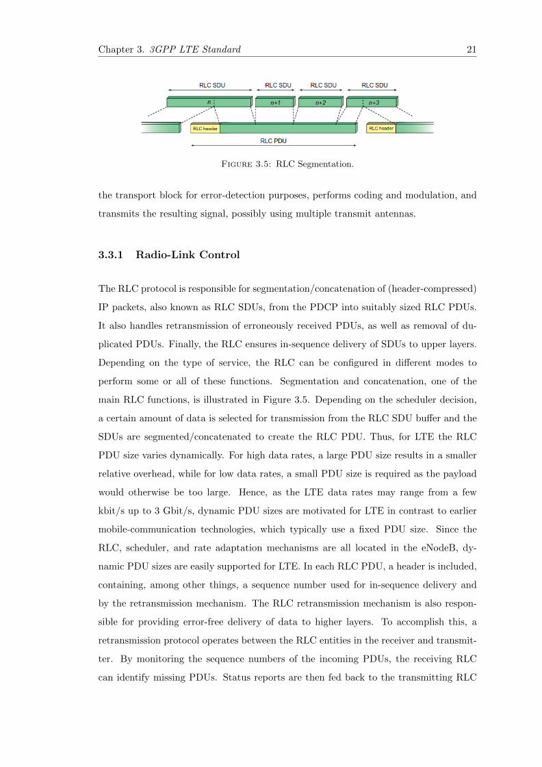
Figure 3.5: RLC Segmentation.
the transport block for error-detection purposes, performs coding and modulation, and
transmits the resulting signal, possibly using multiple transmit antennas.
3.3.1 Radio-Link Control
The RLC protocol is responsible for segmentation/concatenation of (header-compressed)
IP packets, also known as RLC SDUs, from the PDCP into suitably sized RLC PDUs.
It also handles retransmission of erroneously received PDUs, as well as removal of du-
plicated PDUs. Finally, the RLC ensures in-sequence delivery of SDUs to upper layers.
Depending on the type of service, the RLC can be configured in different modes to
perform some or all of these functions. Segmentation and concatenation, one of the
main RLC functions, is illustrated in Figure 3.5. Depending on the scheduler decision,
a certain amount of data is selected for transmission from the RLC SDU buffer and the
SDUs are segmented/concatenated to create the RLC PDU. Thus, for LTE the RLC
PDU size varies dynamically. For high data rates, a large PDU size results in a smaller
relative overhead, while for low data rates, a small PDU size is required as the payload
would otherwise be too large. Hence, as the LTE data rates may range from a few
kbit/s up to 3 Gbit/s, dynamic PDU sizes are motivated for LTE in contrast to earlier
mobile-communication technologies, which typically use a fixed PDU size. Since the
RLC, scheduler, and rate adaptation mechanisms are all located in the eNodeB, dy-
namic PDU sizes are easily supported for LTE. In each RLC PDU, a header is included,
containing, among other things, a sequence number used for in-sequence delivery and
by the retransmission mechanism. The RLC retransmission mechanism is also respon-
sible for providing error-free delivery of data to higher layers. To accomplish this, a
retransmission protocol operates between the RLC entities in the receiver and transmit-
ter. By monitoring the sequence numbers of the incoming PDUs, the receiving RLC
can identify missing PDUs. Status reports are then fed back to the transmitting RLC

Chapter 3. 3GPP LTE Standard 22
entity, requesting retransmission of missing PDUs. Based on the received status report,
the RLC entity at the transmitter can take the appropriate action and retransmit the
missing PDUs if needed. Although the RLC is capable of handling transmission errors
due to noise, unpredictable channel variations, etc., error-free delivery is in most cases
handled by the MAC-based hybrid-ARQ protocol.
3.3.2 Medium-Access Control
The MAC layer handles logical-channel multiplexing, hybrid-ARQ retransmissions, and
uplink and downlink scheduling. It is also responsible for multiplexing/demultiplexing
data across multiple component carriers when carrier aggregation is used.
3.3.3 Logical Channels and Transport Channels
The MAC provides services to the RLC in the form of logical channels. A logical channel
is defined by the type of information it carries and is generally classified as a control
channel, used for transmission of control and configuration information necessary for
operating an LTE system, or as a traffic channel, used for the user data. The set of
logical-channel types specified for LTE includes:
• The Broadcast Control Channel (BCCH), used for transmission of system infor-
mation from the network to all terminals in a cell. Prior to accessing the system,
a terminal needs to acquire the system information to find out how the system is
configured and, in general, how to behave properly within a cell.
• The Paging Control Channel (PCCH), used for paging of terminals whose location
on a cell level is not known to the network. The paging message therefore needs
to be transmitted in multiple cells.
• The Common Control Channel (CCCH), used for transmission of control infor-
mation in conjunction with random access.
• The Dedicated Control Channel (DCCH), used for transmission of control infor-
mation to/from a terminal. This channel is used for individual configuration of
terminals such as different handover messages.

Chapter 3. 3GPP LTE Standard 23
• The Multicast Control Channel (MCCH), used for transmission of control infor-
mation required for reception of the MTCH.
• The Dedicated Traffic Channel (DTCH), used for transmission of user data
to/from a terminal. This is the logical channel type used for transmission of
all uplink and non-MBSFN downlink user data.
• The Multicast Traffic Channel (MTCH).
From the physical layer, the MAC layer uses services in the form of transport channels.
A transport channel is defined by how and with what characteristics the information
is transmitted over the radio interface. Data on a transport channel is organized into
transport blocks. In each Transmission Time Interval (TTI), at most one transport
block of dynamic size is transmitted over the radio interface to/from a terminal in
the absence of spatial multiplexing. In the case of spatial multiplexing (MIMO), there
can be up to two transport blocks per TTI. Associated with each transport block is a
Transport Format (TF), specifying how the transport block is to be transmitted over
the radio interface. The transport format includes information about the transport-
block size, the modulation-and-coding scheme, and the antenna mapping. By varying
the transport format, the MAC layer can thus realize different data rates. Rate control
is therefore also known as transport-format selection. The following transport-channel
types are defined for LTE:
• The Broadcast Channel (BCH) has a fixed transport format, provided by the
specifications. It is used for transmission of parts of the BCCH system information,
more specifically the so-called Master Information Block (MIB).
• The Paging Channel (PCH) is used for transmission of paging information from
the PCCH logical channel. The PCH supports discontinuous reception (DRX) to
allow the terminal to save battery power by waking up to receive the PCH only at
predefined time instants.
• The Downlink Shared Channel (DL-SCH) is the main transport channel used
for transmission of downlink data in LTE. It supports key LTE features such
as dynamic rate adaptation and channeldependent scheduling in the time and
frequency domains, hybrid ARQ with soft combining, and spatial multiplexing. It

Chapter 3. 3GPP LTE Standard 24
Figure 3.6: Downlink channel mapping.
Figure 3.7: Uplink channel mapping.
also supports DRX to reduce terminal power consumption while still providing an
always-on experience. The DL-SCH is also used for transmission of the parts of
the BCCH system information not mapped to the BCH. There can be multiple
DL-SCHs in a cell, one per terminal scheduled in this TTI, and, in some subframes,
one DL-SCH carrying system information.
• The Multicast Channel (MCH).
• The Uplink Shared Channel (UL-SCH) is the uplink counterpart to the DL-SCH
that is, the uplink transport channel used for transmission of uplink data.
Part of the MAC functionality is multiplexing of different logical channels and mapping
of the logical channels to the appropriate transport channels. The supported mappings
between logical-channel types and transport-channel types are given in Figure 3.6 for
the downlink and Figure 3.7 for the uplink.

Chapter 3. 3GPP LTE Standard 25
Figure 3.8: Transport-format selection in downlink and uplink.
3.4 Scheduling
The purpose of the scheduler is to determine to/from which terminal(s) to transmit
data and on which set of resource blocks. The scheduler is a key element and to a
large degree determines the overall behavior of the system. The basic operation is so-
called dynamic scheduling, where the eNodeB in each 1 ms TTI transmits scheduling
information to the selected set of terminals, controlling the uplink and downlink trans-
mission activity. The scheduling decisions are transmitted on the PDCCHs. To reduce
the control signaling overhead, there is also the possibility of semi-persistent schedul-
ing. Semipersistent scheduling is only supported on the primary component carriers,
motivated by the fact that the main usage is for small payloads not requiring multiple
component carriers. The downlink scheduler is responsible for dynamically controlling
the terminal(s) to transmit to and, for each of these terminals, the set of resource blocks
upon which the terminal’s DL-SCH (or DL-SCHs in the case of carrier aggregation) is
transmitted. Transport-format selection (selection of transport-bock size, modulation-
and-coding scheme, resource-block allocation, and antenna mapping) for each component
carrier and logical channel multiplexing for downlink transmissions are controlled by the
eNodeB, as illustrated in the left part of Figure 3.8. The uplink scheduler serves a sim-
ilar purpose, namely to dynamically control which terminals are to transmit on their
UL-SCH (or UL-SCHs in the case of carrier aggregation) and on which uplink resources.
The uplink scheduler is in complete control of the transport format the terminal will
use, whereas the logical-channel multiplexing is controlled by the terminal according to
Chapter 3. 3GPP LTE Standard 26
a set of rules. Thus, uplink scheduling is per terminal and not per radio bearer. This
is illustrated in the right part of Figure 3.8, where the scheduler controls the transport
format and the terminal controls the logical-channel multiplexing.
3.4.1 Downlink Scheduling
The task of the downlink scheduler is to dynamically determine the terminal(s) to trans-
mit to and, for each of these terminals, the set of resource blocks upon which the ter-
minal’s DL-SCH should be transmitted. In most cases, a single terminal cannot use the
full capacity of the cell, for example due to lack of data. Also, as the channel properties
may vary in the frequency domain, it is useful to be able to transmit to different termi-
nals on different parts of the spectrum. Therefore, multiple terminals can be scheduled
in parallel in a subframe, in which case there is one DL-SCH per scheduled terminal
and component carrier, each dynamically mapped to a (unique) set of frequency re-
sources. The scheduler is in control of the instantaneous data rate used, and the RLC
segmentation and MAC multiplexing will therefore be affected by the scheduling deci-
sion. Although formally part of the MAC layer but to some extent better viewed as a
separate entity, the scheduler is thus controlling most of the functions in the eNodeB
associated with downlink data transmission:
• RLC. Segmentation/concatenation of RLC SDUs is directly related to the instan-
taneous data rate. For low data rates, it may only be possible to deliver a part of
an RLC SDU in a TTI, in which case segmentation is needed. Similarly, for high
data rates, multiple RLC SDUs may need to be concatenated to form a sufficiently
large transport block.
• MAC. Multiplexing of logical channels depends on the priorities between different
streams. For example, radio resource control signaling, such as handover com-
mands, typically has a higher priority than streaming data, which in turn has
higher priority than a background file transfer. Thus, depending on the data rate
and the amount of traffic of different priorities, the multiplexing of different logical
channels is affected. Hybrid-ARQ retransmissions also need to be accounted for.
• L1. Coding, modulation and, if applicable, the number of transmission layers and
the associated precoding matrix are obviously affected by the scheduling decision.

Chapter 3. 3GPP LTE Standard 27
The choices of these parameters are mainly determined by the radio conditions
and the selected data rate – that is, the transport block size.
The scheduling decision is communicated to each of the scheduled terminals through the
downlink L1/L2 control signaling using one PDCCH per downlink assignment. Each
terminal monitors a set of PDCCHs for downlink scheduling assignments. A scheduling
assignment is transmitted in the same subframe as the data. If a valid assignment
matching the identity of the terminal is found, then the terminal receives and processes
the transmitted signal as indicated in the assignment. Once the transport block is
successfully decoded, the terminal will demultiplex the received data into the appropriate
logical channels. The scheduling strategy is implementation specific and not part of the
3GPP specifications. However, the overall goal of most schedulers is to take advantage
of the channel variations between terminals and preferably to schedule transmissions to
a terminal when the channel conditions are advantageous. Most scheduling strategies
therefore need information about:
• channel conditions at the terminal;
• buffer status and priorities of the different data flows;
• the interference situation in neighboring cells (if some form of interference coordi-
nation is implemented).
Information about the channel conditions at the terminal can be obtained in several
ways. In principle, the eNodeB can use any information available, but typically the
channel-state reports from the terminal are used. However, additional sources of channel
knowledge, for example exploiting channel reciprocity to estimate the downlink quality
from uplink channel estimates in the case of TDD, can also be exploited by a particular
scheduler implementation.
3.4.2 Uplink Scheduling
The basic function of the uplink scheduler is similar to its downlink counterpart, namely
to dynamically determine, for each 1 ms interval, which terminals are to transmit and
on which uplink resources. As discussed before, the LTE uplink is primarily based

Chapter 3. 3GPP LTE Standard 28
on maintaining orthogonality between different uplink transmissions and the shared re-
source controlled by the eNodeB scheduler is time–frequency resource units. In addition
to assigning the time–frequency resources to the terminal, the eNodeB scheduler is also
responsible for controlling the transport format the terminal will use for each of the
uplink component carriers. As the scheduler knows the transport format the terminal
will use when it is transmitting, there is no need for outband control signaling from
the terminal to the eNodeB. This is beneficial from a coverage perspective, taking into
account that the cost per bit of transmitting outband control information can be signif-
icantly higher than the cost of data transmission, as the control signaling needs to be
received with higher reliability. It also allows the scheduler to tightly control the uplink
activity to maximize the resource usage compared to schemes where the terminal au-
tonomously selects the data rate, as autonomous schemes typically require some margin
in the scheduling decisions. A consequence of the scheduler being responsible for selec-
tion of the transport format is that accurate and detailed knowledge about the terminal
situation with respect to buffer status and power availability is more accentuated in LTE
compared to systems where the terminal autonomously controls the transmission param-
eters. The basis for uplink scheduling is scheduling grants, containing the scheduling
decision and providing the terminal information about the resources and the associated
transport format to use for transmission of the UL-SCH on one component carrier. Only
if the terminal has a valid grant is it allowed to transmit on the corresponding UL-SCH;
autonomous transmissions are not possible without a corresponding grant. Dynamic
grants are valid for one subframe – that is, for each subframe in which the terminal is to
transmit on the UL-SCH, the scheduler issues a new grant. Uplink component carriers
are scheduled independently; if the terminal is to transmit simultaneously on multiple
component carriers, multiple scheduling grants are needed. The terminal monitors a set
of PDCCHs for uplink scheduling grants. Upon detection of a valid uplink grant, the
terminal will transmit its UL-SCH according to the information in the grant. Obviously,
the grant cannot relate to the same subframe it was received in as the uplink subframe
has already started when the terminal has decoded the grant. The terminal also needs
some time to prepare the data to transmit. Therefore, a grant received in subframe n
affects the uplink transmission in a later subframe. Similarly to the downlink case, the
uplink scheduler can exploit information about channel conditions, buffer status, and
priorities of the different data flows, and, if some form of interference coordination is

Chapter 3. 3GPP LTE Standard 29
employed, the interference situation in neighboring cells. Channel-dependent scheduling,
which typically is used for the downlink, can be used for the uplink as well.
3.4.3 Channel-State Reporting
As mentioned several times, the possibility for downlink channel-dependent scheduling
– that is, selecting the downlink transmission configuration and related parameters de-
pending on the instantaneous downlink channel conditions – is a key feature of LTE. An
important part of the support for downlink channel-dependent scheduling is channel-
state reports provided by terminals to the network, reports on which the latter can base
its scheduling decisions. The channel-state reports consist of one or several pieces of
information:
• Rank indication (RI), providing a recommendation on the transmission rank to use
or, expressed differently, the number of layers that should preferably be used for
downlink transmission to the terminal. RI only needs to be reported by terminals
that are configured to be in one of the spatial multiplexing transmission modes.
There is at most one RI reported, valid across the full bandwidth- that is, the
RI is frequency non-selective. Frequency-dependent transmission rank would be
impossible to utilize since all layers are transmitted on the same set of resource
blocks in LTE.
• Precoder matrix indication (PMI), indicating which of the precoder matrices should
preferably be used for the downlink transmission. The reported precoder matrix
is determined assuming the number of layers indicated by the RI. The precoder
recommendation may be frequency selective, implying that the terminal may rec-
ommend different precoders for different parts of the downlink spectrum. Further-
more, the network can restrict the set of matrices from which the terminal should
select the recommended precoder, so-called codebook subset restriction, to avoid
reporting precoders that are not useful in the antenna setup used.
• Channel-quality indication (CQI), representing the highest modulation-and-coding
scheme that, if used, would mean PDSCCH transmissions (using the recommended
RI and PMI) were received with a block-error rate of at most 10%. The reason to
use CQI as a feedback quantity instead of, for example, the signal-to-noise ratio,

Chapter 3. 3GPP LTE Standard 30
is to account for different receiver implementation in the terminal. Also, basing
the feedback reports on CQI instead of signal-to-noise ratio also simplifies the
testing of terminals; a terminal delivering data with more than 10% block-error
probability when using the modulation-and-coding scheme indicated by the CQI
would fail the test. As will be discussed further below, multiple CQI reports, each
representing the channel quality in a certain part of the downlink spectrum, can
be part of a channel-state report.
Together, a combination of the RI, PMI, and CQI forms a channel-state report.
3.5 HYBRID ARQ WITH SOFT COMBINING
The hybrid-ARQ functionality spans both the physical layer and the MAC layer; gener-
ation of different redundancy versions at the transmitter as well as the soft combining
at the receiver are handled by the physical layer, while the hybrid-ARQ protocol is part
of the MAC layer. In the presence of carrier aggregation, there is, as already stated, one
independent hybrid-ARQ entity per component carrier and terminal. Unless otherwise
noted, the description below holds for one component carrier – that is, the description
is on a per-component carrier basis. The basis for the LTE hybrid-ARQ mechanism is
a structure with multiple stop-and-wait protocols, each operating on a single transport
block. In a stop-and-wait protocol, the transmitter stops and waits for an acknowledge-
ment after each transmitted transport block. This is a simple scheme; the only feedback
required is a single bit indicating positive or negative acknowledgement of the transport
block. However, since the transmitter stops after each transmission, the throughput
is also low. LTE, as illustated in Figure 3.9 , therefore applies multiple stop-and-wait
processes operating in parallel such that, while waiting for acknowledgement from one
process, the transmitter can transmit data to another hybrid-ARQ process. Upon receiv-
ing a transport block for a certain hybrid-ARQ process, the receiver makes an attempt
to decode the transport block and informs the transmitter about the outcome through
a hybrid-ARQ acknowledgement, indicating whether the transport block was correctly
decoded or not. The time from reception of data until transmission of the hybrid-ARQ
acknowledgement is fixed, hence the transmitter knows from the timing relation which
hybrid-ARQ process a received acknowledgement relates to. This is beneficial from an

Chapter 3. 3GPP LTE Standard 31
Figure 3.9: Multiple parallel hybrid-ARQ processes forming one hybrid-ARQ entity.
overhead perspective as there is no need to signal the process number along with the
acknowledgement. An important part of the hybrid-ARQ mechanism is the use of soft
combining, which implies that the receiver combines the received signal from multiple
transmission attempts.
3.6 Physical Layer Organizzation
OFDM is the basic transmission scheme for both the downlink and uplink transmission
directions in LTE although, for the uplink. The LTE OFDM subcarrier spacing equals
15 kHz for both downlink and uplink. The selection of the subcarrier spacing in an
OFDM-based system needs to carefully balance overhead from the cyclic prefix against
sensitivity to Doppler spread/shift and other types of frequency errors and inaccuracies.
The choice of 15 kHz for the LTE subcarrier spacing was found to offer a good balance
between these two constraints. Assuming an FFT-based transmitter/receiver implemen-
tation, 15 kHz subcarrier spacing corresponds to a sampling rate fs = 15000 ∗NFFT ,
where NFFT is the FFT size. It is important to understand though that the LTE
specifications do not in any way mandate the use of FFT-based transmitter/ receiver
implementations and even less so a particular FFT size or sampling rate. Nevertheless,
FFT-based implementations of OFDM are common practice and an FFT size of 2048,
with a corresponding sampling rate of 30.72 MHz, is suitable for the wider LTE carrier
bandwidths, such as bandwidths of the order of 15 MHz and above. However, for smaller
carrier bandwidths, a smaller FFT size and a correspondingly lower sampling rate can
very well be used. The sampling rate above illustrates another factor influencing the
choice of the LTE subcarrier spacing, namely a desire to simplify implementation of

Chapter 3. 3GPP LTE Standard 32
dual-mode LTE/HSPA terminals. Assuming a power-of-two FFT size and a subcarrier
spacing of 15 kHz, the sampling rate ∆f ∗ NFFT will be a multiple or sub-multiple
of the HSPA chip rate of 3.84 Mchip/s. In the time domain, LTE transmissions are
organized into (radio) frames of length 10 ms, each of which is divided into ten equally
sized subframes of length 1 ms, as illustrated in Figure 3.10. Each subframe consists of
two equally sized slots of length Tslot = 0.5 ms, with each slot consisting of a number of
OFDM symbols including cyclic prefix. On a higher level, each frame is identified by a
System Frame Number (SFN). The SFN is used to control different transmission cycles
that may have a period longer than one frame, such as paging sleep-mode cycles and
periods for channel-status reporting. The SFN period equals 1024, thus the SFN repeats
itself after 1024 frames or roughly 10 seconds. LTE defines two cyclic-prefix lengths, the
normal cyclic prefix and an extended cyclic prefix, corresponding to seven and six OFDM
symbols per slot respectively. In particular a longer cyclic prefix, although less efficient
from a cyclic-prefix-overhead point of view, may be beneficial in specific environments
with extensive delay spread, for example in very large cells. It is important to have
in mind, though, that a longer cyclic prefix is not necessarily beneficial in the case of
large cells, even if the delay spread is very extensive in such cases. If, in large cells, link
performance is limited by noise rather than by signal corruption due to residual time
dispersion not covered by the cyclic prefix, the additional robustness to radio-channel
time dispersion, due to the use of a longer cyclic prefix, may not justify the correspond-
ing additional energy overhead of a longer cyclic prefix. The overall Time organizzation
is illustrated in Figure 3.10. A resource element, consisting of one subcarrier during one
OFDM symbol, is the smallest physical resource in LTE. Furthermore, as illustrated in
Figure 3.11, resource elements are grouped into resource blocks, where each resource
block consists of 12 consecutive subcarriers in the frequency domain and one 0.5 ms
slot in the time domain. Each resource block thus consists of 7 ∗ 12 = 84 resource el-
ements in the case of a normal cyclic prefix and 6 ∗ 12 = 72 resource elements in the
case of an extended cyclic prefix. Although resource blocks are defined over one slot, the
basic time-domain unit for dynamic scheduling in LTE is one subframe, consisting of
two consecutive slots. The minimum scheduling unit, consisting of two time-consecutive
resource blocks within one subframe (one resource block per slot), can be referred to as
a resource-block pair. The LTE physical-layer specification allows for a carrier to consist
of any number of resource blocks in the frequency domain, ranging from a minimum of
six resource blocks up to a maximum of 110 resource blocks. This corresponds to an

Chapter 3. 3GPP LTE Standard 33
Figure 3.10: LTE time-domain structure.
Figure 3.11: The LTE physical time–frequency resource.
overall transmission bandwidth ranging from roughly 1 MHz up to in the order of 20
MHz with very fine granularity and thus allows for a very high degree of LTE bandwidth
flexibility, at least from a physical-layer-specification point of view. The resource-block
definition above applies to both the downlink and uplink transmission directions. How-
ever, there is a minor difference between the downlink and uplink in terms of where the
carrier center frequency is located in relation to the subcarriers.


Chapter 4
Analysis of MAC-level
Throughput in LTE Systems
4.1 Introduction
As mentioned in Chapter 3 3GPP-LTE is the emerging standard for future 4G cellular
systems. To achieve high throughput performance, in addition to an advanced physical
layer design, LTE exploits a combination of sophisticated radio resource management
functionalities, such as Channel Quality Indicator (CQI) reporting, link rate adaptation
through Adaptive Modulation and Coding (AMC), and Hybrid Automatic Retransmis-
sion Request (HARQ) [5]. Specifically, a base station (eNB) can simultaneously serve
multiple users on orthogonal subcarriers that are grouped into frequency resource blocks
(RBs). Then, each user (UE) periodically measures channel state information that is
fed back to the eNB in terms of CQI reports. Typically, only aggregate CQI values are
reported to reduce channel feedback information. CQI measurements are used by eNBs
for scheduling and link rate adaptation on the downlink [51]. For instance, the modula-
tion and coding scheme (MCS) is typically selected in order to maximise the data rate to
the scheduled UE subject to a constraint on the error probability. Errors at the physical
layer are also mitigated by exploiting automatic retransmission protocols with channel
coding (HARQ). More precisely, HARQ procedures use the classical stop-and-wait algo-
rithm, in which the eNB decides to perform a retransmission based on the exchange of
ACK/NACK messages with the UE. Then, UEs try to decode the packet by combining
35

Chapter 4. Analysis of MAC-level Throughput in LTE Systems 36
the retransmitted copies. Since user, cell and radio link throughputs are among the most
important performance indicators that the operators adopt to assess the QoS in an LTE
system [52], an extensive literature exists that investigates LTE throughput performance
based on analytical models [28, 29, 31], simulation tools [51] or field tests [53, 54]. How-
ever, it is evident that a complex interplay exists among the various mechanisms that
operate at the MAC layer to improve communication reliability and to increase data
rates. This makes accurate LTE throughput analysis notably difficult. Thus, most stud-
ies limit the analysis only to the radio link throughput or consider single MAC functions
in isolation [8]. Furthermore, simplified error models are typically considered that only
allow deriving upper bounds for the LTE throughput [28]. This Chapter illustrates a
unified modelling framework of the MAC-level downlink throughput [55] that is valid
for homogeneous cells [6] and Rayleigh-distributed fading. This model simultaneously
caters for CQI feedback schemes that use spectral efficiency to generate CQI, as well as
AMC and HARQ protocols. Furthermore, we include in the analysis an accurate link
layer abstraction model that uses the Mean Mutual Information per coded Bit (MMIB)
metric to derive the physical error probability [7]. The throughput estimates of our
model are accurate, as validated using the ns-3 simulator extended with the LENA
module for LTE1. Furthermore, the results confirm that the IR-HARQ mechanism is
very effective in improving error correction. However, the effectiveness of the IR-HARQ
scheme depends on the appropriate selection of the modulation and coding scheme of
the first transmission attempt.
4.2 LTE MAC Protocol Specification
Now a briefly describe relevant details of the LTE MAC for downlink transmissions,
with special attention to frame structure, CQI feedback mechanisms and HARQ pro-
tocols. We also introduce the system model and notation, and we discuss the main
assumptions that underlay our analysis. More details can be found in Chapter 3. In
the downlink, LTE uses the Orthogonal Frequency Division Multiple Access (OFDMA)
scheme. Specifically, in the frequency domain the system bandwidth, W , is divided into
several orthogonal subcarriers. Each subcarrier has a bandwidth of 15 kHz. In the time
domain, the duration of one LTE radio frame is 10 ms. One frame is divided into ten
1http://networks.cttc.es/mobile-networks/software-tools/lena/

Chapter 4. Analysis of MAC-level Throughput in LTE Systems 37
transmission time intervals (TTIs) of 1 ms each. Furthermore, each TTI consists of two
0.5 ms slots. Each slot contains either six or seven OFDM symbols, depending on the
Cyclic Prefix (CP) length. A set of twelve consecutive subcarriers over the duration of
one slot is called a physical Resource Block (RB). Hereafter, we denote with q the total
number of RBs available over the system bandwidth. Since the RB bandwidth is only
180 kHz, it is reasonable to assume that the channel response is frequency-flat across
all the twelve subcarriers of the RB2. Then, let us denote with γi,k the SNR of the ith
RB of the kth UE. Clearly, the statistics of the SNR depend on the channel model and
the multi-antenna diversity mode of operation. As commonly adopted in other LTE
models, e.g. [29], in this study we assume that the fading from the eNB to the UEs is
Rayleigh distributed. This implies that the SNR of each RB is an exponential random
variable (RV) [56]. Furthermore, we also assume an homogeneous cell model [6], i.e. the
SNR is independent for different users and RBs. This also means that the SNRs of all
RBs are uncorrelated in frequency and space, and γi,k can be regarded as independent
and identically distributed (i.i.d.) RV. Popular methods (e.g., EESM and MIESM) that
are typically used in LTE to compute CQI values rely on the concept of effective SNR.
Basically, the UEs map the SNRs of multiple subcarriers/RBs into a single value by ap-
plying complex non-linear transformations. Then, the effective SINR is used to estimate
the BLER experienced by a user and to determine the appropriate MCS, i.e. the MCS
that allows the UE to decode the transport block with an error rate probability not
exceeding 10%. However, the statistics of the effective SNR generated by EESM and
MIESM techniques are not known in closed-form. Thus, they must be approximated or
computed numerically, which makes performance analysis difficult [29, 57]. An alterna-
tive approach proposed in [58] to implement AMC capabilities is based on the spectral
efficiency. Specifically, let us denote the with ηi,k the spectral efficiency of the ith RB
of the kth UE. Then, it holds that [59]
ηi,k=log2
(1 +
γi,kΓ
), (4.1)
where Γ = − ln(5β)/1.5 and β is BLER upper bound. Now a static mapping can be
determined between the spectral efficiency and the CQI index, as well as between the
CQI index and the MCS value [58]. More formally, let us denote with Ci,k the CQI
index for the ith RB of the kth UE. Typically the value of CQI can range between 1
2This assumption will hold for highly dispersive channels with a long delay spread.

Chapter 4. Analysis of MAC-level Throughput in LTE Systems 38
B bits
data bits CRC bits
B >
Z
se
gm
en
tatio
n
24 CRC bits Filler (zero) bits
C o
utp
ut
blo
ck
s
Figure 4.1: Transport block segmentation.
and L. Then, Ci,k = j (j = 0, . . . , L) if Sj ≤ ηi,k ≤ Sj+1, with S0 = 0 and SL+1 = ∞.
In other words the CQI value is a quantised version of the spectral efficiency3. Closely
related to the MCS selection is also the transport block (TB) size determination. More
precisely, let nk the number of RBs allocated to the kth UE during a frame. Then, the
number B of bits that can be delivered in those RBs, which is called transport block, is
a function of the MCS index4. Furthermore, if B > Z (with Z = 6144 bits in 3GPP-
LTE) the transport block is segmented into a number C of code blocks (CBs) that are
independently encoded. Note that the CB size highly impacts the actual BLER perfor-
mance for a given MCS [7]. Figure 4.1 exemplifies the transport block segmentation.
Regarding the HARQ protocol, LTE employs two types of HARQ schemes. In HARQ
type-I, each encoded data frame is retransmitted until the frame passes the CRC test
or the maximum number of retransmissions is reached. Erroneous frames are simply
discarded. In contrast, in HARQ type-II, each transmission contains incremental re-
dundancy (IR) about the data frame. Thus, consecutive transmissions can be combined
at the receiver to improve error correction. Although our model is valid for all HARQ
types, in the following we only consider HARQ type-II that is the most widely used in
LTE. Note that in LTE systems retransmissions typically use the same MCS index as the
initial transmission. It is also important to point out that the transmission of HARQ
feedbacks (i.e. ACK/NACK messages) is not instantaneous but each received packet
experiences a processing delay. According to the LTE standard, the processing delay at
the receiver is about 3 ms. Thus, assuming the same delay to process data transmissions
3Note that in the 3GPP-LTE standard, L = 16 and the Sj thresholds are specified in Table 7.2.3-1of [60]. Furthermore, in the 3GPP-LTE standard the available MCS indexes are 32 but a 4-bit CQIallows selecting only 15 MCS (for CQI=0 no transmission will be scheduled). Thus, in practical LTEsystems only a subset of available MCS is typically used.
4See Table 7.1.7.2.1-1 of [60] for the static mapping between TB size, MCS and number of RBsallocated to the UE.

Chapter 4. Analysis of MAC-level Throughput in LTE Systems 39
HARQ RTT ( )
processing delay (data)
processing delay (ACK/NACK)
Data received
ACK/NACK received
TTI
#0 #1 #2 #3 #4 #5 #6 #7
τARQ
#0 eNB
UE
Figure 4.2: HARQ processes and timing in FDD-LTE DL.
and ACK/NACK messages, the HARQ round trip time, say τARQ, is 7 TTIs, as shown
in Figure 4.2. For this reason, an eNB must support up to 8 parallel HARQ processes
for each UE to enable uninterrupted communications. In this way, an eNB can continue
to transmit new TBs while the UEs are decoding already received TBs.
4.3 MAC-level Throughput Analysis
In this section we develop the mathematical model of the MAC-level downlink through-
put for a single LTE cell with n randomly deployed UEs. Without loss of generality
we assume asymptotic traffic conditions, i.e., infinite traffic is waiting for each user at
the transmission buffer of the eNB. As discussed in Section 4.2, the packet scheduler at
the eNB is responsible for both allocating RBs to UEs every TTI, and controlling up to
8 HARQ processes per UE. Intuitively, the maximum number of HARQ processes that
can be concurrently activated by the scheduler during an HARQ period is bounded by
the number of times the same UE is scheduled during a τarq time interval. For the sake
of simplicity, in this study we consider a Round Robin (RR) scheduler, which works
by dividing the total amount of available radio resources in a fair manner among the
UEs. More precisely, a RR scheduler allocates to each UE a set of consecutive resource
blocks, called resource block groups (RBGs), whose size P depends on the system band-
width [60]. Consequently the number b of RBs assigned to each UE is simply given
by
b=maxP,⌊ qn
⌋. (4.2)
Without loss of generality we consider a non-adaptive HARQ strategy, in which the
scheduler maintains the same RBG and MCS configuration of the original TB when

Chapter 4. Analysis of MAC-level Throughput in LTE Systems 40
1
2
3
4
5
6
7
8
1
2
3
4
5
6
7
8
1
2
3
4
5
6
7
8
1
2
3
4
5
6
7
8
1
2
3
4
5
6
7
8
1
2
3
4
5
6
7
8
q RBs
(1+τARQ)TTIs
RBG = 2 RBs
Figure 4.3: RR operations with q = 12, P = 2 and n = 8.
scheduling the retransmissions. To illustrate the dependency between the number of
times a UE is scheduled during an HARQ period, the RBG size and the total number
of UEs in Figure 4.3 we exemplify the scheduling decisions that are cyclically performed
by the RR scheduler during an HARQ period with q = 12, P = 2 and n = 8. As shown
in the figure, each UE is scheduled six times during an HARQ period. In general, the
average number of times each UE is scheduled in (1 + τARQ) TTIs is simply given by
nRR =
⌊q(1 + τARQ)
n · b
⌋. (4.3)
It must be noted that not all the transmission opportunities allocated by the eNB to
an UE result into a successful transmission due to signal attenuation, shadowing and
fading. In the following we denote with Pe(m, k, r) the TB error probability at the
r retransmission for the kth UE when m is the adopted MCS, with Ps(m, k, r) the
probability that the kth UE correctly decodes a TB after r retransmissions when m is
the adopted MCS, and with Pd(m, k) the probability that the kth UE discards a packet
when m is the adopted MCS because it has reached the maximum number of failed
retransmissions. In Section 4.3.2 we provide closed-form expressions for Ps(m, k, r),
Pe(m, k, r) and Pd(m, k). Finally, to perform the throughput analysis we observe the
system at the end of each successful transmission, because all the processes that define
the occupancy pattern of the channel (i.e., HARQ processing delays and retransmissions)
regenerate with respect to the sequence of time instants corresponding to the completion
of a successful transmission. Then, it follows that the MAC-level throughput for the kth

Chapter 4. Analysis of MAC-level Throughput in LTE Systems 41
UE is
ρk=nRRE[TB|Succ]kE[TARQ]k
, (4.4)
where E[TB|Succ]k is the average number of information bits that are delivered with a
successful transmission of the kth UE, and E[TARQ]k is the average time needed by an
HARQ process to complete a successful transmission of the kth UE. In equation (4.4),
the multiplying factor nRR is used to take into account that nRR independent HARQ
processes run in parallel. The following theorem provides closed-form expressions for
E[TB]k and E[TARQ]k. where E[TB|Succ]k is the average number of information bits
that are delivered with a successful transmission of the kth UE, and E[TARQ]k is the
average time needed by an HARQ process to complete a successful transmission of the
kth UE. In equation (4.4), the multiplying factor nRR is used to take into account that
nRR independent HARQ processes run in parallel. The following theorem provides
closed-form expressions for E[TB]k and E[TARQ]k.
Theorem 1. By assuming an homogenous cell with Rayleigh-distributed fading, and a
RR scheduling policy
E[TB|Succ]k=
L∑j=0
TBS(m(j), b) [1− Pd(m, k)] gk[j] , (4.5a)
E[TARQ]k =L∑j=0
[rmax∑r=0
(r + 1)(1 + τARQ)Ps(m, k, r)
]gk[j] , (4.5b)
where TBS(m(j), b) is a function that computes the number of data bits transmitted
in b RBs using the MCS m(j)5, and gk[j] is the PMF of the CQI value reported by the
kth UE.
Proof. See Appendix.
4.3.1 CQI feedback scheme and AMC strategy
The objective of this section is twofold. First, we develop the analytical tools to charac-
terise the wideband CQI feedback scheme of LTE. Second, we analyse the performance
of a link rate adaptation technique based on wideband CQI reports. Let us assume that
n UEs are randomly distributed in the cell, and let dk be the distance of the kth UE
5For the sake of notation brevity, we indicate with m(j) the MCS that the eNB uses when the CQIvalue reported by a UE is equal to j.

Chapter 4. Analysis of MAC-level Throughput in LTE Systems 42
from the eNB. As discussed in Section ?? we also assume that γi,k ∼ Exp(λk), where the
rate parameter λk of the exponential distribution depends on the UE position. Under
this assumption the statistics of the spectral efficiency for each RB can be expressed in
a closed-form as given by the following Theorem.
Theorem 2. If γi,k ∼ Exp(λk) then the cumulative distribution function (CDF) of the
spectral efficiency ηi,k in equation (4.1) is computed as:
Fη(x; i, k)=
1− e−λkΓ(2x−1) if x ≥ 0
0 if x < 0.
. (4.6)
Proof. See Appendix.
LTE specifies different types of CQI reporting: wideband and subband. Specifically,
the wideband CQI represents the SNR observed by the UE over the whole channel
bandwidth, while the subband CQI represents the SNR observed by the UE over a
collection of adjacent RBs. Note that a vector of CQI values should be transmitted
to the eNB when using the latter feedback scheme. Thus, the subband-level feedback
scheme ensures a finer reporting granularity but it also generates a higher overhead. In
this study, we focus on the wideband feedback scheme and we assume that the CQI
reported by the kth UE, say Ck is the arithmetic mean of the CQI values computed over
all RBs6. Then, we use the spectral efficiency to generate the CQI values from the SNR
measures of all RBs. The statistics of the wideband CQI are mathematically derived
below.
Claim 1. The probability mass function (PMF) of the CQI value for the ith RB assigned
to the kth UE is given by
gi,k[j] = Fη(Sj+1; i, k)− Fη(Sj ; i, k) . (4.7)
Proof. See Appendix.
Claim 2. In an homogenous cell the PMF of the wideband CQI value reported by the
kth UE is given by
gk[j] =
q(j+1)−1∑l=qj
g(q)k [l] , (4.8)
6Note that an alternative solution would be to report the worst CQI value over all (or a subset of)RBs as in [28].

Chapter 4. Analysis of MAC-level Throughput in LTE Systems 43
where g(q)k [l] is the q-fold convolution of gi,k[j].
Proof. See Appendix.
As described in Section 4.2 a static mapping is typically established between the CQI
value received at the eNB and the MCS for the downlink transmissions. Thus, gk[j] also
characterizes the distribution of the MCS index m(j) that is used by the eNB for the
downlink transmission to the kth UE when the reported wideband CQI is j.
4.3.2 Physical layer error model
We now conclude the analysis by introducing the physical layer error model. In this study
we adopt the general approach initially proposed in [61] to accurately approximate the
BLER curves of OFDMA-based wireless systems, and later specialised for the LTE case
in [62]. Specifically, we assume that the mutual information per coded bit (MIB) of
MCS m, as defined in [61], can be accurately approximated by a combination of Bessel
functions of the SNR γ as follows
Im(γ) ≈H∑h=1
αhJ(ψh√γ) , (4.9)
where H, αh and ψh parameters are empirically calibrated as a function of the MCS
index. Subsequently, the mean MIB (MMIB) value for each UE is computed by averaging
the corresponding mutual information of all RBs allocated to that UE. Specifically, let
Ω(k) be the set of RBs that are allocated to the kth UE by the scheduler. Then, the
MMIB value over the vector of SNR values for each RB assigned to the kth UE when m
is the adopted MCS is simply given by
Im,k=1
ω(k)
∑i∈Ω(k)
Im(γi,k) , (4.10)
where ω(k) is the cardinality of the Ω(k) set. The non-linear nature of (4.9) makes an
exact analysis difficult. Thus, previous studies limit the computational complexity of
deriving MMIB values in multi-user scenarios by considering a quantised version of the
Im(γ) function (4.9) in order to discretise the MIB metric [62]. More precisely, let us

Chapter 4. Analysis of MAC-level Throughput in LTE Systems 44
define a set Vm = µm[0], µm[1], . . . , µm[vm] for each MCS m such that
µm[v]=Im(Qm,v) , (4.11)
where (Qm,v+1 − Qm,v) = δγ is the quantisation step size, and Qm,0 is the minimum
usable SNR for MCS m. Now, let us denote with Hi,m,k the discrete MIB value for
the ith RB scheduled to the kth UE when m is the adopted MCS. Similarly to the
approach adopted for CQI mapping, we assume that Hi,m,k = µm[v] (v = 0, . . . , V ) if
Qm,v ≤ γi,k ≤ Qm,v+1. In other words the discrete MIB value is associated to a range
of SNRs. It is straightforward to derive the statistics of the discretised MIB metric as
follows.
Claim 3. In an homogenous cell with Rayleigh-distributed fading, the PMF of Hi,m,k is
given by
hi,m,k[v]=Fγ(Q(v+1),m; i, k)− Fγ(Qv,m; i, k) , (4.12)
where hi,m,k[v] = PrHi,m,k=µm[v].
Proof. See Appendix.
Similarly, we introduce a discrete MMIB metric, say Hm,k, computed over the set of
RBs allocated to the kth UE when m is the adopted MCS. In particular, Hm,k can be
obtained as the mean of the Hi,m,k values over the set Ω(k). Thus, the statistics of the
discretised MMIB value are derived using the same technique of Claim 2.
Claim 4. In an homogenous cell the PMF of Hm,k is given by
hm,k[v] ≈∑l∈Φv
h(ω(k))i,m,k [l] . (4.13)
where h(ω(k))i,m,k [l] is the ω(k)-fold convolution of hi,m,k[l]. The definition of the Φv set is
quite involved and is given in the proof.
Proof. See Appendix.
Once the MMIB value is given, a direct MMIB to BLER mapping can be used to obtain
the code block error rate, without necessarily defining an effective SINR. Following the

Chapter 4. Analysis of MAC-level Throughput in LTE Systems 45
approach proposed in [61], the empirical BLER curve for MCS m can be approximated
with a Gaussian cumulative model as follows
CBLERm(y, e)=1
2
[1− erf
(y − bece
)], (4.14)
where y is the MMIB value, while be and ce are parameters used to fit the Gaussian
distribution to the empirical BLER curve7. These parameters depend on the Effective
Code Rate (ECR), i.e. the ratio between the number of downlink information bits
(including CRC bits) and the number of coded bits. Intuitively, the ECR value is a
result of the selected TB size, MCS, and Ω(k). Then, the overall error probability for
a transport block transmitted as a combination of C code blocks, each one associated
with a MMIB and ECR value, can be computed as
TBLERm(y, e)=1−C∏i=1
(1− CBLERm(yi, ei)) . (4.15)
However equation (4.15) does not take into account the impact of an IR-HARQ mech-
anism that combines retransmissions to improve error correction. To generalise equa-
tion (4.15) for a system with incremental redundancy we adopt the same approach as
in [63]. In particular, we introduce an equivalent MMIB metric as the average of the
mutual informations per HARQ block received on the total number of retransmissions.
More precisely, let us assume that the original transport block has been retransmitted
r times. Then, let (I(0)m,k, I
(1)m,k, . . . , I
(r)m,k) be the vector of MMIB values for each of these
transmissions. The equivalent MMIB for the rth retransmission can be computed as
follows
Im,k,r=1
r + 1
r∑i=0
I(i)m,k , (4.16)
Then, the PMF of the equivalent MMIB value for the rth retransmission is h(r)m,k[v] =
PrIm,k,r=µm[v]. This PMF can be obtained using the same technique as in Claim 4
and it is not reported here for the sake of brevity. Similarly, we compute the effective
ECR after r retransmissions, say e(r), by dividing the number of information bit of the
original transmission with the sum of the number of coded bits of each retransmissions.
Finally, by applying the law of total probability the average TB error probability at the
7Empirical BLER curves can be obtained through field measurements or detailed link-level simula-tions.

Chapter 4. Analysis of MAC-level Throughput in LTE Systems 46
r retransmission for the kth UE when m is the adopted MCS can be computed as
Pe(m, k, r)=
vm∑v=0
TBLERm(µm[v], e(r)) · h(r)m,k[v] . (4.17)
Finally to evaluate Ps(m, k, r) we can observe that the rth retransmission of the kth
UE, when m is the adopted MCS, is a success only if the previous (r−1) transmissions
were TBs received erroneously and the rth transmission is correctly decoded. Hence, it
immediately follows that
Ps(m, k, r) =
[r−1∏i=0
Pe(m, k, i)
]× [1− Pe(m, k, r)] . (4.18)
We conclude this section by noting that the probability Pd(m, k) that the kth UE discards
a packet when m is the adopted MCS because it has reached the maximum number of
failed retransmissions is simply given by:
Pd(m, k) =
rmax∏i=0
Pe(m, k, i) . (4.19)
Finally, it is straightforward to observe that the average probability of discarding a
packet for the kth UE is computed as
Pd(k) =L∑j=0
Pd(m(j), k)gk[j] . (4.20)
4.4 Model Performance Evaluation
In this section we assess the accuracy of the throughput analysis in two different sce-
narios. In the first one, we assume that the mapping function that is used to convert
spectral efficiency into CQI feedbacks, and then into MCS indexes is sufficiently ac-
curate. As better explained in the following, in this condition error probabilities are
typically small and retransmissions may have a negligible impact on the MAC layer
throughput with respect to other protocol overheads. In the second scenario we assume
that a fixed CQI is fed back to the eNB by each UE. Thus, the eNB necessarily selects
a fixed MCS independently of the current channel conditions. This clearly represents a
worst-case scenario, which is useful to assess the robustness of our modelling framework
even when the reported CQI provides a very poor prediction of channel performance.

Chapter 4. Analysis of MAC-level Throughput in LTE Systems 47
Furthermore, it is also useful to better highlight the ability of the HARQ scheme to
improve the overall system throughput without relying on per-subcarrier information.
4.4.1 Simulation setup
All the following experiments have been carried out using the ns3 packet-level simula-
tor, which includes a detailed implementation of the LTE radio protocol stack. The
main simulation parameters are summarised in Table 4.1. Specifically, we consider an
Urban Macro scenario, in which path loss and shadowing are modelled according to
the COST231-Hata model [64], which is widely accepted in the 3GPP community. The
fading is Rayleigh distributed. To limit the computation complexity of the simulator
pre-calculated fading traces are included in the LTE model. Given the downlink sys-
tem bandwidth (see Table 4.1) a RBG comprises two RBs [60], i.e., P = 2. Regarding
the network topology, we considered a single cell with a varying number of static UEs,
chosen in the range [1, 50]. Note that, in our settings a maximum number of 96 (i.e.,
8bq/P c) unique UEs can be scheduled within an HARQ period. Indeed, if n > 96 the
RR period is longer than the HARQ period. All results presented in the following graphs
are averaged over multiple simulation runs with different fading traces and topology lay-
outs. Confidence intervals are generally very tight and they are not shown in the figures
if below 1%. Each simulation run lasts 300 seconds.
Table 4.1: Simulation parameters
Parameter Value
Carrier frequency (GHz) 2.14DL bandwidth (MHz) 5q 25eNB TX Power (dBm) 43CQI processing time (TTI) 2CQI transmission delay (TTI) 4Antenna scheme SISOPDCCH & PCFICH (control ch.) 3 OFDM symbolsPDSCH (data ch.) 11 OFDM symbolsn [10, 50]rmax 3
In this section we validate the accuracy of our modelling approach by evaluating the
throughput of an individual UE under varying channel conditions and congestion levels.
Specifically, we assume that n UEs are randomly deployed in a cell and they are static.

Chapter 4. Analysis of MAC-level Throughput in LTE Systems 48
1
10
100
1000
10000
0 200 400 600 800 1000 1200 1400 1600 1800 2000
DL
Th
rou
gh
pu
t [K
bit
/sec
]
Distance [m]
analysissimulation
n=12n=20n=50
Figure 4.4: Adaptive CQI : Comparison of analytical and simulation results for theMAC-level throughput of a tagged UE versus its distance from the eNB and the total
number of UEs in the cell.
Then, an additional tagged UE is deployed at a known distance d from the center of the
cell. Figure 4.4 shows a comparison between the model predictions and the simulation
results for the MAC-level downlink throughput of the tagged UE versus its distance from
the eNB and for different n values. As a first important consideration, Figure 4.4 proves
that our analysis provides a very accurate approximation of the MAC-level throughput
independently of the fading intensity. Furthermore, the results confirm that increasing
the total number of UEs in the cell has the effect of reducing in a proportional manner
the throughput of the tagged UE. This is due to the fact that RR is a channel-unaware
scheduler that performs fair sharing of time resources among UEs. Finally, it is also
important to point out that the IR-HARQ mechanism is very effective in improving
error correction. As discussed in Section 4.2 the modulation and coding scheme are
selected in such a way that the error probability is well below 10%. As a matter of
fact, our results (not shown here) indicate that the actual error probability for the first
transmission attempt is below 5% up to a distance of 1000 meters, and the probability
to perform more than one retransmission is negligible.

Chapter 4. Analysis of MAC-level Throughput in LTE Systems 49
4.4.2 Results with fixed CQI
In this second set of simulations we consider the same network scenario as in Section ??.
However, independently of the UE position the CQI feedback is assumed constant. Fig-
ure 4.5 shows a comparison between the model predictions and the simulation results
for the MAC-level downlink throughput of the tagged UE versus its distance from the
eNB when n = 12. Note that twelve is the maximum number of UEs such that nRR = 8.
In other words, with n = 12 all the UEs are scheduled during one TTI and 8 HARQ
process needs to be managed simultaneously. As expected a high value for the reported
CQI results into the use of a very efficient MCS, which provides a high data rate at
the cost of high vulnerability to channel fading. Consequently, the tagged UE obtains
a high throughput when close to the eNB, but the throughput performance rapidly de-
grades as it gets farther from the eNB. On the contrary a low reported CQI provides a
much more stable throughput performance due to the robustness of the selected MCS.
However, in this case we must compromise between robustness and efficiency. To quan-
tify this trade-off in Figure 4.6 we show the probability to discard a packet as given
by formula (4.20) in the same network configurations of Figure 4.5. Interestingly, we
can observe that there is a critical distance after which the Pd(k) probability rapidly
increases up to the value of one. Hence, after this critical distance even the IR-HARQ
scheme becomes incapable of controlling the error probability. Furthermore, results in
Figure 4.6(b) indicate that our model underestimates the actual Pd(k) for less reliable
MCSs, while results in Figure 4.6(a) indicate that our model overestimates the actual
Pd for robust MCS.
4.5 Summary
In this Chapter we have developed an analytical framework to estimate the MAC-level
downlink throughput in a LTE system, which carefully models practical mechanisms of
the MAC layer of the LTE technology. As a matter of fact, LTE systems achieve high
communication reliability by adopting a combination of link adaptation and error cor-
rection schemes. This study is a first attempt to tackle the complexity of modelling the
interplay between these mechanisms and to obtain a realistic evaluation of the through-
put performance at the MAC level. Our results confirm that the IR-HARQ mechanism is

Chapter 4. Analysis of MAC-level Throughput in LTE Systems 50
0
200
400
600
800
1000
1200
1400
1600
0 200 400 600 800 1000 1200 1400 1600 1800 2000
DL
Th
rou
gh
pu
t [K
bit
/sec
]
Distance [m]
analysissimulation
CQI=7CQI=15
Figure 4.5: Fixed CQI : comparison of analytical and simulation results for the MAC-level throughput of a tagged UE versus its distance from the eNB for different CQI
values and n = 12.
0
0.1
0.2
0.3
0.4
0.5
0.6
0.7
0.8
0.9
1
0 200 400 600 800 1000 1200 1400 1600 1800 2000
Pd(k
)
Distance [m]
analysissimulation
(a) CQI=7
0
0.2
0.4
0.6
0.8
1
0 200 400 600 800 1000 1200 1400 1600 1800 2000
Pd(k
)
Distance [m]
analysissimulation
(b) CQI=15
Figure 4.6: Fixed CQI: comparison of analytical and simulation results for the prob-ability of discarding a packet for a tagged UE versus its distance from the eNB for
different CQI values and n = 12.
very effective in improving error correction. However, the effectiveness of the IR-HARQ
scheme depends on the appropriate selection of the modulation and coding scheme of
the first transmission attempt. Although there is still the need for detailed system-level
simulations, we believe that the proposed analytical approach will be useful to an LTE
system designer for dimensioning the LTE system and configuring the optimal set of
radio MAC parameters.

Chapter 5
Robust Adaptive Modulation and
Coding (AMC) Selection
5.1 Introduction
Adaptive Modulation and Coding (AMC) in LTE networks is commonly employed to
improve system throughput by ensuring more reliable transmissions. In particular, adap-
tive modulation and coding (AMC) has been proposed for LTE, as well as many other
wireless communication systems, to increase channel throughput [65]. In general, AMC
techniques try to optimally select the channel coding and modulation scheme (MCS),
while fulfilling a certain Block Error Rate (BLER) constraint1 by taking into account
the current channel conditions and the receiver’s characteristics (e.g., antenna configu-
ration). For LTE downlink transmissions, traditional AMC schemes rely on the channel
quality indicator (CQI) feedbacks that are periodically reported by the user terminals
(UEs) to their base stations (eNBs) [66]. How CQI values should be computed by the
UE using channel state information (e.g., SINR measurements) is implementation de-
pendent. In practical implementations the UEs directly selects the MCS value that, if
used by the eNB under the measured channel conditions, would achieve the maximum
possible throughput by guaranteeing that the BLER is below 10%. This value is then
mapped onto a CQI value and fed back to the eNB (that translates it back into the
1The BLER for a certain user is defined as the ratio between the number of erroneous resource blocksand the total number of resource blocks received by that user. In the LTE standard it is mandated thatthe selected MCS ensures an average BLER under the measured channel conditions lower than 10% [66].
51

Chapter 5. Robust Adaptive Modulation and Coding (AMC) Selection 52
corresponding MCS value) [11, 67]. Therefore, the key focus of AMC algorithms is to
define how UEs can compute MCS values that satisfy the BLER requirements. Several
technical challenges have to be addressed to design efficient AMC solutions for LTE
systems. In particular, in practical LTE systems, the SINR values of multiple subcar-
riers are aggregated and translated into a one-dimensional link quality metric (LQM),
since the same MCS must be assigned to all subcarriers assigned to each UE. Popu-
lar methods that are used in LTE to obtain a single effective SINR from a vector of
physical-layer measurements related to subcarriers are the exponential effective SINR
mapping (EESM) [68] or the mean mutual information per coded bit (MMIB) [69]. Once
the LQM is found, AMC schemes typically exploit static mappings between these link
quality metrics and the BLER performance of each MCS to select the best MCS (in
terms of link throughput). In other words, for each MCS a range of LQM values is
associated via a look-up table, over which that MCS maximises link throughput. Ei-
ther link-level simulations or mathematical models can be used to generate such static
BLER curves under a specific channel model. Unfortunately, past research has shown
that it is difficult to derive accurate link performance predictors under realistic channel
assumptions [7, 9–11]. Furthermore, a simulation-based approach to derive the mapping
between LQM values and BLER performance is not scalable since it is not feasible to ex-
haustively analyse all possible channel types or several possible sets of parameters [12].
The second main problem with table-based AMC solutions is that a delay of several
transmission time intervals (TTIs) may exist between the time when a CQI report is
generated and the time when that CQI feedback is used for channel adaptation. This is
due to processing times but also to the need of increasing reporting frequency to reduce
signalling overheads. This mismatch between the current channel state and its CQI
representation, known as CQI ageing, can negatively affect the efficiency of AMC deci-
sions [13, 14]. To deal with the above issues, in this Chapter we illustate a new flexible
AMC framework, called RL-AMC [70], that autonomously and at run-time decides upon
the best MCS (in terms of maximum link-layer throughput) based on the knowledge of
the outcomes of previous AMC decisions. To this end we exploit reinforcement learning
techniques to allow each eNodeB to update its MCS selection rules taking into account
past observations of achieved link-layer throughputs. Specifically, the purpose of the
decision-making agent in our AMC scheme is to discover which is the correction factor
that should be applied to CQI feedbacks in order to guide the transmitters in select-
ing more efficient MCSs. An important feature of our proposed scheme is the use of a

Chapter 5. Robust Adaptive Modulation and Coding (AMC) Selection 53
low-dimensional state space, which ensures a robust and efficient learning even under
time-varying channel conditions and mobility. Through simulations in ns3 we show that
our AMC method can improve the LTE system throughput compared to other schemes
that use static mappings between SINR and MCS both under pedestrian and vehicular
network scenarios. Furthermore, our AMC is capable of discovering the best MCS even
if the CQI feedback provides a poor prediction of the channel performance.
5.2 AMC in LTE
For the sake of illustrative purposes, in Figure 5.1 we show a functional architecture
for a practical AMC scheme for LTE systems. At the receiver’s side, a first module is
responsible for processing the channel state information (e.g., per-subcarrier received
SINR values) to obtain a BLER estimation under the assumption of a specific channel
model. Specifically, the receiver maps the channel measurements into a single link quality
metric. Then, an offline look-up table is used to map this LQM to a BLER estimate
for each MCS. These BLER curves are used to find the highest-rate MCS index that
can satisfy a 10% BLER target. Finally, the selected MCS index is sent in the form
of a CQI feedback to the transmitter. Based on such CQI feedback the transmitter
performs resource scheduling and MCS selection. Most of existing research on AMC
schemes for LTE is focused on the problem of CQI calculation given a link quality
metric. As mentioned in Section 5.1 a popular and sufficiently accurate method for
LQM calculation is EESM. For instance, the authors in [8] study the MCS performance
under an AWGN channel. Accurate packet error prediction for link adaptation via a
Gaussian approximation of coding and decoding performance is proposed in [71]. A novel
LQM metric for link adaptation based on raw bit-error-rate, effective SINR and mutual
information is investigated in [72]. In [67] the authors proposed MCS selection based
on packet-level effective SINR estimates rather than block-level SINR values, and they
describe different averaging schemes to map BLER onto packet error rates. On the other
hand, the authors in [11, 29] develops statistical models of the EESM under different
channel models and use those models to analyse the throughput of EESM-based AMC
for various CQI feedback schemes. A second group paper studies channel predictors to
deal with the CQI ageing. The authors in [13] derive closed-form expressions for the
average throughput of an adaptive OFDMA system under the assumption of imperfect

Chapter 5. Robust Adaptive Modulation and Coding (AMC) Selection 54
BLER Estimation
MCS index Search
CSI
Receivers’ characteristics
CQI
Target
BLER
MAC Statistics
LQM
LQM/BLER mapping
Receiver
CQI /MCS mapping
Transmitter
MCStest
RB Allocation
Figure 5.1: AMC functional architecture.
CQI knowledge. The performance of different CQI predictors, such as Kalman filtering
or linear prediction with stochastic approximation, are evaluated in [14] and [73].
5.3 Background on Reinforcement Learning (RL)
Reinforcement Learning (RL) is a popular machine learning technique, which allows
an agent to automatically determine the optimal behaviour to achieve a specific goal
based on the positive or negative feedbacks it receives from the environment in which
it operates after taking an action from a known set of admissible actions [74]. Typi-
cally, reinforcement learning problems are instances of the more general class of Markov
Decision Processes (MDPs), which are formally defined through:
• a finite set S=s1, s2,. . ., sn of the n possible states in which the environment can be;
• a finite set A(t) = a1(t), a2(t),. . ., am(t) of the m admissible actions that the agent
may perform at time t;
• a transition matrix P over the space S. The element P (s, a, s′) of the matrix provides
the probability of making a transition to state s′∈S when taking action a∈A in state
s∈S;
• a reward function R that maps a state-action pair to a scalar value r, which represents
the immediate payoff of taking action a∈A in state s∈S.

Chapter 5. Robust Adaptive Modulation and Coding (AMC) Selection 55
The goal of a MDP is to find a policy π for the decision agent, i.e., a function that
specifies the action that the agent should choose when in state s ∈ S to maximise its
expected long-term reward. More formally, if an agent follows a policy π starting from
a certain state s at time t the policy value over an infinite time horizon, also called the
value-state function, is simply given by
V π(s) =
∞∑k=0
γkrt+k , (5.1)
where γ ∈ [0, 1] is a discount factor that weights future rewards. Then an optimal policy
π∗ is, by definition, the one that maximise the value-state function. As a consequence,
the policy that ensures the maximum possible expected reward, say V ∗(s), could be
obtained by solving an optimisation problem V ∗(s) = maxπ Vπ(s). If the transition
matrix is known such optimisation problem can be expressed using a system of nonlinear
equations by using techniques such as dynamic programming [74]. However, in most
practical conditions it is hard, if not even impossible, to acquire such complete knowledge
of the environment behaviour. In this case there are model-free learning methods that
continuously update the probabilities to perform an action in a certain state by exploiting
the observed rewards. Such methods adopt an alternative characterisation of policy
goodness based on the state-action value function, or Q-function. Formally, the function
Qπ(s, a) computes the expected reward of taking an action a in a starting state s and then
following the policy π hereafter. Owing to the Bellman’s optimality principle, it holds
that a greedy policy (i.e., a policy that at each state selects the action with the largest
Q-value) is the optimal policy. In other words, it holds that V ∗(s) = maxa∈AQ∗(s, a)
with Q∗(s, a) = maxπ Q(s, a). In this scheme we use a model-free solving technique for
reinforcement learning problems known as Q-learning [75], which constructs the optimal
policy by iteratively selecting the action with the highest value in each state. The core
of this algorithm is an iterative value update rule that each time the agent selects an
action and observes a reward makes a correction of the old Q-value for that state based
on the new information. This updating rule is given by:
Q(s, a) = Q(s, a) + α
[r(s, a) + γmax
a′Q(s′, a′)−Q(s, a)
], (5.2)
where α ∈ [0, 1] is the learning rate. Basically, the α parameter determines the weight
of the newly acquired information over state-action value information. In our AMC

Chapter 5. Robust Adaptive Modulation and Coding (AMC) Selection 56
framework we hev used α= 0.5. The advantage of Q-learning is that it is guaranteed
to converge to the optimal policy. On the negative side, the convergence speed may
be slow if the state space is large due to the exploration vs. exploitation dilemma [74].
Basically, when in state s the learning agent should exploit its accumulated knowledge
of the best policy to obtain high rewards, but it must also explore actions that it has not
selected before to find out a better strategy. To deal with this issue, various exploration
strategies have been proposed in the literature, ranging from simple greedy methods
to more sophisticated stochastic techniques, which assign a probabilistic value for each
action a in state s according to the current estimation of Q(s, a). In Section 5.4 we
discuss more in detail such exploration strategies.
5.4 An RL-based AMC Scheme (RL-AMC)
In order to apply the Q-learning approach to the MCS selection problem it is necessary
to define: i) the state space of the problem, ii) the feedbacks that the decision agent
receives from the LTE network, and iii) the admissible actions for the agent with the
action selection strategy. In our RL-based AMC framework, the problem state consists
of CQI feedbacks and their evolution trends. The reward is the instantaneous link
throughput obtained by a user after each transmission. Finally, an action is the selection
of a correction factor to be applied to each CQI feedback to identify the best MCS under
the current channel conditions. In the following, we describe in details the operations
of our proposed AMC algorithm. First of all, it is important to clarify that the AMC
decision agent interacts with the environment (i.e., the LTE network) at discrete time
instants, called epochs. At each epoch the agent receives some representation of the
LTE channel state and on that basis selects an action. In the subsequent epoch the
agent receives a reward, and finds itself in a new state. In our AMC framework we
assume that an epoch is the time when the UE receives a segment of data, either new
or retransmitted. Without loss of generality we also assume that the decision agent is
provided with a mapping rule that establishes a relationship between SINR values and
MCS indexes. Note that our solution is not restricted to any specific BLER models
but an initial MCS value is only needed to bootstrap the learning process and to reduce
the size of the state space. Thus, it is not necessary that this mapping is accurate nor
adjusted to the unique characteristics of each communication channel. In Section 6.3 we

Chapter 5. Robust Adaptive Modulation and Coding (AMC) Selection 57
will investigate the robustness of our AMC scheme to inaccurate CQI representation of
channel performance. Intuitively, a straightforward approach to define the state of the
MCS selection problem would be to use the SINR values of received segments of data2
as state variables, as in [35]. However, the SINR is a continuos variable and it should
be discretised to be compatible with a discrete MDP formulation. The main drawback
is that a fine discretisation leads to a large-dimensional state space, which increases
convergence and exploration times. To avoid this problem, we directly use CQI-based
metrics for the state representation. Specifically, we adopt a two-dimensional space
S = s1, s2 to characterise the LTE communication channel. The first state variable
represents the CQI value (called CQIm) that the UE should select using the internal look-
up table that associates BLER and MCS and received SINR. The second state variable
represents the ∆CQIm value, which is defined as the difference between the last two
consecutive CQIm estimates. In other words, ∆CQIm provides a rough indication of the
trend in channel quality evolution. For instance, ∆CQIm < 0 implies that the channel
quality is temporarily degrading. Since the objective of the MCS selection procedure
should be to maximise the link throughput it is a natural choice to define the reward
function as the instantaneous link-layer throughput achieved when taking action a (i.e.,
applying a correction factor to current CQI value taken from the mapping function)
when in state s (i.e., given the pair CQImt ,∆CQImt ). More precisely, we assume that
the reward value of an erroneous downlink transmission is null. On the other hand, the
reward for a successful downlink transmission is given by
R(st1 , at1) =TB
#TTIs in [t1, t2], (5.3)
where TB is the MAC transport block size (i.e., the number of useful bits that could be
carried in a certain number of RBs with a certain MCS), while the denominator is the
time between the time t1 when that segment of data was first scheduled and the time t2
when it was successfully received3. The core of the Q-learning algorithm is represented by
the set A of admissible actions. In our learning model we assume that an action consists
of applying a correction factor to the CQI value that is initially estimated by means of
2We recall that LTE physical layer relies on the concept of resource blocks. A segment of data ortransport block is basically a group of resource blocks with a common MCS that are allocated to a user.Typically, a packet coming from the upper layers of the protocol stack will be transmitted using multiplesegments of data.
3A segment of data that is discarded after a maximum number of retransmissions has also a nullreward.

Chapter 5. Robust Adaptive Modulation and Coding (AMC) Selection 58
the internal look-up table. As discussed above, the mapping relationship between SINR
values and MCS may be inaccurate and the correction factor allows the agent to identify
the best modulation and coding scheme (in the sense of maximising the link throughput)
for the given channel conditions. For instance, it may happen that the SINR-to-MCS
mapping is too conservative for the current channel conditions and an MCS with an
higher data rate can be used without violating the target BLER requirement. In this
case the correction factor should be positive. Furthermore, a correction factor is also
needed to compensate eventual errors due to CQI feedback delay. More formally, we
assume that an action taken by the AMC decision agent at time t is one possible choice
of an integer number in the set (−k, . . . ,−2,−1, 0, 1, 2, . . . k), that we denote as at in
the following. This index is added to the original CQIm value to compute the CQI to
be sent to the eNB, denoted as CQIf . The line of reasoning for this adjustment is as
follows. Let us assume that the agent state at time t is CQImt ,∆CQIt. We argue that
if ∆CQIt < 0 we should prefer conservative MCS selections (and thus use values of at
lower than 0) because the channel trend is negative, while if ∆CQIt ≥ 0 we can try to
use MCSs offering higher data rates (and thus positive values for at). Recalling that the
CQI is an integer between 0 and 15 [66], this can be expressed by writing that the CQI
feedback, say CQIft , that should be sent to the eNB by the UE to guide the selection of
the MCS index for downlink transmissions at next epoch t+1 should be
CQIft = max [0,min [CQImt + at, 15]] , (5.4)
where a ∈ [0, 1, 2, . . . k] if ∆CQIt ≥ 0 and a ∈ [−k, . . . ,−2,−1, 0] otherwise. Thus, the
set of admissible actions is different whether the channel-quality trend is negative or
non-negative. Before proceeding it is useful to point out that the choice of the k value
determines how aggressively we want to explore the problem state space. In general,
the selection of the k value could take into account the CQI difference statistics, i.e.,
to what extent a current CQI may be different from the reported CQI after a feedback
delay [10]. In Section 5.5.3 we will discuss this aspect more in detail. A very important
learning procedure is the action selection rule, i.e., the policy used to decide which
specific action to select in the set of admissible actions. As discussed in Section 5.3 there
is a tradeoff between exploitation (i.e., to select the action with the highest Q-value for
the current channel state) and exploration (i.e., to select an action randomly). The
simplest approach (called ε-greedy [74]) would be to use a fixed probability ε to decide

Chapter 5. Robust Adaptive Modulation and Coding (AMC) Selection 59
whether to exploit or explore. A more flexible policy (called softmax action-selection
rule [74]) is to assign a probability to each action, basing on the current Q-value for that
action. The most common softmax function used in reinforcement learning to convert
Q-values into action probabilities π(s, a) is the following [74]:
π(s, a) =eQ(s,a)/τ∑
a′∈ΩteQ(s,a′)/τ
, (5.5)
where Ωt is the set of admissible actions at time t. Note that for high τ values the
actions tend to be all (nearly) equiprobable. On the other hand, if τ → 0 the softmax
policy becomes the same as a merely greedy action selection. In our experiments we
have chosen τ=0.5.
5.5 Performance Evaluation
In this section, we assess the performance of our proposed RL-AMC scheme in two dif-
ferent scenarios. In the first one a fixed CQI is fed back to the eNB by each UE. Without
the use of reinforcement learning AMC necessarily selects a fixed MCS independently of
the current channel conditions. Then, we demonstrate that our RL-based AMC is able
to converge towards the best MCS even if the initial CQI estimate are totally wrong. In
the second scenario we compare RL-AMC against the solution described in [76], which
exploits spectral efficiency estimates to select MCS. Specifically, the spectral efficiency
of user i is approximated by log2(1 + γi/Γ), where γi is the effective SINR of user i and
Γ is a scaling factor. Then, the mapping defined in the LTE standard [77] is used to
convert spectral efficiency into MCS indexes and, then, into CQI feedbacks. In this case,
we show that our reinforcement learning algorithm is able to improve the accuracy of
the CQI mapping at run time.
5.5.1 Simulation setup
All the following experiments have been carried out using the ns3 packet-level simu-
lator, which includes a detailed implementation of the LTE radio protocol stack. As
propagation environment, we assume an Urban Macro scenario, where path loss and
shadowing are modelled according to the COST231-Hata model [64], which is widely

Chapter 5. Robust Adaptive Modulation and Coding (AMC) Selection 60
Table 5.1: Simulation parameters.
Parameter Value
Carrier frequency 2GHz
Bandwidth for downlink 5 MHz
eNB power transmission 43 dBm
Subcarrier for RB 12
SubFrame length 1 ms
Subcarrier spacing 15 KHz
Symbols for TTI 14
PDCCH & PCFICH (control ch.) 3 symbols
PDSCH (data ch.) 11 symbols
CQI reporting periodic wide-band
CQI processing time 2 TTIs
CQI transmission delay 4 TTIs
accepted in the 3GPP community. The fast fading model is implemented using the
Jakes model for Rayleigh fading [78]. To limit the computation complexity of the simu-
lator pre-calculated fading traces are included in the LTE model that are based on the
standard multipath delay profiles defined in [79]. In the following tests we have used
the Extended Typical Urban fading propagation model with pedestrian (3 km/h) and
vehicular (30 km/h) users’ speeds. The main LTE physical parameters are summarised
in Table 5.1. Regarding the network topology, the considered scenario is composed by
a single cell and a number of users, chosen in the range [10, 100], which move accord-
ing a Random Waypoint Model (RWM) [80] within the cell, if not otherwise stated. A
downlink flow, modelled with an infinite buffer source, is assumed to be active for each
UE. Finally, the eNode B adopts the resource allocation type 0, thus only allocating
resource block groups (RBGs) to scheduled UEs. Given the downlink system bandwidth
(see Table 5.1) a RBG comprises two RBs [66]. RBGs are assigned to UEs following a
Round Robin (RR) scheduler that divides equally the available RBGs to active flows.
Then, all the RBs in the allocated RBGs used the MCS index that is signalled in the
last received CQI feedback. Furthermore, the implemented version of RR algorithm is
not adaptive, which implies that it maintains the same RBGs and MCS index when
allocating retransmission attempts. All results presented in the following graphs are av-
eraged over five simulation runs with different network topologies. Confidence intervals
are very tight and are not shown in the figures. Each simulation run lasts 150 seconds.
5.5.2 Results for fixed CQI
In this first set of simulations we assume that ten UEs are randomly deployed in the cell
and they are static. Then an additional tagged user is moving with pedestrian speed

Chapter 5. Robust Adaptive Modulation and Coding (AMC) Selection 61
0
200
400
600
800
1000
1200
1400
1600
0 200 400 600 800 1000 1200 1400 1600
Thro
ughput
[Kb/s
]
distance [m]
(CQI=15)
(CQI=7)
Fixed CQIRL-AMC(15)RL-AMC(7)
Figure 5.2: Average throughput as a function of the distance of the tagged user fromthe eNB in a pedestrian scenario.
from the center of the cell to its boundaries. However, independently of the UE position
the CQI feedback is constant. Then, Figure 5.3 shows a comparison of the throughput
achieved by the tagged user with and without reinforcement learning. This is obviously
a limiting case which is analysed to assess the robustness of our RL-AMC scheme even
when CQI provides a very poor prediction of channel performance. As expected with
fixed MCS the user throughput is constant when the MCS is over provisioned, while
it rapidly goes to zero after a critical distance. On the contrary, our RL-AMC is able
to discover the correction factor that should be applied to the initial CQI to force the
selection of a more efficient MCS. In addition, the performance of RL-AMC are almost
independent of the initial CQI value. Note that in this case RL-AMC must explore the
full range of CQI values and we set k in (5.4) equal to 15.
5.5.3 Results with adaptive CQI
In the following experiments we assume that each UE implements the SINR to CQI
mapping described in [76]. First of all we consider the same network scenario as in Fig-
ure 5.2, i.e., ten static UEs randomly deployed and one tagged UE moving at pedestrian
speed. Then, Figure 5.3 shows a comparison of the throughput achieved by the tagged
user with both SE-AMC and RL-AMC schemes at different distances of the tagged UE

Chapter 5. Robust Adaptive Modulation and Coding (AMC) Selection 62
0
200
400
600
800
1000
1200
1400
1600
0 200 400 600 800 1000 1200 1400 1600
Thro
ughput
[Kb/s
]
distance [m]
SE-AMCRL-AMC
Figure 5.3: Average throughput as a function of the distance of the tagged user fromthe eNB in a pedestrian scenario.
from the eNB. We can observe that the MCS selection in SE-AMC is too conservative
and this results in a throughput loss. On the contrary, RL-AMC method is able to
discover the MCS configuration that can ensure a more efficient use of the available
channel resources. This is more evident at intermediate distances from the eNB when
short-term fading may lead to use more frequently low-rate MCSs. As shown in the fig-
ure, the throughput improvement varies between 20% and 55% in the range of distances
between 200 meters and 800 meters. In the second set of simulations we consider a more
dynamic environment in which there is an increasing number of UEs in the cell, and all
the UEs are moving according to RWM with speed 30 km/h and pause time equal to
5 seconds. Figure 5.4 shows a comparison of the aggregate cell throughput with both
SE-AMC and RL-AMC schemes as a function of the network congestion (i.e., number
of UEs). The results clearly indicate that the throughput improvement provided by
RL-AMC is almost independent of the number of UEs and it is about 10%. We can also
observe the the cell capacity initially increases when going from 10 to 20 UEs. This is
due to two main reasons. First, RR is able to allocate RBs in a more efficient way when
the number of UEs is higher. Second, the higher the number of UEs and the higher
the probability that one of the UEs is close to the eNB and it can use high data-rate
MCSs. To investigate more in depth the behaviour of the considered AMC schemes, in
Figure 5.5 we show the probability mass function of the number of retransmissions that
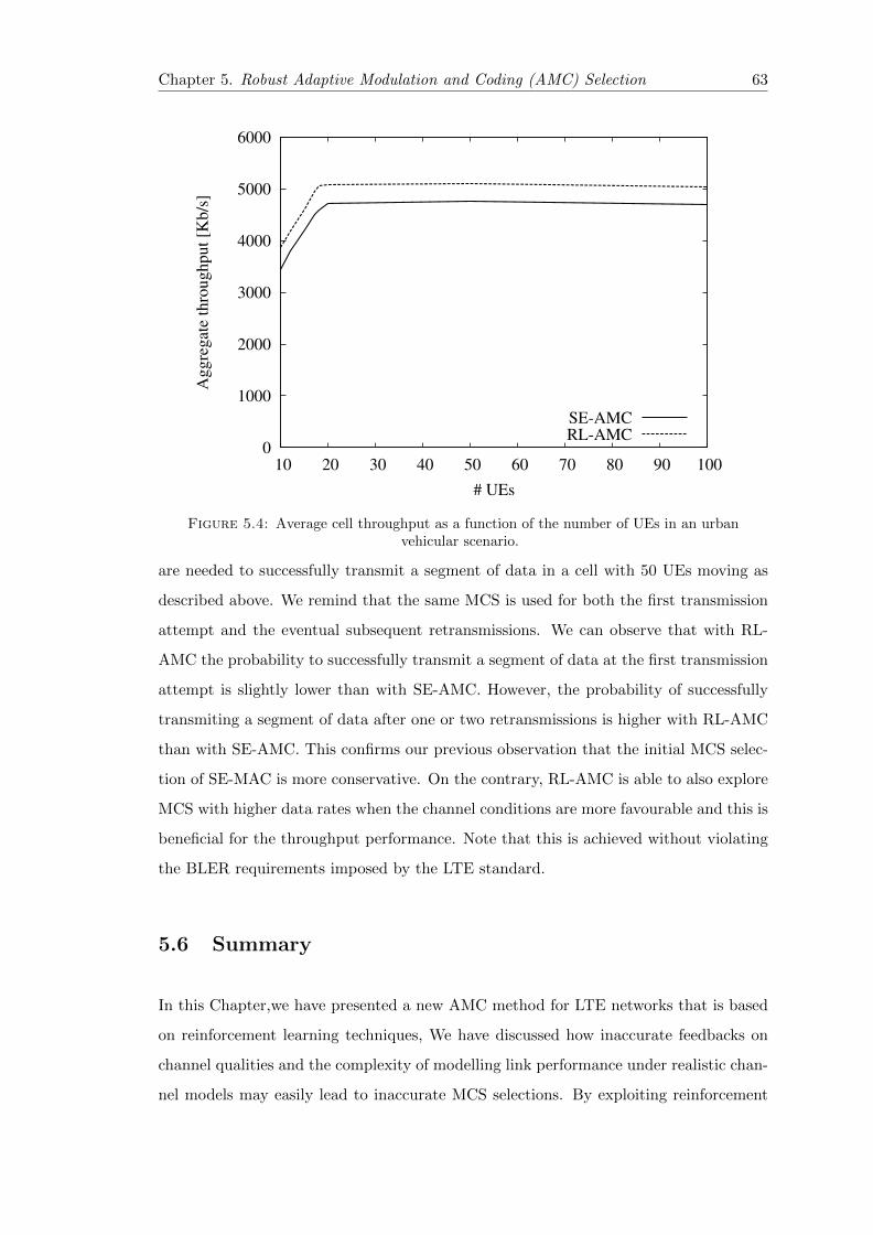
Chapter 5. Robust Adaptive Modulation and Coding (AMC) Selection 63
0
1000
2000
3000
4000
5000
6000
10 20 30 40 50 60 70 80 90 100
Aggre
gat
e th
roughput
[Kb/s
]
# UEs
SE-AMCRL-AMC
Figure 5.4: Average cell throughput as a function of the number of UEs in an urbanvehicular scenario.
are needed to successfully transmit a segment of data in a cell with 50 UEs moving as
described above. We remind that the same MCS is used for both the first transmission
attempt and the eventual subsequent retransmissions. We can observe that with RL-
AMC the probability to successfully transmit a segment of data at the first transmission
attempt is slightly lower than with SE-AMC. However, the probability of successfully
transmiting a segment of data after one or two retransmissions is higher with RL-AMC
than with SE-AMC. This confirms our previous observation that the initial MCS selec-
tion of SE-MAC is more conservative. On the contrary, RL-AMC is able to also explore
MCS with higher data rates when the channel conditions are more favourable and this is
beneficial for the throughput performance. Note that this is achieved without violating
the BLER requirements imposed by the LTE standard.
5.6 Summary
In this Chapter,we have presented a new AMC method for LTE networks that is based
on reinforcement learning techniques, We have discussed how inaccurate feedbacks on
channel qualities and the complexity of modelling link performance under realistic chan-
nel models may easily lead to inaccurate MCS selections. By exploiting reinforcement

Chapter 5. Robust Adaptive Modulation and Coding (AMC) Selection 64
0.001
0.01
0.1
1
0 1 2 3 4
PM
F
# retransmissions
SE-AMC
RL-AMC
Figure 5.5: Probability mass function of the number of retransmissions in an urbanvehicular scenario with 50 UEs.
learning, we can significantly reduce the impact of channel prediction errors on the per-
formance of link adaptation. As side effect has been show as this scheme can improve
the system bandwidth in terms of downlink throughput.

Chapter 6
Offloading through Opportunistic
Networks in LTE environment
6.1 Introduction
Offloading is gaining momentum as a technique to overcome the cellular capacity crunch
due to the surge of mobile data traffic demand. Multiple offloading techniques are cur-
rently under investigation, from modifications inside the cellular network architecture, to
integration of multiple wireless broadband infrastructures, to exploiting direct communi-
cations between mobile devices. In this Chapter we focus on the latter type of offloading,
and specifically on offloading through opportunistic networks. As opposed to most of the
literature looking at this type of offloading, we have considered the case where requests
for content are non-synchronised, i.e. users request content at random points in time.
We support this scenario through a very simple offloading scheme, whereby no epidemic
dissemination occurs in the opportunistic network. Thus our scheme is minimally inva-
sive for users’ mobile devices, as it uses only minimally their resources. Then, we provide
an analysis on the efficiency of our offloading mechanism (in terms of percentage of of-
floaded traffic) in representative vehicular settings, where content needs to be delivered
to (subsets of the) users in specific geographical areas. Depending on various parameters,
we show that a simple and resource-savvy offloading scheme can nevertheless offload a
very large fraction of the traffic (up to more than 90%, and always more than 20%).
We also highlight configurations where such a technique is less effective, and therefore a
65

Chapter 6. Offloading through Opportunistic Networks in LTE environment 66
more aggressive use of mobile nodes resources would be needed. We focus our attention
both in vehicular scenarios and indoor scenarios. We deliberately use a very simple
offloading scheme, described in Section 6.2, whereby resources provided by mobile nodes
are minimally used. Nodes interested in a content store it for a limited amount of time
after receiving it. New requests from other users are satisfied either when the request-
ing user encounters another user storing a copy of the content, or through the cellular
network upon expiration of the delivery deadline. As opposed to most of the literature
looking at offloading through opportunistic networks, in our scheme we do not use any
epidemic dissemination mechanism. On the one hand, this allows us to test a minimally
invasive offloading scheme from the mobile users’ perspective. As additional resources
spent by mobile devices are sometimes considered a possible roadblock for offloading,
our results show the offloading efficiency when this additional burden is extremely low.
On the other hand, this simple scheme allows us to stress the efficiency of offloading in
a particularly unfavourable configuration, thus providing a worst-case analysis, all other
conditions being equal. As regards the vehicular case, we focus on two complementary
scenarios. In the first one, users move in a given physical area, and all request a piece
of content, though at different points in time. This scenario is representative of users
moving inside a limited area, and accessing very popular content, though not particu-
larly time critical (i.e., content that does not generate a surge of requests immediately
when it is generated). In the second scenario, users enter and exit (after a short amount
of time) a given geographical area, and request content after a random amount of time
after they entered the area. This complementary scenario is thus representative of users
traversing a geographical area, as opposed to roaming there. Finally, in this scenario
we also consider the case where content is requested only with a certain probability,
i.e., when content has different levels of popularity. We have also analyzed two case of
indoor scenario. In both scenario users move inside a buildings, thus their mobility is
constrained by the buildings layout. This type of layout, even if more siple, is rappre-
sentative of a museum use case in which visitors can download additional multimedia as
they get close to the different artworks in each room or roam through the halls of the
museum. However each room contains contents that are not present in other rooms. For
this reason a content item can be disseminated only in the room where it is relevant.
then , when a user changes room, the content items that are stores in its lo0cal cache
are not disseminated anymore. We have analyzed several configuration of this scenario
in terms of content’s popularity and requesting rate. In particular we have started from

Chapter 6. Offloading through Opportunistic Networks in LTE environment 67
the basic case when in each room the contents have the same popularity. Then we have
done a more realistic investigation by diving the contents in three class o popularity. In
particular, a coording to a zipf distribution [81], we have introduced contents with high
popularity, intermediate popularity and low popularity. Finally we have observed the
behaviour of the opportunistic network when the requesting rate increase. We analyse
the offloading efficiency in these scenarios, defined as the fraction of nodes receiving con-
tent through the opportunistic network. We characterise efficiency as a function of key
parameters such as the number of users, the deadline of content requests, the time after
which users drop the content after having received it, the popularity of the content. As
we show in Section 6.3, even with an unfavourable opportunistic dissemination scheme,
we find that offloading can be very efficient, as it is possible to offload up to more than
90% of the traffic. In other configurations, we find that the considered offloading scheme
is less efficient, resulting in an offloading of only about 20%. In such cases, however,
there is ample room for improvement, by further leveraging opportunistic networking
resources, e.g., through more aggressive content replication schemes
6.2 Offloading Mechanisms
As anticipated in Section 6.1 we deliberately consider a simple scheme that uses very
little resources of mobile nodes to support the offloading process. In general, we support
scenarios where content is requested by users at random points in time. Similarly to [20],
we assume the existence of a Central Dissemination Manager (CDM), that can commu-
nicate with all nodes through the cellular network and keeps track of the dissemination
process. Without loss of generality1, in the following we focus on the dissemination of a
single piece of content to the set of interested users. The offloading mechanism is defined
by the actions taken by requesting nodes and by the CDM, as described by Algorithms 1
and 2, respectively.
Let us focus first on the actions taken by requesting nodes (Algorithm 1). When a
request is generated at a node, the node sends it to the CDM via the cellular network
(line 3). The node is guaranteed to receive the content within a given content timeout.
During the timeout, the node tries to get the content from encountered nodes (lines
1Strictly, this is the case when congestion on the opportunistic network is low, and therefore theeffect of multiple contents offloaded at the same time can be neglected. This is typically assumed in theliterature on offloading through opportunistic networks.

Chapter 6. Offloading through Opportunistic Networks in LTE environment 68
5-12). If the timeout expires, it receives it directly from the CDM (lines 13-16). Upon
receiving the content, the node sends an ACK to the CDM (line 9 and, implicitly, line
14). In addition, it keeps the content for a sharing timeout, during which it can share the
content with other encountered nodes (lines 18-20). After the expiration of the sharing
timeout the content is deleted from the local cache. Note that requests and ACKs are
supposed to be much shorter than the content size, and thus do not significantly load
the cellular network.
Algorithm 1 Actions taken by requesting nodes
. Run by a tagged node k1: Upon request for content C2: content received = false3: Send content request to CDM4: if C not received immediately from CDM then
. try with opportunistic contacts5: while content timeout is not over do6: request C to encountered nodes7: if content received then8: content received = true9: Send ACK to CDM
10: break11: end if12: end while13: if content received == false then14: Receive C from CDM15: content received = true16: end if17: end if18: while sharing timeout is not over do
. available for opportunistic sharing19: Send C to encountered nodes upon request20: end while21: Cancel content C
Let us now focus on the actions taken by the CDM (Algorithm 2). Thanks to requests
and ACKs, the CDM is always aware of the status of content availability in the network.
Upon receiving a request, it checks whether some other node is already storing a copy
of the content or not. In the latter case (lines 4-6) there is no chance that the user
can get the content opportunistically through another node, and the CDM sends the
content directly through the cellular network. In the former case (lines 7-21), it waits
to receive an ACK during the content timeout (lines 8-15), indicating that the node has
received the content. If this does not happen, it sends the content directly to the node

Chapter 6. Offloading through Opportunistic Networks in LTE environment 69
(lines 16-20). Finally, upon expiration of the sharing timeout for a given node the CDM
updates the view on the number of nodes with the content (lines 22-23)2.
Algorithm 2 Actions taken by CDM
. Run by the CDM for content CInit #nodes with C = 0
1: Upon request from node k2: k served = false3: if #nodes with C == 0 then4: Send C to k5: #nodes with C++6: Set sharing timeout for node k7: else8: while content timeout is not over do9: if ACK received by k then
10: #nodes with C++11: k served = true12: Set sharing timeout for node k13: break14: end if15: end while16: if k served = false then17: Send C to k18: #nodes with C++19: Set sharing timeout for node k20: end if21: end if
22: Upon sharing timeout for node k over23: #nodes with C = #nodes with C-1
With respect to offloading mechanisms proposed for opportunistic networks (e.g., [18,
20]) our algorithms present several differences. First, there is no proactive seeding of
the network. This is because requests arrive at the CDM dynamically, and there is no
knowledge of which nodes will generate a request, and when. Therefore, we adopted a
reactive policy, i.e. we wait for requests without doing any proactive seeding. Second,
we want to use minimally mobile node resources in the opportunistic network. This is
to make the offloading mechanism less intrusive as possible, as the additional mobile
devices’ resource usage brought about by offloading is often considered a possible severe
2Note that the CDM implementation could be further simplified by allowing the nodes that selecta content to send a message over the cellular network to inform the CDM. In this way, the CDM doesnot need to maintain separate timers for each of the nodes that have received the content. It is alsoreasonable to assume that such confirmation message would be a negligile overhead for the cellularnetwork.

Chapter 6. Offloading through Opportunistic Networks in LTE environment 70
drawback. Therefore, we do not use epidemic dissemination in the opportunistic net-
work. For the same reasons, we assume that users drop content some time after receiving
it. Still, our algorithms guarantee bounded delay, and impose similar overhead on the
CDM as in previous proposals [20]. Clearly, Algorithms 1 and 2 can be easily modified
to exploit additional resources of mobile devices (e.g., using more aggressive forms of
dissemination or doing initial proactive seeding), if needed.
6.3 System Performance
6.3.1 Scenarios and performance indices
We test the performance of the proposed offloading schemes in many different scenarios.
In particular we have analyzed two different vehicular scenarios, hereafter denoted as
Scenario V1 and Scenario V2, and two different Indoor scenarios, hereafter denoted as
Scenario I1 and Scenario I2.
In V1 we capture cases where a group of vehicles move inside a geographical area covered
by a cell, and roam always inside that cell. Vehicles move on a stretch of road crossing
the cell, and come back when arriving at the boundary. The resulting traffic is therefore
bidirectional. Nodes move with a speed randomly selected (with uniform distribution)
in an interval [vmin, vmax], and can exchange content directly while being within a maxi-
mum transmission range TRX from each other. We consider N nodes in the simulations,
wich can all request a set of content items (there are M content items in total). Re-
quests are generated from the beginning of the simulation sequentially, according to a
Poisson process with rate λ (i.e. two requests are spaced by an exponentially distributed
time interval). Simulations lasts until all nodes have requested the content, and their
sharing timeouts are all expired. In other words, we start from a condition where no
nodes have any copy of the content, and we analyse the behaviour of the system until
no copy of the content is available after all nodes have received it. While assuming ve-
hicles go back and forth on a given road segment is a simplification, the scenario is still
representative of movement patterns confined in a geographical area served by a cellular
network, where a given content is very popular and thus requested by all users (though
at different points in time). More in general, the scenario is representative of movement

Chapter 6. Offloading through Opportunistic Networks in LTE environment 71
patterns whereby vehicles roam in such a geographical area, can move in opposite di-
rections and can communicate with each other when being close enough, irrespective
whether such movements occur on the same street or on different, nearby streets. In V2
we capture cases where nodes are not necessarily staying in the same area, but there is
a constant flux of vehicles entering and exiting the area. Again, we assume that vehicles
move on a road and we focus on a road segment covered by a cell (we select speeds as
in V1). Traffic is again bidirectional, and we keep the number of nodes constant, and
assume that a new vehicle enters the area when another one has left. When entering the
area, vehicles become interested in the content with a given probability p. If they are
interested, they generate a request after a time interval uniformly distributed between
the time when they enter and the time when they reach the centre of the cell. Taking
the same terminology of [20], we define a panic zone as the area of the cell ∆ meters
before the boundary. The content timeout is set so that the CDM sends the content
directly when vehicles enter the panic zone. Finally, vehicles keep the content while
being inside the cell. At the beginning of simulations, nodes are distributed randomly
(with a uniform distribution) in the cell, are interested in content with probability p,
and generate a request at a point in time uniformly distributed between the simulation
start time and when they are midway towards the border of the cell. Simulations stop
after 100 requests have been generated (50 in the case of low popularity content, without
noticeable loss of statistical significance of the results), and the corresponding users have
been all served. With this scenario we explore different cases with respect to V1. After
an initial transient phase, we are able to show a steady-state behaviour of offloading, in
cases where vehicles enter and exit an area with a given flux and density. In other words,
we can show how much offloading is efficient in making a given content “survive” in a
geographical area, by only exploiting replicas available on vehicles of interested users
passing through that area. This is an application of the basic floating content idea [82]
to the case of vehicular networking environment in presence of offloading. In addition,
only a fraction of the nodes can be interested into the content, i.e. the content can have
different levels of popularity. In Scenario I1 we consider an indoor environment in wich
the mobility of users is constrained by the building layout (rooms, corridors, stairs etc.).
This scenario is used to exemplify a museum use case in wich visitors can download
additional multimedia content as they roam through the halls of the museum and get
close to the different artworks in each room. The visitors can get this content not only
through the cellular network but also by nearby visitors that have that content item in

Chapter 6. Offloading through Opportunistic Networks in LTE environment 72
the local caches of the portable devices (e.g., smartphones) using an opportunistic of-
floading technique. The main target of these simulation is to validate the effectiveness of
the proposed offloading system also for constrained mobility patterns indoor conditions.
In this set of simulations, we consider a grid layout that consists of four squared rooms
with a side length of 20 meters. Then the users moves between rooms and within each
room using a Constrained Randiom Waypoint Mobility (CRWM) model. Specifically, in
a CRWM a user picks a random destination inside the room with a probability Pstay, or
a destination point in one of the other rooms with probability (1−Pstay). Then the user
proceeds to this desination point following a straight-line trajectory with constant speed
v, and pauses for an exponetially distributed time interval with mean Tpause. We assume
that there is a global set of M content items, but each content item is assigned to a room
with an equal probability. Users request content items according to a Poisson process
with rate λ. It is important to point out that the users can request only content items
that are relevant for the room they are visiting. Thus, there is not content dissemination
between rooms. Simulation lasts until all nodes have requestd all the content items and
their sharing timeouts are all expired. In other words, this means that all the nodes
have visited all the rooms. The Scenario I2 has the same enviroments settings of the
Scenario I1. The substantial difference between those scenarios consists on how the set
of the content items are distributed in each room. In this scenario we have considered
a set of M content items equally suddivided into 3 different class of content popularity.
In particular we have considered a class within High popularity contents (CH), a class
within Intermediate popularity contents (CI) and finally a class within Low popularity
contents (CL). Each class is represented by its interest probability, i.e. PCi , which means
that a user results interested in a generic content of class Ci with probability PCi and
in others kind of contents with probability 1− PCi . The contents popularity are chosen
in order to follows a Zipf-like distribution Zipf(x;M) [81]. The distribution is given by
PCi = c/i1−x for each i, where c = 1∑1/i1−x is a normalizzation constant, and respect
the following constraints: ∑PCi = 1;
PCL< PCI
< PCH
(6.1)
Setting x = 0 corresponds to a pure Zipf distribution, which is highly skewed. On
the other hand, setting x = 1 corresponds to a uniform distribution with no skew. In
our tests we have used a pure Zipf distribution. Previous work have dimostrated that

Chapter 6. Offloading through Opportunistic Networks in LTE environment 73
some contents request follows a Zipf-like distribution [83]. However, in other works the
Zipf distribution was used for modelling some content requests. For example in [84]
the Zipf distribution is used to perform a theoretical analysis of the cost of distributing
multimedia files over content distribution networks. After the classification, the global
set of content items has been uniformly distributed among each room. This make us
able to create a generic case in wich each room not necerssary has contents of each class,
but are possible the cases in which one room has contents of only two class or even only
one kind of contents. Due this aspect we performed at least 5 simulation runs for each
set of parameters. Also in this case simulation lasts until all nodes have requestd all the
content items and their sharing timeouts are all expired.
We ran simulations, using the NS3 with the LENA module for LTE3, for various sets
of parameters, as indicated in Table 6.1 and Table 6.2. Specifically, we varied the
number of nodes in all Scenarios, the request rate in V1, the content timeout and the
sharing timeout in Senarios V1, I1 and I2, and the contents popularity in Scenarios V2,
I1 and I2. We performed at least 5 simulation runs for each set of parameters, using
the independent replication method [85]. The main performance figure we consider is
the offloading efficiency, defined as the fraction of content messages that reach the users
through opportunisitc communications. For this index we computed the confidence
intervals (with 95% confidence level) over the replications. To get a more precise idea
on the dynamics of the offloading process over time, we also computed, on each 5s time
window, the average (across simulation replicas) number of copies of content stored on
mobile nodes, and the average number of new content deliveries through the cellular and
the opportunistic network, respectively.
Table 6.1: Simulation parameters Scenarios V1,V2
Scenario V1 Scenario V2
speed (Km/h) [80,120] [80,120]cell diameter (Km) 4 1N (nodes) 20, 40 20, 40TRX (m) 200 50p 1 0.5, 0.75, 1λ (req/s) 1, 0.5, 0.2 –content timeout (s) 60, 90, 120 –sharing timeout (s) 5,10,20,30,60,120 –∆ (m) – 50
3http://networks.cttc.es/mobile-networks/software-tools/lena/

Chapter 6. Offloading through Opportunistic Networks in LTE environment 74
Table 6.2: Simulation parameters Scenarios I1,I2
Scenario I1 Scenario I2
speed (Km/h) 6 6cell diameter (Km) – –N (nodes) 20 20TRX (m) 28 28p 1 1λ (req/s) – –content timeout (s) 10, 20,30 10, 20,30sharing timeout (s) 20, 30, 60 20, 30, 60∆ (m) – –
6.3.2 Analysis of scenario V1
The analisys of this scenario was divided in two steps. In the first step we have in-
vestigated the performance of the offloading system when only one content item was
requested by all the nodes. In the second step we have extended the analysis by ob-
serving the behaviour of the offloading mechanism in the case when all the nodes do a
request from a set of M content items.
We start by analysing the system performance in V1 in the case of only one content
item. To this end, Figure 6.1 shows the offloading efficiency obtained in a wide set of
different network configurations, in which we vary the node density, the content request
rate, as well as the content timeouts and the sharing timeouts. Several general obser-
vations can be drawn from the shown results. First, the offloading efficiency increases
with the node density. The main reason is that the higher the node density, the higher
the contact rate between the mobile devices. Thus, there are more opportunities for
opportunistic dissemination between interested users. As far as the impact of the re-
quest rate (λ) we observe two regimes. When the sharing timeout is low, higher request
rates result in higher offloading. This is intuitive, because higher request rates results
in requests being more concentrated in time. When nodes share the content only for
very short amounts of time (see for example the case of 5s), concentrating the requests
in time increases the probability of encountering other nodes sharing the content. Less
intuitive is the behaviour for large sharing timeouts, where higher request rates results
in lower offloading efficiency. The reason of this will be more clear when analysing the
evolution of dissemination over time (Figure 6.3). Intuitively, when requests are more
concentrated in time, content timeouts for nodes that do not get the content via the
opportunistic network are also more concentrated. As we will discuss later, when a

Chapter 6. Offloading through Opportunistic Networks in LTE environment 75
timeout expires and content is delivered via the cellular network, this kicks off a fast
increase in the dissemination of content via the opportunistic network in the region of
the node whose content timeout has expired. When expirations are less concentrated in
time (i.e., when request rates are lower), the opportunistic diffusion process has more
time to spread content, and therefore the offloading efficiency increases A second in-
0
20
40
60
80
100
0 20 40 60 80 100 120
Off
load
ing e
ffic
iency
(%
)
sharing timeout (s)
λ=1λ=0.5λ=0.2
(a) N = 20, content timeout = 60s,
0
20
40
60
80
100
0 20 40 60 80 100 120O
fflo
adin
g e
ffic
iency
(%
)
sharing timeout (s)
λ=1λ=0.5λ=0.2
(b) N = 40, content timeout = 60s
0
20
40
60
80
100
0 20 40 60 80 100 120
Off
load
ing e
ffic
iency
(%
)
sharing timeout (s)
content timeout = 60scontent timeout = 90s
content timeout = 120s
(c) N = 20, λ = 1,
0
20
40
60
80
100
0 20 40 60 80 100 120
Off
load
ing e
ffic
iency
(%
)
sharing timeout (s)
content timeout = 60scontent timeout = 90s
content timeout = 120s
(d) N = 40, λ = 1s
Figure 6.1: V1: offloading efficiency for varying request rates, content timeouts andthe sharing timeouts.
teresting observation is related to the impact of the sharing timeout on the offloading
efficiency. Our results indicate that if the content is sufficiently persistent in the network
(e.g., sharing timeout≥ content timeout) then the impact of the sharing timeout on
the offloading efficiency is negligible. On the other hand, if the content is volatile, i.e.,
it is cached in the local memory of interested users only for few seconds, then the num-
ber of copies of that content in the environment may be too small to allow an efficient
opportunistic dissemination. For instance, with 20 mobile devices and a content request
rate of 0.2 req/s the offloading efficiency can be as low as 20% (this degradation of the
offloading efficiency is less remarkable in denser networks). Interestingly, if the content

Chapter 6. Offloading through Opportunistic Networks in LTE environment 76
0
5
10
15
20
25
30
35
40
0 20 40 60 80 100
# o
f co
nte
nt
copie
s
time (s)
delivered via cellulardelivered via opportunistic
copies in the network
(a) N = 40, λ = 1 req/s, sharing timeout = 5s,
0
5
10
15
20
25
30
35
40
0 20 40 60 80 100
# o
f co
nte
nt
copie
s
time (s)
delivered via cellulardelivered via opportunistic
copies in the network
(b) N = 40, λ = 1 req/s, sharing timeout = 120s
0
5
10
15
20
25
30
35
40
0 50 100 150 200 250 300
# o
f co
nte
nt
copie
s
time (s)
delivered via cellulardelivered via opportunistic
copies in the network
(c) N = 40, λ = 0.2 req/s, sharing timeout = 5s,
0
5
10
15
20
25
30
35
40
0 20 40 60 80 100 120 140 160 180 200
# o
f co
nte
nt
copie
s
time (s)
delivered via cellulardelivered via opportunistic
copies in the network
(d) N = 20, λ = 0.2 req/s, sharing timeout = 5s
Figure 6.2: V1: temporal evolution of the number of content copies and served contentrequests in different network scenarios.
request rate is high (i.e., λ = 1 req/s) then even a sharing timeout = 5s can still provide
an offloading efficiency up to 60% in a cell with 20 mobile devices. A last observation is
related to the effect of the content timeout. As shown in Figure 6.1(c) and Figure 6.1(d)
an increase in the content timeout results into an increase of the offloading efficiency.
This is more noticeable for large sharing timeouts, i.e. when content stays available
on nodes for opportunistic dissemination longer. This is basically a joint effect of the
fact that (i) content is available longer in the opportunistic networks (longer sharing
timeouts) and (ii) interested nodes wait longer for requesting it via the cellular network
(longer content timeouts). To get a deeper understanding of the offloading dynamics,
plots in Figure 6.3 show the temporal evolution of (i) the total number of mobile devices
that have received the content via the cellular and the opportunistic network, respec-
tively, and (ii) the number of copies of the content available in the network (i.e., the
number of nodes that are storing and sharing a copy of the content at that time). Note
that plots are typically shown until just after the time when the last requesting node has

Chapter 6. Offloading through Opportunistic Networks in LTE environment 77
received the content. The system evolution after that time is not particularly interest-
ing: nodes progressively drop the content when their sharing timeouts expire. We show
plots for extreme values of the considered parameters. Specifically, in Figures 6.3(a)
and 6.3(b) we focus on two extreme values of the sharing timeout parameter, for the
case of 40 nodes and 1 req/s (content timeout is always 60s). As expected, the main
difference is the number of copies of the content available in the network, which is much
higher in Figure 6.3(b), resulting in a higher offloading efficiency. It is very interesting
to observe the behaviour of the system after 60s, i.e. when the content timeouts for
the first nodes generating requests expire. For larger sharing timeouts (larger than the
content timeout), before that time, only 1 node (the first one requesting the content)
can receive the content via the cellular network, as it is clear from Figure 6.3(b). This
is due to the behaviour of the CDM explained in Section 6.2, that sends immediately a
content to the first requesting node (as no other node stores the content yet), and then
waits the content timeouts (i.e. 60s) for the next requests before taking any action. In
other words, it is impossible to have more than one delivery via the cellular network
in the first 60s, due to the CDM algorithm. When the sharing timeout is short, more
copies of the content can be sent via the cellular network also before the first content
timeout expires. This happens whenever a new request is generated and all nodes that
have previously received the content have already dropped it (due to expiration of the
sharing timeout). In both cases, after 60s from the start of the simulation, content
timeouts start expiring, and new copies of the content are sent via the cellular network.
This generates a burst of dissemination in the opportunistic network, that is noticed
by the steep increase of the curve related to opportunistic deliveries around that time.
Note, in particular, that after 60s in both cases the rate of increase of the delivery via
the opportunistic network is higher than the rate of increase of cellular deliveries. This
means that each delivery via the cellular network is significantly amplified by deliveries
in the opportunistic network. Figures 6.3(c) and 6.3(d) show the evolution over time
in the least favourable conditions for offloading, i.e. for low request rates (λ = 0.2)
and very short sharing timeout (5s). Curves confirm the behaviour described before. In
particular at low densities (N = 20) the sharing timeout is not long enough to sustain
significant dissemination over the opportunistic network. The situation improves for
denser networks (N = 40), but still the sharing timeout makes nodes drop content too
fast with respect to the rate of arriving requests (anyway, the offloading efficiency is still
between 20% and 40% even in these cases).

Chapter 6. Offloading through Opportunistic Networks in LTE environment 78
0
5
10
15
20
25
30
35
40
0 20 40 60 80 100
# o
f co
nte
nt
copie
s
time (s)
delivered via cellulardelivered via opportunistic
copies in the network
(a) N = 40, λ = 1 req/s, sharing timeout = 5s,
0
5
10
15
20
25
30
35
40
0 20 40 60 80 100
# o
f co
nte
nt
copie
s
time (s)
delivered via cellulardelivered via opportunistic
copies in the network
(b) N = 40, λ = 1 req/s, sharing timeout = 120s
0
5
10
15
20
25
30
35
40
0 50 100 150 200 250 300
# o
f co
nte
nt
copie
s
time (s)
delivered via cellulardelivered via opportunistic
copies in the network
(c) N = 40, λ = 0.2 req/s, sharing timeout = 5s,
0
5
10
15
20
25
30
35
40
0 20 40 60 80 100 120 140 160 180 200
# o
f co
nte
nt
copie
s
time (s)
delivered via cellulardelivered via opportunistic
copies in the network
(d) N = 20, λ = 0.2 req/s, sharing timeout = 5s
Figure 6.3: V1: temporal evolution of the number of content copies and served contentrequests in different network scenarios.
After this preliminary study, as mentioned above, we have evaluated the performance of
the offloading mechanism in the case when a set of M available contents is present in the
network. In Figure 6.4 we can see how the offloading efficiency vary by incrementing the
number of the available content items. The main effect that is possible to capture, is that
the offloading efficiency decrease while the number of content items increase. This result
is enough easy to understand. In fact, when the number of the content items increas,
the probability that a generic encountered node has a desidered content is his local
cache became smaller. Due to this lower probability, the offloading efficiency decrease.
However this scenario maintains some characterisitcs of the scenario where a single piece
of content is present, such as the dipendence of the system from the content timeout
and the sharing timeout. Both these effects can be observed in Figure 6.5. In fact, for a
fixed content timeout value, we have observed an increment of the offloading efficiency
by increasing the sharing timeout, because as previously explained, the persistence of
a content in the network depends from this parameter. On the other side, an increment

Chapter 6. Offloading through Opportunistic Networks in LTE environment 79
of the content timeout corresponds also to an increment of the offloading efficiency,
because interested nodes wait longer for requesting the content via the cellular network.
Finally, in order to do a complete comparison with the single content scenario, also
0
20
40
60
80
100
0 20 40 60 80 100 120
Off
load
ed e
ffic
ien
cy (
%)
sharing timeout (s)
content timeout = 60s; 1 req/sec; nMex=10content timeout = 60s; 1 req/sec; nMex=20content timeout = 60s; 1 req/sec; nMex=50
(a) N = 20, λ = 1, content timeout= 60 s,
0
20
40
60
80
100
0 20 40 60 80 100 120
Off
load
ed e
ffic
ien
cy (
%)
sharing timeout (s)
content timeout = 90s; 1 req/sec; nMex=10content timeout = 90s; 1 req/sec; nMex=20content timeout = 90s; 1 req/sec; nMex=50
(b) N = 20, λ = 1, content timeout= 90 s
0
20
40
60
80
100
0 20 40 60 80 100 120
Off
load
ed e
ffic
ien
cy (
%)
sharing timeout (s)
content timeout = 120s; 1 req/sec; nMex=10content timeout = 120s; 1 req/sec; nMex=20content timeout = 120s; 1 req/sec; nMex=50
(c) N = 20, λ = 1, content timeout= 120 s
Figure 6.4: Scenario V1: offloading efficiency for varying number of content itemsand the sharing timeouts.
in this case we have performed a temporal analysis of the offloading system. Without
loss of generality, in this case Figure 6.6 shows the temporal evolutionof the average
number of content items that each node has received via the cellular network, the average
number of content items that each node has received via the opportunistic network and
the average number of content items that persists in the network. In particular we
have reported to limit case of sharing timeout. In the case of long sharing timeout
(Figure 6.6(b)), the first node that requests some content, receive it through the cellular
network. Then, nothing happen until th first content timeout elapsed, i.e. around 120s.
After that point in time, a few content timeout expired, and content items are served
via the cellular network (the corresponding curves increase). As the previous case, this
boost the opportunistic dissemination process, wich results in a marked increase of the

Chapter 6. Offloading through Opportunistic Networks in LTE environment 80
number of nodes receiving content items via the opportunisitc network. On the other
hand, for short sharing timeouts (Figure 6.6(a)) nodes receive content through the
cellular network more uniformly over time. This is because content items stay available
in the opportunistic network for short amounts of time. Even during the first 120s, while
content timeouts have not expired the CDM knows that some content requestes can only
be satisfied via the cellular network, because no nodes are storing those items anymore.
All this behaviour has been consistently observed also for the other se of parameters.
0
20
40
60
80
100
0 20 40 60 80 100 120
Off
load
ed e
ffic
ien
cy (
%)
sharing timeout (s)
λ= 1 req/sec.
content timeout = 60scontent timeout = 90s
content timeout = 120s
(a) N = 20, λ = 1,M = 10,
0
20
40
60
80
100
0 20 40 60 80 100 120
Off
load
ed e
ffic
ien
cy (
%)
sharing timeout (s)
λ= 1 req/sec.
content timeout = 60scontent timeout = 90s
content timeout = 120s
(b) N = 20, λ = 1,M = 20
0
20
40
60
80
100
0 20 40 60 80 100 120
Off
load
ed e
ffic
ien
cy (
%)
sharing timeout (s)
λ= 1 req/sec.
content timeout = 60scontent timeout = 90s
content timeout = 120s
(c) N = 20, λ = 1,M = 50
Figure 6.5: Scenario V1: offloading efficiency for varying number of content items,content timeouts and the sharing timeouts.
6.3.3 Analysis of scenario V2
Figure 6.7 shows the offloading efficiency in V2 for the two considered densities of nodes
and the different content popularities (p). Results basically confirm previous observa-
tions. This is nevertheless important, as V2 is more representative of a “steady state”
behaviour of the offloading system, as nodes constantly enter and exit the cell at a

Chapter 6. Offloading through Opportunistic Networks in LTE environment 81
0
2
4
6
8
10
0 50 100 150 200 250 300 350 400
SE
RV
ED
UE
Time [sec.]
Content Tout= 120 sec. ; Sharing Tout= 10 sec. ; λ= 1 req/sec.
LTE WIFI
Copies in Scenario
(a) λ=1, M=10, sharing timeout=10 s
0
2
4
6
8
10
0 50 100 150 200 250 300 350 400 450
SE
RV
ED
UE
Time [sec.]
Content Tout= 120 sec. ; Sharing Tout= 120 sec. ; λ= 1 req/sec.
LTE WIFI
Copies in Scenario
(b) λ=1, M=10, sharing timeout=120 s
Figure 6.6: V1: Temporal Evolution for short and long sharing timeout andcontent timeout=120 s.
given rate, and continuously generate requests (with a given probability). Again, denser
networks (N = 40) achieve higher offloading efficiency. The effect of the popularity
parameter is similar to that of the request rate in V1: the higher the popularity, the
higher the number of nodes sharing content, the higher the offloading efficiency. It is
interesting to note, however, that, due to the mobility of the nodes, they stay within
the cell only for about 30s in total, and, on average, stay in the cell for about 22s after
having generated a request. This is the “useful time window” during which they can
receive content via opportunistic dissemination. Even though this time window is rather
short, offloading is very efficient, even at quite low popularities (p = 0.2). Finally, Fig-
40
50
60
70
80
90
100
0.2 0.4 0.6 0.8 1
Off
load
ing e
ffic
iency
(%
)
p
N=40N=20
Figure 6.7: V2: offloading efficiency for different content popularities.
ures 6.8(a) and 6.8(b) show the evolution over time for N = 40 nodes at the extreme
popularity values. Besides confirming the general behaviour observed also in V1, it is
interesting to note that at high popularity the opportunistic dissemination alone is suf-
ficient to keep enough copies of the content in the cell so that requesting nodes can find
at least one before exiting. This is shown by the fact that the curve of delivery via the

Chapter 6. Offloading through Opportunistic Networks in LTE environment 82
cellular network flattens out after an initial “seeding” interval. Instead, in case of less
popular contents, there are cases where nodes do not encounter other nodes sharing a
copy of the content before getting out of the cell, and therefore the CDM needs to serve
them through the cellular network. Fluctuations in the number of copies stored in the
network are mainly due to statistical fluctuations in the contacts and requests events.
In addition, the curves drop towards the end of the simulation when only few requests
need to be satisfied and no new requests are generated (remember that simulations stop
when a maximum number of requests is reached).
0
5
10
15
20
25
30
35
40
45
0 50 100 150 200 250 300
# o
f co
nte
nt
cop
ies
time (s)
delivered via cellulardelivered via opportunistic
copies in the network
(a) low popularity (p = 0.2)
0
20
40
60
80
100
0 10 20 30 40 50 60 70 80 90 100
# o
f co
nte
nt
cop
ies
time (s)
delivered via cellulardelivered via opportunistic
copies in the network
(b) high popularity (p = 1)
Figure 6.8: V2: temporal evolution of the number of content copies and served contentrequests in a network with N = 40 users.
6.3.4 Analysis of scenario I1
After the illustaration of the vehicular scenarios, now we illustrate the system perfor-
mance related to the indoor sceranios. We start from scenario I1, which differs from the
scenario I2 for the popularity of the content. In particular, in this case, there are different

Chapter 6. Offloading through Opportunistic Networks in LTE environment 83
contents per each room, but all the content in each room have the same popularity. To
this end Figure 6.9(a) shows the offloading efficiency for different content timeouts. It is
interesting to observe how the offloading efficiency, is not affected by the content timeout.
This is a side effect of the environment configurations. In fact all users in a room can di-
rectly communicate with each other. In this condition, the opportunistic dissemination
is tipically fast in distributing the content item to the interested users, and the capacity
of the opportunistic communications is mainly limited by the channel contention. Thus,
increasing the content timeouts does not improve the offloading efficiency because local
copies of the content items are rapidly disseminated to interested users. In this scenario
we have also analyzed the offloading efficiency when the content items that a user can
requests increas. By observing Figure 6.9(b) is possible to observe that, as in Scenario
V1, the more content items there are, the lower is the the offloading efficiency. This can
be explained by observing that a user can randomly request any of the content items
that are assigned to the room where he/she is. Thus, the more the content items and
the lower the probability that two users request the same content (although not at the
same time). Clearly, the opportunistic offloading technique is effective only when there
are multiple requestes of the same content. It is also worth pointing out that a content
item can be disseminated only in the room where it is relevant. In fact, when a user
changes room, the content items that are stored in his/her local cache are not dissemi-
nated anbymore, because in the new room there are not users interested in that content.
thus, the cached content items are simply deleted as the sharing timeouts elapsed.
Finally, in Figure 6.10 we show the temporal evolution of content diffusion for short
25
30
35
40
45
50
55
60
65
20 25 30 35 40 45 50 55 60
Off
load
ing
%
sharing timeout (s)
content timeout = 10s; nMex=20content timeout = 20s; nMex=20content timeout = 30s; nMex=20
(a) λ=1, M=20
0
10
20
30
40
50
60
70
20 25 30 35 40 45 50 55 60
Off
load
ing
%
sharing timeout (s)
content timeout = 10s; nMex=20content timeout = 10s; nMex=40content timeout = 10s; nMex=60
(b) λ=1, content timeout=10 s
Figure 6.9: I1: Comparison for different number of content items and different contenttimeout.

Chapter 6. Offloading through Opportunistic Networks in LTE environment 84
and long sharing timeout and different number of content items. From this Figures, is
important to note that for short sharing timeouts the content items stay available in
the opportunistic network for short amount of time. Thus, the combined effect of short
sharing and content timeouts caused content timeouts to frequently elapse before the
opportunistic diffusion is able to distribute the cached content item to other interested
users. On the other hand, when the sharing timeout increases there are more copies
of the content item in the opportunistic network and this boost the dissemination pro-
cess. Specifically, as show in Figure 6.10(b) the number of nodes receiving content items
via the opportunistic network rapidly increases at the beginning of the simulation and
more nodes are served by the opportunistic network than by cellular network. However,
when nodes start changing rooms (after 180 seconds, on average), the effivciency of the
dissemination process decreases and more content items are sent through LTE.
0
2
4
6
8
10
12
14
16
18
20
0 200 400 600 800 1000 1200 1400 1600
SE
RV
ED
UE
Time [sec.]
Content Tout= 10 sec. ; Sharing Tout= 20 sec. ; nMex=20
LTE WIFI
Copies in Scenario
(a) N = 40, λ = 1 req/s, sharing timeout = 5s,
0
2
4
6
8
10
12
14
16
0 200 400 600 800 1000 1200 1400 1600
SE
RV
ED
UE
Time [sec.]
Content Tout= 10 sec. ; Sharing Tout= 60 sec. ; nMex=20
LTE WIFI
Copies in Scenario
(b) N = 40, λ = 1 req/s, sharing timeout = 120s
0
5
10
15
20
25
0 200 400 600 800 1000 1200 1400 1600
SE
RV
ED
UE
Time [sec.]
Content Tout= 10 sec. ; Sharing Tout= 20 sec. ; nMex=60
LTE WIFI
Copies in Scenario
(c) N = 40, λ = 0.2 req/s, sharing timeout = 5s,
0
5
10
15
20
0 200 400 600 800 1000 1200 1400 1600
SE
RV
ED
UE
Time [sec.]
Content Tout= 10 sec. ; Sharing Tout= 60 sec. ; nMex=60
LTE WIFI
Copies in Scenario
(d) N = 20, λ = 0.2 req/s, sharing timeout = 5s
Figure 6.10: I1: temporal evolution of the number of content copies and servedcontent requests in different configuration of Scenario I1.

Chapter 6. Offloading through Opportunistic Networks in LTE environment 85
6.3.5 Analysis of scenario I2
As mentioned in Section 6.3.1, this scenario has the same environments configurations
of the Scenario I1. The substantial difference is rappressented by the suddivision of
the content items in three class of popularity. As initial step we have evaluated the
global offloading efficiency, thus we have evaluated the fraction of content messages
that have reached the users through the opportunistic communication, without taking
into account the classification of the contents. From this, we have observed the same
characterisitcs shown in Figure 6.9(a), thus the independecy from the content timeouts.
This was an expected result because, due to the enviromnet configurations, also in this
case the opportunistic dissemination is tipically fast in distributing the content item
to the interested users. After this preliminary evaluation, then we have evaluated the
offloading efficiency for each class of popularity. From this analysis, as first result, we
observed that the independece from content timeout persist also in each type of traffic
(Figure 6.11(a)). Another observation that we can do about this analysis, is about the
percentage of offloaded traffic for each type of content. By evaluating the efficiency class
by class, as illustrated in Figure 6.11(b), we can observe that to an high popularity
content correspond an high offloading efficiency. This result is of simple comprension,
because higher is the popularity higher will be the requests for a content of this class,
thus an higher disponibility of this kind of content which result in an high support of
the offloading reception than the content with a decrescent popularity. This results was
been consistently observed also for the other sets of parameter. However this results was
obtained in the case when a generic user do a single request.
However, all the results until now exposed, are referred to the case when the generic
node do a single request. In order to complete the analysis of the offloading mechanism,
we tried to stress the opportunistic network, by incrementing the requesting rate from
1 req/sec. up to M req/sec. In order to increment the requesting rate, intuitively
an increment of the content items per room was necessary. As first step we observed
the offloading efficiency by fixing the requesting rate and incrementing the number of
content items. In this case the results have basically confirmed previous obervation.
In fact in figure 6.12(a), by fixing the requesting rate, is possible to seen that the
offloading efficiency decreae while the number of content items increase. On the other
hand, in Figure 6.12(b), is possible to see the opposite case. In fact, by fixing the

Chapter 6. Offloading through Opportunistic Networks in LTE environment 86
number of content items, to an higher requesting rate corresponds an higher offloading
efficiency.this is simple to understand, because ifall the nodes requests more contents at
the same time. the probability to receive these contents through the cellular network
increase. Even if we have illustrated the case of the global offloading, all these features
was consistently observed for each class of content.
30
35
40
45
50
55
60
65
70
20 25 30 35 40 45 50 55 60
Off
load
ing
%
sharing timeout (s)
High Popularity
content timeout = 10s; nMex=20content timeout = 20s; nMex=20content timeout = 30s; nMex=20
(a) High Popularity, content timeout=10 s
15
20
25
30
35
40
45
50
55
60
65
70
20 25 30 35 40 45 50 55 60
Off
load
ing
%
sharing timeout (s)
content timeout = 10s; nMex=20
High popularityIntermediate popularity
Low popularity
(b) Offloading efficiency per class,content timeout=10 s
Figure 6.11: I1: Evaluation of offloading efficiency in the case of content timeout=10s.
0
20
40
60
80
100
20 25 30 35 40 45 50 55 60
Off
load
ing
%
sharing timeout (s)
Global Offloading, λ=2
contentTimeout= 10 sec, nMex=24contentTimeout= 10 sec, nMex=48contentTimeout= 10 sec, nMex=96
(a) High Popularity, content timeout=10 s
0
20
40
60
80
100
20 25 30 35 40 45 50 55 60
Off
load
ing
%
sharing timeout (s)
Global Offloading, nMex=96
contentTimeout= 10 sec, λ=2contentTimeout= 10 sec, λ=10contentTimeout= 10 sec, λ=20
(b) Offloading efficiency per class,content timeout=10 s
Figure 6.12: I1: Evaluation of offloading efficiency in the case of content timeout=10s.
6.4 Summary
In this chapter we have studied the performance of offloading through opportunistic
networks, in cases where content request are generated dynamically, and are not all

Chapter 6. Offloading through Opportunistic Networks in LTE environment 87
synchronised at the moment when content becomes available. This general scenario is
still to be satisfactorily addressed in the literature, and represents a large number of
more specific scenarios. Interestingly, in such cases no support from cellular multicast
mechanisms can be used, therefore offloading is even more critical. We have defined
offloading mechanisms that guarantee bounded delays in content delivery, but, differently
from existing literature, use as little as possible resources of mobile users’ devices. This
is also a critical point, as additional consumption of mobile devices’ resources (storage,
battery, etc.) is a drawback of offloading with opportunistic networks, that could limit
its practical applicability. By considering minimal use of mobile devices’ resources, we
show that offloading can still be able to drastically reduce the traffic over the cellular
network, also in a configuration that is unfavourable for its efficiency. Specifically, we
tested the performance of our offloading schemes in vehicular environments, considering
different densities of nodes, different popularity of content, and different parameters
of the offloading protocols. Our results show that offloading can be very efficient also
when using very limited resources of mobile devices, achieving offloading ratios up to
more than 90%. Moreover, our results also highlight configurations of the protocols and
parameters of the investigated scenarios where offloading is less efficient, and therefore
would benefit from more aggressive policies, using additional resources of mobile devices.
Then we have also tested the offloading schemes in indoor environments. Through these
scenarios was possible to seen new feature, as the independence of the percentage of
offloaded traffic from the content timeouts or the system behaviour when contents with
different popularity are present in the same scenario. In fact we have illustrated that
efficiency linearly increase with the popularity of the contents. Another pointed out
feature, was related to the dipendence from the number of contemporany requestes that
the generc user do and the number of content items. In this case has been observed
that, by fixing the Requesting rate to an higher number of content items corresponds a
lower offloading wfficiency. On the other side for a fixed number of content items, to an
higher requesting rate correspond an higher offfloading efficiency. It is worth noticing,
however, that offloading efficiency never drops below 20% in the considered cases, even
though they may be quite challenging for the considered offloading mechanisms.


Chapter 7
Conclusions
During my PhD studies, I have dealt with several aspects of optimisation of the per-
formance of 4G networks. In particular, my studies were organized in order to follow
two main branches , i.e., analisys and evaluation of the user’s perceived throughput in
the LTE network and design and evaluation of opportunistic traffic offloading protocols.
With respect to the evaluation of the performance in terms of perceived throughput by
the generic user in LTE network, through the analysis of a wide set of possible scenar-
ios, we have been able to point out the limits of the network service, more precisely at
MAC/PHY level. At this point, I have proposed a modification of the algorithm for the
Adapative Modulation and Coding scheme used at PHY level [70]. This scheme, based
on Reinforcement Learning, is able to improve the system performance, in particular to
increse the throughput received by the users and the the global throughput into the cell
up to 22%.
Furthemore, this analysis step contributes to the development of an analytical model
to estimate the user perceived throughput [55]. The main feature of this mathematical
model is the cross-layer approach. In other words this model takes into account both the
Physical layer behaviour, such as Block Error Rate and link rate adaptation, and the
MAC operations such as Hybrid-ARQ and user scheduling. Through this modellization
process we have been able to understand the dependence between the PHY and MAC
layer mechanisms and how these intaractions impact on the throughput perceived at the
Application level.
With respect to the other branch of study, I focused my attention on how the usage
of Device-to-Device techniques can improve the performance of the LTE networks. In
89

Chapter 7. Conclusions 90
particular the main activity has been the development of offloading protocols when the
requests from a group of user, of a particular contents, are not synchronized and then it
is impossible to use a multicast communications to reduce the network congestion. The
main performance index considered was the offloading efficiency, defined as the frac-
tion of content messages that reach the users through opportunisitc communications.
During this study both the pedestrian and vehicular scenarios were analyzed through a
wide set of possible cases obtained by varyng the main system parameters such as the
content timeuot, the sharing timeout, the requesting rate (λ), the content popularity
(p) and the set of available contents in the network (M).
I used a very simple offloading scheme, whereby no epidemic dissemination occurs in
the opportunistic network. Thus this scheme is minimally invasive for users’ mobile
devices, as it uses only minimally their resources. Through the results obtained from
the simulation of all these scenarios, it has been possible to prove the efficiency of the
offloading tecnique in reducing the network congestion, by achieving offloading ratios up
to more than 90% [4].

Appendix A
Proofs of Chapter 4
A.1 Proof of Theorem 2
By definition, the CDF of the spectral efficiency in equation (4.1) is computed as
Fη(x; i, k)=Prηi,k ≤ x (A.1)
=Pr
log2
(1 +
γi,kΓ
)≤ x
=Pr
1 +
γi,kΓ≤ 2x
=Pr γi,k ≤ Γ(2x − 1) .
Given that γi,k ∼ Exp(λk) it follows that
Fη(x; i, k)=
∫ Γ(2x−1)
0λke−λkydy . (A.2)
Solving the integral in (A.2) provides the formula in (4.6).
91

Appendix A. Proofs of Chapter 4 92
A.2 Proof of Claim 1
Following the procedure described in [58] to derive the CQI index from the corresponding
spectral efficiency we can write that
gi,k[j]=PrCi,k=j (A.3)
=PrSj ≤ ηi,k ≤ Sj+1
=Prηi,k ≤ Sj+1 − Prηi,k ≤ Sj .
By substituting (4.6) in (A.3) we obtain (4.7), and this concludes the proof.
A.3 Proof of Claim 2
The wideband CQI for the kth UE is defined as follows
Ck=
⌊1
q
q∑i=1
Ck
⌋. (A.4)
Let us denote with Zk the sum of the CQI values for each RB, i.e. Zk=∑q
i=1Ci,k. Note
that Zk is a discrete random variable and Zk ∈ [0, qL] since Ci,k ∈ [0, L]. Let zk[j] be
the PMF of Zk. it is a well-known results that the pdf of the sum of i.i.d. RVs is the
convolution of the pdf of the constituent RVs. Thus, it follows that zk[j] = g(q)k [j], i.e.
the q-fold convolution of gi,k[j]. Now we can write that
gk[j]=PrCk=j (A.5)
=Pr
⌊1
qZk
⌋= j
=Prqj ≤ Zk < q(j + 1)− 1
=
q(j+1)−1∑l=qj
PrZk= l .
By substituting g(q)k [l] in (A.5) we obtain (4.8), and this concludes the proof.

Appendix A. Proof of Theorem 1 93
A.4 Proof of Claim 3
By definition Hi,m,k = µm[v] is Qm,v ≤ γi,k ≤ Qm,v+1. The probability hi,m,k[v] that
Hi,m,k is equal to µm[v] is thus
hi,m,k[v]=PrQm,v ≤ γi,k ≤ Qm,v+1 (A.6)
=
∫ Q(v+1),m
Qv,m
fγ(x; i, k)dx .
Solving the integral in (A.6) provides the formula in (4.12).
A.5 Proof of Claim 4
Let us denote with Zm,k =∑
i∈Ω(k)Hi,m,k. Thus, Zm,k is a discrete random variable
which takes on any value equal to the sum of all possible ω(k)-combinations of the V
elements in the set Vm. Then, it holds that
Hm,k =Zm,kω(k)
. (A.7)
However, the analysis is complicated by the fact that the MMIB-to-BLER mapping
is defined only over the discrete set Vm. Thus, approximations are needed to map
Zm,k/ω(k) onto one of the µm[v] values. First of all, we observe that the PMF of Zm,k
is the convolution of the PMFs of the individual constituents because Hi,m,k RVs are
independent. Now, let us define with Φv the set of all attainable values for Zm,k that are
between ω(k)µm[v] and ω(k)µm[v + 1]. Then, we approximate the probability hm,k[v]
that Hi,m,k is equal to µm[v] as
hm,k[v] = PrHm,k = µm (A.8)
≈ Prµm[v] ≤Zm,kω(k)
≤ µm[v + 1]
=∑l∈Φv
h(ωk)i,m,k[l] .
In other words, in formula (A.8) the discrete MMIB value is associated to a range of
values for the variable Zm,k.

Appendix A. Proof of Theorem 1 94
A.6 Proof of Theorem 1
By exploiting the law of total probability we can write that
E[TB|Succ]k=
L∑j=0
E[TB|Succ,MCS=m(j)] (A.9)
PrSucc|MCS=m(j)PrCk=j
=
L∑j=0
TBS(m(j), b) [1− Pd(m, k)] gk[j] ,
where Ck is the CQI value reported by the kth UE. Similarly, by considering the HARQ
protocol behaviours
E[TARQ]k = (A.10)
=L∑j=0
E[TARQ|MCS=m(j)]kPrCk=j
=L∑j=0
[rmax∑r=0
E[TARQ|MCS=m(j), nrtx = r]k
Prnrtx = r|MCS=m(j), ]PrCk=j .
By considering the HARQ timing as illustrated in Figure 4.2 it immediately follows that
E[TARQ|MCS=m(j), nrtx = r]k = (1 + r)(1 + τARQ) . (A.11)
Finally, by substituting (A.11) in (A.10) we obtain (4.5b).

Bibliography
[1] Cisco, “Cisco visual networking index: Global mobile data traffic forecast, up-
date, 2013–2018,” Cisco, Tech. Rep., http://www.cisco.com/c/en/us/solutions/
collateral/service-provider/visual-networking-index-vni/white paper c11-520862.
html, 2013.
[2] J. Wortham, “Customers Angered as iPhones Overload AT&T,” NY Times, 2009,
http://www.nytimes.com/2009/09/03/technology/companies/03att.html? r=0.
[3] “Growing data demands are trouble for verizon, lte capac-
ity nearing limits.” [Online]. Available: http://www.talkandroid.com/
97125-growing-data-demands-are-trouble-for-verizon-lte-capacity-nearing-limits/
[4] R. Bruno, A. Masaracchia, and A. Passarella, “Offloading through opportunistic
networks with dynamic content requests,” in Mobile Ad Hoc and Sensor Systems
(MASS), 2014 IEEE 11th International Conference on. IEEE, 2014, pp. 586–593.
[5] M. Rinne and O. Tirkkonen, “LTE, the radio technology path towards 4G,” Com-
puter Communications, vol. 33, pp. 1894–1906, 2010.
[6] M. Sharif and B. Hassibi, “On the capacity of MIMO broadcast channels with
partial side information,” IEEE Transactions on Information Theory, vol. 51, no. 2,
pp. 506–522, February 2005.
[7] K. Brueninghaus, D. Astely, T. Salzer, S. Visuri, A. Alexiou, S. Karger, and G.-A.
Seraji, “Link performance models for system level simulations of broadband radio
access systems,” in Proc. of IEEE PIMRC’05, 2005.
[8] Z. He and F. Zhao, “Performance of HARQ With AMC Schemes In LTE Downlink,”
in Proc. of IEEE CMC’10, 2010, pp. 250–254.
95

Bibliography 96
[9] Y. Blankenship, P. Sartori, B. Classon, V. Desai, and K. Baum, “Link error predic-
tion methods for multicarrier systems,” in Proc. of IEE VTC-Fall’04, vol. 6, 2004,
pp. 4175–4179.
[10] M. Ni, X. Xu, and R. Mathar, “A channel feedback model with robust SINR pre-
diction for LTE systems,” in Proc. of EuCAP’13, 2013, pp. 1866–1870.
[11] J. Francis and N. Mehta, “EESM-Based Link Adaptation in Point-to-Point and
Multi-Cell OFDM Systems: Modeling and Analysis,” IEEE Transactions on Wire-
less Communications, vol. 13, no. 1, pp. 407–417, January 2014.
[12] J. Ikuno, S. Pendl, M. Simko, and M. Rupp, “Accurate SINR estimation model
for system level simulation of LTE networks,” in Proc. of IEEE ICC’12, 2012, pp.
1471–1475.
[13] A. Kuhne and A. Klein, “Throughput analysis of multi-user ofdma-systems using
imperfect cqi feedback and diversity techniques,” IEEE Journal on Selected Areas
in Communications, vol. 26, no. 8, pp. 1440–1450, October 2008.
[14] R. Akl, S. Valentin, G. Wunder, and S. Stanczak, “Compensating for CQI Aging
By Channel Prediction: The LTE Downlink,” in Proc. of IEEE GLOBECOM’12,
2012, pp. 4821–4827.
[15] S. Dimatteo, P. Hui, B. Han, and V. O. Li, “Cellular traffic offloading through wifi
networks,” in Mobile Adhoc and Sensor Systems (MASS), 2011 IEEE 8th Interna-
tional Conference on. IEEE, 2011, pp. 192–201.
[16] “Data offload-connecting intelligently.” White Paper, Juniper Research,, 2013.
[17] L. Pelusi, A. Passarella, and M. Conti, “Opportunistic networking: data forward-
ing in disconnected mobile ad hoc networks,” Communications Magazine, IEEE,
vol. 44, no. 11, pp. 134–141, November 2006.
[18] M. V. Barbera, A. C. Viana, M. D. de Amorim, and J. Stefa, “Data offloading in
social mobile networks through VIP delegation,” Ad Hoc Net., vol. 19, no. 0, pp.
92 – 110, 2014.
[19] A. Vahdat and D. Becker, “Epidemic routing for partially connected ad hoc net-
works,” Duke University, Tech. Rep. CS-200006, 2006.

Bibliography 97
[20] J. Whitbeck, Y. Lopez, J. Leguay, V. Conan, and M. D. de Amorim, “Push-and-
track: Saving infrastructure bandwidth through opportunistic forwarding,” Perva-
sive and Mob. Comp., vol. 8, no. 5, pp. 682 – 697, 2012.
[21] L. Valerio, R. Bruno, and A. Passarella, “Adaptive data offloading in opportunistic
networks through an actor-critic learning method,” in ACM CHANTS, 2014.
[22] M.-X. Chang and Y.-T. Su, “Performance analysis of equalized OFDM systems in
Rayleigh fading,” IEEE Transactions on Communications, vol. 1, no. 4, pp. 721–
732, October 2002.
[23] P. Tan and N. Beaulieu, “Effect of channel estimation error on bit error probability
in ofdm systems over rayleigh and ricean fading channels,” IEEE Transactions on
Communications, vol. 56, no. 4, pp. 675–685, April 2008.
[24] P. Banelli, “Theoretical analysis and performance of ofdm signals in nonlinear fading
channels,” IEEE Transactions on Wireless Communications, vol. 2, no. 2, pp. 284–
293, March 2003.
[25] H. Bolcskei, D. Gesbert, and A. Paulraj, “On the capacity of OFDM-based spatial
multiplexing systems,” IEEE Transactions on Communications, vol. 50, no. 2, pp.
225–234, February 2002.
[26] E. Lo, P. Chan, V. Lau, R. Cheng, K. Letaief, R. Murch, and W. Mow, “Adaptive
Resource Allocation and Capacity Comparison of Downlink Multiuser MIMO-MC-
CDMA and MIMO-OFDMA,” IEEE Transactions on Wireless Communications,
vol. 6, no. 3, pp. 1083–1093, March 2007.
[27] H. Li, G. Ru, Y. Kim, and L. H., “Ofdma capacity analysis in mimo channels,” IEEE
Transactions on Information Theory, vol. 56, no. 9, pp. 4438–4446, September 2010.
[28] N. Varanese, J. Vicario, and U. Spagnolini, “On the Asymptotic Throughput of
OFDMA Systems with Best-M CQI Feedback,” IEEE Wireless Communications
Letters, vol. 1, no. 3, pp. 145–148, June 2012.
[29] S. Donthi and N. Mehta, “An Accurate Model for EESM and its Application to
Analysis of CQI Feedback Schemes and Scheduling in LTE,” IEEE Transactions on
Wireless Communications, vol. 10, no. 10, pp. 3436–3448, October 2011.

Bibliography 98
[30] ——, “Joint Performance Analysis of Channel Quality Indicator Feedback Schemes
and Frequency-Domain Scheduling for LTE,” IEEE Transactions on Vehicular
Technology, vol. 60, no. 7, pp. 3096–3109, September 2011.
[31] J. Leinonen, J. Hamalainen, and M. Juntti, “Capacity Analysis of Downlink MIMO-
OFDMA Resource Allocation with Limited Feedback,” IEEE Transactions on Com-
munications, vol. 61, no. 1, pp. 120–130, January 2013.
[32] G. Xu and Y. Lu, “Channel and Modulation Selection Based on Support Vector
Machines for Cognitive Radio,” in Proc. of WiCOM’06, 2006, pp. 1–4.
[33] R. Daniels, C. Caramanis, and R. Heath, “Adaptation in Convolutionally Coded
MIMO-OFDM Wireless Systems Through Supervised Learning and SNR Order-
ing,” IEEE Transactions on Vehicular Technology, vol. 59, no. 1, pp. 114–126,
January 2010.
[34] R. Daniels and R. Heath, “Online adaptive modulation and coding with support
vector machines,” in Proc. of EW’10, 2010, pp. 718–724.
[35] J. Leite, P. H. De Carvalho, and R. Vieira, “A flexible framework based on rein-
forcement learning for adaptive modulation and coding in OFDM wireless systems,”
in Proc. of IEEE WCNC’2012, 2012, pp. 809–814.
[36] K. Samdanis, T. Taleb, and S. Schmid, “Traffic offload enhancements for eutran,”
Comm. Surveys Tutorials, IEEE, vol. 14, no. 3, pp. 884–896, Third 2012.
[37] S. Singh and J. G. Andrews, “Joint resource partitioning and offloading in het-
erogeneous cellular networks,” IEEE TWC, vol. 13, no. 2, pp. 888–901, February
2014.
[38] F. Mehmeti and T. Spyropoulos, “Performance analysis of on-the-spot mobile data
offloading,” in IEEE GLOBECOM, Dec 2013.
[39] K. Lee, J. Lee, Y. Yi, I. Rhee, and S. Chong, “Mobile data offloading: How much
can wifi deliver?” IEEE/ACM Trans. Netw., vol. 21, no. 2, pp. 536–550, Apr. 2013.
[40] F. Malandrino, C. E. Casetti, C. F. Chiasserini, and Z. Limani, “Fast resource
scheduling in hetnets with d2d support,” in IEEE INFOCOM 2014.

Bibliography 99
[41] F. Rebecchi, M. D. de Amorim, and V. Conan, “Flooding data in a cell: Is cellular
multicast better than device-to-device communications?” in ACM CHANTS, 2014.
[42] X. Wang, M. Chen, Z. Han, D. Wu, and T. Kwon, “Toss: Traffic offloading by
social network service-based opportunistic sharing in mobile social networks,” in
IEEE INFOCOM, 2014.
[43] F. Malandrino, C. Casetti, C. Chiasserini, and M. Fiore, “Content download in
vehicular networks in presence of noisy mobility prediction,” IEEE TMC, vol. 13,
no. 5, pp. 1007–1021, May 2014.
[44] R. Stanica, M. Fiore, and F. Malandrino, “Offloading floating car data,” in IEEE
WoWMoM, June 2013, pp. 1–9.
[45] 3GPP, “Requirements for evolved utra and evolved utran (release7), 3gpp tr 25.913
version 8.0.0,” 2005-06.
[46] ——, “Physical layer aspects for evolved universal terrestrial radio access (release
7), 3gpp tr 25.814 version 7.1.0,” 2006-09.
[47] E. Dahlman, S. Parkvall, J. Skold, and P. Beming, 3G evolution: HSPA and LTE
for mobile broadband. Academic press, 2010.
[48] H. Holma and A. Toskala, LTE for UMTS-OFDMA and SC-FDMA based radio
access. John Wiley & Sons, 2009.
[49] P. Lescuyer and T. Lucidarme, Front Matter. Wiley Online Library, 2008.
[50] M. Rinne et al., “Convergence of packet communications over the evolved mobile
networks; signal processing and protocol performance,” 2010.
[51] F. Capozzi, G. Piro, L. Grieco, G. Boggia, and P. Camarda, “Downlink Packet
Scheduling in LTE Cellular Networks: Key Design Issues and a Survey,” IEEE
Communications Surveys & Tutorials, vol. 15, no. 2, pp. 678–700, 2013.
[52] “Key Performance Indicators (KPI) for Evolved Universal Terrestrial Radio Access
Network (E UTRAN): Definitions,” TS 32.450, Version 9.1.0 Release 9, June 2010.
[53] A. Elnashar and M. El-Saidny, “Looking at LTE in Practice: A Performance Anal-
ysis of the LTE System Based on Field Test Results,” IEEE Vehicular Technology
Magazine, vol. 8, no. 3, pp. 81–92, September 2013.
Bibliography 100
[54] V. Buenestado, J. Ruiz-Aviles, M. Toril, S. Luna-Ramirez, and A. Mendo, “Analysis
of Throughput Performance Statistics for Benchmarking LTE Networks,” IEEE
Communications Letters, vol. 18, no. 9, pp. 1607–1610, September 2014.
[55] A. Masaracchia, R. Bruno, A. Passarella, and S. Mangione, “Analysis of mac-
level throughput in lte systems with link rate adaptation and harq protocols,” in
World of Wireless, Mobile and Multimedia Networks (WoWMoM), 2015 IEEE 16th
International Symposium on a. IEEE, 2015, pp. 1–9.
[56] Z. Lin, P. Xiao, and B. Vucetic, “SINR distribution for LTE downlink multiuser
MIMO systems,” in Proc. of IEEE ICASSP’09, April 2009, pp. 2833–2836.
[57] H. Song, R. Kwan, and J. Zhang, “General results on SNR statistics involving
EESM-based frequency selective feedbacks,” IEEE Transactions on Wireless Com-
munications, vol. 9, no. 5, pp. 1790–1798, May 2010.
[58] 3GPP, “Conveying MCS and TB size via PDCCH,” R1-081483, September 2010.
[59] H. Seo and B. Lee, “Proportional-fair power allocation with CDF-based scheduling
for fair and efficient multiuser OFDM systems,” IEEE Transactions on Wireless
Communications, vol. 5, no. 5, pp. 978–983, May 2006.
[60] 3GPP, “Evolved Universal Terrestrial Radio Access (E-UTRA): Physical layer pro-
cedures (Release 9),” TS 36.213 V9.3.0, September 2010.
[61] IEEE 802.16 Broadband Wireless Access Working Group, “Evaluation Methodology
for P802.16m-Advanced Air Interface,” IEEE 802.16m-08/004r2, 2008.
[62] M. Mezzavilla, M. Miozzo, M. Rossi, N. Baldo, and M. Zorzi, “A Lightweight and
Accurate Link Abstraction Model for the Simulation of LTE Networks in Ns-3,” in
Proc. of ACM MSWiM ’12, 2012, pp. 55–60.
[63] WiMAX Forum, “WiMAX System Evaluation Methodology,” V2.1, July 2008.
[64] COST Action 231, “Digital mobile radio future generation systems,” Final Report
- EUR 18957, 1999.
[65] R. Fantacci, D. Marabissi, D. Tarchi, and I. Habib, “Adaptive modulation and
coding techniques for OFDMA systems,” IEEE Transactions on Wireless Commu-
nications, vol. 8, no. 9, pp. 4876–4883, Semptember 2009.

Bibliography 101
[66] 3GPP: Technical Specification Group Radio Access Network, “Evolved Universal
Terrestrial Radio Access (E-UTRA); Physical layer procedures (Release 11),” 3GPP
TS 36.213 V11.3.0, June 2013.
[67] J. Fan, Q. Yin, G. Li, B. Peng, and X. Zhu, “MCS Selection for Throughput
Improvement in Downlink LTE Systems,” in PRoc. of IEEE ICCCN’11, 2011, pp.
1–5.
[68] S. Tsai and A. Soong, “Effective-SNR mapping for modeling frame error rates in
multiple-state channels,” 3GPP, Tech. Rep. 3GPP2-C30-20030429-010, 2003.
[69] J. Olmos, S. Ruiz, M. Garcıa-Lozano, and D. Martın-Sacristan, “Link Abstraction
Models Based on Mutual Information for LTE Downlink,” COST 2100, Tech. Rep.
11052, June 2010.
[70] R. Bruno, A. Masaracchia, and A. Passarella, “Robust adaptive modulation and
coding (amc) selection in lte systems using reinforcement learning,” in Vehicular
Technology Conference (VTC Fall), 2014 IEEE 80th. IEEE, 2014, pp. 1–6.
[71] P. Tan, Y. Wu, and S. Sun, “Link adaptation based on adaptive modulation and
coding for multiple-antenna ofdm system,” IEEE Journal on Selected Areas in Com-
munications, vol. 26, no. 8, pp. 1599–1606, October 2008.
[72] T. Jensen, S. Kant, J. Wehinger, and B. Fleury, “Fast link adaptation for mimo
ofdm,” IEEE Transactions on Vehicular Technology, vol. 59, no. 8, pp. 3766–3778,
October 2010.
[73] T. Tao and A. Czylwik, “Combined fast link adaptation algorithm in LTE systems,”
in Proc. of ICST CHINACOM’11, 2011, pp. 415–420.
[74] R. Sutton and A. Barto, Reinforcement Learning: An Introduction. The MIT
Press, March 1998.
[75] C. Watkins and P. Dayan, “Q-Learning,” Machine Learning, vol. 8, pp. 279–292,
1992.
[76] N. Baldo, M. Miozzo, M. Requena-Esteso, and J. Nin-Guerrero, “An Open Source
Product-oriented LTE Network Simulator Based on Ns-3,” in Proc. of ACM
MSWiM’11, 2011, pp. 293–298.

Bibliography 102
[77] 3GPP: Technical Specification Group Radio Access Network, “Conveying MCS and
TB size via PDCCH,” TSG-RAN WG1 R1-081483, March 2008.
[78] W. Jakes, Microwave Mobile Communications. John Wiley & Sons Inc., 1975.
[79] 3GPP: Technical Specification Group Radio Access Network, “Evolved Universal
Terrestrial Radio Access (E-UTRA); Base Station (BS) radio transmission and
reception,” 3GPP TS 36.104 V11.7.0, January 2014.
[80] D. Karamshuk, C. boldrini, M. Conti, and A. Passarella, “Human mobility models
for opportunistic networks,” IEEE Communications Magazine, vol. 49, no. 12, pp.
157–165, 2011.
[81] G. K. Zipf, “Human behavior and the principle of least effort.” 1949.
[82] J. Ott, E. Hyytia, P. Lassila, J. Kangasharju, and S. Santra, “Floating content for
probabilistic information sharing,” Pervasive and Mobile Computing, vol. 7, no. 6,
pp. 671 – 689, 2011.
[83] L. Breslau, P. Cao, L. Fan, G. Phillips, and S. Shenker, “Web caching and zipf-like
distributions: Evidence and implications,” in INFOCOM’99. Eighteenth Annual
Joint Conference of the IEEE Computer and Communications Societies. Proceed-
ings. IEEE, vol. 1. IEEE, 1999, pp. 126–134.
[84] M. Yang and Z. Fei, “A model for replica placement in content distribution networks
for multimedia applications,” in Communications, 2003. ICC ’03. IEEE Interna-
tional Conference on, vol. 1, May 2003, pp. 557–561 vol.1.
[85] A. M. Law and W. D. Kelton, Simulation Modeling and Analysis. McGraw-Hill,
2000.
Related Documents