Ion viscosity mediated by tangled magnetic fields in accretion flows onto black holes

arX

iv:a

stro

-ph/

9601

138v

1 2

4 Ja

n 19

96 ION VISCOSITY MEDIATED BY TANGLED MAGNETIC FIELDS:

AN APPLICATION TO BLACK HOLE ACCRETION DISKS

Prasad Subramanian1, Peter A. Becker,2 and Menas Kafatos2

Center for Earth Observing and Space Research,

Institute for Computational Sciences and Informatics,

George Mason University, Fairfax, VA 22030-4444

[email protected]

2also Department of Physics and Astronomy,

George Mason University, Fairfax, VA 22030-4444

(submitted to the Astrophysical Journal)

2

ABSTRACT

We examine the viscosity associated with the shear stress exerted by ions in the presence

of a tangled magnetic field. As an application, we consider the effect of this mechanism on the

structure of black hole accretion disks. We do not attempt to include a self-consistent description

of the magnetic field. Instead, we assume the existence of a tangled field with coherence length

λcoh, which is the average distance between the magnetic “kinks” that scatter the particles. For

simplicity, we assume that the field is self-similar, and take λcoh to be a fixed fraction of the local

radius R. Ion viscosity in the presence of magnetic fields is generally taken to be the cross-field

viscosity, wherein the effective mean free path is the ion Larmor radius λL, which is much less than

the ion-ion Coulomb mean free path λii in hot accretion disks. However, we arrive at a formulation

for a “hybrid” viscosity in which the tangled magnetic field acts as an intermediary in the transfer

of momentum between different layers in the shear flow. The hybrid viscosity greatly exceeds the

standard cross-field viscosity when (λ/λL) ≫ (λL/λii), and λ = (λ−1ii + λ−1

coh)−1 is the effective

mean free path for the ions. This inequality is well satisfied in hot accretion disks, which suggests

that the ions may play a much larger role in the momentum transfer process in the presence of

magnetic fields than was previously thought. The effect of the hybrid viscosity on the structure

of a steady-state, two-temperature, quasi-Keplerian accretion disk is analyzed, and the associated

Shakura-Sunyaev α parameter is found to lie in the range 0.01 <∼ α <

∼ 0.5. The hybrid viscosity

is influenced by the degree to which the magnetic field is tangled (represented by the parameter

ξ ≡ λcoh/R), and also by the relative accretion rate M/ME, where M

E≡ L

E/c2 and L

Eis the

Eddington luminosity. When the accretion rate is supercritical (M/ME

>∼ 1), the half-thickness of

the disk exceeds the local radius in the hot inner region and vertical motion becomes important. In

such cases the quasi-Keplerian model breaks down, and the radiation viscosity becomes comparable

to the hybrid viscosity.

3

SUBJECT HEADINGS

Accretion disks, Ion viscosity, Plasma viscosity, MHD turbulence, Magnetic fields: tangled,

Black hole physics.

1. INTRODUCTION

1.1. Background

Viscosity in accretion disks around compact objects has been the subject of investigation

for nearly 20 years (for a review, see Pringle 1981). It was recognized very early on that ordinary

molecular viscosity cannot produce the level of angular momentum transport required to provide

accretion rates commensurate with the observed levels of emission in active galaxies, quasars, and

galactic black-hole candidates (Shakura & Sunyaev 1973). Consequently, the actual nature of the

microphysics leading to viscosity in such flows has been the subject of a great deal of speculation.

For plane-parallel flows with shear velocity ~u = u(y) z, the shear stress is defined as the flux of

z-momentum in the y-direction. In lieu of a detailed physical model for the process, the work of

Shakura & Sunyaev (1973) led to the embodiment of all the unknown microphysics into a single

parameter α, defined by writing the shear stress as

αP ≡ −ηdu

dy=

3

2η Ωkepl , (1.1)

where P is the total pressure, η is the dynamic viscosity, and Ωkepl is the local orbital frequency

inside a quasi-Keplerian accretion disk. Note the appearance of the negative sign, which is required

so that η is positive-definite. Order-of-magnitude arguments advanced by Shakura & Sunyaev

(1973) lead to the general conclusion that 0 < α < 1. This stimulated the development of a large

number of theoretical models in which α is treated as a free parameter; in many of these models

α is taken to be a constant. This has been partially motivated by the fact that in quasi-Keplerian

accretion disks around black holes, observational quantities like the luminosity depend only weakly

upon α. This enabled progress to be made without precise knowledge of the microphysical viscosity

mechanisms. However, this does not eliminate the need for an understanding of these mechanisms,

4

and without such an understanding, much of the high temporal resolution data being collected by

space instrumentation cannot be fully interpreted. Several processes have been suggested to explain

the underlying microphysical viscosity mechanism. Initial developments focused on the turbulent

viscosity first proposed by Shakura & Sunyaev (1973), and later investigated more rigorously by

Goldman & Wandel (1995). Although the presence of turbulence in accretion disks is probably

inevitable, it is unclear whether this particular viscosity mechanism will dominate over other pro-

cesses that may be operating in the same disk, such as radiation viscosity (Loeb & Laor 1992),

magnetic viscosity (Eardley & Lightman 1975), and ion viscosity (Paczynski 1978, Kafatos 1988).

The paper is organized as follows. In §1.2 we provide a general introduction to ion viscosity

in accretion disks. In §1.3 we give a heuristic derivation of ion viscosity in the absence of magnetic

fields. In §1.4 we discuss cross-field ion viscosity in the presence of magnetic fields. In §2 we derive

the hybrid viscosity due to ions in the presence of tangled magnetic fields for the general case of a

plane-parallel shear flow. We apply our results to two-temperature accretion disks in §3. The disk

structure equations are outlined in §3.1 and in §3.2 we discuss the main results. we discuss the

main conclusions in §4.

1.2. Ion Viscosity

Ion (plasma) viscosity in accretion flows has been previously investigated by Paczynski

(1978), Kafatos (1988), and Filho (1995). In this process, angular momentum is transferred be-

tween different layers in the shear flow by ions that interact with each other via Coulomb collisions.

The mean free path for the process is then the Coulomb mean free path. Few detailed astrophysical

models have been constructed using the plasma viscosity as the primary means for angular momen-

tum transport because of the presumed sensitivity of this mechanism to the presence of magnetic

fields. The effect of the magnetic field is particularly important when the ion gyroradius is less

than the Coulomb mean free path and the orientation of the local field is perpendicular to the

local velocity gradient, because in this case different layers in the shear flow cannot communicate

effectively. This point was first raised by Paczynski (1978), who argued that even for very weak

fields (as low as 10−7 G), this effect is enough to almost completely quench the ion viscosity. This

5

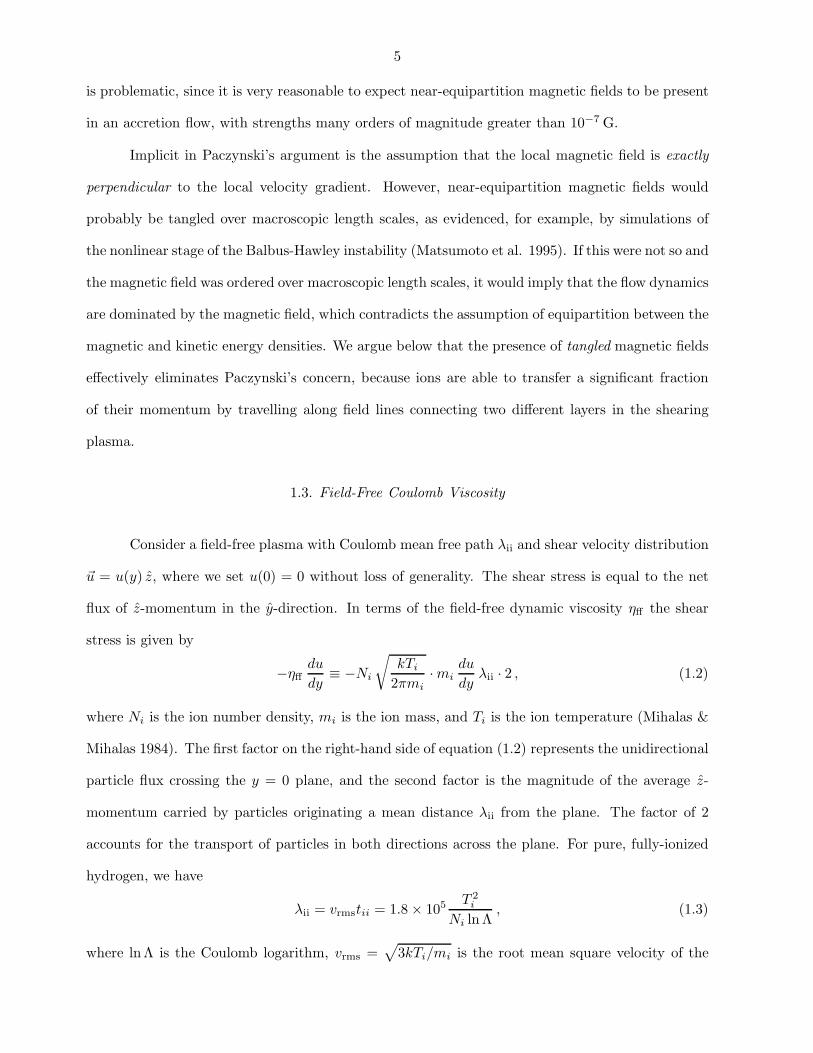
is problematic, since it is very reasonable to expect near-equipartition magnetic fields to be present

in an accretion flow, with strengths many orders of magnitude greater than 10−7 G.

Implicit in Paczynski’s argument is the assumption that the local magnetic field is exactly

perpendicular to the local velocity gradient. However, near-equipartition magnetic fields would

probably be tangled over macroscopic length scales, as evidenced, for example, by simulations of

the nonlinear stage of the Balbus-Hawley instability (Matsumoto et al. 1995). If this were not so and

the magnetic field was ordered over macroscopic length scales, it would imply that the flow dynamics

are dominated by the magnetic field, which contradicts the assumption of equipartition between the

magnetic and kinetic energy densities. We argue below that the presence of tangled magnetic fields

effectively eliminates Paczynski’s concern, because ions are able to transfer a significant fraction

of their momentum by travelling along field lines connecting two different layers in the shearing

plasma.

1.3. Field-Free Coulomb Viscosity

Consider a field-free plasma with Coulomb mean free path λii and shear velocity distribution

~u = u(y) z, where we set u(0) = 0 without loss of generality. The shear stress is equal to the net

flux of z-momentum in the y-direction. In terms of the field-free dynamic viscosity ηff the shear

stress is given by

−ηff

du

dy≡ −Ni

√

kTi

2πmi· mi

du

dyλii · 2 , (1.2)

where Ni is the ion number density, mi is the ion mass, and Ti is the ion temperature (Mihalas &

Mihalas 1984). The first factor on the right-hand side of equation (1.2) represents the unidirectional

particle flux crossing the y = 0 plane, and the second factor is the magnitude of the average z-

momentum carried by particles originating a mean distance λii from the plane. The factor of 2

accounts for the transport of particles in both directions across the plane. For pure, fully-ionized

hydrogen, we have

λii = vrmstii = 1.8 × 105 T 2i

Ni ln Λ, (1.3)

where lnΛ is the Coulomb logarithm, vrms =√

3kTi/mi is the root mean square velocity of the

6

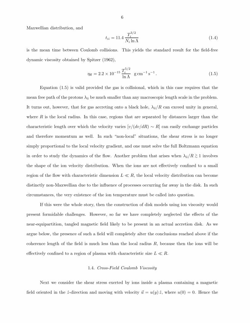
Maxwellian distribution, and

tii = 11.4T

3/2

i

Ni ln Λ(1.4)

is the mean time between Coulomb collisions. This yields the standard result for the field-free

dynamic viscosity obtained by Spitzer (1962),

ηff = 2.2 × 10−15 T5/2

i

ln Λg cm−1 s−1 . (1.5)

Equation (1.5) is valid provided the gas is collisional, which in this case requires that the

mean free path of the protons λii be much smaller than any macroscopic length scale in the problem.

It turns out, however, that for gas accreting onto a black hole, λii/R can exceed unity in general,

where R is the local radius. In this case, regions that are separated by distances larger than the

characteristic length over which the velocity varies [v/(dv/dR) ∼ R] can easily exchange particles

and therefore momentum as well. In such “non-local” situations, the shear stress is no longer

simply proportional to the local velocity gradient, and one must solve the full Boltzmann equation

in order to study the dynamics of the flow. Another problem that arises when λii/R >∼ 1 involves

the shape of the ion velocity distribution. When the ions are not effectively confined to a small

region of the flow with characteristic dimension L ≪ R, the local velocity distribution can become

distinctly non-Maxwellian due to the influence of processes occurring far away in the disk. In such

circumstances, the very existence of the ion temperature must be called into question.

If this were the whole story, then the construction of disk models using ion viscosity would

present formidable challenges. However, so far we have completely neglected the effects of the

near-equipartition, tangled magnetic field likely to be present in an actual accretion disk. As we

argue below, the presence of such a field will completely alter the conclusions reached above if the

coherence length of the field is much less than the local radius R, because then the ions will be

effectively confined to a region of plasma with characteristic size L ≪ R.

1.4. Cross-Field Coulomb Viscosity

Next we consider the shear stress exerted by ions inside a plasma containing a magnetic

field oriented in the z-direction and moving with velocity ~u = u(y) z, where u(0) = 0. Hence the

7

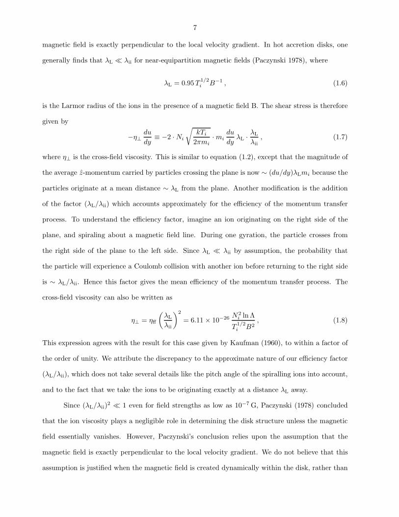
magnetic field is exactly perpendicular to the local velocity gradient. In hot accretion disks, one

generally finds that λL ≪ λii for near-equipartition magnetic fields (Paczynski 1978), where

λL = 0.95T1/2i B−1 , (1.6)

is the Larmor radius of the ions in the presence of a magnetic field B. The shear stress is therefore

given by

−η⊥du

dy≡ −2 · Ni

√

kTi

2πmi· mi

du

dyλL ·

λL

λii

, (1.7)

where η⊥ is the cross-field viscosity. This is similar to equation (1.2), except that the magnitude of

the average z-momentum carried by particles crossing the plane is now ∼ (du/dy)λLmi because the

particles originate at a mean distance ∼ λL from the plane. Another modification is the addition

of the factor (λL/λii) which accounts approximately for the efficiency of the momentum transfer

process. To understand the efficiency factor, imagine an ion originating on the right side of the

plane, and spiraling about a magnetic field line. During one gyration, the particle crosses from

the right side of the plane to the left side. Since λL ≪ λii by assumption, the probability that

the particle will experience a Coulomb collision with another ion before returning to the right side

is ∼ λL/λii. Hence this factor gives the mean efficiency of the momentum transfer process. The

cross-field viscosity can also be written as

η⊥ = ηff

(

λL

λii

)2

= 6.11 × 10−26 N2i ln Λ

T1/2i B2

, (1.8)

This expression agrees with the result for this case given by Kaufman (1960), to within a factor of

the order of unity. We attribute the discrepancy to the approximate nature of our efficiency factor

(λL/λii), which does not take several details like the pitch angle of the spiralling ions into account,

and to the fact that we take the ions to be originating exactly at a distance λL away.

Since (λL/λii)2 ≪ 1 even for field strengths as low as 10−7 G, Paczynski (1978) concluded

that the ion viscosity plays a negligible role in determining the disk structure unless the magnetic

field essentially vanishes. However, Paczynski’s conclusion relies upon the assumption that the

magnetic field is exactly perpendicular to the local velocity gradient. We do not believe that this

assumption is justified when the magnetic field is created dynamically within the disk, rather than

8

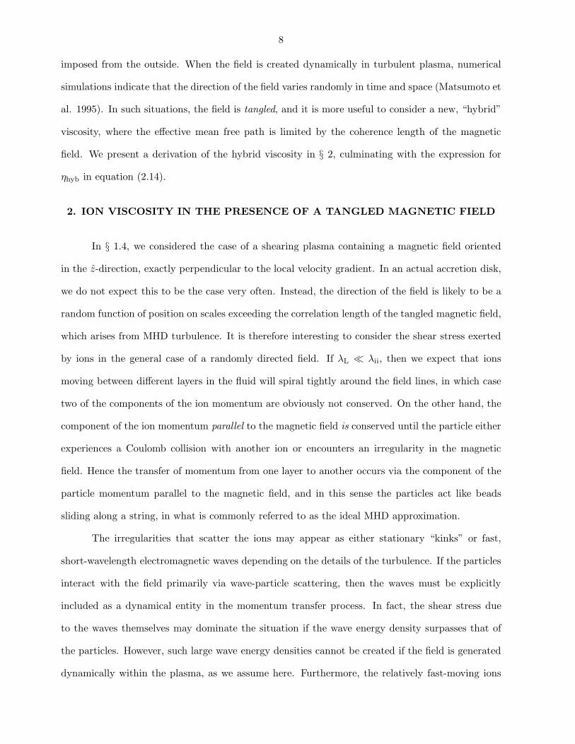
imposed from the outside. When the field is created dynamically in turbulent plasma, numerical

simulations indicate that the direction of the field varies randomly in time and space (Matsumoto et

al. 1995). In such situations, the field is tangled, and it is more useful to consider a new, “hybrid”

viscosity, where the effective mean free path is limited by the coherence length of the magnetic

field. We present a derivation of the hybrid viscosity in § 2, culminating with the expression for

ηhyb in equation (2.14).

2. ION VISCOSITY IN THE PRESENCE OF A TANGLED MAGNETIC FIELD

In § 1.4, we considered the case of a shearing plasma containing a magnetic field oriented

in the z-direction, exactly perpendicular to the local velocity gradient. In an actual accretion disk,

we do not expect this to be the case very often. Instead, the direction of the field is likely to be a

random function of position on scales exceeding the correlation length of the tangled magnetic field,

which arises from MHD turbulence. It is therefore interesting to consider the shear stress exerted

by ions in the general case of a randomly directed field. If λL ≪ λii, then we expect that ions

moving between different layers in the fluid will spiral tightly around the field lines, in which case

two of the components of the ion momentum are obviously not conserved. On the other hand, the

component of the ion momentum parallel to the magnetic field is conserved until the particle either

experiences a Coulomb collision with another ion or encounters an irregularity in the magnetic

field. Hence the transfer of momentum from one layer to another occurs via the component of the

particle momentum parallel to the magnetic field, and in this sense the particles act like beads

sliding along a string, in what is commonly referred to as the ideal MHD approximation.

The irregularities that scatter the ions may appear as either stationary “kinks” or fast,

short-wavelength electromagnetic waves depending on the details of the turbulence. If the particles

interact with the field primarily via wave-particle scattering, then the waves must be explicitly

included as a dynamical entity in the momentum transfer process. In fact, the shear stress due

to the waves themselves may dominate the situation if the wave energy density surpasses that of

the particles. However, such large wave energy densities cannot be created if the field is generated

dynamically within the plasma, as we assume here. Furthermore, the relatively fast-moving ions

9

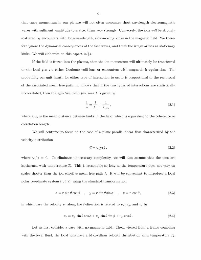
that carry momentum in our picture will not often encounter short-wavelength electromagnetic

waves with sufficient amplitude to scatter them very strongly. Conversely, the ions will be strongly

scattered by encounters with long-wavelength, slow-moving kinks in the magnetic field. We there-

fore ignore the dynamical consequences of the fast waves, and treat the irregularities as stationary

kinks. We will elaborate on this aspect in §4.

If the field is frozen into the plasma, then the ion momentum will ultimately be transferred

to the local gas via either Coulomb collisions or encounters with magnetic irregularities. The

probability per unit length for either type of interaction to occur is proportional to the reciprocal

of the associated mean free path. It follows that if the two types of interactions are statistically

uncorrelated, then the effective mean free path λ is given by

1

λ=

1

λii

+1

λcoh

, (2.1)

where λcoh is the mean distance between kinks in the field, which is equivalent to the coherence or

correlation length.

We will continue to focus on the case of a plane-parallel shear flow characterized by the

velocity distribution

~u = u(y) z , (2.2)

where u(0) = 0. To eliminate unnecessary complexity, we will also assume that the ions are

isothermal with temperature Ti. This is reasonable so long as the temperature does not vary on

scales shorter than the ion effective mean free path λ. It will be convenient to introduce a local

polar coordinate system (r, θ, φ) using the standard transformation

x = r sin θ cos φ , y = r sin θ sin φ , z = r cos θ , (2.3)

in which case the velocity vr along the r-direction is related to vx, vy, and vz by

vr = vx sin θ cos φ + vy sin θ sinφ + vz cos θ . (2.4)

Let us first consider a case with no magnetic field. Then, viewed from a frame comoving

with the local fluid, the local ions have a Maxwellian velocity distribution with temperature Ti.

10

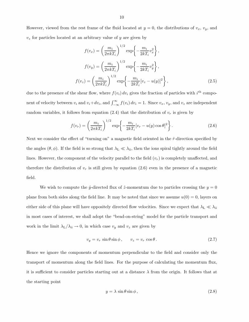
However, viewed from the rest frame of the fluid located at y = 0, the distributions of vx, vy, and

vz for particles located at an arbitrary value of y are given by

f(vx) =

(

mi

2πkTi

)1/2

exp

−mi

2kTiv2

x

,

f(vy) =

(

mi

2πkTi

)1/2

exp

−mi

2kTiv2

y

,

f(vz) =

(

mi

2πkTi

)1/2

exp

−mi

2kTi[vz − u(y)]2

, (2.5)

due to the presence of the shear flow, where f(vi) dvi gives the fraction of particles with ith compo-

nent of velocity between vi and vi+dvi, and∫ ∞

−∞f(vi) dvi = 1. Since vx, vy, and vz are independent

random variables, it follows from equation (2.4) that the distribution of vr is given by

f(vr) =

(

mi

2πkTi

)1/2

exp

−mi

2kTi[vr − u(y) cos θ]2

. (2.6)

Next we consider the effect of “turning on” a magnetic field oriented in the r-direction specified by

the angles (θ, φ). If the field is so strong that λL ≪ λii, then the ions spiral tightly around the field

lines. However, the component of the velocity parallel to the field (vr) is completely unaffected, and

therefore the distribution of vr is still given by equation (2.6) even in the presence of a magnetic

field.

We wish to compute the y-directed flux of z-momentum due to particles crossing the y = 0

plane from both sides along the field line. It may be noted that since we assume u(0) = 0, layers on

either side of this plane will have oppositely directed flow velocities. Since we expect that λL ≪ λii

in most cases of interest, we shall adopt the “bead-on-string” model for the particle transport and

work in the limit λL/λii → 0, in which case vy and vz are given by

vy = vr sin θ sin φ , vz = vr cos θ . (2.7)

Hence we ignore the components of momentum perpendicular to the field and consider only the

transport of momentum along the field lines. For the purpose of calculating the momentum flux,

it is sufficient to consider particles starting out at a distance λ from the origin. It follows that at

the starting point

y = λ sin θ sin φ , (2.8)

11

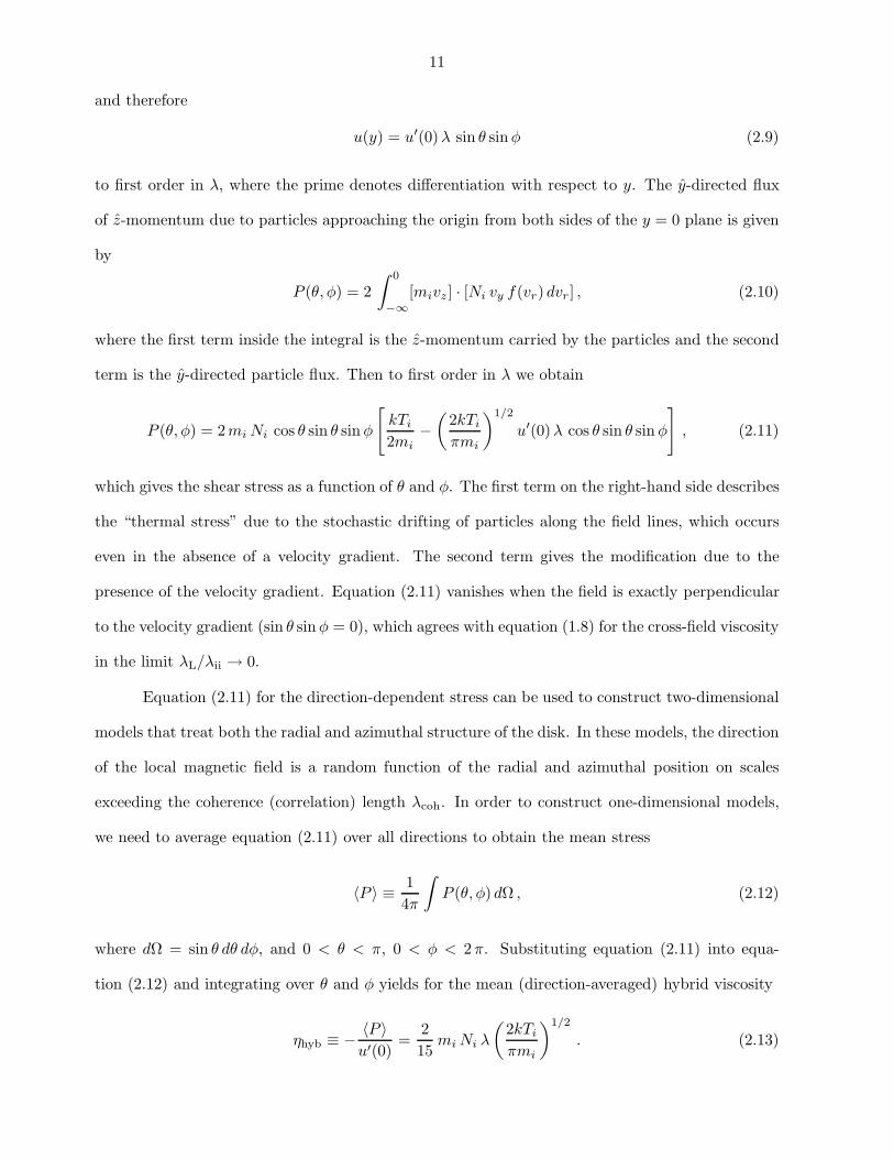
and therefore

u(y) = u′(0)λ sin θ sin φ (2.9)

to first order in λ, where the prime denotes differentiation with respect to y. The y-directed flux

of z-momentum due to particles approaching the origin from both sides of the y = 0 plane is given

by

P (θ, φ) = 2

∫ 0

−∞

[mivz] · [Ni vy f(vr) dvr] , (2.10)

where the first term inside the integral is the z-momentum carried by the particles and the second

term is the y-directed particle flux. Then to first order in λ we obtain

P (θ, φ) = 2mi Ni cos θ sin θ sin φ

[

kTi

2mi−

(

2kTi

πmi

)1/2

u′(0)λ cos θ sin θ sin φ

]

, (2.11)

which gives the shear stress as a function of θ and φ. The first term on the right-hand side describes

the “thermal stress” due to the stochastic drifting of particles along the field lines, which occurs

even in the absence of a velocity gradient. The second term gives the modification due to the

presence of the velocity gradient. Equation (2.11) vanishes when the field is exactly perpendicular

to the velocity gradient (sin θ sin φ = 0), which agrees with equation (1.8) for the cross-field viscosity

in the limit λL/λii → 0.

Equation (2.11) for the direction-dependent stress can be used to construct two-dimensional

models that treat both the radial and azimuthal structure of the disk. In these models, the direction

of the local magnetic field is a random function of the radial and azimuthal position on scales

exceeding the coherence (correlation) length λcoh. In order to construct one-dimensional models,

we need to average equation (2.11) over all directions to obtain the mean stress

〈P 〉 ≡1

4π

∫

P (θ, φ) dΩ , (2.12)

where dΩ = sin θ dθ dφ, and 0 < θ < π, 0 < φ < 2π. Substituting equation (2.11) into equa-

tion (2.12) and integrating over θ and φ yields for the mean (direction-averaged) hybrid viscosity

ηhyb ≡ −〈P 〉

u′(0)=

2

15mi Ni λ

(

2kTi

πmi

)1/2

. (2.13)

12

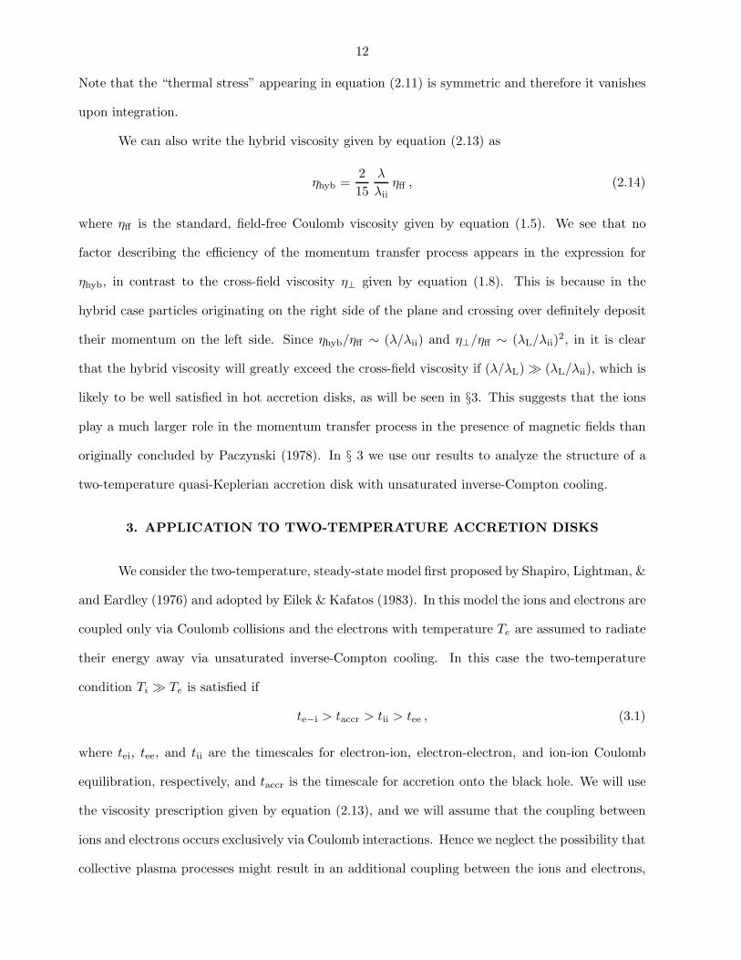
Note that the “thermal stress” appearing in equation (2.11) is symmetric and therefore it vanishes

upon integration.

We can also write the hybrid viscosity given by equation (2.13) as

ηhyb =2

15

λ

λii

ηff , (2.14)

where ηff is the standard, field-free Coulomb viscosity given by equation (1.5). We see that no

factor describing the efficiency of the momentum transfer process appears in the expression for

ηhyb, in contrast to the cross-field viscosity η⊥ given by equation (1.8). This is because in the

hybrid case particles originating on the right side of the plane and crossing over definitely deposit

their momentum on the left side. Since ηhyb/ηff ∼ (λ/λii) and η⊥/ηff ∼ (λL/λii)2, in it is clear

that the hybrid viscosity will greatly exceed the cross-field viscosity if (λ/λL) ≫ (λL/λii), which is

likely to be well satisfied in hot accretion disks, as will be seen in §3. This suggests that the ions

play a much larger role in the momentum transfer process in the presence of magnetic fields than

originally concluded by Paczynski (1978). In § 3 we use our results to analyze the structure of a

two-temperature quasi-Keplerian accretion disk with unsaturated inverse-Compton cooling.

3. APPLICATION TO TWO-TEMPERATURE ACCRETION DISKS

We consider the two-temperature, steady-state model first proposed by Shapiro, Lightman, &

and Eardley (1976) and adopted by Eilek & Kafatos (1983). In this model the ions and electrons are

coupled only via Coulomb collisions and the electrons with temperature Te are assumed to radiate

their energy away via unsaturated inverse-Compton cooling. In this case the two-temperature

condition Ti ≫ Te is satisfied if

te−i > taccr > tii > tee , (3.1)

where tei, tee, and tii are the timescales for electron-ion, electron-electron, and ion-ion Coulomb

equilibration, respectively, and taccr is the timescale for accretion onto the black hole. We will use

the viscosity prescription given by equation (2.13), and we will assume that the coupling between

ions and electrons occurs exclusively via Coulomb interactions. Hence we neglect the possibility that

collective plasma processes might result in an additional coupling between the ions and electrons,

13

over and above the usual Coulomb coupling, which could in principle lead to a violation of the

two-temperature condition. However, Begelman & Chiueh (1988) considered this possibility, and

concluded that such collective processes are not likely to strongly affect the thermal structure of the

disk. Equations (A1–A6) in appendix A list the basic structure equations for the two-temperature

quasi-Keplerian disk model. Equations (A7)–(A9) in appendix A constitute a list of the analytical

solutions to these structure equations, which are derived under the assumption that Ti ≫ Te.

These solutions have an arbitrary α parameter built into them, which in general can be treated as

a constant or allowed to vary with radius using a specific model for the viscosity. In our case the

variation of α is obtained by substituting our expression for ηhyb into equation (1.1).

In order to close the system of equations and obtain solutions for the disk structure, we

must also adopt a model for the variation of the magnetic coherence length λcoh which appears in

the definition of the effective mean free path λ (eq. [2.1]). We assume here that the field topology

varies in a self-similar manner with the local radius R, so that

λcoh ≡ ξ R , (3.2)

where ξ is a free parameter which we set equal to a constant for a given model. It follows from the

definition of λ that

R

λ=

R

λii

+1

ξ, (3.3)

which implies that λ/R ≤ ξ, with equality occurring in the limit ξ → 0. Imposing the restriction

ξ ≤ 1 (which is inherent in the assumption of tangled magnetic fields) thus guarantees that λ/R ≤ 1,

preserving the validity of the fluid description of the plasma.

3.1. A Two-Temperature Accretion Disk Model

In a cylindrically symmetric accretion disk, the relevant component of the stress arising from

the hybrid viscosity is given by

αhyb P ≡ −ηhybRdΩkepl

dR, (3.4)

which is equivalent to equation (1.1). We use equation (3.4) to derive αhyb from ηhyb. Equations

(A7)–(A9) in appendix A and equation (3.4) jointly yield the following self-consistent solutions for

14

the model:

α = 147.31 δ1/3f−1/61 f

2/32

(

M∗

M8

)2/3

τ−1es R−1

∗ (3.5)

Ti = 3.38 × 1011 δ−1/3f1/61 f

1/32

(

M∗

M8

)1/3

R−1/2∗ (3.6)

Te =1.40 × 109y

τes(1 + τes)(3.7)

Ni = 5.70 × 1011 δ1/6f5/121 f

−1/62

(

M∗

M8

)5/6

M∗

−1τes R

−5/4∗ (3.8)

H

R= 0.175 δ−1/6f

−5/121 f

1/62

(

M∗

M8

)1/6

R1/4∗ , (3.9)

where

δ ≡λ

λii

=

(

1 +λii

ξ R

)−1

. (3.10)

and

M∗ ≡M

1M⊙yr−1,M8 ≡

M

108M⊙

, R∗ ≡R

GM/c2. (3.11)

The following two equations jointly define an implicit algebraic equation for determining δ

as a function of R∗ for given (ξ, y, M∗/M8).

τes = 160.214 ξ−1 δ1/6

1 − δf−1/121 f

5/62

(

M∗

M8

)5/6

R−3/4∗ (3.12)

τ7/3es (1 + τes) = 57.8819 δ1/9f

−7/181 f

−1/92 f

2/33 y

(

M∗

M8

)5/9

R−5/6∗ (3.13)

We will restrict our attention to 1 > ξ > 0, since ξ >∼ 1 implies that the field is strongly ordered

over macroscopic length scales, which violates our assumption that the field is tangled.It can be

seen from the definitions of δ and λ that 0 < δ < 1. This simplifies the task of searching for a root

for δ. Once a root for δ is determined for a given ξ, it is used in equation (3.12), and the result

obtained for τes is then used in equations (3.5–3.9) to determine the disk structure. In principle,

therefore, one could compute a disk model for a given y and any combination of ξ, M∗ and M8.

We consider 0.001 < M/ME

< 1, where ME

= LE/c2 and L

E= 4πGMmpc/σT

is the Eddington

luminosity and σT

is the Thomson cross section. Note that ME

= 0.22 M∗/M8. Accretion rates

that are close to the Eddington value are more likely to be significant from the point of view of

observations.

15

3.2. Model Self-Consistency Constraints

For the models to be self-consistent, they have to fufill the following conditions:

(i) λ/R < 1. This assures us of the validity of applying the fluid approximation to the

plasma. As discussed above, imposing ξ < 1 ensures the satisfaction of this criterion.

(ii) Ti/Te >> 1. This is the essence of the two-temperature condition. Furthermore, the

analytical solutions given by equations (A7)–(A9) are valid only if this is true.

(iii) H/R < 1. This ensures that the disk remains geometrically thin. This is yet another

condition that is assumed in deriving the analytical solutions listed in appendix A. As we shall see,

this imposes the most severe restriction on achievable accretion rates.

(iv) Of the different kinds of viscosity that can possibly exist in the accretion disk, we

assume the hybrid viscosity we have derived here to be the dominant form. The hydrodynamic

turbulent viscosity used by Shakura & Sunyaev (1973) is based on dimensional arguments, and,

according to Schramkowski & Torkelsson (1995), is probably less significant than viscosity arising

from MHD turbulence, in which the magnetic field plays a significant role. We will discuss the

contribution of what is referred to as pure magnetic viscosity (as opposed to our hybrid viscosity)

in §4. For relatively high accretion rates (close to the Eddington limit), one would expect rather

high luminosities. Consequently, the contribution of radiation viscosity, which is characterized by

an associated αrad, would be appreciable. Appendix B describes how αrad is calculated. Since

we are not including radiation viscosity in our treatment, we need to remain in a region where

αhyb > αrad, in order to be self-consistent.

Figure 1 shows the nature of these restrictions for a maximally rotating Kerr black hole

(a/M = 0.998). Each point in the parameter space spanned by ξ and M/ME

represents a potential

model. It may be noted that each of these models assumes a constant value of ξ ≡ λcoh/R

throughout the extent of the disk. This implies a certain self-similarity in the manner in which

the embedded magnetic field is tangled. For each criterion (the H/R < 1 criterion, for instance),

“allowed” models are defined as those for which that criterion is satisfied throughout the disk

(Rms < R∗ < 50), where Rms is the radius of marginal stability for the metric under consideration

16

and R∗ is defined in equation (3.11). We take the entire region under consideration to be gas-

pressure dominated (as in Shapiro, Lightman & Eardley 1976), and arbitrarily take the outer

boundary of the disk to be at R∗ = 50. While we have verified that the gas pressure is indeed

dominant over the radiation pressure in all cases of interest here, adopting an outer boundary of

R∗ = 50 is still an arbitrary measure.

Since we have restricted ourselves to ξ < 1, condition (i) is automatically satisfied. It also

turns out that the condition Ti/Te > 1 is satsified throughout the parameter space shown in Figure

1. Constraints (iii) and (iv) are shown in Figure 1. Fully self-consistent models are possible only

in the extreme left hand segment of the plot, indicated by H/R < 1, αhyb > αrad. Evidently,

H/R < 1 is the condition that imposes the most severe restraint on achievable accretion rates.

There is a small range of accretion rates and ξ, represented by the region between the two lines,

where the disk might be puffy (H/R > 1), but the model is partially self-consistent in the sense

that αhyb > αrad. On the extreme right hand side of the plot, the luminosity is high enough to

cause αrad to be greater than αhyb and our models are no longer self-consistent.

Figure 2 illustrates the corresponding constraints for a Schwarzschild black hole. Schwarzschild

black holes are in general cooler than Kerr black holes, because the radius of marginal stability is

greater. Therefore the accretion disks around these objects are apt to be less puffy. This is reflected

in the relatively more benign H/R constraint in Figure 2. It also turns out that, owing to relatively

lower luminosities, the αhyb > αrad constraint is somewhat more forgiving for the Schwarzschild

case, allowing relatively higher accretion rates to be achieved. For both the Kerr and Schwarzschild

cases, it is seen from Figures 1 and 2 that the self-consistency requirements for our model impose

an upper bound on the maximum attainable accretion rate M/ME. However, high accretion rates

are of interest from the point of view of observations, since they result in high luminosities and are

therefore relatively easier to detect. Hence, models with the highest possible accretion rates allowed

by the self-consistency constraints discussed above are likely to be significant from the point of view

of observations.

We now examine a typical model from each of the parameter spaces illustrated in Figures 1

and 2. We choose an accretion rate of M/ME

= 0.5 and a constant value of ξ = 0.8 throughout

17

the flow for both the Kerr and Schwarzschild cases. It can be seen from Figures 1 and 2 that these

values will ensure that both the Kerr and Schwarzschild models will fulfill all the self-consistency

requirements. Figures 3–5 represent the Kerr model with M/ME

= 0.5 and ξ = 0.8, while Fig-

ures 6–8 represent the Schwarzschild model with the same parameters. The relatively high ion

temperatures in both cases are worth noting, and is indicative of the fact that these models are

good candidates for the production of high energy gamma rays (Eilek & Kafatos 1983, Eilek 1980).

Furthermore, as noted earlier, the Schwarzschild disk is relatively cooler and consequently less puffy

than the Kerr disk. Except for the region near the radius of marginal stability, αhyb is seen to be

nearly constant in the Kerr case. This indicates that as far as this particular viscosity mechanism

is concerned, the assumption of a constant α taking on values ranging from 0.01 to 0.1 (as adopted

by the standard disk model of Eilek & Kafatos 1983) is quite good. Closer scrutiny of the region

near the radius of marginal stability reveals that the αhyb and τes curves in the Kerr case are in

fact continuous. The rapid increase in αhyb is due primarily to the drop in pressure caused by the

decrease in temperature near that region, while the sharp drop can be attributed to behavior of

the relativistic correction factors f1, f2 and f3 near the radius of marginal stability.

4. DISCUSSION

We have derived a hybrid viscosity arising from momentum deposition by ions in the presence

of a tangled magnetic field. This viscosity is neither the usual Coulomb viscosity which arises from

Coulomb collisions between ions, nor is it pure magnetic viscosity, which is due to magnetic stresses.

The tangled magnetic field plays a role in confining the ions, which makes the viscosity mechanism

a local process. The field also acts as an intermediary in the momentum transfer between ions, in

situations where the coherence length of the field λcoh ≪ λii, where λii is the usual Coulomb ion-ion

mean free path. Upon application of this form of viscosity to a specific disk model, we observe that

the self-consistency requirements limit valid models to sub-Eddington accretion rates. Otherwise,

the disks become puffy and radiation viscosity dominates over hybrid viscosity. This could be

interpreted as a statement favoring the possibility of quasi-spherical, radiation viscosity-supported

accretion for near-Eddington accretion rates.

18

The Shakura Sunyaev α parameter arising from this hybrid viscosity, αhyb, is seen to lie

roughly between 0.01 and 0.1. It is interesting to compare this with the values of α one would expect

to obtain from pure magnetic viscosity i.e; that arising from magnetic stresses alone. There have

been several attempts at quantifying magnetic viscosity by detailed computations of the magnetic

field arising from dynamo processes (Eardley & Lightman 1975, for instance). If we consider the

magnetic stress to be equal to the magnetic pressure PB = B2/(8π), the α parameter arising out

of pure magnetic viscosity is defined by

αmag P ≡B2

8π. (4.1)

where P is the total pressure. If we define β = Pg/PB , where Pg = Nik(Ti +Te), αmag ∼ 1/(β +1).

The value of αmag can thus vary from 0.5 at β = 1 (equipartition) to as low as ∼ 0.01 for β = 100.

The values of αhyb we obtain are thus seen to be comparable to those obtained from pure magnetic

viscosity. However, the magnitude of the hybrid viscosity is quite insensitive to the magnitude of

the magnetic field, unlike the situation with pure magnetic viscosity. The only restriction on the

magnitude of the magnetic field in our calculations is that it be at least so large as to warrant

the assumption of nearly zero gyroradii for the ions. Our calculations neglect any finite gyroradius

effects, and in effect consider a lower limit on the possible momentum transfer. It is, however, a

realistic one, since a magnetic field as weak as ∼ 10−7 Gauss (which corresponds to a rather large

β, very far below equipartition) is sufficient to cause the gyroradius to be smaller than any of the

macroscopic disk dimensions. It is quite likely that magnetic fields much larger than that value,

and much closer to the equipartition value, will be embedded in the accreting plasma.

We have entirely neglected any momentum transfer arising out of short wavelength plasma

waves in the accretion flow. Since the tangled magnetic field is taken to be arising from plasma

turbulence, the presence of such waves is quite plausible, and it is one aspect of the problem we

have neglected in our calculations. One could model an ensemble of such turbulent plasma waves

as a collection of plasmons, assign a number density and mass to these entities and investigate their

role as intermediaries in momentum transfer. A self-consistent calculation of the tangled magnetic

fields arising as a consequence of the presence of plasma turbulence could also reveal magnetic

19

flutter; temporal variations in the local magnetic field (as distinct from the large scale evolution of

the fields due to dynamo action that we have discussed) that we have also neglected.

We now turn our attention to the deficiencies in our treatment of the disk structure. Our

calculations are time-independent; they assume the presence of a steady state. This might or

might not be true, and there have been a number of investigations of possible disk instabilities

(Shakura & Sunyaev 1976, Piran 1978, for instance) which consider the presence of thermal and

viscous instabilities that could break up the disk and cause variations in the disk luminosity. The

temperature-dependent nature of any viscosity in which ions play a part (like the hybrid viscosity

discussed in this paper) would result in a coupling of viscous and thermal instabilities. The pres-

ence of magnetic fields can be expected to stabilize possible instabilities arising out of the cooling

mechanisms, but it is not clear if it will have any effect upon instabilities in the viscous heating

rate. We are currently in the process of undertaking an investigation of these aspects.

We emphasize that we do not make any attempt to self-consistently calculate the topology

of the tangled magnetic field. Instead, we merely use ξ ≡ λcoh/R as a parameter. The presence of

the tangled magnetic field serves the following purposes:

(i) The ions are effectively caught in the “net” of tangled magnetic field lines, and (since

ξ < 1) are confined to remain well within the accretion flow. The tangled magnetic field cannot

alter the net energy of the distribution, and we therefore assume the temperature of the distribution

to be the same as what it would have been in the absence of the magnetic field. In effect, we assume

that the ions can still relax to a Maxwellian distribution at the same temperature, although we

have not rigorously investigated the relaxation time associated with such a situation.

(ii) Our analysis assumes that the ions traveling from one layer to another along a field line

see no temporal variations in the magnetic field. If we assume the magnetic field to evolve (due

to dynamo action) over timescales comparable to the Keplerian timescale (orbital period), we can

write

∆t

tB≃ [

λcoh

vi]/[

R

vkepl

] = ξvi

vkepl

. (4.2)

where ∆t denotes the time for an ion to travel from one layer to another that is separated by a

20

distance ≃ λcoh, tB denotes the timescale over which the magnetic field evolves and vi is the ion

thermal speed. Since we are restricted to ξ < 1 and we expect vi/vkepl ≤ 1, it is evident from

equation (4.2) that the aforementioned assumption is quite valid.

To emphasize the main points, we have derived a new kind of viscosity called “hybrid”

viscosity and have shown that ions play a much more important role than previously thought in

transporting angular momentum in accretion disks that have tangled magnetic fields embedded

in them. Although we have not modeled the way in which these magnetic fields are dynamically

generated, it is quite plausible that small scale MHD turbulence in the accretion flow can give

rise to such fields. We have also considered this form of viscosity vis-a-vis other forms of viscosity

that can exist in such situations. The temperature-dependent nature of this “hybrid” viscosity also

makes the study of possible instabilities in the disk a very interesting and relevant question to be

resolved.

APPENDIX A

CONSTITUTIVE EQUATIONS FOR TWO-TEMPERATURE, COMPTONIZED MODEL

The basic disk structure equations are the same as those used in the disk structure calcula-

tions of Eilek & Kafatos (1983), which neglect radiation pressure:

P =GMmiNiH

2f1

R3, (A1)

αP =(GMR)

1

2 Mf2

4πR2H, (A2)

3

8π

GMM

R3Hf3 = 3.75 × 1021 mi ln ΛN2

i k(Ti − Te)

T3

2

e

, (A3)

P = Nik(Ti + Te) , (A4)

Te =mec

2y

4k

1

τesg(τes), (A5)

τes = NiσTH , (A6)

where σT

is the Thomson scattering cross-section. The Coulomb logarithm ln Λ is taken to be 15 in

our numerical calculations and the function g(τes) ≡ 1 + τes. It may be noted that this is different

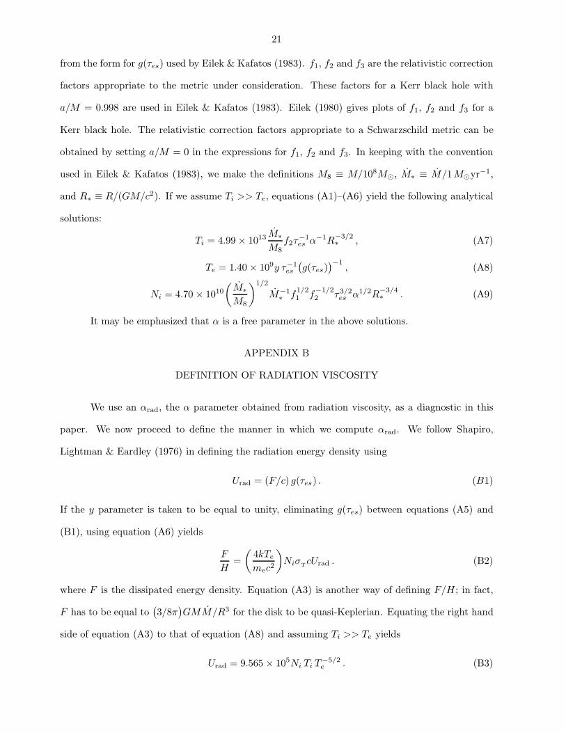
21

from the form for g(τes) used by Eilek & Kafatos (1983). f1, f2 and f3 are the relativistic correction

factors appropriate to the metric under consideration. These factors for a Kerr black hole with

a/M = 0.998 are used in Eilek & Kafatos (1983). Eilek (1980) gives plots of f1, f2 and f3 for a

Kerr black hole. The relativistic correction factors appropriate to a Schwarzschild metric can be

obtained by setting a/M = 0 in the expressions for f1, f2 and f3. In keeping with the convention

used in Eilek & Kafatos (1983), we make the definitions M8 ≡ M/108M⊙, M∗ ≡ M/1M⊙yr−1,

and R∗ ≡ R/(GM/c2). If we assume Ti >> Te, equations (A1)–(A6) yield the following analytical

solutions:

Ti = 4.99 × 1013 M∗

M8

f2τ−1es α−1R

−3/2∗ , (A7)

Te = 1.40 × 109y τ−1es

(

g(τes))−1

, (A8)

Ni = 4.70 × 1010

(

M∗

M8

)1/2

M−1∗ f

1/21 f

−1/22 τ3/2

es α1/2R−3/4∗ . (A9)

It may be emphasized that α is a free parameter in the above solutions.

APPENDIX B

DEFINITION OF RADIATION VISCOSITY

We use an αrad, the α parameter obtained from radiation viscosity, as a diagnostic in this

paper. We now proceed to define the manner in which we compute αrad. We follow Shapiro,

Lightman & Eardley (1976) in defining the radiation energy density using

Urad = (F/c) g(τes) . (B1)

If the y parameter is taken to be equal to unity, eliminating g(τes) between equations (A5) and

(B1), using equation (A6) yields

F

H=

(

4kTe

mec2

)

NiσTcUrad . (B2)

where F is the dissipated energy density. Equation (A3) is another way of defining F/H; in fact,

F has to be equal to(

3/8π)

GMM/R3 for the disk to be quasi-Keplerian. Equating the right hand

side of equation (A3) to that of equation (A8) and assuming Ti >> Te yields

Urad = 9.565 × 105Ni Ti T−5/2e . (B3)

22

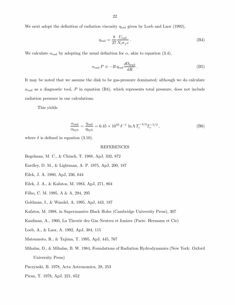
We next adopt the definition of radiation viscosity ηrad given by Loeb and Laor (1992),

ηrad =8

27

Urad

NiσTc

. (B4)

We calculate αrad by adopting the usual definition for α, akin to equation (3.4),

αrad P ≡ −Rηrad

dΩkepl

dR. (B5)

It may be noted that we assume the disk to be gas-pressure dominated; although we do calculate

αrad as a diagnostic tool, P in equation (B4), which represents total pressure, does not include

radiation pressure in our calculations.

This yields

αrad

αhyb

=ηrad

ηhyb

= 6.45 × 1033 δ−1 ln ΛT−3/2

i T−5/2e , (B6)

where δ is defined in equation (3.10).

REFERENCES

Begelman, M. C., & Chiueh, T. 1988, ApJ, 332, 872

Eardley, D. M., & Lightman, A. P. 1975, ApJ, 200, 187

Eilek, J. A. 1980, ApJ, 236, 644

Eilek, J. A., & Kafatos, M. 1983, ApJ, 271, 804

Filho, C. M. 1995, A & A, 294, 295

Goldman, I., & Wandel, A. 1995, ApJ, 443, 187

Kafatos, M. 1988, in Supermassive Black Holes (Cambridge University Press), 307

Kaufman, A., 1960, La Theorie dez Gas Neutres et Ionizes (Paris: Hermann et Cie)

Loeb, A., & Laor, A. 1992, ApJ, 384, 115

Matsumoto, R., & Tajima, T. 1995, ApJ, 445, 767

Mihalas, D., & Mihalas, B. W. 1984, Foundations of Radiation Hydrodynamics (New York: Oxford

University Press)

Paczynski, B. 1978, Acta Astronomica, 28, 253

Piran, T. 1978, ApJ, 221, 652

23

Pringle, J. E. 1981, ARA&A, 19, 137

Schramkowski, G. P., & Torkelsson, U. 1996, A&AR, in press

Shapiro, S. L., Lightman, A. L., & Eardley, D. M. 1976, ApJ, 204, 187

Shakura, N. I., & Sunyaev, R. A. 1973, A&A, 24, 337

Shakura, N. I., & Sunyaev, R. A. 1976, MNRAS, 175, 613

Spitzer, L. 1962, Physics of Fully Ionized Gases (Interscience, New York)

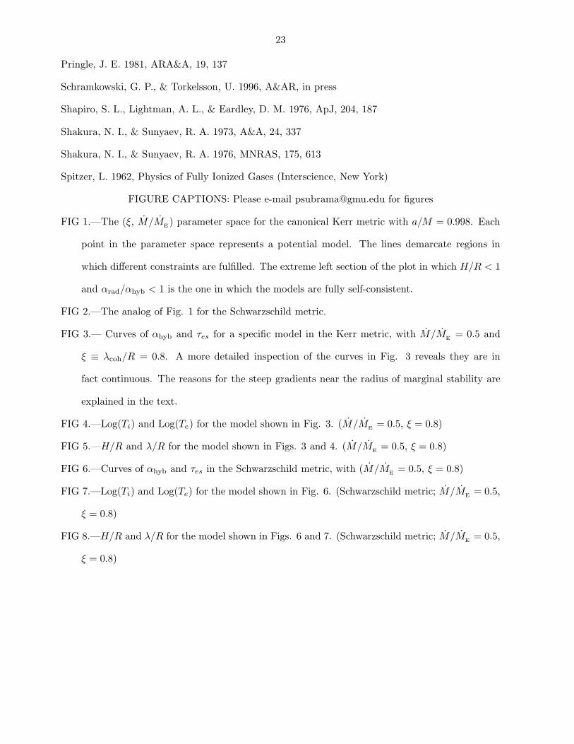
FIGURE CAPTIONS: Please e-mail [email protected] for figures

FIG 1.—The (ξ, M/ME) parameter space for the canonical Kerr metric with a/M = 0.998. Each

point in the parameter space represents a potential model. The lines demarcate regions in

which different constraints are fulfilled. The extreme left section of the plot in which H/R < 1

and αrad/αhyb < 1 is the one in which the models are fully self-consistent.

FIG 2.—The analog of Fig. 1 for the Schwarzschild metric.

FIG 3.— Curves of αhyb and τes for a specific model in the Kerr metric, with M/ME

= 0.5 and

ξ ≡ λcoh/R = 0.8. A more detailed inspection of the curves in Fig. 3 reveals they are in

fact continuous. The reasons for the steep gradients near the radius of marginal stability are

explained in the text.

FIG 4.—Log(Ti) and Log(Te) for the model shown in Fig. 3. (M/ME

= 0.5, ξ = 0.8)

FIG 5.—H/R and λ/R for the model shown in Figs. 3 and 4. (M/ME

= 0.5, ξ = 0.8)

FIG 6.—Curves of αhyb and τes in the Schwarzschild metric, with (M/ME

= 0.5, ξ = 0.8)

FIG 7.—Log(Ti) and Log(Te) for the model shown in Fig. 6. (Schwarzschild metric; M/ME

= 0.5,

ξ = 0.8)

FIG 8.—H/R and λ/R for the model shown in Figs. 6 and 7. (Schwarzschild metric; M/ME

= 0.5,

ξ = 0.8)