Investigation, Prediction and Control of Rubber Friction and Stick-Slip: Experiment, Simulation, Application Fakultät für Maschinenbau der Gottfried Wilhelm Leibniz Universität Hannover zur Erlangung des akademischen Grades DOKTOR-INGENIEUR (Dr- Ing.) genehmigte Dissertation von Diplom-Physiker Leif Busse geboren am 26.10.1968, in Reinbek (2012)

Welcome message from author
This document is posted to help you gain knowledge. Please leave a comment to let me know what you think about it! Share it to your friends and learn new things together.
Transcript
Investigation, Prediction and Control of
Rubber Friction and Stick-Slip:
Experiment, Simulation, Application
Fakultät für Maschinenbau
der Gottfried Wilhelm Leibniz Universität Hannover
zur Erlangung des akademischen Grades
DOKTOR-INGENIEUR
(Dr- Ing.)
genehmigte Dissertation von
Diplom-Physiker Leif Busse
geboren am 26.10.1968, in Reinbek
(2012)

1. Referent: Prof. Dr.-Ing. Gerhard Poll
2. Referent: Prof. Dr.-Ing. Jörg Wallaschek
3. Referent: PD Dr. rer. nat. Manfred Klüppel
Vorsitzender: Prof. Dr.-Ing. Bernd-Arno Behrens
Tag der Promotion: 2012-07-31
Zusammenfassung/ Abstract 3
Zusammenfassung
In dieser Arbeit werden neuartige Methoden zur Analyse und Beeinflussung von
Gummireibung und dabei auftretendem Stick-Slip mit Hilfe von Oberflächenmodifikationen
untersucht. Die Verbindung von Elastomeren, wie sie in Reifen, Schuhen, Scheiben-
wischblättern oder Dichtungsringen verwendet werden, mit harten Oberflächen wie Straßen,
Fußböden, Glasscheiben oder Metallbauteilen macht Verständnis, Vorhersage und
Steuerung von Kontaktmechanik und Reibung unabdingbar.
Reibung zu verstehen bedeutet, die Wechselwirkung von Materialeigenschaften,
Oberflächeneigenschaften und Schmierstoffen zu verstehen. Voraussetzung für eine
mathematische Beschreibung der Reibphänomene ist eine fraktale Sichtweise der
Substratflächen. Basierend auf einem von Klüppel & Heinrich (2000) nach der Greenwood-
Williamson-Theorie aufgestellten Modell mit einer Erweiterung auf bifraktale Skalenbereiche,
lassen sich sowohl Hysteresereibung als auch der adhäsive Anteil beschreiben, die für
Reibung unter nassen und trockenen Bedingungen stehen. Durch Simulationsrechnungen
werden neben Reibwerten noch weitere Kontaktparameter gewonnen und in dieser Arbeit
vorgestellt.
Zu den Materialdaten des Modells gehören die viskoelastischen Eigenschaften der
Gummisorten inklusive ihrer Relaxationszeitspektren. Da Reibung bedeutend von den
systemeigenen Parametern bestimmt wird, was auch die Temperatur einschließt, spielen
diese viskoelastischen Gummieigenschaften eine entscheidende Rolle bei der Beschreibung
und damit auch der Simulation von Reibungssystemen. Viskoelastizität, die letztlich mittels
des Zeit-Temperatur-Superpositionsprinzips von der Temperatur bestimmt wird, darf über die
viskoelastischen Verschiebungsfaktoren, die man aus der dynamisch-mechanischen Analyse
erhält, als mit der Reibungsgeschwindigkeit verknüpft gelten. Deshalb korrelieren hohe
Frequenzen beim Verhalten des Gummis mit niedrigen Temperaturen. Dieselben
Verschiebungsfaktoren werden in dieser Arbeit auf die experimentell ermittelten Reibkurven
für rußgefülltes NR, S-SBR und EPDM auf nassem und trockenem Granit innerhalb eines
Intervalls von Reibgeschwindigkeiten für verschiedene Temperaturen angewandt, um daraus
zusammenhängende Reibmasterkurven über einen extrem großen Geschwindigkeitsintervall
zu bilden. Diese gemessenen Masterkurven werden diskutiert und mit der simulierten
Hysterese- und Adhäsionsreibung verglichen.
Weitere Experimente zielten darauf, Reibung zu reduzieren und in kritischen Systemen das
Entstehen von unerwünschten Stick-Slip-Effekten zu verhindern. Zwei verschiedene
Techniken kamen dabei zum Einsatz: Zunächst wird eine Methode präsentiert, die harte
4 Zusammenfassung/ Abstract
Aluminium-/Silicananostrukturen auf der Elastomeroberfläche erzeugt. Durch geeignete
Präparation werden Partikel aus hyperverzweigtem Polyalkoxysiloxan (PAOS) an der
Gummioberfläche gebildet. Der Einfluss der Menge an Al2O3/PAOS-Dispersion, des
Füllgrads von Ruß und der Temperdauer auf den Reibkoeffizienten wird über einen großen
Geschwindigkeitsbereich hinweg erforscht. Experimente mit und ohne Lubrikanten wurden
durchgeführt und in Hinblick auf Material- und Oberflächeneigenschaften der Proben
diskutiert. Es stellt sich heraus, dass eine hinreichende Menge an PAOS eine nennenswerte
Absenkung der Reibung bewirken und Stick-Slip-Phänomene unterbinden kann.
Zum anderen wurden SBR- und EPDM-Proben unterschiedlicher Oberflächenstrukturen, mit
wie auch ohne Rußfüllung, mit verschiedenen Arten von Polymeren (PU, TPU, PTFE,
Polysiloxan) beschichtet und untersucht, und zwar auf besonders glatten Substratflächen wie
Glas, poliertem Stahl und lackierten Blechen. Es wird gezeigt, wie durch
Probenbeschichtung die Reibung nennenswert abgesenkt wird, gefolgt von einer
umfangreichen Analyse des Stick-Slip-Aspekts, in einem weiten Parameterraum unter
besonderer Berücksichtigung der Einwirkung von Druck und Temperatur. Schließlich wird
noch die Frage aufgeworfen, inwieweit das Reibmodell auf Simulationen für beschichtete
Proben und beschichtete Substrate übertragen werden kann.
Schlagwörter: Gummireibung, Stick-Slip, Oberflächenmodifikation
Abstract
In this work, novel methods of analyzing and controlling rubber friction and stick-slip effects
by means of surface modification shall be investigated. The interaction of elastomers like in
tyres, shoes, wiper blades or seals with hard surfaces like roads, floors, glass or metal parts
makes the understanding, prediction and control of contact mechanics and friction
indispensible.
Understanding friction means understanding the interaction of material properties, surface
properties and lubricant. A fractal point of view for the substrate surfaces becomes the
prerequisite of a mathematical description of friction phenomena. Based on a model by
Klüppel & Heinrich (2000) according to the Greenwood-Williamson theory and expanded to
bifractal scaling ranges, hysteresis friction as well as adhesion contributions can be
described, representing wet and dry lubrication conditions. Additionally to friction, other
contact parameters are gained by simulations and also presented in this work.
Zusammenfassung/ Abstract 5
Part of the material data for the model are the viscoelastic properties of the rubber, including
relaxation time spectra. As friction strongly depends on its system parameters, including
temperature, these viscoelastic properties of rubber play a major role in describing and thus
simulating friction systems. Defined by temperature using the time temperature superposition
principle, viscoelasticity can be assumed to be connected to friction velocity via the
viscoelastic shift factors gained from dynamic mechanical analysis. Thus, high frequencies
correlate with low temperatures for rubber behaviour. In this work, these shift factors are
applied to experimental friction curves for carbon black filled NR, S-SBR and EPDM rubber
on wet and dry granite for various temperatures in order to form continuous friction master
curves over are extremely large velocity interval. These measured master curves are
discussed and compared to simulated hysteresis and adhesion friction.
Further experiments were conducted to reduce friction and prevent critical systems from
exhibiting unwanted stick-slip effects. Two different techniques are employed to achieve this
goal: First, a method of implementing hard alumina/silica nanostructures into the elastomer
surface is presented. With appropriate preparation, particles of hyperbranched
polyalkoxysiloxane (PAOS) are formed on the rubber surface. The influence of variable
amounts of Al2O3/PAOS dispersion, variable amounts of carbon black fillers and annealing
time on the friction coefficient is studied for a large velocity range. Experiments were
conducted with and without lubricant and discussed with respect to material and surface
properties of the samples. It is found that sufficient PAOS concentrations cause a
considerable decrease of friction for all systems and prevent stick-slip phenomena.
Subsequently, SBR and EPDM samples with varying surface structures, filled with and
without carbon black, were coated with several kinds of polymer (PU, TPU, PTFE,
polysiloxane) and tested on especially smooth substrates like glass, polished steel and
varnished metal sheets. It is shown how coating the samples significantly reduces friction,
and an extensive analysis of the stick-slip aspects in a wide parameter range is given, with
special respect on the influence of pressure and temperature. Finally, the question is
investigated whether the contact model can be transferred to simulations of coated samples
and coated substrates.
Keywords: rubber friction, stick-slip, surface modification
6
Table of Content
Zusammenfassung ................................................................................................................ 3
Abstract ................................................................................................................................. 4
Table of Content .................................................................................................................... 6
Abbreviations & Variables ..................................................................................................... 9
1 Introduction ...................................................................................................................13
1.1 Importance of Elastomer Friction ............................................................................13
1.2 Motivation and Agenda of this Work .......................................................................14
1.3 State of the Art .......................................................................................................17
2 Theory of Elastomer Friction on Rough Surfaces ..........................................................21
2.1 Basic Elastomer Mechanics ...................................................................................21
2.2 Time-Temperature-Superposition ...........................................................................26
2.3 Relaxation Time Spectra ........................................................................................30
2.4 Contact Theory .......................................................................................................31
2.5 Self Affinity and Surface Parameters ......................................................................36
2.6 Hysteresis Friction ..................................................................................................40
2.7 Adhesion Friction ...................................................................................................43
2.8 Modelling ................................................................................................................45
3 Experimental Methods & Materials ................................................................................46
3.1 Preparation ............................................................................................................46
3.1.1 Mixing .............................................................................................................46
3.1.2 Vulcanization ...................................................................................................49
3.1.3 Annealing ........................................................................................................50
3.1.4 Sample Shaping ..............................................................................................51
3.1.5 Coating ...........................................................................................................51
3.2 Surface Characterization ........................................................................................53
3.2.1 Profile Measurements .....................................................................................53
3.2.2 Morphology .....................................................................................................54
3.2.3 Chemical Analysis ...........................................................................................55
3.2.4 Surface Tension ..............................................................................................56
3.3 Material Testing ......................................................................................................57
3.3.1 Shore Hardness ..............................................................................................57
3.3.2 Rebound .........................................................................................................57
3.3.3 Tensile Test ....................................................................................................57
3.3.4 Abrasion ..........................................................................................................58
3.4 Dynamic-Mechanical Analysis (DMA) .....................................................................59
7
3.5 Friction Measurements ...........................................................................................61
3.5.1 Tribometer .......................................................................................................61
3.5.2 Universal Testing Machine ..............................................................................65
3.6 Substrates ..............................................................................................................67
3.6.1 Classification ...................................................................................................67
3.6.2 Surface Parameters ........................................................................................67
3.7 Elastomer Samples ................................................................................................72
3.7.1 Chosen Types of Elastomers ..........................................................................72
3.7.2 Reinforcing Fillers ...........................................................................................73
3.7.3 PAOS ..............................................................................................................75
3.7.4 Types of Coating .............................................................................................76
4 Results of Measurements and Simulations ....................................................................78
4.1 Elastomer Characteristics ......................................................................................78
4.1.1 Surface Properties ..........................................................................................79
4.1.2 Mechanical Properties .....................................................................................87
4.1.3 Viscoelastic Properties and Shift Factors ........................................................88
4.1.4 Relaxation Time Spectra .................................................................................95
4.2 Friction Plateaus of Silica Filled Systems ...............................................................98
4.2.1 From Wet Friction to the Silica Plateaus of Dry Friction ...................................98
4.2.2 Fit Parameters and Contact Simulation ......................................................... 101
4.2.3 Simulation Functions ..................................................................................... 103
4.3 Verifying the Friction Model by Friction Master Curves ......................................... 107
4.3.1 Measurement with Lubricant and Simulation of the Hysteresis Friction ......... 107
4.3.2 Friction Measurements on Dry Substrate and Adhesion Simulation .............. 109
4.3.3 Simulation Parameters for Friction Master Curves ........................................ 111
4.4 Parameter Dependence of the Simulation of Contact Variables ........................... 114
4.4.1 True Contact Area ......................................................................................... 115
4.4.2 Gap Distance ................................................................................................ 117
4.4.3 Penetration Depth ......................................................................................... 118
4.4.4 GW Ratio ...................................................................................................... 119
4.4.5 Hysteresis Friction ......................................................................................... 120
4.5 Reduction of Friction by Surface Modification ....................................................... 124
4.5.1 General Explanations on Graphical Friction Results ...................................... 124
4.5.2 Tribology and Diminished Friction by Sample Induction with PAOS .............. 126
4.5.3 Decreasing Friction and Stick-Slip by Coating ............................................... 132
4.5.4 Influence of Environmental Parameters on the Friction of Coated Samples .. 144
4.5.5 Simulation of the Friction on Smooth Substrates ........................................... 150
8
4.6 Stick-Slip and Instabilities ..................................................................................... 157
4.6.1 Layer Stability and Start Peaks ..................................................................... 157
4.6.2 Definition and Evaluation of Stick-Slip ........................................................... 163
4.6.3 Analysis of the Stick-Slip Effects ................................................................... 167
5 Final Considerations .................................................................................................... 181
5.1 General Discussion .............................................................................................. 181
5.2 Summary .............................................................................................................. 184
5.3 Possible Applications ........................................................................................... 188
5.4 Outlook................................................................................................................. 189
Literature ............................................................................................................................ 190
List of Tables ...................................................................................................................... 195
Acknowledgement .............................................................................................................. 196
Curriculum Vitae ................................................................................................................. 198

Abbreviations & Variables 9
Abbreviations & Variables
Abbreviations
AFM atomic force microscopy
CB carbon black
COF coefficient of friction: µ
DIAS dispersion index analysis system
DMA dynamic mechanical analysis
EDX energy dispersive X-ray spectroscopy
EPDM ethylene propylene dien monomer
GW Greenwood-Williamson
HD height distribution
HDC height difference correlation
MC master curve
NR natural rubber
NBR nitrile butadiene rubber
PAOS polyalkoxysiloxane
PSD power spectral density
PTFE polytetrafluorethylene
PU polyurethane
RT room temperature (20°C for TTS, 23°C for other testings)
RTS relaxation time spectrum
SBR styrene butadiene rubber (S-SBR: polymerized in solution)
SEM scanning electron microscopy
SHD summit height distribution
SSE stick-slip effect
TPU thermoplastic polyurethane
TTS time temperature superposition
WLF Williams-Landel-Ferry
XPS X-ray photoelectron spectroscopy
10 Abbreviations & Variables
Latin Variables
< > averaged value
A0 nominal contact area
Ac real contact area
AGW contact area in Greenwood Williamson model
AHz contact area in Hertz model
aHz contact radius in Hertz model
aT horizontal shift factors
b fit factor of hysteresis friction
b0 sample width
C1, C2 WLF constants for horizontal shifting
Cz height difference correlation function
d gap distance
d0 sample thickness
D1 mesoscopic fractal dimension
D2 microscopic fractal dimension
Df fractal dimension
E' storage modulus (elastic modulus)
E'' loss modulus (elastic modulus)
E0 static storage modulus
E∞ maximal storage modulus
Ea activation energy
Ediss dissipated energy
F0, F1, F3/2 Greenwood-Williamson functions
FN normal force on sample
Ffric friction force
f frequency
fs spatial frequency
fsmin minimal spatial frequency
fV vertical shift factors
G' storage modulus (shear modulus)
G'' loss modulus (shear modulus)
h height of asperity
hHz sphere distance in Hertz model
H Hurst exponent
H() relaxation time spectrum function
Abbreviations & Variables 11
l0 sample length
ls contact length
m linear slope in relaxation time spectrum
Me average molecular weight
n fit exponent of critical velocity
nGW number of contact points in Greenwood Williamson model
NGW number of spheres in Greenwood Williamson model
P pressure
R0 radius of asperity
R gas constant
s affine parameter of height distribution
S power density
t normalised distance
tfric duration of friction
T temperature
Tg glass transition temperature
v sliding velocity
vc critical velocity of adhesion
vp velocity of friction peak: v(µmax)
vs velocity of changing friction stability for stick-slip: v(µmin)
V sample volume
z profile height
zmax maximal profile height from average
zs transformed z for summit height distribution
<zp> averaged penetration depth
12 Abbreviations & Variables
Greek Variables
magnification (zoom factor)
averaged excitation depth
tensile strain
s shear strain
surface tension between substrate & sample
filler content
HDSHD height distribution, summit height distribution
contact angle
viscosity
lateral distance between two surface points
transition length microscopic-mesoscopic
c minimal measurable length
min minimal contact length
Adh adhesion friction coefficient
Hys hysteresis friction coefficient (wet friction)
max maximal friction (peak or plateau)
min minimal friction of changing friction stability for stick-slip
plat friction coefficient of stationary plateau
start friction coefficient of start peak
tot total friction coefficient (dry friction)
Poisson number
II horizontal cut-off length
vertical cut-off length
density
mechanical tension
0 normal pressure on sample
HD, SHD standard deviation of height distribution/ of summit height distribution
L surface tension (liquid phase)
LS surface tension (liquid-solid interphase)
S surface tension (solid phase)
relaxation time
s shear tension
angular frequency
Introduction 13
1 Introduction
1.1 Importance of Elastomer Friction
Friction as elemental process in any mechanical system is a ubiquitous phenomenon. In
some cases, there is no alternative to traction: Tyres, shoes and assembly lines simply could
not work without friction, and a maximal effect is desired. On the other hand, for wiper
blades, non-stationary seals, and other flexible contact systems, friction is a harassing side
effect, limiting the efficiency, and has to be avoided. In addition to the pure friction coefficient,
further effects like stick-slip behaviour have to be considered, too, for resonant or vibrating
systems. Finally, friction is linked to mechanical exposure of the surface and thus to stability
and wear of the sliding part. Obviously, there is a need to describe, understand and control
contact parameters and friction. Depending on the environmental conditions, a prediction of
friction is desirable for a multitude of material combinations at any given sliding speed,
temperature and pressure.
Especially important are friction contacts between a soft, elastic material like rubber
(= elastomer) and a hard counter surface, the substrate. Taking the huge usage of rubber
parts into account, from rubber bands over rubberized fabrics to damping elements, this
combination affects virtually every aspect of our world.
14 Introduction
1.2 Motivation and Agenda of this Work
In this work, theoretical and practical aspects of the rubber friction shall be investigated,
focussing on two main topics: the nature of friction curves in respect to velocity and
temperature, and the possibility of reducing friction and stick-slip by surface modification. To
achieve these goals, numerous configurations of elastomer systems combined with various
rough and smooth substrates were considered under several environmental conditions.
Friction strongly depends on its system parameters, including velocity and temperature
(Figure 1). The first topic determines the relationship between friction and its underlying
material cause, namely the viscoelasticity of the sample. As described in chapter 2.1 and 2.2
there is a clearly defined identity of temperature and time induced aspects. Playing a major
part in friction theory to describe and thus simulate friction systems, viscoelastic properties
and thus the time temperature superposition can be expected to appear analogously also in
friction curves by allocating temperature with velocity. Can friction master curves be
constructed by applying the same shift factors as gained for dynamic mechanical
measurements? This question is answered in chapter 4.3 by connecting friction to the shift
factors to measured friction on wet and dry granite over a velocity range for various
temperatures. The measurements are compared to simulated hysteresis and adhesion
friction, which works moreover as a proof of theory to validate our simulation model. Further
simulation results for the real contact area and other parameters complete these
investigations.
Viscoelastic properties of elastomer samples change considerably when the rubber is heated
or cooled. This can be investigated by measuring the storage modulus and loss modulus
over a few decades of frequency in dynamic mechanical analysis (DMA) for various
temperatures. According to the time temperature superposition principle, the single branches
of the DMA results can be shifted to one continuous master curve by applying shift factors
that obey the WLF law [1]. Thus, high frequencies correlate with low temperatures for rubber
behaviour.
Introduction 15
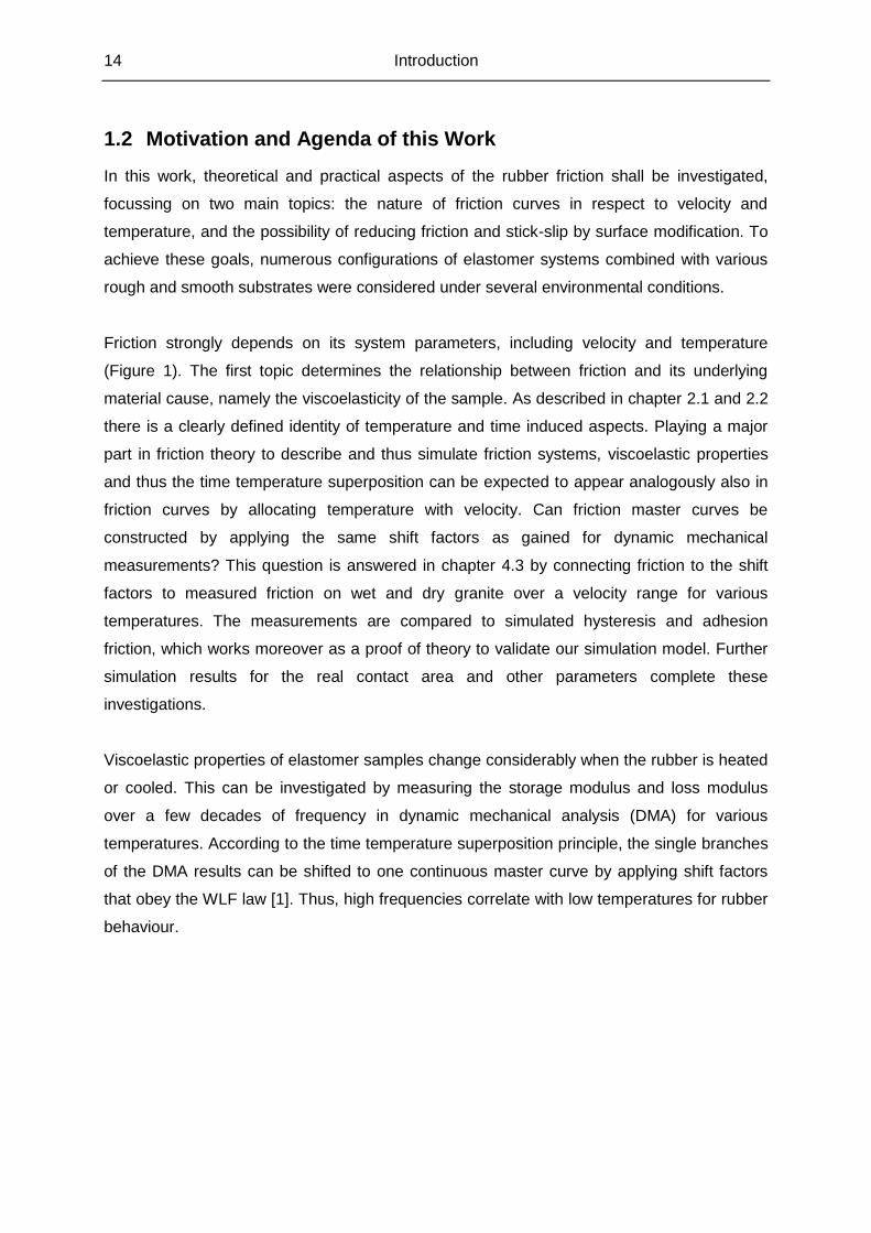
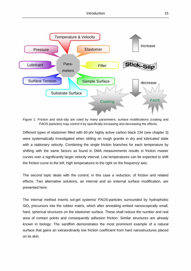
Figure 1: Friction and stick-slip are ruled by many parameters; surface modifications (coating and
PAOS particles) may control it by specifically increasing and decreasing the effects.
Different types of elastomer filled with 60 phr highly active carbon black 234 (see chapter 3)
were systematically investigated when sliding on rough granite in dry and lubricated state
with a stationary velocity. Combining the single friction branches for each temperature by
shifting with the same factors as found in DMA measurements results in friction master
curves over a significantly larger velocity interval. Low temperatures can be expected to shift
the friction curve to the left, high temperatures to the right on the frequency axis.
The second topic deals with the control, in this case a reduction, of friction and related
effects. Two alternative solutions, an internal and an external surface modification, are
presented here:
The internal method inserts sol-gel systems/ PAOS-particles surrounded by hydrophobic
SiO2 precursors into the rubber matrix, which after annealing embed nanoscopically small,
hard, spherical structures on the elastomer surface. These shall reduce the number and real
area of contact points and consequently adhesion friction. Similar structures are already
known in biology: The sandfish demonstrates the most prominent example of a natural
surface that gains an extraordinarily low friction coefficient from hard nanostructures placed
on its skin.
Para-
meters
Elastomer
Filler
Sample Surface
Substrate Surface
Surface Tension
Lubricant
Pressure
Temperature & Velocity
increase
decrease
Coating
PAOS
16 Introduction
The type and amount of PAOS is varied in order to find out a configuration of reducing
friction successfully. Because of their relevance for technical applications, NBR and EPDM
were chosen as rubber material. For counter surfaces, emphasis lies on granite, but other
substrates were tested as well. The influence of the nanostructures on wear and their
junction to the rubber matrix is also a matter of interest. Samples are characterized regarding
to their surface structures and bulk properties, especially with respect to the distribution of
particles and formation of surface patterns. Annealing the PAOS induced sample with
appropriate parameters should build the desired structures predominantly at the sample
surface.
The external method modifies the sample surface directly by depositing a polymer coating.
Several kinds of polymer, with and without particles, were examined to check the influence
on the friction coefficient and stick-slip, with the general goal to reduce both of them or even
completely eliminate the stick-slip.
Coating was done with and without vapour deposition fluorination for bonding enhancement
on SBR and EPDM rubber. To provoke stick-slip in its most intense form, extremely smooth
substrates (glass, coated metal sheets, steel) were combined with the elastomers, which had
been vulcanized with either smooth or rough surface – in general terms, the substrates were
smoother than the samples, unlike in the cases before. The question how well the vulcanized
roughness can be conserved in the coating process and whether our simulation model is still
valid if the sample is too rough to enter tiny substrate cavities shall be discussed, too.
Beside the various sample/ substrate configurations, multiple temperatures and pressures as
main experimental parameters were adjusted to see the effect on friction and stick-slip.
Simulations supplement the experimental point of view. Properties of stick-slip like its
duration and amplitude were analyzed due to their dependency on these variations. An
inspection of layer stability and the changes that the exposure to friction and wear cause
complete the contemplations.
Introduction 17
1.3 State of the Art
From the beginnings of history, people were applying methods to deal with friction:
Lubrication, sledges and wheels were among the earliest inventions of mankind. And from
the beginnings of science, thinkers and experimenters were interested in the laws that dictate
friction. Leonardo da Vinci was one of these early researchers. The first quantitative
description dates from G. Amontons (1699), whose laws say
)(AfFR The friction force does not depend on the nominal sample area.
NR FF The friction force is proportional to the applied normal force and can
be expressed by a factor µ (the coefficient of friction, COF) that correlates with the
tangens of the sliding angle of an inclined plane.
Additionally it was assumed that friction is independent from sliding velocity:
)(vfFR
These empirical laws describe a number of cases more or less adequately, but not
completely. They work sufficiently well for metals or low contact pressures, but fail for
polymers, high pressures and extreme velocities. Obviously, a more sophisticated way of
looking at things was necessary to achieve a general theory.
Later, C.A. Coulomb [2] stated that static friction, being always higher than dynamic (sliding)
friction, rises with the time spent before sliding occurs:
)ln( 0ttbaFstat
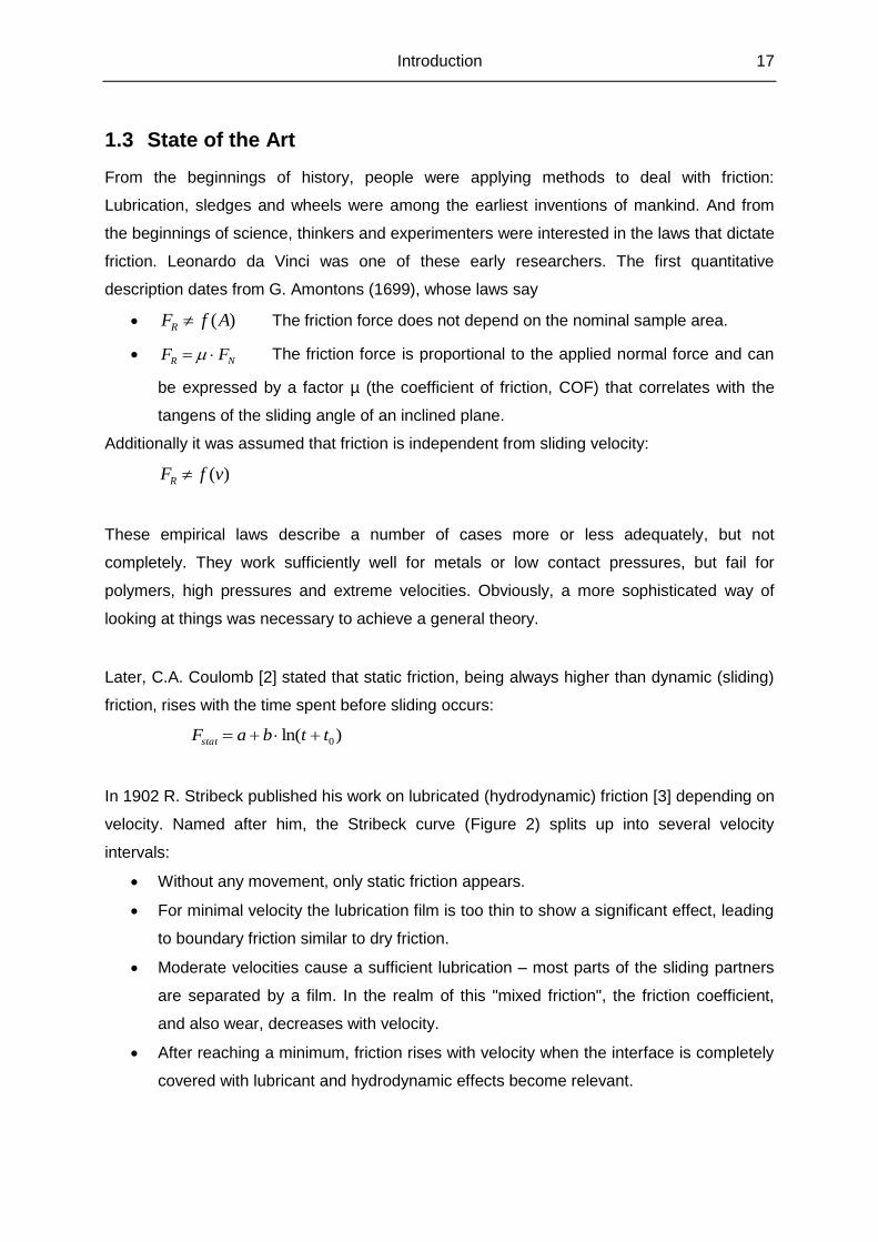
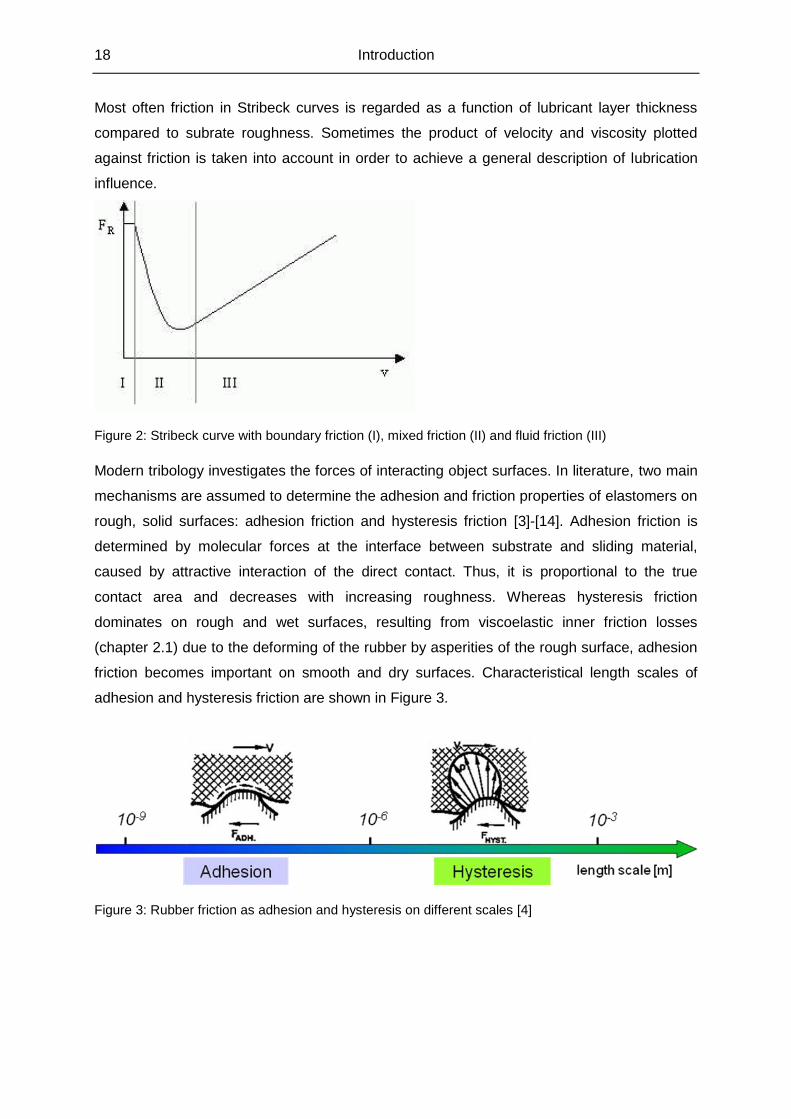
In 1902 R. Stribeck published his work on lubricated (hydrodynamic) friction [3] depending on
velocity. Named after him, the Stribeck curve (Figure 2) splits up into several velocity
intervals:
Without any movement, only static friction appears.
For minimal velocity the lubrication film is too thin to show a significant effect, leading
to boundary friction similar to dry friction.
Moderate velocities cause a sufficient lubrication – most parts of the sliding partners
are separated by a film. In the realm of this "mixed friction", the friction coefficient,
and also wear, decreases with velocity.
After reaching a minimum, friction rises with velocity when the interface is completely
covered with lubricant and hydrodynamic effects become relevant.
18 Introduction
Most often friction in Stribeck curves is regarded as a function of lubricant layer thickness
compared to subrate roughness. Sometimes the product of velocity and viscosity plotted
against friction is taken into account in order to achieve a general description of lubrication
influence.
Figure 2: Stribeck curve with boundary friction (I), mixed friction (II) and fluid friction (III)
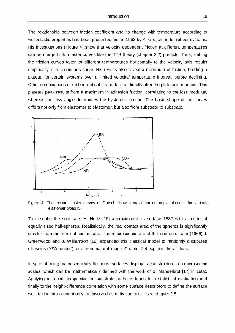
Modern tribology investigates the forces of interacting object surfaces. In literature, two main
mechanisms are assumed to determine the adhesion and friction properties of elastomers on
rough, solid surfaces: adhesion friction and hysteresis friction [3]-[14]. Adhesion friction is
determined by molecular forces at the interface between substrate and sliding material,
caused by attractive interaction of the direct contact. Thus, it is proportional to the true
contact area and decreases with increasing roughness. Whereas hysteresis friction
dominates on rough and wet surfaces, resulting from viscoelastic inner friction losses
(chapter 2.1) due to the deforming of the rubber by asperities of the rough surface, adhesion
friction becomes important on smooth and dry surfaces. Characteristical length scales of
adhesion and hysteresis friction are shown in Figure 3.
Figure 3: Rubber friction as adhesion and hysteresis on different scales [4]
Introduction 19
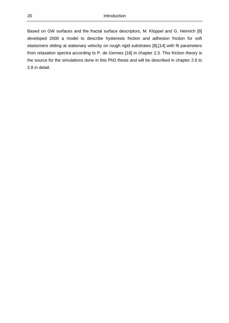
The relationship between friction coefficient and its change with temperature according to
viscoelastic properties had been presented first in 1963 by K. Grosch [5] for rubber systems.
His investigations (Figure 4) show that velocity dependent friction at different temperatures
can be merged into master curves like the TTS theory (chapter 2.2) predicts. Thus, shifting
the friction curves taken at different temperatures horizontally to the velocity axis results
empirically in a continuous curve. His results also reveal a maximum of friction, building a
plateau for certain systems over a limited velocity/ temperature interval, before declining.
Other combinations of rubber and substrate decline directly after the plateau is reached. This
plateau/ peak results from a maximum in adhesion friction, correlating to the loss modulus,
whereas the loss angle determines the hysteresis friction. The basic shape of the curves
differs not only from elastomer to elastomer, but also from substrate to substrate.
Figure 4: The friction master curves of Grosch show a maximum or ample plateaus for various
elastomer types [5].
To describe the substrate, H. Hertz [15] approximated its surface 1882 with a model of
equally sized half-spheres. Realistically, the real contact area of the spheres is significantly
smaller than the nominal contact area, the macroscopic size of the interface. Later (1966) J.
Greenwood and J. Williamson [16] expanded this classical model to randomly distributed
ellipsoids (“GW model”) for a more natural image. Chapter 2.4 explains these ideas.
In spite of being macroscopically flat, most surfaces display fractal structures on microscopic
scales, which can be mathematically defined with the work of B. Mandelbrot [17] in 1982.
Applying a fractal perspective on substrate surfaces leads to a statistical evaluation and
finally to the height-difference correlation with some surface descriptors to define the surface
well, taking into account only the involved asperity summits – see chapter 2.5.
BR
NBR SBR
NR
20 Introduction
Based on GW surfaces and the fractal surface descriptors, M. Klüppel and G. Heinrich [8]
developed 2000 a model to describe hysteresis friction and adhesion friction for soft
elastomers sliding at stationary velocity on rough rigid substrates [8],[14] with fit parameters
from relaxation spectra according to P. de Gennes [18] in chapter 2.3. This friction theory is
the source for the simulations done in this PhD thesis and will be described in chapter 2.6 to
2.8 in detail.
Theory of Elastomer Friction on Rough Surfaces 21
2 Theory of Elastomer Friction on Rough Surfaces
Combining soft elastomers with hard substrates evokes the need for an understanding of the
elasticity of the rubber (chapters 2.1 to 2.3) on one hand and the surface geometry of the
substrate (chapters 2.4 and 2.5) on the other hand. Chapters 2.6 to 2.8 apply the results to a
simulation model.
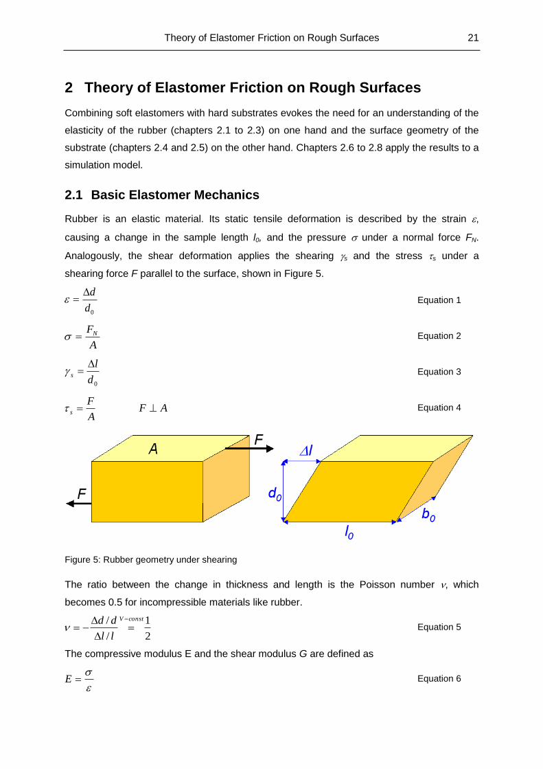
2.1 Basic Elastomer Mechanics
Rubber is an elastic material. Its static tensile deformation is described by the strain ,
causing a change in the sample length l0, and the pressure under a normal force FN.
Analogously, the shear deformation applies the shearing s and the stress s under a
shearing force F parallel to the surface, shown in Figure 5.
0d
d Equation 1
A
FN Equation 2
0d
ls
Equation 3
AFA
Fs Equation 4
Figure 5: Rubber geometry under shearing
The ratio between the change in thickness and length is the Poisson number , which
becomes 0.5 for incompressible materials like rubber.
2
1
/
/ constV
ll
dd
Equation 5
The compressive modulus E and the shear modulus G are defined as
E Equation 6
22 Theory of Elastomer Friction on Rough Surfaces
s
sG
Equation 7
For linear elastic, isotropic material like rubber, Equation 8 holds:
12
G
E Equation 8
In case of incompressibility (Equation 5), both moduli are linked in a simple way. For
simplicity, tensile and shear dimensions may then be used analogously.
GE 3 Equation 9
Rubber is also a viscous material, which is explained by Newtonian behaviour of ideal fluids
with viscosity independent of the shear rate s . A viscosity falling with shear rate is called
shear thinning.
s
s
Equation 10
In the dynamic case, the Equation 1 to Equation 4 become a function of time, leading for
periodic treatment with sufficiently small amplitude (linear viscoelasticity) to
)sin(),( 0 tt Equation 11
)sin(),( 0 tt Equation 12
)(
0
0*
)(
)(
ieGiGG Equation 13
cos
0
0 G Equation 14
sin
0
0 G Equation 15
G
G
tan Equation 16
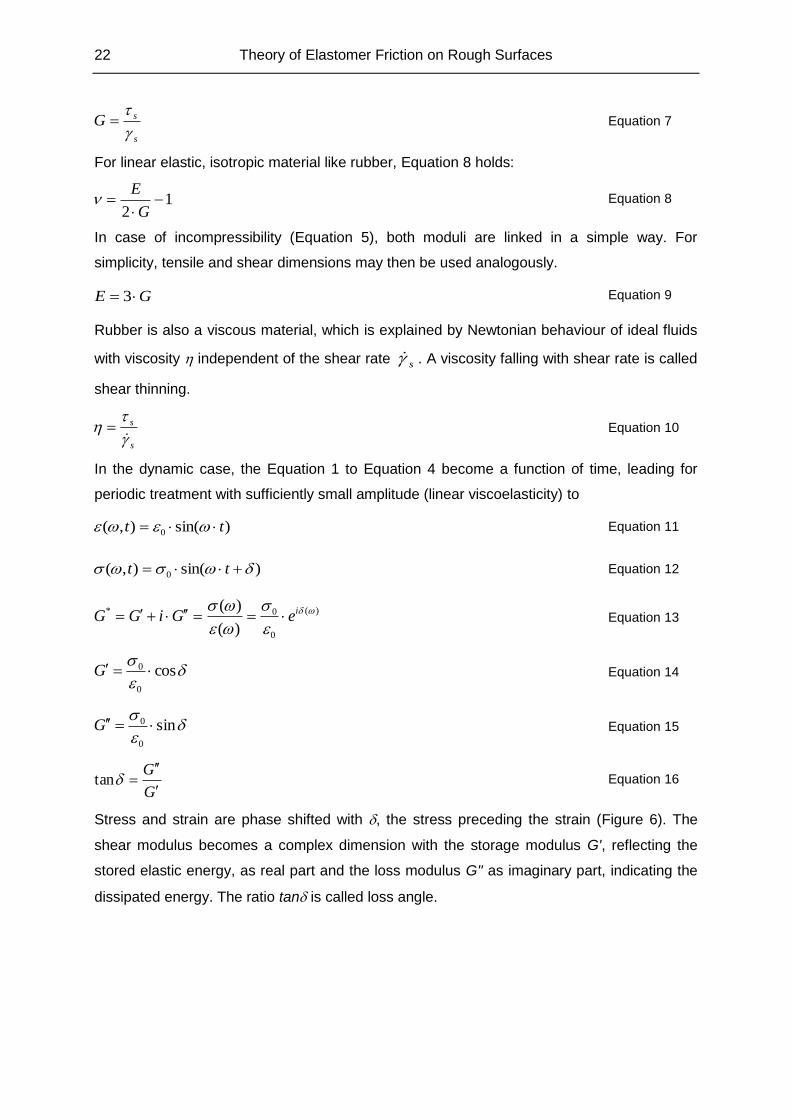
Stress and strain are phase shifted with , the stress preceding the strain (Figure 6). The
shear modulus becomes a complex dimension with the storage modulus G', reflecting the
stored elastic energy, as real part and the loss modulus G'' as imaginary part, indicating the
dissipated energy. The ratio tan is called loss angle.
Theory of Elastomer Friction on Rough Surfaces 23
-1,5
-1
-0,5
0
0,5
1
1,5
0 50 100 150 200 250
time
am
plitu
de
strain
stress
Figure 6: Stress-strain response of harmonically sheared rubber
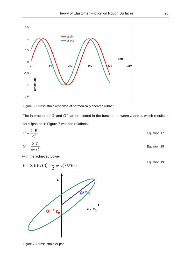
The interaction of G‘ and G‘‘ can be plotted in the function between σ and ε, which results in
an ellipse as in Figure 7 with the relations
2
0
2
EG
Equation 17
2
0
2
PG
Equation 18
with the achieved power
)(2
1)()( 2
0 GttP
Equation 19
Figure 7: Stress-strain ellipse
24 Theory of Elastomer Friction on Rough Surfaces
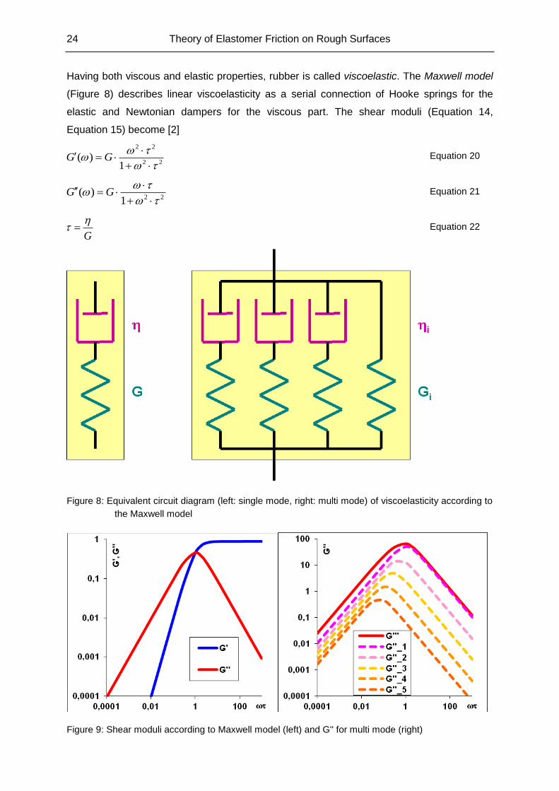
Having both viscous and elastic properties, rubber is called viscoelastic. The Maxwell model
(Figure 8) describes linear viscoelasticity as a serial connection of Hooke springs for the
elastic and Newtonian dampers for the viscous part. The shear moduli (Equation 14,
Equation 15) become [2]
22
22
1)(
GG Equation 20
221)(
GG Equation 21
G
Equation 22
Figure 8: Equivalent circuit diagram (left: single mode, right: multi mode) of viscoelasticity according to
the Maxwell model
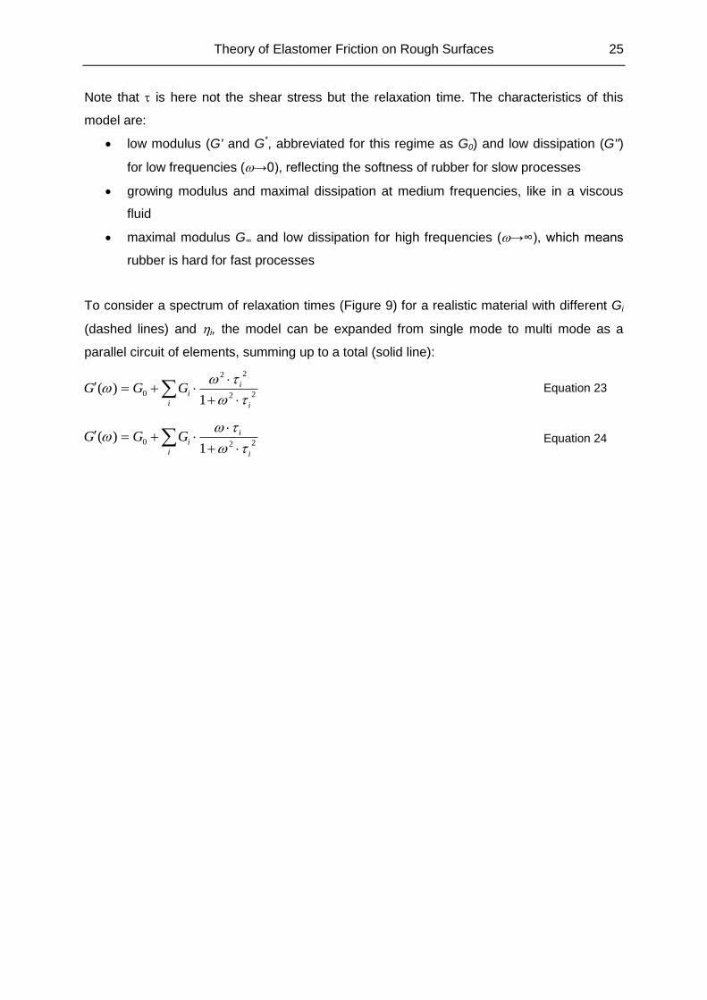
Figure 9: Shear moduli according to Maxwell model (left) and G'' for multi mode (right)
Theory of Elastomer Friction on Rough Surfaces 25
Note that is here not the shear stress but the relaxation time. The characteristics of this
model are:
low modulus (G' and G*, abbreviated for this regime as G0) and low dissipation (G'')
for low frequencies (→0), reflecting the softness of rubber for slow processes
growing modulus and maximal dissipation at medium frequencies, like in a viscous
fluid
maximal modulus G∞ and low dissipation for high frequencies (→∞), which means
rubber is hard for fast processes
To consider a spectrum of relaxation times (Figure 9) for a realistic material with different Gi
(dashed lines) and i, the model can be expanded from single mode to multi mode as a
parallel circuit of elements, summing up to a total (solid line):
i i
iiGGG
22
22
01
)(
Equation 23
i i
iiGGG
2201
)(
Equation 24
26 Theory of Elastomer Friction on Rough Surfaces
2.2 Time-Temperature-Superposition
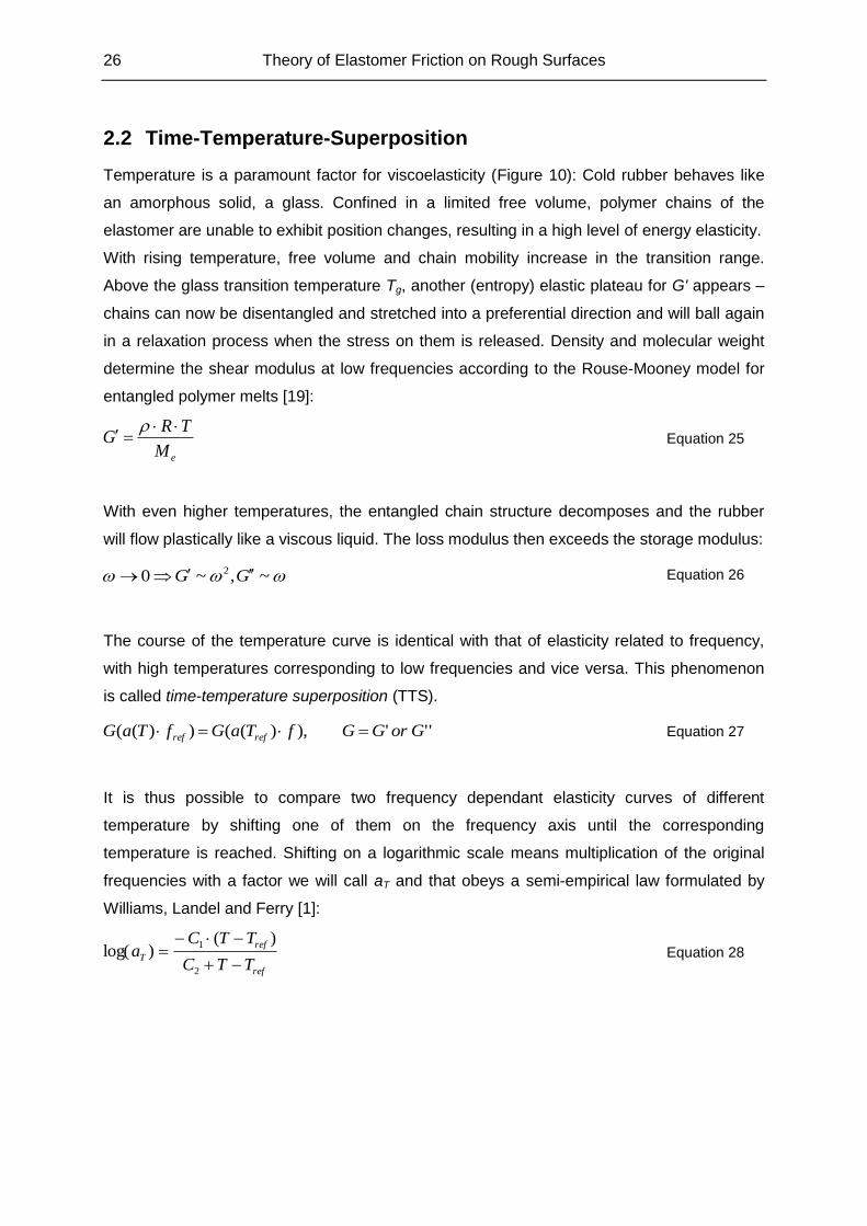
Temperature is a paramount factor for viscoelasticity (Figure 10): Cold rubber behaves like
an amorphous solid, a glass. Confined in a limited free volume, polymer chains of the
elastomer are unable to exhibit position changes, resulting in a high level of energy elasticity.
With rising temperature, free volume and chain mobility increase in the transition range.
Above the glass transition temperature Tg, another (entropy) elastic plateau for G' appears –
chains can now be disentangled and stretched into a preferential direction and will ball again
in a relaxation process when the stress on them is released. Density and molecular weight
determine the shear modulus at low frequencies according to the Rouse-Mooney model for
entangled polymer melts [19]:
eM
TRG
Equation 25
With even higher temperatures, the entangled chain structure decomposes and the rubber
will flow plastically like a viscous liquid. The loss modulus then exceeds the storage modulus:
~,~0 2 GG Equation 26
The course of the temperature curve is identical with that of elasticity related to frequency,
with high temperatures corresponding to low frequencies and vice versa. This phenomenon
is called time-temperature superposition (TTS).
'''),)(())(( GorGGfTaGfTaG refref Equation 27
It is thus possible to compare two frequency dependant elasticity curves of different
temperature by shifting one of them on the frequency axis until the corresponding
temperature is reached. Shifting on a logarithmic scale means multiplication of the original
frequencies with a factor we will call aT and that obeys a semi-empirical law formulated by
Williams, Landel and Ferry [1]:
ref
ref
TTTC
TTCa
2
1 )()log( Equation 28
Theory of Elastomer Friction on Rough Surfaces 27
Figure 10: Temperature dependency of the elastic storage modulus [20]
The WLF law is valid above Tg for a limited range, empirically 100 K above glass transition
with material constants C1 and C2. A reference temperature must be picked within this range,
usually room temperature for easy comparison with experimental data. Alternatively,
universal shift factors of C1 = 17.44 and C2 = 51.6°C may be used when Tg is the reference
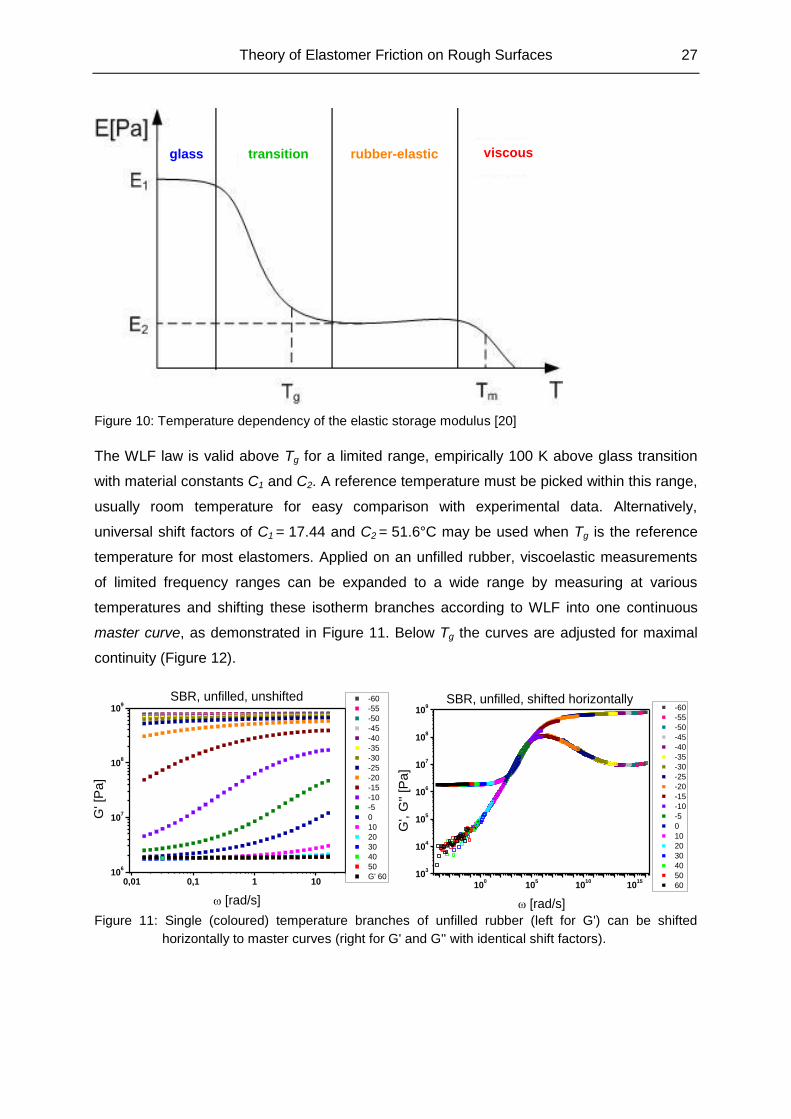
temperature for most elastomers. Applied on an unfilled rubber, viscoelastic measurements
of limited frequency ranges can be expanded to a wide range by measuring at various
temperatures and shifting these isotherm branches according to WLF into one continuous
master curve, as demonstrated in Figure 11. Below Tg the curves are adjusted for maximal
continuity (Figure 12).
Figure 11: Single (coloured) temperature branches of unfilled rubber (left for G') can be shifted
horizontally to master curves (right for G' and G'' with identical shift factors).
glass transition rubber-elastic viscous
0,01 0,1 1 1010
6
107
108
109
-60
-55
-50
-45
-40
-35
-30
-25
-20
-15
-10
-5
0
10
20
30
40
50
G' 60
G' [P
a]
[rad/s]
SBR, unfilled, unshifted
100
105
1010
1015
103
104
105
106
107
108
109
SBR, unfilled, shifted horizontally
-60
-55
-50
-45
-40
-35
-30
-25
-20
-15
-10
-5
0
10
20
30
40
50
60
G', G
'' [P
a]
[rad/s]
28 Theory of Elastomer Friction on Rough Surfaces
-100 -80 -60 -40 -20 0 20 40 60 80 100
-3
0
3
6
9
12
15S
hift
Fac
tors
log
f [H
z]
T [°C]
Horizontal Shift Factors
master curve
WLF fit
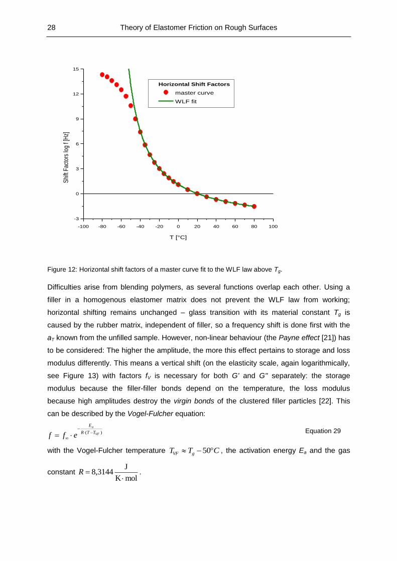
Figure 12: Horizontal shift factors of a master curve fit to the WLF law above Tg.
Difficulties arise from blending polymers, as several functions overlap each other. Using a
filler in a homogenous elastomer matrix does not prevent the WLF law from working;
horizontal shifting remains unchanged – glass transition with its material constant Tg is
caused by the rubber matrix, independent of filler, so a frequency shift is done first with the
aT known from the unfilled sample. However, non-linear behaviour (the Payne effect [21]) has
to be considered: The higher the amplitude, the more this effect pertains to storage and loss
modulus differently. This means a vertical shift (on the elasticity scale, again logarithmically,
see Figure 13) with factors fV is necessary for both G' and G'' separately: the storage
modulus because the filler-filler bonds depend on the temperature, the loss modulus
because high amplitudes destroy the virgin bonds of the clustered filler particles [22]. This
can be described by the Vogel-Fulcher equation:
)( VF
a
TTR
E
eff
Equation 29
with the Vogel-Fulcher temperature CTT gVF 50 , the activation energy Ea and the gas
constant molK
J8,3144
R .
Theory of Elastomer Friction on Rough Surfaces 29
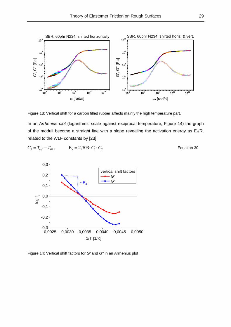
Figure 13: Vertical shift for a carbon filled rubber affects mainly the high temperature part.
In an Arrhenius plot (logarithmic scale against reciprocal temperature, Figure 14) the graph
of the moduli become a straight line with a slope revealing the activation energy as Ea/R,
related to the WLF constants by [23]
21a2 2,303E , CCTTC VFref Equation 30
0,0025 0,0030 0,0035 0,0040 0,0045 0,0050-0,3
-0,2
-0,1
0,0
0,1
0,2
0,3
vertical shift factors
G'
G''
log f
V
1/T [1/K]
Figure 14: Vertical shift factors for G' and G'' in an Arrhenius plot
10-5
100
105
1010
1015
106
107
108
109
1010
SBR, 60phr N234, shifted horizontally
G', G
'' [P
a]
[rad/s]
10-5
100
105
1010
1015
106
107
108
109
1010
SBR, 60phr N234, shifted horiz. & vert.
G', G
'' [P
a]
[rad/s]
~Ea
30 Theory of Elastomer Friction on Rough Surfaces
2.3 Relaxation Time Spectra
As explained in chapter 2.1, a constant strain causes a stress in the elastomer that decays
during time, whereas a constant stress makes the strain rise to a constant level within time.
This is due to relaxation processes with a relaxation time = 1/defined in Equation 22. The
relaxation time spectrum is then [2]
)ln()(ln)( / tdeHtG t Equation 31
Several types of ansatz exist to solve this equation. The method of Ferry and Williams
assumes e-t/ = 0 for t< and e-t/ = 1 for t>, which leads to
)log(
)'log('
d
GdGAH Equation 32
as iterative approximation procedure with the correction term
21
222
2
A
Equation 33
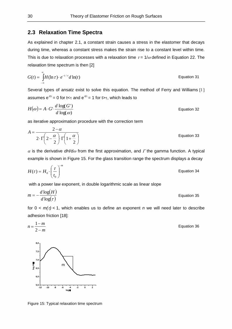
is the derivative dH/d from the first approximation, and the gamma function. A typical
example is shown in Figure 15. For the glass transition range the spectrum displays a decay
m
tHH
0
0)(
Equation 34
with a power law exponent, in double logarithmic scale as linear slope
log
log
d
Hdm Equation 35
for 0 < m() < 1, which enables us to define an exponent n we will need later to describe
adhesion friction [18]:
m
mn
2
1 Equation 36
-12 -10 -8 -6 -4 -2 0 25,5
6,0
6,5
7,0
7,5
8,0
log
H(
)
log
Figure 15: Typical relaxation time spectrum
m
Theory of Elastomer Friction on Rough Surfaces 31
2.4 Contact Theory
Understanding the interaction of two interfaces in contact requires knowledge of the surface
structures. Assuming the elastomer is flexible enough to match the texture of its counterpart,
we can restrict the surface description to the substrate.
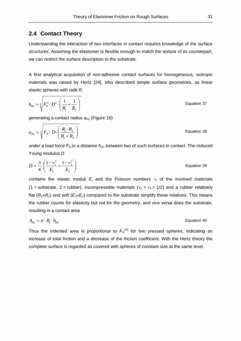
A first analytical acquisition of non-adhesive contact surfaces for homogeneous, isotropic
materials was raised by Hertz [24], who described simple surface geometries, as linear
elastic spheres with radii Ri
3
21
22 11
RRDFh NHz
Equation 37
generating a contact radius aHz (Figure 16)
3
21
21
RR
RRDFa NHz
Equation 38
under a load force FN in a distance hHz between two of such surfaces in contact. The reduced
Young modulus D
2
2
2
1
2
1 11
4
3
EED
Equation 39
contains the elastic moduli Ei and the Poisson numbers i of the involved materials
(1 = substrate, 2 = rubber). Incompressible materials (1 = 2 = 1/2) and a rubber relatively
flat (R1«R2) and soft (E1»E2) compared to the substrate simplify these relations. This means
the rubber counts for elasticity but not for the geometry, and vice versa does the substrate,
resulting in a contact area
HzHz hRA 1 Equation 40
Thus the indented area is proportional to FN2/3 for two pressed spheres, indicating an
increase of total friction and a decrease of the friction coefficient. With the Hertz theory the
complete surface is regarded as covered with spheres of constant size at the same level.
32 Theory of Elastomer Friction on Rough Surfaces
Figure 16: Two Hertz spheres in contact
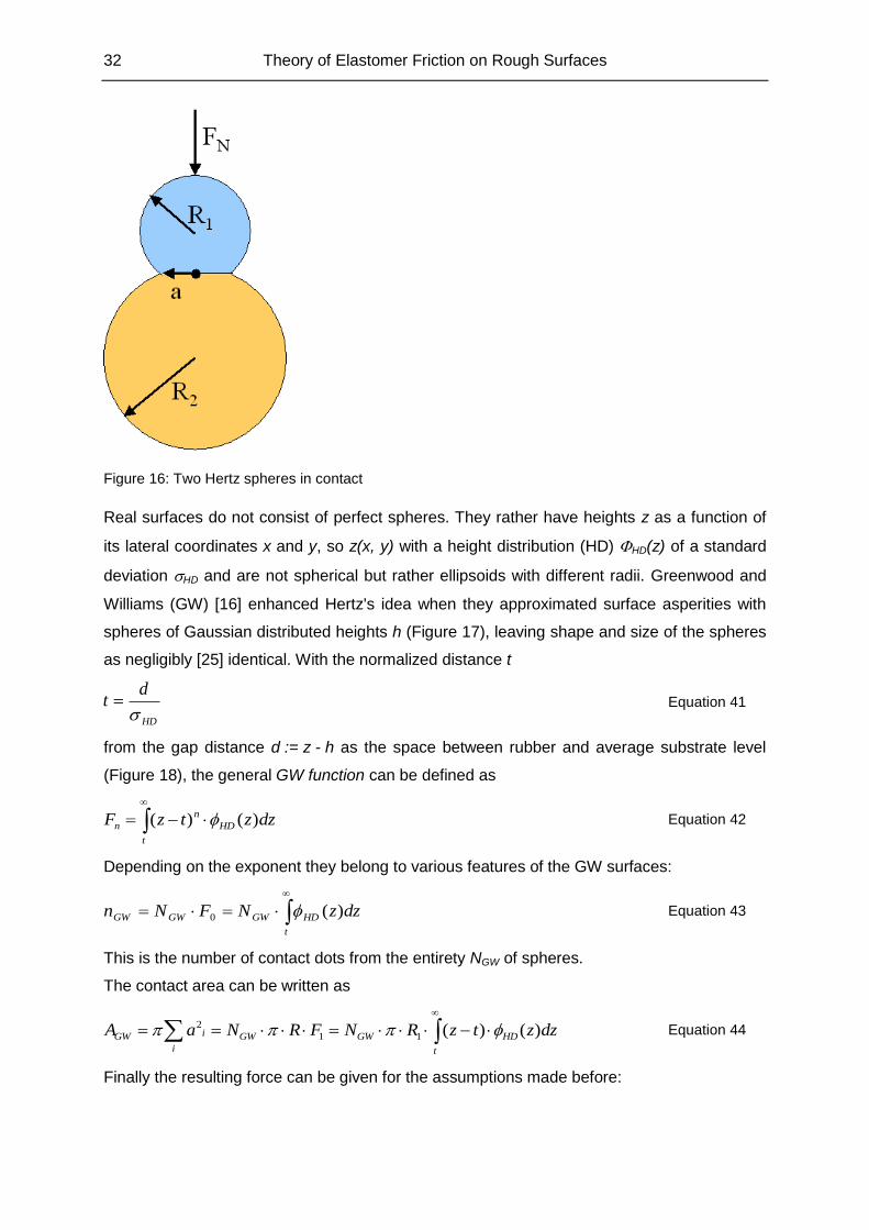
Real surfaces do not consist of perfect spheres. They rather have heights z as a function of
its lateral coordinates x and y, so z(x, y) with a height distribution (HD) HD(z) of a standard
deviation HD and are not spherical but rather ellipsoids with different radii. Greenwood and
Williams (GW) [16] enhanced Hertz's idea when they approximated surface asperities with
spheres of Gaussian distributed heights h (Figure 17), leaving shape and size of the spheres
as negligibly [25] identical. With the normalized distance t
HD
dt
Equation 41
from the gap distance d := z - h as the space between rubber and average substrate level
(Figure 18), the general GW function can be defined as
t
HD
n
n dzztzF )()( Equation 42
Depending on the exponent they belong to various features of the GW surfaces:
t
HDGWGWGW dzzNFNn )(0 Equation 43
This is the number of contact dots from the entirety NGW of spheres.
The contact area can be written as
t
HDGWGW
i
iGW dzztzRNFRNaA )()(11
2 Equation 44
Finally the resulting force can be given for the assumptions made before:
Theory of Elastomer Friction on Rough Surfaces 33
st
SHDsGWGW
N dzztzRENFD
RNF )()(
9
162
3
122/3 Equation 45
Figure 17: Hertz and Greenwood-Williams description of surface geometry
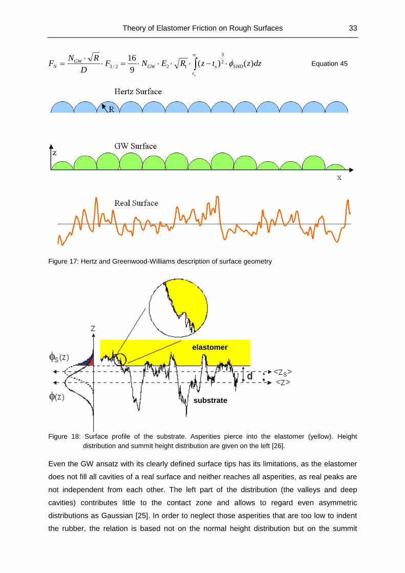
Figure 18: Surface profile of the substrate. Asperities pierce into the elastomer (yellow). Height
distribution and summit height distribution are given on the left [26].
Even the GW ansatz with its clearly defined surface tips has its limitations, as the elastomer
does not fill all cavities of a real surface and neither reaches all asperities, as real peaks are
not independent from each other. The left part of the distribution (the valleys and deep
cavities) contributes little to the contact zone and allows to regard even asymmetric
distributions as Gaussian [25]. In order to neglect those asperities that are too low to indent
the rubber, the relation is based not on the normal height distribution but on the summit
substrate
elastomer
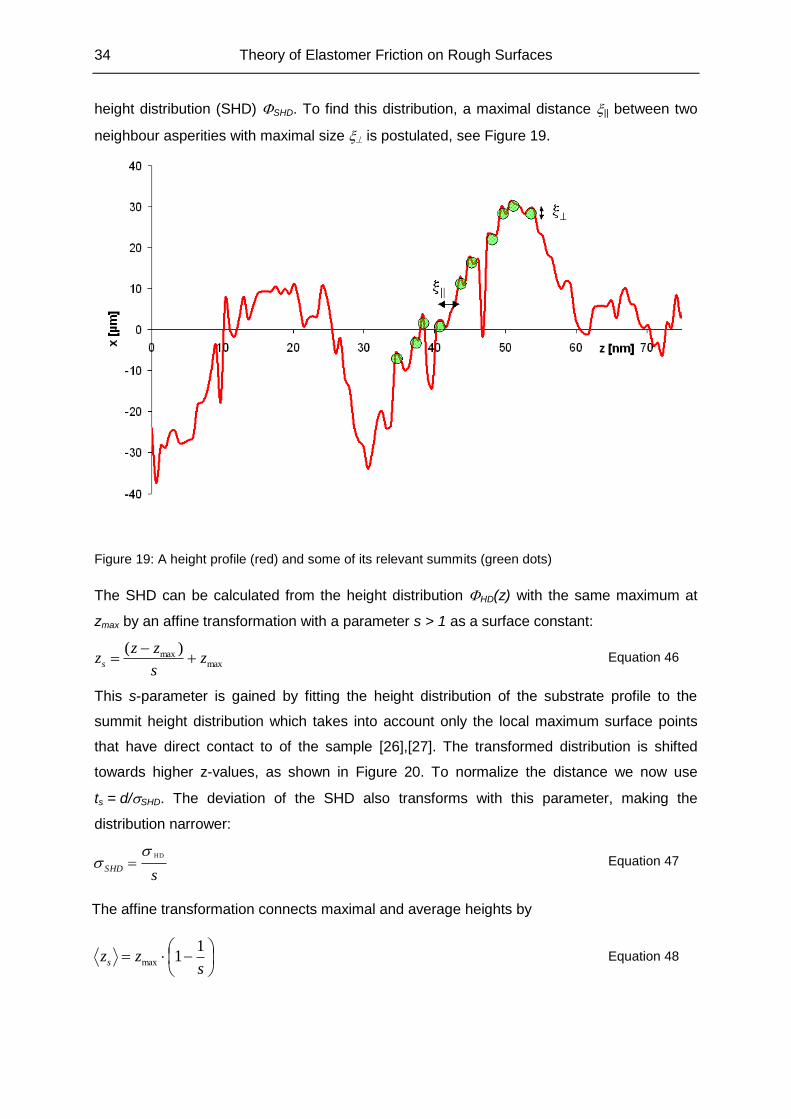
34 Theory of Elastomer Friction on Rough Surfaces
height distribution (SHD) SHD. To find this distribution, a maximal distance || between two
neighbour asperities with maximal size is postulated, see Figure 19.
Figure 19: A height profile (red) and some of its relevant summits (green dots)
The SHD can be calculated from the height distribution HD(z) with the same maximum at
zmax by an affine transformation with a parameter s > 1 as a surface constant:
maxmax )(
zs
zzzs
Equation 46
This s-parameter is gained by fitting the height distribution of the substrate profile to the
summit height distribution which takes into account only the local maximum surface points
that have direct contact to of the sample [26],[27]. The transformed distribution is shifted
towards higher z-values, as shown in Figure 20. To normalize the distance we now use
ts = d/SHD. The deviation of the SHD also transforms with this parameter, making the
distribution narrower:
sSHD
HD Equation 47
The affine transformation connects maximal and average heights by
szzs
11max Equation 48
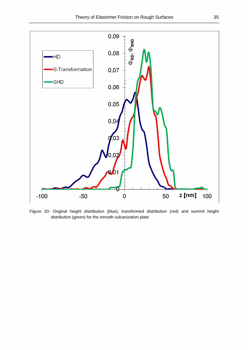
Theory of Elastomer Friction on Rough Surfaces 35
Figure 20: Original height distribution (blue), transformed distribution (red) and summit height
distribution (green) for the smooth vulcanization plate
36 Theory of Elastomer Friction on Rough Surfaces
2.5 Self Affinity and Surface Parameters
In order to take the properties of the rough substrate surface into account, we need to find a
statistical description for its most prominent features. Many natural and technical surfaces,
including the substrates used in this work, turn out to have a self-affine behaviour [17]. The
morphology and statistical properties of self-affine surfaces stay unaffected by an anisotropic
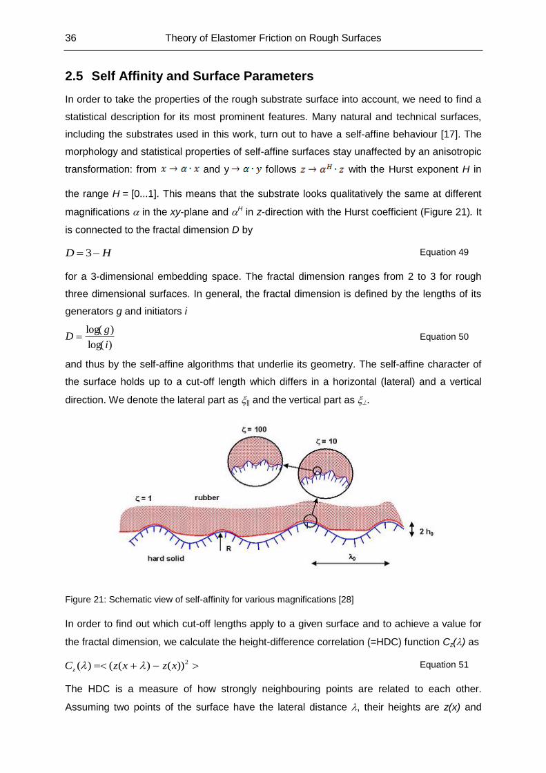
transformation: from and y follows with the Hurst exponent H in
the range H = [0...1]. This means that the substrate looks qualitatively the same at different
magnifications in the xy-plane and H in z-direction with the Hurst coefficient (Figure 21). It
is connected to the fractal dimension D by
HD 3 Equation 49
for a 3-dimensional embedding space. The fractal dimension ranges from 2 to 3 for rough
three dimensional surfaces. In general, the fractal dimension is defined by the lengths of its
generators g and initiators i
)log(
)log(
i
gD Equation 50
and thus by the self-affine algorithms that underlie its geometry. The self-affine character of
the surface holds up to a cut-off length which differs in a horizontal (lateral) and a vertical
direction. We denote the lateral part as || and the vertical part as .
Figure 21: Schematic view of self-affinity for various magnifications [28]
In order to find out which cut-off lengths apply to a given surface and to achieve a value for
the fractal dimension, we calculate the height-difference correlation (=HDC) function Cz() as
2))()(()( xzxzCz Equation 51
The HDC is a measure of how strongly neighbouring points are related to each other.
Assuming two points of the surface have the lateral distance , their heights are z(x) and
Theory of Elastomer Friction on Rough Surfaces 37
z(x+), respectively. The squares are averaged using the "< >" stochastic average over all
possible distance combinations of the rough surface. The profile does not need to be
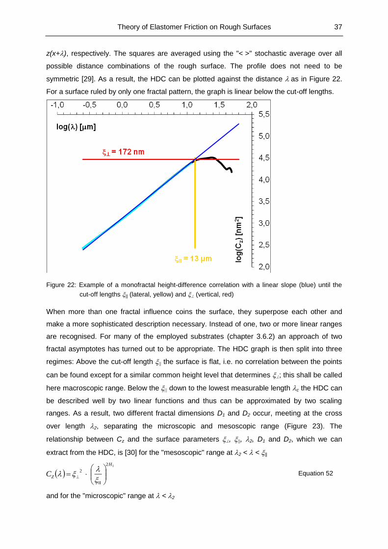
symmetric [29]. As a result, the HDC can be plotted against the distance as in Figure 22.
For a surface ruled by only one fractal pattern, the graph is linear below the cut-off lengths.
Figure 22: Example of a monofractal height-difference correlation with a linear slope (blue) until the
cut-off lengths || (lateral, yellow) and (vertical, red)
When more than one fractal influence coins the surface, they superpose each other and
make a more sophisticated description necessary. Instead of one, two or more linear ranges
are recognised. For many of the employed substrates (chapter 3.6.2) an approach of two
fractal asymptotes has turned out to be appropriate. The HDC graph is then split into three
regimes: Above the cut-off length || the surface is flat, i.e. no correlation between the points
can be found except for a similar common height level that determines ; this shall be called
here macroscopic range. Below the|| down to the lowest measurable length c the HDC can
be described well by two linear functions and thus can be approximated by two scaling
ranges. As a result, two different fractal dimensions D1 and D2 occur, meeting at the cross
over length 2, separating the microscopic and mesoscopic range (Figure 23). The
relationship between Cz and the surface parameters , ||, 2, D1 and D2, which we can
extract from the HDC, is [30] for the "mesoscopic" range at 2 < < ||
12
2
H
ZC
II
Equation 52
and for the "microscopic" range at < 2
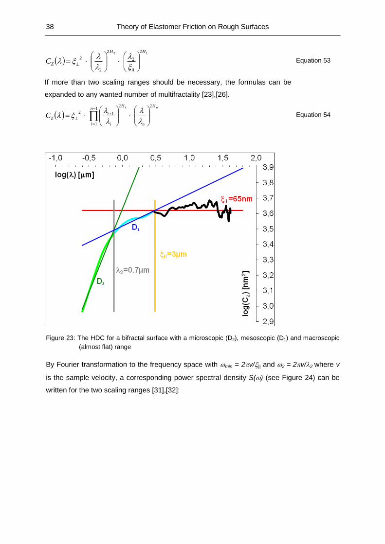
38 Theory of Elastomer Friction on Rough Surfaces
12 2
2
2
2
2
HH
ZC
II
Equation 53
If more than two scaling ranges should be necessary, the formulas can be
expanded to any wanted number of multifractality [23],[26].
1
1
22
12n
i
H
n
H
i
iZ
ni
C
Equation 54
Figure 23: The HDC for a bifractal surface with a microscopic (D2), mesoscopic (D1) and macroscopic
(almost flat) range
By Fourier transformation to the frequency space with min = 2v/|| and 2 = 2v/2 where v
is the sample velocity, a corresponding power spectral density S() (see Figure 24) can be
written for the two scaling ranges [31],[32]:
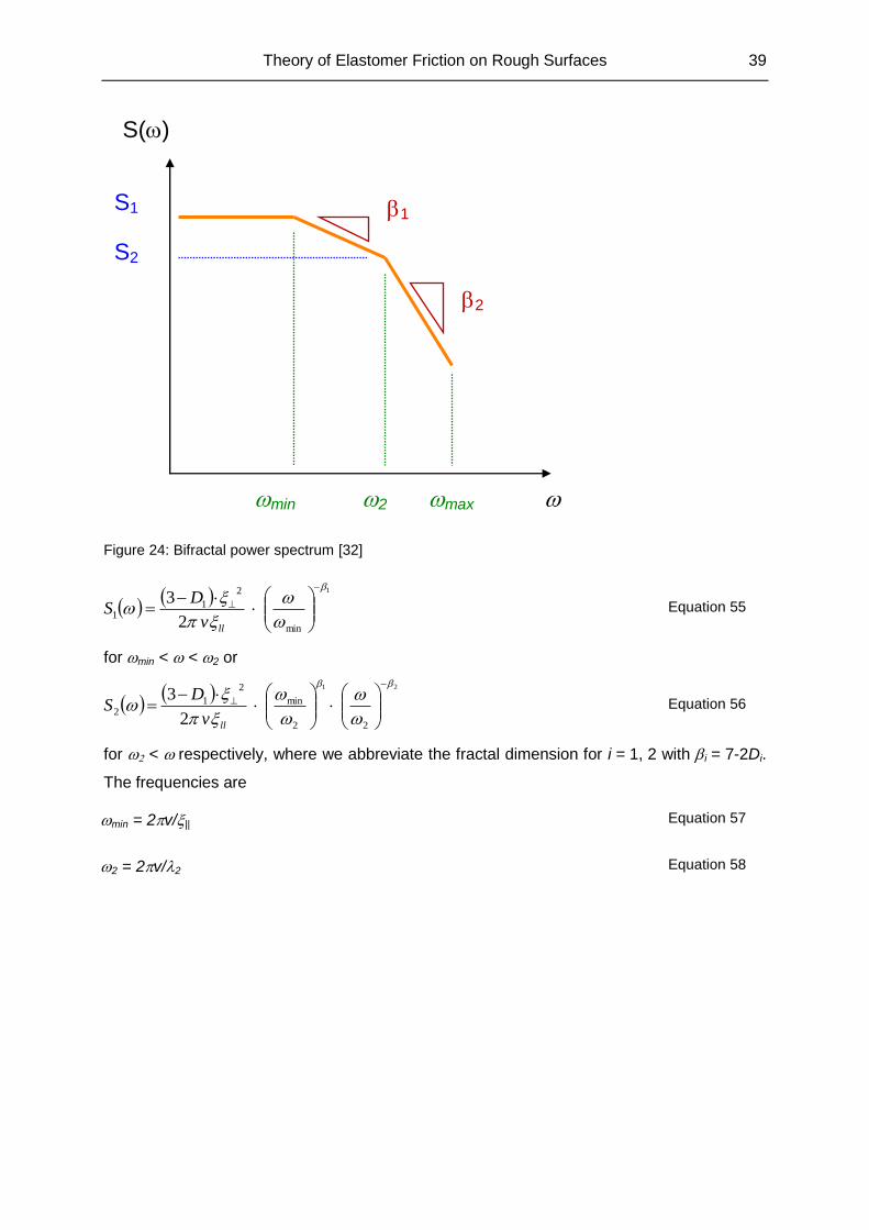
Theory of Elastomer Friction on Rough Surfaces 39
Figure 24: Bifractal power spectrum [32]
1
min
2
11
2
3
llv
DS Equation 55
for min < < 2 or
21
22
min
2
12
2
3
llv
DS Equation 56
for < respectively, where we abbreviate the fractal dimension for i = 1, 2 with i = 7-2Di.
The frequencies are
min = 2v/|| Equation 57
2 = 2v/2 Equation 58
S()
2 max min
S1
S2
1
2
40 Theory of Elastomer Friction on Rough Surfaces
2.6 Hysteresis Friction
Generally speaking, friction is any force that counteracts the mechanical movement of
objects that interact via a common surface by the interaction itself, resulting in a conversion
of kinetic energy into heat by energy dissipation. It occurs as fluid friction when objects move
through liquids or gases. This behaviour is described by the fields of hydrodynamics and
aerodynamics. Other laws hold for the friction of solid bodies, depending on the type of
movement, be it sliding (which means dynamic or kinetic friction as linear movement where
the sample offers a constant surface part to an always new part of the substrate), rolling (a
cyclically changing part of the sample is in non-sliding contact with the substrate) or static
friction (no relative velocity, so movement can only start after the “sticking” is overcome).
This work concentrates on the friction of two macroscopic solids in sliding contact with a
clearly defined, constant (“stationary”) velocity.
Sliding friction tot as ratio of total friction force Ffric and normal force1 FN
pN zEblF )( 0000 Equation 59
determined by pressure σ0 and geometry (or by the corresponding sliding angle α) can be
divided into several superposing parts [32]: most important are the hysteresis friction Hys and
the adhesion friction Adh, which will be treated in chapter 2.7. Two more parts will be not be
considered in this work: the cohesion friction µCoh as an in our system negligible effect
between sample and its own wear particles, and the viscous friction µVis that does not occur
significantly either as even with lubrication the film was rather small and of low viscosity. All
friction parts are subject to parameters like velocity in their own terms.
VisCohHysAdh
N
fric
totF
F tan Equation 60
This chapter deals with hysteresis friction, which is caused by the energy dissipations where
the rubber sample is deformed at local asperities when sliding over a rough ground surface.
The dissipated energy can be written as
max
min
)()(2
0 0
3
dSEtV
xddtEfricV t
diss
fric
Equation 61
with the excited volume V
1 We assume only positive normal forces. Though a negative force is possible as sticking via adhesion
when pulling the sample vertically away, it did not appear in the experiments, and would not have led to friction anyway [39].
Theory of Elastomer Friction on Rough Surfaces 41
00 ALV Equation 62
from the average excitation depth
)(1 tFbzb HVp Equation 63
and the sliding time tfric as integration borders for the pressure σ and change of strain ε, or
tension and deformation, respectively, using the Wiener-Khintchine theorem:
2
)()()()( *
S
Equation 64
that connects the power spectral density (PSD) with the Fourier transformed autocorrelation
function and thus with the squared amplitudes of the excitation by surface asperities.
det ti)(ˆ)( Equation 65
det ti)(ˆ)( *
Equation 66
In this case Dirac’s Delta function is
dte ti
)(
2
1)(
Equation 67
The excited frequencies, which follow the PSD as given in Equation 55 and Equation 56, can
be used for the hysteresis integral [23],[33] to gain the friction force FHys
fric
dissHys
tv
EF
Equation 68
under a normal force FN and thus the friction coefficient Hys is according to our model [27]
dSdSvF
Fv
oN
Hys
Hys 'E' 'E' 2
)( 21
max
2
2
min
Equation 69
Again we assume a bifractal approach to suit best the nature of the HDC. Microstructures
influence mainly to the lower velocities [23]. E'' is the loss modulus of the elastomer, 0 is the
applied pressure and < > is the mean excitation depth inside the rubber
pzb Equation 70
with the mean penetration depth zp of the asperities into the rubber, scaled by the factor b.
Further, only wave lengths above min = 2v/max contribute to Equation 69. It holds [33]
63
1
23
3/2
2
0min
)(3
2min
212
/2
36/209,0
D
s
sc
DD
tFvEs
ntFvE
IIIIIIII
Equation 71
where ns ~ (3 - 2) / (5 - 2) is the summit density, s the affine transformation parameter
(Equation 46) and
42 Theory of Elastomer Friction on Rough Surfaces
t
dzzF )(0 Equation 72
t
dzztzF )()(1
Equation 73
st
s dzztzF )()( 2
3
2/3
Equation 74
are the Greenwood-Williams functions [16] introduced in Equation 42 with the normalized
distances t = d/HD and ts = d/SHD, where the gap distance d indicates the rubber distance
from the mean substrate level;HD and SHD are the standard deviations of the height
distribution or summit height distribution, respectively.
For pure hysteresis friction, λmin becomes [8],[30],[32],[33]
)(
)()(
min
minmin
min
zCE Equation 75
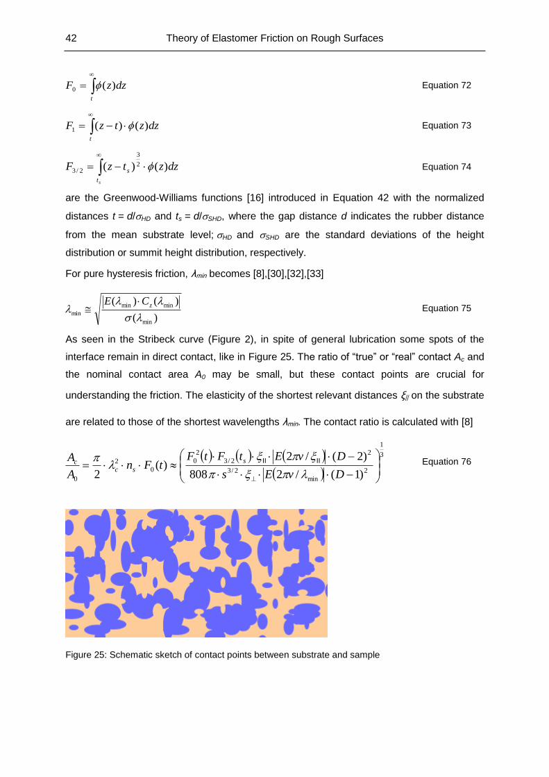
As seen in the Stribeck curve (Figure 2), in spite of general lubrication some spots of the
interface remain in direct contact, like in Figure 25. The ratio of “true” or “real” contact Ac and
the nominal contact area A0 may be small, but these contact points are crucial for
understanding the friction. The elasticity of the shortest relevant distances ξ|| on the substrate
are related to those of the shortest wavelengths λmin. The contact ratio is calculated with [8]
3
1
2
min
2/3
2
2/3
2
0
0
2
0 )1(/2808
)2(/2)(
2
DvEs
DvEtFtFtFn
A
A s
scc
IIII
Equation 76
Figure 25: Schematic sketch of contact points between substrate and sample
Theory of Elastomer Friction on Rough Surfaces 43
2.7 Adhesion Friction
While hysteresis friction is sufficient to describe tribological effects on typical wet contacts,
adhesion has to be considered additionally in only partly lubricated [34], and especially on
dry systems, because direct contact between rubber and substrate allows molecular
interactions with the force FAdh. Consequently, adhesion friction can be used (under the
absence of cohesion friction) as a synonym for dry friction. It is proportional to the ratio of
contact areas from Equation 76. This leads to the adhesion friction coefficient [32],[35],[36]
00 A
A
F
F cs
N
AdhAdh
Equation 77
where the load 0 is the applied pressure, whereas the velocity dependent interfacial shear
stress s produces energy dissipation by peeling effects of the rubber front side at local
asperities causing crack propagation [37], and can be written [38]
n
c
svv
EE
)/(1
/1 0
0 Equation 78
The shear factor
sl
0
Equation 79
relates the stress to a characteristic length scale ls and the corresponding surface tensions γ
which can be measured by contact angles, as part of the Dupré equation
21211221 2
Equation 80
were γ1 stands for the surface tension of the rubber sample, γ2 for the substrate and γ12 for
the disperse interaction of both, or discriminating polar tensions γp2 and γp2 from dispers
tensions γd2 and γd2, as Good’s equation [39]
2121211221 2 ppdd
Equation 81
In Equation 78, the exponent n as a material constant is identical to the same variable found
in the corresponding time relaxation spectra (Equation 36) of the elastomers. The elasticity
ratio E’∞/E’0 as step height for the glass transition is known from the viscoelastic properties,
as found experimentally like chapter 3.4 explains. The parameters 0 = s (v=0) and the
critical velocity vc are subject of free fitting, to give an adequate result. The latter can be
interpreted as the point where the shear stress converges to a maximum [18]: s (vc) s (∞).
The dependency we find on velocity means: Contact cannot be established well when sliding
speeds are high.
44 Theory of Elastomer Friction on Rough Surfaces
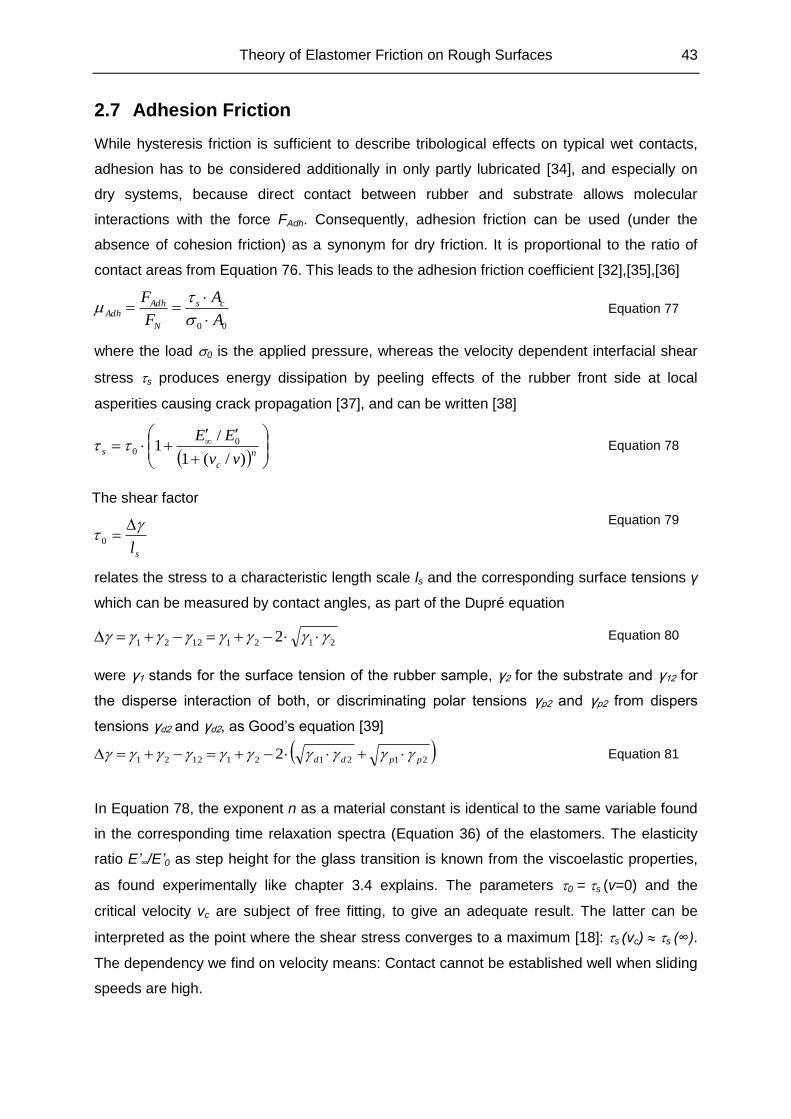
Figure 26: Movement under adhesion causes a bulge in front of asperities.
The adhesion causes an asymmetrical deformation to the rubber (Figure 26): At the leading
edge, i.e. the newly arriving rubber front from point of view of the asperity, the elastomer is
compressed to a bulge before passing the contact zone. Due to the deformation this bulge is
the most probable area where a crack may appear. This implies, for practical reasons, the
necessity to shape the border edges of the sample with flat angles to avoid exaggerated
bulges and, as result, cracks and wear particles. For theoretical considerations, this peeling
process, which has been analyzed by Savkoor & Briggs [40], is connected to the surface
energy Δγ and explains why the bulge building and shear stress depend on velocity.
Theory of Elastomer Friction on Rough Surfaces 45
2.8 Modelling
The theoretical knowledge of chapters 2.6 and 2.7 can be used to achieve a practical
description of real friction systems. According to the DIK model, hysteresis as well as
adhesion friction offer a quantitative description that is the base for numerical simulation. To
gain a complete modelling, the results of these simulations must be compared to
experimental results. Consequently, the process follows two separate steps:
First the hysteresis friction was computed. Necessary data included the statistical geometry
of the substrate (s, ξ⊥, ξ||, λc, D1, D2), characterized with the tools of affine transformation and
HDC, explained in chapters 2.4 and 2.5, further the viscoelastic properties of the rubber
(E’(ω) and E’’(ω) as functional terms (9th degree polynome, or sigmoid for G’), or their shear
equivalents), completed by variables for the experimental environment (σ, A0). Temperature,
though being an important factor, had not to be considered, because most measurements
were performed at room temperature, which was also the reference temperature for elastic
moduli; chapter 4.3 will investigate how far the time temperature superposition of the
viscoelastics can be applied to friction. Velocity was left as an independently increasing
variable for the main loop. All this information was the source for a maple script that had
already been proven in recent works [32] and was improved during this work. Running the
script resulted in a manifold of friction information for various speeds, the most important of
which are the ratio of real contact area Ac/A0 and the average penetration depth <zp>, but
especially of course the friction coefficient µ. The latter is not an absolute number, for the
relation of penetration depth and excitation depth is not covered by this method, so a
proportional factor b is multiplied with the preliminary friction coefficient (Equation 63). To
determine an appropriate value for b, the predicted friction curve was fitted to the
experimentally found curve in lubricated state as best as possible. The accuracy of this
operation is limited because of its strain dependency raised from mechanical-dynamical
analysis. Further deviation might appear especially for extreme velocities due to the in spite
of TTS shifting still confined frequency range of shear moduli. Within these restrictions, a
reasonably maximal accuracy was chosen by defining the velocity steps small enough on a
logarithmic scale.
The second step was to add the adhesion friction to the hysteresis curve. Some of the
needed parameters (σ0, E0/E∞, n and Δγ) had already been gained before, and the area of
real contact is part of the results from hysteresis simulation. Leaving ls and vc as free fit
parameters, hysteresis and adhesion were summed up in a spread sheet and adapted to the
friction curves of tribological measurements on dry surfaces.
46 Experimental Methods & Materials
3 Experimental Methods & Materials
3.1 Preparation
Core of any experiment are the involved samples. For the tribological measurements, those
samples consisted of various types of rubber, treated appropriately according to the
experimental aim. Reproducibility and, especially for the stick-slip experiments, cleanliness is
important to make sure that observed effects are caused by the laws of physics and not by
contamination with dirt, grease or other unwanted chemicals. If possible, samples and
substrates were cleaned residue free with isopropanol not only before the experiment as
whole but also in between to remove possible abrasion particles. Those surfaces that
reacted critically to solvents, like the coated sheets, were treated with distilled water only or
with dry tissues. For experiments with wet surface conditions, an exposure to the lubricant is
of course unavoidable.
The process of sample preparation consisted of several consecutive steps:
1. Mixing a batch of the elastomer substances including carbon black and special
ingredients like PAOS
2. Vulcanization to fulfil the cross-linking
3. Annealing at various conditions, depending on experiment, for PAOS filled samples
4. Shaping the samples to fit the experimental setup
5. Coating, for those samples that were tested in the stick-slip section
Mixing, vulcanization and, if necessary, annealing was done by the DIK staff. The coating
was deposited at FILK Freiberg.
After preparation or usage, the samples were enveloped in aluminium foil to protect them.
Keeping the samples in a refrigerator to slow down aging effects for several months has
proven to be helpful. Samples filled with PAOS on the other hand were stored in a desiccator
(at room pressure and room temperature), so the low moisture would proceed further
annealing only slowly and prevent further silica formation by conserving the state of
annealing.
3.1.1 Mixing
The samples needed for the following experiments consisted of rubber as matrix. Depending
on the type of elastomer, various materials have been made use of. The amount of rubber is
the gauge to which all other components are scaled: The fraction of elastomer is always set
Experimental Methods & Materials 47
to 100 phr (“per hundred rubber”), and all other ingredients relate to this norm in weight
percent compared to the rubber. Those additional substances grant quite different
advantages, from increased mechanical stability for fillers like carbon black and better control
of the cross-linking process to stability against aging and sun rays, plus softeners, dyes or
special materials like PAOS. Chapter 3.7 explains the chemistry and the effect on the
composition for the applied materials. Only pure rubber types (chapter 3.7.1) were employed,
no blends.
For the mixing process an internal mixer, of the type Rheomix 3000, was used. The degree
of filled volume was limited for practical reasons to 75%. To prevent the rubber from
unwanted early cross-linking, temperatures were as best as possible kept constant at 40°C
and rotational frequency at 50 revolutions per minute for the following tables. Components
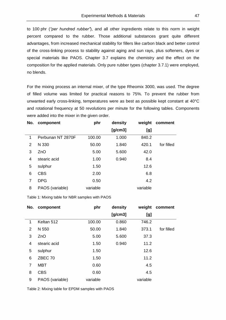
were added into the mixer in the given order.
No. component phr density
[g/cm3]
weight
[g]
comment
1 Perbunan NT 2870F 100.00 1.000 840.2
2 N 330 50.00 1.840 420.1 for filled
3 ZnO 5.00 5.600 42.0
4 stearic acid 1.00 0.940 8.4
5 sulphur 1.50 12.6
6 CBS 2.00 6.8
7 DPG 0.50 4.2
8 PAOS (variable) variable variable
Table 1: Mixing table for NBR samples with PAOS
No. component phr density
[g/cm3]
weight
[g]
comment
1 Keltan 512 100.00 0.860 746.2
2 N 550 50.00 1.840 373.1 for filled
3 ZnO 5.00 5.600 37.3
4 stearic acid 1.50 0.940 11.2
5 sulphur 1.50 12.6
6 ZBEC 70 1.50 11.2
7 MBT 0.60 4.5
8 CBS 0.60 4.5
9 PAOS (variable) variable variable
Table 2: Mixing table for EPDM samples with PAOS
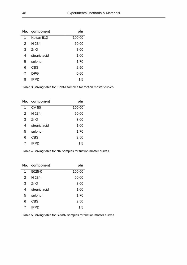
48 Experimental Methods & Materials
No. component phr
1 Keltan 512 100.00
2 N 234 60.00
3 ZnO 3.00
4 stearic acid 1.00
5 sulphur 1.70
6 CBS 2.50
7 DPG 0.60
8 IPPD 1.5
Table 3: Mixing table for EPDM samples for friction master curves
No. component phr
1 CV 50 100.00
2 N 234 60.00
3 ZnO 3.00
4 stearic acid 1.00
5 sulphur 1.70
6 CBS 2.50
7 IPPD 1.5
Table 4: Mixing table for NR samples for friction master curves
No. component phr
1 5025-0 100.00
2 N 234 60.00
3 ZnO 3.00
4 stearic acid 1.00
5 sulphur 1.70
6 CBS 2.50
7 IPPD 1.5
Table 5: Mixing table for S-SBR samples for friction master curves
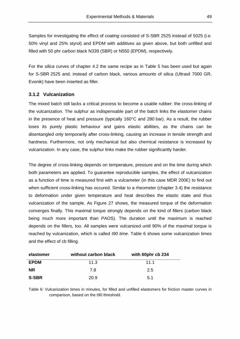
Experimental Methods & Materials 49
Samples for investigating the effect of coating consisted of S-SBR 2525 instead of 5025 (i.e.
50% vinyl and 25% styrol) and EPDM with additives as given above, but both unfilled and
filled with 50 phr carbon black N339 (SBR) or N550 (EPDM), respectively.
For the silica curves of chapter 4.2 the same recipe as in Table 5 has been used but again
for S-SBR 2525 and, instead of carbon black, various amounts of silica (Ultrasil 7000 GR,
Evonik) have been inserted as filler.
3.1.2 Vulcanization
The mixed batch still lacks a critical process to become a usable rubber: the cross-linking of
the vulcanization. The sulphur as indispensable part of the batch links the elastomer chains
in the presence of heat and pressure (typically 160°C and 280 bar). As a result, the rubber
loses its purely plastic behaviour and gains elastic abilities, as the chains can be
disentangled only temporarily after cross-linking, causing an increase in tensile strength and
hardness. Furthermore, not only mechanical but also chemical resistance is increased by
vulcanization. In any case, the sulphur links make the rubber significantly harder.
The degree of cross-linking depends on temperature, pressure and on the time during which
both parameters are applied. To guarantee reproducible samples, the effect of vulcanization
as a function of time is measured first with a vulcameter (in this case MDR 200E) to find out
when sufficient cross-linking has occured. Similar to a rheometer (chapter 3.4) the resistance
to deformation under given temperature and heat describes the elastic state and thus
vulcanization of the sample. As Figure 27 shows, the measured torque of the deformation
converges finally. This maximal torque strongly depends on the kind of fillers (carbon black
being much more important than PAOS). The duration until the maximum is reached
depends on the fillers, too. All samples were vulcanized until 90% of the maximal torque is
reached by vulcanization, which is called t90 time. Table 6 shows some vulcanization times
and the effect of cb filling.
Table 6: Vulcanization times in minutes, for filled and unfilled elastomers for friction master curves in
comparison, based on the t90 threshold.
elastomer without carbon black with 60phr cb 234
EPDM 11.3 11.1
NR 7.8 2.5
S-SBR 20.9 5.1
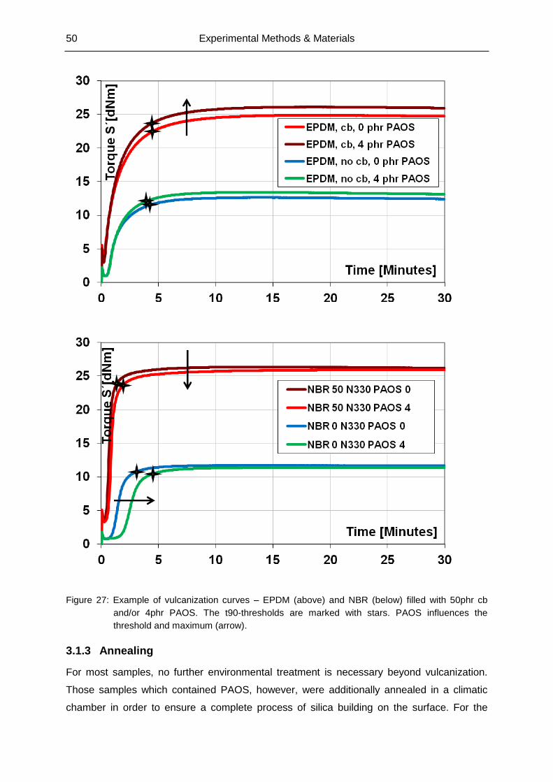
50 Experimental Methods & Materials
Figure 27: Example of vulcanization curves – EPDM (above) and NBR (below) filled with 50phr cb
and/or 4phr PAOS. The t90-thresholds are marked with stars. PAOS influences the
threshold and maximum (arrow).
3.1.3 Annealing
For most samples, no further environmental treatment is necessary beyond vulcanization.
Those samples which contained PAOS, however, were additionally annealed in a climatic
chamber in order to ensure a complete process of silica building on the surface. For the
Experimental Methods & Materials 51
PAOS reaction with water, a constant air humidity of 90% was chosen, and a temperature of
60°C accelerated the process. Apart from test series to verify the development, all samples
(especially those for friction experiments) were treated this way for 24 hours. The reaction
can be regarded as finished then. After this procedure the samples were stored in a
desiccator, interrupted only for measurements.
3.1.4 Sample Shaping
For any standardized tribological measurement, the samples were shaped as flat hexaeders
with 2 mm thickness d0, within the vulcanization process, having square contact surfaces
with lateral sizes l0 and b0 of 50 mm edge length each, by die cutting. A few samples had
6 mm thickness to investigate the influence of the effect on friction, or for abrasion
measurements, keeping to the standard thickness for that characterization.
The leading edge (for friction measurements with the unidirectional universal tester) or both
leading edges (when using the bidirectional tribometer) were ground at approximately 45°,
reducing the lateral length l0 by about 1 mm for each grinding, which had to be considered for
calculating the nominal contact area A0 = l0 * b0 and the pressure σ0 = FN / A0.
Although in theory the microscopical morphology of the rubber surface should be completely
ignored because the elastomer adapts to the substrate structures, this is obviously true only
for rubber surfaces that are significantly flatter than the substrate and for sufficiently large
pressures. A macroscopically rough rubber under a moderate weight might well have valleys
that do not reach interfacial contact, especially if the substrate is extraordinarily flat like, in
our case, glass, steel and coated substrates. In order to investigate this phenomenon,
different types of vulcanization plates were applied:
coarse: rough because it was grit blasted with glass pearls with heights up to 2 µm
fine: between both extremes with heights around 300 nm
polished: very smooth plate with heights of maximal 50 nm
For further description of the plates see Table 7.
3.1.5 Coating
On coarse substrates the structure of the rubber surface is negligible. On very smooth
substrates, a smooth rubber can provoke significantly high friction values. Chapters 4.5.3
and 4.5.4 will investigate the mitigation of friction and stick-slip by coating the contact
interface. The coating layers had to be sufficiently thin, or, instead of the original rubber, the
coating properties would have indeed dominated the viscoelasticity of the sample. On the
other hand, the coating had to be thick enough to be effective and also stable enough
against abrasion (chapter 4.6.1).
52 Experimental Methods & Materials
The coating was sprayed as homogenously as possible onto the friction side of the sample.
The chemical composition of the coating consisted of a varnish matrix in which various types
of particles were embedded:
polysiloxane (PTFE particles and cross-linking agent in PUR varnish)
PTFE (in a 1-component PUR varnish)
PU (2-component PUR varnish)
TPU (pure 1-component PUR varnish without particles)
These chemicals will be discussed in chapter 3.7.4. The purpose was to confine the contact
between sample and substrate to areas where particles emerge the average layer level. This
should reduce friction especially for dry sliding. The particle size was of a similar order than
the complete layer thickness: 10 µm for standard coatings. In order to investigate the
influence of thickness, some samples were coated with a 40 µm layer, however. These
exceptions are indicated when they appear. Due to spraying fluctuations and drying
parameters small variations in thickness are possible.
A problem to overcome was a lack in adherence when the varnish was directly sprayed onto
the sample. The system showed poor connection and the varnish peeled off easily, causing
further abrasion. To solve this, vapour phase fluorination was applied to the sample before
coating it. This prevented peeling for the majority of samples and allowed exploiting the
parameter space to a large extent.
Experimental Methods & Materials 53
3.2 Surface Characterization
Being crucial for friction, the interface of the friction zone should be characterized as
completely as possible. This can be done due to vertical and lateral geometrical description
(profiles and morphology) of the surface, its chemical constitution and chemical bonding
(surface tension) of the contact between both. Surface characterizations were done by
various persons.
3.2.1 Profile Measurements
To gain information on how the height of a surface changes with lateral displacement,
profiles are measured and evaluated. This can either be done with image producing
methods, or with linear scanning techniques, which result in 1-dimensional lines that, if
parallel, can be assembled to 2-dimesional pictures with height information as third
dimension. An example of a profile is given in Figure 18. For achieving surface information
like the HDC, adequate numbers of profiles have been evaluated to gain statistically reliable
results. The most basic statistical information is the arithmetic average Ra of the various
height values.
Mechanical Profilometer
Especially for coarse surfaces like granite or asphalt, the profilometer is a useful tool. A
sensor on a stylus is moved laterally over the surface and measures mechanically the
change of height. Measurements were exact to 0.5 µm laterally and 16 nm vertically, to
maximal ranges of 50 mm horizontally and 1 mm vertically. Alternatively to tactile interaction,
laser profilometers detect the surface without contact.
Atomic Force Microscope (AFM)
The atomic force microscopy (in this case, an FRT-AFM) is a mechanical scanning
instrument. Its advantage is the high resolution, which allows measurements far below the
micron scale, limited mainly by the tip radius and stability of the experimental environment,
and thus is the optimal tool for smooth surfaces. On the other hand, the maximal scanning
area is limited to tiny dimensions about 50 µm * 50 µm. In contrast to other scanning
techniques like STM, electrical conductivity is not required for AFM – a mandatory feature for
unfilled rubber and most substrates.
A small tip is fixed on a cantilever which is bent according to the movement of the tip over the
sample surface, and information of the bending is transmitted with a laser beam to a photo
sensor. Scanning is in lines with a small displacement to each other to build a pixel image.
54 Experimental Methods & Materials
The scanning range is confined to a small area. Depending on the type of interaction
between tip and surface various modes can be used:
contact mode (direct mechanical contact with constant force or constant height
causes repulsion)
non-contact mode (dynamic resonant vibration)
intermittent contact mode (tapping mode with constant amplitude)
White Light Interferometry
The surface descriptors of some substrates have been gained with another technique, the
white light interferometry. A focussed spectrum of various wavelengths (white light) from a
coherent light source is reflected on the substrate’s surface. The interferences caused by
differences in beam lengths give information about the z-coordinate of the illuminated spot,
i.e. the colour is correlated with the height. Dispersion must be considered. Resolution is in
the micron range laterally and up to 10 nm vertically, and comparatively large areas of some
mm can be captured with low resolution. A major advantage of this type of microscopy is the
complete avoidance of mechanical contact.
3.2.2 Morphology
Similar to profile measurements, morphological investigations describe the structural
geometry of the surface. However, aim of this analysis is not the height information itself, but
areal structures of the 2-dimensional image in order to reveal the surface topography:
patterns, artefacts and domains.
The simplest way to accomplish this is optical microscopy. A more sophisticated method is
the Dispersion Index Analysis System (DIAS). It was developed especially to determine the
degree of filler dispersion within the rubber. The light reflected on surface slices passes an
optical microscope, and the digital image is analyzed automatically due to particle pattern
recognition, allowing conclusions to the degree of dispersion and size distribution of
agglomerates.
Another topographical method is scanning electron microscopy (SEM), which will be
described in chapter 3.2.3 as prerequisite for EDX measurements.
Apart from this, the 2-dimensional images gained with profile methods (AFM, White Light
Interferometry) as described above can be used for morphological analysis as well.
Experimental Methods & Materials 55
3.2.3 Chemical Analysis
Even more interesting than size and shape of surface objects are the components they
consist of. Several devices were used for chemical surface analysis:
EDX
A contact free method to analyze surface chemistry is the energy dispersive X-ray
spectroscopy (EDX). A conductive sample is put into a SEM device. A focused electron
beam scans over the sample surface. The detected response signal becomes a pixel of the
resulting image. The beam has a freely tuneable but constant energy, and excites atoms
when hitting the sample as a target. Higher orbital electrons close the gap, generating x-rays.
The spectrum that is produced then is characteristic for the involved chemical elements,
which are discriminated from each other and the bremsstrahlung background by an included
software, resulting in information about the proportional distribution of elements in the
analyzed spot. Although other methods of exciting atoms for X-ray emission exist, SEM-EDX
is the most common technique.
The penetration depth depends on the beam energy and normally does not significantly
exceed a few microns. This means that solely surface composition and almost no bulk is
given – especially important for samples with surface modifications (PAOS, coating). Being
pear-shaped, lateral resolution is of a similar order, if the beam is sufficiently focused.
Infrared Spectroscopy
For this type of characterization, the surface is irradiated with a spectrum of infrared light,
ranging from 700 cm-1 to 4000 cm-1 for this FTIR device. Molecular dipole excitation consists
mainly of oscillation for this near IR part of the spectrum, causing absorption for the
corresponding wavelength, with different molecule spectra superposing each other. With
knowledge of the absorption or transmission reference spectra the amounts of chemical
substances can be calculated.
XPS
The technique of X-ray photoelectron spectroscopy (XPS) uses the photoeffect for surface
atoms: Each element has characteristic binding energies for its electron orbitals. According
to Einstein’s light quantum hypothesis, the energy of a photon is directly proportional to its
frequency, and X-rays are high frequent/ energetic enough to remove electrons from their
atoms. These photoelectrons are detected and, purged from secondary electron signals,
correlated with elements, amounting to chemical ratios. Sensitivity for the photo effect
depends on frequency and effective cross-section.
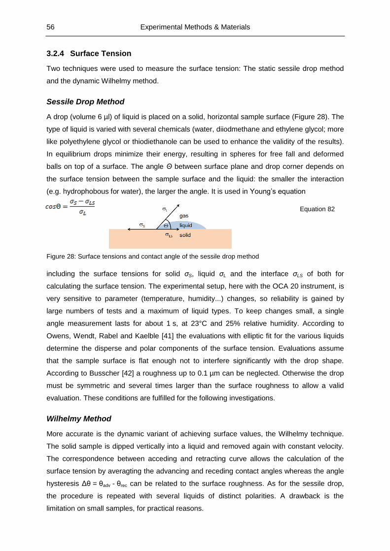
56 Experimental Methods & Materials
3.2.4 Surface Tension
Two techniques were used to measure the surface tension: The static sessile drop method
and the dynamic Wilhelmy method.
Sessile Drop Method
A drop (volume 6 µl) of liquid is placed on a solid, horizontal sample surface (Figure 28). The
type of liquid is varied with several chemicals (water, diiodmethane and ethylene glycol; more
like polyethylene glycol or thiodiethanole can be used to enhance the validity of the results).
In equilibrium drops minimize their energy, resulting in spheres for free fall and deformed
balls on top of a surface. The angle Θ between surface plane and drop corner depends on
the surface tension between the sample surface and the liquid: the smaller the interaction
(e.g. hydrophobous for water), the larger the angle. It is used in Young’s equation
Equation 82
Figure 28: Surface tensions and contact angle of the sessile drop method
including the surface tensions for solid σS, liquid σL and the interface σLS of both for
calculating the surface tension. The experimental setup, here with the OCA 20 instrument, is
very sensitive to parameter (temperature, humidity...) changes, so reliability is gained by
large numbers of tests and a maximum of liquid types. To keep changes small, a single
angle measurement lasts for about 1 s, at 23°C and 25% relative humidity. According to
Owens, Wendt, Rabel and Kaelble [41] the evaluations with elliptic fit for the various liquids
determine the disperse and polar components of the surface tension. Evaluations assume
that the sample surface is flat enough not to interfere significantly with the drop shape.
According to Busscher [42] a roughness up to 0.1 µm can be neglected. Otherwise the drop
must be symmetric and several times larger than the surface roughness to allow a valid
evaluation. These conditions are fulfilled for the following investigations.
Wilhelmy Method
More accurate is the dynamic variant of achieving surface values, the Wilhelmy technique.
The solid sample is dipped vertically into a liquid and removed again with constant velocity.
The correspondence between acceding and retracting curve allows the calculation of the
surface tension by averagting the advancing and receding contact angles whereas the angle
hysteresis Δθ = θadv - θrec can be related to the surface roughness. As for the sessile drop,
the procedure is repeated with several liquids of distinct polarities. A drawback is the
limitation on small samples, for practical reasons.
Experimental Methods & Materials 57
3.3 Material Testing
The various possible methods for material testing are numerous and include mechanical,
chemical, electrical, optical, thermal and other aspects. Unlike the surface testing described
above, the techniques of this chapter characterize some bulk properties of the sample, or
more precisely, mechanical bulk properties. Due to the mechanical exposure, the procedures
are destructive for the sample. The properties concerning shear and torsion are explained in
detail in the next chapter, as they are the key for understanding viscoelasticity.
3.3.1 Shore Hardness
A manifold of standards exist to measure the hardness as a gauge for the resistance against
indentation. The most common standard for elastomers is the Shore hardness: A normed
steel pen indents the sample with a fixed force at room temperature for 15 s; from the
indentation depth the hardness is calculated. Deep indentations equal low hardnesses and
vice versa, ranging from 0 to 100.
Large rubber hardness is an indirect hint for low elasticity and thus is important for friction.
Consequently, it means that hard substances are more brittle than soft ones. Hardness is
also connected to wear because soft materials are abrased by hard ones, the opposite case
is negligible. To build a rubber element with good stability against wear, a hard surface with
an elastic core is a helpful combination – chapter 4.5.2 makes use of this idea.
3.3.2 Rebound
Ideal elastic materials return to their a priori geometry, bouncing back objects with original
momentum. Real elastic materials dissipate a part of the kinetic energy. This is measured
with rebound testing: A standardized hammer hits the sample with predefined parameters;
the deflection is a measure of elasticity.
3.3.3 Tensile Test
With a universal testing machine the sample can be stretched to a specified degree and the
resulting force (and thus the stress tension) is measured with a load cell. The velocity can
freely be chosen, and either tension or elongation can be the actuating variable.
For testing, samples of known geometry with small cross-section are stretched steadily and
sufficiently slowly. As samples in general, and especially elastomers, exhibit not only a linear
function (Hooke’s behaviour) between tension and elongation, several characteristic
parameters are defined to describe the relationship of both in the elastic and plastic regime.
58 Experimental Methods & Materials
For the consideration of the experiments described below, the following parameters were
used:
Tensile strength: This is the maximal tension that is reached during the complete test,
regarding the original cross-section of the sample as fix (nominal tension).
Elongation at break: This value tells the percentile ratio of how far a sample can be
stretched before it breaks.
Stress at 200%: This number gives the stress that is necessary to stretch the sample
to 200% of its original length.
3.3.4 Abrasion
During friction it may happen that the structural stability of one of the interacting partners
(usually the softer one) is not enough to keep the body intact: Small particles, either
microscopic or macroscopic, are detached from the surface into the interface zone. This is
called abrasion. Roughness and hardness determine the abrasion essentially.
To determine the abrasion, the sample (6 mm thick) is treated with a sliding surface of
defined surface parameters, velocity and normal force for a certain time. The amount of
abrased material is evidence for the sensibility to abrasion.
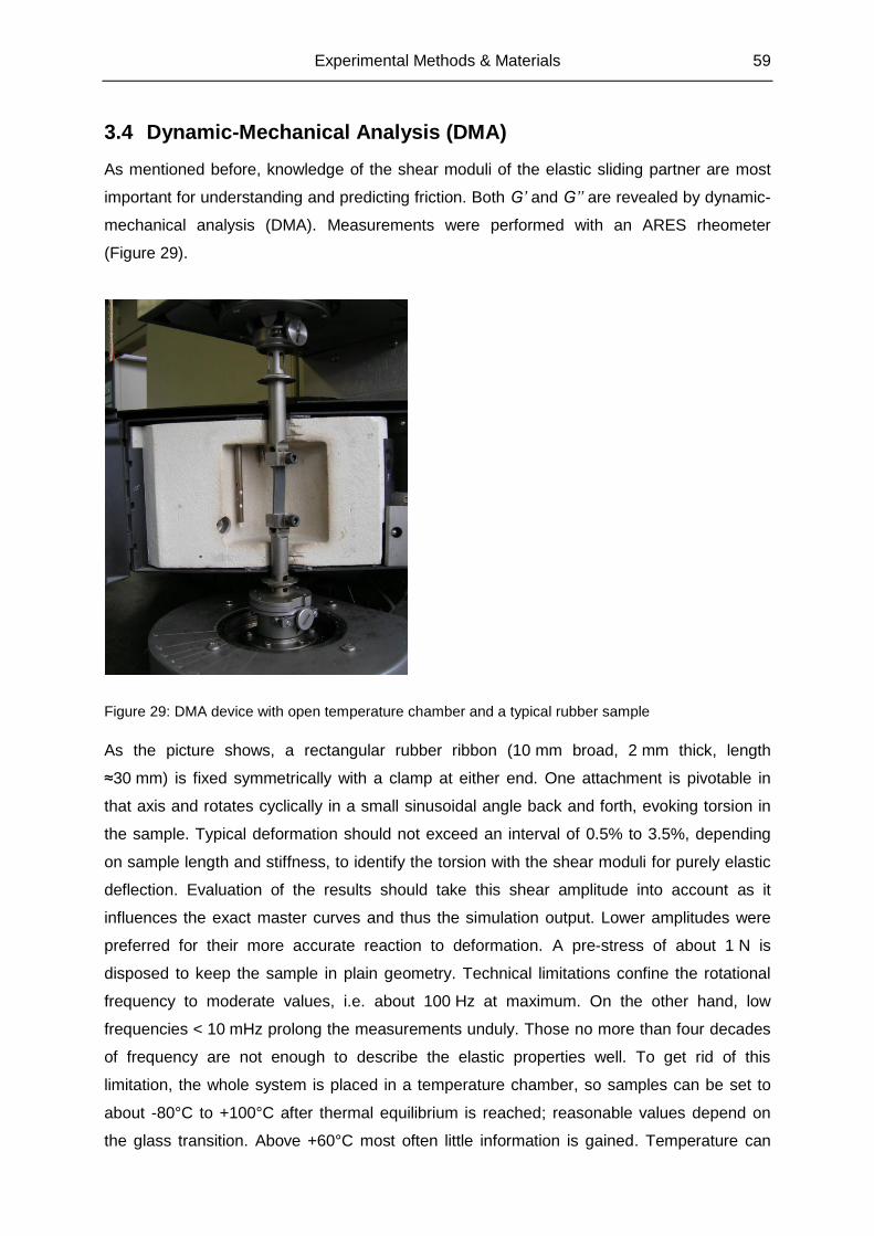
Experimental Methods & Materials 59
3.4 Dynamic-Mechanical Analysis (DMA)
As mentioned before, knowledge of the shear moduli of the elastic sliding partner are most
important for understanding and predicting friction. Both G’ and G’’ are revealed by dynamic-
mechanical analysis (DMA). Measurements were performed with an ARES rheometer
(Figure 29).
Figure 29: DMA device with open temperature chamber and a typical rubber sample
As the picture shows, a rectangular rubber ribbon (10 mm broad, 2 mm thick, length
≈30 mm) is fixed symmetrically with a clamp at either end. One attachment is pivotable in
that axis and rotates cyclically in a small sinusoidal angle back and forth, evoking torsion in
the sample. Typical deformation should not exceed an interval of 0.5% to 3.5%, depending
on sample length and stiffness, to identify the torsion with the shear moduli for purely elastic
deflection. Evaluation of the results should take this shear amplitude into account as it
influences the exact master curves and thus the simulation output. Lower amplitudes were
preferred for their more accurate reaction to deformation. A pre-stress of about 1 N is
disposed to keep the sample in plain geometry. Technical limitations confine the rotational
frequency to moderate values, i.e. about 100 Hz at maximum. On the other hand, low
frequencies < 10 mHz prolong the measurements unduly. Those no more than four decades
of frequency are not enough to describe the elastic properties well. To get rid of this
limitation, the whole system is placed in a temperature chamber, so samples can be set to
about -80°C to +100°C after thermal equilibrium is reached; reasonable values depend on
the glass transition. Above +60°C most often little information is gained. Temperature can
60 Experimental Methods & Materials
either be run through in small steps with constant frequency (temperature sweep) or in
coarse steps (5 K steps in the cold range, 10 K for medium range, 20 K in the hot) for a while
during which the frequency exploits its own range as described above (frequency sweep).
Measured variables are: temperature, the shear moduli G’ and G’’ (and thus complex G* and
tan δ), time, the actual sample length, the resulting torque and for frequency sweeps of
course also the frequency.
Evaluation of these data makes use of the time temperature principle explained in chapter
2.2. Each temperature step gained from a frequency sweep becomes one of many
isothermal branches in a diagram G’(f) or G’’(f) and tan δ (f), respectively. By shifting each
single curve horizontally (i.e. parallel to the f-axis), a continuous master curve (Figure 11) is
constructed from overlapping branches. The factors (or distances, for logarithmic plot) are
not arbitrary, but ruled by the WLF equation (Equation 28) for unfilled samples. Filled
samples lack a good overlap for hot temperature branches (Figure 13) until an additional
vertical shift for the shear axis is applied, with factors in concordance to the Vogel-Fulcher
equation (Equation 29). Both equations are valid above glass transition, which can well be
determined by the DMA results. All master curves shown in this work refer to an unshifted
temperature branch for 20°C.
Experimental Methods & Materials 61
3.5 Friction Measurements
Without any doubt, friction measurements are the centre of experimental testing concerning
a work on investigation, prediction and control of rubber friction. They were carried out
extensively and with the due accuracy. The results are both empirical findings of effects and
comparison of parameter influence as well as the basement for fitting simulations.
The principle of any friction test is simple: A sample (here: rectangular 5 mm * 5 mm and
2 mm thick, with grinded edges) is pressed by a normal force on its sliding partner, the
substrate. In these experiments this was achieved by putting a constant weight on the
sample. Consequently, all sliding took place on horizontally levelled planes. The sample is
moved parallel to this plane, and the resulting friction force is measured. To guarantee a
stable friction behaviour, the sliding speed was kept constant (stationary velocity); non-
stationary parts of the friction curve and artefacts were neglected and not evaluated.
Velocities were comparably low, so the thermal stability of the system due to frictional heat
was well provided for even in dry systems. Samples and substrates were cleaned
adequately, depending on their sensibility with isopropanol (normal case) or only with distilled
water (coated samples and coated metal sheets), before and if required between
measurements to exclude grease, abrasion particles and other unwanted materials.
To perform these experiments, two different devices were used: a special tribometer and a
universal testing machine.
3.5.1 Tribometer
This tribometer is a unique machine, designed especially for the needs of this type of
measurement. It was applied for the vast majority of the following experiments. Figure 30
shows its elements schematically: Any substrate (see chapter 3.6) within a lateral maximum
of 10 cm * 28 cm can be fixed in a pool that is mounted on a sledge. Substrates were always
levelled to set their surface horizontal.
Some measurements were performed on dry substrates. If necessary, the pool can be filled
with a lubricant – this was usually a solution of 5% (volume) of commercial washing tenside
with water. Rarely pure water was used for comparison; if not indicated differently, “lubricant”
or “wet” always means a tenside-water mixture. Ideally the interface of the sliding partners is
only thinly covered by lubricant during the whole measurement to avoid viscous friction.
Adhesion friction is assumed to vanish almost completely because of this procedure.
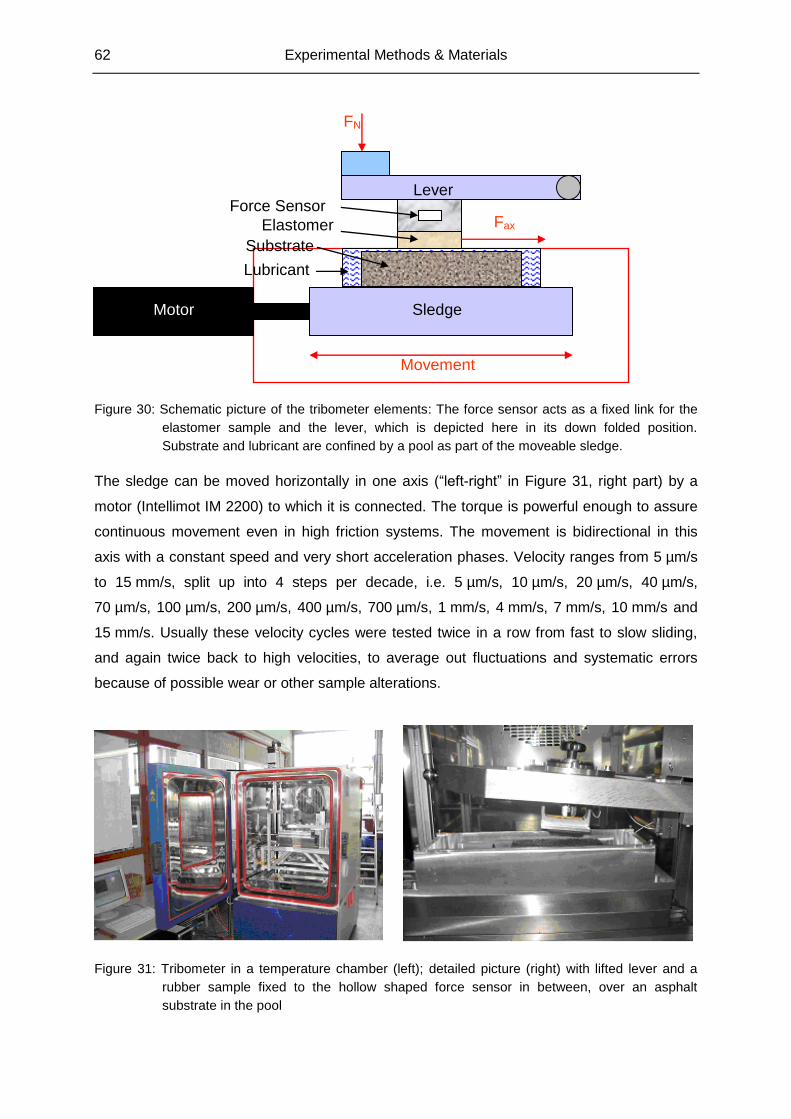
62 Experimental Methods & Materials
Figure 30: Schematic picture of the tribometer elements: The force sensor acts as a fixed link for the
elastomer sample and the lever, which is depicted here in its down folded position.
Substrate and lubricant are confined by a pool as part of the moveable sledge.
The sledge can be moved horizontally in one axis (“left-right” in Figure 31, right part) by a
motor (Intellimot IM 2200) to which it is connected. The torque is powerful enough to assure
continuous movement even in high friction systems. The movement is bidirectional in this
axis with a constant speed and very short acceleration phases. Velocity ranges from 5 µm/s
to 15 mm/s, split up into 4 steps per decade, i.e. 5 µm/s, 10 µm/s, 20 µm/s, 40 µm/s,
70 µm/s, 100 µm/s, 200 µm/s, 400 µm/s, 700 µm/s, 1 mm/s, 4 mm/s, 7 mm/s, 10 mm/s and
15 mm/s. Usually these velocity cycles were tested twice in a row from fast to slow sliding,
and again twice back to high velocities, to average out fluctuations and systematic errors
because of possible wear or other sample alterations.
Figure 31: Tribometer in a temperature chamber (left); detailed picture (right) with lifted lever and a
rubber sample fixed to the hollow shaped force sensor in between, over an asphalt
substrate in the pool
Movement
Lubricant
Elastomer Fax
Substrate
Sledge Motor
Force Sensor Lever
FN

Experimental Methods & Materials 63
As the goal is to gain reproducible data, these alterations have to be considered not only by
maximizing the number of measurements. The state of the sample surface can change
dramatically during the friction process, especially in the beginning when a virgin or stored
sample experiences micro abrasion of its oxidized and more or less aged surface. So before
starting the proper testing sequence, samples have to pass a “running-in” procedure
(compare to Figure 44) of several cycles at high velocity. Friction turns out to converge to a
constant level after less than 10 cycles for most cases, as Figure 44 shows. This behaviour
must not be confused with the Mullins effect, which would affect only filled samples,
happening already during the first stress exposures.
The other parts – sample, sensor and normal weight – are attached to a lever that can be
lowered and lifted to allow or prevent friction contact and for sample exchange. The weight
remains constant, at minimum the lever system weight itself, and can be increased by
additional weights at the far side of the lever. If not proclaimed otherwise, all measurements
with the tribometer resulted in a pressure of 25.3 kPa for the nominal contact area. The
bottom of the lever holds the force sensor, which detects the shearing due to the friction
force. The sample is glued beneath the sensor.
The motor activity and the sensor signals are controlled and recorded by a Labview program
created for this machine. The gathered data (velocity code, friction force and temperature as
a function of time) including static parameters (calibration factors, normal force, contact
area...) were evaluated with a custom-made spread sheet for friction coefficient, actual
distance, plateau characteristics, stick-slip effects (size, frequency, slope) and other
interesting information. Figure 32 displays a plot for some of these parameters in an
example. With two different types of averaged data, also two kinds of errors must be
distinguished: purely statistical fluctuation from averaging the reading points of each single
plateau, which was negligible for most cases, and the error bar of averaging these averaged
values, which as a superposition of statistical and systematical error depended largely on the
stability of elastomer.
The depicted system is surrounded by a temperature chamber. With 20°C being the
reference temperature of DMA master curves, it is reasonable to investigate friction at this
very condition. For assembling friction master curves, however, a broad interval of various
temperatures is needed. Thus, these experiments were performed for dry contact from the
coldest accessible stable environment at -35°C to a maximal temperature before the state of
elastomer or glue caused superposing effects, at about +65°C. Wet contact, of course,
allowed only measurements above freezing point. Prerequisite was the careful achievement
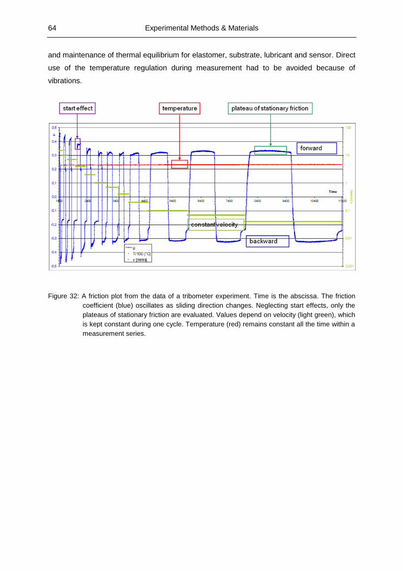
64 Experimental Methods & Materials
and maintenance of thermal equilibrium for elastomer, substrate, lubricant and sensor. Direct
use of the temperature regulation during measurement had to be avoided because of
vibrations.
Figure 32: A friction plot from the data of a tribometer experiment. Time is the abscissa. The friction
coefficient (blue) oscillates as sliding direction changes. Neglecting start effects, only the
plateaus of stationary friction are evaluated. Values depend on velocity (light green), which
is kept constant during one cycle. Temperature (red) remains constant all the time within a
measurement series.
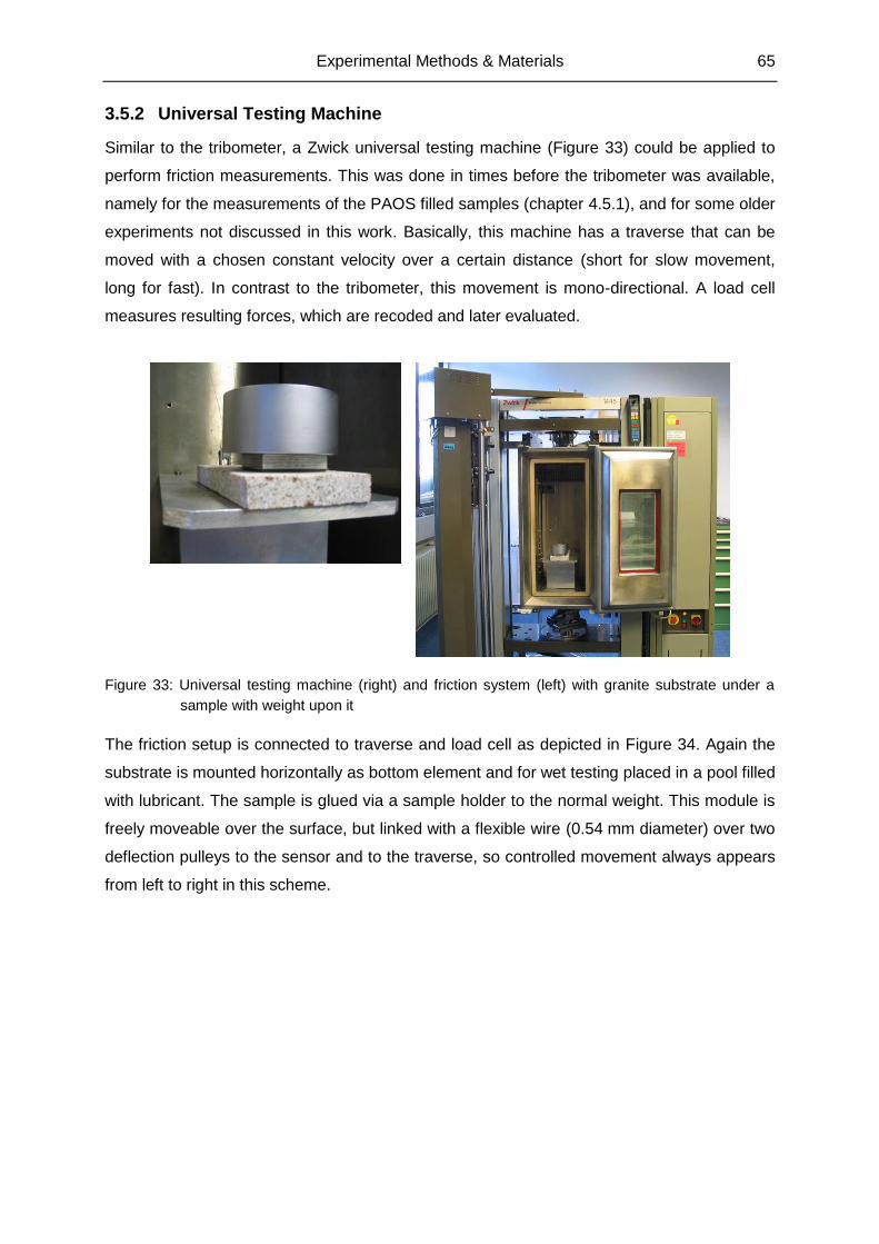
Experimental Methods & Materials 65
3.5.2 Universal Testing Machine
Similar to the tribometer, a Zwick universal testing machine (Figure 33) could be applied to
perform friction measurements. This was done in times before the tribometer was available,
namely for the measurements of the PAOS filled samples (chapter 4.5.1), and for some older
experiments not discussed in this work. Basically, this machine has a traverse that can be
moved with a chosen constant velocity over a certain distance (short for slow movement,
long for fast). In contrast to the tribometer, this movement is mono-directional. A load cell
measures resulting forces, which are recoded and later evaluated.
Figure 33: Universal testing machine (right) and friction system (left) with granite substrate under a
sample with weight upon it
The friction setup is connected to traverse and load cell as depicted in Figure 34. Again the
substrate is mounted horizontally as bottom element and for wet testing placed in a pool filled
with lubricant. The sample is glued via a sample holder to the normal weight. This module is
freely moveable over the surface, but linked with a flexible wire (0.54 mm diameter) over two
deflection pulleys to the sensor and to the traverse, so controlled movement always appears
from left to right in this scheme.
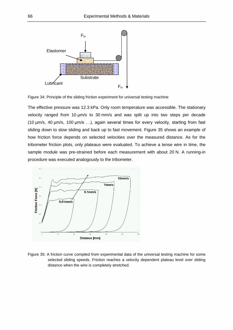
66 Experimental Methods & Materials
Figure 34: Principle of the sliding friction experiment for universal testing machine
The effective pressure was 12.3 kPa. Only room temperature was accessible. The stationary
velocity ranged from 10 µm/s to 30 mm/s and was split up into two steps per decade
(10 µm/s, 40 µm/s, 100 µm/s …), again several times for every velocity, starting from fast
sliding down to slow sliding and back up to fast movement. Figure 35 shows an example of
how friction force depends on selected velocities over the measured distance. As for the
tribometer friction plots, only plateaus were evaluated. To achieve a tense wire in time, the
sample module was pre-strained before each measurement with about 20 N. A running-in
procedure was executed analogously to the tribometer.
Figure 35: A friction curve compiled from experimental data of the universal testing machine for some
selected sliding speeds. Friction reaches a velocity dependent plateau level over sliding
distance when the wire is completely stretched.
Substrate
FN
Elastomer
FH Lubricant
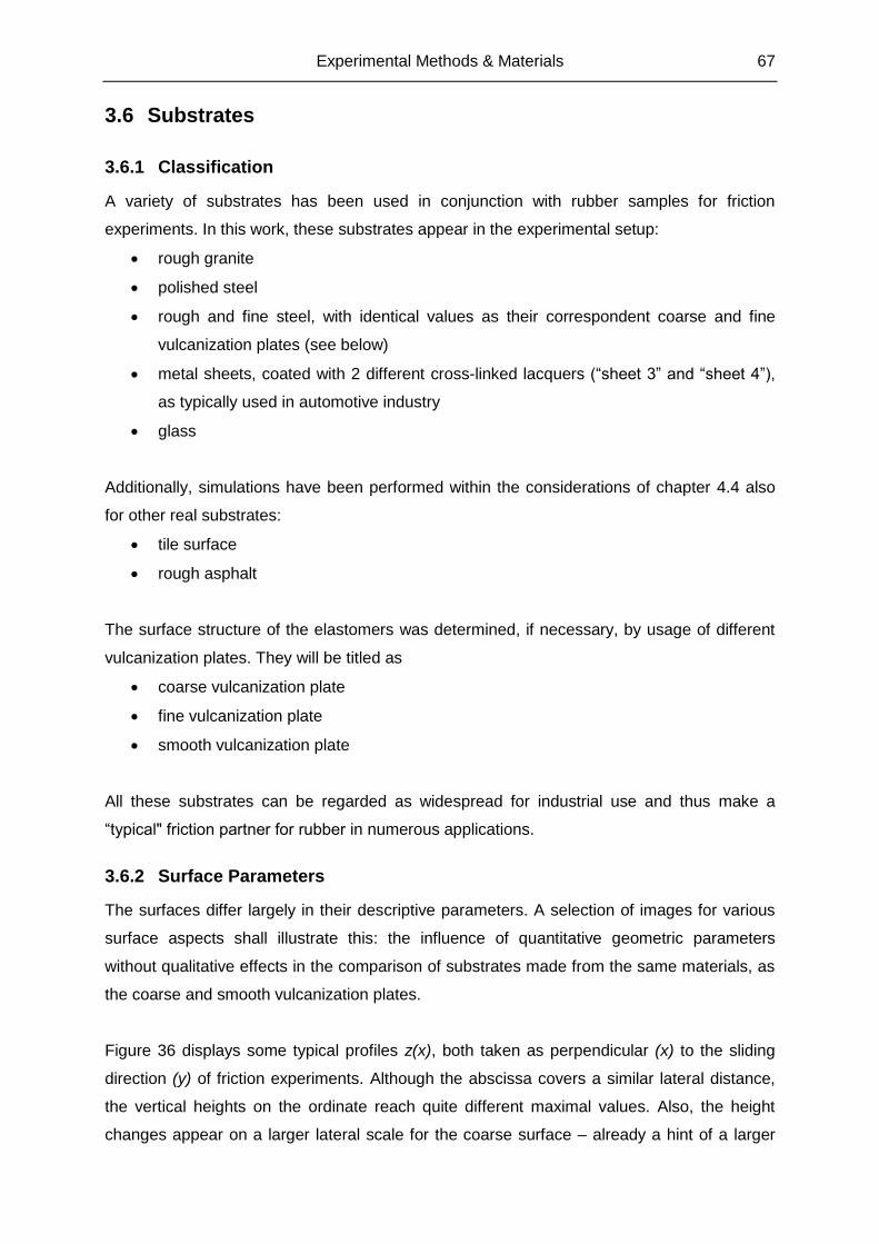
Experimental Methods & Materials 67
3.6 Substrates
3.6.1 Classification
A variety of substrates has been used in conjunction with rubber samples for friction
experiments. In this work, these substrates appear in the experimental setup:
rough granite
polished steel
rough and fine steel, with identical values as their correspondent coarse and fine
vulcanization plates (see below)
metal sheets, coated with 2 different cross-linked lacquers (“sheet 3” and “sheet 4”),
as typically used in automotive industry
glass
Additionally, simulations have been performed within the considerations of chapter 4.4 also
for other real substrates:
tile surface
rough asphalt
The surface structure of the elastomers was determined, if necessary, by usage of different
vulcanization plates. They will be titled as
coarse vulcanization plate
fine vulcanization plate
smooth vulcanization plate
All these substrates can be regarded as widespread for industrial use and thus make a
“typical" friction partner for rubber in numerous applications.
3.6.2 Surface Parameters
The surfaces differ largely in their descriptive parameters. A selection of images for various
surface aspects shall illustrate this: the influence of quantitative geometric parameters
without qualitative effects in the comparison of substrates made from the same materials, as
the coarse and smooth vulcanization plates.
Figure 36 displays some typical profiles z(x), both taken as perpendicular (x) to the sliding
direction (y) of friction experiments. Although the abscissa covers a similar lateral distance,
the vertical heights on the ordinate reach quite different maximal values. Also, the height
changes appear on a larger lateral scale for the coarse surface – already a hint of a larger
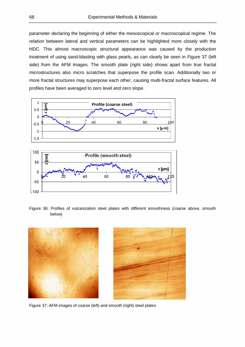
68 Experimental Methods & Materials
parameter declaring the beginning of either the mesoscopical or macroscopical regime. The
relation between lateral and vertical parameters can be highlighted more closely with the
HDC. This almost macroscopic structural appearance was caused by the production
treatment of using sand-blasting with glass pearls, as can clearly be seen in Figure 37 (left
side) from the AFM images. The smooth plate (right side) shows apart from true fractal
microstructures also micro scratches that superpose the profile scan. Additionally two or
more fractal structures may superpose each other, causing multi-fractal surface features. All
profiles have been averaged to zero level and zero slope.
Figure 36: Profiles of vulcanization steel plates with different smoothness (coarse above, smooth
below)
Figure 37: AFM images of coarse (left) and smooth (right) steel plates
Profil
-1,5
-1
-0,5
0
0,5
1
0 20 40 60 80 100
x [m]
z [µ
m] Profile (coarse steel)
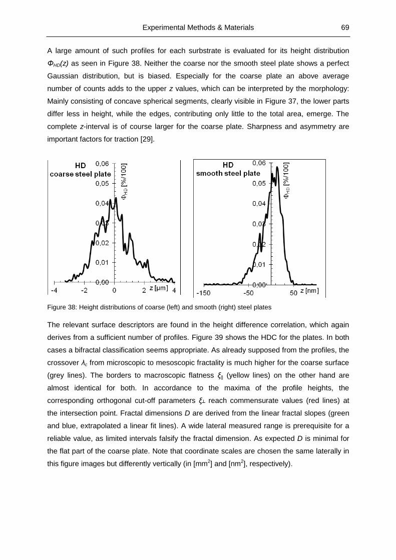
Experimental Methods & Materials 69
A large amount of such profiles for each surbstrate is evaluated for its height distribution
ΦHD(z) as seen in Figure 38. Neither the coarse nor the smooth steel plate shows a perfect
Gaussian distribution, but is biased. Especially for the coarse plate an above average
number of counts adds to the upper z values, which can be interpreted by the morphology:
Mainly consisting of concave spherical segments, clearly visible in Figure 37, the lower parts
differ less in height, while the edges, contributing only little to the total area, emerge. The
complete z-interval is of course larger for the coarse plate. Sharpness and asymmetry are
important factors for traction [29].
Figure 38: Height distributions of coarse (left) and smooth (right) steel plates
The relevant surface descriptors are found in the height difference correlation, which again
derives from a sufficient number of profiles. Figure 39 shows the HDC for the plates. In both
cases a bifractal classification seems appropriate. As already supposed from the profiles, the
crossover λc from microscopic to mesoscopic fractality is much higher for the coarse surface
(grey lines). The borders to macroscopic flatness ξ|| (yellow lines) on the other hand are
almost identical for both. In accordance to the maxima of the profile heights, the
corresponding orthogonal cut-off parameters ξ┴ reach commensurate values (red lines) at
the intersection point. Fractal dimensions D are derived from the linear fractal slopes (green
and blue, extrapolated a linear fit lines). A wide lateral measured range is prerequisite for a
reliable value, as limited intervals falsify the fractal dimension. As expected D is minimal for
the flat part of the coarse plate. Note that coordinate scales are chosen the same laterally in
this figure images but differently vertically (in [mm2] and [nm2], respectively).
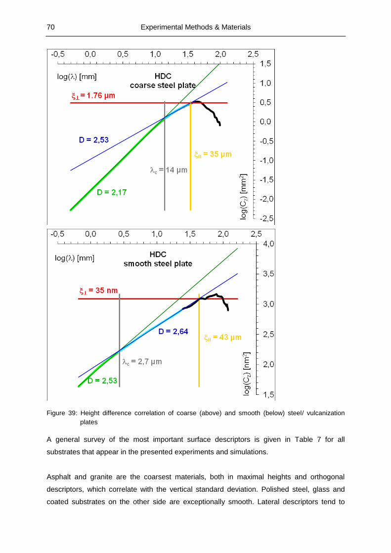
70 Experimental Methods & Materials
Figure 39: Height difference correlation of coarse (above) and smooth (below) steel/ vulcanization
plates
A general survey of the most important surface descriptors is given in Table 7 for all
substrates that appear in the presented experiments and simulations.
Asphalt and granite are the coarsest materials, both in maximal heights and orthogonal
descriptors, which correlate with the vertical standard deviation. Polished steel, glass and
coated substrates on the other side are exceptionally smooth. Lateral descriptors tend to
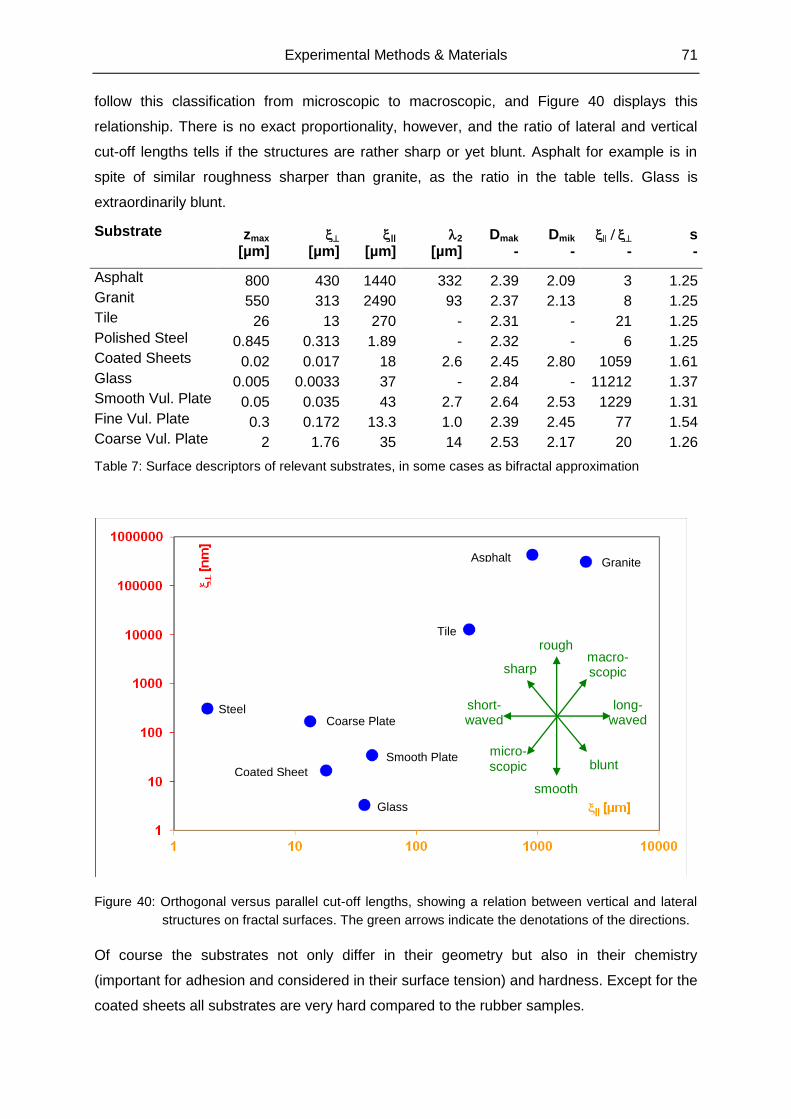
Experimental Methods & Materials 71
follow this classification from microscopic to macroscopic, and Figure 40 displays this
relationship. There is no exact proportionality, however, and the ratio of lateral and vertical
cut-off lengths tells if the structures are rather sharp or yet blunt. Asphalt for example is in
spite of similar roughness sharper than granite, as the ratio in the table tells. Glass is
extraordinarily blunt.
Table 7: Surface descriptors of relevant substrates, in some cases as bifractal approximation
Figure 40: Orthogonal versus parallel cut-off lengths, showing a relation between vertical and lateral
structures on fractal surfaces. The green arrows indicate the denotations of the directions.
Of course the substrates not only differ in their geometry but also in their chemistry
(important for adhesion and considered in their surface tension) and hardness. Except for the
coated sheets all substrates are very hard compared to the rubber samples.
Substrate zmax || 2 Dmak Dmik s
[µm] [µm] [µm] [µm] - - - -
Asphalt 800 430 1440 332 2.39 2.09 3 1.25 Granit 550 313 2490 93 2.37 2.13 8 1.25 Tile 26 13 270 - 2.31 - 21 1.25 Polished Steel 0.845 0.313 1.89 - 2.32 - 6 1.25 Coated Sheets 0.02 0.017 18 2.6 2.45 2.80 1059 1.61 Glass 0.005 0.0033 37 - 2.84 - 11212 1.37 Smooth Vul. Plate 0.05 0.035 43 2.7 2.64 2.53 1229 1.31 Fine Vul. Plate 0.3 0.172 13.3 1.0 2.39 2.45 77 1.54 Coarse Vul. Plate 2 1.76 35 14 2.53 2.17 20 1.26
Glass
Coated Sheet
Tile
Granite Asphalt
Coarse Plate
Smooth Plate
rough
smooth
sharp
blunt
macro-scopic
micro-scopic
long-waved
short-waved
Steel
72 Experimental Methods & Materials
3.7 Elastomer Samples
For our tribological considerations, elastomers play the part of the soft friction partner. This is
also the case in typical applications beyond lab experiments. Their adhesive and flexible
nature makes them a paramount choice in contact systems. But the interface is not
necessarily ruled by the elastomer bulk – surfaces can rather consist of coatings, structure
educing particles, wear debris or lubricant. The search for novel materials and investigation
of sliding systems should take this into account.
3.7.1 Chosen Types of Elastomers
Elastomers [43],[44] are defined as polymers with an extraordinarily low elasticity modulus.
Being well above glass transition at room temperature, stress or pressure will only deform
them temporarily, because the coiled polymer chains are stretched and retract again as soon
as stress is released (relaxation). This process is almost purely entropic elastic for
elastomers. The chains are strengthened by cross-linking them with sulphur during
vulcanization.
Although all elastomers share common features – elasticity with high deformability, softness,
incompressibility – they differ not only in the quantity of these attributes but also in other
properties like glass temperature or stability against thermal, chemical and photonic
(ultraviolet radiation) influences. A manifold of elastomers has been developed since the
discovery of natural rubber to suit all kinds of applications. The following experiments focus
on some wide spread elastomer species that shall be introduced now.
EPDM
Ethylene-Propylene-Dien-Monomer (EPDM) is a synthetic copolymer, i.e. the polymer
consists of different monomer types within each single chain (in contrast to a blend, when
different kinds of chains mix to build the material). It stands out for a high resistance against
heat and cold, sunlight, moisture and ozone and is thus an excellent choice for outdoor
applications. Due to the chemical stability it is furthermore predominantly employed for
hoses, gaskets and other seals in contact with hot or aggressive environments. The good
flexibility of EPDM becomes an important advantage then.
NBR
Nitrile-Butadiene-Rubber (NBR) is another synthetic copolymer. Its stability against oil,
grease and hydrocarbons as well as against heat and abrasion offers a broad usage as
gaskets, hoses and rubberized fabric with small friction coefficients. An important application
are laboratory gloves.
Experimental Methods & Materials 73
NR
Natural rubber (NR) is mainly gained from the latex of the rubber tree Hevea Brasiliensis.
Chemically it consists of isoprene. A reversible strengthening through shear induced
crystallization under mechanical exposure makes NR robust for friction and rolling on rough
interfaces. However, it is sensitive to oil and sunlight. Applications are tyres, gloves, rubber
foams and many others.
SBR
A very common synthetic elastomer is Styrol-Butadiene-Rubber (SBR) as copolymer of styrol
and butadiene (being the larger part). The variant used here is a material from solution
polymerization, called S-SBR. It has a good chemical resistance against inorganic liquids
and a sufficient thermal stability for outdoor usage. SBR is the main contributor for tyre
production but also used for gaskets and conveyor belts.
3.7.2 Reinforcing Fillers
Being a soft material, pure elastomers suffer strong abrasion in sliding situations. Without
reinforcement, devices made for inducing friction like tyres would rather become disposable
products instead of long term machine parts. To overcome this limitation, reinforcing fillers
are added already during the mixing process. They make the rubber harder and significantly
less abrasive. Modern compoundings often make use of silica or even CNT to achieve
special reinforcement, which shall not be treated here as not being part of the utilized
samples.
Carbon Black
The classical reinforcing filler, and the main one used for the experiments of this work,
however, is carbon black (cb).It consists almost completely of the element carbon. In spite of
their chemical identity, various types of cb exist due to structural differences, conditioned by
the parameters of their fabrication (soot from incomplete burning). On the nanometer scale
amorphous cb forms more or less spherical primary particles, surrounded by an envelop of
stiff glassy rubber, the bound rubber, on a nanometer scale [29]. The particles stick together
via glassy bonds and form chain shaped aggregates [45],[46]. When many aggregates
cluster they build agglomerates with a multitude of sterical branches as shown in Figure 41
[47]. It is the breaking of those filler-filler bonds that softens the rubber when exposed to
deformation (Mullins effect) [48],[49].
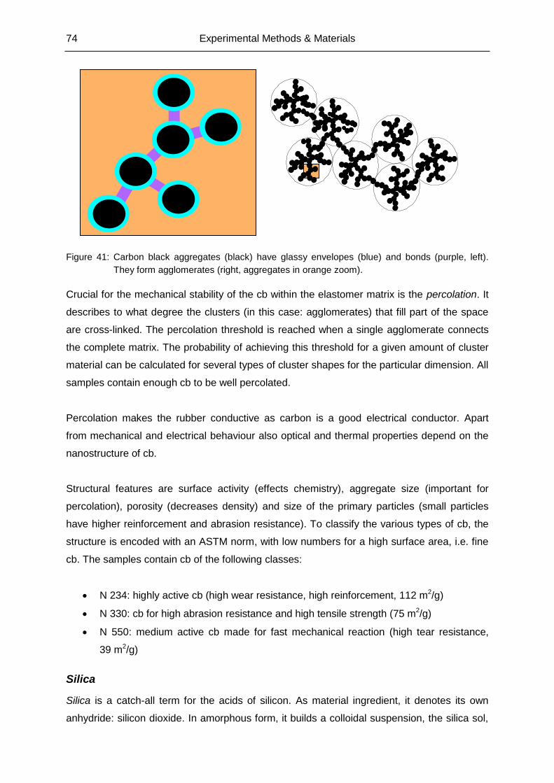
74 Experimental Methods & Materials
Figure 41: Carbon black aggregates (black) have glassy envelopes (blue) and bonds (purple, left).
They form agglomerates (right, aggregates in orange zoom).
Crucial for the mechanical stability of the cb within the elastomer matrix is the percolation. It
describes to what degree the clusters (in this case: agglomerates) that fill part of the space
are cross-linked. The percolation threshold is reached when a single agglomerate connects
the complete matrix. The probability of achieving this threshold for a given amount of cluster
material can be calculated for several types of cluster shapes for the particular dimension. All
samples contain enough cb to be well percolated.
Percolation makes the rubber conductive as carbon is a good electrical conductor. Apart
from mechanical and electrical behaviour also optical and thermal properties depend on the
nanostructure of cb.
Structural features are surface activity (effects chemistry), aggregate size (important for
percolation), porosity (decreases density) and size of the primary particles (small particles
have higher reinforcement and abrasion resistance). To classify the various types of cb, the
structure is encoded with an ASTM norm, with low numbers for a high surface area, i.e. fine
cb. The samples contain cb of the following classes:
N 234: highly active cb (high wear resistance, high reinforcement, 112 m2/g)
N 330: cb for high abrasion resistance and high tensile strength (75 m2/g)
N 550: medium active cb made for fast mechanical reaction (high tear resistance,
39 m2/g)
Silica
Silica is a catch-all term for the acids of silicon. As material ingredient, it denotes its own
anhydride: silicon dioxide. In amorphous form, it builds a colloidal suspension, the silica sol,
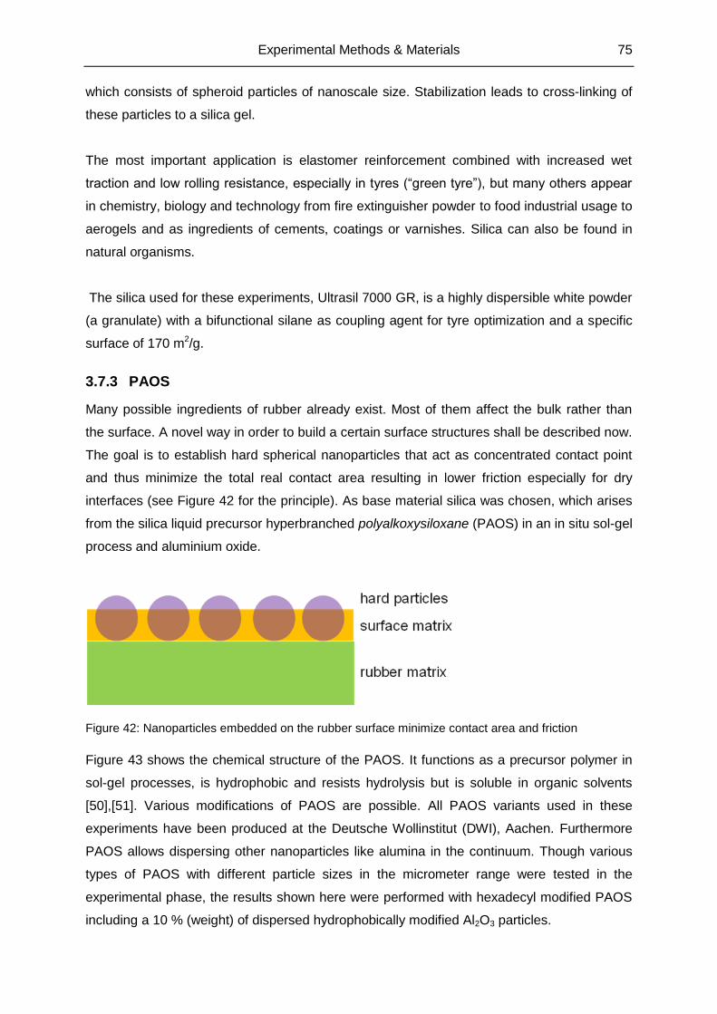
Experimental Methods & Materials 75
which consists of spheroid particles of nanoscale size. Stabilization leads to cross-linking of
these particles to a silica gel.
The most important application is elastomer reinforcement combined with increased wet
traction and low rolling resistance, especially in tyres (“green tyre”), but many others appear
in chemistry, biology and technology from fire extinguisher powder to food industrial usage to
aerogels and as ingredients of cements, coatings or varnishes. Silica can also be found in
natural organisms.
The silica used for these experiments, Ultrasil 7000 GR, is a highly dispersible white powder
(a granulate) with a bifunctional silane as coupling agent for tyre optimization and a specific
surface of 170 m2/g.
3.7.3 PAOS
Many possible ingredients of rubber already exist. Most of them affect the bulk rather than
the surface. A novel way in order to build a certain surface structures shall be described now.
The goal is to establish hard spherical nanoparticles that act as concentrated contact point
and thus minimize the total real contact area resulting in lower friction especially for dry
interfaces (see Figure 42 for the principle). As base material silica was chosen, which arises
from the silica liquid precursor hyperbranched polyalkoxysiloxane (PAOS) in an in situ sol-gel
process and aluminium oxide.
Figure 42: Nanoparticles embedded on the rubber surface minimize contact area and friction
Figure 43 shows the chemical structure of the PAOS. It functions as a precursor polymer in
sol-gel processes, is hydrophobic and resists hydrolysis but is soluble in organic solvents
[50],[51]. Various modifications of PAOS are possible. All PAOS variants used in these
experiments have been produced at the Deutsche Wollinstitut (DWI), Aachen. Furthermore
PAOS allows dispersing other nanoparticles like alumina in the continuum. Though various
types of PAOS with different particle sizes in the micrometer range were tested in the
experimental phase, the results shown here were performed with hexadecyl modified PAOS
including a 10 % (weight) of dispersed hydrophobically modified Al2O3 particles.
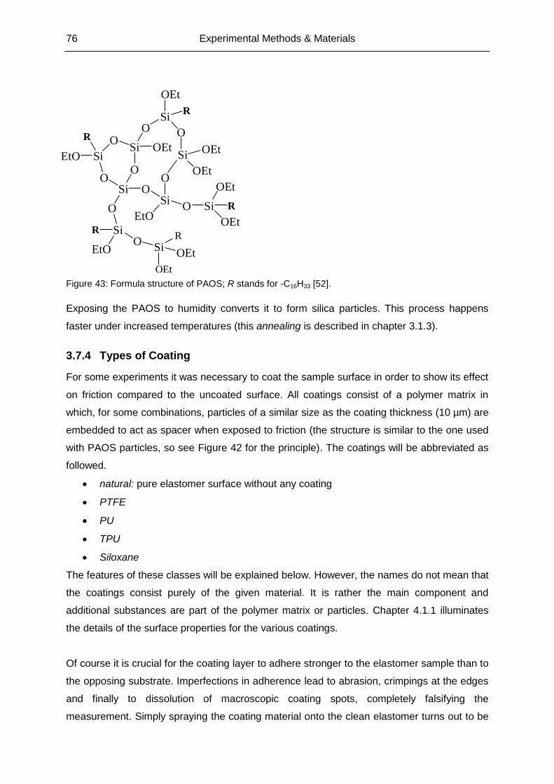
76 Experimental Methods & Materials
Figure 43: Formula structure of PAOS; R stands for -C16H33 [52].
Exposing the PAOS to humidity converts it to form silica particles. This process happens
faster under increased temperatures (this annealing is described in chapter 3.1.3).
3.7.4 Types of Coating
For some experiments it was necessary to coat the sample surface in order to show its effect
on friction compared to the uncoated surface. All coatings consist of a polymer matrix in
which, for some combinations, particles of a similar size as the coating thickness (10 µm) are
embedded to act as spacer when exposed to friction (the structure is similar to the one used
with PAOS particles, so see Figure 42 for the principle). The coatings will be abbreviated as
followed.
natural: pure elastomer surface without any coating
PTFE
PU
TPU
Siloxane
The features of these classes will be explained below. However, the names do not mean that
the coatings consist purely of the given material. It is rather the main component and
additional substances are part of the polymer matrix or particles. Chapter 4.1.1 illuminates
the details of the surface properties for the various coatings.
Of course it is crucial for the coating layer to adhere stronger to the elastomer sample than to
the opposing substrate. Imperfections in adherence lead to abrasion, crimpings at the edges
and finally to dissolution of macroscopic coating spots, completely falsifying the
measurement. Simply spraying the coating material onto the clean elastomer turns out to be
SiO
O
O
O
Si
SiSi
SiR
EtOO
EtO
O
O
EtO
R OOEt
OSi
OEt
R
O
Si
OEt
OEt
Si
OEt
OEt
R
SiR
OEt
OEt
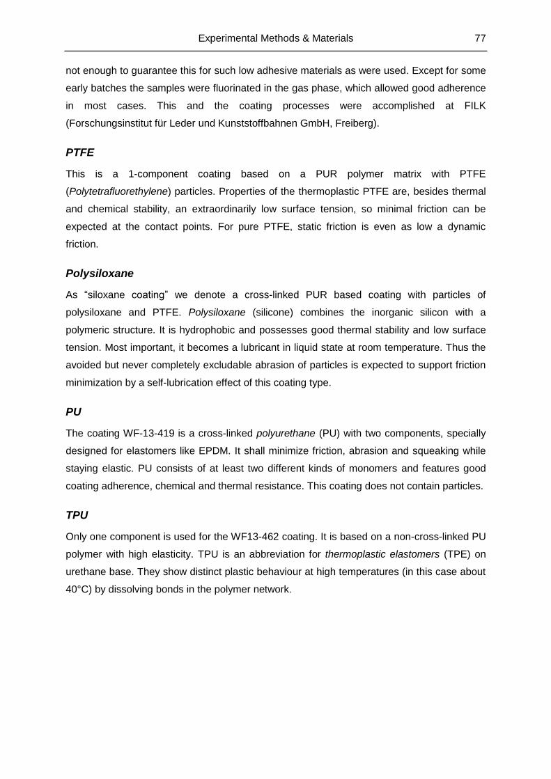
Experimental Methods & Materials 77
not enough to guarantee this for such low adhesive materials as were used. Except for some
early batches the samples were fluorinated in the gas phase, which allowed good adherence
in most cases. This and the coating processes were accomplished at FILK
(Forschungsinstitut für Leder und Kunststoffbahnen GmbH, Freiberg).
PTFE
This is a 1-component coating based on a PUR polymer matrix with PTFE
(Polytetrafluorethylene) particles. Properties of the thermoplastic PTFE are, besides thermal
and chemical stability, an extraordinarily low surface tension, so minimal friction can be
expected at the contact points. For pure PTFE, static friction is even as low a dynamic
friction.
Polysiloxane
As “siloxane coating” we denote a cross-linked PUR based coating with particles of
polysiloxane and PTFE. Polysiloxane (silicone) combines the inorganic silicon with a
polymeric structure. It is hydrophobic and possesses good thermal stability and low surface
tension. Most important, it becomes a lubricant in liquid state at room temperature. Thus the
avoided but never completely excludable abrasion of particles is expected to support friction
minimization by a self-lubrication effect of this coating type.
PU
The coating WF-13-419 is a cross-linked polyurethane (PU) with two components, specially
designed for elastomers like EPDM. It shall minimize friction, abrasion and squeaking while
staying elastic. PU consists of at least two different kinds of monomers and features good
coating adherence, chemical and thermal resistance. This coating does not contain particles.
TPU
Only one component is used for the WF13-462 coating. It is based on a non-cross-linked PU
polymer with high elasticity. TPU is an abbreviation for thermoplastic elastomers (TPE) on
urethane base. They show distinct plastic behaviour at high temperatures (in this case about
40°C) by dissolving bonds in the polymer network.
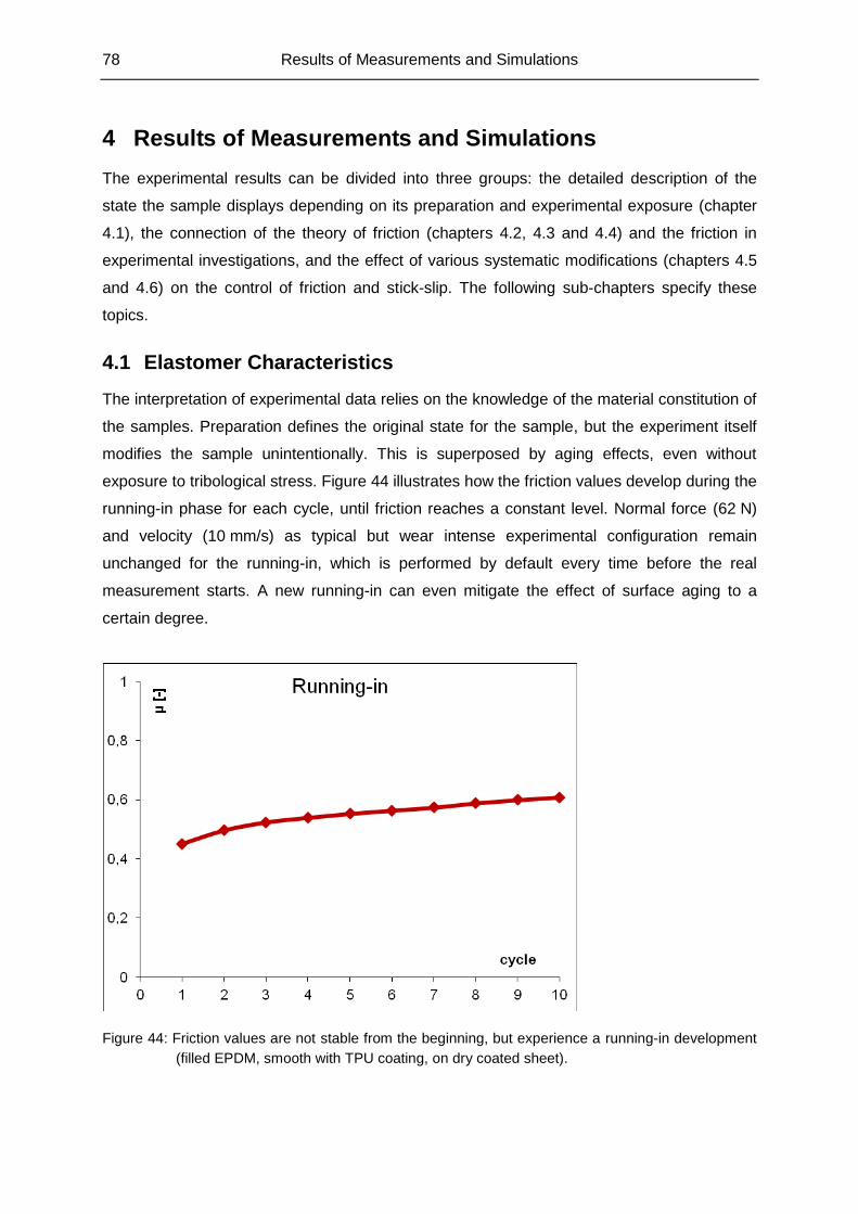
78 Results of Measurements and Simulations
4 Results of Measurements and Simulations
The experimental results can be divided into three groups: the detailed description of the
state the sample displays depending on its preparation and experimental exposure (chapter
4.1), the connection of the theory of friction (chapters 4.2, 4.3 and 4.4) and the friction in
experimental investigations, and the effect of various systematic modifications (chapters 4.5
and 4.6) on the control of friction and stick-slip. The following sub-chapters specify these
topics.
4.1 Elastomer Characteristics
The interpretation of experimental data relies on the knowledge of the material constitution of
the samples. Preparation defines the original state for the sample, but the experiment itself
modifies the sample unintentionally. This is superposed by aging effects, even without
exposure to tribological stress. Figure 44 illustrates how the friction values develop during the
running-in phase for each cycle, until friction reaches a constant level. Normal force (62 N)
and velocity (10 mm/s) as typical but wear intense experimental configuration remain
unchanged for the running-in, which is performed by default every time before the real
measurement starts. A new running-in can even mitigate the effect of surface aging to a
certain degree.
Figure 44: Friction values are not stable from the beginning, but experience a running-in development
(filled EPDM, smooth with TPU coating, on dry coated sheet).
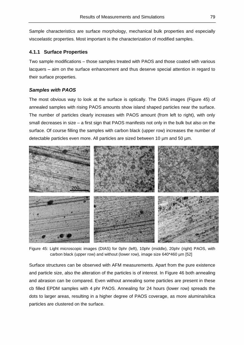
Results of Measurements and Simulations 79
Sample characteristics are surface morphology, mechanical bulk properties and especially
viscoelastic properties. Most important is the characterization of modified samples.
4.1.1 Surface Properties
Two sample modifications – those samples treated with PAOS and those coated with various
lacquers – aim on the surface enhancement and thus deserve special attention in regard to
their surface properties.
Samples with PAOS
The most obvious way to look at the surface is optically. The DIAS images (Figure 45) of
annealed samples with rising PAOS amounts show island shaped particles near the surface.
The number of particles clearly increases with PAOS amount (from left to right), with only
small decreases in size – a first sign that PAOS manifests not only in the bulk but also on the
surface. Of course filling the samples with carbon black (upper row) increases the number of
detectable particles even more. All particles are sized between 10 µm and 50 µm.
Figure 45: Light microscopic images (DIAS) for 0phr (left), 10phr (middle), 20phr (right) PAOS, with
carbon black (upper row) and without (lower row), image size 640*460 µm [52]
Surface structures can be observed with AFM measurements. Apart from the pure existence
and particle size, also the alteration of the particles is of interest. In Figure 46 both annealing
and abrasion can be compared. Even without annealing some particles are present in these
cb filled EPDM samples with 4 phr PAOS. Annealing for 24 hours (lower row) spreads the
dots to larger areas, resulting in a higher degree of PAOS coverage, as more alumina/silica
particles are clustered on the surface.
200
µm
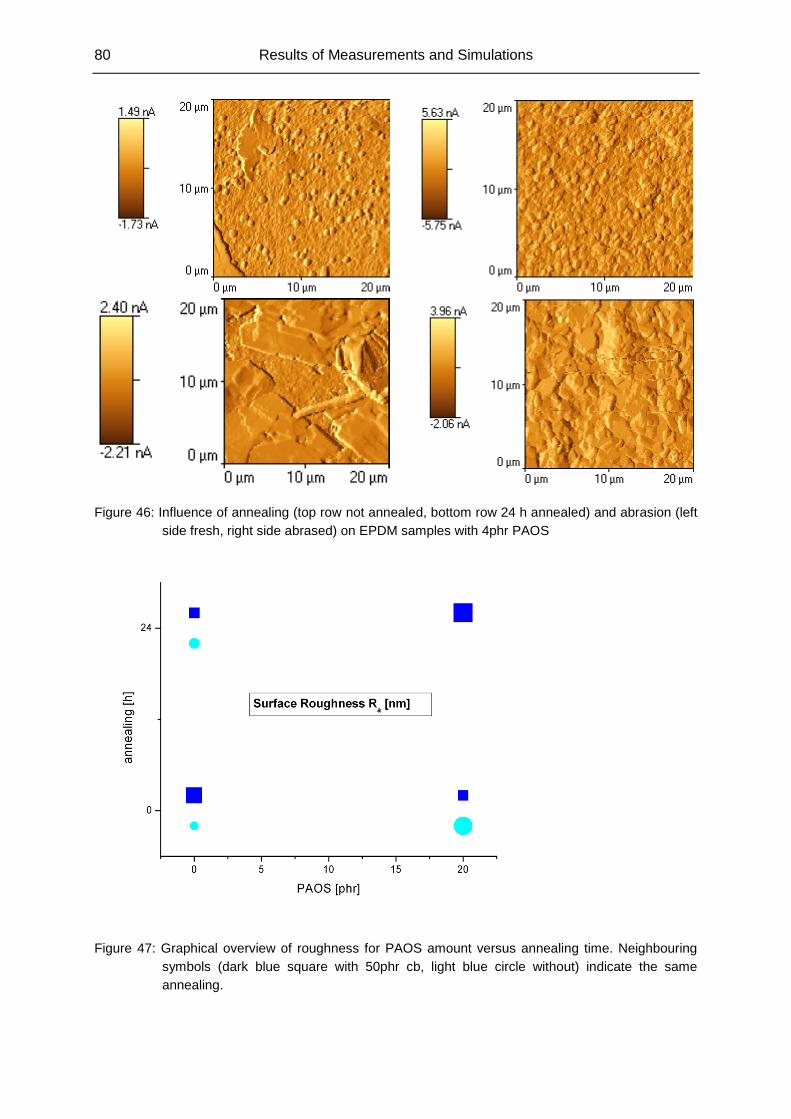
80 Results of Measurements and Simulations
Figure 46: Influence of annealing (top row not annealed, bottom row 24 h annealed) and abrasion (left
side fresh, right side abrased) on EPDM samples with 4phr PAOS
Figure 47: Graphical overview of roughness for PAOS amount versus annealing time. Neighbouring
symbols (dark blue square with 50phr cb, light blue circle without) indicate the same
annealing.
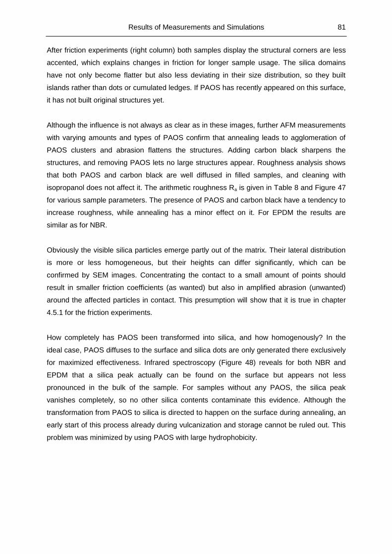
Results of Measurements and Simulations 81
After friction experiments (right column) both samples display the structural corners are less
accented, which explains changes in friction for longer sample usage. The silica domains
have not only become flatter but also less deviating in their size distribution, so they built
islands rather than dots or cumulated ledges. If PAOS has recently appeared on this surface,
it has not built original structures yet.
Although the influence is not always as clear as in these images, further AFM measurements
with varying amounts and types of PAOS confirm that annealing leads to agglomeration of
PAOS clusters and abrasion flattens the structures. Adding carbon black sharpens the
structures, and removing PAOS lets no large structures appear. Roughness analysis shows
that both PAOS and carbon black are well diffused in filled samples, and cleaning with
isopropanol does not affect it. The arithmetic roughness Ra is given in Table 8 and Figure 47
for various sample parameters. The presence of PAOS and carbon black have a tendency to
increase roughness, while annealing has a minor effect on it. For EPDM the results are
similar as for NBR.
Obviously the visible silica particles emerge partly out of the matrix. Their lateral distribution
is more or less homogeneous, but their heights can differ significantly, which can be
confirmed by SEM images. Concentrating the contact to a small amount of points should
result in smaller friction coefficients (as wanted) but also in amplified abrasion (unwanted)
around the affected particles in contact. This presumption will show that it is true in chapter
4.5.1 for the friction experiments.
How completely has PAOS been transformed into silica, and how homogenously? In the
ideal case, PAOS diffuses to the surface and silica dots are only generated there exclusively
for maximized effectiveness. Infrared spectroscopy (Figure 48) reveals for both NBR and
EPDM that a silica peak actually can be found on the surface but appears not less
pronounced in the bulk of the sample. For samples without any PAOS, the silica peak
vanishes completely, so no other silica contents contaminate this evidence. Although the
transformation from PAOS to silica is directed to happen on the surface during annealing, an
early start of this process already during vulcanization and storage cannot be ruled out. This
problem was minimized by using PAOS with large hydrophobicity.
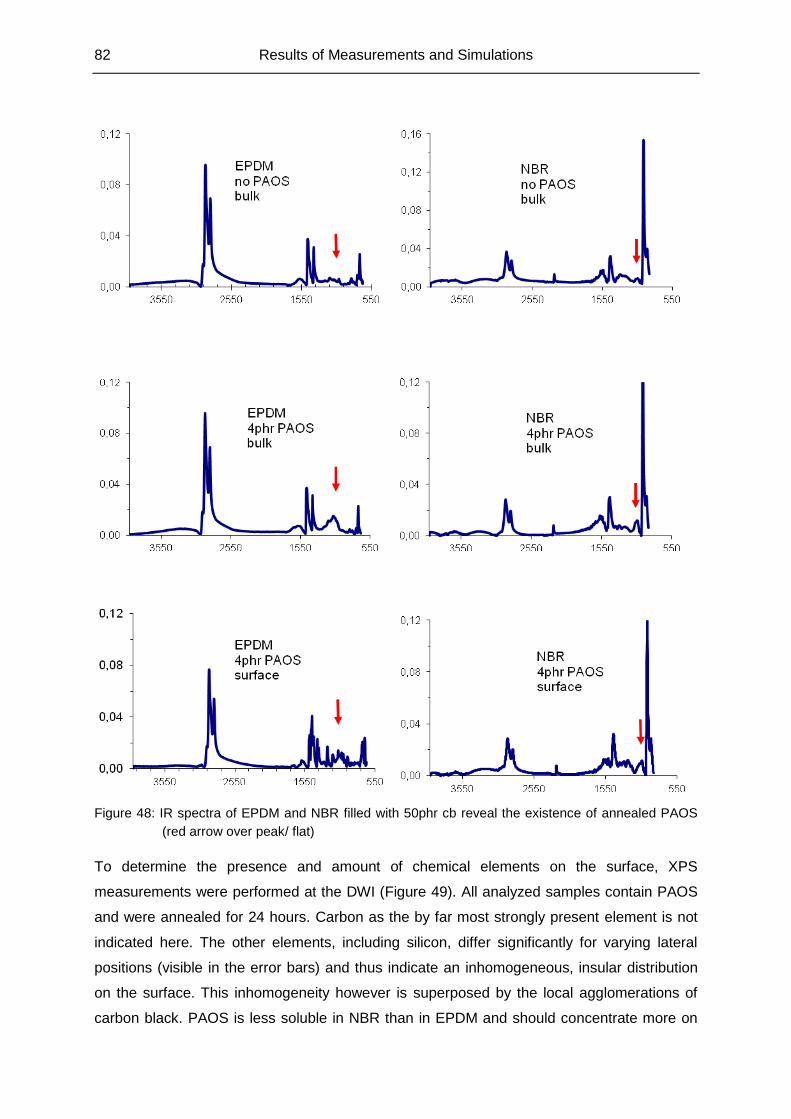
82 Results of Measurements and Simulations
Figure 48: IR spectra of EPDM and NBR filled with 50phr cb reveal the existence of annealed PAOS
(red arrow over peak/ flat)
To determine the presence and amount of chemical elements on the surface, XPS
measurements were performed at the DWI (Figure 49). All analyzed samples contain PAOS
and were annealed for 24 hours. Carbon as the by far most strongly present element is not
indicated here. The other elements, including silicon, differ significantly for varying lateral
positions (visible in the error bars) and thus indicate an inhomogeneous, insular distribution
on the surface. This inhomogeneity however is superposed by the local agglomerations of
carbon black. PAOS is less soluble in NBR than in EPDM and should concentrate more on
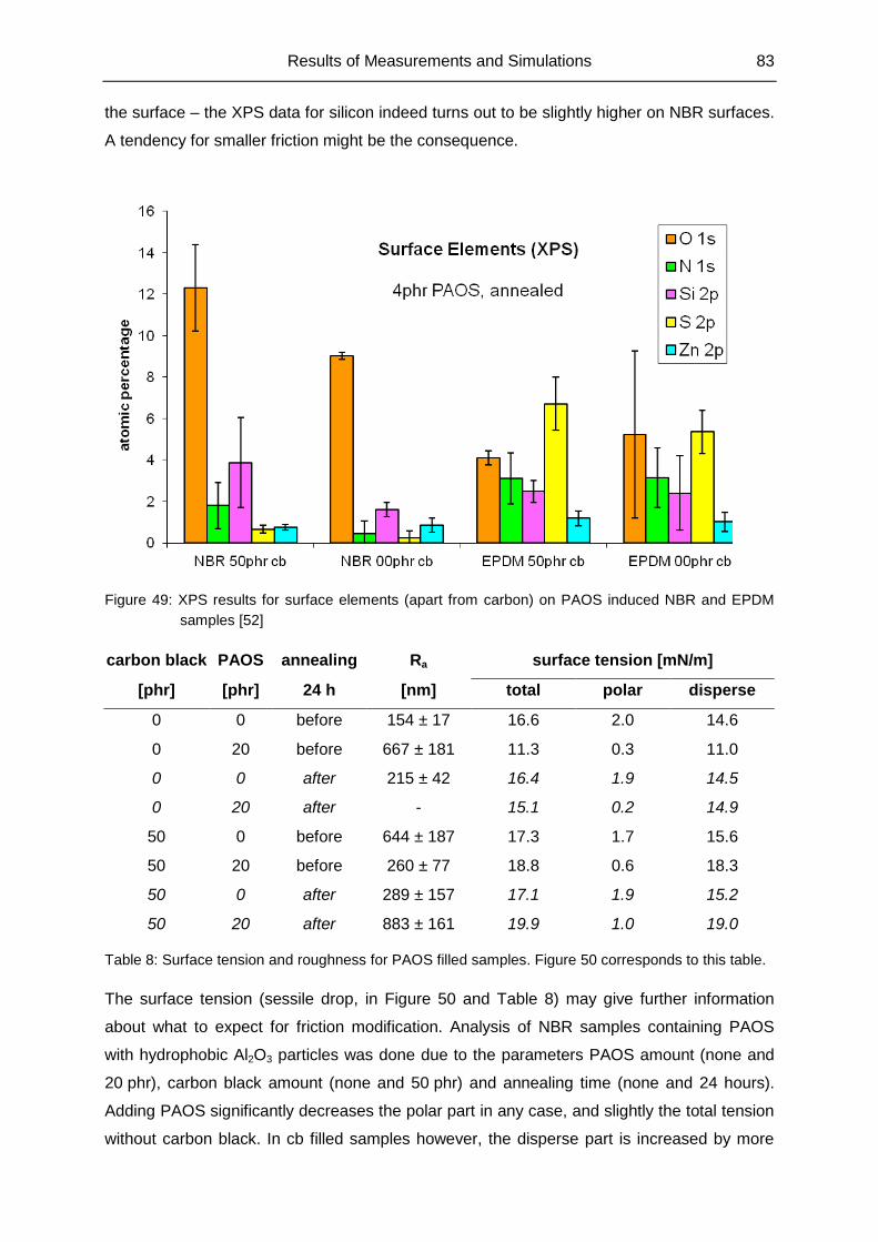
Results of Measurements and Simulations 83
the surface – the XPS data for silicon indeed turns out to be slightly higher on NBR surfaces.
A tendency for smaller friction might be the consequence.
Figure 49: XPS results for surface elements (apart from carbon) on PAOS induced NBR and EPDM
samples [52]
carbon black PAOS annealing Ra surface tension [mN/m]
[phr] [phr] 24 h [nm] total polar disperse
0 0 before 154 ± 17 16.6 2.0 14.6
0 20 before 667 ± 181 11.3 0.3 11.0
0 0 after 215 ± 42 16.4 1.9 14.5
0 20 after - 15.1 0.2 14.9
50 0 before 644 ± 187 17.3 1.7 15.6
50 20 before 260 ± 77 18.8 0.6 18.3
50 0 after 289 ± 157 17.1 1.9 15.2
50 20 after 883 ± 161 19.9 1.0 19.0
Table 8: Surface tension and roughness for PAOS filled samples. Figure 50 corresponds to this table.
The surface tension (sessile drop, in Figure 50 and Table 8) may give further information
about what to expect for friction modification. Analysis of NBR samples containing PAOS
with hydrophobic Al2O3 particles was done due to the parameters PAOS amount (none and
20 phr), carbon black amount (none and 50 phr) and annealing time (none and 24 hours).
Adding PAOS significantly decreases the polar part in any case, and slightly the total tension
without carbon black. In cb filled samples however, the disperse part is increased by more
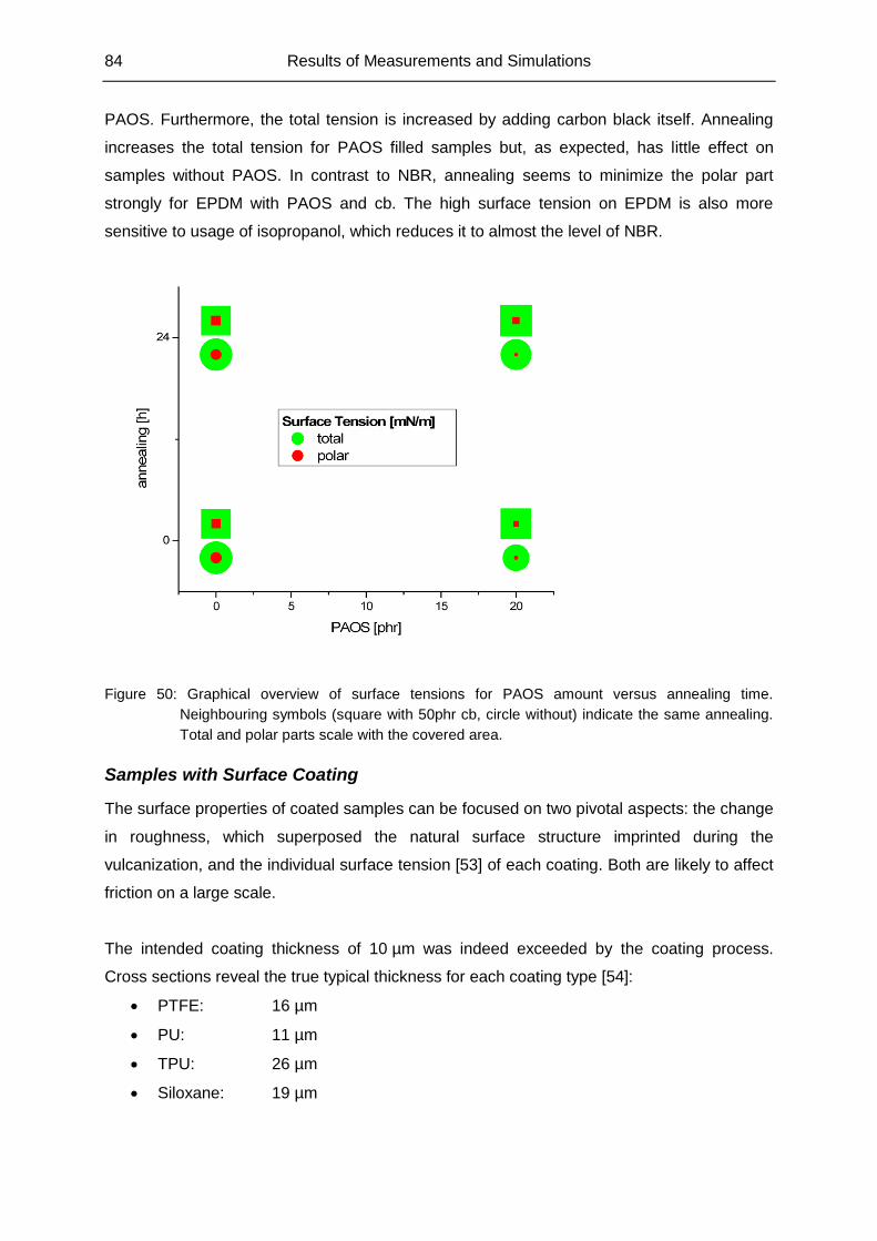
84 Results of Measurements and Simulations
PAOS. Furthermore, the total tension is increased by adding carbon black itself. Annealing
increases the total tension for PAOS filled samples but, as expected, has little effect on
samples without PAOS. In contrast to NBR, annealing seems to minimize the polar part
strongly for EPDM with PAOS and cb. The high surface tension on EPDM is also more
sensitive to usage of isopropanol, which reduces it to almost the level of NBR.
Figure 50: Graphical overview of surface tensions for PAOS amount versus annealing time.
Neighbouring symbols (square with 50phr cb, circle without) indicate the same annealing.
Total and polar parts scale with the covered area.
Samples with Surface Coating
The surface properties of coated samples can be focused on two pivotal aspects: the change
in roughness, which superposed the natural surface structure imprinted during the
vulcanization, and the individual surface tension [53] of each coating. Both are likely to affect
friction on a large scale.
The intended coating thickness of 10 µm was indeed exceeded by the coating process.
Cross sections reveal the true typical thickness for each coating type [54]:
PTFE: 16 µm
PU: 11 µm
TPU: 26 µm
Siloxane: 19 µm
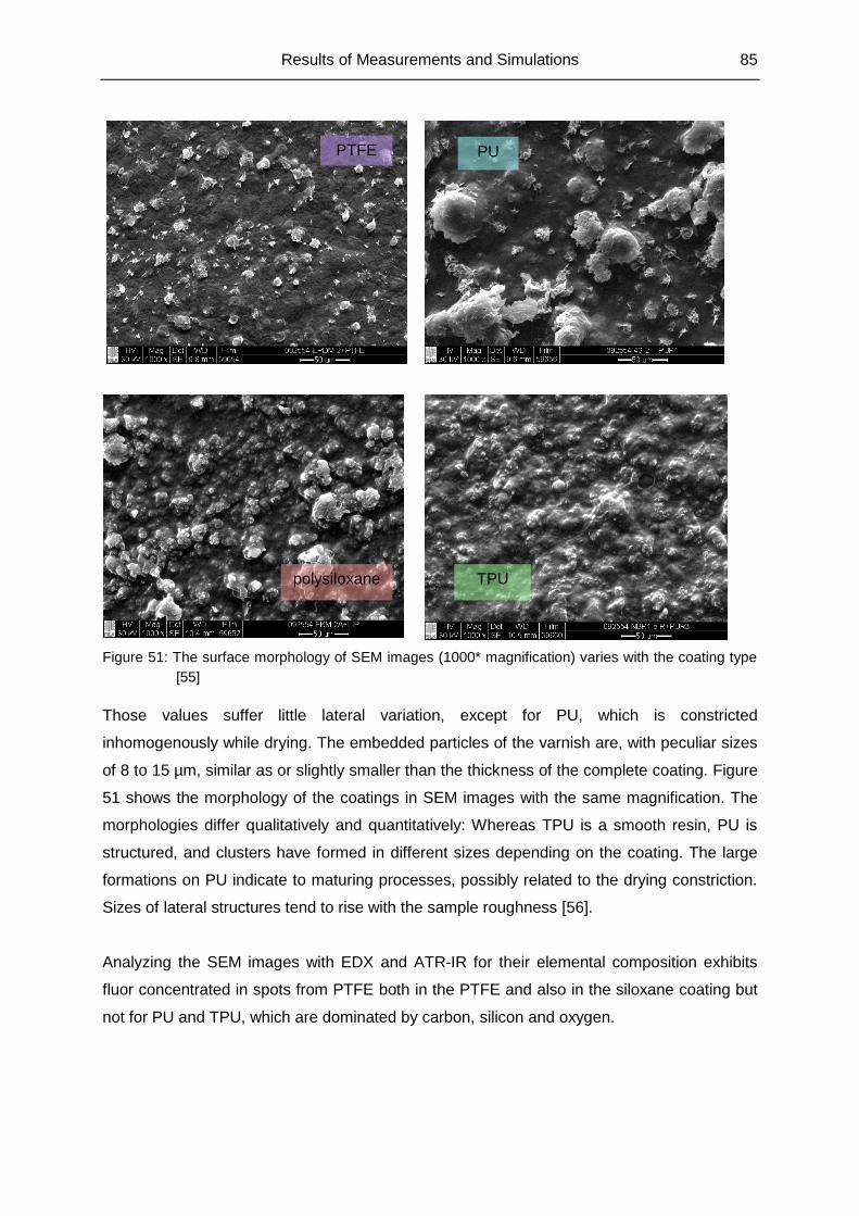
Results of Measurements and Simulations 85
Figure 51: The surface morphology of SEM images (1000* magnification) varies with the coating type
[55]
Those values suffer little lateral variation, except for PU, which is constricted
inhomogenously while drying. The embedded particles of the varnish are, with peculiar sizes
of 8 to 15 µm, similar as or slightly smaller than the thickness of the complete coating. Figure
51 shows the morphology of the coatings in SEM images with the same magnification. The
morphologies differ qualitatively and quantitatively: Whereas TPU is a smooth resin, PU is
structured, and clusters have formed in different sizes depending on the coating. The large
formations on PU indicate to maturing processes, possibly related to the drying constriction.
Sizes of lateral structures tend to rise with the sample roughness [56].
Analyzing the SEM images with EDX and ATR-IR for their elemental composition exhibits
fluor concentrated in spots from PTFE both in the PTFE and also in the siloxane coating but
not for PU and TPU, which are dominated by carbon, silicon and oxygen.
TPU
PU PTFE
polysiloxane
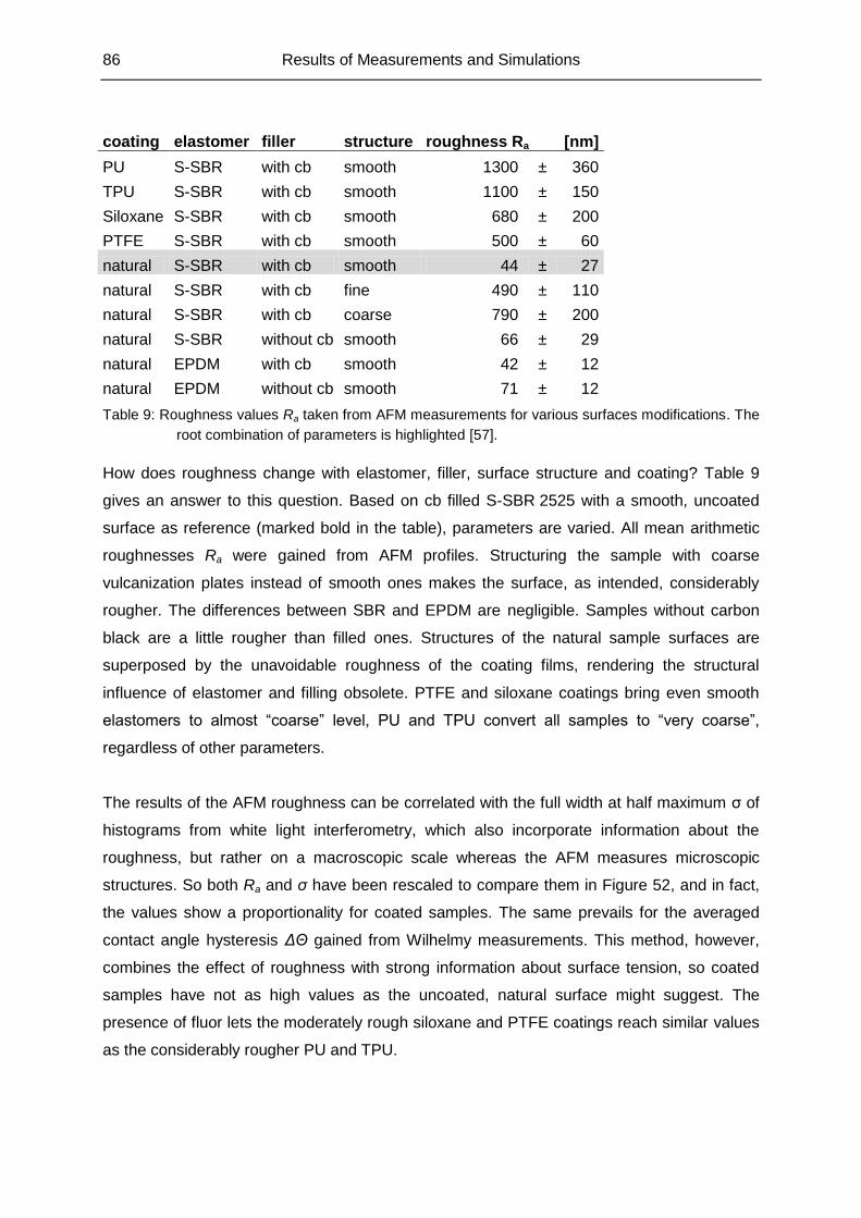
86 Results of Measurements and Simulations
coating elastomer filler structure roughness Ra [nm]
PU S-SBR with cb smooth 1300 ± 360
TPU S-SBR with cb smooth 1100 ± 150
Siloxane S-SBR with cb smooth 680 ± 200
PTFE S-SBR with cb smooth 500 ± 60
natural S-SBR with cb smooth 44 ± 27
natural S-SBR with cb fine 490 ± 110
natural S-SBR with cb coarse 790 ± 200
natural S-SBR without cb smooth 66 ± 29
natural EPDM with cb smooth 42 ± 12
natural EPDM without cb smooth 71 ± 12
Table 9: Roughness values Ra taken from AFM measurements for various surfaces modifications. The
root combination of parameters is highlighted [57].
How does roughness change with elastomer, filler, surface structure and coating? Table 9
gives an answer to this question. Based on cb filled S-SBR 2525 with a smooth, uncoated
surface as reference (marked bold in the table), parameters are varied. All mean arithmetic
roughnesses Ra were gained from AFM profiles. Structuring the sample with coarse
vulcanization plates instead of smooth ones makes the surface, as intended, considerably
rougher. The differences between SBR and EPDM are negligible. Samples without carbon
black are a little rougher than filled ones. Structures of the natural sample surfaces are
superposed by the unavoidable roughness of the coating films, rendering the structural
influence of elastomer and filling obsolete. PTFE and siloxane coatings bring even smooth
elastomers to almost “coarse” level, PU and TPU convert all samples to “very coarse”,
regardless of other parameters.
The results of the AFM roughness can be correlated with the full width at half maximum σ of
histograms from white light interferometry, which also incorporate information about the
roughness, but rather on a macroscopic scale whereas the AFM measures microscopic
structures. So both Ra and σ have been rescaled to compare them in Figure 52, and in fact,
the values show a proportionality for coated samples. The same prevails for the averaged
contact angle hysteresis ΔΘ gained from Wilhelmy measurements. This method, however,
combines the effect of roughness with strong information about surface tension, so coated
samples have not as high values as the uncoated, natural surface might suggest. The
presence of fluor lets the moderately rough siloxane and PTFE coatings reach similar values
as the considerably rougher PU and TPU.
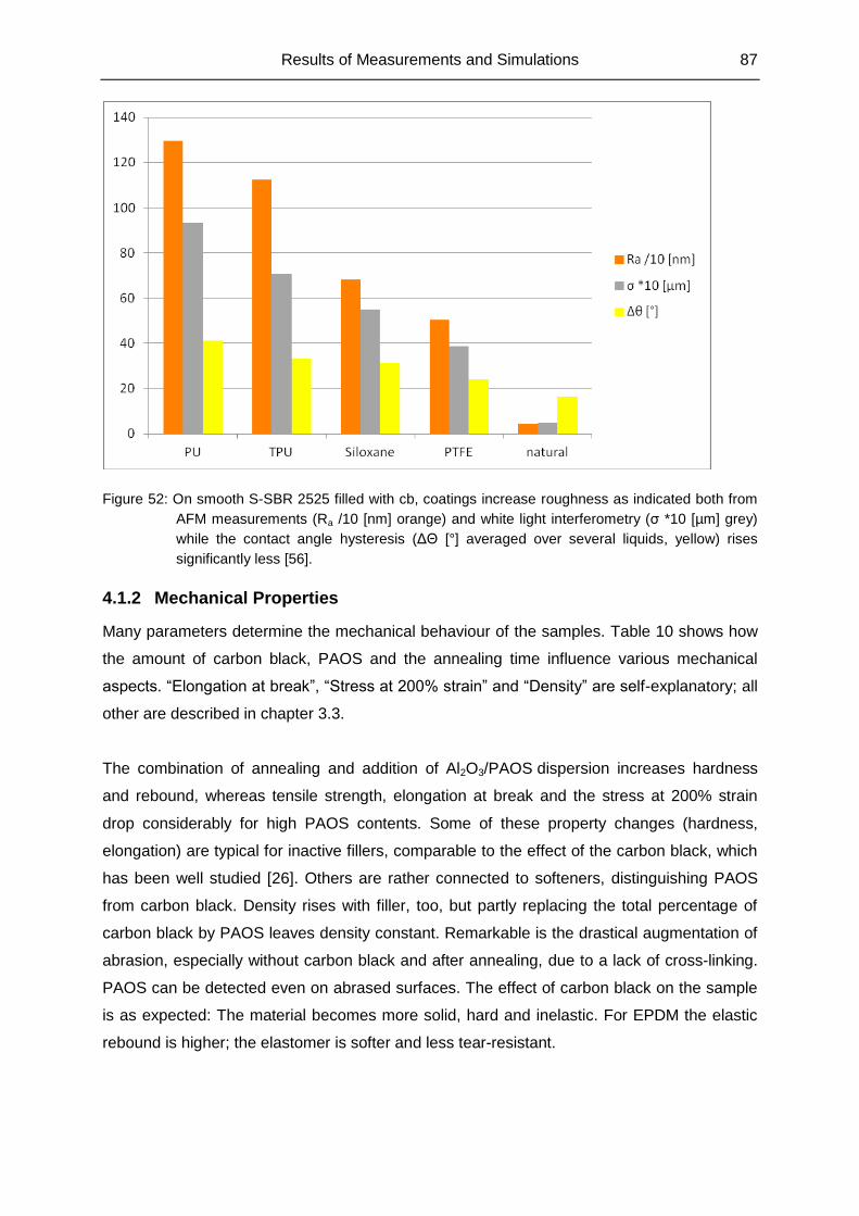
Results of Measurements and Simulations 87
Figure 52: On smooth S-SBR 2525 filled with cb, coatings increase roughness as indicated both from
AFM measurements (Ra /10 [nm] orange) and white light interferometry (σ *10 [µm] grey)
while the contact angle hysteresis (ΔΘ [°] averaged over several liquids, yellow) rises
significantly less [56].
4.1.2 Mechanical Properties
Many parameters determine the mechanical behaviour of the samples. Table 10 shows how
the amount of carbon black, PAOS and the annealing time influence various mechanical
aspects. “Elongation at break”, “Stress at 200% strain” and “Density” are self-explanatory; all
other are described in chapter 3.3.
The combination of annealing and addition of Al2O3/PAOS dispersion increases hardness
and rebound, whereas tensile strength, elongation at break and the stress at 200% strain
drop considerably for high PAOS contents. Some of these property changes (hardness,
elongation) are typical for inactive fillers, comparable to the effect of the carbon black, which
has been well studied [26]. Others are rather connected to softeners, distinguishing PAOS
from carbon black. Density rises with filler, too, but partly replacing the total percentage of
carbon black by PAOS leaves density constant. Remarkable is the drastical augmentation of
abrasion, especially without carbon black and after annealing, due to a lack of cross-linking.
PAOS can be detected even on abrased surfaces. The effect of carbon black on the sample
is as expected: The material becomes more solid, hard and inelastic. For EPDM the elastic
rebound is higher; the elastomer is softer and less tear-resistant.
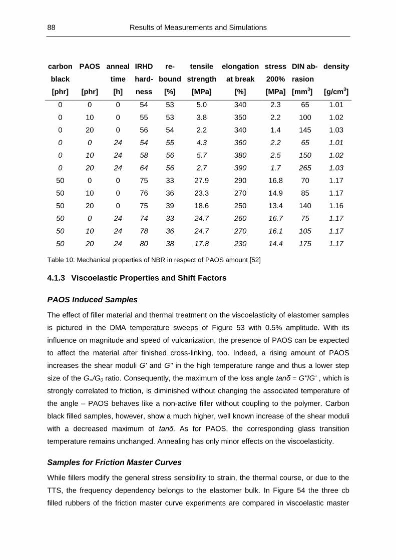
88 Results of Measurements and Simulations
carbon
black
[phr]
PAOS
[phr]
anneal
time
[h]
IRHD
hard-
ness
re-
bound
[%]
tensile
strength
[MPa]
elongation
at break
[%]
stress
200%
[MPa]
DIN ab-
rasion
[mm3]
density
[g/cm3]
0 0 0 54 53 5.0 340 2.3 65 1.01
0 10 0 55 53 3.8 350 2.2 100 1.02
0 20 0 56 54 2.2 340 1.4 145 1.03
0 0 24 54 55 4.3 360 2.2 65 1.01
0 10 24 58 56 5.7 380 2.5 150 1.02
0 20 24 64 56 2.7 390 1.7 265 1.03
50 0 0 75 33 27.9 290 16.8 70 1.17
50 10 0 76 36 23.3 270 14.9 85 1.17
50 20 0 75 39 18.6 250 13.4 140 1.16
50 0 24 74 33 24.7 260 16.7 75 1.17
50 10 24 78 36 24.7 270 16.1 105 1.17
50 20 24 80 38 17.8 230 14.4 175 1.17
Table 10: Mechanical properties of NBR in respect of PAOS amount [52]
4.1.3 Viscoelastic Properties and Shift Factors
PAOS Induced Samples
The effect of filler material and thermal treatment on the viscoelasticity of elastomer samples
is pictured in the DMA temperature sweeps of Figure 53 with 0.5% amplitude. With its
influence on magnitude and speed of vulcanization, the presence of PAOS can be expected
to affect the material after finished cross-linking, too. Indeed, a rising amount of PAOS
increases the shear moduli G' and G'' in the high temperature range and thus a lower step
size of the G∞/G0 ratio. Consequently, the maximum of the loss angle tanδ = G''/G' , which is
strongly correlated to friction, is diminished without changing the associated temperature of
the angle – PAOS behaves like a non-active filler without coupling to the polymer. Carbon
black filled samples, however, show a much higher, well known increase of the shear moduli
with a decreased maximum of tanδ. As for PAOS, the corresponding glass transition
temperature remains unchanged. Annealing has only minor effects on the viscoelasticity.
Samples for Friction Master Curves
While fillers modify the general stress sensibility to strain, the thermal course, or due to the
TTS, the frequency dependency belongs to the elastomer bulk. In Figure 54 the three cb
filled rubbers of the friction master curve experiments are compared in viscoelastic master
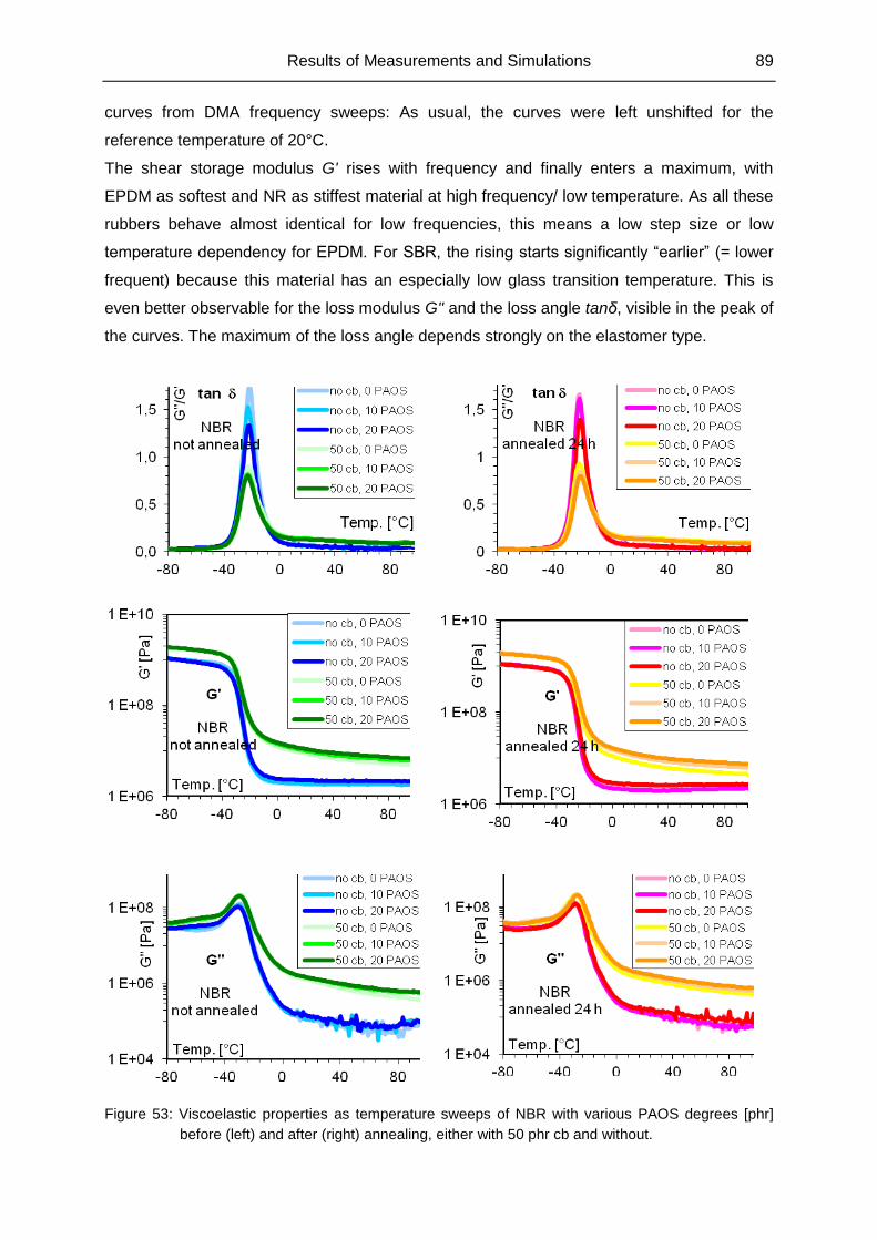
Results of Measurements and Simulations 89
curves from DMA frequency sweeps: As usual, the curves were left unshifted for the
reference temperature of 20°C.
The shear storage modulus G' rises with frequency and finally enters a maximum, with
EPDM as softest and NR as stiffest material at high frequency/ low temperature. As all these
rubbers behave almost identical for low frequencies, this means a low step size or low
temperature dependency for EPDM. For SBR, the rising starts significantly “earlier” (= lower
frequent) because this material has an especially low glass transition temperature. This is
even better observable for the loss modulus G'' and the loss angle tanδ, visible in the peak of
the curves. The maximum of the loss angle depends strongly on the elastomer type.
Figure 53: Viscoelastic properties as temperature sweeps of NBR with various PAOS degrees [phr]
before (left) and after (right) annealing, either with 50 phr cb and without.
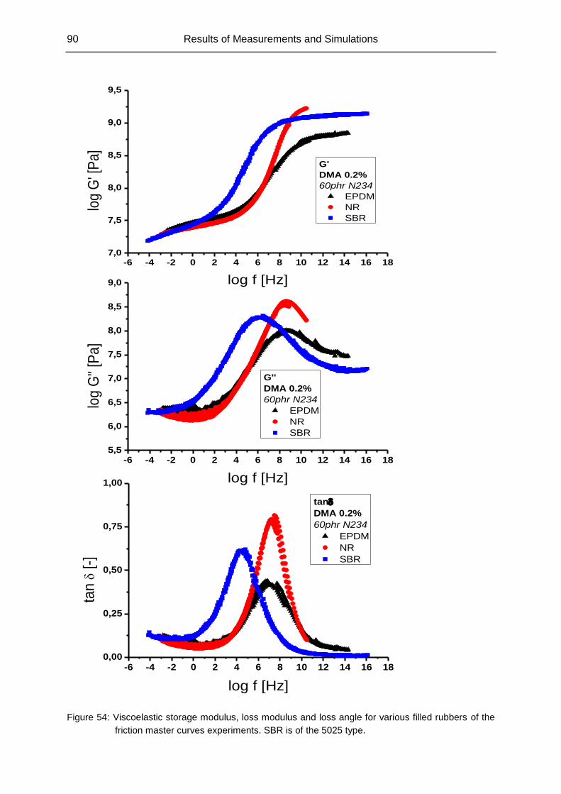
90 Results of Measurements and Simulations
Figure 54: Viscoelastic storage modulus, loss modulus and loss angle for various filled rubbers of the
friction master curves experiments. SBR is of the 5025 type.
-6 -4 -2 0 2 4 6 8 10 12 14 16 187,0
7,5
8,0
8,5
9,0
9,5lo
g G
' [P
a]
log f [Hz]
G'
DMA 0.2%
60phr N234
EPDM
NR
SBR
-6 -4 -2 0 2 4 6 8 10 12 14 16 180,00
0,25
0,50
0,75
1,00
tan
[-]
log f [Hz]
tan
DMA 0.2%
60phr N234
EPDM
NR
SBR
-6 -4 -2 0 2 4 6 8 10 12 14 16 185,5
6,0
6,5
7,0
7,5
8,0
8,5
9,0
log
G''
[Pa
]
log f [Hz]
G''
DMA 0.2%
60phr N234
EPDM
NR
SBR
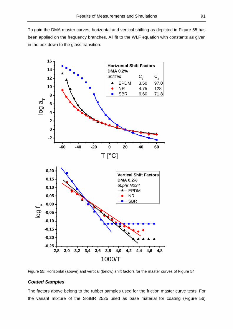
Results of Measurements and Simulations 91
To gain the DMA master curves, horizontal and vertical shifting as depicted in Figure 55 has
been applied on the frequency branches. All fit to the WLF equation with constants as given
in the box down to the glass transition.
Figure 55: Horizontal (above) and vertical (below) shift factors for the master curves of Figure 54
Coated Samples
The factors above belong to the rubber samples used for the friction master curve tests. For
the variant mixture of the S-SBR 2525 used as base material for coating (Figure 56)
-60 -40 -20 0 20 40 60
-2
0
2
4
6
8
10
12
14
16
log
aT
T [°C]
Horizontal Shift Factors
DMA 0.2%
unfilled C1
C2
EPDM 3.50 97.0
NR 4.75 128
SBR 6.60 71.8
2,8 3,0 3,2 3,4 3,6 3,8 4,0 4,2 4,4 4,6 4,8-0,25
-0,20
-0,15
-0,10
-0,05
0,00
0,05
0,10
0,15
0,20
log
fV
1000/T
Vertical Shift Factors
DMA 0,2%
60phr N234
EPDM
NR
SBR
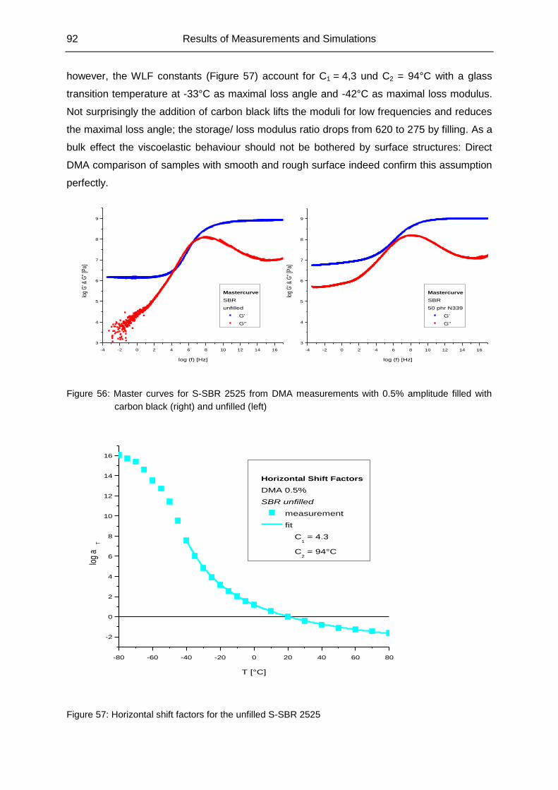
92 Results of Measurements and Simulations
however, the WLF constants (Figure 57) account for C1 = 4,3 und C2 = 94°C with a glass
transition temperature at -33°C as maximal loss angle and -42°C as maximal loss modulus.
Not surprisingly the addition of carbon black lifts the moduli for low frequencies and reduces
the maximal loss angle; the storage/ loss modulus ratio drops from 620 to 275 by filling. As a
bulk effect the viscoelastic behaviour should not be bothered by surface structures: Direct
DMA comparison of samples with smooth and rough surface indeed confirm this assumption
perfectly.
-4 -2 0 2 4 6 8 10 12 14 16
3
4
5
6
7
8
9
log
G' &
G''
[Pa]
log (f) [Hz]
Mastercurve
SBR
unfilled
G'
G''
Figure 56: Master curves for S-SBR 2525 from DMA measurements with 0.5% amplitude filled with
carbon black (right) and unfilled (left)
-80 -60 -40 -20 0 20 40 60 80
-2
0
2
4
6
8
10
12
14
16
log
aT
T [°C]
Horizontal Shift Factors
DMA 0.5%
SBR unfilled
measurement
fit
C1 = 4.3
C2 = 94°C
Figure 57: Horizontal shift factors for the unfilled S-SBR 2525
-4 -2 0 2 4 6 8 10 12 14 16
3
4
5
6
7
8
9
log
G' &
G''
[Pa]
log (f) [Hz]
Mastercurve
SBR
50 phr N339
G'
G''
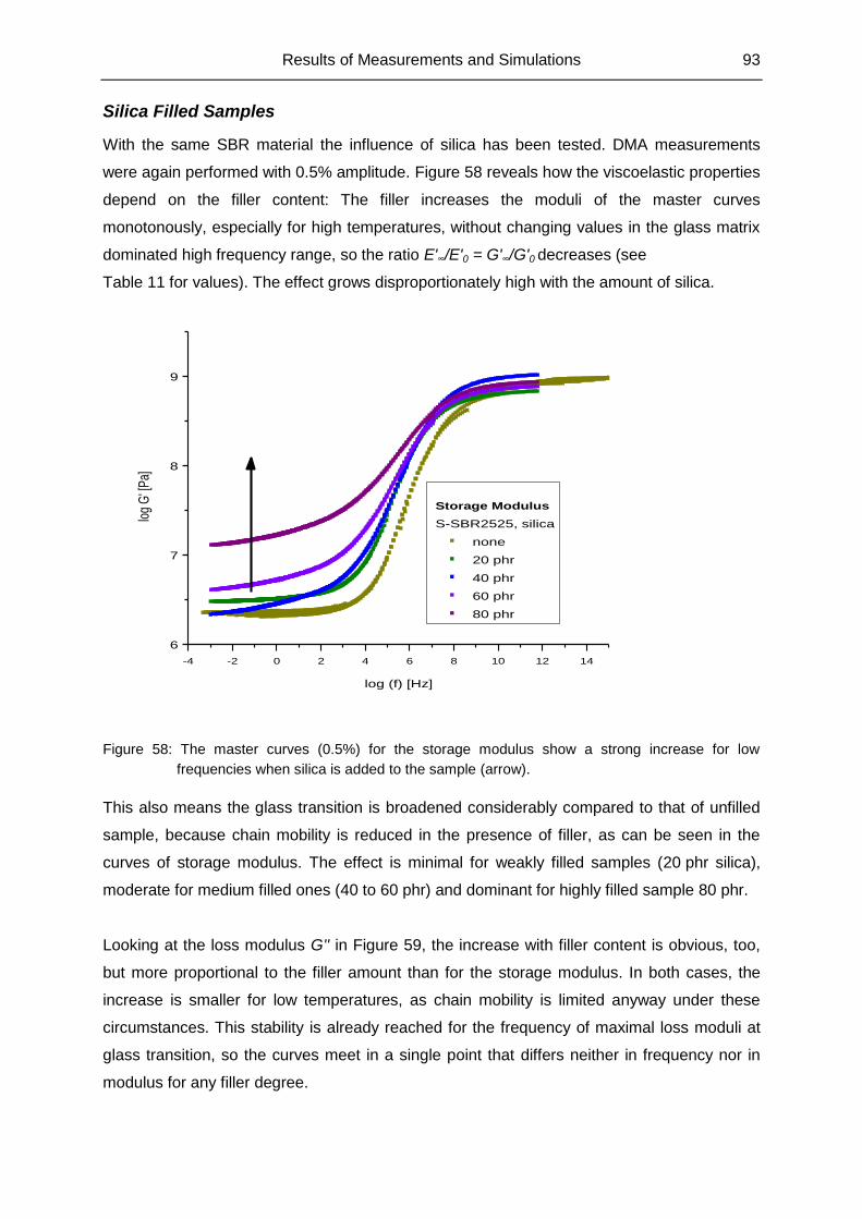
Results of Measurements and Simulations 93
Silica Filled Samples
With the same SBR material the influence of silica has been tested. DMA measurements
were again performed with 0.5% amplitude. Figure 58 reveals how the viscoelastic properties
depend on the filler content: The filler increases the moduli of the master curves
monotonously, especially for high temperatures, without changing values in the glass matrix
dominated high frequency range, so the ratio E'∞/E'0 = G'∞/G'0 decreases (see
Table 11 for values). The effect grows disproportionately high with the amount of silica.
-4 -2 0 2 4 6 8 10 12 14
6
7
8
9
log
G' [
Pa]
log (f) [Hz]
Storage Modulus
S-SBR2525, silica
none
20 phr
40 phr
60 phr
80 phr
Figure 58: The master curves (0.5%) for the storage modulus show a strong increase for low
frequencies when silica is added to the sample (arrow).
This also means the glass transition is broadened considerably compared to that of unfilled
sample, because chain mobility is reduced in the presence of filler, as can be seen in the
curves of storage modulus. The effect is minimal for weakly filled samples (20 phr silica),
moderate for medium filled ones (40 to 60 phr) and dominant for highly filled sample 80 phr.
Looking at the loss modulus G'' in Figure 59, the increase with filler content is obvious, too,
but more proportional to the filler amount than for the storage modulus. In both cases, the
increase is smaller for low temperatures, as chain mobility is limited anyway under these
circumstances. This stability is already reached for the frequency of maximal loss moduli at
glass transition, so the curves meet in a single point that differs neither in frequency nor in
modulus for any filler degree.
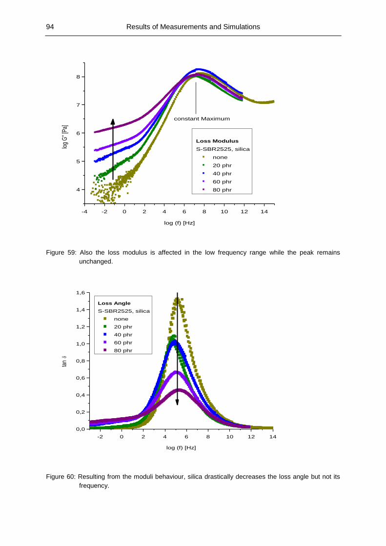
94 Results of Measurements and Simulations
-4 -2 0 2 4 6 8 10 12 14
4
5
6
7
8
log
G''
[Pa]
log (f) [Hz]
Loss Modulus
S-SBR2525, silica
none
20 phr
40 phr
60 phr
80 phr
constant Maximum
Figure 59: Also the loss modulus is affected in the low frequency range while the peak remains
unchanged.
-2 0 2 4 6 8 10 12 14
0,0
0,2
0,4
0,6
0,8
1,0
1,2
1,4
1,6
tan
log (f) [Hz]
Loss Angle
S-SBR2525, silica
none
20 phr
40 phr
60 phr
80 phr
Figure 60: Resulting from the moduli behaviour, silica drastically decreases the loss angle but not its
frequency.
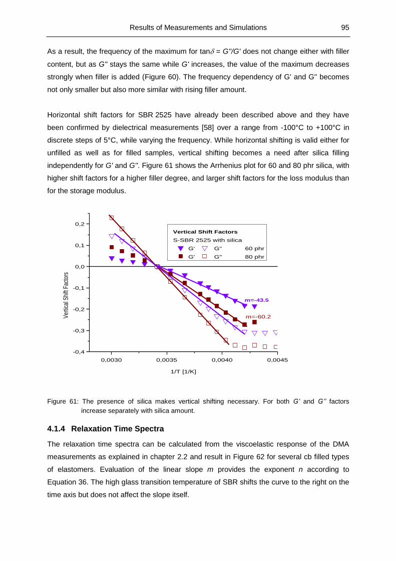
Results of Measurements and Simulations 95
As a result, the frequency of the maximum for tan = G''/G' does not change either with filler
content, but as G'' stays the same while G' increases, the value of the maximum decreases
strongly when filler is added (Figure 60). The frequency dependency of G' and G'' becomes
not only smaller but also more similar with rising filler amount.
Horizontal shift factors for SBR 2525 have already been described above and they have
been confirmed by dielectrical measurements [58] over a range from -100°C to +100°C in
discrete steps of 5°C, while varying the frequency. While horizontal shifting is valid either for
unfilled as well as for filled samples, vertical shifting becomes a need after silica filling
independently for G' and G''. Figure 61 shows the Arrhenius plot for 60 and 80 phr silica, with
higher shift factors for a higher filler degree, and larger shift factors for the loss modulus than
for the storage modulus.
0,0030 0,0035 0,0040 0,0045
-0,4
-0,3
-0,2
-0,1
0,0
0,1
0,2
Ver
tical
Shi
ft Fa
ctor
s
1/T [1/K]
Vertical Shift Factors
S-SBR 2525 with silica
G' G'' 60 phr
G' G'' 80 phr
m=-43.5
m=-60.2
Figure 61: The presence of silica makes vertical shifting necessary. For both G’ and G’’ factors
increase separately with silica amount.
4.1.4 Relaxation Time Spectra
The relaxation time spectra can be calculated from the viscoelastic response of the DMA
measurements as explained in chapter 2.2 and result in Figure 62 for several cb filled types
of elastomers. Evaluation of the linear slope m provides the exponent n according to
Equation 36. The high glass transition temperature of SBR shifts the curve to the right on the
time axis but does not affect the slope itself.
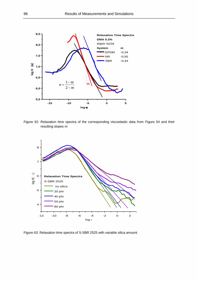
96 Results of Measurements and Simulations
-15 -10 -5 0 5
5,5
6,0
6,5
7,0
7,5
8,0
8,5lo
g H
()
log
Relaxation Time Spectra
DMA 0.2%
60phr N234
System m
EPDM -0,34
NR -0,55
SBR -0,44
m
Figure 62: Relaxation time spectra of the corresponding viscoelastic data from Figure 54 and their
resulting slopes m
-12 -10 -8 -6 -4 -2 0 2
4
5
6
7
8
log
H(
)
log
Relaxation Time Spectra
S-SBR 2525
no silica
20 phr
40 phr
50 phr
80 phr
Figure 63: Relaxation time spectra of S-SBR 2525 with variable silica amount
m
mn
2
1
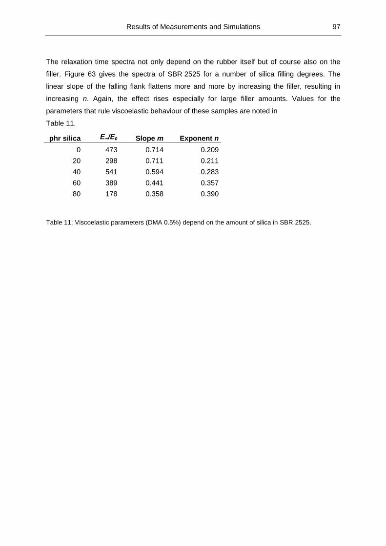
Results of Measurements and Simulations 97
The relaxation time spectra not only depend on the rubber itself but of course also on the
filler. Figure 63 gives the spectra of SBR 2525 for a number of silica filling degrees. The
linear slope of the falling flank flattens more and more by increasing the filler, resulting in
increasing n. Again, the effect rises especially for large filler amounts. Values for the
parameters that rule viscoelastic behaviour of these samples are noted in
Table 11.
phr silica E∞/E0 Slope m Exponent n
0 473 0.714 0.209
20 298 0.711 0.211
40 541 0.594 0.283
60 389 0.441 0.357
80 178 0.358 0.390
Table 11: Viscoelastic parameters (DMA 0.5%) depend on the amount of silica in SBR 2525.
98 Results of Measurements and Simulations
4.2 Friction Plateaus of Silica Filled Systems
In this chapter the influence of strengthening filler on friction will be analyzed systematically.
A series of SBR samples filled with various amounts Φ of silica (from none to 80 phr in steps
of 20 phr) has been investigated tribologically on rough granite and asphalt [59],[60].
Simulation of hysteresis and adhesion friction are compared to the wet and dry
measurements and give results that will prove helpful in the understanding of general friction
dependence on velocity as it is surveyed from a larger view point in chapter 4.3.
4.2.1 From Wet Friction to the Silica Plateaus of Dry Friction
As prerequisite of understanding the total friction and its correlated adhesion simulation, the
measurement of wet friction and simulation of hysteresis friction are the logical first steps.
The results of the wet measurements on granite are shown in Figure 64, and on asphalt in
Figure 65.
On both granite and asphalt surfaces, friction clearly increases with velocity, which means
lubrication is effective especially at lower speeds. On asphalt the slope remains nearly the
same over all measured velocities – temperature effects can largely be ruled out when using
a lubricant – whereas granite displays but a softly increased slope at higher sliding speeds.
Simulations emulate the curves, including their increase, even more pronounced for
extrapolating into the fast range.
The absolute amount of friction is quite similar for both substrates. In general, friction on
granite tends to be only slightly higher than on asphalt. The exact behaviour strongly
depends on the filler amount: For asphalt, the friction increases monotonously with the
degree of filler in the complete velocity range. On granite, this is true only when disregarding
weakly filled samples (the measured friction coefficients of 20 phr silica are hardly
discriminable from those of the unfilled sample), corresponding to the small effect that
marginal silica fillings provoke on the viscoelastic response. 80 phr silica show in any case
the definitely largest effect; a desired result especially for tyre construction. The increase of
friction with velocity can be explained by the increased stiffness and thus hysteresis of filled
elastomers.
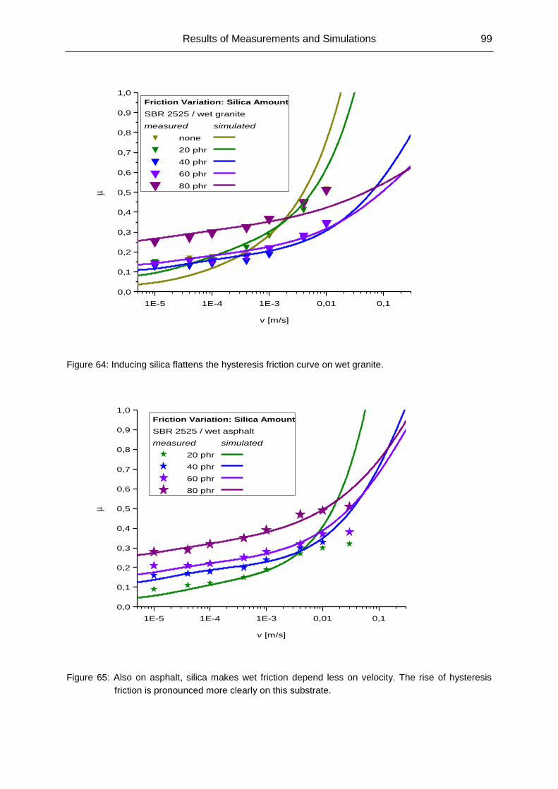
Results of Measurements and Simulations 99
1E-5 1E-4 1E-3 0,01 0,1
0,0
0,1
0,2
0,3
0,4
0,5
0,6
0,7
0,8
0,9
1,0
v [m/s]
Friction Variation: Silica Amount
SBR 2525 / wet granite
measured simulated
none
20 phr
40 phr
60 phr
80 phr
Figure 64: Inducing silica flattens the hysteresis friction curve on wet granite.
1E-5 1E-4 1E-3 0,01 0,1
0,0
0,1
0,2
0,3
0,4
0,5
0,6
0,7
0,8
0,9
1,0
v [m/s]
Friction Variation: Silica Amount
SBR 2525 / wet asphalt
measured simulated
20 phr
40 phr
60 phr
80 phr
Figure 65: Also on asphalt, silica makes wet friction depend less on velocity. The rise of hysteresis
friction is pronounced more clearly on this substrate.
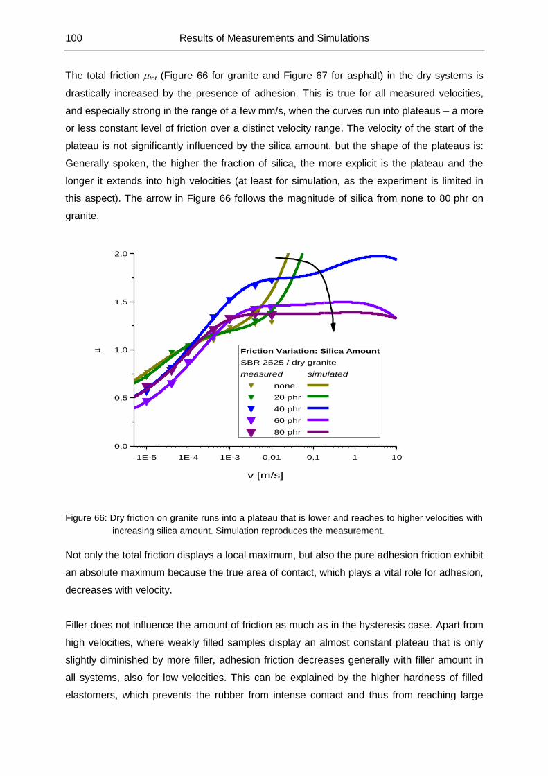
100 Results of Measurements and Simulations
The total friction tot (Figure 66 for granite and Figure 67 for asphalt) in the dry systems is
drastically increased by the presence of adhesion. This is true for all measured velocities,
and especially strong in the range of a few mm/s, when the curves run into plateaus – a more
or less constant level of friction over a distinct velocity range. The velocity of the start of the
plateau is not significantly influenced by the silica amount, but the shape of the plateaus is:
Generally spoken, the higher the fraction of silica, the more explicit is the plateau and the
longer it extends into high velocities (at least for simulation, as the experiment is limited in
this aspect). The arrow in Figure 66 follows the magnitude of silica from none to 80 phr on
granite.
1E-5 1E-4 1E-3 0,01 0,1 1 10
0,0
0,5
1,0
1,5
2,0
v [m/s]
Friction Variation: Silica Amount
SBR 2525 / dry granite
measured simulated
none
20 phr
40 phr
60 phr
80 phr
Figure 66: Dry friction on granite runs into a plateau that is lower and reaches to higher velocities with
increasing silica amount. Simulation reproduces the measurement.
Not only the total friction displays a local maximum, but also the pure adhesion friction exhibit
an absolute maximum because the true area of contact, which plays a vital role for adhesion,
decreases with velocity.
Filler does not influence the amount of friction as much as in the hysteresis case. Apart from
high velocities, where weakly filled samples display an almost constant plateau that is only
slightly diminished by more filler, adhesion friction decreases generally with filler amount in
all systems, also for low velocities. This can be explained by the higher hardness of filled
elastomers, which prevents the rubber from intense contact and thus from reaching large
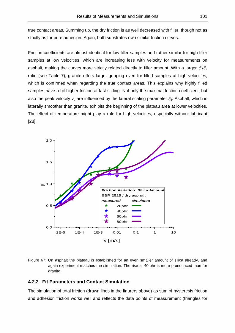
Results of Measurements and Simulations 101
true contact areas. Summing up, the dry friction is as well decreased with filler, though not as
strictly as for pure adhesion. Again, both substrates own similar friction curves.
Friction coefficients are almost identical for low filler samples and rather similar for high filler
samples at low velocities, which are increasing less with velocity for measurements on
asphalt, making the curves more strictly related directly to filler amount. With a larger ||/
ratio (see Table 7), granite offers larger gripping even for filled samples at high velocities,
which is confirmed when regarding the true contact areas. This explains why highly filled
samples have a bit higher friction at fast sliding. Not only the maximal friction coefficient, but
also the peak velocity vp are influenced by the lateral scaling parameter ||: Asphalt, which is
laterally smoother than granite, exhibits the beginning of the plateau area at lower velocities.
The effect of temperature might play a role for high velocities, especially without lubricant
[28].
1E-5 1E-4 1E-3 0,01 0,1 1 10
0,0
0,5
1,0
1,5
2,0
v [m/s]
Friction Variation: Silica Amount
SBR 2525 / dry asphalt
measured simulated
20phr
40phr
60phr
80phr
Figure 67: On asphalt the plateau is established for an even smaller amount of silica already, and
again experiment matches the simulation. The rise at 40 phr is more pronounced than for
granite.
4.2.2 Fit Parameters and Contact Simulation
The simulation of total friction (drawn lines in the figurers above) as sum of hysteresis friction
and adhesion friction works well and reflects the data points of measurement (triangles for
102 Results of Measurements and Simulations
granite, stars for asphalt) nicely. Trusting the extrapolated simulation curve thus seems
appropriate. We will now discuss the parameters that led to this result.
Some parameters (E∞/E0, n…) of the modellation (see chapters 2.6, 2.7 and 2.8) are given by
the material background of the investigated system. Table 12 summarizes the
complementary, free fit parameters b, 0 and vc.
First we compare the simulated hysteresis friction scaled with factor b to the data of wet
friction measurements. The values for b start at high numbers for unfilled samples, then
quickly decrease with filler amount and stay almost constant above the percolation threshold
at 40 phr silica. On granite, b is higher than on asphalt. This means that the effect
penetrating asperities propagates more deeply in the unfilled samples up to 40 phr.
Obviously, the measured curves can be reproduced fairly well with simulation for low and
moderate velocities, but is less accurate when sliding faster than a few mm/s: Then the
simulations are much steeper than measurements for low fillings (up to 20 phr), match to a
large extent for medium fillings (40 and 60 phr) and are not steep enough for high fillings
(80 phr), on a granite surface. For asphalt, simulations behave the same way but are slightly
steeper than on granite in comparison to the measurements, and fit the measurements still at
higher velocity. The answer can be found in the surface: As || indicates, granite is rougher
than asphalt on the lateral scale, so the simulations are valid at higher velocities. The highly
filled simulated curves are less steep and thus less dependent on velocity because their
elasticity depends less on temperature and thus less on frequency than the weakly filled
samples.
The second step is to add an adhesion term to the hysteresis fit. The shear stress rises with
filler amount for both granite and asphalt, especially for highest filler content. Simulation
range and accuracy of the simulation are only limited by knowledge of the regarded
viscoelastic and surface properties. The critical velocity vc displays a maximum at a silica
content of 40 phr for both substrates.
The fit is excellent for most points, even at higher velocities. While temperature effects by
friction heating could be assumed to be negligible on wet surfaces, they may indeed play a
role on dry substrates when the sliding speed is high enough. The heating results in an
increasing elasticity, which means the hysteresis part for dry friction is lower than for wet
friction. Hysteresis friction is still increasing with velocity, but its steepness is reduced by filler
amount already on wet surfaces. Combined with the decreasing real area of contact at high
velocities, dry friction may be reduced in effect, as seen for asphalt when sliding fast. As a
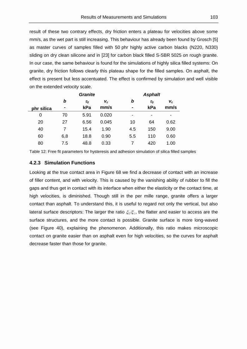
Results of Measurements and Simulations 103
result of these two contrary effects, dry friction enters a plateau for velocities above some
mm/s, as the wet part is still increasing. This behaviour has already been found by Grosch [5]
as master curves of samples filled with 50 phr highly active carbon blacks (N220, N330)
sliding on dry clean silicone and in [23] for carbon black filled S-SBR 5025 on rough granite.
In our case, the same behaviour is found for the simulations of highly silica filled systems: On
granite, dry friction follows clearly this plateau shape for the filled samples. On asphalt, the
effect is present but less accentuated. The effect is confirmed by simulation and well visible
on the extended velocity scale.
phr silica
b
-
Granite
0
kPa
vc
mm/s
b
-
Asphalt
0
kPa
vc
mm/s
0 70 5.91 0.020 - - -
20 27 6.56 0.045 10 64 0.62
40 7 15.4 1.90 4.5 150 9.00
60 6,8 18.8 0.90 5.5 110 0.60
80 7.5 48.8 0.33 7 420 1.00
Table 12: Free fit parameters for hysteresis and adhesion simulation of silica filled samples
4.2.3 Simulation Functions
Looking at the true contact area in Figure 68 we find a decrease of contact with an increase
of filler content, and with velocity. This is caused by the vanishing ability of rubber to fill the
gaps and thus get in contact with its interface when either the elasticity or the contact time, at
high velocities, is diminished. Though still in the per mille range, granite offers a larger
contact than asphalt. To understand this, it is useful to regard not only the vertical, but also
lateral surface descriptors: The larger the ratio ||, the flatter and easier to access are the
surface structures, and the more contact is possible. Granite surface is more long-waved
(see Figure 40), explaining the phenomenon. Additionally, this ratio makes microscopic
contact on granite easier than on asphalt even for high velocities, so the curves for asphalt
decrease faster than those for granite.
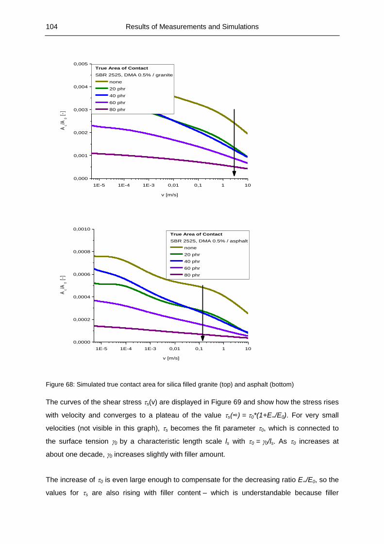
104 Results of Measurements and Simulations
1E-5 1E-4 1E-3 0,01 0,1 1 10
0,000
0,001
0,002
0,003
0,004
0,005A
c/A
0 [
-]
v [m/s]
True Area of Contact
SBR 2525, DMA 0.5% / granite
none
20 phr
40 phr
60 phr
80 phr
1E-5 1E-4 1E-3 0,01 0,1 1 10
0,0000
0,0002
0,0004
0,0006
0,0008
0,0010
Ac/A
0 [
-]
v [m/s]
True Area of Contact
SBR 2525, DMA 0.5% / asphalt
none
20 phr
40 phr
60 phr
80 phr
Figure 68: Simulated true contact area for silica filled granite (top) and asphalt (bottom)
The curves of the shear stress s(v) are displayed in Figure 69 and show how the stress rises
with velocity and converges to a plateau of the value s(∞) = 0*(1+E∞/E0). For very small
velocities (not visible in this graph), s becomes the fit parameter 0, which is connected to
the surface tension 0 by a characteristic length scale ls with 0 = 0/ls. As 0 increases at
about one decade, 0 increases slightly with filler amount.
The increase of 0 is even large enough to compensate for the decreasing ratio E∞/E0, so the
values for s are also rising with filler content – which is understandable because filler
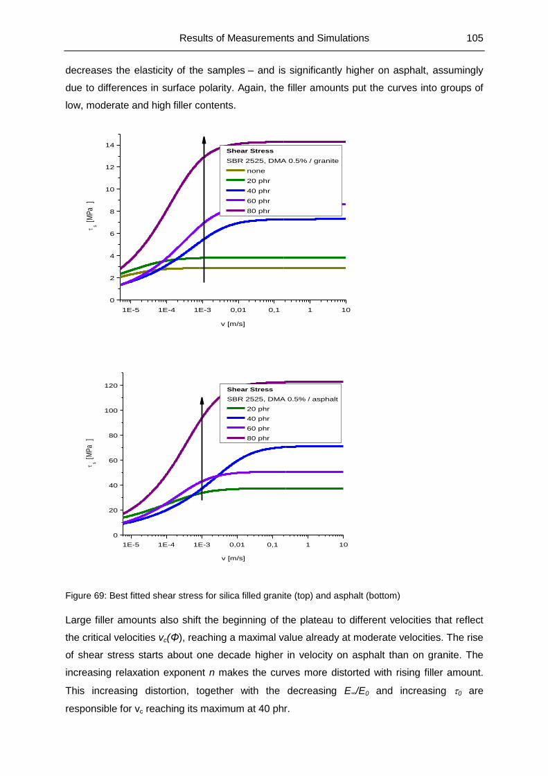
Results of Measurements and Simulations 105
decreases the elasticity of the samples – and is significantly higher on asphalt, assumingly
due to differences in surface polarity. Again, the filler amounts put the curves into groups of
low, moderate and high filler contents.
1E-5 1E-4 1E-3 0,01 0,1 1 10
0
2
4
6
8
10
12
14
s [
MP
a]
v [m/s]
Shear Stress
SBR 2525, DMA 0.5% / granite
none
20 phr
40 phr
60 phr
80 phr
1E-5 1E-4 1E-3 0,01 0,1 1 10
0
20
40
60
80
100
120
s [
MP
a]
v [m/s]
Shear Stress
SBR 2525, DMA 0.5% / asphalt
20 phr
40 phr
60 phr
80 phr
Figure 69: Best fitted shear stress for silica filled granite (top) and asphalt (bottom)
Large filler amounts also shift the beginning of the plateau to different velocities that reflect
the critical velocities vc(Φ), reaching a maximal value already at moderate velocities. The rise
of shear stress starts about one decade higher in velocity on asphalt than on granite. The
increasing relaxation exponent n makes the curves more distorted with rising filler amount.
This increasing distortion, together with the decreasing E∞/E0 and increasing 0 are
responsible for vc reaching its maximum at 40 phr.
106 Results of Measurements and Simulations
The minimal contact length min in the lateral direction is also a simulated function, but not
shown here. Higher velocities result in a strongly increasing minimal contact length, which
means that at high velocities only large structures contribute to the friction process as fewer
small asperities become accessible for the fast sliding rubber.
Higher filler contents also result in higher minimal length, too, because the poorly elastic filled
sample cannot enter the cavities deeply to establish a laterally broad contact. For asphalt,
this is true only at a second glance: As the highly filled samples have a weaker slope in
minimal wave length, curves reverse for high velocities. Looking at smaller velocities reveals
the same behaviour as on granite, but on smaller values, as the ratio || is also smaller on
asphalt. The slope is explainable by the fact that at high velocities high frequencies are
excited, and the master curves show that elasticity depends less on frequency for filled
samples.
The gap distance d increases with velocity, as the time for the elastomer to enter the cavities
of the substrate is reduced. It also increases with filler amount : This can be explained by the
lower elasticity of filled samples, preventing the rubber from filling the cavities deeply. On
asphalt the distance is a bit higher than on granite due to the slightly higher . It is easy to
notice the analogy of the filler influence here and in the storage modulus: 20 phr and 40 phr
silica content are almost indiscriminable in this aspect, whereas highly filled samples (80 phr)
display clearly different values for all velocities and the curve of the unfilled sample drifts
apart only for high velocity.This can be interpreted as being caused by the considerably
different glass transition due to filler. Again, high frequencies correspond to large sliding
velocities.
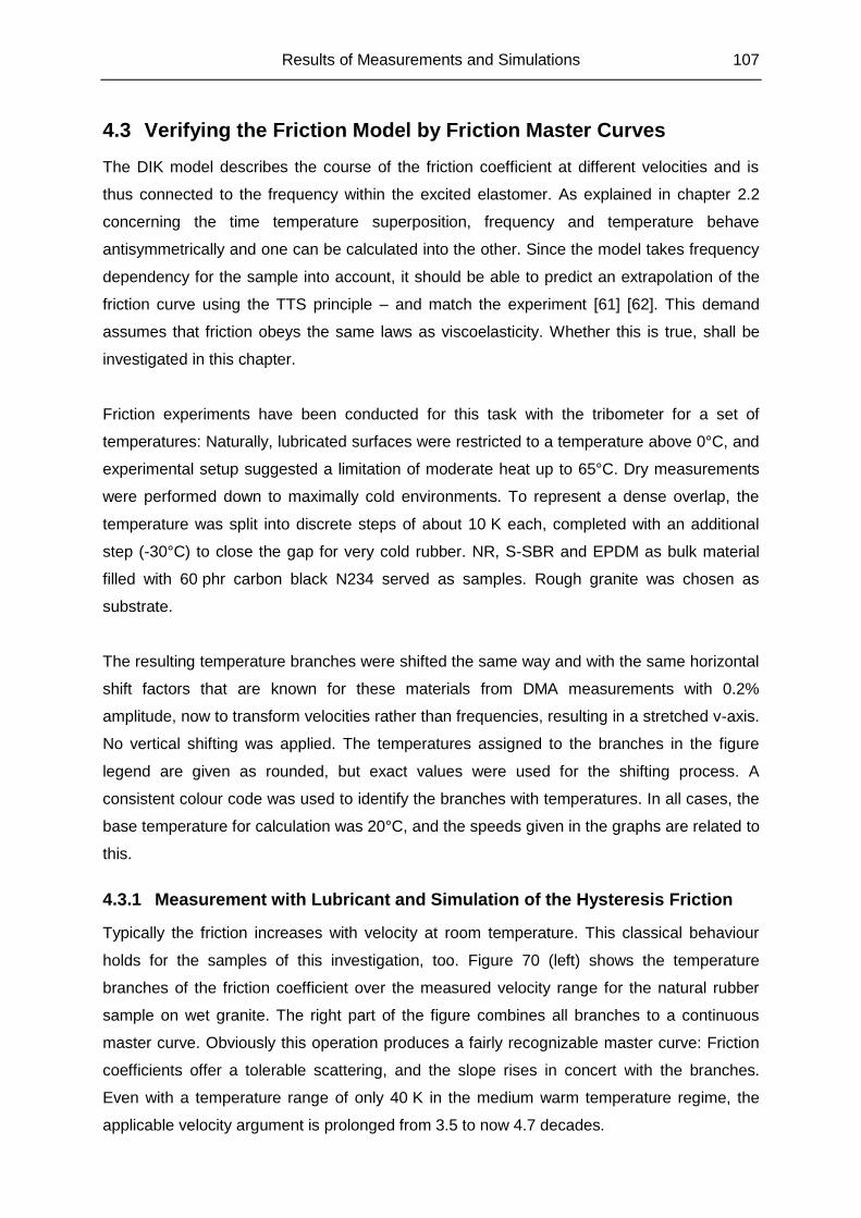
Results of Measurements and Simulations 107
4.3 Verifying the Friction Model by Friction Master Curves
The DIK model describes the course of the friction coefficient at different velocities and is
thus connected to the frequency within the excited elastomer. As explained in chapter 2.2
concerning the time temperature superposition, frequency and temperature behave
antisymmetrically and one can be calculated into the other. Since the model takes frequency
dependency for the sample into account, it should be able to predict an extrapolation of the
friction curve using the TTS principle – and match the experiment [61] [62]. This demand
assumes that friction obeys the same laws as viscoelasticity. Whether this is true, shall be
investigated in this chapter.
Friction experiments have been conducted for this task with the tribometer for a set of
temperatures: Naturally, lubricated surfaces were restricted to a temperature above 0°C, and
experimental setup suggested a limitation of moderate heat up to 65°C. Dry measurements
were performed down to maximally cold environments. To represent a dense overlap, the
temperature was split into discrete steps of about 10 K each, completed with an additional
step (-30°C) to close the gap for very cold rubber. NR, S-SBR and EPDM as bulk material
filled with 60 phr carbon black N234 served as samples. Rough granite was chosen as
substrate.
The resulting temperature branches were shifted the same way and with the same horizontal
shift factors that are known for these materials from DMA measurements with 0.2%
amplitude, now to transform velocities rather than frequencies, resulting in a stretched v-axis.
No vertical shifting was applied. The temperatures assigned to the branches in the figure
legend are given as rounded, but exact values were used for the shifting process. A
consistent colour code was used to identify the branches with temperatures. In all cases, the
base temperature for calculation was 20°C, and the speeds given in the graphs are related to
this.
4.3.1 Measurement with Lubricant and Simulation of the Hysteresis Friction
Typically the friction increases with velocity at room temperature. This classical behaviour
holds for the samples of this investigation, too. Figure 70 (left) shows the temperature
branches of the friction coefficient over the measured velocity range for the natural rubber
sample on wet granite. The right part of the figure combines all branches to a continuous
master curve. Obviously this operation produces a fairly recognizable master curve: Friction
coefficients offer a tolerable scattering, and the slope rises in concert with the branches.
Even with a temperature range of only 40 K in the medium warm temperature regime, the
applicable velocity argument is prolonged from 3.5 to now 4.7 decades.
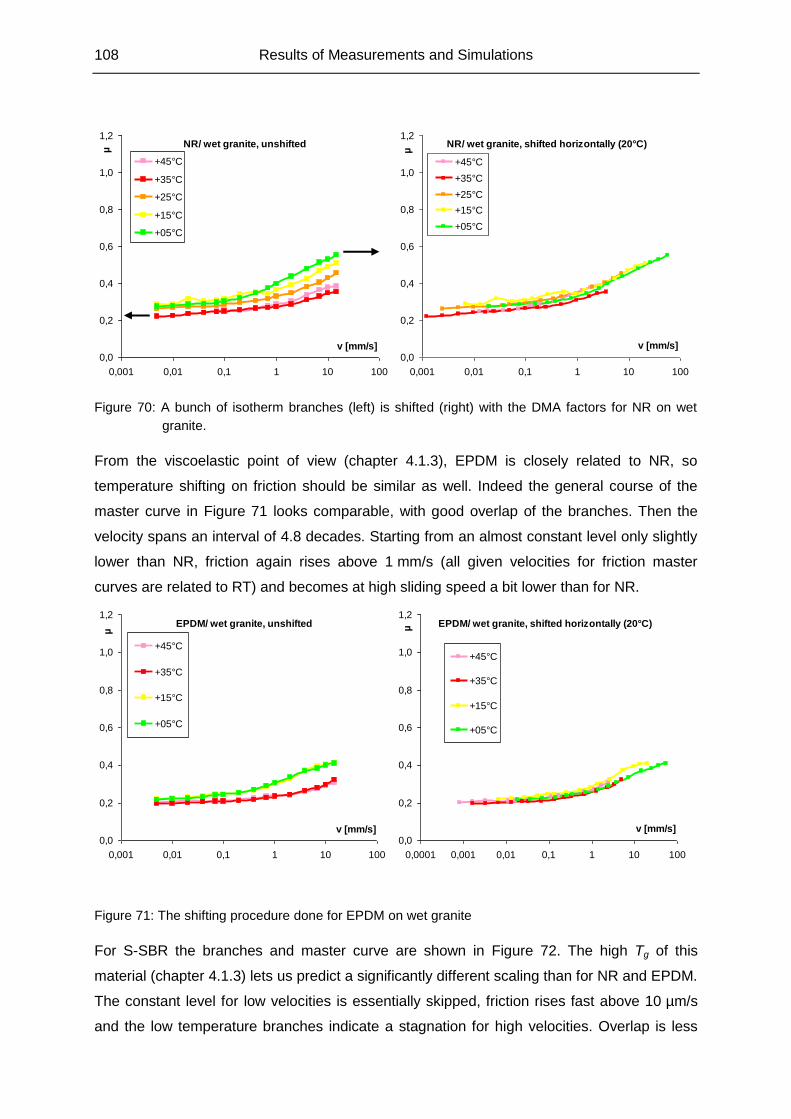
108 Results of Measurements and Simulations
NR/ wet granite, shifted horizontally (20°C)
0,0
0,2
0,4
0,6
0,8
1,0
1,2
0,001 0,01 0,1 1 10 100
v [mm/s]
µ
+45°C
+35°C
+25°C
+15°C
+05°C
NR/ wet granite, unshifted
0,0
0,2
0,4
0,6
0,8
1,0
1,2
0,001 0,01 0,1 1 10 100
v [mm/s]
µ
+45°C
+35°C
+25°C
+15°C
+05°C
Figure 70: A bunch of isotherm branches (left) is shifted (right) with the DMA factors for NR on wet
granite.
From the viscoelastic point of view (chapter 4.1.3), EPDM is closely related to NR, so
temperature shifting on friction should be similar as well. Indeed the general course of the
master curve in Figure 71 looks comparable, with good overlap of the branches. Then the
velocity spans an interval of 4.8 decades. Starting from an almost constant level only slightly
lower than NR, friction again rises above 1 mm/s (all given velocities for friction master
curves are related to RT) and becomes at high sliding speed a bit lower than for NR.
EPDM/ wet granite, unshifted
0,0
0,2
0,4
0,6
0,8
1,0
1,2
0,001 0,01 0,1 1 10 100
v [mm/s]
µ
+45°C
+35°C
+15°C
+05°C
EPDM/ wet granite, shifted horizontally (20°C)
0,0
0,2
0,4
0,6
0,8
1,0
1,2
0,0001 0,001 0,01 0,1 1 10 100
v [mm/s]
µ
+45°C
+35°C
+15°C
+05°C
Figure 71: The shifting procedure done for EPDM on wet granite
For S-SBR the branches and master curve are shown in Figure 72. The high Tg of this
material (chapter 4.1.3) lets us predict a significantly different scaling than for NR and EPDM.
The constant level for low velocities is essentially skipped, friction rises fast above 10 µm/s
and the low temperature branches indicate a stagnation for high velocities. Overlap is less
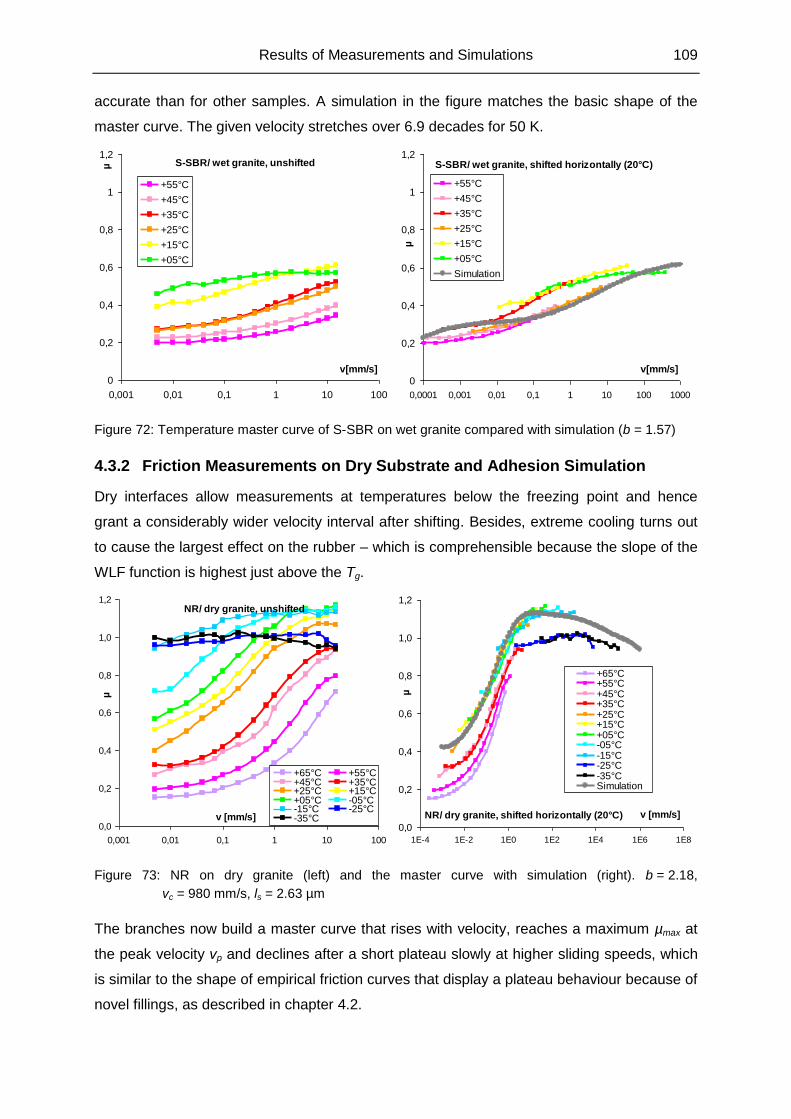
Results of Measurements and Simulations 109
accurate than for other samples. A simulation in the figure matches the basic shape of the
master curve. The given velocity stretches over 6.9 decades for 50 K.
S-SBR/ wet granite, unshifted
0
0,2
0,4
0,6
0,8
1
1,2
0,001 0,01 0,1 1 10 100
v[mm/s]
µ
+55°C
+45°C
+35°C
+25°C
+15°C
+05°C
S-SBR/ wet granite, shifted horizontally (20°C)
0
0,2
0,4
0,6
0,8
1
1,2
0,0001 0,001 0,01 0,1 1 10 100 1000
v[mm/s]
µ
+55°C
+45°C
+35°C
+25°C
+15°C
+05°C
Simulation
Figure 72: Temperature master curve of S-SBR on wet granite compared with simulation (b = 1.57)
4.3.2 Friction Measurements on Dry Substrate and Adhesion Simulation
Dry interfaces allow measurements at temperatures below the freezing point and hence
grant a considerably wider velocity interval after shifting. Besides, extreme cooling turns out
to cause the largest effect on the rubber – which is comprehensible because the slope of the
WLF function is highest just above the Tg.
NR/ dry granite, unshifted
0,0
0,2
0,4
0,6
0,8
1,0
1,2
0,001 0,01 0,1 1 10 100
v [mm/s]
µ
+65°C +55°C+45°C +35°C+25°C +15°C+05°C -05°C-15°C -25°C-35°C NR/ dry granite, shifted horizontally (20°C)
0,0
0,2
0,4
0,6
0,8
1,0
1,2
1E-4 1E-2 1E0 1E2 1E4 1E6 1E8
v [mm/s]
µ
+65°C+55°C+45°C+35°C+25°C+15°C+05°C-05°C-15°C-25°C-35°CSimulation
Figure 73: NR on dry granite (left) and the master curve with simulation (right). b = 2.18,
vc = 980 mm/s, ls = 2.63 µm
The branches now build a master curve that rises with velocity, reaches a maximum µmax at
the peak velocity vp and declines after a short plateau slowly at higher sliding speeds, which
is similar to the shape of empirical friction curves that display a plateau behaviour because of
novel fillings, as described in chapter 4.2.
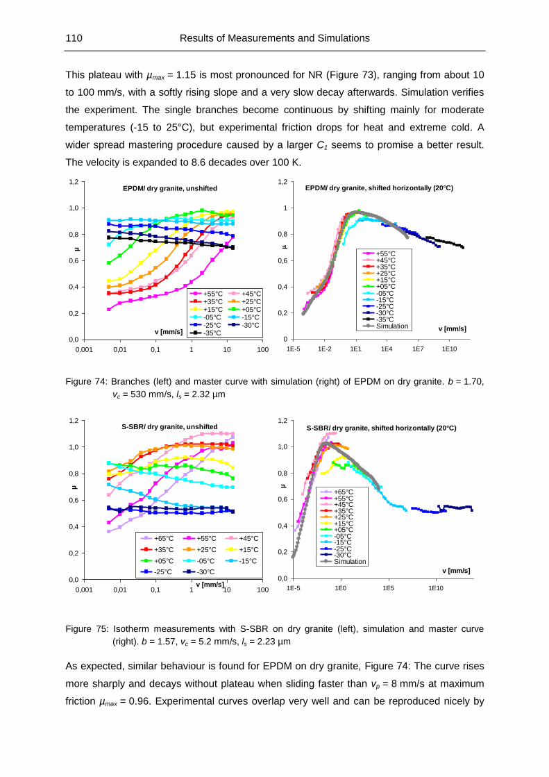
110 Results of Measurements and Simulations
This plateau with µmax = 1.15 is most pronounced for NR (Figure 73), ranging from about 10
to 100 mm/s, with a softly rising slope and a very slow decay afterwards. Simulation verifies
the experiment. The single branches become continuous by shifting mainly for moderate
temperatures (-15 to 25°C), but experimental friction drops for heat and extreme cold. A
wider spread mastering procedure caused by a larger C1 seems to promise a better result.
The velocity is expanded to 8.6 decades over 100 K.
EPDM/ dry granite, unshifted
0,0
0,2
0,4
0,6
0,8
1,0
1,2
0,001 0,01 0,1 1 10 100
v [mm/s]
µ
+55°C +45°C+35°C +25°C+15°C +05°C-05°C -15°C-25°C -30°C-35°C
EPDM/ dry granite, shifted horizontally (20°C)
0
0,2
0,4
0,6
0,8
1
1,2
1E-5 1E-2 1E1 1E4 1E7 1E10
v [mm/s]
+55°C+45°C+35°C+25°C+15°C+05°C-05°C-15°C-25°C-30°C-35°CSimulation
Figure 74: Branches (left) and master curve with simulation (right) of EPDM on dry granite. b = 1.70,
vc = 530 mm/s, ls = 2.32 µm
S-SBR/ dry granite, unshifted
0,0
0,2
0,4
0,6
0,8
1,0
1,2
0,001 0,01 0,1 1 10 100v [mm/s]
µ
+65°C +55°C +45°C
+35°C +25°C +15°C
+05°C -05°C -15°C
-25°C -30°C
S-SBR/ dry granite, shifted horizontally (20°C)
0,0
0,2
0,4
0,6
0,8
1,0
1,2
1E-5 1E0 1E5 1E10
v [mm/s]
µ
+65°C+55°C+45°C+35°C+25°C+15°C+05°C-05°C-15°C-25°C-30°CSimulation
Figure 75: Isotherm measurements with S-SBR on dry granite (left), simulation and master curve
(right). b = 1.57, vc = 5.2 mm/s, ls = 2.23 µm
As expected, similar behaviour is found for EPDM on dry granite, Figure 74: The curve rises
more sharply and decays without plateau when sliding faster than vp = 8 mm/s at maximum
friction µmax = 0.96. Experimental curves overlap very well and can be reproduced nicely by
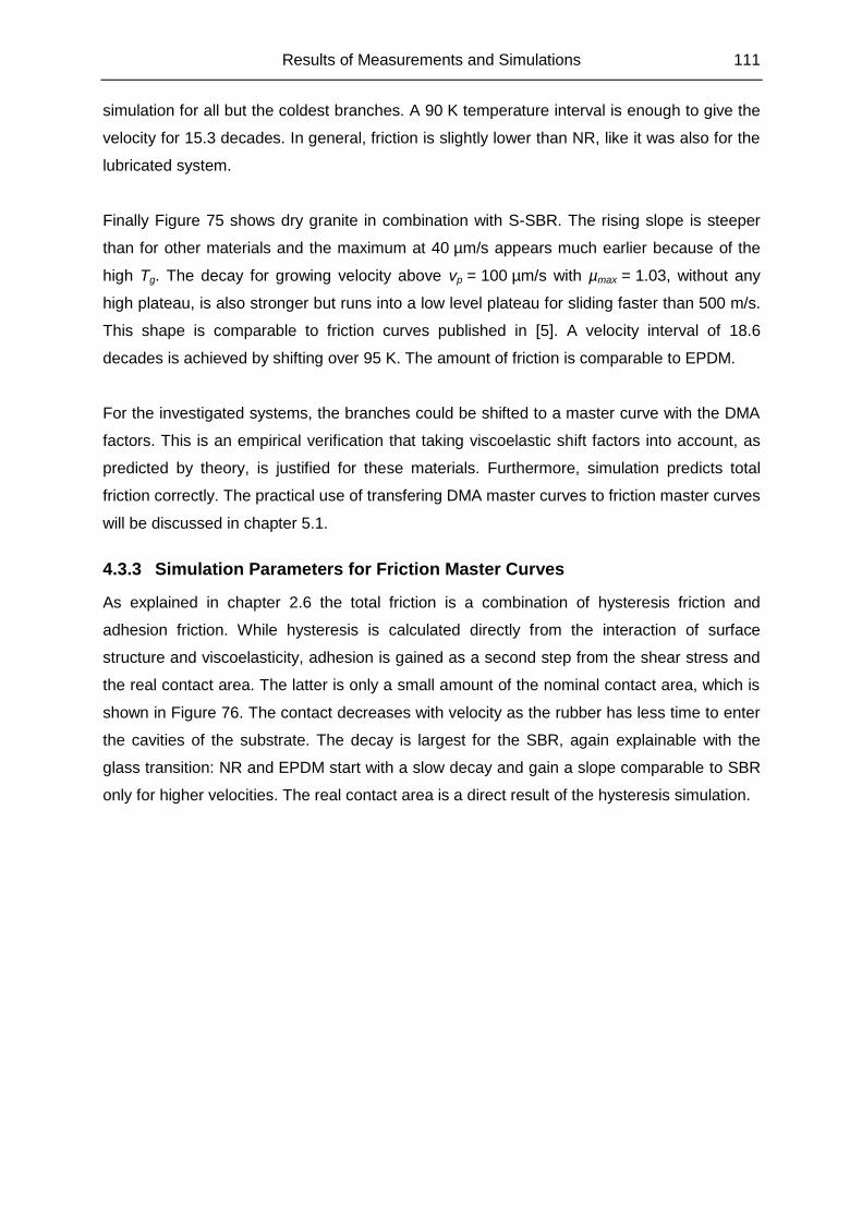
Results of Measurements and Simulations 111
simulation for all but the coldest branches. A 90 K temperature interval is enough to give the
velocity for 15.3 decades. In general, friction is slightly lower than NR, like it was also for the
lubricated system.
Finally Figure 75 shows dry granite in combination with S-SBR. The rising slope is steeper
than for other materials and the maximum at 40 µm/s appears much earlier because of the
high Tg. The decay for growing velocity above vp = 100 µm/s with µmax = 1.03, without any
high plateau, is also stronger but runs into a low level plateau for sliding faster than 500 m/s.
This shape is comparable to friction curves published in [5]. A velocity interval of 18.6
decades is achieved by shifting over 95 K. The amount of friction is comparable to EPDM.
For the investigated systems, the branches could be shifted to a master curve with the DMA
factors. This is an empirical verification that taking viscoelastic shift factors into account, as
predicted by theory, is justified for these materials. Furthermore, simulation predicts total
friction correctly. The practical use of transfering DMA master curves to friction master curves
will be discussed in chapter 5.1.
4.3.3 Simulation Parameters for Friction Master Curves
As explained in chapter 2.6 the total friction is a combination of hysteresis friction and
adhesion friction. While hysteresis is calculated directly from the interaction of surface
structure and viscoelasticity, adhesion is gained as a second step from the shear stress and
the real contact area. The latter is only a small amount of the nominal contact area, which is
shown in Figure 76. The contact decreases with velocity as the rubber has less time to enter
the cavities of the substrate. The decay is largest for the SBR, again explainable with the
glass transition: NR and EPDM start with a slow decay and gain a slope comparable to SBR
only for higher velocities. The real contact area is a direct result of the hysteresis simulation.
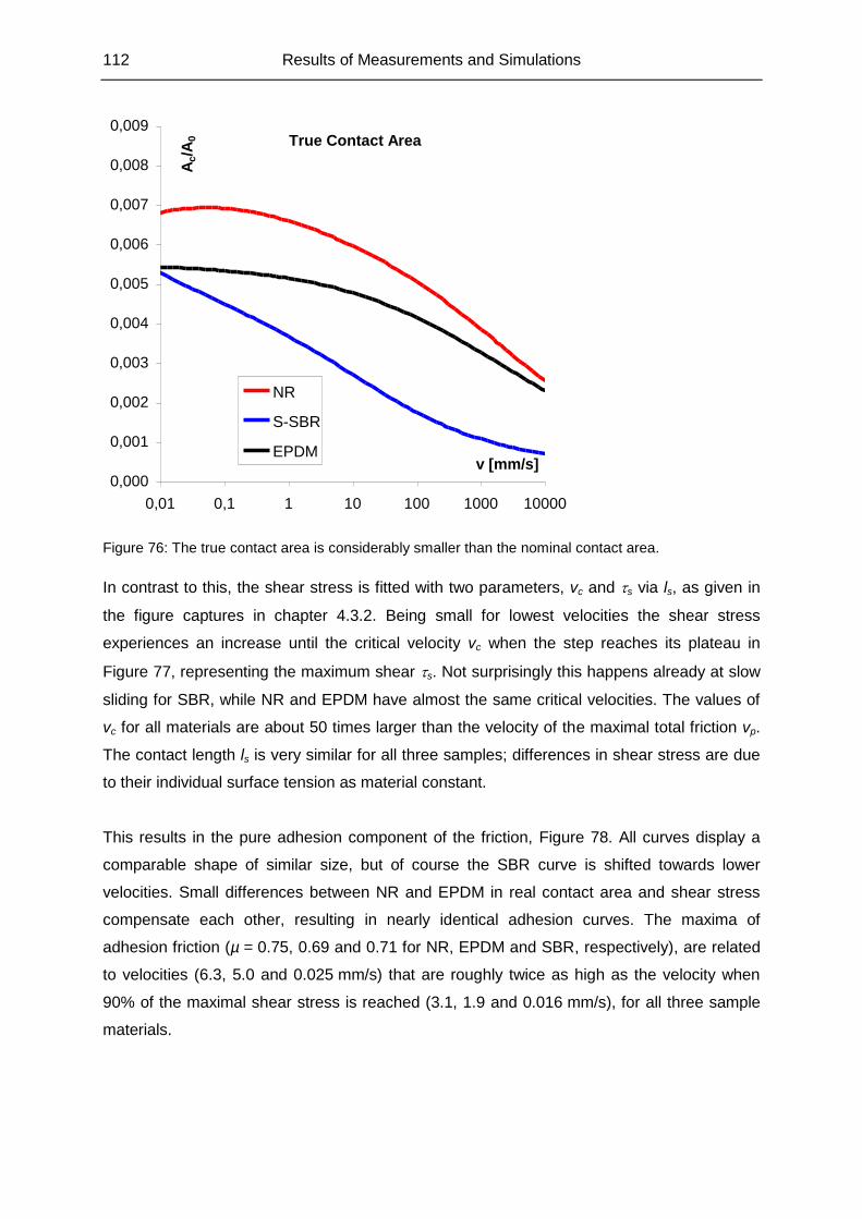
112 Results of Measurements and Simulations
True Contact Area
0,000
0,001
0,002
0,003
0,004
0,005
0,006
0,007
0,008
0,009
0,01 0,1 1 10 100 1000 10000
v [mm/s]
Ac/A
0
NR
S-SBR
EPDM
Figure 76: The true contact area is considerably smaller than the nominal contact area.
In contrast to this, the shear stress is fitted with two parameters, vc and s via ls, as given in
the figure captures in chapter 4.3.2. Being small for lowest velocities the shear stress
experiences an increase until the critical velocity vc when the step reaches its plateau in
Figure 77, representing the maximum shear s. Not surprisingly this happens already at slow
sliding for SBR, while NR and EPDM have almost the same critical velocities. The values of
vc for all materials are about 50 times larger than the velocity of the maximal total friction vp.
The contact length ls is very similar for all three samples; differences in shear stress are due
to their individual surface tension as material constant.
This results in the pure adhesion component of the friction, Figure 78. All curves display a
comparable shape of similar size, but of course the SBR curve is shifted towards lower
velocities. Small differences between NR and EPDM in real contact area and shear stress
compensate each other, resulting in nearly identical adhesion curves. The maxima of
adhesion friction (µ = 0.75, 0.69 and 0.71 for NR, EPDM and SBR, respectively), are related
to velocities (6.3, 5.0 and 0.025 mm/s) that are roughly twice as high as the velocity when
90% of the maximal shear stress is reached (3.1, 1.9 and 0.016 mm/s), for all three sample
materials.
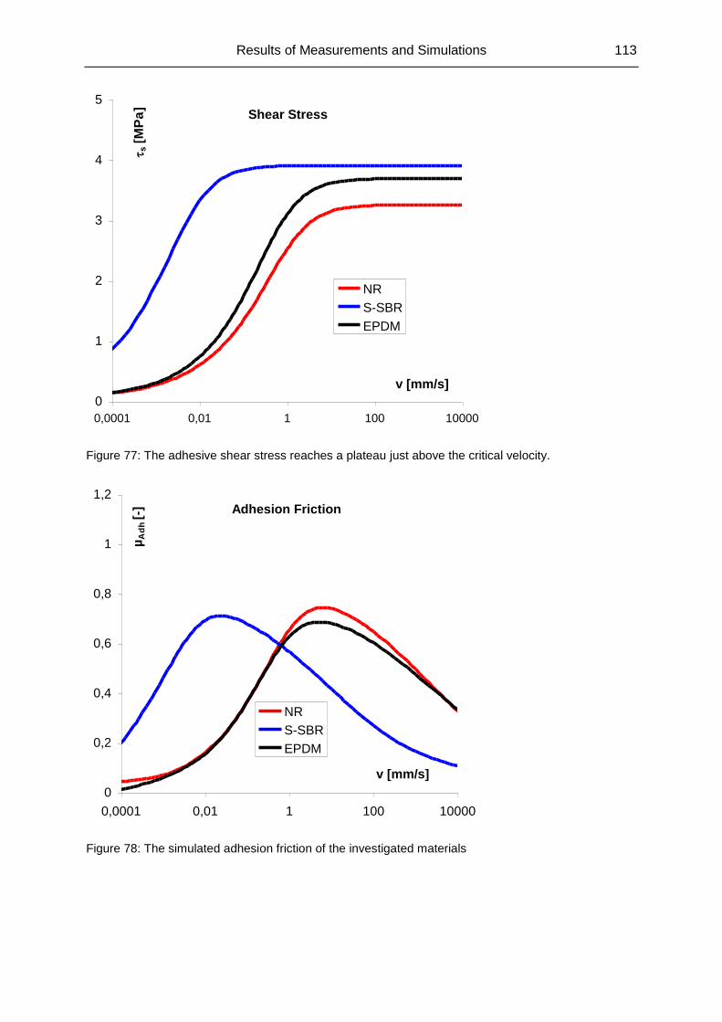
Results of Measurements and Simulations 113
Shear Stress
0
1
2
3
4
5
0,0001 0,01 1 100 10000
v [mm/s]
s [
MP
a]
NR
S-SBR
EPDM
Figure 77: The adhesive shear stress reaches a plateau just above the critical velocity.
Adhesion Friction
0
0,2
0,4
0,6
0,8
1
1,2
0,0001 0,01 1 100 10000
v [mm/s]
µA
dh [
-]
NR
S-SBR
EPDM
Figure 78: The simulated adhesion friction of the investigated materials
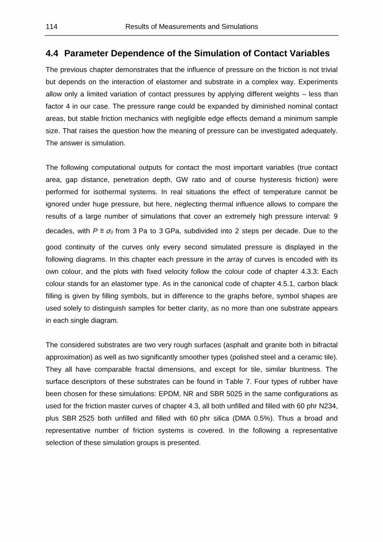
114 Results of Measurements and Simulations
4.4 Parameter Dependence of the Simulation of Contact Variables
The previous chapter demonstrates that the influence of pressure on the friction is not trivial
but depends on the interaction of elastomer and substrate in a complex way. Experiments
allow only a limited variation of contact pressures by applying different weights – less than
factor 4 in our case. The pressure range could be expanded by diminished nominal contact
areas, but stable friction mechanics with negligible edge effects demand a minimum sample
size. That raises the question how the meaning of pressure can be investigated adequately.
The answer is simulation.
The following computational outputs for contact the most important variables (true contact
area, gap distance, penetration depth, GW ratio and of course hysteresis friction) were
performed for isothermal systems. In real situations the effect of temperature cannot be
ignored under huge pressure, but here, neglecting thermal influence allows to compare the
results of a large number of simulations that cover an extremely high pressure interval: 9
decades, with P ≡ σ0 from 3 Pa to 3 GPa, subdivided into 2 steps per decade. Due to the
good continuity of the curves only every second simulated pressure is displayed in the
following diagrams. In this chapter each pressure in the array of curves is encoded with its
own colour, and the plots with fixed velocity follow the colour code of chapter 4.3.3: Each
colour stands for an elastomer type. As in the canonical code of chapter 4.5.1, carbon black
filling is given by filling symbols, but in difference to the graphs before, symbol shapes are
used solely to distinguish samples for better clarity, as no more than one substrate appears
in each single diagram.
The considered substrates are two very rough surfaces (asphalt and granite both in bifractal
approximation) as well as two significantly smoother types (polished steel and a ceramic tile).
They all have comparable fractal dimensions, and except for tile, similar bluntness. The
surface descriptors of these substrates can be found in Table 7. Four types of rubber have
been chosen for these simulations: EPDM, NR and SBR 5025 in the same configurations as
used for the friction master curves of chapter 4.3, all both unfilled and filled with 60 phr N234,
plus SBR 2525 both unfilled and filled with 60 phr silica (DMA 0.5%). Thus a broad and
representative number of friction systems is covered. In the following a representative
selection of these simulation groups is presented.
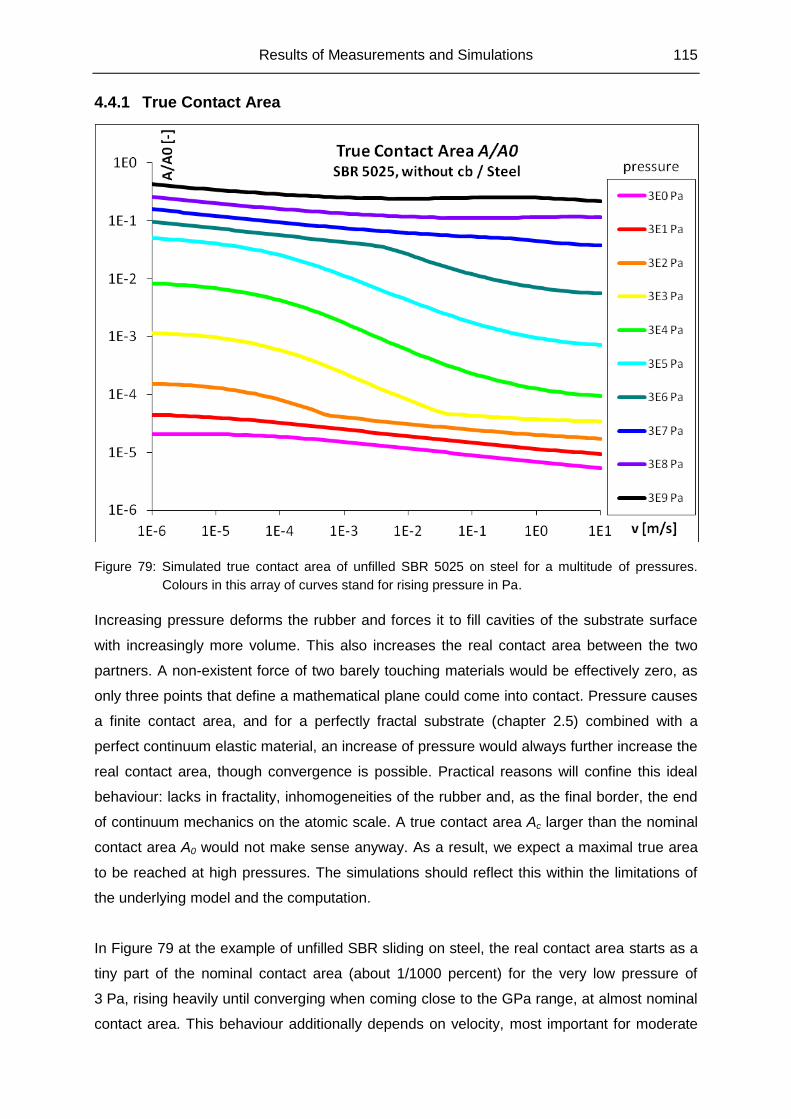
Results of Measurements and Simulations 115
4.4.1 True Contact Area
Figure 79: Simulated true contact area of unfilled SBR 5025 on steel for a multitude of pressures.
Colours in this array of curves stand for rising pressure in Pa.
Increasing pressure deforms the rubber and forces it to fill cavities of the substrate surface
with increasingly more volume. This also increases the real contact area between the two
partners. A non-existent force of two barely touching materials would be effectively zero, as
only three points that define a mathematical plane could come into contact. Pressure causes
a finite contact area, and for a perfectly fractal substrate (chapter 2.5) combined with a
perfect continuum elastic material, an increase of pressure would always further increase the
real contact area, though convergence is possible. Practical reasons will confine this ideal
behaviour: lacks in fractality, inhomogeneities of the rubber and, as the final border, the end
of continuum mechanics on the atomic scale. A true contact area Ac larger than the nominal
contact area A0 would not make sense anyway. As a result, we expect a maximal true area
to be reached at high pressures. The simulations should reflect this within the limitations of
the underlying model and the computation.
In Figure 79 at the example of unfilled SBR sliding on steel, the real contact area starts as a
tiny part of the nominal contact area (about 1/1000 percent) for the very low pressure of
3 Pa, rising heavily until converging when coming close to the GPa range, at almost nominal
contact area. This behaviour additionally depends on velocity, most important for moderate
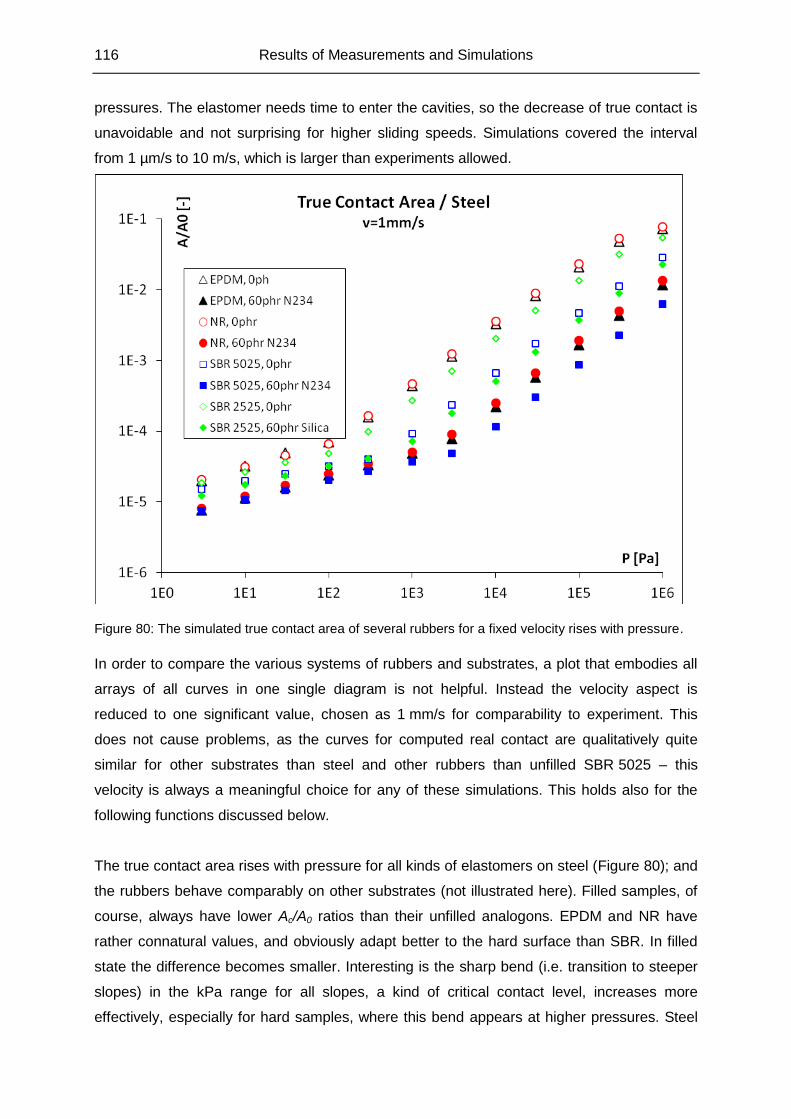
116 Results of Measurements and Simulations
pressures. The elastomer needs time to enter the cavities, so the decrease of true contact is
unavoidable and not surprising for higher sliding speeds. Simulations covered the interval
from 1 µm/s to 10 m/s, which is larger than experiments allowed.
Figure 80: The simulated true contact area of several rubbers for a fixed velocity rises with pressure.
In order to compare the various systems of rubbers and substrates, a plot that embodies all
arrays of all curves in one single diagram is not helpful. Instead the velocity aspect is
reduced to one significant value, chosen as 1 mm/s for comparability to experiment. This
does not cause problems, as the curves for computed real contact are qualitatively quite
similar for other substrates than steel and other rubbers than unfilled SBR 5025 – this
velocity is always a meaningful choice for any of these simulations. This holds also for the
following functions discussed below.
The true contact area rises with pressure for all kinds of elastomers on steel (Figure 80); and
the rubbers behave comparably on other substrates (not illustrated here). Filled samples, of
course, always have lower Ac/A0 ratios than their unfilled analogons. EPDM and NR have
rather connatural values, and obviously adapt better to the hard surface than SBR. In filled
state the difference becomes smaller. Interesting is the sharp bend (i.e. transition to steeper
slopes) in the kPa range for all slopes, a kind of critical contact level, increases more
effectively, especially for hard samples, where this bend appears at higher pressures. Steel
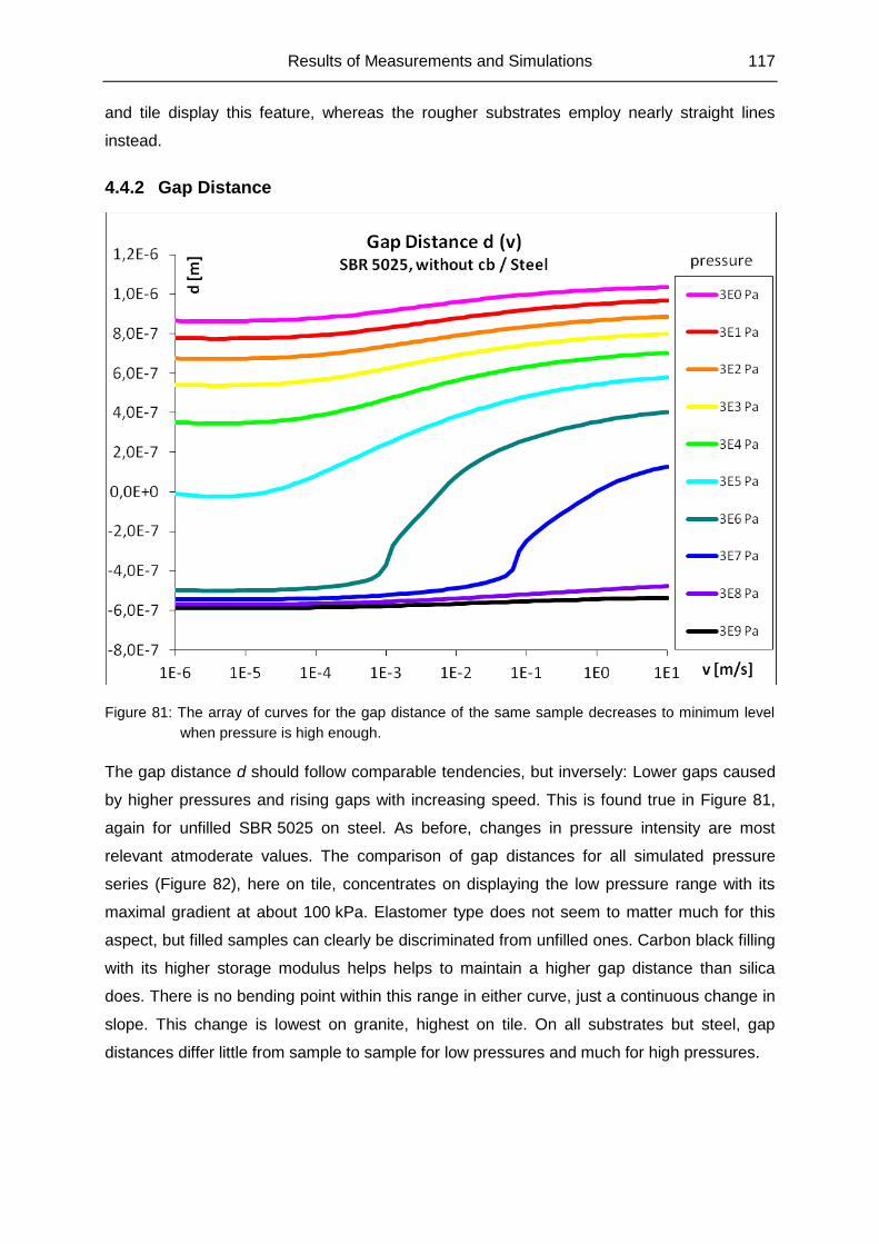
Results of Measurements and Simulations 117
and tile display this feature, whereas the rougher substrates employ nearly straight lines
instead.
4.4.2 Gap Distance
Figure 81: The array of curves for the gap distance of the same sample decreases to minimum level
when pressure is high enough.
The gap distance d should follow comparable tendencies, but inversely: Lower gaps caused
by higher pressures and rising gaps with increasing speed. This is found true in Figure 81,
again for unfilled SBR 5025 on steel. As before, changes in pressure intensity are most
relevant atmoderate values. The comparison of gap distances for all simulated pressure
series (Figure 82), here on tile, concentrates on displaying the low pressure range with its
maximal gradient at about 100 kPa. Elastomer type does not seem to matter much for this
aspect, but filled samples can clearly be discriminated from unfilled ones. Carbon black filling
with its higher storage modulus helps helps to maintain a higher gap distance than silica
does. There is no bending point within this range in either curve, just a continuous change in
slope. This change is lowest on granite, highest on tile. On all substrates but steel, gap
distances differ little from sample to sample for low pressures and much for high pressures.
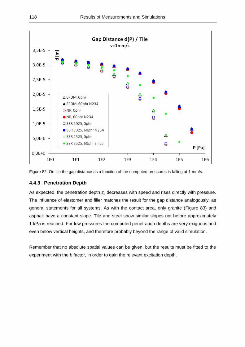
118 Results of Measurements and Simulations
Figure 82: On tile the gap distance as a function of the computed pressures is falling at 1 mm/s.
4.4.3 Penetration Depth
As expected, the penetration depth zp decreases with speed and rises directly with pressure.
The influence of elastomer and filler matches the result for the gap distance analogously, as
general statements for all systems. As with the contact area, only granite (Figure 83) and
asphalt have a constant slope. Tile and steel show similar slopes not before approximately
1 kPa is reached. For low pressures the computed penetration depths are very exiguous and
even below vertical heights, and therefore probably beyond the range of valid simulation.
Remember that no absolute spatial values can be given, but the results must be fitted to the
experiment with the b factor, in order to gain the relevant excitation depth.
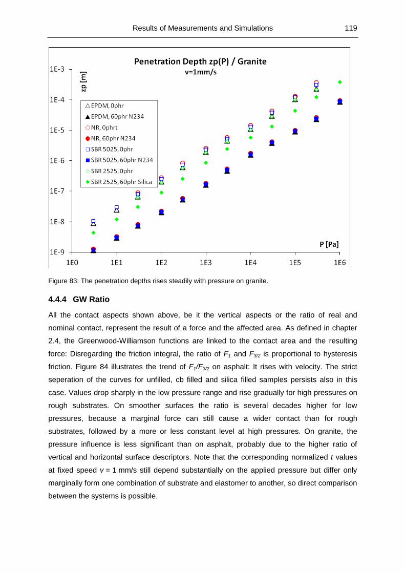
Results of Measurements and Simulations 119
Figure 83: The penetration depths rises steadily with pressure on granite.
4.4.4 GW Ratio
All the contact aspects shown above, be it the vertical aspects or the ratio of real and
nominal contact, represent the result of a force and the affected area. As defined in chapter
2.4, the Greenwood-Williamson functions are linked to the contact area and the resulting
force: Disregarding the friction integral, the ratio of F1 and F3/2 is proportional to hysteresis
friction. Figure 84 illustrates the trend of F1/F3/2 on asphalt: It rises with velocity. The strict
seperation of the curves for unfilled, cb filled and silica filled samples persists also in this
case. Values drop sharply in the low pressure range and rise gradually for high pressures on
rough substrates. On smoother surfaces the ratio is several decades higher for low
pressures, because a marginal force can still cause a wider contact than for rough
substrates, followed by a more or less constant level at high pressures. On granite, the
pressure influence is less significant than on asphalt, probably due to the higher ratio of
vertical and horizontal surface descriptors. Note that the corresponding normalized t values
at fixed speed v = 1 mm/s still depend substantially on the applied pressure but differ only
marginally form one combination of substrate and elastomer to another, so direct comparison
between the systems is possible.
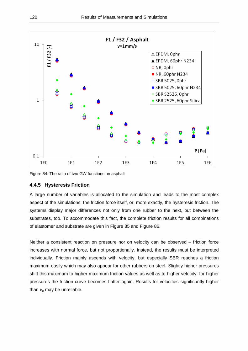
120 Results of Measurements and Simulations
Figure 84: The ratio of two GW functions on asphalt
4.4.5 Hysteresis Friction
A large number of variables is allocated to the simulation and leads to the most complex
aspect of the simulations: the friction force itself, or, more exactly, the hysteresis friction. The
systems display major differences not only from one rubber to the next, but between the
substrates, too. To accommodate this fact, the complete friction results for all combinations
of elastomer and substrate are given in Figure 85 and Figure 86.
Neither a consistent reaction on pressure nor on velocity can be observed – friction force
increases with normal force, but not proportionally. Instead, the results must be interpreted
individually. Friction mainly ascends with velocity, but especially SBR reaches a friction
maximum easily which may also appear for other rubbers on steel. Slightly higher pressures
shift this maximum to higher maximum friction values as well as to higher velocity; for higher
pressures the friction curve becomes flatter again. Results for velocities significantly higher
than vp may be unreliable.
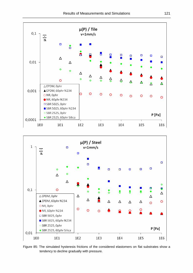
Results of Measurements and Simulations 121
Figure 85: The simulated hysteresis frictions of the considered elastomers on flat substrates show a
tendency to decline gradually with pressure.
122 Results of Measurements and Simulations
On the smooth substrates (steel and tile), friction in general decreases clearly with velocity
when low pressure is applied, and only little for pressures higher than moderate. This
matched basically experimental observations reported previously in this thesis. This “critical
pressure” again depends on the hardness, i.e. filler of the sample, in combination with the
substrate. The sporadic rise in friction for highest pressures might well be an artefact. Filled
samples have a higher friction than unfilled – not unusual, due to the resistance a hard
elastomer poses to deformation.
The elastomers definitely differ in their friction curves, even with the same filler. SBR reaches
the highest friction values, followed by EPDM and at last NR. This holds for all substrates,
with comparably small differences within each substrate for filled samples. Qualitatively it is
also essentially the same order as in experimental measurements on wet surfaces at
1 mm/s. The absolute values of the friction coefficient, however, are not predictable without
the properly fitted b factor. So, the accuracy of comparing the friction of different rubbers is
limited, and a fortiori comparing different substrates, explaining the noticeably different
friction maxima of tile and steel.
The interdependencies are more complicated on the rough substrates: On asphalt, friction
drops within a limited interval at moderate pressures. On granite this pressure dependency is
less pronounced and shifted to higher pressures. Beyond the borders of this interval, friction
ascends with pressure. It is noticeable as well that some values did not converge to results.
This is a serious hint that simulation should be regarded with caution for extreme
parameters, especially for the combination of rough substrates with extraordinarily low or
high pressures. Fortunately the pressures that can be applied in the experiment are in the
moderate range where computations are reliable. The difference between filled and unfilled
samples tends to be slightly more distinct than on smooth substrates, as a rough surface
allows even hard materials to fill cavities, maximizing resistance against deformation and
friction.
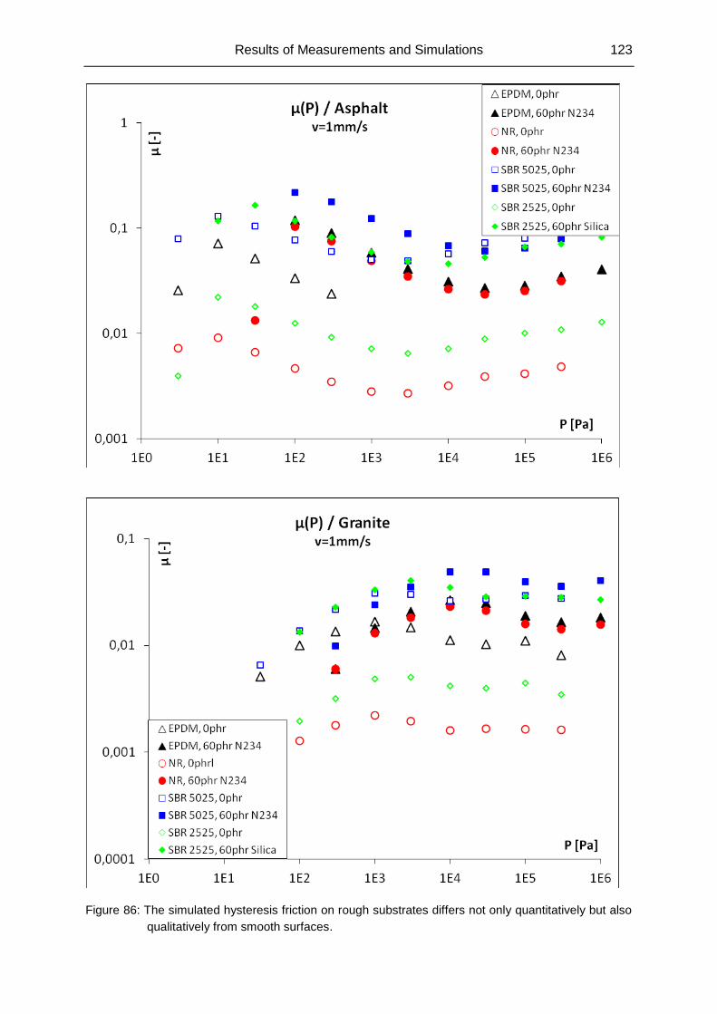
Results of Measurements and Simulations 123
Figure 86: The simulated hysteresis friction on rough substrates differs not only quantitatively but also
qualitatively from smooth surfaces.
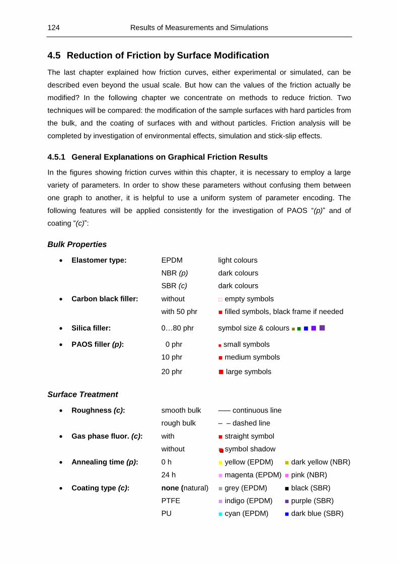
124 Results of Measurements and Simulations
4.5 Reduction of Friction by Surface Modification
The last chapter explained how friction curves, either experimental or simulated, can be
described even beyond the usual scale. But how can the values of the friction actually be
modified? In the following chapter we concentrate on methods to reduce friction. Two
techniques will be compared: the modification of the sample surfaces with hard particles from
the bulk, and the coating of surfaces with and without particles. Friction analysis will be
completed by investigation of environmental effects, simulation and stick-slip effects.
4.5.1 General Explanations on Graphical Friction Results
In the figures showing friction curves within this chapter, it is necessary to employ a large
variety of parameters. In order to show these parameters without confusing them between
one graph to another, it is helpful to use a uniform system of parameter encoding. The
following features will be applied consistently for the investigation of PAOS “(p)” and of
coating “(c)”:
Bulk Properties
Elastomer type: EPDM light colours
NBR (p) dark colours
SBR (c) dark colours
Carbon black filler: without empty symbols
with 50 phr ■ filled symbols, black frame if needed
Silica filler: 0…80 phr symbol size & colours ■ ■ ■ ■ ■
PAOS filler (p): 0 phr ■ small symbols
10 phr ■ medium symbols
20 phr ■ large symbols
Surface Treatment
Roughness (c): smooth bulk ––– continuous line
rough bulk – – dashed line
Gas phase fluor. (c): with ■ straight symbol
without ■■■ symbol shadow
Annealing time (p): 0 h ■ yellow (EPDM) ■ dark yellow (NBR)
24 h ■ magenta (EPDM) ■ pink (NBR)
Coating type (c): none (natural) ■ grey (EPDM) ■ black (SBR)
PTFE ■ indigo (EPDM) ■ purple (SBR)
PU ■ cyan (EPDM) ■ dark blue (SBR)
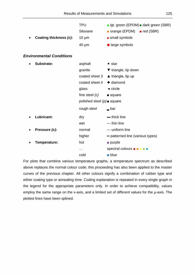
Results of Measurements and Simulations 125
TPU ■ lgt. green (EPDM) ■ dark green (SBR)
Siloxane ■ orange (EPDM) ■ red (SBR)
Coating thickness (c): 10 µm ■ small symbols
40 µm ■ large symbols
Environmental Conditions
Substrate: asphalt star
granite ▼ triangle, tip down
coated sheet 3 ▲ triangle, tip up
coated sheet 4 diamond
glass ● circle
fine steel (c) ■ square
polished steel (p) ■ square
rough steel ▂ bar
Lubricant: dry ▬ thick line
wet — thin line
Pressure (c): normal — uniform line
higher ═ patterned line (various types)
Temperature: hot ■ purple
… spectral colours ■ ■ ■ ■ ■
cold ■ blue
For plots that combine various temperature graphs, a temperature spectrum as described
above replaces the normal colour code; this proceeding has also been applied to the master
curves of the previous chapter. All other colours signify a combination of rubber type and
either coating type or annealing time. Coding explanation is repeated in every single graph in
the legend for the appropriate parameters only. In order to achieve compatibility, values
employ the same range on the v-axis, and a limited set of different values for the µ-axis. The
plotted lines have been splined.
126 Results of Measurements and Simulations
4.5.2 Tribology and Diminished Friction by Sample Induction with PAOS
The friction coefficient µ generally increases with velocity for all friction systems investigated
in this chapter. Friction of a measurement fluctuates below one percent in the evaluated
range. At high velocities the dry friction in some cases becomes almost constant. This
plateau behaviour has already been observed for other systems [5],[60],[61] and is explained
as a superposition of an increasing hysteresis friction and a decreasing adhesion friction, as
defined in chapter 2.7. Consequently, elastic samples without carbon black display higher
friction values (direct comparison between Figure 87 and Figure 88), especially on dry
substrates, because they can enter the cavities more deeply and cover a higher area of real
contact. This concerns predominantly the fast sliding. PAOS is expected to establish a
similar effect but without making the sample harder.
As presumed, the presence of PAOS lowers the friction on dry granite. This is true without
(Figure 87, effect symbolized by arrow) as well as with (Figure 88) carbon black fillers and
fits well to the observed reduction of surface tension. In contrast to carbon black, which
reduces friction mainly because of making the samples harder (a bulk effect), PAOS keeps
the sample soft (even softer than without it) and still reduces friction because of minimizing
the real contact area (a surface effect).
The friction reduction is generally amplified by annealing.Thereby friction becomes also less
dependent on velocity even without any PAOS, so after annealing PAOS is efficient for fast
sliding (more than 20% less friction for 20 phr) but not at low velocities. The flattening of
friction curves by annealing is a feature often observable in the investigated systems. The
averaged (velocity independent) friction may either be slightly increased or decreased after
annealing. Note that natural annealing for non-laboratory samples, components and parts is
unavoidable in a humid, normally pressured environment, so full PAOS establishment is only
a matter of time. Friction measurements and material testing for samples with different
annealing times indicate that a full effect is reached after about 20 hours annealing.
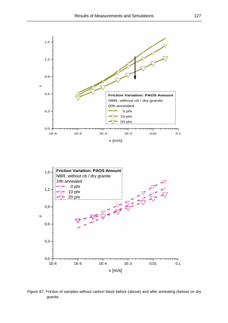
Results of Measurements and Simulations 127
1E-6 1E-5 1E-4 1E-3 0,01 0,1
0,0
0,3
0,6
0,9
1,2
1,5
Friction Variation: PAOS Amount
NBR, without cb / dry granite
00h annealed
0 phr
10 phr
20 phr
v [m/s]
1E-6 1E-5 1E-4 1E-3 0,01 0,1
0,0
0,3
0,6
0,9
1,2
1,5 Friction Variation: PAOS Amount
NBR, without cb / dry granite
24h annealed
0 phr
10 phr
20 phr
v [m/s]
Figure 87: Friction of samples without carbon black before (above) and after annealing (below) on dry
granite
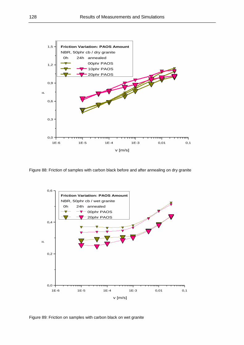
128 Results of Measurements and Simulations
1E-6 1E-5 1E-4 1E-3 0,01 0,1
0,0
0,3
0,6
0,9
1,2
1,5 Friction Variation: PAOS Amount
NBR, 50phr cb / dry granite
0h 24h annealed
00phr PAOS
10phr PAOS
20phr PAOS
v [m/s]
Figure 88: Friction of samples with carbon black before and after annealing on dry granite
1E-6 1E-5 1E-4 1E-3 0,01 0,1
0,0
0,2
0,4
0,6
Friction Variation: PAOS Amount
NBR, 50phr cb / wet granite
0h 24h annealed
00phr PAOS
20phr PAOS
v [m/s]
Figure 89: Friction on samples with carbon black on wet granite
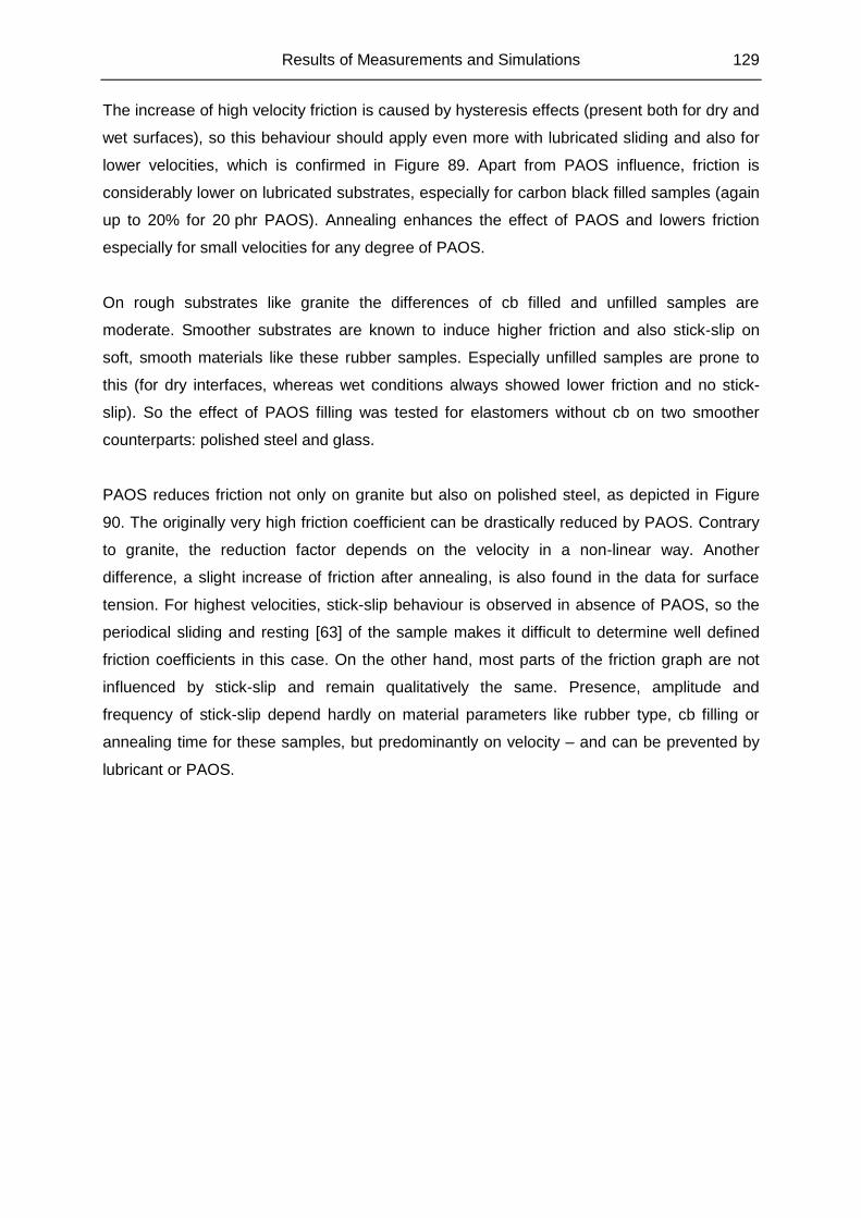
Results of Measurements and Simulations 129
The increase of high velocity friction is caused by hysteresis effects (present both for dry and
wet surfaces), so this behaviour should apply even more with lubricated sliding and also for
lower velocities, which is confirmed in Figure 89. Apart from PAOS influence, friction is
considerably lower on lubricated substrates, especially for carbon black filled samples (again
up to 20% for 20 phr PAOS). Annealing enhances the effect of PAOS and lowers friction
especially for small velocities for any degree of PAOS.
On rough substrates like granite the differences of cb filled and unfilled samples are
moderate. Smoother substrates are known to induce higher friction and also stick-slip on
soft, smooth materials like these rubber samples. Especially unfilled samples are prone to
this (for dry interfaces, whereas wet conditions always showed lower friction and no stick-
slip). So the effect of PAOS filling was tested for elastomers without cb on two smoother
counterparts: polished steel and glass.
PAOS reduces friction not only on granite but also on polished steel, as depicted in Figure
90. The originally very high friction coefficient can be drastically reduced by PAOS. Contrary
to granite, the reduction factor depends on the velocity in a non-linear way. Another
difference, a slight increase of friction after annealing, is also found in the data for surface
tension. For highest velocities, stick-slip behaviour is observed in absence of PAOS, so the
periodical sliding and resting [63] of the sample makes it difficult to determine well defined
friction coefficients in this case. On the other hand, most parts of the friction graph are not
influenced by stick-slip and remain qualitatively the same. Presence, amplitude and
frequency of stick-slip depend hardly on material parameters like rubber type, cb filling or
annealing time for these samples, but predominantly on velocity – and can be prevented by
lubricant or PAOS.
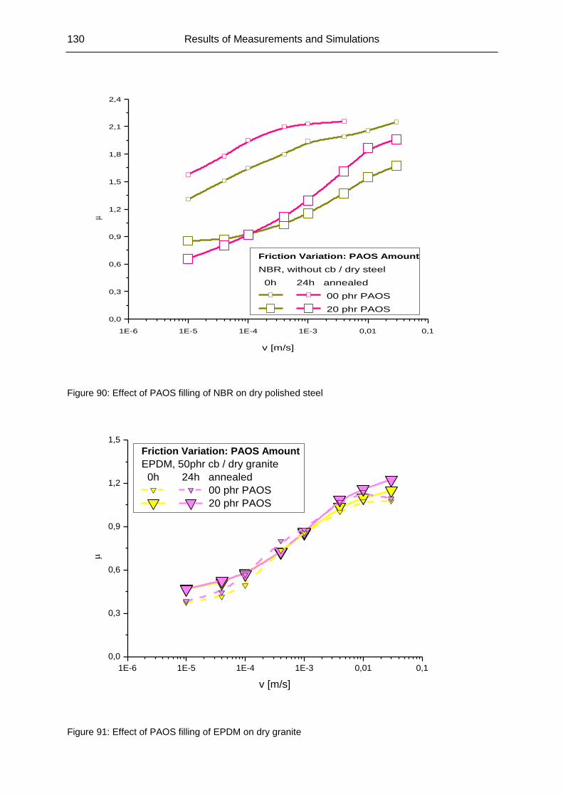
130 Results of Measurements and Simulations
1E-6 1E-5 1E-4 1E-3 0,01 0,1
0,0
0,3
0,6
0,9
1,2
1,5
1,8
2,1
2,4
Friction Variation: PAOS Amount
NBR, without cb / dry steel
0h 24h annealed
00 phr PAOS
20 phr PAOS
v [m/s]
Figure 90: Effect of PAOS filling of NBR on dry polished steel
1E-6 1E-5 1E-4 1E-3 0,01 0,1
0,0
0,3
0,6
0,9
1,2
1,5
Friction Variation: PAOS Amount
EPDM, 50phr cb / dry granite
0h 24h annealed
00 phr PAOS
20 phr PAOS
v [m/s]
Figure 91: Effect of PAOS filling of EPDM on dry granite
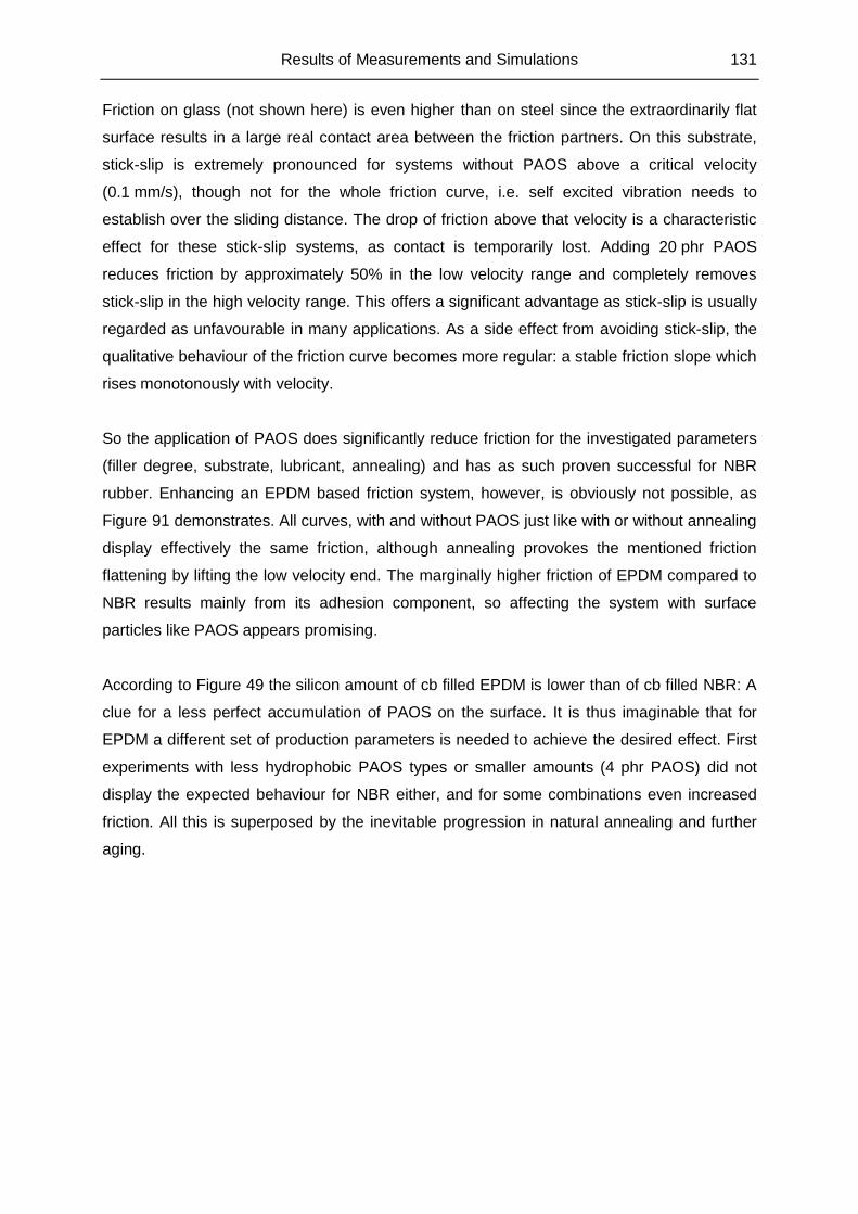
Results of Measurements and Simulations 131
Friction on glass (not shown here) is even higher than on steel since the extraordinarily flat
surface results in a large real contact area between the friction partners. On this substrate,
stick-slip is extremely pronounced for systems without PAOS above a critical velocity
(0.1 mm/s), though not for the whole friction curve, i.e. self excited vibration needs to
establish over the sliding distance. The drop of friction above that velocity is a characteristic
effect for these stick-slip systems, as contact is temporarily lost. Adding 20 phr PAOS
reduces friction by approximately 50% in the low velocity range and completely removes
stick-slip in the high velocity range. This offers a significant advantage as stick-slip is usually
regarded as unfavourable in many applications. As a side effect from avoiding stick-slip, the
qualitative behaviour of the friction curve becomes more regular: a stable friction slope which
rises monotonously with velocity.
So the application of PAOS does significantly reduce friction for the investigated parameters
(filler degree, substrate, lubricant, annealing) and has as such proven successful for NBR
rubber. Enhancing an EPDM based friction system, however, is obviously not possible, as
Figure 91 demonstrates. All curves, with and without PAOS just like with or without annealing
display effectively the same friction, although annealing provokes the mentioned friction
flattening by lifting the low velocity end. The marginally higher friction of EPDM compared to
NBR results mainly from its adhesion component, so affecting the system with surface
particles like PAOS appears promising.
According to Figure 49 the silicon amount of cb filled EPDM is lower than of cb filled NBR: A
clue for a less perfect accumulation of PAOS on the surface. It is thus imaginable that for
EPDM a different set of production parameters is needed to achieve the desired effect. First
experiments with less hydrophobic PAOS types or smaller amounts (4 phr PAOS) did not
display the expected behaviour for NBR either, and for some combinations even increased
friction. All this is superposed by the inevitable progression in natural annealing and further
aging.
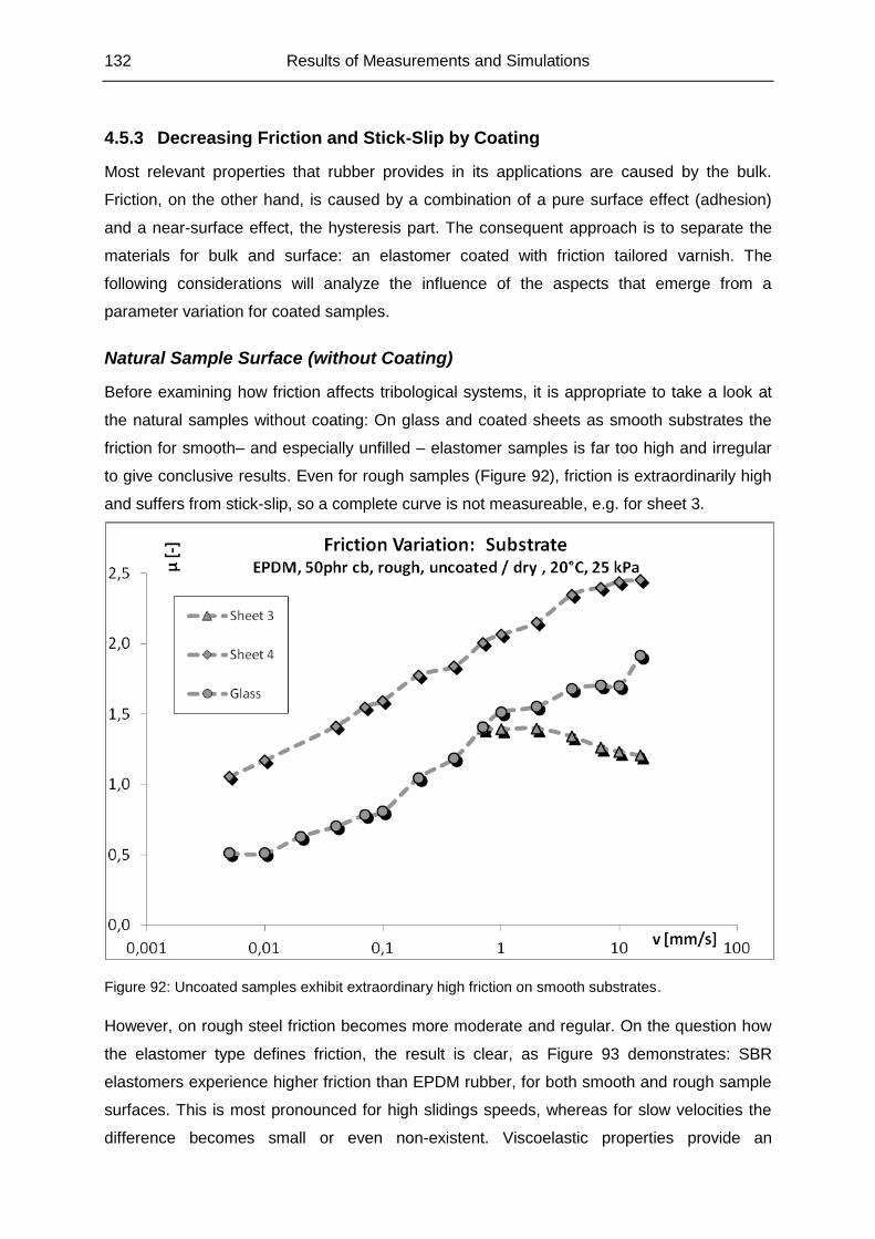
132 Results of Measurements and Simulations
4.5.3 Decreasing Friction and Stick-Slip by Coating
Most relevant properties that rubber provides in its applications are caused by the bulk.
Friction, on the other hand, is caused by a combination of a pure surface effect (adhesion)
and a near-surface effect, the hysteresis part. The consequent approach is to separate the
materials for bulk and surface: an elastomer coated with friction tailored varnish. The
following considerations will analyze the influence of the aspects that emerge from a
parameter variation for coated samples.
Natural Sample Surface (without Coating)
Before examining how friction affects tribological systems, it is appropriate to take a look at
the natural samples without coating: On glass and coated sheets as smooth substrates the
friction for smooth– and especially unfilled – elastomer samples is far too high and irregular
to give conclusive results. Even for rough samples (Figure 92), friction is extraordinarily high
and suffers from stick-slip, so a complete curve is not measureable, e.g. for sheet 3.
Figure 92: Uncoated samples exhibit extraordinary high friction on smooth substrates.
However, on rough steel friction becomes more moderate and regular. On the question how
the elastomer type defines friction, the result is clear, as Figure 93 demonstrates: SBR
elastomers experience higher friction than EPDM rubber, for both smooth and rough sample
surfaces. This is most pronounced for high slidings speeds, whereas for slow velocities the
difference becomes small or even non-existent. Viscoelastic properties provide an
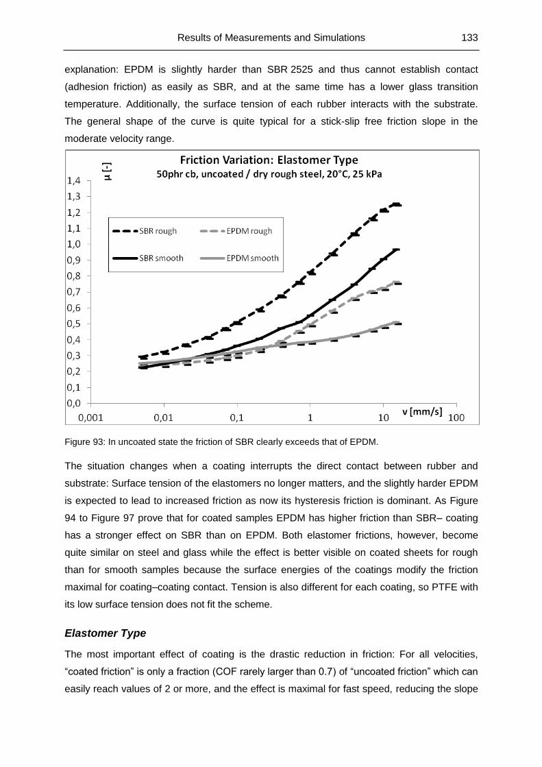
Results of Measurements and Simulations 133
explanation: EPDM is slightly harder than SBR 2525 and thus cannot establish contact
(adhesion friction) as easily as SBR, and at the same time has a lower glass transition
temperature. Additionally, the surface tension of each rubber interacts with the substrate.
The general shape of the curve is quite typical for a stick-slip free friction slope in the
moderate velocity range.
Figure 93: In uncoated state the friction of SBR clearly exceeds that of EPDM.
The situation changes when a coating interrupts the direct contact between rubber and
substrate: Surface tension of the elastomers no longer matters, and the slightly harder EPDM
is expected to lead to increased friction as now its hysteresis friction is dominant. As Figure
94 to Figure 97 prove that for coated samples EPDM has higher friction than SBR– coating
has a stronger effect on SBR than on EPDM. Both elastomer frictions, however, become
quite similar on steel and glass while the effect is better visible on coated sheets for rough
than for smooth samples because the surface energies of the coatings modify the friction
maximal for coating–coating contact. Tension is also different for each coating, so PTFE with
its low surface tension does not fit the scheme.
Elastomer Type
The most important effect of coating is the drastic reduction in friction: For all velocities,
“coated friction” is only a fraction (COF rarely larger than 0.7) of “uncoated friction” which can
easily reach values of 2 or more, and the effect is maximal for fast speed, reducing the slope
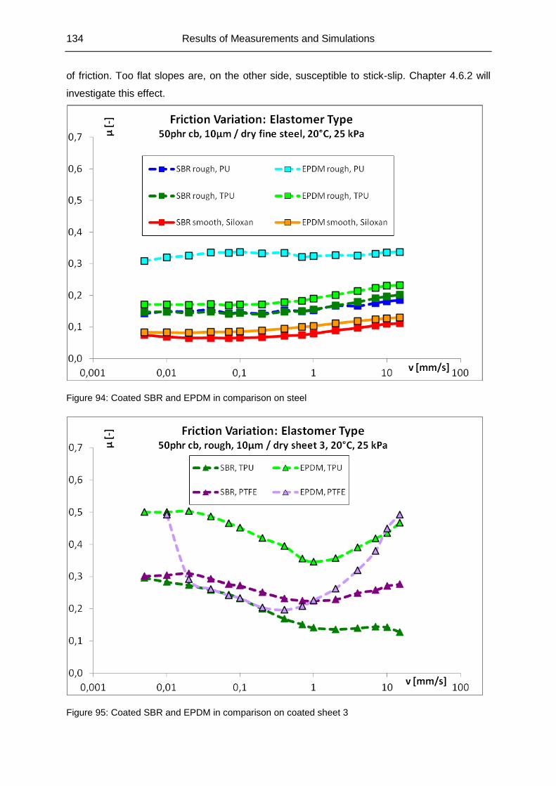
134 Results of Measurements and Simulations
of friction. Too flat slopes are, on the other side, susceptible to stick-slip. Chapter 4.6.2 will
investigate this effect.
Figure 94: Coated SBR and EPDM in comparison on steel
Figure 95: Coated SBR and EPDM in comparison on coated sheet 3
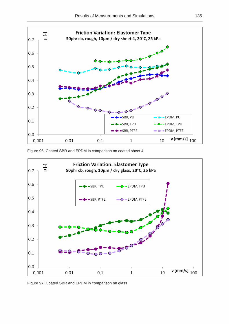
Results of Measurements and Simulations 135
Figure 96: Coated SBR and EPDM in comparison on coated sheet 4
Figure 97: Coated SBR and EPDM in comparison on glass
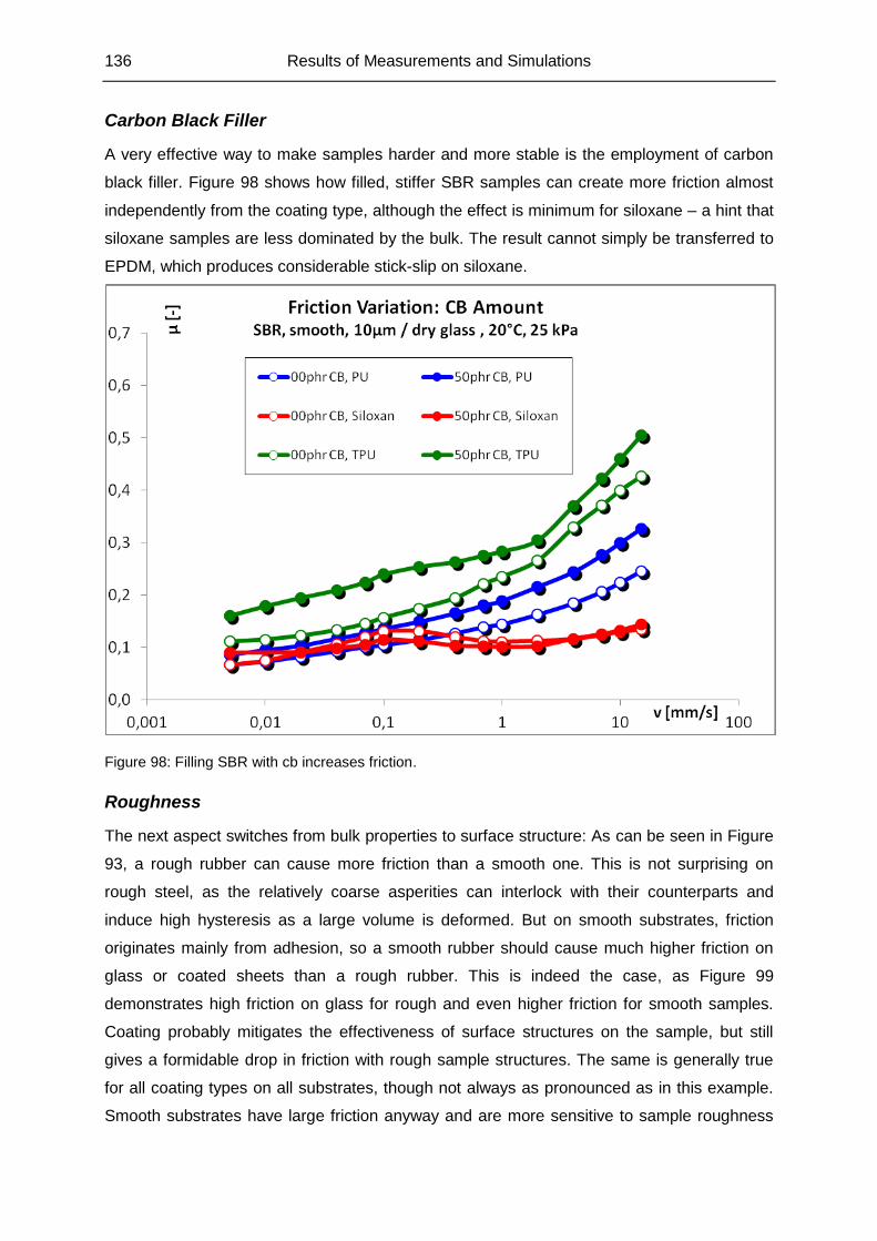
136 Results of Measurements and Simulations
Carbon Black Filler
A very effective way to make samples harder and more stable is the employment of carbon
black filler. Figure 98 shows how filled, stiffer SBR samples can create more friction almost
independently from the coating type, although the effect is minimum for siloxane – a hint that
siloxane samples are less dominated by the bulk. The result cannot simply be transferred to
EPDM, which produces considerable stick-slip on siloxane.
Figure 98: Filling SBR with cb increases friction.
Roughness
The next aspect switches from bulk properties to surface structure: As can be seen in Figure
93, a rough rubber can cause more friction than a smooth one. This is not surprising on
rough steel, as the relatively coarse asperities can interlock with their counterparts and
induce high hysteresis as a large volume is deformed. But on smooth substrates, friction
originates mainly from adhesion, so a smooth rubber should cause much higher friction on
glass or coated sheets than a rough rubber. This is indeed the case, as Figure 99
demonstrates high friction on glass for rough and even higher friction for smooth samples.
Coating probably mitigates the effectiveness of surface structures on the sample, but still
gives a formidable drop in friction with rough sample structures. The same is generally true
for all coating types on all substrates, though not always as pronounced as in this example.
Smooth substrates have large friction anyway and are more sensitive to sample roughness
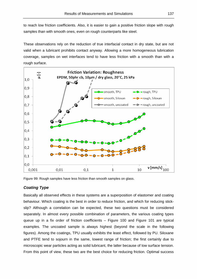
Results of Measurements and Simulations 137
to reach low friction coefficients. Also, it is easier to gain a positive friction slope with rough
samples than with smooth ones, even on rough counterparts like steel.
These observations rely on the reduction of true interfacial contact in dry state, but are not
valid when a lubricant prohibits contact anyway. Allowing a more homogeneous lubrication
coverage, samples on wet interfaces tend to have less friction with a smooth than with a
rough surface.
Figure 99: Rough samples have less friction than smooth samples on glass.
Coating Type
Basically all observed effects in these systems are a superposition of elastomer and coating
behaviour. Which coating is the best in order to reduce friction, and which for reducing stick-
slip? Although a correlation can be expected, these two questions must be considered
separately. In almost every possible combination of parameters, the various coating types
queue up in a fix order of friction coefficients – Figure 100 and Figure 101 are typical
examples. The uncoated sample is always highest (beyond the scale in the following
figures). Among the coatings, TPU usually exhibits the least effect, followed by PU. Siloxane
and PTFE tend to sojourn in the same, lowest range of friction; the first certainly due to
microscopic wear particles acting as solid lubricant, the latter because of low surface tension.
From this point of view, these two are the best choice for reducing friction. Optimal success
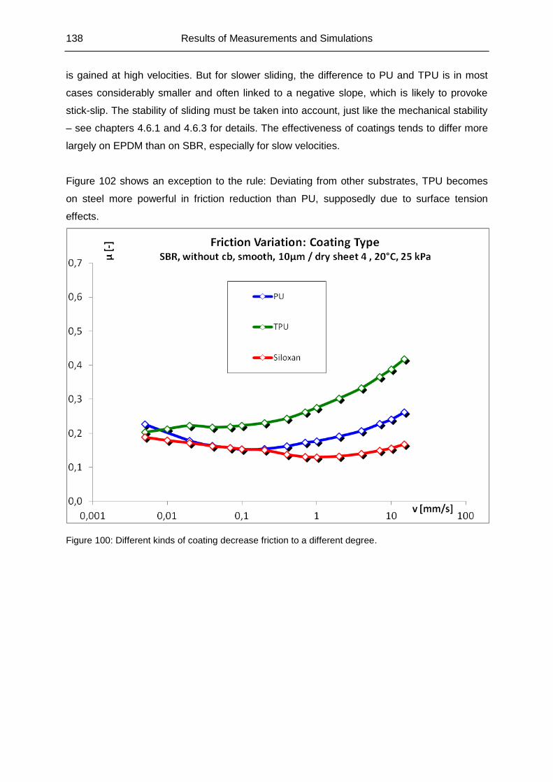
138 Results of Measurements and Simulations
is gained at high velocities. But for slower sliding, the difference to PU and TPU is in most
cases considerably smaller and often linked to a negative slope, which is likely to provoke
stick-slip. The stability of sliding must be taken into account, just like the mechanical stability
– see chapters 4.6.1 and 4.6.3 for details. The effectiveness of coatings tends to differ more
largely on EPDM than on SBR, especially for slow velocities.
Figure 102 shows an exception to the rule: Deviating from other substrates, TPU becomes
on steel more powerful in friction reduction than PU, supposedly due to surface tension
effects.
Figure 100: Different kinds of coating decrease friction to a different degree.
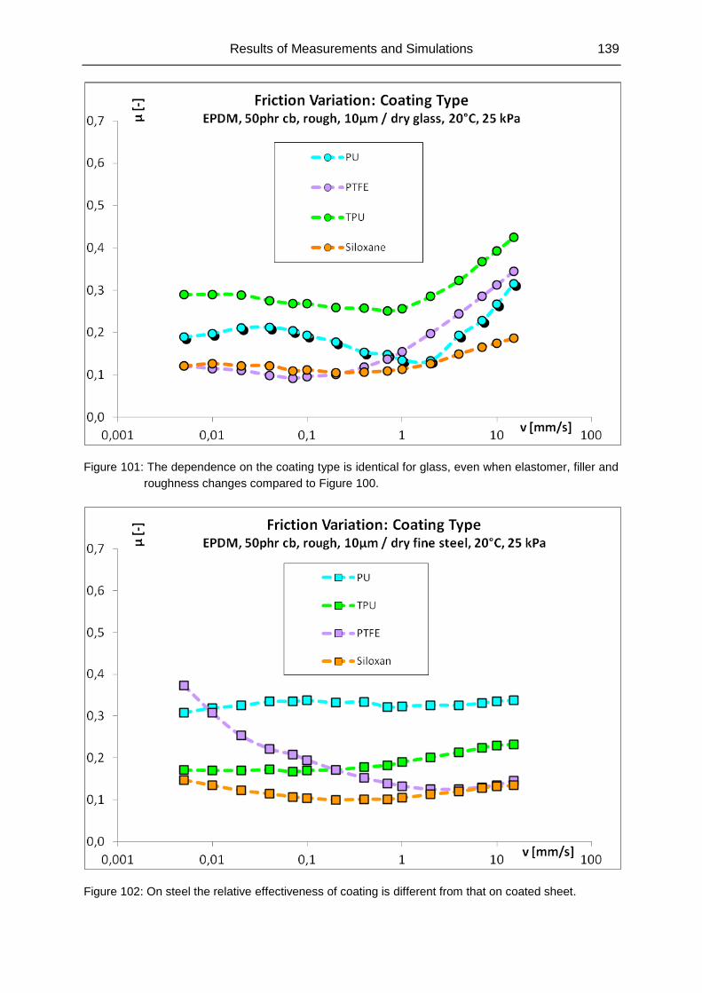
Results of Measurements and Simulations 139
Figure 101: The dependence on the coating type is identical for glass, even when elastomer, filler and
roughness changes compared to Figure 100.
Figure 102: On steel the relative effectiveness of coating is different from that on coated sheet.
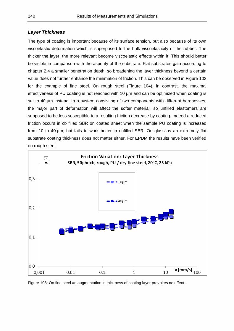
140 Results of Measurements and Simulations
Layer Thickness
The type of coating is important because of its surface tension, but also because of its own
viscoelastic deformation which is superposed to the bulk viscoelasticity of the rubber. The
thicker the layer, the more relevant become viscoelastic effects within it. This should better
be visible in comparison with the asperity of the substrate: Flat substrates gain according to
chapter 2.4 a smaller penetration depth, so broadening the layer thickness beyond a certain
value does not further enhance the minimation of friction. This can be observed in Figure 103
for the example of fine steel. On rough steel (Figure 104), in contrast, the maximal
effectiveness of PU coating is not reached with 10 µm and can be optimized when coating is
set to 40 µm instead. In a system consisting of two components with different hardnesses,
the major part of deformation will affect the softer material, so unfilled elastomers are
supposed to be less susceptible to a resulting friction decrease by coating. Indeed a reduced
friction occurs in cb filled SBR on coated sheet when the sample PU coating is increased
from 10 to 40 µm, but fails to work better in unfilled SBR. On glass as an extremely flat
substrate coating thickness does not matter either. For EPDM the results have been verified
on rough steel.
Figure 103: On fine steel an augmentation in thickness of coating layer provokes no effect.
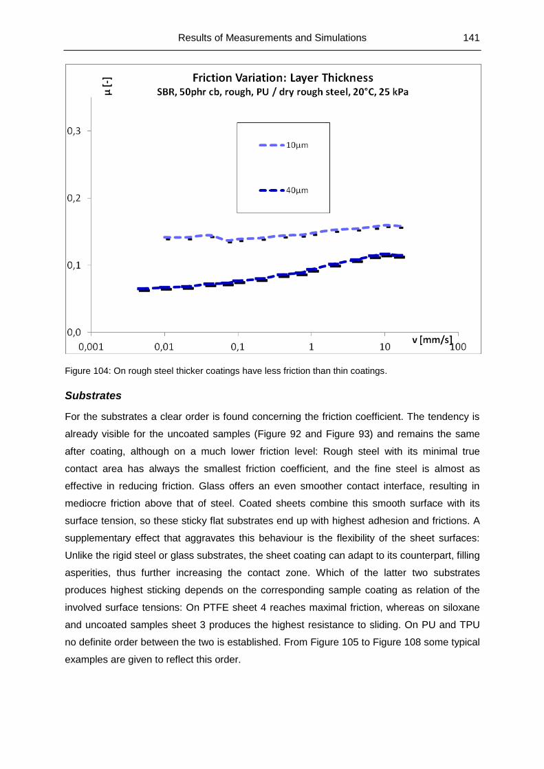
Results of Measurements and Simulations 141
Figure 104: On rough steel thicker coatings have less friction than thin coatings.
Substrates
For the substrates a clear order is found concerning the friction coefficient. The tendency is
already visible for the uncoated samples (Figure 92 and Figure 93) and remains the same
after coating, although on a much lower friction level: Rough steel with its minimal true
contact area has always the smallest friction coefficient, and the fine steel is almost as
effective in reducing friction. Glass offers an even smoother contact interface, resulting in
mediocre friction above that of steel. Coated sheets combine this smooth surface with its
surface tension, so these sticky flat substrates end up with highest adhesion and frictions. A
supplementary effect that aggravates this behaviour is the flexibility of the sheet surfaces:
Unlike the rigid steel or glass substrates, the sheet coating can adapt to its counterpart, filling
asperities, thus further increasing the contact zone. Which of the latter two substrates
produces highest sticking depends on the corresponding sample coating as relation of the
involved surface tensions: On PTFE sheet 4 reaches maximal friction, whereas on siloxane
and uncoated samples sheet 3 produces the highest resistance to sliding. On PU and TPU
no definite order between the two is established. From Figure 105 to Figure 108 some typical
examples are given to reflect this order.
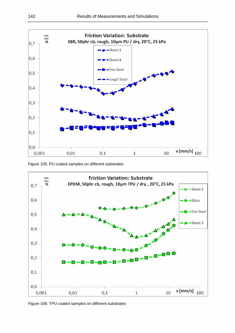
142 Results of Measurements and Simulations
Figure 105: PU coated samples on different substrates
Figure 106: TPU coated samples on different substrates
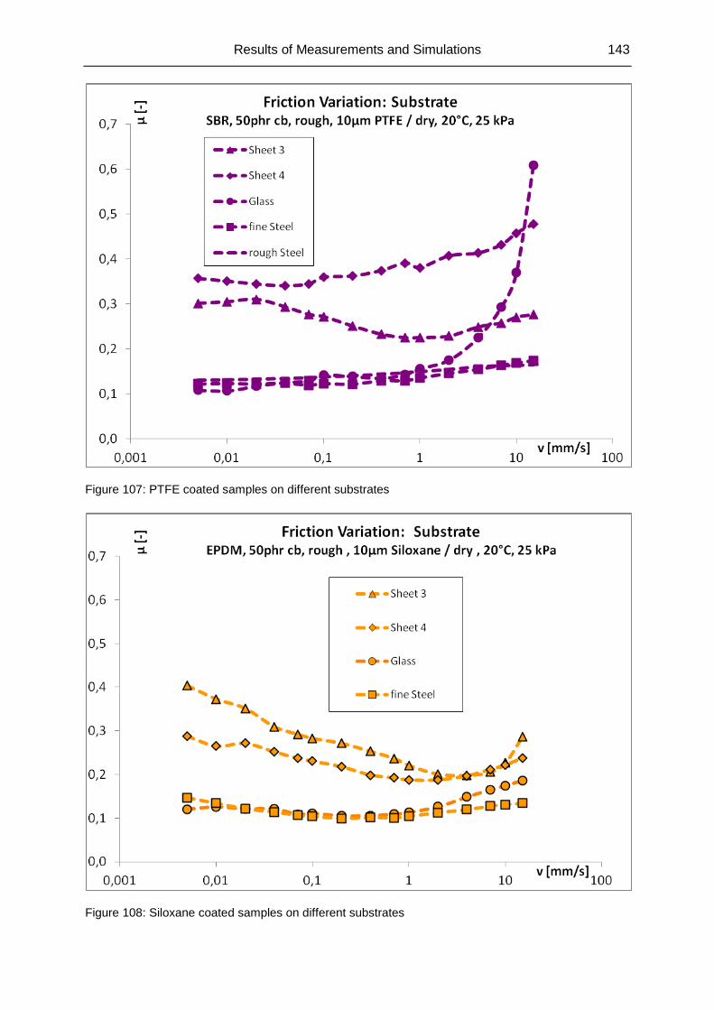
Results of Measurements and Simulations 143
Figure 107: PTFE coated samples on different substrates
Figure 108: Siloxane coated samples on different substrates
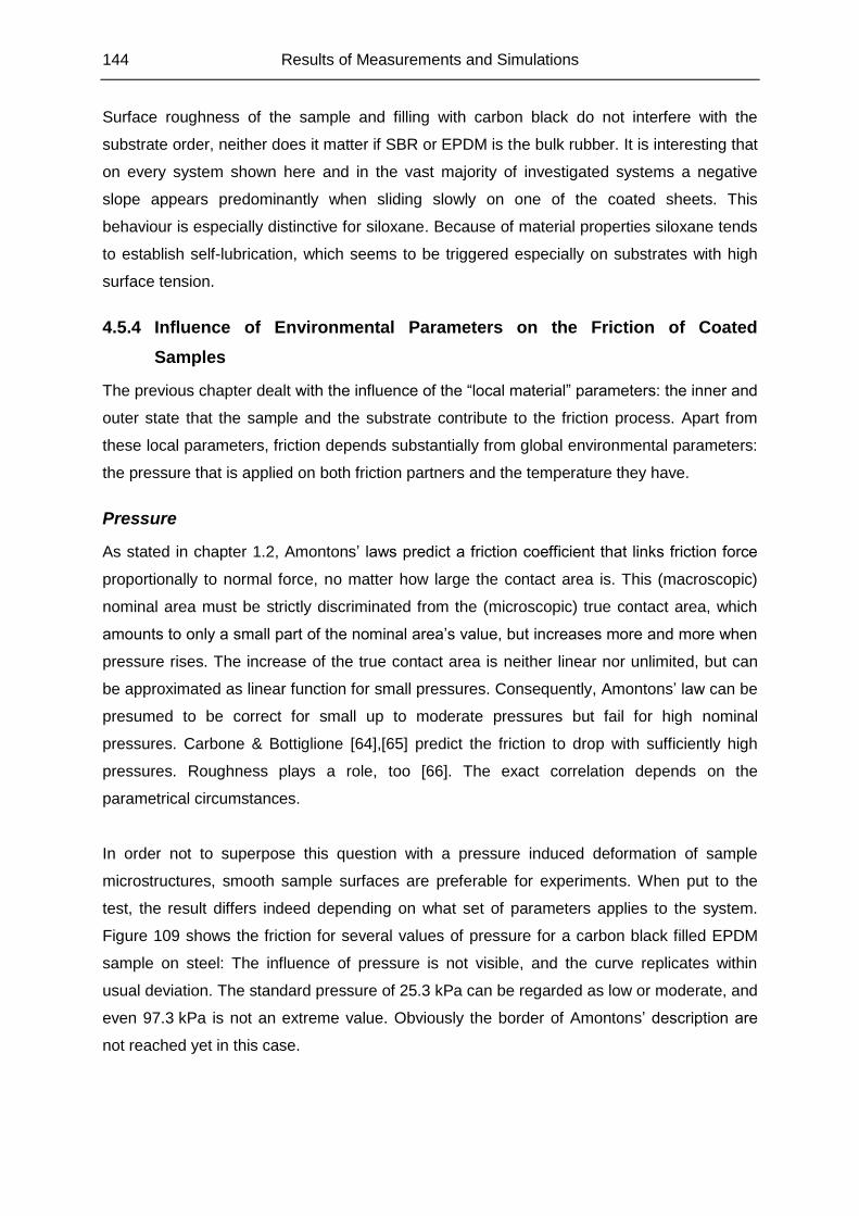
144 Results of Measurements and Simulations
Surface roughness of the sample and filling with carbon black do not interfere with the
substrate order, neither does it matter if SBR or EPDM is the bulk rubber. It is interesting that
on every system shown here and in the vast majority of investigated systems a negative
slope appears predominantly when sliding slowly on one of the coated sheets. This
behaviour is especially distinctive for siloxane. Because of material properties siloxane tends
to establish self-lubrication, which seems to be triggered especially on substrates with high
surface tension.
4.5.4 Influence of Environmental Parameters on the Friction of Coated
Samples
The previous chapter dealt with the influence of the “local material” parameters: the inner and
outer state that the sample and the substrate contribute to the friction process. Apart from
these local parameters, friction depends substantially from global environmental parameters:
the pressure that is applied on both friction partners and the temperature they have.
Pressure
As stated in chapter 1.2, Amontons’ laws predict a friction coefficient that links friction force
proportionally to normal force, no matter how large the contact area is. This (macroscopic)
nominal area must be strictly discriminated from the (microscopic) true contact area, which
amounts to only a small part of the nominal area’s value, but increases more and more when
pressure rises. The increase of the true contact area is neither linear nor unlimited, but can
be approximated as linear function for small pressures. Consequently, Amontons’ law can be
presumed to be correct for small up to moderate pressures but fail for high nominal
pressures. Carbone & Bottiglione [64],[65] predict the friction to drop with sufficiently high
pressures. Roughness plays a role, too [66]. The exact correlation depends on the
parametrical circumstances.
In order not to superpose this question with a pressure induced deformation of sample
microstructures, smooth sample surfaces are preferable for experiments. When put to the
test, the result differs indeed depending on what set of parameters applies to the system.
Figure 109 shows the friction for several values of pressure for a carbon black filled EPDM
sample on steel: The influence of pressure is not visible, and the curve replicates within
usual deviation. The standard pressure of 25.3 kPa can be regarded as low or moderate, and
even 97.3 kPa is not an extreme value. Obviously the border of Amontons’ description are
not reached yet in this case.
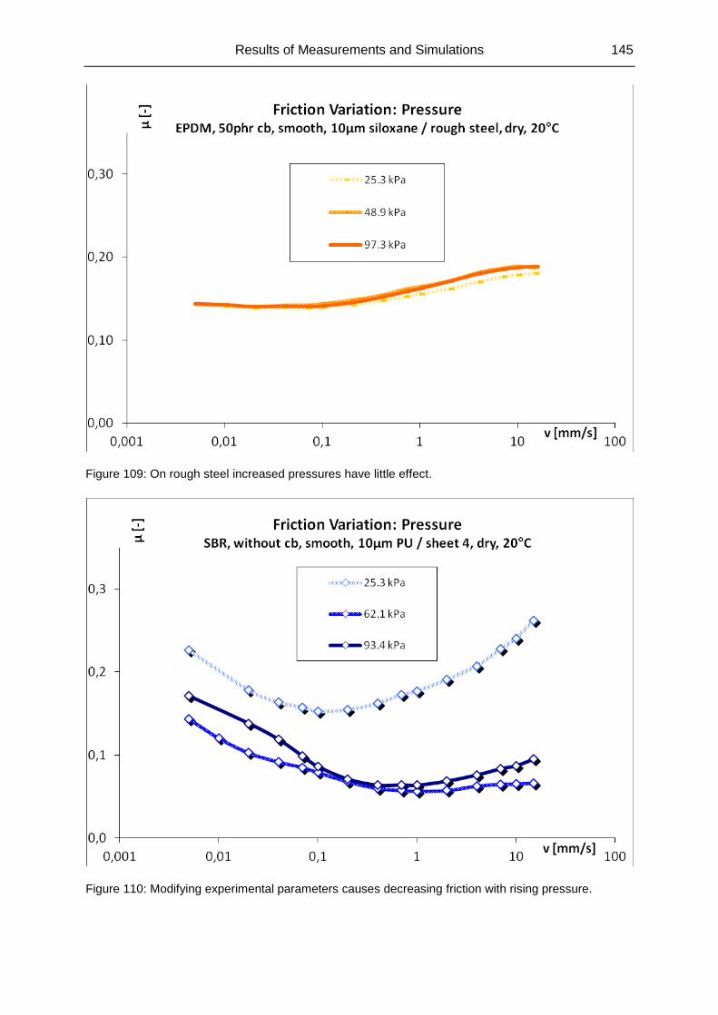
Results of Measurements and Simulations 145
Figure 109: On rough steel increased pressures have little effect.
Figure 110: Modifying experimental parameters causes decreasing friction with rising pressure.
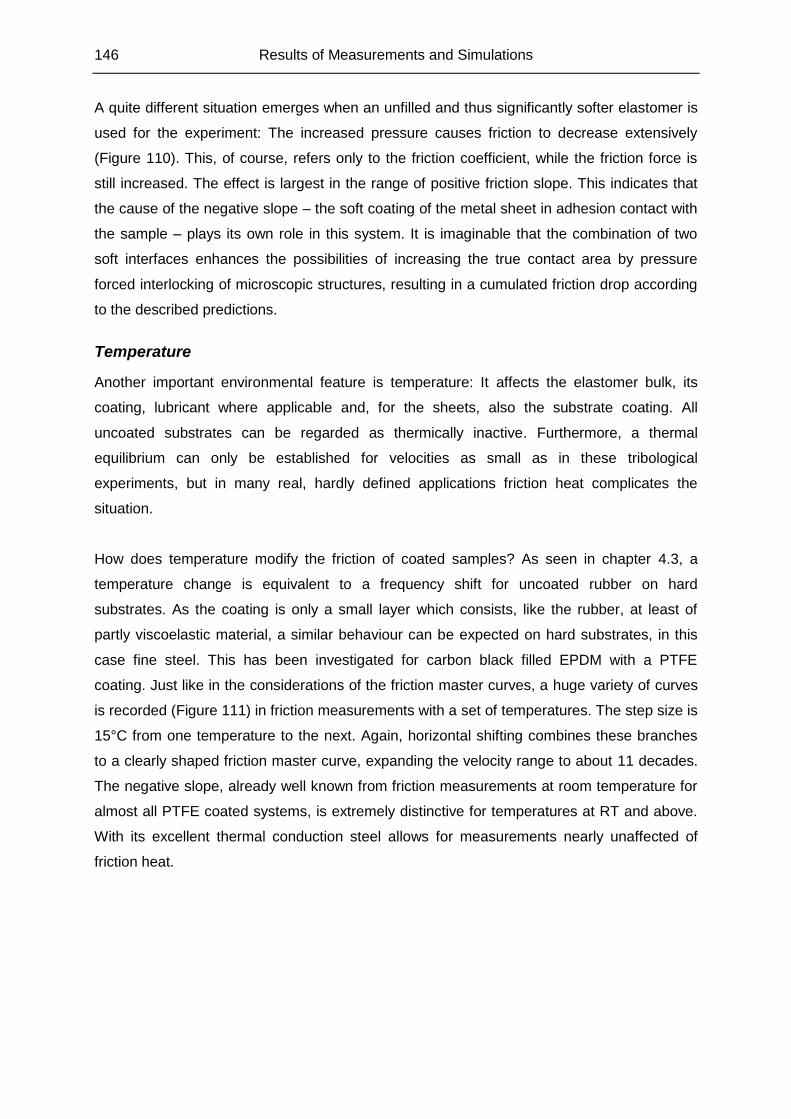
146 Results of Measurements and Simulations
A quite different situation emerges when an unfilled and thus significantly softer elastomer is
used for the experiment: The increased pressure causes friction to decrease extensively
(Figure 110). This, of course, refers only to the friction coefficient, while the friction force is
still increased. The effect is largest in the range of positive friction slope. This indicates that
the cause of the negative slope – the soft coating of the metal sheet in adhesion contact with
the sample – plays its own role in this system. It is imaginable that the combination of two
soft interfaces enhances the possibilities of increasing the true contact area by pressure
forced interlocking of microscopic structures, resulting in a cumulated friction drop according
to the described predictions.
Temperature
Another important environmental feature is temperature: It affects the elastomer bulk, its
coating, lubricant where applicable and, for the sheets, also the substrate coating. All
uncoated substrates can be regarded as thermically inactive. Furthermore, a thermal
equilibrium can only be established for velocities as small as in these tribological
experiments, but in many real, hardly defined applications friction heat complicates the
situation.
How does temperature modify the friction of coated samples? As seen in chapter 4.3, a
temperature change is equivalent to a frequency shift for uncoated rubber on hard
substrates. As the coating is only a small layer which consists, like the rubber, at least of
partly viscoelastic material, a similar behaviour can be expected on hard substrates, in this
case fine steel. This has been investigated for carbon black filled EPDM with a PTFE
coating. Just like in the considerations of the friction master curves, a huge variety of curves
is recorded (Figure 111) in friction measurements with a set of temperatures. The step size is
15°C from one temperature to the next. Again, horizontal shifting combines these branches
to a clearly shaped friction master curve, expanding the velocity range to about 11 decades.
The negative slope, already well known from friction measurements at room temperature for
almost all PTFE coated systems, is extremely distinctive for temperatures at RT and above.
With its excellent thermal conduction steel allows for measurements nearly unaffected of
friction heat.
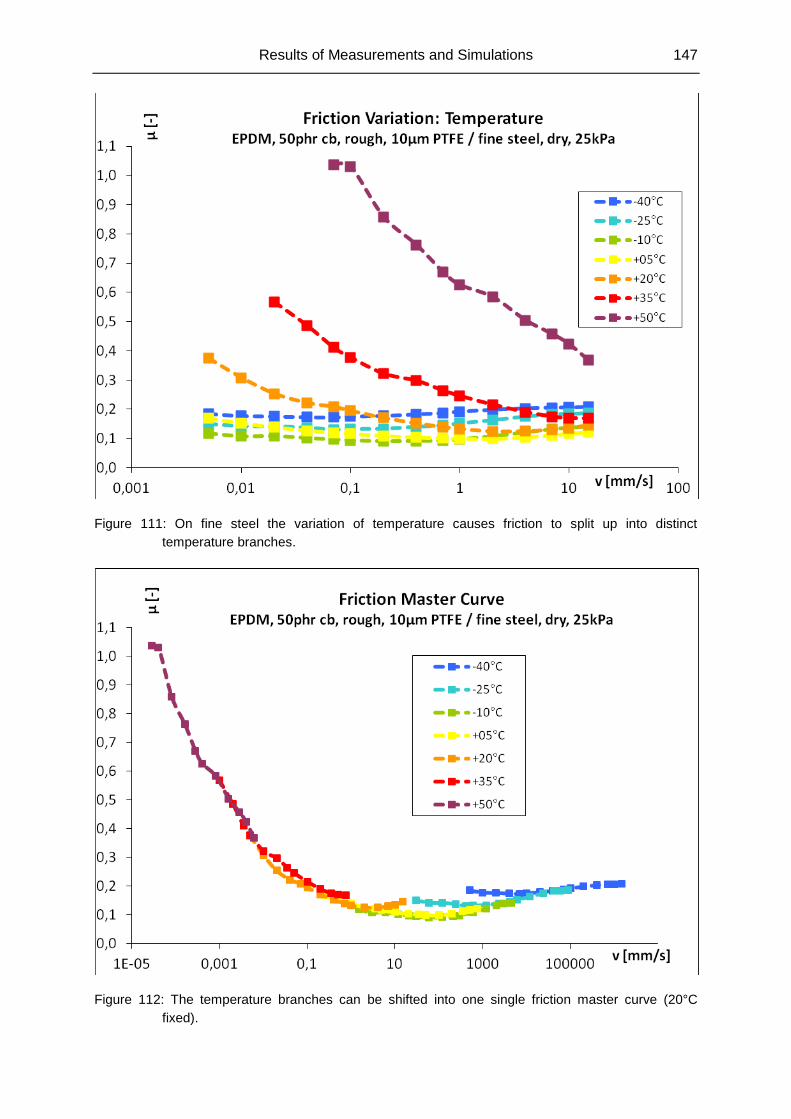
Results of Measurements and Simulations 147
Figure 111: On fine steel the variation of temperature causes friction to split up into distinct
temperature branches.
Figure 112: The temperature branches can be shifted into one single friction master curve (20°C
fixed).
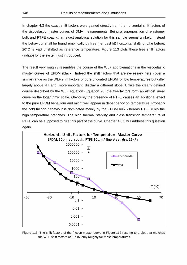
148 Results of Measurements and Simulations
In chapter 4.3 the exact shift factors were gained directly from the horizontal shift factors of
the viscoelastic master curves of DMA measurements. Being a superposition of elastomer
bulk and PTFE coating, an exact analytical solution for this sample seems unlikely. Instead
the behaviour shall be found empirically by free (i.e. best fit) horizontal shifting. Like before,
20°C is kept unshifted as reference temperature. Figure 113 plots these free shift factors
(indigo) for the system just introduced.
The result very roughly resembles the course of the WLF approximations in the viscoelastic
master curves of EPDM (black). Indeed the shift factors that are necessary here cover a
similar range as the WLF shift factors of pure uncoated EPDM for low temperatures but differ
largely above RT and, more important, display a different slope: Unlike the clearly defined
course described by the WLF equation (Equation 28) the free factors form an almost linear
curve on the logarithmic scale. Obviously the presence of PTFE causes an additional effect
to the pure EPDM behaviour and might well appear in dependency on temperature: Probably
the cold friction behaviour is dominated mainly by the EPDM bulk whereas PTFE rules the
high temperature branches. The high thermal stability and glass transition temperature of
PTFE can be supposed to rule this part of the curve. Chapter 4.6.3 will address this question
again.
Figure 113: The shift factors of the friction master curve in Figure 112 resume to a plot that matches
the WLF shift factors of EPDM only roughly for most temperatures.
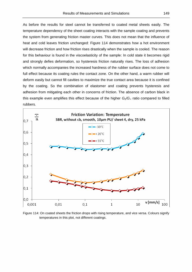
Results of Measurements and Simulations 149
As before the results for steel cannot be transferred to coated metal sheets easily. The
temperature dependency of the sheet coating interacts with the sample coating and prevents
the system from generating friction master curves. This does not mean that the influence of
heat and cold leaves friction unchanged: Figure 114 demonstrates how a hot environment
will decrease friction and how friction rises drastically when the sample is cooled. The reason
for this behaviour is found in the viscoelasticity of the sample: In cold state it becomes rigid
and strongly defies deformation, so hysteresis friction naturally rises. The loss of adhesion
which normally accompanies the increased hardness of the rubber surface does not come to
full effect because its coating rules the contact zone. On the other hand, a warm rubber will
deform easily but cannot fill cavities to maximize the true contact area because it is confined
by the coating. So the combination of elastomer and coating prevents hysteresis and
adhesion from mitigating each other in concerns of friction. The absence of carbon black in
this example even amplifies this effect because of the higher G0/G∞ ratio compared to filled
rubbers.
Figure 114: On coated sheets the friction drops with rising temperature, and vice versa. Colours signify
temperatures in this plot, not different coatings.
150 Results of Measurements and Simulations
4.5.5 Simulation of the Friction on Smooth Substrates
The friction modelling described in chapter 2.8 has proven successful in simulating friction
effects and normally works well in correspondence with real world measurements. The
validation of the friction master curves in chapter 4.3 is only one of many examples where it
has been applied.
The situation is different for the coated samples. The theory is based on a rigid, fractal
substrate in contact with a homogenous, elastic sample with known viscoelastic data. The
coated samples in chapter 4.5.3 defy this approach in several ways:
Two elastic materials, the rubber and the coating, combine as a composite sample
The viscoelastic properties of a 10 µm thin layer are hardly measureable
If the coating should not perfectly adhere to the rubber, internal shifts or even ablation
may occur
Even with perfect rubber-coating connection, the coating may act as its own liquid,
like the self-lubricating ability of the siloxane
The coating on the sheets is definitely not rigid and adds one more viscoelastic
element to the system
Glass and the two sheets are even flatter than the sample surface, so asperities on
the pure sample or sample coating cannot fill microscopic substrate cavities but rather
act as mesoscopic spacers, reducing the true contact area in a so far non-
computable way
These constraints do not only limit a simulation of the investigated systems, they also affect
the laboratory measurements: Without sample coating the extremely high dry friction can be
diminished excellently by using a lubricant, as it is stated in friction theory. For coated
samples, however, the wet sliding does not further decrease the already low friction of the
dry contact. Due to the changed conditions in surface tension – most obvious for PTFE – the
friction may even increase, as seen in Figure 115.
This abnormal behaviour is a significant evidence that a simulation in this case may produce
unexpected results. Nevertheless this computational approach shall be put to the test for this
special case with the best combinations of fit parameters. To minimize the obstacles,
simulations will focus first on fine steel as substrate.
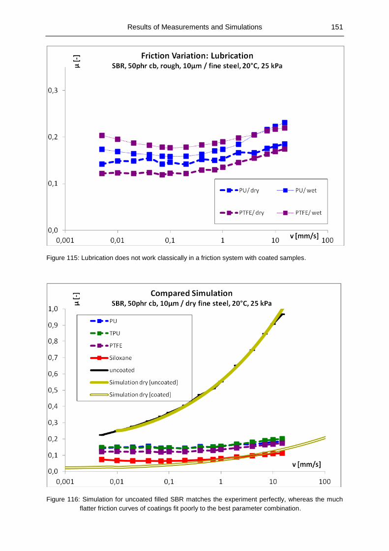
Results of Measurements and Simulations 151
Figure 115: Lubrication does not work classically in a friction system with coated samples.
Figure 116: Simulation for uncoated filled SBR matches the experiment perfectly, whereas the much
flatter friction curves of coatings fit poorly to the best parameter combination.
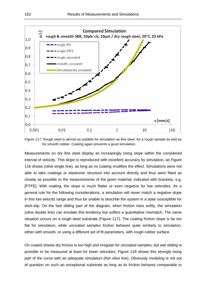
152 Results of Measurements and Simulations
Figure 117: Rough steel is almost as suitable for simulation as fine steel, for a rough sample as well as
for smooth rubber. Coating again prevents a good simulation.
Measurements on dry fine steel display an increasingly rising slope within the considered
interval of velocity. This slope is reproduced with excellent accuracy by simulation, as Figure
116 shows (olive single line), as long as no coating modifies the effect. Simulations were not
able to take coatings or elastomer structure into account directly and thus were fitted as
closely as possible to the measurements of the given material, indicated with brackets, e.g.
[PTFE]. With coating, the slope is much flatter or even negative for low velocities. As a
general rule for the following considerations, a simulation will never match a negative slope
in this low velocity range and thus be unable to describe the system in a state susceptible for
stick-slip. On the fast sliding part of the diagram, when friction rises softly, the simulation
(olive double line) can emulate this tendency but suffers a quantitative mismatch. The same
situation occurs on a rough steel substrate (Figure 117): The coating friction slope is far too
flat for simulation, while uncoated samples friction behaves quite similarly to simulation,
either with smooth, or using a different set of fit parameters, with rough rubber surface.
On coated sheets dry friction is too high and irregular for uncoated samples, but wet sliding is
possible to be measured at least for lower velocities. Figure 118 shows this strongly rising
part of the curve with an adequate simulation (thin olive line). Obviously modeling is not out
of question on such an exceptional substrate as long as its friction behaves comparable to
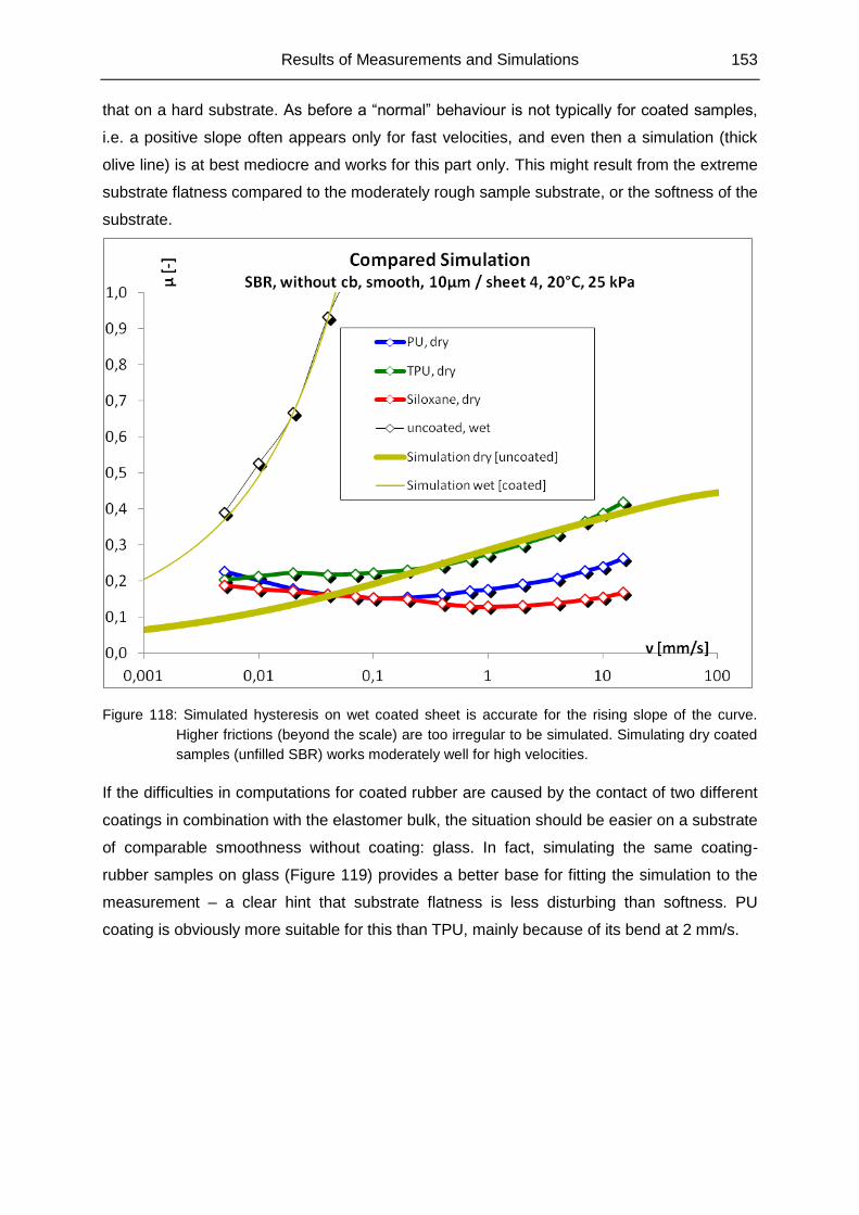
Results of Measurements and Simulations 153
that on a hard substrate. As before a “normal” behaviour is not typically for coated samples,
i.e. a positive slope often appears only for fast velocities, and even then a simulation (thick
olive line) is at best mediocre and works for this part only. This might result from the extreme
substrate flatness compared to the moderately rough sample substrate, or the softness of the
substrate.
Figure 118: Simulated hysteresis on wet coated sheet is accurate for the rising slope of the curve.
Higher frictions (beyond the scale) are too irregular to be simulated. Simulating dry coated
samples (unfilled SBR) works moderately well for high velocities.
If the difficulties in computations for coated rubber are caused by the contact of two different
coatings in combination with the elastomer bulk, the situation should be easier on a substrate
of comparable smoothness without coating: glass. In fact, simulating the same coating-
rubber samples on glass (Figure 119) provides a better base for fitting the simulation to the
measurement – a clear hint that substrate flatness is less disturbing than softness. PU
coating is obviously more suitable for this than TPU, mainly because of its bend at 2 mm/s.
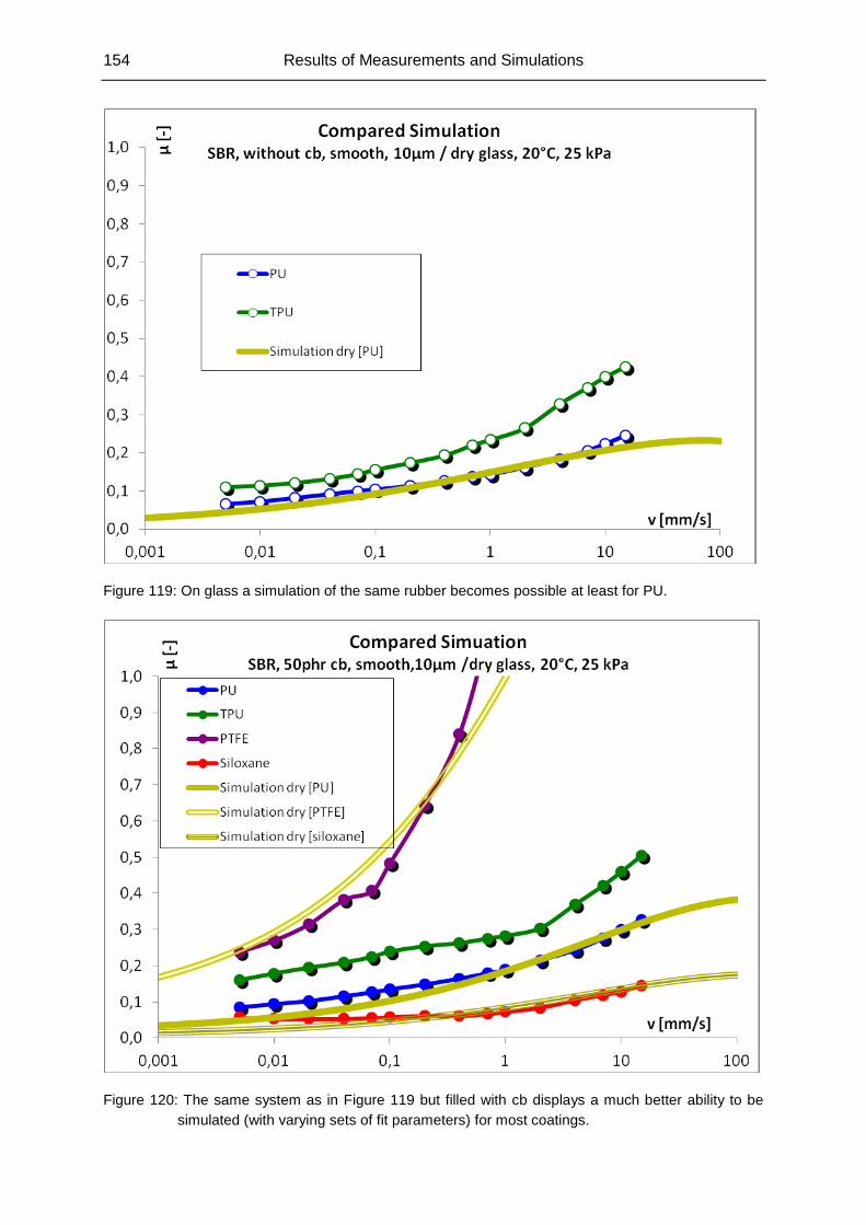
154 Results of Measurements and Simulations
Figure 119: On glass a simulation of the same rubber becomes possible at least for PU.
Figure 120: The same system as in Figure 119 but filled with cb displays a much better ability to be
simulated (with varying sets of fit parameters) for most coatings.
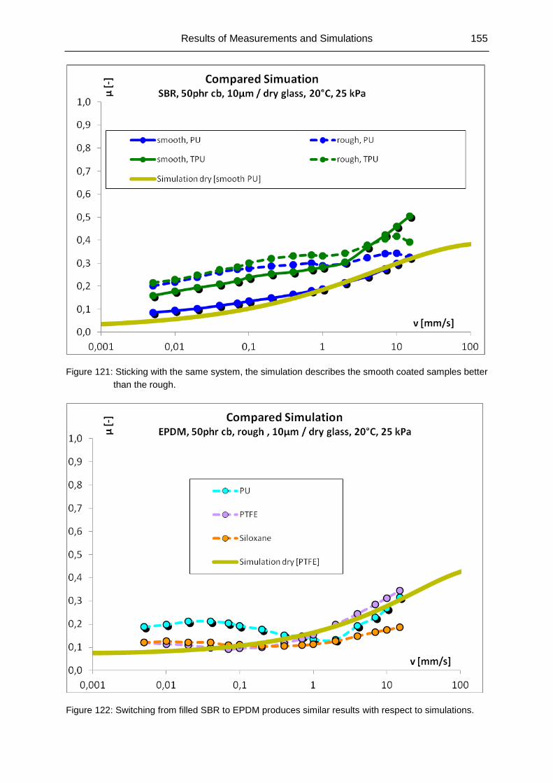
Results of Measurements and Simulations 155
Figure 121: Sticking with the same system, the simulation describes the smooth coated samples better
than the rough.
Figure 122: Switching from filled SBR to EPDM produces similar results with respect to simulations.
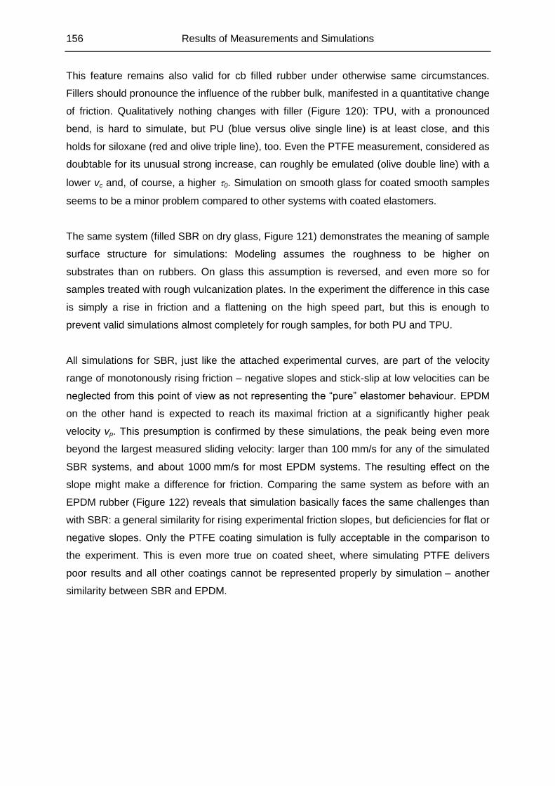
156 Results of Measurements and Simulations
This feature remains also valid for cb filled rubber under otherwise same circumstances.
Fillers should pronounce the influence of the rubber bulk, manifested in a quantitative change
of friction. Qualitatively nothing changes with filler (Figure 120): TPU, with a pronounced
bend, is hard to simulate, but PU (blue versus olive single line) is at least close, and this
holds for siloxane (red and olive triple line), too. Even the PTFE measurement, considered as
doubtable for its unusual strong increase, can roughly be emulated (olive double line) with a
lower vc and, of course, a higher 0. Simulation on smooth glass for coated smooth samples
seems to be a minor problem compared to other systems with coated elastomers.
The same system (filled SBR on dry glass, Figure 121) demonstrates the meaning of sample
surface structure for simulations: Modeling assumes the roughness to be higher on
substrates than on rubbers. On glass this assumption is reversed, and even more so for
samples treated with rough vulcanization plates. In the experiment the difference in this case
is simply a rise in friction and a flattening on the high speed part, but this is enough to
prevent valid simulations almost completely for rough samples, for both PU and TPU.
All simulations for SBR, just like the attached experimental curves, are part of the velocity
range of monotonously rising friction – negative slopes and stick-slip at low velocities can be
neglected from this point of view as not representing the “pure” elastomer behaviour. EPDM
on the other hand is expected to reach its maximal friction at a significantly higher peak
velocity vp. This presumption is confirmed by these simulations, the peak being even more
beyond the largest measured sliding velocity: larger than 100 mm/s for any of the simulated
SBR systems, and about 1000 mm/s for most EPDM systems. The resulting effect on the
slope might make a difference for friction. Comparing the same system as before with an
EPDM rubber (Figure 122) reveals that simulation basically faces the same challenges than
with SBR: a general similarity for rising experimental friction slopes, but deficiencies for flat or
negative slopes. Only the PTFE coating simulation is fully acceptable in the comparison to
the experiment. This is even more true on coated sheet, where simulating PTFE delivers
poor results and all other coatings cannot be represented properly by simulation – another
similarity between SBR and EPDM.
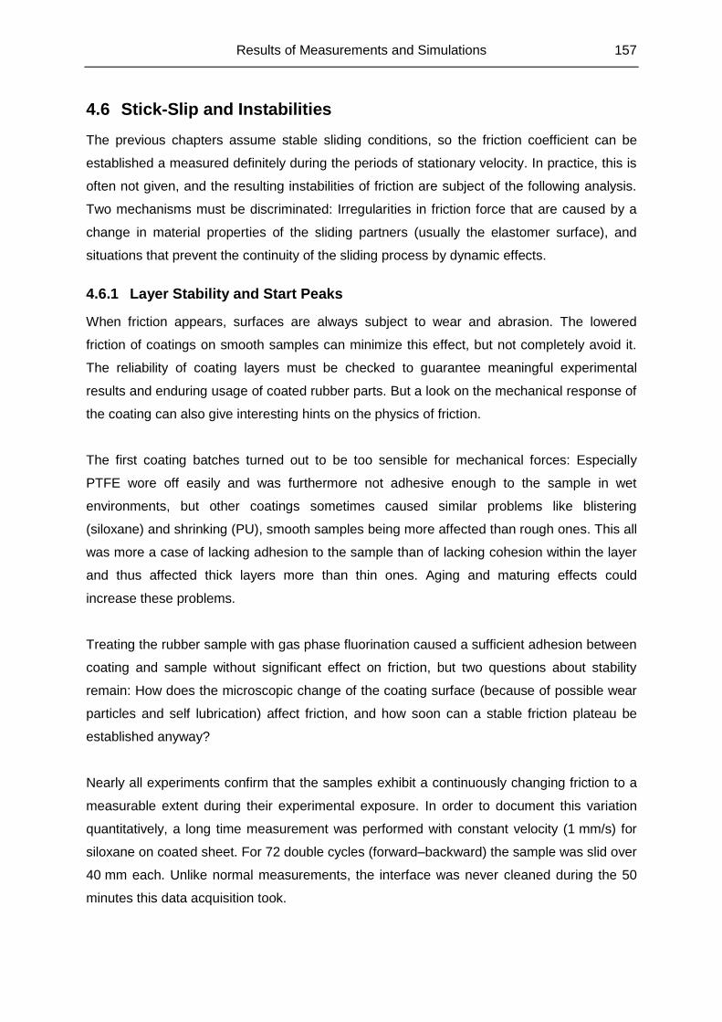
Results of Measurements and Simulations 157
4.6 Stick-Slip and Instabilities
The previous chapters assume stable sliding conditions, so the friction coefficient can be
established a measured definitely during the periods of stationary velocity. In practice, this is
often not given, and the resulting instabilities of friction are subject of the following analysis.
Two mechanisms must be discriminated: Irregularities in friction force that are caused by a
change in material properties of the sliding partners (usually the elastomer surface), and
situations that prevent the continuity of the sliding process by dynamic effects.
4.6.1 Layer Stability and Start Peaks
When friction appears, surfaces are always subject to wear and abrasion. The lowered
friction of coatings on smooth samples can minimize this effect, but not completely avoid it.
The reliability of coating layers must be checked to guarantee meaningful experimental
results and enduring usage of coated rubber parts. But a look on the mechanical response of
the coating can also give interesting hints on the physics of friction.
The first coating batches turned out to be too sensible for mechanical forces: Especially
PTFE wore off easily and was furthermore not adhesive enough to the sample in wet
environments, but other coatings sometimes caused similar problems like blistering
(siloxane) and shrinking (PU), smooth samples being more affected than rough ones. This all
was more a case of lacking adhesion to the sample than of lacking cohesion within the layer
and thus affected thick layers more than thin ones. Aging and maturing effects could
increase these problems.
Treating the rubber sample with gas phase fluorination caused a sufficient adhesion between
coating and sample without significant effect on friction, but two questions about stability
remain: How does the microscopic change of the coating surface (because of possible wear
particles and self lubrication) affect friction, and how soon can a stable friction plateau be
established anyway?
Nearly all experiments confirm that the samples exhibit a continuously changing friction to a
measurable extent during their experimental exposure. In order to document this variation
quantitatively, a long time measurement was performed with constant velocity (1 mm/s) for
siloxane on coated sheet. For 72 double cycles (forward–backward) the sample was slid over
40 mm each. Unlike normal measurements, the interface was never cleaned during the 50
minutes this data acquisition took.
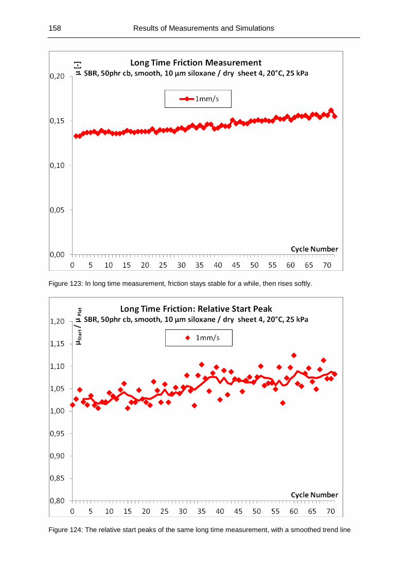
158 Results of Measurements and Simulations
Figure 123: In long time measurement, friction stays stable for a while, then rises softly.
Figure 124: The relative start peaks of the same long time measurement, with a smoothed trend line
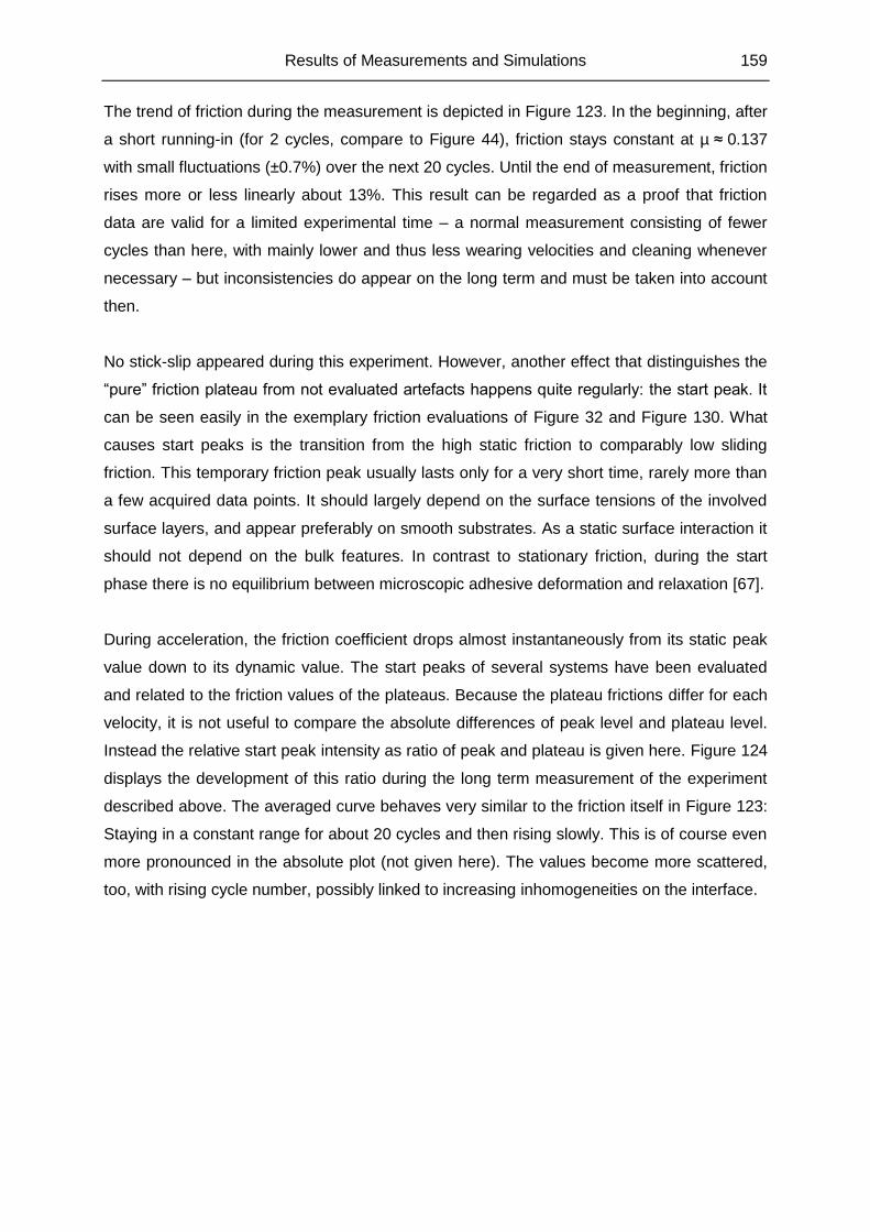
Results of Measurements and Simulations 159
The trend of friction during the measurement is depicted in Figure 123. In the beginning, after
a short running-in (for 2 cycles, compare to Figure 44), friction stays constant at µ ≈ 0.137
with small fluctuations (±0.7%) over the next 20 cycles. Until the end of measurement, friction
rises more or less linearly about 13%. This result can be regarded as a proof that friction
data are valid for a limited experimental time – a normal measurement consisting of fewer
cycles than here, with mainly lower and thus less wearing velocities and cleaning whenever
necessary – but inconsistencies do appear on the long term and must be taken into account
then.
No stick-slip appeared during this experiment. However, another effect that distinguishes the
“pure” friction plateau from not evaluated artefacts happens quite regularly: the start peak. It
can be seen easily in the exemplary friction evaluations of Figure 32 and Figure 130. What
causes start peaks is the transition from the high static friction to comparably low sliding
friction. This temporary friction peak usually lasts only for a very short time, rarely more than
a few acquired data points. It should largely depend on the surface tensions of the involved
surface layers, and appear preferably on smooth substrates. As a static surface interaction it
should not depend on the bulk features. In contrast to stationary friction, during the start
phase there is no equilibrium between microscopic adhesive deformation and relaxation [67].
During acceleration, the friction coefficient drops almost instantaneously from its static peak
value down to its dynamic value. The start peaks of several systems have been evaluated
and related to the friction values of the plateaus. Because the plateau frictions differ for each
velocity, it is not useful to compare the absolute differences of peak level and plateau level.
Instead the relative start peak intensity as ratio of peak and plateau is given here. Figure 124
displays the development of this ratio during the long term measurement of the experiment
described above. The averaged curve behaves very similar to the friction itself in Figure 123:
Staying in a constant range for about 20 cycles and then rising slowly. This is of course even
more pronounced in the absolute plot (not given here). The values become more scattered,
too, with rising cycle number, possibly linked to increasing inhomogeneities on the interface.
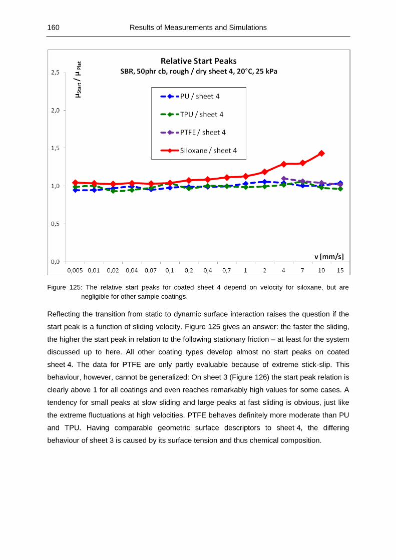
160 Results of Measurements and Simulations
Figure 125: The relative start peaks for coated sheet 4 depend on velocity for siloxane, but are
negligible for other sample coatings.
Reflecting the transition from static to dynamic surface interaction raises the question if the
start peak is a function of sliding velocity. Figure 125 gives an answer: the faster the sliding,
the higher the start peak in relation to the following stationary friction – at least for the system
discussed up to here. All other coating types develop almost no start peaks on coated
sheet 4. The data for PTFE are only partly evaluable because of extreme stick-slip. This
behaviour, however, cannot be generalized: On sheet 3 (Figure 126) the start peak relation is
clearly above 1 for all coatings and even reaches remarkably high values for some cases. A
tendency for small peaks at slow sliding and large peaks at fast sliding is obvious, just like
the extreme fluctuations at high velocities. PTFE behaves definitely more moderate than PU
and TPU. Having comparable geometric surface descriptors to sheet 4, the differing
behaviour of sheet 3 is caused by its surface tension and thus chemical composition.
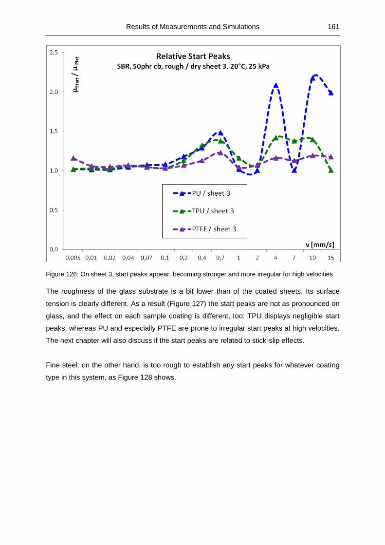
Results of Measurements and Simulations 161
Figure 126: On sheet 3, start peaks appear, becoming stronger and more irregular for high velocities.
The roughness of the glass substrate is a bit lower than of the coated sheets. Its surface
tension is clearly different. As a result (Figure 127) the start peaks are not as pronounced on
glass, and the effect on each sample coating is different, too: TPU displays negligible start
peaks, whereas PU and especially PTFE are prone to irregular start peaks at high velocities.
The next chapter will also discuss if the start peaks are related to stick-slip effects.
Fine steel, on the other hand, is too rough to establish any start peaks for whatever coating
type in this system, as Figure 128 shows.
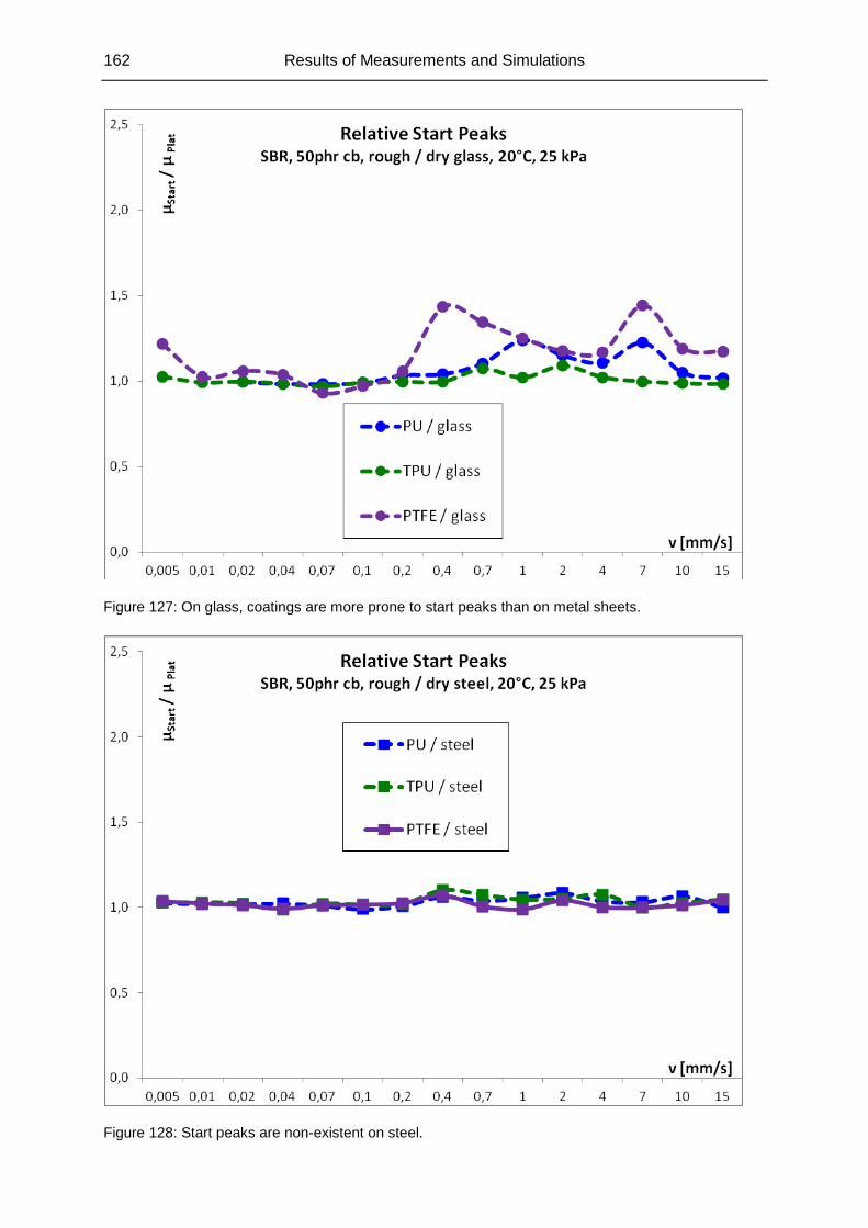
162 Results of Measurements and Simulations
Figure 127: On glass, coatings are more prone to start peaks than on metal sheets.
Figure 128: Start peaks are non-existent on steel.
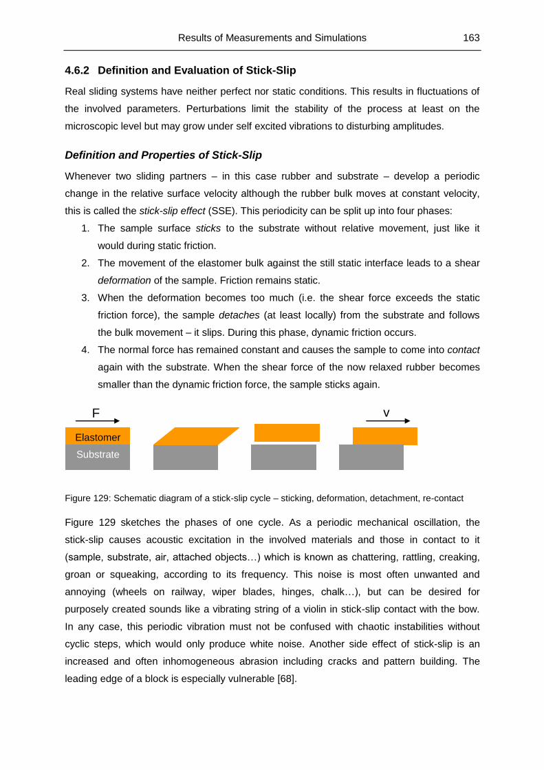
Results of Measurements and Simulations 163
4.6.2 Definition and Evaluation of Stick-Slip
Real sliding systems have neither perfect nor static conditions. This results in fluctuations of
the involved parameters. Perturbations limit the stability of the process at least on the
microscopic level but may grow under self excited vibrations to disturbing amplitudes.
Definition and Properties of Stick-Slip
Whenever two sliding partners – in this case rubber and substrate – develop a periodic
change in the relative surface velocity although the rubber bulk moves at constant velocity,
this is called the stick-slip effect (SSE). This periodicity can be split up into four phases:
1. The sample surface sticks to the substrate without relative movement, just like it
would during static friction.
2. The movement of the elastomer bulk against the still static interface leads to a shear
deformation of the sample. Friction remains static.
3. When the deformation becomes too much (i.e. the shear force exceeds the static
friction force), the sample detaches (at least locally) from the substrate and follows
the bulk movement – it slips. During this phase, dynamic friction occurs.
4. The normal force has remained constant and causes the sample to come into contact
again with the substrate. When the shear force of the now relaxed rubber becomes
smaller than the dynamic friction force, the sample sticks again.
Figure 129: Schematic diagram of a stick-slip cycle – sticking, deformation, detachment, re-contact
Figure 129 sketches the phases of one cycle. As a periodic mechanical oscillation, the
stick-slip causes acoustic excitation in the involved materials and those in contact to it
(sample, substrate, air, attached objects…) which is known as chattering, rattling, creaking,
groan or squeaking, according to its frequency. This noise is most often unwanted and
annoying (wheels on railway, wiper blades, hinges, chalk…), but can be desired for
purposely created sounds like a vibrating string of a violin in stick-slip contact with the bow.
In any case, this periodic vibration must not be confused with chaotic instabilities without
cyclic steps, which would only produce white noise. Another side effect of stick-slip is an
increased and often inhomogeneous abrasion including cracks and pattern building. The
leading edge of a block is especially vulnerable [68].
Elastomer
Substrate
F
v
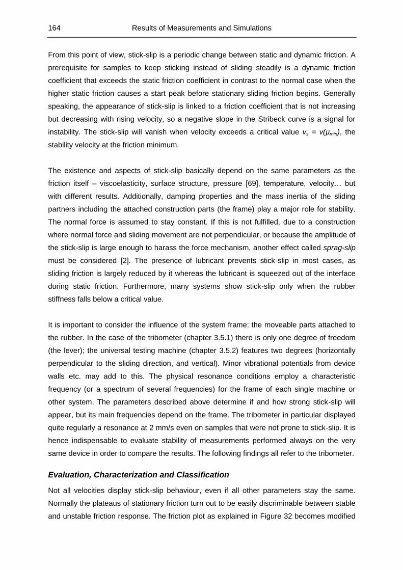
164 Results of Measurements and Simulations
From this point of view, stick-slip is a periodic change between static and dynamic friction. A
prerequisite for samples to keep sticking instead of sliding steadily is a dynamic friction
coefficient that exceeds the static friction coefficient in contrast to the normal case when the
higher static friction causes a start peak before stationary sliding friction begins. Generally
speaking, the appearance of stick-slip is linked to a friction coefficient that is not increasing
but decreasing with rising velocity, so a negative slope in the Stribeck curve is a signal for
instability. The stick-slip will vanish when velocity exceeds a critical value vs = v(µmin), the
stability velocity at the friction minimum.
The existence and aspects of stick-slip basically depend on the same parameters as the
friction itself – viscoelasticity, surface structure, pressure [69], temperature, velocity… but
with different results. Additionally, damping properties and the mass inertia of the sliding
partners including the attached construction parts (the frame) play a major role for stability.
The normal force is assumed to stay constant. If this is not fulfilled, due to a construction
where normal force and sliding movement are not perpendicular, or because the amplitude of
the stick-slip is large enough to harass the force mechanism, another effect called sprag-slip
must be considered [2]. The presence of lubricant prevents stick-slip in most cases, as
sliding friction is largely reduced by it whereas the lubricant is squeezed out of the interface
during static friction. Furthermore, many systems show stick-slip only when the rubber
stiffness falls below a critical value.
It is important to consider the influence of the system frame: the moveable parts attached to
the rubber. In the case of the tribometer (chapter 3.5.1) there is only one degree of freedom
(the lever); the universal testing machine (chapter 3.5.2) features two degrees (horizontally
perpendicular to the sliding direction, and vertical). Minor vibrational potentials from device
walls etc. may add to this. The physical resonance conditions employ a characteristic
frequency (or a spectrum of several frequencies) for the frame of each single machine or
other system. The parameters described above determine if and how strong stick-slip will
appear, but its main frequencies depend on the frame. The tribometer in particular displayed
quite regularly a resonance at 2 mm/s even on samples that were not prone to stick-slip. It is
hence indispensable to evaluate stability of measurements performed always on the very
same device in order to compare the results. The following findings all refer to the tribometer.
Evaluation, Characterization and Classification
Not all velocities display stick-slip behaviour, even if all other parameters stay the same.
Normally the plateaus of stationary friction turn out to be easily discriminable between stable
and unstable friction response. The friction plot as explained in Figure 32 becomes modified
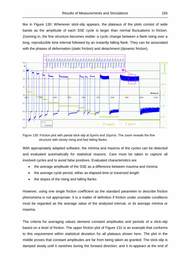
Results of Measurements and Simulations 165
like in Figure 130: Whenever stick-slip appears, the plateaus of the plots consist of wide
bands as the amplitude of each SSE cycle is larger than normal fluctuations in friction.
Zooming in, the fine structure becomes visible: a cyclic change between a flank rising over a
long, reproducible time interval followed by an instantly falling flank. They can be associated
with the phases of deformation (static friction) and detachment (dynamic friction).
Figure 130: Friction plot with partial stick-slip at 5µm/s and 10µm/s. The zoom reveals the fine
structure with slowly rising and fast falling flanks.
With appropriately adapted software, the minima and maxima of the cycles can be detected
and evaluated automatically for statistical reasons. Care must be taken to capture all
involved cycles and to avoid false positives. Evaluated characteristics are
the average amplitude of the SSE as a difference between maxima and minima
the average cycle period, either as elapsed time or traversed length
the slopes of the rising and falling flanks
However, using one single friction coefficient as the standard parameter to describe friction
phenomena is not appropriate: It is a matter of definition if friction under unstable conditions
must be regarded as the average value of the analyzed interval, or its average minima or
maxima.
The criteria for averaging values demand constant amplitudes and periods of a stick-slip
based on a level of friction. The upper friction plot of Figure 131 is an example that conforms
to this requirement within statistical deviation for all plateaus shown here. The plot in the
middle proves that constant amplitudes are far from being taken as granted: The stick-slip is
damped slowly until it vanishes during the forward direction, and it re-appears at the end of
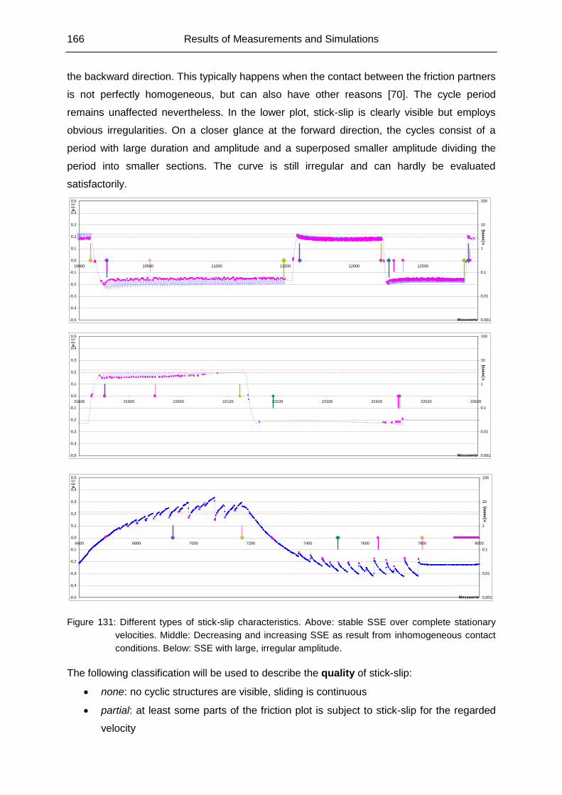
166 Results of Measurements and Simulations
the backward direction. This typically happens when the contact between the friction partners
is not perfectly homogeneous, but can also have other reasons [70]. The cycle period
remains unaffected nevertheless. In the lower plot, stick-slip is clearly visible but employs
obvious irregularities. On a closer glance at the forward direction, the cycles consist of a
period with large duration and amplitude and a superposed smaller amplitude dividing the
period into smaller sections. The curve is still irregular and can hardly be evaluated
satisfactorily.
-0,5
-0,4
-0,3
-0,2
-0,1
0,0
0,1
0,2
0,3
0,4
0,5
10000 10500 11000 11500 12000 12500
Messwerte
µ [
-]
0,001
0,01
0,1
1
10
100
v [
mm
/s]
-0,5
-0,4
-0,3
-0,2
-0,1
0,0
0,1
0,2
0,3
0,4
0,5
21820 21920 22020 22120 22220 22320 22420 22520 22620
Messwerte
µ [
-]
0,001
0,01
0,1
1
10
100
v [
mm
/s]
-0,5
-0,4
-0,3
-0,2
-0,1
0,0
0,1
0,2
0,3
0,4
0,5
6600 6800 7000 7200 7400 7600 7800 8000
Messwerte
µ [
-]
0,001
0,01
0,1
1
10
100
v [
mm
/s]
Figure 131: Different types of stick-slip characteristics. Above: stable SSE over complete stationary
velocities. Middle: Decreasing and increasing SSE as result from inhomogeneous contact
conditions. Below: SSE with large, irregular amplitude.
The following classification will be used to describe the quality of stick-slip:
none: no cyclic structures are visible, sliding is continuous
partial: at least some parts of the friction plot is subject to stick-slip for the regarded
velocity
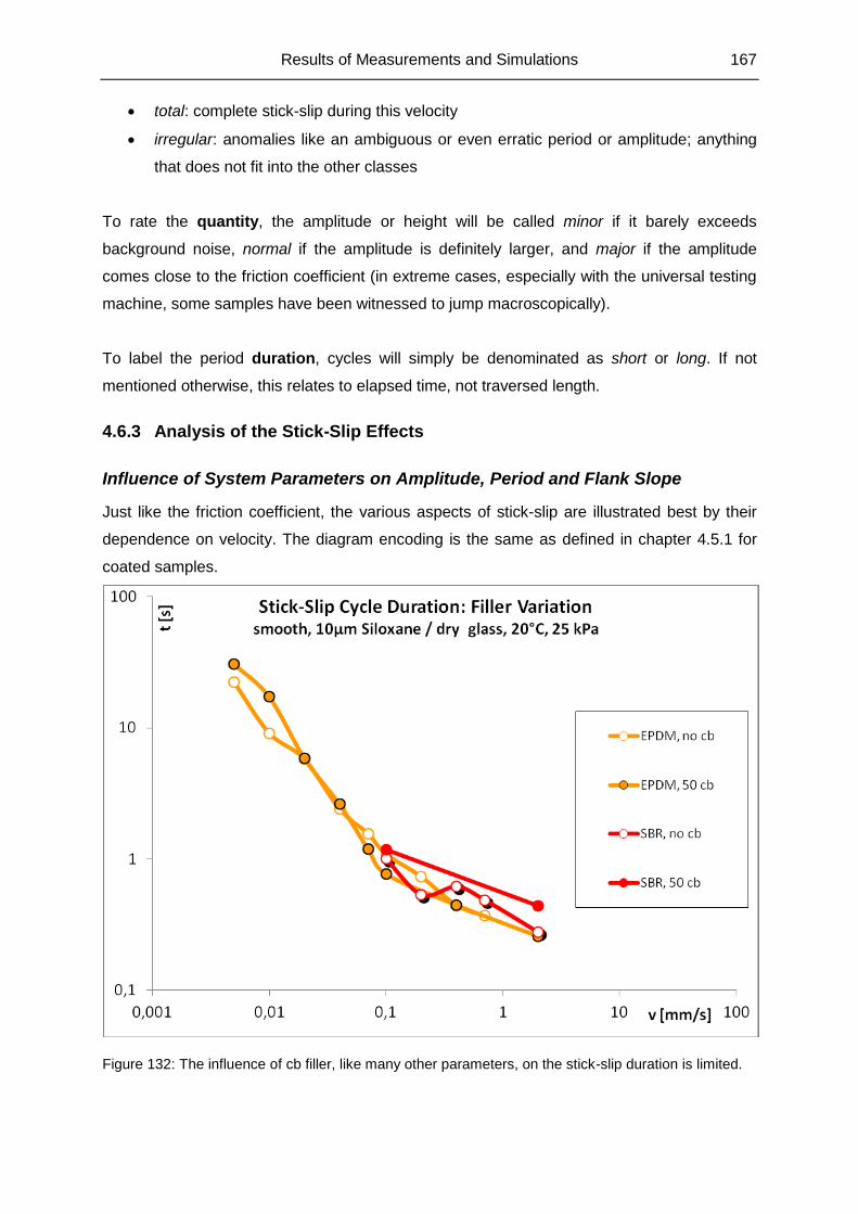
Results of Measurements and Simulations 167
total: complete stick-slip during this velocity
irregular: anomalies like an ambiguous or even erratic period or amplitude; anything
that does not fit into the other classes
To rate the quantity, the amplitude or height will be called minor if it barely exceeds
background noise, normal if the amplitude is definitely larger, and major if the amplitude
comes close to the friction coefficient (in extreme cases, especially with the universal testing
machine, some samples have been witnessed to jump macroscopically).
To label the period duration, cycles will simply be denominated as short or long. If not
mentioned otherwise, this relates to elapsed time, not traversed length.
4.6.3 Analysis of the Stick-Slip Effects
Influence of System Parameters on Amplitude, Period and Flank Slope
Just like the friction coefficient, the various aspects of stick-slip are illustrated best by their
dependence on velocity. The diagram encoding is the same as defined in chapter 4.5.1 for
coated samples.
Figure 132: The influence of cb filler, like many other parameters, on the stick-slip duration is limited.
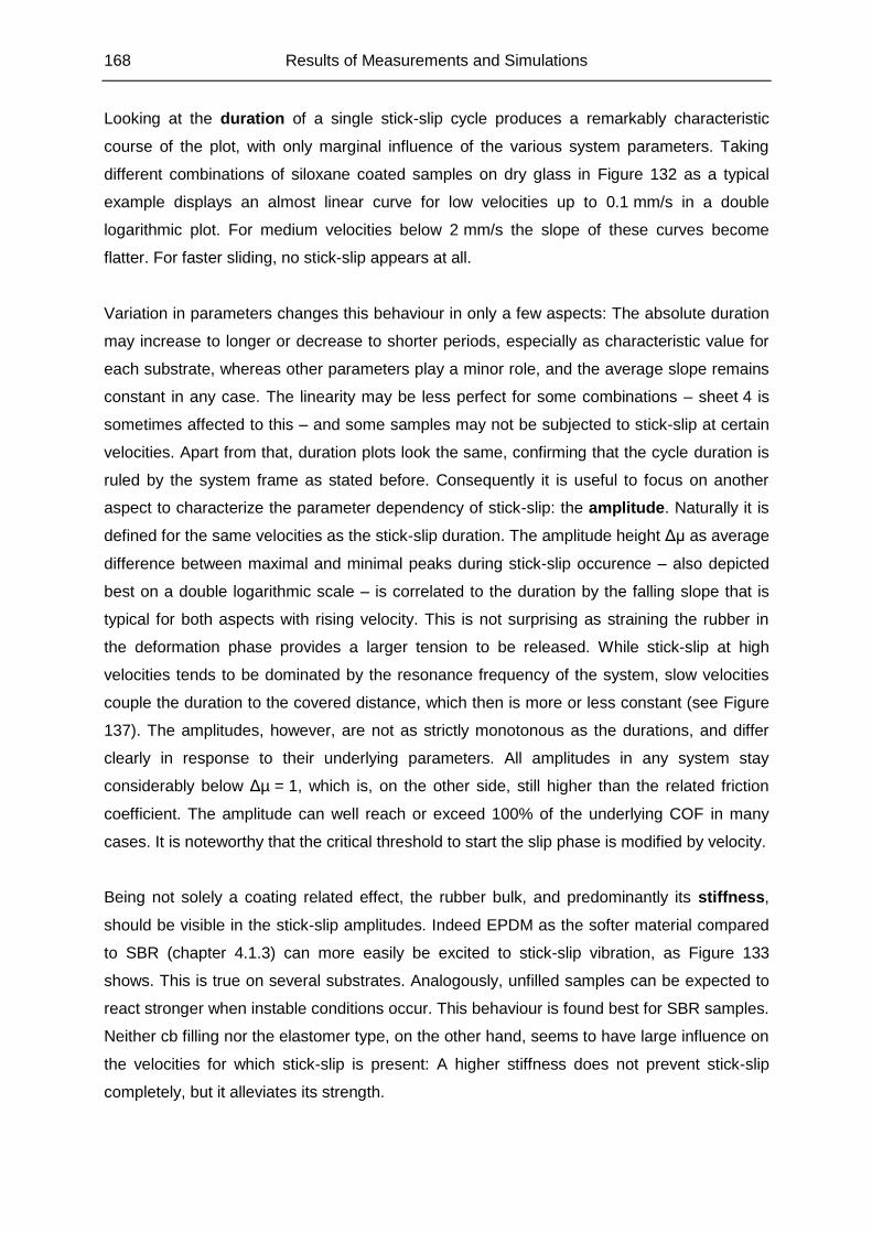
168 Results of Measurements and Simulations
Looking at the duration of a single stick-slip cycle produces a remarkably characteristic
course of the plot, with only marginal influence of the various system parameters. Taking
different combinations of siloxane coated samples on dry glass in Figure 132 as a typical
example displays an almost linear curve for low velocities up to 0.1 mm/s in a double
logarithmic plot. For medium velocities below 2 mm/s the slope of these curves become
flatter. For faster sliding, no stick-slip appears at all.
Variation in parameters changes this behaviour in only a few aspects: The absolute duration
may increase to longer or decrease to shorter periods, especially as characteristic value for
each substrate, whereas other parameters play a minor role, and the average slope remains
constant in any case. The linearity may be less perfect for some combinations – sheet 4 is
sometimes affected to this – and some samples may not be subjected to stick-slip at certain
velocities. Apart from that, duration plots look the same, confirming that the cycle duration is
ruled by the system frame as stated before. Consequently it is useful to focus on another
aspect to characterize the parameter dependency of stick-slip: the amplitude. Naturally it is
defined for the same velocities as the stick-slip duration. The amplitude height Δμ as average
difference between maximal and minimal peaks during stick-slip occurence – also depicted
best on a double logarithmic scale – is correlated to the duration by the falling slope that is
typical for both aspects with rising velocity. This is not surprising as straining the rubber in
the deformation phase provides a larger tension to be released. While stick-slip at high
velocities tends to be dominated by the resonance frequency of the system, slow velocities
couple the duration to the covered distance, which then is more or less constant (see Figure
137). The amplitudes, however, are not as strictly monotonous as the durations, and differ
clearly in response to their underlying parameters. All amplitudes in any system stay
considerably below Δµ = 1, which is, on the other side, still higher than the related friction
coefficient. The amplitude can well reach or exceed 100% of the underlying COF in many
cases. It is noteworthy that the critical threshold to start the slip phase is modified by velocity.
Being not solely a coating related effect, the rubber bulk, and predominantly its stiffness,
should be visible in the stick-slip amplitudes. Indeed EPDM as the softer material compared
to SBR (chapter 4.1.3) can more easily be excited to stick-slip vibration, as Figure 133
shows. This is true on several substrates. Analogously, unfilled samples can be expected to
react stronger when instable conditions occur. This behaviour is found best for SBR samples.
Neither cb filling nor the elastomer type, on the other hand, seems to have large influence on
the velocities for which stick-slip is present: A higher stiffness does not prevent stick-slip
completely, but it alleviates its strength.
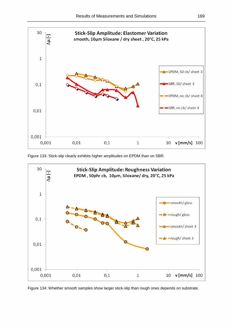
Results of Measurements and Simulations 169
Figure 133: Stick-slip clearly exhibits higher amplitudes on EPDM than on SBR.
Figure 134: Whether smooth samples show larger stick-slip than rough ones depends on substrate.
170 Results of Measurements and Simulations
Also the cycle duration is increased for soft samples (EPDM and unfilled rather than SBR
and cb filled), at least on coated sheets, because they can be deformed to a larger extend
before contact is released. On glass hardness is largely irrelevant. As will be discussed later,
glass has significantly lower values than coated sheet in both duration and amplitude –
obviously low enough to restrain the deformation in presence of this very smooth substrate
mainly to the sample coating layer without ample effect into the elastomer bulk.
Quite contrarily to the bulk influence, the roughness of the rubber coating affects the
stick-slip when the substrate is not coated sheet but glass. This holds for both sheets, and
not only for siloxane like in Figure 134 but also for PTFE, and is mirrored in amplitude and
duration, too.
Again, the presumingly short excitation depth on glass poses a good explanation: A rough
sample surface exhibits a smaller contact area (this concerns to the microscopic true contact
area as well as to the contact area in mesoscopic scale) and thus simply offers only a
confined volume to be excited.
Another difference between the surface and the bulk has to be mentioned: A rougher coating
surface does not only diminish the amplitude of the stick-slip, but can also prevent it from
emerging at all, especially at medium velocities where excitation is still possible for smooth
rubber.
Coatings have been applied in order to modify the surface contact of the samples and
minimize friction and stick-slip. The degree of success differs in respect to which goal is
highlighted: To reduce friction, PU and TPU are good, but PTFE and siloxane are better.
Stick-slip, however, appears almost exclusively for the latter two coatings – and for uncoated
samples, where it is rarely well measureable due to the extremely high and irregular friction.
Although similar in their friction levels, PTFE and siloxane can be separated in regard to their
stick-slip amplitudes (Figure 135), siloxane being higher but slightly more regular concerning
velocity. TPU, where it shows stick-slip at all, is of a comparable order. PU instabilities for
normal layer thicknesses (10 µm) are virtually impossible but occur in some cases for 40 µm
thick coatings. A thin layer thus may be advantageous to prevent stick-slip.
Apart from their viscoelastic properties, the coatings differ in their surface energies, and this
interacts with the substrate: The amplitude of siloxane is extraordinarily high on coated sheet
but drops to PTFE level on glass. When PTFE becomes physically unstable, the mechanical
effects concern not only friction but the amplitude is increased analogously.
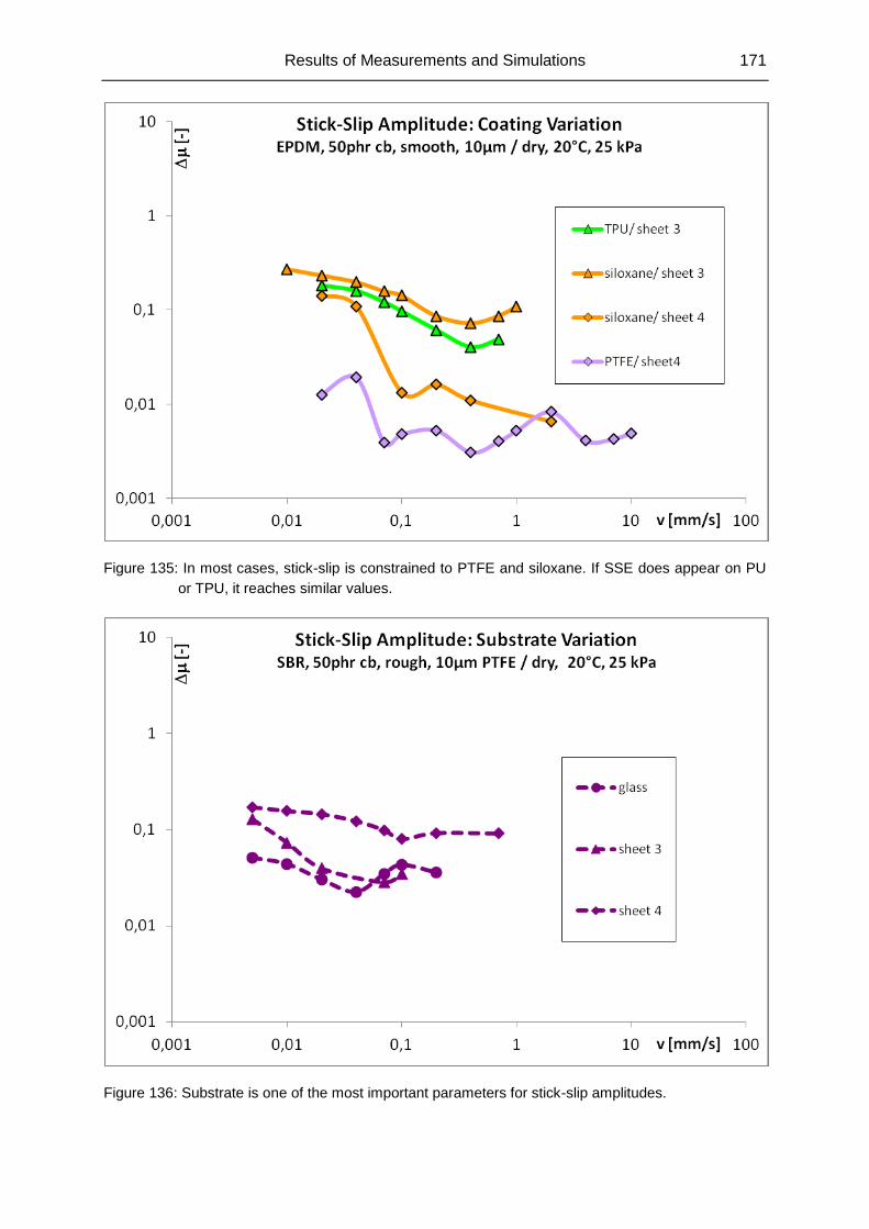
Results of Measurements and Simulations 171
Figure 135: In most cases, stick-slip is constrained to PTFE and siloxane. If SSE does appear on PU
or TPU, it reaches similar values.
Figure 136: Substrate is one of the most important parameters for stick-slip amplitudes.
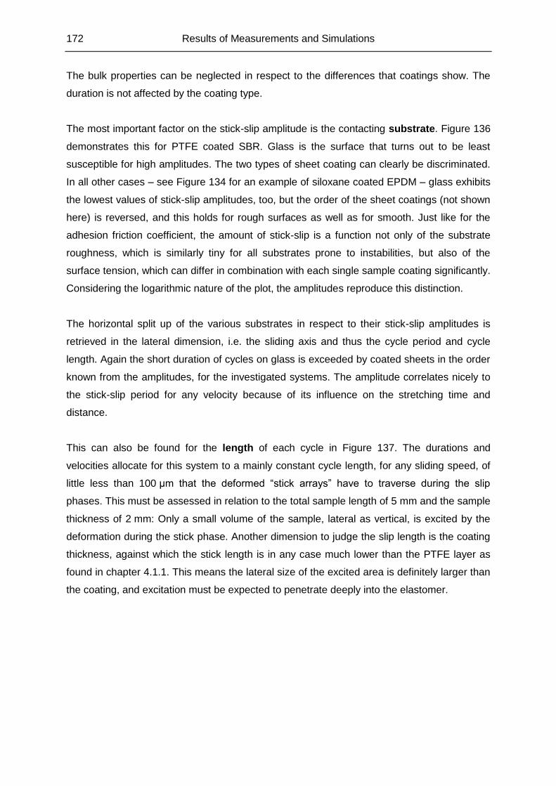
172 Results of Measurements and Simulations
The bulk properties can be neglected in respect to the differences that coatings show. The
duration is not affected by the coating type.
The most important factor on the stick-slip amplitude is the contacting substrate. Figure 136
demonstrates this for PTFE coated SBR. Glass is the surface that turns out to be least
susceptible for high amplitudes. The two types of sheet coating can clearly be discriminated.
In all other cases – see Figure 134 for an example of siloxane coated EPDM – glass exhibits
the lowest values of stick-slip amplitudes, too, but the order of the sheet coatings (not shown
here) is reversed, and this holds for rough surfaces as well as for smooth. Just like for the
adhesion friction coefficient, the amount of stick-slip is a function not only of the substrate
roughness, which is similarly tiny for all substrates prone to instabilities, but also of the
surface tension, which can differ in combination with each single sample coating significantly.
Considering the logarithmic nature of the plot, the amplitudes reproduce this distinction.
The horizontal split up of the various substrates in respect to their stick-slip amplitudes is
retrieved in the lateral dimension, i.e. the sliding axis and thus the cycle period and cycle
length. Again the short duration of cycles on glass is exceeded by coated sheets in the order
known from the amplitudes, for the investigated systems. The amplitude correlates nicely to
the stick-slip period for any velocity because of its influence on the stretching time and
distance.
This can also be found for the length of each cycle in Figure 137. The durations and
velocities allocate for this system to a mainly constant cycle length, for any sliding speed, of
little less than 100 µm that the deformed “stick arrays” have to traverse during the slip
phases. This must be assessed in relation to the total sample length of 5 mm and the sample
thickness of 2 mm: Only a small volume of the sample, lateral as vertical, is excited by the
deformation during the stick phase. Another dimension to judge the slip length is the coating
thickness, against which the stick length is in any case much lower than the PTFE layer as
found in chapter 4.1.1. This means the lateral size of the excited area is definitely larger than
the coating, and excitation must be expected to penetrate deeply into the elastomer.
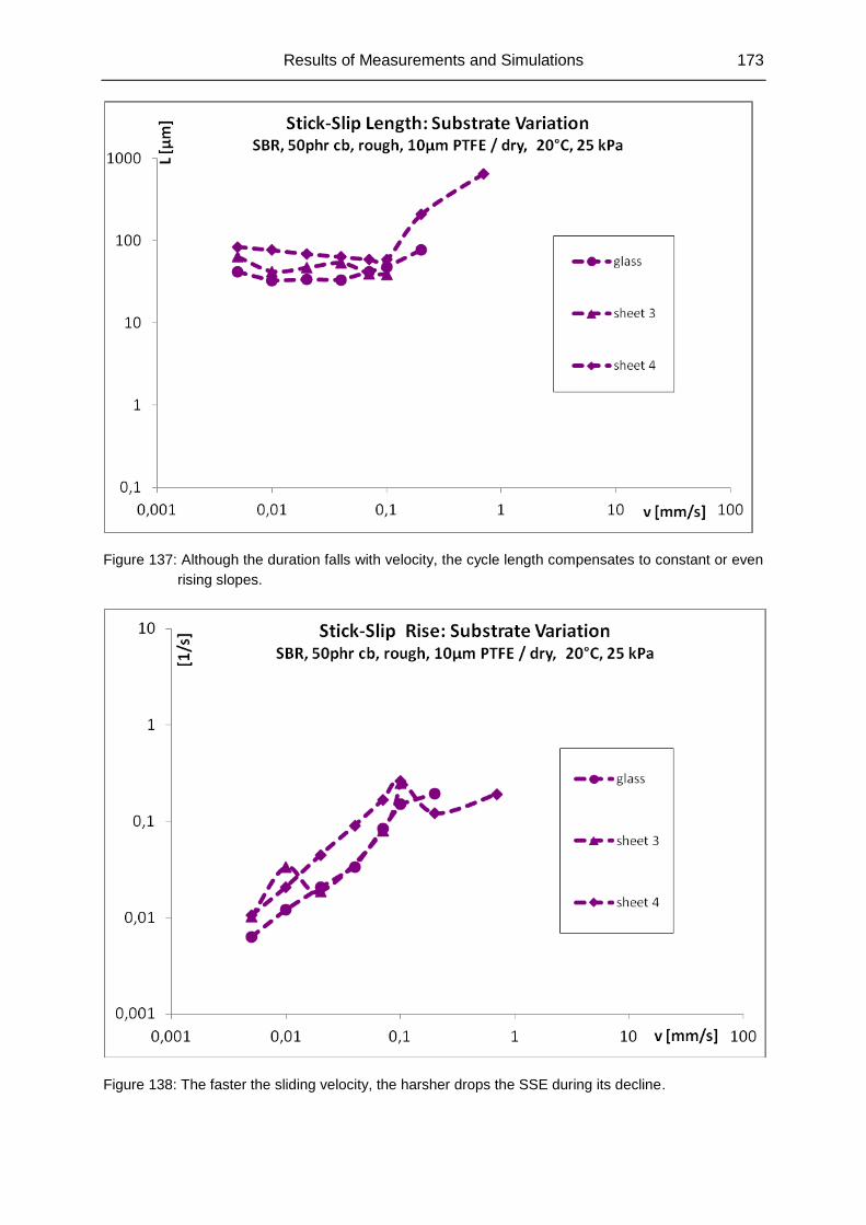
Results of Measurements and Simulations 173
Figure 137: Although the duration falls with velocity, the cycle length compensates to constant or even
rising slopes.
Figure 138: The faster the sliding velocity, the harsher drops the SSE during its decline.
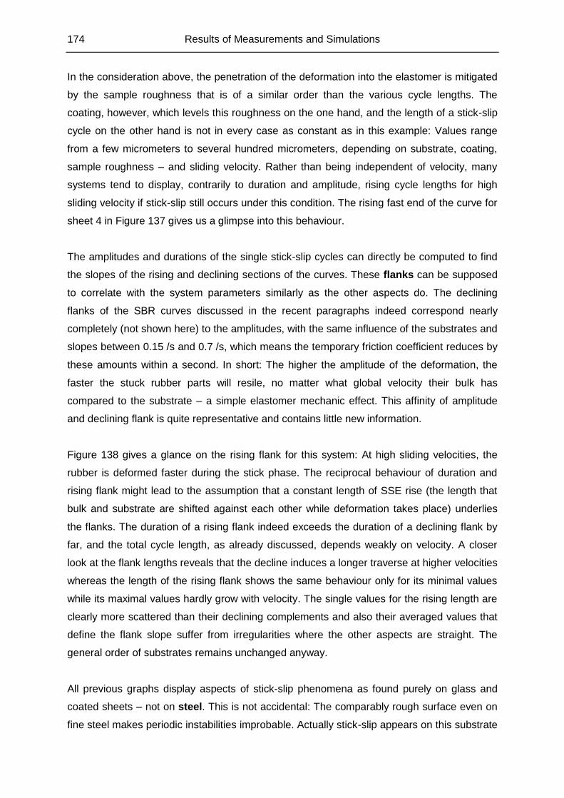
174 Results of Measurements and Simulations
In the consideration above, the penetration of the deformation into the elastomer is mitigated
by the sample roughness that is of a similar order than the various cycle lengths. The
coating, however, which levels this roughness on the one hand, and the length of a stick-slip
cycle on the other hand is not in every case as constant as in this example: Values range
from a few micrometers to several hundred micrometers, depending on substrate, coating,
sample roughness – and sliding velocity. Rather than being independent of velocity, many
systems tend to display, contrarily to duration and amplitude, rising cycle lengths for high
sliding velocity if stick-slip still occurs under this condition. The rising fast end of the curve for
sheet 4 in Figure 137 gives us a glimpse into this behaviour.
The amplitudes and durations of the single stick-slip cycles can directly be computed to find
the slopes of the rising and declining sections of the curves. These flanks can be supposed
to correlate with the system parameters similarly as the other aspects do. The declining
flanks of the SBR curves discussed in the recent paragraphs indeed correspond nearly
completely (not shown here) to the amplitudes, with the same influence of the substrates and
slopes between 0.15 /s and 0.7 /s, which means the temporary friction coefficient reduces by
these amounts within a second. In short: The higher the amplitude of the deformation, the
faster the stuck rubber parts will resile, no matter what global velocity their bulk has
compared to the substrate – a simple elastomer mechanic effect. This affinity of amplitude
and declining flank is quite representative and contains little new information.
Figure 138 gives a glance on the rising flank for this system: At high sliding velocities, the
rubber is deformed faster during the stick phase. The reciprocal behaviour of duration and
rising flank might lead to the assumption that a constant length of SSE rise (the length that
bulk and substrate are shifted against each other while deformation takes place) underlies
the flanks. The duration of a rising flank indeed exceeds the duration of a declining flank by
far, and the total cycle length, as already discussed, depends weakly on velocity. A closer
look at the flank lengths reveals that the decline induces a longer traverse at higher velocities
whereas the length of the rising flank shows the same behaviour only for its minimal values
while its maximal values hardly grow with velocity. The single values for the rising length are
clearly more scattered than their declining complements and also their averaged values that
define the flank slope suffer from irregularities where the other aspects are straight. The
general order of substrates remains unchanged anyway.
All previous graphs display aspects of stick-slip phenomena as found purely on glass and
coated sheets – not on steel. This is not accidental: The comparably rough surface even on
fine steel makes periodic instabilities improbable. Actually stick-slip appears on this substrate
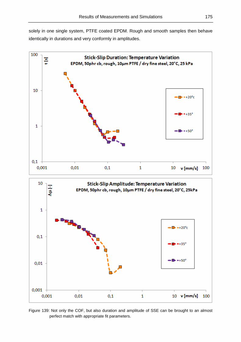
Results of Measurements and Simulations 175
solely in one single system, PTFE coated EPDM. Rough and smooth samples then behave
identically in durations and very conformly in amplitudes.
Figure 139: Not only the COF, but also duration and amplitude of SSE can be brought to an almost
perfect match with appropriate fit parameters.
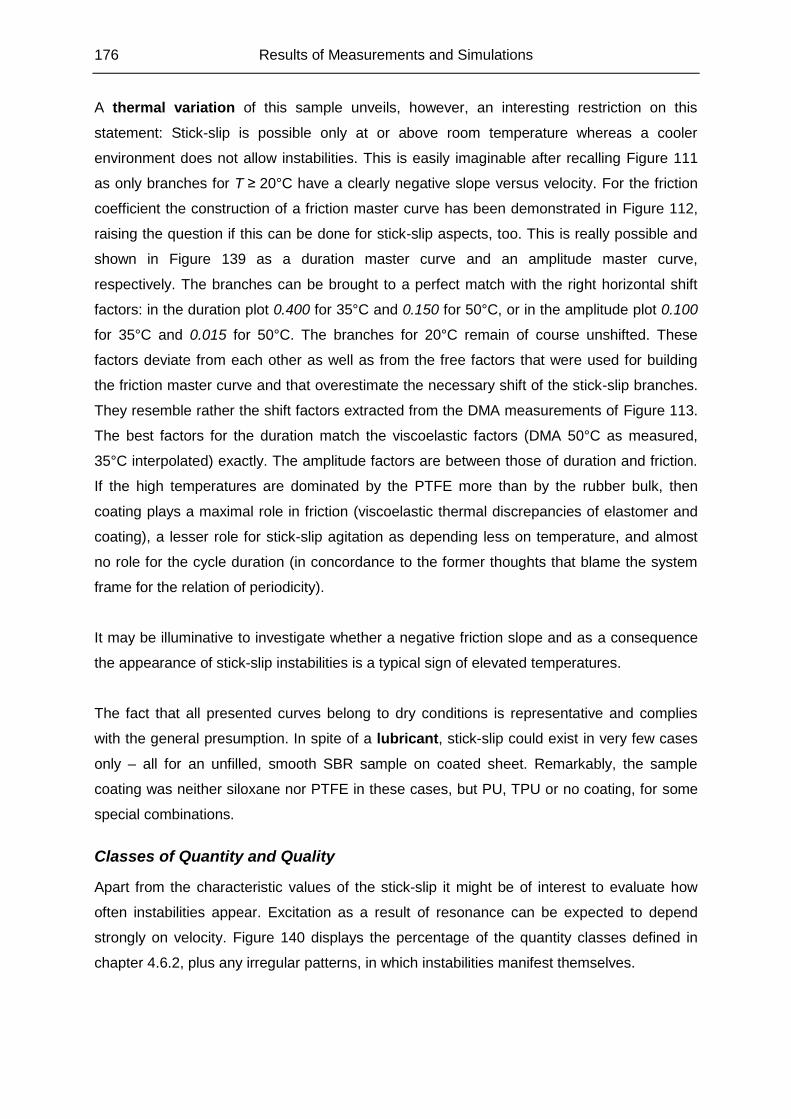
176 Results of Measurements and Simulations
A thermal variation of this sample unveils, however, an interesting restriction on this
statement: Stick-slip is possible only at or above room temperature whereas a cooler
environment does not allow instabilities. This is easily imaginable after recalling Figure 111
as only branches for T ≥ 20°C have a clearly negative slope versus velocity. For the friction
coefficient the construction of a friction master curve has been demonstrated in Figure 112,
raising the question if this can be done for stick-slip aspects, too. This is really possible and
shown in Figure 139 as a duration master curve and an amplitude master curve,
respectively. The branches can be brought to a perfect match with the right horizontal shift
factors: in the duration plot 0.400 for 35°C and 0.150 for 50°C, or in the amplitude plot 0.100
for 35°C and 0.015 for 50°C. The branches for 20°C remain of course unshifted. These
factors deviate from each other as well as from the free factors that were used for building
the friction master curve and that overestimate the necessary shift of the stick-slip branches.
They resemble rather the shift factors extracted from the DMA measurements of Figure 113.
The best factors for the duration match the viscoelastic factors (DMA 50°C as measured,
35°C interpolated) exactly. The amplitude factors are between those of duration and friction.
If the high temperatures are dominated by the PTFE more than by the rubber bulk, then
coating plays a maximal role in friction (viscoelastic thermal discrepancies of elastomer and
coating), a lesser role for stick-slip agitation as depending less on temperature, and almost
no role for the cycle duration (in concordance to the former thoughts that blame the system
frame for the relation of periodicity).
It may be illuminative to investigate whether a negative friction slope and as a consequence
the appearance of stick-slip instabilities is a typical sign of elevated temperatures.
The fact that all presented curves belong to dry conditions is representative and complies
with the general presumption. In spite of a lubricant, stick-slip could exist in very few cases
only – all for an unfilled, smooth SBR sample on coated sheet. Remarkably, the sample
coating was neither siloxane nor PTFE in these cases, but PU, TPU or no coating, for some
special combinations.
Classes of Quantity and Quality
Apart from the characteristic values of the stick-slip it might be of interest to evaluate how
often instabilities appear. Excitation as a result of resonance can be expected to depend
strongly on velocity. Figure 140 displays the percentage of the quantity classes defined in
chapter 4.6.2, plus any irregular patterns, in which instabilities manifest themselves.
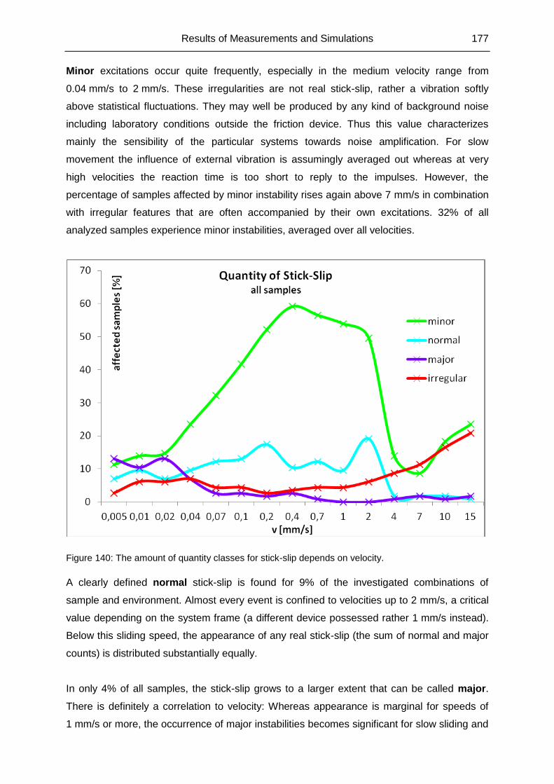
Results of Measurements and Simulations 177
Minor excitations occur quite frequently, especially in the medium velocity range from
0.04 mm/s to 2 mm/s. These irregularities are not real stick-slip, rather a vibration softly
above statistical fluctuations. They may well be produced by any kind of background noise
including laboratory conditions outside the friction device. Thus this value characterizes
mainly the sensibility of the particular systems towards noise amplification. For slow
movement the influence of external vibration is assumingly averaged out whereas at very
high velocities the reaction time is too short to reply to the impulses. However, the
percentage of samples affected by minor instability rises again above 7 mm/s in combination
with irregular features that are often accompanied by their own excitations. 32% of all
analyzed samples experience minor instabilities, averaged over all velocities.
Figure 140: The amount of quantity classes for stick-slip depends on velocity.
A clearly defined normal stick-slip is found for 9% of the investigated combinations of
sample and environment. Almost every event is confined to velocities up to 2 mm/s, a critical
value depending on the system frame (a different device possessed rather 1 mm/s instead).
Below this sliding speed, the appearance of any real stick-slip (the sum of normal and major
counts) is distributed substantially equally.
In only 4% of all samples, the stick-slip grows to a larger extent that can be called major.
There is definitely a correlation to velocity: Whereas appearance is marginal for speeds of
1 mm/s or more, the occurrence of major instabilities becomes significant for slow sliding and
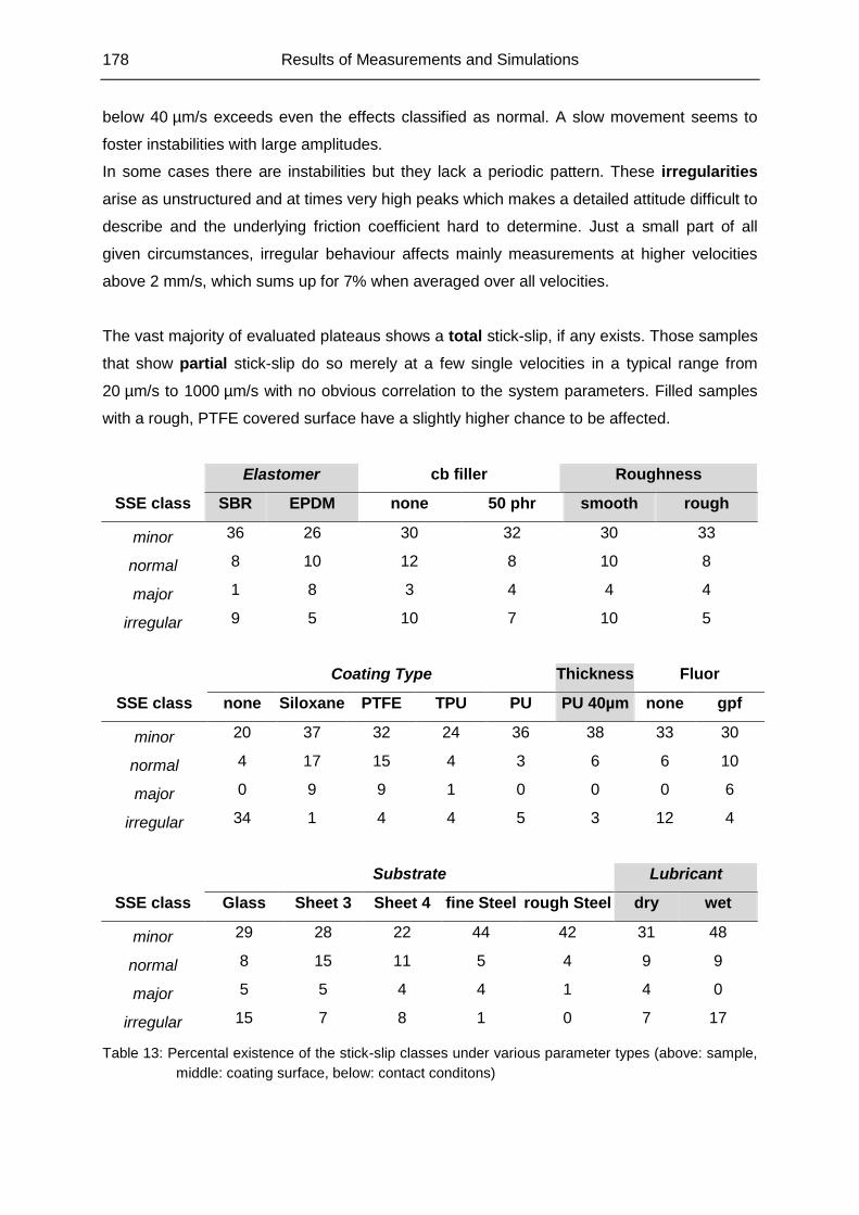
178 Results of Measurements and Simulations
below 40 µm/s exceeds even the effects classified as normal. A slow movement seems to
foster instabilities with large amplitudes.
In some cases there are instabilities but they lack a periodic pattern. These irregularities
arise as unstructured and at times very high peaks which makes a detailed attitude difficult to
describe and the underlying friction coefficient hard to determine. Just a small part of all
given circumstances, irregular behaviour affects mainly measurements at higher velocities
above 2 mm/s, which sums up for 7% when averaged over all velocities.
The vast majority of evaluated plateaus shows a total stick-slip, if any exists. Those samples
that show partial stick-slip do so merely at a few single velocities in a typical range from
20 µm/s to 1000 µm/s with no obvious correlation to the system parameters. Filled samples
with a rough, PTFE covered surface have a slightly higher chance to be affected.
Elastomer cb filler Roughness
SSE class SBR EPDM none 50 phr smooth rough
minor 36 26 30 32 30 33
normal 8 10 12 8 10 8
major 1 8 3 4 4 4
irregular 9 5 10 7 10 5
Coating Type Thickness Fluor
SSE class none Siloxane PTFE TPU PU PU 40µm none gpf
minor 20 37 32 24 36 38 33 30
normal 4 17 15 4 3 6 6 10
major 0 9 9 1 0 0 0 6
irregular 34 1 4 4 5 3 12 4
Substrate Lubricant
SSE class Glass Sheet 3 Sheet 4 fine Steel rough Steel dry wet
minor 29 28 22 44 42 31 48
normal 8 15 11 5 4 9 9
major 5 5 4 4 1 4 0
irregular 15 7 8 1 0 7 17
Table 13: Percental existence of the stick-slip classes under various parameter types (above: sample,
middle: coating surface, below: contact conditons)
Results of Measurements and Simulations 179
The viscoelastic properties seem to have little effect on instability: EPDM is only slightly
less sensitive to stick-slip than the harder SBR, but if it happens the effect can become larger
more easily. The rubber bulk features the peculiarity of stick-slip, not its existence.
Especially for filled uncoated samples, the universal testing machine showed stick-slip more
often for smooth than rough ones, but the roughness has small influence on tribometer
measurements. At high velocity, smooth samples tend to have major stick-slip, whereas
rough surfaces constrain to normal amplitudes.
Coating is crucial for avoidance and control of instability. The pure elastomer is extremely
prone to irregular friction. Classical stick-slip may superpose this but is oppressed by chaotic
friction forces. Siloxane and PTFE experience stick-slip comparably often for normal and
major amplitudes, whereas PU and TPU have almost none. This is exactly reciprocal to the
reduction of friction. All coatings prevent irregularities well.
The effect of a thick layer can be compared only for PU and causes normal stick-slip more
often but further lowers the chance of irregular events.
The use of fluorination, though necessary to provide the needed adhesion to the elastomer,
seems to be counterproductive at first glance as it augments both normal and major
stick-slip. But actually an unfluorinated surface will rather lose its coating integrity before
periodic effects truly come into play. A drastically increased number of irregular counts is the
result instead.
The choice of the substrate is important. Stick-slip appears on smooth interfaces: on glass
and even more on coated sheet. Irregular behaviour can appear on glass especially at high
velocity. Steel, on the other hand, is not likely to create real stick-slip – the rougher the steel,
the more improbable it becomes. Events focus on high temperatures.
Connecting both friction partners with a lubricant does not automatically prevent stick-slip
but rules out large amplitudes completely in the investigated cases.
Existence of Stick-Slip in Correlation to Negative COF Slope
In the vast majority of cases the relationship between a friction slope falling with velocity and
the appearance of stick-slip is obvious. There is in several curves an approximate
proportionality of the slope angle and the complementary stick-slip amplitude. This includes
environmental parameters, in particular the temperature variation discussed above. Very few
systems develop stick-slip with an astonishingly flat negative friction slope, but in no case a
180 Results of Measurements and Simulations
clear stick-slip is established in spite of a positive slope over velocity. On the other hand,
there are diverse examples of curves with a significant negative slope without attributed
stick-slip or only for some of the affected velocities. On steel, this happens with higher
probability. As a conclusion, a negative slope, even a flat one, is a necessary but not
sufficient premise for the existence of stick-slip.
Stick-Slip and Start Peak
Finally, stick-slip effects might be related to the start peaks known from chapter 4.6.1. Both
are provoked by a temporary stop of relative movement by sticking to the substrate, and both
situations terminate with an abrupt break off, resulting in a sudden drop of friction. From this
point of view a start peak could be a stick-slip with a single period.
However, the first peak of a stick-slip cycle may exceed the following stick maxima
significantly, indicating a substantial difference in concept. Indeed stick-slip is often found
only for velocities where no start peak arises and vice versa. As discussed before the start
peak tends to be maximal for high velocities, contrary to stick-slip. Apart from the pure
existence, also the coating dependent order of heights of the start peak is frequently
complementary to those of the stick-slip as well as complementary to those of the friction
coefficient.
A possible difference in the principle of the two phenomena is the spatial expansion of the
deformation that leads to the peaks in both cases: The start peak affects the complete
sample because its whole surface is in touch with the substrate before a new measurements
starts. The comparably long time between measurements (at least 1 second) allows the
adhesion to rise to an amount of only slow further increasing. When the movement starts the
mass inertia of the sample causes a delay of reaction, which is largest for highest velocities.
Movement is clearly non-stationary. The stick-slip on the other hand does not necessarily
happen on the whole interface but can be regarded as local deformation. A slow movement
may be more suitable to build up local deformations. Apart from this the global movement is
stationary during this phase.
In any case a strong adhesion – a large true contact zone via smooth surfaces with
appropriate tension – is important to make samples stick. Thus, on steel neither stick-slip nor
start peaks are seen regularly.
Final Considerations 181
5 Final Considerations
5.1 General Discussion
The previous chapter explained the details of the experimental and computational results for
various aspects of tribology. Now these results shall be reviewed in an overall scope of the
basic goals in order to point out coherence and interactions, and answer how successfully
the objectives have been reached or where confinements exist.
One goal was the investigation of friction and stick-slip in a manifold of conceivable
systems. The parameter space is huge and truly impossible to fathom completely. Limiting
the elements for each parameter to a finite number – only few but relevant elastomers, etc. –
created a large but finite number of parameter combinations. Furthermore, the focus was put
on interesting and promising systems by separating the variables if necessary instead of
grazing the entire mash. A digest of the most important and most meaningful results has
been presented. The effect of each single aspect could be assessed clearly in most cases.
Apart from a reproducible general description of friction, some exciting common features
become evident. The wet friction starts at a low level for slow sliding speeds and rises mainly
monotonously with velocity whereas the maximum peak of the adhesion component in the
dry friction regime causes a plateau at medium velocity. It is noteworthy that this plateau
appears on “naturally” measured Stribeck curves in the same way as in synthetic friction
master curves and especially when adding silica to the elastomer batch. The master curve
on its part is based on the same horizontal shift factors no matter if they were applied to
viscoelastic shear moduli or friction coefficients.
The investigation of dynamic effects like stick-slip, start peaks and running-in phases blends
into the results for purely stationary friction. The connection between stick-slip and velocity
dependence of friction is obvious with regard to strength and time scale, and reproduces the
thermal influence resulting in frequency shifts.
The second goal was the prediction of tribological behaviour. Three different types of
prediction must be discriminated here:
the way that the parameters of bulk, surface and environment determine the friction
the interpolation and extrapolation of sliding velocities, including master curves
the simulation of friction according to the model
182 Final Considerations
By understanding the role of the parameters in the friction mechanism it should be possible
to estimate how a yet untested combination of rubber, filler material, surface structure and
chemistry might slide on a certain substrate. However, predictions remain merely qualitative
until measured practically. Some parameters behave not consistently in every case, and
interactions between them must be taken into account, but universal trends can be spotted.
Stationary friction is probably easier to gauge than dynamic effects. Predictability of dry and
wet interfaces may differ.
Interpolation of blank velocities between measured values should not cause any problems,
as the curves display a continuity in almost every case. Caution should be exercised for
extreme sample exposures, be it due to high pressure (some applications may outrange the
experimental setup by decades in pressure) or long experimental durations. Extrapolating a
measured curve is doubtful for normal experimental data, but tribology enjoys the availability
of the time temperature superposition principle. Via master curves an incredibly large range
of velocity can be explored if measurements at variable temperatures are feasible. The
results are plausible and reliable for ordinary velocities. A natural border of course exists, as
the most extreme low temperature branches for SBR show impressively: The assigned
sliding velocity exceeds even the speed of light – obviously no realistic interpretation and a
proof that master curves are confined to “normal” velocities to remain valid. Simulation is
consequently not possible for excessive velocities in this system, and for any really high
velocity the influence of friction heat must be considered. The use of friction master curves at
moderate and slow velocities, however, is not restricted, and extrapolating to super slow
speed can be expected to work smoothly. If shift factors are unknown, like for coated
samples, it is still possible to determine horizontal shift factors empirically. The non-existent
need for vertical shift factors turns out very helpful then.
Simulation has proven successful in many cases and verifies the validity of the DIK friction
model. Hysteresis and especially adhesion match the reality of wet and dry friction well, for
standard curves as well as for master curves and silica samples. It is thus an excellent
opportunity to forecast tribology when a measurement is unwanted or limited in parameters.
An exact knowledge of viscoelasticity and surface descriptors is a prerequisite for a
meaningful simulation. Some free fit parameters leave space for interpretation of the
computed curves. An extensive analysis how the contact variables depend on external
parameters has been provided. The model assumes a rigid substrate and an elastic sample
with full contact at least on the macroscopic scale. It does not cover the friction of two flexible
objects or a patterned sample surface. Within its frame, it is a useful tool for prediction.
Final Considerations 183
Finally, there was the goal to control the friction coefficient and the appearance and
attributes of stick-slip effects. In this work the target was a minimal friction with no or small
instabilities. A reasonable choice of elastomer and its contact partner may already provide
the desired effect. This is certainly not possible in many applications. Two investigated
techniques promise a solution: coating the sample, and inserting hard particles into the
sample surface. Which one is better?
The answer depends on the exact request. The first difference lies in the preparation: PAOS
must be inserted already during the batch mixing process, coating is possible any time
before usage. Adding one more component and annealing is, on the other hand, an easy
step and thus cheaper and less time consuming than coating.
Both methods diminish friction and stick-slip and can be regarded successful in this
perspective. The presented results should not be compared directly because measurements
took place on different machines and on substrates of diverging smoothness. Coating with
PTFE and siloxane gives definitely the best results in respect to low friction, but PU and TPU
prevent instability much better. PAOS manages both to a certain degree if its content in the
sample is high enough.
The effect vanishes when the sample surface is damaged. Gas phase fluorination before
coating shows mostly good stability and allows longer usage and applying higher pressures
than usual. PAOS wears off fast and is thus not dedicated to these conditions. Storing the
sample for a long time or undefined environments alter the state of annealing for PAOS but
leave coating untouched.
The environment itself can be another alternative to control friction and stick-slip. Sample
and substrate may be arranged as fix, but for some systems the pressure, the temperature
and the frame provide the key to a lower friction and less stick-slip. The temperature
dependence of stick-slip in friction master curves is a formidable example.
184 Final Considerations
5.2 Summary
Aim of this work was the investigation, prediction and control of friction and stick-slip for
rubber sliding on rigid substrates. This included experimental testing of friction forces for a
large number of tribological systems, i.e. combinations of various elastomers, surface
structures and environmental conditions, on the one hand, and a comparison to simulations
on the other hand.
All computational results of wet (hysteresis) as well as for dry (hysteresis plus adhesion)
friction are based on the friction model developed at the DIK previously, which incorporates
the viscoelastic properties of the rubber sample and the surface descriptors of the substrate
at room temperature for variable velocities and pressures. Viscoelastic shear moduli were
gained from dynamic-mechanical measurements (DMA) for the involved samples, and shear
master curves were constructed using the time-temperature superposition principle of the
WLF law with horizontal and for filled samples also vertical shifting. The substrates were
characterized by surface techniques and analyzed due to their fractal surface parameters.
As samples the elastomers EPDM, NBR, NR and SBR were chosen because of their
importance in not only scientific but also industrial application. Some bulks were filled with
carbon black, silica or PAOS (followed by annealing) in order to enhance stabilty, hardness
and surface structure. Vulcanization plates of different degrees in roughness were used to
modify the sample surfaces. To analyze the effect of polymer layers, a class of samples was
coated with lackers based on PU, TPU, PTFE and siloxane.
Friction measurements were carried out on a special tribometer sliding on one axis forward
and backward with stationary velocity ranging from 5 µm/s to 15 mm/s, or on a universal
tester. A tenside-water lubricant provided a wet environment for pure hysteresis friction if
needed. Pressure and temperature were varied in relevant cases.
While wet friction on rough substrates like asphalt and granite rises monotonously at rising
slope with the sliding velocity, dry friction reaches a plateau at medium velocity. This is only
sparsely visible for unfilled SBR samples but becomes more pronounced and longer when
silica filler (up to 80 phr) is added; the velocity above which the plateau begins is not
affected. Under wet conditions, the silica makes the samples harder and increases friction for
all velocities. Both substrates behave quite similar in experiment. Simulation reproduces the
data well, and extrapolation confirms the tendency of the plateaus to become flatter and
extend to higher velocites.
Final Considerations 185
The plateau of many systems is barely detectable because the velocity scale does not reach
far enough at room temperature. Combining the branches measured at different
temperatures creates a friction master curve. Like the shear modulus master curves known
from DMA and using the same horizontal shift factors, they form a continuous shape. After
rising with velocity at high temperatures/ low velocity, a maximal dry friction is clearly visible
at a velocity connected to the glass transition temperature of the material (EPDM, NR, SBR),
followed by a plateau or a direct decrease. Simulation fits this course very well for all
elastomers over reasonable velocities. Friction master curves for wet interfaces are also
possible but limited to temperatures above freezing and thus less meaningful. Vertical
shifting is not necessary. Taking temperatures form -30 to +65°C into account results in
master curves that cover the huge range of 10 to more than 15 decades of velocity.
Simulating the friction process generates not only results for the friction coefficient but also
for related contact parameters. A systematic analysis of this as function of velocity and
pressure (several decades around the 23 kPa of the tribometer) for the investigated
combinations of sample and substrate reveals some general insights: The true contact area,
a tiny part of the nominal contact area, decreases with velocity and sample hardness but
rises with pressure. The same holds true for the mean penetration depth. The gap distance
displays a reciprocal reaction to these input parameters. The shear stress increases with
velocity, too, but approaches a maximum asymptotically. The exact course of the functions
depends on the parameter set that defines the system.
One way to reduce friction consists in minimizing the contact area on the microscopic scale.
To achieve this, NBR samples have been prepared with different degrees of PAOS with
Al2O3 particles that work as spacers at the sample surface. A sufficiently high concentration
of PAOS (20 phr) can decrease friction up to 20%, depending on velocity, for all samples
(with and without carbon black) on dry and wet granite, steel and glass. Additionally, PAOS
can prevent stick-slip phenomena that appear otherwise on very flat substrates. Applications
must consider the increased abrasion induced by PAOS and temporal alteration of the
surface (annealing brings the sample to a defined state).
Another way to reduce friction is to uncouple the sample properties of bulk and surface. This
can be done by coating the preferred elastomer bulk (SBR, EPDM) with a well sliding
polymer. The effect is observed best on very smooth dry substrates (glass, coated sheet),
which produce extremely high and irregular friction with stick-slip and chaotic instabilities
otherwise. Especially siloxane and PTFE show an excellent reduction of friction, but PU and
186 Final Considerations
TPU offer good results, too, without touching the ranking order of the substrates (highest
friction for coated sheets, less for glass, low for fine steel and even less for rough). The
typical layer thickness was 10 µm. A thicker layer could further decrease friction in some
cases. Surface structures imprinted on the sample surface were mitigated by coating but not
completely abolished: Smooth samples still display a higher friction than rough ones; no
difference is found in case the substrate roughness exceeds the sample roughness. Normal
samples filled with carbon black are subject to increased wet friction due to their hardness
but dry friction is lower for unfilled ones. Coating prevents soft rubber from establishing
optimal contact, so coated samples display lower friction when unfilled even on dry
interfaces.
The influence of the environmental parameters was investigated as well. On rough
substrates like steel a variation of pressure shows little effect, as for the case of uncoated
samples, but on a coated sheet a rising pressure can decrease friction of coated rubber. A
higher temperature lowers friction, while a cold environment increases friction. On the other
hand, a modified temperature on steel does not change the height of friction but shifts the
measured temperature branches analogously to mechanical shear branches to overlap as
master curve. The shift factors are not identical but similar to DMA and reflect a
superposition of bulk and coating layer. This additionally aggravates the difficulties of
simulation.
Apart from the mechanical stability that can be achieved by gas phase fluorination before
coating, stability of the friction coefficient is important. Static friction causes start peaks
especially at high velocity on smooth substrates and may slowly increase for long friction
exposure. A negative slope in the Stribeck curve is the fundament of a periodic change in
friction, the stick-slip. A cycle consists of several phases (stick, deformation, slip, contact)
that manifest in a slow rise in friction followed by a sharp drop. The duration of a cycle does
little depend on the system of sample and substrate but rather on the system framework and
is thus characteristic for every single device. The amplitude, however, is a function of the
system parameters: Siloxane and PTFE coatings, though optimal for friction diminishment,
show stick-slip regularly while PU and TPU rarely are affected. Uncoated samples on smooth
substrates show large stick-slip and even larger irregular instability especially for fast sliding.
Glass and coated sheet exhibit large effects, steel almost none. EPDM tends to have more
stick-slip than SBR, and smooth sample surfaces more than rough. A thicker layer decreases
the chance of irregular behaviour. Lubricant limits the amplitude of stick-slip. On dry
interfaces, major amplitudes are found mainly for slow sliding speeds. The spatial length of a
cycle is almost constant at any velocity, while the slope of the rising flank ascends with
Final Considerations 187
velocity. It is possible to construct a master curve of the stick-slip parameters (duration,
amplitude…) from branches of various temperatures.
188 Final Considerations
5.3 Possible Applications
The results of the experiments and simulations have been described and interpreted. The
final step is to judge their impact on science and technology. The scientific use of the findings
and tools has already been discussed. The following thoughts debate possible applications.
The most important potential that the previous insights allow is the construction of elastomer
devices with minimal susceptibility to friction – e.g. gaskets, hoses, rubberized fabrics etc.
The choice of the method is determined by the conditions the sample must fulfil as discussed
in chapter 5.1. PAOS induction may be a good solution for cheap, disposable devices;
coating poses an enduring reduction of friction for devices with higher quality. Deciding which
coating type is applied also determines if friction or stick-slip shall be minimized.
On the other hand it might even be desired to generate vibration via stick-slip for special
applications. In this case it is useful to identify the typical velocity of the working device for
the particular ambience temperature and then select PTFE or siloxane coated sample
system with negative slope in this range. The possibility of calculating the course of the curve
from master curves when knowing only either temperature or velocity exhibits as useful as
the prediction by means of simulation.
A targeted reaction to temperature can be achieved by coating. The bulk behaviour is
detached from the layer behaviour and thus “conserved” for its own characteristic
temperature response without affecting the interface. The drastic thermal dependence shown
in Figure 114 suggests devices which move easily in hot environments but block movement
when the system becomes cold.
The existence of a maximal COF, often shaped as a plateau, offers another chance: The
system replies with a constant friction for a range of certain velocities/ temperatures (stable,
reliable conditions independent from input parameters) or maximal friction can be used to
build a system with a stable equilibrium around the peak velocity. Choosing a rubber with the
right glass transition temperature designs the position of the peak; coating can modify this
effect and enhance sliding. Besides, the influence of coating on the start peak alters the ratio
of static and dynamic friction for further application opportunities.
A modification of sample roughness induces effects which might prove helpful. This can be
done by patterning during vulcanisation, or the presence of particles like PAOS may function,
apart from friction reduction, as spacers to enlarge the gap between sample and substrate.
Final Considerations 189
5.4 Outlook
This work has presented an extensive view on friction and stick-slip under a multitude of
parameters. Still, some questions remain and some ideas are worth pursuing in future
investigations.
Possible ways to continue investigations for further insight split up into tribological
measurements, secondary characterizations and improvements of the software and
hardware tools.
A promising advancement might be the combination of coating and surface particles. PAOS
would decrease the contact between substrate and coated layer, which would prevent the
particles from abrasion. Another field of investigation is the inexhaustible number of
tribological systems, with focus on the interaction of temperature and pressure. The resulting
master curves would allow a widespread description of friction for parameter sets and explain
how common the existence of stick-slip is for high temperatures. As the available data
concentrate on mainly dry interfaces, the role of lubricant could be of interest especially for
high pressures that might squeeze the contact zone of flat substrates.
Rating the significance of wear is possible with a systematic characterization of the sample
surfaces, with and without coating, at different degrees of load exposure. The morphology,
the HDC, height profiles and distributions would document erosion and anisotropies of the
sample as well as the amount of abrasion. Knowing the dynamic-mechanical properties of
the pure coatings without rubber would open the simulation for two-component samples in
concert of bulk and layer.
Refining the tools makes experiments not only more efficient but also improves them
qualitatively. An optical survey of the interface in real-time, ideally supplemented by means of
an infrared camera, or an acoustic detection to analyze the vibrations induced by stick-slip
might come in handy for future generations of scientists on this subject, just like an
implementation of temperature as parameter in the simulation model for direct calculation of
friction in any environment.
190 Literature
Literature
[1] M. Williams, J. Ferry: "Second Approximation Calculations of Mechanical and Electrical
Relaxation and Retardation Distributions", J. Polym. Sci. 11, 169 (1953)
[2] V. L. Popov: "Contact Mechanics and Friction - Physical Principles and Applications",
Springer-Verlag (2010)
[3] R. Stribeck: "Die Wesentlichen Eigenschaften der Gleit- und Rollenlager", Z. Verein.
Deut. Ing. 46, 38, 1341-1348 (1902)
[4] D. Moore: "The Friction and Lubrication of Elastomers", Pergamon Press, Oxford
(1972)
[5] K. Grosch: "The relation between the friction and visco-elastic properties of rubber",
Proc. R. Soc. London A 274, 21-39 (1963)
[6] D. Moore, W. Geyer: “A review of Hysteresis Theories for Elastomers”, Wear 30, 1-34
(1974)
[7] K. Grosch: “The Rolling Resistance, Wear and Traction Properties of Tread
Compounds”, Rubber Chem. Technol. 69, 495 (1996)
[8] M. Klüppel, G. Heinrich: "Rubber Friction on Self-Affine Road Tracks", Rubber Chem.
Technol. 73, 578, (2000)
[9] A. Roberts: “A Guide to Estimation the Friction of Rubber”, Rubber Chem. Technol. 65,
673 (1992)
[10] G. Heinrich, L. Grave, M. Stanzel: “Material- und Reifenphysikalische Aspekte bei der
Kraftschlußoptimierung von Nutzfahrzeugreifen“, VDI-Berichte 1188, 49-67 (1995)
[11] B. Persson: “Sliding Friction: Physical Principles and Applications“, Springer Verlag,
Berlin, Heidelberg, N. Y. (1998)
[12] A. Schallamach: ''The velocity and temperature dependence of rubber friction,'' Proc.
Phys. Soc. B 66, 386-392 (1953)
[13] B. Persson: “Theory of rubber friction and contact mechanics”, J. Chem. Phys. 115,
3840-3861 (2001)
[14] G. Heinrich: “Hysteresis Friction of Sliding Rubbers on Rough and Fractal Surfaces”,
Rubber Chem. Technol. 70, 1-14 (1997)
[15] H. Hertz: "Miscellaneous Papers", Macmillan, London, 146 (1896)
[16] J. Greenwood, J. B. P. Williamson: "Contact of nominally flat surfaces", Proc. R. Soc.
London A 295, 300 (1966)
[17] B. Mandelbrot: "The fractal geometry of nature", W.H. Freeman, N.Y. (1982)
[18] P. de Gennes: "Soft Adhesives", Langmuir 12, 4497 (1996)
[19] M. Klüppel: „Molekulare Rheologie polymerer Schmelzen und Lösungen“,
Vorlesungsscript Universität Hannover WS 2010/2011 (2010)
Literature 191
[20] C. Wrana: “Bestimmung der Glastemperatur mittels dynamisch-mechanischer
Analyse”, UserCom 2 (2002)
[21] A. Payne: "The dynamic properties of carbon black-loaded natural rubber vulcanisates"
Rubber Chem. Technol. 36, 432 & 444 (1963)
[22] M. Klüppel: "Evaluation of viscoelastic master curves of filled elastomers and
applications to fracture mechanics", J. Phys. Condens. Matter 21, 035104, (2009)
[23] A. Le Gal, M. Klüppel: "Investigation and Modelling of Rubber Stationary Friction on
Rough Surfaces", J. Phys. Condens. Matter 20, 015007 (2008)
[24] H. Hertz: "Ueber die Berührung elastischer Körper" (1881)
[25] T. Geike: "Theoretische Grundlagen eines schnellen Berechnungsverfahrens für den
Kontakt rauer Oberflächen" (Dissertation) TU Berlin (2008)
[26] J. Schramm: "Reibung von Elastomeren auf rauen Oberflächen und Beschreibung von
Nassbremseigenschaften von PKW-Reifen", (Dissertation) Universität Regensburg
(2002)
[27] A. Le Gal, L. Guy, G. Orange, Y. Bomal, M. Klüppel: " Modelling of sliding friction for
carbon black and silica filled elastomers on road tracks", Wear 264, 606 (2007)
[28] B. Persson: "Rubber friction: role of the flash temperature", J. Phys. Condens. Matter
18, 7789 (2006)
[29] G. Heinrich, M. Klüppel: "Rubber Friction, Tread Deformation and Tire Traction", Wear
265, 1052-1060 (2008)
[30] A. Le Gal, X. Yang, M. Klüppel: "Sliding friction and contact mechanics of elastomers
on rough surfaces", (P. Wriggers & U. Nackenhorst: Analysis and Simulation of
Contact Problems), Lecture Notes in Applied and Computational Mechanics Vol. 27,
Springer, 253-260 (2006)
[31] T. Meyer, L. Busse, A. Le Gal, M. Klüppel: "Simulations of hysteresis friction and
temperature effects between elastomers and rough or microscopically smooth
interfaces", (Boukamel, Laiarinandrasana, Meo, Verron: Constitutive Models for
Rubber V), 351-355, Taylor & Francis Group, London (2008)
[32] A. Le Gal: "Investigation and Modelling of Rubber Stationary Friction on Rough
Surfaces" (PhD Thesis) University of Hannover (2007)
[33] A. Müller, J. Schramm, M. Klüppel: "Ein neues Modell der Hysteresereibung von
Elastomeren auf fraktalen Oberflächen", Kautschuk Gummi Kunstst. 55, 432 (2002)
[34] H. Kummer: "Lubricated Friction of Rubber Discussion", Rubber Chem. Technol. 41,
895 (1968)
[35] A. Le Gal, M. Klüppel: "Modelling of rubber friction: A quantitative description of the
hysteresis and adhesion contribution", (P.E. Austrell & L. Kari: Constitutive Models
for Rubber IV), Taylor & Francis Group, London, 509 (2005)
192 Literature
[36] A. Le Gal, X. Yang, M. Klüppel: "Evaluation of sliding friction and contact mechanics of
elastomers based on dynamic mechanical analysis", J. Chem. Phys. 123, 014704
(2005)
[37] B. Persson, E. Brener: "Crack propagation in viscoelastic solids", Phys. Rev. E 71;
036123 (2005)
[38] A. Le Gal, M. Klüppel: "Investigation and Modelling of Adhesion Friction on Rough
Surfaces", Kautschuk Gummi Kunstst. 59, 308 (2006)
[39] R. Good, L. Girifalco: “A Theory for Estimation of Surface and Interfacial Energies 3:
Estimation of Surface Energies of Solids From Contact Angle Data”, J. Phys. Chem.
64, 561-565 (1960)
[40] A. Savkoor, A. Briggs: “The effect of a tangential force on the contact of elastic solids in
adhesion”, Proc. R. Soc. Lond A, 356, 103-114 (1977)
[41] D. Owens, R.J. Wendt: "Estimation of the surface free energy of polymers", J. Appl.
Polym. Sci. 13, 1741-1747 (1969)
[42] H. Busscher et al: "The Effect of Surface Roughness of Polymers on Measured
Contact Angles of Liquids", Colloids and Surfaces 9, 319-331 (1984)
[43] H. Batzer: "Polymere Werkstoffe III: Technologie 2", Georg Thieme Verlag Stuttgart,
New York (1984)
[44] T. Kempermann: "Handbuch für die Gummi-Industrie", Bayer AG (1991)
[45] M. Klüppel: "The Role of Disorder in Filler Reinforcement of Elastomers on Various
Length Scales", Adv. Polym. Sci. 164, 1-86 (2003)
[46] G. Heinrich, M. Klüppel: "Role of Polymer-Filler-Interphase in Reinforcement of
Elastomers" Kautschuk Gummi Kunstst. 57, 452 (2004)
[47] M. Klüppel, J. Schramm: "A generalized tube model of rubber elasticity and stress
softening of filler reinforced elastomer systems", Macromol. Theory Simul. 9, 742
(2000)
[48] M. Klüppel, G. Heinrich: "Physics and Engineering of Reinforced Elastomers",
Kautschuk Gummi Kunstst. 58, 217 (2005)
[49] M. Qu, F. Deng, S. Kalkhoran, A. Gouldstone, A. Robisson, K. Van Vliet : “Nanoscale
visualization and multiscale mechanical implications of bound rubber interphases in
rubber-carbon black nanocomposites”, Soft Matter 7, 1066-1077 (2011)
[50] X. Zhu, M. Jaumann, K. Peter, M. Möller, C. Melian, A. Adams-Buda, D.E. Demco, B.
Blümich: "One-Pot Synthesis of Hyperbranched Polyethoxysoloxanes", Macromol.
39, 1701 - 1708. (2006)
[51] Q. Dou, X. Zhu, K. Peter, D.E. Demco, M. Möller: "Preparation of polypropylene/ silica
composites by in-situ sol-gel processing using hyperbranched polyethoxysiloxane",
J.Sol-Gel Sci Technol 48, 51-60 (2008)
Literature 193
[52] L. Busse, K. Peter, C.W. Karl, H. Geisler, M. Klüppel: "Reducing Friction with
Al2O3/SiO2-Nanoparticles in NBR", Wear 271, 1066-1071 (2011)
[53] C. Karl, L. Busse, M. Klüppel, U. Giese: „ Varnish Coating of Elastomers: Morphology,
Friction and Surface Energies”, 9. Kautschuk Herbst Kolloquium, Hannover (2010)
[54] C. Karl, A. Lang, A. Stoll, A. Weiße, M. Stoll, M. Klüppel: „Tribologische Eigenschaften
beschichteter Elastomere - Teil 1: Charakterisierung der Oberflächen mittels
modifizierter Wilhelmy-Methode“, Kautschuk Gummi Kunstst. 75, 44-49 (April 2012)
[55] C. Karl, A. Lang, L. Busse, A. Stoll, A. Weiße, M. Stoll, M. Klüppel: „Tribologische
Eigenschaften beschichteter Elastomere - Teil 2: Charakterisierung der stationären
Reibung gegenüber glatten Substraten“, Kautschuk Gummi Kunstst. 76, 33-36 (May
2012)
[56] C. Karl, L. Busse, A. Stoll, M. Klüppel: „AIF-Abschlussbericht: Vermeidung von Stick-
Slip Reibinstabilitäten beschichteter Elastomere auf mikroskopisch rauen und
glatten Oberflächen“ (2011)
[57] C. Karl, M. Klüppel: „Characterization of Elastomers by Wetting: Roughness and
Chemical Heterogeneiy“, Chem. Listy 105, 233-234 (2011)
[58] J. Fritzsche, M. Klüppel: "Filler networking and reinforcement of carbon black filled
styrene butadiene rubber", Kautschuk Herbst Kolloquium, Hannover (2008)
[59] L. Busse, M. Klüppel: "Wet and Dry Friction of Elastomers in Advanced Simulation
Compared to Experiment", (Heinrich, Kalliske, Lion, Reese: Constitutive Models for
Rubber VI) Taylor & Francis Group, London, 295-300 (2010)
[60] L. Busse, A. Le Gal, M. Klüppel: “Modelling of Dry and Wet Friction of Silica Filled
Elastomers on Self-Affine Road Surfaces”, Lecture Notes in Applied and
Computational Mechanics Vol. 51 (Besdo, Heimann, Klüppel, Kröger, Wriggers,
Nackenhorst), Springer, 1-26 (2010)
[61] L. Busse, I. Boubakri, M. Klüppel: “Friction Master Curves for Rubber on Dry and Wet
Granite: Experiments and Simulations”, Kautschuk Gummi Kunstst. 64, 35-39 (May
2011)
[62] L. Busse, C. W. Karl, I. Boubakri, M. Klüppel: „Praxis and Theory of rubber Friction on
rough and smooth surfaces”, 9. Kautschuk Herbst Kolloquium, 31-34 Hannover
(2010)
[63] T. Papatheodorou: "Weniger Reibung", Kautschuk Gummi Kunstst. 60, 586‚ (2007)
[64] G. Carbone, F. Bottiglione: "Asperity contact theories: Do they predict linearity between
contact area and load?", J. Mech. Phys. Solids 56, 2555-2572 (2008)
[65] G. Carbone, F. Bottiglione: "Contact mechanics of rough surfaces: a comparison
between theories", Meccanica (2010)
194 Literature
[66] Q. Bui, J. Ponthot: "Estimation of rubber sliding friction from asperity interaction
modeling", Wear 252, 150-160 (2002)
[67] M. Barquins: "Adherence, friction and wear of rubber-like materials", Wear 158, 87-117
(1992)
[68] M. Lindner: "Experimentelle und theoretische Untersuchungen an Profilklötzen und
Dichtungen" (PhD Thesis) Universität Hannover (2005)
[69] B. Lorenz, B. Persson: "Interfacial separation between elastic solids with randomly
rough surface - comparison of experiment with theory", J. Phys. Condens. Matter
21, 015003 (2009)
[70] M. Kröger, P. Moldenhauer: "Modellierung von Elastomerkontakten", Kautschuk
Gummi Kunstst. 63, 30-35 (2010)
List of Tables 195
List of Tables
Table 1: Mixing table for NBR samples with PAOS ...............................................................47
Table 2: Mixing table for EPDM samples with PAOS ............................................................47
Table 3: Mixing table for EPDM samples for friction master curves ......................................48
Table 4: Mixing table for NR samples for friction master curves ...........................................48
Table 5: Mixing table for S-SBR samples for friction master curves ......................................48
Table 6: Vulcanization times in minutes. ...............................................................................49
Table 7: Surface descriptors of relevant substrates ..............................................................71
Table 8: Surface tension and roughness for PAOS filled samples ........................................83
Table 9: Roughness values Ra taken from AFM measurements ...........................................86
Table 10: Mechanical properties of NBR in respect of PAOS amount ...................................88
Table 11: Viscoelastic parameters depend on the amount of silica in SBR 2525. .................97
Table 12: Free fit parameters for simulation of silica filled samples .................................... 103
Table 13: Percental existence of the stick-slip classes ....................................................... 178
196 Acknowledgement
Acknowledgement
A dissertation is unthinkable without support from other people who deserve my gratitude. A
doctoral advisor – in my case Professor Dr. Gerhard Poll from the IMKT, where also the
employed tribometer had been build, at the university of Hannover – agrees to support a
common field of interest, to foster the progress and finally to judge the result. He gave me
the opportunity to realize my PhD thesis, although being a physicist, in the engineer
department. Thanks for the frictionless course my treatment of friction took.
The one who spawned this interest, the fascination for the world of rubber friction, was PD
Dr. Manfred Klüppel, under whose advice I worked at the DIK and accomplished the
experiments that led to this thesis. Thank you for the many discussions that helped me to
achieve a deeper understanding of tribology and hone the abilities that were needed to fulfil
this task.
The DIK (Deutsches Institut für Kautschuktechnologie), first under guidance of Professor Dr.
Robert Schuster, later under Professor Dr. Ulrich Giese, gave me the resources for this
work: material, devices, know-how… and a pleasant working atmosphere which was due to
the many friendly colleagues, too many to mention. Some of them deserve special
appreciative credits because of their scientific contributions: Christian Karl characterized
surface structures with SEM/EDX, AFM, DIAS and white light microscopy, and surface
tension by means of sessile drop and Wilhelmy method. I warmly thank Ines Boubakri,
Andrej Lang and Krzysztof Kaczmarek for some of the friction measurements and many
enjoyable discussions. The DMA measurements that led to the shift factors for the friction
master curves were gained by Dagmar Steinhauser, the IR spectra by Burkhard
Matschke, and no measurement could have been done without samples, so I own thank to
Jürgen Hamann and Joachim Heier for mixing and vulcanization. The AFM image of the
PAOS samples was performed by Andrea Geisler. The evaluation of the silica data is based
on preliminary work of Ning Zhang and Andre Le Gal. Thanks to all of them.
I would like to thank Anja Weiße from the FILK (Freiberger Institut für Leder und
Kunststoffbahnen) who coated the samples and Dr. Andrea Stoll for the discussions on this
topic.
The PAOS material and the XPS spectra originate from the DWI (Deutsches Wollinstitut),
Aachen. I thank Dr. Karin Peter for this and the discussions.

Acknowledgement 197
The financial support of the experiments with coated elastomers as AIF 15810 BG /2
"Vermeidung von Stick-Slip Reibinstabilitäten beschichteter Elastomere auf mikroskopisch
rauen und glatten Oberflächen" and for the experiments with PAOS as AIF-Nr. 196 ZN
„Reibung und Verschleiß“ from the DECHEMA is gratefully acknowledged.
I thank Paul Rutledge for proofreading this text in respect to the English language and Dr.
Christian Weichmann for general hints about dissertations.
I appreciate the internet for the pivotal last information I needed to programme my custom-
made spreadsheet for a more efficient friction evaluation.
Very cordially I would like to thank my parents for letting spark my joy for science, giving me
the opportunity to study and for my existence… and theirs.
Finally, my gratitude holds for my girlfriend Evelyn Rzymelka, who always believed in me,
for her support and love.
198 Curriculum Vitae
Curriculum Vitae
Personal Data
Name: Leif Busse
Date of birth: 1968-10-26
Place of birth: Reinbek
Nationality: German
Marital status: unmarried
Education & Professional Experience
2007 - 2010 PhD student and scientific associate at the
Deutsches Kautschukinstitut (DIK) in Hannover
Topics: friction and stick-slip of elastomers in experiment and
simulation, dynamic-mechanical measurements
2001 - 2006 scientific associate at the Research Center Caesar in Bonn
Topics: nano-optics, electron beam lithography,
surface characterization and material testing
2000 associate in the IT department of the Allergopharma in Reinbek
1990 - 2000 studies of physics at the University of Hamburg
diploma topic:
„STM / STS on binary layers of iron and gadolinium on W(110)“
1988 - 1990 civilian service
1979 - 1988 gymnasium, abitur at the Sachsenwaldschule Reinbek
1976 - 1979 primary school in Reinbek
Related Documents