Investigation of unsteady parameter eects on aerodynamic coecients of pitching airfoil using coarse grid simulation

Scientia Iranica B (2014) 21(2), ??{??

Sharif University of TechnologyScientia Iranica

Transactions B: Mechanical Engineeringwww.scientiairanica.com

Investigation of unsteady parameter e�ects onaerodynamic coe�cients of pitching airfoil using coarsegrid simulation

A. Heydaria,*, Ma. Pasandideh-Farda and M. Malekjafarianb

a. Department of Mechanical Engineering, Faculty of Engineering, Ferdowsi University of Mashhad, Mashhad, P.O. Box91775-1111I, Iran.

b. Department of Mechanical Engineering, Faculty of Engineering, University of Birjand, Birjand, Iran.

Received 1 September 2012; received in revised form 10 July 2013; accepted 21 September 2013

KEYWORDSPitching airfoil;Coarse grid CFD;Surface vorticitycon�nement;Multi zone adaptivespring network.

Abstract. In this article, the e�ects of unsteady parameters, including mean angleof attack, oscillation amplitude, reduced frequency, and pitching axis position, on theaerodynamic coe�cients of a pitching airfoil are studied. This investigation is implementedfor high Reynolds number ows around a dynamic stall condition. The employed numericalmethod is a Coarse Grid CFD (CGCFD) method, in which the Euler equations are solvedusing a coarse grid with no slip boundary conditions, and a compressible surface vorticitycon�nement technique. The required computational time for this method is signi�cantlylower compared to that of the full Navier-Stokes equations with a simple one-equationturbulence model. In addition, a multi zone adaptive spring grid network is applied tosimulate the moving boundary, which further reduces the computational time. Usingthe described numerical setup separates the current work from the others. The obtainednumerical predictions are in very good agreement with experimental data for the highReynolds number ow. It is found that moving the pitching axis position to the right orleft outside, and distancing it from the trailing edge or leading edge, has an inverse e�ecton aerodynamic characteristics. Furthermore, increasing reduced frequency results in areduction in the lift hysteresis loop slope, and in the maximum lift and drag coe�cients.© 2014 Sharif University of Technology. All rights reserved.

1. Introduction

In the past two decades, research into apping airfoilssuitable for Micro Air Vehicles (MAVs) and rotorsdynamics has increased continuously. Rotary-wingaircraft frequently work in very complex aerodynamicsituations that limit their performance, creating anextended range of di�cult problems for engineers.The most serious problems to be considered are those

*. Corresponding author. Tel./Fax: +98 511 8763304E-mail addresses: [email protected] (M. Heydari);Fard [email protected] (M. Pasandideh-Fard);[email protected] (M. Malekjafarian)

related to the main rotor system with pitching motion,which include shear layers, vortices around body sur-faces and vortex dominated regions behind the bodies.At very high speeds and in maneuvering ights, arotor can experience the e�ects of transonic ow, owreversal, and dynamic stall, due to the strong induced ow e�ects and interaction with the wake in the customoperation. Unsteady studies are extremely useful inunderstanding ow characteristics and estimating thedependence of the aerodynamic performance on di�er-ent parameters, such as the amplitude of oscillation,reduced frequency, pitching axis position, Re, and kine-matic patterns. For the same angle of attack, the airfoilproduces higher lift and drag forces during the down-

2 A. Heydari et al./Scientia Iranica, Transactions B: Mechanical Engineering 21 (2014) ??{??

stroke phase than during the up-stroke. The generationof hysteresis loops is the result of induced velocities,which lead to di�erent lift and drag coe�cients betweenup-stroke and down-stroke.

In the �rst investigations, McCroskey [1] andPiziali [2] expressed a perfect experimental review ofpitching airfoils. Tuncer et al. [3] investigated a numer-ical model for the unsteady ow around airfoils thatpitch sinusoidally, associating this with the dynamicstall phenomenon. They have also added the algebraicBaldwin-Lomax turbulence model. The airfoils pitchbetween (5�-25�), at reduced frequencies equal to 0.2,0.3 and 0.5, at a Reynolds number (Re) of 1 �106. The growth and movement of the leading edgevortex have been investigated in detail with a fullyviscous ow analysis and high required computationaltime. Numerical observations have been comparedwith experiments and good agreement has been re-ported. Akbari and Price [4] solved incompressibleNavier-Stokes equations to simulate ows around apitching airfoil with high oscillation amplitudes. Alaminar ow has been modeled at Reynolds number,Re = 1� 104. They checked the e�ects of parameters,including reduced frequency, Reynolds number andmean angle of attack. The pitching angles have beenchanged around the static stall angle of attack 15�,and the reduced frequencies were set at 0.3, 0.5 and1. Results under these conditions have been comparedwith Tuncer's observations [3].

Recently, investigations into unsteady parame-ter e�ects in pitching motion have been extended.Sarkar and Venkatraman [5] studied the dynamic stallof a symmetric airfoil at medium to high reducedfrequencies (beyond 1), as maximum angle of attackvaries from 25� to 45�. They modeled the uid ow�eld using a discrete vortex technique. The e�ectof reduced frequencies on the vortex structure andthe aerodynamic load coe�cients is evaluated. Theydetected a periodic doubling pattern in the vortexbehavior at higher frequency range, which has notpreviously been reported. Martinat et al. [6] provided2-D and 3-D numerical simulations of the NACA0012dynamic stall at Reynolds numbers 105 and 106 usingvarious turbulence models. The turbulent e�ect on thehysteresis curve of aerodynamic coe�cients was studiedby statistical modeling. The turbulence modelingperformance was checked by comparing classical andadvanced URANS approaches. Also, it has been indi-cated that the down-stroke phases of pitching motionare faced with strong three-dimensional turbulencee�ects along the span, whereas the ow can be assumedpractically two-dimensional during the upward motion.Amiralaei et al. [7] studied the LRN aerodynamics ofa harmonically pitching NACA0012 airfoil. In theirwork, the in uence of unsteady parameters, namely,oscillation amplitude, reduced frequency, and Reynolds

number, on the aerodynamic performance of the model,is investigated. This study is conducted to investigatethe e�ect of Re number in the range 555 < Re < 5000,oscillation amplitude between 2� and 10�, and reducedfrequency in the range of 0:1 < k < 0:25. Thesimulation was performed in an OpenFOAM simula-tor. You and Bromby [8] performed a Large-EddySimulation (LES) of turbulent ow over a pitchingairfoil at realistic Reynolds and Mach numbers. Theyemployed an unstructured-grid LES technology anda hybrid implicit-explicit time-integration scheme toprovide a highly e�cient way for treating time-step sizerestriction in the separated ow region. It indicatedthat characteristics of ow separation and reattach-ment processes are qualitatively congruent with exper-imental observation. Ou and Jameson [9] simulated alow Reynolds ow around plunging and pitching airfoilswith deformation, separately and simultaneously. Forthis purpose, a high order Navier-Stokes solver, basedon the spectral di�erence method, was used. Theychanged two parameters: the amount and locationof maximum curvature, to deform the shape of thesection. Then, the conditions of maximum thrustgeneration were obtained.

Since shear layers and, also, the vortices aroundthe body surfaces become more important in the ow around the airfoil undergoing pitching motion,boundary layer growth and ow separation must beestimated properly. One way to prevent arti�cialboundary layer growth due to arti�cial viscosity is toapply the compressible surface vorticity con�nementtechnique. In this method, a body force and thework done by this force are added as a source termto the momentum and conservation energy equations,respectively. A non-di�usive solution of the Eulerequations with a non-slip boundary condition andcoarse grid could be obtained. This technique re-duces arti�cial viscosity, cancels vortex distributionand prevents the unrealistic growth of the boundarylayer and separation region in coarse grids. Thevorticity con�nement theory was �rst introduced bySteinho� [10] and Hu [11]. Further, Steinho� used thismethod as a LES turbulent model [12]. It was improvedand employed for di�erent applications by Moultonand Steinho� [13], Wenren et al. [14] and Dietz [15].They indicated that by using this method, the vortexdoes not spread out over large distances and keepsits power. Also, the accuracy of the obtained resultsis close to RANS computations with less requiredcomputational time. Butsuntorn and Jameson [16]used this model for the ow around the propellers andwings of the helicopter and showed that this methodis very e�ective in improving results. Initial worksare �nally completed with an arbitrary factor, calleda con�nement parameter, which must be determinedby the user. This factor could be found, according

A. Heydari et al./Scientia Iranica, Transactions B: Mechanical Engineering 21 (2014) ??{?? 3

to experimental results. Bagheri-Esfeh and Malek-Jafarian [17] implemented this method for di�erentnumerical dissipation schemes. They found that foreach scheme, the con�nement parameter could beestimated systematically instead of by trial and error.The vorticity con�nement method was initially andextensively used to preserve vortex convection for longdistances. But, fewer investigations were done in the�eld of preventing boundary layer growth and arti�cialboundary layer simulations. Therefore, using thevorticity con�nement method to thoroughly investigateturbulent ows around pitching airfoils is one of themain speci�cations of the present paper.

Further, a particular adaptive grid method isrequired to simulate the motion. In the presentwork, a spring network analogy is employed with somere�nements. The origin of this method is presentedby Nakahashi and Deiwert [18] and Murayama etal. [19]. In this method, each mesh edge is replacedby a tensional spring, whose sti�ness is inverselyproportional to the edge length. To avoid possiblecollapse, they utilized torsional springs for each node.In the present work, secondary linear springs have beenapplied instead of torsional springs to prevent networkcollapse; a multi zone adaptive grid is also presented.This technique leads to a considerable reduction incomputational time and has the ability to take largesteps forward.

Therefore, in the present work, �rstly, the un-steady two dimensional compressible ow around apitching airfoil at a high Reynolds number is conductedin which oscillation amplitude is varied in the rangeof 1� to 11�, and the reduced frequency is changedbetween 0.133 and 1. Some of these unsteady pa-rameters were investigated by other researchers, butthe described method has the ability to calculate thesame results for these parameters in extremely lowcomputational time. Also, the e�ect of pitching axisposition out of the airfoil section, which has beenconsidered in this paper, has not yet been investigatedby others. Secondly, Coarse Grid CFD (CGCFD)is applied to greatly reduce the computational timefor pitching airfoils analysis. In this method, Eulerequations are solved with a coarse grid and no slipboundary conditions with compressible surface vor-ticity con�nement. It is well known that the timestep and also the moving step of unsteady movingairfoils depend directly on the minimum mesh sizein a computational domain. Therefore, to estimatereal unsteady vortex patterns around the airfoils, ittakes much time and cost, due to very �ne gridsadjacent to the airfoil wall required for viscous ow.Therefore, this numerical setup has the ability toachieve widespread results for unsteady cases in justone week, while the RANS computations need at leastseveral months.

2. Numerical method

For the initial analysis, the general form of governingequations for 2-D compressible Navier-Stokes equationswith a vorticity con�nement source term is as follows:@W@t

+@Ei@x

+@Fi@y

=@Ev@x

+@Fv@y

+ S; (1)

where W is the ow components, and Fi; Ei; Fv andEv are inviscid and viscous ux vectors, respectively.Viscous ux vectors are eliminated for Euler equationsolutions. S is also the vorticity con�nement sourceterm that will be de�ned later. Flow components andinviscid ux vectors are de�ned as follows:

W =

2664 ��u�v�e

3775 Ei =

2664 �(v � vm)�u(v � vm)

�v(v � vm) + P�e(v � vm) + Pv

3775Ei =

2664 �(u� um)�u(u� um) + P�v(u� um)

�e(u� um) + Pu

3775 (2)

in which, �, E and P are the density, total energyand pressure, respectively, u and v are the velocitycomponents in x and y directions, and um and vmare also mesh velocities. By adding the velocity ofthe elements to the governing equations, according toEq. (2), the condition of mass conservation will besatis�ed [20].

In the following equations, H and P are obtained,in which H is the stagnation enthalpy, c is the soundvelocity and is the speci�c heat ratio:

H = E +p�

=c2

� 1+u2

2; c2 =

P�;

P = ( � 1)�(E � u2

2): (3)

Eq. (1) can be expanded in one-dimensional form asfollows:

�xdWi

dt+ Fi+1=2 � Fi�1=2 = 0; (4)

Fi+1=2 =12

(Fi+1 + Fi)� di+1=2; (5)

where di+1=2 is the dissipation term added to the gov-erning equation to prevent oscillations and instabilities.This is the main reason for arti�cial boundary layergrowth. Some schemes have calculated this term as afunction of ow gradients and conditions. In this work,the SCalar Dissipation Scheme (SCDS) is applied toestimate this term. (For more information, see [21].)

The fourth order Runge-Kutta method is used fortime stepping, in order to reach higher accuracy. Also,the Spalar-Allmaras turbulence model [22] is appliedto the original code for the viscous solution.


2.1. Vorticity con�nementCompressible Vorticity Con�nement (CVC) will bede�ned by adding a body force to the momentumequations, and its correlated work to the energyequation, in regions with high velocity gradient, likevortical zones or surface boundary layers. It results inreduction or omission of inherent dissipation related tothe governing equations. The source term, S, is addedto the Euler equations as a CVC function (Eq. (1)),whose components are de�ned as follows [14]:

~S = (0 �~fb:j � ~fb:~V ); (6)

in which ~fb is the body force per unit mass, whichbalances the di�usion of the numerical errors andthe conservation of momentum in the high velocitygradient regions. This force produces a velocity vectortoward the center of the vortex in fully separatedregions or toward the solid walls in regions near bodysurfaces.

~fb = �Dcnc � ~!: (7)

Ec is the VC parameter that controls the power ofcon�nement. VC can be applied in two distinct ways:�eld and surface con�nements, which depend on thede�nition of the unit vector, nc. The �eld con�nementacts upon freely convecting vortical structures. ncis de�ned as the normalized gradient of the vorticityvector magnitude. With surface con�nement, nc isthe unit vector normal to the solid surfaces of thecon�guration. In this case, by adjustment of the con-�nement parameter, ow near a body surface remainsattached against an adverse pressure gradient. As aresult, surface con�nement can be considered a simpleimplicit model for a turbulent boundary layer. Theoriginal form of VC in compressible ow solvers can befound in [10,15].

When numerical dissipation and VC are appliedsimultaneously, the right hand side of the Euler equa-tions will be concluded as Eq. (9):

RHS = di+1=2 + �Ec!z �@@x j!zjjrj!zjjcons tan t

;

!z =@v@x� @u@y: (8)

The �rst term of this equation refers to numericaldissipation, and the second one is due to VC. Since,within the boundary layer, we have: @v

@x hh@u@y , the VCterm is negative, which leads to a reduction in numer-ical dissipation and arti�cial viscosity, thus preventingarti�cial boundary layer growth. In the boundary layer,VC becomes more important, because @u

@y is large.

3. Multi zone adaptive grid

In this paper, when the airfoil boundary moves orrotates, the computational ow �eld meshes are re�nedby using a spring network analogy [18]. An advantageof using this technique is that the computer timerequired for running is reduced signi�cantly. In thispaper, the structured grid edges are replaced withlinear springs, which are balanced in several iterates.A logical de�nition is assumed for linear spring coe�-cients and displacement of nodes.

For the �rst step of this analogy, each mesh edgeis replaced by a spring, whose sti�ness is inverselyproportional to the edge length. In this way, longeredges will be softer, while shorter ones will be sti�er;this assumption somewhat prevents the collision ofneighboring vertices. If the displacements are large,the edge spring method cannot prevent the creation ofnearly at elements, and will lead to the collapse ofmesh networks. In order to avoid the possible collapseof grid networks, secondary linear springs have beenalso applied.

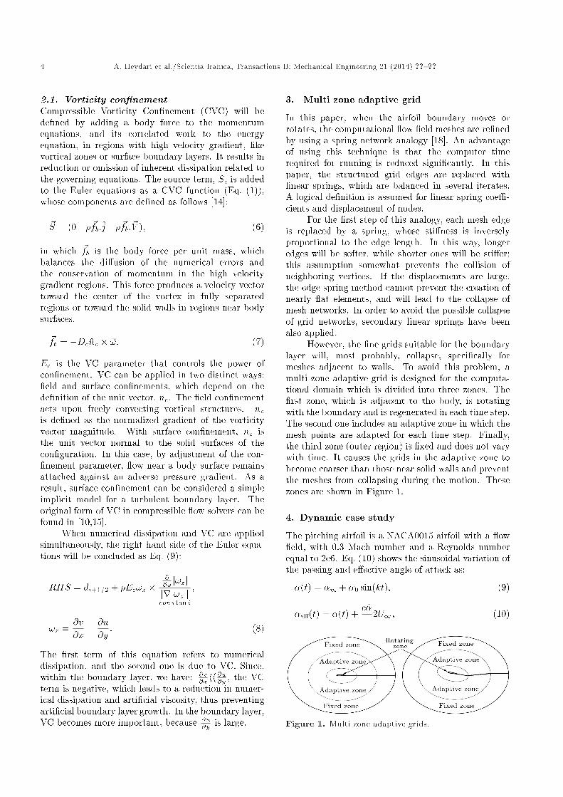
However, the �ne grids suitable for the boundarylayer will, most probably, collapse, speci�cally formeshes adjacent to walls. To avoid this problem, amulti zone adaptive grid is designed for the computa-tional domain which is divided into three zones. The�rst zone, which is adjacent to the body, is rotatingwith the boundary and is regenerated in each time step.The second one includes an adaptive zone in which themesh points are adapted for each time step. Finally,the third zone (outer region) is �xed and does not varywith time. It causes the grids in the adaptive zone tobecome coarser than those near solid walls and preventthe meshes from collapsing during the motion. Thesezones are shown in Figure 1.

4. Dynamic case study

The pitching airfoil is a NACA0015 airfoil with a ow�eld, with 0.3 Mach number and a Reynolds numberequal to 2e6. Eq. (10) shows the sinusoidal variation ofthe passing and e�ective angle of attack as:

�(t) = �m + �0 sin(kt); (9)

�e�(t) = �(t) +c _�

2U1; (10)

Figure 1. Multi zone adaptive grids.


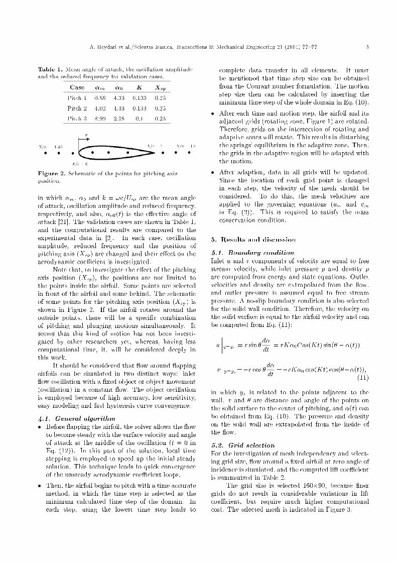
Table 1. Mean angle of attack, the oscillation amplitudeand the reduced frequency for validation cases.

Case �m �0 K Xcp

Pitch 1 0.88 4.33 0.133 0.25

Pitch 2 4.02 4.33 0.133 0.25

Pitch 3 8.99 2.08 0.1 0.25

Figure 2. Schematic of the points for pitching axisposition.

in which �m, �0 and k = !c=U1 are the mean angleof attack, oscillation amplitude and reduced frequency,respectively, and also, �e�(t) is the e�ective angle ofattack [21]. The validation cases are shown in Table 1,and the computational results are compared to theexperimental data in [2]. In each case, oscillationamplitude, reduced frequency and the position ofpitching axis (Xcp) are changed and their e�ect on theaerodynamic coe�cient is investigated.

Note that, to investigate the e�ect of the pitchingaxis position (Xcp), the positions are not limited tothe points inside the airfoil. Some points are selectedin front of the airfoil and some behind. The schematicof some points for the pitching axis position (Xcp) isshown in Figure 2. If the airfoil rotates around theoutside points, there will be a speci�c combinationof pitching and plunging motions simultaneously. Itseems that this kind of motion has not been investi-gated by other researchers yet, whereas, having lesscomputational time, it, will be considered deeply inthis work.

It should be considered that ow around appingairfoils can be simulated in two distinct ways: inlet ow oscillation with a �xed object or object movement(oscillation) in a constant ow. The object oscillationis employed because of high accuracy, low sensitivity,easy modeling and fast hysteresis curve convergence.

4.1. General algorithm� Before apping the airfoil, the solver allows the ow

to become steady with the surface velocity and angleof attack at the middle of the oscillation (t = 0 inEq. (12)). In this part of the solution, local timestepping is employed to speed up the initial steadysolution. This technique leads to quick convergenceof the unsteady aerodynamic coe�cient loops.

� Then, the airfoil begins to pitch with a time accuratemethod, in which the time step is selected as theminimum calculated time step of the domain. Ineach step, using the lowest time step leads to

complete data transfer in all elements. It mustbe mentioned that time step size can be obtainedfrom the Courant number formulation. The motionstep size then can be calculated by inserting theminimum time step of the whole domain in Eq. (10).

� After each time and motion step, the airfoil and itsadjacent grids (rotating zone, Figure 1) are rotated.Therefore, grids on the intersection of rotating andadaptive zones will rotate. This results in disturbingthe springs' equilibrium in the adaptive zone. Then,the grids in the adaptive region will be adapted withthe motion.

� After adaption, data in all grids will be updated.Since the location of each grid point is changedin each step, the velocity of the mesh should beconsidered. To do this, the mesh velocities areapplied to the governing equations (um and vmin Eq. (2)). This is required to satisfy the massconservation condition.

5. Results and discussion

5.1. Boundary conditionInlet u and v components of velocity are equal to freestream velocity, while inlet pressure p and density �are computed from energy and state equations. Outletvelocities and density are extrapolated from the ow,and outlet pressure is assumed equal to free streampressure. A no-slip boundary condition is also selectedfor the solid wall condition. Therefore, the velocity onthe solid surface is equal to the airfoil velocity and canbe computed from Eq. (11):

u��y=ys = r sin �

d�dt

= rK�0Cos(Kt) sin(� � �(t))

v��y=ys =�r cos �

d�dt

=�rK�0 cos(Kt) cos(��(t));(11)

in which ys is related to the points adjacent to thewall. r and � are distance and angle of the points onthe solid surface to the center of pitching, and �(t) canbe obtained from Eq. (10). The pressure and densityon the solid wall are extrapolated from the inside ofthe ow.

5.2. Grid selectionFor the investigation of mesh independency and select-ing grid size, ow around a �xed airfoil at zero angle ofincidence is simulated, and the computed lift coe�cientis summarized in Table 2.

The grid size is selected 160�90, because �nergrids do not result in considerable variations in liftcoe�cient, but require much higher computationalcost. The selected mesh is indicated in Figure 3.


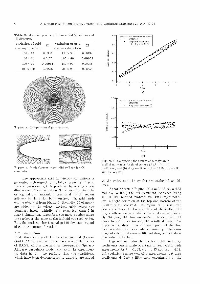
Table 2. Mesh independency in tangential (i) and normal(j) direction.Variation of gridsize inj direction

Cl Variation of gridsize in i direction

Cl

100� 70 0.0336 140� 90 0.00732

100� 80 0.0207 160� 90 0.00602

100� 90 0.00951 180� 90 0.00588

100� 100 0.00896 200� 90 0.00555

Figure 3. Computational grid network.

Figure 4. Mesh elements near solid wall for RANSsimulation.

The appropriate grid for viscous simulations isgenerated with respect to the following points: Firstly,the computational grid is produced by solving a twodimensional Poissan equation. Thus, an approximatelyorthogonal grid network is generated for the regionadjacent to the airfoil body surface. The grid meshcan be observed from Figure 4. Secondly, 20 elementsare added to the selected inviscid grids across theboundary layer. Thirdly, Y+ keeps less than 5 inRANS simulation. Therefore, the mesh number alongthe surface is the same as the inviscid one (160 grids).But, the mesh number is equal to 110 elements insteadof 90 in the normal direction.

5.3. ValidationFirst, the accuracy of the described method (CoarseGrid CFD) is examined in comparison with the resultsof RANS, with a �ne grid, a one-equation Spalart-Allmaras turbulence model, and also, the experimen-tal data in [2]. To perform this, the conditions,which have been demonstrated in Table 1, are added

Figure 5. Comparing the results of aerodynamiccoe�cients versus Angle of Attack (AoA): (a) Liftcoe�cient; and (b) drag coe�cient (k = 0:133;, �0 = 4:33and �m = 0:88).

to the code, and the results are evaluated as fol-lows.

As can be seen in Figure 5(a) k = 0:133, �0 = 4:33and �m = 0:88, the lift coe�cient, obtained usingthe CGCFD method, matches well with experiments,but, a slight deviation at the top and bottom of theoscillation is perceived. In Figure 5(b), when the ow encounters the lower surface of the airfoil, thedrag coe�cient is estimated close to the experiments.By changing the ow incidence direction from thelower to the upper surface, the results deviate fromexperimental data. The changing point of the owincidence direction is calculated correctly. The sum-mary of calculated average lift and drag coe�cients isillustrated in Table 3.

Figure 6 indicates the results of lift and dragcoe�cients versus angle of attack in comparison withexperiments for k = 0:133, �0 = 4:33 and �m = 4:02.Lift coe�cients agree well with experiments, but dragcoe�cients deviate a little from experiments at the


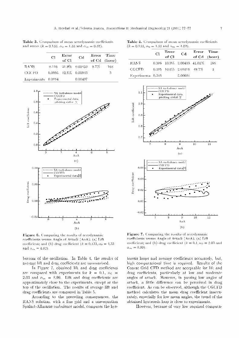
Table 3. Comparison of mean aerodynamic coe�cientsand errors (k = 0:133, �0 = 4:33 and �m = 0:88).

Cl Errorof Cl

Cd Errorof Cd

Time(hour)

RANS 0.116 21.9% 0.00453 9.7% 168

CGCFD 0.0995 12.5% 0.00943 3

Experiments 0.0884 0.00497

Figure 6. Comparing the results of aerodynamiccoe�cients versus Angle of Attack (AoA): (a) Liftcoe�cient; and (b) drag coe�cient (k = 0:133; �0 = 4:33and �m = 4:02).

bottom of the oscillation. In Table 4, the results ofaverage lift and drag coe�cients are summarized.

In Figure 7, obtained lift and drag coe�cientsare compared with experiments for k = 0:1, �0 =2:03 and �m = 8:99. Lift and drag coe�cients areapproximately close to the experiments, except at thetop of the oscillation. The results of average lift anddrag coe�cients are compared in Table 5.

According to the preceding consequences, theRANS solution, with a �ne grid and a one-equationSpalart-Allmaras turbulence model, computes the hys-

Table 4. Comparison of mean aerodynamic coe�cients(k = 0:133, �0 = 4:33 and �m = 4:02).

Cl Errorof Cl

Cd Errorof Cd

Time(hour)

RANS 0.386 10.9% 0.00403 41.01% 168

CGCFD 0.385 10.6% 0.01018 49.7% 3


Figure 7. Comparing the results of aerodynamiccoe�cients versus Angle of Attack (AoA): (a) Liftcoe�cient; and (b) drag coe�cient (k = 0:1; �0 = 2:03 and�m = 8:99).

teresis loops and average coe�cients accurately, but,high computational time is required. Results of theCoarse Grid CFD method are acceptable for lift anddrag coe�cients, particularly at low and moderateangles of attack. However, in passing low angles ofattack, a little di�erence can be perceived in dragcoe�cient. As can be observed, although the CGCFDmethod calculates the mean drag coe�cient inaccu-rately, especially for low mean angles, the trend of theobtained hysteresis loop is close to experiments.

However, because of very low required computa-


Table 5. Comparison of mean aerodynamic coe�cients(k = 0:1, �0 = 2:03 and �m = 8:99).

Cl Errorof Cl

Cd Errorof Cd

Time(hour)

RANS 0.8993 3.7% 0.0271 53.78% 168

CGCFD 0.9192 1.6% 0.0278 62.5% 3


tional time, the CGCFD method has a major advan-tage to be employed. To investigate the in uence ofunsteady parameters, this method assists in performingmore runs in the lowest possible time. Since, it takesonly three hours for one loop oscillation in each run,with a Corei5 Cpu and 4 Gigabite Ram computersystem, three to four days are enough to do all theruns needed in this paper. While, if the RANScomputation with a conventional �ne grid is used withthe same computer system, it will take about oneweek for one loop of oscillation in each run. Thus, toobtain these results, the computational time will takeat least several months. Therefore, the Coarse GridCFD method can be applied as a quick and acceptabletechnique to estimate the approximate aerodynamicbehavior of unsteady apping airfoils under greatlyvarying conditions.

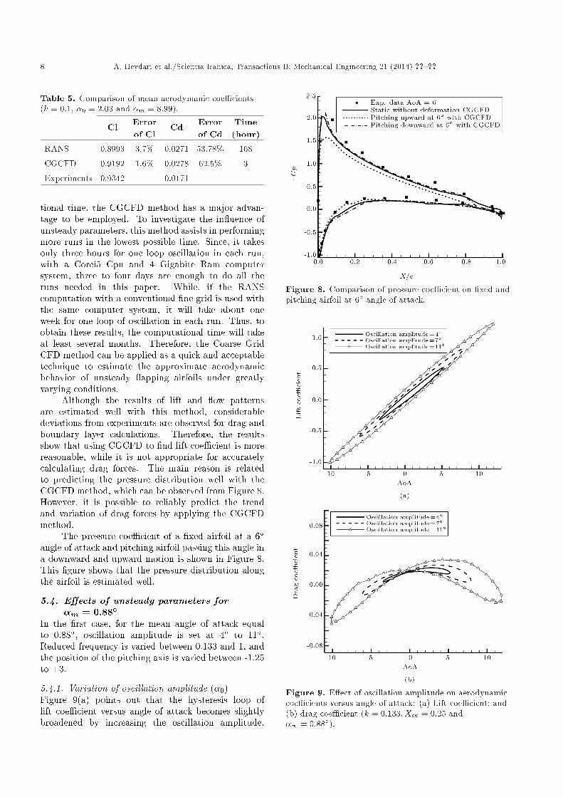
Although the results of lift and ow patternsare estimated well with this method, considerabledeviations from experiments are observed for drag andboundary layer calculations. Therefore, the resultsshow that using CGCFD to �nd lift coe�cient is morereasonable, while it is not appropriate for accuratelycalculating drag forces. The main reason is relatedto predicting the pressure distribution well with theCGCFD method, which can be observed from Figure 8.However, it is possible to reliably predict the trendand variation of drag forces by applying the CGCFDmethod.

The pressure coe�cient of a �xed airfoil at a 6�angle of attack and pitching airfoil passing this angle ina downward and upward motion is shown in Figure 8.This �gure shows that the pressure distribution alongthe airfoil is estimated well.

5.4. E�ects of unsteady parameters for�m = 0:88�

In the �rst case, for the mean angle of attack equalto 0.88�, oscillation amplitude is set at 4� to 11�.Reduced frequency is varied between 0.133 and 1, andthe position of the pitching axis is varied between -1.25to +3.

5.4.1. Variation of oscillation amplitude (�0)Figure 9(a) points out that the hysteresis loop oflift coe�cient versus angle of attack becomes slightlybroadened by increasing the oscillation amplitude.

Figure 8. Comparison of pressure coe�cient on �xed andpitching airfoil at 6� angle of attack.

Figure 9. E�ect of oscillation amplitude on aerodynamiccoe�cients versus angle of attack: (a) Lift coe�cient; and(b) drag coe�cient (k = 0:133;Xcp = 0:25 and�m = 0:88�).


But, the slope of the loop does not change. Themain reason for these behaviors is the coe�cient �0in Eq. (12). It leads to increasing the wall velocityand e�ective angle of attack (�e�), except at thetop and bottom of the cycle. Since the upper lineof the curve is related to the down-stroke and thelower line refers to the upward phase of motion, thevariation of lift coe�cient with oscillation amplitudeat the down-stroke stage is more than at the up-strokestage. From Figure 9(b), it can be seen that up anddown-stroke curves intersect each other at a point thatrefers to the e�ective angle of attack, in which the owincidence direction changes from the lower to the uppersurface. It results in a bow tie shape for the hysteresisdrag curve. Increasing the oscillation amplitude isine�ective on the position (angle) of the intersectionpoint. In high oscillation amplitudes, for example,�0 = 11�, some uctuations in drag coe�cient canbe detected at the top and bottom of the oscillationcycle. The reason is the interaction of the low pressurezones moving on the upper surface of the airfoil in theup-stroke stage and also of those zones existing on thelower surface in the downward motion.

It can be seen that by enhancing the oscillationamplitude, the maximum of the lift coe�cient isincreased and the minimum comes down. This �gureindicates that variations in maximum drag coe�cientare negligible in comparison with changes in, the lowestone. Increasing the oscillation amplitude leads to areduction in minimum drag coe�cient.

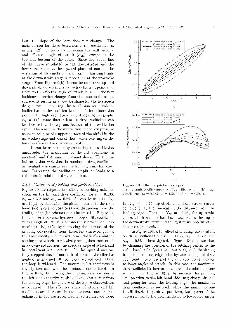
5.4.2. Variation of pitching axis position (Xcp)Figure 10 investigates the e�ect of pitching axis po-sition on the lift and drag coe�cient for k = 0:133,�0 = 4:33� and �m = 0:88. As can be seen in Fig-ure 10(a), by displacing the pitching center to the righthand side (positive positions) and distancing from thetrailing edge (its schematic is illustrated in Figure 2),the counter clockwise hysteresis loop of lift coe�cientversus angle of attack is considerably broadened. Ac-cording to Eq. (12), by increasing the distance of thepitching axis position from the surface (increasing in r),the wall velocity is increased. Since the surface and in-coming ow velocities relatively strengthen each otherin a downward motion, the e�ective angle of attack andlift coe�cient are increased. In the upward motion,they stepped down from each other and the e�ectiveangle of attack and lift coe�cient are reduced. Thus,the loop is widened. The maximum lift coe�cient isslightly increased and the minimum one is �xed. InFigure 10(a), by moving the pitching axis position tothe left side (negative positions) and distancing fromthe leading edge, the inverse of the above observationsis occurred. The e�ective angle of attack and liftcoe�cient are decreased in the downward motion, butenhanced in the upstroke, leading to a narrower loop.

Figure 10. E�ect of pitching axis position onaerodynamic coe�cients: (a) Lift coe�cient; and (b) dragCoe�cient ((k = 0:133; �0 = 4:33� and �m = 0:88�).

In Xcp = �0:75, up-stroke and down-stroke curvescoincide by further increasing the distance from theleading edge. Then, in Xcp = �1:25, the up-strokecurve, which was further down, ascends to the top ofthe down-stroke curve and the hysteresis loop directionchanges to clockwise.

In Figure 10(b), the e�ect of pitching axis positionon drag coe�cient for k = 0:133, �0 = 4:33� and�m = 0:88 is investigated. Figure 10(b) shows thatby changing the position of the pitching center to theright hand side (positive positions), and displacingfrom the trailing edge, the hysteresis loop of dragcoe�cient moves up and the intersect point inclinesto lower angles of attack. In this case, the maximumdrag coe�cient is increased, whereas the minimum oneis �xed. In Figure 10(b), by moving the pitchingaxis position to the left hand side (negative positions)and going far from the leading edge, the maximumdrag coe�cient is reduced, while the minimum oneis still �xed. In positive positions, both parts of thecurve related to the ow incidence to lower and upper


surfaces are in uenced. But, in negative places, justthe curve part related to the ow incidence to the lowersurface is a�ected. Changing the drag hysteresis loopdirection can be observed at position Xcp = �0:75.From Figure 10, the lift and drag coe�cients relatedto the top and bottom of the cycle are not a�ected bymoving the pitching axis position. Because, in thesepoints, cos(Kt) is equal to zero (Eq. (12)), the surfacevelocities vanish.

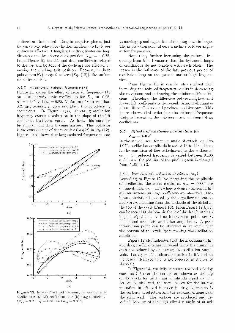
5.4.3. Variation of reduced frequency (k)Figure 11 shows the e�ect of reduced frequency (k)on mean aerodynamic coe�cients for Xcp = 0:25,�0 = 4:33� and �m = 0:88. Variation of k to less than0.2, approximately, does not a�ect the aerodynamiccoe�cients. In Figure 11(a), increasing oscillationfrequency causes a reduction in the slope of the liftcoe�cient hysteresis curve. At �rst, this curve isbroadened, and then become narrow. This behavioris the consequence of the term k�Cos(kt) in Eq. (12).Figure 11(b) shows that large reduced frequencies lead

Figure 11. E�ect of reduced frequency on aerodynamiccoe�cients: (a) Lift coe�cient; and (b) drag coe�cient(Xcp = 0:25, �0 = 4:33� and �m = 0:88�).

to moving up and expansion of the drag bow tie shape.The intersection point of curves inclines to lower anglesat low frequencies.

Note that, further increasing the reduced fre-quency from k = 1 ensures that the hysteresis loopsof oscillations do not coincide with each other. Thereason is the in uence of the last previous period ofoscillation loop on the present one at high frequen-cies.

From Figure 11, it can be also realized thatincreasing the reduced frequency results in decreasingthe maximum and enhancing the minimum lift coe�-cient. Therefore, the di�erence between highest andlowest lift coe�cients is decreased. Also, it eliminatesminus lift coe�cients and produces positive ones. This�gure shows that enlarging the reduced frequencyleads to increasing the maximum and minimum dragcoe�cients.

5.5. E�ects of unsteady parameters for�m = 4:02�

In the second case, for mean angle of attack equal to4.02�, oscillation amplitude is set at 1� to 11�. Then,in the condition of ow attachment to the surface at�0 = 4�, reduced frequency is varied between 0.133and 1, and the position of the pitching axis is changedfrom -1.25 to +3.

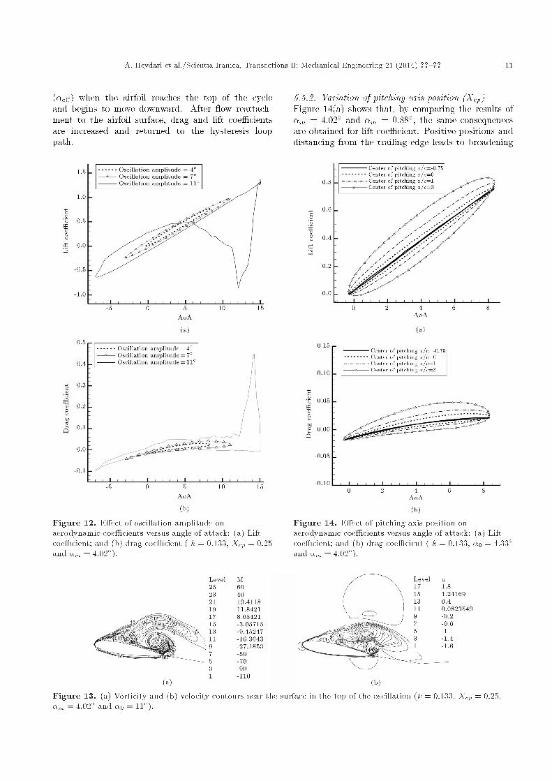
5.5.1. Variation of oscillation amplitude (�0)According to Figure 12, by increasing the amplitudeof oscillation, the same results as �m = 0:88� areobtained, until �0 = 11�, where a deep reduction in liftand an increase in drag coe�cient are observed. Thisintense variation is caused by the large ow separationand vortex shedding from the backside of the airfoil atthe top of the cycle (Figure 13). From Figure 12(b), itcan be seen that the bow tie shape of the drag hysteresisloop is wiped out, and no intersection point occursin low and moderate oscillation amplitudes. A poorintersection point can be observed in an angle nearthe bottom of the cycle by increasing the oscillationamplitude.

Figure 12 also indicates that the maximum of liftand drag coe�cients are increased while the minimumones are reduced by enhancing the oscillation ampli-tude. For �0 = 11�, intense reduction in lift and anincrease in drag coe�cients are observed at the top ofthe cycle.

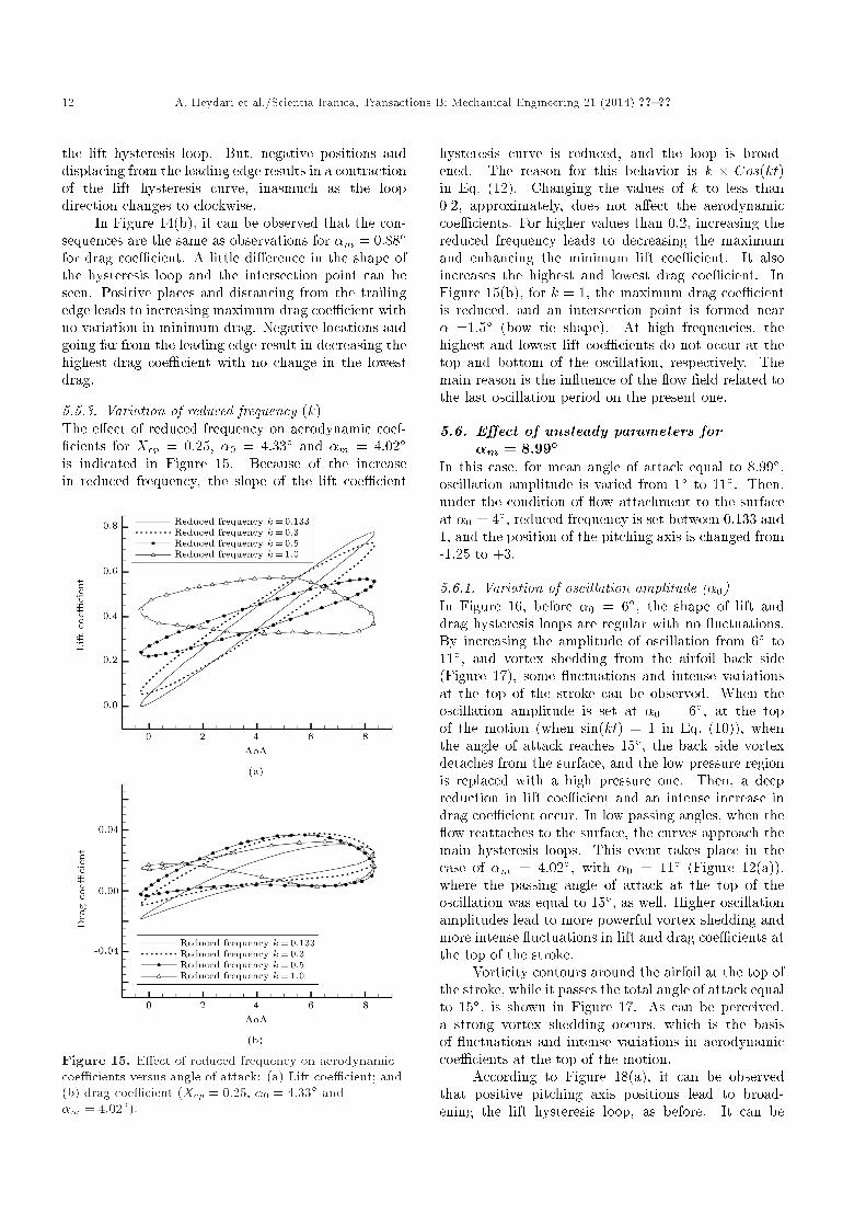
In Figure 13, vorticity contours (a) and velocitycontours (b) near the surface are shown at the topof the cycle for oscillation amplitude equal to 11�.As can be observed, the main reason for the intensereduction in lift and increase in drag coe�cient isthe vorticity production and the separation zone nearthe solid wall. The vortices are produced and de-tached because of the high e�ective angle of attack


(�e�) when the airfoil reaches the top of the cycleand begins to move downward. After ow reattach-ment to the airfoil surface, drag and lift coe�cientsare increased and returned to the hysteresis looppath.

Figure 12. E�ect of oscillation amplitude onaerodynamic coe�cients versus angle of attack: (a) Liftcoe�cient; and (b) drag coe�cient ( k = 0:133, Xcp = 0:25and �m = 4:02�).

5.5.2. Variation of pitching axis position (Xcp)Figure 14(a) shows that, by comparing the results of�m = 4:02� and �m = 0:88�, the same consequencesare obtained for lift coe�cient. Positive positions anddistancing from the trailing edge leads to broadening

Figure 14. E�ect of pitching axis position onaerodynamic coe�cients versus angle of attack: (a) Liftcoe�cient; and (b) drag coe�cient ( k = 0:133, �0 = 4:33�and �m = 4:02�).

Figure 13. (a) Vorticity and (b) velocity contours near the surface in the top of the oscillation (k = 0:133, Xcp = 0:25,�m = 4:02� and �0 = 11�).


the lift hysteresis loop. But, negative positions anddisplacing from the leading edge results in a contractionof the lift hysteresis curve, inasmuch as the loopdirection changes to clockwise.

In Figure 14(b), it can be observed that the con-sequences are the same as observations for �m = 0:88�for drag coe�cient. A little di�erence in the shape ofthe hysteresis loop and the intersection point can beseen. Positive places and distancing from the trailingedge leads to increasing maximum drag coe�cient withno variation in minimum drag. Negative locations andgoing far from the leading edge result in decreasing thehighest drag coe�cient with no change in the lowestdrag.

5.5.3. Variation of reduced frequency (k)The e�ect of reduced frequency on aerodynamic coef-�cients for Xcp = 0:25, �0 = 4:33� and �m = 4:02�is indicated in Figure 15. Because of the increasein reduced frequency, the slope of the lift coe�cient

Figure 15. E�ect of reduced frequency on aerodynamiccoe�cients versus angle of attack: (a) Lift coe�cient; and(b) drag coe�cient (Xcp = 0:25, �0 = 4:33� and�m = 4:02�).

hysteresis curve is reduced, and the loop is broad-ened. The reason for this behavior is k � Cos(kt)in Eq. (12). Changing the values of k to less than0.2, approximately, does not a�ect the aerodynamiccoe�cients. For higher values than 0.2, increasing thereduced frequency leads to decreasing the maximumand enhancing the minimum lift coe�cient. It alsoincreases the highest and lowest drag coe�cient. InFigure 15(b), for k = 1, the maximum drag coe�cientis reduced, and an intersection point is formed near� =1.5� (bow tie shape). At high frequencies, thehighest and lowest lift coe�cients do not occur at thetop and bottom of the oscillation, respectively. Themain reason is the in uence of the ow �eld related tothe last oscillation period on the present one.

5.6. E�ect of unsteady parameters for�m = 8:99�

In this case, for mean angle of attack equal to 8.99�,oscillation amplitude is varied from 1� to 11�. Then,under the condition of ow attachment to the surfaceat �0 = 4�, reduced frequency is set between 0.133 and1, and the position of the pitching axis is changed from-1.25 to +3.

5.6.1. Variation of oscillation amplitude (�0)In Figure 16, before �0 = 6�, the shape of lift anddrag hysteresis loops are regular with no uctuations.By increasing the amplitude of oscillation from 6� to11�, and vortex shedding from the airfoil back side(Figure 17), some uctuations and intense variationsat the top of the stroke can be observed. When theoscillation amplitude is set at �0 = 6�, at the topof the motion (when sin(kt) = 1 in Eq. (10)), whenthe angle of attack reaches 15�, the back side vortexdetaches from the surface, and the low pressure regionis replaced with a high pressure one. Then, a deepreduction in lift coe�cient and an intense increase indrag coe�cient occur. In low passing angles, when the ow reattaches to the surface, the curves approach themain hysteresis loops. This event takes place in thecase of �m = 4:02�, with �0 = 11� (Figure 12(a)),where the passing angle of attack at the top of theoscillation was equal to 15�, as well. Higher oscillationamplitudes lead to more powerful vortex shedding andmore intense uctuations in lift and drag coe�cients atthe top of the stroke.

Vorticity contours around the airfoil at the top ofthe stroke, while it passes the total angle of attack equalto 15�, is shown in Figure 17. As can be perceived,a strong vortex shedding occurs, which is the basisof uctuations and intense variations in aerodynamiccoe�cients at the top of the motion.

According to Figure 18(a), it can be observedthat positive pitching axis positions lead to broad-ening the lift hysteresis loop, as before. It can be


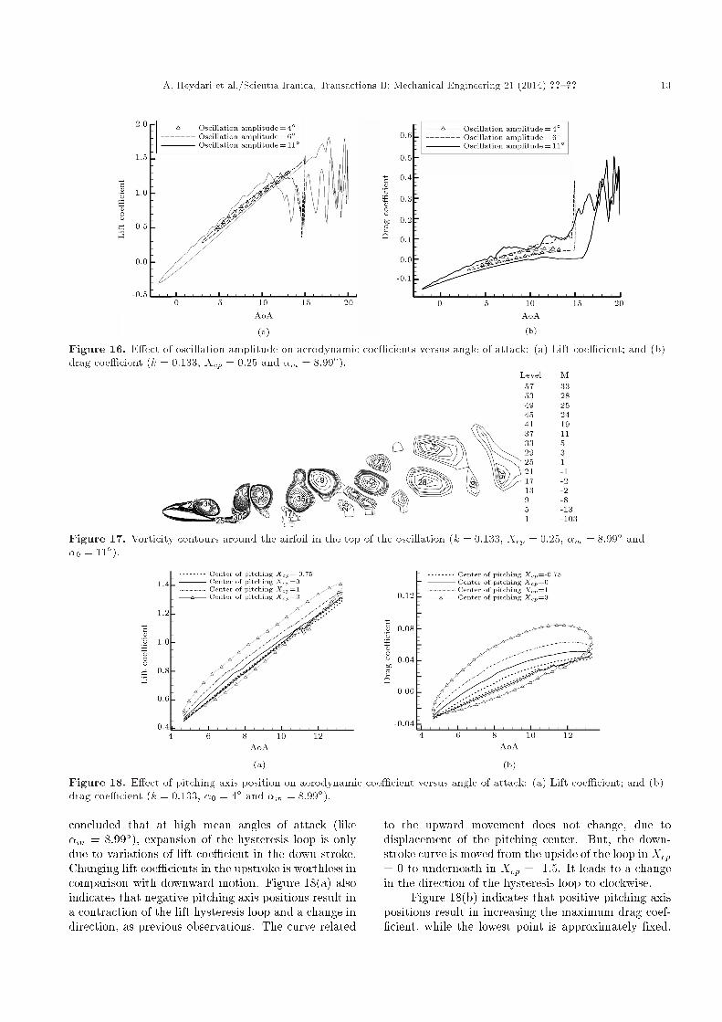
Figure 16. E�ect of oscillation amplitude on aerodynamic coe�cients versus angle of attack: (a) Lift coe�cient; and (b)drag coe�cient (k = 0:133, Xcp = 0:25 and �m = 8:99�).

Figure 17. Vorticity contours around the airfoil in the top of the oscillation (k = 0:133, Xcp = 0:25, �m = 8:99� and�0 = 11�).

Figure 18. E�ect of pitching axis position on aerodynamic coe�cient versus angle of attack: (a) Lift coe�cient; and (b)drag coe�cient (k = 0:133, �0 = 4� and �m = 8:99�).

concluded that at high mean angles of attack (like�m = 8:99�), expansion of the hysteresis loop is onlydue to variations of lift coe�cient in the down stroke.Changing lift coe�cients in the upstroke is worthless incomparison with downward motion. Figure 18(a) alsoindicates that negative pitching axis positions result ina contraction of the lift hysteresis loop and a change indirection, as previous observations. The curve related

to the upward movement does not change, due todisplacement of the pitching center. But, the down-stroke curve is moved from the upside of the loop in Xcp= 0 to underneath in Xcp = -1.5. It leads to a changein the direction of the hysteresis loop to clockwise.

Figure 18(b) indicates that positive pitching axispositions result in increasing the maximum drag coef-�cient, while the lowest point is approximately �xed.


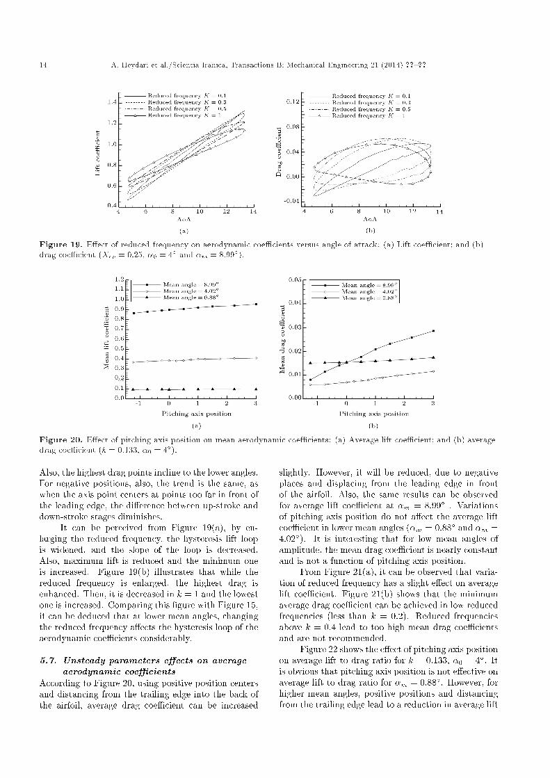
Figure 19. E�ect of reduced frequency on aerodynamic coe�cients versus angle of attack: (a) Lift coe�cient; and (b)drag coe�cient (Xcp = 0:25, �0 = 4� and �m = 8:99�).

Figure 20. E�ect of pitching axis position on mean aerodynamic coe�cients: (a) Average lift coe�cient; and (b) averagedrag coe�cient (k = 0:133, �0 = 4�).

Also, the highest drag points incline to the lower angles.For negative positions, also, the trend is the same, aswhen the axis point centers at points too far in front ofthe leading edge, the di�erence between up-stroke anddown-stroke stages diminishes.

It can be perceived from Figure 19(a), by en-larging the reduced frequency, the hysteresis lift loopis widened, and the slope of the loop is decreased.Also, maximum lift is reduced and the minimum oneis increased. Figure 19(b) illustrates that while thereduced frequency is enlarged, the highest drag isenhanced. Then, it is decreased in k = 1 and the lowestone is increased. Comparing this �gure with Figure 15,it can be deduced that at lower mean angles, changingthe reduced frequency a�ects the hysteresis loop of theaerodynamic coe�cients considerably.

5.7. Unsteady parameters e�ects on averageaerodynamic coe�cients

According to Figure 20, using positive position centersand distancing from the trailing edge into the back ofthe airfoil, average drag coe�cient can be increased

slightly. However, it will be reduced, due to negativeplaces and displacing from the leading edge in frontof the airfoil. Also, the same results can be observedfor average lift coe�cient at �m = 8:99� . Variationsof pitching axis position do not a�ect the average liftcoe�cient in lower mean angles (�m = 0:88� and �m =4:02�). It is interesting that for low mean angles ofamplitude, the mean drag coe�cient is nearly constantand is not a function of pitching axis position.

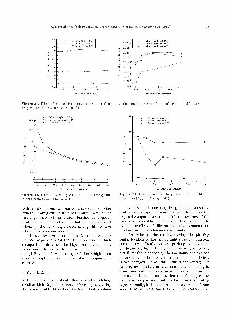
From Figure 21(a), it can be observed that varia-tion of reduced frequency has a slight e�ect on averagelift coe�cient. Figure 21(b) shows that the minimumaverage drag coe�cient can be achieved in low reducedfrequencies (less than k = 0:2). Reduced frequenciesabove k = 0:4 lead to too high mean drag coe�cientsand are not recommended.

Figure 22 shows the e�ect of pitching axis positionon average lift to drag ratio for k = 0:133, �0 = 4�. Itis obvious that pitching axis position is not e�ective onaverage lift to drag ratio for �m = 0:88�. However, forhigher mean angles, positive positions and distancingfrom the trailing edge lead to a reduction in average lift


Figure 21. E�ect of reduced frequency on mean aerodynamic coe�cients: (a) Average lift coe�cient; and (b) averagedrag coe�cient (Xcp = 0:25, �0 = 4�).

Figure 22. E�ect of pitching axis position on average liftto drag ratio (k = 0:133, �0 = 4�).

to drag ratio. Inversely, negative values and displacingfrom the leading edge in front of the airfoil bring aboutvery high values of this ratio. Further, in negativepositions, it can be observed that if mean angle ofattack is selected at high value, average lift to dragratio will become maximum.

It can be seen from Figure 23 that very lowreduced frequencies (less than k = 0:2) result in highaverage lift to drag ratio for high mean angles. Thus,to maximize the ratio or to improve the ight e�ciencyin high Reynolds ows, it is required that a high meanangle of amplitude with a low reduced frequency isselected.

6. Conclusions

In this article, the unsteady ow around a pitchingairfoil at high Reynolds number is investigated. Usingthe Coarse Grid CFD method, surface vorticity con�ne-

Figure 23. E�ect of reduced frequency on average lift todrag ratio (Xcp = 0:25, �0 = 4�).

ment and a multi zone adaptive grid, simultaneously,leads to a high-speed scheme that greatly reduces therequired computational time, while the accuracy of theresults is acceptable. Therefore, we have been able toexplore the e�ects of di�erent unsteady parameters onpitching airfoil aerodynamic coe�cients.

According to the results, moving the pitchingcenter location to the left or right sides has di�erentconsequences. Firstly, positive pitching axis positionsor distancing from the trailing edge in back of theairfoil, results in enhancing the maximum and averagelift and drag coe�cients, while the minimum coe�cientis not changed. Also, this reduces the average liftto drag ratio mainly at high mean angles. Thus, insome practical situations, in which only lift force isimportant, it is appropriate that the pitching centerbe placed in positive positions far from the trailingedge. Secondly, if the purpose is increasing the lift andsimultaneously decreasing the drag, it is necessary that


the pitching axis position be situated in front of theairfoil far from the leading edge. This also results in theincreasing of average lift to drag ratio. Furthermore,the enlarging oscillation amplitude at high Reynolds ow, generally, has no considerable in uence on thelift to drag ratio or e�ciency of the ight. In addition,to maximize the average lift to drag ratio at highReynolds ows, lower frequencies are desired. Finally,it should be stated that at lower mean angles of attack,unsteady parameters have no in uence on the averagelift coe�cient.

References

1. McCroskey, W.J. \The phenomenon of dynamic stall",NASA report: NASA/TM-81264-1981.

2. Piziali, R.A. \An experimental investigation of 2Dend 3D oscillating wing aerodynamics for a range ofangle of attack including stall", NASA Technical Mem-orandum, No. 4632. Ames, CA:NASA 4632, ChalmersUniversity of Technology (1993).

3. Tuncer, I., Wu, J. and Wang, C. \Theoretical and nu-merical studies of oscillating airfoils", AIAA Journal,28(9), pp. 1615-1624 (1990).

4. Akbari, M. and Price, S. \Simulation of dynamic stallfor a naca 0012 airfoil using a vortex method", Journalof Fluids and Structures, 17, pp. 855-874 (2003).

5. Sarkar, S. and Venkatraman, K. \In uence of pitchingangle of incidence on the dynamic stall behavior ofa symmetric airfoil", European Journal of MechanicsB/Fluids, 27, pp. 219-238 (2008).

6. Martinat, G., Braza, M., Hoarau, Y. and Harran,G. \Turbulence modelling of the ow past a pitchingNACA0012 airfoil at105 and 106 Reynolds numbers",Journal of Fluids and Structures, 24, pp. 1294-1303(2008).

7. Amiralaei, M.R., Alighanbari, H. and Hashemi, S.M.\An investigation into the e�ects of unsteady param-eters on the aerodynamics of a low Reynolds numberpitching airfoil", Journal of Fluids and Structures, 26,pp. 979-993 (2010).

8. You D. and Bromby W. \Large-eddy simulation ofunsteady separation over a pitching airfoil at highReynolds number", Seventh International Conferenceon Computational Fluid Dynamics (ICCFD7), BigIsland, Hawaii, July 9-13 (2012).

9. Ou, K. and Jameson, A. \Optimization of ow pasta moving deformable airfoil using spectral di�erencemethod", 41st AIAA Fluid Dynamics Conference andExhibit, 27-30 June 2011, Honolulu, Hawaii, AIAA2011-3719 (2011).

10. Steinho�, J. \Vorticity con�nement: a new techniquefor computing vortex dominated ows", Frontiers of

Computational Fluid Dynamics, D.A. Caughey andM.M. Hafez, Eds., J. Wiley & Sons (1994).

11. Hu, G., Grossman, B. and Steinho�, J. \A numericalmethod for vortex con�nement in compressible ow",AIAA-00-0281 (2000).

12. Lynn, N.F. and Steinho�, J. \Large Reynolds numberturbulence modeling with vorticity con�nement", 18thAIAA Computational Fluid Dynamics Conference, 25-28, Miami, FL June (2007).

13. Moulton, M. and Steinho�, J. \A technique for thesimulation of stall with coarse-grid CFD", AIAA-00-0277 (2000).

14. Wenren, Y., Fan, M., Dietz, W., Hu, G., Braun,C., Steinho�, J. and Grossman, B. \E�cient Euleriancomputation of realistic rotorcraft ows using vorticitycon�nement", AIAA-01-0996 (2001).

15. Dietz, W.E. \Application of vorticity con�nement tocompressible ow", 42nd AIAA Aerospace SciencesMeeting and Exhibit, Reno, Nevada, 5-8 January(2004).

16. Butsuntorn, N., Jameson, A. \Time spectral methodfor rotorcraft ow with vorticity con�nement", 26thAIAA Applied Aerodynamics Conference, Honolulu,Hawaii, pp. 18-21 (2008).

17. Bagheri-Esfeh, H. and Malek-jafarian, M. \Develop-ment of arti�cial dissipation schemes and compressiblevorticity con�nement methods", Journal of AerospaceEngineering, 225(8), pp. 929-945 (2011).

18. Nakahashi, k. and Deiwert, G.S. \Three dimensionaladaptive grid method", AIAA Journal, 124(6), pp.948-954 (1999).

19. Murayama, M., Nakahashi, K. and Matsushima, K.\Unstructured dynamic mesh for large movement anddeformation", AIAA Conf., Paper 122 (2002).

20. Nadarajah, S.K. and Jameson, A. \Optimal controlof unsteady ows using a time accurate method",9th AIAA/ISSMO Symposium on MultidisciplinaryAnalysis and Optimization Conference, Paper 5436(2002).

21. Jameson, A., Schmidt, W. and Turkel, E. \Numericalsolutions of the Euler equations by �nite volumemethods using runge-kutta time-stepping schemes",AIAA Journal, 81, pp. 1259 (1981).

22. Spalart, P.R. and Allmaras, S.R. \A one equationturbulence model for aerodynamic ows", AIAA 92-0439, AIAA 30th Aerospace Sciences Meeting andExhibit , Reno, NV, January (1992).

Biographies

Mahmoud Pasandideh Fard obtained a BS degreein Heat and Fluid Engineering, in 1985, an MS degreein Energy Conversion Engineering from Ferdowsi Uni-versity of Mashhad, Iran, in 1988, and a PhD degree


in Aerodynamics from Sydney University, Australia, in1996. He is currently on the academic sta� of FerdowsiUniversity of Mashhad, Iran. His research interestsinclude supersonic and subsonic aerodynamics, hydro-dynamics, cavitation and supercavitation, aerodynam-ics and hydrodynamics of projectiles and missiles, andturbulent boundary ow. He has completed severalindustrial projects and has presented and publishedmore than 50 conference and 20 journal papers in his�elds of interest.

Majid Malek-Jafarian was born in Mashhad, Iran,in 1975. He received a BS in Fluid Mechanics, anMS degree in Energy Conversion, in 1999, and a PhDdegree, in 2006, all from the Mechanical EngineeringDepartment of Ferdowsi University of Mashhad, Iran.

His research interests include turbulence modeling,aerodynamics and optimization, and he is currentlyworking in the Mechanical Engineering Department ofthe University of Birjand, Iran.

Ali Heydari was born in Mashhad, Iran, in 1983.He received a BS degree in Mechanics, in 2006, andan MS degree in Energy Conversion, in 2006, fromthe Mechanical Engineering Department of FerdowsiUniversity, Iran, where he is currently a PhD degreestudent in the same subject. His research interestsinclude CFD, unsteady aerodynamics, boundary layercharacteristics and solar energy, and he is currentlyworking on the academic sta� of the Mechanical En-gineering Department at the Islamic Azad Universityof Semnan, Iran.

Investigation of unsteady parameter eects on aerodynamic coecients of pitching airfoil using coarse grid simulation

Documents