Investigation of the response time of the equatorial ionosphere in context of the equatorial electrojet and equatorial ionization anomaly

Ann. Geophys., 29, 1267–1275, 2011www.ann-geophys.net/29/1267/2011/doi:10.5194/angeo-29-1267-2011© Author(s) 2011. CC Attribution 3.0 License.

AnnalesGeophysicae

Investigation of the response time of the equatorial ionosphere incontext of the equatorial electrojet and equatorial ionizationanomaly

L. Jose1, S. Ravindran1, C. Vineeth1, T. K. Pant1, and S. Alex2

1Space Physics Laboratory, Vikram Sarabhai Space Centre, Trivandrum, India2Indian Institute of Geomagnetism, Navi Mumbai, India

Received: 29 November 2010 – Revised: 22 June 2011 – Accepted: 4 July 2011 – Published: 19 July 2011

Abstract. Equatorial Electrojet (EEJ) and Equatorial Ion-ization Anomaly (EIA) are two large-scale processes in theequatorial/low latitude ionosphere, driven primarily by theeastward electric field during daytime. In the present pa-per we investigate the correlation between the Integrated EEJstrength (IEEJ) and the EIA parameters like the total elec-tron content at the northern crest, location of crest in Mag-netic latitude and strength of the EIA for the Indian sector.A good correlation has been observed between the IEEJ andEIA when a time delay is introduced between IEEJ and EIAparameters. This time delay is regarded as the response timeof equatorial ionosphere in context of the evolution of EIAvis-a-vis EEJ. Further, a seasonal variation in the time delayhas been observed, which is believed to be due to changes inthermospheric wind. Using the response time and the linearrelationship obtained, the possibility of near-real time pre-diction of EIA parameters has been attempted and found thatthe prediction holds well during the geomagnetically quietperiods. The paper discusses these aspects in detail.

Keywords. Ionosphere (Electric fields and currents; Equa-torial ionosphere)

1 Introduction

Equatorial and low latitude ionosphere has many unique fea-tures like Equatorial Electrojet (EEJ), Equatorial IonizationAnomaly (EIA) and is more likely to have Equatorial spreadF (ESF)/scintillations and other irregularities. These phe-nomena are the manifestation of the unique electrodynamicsin this region. The EEJ refers to an intense band of eastwardcurrent centered at dip equator flowing in the height range of90–130 km, during daytime (Forbes, 1981; Richmond, 1989;

Correspondence to:L. Jose([email protected])

Reddy, 1989). In simple thin shell model, generation of EEJcan be explained as follows. The mutually perpendicular na-ture of the primary electric field (generated due to the tidalwind) and magnetic field in the equatorial E-region give riseto a vertical polarization electric field. This in turn being per-pendicular to the northward horizontal magnetic field givesrise to an enhanced current in the E-region, called the EEJ.

The EIA was discovered by Appleton (1946) and laterexplained by Mitra (1946) and Martyn (1947) in terms of“fountain effect”. The upward plasma drift associated withthe EIA is produced by the F-region electric field, which ismapped from the E-region along the magnetic field lines dur-ing daytime. Because of the perpendicular nature of the elec-tric and magnetic fields the plasma is lifted upward byE×B

drift. At higher altitudes, plasma diffuses downward alongthe geomagnetic field lines on either sides of the dip equatorby the action of gravitational and pressure gradient forces.This creates a double hump structure in the horizontal dis-tribution of the electron density over equatorial/low latitudeionosphere, known as the EIA. Apart from this, the genera-tion, evolution and latitudinal extent of the EIA is stronglydepend on the variability of the zonal electric field, prevail-ing space weather conditions, high-latitude low-latitude cou-pling, season and solar activity (Anderson, 1973a, b; Ras-togi, 1959; Abdu et al., 1990; Sastri, 1990). From the abovedescriptions it is clear that both the EEJ and EIA are drivenprimarily by the same eastward electric field. Therefore itis quite natural to expect a correlation between these two.However, it should be noted that the EEJ strength is only anindirect measure of electric field as it is also determined byconductivities, which is a function of solar flux. In the ab-sence of direct electric field measurements, this can be usedas a proxy for the electric field and many studies have alreadybeen conducted in this direction.

Dunford (1967) was the first to report significant correla-tion between the strength of EIA and daily range of horizon-tal magnetic field at the equatorial station using the topside

Published by Copernicus Publications on behalf of the European Geosciences Union.

1268 L. Jose et al.: Investigation of the response time of the equatorial ionosphere

sounder data. The strength of the EIA was defined as thedepth of the EIA,D = (Np −Ne)/Ne multiplied by widthW = Latp−Late of the anomaly. WhereNp andNe are elec-tron densities at the peak and magnetic equator respectivelyandW is the location of crest (Latp) with respect to mag-netic equator (Late). Later on, using ground-based iono-grams, Rastogi and Rajaram (1971) reported that the mid-day bite out ofNmF2 at trough and afternoon peak ofNmF2at crest are systematically enhanced in accordance with thehorizontal geomagnetic field at the equatorial station. Rushand Richmond (1973) usedfoF2 data to study the correlationbetween midday EEJ values and EIA. They found maximumcorrelation for EIA parameters obtained between 14:00 and16:00 LT and a lag of 2–3 h between the two. The correlationis found to be maximum during the equinoxes and minimumin June solstice. This was attributed to the strong electro-dynamical control during equinoxial months. Deshpande etal. (1977) showed that crest development is strong during astrong EEJ day, weak during Counter Electrojet (CEJ) dayand not at all developed during a geomagnetically disturbedday. They found a time delay of∼2 h between the startingof CEJ and the near-end of the EIA. Raghavarao et al. (1978)have reported a correlation of∼0.9 between the electron den-sity at 500 km altitude and the time integrated EEJ strength.Rastogi and Klobuchar (1990) observed a further increase incorrelation between these two when mean EEJ strength be-tween 07:00 and 14:00 LT is used.

The aforesaid studies confirmed that the development ofEIA depends not only on the midday instantaneous valuesbut also on the past history of EEJ variation. Using the To-tal Electron Content (TEC) data from ATS 6 geostationarysatellite, Balan and Iyer (1983) have brought out the seasonalvariation (summer, winter and equinox) of the EIA with re-spect to the EEJ strength. They found high correlation be-tween the peak EIA strength and the peak value of horizontalfield for all the seasons. They also reported a consistent timelag of 3–4 h between the maximum EIA and the EEJ current,which was regarded as the time required for the evolution ofthe EIA. Using the data from the Navy Navigation SatelliteSystem (NNSS) and the ETS-2 satellite, Huang et al. (1989)have shown that the latitude of the EIA crest is more cor-related to the EEJ strength than its magnitude. Similarly,a high correlation between the height of the peak F2 layerat the trough region and the EEJ strength has been reportedfrom the Brazilian sector (Abdu et al., 1990). They found aresponse time of 2.5–4 h between height of F2 peak over theequator and enhanced electron density at the EIA crest. Theresponse time is suggested to be dependent on vertical driftvelocity, height of the populated flux tube (longer time forhigher flux tubes) and the intensity of the meridional winds.

The dependence of EIA on EEJ got further confirmationwhen using the Global Positioning System (GPS) TEC dataof solar minimum period. The daily values of maximumEIA parameters were shown to be highly correlated withdaily-integrated EEJ strength (Rao et al., 2006). Using the

measurements from satellite based Planar Langmuir Probe(PLP), Stolle et al. (2008) have shown that the Crest to troughratio of EIA responds to the variations of vertical drift val-ues with a time delay of∼1–2 h and EEJ strength∼2–4 h.On the whole, the time delay between EIA and EEJ appearsto be∼2–4 h on geomagnetically quiet days. Over the In-dian region, most of these studies have been performed usingionograms or satellite data. In the present paper, we usedGPS TEC data from a longitudinal network of stations in theIndian region for finding the response time of EEJ on EIA inthe Indian sector. The advantage of using GPS data is thatthe TEC values are available round the clock and the exactresponse time could be found out. Most of the previous stud-ies used instantaneous values of EEJ or integrated value forthe whole day to find out the correlation. Here, instead oftaking a single value, Integrated EEJ (IEEJ) strength is ob-tained at every 20 min from 07:00 LT onwards till the peakof the EEJ. This is correlated with EIA parameters averagedfor every 20 min by introducing a time delay between thetwo. The time delay at which the maximum correlation ob-tained is considered to be the response time of the EIA. Us-ing this, a near-real time prediction of EIA parameters havebeen attempted and found that the prediction holds well dur-ing all the days, which are geomagnetically quiet. This isbelieved to have great importance in space based navigationsystems where the near-real time ionospheric predictions arerequired.

2 Experimental data and method of analysis

The GPS satellite system is one of the widely used toolsfor ionospheric studies. GPS uses two L-band signals L1(1.5754 GHz) and L2 (1.2276 GHz) for deriving Total Elec-tron Content (TEC) along the signal path (Klobuchar, 1996).Since GPS satellites are available all the time, it is a verygood tool for studying the time evolution EIA. As a part ofGAGAN, (GPS Aided Geo Augmented Navigation) a com-bined project by Indian Space Research Organization (ISRO)and Airport Authority of India (AAI), a network of eigh-teen dual frequency GPS TEC monitoring stations have beensetup over the Indian region. To study the day-to-day vari-ability of EIA for the solar minimum epoch, a chain of sixTEC stations along 77–78◦ E longitude [Trivandrum (8.5◦ N,77◦ E, 0.31◦ S mag. lat.), Bangalore (12.5◦ N, 77.5◦ E, 3.6◦ Nmag. lat.), Hyderabad (17◦ N, 78.5◦ E, 8.5◦ N mag. lat.),Bhopal (23◦ N, 77.5◦ E, 14.25◦ N mag. lat), Delhi (28.5◦ N,77◦ E, 19.5◦ N mag. lat) and Shimla (31◦ N, 77◦ E, 22◦ Nmag. lat)] are selected. While converting the measured slantTEC to vertical TEC, satellite elevation angle cut off of 60◦

(to eliminate the errors due to large gradient changes in theequatorial and low latitude regions) and IPP (IonosphericPierce Point) altitude of 350 km are used.

The Magnetic field data from two stations, an equatorialstation Tirunelveli (8.7◦ N, 77.8◦ E, 0.17◦ S dip lat.) and

Ann. Geophys., 29, 1267–1275, 2011 www.ann-geophys.net/29/1267/2011/

L. Jose et al.: Investigation of the response time of the equatorial ionosphere 1269

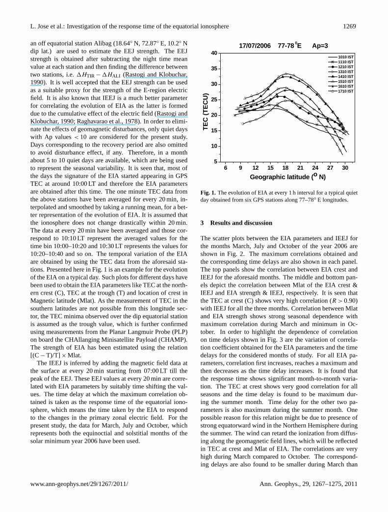
an off equatorial station Alibag (18.64◦ N, 72.87◦ E, 10.2◦ Ndip lat.) are used to estimate the EEJ strength. The EEJstrength is obtained after subtracting the night time meanvalue at each station and then finding the difference betweentwo stations, i.e.1HTIR −1HALI (Rastogi and Klobuchar,1990). It is well accepted that the EEJ strength can be usedas a suitable proxy for the strength of the E-region electricfield. It is also known that IEEJ is a much better parameterfor correlating the evolution of EIA as the latter is formeddue to the cumulative effect of the electric field (Rastogi andKlobuchar, 1990; Raghavarao et al., 1978). In order to elimi-nate the effects of geomagnetic disturbances, only quiet dayswith Ap values< 10 are considered for the present study.Days corresponding to the recovery period are also omittedto avoid disturbance effect, if any. Therefore, in a monthabout 5 to 10 quiet days are available, which are being usedto represent the seasonal variability. It is seen that, most ofthe days the signature of the EIA started appearing in GPSTEC at around 10:00 LT and therefore the EIA parametersare obtained after this time. The one minute TEC data fromthe above stations have been averaged for every 20 min, in-terpolated and smoothed by taking a running mean, for a bet-ter representation of the evolution of EIA. It is assumed thatthe ionosphere does not change drastically within 20 min.The data at every 20 min have been averaged and those cor-respond to 10:10 LT represent the averaged values for thetime bin 10:00–10:20 and 10:30 LT represents the values for10:20–10:40 and so on. The temporal variation of the EIAare obtained by using the TEC data from the aforesaid sta-tions. Presented here in Fig. 1 is an example for the evolutionof the EIA on a typical day. Such plots for different days havebeen used to obtain the EIA parameters like TEC at the north-ern crest (C), TEC at the trough (T) and location of crest inMagnetic latitude (Mlat). As the measurement of TEC in thesouthern latitudes are not possible from this longitude sec-tor, the TEC minima observed over the dip equatorial stationis assumed as the trough value, which is further confirmedusing measurements from the Planar Langmuir Probe (PLP)on board the CHAllanging Minisatellite Payload (CHAMP).The strength of EIA has been estimated using the relation[(C − T)/T] × Mlat.

The IEEJ is inferred by adding the magnetic field data atthe surface at every 20 min starting from 07:00 LT till thepeak of the EEJ. These EEJ values at every 20 min are corre-lated with EIA parameters by suitably time shifting the val-ues. The time delay at which the maximum correlation ob-tained is taken as the response time of the equatorial iono-sphere, which means the time taken by the EIA to respondto the changes in the primary zonal electric field. For thepresent study, the data for March, July and October, whichrepresents both the equinoctial and solstitial months of thesolar minimum year 2006 have been used.

17

Figure. 1.

6 9 12 15 18 21 24 27 305

10

15

20

25

30

35

40

TEC

(TEC

U)

Geographic latitude (o N)

1010 IST 1110 IST 1210 IST 1310 IST 1410 IST 1510 IST 1610 IST 1710 IST

17/07/2006 77-78 0E Ap=3

Fig. 1. The evolution of EIA at every 1 h interval for a typical quietday obtained from six GPS stations along 77–78◦ E longitudes.

3 Results and discussion

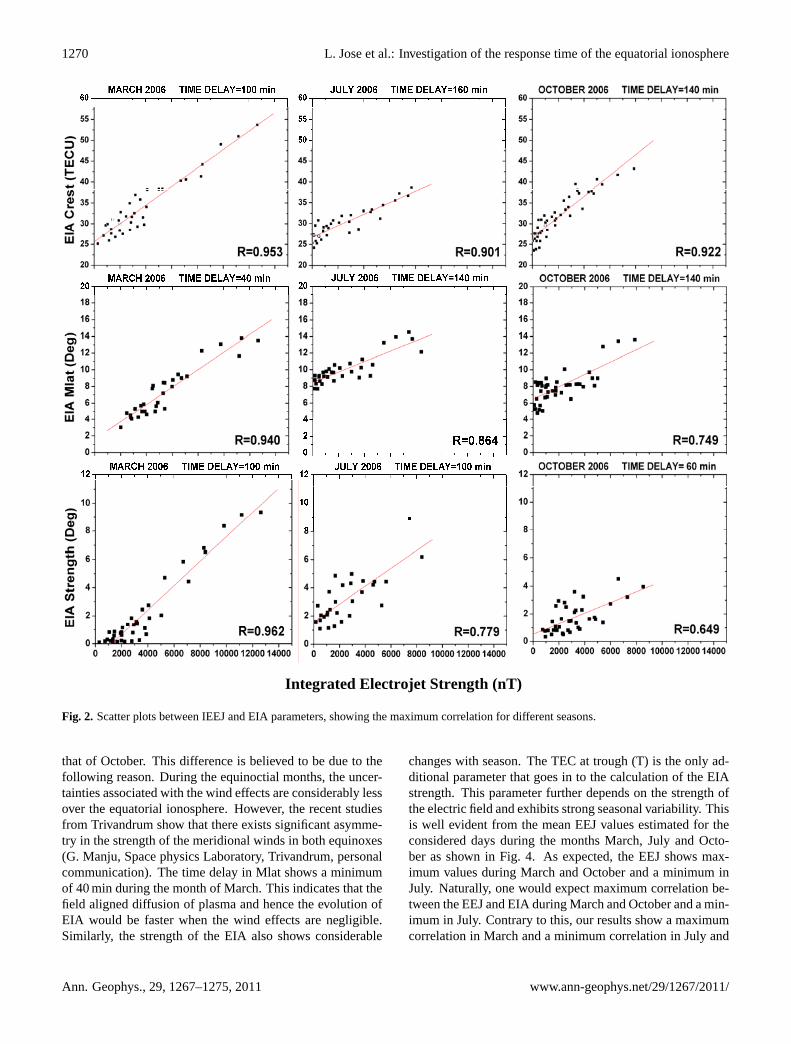
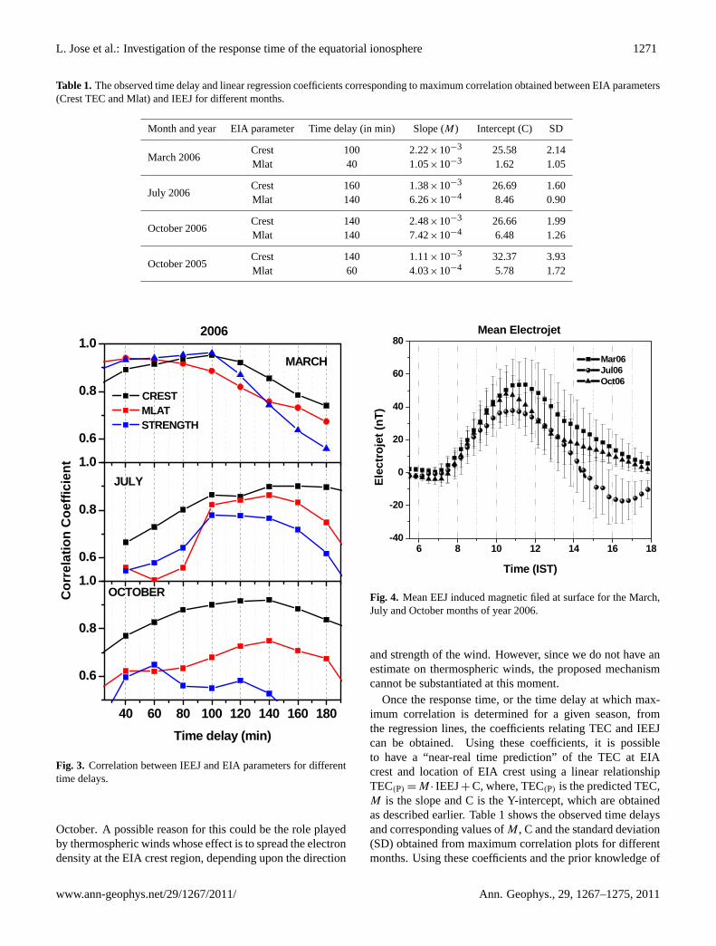
The scatter plots between the EIA parameters and IEEJ forthe months March, July and October of the year 2006 areshown in Fig. 2. The maximum correlations obtained andthe corresponding time delays are also shown in each panel.The top panels show the correlation between EIA crest andIEEJ for the aforesaid months. The middle and bottom pan-els depict the correlation between Mlat of the EIA crest &IEEJ and EIA strength & IEEJ, respectively. It is seen thatthe TEC at crest (C) shows very high correlation (R > 0.90)with IEEJ for all the three months. Correlation between Mlatand EIA strength shows strong seasonal dependence withmaximum correlation during March and minimum in Oc-tober. In order to highlight the dependence of correlationon time delays shown in Fig. 3 are the variation of correla-tion coefficient obtained for the EIA parameters and the timedelays for the considered months of study. For all EIA pa-rameters, correlation first increases, reaches a maximum andthen decreases as the time delay increases. It is found thatthe response time shows significant month-to-month varia-tion. The TEC at crest shows very good correlation for allseasons and the time delay is found to be maximum dur-ing the summer month. Time delay for the other two pa-rameters is also maximum during the summer month. Onepossible reason for this relation might be due to presence ofstrong equatorward wind in the Northern Hemisphere duringthe summer. The wind can retard the ionization from diffus-ing along the geomagnetic field lines, which will be reflectedin TEC at crest and Mlat of EIA. The correlations are veryhigh during March compared to October. The correspond-ing delays are also found to be smaller during March than

www.ann-geophys.net/29/1267/2011/ Ann. Geophys., 29, 1267–1275, 2011

1270 L. Jose et al.: Investigation of the response time of the equatorial ionosphere

18

Figure. 2.

Integrated Electrojet Strength (nT)

Fig. 2. Scatter plots between IEEJ and EIA parameters, showing the maximum correlation for different seasons.

that of October. This difference is believed to be due to thefollowing reason. During the equinoctial months, the uncer-tainties associated with the wind effects are considerably lessover the equatorial ionosphere. However, the recent studiesfrom Trivandrum show that there exists significant asymme-try in the strength of the meridional winds in both equinoxes(G. Manju, Space physics Laboratory, Trivandrum, personalcommunication). The time delay in Mlat shows a minimumof 40 min during the month of March. This indicates that thefield aligned diffusion of plasma and hence the evolution ofEIA would be faster when the wind effects are negligible.Similarly, the strength of the EIA also shows considerable

changes with season. The TEC at trough (T) is the only ad-ditional parameter that goes in to the calculation of the EIAstrength. This parameter further depends on the strength ofthe electric field and exhibits strong seasonal variability. Thisis well evident from the mean EEJ values estimated for theconsidered days during the months March, July and Octo-ber as shown in Fig. 4. As expected, the EEJ shows max-imum values during March and October and a minimum inJuly. Naturally, one would expect maximum correlation be-tween the EEJ and EIA during March and October and a min-imum in July. Contrary to this, our results show a maximumcorrelation in March and a minimum correlation in July and

Ann. Geophys., 29, 1267–1275, 2011 www.ann-geophys.net/29/1267/2011/

L. Jose et al.: Investigation of the response time of the equatorial ionosphere 1271

Table 1. The observed time delay and linear regression coefficients corresponding to maximum correlation obtained between EIA parameters(Crest TEC and Mlat) and IEEJ for different months.

Month and year EIA parameter Time delay (in min) Slope (M) Intercept (C) SD

March 2006Crest 100 2.22×10−3 25.58 2.14Mlat 40 1.05×10−3 1.62 1.05

July 2006Crest 160 1.38×10−3 26.69 1.60Mlat 140 6.26×10−4 8.46 0.90

October 2006Crest 140 2.48×10−3 26.66 1.99Mlat 140 7.42×10−4 6.48 1.26

October 2005Crest 140 1.11×10−3 32.37 3.93Mlat 60 4.03×10−4 5.78 1.72

19

Figure. 3.

40 60 80 100 120 140 160 180

0.6

0.8

1.0

0.6

0.8

1.0

0.6

0.8

1.0

OCTOBER

CREST MLAT STRENGTH

Time delay (min)

2006

JULY

Cor

rela

tion

Coe

ffici

ent

MARCH

Fig. 3. Correlation between IEEJ and EIA parameters for differenttime delays.

October. A possible reason for this could be the role playedby thermospheric winds whose effect is to spread the electrondensity at the EIA crest region, depending upon the direction

20

Figure. 4.

6 8 10 12 14 16 18-40

-20

0

20

40

60

80Mean Electrojet

Mar06 Jul06 Oct06

Elec

troj

et (n

T)

Time (IST)

Fig. 4. Mean EEJ induced magnetic filed at surface for the March,July and October months of year 2006.

and strength of the wind. However, since we do not have anestimate on thermospheric winds, the proposed mechanismcannot be substantiated at this moment.

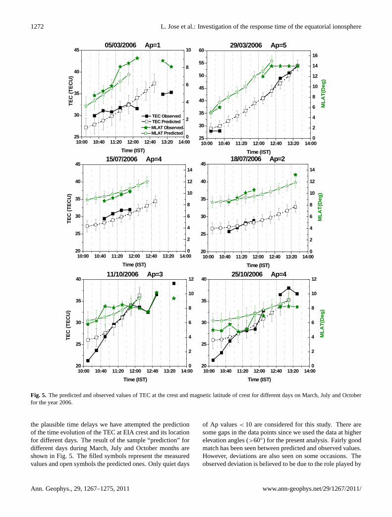
Once the response time, or the time delay at which max-imum correlation is determined for a given season, fromthe regression lines, the coefficients relating TEC and IEEJcan be obtained. Using these coefficients, it is possibleto have a “near-real time prediction” of the TEC at EIAcrest and location of EIA crest using a linear relationshipTEC(P) = M· IEEJ+ C, where, TEC(P) is the predicted TEC,M is the slope and C is the Y-intercept, which are obtainedas described earlier. Table 1 shows the observed time delaysand corresponding values ofM, C and the standard deviation(SD) obtained from maximum correlation plots for differentmonths. Using these coefficients and the prior knowledge of

www.ann-geophys.net/29/1267/2011/ Ann. Geophys., 29, 1267–1275, 2011

1272 L. Jose et al.: Investigation of the response time of the equatorial ionosphere

21

Figure. 5.

10:00 10:40 11:20 12:00 12:40 13:20 14:0020

25

30

35

40

45

0

2

4

6

8

10

12

14

MLA

T(D

eg)

Time (IST)

18/07/2006 Ap=2

10:00 10:40 11:20 12:00 12:40 13:20 14:0020

25

30

35

40

45

0

2

4

6

8

10

12

14

TEC

(TEC

U)

Time (IST)

15/07/2006 Ap=4

10:00 10:40 11:20 12:00 12:40 13:20 14:0025

30

35

40

45

0

2

4

6

8

10

TEC Observed TEC Predicted

TEC

(TEC

U)

Time (IST)

05/03/2006 Ap=1

MLAT Observed MLAT Predicted

10:00 10:40 11:20 12:00 12:40 13:20 14:0025

30

35

40

45

50

55

60

0

2

4

6

8

10

12

14

16

MLA

T(D

eg)

Time (IST)

29/03/2006 Ap=5

10:00 10:40 11:20 12:00 12:40 13:20 14:0020

25

30

35

40

0

2

4

6

8

10

12

TEC

(TEC

U)

Time (IST)

11/10/2006 Ap=3

10:00 10:40 11:20 12:00 12:40 13:20 14:0020

25

30

35

40

0

2

4

6

8

10

12

MLA

T(D

eg)

Time (IST)

25/10/2006 Ap=4

Fig. 5. The predicted and observed values of TEC at the crest and magnetic latitude of crest for different days on March, July and Octoberfor the year 2006.

the plausible time delays we have attempted the predictionof the time evolution of the TEC at EIA crest and its locationfor different days. The result of the sample “prediction” fordifferent days during March, July and October months areshown in Fig. 5. The filled symbols represent the measuredvalues and open symbols the predicted ones. Only quiet days

of Ap values< 10 are considered for this study. There aresome gaps in the data points since we used the data at higherelevation angles (>60◦) for the present analysis. Fairly goodmatch has been seen between predicted and observed values.However, deviations are also seen on some occasions. Theobserved deviation is believed to be due to the role played by

Ann. Geophys., 29, 1267–1275, 2011 www.ann-geophys.net/29/1267/2011/

L. Jose et al.: Investigation of the response time of the equatorial ionosphere 1273

22

Figure. 6.

10:00 10:30 11:00 11:30 12:00 12:30 13:00 13:30

25

30

35

40

45

0

2

4

6

8

10

12

TEC Observed TEC Predicted

TEC

(TEC

U)

MLA

T(D

eg)

Time (IST)

11/03/2006 Ap=10

MLAT Observed MLAT Predicted

10:00 10:40 11:20 12:00 12:40 13:20 14:0025

30

35

40

45

50

0

2

4

6

8

10

12

14

16

TEC

(TEC

U)

MLA

T(D

eg)

Time (IST)

27/03/2006 Ap=10

Fig. 6. Same as Fig. 5 but for two moderately disturbed days duringMarch 2006.

the horizontal winds in the day-to-day evolution of the EIA.However at present we do not have any means to delineatetheir individual effects.

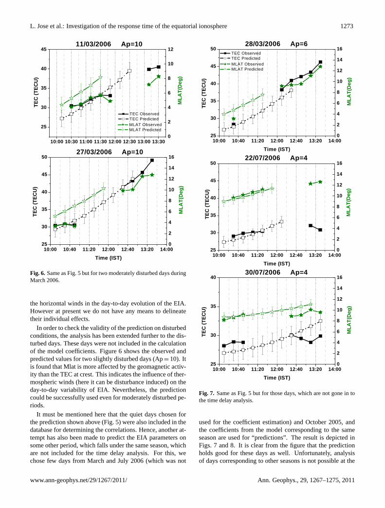
In order to check the validity of the prediction on disturbedconditions, the analysis has been extended further to the dis-turbed days. These days were not included in the calculationof the model coefficients. Figure 6 shows the observed andpredicted values for two slightly disturbed days (Ap= 10). Itis found that Mlat is more affected by the geomagnetic activ-ity than the TEC at crest. This indicates the influence of ther-mospheric winds (here it can be disturbance induced) on theday-to-day variability of EIA. Nevertheless, the predictioncould be successfully used even for moderately disturbed pe-riods.

It must be mentioned here that the quiet days chosen forthe prediction shown above (Fig. 5) were also included in thedatabase for determining the correlations. Hence, another at-tempt has also been made to predict the EIA parameters onsome other period, which falls under the same season, whichare not included for the time delay analysis. For this, wechose few days from March and July 2006 (which was not

23

Figure. 7.

10:00 10:40 11:20 12:00 12:40 13:20 14:00

25

30

35

40

0

2

4

6

8

10

12

14

16

TEC

(TEC

U)

MLA

T(D

eg)

Time (IST)

30/07/2006 Ap=4

10:00 10:40 11:20 12:00 12:40 13:20 14:0025

30

35

40

45

50

0

2

4

6

8

10

12

14

16 TEC Observed TEC Predicted

TEC

(TEC

U)

MLA

T(D

eg)

Time (IST)

28/03/2006 Ap=6

MLAT Observed MLAT Predicted

10:00 10:40 11:20 12:00 12:40 13:20 14:0025

30

35

40

45

50

0

2

4

6

8

10

12

14

16

TEC

(TEC

U)

MLA

T(D

eg)

Time (IST)

22/07/2006 Ap=4

Fig. 7. Same as Fig. 5 but for those days, which are not gone in tothe time delay analysis.

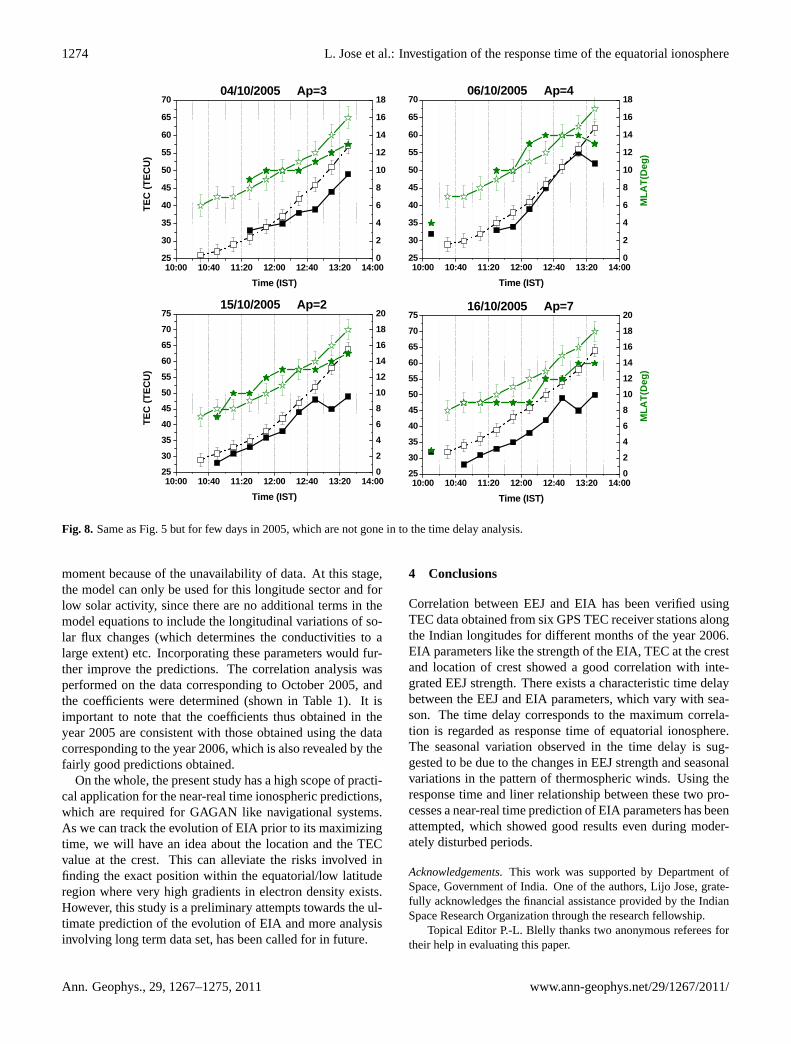
used for the coefficient estimation) and October 2005, andthe coefficients from the model corresponding to the sameseason are used for “predictions”. The result is depicted inFigs. 7 and 8. It is clear from the figure that the predictionholds good for these days as well. Unfortunately, analysisof days corresponding to other seasons is not possible at the

www.ann-geophys.net/29/1267/2011/ Ann. Geophys., 29, 1267–1275, 2011

1274 L. Jose et al.: Investigation of the response time of the equatorial ionosphere

24

Figure 8

10:00 10:40 11:20 12:00 12:40 13:20 14:0025

30

35

40

45

50

55

60

65

70

0

2

4

6

8

10

12

14

16

18

MLA

T(D

eg)

Time (IST)

06/10/2005 Ap=4

10:00 10:40 11:20 12:00 12:40 13:20 14:0025

30

35

40

45

50

55

60

65

70

0

2

4

6

8

10

12

14

16

18

TEC

(TEC

U)

Time (IST)

04/10/2005 Ap=3

10:00 10:40 11:20 12:00 12:40 13:20 14:0025

30

35

40

45

50

55

60

65

70

75

0

2

4

6

8

10

12

14

16

18

20

TEC

(TEC

U)

Time (IST)

15/10/2005 Ap=2

10:00 10:40 11:20 12:00 12:40 13:20 14:0025

30

35

40

45

50

55

60

65

70

75

0

2

4

6

8

10

12

14

16

18

20

MLA

T(D

eg)

Time (IST)

16/10/2005 Ap=7

Fig. 8. Same as Fig. 5 but for few days in 2005, which are not gone in to the time delay analysis.

moment because of the unavailability of data. At this stage,the model can only be used for this longitude sector and forlow solar activity, since there are no additional terms in themodel equations to include the longitudinal variations of so-lar flux changes (which determines the conductivities to alarge extent) etc. Incorporating these parameters would fur-ther improve the predictions. The correlation analysis wasperformed on the data corresponding to October 2005, andthe coefficients were determined (shown in Table 1). It isimportant to note that the coefficients thus obtained in theyear 2005 are consistent with those obtained using the datacorresponding to the year 2006, which is also revealed by thefairly good predictions obtained.

On the whole, the present study has a high scope of practi-cal application for the near-real time ionospheric predictions,which are required for GAGAN like navigational systems.As we can track the evolution of EIA prior to its maximizingtime, we will have an idea about the location and the TECvalue at the crest. This can alleviate the risks involved infinding the exact position within the equatorial/low latituderegion where very high gradients in electron density exists.However, this study is a preliminary attempts towards the ul-timate prediction of the evolution of EIA and more analysisinvolving long term data set, has been called for in future.

4 Conclusions

Correlation between EEJ and EIA has been verified usingTEC data obtained from six GPS TEC receiver stations alongthe Indian longitudes for different months of the year 2006.EIA parameters like the strength of the EIA, TEC at the crestand location of crest showed a good correlation with inte-grated EEJ strength. There exists a characteristic time delaybetween the EEJ and EIA parameters, which vary with sea-son. The time delay corresponds to the maximum correla-tion is regarded as response time of equatorial ionosphere.The seasonal variation observed in the time delay is sug-gested to be due to the changes in EEJ strength and seasonalvariations in the pattern of thermospheric winds. Using theresponse time and liner relationship between these two pro-cesses a near-real time prediction of EIA parameters has beenattempted, which showed good results even during moder-ately disturbed periods.

Acknowledgements.This work was supported by Department ofSpace, Government of India. One of the authors, Lijo Jose, grate-fully acknowledges the financial assistance provided by the IndianSpace Research Organization through the research fellowship.

Topical Editor P.-L. Blelly thanks two anonymous referees fortheir help in evaluating this paper.

Ann. Geophys., 29, 1267–1275, 2011 www.ann-geophys.net/29/1267/2011/

L. Jose et al.: Investigation of the response time of the equatorial ionosphere 1275

References

Abdu, M. A., Walker, G. O., Reddy, B. M., Sobral, J. H. A., Fejer,B. G., Kikuchi, T., Trivedi, N. B., and Szuszczewicz, E. P: Elec-tric field versus neutral wind control of the equatorial anomalyunder quiet and disturbed condition: A global perspective fromSUNDIAL 86, Ann. Geophys., 8, 419–430, 1990.

Anderson, D. N.: A theoretical study of the ionospheric F-regionequatorial anomaly I., Planet. Space Sci., 21, 409–419, 1973a.

Anderson, D. N.: A theoretical study of the ionospheric F-regionequatorial anomaly II. Results in the American and Asian sectors,Planet. Space Sci., 21, 421–442, 1973b.

Appleton, E. V.: Two anomalies in the ionosphere, Nature, 157,691–693, 1946.

Balan, N. and Iyer, K. N.: Equatorial anomaly in ionospheric elec-tron content and its relation to dynamo currents, J. Geophys.Res., 88, 10259–10262, 1983.

Deshpande, M. R., Rastogi, R. G., Vats, H. O., Klobuchar, J. A.,Sethia, G., Jain, A. R., Subbarao, B. S., Patwari, V. M., Janve,A. V., Rai, R. K., Singh, Malkiat, Gurm, H. S., and Murthy, B.S: Effect of electrojet on the TEC of the ionosphere over Indiasubcontinent, Nature, 267, 599–600, 1977.

Dunford, E.: The relationship between the ionospheric equatorialanomaly and the E-region current system, J. Atmos. Terr. Phys.,29, 1489–1498, 1967.

Forbes, J. M.: The equatorial electrojet, Rev. Geophys. Space Phys.,19, 469–504, 1981.

Huang, Y.-N., Cheng, K., and Chen, S.-W.: On the equatorialanomalyof the ionospheric total electron content near the North-ern Anomaly Crest Region, J. Geophys. Res., 94, 515–525, 1989.

Klobuchar, J. A.: Ionospheric Effects on GPS, vol. 2, Progress inAstronautics and Aeronautics, 1996.

Martyn, D. F.: Atmospheric tides in the ionosphere – I. Solar tidesin the F2 region, Proc. Roy. Soc. London A, 189, 241–260, 1947.

Mitra, S. K.: Geomagnetic control of region F2 of the ionosphere,Nature, 158, 668–669, 1946.

Raghavarao, R., Sharma, P., and Sivaraman, M. R.: Correlation ofionization anomaly with the intensity of electrojet, Space Res.,18, 277–280, 1978.

Rama Rao, P. V. S., Gopi Krishna, S., Niranjan, K., and Prasad, D.S. V. V. D.: Temporal and spatial variations in TEC using simul-taneous measurements from the Indian GPS network of receiversduring the low solar activity period of 2004–2005, Ann. Geo-phys., 24, 3279–3292,doi:10.5194/angeo-24-3279-2006, 2006.

Rastogi, R. G.: The Diurnal Development of the Anomalous Equa-torial Belt in the F2 Region of the Ionosphere, J. Geophys. Res.,64, 727–732, 1959.

Rastogi, R. G. and Klobuchar, J. A.: Ionospheric electron contentwithin the equatorial F2 layer anomaly belt, J. Geophys. Res.,95, 045–052, 1990.

Rastogi, R. G. and Rajaram, G.: Electrojet effects on the equatorialF-region during magnetically quiet and disturbed days, Ind. J.Pure Appl. Phys., 9, 531–536, 1971.

Reddy, C. A.: The equatorial electrojet, Pageoph., 131, 485–508,1989.

Richmond, A. D.: Modeling the ionospheric wind dynamo: A re-view, Pageoph., 131, 413–435, 1989.

Rush, C. M. and Richmond, A. D.: The relationship between thestructure of the equatorial anomaly and the strength of the equa-torial electrojet, J. Atmos. Terr. Phys., 35, 1171–1180, 1973.

Sastri, J. H.: The relationship between the structure of the equato-rial anomaly and the strength of the equatorial electrojet, Ind. J.Radio Space Phys., 19, 225–240, 1990.

Stolle, C., Manoj, C., Luhr, H., Maus, S., and Alken, P.: Es-timating the daytime Equatorial Ionization Anomaly strengthfrom electric field proxies, J. Geophys. Res., 113, A09310,doi:10.1029/2007JA012781, 2008.

www.ann-geophys.net/29/1267/2011/ Ann. Geophys., 29, 1267–1275, 2011