investigation of the relationship between - CiteSeerX

INVESTIGATION OF THE RELATIONSHIP BETWEEN

VEHICLE COLOR AND SAFETY

Thesis

Submitted to

The School of Engineering of the

UNIVERSITY OF DAYTON

In Partial Fulfillment of the Requirements for

The Degree of

Master of Science in Civil Engineering

By

Stephen O. Owusu-Ansah

UNIVERSITY OF DAYTON

Dayton, Ohio

May, 2010

ii

INVESTIGATION OF THE RELATIONSHIP BETWEEN

VEHICLE COLOR AND SAFETY

APPROVED BY: ___________________________ __________________________ Deogratias Eustace, Ph.D., P.E., PTOE Peter Hovey, Ph.D. Advisory Committee Chairperson Committee Member Assistant Professor, Department of Associate Professor, Department Civil and Environmental Engineering of Mathematics and Engineering Mechanics ___________________________ __________________________ Gary Shoup, P.E. Donald V. Chase, Ph.D., P.E. Committee Member Interim Chairperson, Department Senior Engineer Civil and Environmental Montgomery County Engineering Engineering and Engineering Department Mechanics ___________________________ __________________________ Malcolm Daniels, Ph.D. Tony Saliba, Ph.D. Associate Dean, Graduate Dean, School of Engineering Engineering Programs and Research School of Engineering

iii

ABSTRACT

INVESTIGATION OF THE RELATIONSHIP BETWEEN

VEHICLE COLOR AND SAFETY

Name: Owusu-Ansah, Stephen Osei University of Dayton

Advisor: Dr. Deogratias Eustace

Over the years, the concern of many, consumers and insurance

companies alike, has been geared towards the contribution of vehicle color to the

risk of crash. Consequently, there is a need to provide sufficient scientific

evidence to back consumers in selecting the appropriate vehicle color that

enhances their safety on the road. The present study utilized the induced

exposure study design where data was stratified into two groups: color-prone

crash group and induced exposure crash group. The color prone crash group

includes the types of crashes where vehicle color visibility may play a part in

crash occurring such as two or more vehicles in transport crashing, or where

pedestrians or motor cyclists are struck. The induced exposure crash group

generally includes crashes where vehicle visibility is not likely to be a factor in the

crash occurring, such as single vehicle crashes and a vehicle crashing into a

parked vehicle or other fixed/stationery objects such as trees, utility poles, etc.

iv

The negative binomial (NB) and Poisson distributions were utilized in fitting a

generalized linear model to the data. As opposed to previous studies, this study

first desired the appropriate model between the mostly used Poisson and the NB

models for crash data modeling. Model goodness-of-fit tests performed indicate

that the negative binomial model reflected a better fit to the data. Based on the

NB model, no single vehicle color was found to be significantly safer or riskier

than white, the baseline color. All the differences noted were not supported by a

sound statistical analysis performed.

v

ACKNOWLEDGEMENTS

My first thanks go to the Almighty God, without whose provisions and

guidance, my participation in this program of study would have been futile. I

would like to express my heartfelt gratitude to my principal advisor, Dr.

Deogratias Eustace, who read, criticized and provided necessary support and

encouragement to accomplish this research. To Dr. Peter Hovey, I extend special

thanks for his immense contribution and support, particularly, in the area of

statistics applied in this research. I count myself blessed to have you both.

To friends and classmates that contributed in diverse ways to my success

in this program, I say a big thank you. Finally, my thanks go to my family, both

home and abroad for their continued support, prayer, contributions and bearing

with me throughout this program of study.

vi

TABLE OF CONTENTS

ABSTRACT …………………………………………………………………………. …iii

ACKNOWLEDGEMENTS …………………………………………………………. …v

TABLE OF CONTENTS …………………………………………………………… ..vi

LIST OF FIGURES ………………………………………………………………… ..viii

LIST OF TABLES …………………………………………………………………... ...ix

INTRODUCTION ……………………………………………………………………….1

1.1 Introduction ………………………………………………………………….. ...1

1.2 Problem Statement …………………………………………………………. ...1

1.3 Research Objectives ……………………………………………………….. ...2

1.4 Outline of the Thesis …………………………………………………………..3

LITERATURE REVIEW ……………………………………………………………. …4

STUDY METHODOLOGY ………………………………………………………… ..10

3.1 Source of Data ………………………………………………………………..10

3.2 Methodology …………………………………………………………………..15

3.2.1 Creation of Crash Groups ………………………………………….. 16

3.2.2 Statistical Modeling …………………………………………………. 17

3.2.2.1 General ………………………………………………………. 17

3.2.2.2 Review of Statistical Models Used ………………………... 19

vii

3.2.2.2.1 Poisson Regression Model ……………………… 19

3.2.2.2.2 Negative Binomial Regression Model ...………... 21

3.2.2.3 Model Selection Criteria ……………………………………. 22

3.2.2.4 Model Formulation ………………………………………….. 23

3.3 Summary of Methodology ………………………………………………….. 28

ANALYSIS AND DISCUSSION OF RESULTS ……………………………………30

4.1 Introduction …………………………………………………………………... 30

4.2 Criteria for Assessing Model Goodness of Fit Results ………………….. 30

4.3 Results of the Estimated Crash Risks …………………………………….. 32

4.4 Discussion ……………………………………………………………………. 35

CONCLUSIONS AND RECOMMENDATIONS ………………….. ……………….38

REFERENCES ………………………………………………………………………..40

APPENDICES ………………………………………………………………………... 47

Appendix A: SAS Source Code ….…………………………………………….48

Appendix B: Classification of Interactive Effects …………………………… 50

Appendix C: Extended Negative Binomial Model Results ………………... .52

Appendix D: Extended Poisson Model Results ……………………………..71

viii

LIST OF FIGURES

3.1 Diagrammatic Presentation of MS Relational Tables …………………… 11

ix

LIST OF TABLES

3.1 Codes Used for Attributes of Interest in SAS ……………………………. .12

3.2 Characteristics of Nevada 2003-2008 Crash Data ……………………… .13

3.3 Passenger Vehicle Color Proportions in the State of Nevada: 2003-2008

Crash Data …………………………………………………………………… 15

3.4 Contingency Matrix Table ………………………………………………...… 24

4.1 Model Criteria Selection Summary Results of Poisson and Negative

Binomial Regression Models ……………………………………………….. 31

4.2 Relative Crash Risks Odds Ratio Estimates with White as Baseline Color

– Poisson Regression Model ……………………………………………….. 33

4.3 Relative Crash Risks Odds Ratio Estimates with White as Baseline Color

– Negative Binomial Regression Model …………………………………… 34

1

CHAPTER I

INTRODUCTION

1.1 Introduction

Most people make purchasing decisions of important items of their lives

such as cars, clothes, etc., based on the color of the items of interest. Some

colors are more visible than others and there are some known facts about the

relationship between color and conspicuity. For many years deaths and injuries

due to traffic crashes have become a global public health issue. Many risk factors

pertaining to highway safety have been identified such as driving under the

influence of alcohol and/or drugs, speeding, inclement weather conditions, lack of

road lighting, etc. One aspect that has not been widely studied but has caused

some speculations is whether the vehicle color may affect its conspicuity and

hence contribute in the occurrences of traffic crashes.

1.2 Problem Statement

Over the years, the concern of many, consumers and insurance

companies alike, has been geared towards the contribution of vehicle color to

risk of crash. Moreover, some even wonder about how to justify the differential in

cost, of the various vehicle-color models and insurance premiums. This research

was designed to provide results that may help identify the vehicle color(s) that

2

may be associated with better vehicle conspicuity and consequently to provide

sufficient scientific evidence to back consumers in selecting the appropriate

vehicle color that enhances their safety on the road.

Color perception varies with time among individuals. For instance, the

color red has traditionally been assigned attributes of passion, comfort, warmth

and security but for safety’s sake, lime-yellow is gaining a momentous

acceptance (Solomon and King, 1995; Shuman, 1991). Psychological studies

also suggest that color has an effect on behavior and conspicuity. In other words,

colors may tend to induce decreased visual perception with subsequent error that

may be aggravated by color blindness (Morton, 2008). Previous studies on the

relationship between risk of crash and color of vehicles are very few and some of

their findings are contradictory. Moreover, some of the methodologies used are

questionable (Newstead and D’Elia, 2007).

1.3 Research Objectives

The objective of this thesis is threefold: to determine if there is a significant

association between vehicle color and crash risk; to determine the differential in

crash risk by vehicle color, and to quantify if driver age, driver gender, vehicle

color, weather conditions, and lighting conditions have profound effect on vehicle

conspicuity and hence crash risk.

3

1.4 Outline of the Thesis

The rest of the thesis is organized as follows. Chapter Two presents the

literature review. It discusses available literature on color, conspicuity, and

related motor vehicle crash risks. Study results and statistical procedures used

by various researchers who previously attempted to quantify the relationship

between the vehicle color and risk of being involved in traffic crashes are

presented and their methodological flaws are discussed. Chapter Three outlines

the study methodology. It covers the data collection and detailed statistical

methodologies used in this thesis to quantify the potential risk of various vehicle

colors in causing motor vehicle crashes (due to low conspicuity problem). Also,

Chapter Three describes how to the select the best model that fits best the

observed data based on statistical data fitting procedures used in this thesis.

Chapter Four covers the analysis and discussion of results. This chapter

summarizes the results from the statistical analyses and provides a detailed

discussion of their implications. Chapter Five presents conclusions and

recommendations.

4

CHAPTER II

LITERATURE REVIEW

Numerous studies modeling risk factors pertaining to traffic safety have

been conducted. Examples include modeling injury severity studies (e.g., Chang

and Yeh, 2006; Harb et al., 2008); seat belt use effects on traffic safety (e.g.,

Houston and Richardson, 2002; Koushki et al., 2003); geometric effects on safety

(e.g., Gross et al., 2009); impaired driving effects (e.g., Baum, 2000); large truck

crashes (e.g., Braver et al., 1996; Neeley and Richardson, 2009), etc. Also, many

studies have investigated the relationship between color and visibility (e.g.,

FEMA, 2009) and most of them have focused on reflectivity of sign visibility (e.g.,

Anders, 2000; Hawkins et al., 2000; Gates and Hawkins, 2004). However, very

little research has been conducted to study whether vehicle color may have an

effect on motor vehicle crash. Particularly, scientific studies to determine the

relationship between vehicle color and crash risks have been scarcely

investigated (Newstead and D’Elia, 2007).

A study that measured divided attention capability of young and older

drivers suggested that older drivers are less effective than younger drivers when

multi-tasked due to the impaired vision of the older drivers (Mourant et al., 2001).

Also, a study that investigated the relationship between British driver crash data

and vision performance determined a significant association and recommended a

5

re-screening exam for drivers over fifty years old (Davison, 1985). However, in

both studies visual deterioration of older drivers was not investigated to

determine whether or not would put them in danger of causing crashes due to

their inability to see vehicles on the road due to conspicuity problems. A study

that reviewed the relationships between age and driver-vision performance

concludes that even though older drivers are bound to have vision impairment

but incur less crash incidences (Charman, 1997). Also another study that

reviewed the licensing procedures to improve roadway safety of older drivers in

Europe indicates a less crash fatality for drivers 65+ years old and countries with

less stringent license renewal procedures for older drivers incur less fatal

crashed than countries with stringent procedures (Mitchell, 2008).

A study investigating the effect of visibility in relation to fatal crashes

indicated that reduced visibility is a major contributing factor to both pedestrian

and pedal cyclist accidents (Owens, 1993). In that study, data retrieved from the

fatal accident reporting systems (FARS), spanning from 1980 to 1990 found that

a total of 104,235 crashes that occurred in the morning and evening hours

analyzed in relation to twilight zones were incurred under conditions pertained to

reduced visibility. In that study, the relationship between visibility and seasonal

variables was made. Also, the study analyzed traffic crashes in relation to twilight

zones within equal time periods of daylight and dark. While there was no

variation in fatal crashes within the control periods, variations occurred between

fatal crashes and natural illumination within twilight zones. Moreover, a study by

Vorko-Jović et al. (2006) on the risk factors in urban traffic accidents revealed

6

that the risk of fatal crashes was most significant during the period from midnight

to early morning when visibility was relatively reduced when compared with

incidences at all other times.

One of the earliest publications that discussed the possible linkage

between the vehicle color and a crash risk was by Nathan (1969). Nathan (1969)

argues that for rear-end type of crashes the vehicle color may have an effect

pertaining to visibility problems. He refers to a study conducted at the University

of California at Los Angeles that showed that color of an approaching vehicle

influences a driver’s judgment of how far the approaching vehicle is. For

example, they found that blue and yellow made distant objects seem closer and

gray shades made objects appear to be farther than they actually are. Nathan

(1969) points out that the safest color would be the one that is highly visible

under different lighting, weather, and perceptual conditions. Nathan (1969) also

quotes another study conducted in Sweden where a researcher analyzed 31,000

car crashes who concluded that black was not a safe color because 22.5% of the

accidents involved black vehicles while they constituted only 4.4% of the vehicles

surveyed. At the same time pink was regarded the safety color because pink cars

were involved in only 2.4% of the accidents but the percentage of the pink cars

was not given.

A study by Solomon and King (1995) investigated the association between

fire vehicle color and crash involvement in the city of Dallas, Texas. The city fire

department used fire vehicles painted with two different color combinations, that

is, red/white and lime-yellow/white. A Bayes conditional probability theory was

7

utilized in this study. This study found that the lime-yellow/white combination has

a significantly lower likelihood of being involved in a visibility-related crash than

the red/white fire vehicle. They assumed that the influence of confounding factors

such as weather-conditions, driver training, law enforcement conditions, etc.,

were controlled by using data from a single fire department with vehicles of both

color categories running at the same time. The dataset consisted of only 20

traffic crashes.

A study conducted in Spain (Lardelli-Claret et al., 2002) found that

vehicles with light-colored (yellow and white) were slightly less likely to be

passively (being hit by others) involved in traffic crashes compared with vehicles

of other colors and especially under worsening visibility weather conditions. A

paired case-control study was performed using Spanish traffic crash database in

which one driver was judged to have committed a violation. The control group

constituted the violating drivers and the non-violated formed the case group. The

data were analyzed using the conditional logistic regression method. Also, the

study accounted for a number of confounding factors such as driver age and

gender, type of vehicle, weather and environmental conditions, etc.

Another notable study was conducted in Auckland, New Zealand by

Furness et al. (2003), which used a method almost similar to that of Lardelli-

Claret et al. (2002) investigated the effect of car color on the risk of a serious

injury by using the case-control study design. The case group constituted of car

drivers involved in crashes in which one or more occupants of the car were

hospitalized or died while the control group consisted of randomly selected car

8

drivers at randomly selected times. They utilized the multivariate analysis

adjusted for a number of confounding factors such as age and gender of driver,

educational level, ethnicity, alcohol consumption, seatbelt use, vehicle speed,

vehicle age, etc. They found that silver cars were about 50% less likely to be

involved in a crash resulting in serious injury compared with white cars. Also,

they found a significant increase in risk of a serious injury in brown, black, and

green cars. Moreover, the risk of a serious injury for yellow, grey, red, and blue

cars was not found to be significantly higher than that of white cars.

A more recent and extensive study was done in Australia (Newstead and

D’Elia, 2007). In this study they tried to reduce the weaknesses observed in the

previous studies by incorporating more confounding factors and improving the

statistical methodology. They used the induced exposure method by identifying

the types of crashes that are potentially influenced by the vehicle color and those

that are not affected by it. They utilized the log-linear Poisson regression analysis

to analyze their data. This study found that black, blue, grey, green, red and

silver were associated with significantly higher crash risk than white. No color

was significantly safer than white. All other colors besides black, blue, grey,

green, red and silver were not significantly different from white in terms of relative

crash risk.

Besides the fact that the literature on the association of vehicle color and

crash risk is limited, the findings in these studies are somewhat contradictory. For

example, while a study by Furness et al., (2003) found a silver colored vehicle to

be safer, a study by Newstead and D’Elia (2007) indicated otherwise. On the

9

other hand, the Lardelli-Claret et al. (2002) study found that yellow and white

colored vehicles were just slightly safer than other vehicle colors.

10

CHAPTER III

STUDY METHODOLOGY

3.1 Source of Data

This thesis utilized traffic crash data from the state of Nevada traffic crash

database. Although police officers include the color of vehicles involved when

compiling traffic crash reports, most states don’t keep this variable in their state-

level databases because currently vehicle color is not among the variables

required for reporting by the National Highway Traffic Safety Administration

(NHTSA). Besides all other variables required by NHTSA reporting, the Nevada

Department of Transportation keeps records of the color of vehicles involved in

traffic crashes in their database. The confounding factors of interest besides the

vehicle color in this study include vehicle type, light condition, location, land use

(rural/urban), age and gender of driver, crash injury severity, and alcohol/drug

abuse involvement. The State of Nevada police reported crash database over a

period of 6 consecutive years, 2003-2008, in Access format was processed,

manipulated and analyzed by use of MS Excel, Arc-GIS, SPSS and SAS. From

the Access database, a relationship was established between the tables:

Collision, Conditions, Location, Vehicle and Occupant as shown in Figure 3.1.

11

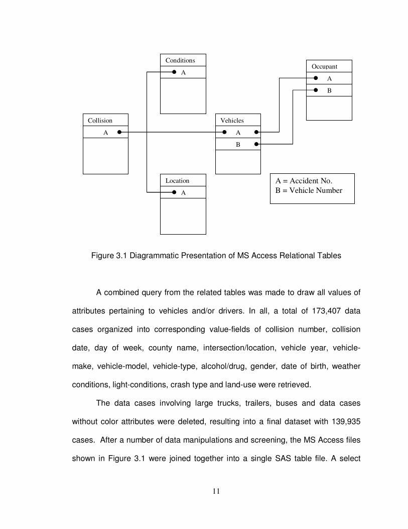
Figure 3.1 Diagrammatic Presentation of MS Access Relational Tables

A combined query from the related tables was made to draw all values of

attributes pertaining to vehicles and/or drivers. In all, a total of 173,407 data

cases organized into corresponding value-fields of collision number, collision

date, day of week, county name, intersection/location, vehicle year, vehicle-

make, vehicle-model, vehicle-type, alcohol/drug, gender, date of birth, weather

conditions, light-conditions, crash type and land-use were retrieved.

The data cases involving large trucks, trailers, buses and data cases

without color attributes were deleted, resulting into a final dataset with 139,935

cases. After a number of data manipulations and screening, the MS Access files

shown in Figure 3.1 were joined together into a single SAS table file. A select

A = Accident No.

B = Vehicle Number

Collision

A

Conditions

A

Location

A

Occupant

A

B

Vehicles

A

B

12

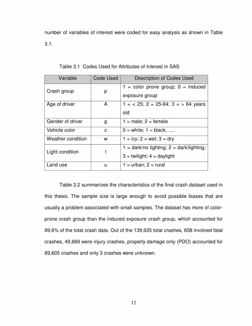
number of variables of interest were coded for easy analysis as shown in Table

3.1.

Table 3.1 Codes Used for Attributes of Interest in SAS

Variable Code Used Description of Codes Used

Crash group p 1 = color prone group; 0 = induced

exposure group

Age of driver A 1 = < 25; 2 = 25-64; 3 = > 64 years

old

Gender of driver g 1 = male; 2 = female

Vehicle color c 0 = white; 1 = black, ….

Weather condition w 1 = icy; 2 = wet; 3 = dry

Light condition l 1 = dark/no lighting; 2 = dark/lighting;

3 = twilight; 4 = daylight

Land use u 1 = urban; 2 = rural

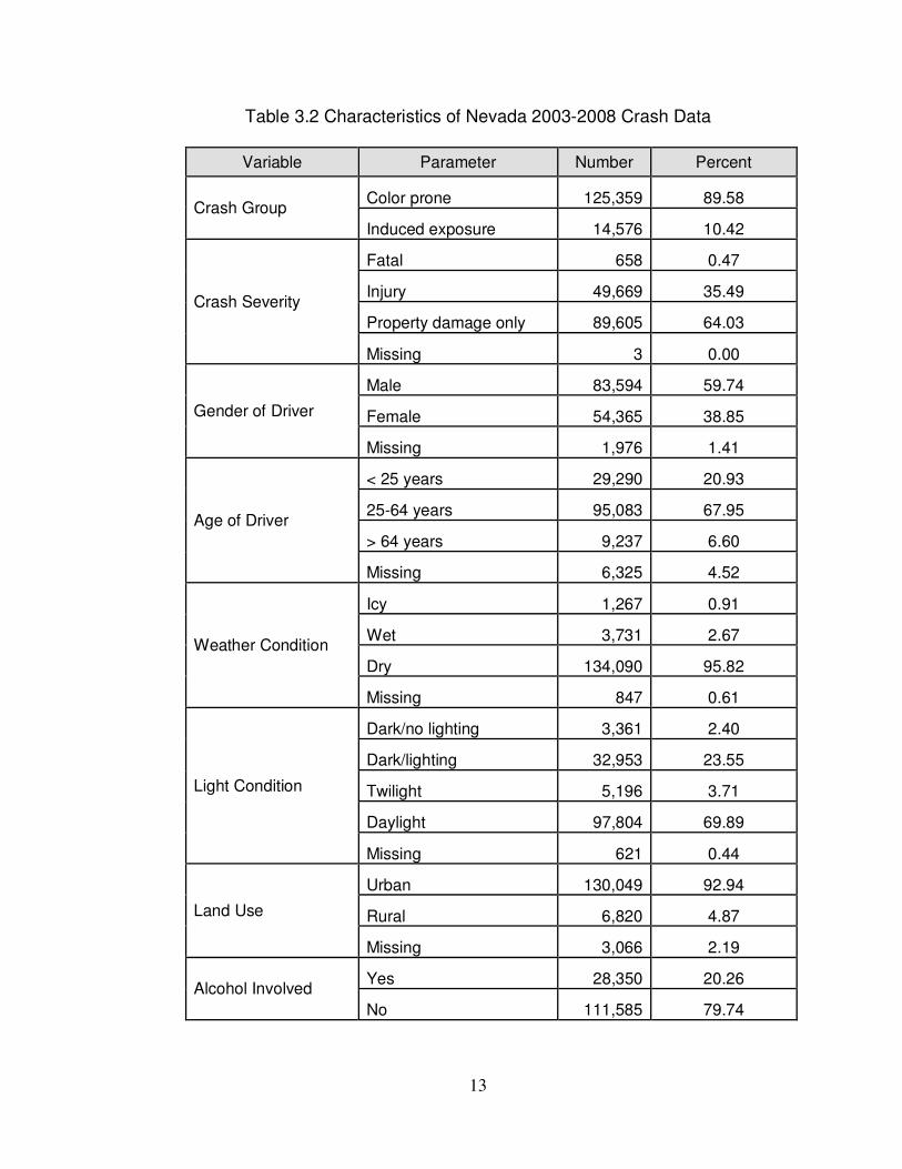
Table 3.2 summarizes the characteristics of the final crash dataset used in

this thesis. The sample size is large enough to avoid possible biases that are

usually a problem associated with small samples. The dataset has more of color-

prone crash group than the induced exposure crash group, which accounted for

89.6% of the total crash data. Out of the 139,935 total crashes, 658 involved fatal

crashes, 49,669 were injury crashes, property damage only (PDO) accounted for

89,605 crashes and only 3 crashes were unknown.

13

Table 3.2 Characteristics of Nevada 2003-2008 Crash Data

Variable Parameter Number Percent

Crash Group Color prone 125,359 89.58

Induced exposure 14,576 10.42

Crash Severity

Fatal 658 0.47

Injury 49,669 35.49

Property damage only 89,605 64.03

Missing 3 0.00

Gender of Driver

Male 83,594 59.74

Female 54,365 38.85

Missing 1,976 1.41

Age of Driver

< 25 years 29,290 20.93

25-64 years 95,083 67.95

> 64 years 9,237 6.60

Missing 6,325 4.52

Weather Condition

Icy 1,267 0.91

Wet 3,731 2.67

Dry 134,090 95.82

Missing 847 0.61

Light Condition

Dark/no lighting 3,361 2.40

Dark/lighting 32,953 23.55

Twilight 5,196 3.71

Daylight 97,804 69.89

Missing 621 0.44

Land Use

Urban 130,049 92.94

Rural 6,820 4.87

Missing 3,066 2.19

Alcohol Involved Yes 28,350 20.26

No 111,585 79.74

14

Male drivers were involved in 59.7% of the total crashes; female drivers in

38.9% and 1.4% were unknown. Most of the crashes (95.8%) occurred during

good dry weather condition and also 92.9% of the crashes occurred in urban

settings. Most of the crashes (79.7%) did not involve the use of alcohol. About

69.9% of the total crashes occurred during daylight and 23.6% when it was night

but with lighting. While young drivers (< 25 years) were involved in 20.9% of the

total crashes, older drivers (> 64 years) were involved in only 6.6% of the total

crashes.

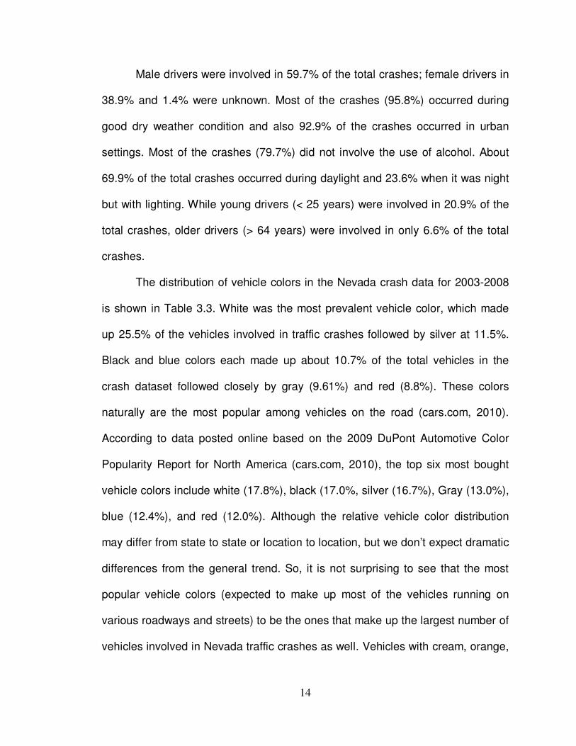
The distribution of vehicle colors in the Nevada crash data for 2003-2008

is shown in Table 3.3. White was the most prevalent vehicle color, which made

up 25.5% of the vehicles involved in traffic crashes followed by silver at 11.5%.

Black and blue colors each made up about 10.7% of the total vehicles in the

crash dataset followed closely by gray (9.61%) and red (8.8%). These colors

naturally are the most popular among vehicles on the road (cars.com, 2010).

According to data posted online based on the 2009 DuPont Automotive Color

Popularity Report for North America (cars.com, 2010), the top six most bought

vehicle colors include white (17.8%), black (17.0%, silver (16.7%), Gray (13.0%),

blue (12.4%), and red (12.0%). Although the relative vehicle color distribution

may differ from state to state or location to location, but we don’t expect dramatic

differences from the general trend. So, it is not surprising to see that the most

popular vehicle colors (expected to make up most of the vehicles running on

various roadways and streets) to be the ones that make up the largest number of

vehicles involved in Nevada traffic crashes as well. Vehicles with cream, orange,

15

and purple colors were relatively few in the crash dataset, each of them

representing less than 1% of all vehicles recorded.

Table 3.3 Passenger Vehicle Color Proportions in Nevada Crash Data Used in this Thesis, 2003-2008

Color Color Code Quantity Percent

Black BLK 14,975 10.70

Blue BLU 14,939 10.68

Burgundy BRG 5,515 3.94

Brown BRN 6,952 4.97

Cream CRM 152 0.11

Gold GLD 8,318 5.94

Green GRN 10,380 7.42

Gray GRY 13,452 9.61

Orange ONG 420 0.30

Purple PRP 846 0.60

Red RED 12,259 8.76

Silver SLV 16,101 11.51

White WHI 35,626 25.46

Total 139,935 100.00

3.2 Methodology

The present research utilized the induced exposure study design, which

has been demonstrated to be better than the case-control study design (which is

widely used in epidemiology and medical studies) when dealing with traffic safety

and crash risks (Newstead and D’Elia, 2007). The induced exposure study

16

design was successfully utilized by Newstead and D’Elia (2007) when

investigating the relationship between vehicle color and crash risk using

Australian crash database. Other studies that utilized this method include Burton

et al. (2004) and Evans (1998) in assessing crash risk associated with anti-lock

braking system (ABS) using the Australian and the U.S. crash data, respectively.

The induced-exposure method unlike most traditional methods, lends itself to the

use of a feature (a crash type) that is unaffected by a study focus to both induce

a baseline measure and also to control for other confounding factors influencing

crash risk. The induced exposure method offers control on measurable and

immeasurable confounding factors and to definitively assess the relationship

between vehicle color and crash risk (Newstead and D’Elia, 2007).

3.2.1 Creation of Crash Groups

The use of induced exposure method requires data be classified into two

groups. The data was therefore stratified into two groups, namely, color-prone

group and induced exposure group crashes, which are defined broadly as

follows:

i) Color prone crash group: generally, this group includes the types of

crashes where vehicle color visibility may play a part in crash occurring. It

includes two or more vehicles crashing at the intersections and those

traveling in the same or opposite directions, or where pedestrians or motor

cyclists are struck.

17

ii) Induced exposure crash group: generally, this group includes crashes

where vehicle visibility is not likely to be a factor in the crash occurring,

such as single vehicle crashes and a vehicle crashing into a parked

vehicle or other fixed/stationery objects such as trees, utility poles, etc.

3.2.2 Statistical Modeling

3.2.2.1 General

A good statistical model is the one that provides a good approximate

mathematical representation of the data being modeled with particular emphasis

being on structure or patterns in the data (White and Bennetts, 1996). Statistical

analysis and modeling of data have become increasingly important in scientific

research and study inquiries and the process involves application of appropriate

statistical procedure, testing hypotheses, interpreting data results, and coming up

with valid conclusions (CSR, 2009).

Although a previous study whose modeling procedure was more

acceptable compared to others mentioned in the literature review chapter utilized

a Poisson model for crash counts (Newstead and D’Elia, 2007), a better fit might

be obtained by using the negative binomial distribution. The negative binomial

can be derived as a mixture of Poisson distributions with different rates. Since

accident counts represent the total crashes for all drivers and it is reasonable to

assume that different drivers have different crash rates, the negative binomial

distribution could provide a better fit. Negative binomial distribution has been

established by researchers as a more accurate description of crash variation

18

from year to year or site to site and has been successfully used in the past to

model and evaluate various transportation safety projects involving crash counts

(e.g., Hauer et al., 2002; Hovey and Chowdhury, 2005; Persaund et al., 2001).

Poisson distribution was formerly a preferred method for such analyses, but

inconsistencies in model predictions led to widespread switch to binomial

distribution (Hauer, 2002).

It is a simple matter to fit both the Poisson and negative binomial

distributions and perform model tests to determine which model is more

appropriate for the given set of data. In either case, generalized linear regression

is used to account for factors that may influence the crash rates. The generalized

linear model (GLM) was used due to its ability to account for confounding factors

that may influence crash rates. Generalized linear model provides the framework

for using a discrete variable (crash counts) as the response variable and for

incorporating factors such as driver age that would have an impact on crash

counts. The SAS statistical software (version 9.2) was utilized in performing all

model fitting. The GENMOD Procedure in SAS allows the specification of a

negative binomial distribution, Poisson distribution, etc., by fitting a generalized

linear model to the data by using the maximum likelihood estimation techniques.

19

3.2.2.2 Review of Statistical Models Used

3.2.2.2.1 Poisson Regression Model

Poisson regression models are often used for analyzing count data that

normally has no limit or upper bound on how large the observed count can be. It

is usually used for modeling the number of occurrences of an event or the rate of

event occurrences as a function of some independent variables. For example,

the occurrences of number of traffic crashes per year at a particular roadway

location or segment can be modeled by using the Poisson model. When the

Poisson regression is used to model the count data it is assumed that the

dependent (outcome) variable Y has a Poisson distribution and the probability of

observing any specific count y is given as shown in Equation 3.1.

!

)(y

eyYP

yµµ−

== ...................................................................................................................................................................................................................................................................................................... .............. .............. .............. (3.1)

Where:

µ = the mean number of occurrences within a given time interval;

When modeling an outcome event (Y) using a given set of independent

variables X1, X2, X3, …, Xn, the mean, µ, can be expressed as a multivariate log-

linear function as shown in Equation 3.2:

log(µ) = log(T) + β0 + β1X1+ β2X2 + … + βnXn ……………………. (3.2)

20

Where:

β0 = regression constant (model intercept)

β1… βn = model regression coefficients

T = offset

The offset variable log(T) is used to account for possible different

observation periods (Ti) for different subjects (Pedan, 2001), for example,

different traffic crashes at a certain location for different years. The maximum

likelihood method in SAS GENMOD procedure is used to estimate the

parameters of the Poisson regression model for log(µ). A major assumption of a

Poisson model is that the expected value (mean) of the random variable Y

equals its variance (Ramaswamy et al., 1994; Pedan, 2001) as shown in

Equation 3.3:

µ = E(Y) = Var(Y) ………………………………………………………………. (3.3)

Although the randomness of accident occurrence has generally been

assumed to follow the Poisson assumption (Nicholson, 1985), but requires a

careful examination of the counts over a number of years for a given location to

check whether the expectation (mean) and variance agree. The Poisson

distribution requirement of having identical mean and variance sets a severe

limitation because count data often vary more than expected, i.e., variances are

usually larger than means (Agresti, 2007). This phenomenon of data having

21

larger variability than expected is called overdispersion (Agresti, 2007). Thus,

Poisson regression does not model adequately the count data having larger

variability than expected (Ramaswamy et al., 1994; Pedan, 2001; Agresti, 2007).

3.2.2.2.2 Negative Binomial Regression Model

If the Poisson regression model is determined inappropriate to model the

count data due to overdispersion in the data, a negative binomial (NB) regression

is usually utilized to accommodate overdispersion (Ramaswamy et al., 1994;

Pedan, 2001; Agresti, 2007). The NB model allows the variance to exceed the

mean for data having greater variability than expected, overcoming the Poisson

model limitation (Pedan, 2001; Agresti, 2007). The negative binomial distribution

can be derived as a mixture of Poisson distributions when the mean is not

identical for all entities being modeled and that the Poisson means follow a

gamma distribution (Pedan, 2001; Agresti, 2007). For instance, the mean

parameter (µi) of the occurrence of traffic crashes at each intersection being

modeled is Poisson distributed, but the joint (combined) distribution is no longer

Poisson, instead, it is gamma distributed. In other words, while Poisson assumes

homogeneity in the data, NB assumes heterogeneity. The mean and variance of

the negative binomial distribution are given as shown in Equation 3.4.

E(Y) = µ, Var(Y) = µ + k µ2 ……………………………………………………. (3.4)

22

Where:

k = a nonnegative dispersion parameter

The greater heterogeneity in the data results in a larger value of k. For

small k, i.e., as k→0, Var(Y) → µ (refer to Equation 3.4) and the NB distribution

approaches the Poisson distribution (Pedan, 2001; Agresti, 2007). Conversely,

the larger the k values in relation to 0, the greater the overdispersion relative to

Poisson variability. Also, the maximum likelihood method in SAS GENMOD

procedure is used to estimate the parameters of the negative binomial regression

model for log(µ) and the overdispersion parameter k.

3.2.2.3 Model Selection Criteria

If the over-dispersion in the data is not captured in the analysis it results

into underestimation of standard errors and hence over-statement of significance

in hypothesis testing (Pedan, 2001). Consequently, using an inappropriate model

for count data can grossly affect the statistical inference and the resulting

conclusions. Deviance (D) and Pearson Chi-Square statistic (χ2) divided by the

degrees of freedom (DF) are used to detect whether overdispersion or

underdispersion exists in the data and also can be used to indicate other

problems such as incorrectly specified model or presence of outliers in the data

(SAS, 2004). Evidence of either overdispersion or underdispersion indicates

inadequate fit of the Poisson model. The goodness of fit between the observed

data and the estimated values from a Poisson distribution or a negative binomial

distribution are usually measured by using the log-likelihood ratio G2 statistic (i.e.,

23

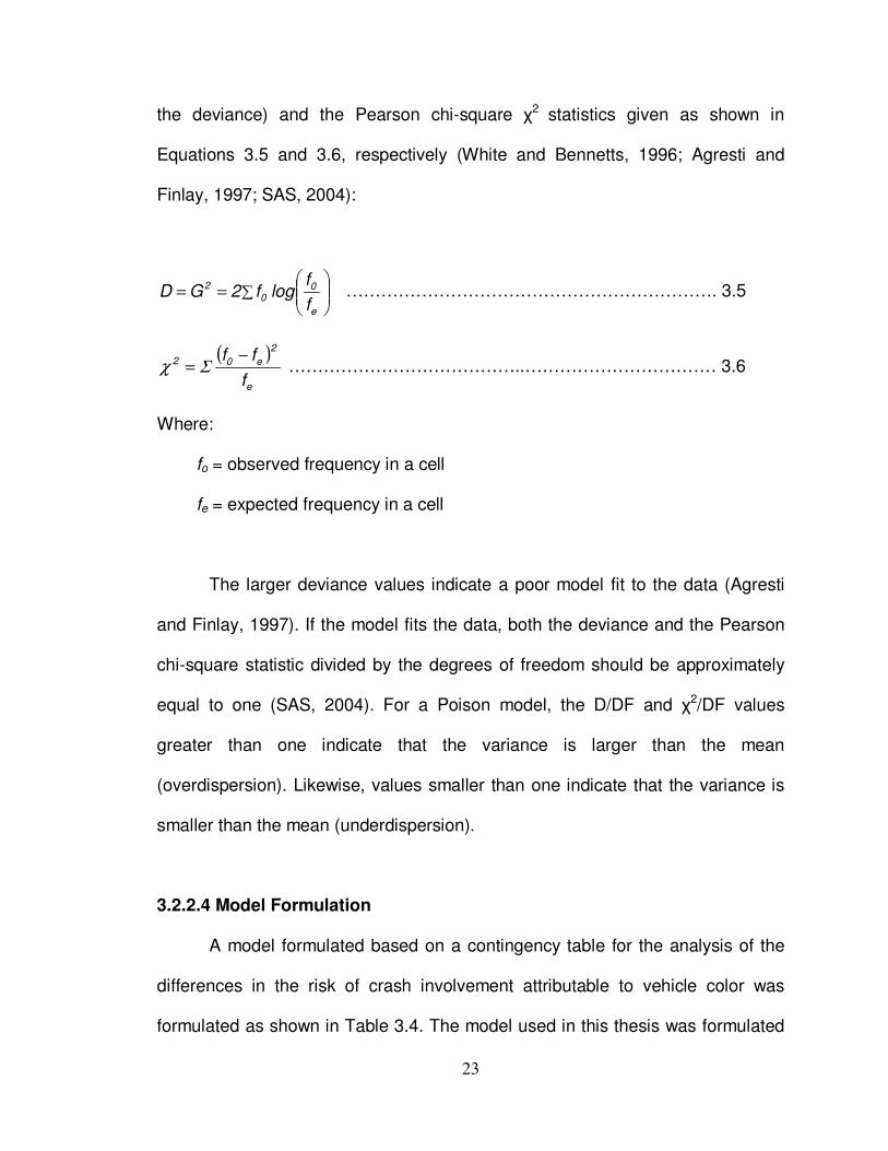
the deviance) and the Pearson chi-square χ2 statistics given as shown in

Equations 3.5 and 3.6, respectively (White and Bennetts, 1996; Agresti and

Finlay, 1997; SAS, 2004):

∑

==

e

00

2

f

flogf2GD ………………………………………………………. 3.5

( )

e

2

e02

f

ff −= Σχ …………………………………..…………………………… 3.6

Where:

fo = observed frequency in a cell

fe = expected frequency in a cell

The larger deviance values indicate a poor model fit to the data (Agresti

and Finlay, 1997). If the model fits the data, both the deviance and the Pearson

chi-square statistic divided by the degrees of freedom should be approximately

equal to one (SAS, 2004). For a Poison model, the D/DF and χ2/DF values

greater than one indicate that the variance is larger than the mean

(overdispersion). Likewise, values smaller than one indicate that the variance is

smaller than the mean (underdispersion).

3.2.2.4 Model Formulation

A model formulated based on a contingency table for the analysis of the

differences in the risk of crash involvement attributable to vehicle color was

formulated as shown in Table 3.4. The model used in this thesis was formulated

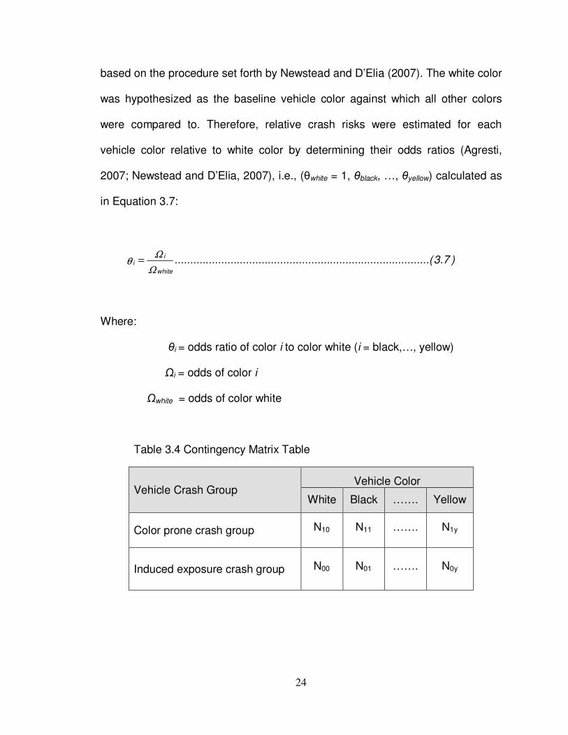
24

based on the procedure set forth by Newstead and D’Elia (2007). The white color

was hypothesized as the baseline vehicle color against which all other colors

were compared to. Therefore, relative crash risks were estimated for each

vehicle color relative to white color by determining their odds ratios (Agresti,

2007; Newstead and D’Elia, 2007), i.e., (θwhite = 1, θblack, …, θyellow) calculated as

in Equation 3.7:

)7.3..(................................................................................white

ii

Ω

Ωθ =

Where:

θi = odds ratio of color i to color white (i = black,…, yellow)

Ωi = odds of color i

Ωwhite = odds of color white

Table 3.4 Contingency Matrix Table

Vehicle Crash Group Vehicle Color

White Black ……. Yellow

Color prone crash group N10 N11 ……. N1y

Induced exposure crash group N00 N01 ……. N0y

25

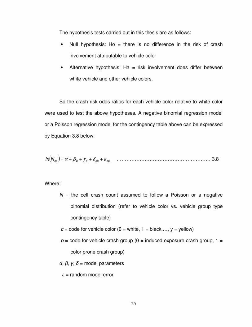
The hypothesis tests carried out in this thesis are as follows:

• Null hypothesis: Ho = there is no difference in the risk of crash

involvement attributable to vehicle color

• Alternative hypothesis: Ha = risk involvement does differ between

white vehicle and other vehicle colors.

So the crash risk odds ratios for each vehicle color relative to white color

were used to test the above hypotheses. A negative binomial regression model

or a Poisson regression model for the contingency table above can be expressed

by Equation 3.8 below:

( ) cpcpcpcpNln εδγβα ++++= ………………………………………………… 3.8

Where:

N = the cell crash count assumed to follow a Poisson or a negative

binomial distribution (refer to vehicle color vs. vehicle group type

contingency table)

c = code for vehicle color (0 = white, 1 = black,…, y = yellow)

p = code for vehicle crash group (0 = induced exposure crash group, 1 =

color prone crash group)

α, β, γ, δ = model parameters

ε = random model error

26

The analysis based on Equation 3.8 may be influenced by distribution of

different colored vehicles on the roads or vehicles of certain colors being

preferred by certain types of drivers, e.g., more young male drivers owning red

cars. In addition, other factors that may influence the analysis results include age

of driver, gender of driver, weather conditions, time of day, and light condition

when the crash occurred. All of these are potential confounding factors/variables

that needed to be controlled in this study. In order to control for the confounding

factors of interest, Equation 3.8 was modified by stratifying the data as shown in

Equation 3.9 below:

( ) cpagluwcpagluwcagluwpagluwcpagluwNln εδγβα ++++= ……………………………. 3.9

Where:

a = code for age group of driver

g = code for gender of driver (male, female)

l = code for light condition

u = code for land use (rural, urban)

w = code for weather condition

From Equation 3.9, the interactive effect (δcpagluw) is determined by

referencing white color as baseline and considering color-prone crash group (p =

1), the interactive effect becomes direct estimate for the color-prone crash group

(δc1agluw). Also, the interactive effect can be simplified depending on a given

27

contingency table. For instance, the statistical significance of color-prone

incidence compounded by weather conditions alone would be δc1w (See Appendix

B for more classifications). Hence, with white color as reference (δcpagluw = 0, with

c = white), the relative odds ratio ( θ i) representing the risk of crash for a vehicle

of color i relative to vehicle of color white from Equation 3.7 becomes an

exponential function as shown in Equation 3.10 below:

( )agluw1ci exp δθ = …………………………………………………………... 3.10

Then the 95% confidence limits were calculated for the interaction parameter,

δcpagluw, for each color using the standard confidence interval statistical equation

as depicted in Equation 3.11 below (Agresti, 2007):

( )SEzln 2/i αθ ± ………………………………………………………………… 3.11

Where:

i = color code (1 = black, …, y = yellow);

zα/2 = value of the standard normal distribution with (1-α) confidence level,

which equals to 1.96 for 95% or α = 0.05);

SE = estimated standard error.

It is preferred to construct confidence intervals for ln(θ), that is why it is

used in Equation 3.11, because its sampling distribution is closer to normality

28

than that of θ (which is normally skewed) (Agresti, 2007). Then, the resulting

values were transformed back, i.e., by taking the antilogs, using the exponential

function. The sample odds ratio, which is approximately normally distributed, has

a mean of ln(θ) and a standard error computed as shown in Equation 3.12

(Agresti, 2007) (for notations used, refer to Table 3.4):

y00100y11110 N

1...

N

1

N

1

N

1...

N

1

N

1SE +++++++= ………………………… (3.12)

For a color with an odds ratio, θ, larger than 1.0 is expected to exhibit a

higher crash risk than color white and likewise, the color with an odds ratio

smaller than 1.0 is expected to have a lower crash risk than color white. In order

the difference to be statistically significant, i.e., having either a significantly higher

or lower crash risk, the odds ratio limits (the upper and lower bound values)

should both either be higher than 1.0 or lower than 1.0, respectively. In other

words, the confidence interval for θ should not contain 1.0 (Agresti, 2007).

3.3 Summary of Methodology

The traffic crash data was obtained from database maintained by the

Nevada Department of Transportation and this data was preferred because they

record the color of vehicles involved in traffic crashes. Besides the vehicle color,

confounding factors of interest that were used in the model include the age and

gender of drivers involved in the traffic crash, lighting and weather conditions and

29

time of day when the crash occurred. Both the Poisson regression and negative

binomial regression analyses were performed on the sorted data using SAS 9.1

software’s PROC GENMOD procedure and the results from this analysis are

presented in the following chapter. In addition, Chapter 4 compares the two

models based on the SAS’ model goodness of fit summary results and the model

that fits the data better was used to perform the inferences on the color crash risk

based on the odds ratio results.

30

CHAPTER IV

ANALYSIS AND DISCUSSION OF RESULTS

4.1 Introduction

It has been a trend that many vehicle buyers get concerned about relative

safety and cost between vehicle models. Additionally, another aspect that

consumers frequently ask is whether a choice of vehicle color influences a crash

risk or an increased car insurance premium. Very little research has been

conducted to study the relationship between the vehicle color and the possibility

of being involved in a crash. Besides the fact that literature on the association of

vehicle color and crash risk is limited, the findings in previous studies are

somewhat contradictory and the methodologies used are generally questionable.

This study has proposed a better methodology in conducting such kind of

studies.

4.2 Criteria for Assessing Model Goodness of Fit Results

The model goodness of fit assessment criteria results as outputted from

the SAS GENMOD procedure for both regression models are depicted in Table

4.1. The model goodness of fit measures the fit between the observed data and

the values predicted by the models.

31

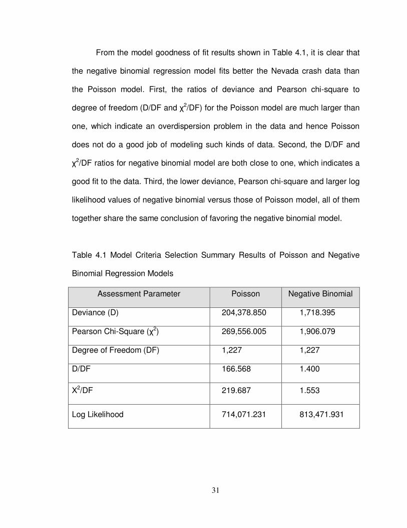
From the model goodness of fit results shown in Table 4.1, it is clear that

the negative binomial regression model fits better the Nevada crash data than

the Poisson model. First, the ratios of deviance and Pearson chi-square to

degree of freedom (D/DF and χ2/DF) for the Poisson model are much larger than

one, which indicate an overdispersion problem in the data and hence Poisson

does not do a good job of modeling such kinds of data. Second, the D/DF and

χ2/DF ratios for negative binomial model are both close to one, which indicates a

good fit to the data. Third, the lower deviance, Pearson chi-square and larger log

likelihood values of negative binomial versus those of Poisson model, all of them

together share the same conclusion of favoring the negative binomial model.

Table 4.1 Model Criteria Selection Summary Results of Poisson and Negative

Binomial Regression Models

Assessment Parameter Poisson Negative Binomial

Deviance (D) 204,378.850 1,718.395

Pearson Chi-Square (χ2) 269,556.005 1,906.079

Degree of Freedom (DF) 1,227 1,227

D/DF 166.568 1.400

Χ2/DF 219.687 1.553

Log Likelihood 714,071.231 813,471.931

32

4.3 Results of the Estimated Crash Risks

After data analysis and modeling using the SAS software, the overall

model results are shown in Tables 4.2 and 4.3 for Poisson regression and

negative binomial regression models, respectively. Tables 4.2 and 4.3 report the

estimated crash risk for each particular color relative to white in terms of odds

ratios as the parameter estimate (refer to Equation 3.10), the 95% confidence

limits on the estimated odds ratios (refer to Equation 3.11), and the parameter

estimate’s statistical significance (p-values).

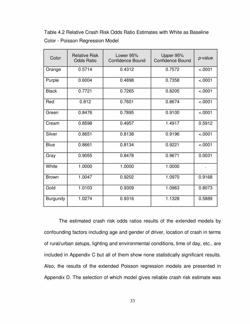
From Table 4.2, the Poisson regression model indicate highly statistically

significantly decreased crash risk for orange, pink, blue, red, green, silver, blue,

and gray colors relative to white color. Cream color also indicates lower crash

risk relative to white but the difference is not statistically significant. The rest of

the colors, i.e., brown, gold, and burgundy indicate increased crash risk relative

to white but all of them are not statistically significant.

The negative binomial regression model results shown in Table 4.3

indicate that none of the crash risks for the vehicle colors modeled are

statistically significantly different from that of white color. While orange, purple,

black, red, green, cream, silver, blue, and gray indicate none significant lower

crash risk relative to white, brown, gold, and burgundy indicate none significant

higher crash risks relative to white color.

33

Table 4.2 Relative Crash Risk Odds Ratio Estimates with White as Baseline

Color - Poisson Regression Model

Color Relative Risk Odds Ratio

Lower 95% Confidence Bound

Upper 95% Confidence Bound

p-value

Orange 0.5714 0.4312 0.7572 <.0001

Purple 0.6004 0.4898 0.7358 <.0001

Black 0.7721 0.7265 0.8205 <.0001

Red 0.812 0.7601 0.8674 <.0001

Green 0.8476 0.7895 0.9100 <.0001

Cream 0.8598 0.4957 1.4917 0.5912

Silver 0.8651 0.8138 0.9196 <.0001

Blue 0.8661 0.8134 0.9221 <.0001

Gray 0.9055 0.8478 0.9671 0.0031

White 1.0000 1.0000 1.0000 .

Brown 1.0047 0.9202 1.0970 0.9168

Gold 1.0103 0.9309 1.0963 0.8073

Burgundy 1.0274 0.9316 1.1328 0.5889

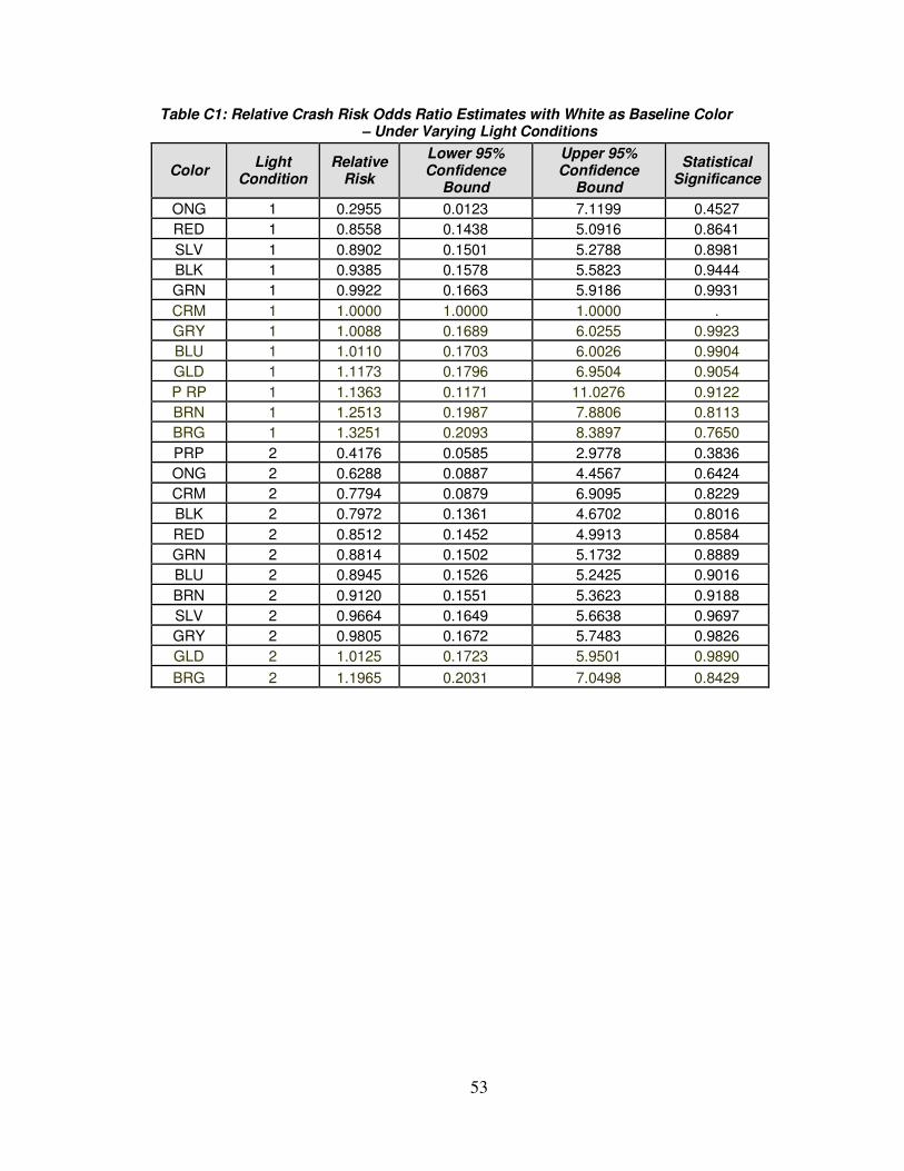
The estimated crash risk odds ratios results of the extended models by

confounding factors including age and gender of driver, location of crash in terms

of rural/urban setups, lighting and environmental conditions, time of day, etc., are

included in Appendix C but all of them show none statistically significant results.

Also, the results of the extended Poisson regression models are presented in

Appendix D. The selection of which model gives reliable crash risk estimate was

34

based on the model goodness of fit criteria (refer to Section 3.2.2.3) and the

results are reported in Section 4.1 above.

Table 4.3 Relative Crash Risk Odds Ratio Estimates with White as Baseline

Color - Negative Binomial Regression Model

Color Relative Risk Odds Ratio

Lower 95% Confidence Bound

Upper 95% Confidence Bound

p-value

Orange 0.5714 0.0915 3.5669 0.5492

Purple 0.6004 0.0972 3.7088 0.5829

Black 0.7721 0.1310 4.5508 0.7750

Red 0.8120 0.1377 4.7870 0.8180

Green 0.8476 0.1437 4.9983 0.8551

Cream 0.8598 0.1196 6.1836 0.8808

Silver 0.8651 0.1468 5.0993 0.8728

Blue 0.8661 0.1469 5.1054 0.8738

Gray 0.9055 0.1536 5.3383 0.9127

White 1.0000 1.0000 1.0000

Brown 1.0047 0.1702 5.9293 0.9959

Gold 1.0103 0.1712 5.9602 0.9910

Brown 1.0274 0.1740 6.0654 0.9763

The results presented in this section reveal an important aspect of using

an inappropriate model, which has a danger of directing us into misleading

results and hence wrong conclusions. According to Pedan (2001), the Poisson

35

model would have erroneously led us into concluding that orange, purple, black,

red, silver, blue, and gray colors to be relatively safer than white. Because it is a

wrong model for the data we have, therefore it over-stated the significance in

hypothesis testing.

4.4 Discussion

Generally, very few studies have been conducted using crash data or

other means with a focus of determining the influence of vehicle color on crash

risks. As opposed to previous studies, this study first desired the appropriate

model between the mostly used Poisson and the negative binomial models for

crash data analysis and modeling. Based on the discussion on model selection

criteria in Chapter 3 coupled with the established model outputs from both

Poisson and negative binomial models discussed in the previous section, the

negative binomial model was selected based on its relatively low ratios of

deviance and Pearson chi-square to the degree of freedom values (reflecting

better model fit to the data). The study by Newstead and D’Elia (2007), which

used a better methodology compared to other previous studies, did not mention if

they checked their model results for overdispersion or whether their model

represented well the structure or patterns in their data. Without such important

statistical model checks the conclusions drawn can be questionable due to

inability to assess the model fit. Although Newstead and D’Elia (2007) overcame

the weaknesses of the case-control methods as previously used by Lardelli-

Claret et al. (2002) and Furness et al. (2003) studies by employing the more

36

accepted induced-exposure methodology, their conclusions become

questionable mainly due to their inability to justify whether their model statistically

fit the data being modeled. Since all three major studies that investigated a

connection between vehicle color and crash risks used potentially flawed

methodologies, no wonder why their findings were grossly contradictory.

AAA Foundation for Traffic Safety report that consumers frequently ask

whether a choice of vehicle color influences a crash risk, in other words, what is

the safest vehicle color (AAA, 2004). In order to provide a reliable answer to such

complicated questions you need to have a reliable evidence to back up your

statement. Unfortunately the available research results have contradictory results

and therefore it was very difficult to draw the right conclusion based on those

research findings. However, during the course of the present study we have

noted that the methodological flaws in the previous studies and we tried to

overcome their weaknesses. The study by Newstead and D’Elia (2007) had a

promising methodology with the exception of unreliable statistical model.

Therefore, we decided to use their procedure by using a better statistical model,

and our study went one step farther by checking to make sure that the model

whose results are selected is the one that fits well the data being analyzed.

Based on our results, no single vehicle color was found to be significantly safer

or riskier than white color. All the differences noted were not supported by a

sound statistical analysis performed.

37

In absence of the actual driving exposures in term of miles each driver and

vehicle travels every year in assessing the crash risk, the induced exposure

techniques have been accepted as reliable alternative when properly accounting

for the confounding factors. Also, using a stratified induced exposure design in

the present study appropriately adjusted the analysis for potential influences of

confounding factors such as weather and lighting conditions, age and gender of

drivers, time of crash, etc. In addition, this study design takes in account

distribution of different colored vehicles on the road and whether certain colors

are over or under-represented among certain types of drivers. For example, red

or white cars may seem to be more prone to crashes due to higher number of red

or white cars on the road or disproportionate numbers of bad drivers owning cars

with such colors, e.g., young males owning red cars.

38

CHAPTER V

CONCLUSIONS AND RECOMMENDATIONS

The objective of this study was to determine if there is a significant

association between vehicle color and crash risk; to determine the differential in

crash risk by vehicle color, and to quantify if driver age, driver gender, vehicle

color, weather conditions, and lighting conditions have profound effect on vehicle

conspicuity and hence crash risk. Police reported crash data from the State of

Nevada were utilized in this study.

A stratified induced exposure design was utilized in this study with crashes

involving vehicles in multiple cars making a crash prone group and vehicles

involved in single vehicle crashes making an induced exposure group. Both

Poisson regression and negative binomial regression models were used and the

well known statistical goodness of fit model assessment criteria were used in

selecting which model to fitted better the Nevada crash data. Based on the

results obtained, the negative binomial regression model was determined to fit

the data better than the Poisson regression model. The SAS outputs provided

relative crash risk odds ratios along with lower and upper confidence bounds and

statistical significance (p-values) for each featured color. Although the Poisson

regression model identified some colors that showed to be statistically

significantly riskier than white, however, this conclusion was not drawn due to its

39

lack of fit and the violation of one of its main assumption of the equality of mean

and variance parameters. Data results show that there was significant

overdispersion in the data, which automatically disqualifies the use of Poisson

distribution in modeling such kinds of data. On the other hand, the negative

binomial regression model indicated that there was no strong relationship

between the vehicle color and crash risk, i.e., there was evidence to show that

there was no color that was statistically significantly different than the baseline

color, white in terms of crash risk.

Consequently, we draw a conclusion based on the results of the present

study that no vehicle color was found to be statistically significant. As a result, the

present study encourages more research in this area. Also, crash data from other

states with different environmental and weather conditions compared to that of

the state of Nevada (the only source of data for the present study) should be

utilized and comparison be drawn in order to provide a more robust conclusion.

40

REFERENCES

AAA Foundation for Traffic Safety. Car Color and Safety. White Paper.

Foundation for Traffic Safety, 2004. Available at

http://www.aaafoundation.org/pdf/CarColorAndSafety.pdf. Accessed on July 7,

2008.

Agresti, A. An Introduction to Categorical Data Analysis, 2nd Edition. John Wiley

& Sons, Inc., Hoboken, NJ, 2007.

Agresti, A. and B. Finlay. Statistical Methods for the Social Sciences, 3rd Edition.

Prentice Hall, Inc., Upper Saddle River, NJ, 1997.

Anders, R. L. On-road Investigation of Fluorescent Sign Colors to Improve

Conspicuity. Virginia Polytechnic Institute and State University, Blacksburg, VA,

2000.

Baum, S. Drinking driving a Social Problem: Comparing the Attitudes and

Knowledge of Drink Driving Offenders and the General Community. In Accident

Analysis and Prevention, 32, 2000, pp. 689-694.

41

Braver, E. R., D. F. Preusser, A. F. Williams, and H. B. Weinstein. Major Types of

Fatal Crashes Between Large Trucks and Cars, Insurance Institute for Highway

Safety, Arlington, VA, 1996.

Burton, D., A. Delaney, S. Newstead, D. Logan, and B. Fildes. Evaluation of

Antilock Braking Systems Effectiveness. Research Report 04/01, Royal

Automobile Club of Victoria, Melbourne, Australia.

Cars.com. Most Popular Colors. http://www.cars.com/go/index.jsp. Accessed on

October 10, 2009.

Center for System Reliability (CSR). Statistical Modeling.

http://reliability.sandia.gov/Manuf_Statistics/Statistical_Modeling/statistical_model

ing.html. Accessed on October 10, 2009.

Chang, H. and T. Yeh. Risk Factors to Driver Fatalities in Single-vehicle Crashes:

Comparisons between Non-motorcycle Drivers and Motorcyclists. In Journal of

Transportation Engineering, 132, 2006, pp. 227-236.

Charman, W. N. Vision and Driving-A Literature Review and Commentary, In

Ophthalmic and Physiological Optics, 17, 1997, pp. 371-391

Davison, P. A. Inter-Relationships Between British Drivers' Visual Abilities, Age

and Road Accident Histories, In Ophthalmic and Physiological Optics, 5, 1985,

pp.195-204.

42

Evans, L. Antilock Brake Systems and Risk of Different Types of Crashes in

Traffic. In Journal of Crash Prevention and Injury Control, 1, 1999, pp. 5-23.

FEMA. Emergency Vehicle Visibility and Conspicuity Study, U.S. Department of

Homeland Security, Washington, DC, 2009.

Furness, S., J. Connor, E. Robinson, R. Norton, S. Ameratunga, and R. Jackson.

Car Color and Risk of Car Crash Injury: Population Based Case Control Study, In

British Medical Journal, 327, 2003, pp. 1455-1456.

Gates, T. J. and H. G. Hawkins. Effect of Higher-conspicuity Warning and

Regulatory Signs on Driver Behavior, Report #0-4271-S, Texas Transportation

Institute, Texas A&M University, College Station, TX, 2004.

Gross, F., P. P. Jovanis, K. Eccles, and K-Y. Chen. Safety Effects of Lane and

Shoulder Combinations on Rural, Two-lane, Undivided Roads, Pub. FHWA-HRT-

09-031, U.S. Department of Transportation, Washington, DC, 2009.

Harb, R., E. Radwan, X. Yan, A. Pande, and M. Abdel-Aty. Freeway Work-Zone

Crash Identification Using Multiple And Conditional Logistic Regression. In

Journal of Transportation Engineering, 134, 2008, pp. 203-214.

43

Hauer, E., D. Harwood, F. Council, and M. Griffith. Estimating Safety by the

Empirical Bayes Method: A Tutorial. In Transportation Research Record, 2002,

1784, pp. 126-131.

Hauer, E. Observational Before-After Studies in Road Safety, 2nd Edition.

Elsevier Science Ltd., Oxford, U.K., 2002.

Hawkins, H. G., P. J. Carlson, and M. Elmquist. Evaluation of Fluorescent

Orange Signs. Report #0-2962-S, Texas Transportation Institute, Texas A&M

University, College Station, TX, 2000.

Houston, D. J. and L. E. Richardson. Traffic Safety and Switch to a Primary

Seatbelt Law: the California Experience. In Accident Analysis and Prevention, 34,

2002, pp. 743-751.

Hovey, P. and M. Chowdhury. Development of Crash Reduction Factors. Final

Report. Ohio Department of Transportation, Columbus, Ohio, 2005.

Koushki, P. A., B. A. Bustan, and N. Kartam. Impact of Safety Belt Use on Road

Accident Injury and Injury Type in Kuwait. In Accident Analysis and Prevention,

35, 2003, pp. 237-241.

44

Lardelli-Claret, P., J. De Dios Luna-del-Castillo, J. J. Jimenez-Moleon, P. Femia-

Marzo, O. Moreno-Abril, and A. Bueno-Cavanillas. Does Vehicle Color Influence

the Risk of Being Passively Involved in a Collision? In Epidemiology, 13, 2002,

pp. 721-724.

Mitchell, C. G. The Licensing of Older Drivers in Europe-A Case Study, Transport

Research Laboratory, UK, 2008.

Mourant, R. R., F. Tsai, T. Al-Shihabi and B. K. Jaeger. Divided Attention Ability

of Young and Older Drivers. In the Transportation, Research Record, 1779,

2001, pp. 40-45.

Nathan, R. A. What’s the Safest Color for a Motor Vehicle? In Traffic Safety, 69,

1969, pp. 13.

Neeley, G. W. and L. E. Richardson. The Effect of State Regulations on Truck-

Crash Fatalities. In American Journal of Public Health, 99, 2009, pp. 408-415.

Newstead, S. and A. D’Elia. An Investigation into the Relationship between

Vehicle Color and Crash Risk, Report No. 263, Accident Research Centre,

Monash University, Victoria, Australia, 2007.

45

Nicholson, A. J. The Variability of Accident Counts. In Accident Analysis and

Prevention, 17, 1985, pp. 47-56.

Owens, D. A. The Role of Reduced Visibility in Nighttime Road Fatalities.

University of Michigan, Ann Arbor, Transportation Research Institute, 1993.

Pedan, A. Analysis of Count Data Using the SAS System, Paper 247-26. In the

Proceedings of the 26th Annual SAS Users Group International Conference,

2001,

Persaund, B. N., R. A. Retting, P. E. Garder, and D. Lord. Safety Effect of

Roundabout Conversions in the United States: Empirical Bayes Observational

Before-After Study. In Transportation Research Record, 1751, 2001, pp. 1-8.

Ramaswamy, V., E. W. Anderson, and W. S. DeSarbo. A Disaggregate Negative

Binomial Regression Procedure for Count Data Analysis. In Management

Science, 40, 1994, pp. 405-417.

SAS Institute Inc. SAS/STAT® 9.1 User’s Guide. Cary, NC, 2004.

Shuman, M. Traditional Red Colors Safety. In Traffic Safety, 91, 1991 pp. 22-24.

46

Solomon, S. S and J. G. King. Influence of Color on Fire Vehicles. In Journal of

Safety Research, 26, 1995, pp. 41-48.

Vorko-Jović, A., J. Kern and Z. Biloglav. Risk Factors in Urban Road Traffic

Accidents. In Journal of Safety Research, 37, 2006, pp. 93-98.

White, G. C. and R. E. Bennetts. Analysis of Frequency Count Data Using the

Negative Binomial Distribution. In Ecology, 77, 1996, pp. 2549-2557.

47

APPENDICES

48

APPENDIX A

SAS Source Code

49

DATA CRASHDAT1 SET CRASHDAT1; YEAR = YEAR (DCOL); PROC SORT DATA = NEVADAT.CRASHDAT1; BY CRSHT COL YEAR AGE; PROC SUMMARY DATA=NEVADAT.CRASHDATY1; BY CRSHT COL YEAR AGE; VAR FREQ; OUTPUT OUT = NEVADAT.CRSHTCOLAGE N = COUNT; PROC GENMOD DATA = NEVADAT.CRSHTCOLAGEY; CLASS CRSHT COL AGE; MODEL _FREQ_ = CRSHT*AGE COL*AGE CRSHT*COL*AGE / DIST = NB LINK = LOG TYPE3 WALD:

50

APPENDIX B

Classifications of Interactive Effects

51

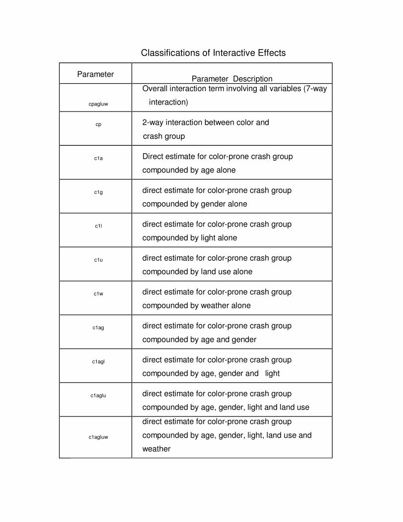
Classifications of Interactive Effects

Parameter Parameter Description

cpagluw

Overall interaction term involving all variables (7-way

interaction)

cp

2-way interaction between color and

crash group

c1a

Direct estimate for color-prone crash group

compounded by age alone

c1g

direct estimate for color-prone crash group

compounded by gender alone

c1l

direct estimate for color-prone crash group

compounded by light alone

c1u

direct estimate for color-prone crash group

compounded by land use alone

c1w

direct estimate for color-prone crash group

compounded by weather alone

c1ag

direct estimate for color-prone crash group

compounded by age and gender

c1agl

direct estimate for color-prone crash group

compounded by age, gender and light

c1aglu

direct estimate for color-prone crash group

compounded by age, gender, light and land use

c1agluw

direct estimate for color-prone crash group

compounded by age, gender, light, land use and

weather

52

APPENDIX C

Extended Negative Binomial Model Results

53

Table C1: Relative Crash Risk Odds Ratio Estimates with White as Baseline Color – Under Varying Light Conditions

Color Light

Condition Relative

Risk

Lower 95% Confidence

Bound

Upper 95% Confidence

Bound

Statistical Significance

ONG 1 0.2955 0.0123 7.1199 0.4527

RED 1 0.8558 0.1438 5.0916 0.8641

SLV 1 0.8902 0.1501 5.2788 0.8981

BLK 1 0.9385 0.1578 5.5823 0.9444

GRN 1 0.9922 0.1663 5.9186 0.9931

CRM 1 1.0000 1.0000 1.0000 .

GRY 1 1.0088 0.1689 6.0255 0.9923

BLU 1 1.0110 0.1703 6.0026 0.9904

GLD 1 1.1173 0.1796 6.9504 0.9054

P RP 1 1.1363 0.1171 11.0276 0.9122

BRN 1 1.2513 0.1987 7.8806 0.8113

BRG 1 1.3251 0.2093 8.3897 0.7650

PRP 2 0.4176 0.0585 2.9778 0.3836

ONG 2 0.6288 0.0887 4.4567 0.6424

CRM 2 0.7794 0.0879 6.9095 0.8229

BLK 2 0.7972 0.1361 4.6702 0.8016

RED 2 0.8512 0.1452 4.9913 0.8584

GRN 2 0.8814 0.1502 5.1732 0.8889

BLU 2 0.8945 0.1526 5.2425 0.9016

BRN 2 0.9120 0.1551 5.3623 0.9188

SLV 2 0.9664 0.1649 5.6638 0.9697

GRY 2 0.9805 0.1672 5.7483 0.9826

GLD 2 1.0125 0.1723 5.9501 0.9890

BRG 2 1.1965 0.2031 7.0498 0.8429

54

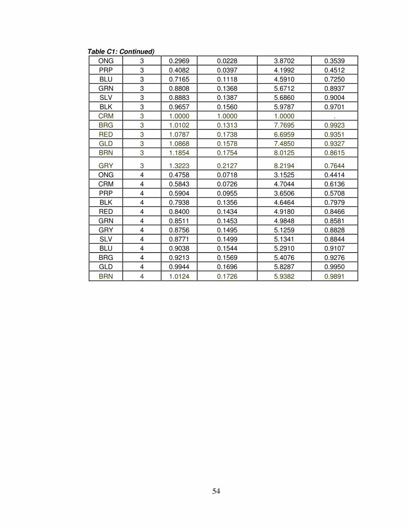
Table C1: Continued)

ONG 3 0.2969 0.0228 3.8702 0.3539

PRP 3 0.4082 0.0397 4.1992 0.4512

BLU 3 0.7165 0.1118 4.5910 0.7250

GRN 3 0.8808 0.1368 5.6712 0.8937

SLV 3 0.8883 0.1387 5.6860 0.9004

BLK 3 0.9657 0.1560 5.9787 0.9701

CRM 3 1.0000 1.0000 1.0000 .

BRG 3 1.0102 0.1313 7.7695 0.9923

RED 3 1.0787 0.1738 6.6959 0.9351

GLD 3 1.0868 0.1578 7.4850 0.9327

BRN 3 1.1854 0.1754 8.0125 0.8615

GRY 3 1.3223 0.2127 8.2194 0.7644

ONG 4 0.4758 0.0718 3.1525 0.4414

CRM 4 0.5843 0.0726 4.7044 0.6136

PRP 4 0.5904 0.0955 3.6506 0.5708

BLK 4 0.7938 0.1356 4.6464 0.7979

RED 4 0.8400 0.1434 4.9180 0.8466

GRN 4 0.8511 0.1453 4.9848 0.8581

GRY 4 0.8756 0.1495 5.1259 0.8828

SLV 4 0.8771 0.1499 5.1341 0.8844

BLU 4 0.9038 0.1544 5.2910 0.9107

BRG 4 0.9213 0.1569 5.4076 0.9276

GLD 4 0.9944 0.1696 5.8287 0.9950

BRN 4 1.0124 0.1726 5.9382 0.9891

55

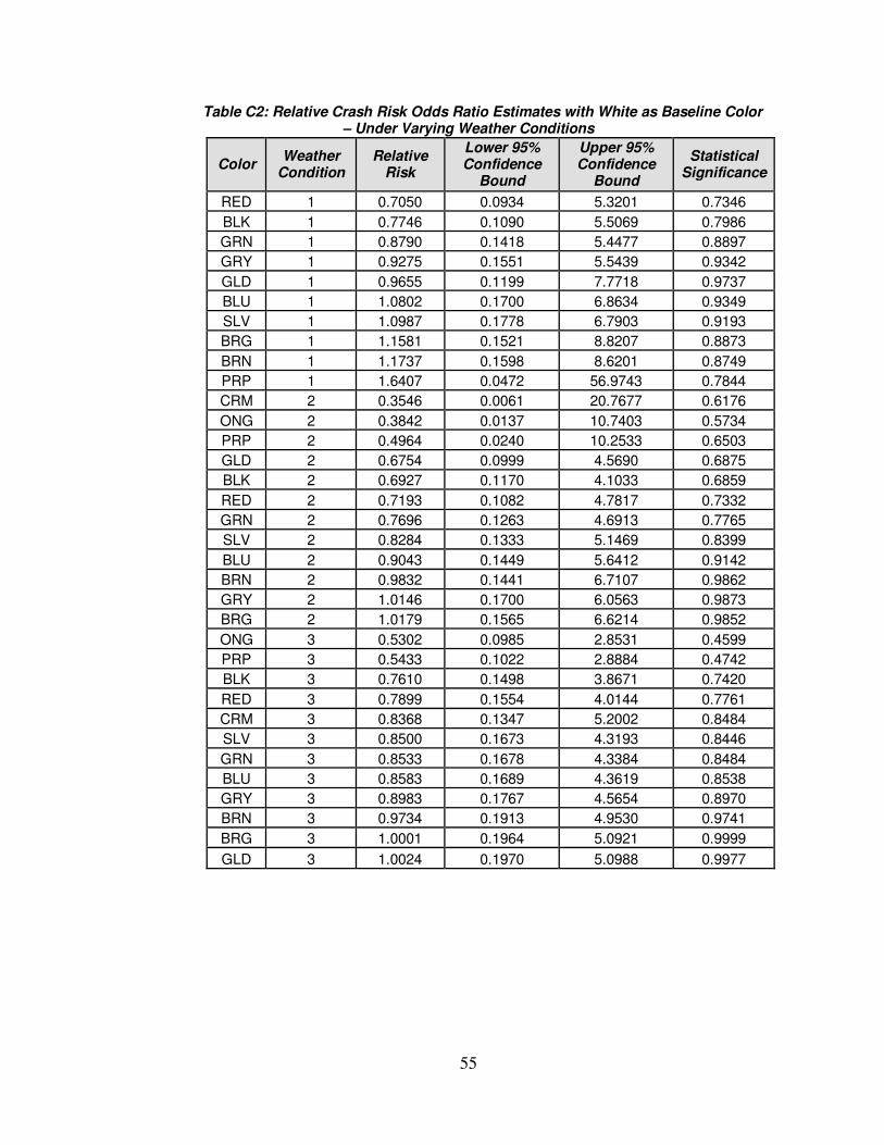
Table C2: Relative Crash Risk Odds Ratio Estimates with White as Baseline Color – Under Varying Weather Conditions

Color Weather

Condition Relative

Risk

Lower 95% Confidence

Bound

Upper 95% Confidence

Bound

Statistical Significance

RED 1 0.7050 0.0934 5.3201 0.7346

BLK 1 0.7746 0.1090 5.5069 0.7986

GRN 1 0.8790 0.1418 5.4477 0.8897

GRY 1 0.9275 0.1551 5.5439 0.9342

GLD 1 0.9655 0.1199 7.7718 0.9737

BLU 1 1.0802 0.1700 6.8634 0.9349

SLV 1 1.0987 0.1778 6.7903 0.9193

BRG 1 1.1581 0.1521 8.8207 0.8873

BRN 1 1.1737 0.1598 8.6201 0.8749

PRP 1 1.6407 0.0472 56.9743 0.7844

CRM 2 0.3546 0.0061 20.7677 0.6176

ONG 2 0.3842 0.0137 10.7403 0.5734

PRP 2 0.4964 0.0240 10.2533 0.6503

GLD 2 0.6754 0.0999 4.5690 0.6875

BLK 2 0.6927 0.1170 4.1033 0.6859

RED 2 0.7193 0.1082 4.7817 0.7332

GRN 2 0.7696 0.1263 4.6913 0.7765

SLV 2 0.8284 0.1333 5.1469 0.8399

BLU 2 0.9043 0.1449 5.6412 0.9142

BRN 2 0.9832 0.1441 6.7107 0.9862

GRY 2 1.0146 0.1700 6.0563 0.9873

BRG 2 1.0179 0.1565 6.6214 0.9852

ONG 3 0.5302 0.0985 2.8531 0.4599

PRP 3 0.5433 0.1022 2.8884 0.4742

BLK 3 0.7610 0.1498 3.8671 0.7420

RED 3 0.7899 0.1554 4.0144 0.7761

CRM 3 0.8368 0.1347 5.2002 0.8484

SLV 3 0.8500 0.1673 4.3193 0.8446

GRN 3 0.8533 0.1678 4.3384 0.8484

BLU 3 0.8583 0.1689 4.3619 0.8538

GRY 3 0.8983 0.1767 4.5654 0.8970

BRN 3 0.9734 0.1913 4.9530 0.9741

BRG 3 1.0001 0.1964 5.0921 0.9999

GLD 3 1.0024 0.1970 5.0988 0.9977

56

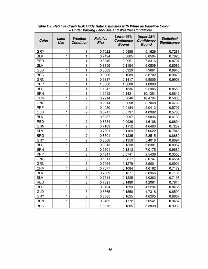
Table C3: Relative Crash Risk Odds Ratio Estimates with White as Baseline Color – Under Varying Land-Use and Weather Conditions

Color Land Use

Weather Condition

Relative Risk

Lower 95% Confidence

Bound

Upper 95% Confidence

Bound

Statistical Significance

GRY 1 1 0.7022 0.0955 5.1629 0.7283

BLK 1 1 0.7424 0.0805 6.8504 0.7928

RED 1 1 0.8349 0.0951 7.3316 0.8707

SLV 1 1 0.8356 0.1154 6.0509 0.8589

GLD 1 1 0.8602 0.0929 7.9661 0.8945

BRG 1 1 0.9830 0.1089 8.8702 0.9878

GRN 1 1 0.9887 0.1417 6.9005 0.9908

PRP 1 1 1.0000 1.0000 1.0000 .

BLU 1 1 1.1947 0.1536 9.2906 0.8650

BRN 1 1 1.2042 0.1431 10.1351 0.8642

CRM 1 2 0.2914 0.0046 18.4784 0.5603

ONG 1 2 0.2914 0.0098 8.7068 0.4769

PRP 1 2 0.4080 0.0184 9.0413 0.5707

GLD 1 2 0.5717 0.0797 4.0992 0.5780

BLK 1 2 0.6237 0.0997 3.9036 0.6139

RED 1 2 0.6534 0.0926 4.6108 0.6694

GRN 1 2 0.7189 0.1112 4.6483 0.7289

SLV 1 2 0.7691 0.1169 5.0622 0.7848

BRG 1 2 0.8501 0.1235 5.8515 0.8689

GRY 1 2 0.8568 0.1359 5.4016 0.8694

BLU 1 2 0.8813 0.1330 5.8381 0.8957

BRN 1 2 0.9601 0.1313 7.0175 0.9680

PRP 1 3 0.4341 0.0741 2.5436 0.3550

ONG 1 3 0.5011 0.0817 3.0747 0.4554

GRN 1 3 0.7064 0.1279 3.9001 0.6901

CRM 1 3 0.7077 0.1084 4.6182 0.7179

BLK 1 3 0.7309 0.1371 3.8966 0.7135

SLV 1 3 0.7314 0.1325 4.0362 0.7196

RED 1 3 0.7891 0.1480 4.2081 0.7814

BLU 1 3 0.8494 0.1593 4.5294 0.8485

GLD 1 3 0.8565 0.1550 4.7318 0.8590

GRY 1 3 0.8665 0.1625 4.6205 0.8667

BRN 1 3 0.9465 0.1772 5.0541 0.9487

BRG 1 3 1.0075 0.1885 5.3838 0.9930

57

Table C3: Continued

RED 2 1 0.4332 0.0285 6.5844 0.5468

BLK 2 1 0.5350 0.0488 5.8644 0.6087

GRN 2 1 0.5755 0.0522 6.3446 0.6519

GLD 2 1 0.6819 0.0435 10.6953 0.7852

BRG 2 1 0.8813 0.0454 17.0884 0.9334

GRY 2 1 0.8992 0.0786 10.2872 0.9319

SLV 2 1 0.9711 0.0762 12.3790 0.9820

BLU 2 1 1.2316 0.1108 13.6877 0.8654

BRN 2 1 1.2590 0.0788 20.1237 0.8707

PRP 2 1 1.2590 0.0137 115.6537 0.9205

SLV 2 2 0.2456 0.0104 5.7817 0.3837

BRN 2 2 0.4421 0.0176 11.1273 0.6199

BLU 2 2 0.9378 0.0723 12.1715 0.9608

BRG 2 2 1.0000 1.0000 1.0000 .

ONG 2 2 1.0000 1.0000 1.0000 .

BLK 2 2 1.0132 0.0558 18.4064 0.9929

GRN 2 2 1.4737 0.0905 24.0059 0.7854

RED 2 2 1.5965 0.0863 29.5387 0.7533

GRY 2 2 1.9648 0.1090 35.4244 0.6471

GLD 2 2 2.9473 0.0462 188.1049 0.6102

ONG 2 3 0.2973 0.0266 3.3231 0.3247

BRG 2 3 0.6389 0.1125 3.6288 0.6132

BLK 2 3 0.7336 0.1359 3.9590 0.7187

RED 2 3 0.7701 0.1381 4.2952 0.7658

GRY 2 3 0.8178 0.1462 4.5759 0.8190

BLU 2 3 0.8251 0.1481 4.5961 0.8263

GLD 2 3 0.8300 0.1366 5.0445 0.8396

PRP 2 3 0.8599 0.0901 8.2079 0.8957

SLV 2 3 0.8847 0.1644 4.7602 0.8865

BRN 2 3 0.9082 0.1536 5.3704 0.9154

GRN 2 3 1.0250 0.1832 5.7356 0.9776

58

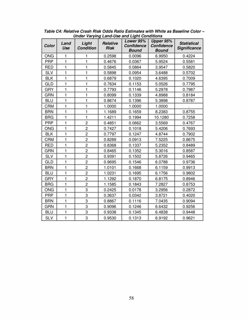
Table C4: Relative Crash Risk Odds Ratio Estimates with White as Baseline Color – Under Varying Land-Use and Light Conditions

Color Land Use

Light Condition

Relative Risk

Lower 95% Confidence

Bound

Upper 95% Confidence

Bound

Statistical Significance

ONG 1 1 0.2598 0.0096 6.9950 0.4224

PRP 1 1 0.4676 0.0367 5.9524 0.5581

RED 1 1 0.5845 0.0864 3.9547 0.5820

SLV 1 1 0.5898 0.0954 3.6488 0.5702

BLK 1 1 0.6879 0.1020 4.6395 0.7009

GLD 1 1 0.7634 0.1153 5.0526 0.7795

GRY 1 1 0.7793 0.1146 5.2978 0.7987

GRN 1 1 0.8099 0.1339 4.8988 0.8184

BLU 1 1 0.8674 0.1396 5.3898 0.8787

CRM 1 1 1.0000 1.0000 1.0000 .

BRN 1 1 1.1689 0.1659 8.2383 0.8755

BRG 1 1 1.4211 0.1994 10.1280 0.7258

PRP 1 2 0.4851 0.0662 3.5569 0.4767

ONG 1 2 0.7427 0.1018 5.4206 0.7693

BLK 1 2 0.7797 0.1247 4.8744 0.7902

CRM 1 2 0.8289 0.0913 7.5225 0.8675

RED 1 2 0.8368 0.1337 5.2352 0.8489

GRN 1 2 0.8465 0.1352 5.3016 0.8587

SLV 1 2 0.9391 0.1502 5.8726 0.9465

GLD 1 2 0.9695 0.1546 6.0788 0.9736

BRN 1 2 1.0101 0.1668 6.1159 0.9913

BLU 1 2 1.0231 0.1695 6.1756 0.9802

GRY 1 2 1.1292 0.1870 6.8175 0.8946

BRG 1 2 1.1585 0.1843 7.2827 0.8753

ONG 1 3 0.2425 0.0178 3.2956 0.2872

PRP 1 3 0.3637 0.0342 3.8721 0.4020

BRN 1 3 0.8867 0.1116 7.0435 0.9094

GRN 1 3 0.9096 0.1246 6.6432 0.9256

BLU 1 3 0.9338 0.1345 6.4838 0.9448

SLV 1 3 0.9530 0.1313 6.9192 0.9621

59

Table C4: Continued

BLK 1 3 0.9719 0.1401 6.7430 0.9770

CRM 1 3 1.0000 1.0000 1.0000 .

BRG 1 3 1.0912 0.1355 8.7890 0.9346

GLD 1 3 1.1915 0.1487 9.5487 0.8690

GRY 1 3 1.2256 0.1816 8.2689 0.8346

RED 1 3 1.3094 0.2006 8.5455 0.7782

ONG 1 4 0.4320 0.0587 3.1791 0.4098

CRM 1 4 0.4819 0.0603 3.8524 0.4913

PRP 1 4 0.5212 0.0779 3.4876 0.5016

GRN 1 4 0.7123 0.1180 4.2982 0.7114

SLV 1 4 0.7577 0.1257 4.5686 0.7621

BLK 1 4 0.7691 0.1323 4.4723 0.7701

RED 1 4 0.8272 0.1422 4.8124 0.8327

GRY 1 4 0.8489 0.1459 4.9382 0.8553

GLD 1 4 0.8732 0.1445 5.2751 0.8825

BRN 1 4 0.8848 0.1463 5.3495 0.8939

BLU 1 4 0.8968 0.1542 5.2164 0.9035

BRG 1 4 0.9293 0.1592 5.4238 0.9351

ONG 2 1 0.6173 0.0089 42.8669 0.8236

BLK 2 1 0.7576 0.1095 5.2399 0.7784

GRY 2 1 0.8547 0.1090 6.7006 0.8812

RED 2 1 0.9927 0.1357 7.2638 0.9943

GLD 2 1 1.0559 0.1335 8.3503 0.9589

BRN 2 1 1.1112 0.1055 11.7060 0.9301

BRG 2 1 1.1852 0.1095 12.8289 0.8888

SLV 2 1 1.3040 0.1716 9.9096 0.7976

BLU 2 1 1.3144 0.1612 10.7210 0.7984

GRN 2 1 1.7642 0.2149 14.4819 0.5971

PRP 2 1 2.4692 0.0801 76.1496 0.6054

ONG 2 2 0.3715 0.0040 34.8795 0.6692

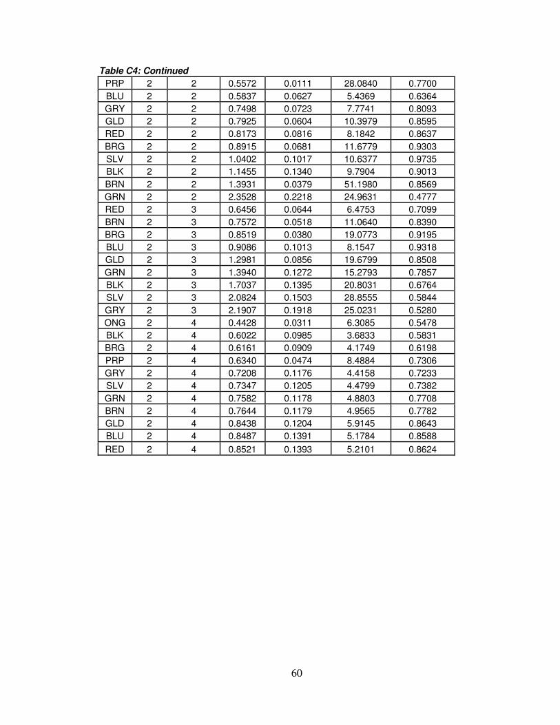
60

Table C4: Continued

PRP 2 2 0.5572 0.0111 28.0840 0.7700

BLU 2 2 0.5837 0.0627 5.4369 0.6364

GRY 2 2 0.7498 0.0723 7.7741 0.8093

GLD 2 2 0.7925 0.0604 10.3979 0.8595

RED 2 2 0.8173 0.0816 8.1842 0.8637

BRG 2 2 0.8915 0.0681 11.6779 0.9303

SLV 2 2 1.0402 0.1017 10.6377 0.9735

BLK 2 2 1.1455 0.1340 9.7904 0.9013

BRN 2 2 1.3931 0.0379 51.1980 0.8569

GRN 2 2 2.3528 0.2218 24.9631 0.4777

RED 2 3 0.6456 0.0644 6.4753 0.7099

BRN 2 3 0.7572 0.0518 11.0640 0.8390

BRG 2 3 0.8519 0.0380 19.0773 0.9195

BLU 2 3 0.9086 0.1013 8.1547 0.9318

GLD 2 3 1.2981 0.0856 19.6799 0.8508

GRN 2 3 1.3940 0.1272 15.2793 0.7857

BLK 2 3 1.7037 0.1395 20.8031 0.6764

SLV 2 3 2.0824 0.1503 28.8555 0.5844

GRY 2 3 2.1907 0.1918 25.0231 0.5280

ONG 2 4 0.4428 0.0311 6.3085 0.5478

BLK 2 4 0.6022 0.0985 3.6833 0.5831

BRG 2 4 0.6161 0.0909 4.1749 0.6198

PRP 2 4 0.6340 0.0474 8.4884 0.7306

GRY 2 4 0.7208 0.1176 4.4158 0.7233

SLV 2 4 0.7347 0.1205 4.4799 0.7382

GRN 2 4 0.7582 0.1178 4.8803 0.7708

BRN 2 4 0.7644 0.1179 4.9565 0.7782

GLD 2 4 0.8438 0.1204 5.9145 0.8643

BLU 2 4 0.8487 0.1391 5.1784 0.8588

RED 2 4 0.8521 0.1393 5.2101 0.8624

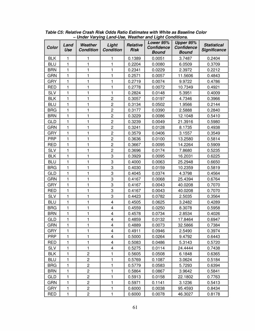
61

Table C5: Relative Crash Risk Odds Ratio Estimates with White as Baseline Color – Under Varying Land-Use, Weather and Light Conditions.

Color Land Use

Weather Condition

Light Condition

Relative Risk

Lower 95% Confidence

Bound

Upper 95% Confidence

Bound

Statistical Significance

BLK 1 1 1 0.1389 0.0051 3.7487 0.2404

BLU 1 1 1 0.2204 0.0080 6.0509 0.3709

BRN 1 1 1 0.2341 0.0229 2.3972 0.2212

GRN 1 1 1 0.2571 0.0057 11.5606 0.4843

GRY 1 1 1 0.2719 0.0074 9.9722 0.4786

RED 1 1 1 0.2778 0.0072 10.7349 0.4921

SLV 1 1 1 0.2824 0.0148 5.3951 0.4009

BLK 1 1 2 0.3057 0.0197 4.7346 0.3966

BLU 1 1 2 0.3134 0.0502 1.9566 0.2144

BRG 1 1 2 0.3177 0.0390 2.5888 0.2840

BRN 1 1 2 0.3229 0.0086 12.1048 0.5410

GLD 1 1 2 0.3239 0.0049 21.3916 0.5980

GRN 1 1 2 0.3241 0.0128 8.1735 0.4938

GRY 1 1 2 0.3579 0.0406 3.1557 0.3549

PRP 1 1 2 0.3636 0.0100 13.2580 0.5814

RED 1 1 2 0.3667 0.0095 14.2264 0.5909

SLV 1 1 2 0.3696 0.0174 7.8680 0.5235

BLK 1 1 3 0.3929 0.0095 16.2031 0.6225

BLU 1 1 3 0.4000 0.0063 25.2948 0.6650

BRG 1 1 3 0.4030 0.0159 10.2359 0.5819

GLD 1 1 3 0.4045 0.0374 4.3798 0.4564

GRN 1 1 3 0.4167 0.0068 25.4394 0.6764

GRY 1 1 3 0.4167 0.0043 40.0208 0.7070

RED 1 1 3 0.4167 0.0043 40.0208 0.7070

SLV 1 1 3 0.4423 0.0782 2.5035 0.3564

BLU 1 1 4 0.4505 0.0625 3.2482 0.4289

BRG 1 1 4 0.4559 0.0250 8.3078 0.5958

BRN 1 1 4 0.4578 0.0734 2.8534 0.4026

GLD 1 1 4 0.4859 0.0132 17.8464 0.6947

GRN 1 1 4 0.4889 0.0073 32.5866 0.7384

GRY 1 1 4 0.4911 0.0946 2.5490 0.3974

PRP 1 1 4 0.5000 0.0264 9.4792 0.6443

RED 1 1 4 0.5083 0.0486 5.3143 0.5720

SLV 1 1 4 0.5275 0.0114 24.4444 0.7438

BLK 1 2 1 0.5605 0.0508 6.1848 0.6365

BLU 1 2 1 0.5769 0.1087 3.0624 0.5184

BRG 1 2 1 0.5779 0.0583 5.7293 0.6394

BRN 1 2 1 0.5864 0.0867 3.9642 0.5841

GLD 1 2 1 0.5913 0.0158 22.1802 0.7763

GRN 1 2 1 0.5971 0.1141 3.1236 0.5413

GRY 1 2 1 0.6000 0.0038 95.4593 0.8434

RED 1 2 1 0.6000 0.0078 46.3027 0.8178

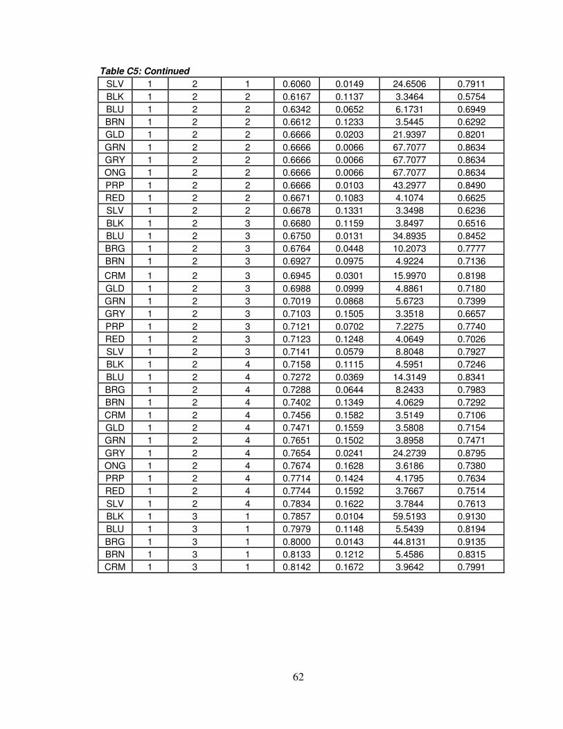
62

Table C5: Continued

SLV 1 2 1 0.6060 0.0149 24.6506 0.7911

BLK 1 2 2 0.6167 0.1137 3.3464 0.5754

BLU 1 2 2 0.6342 0.0652 6.1731 0.6949

BRN 1 2 2 0.6612 0.1233 3.5445 0.6292

GLD 1 2 2 0.6666 0.0203 21.9397 0.8201

GRN 1 2 2 0.6666 0.0066 67.7077 0.8634

GRY 1 2 2 0.6666 0.0066 67.7077 0.8634

ONG 1 2 2 0.6666 0.0066 67.7077 0.8634

PRP 1 2 2 0.6666 0.0103 43.2977 0.8490

RED 1 2 2 0.6671 0.1083 4.1074 0.6625

SLV 1 2 2 0.6678 0.1331 3.3498 0.6236

BLK 1 2 3 0.6680 0.1159 3.8497 0.6516

BLU 1 2 3 0.6750 0.0131 34.8935 0.8452

BRG 1 2 3 0.6764 0.0448 10.2073 0.7777

BRN 1 2 3 0.6927 0.0975 4.9224 0.7136

CRM 1 2 3 0.6945 0.0301 15.9970 0.8198

GLD 1 2 3 0.6988 0.0999 4.8861 0.7180

GRN 1 2 3 0.7019 0.0868 5.6723 0.7399

GRY 1 2 3 0.7103 0.1505 3.3518 0.6657

PRP 1 2 3 0.7121 0.0702 7.2275 0.7740

RED 1 2 3 0.7123 0.1248 4.0649 0.7026

SLV 1 2 3 0.7141 0.0579 8.8048 0.7927

BLK 1 2 4 0.7158 0.1115 4.5951 0.7246

BLU 1 2 4 0.7272 0.0369 14.3149 0.8341

BRG 1 2 4 0.7288 0.0644 8.2433 0.7983

BRN 1 2 4 0.7402 0.1349 4.0629 0.7292

CRM 1 2 4 0.7456 0.1582 3.5149 0.7106

GLD 1 2 4 0.7471 0.1559 3.5808 0.7154

GRN 1 2 4 0.7651 0.1502 3.8958 0.7471

GRY 1 2 4 0.7654 0.0241 24.2739 0.8795

ONG 1 2 4 0.7674 0.1628 3.6186 0.7380

PRP 1 2 4 0.7714 0.1424 4.1795 0.7634

RED 1 2 4 0.7744 0.1592 3.7667 0.7514

SLV 1 2 4 0.7834 0.1622 3.7844 0.7613

BLK 1 3 1 0.7857 0.0104 59.5193 0.9130

BLU 1 3 1 0.7979 0.1148 5.5439 0.8194

BRG 1 3 1 0.8000 0.0143 44.8131 0.9135

BRN 1 3 1 0.8133 0.1212 5.4586 0.8315

CRM 1 3 1 0.8142 0.1672 3.9642 0.7991

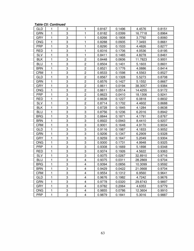
63

Table C5: Continued

GLD 1 3 1 0.8167 0.1496 4.4576 0.8151

GRN 1 3 1 0.8182 0.0399 16.7718 0.8964

GRY 1 3 1 0.8266 0.1808 3.7792 0.8060

ONG 1 3 1 0.8288 0.0935 7.3493 0.8661

PRP 1 3 1 0.8290 0.1533 4.4826 0.8277

RED 1 3 1 0.8316 0.1706 4.0536 0.8195

SLV 1 3 1 0.8411 0.1465 4.8278 0.8461

BLK 1 3 2 0.8448 0.0606 11.7823 0.9001

BLU 1 3 2 0.8504 0.1401 5.1603 0.8601

BRN 1 3 2 0.8521 0.1776 4.0886 0.8414

CRM 1 3 2 0.8533 0.1598 4.5563 0.8527

GLD 1 3 2 0.8567 0.1328 5.5273 0.8708

GRN 1 3 2 0.8576 0.1427 5.1552 0.8667

GRY 1 3 2 0.8611 0.0194 38.3057 0.9384

ONG 1 3 2 0.8611 0.0514 14.4255 0.9172

PRP 1 3 2 0.8623 0.0410 18.1306 0.9241

RED 1 3 2 0.8638 0.1227 6.0818 0.8832

SLV 1 3 2 0.8714 0.1702 4.4602 0.8688

BLK 1 3 3 0.8728 0.1845 4.1284 0.8638

BLU 1 3 3 0.8756 0.1236 6.2016 0.8942

BRG 1 3 3 0.8844 0.1871 4.1791 0.8767

BRN 1 3 3 0.8922 0.0943 8.4410 0.9207

CRM 1 3 3 0.9001 0.1648 4.9170 0.9034

GLD 1 3 3 0.9116 0.1987 4.1833 0.9052

GRN 1 3 3 0.9206 0.1347 6.2909 0.9328

GRY 1 3 3 0.9259 0.1647 5.2049 0.9304

ONG 1 3 3 0.9300 0.1731 4.9948 0.9325

PRP 1 3 3 0.9308 0.1669 5.1898 0.9348

RED 1 3 3 0.9374 0.1926 4.5622 0.9363

SLV 1 3 3 0.9375 0.0267 32.8910 0.9716

BLU 1 3 4 0.9375 0.0311 28.2869 0.9704

BRG 1 3 4 0.9394 0.0856 10.3099 0.9592

BRN 1 3 4 0.9429 0.0422 21.0668 0.9704

CRM 1 3 4 0.9554 0.1312 6.9560 0.9641

GLD 1 3 4 0.9676 0.1982 4.7242 0.9676

GRN 1 3 4 0.9778 0.0320 29.8743 0.9897

GRY 1 3 4 0.9782 0.2064 4.6353 0.9779

ONG 1 3 4 0.9855 0.0786 12.3604 0.9910

PRP 1 3 4 0.9879 0.1841 5.3016 0.9887

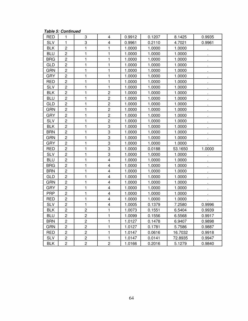
64

Table 5: Continued

RED 1 3 4 0.9912 0.1207 8.1425 0.9935

SLV 1 3 4 0.9961 0.2110 4.7021 0.9961

BLK 2 1 1 1.0000 1.0000 1.0000 .

BLU 2 1 1 1.0000 1.0000 1.0000 .

BRG 2 1 1 1.0000 1.0000 1.0000 .

GLD 2 1 1 1.0000 1.0000 1.0000 .

GRN 2 1 1 1.0000 1.0000 1.0000 .

GRY 2 1 1 1.0000 1.0000 1.0000 .

RED 2 1 1 1.0000 1.0000 1.0000 .

SLV 2 1 1 1.0000 1.0000 1.0000 .

BLK 2 1 2 1.0000 1.0000 1.0000 .

BLU 2 1 2 1.0000 1.0000 1.0000 .

GLD 2 1 2 1.0000 1.0000 1.0000 .

GRN 2 1 2 1.0000 1.0000 1.0000 .

GRY 2 1 2 1.0000 1.0000 1.0000 .

SLV 2 1 2 1.0000 1.0000 1.0000 .

BLK 2 1 3 1.0000 1.0000 1.0000 .

BRN 2 1 3 1.0000 1.0000 1.0000 .

GRN 2 1 3 1.0000 1.0000 1.0000 .

GRY 2 1 3 1.0000 1.0000 1.0000 .

RED 2 1 3 1.0000 0.0188 53.1650 1.0000

SLV 2 1 3 1.0000 1.0000 1.0000 .

BLU 2 1 4 1.0000 1.0000 1.0000 .

BRG 2 1 4 1.0000 1.0000 1.0000 .

BRN 2 1 4 1.0000 1.0000 1.0000 .

GLD 2 1 4 1.0000 1.0000 1.0000 .

GRN 2 1 4 1.0000 1.0000 1.0000 .

GRY 2 1 4 1.0000 1.0000 1.0000 .

PRP 2 1 4 1.0000 1.0000 1.0000 .

RED 2 1 4 1.0000 1.0000 1.0000 .

SLV 2 1 4 1.0005 0.1379 7.2580 0.9996

BLK 2 2 1 1.0073 0.1551 6.5404 0.9939

BLU 2 2 1 1.0099 0.1556 6.5568 0.9917

BRN 2 2 1 1.0127 0.1478 6.9407 0.9898

GRN 2 2 1 1.0127 0.1781 5.7586 0.9887

RED 2 2 1 1.0147 0.0616 16.7032 0.9918

SLV 2 2 1 1.0147 0.0141 72.8935 0.9947

BLK 2 2 2 1.0166 0.2016 5.1279 0.9840

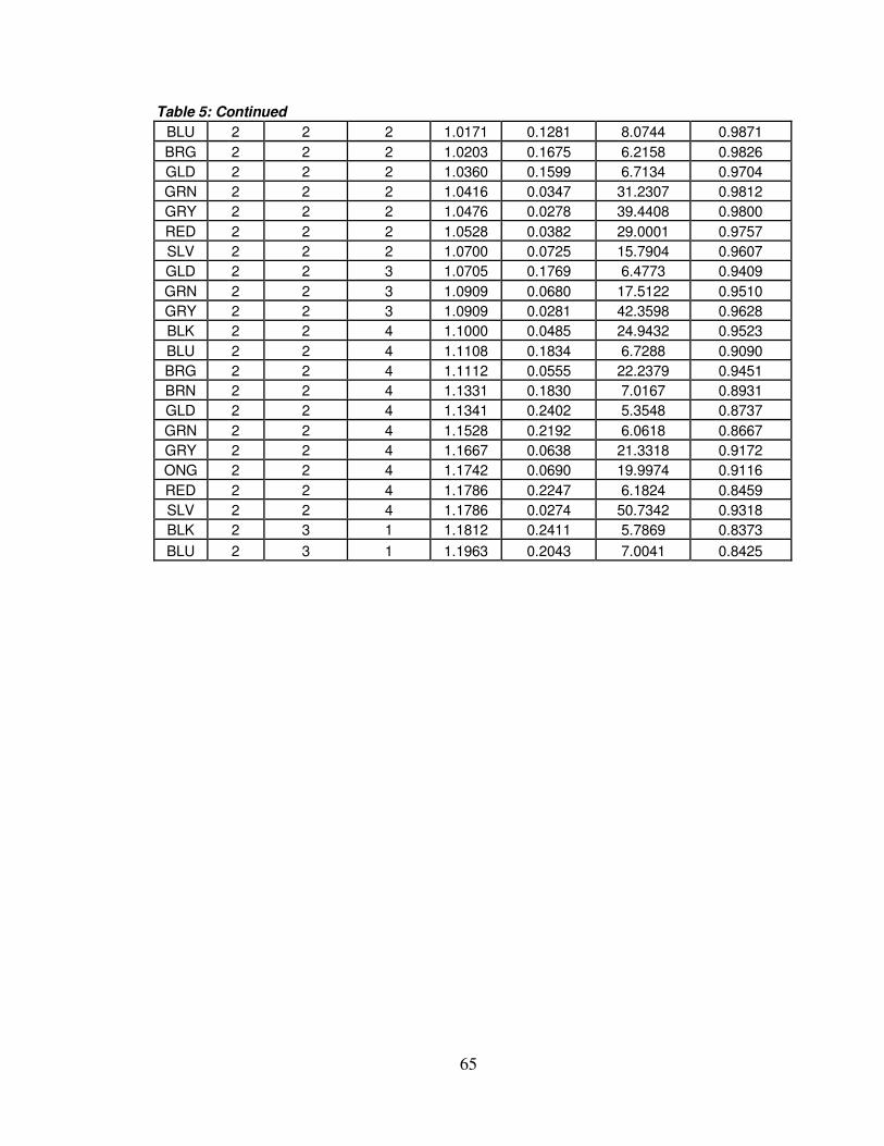
65

Table 5: Continued

BLU 2 2 2 1.0171 0.1281 8.0744 0.9871

BRG 2 2 2 1.0203 0.1675 6.2158 0.9826

GLD 2 2 2 1.0360 0.1599 6.7134 0.9704

GRN 2 2 2 1.0416 0.0347 31.2307 0.9812

GRY 2 2 2 1.0476 0.0278 39.4408 0.9800

RED 2 2 2 1.0528 0.0382 29.0001 0.9757

SLV 2 2 2 1.0700 0.0725 15.7904 0.9607

GLD 2 2 3 1.0705 0.1769 6.4773 0.9409

GRN 2 2 3 1.0909 0.0680 17.5122 0.9510

GRY 2 2 3 1.0909 0.0281 42.3598 0.9628

BLK 2 2 4 1.1000 0.0485 24.9432 0.9523

BLU 2 2 4 1.1108 0.1834 6.7288 0.9090

BRG 2 2 4 1.1112 0.0555 22.2379 0.9451

BRN 2 2 4 1.1331 0.1830 7.0167 0.8931

GLD 2 2 4 1.1341 0.2402 5.3548 0.8737

GRN 2 2 4 1.1528 0.2192 6.0618 0.8667

GRY 2 2 4 1.1667 0.0638 21.3318 0.9172

ONG 2 2 4 1.1742 0.0690 19.9974 0.9116

RED 2 2 4 1.1786 0.2247 6.1824 0.8459

SLV 2 2 4 1.1786 0.0274 50.7342 0.9318

BLK 2 3 1 1.1812 0.2411 5.7869 0.8373

BLU 2 3 1 1.1963 0.2043 7.0041 0.8425

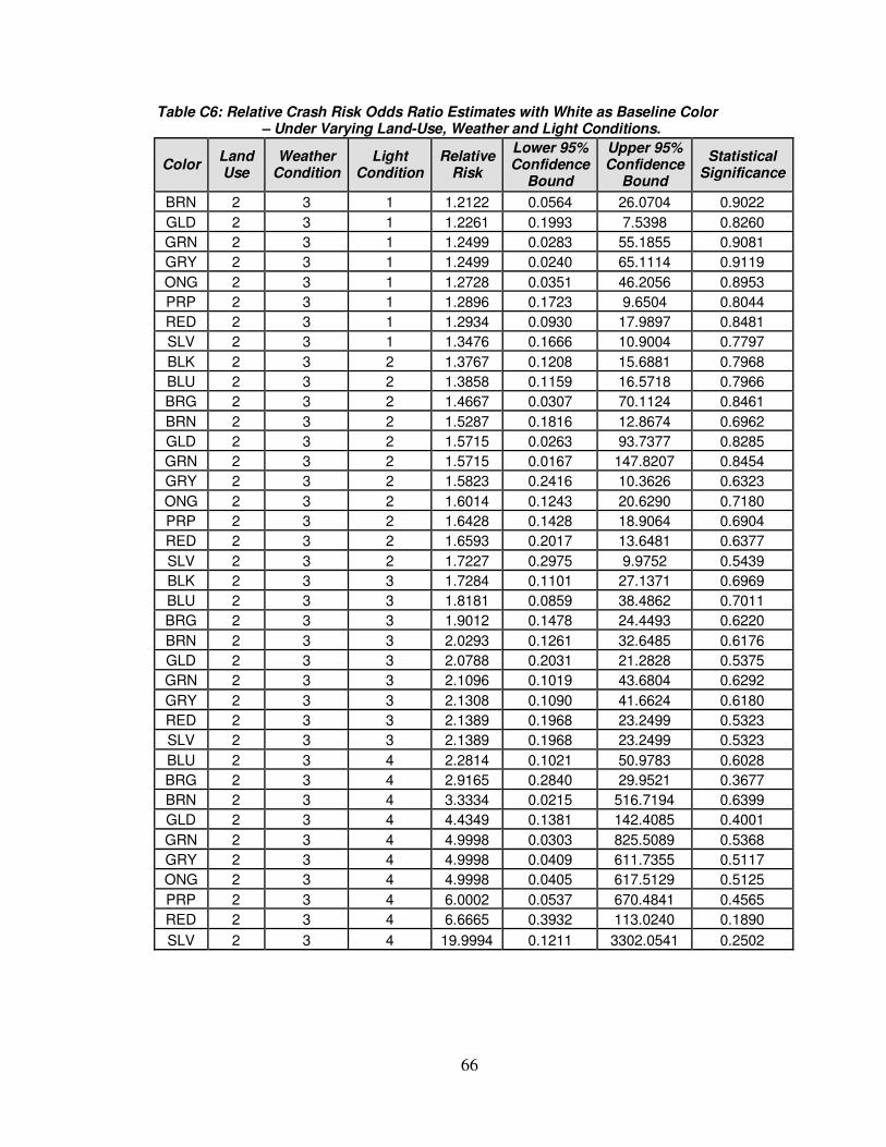
66

Table C6: Relative Crash Risk Odds Ratio Estimates with White as Baseline Color – Under Varying Land-Use, Weather and Light Conditions.

Color Land Use

Weather Condition

Light Condition

Relative Risk

Lower 95% Confidence

Bound

Upper 95% Confidence

Bound

Statistical Significance

BRN 2 3 1 1.2122 0.0564 26.0704 0.9022

GLD 2 3 1 1.2261 0.1993 7.5398 0.8260

GRN 2 3 1 1.2499 0.0283 55.1855 0.9081

GRY 2 3 1 1.2499 0.0240 65.1114 0.9119

ONG 2 3 1 1.2728 0.0351 46.2056 0.8953

PRP 2 3 1 1.2896 0.1723 9.6504 0.8044

RED 2 3 1 1.2934 0.0930 17.9897 0.8481

SLV 2 3 1 1.3476 0.1666 10.9004 0.7797

BLK 2 3 2 1.3767 0.1208 15.6881 0.7968

BLU 2 3 2 1.3858 0.1159 16.5718 0.7966

BRG 2 3 2 1.4667 0.0307 70.1124 0.8461

BRN 2 3 2 1.5287 0.1816 12.8674 0.6962

GLD 2 3 2 1.5715 0.0263 93.7377 0.8285

GRN 2 3 2 1.5715 0.0167 147.8207 0.8454

GRY 2 3 2 1.5823 0.2416 10.3626 0.6323

ONG 2 3 2 1.6014 0.1243 20.6290 0.7180

PRP 2 3 2 1.6428 0.1428 18.9064 0.6904

RED 2 3 2 1.6593 0.2017 13.6481 0.6377

SLV 2 3 2 1.7227 0.2975 9.9752 0.5439

BLK 2 3 3 1.7284 0.1101 27.1371 0.6969

BLU 2 3 3 1.8181 0.0859 38.4862 0.7011

BRG 2 3 3 1.9012 0.1478 24.4493 0.6220

BRN 2 3 3 2.0293 0.1261 32.6485 0.6176

GLD 2 3 3 2.0788 0.2031 21.2828 0.5375

GRN 2 3 3 2.1096 0.1019 43.6804 0.6292

GRY 2 3 3 2.1308 0.1090 41.6624 0.6180

RED 2 3 3 2.1389 0.1968 23.2499 0.5323

SLV 2 3 3 2.1389 0.1968 23.2499 0.5323

BLU 2 3 4 2.2814 0.1021 50.9783 0.6028

BRG 2 3 4 2.9165 0.2840 29.9521 0.3677

BRN 2 3 4 3.3334 0.0215 516.7194 0.6399

GLD 2 3 4 4.4349 0.1381 142.4085 0.4001

GRN 2 3 4 4.9998 0.0303 825.5089 0.5368

GRY 2 3 4 4.9998 0.0409 611.7355 0.5117

ONG 2 3 4 4.9998 0.0405 617.5129 0.5125

PRP 2 3 4 6.0002 0.0537 670.4841 0.4565

RED 2 3 4 6.6665 0.3932 113.0240 0.1890

SLV 2 3 4 19.9994 0.1211 3302.0541 0.2502

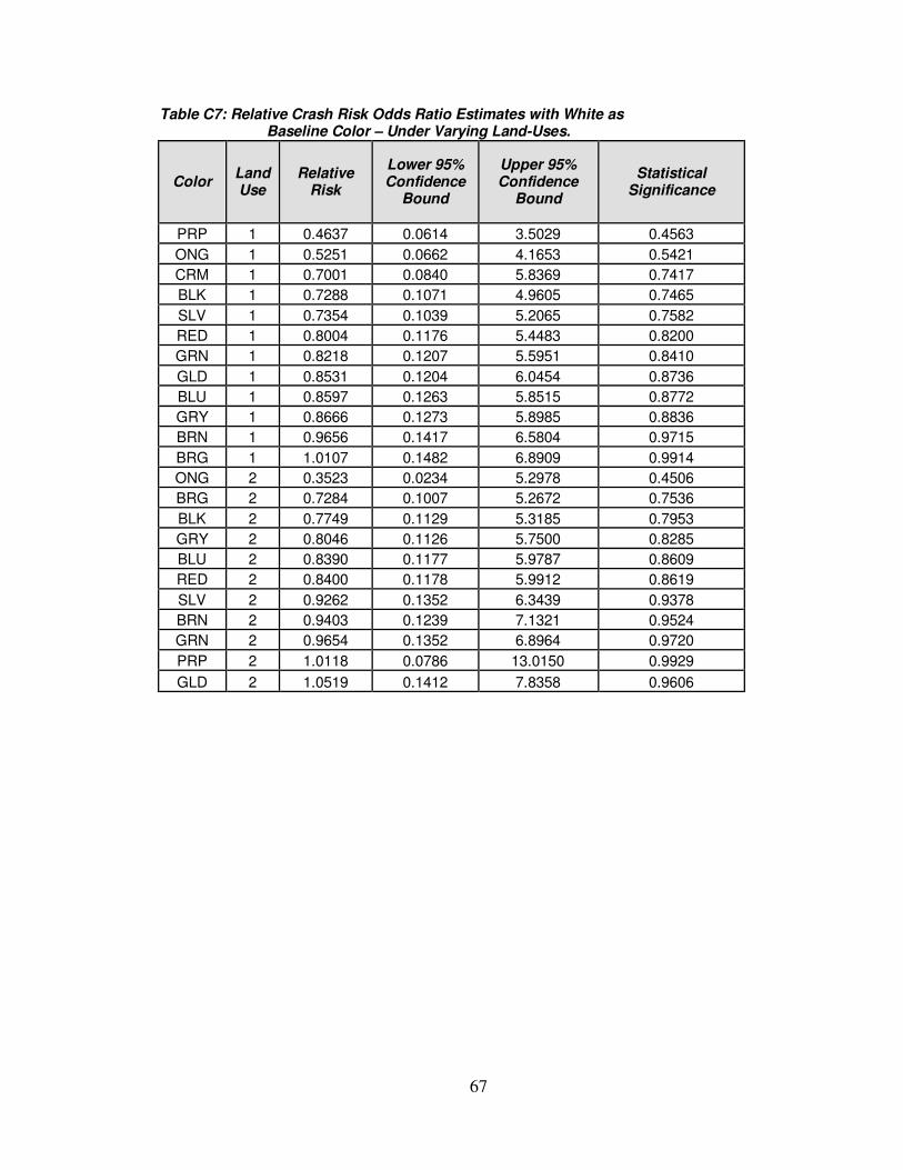
67

Table C7: Relative Crash Risk Odds Ratio Estimates with White as Baseline Color – Under Varying Land-Uses.

Color Land Use

Relative Risk

Lower 95% Confidence

Bound

Upper 95% Confidence

Bound

Statistical Significance

PRP 1 0.4637 0.0614 3.5029 0.4563

ONG 1 0.5251 0.0662 4.1653 0.5421

CRM 1 0.7001 0.0840 5.8369 0.7417

BLK 1 0.7288 0.1071 4.9605 0.7465

SLV 1 0.7354 0.1039 5.2065 0.7582

RED 1 0.8004 0.1176 5.4483 0.8200

GRN 1 0.8218 0.1207 5.5951 0.8410

GLD 1 0.8531 0.1204 6.0454 0.8736

BLU 1 0.8597 0.1263 5.8515 0.8772

GRY 1 0.8666 0.1273 5.8985 0.8836

BRN 1 0.9656 0.1417 6.5804 0.9715

BRG 1 1.0107 0.1482 6.8909 0.9914

ONG 2 0.3523 0.0234 5.2978 0.4506

BRG 2 0.7284 0.1007 5.2672 0.7536

BLK 2 0.7749 0.1129 5.3185 0.7953

GRY 2 0.8046 0.1126 5.7500 0.8285

BLU 2 0.8390 0.1177 5.9787 0.8609

RED 2 0.8400 0.1178 5.9912 0.8619

SLV 2 0.9262 0.1352 6.3439 0.9378

BRN 2 0.9403 0.1239 7.1321 0.9524

GRN 2 0.9654 0.1352 6.8964 0.9720

PRP 2 1.0118 0.0786 13.0150 0.9929

GLD 2 1.0519 0.1412 7.8358 0.9606

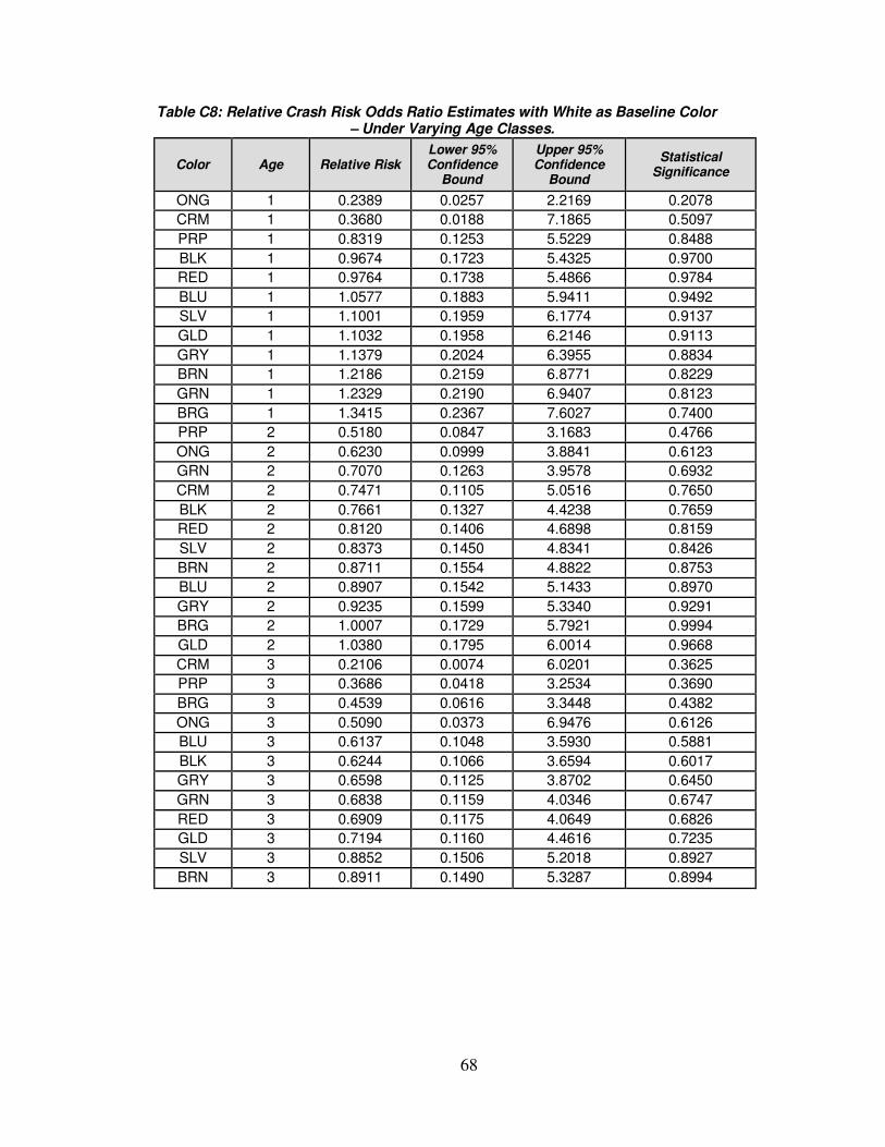
68

Table C8: Relative Crash Risk Odds Ratio Estimates with White as Baseline Color – Under Varying Age Classes.

Color Age Relative Risk Lower 95% Confidence

Bound

Upper 95% Confidence

Bound

Statistical Significance

ONG 1 0.2389 0.0257 2.2169 0.2078

CRM 1 0.3680 0.0188 7.1865 0.5097

PRP 1 0.8319 0.1253 5.5229 0.8488

BLK 1 0.9674 0.1723 5.4325 0.9700

RED 1 0.9764 0.1738 5.4866 0.9784

BLU 1 1.0577 0.1883 5.9411 0.9492

SLV 1 1.1001 0.1959 6.1774 0.9137

GLD 1 1.1032 0.1958 6.2146 0.9113

GRY 1 1.1379 0.2024 6.3955 0.8834

BRN 1 1.2186 0.2159 6.8771 0.8229

GRN 1 1.2329 0.2190 6.9407 0.8123

BRG 1 1.3415 0.2367 7.6027 0.7400

PRP 2 0.5180 0.0847 3.1683 0.4766

ONG 2 0.6230 0.0999 3.8841 0.6123

GRN 2 0.7070 0.1263 3.9578 0.6932

CRM 2 0.7471 0.1105 5.0516 0.7650

BLK 2 0.7661 0.1327 4.4238 0.7659

RED 2 0.8120 0.1406 4.6898 0.8159

SLV 2 0.8373 0.1450 4.8341 0.8426

BRN 2 0.8711 0.1554 4.8822 0.8753

BLU 2 0.8907 0.1542 5.1433 0.8970

GRY 2 0.9235 0.1599 5.3340 0.9291

BRG 2 1.0007 0.1729 5.7921 0.9994

GLD 2 1.0380 0.1795 6.0014 0.9668

CRM 3 0.2106 0.0074 6.0201 0.3625

PRP 3 0.3686 0.0418 3.2534 0.3690

BRG 3 0.4539 0.0616 3.3448 0.4382

ONG 3 0.5090 0.0373 6.9476 0.6126

BLU 3 0.6137 0.1048 3.5930 0.5881

BLK 3 0.6244 0.1066 3.6594 0.6017

GRY 3 0.6598 0.1125 3.8702 0.6450

GRN 3 0.6838 0.1159 4.0346 0.6747

RED 3 0.6909 0.1175 4.0649 0.6826

GLD 3 0.7194 0.1160 4.4616 0.7235

SLV 3 0.8852 0.1506 5.2018 0.8927

BRN 3 0.8911 0.1490 5.3287 0.8994

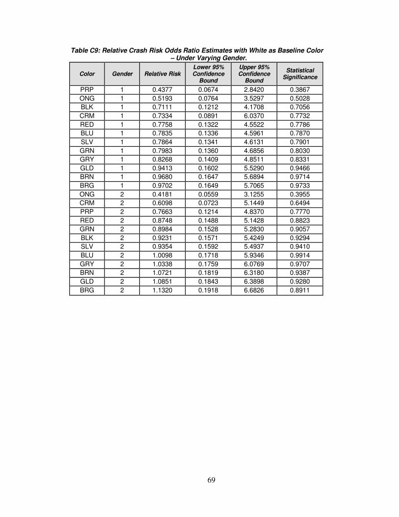
69

Table C9: Relative Crash Risk Odds Ratio Estimates with White as Baseline Color – Under Varying Gender.

Color Gender Relative Risk Lower 95% Confidence

Bound

Upper 95% Confidence

Bound

Statistical Significance

PRP 1 0.4377 0.0674 2.8420 0.3867

ONG 1 0.5193 0.0764 3.5297 0.5028

BLK 1 0.7111 0.1212 4.1708 0.7056

CRM 1 0.7334 0.0891 6.0370 0.7732

RED 1 0.7758 0.1322 4.5522 0.7786

BLU 1 0.7835 0.1336 4.5961 0.7870

SLV 1 0.7864 0.1341 4.6131 0.7901

GRN 1 0.7983 0.1360 4.6856 0.8030

GRY 1 0.8268 0.1409 4.8511 0.8331

GLD 1 0.9413 0.1602 5.5290 0.9466

BRN 1 0.9680 0.1647 5.6894 0.9714

BRG 1 0.9702 0.1649 5.7065 0.9733

ONG 2 0.4181 0.0559 3.1255 0.3955

CRM 2 0.6098 0.0723 5.1449 0.6494

PRP 2 0.7663 0.1214 4.8370 0.7770

RED 2 0.8748 0.1488 5.1428 0.8823

GRN 2 0.8984 0.1528 5.2830 0.9057

BLK 2 0.9231 0.1571 5.4249 0.9294

SLV 2 0.9354 0.1592 5.4937 0.9410

BLU 2 1.0098 0.1718 5.9346 0.9914

GRY 2 1.0338 0.1759 6.0769 0.9707

BRN 2 1.0721 0.1819 6.3180 0.9387

GLD 2 1.0851 0.1843 6.3898 0.9280

BRG 2 1.1320 0.1918 6.6826 0.8911

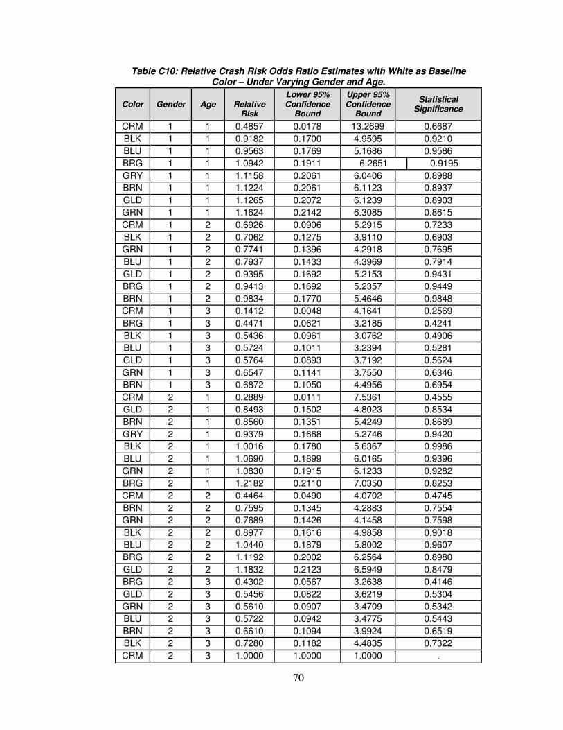
70

Table C10: Relative Crash Risk Odds Ratio Estimates with White as Baseline Color – Under Varying Gender and Age.

Color Gender Age

Relative Risk

Lower 95% Confidence

Bound

Upper 95% Confidence

Bound

Statistical Significance

CRM 1 1 0.4857 0.0178 13.2699 0.6687

BLK 1 1 0.9182 0.1700 4.9595 0.9210

BLU 1 1 0.9563 0.1769 5.1686 0.9586

BRG 1 1 1.0942 0.1911 6.2651 0.9195

GRY 1 1 1.1158 0.2061 6.0406 0.8988

BRN 1 1 1.1224 0.2061 6.1123 0.8937

GLD 1 1 1.1265 0.2072 6.1239 0.8903

GRN 1 1 1.1624 0.2142 6.3085 0.8615

CRM 1 2 0.6926 0.0906 5.2915 0.7233

BLK 1 2 0.7062 0.1275 3.9110 0.6903

GRN 1 2 0.7741 0.1396 4.2918 0.7695

BLU 1 2 0.7937 0.1433 4.3969 0.7914

GLD 1 2 0.9395 0.1692 5.2153 0.9431

BRG 1 2 0.9413 0.1692 5.2357 0.9449

BRN 1 2 0.9834 0.1770 5.4646 0.9848

CRM 1 3 0.1412 0.0048 4.1641 0.2569

BRG 1 3 0.4471 0.0621 3.2185 0.4241

BLK 1 3 0.5436 0.0961 3.0762 0.4906

BLU 1 3 0.5724 0.1011 3.2394 0.5281

GLD 1 3 0.5764 0.0893 3.7192 0.5624

GRN 1 3 0.6547 0.1141 3.7550 0.6346

BRN 1 3 0.6872 0.1050 4.4956 0.6954

CRM 2 1 0.2889 0.0111 7.5361 0.4555

GLD 2 1 0.8493 0.1502 4.8023 0.8534

BRN 2 1 0.8560 0.1351 5.4249 0.8689

GRY 2 1 0.9379 0.1668 5.2746 0.9420

BLK 2 1 1.0016 0.1780 5.6367 0.9986

BLU 2 1 1.0690 0.1899 6.0165 0.9396

GRN 2 1 1.0830 0.1915 6.1233 0.9282

BRG 2 1 1.2182 0.2110 7.0350 0.8253

CRM 2 2 0.4464 0.0490 4.0702 0.4745

BRN 2 2 0.7595 0.1345 4.2883 0.7554

GRN 2 2 0.7689 0.1426 4.1458 0.7598

BLK 2 2 0.8977 0.1616 4.9858 0.9018

BLU 2 2 1.0440 0.1879 5.8002 0.9607

BRG 2 2 1.1192 0.2002 6.2564 0.8980

GLD 2 2 1.1832 0.2123 6.5949 0.8479

BRG 2 3 0.4302 0.0567 3.2638 0.4146

GLD 2 3 0.5456 0.0822 3.6219 0.5304

GRN 2 3 0.5610 0.0907 3.4709 0.5342

BLU 2 3 0.5722 0.0942 3.4775 0.5443

BRN 2 3 0.6610 0.1094 3.9924 0.6519

BLK 2 3 0.7280 0.1182 4.4835 0.7322

CRM 2 3 1.0000 1.0000 1.0000 .

71

APPENDIX D

Extended Poisson Model Results

72

Table D1: Relative Crash Risk Odds Ratio Estimates with White as Baseline Color – Under Varying Light Conditions

Color Light

Condition Relative

Risk

Lower 95% Confidence

Bound

Upper 95% Confidence

Bound

Statistical Significance

BLK 1 0.9385 0.7279 1.2101 0.6245

BLU 1 1.0110 0.7943 1.2869 0.9291

BRG 1 1.3251 0.8869 1.9798 0.1694

BRN 1 1.2513 0.8588 1.8232 0.2430

CRM 1 1.0000 1.0000 1.0000 .

GLD 1 1.1173 0.8188 1.5244 0.4843

GRN 1 0.9922 0.7546 1.3046 0.9553

GRY 1 1.0088 0.7612 1.3371 0.9510

ONG 1 0.2955 0.0944 0.9244 0.0362

PRP 1 1.1363 0.4921 2.6240 0.7646

RED 1 0.8558 0.6625 1.1056 0.2333

SLV 1 0.8902 0.7061 1.1223 0.3251

BLK 2 0.7972 0.7182 0.8848 <.0001

BLU 2 0.8945 0.8000 1.0000 0.0499

BRG 2 1.1965 1.0037 1.4263 0.0454

BRN 2 0.9120 0.7821 1.0635 0.2401

CRM 2 0.7794 0.3277 1.8543 0.5731

GLD 2 1.0125 0.8742 1.1728 0.8682

GRN 2 0.8814 0.7731 1.0049 0.0592

GRY 2 0.9805 0.8743 1.0995 0.7366

ONG 2 0.6288 0.3709 1.0661 0.0850

PRP 2 0.4176 0.2797 0.6234 <.0001

RED 2 0.8512 0.7574 0.9568 0.0069

SLV 2 0.9664 0.8651 1.0795 0.5444

BLK 3 0.9657 0.7286 1.2799 0.8081

BLU 3 0.7165 0.5441 0.9436 0.0176

BRG 3 1.0102 0.6431 1.5866 0.9650

BRN 3 1.1854 0.8073 1.7407 0.3856

CRM 3 1.0000 1.0000 1.0000 .

GLD 3 1.0868 0.7214 1.6371 0.6908

GRN 3 0.8808 0.6482 1.1967 0.4170

GRY 3 1.3223 0.9736 1.7959 0.0737

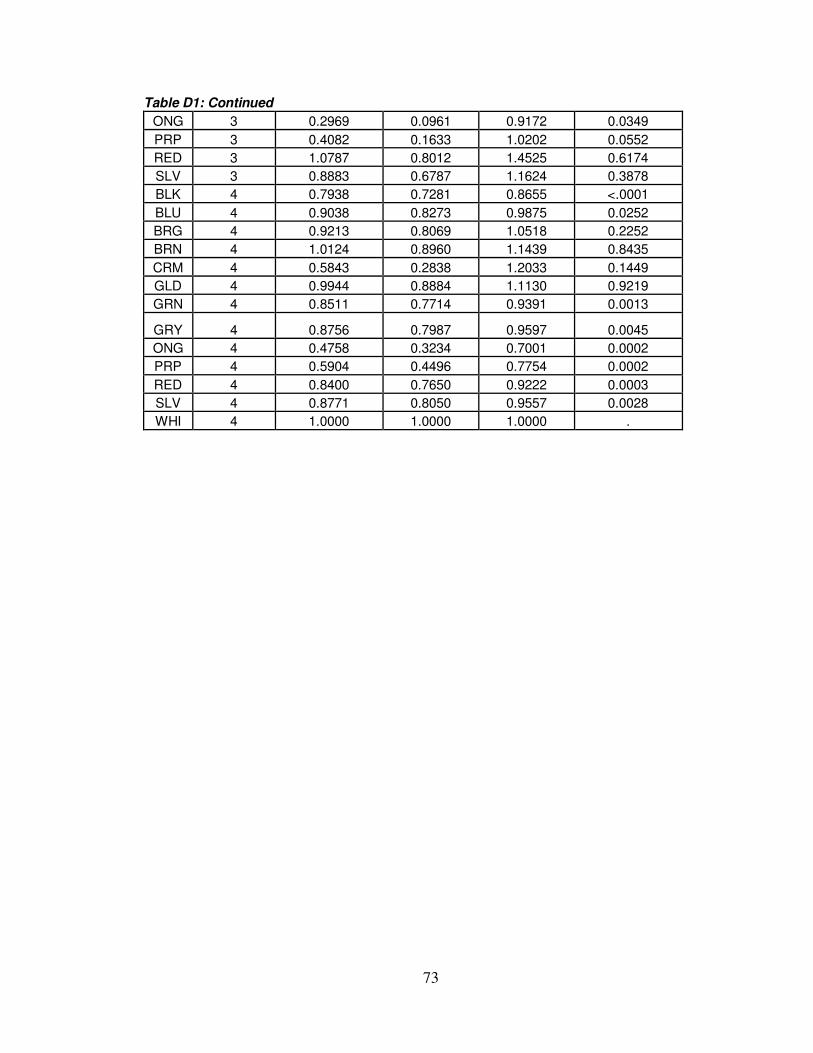
73

Table D1: Continued

ONG 3 0.2969 0.0961 0.9172 0.0349

PRP 3 0.4082 0.1633 1.0202 0.0552

RED 3 1.0787 0.8012 1.4525 0.6174

SLV 3 0.8883 0.6787 1.1624 0.3878

BLK 4 0.7938 0.7281 0.8655 <.0001

BLU 4 0.9038 0.8273 0.9875 0.0252

BRG 4 0.9213 0.8069 1.0518 0.2252

BRN 4 1.0124 0.8960 1.1439 0.8435

CRM 4 0.5843 0.2838 1.2033 0.1449

GLD 4 0.9944 0.8884 1.1130 0.9219

GRN 4 0.8511 0.7714 0.9391 0.0013

GRY 4 0.8756 0.7987 0.9597 0.0045

ONG 4 0.4758 0.3234 0.7001 0.0002

PRP 4 0.5904 0.4496 0.7754 0.0002

RED 4 0.8400 0.7650 0.9222 0.0003

SLV 4 0.8771 0.8050 0.9557 0.0028

WHI 4 1.0000 1.0000 1.0000 .

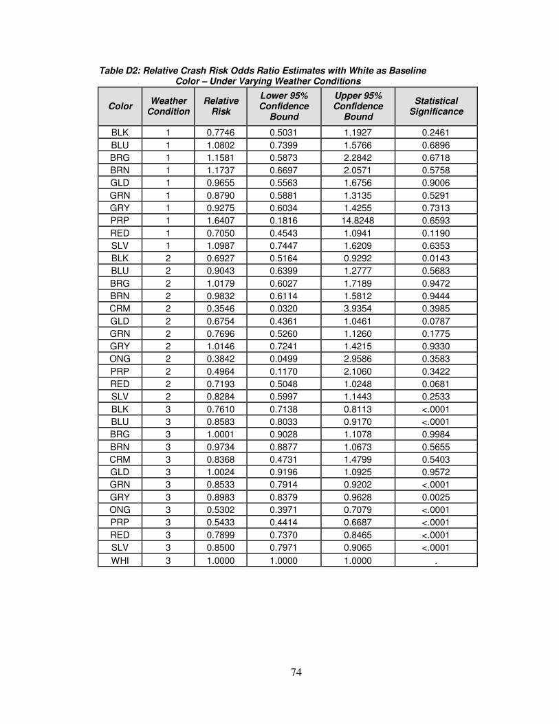
74

Table D2: Relative Crash Risk Odds Ratio Estimates with White as Baseline Color – Under Varying Weather Conditions

Color Weather

Condition Relative

Risk

Lower 95% Confidence

Bound

Upper 95% Confidence

Bound

Statistical Significance

BLK 1 0.7746 0.5031 1.1927 0.2461

BLU 1 1.0802 0.7399 1.5766 0.6896

BRG 1 1.1581 0.5873 2.2842 0.6718

BRN 1 1.1737 0.6697 2.0571 0.5758

GLD 1 0.9655 0.5563 1.6756 0.9006

GRN 1 0.8790 0.5881 1.3135 0.5291

GRY 1 0.9275 0.6034 1.4255 0.7313

PRP 1 1.6407 0.1816 14.8248 0.6593

RED 1 0.7050 0.4543 1.0941 0.1190

SLV 1 1.0987 0.7447 1.6209 0.6353

BLK 2 0.6927 0.5164 0.9292 0.0143

BLU 2 0.9043 0.6399 1.2777 0.5683

BRG 2 1.0179 0.6027 1.7189 0.9472

BRN 2 0.9832 0.6114 1.5812 0.9444

CRM 2 0.3546 0.0320 3.9354 0.3985

GLD 2 0.6754 0.4361 1.0461 0.0787

GRN 2 0.7696 0.5260 1.1260 0.1775

GRY 2 1.0146 0.7241 1.4215 0.9330

ONG 2 0.3842 0.0499 2.9586 0.3583

PRP 2 0.4964 0.1170 2.1060 0.3422

RED 2 0.7193 0.5048 1.0248 0.0681

SLV 2 0.8284 0.5997 1.1443 0.2533

BLK 3 0.7610 0.7138 0.8113 <.0001

BLU 3 0.8583 0.8033 0.9170 <.0001

BRG 3 1.0001 0.9028 1.1078 0.9984

BRN 3 0.9734 0.8877 1.0673 0.5655

CRM 3 0.8368 0.4731 1.4799 0.5403

GLD 3 1.0024 0.9196 1.0925 0.9572

GRN 3 0.8533 0.7914 0.9202 <.0001

GRY 3 0.8983 0.8379 0.9628 0.0025

ONG 3 0.5302 0.3971 0.7079 <.0001

PRP 3 0.5433 0.4414 0.6687 <.0001

RED 3 0.7899 0.7370 0.8465 <.0001

SLV 3 0.8500 0.7971 0.9065 <.0001

WHI 3 1.0000 1.0000 1.0000 .

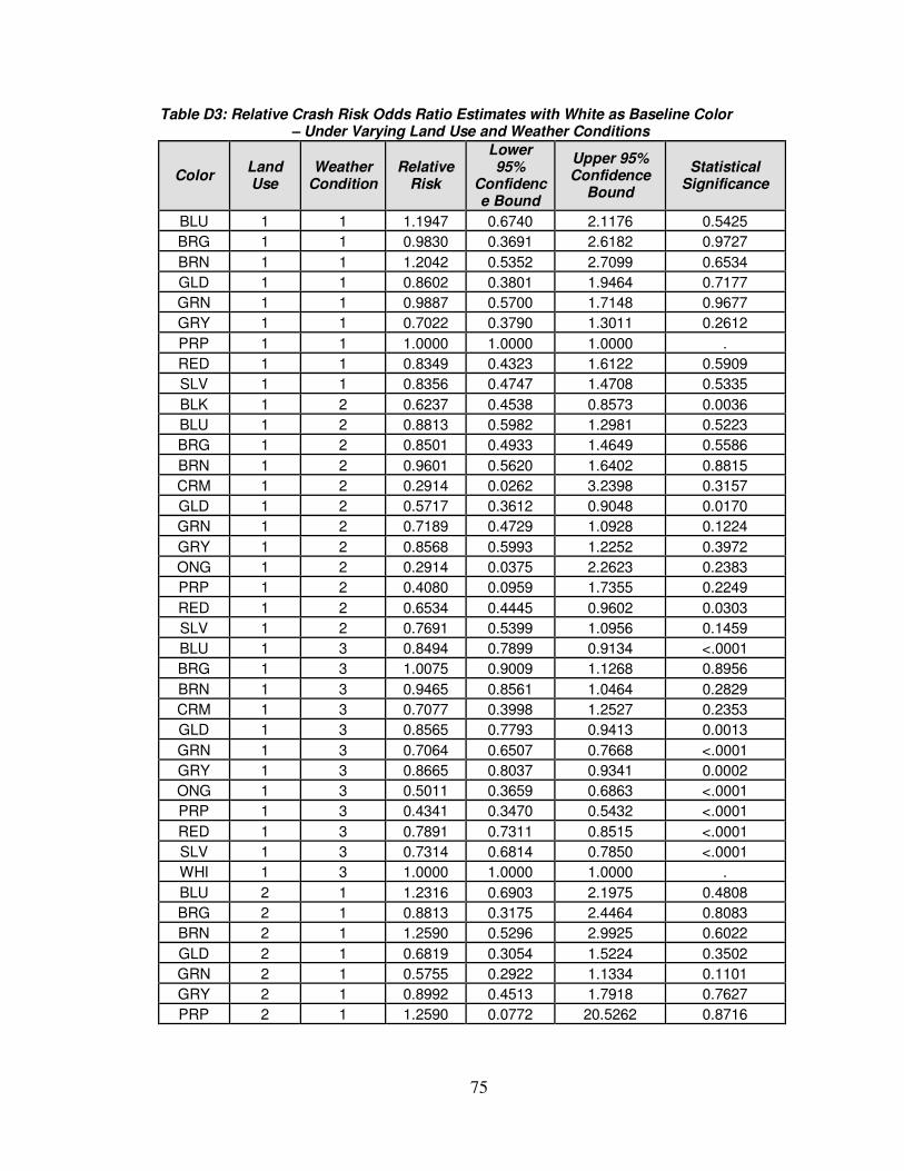
75

Table D3: Relative Crash Risk Odds Ratio Estimates with White as Baseline Color – Under Varying Land Use and Weather Conditions

Color Land Use

Weather Condition

Relative Risk

Lower 95%

Confidence Bound

Upper 95% Confidence

Bound

Statistical Significance

BLU 1 1 1.1947 0.6740 2.1176 0.5425

BRG 1 1 0.9830 0.3691 2.6182 0.9727

BRN 1 1 1.2042 0.5352 2.7099 0.6534

GLD 1 1 0.8602 0.3801 1.9464 0.7177

GRN 1 1 0.9887 0.5700 1.7148 0.9677

GRY 1 1 0.7022 0.3790 1.3011 0.2612

PRP 1 1 1.0000 1.0000 1.0000 .

RED 1 1 0.8349 0.4323 1.6122 0.5909

SLV 1 1 0.8356 0.4747 1.4708 0.5335

BLK 1 2 0.6237 0.4538 0.8573 0.0036

BLU 1 2 0.8813 0.5982 1.2981 0.5223

BRG 1 2 0.8501 0.4933 1.4649 0.5586

BRN 1 2 0.9601 0.5620 1.6402 0.8815

CRM 1 2 0.2914 0.0262 3.2398 0.3157

GLD 1 2 0.5717 0.3612 0.9048 0.0170

GRN 1 2 0.7189 0.4729 1.0928 0.1224

GRY 1 2 0.8568 0.5993 1.2252 0.3972

ONG 1 2 0.2914 0.0375 2.2623 0.2383

PRP 1 2 0.4080 0.0959 1.7355 0.2249

RED 1 2 0.6534 0.4445 0.9602 0.0303

SLV 1 2 0.7691 0.5399 1.0956 0.1459

BLU 1 3 0.8494 0.7899 0.9134 <.0001

BRG 1 3 1.0075 0.9009 1.1268 0.8956

BRN 1 3 0.9465 0.8561 1.0464 0.2829

CRM 1 3 0.7077 0.3998 1.2527 0.2353

GLD 1 3 0.8565 0.7793 0.9413 0.0013

GRN 1 3 0.7064 0.6507 0.7668 <.0001

GRY 1 3 0.8665 0.8037 0.9341 0.0002

ONG 1 3 0.5011 0.3659 0.6863 <.0001

PRP 1 3 0.4341 0.3470 0.5432 <.0001

RED 1 3 0.7891 0.7311 0.8515 <.0001

SLV 1 3 0.7314 0.6814 0.7850 <.0001

WHI 1 3 1.0000 1.0000 1.0000 .

BLU 2 1 1.2316 0.6903 2.1975 0.4808

BRG 2 1 0.8813 0.3175 2.4464 0.8083

BRN 2 1 1.2590 0.5296 2.9925 0.6022

GLD 2 1 0.6819 0.3054 1.5224 0.3502

GRN 2 1 0.5755 0.2922 1.1334 0.1101

GRY 2 1 0.8992 0.4513 1.7918 0.7627

PRP 2 1 1.2590 0.0772 20.5262 0.8716

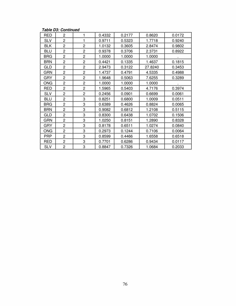
76

Table D3: Continued

RED 2 1 0.4332 0.2177 0.8620 0.0172

SLV 2 1 0.9711 0.5323 1.7718 0.9240

BLK 2 2 1.0132 0.3605 2.8474 0.9802

BLU 2 2 0.9378 0.3706 2.3731 0.8922

BRG 2 2 1.0000 1.0000 1.0000 .

BRN 2 2 0.4421 0.1335 1.4637 0.1815

GLD 2 2 2.9473 0.3122 27.8240 0.3453

GRN 2 2 1.4737 0.4791 4.5335 0.4988

GRY 2 2 1.9648 0.5063 7.6255 0.3289

ONG 2 2 1.0000 1.0000 1.0000 .

RED 2 2 1.5965 0.5403 4.7176 0.3974

SLV 2 2 0.2456 0.0901 0.6699 0.0061

BLU 2 3 0.8251 0.6800 1.0009 0.0511

BRG 2 3 0.6389 0.4626 0.8824 0.0065

BRN 2 3 0.9082 0.6812 1.2108 0.5115

GLD 2 3 0.8300 0.6438 1.0702 0.1506

GRN 2 3 1.0250 0.8151 1.2890 0.8328

GRY 2 3 0.8178 0.6511 1.0274 0.0840

ONG 2 3 0.2973 0.1244 0.7106 0.0064

PRP 2 3 0.8599 0.4466 1.6558 0.6518

RED 2 3 0.7701 0.6286 0.9434 0.0117

SLV 2 3 0.8847 0.7326 1.0684 0.2033

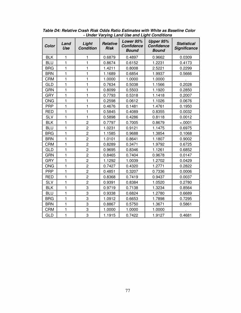
77

Table D4: Relative Crash Risk Odds Ratio Estimates with White as Baseline Color - Under Varying Land Use and Light Conditions

Color Land Use

Light Condition

Relative Risk

Lower 95% Confidence

Bound

Upper 95% Confidence

Bound

Statistical Significance

BLK 1 1 0.6879 0.4897 0.9662 0.0309

BLU 1 1 0.8674 0.6152 1.2231 0.4173

BRG 1 1 1.4211 0.8008 2.5221 0.2299

BRN 1 1 1.1689 0.6854 1.9937 0.5666

CRM 1 1 1.0000 1.0000 1.0000 .

GLD 1 1 0.7634 0.5038 1.1566 0.2028

GRN 1 1 0.8099 0.5503 1.1920 0.2850

GRY 1 1 0.7793 0.5318 1.1418 0.2007

ONG 1 1 0.2598 0.0612 1.1026 0.0676

PRP 1 1 0.4676 0.1481 1.4761 0.1950

RED 1 1 0.5845 0.4089 0.8355 0.0032

SLV 1 1 0.5898 0.4286 0.8118 0.0012

BLK 1 2 0.7797 0.7005 0.8679 <.0001

BLU 1 2 1.0231 0.9121 1.1475 0.6975

BRG 1 2 1.1585 0.9688 1.3854 0.1068

BRN 1 2 1.0101 0.8641 1.1807 0.9002

CRM 1 2 0.8289 0.3471 1.9792 0.6725

GLD 1 2 0.9695 0.8346 1.1261 0.6852

GRN 1 2 0.8465 0.7404 0.9678 0.0147

GRY 1 2 1.1292 1.0039 1.2702 0.0429

ONG 1 2 0.7427 0.4320 1.2771 0.2822

PRP 1 2 0.4851 0.3207 0.7336 0.0006

RED 1 2 0.8368 0.7419 0.9437 0.0037

SLV 1 2 0.9391 0.8384 1.0520 0.2780

BLK 1 3 0.9719 0.7138 1.3234 0.8564

BLU 1 3 0.9338 0.6824 1.2780 0.6689

BRG 1 3 1.0912 0.6653 1.7898 0.7295

BRN 1 3 0.8867 0.5750 1.3671 0.5861

CRM 1 3 1.0000 1.0000 1.0000 .

GLD 1 3 1.1915 0.7422 1.9127 0.4681

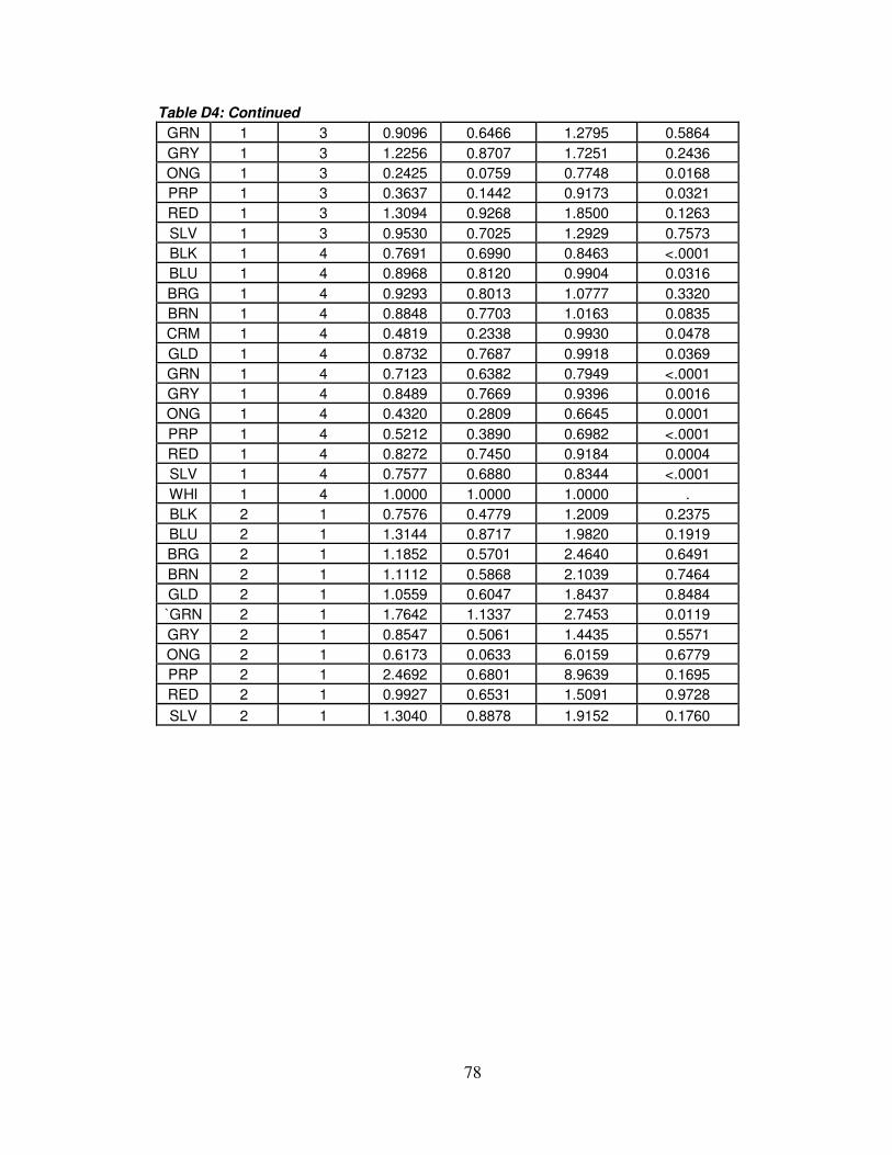
78

Table D4: Continued

GRN 1 3 0.9096 0.6466 1.2795 0.5864

GRY 1 3 1.2256 0.8707 1.7251 0.2436

ONG 1 3 0.2425 0.0759 0.7748 0.0168

PRP 1 3 0.3637 0.1442 0.9173 0.0321

RED 1 3 1.3094 0.9268 1.8500 0.1263

SLV 1 3 0.9530 0.7025 1.2929 0.7573

BLK 1 4 0.7691 0.6990 0.8463 <.0001

BLU 1 4 0.8968 0.8120 0.9904 0.0316

BRG 1 4 0.9293 0.8013 1.0777 0.3320

BRN 1 4 0.8848 0.7703 1.0163 0.0835

CRM 1 4 0.4819 0.2338 0.9930 0.0478

GLD 1 4 0.8732 0.7687 0.9918 0.0369

GRN 1 4 0.7123 0.6382 0.7949 <.0001

GRY 1 4 0.8489 0.7669 0.9396 0.0016

ONG 1 4 0.4320 0.2809 0.6645 0.0001

PRP 1 4 0.5212 0.3890 0.6982 <.0001

RED 1 4 0.8272 0.7450 0.9184 0.0004

SLV 1 4 0.7577 0.6880 0.8344 <.0001

WHI 1 4 1.0000 1.0000 1.0000 .

BLK 2 1 0.7576 0.4779 1.2009 0.2375

BLU 2 1 1.3144 0.8717 1.9820 0.1919

BRG 2 1 1.1852 0.5701 2.4640 0.6491

BRN 2 1 1.1112 0.5868 2.1039 0.7464

GLD 2 1 1.0559 0.6047 1.8437 0.8484

`GRN 2 1 1.7642 1.1337 2.7453 0.0119

GRY 2 1 0.8547 0.5061 1.4435 0.5571

ONG 2 1 0.6173 0.0633 6.0159 0.6779

PRP 2 1 2.4692 0.6801 8.9639 0.1695

RED 2 1 0.9927 0.6531 1.5091 0.9728

SLV 2 1 1.3040 0.8878 1.9152 0.1760

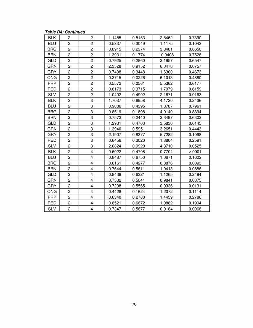
79

Table D4: Continued

BLK 2 2 1.1455 0.5153 2.5462 0.7390

BLU 2 2 0.5837 0.3049 1.1175 0.1043

BRG 2 2 0.8915 0.2374 3.3481 0.8650

BRN 2 2 1.3931 0.1774 10.9408 0.7526

GLD 2 2 0.7925 0.2860 2.1957 0.6547

GRN 2 2 2.3528 0.9152 6.0478 0.0757

GRY 2 2 0.7498 0.3448 1.6300 0.4673

ONG 2 2 0.3715 0.0226 6.1013 0.4880

PRP 2 2 0.5572 0.0561 5.5362 0.6177

RED 2 2 0.8173 0.3715 1.7979 0.6159

SLV 2 2 1.0402 0.4992 2.1671 0.9163

BLK 2 3 1.7037 0.6958 4.1720 0.2436

BLU 2 3 0.9086 0.4395 1.8787 0.7961

BRG 2 3 0.8519 0.1808 4.0140 0.8394

BRN 2 3 0.7572 0.2440 2.3497 0.6303

GLD 2 3 1.2981 0.4703 3.5830 0.6145

GRN 2 3 1.3940 0.5951 3.2651 0.4443

GRY 2 3 2.1907 0.8377 5.7282 0.1098

RED 2 3 0.6456 0.3020 1.3804 0.2591

SLV 2 3 2.0824 0.9920 4.3710 0.0525

BLK 2 4 0.6022 0.4708 0.7704 <.0001

BLU 2 4 0.8487 0.6750 1.0671 0.1602

BRG 2 4 0.6161 0.4277 0.8876 0.0093

BRN 2 4 0.7644 0.5611 1.0413 0.0886

GLD 2 4 0.8438 0.6321 1.1265 0.2494

GRN 2 4 0.7582 0.5841 0.9841 0.0375

GRY 2 4 0.7208 0.5565 0.9336 0.0131

ONG 2 4 0.4428 0.1624 1.2072 0.1114

PRP 2 4 0.6340 0.2780 1.4459 0.2786

RED 2 4 0.8521 0.6672 1.0882 0.1994

SLV 2 4 0.7347 0.5877 0.9184 0.0068

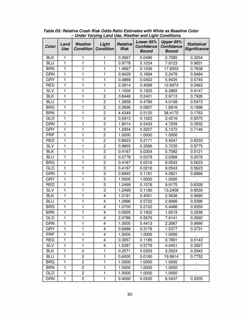
80

Table D5: Relative Crash Risk Odds Ratio Estimates with White as Baseline Color – Under Varying Land Use, Weather and Light Conditions.

Color Land Use

Weather Condition

Light Condition

Relative Risk

Lower 95% Confidence

Bound

Upper 95% Confidence

Bound

Statistical Significance

BLK 1 1 1 0.3667 0.0496 2.7085 0.3254

BLU 1 1 1 0.9778 0.1224 7.8123 0.9831

BRN 1 1 1 1.4667 0.1206 17.8303 0.7638

GRN 1 1 1 0.9429 0.1694 5.2478 0.9464

GRY 1 1 1 0.4889 0.0402 5.9435 0.5745

RED 1 1 1 2.2814 0.4099 12.6974 0.3463

SLV 1 1 1 1.1000 0.1925 6.2865 0.9147

BLK 1 1 2 0.8448 0.2401 2.9713 0.7926

BLU 1 1 2 1.3858 0.4789 4.0108 0.5473

BRG 1 1 2 0.3696 0.0807 1.6916 0.1996

BRN 1 1 2 4.4349 0.5120 38.4170 0.1763

GLD 1 1 2 0.5913 0.1022 3.4216 0.5575

GRN 1 1 2 1.6014 0.5433 4.7209 0.3932

GRY 1 1 2 1.2934 0.3257 5.1372 0.7146

PRP 1 1 2 1.0000 1.0000 1.0000 .

RED 1 1 2 0.8623 0.2171 3.4247 0.8333

SLV 1 1 2 0.9855 0.3566 2.7235 0.9775

BLK 1 1 3 0.4167 0.0304 5.7082 0.5121

BLU 1 1 3 0.2778 0.0379 2.0368 0.2076

BRG 1 1 3 0.4167 0.0216 8.0543 0.5623

GLD 1 1 3 0.4167 0.0216 8.0543 0.5623

GRN 1 1 3 0.6945 0.1181 4.0821 0.6866

GRY 1 1 3 1.0000 1.0000 1.0000 .

RED 1 1 3 1.2499 0.1576 9.9175 0.8328

SLV 1 1 3 1.2499 0.1180 13.2408 0.8530

BLK 1 1 4 1.0191 0.4051 2.5636 0.9680

BLU 1 1 4 1.2896 0.5722 2.9066 0.5396

BRG 1 1 4 1.0700 0.2102 5.4466 0.9350

BRN 1 1 4 0.5605 0.1902 1.6519 0.2938

GLD 1 1 4 2.0788 0.5676 7.6141 0.2692

GRN 1 1 4 1.0005 0.4413 2.2687 0.9990

GRY 1 1 4 0.6988 0.3176 1.5377 0.3731

PRP 1 1 4 1.0000 1.0000 1.0000 .

RED 1 1 4 0.3057 0.1185 0.7891 0.0143

SLV 1 1 4 1.5287 0.5776 4.0451 0.3927

BLK 1 2 1 0.2571 0.0203 3.2524 0.2942

BLU 1 2 1 0.6000 0.0180 19.9914 0.7752

BRG 1 2 1 1.0000 1.0000 1.0000 .

BRN 1 2 1 1.0000 1.0000 1.0000 .

GLD 1 2 1 1.0000 1.0000 1.0000 .

GRN 1 2 1 0.4000 0.0245 6.5437 0.5205

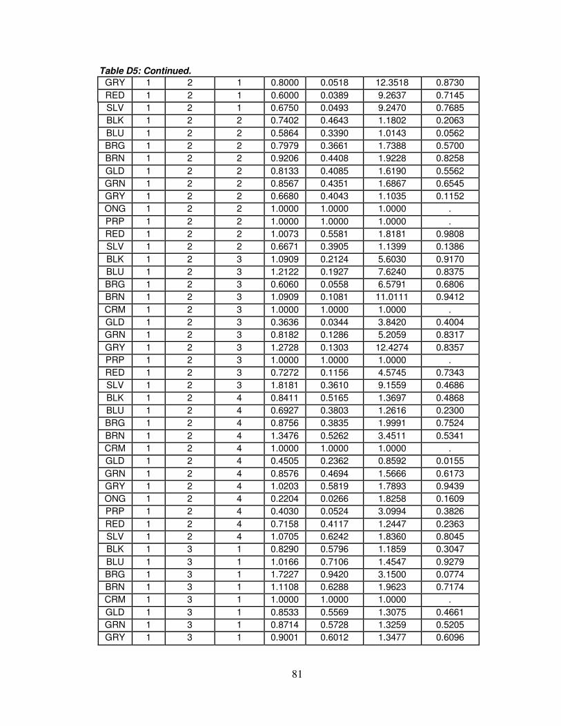
81

Table D5: Continued.

GRY 1 2 1 0.8000 0.0518 12.3518 0.8730

RED 1 2 1 0.6000 0.0389 9.2637 0.7145

SLV 1 2 1 0.6750 0.0493 9.2470 0.7685

BLK 1 2 2 0.7402 0.4643 1.1802 0.2063

BLU 1 2 2 0.5864 0.3390 1.0143 0.0562

BRG 1 2 2 0.7979 0.3661 1.7388 0.5700

BRN 1 2 2 0.9206 0.4408 1.9228 0.8258

GLD 1 2 2 0.8133 0.4085 1.6190 0.5562

GRN 1 2 2 0.8567 0.4351 1.6867 0.6545

GRY 1 2 2 0.6680 0.4043 1.1035 0.1152

ONG 1 2 2 1.0000 1.0000 1.0000 .

PRP 1 2 2 1.0000 1.0000 1.0000 .

RED 1 2 2 1.0073 0.5581 1.8181 0.9808

SLV 1 2 2 0.6671 0.3905 1.1399 0.1386

BLK 1 2 3 1.0909 0.2124 5.6030 0.9170

BLU 1 2 3 1.2122 0.1927 7.6240 0.8375

BRG 1 2 3 0.6060 0.0558 6.5791 0.6806

BRN 1 2 3 1.0909 0.1081 11.0111 0.9412

CRM 1 2 3 1.0000 1.0000 1.0000 .

GLD 1 2 3 0.3636 0.0344 3.8420 0.4004

GRN 1 2 3 0.8182 0.1286 5.2059 0.8317

GRY 1 2 3 1.2728 0.1303 12.4274 0.8357

PRP 1 2 3 1.0000 1.0000 1.0000 .

RED 1 2 3 0.7272 0.1156 4.5745 0.7343

SLV 1 2 3 1.8181 0.3610 9.1559 0.4686

BLK 1 2 4 0.8411 0.5165 1.3697 0.4868

BLU 1 2 4 0.6927 0.3803 1.2616 0.2300

BRG 1 2 4 0.8756 0.3835 1.9991 0.7524

BRN 1 2 4 1.3476 0.5262 3.4511 0.5341

CRM 1 2 4 1.0000 1.0000 1.0000 .

GLD 1 2 4 0.4505 0.2362 0.8592 0.0155

GRN 1 2 4 0.8576 0.4694 1.5666 0.6173

GRY 1 2 4 1.0203 0.5819 1.7893 0.9439

ONG 1 2 4 0.2204 0.0266 1.8258 0.1609

PRP 1 2 4 0.4030 0.0524 3.0994 0.3826

RED 1 2 4 0.7158 0.4117 1.2447 0.2363

SLV 1 2 4 1.0705 0.6242 1.8360 0.8045

BLK 1 3 1 0.8290 0.5796 1.1859 0.3047

BLU 1 3 1 1.0166 0.7106 1.4547 0.9279

BRG 1 3 1 1.7227 0.9420 3.1500 0.0774

BRN 1 3 1 1.1108 0.6288 1.9623 0.7174

CRM 1 3 1 1.0000 1.0000 1.0000 .

GLD 1 3 1 0.8533 0.5569 1.3075 0.4661

GRN 1 3 1 0.8714 0.5728 1.3259 0.5205

GRY 1 3 1 0.9001 0.6012 1.3477 0.6096

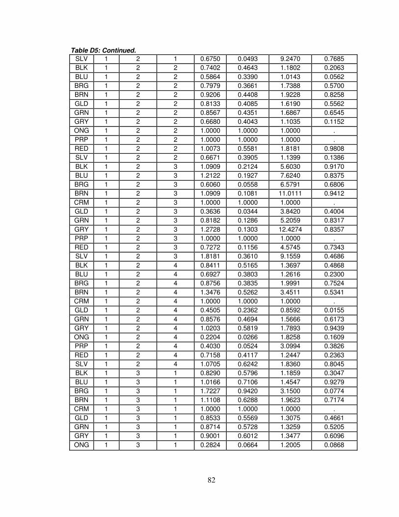
82

Table D5: Continued.

SLV 1 2 1 0.6750 0.0493 9.2470 0.7685

BLK 1 2 2 0.7402 0.4643 1.1802 0.2063

BLU 1 2 2 0.5864 0.3390 1.0143 0.0562

BRG 1 2 2 0.7979 0.3661 1.7388 0.5700

BRN 1 2 2 0.9206 0.4408 1.9228 0.8258

GLD 1 2 2 0.8133 0.4085 1.6190 0.5562

GRN 1 2 2 0.8567 0.4351 1.6867 0.6545

GRY 1 2 2 0.6680 0.4043 1.1035 0.1152

ONG 1 2 2 1.0000 1.0000 1.0000 .

PRP 1 2 2 1.0000 1.0000 1.0000 .

RED 1 2 2 1.0073 0.5581 1.8181 0.9808

SLV 1 2 2 0.6671 0.3905 1.1399 0.1386

BLK 1 2 3 1.0909 0.2124 5.6030 0.9170

BLU 1 2 3 1.2122 0.1927 7.6240 0.8375

BRG 1 2 3 0.6060 0.0558 6.5791 0.6806

BRN 1 2 3 1.0909 0.1081 11.0111 0.9412

CRM 1 2 3 1.0000 1.0000 1.0000 .

GLD 1 2 3 0.3636 0.0344 3.8420 0.4004

GRN 1 2 3 0.8182 0.1286 5.2059 0.8317

GRY 1 2 3 1.2728 0.1303 12.4274 0.8357

PRP 1 2 3 1.0000 1.0000 1.0000 .

RED 1 2 3 0.7272 0.1156 4.5745 0.7343

SLV 1 2 3 1.8181 0.3610 9.1559 0.4686

BLK 1 2 4 0.8411 0.5165 1.3697 0.4868

BLU 1 2 4 0.6927 0.3803 1.2616 0.2300

BRG 1 2 4 0.8756 0.3835 1.9991 0.7524

BRN 1 2 4 1.3476 0.5262 3.4511 0.5341

CRM 1 2 4 1.0000 1.0000 1.0000 .

GLD 1 2 4 0.4505 0.2362 0.8592 0.0155

GRN 1 2 4 0.8576 0.4694 1.5666 0.6173

GRY 1 2 4 1.0203 0.5819 1.7893 0.9439

ONG 1 2 4 0.2204 0.0266 1.8258 0.1609

PRP 1 2 4 0.4030 0.0524 3.0994 0.3826

RED 1 2 4 0.7158 0.4117 1.2447 0.2363

SLV 1 2 4 1.0705 0.6242 1.8360 0.8045

BLK 1 3 1 0.8290 0.5796 1.1859 0.3047

BLU 1 3 1 1.0166 0.7106 1.4547 0.9279

BRG 1 3 1 1.7227 0.9420 3.1500 0.0774

BRN 1 3 1 1.1108 0.6288 1.9623 0.7174

CRM 1 3 1 1.0000 1.0000 1.0000 .

GLD 1 3 1 0.8533 0.5569 1.3075 0.4661

GRN 1 3 1 0.8714 0.5728 1.3259 0.5205

GRY 1 3 1 0.9001 0.6012 1.3477 0.6096

ONG 1 3 1 0.2824 0.0664 1.2005 0.0868

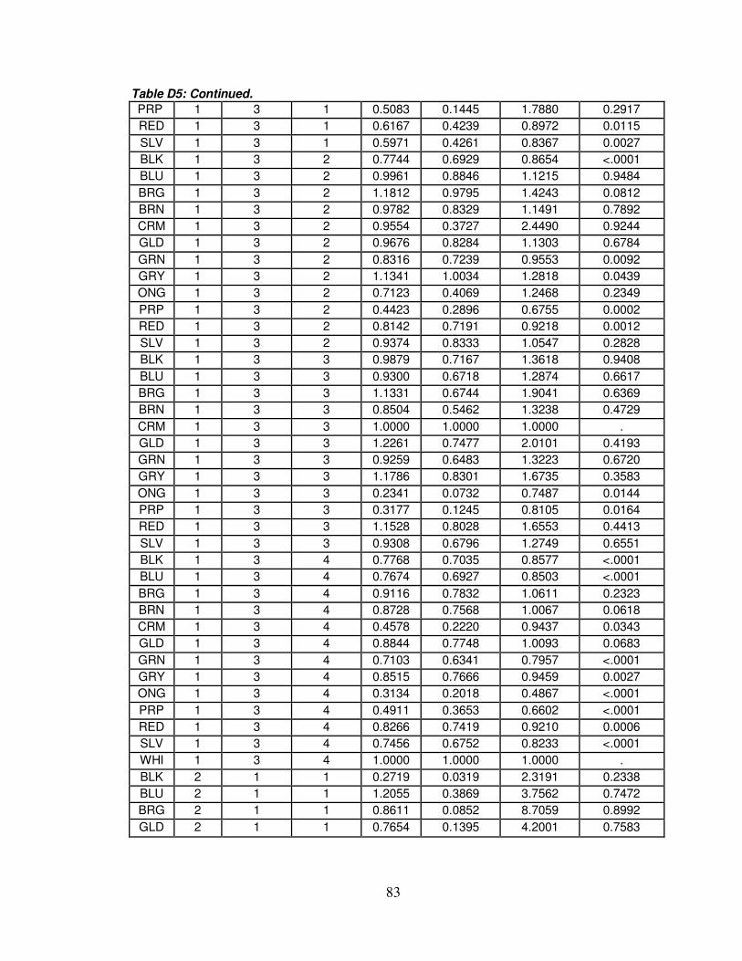
83

Table D5: Continued.

PRP 1 3 1 0.5083 0.1445 1.7880 0.2917

RED 1 3 1 0.6167 0.4239 0.8972 0.0115

SLV 1 3 1 0.5971 0.4261 0.8367 0.0027

BLK 1 3 2 0.7744 0.6929 0.8654 <.0001

BLU 1 3 2 0.9961 0.8846 1.1215 0.9484

BRG 1 3 2 1.1812 0.9795 1.4243 0.0812

BRN 1 3 2 0.9782 0.8329 1.1491 0.7892

CRM 1 3 2 0.9554 0.3727 2.4490 0.9244

GLD 1 3 2 0.9676 0.8284 1.1303 0.6784

GRN 1 3 2 0.8316 0.7239 0.9553 0.0092

GRY 1 3 2 1.1341 1.0034 1.2818 0.0439

ONG 1 3 2 0.7123 0.4069 1.2468 0.2349

PRP 1 3 2 0.4423 0.2896 0.6755 0.0002

RED 1 3 2 0.8142 0.7191 0.9218 0.0012

SLV 1 3 2 0.9374 0.8333 1.0547 0.2828

BLK 1 3 3 0.9879 0.7167 1.3618 0.9408

BLU 1 3 3 0.9300 0.6718 1.2874 0.6617

BRG 1 3 3 1.1331 0.6744 1.9041 0.6369

BRN 1 3 3 0.8504 0.5462 1.3238 0.4729

CRM 1 3 3 1.0000 1.0000 1.0000 .

GLD 1 3 3 1.2261 0.7477 2.0101 0.4193

GRN 1 3 3 0.9259 0.6483 1.3223 0.6720

GRY 1 3 3 1.1786 0.8301 1.6735 0.3583

ONG 1 3 3 0.2341 0.0732 0.7487 0.0144

PRP 1 3 3 0.3177 0.1245 0.8105 0.0164

RED 1 3 3 1.1528 0.8028 1.6553 0.4413

SLV 1 3 3 0.9308 0.6796 1.2749 0.6551

BLK 1 3 4 0.7768 0.7035 0.8577 <.0001

BLU 1 3 4 0.7674 0.6927 0.8503 <.0001

BRG 1 3 4 0.9116 0.7832 1.0611 0.2323

BRN 1 3 4 0.8728 0.7568 1.0067 0.0618

CRM 1 3 4 0.4578 0.2220 0.9437 0.0343

GLD 1 3 4 0.8844 0.7748 1.0093 0.0683

GRN 1 3 4 0.7103 0.6341 0.7957 <.0001

GRY 1 3 4 0.8515 0.7666 0.9459 0.0027

ONG 1 3 4 0.3134 0.2018 0.4867 <.0001

PRP 1 3 4 0.4911 0.3653 0.6602 <.0001

RED 1 3 4 0.8266 0.7419 0.9210 0.0006

SLV 1 3 4 0.7456 0.6752 0.8233 <.0001

WHI 1 3 4 1.0000 1.0000 1.0000 .

BLK 2 1 1 0.2719 0.0319 2.3191 0.2338

BLU 2 1 1 1.2055 0.3869 3.7562 0.7472

BRG 2 1 1 0.8611 0.0852 8.7059 0.8992

GLD 2 1 1 0.7654 0.1395 4.2001 0.7583

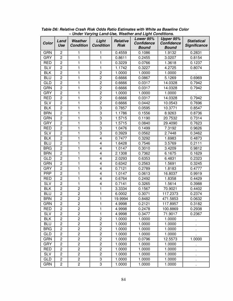
84

Table D6: Relative Crash Risk Odds Ratio Estimates with White as Baseline Color – Under Varying Land-Use, Weather and Light Conditions.

Color Land Use

Weather Condition

Light Condition

Relative Risk

Lower 95% Confidence

Bound

Upper 95% Confidence

Bound

Statistical Significance

GRN 2 1 1 0.4559 0.1086 1.9132 0.2831

GRY 2 1 1 0.8611 0.2455 3.0207 0.8154

RED 2 1 1 0.3229 0.0766 1.3618 0.1237

SLV 2 1 1 1.1742 0.3227 4.2725 0.8074

BLK 2 1 2 1.0000 1.0000 1.0000 .

BLU 2 1 2 0.6666 0.0867 5.1269 0.6969

GLD 2 1 2 0.6666 0.0317 14.0328 0.7942

GRN 2 1 2 0.6666 0.0317 14.0328 0.7942

GRY 2 1 2 1.0000 1.0000 1.0000 .

RED 2 1 2 0.6666 0.0317 14.0328 0.7942

SLV 2 1 2 0.6666 0.0442 10.0543 0.7696

BLK 2 1 3 0.7857 0.0595 10.3771 0.8547

BRN 2 1 3 1.1786 0.1556 8.9263 0.8736

GRN 2 1 3 1.5715 0.1190 20.7532 0.7314

GRY 2 1 3 1.5715 0.0840 29.4090 0.7623

RED 2 1 3 1.0476 0.1499 7.3192 0.9626

SLV 2 1 3 0.3929 0.0562 2.7448 0.3462

BLK 2 1 4 0.7477 0.3292 1.6983 0.4873

BLU 2 1 4 1.6428 0.7546 3.5769 0.2111

BRG 2 1 4 1.0147 0.3010 3.4209 0.9812

BRN 2 1 4 2.1308 0.7362 6.1675 0.1629

GLD 2 1 4 2.0293 0.6353 6.4831 0.2323

GRN 2 1 4 0.6342 0.2563 1.5691 0.3245

GRY 2 1 4 0.7121 0.2789 1.8183 0.4777

PRP 2 1 4 1.0147 0.0613 16.8037 0.9919

RED 2 1 4 0.6764 0.2492 1.8358 0.4429

SLV 2 1 4 0.7141 0.3265 1.5614 0.3988

BLK 2 2 1 3.3334 0.1567 70.9021 0.4402

BLU 2 2 1 6.0002 0.3071 117.2373 0.2374

BRN 2 2 1 19.9994 0.8482 471.5853 0.0632

GRN 2 2 1 4.9998 0.2121 117.8957 0.3182

RED 2 2 1 4.9998 0.2478 100.8869 0.2938

SLV 2 2 1 4.9998 0.3477 71.9017 0.2367

BLK 2 2 2 1.0000 1.0000 1.0000 .

BLU 2 2 2 1.0000 1.0000 1.0000 .

BRG 2 2 2 1.0000 1.0000 1.0000 .

GLD 2 2 2 1.0000 1.0000 1.0000 .

GRN 2 2 2 1.0000 0.0796 12.5573 1.0000

GRY 2 2 2 1.0000 1.0000 1.0000 .

RED 2 2 2 1.0000 1.0000 1.0000 .

SLV 2 2 2 1.0000 1.0000 1.0000 .

GLD 2 2 3 1.0000 1.0000 1.0000 .

GRN 2 2 3 1.0000 1.0000 1.0000 .

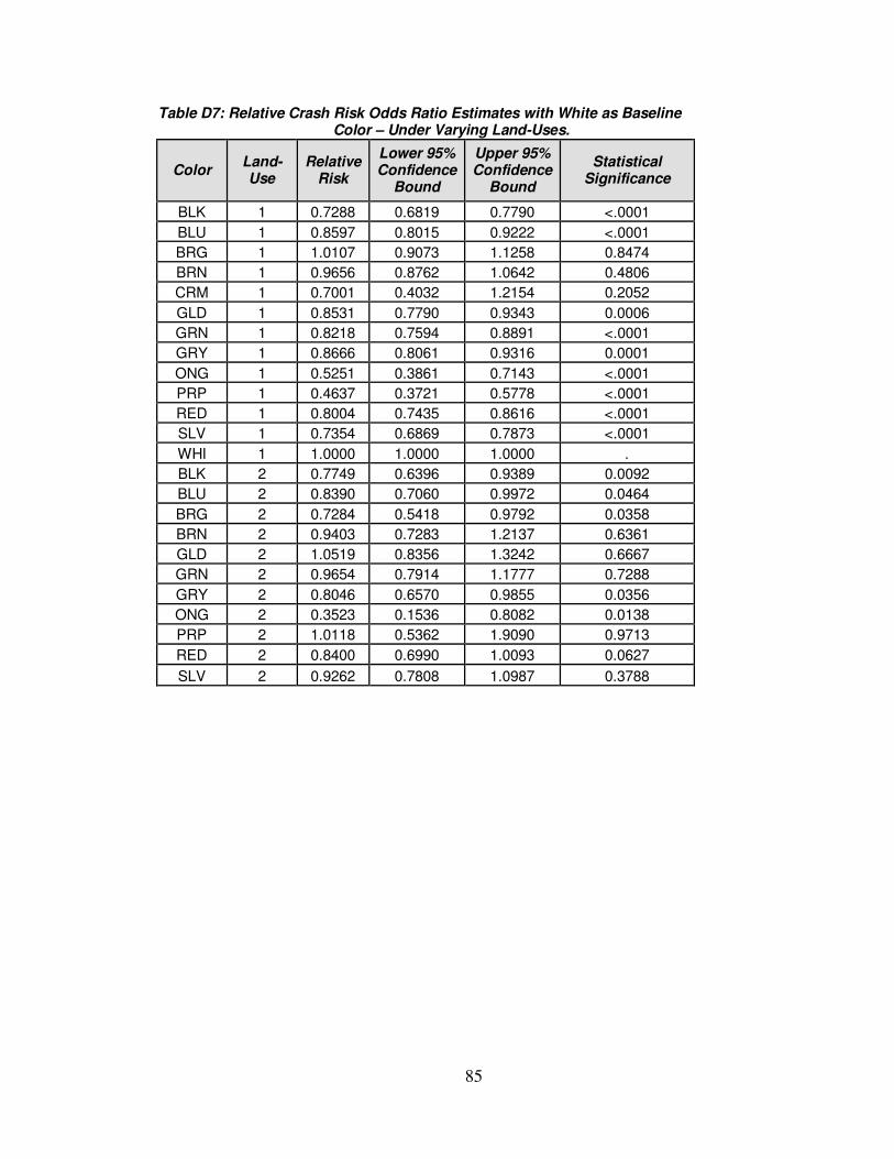
85

Table D7: Relative Crash Risk Odds Ratio Estimates with White as Baseline Color – Under Varying Land-Uses.

Color Land-Use

Relative Risk

Lower 95% Confidence

Bound

Upper 95% Confidence

Bound

Statistical Significance

BLK 1 0.7288 0.6819 0.7790 <.0001

BLU 1 0.8597 0.8015 0.9222 <.0001

BRG 1 1.0107 0.9073 1.1258 0.8474

BRN 1 0.9656 0.8762 1.0642 0.4806

CRM 1 0.7001 0.4032 1.2154 0.2052

GLD 1 0.8531 0.7790 0.9343 0.0006

GRN 1 0.8218 0.7594 0.8891 <.0001

GRY 1 0.8666 0.8061 0.9316 0.0001

ONG 1 0.5251 0.3861 0.7143 <.0001

PRP 1 0.4637 0.3721 0.5778 <.0001

RED 1 0.8004 0.7435 0.8616 <.0001

SLV 1 0.7354 0.6869 0.7873 <.0001

WHI 1 1.0000 1.0000 1.0000 .

BLK 2 0.7749 0.6396 0.9389 0.0092

BLU 2 0.8390 0.7060 0.9972 0.0464

BRG 2 0.7284 0.5418 0.9792 0.0358

BRN 2 0.9403 0.7283 1.2137 0.6361

GLD 2 1.0519 0.8356 1.3242 0.6667

GRN 2 0.9654 0.7914 1.1777 0.7288

GRY 2 0.8046 0.6570 0.9855 0.0356

ONG 2 0.3523 0.1536 0.8082 0.0138

PRP 2 1.0118 0.5362 1.9090 0.9713

RED 2 0.8400 0.6990 1.0093 0.0627

SLV 2 0.9262 0.7808 1.0987 0.3788

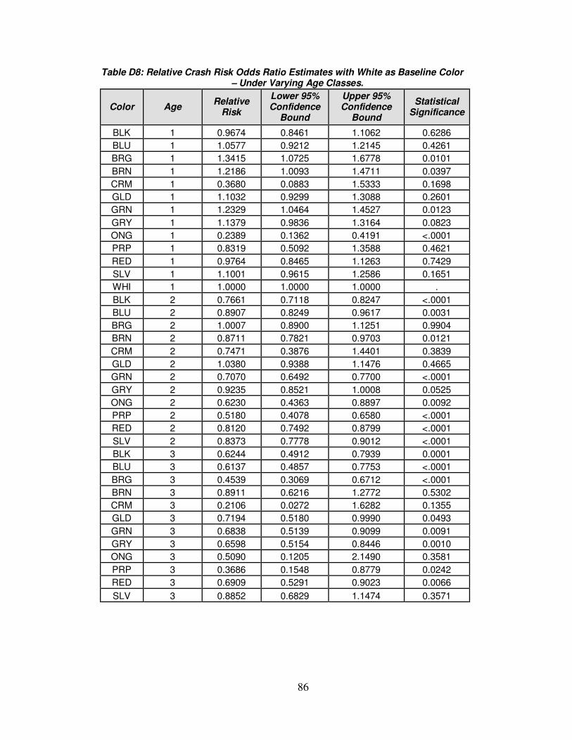
86

Table D8: Relative Crash Risk Odds Ratio Estimates with White as Baseline Color – Under Varying Age Classes.

Color Age Relative

Risk

Lower 95% Confidence

Bound

Upper 95% Confidence

Bound

Statistical Significance

BLK 1 0.9674 0.8461 1.1062 0.6286

BLU 1 1.0577 0.9212 1.2145 0.4261

BRG 1 1.3415 1.0725 1.6778 0.0101

BRN 1 1.2186 1.0093 1.4711 0.0397

CRM 1 0.3680 0.0883 1.5333 0.1698

GLD 1 1.1032 0.9299 1.3088 0.2601

GRN 1 1.2329 1.0464 1.4527 0.0123

GRY 1 1.1379 0.9836 1.3164 0.0823

ONG 1 0.2389 0.1362 0.4191 <.0001

PRP 1 0.8319 0.5092 1.3588 0.4621

RED 1 0.9764 0.8465 1.1263 0.7429

SLV 1 1.1001 0.9615 1.2586 0.1651

WHI 1 1.0000 1.0000 1.0000 .

BLK 2 0.7661 0.7118 0.8247 <.0001

BLU 2 0.8907 0.8249 0.9617 0.0031

BRG 2 1.0007 0.8900 1.1251 0.9904

BRN 2 0.8711 0.7821 0.9703 0.0121

CRM 2 0.7471 0.3876 1.4401 0.3839

GLD 2 1.0380 0.9388 1.1476 0.4665

GRN 2 0.7070 0.6492 0.7700 <.0001

GRY 2 0.9235 0.8521 1.0008 0.0525

ONG 2 0.6230 0.4363 0.8897 0.0092

PRP 2 0.5180 0.4078 0.6580 <.0001

RED 2 0.8120 0.7492 0.8799 <.0001

SLV 2 0.8373 0.7778 0.9012 <.0001

BLK 3 0.6244 0.4912 0.7939 0.0001

BLU 3 0.6137 0.4857 0.7753 <.0001

BRG 3 0.4539 0.3069 0.6712 <.0001

BRN 3 0.8911 0.6216 1.2772 0.5302

CRM 3 0.2106 0.0272 1.6282 0.1355

GLD 3 0.7194 0.5180 0.9990 0.0493

GRN 3 0.6838 0.5139 0.9099 0.0091

GRY 3 0.6598 0.5154 0.8446 0.0010

ONG 3 0.5090 0.1205 2.1490 0.3581

PRP 3 0.3686 0.1548 0.8779 0.0242

RED 3 0.6909 0.5291 0.9023 0.0066

SLV 3 0.8852 0.6829 1.1474 0.3571

87

Table D9: Relative Crash Risk Odds Ratio Estimates with White as Baseline Color – Under Varying Gender.

Color Gender Relative

Risk

Lower 95% Confidence

Bound

Upper 95% Confidence

Bound

Statistical Significance

BLK 1 0.7111 0.6596 0.7666 <.0001

BLU 1 0.7835 0.7246 0.8472 <.0001

BRG 1 0.9702 0.8562 1.0993 0.6346

BRN 1 0.9680 0.8644 1.0842 0.5743

CRM 1 0.7334 0.3373 1.5947 0.4341

GLD 1 0.9413 0.8480 1.0449 0.2557

GRN 1 0.7983 0.7290 0.8742 <.0001

GRY 1 0.8268 0.7610 0.8982 <.0001

ONG 1 0.5193 0.3748 0.7196 <.0001

PRP 1 0.4377 0.3401 0.5632 <.0001

RED 1 0.7758 0.7146 0.8424 <.0001

SLV 1 0.7864 0.7268 0.8509 <.0001

WHI 1 1.0000 1.0000 1.0000 .

BLK 2 0.9231 0.8249 1.0329 0.1628

BLU 2 1.0098 0.9022 1.1302 0.8650

BRG 2 1.1320 0.9559 1.3406 0.1507

BRN 2 1.0721 0.9224 1.2461 0.3645

CRM 2 0.6098 0.2628 1.4148 0.2493

GLD 2 1.0851 0.9437 1.2477 0.2514

GRN 2 0.8984 0.7956 1.0144 0.0839

GRY 2 1.0338 0.9204 1.1609 0.5751

ONG 2 0.4181 0.2341 0.7469 0.0032

PRP 2 0.7663 0.5266 1.1152 0.1643

RED 2 0.8748 0.7771 0.9847 0.0268

SLV 2 0.9354 0.8437 1.0369 0.2037

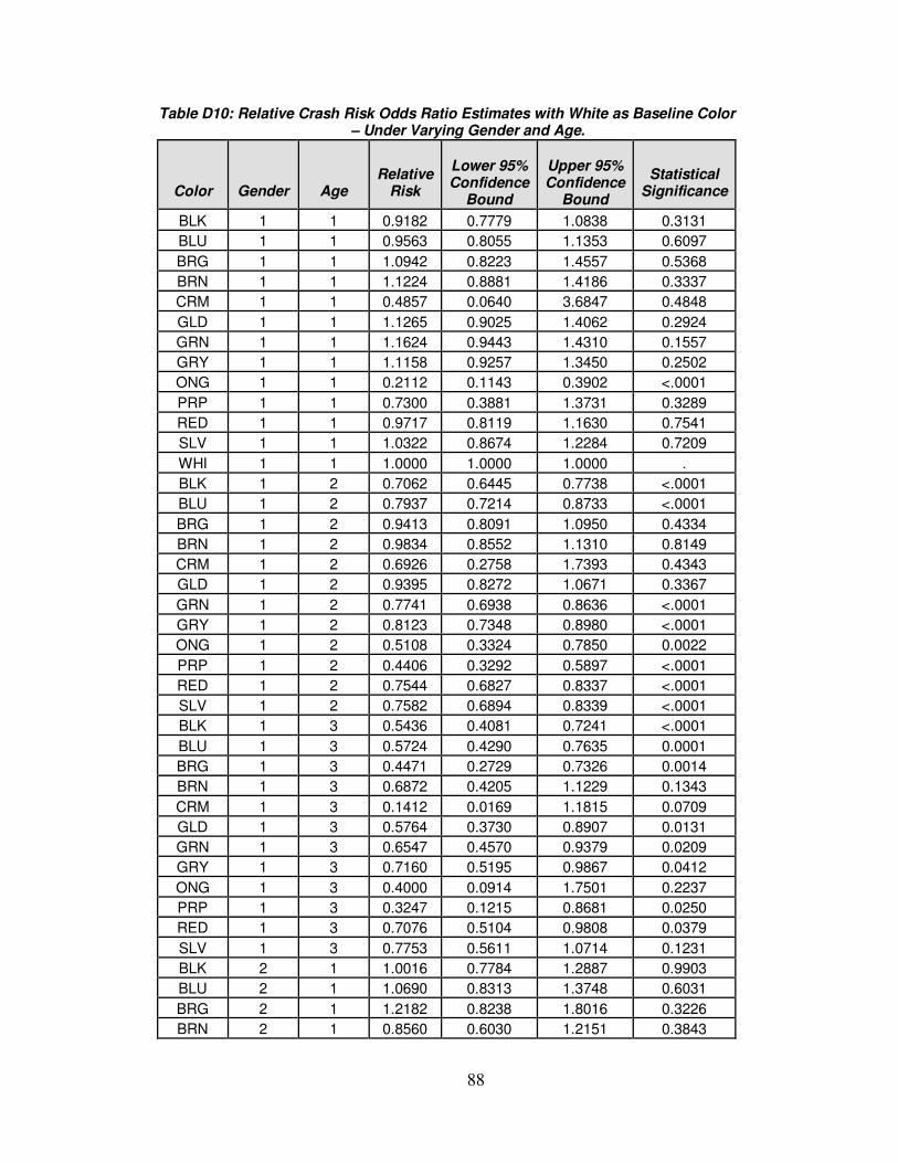
88

Table D10: Relative Crash Risk Odds Ratio Estimates with White as Baseline Color – Under Varying Gender and Age.

Color

Gender

Age

Relative

Risk

Lower 95% Confidence

Bound

Upper 95% Confidence

Bound

Statistical

Significance

BLK 1 1 0.9182 0.7779 1.0838 0.3131

BLU 1 1 0.9563 0.8055 1.1353 0.6097

BRG 1 1 1.0942 0.8223 1.4557 0.5368

BRN 1 1 1.1224 0.8881 1.4186 0.3337

CRM 1 1 0.4857 0.0640 3.6847 0.4848

GLD 1 1 1.1265 0.9025 1.4062 0.2924

GRN 1 1 1.1624 0.9443 1.4310 0.1557

GRY 1 1 1.1158 0.9257 1.3450 0.2502

ONG 1 1 0.2112 0.1143 0.3902 <.0001

PRP 1 1 0.7300 0.3881 1.3731 0.3289

RED 1 1 0.9717 0.8119 1.1630 0.7541

SLV 1 1 1.0322 0.8674 1.2284 0.7209

WHI 1 1 1.0000 1.0000 1.0000 .

BLK 1 2 0.7062 0.6445 0.7738 <.0001

BLU 1 2 0.7937 0.7214 0.8733 <.0001

BRG 1 2 0.9413 0.8091 1.0950 0.4334

BRN 1 2 0.9834 0.8552 1.1310 0.8149

CRM 1 2 0.6926 0.2758 1.7393 0.4343

GLD 1 2 0.9395 0.8272 1.0671 0.3367

GRN 1 2 0.7741 0.6938 0.8636 <.0001

GRY 1 2 0.8123 0.7348 0.8980 <.0001

ONG 1 2 0.5108 0.3324 0.7850 0.0022

PRP 1 2 0.4406 0.3292 0.5897 <.0001

RED 1 2 0.7544 0.6827 0.8337 <.0001

SLV 1 2 0.7582 0.6894 0.8339 <.0001

BLK 1 3 0.5436 0.4081 0.7241 <.0001

BLU 1 3 0.5724 0.4290 0.7635 0.0001

BRG 1 3 0.4471 0.2729 0.7326 0.0014

BRN 1 3 0.6872 0.4205 1.1229 0.1343

CRM 1 3 0.1412 0.0169 1.1815 0.0709

GLD 1 3 0.5764 0.3730 0.8907 0.0131

GRN 1 3 0.6547 0.4570 0.9379 0.0209

GRY 1 3 0.7160 0.5195 0.9867 0.0412

ONG 1 3 0.4000 0.0914 1.7501 0.2237

PRP 1 3 0.3247 0.1215 0.8681 0.0250

RED 1 3 0.7076 0.5104 0.9808 0.0379

SLV 1 3 0.7753 0.5611 1.0714 0.1231

BLK 2 1 1.0016 0.7784 1.2887 0.9903

BLU 2 1 1.0690 0.8313 1.3748 0.6031

BRG 2 1 1.2182 0.8238 1.8016 0.3226

BRN 2 1 0.8560 0.6030 1.2151 0.3843

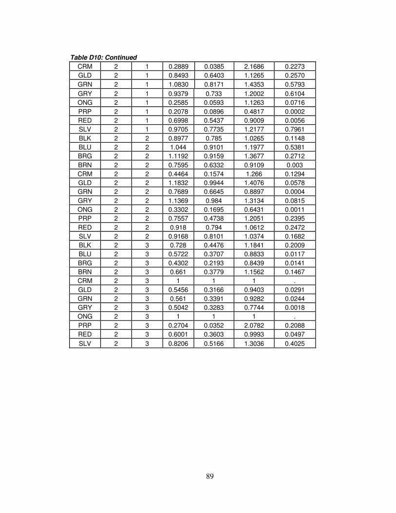
89

Table D10: Continued

CRM 2 1 0.2889 0.0385 2.1686 0.2273

GLD 2 1 0.8493 0.6403 1.1265 0.2570

GRN 2 1 1.0830 0.8171 1.4353 0.5793

GRY 2 1 0.9379 0.733 1.2002 0.6104

ONG 2 1 0.2585 0.0593 1.1263 0.0716

PRP 2 1 0.2078 0.0896 0.4817 0.0002

RED 2 1 0.6998 0.5437 0.9009 0.0056

SLV 2 1 0.9705 0.7735 1.2177 0.7961

BLK 2 2 0.8977 0.785 1.0265 0.1148

BLU 2 2 1.044 0.9101 1.1977 0.5381

BRG 2 2 1.1192 0.9159 1.3677 0.2712

BRN 2 2 0.7595 0.6332 0.9109 0.003

CRM 2 2 0.4464 0.1574 1.266 0.1294

GLD 2 2 1.1832 0.9944 1.4076 0.0578

GRN 2 2 0.7689 0.6645 0.8897 0.0004

GRY 2 2 1.1369 0.984 1.3134 0.0815

ONG 2 2 0.3302 0.1695 0.6431 0.0011

PRP 2 2 0.7557 0.4738 1.2051 0.2395

RED 2 2 0.918 0.794 1.0612 0.2472

SLV 2 2 0.9168 0.8101 1.0374 0.1682

BLK 2 3 0.728 0.4476 1.1841 0.2009

BLU 2 3 0.5722 0.3707 0.8833 0.0117

BRG 2 3 0.4302 0.2193 0.8439 0.0141

BRN 2 3 0.661 0.3779 1.1562 0.1467

CRM 2 3 1 1 1 .

GLD 2 3 0.5456 0.3166 0.9403 0.0291

GRN 2 3 0.561 0.3391 0.9282 0.0244

GRY 2 3 0.5042 0.3283 0.7744 0.0018

ONG 2 3 1 1 1 .

PRP 2 3 0.2704 0.0352 2.0782 0.2088

RED 2 3 0.6001 0.3603 0.9993 0.0497

SLV 2 3 0.8206 0.5166 1.3036 0.4025