Investigation of the hydraulic effects of ... - IDEALS @ Illinois

LIBRARY.

JUN 1 % 1997

IL ocvjl ourtVEY

EG 135

HWRIC RR 051

e^H 135"

QtuJi SmaaK*j

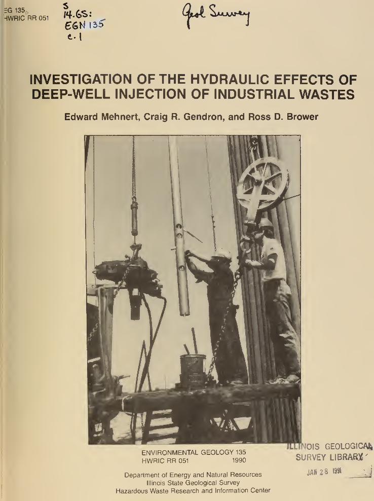
INVESTIGATION OF THE HYDRAULIC EFFECTS OFDEEP-WELL INJECTION OF INDUSTRIAL WASTES

Edward Mehnert, Craig R. Gendron, and Ross D. Brower

ENVIRONMENTAL GEOLOGY 135

HWRIC RR 051 1990

Department of Energy and Natural Resources

Illinois State Geological Survey

Hazardous Waste Research and Information Center

OIS GEOLOGICAL

SURVEY LIBRARY

JAN 2 8 Ml J

LIBRARY.

ILLINOIS STATE GEOLOGICAL SURVEY

3 3051 00005 4753

INVESTIGATION OF THE HYDRAULIC EFFECTS OFDEEP-WELL INJECTION OF INDUSTRIAL WASTES

Edward Mehnert, Craig R. Gendron, and Ross D. BrowerIllinois State Geological Survey

Final Report

Prepared for

United States Environmental Protection Agency

Office of Drinking Water

David Morganwalp, Project Officer

EPA Cooperative Agreement No. CR-813508-01-0

and

Hazardous Waste Research and Information Center

Department of Energy and Natural Resources

Jacqueline Peden, Project Officer

ENR Contract No. HWR 86022

1990

ENVIRONMENTAL GEOLOGY 135

HWRIC RR 051

ILLINOIS STATE GEOLOGICAL SURVEYNatural Resources Building

615 East Peabody Drive

Champaign, Illinois 61820

HAZARDOUS WASTE RESEARCH AND INFORMATION CENTEROne East Hazelwood Drive

Champaign, Illinois 61820

SURVEY LIBRARY

2 8 I99I

Digitized by the Internet Archive

in 2012 with funding from

University of Illinois Urbana-Champaign

http://archive.org/details/investigationofh135mehn

CONTENTS

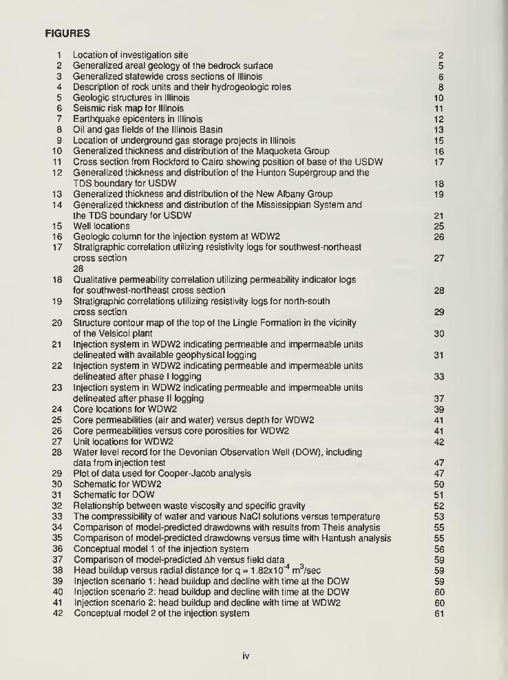
FIGURES iv

TABLES vi

ACKNOWLEDGMENTS vii

ABSTRACT viii

EXECUTIVE SUMMARY ix

GLOSSARY xi

1. INTRODUCTION 1

Background 1

Purpose 2

2. GEOLOGY OF THE INJECTION SYSTEM 3

Overview of the Geologic Environment 3

Regional Geology and Hydrogeology 14

3. HYDROGEOLOGIC INVESTIGATION OF THE INJECTION SYSTEM 23Stratigraphic and Structural Definition of the Injection System 23Field Investigations 32

4. NUMERICAL MODELING 48Model Selection 48Model Description 48Input Data 49Modeling Results 54Model Projections for Long-Term Injection 58Hypothetical Conduits 61

5. SUMMARY AND CONCLUSIONS 64Evaluation of Injection Scenarios 64Evaluation of Monitoring Strategies 64

REFERENCES 66

APPENDIX A Theory and practical application of geophysical

logging instruments 70

APPENDIX B Reduction and analysis of geophysical log data 81

APPENDIX C Brucite formation: proposed mechanism of formation 88

APPENDIX D Sensitivity analysis 96

in

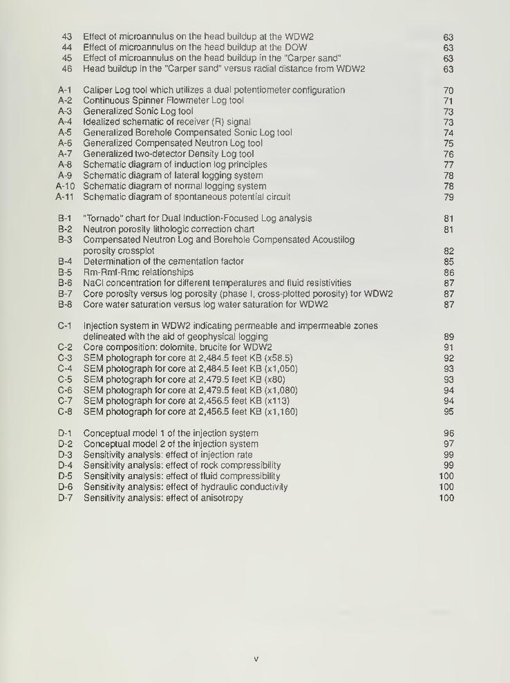
FIGURES

1 Location of investigation site 2

2 Generalized areal geology of the bedrock surface 5

3 Generalized statewide cross sections of Illinois 64 Description of rock units and their hydrogeologic roles 8

5 Geologic structures in Illinois 10

6 Seismic risk map for Illinois 11

7 Earthquake epicenters in Illinois 12

8 Oil and gas fields of the Illinois Basin 13

9 Location of underground gas storage projects in Illinois 15

1 Generalized thickness and distribution of the Maquoketa Group 1

6

1

1

Cross section from Rockford to Cairo showing position of base of the USDW 1

7

1

2

Generalized thickness and distribution of the Hunton Supergroup and the

TDS boundary for USDW 1

8

13 Generalized thickness and distribution of the New Albany Group 19

14 Generalized thickness and distribution of the Mississippian System and

the TDS boundary for USDW 21

15 Well locations 251

6

Geologic column for the injection system at WDW2 261

7

Stratigraphic correlation utilizing resistivity logs for southwest-northeast

cross section 2728

18 Qualitative permeability correlation utilizing permeability indicator logs

for southwest-northeast cross section 28

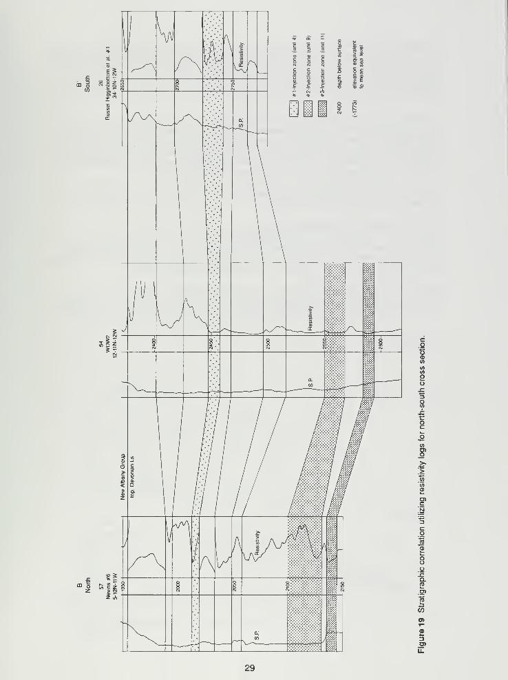
19 Stratigraphic correlations utilizing resistivity logs for north-south

cross section 29

20 Structure contour map of the top of the Lingle Formation in the vicinity

of the Velsicol plant 3021 Injection system in WDW2 indicating permeable and impermeable units

delineated with available geophysical logging 31

22 Injection system in WDW2 indicating permeable and impermeable units

delineated after phase I logging 3323 Injection system in WDW2 indicating permeable and impermeable units

delineated after phase II logging 3724 Core locations for WDW2 3925 Core permeabilities (air and water) versus depth for WDW2 41

26 Core permeabilities versus core porosities for WDW2 41

27 Unit locations for WDW2 4228 Water level record for the Devonian Observation Well (DOW), including

data from injection test 4729 Plot of data used for Cooper-Jacob analysis 4730 Schematic for WDW2 5031 Schematic for DOW 51

32 Relationship between waste viscosity and specific gravity 5233 The compressibility of water and various NaCI solutions versus temperature 5334 Comparison of model-predicted drawdowns with results from Theis analysis 5535 Comparison of model-predicted drawdowns versus time with Hantush analysis 5536 Conceptual model 1 of the injection system 5637 Comparison of model-predicted Ah versus field data 5938 Head buildup versus radial distance for q = 1 .82x1

0"4 m3/sec 59

39 Injection scenario 1 : head buildup and decline with time at the DOW 5940 Injection scenario 2: head buildup and decline with time at the DOW 6041 Injection scenario 2: head buildup and decline with time at WDW2 6042 Conceptual model 2 of the injection system 61

IV

43 Effect of microannulus on the head buildup at the WDW2 6344 Effect of microannulus on the head buildup at the DOW 6345 Effect of microannulus on the head buildup in the "Carper sand" 6346 Head buildup in the "Carper sand" versus radial distance from WDW2 63

A-1 Caliper Log tool which utilizes a dual potentiometer configuration 70A-2 Continuous Spinner Flowmeter Log tool 71

A-3 Generalized Sonic Log tool 73A-4 Idealized schematic of receiver (R) signal 73A-5 Generalized Borehole Compensated Sonic Log tool 74A-6 Generalized Compensated Neutron Log tool 75A-7 Generalized two-detector Density Log tool 76A-8 Schematic diagram of induction log principles 77A-9 Schematic diagram of lateral logging system 78A-1 Schematic diagram of normal logging system 78

A-11 Schematic diagram of spontaneous potential circuit 79

B-1 "Tornado" chart for Dual Induction-Focused Log analysis 81

B-2 Neutron porosity lithologic correction chart 81

B-3 Compensated Neutron Log and Borehole Compensated Acoustilog

porosity crossplot 82B-4 Determination of the cementation factor 85B-5 Rm-Rmf-Rmc relationships 86B-6 NaCI concentration for different temperatures and fluid resistivities 87B-7 Core porosity versus log porosity (phase I, cross-plotted porosity) for WDW2 87B-8 Core water saturation versus log water saturation for WDW2 87

C-1 Injection system in WDW2 indicating permeable and impermeable zones

delineated with the aid of geophysical logging 89C-2 Core composition: dolomite, brucite for WDW2 91

C-3 SEM photograph for core at 2,484.5 feet KB (x58.5) 92C-4 SEM photograph for core at 2,484.5 feet KB (x1 ,050) 93C-5 SEM photograph for core at 2,479.5 feet KB (x80) 93C-6 SEM photograph for core at 2,479.5 feet KB (x1 ,080) 94C-7 SEM photograph for core at 2,456.5 feet KB (x1 1 3) 94C-8 SEM photograph for core at 2,456.5 feet KB (x1 ,1 60) 95

D-1 Conceptual model 1 of the injection system 96D-2 Conceptual model 2 of the injection system 97D-3 Sensitivity analysis: effect of injection rate 99D-4 Sensitivity analysis: effect of rock compressibility 99D-5 Sensitivity analysis: effect of fluid compressibility 100

D-6 Sensitivity analysis: effect of hydraulic conductivity 100

D-7 Sensitivity analysis: effect of anisotropy 100

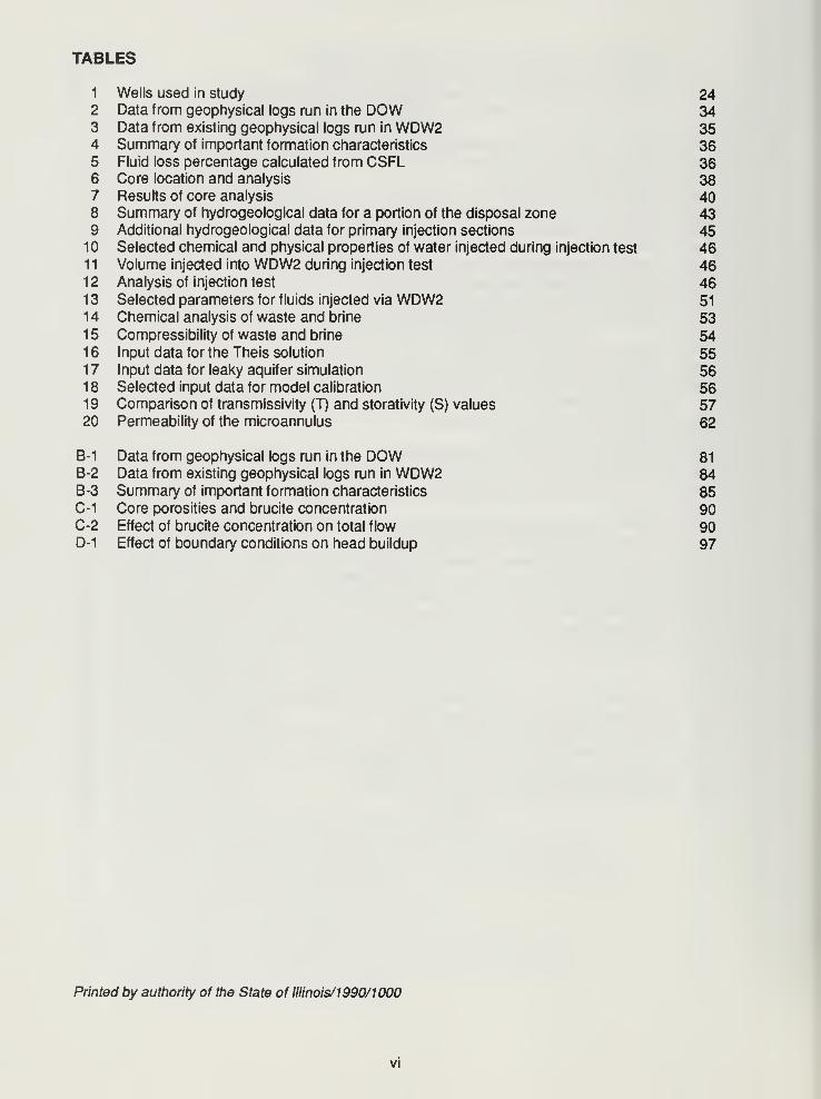
TABLES

1 Wells used in study 242 Data from geophysical logs run in the DOW 343 Data from existing geophysical logs run in WDW2 354 Summary of important formation characteristics 365 Fluid loss percentage calculated from CSFL 366 Core location and analysis 387 Results of core analysis 408 Summary of hydrogeological data for a portion of the disposal zone 439 Additional hydrogeological data for primary injection sections 45

1 Selected chemical and physical properties of water injected during injection test 4611 Volume injected into WDW2 during injection test 4612 Analysis of injection test 4613 Selected parameters for fluids injected via WDW2 51

14 Chemical analysis of waste and brine 5315 Compressibility of waste and brine 541

6

Input data for the Theis solution 551

7

Input data for leaky aquifer simulation 561

8

Selected input data for model calibration 5619 Comparison of transmissivity (T) and storativity (S) values 5720 Permeability of the microannulus 62

B-1 Data from geophysical logs run in the DOW 81

B-2 Data from existing geophysical logs run in WDW2 84B-3 Summary of important formation characteristics 85C-1 Core porosities and brucite concentration 90C-2 Effect of brucite concentration on total flow 90D-1 Effect of boundary conditions on head buildup 97

Printed by authority of the State of Illinois/1990/1000

VI

ACKNOWLEDGMENTS

We thank the following people for their assistance throughout this project.

Jeffrey S. Brown, Robert Colvin, and Thomas Capps, Velsicol Chemical Corporation, for allowing

us access to their site and assistance in the completion of the field tests conducted on-site.

Frank Brookfield and Lance Perry, Hazardous Waste Research and Information Center (HWRIC),

for their tireless assistance with the PRIME computer—from debugging and compiling code to not

complaining when we monopolized the computer time.

Richard A. Cahill, Beverly Seyler, Robert R. Frost, Herbert Glass, and William R. Roy, Illinois

State Geological Survey (ISGS), for performing various chemical and physical analyses on

samples of the core, waste stream, and native formation brine. These analyses included ther-

modynamic modeling, x-ray fluorescence, microprobe, scanning electron microscopy, and x-ray

diffraction.

Lynn R. Evans, ISGS, for compiling the data regarding the chemical and physical characteristics

of the UIC wastes.

David Morganwalp, project manager for the U.S. Environmental Protection Agency, for his assis-

tance and patience during this project.

Jackie Peden, HWRIC project manager, and Gary D. Miller, former project manager, for their as-

sistance and patience during this project.

Adrian Visocky, Illinois State Water Survey, for his advice regarding the analysis of the data from

the injection test.

Anne M. Graese, Bruce R. Hensel, Timothy H. Larson, Janis D. Treworgy, and Steven TWhitaker, ISGS, for their insightful review of this report.

VII

ABSTRACT

A numerical modeling study was conducted to investigate the hydraulic effects of liquid waste in-

jection on an injection system. The site investigated was a chemical refinery with an operational

Class I well and an observation well, both completed in Devonian limestone. Input data for the

model were obtained from available records and field investigations.

The regional geologic investigation indicated that the injection system (defined here as the injec-

tion zone and its associated confining units) was laterally continuous. The hydraulic response of

the injection system was numerically modeled under two injection scenarios: average historical in-

jection rate and maximum average permitted rate. For both scenarios, pressure buildup from

waste injection during the simulated 30-year injection and 30-year postinjection periods did not ap-

proach the pressure calculated to be necessary to initiate or propagate fractures in the injection

system. Therefore, injected waste would be contained, and waste injection at this site and for the

scenarios modeled would not endanger human health or the environment.

This analysis assumes that hydraulic conductivity remains constant; however, the formation of

brucite within the injection zone may invalidate this assumption and the preceding analysis.

Brucite formation within the injection zone requires additional study.

The model was also used to investigate the response of the injection system when a hypothetical

conduit was introduced. This hypothetical conduit connected the uppermost injection zone with anoverlying aquifer. Differences in head buildup were not monitorable in the injection well or in an

observation well completed in the injection zone. Monitorable head differences were observed

only in the overlying aquifer, when the hydraulic conductivity of the hypothetical conduit wasgreater than or equal to 1x10"

10 m2.

VIII

EXECUTIVE SUMMARY

Concern over the potential for groundwater contamination from waste injection prompted a multi-

faceted research effort funded by the U.S. Environmental Protection Agency (USEPA) and in-

dustry. The research will provide the USEPA with data needed to determine if underground

injection of hazardous waste endangers human health or the environment. One facet of this re-

search effort was an investigation of the hydraulic effects of deep-well injection on the injection

system.

The injection system includes the geologic units constituting the injection zone and the upper andlower confining units. The site of this investigation was a chemical refinery in Illinois that has an

operational injection well and an observation well completed in Devonian limestone.

Data Collection and Analysis

Before numerical modeling could be conducted, a hydrogeologic description of the site wasdeveloped from available records and geophysical logs. Numerous records and logs were avail-

able from oil- and gas-related tests and wells within a 10-mile radius of the site. Logs and records

for on-site wells were also used.

In addition, hydraulic tests and geophysical logs were run to obtain detailed hydrogeologic data

on the injection system. Two hydraulic tests were run in the injection well: a continuous spinner

flowmeter survey and a 15-day injection test. Sidewall cores were also retrieved from the injection

well. The following geophysical logs were run in the observation well: Compensated Neutron Log,

Borehole Compensated Sonic Log, Minilog, Dual Induction Spherically Focused Log, and GammaRay Log.

Although analyses of the data from these logs and tests yielded much information concerning the

hydrogeologic character of the injection system, there was one discrepancy—the results of the

spinner flowmeter indicated that the waste was flowing through different zones of the injection sys-

tem than had been theorized from the results of geophysical logging. To clarify this discrepancy,

we conducted additional analyses (x-ray diffraction and scanning electron microscopy). The dis-

crepancy can be explained briefly as follows. Because of its high pH, the injected wastewater

reacts with the Mg2+present in the injection zones or in solution, forming brucite (Mg[OH]2).

Brucite accumulation reduces the permeability of the injection zone. Greater amounts of brucite

apparently formed in the injection zones where the flow of fluid was greater; thus the zones with

higher permeability were affected first. Additional work beyond the scope of this project is neededto verify the brucite-formation hypothesis. Also, the long-term effect of this decrease in per-

meability on injectivity needs to be investigated.

Numerical Modeling

Site Analysis

A description of the regional and site-specific stratigraphy, structural geology, and hydrogeology

of the injection system was generated from a review of available data and the field work con-

ducted during this project. This description formed the basis of input for the numerical model.

Model input also included data on the physical and chemical characteristics of the injected waste-

water and the native brine in the injection system.

These data were employed as input data for a three-dimensional groundwater flow model

(HST3D). Before the effects of various injection scenarios were evaluated, HST3D was verified

with respect to two analytical solutions and calibrated by the use of data collected during a 2-

week injection test. Both verification and calibration were considered satisfactory.

IX

Once calibrated, the model was used to predict the effects of various injection scenarios. The ef-

fect of long-term injection was investigated at two constant injection rates—the average historical

rate (1.1 5x10~2 m3

/sec) and the maximum average rate permitted under Class I regulations

(2.21 x10"2 m3

/sec). With both scenarios, significant head buildup was observed at the injection

well and radially from it. During the simulated 30-year injection period, steady state was ap-

proached but not obtained for both injection scenarios. During the subsequent 30-year postinjec-

tion period, dropoff in head buildup was fairly rapid, falling to half in less than 2,000 hours for both

scenarios. The maximum hydraulic pressures at the bottom of the well and at the base of the

upper confining unit were significantly lower than the pressures calculated to initiate hydraulic frac-

turing. A fracture gradient of 1.5x14 Pa/m (Pascals/meter) (0.65 psi/ft) was used to calculate the

hydraulic fracture pressures.

The regional and site-specific geological analysis revealed the continuity of the stratigraphy and

qualitative permeability on a regional basis. The numerical modeling indicated that injection pres-

sures were lower than calculated pressures required to initiate hydraulic fracturing. Therefore,

from a hydraulic viewpoint, waste injected into this injection system would be contained, and

waste injection at this site and for the scenarios modeled would be considered protective of

human health and the environment.

These results were based on an assumption that the permeability remains constant. If the

hypothesis concerning the formation of brucite is correct, its formation may reduce the per-

meability of the injection zones and invalidate this analysis. Any reduction in permeability of the in-

jection zones will probably increase the hydraulic pressure resulting from waste injection if the

injection rate remains constant. In such a situation, hydraulic fracturing may be of concern. Be-

cause of the potential ramifications, formation of brucite within the injection zone requires addition-

al geochemical analysis.

Effects of Hypothetical Conduit

The model was also used to investigate the hydraulic response of the injection system to the intro-

duction of a hypothetical conduit. The conduit, a microannulus (0.01 m wide) at the injection well,

hydraulically connects the uppermost injection zone and an aquifer immediately overlying the

upper confining unit. To determine the impact of the microannulus, the head buildup with the

microannulus present was compared with the buildup from runs with the microannulus not pre-

sent. Differences in head buildup at selected positions and for certain times were computed. Dif-

ferences in the head buildup were considered unmonitorable at the injection well and the

observation well. The difference in head buildup in the overlying aquifer was monitorable only

when the microannulus had a hydraulic conductivity greater than or equal to 1 .00x10" 10 m2

. The

head buildup in the overlying aquifer is a function of its hydraulic conductivity, the hydraulic con-

ductivity of the microannulus, and the radial distance from the microannulus. Thus for the

scenario modeled, leakage via a microannulus could not be hydraulically monitored by use of the

injection well or an observation well completed within the injection zone. This leakage wasmonitorable only through the use of an observation well in the overlying aquifer.

GLOSSARY

AIF aquifer influence boundary

b thickness

DOW Devonian Observation Well

GL ground level

HST3D Heat and Solute Transport ModelISGS Illinois State Geological Survey

k permeability

K hydraulic conductivity

KB Kelly Bushing

m modulus of shear for the mediumPa Pascals

POR porosity

psi pounds per square inch

q pumping rate

s storativity

SEM scanning electron microscopy

SWIFT Sandia Waste Isolation Flow and Transport ModelSWIP Survey Waste Isolation Program

T transmissivity

TDS total dissolved solids

USDW underground sources of drinking water

USEPA United States Environmental Protection AgencyWDW2 Waste Disposal Well 2

a matrix compressibility

P fluid compressibility

Ah head buildup

P fluid density

M- fluid viscosity

XI

1. INTRODUCTION

Background

Liquid waste is disposed of through underground injection by pumping the waste into or allowing

it to flow through a specially designed and monitored well. Developed by the petroleum industry in

the 1930s as a method for brine disposal, the technique was adapted by other industries in the

1950s for the disposal of industrial waste streams. As regulations for the disposal of waste into

landfills and surface waters became more stringent, the volume of waste disposed of by under-

ground injection increased.

Regulatory agencies have classified injection wells according to the purpose of the wells and the

proximity of injection reservoirs to the lowermost underground source of drinking water (USDW).The five classes of injection wells are:

Class I — wells used to inject hazardous and nonhazardous wastes below the

lowermost USDW (this report is concerned with this class of wells).

Class II — wells associated with the production and storage of oil and gas belowthe lowermost USDW.

Class III — wells used in special process (mining) operations to inject fluid above,

into, or below an USDW.

Class IV — wells used to inject hazardous waste into or above an USDW (this

class of wells is currently banned).

Class V — wells used to inject all other wastes into or above an USDW.

According to the U.S. Environmental Protection Agency (USEPA), there were 429 Class I injec-

tion wells active in 1986 (USEPA 1986). Although the volume of waste disposed of nationwide via

these wells is difficult to estimate, accurate figures are available from some states. In Illinois,

nine Class I wells were used in 1984 to dispose of 310 million gallons of waste (Brower et al.

1989).

With the promulgation of the Hazardous and Solid Waste Amendments of 1984, the level of inter-

est in underground injection increased tremendously. Provisions of the act mandated that the ad-

ministrator of USEPA determine if underground injection is a threat to human health and the

environment for the period the waste remains hazardous. If underground injection is found to be

hazardous to human health and the environment, or if the determination is not made by the Con-

gressionally mandated date, all underground injection will be banned. Some environmental

groups want situations detailed in which underground injection has endangered or may endanger

human health or the environment.

The USEPA developed an extensive research agenda to examine pertinent issues. The USEPAhas funded to date one or more projects in each of the following areas: identification and clas-

sification of Class I well failures; techniques to detect abandoned wells; monitoring of various

aspects of the well; flow and transport modeling of various injection scenarios; geochemical

modeling of injected waste, injection formation, and brine; and hydrogeologic characterization of

important injection formations and associated confining formations. Industry also has conducted

research into pertinent topics of underground injection.

In this project, a numerical model was used to investigate the hydraulic effects of waste injection

on the geologic reservoir. The site of the investigation is a chemical refinery located near Mar-

shall, Illinois, in north-central Clark County (fig. 1). The chemical company used the injection well

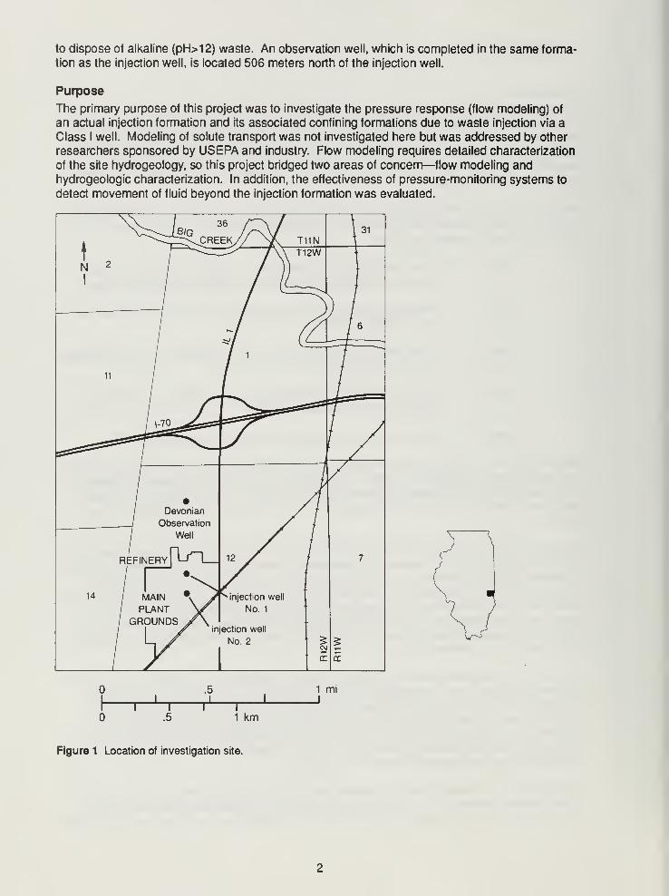
to dispose of alkaline (pH>12) waste. An observation well, which is completed in the same forma-

tion as the injection well, is located 506 meters north of the injection well.

Purpose

The primary purpose of this project was to investigate the pressure response (flow modeling) of

an actual injection formation and its associated confining formations due to waste injection via aClass I well. Modeling of solute transport was not investigated here but was addressed by other

researchers sponsored by USEPA and industry. Flow modeling requires detailed characterization

of the site hydrogeology, so this project bridged two areas of concern—flow modeling andhydrogeologic characterization. In addition, the effectiveness of pressure-monitoring systems to

detect movement of fluid beyond the injection formation was evaluated.

t

/ 36 /^\ /^^=^>creek// \X T11N

131

T12W

NI

2 / / V

^\

/ ^/ (A' 6

/ / 1

VJ'

11 / /

jjiSs^^^

/ •/ Devonian

/ Observation

jWell

refinery| L-tH— 12 X 7

/ •^^

14 / main #v y

/ PLANT \f^ injection well

No. 1

/ GROUNDS J\/ jf injection well

/ L / No. 2

/ y i

5

E5

E

~r.5

.5 1 mi

1 km

Figure 1 Location of investigation site.

2. GEOLOGY OF THE INJECTION SYSTEM

The geologic environment of an injection well site controls many aspects of the disposal operation

and the fate of the injected wastes. This section includes a summary of the regional geology andhydrogeology of the units involved with the deep-well injection operation. The geologic setting is

described within the context of the regional geology to show regional trends and the degree of

uniformity in geologic conditions.

Only those aspects of geology pertinent to underground injection are described. The major em-phasis is on the hydrogeology of the confining units and the injection interval, specifically, the

hydrogeology of the upper confining unit (New Albany Group), the lower confining unit (Ma-

quoketa Group), and the injection interval (Hunton Supergroup). The Borden Siltstone, which

overlies the New Albany Group, acts as an additional confining zone.

Overview of Geologic Conditions Affecting Waste Injection

The principal geologic factors for the regional evaluation are those affecting (1) the capacity of

geologic units in the injection system to accept and confine injected waste, (2) the chemical inter-

action of the waste with injection system components, (3) the generation of dislocations that

developed during the forming of structural features or seismic events, and (4) the use of subsur-

face space and commercial grade resources in the area of disposal influence.

In this section we have focused on the broader regional issues that relate to local geologic condi-

tions. Broadly defined lithologic units form a key component of the regional discussion. Theseunits have been described in the literature, and the uniformity of their general geologic conditions

and structural trends have been established by oil, gas, water, and mineral resource exploration

activities in the region.

The character and trends of the regional geology have been determined from data gathered from

key well records, reports, and publications. This information reveals the distribution of aquifers

that meet regulatory requirements for Class I injection, i.e., aquifers that contain saline water

(>1 0,000 mg/L total dissolved solids [TDS]) and that have confining intervals capable of protect-

ing all USDW from contamination by injection activities. Injection is limited to selected aquifers in

the southern two-thirds of Illinois, including the Hunton Supergroup and the Salem Limestone,

which have been used for disposal at the study site. Injection system response to waste injection

is primarily controlled by porosity and permeability characteristics, which can be directly related

regionally to specific geologic units.

Porosity and permeability develop during sedimentation processes and are modified by other

geologic processes. Thus porosity and permeability have a general relationship with specific

lithologies. Each geologic unit in the region exhibits a range of values and areal trends. Thesedimentary geologic units in east-central Illinois exhibit relatively uniform characteristics over

large areas; however, both vertical and radial trends are noted within each unit. Similar patterns

can also be expected within the subdivisions of each unit, but determining this would require adetailed study of subsurface records.

The lithology of the geologic units forming the injection system plays an important role in the

chemical interaction between the injected waste and injection system. Chemical interaction be-

tween injected waste and the injection system can affect flow conditions (porosity and per-

meability) and under certain disposal conditions can compromise the integrity of the confining

intervals. However, beneficial interactions may also occur that would improve flow conditions, in-

volve retention of some waste components near the well, and provide treatment for selected, un-

desirable components in the waste.

This discussion focuses on the general regional characteristics of principal geologic units and re-

lates these characteristics to hydrogeologic parameters for characterizing flow in the injection sys-

tem. An effective evaluation by numerical modeling requires that the hydrogeologic character of

the geologic units accepting and retaining injected waste be predictable and relatively uniform

throughout the area influenced by injection. A more detailed description of the character andradial uniformity of the units in the injection system is presented in chapter 3.

General Geologic Setting

The geologic framework of Illinois in which deep-well disposal is practiced can be described as a

sequence of areally extensive sedimentary rock units deposited in a large midcontinent basin

known as the Illinois Basin. The study site, in the east-central part of the basin, is immediately

east of the axis of the Marshall-Sidell Syncline and about 14 miles east of the La Salle Anticlinal

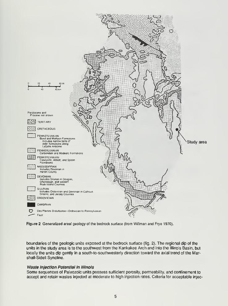
Belt, the most dominant structural feature in the area. Figure 2 shows the generalized geology of

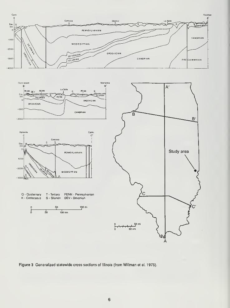
the bedrock surface in Illinois. Generalized geologic cross sections of Illinois are depicted in fig-

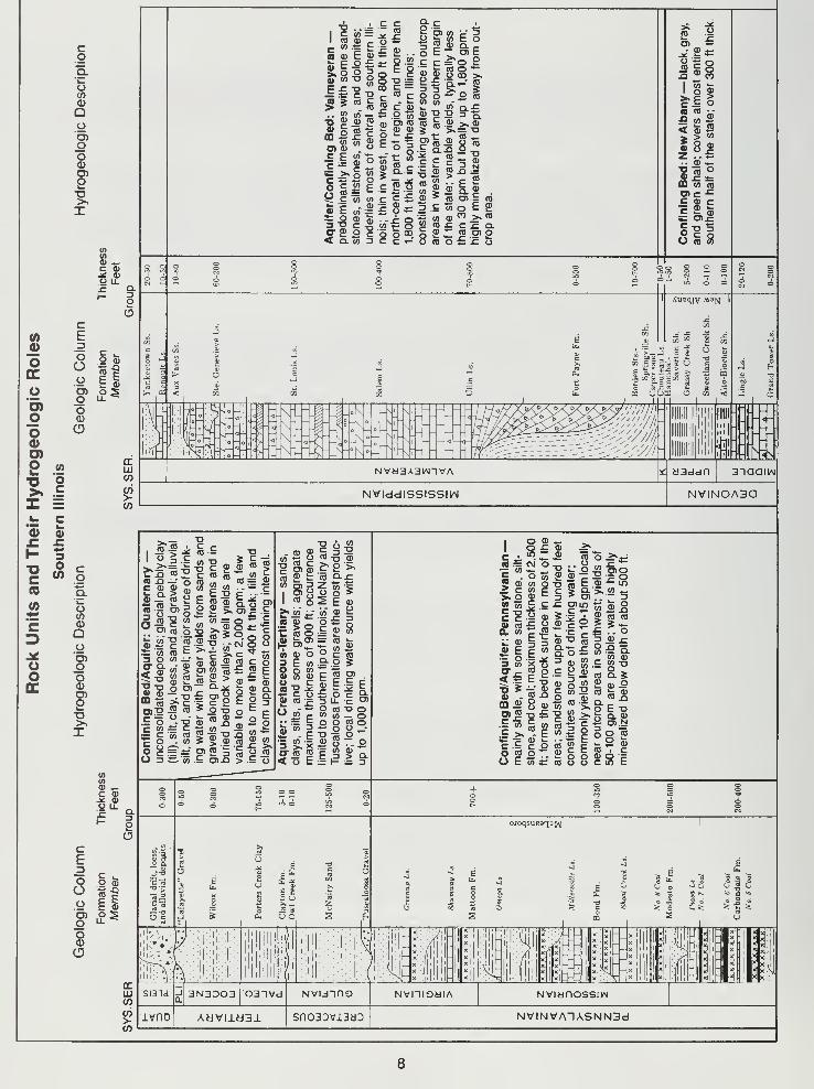
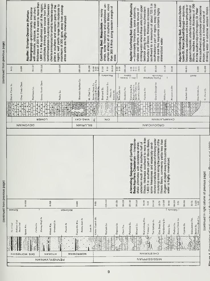
ure 3. Figure 4 provides a generalized geologic column and comments on the stratigraphy, lithol-

ogy, hydrogeology, and groundwater geochemistry of the geologic units associated with or

protected from waste injection. Additional details on geologic units covered in this report are avail-

able in the Handbook for Illinois Stratigraphy (Willman et al. 1975), the Bibliography of Illinois

Geology (Willman et al. 1968) and reports prepared by Brower et al. (1989), Cluff et al. (1981),

Gray et al. (1979), and Piskin and Bergstrom (1975).

In Illinois, lithologies range from very fine- to coarse-grained elastics, a variety of carbonates, anda few evaporites and organics. Relatively uniform lithologic characteristics exist on a regional

basis within individual units as a whole and within the subdivisions of each unit.

Many processes have been involved in forming, altering, and structurally readjusting these units

from the time of deposition to the present day. Sedimentary deposition began early in the

Paleozoic Era on the eroded surface of igneous and metamorphic rock of the Precambrian base-

ment complex. Deposition and some erosion continued throughout the Paleozoic. Several

episodes of deposition in the Mesozoic and Cenozoic Eras produced nonlithified sedimentary

units. The present-day landscape has developed principally on these nonlithified sediments.

Marine carbonate and clastic lithologies are dominant in the Paleozoic units, but terrestrial elas-

tics and some organic deposits are present in the upper part of the Paleozoic (Mississippian and

Pennsylvanian Systems).

The thickness of the sedimentary sequence in Illinois ranges from approximately 2,000 feet

northwest of Rockford to more than 20,000 feet in the southeastern corner of the state, the

deepest part of the Illinois Basin (Sargent and Buschbach 1985). In the project area, the total

thickness of the sedimentary units is approximately 8,500 feet. Lithologies include dolomite, lime-

stone, sandstone, siltstone, shale, and some coal and evaporite. The stratigraphic column in

figure 4 provides a summary of the typical sedimentary sequence in the Illinois Basin.

Widespread carbonate lithologies are dominant in the lower part of the Paleozoic, and a few

sandstones and some shales are interbedded with these carbonates. Most of the carbonates be-

come sandy to the north, and a few grade into sandstones in the far northern part of the state.

Greater variations in regional lithology exist in the upper part of the Devonian through the middle

part of the Mississippian. Cyclic deposits of fine-grained elastics (shales and siltstones), some car-

bonates, and some coarse-grained elastics (sandstones) accumulated in the upper part of the

Mississippian and in all of the Pennsylvanian as numerous sea-level oscillations shifted

shorelines across shallow-marine and flat-lowland terrestrial environments.

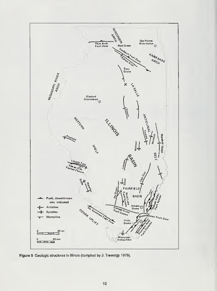
The study site is in the Marshall-Sidell Syncline (see fig. 5), a broad structural feature of low relief

between the La Salle Anticlinal Belt, about 14 miles to the west, and the Kankakee Arch morethan 90 miles to the northeast. These two structures are reflected in the distribution of the

boundaries of the geologic units exposed at the bedrock surface (fig. 2). The regional dip of the

units in the study area is to the southwest from the Kankakee Arch and into the Illinois Basin, but

Pleistocene andPliocene not shown

M'/A TERITIARY

\z-Z-Z-] CRETACEOUS

m

PENNSYLVANIANBond and Mattoon Formations

Includes narrow belts o)

older formations alongLaSalle Anticline

PENNSYLVANIANCarbondale and Modesto Formations

PENNSYLVANIANCaseyville, Abbott, and SpoonFormations

MISSISSIPPIANIncludes Devonian in

Hardin County

DEVONIANIncludes Silurian in Douglas,Champaign, and westernRock Island Counties

SILURIANIncludes Ordovician and Devonian in CalhounGreene, and Jersey Counties

ORDOVICIAN

CAMBRIAN

^ Des Plaines Disturbance—Ordovician to Pennsylvaman

^-— Fault

Study area

Figure 2 Generalized areal geology of the bedrock surface (from Willman and Frye 1970).

boundaries of the geologic units exposed at the bedrock surface (fig. 2). The regional dip of the

units in the study area is to the southwest from the Kankakee Arch and into the Illinois Basin, but

locally the units dip gently in a south-to-southwesterly direction toward the axial trend of the Mar-

shall-Sidell Syncline.

Waste Injection Potential In Illinois

Some sequences of Paleozoic units possess sufficient porosity, permeability, and confinement to

accept and retain wastes injected at moderate to high injection rates. Criteria for acceptable injec-

Cairo

ARocktord

A'

Centrolio

1 _^.Decoiur Lo Solle

T "7^W—rt"\^Ekv. ^^,

<

«s=s=^^«^ . ^^J^-^y^—

w

0/ J ^^OAJO-(ID

0- PENNSYLVANIAN

r^S

-1000-\ CAMBRIAN

2000-

\\ o \

\\°A

MISSISSIPPIAN ^y3000-

OROOVICIAN

CAMBRIAN PRE CAMBRIAN

Rock Island

B

Momence

B'

Elev

(It)

PENN 0£v PENNLo Solle

\Q PENN

.

—

:==^-^*-^-' " ' 'i

so

'PENN J^-—I^ZI—^*^^—-siL URIAH

SILURIAN

OROOVICIAN

ORDOVICIAN

CAMBRIAN

~~~~~-

Q - Quaternary T - Tertiary PENN - Pennsylvanian

K - Cretaceous S - Silurian DEV - Devonian

100 mi_l

50 100 km

Figure 3 Generalized statewide cross sections of Illinois (from Willman et al. 1975).

Protection Act (Title 35, Illinois Administrative Code). Within Illinois, the base of the USDW ranges

in depth from 500 to slightly more than 3,000 feet. All units below the lowermost USDW contain

groundwater with a TDS content exceeding 10,000 mg/L (milligrams/liter). Injection is feasible

only in portions of Cambrian through basal Pennsylvanian units that meet the criteria for waste in-

jection established in the Illinois Environmental Protection Act.

In the study area, the base of the USDW has been established at a depth of about 500 feet (Pis-

kin 1986). In the immediate vicinity of the study site, significant injection potential for the Salemand Hunton carbonate units has been proved by oil exploration and waste-injection testing con-

ducted to a depth of 6,000 feet. Recently, injection has been limited to the Devonian portion of the

Hunton. Very limited groundwater supplies have been obtained from the uppermost part of the

Pennsylvanian bedrock. The City of Marshall obtains a moderate to large water supply from a

shallow sand and gravel aquifer in the nearby valley of Big Creek.

Seismic Activity in Illinois

Earthquake waves traveling through earth materials can affect deep-well disposal systems.

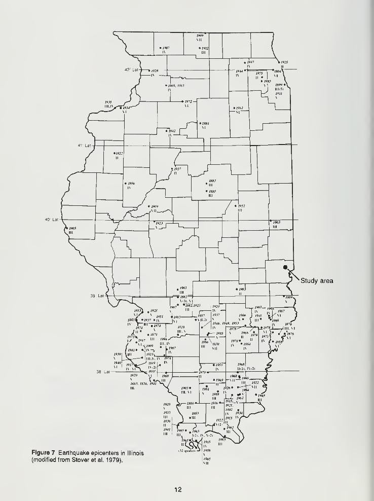
Earthquakes are infrequent in Illinois, and most have been low to moderate in magnitude and in-

tensity (fig. 7). Several earthquakes of low-to-moderate magnitude recently occurred in the

vicinity of the Wabash Valley Fault System, which extends northward into Edwards and WabashCounties from southeastern Illinois (fig. 5). The largest earthquakes affecting Illinois in recorded

history occurred near New Madrid, Missouri, in 1811 and 1812 (Heigold 1968, 1972). Although

faulting is reported in other areas of Illinois, field studies and drilling records available to the Il-

linois State Geological Survey indicate that no faults are mapped at the surface or known to have

occurred in the subsurface in the vicinity of the study area.

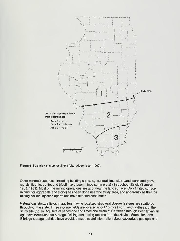
The greatest likelihood for major damage from earthquakes exists in 14 southern Illinois counties

(figs. 6 and 7). This region of the state is in Area 3 on the Seismic Risk Map (fig. 6) compiled by

Algermissen (1969). The project site is near the southern margin of Area 1 , the area in which the

damage expectancy from potential earthquakes is rated as minor.

Subsurface ResourcesSubsurface resources in Illinois exclusive of groundwater resources include mineral deposits,

hydrocarbon deposits, and subsurface storage space. Many of the geologic units containing sub-

surface resources also qualify as potential disposal horizons. The regulations for deep-well dis-

posal require a review of all subsurface resources of commercial value in order to reduce the

potential for conflicts between injection and resource extraction.

Oil and limited natural gas resources have been exploited in numerous permeable units abovethe St. Peter Sandstone. Oil production is mainly associated with Mississippian units; however,

significant production has come from other Paleozoic units. The petroleum-producing regions in Il-

linois are confined to the Illinois Basin (fig. 8). Wells drilled for production provide valuable infor-

mation about subsurface conditions; however, if not properly sealed, these wells can be potential

avenues for fluid movement into overlying geologic units.

Oil has been produced in the Weaver Field about 9 miles to the east-southeast of the study area

and in several small fields on the La Salle Anticlinal Belt, more than 14 miles to the west. Ex-

ploratory wells have been drilled throughout the vicinity of the study site; a few of these wells are

within the 2.5-mile area of review of the disposal well. No commercial oil pools have beenreported in the Marshall-Sidell Syncline in the vicinity of the study site.

Coal deposits are more widespread than petroleum deposits in the Pennsylvanian units, and mul-

tiple coal deposits are often found where Pennsylvanian units are present. Although more than 50potential coal horizons have been found in Illinois, only a few are thick enough for commercial

development. The coals in the project area tend to be relatively thin and deeply buried. Most coal

deposits mined in Illinois are shallow (less than 500 ft) and lie within units designated as USDW.

_ c <D

2 «5 o

I = (0*"** >t <d

gc«™ It iC c <"

S'E ©QTJO£ 2 «5

coreCL

(0

o>0)

co g E-coVT T '^ ft +•* — *S rft

o 28»_£ E©2.c

II03 toCL ^— 0)

© S£ en3 CO ^« c

(0

a)C Q.

£ to Bo IB -s£ « °9 fc to

to F2> o EtO * ©

111

= ©

§1* o

_ "Oo o cc

©

ll

- ; =

to© vE re— to

"S r sJ 41 (I

5 O CL

° CL

a. 9fog|° .

I isE-^22 to a>

d) to cO) •- c£. E>^

to °».S>p o -c

2.8 2><»_ to

*iia isco re ©£ E re

c3

>. • -

1- cre oF (0O

1 cr

re

?!to

a> uV l_

o re

3 a>erea o2 to

S

1b

CD ©CO &c oc (0

Oto

a>

§1to 2*o re

E E— cE ©© to

8 °>to c

1%re -*o

t5 !co —I*to oto°

J c 2•o £ to

> © »- CL

5 E © 3

c a> w to

® E »£S -° 3" «

to a>a

i § °-£CO -S to a)

to a> a>O a>e c *" z:.r E -r -CC= 5 5

~ O © £

E to«a> t» in

IIS6 c o3 — .Qo to wto to *_ego

111

o>== re

< I to "D

S - 2o o *-

« >,"£

2?iO 3 3(too-O JD to

>.

E ro ni*- si

re

tocre

cc oo oen a>a> o

c01

o 3rre

ain

ai

ci mr in 5

7n re

oNm U;

-C

3O

re

Q.o

re

aicEw o

i 2 ° o ^

ilfir

O 3»- l»tT P « II) .

«= S o Efi I g ig

|C0C o 3 c.E<^ io'E

c ^T"o s: to

ri « or5 5 to o. ox£ -oreO . O T3 O

151 latiihc 9- o c E o .5

£ f^= Z. ^ sz -^1 x i= C0=

1 oco o o ^

Ria>(onb»^SUJUJ1>I I -D8Q dnoj3qns uiheij

OCOreo.

to3o>2CL

Eo

a>

3ccoo

coi^"g to re

c c to

•ft = tb

I 'It 5 "o

a I 9C O -c

2.0 *

£ Oo re

OtS C= =. O«<«k w o

111< CD to

3 to o 5.

i

ore o.c Fc oo^ T)

3 moto ro 3

omo to

.co3E

(0a>c-1£

oto ^a>

*'

to

o oc

to ^bj §to »o >.

ire

^®CLT3

e§

IIto to

ilo oS E* ol- to

o 0)

re-C

$ oCTC 0)

J£ fl)c E•o ©o CLto ©© £t)

3oto

COco

(1>re

inJ

1or

re©re

o a.o o<0 i><1>

r _j

o u

S "»re to

£ 2to <oto CL© oto 22 3I]) O•5>E"g>< 2 N

ill8.ilc © x:

re to -cm • - to

"'Si-'|Ss^ LO «= CM 5

©COreo.

to3O

1

daUBMd^ BpUOOJOQ

-f-

Fault, downthrown

side indicated

Anticline

Syncline

Monocline

40 mi

50 km

Figure 5 Geologic structures in Illinois (compiled by J. Treworgy 1979).

10

,-

i'

"V

! I |

ii

\

r!— yj

iI '"i

i ...

1

1

C

i

\f—

, -I

I

L--' r'

Areal damage expectancy

from earthquakes

Area 1 - minor

Area 2 - moderate

Area 3 - major

Study area

Figure 6 Seismic risk map for Illinois (after Algermissen 1 969).

Other mineral resources, including building stone, agricultural lime, clay, sand, sand and gravel,

metals, fluorite, barite, and tripoli, have been mined commercially throughout Illinois (Samson1983, 1989). Most of the mining operations are at or near the land surface. Only limited surface

mining (for aggregate and stone) has been done near the study area, and apparently neither the

mining nor the injection operations have affected each other.

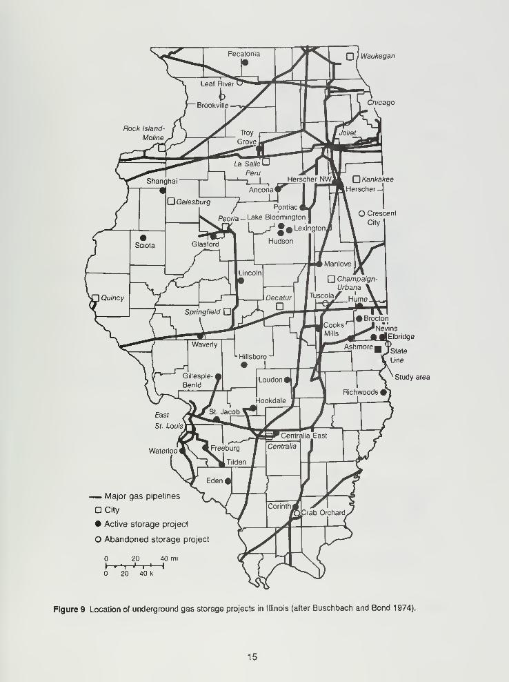
Natural gas storage fields in aquifers having localized structural closure features are scattered

throughout the state. Three storage fields are located about 10 miles north and northeast of the

study site (fig. 9). Aquifers of sandstone and limestone strata of Cambrian through Pennsylvanian

age have been used for storage. Drilling and testing records from the Nevins, State Line, andElbridge storage facilities have provided much useful information about subsurface geologic and

11

Study area

V19SI•J9J7 »|v

ill*%

,A ""'| / 1947 "

VI

38 Lal-

*1909v

J».'Oj ~~l ,«,.,_ . (iv — ^,n JctTww s19." 1906 J 1915 ^KVI 1

> > • \ 111 • *»I98S yJ1946. 1948. /95.I >

, x ,«76

IN1 197g^ /* \± '9H-< /"I. M

' - * 1 \ _ / m

Figure 7 Earthquake epicenters in Illinois

(modified from Stover et al. 1979).

12

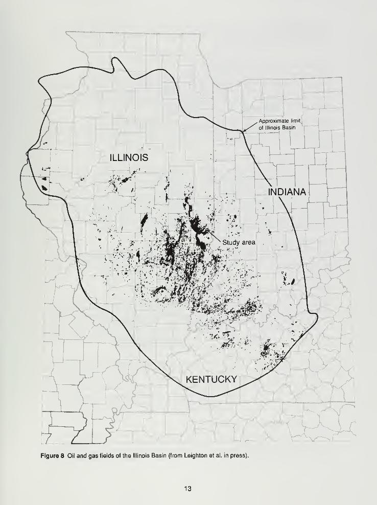
Figure 8 Oil and gas fields of the Illinois Basin (from Leighton et al. in press).

13

hydrogeologic conditions at the study site. Injection activities in the nearby natural gas storage

fields and at the study site do not appear to affect each other significantly, although both utilize

the same units of the Hunton.

Regional Geology and Hydrogeology

The units that are part of the injection system and are penetrated by the disposal well include the

basal confining interval (Maquoketa Group), the injection interval (Hunton carbonate sequence),

and the upper confining interval (New Albany shale sequence). Additional impermeable units andsome aquifers lie between the upper confining interval and land surface. The first significant

aquifer above the injection interval is the Salem Limestone.

Waste Disposal Well 2 (WDW2) was originally drilled to 6,000 feet (Eminence-Potosi Dolomites).

It was plugged back into the uppermost unit of the Silurian limestone part of the Hunton because

the immediately overlying Devonian limestone was the deepest, most receptive injection interval

available.

Ordovician SystemOrdovician strata (fig. 4) range in thickness from 700 feet (in northern Illinois) to more than 6,000

feet (in southern Illinois). The thickness increases gradually toward the south. Dolomites and lime-

stones are the predominant lithologies; however, several distinct sandstones are found in the

lower (Gunter and New Richmond Sandstones) and middle (St. Peter Sandstone) parts of the Or-

dovician. A thick shale-shaly carbonate sequence (Maquoketa Group) forms the upper part of the

Ordovician. Many of the units below the Maquoketa are relatively impermeable and act as

aquitards. The St. Peter Sandstone, a thin (50-ft), fine-grained, low-permeability sandstone in

Clark County, is the first significant aquifer below the Hunton injection interval.

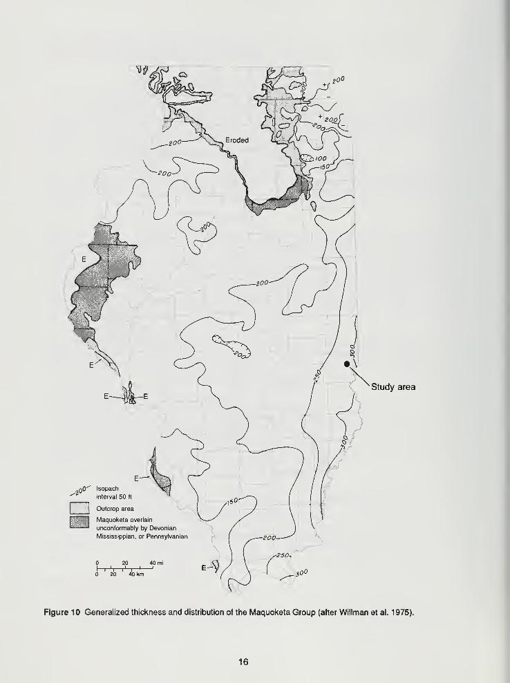
Maquoketa Group (Lower Confining Unit)

The Maquoketa Group (fig. 4) consists of two shale units and an interbedded shaly limestone-

dolomite unit. The thickness of the Maquoketa ranges from approximately 150 feet in the western

part of the state, where the top is eroded, to nearly 300 feet along the eastern edge of the state

(fig. 10). In the vicinity of Marshall, the Maquoketa is less than 300 feet thick.

Hydrologlc Characteristics of the Ordovician SystemIn northern Illinois, carbonate units of the Ordovician that are at or near land surface have

moderate to relatively low permeabilities. As the burial depth of these units increases toward the

south, the permeabilities of the units generally decrease. Carbonate units lying below freshwater

zones (groundwater with less than 10,000 mg/LTDS) are essentially aquitards. Figure 11 showsthe basal position of USDW in a north-south cross section from Rockford to Cairo. The southward-

pointing tongue of USDW in the Ordovician lies in the St. Peter Sandstone. The TDS level of the

St. Peter in the Marshall area is greater than 50,000 mg/L (Meents 1952).

Porosities in carbonate units in the southern half of the state are generally less than 10 percent;

permeabilities in the more permeable units rarely exceed 1 to 30 millidarcys (Ford et al. 1981,

Mast 1967). Porosities and permeabilities across vertical sections of the St. Peter are quite varia-

ble. The more permeable horizons measured in northern Illinois had porosities ranging from 12 to

17 percent and permeabilities ranging from 25 to 250 millidarcys. In the south, where the St. Pe-

ter is thinner, finer-grained, and more shaly, porosity and permeability values can be expected to

be smaller. The shale units in the Maquoketa Group are expected to be very tight (<1 millidarcy).

Hunton Supergroup (Injection Interval)

The limestone and dolomite units of the Silurian and Devonian Systems have similar lithologic

and hydrogeologic characteristics and thus are considered one large unit, the Hunton Super-

group. The thickness of the Hunton ranges from a featheredge along the Mississippi River to

more than 1 ,800 feet near the southern tip of the state. Figure 1 2 shows the thickness and dis-

14

J

Waukegan

Chicago

'Nevins

lEIbridge

' Study area

— Major gas pipelines

DCity

• Active storage project

O Abandoned storage project

20 40 mi

\'

I t i 1

20 40 k

Figure 9 Location of underground gas storage projects in Illinois (after Buschbach and Bond 1974).

15

Study area

qO^ Isopach^ interval 50 ft

Outcrop area

HI Maquoketa overlain

™ unconformably by Devonian

Mississippian, or Pennsylvanian

20 40 mi

1 i'

i i

1'

20 40 km

Figure 10 Generalized thickness and distribution of the Maquoketa Group (after Wiliman et al. 1975).

16

-2000-

-4000

-6000

Study area

Boundary between USDW andaquifers with groundwater

containing > 10.000 mg/L TDS

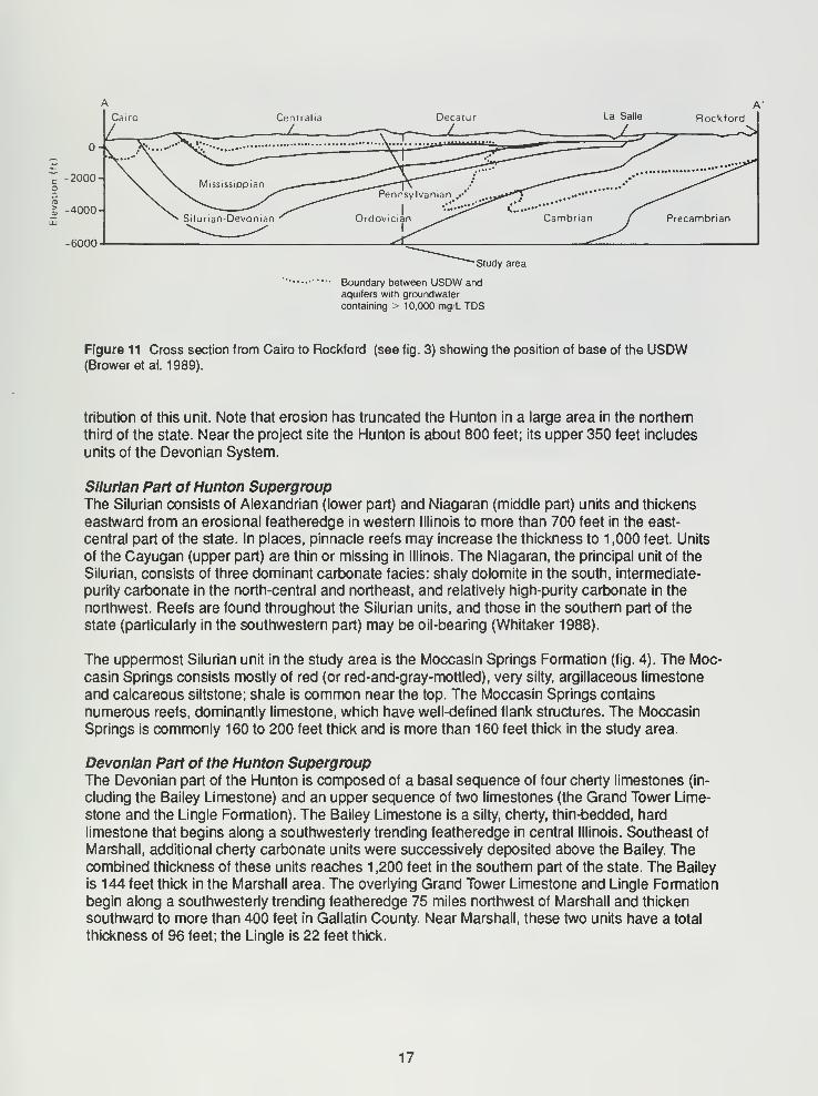
Figure 11 Cross section from Cairo to Rockford (see fig. 3) showing the position of base of the USDW(Broweretal. 1989).

tribution of this unit. Note that erosion has truncated the Hunton in a large area in the northern

third of the state. Near the project site the Hunton is about 800 feet; its upper 350 feet includes

units of the Devonian System.

Silurian Part of Hunton SupergroupThe Silurian consists of Alexandrian (lower part) and Niagaran (middle part) units and thickens

eastward from an erosional featheredge in western Illinois to more than 700 feet in the east-

central part of the state. In places, pinnacle reefs may increase the thickness to 1 ,000 feet. Units

of the Cayugan (upper part) are thin or missing in Illinois. The Niagaran, the principal unit of the

Silurian, consists of three dominant carbonate facies: shaly dolomite in the south, intermediate-

purity carbonate in the north-central and northeast, and relatively high-purity carbonate in the

northwest. Reefs are found throughout the Silurian units, and those in the southern part of the

state (particularly in the southwestern part) may be oil-bearing (Whitaker 1988).

The uppermost Silurian unit in the study area is the Moccasin Springs Formation (fig. 4). The Moc-

casin Springs consists mostly of red (or red-and-gray-mottled), very silty, argillaceous limestone

and calcareous siltstone; shale is common near the top. The Moccasin Springs contains

numerous reefs, dominantly limestone, which have well-defined flank structures. The Moccasin

Springs is commonly 160 to 200 feet thick and is more than 160 feet thick in the study area.

Devonian Part of the Hunton SupergroupThe Devonian part of the Hunton is composed of a basal sequence of four cherty limestones (in-

cluding the Bailey Limestone) and an upper sequence of two limestones (the Grand Tower Lime-

stone and the Lingle Formation). The Bailey Limestone is a silty, cherty, thin-bedded, hard

limestone that begins along a southwesterly trending featheredge in central Illinois. Southeast of

Marshall, additional cherty carbonate units were successively deposited above the Bailey. Thecombined thickness of these units reaches 1 ,200 feet in the southern part of the state. The Bailey

is 144 feet thick in the Marshall area. The overlying Grand Tower Limestone and Lingle Formation

begin along a southwesterly trending featheredge 75 miles northwest of Marshall and thicken

southward to more than 400 feet in Gallatin County. Near Marshall, these two units have a total

thickness of 96 feet; the Lingle is 22 feet thick.

17

Hydrogeology of the Hunton SupergroupFresh water is found at or near the surface in the Hunton in the northern half of the state andalong the margins of the Illinois Basin. Well yields vary, depending mostly on the degree of frac-

ture development. Variations in primary porosity and permeability can be related to lithology,

which exerts some control on the degree of fracture development. Fracture development is

greatest near the surface and generally decreases as depth of burial increases, particularly wherethe Hunton is overlain by impermeable shale units of the New Albany and Pennsylvanian.

The boundary marking the base of USDW in the Hunton is shown in figure 12. Typically,

groundwater mineralization increases rapidly southward from this boundary. However, in Clark

County the rate of increase in the TDS of the brine is relatively lower southwest of the USDWboundary, resulting in a TDS content of approximately 16,000 mg/L in the permeable Devonianunits. Increased groundwater circulation in units with higher permeabilities allows less mineralized

water to advance greater distances downdip (Brower et al. 1989). Other examples of this

phenomenon are shown in figure 11 ; tongues of fresher water in the St. Peter Sandstone (Or-

dovician), the Ironton-Galesville Sandstone (Cambrian), and in certain shallow units (Silurian

through basal Pennsylvanian near Cairo) move downdip into the Illinois Basin (Student et al.

1981). In the deeper parts of the basin, the mineral content of groundwater in the Hunton mayreach from 150,000 to more than 200,000 mg/L TDS (Graf et al. 1966).

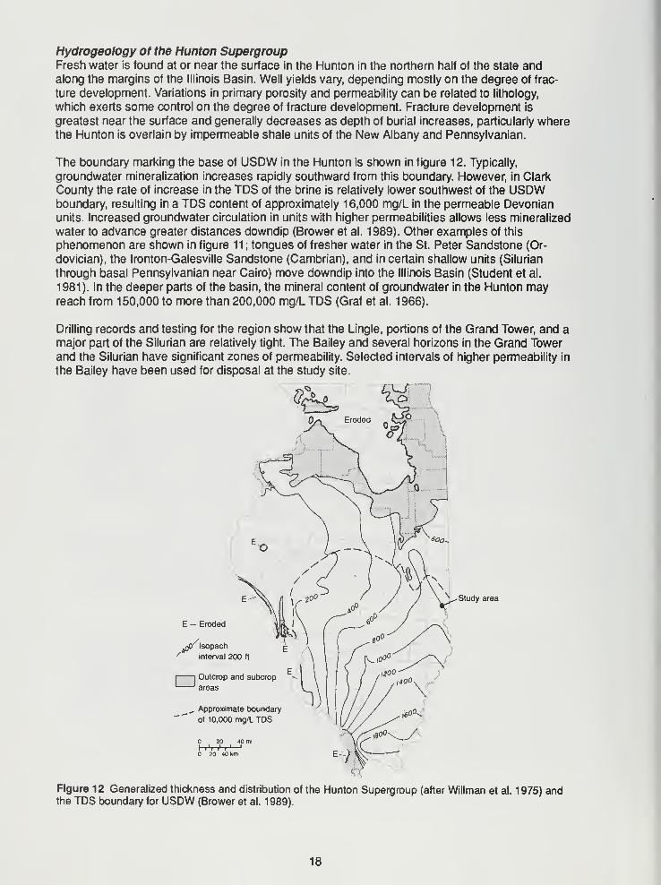
Drilling records and testing for the region show that the Lingle, portions of the Grand Tower, and amajor part of the Silurian are relatively tight. The Bailey and several horizons in the Grand Towerand the Silurian have significant zones of permeability. Selected intervals of higher permeability in

the Bailey have been used for disposal at the study site.

E - Eroded

a0Isopach

/ interval 200 ft

Study area

Outcrop and subcrop

Approximate boundary

ot 10,000 mg/L TDS

20 40 mi

1 .'l l1

l '

20 40 km

Figure 12 Generalized thickness and distribution of the Hunton Supergroup (after Willman et al. 1975) andthe TDS boundary for USDW (Brower et al. 1989).

18

Porosity and permeability data obtained from tests run on samples collected from oil exploratory

and gas storage wells scattered around the state show a mean porosity of 13 percent and amean permeability of 40 millidarcys (Mast 1967). These data included values obtained from units

in the Galena Group. Ford et al. (1981) reported porosity values of 12 to 19.5 percent and per-

meability values of 50 to 300 millidarcys for 269 wells completed in Devonian carbonate reser-

voirs of Illinois.

Evaluation of geophysical logs and sample cuttings conducted during the course of this study andfor related studies of the disposal wells indicated that discrete, areally extensive horizons having

high, moderate, and low permeabilities occur in the Bailey. Pore sizes range from 5 microns (u.m)

to over 300 (average range, 10 to 25 |im), and the pores have a fair degree of interconnection.

New Albany GroupSedimentation during Late Devonian and Kinderhookian (Mississippian) time produced

widespread accumulation of black, gray, and green shales and some limestones and siltstones.

The rock units that accumulated during this time attained a total thickness of 100 to 450 feet

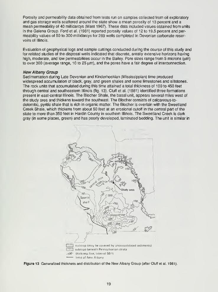
through central and southeastern Illinois (fig. 13). Cluff et al. (1981) identified three formations

present in east-central Illinois. The Blocher Shale, the basal unit, appears several miles west of

the study area and thickens toward the southeast. The Blocher consists of calcareous-to-

dolomitic, pyritic shale that is rich in organic matter. The Blocher is overlain with the Sweetland

Creek Shale, which thickens from about 50 feet at an erosional cutoff in the central part of the

state to more than 350 feet in Hardin County in southern Illinois. The Sweetland Creek is dark

gray (in some places, green) and has poorly developed, laminated bedding. The unit is similar in

I l outcrop (may be covered by unconsolidated sediments)

Iff&Sl subcrop beneath Pennsylvanian strata

-100- thickness line; interval 50 ft

limit of New Albany

Figure 13 Generalized thickness and distribution of the New Albany Group (after Cluff et al. 1981]

19

appearance to both the Blocher and the overlying Hannibal Shale, but has widely traceable key

beds. The overlying Hannibal Shale or its equivalent is less than 10 teet thick and indistinctly

bedded. These formations are not differentiated at the study site.

Hydrogeology of the New Albany GroupThe units of this group are very tight and therefore serve as an upper confining interval for the

Hunton Supergroup. Natural gas storage fields completed in the Hunton utilize the low porosity

and very low permeability of these units to retain gas in the underlying storage reservoirs

(Buschbach and Bond 1974). The shale units in this group have essentially no water- or oil-yield-

ing potential.

Mlssissippian Units

Mississippian units cover the southern two-thirds of the state and reach a maximum thickness of

3,300 feet in Williamson and Saline Counties (fig. 14). The widespread, thin, irregularly beddedChouteau Limestone (Buschbach 1952) rests on the top of the New Albany and marks the base

of three simultaneously deposited units: (1) the deltaic, tongue-shaped Borden Siltstone trending

southwesterly across the state from the west-central part of Indiana; (2) the Burlington-Keokuk

Limestones to the northwest; and (3) the Fort Payne Formation and Ullin Limestone to the

southeast. The Borden consists of siltstone, some silty shale, and a few beds of fine sandstone

and coarse siltstone. The "Carper sand" is present in places near the base of the Borden. TheUllin or its equivalent overlaps the top of the Borden with 150 feet of limestone and some shale in

the Marshall area. Widespread limestone units, including the Salem, St. Louis, and Ste.

Genevieve Limestones, accumulated between the Borden and the overlying alternating sequen-

ces of shale-limestone and shale-sandstone units that were deposited during Chesterian time.

The Mississippian section above the Chouteau is approximately 1 ,200 feet thick in the Marshall

area and includes 450 feet of Borden Siltstone. The "Carper sand" is approximately 20 feet thick

and lies very near the base of the Borden.

Hydrogeologic Conditions in the Mississippian

Mississippian units are used extensively for small (and some moderate) water supplies in andnear outcrop areas. Most wells are finished at shallow depths, typically less than 300 to 500 feet.

Groundwater mineralization increases rapidly with increasing depth of burial and in a down-dip

direction toward the Illinois Basin (Meents 1952).

The Borden Siltstone is a thick unit of very low-permeability material that provides confinement in

addition to the New Albany Group, the primary confining unit of the Hunton injection interval. The"Carper sand" provides the first somewhat permeable horizon above the top of the Hunton.

Several thin, fine-grained sandstones also lie near the top of the Borden. Available porosity logs

suggest that porosities of about 8 to 12 percent can be expected in these sandstones. At the

study site, the Salem Limestone is the first overlying aquifer having significant permeability; it has

been used for waste injection in the past. The measured static water level in the Salem is about

50 feet lower than the water level in the Bailey. The mineral content of the Salem and the Bailey

in the Marshall area is similar (about 15,000 to 16,000 mg/LTDS). The groundwater in these units

has an anomalously low mineral content, which appears to be related to the relatively high

porosity and permeability of these units. Figures 12 and 14 show the location of the USDW bound-ary in Hunton and Mississippian units. The less permeable units of the Mississippian, particularly

those in the upper part, contain groundwater with a much higher mineral content.

Pennsylvanian Units

The bedrock surface in the southern two-thirds of the state has been formed on Pennsylvanian

units. Shale and clay units (more than 50% of the total thickness), sandstones and siltstones

(more than 25%), limestones (less than 10%), and coals comprise more than 500 distinguishable

units. Pennsylvanian strata reach a maximum thickness of 2,500 feet in the south-central part of

the basin. Sandstones are interbedded with the shale throughout the Pennsylvanian but are most

20

y Approximate boundaryS of 10,000 mg/L TDS

in Valmeyran

E — Eroded

(-0 Isopach interval 200 ft /

Outcrop area

Top eroded beneath Pennsylvanian

(Cretaceous in south)

20 40 mi

1 . 'l l

1

I'

'

20 40 km

Figure 14 Generalized thickness and distribution of the Mississippian System (after Willman et al. 1975)

and the TDS boundary for USDW (Brower et al. 1989).

21

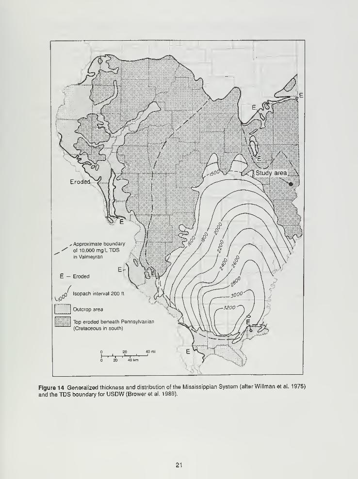
abundant in the lower two of seven formations. Limestones are more abundant in the second for-

mation from the top, and the most well-developed coal units are in the middle (fourth) formation.

In the Marshall area, the Pennsylvanian is about 1 ,050 feet thick. The thicker sandstones are

found near the base of the Pennsylvanian. Coal units are present but thin. The more prominent

coals occur below a depth of 400 feet.

Hydrogeologlc Conditions In the Pennsylvanian Units

Fresh water exists in the upper 300 to 500 feet of the Pennsylvanian units and is a principal

source for low-volume water supplies where no potential for supply exists in overlying glacial

deposits. Near the margins of the basal formations, the more permeable sandstones contain

fresh water to depths of more than 1 ,000 feet. In the Marshall area, mineralization of groundwater

increases rapidly below depths of 50 to 75 feet, and water wells rarely penetrate to depths below

1 00 to 200 feet. The base of USDW is estimated from geophysical logs to lie about 500 feet

below the surface (Piskin 1986).

Sandstones in the upper three-fourths of the Pennsylvanian are thin and widely spaced and yield

very little water. The basal sandstones in the Marshall area may yield up to 20 gpm; however,

water from these sandstones has a very high mineral content (38,000 mg/LTDS) (ISGS UIC files).

Porosity and permeability values measured from cores and wells collected from or finished in all

types of Pennsylvanian units range from 9 to 25 percent and 10 to 10,000 millidarcys (Ford et al.

1981). Porosities measured in oil-producing sandstones are relatively uniform, averaging 17 to 20percent (Whiting et al. 1964). Whiting also reported permeabilities of 100 to 400 millidarcys, which

decrease as depth of burial increases.

Quaternary SystemGlacial deposits consisting of loess, silt, clay, till, sand, and gravel cover a large part of the

bedrock surface of Illinois. In the Marshall area, the drift is less than 10 to 50 feet thick in the

upland areas and up to 30 to 100 feet thick in the larger stream valleys. Peoria Loess (2 to 6 ft

thick) and Roxana Silt (0 to 3 ft thick) mantle the Glasford Formation (clay, sand, and till, to >21ft thick) on the upland. The Banner Formation (clay and till to >20 ft) underlies Glasford Forma-tion till where thicker drift is present in the upland areas (ISGS UIC files 1981). Cahokia Alluvium

(silt, sand, and clay) overlies Henry Formation (outwash sand and gravel up to 70 ft thick) in the

valley of Big Creek. Very limited to small water supplies are available from the upland glacial

deposits. Moderate to large water supplies are available along some segments of Big Creek val-

ley. Marshall obtains its water supply from the Henry Formation, about 2.25 miles east of the

study site.

22

3. HYDROGEOLOGIC INVESTIGATION OF THE INJECTION SYSTEM

This chapter briefly discusses techniques used to collect and analyze hydrogeologic data. Details

of the techniques and analyses are in appendices A and B. Specifically, stratigraphic correlations

within the injection system from regional (5 to 1 miles) and local (3 miles) perspectives are dis-

cussed, along with methods used to collect additional data from the site of the injection well.

These methods include geophysical logging, sidewall coring and associated analysis, andhydraulic testing. A hydrogeologic description of the injection system at the site is also given.

Stratigraphic and Structural Definition of the Injection System

The injection system consists of the geologic materials constituting the injection zone and its as-

sociated upper and lower confining units. To evaluate the confining and injection potential for the

Devonian injection system, data were collected from wells in three gas storage fields (Nevins,

Elbridge, and State Line), wells within 5 to 10 miles from the project site, and wells within 3 miles

of the site (see figure 15 and table 1). The gas storage fields are approximately 9 miles northeast

of Velsicol's Waste Disposal Well 2 (WDW2). Data from these wells were used to correlate

hydrogeologic units within the injection system and to construct a structure map of the top of the

Lingle Formation. The injection interval for WDW2 lies within the Devonian limestone sequence,

immediately below the Lingle and Grand Tower Formations.

Each of the three gas storage fields utilizes a domal structure with closure to concentrate andstore the gas. Each domal structure was formed by the deposition of Devonian- and Silurian-age

shelf fades sediments over Silurian-age reef facies sediments.

Although this type of structure is not present in the area immediately surrounding the Velsicol

plant, the general stratigraphic relationship of the rock units near the storage fields and those

near the disposal well was shown to be consistent. Inferences were then made regarding data

from the gas storage fields to the disposal well at Velsicol.

Geophysical logs from wells at a 5- to 1 0-mile radius from the plant were used to correlate stratig-

raphy and to give a regional picture of the configuration of the injection system. Geophysical logs

from wells within 3 miles of the injection well were used to construct a structure map consistent

with regional data.

Stratigraphic Description of the Injection SystemThe stratigraphy of the injection system includes the Silurian-age Moccasin Springs Formation at

the base through the Grassy Creek Shale, the uppermost Devonian unit of the New Albany

Group. Figure 16 is a geologic column showing the stratigraphic position and hydrogeologic char-

acteristics of these units at the waste disposal well studied. Much of the strata information is from

Willman et al. (1975). Additional data were obtained for the Middle Devonian strata from North

(1969) and for the strata of the New Albany Group from Cluff et al. (1981).

The Devonian strata comprise three series—the Lower, Middle, and Upper. The Bailey Lime-

stone, basal unit of the Lower Devonian Series, is dominantly gray to greenish gray, silty, cherty,

thin-bedded, very hard limestone. Some beds are argillaceous. The chert, black to dark gray, oc-

curs in bands up to 2 feet thick. An upper zone, to 100 feet thick, is limestone that is pure,

white, coarsely crystalline, and only slightly cherty.

A major unconformity occurs at the Lower and Middle Devonian interface. The basal formation of

the Middle Devonian Series is the Grand Tower Limestone, which is mostly coarse-grained, light

gray, medium- to thick-bedded, cross-bedded, pure, fossiliferous limestone. It also contains

lithographic limestone, which becomes more abundant upward. One member differentiated at the

study site is the Tioga Bentonite Bed, which is found 10 to 30 feet from the top of the Grand

23

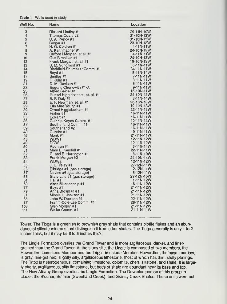
Table 1 Wells used in study

Well No. Name Location

3 Richard Lindley #1 29-11N-10W4 Thomas Coats #2 31-10N-13W5 C. A. Pence #1 31-10N-13W6 Burger #1

H. 0. Coldren #1

23-10N-13W7 4-11N-11W8 A. Kannmacher #1 24-10N-13W9 Clifford I Morgan, et al. #1 4-11N-11W10 Gus Birchfield #1 24-10N-13W12 Frank Morgan, et. al. #1 19-10N-13W13 S. M. Scholfield #1 6-11N-11W14 Birchfield-Shumaker Comm. #1 34-11N-11W15 Boyd #1 5-11N-14W17 Smitley #1 7-11N-11W19 F. Kuhn #1 8-11N-11W21 D. M. Davison #1 8-11N-11W23 Eugene Chenowith #1-A 9-11N-11W25 Alfred Seidel #1 15-10N-11W26 Russel Higginbottom, et. al. #1 34-10N-12W27 E. P. Daly #1 8-11N-14W28 E. F. Newman, et. al. #1 30-10N-13W29 Ella Mae Young #1 19-10N-13W30 Ormal Higginbotham #1 22-11N-13W33 Fraker #1 16-11N-11W35 Lickert #1 16-11N-11W36 Guinnip-Keyes Comm. #1 10-11N-12W37 Southerland Comm. #1 16-11N-11W39 Southerland #2 16-11N-11W43 Gunder#1 19-11N-11W45 Monk #1 21-11N-11W48 WDW1 12-11N-12W49 DOW 12-11N-12W50 Redman #1 5-11N-14W51 Mary E. Kendall #1 22-11N-11W52 G. and E. Herrington #1 8-11N-10W53 Frank Morgan #2 24-10N-14W54 WDW2 12-11N-12W55 J. C. Yeley #1 27-12N-11W56 Elbridge #1 (gas storage) 2-12N-11W57 Nevins #6 (gas storage) 5-12N-11W58 State Line #1 (gas storage) 28-12N-10W61 Hall #1 1-11N-12W69 Alton Blankenship #1 16-11N-12W77 Bays #1 21-11N-12W79 Anna Brosman #1 21-11N-12W81 Minnie L Jackson #1 21-11N-12W85 John W. Dawson #1 22-11N-12W87 Frahm-Cole-Lee Comm. #1 28-11N-12W103 Glen Morgan #1 21-11N-12W111 Waller Comm. #1 21-11N-11W

Tower. The Tioga is a greenish to brownish gray shale that contains biotite flakes and an abun-

dance of silicate minerals that distinguish it from other shales. The Tioga generally is only 1 to 2

inches thick, but it may be 6 to 8 inches thick.

The Lingle Formation overlies the Grand Tower and is more argillaceous, darker, and finer-

grained than the Grand Tower. At the study site, the Lingle is composed of two members, the

Howardton Limestone Member and the Tripp Limestone Member. Howardton, the basal member,is gray, fine-grained, slightly silty, argillaceous limestone, most of which has thin, shaly partings.

The Tripp is heterogeneous, containing limestone, dolomite, chert, siltstone, and shale. It is large-

ly cherty, argillaceous, silty limestone, but beds of shale are abundant near its base and top.

The New Albany Group overlies the Lingle Formation. The Devonian portion of this group in-

cludes the Blocher, Selmier (Sweetland Creek), and Grassy Creek Shales. These units were not

24

T12N

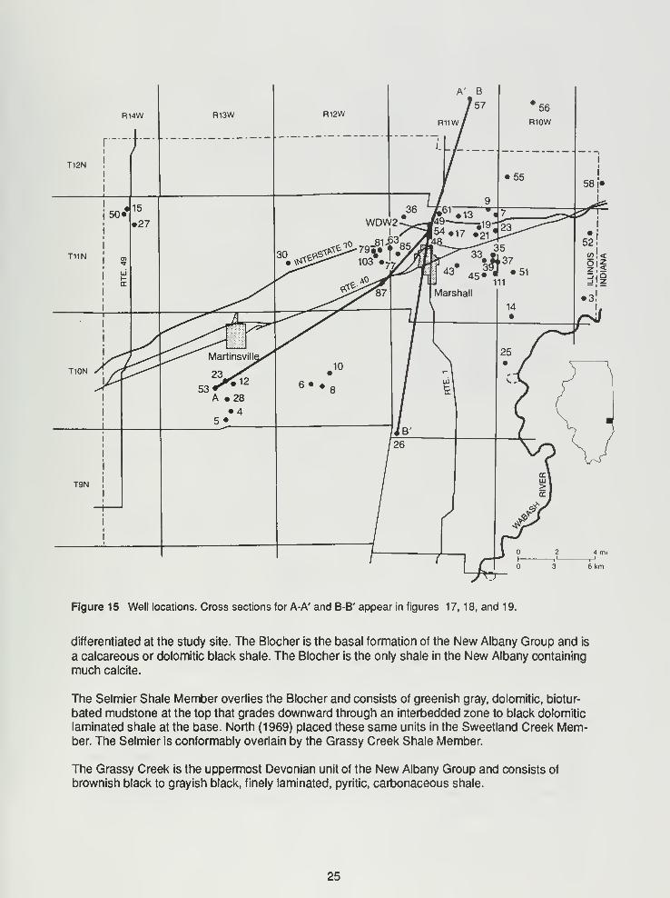
Figure 15 Well locations. Cross sections for A-A' and B-B' appear in figures 17, 18, and 19.

differentiated at the study site. The Blocher is the basal formation of the New Albany Group and is

a calcareous or dolomitic black shale. The Blocher is the only shale in the New Albany containing

much calcite.

The Selmier Shale Member overlies the Blocher and consists of greenish gray, dolomitic, biotur-

bated mudstone at the top that grades downward through an interbedded zone to black dolomitic

laminated shale at the base. North (1969) placed these same units in the Sweetland Creek Mem-ber. The Selmier is conformably overlain by the Grassy Creek Shale Member.

The Grassy Creek is the uppermost Devonian unit of the New Albany Group and consists of

brownish black to grayish black, finely laminated, pyritic, carbonaceous shale.

25

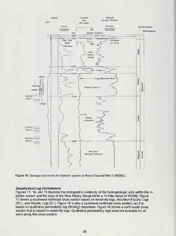
WDW2

-SP +

GammaRay

(API units)

Sidewall

Neutron Porosity

Injection *-

Zone 1

Kinderhookian

Mississippian

A

Injection ^<^:

Injection

Zone 3

Figure 16 Geologic column for the injection system at Waste Disposal Well 2 (WDW2).

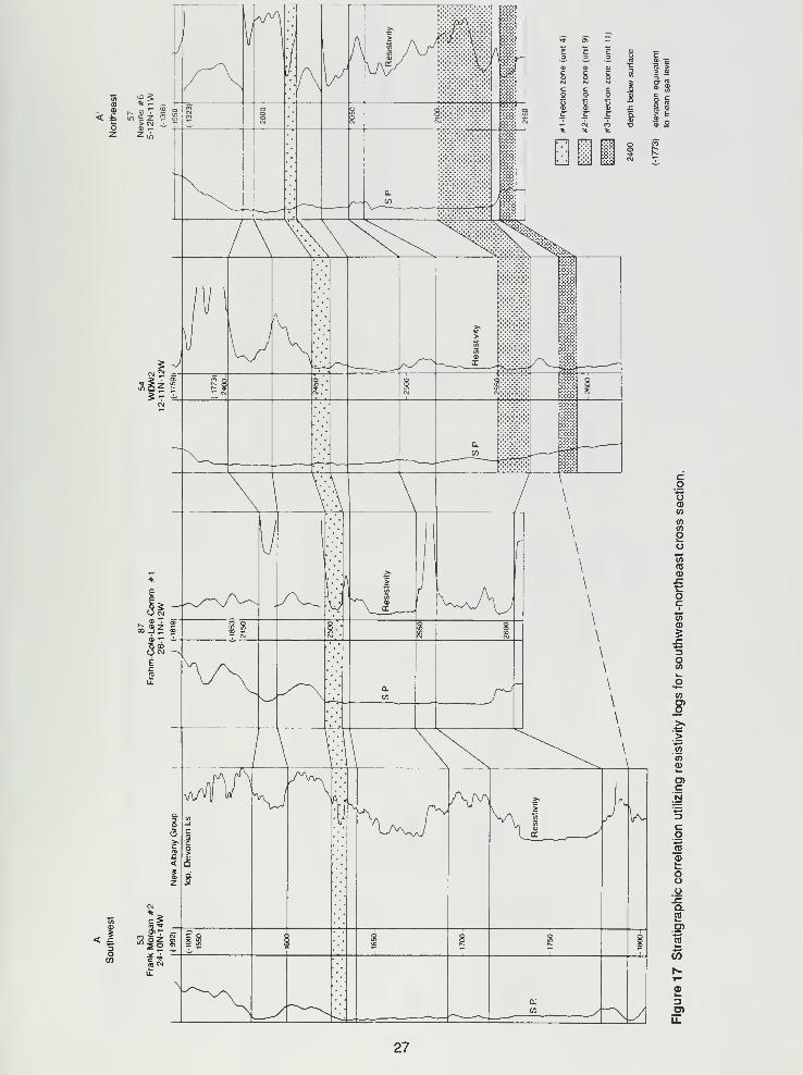
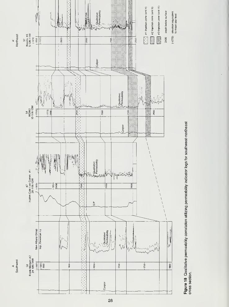
Geophysical Log Correlations

Figures 17, 18, and 19 illustrate the stratigraphic continuity of the hydrogeologic units within the in-

jection system and the base of the New Albany Group within a 10-mile radius of WDW2. Figure

17 shows a southwest-northeast cross section based on resistivity logs, Induction Electric Logs(IEL), and Electric Logs (EL). Figure 18 is also a southwest-northeast cross section, but it is

based on qualitative permeability log (Minilog) responses. Figure 19 shows a north-south cross

section that is based on resistivity logs. Qualitative permeability logs were not available for all

wells along this cross section.

26

< £

<!oCO

27

«<Dszeoc

toCD

JZ

O(A

(0COCj

OToOXIc

raCD

ECDa.coc

(0CD

ECDa.CD>

(0

a <=

ir wO) oU. O

28

CO oco

*s

3oV)

Aco

2w

s>wCO

2

c

g12h_

oog

2g>

T3

O)T-

23

u.

29

The data presented in figures 17 and 19 show the hydrogeologic units within the injection system

to be laterally continuous across the study area with one exception. Likewise, the continuity of the

qualitative permeability of these units is inferred from figure 18. On the basis of resistivity andqualitative permeability logs, injection zone no. 2 could not be differentiated from the overlying

unit in some wells in the study area. These unit designations are not included in these cross sec-

tions.

Nevertheless, the stratigraphic and qualitative permeability continuity of the Devonian limestone

and the New Albany shale between the wells at Velsicol and the wells in the gas storage fields

can be inferred; thus, continuity of quantitative permeability can be inferred. Analysis of core

retrieved from WDW2 provided quantitative permeability data for the various hydrogeologic units.

The quantitative permeability data obtained from wells at the three gas storage field wells are

summarized later in this chapter (see Hydrogeology of the Site, p. 40).

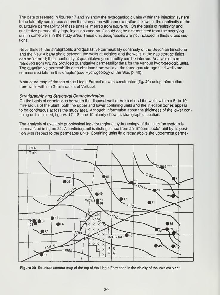
A structure map of the top of the Lingle Formation was constructed (fig. 20) using information

from wells within a 3-mile radius of Velsicol.

Stratigraphic and Structural Characterization

On the basis of correlations between the disposal well at Velsicol and the wells within a 5- to 10-

mile radius of the plant, both the upper and lower confining units and the injection zones appear

to be continuous across the study area. Although information about the thickness of the lower con-

fining unit is limited, figures 17, 18, and 19 clearly show its stratigraphic location.

The analysis of available geophysical logs for regional hydrogeology of the injection system is

summarized in figure 21 . A confining unit is distinguished from an "impermeable" unit by its posi-

tion with respect to the permeable units. Confining units lie directly above the uppermost perme-

Figure 20 Structure contour map of the top of the Lingle Formation in the vicinity of the Velsicol plant.

30

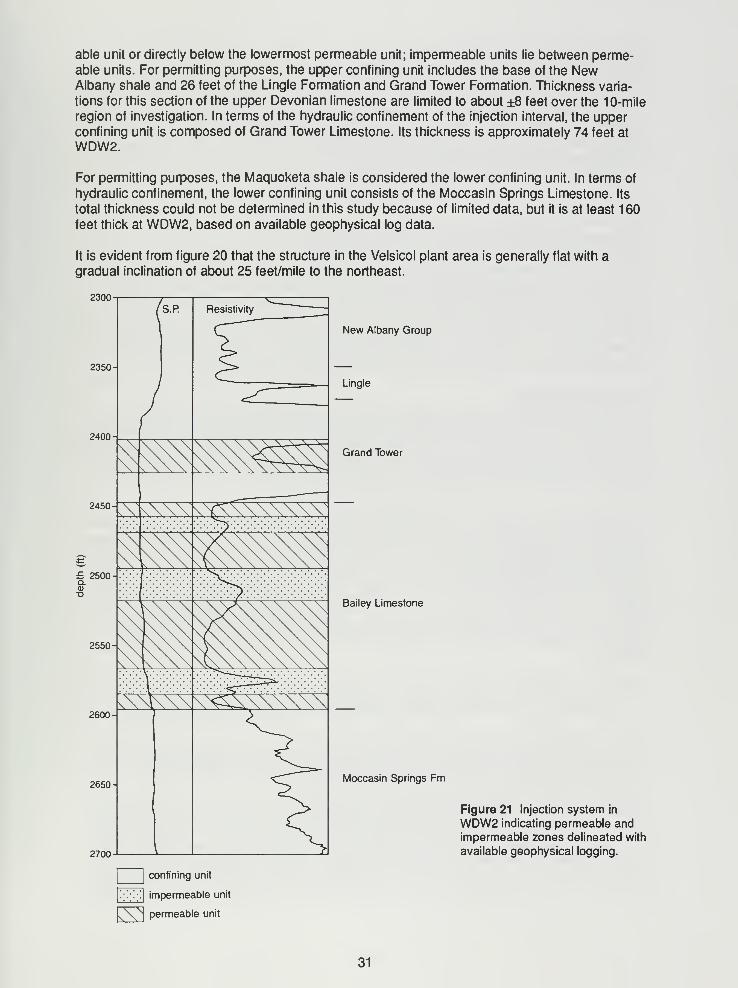
able unit or directly below the lowermost permeable unit; impermeable units lie between perme-able units. For permitting purposes, the upper confining unit includes the base of the NewAlbany shale and 26 feet of the Lingle Formation and Grand Tower Formation. Thickness varia-

tions for this section of the upper Devonian limestone are limited to about ±8 feet over the 10-mile

region of investigation. In terms of the hydraulic confinement of the injection interval, the upperconfining unit is composed of Grand Tower Limestone. Its thickness is approximately 74 feet at

WDW2.

For permitting purposes, the Maquoketa shale is considered the lower confining unit. In terms of

hydraulic confinement, the lower confining unit consists of the Moccasin Springs Limestone. Its

total thickness could not be determined in this study because of limited data, but it is at least 160

feet thick at WDW2, based on available geophysical log data.

It is evident from figure 20 that the structure in the Velsicol plant area is generally flat with agradual inclination of about 25 feet/mile to the northeast.

2300

2350-

New Albany Group

Lingle

Grand Tower

Bailey Limestone

Moccasin Springs Fm

2700

Figure 21 Injection system in

WDW2 indicating permeable andimpermeable zones delineated with

available geophysical logging.

confining unit

impermeable unit

" permeable unit

31

Determination of Horizontal Hydraulic Gradient

If the horizontal gradient is to be properly calculated, the hydraulic head within the injection sys-

tem must be known for various locations. The initial reservoir pressure, obtainable from drill stem

tests (DSTs), would be an excellent source of data. For initial reservoir pressure calculations, the

pressure versus time chart from the DST is needed. This chart, however, was not available for

wells in this area. Final flow and final closed-in pressures, as well as static water levels, were

used to calculate the horizontal gradient. According to limited, high-quality data, the greatest

horizontal gradient existed between wells 54 (WDW2) and 57. The hydraulic gradient (dh/dl) has

a magnitude of 3.5x10"4

in a general direction of north to south.

Field Investigations

Two phases of geophysical logging were performed at the Velsicol site. During phase I, data onporosity and qualitative permeability, stratigraphic orientation, and the lithology of the rock units

within the disposal zone were obtained from the Devonian Observation Well (DOW), Well 49.

Data reduction indicated the units most favorable for fluid infiltration. Phase II was a detailed

study based on information obtained from phase I. Results from phase II included quantitative

data on permeability (air and water), bulk compressibility, hydraulic conductivity, specific dis-

charge, and specific storage of the injection horizon. Those units with the greatest injection poten-

tial were further characterized for thickness, storativity, and transmissivity. In addition, hydraulic

testing (flowmeter and injection testing) of the injection system was conducted.

Phase I Investigations

Records (well logs, drilling records, and other data) provided a general overview of the structure

and regional continuity of stratigraphic units particularly important to waste injection and confine-

ment. These data, however, were only one aspect of the overall integrated approach used to char-

acterize the injection system. Additional data were needed to precisely define the character of

possible confining and injection intervals. The methods and techniques used to characterize the

disposal zone are discussed briefly and considered in detail in appendix A.

Existing geophysical logs. After a review of the historical records, a preliminary estimate wasmade of the stratigraphic location of the potential confining units (upper and lower) and the imper-

meable units associated with the operational waste disposal well (WDW2). These hydrogeologic

units were delineated using four principal downhole geophysical logs, which were run during ini-

tial well (WDW2) construction in 1971. The logs were the Sidewall Neutron Log (SNL), Induction

Electric Log (IEL), Gamma Ray Log (GRL), and Microlog (MIL). The hydrogeologic units deter-

mined from analysis of these logs are presented in figure 22. Consideration of all four logs wasnecessary to fully evaluate porosity, qualitative permeability, shale percentage, and lithology of

the geologic materials. Interpretation methods used in the evaluation of these logs are discussed

in appendix B.

Additional existing geophysical logs include the Temperature/Salinometer and GR/Neutron Logs

run in the DOW in 1981 and 1973, respectively, and a Sonic Log (SL) run in WDW1 in 1965.

However, since logging instrument technology has progressed dramatically and subsequent equa-tions and modeling of formation characteristics have advanced since these logs were run, a newsuite of logs was run. Use of these geophysical logs enabled further delineation of the

hydrogeologic characteristics of the injection system.

Phase I geophysical logging. A suite of logs was selected on the basis of the considerations

discussed above and the physical dimensions of the casing and tubing in the three wells at Vel-

sicol. The only well suitable for study during phase I was the DOW. Dresser Atlas performed the

logging. The two types of porosity logs run were the Compensated Neutron Log (CNL) and the

Borehole Compensated Sonic Log (BCS). The Minilog (MIL) was run to qualitatively determinepermeability. Resistivity parameters were determined by the Dual Induction Spherically Focused

32

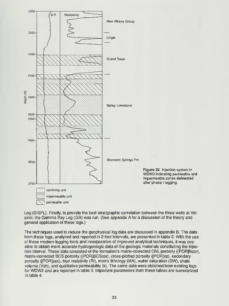
2300

New Albany Group

Lingle

Grand Tower

Bailey Limestone

Moccasin Springs Fm

2700

Figure 22 Injection system in

WDW2 indicating permeable and

impermeable zones delineated

after phase I logging.

confining unit

impermeable unit

[Qx^ permeable unit

Log (DISFL). Finally, to provide the best stratigraphic correlation between the three wells at Vel-

sicol, the Gamma Ray Log (GR) was run. (See appendix A for a discussion of the theory and

general application of these logs.)

The techniques used to reduce the geophysical log data are discussed in appendix B. The data

from these logs, analyzed and reported in 2-foot intervals, are presented in table 2. With the use

of these modern logging tools and incorporation of improved analytical techniques, it was pos-

sible to obtain more accurate hydrogeologic data of the geologic materials constituting the injec-

tion interval. These data consisted of the formation's matrix-corrected CNL porosity ([PORjNcor),

matrix-corrected BCS porosity ([POR]BCScor), cross-plotted porosity ([POR]xp), secondary

porosity ([POR]sec), true resistivity (Rt), matrix lithology (MA), water saturation (SW), shale

volume (Vsh), and qualitative permeability (k). The same data were obtained from existing logs

for WDW2 and are reported in table 3. Important parameters from these tables are summarizedin table 4.

33

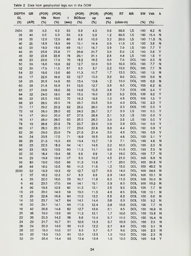
Table 2 Data from geophysical logs run in the DOW

DEPTH GR (POR) (POR) (POR) (POR) (POR) RT MA SW Vsh k

GL NIs Ncor t BCScor xp sec

(ft) (API) (%) (%) (sec) (%) (%) (%) (ohm-m) (%) (%)

2434 28 4.3 4.3 53 3.8 4.3 0.5 50.0 LS 100 6.2 N

36 40 5.0 5.0 53 3.8 5.0 1.2 65.0 LS 100 15.4 N

38 35 12.0 12.0 60 8.8 10.0 3.2 20.0 LS 100 11.5 N.

40 25 18.0 18.0 69 15.1 16.4 2.9 11.0 LS 100 3.8 N

42 30 19.0 19.0 69 15.1 16.7 3.9 7.0 LS 100 7.7 Y44 25 23.8 23.8 77 20.8 21.7 3.0 5.0 LS 100 3.8 Y46 22 22.6 22.6 76 20.1 21.1 2.5 4.8 LS 100 1.5 Y48 23 23.0 17.0 70 18.2 18.2 0.0 7.0 DOL 100 2.3 N

50 30 16.0 10.0 62 12.7 12.0 0.0 10.0 DOL 100 7.7 N

52 30 17.5 11.5 57 9.3 9.7 2.2 16.0 DOL 100 7.7 N

54 22 19.0 13.0 60 11.3 11.7 1.7 13.0 DOL 100 1.5 N

56 17 22.0 16.0 62 12.7 13.3 3.3 9.0 DOL 100 0.0 N

58 20 20.6 14.6 63 13.4 13.6 1.2 10.0 DOL 100 0.0 N

60 28 21.8 15.8 61 12.0 12.7 3.8 9.0 DOL 100 6.2 N

62 27 24.6 18.6 65 14.8 15.6 3.8 7.0 DOL 100 5.4 Y

64 32 24.0 18.0 66 15.5 16.0 2.5 5.5 DOL 100 9.2 Y

66 22 25.5 19.5 70 18.2 18.5 1.3 4.8 DOL 100 1.5 Y68 23 28.5 22.5 78 23.7 23.5 0.0 4.0 DOL 100 2.3 Y70 17 29.2 23.2 82 26.5 26.0 0.0 3.3 DOL 100 0.0 Y72 18 28.0 28.0 82 24.3 25.7 3.7 3.0 LS 100 0.0 Y74 17 30.0 30.0 87 27.9 28.8 2.1 3.2 LS 100 0.0 Y

76 17 28.0 28.0 83 25.0 26.3 3.0 3.5 LS 100 0.0 Y78 19 26.8 20.8 78 23.7 23.2 0.0 3.9 DOL 100 0.0 Y80 17 26.3 20.3 77 23.0 22.6 0.0 4.4 DOL 100 0.0 Y82 20 29.0 23.0 74 21.0 21.4 2.0 4.0 DOL 100 0.0 Y84 24 23.5 17.5 71 18.9 18.5 0.0 4.6 DOL 100 3.1 Y86 26 21.3 15.3 63 13.4 13.7 1.9 7.1 DOL 100 4.6 N

88 23 22.3 16.3 64 14.1 14.5 2.2 10.0 DOL 100 2.3 N

90 23 16.5 10.5 60 11.3 11.1 0.0 11.0 DOL 100 2.3 N

92 30 16.4 10.4 56 8.6 8.9 1.8 16.0 DOL 100 7.7 N

94 29 19.8 13.8 57 9.3 10.2 4.5 21.0 DOL 100 6.9 N

96 60 19.0 13.0 60 11.3 11.6 1.7 20.0 DOL 100 30.8 N

98 84 18.5 12.5 60 11.3 11.5 1.2 15.0 DOL 100 49.2 N

2500 52 19.3 13.3 62 12.7 12.7 0.6 14.0 DOL 100 24.6 N

2 37 18.2 12.2 57 9.3 9.8 2.9 14.0 DOL 100 13.1 N

4 33 22.0 16.0 59 10.7 11.8 5.3 11.0 DOL 100 10.0 N

6 45 23.0 17.0 64 14.1 15.1 2.9 8.0 DOL 100 19.2 N8 30 19.8 13.8 60 11.3 12.1 2.5 9.0 DOL 100 7.7 N

10 23 20.0 14.0 58 10.0 11.3 4.0 8.5 DOL 100 13.1 N12 20 22.8 16.8 60 11.3 13.2 5.5 8.2 DOL 100 0.0 N

14 32 20.7 14.7 64 14.1 14.4 0.6 9.0 DOL 100 9.2 N

16 30 20.1 14.1 60 11.3 12.4 2.8 10.5 DOL 100 7.7 N18 42 20.8 14.8 62 12.7 13.6 2.1 8.5 DOL 100 16.9 N

20 38 19.0 13.0 60 11.3 12.1 1.7 10.0 DOL 100 13.8 N22 30 20.3 14.3 56 8.6 10.4 5.7 11.0 DOL 100 15.4 N24 23 21.7 15.7 61 12.0 13.3 3.7 10.0 DOL 100 2.3 N26 24 20.0 14.0 60 11.3 12.2 2.7 8.0 DOL 100 3.1 N28 23 16.0 10.0 57 9.3 9.7 0.7 9.0 DOL 100 2.3 N30 23 19.0 13.0 61 12.0 12.5 1.0 10.0 DOL 100 2.3 N32 21 20.4 14.4 63 13.4 13.8 1.0 12.0 DOL 100 0.8 Y

34

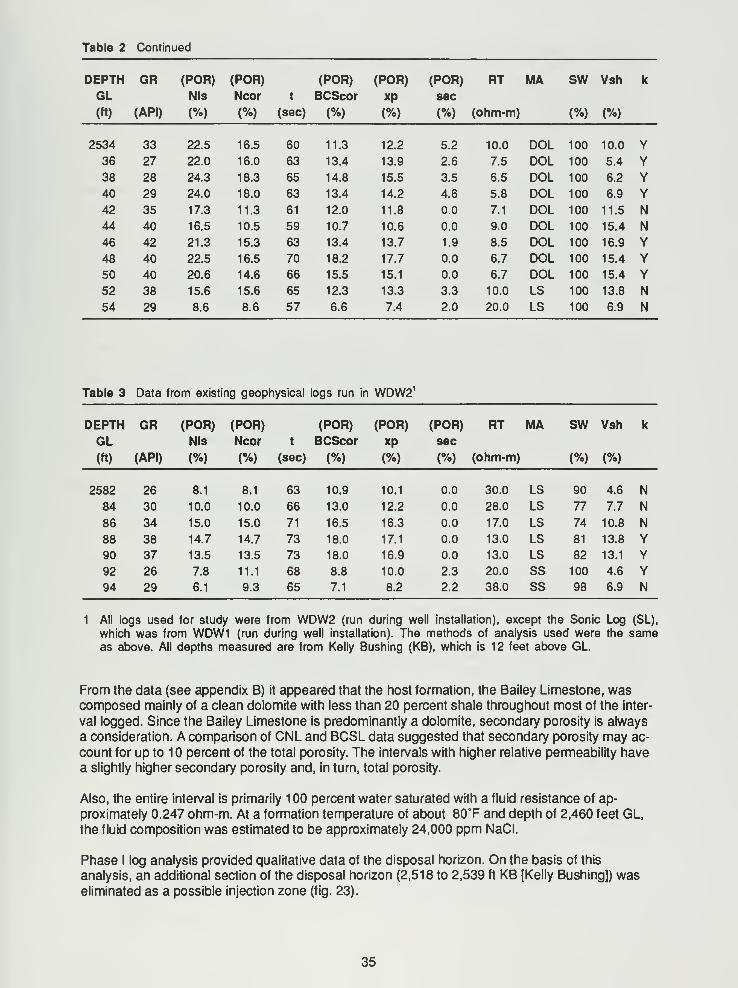
Table 2 Continued

DEPTH GR (POR) (POR) (POR) (POR) (POR) RT MA SW Vsh k

GL Nts Ncor t BCScor XP sec

(ft) (API) (%) (%) (sec) (%) (%) (%) (ohm-m) (%) (%)

2534 33 22.5 16.5 60 11.3 12.2 5.2 10.0 DOL 100 10.0 Y36 27 22.0 16.0 63 13.4 13.9 2.6 7.5 DOL 100 5.4 Y38 28 24.3 18.3 65 14.8 15.5 3.5 6.5 DOL 100 6.2 Y40 29 24.0 18.0 63 13.4 14.2 4.6 5.8 DOL 100 6.9 Y42 35 17.3 11.3 61 12.0 11.8 0.0 7.1 DOL 100 11.5 N

44 40 16.5 10.5 59 10.7 10.6 0.0 9.0 DOL 100 15.4 N

46 42 21.3 15.3 63 13.4 13.7 1.9 8.5 DOL 100 16.9 Y48 40 22.5 16.5 70 18.2 17.7 0.0 6.7 DOL 100 15.4 Y50 40 20.6 14.6 66 15.5 15.1 0.0 6.7 DOL 100 15.4 Y52 38 15.6 15.6 65 12.3 13.3 3.3 10.0 LS 100 13.8 N54 29 8.6 8.6 57 6.6 7.4 2.0 20.0 LS 100 6.9 N

Table 3 Data from existing geophysical logs run in WDW2 1

DEPTH GR (POR) (POR) (POR) (POR) (POR) RT MA SW Vsh k

GL NIs Ncor t BCScor xp sec

(ft) (API) (%) (%) (sec) (%) (%) (%) (ohm-m) (%) (%)

2582 26 8.1 8.1 63 10.9 10.1 0.0 30.0 LS 90 4.6 N

84 30 10.0 10.0 66 13.0 12.2 0.0 28.0 LS 77 7.7 N

86 34 15.0 15.0 71 16.5 16.3 0.0 17.0 LS 74 10.8 N

88 38 14.7 14.7 73 18.0 17.1 0.0 13.0 LS 81 13.8 Y90 37 13.5 13.5 73 18.0 16.9 0.0 13.0 LS 82 13.1 Y92 26 7.8 11.1 68 8.8 10.0 2.3 20.0 SS 100 4.6 Y94 29 6.1 9.3 65 7.1 8.2 2.2 38.0 SS 98 6.9 N

1 All logs used for study were from WDW2 (run during well installation), except the Sonic Log (SL),

which was from WDW1 (run during well installation). The methods of analysis used were the sameas above. All depths measured are from Kelly Bushing (KB), which is 12 feet above GL.

From the data (see appendix B) it appeared that the host formation, the Bailey Limestone, wascomposed mainly of a clean dolomite with less than 20 percent shale throughout most of the inter-

val logged. Since the Bailey Limestone is predominantly a dolomite, secondary porosity is always

a consideration. A comparison of CNL and BCSL data suggested that secondary porosity may ac-

count for up to 10 percent of the total porosity. The intervals with higher relative permeability have

a slightly higher secondary porosity and, in turn, total porosity.

Also, the entire interval is primarily 100 percent water saturated with a fluid resistance of ap-

proximately 0.247 ohm-m. At a formation temperature of about 80T and depth of 2,460 feet GL,

the fluid composition was estimated to be approximately 24,000 ppm NaCI.

Phase I log analysis provided qualitative data of the disposal horizon. On the basis of this

analysis, an additional section of the disposal horizon (2,518 to 2,539 ft KB [Kelly Bushing]) waseliminated as a possible injection zone (fig. 23).

35

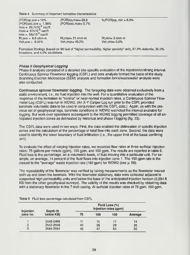
Table 4 Summary of important formation characteristics

(POR)xp.ave = 1 6% (POR)xp,max= 28.8 %(POR)xp, min = 8.9%(POR)sec.ave = 1.98% (POR)sec,max= 5.7%tave= 66.7x1

0"6sec/ft

tmax= 87x10"6

sec/ft

tmin= 56x10"6

sec/ft

Rt.ave = 8.6 ohm-m Rt,max= 21 ohm-m Rt,min= 3 ohm-mVsh,ave= 8.05% Vsh,max= 49.2% Vsh,min= 0.0%

Formation lithology (based on 98 feet of "higher permeability, higher porosity" unit), 61.0% dolomite, 35.0%limestone, and 4.0% sandstone.

Phase II Geophysical LoggingPhase II analysis consisted of a detailed site-specific evaluation of the injection/confining interval.

Continuous Spinner Flowmeter logging (CSFL) and core analysis formed the basis of the study.

Scanning Electron Microscope (SEM) analysis and formation brine/wastewater analysis were

also conducted.

Continuous spinner flowmeter logging. The foregoing data were obtained exclusively from a

static environment, i.e., no fluid injection into the well. For a quantitative evaluation of the

response of the formation to "normal" or near-normal injection rates, a Continuous Spinner Flow-

meter Log (CSFL) was run in WDW2. (An X-Y Caliper Log run prior to the CSFL provided

borehole volumetric data to be used in conjunction with the CSFL data.) Again, as with the pre-

vious set of geophysical logs, borehole conditions in WDW2 restricted the interval available for

logging. But work-over operations subsequent to the WDW2 logging permitted coverage of all an-

ticipated injection zones as delineated by historical and phase I logging (fig. 23).

The CSFL data were used in two ways. First, the data enabled the delineation of specific injection

zones and the calculation of the percentage of total flow into each zone. Second, the data were

used to identify the lower boundary of fluid infiltration (i.e., the upper limit of the basal confining

unit).

To evaluate the effect of varying injection rates, we recorded flow rates at three surficial injection

rates: 75 gallons per minute (gpm), 100 gpm, and 150 gpm. The results are reported in table 5.

Fluid loss is the percentage, on a volumetric basis, of fluid moving into a particular unit. For ex-

ample, on average, 14 percent of the fluid flows into injection zone 1 . The 150-gpm rate is the

closest to the "average" waste injection rate (182 gpm) for WDW2 (see p. 58).

The repeatability of the flowmeter was verified by taking measurements as the flowmeter movedboth up and down the borehole. With the flowmeter stationary, data were collected adjacent to

suspected high permeability units and below the base of the anticipated injection horizon (2,594 ft

KB from the other geophysical surveys). The validity of the results was checked by obtaining data

with a stationary flowmeter in the 7-inch casing. At surficial injection rates of 75 gpm, 100 gpm,

Table 5 Fluid loss percentage calculated from CSFL

Injection

zone no.

Depth (ft

below KB)

Fluid Loss (%)injection rates (gpm)

75 100 150 Average

1

2

3

2448-2458

2552-2558

2584-2594

11

4049

15

3847

17

2954

14

3650

36

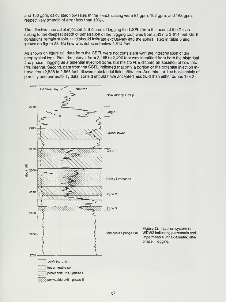
and 150 gpm, calculated flow rates in the 7-inch casing were 81 gpm, 107 gpm, and 163 gpm,respectively (margin of error less than 10%).

The effective interval of injection at the time of logging the CSFL (from the base of the 7-inch

casing to the deepest depth of penetration of the logging tool) was from 2,437 to 2,614 feet KB. If

conditions remain stable, fluid should infiltrate exclusively into the zones listed in table 5 andshown on figure 23. No flow was detected below 2,614 feet.

As shown on figure 23, data from the CSFL were not consistent with the interpretation of the

geophysical logs. First, the interval from 2,468 to 2,496 feet was identified from both the historical

and phase I logging as a potential injection zone, but the CSFL indicated an absence of flow into

this interval. Second, data from the CSFL indicated that only a portion of the potential injection in-

terval from 2,538 to 2,568 feet allowed substantial fluid infiltration. And third, on the basis solely of

porosity and permeability data, zone 3 should have accepted less fluid than either zones 1 or 2;

2300

2350-

2400

2450

£ 2500

H

Q.

2550

2600

2650-

2700

Gamma Ray Neutron

^^^^^^^^ _*?»3

New Albany Group

Lingle

Grand Tower

Zone 1

Bailey Limestone

Zone 2

Figure 23 Injection system in

Moccasin Springs Fm WDW2 indicating permeable and

impermeable units delinated after

phase II logging.

confining unit

impermeable unit

L^^j permeable unit - phase I

permeable unit - phase II

37

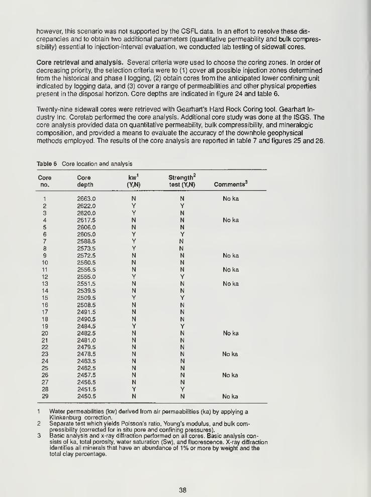
however, this scenario was not supported by the CSFL data. In an effort to resolve these dis-

crepancies and to obtain two additional parameters (quantitative permeability and bulk compres-sibility) essential to injection-interval evaluation, we conducted lab testing of sidewall cores.

Core retrieval and analysis. Several criteria were used to choose the coring zones. In order of

decreasing priority, the selection criteria were to (1) cover all possible injection zones determined

from the historical and phase I logging, (2) obtain cores from the anticipated lower confining unit

indicated by logging data, and (3) cover a range of permeabilities and other physical properties

present in the disposal horizon. Core depths are indicated in figure 24 and table 6.

Twenty-nine sidewall cores were retrieved with Gearhart's Hard Rock Coring tool. Gearhart In-

dustry Inc. Corelab performed the core analysis. Additional core study was done at the ISGS. Thecore analysis provided data on quantitative permeability, bulk compressibility, and mineralogic

composition, and provided a means to evaluate the accuracy of the downhole geophysical

methods employed. The results of the core analysis are reported in table 7 and figures 25 and 26.

Table 6 Core location and analysis

Core Core kw1Strength

2

no. depth (Y,N) test (Y,N) Comments3

1 2663.0 N N Noka2 2622.0 Y Y3 2620.0 Y N4 2617.5 N N Noka5 2606.0 N N6 2605.0 Y Y7 2588.5 Y N8 2573.5 Y N9 2572.5 N N Noka10 2560.5 N N11 2556.5 N N Noka12 2555.0 Y Y13 2551.5 N N Noka14 2539.5 N N15 2509.5 Y Y16 2508.5 N N17 2491.5 N N18 2490.5 N N19 2484.5 Y Y20 2482.5 N N Noka21 2481.0 N N22 2479.5 N N23 2478.5 N N Noka24 2463.5 N N25 2462.5 N N26 2457.5 N N Noka27 2456.5 N N28 2451.5 Y Y29 2450.5 N N Noka

Water permeabilities (kw) derived from air permeabilities (ka) by applying aKlinkenburg correction.

Separate test which yields Poisson's ratio, Young's modulus, and bulk com-pressibility (corrected for in situ pore and confining pressures).Basic analysis and x-ray diffraction performed on all cores. Basic analysis con-sists of ka, total porosity, water saturation (Sw), and fluorescence. X-ray diffraction

identifies all minerals that have an abundance of 1% or more by weight and thetotal clay percentage.

38

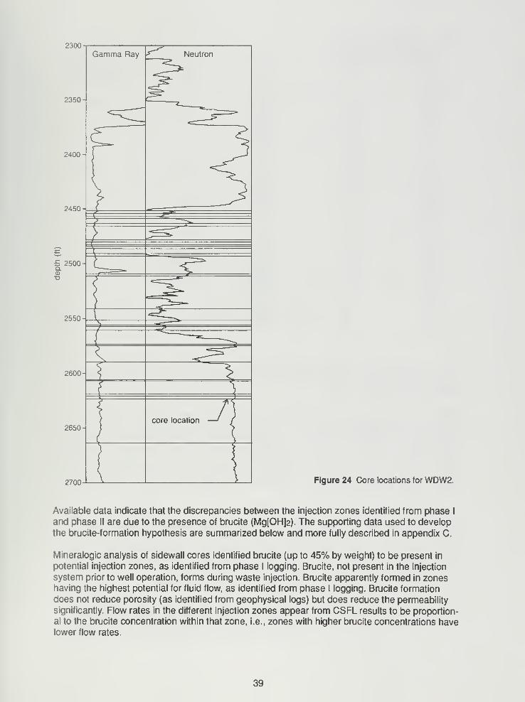
2300

2350-

2700

Gamma Ray Neutron

Figure 24 Core locations for WDW2.

Available data indicate that the discrepancies between the injection zones identified from phase I

and phase II are due to the presence of brucite (Mg[OH]2). The supporting data used to develop

the brucite-formation hypothesis are summarized below and more fully described in appendix C.

Mineralogic analysis of sidewall cores identified brucite (up to 45% by weight) to be present in

potential injection zones, as identified from phase I logging. Brucite, not present in the injection

system prior to well operation, forms during waste injection. Brucite apparently formed in zoneshaving the highest potential for fluid flow, as identified from phase I logging. Brucite formation

does not reduce porosity (as identified from geophysical logs) but does reduce the permeability

significantly. Flow rates in the different injection zones appear from CSFL results to be proportion-

al to the brucite concentration within that zone, i.e., zones with higher brucite concentrations havelower flow rates.

39

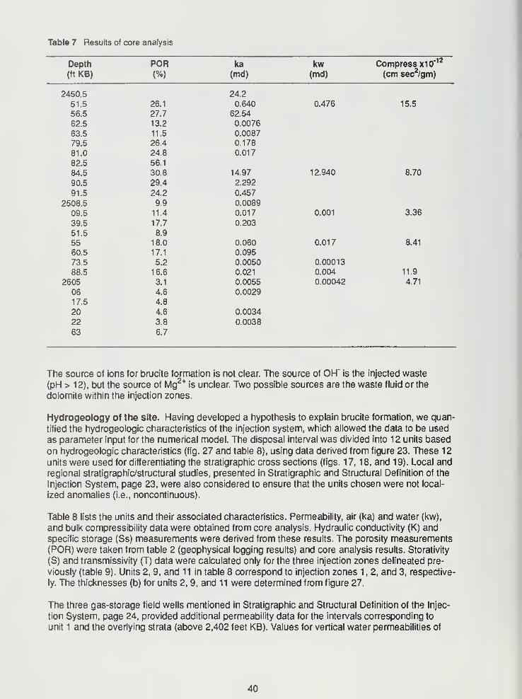
Table 7 Results of core analysis

Depth POR ka kw Compress X10"12

(ft KB) (%) (md) (md) (cm sec2/gm)

2450.5 24.2

51.5 26.1 0.640 0.476 15.5

56.5 27.7 62.54

62.5 13.2 0.0076

63.5 11.5 0.0087

79.5 26.4 0.178

81.0 24.8 0.017

82.5 56.1

84.5 30.8 14.97 12.940 8.70

90.5 29.4 2.292

91.5 24.2 0.457

2508.5 9.9 0.0089

09.5 11.4 0.017 0.001 3.36

39.5 17.7 0.203

51.5 8.9

55 18.0 0.060 0.017 8.41

60.5 17.1 0.095

73.5 5.2 0.0050 0.00013

88.5 16.6 0.021 0.004 11.9

2605 3.1 0.0055 0.00042 4.71

06 4.6 0.0029

17.5 4.8

20 4.6 0.0034

22 3.8 0.0038

63 6.7

The source of ions for brucite formation is not clear. The source of OH" is the injected waste

(pH > 12), but the source of Mg2+is unclear. Two possible sources are the waste fluid or the

dolomite within the injection zones.

Hydrogeology of the site. Having developed a hypothesis to explain brucite formation, we quan-

tified the hydrogeologic characteristics of the injection system, which allowed the data to be used

as parameter input for the numerical model. The disposal interval was divided into 12 units based

on hydrogeologic characteristics (fig. 27 and table 8), using data derived from figure 23. These 12

units were used for differentiating the stratigraphic cross sections (figs. 17, 18, and 19). Local and

regional stratigraphic/structural studies, presented in Stratigraphic and Structural Definition of the

Injection System, page 23, were also considered to ensure that the units chosen were not local-

ized anomalies (i.e., noncontinuous).

Table 8 lists the units and their associated characteristics. Permeability, air (ka) and water (kw),

and bulk compressibility data were obtained from core analysis. Hydraulic conductivity (K) and

specific storage (Ss) measurements were derived from these results. The porosity measurements(POR) were taken from table 2 (geophysical logging results) and core analysis results. Storativity

(S) and transmissivity (T) data were calculated only for the three injection zones delineated pre-

viously (table 9). Units 2, 9, and 11 in table 8 correspond to injection zones 1 , 2, and 3, respective-

ly. The thicknesses (b) for units 2, 9, and 11 were determined from figure 27.

The three gas-storage field wells mentioned in Stratigraphic and Structural Definition of the Injec-

tion System, page 24, provided additional permeability data for the intervals corresponding to

unit 1 and the overlying strata (above 2,402 feet KB). Values for vertical water permeabilities of

40

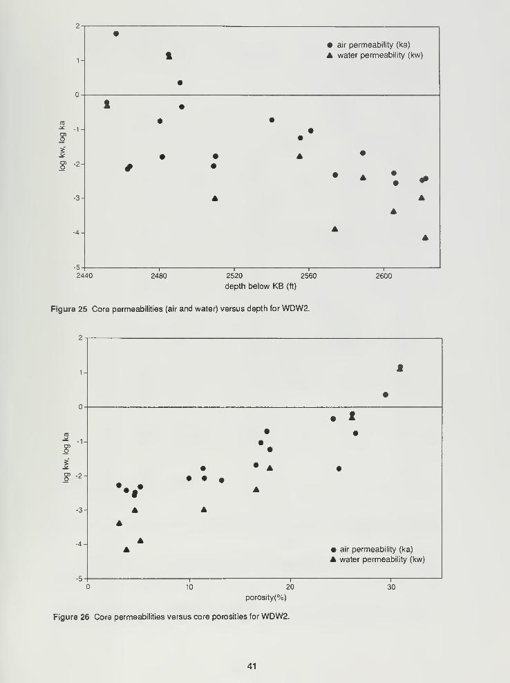
•• air permeability (ka)

1- t A water permeability (kw)

•r> -

1 •

log

ka• •

••

5• • •

O) .0-2. # •

• > : --3- A A

A

-4- AA

-5-i i i i

2440 2480 2520 2560

depth below KB (ft)

2600

Figure 25 Core permeabilities (air and water) versus depth for WDW2.

• 1

-1-O)O

§"

O <L

A

*•••

-3

air permeability (ka)

water permeability (kw)

10

—1—20 30

porosity(%)

Figure 26 Core permeabilities versus core porosities for WDW2.

41

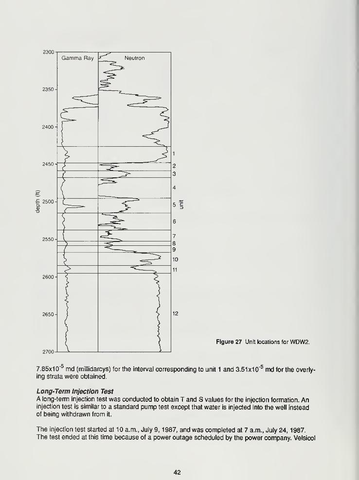
2300

2350-

2400-

2450-

£ 2500

H

o.03T3

2550

2600-

2650

2700

Figure 27 Unit locations for WDW2.

7.85x10"5 md (millidarcys) for the interval corresponding to unit 1 and 3.51 x10"

5 md for the overly-

ing strata were obtained.

Long-Term Injection Test

A long-term injection test was conducted to obtain T and S values for the injection formation. Aninjection test is similar to a standard pump test except that water is injected into the well instead

of being withdrawn from it.

The injection test started at 10 a.m., July 9, 1987, and was completed at 7 a.m., July 24, 1987.The test ended at this time because of a power outage scheduled by the power company. Velsicol

42

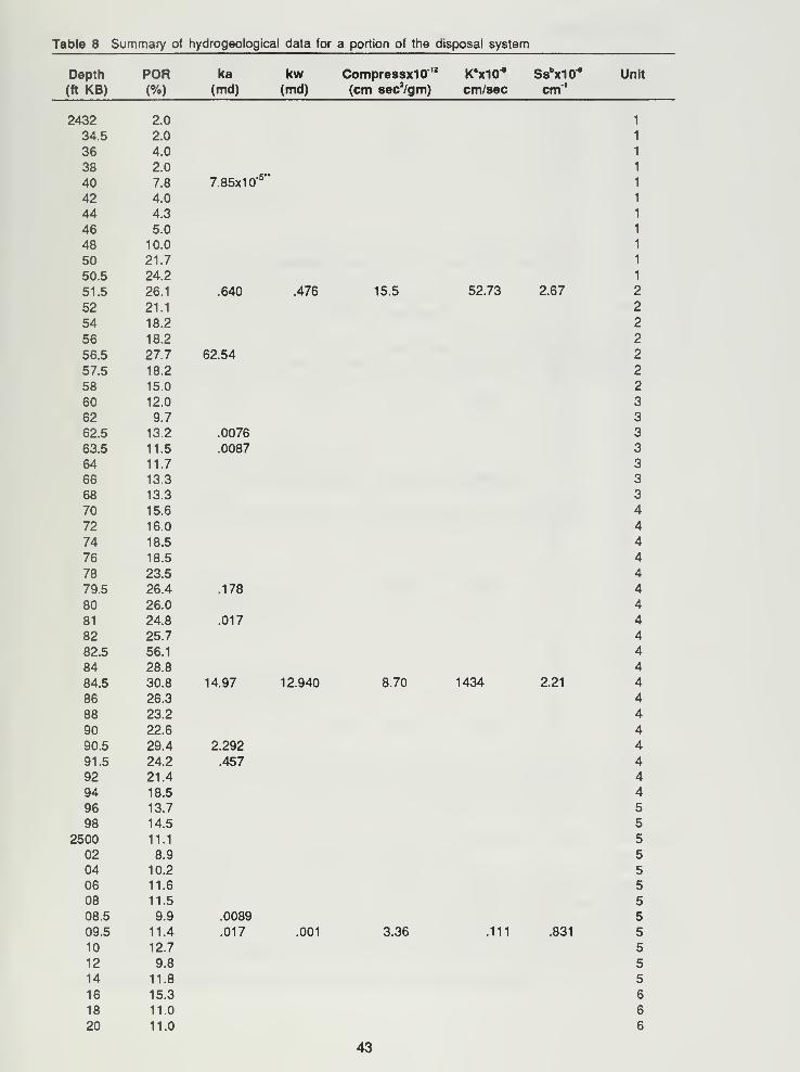
Table 8 Summary of hydrogeological data for a portion of the disposal system

Depth POR ka kw CompressxIO'12

K°x10* Ssbx10"" Unit

(ft KB) (%) (md) (md) (cm sec2/gm) cm/sec cm 1

2432 2.0

34.5 2.0

36 4.0

38 2.0

40 7.8 7.85x10'5

42 4.0

44 4.3

46 5.0

48 10.0

50 21.7

50.5 24.2

51.5 26.1 .640

52 21.1

54 18.2

56 18.2

56.5 27.7 62.54

57.5 18.2

58 15.0

60 12.0

62 9.7

62.5 13.2 .0076

63.5 11.5 .0087

64 11.7

66 13.3

68 13.3

70 15.6

72 16.0

74 18.5

76 18.5

78 23.5

79.5 26.4 .178

80 26.0

81 24.8 .017

82 25.7

82.5 56.1

84 28.8

84.5 30.8 14.97

86 26.3

88 23.2

90 22.6

90.5 29.4 2.292

91.5 24.2 .457

92 21.4

94 18.5

96 13.7

98 14.5

2500 11.1

02 8.9

04 10.2

06 11.6

08 11.5

08.5 9.9 .0089

09.5 11.4 .017

10 12.7

12 9.8

14 11.8

16 15.3

18 11.0

20 11.0

.476 15.5 52.73 2.67 2

2

2

2

2

2

2

3

3

3

3

3

3

3

4

4

4

4

4

44

4

4

4

4

12.940 8.70 1434 2.21 4

4

4

4

4

44

4

5

5

5

5

5

5

5

5

.001 3.36 .111 .831 5

5

5

5

6

43

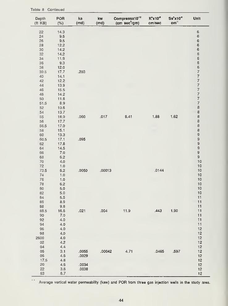
Table 8 Continued

Depth POR ka kw CompressxIO'12

K'xIO"8 Ssb

x10* Unit

(ft KB) (%) (md) (md) (cm sec2/gm) cm/sec cm"

1

22 14.3 6

24 9.5 6

26 9.5 6

28 12.2 6

30 14.2 6

32 14.2 6

34 11.9 6

36 9.3 6

38 12.0 6

39.5 17.7 .203 7

40 14.1 7

42 12.2 7

44 13.9 7

46 15.5 7

48 14.2 7

50 11.8 7

51.5 8.9 7

52 10.6 8

54 13.7 8

55 18.0 .060 .017 8.41 1.88 1.62 8

56 17.7 8

56.5 17.0 8

58 15.1 8

60 13.3 9

60.5 17.1 .095 9

62 17.8 9

64 14.5 9

66 7.0 9

68 6.2 9

70 4.0 10

72 1.0 10

73.5 5.2 .0050 .00013 .0144 10

74 1.0 10

76 1.0 10

78 6.2 10

80 5.0 10

82 5.0 10

84 5.5 11

86 8.9 11

88 9.8 11

88.5 16.6 .021 .004 11.9 .443 1.90 11

90 7.0 11

92 4.0 11

94 4.0 11

96 4.0 12

98 4.0 12

2600 4.0 12

02 4.2 12

04 4.4 12

05 3.1 .0055 .00042 4.71 .0465 .597 12

06 4.6 .0029 12

17.5 4.8 12

20 4.6 .0034 12

22 3.8 .0038 12

63 6.7 12

Average vertical water permeability (kaw) and POR from three gas injection wells in the study area.

44

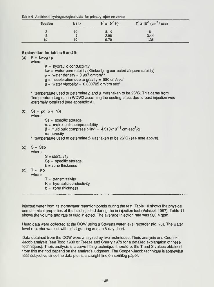
Table 9 Additional hydrogeological data for primary injection zones

Section b(ft) Sc x10-8

(-) Td x10"6 (cm2

/sec)

2

8

10

10

6

10

8.14

2.96

5.79

161

3.44

1.35

Explanation for tables 8 and 9:

(a) K = kwpg / u.

whereK = hydraulic conductivity

kw water permeability (Klinkenburg corrected air permeability)

p = water density = 0.997 gm/cm3*

g = acceleration due to gravity = 980 cm/sec2

u. = water viscosity = 0.008705 gm/cm sec*

* temperature used to determine p and p. was taken to be 26°C. This came from

Temperature Log run in WDW2 assuming the cooling effect due to past injection wasextremely localized (see appendix A).

(b) Ss= pg(a+ np)

where

Ss = specific storage

a = matrix bulk compressibility

P = fluid bulk compressibility* = 4.51 3x10"

1 1cm-sec

2/g

n= porosity* temperature used to determine p was taken to be 26°C (see note above).

(c) S = Ssbwhere

S = storativity

Ss= specific storage

b = zone thickness

(d) T= Kbwhere

T= transmissivity

K = hydraulic conductivity

b = zone thickness

injected water from its stormwater retention ponds during the test. Table 10 shows the physical

and chemical properties of the fluid injected during the in injection test (Velsicol, 1987). Table 11

shows the volume and rate of fluid injected. The average injection rate was 288.4 gpm.

Head data were collected at the DOW using a Stevens water level recorder (fig. 28). The water

level recorder was set with a 1 :1 gearing and an 8-day chart.

Data obtained from the DOW were analyzed by two techniques: Theis analysis and Cooper-

Jacob analysis (see Todd 1980 or Freeze and Cherry 1979 for a detailed explanation of these

techniques). Theis analysis is a curve-fitting technique; therefore, the T and S values obtained

from this method depend on the analyst's judgment. The Cooper-Jacob technique is somewhatless subjective since the data plot is a straight line on semilog paper.

45

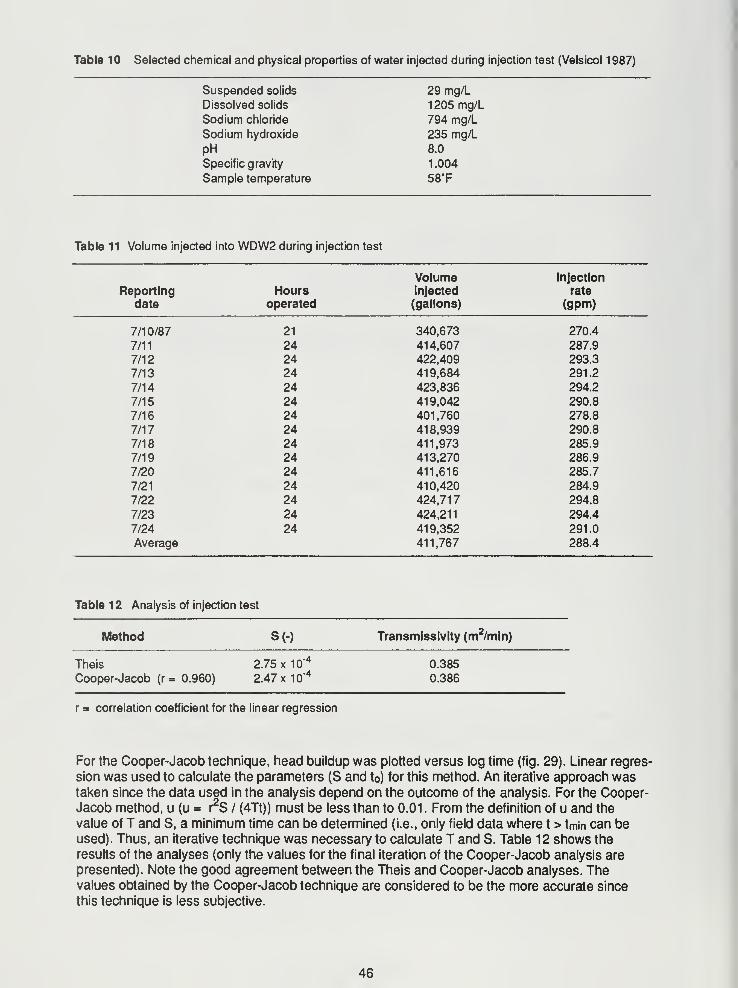
Table 10 Selected chemical and physical properties of water injected during injection test (Velsicol 1987)

Suspended solids

Dissolved solids

Sodium chloride

Sodium hydroxide

pHSpecific gravity

Sample temperature

29mg/L1205 mg/L

794 mg/L

235 mg/L

8.0

1.004

58T

Table 11 Volume injected into WDW2 during injection test

Volume Injection

Reporting Hours Injected rate

date operated (gallons) (gpm)

7/10/87 21 340,673 270.4

7/11 24 414,607 287.9

7/12 24 422,409 293.3

7/13 24 419,684 291.2

7/14 24 423,836 294.2

7/15 24 419,042 290.8

7/16 24 401 ,760 278.8

7/17 24 418,939 290.8

7/18 24 411,973 285.9

7/19 24 413,270 286.9

7/20 24 411,616 285.7

7/21 24 410,420 284.9

7/22 24 424,717 294.8

7/23 24 424,211 294.4

7/24 24 419,352 291.0

Average 411,767 288.4

Table 1 2 Analysis of injection test

Method S(-) Transmlssivity (m /min)

-4Theis 2.75x10Cooper-Jacob (r= 0.960) 2.47 x10"

40.385

0.386

r = correlation coefficient for the linear regression

For the Cooper-Jacob technique, head buildup was plotted versus log time (fig. 29). Linear regres-

sion was used to calculate the parameters (S and to) for this method. An iterative approach wastaken since the data used in the analysis depend on the outcome of the analysis. For the Cooper-Jacob method, u (u = i^S / (4Tt)) must be less than to 0.01 . From the definition of u and the

value of T and S, a minimum time can be determined (i.e., only field data where t > tmin can beused). Thus, an iterative technique was necessary to calculate T and S. Table 12 shows the

results of the analyses (only the values for the final iteration of the Cooper-Jacob analysis are

presented). Note the good agreement between the Theis and Cooper-Jacob analyses. Thevalues obtained by the Cooper-Jacob technique are considered to be the more accurate since

this technique is less subjective.

46

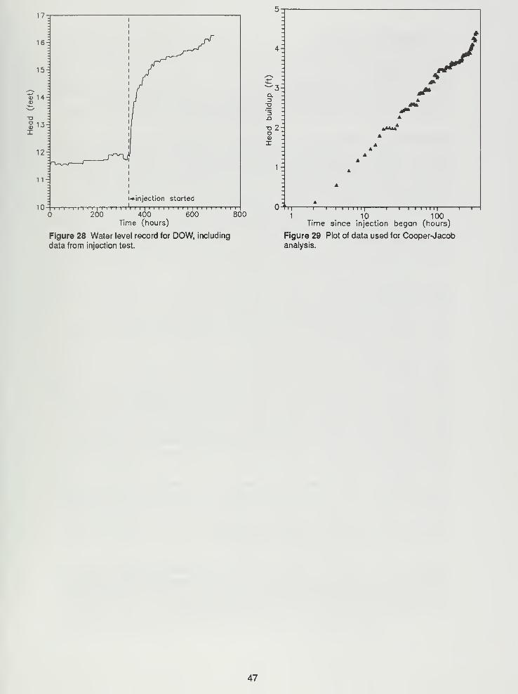
17tt

I I I I 1 I I I 1J

I T T

200 400 600 800Time (hours)

Figure 28 Water level record for DOW, including

data from injection test.

10 100Time since injection began (hours)

Figure 29 Plot of data used for Cooper-Jacobanalysis.

47

4. NUMERICAL MODELING

Model Selection

Model selection is an important step in conducting a modeling investigation of a groundwater flow

problem. The model should be able to handle all significant physical processes of the

groundwater flow system. If the model does not incorporate these processes, it cannot be ex-

pected to simulate the field situation with any degree of accuracy.

The literature contains descriptions of many general and specialized numerical models. At the out-

set of this project, it was thought that a model capable of simulating three-dimensional (3D) flow

and flow through complex hydrogeologic regimes would be required. Several 3D groundwater

flow models have been developed, including the Sandia Waste Isolation Flow and Transport

Model (SWIFT) (Reeves and Cranwell, 1981) and the Heat and Solute Transport Program

(HST3D) (Kipp 1987). SWIFT and HST3D are finite difference groundwater flow and transport

models that are independent modifications of SWIP (INTERCOMP, 1976). This original model,

developed to model the effects of deep-well waste injection, includes sophisticated well functions

rarely incorporated into other models. Although SWIFT and HST3D have a more general focus

than does their predecessor, both models retain these well functions, and either model could be

used for this project. Since a version of HST3D compatible with the Prime 9650 computer used in

this project was available before a similar version of SWIFT (II), HST3D was selected.

Model Description

HST3D is a descendent of the Survey Waste Isolation Program (SWIP) written for the U.S.

Geological Survey by INTERCOMP Resource Development and Engineering Consultants.

HST3D represents a complete rewrite of SWIP with many major and minor modifications, im-

provements, and corrections.

Overview of ModelHST3D simulates saturated groundwater flow and associated heat and solute transport in three

dimensions. The following equations are solved numerically: the saturated groundwater flow equa-

tion, formed from combining the conservation of total fluid mass and Darcy's Law for flow through

porous media; the heat transport equation from the conservation of enthalpy for the fluid and

porous medium; and the solute transport equation from the conservation of mass for a single

solute, which may adsorb onto the porous medium and/or decay (Kipp 1987). These equations

are coupled through the dependence of advective transport on the interstitial fluid velocity field,

fluid viscosity on temperature and solute concentration, and fluid density on pressure, tempera-

ture, and solute concentration.

For the dependent variables of pressure, temperature, and mass fraction, numerical solutions are

obtained successively using a set of modified equations that more directly link the original equa-

tions through the velocity, density, and viscosity coupling terms. Finite difference techniques are

used for the spatial and temporal discretization of the equations. When supplied with appropriate

boundary and initial conditions and system-parameter distributions, a wide variety of heat andsolute transport simulations can be performed (Kipp 1987).

The basic source-sink term represents wells. A complex well-flow model may be used to simulate

specified flow rate and pressure conditions at the land surface or within the aquifer, with or

without pressure constraints. Types of boundary conditions include specified value, specified flux,

leakage, heat conduction, an approximate free surface, and two types of aquifer influence func-

tions. All boundary conditions may be functions of time (Kipp 1987).

48

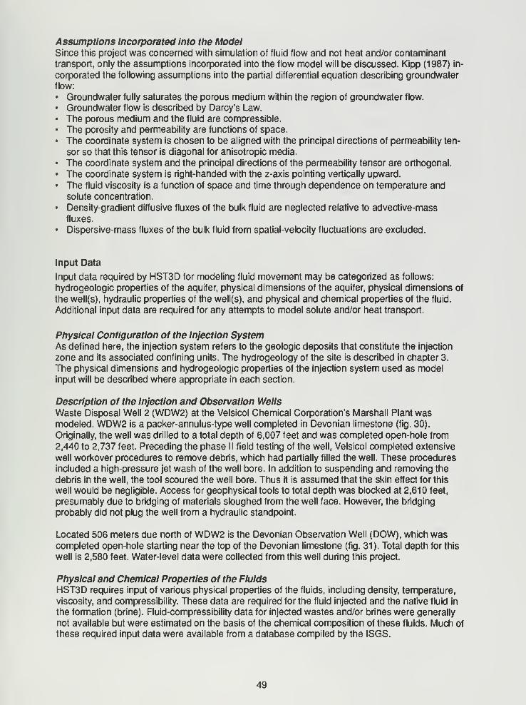
Assumptions Incorporated into the ModelSince this project was concerned with simulation of fluid flow and not heat and/or contaminant

transport, only the assumptions incorporated into the flow model will be discussed. Kipp (1987) in-

corporated the following assumptions into the partial differential equation describing groundwater

flow:

• Groundwater fully saturates the porous medium within the region of groundwater flow.

• Groundwater flow is described by Darcy's Law.

• The porous medium and the fluid are compressible.

• The porosity and permeability are functions of space.

• The coordinate system is chosen to be aligned with the principal directions of permeability ten-

sor so that this tensor is diagonal for anisotropic media.

• The coordinate system and the principal directions of the permeability tensor are orthogonal.

• The coordinate system is right-handed with the z-axis pointing vertically upward.

• The fluid viscosity is a function of space and time through dependence on temperature andsolute concentration.

• Density-gradient diffusive fluxes of the bulk fluid are neglected relative to advective-mass

fluxes.

• Dispersive-mass fluxes of the bulk fluid from spatial-velocity fluctuations are excluded.

Input Data

Input data required by HST3D for modeling fluid movement may be categorized as follows:

hydrogeologic properties of the aquifer, physical dimensions of the aquifer, physical dimensions of

the well(s), hydraulic properties of the well(s), and physical and chemical properties of the fluid.

Additional input data are required for any attempts to model solute and/or heat transport.

Physical Configuration of the Injection SystemAs defined here, the injection system refers to the geologic deposits that constitute the injection

zone and its associated confining units. The hydrogeology of the site is described in chapter 3.

The physical dimensions and hydrogeologic properties of the injection system used as modelinput will be described where appropriate in each section.

Description of the Injection and Observation Wells

Waste Disposal Well 2 (WDW2) at the Velsicol Chemical Corporation's Marshall Plant wasmodeled. WDW2 is a packer-annulus-type well completed in Devonian limestone (fig. 30).

Originally, the well was drilled to a total depth of 6,007 feet and was completed open-hole from

2,440 to 2,737 feet. Preceding the phase II field testing of the well, Velsicol completed extensive

well workover procedures to remove debris, which had partially filled the well. These procedures

included a high-pressure jet wash of the well bore. In addition to suspending and removing the

debris in the well, the tool scoured the well bore. Thus it is assumed that the skin effect for this

well would be negligible. Access for geophysical tools to total depth was blocked at 2,610 feet,

presumably due to bridging of materials sloughed from the well face. However, the bridging

probably did not plug the well from a hydraulic standpoint.

Located 506 meters due north of WDW2 is the Devonian Observation Well (DOW), which wascompleted open-hole starting near the top of the Devonian limestone (fig. 31). Total depth for this

well is 2,580 feet. Water-level data were collected from this well during this project.

Physical and Chemical Properties of the Fluids

HST3D requires input of various physical properties of the fluids, including density, temperature,

viscosity, and compressibility. These data are required for the fluid injected and the native fluid in

the formation (brine). Fluid-compressibility data for injected wastes and/or brines were generally

not available but were estimated on the basis of the chemical composition of these fluids. Much of

these required input data were available from a database compiled by the ISGS.

49

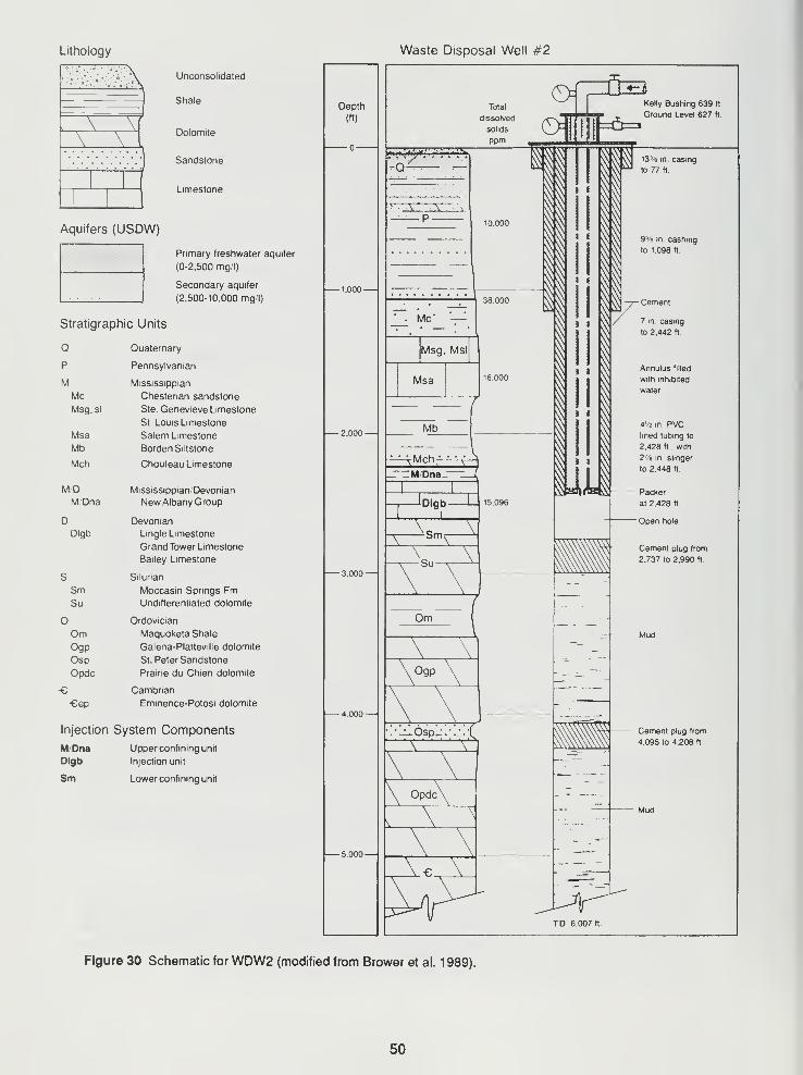
Lithology

W&Sk.H

. \ \'

..VA,,J

1 1

Aquifers (USD

',

Waste Disposal Well #2

Unconsolidated

Shale

Dolomite

Sandstone

Limestone

Primary freshwater aquifer

(0-2,500 mg/l)

Secondary aquifer

(2,500-10,000 mg/l)

Stratigraphic Units

Q Quaternary

P Pennsylvanian

M Mississippian

Mc Chesterian sandstone

Msg, si Ste. Genevieve Limestone

St. Louis Limestone

Msa Salem Limestone

Mb Borden Siltstone

Mch Chouteau Limestone

M D Mississippian/Devonian

MDna New Albany Group

D Devonian

Dlgb Lmgle Limestone

Grand Tower Limestone

Bailey Limestone

S Silurian

Sm Moccasin Springs FmSu Undifferentiated dolomite

O Ordovician

Om Maquoketa Shale

Ogp Galena-Platteville dolomite

Osp St. Peter Sandstone

Opdc Prairie du Chien dolomite

-G Cambrian

-Cep Eminence-Potosi dolomite

Injection System Components

MDna Upper confining unit

Dlgb Injection unit

Sm Lower confining unit

Depth

(ft)

-1.000-

-5.000—

Figure 30 Schematic for WDW2 (modified from Brower et al. 1989).

50

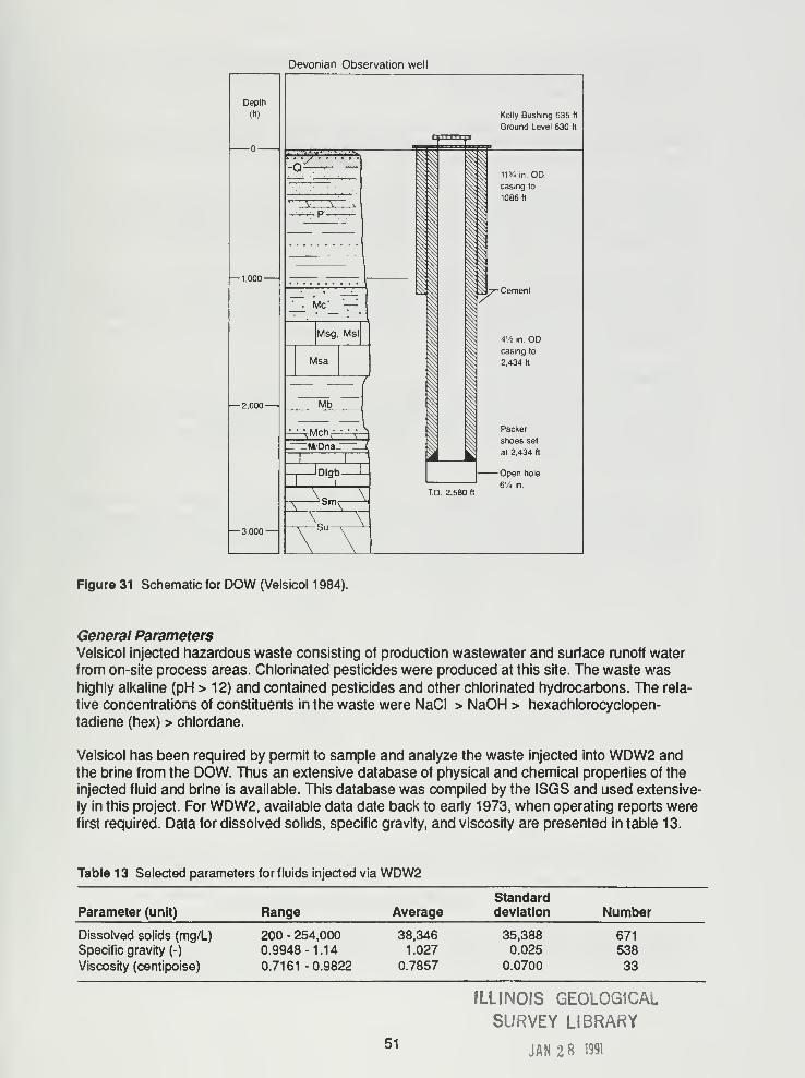
Devonian Observation well

Figure 31 Schematic for DOW (Velsicol 1 984).

General ParametersVelsicol injected hazardous waste consisting of production wastewater and surface runoff water

from on-site process areas. Chlorinated pesticides were produced at this site. The waste washighly alkaline (pH > 12) and contained pesticides and other chlorinated hydrocarbons. The rela-

tive concentrations of constituents in the waste were NaCI > NaOH > hexachlorocyclopen-

tadiene (hex) > chlordane.

Velsicol has been required by permit to sample and analyze the waste injected into WDW2 and

the brine from the DOW. Thus an extensive database of physical and chemical properties of the

injected fluid and brine is available. This database was compiled by the ISGS and used extensive-

ly in this project. For WDW2, available data date back to early 1973, when operating reports werefirst required. Data for dissolved solids, specific gravity, and viscosity are presented in table 13.

Table 13 Selected parameters for fluids injected via WDW2

Parameter (unit) Range AverageStandarddeviation Number

Dissolved solids (mg/L)

Specific gravity (-)

Viscosity (centipoise)

200 - 254,0000.9948-1.14

0.7161 -0.9822

38,346

1.027

0.7857

35,3880.025

0.0700

671

538

33

51

ILLINOIS GEOLOGICAL

SURVEY LIBRARY

JAN 2 8 1991

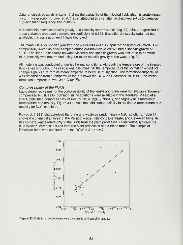
Data for dissolved solids in table 13 show the variability of the injected fluid, which is predominant-

ly storm water runoff. Brower et al. (1989) attributed this variation in dissolved solids to variation

of precipitation frequency and intensity.

A relationship between specific gravity and viscosity seems to exist (fig. 32). Linear regression of

these variables produced a correlation coefficient of 0.873. If additional viscosity data had beenavailable, this correlation might have improved.

The mean value for specific gravity of the waste was used as input for the numerical model. For

comparison, Devonian brine sampled during construction of WDW2 had a specific gravity of

1 .011 . The linear relationship between viscosity and specific gravity was assumed to be valid;

thus, viscosity was determined using the mean specific gravity of the waste (fig. 32).

All modeling was conducted under isothermal conditions. Although the temperature of the injected

fluid varied throughout the year, it was assumed that the temperature of the formation would not

change significantly from its mean temperature because of injection. The formation temperature

was determined from a temperature log run down the DOW on December 18, 1986. The meanformation temperature was 34.4°C (94° F).

Compressibility of the Fluids

Lab-determined values for the compressibility of the waste and brine were not available; however,

compressibility values for common saline solutions were available in the literature. Millero et al.

(1974) published compressibility values for NaCI, MgCl2, NaS04, and MgS04 as a function of

temperature and molality. Figure 33 depicts the fluid compressibility in relation to temperature and

molality for NaCI solutions.

Roy et al. (1989) characterized the brine and waste as predominantly NaCI solutions. Table 14

shows the chemical analysis of the Velsicol waste, Velsicol dilute waste, and Devonian brine. In

this context, waste refers only to the fluids from the plant processes. Dilute waste, typically the

fluid injected, comprises fluids from the plant processes and surface runoff. The sample of

Devonian brine was obtained from the DOW in June 1987.

1.00 -3

0.95

0.90 i

o.0-0.85

0.80 -.

moo^0.75

0.70 -.

0.65 |ii 1 1 1 ii ii|ii 1 1 ii 1 1 1 1 1 1 ii 1 1 ii 1 1 in 1 1 ni| ii i ii mi 1 1 1 ii ii i ii| 1 1 mi i ii

0.98 1.00 1.02 1.04 1.06 1.08 1.10 1.12

Specific Gravity

Figure 32 Relationship between waste viscosity and specific gravity.

52

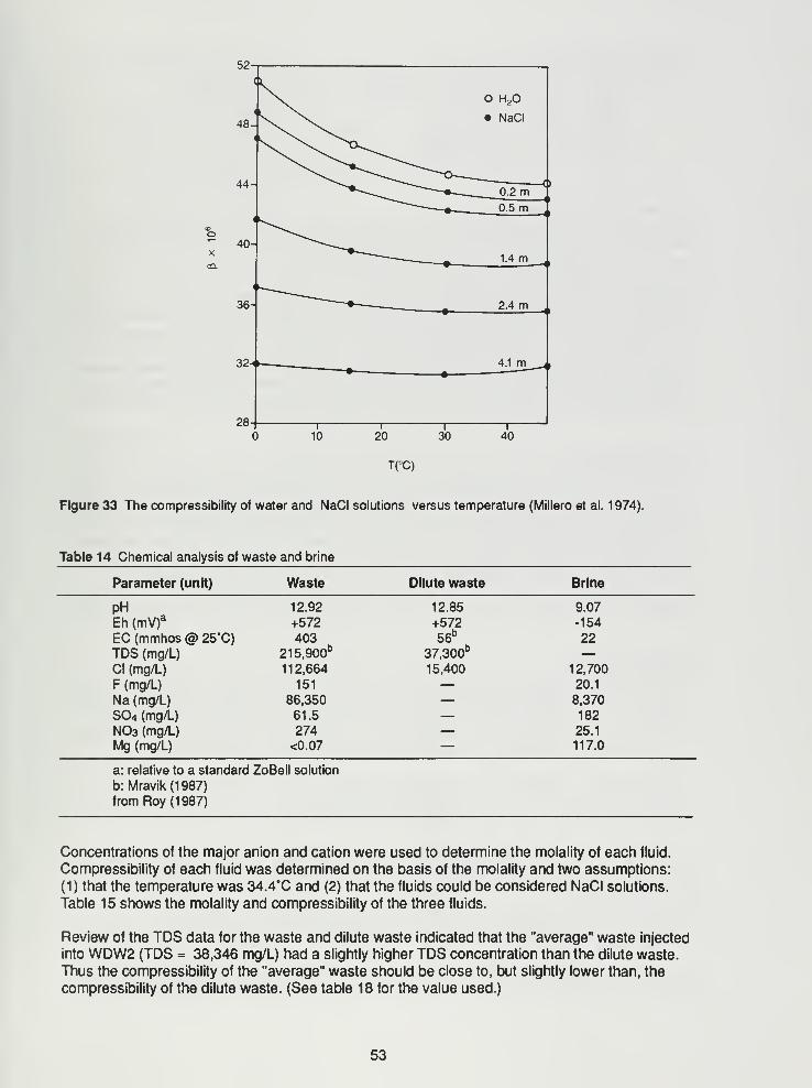
X00.

T(°C)

Figure 33 The compressibility of water and NaCI solutions versus temperature (Millero et al. 1974).

Table 14 Chemical analysis of waste and brine

Parameter (unit) Waste Dilute waste Brine

PH 12.92 12.85 9.07

Eh (mV)a +572 +572 -154

EC (mmhos @ 25'C) 403 56b

22TDS (mg/L) 215,900

b37,300

b —CI (mg/L) 112,664 15,400 12,700

F (mg/L) 151 — 20.1

Na (mg/L) 86,350 — 8,370

SO4 (mg/L) 61.5 — 182

NO3 (mg/L) 274 — 25.1

Mg (mg/L) <0.07 — 117.0

a: relative to a standard ZoBell solution

b:Mravik(1987)

from Roy (1987)

Concentrations of the major anion and cation were used to determine the molality of each fluid.

Compressibility of each fluid was determined on the basis of the molality and two assumptions:

(1) that the temperature was 34.4°C and (2) that the fluids could be considered NaCI solutions.

Table 15 shows the molality and compressibility of the three fluids.

Review of the TDS data for the waste and dilute waste indicated that the "average" waste injected

into WDW2 (TDS = 38,346 mg/L) had a slightly higher TDS concentration than the dilute waste.

Thus the compressibility of the "average" waste should be close to, but slightly lower than, the

compressibility of the dilute waste. (See table 18 for the value used.)

53

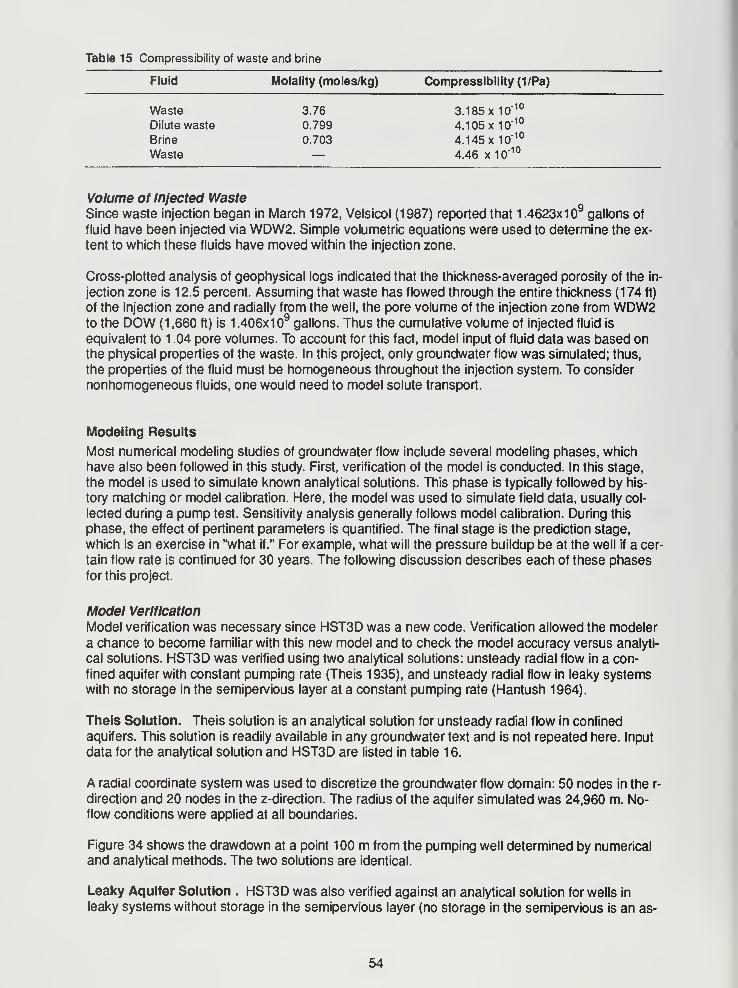
Table 15 Compressibility of waste and brine

Waste 3.76

Dilute waste 0.799

Brine 0.703

Waste —

Fluid Molality (moles/kg) Compressibility (1/Pa)

3.185 X10"10

4.105 x10"10

4.145 X10"10

4.46 x10"10

Volume of Injected WasteSince waste injection began in March 1972, Velsicol (1987) reported that 1 .4623x1

9gallons of

fluid have been injected via WDW2. Simple volumetric equations were used to determine the ex-

tent to which these fluids have moved within the injection zone.

Cross-plotted analysis of geophysical logs indicated that the thickness-averaged porosity of the in-

jection zone is 12.5 percent. Assuming that waste has flowed through the entire thickness (174 ft)

of the injection zone and radially from the well, the pore volume of the injection zone from WDW2to the DOW (1 ,660 ft) is 1 .406x1

9gallons. Thus the cumulative volume of injected fluid is

equivalent to 1 .04 pore volumes. To account for this fact, model input of fluid data was based onthe physical properties of the waste. In this project, only groundwater flow was simulated; thus,

the properties of the fluid must be homogeneous throughout the injection system. To consider

nonhomogeneous fluids, one would need to model solute transport.

Modeling Results

Most numerical modeling studies of groundwater flow include several modeling phases, which

have also been followed in this study. First, verification of the model is conducted. In this stage,

the model is used to simulate known analytical solutions. This phase is typically followed by his-

tory matching or model calibration. Here, the model was used to simulate field data, usually col-

lected during a pump test. Sensitivity analysis generally follows model calibration. During this

phase, the effect of pertinent parameters is quantified. The final stage is the prediction stage,

which is an exercise in "what if." For example, what will the pressure buildup be at the well if a cer-

tain flow rate is continued for 30 years. The following discussion describes each of these phasesfor this project.

Model Verification

Model verification was necessary since HST3D was a new code. Verification allowed the modeler

a chance to become familiar with this new model and to check the model accuracy versus analyti-

cal solutions. HST3D was verified using two analytical solutions: unsteady radial flow in a con-

fined aquifer with constant pumping rate (Theis 1935), and unsteady radial flow in leaky systemswith no storage in the semipervious layer at a constant pumping rate (Hantush 1964).

Theis Solution. Theis solution is an analytical solution for unsteady radial flow in confined

aquifers. This solution is readily available in any groundwater text and is not repeated here. Input

data for the analytical solution and HST3D are listed in table 16.

A radial coordinate system was used to discretize the groundwater flow domain: 50 nodes in the r-

direction and 20 nodes in the z-direction. The radius of the aquifer simulated was 24,960 m. No-flow conditions were applied at all boundaries.

Figure 34 shows the drawdown at a point 100 m from the pumping well determined by numericaland analytical methods. The two solutions are identical.

Leaky Aquifer Solution . HST3D was also verified against an analytical solution for wells in

leaky systems without storage in the semipervious layer (no storage in the semipervious is an as-

54

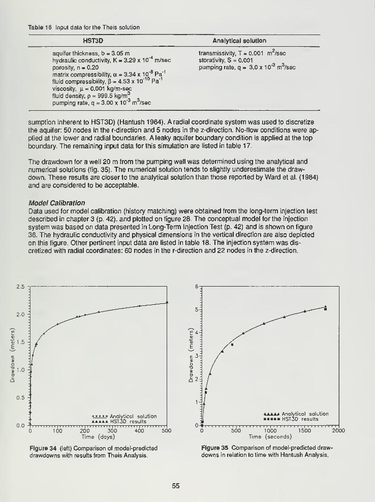
Table 1 6 Input data for the Theis solution

HST3D Analytical solution

-4m/sec

aquifer thickness, b = 3.05 mhydraulic conductivity, K = 3.29 x 10

porosity, n = 0.20

matrix compressibility, a = 3.34 x 10"8 Pa*1

fluid compressibility, p = 4.53 x 10" 10 Pa'1

viscosity, u. = 0.001 kg/m-sec

fluid density, p = 999.5 kg/m

pumping rate, q = 3.00 x 10° m°/sec3„3,

transmissivity, T = 0.001 m2/sec

storativity, S = 0.001

pumping rate, q = 3.0 x 1

0"3 m3/sec

sumption inherent to HST3D) (Hantush 1964). A radial coordinate system was used to discretize

the aquifer: 50 nodes in the r-direction and 5 nodes in the z-direction. No-flow conditions were ap-

plied at the lower and radial boundaries. A leaky aquifer boundary condition is applied at the top

boundary. The remaining input data for this simulation are listed in table 17.

The drawdown for a well 20 m from the pumping well was determined using the analytical and

numerical solutions (fig. 35). The numerical solution tends to slightly underestimate the draw-

down. These results are closer to the analytical solution than those reported by Ward et al. (1984)

and are considered to be acceptable.

Model Calibration

Data used for model calibration (history matching) were obtained from the long-term injection test

described in chapter 3 (p. 42). and plotted on figure 28. The conceptual model for the injection

system was based on data presented in Long-Term Injection Test (p. 42) and is shown on figure

36. The hydraulic conductivity and physical dimensions in the vertical direction are also depicted

on this figure. Other pertinent input data are listed in table 18. The injection system was dis-

cretized with radial coordinates: 60 nodes in the r-direction and 22 nodes in the z-direction.

2.5

0.5

0.0

***** Analytical solutionaaaaa HST3D results

1 1 i i i i i i ii

i i i i i i 1 1 ii

i i i i i i i i i|

i i i i i 1 1 i 1 1 i 1 1 1 1 i 1 1 i

100 200 300 400 500Time (days)

Figure 34 (left) Comparison of model-predicted

drawdowns with results from Theis Analysis.

Analytical solution

HST3D results

500 1 000Time (seconds)

ii

i i i i i i i i

1500 2000

Figure 35 Comparison of model-predicted draw-

downs in relation to time with Hantush Analysis.

55

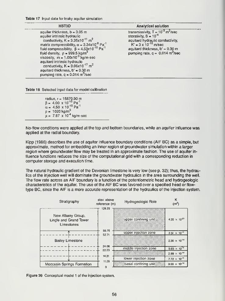
Table 17 Input data for leaky aquifer simulation

HST3D Analytical solution

aquifer thickness, b = 3.05 maquifer intrinsic hydraulic

conductivity, K = 3.35x10" 11 m2

matrix compressibility, a = 3.34x10"8

Pa"1

fluid compressibility, p = 4.53x10" 10

Pa"1

fluid density, p = 999.5 kg/m3

viscosity, m = 1.00x10"3kg/m-sec

aquitard intrinsic hydraulic

conductivity, K = 3.06x10" 17 m2

aquitard thickness, b' = 0.30 mpumping rate, q = 0.014 m3

/sec

transmissivity, T = 1

0"3 m2/sec

storativity, S = 10"4

aquitard hydraulic conductivity,

K' = 3x10' 10m/sec

aquitard thickness, b' = 0.30 mpumping rate, q = 0.014 m3

/sec

Table 18 Selected input data for model calibration

radius, r= 15870.90 mP= 4.00 x10"

10Pa"

1

<x= 4.50 x10"10

Pa"1

p= 1020 kg/m3

u. = 7.87 x 1

0"4kg/m-sec

No-flow conditions were applied at the top and bottom boundaries, while an aquifer influence wasapplied at the radial boundary.

Kipp (1986) describes the use of aquifer influence boundary conditions (AIF BC) as a simple, but

approximate, method for embedding an inner region of groundwater simulation within a larger

region where groundwater flow may be treated in an approximate fashion. The use of aquifer in-

fluence functions reduces the size of the computational grid with a corresponding reduction in

computer storage and execution time.

The natural hydraulic gradient of the Devonian limestone is very low (see p. 32); thus, the hydrau-

lics of the injection well will dominate the groundwater hydraulics in the area surrounding the well.

The flow rate across an AIF boundary is a function of the potentiometric head and hydrogeologic

characteristics of the aquifer. The use of the AIF BC was favored over a specified head or flow-

type BC, since the AIF is a more accurate representation of the hydraulics of the injection system.

Stratigraphy

New Albany Group,

Lingle and Grand Tower

Limestones

TBailey Limestone

24.06

elev. above

reference (m)

128.29

Moccasin Springs Formation

55.76

52.71

14.31

11.28

Hydrogeologic RoleK

(m2)

4.35 x 10' 21' upper confining unit

upper injection zone 2.51 x 10"

2.30 x 10"14

middle injection zone 9.65 x 10"

2.99 x 10" 14

lower injection zone 7.72 x 10"

basal confining unit:::. 9.68 x 1014

Figure 36 Conceptual model 1 of the injection system.

56

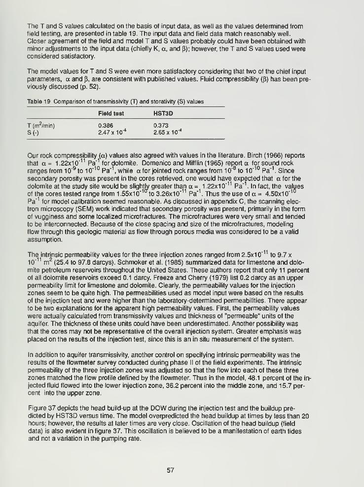
The T and S values calculated on the basis of input data, as well as the values determined from

field testing, are presented in table 19. The input data and field data match reasonably well.

Closer agreement of the field and model T and S values probably could have been obtained with

minor adjustments to the input data (chiefly K, a, and P); however, the T and S values used wereconsidered satisfactory.

The model values for T and S were even more satisfactory considering that two of the chief input

parameters, a and p, are consistent with published values. Fluid compressibility (P) has been pre-

viously discussed (p. 52).

Table 19 Comparison of transmissivity (T) and storativity (S) values

Field test HST3D

T (m2/min) 0.386 0.373

S(-) 2.47 X10"4

2.65x10""

Our rock compressibility (a) values also agreed with values in the literature. Birch (1966) reports

that a = 1 .22x10" 11

Pa"1for dolomite. Domenico and Mifflin (1965) report a for sound rock

ranges from 10"9 to 10"10 Pa"1

, while a for jointed rock ranges from 10"8 to 10"10 Pa"1

. Since

secondary porosity was present in the cores retrieved, one would have expected that a for the

dolomite at the study site would be slightly greater than a = 1 .22x10" 11

Pa"1

. In fact, the values

of the cores tested range from 1.55x10 to 3.26x10" 11

Pa"1

. Thus the use of a = 4.50x10"10

Pa"1for model calibration seemed reasonable. As discussed in appendix C, the scanning elec-

tron microscopy (SEM) work indicated that secondary porosity was present, primarily in the form

of vugginess and some localized microfractures. The microfractures were very small and tended

to be interconnected. Because of the close spacing and size of the microfractures, modeling

flow through this geologic material as flow through porous media was considered to be a valid

assumption.

The intrinsic permeability values for the three injection zones ranged from 2.5x10" 11

to 9.7 x10" 11 m2

(25.4 to 97.8 darcys). Schmoker et al. (1985) summarized data for limestone and dolo-

mite petroleum reservoirs throughout the United States. These authors report that only 11 percent

of all dolomite reservoirs exceed 0.1 darcy. Freeze and Cherry (1979) list 0.2 darcy as an upper

permeability limit for limestone and dolomite. Clearly, the permeability values for the injection

zones seem to be quite high. The permeabilities used as model input were based on the results

of the injection test and were higher than the laboratory-determined permeabilities. There appear

to be two explanations for the apparent high permeability values. First, the permeability values

were actually calculated from transmissivity values and thickness of "permeable" units of the

aquifer. The thickness of these units could have been underestimated. Another possibility wasthat the cores may not be representative of the overall injection system. Greater emphasis wasplaced on the results of the injection test, since this is an in situ measurement of the system.

In addition to aquifer transmissivity, another control on specifying intrinsic permeability was the

results of the flowmeter survey conducted during phase II of the field experiments. The intrinsic

permeability of the three injection zones was adjusted so that the flow into each of these three

zones matched the flow profile defined by the flowmeter. Thus in the model, 48.1 percent of the in-

jected fluid flowed into the lower injection zone, 36.2 percent into the middle zone, and 15.7 per-

cent into the upper zone.

Figure 37 depicts the head build-up at the DOW during the injection test and the buildup pre-

dicted by HST3D versus time. The model overpredicted the head buildup at times by less than 20hours; however, the results at later times are very close. Oscillation of the head buildup (field

data) is also evident in figure 37. This oscillation is believed to be a manifestation of earth tides

and not a variation in the pumping rate.

57

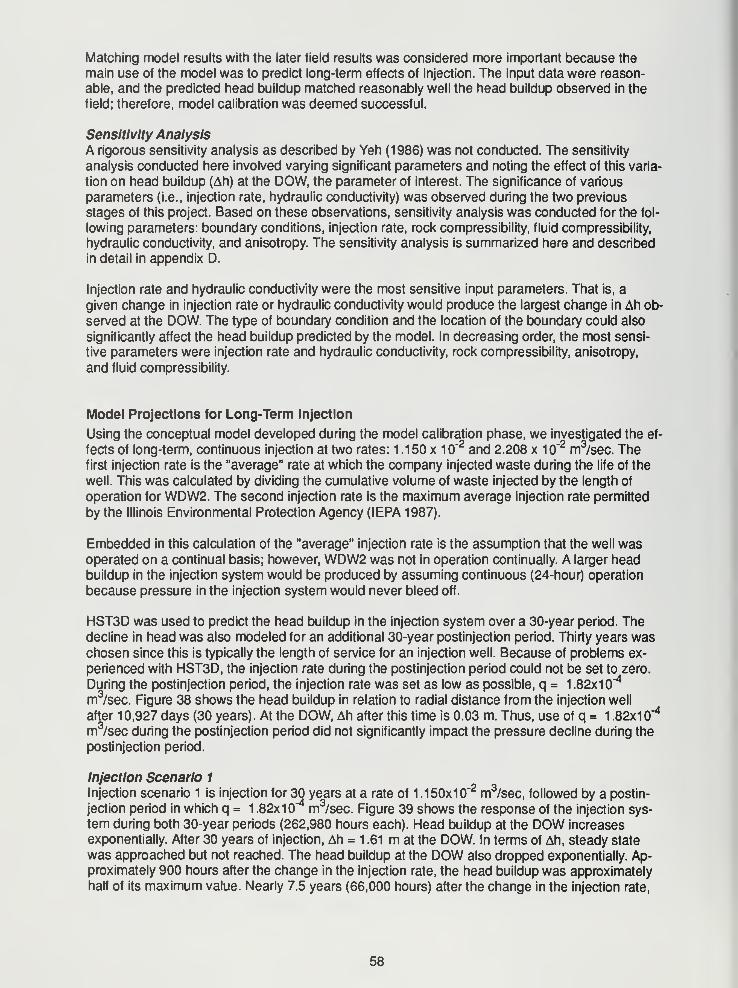
Matching model results with the later field results was considered more important because the

main use of the model was to predict long-term effects of injection. The input data were reason-

able, and the predicted head buildup matched reasonably well the head buildup observed in the

field; therefore, model calibration was deemed successful.

Sensitivity Analysis

A rigorous sensitivity analysis as described by Yeh (1986) was not conducted. The sensitivity

analysis conducted here involved varying significant parameters and noting the effect of this varia-

tion on head buildup (Ah) at the DOW, the parameter of interest. The significance of various

parameters (i.e., injection rate, hydraulic conductivity) was observed during the two previous

stages of this project. Based on these observations, sensitivity analysis was conducted for the fol-

lowing parameters: boundary conditions, injection rate, rock compressibility, fluid compressibility,

hydraulic conductivity, and anisotropy. The sensitivity analysis is summarized here and described

in detail in appendix D.

Injection rate and hydraulic conductivity were the most sensitive input parameters. That is, a

given change in injection rate or hydraulic conductivity would produce the largest change in Ah ob-

served at the DOW. The type of boundary condition and the location of the boundary could also

significantly affect the head buildup predicted by the model. In decreasing order, the most sensi-

tive parameters were injection rate and hydraulic conductivity, rock compressibility, anisotropy,

and fluid compressibility.

Model Projections for Long-Term Injection

Using the conceptual model developed during the model calibration phase, we investigated the ef-

fects of long-term, continuous injection at two rates: 1 .150 x 10"2 and 2.208 x 10"2 m3/sec. The

first injection rate is the "average" rate at which the company injected waste during the life of the

well. This was calculated by dividing the cumulative volume of waste injected by the length of

operation for WDW2. The second injection rate is the maximum average injection rate permitted

by the Illinois Environmental Protection Agency (IEPA 1987).

Embedded in this calculation of the "average" injection rate is the assumption that the well wasoperated on a continual basis; however, WDW2 was not in operation continually. A larger headbuildup in the injection system would be produced by assuming continuous (24-hour) operation

because pressure in the injection system would never bleed off.

HST3D was used to predict the head buildup in the injection system over a 30-year period. Thedecline in head was also modeled for an additional 30-year postinjection period. Thirty years waschosen since this is typically the length of service for an injection well. Because of problems ex-

perienced with HST3D, the injection rate during the postinjection period could not be set to zero.

During the postinjection period, the injection rate was set as low as possible, q = 1 .82x10"4

m3/sec. Figure 38 shows the head buildup in relation to radial distance from the injection well

after 10,927 days (30 years). At the DOW, Ah after this time is 0.03 m. Thus, use of q = 1 .82x10"4

m3/sec during the postinjection period did not significantly impact the pressure decline during the

postinjection period.

Injection Scenario 1

Injection scenario 1 is injection for 30 years at a rate of 1 .150x10"2 m3

/sec, followed by a postin-

jection period in which q = 1 .82x10"4 m3

/sec. Figure 39 shows the response of the injection sys-

tem during both 30-year periods (262,980 hours each). Head buildup at the DOW increases

exponentially. After 30 years of injection, Ah = 1 .61 m at the DOW. In terms of Ah, steady state

was approached but not reached. The head buildup at the DOW also dropped exponentially. Ap-proximately 900 hours after the change in the injection rate, the head buildup was approximately

half of its maximum value. Nearly 7.5 years (66,000 hours) after the change in the injection rate,

58

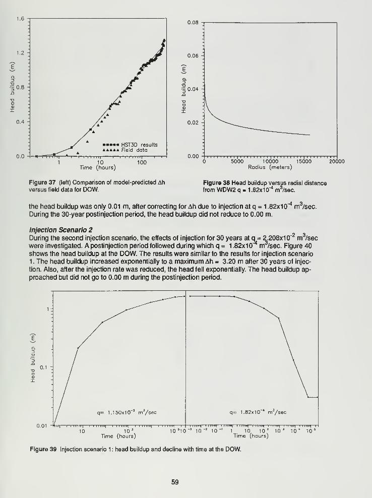
1.6

1.2

Q.

XI0.8

XID

0.4

0.0

HST3D results

Field data

0.08

10Time (hours)

1000.00 -i i i i

ii i i i i i i i i

ii i i i i i i i i

ii i i i i i

5000 10000 15000 20000Radius (meters)

Figure 37 (left) Comparison of model-predicted Ahversus field data for DOW.

Figure 38 Head buildup versus radial distance

from WDW2 q - 1 .82x10"4 m3

/sec.

^4 _3,the head buildup was only 0.01 m, after correcting for Ah due to injection at q = 1 .82x10 m /sec.

During the 30-year postinjection period, the head buildup did not reduce to 0.00 m.

-2 m3,Injection Scenario 2During the second injection scenario, the effects of injection for 30 years at q = 2.208x1 Q~* m°/sec

were investigated. A postinjection period followed during which q = 1 .82x10"4 m3

/sec. Figure 40shows the head buildup at the DOW. The results were similar to the results for injection scenario

1 . The head buildup increased exponentially to a maximum Ah = 3.20 m after 30 years of injec-

tion. Also, after the injection rate was reduced, the head fell exponentially. The head buildup ap-

proached but did not go to 0.00 m during the postinjection period.

ex

X)

XIo

X

0.01 I i i m ii| 1—i i 1 1 1 1

1

1

1—i i iiiii| 1—i i m ii| 1—i i i i r ri|

1—|—i i iuin|—i I iimh|—i 1 1 mi|—i i i iinf—i i nniq—i i iniii|—i i iniii|—i i iiini|—

r

10 103 10

510 ~3 10

~210 "

1 10 102

105 10*10'

Time (hours) Time (hours)

Figure 39 Injection scenario 1 : head buildup and decline with time at the DOW.

59

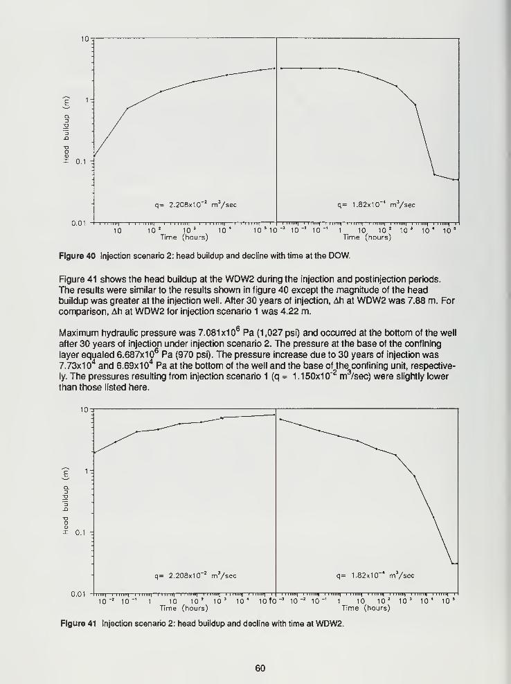
10-

1-

4)

x 0.1

q= 2.208x10"2 m 3

/sec q= 1.82x10"* m 3/sec

0.01 i—i i 1 1 1 ii| 1—i i i m i| 1—i i i iiiii 1—i i i • r j1

1

1—i i i iim| 1—I in iiiii|—i i mm—i i iiiiiii—i i iiiiiii—i i iiiiiii—i i m ini

—

i 1 1 m ii|—i i iii n q—rl

10 10 2 10' 10* 10 s 10"3 10~2 10" 1

1 10 10 2 10 J 10* 10 s

Time (hours) Time (hours)

Figure 40 Injection scenario 2: head buildup and decline with time at the DOW.

Figure 41 shows the head buildup at the WDW2 during the injection and postinjection periods.

The results were similar to the results shown in figure 40 except the magnitude of the head

buildup was greater at the injection well. After 30 years of injection, Ah at WDW2 was 7.88 m. For

comparison, Ah at WDW2 for injection scenario 1 was 4.22 m.

Maximum hydraulic pressure was 7.081 x106 Pa (1 ,027 psi) and occurred at the bottom of the well

after 30 years of injection under injection scenario 2. The pressure at the base of the confining

layer equaled 6.687x16 Pa (970 psi). The pressure increase due to 30 years of injection was

7.73x14and 6.69x1

4 Pa at the bottom of the well and the base of the confining unit, respective-

ly. The pressures resulting from injection scenario 1 (q = 1.150x10"2 m3

/sec) were slightly lower

than those listed here.

1-

3o

x 0.1

q= 2.208x10"2 m 3

/sec q= 1.82x10"* m 3/sec

0.01 I iii i iii—i 1 1 m ill—i i m i ni—i 1

1

|—i i iiiiiii—i i iiiiiii—i |—i I iiiiiii—r)—I i iiiiiii—i iiiiiii—i i iiiiiii—i i mm—i i iiiiiii

—|—i i iiiiiii—I I iimq—

r

10"' 10" 1 10 102

103

104

10 fO "" 10"210 "'

1 10 102

103 10* 10

s

Time (hours) Time (hours)

Figure 41 Injection scenario 2: head buildup and decline with time at WDW2.

60

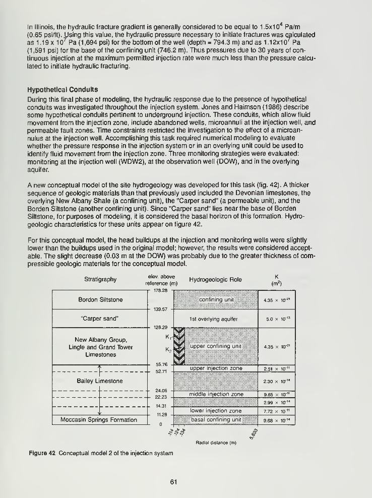
In Illinois, the hydraulic fracture gradient is generally considered to be equal to 1.5x104 Pa/m

(0.65 psi/ft). Using this value, the hydraulic pressure necessary to initiate fractures was calculated

as 1 .19 x 107 Pa (1 ,694 psi) for the bottom of the well (depth = 794.3 m) and as 1 .12x10

7 Pa

(1 ,591 psi) for the base of the confining unit (746.2 m). Thus pressures due to 30 years of con-

tinuous injection at the maximum permitted injection rate were much less than the pressure calcu-

lated to initiate hydraulic fracturing.

Hypothetical Conduits

During this final phase of modeling, the hydraulic response due to the presence of hypothetical

conduits was investigated throughout the injection system. Jones and Haimson (1986) describe

some hypothetical conduits pertinent to underground injection. These conduits, which allow fluid

movement from the injection zone, include abandoned wells, microannuli at the injection well, and

permeable fault zones. Time constraints restricted the investigation to the effect of a microan-

nulus at the injection well. Accomplishing this task required numerical modeling to evaluate

whether the pressure response in the injection system or in an overlying unit could be used to

identify fluid movement from the injection zone. Three monitoring strategies were evaluated:

monitoring at the injection well (WDW2), at the observation well (DOW), and in the overlying

aquifer.

A new conceptual model of the site hydrogeology was developed for this task (fig. 42). A thicker

sequence of geologic materials than that previously used included the Devonian limestones, the

overlying New Albany Shale (a confining unit), the "Carper sand" (a permeable unit), and the

Borden Siltstone (another confining unit). Since "Carper sand" lies near the base of Borden

Siltstone, for purposes of modeling, it is considered the basal horizon of this formation. Hydro-

geologic characteristics for these units appear on figure 42.

For this conceptual model, the head buildups at the injection and monitoring wells were slightly

lower than the buildups used in the original model; however, the results were considered accept-

able. The slight decrease (0.03 m at the DOW) was probably due to the greater thickness of com-pressible geologic materials for the conceptual model.

Stratigraphyelev. above

reference (m)

178.28

Hydrogeologic Rolem'

Bordon Siltstone

"Carper sand"

New Albany Group,

Lingle and Grand Tower

Limestones

TBailey Limestone

11.28

Moccasin Springs Formation

confining unit

1st overlying aquifer

upper confining unit:

upper injection zone

middle injection zone

lower injection zone

basal confining unit!

4.35 x 1021

5.0 x 1Q- 13

4.35 x 10-

2.51 x 10"

2.30 x 10"'

9.65 x 10"

2.99 x 10'

7.72 x 10-

9.68 x 10" 1

Radial distance (m)

$

Figure 42 Conceptual model 2 of the injection system

61

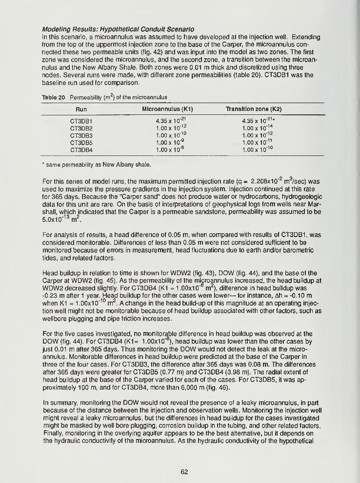
Modeling Results: Hypothetical Conduit ScenarioIn this scenario, a microannulus was assumed to have developed at the injection well. Extending

from the top of the uppermost injection zone to the base of the Carper, the microannulus con-

nected these two permeable units (fig. 42) and was input into the model as two zones. The first

zone was considered the microannulus, and the second zone, a transition between the microan-

nulus and the New Albany Shale. Both zones were 0.01 m thick and discretized using three

nodes. Several runs were made, with different zone permeabilities (table 20). CT3DB1 was the

baseline run used for comparison.

Table 20 Permeability (m2

) of the microannulus

Run Microannulus (K1) Transition zone (K2)

CT3DB1 4.35 x10"21

4.35 x10"21 *

CT3DB2 1.00 X10"12

1.00 x10'14

CT3DB3 1.00 X10"10

1.00 x10"12

CT3DB5 1.00 x10"9

1.00 x10"11

CT3DB4 1.00 x10"8

1.00 x10"10

* same permeability as New Albany shale.

For this series of model runs, the maximum permitted injection rate (q = 2.208x10"2 m3

/sec) wasused to maximize the pressure gradients in the injection system. Injection continued at this rate

for 365 days. Because the "Carper sand" does not produce water or hydrocarbons, hydrogeologic

data for this unit are rare. On the basis of interpretations of geophysical logs from wells near Mar-

shall, which indicated that the Carper is a permeable sandstone, permeability was assumed to be

5.0x10" 13 m2

.

For analysis of results, a head difference of 0.05 m, when compared with results of CT3DB1 , wasconsidered monitorable. Differences of less than 0.05 m were not considered sufficient to be

monitored because of errors in measurement, head fluctuations due to earth and/or barometric

tides, and related factors.

Head buildup in relation to time is shown for WDW2 (fig. 43), DOW (fig. 44), and the base of the

Carper at WDW2 (fig. 45). As the permeability of the microannulus increased, the head buildup at

WDW2 decreased slightly. ForCT3DB4 (K1 = 1.00x10"8 m2

), difference in head buildup was-0.23 m after 1 year. Head buildup for the other cases were lower— for instance, Ah = -0.10 mwhen K1 = 1 .00x1

0" 10 m2. A change in the head build-up of this magnitude at an operating injec-

tion well might not be monitorable because of head buildup associated with other factors, such as

wellbore plugging and pipe friction increases.

For the five cases investigated, no monitorable difference in head buildup was observed at the

DOW (fig. 44). For CT3DB4 (K1= 1 .00x10"8

), head buildup was lower than the other cases by

just 0.01 m after 365 days. Thus monitoring the DOW would not detect the leak at the micro-

annulus. Monitorable differences in head buildup were predicted at the base of the Carper in

three of the four cases. For CT3DB3, the difference after 365 days was 0.08 m. The differences

after 365 days were greater for CT3DB5 (0.77 m) and CT3DB4 (3.98 m). The radial extent of

head buildup at the base of the Carper varied for each of the cases. For CT3DB5, it was ap-

proximately 100 m, and for CT3DB4, more than 6,000 m (fig. 46).

In summary, monitoring the DOW would not reveal the presence of a leaky microannulus, in part

because of the distance between the injection and observation wells. Monitoring the injection well

might reveal a leaky microannulus, but the differences in head buildup for the cases investigated

might be masked by well bore plugging, corrosion buildup in the tubing, and other related factors.

Finally, monitoring in the overlying aquifer appears to be the best alternative, but it depends onthe hydraulic conductivity of the microannulus. As the hydraulic conductivity of the hypothetical

62

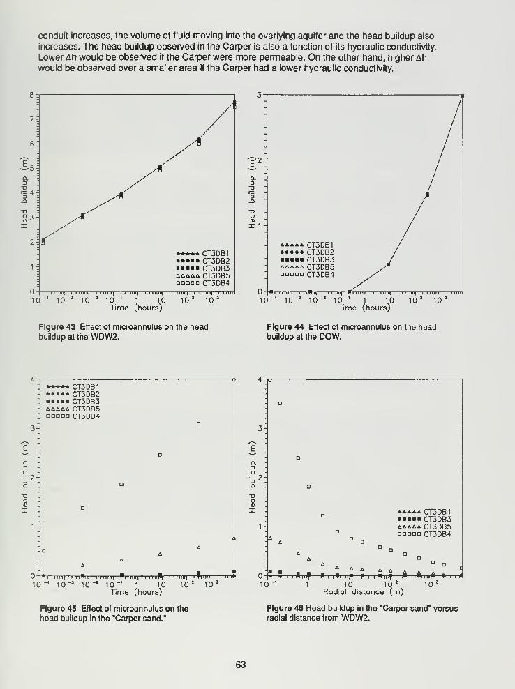
conduit increases, the volume of fluid moving into the overlying aquifer and the head buildup also

increases. The head buildup observed in the Carper is also a function of its hydraulic conductivity.

Lower Ah would be observed if the Carper were more permeable. On the other hand, higher Ahwould be observed over a smaller area if the Carper had a lower hydraulic conductivity.

7-.

6-.

CLDX>

X) :

"D :

° 3-X :

2

CT3DB1CT3DB2CT3DB3

44^44 CT3DB5odooq CT3DB4

I llllll| 1 I I lllll| 1 I llllll| 1 I I 1 1 1 Il| 1 I llllll| 1 I II llll| 1 I I I Mll| 1 I llllll

10"4

10"3

10"2 10"' 1 10 10

210

3

Time (hours)

a.

XJ'5

XI

X>Ot)

x HCT3DB1

••••• CT3DB2CT3DB3

4A4A4 CT3DB5DDDDQ CT3DB4

'i 1

1

iiiii|—i 1

1

Wi ii|—i i min|—Pi iiiiii|—i i miiii|—i i iuiii|—i i iniii|—i i mill

10"4

10"3

10"2 10"' 1 10 10

210

Time (hours)

Figure 43 Effect of microannulus on the head

buildup at the WDW2.Figure 44 Effect of microannulus on the headbuildup at the DOW.

XI= 2

XIo4)

X

CT3DB1CT3DB2CT3DB3

Aiaa4 CT3DB5dodo CT3DB4

rmrri—i i iPiii|—i i nun

10 10 10 10"'1 10

Time (hours)

i i i iiiiii—

n

102

"""I

10

3-

X)•12-O

XIoVX

1-

A A

CT3DB1CT3DB3

iiAii CT3DB5DDDDD CT3DB4

+ i i miXttI P i i*m i P P i i m i f ^ i r$mtjft

10

i ipinif

10 102

10Radial distance (m)

Figure 45 Effect of microannulus on the

head buildup in the "Carper sand."

Figure 46 Head buildup in the "Carper sand" versus

radial distance from WDW2.

63

5. SUMMARY AND CONCLUSIONS

Evaluation of Injection Scenarios

Available records and logs pertinent to the injection system were studied, hydraulic tests wereconducted, geophysical logs were run, and other tests were conducted on-site to determine the

hydrogeologic characteristics of the injection system. Regional and site-specific descriptions of

the system's stratigraphy, structural geology, and hydrogeology were generated from analyses of

these logs and test results. These descriptions formed the basis of input for the numerical

groundwater flow model (HST3D) used to investigate the hydraulic effects of injection upon the in-

jection system. Other input included data on the physical and chemical characteristics of the in-

jected wastewater and the native brine in the injection system.

Before the effects of various injection scenarios were investigated, HST3D was verified with

respect to two analytical solutions (figs. 34 and 35) and calibrated with respect to data collected

during an injection test (fig. 37). Both verification and calibration were considered satisfactory.

Once calibrated, the model was used to predict the effects of various injection scenarios. The ef-

fect of long-term injection was investigated at two constant injection rates: the average historical

rate (1.1 50x10"2 m /sec) and the maximum average permitted rate (2.208x10 m3

/sec). Under

both scenarios, significant head buildup was observed at the injection well and radially from it.

During the simulated 30-year injection period, steady state was approached but not obtained

during either injection scenario. During the subsequent 30-year postinjection period, decrease in

head buildup was fairly rapid—dropping to half in less than 2,000 hours for both scenarios. Themaximum hydraulic pressures at the bottom of the well and at the base of the upper confining unit

were significantly lower than the pressures calculated to initiate hydraulic fracturing.

The continuity of the regional stratigraphy and its qualitative permeability were determined from

the regional and site-specific study. Numerical modeling indicated that the pressures resulting

from waste injection were lower than pressures calculated to initiate hydraulic fracturing; thus newfractures would not be initiated. From a hydraulic viewpoint, therefore, waste injected within this

injection system would be contained and would be considered protective of human health and the

environment for the two injection scenarios investigated.

These results are based on an assumption that hydraulic conductivity remains constant. How-ever, from available data it appears that the high pH of the injected wastewater causes it to react

with the dolomite present in the injection zones, forming brucite (Mg[OH]2), which reduces the

hydraulic conductivity of the injection zone. Apparently, greater amounts of brucite formed in the

zones where there was a greater flow of fluids; thus the zones with higher permeability were af-

fected first. This hypothesis must be verified by additional work, which is beyond the scope of

this project. At the study site, the long-term effect of this decrease in permeability on injectivity

needs to be investigated. Any further decrease in the hydraulic conductivity of the injection zoneswill invalidate the results of the numerical modeling conducted for this study. In addition, any

reduction in hydraulic conductivity of the injection zones will most likely cause an increase in

hydraulic pressure if the injection rate remains constant. In such a case, hydraulic fracturing maybe of concern.

Evaluation of Monitoring Strategies

The model was also used to investigate the hydraulic response throughout the injection systemwhen a hypothetical conduit was introduced. In this scenario, a microannulus at the injection well

was introduced, hydraulically connecting the uppermost injection zone and an aquifer immedi-ately overlying the upper confining unit.

64

Model results were reported in terms of difference in head build-up when the microannulus wasand was not present. At the WDW2, Ah (-0.23 m) was greatest for the scenario with the greatest

microannulus permeability (1x10"8 m2

). A difference of this magnitude at an operating well would

be considered unmonitorable because of interferences such as increased Ah resulting from well

bore plugging or tubing corrosion. At the DOW, Ah was considered too low to be monitorable.

The difference in the overlying aquifer (Carper sand) was considered monitorable for the microan-

nulus permeability greater than or equal to 1x10"10 m2

. The head buildup in the Carper is a func-

tion of its hydraulic conductivity, the hydraulic conductivity of the microannulus, and the radial

distance from the microannulus. Thus from a practical standpoint and for the scenario modeled,

the overlying aquifer is the only viable location for hydraulically monitoring leakage via the

microannulus.

65

REFERENCES

Algermissen, S. T., January 1969, Seismic risk studies in the United States: Fourth World Con-ference on Earthquake Engineering, Santiago, Chile.

Bateman, R. M., 1985a, Cased-hole log analysis and reservoir performance monitoring: Interna-

tional Human Resources Development Corporation, Boston, MA, 319 p.

Bateman, R. M., 1985b, Open-hole log analysis and formation evaluation: International HumanResources Development Corporation, Boston, MA, 647 p.

Birch, R, 1966, Compressibility: Elastic Constants, Section 7: in S. P. Clark Jr., editor, Handbookof Physical Constants, revised edition, Geological Society of America, Memoir 97, 173 p.

Brock, J., 1984a, Analyzing Your Logs, v. II (Advanced Open Hole Log Interpretation): Petro-

Media, Tyler, TX, 188 p.

Brock, J., 1984b, Analyzing Your Logs, v. I (Fundamentals of Open Hole Log Interpretation): Petro-

Media, Tyler, TX, 236 p.

Brower, R. D., A. P. Visocky, I. G. Krapac, B. R. Hensel, G. R. Peyton, J.S. Nealon, and M.

Guthrie, 1989, Evaluation of underground injection of industrial waste in Illinois: Illinois

Scientific Surveys Joint Report 2, 184 p.

Buschbach, T. C, 1952, The Chouteau Formation of Illinois: Illinois State Geological Survey, Cir-

cular 183, p. 108-115.

Buschbach, T O, and D. C. Bond, 1974, Underground storage of natural gas in Hlinois1973: Il-

linois State Geological Survey, Illinois Petroleum 101, 71 p.

Cluff, R. M., M. L. Reinbold, and J. A. Lineback, 1981 , The New Albany Shale Group of Illinois: Il-

linois State Geological Survey, Circular 518, 83 p.

Curtis, R. M., 1966, Flow analysis with the gradiometer and flowmeter: Schlumberger Well Ser-

vice, 36 p.

Dobrin, M. B., 1976, Introduction to Geophysical Prospecting: McGraw-Hill, New York, NY, 630 p.

Domenico, P. A., and M. D. Mifflin, 1965, Water from low-permeability sediments and land sub-

sidence: Water Resources Research, v. 1, p. 563-576.

Dresser Atlas, 1985a, Log Interpretation Charts: Dresser Industries, 157 p.

Dresser Atlas, 1985b, Dresser Atlas Services Catalog: Dresser Industries, 136 p.

Dresser Atlas, 1985c, Dresser Atlas Casing Evaluation Services: Dresser Industries, 140 p.

Dresser Atlas, 1981, Interpretive Methods for Production Well Logs: Dresser Industries, 113 p.

Ford, M. D., R. Piskin, M. Hagele, R. Strom, and J. Dickman, 1981, Inventory and preliminary as-

sessment of class I and class II injection wells in Illinois: Illinois Environmental Protection

Agency, 111 p.

Franke, O. L, and T E. Reilly, 1987, The effects of boundary conditions on the steady-state

response of three hypothetical ground-water systems—results and implications of numerical

experiments: United States Geological Survey, Water-Supply Paper 2315, 19 p.

Freeze, R. A., and J. A. Cherry, 1979, Groundwater: Prentice-Hall, Englewood Cliffs, N.J., 604 p.

Gearhart, 1983, Formation Evaluation Chart Book: Gearhart Industries, Fort Worth, TX, 104 p.

Gearhart, Well Service Systems: Gearhart Industries, Fort Worth, TX, 137 p.

Graf, D. L, W. F Meents, I. Friedman, and N. F. Shimp, 1966, The origin of saline formation

waters, III: calcium chloride waters: Illinois State Geological Survey, Circular 397, 60 p.

Gray, H. H., N. K. Bleuer, J. R. Hill, and J. A. Lineback, 1979, Geologic map of the 1 x 2 In-

dianapolis Quadrangle, Indiana and Illinois: Indiana Department of Natural Resources.

Hallenburg, J. K., 1984, Geophysical Logging for Mineral and Engineering Applications: PennWellPublishing Co., Tulsa, OK, 254 p.

Hantush, M. S., 1964, Hydraulics of Wells in Advances in Hydrosciences, v. 1, V.T Chow, editor:

Academic Press, New York, NY, p. 281-432.

Heigold, P. 0, 1972, Notes on the earthquake of September 15, 1972, in northern Illinois: Illinois

State Geological Survey, Environmental Geology Notes 59, 15 p.

Heigold, P. 0, 1968, Notes on the earthquake of November 9, 1968, in southern Illinois: Illinois

State Geological Survey, Environmental Geology Notes 24, 16 p.

66

Helander, D. P., 1983, Fundamentals of Formation Evaluation: Oil and Gas Consultants Interna-

tional, Tulsa, OK, 332 p.

Hilchie, D. W., 1977, Caliper and temperature logging: in L. W. LeRoy, D. O. LeRoy, and J. W.Raese, editors, 1977, Subsurface Geology: Petroleum, Mining, Construction, 4th edition:

Colorado School of Mines Press, Colorado School of Mines, Golden, CO, p. 342-346.

Illinois Environmental Protection Agency, 1987, Draft Underground Injection Permit for Waste Dis-

posal Well No. 2, August 28, 46 p.

Illinois-Indiana-Kentucky Geological Societies, 1968, Geology and petroleum production in the Il-

linois Basin, 32 p.

INTERCOMP, 1976, A model for calculating effects of the liquid waste disposal in deep saline

aquifers: United States Geological Survey, Water-Resources Investigations 76-61, 253 p.

Jones, T. A., and J. S. Haimson, 1986, Demonstration of confinement: an assessment of class I

wells in the Great Lakes and Gulf Coast regions: Journal of the Underground Injection Con-

trol Practices Council, p. 279-317.

Keys, S. W., and L. M. MacCary, 1971 , Application of Borehole Geophysics to Water-Resources

Investigations: United States Government Printing Office, Washington, DC, 126 p.

Kipp, K. L, Jr., 1987, HST3D: A computer code for simulation of heat and solute transport in three-

dimensional ground-water flow systems: United States Geological Survey, Water Resour-

ces Investigations Report 86-4095, 515 p.

Kipp, K. L, Jr., 1986, Adaptation of the Carter-Tracy water influx calculation to groundwater flow

simulation: Water Resources Research, v. 22, n. 3, p. 423-428.

Kovacs, G., and Associates, 1981, Subterranean Hydrology: Water Resources Publications, Lit-

tleton, CO, p. 609-713.

Leach et al., 1974, The full bore flowmeter: Society of Petroleum Engineers of AIME, paper No.

SPE5089, Dallas, TX, 16 p.

Leighton, M. W., D. R. Kolata, D. F. Oltz, and J. J. Eidel, editors, in press, Interior Cratonic

Basins: American Association of Petroleum Geologists Memoir (World Petroleum Basins),

Tulsa, OK.

Lohman, S. W., 1972, Ground-water hydraulics: United States Geological Survey, Professional

Paper 708, 70 p.

Martin, K. I., 1982, The application of log derived transmissibility in well completion design and

well performance evaluation: in Proceedings of the Indonesian Petroleum Association,

Eleventh Annual Convention, June 1982, Jakarta, Indonesia, p. 401-414.

Mast, R. F, 1967, The development of a reservoir data system with examples of applications in Il-

linois: Interstate Oil Compact Commission: Commission Bulletin, v. 9, n. 1, p. 21-28.

Meents, W. F, 1952, Illinois oil-field brines—their geologic occurrence and chemical composition:

Illinois State Geological Survey, Illinois Petroleum 66, 38 p.

Millero, F J., G. K. Ward, F K. Lepple, and E. V. Hoff, 1974, Isothermal compressibility of

aqueous sodium chloride, magnesium chloride, sodium sulfate, and magnesium sulfate solu-

tions from to 45 at 1 atm: Journal of Physical Chemistry, v. 78, n.16, p. 1636-1643.

North, W. G., 1969, The Middle Devonian strata of southern Illinois: Illinois State Geological Sur-

vey, Circular 441 , 45 p.

Peebler, B., Multipass Interpretation of the Full Bore Spinner: Schlumberger Well Service, 28 p.

Pickett, G. R., 1977, Resistivity, radioactivity, and acoustic logs: in L. W. LeRoy, D. O. LeRoy, andJ. W. Raese, editors, Subsurface Geology: Petroleum, Mining, Construction, 4th edition,

Colorado School of Mines Press, Colorado School of Mines, Golden, CO, p. 304-336.

Piskin, K., and R. E. Bergstrom, 1975, Glacial drift in Illinois: thickness and character: Illinois

State Geological Survey, Circular 490, 36 p., 2 plates.

Piskin, R., 1986, Letter to L. W. Eastep, Illinois Environmental Protection Agency, March 27.

Pough, F H., 1953, A Field Guide to Rocks and Minerals: The Riverside Press, Cambridge, MA,137 p.

Prasada Rao, S. V. V., 1985, Aquifer and aquiclude delineation and correlation of Quaternary sedi-

ments by borehole geophysical logs in Banganga River Basin, Rajasthan: in Geophysical

Research Bulletin, v. 23, n. 3, National Geophysical Research Institute, Hyderabad, India, p.

169-176.

67

Reeves, M., and R. M. Cranwell, 1981, User's Manual for the Sandia Waste Isolation Flow andTransport Model (SWIFT), Release 4.81: U.S. Nuclear Regulatory Commission,NUREG/CR-2324, SAND81-2516, 146 p.

Rider, M. H., 1986, The Geological Interpretation of Well Logs: Blackie and Son, Limited, London,England, 175 p.

Roy, W. R., S. C. Mravik, I. G. Krapac, D. R. Dickerson, and R. A. Griffin, 1989, Geochemical in-

teractions of hazardous wastes with geological formations in deep-well systems: Illinois

State Geological Survey, Environmental Geology Note 130, 52 p.

Samson, I.E., 1989, Illinois mineral industry in 1986 and review of preliminary mineral production

data for 1987: Illinois State Geological Survey, Illinois Mineral Notes 100, 40 p.

Samson, I.E., 1983, Illinois mineral industry in 1979/1980 and review of preliminary mineral

production data for 1981 : Illinois State Geological Survey, Illinois Mineral Notes 84, 40 p.

Sargent, M. L., and T C. Bushbach, 1985, Morphology of the top of Precambrian crystalline

rocks: Geological Society of America Abstracts With Program, v. 17, n. 5, p. 324.

Schlumberger, 1985, Schlumberger Openhole Services Catalog: Schlumberger Well Services,

76 p.

Schlumberger, 1984, Schlumberger Production Services Catalog: Schlumberger Well Services,

60 p.

Schmoker, J. W., K. B. Krystinik, and R. B. Halley, 1985, Selected characteristics of limestone

and dolomite reservoirs in the United States: American Association of Petroleum Geologists,

Bulletin, v. 69, n. 5, p. 733-741.

Stover, C. W., B. G. Reagor, and S. T Algermissen, 1979, Seismicity map of the State of Illinois:

U.S. Geological Survey, Miscellaneous Field Studies Map MF-1143.

Student, J. D., R. Piskin, L. J. Withers, and J. Dickman, 1981, Aquifers of Illinois: Underground

Sources of Drinking Water and Nondrinking Water: Illinois Environmental Protection Agency,

98 p.

Swann, D. H., and H. B. Willman, 1961 , Megagroups in Illinois: American Association of

Petroleum Geologists, Bulletin, v. 45, n. 4, p. 471-483.

Theis, C.V., 1935, The relation between the lowering of the piezometric surface and the rate andduration of discharge of a well using ground-water storage: Transactions of the American

Geophysical Union, v. 16, p. 519-524.

Todd, D. K., 1980, Groundwater Hydrology, 2nd edition: John Wiley & Sons, New York, NY, 535 p.

Treworgy, J. D., 1981 , Structural features in Illinois—a compendium: Illinois State Geological Sur-

vey, Circular 519, 22 p.

Treworgy, J. D., 1979, Map of major structural features in Illinois: Illinois State Geological Survey.

U.S. Environmental Protection Agency, 1986, Federal underground injection control reporting sys-

tem, summary report: Office of Drinking Water, Washington, DC, August 15, 54 p.

Velsicol, 1987, Monthly disposal well report for July 1987, sent to Illinois Environmental Protection

Agency, September 10.

Velsicol, 1984, Underground injection control permit application for Wells Nos. 1 and 2, submitted

to the Illinois Environmental Protection Agency, September 10.

Ward, D. S., M. Reeves, and L. E. Duda, 1984, Verification and Field Comparison of the Sandia

Waste-Isolation Flow and Transport Model (SWIFT): Sandia National Laboratory, SAND83-1154, NUREG/CR-3316, 155 p.

Whitaker, S. T, 1988, Silurian pinnacle reef distribution in Illinois: model for hydrocarbon explora-

tion: Illinois State Geological Survey, Illinois Petroleum 130, 32 p.

Whiting, L. L, J. Van Den Berg, T F. Lawry, R. F. Mast, and C. W. Sherman, 1964, Petroleum in Il-

linois, 1963: Illinois State Geological Survey, Illinois Petroleum 79, 99 p.

Willman, H. B., and J. C. Frye, 1970, Pleistocene stratigraphy of Illinois: Illinois State Geological

Survey, Bulletin 94, 204 p.

Willman, H. B., J. A. Simon, B. M. Lynch, and V. A. Langenheim, 1968, Bibliography and index of

Illinois geology through 1965: Illinois State Geological Survey, Bulletin 92, 373 p.

Willman, H. B., E. Atherton, T. C. Buschbach, C. Collinson, J. C. Frye, M. E. Hopkins, J. A.

Lineback, and J. A. Simon, 1975, Handbook of Illinois stratigraphy: Illinois State Geological

Survey, Bulletin 95, 261 p.

68

Yeh, W. W-G., 1986, Review of Parameter Identification Procedures in Groundwater Hydrology:

The Inverse Problem: Water Resources Research, v. 22, n. 2, p. 95-108.

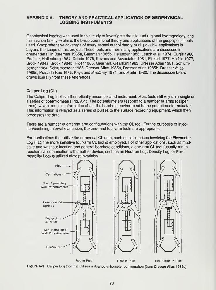
APPENDIX A. THEORY AND PRACTICAL APPLICATION OF GEOPHYSICALLOGGING INSTRUMENTS

Geophysical logging was used in this study to investigate the site and regional hydrogeology, andthis section briefly explains the basic operational theory and applications of the geophysical tools

used. Comprehensive coverage of every aspect of tool theory or all possible applications is

beyond the scope of this project. These tools and their many applications are discussed in

greater detail in Bateman 1985a, Bateman 1985b, Helander 1983, Leach et al. 1974, Curtis 1966,

Peebler, Hallenburg 1984, Dobrin 1976, Kovacs and Associates 1981, Pickett 1977, Hilchie 1977,

Brock 1984a, Brock 1984b, Rider 1986, Gearhart, Gearhart 1983, Dresser Atlas 1981, Schlum-

berger 1984, Schlumberger 1985, Dresser Atlas 1985a, Dresser Atlas 1985b, Dresser Atlas

1985c, Prasada Rao 1985, Keys and MacCary 1971, and Martin 1982. The discussion below

draws liberally from these references.

Caliper Log (CL)

The Caliper Log tool is a theoretically uncomplicated instrument. Most tools still rely on a single or

a series of potentiometers (fig. A-1). The potentiometers respond to a number of arms (caliper

arms), which transmit information about the borehole environment to the potentiometer actuator.

This information is relayed as a series of pulses to the surface recording equipment, which then

processes the data.

There are a number of different arm configurations with the CL tool. For the purposes of injec-

tion/confining interval evaluation, the one- and four-arm tools are appropriate.

For applications that utilize the numerical CL data, such as calculations involving the Flowmeter

Log (FL), the more sensitive four-arm CL tool is employed. For other applications, such as mud-cake and washout location and general borehole conditions, a one-arm CL tool (usually run in

mechanical combination with another device, such as an Neutron Log, Density Log, or Per-

meability Log) is utilized almost invariably.

Pipe

Centralizer

Max. Remaining

Wall Potentiometer

CompressionSprings

Feeler Arm40 or 60

Min. RemainingWall Potentiometer

Centralizer

Round Pipe Hole in Pipe Restriction in Pipe

Figure A-1 Caliper Log tool that utilizes a dual potentiometer configuration (from Dresser Atlas 1 985c)

70

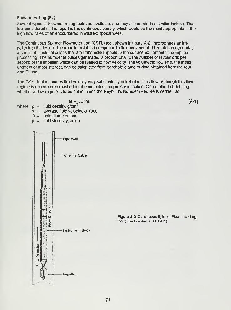
Flowmeter Log (FL)

Several types of Flowmeter Log tools are available, and they all operate in a similar fashion. Thetool considered in this report is the continuous variety, which would be the most appropriate at the

high flow rates often encountered in waste-disposal wells.

The Continuous Spinner Flowmeter Log (CSFL) tool, shown in figure A-2, incorporates an im-

peller into its design. The impeller rotates in response to fluid movement. This rotation generates

a series of electrical pulses that are transmitted uphole to the surface equipment for computer

processing. The number of pulses generated is proportional to the number of revolutions per

second of the impeller, which can be related to flow velocity. The volumetric flow rate, the meas-urement of most interest, can be calculated from borehole diameter data obtained from the four-

arm CL tool.

The CSFL tool measures fluid velocity very satisfactorily in turbulent fluid flow. Although this flow

regime is encountered most often, it nonetheless requires verification. One method of defining

whether a flow regime is turbulent is to use the Reynold's Number (Re). Re is defined as

Re= vDp/u.

where p = fluid density, g/cm3

v = average fluid velocity, cm/sec

D = hole diameter, cm|i = fluid viscosity, poise

[A-1]

*^ o

l.:l

Pipe Wall

Wireline Cable

Figure A-2 Continuous Spinner Flowmeter Logtool (from Dresser Atlas 1 981 ).

Instrument Body

Impeller

71

Re values of 3,000 or greater are used to represent turbulent flow in most literature dealing with

fluid flow. For most applications of the CSFLtool in injection/confining interval evaluation, fluid will

be injected at the surface to initiate impeller movement. A useful conversion in Re calculations is

v= (0.3637)Q/D2

[A-2]

where v = average fluid velocity, cm/sec

D = hole diameter, cmQ = flowrate, barrels per day

This conversion is combined with the definition of the Reynold's Number to yield

Re= (0.3637)Qp/u.D [A-3]

Gamma Ray Log (GRL)

As its name suggests, the GRL detects gamma rays—random, high-energy electromagnetic

waves emitted during the decay of unstable radioisotopes. The radioisotopes normally found in

rocks are40K and the daughter products of the uranium and thorium decay series. The GRL dis-

cussed here is unable to differentiate the contribution of each individual radioisotope to the total

intensity of gamma radiation.

The detector of the tool normally consists of a sodium iodide (Nal) crystal optically coupled to a

photomultiplier tube. Atoms of the Nal crystal absorb gamma ray collision energy, which places

the electrons of the atoms in a higher energy state. When the excited electrons lose this acquired

energy and fall back into their original state, they give off light that is converted to a voltage pulse

through the photomultiplier tube. These pulses are transmitted uphole and converted, on the ap-

propriate scale, to a measure of the gamma ray intensity.

Because of the high natural concentration of40K in clay minerals, shales generally exhibit a high

gamma ray intensity. On the other hand, sandstones and carbonates generally produce a lower

gamma ray count because of their relatively low concentration of clays and other highly radioac-

tive constituents. Because of this difference in gamma ray intensity, various lithologies can easily

be identified (allowing correlation of lithologic units), and a rock unit's shale volume can be deter-

mined.

During phase I logging, a GRL that used a Geiger Mueller type of detector was run. The Geiger

Mueller replaced the Scintillation type of detector employed in the previous GRL. This change

results in a smoother, less fluctuating GR, which provides a better estimate of the formation's

natural gamma ray activity (GR, measured in API units).

Sonic Log (SL)

The Sonic Log is an acoustic device that generates acoustic waves and measures reflected

acoustic waves. The measurements taken from the SL tool are the direct result of the propagation

of acoustic (elastic) waves through the borehole environment. The two important waves to the SLtool are the compressional (longitudinal) and the shear (transverse) waves.

The initial energy to produce the sound (acoustic) waves is generated by the transmitter (T) por-

tion of the tool (fig. A-3). The velocity of a shear wave (Vs) is given by:

Vs= (u/p)05

[A-4]

where u. = modulus of shear for the medium

p = density of the medium

72

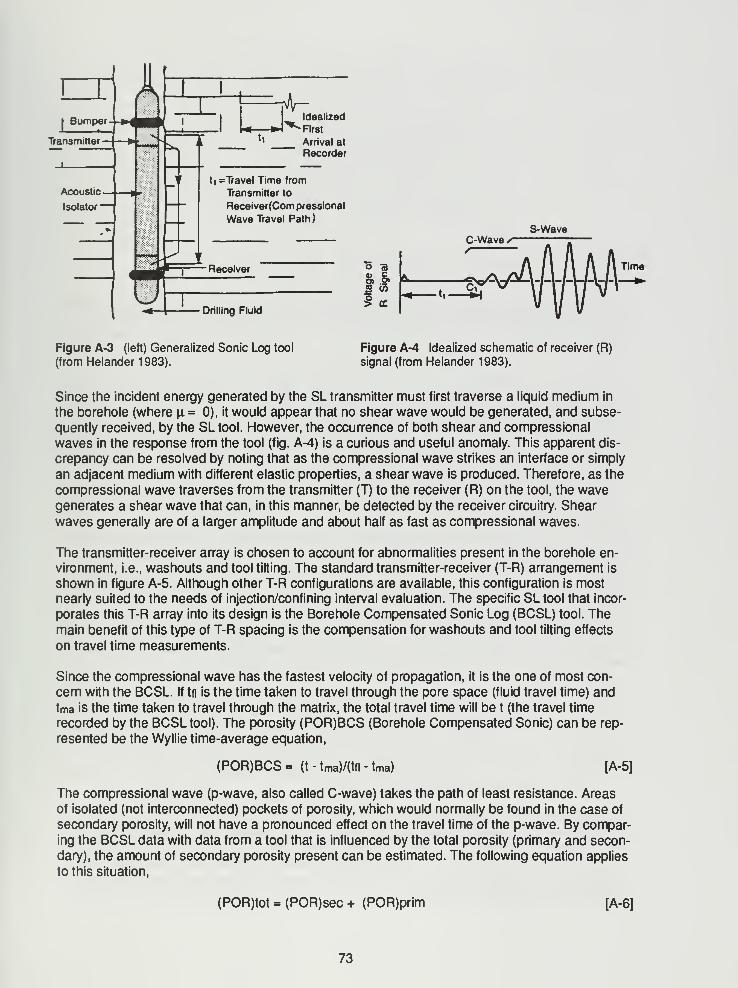
IBumper

Transmitter

Idealized

» First

Arrival at

Recorder

tt * Travel Time from

Transmitter to

Receiver(Com pressional

Wave Travel Path

)

S-Wave

Receiver

Drilling Fluid

Time

Figure A-3 (left) Generalized Sonic Log tool

(from Helander 1 983).

Figure A-4 Idealized schematic of receiver (R)

signal (from Helander 1983).

Since the incident energy generated by the SL transmitter must first traverse a liquid medium in

the borehole (where u. = 0), it would appear that no shear wave would be generated, and subse-

quently received, by the SL tool. However, the occurrence of both shear and compressional

waves in the response from the tool (fig. A-4) is a curious and useful anomaly. This apparent dis-

crepancy can be resolved by noting that as the compressional wave strikes an interface or simply

an adjacent medium with different elastic properties, a shear wave is produced. Therefore, as the

compressional wave traverses from the transmitter (T) to the receiver (R) on the tool, the wavegenerates a shear wave that can, in this manner, be detected by the receiver circuitry. Shear

waves generally are of a larger amplitude and about half as fast as compressional waves.

The transmitter-receiver array is chosen to account for abnormalities present in the borehole en-

vironment, i.e., washouts and tool tilting. The standard transmitter-receiver (T-R) arrangement is

shown in figure A-5. Although other T-R configurations are available, this configuration is mostnearly suited to the needs of injection/confining interval evaluation. The specific SL tool that incor-

porates this T-R array into its design is the Borehole Compensated Sonic Log (BCSL) tool. The

main benefit of this type of T-R spacing is the compensation for washouts and tool tilting effects

on travel time measurements.

Since the compressional wave has the fastest velocity of propagation, it is the one of most con-

cern with the BCSL. If tti is the time taken to travel through the pore space (fluid travel time) and

tma is the time taken to travel through the matrix, the total travel time will be t (the travel time

recorded by the BCSL tool). The porosity (POR)BCS (Borehole Compensated Sonic) can be rep-

resented be the Wyllie time-average equation,

(POR)BCS= (t-tma)/(tf|-tma) [A-5]

The compressional wave (p-wave, also called C-wave) takes the path of least resistance. Areas

of isolated (not interconnected) pockets of porosity, which would normally be found in the case of

secondary porosity, will not have a pronounced effect on the travel time of the p-wave. By compar-ing the BCSL data with data from a tool that is influenced by the total porosity (primary and secon-

dary), the amount of secondary porosity present can be estimated. The following equation applies

to this situation,

(POR)tot = (POR)sec + (POR)prim [A-6]

73

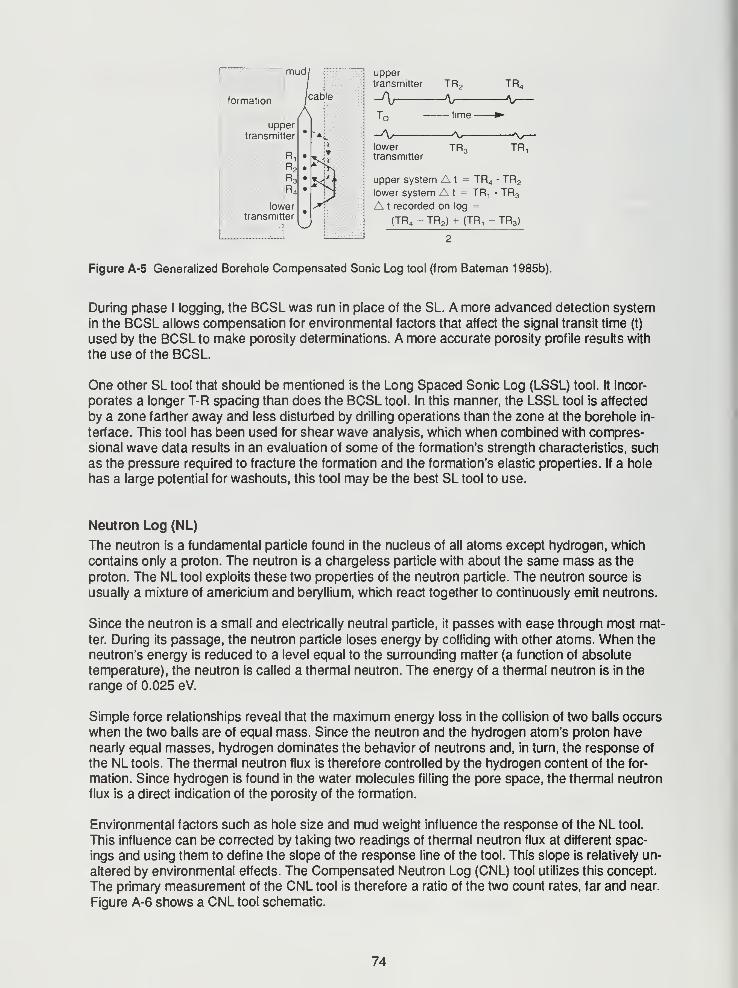
uppertransmitter TR2 TR4

-A/ \j V-Tr, time »-

-A, \r-

lower TR 3 TR,transmitter

upper system A t = TR4 - TR2

lower system A t = TR, - TR3

A t recorded on log =

(TR 4- TR2 ) + (TR, - TR 3 )

Figure A-5 Generalized Borehole Compensated Sonic Log tool (from Bateman 1985b).

During phase I logging, the BCSL was run in place of the SL. A more advanced detection system

in the BCSL allows compensation for environmental factors that affect the signal transit time (t)

used by the BCSL to make porosity determinations. A more accurate porosity profile results with

the use of the BCSL.

One other SL tool that should be mentioned is the Long Spaced Sonic Log (LSSL) tool. It incor-

porates a longer T-R spacing than does the BCSL tool. In this manner, the LSSL tool is affected

by a zone farther away and less disturbed by drilling operations than the zone at the borehole in-

terface. This tool has been used for shear wave analysis, which when combined with compres-

sional wave data results in an evaluation of some of the formation's strength characteristics, such

as the pressure required to fracture the formation and the formation's elastic properties. If a hole

has a large potential for washouts, this tool may be the best SL tool to use.

Neutron Log (NL)

The neutron is a fundamental particle found in the nucleus of all atoms except hydrogen, which

contains only a proton. The neutron is a chargeless particle with about the same mass as the

proton. The NLtool exploits these two properties of the neutron particle. The neutron source is

usually a mixture of americium and beryllium, which react together to continuously emit neutrons.

Since the neutron is a small and electrically neutral particle, it passes with ease through most mat-

ter. During its passage, the neutron particle loses energy by colliding with other atoms. When the

neutron's energy is reduced to a level equal to the surrounding matter (a function of absolute

temperature), the neutron is called a thermal neutron. The energy of a thermal neutron is in the

range of 0.025 eV.

Simple force relationships reveal that the maximum energy loss in the collision of two balls occurs

when the two balls are of equal mass. Since the neutron and the hydrogen atom's proton have

nearly equal masses, hydrogen dominates the behavior of neutrons and, in turn, the response of

the NL tools. The thermal neutron flux is therefore controlled by the hydrogen content of the for-

mation. Since hydrogen is found in the water molecules filling the pore space, the thermal neutron

flux is a direct indication of the porosity of the formation.

Environmental factors such as hole size and mud weight influence the response of the NL tool.

This influence can be corrected by taking two readings of thermal neutron flux at different spac-

ings and using them to define the slope of the response line of the tool. This slope is relatively un-

altered by environmental effects. The Compensated Neutron Log (CNL) tool utilizes this concept.

The primary measurement of the CNL tool is therefore a ratio of the two count rates, far and near.

Figure A-6 shows a CNL tool schematic.

74

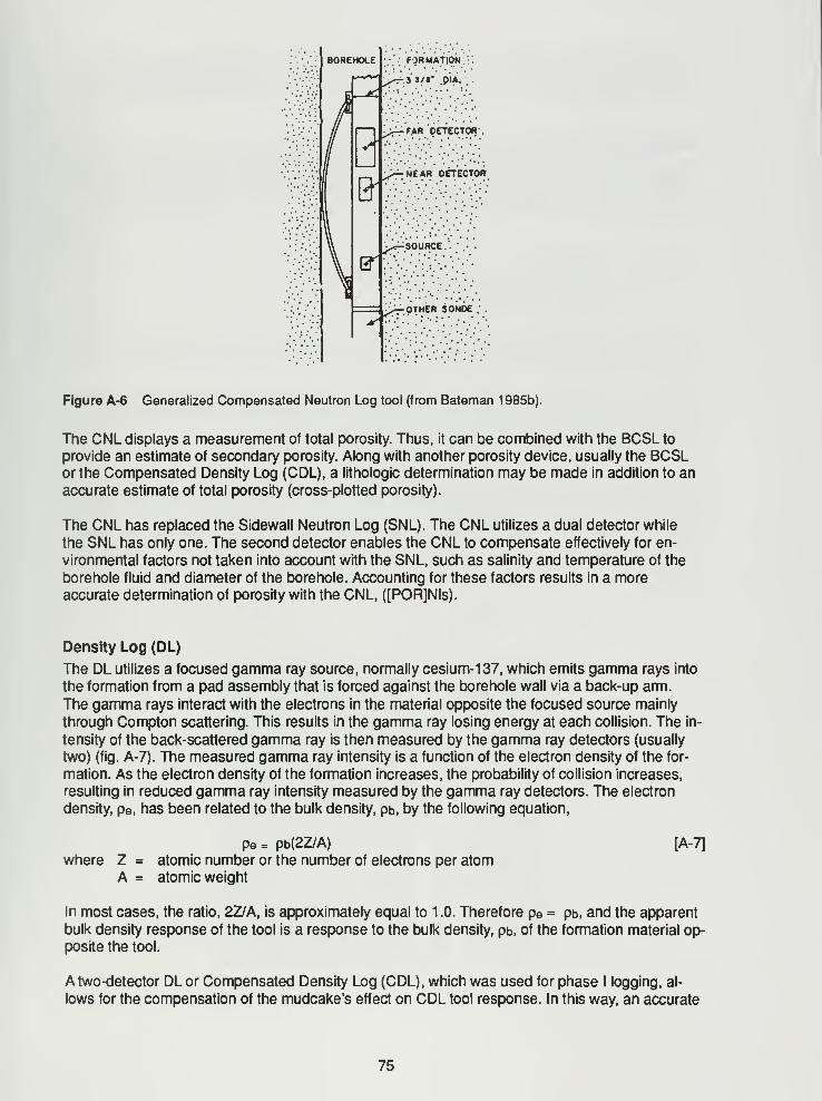
FORMATION.

3S/I* OIA.

^r-FAR DETECTOR .

NEAR DETECTOR-

SOURCE..

OTHER SONDE

Figure A-6 Generalized Compensated Neutron Log tool (from Bateman 1 985b).

The CNL displays a measurement of total porosity. Thus, it can be combined with the BCSL to

provide an estimate of secondary porosity. Along with another porosity device, usually the BCSLor the Compensated Density Log (CDL), a lithologic determination may be made in addition to an

accurate estimate of total porosity (cross-plotted porosity).

The CNL has replaced the Sidewall Neutron Log (SNL). The CNL utilizes a dual detector while

the SNL has only one. The second detector enables the CNL to compensate effectively for en-

vironmental factors not taken into account with the SNL, such as salinity and temperature of the

borehole fluid and diameter of the borehole. Accounting for these factors results in a moreaccurate determination of porosity with the CNL, ([PORJNIs).

Density Log (DL)

The DL utilizes a focused gamma ray source, normally cesium-137, which emits gamma rays into

the formation from a pad assembly that is forced against the borehole wall via a back-up arm.

The gamma rays interact with the electrons in the material opposite the focused source mainly

through Compton scattering. This results in the gamma ray losing energy at each collision. The in-

tensity of the back-scattered gamma ray is then measured by the gamma ray detectors (usually

two) (fig. A-7). The measured gamma ray intensity is a function of the electron density of the for-

mation. As the electron density of the formation increases, the probability of collision increases,

resulting in reduced gamma ray intensity measured by the gamma ray detectors. The electron

density, pe , has been related to the bulk density, pt>, by the following equation,

pe= pb(2Z/A)

where Z = atomic number or the number of electrons per atomA = atomic weight

[A-7]

In most cases, the ratio, 2Z/A, is approximately equal to 1 .0. Therefore pe = pb, and the apparent

bulk density response of the tool is a response to the bulk density, pb, of the formation material op-

posite the tool.

A two-detector DL or Compensated Density Log (CDL), which was used for phase I logging, al-

lows for the compensation of the mudcake's effect on CDL tool response. In this way, an accurate

75

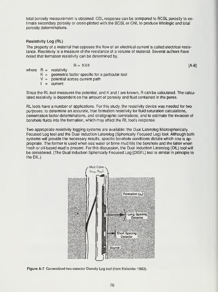
total porosity measurement is obtained. CDL response can be compared to BCSL porosity to es-

timate secondary porosity or cross-plotted with the BCSL or CNL to produce lithologic and total

porosity determinations.

Resistivity Log (RL)

The property of a material that opposes the flow of an electrical current is called electrical resis-

tance. Resistivity is a measure of the resistance of a volume of material. Several authors have

noted that formation resistivity can be determined by,

R = KV/I [A-8]

where R = resistivity

K = geometric factor specific for a particular tool

V = potential across current path

I = current.

Since the RL tool measures the potential, and K and I are known, R can be calculated. The calcu-

lated resistivity is dependent on the amount of porosity and fluid contained in the pores.

RL tools have a number of applications. For this study, the resistivity device was needed for two

purposes: to determine an accurate, true formation resistivity for fluid saturation calculations,

cementation factor determinations, and stratigraphic correlations; and to estimate the invasion of

borehole fluids into the formation, which may affect the RL tool's response.

Two appropriate resistivity logging systems are available: the Dual Laterolog Microspherically

Focused Log tool and the Dual Induction Laterolog (Spherically Focused Log) tool. Although both

systems will provide the necessary results, specific borehole conditions dictate which one is ap-

propriate. The former is used when sea water or brine mud fills the borehole and the latter whenfresh or oil-based mud is present. For this discussion, the Dual Induction Laterolog (DIL) tool will

be considered. (The Dual Induction Spherically Focused Log [DISFL] tool is similar in principle to

the DIL.)

Mud Cake

Figure A-7 Generalized two-detector Density Log tool (from Helander 1 983).

76

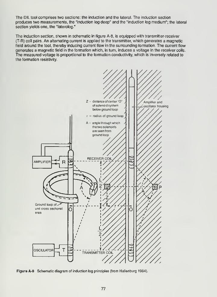
The DIL tool comprises two sections: the induction and the lateral. The induction section

produces two measurements, the "induction log deep" and the "induction log medium"; the lateral

section yields one, the "laterolog."

The induction section, shown in schematic in figure A-8, is equipped with transmitter-receiver

(T-R) coil pairs. An alternating current is applied to the transmitter, which generates a magnetic

field around the tool, thereby inducing current flow in the surrounding formation. The current flow

generates a magnetic field in the formation which, in turn, induces a voltage in the receiver coils.

The measured voltage is proportional to the formation conductivity, which is inversely related to

the formation resistivity.

AMPLIFIER

Ground loop of

.

unit cross sectional

area

OSCILLATOR

/Amplifier and

-Zoscillator housing

Figure A-8 Schematic diagram of induction log principles (from Hallenburg 1984).

77

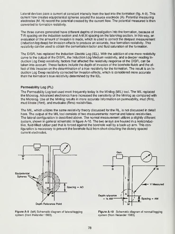
Lateral devices pass a current of constant intensity from the tool into the formation (fig. A-9). This

current flow creates equipotential spheres around the source electrode (A). Potential measuring

electrodes (M, N) record the potential created by the current flow. The potential measured is then

converted to formation resistivity.

The three curves generated have different depths of investigation into the formation, because of

T-R spacing on the induction section and A-M.N spacing on the laterolog section. In this way, an

evaluation of the amount of invasion is made, which is used to correct the deepest measurement(induction log deep) for invasion effects to produce an accurate, true formation resistivity. This

resistivity can be used to obtain the cementation factor and fluid saturation of the formation.

The DISFL has replaced the Induction Electric Log (I EL). With the addition of one more resistivity

curve to the output of the DISFL, the Induction Log Medium resistivity, and a deeper reading In-

duction Log Deep resistivity, factors that affected the resistivity response of the DISFL can be

taken into account. These factors include the depth of invasion of the borehole fluids and the ef-

fect of this invasion on the determination of a true resistivity for the formation. The result is an In-

duction Log Deep resistivity corrected for invasion effects, which is considered more accurate

than the formation's true resistivity determined by the IEL.

Permeability Log (PL)

The Permeability Log tool used most frequently today is the Minilog (MIL) tool. The MIL replaced

the Microlog. Advanced electronics have increased the sensitivity of the Minilog as compared with

the Microlog. Use of the Minilog results in more accurate information on permeability, mud (Rm),

mud filtrate (Rmf), and mudcake (Rmc) resistivities.

The MIL, which utilizes the same resistivity theory discussed for the RL, is not discussed in detail

here. The output of the MIL tool consists of two measurements: normal and lateral resistivities.

The lateral configuration is described above. The normal measurement utilizes a slightly different

system, shown in general schematic in figure A-10. The two arrays are housed in a nonconduc-

tive, fluid-filled rubber pad that is forced against the borehole wall by a back-up arm. This con-

figuration is necessary to prevent the borehole fluid from short-circuiting the closely spaced

current electrodes.

Equipotential

Spheres

Spacing = AO

Depth Reference Point

V Measured

Depth reference '

= V4AM \> Spacing = AM

Figure A-9 (left) Schematic diagram of lateral logging

system (from Helander 1 983).

Figure A-10 Schematic diagram of normal logging

system (from Helander 1 983)

78

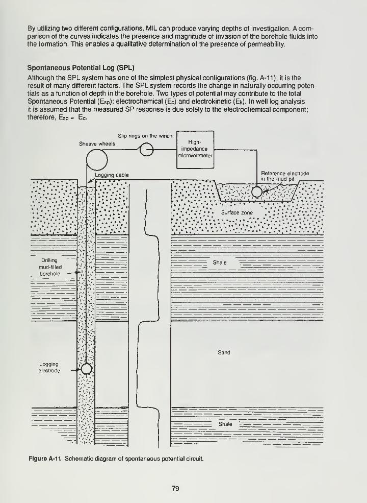
By utilizing two different configurations, MIL can produce varying depths of investigation. A com-parison of the curves indicates the presence and magnitude of invasion of the borehole fluids into

the formation. This enables a qualitative determination of the presence of permeability.

Spontaneous Potential Log (SPL)

Although the SPL system has one of the simplest physical configurations (fig. A-11), it is the

result of many different factors. The SPL system records the change in naturally occurring poten-

tials as a function of depth in the borehole. Two types of potential may contribute to the total

Spontaneous Potential (ESp): electrochemical (Ec) and electrokinetic (Ek). In well log analysis

it is assumed that the measured SP response is due solely to the electrochemical component;therefore, ESp = Ec .

Slip rings on the winch

Sheave wheels

r

T» • • •

, • «

Drilling

mud-filled

borehole,i

, v r

-I

/-

Logging

electrode

14V- /

-

'l

1

1

» ..

Lx '

o-High-

impedance

microvoltmeter

Logging cable

y\ . .* »

,

I

- I \, -

- V ~ v

'm /fcri-s7 .

« » .

» » « »

. « « »

. a »

» «« « * »

• 4 4

. » » * « « « -v ^ \ — // <

• • • '*\\ •"

"'V- J M >, *»

J

Reference electrodein the mud pit

N /

• J - '. I »

• • » Surface zone» «

4 4 •

4 4

t *

4 *

4 ».'4 »

Shale

Sand

Figure A-11 Schematic diagram of spontaneous potential circuit.

79

The electrochemical potential is composed of the membrane potential (Em ) and the liquid junction

potential (Ej). The membrane potential is caused by the separation of two fluids of different ac-

tivity by a permeable, charged membrane. An analogy might be mud and formation water

separated by shale. The liquid junction potential is the result of the contact of two solutions of dif-

fering activity, such as mud filtrate and formation water.

The ESp is commonly written as

ESp= -Kclog(Rmf/Rw) [A-9]

where Kc = 61 + 0.133T(°F)

Rmf = mud filtrate resistivity

Rw = formation water resistivity.

This equation illustrates one application of the SPL system, namely Rw determination. The other

applications relevant to this study are stratigraphic correlation and qualitative permeability estima-

tion. The latter two are available through a consideration of the fluids and formation materials that

give rise to the membrane and liquid junction potentials.

Temperature Log (TL)

The TL tool is simply a device that records the magnitude of the subsurface temperature. This is

accomplished by incorporating into the tool's design a sensor element that provides ultrasensi-

tive, stable readings over a suitable temperature range. A temperature probe in contact with the

borehole environment transmits the thermal energy to the sensor, which converts the energy to a

signal coverted by the surface equipment to absolute and differential temperature. These data

can be useful to injection/confining interval evaluation in several ways. First, in many injection

wells the temperature of the injection fluid is anomalously cooler than the native formation

temperature. This anomaly can often be detected by the TL, providing another method, along with

the CSFL, for delineating the location of fluid infiltration into a formation. Also, data from the TLprovide temperature values to be used in the selection of appropriate temperature-corrected fluid

and formation parameters (such as fluid density and water compressibility) necessary in many cal-

culations.

Radioactive Tracer Log (RATL)

The Radioactive Tracer Log tool "traces" the movement of a radioactive source. This is ac-

complished by injecting a short-lived, radioactive isotope (usually131

l) from one section of the

tool and recording its movement with a detection gamma ray package housed in another section

of the tool. As the radioactive isotope decays, it emits gamma rays that are detected by the

gamma ray apparatus. It is in this way that the position of the radioactive "slug" can be monitored

as it makes its way through the cased and uncased borehole. Thus it is another technique for

delineating fluid flow within the injection zone.

80

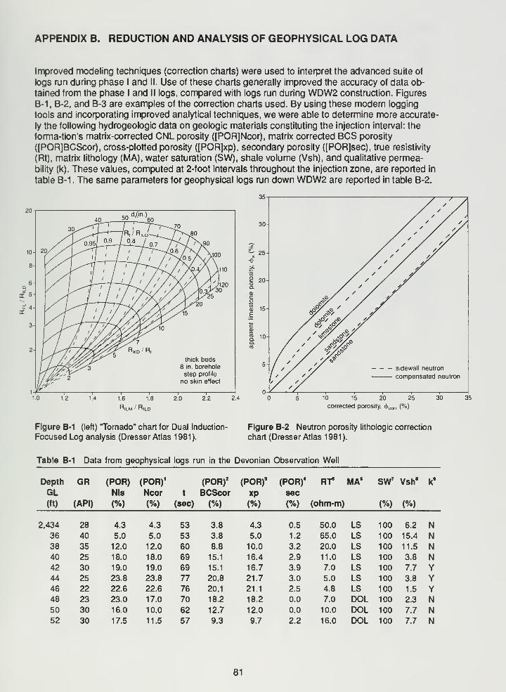
APPENDIX B. REDUCTION AND ANALYSIS OF GEOPHYSICAL LOG DATA

Improved modeling techniques (correction charts) were used to interpret the advanced suite of

logs run during phase I and II. Use of these charts generally improved the accuracy of data ob-

tained from the phase I and II logs, compared with logs run during WDW2 construction. Figures

B-1, B-2, and B-3 are examples of the correction charts used. By using these modern logging

tools and incorporating improved analytical techniques, we were able to determine more accurate-

ly the following hydrogeologic data on geologic materials constituting the injection interval: the

forma-tion's matrix-corrected CNL porosity ([POR]Ncor), matrix corrected BCS porosity

([POR]BCScor), cross-plotted porosity ([POR]xp), secondary porosity ([POR]sec), true resistivity

(Rt), matrix lithology (MA), water saturation (SW), shale volume (Vsh), and qualitative permea-

bility (k). These values, computed at 2-foot intervals throughout the injection zone, are reported in

table B-1 . The same parameters for geophysical logs run down WDW2 are reported in table B-2.

Figure B-1 (left) "Tornado" chart for Dual Induction-

Focused Log analysis (Dresser Atlas 1 981 ).

Figure B-2 Neutron porosity lithologic correction

chart (Dresser Atlas 1 981 ).

Table B-1 Data from geophysical logs run in the Devonian Observation Well

Depth GR (POR) (POR)1

(POR)2

(POR)3

(POR)4

RT* MAS SW7Vsh

ak9

GL NIs Ncor t BCScor xp sec

(ft) (API) (%) (%) (sec) (%) (%) (%) (ohm-m) (%) (%)

2,434 28 4.3 4.3 53 3.8 4.3 0.5 50.0 LS 100 6.2 N36 40 5.0 5.0 53 3.8 5.0 1.2 65.0 LS 100 15.4 N38 35 12.0 12.0 60 8.8 10.0 3.2 20.0 LS 100 11.5 N40 25 18.0 18.0 69 15.1 16.4 2.9 11.0 LS 100 3.8 N42 30 19.0 19.0 69 15.1 16.7 3.9 7.0 LS 100 7.7 Y44 25 23.8 23.8 77 20.8 21.7 3.0 5.0 LS 100 3.8 Y46 22 22.6 22.6 76 20.1 21.1 2.5 4.8 LS 100 1.5 Y48 23 23.0 17.0 70 18.2 18.2 0.0 7.0 DOL 100 2.3 N50 30 16.0 10.0 62 12.7 12.0 0.0 10.0 DOL 100 7.7 N52 30 17.5 11.5 57 9.3 9.7 2.2 16.0 DOL 100 7.7 N

81

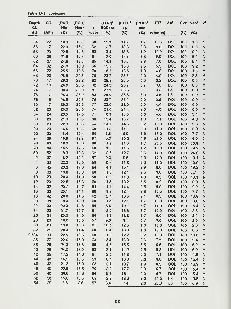
Table B-1 continued

Depth GR (POR) (POR)1

(POR)2

(POR)3

(POR)4 RT9 MA6 SW7

Vsh8k9

GL NIs Ncor t BCScor XP sec

(ft) (API) (%) (%) (sec) (%) (%) (%) (ohm-m) (%) (%)

54 22 19.0 13.0 60 11.3 11.7 1.7 13.0 DOL 100 1.5 N56 17 22.0 16.0 62 12.7 13.3 3.3 9.0 DOL 100 0.0 N58 20 20.6 14.6 63 13.4 13.6 1.2 10.0 DOL 100 0.0 N60 28 21.8 15.8 61 12.0 12.7 3.8 9.0 DOL 100 6.2 N62 27 24.6 18.6 65 14.8 15.6 3.8 7.0 DOL 100 5.4 Y64 32 24.0 18.0 66 15.5 16.0 2.5 5.5 DOL 100 9.2 Y66 22 25.5 19.5 70 18.2 18.5 1.3 4.8 DOL 100 1.5 Y68 23 28.5 22.5 78 23.7 23.5 0.0 4.0 DOL 100 2.3 Y70 17 29.2 23.2 82 26.5 26.0 0.0 3.3 DOL 100 0.0 Y72 18 28.0 28.0 82 24.3 25.7 3.7 3.0 LS 100 0.0 Y74 17 30.0 30.0 87 27.9 28.8 2.1 3.2 LS 100 0.0 Y76 17 28.0 28.0 83 25.0 26.3 3.0 3.5 LS 100 0.0 Y78 19 26.8 20.8 78 23.7 23.2 0.0 3.9 DOL 100 0.0 Y80 17 26.3 20.3 77 23.0 22.6 0.0 4.4 DOL 100 0.0 Y82 20 29.0 23.0 74 21.0 21.4 2.0 4.0 DOL 100 0.0 Y84 24 23.5 17.5 71 18.9 18.5 0.0 4.6 DOL 100 3.1 Y86 26 21.3 15.3 63 13.4 13.7 1.9 7.1 DOL 100 4.6 N88 23 22.3 16.3 64 14.1 14.5 2.2 10.0 DOL 100 2.3 N90 23 16.5 10.5 60 11.3 11.1 0.0 11.0 DOL 100 2.3 N92 30 16.4 10.4 56 8.6 8.9 1.8 16.0 DOL 100 7.7 N94 29 19.8 13.8 57 9.3 10.2 4.5 21.0 DOL 100 6.9 N96 60 19.0 13.0 60 11.3 11.6 1.7 20.0 DOL 100 30.8 N98 84 18.5 12.5 60 11.3 11.5 1.2 15.0 DOL 100 49.2 N50 52 19.3 13.3 62 12.7 12.7 0.6 14.0 DOL 100 24.6 N2 37 18.2 12.2 57 9.3 9.8 2.9 14.0 DOL 100 13.1 N4 33 22.0 16.0 59 10.7 11.8 5.3 11.0 DOL 100 10.0 N6 45 23.0 17.0 64 14.1 15.1 2.9 8.0 DOL 100 19.2 N8 30 19.8 13.8 60 11.3 12.1 2.5 9.0 DOL 100 7.7 N

10 23 20.0 14.0 58 10.0 11.3 4.0 8.5 DOL 100 13.1 N12 20 22.8 16.8 60 11.3 13.2 5.5 8.2 DOL 100 0.0 N14 32 20.7 14.7 64 14.1 14.4 0.6 9.0 DOL 100 9.2 N16 30 20.1 14.1 60 11.3 12.4 2.8 10.5 DOL 100 7.7 N18 42 20.8 14.8 62 12.7 13.6 2.1 8.5 DOL 100 16.9 N20 38 19.0 13.0 60 11.3 12.1 1.7 10.0 DOL 100 13.8 N22 30 20.3 14.3 56 8.6 10.4 5.7 11.0 DOL 100 15.4 N24 23 21.7 15.7 61 12.0 13.3 3.7 10.0 DOL 100 2.3 N26 24 20.0 14.0 60 11.3 12.2 2.7 8.0 DOL 100 3.1 N28 23 16.0 10.0 57 9.3 9.7 0.7 9.0 DOL 100 2.3 N30 23 19.0 13.0 61 12.0 12.5 1.0 10.0 DOL 100 2.3 N32 21 20.4 14.4 63 13.4 13.8 1.0 12.0 DOL 100 0.8 Y

2,534 33 22.5 16.5 60 11.3 12.2 5.2 10.0 DOL 100 10.0 Y36 27 22.0 16.0 63 13.4 13.9 2.6 7.5 DOL 100 5.4 Y38 28 24.3 18.3 65 14.8 15.5 3.5 6.5 DOL 100 6.2 Y40 29 24.0 18.0 63 13.4 14.2 4.6 5.8 DOL 100 6.9 Y42 35 17.3 11.3 61 12.0 11.8 0.0 7.1 DOL 100 11.5 N44 40 16.5 10.5 59 10.7 10.6 0.0 9.0 DOL 100 15.4 N46 42 21.3 15.3 63 13.4 13.7 1.9 8.5 DOL 100 16.9 Y48 40 22.5 16.5 70 18.2 17.7 0.0 6.7 DOL 100 15.4 Y50 40 20.6 14.6 66 15.5 15.1 0.0 6.7 DOL 100 15.4 Y52 38 15.6 15.6 65 12.3 13.3 3.3 10.0 LS 100 13.8 N54 29 8.6 8.6 57 6.6 7.4 2.0 20.0 LS 100 6.9 N

82

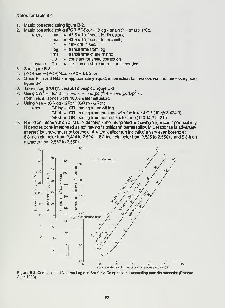
Notes for table B-1

Matrix corrected using figure B-2.

Matrix corrected using (POR)BCScor = (tlog

where 47.6 x 10~6 sec/ft for limestone-6

tma)/(tf1 -tma)x1/Cp,

43.5 x 10 sec/ft for dolomite

189 X10"6sec/ft

transit time from log

transit time of the matrix

constant for shale correction

1 , since no shale correction is needed

tmatmatfl

tlog

tmaCp

assume CpSee figure B-3

(POR)sec = (POR)Ncor - (POR)BCScorSince Rilm and Rild are approximately equal, a correction for invasion was not necessary; seefigure B-1

Taken from (POR)N versus t crossplot, figure B-3

Using SW2 = Ro/Rt= FRw/Rt= Rw/(por)2Rt= Rw/(por)xp

2Rt,

from this, all zones were 100% water saturated.

Using Vsh = (GRIog - GRc1)/(GRsh - GRd),where GRIog = GR reading taken off log.

GRcl = GR reading from the zone with the lowest GR (1 @ 2,474 ft).

GRsh = GR reading from nearest shale zone (140 @ 2,242 ft).

Based on interpretation of MIL, Y denotes zone interpreted as having "significant" permeability.

N denotes zone interpreted as not having "significant" permeability. MIL response is adversely

affected by unevenness of borehole. A 4-arm caliper run indicated a very even borehole:

6.3-inch diameter from 2,424 to 2,524 ft, 6.2-inch diameter from 2,525 to 2,556 ft, and 5.8-inch

diameter from 2,557 to 2,560 ft.

40-i

35-

_ 30

25

O) 20-

!S 15

10--

5H

-10 10 20 30 40

compensated neutron apparent limestone porosity (%)

Figure B-3 Compensated Neutron Log and Borehole Compensated Acoustilog porosity crossplot (Dresser

Atlas 1983).

83

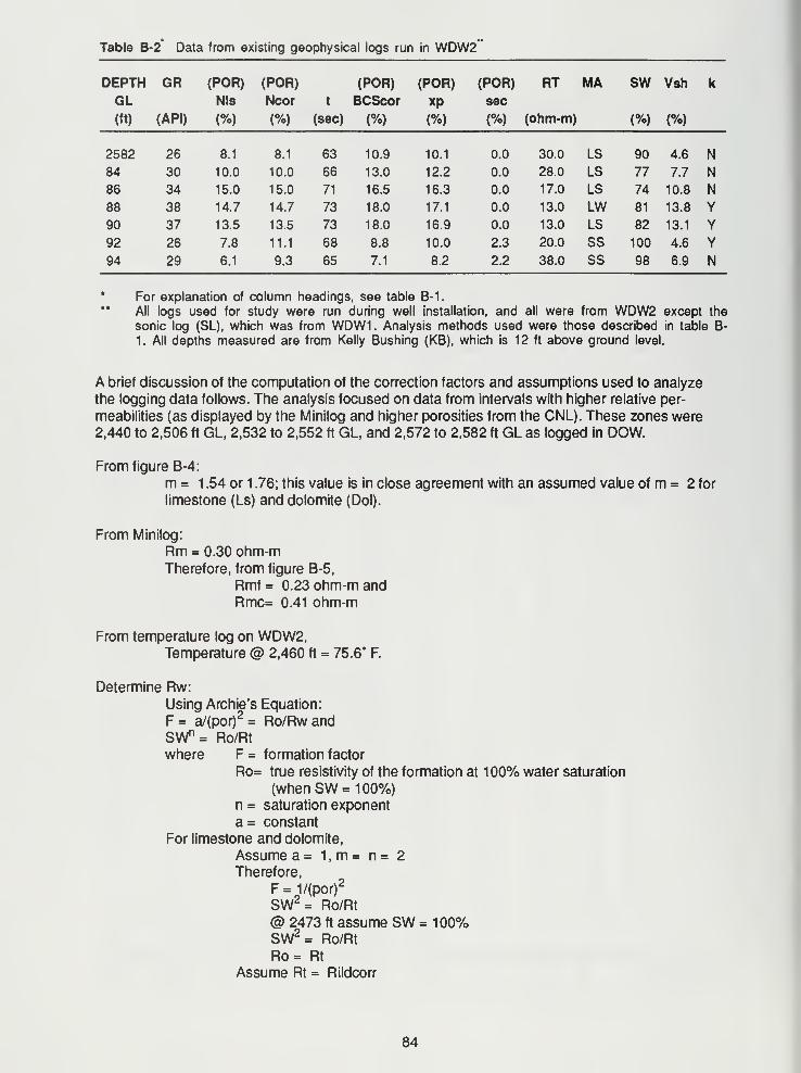
Table B-2 Data from existing geophysical logs run in WDW2

DEPTH GR (POR) (POR) (POR) (POR) (POR) RT MA sw Vsh k

GL NIs Ncor t BCScor xp sec

(ft) (API) (%) (%) (sec) (%) (%) (%) (ohm-m) (%) (%)

2582 26 8.1 8.1 63 10.9 10.1 0.0 30.0 LS 90 4.6 N

84 30 10.0 10.0 66 13.0 12.2 0.0 28.0 LS 77 7.7 N86 34 15.0 15.0 71 16.5 16.3 0.0 17.0 LS 74 10.8 N

88 38 14.7 14.7 73 18.0 17.1 0.0 13.0 LW 81 13.8 Y

90 37 13.5 13.5 73 18.0 16.9 0.0 13.0 LS 82 13.1 Y92 26 7.8 11.1 68 8.8 10.0 2.3 20.0 SS 100 4.6 Y94 29 6.1 9.3 65 7.1 8.2 2.2 38.0 SS 98 6.9 N

For explanation of column headings, see table B-1

.

All logs used for study were run during well installation, and all were from WDW2 except the

sonic log (SL), which was from WDW1. Analysis methods used were those described in table B-

1. All depths measured are from Kelly Bushing (KB), which is 12 ft above ground level.

A brief discussion of the computation of the correction factors and assumptions used to analyze

the logging data follows. The analysis focused on data from intervals with higher relative per-

meabilities (as displayed by the Minilog and higher porosities from the CNL). These zones were2,440 to 2,506 ft GL, 2,532 to 2,552 ft GL, and 2,572 to 2,582 ft GL as logged in DOW.

From figure B-4:

m = 1 .54 or 1 .76; this value is in close agreement with an assumed value of m = 2 for

limestone (Ls) and dolomite (Dol).

From Minilog:

Rm = 0.30 ohm-mTherefore, from figure B-5,

Rmf= 0.23 ohm-m andRmc= 0.41 ohm-m

From temperature log on WDW2,Temperature @ 2,460 ft = 75.6° F.

Determine Rw:

Using Archie's Equation:

F= a/(por)2 = Ro/Rwand

SWn = Ro/Rt

where F = formation factor

Ro= true resistivity of the formation at 100% water saturation

(when SW = 100%)n = saturation exponent

a= constant

For limestone and dolomite,

Assume a= 1,m= n= 2

Therefore,

F = 1/(por)2

SW2 = Ro/Rt

@ 2473 ft assume SW = 100%SW2 = Ro/Rt

Ro= Rt

Assume Rt = Rildcorr

84

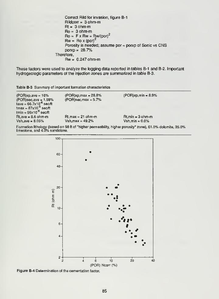
Correct Rild for invasion, figure B-1

Rildcorr= 3ohm-mRt= 3ohm-mRo = 3 ohm-mRo = FxRw = Rw/(por)

2

Rw = Ro x (por)2

Porosity is needed; assume por = porxp of Sonic vs CNSporxp= 28.7%

Therefore,

Rw= 0.247 ohm-m

These factors were used to analyze the logging data reported in tables B-1 and B-2. Important

hydrogeologic parameters of the injection zones are summarized in table B-3.

Table B-3 Summary of important formation characteristics

(POR)xp,ave = 16%(POR)sec,ave = 1.98%tave = 66.7X10"

6sec/ft

tmax = 87x10"6

sec/ft

tmin = 56x10"6sec/ft

Rt.ave = 8.6 ohm-mVsh.ave = 8.05%

(POR)xp.max = 28.8%(POR)secmax = 5.7%

Rt.max = 21 ohm-mVsh.max = 49.2%

(POR)xp.min = 8.9%

Rt.min - 3 ohm-mVsh.min = 0.0%

Formation lithology (based on 98 ft of "higher permeability, higher porosity" zone), 61.0% dolomite, 35.0%limestone, and 4.0% sandstone.

100

60-

40

20-

10-

6-

4-

".I• •

• •'##•

-~r-

102 4 6

(POR) Ncorr (%)

Figure B-4 Determination of the cementation factor.

20 40

85

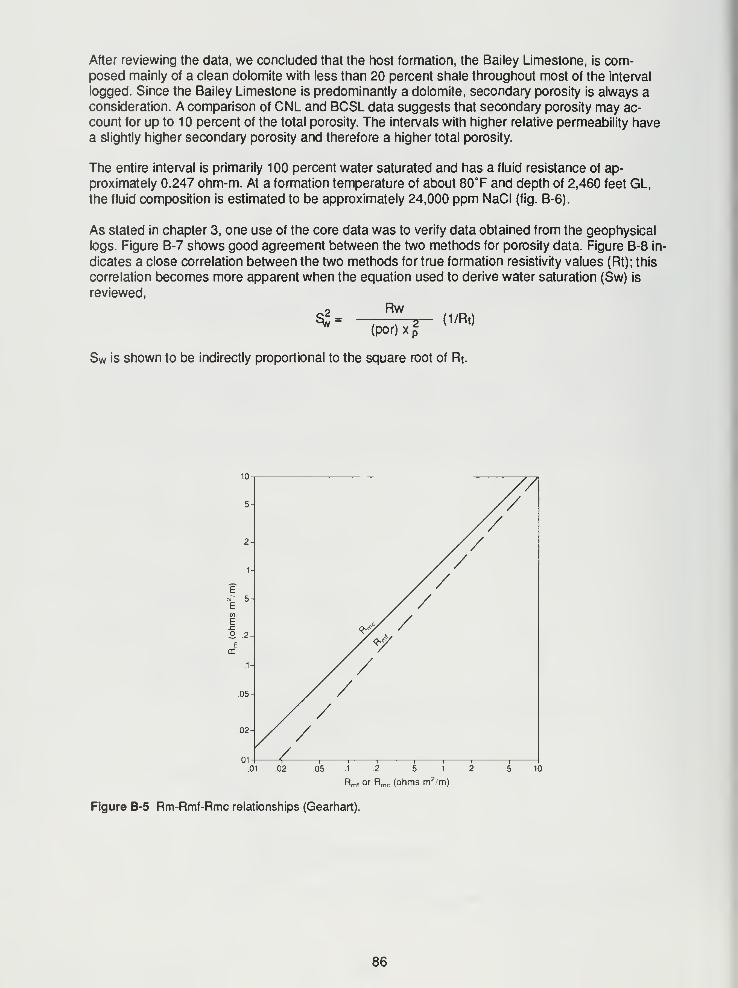
After reviewing the data, we concluded that the host formation, the Bailey Limestone, is com-posed mainly of a clean dolomite with less than 20 percent shale throughout most of the interval

logged. Since the Bailey Limestone is predominantly a dolomite, secondary porosity is always aconsideration. A comparison of CNL and BCSL data suggests that secondary porosity may ac-

count for up to 10 percent of the total porosity. The intervals with higher relative permeability have

a slightly higher secondary porosity and therefore a higher total porosity.

The entire interval is primarily 100 percent water saturated and has a fluid resistance of ap-

proximately 0.247 ohm-m. At a formation temperature of about 80°F and depth of 2,460 feet GL,

the fluid composition is estimated to be approximately 24,000 ppm NaCI (fig. B-6).

As stated in chapter 3, one use of the core data was to verify data obtained from the geophysical

logs. Figure B-7 shows good agreement between the two methods for porosity data. Figure B-8 in-

dicates a close correlation between the two methods for true formation resistivity values (Rt); this

correlation becomes more apparent when the equation used to derive water saturation (Sw) is

reviewed,

RwSS-

(por) x I

(1/Rt)

Sw is shown to be indirectly proportional to the square root of Rt.

.05 .1 .2 .5 1

Rm ,or Rmc (ohms m2/m)

10

Figure B-5 Rm-Rmf-Rmc relationships (Gearhart).

86

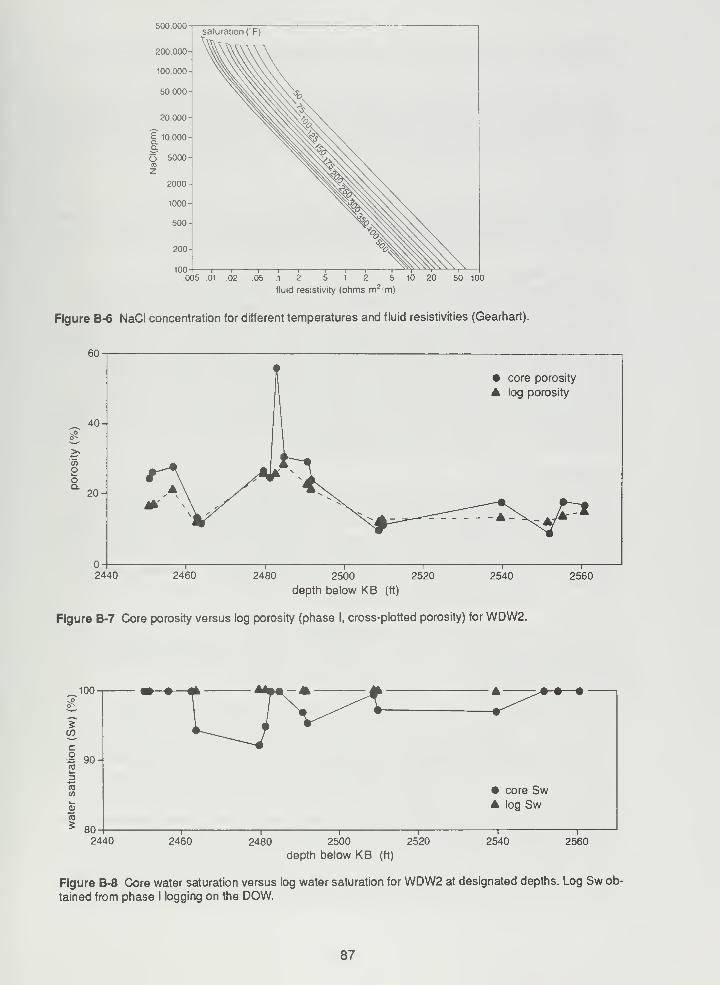
500.000saturation) F)

.005 01 .02 .05 .12 .5 12 5 10 20

fluid resistivity (ohms m2 m)

50 100

Figure B-6 NaCI concentration for different temperatures and fluid resistivities (Gearhart).

60

ooQ.

40-

20-

• core porosity

log porosity

2440 2460 2480 2500 2520

depth below KB (ft)

2540 2560

Figure B-7 Core porosity versus log porosity (phase I, cross-plotted porosity) for WDW2.

100

5

I 90 A

• core Swlog Sw

80-

2440 2460 2480 2500

depth below KB (ft)

2520 2540 2560

Figure B-8 Core water saturation versus log water saturation for WDW2 at designated depths. Log Sw ob-

tained from phase I logging on the DOW.

87

APPENDIX C. BRUCITE FORMATION: PROPOSED MECHANISM OF FORMATION

The hydrogeologic site descriptions developed from phase I and phase II data (see chapter 3) dif-

fered from each other significantly; however, the reason for these differences was not readily ap-

parent. To develop a hypothesis to explain the results and increase our understanding of the site

hydrogeology, we conducted additional analyses.

Core Analysis

Analysis of sidewall core obtained during phase II was critical to the development of a hypothesis

to explain the discrepancies described in chapter 3. Our core analysis included hydraulic testing,

mineralogic analysis, and scanning electron microscope (SEM) investigation.

Hydraulic Testing

Hydraulic testing provided no hard evidence to resolve the discrepancies between phase I and

phase II data. Injection zones 1, 2, and 3 (fig. C-1) had abnormally high porosities and per-

meabilities, but core analysis data did not agree with the results from the CSFL. First, the zone

from 2,468 to 2,496 feet KB showed some injection potential. Core analysis indicated that at least

some portions of this zone (e.g., 2,481 .0 ft KB) were not permeable enough to allow fluid flow;

however, most of this zone appeared to have sufficient permeability. Second, the core from

2539.5 feet KB seemed to have sufficient porosity and permeability to allow fluid flow, but the

CSFL did not show any flow at this location. On the basis of CSFL results, zone 3 should have

had the highest porosity and permeability, zone 2 the next highest, and zone 1 the lowest; how-

ever, core analysis indicated just the opposite. Therefore, the same discrepancies were en-

countered with core analysis as with geophysical logging.

Mineralogic Analysis

Cores were also analyzed for their mineralogical content. Brucite was found in the anomalouszones, and its presence was confirmed by x-ray diffraction (XRD) analysis. Brucite was not ex-

pected to be present in the injection system environment of WDW2. Brucite is normally found in

veins in serpentine and basic rocks and as flakes scattered through some marbles (Pough 1953).

Roy et al. (1989) analyzed a sample of the native formation brine taken from the DOW. Thesample was vastly undersaturated with respect to brucite, Mg(OH)2. The ion activity product of

Mg2+and OH" (brucite) in the sample was 3 percent of that predicted by the solubility of brucite

determined by thermodynamic modeling (Roy 1987).

Mineralogical analysis conducted on a few representative samples of the original well cuttings col-

lected during the drilling of WDW2 indicated that none of these samples contained brucite.

Downhole geophysical data (table 2) also confirmed the absence of brucite and indicated that

prior to injection, the disposal horizon was predominantly dolomitic.

Apparently the injected waste, which consisted of a number of organics in a very alkaline

(pH>l2), brinelike solution, created an environment in the injection system that promoted the for-

mation of brucite. Although the waste had a component of Mg2+, dolomite (from injection zone

rock) was the most likely source of Mg2+for two reasons. First, an increase in the brucite con-

centration accompanied a corresponding decrease in the dolomite concentration (fig. C-2).

Second, the porosity throughout the injection zone subsequent to brucite precipitation should

have been lower than the original (pre-injection) porosity if the brine was the source of the Mg2+.

Data from log analysis did not indicate a decrease in porosity. Therefore, on the basis of available

data, the most plausible hypothesis is that dissolution of dolomite from injection zone rock

released magnesium, which then combined with the OH" in the waste stream to form brucite.

If this hypothesis is correct, the zones that originally had the highest porosities and permeabilities

would accept the greatest volume of waste fluid and thus would show the highest brucite con-

88

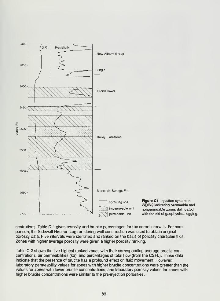
2300

2350-

2600

2650

2700

\M\\\\^1\\\\\\\

New Albany Group

Lingle

Grand Tower

Bailey Limestone

Moccasin Springs Fm

confining unit

impermeable unit

~ permeable unit

Figure C1 Injection system in

WDW2 indicating permeable and

nonpermeable zones delineated

with the aid of geophysical logging.

centrations. Table C-1 gives porosity and brucite percentages for the cored intervals. For com-parison, the Sidewall Neutron Log run during well construction was used to obtain original

porosity data. Five intervals were identified and ranked on the basis of porosity characteristics.

Zones with higher average porosity were given a higher porosity ranking.

Table C-2 shows the five highest ranked zones with their corresponding average brucite con-

centrations, air permeabilities (ka), and percentages of total flow (from the CSFL). These data

indicate that the presence of brucite has a profound effect on fluid movement. However,

laboratory permeability values for zones with higher brucite concentrations were greater than the

values for zones with lower brucite concentrations, and laboratory porosity values for zones with

higher brucite concentrations were similar to the pre-injection porosities.

89

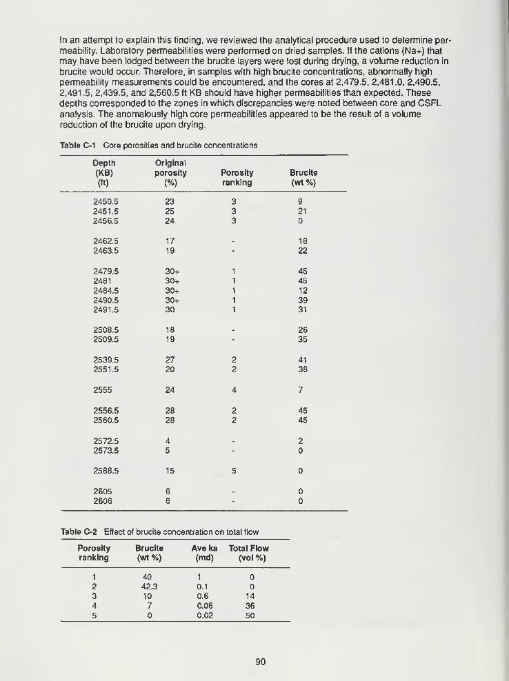
In an attempt to explain this finding, we reviewed the analytical procedure used to determine per-

meability. Laboratory permeabilities were performed on dried samples. If the cations (Na+) that

may have been lodged between the brucite layers were lost during drying, a volume reduction in

brucite would occur. Therefore, in samples with high brucite concentrations, abnormally high

permeability measurements could be encountered, and the cores at 2,479.5, 2,481 .0, 2,490.5,

2,491 .5, 2,439.5, and 2,560.5 ft KB should have higher permeabilities than expected. Thesedepths corresponded to the zones in which discrepancies were noted between core and CSFLanalysis. The anomalously high core permeabilities appeared to be the result of a volume

reduction of the brucite upon drying.

Table C-1 Core porosities and brucite concentrations

Depth

(KB)

(ft)

Original

porosity

(%)

Porosity

ranking

Table C-2 Effect of brucite concentration on total flow

Porosity Brucite Ave ka Total Flowranking (wt%) (md) (vol%)

Brucite

(wt %)

2450.5 23 3 9

2451.5 25 3 21

2456.5 24 3

2462.5 17 . 18

2463.5 19 - 22

2479.5 30+ 452481 30+ 45

2484.5 30+ 12

2490.5 30+ 392491.5 30 31

2508.5 18 . 262509.5 19 - 35

2539.5 27 2 41

2551.5 20 2 38

2555 24 4 7

2556.5 28 2 452560.5 28 2 45

2572.5 4 . 2

2573.5 5 -

2588.5 15 5

2605 6 .

2606 6 -

1 40 1

2 42.3 0.1

3 10 0.6 14

4 7 0.06 365 0.02 50

90

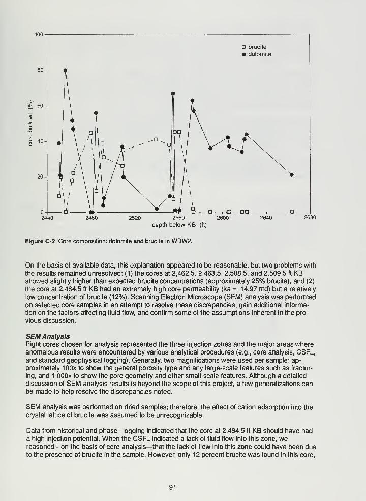
100

2440 2480 2520 2560

depth below KB (ft)

D —rO — DO2600 2640 2680

Figure C-2 Core composition: dolomite and brucite in WDW2.

On the basis of available data, this explanation appeared to be reasonable, but two problems with

the results remained unresolved: (1) the cores at 2,462.5, 2,463.5, 2,508.5, and 2,509.5 ft KBshowed slightly higher than expected brucite concentrations (approximately 25% brucite), and (2)

the core at 2,484.5 ft KB had an extremely high core permeability (ka = 14.97 md) but a relatively

low concentration of brucite (12%). Scanning Electron Microscope (SEM) analysis was performed

on selected core samples in an attempt to resolve these discrepancies, gain additional informa-

tion on the factors affecting fluid flow, and confirm some of the assumptions inherent in the pre-

vious discussion.

SEM Analysis

Eight cores chosen for analysis represented the three injection zones and the major areas whereanomalous results were encountered by various analytical procedures (e.g., core analysis, CSFL,and standard geophysical logging). Generally, two magnifications were used per sample: ap-

proximately 100x to show the general porosity type and any large-scale features such as fractur-

ing, and 1 ,000x to show the pore geometry and other small-scale features. Although a detailed

discussion of SEM analysis results is beyond the scope of this project, a few generalizations canbe made to help resolve the discrepancies noted.

SEM analysis was performed on dried samples; therefore, the effect of cation adsorption into the

crystal lattice of brucite was assumed to be unrecognizable.

Data from historical and phase I logging indicated that the core at 2,484.5 ft KB should have had

a high injection potential. When the CSFL indicated a lack of fluid flow into this zone, wereasoned—on the basis of core analysis—that the lack of flow into this zone could have been dueto the presence of brucite in the sample. However, only 12 percent brucite was found in this core,

91

compared with an average of 40 percent in the other adjacent samples. Another explanation for

the lack of flow was obviously needed. Figures C-3 and C-4 indicate that the predominant type of

porosity in this sample is fracture porosity. Figure C-3 shows that the fracturing is discontinuous

on a large scale. Figure C-4 is a close-up of the fracture depicted in figure C-3. The platy material

on the fracture walls was interpreted to be brucite.

Another sample selected was the core at 2,479.5 feet KB, which is from the same zone as the

previous sample. No fractures can be seen in figures C-5 and C-6, and the crystals and matrix of

the sample are coated. Core analysis indicated that this sample was 45 percent brucite, so this

coating was assumed to be brucite. With such a widespread occurrence of brucite, the decrease

in permeability seems reasonable.

A sample from the uppermost injection zone (2,456.5 ft KB) (figs. C-7 and C-8) is free of the coat-

ing present in the previous samples. Core analysis indicated that this sample had no brucite,

which agrees with SEM analysis and the supposition that brucite has not affected fluid flow in the

uppermost injection zone.

The hypothesis used to resolve the brucite formation explains the available data and was con-

firmed to some extent by SEM analysis. But to evaluate this hypothesis more fully, additional workbeyond the scope of this project is necessary.

Additional Research

To support the hypothesis developed regarding brucite formation, the following work should bedone. A hydrogeochemical investigation of the Velsicol waste stream and the Devonian lime-

stone, similar to that of Roy et al. (1989), should be conducted. Core from the DOW could be

used in this type of investigation. This type of work would help define the conditions favorable for

brucite formation.

92

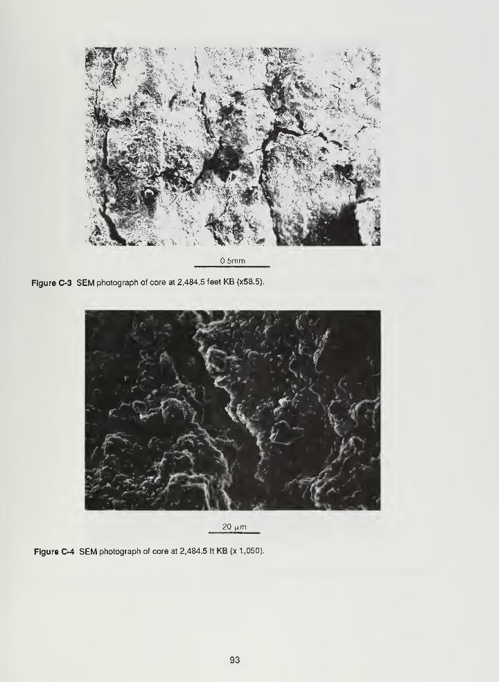
*'&l JMt* \ ','< m

*">-i ft

*s

i

as* i

k

&3fe i

harmrv

%.^5h#ir'ifiU >. V.

0.5mm

Figure C-3 SEM photograph of core at 2,484.5 feet KB (x58.5).

20 (xm

Figure C-4 SEM photograph of core at 2,484.5 ft KB (x 1 ,050).

93

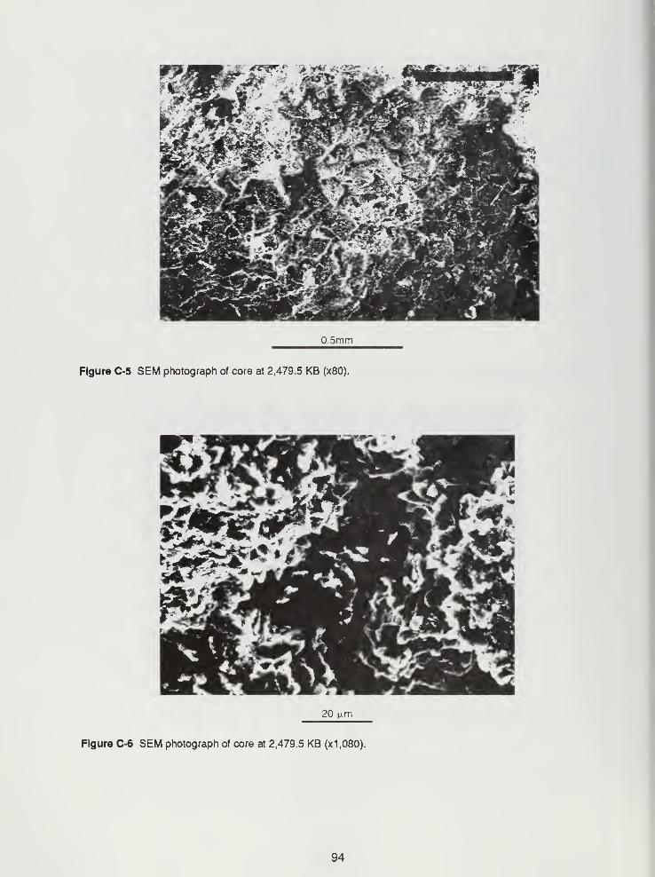
0.5mm

Figure C-5 SEM photograph of core at 2,479.5 KB (x80).

20 urn

Figure C-6 SEM photograph of core at 2,479.5 KB (x1,080).

94

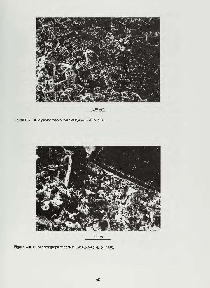
vlr « - a,,. K '.- ^^ \V »* •-«*< •>-.

.

$*>.* tt i -- «.-

. ? *^ **\SC*<S? :f>- \?~ ''•I

s

W&>i9-JT '^%\/i •

* >^^CfcJ^r^Cfl'

.

200 lam

Figure C-7 SEM photograph of core at 2,456.5 KB (x113).

20 (xm

Figure C-8 SEM photograph of core at 2,456.5 feet KB (x1 ,1 60).

95

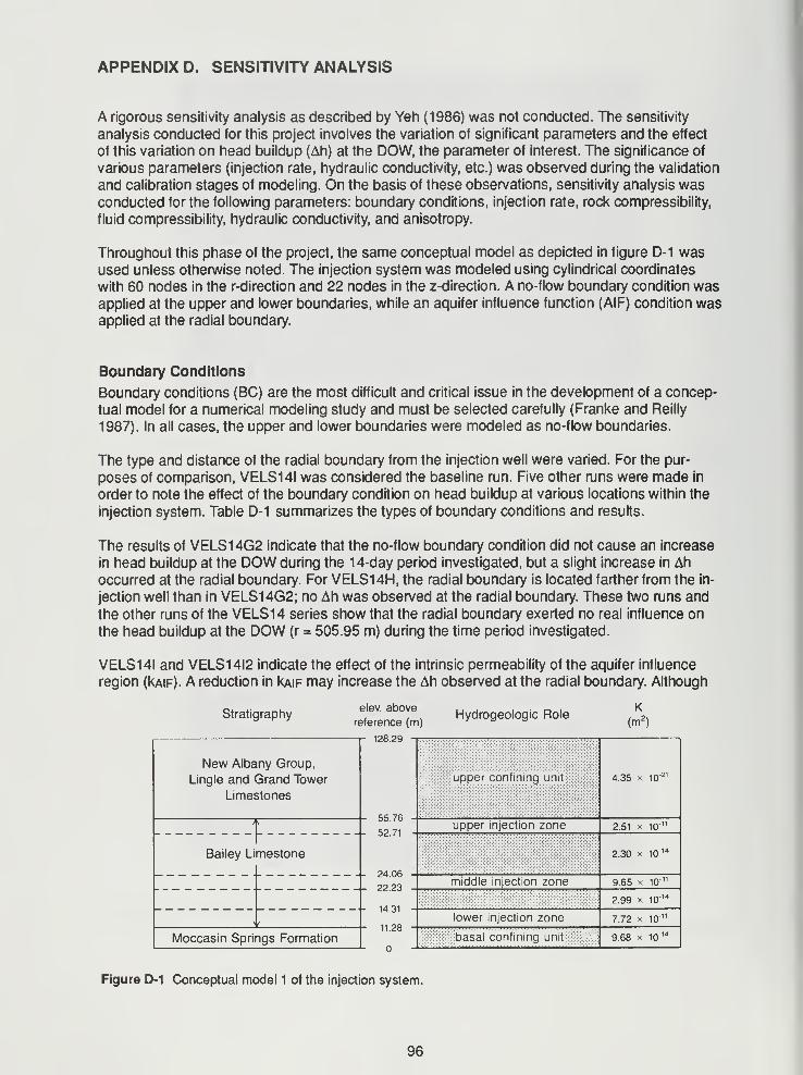
APPENDIX D. SENSITIVITY ANALYSIS

A rigorous sensitivity analysis as described by Yeh (1986) was not conducted. The sensitivity

analysis conducted for this project involves the variation of significant parameters and the effect

of this variation on head buildup (Ah) at the DOW, the parameter of interest. The significance of

various parameters (injection rate, hydraulic conductivity, etc.) was observed during the validation

and calibration stages of modeling. On the basis of these observations, sensitivity analysis wasconducted for the following parameters: boundary conditions, injection rate, rock compressibility,

fluid compressibility, hydraulic conductivity, and anisotropy.

Throughout this phase of the project, the same conceptual model as depicted in figure D-1 wasused unless otherwise noted. The injection system was modeled using cylindrical coordinates

with 60 nodes in the r-direction and 22 nodes in the z-direction. A no-flow boundary condition wasapplied at the upper and lower boundaries, while an aquifer influence function (AIF) condition wasapplied at the radial boundary.

Boundary Conditions

Boundary conditions (BC) are the most difficult and critical issue in the development of a concep-

tual model for a numerical modeling study and must be selected carefully (Franke and Reilly

1987). In all cases, the upper and lower boundaries were modeled as no-flow boundaries.

The type and distance of the radial boundary from the injection well were varied. For the pur-

poses of comparison, VELS14I was considered the baseline run. Five other runs were made in

order to note the effect of the boundary condition on head buildup at various locations within the

injection system. Table D-1 summarizes the types of boundary conditions and results.

The results of VELS14G2 indicate that the no-flow boundary condition did not cause an increase

in head buildup at the DOW during the 14-day period investigated, but a slight increase in Ahoccurred at the radial boundary. For VELS14H, the radial boundary is located farther from the in-

jection well than in VELS14G2; no Ah was observed at the radial boundary. These two runs and

the other runs of the VELS14 series show that the radial boundary exerted no real influence on

the head buildup at the DOW (r = 505.95 m) during the time period investigated.

VELS14I and VELS14I2 indicate the effect of the intrinsic permeability of the aquifer influence

region (kAiF). A reduction in I<aif may increase the Ah observed at the radial boundary. Although

Stratigraphyelev. above

reference (m)

128.29

Hydrogeologic RoleK

(m2)

New Albany Group,

Lingle and Grand Tower

Limestones—r—

Bailey Limestone

Moccasin Springs Formation

55.76

52.71

24.06

22.23

14.31

11.28

4.35 x 10" 21upper confining unit

upper injection zone 2.51 x 10"

2.30 x 1014

middle injection zone 9.65 x 10' 11

2.99 x 1014

lower injection zone 7.72 x 10"

basal confining unit 9.68 x 10"

Figure D-1 Conceptual model 1 of the injection system.

96

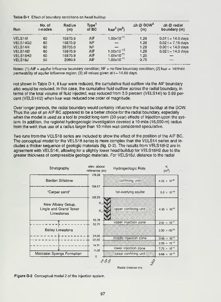
Table D-1 Effect of boundary conditions on head buildup

RunNo. of

r-nodesRadius(m)

Type 1

of BC kAiF2 (m2)

Ah @ DOW3

(m)Ah @ radial

boundary (m)

VELS14I 60 15870.9 AIF

VELS14G2 60 15870.9 NFVELS14H 60 35703.0 NFVELS14I2 60 15870.9 AIF

VELS18H2 60 15870.9 AIF

VELS18J 50 2090.8 AIF

1.00X10"11

1.00x10

1.00x10

1.00x10

-12

-11

-11

1.28 0.01 t= 14.0 days

1.28 0.02 1 = 7.16 days

1.28 0.00 1< 14.0 days

1.28 0.02 1 = 14.0 days

1.25 —0.75 —

Notes: (1) AIF = aquifer influence boundary condition; NF = no-flow boundary condition; (2) kAiF = intrinsic

permeability of aquifer influence region; (3) all values given at t = 14.00 days.

not shown in Table D-1 , if kAiF were reduced, the cumulative fluid outflow via the AIF boundary

also would be reduced. In this case, the cumulative fluid outflow across the radial boundary, in

terms of the total volume of fluid injected, was reduced from 3.0 percent (VELS14I) to 0.69 per-

cent (VELS14I2) when kAiF was reduced one order of magnitude.

Over longer periods, the radial boundary would certainly influence the head buildup at the DOW.Thus the use of an AIF BC appeared to be a better choice for the radial boundary, especially

when the model is used as a tool to predict long-term (30-year) effects of injection upon the sys-

tem. In addition, the regional hydrogeologic investigation covered a 10-mile (16,000-m) radius

from the well; thus use of a radius larger than 10 miles was considered speculative.

Two runs from the VELS18 series are included to show the effect of the position of the AIF BC.

The conceptual model for the VELS18 series is more complex than the VELS14 series and in-

cludes a thicker sequence of geologic materials (fig. D-2). The results from VELS18H2 are in

agreement with VELS14I, allowing for a slightly lower head buildup for VELS18H2 due to the

greater thickness of compressible geologic materials. For VELS18J, distance to the radial

Stratigraphy

Bordon Siltstone

"Carper sand"

New Albany Group,

Lingle and Grand Tower

Limestones

TBailey Limestone

elev. above

reference (m)

178.28

Hydrogeologic Role

11.28

Moccasin Springs Formation

139.57

128.29

K,

K

55.76

-I- 52.71

24.06

-+- 2223

s/s/s/

confining unit:

1st overlying aquifer

Iupper confining unit;

upper injection zone

middle miection zone

lower injection zone

K(m2

)

basal confining unit ....::

.

4.35 x 1021

5.0 x 1013

4.35 x 10"21

2.51 x 10'

2.30 x/10"'

9.65 x 10"

2.99 x 10 H

7.72 x 10"

9.68 x 10" 1

*&&Radial distance (m)

Figure D-2 Conceptual model 2 of the injection system.

97

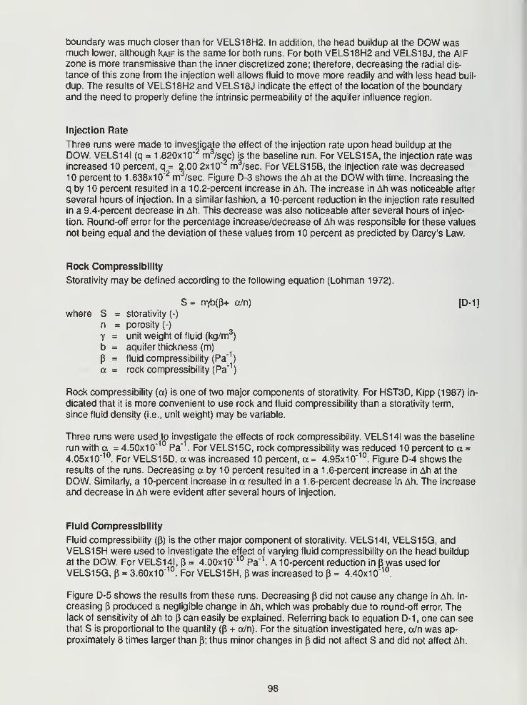
boundary was much closer than for VELS18H2. In addition, the head buildup at the DOW wasmuch lower, although kAiF is the same for both runs. For both VELS18H2 and VELS18J, the AIFzone is more transmissive than the inner discretized zone; therefore, decreasing the radial dis-

tance of this zone from the injection well allows fluid to move more readily and with less head buil-

dup. The results of VELS18H2 and VELS18J indicate the effect of the location of the boundaryand the need to properly define the intrinsic permeability of the aquifer influence region.

Injection Rate

Three runs were made to investigate the effect of the injection rate upon head buildup at the

DOW. VELS14I (q = 1.820x10~2 m3

/sec) is the baseline run. For VELS15A, the injection rate wasincreased 10 percent, q = 2.00 2x1

0"2 m3/sec. For VELS15B, the injection rate was decreased

10 percent to 1 .638x10"2 m3

/sec. Figure D-3 shows the Ah at the DOW with time. Increasing the

q by 10 percent resulted in a 10.2-percent increase in Ah. The increase in Ah was noticeable after

several hours of injection. In a similar fashion, a 10-percent reduction in the injection rate resulted

in a 9.4-percent decrease in Ah. This decrease was also noticeable after several hours of injec-

tion. Round-off error for the percentage increase/decrease of Ah was responsible for these values

not being equal and the deviation of these values from 10 percent as predicted by Darcy's Law.

Rock Compressibility

Storativity may be defined according to the following equation (Lohman 1972).

S = nyb(p+ o/n) [D-1]

where S = storativity (-)

n = porosity (-)

Y = unit weight of fluid (kg/m3

)

b = aquifer thickness (m)

p = fluid compressibility (Pa"1

)

a = rock compressibility (Pa"1

)

Rock compressibility (a) is one of two major components of storativity. For HST3D, Kipp (1987) in-

dicated that it is more convenient to use rock and fluid compressibility than a storativity term,

since fluid density (i.e., unit weight) may be variable.

Three runs were used to investigate the effects of rock compressibility. VELS14I was the baseline

run with a = 4.50x10" 10

Pa"1

. For VELS15C, rock compressibility was reduced 10 percent to a =

4.05x10"10

. For VELS15D, a was increased 10 percent, a= 4.95x10"10

. Figure D-4 shows the

results of the runs. Decreasing a by 10 percent resulted in a 1 .6-percent increase in Ah at the

DOW. Similarly, a 10-percent increase in a resulted in a 1.6-percent decrease in Ah. The increase

and decrease in Ah were evident after several hours of injection.

Fluid Compressibility

Fluid compressibility (P) is the other major component of storativity. VELS14I, VELS15G, andVELS15H were used to investigate the effect of varying fluid compressibility on the head buildup

at the DOW. For VELS14I, p = 4.00x10" 10

Pa"1

. A 10-percent reduction in p was used for

VELS15G,p = 3.60x10"10

. For VELS15H, p was increased to p = 4.40x10"10

.

Figure D-5 shows the results from these runs. Decreasing p did not cause any change in Ah. In-

creasing p produced a negligible change in Ah, which was probably due to round-off error. Thelack of sensitivity of Ah to p can easily be explained. Referring back to equation D-1 , one can seethat S is proportional to the quantity (P + a/n). For the situation investigated here, a/n was ap-

proximately 8 times larger than P; thus minor changes in p did not affect S and did not affect Ah.

98

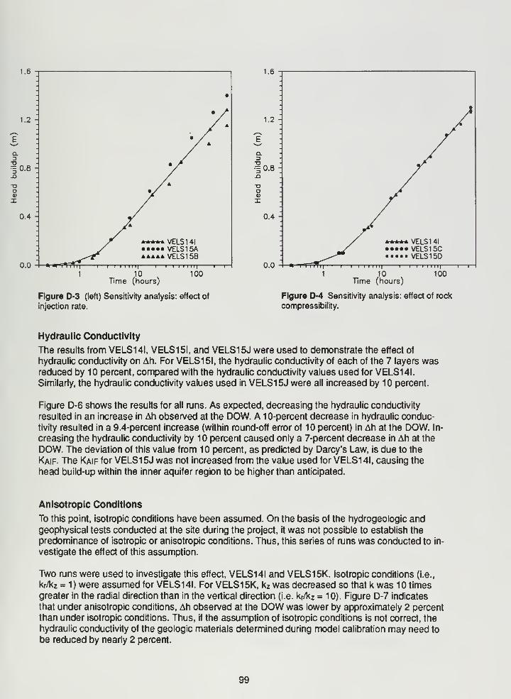
1.6

1.2 -

CL

| 0.8

X)oVX

0.4 -

0.0

VELSUIVELS15AVELS15B

i 1 1 hi i

10Time (hours)

rn

—

100

Figure D-3 (left) Sensitivity analysis: effect of

injection rate.

1.6

1.2 -

a.

I 0.8

OVI

0.4 -

0.0

VELSHIVELS15CVELS15D

11 I I • | 1

1

-

10Time (hours)

Figure D-4 Sensitivity analysis: effect of rock

compressibility.

Hydraulic Conductivity

The results from VELSUI, VELS15I, and VELS15J were used to demonstrate the effect of

hydraulic conductivity on Ah. For VELS15I, the hydraulic conductivity of each of the 7 layers wasreduced by 10 percent, compared with the hydraulic conductivity values used for VELS14I.

Similarly, the hydraulic conductivity values used in VELS15J were all increased by 10 percent.

Figure D-6 shows the results for all runs. As expected, decreasing the hydraulic conductivity

resulted in an increase in Ah observed at the DOW. A 10-percent decrease in hydraulic conduc-

tivity resulted in a 9.4-percent increase (within round-off error of 10 percent) in Ah at the DOW. In-

creasing the hydraulic conductivity by 10 percent caused only a 7-percent decrease in Ah at the

DOW. The deviation of this value from 10 percent, as predicted by Darcy's Law, is due to the

Kaif. The Kaif for VELS15J was not increased from the value used for VELS14I, causing the

head build-up within the inner aquifer region to be higher than anticipated.

Anisotropic Conditions

To this point, isotropic conditions have been assumed. On the basis of the hydrogeologic andgeophysical tests conducted at the site during the project, it was not possible to establish the

predominance of isotropic or anisotropic conditions. Thus, this series of runs was conducted to in-

vestigate the effect of this assumption.

Two runs were used to investigate this effect, VELS14I and VELS15K. Isotropic conditions (i.e.,

kr/kz = 1) were assumed for VELS14I. For VELS15K, kz was decreased so that k was 10 times

greater in the radial direction than in the vertical direction (i.e. kr/kz = 10). Figure D-7 indicates

that under anisotropic conditions, Ah observed at the DOW was lower by approximately 2 percent

than under isotropic conditions. Thus, if the assumption of isotropic conditions is not correct, the

hydraulic conductivity of the geologic materials determined during model calibration may need to

be reduced by nearly 2 percent.

99

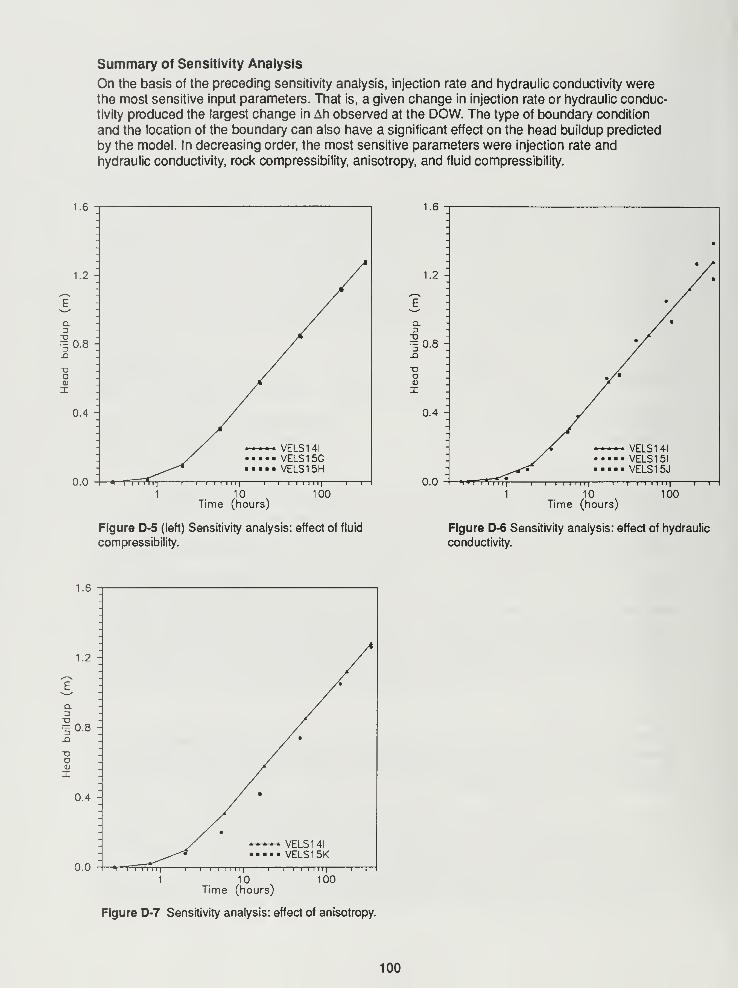
Summary of Sensitivity Analysis

On the basis of the preceding sensitivity analysis, injection rate and hydraulic conductivity werethe most sensitive input parameters. That is, a given change in injection rate or hydraulic conduc-

tivity produced the largest change in Ah observed at the DOW. The type of boundary condition

and the location of the boundary can also have a significant effect on the head buildup predicted

by the model. In decreasing order, the most sensitive parameters were injection rate and

hydraulic conductivity, rock compressibility, anisotropy, and fluid compressibility.

1.6

1.2

Q.

I 0.8

aCD

x

0.4 -

0.0

VELSUIVELS15GVELS15H

10Time (hours)

100

1.6

1.2

| 0.8jQ

oCD

X

0.4

0.0

Figure D-5 (left) Sensitivity analysis: effect of fluid

compressibility.

10Time (hours)

Figure D-6 Sensitivity analysis: effect of hydraulic

conductivity.

1.6

1.2

Q.D

'5

XI

T3OCD

X

0.8

0.4 -

0.0

VELSUIVELS15K

i i 1 11

1

1—i—i—i i 1 11

1

1—i—i—i i 1 11

1

1—1~

1 10 1 00Time (hours)

Figure D-7 Sensitivity analysis: effect of anisotropy.

100

HECKMAN |±lBINDERY INC. |§|

JUN97Bound -To -Please

1 N.MANCHESTERINDIANA 46962 '

limHWHIIIIHIIi 1111111111111 IH hlllllllHIillWMWHiyilM