Investigation of stereo-based 3D surface reconstruction

E. Hemayed, A. Sandbek, A. Wassal and A. Farag Proc. SPIE, Vol. 3023, pp. 191-202, Feb. 1997Investigation of stereo-based 3D surface reconstructionE. E. Hemayed, A. Sandbek, A. G. Wassal, and A. A. FaragCVIP Lab., University of Louisville,Louisville, Kentucky 40292 USAABSTRACTThis article presents an investigation study of stereo-based 3D surface reconstruction algorithms by providing anoverview of the di�erent approaches that have been investigated in the stereo literature during the last decade.This study considers only the two-views plain stereo algorithms� and provides another classi�cation for the stereoapproaches based on the features used in the stereo literature. In addition, the article provides full details of twodi�erent stereo algorithms that give an idea of how stereo works.Keywords: Stereo Vision, 3D surface reconstruction, Survey1. INTRODUCTIONMany algorithms have been developed to estimate surfaces from two stereo images of a scene acquired using a �xed,known camera con�guration. The paradigm used by most of these algorithms consists of three main phases or anintegration of them:1. Feature Detection: Detects suitable features in each image.2. Feature Matching: Finds corresponding features in the two images.3. Depth Estimation: Determines the 3D locations associated with corresponding pairs of image features, and�ts a surface to these 3D points.During the last decade, researchers suggested many di�erent stereo approaches. These approaches have beenclassi�ed into two categories, region-based and edge-based approaches. The former gives a dense disparity map whilethe latter gives a sparse disparity map. Another classi�cation is introduced in this article based on the featuresused in the stereo literature. Five di�erent categories are proposed for the stereo approaches. These categories arediscussed in the next section. We also add two sections describing the two main paradigms used in stereo visionalgorithms, the MPG algorithm and Tanaka-Kak algorithm. These two algorithms provide good presentation ofhow stereo works. The framework of the discussion includes the essential three steps of stereo algorithms, featureextraction, feature matching and depth estimation. We end up with results and conclusion section.2. AN OVERVIEW OF DIFFERENT STEREO APPROACHESThis section presents an overview of the di�erent stereo approaches that have been investigated during the lastdecade. We classify these approaches into �ve di�erent categories based on the matching technique that they use.These categories are: point matching, scan line matching, curved-segment matching, line-segment matching, andedges with region matching. The framework of the discussion of these approaches is the essential three steps that weintroduced before. We discuss an article of each category and refer to other articles that belong to the same category.The articles that we mention in this paper are not the only articles in the stereo literature but they are onlysamples that support our proposed classi�cations. Other articles, not mention here, may also �t in one of theproposed categories.Send correspondence to A. A. Farag Email: [email protected]; Telephone: 502-852-6130; Fax: 502-852-1580.This work is Supported by the Whitekar Foundation and National Science Foundation (NSF).�The article does not consider stereo using three views or stereo integrated with other cues.1

E. Hemayed, A. Sandbek, A. Wassal and A. Farag Proc. SPIE, Vol. 3023, pp. 191-202, Feb. 19972.1. Point matching stereo basedLee et al., in Ref. 1, view the stereo correspondence process as an optimization problem that satis�ed three com-peting constraints: (1)Similarity, matched points have similar local features; (2)Smoothness, disparity values changesmoothly, except at a few depth discontinuities; (3)Uniqueness, each point in an image should be assigned at mostone disparity value. They present a new energy function that can be used with the Hope�eld neural network to dothe stereo correspondence process. Their approach is a modi�ed version of Zhou and Chellappa's network, see Ref. 2.Feature extraction: Lee et al in their article, do not choose speci�c features. However, they use the word primitiveand mention that it can be the intensity or intensity derivative patterns in a small window. They refer to Ref. 3 forthe extraction of these primitives.Feature matching: Lee et al. use a neural representation scheme that consists of Nr � Nc � (D + 1) mutuallyinterconnected binary neurons in 3D form, where Nr and Nc are the row and column sizes of the image, respectively,and D is the allowed maximum disparity. The state of each neuron (active or inactive) in the network representspossible match between interesting points in the left image and in the right image. They provide a derivation ofan energy function that ensures the convergence of the Hope�eld neural network. This energy function satis�es thethree constraints of the stereo correspondence problem. The output of the stereo correspondence process is a list ofpixel indices pairs; left pixel index and its corresponding right pixel index.Depth estimation: In the case of row registered stereo pairs, the depth can be estimated directly from the outputlist of the stereo correspondence process. Simply, the disparity of pixel l 2 row x in the left image is d = l� r, wherer is the correspondent pixel in row x in the right image. For other point matching stereo based, see Refs. 4{8.2.2. Scan line matching stereo basedBensrhair et al., in Ref. 9, handle the stereo problem from a di�erent view. They treat the matching problem ina stereo vision process as the problem of �nding an optimal path on a two-dimensional (2D) search plane. Theyconsider a non-linear gain function which varies as a function of threshold values calculated during the preliminarystatistical analysis of the right and left images.Feature extraction: Bensrhair et al. de�ne a new primitive to be used as a feature. They call it declivity,see Ref. 10. Consider an image line, a declivity is de�ned as a cluster of contiguous pixels, limited by two end-pointswhich correspond to two consecutive local extrema (xi; xi+1) of grey-level intensity (I(xi); I(xi+1)). Each declivity ischaracterized by its amplitude de�ned by di = I(xi+1)� I(xi). The low-amplitude declivities are discarded as theycorrespond to noise. The high-amplitude declivities are used as features in the stereo matching process.Feature matching: The matching problem is treated as the problem of �nding an optimal path on a two-dimensionalplane whose vertical and horizontal axes are the right and left scan lines and their intersection corresponds to hy-pothetical declivity associations. Optimal matches are obtained by the selection of the path which corresponds tomaximum photometric similarity that estimated by the grey-level of the mean position of the declivity and its neigh-bors. The nodes of the optimal path correspond to the mean positions of the declivities of the left image and theircorresponding in the right image.Depth estimation: The depth is estimated as the di�erence between the mean position of the declivities of theleft image and the corresponding declivities of the right image. This depth can be computed from the nodes of theoptimal path obtained in the matching process. The di�erence between the vertical and horizontal coordinates ofthe nodes are the disparities that we are looking for. For other scan line matching stereo based, see Refs. 11{152.3. Curved-segment matching stereo basedMa et al., in Ref. 16, present another stereo matching approach that is based on quadratic curves. They provide aclosed form solution for the global matching criterion of two quadratic curves in two images along with a closed formsolution for the global reconstruction of the conical objects in the scene.2

E. Hemayed, A. Sandbek, A. Wassal and A. Farag Proc. SPIE, Vol. 3023, pp. 191-202, Feb. 1997Feature extraction: The feature that has been used in this approach is the quadratic curves in the left andright image. The authors do not provide a discussion of feature extraction. However, this can be done by extractingthe edges of the image and clustering them into connected contours of prede�ned lengths. Then a quadratic curvecan be �tted to these contours using a �tting technique such as the least squared method. Those contours thatachieve a prede�ned threshold are accepted as quadratic curves while others are discarded.Feature matching: Ma et al. derive the basic constraints which should be satis�ed for a pair of quadratic curvesin the two images if they correspond to the same planar quadratic curve in the scene. They summarize their resultsin a theorem called correspondence theorem. They also de�ne a matching criterion that is used to disambiguatemultiple matches between curves.Depth estimation: The quadratic curve in 3D space can be reconstructed globally by determining the inter-section of a plane and a cone. The cone can be the one that is passing through the optical center of the left camera,the quadratic curve in the left image and the quadratic curve in 3D space. For other curved-segment matching stereobased, see Refs. 17{192.4. Line segment matching stereo basedThe key step handled in Ref. 20 is the feature matching step. Line segments are matched locally and then ambiguitiesbetween potential matches are resolved using an evaluation function based on the minimal di�erential disparity.Feature extraction: In this algorithm, line segments are matched. They are derived by Nevatia-Babu method, inRef. 21, by detecting local edges from the zero-crossings of a Laplacian-of-a-Gaussian edge mask. Then, these edgesare processed to produce line segments that are described by: coordinates of the end-points, orientation and strength(average contrast).Feature matching: For each segment ai in the left image, a window w(ai) is de�ned in which correspondingsegments from the right image must lie and, similarly, for each segment bi in the right image. Also, one segment isallowed to possibly match with more than one segment (for fragmented segments). Segments in w(ai) are said tooverlap with ai if by sliding one of them in the direction parallel to the epipolar line, they would intersect. Overlap-ping segments with similar orientation and contrast are potential matches. Then, an evaluation function v(i; j) iscomputed for all potential matches measuring how close their disparity is to the disparities of the other segments intheir neighborhoods. The algorithm iterates trying to minimize that di�erential disparity using a relaxation process.Depth estimation: Depth is derived from the average disparity for the line segment which is simply the aver-age of the displacement along the epipolar line of the corresponding points. For other line segment matching stereobased, see Refs. 22{292.5. Edges with regions matching stereo basedThe main idea of Ref. 30 is to use an area-based primitive to create a very dense disparity map and then re�ne itusing matches from a sparse feature-based primitive that localize the discontinuities, like edges.Feature extraction: This paper integrates area-based and feature-based primitives. The area-based primitiveused is the cross correlation with an ordering constraint and a weak surface smoothness assumption and it providesa dense disparity map. This disparity map is a blurred version of the true one because of the blurring inherent in thesmoothing and the correlation. That blurring is emphasized at the depth discontinuities. Feature-based primitivesprovide accurate locations of discontinuities so edge information is introduced. Combining both primitives togetheris useful since feature-based primitives produce sparse disparity maps and are often confused by large local changesin disparity.Feature matching: Edges are matched using the Medioni-Nevatia method, in Ref. 20, and each point in thecross correlation volume that has a value greater than or equal to its 4-connected neighbors and has a value greaterthan or equal to one half of the value of the strongest peak along each viewing direction, is considered a peak or a3

E. Hemayed, A. Sandbek, A. Wassal and A. Farag Proc. SPIE, Vol. 3023, pp. 191-202, Feb. 1997likely match. Correlation-based matches (peaks) are then overlaid with edge-based matches. A disparity estimate isfound by simply extracting a value from the array. Also, interpolation is done for those regions for which no disparitycan be found. This is done by using the high con�dence matches as seeds and expand the disparity estimate alongthe disparity surface formed by adjacent peaks. The output of the interpolation process is the disparity map thatwe are looking for. For other edges with regions matching stereo based, see Refs. 31{353. THE MARR-POGGIO-GRIMSON (MPG) ALGORITHMIn 1981, W. Grimson presented an implementation of the human stereo vision theory that was developed by Marrand Poggio (1979). This implementation is known as the Marr-Poggio-Grimson algorithm, (MPG). The Marr-Poggiotheory, see Ref. 36, proposes extracting point features by �ltering the images with a set of 12 orientation-speci�c�lters where each is represented by the di�erence of two Gaussian functions and then extracting zero-crossing points.Marr and Hildreth in Ref. 37 showed that intensity changes occurring at a particular resolution may be detectedby locating such zero-crossing points. However, in Grimson implementation, see Refs. 38,39, a single circularlysymmetric Laplacian-of-a-Gaussian (LOG) �lter is used. The use of a single �lter is not only more computationallye�cient, but, as discussed in Mayhew and Frisby, in Ref. 40, there is also a psychophysical evidence that humansmay utilize a single circularly symmetric �lter.In the following discussion of MPG we'll use the word `channel' to refer to a LOG �lter with a speci�c width `w'.The coarsest channel is the channel that uses a LOG �lter with width w = 63 while the �nest channel is the channelthat uses a LOG �lter with width w = 4.3.1. Feature extractionThe feature extraction process mainly consists of two steps, LOG �ltering and extracting zero crossings with theirattributes. The attributes that have been used by Grimson are the sign of the zero-crossing and its approximateorientation.3.1.1. LOG �lteringThe LOG is a smoothed second derivative of the image signal. The LOG operator assumes the following form:52G(x; y) = �x2 + y2�2 � 2� exp��(x2 + y2)2�2 � (1)where 52 is the Laplacian 52 = (�2=�x2) + (�2=�y2) and G(x; y) is the Gaussian function, which acts as a low-pass-�lter to the image: G(x; y) = �2 exp��(x2 + y2)2�2 � (2)where the width of the channel `w' is related to � as follows: w = p2�.3.1.2. Extracting zero crossingsThe detection of zero crossings can be accomplished by scanning the convolved image horizontally for adjacentelements of opposite sign or for three horizontally adjacent elements, where the middle one is zero. The other twocontain convolution values of opposite signs. This gives the position of zero crossing to within a pixel. The sign isconsidered positive if the signs of the convolution values change from negative to positive from left to right whileit is considered negative if the signs change from positive to negative. In addition, a rough estimate of the localorientation of the zero crossings is recorded in increments of 30�. The orientation is computed as the direction of thegradient of the convolution values.3.2. Feature matchingThe feature matching is performed in two steps. The �rst step is to match the zero-crossings of each individualchannel. The second step is to use the matched points in the coarse channels to bring the �ne channels intomatching, which is de�ned as vergence control. 4

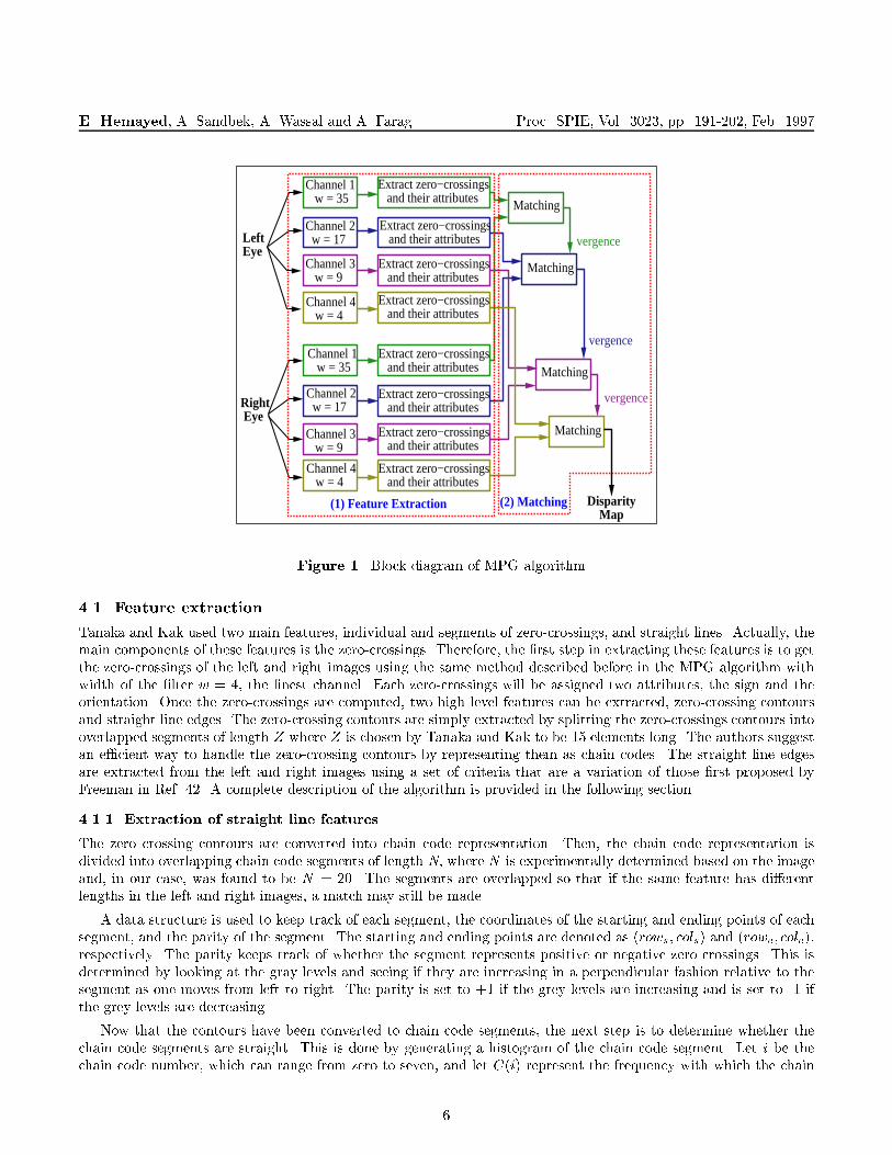
E. Hemayed, A. Sandbek, A. Wassal and A. Farag Proc. SPIE, Vol. 3023, pp. 191-202, Feb. 19973.2.1. Matching zero crossingsAssuming that the average disparity, dav, in the image is known, then the following steps are performed to �ndmatches for a left-image zero-crossing point, p = (xl; yl):1. Search on the yl scan line of the right image in a 1D window �w centered at the point (xl + dav ; yl) for thepossible candidate zero-crossing matches.2. If a zero-crossing on the window is of the same sign and the same orientation of the left image zero-crossing inquestion, then this zero-crossing produces a match. The di�erence between the two x locations (xl�xr) whichis de�ned as disparity, is stored in a dynamic bu�er that will be called the disparity map.3. Based on the matching process, the left-image zero-crossing will be marked as:� Unique match, if only one right image zero-crossing is matched with the left one.� Multiple matches, if more than one match is found.� No match, if no match is found. The Vergence control will handle this case later.The case of multiple matches is disambiguated by scanning a neighborhood about the point in question, andrecording the signs of the disparity of the unambiguous matches (unique matches) within that neighborhood. If theambiguous point has a potential match of the same sign as the dominant type within the neighborhood, then that ischosen as the match. This method is called the pulling e�ect. However, if the pulling e�ect can not be applied, thedisparity can be approximated by taking the average of the multiple match disparities.3.2.2. Vergence controlAs a result of performing more low pass �ltering in the coarser channels than in the �ner channels, small variationsin the intensity disappear in the coarser channels so that very accurate disparity calculations are not possible. In a�ner channel, the positions of the zero-crossings will be more accurate since not as much smearing of the intensityvariations occurs. However, a correct value of dav for the point in question is more critical for �ner channels becausethe search window is smaller than the one used by the coarser channel. This leads to the concept of vergence control,which is the concept of using the disparities from the coarser channels in calculating the average disparity in aneighborhood of the left-image point in question, and then this is used to shift the search window to the appropriateposition in the right image for matching to occur.3.3. Depth estimationThe depth is estimated as the di�erence between the columns locations of the left zero-crossing points and theirmatched points in the right image which is called the disparity. The estimated depth of the �nest channel is used asthe depth of the surface. The estimated depth is called the depth map, or the 2 12D sketch.A block diagram of MPG algorithm is provided in Fig. 1. This block diagram shows four channels of the MPGsystem. In each channel box, the image is convolved with a Laplacian-of-a-Gaussian operator of width `w'. In thefeature extraction box, the zero-crossings of each image are extracted along with their signs and orientations. Thenthe matching process is performed between the right and the left zero-crossings in each channel with the help of thevergence control. The output of the �nest channel, w = 4, is the disparity map of the acquired scene.4. THE RULE-BASED STEREO VISION ALGORITHMTanaka and Kak, in Ref. 41, present a hierarchical stereo vision algorithm that produces a dense disparity map. Therule-based algorithm combines the low level based processing, e.g. zero-crossings, and the high level based processing,e.g. straight line segments, curve segments and planar patches.An overview of the essential three steps of the algorithm, feature extraction, feature matching, and depth esti-mation is presented in the following discussion. 5

E. Hemayed, A. Sandbek, A. Wassal and A. Farag Proc. SPIE, Vol. 3023, pp. 191-202, Feb. 1997 Channel 1 w = 35

Channel 2 w = 17

Channel 3 w = 9

Channel 4 w = 4

Channel 1 w = 35

Channel 2 w = 17

Channel 3 w = 9

Channel 4 w = 4

Extract zero−crossings and their attributes

Extract zero−crossings and their attributes

Extract zero−crossings and their attributes

Extract zero−crossings and their attributes

Extract zero−crossings and their attributes

Extract zero−crossings and their attributes

Extract zero−crossings and their attributes

Extract zero−crossings and their attributes

Matching

Matching

Matching

Matching

vergence

vergence

vergence

Disparity Map

LeftEye

Right Eye

(1) Feature Extraction (2) MatchingFigure 1. Block diagram of MPG algorithm.4.1. Feature extractionTanaka and Kak used two main features, individual and segments of zero-crossings, and straight lines. Actually, themain components of these features is the zero-crossings. Therefore, the �rst step in extracting these features is to getthe zero-crossings of the left and right images using the same method described before in the MPG algorithm withwidth of the �lter w = 4, the �nest channel. Each zero-crossings will be assigned two attributes, the sign and theorientation. Once the zero-crossings are computed, two high level features can be extracted, zero-crossing contoursand straight line edges. The zero-crossing contours are simply extracted by splitting the zero-crossings contours intooverlapped segments of length Z where Z is chosen by Tanaka and Kak to be 15 elements long. The authors suggestan e�cient way to handle the zero-crossing contours by representing them as chain codes. The straight line edgesare extracted from the left and right images using a set of criteria that are a variation of those �rst proposed byFreeman in Ref. 42. A complete description of the algorithm is provided in the following section.4.1.1. Extraction of straight line featuresThe zero crossing contours are converted into chain code representation. Then, the chain code representation isdivided into overlapping chain code segments of length N, where N is experimentally determined based on the imageand, in our case, was found to be N = 20. The segments are overlapped so that if the same feature has di�erentlengths in the left and right images, a match may still be made.A data structure is used to keep track of each segment, the coordinates of the starting and ending points of eachsegment, and the parity of the segment. The starting and ending points are denoted as (rows; cols) and (rowe; cole),respectively. The parity keeps track of whether the segment represents positive or negative zero crossings. This isdetermined by looking at the gray levels and seeing if they are increasing in a perpendicular fashion relative to thesegment as one moves from left to right. The parity is set to +1 if the grey levels are increasing and is set to -1 ifthe grey levels are decreasing.Now that the contours have been converted to chain code segments, the next step is to determine whether thechain code segments are straight. This is done by generating a histogram of the chain code segment. Let i be thechain code number, which can range from zero to seven, and let C(i) represent the frequency with which the chain6

E. Hemayed, A. Sandbek, A. Wassal and A. Farag Proc. SPIE, Vol. 3023, pp. 191-202, Feb. 1997code number occurs. There are four cases in which the �rst criteria will be satis�ed. The histogram may have onebar (i.e., there is one i where C(i) 6= 0), two bars, three bars, or four or more bars. For the case of one bar, thechain code segment is automatically declared straight and the segment should be stored so that it can be used in thematching process later. For the case of four or more bars, the chain code segment is automatically declared not tobe straight.For the cases of two and three bars in the histogram, let us denote the chain code number with the highest C(i)to be the major code number and the one with the smaller C(i) to be the minor code number. For the second casethere are two scenarios to consider, one where the two bars are not adjacent and the other where they are adjacent.If the two bars are not adjacent to each other, then the chain code segment is not straight and is discarded. If thetwo bars are adjacent to one another then the segment is considered straight if the maximum run length of the minorcode is less than an experimentally determined threshold, T2. In our case, T2 = 2.For the case where the histogram has three bars, there are again two scenarios to consider. If no two of the threebars are adjacent then the chain code segment is declared as a non-straight segment and is discarded. If the threebars are adjacent to one another, with the center bar being the major chain code number, and the C(i) of the twominor chain code numbers is less than an experimentally determined threshold, T1, then the chain code segment isstraight. In our case, T1 = 3. Otherwise, the segment is declared not to be straight.4.2. Feature matchingTanaka-Kak approach represents an integration of four methods of stereo matching: (1) straight line matching, (2)�tting planar patches, (3) curve segment matching, and (4) the full MPG matching. In this section, we discuss the�rst three matching methods only since we have already described the full MPG.4.2.1. Straight line matchingThe matching of the straight line segments is discussed in terms of its chain code where each chain code segmentin the left image, denoted by L(i), is compared to all chain code segments in the right image. For each right imagechain code segment, denoted by R(i), a comparison is made between the coordinates of the starting points of it andthe left image chain code segment in question. If the coordinates are within �1 of those for the left image chain codesegment, then continue. Otherwise move on to the next right image chain code segment.If the coordinates match, then a similarity score, denoted by T, is calculated using L(i) and R(i). T is a summationof values given to each chain code element, i, based on how well a chain code element, i, in one segment matchesits corresponding element in the other segment. Each is scored as follows: (1) if L(i) = R(i) then a score of one isgiven; (2) if L(i) = R(i� 1) or L(i) = R(i+ 1), then a score of W is given, where 0 �W � 1 and in this case is setto 0.5; (3) otherwise no score is given. If T is above T3, a user de�ned threshold, then a match is declared. If not, amatch is not declared and the next segment is compared as described above.4.2.2. Fitting planar patchesA straight line is de�ned as the intersection of two planes. Therefore, the straight line features that were successfullymatched in the previous section can be used to match the surrounding area of these lines. The following process isTanaka and Kak's version of geometrically constrained matching which is derived from Eastman and Waxman, seeRef. 43.The algorithm assumes that the surfaces in the scene are all planar and the orientation of each planar surfaceis one of a known set of orientations �. Given an orientation � 2 � for a hypothesized plane and the endpoints(x1; y1; z1) and (x2; y2; z2) of L that lies in the plane, the complete equation of the plane is given by�������� x y z 1x1 y1 z1 1x2 y2 z2 1x1 + 1 y1 z1 + tan� 1 �������� = 0; (3)where j � j is the determinant function. Eq. 3 can be solved for z in terms of x and y.7

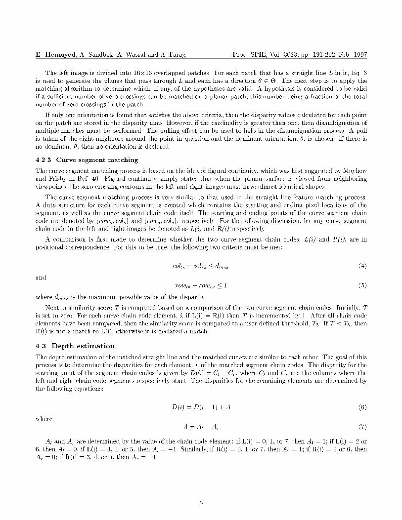
E. Hemayed, A. Sandbek, A. Wassal and A. Farag Proc. SPIE, Vol. 3023, pp. 191-202, Feb. 1997The left image is divided into 16�16 overlapped patches. For each patch that has a straight line L in it, Eq. 3is used to generate the planes that pass through L and each has a direction � 2 �. The next step is to apply thematching algorithm to determine which, if any, of the hypotheses are valid. A hypothesis is considered to be validif a su�cient number of zero crossings can be matched on a planar patch, this number being a fraction of the totalnumber of zero crossings in the patch.If only one orientation is found that satis�es the above criteria, then the disparity values calculated for each pointon the patch are stored in the disparity map. However, if the cardinality is greater than one, then disambiguation ofmultiple matches must be performed. The pulling e�ect can be used to help in the disambiguation process. A pollis taken of the eight neighbors around the point in question and the dominant orientation, �, is chosen. If there isno dominant �, then no orientation is declared.4.2.3. Curve segment matchingThe curve segment matching process is based on the idea of �gural continuity, which was �rst suggested by Mayhewand Frisby in Ref. 40. Figural continuity simply states that when the planar surface is viewed from neighboringviewpoints, the zero-crossing contours in the left and right images must have almost identical shapes.The curve segment matching process is very similar to that used in the straight line feature matching process.A data structure for each curve segment is created which contains the starting and ending pixel locations of thesegment, as well as the curve segment chain code itself. The starting and ending points of the curve segment chaincode are denoted by (rows; cols) and (rowe ; cole), respectively. For the following discussion, let any curve segmentchain code in the left and right images be denoted as L(i) and R(i) respectively.A comparison is �rst made to determine whether the two curve segment chain codes, L(i) and R(i), are inpositional correspondence. For this to be true, the following two criteria must be met:colls � colrs � dmax (4)and rowls � rowrs � 1 (5)where dmax is the maximum possible value of the disparity.Next, a similarity score T is computed based on a comparison of the two curve segment chain codes. Initially, Tis set to zero. For each curve chain code element, i, if L(i) = R(i) then T is incremented by 1. After all chain codeelements have been compared, then the similarity score is compared to a user de�ned threshold, T5. If T < T5, thenR(i) is not a match to L(i), otherwise it is declared a match.4.3. Depth estimationThe depth estimation of the matched straight line and the matched curves are similar to each other. The goal of thisprocess is to determine the disparities for each element, i, of the matched segment chain codes. The disparity for thestarting point of the segment chain codes is given by D(0) = Cl � Cr, where Cl and Cr are the columns where theleft and right chain code segments respectively start. The disparities for the remaining elements are determined bythe following equations: D(i) = D(i� 1) +A (6)where A = Al �Ar (7)Al and Ar are determined by the value of the chain code element: if L(i) = 0, 1, or 7, then Al = 1; if L(i) = 2 or6, then Al = 0, if L(i) = 3, 4, or 5, then Al = �1. Similarly, if R(i) = 0, 1, or 7, then Ar = 1; if R(i) = 2 or 6, thenAr = 0; if R(i) = 3, 4, or 5, then Ar = �1.8

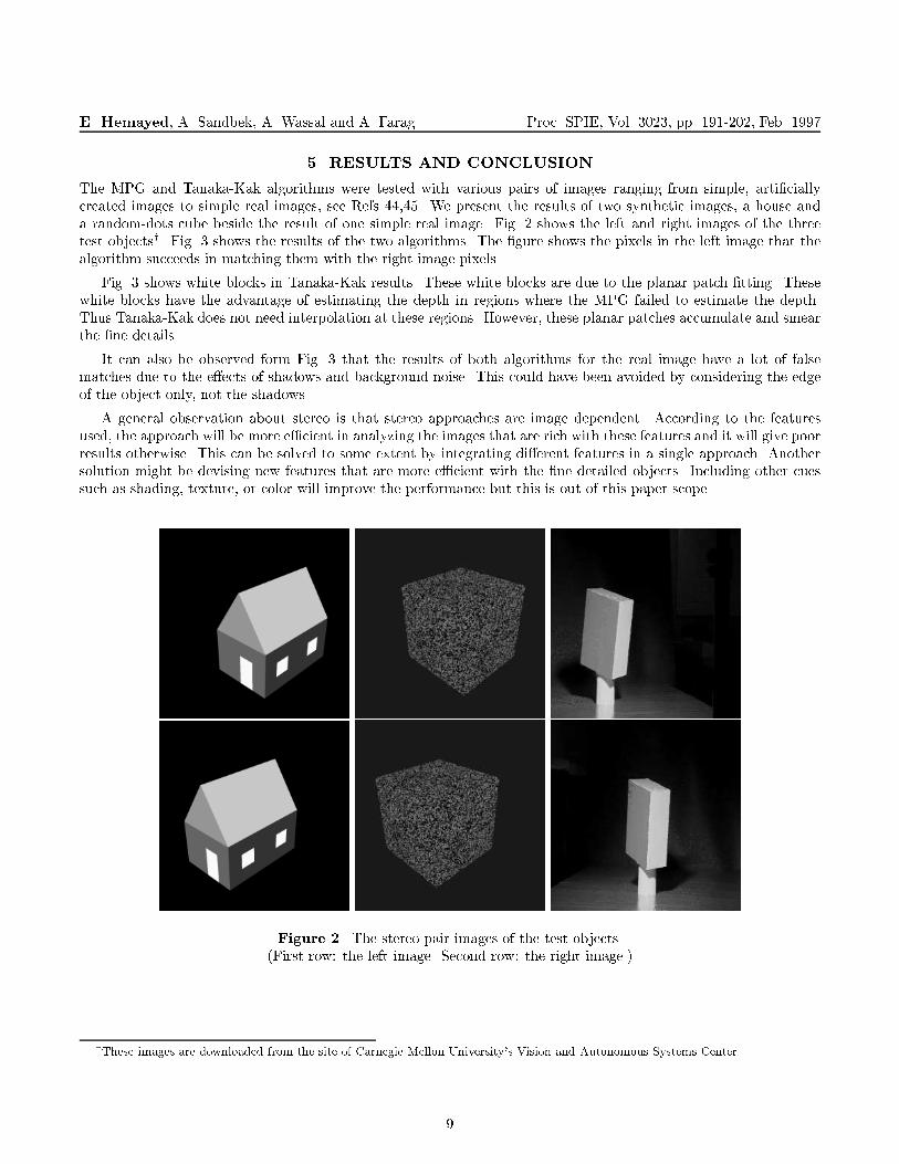
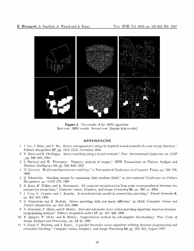
E. Hemayed, A. Sandbek, A. Wassal and A. Farag Proc. SPIE, Vol. 3023, pp. 191-202, Feb. 19975. RESULTS AND CONCLUSIONThe MPG and Tanaka-Kak algorithms were tested with various pairs of images ranging from simple, arti�ciallycreated images to simple real images, see Refs 44,45. We present the results of two synthetic images, a house anda random-dots cube beside the result of one simple real image. Fig. 2 shows the left and right images of the threetest objectsy. Fig. 3 shows the results of the two algorithms. The �gure shows the pixels in the left image that thealgorithm succeeds in matching them with the right image pixels.Fig. 3 shows white blocks in Tanaka-Kak results. These white blocks are due to the planar patch �tting. Thesewhite blocks have the advantage of estimating the depth in regions where the MPG failed to estimate the depth.Thus Tanaka-Kak does not need interpolation at these regions. However, these planar patches accumulate and smearthe �ne details.It can also be observed form Fig. 3 that the results of both algorithms for the real image have a lot of falsematches due to the e�ects of shadows and background noise. This could have been avoided by considering the edgeof the object only, not the shadows.A general observation about stereo is that stereo approaches are image dependent. According to the featuresused, the approach will be more e�cient in analyzing the images that are rich with these features and it will give poorresults otherwise. This can be solved to some extent by integrating di�erent features in a single approach. Anothersolution might be devising new features that are more e�cient with the �ne detailed objects. Including other cuessuch as shading, texture, or color will improve the performance but this is out of this paper scope.

Figure 2. The stereo pair images of the test objects.(First row: the left image. Second row: the right image.)yThese images are downloaded from the site of Carnegie Mellon University's Vision and Autonomous Systems Center9

E. Hemayed, A. Sandbek, A. Wassal and A. Farag Proc. SPIE, Vol. 3023, pp. 191-202, Feb. 1997

Figure 3. The results of the MPG algorithm.(�rst row: MPG results. Second row: Tanaka-Kak results)REFERENCES1. J. Lee, J. Shim, and Y. Ha, \Stereo correspondence using the hop�eld neural-network of a new energy function,"Pattern Recognition 27, pp. 1513{1522, November 1994.2. Y. Zhou and R. Chellappa, \Stereo matching using a neural network," Proc. International Conference on ASSP, pp. 940{943, 1988.3. S. Barnard and W. Thompson, \Disparity analysis of images," IEEE Transactions on Pattern Analysis andMachine Intelligence 13, pp. 333{340, 1982.4. M. Gennert, \Brightness-based stereo matching," in International Conference on Computer Vision, pp. 139{143,1988.5. D. Scharstein, \Matching images by comparing their gradient �elds," in International Conference on PatternRecognition, pp. A:572{575, 1994.6. A. Kara, D. Wilkes, and K. Kawamura, \3d structure reconstruction from point correspondences between twoperspective projections," Computer vision, Graphics, and Image Processing 60, pp. 392{yy, 1994.7. J. Cruz, G. Pajares, and J. Aranda, \A neural-network model in stereovision matching," Neural Networks 8,pp. 805{813, 1995.8. D. Scharstein and R. Szeliski, \Stereo matching with non-linear di�usion," in IEEE Computer Vision andPattern Recognition, pp. 343{350, 1996.9. A. Bensrhair, P. Miche, and R. Debrie, \Fast and automatic stereo vision matching algorithm-based on dynamic-programming method," Pattern recognition Letter 17, pp. 457{466, 1996.10. T. Quiguer, P. Miche, and R. Debrie, \Segmentation method by self-adaptive thresholding," Proc. Conf. ofImage Analysis and Processing , pp. 34{41, 1991.11. S. Lloyd, E. Haddow, and J. Boyce, \A parallel binocular stereo algorithm utilizing dynamic programming andrelaxation labelling," Computer vision, Graphics, and Image Processing 39, pp. 202{225, August 1987.10

E. Hemayed, A. Sandbek, A. Wassal and A. Farag Proc. SPIE, Vol. 3023, pp. 191-202, Feb. 199712. Y. Wang and T. Pavlidis, \Optimal correspondence for string subsequences," IEEE Transactions on PatternAnalysis and Machine Intelligence 12, pp. 1080{1087, November 1990.13. D. McKeown and Y. Hsieh, \Hierarchical waveform matching: A new feature-based stereo technique," in IEEEComputer Vision and Pattern Recognition, pp. 513{519, 1992.14. M. Adjouadi and F. Candocia, \A stereo matching paradigm-based on the walsh transformation," IEEE Trans-actions on Pattern Analysis and Machine Intelligence 16, pp. 1212{1218, December 1994.15. S. Hongo, N. Sonehara, and I. Yoriozawa, \Edge-based binocular stereopsis algorithm: A matching mechanismwith probabilistic feedback," Neural Networks 9, pp. 379{395, April 1996.16. S. Ma, S. Si, and Z. Chen, \Quadric curve based stereo," in International Conf. on Pattern Recognition, vol. 1,pp. 1{4, 1992.17. H. Lim and T. Binford, \Curved surface reconstruction using stereo correspondence," in Image UnderstandingWorkshop, pp. 809{819, 1988.18. J. Porrill and S. Pollard, \Curve matching and stereo calibration," Image and Vision Computing 9, pp. 45{50,1991.19. L. Quan, \Conic reconstruction and correspondence from two views," IEEE Transactions on Pattern Analysisand Machine Intelligence 18, pp. 151{160, February 1996.20. G. Medioni and R. Nevatia, \Segemnt based stereo matching," Computer vision, Graphics, and Image Processing31, pp. 2{18, 1985.21. R. Nevatia and K. Babu, \Linear feature extraction and description," Computer Graphics Image Processing 13,pp. 257{269, 1980.22. M. Kass, \Linear image features in stereopsis," International Journal of Computer Vision 1, pp. 357{368,January 1988.23. N. Kim and A. Bovik, \A contour-based stereo matching algorithm using disparity continuity," Pattern Recog-nition 21, pp. 505{514, 1988.24. C. Ji and Z. Zhang, \Stereo match based on linear feature," in International Conference on Pattern Recognition,pp. 875{878, 1988.25. J. Crowley, P. Bobet, and K. Sarachik, \Dynamic world modeling using vertical line stereo," in EuropeanConference on Computer Vision, pp. 241{246, 1990.26. K. Boyer, D. Wuescher, and S. Sarkar, \Dynamic edge warping: An experimental system for recovering disparitymaps in weakly constrained systems," IEEE Trans. Systems, Man and Cybernetics 21, pp. 143{158, 1991.27. T. Kanade and M. Okutomi, \A stereo matching algorithm with an adaptive window: Theory and experiment,"IEEE Transactions on Pattern Analysis and Machine Intelligence 16, pp. 920{932, September 1994.28. S. Lee and J. Leou, \A dynamic-programming approach to line segment matching in stereo vision," PatternRecognition 27, pp. 961{986, August 1994.29. Y. Ruichek and J. Postaire, \A neural matching algorithm for 3-d reconstruction from stereo pairs of linearimages," Pattern Recognition Letters 17, pp. 387{398, April 1996.30. S. D. Cochran and G. Medioni, \3-d surface description from binocular stereo," IEEE Transactions on PatternAnalysis and Machine Intelligence 14, pp. 981{994, 1992.31. W. Ho� and N. Ahuja, \Surfaces from stereo: Integrating feature matching, disparity estimation, and contourdetection," IEEE Transactions on Pattern Analysis and Machine Intelligence 11, pp. 121{136, February 1989.32. M. Fleck, \A topological stereo matcher," International Journal of Computer Vision 6, pp. 197{226, August1991.33. P. Fua, \A parallel stereo algorithm that produces dense depth maps and preserves image features," MachineVision and Applications 6(1), pp. 35{49, 1993.34. J. Liu and S. Huang, \Using topological information of images to improve stereo matching," in IEEE ComputerVision and Pattern Recognition, pp. 653{654, 1993.35. D. Huynh and R. Owens, \Line labeling and region-segmentation in stereo image pairs," Image and VisionComputing 12, pp. 213{225, May 1994.36. D. Marr and T. Poggio, \A computational theory of human stereo vision," Proc. R. Soc. London, Ser. B 204,pp. 301{328, 1979.37. D. Marr and E. Hildreth, \Theory of edge detection," Proc. R. Soc. London, Ser. B 207, pp. 187{217, 1980.11

E. Hemayed, A. Sandbek, A. Wassal and A. Farag Proc. SPIE, Vol. 3023, pp. 191-202, Feb. 199738. W. Grimson, \A computer implementation of a theory of human stereo vision," Philos. Trans. R. soc. London,Ser. B 292, pp. 217{253, 1981.39. W. Grimson, \Computational experiments with a feature based stereo algorithm," IEEE Transactions on Pat-tern Analysis and Machine Intelligence 7, pp. 17{34, 1985.40. J. Mayhew and J. Frisby, \Psychophysical and computational studies towards a theory of human stereopsis,"Artif. Intell. 17, pp. 349{385, 1981.41. S. Tanaka and A. Kak, \A rule based approach to binocular stereopasis," in Analysis and Interpretation ofRange Images, R. C. Jain and A. K. Jain, eds., Springer-Verlag, Berlin, 1990.42. H. Freeman, \Computer processing of line-drawing images," Computing Surveys 6, pp. 57{97, 1974.43. R. Eastman and A. Waxman, \Using disparity functionals for stereo correspondence and surface reconstruction,"Computer vision, Graphics, and Image Processing 39, pp. 73{101, 1987.44. E. E. Hemayed and A. A. Farag, 3D model building in computer vision, Technical Report TR-CVIP-96-3, Dept.of Electrical Engineering, University of Louisville, 1996.45. A. E. Sandbek, Evaluation of stereo-based object reconstruction algorithms for orthodontic application, M.Eng.thesis, Dept. of Electrical Engineering, University of Louisville, 1996.

12