Investigation of Mixed Flow Turbine Under Inlet Pulsating Flow

C. R. Mecanique 340 (2012) 165–176

Contents lists available at SciVerse ScienceDirect

Comptes Rendus Mecanique

www.sciencedirect.com

Investigation of the mixed flow turbine performance under inletpulsating flow conditions

Mohammed Hamel a,∗, Miloud Abidat a, Sid Ali Litim b

a Laboratoire de mécanique appliquée, faculté de génie mécanique, université des sciences et de la technologie d’Oran – Mohamed-Boudiaf, BP 1505, Oran El M’Naouer,31000, Oran, Algeriab École normale supérieure de l’enseignement technique d’Oran, Oran, Algeria

a r t i c l e i n f o a b s t r a c t

Article history:Received 25 May 2011Accepted after revision 31 January 2012Available online 11 February 2012

Keywords:Computational fluid mechanicsTurbulenceMixed flow turbinePerformanceTurbochargerEfficiencyPulsating flow

Turbochargers are widely used in Diesel engines as a means of increasing the output power.Most of them are fitted with radial or mixed flow turbines. In applications where highboost pressure is required, radial turbines are replaced by mixed flow turbines which canachieve a maximum efficiency at a lower value of blade speed to isentropic expansionvelocity ratio than the usual 0.7 (for radial turbines). This study, performed with theANSYS-CFX software, presents a numerical performance prediction of a mixed flow turbineunder inlet pulsating flow conditions. In addition, the influence of the pulse frequency isstudied and the numerical results are compared with those of a one-dimensional modeland experimental data.

© 2012 Académie des sciences. Published by Elsevier Masson SAS. All rights reserved.

1. Introduction

Turbochargers are widely used in Diesel engines as a means of increasing the output power. They were used principallyin the marine propulsion field at their early apparition and became in recent years commonly used for road transportapplications. A turbocharger has four principal components, a compressor, a turbine, a shaft and bearings. In a turbocharger,the energy of the engine exhaust gas is extracted by expanding it through the turbine which drives the compressor by ashaft. This means that the wasted energy in the exhaust gas, which can be roughly 30 to 40 percent of the chemical energyreleased by the combustion, is used to increase the density of the air admitted to the cylinder.

Turbochargers with radial compressors and radial turbines are the most commonly used because of their ability to deliveror absorb more power in comparison to axial ones of similar size. Radial turbines are mainly used for automotive enginesapplications and have the advantage of retaining a high efficiency when reduced to small sizes. They can operate at a highexpansion ratio for one single stage. On the other hand, axial turbines, which are used for large turbocharger engines inmarine and power generation applications, are generally made of several stages.

The turbine which is an important component of a turbocharger consists essentially of a casing or volute, a rotor and adiffuser. The casing, whose function is to convert a part of the engine exhaust gas energy into kinetic energy and direct theflow towards the rotor inlet at an appropriate flow angle, can be vaneless or fitted with a nozzle guided vanes. In the secondcase, the turbine has a good aerodynamic performance at design conditions but a poor efficiency at off design conditionscompared with a vaneless stator.

* Corresponding author.E-mail addresses: [email protected] (M. Hamel), [email protected] (M. Abidat), [email protected] (S.A. Litim).

1631-0721/$ – see front matter © 2012 Académie des sciences. Published by Elsevier Masson SAS. All rights reserved.doi:10.1016/j.crme.2012.01.004

http://dx.doi.org/10.1016/j.crme.2012.01.004

http://www.ScienceDirect.com/

http://www.sciencedirect.com

mailto:[email protected]



http://dx.doi.org/10.1016/j.crme.2012.01.004

166 M. Hamel et al. / C. R. Mecanique 340 (2012) 165–176

Radial turbines have been adopted for small engine applications because of their simplicity, low cost, reliability andrelatively high efficiency. The turbine requirements in highly loaded turbocharger engines are changing: higher air/fuel ratiorequired for emissions and the use of intercoolers result in significantly lower exhaust temperatures. This together with thefact that more power required for boost pressure has to be taken from the exhaust has resulted in smaller turbine housingsbeing used, which reduces the turbine efficiency. The turbine rotational speed is limited by stress considerations, so thatthe requirement is for a turbine stage with maximum efficiency at a lower value of blade speed to isentropic expansionvelocity ratio (U/Cis) than the usual 0.7 (for radial turbines). The most feasible way to do this is to make the inlet bladeangle positive as opposed to the usual value of zero for radial turbines with radial blade fibers. This means that the rotorinlet cannot be radial but mixed, so that inlet streamlines in the meridional plane have both radial and axial components.It is the only possible way to have non-zero inlet rotor blade angle while retaining radial blade fibers. This type of bladegeometry with radially directed fibers, used for mixed flow rotors, has the advantage of avoiding additional stresses due tobending.

The design of turbomachines has reached the stage where improvements can only be achieved through a detailed under-standing of the internal flow. The prediction of the flow is very complicated due to its three-dimensionality and the highlycurved passages in rotating impellers. Furthermore, radial turbines show unsteady behavior, especially under off design con-ditions, as a result of the interaction between the impeller and the volute in one hand and the pulsation of the exhaust gason the other hand. Considering these complexities, computer simulations are becoming increasingly important.

Three mixed flow turbines, with rotor A, B and C, have been designed to meet the above mentioned constrains and thentested at Imperial College by Abidat [1] and Abidat et al. [2]. The two rotors A and C have a 20 degrees constant rotorinlet blade angle and differ only by the number of blades: Rotor A has 12 blades while turbine C has only 10. Rotor Bwas designed for a constant incidence angle at design conditions. It has the same number of blades and the same exducergeometry as rotor A but shorter axial length.

This turbine (referred to as turbine A) has been used in cold test rig by Abidat et al. [3], Arcoumanis et al. [4], Chen et al.[5], Szymko et al. [6] and Hakeem et al. [7] for steady and unsteady flow performance analyses. Turbine B on the otherhand has been investigated under steady and pulsating flow conditions by Arcoumanis et al. [8], Karamanis et al. [9,10] andHakeem et al. [7]. Although, a relatively abundant literature on the performance of radial turbines (Bhinder and Gulati [11],Gabette et al. [12], Dale and Watson [13], Chen and Winterbone [14] and Hammoud et al. [15]) is available, more workon mixed flow turbines needs to be done. In the available literature some 1D computations have been done to calculatethe performance of the radial and the mixed flow turbine under unsteady flow conditions [3,5]. Therefore it will be verybeneficial if a full 3D flow analysis of the pulsating flow through the turbine can be done.

Lam et al. [16] performed a complete three-dimensional calculation of unsteady flow propagation and work transfer in aradial and mixed flow turbocharger turbine. They used the frozen rotor technique to model the rotation of the wheel. In theirreport, several important points are made. First it is stated that the propagation time from housing inlet to halfway aroundthe circumference is correlated to the acoustic velocity for the mass flow and bulk flow propagation for the temperature.Secondly, it is pointed out that the pulse amplitude is damped quite heavily through the volute and nozzle-vanes. Forefficiency defined as the ratio of time averages of input and output work there is a 5.2% discrepancy between the efficienciesfor the entire stage but only 0.2% discrepancy if only the rotor is considered. The conclusion is thus that the rotor works inQS-mode while the stator is unsteady. This is the same conclusion reached by Chen and Winterbone [14] with the Strouhalnumber method.

Palfreyman et al. [17] used a pulse frequency of 40 Hz to investigate numerically the pulsed flow in a mixed flow turbine.They concluded that the used method with explicit rotation of the wheel better captures the non-quasi-stationary behaviorof the turbine than the method used by Lam et al. [16]. At the rotor inlet, large variation of incidence angle is observed,indicating poor flow guidance throughout the pulse period. Blade torque, work output and loading fluctuate substantially atthe frequency of the pulse. The effect of the blades passing the tongue of the volute is observed. This is most influential inthe inducer portion of the turbine. Also, the velocity field within the turbine wheel varies substantially during the pulse dueto poor flow guidance at the entrance to the turbine wheel. Palfreyman et al. [17], found that the imbalance between inletand outlet mass flow during the pulse and the “filling and emptying” of the volute leads to a hysteresis loop characteristicof the mass flow versus the pressure ratio which encapsulates the quasi-steady values.

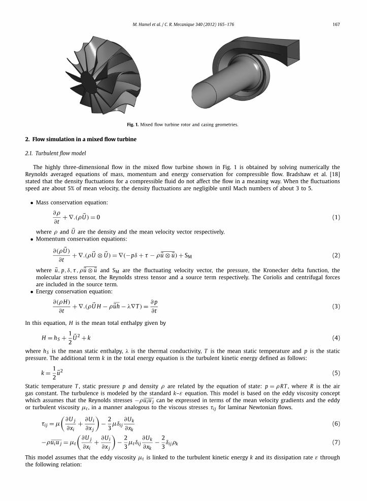
The present paper deals with the performance prediction of a mixed flow turbine (Fig. 1) under pulsating flow conditions.The pulsating flow model consists in solving the unsteady three-dimensional flow equations in the mixed flow turbine Awith appropriate inlet and exit flow boundary conditions. The instantaneous total pressure and a constant cycle meantotal temperature along with the flow direction are specified at the turbine inlet, corresponding to the experimental inletmeasuring location, while a constant static pressure is imposed at the turbine exit. The total pressure is calculated from theinstantaneous mass flow rate, the instantaneous static pressure and the assumed constant mean cycle total temperature [5].The unsteady flow model is used to study the influence of the frequency of the pulse on the turbine performance. The ICEMtool is used to build the full turbine geometry and to generate the mesh while the computational tests are performed withthe ANSYS-CFX software. Four air pulse frequencies of 20, 40, 56.8 and 80 Hz are selected in the present investigation tomimic a four stroke, six cylinder engine running at 800, 1600, 2272 and 3200 rpm, respectively. The numerical results arecompared with experimental and one-dimensional model results in the aim of indicating the capability of the code and themodeling approach to capture the details of the flow field under pulsed flow conditions.

M. Hamel et al. / C. R. Mecanique 340 (2012) 165–176 167

Fig. 1. Mixed flow turbine rotor and casing geometries.

2. Flow simulation in a mixed flow turbine

2.1. Turbulent flow model

The highly three-dimensional flow in the mixed flow turbine shown in Fig. 1 is obtained by solving numerically theReynolds averaged equations of mass, momentum and energy conservation for compressible flow. Bradshaw et al. [18]stated that the density fluctuations for a compressible fluid do not affect the flow in a meaning way. When the fluctuationsspeed are about 5% of mean velocity, the density fluctuations are negligible until Mach numbers of about 3 to 5.

• Mass conservation equation:

∂ρ

∂t+ ∇.(ρ �U ) = 0 (1)

where ρ and �U are the density and the mean velocity vector respectively.• Momentum conservation equations:

∂(ρ �U )

∂t+ ∇.(ρ �U ⊗ �U ) = ∇(−pδ + τ − ρ�u ⊗ �u) + SM (2)

where �u, p, δ, τ ,ρ�u ⊗ �u and SM are the fluctuating velocity vector, the pressure, the Kronecker delta function, themolecular stress tensor, the Reynolds stress tensor and a source term respectively. The Coriolis and centrifugal forcesare included in the source term.

• Energy conservation equation:

∂(ρH)

∂t+ ∇.(ρ �U H − ρ�uh − λ∇T ) = ∂ p

∂t(3)

In this equation, H is the mean total enthalpy given by

H = hS + 1

2�U 2 + k (4)

where hS is the mean static enthalpy, λ is the thermal conductivity, T is the mean static temperature and p is the staticpressure. The additional term k in the total energy equation is the turbulent kinetic energy defined as follows:

k = 1

2�u2 (5)

Static temperature T , static pressure p and density ρ are related by the equation of state: p = ρRT , where R is the airgas constant. The turbulence is modeled by the standard k–ε equation. This model is based on the eddy viscosity conceptwhich assumes that the Reynolds stresses −ρuiu j can be expressed in terms of the mean velocity gradients and the eddyor turbulent viscosity μt , in a manner analogous to the viscous stresses τi j for laminar Newtonian flows.

τi j = μ

(∂U j

∂xi+ ∂Ui

∂x j

)− 2

3μδi j

∂Uk

∂xk(6)

−ρuiu j = μt

(∂U j

∂xi+ ∂Ui

∂x j

)− 2

3μtδi j

∂Uk

∂xk− 2

3δi jρk (7)

This model assumes that the eddy viscosity μt is linked to the turbulent kinetic energy k and its dissipation rate ε throughthe following relation:


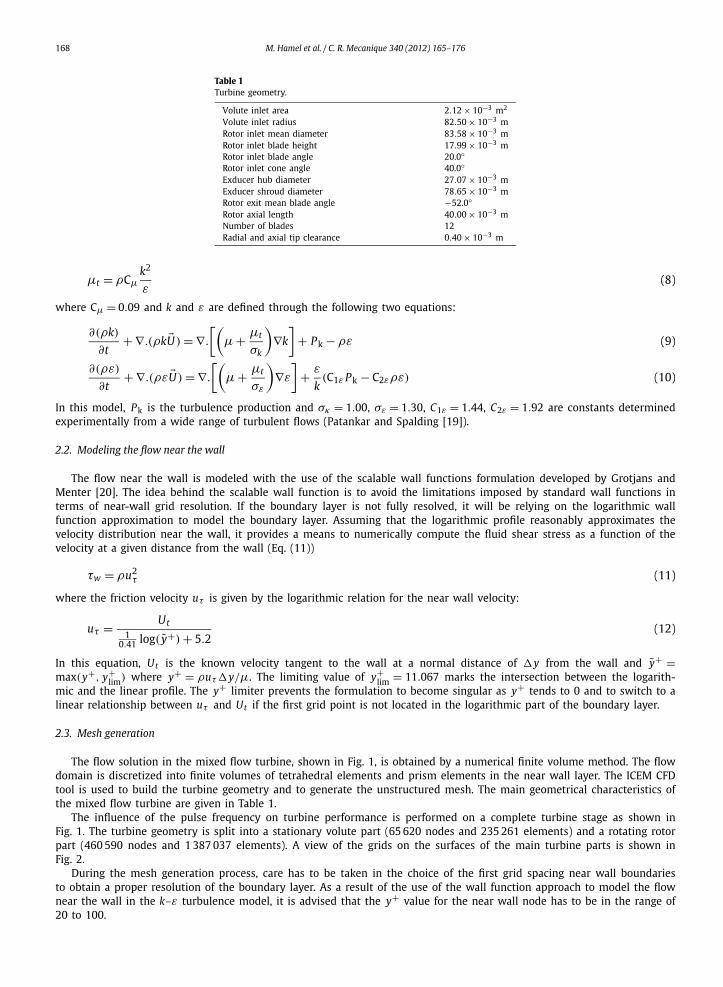
Table 1Turbine geometry.

Volute inlet area 2.12 × 10−3 m2

Volute inlet radius 82.50 × 10−3 mRotor inlet mean diameter 83.58 × 10−3 mRotor inlet blade height 17.99 × 10−3 mRotor inlet blade angle 20.0◦Rotor inlet cone angle 40.0◦Exducer hub diameter 27.07 × 10−3 mExducer shroud diameter 78.65 × 10−3 mRotor exit mean blade angle −52.0◦Rotor axial length 40.00 × 10−3 mNumber of blades 12Radial and axial tip clearance 0.40 × 10−3 m

μt = ρCμk2

ε(8)

where Cμ = 0.09 and k and ε are defined through the following two equations:

∂(ρk)

∂t+ ∇.(ρk �U ) = ∇.

[(μ + μt

σk

)∇k

]+ Pk − ρε (9)

∂(ρε)

∂t+ ∇.(ρε �U ) = ∇.

[(μ + μt

σε

)∇ε

]+ ε

k(C1ε Pk − C2ερε) (10)

In this model, Pk is the turbulence production and σκ = 1.00, σε = 1.30, C1ε = 1.44, C2ε = 1.92 are constants determinedexperimentally from a wide range of turbulent flows (Patankar and Spalding [19]).

2.2. Modeling the flow near the wall

The flow near the wall is modeled with the use of the scalable wall functions formulation developed by Grotjans andMenter [20]. The idea behind the scalable wall function is to avoid the limitations imposed by standard wall functions interms of near-wall grid resolution. If the boundary layer is not fully resolved, it will be relying on the logarithmic wallfunction approximation to model the boundary layer. Assuming that the logarithmic profile reasonably approximates thevelocity distribution near the wall, it provides a means to numerically compute the fluid shear stress as a function of thevelocity at a given distance from the wall (Eq. (11))

τw = ρu2τ (11)

where the friction velocity uτ is given by the logarithmic relation for the near wall velocity:

uτ = Ut1

0.41 log( y+) + 5.2(12)

In this equation, Ut is the known velocity tangent to the wall at a normal distance of y from the wall and y+ =max(y+, y+

lim) where y+ = ρuτ y/μ. The limiting value of y+lim = 11.067 marks the intersection between the logarith-

mic and the linear profile. The y+ limiter prevents the formulation to become singular as y+ tends to 0 and to switch to alinear relationship between uτ and Ut if the first grid point is not located in the logarithmic part of the boundary layer.

2.3. Mesh generation

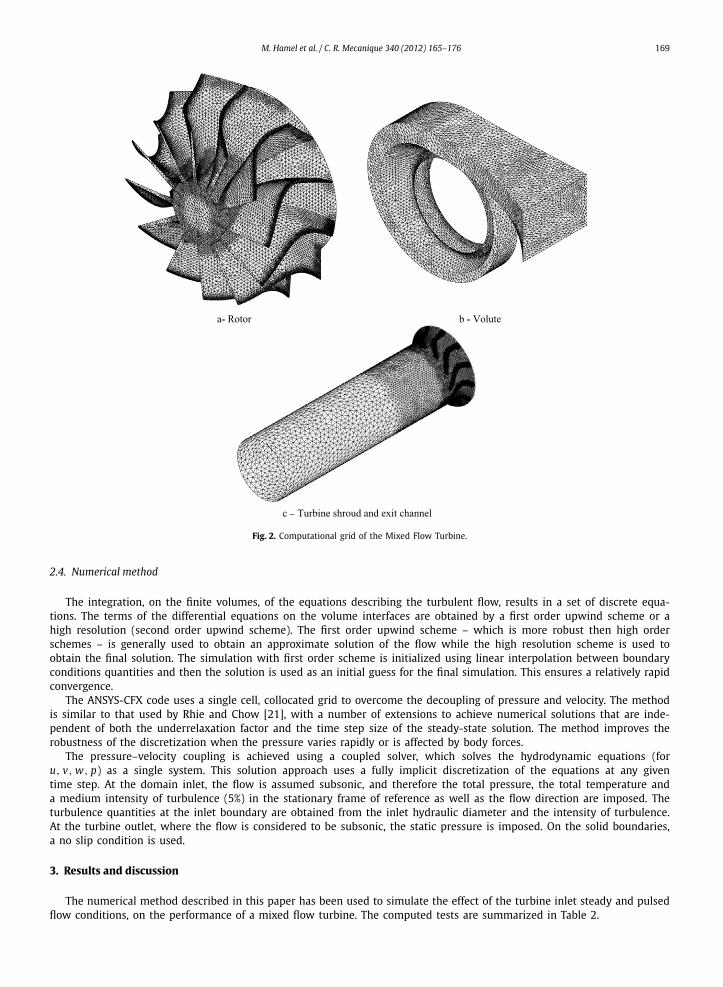
The flow solution in the mixed flow turbine, shown in Fig. 1, is obtained by a numerical finite volume method. The flowdomain is discretized into finite volumes of tetrahedral elements and prism elements in the near wall layer. The ICEM CFDtool is used to build the turbine geometry and to generate the unstructured mesh. The main geometrical characteristics ofthe mixed flow turbine are given in Table 1.

The influence of the pulse frequency on turbine performance is performed on a complete turbine stage as shown inFig. 1. The turbine geometry is split into a stationary volute part (65 620 nodes and 235 261 elements) and a rotating rotorpart (460 590 nodes and 1 387 037 elements). A view of the grids on the surfaces of the main turbine parts is shown inFig. 2.

During the mesh generation process, care has to be taken in the choice of the first grid spacing near wall boundariesto obtain a proper resolution of the boundary layer. As a result of the use of the wall function approach to model the flownear the wall in the k–ε turbulence model, it is advised that the y+ value for the near wall node has to be in the range of20 to 100.


Fig. 2. Computational grid of the Mixed Flow Turbine.

2.4. Numerical method

The integration, on the finite volumes, of the equations describing the turbulent flow, results in a set of discrete equa-tions. The terms of the differential equations on the volume interfaces are obtained by a first order upwind scheme or ahigh resolution (second order upwind scheme). The first order upwind scheme – which is more robust then high orderschemes – is generally used to obtain an approximate solution of the flow while the high resolution scheme is used toobtain the final solution. The simulation with first order scheme is initialized using linear interpolation between boundaryconditions quantities and then the solution is used as an initial guess for the final simulation. This ensures a relatively rapidconvergence.

The ANSYS-CFX code uses a single cell, collocated grid to overcome the decoupling of pressure and velocity. The methodis similar to that used by Rhie and Chow [21], with a number of extensions to achieve numerical solutions that are inde-pendent of both the underrelaxation factor and the time step size of the steady-state solution. The method improves therobustness of the discretization when the pressure varies rapidly or is affected by body forces.

The pressure–velocity coupling is achieved using a coupled solver, which solves the hydrodynamic equations (foru, v, w, p) as a single system. This solution approach uses a fully implicit discretization of the equations at any giventime step. At the domain inlet, the flow is assumed subsonic, and therefore the total pressure, the total temperature anda medium intensity of turbulence (5%) in the stationary frame of reference as well as the flow direction are imposed. Theturbulence quantities at the inlet boundary are obtained from the inlet hydraulic diameter and the intensity of turbulence.At the turbine outlet, where the flow is considered to be subsonic, the static pressure is imposed. On the solid boundaries,a no slip condition is used.

3. Results and discussion

The numerical method described in this paper has been used to simulate the effect of the turbine inlet steady and pulsedflow conditions, on the performance of a mixed flow turbine. The computed tests are summarized in Table 2.


Table 2Computed test conditions.

(a) Steady state performance test conditions.

Speed Turbine inlet total temperature Pressure ratio

50% (29 500 rpm) 340.0 K 1.1–3

(b) Unsteady performance test conditions.

Speed Turbine inlet total temperature Pulse frequency

50% (29 500 rpm) 341.0 K 20.0–80.0 Hz

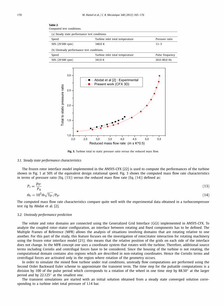
Fig. 3. Turbine total to static pressure ratio versus the reduced mass flow.

3.1. Steady state performance characteristics

The frozen rotor interface model implemented in the ANSYS-CFX [22] is used to compute the performances of the turbineshown in Fig. 1 at 50% of the equivalent design rotational speed. Fig. 3 shows the computed mass flow rate characteristicsin terms of pressure ratio (Eq. (13)) versus the reduced mass flow rate (Eq. (14)) defined as:

Pr = p0∗

P4(13)

mr = 105m√

T0∗/P0∗ (14)

The computed mass flow rate characteristics compare quite well with the experimental data obtained in a turbocompressortest rig by Abidat et al. [2].

3.2. Unsteady performance prediction

The volute and rotor domains are connected using the Generalized Grid Interface (GGI) implemented in ANSYS-CFX. Toanalyze the coupled rotor–stator configuration, an interface between rotating and fixed components has to be defined. TheMultiple Frames of Reference (MFR) allows the analysis of situations involving domains that are rotating relative to oneanother. For this part of the study, this feature focuses on the investigation of rotor/stator interaction for rotating machineryusing the frozen rotor interface model [21]; this means that the relative position of the grids on each side of the interfacedoes not change. In the MFR concept one uses a coordinate system that rotates with the turbine. Therefore, additional sourceterms including Coriolis and centrifugal forces have to be considered. Since the housing of the turbine is not rotating, thecomputational domain contains also regions which are described in non-rotating coordinates. Hence the Coriolis terms andcentrifugal forces are activated only in the region where rotation of the geometry occurs.

In order to simulate the mixed flow turbine under real conditions, unsteady flow computations are performed using theSecond Order Backward Euler scheme to approximate the transient term. The time step for the pulsatile computations is adivision by 100 of the pulse period which corresponds to a rotation of the wheel in one time step by 88.50◦ at the largerperiod and by 22.125◦ at the smallest one.

The transient simulations are started with an initial solution obtained from a steady state converged solution corre-sponding to a turbine inlet total pressure of 1.14 bar.


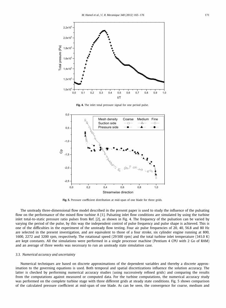
Fig. 4. The inlet total pressure signal for one period pulse.

Fig. 5. Pressure coefficient distribution at mid-span of one blade for three grids.

The unsteady three-dimensional flow model described in the present paper is used to study the influence of the pulsatingflow on the performance of the mixed flow turbine A [1]. Pulsating inlet flow conditions are simulated by using the turbineinlet total-to-static pressure ratio pulses from Ref. [2], as shown in Fig. 4. The frequency of the pulsation can be varied byvarying the period of the pulse, by this way the independent control of pulse frequency and pulse shape is achieved. This isone of the difficulties in the experiment of the unsteady flow testing. Four air pulse frequencies of 20, 40, 56.8 and 80 Hzare selected in the present investigation, and are equivalent to those of a four stroke, six cylinder engine running at 800,1600, 2272 and 3200 rpm, respectively. The rotational speed (29 500 rpm) and the total turbine inlet temperature (341.0 K)are kept constants. All the simulations were performed in a single processor machine (Pentium 4 CPU with 2 Go of RAM)and an average of three weeks was necessary to run an unsteady state simulation case.

3.3. Numerical accuracy and uncertainty

Numerical techniques are based on discrete approximations of the dependent variables and thereby a discrete approx-imation to the governing equations is used. Both temporal and spatial discretizations influence the solution accuracy. Thelatter is checked by performing numerical accuracy studies (using successively refined grids) and comparing the resultsfrom the computations against measured or computed data. For the turbine computations, the numerical accuracy studywas performed on the complete turbine stage with three different grids at steady state conditions. Fig. 5 shows comparisonof the calculated pressure coefficient at mid-span of one blade. As can be seen, the convergence for coarse, medium and


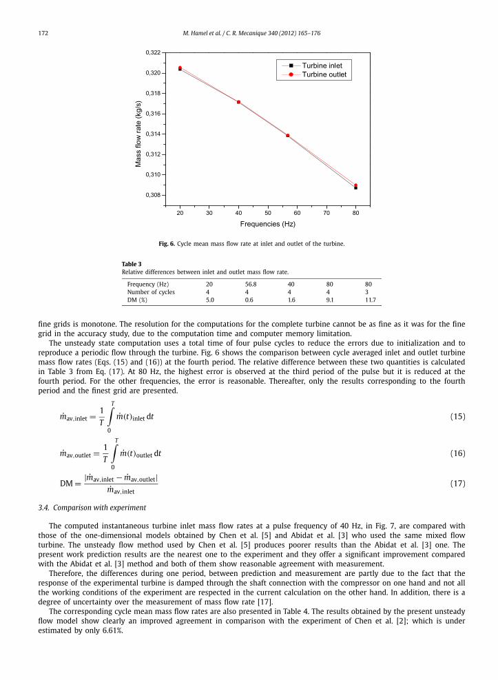
Fig. 6. Cycle mean mass flow rate at inlet and outlet of the turbine.

Table 3Relative differences between inlet and outlet mass flow rate.

Frequency (Hz) 20 56.8 40 80 80Number of cycles 4 4 4 4 3DM (%) 5.0 0.6 1.6 9.1 11.7

fine grids is monotone. The resolution for the computations for the complete turbine cannot be as fine as it was for the finegrid in the accuracy study, due to the computation time and computer memory limitation.

The unsteady state computation uses a total time of four pulse cycles to reduce the errors due to initialization and toreproduce a periodic flow through the turbine. Fig. 6 shows the comparison between cycle averaged inlet and outlet turbinemass flow rates (Eqs. (15) and (16)) at the fourth period. The relative difference between these two quantities is calculatedin Table 3 from Eq. (17). At 80 Hz, the highest error is observed at the third period of the pulse but it is reduced at thefourth period. For the other frequencies, the error is reasonable. Thereafter, only the results corresponding to the fourthperiod and the finest grid are presented.

mav,inlet = 1

T

T∫0

m(t)inlet dt (15)

mav,outlet = 1

T

T∫0

m(t)outlet dt (16)

DM = |mav,inlet − mav,outlet|mav,inlet

(17)

3.4. Comparison with experiment

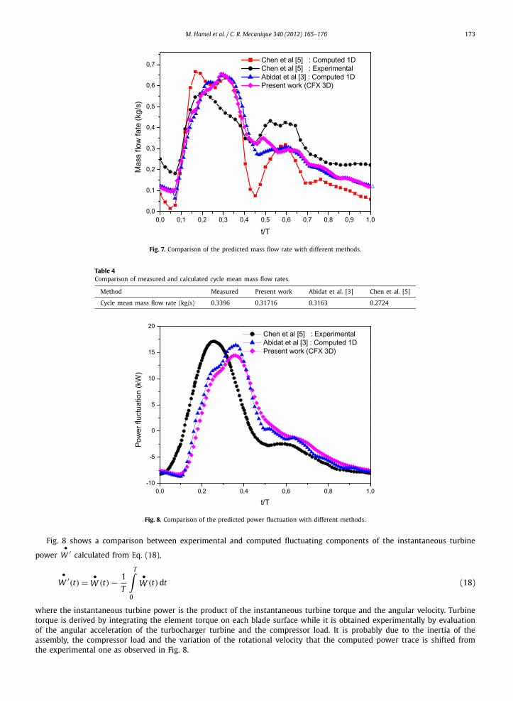
The computed instantaneous turbine inlet mass flow rates at a pulse frequency of 40 Hz, in Fig. 7, are compared withthose of the one-dimensional models obtained by Chen et al. [5] and Abidat et al. [3] who used the same mixed flowturbine. The unsteady flow method used by Chen et al. [5] produces poorer results than the Abidat et al. [3] one. Thepresent work prediction results are the nearest one to the experiment and they offer a significant improvement comparedwith the Abidat et al. [3] method and both of them show reasonable agreement with measurement.

Therefore, the differences during one period, between prediction and measurement are partly due to the fact that theresponse of the experimental turbine is damped through the shaft connection with the compressor on one hand and not allthe working conditions of the experiment are respected in the current calculation on the other hand. In addition, there is adegree of uncertainty over the measurement of mass flow rate [17].

The corresponding cycle mean mass flow rates are also presented in Table 4. The results obtained by the present unsteadyflow model show clearly an improved agreement in comparison with the experiment of Chen et al. [2]; which is underestimated by only 6.61%.


Fig. 7. Comparison of the predicted mass flow rate with different methods.

Table 4Comparison of measured and calculated cycle mean mass flow rates.

Method Measured Present work Abidat et al. [3] Chen et al. [5]

Cycle mean mass flow rate (kg/s) 0.3396 0.31716 0.3163 0.2724

Fig. 8. Comparison of the predicted power fluctuation with different methods.

Fig. 8 shows a comparison between experimental and computed fluctuating components of the instantaneous turbine

power•

W ′ calculated from Eq. (18),

•W ′(t) = •

W (t) − 1

T

T∫0

•W (t)dt (18)

where the instantaneous turbine power is the product of the instantaneous turbine torque and the angular velocity. Turbinetorque is derived by integrating the element torque on each blade surface while it is obtained experimentally by evaluationof the angular acceleration of the turbocharger turbine and the compressor load. It is probably due to the inertia of theassembly, the compressor load and the variation of the rotational velocity that the computed power trace is shifted fromthe experimental one as observed in Fig. 8.


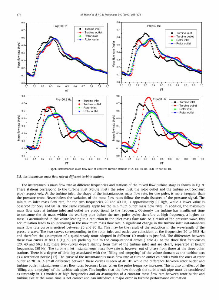
Fig. 9. Instantaneous mass flow rate at different turbine stations at 20 Hz, 40 Hz, 56.8 Hz and 80 Hz.

3.5. Instantaneous mass flow rate at different turbine stations

The instantaneous mass flow rate at different frequencies and stations of the mixed flow turbine stage is shown in Fig. 9.These stations correspond to the turbine inlet (volute inlet), the rotor inlet, the rotor outlet and the turbine exit (exhaustpipe) respectively. At the turbine inlet, the shape of the instantaneous mass flow rate, for one pulse, is more irregular thanthe pressure trace. Nevertheless the variation of the mass flow rates follow the main features of the pressure signal. Theminimum inlet mass flow rate, for the two frequencies 20 and 40 Hz, is approximately 0.1 kg/s, while a lower value isobserved for 56.8 and 80 Hz. The same remarks apply for the minimum outlet mass flow rates. In addition, the maximummass flow rates at turbine inlet and outlet are proportional to the frequency. Obviously the turbine has insufficient timeto consume the air mass within the working pipe before the next pulse cycle; therefore at high frequency, a higher airmass is accumulated in the volute leading to a reduction in the inlet mass flow rate. As a result of the pressure wave, thisaccumulation leads to an increasing in the maximum mass flow rate. A significant change in the turbine inlet instantaneousmass flow rate curve is noticed between 20 and 80 Hz. This may be the result of the reduction in the wavelength of thepressure wave. The two curves corresponding to the rotor inlet and outlet are coincident at the frequencies 20 to 56.8 Hzand therefore the assumption of a quasi-steady rotor adopted in different 1D models is justified. The differences betweenthese two curves at 80 Hz (Fig. 9) are probably due to the computational errors (Table 4). At the three first frequencies(20, 40 and 56.8 Hz), these two curves depart slightly from that of the turbine inlet and are clearly separated at heightfrequencies (80 Hz). The turbine inlet instantaneous mass flow rate is however out of phase from those at the three otherstations. There is a degree of time lag associated with the “filling and emptying” of the volute domain as the turbine actsas a restriction nozzle [17]. The curve of the instantaneous mass flow rate at turbine outlet coincides with the ones at rotoroutlet at 20 Hz. A small difference between these curves is seen at 40 Hz, while the difference between rotor outlet andturbine outlet instantaneous mass flow rates becomes larger when the pulse frequency increases. This is also an effect of the“filling and emptying” of the turbine exit pipe. This implies that the flow through the turbine exit pipe must be consideredas unsteady in 1D models at high frequencies and an assumption of a constant mass flow rate between rotor outlet andturbine exit at the same time is not correct and can introduce a major error in turbine performance estimation.


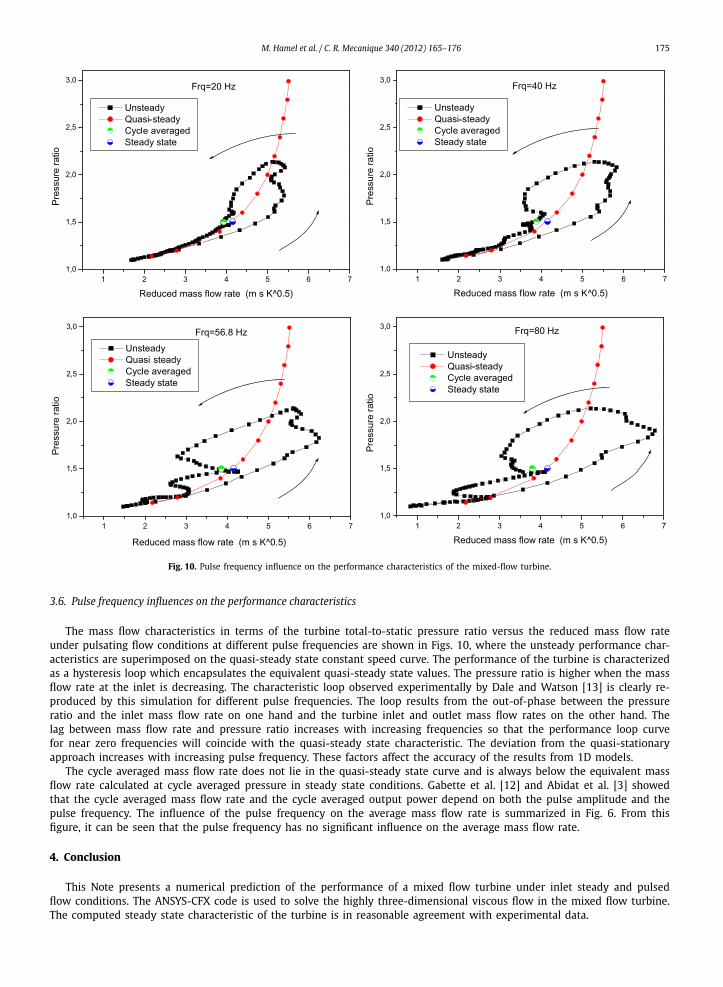
Fig. 10. Pulse frequency influence on the performance characteristics of the mixed-flow turbine.

3.6. Pulse frequency influences on the performance characteristics

The mass flow characteristics in terms of the turbine total-to-static pressure ratio versus the reduced mass flow rateunder pulsating flow conditions at different pulse frequencies are shown in Figs. 10, where the unsteady performance char-acteristics are superimposed on the quasi-steady state constant speed curve. The performance of the turbine is characterizedas a hysteresis loop which encapsulates the equivalent quasi-steady state values. The pressure ratio is higher when the massflow rate at the inlet is decreasing. The characteristic loop observed experimentally by Dale and Watson [13] is clearly re-produced by this simulation for different pulse frequencies. The loop results from the out-of-phase between the pressureratio and the inlet mass flow rate on one hand and the turbine inlet and outlet mass flow rates on the other hand. Thelag between mass flow rate and pressure ratio increases with increasing frequencies so that the performance loop curvefor near zero frequencies will coincide with the quasi-steady state characteristic. The deviation from the quasi-stationaryapproach increases with increasing pulse frequency. These factors affect the accuracy of the results from 1D models.

The cycle averaged mass flow rate does not lie in the quasi-steady state curve and is always below the equivalent massflow rate calculated at cycle averaged pressure in steady state conditions. Gabette et al. [12] and Abidat et al. [3] showedthat the cycle averaged mass flow rate and the cycle averaged output power depend on both the pulse amplitude and thepulse frequency. The influence of the pulse frequency on the average mass flow rate is summarized in Fig. 6. From thisfigure, it can be seen that the pulse frequency has no significant influence on the average mass flow rate.

4. Conclusion

This Note presents a numerical prediction of the performance of a mixed flow turbine under inlet steady and pulsedflow conditions. The ANSYS-CFX code is used to solve the highly three-dimensional viscous flow in the mixed flow turbine.The computed steady state characteristic of the turbine is in reasonable agreement with experimental data.


The effect of the pulsed flow on the turbine performance has been investigated by conducting computation at differentfrequencies. Some special numerical techniques are employed in order to reduce the computing time and to increase thenumerical accuracy.

The numerical simulation of the turbine under pulsed inlet flow conditions is performed with a constant inlet totaltemperature and rotational speed. For one pulse frequency, a comparison with measured data and one-dimensional modelhas also been performed. The results show clearly an improved agreement with experiment which indicates the capabilityof the code and the modeling approach to capture the details of the flow field under pulsating inlet flow conditions. Ithas been shown that the turbine characteristics depart from those obtained under steady state inlet flow conditions in ahysteresis like shape.

The surge in mass flow accompanying the inlet pulse wave and the time taken for convection through the volute andturbine domain leads primarily to the mass imbalance. Further there is a degree of time lag associated with the “filling andemptying” of the volute domain as the turbine acts as a restriction nozzle.

The instantaneous performance data of a mixed-flow turbine have been obtained at 50% equivalent design speed(29 500 rpm) at four different pulse frequencies: 20, 40, 56.8 and 80 Hz. When the air pulse frequency increases, theflow conditions within the turbine tend towards unsteadiness and the cycle averaged mass flow rate is lower than thesteady-state value under the equivalent operating conditions. The unsteady performance test results have indicated thatthe turbine instantaneous performance and flow characteristics deviate substantially from their steady-state values, whichimplies that the quasi-steady assumption normally used in the performance assessment of turbines is inadequate for thecharacterization of efficiencies in a highly pulsating environment of an automotive turbocharger.

References

[1] M. Abidat, Design and testing of a highly loaded mixed flow turbine, PhD thesis, Imperial College, London, 1991.[2] M. Abidat, H. Chen, N.C. Baines, M.R. Firth, Design of a highly loaded mixed flow turbine, Proc. IMechE, Part A: J. Power and Energy 206 (1992) 95–107.[3] M. Abidat, M. Hachemi, M.k. Hamidou, N.C. Baines, Prediction of the steady and non-steady flow performance of a highly loaded mixed flow turbine,

Proc. IMechE, Part A: J. Power and Energy (1998) 173–184.[4] C. Arcoumanis, I. Hakeem, R.F. Martinez-Botas, L. Khezzar, N.C. Baines, Performance of a mixed flow turbocharger turbine under pulsating flow condi-

tions, ASME, Paper 95-GT-210, 1995.[5] H. Chen, I. Hakeem, R.F. Martinez-Botas, Modelling of a turbocharger turbine under pulsating inlet conditions, Proc. IMechE, Part A: J. Power and

Energy 210 (1996) 397–408.[6] S. Szymko, R.F. Martinez-Botas, K.R. Pullen, Experimental evaluation of turbocharger turbine performance under pulsating flow conditions, in: Proceed-

ings of GT2005: ASME TURBO EXPO 2005, June 6–9, 2005, Reno-Tahoe, Nevada, USA.[7] I. Hakeem, C.-C. Su, A. Costall, R.F. Martinez-Botas, Effect of volute geometry on the steady and unsteady performance of mixed-flow turbines, Proc.

IMechE, Part A: J. Power and Energy 221 (2007) 535–550.[8] C. Arcoumanis, R.F. Martinez-Botas, J.M. Nouri, C.C. Su, Performance and exit flow characteristics of mixed-flow turbines, Int. J. of Rotating Machin-

ery 3 (4) (1997) 277–293.[9] N. Karamanis, R.F. Martinez-Botas, C.C. Su, Mixed flow turbines: Inlet and exit flow under steady and pulsating conditions, ASME J. of Turbomachin-

ery 123 (2001) 359–371.[10] N. Karamanis, R.F. Martinez-Botas, Mixed-flow turbines for automotive, IMechE, Int. J. Engine Research 3 (3) (2002) 127–138.[11] F.S. Bhinder, P.S. Gulati, Method for predicting the performance of centripetal turbines in non-steady flow, in: IMechE, Conference Publications, 1978,

pp. 233–240.[12] V. Gabette, Ph. San Emeterio, Ph. Arques, Influence d’un écoulement pulsé sur les caractéristiques de fonctionnement d’une turbine de suralimentation

de moteur thermique, Mécanique Matériaux Electricité (Octobre/Novembre 1982) 394–395.[13] A. Dale, N. Watson, Vaneless radial turbocharger turbine performance, in: Conference on Turbochargers and Turbocharging, IMechE C 110 (86) (1986)

65–76.[14] H. Chen, D.E. Winterbone, A method to predict performance of vaneless radial turbines under steady and unsteady flow conditions, in: Conference on

Turbochargers and Turbocharging, IMechE (1990) 13–22.[15] A. Hammoud, Q.C. Duan, J. Julien, Etude de la validité de l’hypothèse de quasi-stationnarité appliquée au fonctionnement d’une turbine de suralimen-

tation en régime pulsé, in: ENTROPIE, 1993, pp. 174–175.[16] J.K.W. Lam, Q.D.H. Roberts, McDonnell, Flow modelling of a turbocharger turbine under pulsating flow, in: ImechE Conference Transactions from 7th

International Conference on Turbochargers and Turbocharging, London, UK, 14–15 May 2002, pp. 181–196.[17] D. Palfreyman, R.F. Martinez-Botas, The pulsating flow field in a mixed flow turbocharger turbine: an experimental and computational study, J. of

Turbomachinery, Transactions of the ASME 127 (2005) 144–155.[18] P. Bradshaw, T. Cebeci, J.H. Whitelaw, Engineering Calculation Methods for Turbulent Flow, Academic Press, 1981.[19] S.V. Patankar, D.B. Spalding, A calculation procedure for heat, mass and momentum transfer in three-dimensional parabolic flows, Int. J. of Heat and

Mass Transfer 15 (1972) 1778–1806.[20] H. Grotjans, F.R. Menter, Wall functions for industrial applications, in: K.D. Papailiou (Ed.), ECCOMAS CFD’98, vol. 1(2), 1998, pp. 1112–1117.[21] C.M. Rhie, W.L.A. Chow, Numerical study of the turbulent flow past an isolated airfoil with trailing edge separation, AIAA J. (1982) 1525–1532.[22] CFX 10 Solver Theory, 2004.