Louisiana State University LSU Digital Commons LSU Doctoral Dissertations Graduate School 8-27-2018 Investigation of Flow Mechanisms in Gas-Assisted Gravity Drainage Process Iskandar Dzulkarnain Louisiana State University and Agricultural and Mechanical College, [email protected] Follow this and additional works at: hps://digitalcommons.lsu.edu/gradschool_dissertations Part of the Petroleum Engineering Commons is Dissertation is brought to you for free and open access by the Graduate School at LSU Digital Commons. It has been accepted for inclusion in LSU Doctoral Dissertations by an authorized graduate school editor of LSU Digital Commons. For more information, please contact[email protected]. Recommended Citation Dzulkarnain, Iskandar, "Investigation of Flow Mechanisms in Gas-Assisted Gravity Drainage Process" (2018). LSU Doctoral Dissertations. 4699. hps://digitalcommons.lsu.edu/gradschool_dissertations/4699

Welcome message from author
This document is posted to help you gain knowledge. Please leave a comment to let me know what you think about it! Share it to your friends and learn new things together.
Transcript

Louisiana State UniversityLSU Digital Commons
LSU Doctoral Dissertations Graduate School
8-27-2018
Investigation of Flow Mechanisms in Gas-AssistedGravity Drainage ProcessIskandar DzulkarnainLouisiana State University and Agricultural and Mechanical College, [email protected]
Follow this and additional works at: https://digitalcommons.lsu.edu/gradschool_dissertations
Part of the Petroleum Engineering Commons
This Dissertation is brought to you for free and open access by the Graduate School at LSU Digital Commons. It has been accepted for inclusion inLSU Doctoral Dissertations by an authorized graduate school editor of LSU Digital Commons. For more information, please [email protected].
Recommended CitationDzulkarnain, Iskandar, "Investigation of Flow Mechanisms in Gas-Assisted Gravity Drainage Process" (2018). LSU DoctoralDissertations. 4699.https://digitalcommons.lsu.edu/gradschool_dissertations/4699

INVESTIGATION OF FLOW MECHANISMS IN GAS-ASSISTED GRAVITYDRAINAGE PROCESS
A Dissertation
Submitted to the Graduate Faculty of theLouisiana State University and
Agricultural and Mechanical Collegein partial fulfillment of the
requirements for the degree ofDoctor of Philosophy
in
The Craft & Hawkins Department of Petroleum Engineering
byIskandar Dzulkarnain
B.Eng., University of Technology PETRONAS, 2007M.S., University of Technology PETRONAS & Heriot-Watt University, 2010
December 2018

AcknowledgmentsThis work would not be possible without the guidance and patience from my advisor,
Dr. Dandina Rao. He has a way of interacting with his students that make them feel
appreciated , inspired and always motivated to push more, and when the time gets tough,
to endure and persevere over the course of their graduate study to see to it until its eventual
completion. To him I would say thank you and extend my heartfelt gratitude.
I would also like to thank my former advisor, Dr. Seung Kam for his guidance in the
beginning of my doctoral study. He is the role model I seek to emulate when it comes to
teaching and research.
I thank my committee members, Dr. Mehdi Zeidouni, Dr. Mayank Tyagi and Dr.
Samuel Snow for their support and useful comments as my committee members. My thank
also goes to Dr. Mileva Radonjic who was on my committee initially and had provided
valuable suggestions during the Proposal Defense.
I would like to acknowledge the funding received toward completion of this study which
came from two sources. Craft and Hawkins Department of Petroleum Engineering has given
me the opportunity as graduate teaching assistant during the duration of my study while
University of Technology PETRONAS provided me with financial support under their Staff
Development Program.
I would also take this opportunity to thank the members of Enhanced Oil recovery
group past and present including Dr. Mohamed Al Riyami, Dr. Bikash D. Saikia, Dr.
Paulina Mwangi, Dr. Watheq Al-Mudhafar, Mohammad Foad Haeri, Alok Shah and Ab-
dullah At-Tamimi.
Many thanks also go to the Malaysian and Indonesian communities in Lafayette, Baton
Rouge and New Orleans for their hospitality and many memorable moments shared during
our frequent gatherings. I would like to mention Melati Tessier and Aunt Rubaiyah for
their kindness and help during our stay in Baton Rouge. It was also due to them that we
are introduced to Louisiana dishes such as crawfish etouffee, gumbo and jambalaya. This
ii

work is dedicated to my parents and to my beloved wife Norashikin Mohd Said and our
children: Mushab, Wafa, Abdullah and Asma.
iii
Table of ContentsACKNOWLEDGMENTS . . . . . . . . . . . . . . . . . . . . . . . . . . . . . . . . . . . . . . . . . . . . . . . . . . . . . . . . . ii
LIST OF TABLES . . . . . . . . . . . . . . . . . . . . . . . . . . . . . . . . . . . . . . . . . . . . . . . . . . . . . . . . . . . . . . . vi
LIST OF FIGURES . . . . . . . . . . . . . . . . . . . . . . . . . . . . . . . . . . . . . . . . . . . . . . . . . . . . . . . . . . . . . . vii
ABSTRACT . . . . . . . . . . . . . . . . . . . . . . . . . . . . . . . . . . . . . . . . . . . . . . . . . . . . . . . . . . . . . . . . . . . . . . xi
CHAPTER1 INTRODUCTION . . . . . . . . . . . . . . . . . . . . . . . . . . . . . . . . . . . . . . . . . . . . . . . . . . . . . . . . . 1
1.1 Background of the research . . . . . . . . . . . . . . . . . . . . . . . . . . . . . . . . . . . . . . . . . . . 11.2 Problem statement and motivation of research. . . . . . . . . . . . . . . . . . . . . . . . . 41.3 Aim and scope of the research . . . . . . . . . . . . . . . . . . . . . . . . . . . . . . . . . . . . . . . . 51.4 Significance of the research . . . . . . . . . . . . . . . . . . . . . . . . . . . . . . . . . . . . . . . . . . . 51.5 Overview of the dissertation . . . . . . . . . . . . . . . . . . . . . . . . . . . . . . . . . . . . . . . . . . 6
2 LITERATURE REVIEW . . . . . . . . . . . . . . . . . . . . . . . . . . . . . . . . . . . . . . . . . . . . . . . . . . 72.1 Pioneering study . . . . . . . . . . . . . . . . . . . . . . . . . . . . . . . . . . . . . . . . . . . . . . . . . . . . . 72.2 Investigation of displacement mechanism . . . . . . . . . . . . . . . . . . . . . . . . . . . . . . 102.3 Modeling studies for gravity drainage . . . . . . . . . . . . . . . . . . . . . . . . . . . . . . . . . 25
3 EXPERIMENTAL SETUP, MATERIAL, AND PROCEDURE . . . . . . . . . . . . . 283.1 Experimental setup . . . . . . . . . . . . . . . . . . . . . . . . . . . . . . . . . . . . . . . . . . . . . . . . . . . 283.2 The material . . . . . . . . . . . . . . . . . . . . . . . . . . . . . . . . . . . . . . . . . . . . . . . . . . . . . . . . . 333.3 Experimental procedures. . . . . . . . . . . . . . . . . . . . . . . . . . . . . . . . . . . . . . . . . . . . . . 34
4 GRAVITY DRAINAGE EXPERIMENTS FOR SPREAD-ING AND NON-SPREADING SYSTEMS. . . . . . . . . . . . . . . . . . . . . . . . . . . . . . . . . . 424.1 Experimental results . . . . . . . . . . . . . . . . . . . . . . . . . . . . . . . . . . . . . . . . . . . . . . . . . . 424.2 Pore-scale mechanisms . . . . . . . . . . . . . . . . . . . . . . . . . . . . . . . . . . . . . . . . . . . . . . . . 814.3 Analysis of results with dimensionless groups . . . . . . . . . . . . . . . . . . . . . . . . . . 97
5 EVALUATION OF EXISTING GRAVITY DRAINAGE MODELS . . . . . . . . . 1185.1 Goodness-of-fit parameter for gravity drainage
models . . . . . . . . . . . . . . . . . . . . . . . . . . . . . . . . . . . . . . . . . . . . . . . . . . . . . . . . . . . . . . . 1185.2 Dykstra model . . . . . . . . . . . . . . . . . . . . . . . . . . . . . . . . . . . . . . . . . . . . . . . . . . . . . . . 1205.3 Schechter-Guo model . . . . . . . . . . . . . . . . . . . . . . . . . . . . . . . . . . . . . . . . . . . . . . . . . 1275.4 Li-Horne model . . . . . . . . . . . . . . . . . . . . . . . . . . . . . . . . . . . . . . . . . . . . . . . . . . . . . . . 1355.5 Discussion and summary . . . . . . . . . . . . . . . . . . . . . . . . . . . . . . . . . . . . . . . . . . . . . . 141
6 CONCLUSIONS AND RECOMMENDATIONS . . . . . . . . . . . . . . . . . . . . . . . . . . . . 146
REFERENCES . . . . . . . . . . . . . . . . . . . . . . . . . . . . . . . . . . . . . . . . . . . . . . . . . . . . . . . . . . . . . . . . . . . . 150
APPENDIX
iv

A PROGRAM CODES FOR SCHECHTER-GUO MODEL . . . . . . . . . . . . . . . . . . . 156
B PROGRAM CODES FOR DYKSTRA MODEL . . . . . . . . . . . . . . . . . . . . . . . . . . . . 158
C PROGRAM CODES FOR LI-HORNE MODEL . . . . . . . . . . . . . . . . . . . . . . . . . . . . 163
VITA . . . . . . . . . . . . . . . . . . . . . . . . . . . . . . . . . . . . . . . . . . . . . . . . . . . . . . . . . . . . . . . . . . . . . . . . . . . . . 165
v

List of Tables2.1 Residual oil saturation (Sorg) after gravity drainage under var-
ious spreading and wetting conditions . . . . . . . . . . . . . . . . . . . . . . . . . . . . . . . . . . . . . . . . 15
3.1 Fluid systems used in experiments. . . . . . . . . . . . . . . . . . . . . . . . . . . . . . . . . . . . . . . . . . . 33
3.2 Fluid densities and viscosities used in experiments. . . . . . . . . . . . . . . . . . . . . . . . . . . . 33
3.3 Matrix of experimental work . . . . . . . . . . . . . . . . . . . . . . . . . . . . . . . . . . . . . . . . . . . . . . . . 34
4.1 Summary of experimental results for free-fall gravity drainage,secondary controlled gravity drainage and tertiary controlledgravity drainage . . . . . . . . . . . . . . . . . . . . . . . . . . . . . . . . . . . . . . . . . . . . . . . . . . . . . . . . . . . . . 43
4.2 Pore scale configurations and oil recoveries for gravity drainageexperiments. . . . . . . . . . . . . . . . . . . . . . . . . . . . . . . . . . . . . . . . . . . . . . . . . . . . . . . . . . . . . . . . . 89
5.1 Performance of Dykstra model in FGD, secondary GAGD andtertiary GAGD experiments. . . . . . . . . . . . . . . . . . . . . . . . . . . . . . . . . . . . . . . . . . . . . . . . . . 126
5.2 Performance of Schechter-Guo model in FGD, secondary GAGDand tertiary GAGD experiments. . . . . . . . . . . . . . . . . . . . . . . . . . . . . . . . . . . . . . . . . . . . . 134
5.3 Performance of Li and Horne model in FGD, secondary GAGDand tertiary GAGD experiments. . . . . . . . . . . . . . . . . . . . . . . . . . . . . . . . . . . . . . . . . . . . . 140
5.4 Best curve fit results from Dykstra, Schechter and Guo andLi and Horne models for FGD, secondary GAGD and tertiaryGAGD experiments. . . . . . . . . . . . . . . . . . . . . . . . . . . . . . . . . . . . . . . . . . . . . . . . . . . . . . . . . . 141
vi
List of Figures1.1 Schematic of Gas-Assisted Gravity Drainage (GAGD) process . . . . . . . . . . . . . . . . 3
2.1 Three phases fluid configuration on a water-wet surface . . . . . . . . . . . . . . . . . . . . . . 11
2.2 Spreading oil covering water-wet surface . . . . . . . . . . . . . . . . . . . . . . . . . . . . . . . . . . . . . 12
2.3 Geometry model showing formation of oil layer in wedge-shaped pore . . . . . . . . . . . . . . . . . . . . . . . . . . . . . . . . . . . . . . . . . . . . . . . . . . . . . . . . . . . . . . . . . 22
3.1 Experimental setup for water injection. . . . . . . . . . . . . . . . . . . . . . . . . . . . . . . . . . . . . . . 29
3.2 Experimental setup for oil injection. . . . . . . . . . . . . . . . . . . . . . . . . . . . . . . . . . . . . . . . . . 293.3 Experimental setup for gas injection.. . . . . . . . . . . . . . . . . . . . . . . . . . . . . . . . . . . . . . . . . 30
3.4 Procedures to measure contact angle of oil-wet sand. . . . . . . . . . . . . . . . . . . . . . . . . . 37
3.5 The steps performed during each experiment with water-wet sand. . . . . . . . . . . . . 39
3.6 The steps performed during each experiment with oil-wet sand. . . . . . . . . . . . . . . . 39
4.1 Recovery profile of FGD, secondary CGD and tertiary CGDin water-wet sand. . . . . . . . . . . . . . . . . . . . . . . . . . . . . . . . . . . . . . . . . . . . . . . . . . . . . . . . . . . . 44
4.2 Time-lapsed photos of water-wet GAGD in FGD mode . . . . . . . . . . . . . . . . . . . . . . . 46
4.3 Time-lapsed photos of water-wet GAGD in secondary CGD mode . . . . . . . . . . . . 47
4.4 Time-lapsed photos of water-wet GAGD in tertiary CGD mode. . . . . . . . . . . . . . . 48
4.5 Recovery profile for secondary CGD in water-wet sand withspreading oil (Soltrol), showing regions of bulk flow and layer flow . . . . . . . . . . . . 51
4.6 Gas velocity profiles for all injection modes of GAGD in water-wet sand. . . . . . . . . . . . . . . . . . . . . . . . . . . . . . . . . . . . . . . . . . . . . . . . . . . . . . . . . . . . . . . . . . . . 53
4.7 Recovery profile of FGD, secondary CGD and tertiary CGDin oil-wet sand. . . . . . . . . . . . . . . . . . . . . . . . . . . . . . . . . . . . . . . . . . . . . . . . . . . . . . . . . . . . . . 55
4.8 Time-lapsed photos of FGD in oil-wet sand. . . . . . . . . . . . . . . . . . . . . . . . . . . . . . . . . . . 57
4.9 Time-lapsed photos of secondary CGD in oil-wet sand. . . . . . . . . . . . . . . . . . . . . . . . 58
4.10 Time-lapsed photos of tertiary CGD in oil-wet sand. . . . . . . . . . . . . . . . . . . . . . . . . . 59
4.11 Gas velocity profiles for all injection modes of GAGD in oil-wet sand. . . . . . . . . . . . . . . . . . . . . . . . . . . . . . . . . . . . . . . . . . . . . . . . . . . . . . . . . . . . . . . . . . . . 61
vii

4.12 Recovery profile of FGD, secondary CGD and tertiary CGDin fractional-wet sand. . . . . . . . . . . . . . . . . . . . . . . . . . . . . . . . . . . . . . . . . . . . . . . . . . . . . . . . 63
4.13 Time-lapsed photos of FGD in fractional-wet sand. . . . . . . . . . . . . . . . . . . . . . . . . . . . 65
4.14 Time-lapsed photos of secondary CGD in fractional-wet sand. . . . . . . . . . . . . . . . . 66
4.15 Time-lapsed photos of tertiary CGD in fractional-wet sand. . . . . . . . . . . . . . . . . . . 67
4.16 Gas velocity profile for FGD experiments in fractional-wetsand. . . . . . . . . . . . . . . . . . . . . . . . . . . . . . . . . . . . . . . . . . . . . . . . . . . . . . . . . . . . . . . . . . . . . . . 69
4.17 Gas velocity profiles for secondary CGD in fractional-wet sand. . . . . . . . . . . . . . . . 71
4.18 Gas velocity and liquid production profile for tertiary CGDin fractional-wet sand. . . . . . . . . . . . . . . . . . . . . . . . . . . . . . . . . . . . . . . . . . . . . . . . . . . . . . . . 71
4.19 Flow-regime for FGD experiments in fractional-wet sand. . . . . . . . . . . . . . . . . . . . . . 73
4.20 Oil recovery for GAGD under FGD and secondary CGD modewith all wettability conditions. . . . . . . . . . . . . . . . . . . . . . . . . . . . . . . . . . . . . . . . . . . . . . . . 76
4.21 Oil recovery for GAGD under tertiary CGD mode with allwettability conditions . . . . . . . . . . . . . . . . . . . . . . . . . . . . . . . . . . . . . . . . . . . . . . . . . . . . . . . 77
4.22 Ternary diagrams showing saturation paths for tertiary CGDexperiments under all wettability conditions. . . . . . . . . . . . . . . . . . . . . . . . . . . . . . . . . . 79
4.23 Configuration A . . . . . . . . . . . . . . . . . . . . . . . . . . . . . . . . . . . . . . . . . . . . . . . . . . . . . . . . . . . . . 84
4.24 Configuration B . . . . . . . . . . . . . . . . . . . . . . . . . . . . . . . . . . . . . . . . . . . . . . . . . . . . . . . . . . . . . 85
4.25 Configuration C . . . . . . . . . . . . . . . . . . . . . . . . . . . . . . . . . . . . . . . . . . . . . . . . . . . . . . . . . . . . . 85
4.26 Pore scale fluid configuration in water-wet experiments . . . . . . . . . . . . . . . . . . . . . . . 91
4.27 Pore scale fluid configuration in oil-wet experiments with Soltrol-based fluid system . . . . . . . . . . . . . . . . . . . . . . . . . . . . . . . . . . . . . . . . . . . . . . . . . . . . . . . . . . . 93
4.28 Pore scale fluid configuration in oil-wet experiments with lowviscosity, non-spreading Decane . . . . . . . . . . . . . . . . . . . . . . . . . . . . . . . . . . . . . . . . . . . . . . 94
4.29 Pore scale fluid configuration in fractional-wet experiments . . . . . . . . . . . . . . . . . . . 96
4.30 Profile of Bond Number, NB for FGD experiments in water-wet, oil-wet and fractional-wet sand. . . . . . . . . . . . . . . . . . . . . . . . . . . . . . . . . . . . . . . . . . 99
4.31 Effect of Bond Number, NB on oil recovery for FGD experi-ments in water-wet, oil-wet and fractional-wet sand. . . . . . . . . . . . . . . . . . . . . . . . . . . 101
viii

4.32 Profile of Capillary Number NC for FGD experiments in water-wet, oil-wet and fractional-wet sand. . . . . . . . . . . . . . . . . . . . . . . . . . . . . . . . . . . . . . . . . . 104
4.33 Effect of Capillary Number, NC on oil recovery for FGD ex-periments in water-wet, oil-wet and fractional-wet sand. . . . . . . . . . . . . . . . . . . . . . . 105
4.34 Profile of Gravity Number, NG for FGD experiments in water-wet, oil-wet and fractional-wet sand. . . . . . . . . . . . . . . . . . . . . . . . . . . . . . . . . . . . . . . . . . 107
4.35 Effect of Gravity Number, NG on oil recovery for FGD exper-iments in water-wet, oil-wet and fractional-wet sand. . . . . . . . . . . . . . . . . . . . . . . . . . 108
4.36 Effect of NB, NC and NG on liquid production in tertiary CGDexperiments in water-wet, oil-wet and fractional-wet sand forboth spreading and non-spreading fluid system. . . . . . . . . . . . . . . . . . . . . . . . . . . . . . . 111
4.37 Gas velocity as a function of time during FGD experiments inwater-wet, oil-wet and fractional-wet sand showing the extentwhere flow is dominated either by capillary, viscous or gravity force. . . . . . . . . . . 113
5.1 Curve fit results using data from FGD experiments for Dyk-stra model. . . . . . . . . . . . . . . . . . . . . . . . . . . . . . . . . . . . . . . . . . . . . . . . . . . . . . . . . . . . . . . . . . . 122
5.2 Curve fit results using data from secondary GAGD experi-ments for Dykstra model. . . . . . . . . . . . . . . . . . . . . . . . . . . . . . . . . . . . . . . . . . . . . . . . . . . . . 123
5.3 Curve fit results using data from tertiary GAGD experimentsfor Dykstra model. . . . . . . . . . . . . . . . . . . . . . . . . . . . . . . . . . . . . . . . . . . . . . . . . . . . . . . . . . . 124
5.4 MATLAB GUI for solving Schechter and Guo (1996) model . . . . . . . . . . . . . . . . . . 129
5.5 Curve fit results using data from FGD experiments for Schechter-Guo model. . . . . . . . . . . . . . . . . . . . . . . . . . . . . . . . . . . . . . . . . . . . . . . . . . . . . . . . . . . . . . . . . . 130
5.6 Curve fit results using data from secondary GAGD experi-ments for Schechter-Guo model. . . . . . . . . . . . . . . . . . . . . . . . . . . . . . . . . . . . . . . . . . . . . . 131
5.7 Curve fit results using data from tertiary GAGD experimentsfor Schechter-Guo model. . . . . . . . . . . . . . . . . . . . . . . . . . . . . . . . . . . . . . . . . . . . . . . . . . . . . 132
5.8 Curve fit results using data from FGD experiments for Li-Horne model. . . . . . . . . . . . . . . . . . . . . . . . . . . . . . . . . . . . . . . . . . . . . . . . . . . . . . . . . . . . . . . . 137
5.9 Curve fit results using data from secondary GAGD experi-ments for Li-Horne model. . . . . . . . . . . . . . . . . . . . . . . . . . . . . . . . . . . . . . . . . . . . . . . . . . . . 138
5.10 Curve fit results using data from tertiary GAGD experimentsfor Li-Horne model. . . . . . . . . . . . . . . . . . . . . . . . . . . . . . . . . . . . . . . . . . . . . . . . . . . . . . . . . . 139
ix
5.11 Performance comparison between Schechter-Guo and Li-Hornemodel in tertiary GAGD of fractional-wet sand for both spread-ing and non-spreading system . . . . . . . . . . . . . . . . . . . . . . . . . . . . . . . . . . . . . . . . . . . . . . . 142
x
AbstractIn this study we investigate displacement mechanism for oil recovered using Gas-
Assisted Gravity Drainage (GAGD) method. For a typical oil recovery under gravity
drainage, the recovery profile can be characterized by an initial bulk flow which occurs
rapidly and a later film flow that extends for a longer duration. It is the latter period
where film spreading, the ability of oil to spread above water in the presence of gas, is
identified as the displacement mechanism responsible for recovering the remaining oil in
gravity drainage process.
Literature survey indicates that mathematical models for gravity drainage do not ac-
count for film spreading mechanism adequately. To address this knowledge gap in the
literature, we would conduct experiments and simulation of mathematical model. The ex-
periments aim to understand the role of film spreading in gravity drainage recovery. This
is achieved by using spreading and non-spreading oils in sand packs, where the sand is
either water-wet, oil-wet or fractional-wet. We would then evaluate the existing models to
account for the observations obtained from these experiments.
The experimental results show that oil recovery is higher in spreading fluid system in
water-wet sands. In oil-wet sands recovery from non-spreading fluid system is higher than
that of spreading fluid. For fractional-wet sands, the recovery trend is similar to that of
oil-wet experiments in that the non-spreading fluid produces more oil than spreading fluid
system. We explain the results in terms of pore scale mechanism and investigate the role of
gravity, capillary and viscous forces during gravity drainage experiment. Curve fitting of the
experimental data with gravity drainage models show that the model which incorporates
film flow mechanism in its formulations is able to match most of the experimental data.
xi

Chapter 1
IntroductionIn this chapter we will present the background of the project, problem statement, aim
and scope of the project, and significance of the study. Toward the end, we will give an
overview of the chapters to follow.
1.1 Background of the research
Enhanced oil recovery (EOR) is the umbrella term used to describe various processes
to recover additional oil from a reservoir after the reservoir undergoes natural depletion
or water flooding stage. The processes that encompass EOR can fall under chemical, gas,
thermal, or microbial. One common theme that unites these processes are that they employ
external agents in their operations. For gas injection EOR, gases such as carbon dioxide
(CO2), nitrogen (N2), flue gas (hot gases coming out from factory stacks) or hydrocarbon
gas are the agents injected into the reservoir to effect recovery.
Under gas EOR, processes that are commonly used are continuous gas injection (CGI),
water alternating gas (WAG) and Gas-Assisted Gravity Drainage (GAGD). Both CGI and
WAG propagate gas horizontally through the payzone to sweep oil to the producer well.
Gas-Assisted Gravity Drainage (GAGD) injects gas at the top of the payzone through a
vertical well and produces the oil through horizontal well at the bottom of the payzone.
CGI commonly uses CO2 as its injectant to take advantage of the miscible condition
that develops when the injection pressure is above miscibility pressure. In this condition,
CO2 behaves as oil phase, which facilitates mass transfer of light and intermediate compo-
nents in the oil into gas. Repeated contacts between CO2 and oil enables this extraction
process to continue throughout the payzone until a point is reached, where the lighter den-
sity CO2, laden with the extracted oil components, is produced. This process works at the
microscopic level; however, due to the density difference gas tends to override, which limits
the number of contacts required to make this process successful. Furthermore, macroscopic
1

sweep is further hampered due to viscous fingering as a consequence of adverse mobility
ratio inherent in this proces.
One method to improve mobility ratio in gas injection EOR is to inject water alternately
with gas. This is the basic concept of WAG. Since the viscosity of water is greater than
gas and oil, the mobility ratio is reduced and the displacement front travels uniformly with
less fingering. Consequently, the microscopic sweep efficiency is improved.
Nonetheless, despite its supposed improvement, Rao et al. (2004) noted that in actual
implementation it is difficult to maintain a uniform displacement front throughout the
payzone. This is because density difference is still prevalent, leading to gas override and
water underride in a typical WAG process. This creates an unswept region where the oil
is bypassed by either gas or water. In terms of performance, this accounts for meager
additional recovery of 5-10% as reported by Rao et al. (2004). In addition, if the reservoir
is waterflooded for a long time prior to WAG, the excess water will contribute to water
blocking effect. This effect blocks the gas from contacting oil, thus reduces the extraction
process described earlier.
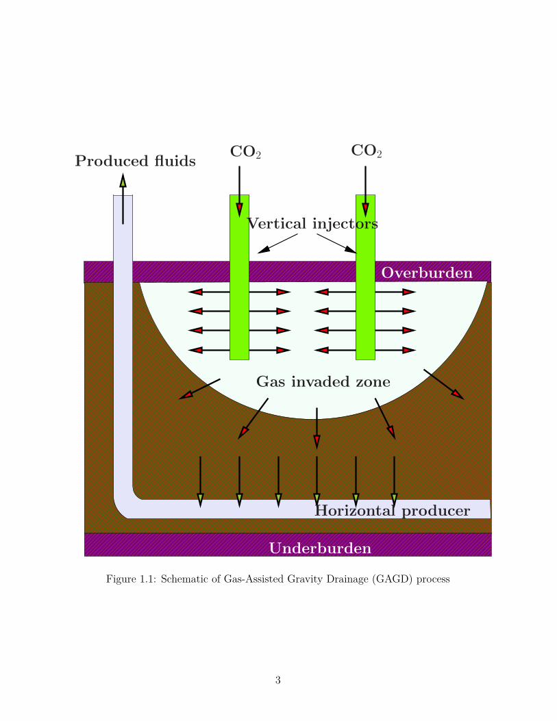
GAGD aims to overcome the limitation posed by CGI and WAG by using the density
difference between oil and gas to its advantage. Since in nature gas tends to override,
GAGD allows this to happen so that eventually a gas dome is formed at the top of the
payzone (see Figure 1.1). This dome gradually descends to the bottom, replaces the pore
space initially occupied by oil while the oil drains by gravity to the horizontal producer
well. Rao et al. (2004) showed that the gravity stabilized displacement front achieved by
GAGD can recover more oil than the previous processes.
One advantage of GAGD is that it can deliver better performance over CGI and WAG
regardless whether the injection gas is miscible or immiscible with oil. Since not all reser-
voirs could withstand the high injection pressure required to develop miscibility; and like-
wise not all fields have ready access to CO2, immiscible gas injection with GAGD would
be the preferred method to realize the benefits of GAGD to a wider range of reservoirs.
2
Gas invaded zone
Horizontal producer
Produced fluids
Vertical injectors
CO2
Overburden
Underburden
CO2
2
Figure 1.1: Schematic of Gas-Assisted Gravity Drainage (GAGD) process
3

On a pore-scale level, immiscible gravity drainage works by creating oil bank ahead of
the displacement front which is then produced at the bottom of the payzone. This oil bank
is formed after some time when the isolated oil blobs are reconnected through spreading
film. In a water-wet rock, the oil can spread over water in the presence of the injected
gas. This spreading film forms the bridge linking the bypassed oil blobs which eventually
coalesce to form oil bank.
In literature, a few mathemathical models have been developed for gravity drainage.
However, not all models incorporate the spreading phenomenon described earlier. This
leads to the model over-predicting or under-predicting the oil recovery when compared
with experimental data. Furthermore, it is not known whether the existing models could
match experimental data from rocks other than water-wet system. In this work the exper-
imental results will be presented and the existing models will be evaluated to gauge their
performance in characterizing gravity drainage process.
1.2 Problem statement and motivation of research
Although the literature suggests that spreading film influences oil recovery in gravity
drainage, it seems paradoxical that systematic experimental investigation to understand
this phenomenon is lacking. In the course of this research, we are motivated to answer the
following questions:
• How would GAGD perform in water-wet, oil-wet and fractional-wet media?
• How would GAGD perform in the above conditions with spreading and non-spreading
oil?
• Do the existing models account for spreading film mechanism?; and if they do,
• How would the models perform when matching gravity drainage experiments with
the conditions above?
4
We hope the answers to the above questions illuminated by this research would help to
advance understanding of oil recovery using gravity drainage process.
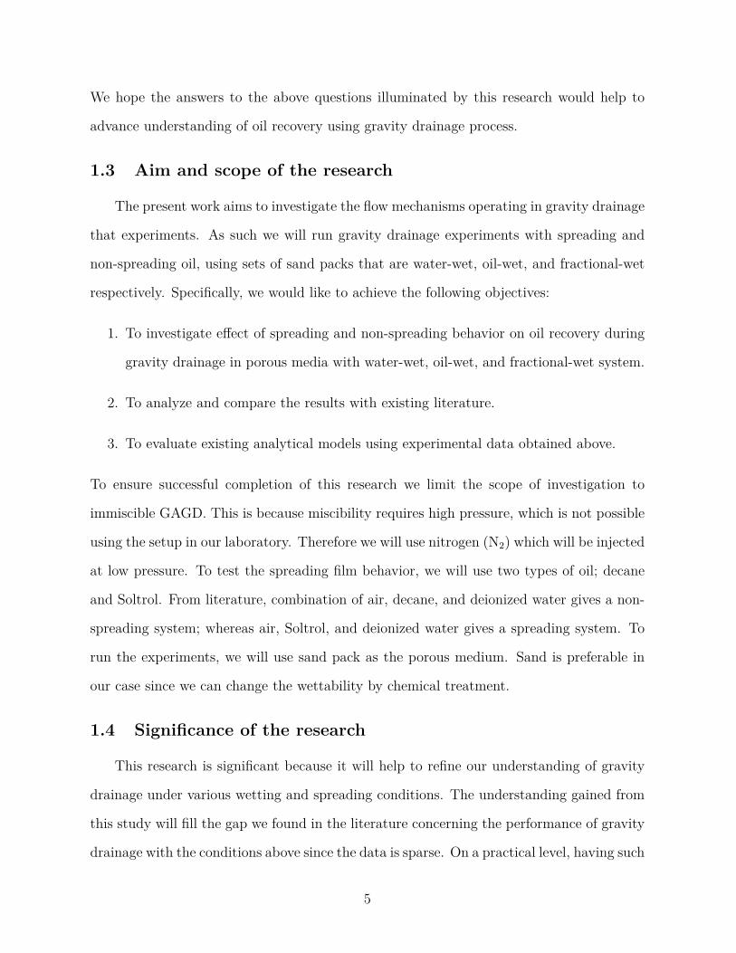
1.3 Aim and scope of the research
The present work aims to investigate the flow mechanisms operating in gravity drainage
that experiments. As such we will run gravity drainage experiments with spreading and
non-spreading oil, using sets of sand packs that are water-wet, oil-wet, and fractional-wet
respectively. Specifically, we would like to achieve the following objectives:
1. To investigate effect of spreading and non-spreading behavior on oil recovery during
gravity drainage in porous media with water-wet, oil-wet, and fractional-wet system.
2. To analyze and compare the results with existing literature.
3. To evaluate existing analytical models using experimental data obtained above.
To ensure successful completion of this research we limit the scope of investigation to
immiscible GAGD. This is because miscibility requires high pressure, which is not possible
using the setup in our laboratory. Therefore we will use nitrogen (N2) which will be injected
at low pressure. To test the spreading film behavior, we will use two types of oil; decane
and Soltrol. From literature, combination of air, decane, and deionized water gives a non-
spreading system; whereas air, Soltrol, and deionized water gives a spreading system. To
run the experiments, we will use sand pack as the porous medium. Sand is preferable in
our case since we can change the wettability by chemical treatment.
1.4 Significance of the research
This research is significant because it will help to refine our understanding of gravity
drainage under various wetting and spreading conditions. The understanding gained from
this study will fill the gap we found in the literature concerning the performance of gravity
drainage with the conditions above since the data is sparse. On a practical level, having such
5
understanding will help engineers to understand interplay of various elements in gravity
drainage process. This understanding will give them insights in designing field project for
GAGD.
1.5 Overview of the dissertation
This study consists of six chapters. In Chapter 2, we position the research within
the current literature and identify gaps that need to be addressed, particularly on the
experimental aspect. By identifying the gaps we can better design the experiments and
evaluate the existing models. The experimental design is the subject of Chapter 3. In that
chapter we present the experimental setup, the materials used and the procedures to run
the experiments. The experimental results are presented in Chapter 4. This also marks
the beginning of our contribution to this research. Apart from presenting the results, we
also analyze and discuss the results in light of existing literature. In Chapter 5 we used the
experimental data as inputs to gravity drainage models to test their performance. Finally,
Chapter 6 presents the conclusion and recommendations for future work..
6

Chapter 2
Literature ReviewIn this chapter we review the literature to identify opportunities for research. We
begin with the earliest study on gravity drainage to see the extent of research during that
period. Understanding research activities on gravity drainage during this time helps to
set the context chronologically for later studies. This is followed by review of existing
experimental studies in subsequent years.
The experimental studies we reviewed cover both the core and pore level. At the core
level we look at gravity drainage experiments conducted either in sand packs or coreflood
apparatus. By looking at these experimental studies, we can find areas where experimental
results are lacking. These insights can be used later on when we carry out the experiments
and compare the results.
Review of studies at the pore level covers experimental work using micromodels with
three-phase fluids: water, oil and gas. Since we are particularly interested to understand
mechanism of gravity drainage, pore level experimental work helps to understand both fluid-
fluid and fluid-rock interactions occurring during three-phase flow. Such understanding
establish the framework for explaining the results of experimental work at the core scale.
We then review the models that describe recovery from gravity drainage process. Our
motivation here is to learn how far the existing models incorporate the mechanisms revealed
from experimental work. Toward this end we will cover analytical models existing in the
literature. The end of the chapter summarizes key opportunities for further investigation
and outline our plan to address the knowledge gaps found in the literature, particularly
with respect to experimental work and modeling study.
2.1 Pioneering study
The first reported systematic work to investigate gravity drainage as viable oil recovery
method was the experimental work performed by Stahl et al. (1943). In their work Stahl
7

et al. (1943) observed that some mature reservoirs in Oklahoma City field developed gravity
segregation and produced oil through gravity drainage. They initiated experimental study
using a vertical sand pack filled with Wilcox sand to verify their observation in the field.
They measured the transient and equilibrium liquid saturation distribution in the sand
column and found that the liquid recovery ranged from 50 to 75 percent.
The following year Lewis (1944) published his work discussing the concept of gravity
drainage in oil reservoirs and highlighted the state of the art extant at the time. Lewis
work delineates the difference between gas-drive and gravity drainage conditions. In his
paper he defined gravity drainage as the ”self-propulsion of oil downward in the reservoir
rock”. This can be achieved by properly controlling the pressure reduction and withdrawal
rate so that gravity segregation occurs deliberately followed by counter-current flow of gas
and oil. Gas that flows to the top of the reservoir is allowed to expand as the pressure
declines, creating gas cap in the process. The expanding gas cap slowly forms gas-oil front
with the displaced oil forming oil bank ahead of the front. At the core of this principle is
the concept of voidage replacement where gas occupies the voids left by the displaced oil
as the gas cap expands. He explained that one way to gauge gravity drainage condition
is taking place is by monitoring the gas-oil ratio. In a typical gas-drive displacement the
GOR increases steadily and reaches maximum as the ultimate recovery is achieved which
is then followed by GOR decline. For a gravity drainage condition, the GOR increases
gradually towards solution GOR before it suddenly rises as the gas-oil front reaches the
production well. In presenting several field examples operating under gravity drainage he
suggested that more studies should be conducted to better understand the mechanism and
inform operators of the possibility of producing their fields using gravity drainage.
Publication of the work above initiated work by Cardwell and Parsons (1949). They
were motivated to find analytical solution to gravity drainage since the body of work
concerning gravity drainage was limited to experimental study. Their derivation started
with the equivalent expression for Darcy velocities of the unsaturated and saturated region
8

in a column. Unsaturated region is at the top of the column where gas has displaced
most of the oil. The bottom of the column is the saturated region where the displaced
oil accumulated before it is produced. By solving the continuity equation they formulated
a partial differential equation (p.d.e) which is second order and non-linear. Since the
solution is difficult they simplified the model by neglecting capillary pressure term to make
the p.d.e quasilinear. The model uses empirical permeability-saturation relationship and
equilibrium saturation height to predict the trajectory of gas-oil front over time. The model
was validated using the experimental data from Stahl et al. (1943).
Subsequent work on gravity drainage also focused on mathematical modeling. Ter-
williger et al. (1951) were motivated to investigate the effect of drainage rate on gravity
drainage performance. It was understood that gravity drainage condition would develop
when a suitable reservoir is drained at low rate but there was no practical method to calcu-
late the rate at which gravity drainage is most effective. They approached this problem by
conducting experiment in a vertical sand pack and measuring the conductivity over time
to determine the brine saturation distribution in the column. By repeating the experi-
ment at different drainage rate they were able to compare the saturation profiles. Their
experiments showed that at low drainage rate the individual curve in the saturation profile
traveled at the same rate and maintain its shape until breakthrough. The almost piston-like
curve was called ”stabilized zone”. It was under the stabilized zone condition that most
of the brine was displaced. They used Buckley and Leverett (1942) solution to calculate
the saturation profile and found close match with experimental data. Their work showed
the practical use of Buckley-Leverett solution to calculate the saturation profile in gravity
drainage experiment and determine which drainage rate would lead to a stabilized zone.
In the 1950’s publications from several workers further extend our understanding of
gravity drainage. Marx (1956) showed that centrifuge experiment can be used to replicate
gravity drainage recovery in consolidated porous media. Matthews and Lefkovits (1956)
conducted gravity drainage experiments and analyzed the results using hyperbolic decline
9
curve. Essley et al. (1958) discussed application of gravity drainage in steeply dipping
reservoir and presented calculations to predict gravity drainage performance.
So far the pertinent aspect of gravity drainage recovery, which is the spreading film
mechanism has not been addressed in the literature. One exception is the work from
Nenniger and Storrow (1958). They presented a model to calculate the saturation-time
profile for liquid drainage in a packed bed under gravity. The differential equation is solved
using a series solution. The effect of film drainage on the packed bed is incorporated using
integration of Navier-Stokes approximate solution for film drainage down a vertical plane.
2.2 Investigation of displacement mechanism
In the previous section it was revealed that only one work incorporated film mechanism
in their mathematical model (Nenniger and Storrow, 1958). However the film described in
their model is not formed because of spreading or wetting phenomenon. This is because
the volume of fluid contributed by the film does not distinguish whether it comes from
a spreading film (fluid-fluid interaction) or wetting film (fluid-rock interaction). The lack
of distinction between the film formed was because the experimental studies conducted
so far had limited ability to make the spreading and wetting phenomena manifest in the
experiments. This was perhaps due to the design of the experiment itself or the limited
capability of the equipment used.
Only in later years, as technology improved researchers began to direct their focus to
understanding the mechanisms at the physical level which contribute to gravity drainage
recovery. As we will see later more experiments were conducted, both at core and pore levels
to gain insights on the recovery mechanism. In the following core level refers to macroscale
experimental work while pore level concerns with investigation at the microscale.
2.2.1 Experimental studies at core scale
The underlying mechanism operating in gravity drainage recovery was first identified
by Dumore and Schols (1974). They conducted gravity drainage experiment by using
10
immiscible gas to displace oil at connate water saturation and found that the oil can be
drained to very low saturation. They suggested that the residual oil was drained through
spreading film. Later work by Kantzas et al. (1988a) also showed the same behavior in
their experiments using consolidated and unconsolidated samples. They reported recovery
of 99% for gravity drainage experiment conducted using unconsolidated sample at residual
water condition. For condition at residual oil the recovery was 94%. In both cases the oil
phase was Soltrol, which is a spreading oil.
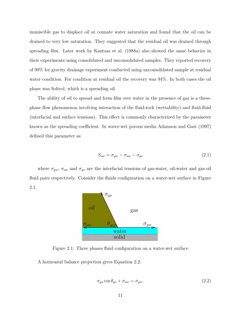
The ability of oil to spread and form film over water in the presence of gas is a three-
phase flow phenomenon involving interaction of the fluid-rock (wettability) and fluid-fluid
(interfacial and surface tensions). This effect is commonly characterized by the parameter
known as the spreading coefficient. In water-wet porous media Adamson and Gast (1997)
defined this parameter as
Sow = σgw − σow − σgo (2.1)
where σgw, σow and σgo are the interfacial tensions of gas-water, oil-water and gas-oil
fluid pairs respectively. Consider the fluids configuration on a water-wet surface in Figure
2.1.
oil
watersolid
gas
θgoσow σgw
σgo
Figure 2.1: Three phases fluid configuration on a water-wet surface
A horizontal balance projection gives Equation 2.2:
σgo cos θgo + σow = σgw. (2.2)
11
A manipulation of Equation 2.1 and 2.2 shows that the spreading coefficient Sow can
be related to gas-oil contact angle θgo (Kalaydjian and Tixier, 1991):
cos θgo = 1 + Sowσgo
. (2.3)
From Equation 2.2 equilibrium is possible when the spreading coefficient is negative
because | cos θgo |≤ 1. Therefore oil phase forms droplet or lens on the water surface when
Sow becomes less than −2σgo.
A positive spreading coefficient, Sow > 0 means gas-water interfacial tension, σgw is
greater than the sum of oil-water and gas-oil interfacial tensions (σow + σgo). As such the
surface tension σgo becomes the dominant force per unit length over the sum of σow and
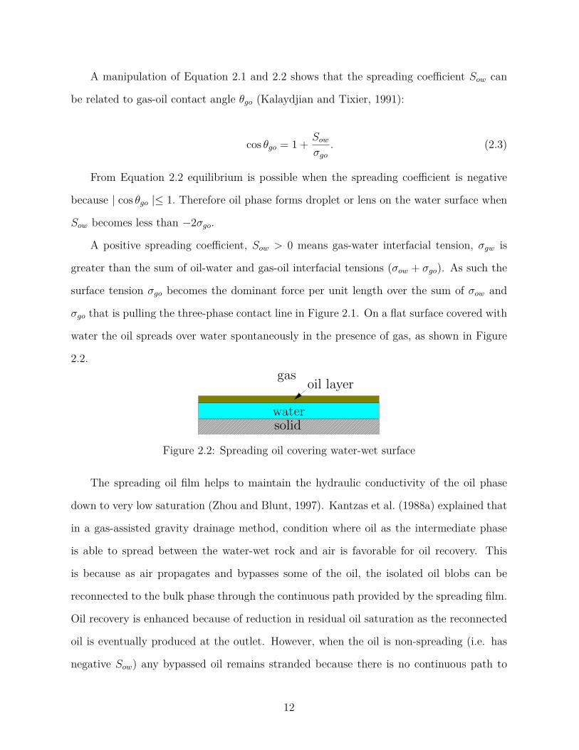
σgo that is pulling the three-phase contact line in Figure 2.1. On a flat surface covered with
water the oil spreads over water spontaneously in the presence of gas, as shown in Figure
2.2.
watersolid
gasoil layer
Figure 2.2: Spreading oil covering water-wet surface
The spreading oil film helps to maintain the hydraulic conductivity of the oil phase
down to very low saturation (Zhou and Blunt, 1997). Kantzas et al. (1988a) explained that
in a gas-assisted gravity drainage method, condition where oil as the intermediate phase
is able to spread between the water-wet rock and air is favorable for oil recovery. This
is because as air propagates and bypasses some of the oil, the isolated oil blobs can be
reconnected to the bulk phase through the continuous path provided by the spreading film.
Oil recovery is enhanced because of reduction in residual oil saturation as the reconnected
oil is eventually produced at the outlet. However, when the oil is non-spreading (i.e. has
negative Sow) any bypassed oil remains stranded because there is no continuous path to
12

reconnect the oil to the bulk phase. Consequently the residual oil saturation is higher for
water-wet rock with non-spreading oil.
At the core level experimental work can be broadly categorized into free-fall gravity
drainage (FGD) and controlled gravity drainage (CGD) (Schechter and Guo, 1996). In
FGD system the top column is open to atmosphere and ambient air is used to displace the
oil. It is called free-fall because the column is drained due to the height of the saturated
fluid in the column. This system replicates the gravity drainage occurring in naturally
fractured rock, specifically the drainage of oil from the matrix and fracture. CGD system
injects gas at fixed pressure or rate to simulate gas injection process in a typical reservoir.
In most cases gas is injected at constant pressure since it is desirable for the operator to
maintain the reservoir condition such that the oil phase is undersaturated and the solution
gas does not evolve out of the oil phase. As Lewis (1944) explained earlier, the condition for
gravity stabilized drainage can be achieved in the reservoir by simultaneously controlling
both the gas injection pressure and the fluid withdrawal rate.
Experimental work by Vizika and Lombard (1996), Ren et al. (2004) and Ren et al.
(2005) showed typical characteristic of film flow mechanism in action during gravity drainage.
In their experimental work they observed two recovery stages characterized by time before
and after break through. They reported that in the early stage of the experiment significant
amount of oil is produced within a short period “bulk flow” until the gas breaks through.
After break through, the oil production rate reduces dramatically over a long period “film
flow” until the recovery curve reaches asymptote. It is during this second phase that the
role of spreading film becomes dominant in draining residual oil behind the gas-oil front.
Since the effect of film flow becomes dominant later in the life of the reservoir, experi-
mental work investigating the effect of film flow were often conducted under the condition
of residual oil saturation. This is evident from experimental work performed by Kantzas
et al. (1988a), Dullien et al. (1991), Chatzis and Ayatollahi (1993), Catalan et al. (1994),
Skurdal et al. (1995), Paidin and Rao (2007), Sharma and Rao (2008), Maeda and Okatsu
13

(2008) and Parsaei and Chatzis (2011). This means the gas-assisted gravity drainage
method is implemented as tertiary recovery after waterflooding to manifest the effect of
film flow. Nevertheless experimental studies for gravity drainage under residual water sat-
uration have also been performed by most of the authors cited above. Both setups create
three-phase flow condition where water, oil and gas exist simultaneously which is a pre-
requisite as shown in Equation 2.1. Typically investigators would compare the oil recovery
or residual oil saturation between spreading and non-spreading oil after gravity drainage
experiment. Higher oil recovery or lower residual oil saturation is often attributed to the
spreading oil film (Kantzas et al., 1988a; Chatzis and Ayatollahi, 1993; Vizika, 1993; Vizika
and Lombard, 1996; Ren et al., 2004).
Water-wet media is typically used in experimental work investigating gravity drainage.
This is because apart from spreading of the intermediate phase, another factor that in-
fluences oil recovery in three-phase flow is the wettability condition of the porous media
(Vizika and Lombard, 1996). Hence in three-phase flow, such as the condition created under
GAGD, both fluid-fluid interaction (spreading effect) and fluid-rock interaction (wettability
effect) underlie the principal mechanism for oil recovery.
However, there still exists the need to study the oil recovery mechanism using spreading
and non-spreading fluids in wettability conditions other than water-wet. We have compiled
the experimental studies on gravity drainage in chronological order in Table 2.1. From
the table it is seen that most of the experimental work on gravity drainage over the years
concerned mainly with displacement in water-wet porous media using spreading or non-
spreading oil. Based on the residual oil saturations tabulated, it is not possible to make
an unambiguous conclusion regarding the performance of gravity drainage in water-wet
media. Although higher recovery (lower residual oil saturation) is attributed to gravity
drainage with spreading fluid in water-wet system, it is suspected that the duration of
the experiment itself determines the lower bound of residual oil saturation that can be
achieved after termination of the experiment. For example experimental work by Zhou
14

Table 2.1: Residual oil saturation (Sorg) after gravity drainage under various spreading andwetting conditions
References Porous media Gravity drainagemode
Sorg(% PV)
Water-wet Oil-wet
Spreading(Sow>0)
Non-spreading(Sow<0)
Spreading(Sow>0)
Non-spreading(Sow<0)
Dumore and Schols (1974) Bentheimersandstone
N/A 2.9 3.2
Kantzas et al. (1988a) Bead pack Controlled 0.6 to 1.9Free-fall 3.3 to 9.1
Dullien et al. (1991) Bead pack Controlled 2 16.9Free-fall 12.7
Chatzis and Ayatollahi(1993)
Bead pack(250-420 µm)
Controlled 1.6 to 13Free-fall 14
Bead pack(600-710 µm)
Controlled 1 to 7Free-fall 16
Catalan et al. (1994)Bead pack Controlled 2 16.9
Free-fall 12.7Berea sandstone Controlled 11.5 to 27.1 13.8
Pembinasandstone
Controlled 14.2 & 32.1
Blunt et al. (1994) Sand pack Free-fall/Controlled
4 & 10.5
Blunt et al. (1995) Sand pack (longcolumn)
Free-fall/Controlled
7.6 to 14 16.3
Sand pack(short column)
Free-fall/Controlled
14.5 to 20.6 21.8
Catalan and Dullien (1995) Sand pack(homogenous)
Controlled 6.1
Sand pack(heterogenous)
Controlled 10.7
Skurdal et al. (1995) Bentheimersandstone
Controlled 4.7 6.7 12.6 1.1
Vizika and Lombard (1996) Sand pack Free-fall 11 23 21 22
Zhou and Blunt (1997) Sand pack(purified sand)
Free-fall 0.13 1.13 & 1.49
Sand pack (redsand)
Free-fall 0.35 3.11 & 5.25
Kulkarni and Rao (2006a) Berea sandstone Controlled 22 to 39.1Maeda and Okatsu (2008) Berea sandstone Controlled 34.2Parsaei and Chatzis (2011) Bead pack Controlled 3.98 to 11.3
15

and Blunt (1997) showed very low residual oil saturation (Sorg= 0.13 %PV) for spreading
system compared to non-spreading system after the experiment was run for three weeks.
Table 2.1 also shows that experimental studies on gravity drainage in non-water-wet
porous media are sparse. To date only Dullien et al. (1991), Catalan et al. (1994), Skurdal
et al. (1995), Vizika and Lombard (1996), and Paidin and Rao (2007) (not tabulated be-
cause Sorg data was absent) have moved in this direction. Using sand pack and positive
spreading oil (Soltrol), Catalan et al. (1994) found that oil-wet system recovered less resid-
ual oil than water-wet system. Vizika and Lombard (1996) observed that the residual oil
saturation in oil-wet system is similar regardless the sign of the spreading coefficient. Prior
study by Skurdal et al. (1995) exhibited contrary trend to that of Vizika and Lombard
(1996) in which residual oil saturation is lower for non-spreading oil than spreading oil in
oil-wet system. Paidin and Rao (2007) found that oil-wet system with negative spreading
oil recovered more oil than water-wet system. From these studies it is evident that more
systematic study is needed to investigate this aspect of gravity drainage.
2.2.2 Experimental studies at pore scale
Kantzas et al. (1988b) conducted gravity drainage experiment in a vertical micro-
model to visualize the pore-level mechanisms. They observed in a typical water-wet gravity
drainage experiment when the gas-oil front was advancing the oil blobs downstream could
behave in several ways. The blobs either coalesced into an oil bank which then drained
to the outlet or pushed into smaller pores which were then bypassed. If there were no oil
blobs downstream the advancing front would thin out with oil film being formed along the
pathway. Their work shows the importance of oil film mechanism in water-wet media for
oil recovery with gas-assisted gravity drainage.
Further investigations at the pore level were conducted by Øren and Pinczewski (1991),
Oren et al. (1992) and Oren and Pinczewski (1994). They were motivated to investigate the
three-phase flow mechanism during immiscible gas injection from micromodel experiments.
16

Their work revealed that three-phase flow process such as that occurring in gravity drainage
could be very complex. This is because spreading behavior and wettability affect the fluids
pore occupancy and their subsequent mobility. Compared to two-phase system where
one phase is wetting and the other non-wetting, in three-phase there is a third phase
which is the intermediate phase. The presence of the intermediate phase complicates the
fluid configuration at the pore scale and affects the displacement mechanism. In their
micromodel experiments they have identified three mechanisms for fluid transport namely
direct drainage, double drainage and imbibition-drainage. Direct drainage is a mechanism
where a non-wetting or intermediate phase displaces a wetting phase. Double drainage
involves two adjacent direct drainage events happening one after another with a non-wetting
phase displacing an intermediate phase followed by the intermediate phase displacing a
wetting phase. In imbibition-drainage an intermediate phase displaces a non-wetting phase
(imbibition event) followed by the non-wetting phase displaces the wetting phase (drainage
event).
Øren and Pinczewski (1991) calculated the film thickness for wetting film (water) and
spreading film (oil) using augmented Young-Laplace equation. The stability of the film
was due to positive disjoining pressure. The calculated film thickness matched measured
film thickness from micromodel. They also calculated the velocity field from the film
thickness which was then used to estimate the conductivity of the film. The velocity field
was integrated over the film cross-section in order to get the average phase velocity. Their
calculations showed that average phase velocity increased rapidly when the oil viscosity
was low. Their work quantified film thickness for wetting and spreading phase and showed
realistic estimate of the film conductivity in a micromodel experiment.
The implication of this phenomenon on oil recovery is further studied by Oren et al.
(1992) using micromodel. Oren et al. (1992) investigated the pore-level physics of thin
film flow in immiscible tertiary gas displacement and introduced the ”double displacement
drainage” mechanism as responsible in propagating the gas-oil and oil-water front for a
17
spreading, water-wet system. The mechanism is possible when spreading oil film exists
between water phase and gas phase. Oren et al. (1992) explained that in order to mobilize
the stranded residual oil blobs, they need to be reconnected to form larger oil bank through
hydraulic path established by the spreading film. Oren et al. (1992) further observed that
early in the flow, as gas invaded the pores, the oil-water interfaces propagated easily to
outlet through low resistance path provided by the water-wetting film. Later, as the water
drained out, the oil-water interfaces had to go through high resistance path provided by
the spreading film, which slowed down their propagation. Comparison with non-spreading
system using the same micromodel showed the spreading system yields 40% of the residual
oil while only 18% for the non-spreading system.
The reason non-spreading system yields lower tertiary recovery is further explained by
Oren (1994). In negative spreading water-wet system, oil does not spread in thin film in
the presence of gas and water. Instead there exist three phase contact line between gas-oil
and oil-water interfaces to minimize the free energy of the system. Additional three phase
contact lines are formed when gas invades pores containing oil. This causes the displaced
oil to be broken into smaller blobs and trapped in the surrounding pore throats. Film
flow occurs mostly in pore throat connecting the pore bodies. When gas-oil front advances
from pore throat to pore body, there exists a pressure gradient for oil flow. The pressure
gradient causes the oil displaced in the pore body to flow counter current through the film
along the pore throat.
Experimental results from Oren et al. (1992) were further analyzed and simulated using
invasion percolation network model by Oren (1994). The simulation results were shown
to be generally agreed with experiments. Negative spreading system showed lower oil
recovery because there was less gas saturation distributed across the network model. This
was because little bypassed oil was reconnected due to lack of double drainage displacement
taking place. Even when double drainage displacement occurred, the displaced oil broke
down into isolated oil blobs. Since there was absence of spreading film, the oil had no
18

path to reconnect with oil behind the gas front and consequently was trapped in pore
throats. Capillary fingering of gas continued throughout the system, which resulted in
early gas breakthrough and higher residual oil saturation.When gas invasion occurred in
an oil filled-pore for a positive spreading system, the presence of oil film provided a path for
the displaced oil to reconnect with the oil behind the gas front. This process was observed
to be repeated across the network, which lead to formation of oil bank and later, lower
residual oil saturation when the oil bank was produced.
Interestingly, Oren (1994) also demonstrated that increasing the magnitude of the
positive spreading coefficient did not affect oil recovery for an already spreading system.
Instead, for a spreading system the recovery was influenced by film flow resistance, which
was quantified by film capillary number. Their results showed: i. When film capillary
number was low, film conductivity was high, which lead to high oil recovery; ii. When film
capillary number was high, film conductivity was low, which resulted in low oil recovery;
iii. When film capillary number intermediate, the oil recovery was controlled by capillary
pressure and film flow pressure. However, for negative spreading system the more negative
the spreading coefficient, the less oil recovery.
Soll et al. (1993) conducted micromodel experiment to study three-phase flow fluid
behavior in a capillary driven displacement. In their study they found that film transport
played important role in mobilizing wetting (water) and intermediate (oil) phase fluids.
This was confirmed from analysis of digital images taken during the experiment. From
their observation the film was sufficiently thick to drain the wetting and spreading layer.
They also found that in most cases although all three fluids were mobile, interactions at
local pore involved only two phases. For example in their water-wet system the injected
gas tend to prefer displacing oil either in continuous or isolated blobs before displacing
water. Their work demonstrates the role of film flow during drainage and imbibition of
three-phase system.
19
Hayden and Voice (1993) performed scanning-electron microscopy analysis to obtain
images of NAPL (non-aqueous phase liquid) in a moist soil sample. The sample was
saturated with brine, iodobenzene and air before frozen with liquid nitrogen to facilitate
the analysis. They found that iodobenzene, which was used as the NAPL phase and has
negative spreading coefficient (-8.7 mN/m) formed continuous phase at high, intermediate
and low saturation. Some of the NAPL phase was found in pore wedges or irregular-
shaped pore geometry. Their study gives evidence that a non-spreading oil can also form
continuous phase in porous media, if the phase is located in crevices or angular features of
pore spaces. This challenges the previous understanding that only spreading oil can form
continuous phase when it is intermediate wetting.
Oren and Pinczewski (1994) conducted three-phase flow experiment using oil-wet micro-
model to investigate the effect of spreading and wettability during immiscible gas injection.
They used two sets of fluids, spreading and non-spreading oil to observe the displacement
mechanisms. When comparing their results with previous work using water-wet micro-
models, they found that oil recovery was higher in the oil-wet case for both spreading and
non-spreading oils. They explained that better recovery was achieved in oil-wet case due to
transport of the mobilized oil through thicker and more conductive oil film. In their com-
parison, recovery from spreading oil in water-wet micromodel was second and the lowest
recovery came from non-spreading oil in water-wet system. Their work demonstrates the
role of oil film, both spreading film in the water-wet case and wetting film in the oil-wet
case in transporting the mobilized oil to outlet.
Blunt et al. (1994),Blunt et al. (1995), and Fenwick and Blunt (1995) approached the
pore-level study of three-phase flow from geometry and intermolecular forces perspective.
According to Blunt et al. (1994), oil recovery was higher for system where spreading coeffi-
cient was positive because the film was stable, and this stability determined the thickness
of the film layer. The film stability is a function of capillary and intermolecular forces.
The film is stable at equilibrium thickness when combination of intermolecular forces per
20
surface area, the disjoining pressure, is equal to capillary pressure. Components of the in-
termolecular forces that affect film stability are van der Waals force (vdW), the electrostatic
forces and the structural force. In their paper Blunt et al. (1994) showed that structural
force helped in forming stable film for the fluid system observed. The authors based their
claim by comparing disjoining pressure from vdW and structural forces. vdW contributes
to negative disjoining pressure, which makes the film unstable. Structural force, which is
oscillatory, has an initial maximum positive disjoining pressure which decrease with time
so that it is equal to capillary pressure at equilibrium thickness.
Based on pore geometry calculation, Blunt et al. (1995) and Fenwick and Blunt (1995)
claimed that non-spreading system could actually form film under the initial condition
that the thick oil layer was thinning, which usually happened behind the gas-oil front as
it advanced. Their finding was contrary to what had been observed by Oren et al. (1992).
Subsequent experimental study with micromodel by Keller et al. (1997) using decane as
non-spreading oil phase seemed to support Blunt et al. (1995) and Fenwick and Blunt
(1995) assertion.
Keller et al. (1997) conducted micromodel experiment to investigate whether oil with
negative spreading coefficient could form layer of oil between gas-water interface in a water-
wet media. Their study was motivated by previous work from Dong et al. (1995). Dong
et al. performed theoretical study involving free-energy calculation and demonstrated that
depending on the pore geometry, oil with negative spreading coefficient could form stable
layer. This was validated by their experimental work using capillary tube with angular
cross-section. Keller et al. (1997) extended this result by performing experiment using mi-
cromodel etched with pattern extracted from a Berea sandstone. Since the pore geometries
contained features such as angularities and crevices, they demonstrated that a stable oil
layer with negative spreading coefficient could be supported in such pores when oil-water
capillary pressure was greater than gas-oil capillary pressure. Using simple geometry model
they showed mathematically that this was controlled by the ratio of oil-water to gas-oil radii
21
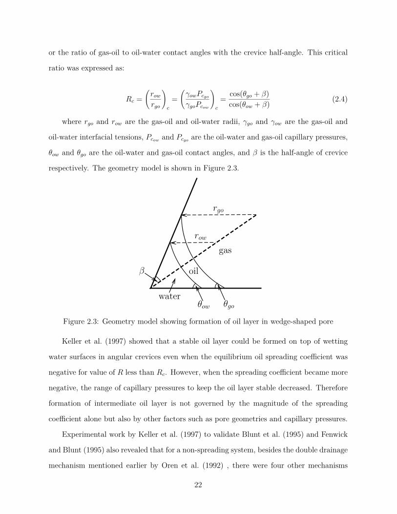
or the ratio of gas-oil to oil-water contact angles with the crevice half-angle. This critical
ratio was expressed as:
Rc =(rowrgo
)c
=(γowPcgo
γgoPcow
)c
= cos(θgo + β)cos(θow + β) (2.4)
where rgo and row are the gas-oil and oil-water radii, γgo and γow are the gas-oil and
oil-water interfacial tensions, Pcow and Pcgo are the oil-water and gas-oil capillary pressures,
θow and θgo are the oil-water and gas-oil contact angles, and β is the half-angle of crevice
respectively. The geometry model is shown in Figure 2.3.
water
oil
gas
rgo
row
β
θow θgo
Figure 2.3: Geometry model showing formation of oil layer in wedge-shaped pore
Keller et al. (1997) showed that a stable oil layer could be formed on top of wetting
water surfaces in angular crevices even when the equilibrium oil spreading coefficient was
negative for value of R less than Rc. However, when the spreading coefficient became more
negative, the range of capillary pressures to keep the oil layer stable decreased. Therefore
formation of intermediate oil layer is not governed by the magnitude of the spreading
coefficient alone but also by other factors such as pore geometries and capillary pressures.
Experimental work by Keller et al. (1997) to validate Blunt et al. (1995) and Fenwick
and Blunt (1995) also revealed that for a non-spreading system, besides the double drainage
mechanism mentioned earlier by Oren et al. (1992) , there were four other mechanisms
22
involve in fluid transport. The author noted that since these four mechanisms involve gas
or water displacement by either phase, they rarely occurs when oil spreads over water in the
presence of gas since that will prevent gas from contacting the water directly. Keller et al.
(1997) observed that in most cases, double displacement either by drainage or imbibition
occurred involving two phases since the third phase usually reside in smaller pores and
became immobile due to capillary force.
Keller et al. (1997) observation further explained why non-spreading system in Oren
et al. (1992) micromodel did not exhibit spreading layer but Keller et al. (1997) experiment
did . The difference was due to the geometry of the pores in the micromodel. In Oren’s
micromodel, the pore cross-section was circular while the pore space in Keller’s model has
rectangular cross-section. According to Keller et al. (1997) , rectangular cross-section could
support formation of thick oil layer for non-spreading oil based on condition in Equation
2.4. Since β = 90◦ for circular pore, R will be equal to Rc and non-spreading oil will
thin out. However in rectangular or angular crevice, β < 90◦ and for water-wet surface,
θow < θgo and R will be less than Rc. This means a thick oil layer with negative spreading
coefficient could be formed across the wedge-shaped pore since oil-water capillary pressure
was higher than gas-oil capillary pressure.
Vizika et al. (1998) visualized three-phase fluids in rock samples using cryo-scanning
electron microscopy. They wanted to study the fluids distribution and the effect of spread-
ing and wettability during three-phase gas injection. The experiment used two sets of
fluid samples; spreading and non-spreading oil and two sets of Fountainebleau sandstones;
water-wet and oil-wet. Images obtained from the experiments showed existence of oil film
for spreading fluid in water-wet sample. In oil-wet sample, their results demonstrated that
distribution of residual oil was not influenced by the magnitude of the spreading coeffi-
cient. They also found that distribution of water phase differed between spreading and
non-spreading condition. In spreading system water was mostly mobilized while in non-
spreading system most of the water was stranded.
23

Sohrabi et al. (2004) reported experiment using high pressure micromodel with live
oil and water to investigate three-phase flow during WAG displacement. They built set
of micromodels with diverse wettability conditions each (water-wet, oil-wet and mixed-
wet) and saturated the micromodel with decane, a non-spreading oil.They found that in
water-wet experiment, corner filament flow, through which the wetting phase is transported
plays important role in oil displacement. They observed multiple displacement mechanisms
taking place in the water-wet experiment; however this was absent in the oil-wet experiment.
Their results showed that oil recovery was higher in the oil-wet and mixed-wet experiments.
This occurred because given two pores of equal radii, gas would prefer to displace the one
filled with oil rather than water since gas-oil IFT was lower.
Studies on pore-level physics above were done primarily using water-wet porous media
with spreading or non-spreading oil phase. From the literature, studies on non-spreading
system is lacking, possibly because the general assumption that non-spreading system re-
covers less residual oil than spreading system. However, non-spreading oil phase is more
prevalent in actual reservoir, since reservoir crude oil consisted of higher order alkanes ho-
mologues. According to Richmond et al. (1973) and Takii and Mori (1993), alkanes series
beginning with octane does not spread on water. What if it is possible to enhance the
spreading ability of these higher homologues from negative spreading to positive spread-
ing? Studies from Richmond et al. (1973), Thanh-Khac Pham and Hirasaki (1998), and
Boinovich and Emelyanenko (2009) have shown that this is possible by changing the salin-
ity of the aqueous phase. However a systematic study of changing spreading coefficient of
the oil phase in a gravity drainage experiment has yet to be seen.
Review of experimental work performed above show that even at microscopic level
the effect of spreading film improves oil recovery in three-phase flow in water-wet media
(Kantzas et al., 1988b; Oren et al., 1992). The thickness and conductivity of the spreading
layer has been calculated by Øren and Pinczewski (1991). Pore scale visualization with
cryo-scanning electron microscopy (SEM) on actual core sample confirmed the existence of
24
spreading film Vizika et al. (1998). However, other investigators have also shown that an
intermediate oil layer can be formed in wedge-shaped pores for oil with negative spreading
coefficient (Dong et al., 1995). This was investigated theoretically (Blunt et al., 1994, 1995)
as well as experimentally (Keller et al., 1997). Visualization using cryo-SEM by Hayden
and Voice (1993) further confirmed the existence of continuous oil layer for non-spreading
oil at high, intermediate and low oil saturation. Although higher oil recovery is often shown
for drainage in spreading system with water-wet media, experimental studies by Oren and
Pinczewski (1994) and Sohrabi et al. (2004) have proved otherwise. They demonstrated
that higher oil recovery was achieved in oil-wet media instead.
Comparison between experimental studies at core and pore levels further underscore the
need to investigate gravity drainage mechanism in porous media with wettability condition
other than water-wet. This is because the experimental work reviewed so far has not
provided a consistent conclusion regarding performance of gravity drainage in such systems.
Therefore there exists opportunity to conduct experimental work in gravity drainage not
only using water-wet medium, but also oil-wet and fractional-wet media, coupled with
spreading and non-spreading fluids system.
2.3 Modeling studies for gravity drainage
In this section we present review of existing modeling studies for gravity drainage.
Based on experimental work at core and pore scale it is determined that both spreading
and wettability influence gravity drainage recovery. Here in this section we are interested
to see whether such mechanisms are captured in the models.
2.3.1 Analytical modeling studies
Analytical model for gravity drainage was first derived by Cardwell and Parsons (1949)
using non-linear partial differential equation.Cardwell and Parsons (1949) had to neglect
the capillary pressure term in their derivation to make the solution tractable. In explaining
their model, Cardwell and Parsons (1949) introduced the “demarcator” concept, which
25
is the gas/oil front propagation from top to bottom. This model was validated using
experimental data from Stahl et al. (1943).
Terwilliger et al. (1951) used Buckley and Leverett (1942) solution to match saturation
distribution data over time for their gas/water gravity drainage experiment. Hagoort (1980)
also formulated his analytical model based on Buckley and Leverett (1942), but his model
is in dimensionless form. Hagoort (1980) introduced an approximate solution by omitting
the capillary term.
Dykstra (1978) reformulated Cardwell and Parsons (1949) equations to make it amenable
for solution. He also derived a new equation to calculate the oil recovery which was absent
in Cardwell and Parsons (1949) model. Similar to Cardwell and Parsons (1949) earlier, he
matched the model with experimental data from Stahl et al. (1943).
All the models described so far did not consider the effect of film flow in their derivation
except the model from Schechter and Guo (1996). In his derivation, Schechter and Guo
(1996) began with volumetric balance and included volume contribution from film flow.
Their solution retained the demarcator concept of Cardwell and Parsons (1949) and looked
similar, although Schechter and Guo (1996) model was in dimensionless form .
Li and Horne (2008) included capillary pressure term explicitly in their model. By
fitting experimental data to their model, one can find the initial oil production rate, the
pore distribution index, and the entry capillary pressure index. These parameters were
used to predict the oil recovery with their model.
The models described above mostly were designed for FGD system. The models that
fall in this category were the ones from Cardwell and Parsons (1949), Dykstra (1978),
Schechter and Guo (1996), Zhou and Blunt (1997), Li and Horne (2003) and Li and Horne
(2008). The models that work for CGD were mainly based on Buckley and Leverett (1942)
model such as Terwilliger et al. (1951) and Hagoort (1980). According to Schechter and
Guo (1996), one distinction between FGD and CGD model is that for FGD, the flow rate is
not known a priori. In contrast CGD models based on Buckley and Leverett (1942) either
26

used constant pressure or constant rate in their formulations. However this does not mean
that FGD models strictly cannot be used at all for CGD experiments. In the literature
there is at least one paper by Kulkarni and Rao (2006a) which attempted to model their
CGD experiments using Li and Horne (2003) model.
The experimental data used to validate the models above mostly came from water-wet
porous media. However, there was lack of documentation whether the oil phase used was
spreading or non-spreading. More over, it was not explicitly mentioned whether the models
work for other wettability systems as well. This gap is probably due to lack of experimental
data with suitable parameters to test these models. Therefore there exists an opportunity
to evaluate spreading or non-spreading experiments from wetting porous media other than
water-wet using these models. The insights gained could be used to analyze performance
of gravity drainage experiments.
27
Chapter 3
Experimental Setup, Material, and ProcedureIn previous chapter the literature shows that most gravity drainage models do not
account for spreading film behavior. Furthermore, it is not known whether the models
would work if the oil recovery data comes from non-water-wet rocks. Although we can use
experimental data in the literature to evaluate the models, not all reported data contain the
parameters required. Moreover, there is few gravity drainage experimental data for systems
such as non-spreading fluid and non-water-wet rocks. Therefore, the lack of suitable data
limit our ability to evaluate the full range where the models are effective. Consequently,
in this research we will conduct gravity drainage experiments to analyze the results with
existing literature and evaluate the analytical models with the experimental data.
This chapter will discuss the experimental setup, the materials used and the experimen-
tal procedures. The experimental setup covers the apparatus used; the materials section
describes the fluid systems and the porous media; and the section on procedures elaborates
the steps performed to run the experiments.
3.1 Experimental setup
The experimental setup was designed to be modular. This means the connections and
components can be rearranged and interchanged to suit the experiment. Figures 3.1, 3.2,
and 3.3 respectively show the experimental setup for water, oil, and gas injection. The
components that make up each system can be grouped into the fluid injection system, fluid
measurement system, and sand holder.
28
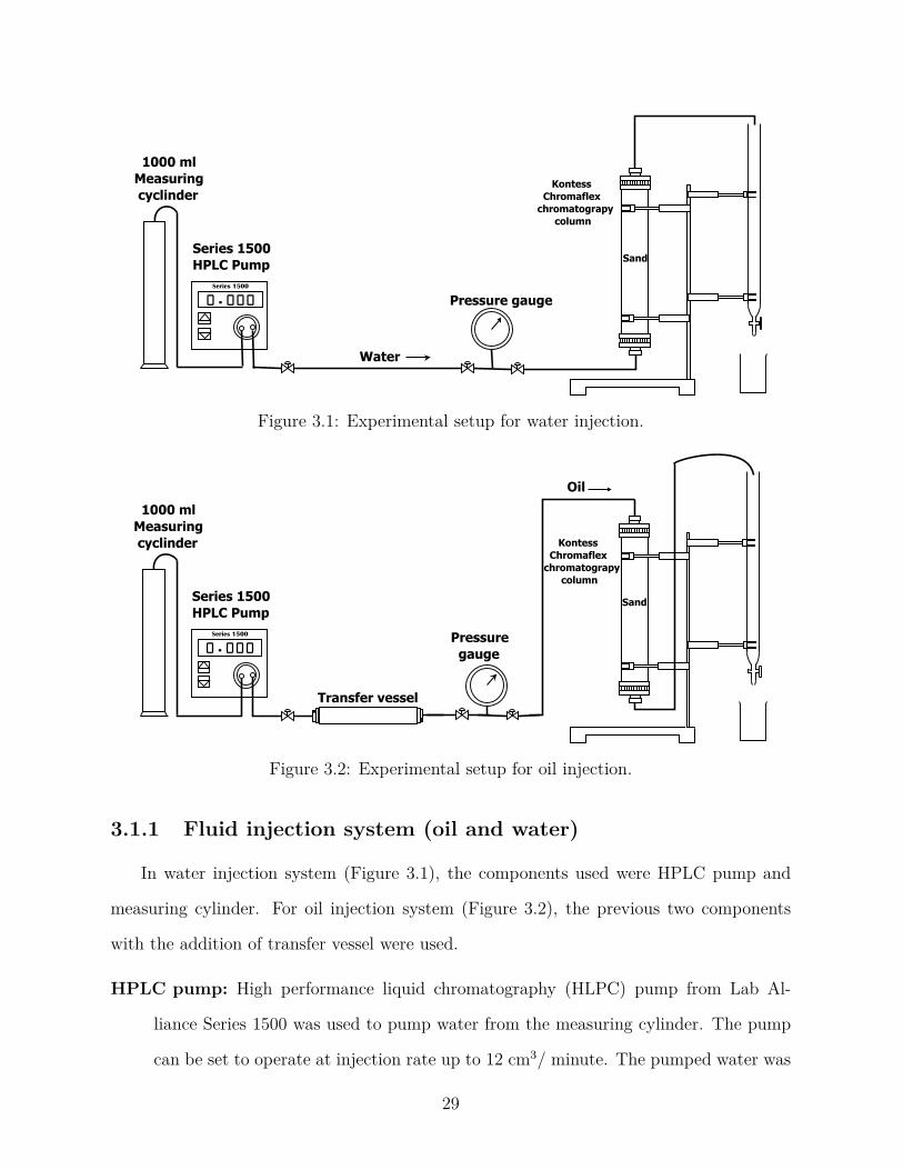
0.000Series 1500
1000 ml Measuring cyclinder
Series 1500 HPLC Pump
Kontess Chromaflex chromatograpy column
Pressure gauge
Water
Sand
Figure 3.1: Experimental setup for water injection.
0.000Series 1500
1000 ml Measuring cyclinder
Series 1500 HPLC Pump
Kontess Chromaflex chromatograpy column
Pressure gauge
Oil
Sand
Transfer vessel
Figure 3.2: Experimental setup for oil injection.
3.1.1 Fluid injection system (oil and water)
In water injection system (Figure 3.1), the components used were HPLC pump and
measuring cylinder. For oil injection system (Figure 3.2), the previous two components
with the addition of transfer vessel were used.
HPLC pump: High performance liquid chromatography (HLPC) pump from Lab Al-
liance Series 1500 was used to pump water from the measuring cylinder. The pump
can be set to operate at injection rate up to 12 cm3/ minute. The pumped water was
29

used to saturate the sand pack to get the pore volume and porosity. In addition, the
pump was also used during waterflooding.
Measuring cylinder: The cylinder is graduated at 5 ml interval and can hold 1000 ml of
liquid. In our experiments, the measuring cylinder was used as a water reservoir for
the pump.
Transfer vessel: The vessel contains a piston which separates the inner chamber into two
parts. It can hold 500 ml of liquid. The transfer vessel was used to hold the oil.
During oil injection, pumped water came through the inlet port at the bottom of the
transfer vessel and pushed the piston upward, which then displaced the oil through
the outlet port to saturate the sand pack. The reason we used transfer vessel during
oil injection is because the wetted parts inside the HPLC pump will deteriorate if the
pump is used directly to pump oil.
3.1.2 Fluid injection system (gas)
For gas injection system (Figure 3.3), the components used were gas cylinder, pressure
regulator, mass flow controller and master control unit (MCU).
Gas cylinder
Brooks Series 5850 Gas Mass Flow Controller
Kontess Chromaflex chromatograpy column 250 ml
Burette
0-15 psi Pressure gauge
Up
Down
Setpoint/Selection
MenuChannelSelection
0152
Enter
Masterselection
Blending
Open, closecontrol mode
Valve
Local/ remote
Control
Power
Gasometer
Brooks MCU Model 0152
Sand
Figure 3.3: Experimental setup for gas injection.
30

Gas cylinder: The cylinder contained pressurized nitrogen (N2) for use in gas injection.
The cylinder was secured firmly to the work bench using a stretch band wrapped
around its body and a clamp.
Pressure regulator: The regulator was attached to the gas cylinder to set the outlet gas
pressure. It was used to maintain a constant pressure during gas injection. In a
typical experiment, the outlet pressure was set to 1 - 3 psi. This low pressure range
was desired for gas injection experiments to achieve gravity-stabilized flow.
Mass flow controller and MCU: We used Brooks 5850i Mass Flow Controller to set the
gas flow rate by adjusting the valve opening through the master control unit (MCU).
These two components work together to deliver a constant rate injection. Note that
in most experiments, unless otherwise noted, the gas injection was performed in
constant pressure mode. This means the control valve was set to 100% open by the
MCU to allow the rate to vary while the pressure was set to a constant value by the
regulator.
3.1.3 Fluid measurement system
The fluid measurement system in Figures 3.1, 3.2, and 3.3 consisted of the pressure
gauge, burette and gasometer. The parameters they measure are pressure, liquid volume,
and gas volume respectively.
Pressure gauge: A low-pressure analogue gauge was used in the experiments. The gauge
can measure pressures within the range 0 - 5 psi. Because the porous media used
was unconsolidated sand, a low-pressure gauge would help to give accurate readings.
This is particularly useful, for example in calculating the permeability from Darcy’s
law.
31
Burette: The burette functioned as separator for the effluent. The cylinder is graduated
at 1 ml interval and can hold up to 250 ml of liquid. At the bottom of the burette,
water was filled up to the first graduated line to mark as the base of the volume
measurement.
Gasometer: The gasometer was used for volumetric measurement of breakthrough gas.
It was connected to the top of the burette with a tube and a steel port attached to
the tube’s end. The steel port was inserted into an opening on a rubber stopper on
top of the burette. Although the volume of gas that broke through was not used in
calculation, we used the volumetric measurement by the gasometer to indicate gas
breakthrough.
3.1.4 Sand holder
We used Kontes chromatography glass column to pack the sand. The glass column has
diameter of 4.8 cm and length of 30 cm, which gives a bulk volume of 543 cm3. It can
withstand pressure up to 50 psi. Both end caps are fitted with high-density polyethylene
(HDPE) bed supports. These bed supports with microporosity filter prevent sand from
coming out of the glass column during experiment. The glass column was used to hold the
sand because it is easy to replace the sand when necessary to suit the experiment.
3.1.5 Video capture system
All experimental runs were captured on video using Sony HDR CX440 video recorder.
This helped us to observe the gas-oil interfaces later after the experiments were completed.
Because a typical run would take several hours, the videos were recorded in Long Play (LP)
mode.
32

3.2 The material
In the experiments, the fluids used were Soltrol and Decane as the oil phase, deionized
water as the aqueous phase, and nitrogen as the gas phase. The sand used for the sand
pack was AFS 50/70 sand. Further descriptions of the materials used are given below.
3.2.1 Fluid system
The fluid systems used are shown in Table 3.1 together with their respective interfacial
tensions and spreading coefficients. The fluid combinations were chosen to give spreading
and non-spreading behavior as indicated by the spreading coefficients, Sow. A positive Sow
means the oil spreads over water in the presence of gas. Conversely a negative Sow indicates
the oil does not spread over water. We did not measure the parameters. Rather the values
were obtained from literature. The oil was dyed red with Sudan IV dye to give better
contrast when observing the fluids displacement during the experiment. The densities and
viscosities of the fluids used are shown in Table 3.2. Likewise with the parameters before,
we used values from literature.
Table 3.1: Fluid systems used in experiments.
σwg σgo σow Sow Reference(dyne cm−1) (dyne cm−1) (dyne cm−1) (dyne cm−1)
N2\Soltrol\ DIwater
71.0 24.0 35.0 +12.0 Chatzis andAyatollahi (1993)
N2\Decane\ DIwater
72.1 23.5 52.0 -3.4 Zhou and Blunt(1997)
Table 3.2: Fluid densities and viscosities used in experiments.
ρ (g/cm3) µ (g/cm.s) ReferenceDecane 0.734 0.0084 Sharma and Rao (2008)Soltrol 0.781 0.0274 Chatzis and Ayatollahi (1993)Water 0.9982 0.0100 Sharma and Rao (2008)Nitrogen 0.001165 0.0001755 Sharma and Rao (2008)
33

3.2.2 Sand
The sand used was AFS 50/70 sand from US Silica. This is fine sand with specific
gravity of 2.65 and median particle size (D50) of 0.26 mm. The sand was packed in the
glass column before running the experiments. We replaced the sand with a new batch after
completing each run. Some batches were treated with chemicals to change their wettability
to oil-wet.
3.3 Experimental procedures
The experimental work was carried out according to procedures described in this sec-
tion. The plan of experimental work is described first, followed by the procedures. These
procedures include preparing the sand pack, altering the sand pack wettability, measuring
the porosity and absolute permeability; and running the experiments.
3.3.1 Plan of experimental work
The experimental work was designed to cover gravity drainage experiments for spread-
ing and non-spreading oil; in water-wet, oil-wet, and fractional-wet sand. The plan of
experimental work is shown in Table 3.3. We followed this plan when conducting the ex-
periments to give us the data which is used to compare to the mathematical models later
on.
Table 3.3: Matrix of experimental work showing the combination of fluid and wettabil-ity system used in gravity drainage experiments. The numbering is used to identify theexperiments.
WettabilityFluid N2\S\DIW N2\D\DIW
Water-wet WW1 WW2Oil-wet OW1 OW2Fractional-wet FW1 FW2
N2= nitrogen, S = Soltrol, DIW = deionized water, D = n-decane
34
3.3.2 Preparing the sand pack
The sand was packed inside the glass column using the dry packing method. In this
method the sand was sprinkled from a spoon containing 40 g of the sand. The spoon was
always held at a height of 1 cm above the sand mound inside the glass column. After every
1 cm of sand layer is formed, we used a solid object to pack the sand. According to Oliviera
et al. (1996), this method achieved a uniform and reproducible packing.
For a fractional-wet experiment, the weight of sand needed to fill up the glass column
was measured. Then equal proportion by weigh of water-wet and oil-wet sand were mixed
according to the packing procedures described above. In this work the fractional-wet sand
was prepared with 50:50 ratio.
3.3.3 Altering the wettability of the sand pack
To study the effect of wettability we treated the sand with chemicals using a process
known as silanization. In this process, dichlorodimethylsilane ((CH3)2SiCl2 or DCDMS) is
used as the silylating agent to make the sand grain water repellent. According to Seed
(2001), the surface of the sand grain is water-wet because it contains silanol groups.
DCDMS reacts with the surface to form a light oil coating which is chemically bonded
to the surface. This oil coating changes the sand wettability to oil-wet.
Specifically, when DCDMS reacts with the silanol groups, it forms siloxane Si−O−Si
linkage and releases HCl. From Herzberg and Erwin (1970), the reaction is a chemisorption
on the surface which is described by the chemical equations below:
(CH3)2SiCl2 + surface−OH −−→ surface−OSi(CH3)2Cl + HCl (3.1)
The second chlorine in (CH3)2SiCl2 further reacts with the hydroxyl group on the sand
surface:
(CH3)2SiCl2 + surface−(OH)2 −−→ surface−O2Si(CH3)2 + 2 HCl (3.2)
35

The reaction in Equation 3.2 forms more siloxane polymer and gives HCl. In this
process the adsorbed water on the sand surface hydrolizes the silanes and acts as catalyst.
The polymeric siloxane that resuls from these reactions is the silicone oil that coats the
grain surface and turns it hydrophobic.
The procedures to change the sand wettability are described as follows: a solution of
5% by volume of DCDMS was prepared by dissolving DCDMS in toluene. Because the
reactions produce hazardous HCl, this step and subsequent ones were performed in a fume
hood with the operator wearing personal protective equipment. The batch of sand to be
processed was soaked in this solution for 15 minutes and then the sand was rinsed with
methanol. The sand was then left overnight in the fume hood to dry and evaporate the
organic solvent. Finally the sand was cured by baking in an oven at 80 − 100◦C for four
hours.
The wettability was evaluated qualitatively by placing samples of treated sand on a
cellophane strip and pipetting a droplet of water on top. The sand is oil-wet if the water
droplet beads up. A low-cost method to measure contact angle was proposed by Ribe
et al. (2016). We modified their procedures by using open-source image analysis software,
ImageJ with the DropSnake plugin. Following this new procedure we were able to confirm
that the treated sand is oil-wet (θgw > 90◦). This is shown in Figure 3.4. Although
silanization treatment changes the grain surface chemically, Vizika and Lombard (1996)
observed through microscope that the treatment does not affect the grain size distribution
or its morphology.
3.3.4 Measuring the porosity and absolute permeability
The porosity was measured by saturating the sand with water from bottom up. Water
was injected at a constant rate of 1 cm3/min. The pore volume was determined first from
the amount of water it took to saturate the sand. Then, porosity was calculated from:
36

(a) Water droplet on treated sand
CA Left=135.999 Right=149.439
(b) Contact angle measurement
Figure 3.4: Procedures to measure contact angle of oil-wet sand: (a) Droplet of water ispipetted on strip of treated sand taped to a glass slide; (b) Photo of (a) taken and analyzedin ImageJ software to calculate the contact angle.
Porosity, φ = PV
BV(3.3)
where PV is the pore volume and BV is the bulk volume. In this case, bulk volume is
the volume of the sand that is contained in the glass column, which is 543 cm3.
The absolute permeability was measured by allowing water to continue saturating the
sand pack at the current injection rate (1 cm3/min) and be produced. Then pressure was
read from the pressure gauge after five minutes. Pressure reading was recorded for each
increment of injection rate until 5 cm3/min. Absolute permeability, kabs was calculated
from Darcy’s law:
kabs = qµL
A4P(3.4)
where kabs is the absolute permeability in Darcy, q is the average flow rate in cm3/s, µ
is the viscosity of displaced fluid in cp, L and A are the sand pack length and cross-section
area in cm and cm2 respectively; and 4P is the average pressure drop in atm. With the
37

data collected we can use Equation 3.4 by plotting q/A as the y-axis and ∆P/Lµ as the x-axis.
A trendline is fitted to the data and the slope will give us kabs.
According to Holbrook and Bernard (1958), the fluid that first contacted the dry sand
affects its initial wettability. Therefore for experiments requiring oil-wet or fractional-wet
sand, the silanized sand was initially saturated with oil phase and left overnight for aging
and to establish its wettability. Then the above procedures were used by replacing water
with oil to find φ and kabs.
3.3.5 Running the experiments
The gravity drainage experiments we plan to perform consisted of secondary and ter-
tiary mode. In secondary mode we perform free-fall gravity drainage (FGD) where the top
of the glass column is opened to atmosphere; and controlled gravity drainage (sec.CGD)
where gas is injected at constant pressure. In tertiary mode (tert. CGD) gravity drainage
experiment with constant gas injection is performed after waterflooding. The steps per-
formed during each experiment is shown in Figure 3.5 for water-wet sand and Figure 3.6
for oil-wet and fractional-wet sand.For a water-wet experiment using either spreading or non-spreading fluid system (Fig-
ure 3.5), a typical run would begin by saturating the sand with water bottom-up to get
the pore volume, porosity and the absolute permeability. This is followed with oilflooding
from top-down to get the original oil in place (OOIP) and end-point oil relative perme-
ability at connate water saturation (Kro*). Free-fall gravity drainage (FGD) commences
after establishing the saturation history. After FGD, the sand pack is resaturated with oil
top-down before starting the secondary controlled gravity drainage experiment. For the
tertiary controlled gravity drainage, we resaturate the sand pack again with oil followed by
0.35 pore volume of water injection at 1 cm3/min from bottom-up. In both secondary and
tertiary CGD the gas injection was controlled by setting the pressure constant at 1 psig.
The procedures for running FGD and both secondary and tertiary CGD remain the same
for oil-wet and fractional-wet sand (Figure 3.6). However, the saturation history was first
38

water
water
PV,φ,Kabs
oil
oil &
Soi,Kro at Swc
water
water
oil
air
oil
gas N2
oil gas N2
wateroil &
tert.CGD
sec.CGD
free-fall GD
Figure 3.5: The steps performed during each experiment with water-wet sand.
water
oil
oil &
Soi,Kro at Swc
water
water
oil
air
oil
gas N2
oil gas N2
wateroil &
tert.CGD
sec.CGD
free-fall GD
oil
oil
PV,φ,Kabs
oil &water
Krw at Sor
Figure 3.6: The steps performed during each experiment with oil-wet sand.
39

established by saturating the sand with oil to get the pore volume, porosity and absolute
permeability; followed by water flooding to get end-point water relative permeability at
residual oil saturation; and lastly oil flooding to get OOIP and Kro*. The procedures to
carry out these experiments are further explained below.
3.3.5.1 Free-fall gravity drainage (FGD)
Before FGD experiment was run, we displaced the water initially present by injecting
oil from the top down to establish connate water saturation, Swc. The Swc was calculated
below:
Swc = PV −OOIPPV
(3.5)
where OOIP , the original oil in place, was the oil volume it took to displace the water
until breakthrough. The initial oil saturation was calculated as Soi = 1 − Swc. The oil
was allowed to continue saturating the sand pack. The oil effective permeability, keo, was
calculated using the procedures described in subsection 3.3.4. Then we calculated the
end-point oil relative permeability, K∗ro at Swc:
K∗ro = keokabs
(3.6)
The FGD experiment began by opening the top lid of the glass column to allow atmo-
spheric pressure to displace the oil. The experiment was run for twelve hours. During the
course of the experiment, the volume of oil recovered and the pressure were recorded.
3.3.5.2 Secondary controlled gravity drainage (sec. CGD)
Before running this experiment, the sand pack was resaturated with oil. We assumed
that Swc, Soi, and K∗ro were the same with the ones from FGD experiment. In secondary
CGD, the top lid was closed and the fluid injection system for gas was set up according
to Figure 3.3. In this experiment, the gas was injected from the top and injection was set
40

at constant pressure. The experiment began as soon as the gas valve was opened. Similar
to FGD experiment, we ran it for twelve hours and recorded the oil recovery and pressure
drop.
3.3.5.3 Secondary waterflooding
Secondary water flooding was performed prior to running tertiary CGD. The purpose
was to establish water flood residual oil saturation, Sorw. The water injection system
was set up according to Figure 3.1. To ensure sufficient oil remained for tertiary CGD,
waterflooding was carried out by injecting 0.35 PV of water at 1 cm3/minute. During the
course of this experiment, we recorded the oil recovery and the pressure drop.
3.3.5.4 Tertiary controlled gravity drainage (tert. CGD)
Tertiary CGD was run after secondary waterflooding. The experiment was set up
according to Figure 3.3. The gas was injected at constant pressure of 1 psig from the top
for twelve hours. Similar to previous experiments, we recorded the oil recovery and pressure
drop.
41

Chapter 4
Gravity Drainage Experiments for Spreading and Non-Spreading Systems
In this chapter we present the results from gravity drainage experiments performed
in secondary and tertiary mode. Free-fall gravity drainage (FGD) and secondary con-
trolled gravity drainage (sec.CGD) are categorized under the secondary mode and tertiary
controlled gravity drainage (tert.CGD) is in tertiary mode. Our experiments consisted
of gravity drainage in glass columns with water-wet, oil-wet and fractional-wet sand. We
used Soltrol as spreading oil and Decane as non-spreading. The results were compared with
those from literature and we found cases where our experimental data contradict available
reports. We explained the underlying mechanisms at pore level and analyzed the results
with dimensionless numbers.
4.1 Experimental results
The experimental results are summarized in Table 4.1. We arranged the results accord-
ing to wettability and its corresponding fluid system to observe the effect of spreading on
oil recovery. The results presented here came from gravity drainage experiments that were
run for twelve hours. The same duration for all experiments provided consistent basis for
comparison. The oil recoveries tabulated represent the terminal point at the conclusion of
each experiment.
From Table 4.1 it is shown that gravity drainage experiments in water-wet sand pro-
duced more oil in secondary and tertiary mode when the fluid system is spreading. In oil-wet
sand the higher oil recovery came from experiments using non-spreading fluid. Higher re-
covery from non-spreading fluid system is also observed from fractional-wet experiments.
We discuss these observations in the following sections.
42

Table 4.1: Summary of experimental results for free-fall gravity drainage, secondary con-trolled gravity drainage and tertiary controlled gravity drainage
Wettability Fluidsystem
φ k (Darcy) Swc Sorg,fgd Sorg,cgd2 Sorw Sorg,cgd3 RFfgd RFcgd2 RFcgd3
w-w sp 0.346 3.8 0.09 0.287 0.229 0.559 0.330 68.4 74.9 41.0w-w non-sp 0.363 3.8 0.244 0.325 0.284 0.442 0.299 57.0 62.4 32.2
o-w sp 0.413 6.6 0.134 0.393 0.379 0.594 0.379 54.6 56.2 36.1o-w non-sp 0.346 3.2 0.144 0.271 0.213 0.537 0.223 68.3 75.2 58.4
f-w sp 0.365 8.9 0.172 0.424 0.384 0.556 0.369 48.8 53.7 33.6f-w non-sp 0.355 5.5 0.181 0.269 0.241 0.534 0.249 67.1 70.3 54.4
φ: Porosity (dimensionless) RFcgd2: Recovery factor for secondary controlled
gravity drainage (% OOIP)
k: Absolute permeability (Darcy) RFcgd3: Recovery factor for tertiary controlled gravity
drainage (% ROIP)
Swc: Connate water saturation (dimensionless) sp: Spreading fluid (N2\Soltrol\Deionized Water
(DIW)
Sorg,fgd: Residual oil saturation after free-fall gravity drainage
(dimensionless)
non-sp: non-spreading fluid (N2\Decane\DIW)
Sorg,cgd2: Residual oil saturation after secondary controlled gravity
drainage (dimensionless)
w-w: Water-wet sand
Sorw: Residual oil saturation after waterflooding (dimensionless) o-w: Oil-wet sand
Sorg,cgd3: Reduced residual oil saturation after tertiary controlled
gravity drainage (dimensionless)
f-w: Fractional-wet sand
RFfgd: Recovery factor for free-fall gravity drainage (%OOIP)
4.1.1 Gravity drainage in water-wet sand
From Figure 4.1 it is observed that GAGD in water-wet sand with spreading fluid
system typically recovers more oil than the corresponding non-spreading fluid. Free-fall
gravity drainage with Soltrol for example, recovered 68.4% OOIP compared to decane with
only 57% OOIP. High oil recovery trends were observed for all GAGD injection modes
performed in water-wet sand. From Table 4.1 the average recovery of all injection modes
(secondary and tertiary) for the spreading group in water-wet sand is 61.4% while the
average for non-spreading group is 50.5%.
Our results confirm similar findings from other workers (Kantzas et al. (1988a), Vizika
(1993), Kalaydjian et al. (1995), and Maeda and Okatsu (2008)). In their work they also
reported higher recovery for gravity drainage performed in water-wet sand with spreading
oil. According to Kantzas et al. (1988b) and Oren et al. (1992), the higher oil recovery
observed in these experiments can be explained by the spreading film phenomenon. In
43
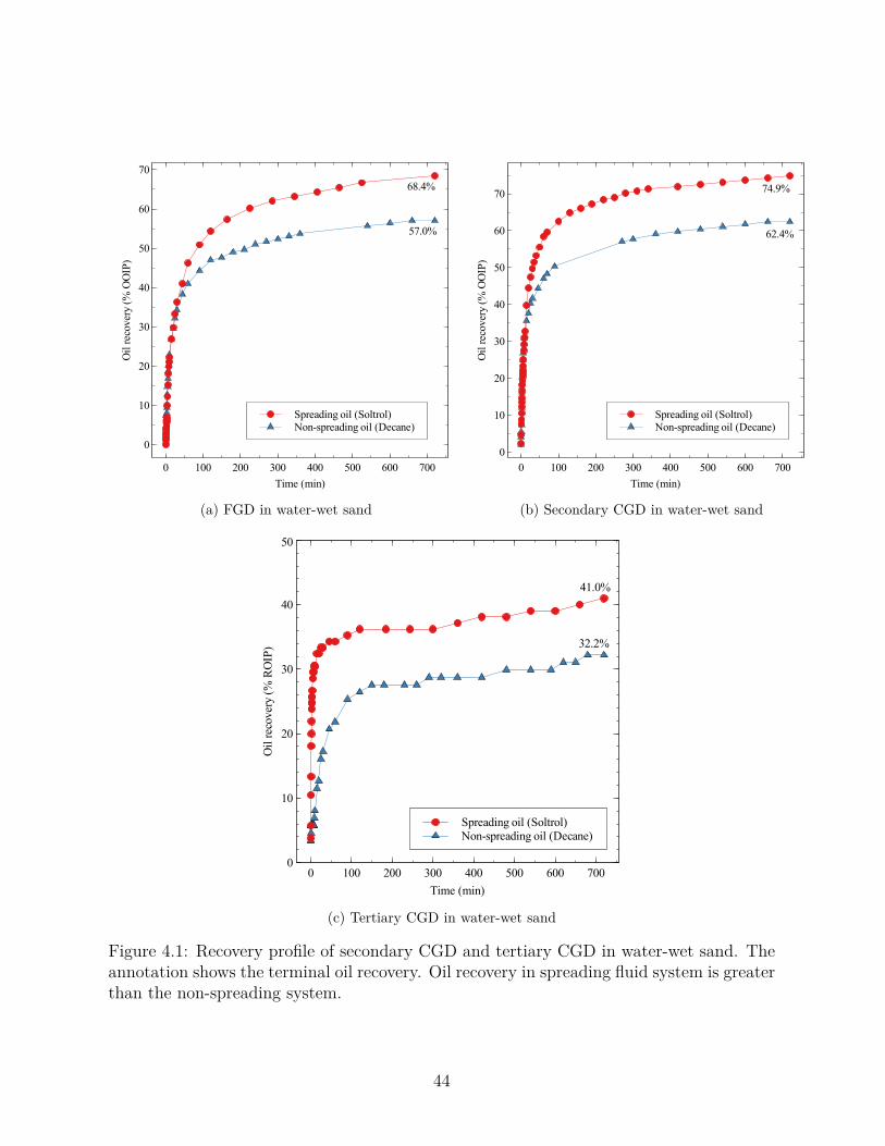
57.0%
68.4%
Spreading oil (Soltrol)Non-spreading oil (Decane)
Oil
reco
very
(% O
OIP
)
0
10
20
30
40
50
60
70
Time (min)0 100 200 300 400 500 600 700
(a) FGD in water-wet sand
62.4%
74.9%
Spreading oil (Soltrol)Non-spreading oil (Decane)
Oil
reco
very
(% O
OIP
)
0
10
20
30
40
50
60
70
Time (min)0 100 200 300 400 500 600 700
(b) Secondary CGD in water-wet sand
32.2%
41.0%
Spreading oil (Soltrol)Non-spreading oil (Decane)
Oil
reco
very
(% R
OIP
)
0
10
20
30
40
50
Time (min)0 100 200 300 400 500 600 700
(c) Tertiary CGD in water-wet sand
Figure 4.1: Recovery profile of secondary CGD and tertiary CGD in water-wet sand. Theannotation shows the terminal oil recovery. Oil recovery in spreading fluid system is greaterthan the non-spreading system.
44

water-wet media, oil phase is the intermediate phase. When the sign of the oil spreading
coefficient is positive, the oil spreads and forms thin film spontaneously in the presence
of water and air. This film maintains hydraulic conductivity even at low saturation, as
reported in a three-phase relative permeability study by DiCarlo et al. (2000). In their
experimental work DiCarlo et al. (2000) observed that oil relative permeability for the
spreading oil (hexane and octane) remained finite, spanning six orders of magnitude at
low saturation while oil relative permeability for non-spreading oil (decane) dropped off
to zero. This means the film formed by the spreading oil provides a continuous path so
that bypassed oil blobs behind the advancing gas front in the sand column can be recon-
nected and effectively drained. In a non-spreading system, since the spreading coefficient
is negative (c.f. Table 3.1 on page 33), the oil did not spread and the conductivity layer
for residual oil flow was not established.
We have recorded continuous video for each experimental runs. Since the file sizes
were large, the videos were processed using the open-source software package ffmpeg. The
time-lapsed photos captured from the videos are presented in Figures 4.2, 4.3, and 4.4 for
FGD, secondary CGD and tertiary CGD respectively.
Figure 4.2 shows the sequence of displacements taking place over time in free-fall gravity
drainage (FGD). In this experiment oil production is allowed to proceed by the action of
gravity forces after we opened the top and bottom valves of the column to atmosphere. We
can see the progression of the gas-oil interface for both spreading (4.2a) and non-spreading
(4.2b) as it advanced through the sand column. At t = 60 seconds, the beginning of the gas
front was observed. At this stage, gas as the non-wetting phase occupied the larger pores
and simultaneously displaced oil, which is the intermediate phase. From t = 10 minutes
until t = 2 hours the front propagated and displaced the bulk of the oil to the outlet.
Under free-fall mode we observed the gas front advanced at a faster rate for both spreading
and non-spreading systems. Consequently there was no instance of a stable oil bank being
formed ahead of the gas front. According to Chatzis and Ayatollahi (1993) in free-fall mode
45
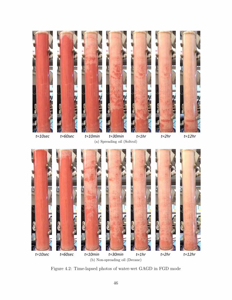
t=10sec t=60sec t=10min t=30min t=1hr t=2hr t=12hr (a) Spreading oil (Soltrol)
t=10sec t=60sec t=10min t=30min t=1hr t=2hr t=12hr (b) Non-spreading oil (Decane)
Figure 4.2: Time-lapsed photos of water-wet GAGD in FGD mode
46
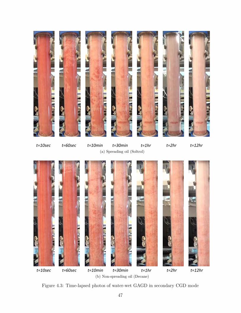
t=10sec t=60sec t=10min t=30min t=1hr t=2hr t=12hr (a) Spreading oil (Soltrol)
t=10sec t=60sec t=10min t=30min t=1hr t=2hr t=12hr (b) Non-spreading oil (Decane)
Figure 4.3: Time-lapsed photos of water-wet GAGD in secondary CGD mode
47

t=10sec t=60sec t=10min t=30min t=1hr t=2hr t=12hr (a) Spreading oil (Soltrol)
t=10sec t=60sec t=10min t=30min t=1hr t=2hr t=12hr (b) Non-spreading oil (Decane)
Figure 4.4: Time-lapsed photos of water-wet GAGD in tertiary CGD mode
48
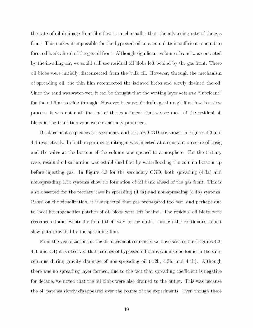
the rate of oil drainage from film flow is much smaller than the advancing rate of the gas
front. This makes it impossible for the bypassed oil to accumulate in sufficient amount to
form oil bank ahead of the gas-oil front. Although significant volume of sand was contacted
by the invading air, we could still see residual oil blobs left behind by the gas front. These
oil blobs were initially disconnected from the bulk oil. However, through the mechanism
of spreading oil, the thin film reconnected the isolated blobs and slowly drained the oil.
Since the sand was water-wet, it can be thought that the wetting layer acts as a “lubricant”
for the oil film to slide through. However because oil drainage through film flow is a slow
process, it was not until the end of the experiment that we see most of the residual oil
blobs in the transition zone were eventually produced.
Displacement sequences for secondary and tertiary CGD are shown in Figures 4.3 and
4.4 respectively. In both experiments nitrogen was injected at a constant pressure of 1psig
and the valve at the bottom of the column was opened to atmosphere. For the tertiary
case, residual oil saturation was established first by waterflooding the column bottom up
before injecting gas. In Figure 4.3 for the secondary CGD, both spreading (4.3a) and
non-spreading 4.3b systems show no formation of oil bank ahead of the gas front. This is
also observed for the tertiary case in spreading (4.4a) and non-spreading (4.4b) systems.
Based on the visualization, it is suspected that gas propagated too fast, and perhaps due
to local heterogeneities patches of oil blobs were left behind. The residual oil blobs were
reconnected and eventually found their way to the outlet through the continuous, albeit
slow path provided by the spreading film.
From the visualizations of the displacement sequences we have seen so far (Figures 4.2,
4.3, and 4.4) it is observed that patches of bypassed oil blobs can also be found in the sand
columns during gravity drainage of non-spreading oil (4.2b, 4.3b, and 4.4b). Although
there was no spreading layer formed, due to the fact that spreading coefficient is negative
for decane, we noted that the oil blobs were also drained to the outlet. This was because
the oil patches slowly disappeared over the course of the experiments. Even though there
49
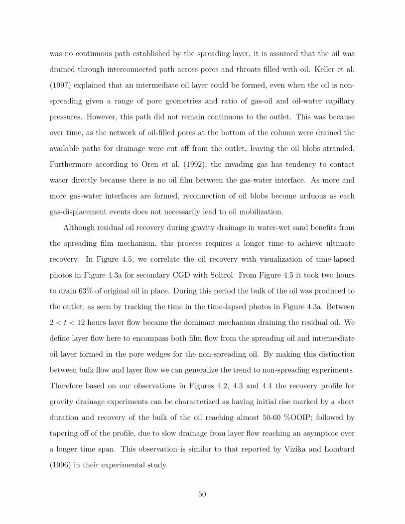
was no continuous path established by the spreading layer, it is assumed that the oil was
drained through interconnected path across pores and throats filled with oil. Keller et al.
(1997) explained that an intermediate oil layer could be formed, even when the oil is non-
spreading given a range of pore geometries and ratio of gas-oil and oil-water capillary
pressures. However, this path did not remain continuous to the outlet. This was because
over time, as the network of oil-filled pores at the bottom of the column were drained the
available paths for drainage were cut off from the outlet, leaving the oil blobs stranded.
Furthermore according to Oren et al. (1992), the invading gas has tendency to contact
water directly because there is no oil film between the gas-water interface. As more and
more gas-water interfaces are formed, reconnection of oil blobs become arduous as each
gas-displacement events does not necessarily lead to oil mobilization.
Although residual oil recovery during gravity drainage in water-wet sand benefits from
the spreading film mechanism, this process requires a longer time to achieve ultimate
recovery. In Figure 4.5, we correlate the oil recovery with visualization of time-lapsed
photos in Figure 4.3a for secondary CGD with Soltrol. From Figure 4.5 it took two hours
to drain 63% of original oil in place. During this period the bulk of the oil was produced to
the outlet, as seen by tracking the time in the time-lapsed photos in Figure 4.3a. Between
2 < t < 12 hours layer flow became the dominant mechanism draining the residual oil. We
define layer flow here to encompass both film flow from the spreading oil and intermediate
oil layer formed in the pore wedges for the non-spreading oil. By making this distinction
between bulk flow and layer flow we can generalize the trend to non-spreading experiments.
Therefore based on our observations in Figures 4.2, 4.3 and 4.4 the recovery profile for
gravity drainage experiments can be characterized as having initial rise marked by a short
duration and recovery of the bulk of the oil reaching almost 50-60 %OOIP; followed by
tapering off of the profile, due to slow drainage from layer flow reaching an asymptote over
a longer time span. This observation is similar to that reported by Vizika and Lombard
(1996) in their experimental study.
50

Layer flowBulk flow dominant
1 m
in
8.8 %OOIP
10 m
in
32.7 %OOIP
58.5 %OOIP
1 hr
63 %OOIP
2 hr
74.9 %OOIP
Oil
reco
very
(% O
OIP
)
0
20
40
60
80
100
Time (min)1 10 100 1000
Figure 4.5: Recovery profile for secondary CGD in water-wet sand with spreading oil(Soltrol), showing regions of bulk flow and layer flow
51

In the literature Parsaei and Chatzis (2011) has shown that the reconnected oil through
the spreading film eventually forms oil bank; and the oil bank further reconnects more
isolated blobs as it is displaced to the outlet. It is believed that the formation of oil
bank during gravity drainage is possible when gravity forces overcome the viscous forces
at a velocity lower than the critical gravity drainage velocity (Rostami et al., 2010). The
critical gravity drainage velocity concept comes from the work of Dumore (1964) and the
equation is given as:
vc = k
µo(∆ρg) (4.1)
where k is the absolute permeability, µo is the oil velocity, ∆ρ is the gas-oil density
difference and g is the gravity acceleration constant. Using the fluid properties from Table
3.2 and the permeabilities from Table 4.1 on page 43 we calculated the critical velocity to
be 0.00103 cm/s or 0.89 m/day for the spreading case and 0.0032 cm/s or 2.76 m/day for
the non-spreading case. This can be achieved in the laboratory setup by producing the
oil at a constant rate of 0.13 cm3/min for the spreading case and 0.42 cm3/min for the
non-spreading case. However this was not attempted in our case due to limitation of the
equipment.
Using production data and the method introduced by Grattoni et al. (2001), we cal-
culated the gas velocity profiles for the spreading and non-spreading system in water-wet
media for all injection modes. Our calculation in Figure 4.6 shows that the initial veloc-
ities exceeded the critical gas velocity with the maximum over 0.05 cm/s. Only later in
the displacement, when t > 100 minutes we see the velocities decreasing to values close to
the critical velocity. However at this point the bulk of the oil has already been produced,
which left little oil in sufficient quantity to form a visible oil bank. This coincides with the
visual observation when t = 2 hours in Figures 4.2, 4.3 and 4.4.
From the experimental results and the calculations, we see that GAGD recovery delivers
higher recovery when performed in a water-wet sand and the fluid system has a positive
52

Spreading oil (Soltrol)Non-spreading oil (Decane)
Gas
vel
ocity
(cm
/sec
)
0
0.01
0.02
0.03
0.04
0.05
Time (min)0.1 1 10 100 1000
(a) FGD
Spreading oil (Soltrol)Non-spreading oil (Decane)
Gas
vel
ocity
(cm
/sec
)
0
0.01
0.02
0.03
0.04
0.05
Time (min)0.1 1 10 100 1000
(b) Secondary CGD
Spreading oil (Soltrol)Non-spreading oil (Decane)
Gas
vel
ocity
(cm
/sec
)
0
0.01
0.02
0.03
0.04
0.05
0.06
Time (min)0.1 1 10 100 1000
(c) Tertiary CGD
Figure 4.6: Gas velocity profiles for all injection modes of GAGD in water-wet sand.
53

spreading coefficient. The reason for higher recovery is explained based on literature and
the recovery profile is characterized and generalized for both spreading and non-spreading
fluid system. Although we did not observe formation of oil bank the reason is explained
based on gas velocity calculation. In the next section we will see how the recovery profiles
change when GAGD is conducted in oil-wet media.
4.1.2 Gravity drainage in oil-wet sand
For oil-wet experiments, Figure 4.7 shows that gravity drainage with non-spreading
fluid system produced more oil compared to spreading fluid system. For example in free-fall
mode (FGD) oil recovery from non-spreading decane was 68.3% OOIP compared to 54.6%
OOIP for spreading Soltrol. This trend is consistent for all injection modes. From Table
4.1 on average the oil recovery in oil-wet sand for all three modes for non-spreading system
is 67.3% while the spreading system is 49%. In the literature we found two conflicting
reports about oil recovery in three-phase oil-wet porous media.
Oren and Pinczewski (1994) reported that highest oil recovery was achieved in oil-wet
media for both spreading and non-spreading oil. The result came from three-phase flow
experiment with micromodel. When the recoveries were ranked, the highest oil recovery
went to oil-wet media, followed by water-wet media with spreading fluid and the last was
water-wet media with non-spreading fluid. They explained that in oil-wet media the sign of
the spreading coefficient was not important because oil was drained through the continuous
wetting phase. The drainage rate which also corresponds to oil recovery, was faster because
the wetting film was thicker which lead to higher conductivity flow path.
Vizika and Lombard (1996) presented their results and observed that oil recovery in
oil-wet media was the lowest overall when compared to oil recovery from water-wet and
fractional-wet sand. Both spreading and non-spreading oil have similar recovery in oil-wet
media, which suggested that the spreading behavior was not important in oil-wet system.
54

54.6%
68.3%
Spreading oil (Soltrol)Non-spreading oil (Decane)
Oil
reco
very
(% O
OIP
)
0
10
20
30
40
50
60
70
Time (min)0 100 200 300 400 500 600 700
(a) FGD in oil-wet sand
56.2%
75.2%
Spreading oil (Soltrol)Non-spreading oil (Decane)
Oil
reco
very
(% O
OIP
)
0
10
20
30
40
50
60
70
Time (min)0 100 200 300 400 500 600 700
(b) Secondary CGD in oil-wet sand
36.1%
58.4%
Spreading oil (Soltrol)Non-spreading oil (Decane)
Oil
reco
very
(% R
OIP
)
0
10
20
30
40
50
Time (min)0 100 200 300 400 500 600 700
(c) Tertiary CGD in oil-wet sand
Figure 4.7: Recovery profile of FGD, secondary CGD and tertiary CGD in oil-wet sand.In all injection modes, non-spreading system shows greater oil recovery than spreadingsystem.
55
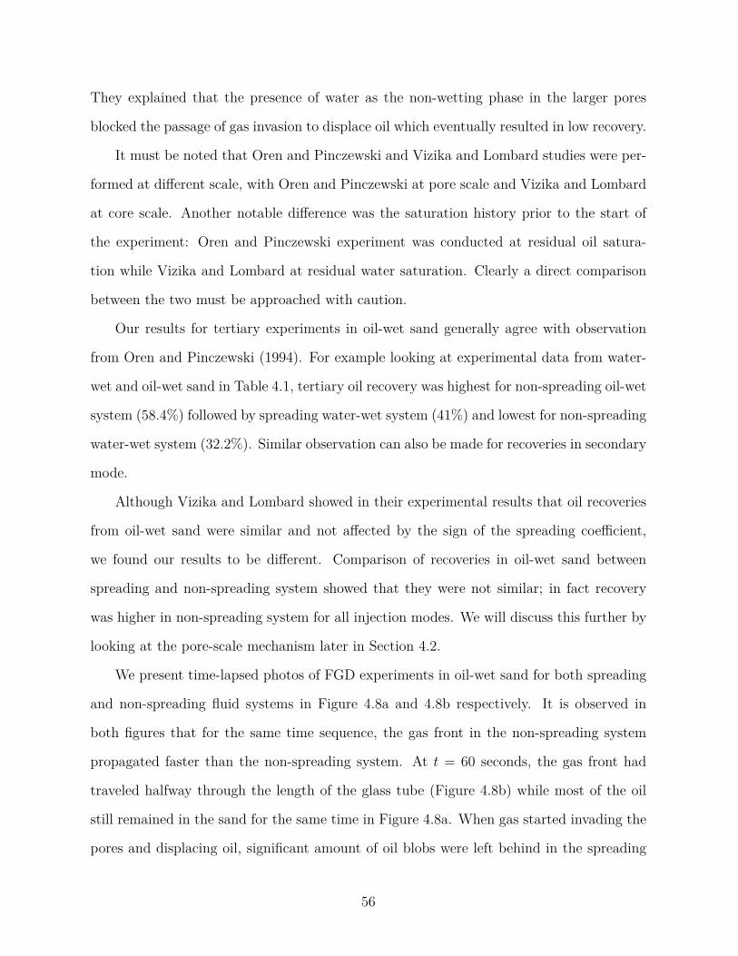
They explained that the presence of water as the non-wetting phase in the larger pores
blocked the passage of gas invasion to displace oil which eventually resulted in low recovery.
It must be noted that Oren and Pinczewski and Vizika and Lombard studies were per-
formed at different scale, with Oren and Pinczewski at pore scale and Vizika and Lombard
at core scale. Another notable difference was the saturation history prior to the start of
the experiment: Oren and Pinczewski experiment was conducted at residual oil satura-
tion while Vizika and Lombard at residual water saturation. Clearly a direct comparison
between the two must be approached with caution.
Our results for tertiary experiments in oil-wet sand generally agree with observation
from Oren and Pinczewski (1994). For example looking at experimental data from water-
wet and oil-wet sand in Table 4.1, tertiary oil recovery was highest for non-spreading oil-wet
system (58.4%) followed by spreading water-wet system (41%) and lowest for non-spreading
water-wet system (32.2%). Similar observation can also be made for recoveries in secondary
mode.
Although Vizika and Lombard showed in their experimental results that oil recoveries
from oil-wet sand were similar and not affected by the sign of the spreading coefficient,
we found our results to be different. Comparison of recoveries in oil-wet sand between
spreading and non-spreading system showed that they were not similar; in fact recovery
was higher in non-spreading system for all injection modes. We will discuss this further by
looking at the pore-scale mechanism later in Section 4.2.
We present time-lapsed photos of FGD experiments in oil-wet sand for both spreading
and non-spreading fluid systems in Figure 4.8a and 4.8b respectively. It is observed in
both figures that for the same time sequence, the gas front in the non-spreading system
propagated faster than the non-spreading system. At t = 60 seconds, the gas front had
traveled halfway through the length of the glass tube (Figure 4.8b) while most of the oil
still remained in the sand for the same time in Figure 4.8a. When gas started invading the
pores and displacing oil, significant amount of oil blobs were left behind in the spreading
56
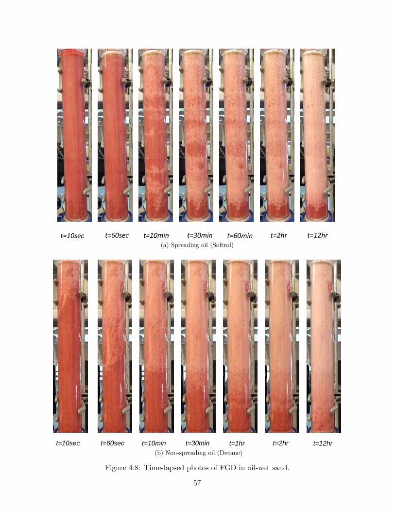
t=10sec t=12hrt=2hrt=60mint=30mint=10mint=60sec(a) Spreading oil (Soltrol)
t=10sec t=60sec t=12hrt=2hrt=1hrt=30mint=10min
(b) Non-spreading oil (Decane)
Figure 4.8: Time-lapsed photos of FGD in oil-wet sand.
57
t=10sec t=60sec t=10min t=30min t=1hr t=2hr t=12hr (a) Spreading oil (Soltrol)
t=10sec t=60sec t=10min t=30min t=1hr t=2hr t=12hr (b) Non-spreading oil (Decane)
Figure 4.9: Time-lapsed photos of secondary CGD in oil-wet sand.
58

t=10sec t=60sec t=10min t=30min t=1hr t=2hr t=12hr (a) Spreading oil (Soltrol)
t=10sec t=60sec t=10min t=30min t=1hr t=2hr t=12hr (b) Non-spreading oil (Decane)
Figure 4.10: Time-lapsed photos of tertiary CGD in oil-wet sand.
59

case (4.8a). This was evident from the oil patches left behind along the length of the sand
column. This continued for the remainder of the experiment. It took almost twelve hours
to drain most of the residual oil, and yet a short column of oil can still be seen at the
bottom after the experiment was stopped. This contrasts with drainage sequences in the
non-spreading, oil-wet sand. At early time, the recovery was contributed mostly from bulk
oil drainage. There were few oil patches visible as the gas front migrated downward. At
later time, most of the residual oil was drained through the wetting film.
It must be pointed out here that in both cases (4.8a and 4.8b) a clear demarcator
separating gas-oil front with oil bank was not seen . Using the critical velocity Equation 4.1
on page 52 the calculated velocity was 0.00179 cm/s for spreading case and 0.00270 cm/s for
the non-spreading case. This corresponds to withdrawal rate of 0.266 cm3/min and 0.337
cm3/min for spreading and non-spreading respectively. This means a stabilized drainage
where oil bank can be formed ahead of the gas-oil front can be achieved by producing the
oil below the calculated withdrawal rate.
The time-lapsed photos for secondary CGD in Figure 4.9 look almost similar between
the spreading (4.9a) and non-spreading case (4.9b) when compared at each time steps. This
was despite the fact that oil recovery for the non-spreading case was higher (75.2 %OOIP)
compared to spreading case (cf. Figure 4.7). One notable difference was that oil drainage
started earlier in non-spreading case. At 10 < t < 60 seconds gas had already displaced
oil in the top quarter of the column in Figure 4.9b compared to the spreading case for the
same period. Earlier onset of bulk flow regime could be a possible reason for higher oil
production in the non-spreading case.
In tertiary CGD it appears that drainage rate is faster for non-spreading system. Com-
paring the time-lapsed photos from t = 10 minutes onward we see that patches of residual
oil were left behind in the top half of the column in the spreading case (4.10a). The residual
oil was eventually drained at t = 12 hours but there was still a small accumulation of oil
at the bottom. In the same duration it is noted that there was also oil patches for the
60

Spreading oil (Soltrol)Non-spreading oil (Decane)
Gas
vel
ocity
(cm
/sec
)
0
0.01
0.02
0.03
0.04
0.05
Time (min)0.1 1 10 100 1000
(a) FGD
Spreading oil (Soltrol)Non-spreading oil (Decane)
Gas
vel
ocity
(cm
/sec
)
0
0.02
0.04
0.06
0.08
0.1
Time (min)0.1 1 10 100 1000
(b) Secondary CGD
Spreading oil (Soltrol)Non-spreading oil (Decane)
Gas
vel
ocity
(cm
/sec
)
0
0.01
0.02
0.03
0.04
0.05
0.06
Time (min)0.1 1 10 100 1000
(c) Tertiary CGD
Figure 4.11: Gas velocity profiles for all injection modes of GAGD in oil-wet sand.
61
non-spreading case (4.10b) but they were located mostly in the bottom half of the column
and their density was much less than that of the spreading case.
When analyzing the displacement sequences from the time-lapsed photos, particularly
for the secondary and tertiary experiments we admit that some of our observations were
qualitative in nature. Therefore we calculated the gas velocity profile to correlate with our
visual observations.
The gas velocity profiles were plotted in Figure 4.11 to better understand these ob-
servations. The procedure to obtain the plot was explained in Grattoni et al. (2001). In
the FGD (4.11a) and secondary CGD (4.11b) experiments the gas velocity for the non-
spreading system was higher initially, which coincided with the beginning of bulk flow
regime. Flow through the wetting film became dominant at a later time (t > 100 minutes)
when the gas was slowing down. In oil-wet sand with spreading oil the gas velocity was
lower initially, which accounted for the oil remaining in the sand when t < 60 seconds
(cf. 4.8a and 4.9a). The recovery from bulk flow regime also happened gradually, which
matched the gas velocity profile for 10 < t < 100 minutes. It was only at a later time
(t > 100 minutes) that drainage from wetting film became dominant.
In Figure 4.11c for tertiary CGD the gas velocities for the spreading and non-spreading
system almost tracked each other. However the velocity for the non-spreading case was
consistently higher than the spreading case for duration t < 100 minutes. This resulted in
more oil being drained overall, which lead to oil recovery of 58.4% ROIP compared to only
36.1% ROIP for the non-spreading system.
4.1.3 Gravity drainage in fractional-wet sand
In Figure 4.12 we observed higher recovery for the non-spreading oil in fractional-wet
sand compared to the spreading oil in all injection modes. This observation is similar to
that observed in the previous section for oil-wet sand.
62

48.8%
67.1%
Spreading oil (Soltrol)Non-spreading oil (Decane)
Oil
reco
very
(% O
OIP
)
0
10
20
30
40
50
60
70
Time (min)0 100 200 300 400 500 600 700
(a) FGD in fractional-wet sand
53.7%
70.3%
Spreading oil (Soltrol)Non-spreading oil (Decane)
Oil
reco
very
(% O
OIP
)0
10
20
30
40
50
60
70
Time (min)0 100 200 300 400 500 600 700
(b) Secondary CGD in fractional-wet sand
33.6%
54.4%
Spreading oil (Soltrol)Non-spreading oil (Decane)
Oil
reco
very
(% R
OIP
)
0
10
20
30
40
50
Time (min)0 100 200 300 400 500 600 700
(c) Tertiary CGD in fractional-wet sand
Figure 4.12: Recovery profile of FGD, secondary CGD and tertiary CGD in fractional-wetsand.
63
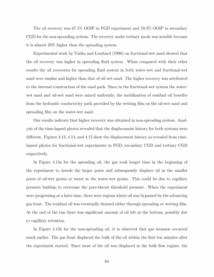
The oil recovery was 67.1% OOIP in FGD experiment and 70.3% OOIP in secondary
CGD for the non-spreading system. The recovery under tertiary mode was notable because
it is almost 20% higher than the spreading system.
Experimental work by Vizika and Lombard (1996) on fractional-wet sand showed that
the oil recovery was higher in spreading fluid system. When compared with their other
results the oil recoveries for spreading fluid system in both water-wet and fractional-wet
sand were similar and higher than that of oil-wet sand. The higher recovery was attributed
to the internal construction of the sand pack. Since in the fractional-wet system the water-
wet sand and oil-wet sand were mixed uniformly, the mobilization of residual oil benefits
from the hydraulic conductivity path provided by the wetting film on the oil-wet sand and
spreading film on the water-wet sand.
Our results indicate that higher recovery was obtained in non-spreading system. Anal-
ysis of the time-lapsed photos revealed that the displacement history for both systems were
different. Figures 4.13, 4.14, and 4.15 show the displacement history as revealed from time-
lapsed photos for fractional-wet experiments in FGD, secondary CGD and tertiary CGD
respectively.
In Figure 4.13a for the spreading oil, the gas took longer time in the beginning of
the experiment to invade the larger pores and subsequently displace oil in the smaller
pores of oil-wet grains or water in the water-wet grains. This could be due to capillary
pressure buildup to overcome the pore-throat threshold pressure. When the experiment
were progressing at a later time, there were regions where oil was bypassed by the advancing
gas front. The residual oil was eventually drained either through spreading or wetting film.
At the end of the run there was significant amount of oil left at the bottom, possibly due
to capillary retention.
In Figure 4.13b for the non-spreading oil, it is observed that gas invasion occurred
much earlier. The gas front displaced the bulk of the oil within the first ten minutes after
the experiment started. Since most of the oil was displaced in the bulk flow regime, the
64

t=10sec t=60sec t=10min t=30min t=1hr t=2hr t=12hr (a) Spreading oil (Soltrol)
t=10sec t=60sec t=10min t=30min t=1hr t=2hr t=12hr (b) Non-spreading oil (Decane)
Figure 4.13: Time-lapsed photos of FGD in fractional-wet sand.
65

t=10sec t=60sec t=10min t=30min t=1hr t=2hr t=12hr (a) Spreading oil (Soltrol)
t=10sec t=60sec t=10min t=30min t=1hr t=2hr t=12hr (b) Non-spreading oil (Decane)
Figure 4.14: Time-lapsed photos of secondary CGD in fractional-wet sand.
66
t=10sec t=60sec t=10min t=30min t=1hr t=2hr t=12hr (a) Spreading oil (Soltrol)
t=10sec t=60sec t=10min t=30min t=1hr t=2hr t=12hr (b) Non-spreading oil (Decane)
Figure 4.15: Time-lapsed photos of tertiary CGD in fractional-wet sand.
67

remaining oil was displaced at later time through wetting film. Rapid production through
bulk flow at early time followed by drainage through wetting film at later time could
possibly explain the higher oil recovery observed for this system.
For secondary CGD the same behavior is observed for the spreading system (4.14a).
Oil drainage was delayed in the first 60 seconds with oil patches were seen in the middle
of the sand column during the course of the experiment. Although the residual oil was
eventually drained, there was still a small accumulation of oil at the bottom of the column
when the experiment finished. In the non-spreading system (4.14b) oil drainage occurred
immediately after the experiment started. The bulk of the oil was displaced within the
first hour and the remaining oil was drained through wetting film for the remainder of the
experiment. One notable difference was that there was no visible oil accumulation at the
bottom of the column when the experiment was stopped.
In tertiary CGD for the spreading system (4.15a) oil recovery was initially preceded
by water production, as can be seen at the bottom of the column in the first 60 seconds.
From 60 seconds onward the oil was produced alongside water. This continued for some
time, approximately within the first 30 minutes after which the outlet started producing
pnly oil in diminishing amount. During the course of the experiment oil patches were seen,
similar to that observed in the previous two experiments. Eventually the residual oil in the
patches was drained, but there was still a visible oil accumulation at the bottom when the
experiment terminated.
In non-spreading system under tertiary CGD (4.15b) oil and water was produced si-
multaneously since the beginning of the experiment. There were few oil patches, with
most of them observed to be moving downward toward the outlet beginning at t = 10
minutes. The concentration of oil patches eventually became more dispersed and sparse as
the experiment progressed.
We plot the gas velocity profiles and correlate with the time-lapsed photos of the FGD
experiments in Figure 4.16a for spreading oil and Figure 4.16b for non-spreading oil. For
68

t=12 hr
t=10 min
t=1 min
Gas
vel
ocity
(cm
/sec
)
0
0.005
0.015
Time (min)0.1 1 10 100 1000
(a)
t=12 hr
t=10 min
t=1 min
Gas
vel
ocity
(cm
/sec
)
0
0.01
0.04
Time (min)0.1 1 10 100 1000
(b)
Figure 4.16: Gas velocity profile for FGD experiments in fractional-wet sand correlatedwith time-lapsed photos of (a) spreading fluid system (Soltrol) (b) non-spreading fluidsystem (Decane).
69

the spreading oil the initial velocity profile in Figure 4.16a remained constant until t = 2
minutes when the velocity increased for a short time before decreasing gradually until
the end of the experiment. The initial flat profile corresponds to the visual observation
where capillary pressure was building up to overcome capillary threshold for subsequent
invasion. The peak after the flat profile was the maximum velocity attained in the spreading
oil system. This also marked the point where sufficient pressure had been generated for
successive gas invasion into smaller pores. Since the peak for spreading system was lower
than non-spreading system, the average viscous force operating to displace the oil during
bulk flow regime was smaller. At later time gas velocity decreased significantly and capillary
retention trapped the oil at the bottom.
In non-spreading system, Figure 4.16b showed rapid increase of the gas velocity toward
maximum after the experiment started. Capillary pressure build-up occurred much sooner,
and consequently most of the pores in the top column were invaded by the gas phase. The
maximum velocity was higher, meaning there was greater average viscous force available to
the gas front to mobilize the bulk of the oil. This coincided with the rapid oil displacement
as seen in the time-lapsed photo for t = 10 minutes. Eventually the velocity decreased
since most of the pore spaces in the sand have been invaded by gas, and further invasion
into even smaller pores would require higher capillary pressure to overcome even greater
capillary threshold. At this later stage the oil was drained mostly through the wetting film.
The gas velocity profile for secondary CGD in Figure 4.17 also shows similar trend
with the profile for FGD experiment in Figure 4.16. This is not surprising because the
displacement sequences as visualized in the time-lapsed photos are similar (cf. Figures 4.13
and 4.14).
In Figure 4.18 the gas velocity profile for tertiary CGD exhibits different behavior from
the previous two experiments. Although the velocity was higher initially for the spreading
system, it gradually decreased before it jumped to the peak followed by steep decline to
very low value. After 10 minutes the gas velocity remained at low value until the end. In
70

Spreading oil (Soltrol)Non-spreading oil (Decane)
Gas
vel
ocity
(cm
/sec
)
0
0.02
0.04
0.06
0.08
0.1
Time (min)0.1 1 10 100 1000
Figure 4.17: Gas velocity profiles for secondary CGD in fractional-wet sand.
Spreading oil (Soltrol)Non-spreading oil (Decane)
Gas
vel
ocity
(cm
/sec
)
00.01
0.02
0.03
0.04
0.05
Soltrol
TotalOil
Prod
uctio
n (P
V)
0.1
0.2
0.3
0.4
Decane
TotalOil
Prod
uctio
n (P
V)
0.10.20.30.40.50.6
Time (min)0.1 1 10 100 1000
Figure 4.18: Gas velocity and liquid production profile for tertiary CGD in fractional-wetsand.
71
the non-spreading system the gas velocity increased gradually until t = 1 minutes where
it jumped to the peak and remained there slightly longer than the spreading case before a
steep decline to a very low value. It is observed that during the decline the profile for the
non-spreading system was consistently higher than the spreading system.
To understand this behavior further we plot the liquid production profile for both
Soltrol and Decane system in Figure 4.18. In the Soltrol case water was produced initially
for the first 30 minutes before oil production picked up. This coincided with our observation
previously in the time-lapsed photos (4.15a). In the Decane case both water and oil was
produced together since the start of the experiment until the end. This is also consistent
with the displacement observed in the time-lapsed photos (4.15b).
Therefore we could infer that during tertiary CGD the gas in the spreading system
occupied the larger pores since it is non-wetting phase. The gas entered the larger pores in
the oil-wet regions where water, also a non-wetting phase, and displaced the water there.
This could explain the gradual decrease in velocity initially in the velocity profile. The
velocity profile increased afterward because gas was entering the smaller pores in the oil-
wet regions to displace the oil there and at the same time displacing oil in the larger pores
in the water-wet regions in the sand pack.
In the non-spreading system gas is also the non-wetting phase. The gas velocity grad-
ually increased because early on gas was displacing water in the larger pores in the oil-wet
regions and oil in the larger pores in the water-wet regions. Later the velocity peaked to
maximum because gas was entering the smaller pores to displace oil in the oil-wet regions
and water in the water-wet regions. This explains the simultaneous production of both oil
and water in the first 10 minutes into the experiment. Later in the experiment gas velocity
both decreased to very low value and remained there until the end for both spreading and
non-spreading system. It was during this time that oil drainage was mainly controlled by
wetting and spreading film flow.
72

Spreading oil (Soltrol)Non-spreading oil (Decane)
Gas
vel
ocity
(cm
/sec
)
0
0.01
0.04
0.05
Oil recovery (%OOIP)0 10 20 30 40 50 60 70
spreading filmGravity-wetting/
Vis
cous
-bul
k
Cap
illar
y-th
resh
old
0
0.005
0.01
0.015
0 25 50
wetting filmGravity-
Vis
cous
-bul
k
Cap
illar
y-th
resh
old
0
0.025
0.05
0 35 70
Figure 4.19: Flow-regime for FGD experiments in fractional-wet sand.
73

Based on visual observation of the displacement process and analysis of the gas profiles,
we propose a flow regime map for the particular case of FGD experiment in fractional-wet
sand. Figure 4.19 shows the gas velocity profiles plotted against the oil recovery. The top
right inset shows the flow regime for the non-spreading fluid system and the bottom right
inset for the spreading fluid system. Although the demarcation line separating the bound-
ary between each flow regimes is placed arbitrarily, we based our placement by correlating
the oil recoveries, gas velocities and the visuals obtained from time-lapsed photos. For the
non-spreading system we identified three main flow regimes, namely the capillary-threshold
regime, the viscous-bulk flow regime, and the gravity-wetting film regime. The spreading
system exhibits the same regimes, except in the last part it is gravity-wetting/spreading
flow regime.
In capillary-threshold regime, capillary pressure is building up to overcome pore-throat
threshold pressure to allow gas invasion into smaller pores. This is followed by the viscous-
bulk region where viscous forces become dominant and bulk of the oil in the column
is displaced in this regime. After a prolonged time the displacement enters gravity-
wetting/spreading film regime for the spreading oil case and gravity-wetting film regime
for the non-spreading oil. Comparison between both cases allow us to assess qualitatively
the relative dominance of particular forces and their corresponding contributions to oil
recovery throughout the displacement history. As discussed previously, in non-spreading
system almost half the oil is recovered under the first two regimes while the remaining half
through the gravity-wetting film regime. In contrast, most of the oil recovery for spreading
system occurs through the gravity-wetting/spreading film regime. These observations tie
in with our discussion based on the experimental results earlier.
4.1.4 Comparison of wettability effect in secondary GAGD
To evaluate the effect of wettability on oil recovery we plot Figure 4.20 for FGD and
secondary CGD experiments respectively. For the spreading system both FGD and sec-
74
ondary CGD experiments show that oil recovery is highest in water-wet sand. This is
followed by oil-wet sand and the least recovery is in fractional-wet sand.
In water-wet sand spreading film flow helps to connect the residual oil bypassed initially
by gas to the bulk oil phase. The water coated sand grains form a layer upon which the oil
can spread and establish hydraulic path to link up oil elsewhere in the sand. In oil-wet and
fractional-wet sand this mechanism is shown to be less effective in recovering additional
oil for the spreading system. One possible explanation could be that water, now the non-
wetting phase resides in the larger pores. Oil mobilization could be hindered because water
is blocking the path. Consequently oil relative permeability would decrease and this affect
the transport of the mobilized oil.
In non-spreading system Figure 4.20 shows that oil recovery is higher in oil-wet and
fractional-wet sand compared to water-wet sand. This is because in both oil-wet and
fractional-wet sand oil is transported through the wetting film flow instead of the spreading
mechanism. There is evidence from experimental study using micromodel that support this
observation (Sohrabi et al., 2004). At the core scale experimental results using oil-wet sand
by Paidin and Rao (2007) also arrive at the same conclusion. The sand grains with oleophilic
surface provides the hydraulic path for oil mobilization and transport. In oil-wet sand the
wetting film connects pore bodies and pore throats filled with oil everywhere in the sand
column. In fractional-wet sand oil in the larger pores displaced by gas in the water-wet
regions is linked up with the oil wetting film in the oil-wet regions for subsequent transport.
Another explanation for the high recovery as revealed from the analysis of gas velocity and
time-lapsed photos is that the drainage of bulk oil occurred earlier and faster than its
counterpart in the spreading system. Therefore most of the oil recovery is accounted for
through bulk flow and the remaining oil is drained later through the wetting film.
75

FGD
Spreading (Soltrol)
WWOWFW
Oil
reco
very
(%O
OIP
)
0
10
20
30
40
50
60
70
Time (min)0 200 400 600 800
FGD
Non-spreading (Decane)
WWOWFW
Oil
reco
very
(%O
OIP
)0
10
20
30
40
50
60
70
Time (min)0 200 400 600 800
CGD2
Spreading (Soltrol)
WWOWFW
Oil
reco
very
(%O
OIP
)
0
20
40
60
80
Time (min)0 200 400 600 800
CGD2
Non-spreading (Decane)
WWOWFW
Oil
reco
very
(%O
OIP
)
0
20
40
60
80
Time (min)0 200 400 600 800
Figure 4.20: Oil recovery for GAGD under FGD and secondary CGD mode with all wet-tability conditions.
76

4.1.5 Discussion of GAGD under tertiary mode
33.6%
36.1%
41.0%
Water-wetOil-wetFractional-wet
Oil
reco
very
(% R
OIP
)
0
10
20
30
40
50
Time (min)0 100 200 300 400 500 600 700
(a) Spreading oil (Soltrol)
32.2%
58.4% →
↑ 54.4%
Water-wetOil-wetFractional-wet
Oil
reco
very
(% R
OIP
)0
10
20
30
40
50
Time (min)0 100 200 300 400 500 600 700
(b) Non-spreading oil (Decane)
Figure 4.21: Oil recovery for GAGD under tertiary CGD mode with all wettability condi-tions
In tertiary CGD experiments Figure 4.21 shows that the oil recovery follows similar
trend to that observed in the previous section for both spreading (4.21a) and non-spreading
(4.21b) system. As expected the oil recovery is higher in the spreading system with water-
wet sand compared to oil recovery in both oil-wet and fractional-wet sand. The underlying
reason for the high recovery is similar to that discussed in the previous section. What is
most remarkable is that oil recovery is almost twofold for non-spreading system in both oil-
wet and fractional-wet sand compared to water-wet sand. Our results suggest that tertiary
recovery of non-spreading oil with GAGD works best when the porous media is oil-wet
or fractional-wet. This finding would serve as a useful guide to engineers when designing
GAGD project in the field.
We plot ternary diagrams in Figure 4.22 to show the saturation paths taken by each
phase during the course of the tertiary CGD experiments. In the water-wet experiment with
Soltrol, Figure 4.22a shows that initially water saturation was constant because the injected
77

gas prefers to enter the larger pores and displaces the oil there rather than displacing water
which resides in the smaller pores. The bend in the curve marks the point where gas started
entering the smaller pores to displace the water until Sw ≈ 0.1. At the same time the oil
saturation changed very little from So ≈ 0.4 at the beginning of the bend until the end of
the experiment. Slight decrease during this period indicates that the residual oil reduction
is attributed to the spreading mechanism.
For the non-spreading system with Decane, at the beginning of the experiment water
saturation was decreasing because gas prefers to enter the smaller pores containing water
than displacing the oil. During this same period oil saturation remained at So ≈ 0.4,
possibly because gas bypassed the oil, and the stranded oil found no continuous path to
outlet to be mobilized and produced. A point is reached which is marked by a bend in
the Decane curve where oil eventually established a continuous path to the outlet. This
can be seen where So gradually decreased from approximately 0.4 to 0.3. At the point
beyond the bend, gas entered both smaller and larger pores to displace the water and
oil there respectively. This is because during this period both So and Sw was decreasing
simultaneously.
In oil-wet sand Figure 4.22b shows that for the spreading system (red curve), water
saturation decreased steeply at the beginning of the experiment before the curve reached
a bend. This is because water as the non-wetting phase in oil-wet sand resides in the
larger pores, hence gas prefers to invade these pores and displaces the water within. At
the same time oil saturation remained almost constant because oil resides in the smaller
pores, thus it was more difficult for gas to enter the oil-filled pores. A bend in the Soltrol
curve marks the point where oil saturation decreased precipitously while water saturation
remained constant. The bend indicates that gas has started to invade the smaller pores
containing oil and displace them. The oil saturation terminated at a point slightly less than
78
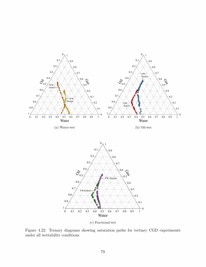
0 0.1 0.2 0.3 0.4 0.5 0.6 0.7 0.8 0.9 1
0
0.1
0.2
0.3
0.4
0.5
0.6
0.7
0.8
0.9
1 0
0.1
0.2
0.3
0.4
0.5
0.6
0.7
0.8
0.9
1
Water
Oil
Gas
← WW,Decane
WW,Soltrol →
(a) Water-wet
0 0.1 0.2 0.3 0.4 0.5 0.6 0.7 0.8 0.9 1
0
0.1
0.2
0.3
0.4
0.5
0.6
0.7
0.8
0.9
1 0
0.1
0.2
0.3
0.4
0.5
0.6
0.7
0.8
0.9
1
WaterO
il
Gas
OW, Decane ↓
OW,Soltrol →
(b) Oil-wet
0 0.1 0.2 0.3 0.4 0.5 0.6 0.7 0.8 0.9 1
0
0.1
0.2
0.3
0.4
0.5
0.6
0.7
0.8
0.9
1 0
0.1
0.2
0.3
0.4
0.5
0.6
0.7
0.8
0.9
1
Water
Oil
Gas
← FW, Decane
FW,Soltrol→
(c) Fractional-wet
Figure 4.22: Ternary diagrams showing saturation paths for tertiary CGD experimentsunder all wettability conditions
79

So ≈ 0.4 because gas could not penetrate even smaller pores or the path of oil mobilization
was blocked by water.
In the non-spreading system (blue curve) water and oil was produced simultaneously in
the beginning of the experiment. This is seen from the gradual decline of both water and oil
saturation during this period. This means that gas entering the sand column simultaneously
invaded both small and large pores filled with oil and water respectively. At some point a
bend was reached where the water saturation settled on a constant value of approximately
0.2 while oil saturation continued to decrease steeply. During this time gas has invaded
most of the larger pores and now displacing oil in the smaller ones. Residual oil saturation
at the end of the experiment was significantly smaller than that of the spreading case. This
is possibly because the wetting film in the non-spreading case has more transport capability
due to having greater conductance than its counterpart in the spreading system. This will
be elaborated further in Section 4.2.
The saturation paths in fractional-wet experiments is shown in Figure 4.22c. For the
Soltrol curve water saturation decreased steeply in the beginning before the curve reached a
bend whereby afterward water saturation remained almost constant. At the same time oil
saturation appeared to be almost constant before the bend and decreased steeply afterward.
This observation can be correlated with analysis of the gas velocity profile and time-lapsed
photos previously (cf. Figures 4.15a and 4.18). Comparison with the saturation path for
the spreading case in oil-wet sand in Figure 4.22b revealed similar pattern. Therefore
the mechanism that operates during oil-wet experiment with Soltrol also applies in the
fractional-wet case. The trend in the Decane curve is also similar to the one in oil-wet
system. One notable difference however is that there appears to be no clear point where
the curve bends and water saturation reached a constant value.
80
4.1.6 Summary of gravity drainage results
We have performed a series of gravity drainage experiments in water-wet, oil-wet and
fractional-wet sand packs. Analysis of the results based on time-lapsed photos and gas-
velocity profiles helps us to understand the internal mechanics of the displacement process.
For gravity drainage in water-wet sand, higher oil recovery is achieved with Soltrol as the
spreading oil. This is attributed to the spreading oil forming film when all three phases
are present.In oil-wet sand, experiments using Decane as non-spreading oil resulted in
higher recovery. The same trend is observed for experiments with fractional-wet sand. In
both cases significant portion of oil in the column is recovered through bulk flow in the
early time and subsequent recovery occurred through wetting film until termination of the
experiments. In the next section we investigate the pore-scale dynamics to understand the
underlying mechanisms, particularly for the cases where our results differed from findings
in the literature.
4.2 Pore-scale mechanisms
To gain better understanding of the displacement mechanism, it is instructive to fo-
cus on the pore-level mechanism. This is because analysis of the core-level experiments
has limitation particularly when explaining the behavior of our oil-wet and fractional-wet
experiments. The pore-level mechanism would involve all three phases because in grav-
ity drainage process the gas phase invades a vertical column saturated with water and
oil. The introduction of a third phase to an existing two-phase system presents additional
problem of determining the fluid distribution and pore occupancy, which altogether affect
the displacement behavior. Although we did not perform experiments at the pore-scale,
we used results from micromodel studies available in the literature to help us understand
the pore-level mechanism.
In a three-phase process, the simultaneous interactions between fluid-fluid and fluid-
rock influence the trapping and mobilization of the oil phase. The spreading behavior de-
81

scribes the fluid-fluid interaction while wettability affect the fluid-rock interaction. There-
fore to enable direct comparison at the pore-level, we used micromodel studies with similar
setup that match the spreading behavior and wettability system of our core-scale experi-
ments.
In the literature, we found such studies from experiments and network model simula-
tions conducted by Øren and Pinczewski (1991),Oren et al. (1992),Oren and Pinczewski
(1994) and Oren (1994). Their work investigate the effect of spreading and wettability on
a three-phase displacement during immiscible gas injection in water-wet and oil-wet sys-
tems. Later work by Øren and Pinczewski (1995) summarized their previous results and
systematically characterized the pore-scale fluid configuration based on interfacial tension,
contact angle and capillary pressure.
In order to relate their pore-level results to our core-level experiments, we will use their
naming convention, whenever necessary for the fluid phases. Hence the non-wetting phase
is fluid-1, the intermediate phase is fluid-2 and the wetting phase is fluid-3.
4.2.1 Pore-scale fluid configuration
In a two-phase system, one phase wets the rock surface while the other phase becomes
the non-wetting phase. Based on capillary pressure requirement, the wetting phase tends
to occupy the smaller pores while the non-wetting phase prefers to reside in larger pores.
In a three-phase system, the fluid arrangement is less straightforward because the non-
wetting, intermediate and wetting phase interact with spreading, wettability and capillary
pressure to determine the pore occupancy. According to Blunt et al. (1994), the wetting
phase (fluid-3) will occupy the smaller pores or the crevices and angularities in the larger
pores. The other two phases (fluid-1 and fluid-2) will compete to occupy the larger pores.
Although both fluids are non-wetting, for the same pore geometry, the fluid that has the
larger capillary pressure difference relative to fluid-3 will occupy the larger pore space.
Øren and Pinczewski (1995) simplify this condition as:
82
σ13 > σ23 (4.2)
where σ refers to the interfacial tension and the subscripts refer to fluid-1-fluid-3 and
fluid-2-fluid-3 pair respectively. The fluid that satisfies the condition in Equation 4.2 is the
most non-wetting phase fluid-1, leaving the other phase as the intermediate phase fluid-2.
For example using the fluid properties in Table 3.1 on page 33 for water-wet spreading
system, fluid-3 is water, fluid-1 (non-wetting phase) is gas and fluid-2 (intermediate phase)
is oil. To satisfy the capillary pressure requirement, the intermediate phase cannot occupy
the larger pore if it already contained the non-wetting phase. From micromodel observation,
Øren and Pinczewski (1995) noted that the intermediate phase tends to occupy the space
between the pore throat and entrance to the pore body.
The intermediate phase in a three-phase system determines the spreading behavior.
When the intermediate phase spreads over the wetting surface, the process is spontaneous
due to decrease in free energy (Adamson and Gast, 1997). This is characterized by the
spreading coefficient S23:
S23 = σ31 − σ32 − σ12 (4.3)
where σ is the interfacial tension and the subscripts refer to fluid 3-fluid 1, fluid 3-fluid
2, and fluid 1-fluid 2 interfaces respectively. In a water-wet system, this becomes
Sow = σwg − σwo − σgo (4.4)
For all cases the intermediate phase can only spread when S23 > 0. Three-phase system
that meets this condition is defined as having Configuration A according to Øren and
Pinczewski (1995). This is shown in Figure 4.23 where fluid-2 the intermediate phase
spreads between fluid-1 and fluid-3 and at the same time envelops fluid-1 completely.
83
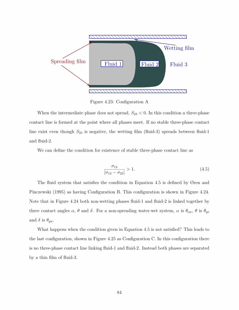
Fluid 3
Wetting film
Fluid 2Fluid 1Spreading film
Figure 4.23: Configuration A
When the intermediate phase does not spread, S23 < 0. In this condition a three-phase
contact line is formed at the point where all phases meet. If no stable three-phase contact
line exist even though S23 is negative, the wetting film (fluid-3) spreads between fluid-1
and fluid-2.
We can define the condition for existence of stable three-phase contact line as
σ13
|σ12 − σ23|> 1. (4.5)
The fluid system that satisfies the condition in Equation 4.5 is defined by Øren and
Pinczewski (1995) as having Configuration B. This configuration is shown in Figure 4.24.
Note that in Figure 4.24 both non-wetting phases fluid-1 and fluid-2 is linked together by
three contact angles α, θ and δ. For a non-spreading water-wet system, α is θow, θ is θgo
and δ is θgw.
What happens when the condition given in Equation 4.5 is not satisfied? This leads to
the last configuration, shown in Figure 4.25 as Configuration C. In this configuration there
is no three-phase contact line linking fluid-1 and fluid-2. Instead both phases are separated
by a thin film of fluid-3.
84

Fluid 3Wetting film
Fluid 2Fluid 1
δαθ
δαθ
Figure 4.24: Configuration B
Fluid 3Wetting film
Fluid 2Fluid 1
Figure 4.25: Configuration C
85

4.2.2 Dynamic three-phase pore-scale fluid displacement
The fluid configurations discussed above were observed to maintain their morphology
during displacement (Øren and Pinczewski, 1995). Although three phases are involved, at
any particular time only one interface is advanced. Pereira et al. (1996) in their network
model simulations explained that based on micromodel experiments, the fundamental dis-
placement occurring in a three-phase system actually consisted of sequences of two-phase
displacement. This means the displacement process can be described using the familiar
two-phase flow such as drainage and imbibition. More description on two-phase displace-
ment process can be found in Lenormand et al. (1983) and Lenormand and Zarcone (1984).
In a drainage process, a non-wetting fluid displaces the wetting fluid in a piston-like fashion
when the interface capillary pressure is greater than the threshold pressure. During imbibi-
tion, the wetting fluid displaces the non-wetting fluid when the interface capillary pressure
is smaller than the threshold pressure. The imbibition process allows the defending fluid to
be displaced either through piston-like invasion or snap-off. When the fluid is intermediate
phase it is non-wetting with respect to the wetting fluid but wetting with respect to the
non-wetting fluid. Thus displacement process involving the intermediate phase (fluid-2)
can be either drainage or imbibition process.
In our experiments the invading fluid is either fluid-1 (non-wetting) or fluid-2 (interme-
diate). When the invading fluid is a non-wetting phase its interface has greater capillary
pressure, therefore it can fill a pore body that contains either wetting or intermediate fluid
and displace them. However when the pore already contained fluid of the same phase, it
will merge with the fluid. For invasion with intermediate fluid it will displace a pore that
contains a wetting fluid. If the pore contains fluid of intermediate phase the fluids will
merge. Its advance will be halted if the pore body is already occupied by a non-wetting
fluid.
For actual displacement to take place, the invading fluid has to arrive at the invasion site
(the pore) while the defending fluid has to move away from the invasion site. The transport
86

of invading or defending fluid occurs through bulk or film flow. The non-wetting fluid flows
to an invasion site through a series of adjoining pore bodies and pore throats filled with
the same phase (bulk flow). The wetting fluid is transported away from the site through a
series of adjoining pore bodies and pore throats filled with the wetting phase (bulk flow)
and linked by wetting film. This makes the wetting fluid to be hydraulically connected
anywhere in the porous media. When the invading fluid is fluid-2 (intermediate phase), the
manner in which it is transported depends on the sign of the spreading coefficient S23. A
positive spreading coefficient indicates a spreading film exists (Figure 4.23) therefore the
fluid flow is similar to that of the wetting fluid, with bulk flow through adjoining pores
and throats linked by spreading film. If the spreading coefficient is negative, there is no
spreading film thus the fluid flow is through bulk flow similar to that of the non-wetting
fluid.
Visualizations from micromodel experiments conducted by Øren and Pinczewski (1991),
Oren and Pinczewski (1994) and Øren and Pinczewski (1995) have identified three displace-
ment mechanisms operating in three-phase system: direct-drainage, double drainage and
imbibition-drainage. These mechanisms are controlled by wettability, capillary pressure
and the spreading behavior of the fluids. Direct drainage mechanism is a two-phase pro-
cess where either fluid-1 (non-wetting) or fluid-2 (intermediate) directly displaces fluid-3
(wetting). Alternate course would be fluid-1 displacing fluid-2. Double drainage mechanism
is a sequence of two drainage events: the non-wetting displacing intermediate fluid followed
by the intermediate fluid displacing the wetting fluid. In imbibition-drainage mechanism,
fluid-2 first displaces fluid-1. This is an imbibition event because fluid-2 is wetting relative
to fluid-1 and the capillary threshold pressure is negative. This is followed by drainage
event where the displaced fluid-1 then displaces fluid-3. In all drainage events the invading
fluid can only advance when the capillary pressure is greater than the defending fluid’s
capillary threshold pressure. Note that all drainage mechanisms result in mobilization of
fluid-3 because the wetting fluid is continuous throughout the system. When fluid-2 is the
87

defending fluid, it can only be mobilized through the double drainage mechanism because
it depends on continuity of fluid-3 for transport.
Mobilization of fluids in Configuration A, B and C occur through the direct drainage
and double drainage mechanism when fluid-1 is the injected fluid. In Configuration B
and C for oil-wet system the injected fluid can be of intermediate phase (fluid-2). Fluids
mobilization in this particular case occur through direct drainage and imbibition-drainage
mechanism.
4.2.3 Discussion of pore-scale mechanisms in experimental re-sults
Based on previous discussion, and using fluid properties in Table 3.1 on page 33 we have
determined the pore-level fluid configurations in our experiments. This is shown in Table 4.2
on the next page. For comparison we also determined the pore-level fluid configuration for
oil-wet case in Vizika and Lombard (1996) using their fluid properties. To facilitate the
comparison, the result from additional oil-wet experiment we performed using the non-
spreading fluid system of Vizika and Lombard (1996) is also shown. In Table 4.2 on the
following page we can see which fluid is non-wetting (fluid-1), intermediate (fluid-2) and
wetting (fluid-3) for each experiment. Note that for fractional-wet experiments the fluid
that become the non-wetting, intermediate and wetting phase could interchange. This
depends on the local spreading behavior and the local wettability of the sand grains. The
table also listed the oil recoveries corresponding to each experiment in the free-fall mode
(FGD).
There are several observations we can make in Table 4.2. For example the only instance
when the intermediate phase (oil) is spreading is when the fluid configuration is A in water-
wet system. This might affect the oil recovery because higher recovery is achieved for
Configuration A than that for Configuration B. The oil recoveries in oil-wet experiments
are similar when using spreading and non-spreading fluid system based on Soltrol, regardless
the fluid configurations. However the oil recovery is significantly higher in oil-wet system
88
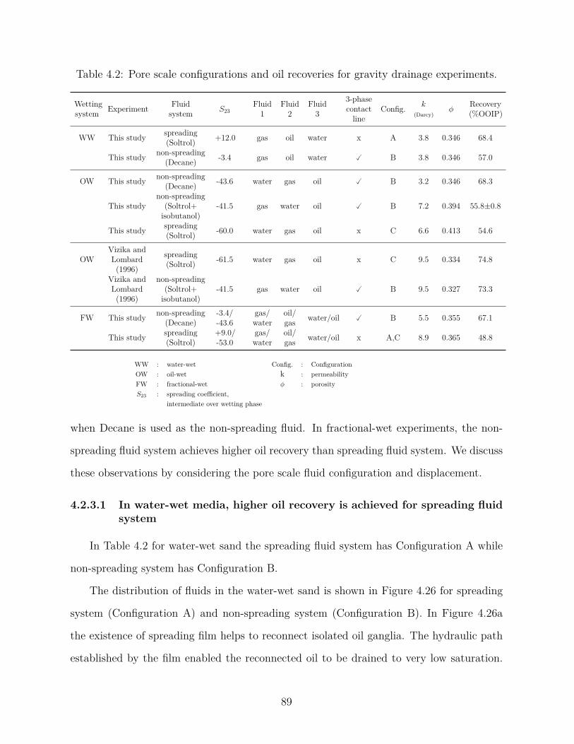
Table 4.2: Pore scale configurations and oil recoveries for gravity drainage experiments.
Wettingsystem Experiment Fluid
system S23Fluid
1Fluid
2Fluid
3
3-phasecontact
lineConfig. k
(Darcy)φ
Recovery(%OOIP)
WW This study spreading(Soltrol) +12.0 gas oil water x A 3.8 0.346 68.4
This study non-spreading(Decane) -3.4 gas oil water � B 3.8 0.346 57.0
OW This study non-spreading(Decane) -43.6 water gas oil � B 3.2 0.346 68.3
This studynon-spreading
(Soltrol+isobutanol)
-41.5 gas water oil � B 7.2 0.394 55.8±0.8
This study spreading(Soltrol) -60.0 water gas oil x C 6.6 0.413 54.6
OWVizika andLombard
(1996)
spreading(Soltrol) -61.5 water gas oil x C 9.5 0.334 74.8
Vizika andLombard
(1996)
non-spreading(Soltrol+
isobutanol)-41.5 gas water oil � B 9.5 0.327 73.3
FW This study non-spreading(Decane)
-3.4/-43.6
gas/water
oil/gas water/oil � B 5.5 0.355 67.1
This study spreading(Soltrol)
+9.0/-53.0
gas/water
oil/gas water/oil x A,C 8.9 0.365 48.8
WW : water-wet Config. : ConfigurationOW : oil-wet k : permeabilityFW : fractional-wet φ : porosityS23 : spreading coefficient,
intermediate over wetting phase
when Decane is used as the non-spreading fluid. In fractional-wet experiments, the non-
spreading fluid system achieves higher oil recovery than spreading fluid system. We discuss
these observations by considering the pore scale fluid configuration and displacement.
4.2.3.1 In water-wet media, higher oil recovery is achieved for spreading fluidsystem
In Table 4.2 for water-wet sand the spreading fluid system has Configuration A while
non-spreading system has Configuration B.
The distribution of fluids in the water-wet sand is shown in Figure 4.26 for spreading
system (Configuration A) and non-spreading system (Configuration B). In Figure 4.26a
the existence of spreading film helps to reconnect isolated oil ganglia. The hydraulic path
established by the film enabled the reconnected oil to be drained to very low saturation.
89
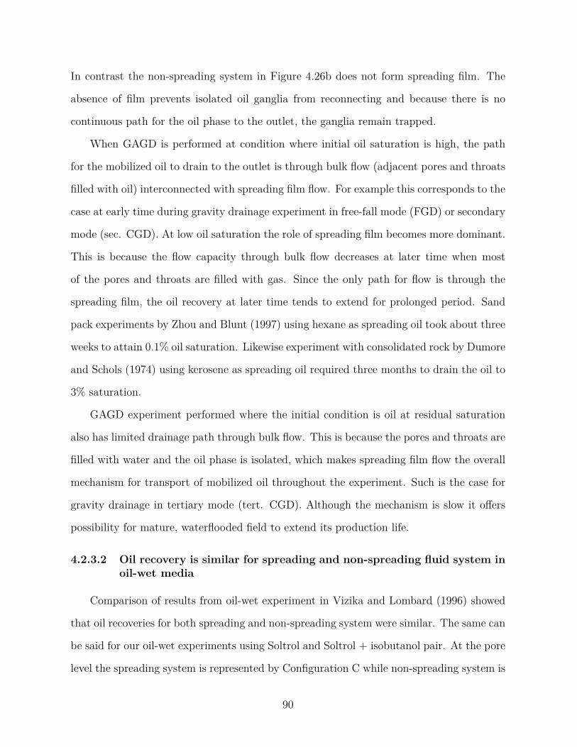
In contrast the non-spreading system in Figure 4.26b does not form spreading film. The
absence of film prevents isolated oil ganglia from reconnecting and because there is no
continuous path for the oil phase to the outlet, the ganglia remain trapped.
When GAGD is performed at condition where initial oil saturation is high, the path
for the mobilized oil to drain to the outlet is through bulk flow (adjacent pores and throats
filled with oil) interconnected with spreading film flow. For example this corresponds to the
case at early time during gravity drainage experiment in free-fall mode (FGD) or secondary
mode (sec. CGD). At low oil saturation the role of spreading film becomes more dominant.
This is because the flow capacity through bulk flow decreases at later time when most
of the pores and throats are filled with gas. Since the only path for flow is through the
spreading film, the oil recovery at later time tends to extend for prolonged period. Sand
pack experiments by Zhou and Blunt (1997) using hexane as spreading oil took about three
weeks to attain 0.1% oil saturation. Likewise experiment with consolidated rock by Dumore
and Schols (1974) using kerosene as spreading oil required three months to drain the oil to
3% saturation.
GAGD experiment performed where the initial condition is oil at residual saturation
also has limited drainage path through bulk flow. This is because the pores and throats are
filled with water and the oil phase is isolated, which makes spreading film flow the overall
mechanism for transport of mobilized oil throughout the experiment. Such is the case for
gravity drainage in tertiary mode (tert. CGD). Although the mechanism is slow it offers
possibility for mature, waterflooded field to extend its production life.
4.2.3.2 Oil recovery is similar for spreading and non-spreading fluid system inoil-wet media
Comparison of results from oil-wet experiment in Vizika and Lombard (1996) showed
that oil recoveries for both spreading and non-spreading system were similar. The same can
be said for our oil-wet experiments using Soltrol and Soltrol + isobutanol pair. At the pore
level the spreading system is represented by Configuration C while non-spreading system is
90
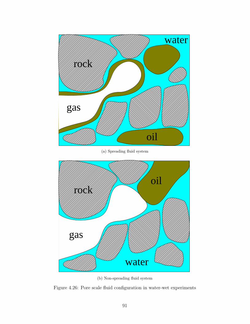
oil
rock
water
gas
(a) Spreading fluid system
rock
water
oil
gas
(b) Non-spreading fluid system
Figure 4.26: Pore scale fluid configuration in water-wet experiments
91
Configuration B. This is shown in Figure 4.27. The significant differences between the two
systems are that water and gas is separated by a thin film of oil in the spreading system;
while in non-spreading system both non-wetting phases are linked by a three-phase contact
line. Oren and Pinczewski (1994) explained that for oil-wet system the fluid configuration
at the pore level has little effect on the eventual oil recovery because oil is always the
continuous phase. This means that oil is drained through both bulk flow (adjacent pores
and throat filled with oil) and wetting film flow.
Given the same pore geometry, gas as the invading phase favors entry into oil-filled
pores since the gas-oil interfacial tension is lower (σgo = 22 mN/m for spreading, 25.5
mN/m for non-spreading) and the capillary threshold is smaller. For oil-wet GAGD at
high initial oil saturation (free-fall and secondary mode) direct drainage of gas-oil interface
is the mechanism that contributes to oil production. When GAGD in oil-wet media is
performed after waterflooding (oil at residual saturation) high water saturation prevents
the displaced oil to be transported through bulk flow because the adjacent pores and
throats are filled with water. In this condition oil is displaced through wetting film either
through double drainage mechanism when gas is the non-wetting phase (Configuration B)
or imbibition-drainage mechanism when gas is the intermediate phase (Configuration C).
4.2.3.3 Oil recovery is higher for low viscosity, non-spreading fluid system inoil-wet media
Studies investigating the effect of spreading and wettability in three-phase flow such as
those from Chatzis et al. (1988), Oren and Pinczewski (1994), Øren and Pinczewski (1995)
and Vizika and Lombard (1996) used the same fluid pairs to model the spreading and non-
spreading fluid system. Both Soltrol and Soltrol + isobutanol pair have similar density and
viscosity. Their experimental designs used such fluid systems in order to highlight the effect
of spreading and wettability; and at the same time minimize variations caused by changing
fluid properties. This helps to provide clear interpretation of the results. Consequently the
92
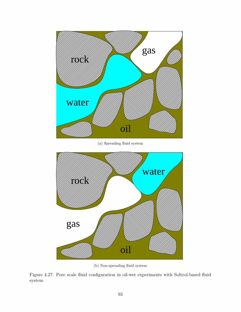
rock
oil
gas
water
(a) Spreading fluid system
rock
oil
water
gas
(b) Non-spreading fluid system
Figure 4.27: Pore scale fluid configuration in oil-wet experiments with Soltrol-based fluidsystem
93

rock
oil
gas
water
Figure 4.28: Pore scale fluid configuration in oil-wet experiments with low viscosity, non-spreading Decane
results from these experiments with oil-wet media share similar conclusion as that discussed
in Section 4.2.3.2 previously.
In this study we used Decane as the non-spreading fluid. The fluid configuration at the
pore scale is shown in Figure 4.28. The configuration is similar to that of Soltrol in oil-wet
(Figure 4.27a) except that both water and gas is attached to a three-phase contact line. As
discussed previously the fluid configuration at the pore scale has little effect on the eventual
oil recovery in oil-wet media. However if we consider the pores and throats as bundles of
capillary tubes and assume that the flow of the wetting phase follows Posseuille’s law, we
can define its conductance as (Blunt, 1997)
g = Ar2
βµL(4.6)
where A is the area occupied by the wetting phase of contact angle θ in a pore of square
cross-section, r is the curvature radius of the fluid interface, β is a dimensionless resistance
94
factor, µ is the wetting phase viscosity and L is length of the element. In Equation 4.6 by
assuming all the terms are the same, oil that has higher viscosity (Soltrol, µ= 2.75 cp) will
have lower conductance than that for Decane (µ= 0.84 cp). The conductance affects the
drainage rate of the wetting phase (Blunt, 1997):
Q = g∆P (4.7)
where Q is the volumetric flow of the wetting phase through pore or throat per unit
time and ∆P is the pressure drop across the element. It is possible that the hydraulic
path established by Decane through the wetting film has higher conductance than that of
Soltrol, and consequently the drainage rate is faster. This eventually leads to higher oil
recovery observed for non-spreading fluid system with Decane in oil-wet media.
4.2.3.4 In fractional-wet media oil recovery for non-spreading fluid system ishigher
For the spreading system, in the water-wet regions oil is the intermediate phase and
it becomes the wetting phase in oil-wet regions. The same applies for the non-spreading
system.
The fluid configuration at the pore scale is shown in Figure 4.29. The spreading system
has combinations of Configuration A and C in Figure 4.29a. The intermediate phase is
spreading in regions of water-wet sand and non-spreading in regions of oil-wet sand. In
non-spreading system Figure 4.29b shows the fluids assume Configuration B. This means
both the non-wetting and intermediate phases in water-wet and oil-wet sand are linked by
three-phase contact line.
Observations from our experiments indicate that recovery at early stage occurred
mostly from bulk flow for both spreading and non-spreading system and wetting/spreading
film at later stage. In non-spreading system the recovery is higher because gas as the non-
wetting phase in water-wet regions prefers invading pores filled with oil since the capillary
95
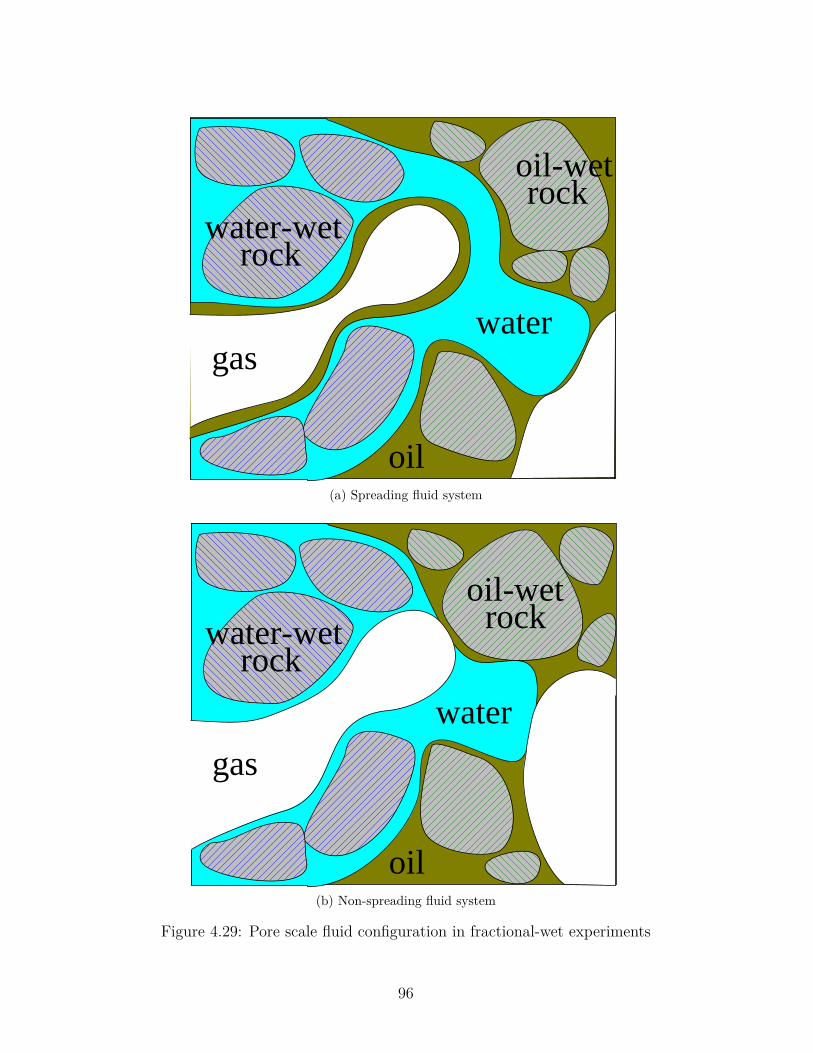
oil
watergas
rock
rockwater-wet
oil-wet
(a) Spreading fluid system
oil
water
gas
rockrock
water-wetoil-wet
(b) Non-spreading fluid system
Figure 4.29: Pore scale fluid configuration in fractional-wet experiments
96

threshold pressure is lower (σgo = 23.5 mN/m). Hence the displacement mechanism is
mostly through the direct drainage method. Although there is no spreading film to recon-
nect the displaced oil, the oil can still be mobilized through the wetting film in the oil-wet
regions. Øren and Pinczewski (1991) shows in their micromodel experiments that the flow
capacity through the wetting film is greater than that for the spreading film for the same
oil phase since the wetting film is thicker. Thicker wetting film and smaller viscosity means
the conductance through the wetting film is higher. This possibly accounts for the faster
drainage rate observed in the non-spreading case.
In the spreading system, gas mobilized the oil through the double drainage mechanism.
This mechanism is efficient if water as the wetting phase is continuous throughout the
porous media. This is because this mechanism depends on the continuity of the water phase
to advance the gas-oil interface. However, since the sand grains were distributed randomly,
there were regions where water was disconnected. Consequently the oil mobilized in the
water-wet regions were trapped, leaving the oil production coming mostly from the oil-wet
regions.
4.3 Analysis of results with dimensionless groups
Dimensionless groups have been used by previous investigators to study the interplay
of mechanisms operating in gravity drainage recovery. Grattoni et al. (2001) have identified
capillary, viscous and gravity forces to be important in characterizing oil recovery under
gravity drainage process. Ratios of these forces are used to define dimensionless parameters
such as capillary and Bond numbers. Capillary number measures the relative strength of
viscous over capillary forces and Bond number determines the relative strength of gravity
over capillary. In their work they used capillary and Bond numbers to correlate the oil
production in their gravity drainage experiments. Kulkarni et al. (2005) and Kulkarni and
Rao (2006b) used gravity number (ratio of gravity over viscous) in addition to the other two
to characterize field-scale gravity drainage projects. Their aim was to scale the mechanisms
97

operating at field-scale for gravity drainage experiments in laboratory. In this regard they
attempted to reduce the unknown parameters that might affect oil recovery in larger scale
down to a few parameters they could replicate in a laboratory setting. Subsequent work
by Sharma and Rao (2008) and Mahmoud and Rao (2008) as well as Rostami et al. (2010)
and Sadati and Kharrat (2013) further demonstrate the application of these numbers.
The dimensionless numbers used in the studies mentioned were derived assuming two-
phase flow condition in water-wet media. Furthermore they were used to correlate with oil
recovery at the end of the experiment. This means the entire dynamics of the displacement
process is represented by a single number. It would lead to more insight if we could track
the changes in the dimensionless numbers over the course of the experiment. In light of
our understanding of pore and core scale mechanisms, the dimensionless numbers used to
characterize gravity drainage process should incorporate three-phase flow mechanisms in
porous media of varying wettability states. In this study we use dimensionless numbers
developed by Grattoni et al. (2001) that address these issues. The capillary and Bond
numbers used in Grattoni et al. (2001) are dynamic parameters, meaning they change
values as function of time. This allows us to see the interplay of forces affecting gravity
drainage recovery as the experiments progress. In their work Grattoni et al. (2001) used
their dimensionless numbers to characterize gravity drainage in water-wet and oil-wet sand.
We extend their results by including our dataset for water-wet, oil-wet, and fractional-wet
experiments with spreading and non-spreading fluid.
4.3.1 Effect of Bond Number, NB
Bond number is defined by Grattoni et al. (2001) as
NB = ∆ρgZRa
2σ (4.8)
where ∆ρ is the gas-oil density difference, g is the gravity acceleration constant, Z is
the average position of the gas interface, Ra is the average pore throat radius and σ is
98
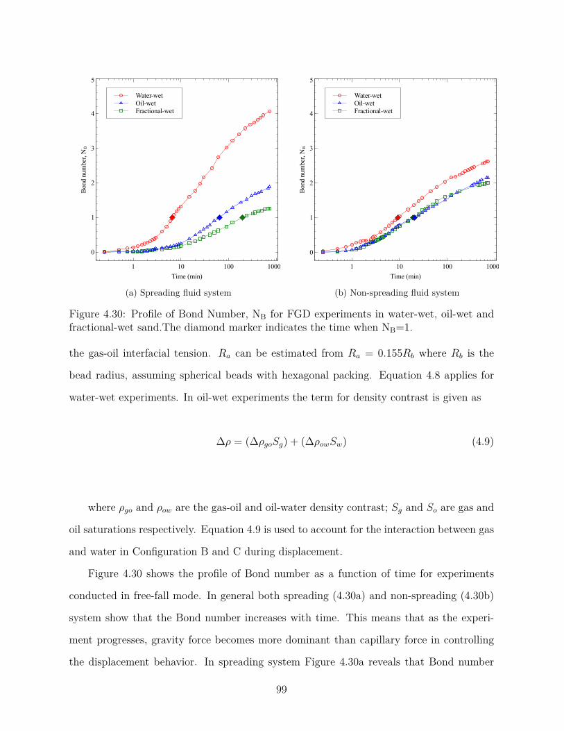
Water-wetOil-wetFractional-wet
Bon
d nu
mbe
r, N
B
0
1
2
3
4
5
Time (min)1 10 100 1000
(a) Spreading fluid system
Water-wetOil-wetFractional-wet
Bon
d nu
mbe
r, N
B
0
1
2
3
4
5
Time (min)1 10 100 1000
(b) Non-spreading fluid system
Figure 4.30: Profile of Bond Number, NB for FGD experiments in water-wet, oil-wet andfractional-wet sand.The diamond marker indicates the time when NB=1.
the gas-oil interfacial tension. Ra can be estimated from Ra = 0.155Rb where Rb is the
bead radius, assuming spherical beads with hexagonal packing. Equation 4.8 applies for
water-wet experiments. In oil-wet experiments the term for density contrast is given as
∆ρ = (∆ρgoSg) + (∆ρowSw) (4.9)
where ρgo and ρow are the gas-oil and oil-water density contrast; Sg and So are gas and
oil saturations respectively. Equation 4.9 is used to account for the interaction between gas
and water in Configuration B and C during displacement.
Figure 4.30 shows the profile of Bond number as a function of time for experiments
conducted in free-fall mode. In general both spreading (4.30a) and non-spreading (4.30b)
system show that the Bond number increases with time. This means that as the experi-
ment progresses, gravity force becomes more dominant than capillary force in controlling
the displacement behavior. In spreading system Figure 4.30a reveals that Bond number
99
increased almost fourfold since the beginning of the experiment with water-wet sand. In
the same period Bond number increased less than twofold for experiments in oil-wet and
fractional-wet sand. This indicates that gravity-dominated flow becomes more significant
over the course of the experiment. Likewise in the non-spreading system Bond number also
grows with time, although the maximum value attained was less than four.
It is instructive to determine the exact time the displacement process transitions from
capillary-dominated flow to gravity-dominated flow. This transition happens when NB = 1,
which by definition means that gravity force is balanced by capillary force.
In Figure 4.30a and 4.30b this is marked by a diamond marker. Our calculation shows
that for spreading system, it took about seven minutes for the transition to occur in water-
wet sand. In oil-wet and fractional-wet sand the time became progressively longer, at 65
minutes and 195 minutes respectively. In non-spreading system our calculation shows that
the transition occurred after nine minutes in water-wet sand, and 19 minutes and 21 minutes
for fractional-wet and oil-wet sand respectively. This shows that gravity-dominated flow
occurred earlier for spreading system in water-wet sand and was delayed significantly as
the wettability became less water-wet.
The effect of Bond number in oil recovery for gravity drainage experiments is shown in
Figure 4.31. In Figure 4.31a for the water-wet case the oil recovery increases linearly with
Bond number. Similar trend is seen for water-wet experiment with non-spreading fluid in
Figure 4.31b. This shows that oil recovery in gravity drainage experiment in water-wet
sand is strongly influenced by gravity forces. In spreading system, gravity forces increases
almost fourfold with respect to capillary forces. For non-spreading system in water-wet
sand the increase is slightly over twofold.
The reason the final value for NB is less in water-wet sand with non-spreading fluid
system than its spreading counterpart is because of the term Z, the average position of gas
interface in Equation 4.8. In spreading system during gas invasion, gas-oil and oil-water
100

Water-wetOil-wetFractional-wet
Oil
reco
very
(%O
OIP
)
0
10
20
30
40
50
60
70
Bond number, NB
0 1 2 3 4
(a) Spreading fluid system
Water-wetOil-wetFractional-wet
Oil
reco
very
(%O
OIP
)
0
10
20
30
40
50
60
70
Bond number, NB
0 0.5 1 1.5 2 2.5
(b) Non-spreading fluid system
Figure 4.31: Effect of Bond Number, NB on oil recovery for FGD experiments in water-wet,oil-wet and fractional-wet sand.The diamond marker indicates the oil recovery when NB=1.
interfaces are formed and the advancement of these interfaces mobilize the oil phase. Since
water is the continuous phase, propagation of the interfaces help to transport the oil phase
all the way to the outlet. Therefore Z is increasing as the gas-oil and oil-water interfaces
are advancing.
In non-spreading system since the oil phase does not spread, the invading gas contacts
the water phase directly since there is no oil film separating them. This creates either
gas-water, gas-oil or oil-water interfaces in the pores. The transport of the oil phase is
retarded because the advancement of the interfaces do not directly lead to oil mobilization
and eventual transport to the outlet. Although Z is increasing oil production is slowing.
As NB > 1, the proportion of oil recovery contributed by gravity forces becomes greater.
For example in Figure 4.31a oil recovered during capillary-dominated flow (NB < 1)
in water-wet sand is 16.9% OOIP. The remaining oil recovery (51.5%) occurred during
gravity-dominated flow. As the sand pack becomes less water-wet, the contribution of
gravity-dominated flow toward oil recovery is reduced. In Figure 4.31a the oil recovered
101

during capillary-dominated flow is 39.3% and 43.1% OOIP for oil-wet and fractional-wet
sand respectively. For the same set of experiments the remaining 15.3% and 5.7% OOIP
were recovered during gravity-dominated flow. In non-spreading system the oil recovered
during capillary-dominated flow is 21.8%, 45.6% and 46.3% OOIP for experiments con-
ducted in water-wet, oil-wet and fractional-wet sand respectively. From our calculations
in both Figures 4.31a and 4.31b we can infer that in water-wet sand, the proportion of
oil-recovery that is recovered during gravity-dominated flow is greater than those in oil-wet
and fractional-wet sand. In oil-wet and fractional-wet sand significant portion of the oil is
recovered during capillary-dominated flow.
Figures 4.31a and 4.31b also show that oil recovery has non-linear relationship with
Bond number in experiments with oil-wet and fractional-wet sand. The non-linear behavior
is caused by the term ∆ρ used in Equation 4.9 to obtain NB in Equation 4.8. In oil-wet
and fractional-wet sand the gas and water phase occupy the larger pores since they are
non-wetting with respect to oil. During gas invasion all three phases are mobile. The
mobilization and transport of the oil phase is accounted for by the term Z. For water,
although it is at residual saturation, the water phase is redistributed along the column.
Eventually water is accumulated at the bottom, albeit no production is reported. The
tendency for the water phase to accumulate at the bottom of the column, during gravity
drainage at residual water saturation in oil-wet and fractional-wet sand packs has been
confirmed through CT study by Vizika and Lombard (1996). The ∆ρ term used in Equation
4.9 considers this fact by accounting the interaction between water and gas phase along
the column, and their movement toward the bottom controlled by buoyancy effect.
In Figure 4.31 the end-point NB value in spreading system is less than that for non-
spreading system in oil-wet and fractional-wet sand. This is because after accounting
for the gas and water interactions in the ∆ρ term, the end-point NB value is ultimately
determined by the movement of the gas front given by the Z term. As discussed in Section
4.2.3.3 for the same gas front advancement that directly leads to oil mobilization, the one
102
in non-spreading system transports more oil to the outlet. This is because the wetting
film that provides the continuous path for oil mobilization in the non-spreading system has
greater conductance. Thus for the same pressure gradient the volumetric flow through this
path is greater in the non-spreading system. In the fractional-wet system our analysis of
time-lapsed photos and gas velocity profiles revealed that significant portion of the oil was
produced through bulk flow early on in the experiment. Our results also indicate that the
bulk oil drainage in the non-spreading case occurred earlier than that for the spreading
case. This is because the gas velocity was higher in the non-spreading case, which means
the gas front was able to penetrate more smaller pores to displace the oil therein. The
cumulative effect is that the increase in the Z term is associated with more oil recovery for
the non-spreading case.
4.3.2 Effect of Capillary Number, NC
Capillary number from Grattoni et al. (2001) is defined as
NC = 2vgµgPcRa
(4.10)
where vg and µg is the gas velocity and viscosity respectively, Pc is capillary pressure
defined as Pc = 2σgo
r, and Ra is the average pore throat radius.
In Figure 4.32 Capillary Number, NC is shown to decrease with time as the experiments
progress. The same behavior is observed for spreading (4.32a) and non-spreading (4.32b)
fluid systems. NC is decreasing over time because during the experiment the gas front
travels with varying velocity. The velocity of the gas front is controlled by interactions
between capillary, viscous and gravity forces. From our plot of gas velocity profile in each
experiment the gas velocity is seen to decrease with time. This indicates that over time
the influence of viscous forces is counter-balanced by greater capillary forces.
Based on our calculations we put a diamond marker on each curve in Figures 4.32a
and 4.32b to indicate the time and the corresponding NC when NB = 1. This marks
103

Water-wetOil-wetFractional-wet
Cap
illar
y nu
mbe
r, N
C
10−10
10−9
10−8
10−7
10−6
10−5
Time (min)0.1 1 10 100 1000
(a) Spreading fluid system
Water-wetOil-wetFractional-wet
Cap
illar
y nu
mbe
r, N
C
10−10
10−9
10−8
10−7
10−6
10−5
Time (min)0.1 1 10 100 1000
(b) Non-spreading fluid system
Figure 4.32: Profile of Capillary Number NC for FGD experiments in water-wet, oil-wetand fractional-wet sand.The diamond marker indicates NC when NB=1.
the time when viscous and capillary-dominated flow transition to gravity-dominated flow.
As discussed in the previous section for the spreading system the transition occurs earlier
in the water-wet sand and much later in the oil-wet and fractional-wet sand. In non-
spreading system the transition also occurs earlier in water-wet sand but the timespan for
the transition happening in oil-wet and fractional-wet sand is very close.
104

Water-wetOil-wetFractional-wet
Oil
reco
very
(% O
OIP
)
0
20
40
60
80
100
Capillary number, NC
10−10 10−9 10−8 10−7 10−6 10−5
(a) Spreading fluid system
Water-wetOil-wetFractional-wet
Oil
reco
very
(% O
OIP
)
0
20
40
60
80
100
Capillary number, NC
10−10 10−9 10−8 10−7 10−6 10−5
(b) Non-spreading fluid system
Figure 4.33: Effect of Capillary Number, NC on oil recovery for FGD experiments in water-wet, oil-wet and fractional-wet sand. The diamond marker indicates the oil recovery whenNB=1.
In Figure 4.33 we plot the oil recovery as a function of NC . We note that as the oil
recovery increases NC shows the opposite behavior. In both spreading and non-spreading
system, experiments in water-wet, oil-wet and fractional-wet sand demonstrate that NC
decreases to a very small value as more oil is produced. In spreading system (4.33a) the
changes in NC is minimal given the steep gradient before NB = 1, as indicated by the
diamond marker. After NB > 1, the gradient increases, meaning greater changes in NC
in the negative direction leads to corresponding changes in the positive direction for the
oil recovery. This is because during this period gravity forces exert more influence on the
overall displacement than capillary forces. The same trend is shown for non-spreading
system in water-wet sand.
For the spreading system in the oil-wet and fractional-wet experiments (4.33a) when
NB < 1, the gradient is larger initially in the negative direction. As NB > 1, the gradient
is reduced in the negative direction. This means that when the flow is gravity-dominated
for these experiments, a large decrease in NC resulted in minimal increase in oil recovery.
105
In the non-spreading system for oil-wet and fractional-wet experiments (4.33b) we
observe a steep gradient initially for both experiments. This indicates that viscous forces
are active during this period since only a small reduction in NC leads to significant jump in
oil production. This observation is supported by our analysis with time-lapsed photos and
gas velocity profiles for these experiments before. Later gas velocity slowed down which
corresponds to greater reduction in NC but oil production continued to increase because
during this period most of the oil is still drained through bulk flow. When NB = 1, 45.6%
OOIP and 46.3% OOIP has been produced from the oil-wet and fractional-wet sand. After
NB > 1, the gradient continues its ascent in the negative direction. Although the flow is
gravity-dominated at this stage only about 20% OOIP additional oil was produced in either
experiments. Note that in the non-spreading system the curves for oil-wet and fractional-
wet sand are consistently higher than that of water-wet sand, indicating that viscous forces
are generally greater in these experiments.
4.3.3 Effect of Gravity Number, NG
Gravity number, NG is a measure of the relative strength of gravity to viscous force.
According to Hagoort (1980) and Chatzis and Ayatollahi (1993) NG is defined as
NG = gK∆ρogµoVpg
(4.11)
where g is the gravity acceleration, K is the absolute permeability, ∆ρog is the oil-
gas density difference, µo is the oil viscosity and Vpg is the pore velocity of the gas-liquid
interface. For oil-wet and fractional-wet experiments ∆ρog is calculated using Equation 4.9
on page 99 to account for the fact that gas and water are the non-wetting phases, thus they
tend to occupy larger pores and move downward under gravity. Although in the original
paper Chatzis and Ayatollahi (1993) measured Vpg in their experiments, they also suggested
that this parameter can be calculated using production data, porosity of the sand pack and
106

Water-wetOil-wetFractional-wet
Gra
vity
num
ber,
NG
0.01
0.1
1
10
100
Time (min)1 10 100 1000
(a) Spreading fluid system
Water-wetOil-wetFractional-wet
Gra
vity
num
ber,
NG
0.01
0.1
1
10
100
Time (min)1 10 100 1000
(b) Non-spreading system
Figure 4.34: Profile of Gravity Number, NG, for FGD experiments in water-wet, oil-wetand fractional-wet sand.The star marker indicates the time when NG=1.
connate water saturation. In this study the gas velocity we calculated using the method
presented in Grattoni et al. (2001) is used as Vpg.
Based on their previous study using square capillary tubes, Chatzis and Ayatollahi
(1993) explained that the velocity of the oil film in the corners of the square during gas
invasion is proportional to the permeability of the tube and also proportional to ∆ρog
µo. In
their study they defined the term K∆ρog
µoto represent the action of gravity forces influencing
the downward direction of average oil velocity by film flow as gas is invading the top of the
column. In the denumerator the term Vpg represents the action of viscous pressure gradient
influencing the pore velocity of the oil bank at the gas-oil contact.
Figure 4.34 shows that NG increases with time. This trend is observed for both spread-
ing (4.34a) and non-spreading (4.34b) fluid systems in water-wet, oil-wet and fractional-wet
sand packs. In the plot the time when NG = 1 indicated by the star marker marks the point
when the flow shifts from viscous-dominated to gravity-dominated flow. In the spreading
system (4.34a) this transition occurred almost at the same time beginning with fractional-
wet sand at 43 minutes, oil-wet sand at 47 minutes and water-wet sand at 55 minutes. It is
107

Water-wetOil-wetFractional-wet
Oil
reco
very
(%O
OIP
)
0
10
20
30
40
50
60
70
Gravity number, NG
0.01 0.1 1 10 100
(a) Spreading fluid system
Water-wetOil-wetFractional-wet
Oil
reco
very
(%O
OIP
)
0
10
20
30
40
50
60
70
Gravity number, NG
0.01 0.1 1 10 100
(b) Non-spreading fluid system
Figure 4.35: Effect of Gravity Number, NG on oil recovery for FGD experiments in water-wet, oil-wet and fractional-wet sand.The star marker indicates the oil recovery when NG=1.
notable that in spreading fluid system, beyond the point where gravity is dominating the
flow, the curves for each experiment almost collapse into a single curve.
In non-spreading system (4.34b) the same pattern of increasing NG with time is ob-
served. The transition to gravity-dominated flow occurred earlier in fractional-wet sand,
followed by water-wet sand and finally oil-wet sand at ten, 15, and 29 minutes respectively.
In contrast to the spreading fluid system, the curves did not collapse into one curve after
the transition to gravity-dominated flow.
The effect of NG on oil recovery is shown in Figure 4.35. In general oil recovery is
increasing as a logarithmic function of NG. Both spreading (4.35a) and non-spreading
(4.35b) fluid systems show the same trend. The one notable difference is the relative
position of the curves. In spreading fluid system the water-wet curve was below the oil-wet
and fractional-wet curves initially. However when NG > 1, the oil recovery for the water-
wet curve increased to surpass both oil-wet and fractional-wet curves and maintained its
leading position until the end of the experiment. This is because after NG = 1, the gravity
forces grew stronger relative to viscous forces in water-wet sand. More oil was drained
108

through spreading film under the influence of gravity forces after this transition. Figure
4.35a clearly demonstrates the effectiveness of spreading film flow in recovering additional
oil in water-wet sand.
Figure 4.35b shows the opposite trend. In the plot instead of water-wet curve, the
oil-wet and fractional-wet curves were leading. Before and after NG = 1, both oil-wet and
fractional-wet curves consistently exceeded the water-wet curve. This is because gravity
forces were stronger in this sand relative to viscous forces since the start of the experiment.
Since the oil phase (Decane) has lower viscosity the drainage rate through the wetting film
is greater because lower viscosity leads to higher conductance. As a result combination of
stronger gravity forces and faster drainage rate helped to drain more oil downward through
the wetting film.
4.3.4 Effect of dimensionless numbers in tertiary GAGD
Dimensionless numbers analysis discussed so far concerned mainly on gravity drainage
experimental results performed at residual water saturation (FGD and secondary CGD).
Since both FGD and secondary CGD experiments exhibited similar trends we chose to
present in the previous sections analysis of FGD experiments only. In this section we
performed the same analysis on tertiary CGD experiments. We would like to see whether
the same observations hold for gravity drainage at residual oil saturation. The results are
shown in Figure 4.36.
In Figure 4.36 the dimensionless numbers are plotted with total liquid production as
the dependent variable (y-axis). This is because during gas invasion, both oil and water
are produced. At the top of the figure liquid production exhibits linear trend with NB
for water-wet sand in both spreading and non-spreading fluid systems. In oil-wet and
fractional-wet sand the trend with NB is nonlinear. Comparing with Figure 4.31 we see
similar trends.
109

The center of Figure 4.36 shows the liquid production as a function of NC . Similar
to Figure 4.33 the water-wet curve in spreading fluid system surpassed both oil-wet and
fractional-wet curves. In non-spreading fluid system the oil-wet and fractional-wet curves
were leading instead. In both plots as liquid production increases, Nc decreases spanning
three to four orders of magnitude.
The effect of NG on liquid production is shown at the bottom of Figure 4.36. The trends
observed for spreading and non-spreading fluid systems are similar to that in Figure 4.35.
In spreading fluid system the water-wet curve was leading ahead of oil-wet and fractional-
wet curves. The trend is reversed in the non-spreading fluid system. Both plots show the
liquid production increases as NG increases over the span of more than three orders of
magnitude.
Since the trends shown for liquid production when plotted against NB, NC , and NG are
similar to that observed in experiments at residual water saturation, the same discussions
pertaining these experiments also apply to experiments at residual oil saturation.
4.3.5 Flow regime characterization based on dimensionless num-bers
Earlier when discussing experimental results for fractional-wet experiments we pre-
sented the flow regime map in Figure 4.19. The shaded area delineating region where
capillary, viscous and gravity force is dominant was placed arbitrarily to illustrate the
interplay of forces influencing oil production in gravity drainage process.
Now with insights gained from analysis of dimensionless numbers we are able to refine
the flow regime map by locating exactly the time when the transition between the forces
occur. This has the benefit of clearly attributing which force is dominating the flow during
the course of the experiment. In addition pinpointing the exact time for the transition
enable us to correlate the amount of oil produced in each flow regime.
110
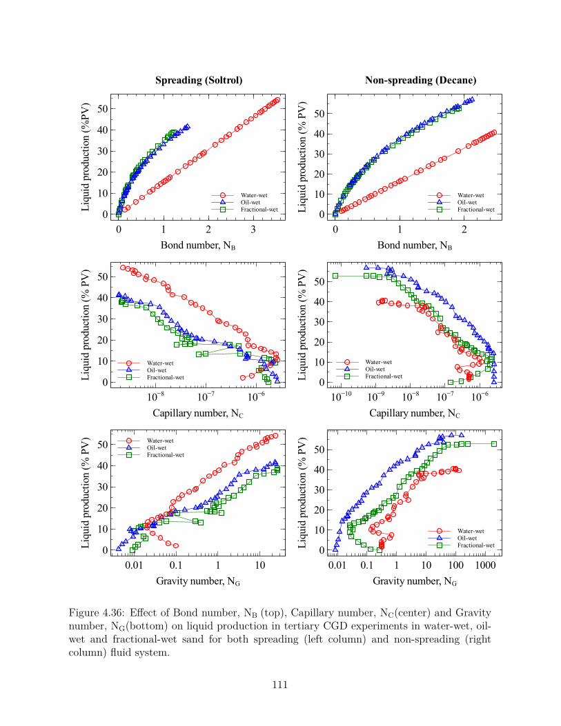
Non-spreading (Decane)Spreading (Soltrol)
Water-wetOil-wetFractional-wetLi
quid
pro
duct
ion
(%PV
)
0
10
20
30
40
50
Bond number, NB
0 1 2 3
Water-wetOil-wetFractional-wetLi
quid
pro
duct
ion
(% P
V)
0
10
20
30
40
50
Bond number, NB
0 1 2
Water-wetOil-wetFractional-wetLi
quid
pro
duct
ion
(% P
V)
0
10
20
30
40
50
Capillary number, NC
10−8 10−7 10−6
Water-wetOil-wetFractional-wetLi
quid
pro
duct
ion
(% P
V)
0
10
20
30
40
50
Capillary number, NC
10−10 10−9 10−8 10−7 10−6
Water-wetOil-wetFractional-wet
Liqu
id p
rodu
ctio
n (%
PV
)
0
10
20
30
40
50
Gravity number, NG
0.01 0.1 1 10
Water-wetOil-wetFractional-wetLi
quid
pro
duct
ion
(% P
V)
0
10
20
30
40
50
Gravity number, NG
0.01 0.1 1 10 100 1000
Figure 4.36: Effect of Bond number, NB (top), Capillary number, NC(center) and Gravitynumber, NG(bottom) on liquid production in tertiary CGD experiments in water-wet, oil-wet and fractional-wet sand for both spreading (left column) and non-spreading (rightcolumn) fluid system.
111

The revised flow regime map is shown in Figure 4.37 for FGD experiments in water-
wet, oil-wet and fractional-wet sand. We chose to show the flow regime map for only FGD
experiments for the sake of brevity. It is expected that the flow regime map for experiments
at residual oil saturation (tertiary CGD) would be similar since the forces interacting during
the experiments exhibited similar trends (refer to Figure 4.36). However the width of each
region might be different depending on interactions between the forces.
We plotted the gas velocity as the ordinate to track the movement of gas-oil interface
with time. The time when NB = 1 indicates the transition from capillary-dominated to
gravity-dominated flow. When NG = 1, this marks the transition from viscous-dominated
to gravity-dominated flow. The set of times when the transition occurred was determined
by interpolation of curves plotted previously in Figure 4.30 and Figure 4.34. The shaded
area in each plot denotes the region where capillary (green), viscous (pink) or gravity force
(cyan) is dominating. The transition time calculated earlier was also used to mark the
extent of each flow region. For example when the time for NG = 1 is greater than the time
for NB = 1 (tNG=1 > tNB=1) an overlap of dominating forces is possible. This means that
at tNB<1 both capillary and viscous forces are dominating the flow. Between tNB=1 and
tNG=1 both viscous forces and gravity forces are dominant and when tNG>1 only gravity
forces are controlling the flow. Overlap of dominating forces also happens when tNG=1
occurs earlier than tNB=1.
In water-wet experiments (top of Figure 4.37) the flow was dominated by capillary and
viscous forces initially before the transition to viscous and gravity-dominated flow. This
is followed by gravity-dominated flow which continued until the end of the experiment.
In spreading system the time span for the viscous-dominated flow was wider than that
in non-spreading system. In contrast the onset of gravity-dominated flow was earlier in
non-spreading system. At the beginning of the experiment when the flow was capillary
and viscous-dominated, gas was invading the larger pores to displace the oil within. The
oil was retained by capillary force and viscous force set the pressure gradient required for
112
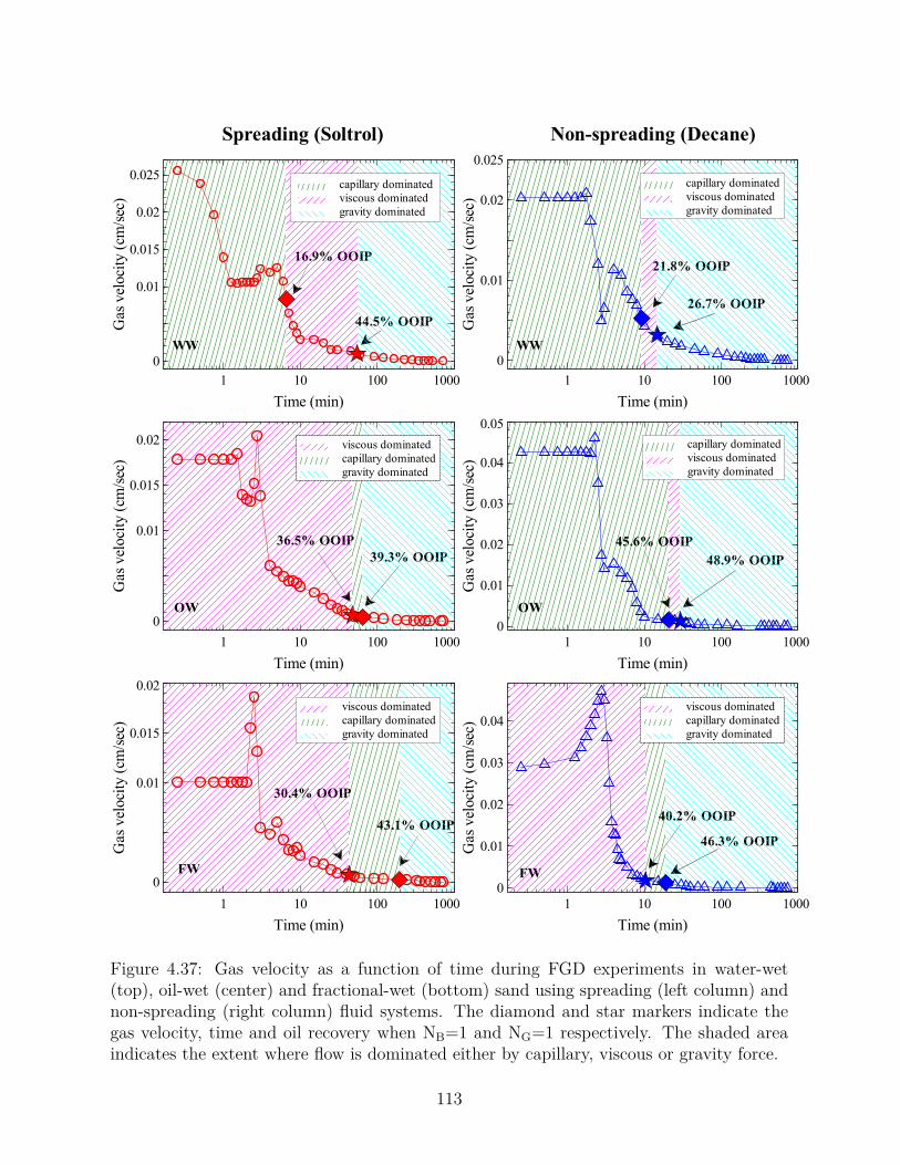
Non-spreading (Decane)Spreading (Soltrol)
44.5% OOIP
16.9% OOIP
WW
capillary dominatedviscous dominatedgravity dominated
Gas
vel
ocity
(cm
/sec
)
0
0.01
0.015
0.02
0.025
Time (min)1 10 100 1000
26.7% OOIP
21.8% OOIP
WW
capillary dominatedviscous dominatedgravity dominated
Gas
vel
ocity
(cm
/sec
)
0
0.01
0.02
0.025
Time (min)1 10 100 1000
36.5% OOIP39.3% OOIP
OW
viscous dominatedcapillary dominatedgravity dominated
Gas
vel
ocity
(cm
/sec
)
0
0.01
0.015
0.02
Time (min)1 10 100 1000
48.9% OOIP45.6% OOIP
OW
capillary dominatedviscous dominatedgravity dominated
Gas
vel
ocity
(cm
/sec
)
0
0.01
0.02
0.03
0.04
0.05
Time (min)1 10 100 1000
43.1% OOIP
30.4% OOIP
FW
viscous dominatedcapillary dominatedgravity dominated
Gas
vel
ocity
(cm
/sec
)
0
0.01
0.015
0.02
Time (min)1 10 100 1000
46.3% OOIP
40.2% OOIP
FW
viscous dominatedcapillary dominatedgravity dominated
Gas
vel
ocity
(cm
/sec
)
0
0.01
0.02
0.03
0.04
Time (min)1 10 100 1000
Figure 4.37: Gas velocity as a function of time during FGD experiments in water-wet(top), oil-wet (center) and fractional-wet (bottom) sand using spreading (left column) andnon-spreading (right column) fluid systems. The diamond and star markers indicate thegas velocity, time and oil recovery when NB=1 and NG=1 respectively. The shaded areaindicates the extent where flow is dominated either by capillary, viscous or gravity force.
113

gas to penetrate the pore and access the oil. The pressure gradient required to overcome
pore capillary threshold depends on the interfacial tensions, wettability and pore geometry,
with larger pore size having smaller capillary threshold; thus making it more amenable
to gas invasion. In the viscous and gravity-dominated flow some oil was bypassed by
the invading gas initially. In this region the bypassed oil which existed as isolated blobs
started coalescing to form bigger blobs. In spreading system the span where viscous force is
dominating was wider and started earlier to account for the effect of film flow reconnecting
the stranded oil and providing continuous hydraulic path. This can be correlated with the
time-lapsed photos during this period (see Figure 4.2a). In the gravity-dominated region
the remaining oil was displaced either through the hydraulic path established earlier for
spreading system or through interconnecting oil layer formed between the pore crevices
and wedges for non-spreading system. The rate of oil drainage in this region is controlled
by gas-oil density difference and the oil viscosity.
In oil-wet experiments (center of Figure 4.37) overlap of dominating forces is seen at
the beginning of both spreading and non-spreading system. In spreading system viscous
and capillary forces dominated the flow and accounted for 36.5% OOIP recovered. Between
tNG=1 and tNB=1 both viscous and gravity forces were dominant while at tNB>1 only gravity
forces were dominant. In non-spreading system combination of capillary and viscous forces
in the first stage accounted for 45.6% OOIP recovery. Higher recovery was attained in the
first stage for the non-spreading system because the viscous pressure gradient was higher,
which is evident from the higher initial gas velocity in the plot. In the spreading system
lower initial gas velocity limited the viscous pressure gradient available to drain the oil.
During gravity-dominated flow regime, residual oil in both systems was drained through
the wetting layer. Since the density difference of the oil phase is about the same in the
spreading and non-spreading system, the drainage rate is controlled by oil viscosity. More
oil can be transported through the wetting layer in non-spreading system since it has greater
conductance (refer to Equation 4.6 on page 94).
114
Flow regime maps for fractional-wet experiments are shown at the bottom of Figure
4.37. The difference with Figure 4.19 is that we did not know then the extent of capillary
or viscous forces controlling the flow during the early part of the experiments. With
analysis of dimensionless numbers this can be located easily. In spreading system the
flow was dominated by both viscous and capillary forces until tNB=1 at 43 minutes after
the experiment began. Between 43 < t < 195 minutes both capillary and viscous forces
controlled the flow. At the onset of gravity-dominated flow (t = 195 minutes) about
43.1% OOIP has been recovered. In non-spreading system similar arrangement of flow
regimes is observed. However the extent of viscous and capillary-dominated region was
shorter and gravity-dominated region was longer but the amount of oil recovered at the
beginning of gravity-dominated region was greater (46.3% OOIP). This observation ties in
with visualizations of time-lapsed photos (cf. Figures 4.13a and 4.13b). Since gas velocity
was higher in non-spreading system the viscous pressure gradient was greater. This helped
to penetrate more pores and drained more oil than that in spreading system during the
same period.
4.3.6 Summary of dimensionless groups analysis
In this section we analyzed the results of gravity drainage experiments using dimension-
less groups to evaluate the effect of capillary, gravity and viscous forces on oil production.
The forces are combined in dimensionless numbers to consolidate the parameters affecting
the gravity drainage process. The dimensionless numbers are Bond number, NB, Capillary
number, NC , and Gravity number, NG.
It is shown that NB increases with time for all experiments in spreading and non-
spreading fluid systems. The increasing trend indicates that gravity forces grow stronger
over capillary forces as the experiment progresses. The transition from capillary-dominated
flow to gravity-dominated flow occurs when NB = 1. In water-wet sand for spreading fluid
system the transition occurs earlier while for oil-wet and fractional-wet sand the transition
115
takes longer time. In non-spreading system the transition time is located very close to each
other for each experiment. Oil recovery is also shown to increase as a function of NB. In
water-wet sand for both spreading and non-spreading systems this relationship is linear. A
nonlinear relationship is observed for oil-wet and fractional-wet sand in both fluid systems.
A linear relationship is shown for water-wet sand because the oil production is strongly
controlled by the average position of the gas interface. In oil-wet and fractional-wet sands
the effect of NB on oil recovery is nonlinear because the NB in these sands is also a function
of gas and water saturations. Since both phases are non-wetting relative to oil, they reside
in the larger pores, thus have tendency to move. Their movement could advance or impede
oil production, hence the nonlinear relationship with oil recovery.
Capillary number, NC is shown to decrease with time for all experiments in both
spreading and non-spreading fluid systems. In water-wet sand the decline starts at the
onset when NB = 1. In oil-wet and fractional-wet sand the decline is observed to occur
earlier before NB = 1. As oil recovery increases NC decreases. For water-wet sand the
decline happens when NB > 1. In oil-wet and fractional-wet sand NC is declining well
before NB = 1. In the spreading system water-wet sand shows it has stronger viscous
forces to overcome capillary forces in the sand. In non-wetting system both oil-wet and
fractional-wet sand show greater viscous forces relative to capillary forces. When viscous
forces are stronger it resulted in higher oil recovery as more oil can be drained from the
pores which was initially held by capillary forces.
Analysis using Gravity number, NG shows it increases with time for all experiments in
spreading and non-spreading fluid systems. This means gravity forces are growing stronger
relative to viscous forces as the experiment continues. Oil recovery also increases as NG in-
creases. In spreading fluid system water-wet sand is shown to have a bump in oil production
after the transition from viscous-dominated to gravity-dominated flow. In non-spreading
system the curves for both oil-wet and fractional-wet sand are observed to surpass water-
wet sand since the beginning. This is because gravity forces present in these sand packs
116

are relatively stronger than that of water-wet sands. Stronger gravity forces coupled with
faster drainage rate through the wetting layer help to mobilize more oil in these sand packs.
All the above analyses are also performed on gravity drainage experiments at residual
oil saturations. It is shown that relationship between NB, NC and NG with oil recovery
follow the same patterns as observed earlier for experiments under residual water satura-
tion. Therefore it is expected that the explanations hitherto for the patterns observed in
experiments at residual water saturation also applies to the set of results from experiments
at residual oil saturation.
The final part of the analysis concerns application of dimensionless numbers to deter-
mine the extent of flow regime operating during the experiment. The exact time for the
transition between the forces can be determined by setting NB = 1 for the transition from
capillary-dominated to gravity-dominated flow and NG = 1 for the transition from viscous
to gravity-dominated flow. It is observed that overlap of capillary and viscous forces occurs
in the early stage of the experiment. In the middle stage there is overlap between viscous
or capillary forces and gravity forces. Toward the end of the experiment gravity forces
are dominating the flow. In the early stage viscous forces provide the pressure gradient
to overcome capillary forces retaining the fluids in the pores. In the middle stage gravity
forces started to grow in strength relative to capillary or viscous forces. Finally in the late
stage gravity forces controlled the drainage of oil either through spreading or wetting film.
117

Chapter 5
Evaluation of Existing Gravity Drainage ModelsIn the previous chapter we have discussed the experimental results for gravity drainage
in sand packs. The experiments were run with sand under water-wet, oil-wet and fractional
wet conditions with the fluid system having positive or negative spreading coefficient. We
explained the results based on interactions at the pore scale between the fluids themselves
and between the fluids and sand surfaces. The results were then analyzed with dimension-
less numbers to evaluate the extent of gravity, capillary and viscous forces in controlling
the drainage behavior.
In this chapter we investigate the existing models in the literature for gravity drainage
process. This is done by evaluating their performance in predicting the results based on
the match between the model and experimental data. This is assessed objectively using
goodness-of-fit statistics such as coefficient of determination (r2) and root mean squared
error (RMSE). By using these objective parameters as the model’s performance marker,
we can infer which model is capable of capturing the essential physics as discussed in the
previous section. In addition the insights from this study provide guidance on how to select
the best analytical model for gravity drainage, given the rock condition (wettability) and
the fluid properties (interfacial tensions and spreading coefficient).
5.1 Goodness-of-fit parameter for gravity drainagemodels
When fitting analytical model to experimental data, we need to quantify the accuracy of
the model. This will help in selecting the best model that characterize the experiments. In
statistics this can be achieved by calculating the goodness-of-fit parameter. Although there
are various metrics to assess goodness-of-fit (James et al., 2013), we will use the coefficient
of determination (r2) and root mean squared error (RMSE) since these parameters provide
useful insight regarding the accuracy of the model.
118

In MATLAB (2018) r2 is defined as
r2 = 1− SSESST
, (5.1)
where SSE is the sum of squared errors and SST is the total sum of squares. Given
n data points for the experimental data yi and y is the value calculated from the model,
SSE is
SSE =n∑i=1
(yi − yi)2, (5.2)
and SST is given as
SST =n∑i=1
(yi − y)2, (5.3)
with y is defined as
y = 1n
n∑i=1
yi. (5.4)
Evaluating a model based on r2 is intuitive because the output ranges from zero to
one, with one indicating the model is the best fit for the experimental data. This is
because a value of r2 closer to one means the model is more successful in accounting for
the proportion of variance in the experimental data. Therefore according to Equation 5.1,
r2 can be maximized by minimizing the sum of squared errors, SSE in Equation 5.2. Since
SSE measures how far the experimental data (yi) from the model’s predicted value (y), a
model that is able to minimize the distance between yi and y will show higher r2 value.
However, since the models that we use in the curve fitting are nonlinear, certain authors
have expressed caution against using r2 as the best-fit paramaeter to evaluate nonlinear
model. Kva°Lseth (1983) explained that in a linear model, SST or the total variance is
always equal to the sum of SSE, the error variance and regression variance, ∑ni=1(y − y)2.
119
This arrangement leads to r2 value between zero to one. In a nonlinear model, the sum of
error variance and the regression variance often do not add up to the total variance, thus
negating the validity of Equation 5.1.
Furthermore Spiess and Neumeyer (2010) evaluated the validity of using r2 to assess
the goodness-of-fit for nonlinear models. After running thousands of simulations, they
found that using r2 does not necessarily lead to the best model although its r2 value is
high. This is because r2 is shown to consistently give a high value regardless whether the
model is best or mediocre. The studies from Kva°Lseth (1983) and Spiess and Neumeyer
(2010) underscore the need to use another goodness-of-fit parameter to complement the
value given by r2.
In the literature (James et al., 2013) another measure of the model’s accuracy is given
by the mean squared error (MSE). This is the sum of squared error (SSE) over the total
number of data points, n. Thus MSE = SSE/n. Based on the definition, root mean squared
error (RMSE) is the square root of MSE, thus RMSE =√MSE. This parameter is
also known as the standard error of the regression. For both linear and nonlinear models
RMSE gives the absolute measure of fit to the experimental data. This contrasts with r2
which only gives the relative measure of fit. This means the parameter RMSE indicates
how close the observed experimental data points to the model’s predicted values. Since it
has the same unit as the dependent variable, lower value of RMSE is desirable because
this shows smaller deviation of the model’s value from experimental data.
In this work RMSE values are shown to gauge the performance of the model. Since
the models used are nonlinear, RMSE values will be used primarily to rank the model.
5.2 Dykstra model
Dykstra (1978) model incorporates previous work by Cardwell and Parsons (1949)
in calculating the advance of the demarcator gas-oil interface. In formulating the model
they noted that gravity drainage models that came after Cardwell and Parsons are mostly
120

suitable for the case where the operation mode is at constant rate. Model such as the
one used in experimental study from Terwilliger et al. (1951) suits this purpose since it
used the Buckley and Leverett (1942) solution to calculate the saturation profile. The
calculation procedures usually require the production rate to be known a priori or obtained
from historical data in order to determine the oil recovery.
For reservoirs under pressure maintenance, the operation mode is constant pressure.
Over time a condition emerges where it is advantageous to employ gravity force to assist the
oil recovery. When coupled with high effective oil permeability, low oil viscosity and steep
formation dip, the oil recovery can be improved substantially. In their paper they argued
that a model for gravity drainage developed for such condition under constant pressure
would help engineer to calculate the oil recovery as a function of time even when there is
no historical production data available. Such knowledge can be used to justify economically
the continued operation under gravity force.
In their work they modify the relative permeability expression used in Cardwell and
Parsons paper to allow the oil relative permeability to go to zero at residual oil saturation
instead of zero saturation by defining a normalized saturation variable. This definition
enables them to come out with a new expression to calculate oil recovery, which was absent
in the original Cardwell and Parsons paper. The governing equations are given below:
Demarcator equation:
dZddt
= ρgk
µφ′
Kr(Si)(1− HL−Zd
)−(mZd
t
) BB−1
Si −(mZd
t
) 1B−1
(5.5)
where Zd is the distance of demarcator or gas-liquid interface from the top of the
column, t is time, ρ the oil density, g the gravity acceleration constant, k the absolute
permeability, µ the oil viscosity, φ′ the adjusted porosity, Kr the oil relative permeability,
H the equilibrium height of capillary rise, L the column length, B the exponent in oil
relative permeability equation and Si the initial oil saturation. In Equation 5.5, m is the
121

RMSE=0.1149
ModelExperimental
WW, spreading
Oil
reco
very
(fra
c. O
OIP
)
0
0.1
0.2
0.3
0.4
0.5
0.6
0.7
Dimensionless time, tD
0 0.5 1 1.5
RMSE=0.0751
ModelExperimental
WW, non-spreading
Oil
reco
very
(fra
c. O
OIP
)
0
0.1
0.2
0.3
0.4
0.5
Dimensionless time, tD
0 0.5 1 1.5 2
RMSE=0.0861
ModelExperimental
OW, spreading
Oil
reco
very
(fra
c. O
OIP
)
0
0.1
0.2
0.3
0.4
0.5
Dimensionless time, tD
0 0.5 1 1.5 2 2.5
RMSE=0.1681
ModelExperimental
OW, non-spreading
Oil
reco
very
(fra
c. O
OIP
)
0
0.1
0.2
0.3
0.4
0.5
0.6
0.7
Dimensionless time, tD
0 1 2 3 4
RMSE=0.0621
ModelExperimental
FW, spreading
Oil
reco
very
(fra
c. O
OIP
)
0
0.1
0.2
0.3
0.4
0.5
Dimensionless time, tD
0 0.5 1 1.5
RMSE=0.1689
ModelExperimental
FW, non-spreading
Oil
reco
very
(fra
c. O
OIP
)
0
0.1
0.2
0.3
0.4
0.5
0.6
0.7
Dimensionless time, tD
0 1 2 3
Figure 5.1: Curve fit results using data from FGD experiments for Dykstra model.
122

RMSE=0.1916
ModelExperimental
WW, spreading
Oil
reco
very
(fra
c. O
OIP
)
0
0.1
0.2
0.3
0.4
0.5
0.6
0.7
Dimensionless time, tD
0 0.5 1 1.5
RMSE=0.1356
ModelExperimental
WW, non-spreading
Oil
reco
very
(fra
c. O
OIP
)
0
0.1
0.2
0.3
0.4
0.5
0.6
Dimensionless time, tD
0 0.5 1 1.5 2
RMSE=0.0940
ModelExperimental
OW, spreading
Oil
reco
very
(fra
c. O
OIP
)
0
0.1
0.2
0.3
0.4
0.5
Dimensionless time, tD
0 0.5 1 1.5 2 2.5
RMSE=0.2444
ModelExperimental
OW, non-spreading
Oil
reco
very
(fra
c. O
OIP
)
0
0.1
0.2
0.3
0.4
0.5
0.6
0.7
Dimensionless time, tD
0 1 2 3 4
RMSE=0.0722
ModelExperimental
FW, spreading
Oil
reco
very
(fra
c. O
OIP
)
0
0.1
0.2
0.3
0.4
0.5
Dimensionless time, tD
0 0.5 1 1.5
RMSE=0.1726
ModelExperimental
FW, non-spreading
Oil
reco
very
(fra
c. O
OIP
)
0
0.1
0.2
0.3
0.4
0.5
0.6
0.7
Dimensionless time, tD
0 1 2 3
Figure 5.2: Curve fit results using data from secondary GAGD experiments for Dykstramodel.
123
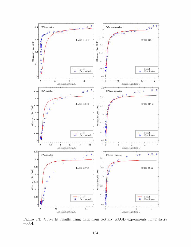
RMSE=0.1855
ModelExperimental
WW, spreading
Oil
reco
very
(fra
c. O
OIP
)
0
0.1
0.2
0.3
0.4
Dimensionless time, tD
0 0.5 1 1.5
RMSE=0.0241
ModelExperimental
WW, non-spreading
Oil
reco
very
(fra
c. O
OIP
)
0
0.05
0.1
0.15
0.2
0.25
0.3
Dimensionless time, tD
0 0.5 1 1.5 2
RMSE=0.0308
ModelExperimental
OW, spreading
Oil
reco
very
(fra
c. O
OIP
)
0
0.05
0.1
0.15
0.2
0.25
0.3
0.35
Dimensionless time, tD
0 0.5 1 1.5 2 2.5
RMSE=0.0746
ModelExperimental
OW, non-spreading
Oil
reco
very
(fra
c. O
OIP
)
0
0.1
0.2
0.3
0.4
0.5
0.6
Dimensionless time, tD
0 1 2 3 4
RMSE=0.0720
ModelExperimental
FW, spreading
Oil
reco
very
(fra
c. O
OIP
)
0
0.05
0.1
0.15
0.2
0.25
0.3
0.35
Dimensionless time, tD
0 0.5 1 1.5
RMSE=0.0432
ModelExperimental
FW, non-spreading
Oil
reco
very
(fra
c. O
OIP
)
0
0.1
0.2
0.3
0.4
0.5
Dimensionless time, tD
0 1 2 3
Figure 5.3: Curve fit results using data from tertiary GAGD experiments for Dykstramodel.
124

constant defined as µφ′
Bkρgwhere φ′, the adjusted porosity is φ(1−Sor) for a two-phase system
and φ(1− Sor − Swc) for a three-phase system.
Oil recovery equation:
R = ZdL
(1− BoiSorSoiBo
)− Boi
Soi
(1− SorBo
)(B − 1B
)(mZdt
) 1B−1
(5.6)
where R is the oil recovery, Bo is the oil formation volume factor, Soi the initial oil
saturation and Sor the residual oil saturation.
In order to fit Equation 5.6 to the experimental data, first we have to solve the demar-
cator Equation 5.5 to obtain Zd. This is because the term Zd is required in Equation 5.6
to calculate the oil recovery, R. In order to find Zd from Equation 5.5 we used MATLAB
built-in solver ode45 or ode113 to ensure fast convergence since Equation 5.5 is a nonlinear
ordinary differential equation. The actual matching to experimental data is achieved by
using the MATLAB function lsqcurvefit from the Optimization Toolbox with B, H and
Si set as the fitting parameters.
In Appendix B on page 158 we have included a working .m files with the associated
functions for this model. The program was developed initially to be used in Octave version
4.2.1, a MATLAB-compatible open-source program before the codes were migrated to
MATLAB in order to use the proprietary toolboxes. The earlier program written for Octave
used Euler’s method to obtain Zd. When the codes were migrated to MATLAB and used
together with lsqcurvefit it lead to erroneous results, particularly in the early time with
fluctuations in the predicted recovery. After rewriting the codes to solve Equation 5.5 with
ode45 or ode113 and fitting Equation 5.6 to recovery data using lsqcurvefit we successfully
removed the unphysical fluctuations from the model output.
The curve fit results are shown in Figures 5.1, 5.2 and 5.3 for free-fall gravity drainage
(FGD), secondary GAGD and tertiary GAGD respectively. The experimental results are
plotted with the horizontal axis using dimensionless time, tD from Equation 5.9 on page 128
in Schechter and Guo model.
125

In Figure 5.1 under free-fall mode, the predicted values for oil recovery at the end of
the experiment tend to be lower than the experimental values. Performance of the model
varies with experiments. For example the best match for this set of experiments came
from fractional-wet, spreading case with RMSE = 0.0621. This is followed by water-wet,
non-spreading experiment with RMSE = 0.751 and oil-wet, spreading experiment with
RMSE = 0.0861. The greater the value of RMSE than zero, the more the prediction of
terminal oil recovery differs from experimental value. The results for this group indicate
that Dykstra model works best to predict oil recovery from experiment in fractional-wet,
spreading condition.
Table 5.1: Performance of Dykstra model in FGD, secondary GAGD and tertiary GAGD experi-ments.
Experimentmode
Wettabilitycondition
Spreadingcondition
RMSE
FGD
fractional-wet spreading 0.0621water-wet non-spreading 0.0751
oil-wet spreading 0.0861water-wet spreading 0.1149
oil-wet non-spreading 0.1681fractional-wet non-spreading 0.1689
SecondaryGAGD
fractional-wet spreading 0.0722oil-wet spreading 0.0940
water-wet non-spreading 0.1356fractional-wet non-spreading 0.1726
water-wet spreading 0.1916oil-wet non-spreading 0.2444
Tertiary GAGD
water-wet non-spreading 0.0241oil-wet spreading 0.0308
fractional-wet non-spreading 0.0432fractional-wet spreading 0.0720
oil-wet non-spreading 0.0746water-wet spreading 0.1855
The results for secondary GAGD experiments are shown in Figure 5.2. Similar to free-
fall mode, Dykstra model is also shown to underpredict the oil recovery at late time. The
best match came from fractional-wet, spreading case with RMSE = 0.0722. The second
126

and third best match for this group came from oil-wet, spreading experiment and water-
wet, non-spreading experiment respectively at RMSE = 0.0940 and 0.1356 each. The top
three results are consistent with that to the previous group of experiments in free-fall mode.
In both free-fall and secondary GAGD (both performed at residual water saturation) the
results again demonstrate that Dykstra model can be used to predict oil recovery from
fractional-wet, spreading experiment.
In tertiary GAGD experiments the results in Figure 5.3 indicate that the model also
underpredict the oil recovery at late time. In tertiary mode the model exhibits best match
for experiment performed in water-wet, spreading condition (RMSE = 0.0241). This
is followed by oil-wet, spreading experiment and fractional-wet non-spreading experiment
at RMSE = 0.0308 and 0.0432 respectively. The results for experiments performed in
this group show that Dykstra model works best to predict oil recovery in water-wet, non-
spreading condition.
We tabulate the experimental results for each group and arrange them according to
increasing RMSE values in Table 5.1. As mentioned earlier, results with RMSE values
approaching zero would show better match between the model and experimental data. From
Table 5.1 we can infer that for FGD and secondary GAGD experiments under varying
wettability and spreading conditions, Dykstra model performs better in fractional-wet,
spreading system. In tertiary GAGD under varying wettability and spreading, Dykstra
model is found to match reliably oil recovery from water-wet, non-spreading experiment.
5.3 Schechter and Guo model
The Schechter and Guo model is considered in this study because it takes into account
the effect of film flow in gravity drainage displacement. In their model they divided a
tall column where gravity drainage takes place into saturated and unsaturated zone. This
approach is similar to that taken by Cardwell and Parsons (1949) and Dykstra (1978) when
developing their gravity drainage models. In the saturated zone Darcy velocity is assumed
127

to be valid while in the top, unsaturated zone they consider the volume contributed by
bulk and film flow. They derived a differential equation by equating the volume change
due to Darcy flow in the saturated zone with the volume change due to bulk and film flow
in the unsaturated zone. The resulting set of equations were solved numerically to obtain
the demarcator (gas-oil interface) and the oil recovery. Below are the equations used:
Demarcator equation:
4zD =−φzD
3tD
√FsφzD
5tD +[1− HD
1−zD
]φ[Soi − Sor −
√FsφzD
5tD
] 4tD (5.7)
where zD is the dimensionless demarcator depth, tD is the dimensionless time, φ is
porosity, Fs is the Kozeny correction factor, HD is the dimensionless capillary pressure
threshold, Soi is the initial oil saturation and Sor is the residual oil saturation respectively.
Oil recovery equation:
R =(
1− SorSoi
)zD −
2zD3Soi
√FsφzD
5tD. (5.8)
The dimensionless time tD is given as
tD = ke∆ρgtµL
(5.9)
where ke is the effective permeability, ∆ρ is the density difference, g is the gravity
acceleration constant, t is time, µ is viscosity and L is the column length respectively.
In this model the film flow effect is accounted by considering the volume contributed by
the film. This is possible because they used earlier work by Nenniger and Storrow (1958).
In their paper Nenniger and Storrow derived a gravity drainage model for a column of
packed bed and solved the differential equation using a series solution. The effect of film
drainage on the packed bed is incorporated using integration of Navier-Stokes approximate
solution for film drainage down a vertical plane. The phase volume in the film is given as
128
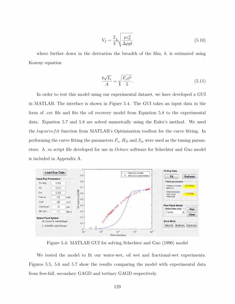
Vf = 23b
√√√√ µz3d
∆ρgt (5.10)
where further down in the derivation the breadth of the film, b, is estimated using
Kozeny equation
b√keA
=√Fsφ3
5 . (5.11)
In order to test this model using our experimental dataset, we have developed a GUI
in MATLAB. The interface is shown in Figure 5.4. The GUI takes an input data in the
form of .csv file and fits the oil recovery model from Equation 5.8 to the experimental
data. Equation 5.7 and 5.8 are solved numerically using the Euler’s method. We used
the lsqcurvefit function from MATLAB’s Optimization toolbox for the curve fitting. In
performing the curve fitting the parameters Fs, HD and Soi were used as the tuning param-
eters. A .m script file developed for use in Octave software for Schechter and Guo model
is included in Appendix A.
Figure 5.4: MATLAB GUI for solving Schechter and Guo (1996) model
We tested the model to fit our water-wet, oil wet and fractional-wet experiments.
Figures 5.5, 5.6 and 5.7 show the results comparing the model with experimental data
from free-fall, secondary GAGD and tertiary GAGD respectively.
129

WW, spreading
RMSE=0.0398
ModelExperimental
Oil
reco
very
(fra
c. O
OIP
)
0
0.1
0.2
0.3
0.4
0.5
0.6
0.7
Dimensionless time,tD
0 0.25 0.5 0.75 1 1.25 1.5 1.75
WW, non-spreading
RMSE=0.0216
ModelExperimental
Oil
reco
very
(fra
c. O
OIP
)
0
0.1
0.2
0.3
0.4
0.5
Dimensionless time,tD
0 0.5 1 1.5 2
OW, spreading
RMSE=0.0213
ModelExperimental
Oil
reco
very
(fra
c. O
OIP
)
0
0.1
0.2
0.3
0.4
0.5
Dimensionless time,tD
0 0.5 1 1.5 2 2.5
OW, non-spreading
RMSE=0.0334
ModelExperimental
Oil
reco
very
(fra
c. O
OIP
)
0
0.1
0.2
0.3
0.4
0.5
0.6
0.7
Dimensionless time,tD
0 1 2 3 4
FW, spreading
RMSE=0.0208
ModelExperimental
Oil
reco
very
(fra
c. O
OIP
)
0
0.1
0.2
0.3
0.4
0.5
Dimensionless time,tD
0 0.25 0.5 0.75 1 1.25 1.5 1.75
FW, non-spreading
RMSE=0.0302
ModelExperimental
Oil
reco
very
(fra
c. O
OIP
)
0
0.1
0.2
0.3
0.4
0.5
0.6
0.7
Dimensionless time,tD
0 0.5 1 1.5 2 2.5 3
Figure 5.5: Curve fit results using data from FGD experiments for Schechter and Guomodel.
130

WW, spreading
RMSE=0.0550
ModelExperimental
Oil
reco
very
(fra
c. O
OIP
)
0
0.1
0.2
0.3
0.4
0.5
0.6
0.7
Dimensionless time,tD
0 0.25 0.5 0.75 1 1.25 1.5
WW, non-spreading
RMSE=0.0320
ModelExperimental
Oil
reco
very
(fra
c. O
OIP
)
0
0.1
0.2
0.3
0.4
0.5
0.6
Dimensionless time,tD
0 0.5 1 1.5 2
OW, spreading
RMSE=0.0237
ModelExperimental
Oil
reco
very
(fra
c. O
OIP
)
0
0.1
0.2
0.3
0.4
0.5
Dimensionless time,tD
0 0.5 1 1.5 2 2.5
OW, non-spreading
RMSE=0.0402
ModelExperimental
Oil
reco
very
(fra
c. O
OIP
)
0
0.1
0.2
0.3
0.4
0.5
0.6
0.7
Dimensionless time,tD
0 1 2 3 4
FW, spreading
RMSE=0.0256
ModelExperimental
Oil
reco
very
(fra
c. O
OIP
)
0
0.1
0.2
0.3
0.4
0.5
Dimensionless time,tD
0 0.25 0.5 0.75 1 1.25 1.5 1.75
FW, non-spreading
RMSE=0.0327
ModelExperimental
Oil
reco
very
(fra
c. O
OIP
)
0
0.1
0.2
0.3
0.4
0.5
0.6
0.7
Dimensionless time,tD
0 0.5 1 1.5 2 2.5 3
Figure 5.6: Curve fit results using data from secondary GAGD experiments for Schechterand Guo model.
131

WW, spreading
RMSE=0.0209
ModelExperimental
Oil
reco
very
(fra
c. R
OIP
)
0
0.1
0.2
0.3
0.4
Dimensionless time,tD
0 0.25 0.5 0.75 1 1.25 1.5 1.75
WW, non-spreading
RMSE=0.0079
ModelExperimental
Oil
reco
very
(fra
c. R
OIP
)
0
0.05
0.1
0.15
0.2
0.25
0.3
Dimensionless time,tD
0 0.5 1 1.5 2
OW, spreading
RMSE=0.0074
ModelExperimental
Oil
reco
very
(fra
c. R
OIP
)
0
0.05
0.1
0.15
0.2
0.25
0.3
0.35
Dimensionless time,tD
0 0.5 1 1.5 2 2.5
OW, non-spreading
RMSE=0.0160
ModelExperimental
Oil
reco
very
(fra
c. R
OIP
)
0
0.1
0.2
0.3
0.4
0.5
0.6
Dimensionless time,tD
0 1 2 3 4
FW, spreading
RMSE=0.0061
ModelExperimental
Oil
reco
very
(fra
c. R
OIP
)
0
0.05
0.1
0.15
0.2
0.25
0.3
0.35
Dimensionless time,tD
0 0.25 0.5 0.75 1 1.25 1.5 1.75
FW, non-spreading
RMSE=0.0095
ModelExperimental
Oil
reco
very
(fra
c. R
OIP
)
0
0.1
0.2
0.3
0.4
0.5
Dimensionless time,tD
0 0.5 1 1.5 2 2.5 3
Figure 5.7: Curve fit results using data from tertiary GAGD experiments for Schechter andGuo model.
132

From the results in Figure 5.5 Schechter and Guo model is shown to achieve very close
match with experimental data from fractional-wet, spreading system (RMSE = 0.0208).
This is followed by oil-wet, spreading system (RMSE = 0.0213) and water-wet, non-
spreading system (RMSE = 0.0216). In this set of experiments notable difference between
oil recovery from experimental data and that predicted by the model is seen for the case
of water-wet, spreading experiment with RMSE = 0.0398. Based on our results for this
group Schechter and Guo model performs best in predicting oil recovery from fractional-
wet, spreading experiment.
In Figure 5.6 for secondary GAGD, Schechter and Guo model is able to match closely
experimental data from oil-wet, spreading system (RMSE = 0.0237). However the pre-
dicted oil recovery from the model is slightly less than that of the experimental data at
late time for this experiment. Observations of other experimental data from this group also
show the Schechter and Guo model underpredicts the oil recovery at late time, with the
difference between model and experimental data increasing the higher the value of RMSE.
This is clearly shown for matching of the model to water-wet, spreading experiment with
RMSE = 0.0550. Results from this group indicate that the model works best for predicting
oil recovery in oil-wet, spreading system.
For the set of experiments performed under tertiary mode the results in Figure 5.7
show that the model demonstrates satisfactory match overall with the experimental data
as indicated by the very low RMSE values. The best matching achieved by the model
comes from fractional-wet, spreading system with RMSE = 0.0061. This infers that in
tertiary experiments the model works best to predict the oil recovery from fractional-wet,
spreading experiment. In the same group the prediction of the oil recovery at late time
from the model is seen to deviate from the experimental data the greater the RMSE
value is from zero. This is shown for example with water-wet, spreading system with
RMSE = 0.0209.
133

Table 5.2: Performance of Schechter-Guo model in FGD, secondary GAGD and tertiaryGAGD experiments.
Experimentmode
Wettabilitycondition
Spreadingcondition
RMSE
FGD
fractional-wet spreading 0.0208oil-wet spreading 0.0213
water-wet non-spreading 0.0216fractional-wet non-spreading 0.0302
oil-wet non-spreading 0.0334water-wet spreading 0.0398
SecondaryGAGD
oil-wet spreading 0.0237fractional-wet spreading 0.0256
water-wet non-spreading 0.0320fractional-wet non-spreading 0.0327
oil-wet non-spreading 0.0402water-wet spreading 0.0550
Tertiary GAGD
fractional-wet spreading 0.0061oil-wet spreading 0.0074
water-wet non-spreading 0.0079fractional-wet non-spreading 0.0095
oil-wet non-spreading 0.0160water-wet spreading 0.0209
We have compiled the performance of Schechter and Guo model in terms of the best-fit
with experimental data in Table 5.2. Table 5.2 summarizes the results for all experiments
under different wettability and spreading conditions. To recapitulate in FGD experiments
the model works best to predict oil recovery in fractional-wet, spreading system. In sec-
ondary GAGD curve fitting results indicate that the model can be used best for oil-wet,
spreading system. In tertiary mode Table 5.2 shows that the RMSE values for all ex-
periments in this group are significantly lower than the best matching results from FGD
and secondary GAGD experiments. Thus it can be inferred that Schechter and Guo model
works particularly well for experiments conducted in tertiary mode. Furthermore the model
seems to perform well under all wettability and spreading conditions for this group. Al-
though we recommended earlier to use Schechter and Guo model to predict oil recovery in
fractional-wet, spreading experiment we would like to point out that based on the lower
134
RMSE values overall, Schechter and Guo model can be used to predict gravity drainage
recovery in all tertiary GAGD experiments.
5.4 Li and Horne model
Li and Horne (2003) derived gravity drainage model in free-fall mode by assuming that
free-fall drainage mechanism is similar to that of spontaneous imbibition. Their model was
based on earlier work from Aronofsky et al. (1958) for spontaneous imbibition. In Aronofsky
et al. model a single fit parameter called rate constant is used in the exponential expression
to obtain match with experimental data.
Li and Horne (2003) proposes the following equation to match oil recovery of FGD
system:
R = 1− Swi − Sor1− Swi
(1− e−βt
)(5.12)
where R is the recovery, Swi is the initial water saturation, Sor is the average residual
oil saturation and β is the constant used as parameter to give the rate of convergence in
Equation 5.12.
Compared to Aronofsky et al. model they used two parameters, Sor and β to fit the
experimental data. The value Sor is different from the values of residual oil saturation
in the core because in the latter the value changes with depth. Sor is calculated assum-
ing equilibrium between gravity and capillary forces after completion of gravity drainage
experiment.
In their model they relaxed the assumption that the oil saturation at the top of the
column is at residual oil saturation. The derivation of the model aims to find the ultimate
oil recovery by assuming that gravity force is balanced by capillary force everywhere in the
column.
For a given data of gravity drainage experiment, we perform a nonlinear regression
analysis to obtain the matching parameter Sor and β. According to Li and Horne (2003)
135

parameter β can be used to calculate pe , the entry capillary pressure and both Sor and β
can be used to obtain λ, the pore size distribution index. A working computer program
for this model is included in Appendix C.
The curve fit results are shown in Figures 5.8, 5.9, and 5.10 for FGD, secondary GAGD
and tertiary GAGD respectively. In free-fall mode the model typically matches the recovery
at early time but underpredicts at late time. The best matching for this group comes from
fractional-wet, spreading experiment with RMSE = 0.0230 followed by oil-wet, spread-
ing experiment with RMSE = 0.0257 and fractional-wet, non-spreading experiment with
RMSE = 0.0289. Results from this group show that for FGD experiments, the model can
be used to match the oil recovery from fractional-wet, spreading experiment. However we
caution against using it for predicting the oil recovery since the matched result was lower
than the experimental data.
In secondary GAGD experiments Figure 5.9 shows that the model underpredicts oil
recovery at late time. The best match is obtained for oil-wet, spreading experiment with
RMSE = 0.0280. Within the same group the model’s prediction of oil recovery differs
greatly from experimental data as shown by the increasing RMSE values. This can be
seen for the case of water-wet, non-spreading experiment which has RMSE value of 0.0368.
Based on the results the model is suitable to be used to match the experimental data
from oil-wet, spreading experiment. However since the matching result for this particular
experiment does not reproduce the experimental data exactly, we again caution against
using it for prediction of oil recovery.
For tertiary GAGD experiments Figure 5.10 shows that the model underpredicts the
late time recovery overall and matches the early time recovery on select cases. The
best match in this set of experiments goes to fractional-wet, spreading experiment with
RMSE = 0.0085. This is followed by oil-wet, spreading experiment and water-wet non-
spreading experiment with RMSE values of 0.0117 and 0.0140 respectively. Although the
results indicate that the model can be used to match experimental data from fractional-wet,
136
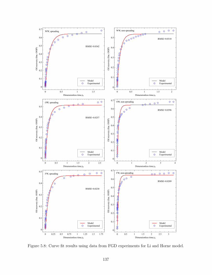
WW, spreading
RMSE=0.0342
ModelExperimental
Oil
reco
very
(fra
c. O
OIP
)
0
0.1
0.2
0.3
0.4
0.5
0.6
0.7
Dimensionless time,tD
0 0.5 1 1.5
WW, non-spreading
RMSE=0.0318
ModelExperimental
Oil
reco
very
(fra
c. O
OIP
)
0
0.1
0.2
0.3
0.4
0.5
Dimensionless time,tD
0 0.5 1 1.5 2
OW, spreading
RMSE=0.0257
ModelExperimental
Oil
reco
very
(fra
c. O
OIP
)
0
0.1
0.2
0.3
0.4
0.5
Dimensionless time,tD
0 0.5 1 1.5 2 2.5
OW, non-spreading
RMSE=0.0396
ModelExperimental
Oil
reco
very
(fra
c. O
OIP
)
0
0.1
0.2
0.3
0.4
0.5
0.6
0.7
Dimensionless time,tD
0 1 2 3 4
FW, spreading
RMSE=0.0230
ModelExperimental
Oil
reco
very
(fra
c. O
OIP
)
0
0.1
0.2
0.3
0.4
0.5
Dimensionless time,tD
0 0.25 0.5 0.75 1 1.25 1.5 1.75
FW, non-spreading
RMSE=0.0289
ModelExperimental
Oil
reco
very
(fra
c. O
OIP
)
0
0.1
0.2
0.3
0.4
0.5
0.6
0.7
Dimensionless time,tD
0 0.5 1 1.5 2 2.5 3
Figure 5.8: Curve fit results using data from FGD experiments for Li and Horne model.
137
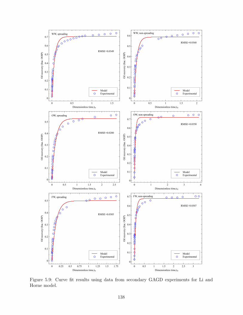
WW, spreading
RMSE=0.0349
ModelExperimental
Oil
reco
very
(fra
c. O
OIP
)
0
0.1
0.2
0.3
0.4
0.5
0.6
0.7
Dimensionless time,tD
0 0.5 1 1.5
WW, non-spreading
RMSE=0.0368
ModelExperimental
Oil
reco
very
(fra
c. O
OIP
)
0
0.1
0.2
0.3
0.4
0.5
0.6
Dimensionless time,tD
0 0.5 1 1.5 2
OW, spreading
RMSE=0.0280
ModelExperimental
Oil
reco
very
(fra
c. O
OIP
)
0
0.1
0.2
0.3
0.4
0.5
Dimensionless time,tD
0 0.5 1 1.5 2 2.5
OW, non-spreading
RMSE=0.0350
ModelExperimental
Oil
reco
very
(fra
c. O
OIP
)
0
0.1
0.2
0.3
0.4
0.5
0.6
0.7
Dimensionless time,tD
0 1 2 3 4
FW, spreading
RMSE=0.0305
ModelExperimental
Oil
reco
very
(fra
c. O
OIP
)
0
0.1
0.2
0.3
0.4
0.5
Dimensionless time,tD
0 0.25 0.5 0.75 1 1.25 1.5 1.75
FW, non-spreading
RMSE=0.0307
ModelExperimental
Oil
reco
very
(fra
c. O
OIP
)
0
0.1
0.2
0.3
0.4
0.5
0.6
0.7
Dimensionless time,tD
0 0.5 1 1.5 2 2.5 3
Figure 5.9: Curve fit results using data from secondary GAGD experiments for Li andHorne model.
138

WW, spreading
RMSE=0.0192
ModelExperimental
Oil
reco
very
(fra
c. R
OIP
)
0.05
0.1
0.15
0.2
0.25
0.3
0.35
0.4
Dimensionless time,tD
0 0.5 1 1.5
WW, non-spreading
RMSE=0.0140
ModelExperimental
Oil
reco
very
(fra
c. R
OIP
)
0
0.05
0.1
0.15
0.2
0.25
0.3
Dimensionless time,tD
0 0.5 1 1.5 2
OW, spreading
RMSE=0.0117
ModelExperimental
Oil
reco
very
(fra
c. R
OIP
)
0
0.05
0.1
0.15
0.2
0.25
0.3
0.35
Dimensionless time,tD
0 0.5 1 1.5 2 2.5
OW, non-spreading
RMSE=0.0338
ModelExperimental
Oil
reco
very
(fra
c. R
OIP
)
0
0.1
0.2
0.3
0.4
0.5
0.6
Dimensionless time,tD
0 1 2 3 4
FW, spreading
RMSE=0.0085
ModelExperimental
Oil
reco
very
(fra
c. O
OIP
)
0
0.05
0.1
0.15
0.2
0.25
0.3
0.35
Dimensionless time,tD
0 0.25 0.5 0.75 1 1.25 1.5 1.75
FW, non-spreading
RMSE=0.0251
ModelExperimental
Oil
reco
very
(fra
c. O
OIP
)
0
0.1
0.2
0.3
0.4
0.5
Dimensionless time,tD
0 0.5 1 1.5 2 2.5 3
Figure 5.10: Curve fit results using data from tertiary GAGD experiments for Li and Hornemodel.
139

Table 5.3: Performance of Li and Horne model in FGD, secondary GAGD and tertiaryGAGD experiments.
Experimentmode
Wettabilitycondition
Spreadingcondition
RMSE
FGD
fractional-wet spreading 0.0230oil-wet spreading 0.0257
fractional-wet non-spreading 0.0289water-wet non-spreading 0.0318water-wet spreading 0.0342
oil-wet non-spreading 0.0396
SecondaryGAGD
oil-wet spreading 0.0280fractional-wet spreading 0.0305fractional-wet non-spreading 0.0307
water-wet spreading 0.0349oil-wet non-spreading 0.0350
water-wet non-spreading 0.0368
Tertiary GAGD
fractional-wet spreading 0.0085oil-wet spreading 0.0117
water-wet non-spreading 0.0140water-wet spreading 0.0192
fractional-wet non-spreading 0.0251oil-wet non-spreading 0.0338
spreading experiment, the matched result is still lower than the experimental data at late
time. Thus the user is advised to compare prediction result of this particular experiment
from this model with other models (Dykstra and Schechter and Guo) to decide on the best
model to use.
Table 5.3 shows the performance of Li and Horne model in matching the experimental
data from FGD, secondary GAGD and tertiary GAGD experiments under different wet-
tability and spreading conditions. In Table 5.3 the curve fit results from tertiary GAGD
experiments exhibit the least RMSE values compared to that of FGD and secondary
GAGD experiments. This seem to indicate that the model would be suitable to use for
matching experimental data from tertiary experiments. However caution is advised when
using this model for predicting oil recovery because the model consistently underpredicts
the late time recovery. This pattern of underprediction of oil recovery at late time is also
observed for the best matching result from FGD (fractional-wet, spreading) and secondary
140

Table 5.4: Best curve fit results from Dykstra, Schechter and Guo and Li and Horne modelsfor FGD, secondary GAGD and tertiary GAGD experiments.
Experiment mode Model Experiment RMSE
FGDSchechter and Guo fractional-wet, spreading 0.0208Li and Horne fractional-wet, spreading 0.0230Dykstra fractional-wet, spreading 0.0621
Secondary GAGDSchechter and Guo oil-wet, spreading 0.0237Li and Horne oil-wet, spreading 0.0280Dykstra fractional-wet, spreading 0.0722
Tertiary GAGDSchechter and Guo fractional-wet, spreading 0.0061Li and Horne fractional-wet, spreading 0.0085Dykstra water-wet, non-spreading 0.0241
GAGD (oil-wet, spreading) experiments. Although Li and Horne (2003) intended this
model for free-fall gravity drainage, our results further clarify that in FGD mode the model
demonstrates best matching for experiment under fractional-wet condition with spreading
oil.
5.5 Discussion and summary
In this chapter we have evaluated the performance of gravity drainage models from
Dykstra (1978), Schechter and Guo (1996) and Li and Horne (2003). Using root mean
squared error (RMSE) as the metric for comparison, we were able to rank the performance
of each model according to closeness of the model fit to the experimental data. It is assumed
that a close fit overall would infer that the model successfully capture the pore-scale physics
discussed in Section 4.2 on page 81. According to Grattoni et al. (1997) the core-scale
displacement is affected by many small events occurring at the pore-scale. Depending on
wettability and three-phase fluid distribution, the pore-scale events when taken as average,
would affect the residual oil saturation.
We have compiled the best matching results for each model and sorted them according
to the mode of gravity drainage experiment in Table 5.4. In Table 5.4 the results for curve
fit in FGD experiments indicate that all models can be used to match experiment from
141

RMSE=0.0061
Li-Horne
Schechter-Guo
FW, spreading
RMSE=0.0085
Model Schechter-GuoModel Li-HorneExperimental
Oil
reco
very
(fra
c. R
OIP
)
0
0.05
0.1
0.15
0.2
0.25
0.3
0.35
Dimensionless time,tD
10−3 0.01 0.1 1
(a) Spreading fluid system (Soltrol)
RMSE=0.0251Li-Horne
Schechter-Guo
FW, non-spreading
RMSE=0.0095
Model Schechter-GuoModel Li-HorneExperimental
Oil
reco
very
(fra
c. R
OIP
)
0
0.1
0.2
0.3
0.4
0.5
Dimensionless time,tD
10−3 0.01 0.1 1
(b) Non-spreading fluid system (decane)
Figure 5.11: Performance comparison between Schechter-Guo and Li-Horne model in ter-tiary GAGD of fractional-wet sand for both spreading and non-spreading system
fractional-wet sand with spreading oil. Since Schechter and Guo model achieved the lowest
RMSE value for this group it can also be used for predicting oil recovery from the same
experiment. In secondary GAGD group, Schechter and Guo and Li and Horne models both
show that they were able to model experiment from oil-wet sand with spreading oil. In the
same group, Dykstra model is shown to work best with experiment from fractional-wet,
spreading system. Using RMSE value as the criterion we determined that in secondary
GAGD experiments, Schechter and Guo model is chosen as the model that is suitable
to match and subsequently predict the oil recovery from experiment using oil-wet sand
with spreading oil. For tertiary GAGD experiments Table 5.4 show that fractional-wet,
spreading experiment can be modeled by both Schechter and Guo and Li and Horne models.
Within the same group Dykstra model shows that it can best be used with water-wet, non-
spreading experiment. Again using RMSE values we determined that in tertiary mode,
experiment from fractional-wet sand with spreading oil can be modeled best with Schechter
and Guo model.
142

The model that is able to fit early time data is inferred to be better at capturing the
bulk flow mechanism successfully. Likewise for late time, the model that successfully match
the experiment during this period can be assumed to capture the spreading and wetting film
flow behavior. In Figure 5.11 we plot the recovery profiles for tertiary GAGD experiments
in fractional-wet sand packs for both spreading and non-spreading fluid system. We include
the curve fit results from Schechter and Guo and Li and Horne models to observe their
performance at early and late time. Thus the horizontal axes are in log scale to highlight
the early time behavior. The fractional-wet experiment is selected for comparison because
this wettability system could represent reservoir condition since a typical reservoir rock is
neither strongly water-wet or oil-wet. More over tertiary mode is chosen since the effect of
spreading or wetting film flow is readily manifested at late time under residual oil condition.
We omitted comparison of both experiments with Dykstra model since Figure 5.3 showed
that the curve fitting of the model to both experiments were not satisfactory.
For the spreading system it is observed that both Schechter and Guo and Li and
Horne models capture the early time behavior. However in the middle time both models
overpredict the recovery. Between the middle time and late time both models match the
experimental data and track each other until the end of the experiment. At late time
the modeled oil recoveries from Schechter and Guo and Li and Horne are both below the
experimental value. Even though the predicted terminal oil recovery is lower than actual,
Schechter and Guo model managed to capture the behavior at late time because it is
observed to track the trajectory of the experimental data closely.
For the non-spreading system both models start out matching the experiment at early
time but underpredict the experiment in the middle time. Between the middle time and
late time both models track each other but Schechter and Guo model is observed to better
match the experimental data than Li and Horne model. Finally at late time Schechter and
Guo model fits the data well but Li and Horne model tapers off and underpredicts the
recovery.
143

By comparing the performance of both models in Figure 5.11 we can observe that
both models successfully capture the early time behavior in spreading and non-spreading
experiments. Both models overpredict the middle time recovery in spreading system but the
modeled oil recovery is below the experimental value in non-spreading system. At late time
when additional recovery is obtained with the help of spreading or wetting film mechanism,
Schechter and Guo model shows that it managed to capture the behavior during this time
for both spreading and non-spreading system.
Our evaluation of the models and their performance in matching experimental data
from diverse set of experiments encompassing varying wettability and spreading conditions
demonstrate that in most cases Schechter and Guo is found to be suitable model to be
used. This is possibly because the model incorporates film flow mechanism in its derivation.
Whether the experiment is conducted in FGD, secondary GAGD or tertiary GAGD mode,
comparison of results from this model in Table 5.2 indicates that this model can be expected
to match and subsequently predict the oil recovery. Although the model seems to give
satisfactory match for most of the experiments, this does not mean that the model should
be the default option to be used. This is because the performance of the model at early,
middle or late time varies according to experiments. Hence it is suggested to match the
target experiment with several models before deciding on the best model since some models
work best for a given wettability, spreading and injection conditions.
Our results in this chapter using models available in the literature underscore the need
for gravity drainage model that is able to capture the behavior at early, middle and late
time. Even though Schechter and Guo appears to be the best choice the model does not
always capture the behavior at each time segment. As mentioned the early and middle time
represent the period where bulk flow is dominant. In late time the spreading or wetting
film flow mechanism is most active recovering additional oil. Since the matching of each
model to experimental data varies given wettability and spreading condition, a new model
144

for gravity drainage that aims to capture the physical behavior should be able to achieve
satisfactory match during each time segment.
145

Chapter 6
Conclusions and RecommendationsIn this study we have accomplished the following:
1. Performed gravity drainage experiments using spreading and non-spreading fluid sys-
tem in water-wet, oil-wet and fractional-wet sand.
2. Analyzed and compared the results with existing literature.
3. Discussed the pore level mechanisms affecting oil recovery at the core scale.
4. Performed analysis with dimensionless numbers to investigate the effect of gravity,
capillary and viscous forces.
5. Evaluated and ranked the performance of gravity drainage models in matching ex-
perimental data.
We conclude our findings so far as follows:
The experimental results show that oil recovery is higher in spreading fluid system in
water-wet sand. In oil-wet sand recovery from non-spreading fluid system is higher than
that of spreading fluid. For fractional-wet sand, the recovery trend is similar to that of
oil-wet experiments in that the non-spreading fluid produces more oil than spreading fluid
system.
At the pore level oil recovery is higher for spreading fluid system in water-wet ex-
periments because the spreading film reconnects isolated oil ganglia. Oil recoveries in
oil-wet experiments are similar for both spreading and non-spreading fluid system because
regardless the pore-level fluid configurations, the oil is drained through the continuous
wetting phase. Oil-wet experiment with Decane shows higher recovery for non-spreading
fluid system due to improved drainage rate from higher conductance path established by
low viscosity wetting film. In fractional-wet experiments the non-spreading fluid system
achieved higher recovery because oil is drained through higher conductance wetting film.
146
Oil recovery for spreading fluid system is lower because the displaced oil in the water-wet
regions was trapped due to discontinuous water phase, and oil is produced mostly from the
oil-wet regions.
Using a modified Bond number it is seen that the role of gravity force is significant
very early in gravity drainage displacement. This is particularly so in water-wet experi-
ment with spreading fluid system. In the spreading fluid system for water-wet experiment
the transition from capillary-dominated to gravity-dominated flow occurs early in the ex-
periment. In oil-wet and fractional-wet experiments the transition occurs much later. In
non-spreading system the time for the transition to happen is early in the experiment and
the exact time for its occurence is almost the same for each experiment. Oil recovery is
shown to have linear relationship with Bond number in water-wet experiments and non-
linear relationship in oil-wet and fractional-wet experiments. In water-wet experiments
for both spreading and non-spreading system the contribution of gravity-dominated flow
toward oil recovery is significant. However in oil-wet and fractional-wet experiments a
greater proportion of oil recovery comes from the capillary-dominated flow. In water-wet,
oil-wet and fractional-wet experiments Capillary number decreases with time. The results
also show that as the oil production increases, Capillary number decreases. Viscous forces
are more dominant in experiment with spreading fluid in water-wet sand, which resulted
in higher recovery. In experiments with non-spreading fluid, viscous forces are relatively
stronger than capillary forces in both oil-wet and fractional-wet sand; which helped to
mobilize and produce more oil. Analysis with Gravity number demonstrates that gravity
forces increase with time. Oil recovery is also shown to be increasing with Gravity number.
In experiments with spreading fluid, gravity forces become more dominant in water-wet
sand after transition from viscous-dominated flow. Consequently this resulted in higher oil
recovery. In non-spreading fluid system the presence of gravity forces are more dominant
in oil-wet and fractional-wet sand. We also used dimensionless numbers to analyze exper-
imental results from tertiary CGD. It is shown that the trend for total liquid production
147

exhibits similar relationship with Bond, Capillary and Gravity numbers as shown earlier for
experiments conducted at residual water saturation. This means the same forces are also
in effect for gravity drainage experiments at residual oil saturation. We also proposes flow
regime map for gravity drainage experiments based on analysis of dimensionless numbers.
By calculating the time for transition from capillary-dominated and viscous-dominated to
gravity-dominated flow we are able to determine the extent to which each force is domi-
nant over the course of the experiment. In general the early stage is marked by overlap of
capillary and viscous forces. At middle stage either capillary or viscous forces and gravity
forces are dominant. At late stage gravity forces are dominating the flow regime.
Curve fitting the experimental data are performed with Dykstra, Schechter-Guo and
Li-Horne models. In FGD experiments all three models are shown to work best in match-
ing experimental data from fractional-wet, spreading system. Among the three models
Schechter-Guo model gives the best matching and hence can be used to predict oil recovery
for this experiment. In secondary mode Schechter-Guo model again shows the best match
to experimental data from oil-wet sand with spreading system. In tertiary mode the results
show that fractional-wet, spreading experiment can be best modeled with Schechter-Guo
model. In addition comparison of fractional-wet experiments in tertiary mode between
Schechter-Guo and Li-Horne model again exhibits that Schechter-Guo model is able to
capture the drainage behavior at early and late time. However both models overpredict
the recovery during middle time for spreading system and underpredict the recovery during
the same time segment in non-spreading system. Our results demonstrate that Schechter-
Guo model is possibly the model that can be used for all gravity drainage experiments
under various wetting and spreading conditions. However opportunity exists to develop a
better gravity drainage model since the current models do not capture fully the behavior
during early, middle and late time.
From this study we recommend the following:
148

1. Further experiments to evaluate the fractional-wet system. In this study the fractional-
wet sand was 50% water-wet and 50% oil-wet. Additional experiments is recom-
mended to understand the performance of gravity drainage process in fractional-wet
system under different mixing ratio.
2. A new set of experiments based on the same experimental design but implemented
with fluids at high pressure and temperature. This is because experimental data with
similar condition in the reservoir evaluating the effect of wettability and spreading
condition is scarce.
3. Development of gravity drainage model that incorporates the wetting and spreading
flow mechanism. Although this mechanism has been applied in three-phase network
modeling, there is opportunity to develop similar model at the core scale.
149

References
Adamson, A. W. and A. P. Gast (1997). Physical Chemistry of Surfaces (6 edition ed.).New York: Wiley-Interscience.
Aronofsky, J. S., L. Masse, and S. G. Natanson (1958). A Model for the Mechanism ofOil Recovery from the Porous Matrix Due to Water Invasion in Fractured Reservoirs.Petroleum Transactions, AIME 213, 17–19.
Blunt, M., D. Fenwick, and D. Zhou (1994). What Determines Residual Oil Saturation inThree-Phase Flow? In SPE/DOE Improved Oil Recovery Symposium, SPE. Society ofPetroleum Engineers.
Blunt, M., D. Zhou, and D. Fenwick (1995). Three-phase flow and gravity drainage inporous media. Transport in Porous Media 20 (1), 77–103.
Blunt, M. J. (1997). Effects of Heterogeneity and Wetting on Relative Permeability UsingPore Level Modeling. SPE Journal 2 (01), 70–87.
Boinovich, L. and A. Emelyanenko (2009, March). Wetting behaviour and wetting transi-tions of alkanes on aqueous surfaces. Colloids, polymers and surfactants.Special Issue inhonour of Brian Vincent 147–148, 44–55.
Buckley, S. E. and M. C. Leverett (1942). Mechanism of Fluid Displacement in Sands.Transactions of the AIME 146 (01), 107–116.
Cardwell, W. and R. Parsons (1949). Gravity Drainage Theory. Transactions of theAIME 179 (01), 199–215.
Catalan, L. J. and F. A. Dullien (1995). Application of gravity drainage to the recoveryof residual LNAPL in homogeneous and lensed sand packs. Journal of ContaminantHydrology 18 (4), 279–306.
Catalan, L. J., F. A. Dullien, and I. Chatzis (1994). The Effects of Wettability and Het-erogeneities on the Recovery of Waterflood Residual Oil With Low Pressure Inert GasInjection Assisted by Gravity Drainage. SPE Advanced Technology Series 2 (02), 140–149.
Chatzis, I. and S. Ayatollahi (1993). The Effect Of Gas Injection Rate On The Recovery OfWaterflood Residual Oil Under Gravity Assisted Inert Gas Injection. In Technical Meet-ing / Petroleum Conference of The South Saskatchewan Section, PETSOC. PetroleumSociety of Canada.
Chatzis, I., A. Kantzas, and F. Dullien (1988). On the Investigation of Gravity-AssistedInert Gas Injection Using Micromodels, Long Berea Sandstone Cores, and Computer-Assisted Tomography. Society of Petroleum Engineers.
DiCarlo, D., S. Akshay, and M. Blunt (2000). Three-Phase Relative Permeability of Water-Wet, Oil-Wet, and Mixed-Wet Sandpacks. SPE Journal 5 (01), 82–91.
150
Dong, M., F. A. Dullien, and I. Chatzis (1995). Imbibition of Oil in Film Form over WaterPresent in Edges of Capillaries with an Angular Cross Section. Journal of Colloid andInterface Science 172 (1), 21–36.
Dullien, F. A., L. Catalan, I. Chaizis, and A. Collins (1991). Recovery Of WaterfloodResidual Oil With Low Pressure Inert Gas Injection, Assisted By Gravity DrainageFrom Water-Wet And Oil-Wet Cores. In Annual Technical Meeting, PETSOC. PetroleumSociety of Canada.
Dumore, J. and R. Schols (1974). Drainage Capillary-Pressure Functions and the Influenceof Connate Water. Society of Petroleum Engineers Journal 14 (05), 437–444.
Dumore, J. M. (1964). Stability Considerations in Downward Miscible Displacements.Society of Petroleum Engineers Journal 4 (04), 356–362.
Dykstra, H. (1978). The Prediction of Oil Recovery by Gravity Drainage. Journal ofPetroleum Technology 30 (05), 818–830.
Essley, Jr., P., G. Hancock, Jr., and K. Jones (1958, January). Gravity Drainage Conceptsin a Steeply Dipping Reservoir. SPE-1029-G.
Fenwick, D. and M. Blunt (1995, May). Pore Level Modelling of Three Phase Flow inPorous Media. Volume 1, Vienna, Austria, pp. 211–218.
Grattoni, C., M. P. Almada, and R. Dawe (1997). Pore and Core-Scale DisplacementMechanisms with Spreading and Wetting Effects During Three-Phase Flow. In LatinAmerican and Caribbean Petroleum Engineering Conference, SPE. Society of PetroleumEngineers.
Grattoni, C., X. Jing, and R. Dawe (2001). Dimensionless groups for three-phase gravitydrainage flow in porous media. Journal of Petroleum Science and Engineering 29 (1),53–65.
Hagoort, J. (1980). Oil Recovery by Gravity Drainage. Society of Petroleum EngineersJournal 20 (03), 139–150.
Hayden, N. J. and T. C. Voice (1993). Microscopic observation of a NAPL in a three-fluid-phase soil system. Journal of contaminant hydrology 12 (3), 217–226.
Herzberg, W. J. and W. R. Erwin (1970, May). Gas-chromatographic study of the reac-tion of glass surfaces with dichlorodimethylsilane and chlorotrimethylsilane. Journal ofColloid and Interface Science 33 (1), 172–177.
Holbrook, O. C. and G. G. Bernard (1958). Determination of Wettability by Dye Adsorp-tion. Transactions of the AIME 213, 261–264.
James, G., D. Witten, T. Hastie, and R. Tibshirani (2013). An Introduction to StatisticalLearning: with Applications in R. Springer Texts in Statistics. New York: Springer-Verlag.
151

Kalaydjian, F.-M. and M. Tixier (1991, August). Effect of the Spreading Coefficient onGas/Oil Capillary Pressure Curves in Presence of Connate Water. In SCA paper No.9106, San Antonio, TX.
Kalaydjian, F.-M., O. Vizika, J.-C. Moulu, and P. K. Munkerud (1995). The role of wet-tability and spreading in gas injection processes under secondary conditions. GeologicalSociety, London, Special Publications 84 (1), 63–71.
Kantzas, A., I. Chatzis, and F. Dullien (1988a). Enhanced Oil Recovery by Inert Gas Injec-tion. In SPE Enhanced Oil Recovery Symposium, SPE. Society of Petroleum Engineers.
Kantzas, A., I. Chatzis, and F. Dullien (1988b). Mechanisms of Capillary Displacement ofResidual Oil by Gravity-Assisted Inert Gas Injection. In SPE Rocky Mountain RegionalMeeting, SPE. Society of Petroleum Engineers.
Keller, A. A., M. J. Blunt, and A. P. V. Roberts (1997). Micromodel Observation of theRole of Oil Layers in Three-Phase Flow. Transport in Porous Media 26 (3), 277–297.
Kulkarni, M. and D. Rao (2006a, November). Analytical Modeling of the Forced GravityDrainage GAGD Process. San Francisco, California.
Kulkarni, M., A. Sharma, and D. Rao (2005, August). Use of Dimensional Analysis forScaling Immiscible Gas Assisted Gravity Drainage (GAGD) Experiments. In SCA2005-50, Toronto,Canada.
Kulkarni, M. M. and D. N. Rao (2006b). Characterization of Operative Mechanisms inGravity Drainage Field Projects Through Dimensional Analysis. In SPE Annual Tech-nical Conference and Exhibition, SPE. Society of Petroleum Engineers.
Kva°Lseth, T. O. (1983, January). Note on the R2 measure of goodness of fit for nonlinearmodels. Bulletin of the Psychonomic Society 21 (1), 79–80.
Lenormand, R. and C. Zarcone (1984). Role Of Roughness And Edges During ImbibitionIn Square Capillaries. In SPE Annual Technical Conference and Exhibition, SPE. Societyof Petroleum Engineers.
Lenormand, R., C. Zarcone, and A. Sarr (1983). Mechanisms of the displacement of onefluid by another in a network of capillary ducts. Journal of Fluid Mechanics 135 (-1),337–353.
Lewis, J. O. (1944). Gravity Drainage in Oil Fields. Transactions of the AIME 155 (01),133–154.
Li, K. and R. N. Horne (2003). Prediction of Oil Production by Gravity Drainage. In SPEAnnual Technical Conference and Exhibition, SPE. Society of Petroleum Engineers.
Li, K. and R. N. Horne (2008). Modeling of oil production by gravity drainage. Journal ofPetroleum Science and Engineering 60 (3–4), 161–169.
152
Maeda, H. and K. Okatsu (2008). EOR Using Thin Oil Film Drainage Mechanism In WaterWet Oil Reservoir. In SPE Asia Pacific Oil and Gas Conference and Exhibition. Societyof Petroleum Engineers.
Mahmoud, T. and D. N. Rao (2008). Range of Operability of Gas-Assisted Gravity DrainageProcess. In SPE Symposium on Improved Oil Recovery, SPE. Society of PetroleumEngineers.
Marx, J. (1956, January). Determining Gravity Drainage Characteristics on the Centrifuge.SPE-545-G.
MATLAB (2018). Evaluating Goodness of Fit - MATLAB & Simulink.
Matthews, C. and H. Lefkovits (1956, January). Gravity Drainage Performance ofDepletion-Type Reservoirs in the Stripper Stage. SPE-665-G-P.
Nenniger, E. and J. A. Storrow (1958). Drainage of packed beds in gravitational andcentrifugal-force fields. AIChE Journal 4 (3), 305–316.
Oliviera, I. B., A. H. Demond, and A. Salehzadeh (1996). Packing of sands for the pro-duction of homogeneous porous media. Soil Science Society of America Journal 60 (1),49–53.
Oren, P., J. Billiotte, and W. Pinczewski (1992). Mobilization of Waterflood Residual Oilby Gas Injection for Water-Wet Conditions. SPE Formation Evaluation 7 (01), 70–78.
Oren, P. and W. Pinczewski (1994). The Effect of Wettability and Spreading on theRecovery of Waterflood Residual Oil by Immiscible Gasflooding. SPE Formation Eval-uation 9 (02), 149–156.
Oren, P.-E. (1994). Pore-Scale Network Modelling of Waterflood Residual Oil Recoveryby Immiscible Gas Flooding. In SPE/DOE Improved Oil Recovery Symposium, SPE.Society of Petroleum Engineers.
Paidin, W. R. and D. N. Rao (2007, September). Physical Model Experiments to Evaluatethe Effect of Wettability and Fractures on the Performance of the Gas Assisted GravityDrainage (GAGD) Process. In SCA2007-48, Calgary.
Parsaei, R. and I. Chatzis (2011). Experimental Investigation of Production Characteristicsof the Gravity-Assisted Inert Gas Injection (GAIGI) Process for Recovery of WaterfloodResidual Oil: Effects of Wettability Heterogeneity. Energy & Fuels 25 (5), 2089–2099.
Pereira, G. G., W. V. Pinczewski, D. Y. C. Chan, L. Paterson, and P. E. Øren (1996). Pore-scale network model for drainage-dominated three-phase flow in porous media. Transportin Porous Media 24 (2), 167–201.
Rao, D., S. Ayirala, M. Kulkarni, and A. Sharma (2004). Development of Gas AssistedGravity Drainage (GAGD) Process for Improved Light Oil Recovery. In SPE/DOESymposium on Improved Oil Recovery, SPE. Society of Petroleum Engineers.
153

Ren, W., R. Bentsen, and L. Cunha (2004). Pore-Level Observation of Gravity-AssistedTertiary Gas-Injection Processes. SPE Reservoir Evaluation & Engineering 7 (03), 194–201.
Ren, W., R. Bentsen, and L. Cunha (2005). A Study of the Gravity Assisted Tertiary GasInjection Processes. Journal of Canadian Petroleum Technology 44 (02).
Ribe, J. M., S. Nils R., K. Ole-Andreas K., H. Armend G., B. Henrik, and S. Bjorn T.(2016, July). Simple and Low-cost Contact Angle Measurements Using a Smartphonewith a PDMS-Lens – Chips and Tips.
Richmond, P., B. W. Ninham, and R. H. Ottewill (1973, October). A theoretical study ofhydrocarbon adsorption on water surfaces using Lifshitz theory. Journal of Colloid andInterface Science 45 (1), 69–80.
Rostami, B., R. Kharrat, M. Pooladi-Darvish, and C. Ghotbi (2010). Identification of FluidDynamics in Forced Gravity Drainage Using Dimensionless Groups. Transport in PorousMedia 83 (3), 725–740.
Sadati, S. E. and R. Kharrat (2013). The Scaling of the Gas-assisted Gravity DrainageProcess Using Dimensionless Groups. Energy Sources, Part A: Recovery, Utilization,and Environmental Effects 35 (2), 164–172.
Schechter, D. and B. Guo (1996). Mathematical Modeling of Gravity Drainage After GasInjection into Fractured Reservoirs. In Permian Basin Oil and Gas Recovery Conference,SPE. Society of Petroleum Engineers.
Seed, B. (2001). Silanizing Glassware. In Current Protocols in Cell Biology. John Wiley &Sons, Inc. DOI: 10.1002/0471143030.cba03es08.
Sharma, A. and D. N. Rao (2008). Scaled Physical Model Experiments to Characterizethe Gas-Assisted Gravity Drainage EOR Process. In SPE Symposium on Improved OilRecovery, SPE. Society of Petroleum Engineers.
Skurdal, H., O. St. Hustad, and T. Holt (1995). Oil Recovery by Gravity Drainage dur-ing Gas Injection. In IOR 1995 - 8th European Symposium on Improved Oil Recovery,Vienna, Austria. EAGE Publications BV.
Sohrabi, M., D. Tehrani, A. Danesh, and G. Henderson (2004). Visualization of Oil Recov-ery by Water-Alternating-Gas Injection Using High-Pressure Micromodels. SPE Jour-nal 9 (03), 290–301.
Soll, W. E., M. A. Celia, and J. L. Wilson (1993). Micromodel studies of three-fluid porousmedia systems: Pore-scale processes relating to capillary pressure-saturation relation-ships. Water Resources Research 29 (9), 2963–2974.
Spiess, A.-N. and N. Neumeyer (2010, June). An evaluation of R2 as an inadequate mea-sure for nonlinear models in pharmacological and biochemical research: a Monte Carloapproach. BMC Pharmacology 10, 6.
154

Stahl, R. F., W. Martin, and R. Huntington (1943). Gravitational Drainage of Liquidsfrom Unconsolidated Wilcox Sand. Transactions of the AIME 151 (01), 138–146.
Takii, T. and Y. H. Mori (1993, November). Spreading Coefficients of Aliphatic Hydrocar-bons on Water. Journal of Colloid and Interface Science 161 (1), 31–37.
Terwilliger, P., L. Wilsey, H. N. Hall, P. Bridges, and R. Morse (1951). An Experimentaland Theoretical Investigation of Gravity Drainage Performance. Journal of PetroleumTechnology 3 (11), 285–296.
Thanh-Khac Pham, D. and G. J. Hirasaki (1998). Wettability/spreading of alkanes atthe water–gas interface at elevated temperatures and pressures. Journal of PetroleumScience and Engineering 20 (3–4), 239–246.
Vizika, O. (1993, April). Effect of the spreading coefficient on the efficiency of oil recoverywith gravity drainage. In Proceeding of Symposium on Enhanced Oil Recovery, presentedbefore Division of Petroleum Chemistry,Inc., American Chemical Society, Denver,CO.
Vizika, O. and J.-M. Lombard (1996). Wettability and Spreading: Two key Parameters inOil Recovery With Three-Phase Gravity Drainage. SPE Reservoir Engineering 11 (01),54–60.
Vizika, O., E. Rosenberg, and F. Kalaydjian (1998). Study of wettability and spreadingimpact in three-phase gas injection by cryo-scanning electron microscopy. Journal ofPetroleum Science and Engineering 20 (3–4), 189–202.
Zhou, D. and M. Blunt (1997). Effect of spreading coefficient on the distribution of lightnon-aqueous phase liquid in the subsurface. Journal of Contaminant Hydrology 25 (1),1–19.
Øren, P. E. and W. Pinczewski (1991). The effect of film-flow on the mobilization ofwaterflood residual oil by gas flooding. In IOR 1991 - 6th European Symposium onImproved Oil Recovery. EAGE Publications BV.
Øren, P. E. and W. V. Pinczewski (1995). Fluid distribution and pore-scale displacementmechanisms in drainage dominated three-phase flow. Transport in Porous Media 20 (1-2),105–133.
155

Appendix A
Program Codes for Schechter-Guo Model1 % Another way to code Schechter and Guo 1996 Eq.52 % 1/21/2017 Modify for 20/40 FFGD3 clear all4 close all5 % Set global variables67 global Fs theta hd soi sor89 % Model parameters
10 Fs =3100;11 theta =0.386740331;12 hd =0.1;13 soi =0.804761905;14 sor =0.123809524;15 td_fgd= csvread ('td_fgd.csv ');16 recovery_fgd = csvread ('recovery_fgd .csv ');1718 % Initial conditions1920 dt = input (" Give time step size: "); % Usually 1e-421 T = input (" Give time simulation ends ( dimensionless ): "); %
Usually 1022 zd0 = 0;23 zdnew =1;24 R=0;2526 N_t = floor(T/dt);27 u = zeros(N_t+1, 1);28 t = linspace (dt , N_t*dt , length(u));29 u(1) = zd0;30 for n = 1: N_t31 u(n+1) = u(n) + dt*@ func_dzdt2 (u(n), n);3233 R=(1- sor/soi).*u .-(2 .*u/(3* soi)).* sqrt ((Fs*theta .*u)/(5 .*n)
);34 end35 sol = u;36 time = t;37 zdnew =[1 .-sol ];3839
156

40 % Plot results41 graphics_toolkit (" gnuplot ");42 hold on43 figure( 1 )44 semilogx (time ,zdnew ,' b ') ;45 semilogx (time ,R,' r ') ;46 semilogx (td_fgd ,recovery_fgd ,'g*','markersize ' ,3);47 xlabel (' Dimensionless time ,t_{D} ') ;48 ylabel ('1-z_{D}') ;49 title (' Demarcator equation ') ;5051 %Save functions52 filestem = 'Schecter_Guo_1996_v7_fgd ';53 print(filestem , '-dpng '); print(filestem , '-dpdf ');
When using this model care must be exercised in selecting the tuning parameters for match-ing with experimental data. Initially the author used only two parameters, Fs and HD.This worked for matching the model to most experiments. However problem arose whenmatching experimental data from tertiary GAGD experiment under fractional-wet, spread-ing system. We obtained the figure below which shows unphysical oil production at earlytime. Only after using three parameters Fs,HD, and Soi were we able to obtain satisfactoryresult from this particular experiment.
FW, spreading
RMSE=0.0090
ModelExperimental
Oil
reco
very
(fra
c. R
OIP
)
0
0.05
0.1
0.15
0.2
0.25
0.3
0.35
Dimensionless time,tD
0 0.25 0.5 0.75 1 1.25 1.5 1.75
157

Appendix B
Program Codes for Dykstra Model1 % Main script file to demonstrate Dykstra (1978) Eq. 21
and Eq. 242 % Plot demarcator over time and recovery over time3 %Use parameters for free -fall gravity drainage 50/7045 clear all6 close all78 % Set global variables9 global theta si sr rho kabs krsi g mu B H L Boi Bo
1011 %Use data from experiment 50/70 free -fall GD12 theta =0.346224678; % porosity13 si =0.936170213; %So initial14 sr =0.393617021; %So residual15 rho =0.734; % density of displaced phase (
oil), g/cm316 kabs =6.91E -08; %Abs perm ,cm217 krsi =0.57; %Kro @ Swi18 g=980; % gravity constant 980 cm/s219 mu =0.0084; % viscosity of displaced phase
(oil), g/cm.s20 B=2; % exponent in relperm r/ship21 H=3; % equilibrium height of
capillary rise , cm22 L=30; %length of column23 Boi=Bo =1; %oil FVF24 t_fgd= csvread ('t_fgd.csv ');25 recovery_fgd = csvread ('recovery_fgd .csv ');26 recovery_in_percent_fgd =100 .* recovery_fgd ;27 % recovery2_ffgd = csvread (' recovery2_ffgd .csv ');2829 % Initial conditions3031 dt = input (" Give time step size (in seconds ): ");32 T = input (" Give time simulation ends (in seconds ): ");33 zd0 = 0;3435 [zd ,zdnew ,R,t] = dykstra2 (zd0 , dt , T);3637 % Plot functions
158

38 graphics_toolkit (" gnuplot ");39 semilogx (t, zdnew , 'b-',t,R,'r--');40 hold on41 % semilogx (t_ffgd , recovery_ffgd , 'g-',t_ffgd ,
recovery2_ffgd ,'m-');42 semilogx (t_fgd , recovery_in_percent_fgd , 'g*','markersize '
,3);43 xlabel ('Drainage time ( seconds )') ;44 ylabel ('Demarcator height (cm)') ;45 title (' Dykstra Demarcator equation ') ;46 legend('Gas -oil interface ','Recovery ','location ','
northeast ');4748 %save results for plotting in veusz49 csvwrite ('recovery_model_50_70_fgd .csv ',R);50 csvwrite ('model_time_50_70_fgd .csv ',t);51 csvwrite ('demarcator_50_70_fgd .csv ',zdnew);5253 %Save functions54 filestem = 'demo_dykstra2_50_70_fgd ';55 print(filestem , '-dpng '); print(filestem , '-dpdf ');
1 % Function call to Dykstra (1978)2 % Includes Eq .21 and Eq .243 %Code use Euler method to step forward in time.4 %To call function : [zd ,zdnew ,t] = dykstra (zd0 , dt , T)5 % Typically zd0=0,dt=1 (secs), T=10k to 100k (secs)67 function [zd ,zdnew ,R,t] = dykstra2 (zd0 , dt , T)89 % Set global variables
10 global theta si sr rho kabs krsi g mu B H L Boi Bo1112 N_t = floor(T/dt);13 zd = zeros(N_t+1, 1);14 R = zeros(N_t+1, 1);15 t = linspace (dt , N_t*dt ,length (zd));1617 % Initial condition18 zd (1) = zd0;19 R(1) = [0];20 zdnew (1) =[L]; %Set initial zd to height of column or
formation2122
159

23 % Step equations forward in time24 for n = 1: N_t25 zd(n+1) = zd(n) + dt*@ func_dzdyk (zd(n), n);26 R(n+1) =100*@ func_recov_dyk (zd(n),n);27 zdnew(n+1)=zdnew (1) -zd(n+1);28 end29 end
1 function dz = func_dzdyk (zd ,t)23 %Eq. 21 of Dykstra 1978 "The Prediction of Oil Recovery by
Gravity4 % Drainage "5 %zd is not dimensionless .Its unit is cm; t is also no
dimensionless .6 %t is in seconds78 % Declare global variables .9
10 global theta si sr rho kabs krsi g mu B H L1112 %theta= porosity ( dimensionless )13 %si= initial saturation of the displaced phase ( dimensionless )14 %sr= residual saturation of the displaced phase ( dimensionless )15 %rho= density of the displaced phase (g/cm3)16 %g= gravity acceleration (980 cm/s2)17 %kabs= absolute permeability of rock (cm2)18 %krsi=end point rel perm of displaced phase at initial
saturation19 % Kro @ Swir20 %mu= viscosity of displaced phase (cp or g/cm.sec)21 %B= exponent in relative permeability equation22 %H= equilibrium height of capillary rise (cm)23 %L=length of draining column or formation (cm)24 %For three phase - replace sr with sor , introduce swc2526 ptheta=theta *(1-sr); %Eq. 9a for 2 phase27 %ptheta=theta *(1-sor -swc) %Eq. 9b for 3 phase.
Uncomment to use2829 m=mu*ptheta /(B*kabs*rho*g); %Eq. 2030 n=rho*g*kabs /(mu* ptheta); % constants in Eq. 2131 o=(1-H/(L.-zd)); %First term , numerator ,
in Eq. 21
160
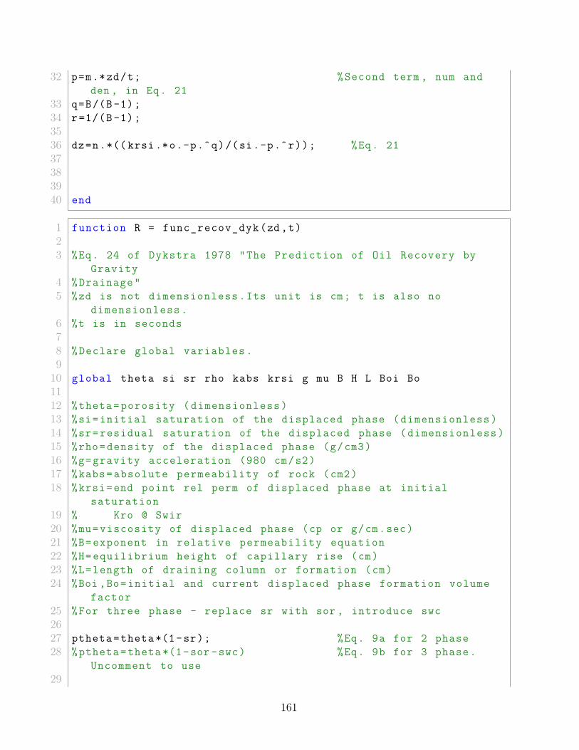
32 p=m.*zd/t; %Second term , num andden , in Eq. 21
33 q=B/(B -1);34 r=1/(B -1);3536 dz=n.*(( krsi .*o.-p.ˆq)/(si.-p.ˆr)); %Eq. 2137383940 end
1 function R = func_recov_dyk (zd ,t)23 %Eq. 24 of Dykstra 1978 "The Prediction of Oil Recovery by
Gravity4 % Drainage "5 %zd is not dimensionless .Its unit is cm; t is also no
dimensionless .6 %t is in seconds78 % Declare global variables .9
10 global theta si sr rho kabs krsi g mu B H L Boi Bo1112 %theta= porosity ( dimensionless )13 %si= initial saturation of the displaced phase ( dimensionless )14 %sr= residual saturation of the displaced phase ( dimensionless )15 %rho= density of the displaced phase (g/cm3)16 %g= gravity acceleration (980 cm/s2)17 %kabs= absolute permeability of rock (cm2)18 %krsi=end point rel perm of displaced phase at initial
saturation19 % Kro @ Swir20 %mu= viscosity of displaced phase (cp or g/cm.sec)21 %B= exponent in relative permeability equation22 %H= equilibrium height of capillary rise (cm)23 %L=length of draining column or formation (cm)24 %Boi ,Bo= initial and current displaced phase formation volume
factor25 %For three phase - replace sr with sor , introduce swc2627 ptheta=theta *(1-sr); %Eq. 9a for 2 phase28 %ptheta=theta *(1-sor -swc) %Eq. 9b for 3 phase.
Uncomment to use29
161
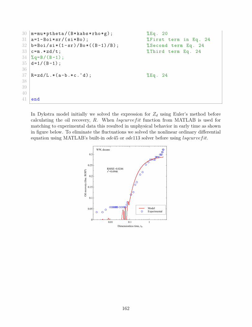
30 m=mu*ptheta /(B*kabs*rho*g); %Eq. 2031 a=1-Boi*sr/(si*Bo); %First term in Eq. 2432 b=Boi/si*(1-sr)/Bo *((B -1)/B); %Second term Eq. 2433 c=m.*zd/t; %Third term Eq. 2434 %q=B/(B -1);35 d=1/(B -1);3637 R=zd/L.*(a-b.*c.ˆd); %Eq. 2438394041 end
In Dykstra model initially we solved the expression for Zd using Euler’s method beforecalculating the oil recovery, R. When lsqcurvefit function from MATLAB is used formatching to experimental data this resulted in unphysical behavior in early time as shownin figure below. To eliminate the fluctuations we solved the nonlinear ordinary differentialequation using MATLAB’s built-in ode45 or ode113 solver before using lsqcurvefit.
WW, decane
r2=0.6946RMSE=0.0246
ModelExperimental
Oil
reco
very
(fra
c. R
OIP
)
0
0.05
0.1
0.15
0.2
0.25
0.3
Dimensionless time, tD
0.01 0.1 1
162
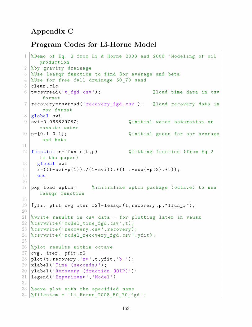
Appendix C
Program Codes for Li-Horne Model1 %Demo of Eq. 2 from Li & Horne 2003 and 2008 " Modeling of oil
production2 %by gravity drainage3 %Use leasqr function to find Sor average and beta4 %Use for free -fall drainage 50 _70 sand5 clear ,clc6 t= csvread ('t_fgd.csv '); %load time data in csv
format7 recovery = csvread ('recovery_fgd .csv '); %load recovery data in
csv format8 global swi9 swi =0.063829787; % initial water saturation or
connate water10 p=[0.1 0.1]; % initial guess for sor average
and beta1112 function r=ffun_r(t,p) % fitting function (from Eq.2
in the paper)13 global swi14 r=((1 -swi -p(1))./(1 - swi)).*(1 .-exp(-p(2) .*t));15 end1617 pkg load optim; % initialize optim package (octave) to use
leasqr function1819 [yfit pfit cvg iter r2]= leasqr (t,recovery ,p," ffun_r ");2021 %write results in csv data - for plotting later in veusz22 % csvwrite (' model_time_fgd .csv ',t);23 % csvwrite (' recovery .csv ', recovery );24 % csvwrite (' model_recovery_fgd .csv ',yfit);2526 %plot results within octave27 cvg , iter , pfit ,r228 plot(t,recovery ,'r*',t,yfit ,'b-');29 xlabel('Time ( seconds )');30 ylabel('Recovery ( fraction OOIP)');31 legend('Experiment ','Model ')3233 %save plot with the specified name34 % filestem = 'Li_Horne_2008_50_70_fgd ';
163

35 %print(filestem , '-dpng '); print(filestem , '-dpdf ');36 %print(filestem , '-dsvg ');
164
VitaIskandar Dzulkarnain, son of Dzulkarnain Abdullah and Rashidah Ismail was born in
1984 in the state of Johore, south of Malaysia. He started his B.Eng study in Electrical
and Electronics Engineering at University of Technology PETRONAS and obtained his
diploma in 2007. He continued his study in Petroleum Engineering through the joint-degree
program offered by University of Technology PETRONAS and Heriot-Watt University and
graduated with M.S. in 2010. He worked as a lecturer in the same university before joining
the doctoral program in 2013 in Craft and Hawkins Department of Petroleum Engineering
at Louisiana State University. He is expected to receive his degree of Doctor of Philosophy
in Petroleum Engineering in December 2018.
165
Related Documents