Investigation of Factors that Influence Coloration in ... · relationship between process variables and output colour. Such a relationship and optimal processing conditions were investigated

Investigation of Factors that Influence Coloration

in Polycarbonate based Compounded Plastics

by

Shahid Ahmed

A Thesis Submitted in Partial Fulfillment

of the Requirements for the Degree of

DOCTOR OF PHILOSOPHY

In

The Faculty of Engineering and Applied Science

Mechanical Engineering

University of Ontario Institute of Technology

August, 2015

©, Shahid Ahmed, 2015

ii

This research is part of:

Fundamental Studies into Causes that Influence

Colour Quality of Compounded Plastics

A Collaborative Project of

University of Ontario Institute of Technology &

SABIC Innovative Plastics Cobourg

Supported by: SABIC IP and NSERC - CRD

Principal Investigator:

Associate Prof. Dr. Ghaus M. Rizvi

Faculty of Engineering and Applied Science

University of Ontario Institute of Technology Copyright © University of Ontario Institute of Technology. All rights reserved.

.

iii

I hereby declare that I am the sole author of this thesis. This is a true copy of the thesis,

including any required final revisions, as accepted by my examiners.

I understand that my thesis may be made electronically available to the public.

iv

Abstract

Consistently producing compounded plastics in the correct colour without making

adjustments of the colour formulation or the processing conditions is very challenging for

coloured plastics manufacturers. Conversely, the principal objective of the present research

was to identify the scientific and engineering factors that directly or indirectly cause deviation

and inconsistency in the output colour of compounded plastics grades and suggest viable

solutions to prevent these colour variations.

The current study mainly focused on investigating and analysing the individual and/or

combined effect of the processing conditions on the colour and appearance of resulting

compounded plastic grades. This study highlights individual and combined influences on the

output colour, of three process parameters: temperature, screw speed and feed rate. Typical

plastic grades and associated colour formulations were selected for experimentation and

analysis in consultation with the innovation team of SABIC IP at their Cobourg plant. Included

among the selection criteria was the frequency of colour variation encountered by a plastic

grade during regular production. A wide variety of research tools and techniques were

employed in this study, these include, for example, statistical methods such as Box-Behnken

design (BBD); characterization techniques such as thermogravimetric analysis (TGA); imaging

and image analysis using scanning electron microscopy (SEM); numerical analysis of the

kneading discs zone to evaluate the mixing efficiency under varying processing conditions in

a co-rotating intermeshing twin screw extruder.

Past production data of two low Chroma opaque polycarbonate (PC) plastic grades - PC1

and PC2, were statistically analysed with the aim to quantify the influence on output colour

caused by small adjustments in colour formulation made during production. This study

revealed that the output colour is quite sensitive to minute changes in the amount of white,

black, and yellow pigments in units of PPH – parts per hundred parts of polymeric resin. A

Design of Experiments (DoE) approach was applied to develop a better understanding of the

relationship between process variables and output colour. Such a relationship and optimal

processing conditions were investigated using Box-Behnken design of response surface for

three polycarbonate resin-based plastic grades: a low Chroma translucent grade (G1), a high

Chroma opaque grade (G2), and a high luminous opaque grade (G3). The obtained

experimental results verify the fitness of the statistical model employed and suggests

processing conditions that ensure consistency in output colour of the plastic grades examined.

v

To further investigate the relationship explained by statistical analysis, a novel technique was

introduced to quantify dispersion of colour pigments in polymeric matrix under varying

processing conditions, it is based on scanning electron micrography and image analysis. A

correlation between the processing conditions and distribution graphs for pigments particle size

and inter-particle distance was established and compared with the colorimetric data. The results

obtained through these investigations could help plastics compounders achieve consistency in

plastics coloration. To visualize the flow behaviour of kneading discs zone in a co-rotating

intermeshing twin screw extruder used in experimentation, a 3D numerical analysis was carried

out using OpenFOAM® software. This study evaluates the dispersive mixing parameter λ for

a high Chroma opaque polycarbonate grade (G2) by simulating a 3-D isothermal flow pattern

in the kneading discs region of the twin screw extruder. A quasi-steady state finite element

method was implemented to avoid time dependent moving boundaries. The values of the

mixing parameter λ obtained compare the flow behaviour of the kneading discs zone under

varying processing conditions. Simulation results correlate well the input process variables

with the dispersive mixing in the zone of the kneading discs and compare well with

experimental colorimetric data.

The research work presented in this thesis significantly contributes to understanding the

influence of process variables to the extrusion process, especially of temperature, screw speed

and feed rate, on the output colour of polycarbonate resin grades.

vi

Acknowledgements

First of all, I ‘m greatly indebted to my wife- Nayyer, my son- Usama, and my lovely daughter-

Momina, for providing me the peace of mind necessary to focus on my work.

Secondly, I express my deepest respect to my upright parents, for their all-time love, prayers,

support and encouragement.

I would like to extend my profound and sincere gratitude and appreciation to my supervisors,

Dr. Ghaus M. Rizvi, and Dr. Remon Pop-Iliev, for the years of guidance, insightful advice,

support, and continuous encouragement in the development and writing of this thesis.

My special thanks and appreciation to SABIC Innovative Plastics Cobourg Plant, ON, Canada,

for providing material and financial support, and their staff members in the experimentation

and data collection.

I also express my sincere gratitude to the National Science and Engineering Research Council

for their all the years financial support.

My special thanks are also extended to my colleagues at advanced materials lab, for their moral

support, particularly to my friend, Ali Goger, for his kind help in installing and running

OpenFOAM® software.

vii

Table of Contents

Declaration …………………………………………………………………………………..iii

Abstract ………………………………………………………………………………………iv

Acknowledgements…………………………………………………………………………..vi

List of Publications …………………………………………………………………………..ix

List of Tables….....……………………………………………………………………………x

List of Fig.s ………………………………………………………………………………..xii

Chapter 1 Introduction ………………………………………………………………………1

1.1 Mixing of polycarbonate blends in twin screw extruders……………………..3

1.2 Polymeric materials …………………………………………………………6

1.3 Colorants / additives for polymeric materials…………………………………7

1.4 Colour science and the basis of colour sensation ….........................................9

1.5 3D colour space – CIE lab model ..………………………………………….15

1.6 Statistical methods and response surface methodology ……………………..16

1.7 Characterization techniques …………………………………………………19

1.8 Modelling and computer simulation ………………………………………...21

1.9 Problem Statement – Inconsistency in Plastics Coloration ………………….24

1.10 Objectives ……………………………………………………………………25

1.11 Overview of the Thesis………………………………………………………25

Chapter 2 Influence of Small Perturbations in Colour Formulation on Output Colour of

Polycarbonate-based Compounded Plastics ……………………………………27

2.1 Introduction ………………………………………………………………….27

2.2 Experimentation ……………………………………………………………..28

2.3 Results and discussion……………………………………………………….30

2.4 Conclusions ………………………………………………………………….41

2.5 Summary …………………………………………………………………….42

Chapter 3 Process Optimization through Designed Experiments to achieve Consistent

Output Color in Compounded Plastics ………………………………………..43

3.1 Introduction ………………………………………………………………….43

3.2 Experimentation ……………………………………………………………..46

3.3 Results and discussion……………………………………………………….49

viii

3.4 Conclusions ………………………………………………………………….82

3.5 Summary……………………………………………………………………..83

Chapter 4 Evaluation of Pigments Dispersion Level in Compounded Plastics using Image

Analysis Technique ……………………………………………………………..84

4.1 Introduction ………………………………………………………………….84

4.2 Materials, equipment and process …………………………………………86

4.3 Results and discussion……………………………………………………….89

4.4 Conclusions ………………………………………………………………….94

4.5 Summary……………………………………………………………………..95

Chapter 5 Numerical Analysis of Mixing Efficiency under Varying Process Conditions in

Intermeshing Co-rotating Twin Screw Extruder………………………………..96

5.1 Introduction…………………………………………………………………..96

5.2 Geometry, Material and Process Considerations…………………………….99

5.3 Simulation with OpenFOAM® …………………………………………….101

5.4 Results and discussion.……………………………………………………..104

5.5 Conclusions ..………………………………………………………………107

5.6 Summary……………………………………………………………………107

Chapter 6 Contribution and Recommendations…………………………………………..109

6.1 Contribution ………………………………………………………………..109

6.2 Recommendations …………………………………………………………110

Bibliography ……………………………………………………………………………….xv

ix

List of Publications

1. S. Ahmed, J. AlSadi, U. Saeed, G. Rizvi, D. Ross, R. Clarke and J. Price, “Process

optimization through designed experiments to achieve consistency in output color of a

compounded plastic grade” Quality Engineering, 27 (2), pp. 144-160, April 29, 2015.

2. S. Ahmed, J. AlSadi, U. Saeed, G. Rizvi, D. Ross, R. Clarke and J. Price, “Implementation

of Box-Behnken design for optimizing compounding process ensuring consistent output colour

of a polycarbonate grade” Quality Engineering, 2015 (submitted; Rev1 under review).

3. S. Ahmed, R. Pop-Iliev, G. Rizvi, “Effect of process variables on pigments dispersion in

compounded plastics” SPE Antec2015, Orlando, 2015.

4. S. Ahmed, R. Pop-Iliev, G. Rizvi, “Experimental study to investigate optimal process

conditions for consistency in coloration of a compounded plastic grade” SPE Antec2015,

Orlando, 2015.

5. S. Ahmed, R. Pop-Iliev, G. Rizvi, “Evaluating pigment dispersion for better color in

plastics” Plastics Research Online, SPEPRO, April 13, 2015.

http://www.4spepro.org/view.php?article=005884-2015-04-07&category=Injection+Molding

6. J. AlSadi, U. Saeed, S. Ahmad, G. Rizvi, and D. Ross, “Processing issues of color

mismatch: rheological characterization of polycarbonate blends” Polymer Engineering and

Science, Dec 2014. http://onlinelibrary.wiley.com/doi/10.1002/pen.24041/abstract

7. U. Saeed, J. AlSadi, S. Ahmad, G. Rizvi, and D. Ross, “Neural Network: a potential

approach for error reduction in color values of polycarbonate” Adv In Poly Tech, 33 (2), 2014.

8. S. Ahmed, J. AlSadi, U. Saeed, G. Rizvi, and D. Ross, “Effect of small perturbations in

colour formulation on output colour of a plastic grade compounded with two polycarbonate

resins” SPE Antec2013, Cincinnati, 2013.

9. S. Ahmed, J. AlSadi, U. Saeed, G. Rizvi, D. Ross, R. Clarke and J. Price, “Effect of small

perturbations in colour formulation on output colour of a plastic grade compounded with two

polycarbonate resins” SPE Antec2013, Cincinnati, 2013.

10. S. Ahmed, J. AlSadi, U. Saeed, G. Rizvi, and D. Ross, “A study on effect of small

perturbations in colour formulation on output colour of a plastic grade compounded with a

single polycarbonate resin” SPE Antec2012, Orlando, 2012.

x

List of Tables

Table 1.1: Requirements for colorants

Table 1.2: A comparison between organic and inorganic pigments

Table 2.1: Reference Colour Formulation – PC1

Table 2.2: Percent adjustments made in reference formulation during production – PC1

Table 2.3: Reference Colour Formulation – PC2

Table 2.4: Percent adjustments made in reference formulation during production – PC2

Table 2.5: ANOVA for ∆L*, ∆a* and ∆b*

Table 2.6: ANOVA Results of ∆L*, ∆a* and ∆b*

Table 3.1: Designed Experimental Runs and Colour Data – Grade G1

Table 3.2: Designed Experimental Runs and Colour Data – Grade G2

Table 3.3: Designed experimental runs and colour data – Grade G3

Table 3.4: Colour Formulation – Grade G1

Table 3.5: Colour Formulation – Grade G2

Table 3.6: Colour Formulation – Grade G3

Table 3.7: ANOVA Results for L*, a* and b*

Table 3.8: Final equations in terms of actual factors

Table 3.9: Predicted Mean vs. Experimental Colour Data - Confirmatory Test

Table 3.10: Predicted Mean vs. Experimental Colour Data - Delta Values

Table 3.11: Criterion Set for Process Optimization

Table 3.12: List of Optimal Solutions for Input Factors

Table 3.13: ANOVA results for L*, a* and b*

Table 3.14: Final equations in terms of actual factors

Table 3.15: Predicted Mean vs. Experimental Colour Data – Confirmatory Test

Table 3.16: Criterion Set for Process Optimization

Table 3.17: List of Optimal Solutions for Input Factors

Table 3.18: ANOVA results for L*, a* and b*

Table 3.19: Final equations in terms of actual factors

Table 3.20: Confirmation DoE results - predicted and experimental colour data

Table 3.21: Optimization criteria set to reach the target

Table 3.22: Three Solutions from Process Optimization

Table 4.1: Colour Standard Formulation

Table 4.2: Designed Experimental Runs and Colour Data

xi

Table 4.3: Pigments Particle Size Distribution

Table 4.4: Inter-Particle Distance Distribution

Table 5.1: Technical Data ZSK26 Twin Screw Extruder

Table 5.2: Material Properties and Processing Conditions

Table 5.3: Boundary Conditions for Velocity and Pressure

Table 5.4: Mixing parameter values for simulated cases

Table 5.5: Mixing parameter values vs measured colour coordinates

xii

List of Fig.s

Fig. 1.1: A cross-sectioned view of an extruder with extrusion process flow chart [10]

Fig. 1.2: A schematic view mixing operation in extruders and mixing elements [8]

Fig. 1.3: Classification of twin screw extruders [7]

Fig. 1.4: Visible spectrum of sunlight [22]

Fig. 1.5: Cross section of human eye [19]

Fig. 1.6: Magnified view of fovea near center of human eye retina [19]

Fig. 1.7: Spectral power distribution of daylight [19]

Fig. 1.8: Incident light and spectral reflectance curve of a red ball [19]

Fig. 1.9 CIE Lab Model – (a) Cartesian Notation L*a*b*, (b) Polar Notation L*C*h°

[22]

Fig. 2.1: Desirability with yellow and black pigments

Fig. 2.3: Perturbation graph of desirability

Fig. 2.4: Perturbation graph of ∆L*

Fig. 2.5: Perturbation graph of ∆a*

Fig. 2.6: Perturbation graph of ∆b*

Fig. 2.7: Contour graph of ∆L*

Fig. 2.8: Contour graph of ∆a*

Fig. 2.9: Contour graph of ∆b*

Fig. 2.10: Desirability with yellow and black pigments

Fig. 2.11: Perturbation graph of desirability

Fig. 2.12: Perturbation graph of ∆L*

Fig. 2.13: Perturbation graph of ∆a*

Fig. 2.14: Perturbation graph of ∆b*

Fig. 2.15: Contour graph of ∆L*

Fig. 2.16: Contour graph of ∆a*

Fig. 2.17: Contour graph of ∆b*

Fig. 3.1: Evaluation of FDS and d for error type “Diff”

Fig. 3.2: Evaluation of FDS and d for error type “Pred”

Fig. 3.3: POE (a*) plot with factor B at Mid-Point

Fig. 3.4: POE (b*) plot with factor B at Mid-Point

Fig. 3.5: Perturbation plot for L*

xiii

Fig. 3.6: 2FI graphs affecting L* using ANOVA noise estimate (left), experimental error

(right)

Fig. 3.7: Contour plot for L* slicing along factor B

Fig. 3.8: L* values of confirmatory test

Fig. 3.9: a* values of confirmatory test

Fig. 3.10: b* values of confirmatory test

Fig. 3.11: Bar graph displaying individual and combined desirability level of variables and

POEs

Fig. 3.12: Graphical optimization and sweet spot flagged for a desired solution

Fig. 3.13: 3D surface graph flagged with optimal desirability

Fig. 3.14: 2D contour graph flagged with optimal desirability

Fig. 3.15: Perturbation graph for L*

Fig. 3.16: POE (L*) plot with factor B and C at Mid-Point

Fig. 3.17: POE (a*) plot with factor B and C at Mid-Point

Fig. 3.18: POE (b*) plot with factor B and C at Mid-Point

Fig. 3.19: 2FI graphs affecting L* using ANOVA noise estimate (left), experimental error

(right)

Fig. 3.20: Contour plot for L* slicing along Factor B

Fig. 3.21: Desirability levels for 4th optimal solution – Table 3.17

Fig. 3.22: Graphical optimization and sweet spot flagged for selected optimal solution –

Table 3.17

Fig. 3.23: L* values of verification test

Fig. 3.24: Evaluation of FDS and d for error type Diff

Fig. 3.25: Evaluation of FDS and d for error type Pred

Fig. 3.26: Perturbation plot for L*

Fig. 3.27: Interaction b/w factors C and B affecting b*

Fig. 3.28: Contour plot for L* slicing along factor B

Fig. 3.29: (a) POE (L*) transmitted by temperature; (b) POE (a*) transmitted by

temperature; (c) POE (b*) transmitted by temperature

Fig. 3.30: 3rd optimal solution flagged in sweet spot

Fig. 4.1: Schematic of moulded chip and sample for thin sections

Fig. 4.3: ESEM image @ 5000x - Run 17 sample chip: Top layer (a); Centre layer (b)

Fig. 4.4: Particle size distribution graph - top layers

xiv

Fig. 4.5: Particle size distribution graph - centre layers

Fig. 4.6: Nearest neighbour distance graph - top layers

Fig. 4.7: Nearest neighbour distance graph - centre layers

Fig. 4.8: Colour data of samples and the standard reference – CIE Lab colour space

Fig. 4.9: Colour difference between samples and the standard reference

Fig. 4.10: Spectral Curves: reflectance intensity @ full visible spectrum (a); @ red

spectrum (b)

Fig. 5.1: Kneading discs staggered at 45° in forward (right handed) configuration

Fig. 5.2: Mesh view in z-direction with ParaFoam®

Fig. 5.3: Sequential geometries for a complete rotation of kneading discs staggered at 45°

Fig. 5.4: 3D Distribution graph of mixing parameter λ – R7

Fig. 5.5: 3D Distribution graph of mixing parameter λ – R17

1

Chapter 1

Introduction

A recent industry profile provided by Canadian Plastics Industry Association-CPIA,

indicates there are 95,400 employees enlisted on Canada’s plastics industry payroll. Industry

comprises over 3,170 companies, most of which are Canadian owned, and represents a $29.2

billion industrial sector, which is sophisticated, multi-faceted and embraces plastic products

manufacture, machinery, moulds and resins. Plastics industrial sector plays a vital role in

Canada’s global competitiveness, which is becoming more challenging due to increasing trend

in plastic products usage both as consumer goods and in advanced applications such as

telecommunication, electronics, aviation and aerospace, medicine and life sciences, building

materials, automotive, and renewable energy. It also plays a significant role in reduction of

greenhouse gases, for example products made from plastics are light weight that translates into

less fuel consumption during transportation, their insulation, packaging and recyclability

characteristics significantly add to fuel saving. Recent studies revealed if plastics were to be

replaced with alternative materials across the whole Europe, it would require an additional 10%

fuel or equivalently 25 million tonnes of crude oil, which corresponds to 105 million tonnes of

CO2 greenhouse gas emission per year. Similarly plastics packaging alone claims 582.6 million

gigajoules of energy saving per year. A recent study by University of Toronto found replacing

of old water pipes with plastic pipes would help Canada to achieve 10% of its Kyoto reduction

targets. Industry as a whole is concentrated in Ontario, Quebec, British Columbia and Alberta,

however Ontario is the largest plastics producing region in Canada and third largest in North

America after California (No.1) and Ohio (No.2) [1].

North American plastic industry experienced both a substantial growth over the past

decade and adverse effects imposed by recent economic recession and tight profit margins.

North American compounding industry members, however, have an optimistic view of the

changing paradigm and see the industry survival in providing innovative solutions for North

American markets and expanding globally. They further realize mere innovative solutions

would not suffice in maintaining a competitive edge as industry leader, cost effectiveness must

compliment innovative solutions. Avoidance of waste is the key to cost effectiveness, which is

also a driving philosophy in lean manufacturing / compounding. One key characteristics of

plastics is their availability in a wide array of colours to meet aesthetic as well as functional

needs. Over the time, producing plastics with consistent output colour and minimal wastage

2

has imposed a greater challenge to plastic compounders particularly those who manufacture

coloured plastics in large quantities to feed plastic processing industry such as automotive or

develop prototypes / master-batches in small lots at short lead times to cater for innovation and

changing market needs. The challenge becomes even bigger under world’s weak economic

conditions, increasing prices of raw materials - resins, pigments and additives, and higher costs

of energy, packaging, equipment parts and transportation. Such difficult times, however,

should encourage plastic compounders to find new ways along with continued creativity and

innovation to help their customers manage cost [2~4].

One of the many plastic compounders confronting the challenge of having inconsistency

in output colour of compounded plastics, is SABIC Innovative Plastics (IP), formerly known

as GE Innovative Plastics - a world recognized industry leader, at its manufacturing plant in

Cobourg, Ontario. With 15 production lines and one technology line SABIC IP has developed

its capability to produce about 200 batches a day with different grades and colours of

compounded plastics. A core component of SABIC’s Cobourg plants business is the supply of

tailored plastics with customer specified colours at short order times. Companies like SABIC

play a significant role in rapid development of prototypes to facilitate innovation and maintain

a competitive edge in global market. Manufacturing coloured plastics with correct colour in

one-go during production is critical to such operations as minute deviation from target colour

could cause rejection of the entire production lot. Therefore SABIC IP decided to collaborate

with University of Ontario Institute of Technology (UOIT) with the aim to investigate scientific

reasons that cause colour deviation in compounded plastics and then develop methods to

prevent or reduce it [5].

Present research undertakes fundamental studies of compounding process and associated

auxiliary processes such as preparing colour formulation, and injection molding of test samples

(rectangular plaques) as practiced at SABIC IP Cobourg plant for manufacture of coloured

plastics. Aim was to identify factors involved directly or indirectly causing deviation and

inconsistency in output colour during compounding, and suggest viable solutions to prevent

these colour variations. Various factors were short listed for a detailed and comprehensive

investigation of their individual and/or combined effect on colour and appearance of

compounded plastic grades. However current study mainly focused on processing conditions

to see their impact on output colour. Various techniques employed in this study include

statistical methods such as Box-Behnken design (BBD) [6], characterization techniques such

3

as thermogravimetric analysis (TGA), and imaging and image analysis using scanning electron

microscopy (SEM), and numerical analysis of the kneading discs zone to evaluate mixing

efficiency under varying processing conditions in a co-rotating intermeshing twin screw

extruder. Typical plastic grades and associated colour formulations were selected for

experimentation and analysis in consultation with innovation team of SABIC IP at their

Cobourg plant. Included among the selection criteria was the frequency a colour variation

encountered by a plastic grade during regular production.

Polymer blending has been extensively studied and numerous publications are available

to address various aspects of these systems. The literature on plastics coloration however, is

not frequently available particularly about compounding. One of the main objectives of this

research was to develop basic understanding of the entire compounding process, and

investigate factors behind colour deviation implementing various statistical and

characterization techniques. Therefore, fundamental ideas about colour and its measurement,

compounding process and equipment, and colour pigments are discussed in following sections.

1.1 Mixing of polycarbonate blends in twin screw extruders

Constantly increasing demands on plastic products need constant refinement in their

properties, therefore, deliberate modification in properties of a base polymer by blending with

additives and/or with other polymers is becoming increasingly important. The process of

blending polymer resins with colorants and additives in specific proportions using extruders to

produce plastics with desired properties is recognized as compounding, and the plastics

produced as compounded plastics. The word “compounding” is used because a compound

distinguishes from a mixture in that its constituents lose their individual characteristics adding

new characteristics such as colour, surface appearance, impact strength, flexural stiffness,

dielectric strength, conductivity, and flame retardancy [7 ~ 9]. In a broader sense, mixing is a

process of reducing non-uniformity of a composition, however basic mechanism is to induce

physical relative movement of ingredients. Types of motion that can happen in mixing include

molecular diffusion, turbulent motion and convective motion. First two types essentially are

limited to gases and low viscosity liquids. Convective motion is specific to high viscosity

liquids such as polymer melts. Because of their high viscosity polymer melts are capable of

only laminar flow. Convective mixing by laminar flow is termed as laminar mixing and this is

the type of mixing that occurs in polymer melt extrusion. Mixing action is generally described

by shear flow and elongational flow. Now if the ingredients to be mixed are compatible fluids

4

and exhibit no yield point, the mixing is distributive, however if a component of the mixture

exhibits a yield stress then actual stresses involved in the process become very important. Now

if one or more components in a polymer melt showing up yield point are solid, then this type

of mixing is referred to as dispersive mixing, sometimes as intensive mixing. Dispersive

mixing involves breakdown of solid component but that could happen only when yield stress

exceeds a certain limit. If the component exhibiting yield point is a liquid, the process of mixing

is termed as homogenization. Manufacture of colour concentrate can be taken as an example

of dispersive mixing, where breakdown of colour pigment agglomerates below a certain critical

size is of great significance. An example of distributive mixing is the manufacture of polymer

blend, where two or more compatible polymers of different melt flow index (MFI) are mixed

in molten state and none of the component exhibits yield point. Physically, the distributive and

the dispersive mixings are not separated from each other, in fact dispersive mixing is always

followed by distributive mixing, however reverse is not always true. Dispersive mixing can

occur after distributive mixing only if a solid component has a yield point and the applied stress

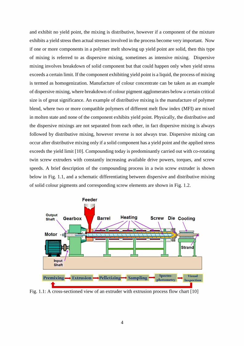
exceeds the yield limit [10]. Compounding today is predominantly carried out with co-rotating

twin screw extruders with constantly increasing available drive powers, torques, and screw

speeds. A brief description of the compounding process in a twin screw extruder is shown

below in Fig. 1.1, and a schematic differentiating between dispersive and distributive mixing

of solid colour pigments and corresponding screw elements are shown in Fig. 1.2.

Fig. 1.1: A cross-sectioned view of an extruder with extrusion process flow chart [10]

5

Fig. 1.2: A schematic view of mixing operation in extruders and mixing elements [8]

Extruders are widely used not only in plastics industry, but also in petrochemical and

food industries for melting, mixing, blending, reacting, devolatilizing and numerous other

tasks. Based on number of screws they are classified into two types: single screw and twin

screw extruders (TSEs). In single screw extruders, extrusion process and conveying mechanism

are highly dependent on frictional and viscous properties of material. In TSEs however, these

properties play a lesser role on conveying behaviour.

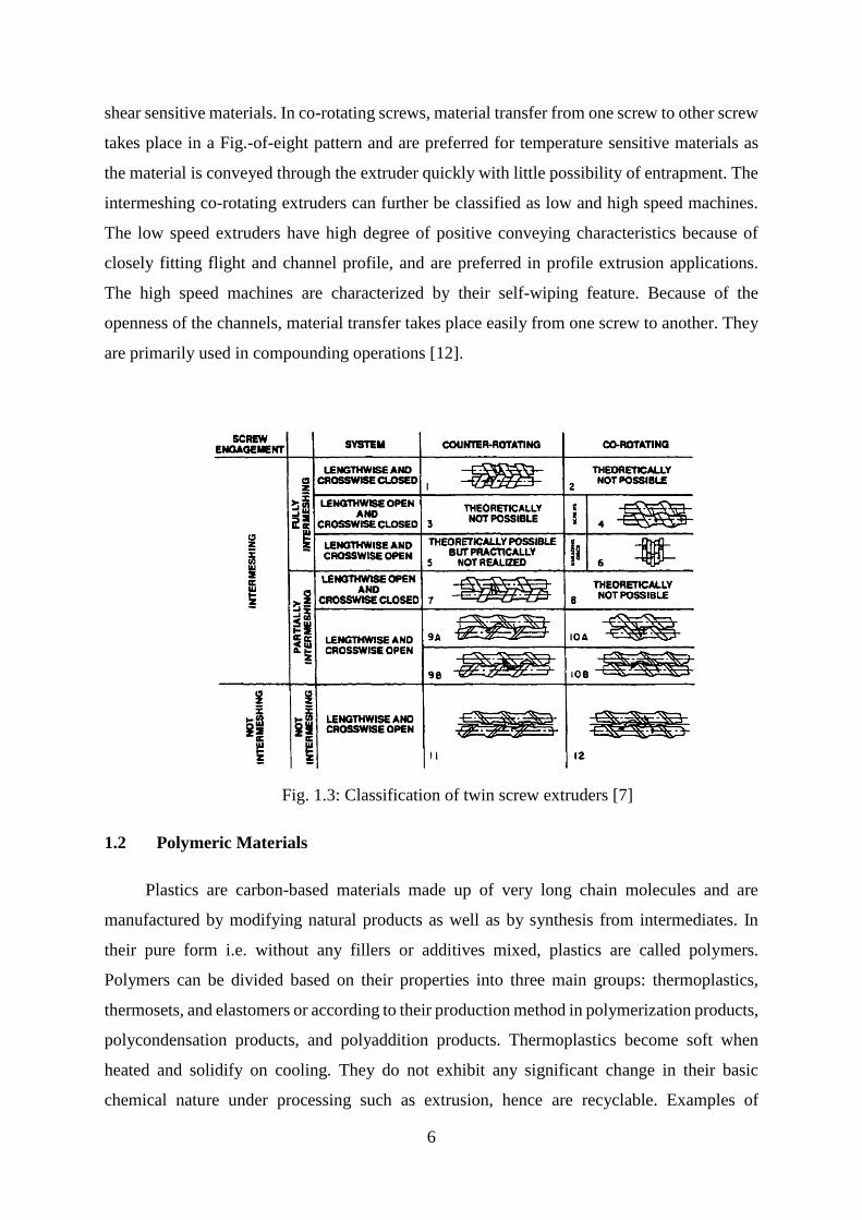
TSEs can be designed in various configurations, however main classification is made if

the screws are intermeshing or non-intermeshing, and whether co-rotating or counter-rotating.

A description of the classification is shown below in Fig. 1.3. The non-intermeshing TSEs do

not have the benefit of positive conveying characteristics as no protrusion exists between the

flights of one screw and the channels of the other screw. In intermeshing TSEs, flights of one

screw protrude into the channels of other screw and their positive conveying characteristics

depends upon the degree of intermeshing that ranges from fully intermeshing to partially

intermeshing (in some cases near to non-intermeshing).

As regards classification due to direction of screw rotation, in counter-rotating extruders,

material is sheared and pressurized in a mechanism quite similar to calendering where a

material is effectively squeezed between two counter rotating rolls [11], and are preferred for

6

shear sensitive materials. In co-rotating screws, material transfer from one screw to other screw

takes place in a Fig.-of-eight pattern and are preferred for temperature sensitive materials as

the material is conveyed through the extruder quickly with little possibility of entrapment. The

intermeshing co-rotating extruders can further be classified as low and high speed machines.

The low speed extruders have high degree of positive conveying characteristics because of

closely fitting flight and channel profile, and are preferred in profile extrusion applications.

The high speed machines are characterized by their self-wiping feature. Because of the

openness of the channels, material transfer takes place easily from one screw to another. They

are primarily used in compounding operations [12].

Fig. 1.3: Classification of twin screw extruders [7]

1.2 Polymeric Materials

Plastics are carbon-based materials made up of very long chain molecules and are

manufactured by modifying natural products as well as by synthesis from intermediates. In

their pure form i.e. without any fillers or additives mixed, plastics are called polymers.

Polymers can be divided based on their properties into three main groups: thermoplastics,

thermosets, and elastomers or according to their production method in polymerization products,

polycondensation products, and polyaddition products. Thermoplastics become soft when

heated and solidify on cooling. They do not exhibit any significant change in their basic

chemical nature under processing such as extrusion, hence are recyclable. Examples of

7

thermoplastics materials include polystyrene (PS), polyethylene (PE), polypropylene (PP) and

polycarbonate (PC) – the one studied in this research. Thermosets on the other hand become

hard when heated above a certain temperature. This hardening happens because of a curing or

crosslinking reaction that bonds individual polymer molecules together causing the formation

of a three dimensional network. This network remains intact upon cooling because crosslinking

is irreversible and that is why thermosets cannot be recycled like thermoplastic materials.

Thermosets usually are shaped by processing them below curing or crosslinking temperatures.

Elastomers or rubbers are materials that exhibit very large deformations under applied force

while behaving in a largely elastic manner. They regain their shape and size completely or

mostly when the applied force is removed. Thermoplastics can further be classified as

amorphous and semi-crystalline plastics. Amorphous materials are designated by their random,

irregular molecular structure without any crystalline regions. Examples are PC, PS, acrylic

(PMMA), acrylonitrile butadiene styrene (ABS), and polyvinylchloride (PVC). Semi-

crystalline thermoplastics can form highly regular regions called crystallites where molecules

come together to form crystals. Formation of crystals depends upon shape of the polymer

molecules. Plastics having linear molecular structure without large side-groups can form

crystallites e.g. high density polyethylene (HDPE). HDPE can achieve as high a level of

crystallinity as 90%. Polystyrene on the other hand cannot form crystallites due to having bulky

side-groups [13~15].

1.3 Colorants / Additives for Polymeric Materials

Principally all substances that can be used in polymers coloration, are defined as colorant.

The colorants can be divided based on their chemical nature into two groups: inorganic

colorants and organic colorants. They can further be classified as pigments and dyes; if a

colorant is insoluble in polymer it is defined as a pigment and if it is soluble in polymer it is a

dye. However definition of a colorant as pigment is not always true because there are some

organic pigments such as Pigment red 254 (DPP-Red) that dissolve in some polymers but are

insoluble in most of the polymers. Pigment red 254 dissolves in PC at temperatures above

approx. 330°C behaving like a dye. A colorant can be used as a colorant for polymers if it meets

the requirements as listed below in Table 1.1. However depending on the intended use of

coloured polymer a compromise is possible and quite normal in meeting the requirements.

Because, practically only few colorants can fulfil all the requirements and on the other hand

experience shows that not every coloured polymer requires the colorant to fulfil all the

8

requirements. Inorganic and organic pigments can be used to colour all types of polymers.

Inorganic and organic pigments can be used in all types of polymers, however heat stability

should be good enough in the polymer to be coloured. Use of dyes on the other hand is limited

to amorphous polymers with high glass transition temperature such as PS, PC, and PMMA etc.

A comparison of properties between inorganic and organic pigments is also presented in Table

1.2.

Inorganic pigments are available in numerous variations even though have only a few

basic chemical formulas. They can be classified by either their chemical composition or by

colour. Broad categories include pigments consisting of pure elements, oxide pigments,

hydroxide pigments and complex inorganic pigments consisting of mixed phase metal oxides

etc. Worldwide discussion on “heavy metals in our environment” has restricted the use of

pigments to only those that are free from lead and cadmium [13, 16, 17]

Table 1.1: Requirements for colorants

S.No. Requirements for pigments Requirements for dyes

1 High hiding power -

2 Good dispersibility Good solubility

3 High heat stability High heat stability

4 High tinting strength High tinting strength

5 Good fastness properties

(light/weather)

Good fastness properties

(light/weather)

6 No migration No migration

7 No warpage No sublimation

8 Toxicologically safe Toxicologically safe

Table 1.2: A comparison between organic and inorganic pigments

Property Organic pigments Inorganic pigments

Density Low, mostly < 2.5 g/cm3 High, mostly > 2.5 g/cm3

Particle size Mostly < 1μm, thereby high specific

surface area

Mostly >1μm, thereby

low specific surface area

Tendency to form

agglomerates

High Low

Dispersibility Not very good Much better

Solubility Partial solubility, depends on

concentration

Totally insoluble

Transparency High, thereby low hiding power Low, thereby high hiding

power

Tinting strength High, good brilliance Low, mostly not brilliant

Heat fastness Limited, sometimes low Very high

Light fastness Limited, sometimes low Very good

Warpage Sometimes very strong None

9

Other than colorants, additives are most commonly used materials in plastics blends to

improve various properties. The selection and use of additives are determined by the property

to be improved. Most important additives are listed below with their names reflecting against

specific function [14, 15, 18].

Antistatic Agent

Flame retardant

Filler

Dispersing agents / lubricant / release agent

Nucleating agent

Stabilizer

Blowing agent

Plasticizer

All these additives neither are chemically inert nor can their interactions with colorants

be excluded. To predict the effect whether positive or negative on colorants caused by these

interactions is almost impossible.

1.4 Colour Science and the Basis of Colour Sensation

Colour can be seen as an essential part of our life that influences our bodies, our minds

and our souls. Our response to colour whether physiological, psychological or emotional has

been studied in great detail. Over time the appeal of various colours changes, which leads to

new colour trends in market place. In the presence of new colorant and special effect

technologies, our colour choices and preferences continually evolve. Studying colour

perception and trends provides us a better understanding of the market place. Basically a colour

results from an interaction between light, object, and the viewer. It is in fact the light that is

modified by an object in a manner that the viewer i.e. human eye perceives the modified light

as a distinct colour. All three elements must be present for a colour to exist [13, 19~22].

To understand what exactly a colour means, first we need to know the basis of colour

sensation by human eye. Daylights both natural and artificial are composed of wide range of

electromagnetic waves such as radio waves, ultraviolet, X-rays etc. By nature they all are same,

differing solely in their wavelength and frequency. From this very wide spectrum of

wavelengths, only a small fraction between 400 and 700 nm is visible. Visible white sunlight

10

as shown below in Fig. 1.4, consists of a mixture of colours ranging from red to violet as

discovered first time by Sir Isaac Newton with his famous prism experiment.

Fig. 1.4: Visible Spectrum of Sunlight [22]

When sunlight is incident on an object, a portion of it is absorbed by the object and rest

is reflected back. The absorbed portion is transformed into heat and practically speaking is lost

for sensation of colour. The reflected part however is detected by the human eye and after

passing through pupil and lens impinges on the retina, where an inverted image of the object is

formed. The retina contains two different types of cells, the so-called rods and cones as shown

in the Fig. 1.5. Rods are not sensitive to colour i.e. hue and can only differentiate between light

and dark. Cones however are pretty sensitive to colour and found in three types differing in

their maximum spectral sensitivity to colours. One group of cones is sensitive to reds, another

to greens, and third to blues as can be seen in the Fig. 1.6. At this point it is pertinent to mention

that all colorimetric measurement methods find their basis in these three colours - RGB plus a

light-dark differentiation. These sensors i.e. cones and rods send electrical signals in unique

patterns to the brain, which processes the signals into sensation of sight i.e. of light as well as

of colour. This means colour is the brain’s interpretation of a mixture of these stimuli i.e. red,

green and blue. Reflected part of sunlight is just a fraction of the whole spectrum, and based

upon the wavelengths and intensity the reflected part owns, we see a definite colour. The object

11

that reflects 100% of the light is seen as white and the one that absorbs 100% of the light

appears black. There is a small pit named fovea located almost in middle of the retina. Fovea

is the portion of retina that has only cones in it, so maximum information about the colour i.e.

hue is sensed here and sent to the brain. Angle of view that it forms with the lens is 2 degree

that is where 2 degree observer is originated from. However later on a 10 degree observer was

introduced by CIE and is considered more accurate. Reason being that if we stare at our

thumbnail located at arm’s length, it’s almost impossible to see it alone, you also see some of

the surrounding that makes your angle of view obviously bigger than that you are trying to

focus on [13].

Fig. 1.5: Cross Section of Human Eye [19]

Fig. 1.6: Magnified View of Fovea near Center of Human Eye Retina [19]

Like other senses such as hearing or taste, our colour vision varies individual to

individual, in some cases more obviously such as colour blindness. Capability to perceive a

12

colour is closely associated to individual differences in sensitivity of human eyes. This

important fact, when final plastic specimen of matched colour is inspected only visually, has

been a point of long discussions not only between customer and supplier but also among the

experts within supplier’s own quality assurance wing. That is why having same person

involved in final visual inspection is highly recommended. Such controversies eventually led

to development of different colorimetric systems involving instruments such as

spectrophotometers. The most often used system is CIE Lab; others are Munsell and Hunter

Lab. These systems are valuable tools to measure a colour, however are not able to perfectly

describe what we see and cannot be a substitute to visual judgment. However in order to fully

understand the scientific basis to derive a colour measuring system being used by instruments,

one needs to understand the three components - elements of colour, necessary to see a colour:

the light source, the object interacting with light, and the receiver that views and interprets

colour of the object. If any of the elements is missing we will not be able to see any colour [13,

19~22].

1.4.1 Light Source

Colour is light and the light is energy that travels in straight lines at a speed of 299,792458

meters per second. Various physical light sources such as sunlight, incandescent lamp, candle

etc. have specific spectral power distribution (SPD) i.e. energy levels associated to individual

wavelengths on their emission spectrum of light. Mathematical description of the relative

spectral power distribution of physical light source is termed as illuminant. Various standard

illuminants such as A, C, D65, D55, D75, F2 etc. to simulate physical light sources have been

described by global standards committee comprising mainly of CIE, ASTM and DIN. A careful

and proper implementation of these standard illuminants in software application or in

instrument firmware has allowed companies to build today’s modern colour measuring devices,

which are used for an accurate and standard evaluation of the object colour. A brief description

of the relative spectral power distribution of various light sources is given below:

Spectral power distribution of daylight is biased towards blue as shown in the Fig. 1.7,

which is a measurement of light energy on a clear day. This bias is caused by selective

absorption and scattering of high energy shorter wavelength violet and blue light in the upper

atmosphere, which makes our sky a clear blue canopy. Daylight varies in three different ways

as illustrated in Fig. 1.7. The Daylight near sunrise or sunset contains comparatively less blue

energy than red because the light has to pass through a longer slice of atmosphere causing more

13

absorption of blue light. It’s relative spectral power distribution that can be represented by a

blackbox illuminant at 5500K (D55). The daylight close to noon is represented by 6500K

(D65) and illustrates a SPD of noon when both the sky and sun together light us resulting into

a higher blue energy than that near sunrise or sunset. Near noon SPD designated with 7500K

(D75), represents the day time near noon with the sun may have gone out of sight and only

blue canopy of the sky is illuminating us. In conclusion, the SPD denoted by a low temperature

i.e. D55, will have deep red, however apparent red shifts to yellow, then whiteness, and finally

blues for SPDs designated by D65 and D75 respectively. Therefore, it is of great importance

to know various light conditions under which an object is expected to be viewed and how it

would respond to various light conditions. Light booths are the tools that can simulate various

light conditions and can be used to analyse the apparent colour of an object [19, 22].

Fig. 1.7: Spectral power distribution of daylight [19]

One more point, which is worth-mentioning, is CRI – colour rendering index. CRI ranges

from 0 to 100. CRI is used to compare two lights that have same temperature, e.g. for the same

temperature, Xenon source light has a CRI of approx. 100 whereas that of a mercury vapour

lamp goes below 20. Manufacturers of fluorescent, metal halide and other non-incandescent

lighting equipment mostly use CRI to describe visual effects of light on coloured surfaces.

Again the bottom line is while analysing or predicting apparent colour of an object to have

standard lighting conditions is important [13, 19].

14

1.4.2 Object

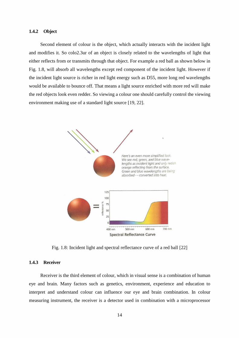
Second element of colour is the object, which actually interacts with the incident light

and modifies it. So colo2.3ur of an object is closely related to the wavelengths of light that

either reflects from or transmits through that object. For example a red ball as shown below in

Fig. 1.8, will absorb all wavelengths except red component of the incident light. However if

the incident light source is richer in red light energy such as D55, more long red wavelengths

would be available to bounce off. That means a light source enriched with more red will make

the red objects look even redder. So viewing a colour one should carefully control the viewing

environment making use of a standard light source [19, 22].

Fig. 1.8: Incident light and spectral reflectance curve of a red ball [22]

1.4.3 Receiver

Receiver is the third element of colour, which in visual sense is a combination of human

eye and brain. Many factors such as genetics, environment, experience and education to

interpret and understand colour can influence our eye and brain combination. In colour

measuring instrument, the receiver is a detector used in combination with a microprocessor

15

programmed to understand and interpret the colour viewed by detector. In other words,

eye/brain combination is replaced with a colorimeter or spectrophotometer. For an instrument

to be effective, it must see in a manner similar to the human eye so the colour data produced

makes good sense to the operator [19, 22].

1.5 3D Colour Space - CIE Lab Model

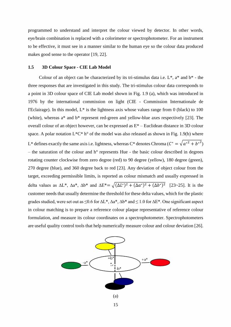
Colour of an object can be characterized by its tri-stimulus data i.e. L*, a* and b* - the

three responses that are investigated in this study. The tri-stimulus colour data corresponds to

a point in 3D colour space of CIE Lab model shown in Fig. 1.9 (a), which was introduced in

1976 by the international commission on light (CIE - Commission Internationale de

I'Eclairage). In this model, L* is the lightness axis whose values range from 0 (black) to 100

(white), whereas a* and b* represent red-green and yellow-blue axes respectively [23]. The

overall colour of an object however, can be expressed as E* – Euclidean distance in 3D colour

space. A polar notation L*C* h° of the model was also released as shown in Fig. 1.9(b) where

L* defines exactly the same axis i.e. lightness, whereas C* denotes Chroma (𝐶∗ = √𝑎∗2 + 𝑏∗2)

– the saturation of the colour and h° represents Hue - the basic colour described in degrees

rotating counter clockwise from zero degree (red) to 90 degree (yellow), 180 degree (green),

270 degree (blue), and 360 degree back to red [23]. Any deviation of object colour from the

target, exceeding permissible limits, is reported as colour mismatch and usually expressed in

delta values as ∆L*, ∆a*, ∆b* and ∆E*= √(∆𝐿∗)2 + (∆𝑎∗)2 + (∆𝑏∗)2 [23~25]. It is the

customer needs that usually determine the threshold for these delta values, which for the plastic

grades studied, were set out as ≤0.6 for ∆L*, ∆a*, ∆b* and ≤ 1.0 for ∆E*. One significant aspect

in colour matching is to prepare a reference colour plaque representative of reference colour

formulation, and measure its colour coordinates on a spectrophotometer. Spectrophotometers

are useful quality control tools that help numerically measure colour and colour deviation [26].

(a)

16

(b)

Fig. 1.9: CIE Lab Model - (a) Cartesian Notation L*a*b* (b) Polar Notation L*C*h° [22]

1.6 Statistical Methods and Response Surface Methodology (RSM)

Understanding the relationship between input process variables and final output colour

of compounded / moulded plastic part is critical for consistency and reproducibility of response

attributes of a process. Statistical methods are frequently used by researchers, to investigate

and optimize the effect of process variables on responses such as colour and appearance of

compounded plastics. For this purpose, they employ various statistical designs and models to

fit in the response data obtained through designed experiments or past production data. Effertz

[27] investigated a PVC sheet for the effect of processing conditions on its gloss and surface

appearance using modified general factorial model. Bender [28] investigated the process

variables causing high viscosity variability in wood-fiber compounds by executing Box-

Behnken design (BBD). With Statistica®, Eric et al [29] executed a design of experiments

(DoE) for 1/8th fractional factorial design to investigate the effect of seven process variables

including barrel and mould temperature, injection speed, screw speed, pack and hold pressure,

on five output parameters: tri-stimulus colour data, gloss and part weight.

17

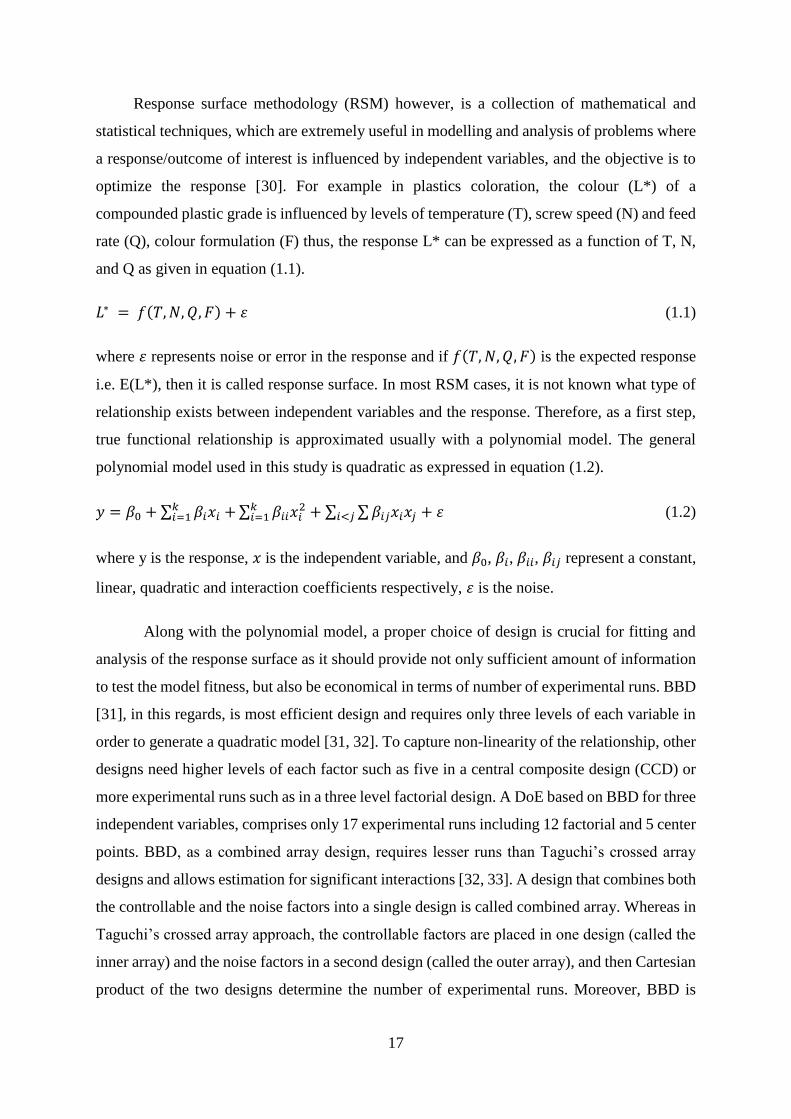
Response surface methodology (RSM) however, is a collection of mathematical and

statistical techniques, which are extremely useful in modelling and analysis of problems where

a response/outcome of interest is influenced by independent variables, and the objective is to

optimize the response [30]. For example in plastics coloration, the colour (L*) of a

compounded plastic grade is influenced by levels of temperature (T), screw speed (N) and feed

rate (Q), colour formulation (F) thus, the response L* can be expressed as a function of T, N,

and Q as given in equation (1.1).

𝐿∗ = 𝑓(𝑇, 𝑁, 𝑄, 𝐹) + 𝜀 (1.1)

where 𝜀 represents noise or error in the response and if 𝑓(𝑇, 𝑁, 𝑄, 𝐹) is the expected response

i.e. E(L*), then it is called response surface. In most RSM cases, it is not known what type of

relationship exists between independent variables and the response. Therefore, as a first step,

true functional relationship is approximated usually with a polynomial model. The general

polynomial model used in this study is quadratic as expressed in equation (1.2).

𝑦 = 𝛽0 +∑ 𝛽𝑖𝑥𝑖 +𝑘𝑖=1 ∑ 𝛽𝑖𝑖𝑥𝑖

2 + ∑ ∑𝛽𝑖𝑗𝑥𝑖𝑥𝑗 + 𝜀𝑖<𝑗𝑘𝑖=1 (1.2)

where y is the response, 𝑥 is the independent variable, and 𝛽0, 𝛽𝑖, 𝛽𝑖𝑖, 𝛽𝑖𝑗 represent a constant,

linear, quadratic and interaction coefficients respectively, 𝜀 is the noise.

Along with the polynomial model, a proper choice of design is crucial for fitting and

analysis of the response surface as it should provide not only sufficient amount of information

to test the model fitness, but also be economical in terms of number of experimental runs. BBD

[31], in this regards, is most efficient design and requires only three levels of each variable in

order to generate a quadratic model [31, 32]. To capture non-linearity of the relationship, other

designs need higher levels of each factor such as five in a central composite design (CCD) or

more experimental runs such as in a three level factorial design. A DoE based on BBD for three

independent variables, comprises only 17 experimental runs including 12 factorial and 5 center

points. BBD, as a combined array design, requires lesser runs than Taguchi’s crossed array

designs and allows estimation for significant interactions [32, 33]. A design that combines both

the controllable and the noise factors into a single design is called combined array. Whereas in

Taguchi’s crossed array approach, the controllable factors are placed in one design (called the

inner array) and the noise factors in a second design (called the outer array), and then Cartesian

product of the two designs determine the number of experimental runs. Moreover, BBD is

18

rotatable and spherical with a radius √2 where all design points are located. However, the

sphere it forms, does not contain vertices of cuboid region that represent extremes of each input

variable [30].

1.6.1 Optimization of Multiple Responses

Many RSM problems involve analysis of several responses, such as in this study we

measured three responses i.e. L*, a* and b* that together represent the colour of the

compounded plastic grades. However, in simultaneous consideration of multiple responses,

first step is to build an appropriate response surface model for each response, and then look for

a set of operating conditions that optimizes all responses, or at least keep them within the

desired ranges [31].

For optimizing several responses, a relatively straight forward approach (also called

graphical optimization) is to overlay contour plots for each response, however, it works well

only when there are three or fewer design variables involved. The most popular technique

however, is the numerical optimization technique by Derringer and Suich [34]. The technique

involves use of desirability functions. The procedure is to first convert each response 𝑦𝑖 into

an individual desirability function 𝑑𝑖 that varies from 0 to 1. A 𝑑𝑖 = 1 tells the response is at

its target, whereas a 𝑑𝑖 = 0, means the response lies outside the desired region. Then the overall

desirability is maximized by choosing the design variables as expressed in equation (1.3).

𝐷 = (𝑑1𝑑2…𝑑𝑚)1/𝑚 (1.3)

where m is the number of responses to be optimized. Individual desirability functions can be

expressed based upon the target value T as given in equations (1.4) to (1.6):

𝑑 = {

0 𝑦 < 𝐿

(𝑦−𝐿

𝑇−𝐿)𝑟

𝐿 ≤ 𝑦 ≤ 𝑇

1 𝑦 > 𝑇

if target T is a maximum value (1.4)

19

𝑑 = {

1 𝑦 < 𝑇

(𝑈−𝑦

𝑈−𝑇)𝑟

𝑇 ≤ 𝑦 ≤ 𝑈

0, 𝑦 > 𝑈

if target T is a minimum value (1.5)

𝑑 =

{

0 𝑦 < 𝐿

(𝑦−𝐿

𝑇−𝐿)𝑟

𝐿 ≤ 𝑦 ≤ 𝑇

(𝑈−𝑦

𝑈−𝑇)𝑟

𝑇 ≤ 𝑦 ≤ 𝑈

0 𝑦 > 𝑈

if target T is located between L and U (1.6)

where r is the weight, when r = 1 the desirability function is linear, however choosing 𝑟 > 1

put greater emphasis on to be closer to target, whereas 0 < 𝑟 < 1 makes it less important. In

present study Design-Expert® is used to implement this optimization technique.

1.7 Characterization Techniques

Characterization of a mixture is quite an important aspect in the study of mixing. A

comprehensive characterization requires specification of the size, shape, orientation and spatial

location of every discrete element of the minor component, which of course is almost

impossible. However various qualitative and quantitative theories and techniques have been

developed to measure and describe the mixing wellness such as thermo-gravimetric analysis

(TGA), differential scanning calorimetry (DSC), X-ray Diffraction (XRD), X-ray Fluorescence

(XRF), light microscopy, scanning electron microscope (SEM), energy dispersive X-ray

spectroscopy (EDX), and ash content [35~37]. Recent development in X-ray imaging

technique available with micro CT scanners (computed tomography) has offered significant

improvement in mixing characterization [14, 15].

Various researchers have employed thermo-gravimetric analysis (TGA) for colorants

quantification in a compounded plastic part. TGA can further be followed by FT-IR or mass

spectrometry for identification of elements. In 2008, a supplier of automotive body panels

encountered an issue with a customer – an automotive manufacturer that rejected a big lot of

products delivered in year 2007 due to slight variation in colour compared with lot delivered

in 2006. The issue was investigated by D. Grewell et al [37] and making use of various

techniques including TGA, they concluded two reasons associated with the raw material -

thermoplastic composite sheets comprising two ABS substrates (white) over-coated with clear

20

acrylic forming a three layer composite. One reason they identified was significant variation in

outer layers thickness of the two lots and another was variation in colorant loading in the middle

layers of the two lots. M. Kosrzycki et al [35] in 2008 made use of three different techniques

including TGA for determination of colour concentrate in moulded Polyacetal components. I.

Groves et al [36] of TA Instrument Ltd. of UK carried out a quantification analysis for making

determination of Carbon black pigment content in Nylon 66. Purpose was to ensure consistency

in level and dispersion of the pigments in the plastic material.

None of the above referred techniques quantified pigments dispersion level in

compounded plastics. This research however, successfully employs response surface

methodology, scanning electron microscopy (SEM) and image analysis, modelling mixing

zone of twin screw extruders, to analyse pigment dispersion in polycarbonate grades.

Evaluating pigments dispersion level within a polymer matrix determines the mixing efficiency

of a compounding process, which can be correlated with processing conditions employed.

Contrary to paints and coatings, compounding of plastics involves high shear rates, elevated

temperatures, and high pressures. To date, only a few studies are reported in literature about

effect of process variables on plastics coloration. In 2005, D. Colquhoun et al [38] investigated

that control of Pigment Yellow 62 (PY62) particle size and dispersion directly affected the

properties of extruded polyethylene film (1 mil thick), such as film transparency, colour

development, extruder pressure build and processing time. Using that knowledge they

developed and successfully tested a new PY 62 for polyethylene film. This study investigates

distributive mixing in the flow direction for a single-screw extruder. S. P. Rwei [39] in 2001

carried out an investigation of the distributive mixing in the flow direction for a single-screw

extruder under varying processing conditions. Experiment involved blending of a fine grade of

poly(dimethyl siloxane) (PDMS, 99.6% purity) with red ink representing a single concentrate

chip and results showed improved longitudinal distribution with an increasing RPM, a longer

metering section, or a decreasing diameter of the die.

1.7.1 Scanning Electron Microscopy (SEM) and Image Analysis

In scanning electron microscopy (SEM), an electron beam scans the surface of a

specimen to be examined, and the reflected (or back-scattered) beam of electrons is collected,

then displayed at the same scanning rate on a cathode ray tube (similar to a CRT television

screen). The image displayed on the screen, which may be photographed, replicates the

specimen surface features. The surface may or may not be polished and etched, but it must be

21

electrically conductive; a very thin metallic surface coating must be applied to nonconductive

materials such as polymers [40]. This condition however, is no more needed in ESEM, where

to eliminate electrostatic charge build-up during examination, a bridge between specimen

edges and conductive tape underneath is formed by applying a conductive adhesive.

Magnifications over 200,000 times, are possible, and great depths of field are possible.

Qualitative and semi-quantitative analysis of the elemental composition for quite localized

surface areas, are also possible when equipped with accessories such as energy dispersive X-

ray spectroscopy (EDX).

Various commercially available image analysis software such as Image-Pro can be used

for image processing and analysis, but they are expensive. ImageJ however, is a public domain

software [41], which is available as an online applet as well as in downloadable application

format, for Windows, Mac OSX and Linux. The software is enriched with quite powerful

features such as spatial calibration, stacking, filtering and geometric transformations to name

a few.

1.8 Modelling and Computer Simulation of Extrusion Process

Many researchers have made use of numerical methods to simulate the mixing of

particles in a base resin via extrusion process both for single screw extruders (SSEs) and twin

screw extruders (TSEs). In 1999, Eduardo of PolyTech discussed various characteristics of a

practical successful process simulator and detailed the functions of a one dimensional (1D)

simulator for plastics compounding operations in modular co-rotating intermeshing twin screw

extruders [42].

J. Markarian in 2005 reviewed various software available in the market for plastic

compounders to simulate extrusion process on extruders. Software she compared included Win

TXS of PolyTech USA – a 1D model, Akro-Co-Twin-Screw of Temarex Corporation USA –

a 1D model, Ludovic of CEMEF (Centre for Material Forming) France – a 3D model, Morex

of Institute of Plastics Processing (IKV) Germany – a 1D model, Polyflow of Ansys Inc. USA

– a 3D model, and Sigma of Institute of Plastics Engineering (KTP) of University of Paderborn

and ten industrial companies including raw material suppliers and extruder manufacturers – a

1D model. She indicated an increasing trend in plastic compounders of utilizing sophisticated

computer software for simulating various process parameters [43]. Surprisingly she didn’t

22

mention OpenFOAM® - a public domain software, probably because it was developed and

released in 2004 by Open CFD Ltd, after she wrote her article.

In 2005, Kirill carried out numerical simulation of mixing of two coloured particles

population in acrylonitrile-butadiene-styrene copolymer (ABS) resin by extrusion in an

industrial conventional SSE and evaluated degree of mixing and colour homogeneity. Results

were found consistent with experimental data [44]. Robin et al, in 2006, evaluated the mixing

in single screw and co-rotating twin screw dough mixers by simulating 2D model using

Polyflow® software. They concluded that overall mixing effectiveness and efficiency of twin

screw mixer was much better than that in single screw mixer [45].

In 2008, Chantal et al developed a full 3D finite element code called Ximex® and

simulated mixing processes of complex fluids; as a case study, flow within a TSE and flow in

a batch mixer were presented [46]. Then in 2009 they employed full 3D simulation software

Ximex® for characterizing flow conditions in mixing processes such as SSE, TSE and

analysing the influence of geometrical parameters such as staggering angle and disc thickness

of kneaders on flow conditions [47].

In 2009 and 2010, Estanislao et al carried out three dimensional (3D) simulation of

reactive flow in fully-filled screw elements of co-rotating closely intermeshing twin screw

extruders (COTSEs) with the aim to analyse peroxide-initiated degradation of polypropylene

(PP). To achieve that end, they modelled special designs of screw elements and simulated

mixing process using Polyflow® software to see their effect on the process output. However

they have suggested that both 1D and 3D models should complement each other [48, 49]. Later

in 2010, Wang et al carried out numerical investigation to analyse the role of screw geometry

on mixing of a viscous polymer melt, they successfully modelled four geometries of cooling

screws being used by extrusion industry and made use of finite element solvers for 3D non-

Newtonian fluid flow and advection-diffusion heat transfer [50].

Modelling techniques that have been presented by various authors include: analytical

modelling; flow analysis network (FAN); quasi steady state approximation; moving reference

frame (MRF) method; mesh superimposition technique. Each approach has its own pros and

cons as discussed below. Analytical modelling provides the simplest way to understand the

pumping behaviour of extruders, however is valid only for Newtonian fluids, furthermore mere

throughput behaviour would not suffice to understand the flow mechanism in extruders, but

23

rather shear stress and velocity distributions are more important to know for an insight of the

flow behaviour, which require numerical solution of the problem. The most common simplified

numerical approach is FAN method, which works based on dividing flow region into control

volumes and then carrying out flux balance on each volume. However because of geometric

and information limitations restrict its use to simple geometries only.

Quasi-steady state approximation was introduced by Lee and Castro [51]. They

mentioned that the transient part in the continuum equation could be considered negligible if

the Reynolds number was very small as usually the case in polymer processing. With this

approximation, the resulting solution is dependent only on instantaneous material properties

and boundary conditions, and screws relative positions within the barrel i.e. sequential

geometries at defined angles of rotor position, can be selected and simulated under a steady

state condition. Each screws relative position however, requires new meshes to be generated

for a solution to run, results are then compiled together for those relative positions to understand

the flow behaviour over a complete rotation cycle. Transient nature and complexity of flow

geometry in twin screw extruders do not allow to reach a truly steady state condition. Many

researchers therefore successfully employed quasi-steady state approximation in simulating

dispersive mixing behaviour of twin screw extruders.

Yang and Manas-Zloczower [52, 53] implemented the quasi-steady technique for

simulating dispersive mixing behaviour of a Banbury mixer and for an intermeshing co-rotating

twin screw extruder (ICRTSE). Bravo [54] employed same approximation for obtaining

flowfield solution in kneading discs region of an ICRTSE. Recently, using same

approximation, Sobhani et al [55] characterized mixing flow behaviour in co-rotating twin

screw extruder, and Goger [56] analysed dispersive mixing behaviour in conveying elements

of a counter rotating twin screw extruder. Disadvantage of this technique is that it involves lot

of meshing work, and neglecting transient term in energy equation is not justified. Moving

reference frame (MRF) provides an alternate to quasi-steady state approximation, however

Ortiz-Rodriquez [48] stated its limitation in predicting flow behaviour of double flighted screw

as two different radial vectors were defined. Another disadvantage he mentioned was its

restricted capability in describing distributive mixing behaviour in twin screw extruders. Mesh

superimposition technique [57] is pretty close to quasi-steady state in nature and even more

sensitive to transient effects, however geometric complexities involved in twin screw extrusion

restrict it to relatively course mesh patterns causing error to the results.

24

In lieu of the extensive literature survey presented above, this study employs quasi-steady

state approximation for simulating the flow behaviour of kneading discs zone in a twin screw

extruder using OpenFOAM® software.

1.9 Problem Statement – Inconsistency in Plastics Coloration

SABIC Innovative Plastics manufactures coloured plastics via compounding process

using co-rotating intermeshing twin screw extruders installed on its 15 production lines at

Cobourg manufacturing facility. The raw material used include resins, fillers and colour

pigments, usually one or two resins with 3 to 4 fillers and 4 to 5 pigments are premixed on a

super floater, in proportions specified as reference colour formulation. The premixed is then

poured into hopper of twin screw extruder under pre-defined processing conditions i.e. levels

of temperature, screw speed and feed rate, all the ingredients undergoing various sections of

barrel and screws system, are uniformly blended under high shear and elongational stresses.

The homogenized blend of materials is then pushed to exit through a die hole located at tail

end of the extruder forming a strand of compounded plastic. The extruded strand, immediately

after exiting from die hole, is water quenched in a water bath, air-dried under an air-knife and

cut by a pelletizer into small pellets of size 2mm x 2mm. The pellets are then moulded into

rectangular plaques of size 70mm x 50mm x 2.6mm on injection moulding machine, these

sample chips along with a reference chip are colour evaluated on a spectrophotometer, and

visually inspected by a colour expert as well. Any colour deviation, exceeding permissible

tolerance limits, between the reference and the sample chips raises colour inconsistency issue,

and the whole production lot may go scrapped. New production lot with minute adjustments in

pigments reference formulation under the advice of a colour expert, is loaded and the colour

evaluation process is repeated until the colour deviation comes out to be within tolerance limits.

Frequency of such adjustments in standard formulation varies with different plastic grades and

associated output colours. These colour mismatch issues cause delay in delivery schedules,

wastage of materials, man-hours and most importantly loss of competitive edge in global

market. Each step in the entire compounding and colour evaluation process is critical and needs

particular attention to study for identifying all possible factors causing colour mismatch [9].

25

1.10 Objectives

Main objectives of this study include following:

Develop basic understanding of the compounding process used for plastics coloration. This

is achieved by going through intensive literature review, executing experimentation and

analysing 3D simulation results.

Analyse the effect of small adjustments in colour formulation on colour of the PC grades.

This is done by statistically analysing past production data of the PC grades using Design-

Expert® software.

Analyse the process variables and two factor interactions that affect colour of the PC

grades, and thus optimize levels of the process variables to ensure consistency in colour.

This has accomplished by implementing Box-Behnken design (BBD) using Design-

Expert® software.

Evaluate pigments dispersion level in terms of particles size and spatial distribution in PC

grades. This is achieved using SEM for imaging and ImageJ® for image analysis.

Undertake 3D simulation of the dispersive mixing behaviour in the kneading discs zone

(staggered at 45°) under varying processing conditions, and correlate with experimental

colorimetric data of the PC grades. This is achieved by 3D simulation of the kneading discs

zone in a twin screw extruder system.

1.11 Overview of the Thesis

The entire thesis is divided into 6 chapters including introduction and background.

Chapter 2 presents statistical analysis of the past production data respecting effect of small

adjustments in colour formulation on output colour of two PC grades, PC1 and PC2. Technique

involves implementation of historical data design using Design-Expert® software. Results

identify pigments most responsive to colour variation under small adjustments in formulation,

and suggests optimal adjustments to avoid repetition. Chapter 3 is devoted to implementation

of Box-Behnken design (BBD) through designed experiments and investigate the effect of

processing conditions on output colour of three PC grades, G1, G2, and G3. Technique involves

two step methodology: first step is to select an appropriate design of experiments (DoE) such

as BBD, and then to choose a polynomial model to fit in the data at hand. Optimization of

multiple responses is also covered in chapter 3. Chapter 4 presents a novel technique, which

characterizes solid structure samples using ESEM for imaging and for image analysis, the

26

ImageJ® - a public domain software; aim was to evaluate pigments dispersion level in PC

grade G2 and correlate it to colour deviation. In chapter 5, 3D simulation of mixing zone in a

twin screw extruder is presented using processing condition employed in compounding of PC

grade G2. Results evaluate mixing efficiency of the kneading discs zone in terms of a flow

parameter called lamda, λ. Finally in chapter 6, main conclusions and thesis contributions are

summarized. Some future recommendations are also included in chapter 6.

27

Chapter 2

Influence of Minute Adjustments in Colour Formulation on output Colour of

Compounded PC Grades

2.1 Introduction

To develop various operational and aesthetic attributes in plastics / products, such as

ultraviolet stability, thermal and mechanical properties, plastics compounders blend polymer

resins with different additives, modifiers and fillers. However, the colour and special

appearance effects in plastics offer them countless possibilities for innovation and marketing

of their products in a fast growing and highly competitive global market. Successful addition

of a desired colour to a plastic grade requires adequate mixing of colour pigments in base

polymeric resin. The mixing involves wetting the pigment surface with the polymer, breaking

up of agglomerates into primary particles, and uniformly distributing the pigment particles

within the polymer matrix. While plastic compounders, to ensure better dispersion, typically

use twin-screw extruders, internal lubricants or slip additives, and optimized processing

conditions, the suppliers of pigments however, focus on balancing the particle size, shape and

surface treatments [16, 20, 40].

Each target colour is associated with a reference recipe of colour formulation that reflects

pigments type, and their concentration level in base resin(s), usually expressed in units of PPH

- parts per hundred parts of base resin(s). Associated with the colour formulation is a reference

colour described by tri-stimulus colour data such as L*, a* and b*. Any deviation from

reference colour of the output colour of a compounded plastic, is declared as colour mismatch

- a key issue confronted by plastics compounders and described in delta values i.e. ∆L*, ∆a*,

∆b*, ∆E*. Such colour deviations call for small adjustments in colour formulation during

production so the desired target colour can be achieved [10, 25, 40, 41, 61]. Present study

addresses this issue by investigating the response of output colour to minute changes made in

reference colour formulation.

Statistical methods are frequently used by researchers, to investigate and optimize the

effect of process variables on responses such as colour and appearance of compounded plastics.

For this purpose, they employ various statistical designs and models to fit in the response data

obtained through designed experiments or past production data. Effertz [27] investigated a PVC

sheet for the effect of processing conditions on its gloss and surface appearance using modified

general factorial model. Bender [28] investigated the process variables causing high viscosity

variability in wood-fiber compounds by executing Box-Behnken design (BBD). Present study

28

however, employs historical data design with the aim to investigate influence of small

adjustments made in colour formulation, on the output colour of two PC grades assuming other

factors are invariant. Historical data design is a response surface method, and to execute such

a design present study uses Design-Expert® software.

Main objectives of this study include: 1) statistically analyze the effect of minute changes

in colour formulation on output colour of two PC grades i.e. PC1 and PC2 using past production

data collected at SABIC IP Cobourg Plant; 2) identify the colour pigments that significantly

influence the output colour under minute adjustments; 3) optimize the process so the

adjustments in colour formulation are precisely made and multiple adjustments can be avoided.

2.2 Experimentation

Experimental set up used was a 40 mm, 112 kW twin- screw intermeshing co-rotational

extruder with L/D ratio of 37 having 9 zones barrel and a 4 zone die, representing a production

line at SABIC IP Cobourg plant. Processing conditions i.e. the barrel and die zones

temperatures, screw speed and feed rate were kept constant. The reference colour formulation

and the past data of various adjustments made were collected from SABIC IP Cobourg plant

and is presented in tables 2.1 to 2.4, for the two PC grades: PC1 and PC2. As mentioned earlier,

both grades low Chroma opaque compounded PC grades, the only difference between the two

formulations is that, PC1 was a blend of single PC resin and colour pigments, whereas PC2

represented a blend of two PC resins and colour pigments. The target colour coordinates were

L*=67.29, a*=1.47, and b*=4.89 for both PC grades. For brevity the delta values representing

each adjustment are shown in tables 2.2 and 2.4.

Table 2.1: Reference Colour Formulation – PC1

S-No Type PPH gram

1 Polycarbonate Resin

(MFI=6.5g/10min) 100 6000

2 White Pigment 1.76 105.6

3 Black Pigment 0.00968 0.5808

4 Red Pigment 0.01602 0.9612

5 Yellow Pigment 0.1084 6.504

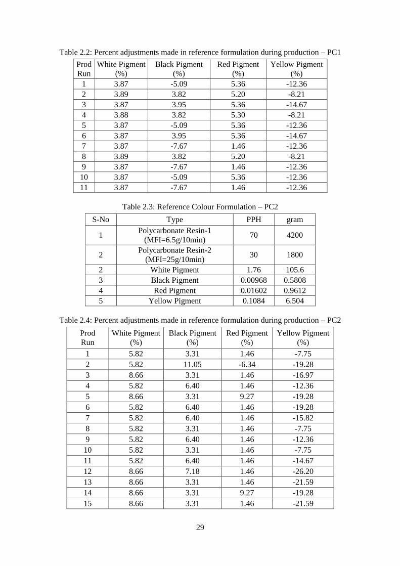
29

Table 2.2: Percent adjustments made in reference formulation during production – PC1

Prod

Run

White Pigment

(%)

Black Pigment

(%)

Red Pigment

(%)

Yellow Pigment

(%)

1 3.87 -5.09 5.36 -12.36

2 3.89 3.82 5.20 -8.21

3 3.87 3.95 5.36 -14.67

4 3.88 3.82 5.30 -8.21

5 3.87 -5.09 5.36 -12.36

6 3.87 3.95 5.36 -14.67

7 3.87 -7.67 1.46 -12.36

8 3.89 3.82 5.20 -8.21

9 3.87 -7.67 1.46 -12.36

10 3.87 -5.09 5.36 -12.36

11 3.87 -7.67 1.46 -12.36

Table 2.3: Reference Colour Formulation – PC2

S-No Type PPH gram

1 Polycarbonate Resin-1

(MFI=6.5g/10min) 70 4200

2 Polycarbonate Resin-2

(MFI=25g/10min) 30 1800

2 White Pigment 1.76 105.6

3 Black Pigment 0.00968 0.5808

4 Red Pigment 0.01602 0.9612

5 Yellow Pigment 0.1084 6.504

Table 2.4: Percent adjustments made in reference formulation during production – PC2

Prod

Run

White Pigment

(%)

Black Pigment

(%)

Red Pigment

(%)

Yellow Pigment

(%)

1 5.82 3.31 1.46 -7.75

2 5.82 11.05 -6.34 -19.28

3 8.66 3.31 1.46 -16.97

4 5.82 6.40 1.46 -12.36

5 8.66 3.31 9.27 -19.28

6 5.82 6.40 1.46 -19.28

7 5.82 6.40 1.46 -15.82

8 5.82 3.31 1.46 -7.75

9 5.82 6.40 1.46 -12.36

10 5.82 3.31 1.46 -7.75

11 5.82 6.40 1.46 -14.67

12 8.66 7.18 1.46 -26.20

13 8.66 3.31 1.46 -21.59

14 8.66 3.31 9.27 -19.28

15 8.66 3.31 1.46 -21.59

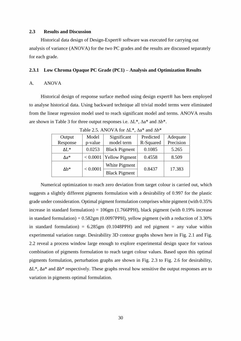
30

2.3 Results and Discussion

Historical data design of Design-Expert® software was executed for carrying out

analysis of variance (ANOVA) for the two PC grades and the results are discussed separately

for each grade.

2.3.1 Low Chroma Opaque PC Grade (PC1) – Analysis and Optimization Results

A. ANOVA

Historical design of response surface method using design expert® has been employed

to analyse historical data. Using backward technique all trivial model terms were eliminated

from the linear regression model used to reach significant model and terms. ANOVA results

are shown in Table 3 for three output responses i.e. ∆L*, ∆a* and ∆b*.

Table 2.5. ANOVA for ∆L*, ∆a* and ∆b*

Output

Response

Model

p-value

Significant

model term

Predicted

R-Squared

Adequate

Precision

∆L* 0.0253 Black Pigment 0.1085 5.265

∆a* < 0.0001 Yellow Pigment 0.4558 8.509

∆b* < 0.0001 White Pigment

0.8437 17.383 Black Pigment

Numerical optimization to reach zero deviation from target colour is carried out, which

suggests a slightly different pigments formulation with a desirability of 0.997 for the plastic

grade under consideration. Optimal pigment formulation comprises white pigment (with 0.35%

increase in standard formulation) = 106gm (1.766PPH), black pigment (with 0.19% increase

in standard formulation) = 0.582gm (0.0097PPH), yellow pigment (with a reduction of 3.30%

in standard formulation) = 6.285gm (0.1048PPH) and red pigment = any value within

experimental variation range. Desirability 3D contour graphs shown here in Fig. 2.1 and Fig.

2.2 reveal a process window large enough to explore experimental design space for various

combination of pigments formulation to reach target colour values. Based upon this optimal

pigments formulation, perturbation graphs are shown in Fig. 2.3 to Fig. 2.6 for desirability,

∆L*, ∆a* and ∆b* respectively. These graphs reveal how sensitive the output responses are to

variation in pigments optimal formulation.

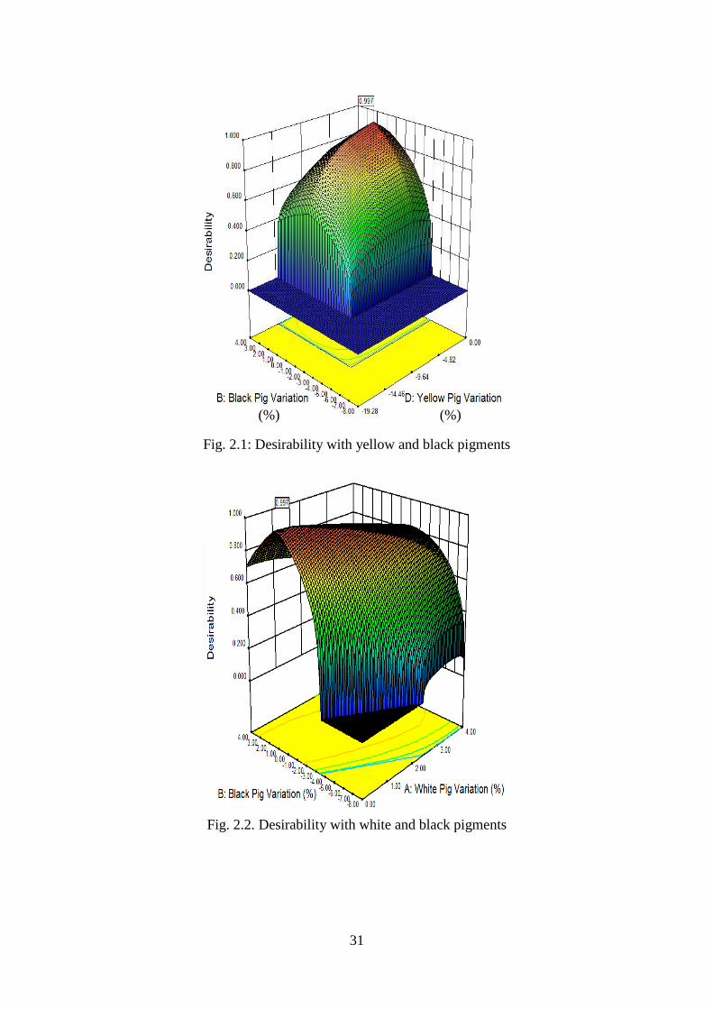
31

Fig. 2.1: Desirability with yellow and black pigments

Fig. 2.2. Desirability with white and black pigments

(%) (%)

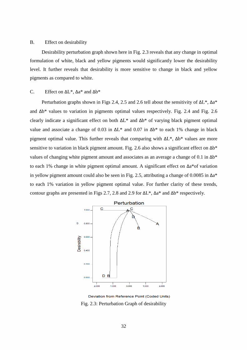
32

B. Effect on desirability

Desirability perturbation graph shown here in Fig. 2.3 reveals that any change in optimal

formulation of white, black and yellow pigments would significantly lower the desirability

level. It further reveals that desirability is more sensitive to change in black and yellow

pigments as compared to white.

C. Effect on ∆L*, ∆a* and ∆b*

Perturbation graphs shown in Figs 2.4, 2.5 and 2.6 tell about the sensitivity of ∆L*, ∆a*

and ∆b* values to variation in pigments optimal values respectively. Fig. 2.4 and Fig. 2.6

clearly indicate a significant effect on both ∆L* and ∆b* of varying black pigment optimal

value and associate a change of 0.03 in ∆L* and 0.07 in ∆b* to each 1% change in black

pigment optimal value. This further reveals that comparing with ∆L*, ∆b* values are more

sensitive to variation in black pigment amount. Fig. 2.6 also shows a significant effect on ∆b*

values of changing white pigment amount and associates as an average a change of 0.1 in ∆b*

to each 1% change in white pigment optimal amount. A significant effect on ∆a*of variation

in yellow pigment amount could also be seen in Fig. 2.5, attributing a change of 0.0085 in ∆a*

to each 1% variation in yellow pigment optimal value. For further clarity of these trends,

contour graphs are presented in Figs 2.7, 2.8 and 2.9 for ∆L*, ∆a* and ∆b* respectively.

Fig. 2.3: Perturbation Graph of desirability

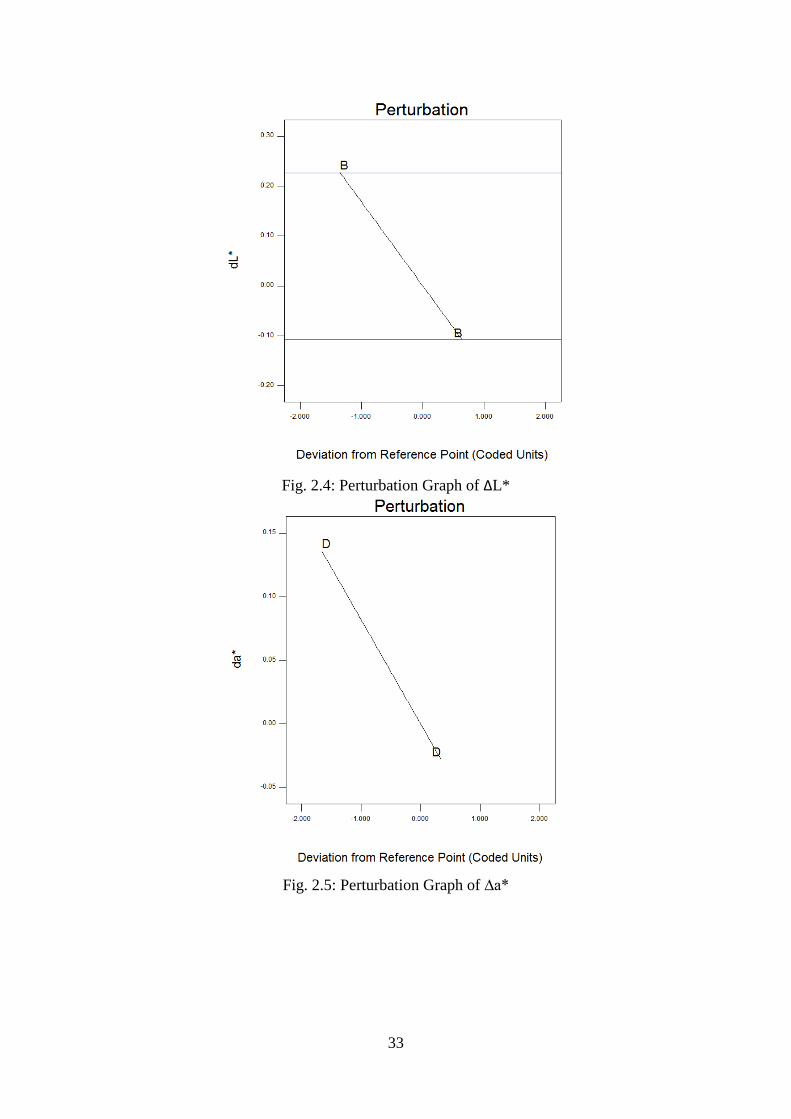
33

Fig. 2.4: Perturbation Graph of ∆L*

Fig. 2.5: Perturbation Graph of ∆a*

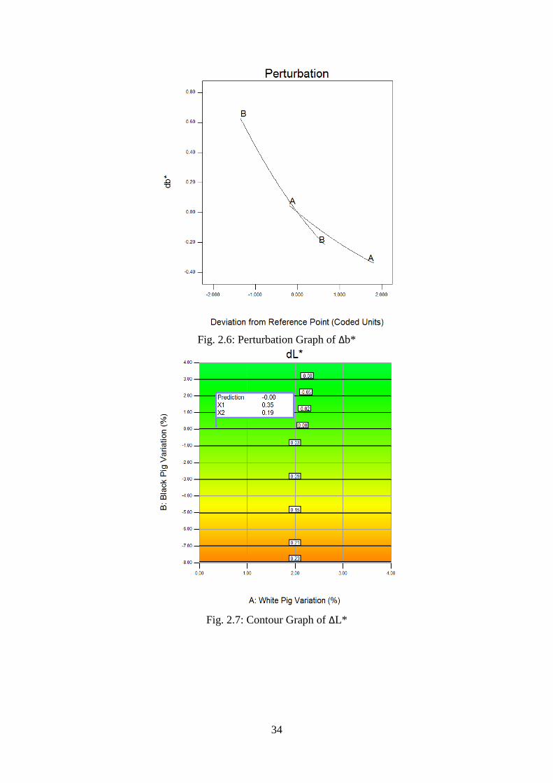
34

Fig. 2.6: Perturbation Graph of ∆b*

Fig. 2.7: Contour Graph of ∆L*

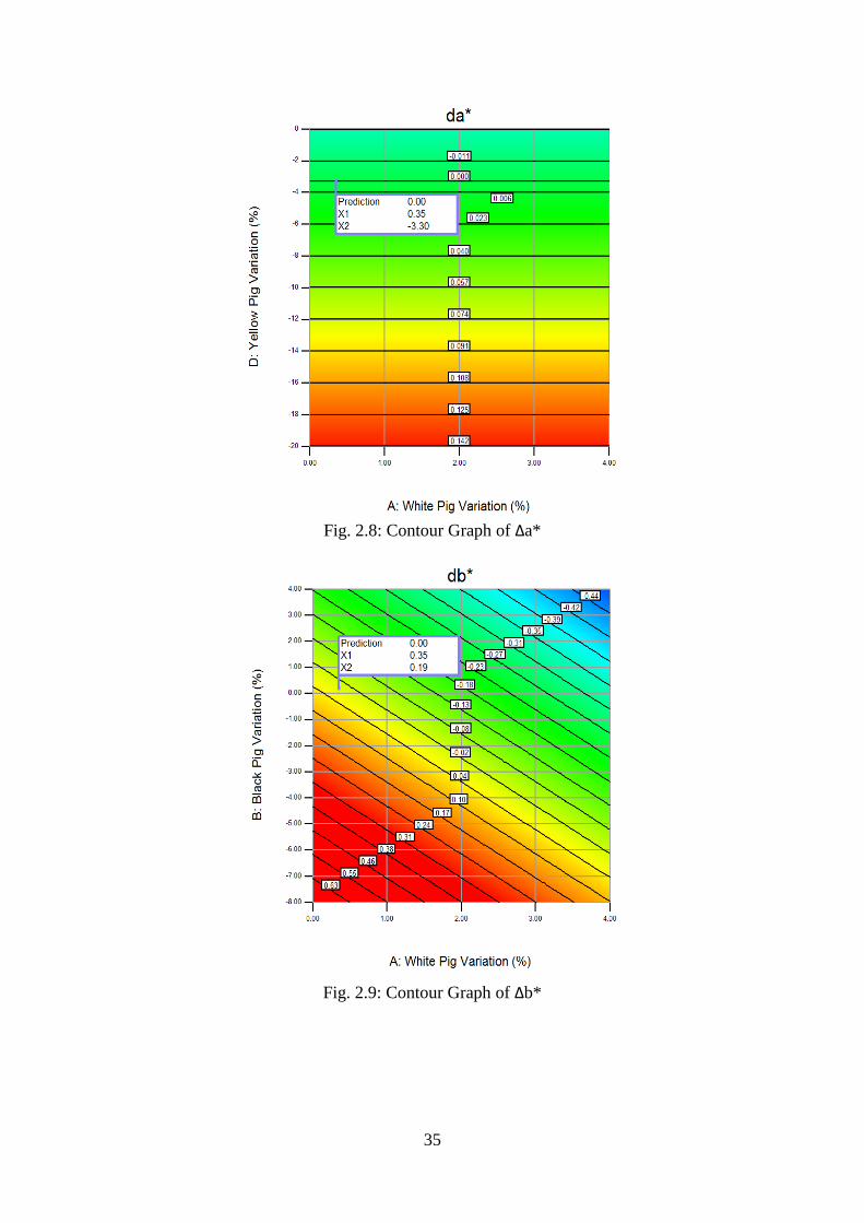
35

Fig. 2.8: Contour Graph of ∆a*

Fig. 2.9: Contour Graph of ∆b*

36

2.3.2 Low Chroma Opaque PC Grade (PC2) – Analysis and Optimization Results

A. ANOVA

Historical data design of response surface method has been employed to analyse data.

Using backward technique all trivial model terms were eliminated from the linear regression

model used to make it significant. ANOVA results are shown in Table 2.6 for the three output

responses i.e. ∆L*, ∆a* and ∆b*.

Table 2.6. ANOVA Results of ∆L*, ∆a* and ∆b*

Output

Response

Model

p-value

Significant

model term

Predicted

R-Squared

Adequate

Precision

∆L* 0.0066 White Pig

0.1464 6.486 0.0044 Yellow Pig

∆a* 0.0187 White Pig

0.0112 4.279 0.0447 Yellow Pig

∆b* 0.0133 White Pig

0.3584 8.894 0.0011 Yellow Pig

Numerical optimization to reach zero deviation from target colour is carried out, which

suggests slightly different pigments formulation compared to the standard given in Table 2.1,

with desirability of 0.755 for the plastic grade under consideration. Optimal pigment

formulation comprises white pigment (with 5.29% increase in standard formulation) =

111.2gm (1.853PPH), yellow pigment (with a reduction of 13.59% in standard formulation) =

5.62gm (0.0937PPH) and black and red pigment = any value within experimental variation

range. Desirability 3D graph shown here in Fig. 2.10 reveals a process window large enough

to explore experimental design space for various combination of pigments formulation to reach

target colour values. Based upon optimal pigments formulation suggested, perturbation graphs

are shown in Fig. 2.11 to Fig. 2.14 for desirability, ∆L*, ∆a* and ∆b* respectively. These

graphs reveal how sensitive the output responses are to variation in pigments optimal

formulation.

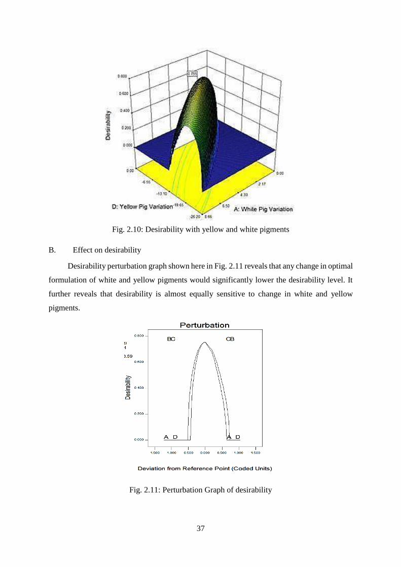
37

Fig. 2.10: Desirability with yellow and white pigments

B. Effect on desirability

Desirability perturbation graph shown here in Fig. 2.11 reveals that any change in optimal

formulation of white and yellow pigments would significantly lower the desirability level. It

further reveals that desirability is almost equally sensitive to change in white and yellow

pigments.

Fig. 2.11: Perturbation Graph of desirability

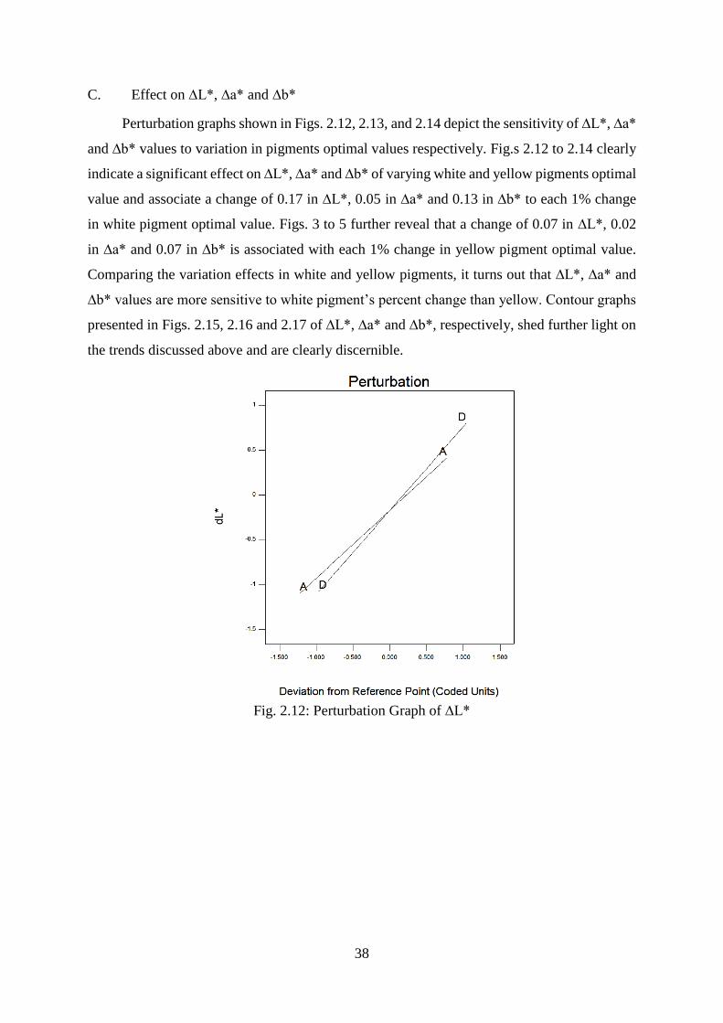
38

C. Effect on ∆L*, ∆a* and ∆b*

Perturbation graphs shown in Figs. 2.12, 2.13, and 2.14 depict the sensitivity of ∆L*, ∆a*

and ∆b* values to variation in pigments optimal values respectively. Fig.s 2.12 to 2.14 clearly

indicate a significant effect on ∆L*, ∆a* and ∆b* of varying white and yellow pigments optimal

value and associate a change of 0.17 in ∆L*, 0.05 in ∆a* and 0.13 in ∆b* to each 1% change

in white pigment optimal value. Figs. 3 to 5 further reveal that a change of 0.07 in ∆L*, 0.02

in ∆a* and 0.07 in ∆b* is associated with each 1% change in yellow pigment optimal value.

Comparing the variation effects in white and yellow pigments, it turns out that ∆L*, ∆a* and

∆b* values are more sensitive to white pigment’s percent change than yellow. Contour graphs

presented in Figs. 2.15, 2.16 and 2.17 of ∆L*, ∆a* and ∆b*, respectively, shed further light on

the trends discussed above and are clearly discernible.

Fig. 2.12: Perturbation Graph of ∆L*

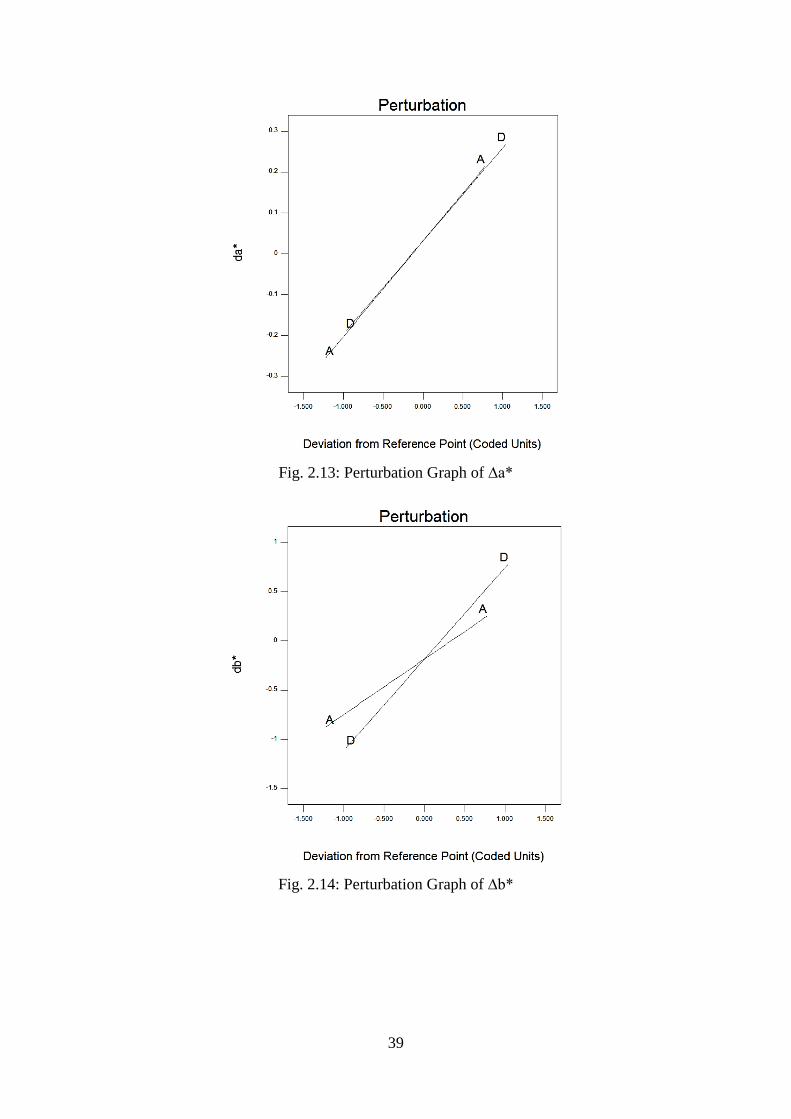
39

Fig. 2.13: Perturbation Graph of ∆a*

Fig. 2.14: Perturbation Graph of ∆b*

40

Fig. 2.15: Contour Graph of ∆L*

Fig. 2.16: Contour Graph of ∆a*

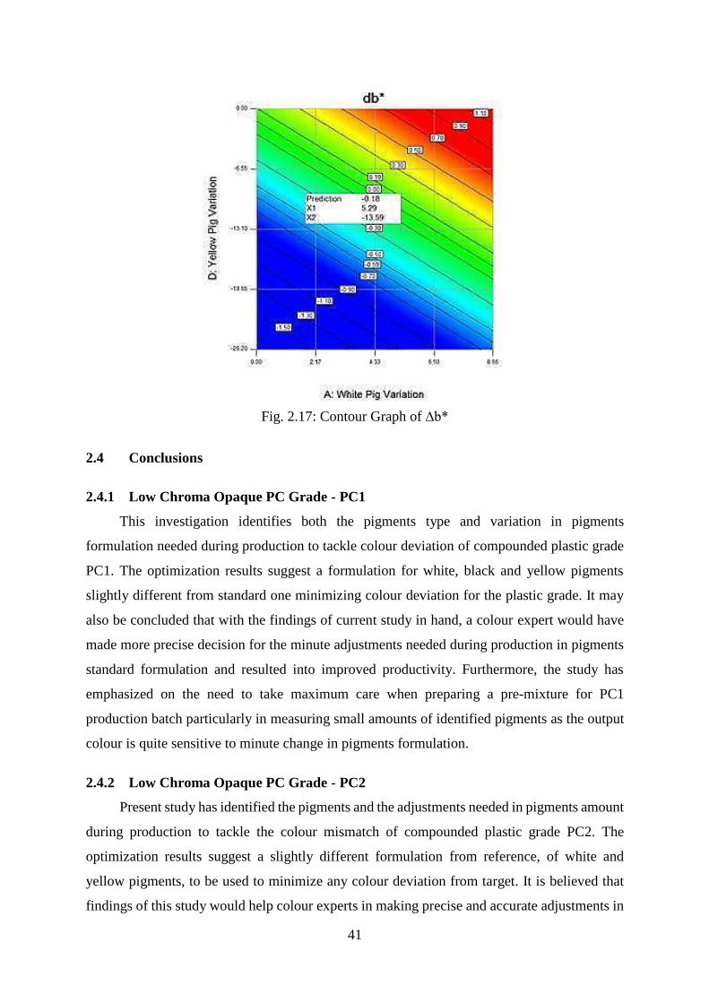
41

Fig. 2.17: Contour Graph of ∆b*

2.4 Conclusions

2.4.1 Low Chroma Opaque PC Grade - PC1

This investigation identifies both the pigments type and variation in pigments

formulation needed during production to tackle colour deviation of compounded plastic grade

PC1. The optimization results suggest a formulation for white, black and yellow pigments

slightly different from standard one minimizing colour deviation for the plastic grade. It may

also be concluded that with the findings of current study in hand, a colour expert would have

made more precise decision for the minute adjustments needed during production in pigments

standard formulation and resulted into improved productivity. Furthermore, the study has

emphasized on the need to take maximum care when preparing a pre-mixture for PC1

production batch particularly in measuring small amounts of identified pigments as the output

colour is quite sensitive to minute change in pigments formulation.

2.4.2 Low Chroma Opaque PC Grade - PC2

Present study has identified the pigments and the adjustments needed in pigments amount

during production to tackle the colour mismatch of compounded plastic grade PC2. The

optimization results suggest a slightly different formulation from reference, of white and

yellow pigments, to be used to minimize any colour deviation from target. It is believed that

findings of this study would help colour experts in making precise and accurate adjustments in

42

colour formulation during production, thus improving productivity. Study further suggests that

maximum care needs to be taken while preparing a colour formulation to be used in

compounding. Special attention is needed in measuring small amounts of identified pigments

being more responsive to variation in output colour.

2.5 Summary

In this study, past production data of two low Chroma opaque polycarbonate (PC) plastic

grades - PC1 and PC2, were statistically analysed with the aim to quantify the influence on

output colour caused by small adjustments in colour formulation made during production.

These PC grades were compounded on a co-rotating intermeshing twin screw extruder, at

SABIC IP Cobourg plant. PC1 represented a blend of four colour pigments and four additives

in one PC resin grade, whereas PC2 was a blend of four colour pigments and five additives in

two PC resin grades. Colour mismatch caused by these adjustments is presented in terms of

∆L*, ∆a*, ∆b* and ∆E*. This study reveals that output colour is quite sensitive to minute

changes in amount of white, black, and yellow pigments. Optimization results suggest precise

adjustments in pigments amount to be made in dealing with colour deviations encountered

during compounding of PC1 and PC2 plastic grades.

43

Chapter 3

Process Optimization through Designed Experiments to achieve Consistent Output

Colour in Compounded Plastics

3.1 Introduction

Plastic compounders use various modifiers, fillers and additives for polymeric material

grades to inculcate and improve upon their desired attributes such as thermal, UV stability and

mechanical properties. All parameters including processing and rheological conditions come

into focus throughout developmental cycle of the plastic grades; however, in the present fast

growing plastic market, adding a specific colour and appearance to plastic grades has become

even more demanding. Taking into account the colourability right from onset of development

cycle of a polymeric material grade is imperative [20].

Presence of three elements of light – a light source, observer and an object, is a must to

see a colour. When a light beam is incident on an object, a part (<1%) of it is reflected back

from the surface interface, which can be specular or diffuse reflection depending upon surface

condition, whereas the rest of the light penetrates into the surface and is modified by three

phenomenon; that is, selective absorption, reflection/transmission, and scattering. It is the

selective absorption and reflection/transmission that determine the colour of the object,

whereas the scattering takes care of the whiteness, brightness, and opacity of the object.

However, scattering occurs only when the refractive index of any additives, pigments, or

regions within plastic grade differ from the base resin and cause a change in both the direction

and velocity of incident light. The refractive index depends on not only the type of substance

itself but the wavelength of the incident light. Scattering may not be a desired phenomenon as

it prevents the light from penetrating deeper into the object and therefore can hinder

achievement of the desired colour; however, scattering can be a choice, where opacity is the

priority. Polycarbonate resins are transparent and do not scatter light; therefore, to achieve a

certain opacity level, white pigment (titanium dioxide) is added to create scattering at the cost

of loss in apparent colour strength [20, 42, 61, 62].

Key factors that can cause colour mismatch to occur include: 1) inadequate mixing, both

dispersive and distributive, of colour pigments; 2) incorrect formulation; 3) pigment particle

size variation; 4) degradation of polymer resin and/or pigments, and 5) particles/regions of

varying refractive index within the polymeric resin causing scattering. All such factors need to

be studied to understand their effect on output colour [10, 20, 40, 41, 61].

44

Design of experiments (DoE) is a planned approach that allows an experimenter to

precisely determine cause-and-effect relationships. Many researchers have employed statistical

techniques to investigate / optimize the effect of input factors on desired output attributes.

Design-Expert® software (Stat-Ease, Inc., Minneapolis, MN, USA) offers the use of various

statistical designs and models to fit the experimental data at hand. Effertz [27] employed a

modified general factorial DoE for investigating the effect of changes in compounding process

variables on gloss and surface appearance of a PVC sheet. Similarly, Bender [28] successfully

executed a DoE involving Box-Behnken design (BBD) to determine the relationship between

processing conditions and viscosity variability for a wood-fiber compound. The present study

utilized a DoE based on BBD in Design-Expert® software. The aim was to investigate the

effect on output colour of three compounded plastic grades under varying processing

conditions employed in an extrusion process. SABIC IP’s technology line at Cobourg Plant,

which comprises a twin screw extruder (TSE), was used to execute the DoEs. Assuming that

previously discussed variables were well under control, the present study suggests optimal

values for process variables to achieve consistency in output colour of the plastic grades.

3.1.1 Response Surface Methodology (RSM) and Box-Behnken Design (BBD)

As explained in chapter 1, RSM involves use of mathematical and statistical techniques,

which are extremely useful in modelling and analysis of problems where a response of interest

is influenced by independent variables, and the objective is to optimize the response. In most

RSM cases like ones examined in this study, type of relationship is not known between

independent variables and the response. Therefore, a true functional relationship is

approximated with a polynomial model as expressed in equation 1.2, followed by a proper

choice of design that should provide sufficient amount of information to test the model fitness,

and is economical too in terms of experimental runs. Therefore, in this study we chose BBD

that requires only three levels of each variable in order to generate a quadratic model and

capture two factor interactions.

3.1.2 Optimization of Multiple Responses

As explained in chapter 1, most RSM problems involve simultaneous analysis of multiple

responses, which was the case in this study where we measured three responses i.e. L*, a* and

b* representing colour of the compounded plastic grades examined. However, in a

simultaneous consideration of multiple responses, first step is to build an appropriate response

surface model for each response, and then look for a set of operating conditions that optimize

all responses, or at least keep them within the desired ranges.

45

The most popular technique however, is the numerical optimization technique by

Derringer and Suich, which involves use of desirability functions. The procedure as explained

in chapter 1, is to first convert each response 𝑦𝑖 into an individual desirability function 𝑑𝑖 that

varies from 0 to 1. A 𝑑𝑖 = 1 tells the response is at its target, whereas a 𝑑𝑖 = 0 means the

response lies outside the desired region. Then the overall desirability is calculated by taking

geometric mean of individual desirability functions as expressed in equation (1.3).

3.1.3 Response and 3D Colour Space - CIE Lab Model

As mentioned earlier, the colour of an object can be characterized by its tri-stimulus data

i.e. L*, a* and b* - the three responses that are investigated in this study. The tri-stimulus colour

data corresponds to a point in 3D colour space of CIE Lab model, which was introduced in

1976 by the international commission on light (CIE - Commission Internationale de

I'Eclairage). Any deviation from the reference target colour that exceeds permissible limits, is

reported as colour mismatch and usually expressed in delta values as ∆L*, ∆a*, ∆b* and ∆E*=

√(∆𝐿∗)2 + (∆𝑎∗)2 + (∆𝑏∗)2. It is the customer needs that usually decide a threshold for these

delta values, which for the plastic grades studied, were set out as ≤0.6 for ∆L*, ∆a*, ∆b* and ≤

1.0 for ∆E*. One significant aspect in colour matching is to prepare a rectangular moulded chip

similar to moulded sample chips, for use as reference representing reference colour

formulation. Colour coordinates of reference chip are measured and stored on a

spectrophotometer. Spectrophotometers are useful quality control tools that help to numerically

measure colour and colour variation.

3.1.4 Propagation of Error (POE) Technique and Process Robustness

Robustness of design is ensured by incorporating propagation of error (POE) technique

in RSM design. POE is taken as a measure of standard deviation of transmitted variability in

output response, which is caused by fluctuations in significant controllable process variables

during experimentation assuming uncontrollable factors noise to zero [30]. Using POE

technique with RSM design, levels of controllable input factors can be found that keep output

responses close to their target values and reduce variation transmitted by lack of control over

input controllable factors. In other words, POE technique makes a process insensitive to

variation in input factors. However, the technique is beneficial only when RSM reveals

curvilinear relationships between input factors and output responses, and transmitted variation

is reduced by moving to plateaus [60]. Mathematical expression for POE is given below in

equation (3.1) [61]. It takes partial derivatives of response polynomials (Y) in actual units with

46

respect to input variables (Xi) and incorporates variation in input variables (𝜎𝑋𝑖) and

unexplained residual i.e. experimental noise (𝜎𝑟𝑒𝑠𝑖𝑑).

ΡΟΕ = √𝜎𝑌2 = √[

𝜕𝑌

𝜕𝑋𝑖]2

𝜎𝑋𝑖2 + 𝜎𝑟𝑒𝑠𝑖𝑑

2 (3.1)

3.1.5 Objectives

Main objectives of this study include following:

1) Identify process variables and their interactions affecting colour of compounded PC

grades

2) Optimize levels of the process variables to ensure consistency in output responses

3) Achieve robustness of the design by incorporating POE technique

3.2 Experimentation

The process equipment used in this study was a 25.4 mm, 27 kW, intermeshing, co-

rotational twin-screw extruder (TSE: ZSK26 Coperion Germany), which represents a

technology line of SABIC IP at Cobourg Plant. TSE with L/D ratio of 37 and Do/Di of 1.55 has

10 heating zones - 9 identified on the barrel and 1 on die. Three process parameters i.e.

temperature, screw speed and feed rate were varied through 3 levels for 17 experimental runs

as per DOE. On exiting from die, plastic strands underwent cooling through a water channel,

were dried under an air knife and cut into pellets. The pellets from each experimental run were

preheated isothermally in an oven at 120°C for about 2 hours and then moulded into at least

three sample chips of the size: 70mm x 50mm x 2.6mm, on an injection moulding machine.

These sample chips and the target colour reference chips were measured on an X-Rite

spectrophotometer - Colour-Eye® 7000A. The average colour data of three sample chips

representing each experimental run of DoE were used for regression analysis with Design-

Expert® software. Colour data obtained as per DoE for the three PC grades: G1, G2 and G3,

are presented in tables 3.1, 3.2 and 3.3 respectively. As mentioned earlier, grade G1 represents

a translucent low Chroma PC compounded plastic, grade G2 is a high Chroma opaque PC

compounded plastic, whereas grade G3 is a high luminous opaque PC compounded plastic.

Colour formulations corresponding to G1, G2, and G3 grades are presented in tables 3.4, 3.5

and 3.6 respectively along with mention of their reference colour coordinates.

47

Table 3.1. Designed Experimental Runs and Colour Data – Grade G1

Run

No.

Process Variable Average

Output Response

Temperature

(°C)

Screw Speed

(rpm)

Feed Rate

(kg/hr) L* a* b*

1 280 650 19 70.00 3.37 17.75

2 280 850 19 69.92 3.39 17.73

3 280 750 11 69.78 3.48 17.82

4 255 650 27 70.23 3.61 17.87

5 255 650 11 70.57 3.78 18.24

6 255 750 19 70.24 3.98 18.46

7 255 850 27 70.59 3.73 18.21

8 230 750 11 70.40 3.70 17.96

9 255 850 11 69.94 3.52 17.78

10 255 750 19 70.31 4.04 18.48

11 280 750 27 70.05 3.38 17.80

12 230 850 19 70.63 3.77 18.20

13 230 750 27 70.51 3.77 18.07

14 255 750 19 70.19 3.97 18.04

15 255 750 19 70.16 3.99 18.09

16 255 750 19 70.19 3.99 18.04

17 230 650 19 70.55 3.79 18.23

Reference colour coordinates 70.4 3.41 18.09

Table 3.2. Designed Experimental Runs and Colour Data – Grade G2

Run

No.

Process Variable Average

Output Response

Temperature

(°C)

Screw Speed

(rpm)

Feed Rate

(kg/hr) L* a* b*

1 240 600 23 42.88 45.31 23.53

2 300 750 11 41.96 42.83 21.82

3 300 750 35 42.58 44.76 23.13

4 300 600 23 42.64 45.01 23.35

5 270 600 11 42.62 44.56 23.1

6 240 750 35 42.74 45.42 23.65

7 240 900 23 42.90 45.19 23.54

8 270 750 23 42.63 45.14 23.22

9 270 750 23 42.65 45.12 23.41

10 270 600 35 42.76 45.25 23.38

11 270 750 23 42.78 45.26 23.38

12 270 900 11 42.29 44.11 22.6

13 240 750 11 42.07 43.65 22.36

14 270 750 23 42.62 44.79 23.26

15 270 750 23 42.77 45.55 23.59

16 270 900 35 42.91 45.33 23.43

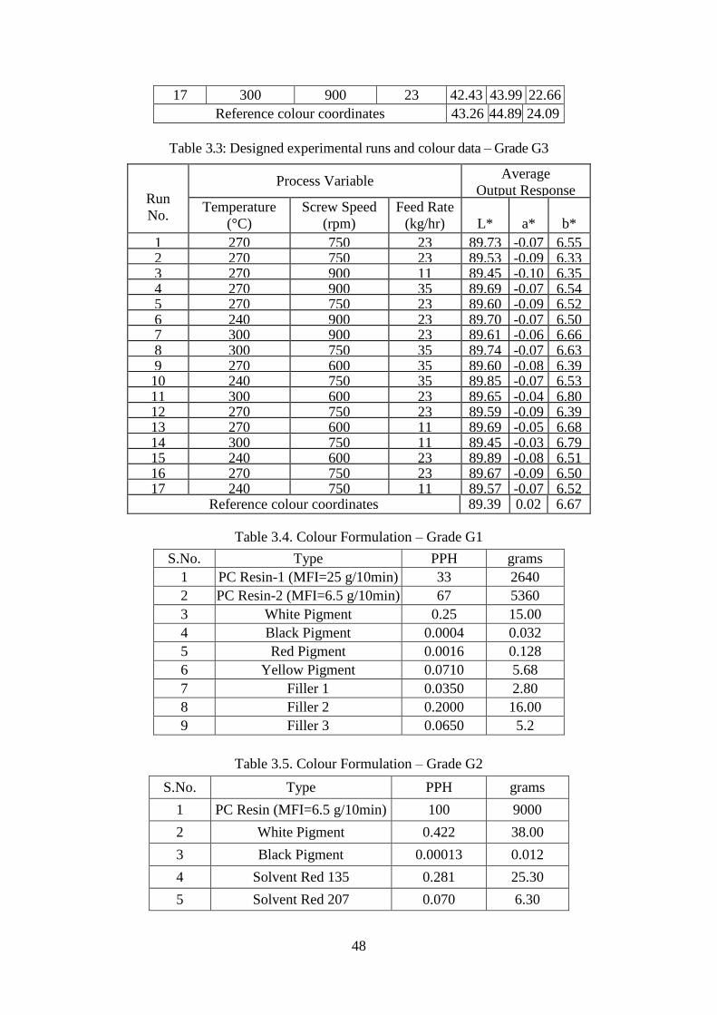
48

17 300 900 23 42.43 43.99 22.66

Reference colour coordinates 43.26 44.89 24.09

Table 3.3: Designed experimental runs and colour data – Grade G3

Run

No.

Process Variable Average

Output Response

Temperature

(°C)

Screw Speed

(rpm)

Feed Rate

(kg/hr)

L*

a*

b*

1 270 750 23 89.73 -0.07 6.55 2 270 750 23 89.53 -0.09 6.33 3 270 900 11 89.45 -0.10 6.35 4 270 900 35 89.69 -0.07 6.54 5 270 750 23 89.60 -0.09 6.52 6 240 900 23 89.70 -0.07 6.50 7 300 900 23 89.61 -0.06 6.66 8 300 750 35 89.74 -0.07 6.63 9 270 600 35 89.60 -0.08 6.39 10 240 750 35 89.85 -0.07 6.53 11 300 600 23 89.65 -0.04 6.80 12 270 750 23 89.59 -0.09 6.39 13 270 600 11 89.69 -0.05 6.68 14 300 750 11 89.45 -0.03 6.79 15 240 600 23 89.89 -0.08 6.51 16 270 750 23 89.67 -0.09 6.50 17 240 750 11 89.57 -0.07 6.52

Reference colour coordinates 89.39 0.02 6.67

Table 3.4. Colour Formulation – Grade G1

S.No. Type PPH grams

1 PC Resin-1 (MFI=25 g/10min) 33 2640

2 PC Resin-2 (MFI=6.5 g/10min) 67 5360

3 White Pigment 0.25 15.00

4 Black Pigment 0.0004 0.032

5 Red Pigment 0.0016 0.128

6 Yellow Pigment 0.0710 5.68

7 Filler 1 0.0350 2.80

8 Filler 2 0.2000 16.00

9 Filler 3 0.0650 5.2

Table 3.5. Colour Formulation – Grade G2

S.No. Type PPH grams

1 PC Resin (MFI=6.5 g/10min) 100 9000

2 White Pigment 0.422 38.00

3 Black Pigment 0.00013 0.012

4 Solvent Red 135 0.281 25.30

5 Solvent Red 207 0.070 6.30

49

6 Pigment Orange 107 0.202 18.20

7 Filler 1 0.050 4.50ml

8 Filler 2 0.022 2.00ml

Table 3.6: Colour Formulation – Grade G3

S-No Type PPH gram

1 PC Resin (MFI=6.5 g/10min) 100 10000

2 White Pigment 2.11 211

3 Black Pigment 0.045 4.5

4 Red Pigment 0.313 31.3

5 C.I. Pigment Brown 24 2.0 200

6 Pigment Yellow 163 0.086 8.6

7 Filler 1 0.20 20

8 Filler 2 0.60 60

9 Filler 3 0.05 5ml

3.3 Results and Discussion

The average colour data obtained from execution of DoEs respecting three PC grades,

were analysed by carrying out analysis of variance (ANOVA) using Design Expert® software.

The effect of significant main factors, quadratic factors and two factor interactions on output

responses are discussed. The fitness of predictive model equations is verified by further

experimentation, and the optimization results are presented.

3.3.1 Low Chroma Translucent PC Grade (G1) – Analysis and Optimization Results

A. ANOVA and Design Evaluation

Quadratic model as suggested by fit summary showing no aliases terms was employed.

ANOVA for all three output responses i.e. L*, a* and b* was executed and significant quadratic

models with p-value < 0.05 were obtained. All trivial model terms with p-value > 0.10 were

eliminated from each significant model employing backward technique. To ensure validity of

model, required design evaluation and diagnostic checks were carried out and all statistics

found well within threshold limits. For instance, lack of fit for the three models was

insignificant with degrees of freedom (df) greater than minimum limit of 3, difference between

adjusted R-squared and predicted R-squared values was below 0.2, adequate precision – a

measure of signal to noise ratio, was well above its threshold of 4, standard error values

associated with coefficients respecting linear, cross product and quadratic terms, were found

exactly same within their specific type, variance inflation factors (VIF) of all coefficients were

found at a Fig. of 1 - an ideal value that ensures design orthogonality, and all residuals behaved

well, except few DFFITS (difference of fits – a statistics helpful in detecting influential runs)

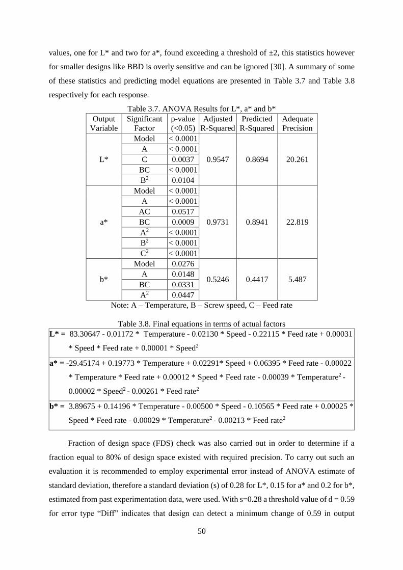
50

values, one for L* and two for a*, found exceeding a threshold of ±2, this statistics however

for smaller designs like BBD is overly sensitive and can be ignored [30]. A summary of some

of these statistics and predicting model equations are presented in Table 3.7 and Table 3.8

respectively for each response.

Table 3.7. ANOVA Results for L*, a* and b*

Output

Variable

Significant

Factor

p-value

(<0.05)

Adjusted

R-Squared

Predicted

R-Squared

Adequate

Precision

L*

Model < 0.0001

0.9547 0.8694 20.261

A < 0.0001

C 0.0037

BC < 0.0001

B2 0.0104

a*

Model < 0.0001

0.9731 0.8941 22.819

A < 0.0001

AC 0.0517

BC 0.0009

A2 < 0.0001

B2 < 0.0001

C2 < 0.0001

b*

Model 0.0276

0.5246 0.4417 5.487 A 0.0148

BC 0.0331

A2 0.0447

Note: A – Temperature, B – Screw speed, C – Feed rate

Table 3.8. Final equations in terms of actual factors

L* = 83.30647 - 0.01172 * Temperature - 0.02130 * Speed - 0.22115 * Feed rate + 0.00031

* Speed * Feed rate + 0.00001 * Speed2

a* = -29.45174 + 0.19773 * Temperature + 0.02291* Speed + 0.06395 * Feed rate - 0.00022

* Temperature * Feed rate + 0.00012 * Speed * Feed rate - 0.00039 * Temperature2 -

0.00002 * Speed2 - 0.00261 * Feed rate2

b* = 3.89675 + 0.14196 * Temperature - 0.00500 * Speed - 0.10565 * Feed rate + 0.00025 *

Speed * Feed rate - 0.00029 * Temperature2 - 0.00213 * Feed rate2

Fraction of design space (FDS) check was also carried out in order to determine if a

fraction equal to 80% of design space existed with required precision. To carry out such an

evaluation it is recommended to employ experimental error instead of ANOVA estimate of

standard deviation, therefore a standard deviation (s) of 0.28 for L*, 0.15 for a* and 0.2 for b*,

estimated from past experimentation data, were used. With s=0.28 a threshold value of d = 0.59

for error type “Diff” indicates that design can detect a minimum change of 0.59 in output

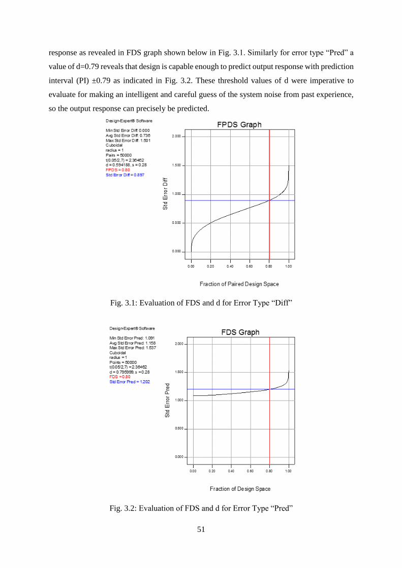
51

response as revealed in FDS graph shown below in Fig. 3.1. Similarly for error type “Pred” a

value of d=0.79 reveals that design is capable enough to predict output response with prediction

interval (PI) ±0.79 as indicated in Fig. 3.2. These threshold values of d were imperative to

evaluate for making an intelligent and careful guess of the system noise from past experience,

so the output response can precisely be predicted.

Fig. 3.1: Evaluation of FDS and d for Error Type “Diff”

Fig. 3.2: Evaluation of FDS and d for Error Type “Pred”

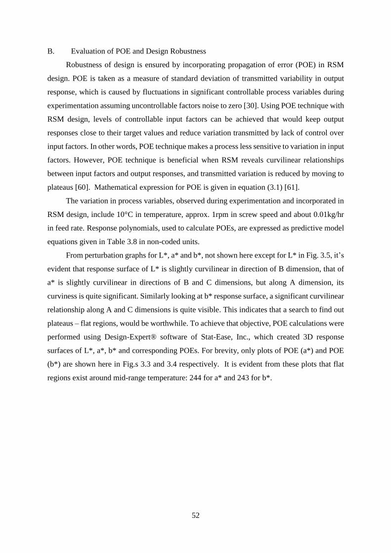
52

B. Evaluation of POE and Design Robustness

Robustness of design is ensured by incorporating propagation of error (POE) in RSM

design. POE is taken as a measure of standard deviation of transmitted variability in output

response, which is caused by fluctuations in significant controllable process variables during

experimentation assuming uncontrollable factors noise to zero [30]. Using POE technique with

RSM design, levels of controllable input factors can be achieved that would keep output

responses close to their target values and reduce variation transmitted by lack of control over

input factors. In other words, POE technique makes a process less sensitive to variation in input

factors. However, POE technique is beneficial when RSM reveals curvilinear relationships

between input factors and output responses, and transmitted variation is reduced by moving to

plateaus [60]. Mathematical expression for POE is given in equation (3.1) [61].

The variation in process variables, observed during experimentation and incorporated in

RSM design, include 10°C in temperature, approx. 1rpm in screw speed and about 0.01kg/hr

in feed rate. Response polynomials, used to calculate POEs, are expressed as predictive model

equations given in Table 3.8 in non-coded units.

From perturbation graphs for L*, a* and b*, not shown here except for L* in Fig. 3.5, it’s

evident that response surface of L* is slightly curvilinear in direction of B dimension, that of

a* is slightly curvilinear in directions of B and C dimensions, but along A dimension, its

curviness is quite significant. Similarly looking at b* response surface, a significant curvilinear

relationship along A and C dimensions is quite visible. This indicates that a search to find out

plateaus – flat regions, would be worthwhile. To achieve that objective, POE calculations were

performed using Design-Expert® software of Stat-Ease, Inc., which created 3D response

surfaces of L*, a*, b* and corresponding POEs. For brevity, only plots of POE (a*) and POE

(b*) are shown here in Fig.s 3.3 and 3.4 respectively. It is evident from these plots that flat

regions exist around mid-range temperature: 244 for a* and 243 for b*.

53

Fig. 3.3: POE (a*) Plot with Factor B at Mid-Point

Fig. 3.4: POE (b*) Plot with Factor B at Mid-Point

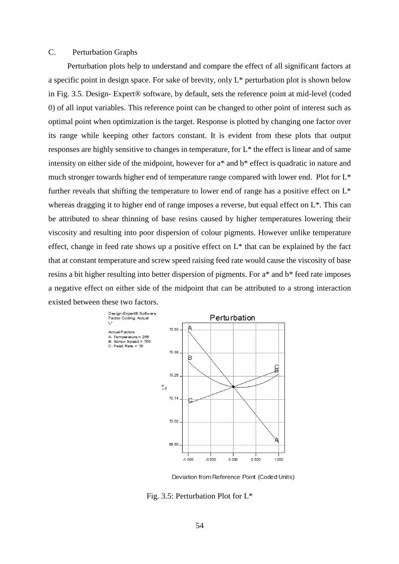
54

C. Perturbation Graphs

Perturbation plots help to understand and compare the effect of all significant factors at

a specific point in design space. For sake of brevity, only L* perturbation plot is shown below

in Fig. 3.5. Design- Expert® software, by default, sets the reference point at mid-level (coded

0) of all input variables. This reference point can be changed to other point of interest such as

optimal point when optimization is the target. Response is plotted by changing one factor over

its range while keeping other factors constant. It is evident from these plots that output

responses are highly sensitive to changes in temperature, for L* the effect is linear and of same

intensity on either side of the midpoint, however for a* and b* effect is quadratic in nature and

much stronger towards higher end of temperature range compared with lower end. Plot for L*

further reveals that shifting the temperature to lower end of range has a positive effect on L*

whereas dragging it to higher end of range imposes a reverse, but equal effect on L*. This can

be attributed to shear thinning of base resins caused by higher temperatures lowering their

viscosity and resulting into poor dispersion of colour pigments. However unlike temperature

effect, change in feed rate shows up a positive effect on L* that can be explained by the fact

that at constant temperature and screw speed raising feed rate would cause the viscosity of base

resins a bit higher resulting into better dispersion of pigments. For a* and b* feed rate imposes

a negative effect on either side of the midpoint that can be attributed to a strong interaction

existed between these two factors.

Fig. 3.5: Perturbation Plot for L*

55

D. Two Factor Interactions and Contours Graphs

Significant two factor interactions (2FI) between B and C affecting L*, a* and b*, and

between A and C affecting a* are captured by ANOVA based on their “p” values as reflected

in Table 3.7. For brevity, only L* plot of 2FI is shown in Fig. 3.6 using both the ANOVA

estimate (left graph) of noise - standard deviation of 0.07, and past experimental estimate (right

graph) of noise i.e. 0.28. It is evident from L* interaction graph that positive effect on L* caused

by increase in feed rate at maximum screw speed, is reversed when speed level is set at

minimum. A similar behaviour is reflected from interaction graphs of a* and b*. This effect

can be attributed to the fact that increase in feed rate, holding screw speed at minimum level

and temperature at its mid-level, would have caused poor dispersion of pigments resulting into

lower response values. However, overlapping of least significant distance (LSD) error bars in

right graph of Fig. 3.6 rejects the significance of these interactions.

Fig. 3.6: 2FI graphs affecting L* using ANOVA noise estimate (left), experimental error

(right)

Contour plot is another representation of the effect of process variables on output

response. For brevity, only L* contour plot is shown below in Fig. 3.7 reflecting effect of

temperature and feed rate on output response while holding screw speed at its midpoint. It is

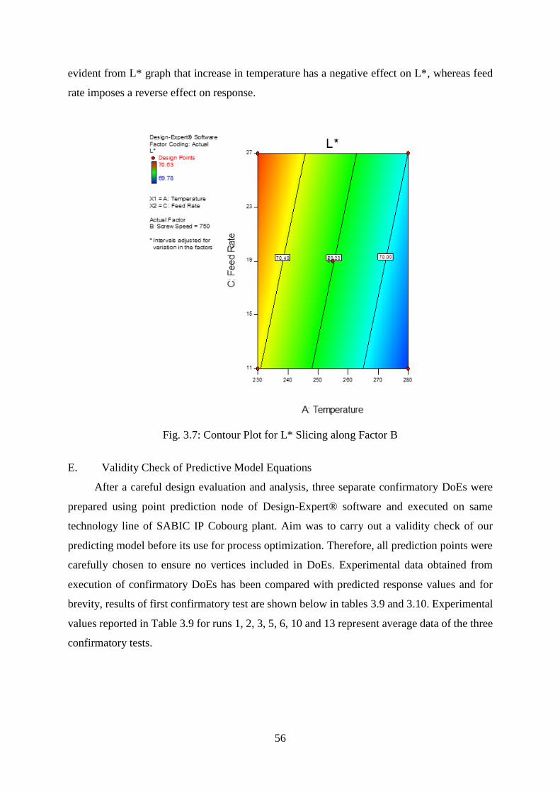
56

evident from L* graph that increase in temperature has a negative effect on L*, whereas feed

rate imposes a reverse effect on response.

Fig. 3.7: Contour Plot for L* Slicing along Factor B

E. Validity Check of Predictive Model Equations

After a careful design evaluation and analysis, three separate confirmatory DoEs were

prepared using point prediction node of Design-Expert® software and executed on same

technology line of SABIC IP Cobourg plant. Aim was to carry out a validity check of our

predicting model before its use for process optimization. Therefore, all prediction points were

carefully chosen to ensure no vertices included in DoEs. Experimental data obtained from

execution of confirmatory DoEs has been compared with predicted response values and for

brevity, results of first confirmatory test are shown below in tables 3.9 and 3.10. Experimental

values reported in Table 3.9 for runs 1, 2, 3, 5, 6, 10 and 13 represent average data of the three

confirmatory tests.

57

Table 3.9. Predicted Mean vs. Experimental Colour Data - Confirmatory Test

Run

No.

Process Parameter Predicted Response Experimental

Response

Temp

(°C)

Speed

(rpm)

Feed

(kg/hr)

L* a* b*

L* a* b*

Mean PI

low

PI

high Mean

PI

Low

PI

high Mean

PI

low

PI

high

1 230 750 11 70.41 69.63 71.19 3.71 3.08 4.35 18.03 17.45 18.6 69.93 3.70 17.98

2 230 750 27 70.58 69.81 71.36 3.81 3.24 4.37 18.07 17.49 18.64 70.05 3.78 17.95

3 230 850 11 70.23 69.35 71.11 3.43 2.73 4.13 17.8 17.16 18.45 69.80 3.82 17.88

4 250 763 11 70.14 69.4 70.89 3.83 3.42 4.23 18.04 17.52 18.56 69.60 3.69 18.04

5 255 650 11 70.5 69.65 71.35 3.77 3.29 4.26 18.26 17.65 18.87 70.17 3.68 18.20

6 255 650 27 70.18 69.33 71.03 3.58 3.05 4.11 17.9 17.29 18.51 70.06 3.58 17.98

7 255 750 25 70.27 69.54 71 3.9 3.46 4.34 18.13 17.62 18.64 69.85 3.52 18.02

8 255 750 25 70.27 69.54 71 3.9 3.46 4.34 18.13 17.62 18.64 69.75 3.57 18.19

9 255 750 25 70.27 69.54 71 3.9 3.46 4.34 18.13 17.62 18.64 69.77 3.56 17.86

10 255 850 11 69.94 69.08 70.79 3.54 3.06 4.03 17.82 17.21 18.43 69.69 3.47 17.78

11 269 745 18.6 70.04 69.32 70.76 3.82 3.23 4.41 18.04 17.45 18.64 69.49 3.46 17.60

12 274 728 22.4 70.01 69.28 70.74 3.66 2.96 4.37 17.93 17.28 18.58 69.46 3.65 17.66

13 280 750 27 70 69.22 70.78 3.37 2.38 4.35 17.73 16.94 18.51 69.76 3.50 17.69

Note: PI – 95% Prediction Interval

58

Table 3.10. Predicted Mean vs. Experimental Colour Data – Delta Values

Run No.

Process Parameter Experimental - Predicted

Temp

(°C)

Speed

(rpm)

Feed

(kg/hr) ∆L* ∆a* ∆b* ∆E*

1 230 750 11.00 -0.48 -0.01 -0.05 0.49

2 230 750 27.00 -0.53 -0.03 -0.12 0.54

3 230 850 11.00 -0.43 0.39 0.08 0.59

4 250 763 11.00 -0.54 -0.14 0.00 0.56

5 255 650 11.00 -0.34 -0.09 -0.07 0.35

6 255 650 27.00 -0.12 0.00 0.08 0.14

7 255 750 25 -0.42 -0.38 -0.11 0.58

8 255 750 25 -0.52 -0.33 0.06 0.62

9 255 750 25 -0.50 -0.34 -0.27 0.66

10 255 850 11.00 -0.25 -0.07 -0.04 0.26

11 269 745 18.60 -0.55 -0.36 -0.44 0.79

12 274 728 22.40 -0.55 -0.01 -0.27 0.61

13 280 750 27.00 -0.24 0.13 -0.04 0.28

A comparison between experimental and predicted values for confirmatory DoEs is

further illustrated in Fig.s 3.8 to 3.10 and discussed hereunder for L*, a* and b* respectively.

It is evident from these Fig.s that observed response values of confirmatory test runs are in

good agreement with PIs of predicted means, thereby verify the fitness of our predicting model.

L* values of run 1 & 2 however, were slightly exceeding PI lower limit in the first confirmatory

test so the runs were repeated in second confirmatory test and average values are shown in

Table 3.10. This slight variation can be attributed to the possibility of having a bit pronounced

experimental error at lower end of the temperature range. Confirmatory tests further reveal that

the gap between experimental and predicted values, in particular for a* and b*, becomes

narrowed for runs representing mid-range temperatures along with odd combination of speed

(B) and feed rate (C) e.g. runs 6 and 10 in Table 3.10. This behaviour can be associated to the

fact that mid-range temperatures and odd combinations of speed and feed rate represent the

plateau with minimum POE as explained above under POE graphs. However, having

experimental and predicted output response values close to each other does not guarantee they

will hit the target response values as well. This clearly indicates the need to adopt for a trade-

off while optimizing a process having multi-objective output responses.

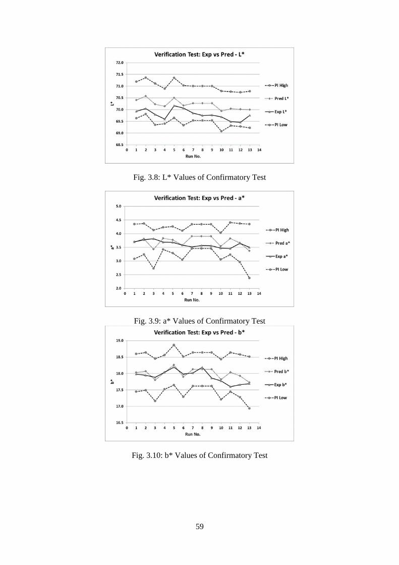
59

Fig. 3.8: L* Values of Confirmatory Test

Fig. 3.9: a* Values of Confirmatory Test

Fig. 3.10: b* Values of Confirmatory Test

60

F. Process Optimization

Once the predicting model is verified through confirmatory tests, process optimization

can be confidently exercised, which allows to determine an optimal set of input process

variables that could satisfy constraints imposed on multiple response output and associated

errors in design. Both numerical and graphical optimization techniques are successfully

employed in present study. Pasted below in Table 3.11 are constraints / criterion set out for

process optimization. Five solutions with overall desirability level ranging from 0.875 to 0.809

are reported in Table 3.12. Overall desirability level reflects the extent to which output response

could be achieved if optimal solution is implemented. As explained earlier, when objective is

to reach multiple output targets and simultaneously reduce POE to ensure robustness of design,

a trade-off is inevitable. All five solutions offer minimum overall colour deviation in terms of

delta values respecting thresholds (∆L*≤0.6, ∆a*≤0.6, ∆b*≤0.6 and ∆E*≤1) set by customer

for the plastic grade studied and a robust design restricting the variation band of delta values

to a narrow and a stable window. Bar graph, shown in Fig. 3.11, displays desirability levels

achieved for individual factors as well as overall objective. It can be noticed that a* desirability

level is the lowest one compared with other factors, this can be improved by adjusting its weight

and importance factors equal to those set for POEs, but at the cost of high POE. This situation

is the one often come across by experimenters while dealing with multi-objective output

response, where intelligent trade-offs help decide best possible solution [30].

Table 3.11. Criterion Set for Process Optimization

Name Goal Lower Limit Upper Limit Lower

Weight

Upper

Weight Importance

A:Temperature is in range 230 280 - - -

B:Screw Speed is in range 650 850 - - -

C:Feed Rate is in range 11 27 - - -

L* is target = 70.04 69.78 70.63 1 1 3

POE(L*) minimize 0.30 0.30 1 10 5

a* is target = 3.41 3.37 4.04 1 1 3

POE(a*) minimize 0.16 0.32 1 10 5

b* is target = 18.09 17.73 18.48 1 1 3

POE(b*) minimize 0.21 0.29 1 10 5

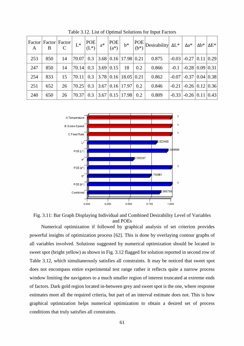
61

Table 3.12. List of Optimal Solutions for Input Factors

Factor

A

Factor

B

Factor

C L*

POE

(L*) a*

POE

(a*) b*

POE

(b*) Desirability ∆L* ∆a* ∆b* ∆E*

253 850 14 70.07 0.3 3.68 0.16 17.98 0.21 0.875 -0.03 -0.27 0.11 0.29

247 850 14 70.14 0.3 3.69 0.15 18 0.2 0.866 -0.1 -0.28 0.09 0.31

254 833 15 70.11 0.3 3.78 0.16 18.05 0.21 0.862 -0.07 -0.37 0.04 0.38

251 652 26 70.25 0.3 3.67 0.16 17.97 0.2 0.846 -0.21 -0.26 0.12 0.36

240 650 26 70.37 0.3 3.67 0.15 17.98 0.2 0.809 -0.33 -0.26 0.11 0.43

Fig. 3.11: Bar Graph Displaying Individual and Combined Desirability Level of Variables

and POEs

Numerical optimization if followed by graphical analysis of set criterion provides

powerful insights of optimization process [62]. This is done by overlaying contour graphs of

all variables involved. Solutions suggested by numerical optimization should be located in

sweet spot (bright yellow) as shown in Fig. 3.12 flagged for solution reported in second row of

Table 3.12, which simultaneously satisfies all constraints. It may be noticed that sweet spot

does not encompass entire experimental test range rather it reflects quite a narrow process

window limiting the navigators to a much smaller region of interest truncated at extreme ends

of factors. Dark gold region located in-between grey and sweet spot is the one, where response

estimates meet all the required criteria, but part of an interval estimate does not. This is how

graphical optimization helps numerical optimization to obtain a desired set of process

conditions that truly satisfies all constraints.

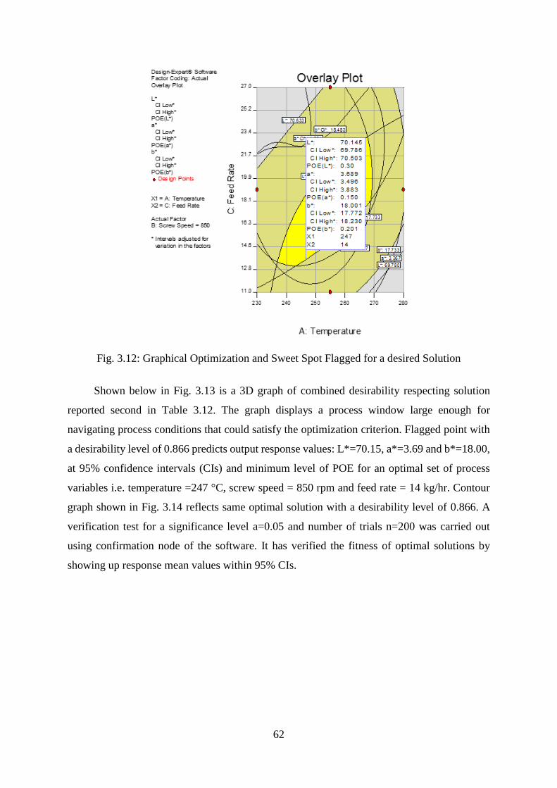
62

Fig. 3.12: Graphical Optimization and Sweet Spot Flagged for a desired Solution

Shown below in Fig. 3.13 is a 3D graph of combined desirability respecting solution

reported second in Table 3.12. The graph displays a process window large enough for

navigating process conditions that could satisfy the optimization criterion. Flagged point with

a desirability level of 0.866 predicts output response values: L*=70.15, a*=3.69 and b*=18.00,

at 95% confidence intervals (CIs) and minimum level of POE for an optimal set of process

variables i.e. temperature =247 °C, screw speed = 850 rpm and feed rate = 14 kg/hr. Contour

graph shown in Fig. 3.14 reflects same optimal solution with a desirability level of 0.866. A

verification test for a significance level a=0.05 and number of trials n=200 was carried out

using confirmation node of the software. It has verified the fitness of optimal solutions by

showing up response mean values within 95% CIs.

63

Fig. 3.13: 3D Surface Graph Flagged with Optimal Desirability

Fig. 3.14: 2D Contour Graph Flagged with Optimal Desirability

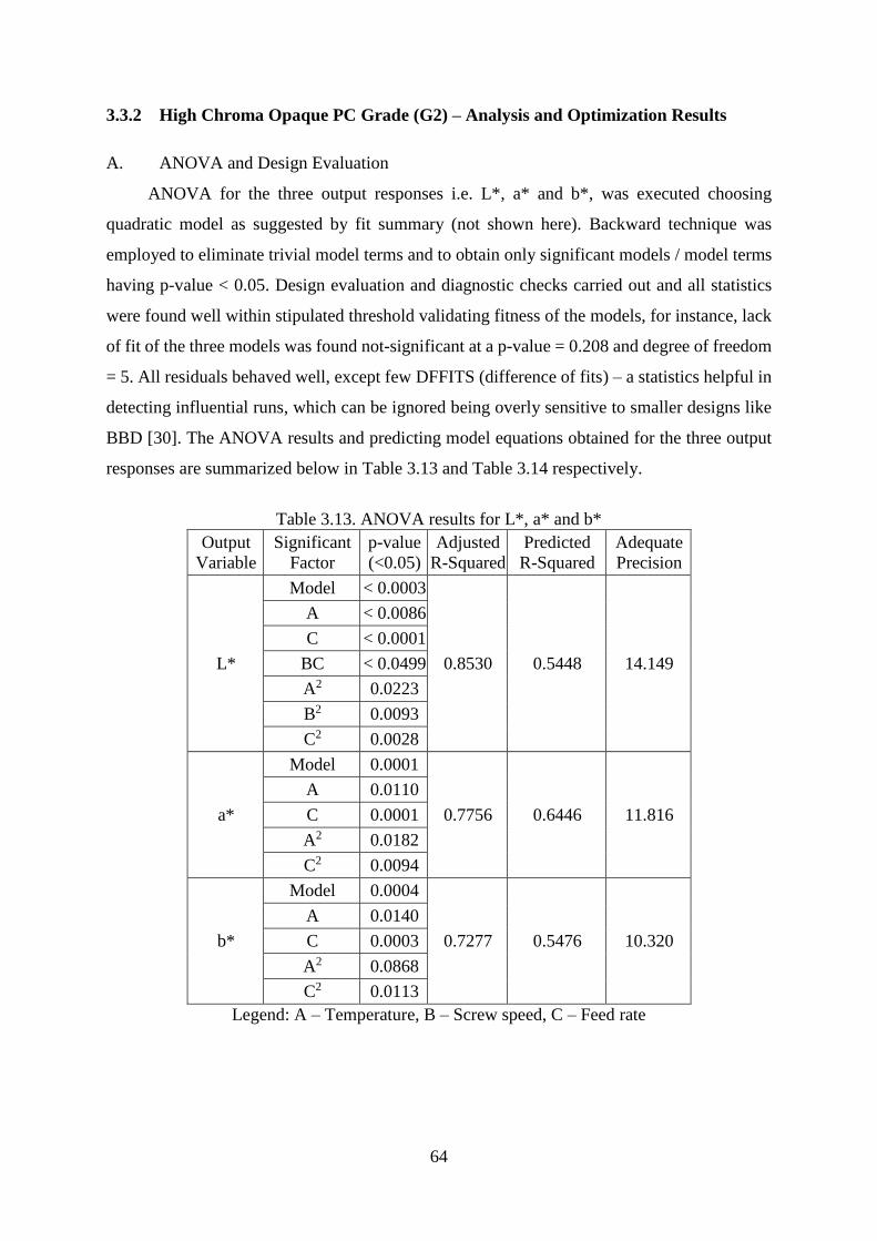
64

3.3.2 High Chroma Opaque PC Grade (G2) – Analysis and Optimization Results

A. ANOVA and Design Evaluation

ANOVA for the three output responses i.e. L*, a* and b*, was executed choosing

quadratic model as suggested by fit summary (not shown here). Backward technique was

employed to eliminate trivial model terms and to obtain only significant models / model terms

having p-value < 0.05. Design evaluation and diagnostic checks carried out and all statistics

were found well within stipulated threshold validating fitness of the models, for instance, lack

of fit of the three models was found not-significant at a p-value = 0.208 and degree of freedom

= 5. All residuals behaved well, except few DFFITS (difference of fits) – a statistics helpful in

detecting influential runs, which can be ignored being overly sensitive to smaller designs like

BBD [30]. The ANOVA results and predicting model equations obtained for the three output

responses are summarized below in Table 3.13 and Table 3.14 respectively.

Table 3.13. ANOVA results for L*, a* and b*

Legend: A – Temperature, B – Screw speed, C – Feed rate

Output

Variable

Significant

Factor

p-value

(<0.05)

Adjusted

R-Squared

Predicted

R-Squared

Adequate

Precision

L*

Model < 0.0003

0.8530 0.5448 14.149

A < 0.0086

C < 0.0001

BC < 0.0499

A2 0.0223

B2 0.0093

C2 0.0028

a*

Model 0.0001

0.7756 0.6446 11.816

A 0.0110

C 0.0001

A2 0.0182

C2 0.0094

b*

Model 0.0004

0.7277 0.5476 10.320

A 0.0140

C 0.0003

A2 0.0868

C2 0.0113

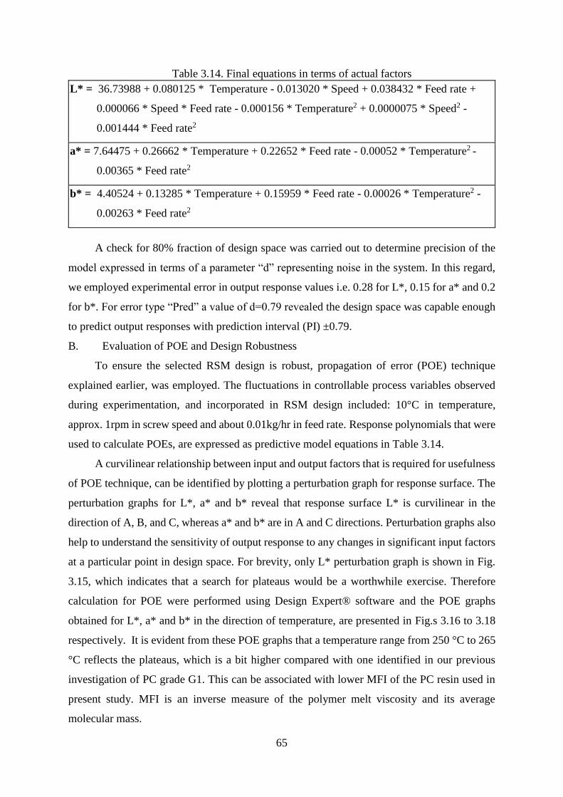
65

Table 3.14. Final equations in terms of actual factors

L* = 36.73988 + 0.080125 * Temperature - 0.013020 * Speed + 0.038432 * Feed rate +

0.000066 * Speed * Feed rate - 0.000156 * Temperature2 + 0.0000075 * Speed2 -

0.001444 * Feed rate2

a* = 7.64475 + 0.26662 * Temperature + 0.22652 * Feed rate - 0.00052 * Temperature2 -

0.00365 * Feed rate2

b* = 4.40524 + 0.13285 * Temperature + 0.15959 * Feed rate - 0.00026 * Temperature2 -

0.00263 * Feed rate2

A check for 80% fraction of design space was carried out to determine precision of the

model expressed in terms of a parameter “d” representing noise in the system. In this regard,

we employed experimental error in output response values i.e. 0.28 for L*, 0.15 for a* and 0.2

for b*. For error type “Pred” a value of d=0.79 revealed the design space was capable enough

to predict output responses with prediction interval (PI) ±0.79.

B. Evaluation of POE and Design Robustness

To ensure the selected RSM design is robust, propagation of error (POE) technique

explained earlier, was employed. The fluctuations in controllable process variables observed

during experimentation, and incorporated in RSM design included: 10°C in temperature,

approx. 1rpm in screw speed and about 0.01kg/hr in feed rate. Response polynomials that were

used to calculate POEs, are expressed as predictive model equations in Table 3.14.

A curvilinear relationship between input and output factors that is required for usefulness

of POE technique, can be identified by plotting a perturbation graph for response surface. The

perturbation graphs for L*, a* and b* reveal that response surface L* is curvilinear in the

direction of A, B, and C, whereas a* and b* are in A and C directions. Perturbation graphs also

help to understand the sensitivity of output response to any changes in significant input factors

at a particular point in design space. For brevity, only L* perturbation graph is shown in Fig.

3.15, which indicates that a search for plateaus would be a worthwhile exercise. Therefore

calculation for POE were performed using Design Expert® software and the POE graphs

obtained for L*, a* and b* in the direction of temperature, are presented in Fig.s 3.16 to 3.18

respectively. It is evident from these POE graphs that a temperature range from 250 °C to 265

°C reflects the plateaus, which is a bit higher compared with one identified in our previous

investigation of PC grade G1. This can be associated with lower MFI of the PC resin used in

present study. MFI is an inverse measure of the polymer melt viscosity and its average

molecular mass.

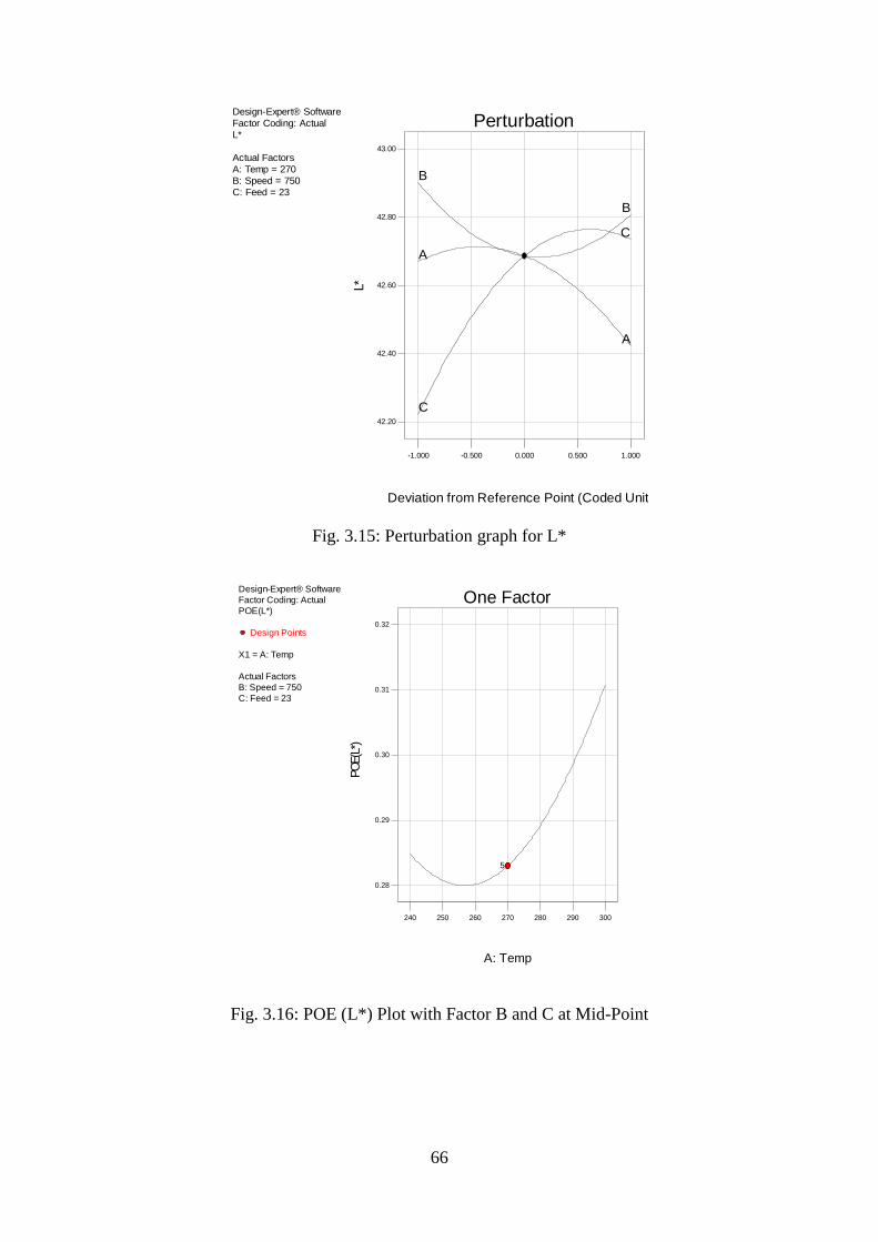
66

Fig. 3.15: Perturbation graph for L*

Fig. 3.16: POE (L*) Plot with Factor B and C at Mid-Point

Design-Expert® Software

Factor Coding: Actual

L*

Actual Factors

A: Temp = 270

B: Speed = 750

C: Feed = 23

Perturbation

Deviation from Reference Point (Coded Units)

L*

-1.000 -0.500 0.000 0.500 1.000

42.20

42.40

42.60

42.80

43.00

A

A

B

B

C

C

Design-Expert® Software

Factor Coding: Actual

POE(L*)

Design Points

X1 = A: Temp

Actual Factors

B: Speed = 750

C: Feed = 23

240 250 260 270 280 290 300

A: Temp

PO

E(L

*)

0.28

0.29

0.30

0.31

0.32

5

One Factor

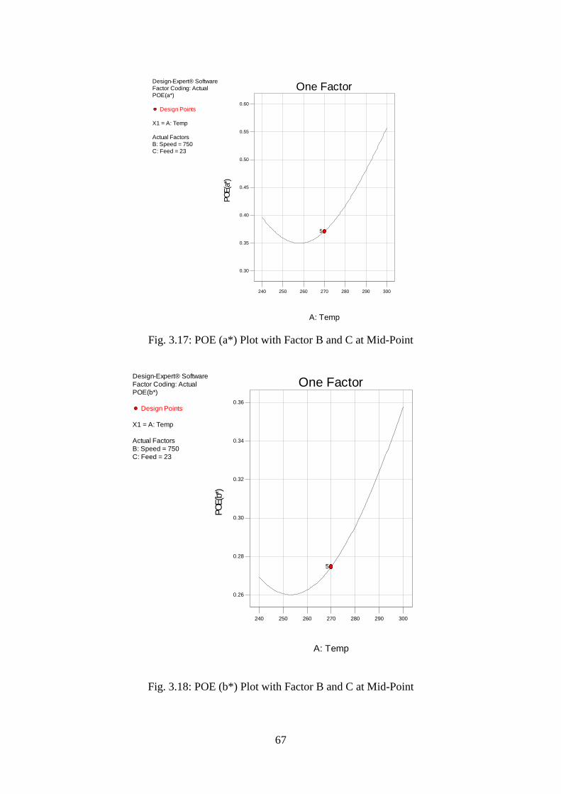
67

Fig. 3.17: POE (a*) Plot with Factor B and C at Mid-Point

Fig. 3.18: POE (b*) Plot with Factor B and C at Mid-Point

Design-Expert® Software

Factor Coding: Actual

POE(a*)

Design Points

X1 = A: Temp

Actual Factors

B: Speed = 750

C: Feed = 23

240 250 260 270 280 290 300

A: Temp

PO

E(a

*)

0.30

0.35

0.40

0.45

0.50

0.55

0.60

5

One Factor

Design-Expert® Software

Factor Coding: Actual

POE(b*)

Design Points

X1 = A: Temp

Actual Factors

B: Speed = 750

C: Feed = 23

240 250 260 270 280 290 300

A: Temp

PO

E(b

*)

0.26

0.28

0.30

0.32

0.34

0.36

5

One Factor

68

C. Two Factor Interactions and Contours Graphs

The only significant two factor interaction (2FI) captured was “BC” i.e. the interaction

between screw speed and feed rate, affecting L*. The 2FI is shown in Fig. 3.19 for both, with

ANOVA estimate of the noise i.e. 0.1 (left) and with experimental error i.e. 0.28 (right). The

two graphs reveal that L* value improves by increasing feed rate level for a fixed screw speed

level until the feed rate reaches a level called critical point (highlighted blue), beyond which

the effect of increasing feed rate turns into negative for minimum speed level. This can be

attributed to inadequate pigments dispersion in polymeric matrix resulting into a lower L*

value. Overlapping of error bars in Fig. 3.19 (right) however, invalidates the significance of

2FI, the error bars represent least significant distance (LSD).

Fig. 3.19: 2FI graphs affecting L* using ANOVA noise estimate (left), experimental error

(right)

Contour plot shown in Fig. 3.20 is a two-dimensional representation of the response L*

across two input variables i.e. temperature and feed rate, and sliced along direction of 3rd

variable i.e. screw speed. The contour graph sliced at a speed of 750rpm, clearly indicates that

L* responds negatively to an increase in temperature and a decrease in feed rate.

Design-Expert® Software

Factor Coding: Actual

L*

Design Points

X1 = C: Feed

X2 = B: Speed

Actual Factor

A: Temp = 270

B- 600

B+ 900

B: Speed

11 17 23 29 35

C: Feed

L*

41.50

42.00

42.50

43.00

43.50

2

2

2

2

Critical Point

InteractionDesign-Expert® Software

Factor Coding: Actual

L*

Design Points

X1 = C: Feed

X2 = B: Speed

Actual Factor

A: Temp = 270

B- 600

B+ 900

B: Speed

11 17 23 29 35

C: Feed

L*

41.50

42.00

42.50

43.00

43.50

2

2

2

2

Critical Point

Interaction

69

Fig. 3.20: Contour Plot for L* Slicing along Factor B

D. Validity Check of Predictive Model Equations

After a careful evaluation of the design and ANOVA discussed in the preceding sections,

a confirmatory DoE prepared using predicting model equations given in Table 3.14, was

executed on the same technology line. Aim was to carry out a validity check of our predicting

model before its use for process optimization. Therefore, all prediction points were carefully

chosen to ensure no vertices included in DoE. Experimental data obtained is compared with

predicted mean of response values and the difference is presented in Table 3.15 in terms of

delta values i.e. ∆L*, ∆a* and ∆b*. All delta values were found well within PI of ±0.79 except

∆a* for run 1, which verified our predicting model.

Table 3.15: Predicted Mean vs. Experimental Colour Data – Confirmatory Test

Run No.

Process Parameter Experimental – Predicted Mean

Temp

(°C)

Speed

(rpm)

Feed

(kg/hr) ∆L* ∆a* ∆b*

1 240 750 11 0.54 0.89 0.65

2 270 600 11 0.06 0.53 0.50

3 270 750 35 0.37 0.44 0.44

4 270 900 23 0.07 0.18 0.22

5 300 750 23 0.37 0.70 0.48

Design-Expert® Software

Factor Coding: Actual

L*

Design Points

42.91

41.96

X1 = A: Temp

X2 = C: Feed

Actual Factor

B: Speed = 750

* Intervals adjusted for

variation in the factors

240 250 260 270 280 290 300

11

17

23

29

35

L*

A: Temp

C: F

eed

42.00

42.20

42.40

42.60

42.75

42.75

42.79

5

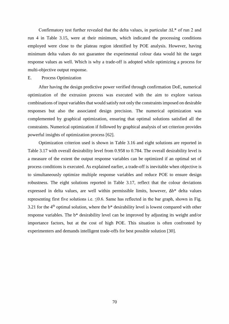
70

Confirmatory test further revealed that the delta values, in particular ∆L* of run 2 and

run 4 in Table 3.15, were at their minimum, which indicated the processing conditions

employed were close to the plateau region identified by POE analysis. However, having

minimum delta values do not guarantee the experimental colour data would hit the target

response values as well. Which is why a trade-off is adopted while optimizing a process for

multi-objective output response.

E. Process Optimization

After having the design predictive power verified through confirmation DoE, numerical

optimization of the extrusion process was executed with the aim to explore various

combinations of input variables that would satisfy not only the constraints imposed on desirable

responses but also the associated design precision. The numerical optimization was

complemented by graphical optimization, ensuring that optimal solutions satisfied all the

constraints. Numerical optimization if followed by graphical analysis of set criterion provides

powerful insights of optimization process [62].

Optimization criterion used is shown in Table 3.16 and eight solutions are reported in

Table 3.17 with overall desirability level from 0.958 to 0.784. The overall desirability level is

a measure of the extent the output response variables can be optimized if an optimal set of

process conditions is executed. As explained earlier, a trade-off is inevitable when objective is

to simultaneously optimize multiple response variables and reduce POE to ensure design

robustness. The eight solutions reported in Table 3.17, reflect that the colour deviations

expressed in delta values, are well within permissible limits, however, ∆b* delta values

representing first five solutions i.e. ≤0.6. Same has reflected in the bar graph, shown in Fig.

3.21 for the 4th optimal solution, where the b* desirability level is lowest compared with other

response variables. The b* desirability level can be improved by adjusting its weight and/or

importance factors, but at the cost of high POE. This situation is often confronted by

experimenters and demands intelligent trade-offs for best possible solution [30].

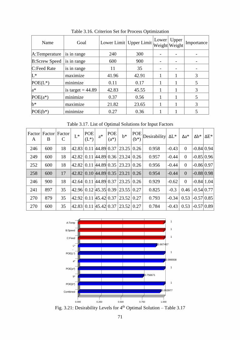
71

Table 3.16. Criterion Set for Process Optimization

Name Goal Lower Limit Upper Limit Lower

Weight

Upper

Weight Importance

A:Temperature is in range 240 300 - - -

B:Screw Speed is in range 600 900 - - -

C:Feed Rate is in range 11 35 - - -

L* maximize 41.96 42.91 1 1 3

POE(L*) minimize 0.11 0.17 1 1 5

a* is target = 44.89 42.83 45.55 1 1 3

POE(a*) minimize 0.37 0.56 1 1 5

b* maximize 21.82 23.65 1 1 3

POE(b*) minimize 0.27 0.36 1 1 5

Table 3.17. List of Optimal Solutions for Input Factors

Factor

A

Factor

B

Factor

C L*

POE

(L*) a*

POE

(a*) b*

POE

(b*) Desirability ∆L* ∆a* ∆b* ∆E*

246 600 18 42.83 0.11 44.89 0.37 23.25 0.26 0.958 -0.43 0 -0.84 0.94

249 600 18 42.82 0.11 44.89 0.36 23.24 0.26 0.957 -0.44 0 -0.85 0.96

252 600 18 42.82 0.11 44.89 0.35 23.23 0.26 0.956 -0.44 0 -0.86 0.97

258 600 17 42.82 0.10 44.89 0.35 23.21 0.26 0.954 -0.44 0 -0.88 0.98

246 900 18 42.64 0.11 44.89 0.37 23.25 0.26 0.929 -0.62 0 -0.84 1.04

241 897 35 42.96 0.12 45.35 0.39 23.55 0.27 0.825 -0.3 0.46 -0.54 0.77

270 879 35 42.92 0.11 45.42 0.37 23.52 0.27 0.793 -0.34 0.53 -0.57 0.85

270 600 35 42.83 0.11 45.42 0.37 23.52 0.27 0.784 -0.43 0.53 -0.57 0.89

Fig. 3.21: Desirability Levels for 4th Optimal Solution – Table 3.17

1

1

1

0.907457

1

0.999008

1

0.756671

1

0.953977

Desirability

0.000 0.250 0.500 0.750 1.000

A:Temp

B:Speed

C:Feed

L*

POE(L*)

a*

POE(a*)

b*

POE(b*)

Combined

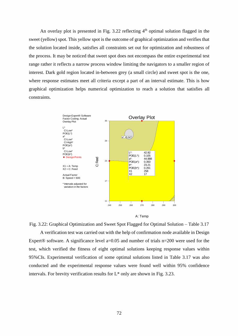
72

An overlay plot is presented in Fig. 3.22 reflecting 4th optimal solution flagged in the

sweet (yellow) spot. This yellow spot is the outcome of graphical optimization and verifies that

the solution located inside, satisfies all constraints set out for optimization and robustness of

the process. It may be noticed that sweet spot does not encompass the entire experimental test

range rather it reflects a narrow process window limiting the navigators to a smaller region of

interest. Dark gold region located in-between grey (a small circle) and sweet spot is the one,

where response estimates meet all criteria except a part of an interval estimate. This is how

graphical optimization helps numerical optimization to reach a solution that satisfies all

constraints.

Fig. 3.22: Graphical Optimization and Sweet Spot Flagged for Optimal Solution – Table 3.17

A verification test was carried out with the help of confirmation node available in Design

Expert® software. A significance level a=0.05 and number of trials n=200 were used for the

test, which verified the fitness of eight optimal solutions keeping response values within

95%CIs. Experimental verification of some optimal solutions listed in Table 3.17 was also

conducted and the experimental response values were found well within 95% confidence

intervals. For brevity verification results for L* only are shown in Fig. 3.23.

Design-Expert® Software

Factor Coding: Actual

Overlay Plot

L*

CI Low*

POE(L*)

a*

CI Low*

CI High*

POE(a*)

b*

CI Low*

POE(b*)

Design Points

X1 = A: Temp

X2 = C: Feed

Actual Factor

B: Speed = 600

* Intervals adjusted for

variation in the factors

240 250 260 270 280 290 300

11

17

23

29

35

Overlay Plot

A: Temp

C: F

eed

a*: 45.547

a* CI*: 45.547L*: 42.82POE(L*): 0.105a*: 44.888POE(a*): 0.350b*: 23.21POE(b*): 0.261X1 258X2 17

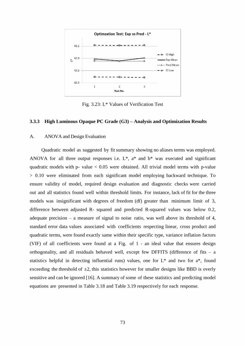
73

Fig. 3.23: L* Values of Verification Test

3.3.3 High Luminous Opaque PC Grade (G3) – Analysis and Optimization Results

A. ANOVA and Design Evaluation

Quadratic model as suggested by fit summary showing no aliases terms was employed.

ANOVA for all three output responses i.e. L*, a* and b* was executed and significant

quadratic models with p- value < 0.05 were obtained. All trivial model terms with p-value

> 0.10 were eliminated from each significant model employing backward technique. To

ensure validity of model, required design evaluation and diagnostic checks were carried

out and all statistics found well within threshold limits. For instance, lack of fit for the three

models was insignificant with degrees of freedom (df) greater than minimum limit of 3,

difference between adjusted R- squared and predicted R-squared values was below 0.2,

adequate precision – a measure of signal to noise ratio, was well above its threshold of 4,

standard error data values associated with coefficients respecting linear, cross product and

quadratic terms, were found exactly same within their specific type, variance inflation factors

(VIF) of all coefficients were found at a Fig. of 1 - an ideal value that ensures design

orthogonality, and all residuals behaved well, except few DFFITS (difference of fits – a

statistics helpful in detecting influential runs) values, one for L* and two for a*, found

exceeding the threshold of ±2, this statistics however for smaller designs like BBD is overly

sensitive and can be ignored [16]. A summary of some of these statistics and predicting model

equations are presented in Table 3.18 and Table 3.19 respectively for each response.

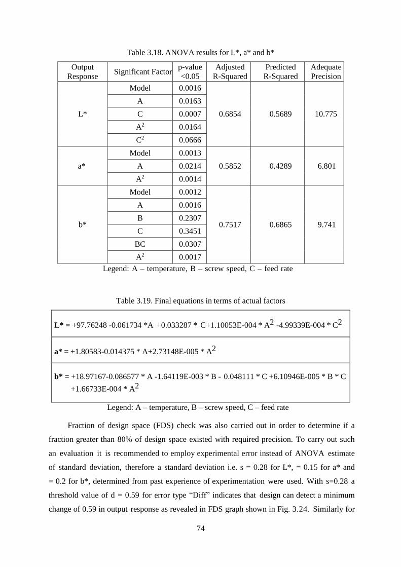
74

Table 3.18. ANOVA results for L*, a* and b*

Output

Response Significant Factor

p-value

<0.05

Adjusted

R-Squared

Predicted

R-Squared

Adequate

Precision

L*

Model 0.0016

0.6854 0.5689 10.775

A 0.0163

C 0.0007

A2 0.0164

C2 0.0666

a*

Model 0.0013

0.5852 0.4289 6.801 A 0.0214

A2 0.0014

b*

Model 0.0012

0.7517 0.6865 9.741

A 0.0016

B 0.2307

C 0.3451

BC 0.0307

A2 0.0017

Legend: A – temperature, B – screw speed, C – feed rate

Table 3.19. Final equations in terms of actual factors

L* = +97.76248 -0.061734 *A +0.033287 * C+1.10053E-004 * A2 -4.99339E-004 * C2

a* = +1.80583-0.014375 * A+2.73148E-005 * A2

b* = +18.97167-0.086577 * A -1.64119E-003 * B - 0.048111 * C +6.10946E-005 * B * C

+1.66733E-004 * A2

Legend: A – temperature, B – screw speed, C – feed rate

Fraction of design space (FDS) check was also carried out in order to determine if a

fraction greater than 80% of design space existed with required precision. To carry out such

an evaluation it is recommended to employ experimental error instead of ANOVA estimate

of standard deviation, therefore a standard deviation i.e. s = 0.28 for L*, = 0.15 for a* and

= 0.2 for b*, determined from past experience of experimentation were used. With s=0.28 a

threshold value of d = 0.59 for error type “Diff” indicates that design can detect a minimum

change of 0.59 in output response as revealed in FDS graph shown in Fig. 3.24. Similarly for

75

error type “Pred” a value of d=0.85 reveals that design is capable to predict output response

with prediction interval (PI) ±0.85 as shown in Fig. 3.25. These threshold values of d were

imperative to evaluate making an intelligent and careful guess of system noise from past

experience so the output response can precisely be predicted.

Fig. 3.24: Evaluation of FDS and d for error type Diff

Fig. 3.25: Evaluation of FDS and d for error type Pred

Design-Expert® Software

Min Std Error Diff: 0.000

Avg Std Error Diff: 0.736

Max Std Error Diff: 1.501

Cuboidal

radius = 1

Pairs = 50000

t(0.05/2,7) = 2.36462

d = 0.594188, s = 0.28

FPDS = 0.80

Std Error Diff = 0.897

FPDS Graph

Fraction of Paired Design Space

Std

Error D

iff

0.00 0.20 0.40 0.60 0.80 1.00

0.000

0.500

1.000

1.500

2.000

Design-Expert® Software

Min Std Error Pred: 1.091Avg Std Error Pred: 1.198Max Std Error Pred: 2.000Cuboidalradius = 1Points = 50000t(0.05/2,6) = 2.44691d = 0.854223, s = 0.28FDS = 0.80Std Error Pred = 1.247

FDS Graph

Fraction of Design Space

Std E

rror P

red

0.00 0.20 0.40 0.60 0.80 1.00

0.000

0.500

1.000

1.500

2.000

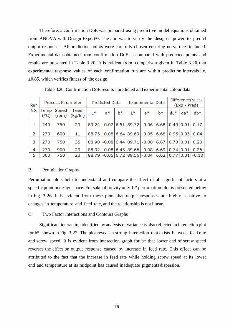
76

Therefore, a confirmation DoE was prepared using predictive model equations obtained

from ANOVA with Design Expert®. The aim was to verify the design’s power to predict

output responses. All prediction points were carefully chosen ensuring no vertices included.

Experimental data obtained from confirmation DoE is compared with predicted points and

results are presented in Table 3.20. It is evident from comparison given in Table 3.20 that

experimental response values of each confirmation run are within prediction intervals i.e.

±0.85, which verifies fitness of the design.

Table 3.20: Confirmation DoE results - predicted and experimental colour data

B. Perturbation Graphs

Perturbation plots help to understand and compare the effect of all significant factors at a

specific point in design space. For sake of brevity only L* perturbation plot is presented below

in Fig. 3.26. It is evident from these plots that output responses are highly sensitive to

changes in temperature and feed rate, and the relationship is not linear.

C. Two Factor Interactions and Contours Graphs

Significant interaction identified by analysis of variance is also reflected in interaction plot

for b*, shown in Fig. 3.27. The plot reveals a strong interaction that exists between feed rate

and screw speed. It is evident from interaction graph for b* that lower end of screw speed

reverses the effect on output response caused by increase in feed rate. This effect can be

attributed to the fact that the increase in feed rate while holding screw speed at its lower

end and temperature at its midpoint has caused inadequate pigments dispersion.

77

Fig. 3.26: Perturbation Plot for L*

Fig. 3.27: Interaction b/w factors C and B affecting b*

Contour plot is another representation of the effect of process variables on output

response. For brevity only L* contour plot is shown in Fig. 3.28 reflecting effect of

temperature and feed rate on output response while holding screw speed at its midpoint. It is

evident from L* contour graph that increase in temperature has a negative effect on L*

whereas feed rate imposes a reverse effect on the response.

Design-Expert® SoftwareFactor Coding: ActualL*

Actual FactorsA: Temp = 270*B: Speed = 750C: Feed = 23

Factors not in ModelB

Perturbation

Deviation from Reference Point (Coded Units)

L*

-1.000 -0.500 0.000 0.500 1.000

89.40

89.50

89.60

89.70

89.80 A

A

C

C

Design-Expert® SoftwareFactor Coding: Actualb*

Design Points

X1 = C: FeedX2 = B: Speed

Actual FactorA: Temp = 270

B- 600B+ 900

B: Speed

11 17 23 29 35

C: Feed

b*

6.00

6.20

6.40

6.60

6.80

7.00

Interaction

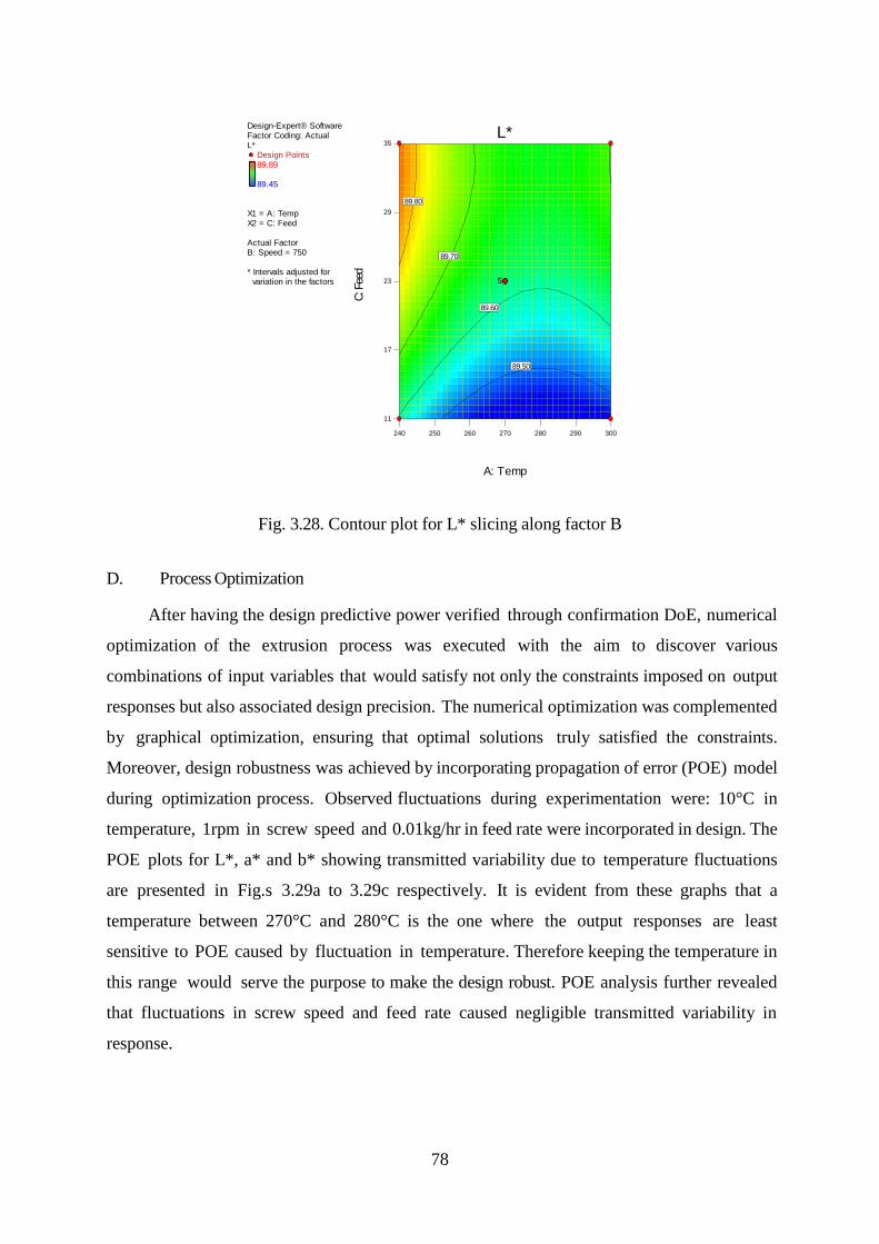
78

Fig. 3.28. Contour plot for L* slicing along factor B

D. Process Optimization

After having the design predictive power verified through confirmation DoE, numerical

optimization of the extrusion process was executed with the aim to discover various

combinations of input variables that would satisfy not only the constraints imposed on output

responses but also associated design precision. The numerical optimization was complemented

by graphical optimization, ensuring that optimal solutions truly satisfied the constraints.

Moreover, design robustness was achieved by incorporating propagation of error (POE) model

during optimization process. Observed fluctuations during experimentation were: 10°C in

temperature, 1rpm in screw speed and 0.01kg/hr in feed rate were incorporated in design. The

POE plots for L*, a* and b* showing transmitted variability due to temperature fluctuations

are presented in Fig.s 3.29a to 3.29c respectively. It is evident from these graphs that a

temperature between 270°C and 280°C is the one where the output responses are least

sensitive to POE caused by fluctuation in temperature. Therefore keeping the temperature in

this range would serve the purpose to make the design robust. POE analysis further revealed

that fluctuations in screw speed and feed rate caused negligible transmitted variability in

response.

Design-Expert® SoftwareFactor Coding: ActualL*

Design Points89.89

89.45

X1 = A: TempX2 = C: Feed

Actual FactorB: Speed = 750

* Intervals adjusted for variation in the factors

240 250 260 270 280 290 300

11

17

23

29

35L*

A: Temp

C: F

eed

89.50

89.60

89.70

89.80

5

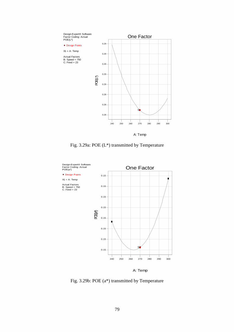
79

Fig. 3.29a: POE (L*) transmitted by Temperature

Fig. 3.29b: POE (a*) transmitted by Temperature

Design-Expert® SoftwareFactor Coding: ActualPOE(L*)

Design Points

X1 = A: Temp

Actual FactorsB: Speed = 750C: Feed = 23

240 250 260 270 280 290 300

A: Temp

PO

E(L

*)

0.28

0.28

0.28

0.29

0.29

0.29

0.29

0.29

5

One Factor

Design-Expert® SoftwareFactor Coding: ActualPOE(a*)

Design Points

X1 = A: Temp

Actual FactorsB: Speed = 750C: Feed = 23

240 250 260 270 280 290 300

A: Temp

POE(

a*)

0.15

0.15

0.15

0.15

0.15

0.15

0.15

0.15

5

One Factor

80

Fig. 3.29c: POE (b*) transmitted by Temperature

Optimization criterion used is shown in Table 3.21 and three solutions out of nine, with

desirability level from 0.79 to 0.71 are reported in Table 3.22. All the three solutions reflect a

colour deviation in terms of delta values well within permissible limits compared with

reference standard.

Table 3.21. Optimization criteria set to reach the target

Name Goal Lower Limit Upper Limit

A: Temperature is in range 240 300

B: Screw Speed is in range 600 900

C: Feed Rate is in range 11 35

L* is target = 89.45 89.45 89.89

POE(L*) minimize 0.281 0.294

a* is target = -0.027 -0.10 -0.027

POE(a*) minimize 0.150 0.151

b* is target = 6.67 6.333 6.697

POE(b*) minimize 0.21 0.29

Design-Expert® SoftwareFactor Coding: ActualPOE(b*)

Design Points

X1 = A: Temp

Actual FactorsB: Speed = 750C: Feed = 23

240 250 260 270 280 290 300

A: Temp

POE(

b*)

0.20

0.21

0.22

0.23

0.24

0.25

5

One Factor

81

Table 3.22. Three Solutions from Process Optimization

Factors 1st

Solution

2nd

Solution

3nd

Solution

Temperature 280 279 276

Screw Speed 600 600 600

Feed Rate 15 15 15

L* 89.49 89.49 89.49

POE(L*) 0.28 0.28 0.28

a* -0.08 -0.08 -0.08

POE(a*) 0.15 0.15 0.15

b* 6.65 6.64 6.62

POE(b*) 0.21 0.21 0.22

∆L* -0.1 -0.1 -0.1

∆a* 0.1 0.1 0.1

∆b* 0.02 0.03 0.05

∆E* 0.0204 0.0209 0.0225

Desirability 0.79 0.77 0.71

An overlay plot is presented in Fig. 3.30 reflecting 3rd optimal solution flagged in

the sweet (yellow) spot. This yellow spot is the outcome of graphical optimization and

verifies that the solution located inside, satisfies the constraints set out for optimization and

process robustness.

Fig. 3.30: 3rd optimal solution flagged in sweet spot

Design-Expert® SoftwareFactor Coding: ActualOverlay Plot

L* CI Low*POE(L*)a* CI Low*POE(a*)b* CI Low*POE(b*)

Design Points

X1 = A: TempX2 = C: Feed

Actual FactorB: Speed = 600

* Intervals adjusted for variation in the factors

240 250 260 270 280 290 300

11

17

23

29

35

Overlay Plot

A: Temp

C: Feed

L*: 89.450

L* CI*: 89.450

POE(L*): 0.285 POE(a*): 0.150b*: 6.500

POE(b*): 0.220

L*: 89.495a*: -0.08b*: 6.619X1 276X2 15

82

A verification test was carried out with the help of confirmation node available in Design

Expert® software. A significance level a=0.05 and number of trials n=200 were used for the

test, which verified the fitness of three optimal solutions keeping response values within

95%Cis. Experimental verification of the optimal solutions listed in Table 3.22 was also

conducted and the experimental response values (not shown here) were found well within

95% confidence intervals.

3.4 Conclusions

3.4.1 Low Chroma Translucent PC Grade (G1)

Present investigation identifies process variables that can significantly influence output

colour of PC grade G1. This study suggests five sets of optimal process conditions. These

optimal process conditions can be employed with greater confidence to achieve consistency in

output colour while restricting POEs at minimum and overall colour deviation (∆E*) to a

narrow range of 0.29 to 0.43, which lies well below the stipulated threshold of 1.0.

The experimental study offers plastic compounders a narrow but a precise process

window - region of interest (sweet spot) shown yellow in overlay plot of Fig. 3.12. This study

would not only help them overcome colour mismatch issue by allowing to choose a set of

optimal process variables that ensures consistency in output colour, but also enable them make

a right choice from available optimal solutions in order to reduce specific mechanical energy

(SME), and thus improve productivity. In this perspective optimal solution reported in last row

of Table 3.12 is the best choice.

3.4.2. High Chroma Opaque PC Grade (G2)

Present experimental study identifies process variables that impose a significant impact

on output colour of the PC grade G2 in individual capacity as well as in 2 factor interactions

(2FIs). The study suggests eight optimal process conditions that can be employed to achieve

consistent output colour for the plastic grade examined, with greater confidence and with least

colour deviation from reference standard. The study further reveals the usefulness of POE

technique to ensure the process robustness along with optimization. Moreover, higher

temperature plateaus compared with grade G1, identified in POE graphs, can be associated

with low MFI of the PC resin used in formulation.

3.4.3 High Luminous Opaque PC Grade (G3)

Present experimental study identifies through statistical analysis, the process input

variables that have a significant impact on output colour of PC grade G3, individually as well

as in terms of their two factor interaction (2FI). The study suggests optimal process conditions

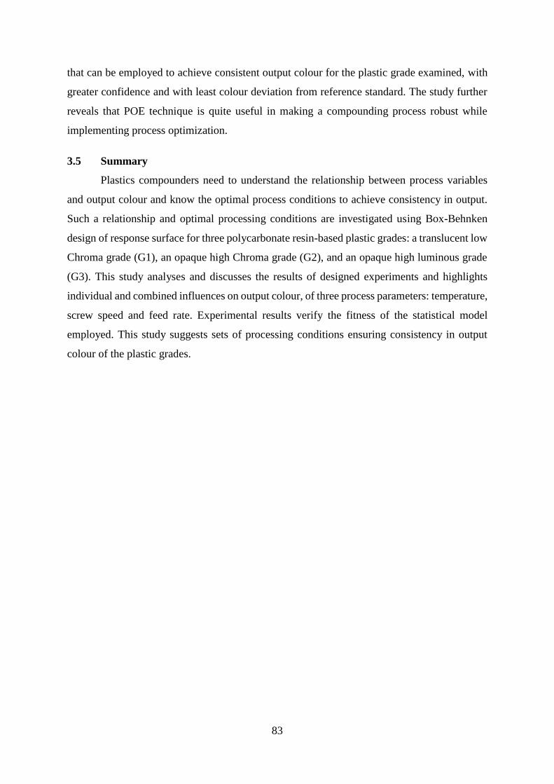
83

that can be employed to achieve consistent output colour for the plastic grade examined, with

greater confidence and with least colour deviation from reference standard. The study further

reveals that POE technique is quite useful in making a compounding process robust while

implementing process optimization.

3.5 Summary

Plastics compounders need to understand the relationship between process variables

and output colour and know the optimal process conditions to achieve consistency in output.

Such a relationship and optimal processing conditions are investigated using Box-Behnken

design of response surface for three polycarbonate resin-based plastic grades: a translucent low

Chroma grade (G1), an opaque high Chroma grade (G2), and an opaque high luminous grade

(G3). This study analyses and discusses the results of designed experiments and highlights

individual and combined influences on output colour, of three process parameters: temperature,

screw speed and feed rate. Experimental results verify the fitness of the statistical model

employed. This study suggests sets of processing conditions ensuring consistency in output

colour of the plastic grades.

84

Chapter 4

Evaluation of Pigments Dispersion Level in Polycarbonate Compounded Plastic

4.1 Introduction

Many colour processing mismatch issues are related to inadequate and inefficient

mixing of colour pigments in a polymer matrix during compounding. During compounding

both dispersive and distributive mixing processes generally take place simultaneously. The

former aims at breaking of agglomerates into primary particle size, whereas the latter process

increases the randomness of the spatial distribution of pigments within the polymer matrix

without any further change in their size [63].

Factors that can possibly cause inadequacy of pigment mixing and eventually colour

deviations, include changes in processing parameters, variation in colour formulation,

degradation behaviour, variation in primary particle size distribution, and regions of variable

refractive index within polymer matrix and pigments. Processing aides are frequently used, and

these also affect rheological properties, and thus dispersibility of pigments in the resin [64].

All these factors need to be considered while doing an assessment of whether the mixing quality

of compounding operations is adequate in regards to plastics coloration [10, 20, 25, 38, 39, 58].

However, for plastics compounders, knowing the optimal levels of process variables such as

temperature, feed rate, and screw speed, is extremely important and help them achieve

consistent output colour by ensuring pigments are adequately mixed and scattering of incident

light is controlled. The transparency of polycarbonate resins does not allow scattering to

happen, therefore in order to create scattering and achieve a certain level of opacity, brightness

and whiteness, white pigments (titanium oxide) are added but at the cost of loss in apparent

colour strength [20, 42, 61].

Optical theory suggests that most efficient scattering occurs when the particle size of

the implemented pigments is slightly smaller than half the wavelength of incident light. The

visible spectrum wavelength range (0.4–0.7μm) suggests a particle size of 0.2–0.35μm will

optimize scattering. However, pigments have tendency to stick together forming agglomerates

- particles larger in size than 0.35 micron. Consequently, higher is the number and size of

agglomerates in compounded plastics, lower would be the pigments scattering power [59, 65].

As the highest refractive index (about 2.7) is associated to TiO2 pigment (rutile phase), it has

the strongest scattering power at an optimum particle size of about 0.2 micron. As per Mie

scattering theory, the angle-weighted scattering coefficient S is estimated as 12 µm-1 at 550 nm

85

(visible spectrum mid-point) assuming a 0.22 micron diameter particles suspended in a clear

binder with a refractive index of 1.5 [66~68].

Various techniques have been used to investigate factors such as pigments volume

concentration, affecting plastics coloration. Included among these techniques are

thermogravimetric analysis (TGA), differential scanning calorimetry (DSC), scanning electron

microscopy (SEM), energy dispersive X-ray spectroscopy (EDX), and ash content [34~36].

None of the techniques were used to quantify pigments dispersion level in compounded

plastics. We however, have successfully employed environmental scanning electron

microscopy (ESEM) and image analysis to analyse pigment dispersion in a high-Chroma

polycarbonate grade. A similar technique is reported to be used by Gunde and co-workers [69],

but for powder-coated, plasma-etched samples.

Evaluating pigments dispersion level within a polymer matrix determines the mixing

efficiency of a compounding process, which can be correlated with processing conditions

employed. Contrary to paints and coatings, compounding of plastics involves high shear rates,

elevated temperatures, and high pressures. To date, only a few studies are reported in literature

about effect of process variables on plastics coloration [38, 39].

4.1.1 Environmental Scanning Electron Microscopy (ESEM)

In scanning electron microscopy (SEM), an electron beam scans the surface of a

specimen to be examined, and the reflected (or back-scattered) beam of electrons is collected,

then displayed at the same scanning rate on a cathode ray tube (similar to a CRT television

screen). The image displayed on the screen, which may be photographed, replicates the

specimen surface features. The surface may or may not be polished and etched, but it must be

electrically conductive; a very thin metallic surface coating must be applied to nonconductive

materials such as polymers [40]. This condition however, is no more needed in ESEM, where

to eliminate electrostatic charge build-up during examination, a bridge between specimen

edges and conductive tape underneath is formed by applying a conductive adhesive.

Magnifications over 200,000 times, are possible, and great depths of field are possible.

Qualitative and semi-quantitative analysis of the elemental composition for quite localized

surface areas, are also possible when equipped with accessories such as energy dispersive X-

ray spectroscopy (EDX).

4.1.2 Image Analysis with ImageJ®

Various commercially available image analysis software such as Image-Pro can be used

for image processing and analysis, but they are expensive. ImageJ however, is a public domain

86

software [41], which is available as an online applet as well as in downloadable application

format, for Windows, Mac OSX and Linux. The software is enriched with quite powerful

features such as spatial calibration, stacking, filtering and geometric transformations to name

a few.

4.1.3 Objectives

Main objectives to carry out this study include following:

1) Evaluate pigments dispersion level by determining their particle size and spatial

distribution in a high Chroma opaque compounded polycarbonate grade.

2) Correlate pigments dispersion to employed processing conditions and hence to output

colour of the plastic grade.

4.2 Materials, equipment and process

As explained in chapter 3, three compounded polycarbonate grades: 1) a translucent

low Chroma grade, 2) opaque high lightness grade, and 3) opaque high Chroma grade, were

statistically analysed using Box-Behnken design (BBD). Model equations were determined to

see the effect of changing processing conditions on their output colour and optimal processing

conditions proposed for achieving colour consistency in compounding. The present study,

however, evaluates pigment dispersion and their spatial distribution within polymer matrix by

characterizing solid structure of opaque high Chroma compounded polycarbonate grade. The

characterization involves use of ESEM (FEI Quanta FEG 250) for imaging, and ImageJ® – a

public domain software for image analysis [41]. A correlation between the processing

parameters and the distribution graphs of particle size and inter-particle distance was

established and compared with colorimetric and statistical analyses.

The plastic grade formulation used in the experimentation comprised LEXAN (105 –

111N) – a bisphenol A - polycarbonate (BPA-PC) resin, five colour pigments including

Titanium dioxide, and two fillers. PC resin used is a highly viscous resin with a melt flow index

(MFI) of 6.5g/10min at 300°C/1.2kg load. All ingredients were precisely weighed in

proportions shown in Table 4.1 and dry -mixed on a super floater. The premix was then

compounded and pelletized using a 25.4 mm, 27 kW, fully intermeshing, co-rotating twin-

screw extruder (ZSK26). After being preheated in an oven isothermally at 120 °C for about 2

hours, these pellets were injection moulded into rectangular chips of the size: 75mm x 50mm

x 2.6mm. These sample chips were then colour measured on Colour-Eye® 7000A - an X-Rite

spectrophotometer, applying large area sample aperture, specular component included and

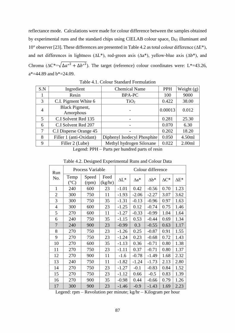
87

reflectance mode. Calculations were made for colour difference between the samples obtained

by experimental runs and the standard chips using CIELAB colour space, D65 illuminant and

10° observer [23]. These differences are presented in Table 4.2 as total colour difference (∆E*),

and net differences in lightness (∆L*), red-green axis (∆a*), yellow-blue axis (∆b*), and

Chroma (∆C*=√∆𝑎∗2 + ∆𝑏∗2). The target (reference) colour coordinates were: L*=43.26,

a*=44.89 and b*=24.09.

Table 4.1. Colour Standard Formulation

S.N Ingredient Chemical Name PPH Weight (g)

1 Resin BPA-PC 100 9000

3 C.I. Pigment White 6 TiO2 0.422 38.00

4 Black Pigment,

Amorphous - 0.00013 0.012

5 C.I Solvent Red 135 - 0.281 25.30

6 C.I Solvent Red 207 - 0.070 6.30

7 C.I Disperse Orange 45 - 0.202 18.20

8 Filler 1 (anti-Oxidant) Diphenyl Isodecyl Phosphite 0.050 4.50ml

9 Filler 2 (Lube) Methyl hydrogen Siloxane 0.022 2.00ml

Legend: PPH – Parts per hundred parts of resin

Table 4.2. Designed Experimental Runs and Colour Data

Run

No.

Process Variable Colour difference

Temp

(°C)

Speed

(rpm)

Feed

(kg/hr) ∆L* ∆a* ∆b* ∆C* ∆E*

1 240 600 23 -1.01 0.42 -0.56 0.70 1.23

2 300 750 11 -1.93 -2.06 -2.27 3.07 3.62

3 300 750 35 -1.31 -0.13 -0.96 0.97 1.63

4 300 600 23 -1.25 0.12 -0.74 0.75 1.46

5 270 600 11 -1.27 -0.33 -0.99 1.04 1.64

6 240 750 35 -1.15 0.53 -0.44 0.69 1.34

7 240 900 23 -0.99 0.3 -0.55 0.63 1.17

8 270 750 23 -1.26 0.25 -0.87 0.91 1.55

9 270 750 23 -1.24 0.23 -0.68 0.72 1.43

10 270 600 35 -1.13 0.36 -0.71 0.80 1.38

11 270 750 23 -1.11 0.37 -0.71 0.80 1.37

12 270 900 11 -1.6 -0.78 -1.49 1.68 2.32

13 240 750 11 -1.82 -1.24 -1.73 2.13 2.80

14 270 750 23 -1.27 -0.1 -0.83 0.84 1.52

15 270 750 23 -1.12 0.66 -0.5 0.83 1.39

16 270 900 35 -0.98 0.44 -0.66 0.79 1.26

17 300 900 23 -1.46 -0.9 -1.43 1.69 2.23

Legend: rpm – Revolution per minute; kg/hr – Kilogram per hour

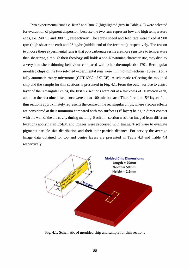
88

Two experimental runs i.e. Run7 and Run17 (highlighted grey in Table 4.2) were selected

for evaluation of pigment dispersion, because the two runs represent low and high temperature

ends, i.e. 240 °C and 300 °C, respectively. The screw speed and feed rate were fixed at 900

rpm (high shear rate end) and 23 kg/hr (middle end of the feed rate), respectively. The reason

to choose these experimental runs is that polycarbonate resins are more sensitive to temperature

than shear rate, although their rheology still holds a non-Newtonian characteristic, they display

a very low shear-thinning behaviour compared with other thermoplastics [70]. Rectangular

moulded chips of the two selected experimental runs were cut into thin sections (15 each) on a

fully automatic rotary microtome (CUT 6062 of SLEE). A schematic reflecting the moulded

chip and the sample for thin sections is presented in Fig. 4.1. From the outer surface to centre

layer of the rectangular chips, the first six sections were cut at a thickness of 50 micron each,

and then the rest nine in sequence were cut at 100 micron each. Therefore, the 15th layer of the

thin sections approximately represents the centre of the rectangular chips, where viscous effects

are considered at their minimum compared with top surfaces (1st layer) being in direct contact

with the wall of the die cavity during melding. Each thin section was then imaged from different

locations applying an ESEM and images were processed with ImageJ® software to evaluate

pigments particle size distribution and their inter-particle distance. For brevity the average

Image data obtained for top and centre layers are presented in Table 4.3 and Table 4.4

respectively.

Fig. 4.1: Schematic of moulded chip and sample for thin sections

89

Table 4.3: Pigments Particle Size Distribution

Equivalent

Circular

Dia. (µm)

Number of Particles, %

Experimental Run-R7 Experimental Run-R17

Top Layer Centre Layer Top Layer Centre Layer

d≤0.2 47.44 61.15 62.91 61.45

0.2<d≤0.25 20.65 21.40 13.35 17.59

0.25<d≤0.3 12.68 7.73 8.51 8.36

0.3<d≤0.4 14.83 7.64 8.51 8.58

0.4<d≤0.5 3.58 1.71 4.06 3.58

d>0.5 0.82 0.36 2.67 0.43

Table 4.4: Inter-Particle Distance Distribution

Nearest Neighbour

Distance - NND

(µm)

Number of Particles, %

Experimental Run-R7 Experimental Run-R17

Top Layer Centre Layer Top Layer Centre Layer

d≤1 22.95 18.62 51.89 37.79

1<d≤2 40.19 26.80 24.15 28.66

2<d≤3 21.81 24.10 13.09 16.50

3<d≤4 11.01 16.91 5.82 9.45

4<d≤5 2.91 8.00 2.33 5.65

5<d≤6 0.62 3.87 2.04 1.41

6<d≤7 0.52 0.72 0.39 0.43

7<d≤8 0.00 0.63 0.10 0.11

8<d≤9 0.00 0.00 0.19 0.00

4.3 Results and Discussions

In order to establish how the variation in process variables impacts the pigments dispersion

in polymer matrix, and hence on the output colour of compounded plastics, image data

provided in Table 4.3 and Table 4.4 were analysed and results are discussed here.

ESEM micrographs of top and centre layers (for brevity only) of the two experimental runs

are presented in Fig.s 4.2 and 4.3. The bright spots (high grey value) in these micrographs

represent dispersion of white pigments (TiO2), which is the dominant inorganic pigment of the

colour formulation used. This was also verified by EDX results (not shown here). The dark

background (low grey value) of micrographs, however, corresponds to polymer resin blended

with solvent red and other fillers.

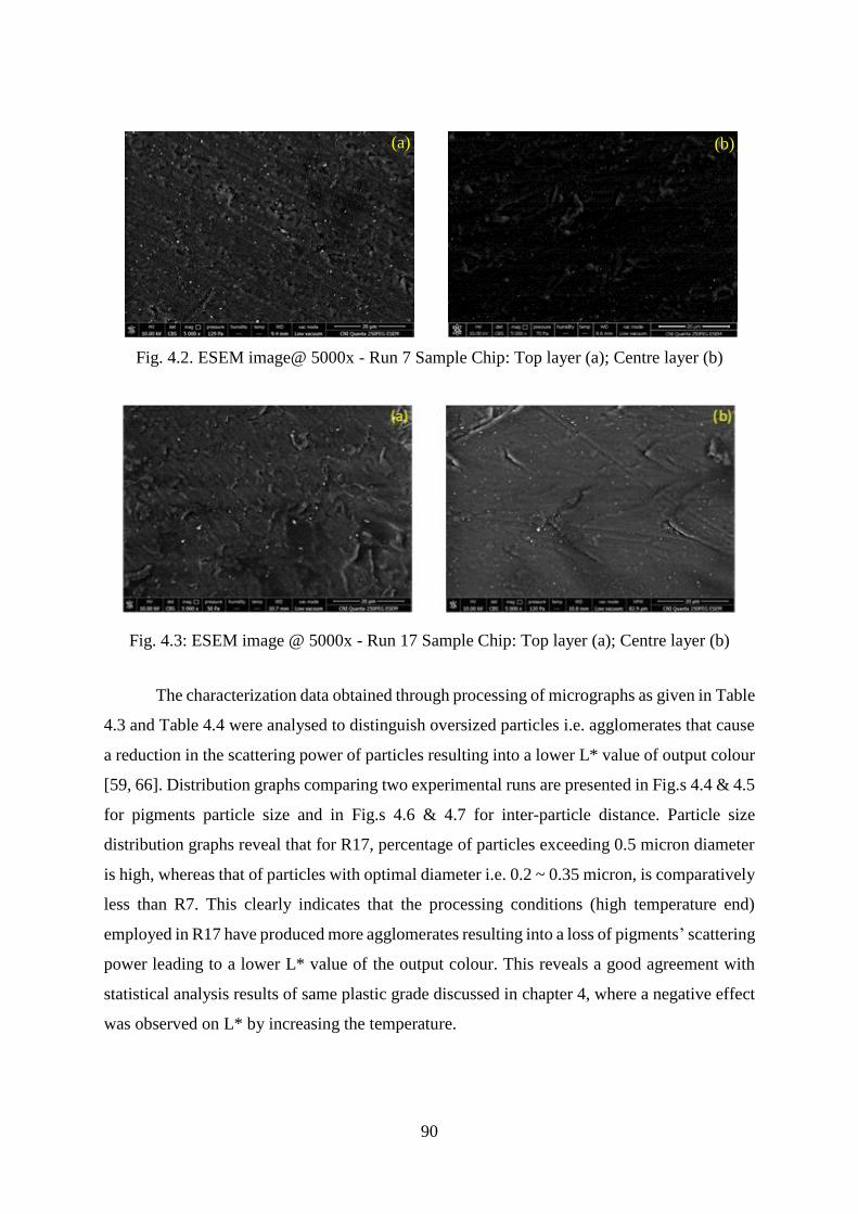
90

Fig. 4.2. ESEM image@ 5000x - Run 7 Sample Chip: Top layer (a); Centre layer (b)

Fig. 4.3: ESEM image @ 5000x - Run 17 Sample Chip: Top layer (a); Centre layer (b)

The characterization data obtained through processing of micrographs as given in Table

4.3 and Table 4.4 were analysed to distinguish oversized particles i.e. agglomerates that cause

a reduction in the scattering power of particles resulting into a lower L* value of output colour

[59, 66]. Distribution graphs comparing two experimental runs are presented in Fig.s 4.4 & 4.5

for pigments particle size and in Fig.s 4.6 & 4.7 for inter-particle distance. Particle size

distribution graphs reveal that for R17, percentage of particles exceeding 0.5 micron diameter

is high, whereas that of particles with optimal diameter i.e. 0.2 ~ 0.35 micron, is comparatively

less than R7. This clearly indicates that the processing conditions (high temperature end)

employed in R17 have produced more agglomerates resulting into a loss of pigments’ scattering

power leading to a lower L* value of the output colour. This reveals a good agreement with

statistical analysis results of same plastic grade discussed in chapter 4, where a negative effect

was observed on L* by increasing the temperature.

(a) (b)

91

Fig. 4.4: Particle size distribution graph - top layers

Fig. 4.5: Particle size distribution graph - centre layers

Similarly spatial distribution graphs shown in Fig.s 4.6 & 4.7 reveal that R7 compared

with R17 have more evenly distributed particles along abscissa representing nearest neighbour

distance (NND). Moreover, for R7 the weighted average of NND values as stamped in

respective Fig.s for top and centre layers comes out to be higher than R17. This gives another

indication that R7 particles are more adequately distributed compared with R17. These graphs

further indicate that percent particles in R17, separated by a NND ≤ 1µm, seem to be almost

twice than that in R7. This clearly points towards concentration of the particles in localized

regions opposing randomness of the inter-particle distance, and causing inadequate spatial

distribution of pigments [20]. The inadequacy of pigments spatial distribution in R17, reduces

their scattering power leading to a lower L* value [66].

92

Fig. 4.6: Nearest Neighbour Distance graph - top layers

Fig. 4.7: Nearest Neighbour Distance graph - centre layers

Presented below in Fig. 4.8 and Fig. 4.9 are the colour data both in coordinates of CIE Lab

colour space, and in delta values i.e. deviation of samples from reference. The colour difference

between the samples is caused in increasing order by L*, b* and a* values. However with

respect to the reference colour, the colour difference is mostly casued by L* value in Run 7

and that in Run 17 by both L* and C*. It is obvious that Run 7 has shown significant reduction

in colour difference in approaching towards the colour of the selected standard reference. The

reduction in L* can be attributed to better dispersion and distribution of white pigments,

whereas that in chroma to better mixing of solvent red in polymer matrix.

Weighted Average

NND

R7 = 2.35µm

R17 = 1.92µm

Weighted Average

NND

R7 = 2.86µm

R17 = 2.23µm

93

Fig. 4.8: Colour data of samples and the standard reference – CIE Lab colour space

Fig. 4.9: Colour difference between samples and the standard reference

Spectral curves of the two experimental runs are shown in Fig. 4.10. Horizontal axis represents

the entire wavelength range of visible light, whereas, the vertical axis shows the reflected

Run 17

Run 7

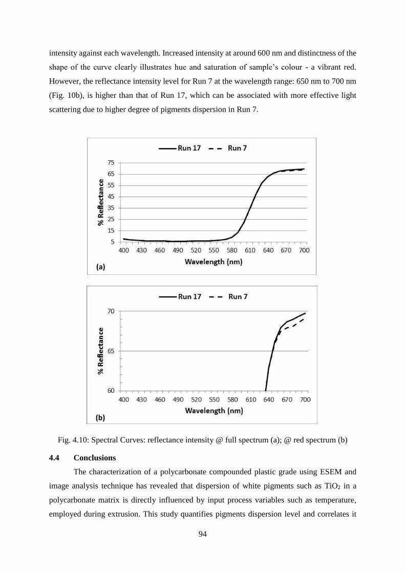
94

intensity against each wavelength. Increased intensity at around 600 nm and distinctness of the

shape of the curve clearly illustrates hue and saturation of sample’s colour - a vibrant red.

However, the reflectance intensity level for Run 7 at the wavelength range: 650 nm to 700 nm

(Fig. 10b), is higher than that of Run 17, which can be associated with more effective light

scattering due to higher degree of pigments dispersion in Run 7.

Fig. 4.10: Spectral Curves: reflectance intensity @ full spectrum (a); @ red spectrum (b)

4.4 Conclusions

The characterization of a polycarbonate compounded plastic grade using ESEM and

image analysis technique has revealed that dispersion of white pigments such as TiO2 in a

polycarbonate matrix is directly influenced by input process variables such as temperature,

employed during extrusion. This study quantifies pigments dispersion level and correlates it

(a)

(b)

95

with processing conditions. The implemented technique is proved to be useful in detection of

small differences in pigments particle size and spatial distribution and relating them to small

variation in colour coordinates such as L*. It further reveals the negative effect that a rise in

temperature can impose on L*. A similar effect was identified by statistical analysis explained

in chapter 4. This study offers plastics compounders a powerful tool in quantifying pigments

dispersion level in polycarbonate compounded plastics under varying processing conditions,

and help them to discover an optimal set of process variables ensuring consistency in desired

colour during compounding.

4.5 Summary

In this part of study, three input variables to the extrusion process - temperature, screw

speed, and feed rate, are investigated for their impact on colour pigments dispersion vis-à-vis

plastics coloration. Pigments dispersion is quantified using scanning electron micrography and

image analysis. A correlation between processing conditions and distribution graphs for

pigments particle size and inter-particle distance is discussed and compared with colorimetric

data. The results obtained through these investigations are quite promising and could help

plastics compounders achieve consistency in plastics coloration.

96

Chapter 5

Numerical Analysis of Mixing Efficiency under Varying Process Conditions in

Intermeshing Co-rotating Twin Screw Extruder

5.1 Introduction

Mixing is a key process in plastics industry, where a variety of additives, such as colour

pigments, stabilizers, antioxidants, fillers, lubes etc., are incorporated into basic polymer

matrix, or a blend of two or more polymers. To carry out mixing process, both batch type (e.g.

Banbury mixer) and continuous type mixer (extruders) are used. Among continuous mixers,

twin screw extruders are widely used in compounding operations for their high throughput,

product uniformity and being economical in energy consumption. Co-rotating, intermeshing

twin-screw extruders are preferred over other extrusion machines because of their self-wiping

feature that provides advantages, such as a complete elimination of any stagnant zone.

Kneading discs are the dominant elements in a modular machine that determine dispersive

mixing efficiency. For a high Chroma opaque compounded polycarbonate grade, 3-D

isothermal flow pattern is simulated in the kneading discs region of a Coperion ZSK-26 co-

rotating twin-screw extruder. A quasi-steady state finite element method was implemented to

avoid time dependent moving boundaries. Mixing parameter λ-lamda, is determined to quantify

dispersive mixing efficiency of the kneading block zone under different processing conditions.

Simulation results are correlated with input process variables, and compared with experimental

colorimetric data.

5.1.1 Twin screw extruders (TSE)

Extruders are widely used not only in plastics industry, but also petrochemical and food

industries for melting, mixing, blending, reacting, devolatilizing and numerous other tasks.

Based on number of screws they are classified in two types: single screw and twin screw

extruders. In single screw extruders, extrusion process and conveying mechanism are highly

dependent on frictional and viscous properties of material. In TSEs however, these properties

play a lesser role on conveying behaviour.

TSEs can be designed in various configurations, however main classification is made

if the screws are intermeshing or non-intermeshing, and whether co-rotating or counter-

rotating. The non-intermeshing TSEs do not have the benefit of positive conveying

characteristics as no protrusion exists between the flights of one screw and the channels of the

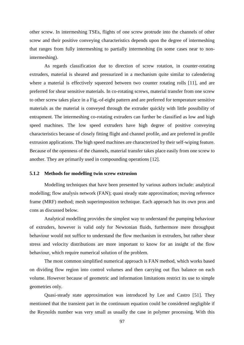
97

other screw. In intermeshing TSEs, flights of one screw protrude into the channels of other

screw and their positive conveying characteristics depends upon the degree of intermeshing

that ranges from fully intermeshing to partially intermeshing (in some cases near to non-

intermeshing).

As regards classification due to direction of screw rotation, in counter-rotating

extruders, material is sheared and pressurized in a mechanism quite similar to calendering

where a material is effectively squeezed between two counter rotating rolls [11], and are

preferred for shear sensitive materials. In co-rotating screws, material transfer from one screw

to other screw takes place in a Fig.-of-eight pattern and are preferred for temperature sensitive

materials as the material is conveyed through the extruder quickly with little possibility of

entrapment. The intermeshing co-rotating extruders can further be classified as low and high

speed machines. The low speed extruders have high degree of positive conveying

characteristics because of closely fitting flight and channel profile, and are preferred in profile

extrusion applications. The high speed machines are characterized by their self-wiping feature.

Because of the openness of the channels, material transfer takes place easily from one screw to

another. They are primarily used in compounding operations [12].

5.1.2 Methods for modelling twin screw extrusion

Modelling techniques that have been presented by various authors include: analytical

modelling; flow analysis network (FAN); quasi steady state approximation; moving reference

frame (MRF) method; mesh superimposition technique. Each approach has its own pros and

cons as discussed below.

Analytical modelling provides the simplest way to understand the pumping behaviour

of extruders, however is valid only for Newtonian fluids, furthermore mere throughput

behaviour would not suffice to understand the flow mechanism in extruders, but rather shear

stress and velocity distributions are more important to know for an insight of the flow

behaviour, which require numerical solution of the problem.

The most common simplified numerical approach is FAN method, which works based

on dividing flow region into control volumes and then carrying out flux balance on each

volume. However because of geometric and information limitations restrict its use to simple

geometries only.

Quasi-steady state approximation was introduced by Lee and Castro [51]. They

mentioned that the transient part in the continuum equation could be considered negligible if

the Reynolds number was very small as usually the case in polymer processing. With this

98

approximation, the resulting solution is dependent only on instantaneous material properties

and boundary conditions, and screws relative positions within the barrel i.e. sequential

geometries at defined angles of rotor position, can be selected and simulated under a steady

state condition. Each screws relative position however, requires new meshes to be generated

for a solution to run, results are then compiled together for those relative positions to understand

the flow behaviour over a complete rotation cycle. Transient nature and complexity of flow

geometry in twin screw extruders do not allow to reach a truly steady state condition. Many

researchers therefore have successfully employed quasi-steady state approximation in

simulating dispersive mixing behaviour of twin screw extruders.

Yang and Manas-Zloczower [52, 53] implemented this technique to simulate dispersive

mixing behaviour of a Banbury mixer and for an intermeshing co-rotating twin screw extruder

(ICRTSE). Bravo [54] employed same approximation for obtaining flowfield solution in

kneading discs region of an ICRTSE. Recently, using same approximation, Sobhani et al [55]

characterized mixing flow behaviour in co-rotating twin screw extruder, and Goger [56]

analysed dispersive mixing behaviour in conveying elements of a counter rotating twin screw

extruder. Disadvantage of this technique is that it involves lot of meshing work, and neglecting

transient term in energy equation is not justified.

Moving reference frame (MRF) provides an alternate to quasi-steady state

approximation, however Ortiz-Rodriquez [48] stated its limitation in predicting flow behaviour

of double flighted screw as two different radial vectors were defined. Another disadvantage he

mentioned was its restricted capability in describing distributive mixing behaviour in twin

screw extruders.

Mesh superimposition technique [57] is pretty close to quasi-steady state in nature and

even more sensitive to transient effects, however geometric complexities involved in twin

screw extrusion restrict it to relatively course mesh patterns causing error to the results.

Keeping in view these pros and cons, quasi-steady state approximation approach has been

adopted for simulation of extrusion process in present study.

5.1.3 Objectives

Main objectives of this study are outlined below:

1). Undertake analysis of dispersive mixing behaviour in the kneading discs (staggered at

45° zone) of Coperion ZSK26 co-rotating twin-screw extruder, under varying processing

99

conditions following a design of experiments (DoE), which was executed for compounding of

a high Chroma opaque polycarbonate grade at SABIC IP Cobourg Plant.

2). Correlate the kneading block mixing efficiency with change in processing conditions

employed, and then compare with experimental colorimetric data of the plastic grade leading

to conclusions.

5.2 Geometry, Material and Process Considerations

Three main considerations that have direct influence on mixing efficiency of a co-

rotating intermeshing twin screw extruder are: 1) Kneading discs geometry, 2) material

rheological properties, and 3) processing conditions is the key geometric parameter that affects

the mixing efficiency. As mentioned in the introduction section, the extruder we simulated is a

Coperion ZSK26 co-rotating intermeshing twin screw extruder. The technical data of this

extruder is provided below in Table 5.1. Kneading discs were staggered at 45° with forward

(right handed) configuration as shown below in Fig. 5.1.

Table 5.1 Technical Data ZSK26 Twin Screw Extruder

Specification Size

Shaft centreline distance 21.1 mm

Screw outside diameter 25.5 mm

Flight depth 4.55 mm

Barrel diameter 26.5 mm

Forward Kneading discs Zone KB45/5/18

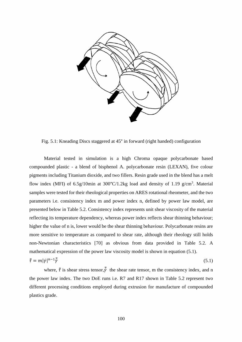
100

Fig. 5.1: Kneading Discs staggered at 45° in forward (right handed) configuration

Material tested in simulation is a high Chroma opaque polycarbonate based

compounded plastic - a blend of bisphenol A. polycarbonate resin (LEXAN), five colour

pigments including Titanium dioxide, and two fillers. Resin grade used in the blend has a melt

flow index (MFI) of 6.5g/10min at 300°C/1.2kg load and density of 1.19 g/cm3. Material

samples were tested for their rheological properties on ARES rotational rheometer, and the two

parameters i.e. consistency index m and power index n, defined by power law model, are

presented below in Table 5.2. Consistency index represents unit shear viscosity of the material

reflecting its temperature dependency, whereas power index reflects shear thinning behaviour;

higher the value of n is, lower would be the shear thinning behaviour. Polycarbonate resins are

more sensitive to temperature as compared to shear rate, although their rheology still holds

non-Newtonian characteristics [70] as obvious from data provided in Table 5.2. A

mathematical expression of the power law viscosity model is shown in equation (5.1).

𝜏̿ = 𝑚|�̇�|𝑛−1�̿̇� (5.1)

where, 𝜏̿ is shear stress tensor,�̿̇� the shear rate tensor, m the consistency index, and n

the power law index. The two DoE runs i.e. R7 and R17 shown in Table 5.2 represent two

different processing conditions employed during extrusion for manufacture of compounded

plastics grade.

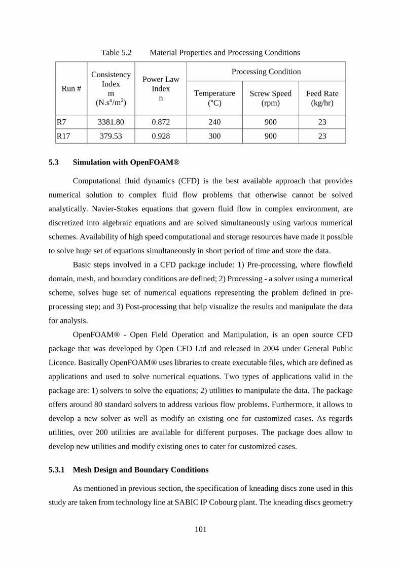
101

Table 5.2 Material Properties and Processing Conditions

Run #

Consistency

Index

m

(N.sn/m2)

Power Law

Index

n

Processing Condition

Temperature

(°C)

Screw Speed

(rpm)

Feed Rate

(kg/hr)

R7 3381.80 0.872 240 900 23

R17 379.53 0.928 300 900 23

5.3 Simulation with OpenFOAM®

Computational fluid dynamics (CFD) is the best available approach that provides

numerical solution to complex fluid flow problems that otherwise cannot be solved

analytically. Navier-Stokes equations that govern fluid flow in complex environment, are

discretized into algebraic equations and are solved simultaneously using various numerical

schemes. Availability of high speed computational and storage resources have made it possible

to solve huge set of equations simultaneously in short period of time and store the data.

Basic steps involved in a CFD package include: 1) Pre-processing, where flowfield

domain, mesh, and boundary conditions are defined; 2) Processing - a solver using a numerical

scheme, solves huge set of numerical equations representing the problem defined in pre-

processing step; and 3) Post-processing that help visualize the results and manipulate the data

for analysis.

OpenFOAM® - Open Field Operation and Manipulation, is an open source CFD

package that was developed by Open CFD Ltd and released in 2004 under General Public

Licence. Basically OpenFOAM® uses libraries to create executable files, which are defined as

applications and used to solve numerical equations. Two types of applications valid in the

package are: 1) solvers to solve the equations; 2) utilities to manipulate the data. The package

offers around 80 standard solvers to address various flow problems. Furthermore, it allows to

develop a new solver as well as modify an existing one for customized cases. As regards

utilities, over 200 utilities are available for different purposes. The package does allow to

develop new utilities and modify existing ones to cater for customized cases.

5.3.1 Mesh Design and Boundary Conditions

As mentioned in previous section, the specification of kneading discs zone used in this

study are taken from technology line at SABIC IP Cobourg plant. The kneading discs geometry

102

was modelled in Solidworks®, a tetrahedral mesh was then generated with the help of

GAMBIT® - a mesh generation software, and the meshed file was converted into

OpenFOAM® file format so it could be opened in OpenFOAM® and used for numerical

analysis.

A 3D mesh view of the flow domain is shown below in Fig. 5.2. The mesh comprises

4196078 cells with no negative volume. Tetrahedral mesh elements were selected because

many researchers [55, 71, 72] found them appropriate and accurate for complex fluid domains

such as in TSEs. A mesh sensitivity analysis was carried out (results not shown here) to ensure

mesh independency of simulation results.

Fig. 5.2: Mesh View in z-direction with ParaFoam®

Boundary conditions employed are reflected below in Table 5.3. No-slip boundary

condition was employed for both the barrel wall and walls of rotating screws, which means

fluid elements are stationary on barrel wall and on screws surface they move with an angular

velocity equivalent to rotating wall velocity (rpm) of the screws. As regards boundary

conditions at entrance and exit planes of the kneading discs, a zero velocity gradient was set,

however due to practical difficulties in calculating exact velocity profiles at these planes, a

nominal value for the normal stress difference (pressure plus viscous stress) in axial direction

was assigned between the two planes.

103

Table 5.3 Boundary Conditions for Velocity and Pressure

Boundary Barrel Screws Inlet Outlet

Velocity

(U)

No-slip Rotating Wall Velocity Zero

Gradient

Zero

Gradient

Pressure

(P)

Zero

Gradient

Zero Gradient Fixed Value Fixed Value

5.3.2 Solver and Algorithm

The OpenFOAM® solver chosen for the numerical solution was incompressible

laminar fluid flow under steady and isothermal conditions. The solver used SIMPLE algorithm

to solve mass and momentum equations (5.2) and (5.3) as shown below respectively. SIMPLE

algorithm that stands for Semi Implicit Methods Pressure Linked Equations, starts with

determination of an initial guess for the flowfield, then using that initial guess calculates

velocity field in momentum equations. The momentum equation is solved under relaxation

with the aim to reduce non-linearity effect. As the momentum equation is not satisfied by the

resulting velocity, therefore pressure equations are solved to obtain new pressure field. This

process continues to repeat unless solution is converged.

∇. �̅� = 0 (5.2)

−∇𝑃 + ∇. τ̿ = 0 (5.3)

where, �̅� denotes the velocity vector, P is the pressure, 𝜏̿ represents stress tensor

A modification in the solver was also incorporated for obtaining other parameters such

as shear stress, shear rate and vorticity tensors. The shear rate and vorticity tensors were then

used to calculate dispersive mixing parameter λ. A mathematical expression of mixing

parameter as defined by Manas-Zloczower [52, 73] is presented in equation (5.4), whereas

expression for shear rate tensor, vorticity tensor and their respective magnitudes, are reflected

in equations (5.5)to (5.8). In order for the solution to converge, the residuals for both velocity

and pressure were set at 5 x 10-5, which means the solver will stop simulation when the

difference between two consecutive iterations reached below specified residual values.

Simulation was run on a standalone Dell Machine (T3400) and for each solution to converge

it took about 4000 iterations spanning over 172,800 seconds. Finally the results were visualized

and examined with the help of ParaView® - an open source scientific visualization software.

𝜆 =|�̇�|

|�̇�|+|𝜔| (5.4)

�̿̇� = ∇𝑉̅̅ ̅̅ + (∇𝑉̅̅ ̅̅ )T (5.5)

�̿� = ∇𝑉̅̅ ̅̅ − (∇𝑉̅̅ ̅̅ )T (5.6)

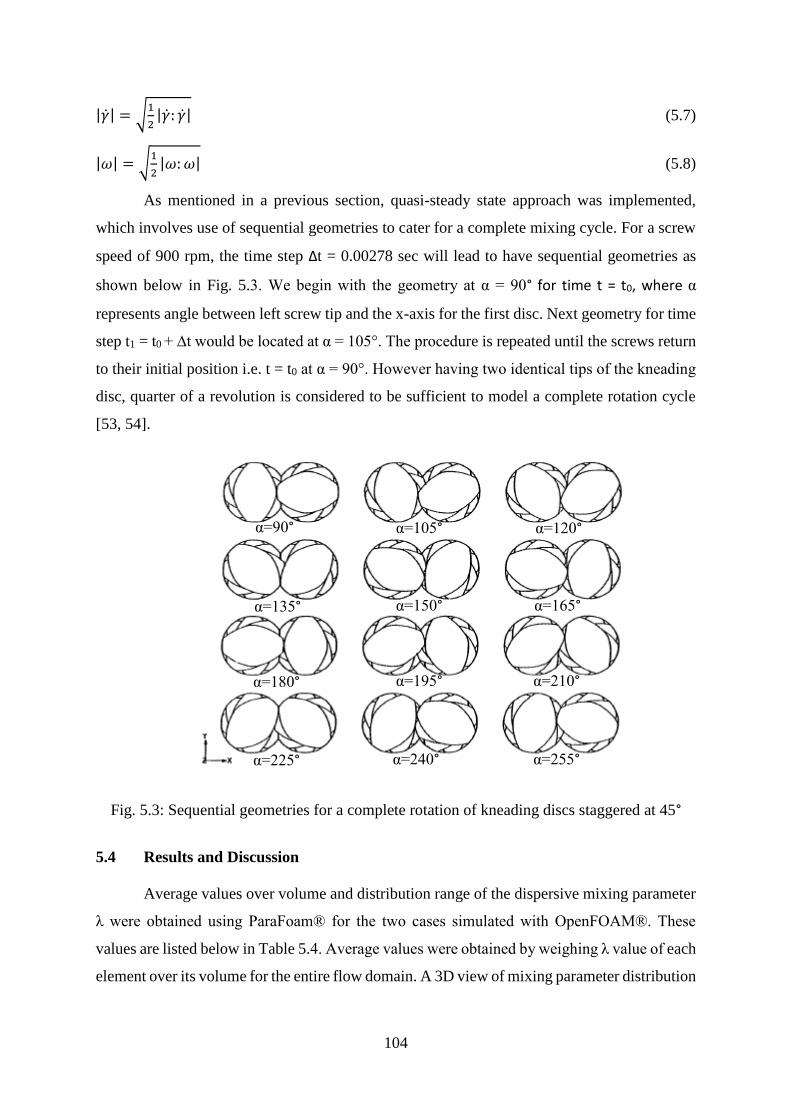
104

|�̇�| = √1

2|�̇�: �̇�| (5.7)

|𝜔| = √1

2|𝜔:𝜔| (5.8)

As mentioned in a previous section, quasi-steady state approach was implemented,

which involves use of sequential geometries to cater for a complete mixing cycle. For a screw

speed of 900 rpm, the time step ∆t = 0.00278 sec will lead to have sequential geometries as

shown below in Fig. 5.3. We begin with the geometry at α = 90° for time t = t0, where α

represents angle between left screw tip and the x-axis for the first disc. Next geometry for time

step t1 = t0 + ∆t would be located at α = 105°. The procedure is repeated until the screws return

to their initial position i.e. t = t0 at α = 90°. However having two identical tips of the kneading

disc, quarter of a revolution is considered to be sufficient to model a complete rotation cycle

[53, 54].

Fig. 5.3: Sequential geometries for a complete rotation of kneading discs staggered at 45°

5.4 Results and Discussion

Average values over volume and distribution range of the dispersive mixing parameter

λ were obtained using ParaFoam® for the two cases simulated with OpenFOAM®. These

values are listed below in Table 5.4. Average values were obtained by weighing λ value of each

element over its volume for the entire flow domain. A 3D view of mixing parameter distribution

α=90° α=105° α=120°

α=165°

α=210°

α=255°

α=150°

α=195°

α=240° α=225°

α=180°

α=135°

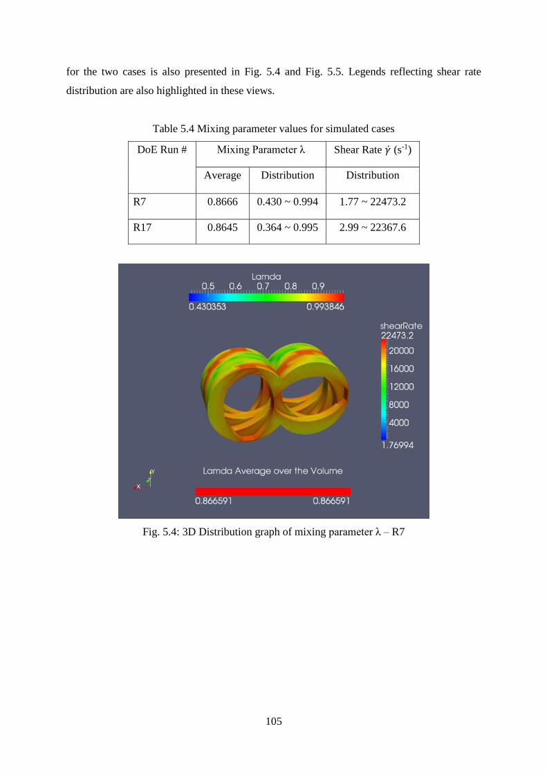
105

for the two cases is also presented in Fig. 5.4 and Fig. 5.5. Legends reflecting shear rate

distribution are also highlighted in these views.

Table 5.4 Mixing parameter values for simulated cases

DoE Run # Mixing Parameter λ Shear Rate �̇� (s-1)

Average Distribution Distribution

R7 0.8666 0.430 ~ 0.994 1.77 ~ 22473.2

R17 0.8645 0.364 ~ 0.995 2.99 ~ 22367.6

Fig. 5.4: 3D Distribution graph of mixing parameter λ – R7

106

Fig. 5.5: 3D Distribution graph of mixing parameter λ – R17

Average λ values of both simulated runs are quite close to 1, which indicates the

dominant flow in both cases is elongational. This confirms the overall mixing efficiency of

kneading discs zone in ZSK26 extruder is extremely good. However a comparatively higher

(0.24%) average λ value in R7 indicates that mixing efficiency is even better in R7 compared

with R17. This little improvement in mixing efficiency can be associated with the processing

conditions employed to R7, where the temperature was kept at 240°C. As we know dispersive

mixing during compounding aims at breaking of agglomerates into primary particle size, so it

would be justified to say R7 has better particle size distribution of colour pigments such as

titanium dioxide. The titanium dioxide being a dominant colour pigment in the formulation

used, is responsible for both the opacity and lightness (i.e. L* value) of the output colour. As

discussed in chapter 8, both opacity and lightness are directly influenced by particle size

distribution of titanium dioxide, therefore it can be concluded that processing conditions

employed in R7 correspond to a better mixing in kneading discs zone compared with those of

R17, resulting into a higher lightness value, which was quite close to the target as shown below

in Table 5.5. This seems to be in complete compliance with our findings of statistical and image

analysis carried out for the same polycarbonate grade.

107

Table 5.5 Mixing parameter values vs measured colour coordinates

DoE Run # Mixing Parameter λ Colour Coordinates

Average L* a* b*

R7 0.8666 42.27 45.19 23.54

R17 0.8645 41.8 43.99 22.66

Keeping in view quite a small difference in average λ values that was reported by

various researchers, simulation runs for sequential geometries shown above in Fig. 5.3 were

postponed. Yang [53] simulated sequential geometries for kneading discs zone of a co-rotating

intermeshing twin screw extruder (Werner & Pfleniderer ZSK-30) while the kneading discs

were staggered at 45° in a forward configuration, and obtained average λ values ranged from

0.5556 to 0.5574 (a difference of 0.0018), similarly Bravo [54] simulated a total of 7 sequential

geometries and average λ values obtained varied from 0.5702 ~ 0.5722 (a difference of 0.002).

Goger [56] also reported quite a small difference in average λ values of 4 sequential geometries

that were simulated under various screw pitch lengths for conveying screw elements of a

counter-rotating twin screw extruder.

5.5 Conclusions

Dispersive mixing parameter λ provides an insight of the flow behaviour in kneading

discs region of ZSK26 twin screw extruder. Average λ values obtained through simulation of

the kneading discs zone under processing conditions represented by R7 and R17, reveal that

the simulation under R7 process (a low temperature) condition, yields better dispersive mixing

of titanium dioxide pigments used in the formulation. This has resulted into a better output

colour of the compounded plastic grade. However to further investigate the effect of process

conditions on the output colour of the plastic grade studied, other runs listed in DoE Table 3.2,

may also be simulated.

5.6 Summary

Co-rotating, intermeshing twin-screw extruders are widely used in plastics industry for

polymer compounding and blending. They are preferred over other extrusion machines because

of their self-wiping feature that provides advantages, such as a complete elimination of any

stagnant zone. Kneading discs are the dominant elements in a modular machine that determine

dispersive mixing efficiency. For a high Chroma opaque compounded polycarbonate grade, 3-

D isothermal flow pattern is simulated in the kneading discs region of a Coperion ZSK-26 co-

rotating twin-screw extruder. A quasi-steady state finite element method was implemented to

108

avoid time dependent moving boundaries. Mixing parameter λ-lamda, is determined to quantify

dispersive mixing efficiency of the kneading block zone under different processing conditions.

Simulation results are correlated with input process variables, and compared with experimental

colorimetric data.

109

Chapter 6

Contribution and Recommendations

6.1 Contribution

As stated in Chapter 1 of this thesis, colour of compounded plastics is directly influenced

by varying processing conditions, pigments type and concentration level in colour formulation.

Furthermore, mixing efficiency of kneading discs zone in a twin screw extruder can be

evaluated by quantifying the pigments dispersion level in polymer blend. Producing a

compounded plastic in correct colour without making adjustments in colour formulation or

processing conditions has been challenging for plastics compounder. The research work

presented in this thesis contributes to understanding the influence of process variables to the

extrusion process, especially of temperature, screw speed and feed rate, on the output colour

of polycarbonate resin grades. Among the major accomplishments of this thesis are:

Identification of pigments type and adjustment levels in pigments formulation needed

during production, to deal with colour variation in polycarbonate compounded plastic

grades, PC1 and PC2. The predictive model equations presented can help a colour expert

to make precise decision regarding minute adjustments needed in reference colour

formulation during production, and thus improve quality and productivity. The

optimization results suggest a colour formulation slightly different from initial reference,

of white, black and yellow pigments for the two plastic grades examined.

Identification of process variables that significantly influence output colour of three PC

grades: 1) a low Chroma translucent grade G1; 2) a high Chroma opaque grade G2; 3) a

high luminous opaque Grade G3. The predictive model equations presented can be used

as a tool to predict output colour by changing processing conditions within the tested range.

The optimization results suggest process conditions that can be employed with greater

confidence to achieve consistency in output colour while restricting POEs at minimum and

the overall colour variation (∆E*) within a stipulated threshold of 1.0. The study further

reveals usefulness of the POE technique for making the compounding process a robust

while implementing process optimization.

Introduction of a novel technique that evaluates pigments dispersion level in polymeric

matrix. This technique involves use of ESEM and image analysis tool, and investigates a

high Chroma opaque polycarbonate grade G2, by quantifying pigments particle size and

spatial distribution within the polymeric base. The implemented technique is proved to be

useful in detection of small differences in pigments particle size and spatial distribution

110

and relating these differences to small variation in colour coordinates such as L*. It further

reveals a negative effect on L* due to rise in temperature. A similar effect was identified

by statistical analysis explained in Chapter 3. This study offers to plastics compounders, a

powerful tool for quantifying pigments dispersion level in polycarbonate resin(s) under

varying processing conditions, and thus helps them optimize process conditions for

consistency in desired output colour during compounding.

Determination of dispersive mixing parameter λ under varying processing conditions using

OpenFOAM® software. The dispersive mixing parameter provides insight of the flow

behavior in kneading discs zone of ZSK26 co-rotating intermeshing twin screw extruder.

Two different processing conditions representing experimental runs R7 and R17 taken

from a DoE executed for statistical study explained in Chapter 3, were simulated to

determine the mixing parameter λ. The λ values obtained in this study reveal that the

simulation run representing R7 - a low temperature process condition, yields better

dispersive mixing of the titanium dioxide pigments used in the formulation. This resulted

into a better output colour of the polycarbonate grade G2 – a high Chroma opaque

compounded plastic. The simulation results are in good agreement with findings of our

study where a novel technique used to quantify pigments dispersion level

6.2 Recommendations

Various assumptions were made during the entire research study. For example in

numerical analysis of the kneading disc zone of twin screw extruder, isothermal condition and

power law viscosity model fitting were used. Similarly in evaluating pigments dispersion level,

only 15 thin slices were assumed to represent the entire molded rectangular plaque. All these

assumptions where reveal the limitations of resources and time, also indicate the potential

improvements that can be introduced. Therefore following is recommended for future work.

Numerical analysis can be extended to a complete DoE executed for statistical study

explained in Chapter 3 so the mixing parameter λ values obtained for each experimental

run can be correlated with respective colour coordinates, and optimal processing

conditions further be explored.

In present numerical study, we assumed isothermal condition and used power law

coefficients to describe polycarbonate rheological properties. The numerical study can be

extended by considering a non-isothermal condition and applying Carreau viscosity model

fitting to viscosity curves of the polycarbonate grades examined. Polycarbonates as

mentioned in Chapter 4 are more sensitive to temperature than shear rate while maintaining

111

their non-Newtonian nature, therefore it would be worthwhile to include thermal effects in

the numerical study.

Application of the novel technique introduced in Chapter 4 can be extended to samples

representing all experimental runs of the DoE executed for statistical study explained in

Chapter 3. This would certainly help investigate the effect of other process variables such

as screw speed and feed rate on pigments dispersion level and consequently on output

colour.

xv

Bibliography

1. Canadian Plastics Industry Association – CPIA, Industry Profile, June 2015.

http://www.plastics.ca/IndustryProfile/index.php,

2. J. Markarian, North American compounders seek growth in innovation, Plastics Additives

& Compounding, 8(3), pp. 42–44, 2006.

3. W. Spook, Lean compounding – key to survival, Plastics Additives & Compounding,

10(4), pp. 26–29, 2008.

4. J. Markarian, US compounding industry faces challenging times, Plastics Additives &

Compounding, 10(6), pp. 38–41, 2008.

5. G. M. Rizvi, Fundamental studies into causes of colour mismatch, Research Proposal

sponsored by SABIC IP and NSERC, 2009.

6. G. E. P. Box, and D. W. Behnken, Some new three-level designs for the study of

quantitative variables, Technometrics, 2, pp. 455–475, 1960.

7. N. P. Cheremisinoff, Polymer mixing and extrusion technology, Marcel Dekker Inc., 1987.

8. A. Dreiblatt, Sabic Innovative Plastics twin screw extrusion training, Century Extrusion,

2008.

9. K. Kohlgr�̈�ber, Co-rotating twin-screw extruders - fundamentals, technology, and

applications, Carl Hanser Publishers, Munich, and Hanser Gardner Publications, Inc.

Cincinnati, 2008.

10. C. Rauwendaal, Polymer mixing, a self-study guide, Hanser Publishers, Munich 1998.

11. R. J. Crawford, Plastics engineering, Elsevier Science, Oxford 1999.

12. Chris J. Rauwendaal, Analysis and experimental evaluation of twin screw extruders,

Polym. Eng. Sci., 21, pp. 1092 – 1100 (1981)

13. A. Muller, Coloring of plastics: fundamentals – colorants – preparations, 1st Ed, Hanser

Publishers, Munich, 2003.

14. C. Rauwendaal, Polymer extrusion, 4th Ed, Hanser Publishers, Munich 2003.

15. C. Rauwendaal, Understanding extrusion, 2nd Ed, Hanser Publishers, Munich 2010.

16. J. Markarian, Back to basics - adding colour to plastics, Plastics Additives and

Compounding, 11(4), pp. 12–15, 2009.

17. J. Murphy, The compounders guide to colour - pigments dyes and special effects, Plastics

Additives and Compounding, 1(6), pp. 10–17, 1999.

18. C. Rauwendaal, New developments in mixing and screw design, Plastics Additives &

Compounding, 10(6), pp. 32–36, 2008.

xvi

19. L. Eidson and M. Steeves, Fundamentals of color and appearance book, Online X-rite

Seminar, 2012. http://www.xrite.com/product_overview.aspx?ID=934

20. B. M. Mulholland, Effect of additives on the color & appearance of plastics, ANTEC-

Conference Proceedings, pp. 1340–1346, 2007.

21. T. Belcher and K. Harvey, The influence of color, ANTEC-Conference Proceedings, pp.

1296–1307, 2007.

22. X-rite Inc., The color guide and glossary, Online 2012.

www.xrite.com/documents/literature/.../L11-029_color_guide_en.pdf

23. CIED65. Colorimetry-Part 4: CIE 1976 L* a* b* colour space. CIE DS 014-4.3/E. Vienna,

Austria: CIE Central Bureau, 2007.

24. ASTM D 2244-93, Standard test method for calculation of color differences from

instrumentally measured colour coordinates, pp. 222-215, 1993.

25. M. C. Yu, M. A. Bisell, and R. S. Whitehouse, The effect of carbon black dispersion on

polymer performance. ANTEC-Conference Proceedings, pp. 3246-3250, 1995.

26. D. I. Meade, Introduction to colorant selection and application technology in coloring of

plastics: fundamentals, 2nd Ed., edited by Robert Charvat 2004.

27. K. Effertz, Understanding the effects of a compounding process on the production of co-

extruded vinyl sheet through the utilization of design of experiments (part II), ANTEC-

Conference Proceedings, 2004.

28. T. M. Bender, Characterization of apparent viscosity with respect to a PVC-Wood fiber

extrusion process, ANTEC-Conference Proceedings, 2002.

29. E. Dawkins, P. Engelmann, K. Horton, and M. Monfore, Color and gloss – the connection

to process conditions, Journal of Injection Molding Technology, 2(1), pp. 1–7, 1998.

30. D. C. Montgomery, Design and analysis of experiments, 6th Ed., John Wiley and Sons,

New York 2005.

31. M. J. Anderson, and P. J. Whitcomb, RSM simplified, optimizing processes using response

surface methods for design of experiments, Productivity Press, New York, NY, 2005.

32. C. N. Borror, D. C. Montgomery, and R. H. Myers, Evaluation of statistical designs for

experiments involving noise variables, Journal of Quality Technology, 34(1), pp. 54-70,

2002.

33. G. Taguchi, System of experimental design: engineering methods to optimize quality and

minimize cost, Quality Resources, White Plains, NJ 1987.

34. G. Derringer and R. Suich, Simultaneous optimization of several response variables.

Journal of Quality Technology, 12(4), pp. 214-219, 1980.

xvii

35. M. Kosarzycki and L. Klebanov, A technique comparison for the quantification of color

concentrate in a Polyacetal component, ANTEC-Conference Proceedings, pp. 1185–1187,

2008.

36. I. Groves, T. Lever, and N. Hawkins, Determination of carbon black pigment in nylon 66

by TGA. Thermal Analysis Application Brief Number TA-122, TA Instruments Ltd UK.

http://www.tainstruments.

37. D. Grewell, G. Srinivasan, M.R. Kessler, and N. Kieffer, Case study of color variation of

thermal formed automotive body components, ANTEC-Conference Proceedings, pp.

1763–1767, 2008.

38. D. Colquhoun et al, Improved dispersion of yellow metal azo pigment in polyethylene

film, ANTEC-Conference Proceedings, pp. 2827-2831, 2005.

39. S. P. Rwei, Distributive mixing in a single-screw extruder – evaluation in the flow

direction, Polymer Engineering and Science, 41, pp. 1665-1673, 2001.

40. W. D. Callister, Jr. and D. J. Rethwisch, Materials science and engineering - An

Introduction, 6th Ed., John Wiley & Sons: New York, 2011.

41. ImageJ, Image processing and analysis in Java, research services branch, NIH 2014.

http://rsb.info.nih.gov/ij/

42. E. L. Canedo, Computer simulation of plastics compounding operations in twin-screw

extruders, ANTEC-Conference Proceedings, pp. 310–316, 1999.

43. J. Markarian, Compounders look to simulation software for savings in time and costs,

Plastics Additives & Compounding, 7(2), pp. 34–37, 2005.

44. K. Alemaskin, I. Manas-Zloczower and M. Kaufman, Color mixing in the metering zone

of a single screw: numerical simulations and experimental validation, Polymer

Engineering and Science, 45(7), pp. 1011–1020, 2005.

45. R. K. Connelly and J. L. Kokini, Examination of the mixing ability of single and twin

screw mixers using 2D finite element method simulation with particle tracking, Journal of

Food Engineering, 79(3), pp. 956–969, 2007.

46. C. David, R. Valette, B. Vergnes and T. Coupez, A direct 3D numerical simulation code

for extrusion and mixing processes, ANTEC-Conference Proceedings, pp. 1825–1828,

2008.

47. C. David, A. Durin, R. Valette, B. Vergnes and T. Coupez, A full 3D simulation for twin

screw extrusion based on an immersion domain method: application to mixing elements,

ANTEC-Conference Proceedings, pp. 2356–2360, 2009.

xviii

48. E. Ortiz-Rodriguez and C. Tzoganakis, 3D simulations of a reactive flow in screw

elements of closely intermeshing twin screw extruders: a scale-up analysis, ANTEC-

Conference Proceedings, pp. 171–175, 2009.

49. E. Ortiz-Rodriguez and C. Tzoganakis, 3D simulations of a reactive flow in screw

elements of closely intermeshing twin screw extruders: conventional and variable speed

extruders, ANTEC-Conference Proceedings, pp. 447–451, 2010.

50. C. Wang, M. Bussmann and C. B. Park, Numerical investigation of the effect of screw

geometry on the mixing of a viscous polymer melt, Journal of Applied Polymer Science,

117(2), pp. 775–784, 2010.

51. C. C. Lee, and J. M. Castro, Model Simplification, in Chapter 3 from Charles Tucker III,

Computer Modelling for Polymer Processing, Hanser 1989.

52. H. H. Yang, and I. Manas-Zloczower, Int. Polym. Proc., VII, pp. 195-203, 1992.

53. H.-H. Yang, Flow field analysis of batch and continuous mixing equipment, PhD Thesis,

Case Western Reserve University, 1993.

54. V. L. Bravo, Finite element simulation of flow in twin screw extruder mixing elements,

PhD Thesis, McMaster University, 1998.

55. H. Sobhani, M. R. Nouri, and M. H. R. Ghoreishy, Iran. Polym. J., 19, pp. 143-154, 2010.

56. Ali Goger, Modelling of counter rotating twin screw extrusion, Masters Thesis, McMaster

University, 2013.

57. A. D. Gotsis, Z. Ji, and D.M. Kalyon, ANTEC-Conference Proceedings, pp. 139-142,

1990.

58. M. O. Zink, The value of transparent and opaque pigments in plastics coloration, CAD

RETEC-Conference Proceedings, pp. 319-328, 2004.

59. DuPontTM Ti-Pure®, Titanium Dioxide for coatings, 2007. http://www2.dupont.com

60. P. J. Whitcomb and M. J. Anderson, Robust design-reducing transmitted variation: finding

the plateaus via response surface methods, annual quality congress, pp. 642-651, 1996.

61. M. J. Anderson, and P. J. Whitcomb, Response surface methods (RSM) for peak process

performance at the most robust operating conditions, Proceeding from International

SEMATECH Manufacturing Initiative (ISMI) Symposium on Manufacturing

Effectiveness, 2007.

62. W. Adams, S. L. Kraber, and P. J. Whitcomb, Handbook for experimenters, version 08.1.,

Minneapolis, MN: Stat-Ease Inc., 2009.

63. J. W. Ess and P.R. Hornsby, Characterization of distributive mixing in thermoplastics

compositions, Polymer Testing, 6, pp. 205-218, 1986.

xix

64. E. C. Achilleos et al, Role of processing aids in the extrusion of molten polymers, Journal

of Vinyl & Additive Technology, 8(1), pp. 7-24, 2002.

65. R. M. Christie, Pigments, dyes and fluorescent brightening agents for plastics: an

overview, Polymer International, 34, pp. 351-361, 1994.

66. R. Levinson et al, Solar spectral optical properties of pigments—Part II: survey of common

colorants. Solar Energy Materials & Solar Cells, 89, pp. 351-389, 2005.

67. B. R. Palmer, P. Stamatakis, C. G. Bohren and G. C. Salzman, J. Coat. Technol., 61, pp.

41–47, 1989.

68. E.S. Thiele, R.H. French, Adv. Mater. 10, 1271–1276, 1998.

69. M. K. Gunde, M. Kunaver, M. Mozetic, and A. Hrovat, Method for the evaluation of

degree of pigment dispersion in powder coatings, Powder Technol. 148, pp. 64–66, 2004.

70. J. M. Margolis, Engineering plastics handbook, The McGraw-Hill Companies Inc., 2006.

71. A. Shah, and M. Gupta, Comparison of the flow in co-rotating and counter-rotating twin-

screw extruders, ANTEC-Conference Proceedings, pp. 443-447 2004.

72. F. Ilinca, J. -F. Hetu, Three-dimensional finite element solution of the flow in single and

twin-screw extruders, Int. Polym. Proc., XXV, pp. 275-286, 2010.

73. I. Manas-Zloczower, and D. L. Feke, Analysis of agglomerate rupture in linear flow fields, Int.

Polym. Proc., IV, pp. 3-8, 1989.