Investigation into discontinuous low temperature waste heat utilisation from a renewable power plant in rural India for absorption refrigeration by Joel A W Hamilton, MEng Thesis submitted to The University of Nottingham for the degree of Doctor of Philosophy December 2016

Welcome message from author
This document is posted to help you gain knowledge. Please leave a comment to let me know what you think about it! Share it to your friends and learn new things together.
Transcript
Investigation into discontinuous lowtemperature waste heat utilisation
from a renewable power plant in ruralIndia for absorption refrigeration
by Joel A W Hamilton, MEng
Thesis submitted toThe University of Nottingham
for the degree of Doctor of PhilosophyDecember 2016
Abstract
This research focusses on utilising low temperature waste heat from a rural
renewable power plant for absorption refrigeration. It forms part of a collab-
orative “Bridging the Urban Rural Divide” (BURD) research group across
the United Kingdom and India investigating rural sustainable development
through the provision of renewable electricity. The group is tasked with
improving the educational environment and healthcare of a 45 household
community (which is part of a larger village) in West Bengal, India.
Working in collaboration with the Indian Institute of Technology Bombay
as part of this thesis, a projected daily electrical demand for the community
of 55 kW·h per day was calculated, providing: lighting, fans and an electrical
device charging station. To allow in excess of the daily electrical demand as
well as for system ancillaries at 12 kW·h, solar trackers at 14 kW·h and
7 kW·h for hydrogen production, a power plant producing 90 kW·h was
specified. This included daily electricity production of 70 kW·h during the
daytime from solar via a 10 kW concentrated photovoltaic (CPV) system and
20 kW·h in the evening from a 5 kW biogas and hydrogen internal combustion
engine electrical generator (genset). The biogas is produced from anaerobic
digestion of food waste and aquatic weeds, and the hydrogen is produced from
the electrolysis of water in an electrolyser powered by excess solar power.
An energy and exergy analysis identified the daily quantity and quality of
recoverable waste heat sources at 25◦C. These are the CPV with an energetic
value of 109 kW·h and an exergetic value of 32 kW·h at 60◦C and the genset
i
radiator with an energetic value of 32 kW·h and an exergetic value of 5 kW·h
at 80◦C. The exhaust heat from the genset has been allocated for other uses
and, though calculated, is outside the scope of this research.
The thesis then focusses on using these low temperature waste heat
sources for absorption refrigeration. The working fluids selected are ace-
tone and zinc bromide as these had been proven in the literature to operate
at temperatures below those of the expected waste heat sources without the
need for rectification (the process of separating two fluid vapours from each
other). Due to the local climate with high ambient temperatures, averaging
24◦C to 35◦C, and the relatively low waste heat source temperatures, a num-
ber of configurations of absorption refrigerator were investigated to achieve
lower, and therefore more versatile, evaporator temperatures. Some of these
involve utilising some of the cooling produced from either or both of the heat
sources to cool the absorber and condenser.
The findings were that the most energy effective way of providing low
evaporator temperatures was to use a small (2%) difference in weak and
strong solution concentrations and not use a proportion of the cooling gener-
ated for the absorber or condenser. By operating two independent refrigera-
tors powered by each heat source independently, the solution concentrations
could be optimised to provide the lowest possible evaporator temperatures
at a given ambient temperature.
At the 25◦C reference ambient temperature used for the energy and exergy
analysis, the CPV waste heat can provide 33.4 kW·h of continuous cooling
per day at 6◦C and the genset radiator 6.3 kW·h at 0◦C. This cooling energy
collectively is sufficient to replace 12.7 kW·h of electricity that would have
been used to power a vapour compression refrigerator to provide the same
amount of cooling, which is equal to 22% of the electrical power provided to
the village.
The genset waste heat source used for absorption refrigeration can pro-
ii

vide cooling for food and medicine storage equivalent to 6 to 8 domestic
refrigerators. The CPV waste heat source can provide space cooling for a
room in a health centre for 6 to 9 hours per day. The investigations within
this thesis highlighted the need for intelligent control systems to optimise
the availability and temperatures of the refrigerators during unfavourable
ambient conditions.
iii
Acknowledgements
Thank you for taking the time to read my thesis. It has been a long and
satisfying journey.
I would like to thank my supervisors, the university, my examiners and
all the technical and administrative staff for their support and perseverance
with me. I would not have made it through this journey without them. At
the same time I also thank the research group and fellow PhD students who
were always there to keep me safe, on track and full of tea. It goes without
saying that I would not have been able to do this without the support and
distraction of family, friends, mentors and my menagerie of pets.
This work has been carried out as a part of the BioCPV project jointly
funded by DST, India (Ref No: DST/SEED/INDO-UK/002/2011) and EP-
SRC, UK, (Ref No: EP/J000345/1). I acknowledge both funding agencies
for their support. I also acknowledge the support of the partner universities
which include: University of Exeter, Indian Institute of Technology Bombay,
Indian Institute of Technology Madras, University of Nottingham, Herriot
Watt University, Visva-Bharati (West Bengal) and University of Leeds.
iv

Contents
Abstract i
Acknowledgements iv
List of Figures x
List of Tables xxi
Acronyms, Abbreviations and Nomenclature xxiii
1 Introduction 1
2 Background and Motivation 5
2.1 Assessment of The Needs of The Case Study Community . . . 8
2.1.1 Lifestyle and Culture . . . . . . . . . . . . . . . . . . . 10
2.1.2 Weather and Conditions . . . . . . . . . . . . . . . . . 12
2.1.3 Resources Available . . . . . . . . . . . . . . . . . . . . 13
2.2 Community Power Demand Rationale . . . . . . . . . . . . . . 13
2.2.1 Demand Estimation . . . . . . . . . . . . . . . . . . . 13
2.2.2 Demand Profile . . . . . . . . . . . . . . . . . . . . . . 17
2.2.3 System Requirements . . . . . . . . . . . . . . . . . . . 18
2.3 Proposed Renewable Power Plant Design . . . . . . . . . . . . 19
2.4 Conclusion . . . . . . . . . . . . . . . . . . . . . . . . . . . . . 20
3 Refrigeration Technology Review 22
3.1 History of Refrigeration . . . . . . . . . . . . . . . . . . . . . 25
v
3.2 Review of Commonly Available Refrigeration Systems . . . . . 31
3.2.1 Vapour Compression . . . . . . . . . . . . . . . . . . . 31
3.2.2 Adsorption Refrigeration . . . . . . . . . . . . . . . . . 32
3.2.3 Gas Cycle . . . . . . . . . . . . . . . . . . . . . . . . . 34
3.2.4 Absorption Refrigeration . . . . . . . . . . . . . . . . . 35
3.2.5 Desiccant Cooling . . . . . . . . . . . . . . . . . . . . . 36
3.2.6 Appraisal of Common Refrigeration Systems . . . . . . 37
3.3 Detailed Review of Absorption Refrigeration . . . . . . . . . . 40
3.3.1 Challenges of Absorption Refrigeration . . . . . . . . . 41
3.3.2 Fluids . . . . . . . . . . . . . . . . . . . . . . . . . . . 44
3.3.3 System Configurations to Maximise Heat Utilisation . . 46
3.3.4 System Configurations to Utilise Discontinuous Heat
Sources . . . . . . . . . . . . . . . . . . . . . . . . . . 51
3.3.5 System Configurations to Reduce the Evaporator Tem-
perature . . . . . . . . . . . . . . . . . . . . . . . . . . 55
3.3.6 Using Discontinuous Heat Sources and Controlling Evap-
orator Temperature . . . . . . . . . . . . . . . . . . . . 59
3.3.7 Appraisal of Absorption Refrigeration Systems . . . . . 62
3.4 Conclusion of Refrigeration Technology Review . . . . . . . . 67
4 Analytical Methodology 69
4.1 Energy Profiling and Heat Source Modelling . . . . . . . . . . 70
4.1.1 Concentrated Photovoltaic . . . . . . . . . . . . . . . . 70
4.1.2 Electrical Generator Radiator Heat Source . . . . . . . 73
4.2 Fluid Properties . . . . . . . . . . . . . . . . . . . . . . . . . . 75
4.2.1 Pure Acetone . . . . . . . . . . . . . . . . . . . . . . . 75
4.2.2 Acetone and Zinc Bromide Solution . . . . . . . . . . . 77
4.3 Absorption Refrigerator Model . . . . . . . . . . . . . . . . . . 80
4.3.1 Solution Concentrations . . . . . . . . . . . . . . . . . 80
vi
4.3.2 Boiler . . . . . . . . . . . . . . . . . . . . . . . . . . . 82
4.3.3 Condenser . . . . . . . . . . . . . . . . . . . . . . . . . 85
4.3.4 Refrigerant Reservoir . . . . . . . . . . . . . . . . . . . 86
4.3.5 Refrigerant Throttle . . . . . . . . . . . . . . . . . . . 87
4.3.6 Evaporator . . . . . . . . . . . . . . . . . . . . . . . . 87
4.3.7 Strong Solution Reservoir . . . . . . . . . . . . . . . . 88
4.3.8 Strong Solution Throttle . . . . . . . . . . . . . . . . . 89
4.3.9 Absorber . . . . . . . . . . . . . . . . . . . . . . . . . . 89
4.3.10 Coefficient of Performance (CoP) . . . . . . . . . . . . 93
4.3.11 Alternative Configurations . . . . . . . . . . . . . . . . 93
4.4 Energy Utilisation . . . . . . . . . . . . . . . . . . . . . . . . . 95
4.4.1 Concentrated Photovoltaic System Exergy . . . . . . . 96
4.4.2 Internal Combustion Engine Electrical Generator Exergy 98
4.4.3 Refrigeration Exergy Replacement . . . . . . . . . . . . 100
4.5 Presentation of Results and Discussions . . . . . . . . . . . . . 102
5 Power Plant Energy Utilisation 104
5.1 Energy Profile . . . . . . . . . . . . . . . . . . . . . . . . . . . 104
5.1.1 Concentrated Photovoltaic . . . . . . . . . . . . . . . . 105
5.1.2 Internal Combustion Engine Electrical Generator . . . 107
5.1.3 Renewable Power Plant Energy Flow . . . . . . . . . . 109
5.2 Exergy Profile . . . . . . . . . . . . . . . . . . . . . . . . . . . 111
5.2.1 Concentrated Photovoltaic . . . . . . . . . . . . . . . . 112
5.2.2 Internal Combustion Engine Electrical Generator . . . 113
5.2.3 Renewable Power Plant Exergy Flow . . . . . . . . . . 115
6 Absorption Refrigeration Experiment 118
6.1 Test Description . . . . . . . . . . . . . . . . . . . . . . . . . . 119
6.2 Results . . . . . . . . . . . . . . . . . . . . . . . . . . . . . . . 121
6.2.1 Overview . . . . . . . . . . . . . . . . . . . . . . . . . 122
vii

6.2.2 Boiler . . . . . . . . . . . . . . . . . . . . . . . . . . . 124
6.2.3 Condenser . . . . . . . . . . . . . . . . . . . . . . . . . 127
6.2.4 Evaporator . . . . . . . . . . . . . . . . . . . . . . . . 128
6.2.5 Absorber . . . . . . . . . . . . . . . . . . . . . . . . . . 129
6.2.6 Error Analysis . . . . . . . . . . . . . . . . . . . . . . . 131
6.3 Absorption Refrigeration Experiment Conclusion . . . . . . . 131
7 Absorption Refrigeration Modelling 137
7.1 Operating Limits . . . . . . . . . . . . . . . . . . . . . . . . . 139
7.1.1 Effect of the Boiler and Condenser Conditions on Strong
Solution Concentration . . . . . . . . . . . . . . . . . . 140
7.1.2 Effect of Heat Exchanger Effectiveness on Condenser
Temperature . . . . . . . . . . . . . . . . . . . . . . . . 141
7.1.3 Effect of Weak Solution on Absorber and Evaporator . 144
7.1.4 Effect of Absorber to Ambient Heat Exchanger Effec-
tiveness . . . . . . . . . . . . . . . . . . . . . . . . . . 145
7.2 Single Effect Cycle Analysis Powered by the CPV and Genset
Radiator Heat Sources . . . . . . . . . . . . . . . . . . . . . . 152
7.2.1 CPV Waste Heat Powered Absorption Refrigerator . . 153
7.2.2 Genset Radiator Waste Heat Powered Absorption Re-
frigerator . . . . . . . . . . . . . . . . . . . . . . . . . 155
7.3 Absorption Refrigerator Configuration Analysis . . . . . . . . 158
7.3.1 Effect of using Evaporator Energy to Cool the Absorber159
7.3.2 Effect of using Evaporator Energy to Cool the Condenser164
7.4 Error Analysis . . . . . . . . . . . . . . . . . . . . . . . . . . . 165
7.5 Configuration Conclusion . . . . . . . . . . . . . . . . . . . . . 167
7.5.1 CPV Waste Heat Powered Absorption Refrigerator . . 168
7.5.2 Genset Radiator Waste Heat Powered Absorption Re-
frigerator . . . . . . . . . . . . . . . . . . . . . . . . . 171
viii

7.6 Within Day Analysis . . . . . . . . . . . . . . . . . . . . . . . 175
7.6.1 High DNI Day . . . . . . . . . . . . . . . . . . . . . . . 178
7.6.2 Low DNI Day . . . . . . . . . . . . . . . . . . . . . . . 181
7.6.3 High Temperature Day . . . . . . . . . . . . . . . . . . 184
7.6.4 Low Temperature Day . . . . . . . . . . . . . . . . . . 187
7.7 Absorption Refrigeration Modelling Conclusion . . . . . . . . 190
8 Conclusion of Thesis and Further Work 193
Bibliography 200
Appendix 211
ix
List of Figures
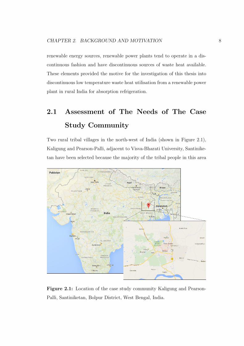
2.1 Location of the case study community Kaligung and Pearson-
Palli, Santiniketan, Bolpur District, West Bengal, India. . . . . 8
2.2 Typical house found in Kaligung and Pearson-Palli, made from
bamboo or wood and mud. . . . . . . . . . . . . . . . . . . . . 9
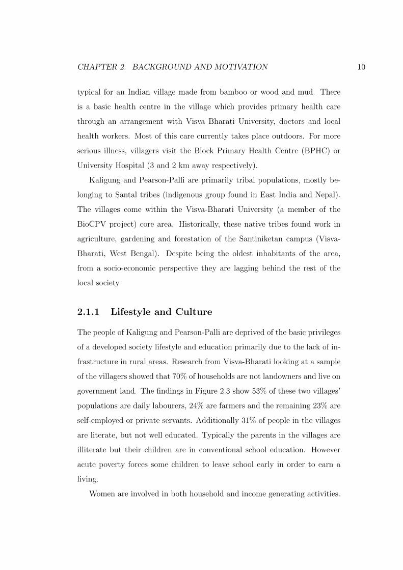
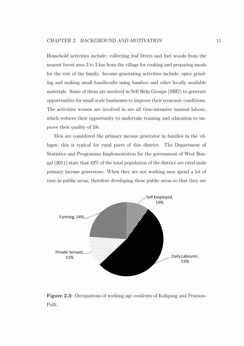
2.3 Occupations of working age residents of Kaligung and Pearson-
Palli. . . . . . . . . . . . . . . . . . . . . . . . . . . . . . . . . 11
2.4 Maximum predicted demand profile elected for the community
on a typical day irrespective of the season. . . . . . . . . . . . 18
2.5 BioCPV renewable power plant schematic, consisting of: 10
kW concentrated photovoltaic (CPV), 5 kW biogas and hydro-
gen internal combustion engine electrical generator set (genset),
electrolyser, metal hydride store and anaerobic digester. . . . . 19
3.1 Earliest recorded patent for a refrigeration machine, issued in
Great Britain in 1834. Where A is the compressor, B the con-
denser, C the throttle and D the evaporator (or refrigerator)
(Jordan and Priester 1950). . . . . . . . . . . . . . . . . . . . 26
3.2 Diagrammatic sketch of Ferdinand Carre’s absorption refrig-
eration machine for which he received a patent in the 1860s
(Jordan and Priester 1950). . . . . . . . . . . . . . . . . . . . 27
3.3 Schematic of a vapour compression refrigeration cycle. . . . . . 31
3.4 Schematic of an adsorption refrigeration system. . . . . . . . . 33
x
3.5 Schematic of a basic gas (or Reverse Brayton) cycle refrigerator. 34
3.6 Schematic of a basic absorption refrigeration cycle . . . . . . . 35
3.7 Schematic of the boiler absorber heat exchanger (BAX) cycle
on a single effect cycle. . . . . . . . . . . . . . . . . . . . . . . 48
3.8 Schematic of the boiler heat recovery cycle on a single effect
cycle. . . . . . . . . . . . . . . . . . . . . . . . . . . . . . . . . 49
3.9 Schematic of half effect cycle, which can operate with low
boiler temperatures at the expense of some of the energy in-
put, where L.P, I.P. and H.P. are low pressure, intermediate
pressure and high pressure respectively. . . . . . . . . . . . . . 50
3.10 Single effect with reservoirs to allow for continuous cooling
from discontinuous heat sources. . . . . . . . . . . . . . . . . . 53
3.11 Double boiler cycle schematic; showing one absorption refrig-
erator powered by two discontinuous heat sources through two
separate boilers with reservoirs to allow for continuous cooling
from discontinuous heat sources. . . . . . . . . . . . . . . . . . 54
3.12 Single effect cycle with evaporator tap-off schematic; where
the thermal coupling is shown as a heat transfer fluid (orange
section). . . . . . . . . . . . . . . . . . . . . . . . . . . . . . . 57
3.13 Coupled cycle schematic; where two absorption refrigerators
are powered by two separate heat sources and are thermally
coupled between the evaporator of one and the absorber and
condenser of the other. The thermal coupling is illustrated as
a heat transfer fluid (orange section). . . . . . . . . . . . . . . 58
3.14 Single effect cycle with reservoirs and evaporator tap-off. This
cycle allows both continuous refrigeration from discontinuous
heat sources and control over the evaporator temperature. The
thermal coupling is illustrated as a heat transfer fluid (orange
section). . . . . . . . . . . . . . . . . . . . . . . . . . . . . . . 59
xi
3.15 Coupled cycle schematic combined with reservoirs, allowing
continuous cooling from discontinuous heat sources; where
two absorption refrigerators are powered by two separate heat
sources and are thermally coupled between the evaporator of
one and the absorber and condenser of the other. The thermal
coupling is illustrated as a heat transfer fluid (orange section). 60
3.16 Double boiler with reservoirs and evaporator tap-off cycle schematic;
showing one absorption refrigerator powered by two heat sources
through two separate boilers. The thermal coupling is illus-
trated by the heat transfer fluid (orange section). . . . . . . . 61
4.1 CAD model of one of the four CPV modules provided by part-
ners at Indian Institute of Technology Madras and University
of Exeter. . . . . . . . . . . . . . . . . . . . . . . . . . . . . . 71
4.2 Pressure and enthalpy (ph) graph for pure acetone (Ajib and
Karno 2008). . . . . . . . . . . . . . . . . . . . . . . . . . . . 78
4.3 Pressure and temperature graph for acetone and zinc bromide
solution, where the saturation temperature of pure acetone
(red) is next to the corresponding vapour pressure and X is
solution concentration inmZnBr2
msolution(Ajib and Karno 2008). . . . 79
5.1 PV cell efficiency as a function of cell temperature using Equa-
tion 4.4 provided in confidence by PV manufacturer Azur Space.106
5.2 Sankey diagram of daily energy flow in BioCPV power plant. . 110
5.3 Grassman diagram of daily exergy flow in BioCPV power plant.117
6.1 Absorption refrigerator experiment testing equipment schematic
(P denotes pressure transducer and T thermocouple). . . . . . 120
xii

6.2 Boiler temperature and evaporator temperature with respect
to experiment time, where the blue line corresponds to the
average boiler temperature and the red line is the evaporator
inlet temperature. Test details: weak solution concentration(mZnBr2
msolution
)at inlet 62% and 703 g of solution collected. . . . . 123
6.3 Boiler schematic showing the positions of all five thermocouples.124
6.4 Boiler temperature showing the temperature readings from all
five thermocouples in the boiler TBO1 to TBO5 (using the ther-
mocouple locations shown in Figure 6.3). Test details: weak
solution concentration(
mZnBr2
msolution
)at inlet 51.7% and 1171 g of
solution collected. . . . . . . . . . . . . . . . . . . . . . . . . . 125
6.5 Average boiler temperature (blue line, right axis) and pressure
of the high pressure side measured by the transducer between
the strong solution reservoir and the condenser (red line, left
axis). Test details: weak solution concentration(
mZnBr2
msolution
)at
inlet 62% and 703 g of solution collected. . . . . . . . . . . . . 126
6.6 Operating temperatures of the condenser (green line for in-
let and red line for outlet) with the high pressure converted
to acetone saturation temperature using Equation 4.15 (blue
line). Test details: weak solution concentration(
mZnBr2
msolution
)at
inlet 62% and 703 g of solution collected. . . . . . . . . . . . . 127
6.7 Operating temperatures of the evaporator (red line for inlet
and green line for outlet) with the low pressure converted
to acetone saturation temperature using Equation 4.15 (blue
line). Test details: weak solution concentration(
mZnBr2
msolution
)at
inlet 62% and 703 g of solution collected. . . . . . . . . . . . . 128
xiii
6.8 Operating input (red line, right axis) and output (blue line,
right axis) temperatures of the absorber along with the pres-
sure between the absorber and evaporator (green line, left
axis). Test details: weak solution concentration(
mZnBr2
msolution
)at inlet 62% and 703 g of solution collected. . . . . . . . . . . 130
6.9 Photo of the left hand side of the absorption refrigerator test
rig, showing all of the high pressure side and some of the low
pressure side. . . . . . . . . . . . . . . . . . . . . . . . . . . . 133
6.10 Photo of the right hand side of the absorption refrigerator
experimental test rig, mainly the low pressure side. . . . . . . 134
6.11 Photo of the condenser in the absorption refrigerator experi-
mental test rig showing the refrigerant leaving the condenser
as a liquid. . . . . . . . . . . . . . . . . . . . . . . . . . . . . . 135
6.12 Photo of the evaporator in the absorption refrigerator experi-
mental test rig showing the refrigerant as a liquid entering the
evaporator and vapour bubbles forming inside the evaporator. 136
7.1 Graph of the operating limits of the boiler and condenser show-
ing the effect of strong solution concentration on condenser
temperature for boiler temperatures of 100◦C to 50◦C. . . . . 140
7.2 Graph of the effect of condenser heat exchanger effectiveness
on condenser temperature, for a boiler temperature of 60◦C at
ambient temperatures of 40◦C to 10◦C. . . . . . . . . . . . . . 142
7.3 Graph of the effect of condenser heat exchanger effectiveness
on the strongest permissible strong solution concentration based
on a boiler temperature of 60◦C at ambient temperatures of
40◦C to 10◦C. . . . . . . . . . . . . . . . . . . . . . . . . . . . 143
xiv
7.4 Graph of the operating limits of the absorber and evaporator
showing the effect of weak solution concentration on evapora-
tor temperature for absorber temperatures of 40◦C to 15◦C. . 144
7.5 Effect of absorber heat exchanger effectiveness on absorber
outlet (weak solution) temperature for a strong solution con-
centration of 60% and weak solution concentration of 54%(mZnBr2
msolution
)for ambient temperatures of 10◦C to 50◦C. . . . . . 147
7.6 Effect of absorber heat exchanger effectiveness on evaporator
temperature for a strong solution concentration of 60% and
weak solution concentration of 54%(
mZnBr2
msolution
)for ambient
temperatures of 10◦C to 50◦C. . . . . . . . . . . . . . . . . . . 148
7.7 Effect of absorber heat exchanger effectiveness on absorber
outlet (weak solution) temperature for a strong solution con-
centration of 60% and weak solution concentration of 56%
( mZnBr
msolution) for ambient temperatures of 10◦C to 50◦C. . . . . . 149
7.8 Effect of absorber heat exchanger effectiveness on evapora-
tor temperature for a strong solution concentration of 60%
and weak solution concentration of 56% ( mZnBr
msolution) for ambient
temperatures of 10◦C to 50◦C. . . . . . . . . . . . . . . . . . . 150
7.9 Analysis of difference between ambient and evaporator tem-
peratures with strong and weak solution concentration differ-
ences of 2%, 4% and 6% and a boiler temperature of 60◦C at
ambient temperatures varying from 0◦C to 50◦C in a single
effect cycle. . . . . . . . . . . . . . . . . . . . . . . . . . . . . 153
7.10 Analysis of single effect cycle CoP with varying the strong and
weak solution concentration difference of 2%, 4% and 6%, with
a boiler temperature of 60◦C at ambient temperatures varying
from 0◦C to 50◦C. . . . . . . . . . . . . . . . . . . . . . . . . . 155
xv

7.11 Analysis of difference between ambient and evaporator tem-
peratures with strong and weak solution concentration differ-
ences of 2%, 4% and 6%, and a boiler temperature of 80◦C
at ambient temperatures varying from 0◦C to 50◦C in a single
effect cycle. . . . . . . . . . . . . . . . . . . . . . . . . . . . . 156
7.12 Analysis of single effect cycle CoP with varying the strong and
weak solution concentration difference of 2%, 4% and 6% with
a boiler temperature of 80◦C at ambient temperatures varying
from 0◦C to 50◦C. . . . . . . . . . . . . . . . . . . . . . . . . . 157
7.13 Analysis of evaporator temperatures achieved with a boiler
temperature of 60◦C at ambient temperatures varying from
0◦C to 50◦C, with evaporator tap off on a single effect cycle
with solution concentration differences of 6% (yellow dashed
line) and 4% (green dashed line) and single effect cycles with
solution concentration differences of 6% (blue line) to 4% (or-
ange line) and 2% (grey line). . . . . . . . . . . . . . . . . . . 159
7.14 Analysis of evaporator heat absorbing energy used with a
boiler temperature of 60◦C at ambient temperatures varying
from 0◦C to 50◦C, when comparing evaporator tap off on a
single effect cycle with solution concentration differences of
4% (grey dashed line) and 6% (orange dashed line) against
reducing the solution concentration difference from 6% to 4%
(yellow line) and 4% to 2% (blue line). . . . . . . . . . . . . . 161
7.15 Analysis of evaporator temperatures achieved with a boiler
temperature of 80◦C at ambient temperatures varying from
0◦C to 50◦C, with the evaporator tap off on a single effect cycle
with solution concentration differences of 6% (yellow dashed
line) and 4% (green dashed line) and single effect cycles with
6%,(blue line) 4% (orange line) and 2% (grey line). . . . . . . 163
xvi
7.16 Analysis of evaporator heat absorbing energy used with a
boiler temperature of 80◦C at ambient temperatures varying
from 0◦C to 50◦C, when comparing evaporator tap off on a
single effect cycle with solution concentration differences of
4% (grey dashed line) and 6% (orange dashed line) against
reducing the solution concentration difference from 6% to 4%
(yellow line) and 4% to 2% (blue line). . . . . . . . . . . . . . 164
7.17 Evaporator temperature of a single effect cycle using the CPV
waste heat as a heat source at 60◦C with a 2% solution con-
centration difference at ambient temperatures from 0◦C to 50◦C.168
7.18 Cooling energy (evaporator heat absorbing energy) of a single
effect cycle using the CPV waste heat as a heat source at
60◦C with a 2% solution concentration difference at ambient
temperatures from 0◦C to 50◦C. . . . . . . . . . . . . . . . . . 169
7.19 Daily electrical energy saved (avoided) from not using a vapour
compression refrigerator to provide the same cooling as a single
effect cycle using the CPV waste heat as a heat source at
60◦C with a 2% solution concentration difference at ambient
temperatures from 0◦C to 50◦C. . . . . . . . . . . . . . . . . . 170
7.20 Evaporator temperature of a single effect cycle using the genset
radiator waste heat as a heat source at 80◦C with a 2% so-
lution concentration difference at ambient temperatures from
0◦C to 50◦C. . . . . . . . . . . . . . . . . . . . . . . . . . . . . 172
7.21 Daily cooling energy of a single effect cycle using the genset
radiator waste heat as a heat source at 80◦C with a 2% solution
concentration difference at ambient temperatures from 0◦C to
50◦C. . . . . . . . . . . . . . . . . . . . . . . . . . . . . . . . . 173
xvii
7.22 Daily electrical energy saved (avoided) from not using a vapour
compression refrigerator to provide the same cooling as a single
effect cycle using the genset radiator waste heat as a heat
source at 80◦C with a 2% solution concentration difference at
ambient temperatures from 0◦C to 50◦C. . . . . . . . . . . . . 174
7.23 High DNI day analysis of the CPV electrical (green line, left
axis) and heat (blue line, left axis) outputs together with the
corresponding DNI (red line, right axis), to be used for the
heating side of the CPV waste heat powered absorption re-
frigerator using ambient temperature and DNI data from the
20th August 2011 from NREL (2016). . . . . . . . . . . . . . . 177
7.24 High DNI day analysis of the CPV waste heat powered absorp-
tion refrigerator showing the evaporator temperature (green
line, left axis), ambient temperature (blue line, left axis) and
cooling power (red line, right axis). Using the ambient tem-
perature from the 21st August 2011 where the previous day
was used to fill the strong solution and refrigerant reservoirs.
Data from NREL (2016). . . . . . . . . . . . . . . . . . . . . . 178
7.25 Low DNI day analysis of the CPV electrical (green line, left
axis) and heat (blue line, left axis) outputs together with the
corresponding DNI (red line, right axis), to be used for the
heating side of the CPV waste heat powered absorption re-
frigerator using ambient temperature and DNI data from the
22nd June 2004 from NREL (2016). . . . . . . . . . . . . . . . 181
xviii

7.26 Low DNI day analysis of the CPV waste heat powered absorp-
tion refrigerator showing the evaporator temperature (green
line, left axis), ambient temperature (blue line, left axis) and
cooling power (red line, right axis). Using the ambient tem-
perature from the 23rd June 2004 where the previous day was
used to fill the strong solution and refrigerant reservoirs. Data
from NREL (2016). . . . . . . . . . . . . . . . . . . . . . . . . 182
7.27 High temperature day analysis of the CPV electrical (green
line, left axis) and heat (blue line, left axis) outputs together
with the corresponding DNI (red line, right axis), to be used
for the heating side of the CPV waste heat powered absorption
refrigerator using ambient temperature and DNI data from the
11th May 2011 from NREL (2016). . . . . . . . . . . . . . . . 184
7.28 High temperature day analysis of the CPV waste heat powered
absorption refrigerator showing the evaporator temperature
(green line, left axis), ambient temperature (blue line, left axis)
and cooling power (red line, right axis). Using the ambient
temperature from the 12th May 2011 where the previous day
was used to fill the strong solution and refrigerant reservoirs.
Data from NREL (2016). . . . . . . . . . . . . . . . . . . . . . 185
7.29 Low temperature day analysis of the CPV electrical (green
line, left axis) and heat (blue line, left axis) outputs together
with the corresponding DNI (red line, right axis), to be used
for the heating side of the CPV waste heat powered absorption
refrigerator using ambient temperature and DNI data from the
4 January 2004 from NREL (2016). . . . . . . . . . . . . . . . 187
xix
7.30 Low temperature day analysis of the CPV waste heat powered
absorption refrigerator showing the evaporator temperature
(green line, left axis), ambient temperature (blue line, left axis)
and cooling power (red line, right axis). Using the ambient
temperature from the 5 January 2004 where the previous day
was used to fill the strong solution and refrigerant reservoirs.
Data from NREL (2016). . . . . . . . . . . . . . . . . . . . . . 188
xx

List of Tables
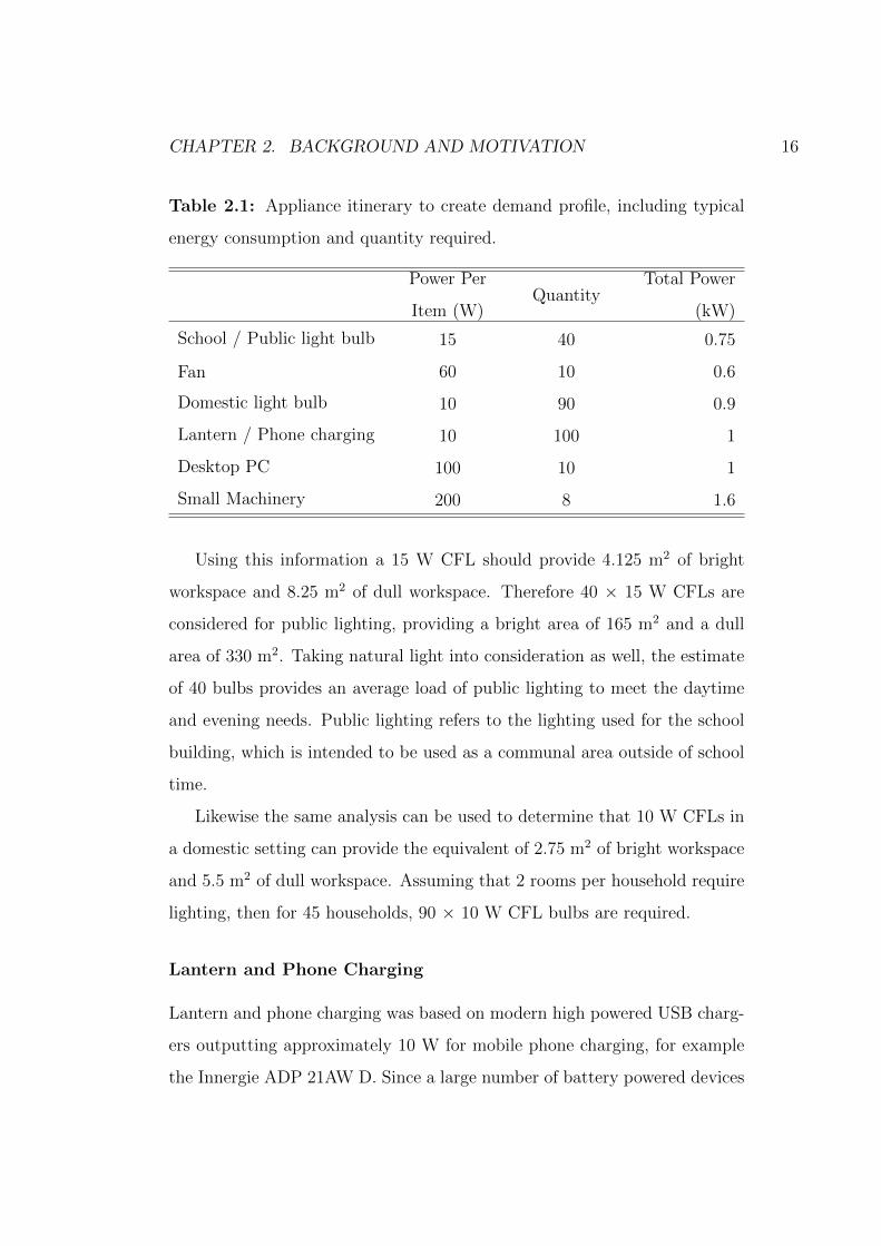
2.1 Appliance itinerary to create demand profile, including typical
energy consumption and quantity required. . . . . . . . . . . . 16
3.1 Appraisal and decision matrix of refrigeration technologies for
their application in using low grade discontinuous waste heat
in rural India, where 5 is desirable and 1 is undesirable. . . . . 39
3.2 Appraisal and decision matrix of absorption refrigeration cy-
cles to use low grade discontinuous waste heat in rural India,
where 5 is desirable and 1 is undesirable. . . . . . . . . . . . . 63
4.1 CPV specifications provided by partners at Indian Institute of
Technology Madras and University of Exeter. . . . . . . . . . 72
4.2 Genset expected efficiency and electrical output. . . . . . . . . 74
4.3 Vapour pressure calculation coefficients (aij) for solutions of
acetone and zinc bromide to use in Equation 4.16 where sub-
script i corresponds to T i and subscript j corresponds to Xj
(Ajib and Karno 2008). . . . . . . . . . . . . . . . . . . . . . . 77
4.4 Solution enthalpy calculation coefficients (bij) to use in Equa-
tion 4.17 where subscript i corresponds to X i and subscript j
corresponds to T j (Ajib and Karno 2008). . . . . . . . . . . . 80
4.5 Data for radiative exergy calculations (Petela 2010). . . . . . . 97
5.1 CPV energy balance. . . . . . . . . . . . . . . . . . . . . . . . 105
xxi
5.2 Combustion calculation to find the energy contained within
the exhaust from the hydrogen part of the fuel. . . . . . . . . 107
5.3 Combustion calculation to find the energy contained within
the exhaust from the biogas part of the fuel. . . . . . . . . . . 108
5.4 Internal combustion engine electrical generator energy balance. 109
5.5 CPV exergy balance. . . . . . . . . . . . . . . . . . . . . . . . 112
5.6 Calculation of flow exergy within the genset exhaust by sepa-
rating each product of combustion of the biogas-hydrogen fuel
mix. . . . . . . . . . . . . . . . . . . . . . . . . . . . . . . . . 113
5.7 Genset exergy balance. . . . . . . . . . . . . . . . . . . . . . . 114
xxii
Acronyms, Abbreviations,
Definitions and Nomenclature
Acronyms, Abbreviations and Definitions
BioCPV - Collaborative research project name encompassing the use of bio-
gas and CPV
CPV - Concentrated photovoltaic
Genset - Internal combustion engine electric generator
AD - Anaerobic digester
DNI - Direct normal irradiance
CoP - Coefficient of Performance
PV - Photovoltaic
Cell - PV cell assembly in CPV unit
ZnBr2 - Zinc bromide
Weak solution - High–in–refrigerant
Strong Solution - Low–in–refrigerant
xxiii
Nomenclature
T - Temperature (◦C and K)
P - Pressure (bar)
h - Specific enthalpy (kJ·kg−1)
s - Specific entropy (kJ·kg−1·K−1)
X - Concentration mZnBr
mtotal× 100 (e.g 50% = 50)
C - Concentration mZnBr
mtotal(%)
m - Mass (kg) or mass flow (time period dependant modelling approach)
Q - Thermal energy (kJ), (kW) or (kW·h)
W - Work (kJ)
E - Electrical energy (kJ), (kW) or (kW·h)
ε - Exergy (kJ), (kW) or (kW·h)
A - Area (m2)
η - Efficiency
n - Number of [item]
ε - Heat exchanger effectiveness
λ - Percentage of cooling energy used
cp - Specific heat capacity (kJ·kg−1·K−1)
∆ - Difference
Energy Analysis
ECPV - CPV electrical output
QCPVconcentrator - Thermal energy entering the CPV concentrator
nCPV - Number of CPV units
ηCPVoptical- Optical efficiency of CPV concentrator
ACPVconcentrator - Area of CPV concentrator
QCPVcell- Thermal energy reaching PV cell assembly in CPV unit
xxiv
ηCPVcell- PV cell efficiency
QCPVthermal- Thermal energy of the PV cell
Qgenset - Genset thermal energy requirement
Wgensetancillary- Genset ancillary losses
Qgensetexhaust - Thermal energy in genset exhaust
mgensetexhausti- Mass flow of individual components of genset exhaust
hgensetexhausti - Specific enthalpy of individual components of genset exhaust
Qgensetradiator - Thermal energy in genset radiator
Absorption Refrigerator
The following explains the general naming method for the symbols used in
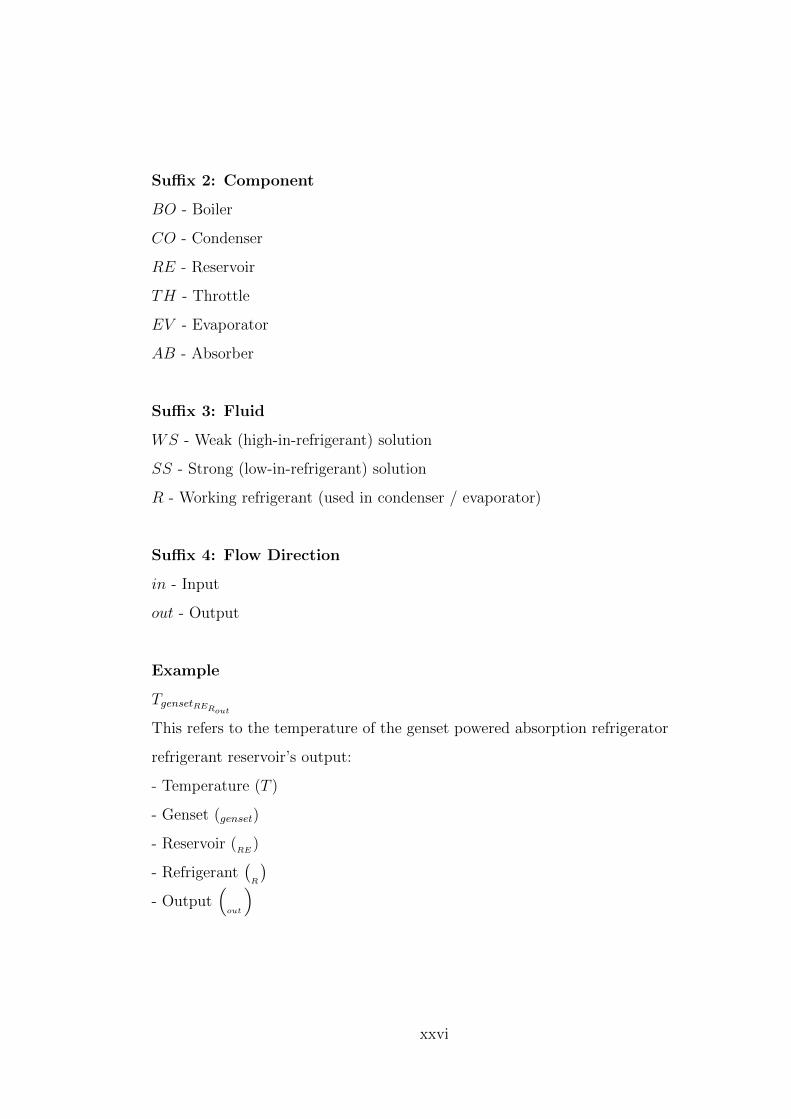
absorption refrigerator modelling in this thesis, where Symbol1234
Suffix 1: General
if blank it refers to both CPV and genset
AMB Ambient
c - Critical
s - Saturation
l - Liquid
v - Vapour
sh - Superheated
genset - Internal combustion engine electrical generator
CPV - Concentrated photovoltaic
HTF - Heat transfer fluid
vc - Vapour compression refrigerator
xxv
Suffix 2: Component
BO - Boiler
CO - Condenser
RE - Reservoir
TH - Throttle
EV - Evaporator
AB - Absorber
Suffix 3: Fluid
WS - Weak (high-in-refrigerant) solution
SS - Strong (low-in-refrigerant) solution
R - Working refrigerant (used in condenser / evaporator)
Suffix 4: Flow Direction
in - Input
out - Output
Example
TgensetRERout
This refers to the temperature of the genset powered absorption refrigerator
refrigerant reservoir’s output:
- Temperature (T )
- Genset (genset)
- Reservoir (RE
)
- Refrigerant(R
)- Output
(out
)
xxvi
Chapter 1
Introduction
The following thesis investigates discontinuous (operating for a proportion
of the day e.g. when the sun shines or the evening) low temperature waste
heat utilisation for absorption refrigeration for a range of ambient conditions.
The research forms part of a Bridging the Urban Rural Divide programme
(BURD) called BioCPV aiming to provide a sustainable development solu-
tion to rural India through the provision of renewable power. The power
plant proposed by the BioCPV research group and its location in rural India
provide the criteria and input information for the investigations within this
thesis.
The BioCPV project is a collaboration between three Indian and four
British universities and the renewable power plant consists of 10 kW (elec-
tric) concentrated photovoltaic (CPV) and 5 kW (electric) biogas-hydrogen
internal combustion engine electrical generator set (genset). The CPV is
solar powered, the biogas is generated in an anaerobic digester powered by
local food waste and aquatic weeds, and the hydrogen is produced from the
electrolysis of water using excess solar power from the CPV. The waste heat
sources being investigated are the CPV maintained at 60◦C and the genset
radiator at 80◦C. Though the waste heat sources are modelled from a specific
case study power plant the research within this thesis is applicable to a wide
1
CHAPTER 1. INTRODUCTION 2
range of waste heat sources from industrial to domestic applications in any
environment where sustainable refrigeration is required.
There is a need to address the future global energy demands and the
significance of the contribution of rural electrification in India. A presenta-
tion of a demand profiling method used to quantify the needs of the case
study community in rural India is necessary to understand how an electricity
generation plant will be used in the context of a rural village in India. An
overview of the proposed power plant by the BioCPV group is provided to
aid contextualisation of the analysis within this thesis. There is also a need
to address the potential global low grade waste heat resource and how its
use has the potential to reduce global energy consumption. This helps place
a level of importance on the issue of waste heat utilisation.
The motivation for this research is that the case study community is lo-
cated in West Bengal, India and due to its high ambient temperatures and
traditional rural lifestyle a sustainable source of refrigeration has been con-
sidered a more beneficial use of waste heat than hot water. Refrigeration has
the potential to provide food and medicine storage or cooling for a medical
recovery area, whereas hot water from these low grade heat sources is not
needed for heating and so would only provide more comfortable washing fa-
cilities. Providing sustainable refrigeration can have a significant impact on
the development of this community without the need for a significant increase
in electricity generation.
The research objective is to investigate discontinuous low temperature
waste heat utilisation from a renewable power plant in rural India for ab-
sorption refrigeration.
The approach consists of:
• Assess and validate the needs of the community.
CHAPTER 1. INTRODUCTION 3
• Appraise refrigeration technologies to determine the most suitable to
investigate.
• Quantify and qualify the waste heat sources.
• Investigate the operating limits of absorption refrigeration from the
waste heat sources identified in a range of ambient temperatures.
• Investigate any alternative configurations that extend the operating
limits.
• Quantify the benefits from the optimised configuration for the commu-
nity.
The thesis structure:
• Background and Motivation outlines the main drivers, objectives
and approach of this research. The rationale behind how low grade
waste heat utilisation can help mitigate some of the negative effects
of global energy consumption is presented. This is followed by a de-
scription of the case study community and their needs together with
a projected electrical demand profile. The renewable power plant pro-
posed by the BioCPV research group is then shown to identify the low
grade heat sources which are used to power the absorption refrigeration
systems modelled later in the thesis.
• Refrigeration Technology Review presents an appraisal of refrig-
eration technologies. Initially a history of refrigeration is introduced
which is followed by a review of common refrigeration systems. An
appraisal process of common refrigeration systems finds absorption re-
frigeration to be suitable for the conditions of the case study community
and the heat sources available. This is followed by a detailed review
of absorption refrigeration working fluids and system configurations.
Acetone and zinc bromide solution is identified as suitable working
CHAPTER 1. INTRODUCTION 4
fluid pair and configurations that reduce evaporator temperatures are
identified to be investigated.
• Analytical Methodology presents the approach used to calculate
the results presented in the following three chapters. This includes the
calculations for the energy analysis within which lies the modelling of
the waste heat sources. This is followed by the modelling approach for
the absorption refrigeration systems. Finishing with the approach for
quantifying energy utilisation using exergy for the BioCPV power plant
and a method for relating the cooling generated from the absorption
refrigeration systems to avoided electricity consumption.
• Power Plant Energy Utilisation presents the results and discussions
of an energy and exergy analysis of the rural renewable power plant
proposed by the BioCPV research group. This process quantifies and
qualifies the energy contained in the heat sources.
• Absorption Refrigeration Experiment presents the results and
discussions from a lab scale absorption refrigerator used to provide
insight into the absorption refrigeration system modelling assumptions
in the analytical methodology and the operational challenges.
• Absorption Refrigeration Modelling presents the results and dis-
cussions of the absorption refrigeration system modelling, investigating
the effects of operating limits and cycle configurations on cooling out-
put and refrigeration temperature.
• Conclusions and Further Work describes the processes used for
the investigations in this thesis and presents the main findings together
with areas of further work that were identified during this research.

Chapter 2
Background and Motivation
Global energy demand and consumption is increasing and the associated
environmental impacts of it are generally accepted amongst the scientific
community. This thesis explores the optimisation of low grade waste heat
sources for absorption refrigeration to address this increasing consumption.
There have been several international conferences, frameworks and treaties
from the United Nations Framework Convention on Climate Change (UN-
FCCC) in 1992 through to the Conference of the Parties (COP) 21 in 2015
where targets were set and plans made to mitigate and adapt to the effects of
emmssions resulting from energy consumption. Non OECD (Organisation for
Economic Co-operation and Development) countries are expected to account
for the majority of this increase in energy consumption where projections
show that by 2040 they could account for 2.5 times that of OECD countries
(EIA 2015). This is largely the result of the economic growth of a country
being directly related to the per capita energy consumption (Ghosh 2002).
In order to study this global issue, this research investigates a key con-
tributing country, India. It has the second largest population, with approx-
imately 1.25 billion people it accounts for approximately 17% of the global
population (CIA 2015). India is one of the non OECD countries expected
to develop rapidly in the coming years resulting in an increase in its en-
5
CHAPTER 2. BACKGROUND AND MOTIVATION 6
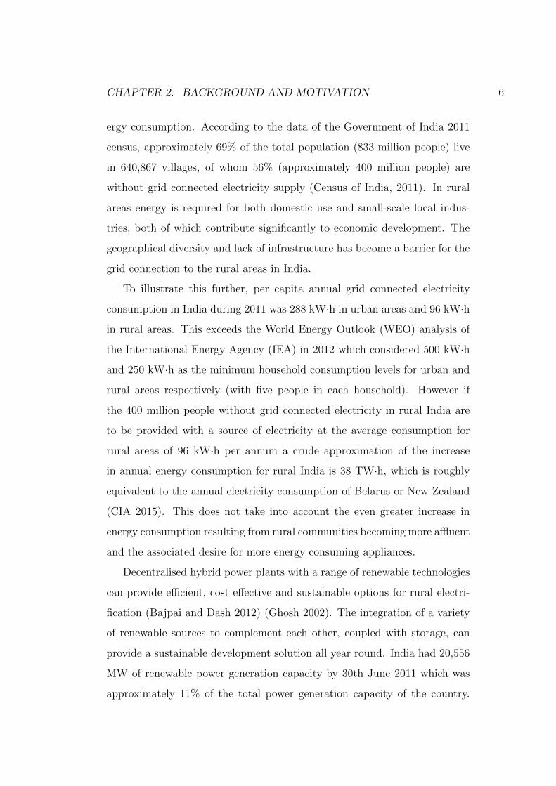
ergy consumption. According to the data of the Government of India 2011
census, approximately 69% of the total population (833 million people) live
in 640,867 villages, of whom 56% (approximately 400 million people) are
without grid connected electricity supply (Census of India, 2011). In rural
areas energy is required for both domestic use and small-scale local indus-
tries, both of which contribute significantly to economic development. The
geographical diversity and lack of infrastructure has become a barrier for the
grid connection to the rural areas in India.
To illustrate this further, per capita annual grid connected electricity
consumption in India during 2011 was 288 kW·h in urban areas and 96 kW·h
in rural areas. This exceeds the World Energy Outlook (WEO) analysis of
the International Energy Agency (IEA) in 2012 which considered 500 kW·h
and 250 kW·h as the minimum household consumption levels for urban and
rural areas respectively (with five people in each household). However if
the 400 million people without grid connected electricity in rural India are
to be provided with a source of electricity at the average consumption for
rural areas of 96 kW·h per annum a crude approximation of the increase
in annual energy consumption for rural India is 38 TW·h, which is roughly
equivalent to the annual electricity consumption of Belarus or New Zealand
(CIA 2015). This does not take into account the even greater increase in
energy consumption resulting from rural communities becoming more affluent
and the associated desire for more energy consuming appliances.
Decentralised hybrid power plants with a range of renewable technologies
can provide efficient, cost effective and sustainable options for rural electri-
fication (Bajpai and Dash 2012) (Ghosh 2002). The integration of a variety
of renewable sources to complement each other, coupled with storage, can
provide a sustainable development solution all year round. India had 20,556
MW of renewable power generation capacity by 30th June 2011 which was
approximately 11% of the total power generation capacity of the country.

CHAPTER 2. BACKGROUND AND MOTIVATION 7
Through the Jawaharlal Nehru National Solar Mission (JNNSM) it is envis-
aged that India will have an installed solar capacity of 20,000 MW by 2020,
100,000 MW by 2030 and 200,000 MW by 2050. (Sharma et al. 2012).
Globally, waste heat is a huge energy resource, which if well utilised can
reduce global energy consumption and the associated negative effects. Olul-
eye et al. (2016) state “process industries are responsible for 27% of global
energy consumption” combined with 20% to 50% of industrial energy being
wasted as heat (DOE 2008), indicates that approximately 10% of global en-
ergy consumption is industrial process waste heat. Considering that Haddad
et al. (2014) state that low grade waste heat (defined as below 200◦C) ac-
counts for 66% of industrial waste heat, it is possible to approximate that
7% of global energy consumption is lost as low grade waste heat through
the process industries. These figures should be used with caution, as Miro
et al. (2015) describe that there are difficulties in obtaining waste heat data
internationally. However the literature suggests that there is currently a
significant amount of wasted low grade heat. If well utilised, these figures
suggest that this energy source could either significantly reduce global en-
ergy consumption or allow greater levels of development growth without the
associated increased energy demand.
The factors mentioned here led to the creation of a collaborative research
group between institutions in the UK and India, called BioCPV, with the ob-
jective of providing a sustainable development solution to rural India through
renewable power. This research group has chosen a small community in
Santiniketan, West Bengal, India, which is adjacent to one of the partner
organisations, Visva-Bharati, to provide renewable power to. In addition
to providing sustainable sources of energy to supply the projected growth
in energy consumption of the community, it is equally important to opti-
mise the use of the energy produced as this, by its nature, can reduce the
amount of energy needed and therefore consumed. Due to the nature of
CHAPTER 2. BACKGROUND AND MOTIVATION 8
renewable energy sources, renewable power plants tend to operate in a dis-
continuous fashion and have discontinuous sources of waste heat available.
These elements provided the motive for the investigation of this thesis into
discontinuous low temperature waste heat utilisation from a renewable power
plant in rural India for absorption refrigeration.
2.1 Assessment of The Needs of The Case
Study Community
Two rural tribal villages in the north-west of India (shown in Figure 2.1),
Kaligung and Pearson-Palli, adjacent to Visva-Bharati University, Santinike-
tan have been selected because the majority of the tribal people in this area
Figure 2.1: Location of the case study community Kaligung and Pearson-
Palli, Santiniketan, Bolpur District, West Bengal, India.

CHAPTER 2. BACKGROUND AND MOTIVATION 9
do not have access to electricity owing to their socio-economic conditions.
Although there is a grid connection in the village, the supply is weak, only
providing a few hours of electricity per day and not all the houses are con-
nected to this grid. The villages comprise 179 households with a population
of approximately 821. Most of the families in the village live below the
poverty line as defined by the World Bank. Out of the total population,
52% are women and 10% are children. The average household income is
approximately INR 2500 per month. The BioCPV research project selected
45 households out of these villages for the case study community to provide
renewable power to.
Basic facilities such as drinking water and sanitation are not available
which leads to an unhygienic lifestyle. The houses, shown in Figure 2.2 are
Figure 2.2: Typical house found in Kaligung and Pearson-Palli, made from
bamboo or wood and mud.
CHAPTER 2. BACKGROUND AND MOTIVATION 10
typical for an Indian village made from bamboo or wood and mud. There
is a basic health centre in the village which provides primary health care
through an arrangement with Visva Bharati University, doctors and local
health workers. Most of this care currently takes place outdoors. For more
serious illness, villagers visit the Block Primary Health Centre (BPHC) or
University Hospital (3 and 2 km away respectively).
Kaligung and Pearson-Palli are primarily tribal populations, mostly be-
longing to Santal tribes (indigenous group found in East India and Nepal).
The villages come within the Visva-Bharati University (a member of the
BioCPV project) core area. Historically, these native tribes found work in
agriculture, gardening and forestation of the Santiniketan campus (Visva-
Bharati, West Bengal). Despite being the oldest inhabitants of the area,
from a socio-economic perspective they are lagging behind the rest of the
local society.
2.1.1 Lifestyle and Culture
The people of Kaligung and Pearson-Palli are deprived of the basic privileges
of a developed society lifestyle and education primarily due to the lack of in-
frastructure in rural areas. Research from Visva-Bharati looking at a sample
of the villagers showed that 70% of households are not landowners and live on
government land. The findings in Figure 2.3 show 53% of these two villages’
populations are daily labourers, 24% are farmers and the remaining 23% are
self-employed or private servants. Additionally 31% of people in the villages
are literate, but not well educated. Typically the parents in the villages are
illiterate but their children are in conventional school education. However
acute poverty forces some children to leave school early in order to earn a
living.
Women are involved in both household and income generating activities.
CHAPTER 2. BACKGROUND AND MOTIVATION 11
Household activities include: collecting leaf litters and fuel woods from the
nearest forest area 2 to 3 km from the village for cooking and preparing meals
for the rest of the family. Income generating activities include: spice grind-
ing and making small handicrafts using bamboo and other locally available
materials. Some of them are involved in Self Help Groups (SHG) to generate
opportunities for small scale businesses to improve their economic conditions.
The activities women are involved in are all time-intensive manual labour,
which reduces their opportunity to undertake training and education to im-
prove their quality of life.
Men are considered the primary income generator in families in the vil-
lages; this is typical for rural parts of this district. The Department of
Statistics and Programme Implementation for the government of West Ben-
gal (2011) state that 43% of the total population of the district are rural male
primary income generators. When they are not working men spend a lot of
time in public areas, therefore developing these public areas so that they are
Figure 2.3: Occupations of working age residents of Kaligung and Pearson-
Palli.
CHAPTER 2. BACKGROUND AND MOTIVATION 12
suitable for education and training could also provide a positive impact for
the villagers.
There is inadequate indoor and outdoor lighting in the villages. This
results in the majority of work and learning taking place during the day.
A survey carried out by Visva-Bharati within the village found that it was
difficult for children to study at home due to inadequate lighting. The current
solution of kerosene lamps has health implications as their emissions reduce
indoor air quality.
Due to a lack of reliable electricity it is not practical to provide refriger-
ation for food and medicine storage or space cooling (for example a recovery
room in the medical centre).
The demographic and socio-economic needs described here can be ad-
dressed by providing reliable electricity to aid the development of this com-
munity. This will improve the educational environment through lighting and
ventilation. It will reduce reliance on technologies damaging to health (such
as kerosene lamps). It will also alleviate some of the time-intensive manual
income generating activities potentially leading to an improved quality of
life. Providing these infrastructural developments in a sustainable way, will
help the long term needs of this community and act as a model for rural
communities across the developing world.
2.1.2 Weather and Conditions
Like most of the remote areas of eastern India, the region of Kaligung and
Pearson-Palli is warm and humid with generous rainfall. Based on data col-
lected from a local weather station at Visva-Bharati, Santiniketan there is
typically 1500 mm of rainfall from June to September and average tempera-
tures of 24◦C to 35◦C with highs approaching 50◦C.

CHAPTER 2. BACKGROUND AND MOTIVATION 13
2.1.3 Resources Available
India has an abundance of solar energy with annual daily average solar ir-
radiance on a horizontal surface of 5 to 7 kW·h·m−2. Nearly 58% of the
geographical area represents regions of exceptional solar power potential (Ra-
machandra et al. 2011). The eastern part of India is rich in both solar irradi-
ation and biomass resources (Reddy and Veershetty 2013) (Banerjee 2006).
A survey by Visva-Bharati also estimated that there is access to a minimum
of 200 kg food waste generated on a daily basis from the university hostels
in the nearby area of the village and plenty of aquatic weeds provided by the
nearby ponds, which can be used as a fuel source.
2.2 Community Power Demand Rationale
The following section describes the process for creating a demand estimation
for the community and presents the renewable power plant proposed by the
group. The following process was developed as part of this thesis and was
a collaboration with the Indian Institute of Technology Bombay. A detailed
overview of the technologies available allowing appropriate selection together
with the design considerations and sizing calculations for each technology
within the plant can be found in Appendix Paper titled “Design and initial
assessments of a biomass/biogas and solar renewable power plant for rural
electrification in India”.
2.2.1 Demand Estimation
The World Energy Outlook analysis for the minimum electricity consump-
tion of a five person household is calculated using the assumption that the
following technologies could be used: a floor fan, a mobile telephone, and
two compact fluorescent lamps (CFL) in rural areas, and might include: an
CHAPTER 2. BACKGROUND AND MOTIVATION 14
efficient refrigerator, a second mobile telephone, and another appliance, such
as a small television or a computer, in urban areas. Electric lighting is seen
to be an influential technology to provide development, from 2001 to 2011
the share of households in rural areas using electricity as their prime source
of lighting changed from 43.5% to 55.3%, and in urban areas from 87.6% to
92.7% [Census of India, 2011].
In light of these findings and studies of the local needs, together with the
desire to provide sustainable development through improving the educational
environment and overall quality of life, this section describes the method used
to calculate a demand profile for the community and others like it. Table
2.1 lists the items and quantities used in the demand profile and Figure 2.4
shows how the energy demand of the items in Table 2.1 would be distributed
through a typical 24 hour period.
Previous work with these communities carried out by Visva-Bharati found
that successful adoption of change requires a holistic approach where the vil-
lagers are involved throughout the project, training and education are pro-
vided and that everything is compatible with their customs and traditions.
Alongside the engineering research there is work and research in promoting
the system and its benefits to the local community. This is equally as im-
portant as the engineering design to avoid rejection of technology resulting
from apprehension of significant change.
Ventilation - Fans
Fans are required for thermal comfort; it is common to see ceiling fans used
in warm climates as they destratify the air providing a sensation of being
cooler. Guidelines in the United Kingdom suggest 70 m2 is required for a
primary or middle school class of 30 students (NUT 2015). A typical ceiling
fan such as Vent-Axia Reversible Hi-Line + requires 60 W at full load and
suggests in tropical climates that they should be placed 3 m apart (and 6 m
CHAPTER 2. BACKGROUND AND MOTIVATION 15
in temperate climates) (Vent-Axia 2015). There are currently 104 students
at the school which are accommodated in 2 large rooms (approximately 11 m
x 5 m) and one small one (3 m x 4 m). The number of students can vary, and
the building may have additional rooms built on to it, so, for the purposes of
repeatable demand profiling, the remaining analysis is based on the guidelines
mentioned here. Therefore the school would require 3 classrooms allowing for
a comfortable learning environment for 90 children. Each 70 m2 classroom
can be allocated 2 fans depending on dimensions. An assembly hall which
can house activities and exercise classes as well, is assumed to be the size
of 3 classrooms and would require 6 fans. Another room the same size as a
classroom used as an office for the teachers and staff would require a further
2 fans. This totals 14 fans, but it will be very unlikely that all the fans would
be at maximum load at the same time. For the purposes of load estimating,
an average fan load equivalent to 10 fans at 60 W each has been assumed.
Lighting
The efficacy of a CFL bulb is 55 lm·W−1 (NREL 2014). The lighting require-
ments for a bright office space requiring perception of detail is 200 lx and for
dull workspaces not requiring perception of detail is 100 lx. (HSE 1997).
By definition
(2.1)efficacy =lumen
electrical power
And
(2.2)lux =lumen
area
Therefore using Equations 2.1 and 2.2 the lit area depending on the light-
ing requirements can be found using Equation 2.3
(2.3)area =efficacy × electrical power
lux
CHAPTER 2. BACKGROUND AND MOTIVATION 16
Table 2.1: Appliance itinerary to create demand profile, including typical
energy consumption and quantity required.
Power Per
Item (W)Quantity
Total Power
(kW)
School / Public light bulb 15 40 0.75
Fan 60 10 0.6
Domestic light bulb 10 90 0.9
Lantern / Phone charging 10 100 1
Desktop PC 100 10 1
Small Machinery 200 8 1.6
Using this information a 15 W CFL should provide 4.125 m2 of bright
workspace and 8.25 m2 of dull workspace. Therefore 40 × 15 W CFLs are
considered for public lighting, providing a bright area of 165 m2 and a dull
area of 330 m2. Taking natural light into consideration as well, the estimate
of 40 bulbs provides an average load of public lighting to meet the daytime
and evening needs. Public lighting refers to the lighting used for the school
building, which is intended to be used as a communal area outside of school
time.
Likewise the same analysis can be used to determine that 10 W CFLs in
a domestic setting can provide the equivalent of 2.75 m2 of bright workspace
and 5.5 m2 of dull workspace. Assuming that 2 rooms per household require
lighting, then for 45 households, 90 × 10 W CFL bulbs are required.
Lantern and Phone Charging
Lantern and phone charging was based on modern high powered USB charg-
ers outputting approximately 10 W for mobile phone charging, for example
the Innergie ADP 21AW D. Since a large number of battery powered devices
CHAPTER 2. BACKGROUND AND MOTIVATION 17
can be charged by these it was assumed to be suitable for lanterns as well.
It was assumed that there would be 2 lanterns per household and 10 phones
in the community resulting in a quantity of 100 × 10 W devices requiring
charge.
Desktop PC
The power demand for a typical PC found on the market is 100 W based on
a basic specification of an HP 110-352na Desktop PC at 65 W and a typical
monitor such as the HP ENVY 24 60.5 cm at 26 W to 54 W (HP 2015). It
was assumed the school could have an average PC load of 10 PCs.
Small Machinery
Small machinery such as spice grinders and sewing machines were estimated
at 200 W based on a range available in the market. A quantity of 8 was
estimated allowing a gentle introduction of the technology, so that those
who want to work together with the machinery can and those who prefer the
traditional methods can maintain their current approach.
2.2.2 Demand Profile
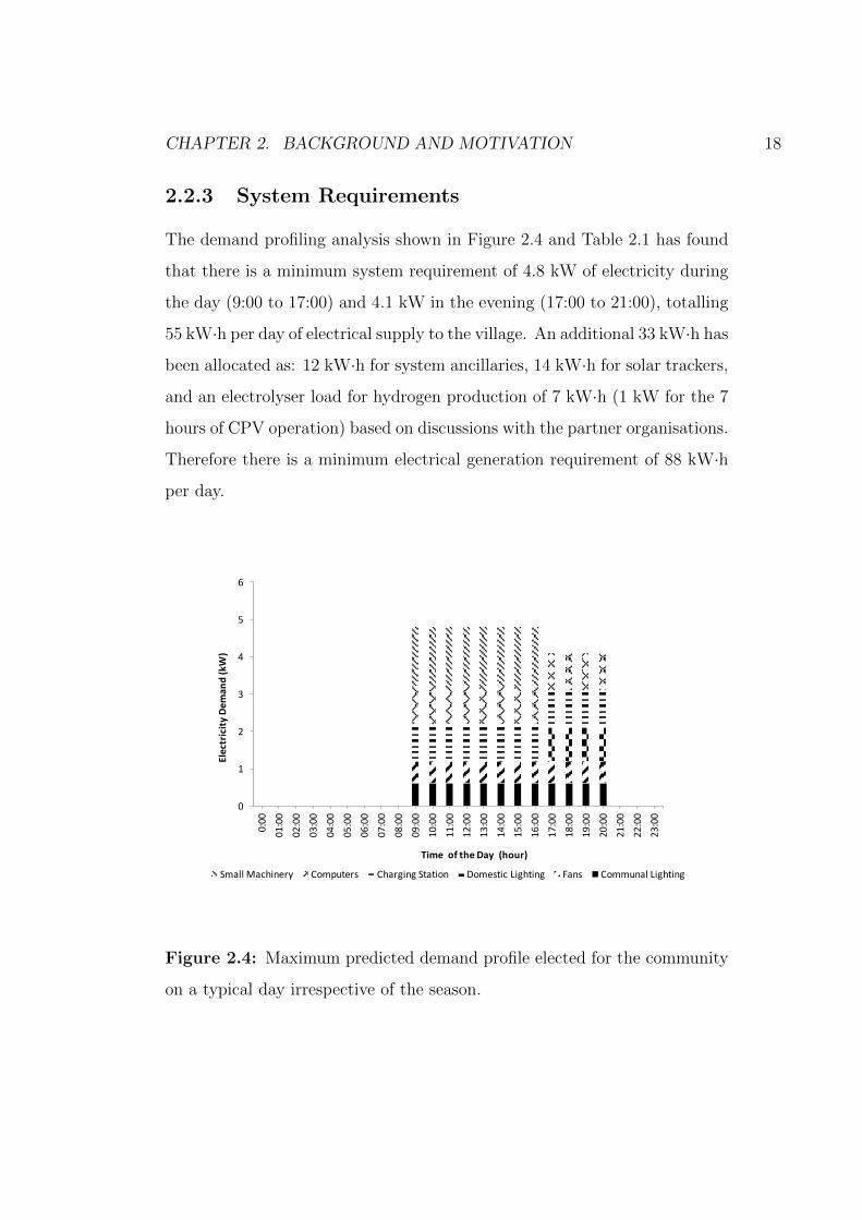
Figure 2.4 shows the expected demand profile of the village over 24 hours.
The demand is divided in to a day load which is from 09:00 to 17:00 and an
evening load from 17:00 to 21:00. Public area lighting, fans, computers and
the charging station are assumed to be used all day from 09:00 to 21:00. This
is a result of the community buildings being used as a school during the day
and then a community centre in the evening, where computers, lighting, fans
and charging station will be used. The use of small machinery is assumed to
only take place during the day; this is mainly because they are noisy.
CHAPTER 2. BACKGROUND AND MOTIVATION 18
2.2.3 System Requirements
The demand profiling analysis shown in Figure 2.4 and Table 2.1 has found
that there is a minimum system requirement of 4.8 kW of electricity during
the day (9:00 to 17:00) and 4.1 kW in the evening (17:00 to 21:00), totalling
55 kW·h per day of electrical supply to the village. An additional 33 kW·h has
been allocated as: 12 kW·h for system ancillaries, 14 kW·h for solar trackers,
and an electrolyser load for hydrogen production of 7 kW·h (1 kW for the 7
hours of CPV operation) based on discussions with the partner organisations.
Therefore there is a minimum electrical generation requirement of 88 kW·h
per day.
0
1
2
3
4
5
6
0:00
01:00
02:00
03:00
04:00
05:00
06:00
07:00
08:00
09:00
10:00
11:00
12:00
13:00
14:00
15:00
16:00
17:00
18:00
19:00
20:00
21:00
22:00
23:00
Electricity
Dem
and(kW)
TimeoftheDay(hour)
SmallMachinery Computers ChargingStation DomesticLighting Fans CommunalLighting
Figure 2.4: Maximum predicted demand profile elected for the community
on a typical day irrespective of the season.

CHAPTER 2. BACKGROUND AND MOTIVATION 19
2.3 Proposed Renewable Power Plant Design
Figure 2.5: BioCPV renewable power plant schematic, consisting of: 10 kW
concentrated photovoltaic (CPV), 5 kW biogas and hydrogen internal com-
bustion engine electrical generator set (genset), electrolyser, metal hydride
store and anaerobic digester.
Due to the abundance of solar irradiation and biomass in the vicinity,
CPV and biogas; created by anaerobic digestion of food waste and aquatic
weeds and used in an internal combustion engine electrical generator set
(genset), were selected as the main electricity generation methods. These
technologies complement each other as the biogas genset can be operated
when the CPV is unavailable. Moreover the production and use of biogas
are decoupled; therefore, depending on storage capacity, it can support both
seasonal and diurnal variation. Hydrogen storage will be used to optimise

CHAPTER 2. BACKGROUND AND MOTIVATION 20
the use of solar electricity and increase the quality of the biogas. A schematic
of the BioCPV power plant can be seen in Figure 2.5.
For system sizing purposes the BioCPV group agreed on a daily genera-
tion load of 90 kW·h per day as it exceeds the estimated daily demand of 88
kW·h. This can be allocated to a daytime solar generation load of 70 kW·h
which can be simplified to 7 hours of generation at 10 kW (electric) and an
evening biogas - hydrogen electrical generator load of 20 kW·h based on 5
kW (electric) for 4 hours per day.
The partners in the project have specified that the CPV PV cells mod-
ule (hereinafter referred to as: PV, cell and CPV waste heat source) should
operate at 60◦C and will require a mechanism to remove the heat generated,
from its operation, to maintain this temperature. Waste heat from the inter-
nal combustion engine electrical generator (genset) is also expected; typically
the sources are the radiator at 80◦C and the exhaust at 350◦C. The CPV
and genset waste heat sources will be discontinuous as the CPV will operate
during the day for 7 hours and the genset at night for 4 hours.
2.4 Conclusion
There is a need to provide renewable power to drive the sustainable develop-
ment of the selected community and communities similar to it internationally.
The BioCPV group have proposed a rural renewable power plant based on
the projected demand profile presented in this chapter and an assessment of
locally available resources.
The community at present conducts most of its minor medical treatment
outside and could benefit from some space cooling for a recovery room. They
also have no means of refrigerating food and medicines. The potential ben-
efits that refrigeration can bring without having a significant impact on the
electricity demand has led to the focus of this research in investigating low

CHAPTER 2. BACKGROUND AND MOTIVATION 21
temperature discontinuous waste heat utilisation from a renewable power
plant in rural India for absorption refrigeration.
Low temperature discontinuous waste heat sources are expected within
the proposed power plant. These typically have a low energy quality and
therefore are not suitable for the generation of work and electricity. Generally
the most efficient uses of low temperature waste heat sources are space or
water heating as this is a direct use, and if designed appropriately, could
make use of almost all of the waste energy. The problem is that hot water
and heating is not an important need in this location whereas refrigeration
would be welcomed.
This situation is not unique to this community; there are many developing
countries with warm climates where a sustainable source of refrigeration can
improve the quality of life. Therefore, the findings and methods presented
in this thesis can be applied to many situations internationally. Moreover,
it was estimated in this chapter that low grade waste heat accounts for 7%
of global energy use; making its efficient utilisation a significant factor in
lowering global energy demand and the associated negative effects.

Chapter 3
Refrigeration Technology
Review
Given the need for refrigeration in rural India identified in Chapters 1 and
2, this chapter aims to provide insight into the refrigeration choices made
in this thesis. This is achieved by presenting a history of refrigeration, a
description of common refrigeration systems and a detailed overview of the
selected technology: absorption refrigeration.
Depending on the energy source available to drive a refrigerator there are
a number of options, which can be broken down into thermally activated and
mechanically activated. Thermally activated include: absorption, adsorp-
tion and desiccant cooling systems. Mechanically activated include: vapour
compression (also known as reverse Rankine) cycle and gas (also known as
reverse Brayton) cycle.
There are a number of other refrigeration technologies which are not
discussed here as they are either only at lab scale or are not suitable for
food storage and thermal comfort, which constitute the main refrigeration
needs in rural India. Today the most common form of refrigeration is the
vapour compression cycle, this is found in almost all domestic refrigerators,
22
CHAPTER 3. REFRIGERATION TECHNOLOGY REVIEW 23
air conditioning units and the majority of industrial refrigeration systems as
well.
This chapter consists of the following sections:
• History of Refrigeration starts with references to the the earliest
forms of refrigeration from ancient civilisations, followed by descrip-
tions of the mechanical ancestors of various forms of refrigerating ma-
chines and provides some insight into the reasoning behind their devel-
opment.
• Review of Commonly Used Refrigeration Systems describes the
following refrigeration systems: vapour compression, adsorption, gas
(or reverse Brayton), absorption and desiccant cooling. It concludes
with a selection process for an appropriate refrigeration technology to
utilise low temperature waste heat in rural India, found to be absorp-
tion refrigeration.
• Detailed Overview of Absorption Refrigeration describes ab-
sorption refrigeration in detail and includes the following:
– Challenges of Absorption Refrigeration describes the funda-
mental challenge with absorption refrigeration which is created by
the desire to maintain high condensing temperatures, low evapo-
rator temperatures, high coefficient of performance (CoP) and low
boiler temperatures.
– Fluids describes the possible working fluids for absorption refrig-
eration systems.
– System Configurations to maximise heat utilisation de-
scribes the following configurations: boiler absorber heat exchange
(BAX, also known as GAX and DAHX), boiler heat recovery, half
effect and dual cycle.

CHAPTER 3. REFRIGERATION TECHNOLOGY REVIEW 24
– System Configurations to Utilise Discontinuous Heat Sources
describes the systems to utilise discontinuous heat from solar power
and focusses on the application of the refrigerant storage method
with the single effect and double boiler cycles.
– System Configurations to Reduce the Evaporator Tem-
perature describes systems that allow cooling of the condenser
and absorber to lower the pressure in the evaporator, these are
evaporator tap-off and coupled cycle.
– Using Discontinuous Heat Sources and Controlling Evap-
orator Temperature combines the ideas from the two previous
subsections to create cycles that can utilise discontinuous waste
heat to provide useful refrigeration in rural India.
– Appraisal of Absorption Refrigeration Systems provides a
comparison of the configurations described to allow selection of ap-
propriate cycles for utilising low temperature discontinuous waste
heat in rural India.
• Conclusion of Refrigeration Technologies Review summarises
the technologies, their history and applications described in this chapter
and justifies the choice of refrigerator technology.
CHAPTER 3. REFRIGERATION TECHNOLOGY REVIEW 25
3.1 History of Refrigeration
Jordan and Priesters book titled “Refrigeration and air conditioning” de-
scribes how there are poetry references from the Ancient Greeks, Chinese
and Romans about using natural ice to cool food and drink. It also explains
how during most of the 19th century natural ice was shipped all over the
world to be used for cold storage and food processing. (Jordan and Priester
1950), (Freidberg 2009)
Artificial refrigeration, not by naturally forming ice, also dates back to
ancient times:
“As early as the fourth century AD the East Indians knew that
certain salts, such as sodium nitrate when placed in water would
result in lowering the temperature.”(Jordan and Priester 1950)
An article in the New Scientist reviewing the book “A History of Refrig-
eration Throughout the World” by Roger Thevenot claims the first artificial
refrigeration device was produced by William Cullen in 1755 (Howard 1980).
One of the earliest patents for a refrigeration machine is from 1834, shown
in Figure 3.1. This device is the predecessor for the vapour compression
cycle, which is currently the most common refrigeration cycle. The machine
operates by compressing the refrigerant at position A increasing its pressure,
then condensing it at position B by removing the heat that was generated
from compression (A) and evaporation (C and D). At point C (throttle) the
pressure is lowered, to correspond with the desired refrigeration temperature,
through moving the piston to increase the volume. The flow of refrigerant is
controlled with the throttle allowing the refrigerant to evaporate and fill the
void created by the piston moving. Part of this void, position D, is called the
refrigerator in this machine (also known as the evaporator in todays vapour
compression machines). The evaporation taking place in the refrigerator (D)
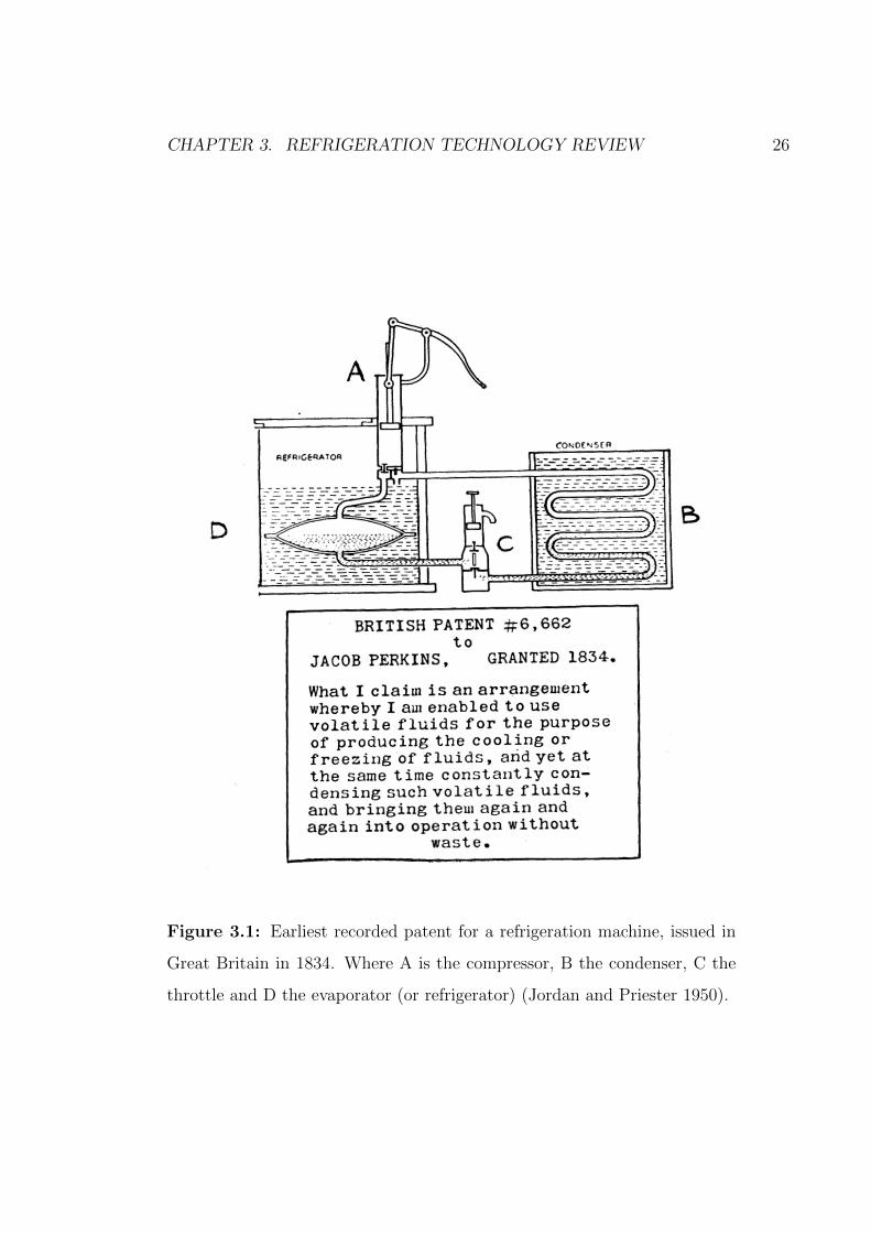
CHAPTER 3. REFRIGERATION TECHNOLOGY REVIEW 26
Figure 3.1: Earliest recorded patent for a refrigeration machine, issued in
Great Britain in 1834. Where A is the compressor, B the condenser, C the
throttle and D the evaporator (or refrigerator) (Jordan and Priester 1950).

CHAPTER 3. REFRIGERATION TECHNOLOGY REVIEW 27
draws in heat which provides the refrigeration effect. The refrigerant then
enters the compressor at A and the cycle repeats.
Dr. John Gorrie designed a refrigeration machine that used compressed
air as the refrigerant and received the first American patent for an ice machine
in 1851. Sulphuric ether was the desired refrigerant for Prof A. C. Twining’s
ice making machine in New Haven, USA which followed the vapour compres-
sion cycle; he gained a patent for it in 1853. All these devices require some
motive power to drive the compressor. (Jordan and Priester 1950)
During the mid nineteenth century there was little access to electricity
which often resulted in vapour compression systems requiring a fossil fuelled
Figure 3.2: Diagrammatic sketch of Ferdinand Carre’s absorption refrig-
eration machine for which he received a patent in the 1860s (Jordan and
Priester 1950).
CHAPTER 3. REFRIGERATION TECHNOLOGY REVIEW 28
engine to provide the motive power. However mass production of internal
combustion engines did not start until the late nineteenth century (Todd
1995), so the motive power for vapour compression refrigeration machines
was limited to external combustion engines. This requirement for an external
heat source to power a vapour compression refrigerator made absorption
refrigeration more attractive as the systems could be directly powered by the
heat source, potentially making them simpler and cheaper at the time. An
early example of a commercial absorption refrigerator is Ferdinand Carre’s
machine, seen in Figure 3.2, which was used during the French civil war as
the supply of ice from the north was cut off. This system used ammonia as
the refrigerant and water as the absorbent (Jordan and Priester 1950). Carre
received the first patent in the USA for a commercial absorption refrigerator
in the 1860s (Deng et al. 2011). This machine changed the approach to
refrigeration globally as ice could be generated locally and no longer had
to be transported around the world. (Freidberg 2009) (Jordan and Priester
1950)
During the twentieth century electricity grids became more widespread
which resulted in electric motor driven vapour compression refrigerators dom-
inating the domestic market. These systems were often smaller, simpler and
cheaper than any of the thermally activated refrigerators. However vapour
compression systems often used highly toxic refrigerants. After an incident
of a family being killed by a leaking refrigerator Albert Einstein and Leo Szi-
lard developed a hermetically sealed absorption refrigerator with no moving
parts to significantly reduce the likelihood of leaks and therefore poisoning
from the refrigerant. Their design was based on the absorption refrigera-
tor designed by Platen and Munters which was originally patented in 1923.
Both refrigerators use heat to cause vapour bubbles to move the solution
from one part of the fridge to another, Einstein and Szilard call it a bubble
pump whereas Platen and Munters call it a thermo-siphon and both use a
CHAPTER 3. REFRIGERATION TECHNOLOGY REVIEW 29
pressure equalising fluid. (Moss 1989) (Dannen 1995) (Munters and Platen
1928) (Einstein and Szilard 1930)
As with absorption, adsorption refrigeration was developed from the mid-
nineteenth to the early twentieth century, when it was overtaken by vapour
compression systems. The first recorded discovery of an adsorption refriger-
ation system was from Faraday with ammonia onto silver chloride in 1848.
For food storage in trains during the 1920’s Hulse investigated a silica gel
and sulphur dioxide system which would reach evaporation temperatures of
-12◦C. (Wang and Oliveira 2006) (Deng et al. 2011)
Solid desiccant cooling systems were introduced in the 1930s using lithium
chloride to dehumidify air (Deng et al. 2011). A desiccant air conditioning
system will typically dehumidify the air with a desiccant and then cool the
air with a separate refrigeration cycle. This technique reduces the need to
over cool the air, often required with other forms of refrigeration for air
conditioning, to allow for temperatures low enough so that the moisture can
condense out. The first desiccant air conditioning cycle was patented in
1955 by Pennington. It used a rotary desiccant wheel and its objective was
to dehumidify air in summer and humidify air in winter (Pennington 1955).
Until the mid 1980s most desiccant air conditioning systems were restricted to
contamination controlled environments such as pharmaceutical, electronics
and food manufacture. In these sectors the cost of the desiccant system
was outweighed by the prevented loss of manufacturing output. Some liquid
desiccant systems can sterilise and clean air which has made them useful for
air conditioning of medical buildings. Since 1985 supermarkets started using
desiccant cooling as the cost benefit of switching from electrical to thermal
energy became favourable. (Mei et al. 1992)
The development of vapour compression systems has been largely dictated
by environmental laws restricting the refrigerants that can be used, such as
banning chlorofluorocarbons (CFCs) in 1987 (ESRL 2015) and more recent

CHAPTER 3. REFRIGERATION TECHNOLOGY REVIEW 30
restrictions on the use of hydrofluorocarbons (HFCs) (EEB 2015). There are
continuous efforts to reduce the energy consumption of vapour compression
refrigerators which is achieved through improvements in compressor technol-
ogy, electric motors, insulation materials and heat exchangers. (Tassou et al.
2010)
As thermally activated refrigerators can be driven by a variety of heat
sources their interest and development has followed a similar path to most
sustainable technologies, i.e. it is proportional to the cost of energy with ad-
ditional spikes of interest occurring when the competing technology is found
to be harmful. Interest in thermally activated refrigeration technologies re-
emerged during the oil crises of the 1970s and has continued with rising fuel
and electricity prices. Interest also increased in the late 1920s and again in
the late 1980s when the harmfulness of the refrigerants in vapour compres-
sion cycles came into the public’s view. Moreover as sustainable operation is
becoming more profitable, both from a cost saving and marketing perspec-
tive, industries are making better use of waste heat sources, which can be
used for thermally activated refrigeration. Interest in the domestic market
is also growing with the development of tri-generation technologies, where
electricity, heating and cooling are provided by either combustion engines or
solar power. (Deng et al. 2011), (Wang and Oliveira 2006) (Dannen 1995)
(Jordan and Priester 1950), (Freidberg 2009) (Mathkor et al. 2015) (Agnew
et al. 2015)
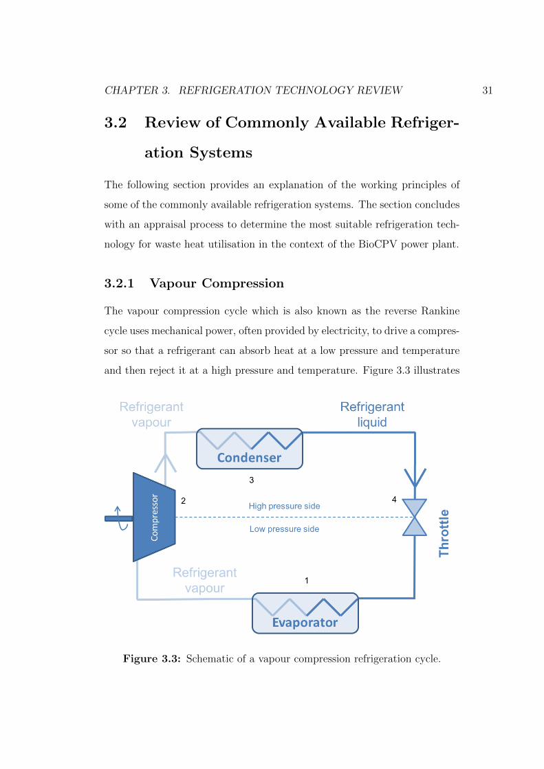
CHAPTER 3. REFRIGERATION TECHNOLOGY REVIEW 31
3.2 Review of Commonly Available Refriger-
ation Systems
The following section provides an explanation of the working principles of
some of the commonly available refrigeration systems. The section concludes
with an appraisal process to determine the most suitable refrigeration tech-
nology for waste heat utilisation in the context of the BioCPV power plant.
3.2.1 Vapour Compression
The vapour compression cycle which is also known as the reverse Rankine
cycle uses mechanical power, often provided by electricity, to drive a compres-
sor so that a refrigerant can absorb heat at a low pressure and temperature
and then reject it at a high pressure and temperature. Figure 3.3 illustrates
Figure 3.3: Schematic of a vapour compression refrigeration cycle.

CHAPTER 3. REFRIGERATION TECHNOLOGY REVIEW 32
the cycle. At position 1, the evaporator, the refrigerant enters as a liquid at
low pressure and starts to evaporate absorbing heat from the space or object
begin cooled. This absorption of heat and evaporation occurs because the
low pressure side of the system has been designed to provide a saturation
temperature for the desired refrigeration conditions. After leaving the evap-
orator the refrigerant vapour enters the compressor (2) where its pressure
is raised so that the saturation temperature is above the ambient tempera-
ture. This results in the refrigerant vapour not being able to maintain its
state and so it condenses back to a liquid in the condenser (3) rejecting the
heat absorbed in the evaporator and compressor. The refrigerant liquid then
passes through a throttle (4) which lowers the pressure so that the cycle can
repeat when the refrigerant re-enters the evaporator (1). The throttle (4)
and compressor (2) maintain the pressure difference between the high and
low pressure sides. (Tassou et al. 2010) (Pita 1984)
3.2.2 Adsorption Refrigeration
Adsorption is the process whereby a substance is drawn on to the surface
of another, usually in the form of a vapour ‘sitting’ on the surface of a
solid. A common example is silica gel and water. This phenomenon coupled
with thermal power can be used to drive a refrigeration circuit. The adsor-
ber/desorber is usually a heat exchanger with the external surfaces covered
in the adsorbent. In its simplest configuration the cycle is discontinuous.
Referring to Figure 3.4 the heat input causes desorption of the refrig-
erant in the adsorber/desorber (1). The refrigerant vapour passes through
non-return valves (2, 4, 6 and 9) to prevent back-flow and resorption after
each component. The refrigerant rejects its heat (gained from the adsor-
ber/desorber) to the environment in the condenser (3), and is condensed
back to a liquid. The refrigerant liquid is then stored in a reservoir (5) un-
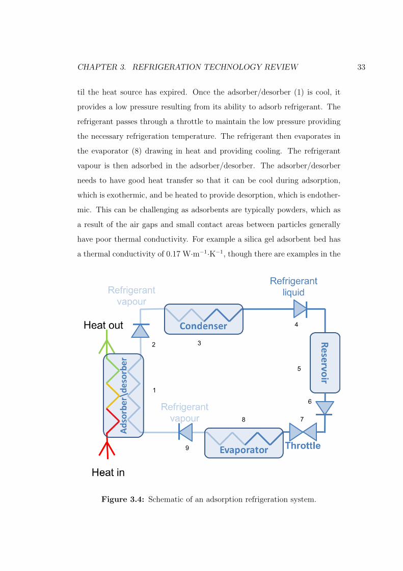
CHAPTER 3. REFRIGERATION TECHNOLOGY REVIEW 33
til the heat source has expired. Once the adsorber/desorber (1) is cool, it
provides a low pressure resulting from its ability to adsorb refrigerant. The
refrigerant passes through a throttle to maintain the low pressure providing
the necessary refrigeration temperature. The refrigerant then evaporates in
the evaporator (8) drawing in heat and providing cooling. The refrigerant
vapour is then adsorbed in the adsorber/desorber. The adsorber/desorber
needs to have good heat transfer so that it can be cool during adsorption,
which is exothermic, and be heated to provide desorption, which is endother-
mic. This can be challenging as adsorbents are typically powders, which as
a result of the air gaps and small contact areas between particles generally
have poor thermal conductivity. For example a silica gel adsorbent bed has
a thermal conductivity of 0.17 W·m−1·K−1, though there are examples in the
Figure 3.4: Schematic of an adsorption refrigeration system.
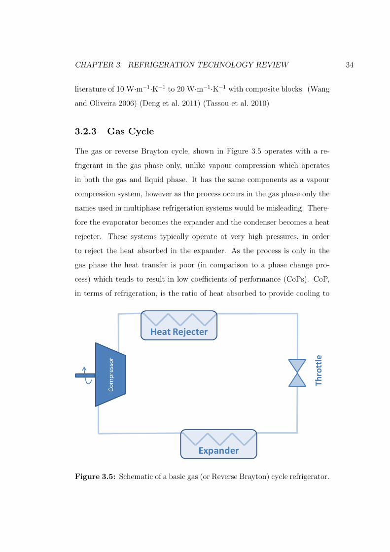
CHAPTER 3. REFRIGERATION TECHNOLOGY REVIEW 34
literature of 10 W·m−1·K−1 to 20 W·m−1·K−1 with composite blocks. (Wang
and Oliveira 2006) (Deng et al. 2011) (Tassou et al. 2010)
3.2.3 Gas Cycle
The gas or reverse Brayton cycle, shown in Figure 3.5 operates with a re-
frigerant in the gas phase only, unlike vapour compression which operates
in both the gas and liquid phase. It has the same components as a vapour
compression system, however as the process occurs in the gas phase only the
names used in multiphase refrigeration systems would be misleading. There-
fore the evaporator becomes the expander and the condenser becomes a heat
rejecter. These systems typically operate at very high pressures, in order
to reject the heat absorbed in the expander. As the process is only in the
gas phase the heat transfer is poor (in comparison to a phase change pro-
cess) which tends to result in low coefficients of performance (CoPs). CoP,
in terms of refrigeration, is the ratio of heat absorbed to provide cooling to
Figure 3.5: Schematic of a basic gas (or Reverse Brayton) cycle refrigerator.
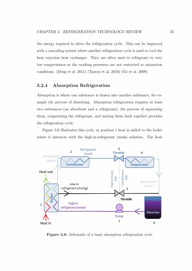
CHAPTER 3. REFRIGERATION TECHNOLOGY REVIEW 35
the energy required to drive the refrigeration cycle. This can be improved
with a cascading system where another refrigeration cycle is used to cool the
heat rejection heat exchanger. They are often used to refrigerate to very
low temperatures as the working pressures are not restricted to saturation
conditions. (Deng et al. 2011) (Tassou et al. 2010) (Ge et al. 2009)
3.2.4 Absorption Refrigeration
Absorption is where one substance is drawn into another substance, for ex-
ample the process of dissolving. Absorption refrigeration requires at least
two substances (an absorbent and a refrigerant); the process of separating
them, evaporating the refrigerant, and mixing them back together provides
the refrigeration cycle.
Figure 3.6 illustrates this cycle; at position 1 heat is added to the boiler
where it interacts with the high-in-refrigerant (weak) solution. The heat
Figure 3.6: Schematic of a basic absorption refrigeration cycle
CHAPTER 3. REFRIGERATION TECHNOLOGY REVIEW 36
releases some of the refrigerant from the weak solution, leaving the low-in-
refrigerant (strong) solution behind. The refrigerant vapour then enters the
condenser (2) where the heat is removed (typically to the environment) and
the refrigerant vapour condenses into a liquid. This liquid passes through a
throttle (3) to maintain a pressure drop. The refrigerant then evaporates in
the evaporator at a low pressure (and temperature) absorbing heat and pro-
viding the refrigeration effect. The refrigerant vapour leaving the evaporator
(4) is absorbed into the strong solution from the boiler (1) in the absorber
(6). Before reaching the absorber (6) the strong solution passes a throttle (5)
to maintain the low pressure at the evaporator (4) and absorber (6). After
the desired amount of refrigerant vapour has been absorbed into the strong
solution the now weak solution is pumped (7) from the absorber (6) back to
the boiler (1). (Herold 1996) (Deng et al. 2011) (Tassou et al. 2010)
3.2.5 Desiccant Cooling
Desiccant cooling is commonly used for air conditioning and can often be
driven by low grade heat. The process separates latent and sensible cool-
ing of air by using the desiccant to remove moisture before cooling the air
(with another refrigeration method) to the desired temperature. The desic-
cant can either be a liquid or a solid. Liquid desiccants are used when it is
simpler to move the desiccant to the heat source and solid desiccants can be
used when the heat source can be moved to the desiccant. Solid desiccants
tend to be in the form of powders in varying particle sizes and therefore
often have poor heat transfer which can limit their application. Commonly
used solid desiccant are: “silica, polymers, zeolites, alumina, hydratable salts
and mixtures. Other available liquid desiccants are calcium chloride, lithium
chloride, lithium bromide, tri-ethylene glycol, and a mixture of 50% calcium
chloride and 50% lithium chloride” (Mohammad et al. 2013). Typical desic-
CHAPTER 3. REFRIGERATION TECHNOLOGY REVIEW 37
cant cooling systems are rotary wheels for solid desiccants and packed bed
for both solid and liquid desiccants. All systems require a dehumidifier to
absorb the moisture from the air and a regenerator (e.g. hot air) to remove
the moisture from the desiccant. (Mei et al. 1992) (Pennington 1955)
3.2.6 Appraisal of Common Refrigeration Systems
This subsection provides a comparison of the refrigeration systems described
earlier in this section to allow the selection of an appropriate technology for
utilising low temperature discontinuous waste heat from distributed renew-
able power plants in rural India. The scale is 1 (undesirable) to 5 (desirable)
and Applications refers to its applicability to rural India, HSE is Health
Safety and Environmental considerations and Driving Energy refers to the
versatility of the energy that powers the refrigeration system; in this study it
is desirable to utilise low temperature (hence low quality) waste heat, there-
fore, 5 indicates low quality energy sources and 1 infers that the energy could
be used for many applications e.g. electricity and work. Each factor investi-
gated here was deemed to be of equal importance and therefore no weighting
was applied.
The decision matrix in Table 3.1 finds that of the refrigeration technolo-
gies examined absorption, adsorption and desiccant cooling had a driving
energy score of 5 as all of these can make use of low temperature waste
heat. Desiccant cooling has an applications score of 1 as it is limited to air
conditioning and requires a further cooling system. Absorption has greater
potential for a variety of cooling applications than adsorption, shown by the
application score of 3 in comparison to 1 respectively. Desiccant cooling, ab-
sorption and adsorption all score 4 for HSE though all of these technologies
have a wide range of fluid choices with varying levels of HSE considerations.
Both adsorption and solid desiccant systems are often powders which typi-
CHAPTER 3. REFRIGERATION TECHNOLOGY REVIEW 38
cally have poor thermal conductivity, which may be problematic in terms of
removing waste heat from the source effectively.
This research is focussed on utilising waste heat sources from a discontinu-
ous renewable electricity generation plant in rural India, where the waste heat
is part of a cooling system for the components in the power plant. Therefore
good heat transfer is important to ensure efficient operation of the compo-
nents, ruling out solid desiccants and adsorption technologies. The variety
of refrigeration applications is greater for absorption than liquid desiccant
systems, scoring 4 and 1 respectively, resulting in the selected technology to
investigate low temperature waste heat utilisation being absorption refriger-
ation.
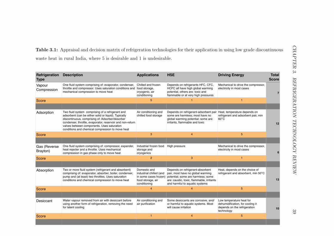
CHAPTER
3.REFRIG
ERATIO
NTECHNOLOGY
REVIE
W39
Table 3.1: Appraisal and decision matrix of refrigeration technologies for their application in using low grade discontinuous
waste heat in rural India, where 5 is desirable and 1 is undesirable.
Refrigeration Type
Description Applications HSE Driving Energy Total Score
Vapour Compression
One fluid system comprising of: evaporator, condenser, throttle and compressor. Uses saturation conditions and mechanical compression to move heat
Chilled and frozen food storage, cryogenic, air conditioning
Depends on refrigerants HFC, CFC, HCFC all have high global warming potential, others are: toxic and flammable or at very high pressures
Mechanical to drive the compressor, electricity in most cases
7
Score 5 1 1
Adsorption Two fluid system comprising of a refrigerant and adsorbent (can be either solid or liquid). Typically discontinuous, comprising of: Adsorber/desorber condenser, throttle, evaporator, reservoir and non-return valves between components. Uses saturation conditions and chemical compression to move heat
Air conditioning and chilled food storage
Depends on refrigerant-adsorbent pair some are harmless; most have no global warming potential; some are: irritants, flammable and toxic
Heat, temperature depends on refrigerant and adsorbent pair, min 60°C
12
Score 3 4 5
Gas (Reverse Brayton)
One fluid system comprising of: compressor, expander, heat rejecter and a throttle. Uses mechanical compression in gas phase only to move heat
Industrial frozen food storage and cryogenics
High pressure Mechanical to drive the compressor, electricity in most cases
6
Score 2 3 1
Absorption Two or more fluid system (refrigerant and absorbent) comprising of: evaporator, absorber, boiler, condenser, pump and (at least) two throttles. Uses saturation conditions and chemical compression to move heat
Domestic and industrial chilled (and in some cases frozen) food storage, air conditioning
Depends on refrigerant-absorbent pair, most have no global warming potential; some are harmless; some are: caustic, toxic, flammable, irritants and harmful to aquatic systems
Heat, depends on the choice of refrigerant and absorbent, min 50°C
13
Score 4 4 5
Desiccant Water vapour removed from air with desiccant before using another form of refrigeration, removing the need for latent cooling
Air conditioning and air purification
Some desiccants are corrosive, and/or harmful to aquatic systems. Most will cause irritation
Low temperature heat for dehumidification, for cooling it depends on the refrigeration technology
10
Score 1 4 5
�1

CHAPTER 3. REFRIGERATION TECHNOLOGY REVIEW 40
3.3 Detailed Review of Absorption Refriger-
ation
Vapour absorption technology has been established for almost 200 years,
however, as already mentioned, due to cheap and reliable electricity vapour
compression refrigerators became more widespread. Therefore research has
not been continuous and has been instigated by: oil crises, rising fuel prices
and environmental concerns pushing more efficient use of energy sources.
(Deng et al. 2011)
To the present day research is being conducted to find optimal working
fluid combinations by either finding new combinations (Jelinek and Borde
1998) (Zohar et al. 2009) (Zacarıas et al. 2011) or through using additives
and surfactants to commonly used working fluids (Saravanan and Maiya
1998) (J. K. Kim et al. 2007). New configurations of refrigerator are being
developed to utilise a wider variety of energy sources such as multiple effect
systems (Deng et al. 2011), hybrids (J. Jeong et al. 2011), co-generation
(Hua et al. 2014) and tri-generation (Mathkor et al. 2015). Others have
been developing specific components of the refrigerator most commonly the
absorber (Xie et al. 2012) (Tae Kang et al. 2000) (Zacarıas et al. 2011). Many
predictive models for specific components (Sieres and Fernandez-Seara 2007)
(Tae Kang et al. 2000) and entire systems (D. S. Kim and Infante Ferreira
2009) (J. Jeong et al. 2011) have been developed. There are also continuing
efforts to model and verify the thermodynamic properties of the working
fluids (Patek and Klomfar 2006) (Ajib and Karno 2008).
Several manufacturers offer industrial scale absorption refrigerators which
can be powered by a fuel source or waste heat such as York, Carrier, Mit-
subishi and Thermax India. Absorption refrigerators are also available on
a domestic scale and mostly used in motorhomes and environments where
either silent operation is desirable or electricity is not available. There is

CHAPTER 3. REFRIGERATION TECHNOLOGY REVIEW 41
also interest in domestic absorption refrigeration systems for air condition-
ing as part of a tri-generation system, where heating, cooling and electricity
is provided by one system (Deng et al. 2011) (Tassou et al. 2010).
This section contains:
• Challenges of Absorption Refrigeration a description of the over-
arching challenge of absorption refrigeration.
• Fluids the working fluids used in absorption refrigeration systems
• System Configurations a selection of system configurations inves-
tigated up to the present day and an appraisal process to determine
suitability for the conditions expected from the BioCPV system.
• Conclusions concludes the main findings of this review and the ap-
praisal processes.
3.3.1 Challenges of Absorption Refrigeration
Absorption refrigerators rely on a delicate balance of solution concentrations
and solution temperatures. These decide how much refrigerant can be con-
tained within the solution and, assuming perfect mass transfer, ultimately
determine the saturation conditions of the pure refrigerant. The greater the
capacity of the solution to hold refrigerant the lower the vapour pressure
as the solution is providing a sucking force for the refrigerant vapour to be
absorbed. This is achieved with low-in-refrigerant (strong) solution concen-
trations and cold temperatures. A strong solution concentration causes little
refrigerant to be available and the low temperature results in the refrigerant
not having enough energy to leave the surface of the solution. Conversely
weak solution concentrations and high temperatures provide a large quantity
of refrigerant with enough energy to leave the surface of the solution resulting
in high pressures. The pressure caused by the solution concentration and its
CHAPTER 3. REFRIGERATION TECHNOLOGY REVIEW 42
temperature determine the saturation conditions of the pure refrigerant in
the condenser and evaporator, especially when a salt is used as the absorbent
as the vapour will only contain refrigerant.
However the condenser temperature is usually limited by the temperature
of the cold reservoir (plus a few degrees for heat transfer), e.g. ambient air,
rivers, lakes, etc. The evaporator temperature is often limited by the appli-
cation e.g. air conditioning, short or long term food storage and their related
temperature requirement. Moreover it is the exit conditions of the solution
leaving the boiler and absorber that determine the operating pressures and
therefore limiting temperatures of the condenser and evaporator respectively.
Which means; the strong solution concentration and the boiler temperature
determine the maximum condenser temperature. The weak solution concen-
tration and the absorber temperature determines the minimum evaporator
temperature. However high condenser temperatures are desirable as it allows
smaller heat exchangers, choice over the cooling fluid and whether passive
or active cooling is used. Low evaporator temperatures are desirable as they
are more versatile.
This creates a conflict; dilute strong solution concentrations are desirable
for high condenser temperatures whereas concentrated weak solution con-
centrations are desirable for low evaporator temperatures. Yet the strong
solution concentration has to be more concentrated than the weak solution,
by definition. Moreover the difference in solution concentrations is propor-
tional to the mass ratio of working refrigerant to total solution. The working
refrigerant is the refrigerant that goes through the condenser and evaporator
and is responsible for providing the refrigeration effect in the evaporator.
Therefore it will be more efficient if the heat source is used to separate more
refrigerant from solution rather than heating a large amount of solution to
provide little working refrigerant.
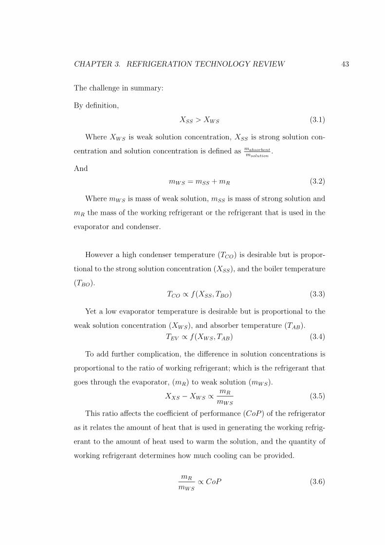
CHAPTER 3. REFRIGERATION TECHNOLOGY REVIEW 43
The challenge in summary:
By definition,
(3.1)XSS > XWS
Where XWS is weak solution concentration, XSS is strong solution con-
centration and solution concentration is defined as mabsorbent
msolution.
And
(3.2)mWS = mSS +mR
Where mWS is mass of weak solution, mSS is mass of strong solution and
mR the mass of the working refrigerant or the refrigerant that is used in the
evaporator and condenser.
However a high condenser temperature (TCO) is desirable but is propor-
tional to the strong solution concentration (XSS), and the boiler temperature
(TBO).
(3.3)TCO ∝ f(XSS, TBO)
Yet a low evaporator temperature is desirable but is proportional to the
weak solution concentration (XWS), and absorber temperature (TAB).
(3.4)TEV ∝ f(XWS, TAB)
To add further complication, the difference in solution concentrations is
proportional to the ratio of working refrigerant; which is the refrigerant that
goes through the evaporator, (mR) to weak solution (mWS).
(3.5)XXS −XWS ∝mR
mWS
This ratio affects the coefficient of performance (CoP ) of the refrigerator
as it relates the amount of heat that is used in generating the working refrig-
erant to the amount of heat used to warm the solution, and the quantity of
working refrigerant determines how much cooling can be provided.
(3.6)mR
mWS
∝ CoP
CHAPTER 3. REFRIGERATION TECHNOLOGY REVIEW 44
3.3.2 Fluids
The fluids for absorption refrigerators can be split into two main categories:
two fluid systems such as a lithium bromide and water refrigerator and three
fluid systems such as the Platen-Munters and Einstein-Szilard refrigerators.
However, rather confusingly, the two fluid system category includes additives
which can bring the number of fluids in the system above two. To eliminate
this confusion, three fluid systems are referred to as systems with a pressure
equalising fluid and two fluid systems are those without. A pressure equalis-
ing fluid is an auxiliary gas providing pressure equalisation for the working
refrigerant between the condenser and evaporator in the Platen-Munters and
Einstein-Szilard style refrigerators. (Herold 1996)
Eames and Wu (2003) and Saravanan and Maiya (1998) suggest that
the presence of the pressure equalising fluid reduces mass transfer as it pro-
vides additional resistance and is responsible for the low CoPs of systems
with a pressure equalising fluid. This may explain why there is considerably
more research available on systems without. An example of the low CoP
achieved from systems with a pressure equalising fluid is found in research
by Delano (1998) using isobutene-ammonia-water, butane-ammonia-water,
neopentane-ammonia-water, pentane-ammonia-water and butane-hydrogen
chloride-water. The highest CoP achieved was 0.225 with isobutene-ammonia-
water, which he discusses is largely due to the high ratio of refrigerant to
solution and the small temperature difference with the absorber/condenser
and evaporator temperatures.
Zohar et al. (2009) investigated the following refrigerants with an organic
absorbent (DMAC - dimethylacetamide) and helium as the pressure equalis-
ing inert gas. The following refrigerants were investigated: R22 (chlorodifluo-
romethane), R32 (difluoromethane), R124 (1-chloro-1,2,2,2-tetrafluoroethane),
R125 (pentafluoroethane) and R134a (1,1,1,2-tetrafluoroethane). As with
CHAPTER 3. REFRIGERATION TECHNOLOGY REVIEW 45
Delano (1998) the CoPs were low, under 0.24. Boiler temperatures ranged
from 135◦C to 160◦C, condenser temperatures 33◦C to 43◦C and evaporator
temperatures −9◦C to 6◦C. (Zohar et al. 2009)
The opinions of Eames and Wu (2003) and Saravanan and Maiya (1998)
together with the results from Delano (1998) and Zohar et al. (2009) indicate
that systems with a pressure equalising fluid are not as effective at converting
a heat source into refrigeration when compared with systems that do not
require a pressure equalising fluid. Deng et al. (2011), Gonzalez-Gil et al.
(2011), Balghouthi et al. (2012), Jelinek, Levy, et al. (2002), Jelinek and
Borde (1998), state CoPs in the range of 0.2 to 1.7, depending on the fluid
choice and system configuration, are achievable from systems that do not
require a pressure equalising fluid.
The category of fluid systems that do not require a pressure equalising
fluid can be split into two distinct groups: those requiring rectification (the
process of separating one fluid from another, in the vapour phase, when they
both follow Dalton’s Law) and those that do not. Systems where the ab-
sorbent and refrigerant have close (less than 200◦C) boiling temperatures,
typically when the absorbent is a liquid, tend to need rectification as there
will be a proportion of the absorbent in the refrigerant vapour leaving the
boiler. If the absorbent vapour is not removed (or at least reduced in pro-
portion) from the refrigerant vapour it reduces the volatility of the working
refrigerant (as it is a mixture) which results in less heat being absorbed in the
evaporator (the refrigeration effect) and therefore reduces the performance
of the refrigerator. The most common fluid pair which requires rectification
is ammonia and water; according to Deng et al. (2011) these systems can
provide cooling temperatures of -60◦C to 10◦C and have CoPs from 0.25 to
1.2 depending on system configuration.
Systems that do not require rectification typically use a salt for the ab-
sorbent, as salts generally have high boiling temperatures in comparison to

CHAPTER 3. REFRIGERATION TECHNOLOGY REVIEW 46
the refrigerants used and are therefore not volatile. The most common fluid
pair in this category is water and lithium bromide. All systems where pure
water (i.e. without additives) is used as the refrigerant are limited to cool-
ing temperatures above 0◦C due to the water freezing in the evaporator and
blocking it at sub zero temperatures. Deng et al. (2011) suggests that CoPs of
lithium bromide-water systems are 0.5 to 1.7 depending on system configura-
tion. This slight increase in CoP compared with water and ammonia systems
is likely to be a result of not requiring rectification as well as typically higher
evaporator temperatures causing a smaller temperature difference between
condenser/absorber and evaporator due to using water as a refrigerant.
Sun et al. (2012) provides an extensive review of the various working fluids
for absorption refrigeration, where acetone and zinc bromide seem to operate
at the lowest boiler temperatures. The acetone and zinc bromide system de-
scribed by Sun et al. (2012) has been proven to work with low temperature
heat sources by Karno and Ajib (2008), with reports of an experimental CoP
of 0.4 and theoretical of 0.6 from a heat source below 60◦C. Acetone has a
melting point of -94.6◦C (Lide 2004) and therefore has the potential to pro-
vide sub 0◦C cooling temperatures when used as a refrigerant. Zinc bromide
has a boiling point of 650◦C (Lide 2004) and is not volatile; it will therefore
not be a constituent of the vapour released from the boiler temperatures
investigated in this thesis and will not need rectification. Acetone and zinc
bromide are therefore the fluid pair chosen for investigation in this thesis.
3.3.3 System Configurations to Maximise Heat Utili-
sation
Several different configurations of absorption refrigeration have been investi-
gated in the literature for a variety of applications. The following review of
cycle configurations has a greater focus on systems that can use discontinu-
CHAPTER 3. REFRIGERATION TECHNOLOGY REVIEW 47
ous low temperature heat sources, such as those found in the rural renewable
electricity plant defined in Chapter 2. If the focus is on system simplic-
ity and using low grade heat sources (<100◦C) then single effect cycles are
useful. Multiple effect cycles can be used for higher grade heat sources,
though the system complexity increases. When high utilisation of the heat
source is important then configurations that allow preheating of the weak
solution into the boiler such as boiler heat recovery can be used. When high
utilisation of the waste heat generated in the refrigerator is important then
boiler-absorber heat exchanger (BAX) also known as generator-absorber heat
exchanger (GAX) and desorber/absorber heat exchanger (DAHX) is used.
Conversely when evaporator temperatures are important, for example refrig-
eration of food, then configurations that provide cooling of the absorber are
used such as: Coupled cycle and evaporator tap-off. And, if utilising waste
heat at temperatures too low to drive a single effect cycle then the half effect
cycle can be used. The following subsections provide an overview of these
configurations, their applications and merits.
Boiler Absorber Heat Exchanger (BAX)
The boiler absorber heat exchanger (BAX) or generator absorber heat ex-
changer (GAX) or desorber/absorber heat exchanger (DAHX), depicted in
Figure 3.7, utilises the rejected heat from the absorber to drive off refrigerant
from the weak solution before the main heat source in the boiler completes
the desorbing process. As the absorber waste heat is reused for latent heating
of the high-in-refrigerant solution, the heating process has to take place in
the boiler as the refrigerant vapour needs to be removed from the solution.
(Srikhirin et al. 2001)

CHAPTER 3. REFRIGERATION TECHNOLOGY REVIEW 48
Boiler Heat Recovery
The boiler heat recovery configuration (known as absorber heat recovery
configuration by Srikhirin et al. (2001)), shown in Figure 3.8, uses the warm
low-in-refrigerant solution from the boiler to preheat the high-in-refrigerant
solution entering the boiler after leaving the absorber. This is a sensible
heating process and therefore does not need to occur inside the boiler as no
separation of refrigerant from solution occurs.
Half Effect
The half effect cycle allows an absorption refrigerator to operate from boiler
temperatures that would otherwise be too low for a single effect cycle. The
effect of a low boiler temperature is that either the condenser temperature
would need to be very low or the evaporator temperature very high, both of
which are undesirable; the theory of this is explained in Section 3.3.1. This
Heat in
Heat out
High in refrigerant (weak)
Low inrefrigerant (strong)
Refrigerantvapour
Refrigerantliquid
Evaporator
Refrigerant vapourThrottle
Pump
Hig
h pr
essu
resi
de
Low
pre
ssur
e si
de
Throttle
Condenser
Boiler
Boiler Absorber Heat Exchanger
Refrigerantvapour
Absorber
Heat Transfer Fluid ( HTF)
Q
Q
Pump
Figure 3.7: Schematic of the boiler absorber heat exchanger (BAX) cycle
on a single effect cycle.
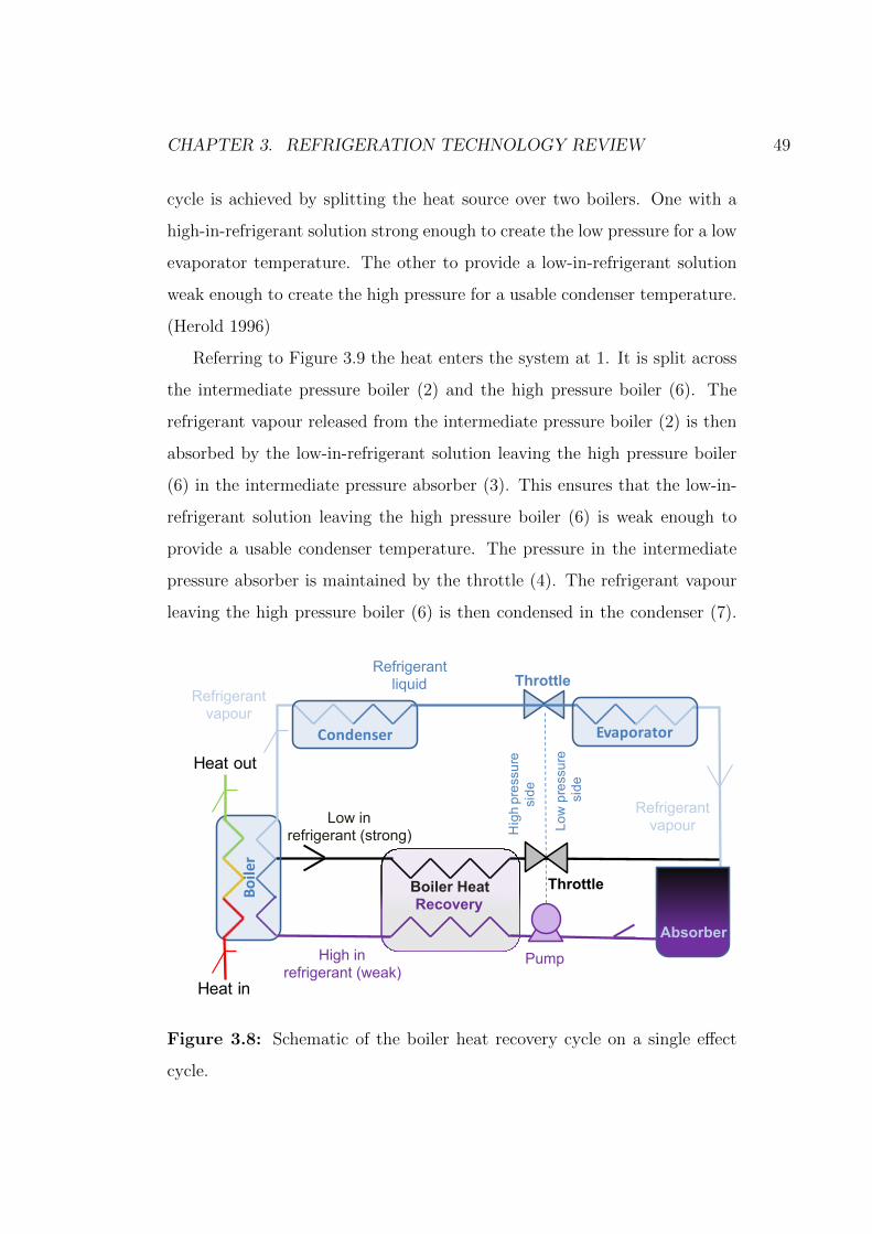
CHAPTER 3. REFRIGERATION TECHNOLOGY REVIEW 49
cycle is achieved by splitting the heat source over two boilers. One with a
high-in-refrigerant solution strong enough to create the low pressure for a low
evaporator temperature. The other to provide a low-in-refrigerant solution
weak enough to create the high pressure for a usable condenser temperature.
(Herold 1996)
Referring to Figure 3.9 the heat enters the system at 1. It is split across
the intermediate pressure boiler (2) and the high pressure boiler (6). The
refrigerant vapour released from the intermediate pressure boiler (2) is then
absorbed by the low-in-refrigerant solution leaving the high pressure boiler
(6) in the intermediate pressure absorber (3). This ensures that the low-in-
refrigerant solution leaving the high pressure boiler (6) is weak enough to
provide a usable condenser temperature. The pressure in the intermediate
pressure absorber is maintained by the throttle (4). The refrigerant vapour
leaving the high pressure boiler (6) is then condensed in the condenser (7).
Boiler
Heat in
Heat out
High in refrigerant (weak)
Low inrefrigerant (strong)
Refrigerantvapour
Condenser
Refrigerantliquid
Evaporator
Refrigerant vapour
Throttle
Pump
Hig
h pr
essu
resi
de
Low
pre
ssur
e si
de
ThrottleBoiler HeatRecovery
Absorber
Figure 3.8: Schematic of the boiler heat recovery cycle on a single effect
cycle.
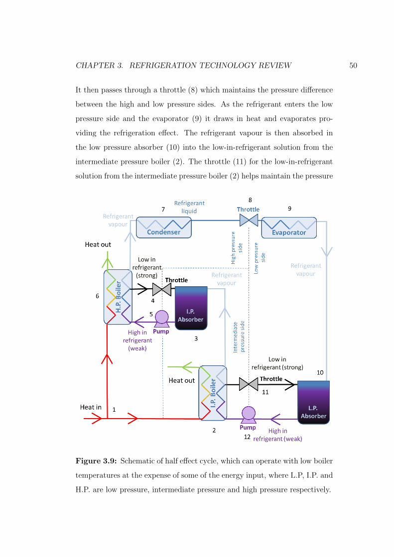
CHAPTER 3. REFRIGERATION TECHNOLOGY REVIEW 50
It then passes through a throttle (8) which maintains the pressure difference
between the high and low pressure sides. As the refrigerant enters the low
pressure side and the evaporator (9) it draws in heat and evaporates pro-
viding the refrigeration effect. The refrigerant vapour is then absorbed in
the low pressure absorber (10) into the low-in-refrigerant solution from the
intermediate pressure boiler (2). The throttle (11) for the low-in-refrigerant
solution from the intermediate pressure boiler (2) helps maintain the pressure
Figure 3.9: Schematic of half effect cycle, which can operate with low boiler
temperatures at the expense of some of the energy input, where L.P, I.P. and
H.P. are low pressure, intermediate pressure and high pressure respectively.
CHAPTER 3. REFRIGERATION TECHNOLOGY REVIEW 51
difference between the intermediate and low pressure sides of the refrigerator.
By operating at three different pressure levels and four different solution
concentrations the half effect cycle allows an absorption refrigerator to be
driven by a boiler temperature that would otherwise be too low. There is
a thermodynamic penalty for this; the heat that is used in the intermediate
pressure boiler has little energetic effect on the useful output of the refrig-
erator (heat that can be absorbed by the evaporator). This is because the
vapour that is released at the intermediate pressure (I.P.) boiler is reabsorbed
before being used as a working refrigerant. It therefore results in a low CoP
in terms of energy. However the ability to use low temperature heat may be
advantageous in terms of exergy.
Dual Cycle
The dual cycle as described by Srikhirin et al. (2001) cascades the input heat
through two absorption refrigerators. The heat is used to drive a standard
single effect cycle, while the rejected heat from the condenser and absorber
is used to drive another cycle. This system tends to be used with different
working fluids and concentrations in each refrigerator.
3.3.4 System Configurations to Utilise Discontinuous
Heat Sources
Said et al. (2012) describe the possible configurations for providing continu-
ous cooling through absorption refrigeration from solar power (a discontinu-
ous heat source). The three main options are:
Hot storage
The heat from the heat source is stored and is released at the required
rate to power the refrigerator, for example insulated hot water tanks,
phase changing materials and thermal mass.
CHAPTER 3. REFRIGERATION TECHNOLOGY REVIEW 52
Cold storage
The cooling output of the refrigerator is stored, this could be in the
form of ice blocks or any working fluid stored in an insulated vessel.
Refrigerant storage
This is where the refrigerant is stored after condensing back to a liquid.
It also requires the low-in-refrigerant solution to be stored between the
boiler and absorber, as well as the weak solution between the absorber
and boiler. If condensing occurs at or above ambient temperature the
refrigerant will not require any insulation. Similarly, as the low-in-
refrigerant solution temperature is high as it leaves the boiler, it too
will benefit from cooling to ambient as less energy will have to be
removed from the absorber to maintain the desired evaporator temper-
ature. This is described as chemical storage by Herold (1996).
Only a few details about the simulation method are presented and the
heat source used by Said et al. (2012) was at 120◦C. The CoP for refrigerant
storage was reported to be 0.427 compared to cold storage at 0.372 and hot
storage at 0.434. Due to the desire to use low temperature heat sources
(<100◦C) in this thesis and the high ambient temperatures in rural India,
the refrigerant storage method is more suitable, as it should not degrade
the temperature of the heat source or cold generated as much as the other
methods.
Ammar, Joyce, et al. (2012) have investigated a similar system to the
refrigerant storage method proposed by Said et al. (2012) across large areas
to connect waste heat from the process industry to users requiring heating
or cooling. This type of absorption system uses the waste heat source for the
boiler process; after which, providing that condensing occurs at (or above)
ambient temperature, the condensed refrigerant can be moved across large
distances without any concern for insulation. Likewise the strong and weak
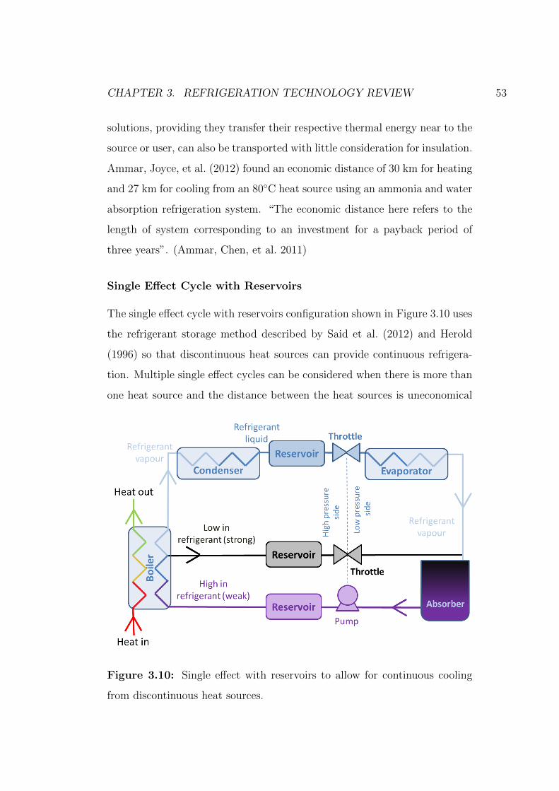
CHAPTER 3. REFRIGERATION TECHNOLOGY REVIEW 53
solutions, providing they transfer their respective thermal energy near to the
source or user, can also be transported with little consideration for insulation.
Ammar, Joyce, et al. (2012) found an economic distance of 30 km for heating
and 27 km for cooling from an 80◦C heat source using an ammonia and water
absorption refrigeration system. “The economic distance here refers to the
length of system corresponding to an investment for a payback period of
three years”. (Ammar, Chen, et al. 2011)
Single Effect Cycle with Reservoirs
The single effect cycle with reservoirs configuration shown in Figure 3.10 uses
the refrigerant storage method described by Said et al. (2012) and Herold
(1996) so that discontinuous heat sources can provide continuous refrigera-
tion. Multiple single effect cycles can be considered when there is more than
one heat source and the distance between the heat sources is uneconomical
Figure 3.10: Single effect with reservoirs to allow for continuous cooling
from discontinuous heat sources.

CHAPTER 3. REFRIGERATION TECHNOLOGY REVIEW 54
to warrant one of the other cycles described in this section. If desired this
cycle can be improved with either or both the heat utilisation configurations
in Section 3.3.3 and the lowering evaporator temperature configurations de-
scribed in Section 3.3.5.
Double Boiler with Reservoirs
The double boiler cycle in Figure 3.11 is similar to the single effect cycle
except it uses two heat sources. This cycle differs from the half effect cycle
as it does not have an intentional intermediate pressure, though different
pressures may occur if the heat sources are at different temperatures which
may add a control requirement. The reservoirs act in the same way as in the
Figure 3.11: Double boiler cycle schematic; showing one absorption re-
frigerator powered by two discontinuous heat sources through two separate
boilers with reservoirs to allow for continuous cooling from discontinuous
heat sources.

CHAPTER 3. REFRIGERATION TECHNOLOGY REVIEW 55
single effect cycle with reservoirs cycle allowing continuous refrigeration from
discontinuous heat sources, with the advantage that in this system multiple
heat sources can be used.
3.3.5 System Configurations to Reduce the Evapora-
tor Temperature
For all refrigeration systems the evaporator temperature determines the ap-
propriate applications. With absorption refrigerators there are two main
strategies to manipulate evaporator temperature: control absorber tempera-
ture and / or control solution concentration.
Control of the solution concentration is limited by the condenser temper-
ature and the crystallisation limit (conditions where salt crystals form in the
solution, typically before the absorber). The crystallisation limit can be re-
duced by increasing operating temperatures, though the crystallisation limit
should generally be avoided to prevent unexpected blockages and therefore
operation close to it will not be considered in this thesis. However, configu-
rations using the idea of the half effect cycle can provide condenser temper-
atures and evaporator temperatures that would not be possible with a single
effect cycle. The alternative is actively cooling the condenser, through using
some of the heat absorbing potential of the evaporator (evaporator tap-off
or coupled cycle) or by an external cold sink, such as: a river, lake or sea to
improve heat transfer over basic ambient air cooling.
The absorber temperature can be controlled by active cooling such as: the
external cold sinks mentioned in this section, coupled cycle and evaporator
tap-off. It can also be controlled through the physical design to increase heat
and mass transfer such as: adiabatic absorbers (Zacarıas et al. 2011), falling
film absorbers (Tae Kang et al. 2000), (Castro et al. 2009), (D. S. Kim and
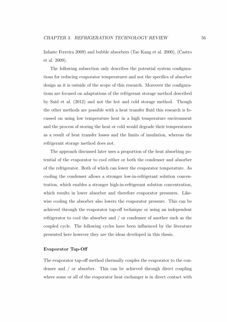
CHAPTER 3. REFRIGERATION TECHNOLOGY REVIEW 56
Infante Ferreira 2009) and bubble absorbers (Tae Kang et al. 2000), (Castro
et al. 2009).
The following subsection only describes the potential system configura-
tions for reducing evaporator temperatures and not the specifics of absorber
design as it is outside of the scope of this research. Moreover the configura-
tions are focused on adaptations of the refrigerant storage method described
by Said et al. (2012) and not the hot and cold storage method. Though
the other methods are possible with a heat transfer fluid this research is fo-
cussed on using low temperature heat in a high temperature environment
and the process of storing the heat or cold would degrade their temperatures
as a result of heat transfer losses and the limits of insulation, whereas the
refrigerant storage method does not.
The approach discussed later uses a proportion of the heat absorbing po-
tential of the evaporator to cool either or both the condenser and absorber
of the refrigerator. Both of which can lower the evaporator temperature. As
cooling the condenser allows a stronger low-in-refrigerant solution concen-
tration, which enables a stronger high-in-refrigerant solution concentration,
which results in lower absorber and therefore evaporator pressures. Like-
wise cooling the absorber also lowers the evaporator pressure. This can be
achieved through the evaporator tap-off technique or using an independent
refrigerator to cool the absorber and / or condenser of another such as the
coupled cycle. The following cycles have been influenced by the literature
presented here however they are the ideas developed in this thesis.
Evaporator Tap-Off
The evaporator tap-off method thermally couples the evaporator to the con-
denser and / or absorber. This can be achieved through direct coupling
where some or all of the evaporator heat exchanger is in direct contact with
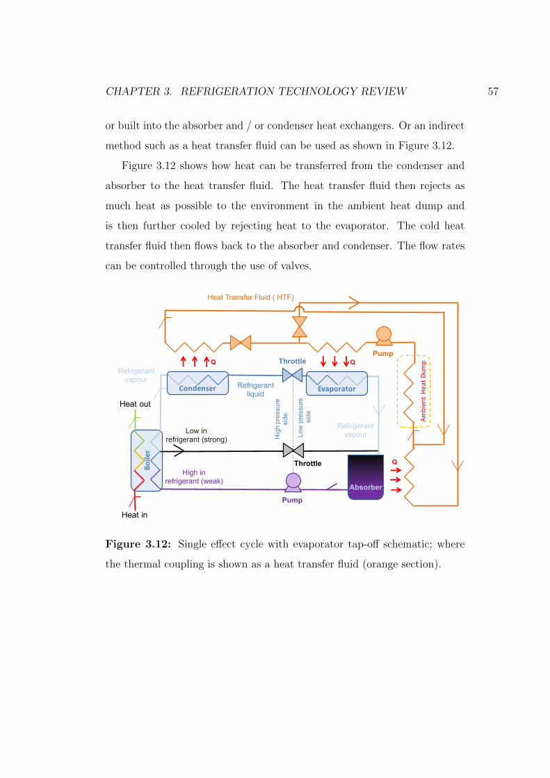
CHAPTER 3. REFRIGERATION TECHNOLOGY REVIEW 57
or built into the absorber and / or condenser heat exchangers. Or an indirect
method such as a heat transfer fluid can be used as shown in Figure 3.12.
Figure 3.12 shows how heat can be transferred from the condenser and
absorber to the heat transfer fluid. The heat transfer fluid then rejects as
much heat as possible to the environment in the ambient heat dump and
is then further cooled by rejecting heat to the evaporator. The cold heat
transfer fluid then flows back to the absorber and condenser. The flow rates
can be controlled through the use of valves.
Boiler
Heat in
Heat out
High in refrigerant (weak)
Low inrefrigerant (strong)
Refrigerantvapour
Condenser Refrigerantliquid
Evaporator
Refrigerant vapour
Throttle
Pump
Hig
h pr
essu
resi
de
Low
pre
ssur
e si
de
Throttle
Heat Transfer Fluid ( HTF)
Absorber
Q
Pump
AmbientHe
atDum
p
Figure 3.12: Single effect cycle with evaporator tap-off schematic; where
the thermal coupling is shown as a heat transfer fluid (orange section).
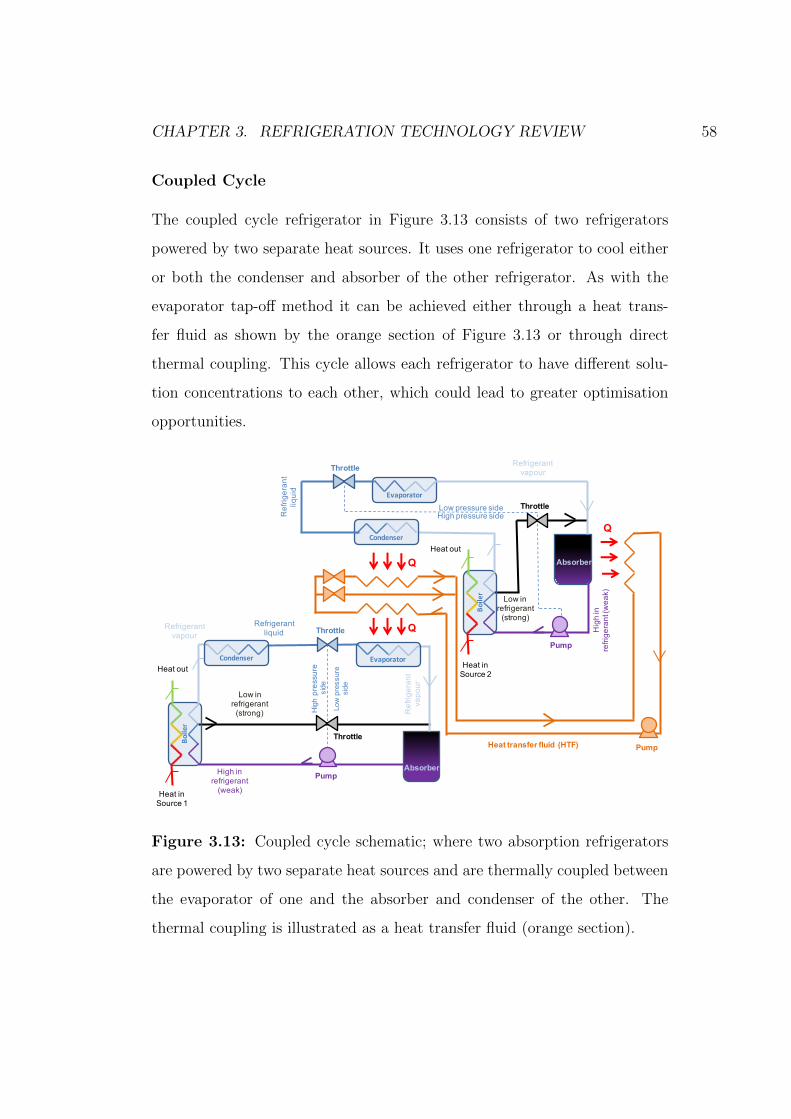
CHAPTER 3. REFRIGERATION TECHNOLOGY REVIEW 58
Coupled Cycle
The coupled cycle refrigerator in Figure 3.13 consists of two refrigerators
powered by two separate heat sources. It uses one refrigerator to cool either
or both the condenser and absorber of the other refrigerator. As with the
evaporator tap-off method it can be achieved either through a heat trans-
fer fluid as shown by the orange section of Figure 3.13 or through direct
thermal coupling. This cycle allows each refrigerator to have different solu-
tion concentrations to each other, which could lead to greater optimisation
opportunities.
Boiler
Heat inSource 1
Heat out
AbsorberHigh inrefrigerant
(weak)
Low inrefrigerant
(strong)
Refrigerantvapour
Condenser
Refrigerantliquid
Evaporator
Ref
riger
ant
vapo
ur
Pump
Hig
h pr
essu
resi
de
Low
pre
ssur
esi
de
Throttle
Boiler
Heat inSource 2
Heat outAbsorber
Hig
h in
re
frige
rant
(wea
k)Low in
refrigerant(strong)
Refrigerantvapour
Condenser
Ref
riger
ant
liqui
d
Evaporator
Throttle
Low pressure sideHigh pressure side
Pump
Throttle
Throttle
Heat transfer fluid (HTF)
Q
Q
Q
Pump
Figure 3.13: Coupled cycle schematic; where two absorption refrigerators
are powered by two separate heat sources and are thermally coupled between
the evaporator of one and the absorber and condenser of the other. The
thermal coupling is illustrated as a heat transfer fluid (orange section).
CHAPTER 3. REFRIGERATION TECHNOLOGY REVIEW 59
3.3.6 Using Discontinuous Heat Sources and Control-
ling Evaporator Temperature
The concepts already mentioned to utilise discontinuous heat sources and
control evaporator temperature can be combined creating the following cy-
cles:
Single Effect with Reservoirs and Evaporator Tap-Off
The single effect with reservoirs and evaporator tap-off combines the con-
cepts in Sections 3.3.4 and 3.3.5 to allow both continuous cooling from dis-
continuous heat sources and control over the evaporator temperature. This
is achieved through reservoirs to store the solutions and refrigerant between
Boiler
Heat in
Heat out
High in refrigerant (weak)
Low inrefrigerant (strong)
Refrigerantvapour
CondenserRefrigerant
liquid
Evaporator
Refrigerant vapour
Throttle
Pump
Hig
h pr
essu
resi
de
Low
pre
ssur
e si
de
Throttle
Heat Transfer Fluid (HTF)
Absorber
Q
PumpAm
bientHe
atDum
p
Reservoir
Reservoir
Reservoir
Figure 3.14: Single effect cycle with reservoirs and evaporator tap-off. This
cycle allows both continuous refrigeration from discontinuous heat sources
and control over the evaporator temperature. The thermal coupling is illus-
trated as a heat transfer fluid (orange section).
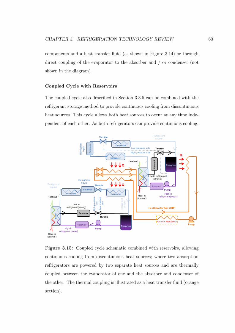
CHAPTER 3. REFRIGERATION TECHNOLOGY REVIEW 60
components and a heat transfer fluid (as shown in Figure 3.14) or through
direct coupling of the evaporator to the absorber and / or condenser (not
shown in the diagram).
Coupled Cycle with Reservoirs
The coupled cycle also described in Section 3.3.5 can be combined with the
refrigerant storage method to provide continuous cooling from discontinuous
heat sources. This cycle allows both heat sources to occur at any time inde-
pendent of each other. As both refrigerators can provide continuous cooling,
Boiler
Heat inSource 1
Heat out
AbsorberHigh in
refrigerant (weak)
Low inrefrigerant (strong)
Refrigerantvapour
Condenser
Refrigerantliquid
Evaporator
Ref
riger
ant
vapo
ur
Pump
Hig
h pr
essu
resi
deLo
w p
ress
ure
side
Throttle
Boiler
Heat inSource 2
Heat outAbsorber
High in refrigerant (weak)
Low in refrigerant(strong)
Refrigerantvapour
Condenser
Ref
riger
ant
liqui
d Evaporator
Throttle
Low pressure side
High pressure side
Pump
Throttle
Throttle
Heat transfer fluid (HTF)
Q
Q
Q
Pump
Reservoir
Reservoir
Reservoir
Reservoir
Reservoir
ReservoirAmbientHeatDump
Figure 3.15: Coupled cycle schematic combined with reservoirs, allowing
continuous cooling from discontinuous heat sources; where two absorption
refrigerators are powered by two separate heat sources and are thermally
coupled between the evaporator of one and the absorber and condenser of
the other. The thermal coupling is illustrated as a heat transfer fluid (orange
section).

CHAPTER 3. REFRIGERATION TECHNOLOGY REVIEW 61
this cycle provides a high level of control over the output evaporator tem-
perature (from the refrigerator powered by heat source 2) as the refrigerator
powered by heat source 1 can be optimised for the desired operating tem-
peratures of the absorber and / or condenser of the refrigerator powered by
heat source 2.
Double Boiler Cycle with Reservoirs and Evaporator Tap-Off
The double boiler cycle in Figure 3.16 has been described in Section 3.3.4,
however here it incorporates the evaporator tap-off technique described in
Boiler
Refrigerantvapour
Boiler
Hig
h in
refri
gera
nt
(wea
k)Refrigerant
liquid
Evaporator
Throttle
PumpHeat
source1
Heatsource2
ThrottleLow in
refrigerant(strong)
Absorber
Condenser
Low pressure sideHigh pressure side
Refrigerantvapour
Heat transfer fluid (HTF)
Q
Pump
AmbientH
eatD
ump
Reservoir
Reservoir
Reservoir
Figure 3.16: Double boiler with reservoirs and evaporator tap-off cycle
schematic; showing one absorption refrigerator powered by two heat sources
through two separate boilers. The thermal coupling is illustrated by the heat
transfer fluid (orange section).

CHAPTER 3. REFRIGERATION TECHNOLOGY REVIEW 62
Section 3.3.5 to allow both continuous cooling from more than one discontin-
uous heat source and control over the evaporator temperature. This config-
uration only requires one condenser, absorber and evaporator with multiple
boilers.
3.3.7 Appraisal of Absorption Refrigeration Systems
Table 3.2 shows the appraisal mechanism which aims to summarise the pre-
viously described system configurations and technologies available for ab-
sorption refrigeration. The table includes descriptions which highlight the
applications, advantages and disadvantages of the systems in question, as
well as a decision matrix to aid the comparison process when applied to the
needs of the community described in Section 2.1, where:
• Heat Source Suitability refers to its ability to use low temperature
discontinuous heat.
• Cooling Application refers to the possible refrigeration uses 5 being
versatile (a range of temperatures) 1 not versatile (limited temperatures
e.g. air conditioning only).
• Impact on CoP refers to the effect on refrigerator performance in terms
of energy 5 is significantly improves CoP and 1 is significantly worsens
CoP.
• Evaporator Temperature refers to the direct impact on evaporator tem-
perature where 5 is lowering the temperature and 1 is increasing it.
The ranked factors in the decision matrix have equal importance and
therefore no weighting was applied.
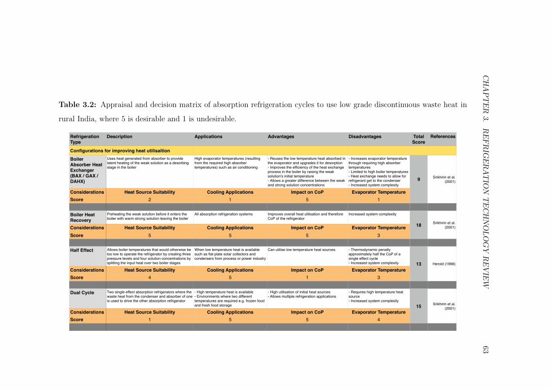
CHAPTER
3.REFRIG
ERATIO
NTECHNOLOGY
REVIE
W63
Table 3.2: Appraisal and decision matrix of absorption refrigeration cycles to use low grade discontinuous waste heat in
rural India, where 5 is desirable and 1 is undesirable.
Refrigeration Type
Description Applications Advantages Disadvantages Total Score
References
Configurations for improving heat utilisaitionBoiler Absorber Heat Exchanger (BAX / GAX / DAHX)
Uses heat generated from absorber to provide latent heating of the weak solution as a desorbing stage in the boiler
High evaporator temperatures (resulting from the required high absorber temperatures) such as air conditioning
- Reuses the low temperature heat absorbed in the evaporator and upgrades it for desorption - Improves the efficiency of the heat exchange process in the boiler by raising the weak solution's initial temperature - Allows a greater difference between the weak and strong solution concentrations
- Increases evaporator temperature through requiring high absorber temperatures- Limited to high boiler temperatures- Heat exchange needs to allow for refrigerant get to the condenser- Increased system complexity
9 Srikhirin et al. (2001)
Considerations Heat Source Suitability Cooling Applications Impact on CoP Evaporator TemperatureScore 2 1 5 1
Boiler Heat Recovery
Preheating the weak solution before it enters the boiler with warm strong solution leaving the boiler
All absorption refrigeration systems Improves overall heat utilisation and therefore CoP of the refrigerator
Increased system complexity
18 Srikhirin et al. (2001)Considerations Heat Source Suitability Cooling Applications Impact on CoP Evaporator Temperature
Score 5 5 5 3
Half Effect Allows boiler temperatures that would otherwise be too low to operate the refrigerator by creating three pressure levels and four solution concentrations by splitting the input heat over two boiler stages
When low temperature heat is available such as flat plate solar collectors and condensers from process or power industry
Can utilise low temperature heat sources - Thermodynamic penalty approximately half the CoP of a single effect cycle - Increased system complexity 13 Herold (1996)
Considerations Heat Source Suitability Cooling Applications Impact on CoP Evaporator TemperatureScore 4 5 1 3
Dual Cycle Two single effect absorption refrigerators where the waste heat from the condenser and absorber of one is used to drive the other absorption refrigerator
- High temperature heat is available - Environments where two different temperatures are required e.g. frozen food and fresh food storage
- High utilisation of initial heat sources- Allows multiple refrigeration applications
- Requires high temperature heat source - Increased system complexity
15 Srikhirin et al. (2001)
Considerations Heat Source Suitability Cooling Applications Impact on CoP Evaporator TemperatureScore 1 5 5 4
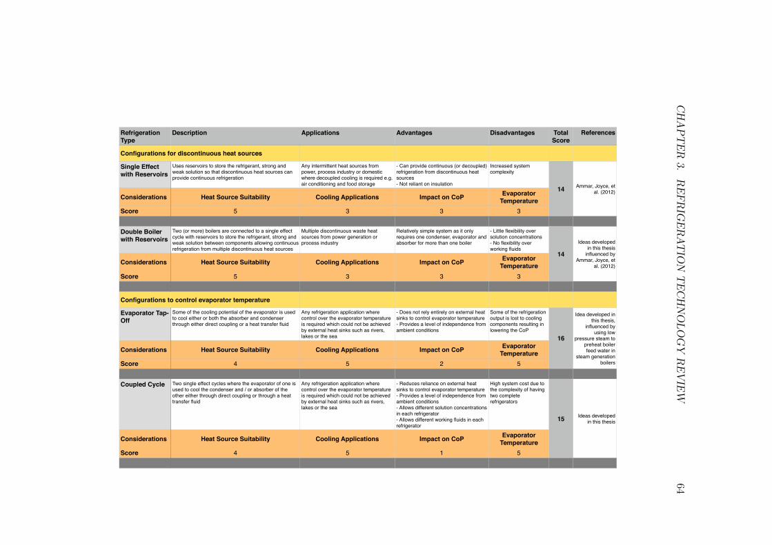
CHAPTER
3.REFRIG
ERATIO
NTECHNOLOGY
REVIE
W64
Refrigeration Type
Description Applications Advantages Disadvantages Total Score
References
Configurations for discontinuous heat sources
Single Effect with Reservoirs
Uses reservoirs to store the refrigerant, strong and weak solution so that discontinuous heat sources can provide continuous refrigeration
Any intermittent heat sources from power, process industry or domestic where decoupled cooling is required e.g. air conditioning and food storage
- Can provide continuous (or decoupled) refrigeration from discontinuous heat sources- Not reliant on insulation
Increased system complexity
14 Ammar, Joyce, et al. (2012)
Considerations Heat Source Suitability Cooling Applications Impact on CoP Evaporator Temperature
Score 5 3 3 3
Double Boiler with Reservoirs
Two (or more) boilers are connected to a single effect cycle with reservoirs to store the refrigerant, strong and weak solution between components allowing continuous refrigeration from multiple discontinuous heat sources
Multiple discontinuous waste heat sources from power generation or process industry
Relatively simple system as it only requires one condenser, evaporator and absorber for more than one boiler
- Little flexibility over solution concentrations- No flexibility over working fluids
14
Ideas developed in this thesis
influenced by Ammar, Joyce, et
al. (2012)Considerations Heat Source Suitability Cooling Applications Impact on CoP Evaporator Temperature
Score 5 3 3 3
Configurations to control evaporator temperature
Evaporator Tap-Off
Some of the cooling potential of the evaporator is used to cool either or both the absorber and condenser through either direct coupling or a heat transfer fluid
Any refrigeration application where control over the evaporator temperature is required which could not be achieved by external heat sinks such as rivers, lakes or the sea
- Does not rely entirely on external heat sinks to control evaporator temperature - Provides a level of independence from ambient conditions
Some of the refrigeration output is lost to cooling components resulting in lowering the CoP
16
Idea developed in this thesis,
influenced by using low
pressure steam to preheat boiler feed water in
steam generation boilers
Considerations Heat Source Suitability Cooling Applications Impact on CoP Evaporator Temperature
Score 4 5 2 5
Coupled Cycle Two single effect cycles where the evaporator of one is used to cool the condenser and / or absorber of the other either through direct coupling or through a heat transfer fluid
Any refrigeration application where control over the evaporator temperature is required which could not be achieved by external heat sinks such as rivers, lakes or the sea
- Reduces reliance on external heat sinks to control evaporator temperature - Provides a level of independence from ambient conditions- Allows different solution concentrations in each refrigerator- Allows different working fluids in each refrigerator
High system cost due to the complexity of having two complete refrigerators
15 Ideas developed in this thesis
Considerations Heat Source Suitability Cooling Applications Impact on CoP Evaporator Temperature
Score 4 5 1 5
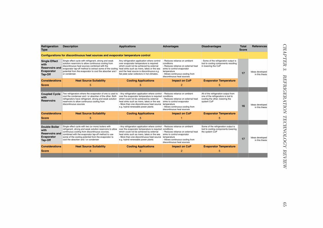
CHAPTER
3.REFRIG
ERATIO
NTECHNOLOGY
REVIE
W65
Refrigeration Type
Description Applications Advantages Disadvantages Total Score
References
Configurations for discontinuous heat sources and evaporator temperature control
Single Effect with Reservoirs and Evaporator Tap-Off
Single effect cycle with refrigerant, strong and weak solution reservoirs to allow continuous cooling from discontinuous heat sources combined with the evaporator tap-off method to extract some of the cooling potential from the evaporator to cool the absorber and / or condenser.
Any refrigeration application where control over evaporator temperature is required which could not be achieved by external heat sinks such as rivers, lakes or the sea and the heat source is discontinuous e.g. flat plate solar collectors in hot climates.
- Reduces reliance on ambient conditions- Reduces reliance on external heat sinks to control evaporator temperature - Allows continuous cooling from discontinuous heat sources
- Some of the refrigeration output is lost to cooling components resulting in lowering the CoP
17 Ideas developed in this thesis
Considerations Heat Source Suitability Cooling Applications Impact on CoP Evaporator TemperatureScore 5 5 2 5
Coupled Cycle with Reservoirs
Two refrigerators where the evaporator of one is used to cool the condenser and / or absorber of the other. Both refrigerators have refrigerant, strong and weak solution reservoirs to allow continuous cooling from discontinuous sources
- Any refrigeration application where control over the evaporator temperature is required which could not be achieved by external heat sinks such as rivers, lakes or the sea - More than one discontinuous heat source e.g. hybrid renewable power plants
- Reduces reliance on ambient conditions- Reduces reliance on external heat sinks to control evaporator temperature- Allows continuous cooling from discontinuous heat sources
All of the refrigeration output from one of the refrigerators is lost to cooling the other, lowering the system CoP
16 Ideas developed in this thesis
Considerations Heat Source Suitability Cooling Applications Impact on CoP Evaporator TemperatureScore 5 5 1 5
Double Boiler with Reservoirs and Evaporator Tap-Off
Single effect cycle with two (or more) boilers with refrigerant, strong and weak solution reservoirs to allow continuous cooling from discontinuous sources, combined with the evaporator tap-off method to use some of the cooling potential from the evaporator to cool the absorber and / or condenser
- Any refrigeration application where control over the evaporator temperature is required which could not be achieved by external heat sinks such as rivers, lakes or the sea - More than one discontinuous heat source e.g. hybrid renewable power plants
- Reduces reliance on ambient conditions- Reduces reliance on external heat sinks to control evaporator temperature - Allows continuous cooling from discontinuous heat sources
Some of the refrigeration output is lost to cooling components lowering the system CoP
17 Ideas developed in this thesis
Considerations Heat Source Suitability Cooling Applications Impact on CoP Evaporator TemperatureScore 5 5 2 5
CHAPTER 3. REFRIGERATION TECHNOLOGY REVIEW 66
Table 3.2 allows immediate identification of systems that are not suitable
for the types of heat sources and community which this research is based
around, which tends to be scores under 16. For example, boiler absorber
heat exchanger has a total score of 9 which is a result of it being a technology
suited for higher temperature heat sources and higher temperature cooling.
Likewise the half effect cycle was deemed unsuitable as it has a total score
of 13 which is largely a result of the impact on CoP (scoring 1) from half of
the input energy being used internally.
Interestingly the boiler heat recovery is the highest scoring system (18)
but it will not be carried forward in this research. This is largely due to
the additional modelling complexity. Though it should be noted that, as a
technology, it can be applied to almost any absorption system to recover the
waste heat in the strong solution at the boiler exit.
The systems that are either for discontinuous heat sources or to con-
trol evaporator temperature but not both scored 14 and 15, apart from the
evaporator tap-off which scored 16. This was slight increase is a result of it
having a less serious impact on CoP than the coupled cycle, scoring 2 and 1
respectively.
The cycles that can utilise discontinuous heat sources and evaporator
temperature control scored 16 and 17 indicating that they are the most suit-
able for the heat sources in this particular setting. The single effect with
reservoirs and evaporator tap-off, coupled cycle with reservoirs and double
boiler with reservoirs and evaporator tap-off all provide the ability to use
discontinuous heat for continuous cooling while also providing some control
over the evaporator temperature. These features are particularly useful in
rural India where the cold sinks may be limited and / or not be effective
and hot, humid weather will not provide the conditions to maintain suitable
absorber and condenser temperatures.

CHAPTER 3. REFRIGERATION TECHNOLOGY REVIEW 67
3.4 Conclusion of Refrigeration Technology
Review
This refrigeration technology review described the history of refrigeration
and an overview of common refrigeration systems. From which it appeared
that absorption refrigeration would be an appropriate technology to utilise
low temperature discontinuous waste heat from a renewable power plant in
rural India. It therefore included a detailed review of absorption refrigeration
including the working fluids available and potential system configurations.
The application for which this research is based has two discontinuous low
temperature (<100◦C) heat sources in a hot environment with only poor
quality cold sinks (e.g. hot humid air) available. Currently acetone and zinc
bromide solution has proven to work from heat source temperatures lower
than 60◦C and has no need for rectification.
The use of reservoirs and cooling of the condenser and / or the absorber
by either the evaporator tap-off or from an independent refrigerator is an
extension of the work by Said et al. (2012), Ammar, Joyce, et al. (2012),
Jelinek and Borde (1998) and Gutierrez-Urueta et al. (2011). The system
configurations that can utilise discontinuous low temperature waste heat and
are less reliant on environmental cold sinks are: single effect with reservoirs
and evaporator tap-off, coupled cycle with reservoirs and double boiler with
reservoirs and evaporator tap-off. These configurations with acetone and zinc
bromide will be investigated in this thesis.
There appears to be a knowledge gap in the literature about using acetone
and zinc bromide absorption systems to utilise low temperature discontinuous
waste heat from renewable power plants in the high ambient temperatures ex-
pected in rural India. Moreover, though there is substantial knowledge about
absorption refrigerator configurations and their effect, there is a knowledge
gap in determining the operating limits when utilising these configurations

CHAPTER 3. REFRIGERATION TECHNOLOGY REVIEW 68
for low temperature waste heat sources to provide low refrigerating temper-
atures in high ambient conditions. Investigating these knowledge gaps will
identify the limits of suitability for absorption refrigeration for requirements
of the case study community identified in Chapter 2.
Chapter 4
Analytical Methodology
The following chapter describes the modelling used in the investigation of
absorption refrigeration from utilising low temperature discontinuous waste
heat from a renewable power plant in rural India. The heat sources are
based on those in the proposed power plant which are a 10 kW (electric)
concentrated photovoltaic (CPV) system and the radiator of a 5 kW (elec-
tric) hydrogen-biogas internal combustion engine electric generator (genset
radiator). The working fluids for the absorption refrigeration system are
acetone and zinc bromide.
This chapter consists of the following sections:
• Energy Profiling and Heat Source Modelling describes how the
energy flows in the BioCPV power plant are quantified. This process
provides the data for a Sankey diagram which includes the waste heat
sources used to drive the absorption refrigerators.
• Fluid Properties describes the calculations required to model the
working fluids in the absorption refrigerator system. This includes
acetone in its pure form as well as acetone and zinc bromide as a
solution.
69
CHAPTER 4. ANALYTICAL METHODOLOGY 70
• Absorption Refrigerator Modelling describes the process used to
model a basic single effect absorption refrigerator and the alternative
configurations used in this thesis.
• Energy Utilisation describes the method of qualifying energy utilisa-
tion within the BioCPV power plant and the absorption refrigerators.
This uses exergy for the power plant energy flows and presents an al-
ternative to exergy for the absorption refrigerators relating the cooling
to avoided electrical consumption from a vapour compression cycle.
4.1 Energy Profiling and Heat Source Mod-
elling
The following section describes the method used to model the electrical and
heat output of the 10 kW (electric) CPV system and the radiator of the 5
kW (electric) genset.
4.1.1 Concentrated Photovoltaic
The proposed CPV system has been designed by the project partners at the
University of Exeter and the Indian Institute of Technology Madras. The
following information has been provided by them for the analysis in this
thesis.
The CPV system aims to achieve optical efficiencies of 80% by addressing
issues of concentrated light such as fuzziness at the receiver and reducing
losses in the optical components. The CPV system consists of four CPV units
with two axis tracking. Each CPV unit consists of two primary concentrators
and receivers. The primary concentrator is a parabolic dish with a square
opening, made up of four sections to achieve an overall entry aperture area of
9m2, though the actual collecting area is calculated to be 7.565 m2 to provide
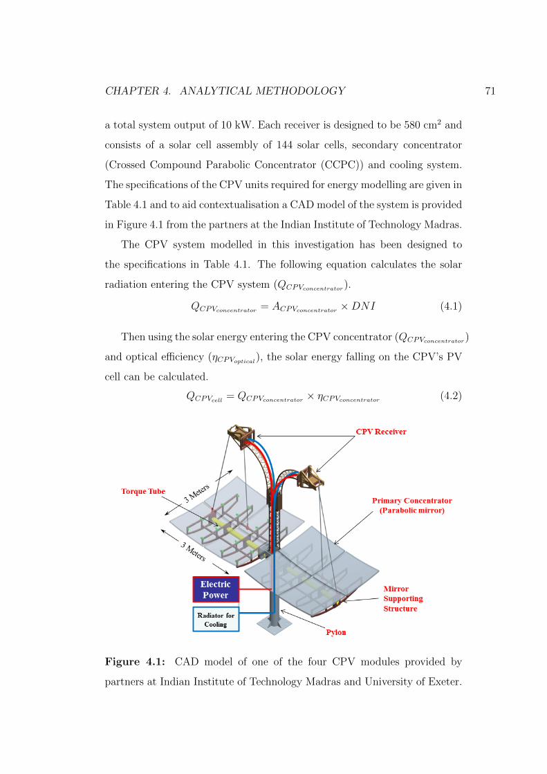
CHAPTER 4. ANALYTICAL METHODOLOGY 71
a total system output of 10 kW. Each receiver is designed to be 580 cm2 and
consists of a solar cell assembly of 144 solar cells, secondary concentrator
(Crossed Compound Parabolic Concentrator (CCPC)) and cooling system.
The specifications of the CPV units required for energy modelling are given in
Table 4.1 and to aid contextualisation a CAD model of the system is provided
in Figure 4.1 from the partners at the Indian Institute of Technology Madras.
The CPV system modelled in this investigation has been designed to
the specifications in Table 4.1. The following equation calculates the solar
radiation entering the CPV system (QCPVconcentrator).
(4.1)QCPVconcentrator = ACPVconcentrator ×DNI
Then using the solar energy entering the CPV concentrator (QCPVconcentrator)
and optical efficiency (ηCPVoptical), the solar energy falling on the CPV’s PV
cell can be calculated.
(4.2)QCPVcell= QCPVconcentrator × ηCPVconcentrator
Figure 4.1: CAD model of one of the four CPV modules provided by
partners at Indian Institute of Technology Madras and University of Exeter.

CHAPTER 4. ANALYTICAL METHODOLOGY 72
Table 4.1: CPV specifications provided by partners at Indian Institute of
Technology Madras and University of Exeter.
Total Installation power rating ECPV 10 kW
Number of CPV modules nCPV 8
Solar irradiance considered DNI 550 W·m−2
Concentration ratio CRCPV 500X
Concentrator optical efficiency ηCPVoptical 80%
Concentrator entry aperture area ACPVconcentrator 7.565 m2
Likewise the electricity generated from the PV cell (ECPV ) can be cal-
culated using the cell efficiency (ηCPVcell) and the solar energy falling on the
PV cell (QCPVcell).
(4.3)ECPV = QCPVcell× ηCPVcell
However the cell efficiency is affected by its temperature and the con-
centration ratio. This system is designed to operate at a high concentration
ratio (500 suns). The cell manufacturer (Azur Space) state a cell tempera-
ture operating range of 25◦C to 80◦C. However, in the interest of reliability
and avoidance of localised over heating the partners responsible for the CPV
system want to maintain the cell temperature at 60◦C. The cell manufacturer
has supplied the following equation at 500 suns to relate PV cell tempera-
ture (TCPVcell) in degrees Celsius to PV cell efficiency (ηCPVcell
), in confidential
communication (at the time) to Prof. Tapas Malik, University of Exeter.
(4.4)ηCPVcell= 0.39− 0.0004134× (TCPVcell
− 25)
The optical losses (QCPVoptical) can be calculated from the difference in
the energy entering the CPV concentrator (QCPconcentrator) and the energy
directed on the PV cell assembly (QCPVcell).
(4.5)QCPVoptical= QCPVconcentrator −QCPVcell

CHAPTER 4. ANALYTICAL METHODOLOGY 73
Reflective losses from the PV cell assembly are included in the concen-
trator efficiency. Therefore the remaining losses at the PV cell assembly are
assumed to be heat. This thermal energy in the CPV system (QCPVthermal)
is calculated from the difference between the solar energy falling on the PV
cell (QCPVcell) and the electrical output (ECPV ).
(4.6)QCPVthermal= QCPVcell
− ECPV
4.1.2 Electrical Generator Radiator Heat Source
The biogas-hydrogen electrical generator set (genset) will be a commercially
available 5 kW biogas internal combustion engine modified to take a biogas-
hydrogen mix; a mixture of the locally produced anaerobic digester product
gas and hydrogen from a local water electrolyser powered by excess electrical
supply from the CPV system. The electrical efficiency, was estimated at 25%
based on common electrical efficiencies of 5 kW natural gas generators found
in the market, for example Yanmar CP5WN (Yanmar 2016).
For this analysis the ratio of hydrogen is 2% of the fuel mix by mass.
This is based on the expected daily production of hydrogen from 7 kW·h per
day of solar electricity via a 60% efficient electrolyser providing 4 kW·h per
day of hydrogen. These figures are based on communication with electrolyser
manufacturer ITM power and the responsible academic parters at the time.
The hydrogen forms part of the daily fuel energy required for the genset,
calculated in Equation 4.7 and presented in Table 4.2, though in reality the
hydrogen content may vary depending on availability and need. Conveniently
results from C. Jeong et al. (2009) show that there are diminishing returns
from ratios greater than 2.3% hydrogen to fuel mix by mass because the
hydrogen displaces air and reduces volumetric efficiency. They also state the
most significant increase in efficiency of 3.34% was achieved from 0% to 0.7%
hydrogen to fuel mix by mass, when compared to an increase of 1.24% with
hydrogen ratios from 1.5% to 2.3%.

CHAPTER 4. ANALYTICAL METHODOLOGY 74
Table 4.2: Genset expected efficiency and electrical output.
Electrical output Egenset 5 kW
Genset efficiency ηgenset 25%
Energy input (fuel) Qgenset 20 kW
Using the genset electrical efficiency (ηgenset) stated in Table 4.2 together
with the required electrical output (Egenset), the energy input of the genset
(Qgenset i.e. the energy of the fuel) can be calculated. The electrical genera-
tion losses between the work out of the internal combustion engine and the
electrical generator are assumed to be negligible, based on personal industrial
experience.
Qgenset =Egenset
ηgenset(4.7)
The US Department of Energy suggest that there are 10% ancillary
losses (Wgensetancillary) on average with automotive internal combustion en-
gines (DOE 2014). This was assumed to be a reasonable assumption for a
generator set as there would be a similar ancillary load to maintain the plant.
Discussions independent of this project with generator suppliers in the in-
dustrial sector confirmed this value to be reasonable for modelling purposes.
(4.8)Wgensetancillary= Qgenset × 0.1
The energy content (or losses contained) within the exhaust (Qgensetexhaust)
was calculated by assuming a biogas - hydrogen fuel mix (2% hydrogen by
mass) and the products of combustion leave the exhaust at 350◦C. This figure
is the average of the exhaust temperatures determined by Tamura (2008) on
natural gas engines. The partners responsible for the anaerobic digester have
suggested the biogas to be 60% methane and 40% carbon dioxide. Tamura
(2008) also found that an excess air ratio (to stoichiometric combustion) of 1.2
was a minimum to allow complete combustion. Therefore combustion here is
CHAPTER 4. ANALYTICAL METHODOLOGY 75
assumed to take place with an excess air ratio of 1.2 times the stoichiometric
air fuel ratio and for simplicity the excess air in the exhaust remains as
oxygen and nitrogen (i.e. no NOx formed). The enthalpy data was extracted
from Cengel and Boles (2006) using linear extrapolation for 350◦C (623K)
and taking the environmental temperature to be 25◦C (298K). Subscript i
denotes a particular component of the products of combustion in the exhaust,
h is enthalpy, m is the mass flow rate.
(4.9)Qgensetexhaust =∑
mgensetexhausti× hgensetexhausti
For simplicity the radiator is assumed to contain the remaining losses
(Qgensetradiator), though in reality there will be losses through the engine casing
to atmosphere.
(4.10)Qgensetradiator = Qgenset −Qgensetancillary−Qgensetexhaust − Egenset
4.2 Fluid Properties
This section is required for the absorption refrigerator modelling described
in Section 4.3. The following equations and coefficients have been taken from
Ajib and Karno (2008) to estimate the thermodynamic and thermophysical
properties of acetone and zinc bromide solution and the enthalpy of pure
acetone. Saturation pressures and temperatures use the Antoine equation
provided by NIST Webbook (2011). Ajib and Karno (2008) suggest that
acetone and zinc bromide absorption refrigeration systems can operate with
solution concentrations between a range of 30% to 70%(
mZnBr2
msolution
)to avoid
crystallisation.
4.2.1 Pure Acetone
The following section describes the calculations for pure acetone. Figure 4.2,
a pressure enthalpy (ph) graph, has been included to aid visualisation of the
fluid properties.
CHAPTER 4. ANALYTICAL METHODOLOGY 76
Pure acetone Enthalpy
For the following set of equations h denotes specific enthalpy in kJ·kg−1, T
temperature in ◦C and P pressure in bar. The subscripts l is for liquid, v
vapour, sh superheated and s saturation.
The enthalpy of acetone as a saturated liquid (Ajib and Karno 2008):
(4.11)hl = 177.185 + 2.154Ts + 1.06× 10⁻⁵T 3s (kJ·kg−1)
The enthalpy of acetone as a saturated vapour (Ajib and Karno 2008):
(4.12)hv =1
0.001336− 2.172× 10⁻⁶Ts + 2× 10⁻¹¹T 3s
(kJ·kg−1)
The enthalpy of superheated acetone where pressure P is in bar (Ajib
and Karno 2008):
(4.13)hsh = exp(6.62 + 0.0017T − 0.003P ) (kJ·kg−1)
Pure Acetone Saturation pressure
The saturation vapour pressure (Ps) of pure acetone provided by the Antoine
equation from NIST Webbook (2011) uses a conversion from Kelvin to Celcius
from Rogers and Mayhew (1995). This form of the equation is simpler to that
from Ajib and Karno (2008) making the extraction of saturation temperature
algebraically easier when the pressure is known. (NIST Webbook 2011)
(4.14)Ps = 104.42448−( 1312.253Ts+240.705) (bar)
Pure Acetone Saturation Temperature
The saturation temperature can be found by rearranging Equation 4.14 in
terms of saturation temperature (Ts), where saturation pressure (Ps) is in
bar (NIST Webbook 2011).
(4.15)Ts =1312.253
4.42448− log10(Ps)− 240.705 (◦C)
CHAPTER 4. ANALYTICAL METHODOLOGY 77
Table 4.3: Vapour pressure calculation coefficients (aij) for solutions of ace-
tone and zinc bromide to use in Equation 4.16 where subscript i corresponds
to T i and subscript j corresponds to Xj (Ajib and Karno 2008).
a00 −2.41 a10 5.35× 10⁻² a20 −2.13× 10⁻⁴
a01 1.72× 10⁻² a11 −1.16× 10⁻⁴ a21 3.66× 10⁻⁶
a02 −5.58× 10⁻⁴ a12 2.38× 10⁻⁶ a22 −4.61× 10⁻⁸
4.2.2 Acetone and Zinc Bromide Solution
The following describes the calculations for an acetone and zinc bromide
solution. Figure 4.3 has been included to aid visualisation of the solution
properties and indicate the crystallisation limit. It also includes the satura-
tion temperatures of pure acetone in red next to the corresponding vapour
pressure.
Acetone and Zinc Bromide Solution Vapour pressure
As with the previous set of equations the following nomenclature corresponds
to an acetone and zinc bromide solution: m is mass in kg (or mass flow over a
desired time period), T is temperature in ◦C, P pressure in bar and h enthalpy
in kJ·kg−1. The solution concentration X is in the formmZnBr2
msolution× 100 e.g.
when X = 50% use 50, this is the form used by Ajib and Karno (2008).
The vapour pressure of acetone and zinc bromide solution (PAcetone−ZnBr2)
can be calculated using Table 4.3 (Ajib and Karno 2008):
(4.16)PAcetone−ZnBr2 = exp2∑
i=0
2∑j=0
aijTiXj (bar)
Ajib and Karno (2008) report a good correlation from solution concen-
trations of 30% to 70% and solution temperatures of 0◦C to 70◦C. Maximum
deviations of 15.85% in solution vapour pressure occurred for solutions at
30% and 58.1◦C and the data is only validated up to 70◦C.

CHAPTER
4.ANALYTIC
ALMETHODOLOGY
78Figure 4.2: Pressure and enthalpy (ph) graph for pure acetone (Ajib and Karno 2008).
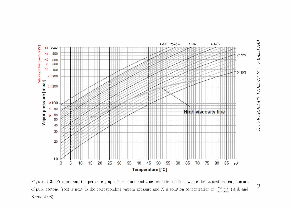
CHAPTER
4.ANALYTIC
ALMETHODOLOGY
79
-9
-4
0
14
23
303640
48
55
Saturatio
nTempe
rature(°C)X=0% X=40% X=50% X=60%
X=70%
X=80%
1000
90
Figure 4.3: Pressure and temperature graph for acetone and zinc bromide solution, where the saturation temperature
of pure acetone (red) is next to the corresponding vapour pressure and X is solution concentration inmZnBr2
msolution(Ajib and
Karno 2008).
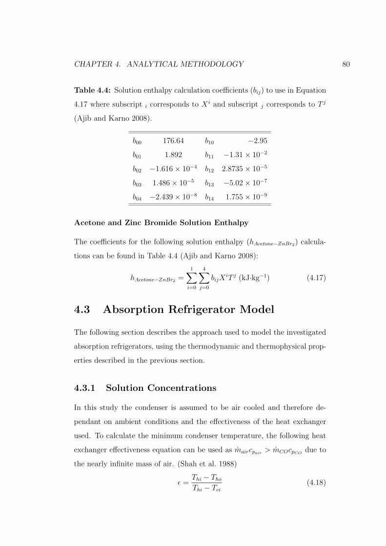
CHAPTER 4. ANALYTICAL METHODOLOGY 80
Table 4.4: Solution enthalpy calculation coefficients (bij) to use in Equation
4.17 where subscript i corresponds to X i and subscript j corresponds to T j
(Ajib and Karno 2008).
b00 176.64 b10 −2.95
b01 1.892 b11 −1.31× 10⁻²
b02 −1.616× 10⁻⁴ b12 2.8735× 10⁻⁵
b03 1.486× 10⁻⁵ b13 −5.02× 10⁻⁷
b04 −2.439× 10⁻⁸ b14 1.755× 10⁻⁹
Acetone and Zinc Bromide Solution Enthalpy
The coefficients for the following solution enthalpy (hAcetone−ZnBr2) calcula-
tions can be found in Table 4.4 (Ajib and Karno 2008):
(4.17)hAcetone−ZnBr2 =1∑
i=0
4∑j=0
bijXiT j (kJ·kg−1)
4.3 Absorption Refrigerator Model
The following section describes the approach used to model the investigated
absorption refrigerators, using the thermodynamic and thermophysical prop-
erties described in the previous section.
4.3.1 Solution Concentrations
In this study the condenser is assumed to be air cooled and therefore de-
pendant on ambient conditions and the effectiveness of the heat exchanger
used. To calculate the minimum condenser temperature, the following heat
exchanger effectiveness equation can be used as maircpair > mCOcpCOdue to
the nearly infinite mass of air. (Shah et al. 1988)
(4.18)ε =Thi − ThoThi − Tci
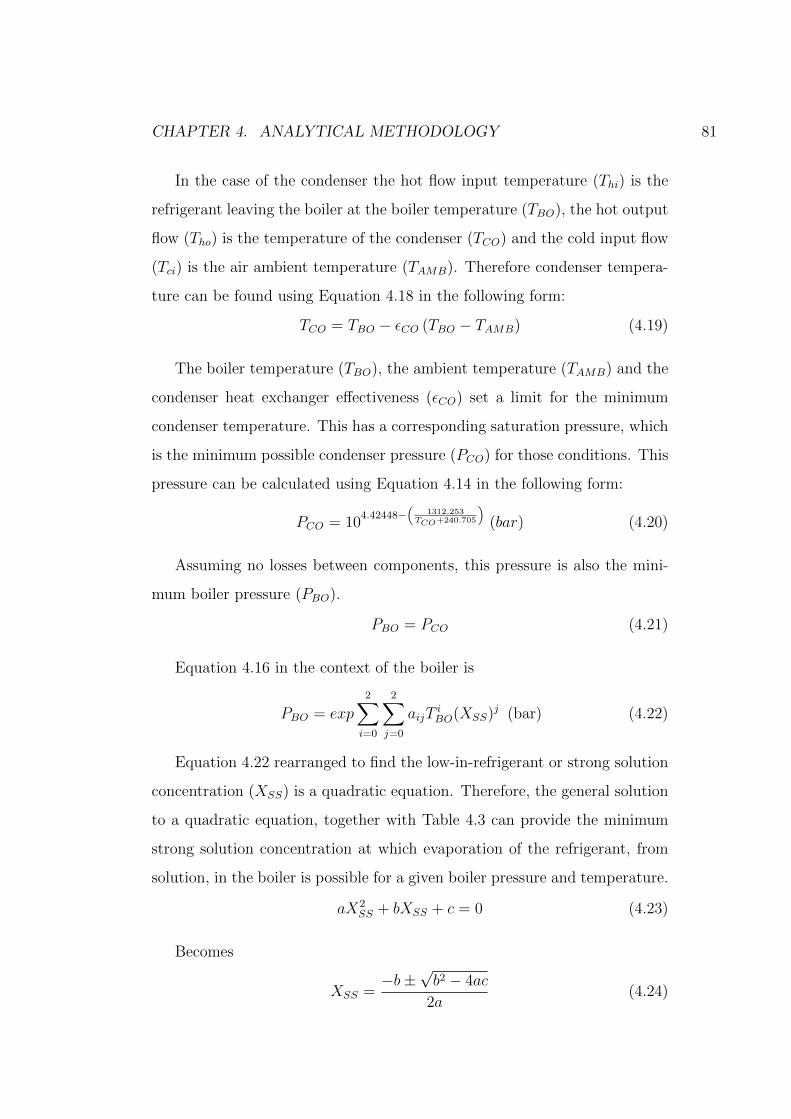
CHAPTER 4. ANALYTICAL METHODOLOGY 81
In the case of the condenser the hot flow input temperature (Thi) is the
refrigerant leaving the boiler at the boiler temperature (TBO), the hot output
flow (Tho) is the temperature of the condenser (TCO) and the cold input flow
(Tci) is the air ambient temperature (TAMB). Therefore condenser tempera-
ture can be found using Equation 4.18 in the following form:
(4.19)TCO = TBO − εCO (TBO − TAMB)
The boiler temperature (TBO), the ambient temperature (TAMB) and the
condenser heat exchanger effectiveness (εCO) set a limit for the minimum
condenser temperature. This has a corresponding saturation pressure, which
is the minimum possible condenser pressure (PCO) for those conditions. This
pressure can be calculated using Equation 4.14 in the following form:
(4.20)PCO = 104.42448−
(1312.253
TCO+240.705
)(bar)
Assuming no losses between components, this pressure is also the mini-
mum boiler pressure (PBO).
(4.21)PBO = PCO
Equation 4.16 in the context of the boiler is
(4.22)PBO = exp
2∑i=0
2∑j=0
aijTiBO(XSS)j (bar)
Equation 4.22 rearranged to find the low-in-refrigerant or strong solution
concentration (XSS) is a quadratic equation. Therefore, the general solution
to a quadratic equation, together with Table 4.3 can provide the minimum
strong solution concentration at which evaporation of the refrigerant, from
solution, in the boiler is possible for a given boiler pressure and temperature.
(4.23)aX2SS + bXSS + c = 0
Becomes
(4.24)XSS =−b±
√b2 − 4ac
2a
CHAPTER 4. ANALYTICAL METHODOLOGY 82
Where
(4.25)a = a02 + a12TBO + a22T2BO
(4.26)b = a01 + a11TBO + a21T2BO
(4.27)c = a00 + a10TBO + a20T2BO − ln(P )
Ajib and Karno (2008) report working solution concentration limits of
30% to 70% (mZnBr2
msolution) and the equations provided by them are only valid
in this range. Beyond this the solution is approaching the crystallisation
limit which can cause blockages in the system, particularly at the absorber
inlet. When the conditions provide a strong solution concentration which is
stronger than 70%, 70% will be used in this model. For conditions which
will provide solution concentrations weaker than 30% it is unlikely that any
useful cooling will be generated due to the resulting high operating pressures.
The weak solution concentration can be set at any concentration weaker
than the strong solution but stronger than 30%. Due to the challenges of
absorption refrigeration described in Section 3.3.1 investigations into the op-
timal difference between strong and weak solution concentrations are re-
quired. This is because more concentrated weak solution concentrations
provide lower evaporator temperatures, while less concentrated strong so-
lution concentrations provide higher condenser temperatures. Yet, the weak
solution concentration has to be less concentrated than the strong solution
concentration and the difference between them is proportional to the ratio
of working refrigerant (the refrigerant used in the condenser and evaporator)
to total solution, which ultimately determines how much cooling can take
place.
4.3.2 Boiler
For the purposes of this study it is assumed that perfect heat exchangers are
used between the waste heat source (PV cell and genset radiator) and the
CHAPTER 4. ANALYTICAL METHODOLOGY 83
boiler resulting in their temperatures being equal. The quantities of heat
available for the boiler (QBO) in Equation 4.28 can be found from the energy
analysis in Section 4.1.
(4.28)QCPVBO= QCPVthermal
or
(4.29)QgensetBO= Qgensetradiator
The boiler energy balance is calculated below where QBO is the boiler
energy, mWS is the mass of the weak solution, hBOWSis the enthalpy of
the weak solution as it enters the boiler, mR is the mass of the working
refrigerant leaving the boiler, hBORis the enthalpy of the refrigerant as it
leaves the boiler, mSS is the mass of the strong solution and hBOSSis the
strong solution enthalpy as it leaves the boiler. (Karno and Ajib 2008)
(4.30)QBO = mWShBOWS−mRhBOR
−mSShBOSS
The high-in-refrigerant (weak) solution temperature (TBOWS) entering the
boiler is assumed to be at ambient temperature. This is because it is assumed
that there is no heat transfer between the low-in-refrigerant (strong) solution
leaving the boiler and, due to the discontinuous nature of the boiler, the weak
solution would have remained in its uninsulated reservoir for some time.
(4.31)TBOWS= TAMB
Weak solution concentration is set by the model operator relative to the
strong solution concentration (calculated as a function of ambient tempera-
ture and condenser heat exchanger effectiveness). The weak solution enthalpy
is calculated using Equation 4.17 and Table 4.4.
(4.32)hBOWS=
1∑i=0
4∑j=0
bij(XWS)iT jBOWS
(kJ·kg−1)
The strong solution leaving the boiler is assumed to be at the boiler
temperature due to thermal equilibrium. Its enthalpy is calculated using
Equation 4.17 and Table 4.4.
CHAPTER 4. ANALYTICAL METHODOLOGY 84
(4.33)hBOSS=
1∑i=0
4∑j=0
bij(XSS)iT jBO (kJ·kg−1)
The refrigerant is assumed to be in a superheated state when leaving the
boiler; as it will be at the boiler temperature due to thermal equilibrium, but
will be at a pressure lower than the saturation pressure for that temperature
due to the pressure gradient from the solution. Its enthalpy is calculated
using Equation 4.13.
(4.34)hBOR= exp (6.62 + 0.0017× TBO − 0.003× PBO) (kJ·kg−1)
The boiler pressure required PBO for Equation 4.34 is calculated in Equa-
tions 4.20 and 4.21.
Daily mass requirement
The energy inputs to the boiler are known from Equation 4.28; the heat
flux from the CPV and the genset radiator. The solution concentrations are
calculated in Section 4.3.1 using ambient temperature and condenser heat ex-
changer effectiveness to determine the saturation temperature with Equation
4.19 and converted saturation pressure in the condenser using Equation 4.20
and boiler pressure using Equation 4.21. This is combined with the boiler
temperature to determine the strong solution concentration using Equations
4.22 and 4.24. Therefore an energy balance across the boiler with the defini-
tion of solution concentration can be used to find the daily mass requirements
in the system. Moreover the mass of zinc bromide is a constant because it is
not heated beyond its boiling temperature.
To avoid confusion with the symbol X for solution concentration which
is in terms of percentage number e.g. 50% is 50 a new symbol for solution
concentration (C) where 50% would be 0.5 is required, it is defined as:
(4.35)C =mZnBr2
msolution
CHAPTER 4. ANALYTICAL METHODOLOGY 85
Therefore the mass of strong solution (mSS) in terms of its solution con-
centration is
(4.36)mSS =mZnBr2
CSS
The mass of the weak solution (mWS) in terms of its solution concentra-
tion is
(4.37)mWS =mZnBr2
CWS
Also the mass of working refrigerant mR is the mass difference between
the strong and weak solutions. This is the refrigerant that is used in the
condenser and evaporator.
(4.38)mR = mWS −mSS
When combined with Equations 4.36 and 4.37 Equation 4.38 becomes
(4.39)mR =mZnBr2
CWS
− mZnBr2
CSS
Combining Equations 4.30, 4.36, 4.37, 4.39 and 4.38, and rearranging for
mass of zinc bromide (mZnBr2)
(4.40)mZnBr2 =QBOCSSCWS
CWS (hBOSS− hBOR
) + CSS (hBOR− hBOWS
)
Then using Equations 4.36, 4.37 and 4.38 with the outputs of Equations
4.19 to 4.24 the mass of the strong and weak solutions as well as the working
refrigerant can be found.
4.3.3 Condenser
The condenser temperature is known from Equation 4.19. The mass of re-
frigerant going through the condenser will be the difference between the mass
of the weak and strong solutions (Equation 4.38).
An energy balance can determine the thermal energy that needs to be
removed from the condenser (QCO). (Karno and Ajib 2008)
CHAPTER 4. ANALYTICAL METHODOLOGY 86
(4.41)QCO = mCOR(hCOin
− hCOout)
Assuming no losses between the boiler and condenser, the enthalpy of the
refrigerant entering the condenser (hCOin) is
(4.42)hCOin= hBOR
The refrigerant leaves the condenser as a saturated liquid so the condenser
output enthalpy (hCOout) can be calculated using Equation 4.11
(4.43)hCOout = 177.185 + 2.154× TCO + 1.06× 10⁻⁵ × T 3CO
Where condenser output temperature TCO is calculated in Equation 4.19.
4.3.4 Refrigerant Reservoir
The refrigerant reservoir, initially shown in Figure 3.10, acts as storage so
that continuous cooling can be provided from discontinuous heat sources. It
also provides space for the refrigerant to cool to ambient temperature. It is
assumed that the refrigerant is in a saturated liquid state within the reservoir
at all times, and that there is no left over refrigerant in the reservoir when
the boiler starts to operate.
The refrigerant reservoir inlet enthalpy(hRERin
)is equal to the outlet
enthalpy of the condenser assuming there are no losses between them.
(4.44)hRERin= hCOout
The refrigerant reservoir outlet enthalpy(hRERout
)is calculated using
Equation 4.11, where the refrigerant reservoir outlet temperature (TRER) is
(4.45)TRER= TAMB
and the enthalpy
(4.46)hRERout= 177.185 + 2.154× TRER
+ 1.06× 10⁻⁵ × T 3RER
(kJ·kg)
CHAPTER 4. ANALYTICAL METHODOLOGY 87
4.3.5 Refrigerant Throttle
The refrigerant is assumed to be a saturated mixture of liquid and vapour
when leaving the throttle. The throttle is assumed to be an isenthalpic
process. Therefore the refrigerant enthalpy leaving the throttle (hTHRout)
will be equal to its enthalpy entering the throttle (hTHRin) which, assuming
no losses, is equal to its enthalpy leaving the refrigerant reservoir between
the condenser and evaporator (hRERout).
(4.47)hTHRout
= hTHRin
= hRERout
4.3.6 Evaporator
The heat energy absorbed by the evaporator (QEV ) is the refrigeration effect
and it is found using an energy balance. (Karno and Ajib 2008)
(4.48)QEV = mEVR(hEVout − hEVin
)
The evaporator input enthalpy (hEVin) is equal to the throttle output
enthalpy (hTHout), calculated in Section 4.3.5.
(4.49)hEVin= hTHout
The refrigerant is assumed to be a dry saturated vapour when leaving the
evaporator to maximise its heat absorbing potential, its enthalpy (hEVout) is
calculated using Equation 4.12.
(4.50)hEVout =1
0.001336− 2.172× 10⁻⁶TEV + 2× 10⁻¹¹T 3EV
(kJ·kg−1)
The maximum temperature of the evaporator (TEV ) is calculated using
Equation 4.51, which is derived from Equation 4.15.
(4.51)TEV =1312.253
4.42448− log10(PEV )− 240.705 (◦C)
The maximum evaporator temperature is determined by the maximum
vapour pressure in the evaporator which, assuming no losses between the

CHAPTER 4. ANALYTICAL METHODOLOGY 88
absorber and evaporator, is equal to the maximum vapour pressure in the
absorber. The maximum absorber pressure is governed by the weak solution
leaving the absorber.
(4.52)PEV = PAB
4.3.7 Strong Solution Reservoir
The strong solution reservoir serves two purposes: It allows the strong solu-
tion generated in the boiler to be stored and released at a constant rate, it is
also a space for the strong solution to cool between the boiler and absorber.
An energy balance can be used to calculate the heat released from the
strong solution reservoir (QRESS), where: mRESSin
and hRESSinare the mass
and enthalpy of the strong solution input to the reservoir, and mRESSoutand
hRESSoutare the mass and enthalpy of the strong solution output from the
reservoir.
This is presented here for completeness as there is a heat dissipation
requirement in the strong solution reservoir, however it is not evaluated in
the thesis.
(4.53)QRESS= mRESSin
hRESSin−mRESSout
hRESSout
Assuming no losses between components, the input enthalpy (hRESSin)
will be equal to output enthalpy of the strong solution from the boiler
(hBOSS), calculated in Equation 4.33.
(4.54)hRESSin= hBOSS
The strong solution temperature at the outlet (TRESSout) will be at am-
bient temperature (TAMB) assuming the solution is held in the reservoir for
long enough.
(4.55)TRESSout= TAMB
This is required to calculate the outlet enthalpy (hRESSout) using Equation
4.17
CHAPTER 4. ANALYTICAL METHODOLOGY 89
(4.56)hRESSout=
1∑i=0
4∑j=0
bij(XSS)iT jRESS
(kJ·kg)
4.3.8 Strong Solution Throttle
The strong solution throttle is assumed to be isenthalpic, therefore its output
enthalpy (hTHSSout) is equal to its input enthalpy (hTHSSin
) which, assuming
no losses, is equal to the strong solution reservoir output enthalpy
(4.57)hTHSSout
= hTHSSin
= hRESSout
4.3.9 Absorber
The absorber calculation requires an iterative approach due to its relationship
with the evaporator. The inputs are the strong solution from the throttle
after the strong solution reservoir and the refrigerant leaving the evaporator.
The output is the weak solution.
The pressure of the absorber determines the evaporator conditions. How-
ever the evaporator output is an input into the absorber which contains
the majority of the thermal energy that has to be removed in the absorber.
The absorber heat exchanger effectiveness determines the absorber operat-
ing temperature which determines the absorber pressure and ultimately the
evaporator temperature. The evaporator temperature and the assumption
that the refrigerant leaves the evaporator as a saturated vapour determines
the input conditions to the absorber.
The amount of cooling required for the absorber (QAB) can be calculated
using an energy balance, where mR and hABRare the mass and enthalpy
of the refrigerant entering the absorber, mSS and hABSSare the mass and
enthalpy of the strong solution entering the absorber and mWS and hABWS
are the mass and enthalpy of the weak solution leaving the absorber. (Karno
and Ajib 2008)

CHAPTER 4. ANALYTICAL METHODOLOGY 90
(4.58)QAB = mRhABR+mSShABSS
−mWShABWS
Assuming no losses the enthalpy of the strong solution entering the ab-
sorber (hABSS) is equal to its enthalpy leaving the strong solution throttle
(hTHSSout) calculated from Equation 4.57.
(4.59)hABSS= hTHSSout
Assuming no losses the enthalpy of the refrigerant entering the absorber is
equal to the enthalpy leaving the evaporator, calculated from Equation 4.50.
However the evaporator enthalpy is determined by its temperature which is
determined by the pressure resulting from the weak solution concentration
and temperature as it leaves the absorber. The weak solution temperature is
determined by the effectiveness of the heat exchanger used in the absorber.
An iterative approach is required to calculate this.
Initially an estimate is required to find the refrigerant enthalpy entering
the absorber, denoted with subscript 1. Since the weak solution leaving
the absorber determines the pressure in the evaporator. The pressure in
the evaporator determines the temperature of the refrigerant and hence its
enthalpy leaving the evaporator and entering the absorber. For this analysis
the initial estimate is based on the assumption that the weak solution leaves
the absorber at ambient temperature.
(4.60)TABWS1= TAMB
Assuming no losses between evaporator and absorber their pressures (PEV
and PAB) are equal.
(4.61)PEV = PAB
The estimated absorber pressure (PABn) is found using the weak solution
concentration and its estimated temperature, where subscript n is an iteration
indicator.
CHAPTER 4. ANALYTICAL METHODOLOGY 91
(4.62)PABn = exp2∑
i=0
2∑j=0
aijTiABWSn
(XWS)j (bar)
Using Equations 4.61, 4.62 and 4.15 to estimate the evaporator temper-
ature (TEVn) we get:
(4.63)TEVn =1312.253
4.42448− log10(PEV )− 240.705 (◦C)
With this temperature and the assumption that the refrigerant leaves the
evaporator and enters the absorber as a saturated vapour its enthalpy can
be found using Equation 4.12.
(4.64)hEVoutn=
1
0.001336− 2.172× 10⁻⁶TEVn + 2× 10⁻¹¹(kJ·kg−1)
Assuming no losses between components the output enthalpy of the evap-
orator (hEVoutn) is the input enthalpy of the refrigerant into the absorber
(hABRn).
(4.65)hABRn= hEVoutn
As this is an ambient air cooled system Equation 4.18 can be used, how-
ever the hot inlet temperature (Thi) needs to be calculated. The hot inlet
temperature is the adiabatic temperature of the weak solution leaving the
absorber. This can be found by calculating the enthalpy of the adiabatic
weak solution leaving the absorber (hABWSadiabaticn) using the masses and en-
thalpies in the absorber of the refrigerant (mRhABRn) and strong solution
(mSShABSS) and the mass of the weak solution in the absorber (mWS).
(4.66)hABWSadiabaticn=mRhABRn
+mSShABSS
mWS
Then the solution enthalpy equation (Equation 4.17) can be used to de-
termine the adiabatic temperature of the weak solution leaving the absorber
(TABWSadiabatic).
(4.67)hABWSadiabaticn=
1∑i=0
4∑j=0
bij(XWS)iT jABWSadiabaticn
(kJ·kg−1)

CHAPTER 4. ANALYTICAL METHODOLOGY 92
This creates the following quartic equation, the coefficients can be found
in Table 4.4
a1T4ABWSadiabaticn
+b1T3ABWSadiabaticn
+c1T2ABWSadiabaticn
+d1TABWSadiabaticn+e1 = 0
(4.68)
Where(4.69)a1 = b04 + b14(XWS)
(4.70)b1 = b03 + b13(XWS)
(4.71)c1 = b02 + b12(XWS)
(4.72)d1 = b01 + b11(XWS)
(4.73)e1 = b00 + b10(XWS)− hABWSadiabatic
This can be solved algebraically or computationally, care must be taken
to select the root that is sensible. In this thesis it was solved computationally.
Once the estimated adiabatic weak solution temperature (TABWSadiabatic)
has been determined, Equation 4.18 can be used to determine the estimated
output temperature of the weak solution (TABWSn+1) based on the heat ex-
changer effectiveness (εAB).
(4.74)TABWSn+1= TABWSadiabaticn
− εAB
(TABWSadiabaticn
− TAMB
)The new weak solution temperature leaving the absorber (TABWSn+1
) can
then be used to replace the old weak solution temperature (TABWSn) in Equa-
tion 4.62.
(4.75)TABWSn= TABWSn+1
The process using Equations 4.62 to 4.75 can be repeated until the dif-
ference between the new and old weak solution absorber outlet temperature
is deemed negligible, for this investigation that difference was 0.001◦C.
CHAPTER 4. ANALYTICAL METHODOLOGY 93
If
(4.76)|TABWSn+1− TABWSn
|≥ 0.001◦C
Then
(4.77)TABWSn= TABWSn+1
Else
(4.78)TABWSn+1= TABWS
The process presented in Equations 4.58 to 4.78 provides the operating
conditions and energy flow in the absorber which also provides the informa-
tion to calculate the conditions and energy flow in the evaporator.
4.3.10 Coefficient of Performance (CoP)
The Coefficient of Performance (CoP) of a refrigerator is its practical effi-
ciency (rather than thermodynamic). For absorption refrigeration (where
pumping load is considered negligible) it is calculated from the ratio of heat
absorbed in the evaporator (cooling energy) to heat absorbed in the boiler
(waste heat source for this investigation). (Karno and Ajib 2008)
(4.79)CoP =QEV
QBO
4.3.11 Alternative Configurations
The method described above will calculate the single effect with reservoirs
system. All other systems in this analysis require a heat transfer fluid which
will be water. The purpose of the alternative configurations is to investigate
whether some of the cooling can be used to improve the performance of the
refrigerators in the conditions expected in rural India.
The heat transfer fluid absorbs the heat from the condenser and absorber
and rejects as much as possible to the environment at ambient conditions. It
is then further cooled by an evaporator from the respective system. The heat
CHAPTER 4. ANALYTICAL METHODOLOGY 94
transfer fluid then enters the condenser and absorber at a lower temperature
than ambient ultimately lowering the evaporator temperature.
Heat Transfer Fluid
To allow a comparative analysis in all cases there will be a heat transfer fluid
will have an approach temperature of 2◦C from the hot inlet. This figure is
based on personal experience with water as a heat transfer fluid in industrial
vapour compression systems. The heat transfer fluid is assumed to have
cooled to ambient before entering at the cold inlet of the heat exchanger.
This information can be used with an energy balance to find the mass flow
rate of the heat transfer fluid.
For the case of the condenser the heat transfer fluid inlet temperature
(THTFCOin) is
(4.80)THTFCOin= TAMB
and the heat transfer outlet temperature (THTFCOout) is
(4.81)THTFCOout= TCOin
− 2◦C
Therefore the mass flow rate of the heat transfer fluid in the condenser
(mHTFCO) can be calculated by rearranging a heat balance between the heat
transfer fluid and the condenser. This uses the heat rejected from the con-
denser (QCO), the specific heat capacity of the heat transfer fluid (CPHTF)
together with the outlet and inlet temperatures of the heat transfer fluid
(THTFCOoutand THTFCOin
).
(4.82)mHTFCO=
QCO
CPHTF
(THTFCOout
− THTFCOin
)Likewise for the heat transfer fluid in the absorber the inlet temperature
(THTFABin) is
(4.83)THTFABin= TAMB

CHAPTER 4. ANALYTICAL METHODOLOGY 95
and the heat transfer fluid outlet temperature (THTFABout) is
(4.84)THTFABout= TABadiabaticout
− 2◦C
Therefore the mass flow rate of the heat transfer fluid in the absorber
(mHTFAB) is
(4.85)mHTFAB=
QAB
CPHTF
(THTFABout
− THTFABin
)Evaporator Tap-Off
To model the evaporator tap off method for cooling either the absorber or
the condenser the quantity of cooling required to lower the heat transfer
fluid from ambient by a set number of degrees Celsius (∆THTFTap Off) can be
calculated with an energy balance.
(4.86)QHTFTap Off= CPHTF
∆THTFTap OffmHTF
This can then be quantified as a percentage of the evaporator cooling
energy (λ)
(4.87)λ =QHTFTap Off
QEV
For the condenser and absorber, the temperature that the heat transfer
fluid has been reduced to becomes the new cold inlet temperature, replacing
what was previously ambient temperature. The respective calculations are
rerun and the change in evaporator temperature can be compared to the
amount of cooling required to achieve it.
4.4 Energy Utilisation
To quantify how well the energy is utilised in the proposed system, a method
of scaling the different energy types based on their quality is required. The
most common method of doing this is exergy. Exergy rationalises energy
CHAPTER 4. ANALYTICAL METHODOLOGY 96
in terms of its quality. It does this by relating the energy to its maximum
possible theoretical work output relative to its environment. As work is (gen-
erally) independent of environmental temperature it has the highest energy
quality therefore its exergy and energy values are equal. As electricity can
almost entirely be converted to work, its energy and exergy are also equal.
Other forms of energy have to be exergetically rationalised. An alternative
way to view exergy is the quantity of reversible work from a given energy
source. Conversely exergy losses are irreversibilities. (Cengel and Boles 2006)
However exergy analysis falls short when trying to quantify the quality
of the cooling produced from a refrigerator powered by a waste heat source.
This is because an exergy analysis will tell you the reversibility of the en-
ergy exchange between the evaporator and environment. A more appropriate
measure of the energy utilisation of a waste heat driven absorption refrigera-
tor is to quantify how much electricity would be required to power a generic
vapour compression refrigerator to provide the same amount of cooling. This
approach allows a direct comparison to electrical output and therefore per-
formance of the renewable power plant. Moreover, as electricity has equal
energetic and exergetic quantities this approach allows a direct comparison
to the thermal exergy of the CPV and genset radiator waste heat.
4.4.1 Concentrated Photovoltaic System Exergy
The following describes how to calculate the exergy of the CPV system.
Solar Exergy (Radiative)
This section extrapolates the exergetic analysis of a PV cell technique de-
scribed by Petela (2010) to a CPV system.
Petela (2010) calculates the total thermal exergy (εPVcell) from the sun
falling on a PV cell, where FSunEarth is the Sun-Earth Factor, σ is the
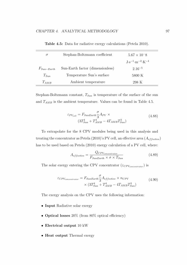
CHAPTER 4. ANALYTICAL METHODOLOGY 97
Table 4.5: Data for radiative exergy calculations (Petela 2010).
σ Stephan-Boltzmann coefficient 5.67× 10⁻⁸
J·s−1·m−2·K−4
FSun−Earth Sun-Earth factor (dimensionless) 2.16−5
TSun Temperature Sun’s surface 5800 K
TAMB Ambient temperature 298 K
Stephan-Boltzmann constant, TSun is temperature of the surface of the sun
and TAMB is the ambient temperature. Values can be found in Table 4.5.
(4.88)εPVcell= FSunEarth
σ
3APV ×
(3T 4Sun + T 4
AMB − 4TAMBT3Sun)
To extrapolate for the 8 CPV modules being used in this analysis and
treating the concentrator as Petela (2010)’s PV cell, an effective area (Aeffective)
has to be used based on Petela (2010) energy calculation of a PV cell, where:
(4.89)Aeffective =QCPVconcentrator
FSunEarth × σ × TSun
The solar exergy entering the CPV concentrator (εCPVconcentrator) is
(4.90)εCPVconcentrator = FSunEarthσ
3Aeffective × nCPV
× (3T 4Sun + T 4
AMB − 4TAMBT3Sun)
The exergy analysis on the CPV uses the following information:
• Input Radiative solar exergy
• Optical losses 20% (from 80% optical efficiency)
• Electrical output 10 kW
• Heat output Thermal exergy
CHAPTER 4. ANALYTICAL METHODOLOGY 98
Exergy of PV Cell Waste Heat (Thermal)
Thermal exergy uses the Carnot efficiency to calculate the maximum work
output of a given heat source. The Carnot efficiency uses the temperature
difference between a hot source (Thot), in this case the PV cell, and a cold
source (Tcold), in this case the surroundings, to predict the efficiency of an
ideal heat engine. (Cengel and Boles 2006) (Bejan 1997)
ηCarnot =Thot − Tcold
Thot(4.91)
εthermal = Q× ηCarnot (4.92)
Therefore the following equation calculates the exergy of the PV cell using
the cell temperature (TCPVcell), ambient temperature (TAMB) and the thermal
energy in the PV cell (QCPVcell) calculated in Equation 4.6.
(4.93)εCPVcell= QCPVcell
× TCPVcell− TAMB
TCPVcell
4.4.2 Internal Combustion Engine Electrical Genera-
tor Exergy
Fuel Exergy (Chemical)
Chemical exergy quantifies the maximum work output of a chemical reaction
in a given environment. The chemical exergy of fuels has been tabulated
by Bejan (1997) at 25◦C and 1 atmosphere. This conveniently lies within
the conditions expected for the BioCPV power plant environment, and is
compatible with the data for the CPV system which is rated to the same
conditions.
• Hydrogen = 235.2 kJ· mol−1 (Bejan 1997)
• Methane = 830.2 kJ· mol−1 (Bejan 1997)
CHAPTER 4. ANALYTICAL METHODOLOGY 99
Exhaust Exergy (Flow)
Exhaust gases are a flow, (whereas the radiator is a stationary heat source)
so flow exergy (εflow) will be used. Flow exergy uses the entropy generated
in the surroundings to determine the maximum reversible work output of
a flow. It has been simplified here by neglecting the kinetic and potential
terms. (Cengel and Boles 2006) (Bejan 1997)
(4.94)εflow = m[(hflow − hsurroundings)−Tsurroundings(sflow − ssurroundings)]
When there are several components of a flow composition the previous
equation can be altered to sum the individual components, where subscript
i denotes a single component of the flow composition. In the case of the
exhaust exergy (εgensetexhaust) this will be the products of combustion.
(4.95)
εgensetexhaust =∑
εflowi
=∑
mi[(hi − hsurroundings) −Tsurroundings(si − ssurroundings)]
Radiator Exergy (Thermal)
The exergy contained in the radiator (εgensetradiator) is a stationary heat source
and therefore uses the same approach as the PV cell. The exergy con-
tained in the radiator is calculated using the genset radiator temperature
(Tgensetradiator), ambient temperature (TAMB) and the heat energy contained
in the radiator (Qgensetradiator) calculated with Equation 4.10.
(4.96)εgensetradiator = Qgensetradiator ×Tgensetradiator − TAMB
Tgensetradiator

CHAPTER 4. ANALYTICAL METHODOLOGY 100
4.4.3 Refrigeration Exergy Replacement
Equivalent Electricity Consumption of a Vapour Compression Re-
frigerator
Calculating the avoided electrical consumption that would have been used to
provide the same amount of cooling as the absorption refrigerators modelled
in this analysis provides an alternative metric to exergy. The exergy output
(cooling) of an absorption refrigerator, quantifies the irreversibility of the
cooling provided which is challenging to relate back to the main output of
the BioCPV power plant, electricity. Whereas using the avoided electrical
consumption provides a metric that can easily be related to the electrical
output of the power plant. The following section provides the modelling
approach for this.
Using R134a (1,1,1,2 - tetrafluoroethane) as a refrigerant and the follow-
ing assumptions:
1. No losses between components.
2. Throttle is isenthalpic.
3. Compressor has an electrical efficiency of 50% (based on personal in-
dustrial experience).
4. The refrigerant leaves the evaporator as a saturated vapour.
5. Condenser temperature is 8◦C above ambient based on average differ-
ence found in absorption refrigerator modelling.
6. Refrigerant leaves the compressor as a superheated vapour calculated as
10 kJ·kg−1 above the enthalpy of dry saturated vapour at the condenser
temperature.
The thermal energy absorbed by the evaporator of the vapour compres-
sion refrigerator (QEVV C) is equal to the thermal energy absorbed by the
evaporator of the absorption refrigerator (QEV ).

CHAPTER 4. ANALYTICAL METHODOLOGY 101
(4.97)QEVV C= QEV
Enthalpy data has been extracted from the Technical Information Sheet
for HFC-134a provided by DuPont Suva Refrigerants (DuPont Suva 2016)
and copied into a spreadsheet. A series of lookup functions find the necessary
values within the model.
The evaporator output enthalpy (hEVoutV C) can be found using the evapo-
rator temperature from the absorption refrigerator and the assumption that
the refrigerant leaves the evaporator as a saturated vapour. The evaporator
input enthalpy can be found with the assumptions for the condenser temper-
ature.
(4.98)TCOV C= TAMB + 8 (◦C)
The condenser output enthalpy (hCOoutV C) can be found using the assump-
tion that that it leaves the condenser as a saturated liquid. This enthalpy can
then be used with the assumptions that there are no losses between compo-
nents and that the throttle is isenthalpic. The input and output enthalpies of
the throttle (hTHinV Cand hTHoutV C
) as well as the evaporator input enthalpy
(hEVinV C) all equal the condenser output enthalpy.
(4.99)hCOoutV C
= hTHinV C
= hTHoutV C
= hEVinV C
Using a rearranged energy balance the mass of the refrigerant in the
vapour compression cycle (mRV C) can be calculated, where QEVV C
is the
cooling energy of the vapour compression refrigerator, hEVoutV Cand hEVinV C
are the output and input enthalpies of the evaporator of the vapour com-
pression refrigerator respectively.
(4.100)mRV C=
QEVV C
hEVoutV C− hEVinV C

CHAPTER 4. ANALYTICAL METHODOLOGY 102
Assuming no losses, the compressor input enthalpy (hcompinV C) equals the
evaporator output enthalpy (hEVoutV C).
(4.101)hcompinV C= hEVoutV C
Likewise the compressor output enthalpy (hcompoutV C) equals the con-
denser input enthalpy (hCOinV C).
(4.102)hcompoutV C= hCOinV C
Therefore the ideal compressor work (EcompV Cideal) can be calculated using
an energy balance across the compressor.
(4.103)EcompV Cideal= mRV C
(hcompoutV C
− hcompinV C
)Taking the compressor efficiency into account (ηcompV C
) the actual elec-
trical consumption of the compressor and therefore the vapour compression
refrigerator (EcompV C) can be calculated.
(4.104)EcompV C=QcompV Cideal
ηcompV C
This provides the metric to compare the performance of the absorption
refrigerators investigated in this thesis to the electrical output of the BioCPV
power plant.
4.5 Presentation of Results and Discussions
The following three chapters present the results and discussions for the in-
vestigation of low temperature discontinuous waste heat utilisation from a
renewable power plant in rural India for absorption refrigeration, using ace-
tone and zinc bromide as the working fluid. They are separated as follows:
• Power Plant Energy Utilisation presents an assessment of the en-
ergy and exergy of the power plant described in Section 2.3 using the
methods described in Section 4.1 and 4.4. This allows quantification of
the amount of waste heat available and its quality.
CHAPTER 4. ANALYTICAL METHODOLOGY 103
• Absorption Refrigeration Experiment presents the findings of a
physical experiment used to provide insight into the validity of the
modelling assumptions and the practicalities of operating an absorption
refrigeration system.
• Absorption Refrigeration Modelling presents the findings from
investigations using the modelling approach described in Section 4.3,
to utilise the waste heat from an internal combustion engine electrical
generator set (genset) radiator and a concentrated photovoltaic (CPV)
system for absorption refrigeration in the conditions expected in rural
India. It also investigates the viability of the absorption refrigerator
system configurations selected in the Chapter 3.
The approach initially identifies the important variables, some of their
operating limitations and their effects on the operation of absorption
refrigeration systems in the conditions expected in rural India using the
specified heat sources. The impact of factors such as ambient temper-
ature and heat exchanger effectiveness on key components (such as the
condenser and absorber) and solution concentration limits form part of
this analysis.
The theoretical cooling output from single effect absorption refrigera-
tion systems powered by each heat source is presented at a variety of
ambient temperatures. The effect of the difference in strong and weak
solution concentration is examined with refrigeration systems powered
by both heat sources at varying ambient temperatures. This is followed
by an investigation of the evaporator tap-off method, which uses water
as a heat transfer fluid to cool the absorber and condenser. The results
are extrapolated to assess the viability of the configurations identified
in Chapter 3.
Chapter 5
Power Plant Energy Utilisation
The following chapter presents the energy and exergy profile of the BioCPV
rural renewable power plant. The energy and exergy flows through power
plant originate with solar power entering the concentrated photovoltaic (CPV)
and a biogas fuel, which is later mixed with hydrogen before being consumed
by the internal combustion engine electrical generator set (genset). These
flows are broken down into losses (such as optical, ancillary and heat) and
electricity. The electrical flow can then be followed to the users which in
this case is the 45 household community within the villages of Kaligung and
Pearson-Palli to determine the systems energetic and exergetic (or rational)
efficiency.
5.1 Energy Profile
The following section presents the energy profile of the BioCPV renewable
power plant. The CPV and genset are assessed to quantify the input energy
into the power plant and the losses from electricity generation. Assumptions
from the partners in the BioCPV research group are used to quantify the
electrical losses within the system. This process provides the information
104

CHAPTER 5. POWER PLANT ENERGY UTILISATION 105
Table 5.1: CPV energy balance.
for a Sankey diagram to be generated allowing a visual representation of the
energy flows through the power plant.
The energy profile of the CPV and generator are calculated differently
as the generator is an “off the shelf” component where generic operating
assumptions have been used. Conversely the CPV is being designed by some
of the partners and details of the specific operating conditions are from their
design specification.
5.1.1 Concentrated Photovoltaic
To simplify the modelling process the CPV is assumed to operate at a con-
stant load for 7 hours per day, this was a collective decision of the research
partners at the time of the initial designs. The electrical output of the CPV
system has been calculated from Section 4.1.1. The heat output is based
on the assumption that all the unused energy falling on the PV cell will be
converted to heat due the optical efficiency taking into account any reflective
losses. Using the rated conditions which are 25◦C and 1 atmosphere Table
5.1 shows the energy balance of the CPV system. This data is later used to
form a Sankey diagram.
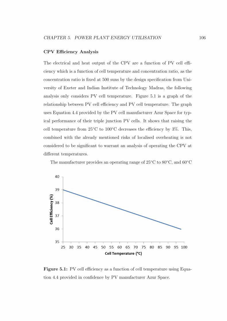
CHAPTER 5. POWER PLANT ENERGY UTILISATION 106
CPV Efficiency Analysis
The electrical and heat output of the CPV are a function of PV cell effi-
ciency which is a function of cell temperature and concentration ratio, as the
concentration ratio is fixed at 500 suns by the design specification from Uni-
versity of Exeter and Indian Institute of Technology Madras, the following
analysis only considers PV cell temperature. Figure 5.1 is a graph of the
relationship between PV cell efficiency and PV cell temperature. The graph
uses Equation 4.4 provided by the PV cell manufacturer Azur Space for typ-
ical performance of their triple junction PV cells. It shows that raising the
cell temperature from 25◦C to 100◦C decreases the efficiency by 3%. This,
combined with the already mentioned risks of localised overheating is not
considered to be significant to warrant an analysis of operating the CPV at
different temperatures.
The manufacturer provides an operating range of 25◦C to 80◦C, and 60◦C
Figure 5.1: PV cell efficiency as a function of cell temperature using Equa-
tion 4.4 provided in confidence by PV manufacturer Azur Space.
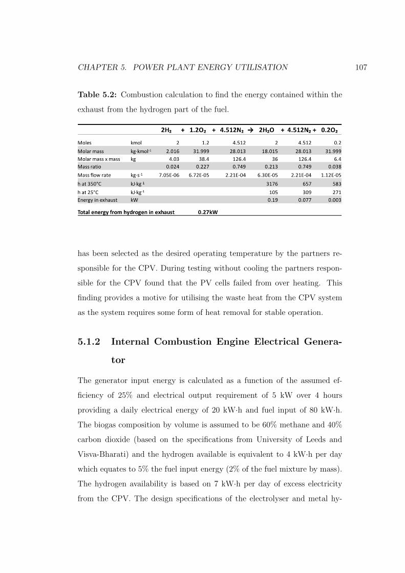
CHAPTER 5. POWER PLANT ENERGY UTILISATION 107
Table 5.2: Combustion calculation to find the energy contained within the
exhaust from the hydrogen part of the fuel.
has been selected as the desired operating temperature by the partners re-
sponsible for the CPV. During testing without cooling the partners respon-
sible for the CPV found that the PV cells failed from over heating. This
finding provides a motive for utilising the waste heat from the CPV system
as the system requires some form of heat removal for stable operation.
5.1.2 Internal Combustion Engine Electrical Genera-
tor
The generator input energy is calculated as a function of the assumed ef-
ficiency of 25% and electrical output requirement of 5 kW over 4 hours
providing a daily electrical energy of 20 kW·h and fuel input of 80 kW·h.
The biogas composition by volume is assumed to be 60% methane and 40%
carbon dioxide (based on the specifications from University of Leeds and
Visva-Bharati) and the hydrogen available is equivalent to 4 kW·h per day
which equates to 5% the fuel input energy (2% of the fuel mixture by mass).
The hydrogen availability is based on 7 kW·h per day of excess electricity
from the CPV. The design specifications of the electrolyser and metal hy-
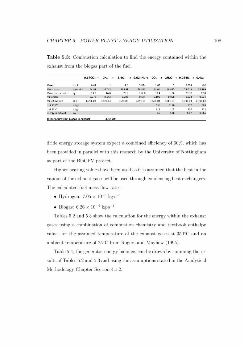
CHAPTER 5. POWER PLANT ENERGY UTILISATION 108
Table 5.3: Combustion calculation to find the energy contained within the
exhaust from the biogas part of the fuel.
dride energy storage system expect a combined efficiency of 60%, which has
been provided in parallel with this research by the University of Nottingham
as part of the BioCPV project.
Higher heating values have been used as it is assumed that the heat in the
vapour of the exhaust gases will be used through condensing heat exchangers.
The calculated fuel mass flow rates:
• Hydrogen: 7.05× 10⁻⁶ kg·s−1
• Biogas: 6.26× 10⁻⁴ kg·s−1
Tables 5.2 and 5.3 show the calculation for the energy within the exhaust
gases using a combination of combustion chemistry and textbook enthalpy
values for the assumed temperature of the exhaust gases at 350◦C and an
ambient temperature of 25◦C from Rogers and Mayhew (1995).
Table 5.4, the generator energy balance, can be drawn by summing the re-
sults of Tables 5.2 and 5.3 and using the assumptions stated in the Analytical
Methodology Chapter Section 4.1.2.

CHAPTER 5. POWER PLANT ENERGY UTILISATION 109
Table 5.4: Internal combustion engine electrical generator energy balance.
5.1.3 Renewable Power Plant Energy Flow
The data presented earlier in this section has been used to draw Figure
5.2 a Sankey diagram which shows the flow of energy through the BioCPV
renewable power plant. It uses the following additional assumptions provided
by the partners in the project:
• The solar trackers use 2 kW and are active during CPV operation (7
hours), providing a daily energy load of 14 kW·h.
• The system ancillaries equal 0.5 kW but run for 24 hours, providing a
daily load of 12 kW·h.
• Electricity generation (rated) values are 10 kW for CPV and 5 kW for
genset
• Waste heat sources are:
– 60◦C for CPV
– 80◦C for genset radiator
– 350◦C for genset exhaust

CHAPTER
5.POW
ER
PLANT
ENERGY
UTILISATIO
N110
Figure 5.2: Sankey diagram of daily energy flow in BioCPV power plant.
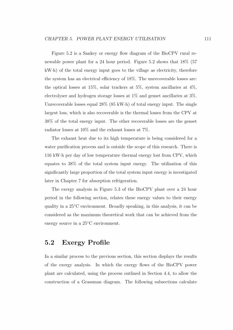
CHAPTER 5. POWER PLANT ENERGY UTILISATION 111
Figure 5.2 is a Sankey or energy flow diagram of the BioCPV rural re-
newable power plant for a 24 hour period. Figure 5.2 shows that 18% (57
kW·h) of the total energy input goes to the village as electricity, therefore
the system has an electrical efficiency of 18%. The unrecoverable losses are:
the optical losses at 15%, solar trackers at 5%, system ancillaries at 4%,
electrolyser and hydrogen storage losses at 1% and genset ancillaries at 3%.
Unrecoverable losses equal 28% (85 kW·h) of total energy input. The single
largest loss, which is also recoverable is the thermal losses from the CPV at
38% of the total energy input. The other recoverable losses are the genset
radiator losses at 10% and the exhaust losses at 7%.
The exhaust heat due to its high temperature is being considered for a
water purification process and is outside the scope of this research. There is
116 kW·h per day of low temperature thermal energy lost from CPV, which
equates to 38% of the total system input energy. The utilisation of this
significantly large proportion of the total system input energy is investigated
later in Chapter 7 for absorption refrigeration.
The exergy analysis in Figure 5.3 of the BioCPV plant over a 24 hour
period in the following section, relates these energy values to their energy
quality in a 25◦C environment. Broadly speaking, in this analysis, it can be
considered as the maximum theoretical work that can be achieved from the
energy source in a 25◦C environment.
5.2 Exergy Profile
In a similar process to the previous section, this section displays the results
of the exergy analysis. In which the exergy flows of the BioCPV power
plant are calculated, using the process outlined in Section 4.4, to allow the
construction of a Grassman diagram. The following subsections calculate
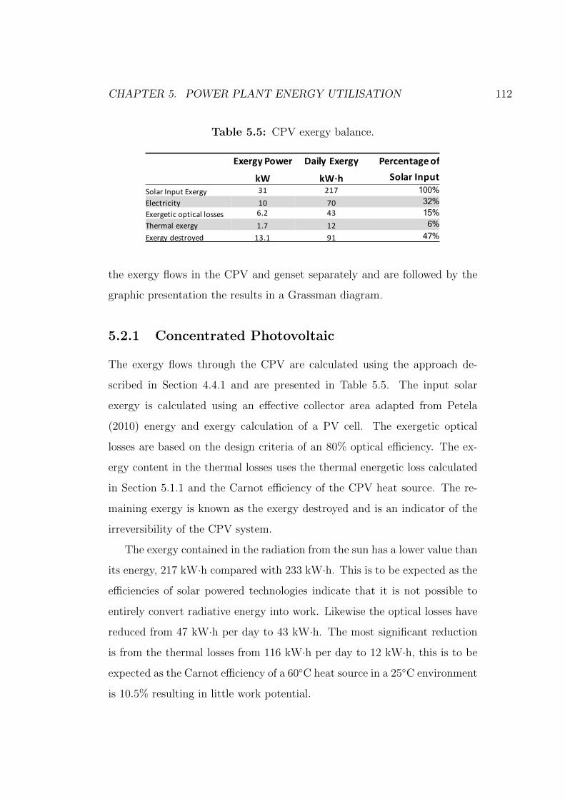
CHAPTER 5. POWER PLANT ENERGY UTILISATION 112
Table 5.5: CPV exergy balance.
ExergyPower DailyExergy Percentageof
kW kW·h SolarInputSolarInputExergy 31 217 100% Electricity 10 70 32% Exergeticopticallosses 6.2 43 15% Thermalexergy 1.7 12 6% Exergydestroyed 13.1 91 47%
the exergy flows in the CPV and genset separately and are followed by the
graphic presentation the results in a Grassman diagram.
5.2.1 Concentrated Photovoltaic
The exergy flows through the CPV are calculated using the approach de-
scribed in Section 4.4.1 and are presented in Table 5.5. The input solar
exergy is calculated using an effective collector area adapted from Petela
(2010) energy and exergy calculation of a PV cell. The exergetic optical
losses are based on the design criteria of an 80% optical efficiency. The ex-
ergy content in the thermal losses uses the thermal energetic loss calculated
in Section 5.1.1 and the Carnot efficiency of the CPV heat source. The re-
maining exergy is known as the exergy destroyed and is an indicator of the
irreversibility of the CPV system.
The exergy contained in the radiation from the sun has a lower value than
its energy, 217 kW·h compared with 233 kW·h. This is to be expected as the
efficiencies of solar powered technologies indicate that it is not possible to
entirely convert radiative energy into work. Likewise the optical losses have
reduced from 47 kW·h per day to 43 kW·h. The most significant reduction
is from the thermal losses from 116 kW·h per day to 12 kW·h, this is to be
expected as the Carnot efficiency of a 60◦C heat source in a 25◦C environment
is 10.5% resulting in little work potential.
CHAPTER 5. POWER PLANT ENERGY UTILISATION 113
Table 5.6: Calculation of flow exergy within the genset exhaust by separat-
ing each product of combustion of the biogas-hydrogen fuel mix.
5.2.2 Internal Combustion Engine Electrical Genera-
tor
The exergy flows through the genset are calculated using the approach de-
scribed in Section 4.4.2 and presented in Table 5.7. This required calculating
the exergy content of the fuel mixture and the exhaust. The thermal energy
in the radiator of the genset calculated in Section 5.1.2 can be converted to
exergy using the Carnot efficiency. The remaining exergy is known as the
exergy destroyed and is an indicator of the irreversibly of genset system.
The exergy in the exhaust presented in Table 5.6 was calculated using
Equation 4.95 for flow exergy and the products of combustion calculated in
Tables 5.2 and 5.3. Table 5.6 shows the flow exergy within the exhaust is
1 kW which over 4 hours operation will provide 4 kW·h per day of exergy
compared to the energetic value of 20 kW·h per day. This indicates that
maximum theoretical efficiency for a system generating work from the ex-
haust would only be 20% and further justifies the use of the exhaust heat for
water purification.
Table 5.7 presents the exergy flow through the genset. The exergy con-

CHAPTER 5. POWER PLANT ENERGY UTILISATION 114
Table 5.7: Genset exergy balance.
tent of the fuels was calculated using the molar exergetic heating values from
Bejan (1997) and converted with their respective molar masses to be used
with the mass flow rates calculated in Tables 5.2 and 5.3. The information
in Table 5.6 provides the exhaust exergy. The exergy in the radiator was
calculated using the Carnot efficiency of the radiator and the thermal energy
contained in the radiator calculated in Table 5.4. The electrical energy gen-
erated has an equal exergetic value and the remaining exergy is the exergy
destroyed.
The exergy content of the biogas-hydrogen fuel mixture is 74 kW·h com-
pared to an energetic value of 80 kW·h indicating a relatively small (7.5%)
irreversibility of chemical energy of the fuel source. The radiator exergy out-
put is low at 5 kW·h per day compared with an energetic value of 32 kW·h
indicating that this energy source is highly irreversible and the generation of
work would not utilise it well. 37 kW·h of exergy would be destroyed daily
with this system which is equivalent to 50% of the total fuel exergy input.
Table 5.7 also shows the exergetic or rational efficiency of the genset is 27%.
This is higher than the energetic efficiency of 25% because exergy takes into
account the exergetic value of the inputs which in this case is fuel.
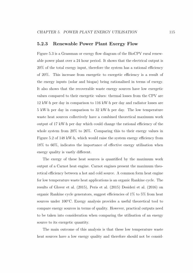
CHAPTER 5. POWER PLANT ENERGY UTILISATION 115
5.2.3 Renewable Power Plant Exergy Flow
Figure 5.3 is a Grassman or exergy flow diagram of the BioCPV rural renew-
able power plant over a 24 hour period. It shows that the electrical output is
20% of the total exergy input, therefore the system has a rational efficiency
of 20%. This increase from energetic to exergetic efficiency is a result of
the energy inputs (solar and biogas) being rationalised in terms of exergy.
It also shows that the recoverable waste energy sources have low exergetic
values compared to their energetic values: thermal losses from the CPV are
12 kW·h per day in comparison to 116 kW·h per day and radiator losses are
5 kW·h per day in comparison to 32 kW·h per day. The low temperature
waste heat sources collectively have a combined theoretical maximum work
output of 17 kW·h per day which could change the rational efficiency of the
whole system from 20% to 26%. Comparing this to their energy values in
Figure 5.2 of 148 kW·h, which would raise the system energy efficiency from
18% to 66%, indicates the importance of effective energy utilisation when
energy quality is vastly different.
The exergy of these heat sources is quantified by the maximum work
output of a Carnot heat engine. Carnot engines present the maximum theo-
retical efficiency between a hot and cold source. A common form heat engine
for low temperature waste heat applications is an organic Rankine cycle. The
results of Glover et al. (2015), Peris et al. (2015) Desideri et al. (2016) on
organic Rankine cycle generators, suggest efficiencies of 1% to 5% from heat
sources under 100◦C. Exergy analysis provides a useful theoretical tool to
compare energy sources in terms of quality. However, practical outputs need
to be taken into consideration when comparing the utilisation of an energy
source to its exergetic quantity.
The main outcome of this analysis is that these low temperature waste
heat sources have a low energy quality and therefore should not be consid-

CHAPTER 5. POWER PLANT ENERGY UTILISATION 116
ered for the generation of work and electricity. However, these waste heat
sources can be better used elsewhere. Generally the optimum uses of low
temperature waste heat sources are space or water heating as this is a direct
use and if designed appropriately could make use of almost all of the waste
energy. The problem is that hot water is not an important need in this loca-
tion whereas refrigeration, which could be used to store food and medicines
or cool a recovery room in a health centre, would be welcomed. This en-
ergy and exergy analysis together with the practical needs of the community
and the objectives of the collaborative research group provides the motive
for this body of research in investigating the utilisation of low temperature
waste heat sources from a renewable power plant in rural India for absorption
refrigeration.
CHAPTER
5.POW
ER
PLANT
ENERGY
UTILISATIO
N117
Figure 5.3: Grassman diagram of daily exergy flow in BioCPV power plant.

Chapter 6
Absorption Refrigeration
Experiment
This chapter presents the results of a lab scale experimental test rig. A
once through single effect cycle with reservoirs absorption refrigerator was
built to gain insight in to the operational performance and challenges of
an acetone and zinc bromide absorption refrigerator. Using reservoirs also
provided the opportunity to assess the possibility of using discontinuous heat
sources to provide continuous refrigeration. Continuous refrigeration in this
context refers to refrigeration that occurs over 24 hour period, 7 days a week,
without disruption.
This chapter consists of:
• Test Description presents the test rig together with the aid of a
schematic describing the process of the experiment.
• Results presents the results of this experimental test.
• Conclusions presents the main findings of this experiment.
• Photos of the experimental test rig are presented at the end of the
chapter to help visualise the system. Some of the photos also provide
evidence for the fluid state.
118
CHAPTER 6. ABSORPTION REFRIGERATION EXPERIMENT 119
6.1 Test Description
The test rig, shown schematically in Figure 6.1 and physically in Figures
6.9 to 6.12, consists of a 1 litre loading reservoir which holds the weak so-
lution. The boiler simulates the heat from CPV or genset radiator by using
a 250 W strip heater mounted to a flat plate heat exchanger with 5 k-type
thermocouples positioned along it, shown schematically in Figure 6.3. The
strong solution leaving the boiler enters the strong solution reservoir which
uses a Dreschel bottle attachment to separate the refrigerant from the strong
solution. The refrigerant vapour flows up to the condenser (a Leibig con-
denser) which is connected to the refrigerant reservoir. The strong solution
leaves the strong solution reservoir via a valve at the base and flows into the
absorber which also uses a Dreschel bottle attachment connected to a Leibig
condenser. The refrigerant flows from the refrigerant reservoir through the
evaporator (another Leibig condenser) where it evaporates and absorbs heat.
It then meets the strong solution in the absorber from the other Dreschel
port. The weak solution leaving the absorber is collected in a second weak
solution reservoir, where the test ends.
Cooling of the condenser and absorber, as well as the heat source for the
evaporator was provided by mains supply water, through the cooling jacket
of the Leibig condenser vessels used for each of these. The condenser had a
dedicated tap supplying cooling water whereas the evaporator and absorber
shared a tap. This was due to limited availability of mains water taps and
that the condenser is likely to have the highest demand for cooling water.
The flow rate and temperature of the cooling water were not controllable as
they would fluctuate depending on other users in the building. Flow rate
tests conducted at the end of the experiment showed 11 to 12 g·s−1 in the
absorber and evaporator and 24 g·s−1 in the condenser.
Between each component there is a k-type thermocouple and there are five
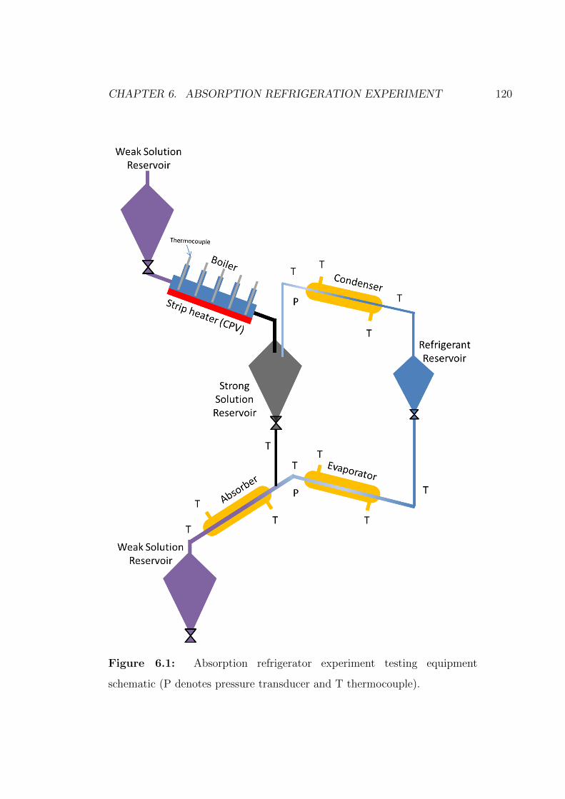
CHAPTER 6. ABSORPTION REFRIGERATION EXPERIMENT 120
Figure 6.1: Absorption refrigerator experiment testing equipment
schematic (P denotes pressure transducer and T thermocouple).
CHAPTER 6. ABSORPTION REFRIGERATION EXPERIMENT 121
thermocouples placed along the boiler. The thermocouples are sealed with
graphite ferrules into Swagelok unions. There are two GE Unik 5000 pressure
transducers; one 0 to 3 bar absolute for the high pressure side between the
strong solution reservoir and the condenser, and another 0 to 2 bar absolute
for the low pressure side between the evaporator and absorber. The pressure
transducers are also connected to Swagelok unions. The Swagelok unions
are sealed to the glass fittings using EPDM hose and o-clips. All the glass
to glass contacts were sealed using Dow Corning High Vacuum Grease. The
system requires the air to be evacuated before commencing a test to minimise
the gas mixing effect of the air and acetone vapour.
The fluids are moved by gravity and vapour pressure alone. The test is
a once through; starting at the highest point and ending at the lowest. At
the end of the test, as part of the reloading procedure, air is let in from the
top to help flush the remaining solution through. When this is complete the
components are cleaned, seals re-greased and the air evacuated. The collected
solution is then transferred to the weak solution reservoir used for loading
at the top of the rig. Tests were repeated to ensure the reproducibility of
results, the results presented here are not all from the same test run.
6.2 Results
The following subsections present the results and are broken down as follows:
• Overview presents the results for the temperature of the boiler and
the evaporator and provides information about the operating times of
the boiler and evaporator.
• Boiler presents a number of tests related to the boiler operation includ-
ing the solutions ability to maintain a boiler operating temperature and
the conditions that determine the pressure of the high pressure side.
CHAPTER 6. ABSORPTION REFRIGERATION EXPERIMENT 122
• Condenser presents the findings to suggest the input and output state
of the refrigerant in the condenser.
• Evaporator presents the findings to indicate the input and output
state of the refrigerant in the evaporator.
• Absorber presents the findings to indicate the operation of the ab-
sorber and provides insights into fluid state within the component.
6.2.1 Overview
Figure 6.2 shows an overview of the experimental results. The blue line
corresponds to the average boiler temperature. The sudden rise in the blue
line after 574 seconds shows the heater was turned on. The sudden drop
at 701 seconds is when the weak solution was released into the boiler. The
period between 701 and 904 seconds is when the boiler is heating the weak
solution and the period after is when the weak solution had stopped flowing
through the boiler and the temperature rose rapidly. The heater was turned
off shortly after as indicated by the period of cooling after 1001 seconds.
The boiler heating period indicates that an acetone and zinc bromide
solution can be used to cool the heat source in these conditions to below
60◦C, suggesting that an acetone and zinc bromide solution can be used to
cool the heat source by utilising that heat for absorption refrigeration. This
also indicates that in the wider context of this project an acetone and zinc
bromide absorption refrigerator can be used to cool the CPV system to below
60◦C. This finding can be further justified with Figure 6.4.
The red line corresponds to the evaporator temperature. At 942 seconds
the drop in temperature indicates the evaporator working and providing cool-
ing. The evaporator continues to provide cooling until 2668 seconds. The
decay at this point could be a result of several factors including: the weak
solution in the absorber and end weak solution reservoir warming up, the

CHAPTER 6. ABSORPTION REFRIGERATION EXPERIMENT 123
strong solution and refrigerant had been used up, or a slow rate of heat
transfer into the components once the test had finished.
The difference in the operating times between the boiler and evapora-
tor, 203 seconds and 1,726 seconds respectively, indicates that an absorption
refrigerator with reservoirs can use a discontinuous heat source to provide
a considerably longer period of cooling. If a solution pump was used, this
system could provide continuous cooling from a discontinuous heat source.
Figure 6.2: Boiler temperature and evaporator temperature with respect to
experiment time, where the blue line corresponds to the average boiler tem-
perature and the red line is the evaporator inlet temperature. Test details:
weak solution concentration(
mZnBr2
msolution
)at inlet 62% and 703 g of solution
collected.
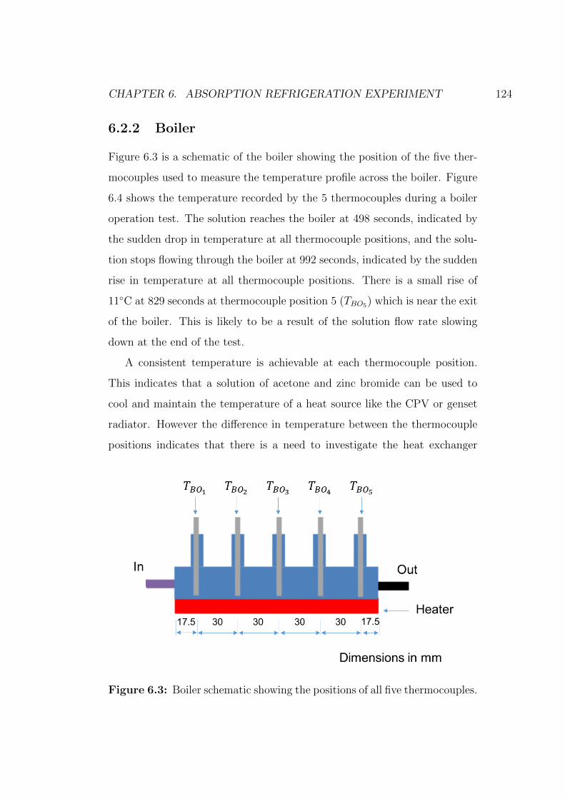
CHAPTER 6. ABSORPTION REFRIGERATION EXPERIMENT 124
6.2.2 Boiler
Figure 6.3 is a schematic of the boiler showing the position of the five ther-
mocouples used to measure the temperature profile across the boiler. Figure
6.4 shows the temperature recorded by the 5 thermocouples during a boiler
operation test. The solution reaches the boiler at 498 seconds, indicated by
the sudden drop in temperature at all thermocouple positions, and the solu-
tion stops flowing through the boiler at 992 seconds, indicated by the sudden
rise in temperature at all thermocouple positions. There is a small rise of
11◦C at 829 seconds at thermocouple position 5 (TBO5) which is near the exit
of the boiler. This is likely to be a result of the solution flow rate slowing
down at the end of the test.
A consistent temperature is achievable at each thermocouple position.
This indicates that a solution of acetone and zinc bromide can be used to
cool and maintain the temperature of a heat source like the CPV or genset
radiator. However the difference in temperature between the thermocouple
positions indicates that there is a need to investigate the heat exchanger
Figure 6.3: Boiler schematic showing the positions of all five thermocouples.
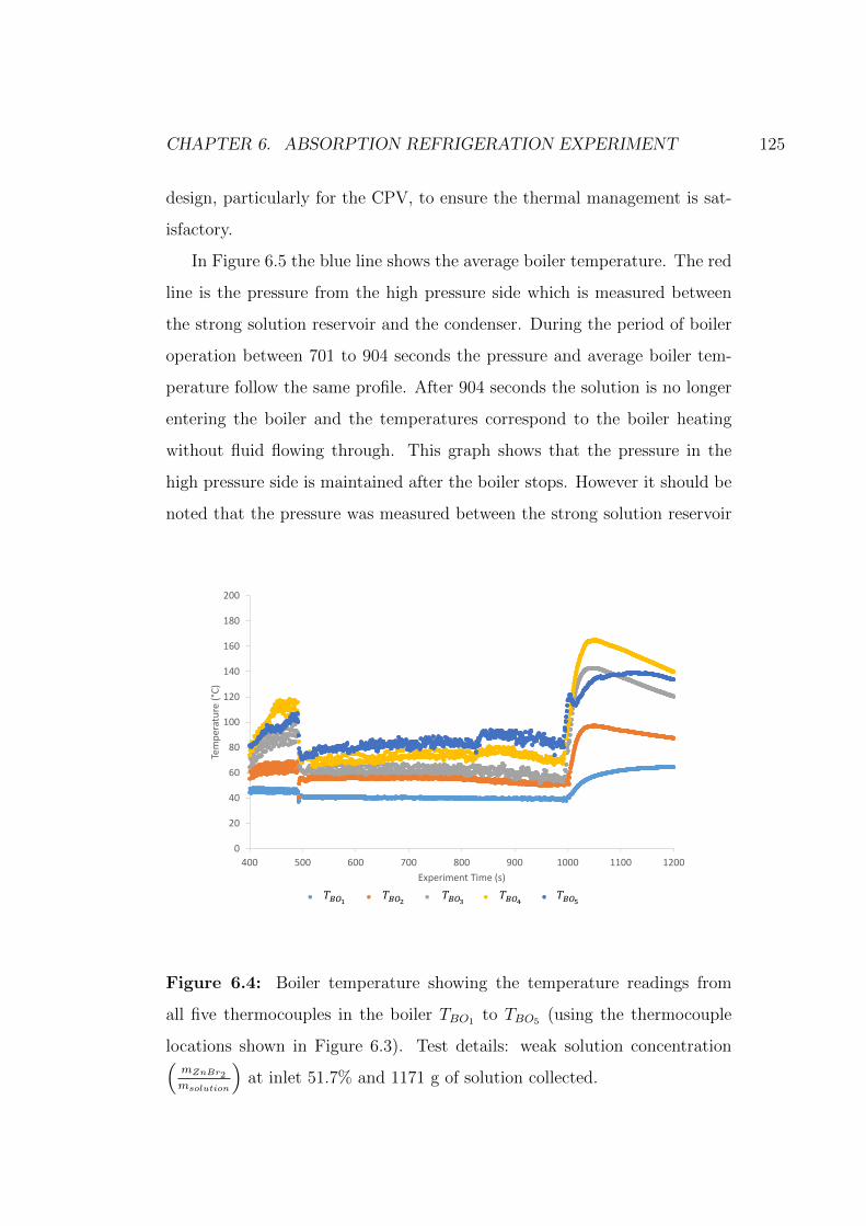
CHAPTER 6. ABSORPTION REFRIGERATION EXPERIMENT 125
design, particularly for the CPV, to ensure the thermal management is sat-
isfactory.
In Figure 6.5 the blue line shows the average boiler temperature. The red
line is the pressure from the high pressure side which is measured between
the strong solution reservoir and the condenser. During the period of boiler
operation between 701 to 904 seconds the pressure and average boiler tem-
perature follow the same profile. After 904 seconds the solution is no longer
entering the boiler and the temperatures correspond to the boiler heating
without fluid flowing through. This graph shows that the pressure in the
high pressure side is maintained after the boiler stops. However it should be
noted that the pressure was measured between the strong solution reservoir
0
20
40
60
80
100
120
140
160
180
200
400 500 600 700 800 900 1000 1100 1200
Tem
pera
ture
(°C)
Experiment Time (s)
Boiler 1 Boiler 2 Boiler 3 Boiler 4 Boiler 5𝑇"#$ 𝑇"#% 𝑇"#& 𝑇"#' 𝑇"#(
Figure 6.4: Boiler temperature showing the temperature readings from
all five thermocouples in the boiler TBO1 to TBO5 (using the thermocouple
locations shown in Figure 6.3). Test details: weak solution concentration(mZnBr2
msolution
)at inlet 51.7% and 1171 g of solution collected.

CHAPTER 6. ABSORPTION REFRIGERATION EXPERIMENT 126
and the condenser. Temperature stratification throughout the strong solu-
tion reservoir (hot at the top and cooler at the bottom) was identified by
touching the wall of the reservoir. Considering the pressure was maintained
after boiler operation. This indicates that the conditions at the top of the
reservoir determine the pressure of the high pressure side, which gradually
cools as shown by the steady drop in pressure in Figure 6.5. This finding
shows the importance of boiler exit and strong solution reservoir inlet design
to maintain the solution temperature until the refrigerant has condensed.
0
20
40
60
80
100
120
140
0
0.2
0.4
0.6
0.8
0 500 1000 1500 2000 2500
Tempe
rature(°C)
Pressure(b
ar)
ExperimentTime(s)
MeasuredPHigh AverageBoilerTemperature
Figure 6.5: Average boiler temperature (blue line, right axis) and pressure
of the high pressure side measured by the transducer between the strong
solution reservoir and the condenser (red line, left axis). Test details: weak
solution concentration(
mZnBr2
msolution
)at inlet 62% and 703 g of solution collected.

CHAPTER 6. ABSORPTION REFRIGERATION EXPERIMENT 127
6.2.3 Condenser
Figure 6.6 shows that once steady state is achieved in the condenser (at 1716
seconds) the red line which is the input to the condenser (from the boiler)
is at a higher temperature than the condenser output temperature (green
line). The condenser output and the saturation temperature based on the
pressure at this point of the experiment appear to follow each other closely,
this indicates that the acetone entering the condenser is in a superheated
state. From visual inspection and shown in Figure 6.11 the refrigerant was
a liquid at the exit of the condenser and its temperature (the green line)
is at the saturation temperature (blue line). In Figure 6.6 it is likely that
0
5
10
15
20
25
30
800 1000 1200 1400 1600 1800 2000 2200 2400 2600
Tempe
rature(°C)
ExperimentTime(s)
TsatCalculatedfromPHigh CondenserIn/BoilerROut CondenserOut/RReservoirIn
Figure 6.6: Operating temperatures of the condenser (green line for inlet
and red line for outlet) with the high pressure converted to acetone saturation
temperature using Equation 4.15 (blue line). Test details: weak solution
concentration(
mZnBr2
msolution
)at inlet 62% and 703 g of solution collected.
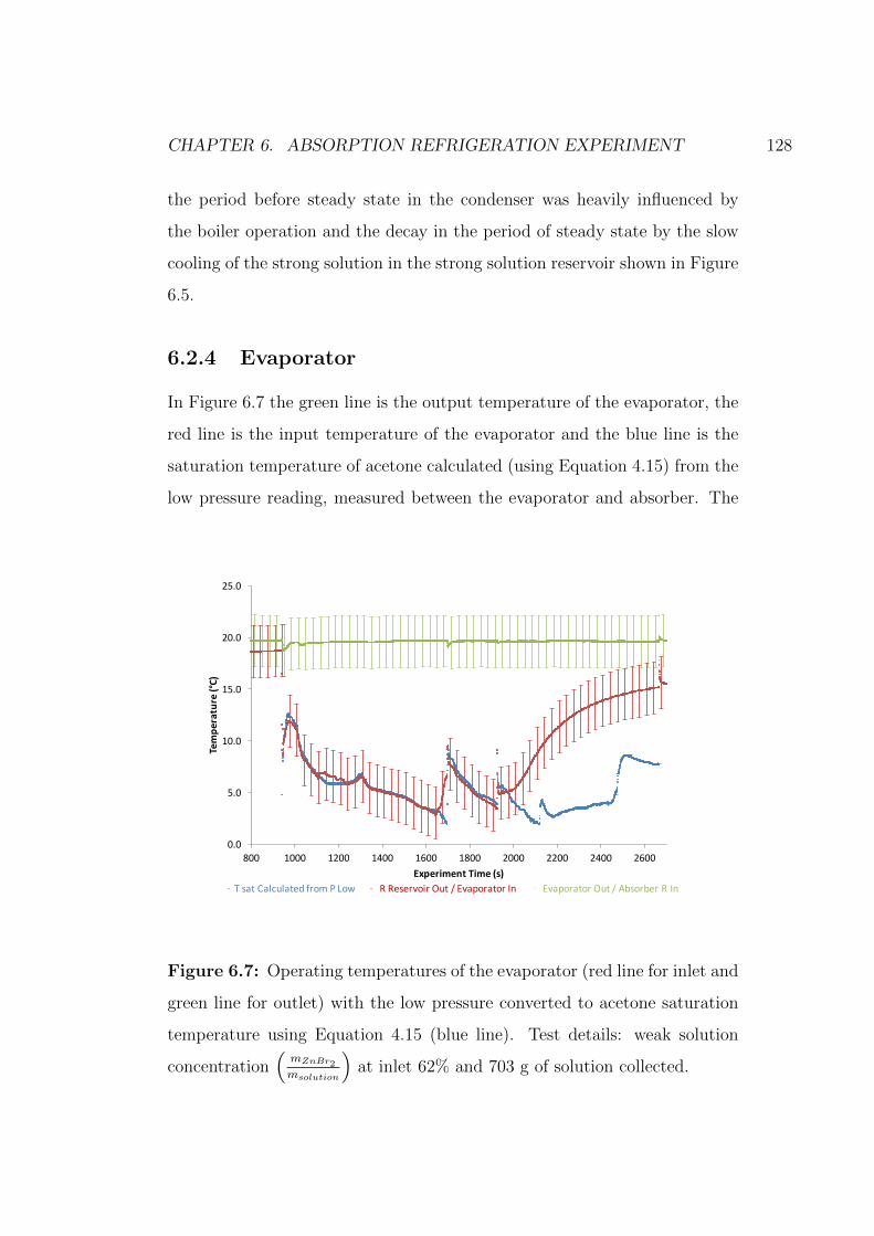
CHAPTER 6. ABSORPTION REFRIGERATION EXPERIMENT 128
the period before steady state in the condenser was heavily influenced by
the boiler operation and the decay in the period of steady state by the slow
cooling of the strong solution in the strong solution reservoir shown in Figure
6.5.
6.2.4 Evaporator
In Figure 6.7 the green line is the output temperature of the evaporator, the
red line is the input temperature of the evaporator and the blue line is the
saturation temperature of acetone calculated (using Equation 4.15) from the
low pressure reading, measured between the evaporator and absorber. The
0.0
5.0
10.0
15.0
20.0
25.0
800 1000 1200 1400 1600 1800 2000 2200 2400 2600
Tempe
rature(°C)
ExperimentTime(s)TsatCalculatedfromPLow RReservoirOut/EvaporatorIn EvaporatorOut/AbsorberRIn
Figure 6.7: Operating temperatures of the evaporator (red line for inlet and
green line for outlet) with the low pressure converted to acetone saturation
temperature using Equation 4.15 (blue line). Test details: weak solution
concentration(
mZnBr2
msolution
)at inlet 62% and 703 g of solution collected.
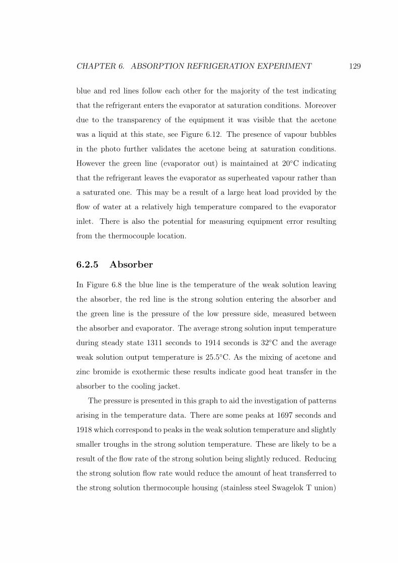
CHAPTER 6. ABSORPTION REFRIGERATION EXPERIMENT 129
blue and red lines follow each other for the majority of the test indicating
that the refrigerant enters the evaporator at saturation conditions. Moreover
due to the transparency of the equipment it was visible that the acetone
was a liquid at this state, see Figure 6.12. The presence of vapour bubbles
in the photo further validates the acetone being at saturation conditions.
However the green line (evaporator out) is maintained at 20◦C indicating
that the refrigerant leaves the evaporator as superheated vapour rather than
a saturated one. This may be a result of a large heat load provided by the
flow of water at a relatively high temperature compared to the evaporator
inlet. There is also the potential for measuring equipment error resulting
from the thermocouple location.
6.2.5 Absorber
In Figure 6.8 the blue line is the temperature of the weak solution leaving
the absorber, the red line is the strong solution entering the absorber and
the green line is the pressure of the low pressure side, measured between
the absorber and evaporator. The average strong solution input temperature
during steady state 1311 seconds to 1914 seconds is 32◦C and the average
weak solution output temperature is 25.5◦C. As the mixing of acetone and
zinc bromide is exothermic these results indicate good heat transfer in the
absorber to the cooling jacket.
The pressure is presented in this graph to aid the investigation of patterns
arising in the temperature data. There are some peaks at 1697 seconds and
1918 which correspond to peaks in the weak solution temperature and slightly
smaller troughs in the strong solution temperature. These are likely to be a
result of the flow rate of the strong solution being slightly reduced. Reducing
the strong solution flow rate would reduce the amount of heat transferred to
the strong solution thermocouple housing (stainless steel Swagelok T union)
CHAPTER 6. ABSORPTION REFRIGERATION EXPERIMENT 130
allowing the solution to cool slightly to ambient conditions. However the slow
flow rate of solution would allow more time for the refrigerant vapour to be
absorbed and the exothermic reaction would cause the now more dilute weak
solution to warm up. As there is little control over the refrigerant vapour
absorption into the strong solution in the absorber the increased dilution
and temperature of the weak solution can cause a slight pressure rise thus
explaining the peaks in pressure and weak solution temperature.
0
5
10
15
20
25
30
35
40
45
0
0.1
0.2
0.3
0.4
700 900 1100 1300 1500 1700 1900 2100 2300 2500
Tempe
rature(°C)
Pressure(b
ar)
ExperimentTime(s)
LowPressure AbsorberOutputTemperature AbsorberSSInputTemperature
Figure 6.8: Operating input (red line, right axis) and output (blue line,
right axis) temperatures of the absorber along with the pressure between the
absorber and evaporator (green line, left axis). Test details: weak solution
concentration(
mZnBr2
msolution
)at inlet 62% and 703 g of solution collected.

CHAPTER 6. ABSORPTION REFRIGERATION EXPERIMENT 131
6.2.6 Error Analysis
Measuring equipment used in this experiment had the following tolerances:
Thermocouples ±2.5◦C and the pressure transducers ±0.04% of full scale
deflection (2 bar and 3 bar for low and high pressure sides respectively)
resulting in ±0.0008 bar and ±0.0012 bar on the low and high pressure
sides respectively. These errors were converted using the respective state
equations depending whether pressure or temperature was required when
analysing pure acetone. Pressure and temperature measurement frequency
was 3 Hz, this provided an accurate picture of the trends taking place with
the experiment. Unfortunately there were issues with leaks and control of
the flow rates. For example the heat transfer fluid (mains water) did not
have adequate flow control to calculate an accurate cooling output, making
calculating an accurate physical CoP impractical.
6.3 Absorption Refrigeration Experiment Con-
clusion
This experiment consisted of a once through single effect absorption refrig-
erator with reservoirs and provided insight into the physical workings and
challenges of an acetone and zinc bromide absorption refrigerator with reser-
voirs. It also provided some confidence in the modelling approach used in
the next chapter. The use of glass allowed visual inspection of the fluid and
its state throughout the cycle. This also aided the understanding of the sys-
tem and the operating complexities. The instrumentation allowed reasonable
analysis of the workings of each component with the system.
The experiment showed considerably longer period of cooling heat trans-
fer in the evaporator to that of the heat transfer in the boiler, indicating that
the use of reservoirs could allow continuous cooling from discontinuous heat
CHAPTER 6. ABSORPTION REFRIGERATION EXPERIMENT 132
sources. The stable temperatures achieved at each thermocouple position
in the boiler indicated that acetone and zinc bromide could be used to cool
and maintain the CPV PV cells at a suitably low temperature while utilising
that extracted heat to provide refrigeration. The pressure in the high pres-
sure side is maintained after boiler operation indicating the importance of
boiler exit and strong solution reservoir inlet design to optimise condensing,
together with effective heat exchange in the condenser, all of which determine
the concentration of the strong solution. The results from the condenser in-
dicated that the inlet was a superheated vapour and outlet was a saturated
liquid. Interestingly the evaporator showed a superheated outlet which was
unexpected, this is likely to be a result of a large heat load applied to the
evaporator.
Issues such as leaks and control would have caused some of the sources of
error which were extremely challenging to measure, such as the continuously
varying flow rates of the solution and the effects these had on solution concen-
trations. The errors resulting from the accuracy of the measuring equipment
and human errors were not sufficient to interfere with the key observations of
the test which showed generally well the predicted behaviour of the system.
This test procedure provided insight into the operation an acetone and zinc
bromide absorption refrigerator and provided confidence for the modelling
approach described in Chapter 4.
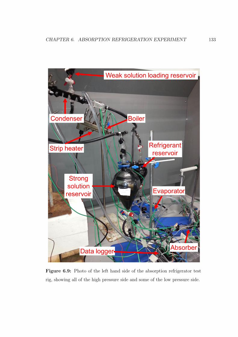
CHAPTER 6. ABSORPTION REFRIGERATION EXPERIMENT 133
Figure 6.9: Photo of the left hand side of the absorption refrigerator test
rig, showing all of the high pressure side and some of the low pressure side.
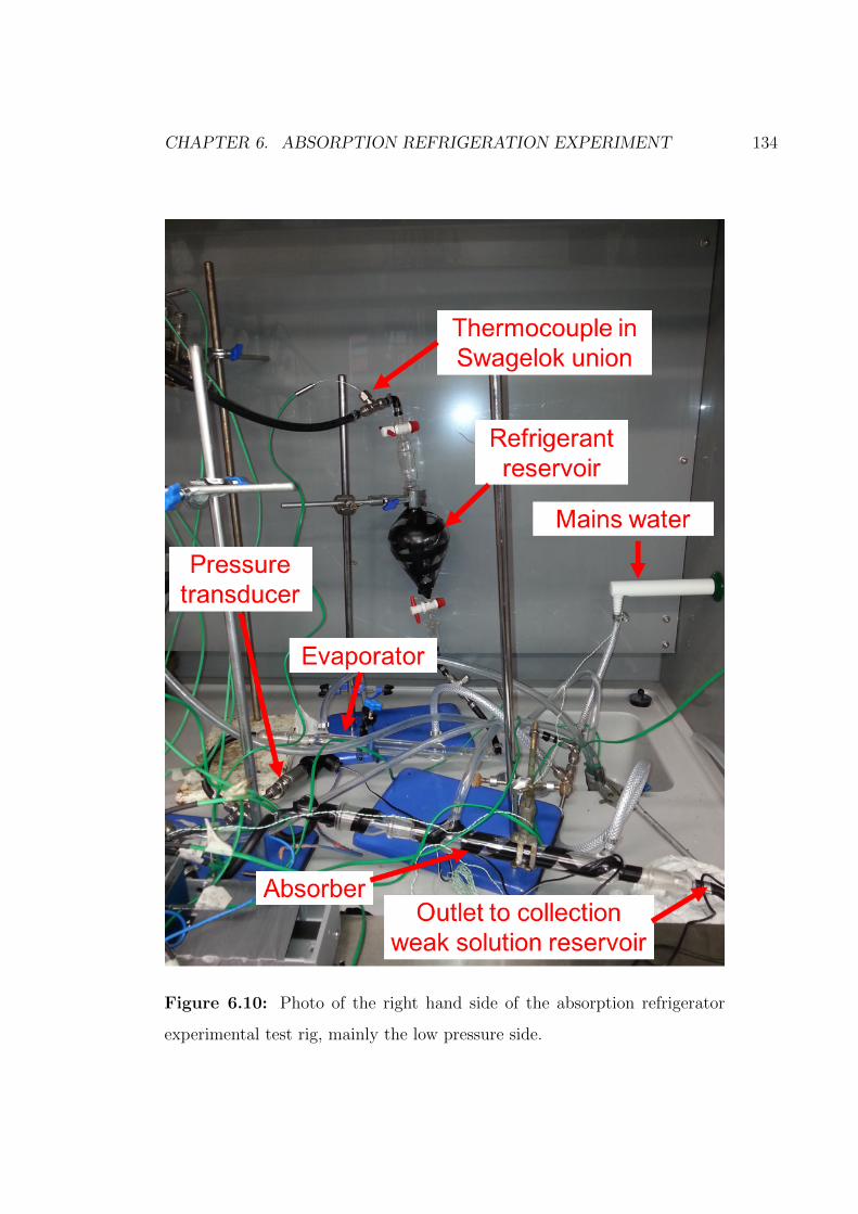
CHAPTER 6. ABSORPTION REFRIGERATION EXPERIMENT 134
Figure 6.10: Photo of the right hand side of the absorption refrigerator
experimental test rig, mainly the low pressure side.
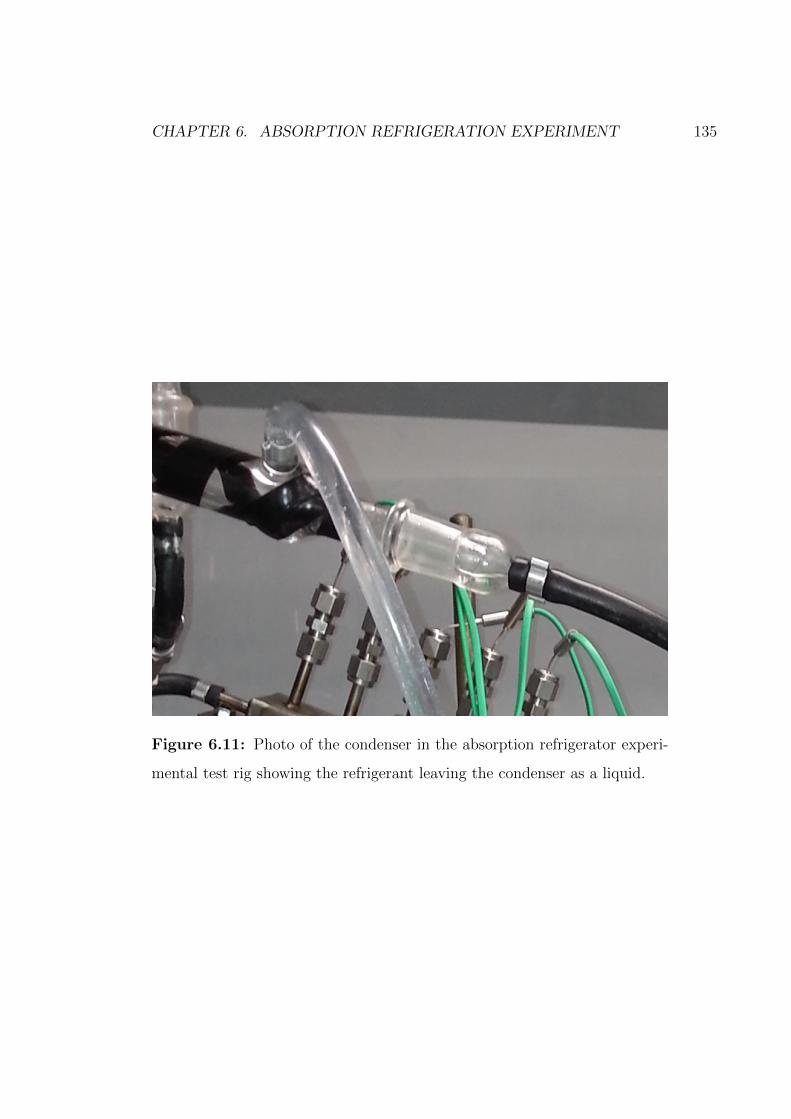
CHAPTER 6. ABSORPTION REFRIGERATION EXPERIMENT 135
Figure 6.11: Photo of the condenser in the absorption refrigerator experi-
mental test rig showing the refrigerant leaving the condenser as a liquid.

CHAPTER 6. ABSORPTION REFRIGERATION EXPERIMENT 136
Figure 6.12: Photo of the evaporator in the absorption refrigerator exper-
imental test rig showing the refrigerant as a liquid entering the evaporator
and vapour bubbles forming inside the evaporator.
Chapter 7
Absorption Refrigeration
Modelling
The following chapter investigates using the waste heat from the CPV and
genset radiator for absorption refrigeration. Initially the operating limits
have been investigated to provide the boundaries of investigation for the
different configurations of absorption refrigerator, which were identified as
suitable in Chapter 3. Each heat source is then investigated separately to
be used in independent absorption refrigerators. This is followed by an eval-
uation of the evaporator tap off method investigating how each heat source
could independently optimise the evaporator temperature. Based on these
results the combined cycle and double boiler with evaporator tap off cycle
will be evaluated, as will the need for further modelling.
For refrigeration benchmarking purposes the Food Standards Agency in
the UK recommend refrigerator temperatures of 5◦C and freezer temper-
atures of -18◦C. (FSA 2015). They also stipulate “Food that is likely to
support the growth of pathogenic micro-organisms or the formation of toxins
must be kept at a temperature of 8◦C or below.” (FSA 2007). Harrison
(1996) states that some root vegetables such as potatoes, sweet potatoes,
137
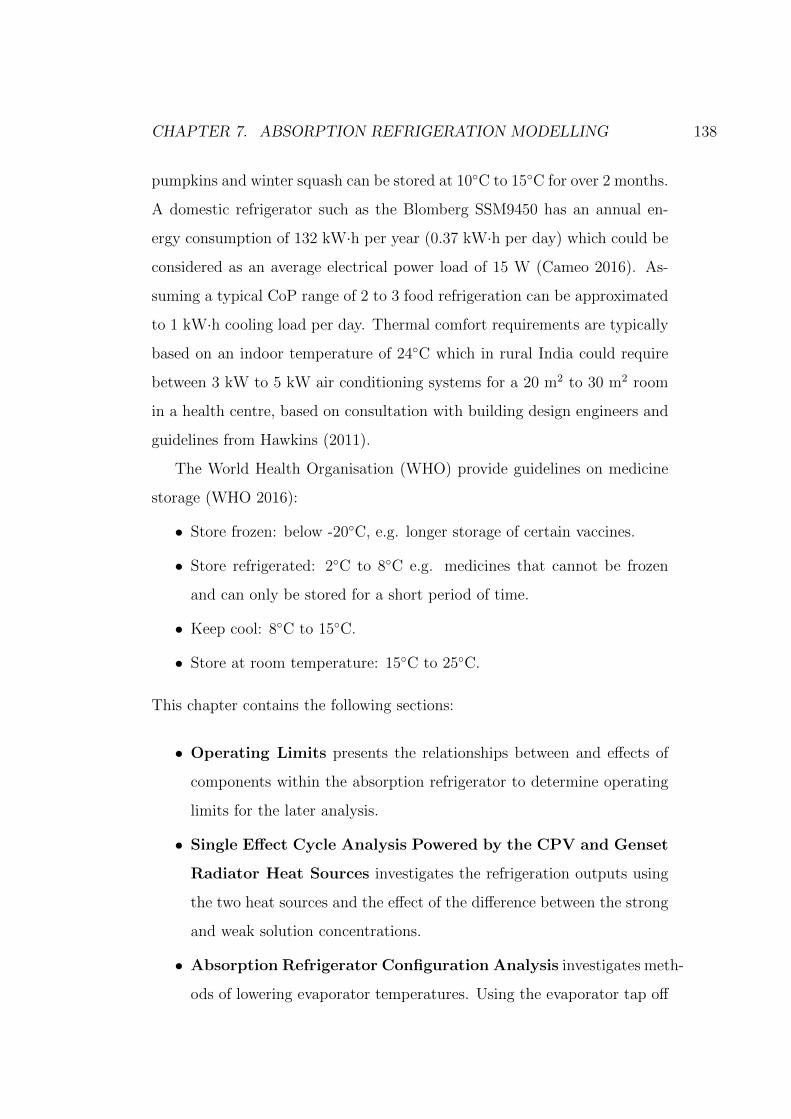
CHAPTER 7. ABSORPTION REFRIGERATION MODELLING 138
pumpkins and winter squash can be stored at 10◦C to 15◦C for over 2 months.
A domestic refrigerator such as the Blomberg SSM9450 has an annual en-
ergy consumption of 132 kW·h per year (0.37 kW·h per day) which could be
considered as an average electrical power load of 15 W (Cameo 2016). As-
suming a typical CoP range of 2 to 3 food refrigeration can be approximated
to 1 kW·h cooling load per day. Thermal comfort requirements are typically
based on an indoor temperature of 24◦C which in rural India could require
between 3 kW to 5 kW air conditioning systems for a 20 m2 to 30 m2 room
in a health centre, based on consultation with building design engineers and
guidelines from Hawkins (2011).
The World Health Organisation (WHO) provide guidelines on medicine
storage (WHO 2016):
• Store frozen: below -20◦C, e.g. longer storage of certain vaccines.
• Store refrigerated: 2◦C to 8◦C e.g. medicines that cannot be frozen
and can only be stored for a short period of time.
• Keep cool: 8◦C to 15◦C.
• Store at room temperature: 15◦C to 25◦C.
This chapter contains the following sections:
• Operating Limits presents the relationships between and effects of
components within the absorption refrigerator to determine operating
limits for the later analysis.
• Single Effect Cycle Analysis Powered by the CPV and Genset
Radiator Heat Sources investigates the refrigeration outputs using
the two heat sources and the effect of the difference between the strong
and weak solution concentrations.
• Absorption Refrigerator Configuration Analysis investigates meth-
ods of lowering evaporator temperatures. Using the evaporator tap off

CHAPTER 7. ABSORPTION REFRIGERATION MODELLING 139
a proportion of the cooling from the evaporator along with ambient
cooling is used to lower the operating temperatures of the condenser
and absorber. This analysis is then used to evaluate the practicality of
the other systems identified in Section 3.3.7.
• Configuration Conclusion presents the outcome of the configuration
analysis and models the daily outputs of the selected configuration of
absorption refrigerators over a range of ambient temperatures.
• Within Day Analysis investigates the performance within a day
of the CPV powered absorption refrigerator for typical conditions ex-
pected in the region using historical weather data.
• Absorption Refrigerator Modelling Conclusion presents the main
findings of this analysis and its application elsewhere.
7.1 Operating Limits
The primary challenge with absorption refrigeration is a balancing act de-
scribed in the Challenges of Absorption Refrigeration (Section 3.3.1). This
subsection addresses the challenge with the following investigations:
• The parameter effects on strong solution concentration on the high
pressure side of the refrigerator, the parameters are: condenser tem-
perature, boiler temperature, ambient temperature and condenser heat
exchanger effectiveness.
• The parameter effects on evaporator temperature on the low pressure
side of the refrigerator, the parameters are: weak solution concentra-
tion, ambient temperature, absorber temperature and absorber heat
exchanger effectiveness.
• The effect of the difference between strong and weak solution concen-
trations on evaporator temperature.
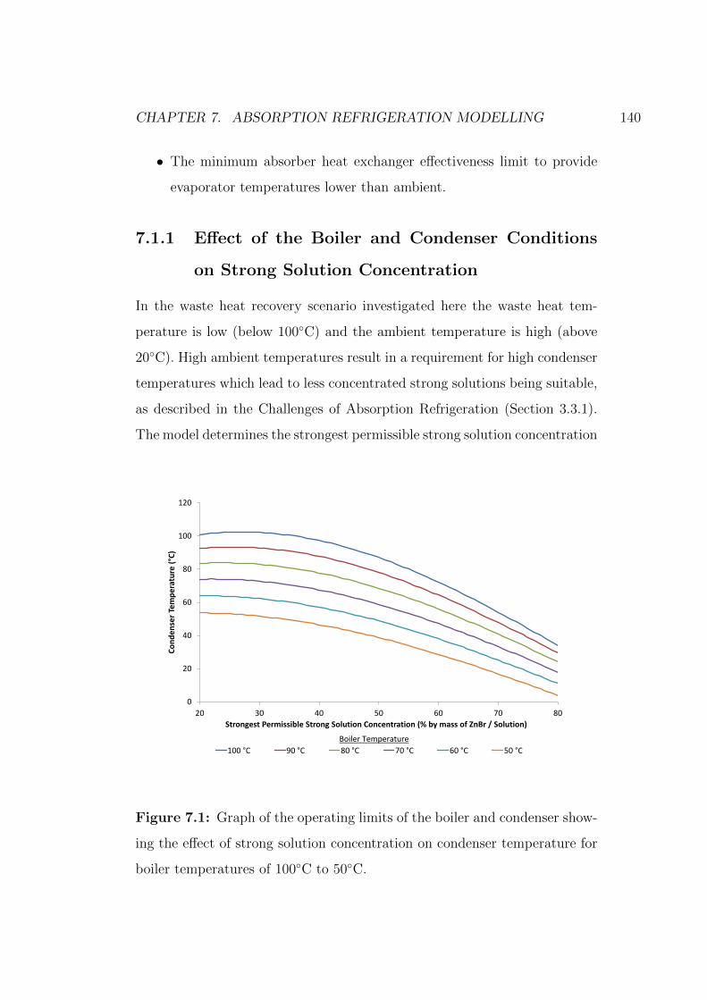
CHAPTER 7. ABSORPTION REFRIGERATION MODELLING 140
• The minimum absorber heat exchanger effectiveness limit to provide
evaporator temperatures lower than ambient.
7.1.1 Effect of the Boiler and Condenser Conditions
on Strong Solution Concentration
In the waste heat recovery scenario investigated here the waste heat tem-
perature is low (below 100◦C) and the ambient temperature is high (above
20◦C). High ambient temperatures result in a requirement for high condenser
temperatures which lead to less concentrated strong solutions being suitable,
as described in the Challenges of Absorption Refrigeration (Section 3.3.1).
The model determines the strongest permissible strong solution concentration
0
20
40
60
80
100
120
20 30 40 50 60 70 80
Co
nd
en
ser
Tem
pe
ratu
re (
°C)
Strongest Permissible Strong Solution Concentration (% by mass of ZnBr / Solution)
100 °C 90 °C 80 °C 70 °C 60 °C 50 °C
Boiler Temperature
Figure 7.1: Graph of the operating limits of the boiler and condenser show-
ing the effect of strong solution concentration on condenser temperature for
boiler temperatures of 100◦C to 50◦C.
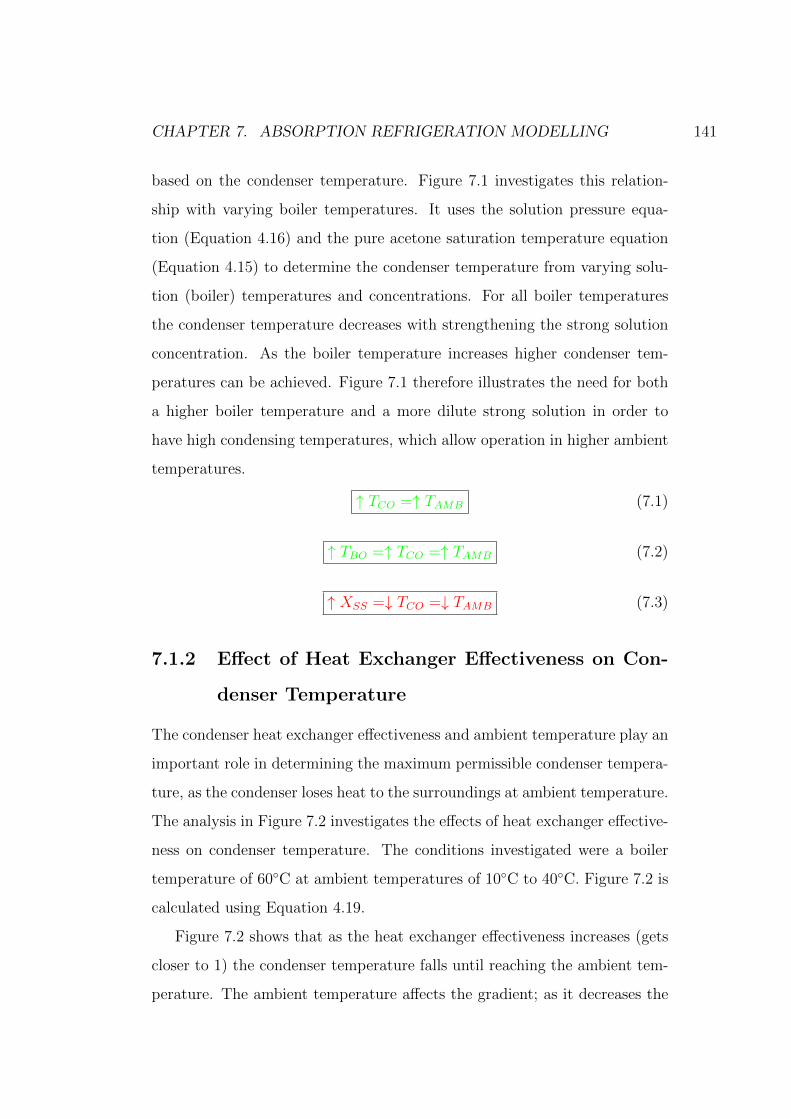
CHAPTER 7. ABSORPTION REFRIGERATION MODELLING 141
based on the condenser temperature. Figure 7.1 investigates this relation-
ship with varying boiler temperatures. It uses the solution pressure equa-
tion (Equation 4.16) and the pure acetone saturation temperature equation
(Equation 4.15) to determine the condenser temperature from varying solu-
tion (boiler) temperatures and concentrations. For all boiler temperatures
the condenser temperature decreases with strengthening the strong solution
concentration. As the boiler temperature increases higher condenser tem-
peratures can be achieved. Figure 7.1 therefore illustrates the need for both
a higher boiler temperature and a more dilute strong solution in order to
have high condensing temperatures, which allow operation in higher ambient
temperatures.
(7.1)↑ TCO =↑ TAMB
(7.2)↑ TBO =↑ TCO =↑ TAMB
(7.3)↑ XSS =↓ TCO =↓ TAMB
7.1.2 Effect of Heat Exchanger Effectiveness on Con-
denser Temperature
The condenser heat exchanger effectiveness and ambient temperature play an
important role in determining the maximum permissible condenser tempera-
ture, as the condenser loses heat to the surroundings at ambient temperature.
The analysis in Figure 7.2 investigates the effects of heat exchanger effective-
ness on condenser temperature. The conditions investigated were a boiler
temperature of 60◦C at ambient temperatures of 10◦C to 40◦C. Figure 7.2 is
calculated using Equation 4.19.
Figure 7.2 shows that as the heat exchanger effectiveness increases (gets
closer to 1) the condenser temperature falls until reaching the ambient tem-
perature. The ambient temperature affects the gradient; as it decreases the
CHAPTER 7. ABSORPTION REFRIGERATION MODELLING 142
gradient increases. This is to be expected since Equation 4.19 is a straight
line equation where (TAMB − TBO) is the gradient and boiler temperature
(TBO) is the y intercept.
(7.4)↑ εCO = TCO → TAMB
If the heat exchanger effectiveness and the ambient temperature are known
the condenser temperature can be calculated. The condenser temperatures
can then be converted into saturation pressures using Equation 4.20. These
pressures along with Equation 4.16 can computationally (in this case us-
ing lookup tables) find the strongest permissible solution concentration at
the chosen boiler temperature. To illustrate this for a boiler temperature
of 60◦C Figure 7.3 shows the effect of heat exchanger effectiveness on the
0
10
20
30
40
50
60
70
0 0.1 0.2 0.3 0.4 0.5 0.6 0.7 0.8 0.9 1
Co
nd
en
ser
Tem
pe
ratu
re (
°C)
Heat Exchanger Effectiveness
10 20 30 40Ambient Temperature (°C)
Figure 7.2: Graph of the effect of condenser heat exchanger effectiveness
on condenser temperature, for a boiler temperature of 60◦C at ambient tem-
peratures of 40◦C to 10◦C.
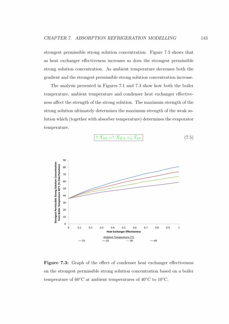
CHAPTER 7. ABSORPTION REFRIGERATION MODELLING 143
strongest permissible strong solution concentration. Figure 7.3 shows that
as heat exchanger effectiveness increases so does the strongest permissible
strong solution concentration. As ambient temperature decreases both the
gradient and the strongest permissible strong solution concentration increase.
The analysis presented in Figures 7.1 and 7.3 show how both the boiler
temperature, ambient temperature and condenser heat exchanger effective-
ness affect the strength of the strong solution. The maximum strength of the
strong solution ultimately determines the maximum strength of the weak so-
lution which (together with absorber temperature) determines the evaporator
temperature.
(7.5)↑ XSS =↑ XWS =↓ TEV
0
10
20
30
40
50
60
70
80
90
0 0.1 0.2 0.3 0.4 0.5 0.6 0.7 0.8 0.9 1
Stro
nge
st P
erm
issi
ble
Str
on
g So
luti
on
Co
nce
ntr
atio
n
fro
m B
oile
r Te
mp
era
ture
60
°C (
% Z
nb
r/So
luti
on
)
Heat Exchanger Effectiveness
10 20 30 40Ambient Temperature (°C)
Figure 7.3: Graph of the effect of condenser heat exchanger effectiveness
on the strongest permissible strong solution concentration based on a boiler
temperature of 60◦C at ambient temperatures of 40◦C to 10◦C.

CHAPTER 7. ABSORPTION REFRIGERATION MODELLING 144
(7.6)↑ εCO =↑ XSS =↓ TEV
(7.7)↑ TAMB =↓ XSS =↑ TEV
7.1.3 Effect of Weak Solution on Absorber and Evap-
orator
Figure 7.4 extends the same analysis used in Figure 7.1 for the weak solution
concentration and absorber temperature. Figure 7.4 demonstrates the evap-
orator temperature with weak solution concentration variation and absorber
temperature variation. The findings show lower evaporator temperatures,
which can provide more versatile cooling, can be achieved by reducing ab-
sorber temperature and strengthening the weak solution concentration leav-
-30
-20
-10
0
10
20
30
40
50
20 30 40 50 60 70 80
Evap
ora
tor
Tem
pe
ratu
re (
°C)
Weak Solution Concentration (% by mass of ZnBr / Solution)
40 °C 35 °C 30 °C 25 °C 20 °C 15 °C
Absorber Temperature
Figure 7.4: Graph of the operating limits of the absorber and evaporator
showing the effect of weak solution concentration on evaporator temperature
for absorber temperatures of 40◦C to 15◦C.
CHAPTER 7. ABSORPTION REFRIGERATION MODELLING 145
ing the absorber. In warmer climates this presents a problem as more con-
centrated weak solutions require more concentrated strong solutions which
require low condenser temperatures and hence low ambient temperatures.
Moreover the absorber needs to reject heat to the surroundings and its tem-
perature is therefore also governed by ambient temperature, unless there is
additional cooling available.
(7.8)↑ XWS =↓ TEV
(7.9)↑ TAB =↑ TEV
7.1.4 Effect of Absorber to Ambient Heat Exchanger
Effectiveness
The output conditions of the absorber are the weak solution concentration
and temperature. In the model used for this subsection the solution con-
centrations are fixed variables. The mixing of refrigerant into solution is
exothermic and the solution vapour pressure is a function of solution tem-
perature and concentration. In the absorber the refrigerant is being absorbed
into the strong solution and heat is generated. The ability to remove this
heat in the absorber will determine the output conditions of the absorber.
In this model, as the solution concentrations are fixed, the heat exchanger
effectiveness of the absorber determines the weak solution temperature (ab-
sorber output); which determines the vapour pressure of the solution. The
weak solution at the outlet of the absorber has reached maximum capacity
to absorb refrigerant at those conditions, therefore determining the vapour
pressure in the absorber. The absorber and evaporator require the free flow
of refrigerant vapour between the components in order to allow the absorp-
tion process of refrigerant vapour into solution. This results in the pressure
of the absorber equalling the pressure in the evaporator. The pressure in the
CHAPTER 7. ABSORPTION REFRIGERATION MODELLING 146
evaporator determines the saturation conditions in the evaporator. The evap-
orator is assumed to operate at saturation conditions. Therefore the vapour
pressure produced from the output conditions of the absorber determines the
evaporator temperature.
The analysis shown in Figures 7.5 and 7.6 determines the conditions in
the absorber for a range of ambient temperatures where example solution
concentrations of 60% strong and 54% weak mZnBr
msolutionare used. These solu-
tion concentrations are based on the analysis in Figure 7.1 which shows a
strong solution concentration of 60% should operate in the ambient condi-
tions expected at the CPV desired operating temperature. The weak solution
concentration (54%) was arbitrarily selected as starting point of this inves-
tigation based on typical strong and weak solution concentration differences
found in the literature. The calculation method is described in Section 4.3.9.
The hot inlet is calculated from the adiabatic mixing of the refrigerant leaving
the evaporator and the strong solution from its reservoir at ambient temper-
ature. The cold stream (which could be air or the heat transfer fluid cooling
to ambient and not below ambient) is at ambient conditions and the hot
outlet is the weak solution leaving the absorber.
(7.10)↑ εAB =↓ TABWS
(7.11)↑ TAMB =↑ TABWS
Figure 7.5 presents the relationship between absorber outlet (weak solu-
tion) temperature and absorber heat exchanger effectiveness at a range of
ambient temperatures for strong and weak solution concentrations of 60%
and 54% respectively. It shows that as the heat exchanger effectiveness in-
creases the absorber outlet temperature decreases for all ambient tempera-
tures investigated. Increasing ambient temperature increases the weak solu-
tion temperature for the range of heat exchanger effectiveness analysed here.

CHAPTER 7. ABSORPTION REFRIGERATION MODELLING 147
This analysis can be converted into evaporator temperature through calcu-
lating the saturation pressure, with Equation 4.16, at the outlet conditions of
the absorber and converting that pressure to a saturation temperature, with
Equation 4.15, for pure acetone, the results of which are shown in Figure 7.6.
Figure 7.6 shows that, for the conditions selected (strong and weak solu-
tion concentrations of 60% and 54% respectively), as absorber heat exchanger
effectiveness increases evaporator temperature decreases and when ambient
temperature decreases the gradient of the trend decreases slightly. The most
important finding is that for fixed solution concentrations there is an ab-
sorber heat exchanger effectiveness limit to achieve evaporator temperatures
lower than ambient, shown with the orange dashed line. For example at
an ambient temperature of 30◦C and heat exchanger effectiveness of 0.6 the
0
10
20
30
40
50
60
70
80
90
100
0 0.1 0.2 0.3 0.4 0.5 0.6 0.7 0.8 0.9 1
Absorber Outlet (Weak So
lutio
n) Te
mpe
rature (°C)
Absorber Heat Exchanger Effectiveness
10 20 30 40 50Ambient Temperature (°C)Ambient Temperature (°C)
Figure 7.5: Effect of absorber heat exchanger effectiveness on absorber
outlet (weak solution) temperature for a strong solution concentration of 60%
and weak solution concentration of 54%(
mZnBr2
msolution
)for ambient temperatures
of 10◦C to 50◦C.
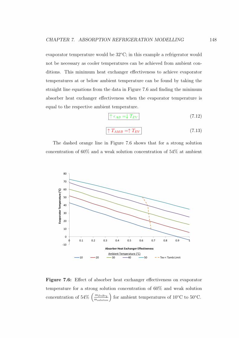
CHAPTER 7. ABSORPTION REFRIGERATION MODELLING 148
evaporator temperature would be 32◦C; in this example a refrigerator would
not be necessary as cooler temperatures can be achieved from ambient con-
ditions. This minimum heat exchanger effectiveness to achieve evaporator
temperatures at or below ambient temperature can be found by taking the
straight line equations from the data in Figure 7.6 and finding the minimum
absorber heat exchanger effectiveness when the evaporator temperature is
equal to the respective ambient temperature.
(7.12)↑ εAB =↓ TEV
(7.13)↑ TAMB =↑ TEV
The dashed orange line in Figure 7.6 shows that for a strong solution
concentration of 60% and a weak solution concentration of 54% at ambient
-10
0
10
20
30
40
50
60
70
80
0 0.1 0.2 0.3 0.4 0.5 0.6 0.7 0.8 0.9 1
Evap
oratorTe
mperature(°C)
AbsorberHeatExchangerEffectiveness
10 20 30 40 50 Tev<TambLimitAmbientTemperature(°C)
Figure 7.6: Effect of absorber heat exchanger effectiveness on evaporator
temperature for a strong solution concentration of 60% and weak solution
concentration of 54%(
mZnBr2
msolution
)for ambient temperatures of 10◦C to 50◦C.
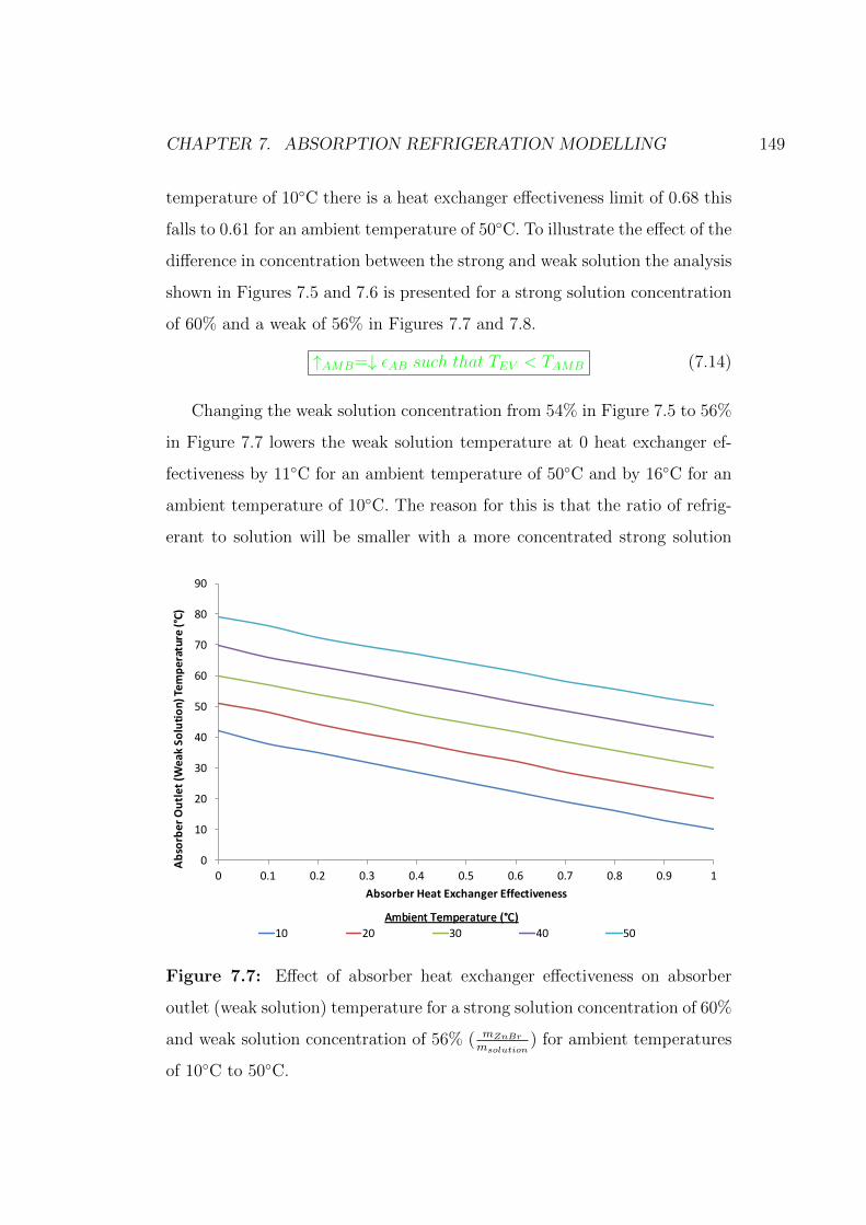
CHAPTER 7. ABSORPTION REFRIGERATION MODELLING 149
temperature of 10◦C there is a heat exchanger effectiveness limit of 0.68 this
falls to 0.61 for an ambient temperature of 50◦C. To illustrate the effect of the
difference in concentration between the strong and weak solution the analysis
shown in Figures 7.5 and 7.6 is presented for a strong solution concentration
of 60% and a weak of 56% in Figures 7.7 and 7.8.
(7.14)↑AMB=↓ εAB such that TEV < TAMB
Changing the weak solution concentration from 54% in Figure 7.5 to 56%
in Figure 7.7 lowers the weak solution temperature at 0 heat exchanger ef-
fectiveness by 11◦C for an ambient temperature of 50◦C and by 16◦C for an
ambient temperature of 10◦C. The reason for this is that the ratio of refrig-
erant to solution will be smaller with a more concentrated strong solution
0
10
20
30
40
50
60
70
80
90
0 0.1 0.2 0.3 0.4 0.5 0.6 0.7 0.8 0.9 1
Absorber Outlet (Weak So
lutio
n) Te
mpe
rature (°C)
Absorber Heat Exchanger Effectiveness
10 20 30 40 50Ambient Temperature (°C)Ambient Temperature (°C)
Figure 7.7: Effect of absorber heat exchanger effectiveness on absorber
outlet (weak solution) temperature for a strong solution concentration of 60%
and weak solution concentration of 56% ( mZnBr
msolution) for ambient temperatures
of 10◦C to 50◦C.

CHAPTER 7. ABSORPTION REFRIGERATION MODELLING 150
and the saturation pressure (absorber and evaporator pressure) caused by
this will be lower. The low saturation pressure will cause lower evaporator
temperatures, the refrigerant leaving the evaporator as a saturated vapour
will be at this lower temperature and therefore has a lower specific enthalpy,
seen in Figure 4.2. This lower specific enthalpy results in a reduction in the
energy removal requirement from the absorber with a smaller difference in
solution concentrations. It has no effect on the weak solution temperature
for a perfect heat exchanger (1) as at these values the weak solution equals
ambient temperature.
(7.15)↓ (XSS −XWS) =↓ QAB =↓ TABWS
The effect of absorber heat exchanger effectiveness and difference in strong
-10
0
10
20
30
40
50
60
70
0 0.1 0.2 0.3 0.4 0.5 0.6 0.7 0.8 0.9 1
Evap
oratorTe
mperature(°C)
AbsorberHeatExchangerEffectiveness
10 20 30 40 50 Tev<TambLimit
AmbientTemperature(°C)
Figure 7.8: Effect of absorber heat exchanger effectiveness on evaporator
temperature for a strong solution concentration of 60% and weak solution
concentration of 56% ( mZnBr
msolution) for ambient temperatures of 10◦C to 50◦C.
CHAPTER 7. ABSORPTION REFRIGERATION MODELLING 151
and weak solution concentrations on evaporator temperature can be seen in
the difference between Figures 7.6 and 7.8. When ambient temperature is
50◦C the evaporator temperature is 12.5◦C lower for a weak solution of 56%
at a heat exchanger effectiveness of 0 but only 2◦C lower for a perfect heat
exchanger. However at an ambient temperature of 10◦C the difference in
evaporator temperatures for a 0 heat exchanger effectiveness is 17.7◦C and
1.6◦C for a perfect heat exchanger. This indicates that if the heat exchangers
are highly effective a greater concentration difference between the strong and
weak solutions can be used without having a significant effect on evaporator
temperature.
(7.16)↑ XWS =↓ TEV
When comparing the dashed orange line, which indicates the limit where
evaporator temperature is equal to ambient temperature in Figures 7.6 and
7.8, changing the weak solution concentration from 54% to 56%, while main-
taining a strong solution concentration of 60%, decreases the heat exchanger
effectiveness limit to achieve evaporator temperatures lower than ambient.
For example for an ambient temperature of 10◦C the limit reduces from 0.68
to 0.47 reducing by 0.21 and for an ambient temperature of 50◦C the limit
reduced from 0.61 to 0.37 reducing by 0.24. These results show that a small
difference in strong and weak solution concentrations reduces the impact of
absorber heat exchanger effectiveness.
(7.17)↓ (XSS −XWS) =↓ εAB such that TEV < TAMB
This illustration of the effect of keeping the strong solution at 60% and
changing the weak from 54% to 56% also shows that more concentrated weak
solution concentrations provide lower evaporator temperatures. The ratio of
working refrigerant to solution is proportional to the solution concentration
difference, as it increases more energy needs to be removed from the ab-
sorber. This results in the absorber heat exchanger effectiveness having a
CHAPTER 7. ABSORPTION REFRIGERATION MODELLING 152
greater effect on the evaporator temperature for large solution concentration
differences. In conclusion if the absorber heat exchangers are ineffective due
to a lack of cold sinks a small difference in solution concentration should be
used to provide low evaporator temperatures.
This analysis provides insight into the need for highly effective heat ex-
changers and the strongest possible weak solution while also having the weak-
est possible strong solution, to operate an absorption refrigerator from low
temperature heat sources in a hot climate. Based on these findings and con-
sultation with individuals who have industrial experience in heat exchangers
a conservative heat exchanger effectiveness of 0.75 has been used for all heat
exchangers in subsequent models
(7.18)↓ (XSS −XWS) =↓ TEV
(7.19)↑ εAB =↓ TEV
The following section presents the theoretical outputs of the various cycle
configurations discussed in Chapter 3. There is further analysis on the effect
of adjusting the difference between the strong and weak solution as part of
the analysis on the Single Effect Cycle.
7.2 Single Effect Cycle Analysis Powered by
the CPV and Genset Radiator Heat Sources
The previous section explored the effects of varying the solution concentra-
tion difference with a fixed strong solution concentration focussing on the
absorber and evaporator. This section investigates a single effect cycle pow-
ered by the heat sources in the BioCPV power plant. These heat sources have
fixed operating temperatures of 60◦C for the CPV and 80◦C for the genset
radiator. The following section investigates a single effect cycle powered by
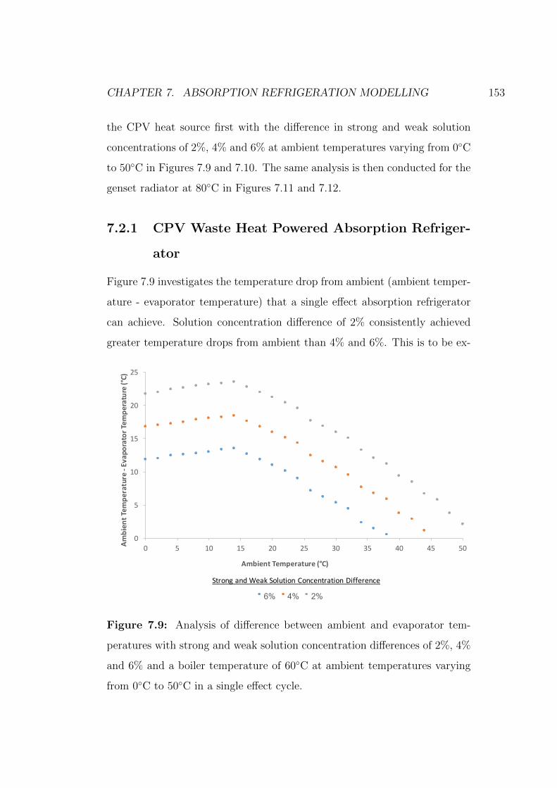
CHAPTER 7. ABSORPTION REFRIGERATION MODELLING 153
the CPV heat source first with the difference in strong and weak solution
concentrations of 2%, 4% and 6% at ambient temperatures varying from 0◦C
to 50◦C in Figures 7.9 and 7.10. The same analysis is then conducted for the
genset radiator at 80◦C in Figures 7.11 and 7.12.
7.2.1 CPV Waste Heat Powered Absorption Refriger-
ator
Figure 7.9 investigates the temperature drop from ambient (ambient temper-
ature - evaporator temperature) that a single effect absorption refrigerator
can achieve. Solution concentration difference of 2% consistently achieved
greater temperature drops from ambient than 4% and 6%. This is to be ex-
0
5
10
15
20
25
0 5 10 15 20 25 30 35 40 45 50Ambien
tTem
perature-EvaporatorTe
mpe
rature(°C)
AmbientTemperature(°C)
6% 4% 2%
Strong andWeakSolution ConcentrationDifference
Figure 7.9: Analysis of difference between ambient and evaporator tem-
peratures with strong and weak solution concentration differences of 2%, 4%
and 6% and a boiler temperature of 60◦C at ambient temperatures varying
from 0◦C to 50◦C in a single effect cycle.
CHAPTER 7. ABSORPTION REFRIGERATION MODELLING 154
pected as the model would find the same strong solution concentration for all
cases but the 2% increase will have a less concentrated weak solution than 4%
and 6%, causing lower pressures in the low pressure side of the refrigerator
and therefore lower evaporator temperatures. The knee in all the curves at
14◦C indicates that up to this point the strong solution concentration was at
the maximum limit to avoid crystallisation (70%mZnBr2
msolution). The x-axis inter-
cept indicates that the evaporator and ambient temperatures are equal. This
is the limit where it is not theoretically (and practically) possible to generate
any cooling at ambient conditions. A 6% and 4% difference cannot operate
theoretically at ambient temperatures above 38◦C and 46◦C respectively. At
and close to these ambient temperatures, the cooling would not practically
be useful as the evaporator temperature will be close to or at ambient and it
is unlikely that the evaporator will be able to absorb any heat from an am-
bient source, as it will not have perfect heat exchangers. That being said it
could be used to cool something warmer than ambient when passive ambient
cooling is insufficient.
Figure 7.10 shows for the same set of conditions their effect on CoP. For
all cases CoP rises with ambient temperature, this is partly a result of the
assumption that the weak solution input to the boiler is at ambient tem-
perature. The 2% difference in strong and weak solution concentrations has
CoPs approximately half of the 6% concentration difference. However from
Figure 7.9 the 2% difference in solution concentrations has colder evaporator
temperatures. This indicates that lowering the solution concentration differ-
ence reduces the cooling energy available but the temperatures achieved are
more versatile.
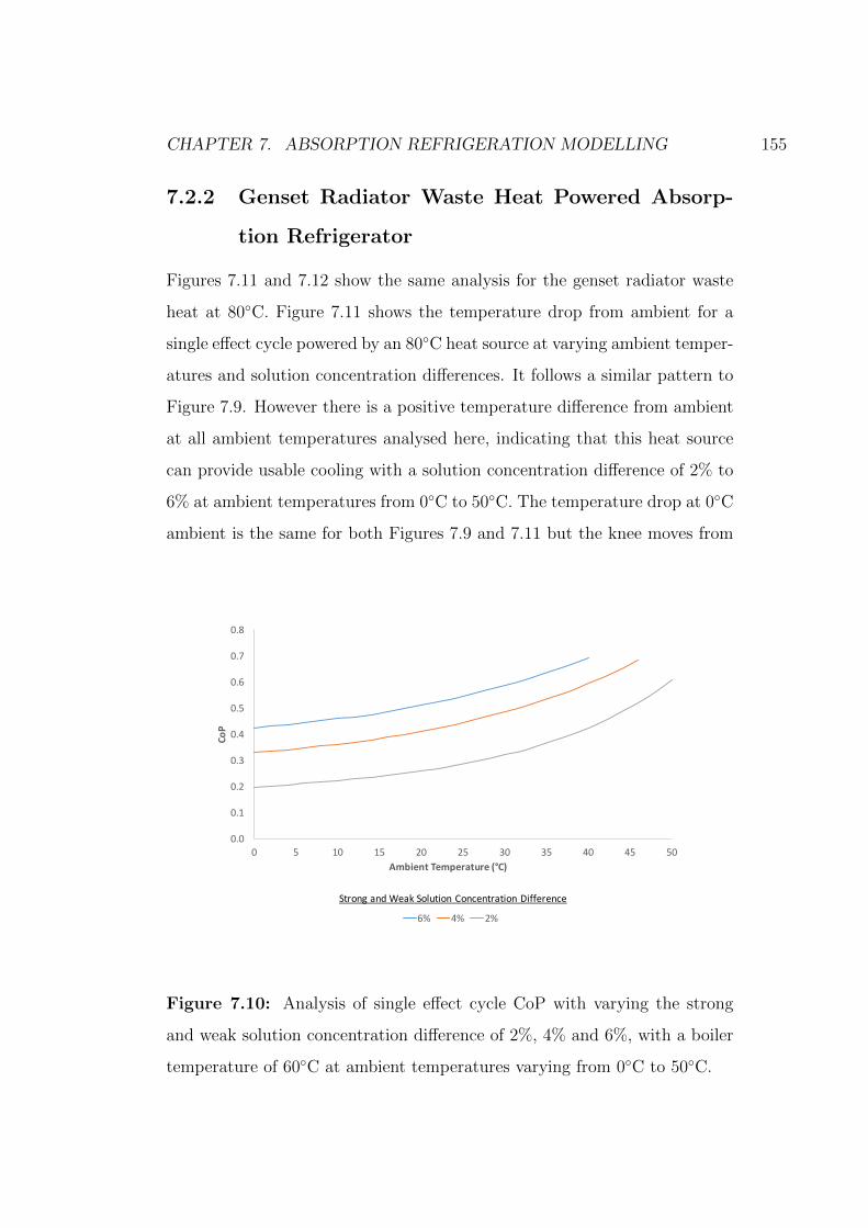
CHAPTER 7. ABSORPTION REFRIGERATION MODELLING 155
7.2.2 Genset Radiator Waste Heat Powered Absorp-
tion Refrigerator
Figures 7.11 and 7.12 show the same analysis for the genset radiator waste
heat at 80◦C. Figure 7.11 shows the temperature drop from ambient for a
single effect cycle powered by an 80◦C heat source at varying ambient temper-
atures and solution concentration differences. It follows a similar pattern to
Figure 7.9. However there is a positive temperature difference from ambient
at all ambient temperatures analysed here, indicating that this heat source
can provide usable cooling with a solution concentration difference of 2% to
6% at ambient temperatures from 0◦C to 50◦C. The temperature drop at 0◦C
ambient is the same for both Figures 7.9 and 7.11 but the knee moves from
0.0
0.1
0.2
0.3
0.4
0.5
0.6
0.7
0.8
0 5 10 15 20 25 30 35 40 45 50
CoP
Ambient Temperature (°C)
6% 4% 2%
Strong and Weak Solution Concentration Difference
Figure 7.10: Analysis of single effect cycle CoP with varying the strong
and weak solution concentration difference of 2%, 4% and 6%, with a boiler
temperature of 60◦C at ambient temperatures varying from 0◦C to 50◦C.
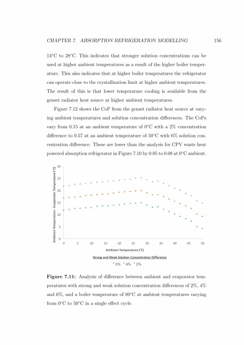
CHAPTER 7. ABSORPTION REFRIGERATION MODELLING 156
14◦C to 28◦C. This indicates that stronger solution concentrations can be
used at higher ambient temperatures as a result of the higher boiler temper-
ature. This also indicates that at higher boiler temperatures the refrigerator
can operate close to the crystallisation limit at higher ambient temperatures.
The result of this is that lower temperature cooling is available from the
genset radiator heat source at higher ambient temperatures.
Figure 7.12 shows the CoP from the genset radiator heat source at vary-
ing ambient temperatures and solution concentration differences. The CoPs
vary from 0.15 at an ambient temperature of 0◦C with a 2% concentration
difference to 0.57 at an ambient temperature of 50◦C with 6% solution con-
centration difference. These are lower than the analysis for CPV waste heat
powered absorption refrigerator in Figure 7.10 by 0.05 to 0.08 at 0◦C ambient.
0
5
10
15
20
25
30
0 5 10 15 20 25 30 35 40 45 50Ambien
tTem
perature-EvaporatorTe
mpe
rature(°C)
AmbientTemperature(°C)
6% 4% 2%
Strong andWeakSolution ConcentrationDifference
Figure 7.11: Analysis of difference between ambient and evaporator tem-
peratures with strong and weak solution concentration differences of 2%, 4%
and 6%, and a boiler temperature of 80◦C at ambient temperatures varying
from 0◦C to 50◦C in a single effect cycle.

CHAPTER 7. ABSORPTION REFRIGERATION MODELLING 157
This difference in CoP between the CPV powered refrigerator and genset ra-
diator powered refrigerator increases as ambient temperature increases (e.g.
0.17 to 0.19 at 40◦C).
In general terms the CPV waste heat can provide up to 96% higher CoPs
but with up to 39% higher (therefore less versatile) evaporator temperatures
than the genset radiator waste heat. As the CPV has considerably more
waste heat available the following section investigates the effects of alterna-
tive configurations to utilise this energy effectively.
0.0
0.1
0.2
0.3
0.4
0.5
0.6
0.7
0 5 10 15 20 25 30 35 40 45 50
CoP
Ambient Temperature (°C)
6% 4% 2%
Strong and Weak Solution Concentration Difference
Figure 7.12: Analysis of single effect cycle CoP with varying the strong
and weak solution concentration difference of 2%, 4% and 6% with a boiler
temperature of 80◦C at ambient temperatures varying from 0◦C to 50◦C.
CHAPTER 7. ABSORPTION REFRIGERATION MODELLING 158
7.3 Absorption Refrigerator Configuration Anal-
ysis
The previous section identified that the CPV heat source at high ambient
temperatures cannot provide low evaporator temperatures. For example an
ambient temperature of 35◦C, at best (2% solution concentration difference),
provides an evaporator temperature of 22◦C. These high evaporator temper-
atures may be useful for space cooling but are not versatile enough to provide
cooling for food or medicine. However, the thermal losses in the CPV ac-
counts for 38% of the total power plant input energy. Therefore, ways to
lower the evaporator temperature of the CPV powered absorption refriger-
ator need to be investigated to maximise the usefulness of this large energy
source.
The following analysis assesses the potential to generate lower evaporator
temperatures using the evaporator tap off method described in Chapter 3. It
continues from the previous section by comparing the effect of reducing the
solution concentration difference in a single effect cycle to the evaporator tap
off method in a single effect cycle. The evaporator tap off method uses water
as a heat transfer fluid to transfer some of the cooling from the evaporator to
the absorber and condenser of the absorption refrigerator. The heat transfer
fluid achieves this by initially rejecting the collected heat from the absorber
and condenser to ambient, reducing its temperature to ambient, after which
it is then further cooled by the evaporator. This allows the condenser and ab-
sorber to potentially operate at temperatures lower than ambient. The mod-
elling approach is described in the Analytical Methodology Chapter Section
4.3.11. The findings from this analysis are then extrapolated to assess the vi-
ability of the combined cycle with reservoirs and double boiler with reservoirs
and evaporator tap off absorption refrigerator system configurations.
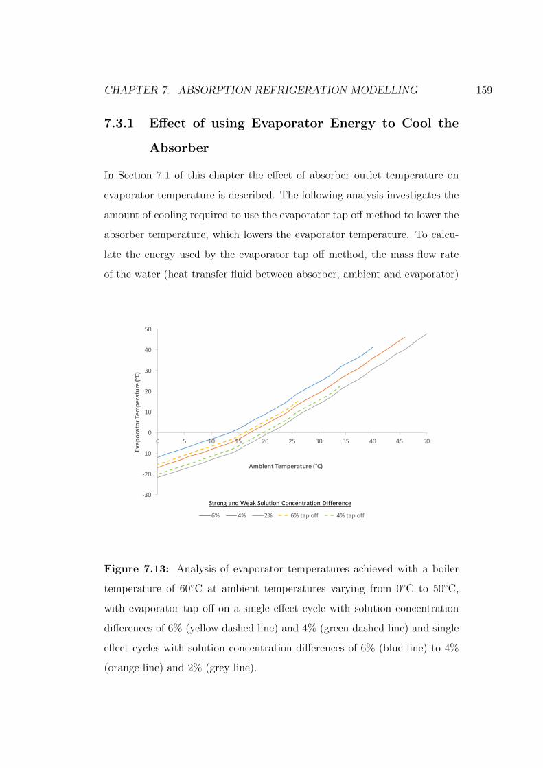
CHAPTER 7. ABSORPTION REFRIGERATION MODELLING 159
7.3.1 Effect of using Evaporator Energy to Cool the
Absorber
In Section 7.1 of this chapter the effect of absorber outlet temperature on
evaporator temperature is described. The following analysis investigates the
amount of cooling required to use the evaporator tap off method to lower the
absorber temperature, which lowers the evaporator temperature. To calcu-
late the energy used by the evaporator tap off method, the mass flow rate
of the water (heat transfer fluid between absorber, ambient and evaporator)
-30
-20
-10
0
10
20
30
40
50
0 5 10 15 20 25 30 35 40 45 50
Evap
oratorTe
mperature(°C)
AmbientTemperature(°C)
6% 4% 2% 6%tapoff 4%tapoff
Strong andWeakSolution ConcentrationDifference
Figure 7.13: Analysis of evaporator temperatures achieved with a boiler
temperature of 60◦C at ambient temperatures varying from 0◦C to 50◦C,
with evaporator tap off on a single effect cycle with solution concentration
differences of 6% (yellow dashed line) and 4% (green dashed line) and single
effect cycles with solution concentration differences of 6% (blue line) to 4%
(orange line) and 2% (grey line).
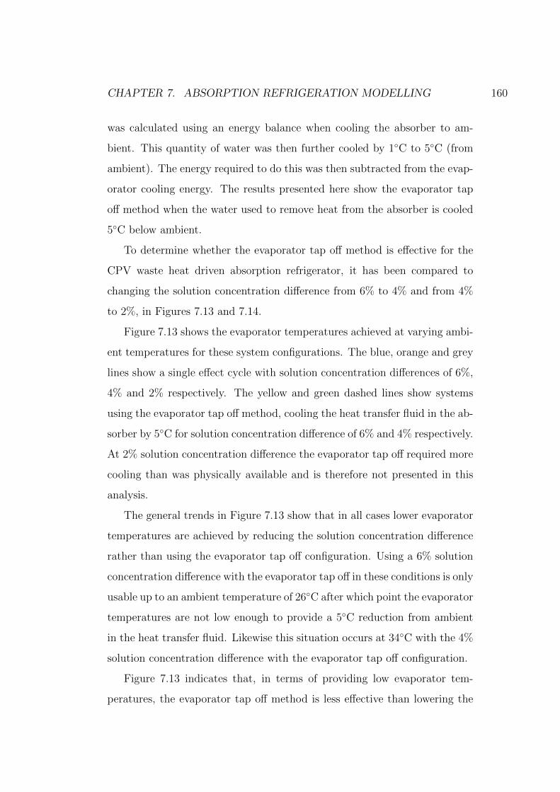
CHAPTER 7. ABSORPTION REFRIGERATION MODELLING 160
was calculated using an energy balance when cooling the absorber to am-
bient. This quantity of water was then further cooled by 1◦C to 5◦C (from
ambient). The energy required to do this was then subtracted from the evap-
orator cooling energy. The results presented here show the evaporator tap
off method when the water used to remove heat from the absorber is cooled
5◦C below ambient.
To determine whether the evaporator tap off method is effective for the
CPV waste heat driven absorption refrigerator, it has been compared to
changing the solution concentration difference from 6% to 4% and from 4%
to 2%, in Figures 7.13 and 7.14.
Figure 7.13 shows the evaporator temperatures achieved at varying ambi-
ent temperatures for these system configurations. The blue, orange and grey
lines show a single effect cycle with solution concentration differences of 6%,
4% and 2% respectively. The yellow and green dashed lines show systems
using the evaporator tap off method, cooling the heat transfer fluid in the ab-
sorber by 5◦C for solution concentration difference of 6% and 4% respectively.
At 2% solution concentration difference the evaporator tap off required more
cooling than was physically available and is therefore not presented in this
analysis.
The general trends in Figure 7.13 show that in all cases lower evaporator
temperatures are achieved by reducing the solution concentration difference
rather than using the evaporator tap off configuration. Using a 6% solution
concentration difference with the evaporator tap off in these conditions is only
usable up to an ambient temperature of 26◦C after which point the evaporator
temperatures are not low enough to provide a 5◦C reduction from ambient
in the heat transfer fluid. Likewise this situation occurs at 34◦C with the 4%
solution concentration difference with the evaporator tap off configuration.
Figure 7.13 indicates that, in terms of providing low evaporator tem-
peratures, the evaporator tap off method is less effective than lowering the
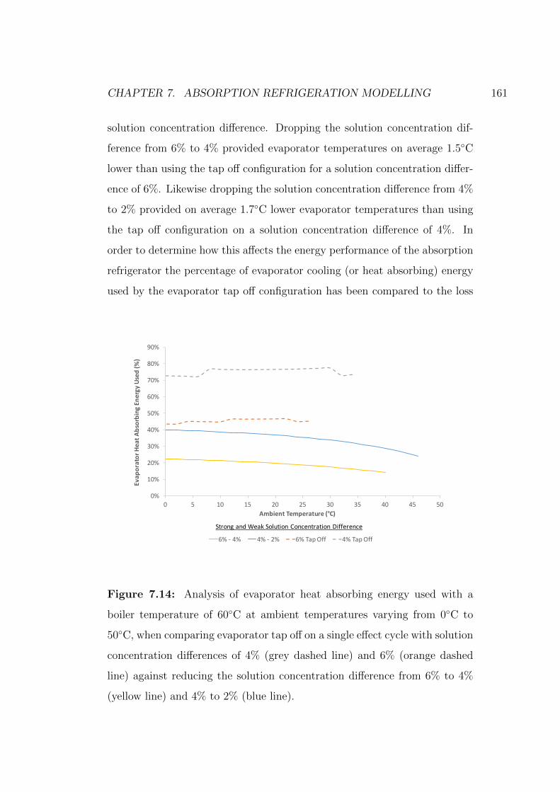
CHAPTER 7. ABSORPTION REFRIGERATION MODELLING 161
solution concentration difference. Dropping the solution concentration dif-
ference from 6% to 4% provided evaporator temperatures on average 1.5◦C
lower than using the tap off configuration for a solution concentration differ-
ence of 6%. Likewise dropping the solution concentration difference from 4%
to 2% provided on average 1.7◦C lower evaporator temperatures than using
the tap off configuration on a solution concentration difference of 4%. In
order to determine how this affects the energy performance of the absorption
refrigerator the percentage of evaporator cooling (or heat absorbing) energy
used by the evaporator tap off configuration has been compared to the loss
0%
10%
20%
30%
40%
50%
60%
70%
80%
90%
0 5 10 15 20 25 30 35 40 45 50
Evap
oratorHeatA
bsorbingEne
rgyUsed
(%)
AmbientTemperature(°C)
6%- 4% 4%- 2% 6%TapOff 4%TapOff
Strong andWeakSolution ConcentrationDifference
Figure 7.14: Analysis of evaporator heat absorbing energy used with a
boiler temperature of 60◦C at ambient temperatures varying from 0◦C to
50◦C, when comparing evaporator tap off on a single effect cycle with solution
concentration differences of 4% (grey dashed line) and 6% (orange dashed
line) against reducing the solution concentration difference from 6% to 4%
(yellow line) and 4% to 2% (blue line).
CHAPTER 7. ABSORPTION REFRIGERATION MODELLING 162
in evaporator cooling energy from using a solution concentration difference
of 6% to 4% and 4% to 2%. Figure 7.14 shows this.
The general trends observed from Figure 7.14 show that the tap off con-
figuration uses more of the evaporator cooling energy than the reduction in
evaporator cooling energy from lowering the solution concentration differ-
ence. The average cooling energy penalty from using a 4% solution concen-
tration difference over 6% is 25 percentage points lower than using the tap
off configuration with a 6% solution concentration difference. Likewise for
solution concentration differences of 4% to 2% compared to 4% with tap off
is 38 percentage points lower. The cooling energy penalty of going from 6%
solution concentration difference to 4% is half that of 4% to 2%. Combining
the results of Figures 7.13 and 7.14 in terms of providing lower evaporator
temperatures and maximising cooling energy it is more effective to use lower
solution concentration differences than the evaporator tap off method.
The result of this analysis is that an absorption refrigerator powered by
a 60◦C heat source in high ambient temperatures should use a 2% or lower
solution concentration difference to provide cooling up to ambient conditions
of 50◦C. The evaporator tap off method is not effective at high ambient
temperatures as the evaporator temperature is not low enough to cool the
heat transfer fluid effectively. Moreover the evaporator tap off method has too
high an energy penalty in comparison to lowering the solution concentration
difference.
Conducting the same analysis for the genset radiator heat source which
is assumed to be at 80◦C in Figures 7.15 and 7.16. These figures show the
evaporator temperatures and the cooling energy penalty respectively for the
same conditions other than the boiler temperature. The general patterns are
the same as those for a 60◦C heat source, with the main difference being that
the evaporator tap off method can operate at higher ambient temperatures,
up to 46◦C for a 6% solution concentration difference compared to 26◦C

CHAPTER 7. ABSORPTION REFRIGERATION MODELLING 163
with the CPV heat source at 60◦C. A 4% solution concentration difference
with genset radiator waste heat tap off is viable for all ambient temperatures
tested here.
The main finding is that the most energy effective way of achieving a
lower evaporator temperature, with acetone and zinc bromide as the working
fluids, is using a small solution concentration difference. The evaporator tap
off configuration does not appear to utilise the waste heat sources well in
terms of reducing evaporator temperature through cooling the absorber.
-30
-20
-10
0
10
20
30
40
50
0 5 10 15 20 25 30 35 40 45 50
Evap
oratorTe
mperature(°C)
AmbientTemperature(°C)
6% 4% 2% 6%tapoff 4%tapoff
Strong andWeakSolution ConcentrationDifference
Figure 7.15: Analysis of evaporator temperatures achieved with a boiler
temperature of 80◦C at ambient temperatures varying from 0◦C to 50◦C, with
the evaporator tap off on a single effect cycle with solution concentration
differences of 6% (yellow dashed line) and 4% (green dashed line) and single
effect cycles with 6%,(blue line) 4% (orange line) and 2% (grey line).

CHAPTER 7. ABSORPTION REFRIGERATION MODELLING 164
7.3.2 Effect of using Evaporator Energy to Cool the
Condenser
The alternative to cooling the absorber to provide lower evaporator temper-
atures is cooling the condenser. The condenser temperature and the cor-
responding saturation pressure determine the strength limit of the strong
solution leaving the boiler. If more concentrated strong solutions can be
used then more concentrated weak solutions are possible. More concentrated
weak solutions provide lower saturation pressures which can lead to lower
0%
10%
20%
30%
40%
50%
60%
70%
80%
90%
0 5 10 15 20 25 30 35 40 45 50
Evap
oratorHeatA
bsorbingEne
rgyUsed
(%)
AmbientTemperature(°C)
6%- 4% 4%- 2% 6%TapOff 4%TapOff
Strong andWeakSolution ConcentrationDifference
Figure 7.16: Analysis of evaporator heat absorbing energy used with a
boiler temperature of 80◦C at ambient temperatures varying from 0◦C to
50◦C, when comparing evaporator tap off on a single effect cycle with solution
concentration differences of 4% (grey dashed line) and 6% (orange dashed
line) against reducing the solution concentration difference from 6% to 4%
(yellow line) and 4% to 2% (blue line).

CHAPTER 7. ABSORPTION REFRIGERATION MODELLING 165
evaporator temperatures.
Modelling tests investigated using up to 50% of the cooling generated in
the evaporator to cool the condenser, using a similar calculation approach to
cooling the absorber in the previous subsection. Using 50% of the evaporator
cooling energy at ambient temperatures from 10◦C to 50◦C and boiler tem-
peratures of 60◦C and 80◦C only allowed a maximum reduction of 1% and
2% respectively in the strong solution concentration. The resulting slight
lowering of evaporator temperatures (less than 3◦C) did not warrant the use
of this much cooling potential, when compared with using a lower solution
concentration difference described in the previous subsection.
These results align with the operational theory; when considering the
specific enthalpy of the flows through the boiler the refrigerant (due to its
phase change) contains most of the boiler input energy. The subsequent heat
removal requirement in the condenser will be considerable resulting in the
need for a large mass flow of heat transfer fluid. The energy requirement
to lower the temperature of this large flow of heat transfer fluid will also be
considerable. Taking into consideration that the highest CoP in this analysis
is less than 0.7 and the typical range depending on solution concentration
difference is 0.2 to 0.5 it is unlikely that there will be sufficient energy to
provide useful cooling of the condenser heat transfer fluid. Cooling the con-
denser with the evaporator tap off method in the conditions addressed in this
thesis can be considered ineffective.
7.4 Error Analysis
Effective error analysis in this kind of modelling is extremely difficult, there
are errors that arise from the equations of state for both the solution and
refrigerant. Some, but not all, of which are presented in Ajib and Karno

CHAPTER 7. ABSORPTION REFRIGERATION MODELLING 166
(2008) and NIST (2011). Further errors are created from the lookup table
resolution; a resolution of 1◦C and 1% of solution concentration was used.
One approach to simplify this process is to determine the most significant
cause of error in the model and use the model to quantify it. The resolution of
the lookup tables is likely to be the most significant error as these determine
the key variables within the system when conditions change.
A resolution of 1% in solution concentration will only affect the strong
solution concentration (as the weak solution concentration is calculated from
adding the desired difference to the strong solution). A 1% change in strong
solution concentration caused a maximum change in evaporator temperature
of 2◦C. The evaporator temperature is determined from a lookup table of
the absorber outlet conditions which has a resolution of 1◦C. Changing the
weak solution temperature at the outlet of the absorber by 1◦C affects the
evaporator by a maximum of 1◦C. Taking the larger of these, 2◦C, provides a
conservative error for the evaporator temperature. Changing the evaporator
temperature by 2◦C has a 0.5% change to cooling energy of the evaporator.
The CoPs calculated were all less than 1 which would reduce this error when
carried through to CoP, to provide a conservative estimate for the CoP error
0.5% will be used.
Karno and Ajib (2008) present simulation results providing a CoP 0.6
when the experimental result was approximately 0.4. This is likely to be a
result of a number of modelling assumptions for example: there are no losses
between components, the effectiveness of the heat exchangers, the effective-
ness of the mass transfer in the boiler, homogeneity of the working fluids
and errors in the thermophysical and thermodynamic property equations.
Though this figure should be used with caution, its presents the reality that
a simulation result can be over 30% greater than a physical result.
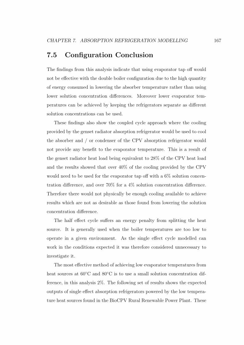
CHAPTER 7. ABSORPTION REFRIGERATION MODELLING 167
7.5 Configuration Conclusion
The findings from this analysis indicate that using evaporator tap off would
not be effective with the double boiler configuration due to the high quantity
of energy consumed in lowering the absorber temperature rather than using
lower solution concentration differences. Moreover lower evaporator tem-
peratures can be achieved by keeping the refrigerators separate as different
solution concentrations can be used.
These findings also show the coupled cycle approach where the cooling
provided by the genset radiator absorption refrigerator would be used to cool
the absorber and / or condenser of the CPV absorption refrigerator would
not provide any benefit to the evaporator temperature. This is a result of
the genset radiator heat load being equivalent to 28% of the CPV heat load
and the results showed that over 40% of the cooling provided by the CPV
would need to be used for the evaporator tap off with a 6% solution concen-
tration difference, and over 70% for a 4% solution concentration difference.
Therefore there would not physically be enough cooling available to achieve
results which are not as desirable as those found from lowering the solution
concentration difference.
The half effect cycle suffers an energy penalty from splitting the heat
source. It is generally used when the boiler temperatures are too low to
operate in a given environment. As the single effect cycle modelled can
work in the conditions expected it was therefore considered unnecessary to
investigate it.
The most effective method of achieving low evaporator temperatures from
heat sources at 60◦C and 80◦C is to use a small solution concentration dif-
ference, in this analysis 2%. The following set of results shows the expected
outputs of single effect absorption refrigerators powered by the low tempera-
ture heat sources found in the BioCPV Rural Renewable Power Plant. These

CHAPTER 7. ABSORPTION REFRIGERATION MODELLING 168
are the CPV with 116 kW·h per day at 60◦C and the genset radiator with
32 kW·h per day at 80◦C, both with a 2% concentration difference. Ambient
temperatures of 0◦C to 50◦C are investigated in all of the following analyses.
7.5.1 CPV Waste Heat Powered Absorption Refriger-
ator
Figure 7.17 shows the evaporator temperatures achieved with the CPV waste
heat source powering an absorption refrigerator with varying ambient tem-
peratures. It shows that sub 0◦C evaporator temperatures can be achieved at
ambient temperatures below 21◦C and evaporator temperatures lower than
10◦C at ambient temperatures below 27◦C. Combining this analysis with
Figure 7.9 the CPV heat source can provide a 10◦C drop from ambient up
-30
-20
-10
0
10
20
30
40
50
60
0 5 10 15 20 25 30 35 40 45 50Evap
oratorTe
mperature(°C)
AmbientTemperature(°C)
Figure 7.17: Evaporator temperature of a single effect cycle using the
CPV waste heat as a heat source at 60◦C with a 2% solution concentration
difference at ambient temperatures from 0◦C to 50◦C.
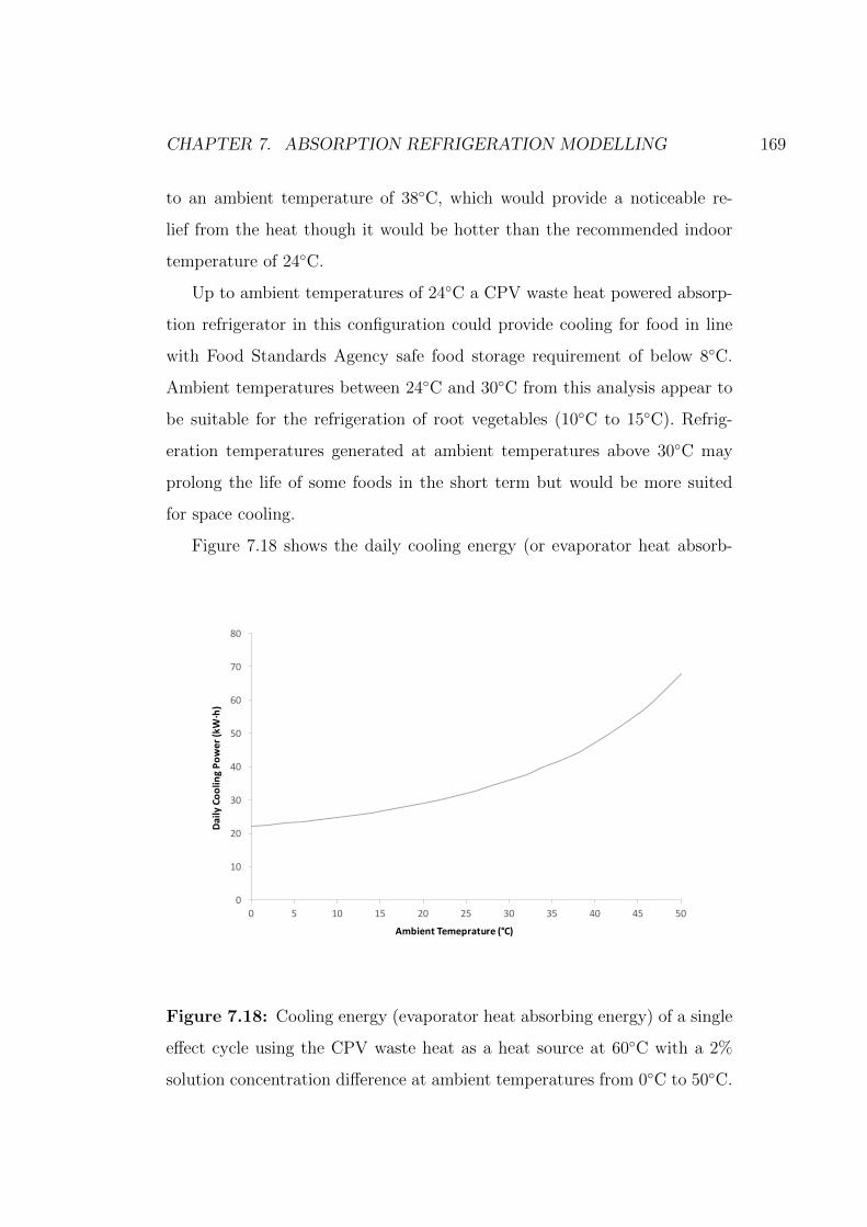
CHAPTER 7. ABSORPTION REFRIGERATION MODELLING 169
to an ambient temperature of 38◦C, which would provide a noticeable re-
lief from the heat though it would be hotter than the recommended indoor
temperature of 24◦C.
Up to ambient temperatures of 24◦C a CPV waste heat powered absorp-
tion refrigerator in this configuration could provide cooling for food in line
with Food Standards Agency safe food storage requirement of below 8◦C.
Ambient temperatures between 24◦C and 30◦C from this analysis appear to
be suitable for the refrigeration of root vegetables (10◦C to 15◦C). Refrig-
eration temperatures generated at ambient temperatures above 30◦C may
prolong the life of some foods in the short term but would be more suited
for space cooling.
Figure 7.18 shows the daily cooling energy (or evaporator heat absorb-
0
10
20
30
40
50
60
70
80
0 5 10 15 20 25 30 35 40 45 50
Daily Coo
ling Po
wer (kW·∙h)
Ambient Temeprature (°C)
Figure 7.18: Cooling energy (evaporator heat absorbing energy) of a single
effect cycle using the CPV waste heat as a heat source at 60◦C with a 2%
solution concentration difference at ambient temperatures from 0◦C to 50◦C.
CHAPTER 7. ABSORPTION REFRIGERATION MODELLING 170
ing energy) that an absorption refrigerator could produce when powered by
the CPV waste heat with a 2% solution concentration difference in ambient
temperatures from 0◦C to 50◦C. The graph shows that there is the poten-
tial to provide 23 kW·h at an ambient temperature of 0◦C to 71 kW·h at
an ambient temperature of 50 ◦C. The increasing quantity of cooling with
ambient temperature is a result of the weak solution being warmer at higher
ambient temperatures when it enters the boiler and that higher evaporator
temperatures (seen in Figure 7.17) are generated.
Combining this analysis with the information in Figure 7.17 refrigeration
of food in line with the Food Standard Agency requirements can be provided
up to ambient temperatures of 24◦C which corresponds to a cooling power of
0
2
4
6
8
10
12
14
16
0 5 10 15 20 25 30 35 40 45 50
DailyElectric
alEne
rgySaved(kW·h)
AmbientTemperature(°C)
Figure 7.19: Daily electrical energy saved (avoided) from not using a vapour
compression refrigerator to provide the same cooling as a single effect cycle
using the CPV waste heat as a heat source at 60◦C with a 2% solution
concentration difference at ambient temperatures from 0◦C to 50◦C.
CHAPTER 7. ABSORPTION REFRIGERATION MODELLING 171
32.6 kW·h per day. This can be considered equivalent to 23 to 32 domestic
refrigerator units. However the temperatures in the location of the power
plant are expected to exceed this.
If the cooling generated at ambient temperatures above 24◦C is used for
space cooling, then there would be 32 kW·h at 24◦C to 46.2 kW·h at 40◦C.
In terms of a 5 kW air conditioning system for a room in a medical centre
this cooling can be considered equivalent to 6 to 9 hours per day of cooling.
To quantify the benefit of this cooling in terms of the electricity, Figure
7.19 presents the daily electrical energy that would have been used by an elec-
trically driven vapour compression refrigerator to provide the same output as
the absorption refrigerator powered by the CPV waste heat at varying ambi-
ent temperatures. The graph shows that between 7 kW·h and 14 kW·h can
be saved per day in ambient conditions of 0◦C to 50◦C respectively. To put
this in perspective of the energy analysis shown in Figure 5.2 the 116 kW·h
of waste heat at 60◦C in a 25◦C environment can provide the same amount
of cooling as 10 kW·h of electricity would provide which is approximately
17.5% of the electrical output of the renewable power plant.
7.5.2 Genset Radiator Waste Heat Powered Absorp-
tion Refrigerator
Figure 7.20 shows the evaporator temperatures achieved with the genset radi-
ator waste heat source at 80◦C powering a single effect absorption refrigerator
with varying ambient temperatures. It shows that sub 0◦C temperatures can
be achieved at ambient temperatures below 25◦C and lower than 10◦C at
ambient temperatures below 33◦C. This refrigerator can provide a temper-
ature drop from ambient greater than 20◦C up to ambient temperatures of
41◦C, even at 50◦C it can provide an evaporator temperature of 35◦C.
In terms of food storage this configuration of absorption refrigerator would
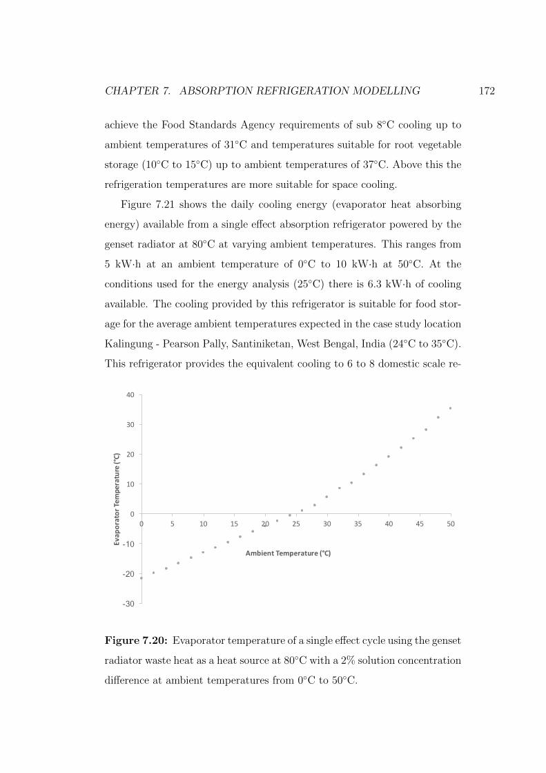
CHAPTER 7. ABSORPTION REFRIGERATION MODELLING 172
achieve the Food Standards Agency requirements of sub 8◦C cooling up to
ambient temperatures of 31◦C and temperatures suitable for root vegetable
storage (10◦C to 15◦C) up to ambient temperatures of 37◦C. Above this the
refrigeration temperatures are more suitable for space cooling.
Figure 7.21 shows the daily cooling energy (evaporator heat absorbing
energy) available from a single effect absorption refrigerator powered by the
genset radiator at 80◦C at varying ambient temperatures. This ranges from
5 kW·h at an ambient temperature of 0◦C to 10 kW·h at 50◦C. At the
conditions used for the energy analysis (25◦C) there is 6.3 kW·h of cooling
available. The cooling provided by this refrigerator is suitable for food stor-
age for the average ambient temperatures expected in the case study location
Kalingung - Pearson Pally, Santiniketan, West Bengal, India (24◦C to 35◦C).
This refrigerator provides the equivalent cooling to 6 to 8 domestic scale re-
-30
-20
-10
0
10
20
30
40
0 5 10 15 20 25 30 35 40 45 50
Evap
oratorTe
mperature(°C)
AmbientTemperature(°C)
Figure 7.20: Evaporator temperature of a single effect cycle using the genset
radiator waste heat as a heat source at 80◦C with a 2% solution concentration
difference at ambient temperatures from 0◦C to 50◦C.
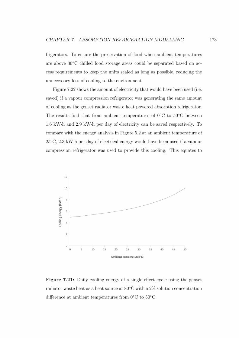
CHAPTER 7. ABSORPTION REFRIGERATION MODELLING 173
frigerators. To ensure the preservation of food when ambient temperatures
are above 30◦C chilled food storage areas could be separated based on ac-
cess requirements to keep the units sealed as long as possible, reducing the
unnecessary loss of cooling to the environment.
Figure 7.22 shows the amount of electricity that would have been used (i.e.
saved) if a vapour compression refrigerator was generating the same amount
of cooling as the genset radiator waste heat powered absorption refrigerator.
The results find that from ambient temperatures of 0◦C to 50◦C between
1.6 kW·h and 2.9 kW·h per day of electricity can be saved respectively. To
compare with the energy analysis in Figure 5.2 at an ambient temperature of
25◦C, 2.3 kW·h per day of electrical energy would have been used if a vapour
compression refrigerator was used to provide this cooling. This equates to
0
2
4
6
8
10
12
0 5 10 15 20 25 30 35 40 45 50
Cooling En
ergy (kW·∙h)
Ambient Temperature (°C)
Figure 7.21: Daily cooling energy of a single effect cycle using the genset
radiator waste heat as a heat source at 80◦C with a 2% solution concentration
difference at ambient temperatures from 0◦C to 50◦C.
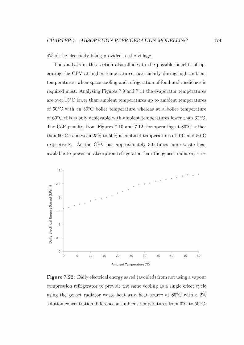
CHAPTER 7. ABSORPTION REFRIGERATION MODELLING 174
4% of the electricity being provided to the village.
The analysis in this section also alludes to the possible benefits of op-
erating the CPV at higher temperatures, particularly during high ambient
temperatures; when space cooling and refrigeration of food and medicines is
required most. Analysing Figures 7.9 and 7.11 the evaporator temperatures
are over 15◦C lower than ambient temperatures up to ambient temperatures
of 50◦C with an 80◦C boiler temperature whereas at a boiler temperature
of 60◦C this is only achievable with ambient temperatures lower than 32◦C.
The CoP penalty, from Figures 7.10 and 7.12, for operating at 80◦C rather
than 60◦C is between 25% to 50% at ambient temperatures of 0◦C and 50◦C
respectively. As the CPV has approximately 3.6 times more waste heat
available to power an absorption refrigerator than the genset radiator, a re-
0
0.5
1
1.5
2
2.5
3
0 5 10 15 20 25 30 35 40 45 50
DailyElectricalEne
rgySaved(kW·h)
AmbientTemperature(°C)
Figure 7.22: Daily electrical energy saved (avoided) from not using a vapour
compression refrigerator to provide the same cooling as a single effect cycle
using the genset radiator waste heat as a heat source at 80◦C with a 2%
solution concentration difference at ambient temperatures from 0◦C to 50◦C.
CHAPTER 7. ABSORPTION REFRIGERATION MODELLING 175
duction in cooling output in favour of lower evaporator temperatures during
the hottest periods is beneficial. In practice, during high (32◦C to 50◦C)
ambient temperatures, a control mechanism allowing the CPV waste heat
powered absorption refrigerator to operate at 80◦C could provide evaporator
temperatures ranging from 8◦C to 35◦C with CoPs ranging from 0.2 to 0.3.
It should be noted that operating the CPV at higher temperatures creates a
risk of localised overheating if the heating and cooling profiles of the PV cells
are not uniform. Therefore, careful monitoring of the PV cell temperature
at multiple locations will be required together with adequate flow control
through the heat exchangers of the PV cells.
Assuming that it is possible to operate an absorption refrigerator from
the CPV operating at 80◦C, this creates an opportunity for further inves-
tigation into the use of the coupled cycle system where the CPV powered
absorption refrigerator could cool the genset powered absorption refrigerator.
At ambient temperatures of 50◦C an absorption refrigerator operating with
a boiler temperature of 80◦C generates an evaporator temperature of 35◦C.
Assuming this could cool both the absorber and condenser to simulate am-
bient conditions between 35◦C and 40◦C, evaporator temperatures of 10◦C
to 19◦C are achievable respectively. These suggested evaporator tempera-
tures could allow medicines with storage requirements of keep cool and store
at room temperature as well some root vegetables to not perish during the
hottest periods of the year.
7.6 Within Day Analysis
In order to gain some insight in how the system will operate on a day-to-day
basis, this section provides an analysis of some typical days that would be
experienced in the region. The typical day criteria are, high DNI, low DNI,
high temperature and low temperature. DNI and ambient temperature data
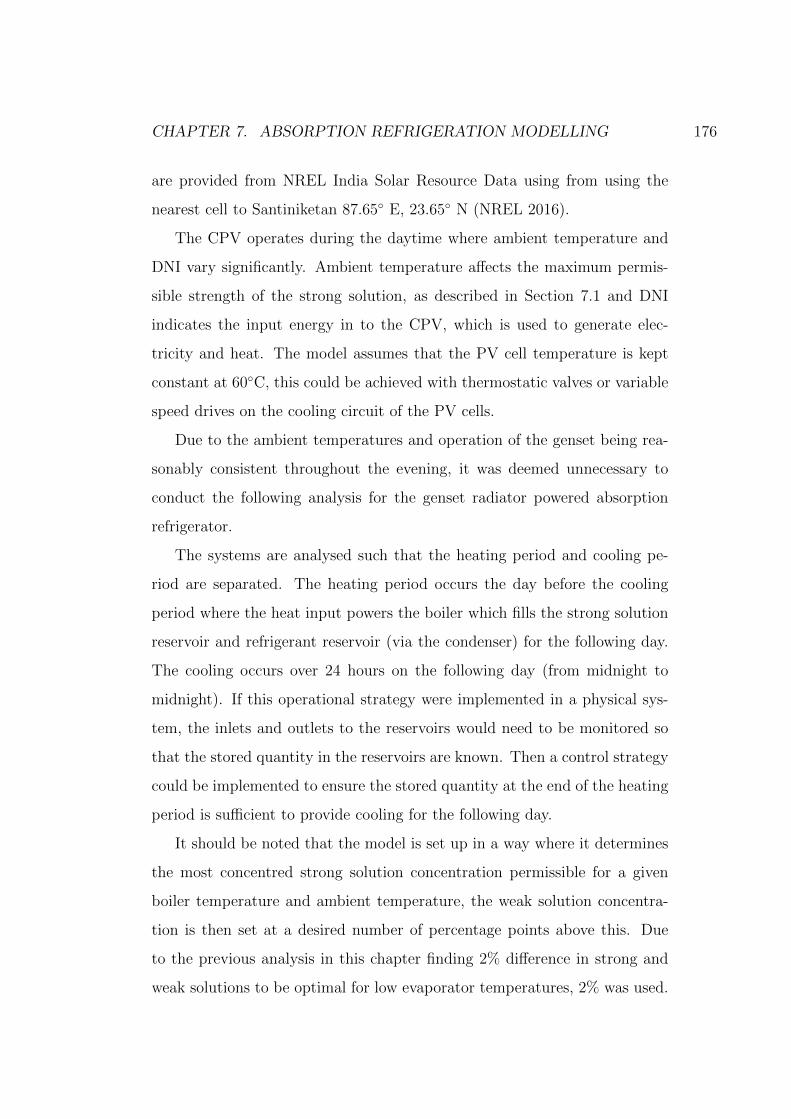
CHAPTER 7. ABSORPTION REFRIGERATION MODELLING 176
are provided from NREL India Solar Resource Data using from using the
nearest cell to Santiniketan 87.65◦ E, 23.65◦ N (NREL 2016).
The CPV operates during the daytime where ambient temperature and
DNI vary significantly. Ambient temperature affects the maximum permis-
sible strength of the strong solution, as described in Section 7.1 and DNI
indicates the input energy in to the CPV, which is used to generate elec-
tricity and heat. The model assumes that the PV cell temperature is kept
constant at 60◦C, this could be achieved with thermostatic valves or variable
speed drives on the cooling circuit of the PV cells.
Due to the ambient temperatures and operation of the genset being rea-
sonably consistent throughout the evening, it was deemed unnecessary to
conduct the following analysis for the genset radiator powered absorption
refrigerator.
The systems are analysed such that the heating period and cooling pe-
riod are separated. The heating period occurs the day before the cooling
period where the heat input powers the boiler which fills the strong solution
reservoir and refrigerant reservoir (via the condenser) for the following day.
The cooling occurs over 24 hours on the following day (from midnight to
midnight). If this operational strategy were implemented in a physical sys-
tem, the inlets and outlets to the reservoirs would need to be monitored so
that the stored quantity in the reservoirs are known. Then a control strategy
could be implemented to ensure the stored quantity at the end of the heating
period is sufficient to provide cooling for the following day.
It should be noted that the model is set up in a way where it determines
the most concentred strong solution concentration permissible for a given
boiler temperature and ambient temperature, the weak solution concentra-
tion is then set at a desired number of percentage points above this. Due
to the previous analysis in this chapter finding 2% difference in strong and
weak solutions to be optimal for low evaporator temperatures, 2% was used.

CHAPTER 7. ABSORPTION REFRIGERATION MODELLING 177
In reality the weak solution being fed into the boiler may be at varying con-
centrations, which will require control over the flow rates in the boiler and
management of the heat transfer at the boiler exit to assist in optimising the
strong solution concentration. For if the strong solution leaving the boiler
cools too quickly the strong solution may reabsorb refrigerant faster than it
can be condensed in the condenser.
0
100
200
300
400
500
600
700
800
0
5
10
15
20
25
30
00:00 02:00 04:00 06:00 08:00 10:00 12:00 14:00 16:00 18:00 20:00 22:00 00:00DN
I(W·m
-2)
Power(k
W)
Time(hh:mm)
ElectricalOutput HeatOutput DNI
Figure 7.23: High DNI day analysis of the CPV electrical (green line, left
axis) and heat (blue line, left axis) outputs together with the corresponding
DNI (red line, right axis), to be used for the heating side of the CPV waste
heat powered absorption refrigerator using ambient temperature and DNI
data from the 20th August 2011 from NREL (2016).
CHAPTER 7. ABSORPTION REFRIGERATION MODELLING 178
7.6.1 High DNI Day
The 20th August 2011 had particularly high DNI using the data from the
India solar resource data set provided by NREL (NREL 2016) and sorting
the data to find an occasion with a high DNI. Figure 7.23 shows this high DNI
day where the DNI is shown by the red line (right axis), the electrical output
by the green line (left axis) and the heat output by the blue line (left axis).
Sunlight was available between 06:00 and 19:00, peaking with 781 W·m−2 at
13:00. There appears to be some cloud cover or minor shading at midday as
2.68
2.7
2.72
2.74
2.76
2.78
2.8
2.82
2.84
0
5
10
15
20
25
30
35
40
45
00:00 02:00 04:00 06:00 08:00 10:00 12:00 14:00 16:00 18:00 20:00 22:00 00:00
CoolingPo
wer(kW)
Tempe
rature(°C)
Time(hh:mm)
EvaporatorTemperature AmbientTemperature CoolingPower
Figure 7.24: High DNI day analysis of the CPV waste heat powered absorp-
tion refrigerator showing the evaporator temperature (green line, left axis),
ambient temperature (blue line, left axis) and cooling power (red line, right
axis). Using the ambient temperature from the 21st August 2011 where the
previous day was used to fill the strong solution and refrigerant reservoirs.
Data from NREL (2016).
CHAPTER 7. ABSORPTION REFRIGERATION MODELLING 179
the DNI dropped to 728 W·m−2. The DNI profile determines the electrical
and heat output profiles peaking at 14.2 kW and 23.6 kW respectively also
at 13:00. The majority of the solar irradiance falls in the period of 09:00 and
16:00 with a steep rise and fall over the 3 hours either side of this respectively.
This profile provides confidence in the modelling approach used in the earlier
parts of this chapter where the irradiance lasted 7 hours at a constant value.
The analysis shown in Figure 7.23 provides the heat input to power the ab-
sorption refrigerator. Due to the changing ambient temperatures, the strong
solution concentration varied from 63% at the coldest period (07:00, 26.1◦C)
and 60% at the hottest (11:00 to 14:00, 30.7◦C to 31.2◦C).
Once the heating period is complete the fluids that will be used for the
cooling part of the circuit the following day can be calculated. The strong
solution concentration mixture was calculated as 60.7%. The strong solution
mass for the cooling period was calculated as 13,595 kg and the working
refrigerant 463 kg.
Taking the mass flow rates over the 24 hour cooling period of the strong
solution and refrigerant together with the ambient temperature of the fol-
lowing day, 21st October 2011, the cooling output of the refrigerator can
be calculated. Figure 7.24 shows the cooling power (red line, right axis),
the ambient temperature (blue line, left axis) and evaporator temperature
(green line, left axis). The ambient temperature rises from 26◦C at night to
a peak of 30.9◦C at 10:00 and the hot period (above 29◦C) was from 08:00
to 16:00. As the cooling part of the model uses constant flow rates and so-
lution concentrations the evaporator temperature rises proportionally from
10◦C at night and peaking at 14.7◦C at 10:00. This is to be expected as the
evaporator temperature is calculated from the ability to exchange heat from
the absorber to ambient conditions.
The cooling power ranges from 2.80 kW to 2.83 kW interestingly it follows
an inverse shape to the evaporator and ambient temperatures. This is likely
CHAPTER 7. ABSORPTION REFRIGERATION MODELLING 180
to be a result of the modelling assumption of the evaporator entry and exit
conditions; the refrigerant enters through an isenthalpic throttle and leaves as
a saturated vapour. This causes a small difference in enthalpy (4.8 kJ·kg−1)
between the highest and lowest temperature in the day, while flow rates
remain constant. This can be seen in Figure 4.2 from the shape of the dry
vapour side of the curve.
The evaporator temperatures correspond reasonably with the results pre-
sented in Figure 7.17 for example at an ambient temperature of 26◦C Figure
7.24 shows an evaporator temperature of 10◦C compared to Figure 7.17 show-
ing an evaporator temperature of 8.3◦C. Likewise at an ambient temperature
of 30◦C Figure 7.17 has an evaporator temperature of 14◦C and Figure 7.24
shows an evaporator temperature 14.9◦C. The slight difference is a result of
the modelling methods where in Figure 7.17 the model optimises the solu-
tion concentrations for one ambient temperature during which heating and
cooling occurs. Whereas, in this section, the analysis has varying ambient
temperatures during the strong solution generation (during the heating day)
and so the strong solution is not optimised for the ambient temperature at
the point of cooling.
When comparing the cooling output in this analysis (Figure 7.23) with
the analysis in Section 7.2 and Figure 7.18 the daily cooling energy is quite
different, 67.6 kW·h and 37.3 kW·h respectively. The reason for this differ-
ence is that the analysis in Section 7.2 and Figure 7.18 uses a flat DNI profile
of 550 W·m−2 for 7 hours totalling 3.85 kW·h·m−2 compared the total DNI
over the 24 hour heating period in this analysis of 6.915 kW·h·m−2. The
outcome of this finding is that, for longer days with high DNI the analy-
sis in Section 7.2 is conservative and higher cooling energy outputs can be
expected.
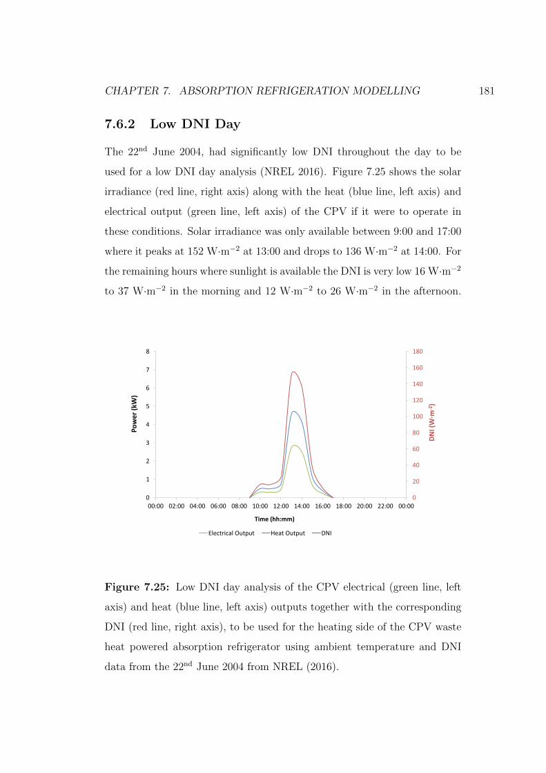
CHAPTER 7. ABSORPTION REFRIGERATION MODELLING 181
7.6.2 Low DNI Day
The 22nd June 2004, had significantly low DNI throughout the day to be
used for a low DNI day analysis (NREL 2016). Figure 7.25 shows the solar
irradiance (red line, right axis) along with the heat (blue line, left axis) and
electrical output (green line, left axis) of the CPV if it were to operate in
these conditions. Solar irradiance was only available between 9:00 and 17:00
where it peaks at 152 W·m−2 at 13:00 and drops to 136 W·m−2 at 14:00. For
the remaining hours where sunlight is available the DNI is very low 16 W·m−2
to 37 W·m−2 in the morning and 12 W·m−2 to 26 W·m−2 in the afternoon.
0
20
40
60
80
100
120
140
160
180
0
1
2
3
4
5
6
7
8
00:00 02:00 04:00 06:00 08:00 10:00 12:00 14:00 16:00 18:00 20:00 22:00 00:00
DNI(W·m
-2)
Power(k
W)
Time(hh:mm)
ElectricalOutput HeatOutput DNI
Figure 7.25: Low DNI day analysis of the CPV electrical (green line, left
axis) and heat (blue line, left axis) outputs together with the corresponding
DNI (red line, right axis), to be used for the heating side of the CPV waste
heat powered absorption refrigerator using ambient temperature and DNI
data from the 22nd June 2004 from NREL (2016).

CHAPTER 7. ABSORPTION REFRIGERATION MODELLING 182
This low DNI provided low heat and electrical generation from the CPV
peaking 4.6 kW and 2.8 kW respectively at 13:00 and less than 0.5 kW for
the remaining sunlight hours. It is worth noting that, with such low outputs,
further investigation is required to determine how much recoverable waste
heat would actually be produced from the CPV in these conditions. However
this analysis provides insight into the absorption refrigerator operation if the
heat were to be recoverable.
The conditions shown in Figure 7.25 provided strong solution concentra-
tions in the range of 60% to 61%. The heating cycle generated 793 kg at
0.12
0.14
0.16
0.18
0
5
10
15
20
25
30
35
40
45
50
00:00 02:00 04:00 06:00 08:00 10:00 12:00 14:00 16:00 18:00 20:00 22:00 00:00
CoolingPo
wer(kW)
Tempe
rature(°C)
Time(hh:mm)
EvaporatorTemperature AmbientTemperature CoolingPower
Figure 7.26: Low DNI day analysis of the CPV waste heat powered absorp-
tion refrigerator showing the evaporator temperature (green line, left axis),
ambient temperature (blue line, left axis) and cooling power (red line, right
axis). Using the ambient temperature from the 23rd June 2004 where the
previous day was used to fill the strong solution and refrigerant reservoirs.
Data from NREL (2016).
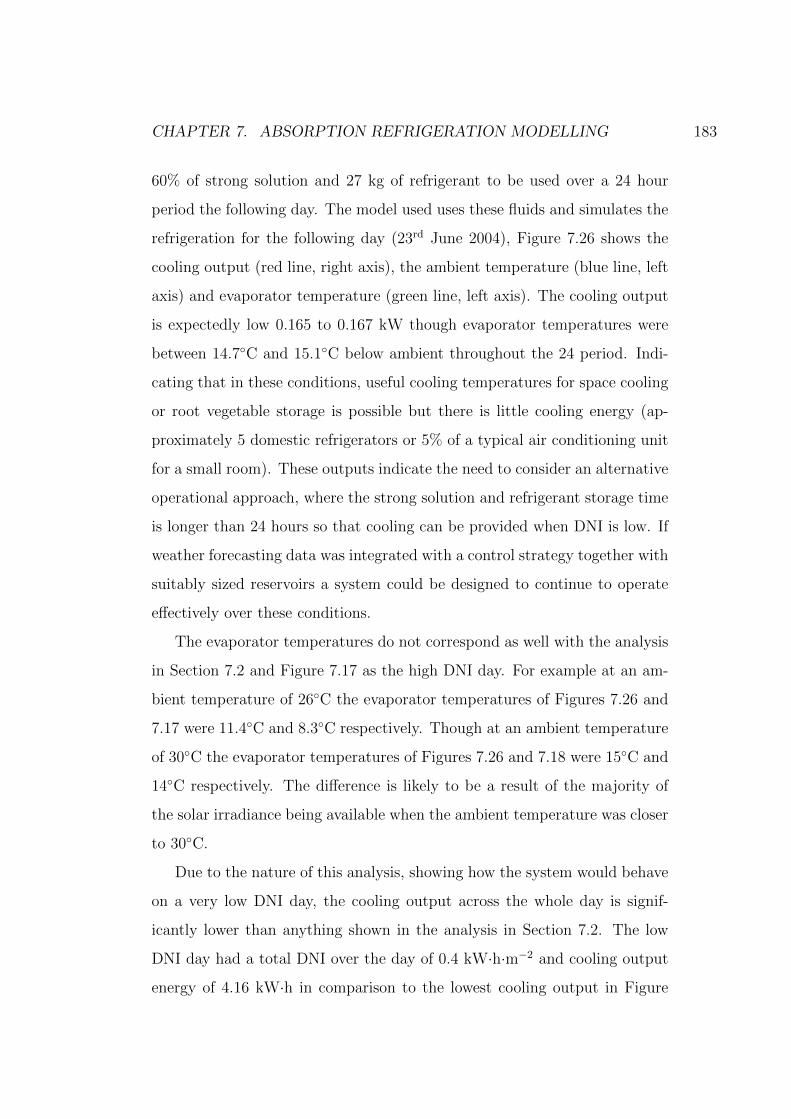
CHAPTER 7. ABSORPTION REFRIGERATION MODELLING 183
60% of strong solution and 27 kg of refrigerant to be used over a 24 hour
period the following day. The model used uses these fluids and simulates the
refrigeration for the following day (23rd June 2004), Figure 7.26 shows the
cooling output (red line, right axis), the ambient temperature (blue line, left
axis) and evaporator temperature (green line, left axis). The cooling output
is expectedly low 0.165 to 0.167 kW though evaporator temperatures were
between 14.7◦C and 15.1◦C below ambient throughout the 24 period. Indi-
cating that in these conditions, useful cooling temperatures for space cooling
or root vegetable storage is possible but there is little cooling energy (ap-
proximately 5 domestic refrigerators or 5% of a typical air conditioning unit
for a small room). These outputs indicate the need to consider an alternative
operational approach, where the strong solution and refrigerant storage time
is longer than 24 hours so that cooling can be provided when DNI is low. If
weather forecasting data was integrated with a control strategy together with
suitably sized reservoirs a system could be designed to continue to operate
effectively over these conditions.
The evaporator temperatures do not correspond as well with the analysis
in Section 7.2 and Figure 7.17 as the high DNI day. For example at an am-
bient temperature of 26◦C the evaporator temperatures of Figures 7.26 and
7.17 were 11.4◦C and 8.3◦C respectively. Though at an ambient temperature
of 30◦C the evaporator temperatures of Figures 7.26 and 7.18 were 15◦C and
14◦C respectively. The difference is likely to be a result of the majority of
the solar irradiance being available when the ambient temperature was closer
to 30◦C.
Due to the nature of this analysis, showing how the system would behave
on a very low DNI day, the cooling output across the whole day is signif-
icantly lower than anything shown in the analysis in Section 7.2. The low
DNI day had a total DNI over the day of 0.4 kW·h·m−2 and cooling output
energy of 4.16 kW·h in comparison to the lowest cooling output in Figure
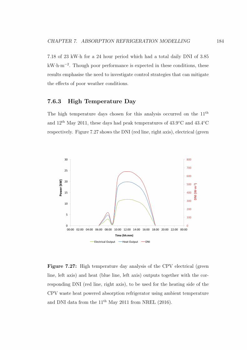
CHAPTER 7. ABSORPTION REFRIGERATION MODELLING 184
7.18 of 23 kW·h for a 24 hour period which had a total daily DNI of 3.85
kW·h·m−2. Though poor performance is expected in these conditions, these
results emphasise the need to investigate control strategies that can mitigate
the effects of poor weather conditions.
7.6.3 High Temperature Day
The high temperature days chosen for this analysis occurred on the 11th
and 12th May 2011, these days had peak temperatures of 43.9◦C and 43.4◦C
respectively. Figure 7.27 shows the DNI (red line, right axis), electrical (green
0
100
200
300
400
500
600
700
800
0
5
10
15
20
25
30
00:00 02:00 04:00 06:00 08:00 10:00 12:00 14:00 16:00 18:00 20:00 22:00 00:00
DNI(W·m
-2)
Power(k
W)
Time(hh:mm)
ElectricalOutput HeatOutput DNI
Figure 7.27: High temperature day analysis of the CPV electrical (green
line, left axis) and heat (blue line, left axis) outputs together with the cor-
responding DNI (red line, right axis), to be used for the heating side of the
CPV waste heat powered absorption refrigerator using ambient temperature
and DNI data from the 11th May 2011 from NREL (2016).
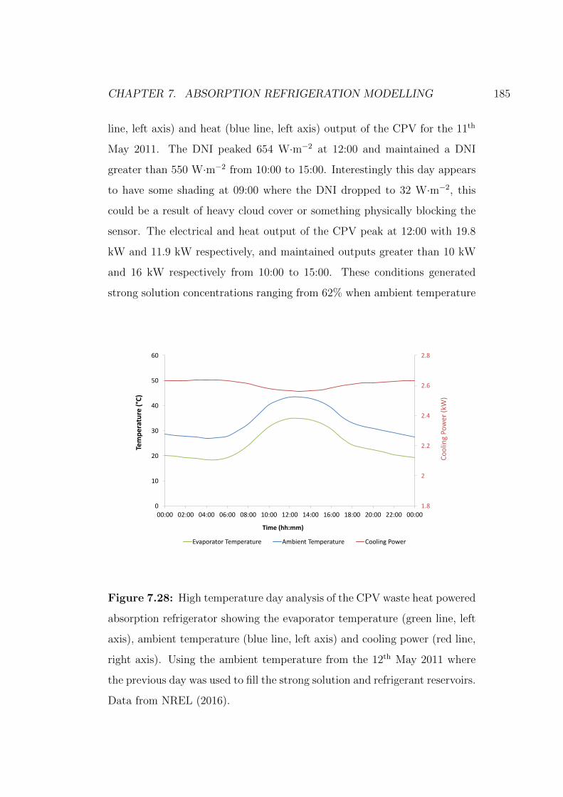
CHAPTER 7. ABSORPTION REFRIGERATION MODELLING 185
line, left axis) and heat (blue line, left axis) output of the CPV for the 11th
May 2011. The DNI peaked 654 W·m−2 at 12:00 and maintained a DNI
greater than 550 W·m−2 from 10:00 to 15:00. Interestingly this day appears
to have some shading at 09:00 where the DNI dropped to 32 W·m−2, this
could be a result of heavy cloud cover or something physically blocking the
sensor. The electrical and heat output of the CPV peak at 12:00 with 19.8
kW and 11.9 kW respectively, and maintained outputs greater than 10 kW
and 16 kW respectively from 10:00 to 15:00. These conditions generated
strong solution concentrations ranging from 62% when ambient temperature
1.8
2
2.2
2.4
2.6
2.8
0
10
20
30
40
50
60
00:00 02:00 04:00 06:00 08:00 10:00 12:00 14:00 16:00 18:00 20:00 22:00 00:00
CoolingPo
wer(kW)
Tempe
rature(°C)
Time(hh:mm)
EvaporatorTemperature AmbientTemperature CoolingPower
Figure 7.28: High temperature day analysis of the CPV waste heat powered
absorption refrigerator showing the evaporator temperature (green line, left
axis), ambient temperature (blue line, left axis) and cooling power (red line,
right axis). Using the ambient temperature from the 12th May 2011 where
the previous day was used to fill the strong solution and refrigerant reservoirs.
Data from NREL (2016).
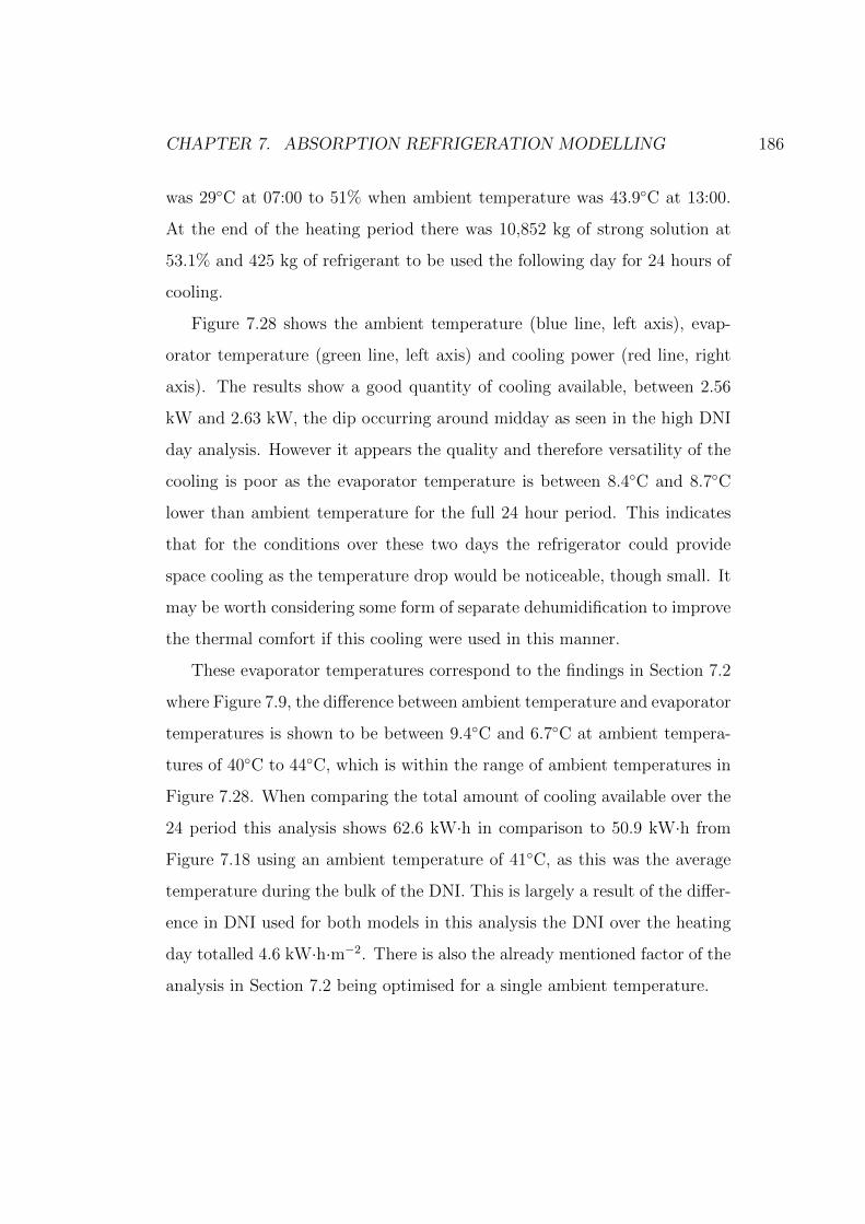
CHAPTER 7. ABSORPTION REFRIGERATION MODELLING 186
was 29◦C at 07:00 to 51% when ambient temperature was 43.9◦C at 13:00.
At the end of the heating period there was 10,852 kg of strong solution at
53.1% and 425 kg of refrigerant to be used the following day for 24 hours of
cooling.
Figure 7.28 shows the ambient temperature (blue line, left axis), evap-
orator temperature (green line, left axis) and cooling power (red line, right
axis). The results show a good quantity of cooling available, between 2.56
kW and 2.63 kW, the dip occurring around midday as seen in the high DNI
day analysis. However it appears the quality and therefore versatility of the
cooling is poor as the evaporator temperature is between 8.4◦C and 8.7◦C
lower than ambient temperature for the full 24 hour period. This indicates
that for the conditions over these two days the refrigerator could provide
space cooling as the temperature drop would be noticeable, though small. It
may be worth considering some form of separate dehumidification to improve
the thermal comfort if this cooling were used in this manner.
These evaporator temperatures correspond to the findings in Section 7.2
where Figure 7.9, the difference between ambient temperature and evaporator
temperatures is shown to be between 9.4◦C and 6.7◦C at ambient tempera-
tures of 40◦C to 44◦C, which is within the range of ambient temperatures in
Figure 7.28. When comparing the total amount of cooling available over the
24 period this analysis shows 62.6 kW·h in comparison to 50.9 kW·h from
Figure 7.18 using an ambient temperature of 41◦C, as this was the average
temperature during the bulk of the DNI. This is largely a result of the differ-
ence in DNI used for both models in this analysis the DNI over the heating
day totalled 4.6 kW·h·m−2. There is also the already mentioned factor of the
analysis in Section 7.2 being optimised for a single ambient temperature.
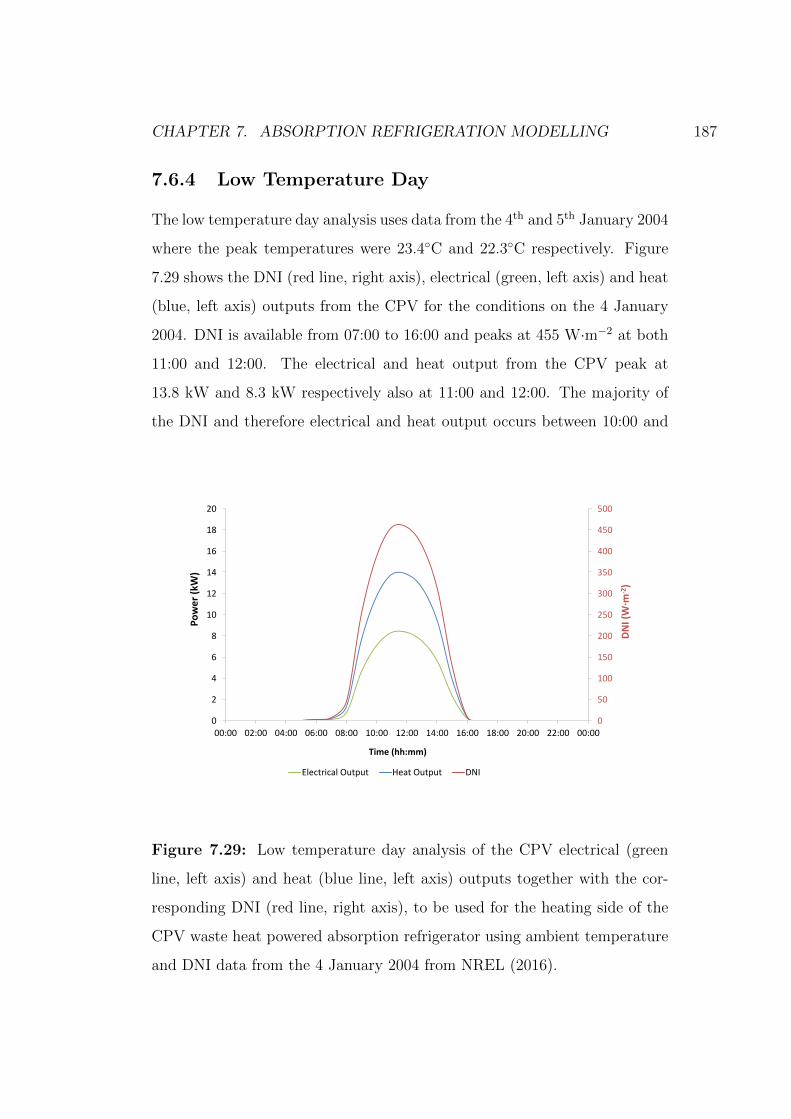
CHAPTER 7. ABSORPTION REFRIGERATION MODELLING 187
7.6.4 Low Temperature Day
The low temperature day analysis uses data from the 4th and 5th January 2004
where the peak temperatures were 23.4◦C and 22.3◦C respectively. Figure
7.29 shows the DNI (red line, right axis), electrical (green, left axis) and heat
(blue, left axis) outputs from the CPV for the conditions on the 4 January
2004. DNI is available from 07:00 to 16:00 and peaks at 455 W·m−2 at both
11:00 and 12:00. The electrical and heat output from the CPV peak at
13.8 kW and 8.3 kW respectively also at 11:00 and 12:00. The majority of
the DNI and therefore electrical and heat output occurs between 10:00 and
0
50
100
150
200
250
300
350
400
450
500
0
2
4
6
8
10
12
14
16
18
20
00:00 02:00 04:00 06:00 08:00 10:00 12:00 14:00 16:00 18:00 20:00 22:00 00:00
DNI(W·m
-2)
Power(k
W)
Time(hh:mm)
ElectricalOutput HeatOutput DNI
Figure 7.29: Low temperature day analysis of the CPV electrical (green
line, left axis) and heat (blue line, left axis) outputs together with the cor-
responding DNI (red line, right axis), to be used for the heating side of the
CPV waste heat powered absorption refrigerator using ambient temperature
and DNI data from the 4 January 2004 from NREL (2016).
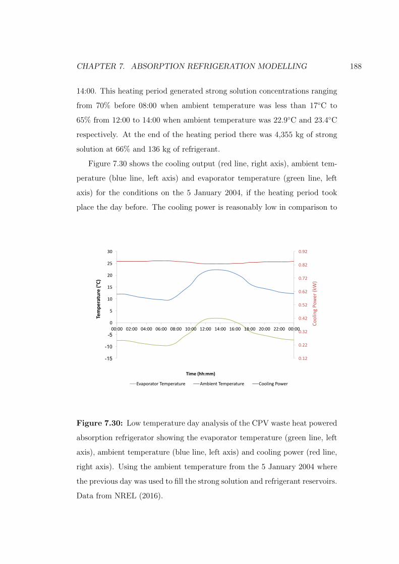
CHAPTER 7. ABSORPTION REFRIGERATION MODELLING 188
14:00. This heating period generated strong solution concentrations ranging
from 70% before 08:00 when ambient temperature was less than 17◦C to
65% from 12:00 to 14:00 when ambient temperature was 22.9◦C and 23.4◦C
respectively. At the end of the heating period there was 4,355 kg of strong
solution at 66% and 136 kg of refrigerant.
Figure 7.30 shows the cooling output (red line, right axis), ambient tem-
perature (blue line, left axis) and evaporator temperature (green line, left
axis) for the conditions on the 5 January 2004, if the heating period took
place the day before. The cooling power is reasonably low in comparison to
0.12
0.22
0.32
0.42
0.52
0.62
0.72
0.82
0.92
-15
-10
-5
0
5
10
15
20
25
30
00:00 02:00 04:00 06:00 08:00 10:00 12:00 14:00 16:00 18:00 20:00 22:00 00:00
CoolingPo
wer(kW)
Tempe
rature(°C)
Time(hh:mm)
EvaporatorTemperature AmbientTemperature CoolingPower
Figure 7.30: Low temperature day analysis of the CPV waste heat powered
absorption refrigerator showing the evaporator temperature (green line, left
axis), ambient temperature (blue line, left axis) and cooling power (red line,
right axis). Using the ambient temperature from the 5 January 2004 where
the previous day was used to fill the strong solution and refrigerant reservoirs.
Data from NREL (2016).
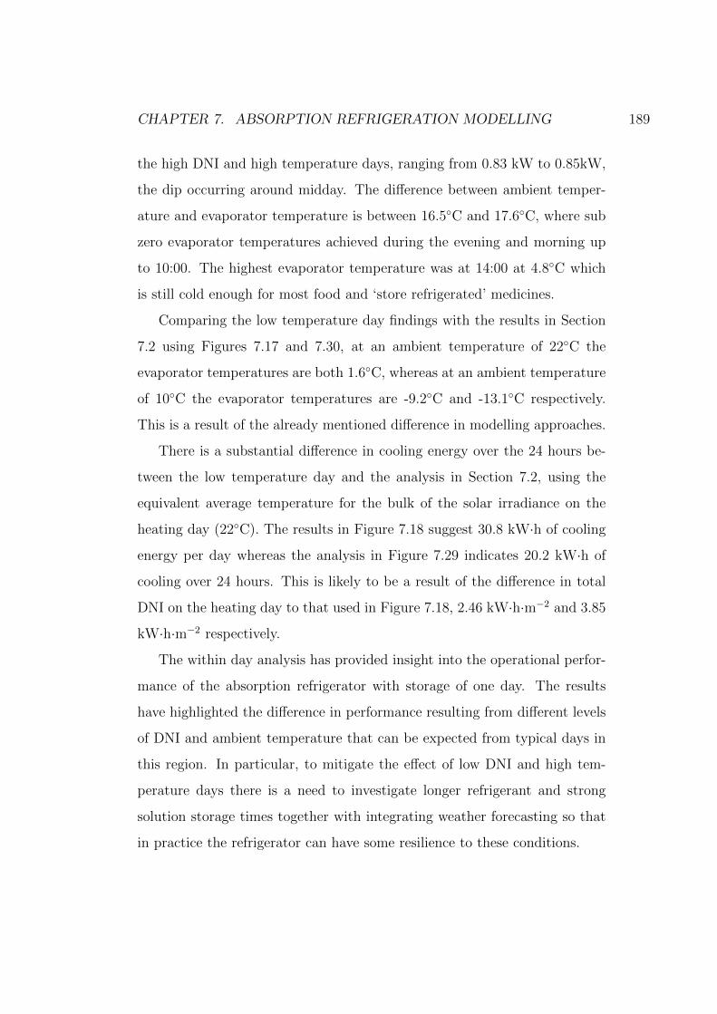
CHAPTER 7. ABSORPTION REFRIGERATION MODELLING 189
the high DNI and high temperature days, ranging from 0.83 kW to 0.85kW,
the dip occurring around midday. The difference between ambient temper-
ature and evaporator temperature is between 16.5◦C and 17.6◦C, where sub
zero evaporator temperatures achieved during the evening and morning up
to 10:00. The highest evaporator temperature was at 14:00 at 4.8◦C which
is still cold enough for most food and ‘store refrigerated’ medicines.
Comparing the low temperature day findings with the results in Section
7.2 using Figures 7.17 and 7.30, at an ambient temperature of 22◦C the
evaporator temperatures are both 1.6◦C, whereas at an ambient temperature
of 10◦C the evaporator temperatures are -9.2◦C and -13.1◦C respectively.
This is a result of the already mentioned difference in modelling approaches.
There is a substantial difference in cooling energy over the 24 hours be-
tween the low temperature day and the analysis in Section 7.2, using the
equivalent average temperature for the bulk of the solar irradiance on the
heating day (22◦C). The results in Figure 7.18 suggest 30.8 kW·h of cooling
energy per day whereas the analysis in Figure 7.29 indicates 20.2 kW·h of
cooling over 24 hours. This is likely to be a result of the difference in total
DNI on the heating day to that used in Figure 7.18, 2.46 kW·h·m−2 and 3.85
kW·h·m−2 respectively.
The within day analysis has provided insight into the operational perfor-
mance of the absorption refrigerator with storage of one day. The results
have highlighted the difference in performance resulting from different levels
of DNI and ambient temperature that can be expected from typical days in
this region. In particular, to mitigate the effect of low DNI and high tem-
perature days there is a need to investigate longer refrigerant and strong
solution storage times together with integrating weather forecasting so that
in practice the refrigerator can have some resilience to these conditions.
CHAPTER 7. ABSORPTION REFRIGERATION MODELLING 190
7.7 Absorption Refrigeration Modelling Con-
clusion
The results presented here investigated the waste heat sources which were
quantified in terms of energy and exergy at an ambient temperature of 25◦C
in Chapter 5. In terms of energy these are CPV at 60◦C with 116 kW·h
per day equivalent to 38% of the total system input energy and the genset
radiator at 80◦C with 32 kW·h equivalent to 10% of the system input energy.
However in terms of exergy they dwindle to 12 kW·h and 5 kW·h respectively,
indicating that there is a high quantity of energy but it is of low quality. This
provided a benchmark for the analysis of absorption refrigeration in terms of
waste heat utilisation. Experimental results in Chapter 6 provided confidence
in the modelling assumptions used for the results presented in this chapter.
The challenge of absorption refrigeration, described in Section 3.3.1, is
managing the trade-offs between conflicting variables, the following were in-
vestigated in this analysis:
• The desire to operate in high ambient temperatures requires dilute
strong solutions whereas the desire to have low evaporator temperatures
require concentrated weak solutions.
• Condenser heat exchanger effectiveness limits the strength of the strong
solution, which either limits the minimum boiler temperature or pushes
the strong solution to be more dilute which causes the weak solution
to be more dilute and therefore increases the evaporator temperature.
• Absorber heat exchanger effectiveness limits the minimum temperature
of the weak solution outlet of the absorber which limits the minimum
evaporator temperature.
• Reducing the difference in strong and weak solution concentration re-
duces the effect of the absorber heat exchanger effectiveness and can

CHAPTER 7. ABSORPTION REFRIGERATION MODELLING 191
provide lower evaporator temperatures.
The configuration analysis of the absorption refrigerators found that lower
evaporator temperatures can be achieved by using a small (2%) difference in
the strong and weak solution concentrations than the methods described
to cool the condenser and absorber. Using a small solution concentration
difference was also more energy efficient than the other methods presented.
Using a 2% solution concentration difference in two separate refrigerators
powered by each waste heat source independently, at the same conditions as
the energy and exergy analysis, can provide 33.4 kW·h of cooling per day at
6◦C and 6.3 kW·h at 0◦C. These can be considered to be equivalent to 12.7
kW·h of electricity that would have been used powering a vapour compression
refrigerator which equates to 22% of the total electricity provided to the
village.
For the average ambient temperatures expected in the case study area
(Kaligung Pearson-Palli, Santiniketan, West Bengal, India) of 24◦C to 35◦C
an absorption refrigerator powered by the CPV would provide 6 to 9 hours
of space cooling of a room in a medical centre. An absorption refrigerator
powered by the genset radiator could provide the equivalent of 6 to 8 domestic
refrigerator units. Collectively these refrigeration options could also be used
for medicines with the following storage requirements: keep refrigerated, keep
cool and store at room temperature.
The following typical within day conditions were investigated with a res-
olution of one hour: high temperature, low temperature, high DNI and low
DNI. The results provided insight into the application of the bulk of this
research which uses a resolution of one day with a constant ambient temper-
ature and DNI. An important outcome was that further research is required
to extend the refrigerant and strong solution storage time beyond 24 hours
together with weather forecasting data to provide resilience to weather con-
ditions that cause poor performance, such as low DNI and high ambient

CHAPTER 7. ABSORPTION REFRIGERATION MODELLING 192
temperatures.
Low grade waste heat was estimated at 7% of global energy consumption
in Chapter 2. Extrapolating the results of this chapter, where at the 25◦C
reference ambient temperature the waste heat utilisation to avoided electri-
cal consumption for cooling efficiency was 8.6%, the 7% global wasted energy
(as low grade heat) if used through absorption refrigeration could mitigate
electrical consumption equal to 0.6% of global energy consumption. 0.6% of
global energy consumption is approximately equal to the energy consump-
tion of Poland (CIA 2015). These figures provide a crude but useful analysis
of the global benefits of utilising low grade waste heat for absorption refrig-
eration. It should be noted that this analysis compares electricity avoided
to global energy consumption and does not take into consideration the con-
version efficiency of producing electricity due to the variances of electricity
generation methods globally.
Chapter 8
Conclusion of Thesis and
Further Work
This thesis focusses on utilising the low grade waste heat sources within a
renewable power plant in rural India for absorption refrigeration. Refrigera-
tion is more useful than low grade heat for communities in rural India as it
can provide food and medicine storage, or space cooling which could be used
for medical centres, recovery rooms or education environments.
This body of research forms part of a larger project called BioCPV which
is a collaboration between British and Indian universities to design and pro-
vide a renewable power plant to a 45 household community within a small ru-
ral village in West Bengal, India with the intention of promoting sustainable
development. The renewable power plant specified by the BioCPV research
group provided the modelling boundaries to conduct the analysis within this
thesis. Though the analysis is focussed on this particular plant the findings
are applicable to a wide range of circumstances where low grade waste heat
is available and sustainable refrigeration could be used.
An analysis of the sustainable development needs of the community iden-
tified that lighting, fans, a charging station, computers and small scale ma-
193
CHAPTER 8. CONCLUSION OF THESIS AND FURTHER WORK 194
chinery would improve the education environment, reduce exposure to indoor
air pollution and alleviate some of the labour intensive work currently under-
taken. A daily energy profile of these items for the community concluded the
projected electrical demand to be 55 kW·h. The total power demand includ-
ing system ancillaries, solar trackers and electrolyser load was estimated at
88 kW·h per day. The power plant proposed by the BioCPV research group
was specified to provide a daily generation of 90 kW·h, through 10 kW of
concentrated photovoltaic (CPV) for 7 hours and a 5 kW biogas-hydrogen
internal combustion engine generator set (genset) for 4 hours. The low grade
waste heat sources from this power plant, which were investigated in this
thesis, are the CPV at 60◦C and the genset radiator at 80◦C.
An assessment of common forms of refrigeration concluded that absorp-
tion refrigeration combines the ability to provide adequate heat removal at
the heat source as well as the potential to provide cooling from low grade
heat. A review of working fluids showed acetone and zinc bromide solution
to be able to work at the waste heat temperatures expected without the need
for rectification.
An energy and exergy analysis of the renewable plant at the rated condi-
tions found that the plant has a daily electrical output of 57 kW·h with an
electrical efficiency of 18%. The greatest energy losses were the low grade
waste heat from the CPV at 116 kW·h per day which is 38% of the total
energy input and the genset radiator at 32 kW·h per day which is 10% of
the total energy input. Due to the low temperature of these heat sources
their exergetic values at a 25◦C environment were much lower, 12 kW·h and
5 kW·h respectively. This indicated that converting these energy sources
to work is not effective and provided a case for their use in heat powered
refrigeration.
A lab scale, once through, experimental absorption refrigerator was built
and tested as part of this thesis in order to investigate the operational perfor-
CHAPTER 8. CONCLUSION OF THESIS AND FURTHER WORK 195
mance and challenges of an absorption refrigerator with reservoirs using ace-
tone and zinc bromide. The results indicated that the modelling approach in
terms of fluid state was appropriate. Interestingly, observations of the boiler
and evaporator temperatures and operating time, found that the evaporator
provided cooling for a significantly longer period than the boiler provided
heat. Indicating that, if a solution pump was present and suitable control
over valve opening were available, this system could have been controlled
to allow continuous cooling from a discontinuous heat source. The find-
ings also showed that the pressure was maintained after the boiler operation
ceased and drew attention to the importance of boiler exit and strong solu-
tion reservoir inlet design to maximise the condensing potential and therefore
the concentration of the strong solution. Temperature measurements across
the boiler, which simulated the heat sources in the power plant, suggested
that with adequate flow control constant temperatures can be maintained.
These observations coupled with the system successfully providing refrigera-
tion through an absorption cycle indicated that absorption refrigeration can
be used to extract waste heat from the power plant components and pro-
vide refrigeration while maintaining the desired operating temperatures of
the power plant components.
The assessment of absorption refrigerator configurations to lower evapo-
rator temperatures in high ambient temperatures concluded that the evap-
orator tap off method is ineffective for low temperature driven absorption
refrigerators. The method uses a proportion of the evaporator cooling output
in addition to ambient cooling to cool the absorber and / or condenser below
ambient temperature. Cooling the absorber required double the cooling loss
of lowering the solution concentration difference by 2% and provided on av-
erage 1.5◦C higher evaporator temperatures. Cooling the condenser, which
leads to stronger weak and strong solutions being usable, had negligible ef-
fect on evaporator temperatures whilst using up to 50% of the evaporator
CHAPTER 8. CONCLUSION OF THESIS AND FURTHER WORK 196
cooling output. The results of this identified the coupled cycle and double
boiler with evaporator tap off to be less effective at lowering evaporator tem-
peratures, in the conditions investigated, than using a smaller difference in
solution concentration. The most energy effective way to generate low evapo-
rator temperatures was to use a small difference (2%) between the strong and
weak solution concentrations. However the investigations did suggest that
there may be an application for the coupled cycle at high ambient temper-
atures which result in high evaporator temperatures. An absorption refrig-
erator powered by a large waste heat source such as the CPV could cool the
absorber and condenser of an absorption refrigerator powered by a smaller
heat source such as the genset radiator to simulate cooler conditions, provid-
ing more versatile evaporator temperatures. Though further investigation is
required.
It can be concluded that at a 25◦C reference ambient temperature (used
for energy and exergy analysis) acetone and zinc bromide absorption refrig-
eration with a 2% solution concentration difference powered by the waste
heat from the CPV at 60◦C and the genset radiator at 80◦C has the poten-
tial to provide 33.4 kW·h of cooling per day at 6◦C and 6.3 kW·h at 0◦C
respectively. The cooling can be quantified as the equivalent of 12.7 kW·h
per day of electricity that would have been consumed by a typical vapour
compression refrigerator. This is equivalent to 22% of the electricity that is
being provided to the end user (the village). This is 75% of the exergetic
value which quantifies the output based on a theoretical Carnot heat engine.
This indicates that the absorption refrigeration systems proposed can utilise
these low grade heat sources but in this configuration they do not surpass
the theoretical maximum work output.
An area for further investigation to identify the effectiveness of absorp-
tion refrigeration in low grade waste heat utilisation would be comparing the
avoided electrical energy to the amount of electrical energy that could be

CHAPTER 8. CONCLUSION OF THESIS AND FURTHER WORK 197
generated from a physical heat engine, rather than the theoretical maximum
provided by a Carnot heat engine. For example the results of Glover et al.
(2015), Peris et al. (2015) and Desideri et al. (2016) on organic Rankine cy-
cle generators, which is a common form of heat engine, suggest efficiencies
of 1% to 5% from heat sources under 100◦C. Using these efficiencies instead
of the Carnot efficiencies of 10.5% for the CPV and 15.5% for the genset
radiator, the avoided electricity consumption from utilising these low tem-
perature waste heat sources for absorption refrigeration outperforms, by at
least a factor of two, using the heat sources to generate electricity directly.
These waste heat sources used for absorption refrigeration produce cool-
ing that can be used for either food and medicine storage or space cooling
in a health centre. The evaporator temperatures are affected by ambient
temperature and careful planning on how to use the cooling and the size
of the reservoirs will be required to maximise its benefit. It was identified
that for the average ambient temperatures expected in the case study area
(Kaligung Pearson-Palli, Santiniketan, West Bengal, India) of 24◦C to 35◦C
an absorption refrigerator powered by the CPV would be suitable for space
cooling of a room in a medical centre for 6 to 9 hours per day. An absorption
refrigerator powered by the genset radiator could provide the equivalent of 6
to 8 domestic refrigerator units.
This thesis identified a technology that could utilise low grade waste heat,
an energy source which accounts for an estimated 7% of global energy con-
sumption. Extrapolating the results of this thesis the 7% wasted energy
(as low grade heat) if used through absorption refrigeration could mitigate
electrical consumption equal to 0.6% of global energy consumption. 0.6% of
global energy consumption is approximately equal to the energy consumption
of Poland. It should be noted that this analysis compares avoided electricity
consumption to global energy consumption and does not take into consider-
ation the conversion efficiency of producing electricity due to the variances
CHAPTER 8. CONCLUSION OF THESIS AND FURTHER WORK 198
of electricity generation methods globally. Therefore the mitigated 0.6% of
global energy consumption is a conservative figure and provides a case for
further investigation into utilising low temperature waste heat for absorption
refrigeration to reduce rising global energy consumption.
During the research that lead to this thesis a number of areas of further
work have been identified, these include:
• Analysis of the operating performance of integrating absorption re-
frigeration into a physical pilot plant similar to that proposed by the
BioCPV group. This could include investigating the temperature op-
erating limits of the plant and its effect on plant lifetime and combined
system performance.
• Modelling and improving the physical aspects of heat and mass transfer
in acetone and zinc bromide absorption refrigeration systems and its
effects on cooling output and evaporator temperature through its effects
on boiler and absorber performance. This could involve investigating
the specifics of absorber and boiler design to maximise fluid surface
area.
• Improving heat and mass transfer characteristics in acetone and zinc
bromide solution through additives such as nano-fluids, these could
facilitate the use of lower grade heat sources and provide lower tem-
perature refrigeration.
• The suitability of ambient air cooling (and its alternatives such as un-
derground cooling or evaporative cooling) and the effect of ambient
humidity. The models presented here can be refined with the use of
physical data and further configuration optimisation analysis can be
conducted.
• Investigating absorption refrigerator system stability, for example: main-
taining solution concentration differences, managing heat and mass

CHAPTER 8. CONCLUSION OF THESIS AND FURTHER WORK 199
transfer within the refrigerator and the associated control mechanisms
for this. Moreover both acetone and zinc bromide are hydrophilic and
over time may degrade due to leakages, loading and general mainte-
nance. The effects of this should be understood to gain insight into
long term operating performance.
• The modelled absorption refrigerators have varying evaporator tem-
peratures to maximise the heat source in a given environment. The
physical process of managing this and the use of the cooling output
requires investigation. This could include control mechanisms such as
feedback loops automating valve positioning and pump speed based
on temperature and flow detection. Optimisation of the storage in
the reservoirs together with the utilisation of weather forecasting data
should be investigated to mitigate the effects of unfavourable condi-
tions.
• Engineering design challenges of integrating the boiler of an absorption
refrigerator directly to a PV cell assembly in a CPV system. These
include: material compatibility, physical flexibility to allow for solar
tracking and the prevention of PV cell assembly overheating.
• Investigating theoretical and physical operating limits for the configu-
rations of absorption refrigeration described in this thesis. This could
be in terms of temperatures or cooling quantity ratio.

Bibliography
Agnew, B. et al. (2015). “Maximum output from a tri-generation cycle”. In:
Applied Thermal Engineering 90, pp. 1015–1020. issn: 13594311. doi:
10.1016/j.applthermaleng.2015.04.063. url: http://linkinghub.
elsevier.com/retrieve/pii/S135943111500407X (visited on 02/27/2016).
Ajib, Salman and Karno, Ali (2008). “Thermo physical properties of acetone
- zinc bromide for using in a low temperature driven absorption refrig-
eration machine”. en. In: Heat and Mass Transfer 45.1, pp. 61–70. issn:
0947-7411, 1432-1181. doi: 10.1007/s00231-008-0409-1. (Visited on
07/05/2013).
Ammar, Y., Chen, Y., et al. (2011). “Absorption process: An efficient way to
economically transfer low grade heat from industrial sources to domestic
sinks”. In: The 2nd PRO˙TEM Network Conference. Ed. by Ling J Chin
and S Spokes.
Ammar, Y., Joyce, S., et al. (2012). “Low grade thermal energy sources and
uses from the process industry in the UK”. In: Applied Energy 89.1, pp. 3–
20. issn: 0306-2619. doi: 10.1016/j.apenergy.2011.06.003.
Bajpai, Prabodh and Dash, Vaishalee (2012). “Hybrid renewable energy sys-
tems for power generation in stand-alone applications: A review”. In: Re-
newable and Sustainable Energy Reviews 16.5, pp. 2926–2939. doi: doi:
10.1016/j.rser.2012.02.009.
200
BIBLIOGRAPHY 201
Balghouthi, M., Chahbani, M. H., and Guizani, A. (2012). “Investigation of a
solar cooling installation in Tunisia”. In: Applied Energy 98, pp. 138–148.
issn: 0306-2619. doi: 10.1016/j.apenergy.2012.03.017.
Banerjee, Rangan (2006). “Comparison of options for distributed generation
in India”. In: Energy Policy 34.1, pp. 101–111. issn: 0301-4215. doi:
http://dx.doi.org/10.1016/j.enpol.2004.06.006.
Bejan, A (1997). Advanced Engineering Thermodynamics second edition. New
York: John Wiley & Sons, Inc.
Cameo (2016). Blomberg SSM9450 white freestanding fridge. url: http :
//www.cameokitchens.co.uk/ (visited on 02/24/2016).
Castro, J. et al. (2009). “Comparison of the performance of falling film and
bubble absorbers for air-cooled absorption systems”. In: International
Journal of Thermal Sciences 48.7, pp. 1355–1366. issn: 1290-0729. doi:
10.1016/j.ijthermalsci.2008.11.021.
Cengel and Boles (2006). Thermodynamics: An engineering approach. New
York: Mc Graw-Hill.
CIA (2015). The World Factbook. url: https://www.cia.gov/library/
publications/the-world-factbook/ (visited on 12/27/2015).
Dannen, Gene (1995). Leo Szilard Online. url: http://www.dannen.com/
szilard.html/ (visited on 09/11/2014).
Delano, Andrew (1998). “Design Analysis of the Einstein Refrigeration Cy-
cle”. English. PhD. Georgia Institute of Technology.
Deng, J., Wang, R. Z., and Han, G. Y. (2011). “A review of thermally acti-
vated cooling technologies for combined cooling, heating and power sys-
tems”. In: Progress in Energy and Combustion Science 37.2, pp. 172–203.
issn: 0360-1285. doi: 10.1016/j.pecs.2010.05.003.
Desideri, Adriano et al. (2016). “Experimental comparison of organic fluids
for low temperature ORC (organic Rankine cycle) systems for waste heat
recovery applications”. In: Energy 97, pp. 460–469. issn: 03605442. doi:

BIBLIOGRAPHY 202
10.1016/j.energy.2015.12.012. url: http://linkinghub.elsevier.
com/retrieve/pii/S0360544215016540 (visited on 02/25/2016).
DOE (2008). Waste Heat Recovery: Technology and Opportunities in U.S.
Industry. url: http : / / www1 . eere . energy . gov / manufacturing /
intensiveprocesses / pdfs / waste _ heat _ recovery . pdf (visited on
12/29/2015).
— (2014). Fuel Economy where energy goes. url: http://www.fueleconomy.
gov/feg/atv.shtml (visited on 04/03/2014).
DuPont Suva (2016). Thermodynamic Properties of HFC-134a. url: https:
//cdm.unfccc.int/filestorage/8/J/K/8JKOV024N9F16TYGISCUZAEM3P5XDW/
(visited on 02/24/2016).
Eames, I. W. and Wu, S. (2003). “A valve operated absorption refrigerator”.
In: Applied Thermal Engineering 23.4, pp. 417–429. issn: 1359-4311. doi:
10.1016/s1359-4311(02)00210-7.
EEB (2015). EU ban ‘Beginning of the End’ for climate changing F gases
- EEB. url: http://www.eeb.org/EEB/index.cfm/news-events/
news/eu-partial-ban-e28098beginning-of-the-ende28099-for-
climate-changing-f-gases/ (visited on 12/20/2015).
EIA (2015). EIA Projects world energy consumption will increase by 56% by
2040 - Today in Energy - US Energy Information Administration. url:
https://www.eia.gov/todayinenergy/detail.cfm?id=12251 (visited
on 12/20/2015).
Einstein, Albert and Szilard, Leo (1930). “Refrigeration”. US1781541 A.
U.S. Classification 62/110, 62/490, 62/112; International Classification
F25B15/10, C09K5/04; Cooperative Classification Y02B30/62, C09K5/047,
F25B15/10; European Classification C09K5/04D, F25B15/10. url: http:
//www.google.co.uk/patents/US1781541 (visited on 12/17/2014).
BIBLIOGRAPHY 203
ESRL (2015). ESRL Monitoring Division Halocarbons and other Atmospheric
Trace Species. url: http://www.esrl.noaa.gov/gmd/hats/publictn/
elkins/cfcs.html (visited on 12/20/2015).
Freidberg, Susanne Elizabeth (2009). Fresh : A Perishable History. Cam-
bridge, MA, USA: Harvard University Press. isbn: 9780674053854. url:
http : / / site . ebrary . com / lib / uon / docDetail . action ? docID =
10402511.
FSA (2007). “Guidance on Temperature Control Legislation in the United
Kingdom, EC Regulation 852/2004, The Food Hygiene Regulations 2006
(as amended)”. In: url: http://www.food.gov.uk/sites/default/
files/multimedia/pdfs/tempcontrolguiduk.pdf (visited on 02/24/2016).
— (2015). [Archived Content] Chilling Food Standards Agency. url: http:
//webarchive.nationalarchives.gov.uk/+/http://www.food.gov.
uk/northern-ireland/nutritionni/niyoungpeople/survivorform/
dontgetsick/chilling (visited on 02/24/2016).
Ge, Y.T., Tassou, S.A., and Chaer, I. (2009). “Modelling and performance
evaluation of a low-temperature ammonia-water absorption refrigeration
system”. In: International Journal of Low-Carbon Technologies 4.2, pp. 68–
77. issn: 1748-1317. doi: 10.1093/ijlct/ctp015. url: http://ijlct.
oxfordjournals.org/cgi/doi/10.1093/ijlct/ctp015 (visited on
02/27/2016).
Ghosh, Sajal (2002). “Electricity consumption and economic growth in In-
dia”. In: Energy Policy 30.2, pp. 125–129. issn: 0301-4215. doi: http:
//dx.doi.org/10.1016/S0301-4215(01)00078-7.
Glover, Stephen et al. (2015). “Simulation of a multiple heat source super-
critical ORC (Organic Rankine Cycle) for vehicle waste heat recovery”.
In: Energy 93, pp. 1568–1580. issn: 03605442. doi: 10.1016/j.energy.
2015.10.004. url: http://linkinghub.elsevier.com/retrieve/
pii/S0360544215013596 (visited on 02/25/2016).
BIBLIOGRAPHY 204
Gonzalez-Gil, A. et al. (2011). “Experimental evaluation of a direct air-cooled
lithium bromide - water absorption prototype for solar air conditioning”.
In: Applied Thermal Engineering 31.16, pp. 3358–3368. issn: 1359-4311.
doi: 10.1016/j.applthermaleng.2011.06.019.
Gutierrez-Urueta, G. et al. (2011). “Experimental performances of a LiBr-
water absorption facility equipped with adiabatic absorber”. In: Interna-
tional Journal of Refrigeration 34.8, pp. 1749–1759. issn: 0140-7007. doi:
10.1016/j.ijrefrig.2011.07.014.
Haddad, Cynthia et al. (2014). “Some Efficient Solutions to Recover Low
and Medium Waste Heat: Competitiveness of the Thermoacoustic Tech-
nology”. In: Energy Procedia 50, pp. 1056–1069. issn: 18766102. doi:
10.1016/j.egypro.2014.06.125. url: http://linkinghub.elsevier.
com/retrieve/pii/S1876610214008613 (visited on 12/29/2015).
Harrison, H C (1996). “Storing Vegetables at Home”. In: url: http://
nchfp.uga.edu/how/store/wisc_vegetables.pdf (visited on 12/28/2015).
Hawkins, G (2011). “BSRIA Rules of Thumb Guidelines for Building Ser-
vices, 5th Edition”. In: url: https://www.bsria.co.uk/download/
product/?file=zxrulZgWBrY= (visited on 01/20/2016).
Herold, K. E. (1996). Absorption chillers and heat pumps. In collab. with
Reinhard Radermacher and Sanford A. Klein. Boca Raton, FL: CRC
Press. 329 pp. isbn: 0849394279.
Howard, John P (1980). “A history of refrigeration throughout the world
by Roger Thevenot”. In: New Scientist 87. 1210, p. 219. url: http:
//books.google.co.uk/books?id=a9hgb5uSVF8C&pg=PA219&dq=
history+of+refrigeration+technology&hl=en&sa=X&ei=uH-JT-
XBJs6z8QPr3s30CQ#v=onepage&q=history%20of%20refrigeration%
20technology&f=true.
HP (2015). HP Online Store. url: http://store.hp.com/UKStore (visited
on 01/14/2015).
BIBLIOGRAPHY 205
HSE (1997). Lighting at Work Web-Friendly Version of HSG38. url: http:
//www.hse.gov.uk/pubns/priced/hsg38.pdf (visited on 01/04/2015).
Hua, Junye et al. (2014). “Thermodynamic analysis of ammonia-water power/chilling
cogeneration cycle with low-grade waste heat”. In: Applied Thermal Engi-
neering 64.1, pp. 483–490. issn: 13594311. doi: 10.1016/j.applthermaleng.
2013.12.043. url: http://linkinghub.elsevier.com/retrieve/pii/
S135943111300940X (visited on 02/27/2016).
Jelinek, M. and Borde, I. (1998). “Single and double stage absorption cycles
based on fluorocarbon refrigerants and organic absorbents”. In: Applied
Thermal Engineering 18.9-10, pp. 765–771. issn: 1359-4311. doi: 10.
1016/s1359-4311(97)00114-2.
Jelinek, M., Levy, A., and Borde, I. (2002). “Performance of a triple-pressure-
level absorption cycle with R125-N, N’- dimethylethylurea”. In: Applied
Energy 71.3, pp. 171–189. issn: 0306-2619. doi: 10.1016/s0306-2619(02)
00003-x.
Jeong, Chulyoung et al. (2009). “Generating efficiency and emissions of a
spark-ignition gas engine generator fuelled with biogas–hydrogen blends”.
In: International Journal of Hydrogen Energy 34.23, pp. 9620–9627. issn:
0360-3199. doi: http://dx.doi.org/10.1016/j.ijhydene.2009.09.
099.
Jeong, Jongsoo, Saito, Kiyoshi, and Kawai, Sunao (2011). “Static charac-
teristics and efficient control of compression- and absorption-type hybrid
air conditioning system”. In: International Journal of Refrigeration 34.3,
pp. 674–685. issn: 0140-7007. doi: 10.1016/j.ijrefrig.2011.01.003.
Jordan, Richard C and Priester, Gayle B (1950). Refrigeration and air coni-
ditioning. 512th ed. New York: Prentice-Hall Inc.
Karno, Ali and Ajib, Salman (2008). “Thermodynamic analysis of an ab-
sorption refrigeration machine with new working fluid for solar applica-

BIBLIOGRAPHY 206
tions”. In: Heat and Mass Transfer, p. 40. issn: 0947-7411. doi: 10.1007/
s00231-008-0408-2. (Visited on 07/05/2013).
Kim, D S and Infante Ferreira, C A (2009). “Air-cooled LiBr-water absorp-
tion chillers for solar air conditioning in extremely hot weathers”. In: En-
ergy Conversion and Management 50.4, pp. 1018–1025. issn: 0196-8904.
doi: 10.1016/j.enconman.2008.12.021.
Kim, Jin Kyeong, Jung, Jun Young, and Kang, Yong Tae (2007). “Absorption
performance enhancement by nano-particles and chemical surfactants in
binary nanofluids”. en. In: International Journal of Refrigeration 30.1,
pp. 50–57. issn: 01407007. doi: 10.1016/j.ijrefrig.2006.04.006.
Lide, David R (2004). Handbook of Chemistry and Physics. 85th ed. Boca
Raton: CRC.
Mathkor, Ratha et al. (2015). “Exergetic Analysis of an Integrated Tri-
Generation Organic Rankine Cycle”. In: Energies 8.8, pp. 8835–8856.
issn: 1996-1073. doi: 10.3390/en8088835. url: http://www.mdpi.
com/1996-1073/8/8/8835/ (visited on 02/27/2016).
Mei, V. C. et al. (1992). An assessment of desiccant cooling and dehumidifi-
cation technology. Tech. rep.
Miro, Laia, Bruckner, Sarah, and Cabeza, Luisa F. (2015). “Mapping and
discussing Industrial Waste Heat (IWH) potentials for different coun-
tries”. In: Renewable and Sustainable Energy Reviews 51, pp. 847–855.
issn: 13640321. doi: 10 . 1016 / j . rser . 2015 . 06 . 035. url: http :
//linkinghub.elsevier.com/retrieve/pii/S1364032115006073 (vis-
ited on 12/29/2015).
Mohammad, Abdulrahman Th. et al. (2013). “Historical review of liquid
desiccant evaporation cooling technology”. In: Energy and Buildings 67,
pp. 22–33. issn: 0378-7788. doi: 10.1016/j.enbuild.2013.08.018.
Moss, Stephen (1989). “Out of the Ice Box, into the Fire”. In: New Scientist,
Google Books 1696/1697, p. 85. url: http://books.google.co.uk/

BIBLIOGRAPHY 207
books?id=yINSqbNUNM0C&pg=PA85&dq=einstein+szilard+fridge&hl=
en&sa=X&ei=TB3aU9_JDKnG7AbCo4DIAQ&ved=0CCoQ6AEwAA#v=onepage&
q=einstein%20szilard%20fridge&f=false (visited on 07/31/2014).
Munters, Carl Georg and Platen, Baltzar Carl von (1928). “Refrigeration”.
US Patent 1,669,269. url: https://www.google.co.uk/patents/
US1669269 (visited on 09/11/2014).
NIST (2011). NIST Acetone. url: http://webbook.nist.gov/cgi/cbook.
cgi?ID=C67641&Mask=4&Type=ANTOINE&Plot=on#ANTOINE (visited on
12/20/2015).
NREL (2014). National Residential Efficiency Measures Database. url: http:
//www.nrel.gov/ap/retrofits/ (visited on 12/14/2014).
— (2016). India Solar Resource Data: Hourly. url: http://rredc.nrel.
gov/solar/new_data/India/nearestcell.cgi (visited on 10/14/2016).
NUT (2015). Space Requirements in Classrooms: NUT Health and Safety
Guidance. url: https : / / www . teachers . org . uk / files / space -
requirements-in-classrooms.doc (visited on 09/27/2015).
Oluleye, Gbemi et al. (2016). “Evaluating the potential of process sites for
waste heat recovery”. In: Applied Energy 161, pp. 627–646. issn: 0306-
2619. doi: http://dx.doi.org/10.1016/j.apenergy.2015.07.011.
Patek, J. and Klomfar, J. (2006). “A computationally effective formulation
of the thermodynamic properties of LiBr - H2O solutions from 273 to 500
K over full composition range”. In: International Journal of Refrigeration
29.4, pp. 566–578. issn: 0140-7007. doi: 10.1016/j.ijrefrig.2005.
10.007.
Pennington, N.A. (1955). “Humidity changer for air-conditioning”. US Patent
2,700,537. url: http://www.google.com/patents/US2700537 (visited
on 09/11/2014).
Peris, Bernardo et al. (2015). “Experimental characterization of an ORC
(organic Rankine cycle) for power and CHP (combined heat and power)
BIBLIOGRAPHY 208
applications from low grade heat sources”. In: Energy 82, pp. 269–276.
issn: 03605442. doi: 10.1016/j.energy.2015.01.037. url: http:
//linkinghub.elsevier.com/retrieve/pii/S0360544215000614 (vis-
ited on 02/25/2016).
Petela, Richard (2010). Engineering Thermodynamics of Thermal Radiation.
1st ed. McGraw-Hill. isbn: 9780071639620.
Pita, Edward (1984). Refrigeration principles and systems: An energy ap-
proach. New York: John Wiley & Sons.
Ramachandra, T.V., Jain, Rishabh, and Krishnadas, Gautham (2011). “Hotspots
of solar potential in India”. en. In: Renewable and Sustainable Energy Re-
views 15.6, pp. 3178–3186. issn: 13640321. doi: http://dx.doi.org/
10.1016/j.rser.2011.04.007.
Reddy, K. S. and Veershetty, G. (2013). “Viability analysis of solar parabolic
dish stand-alone power plant for Indian conditions”. In: Applied Energy.
Special Issue on Advances in sustainable biofuel production and use -
XIX International Symposium on Alcohol Fuels - ISAF 102, pp. 908–922.
issn: 0306-2619. doi: http://dx.doi.org/10.1016/j.apenergy.2012.
09.034.
Rogers, G.F.C. and Mayhew, Y.R. (1995). Thermodyanmic and Transport
Properties of Fluids (SI Units). Fifth. Blackwell Publishing. isbn: 0631197036.
Said, Syed A. M., El-Shaarawi, Maged A.I., and Siddiqui, Muhammad U.
(2012). “Alternative designs for a 24-h operating solar-powered absorption
refrigeration technology”. In: International Journal of Refrigeration 35.7.
issn: 0140-7007. doi: http://dx.doi.org/10.1016/j.ijrefrig.2012.
06.008.
Saravanan, R. and Maiya, M. P. (1998). “Thermodynamic comparison of
water-based working fluid combinations for a vapour absorption refriger-
ation system”. In: Applied Thermal Engineering 18.7, pp. 553–568. issn:
1359-4311. doi: 10.1016/s1359-4311(97)00072-0.
BIBLIOGRAPHY 209
Shah, R. K., Subbarao, E. C., and Mashelkar, R. A. (1988). Heat Transfer
Equipment Design. New York: Hemisphere Publishing Corperation.
Sharma, Naveen Kumar, Tiwari, Prashant Kumar, and Sood, Yog Raj (2012).
“Solar energy in India: Strategies, policies, perspectives and future poten-
tial”. en. In: Renewable and Sustainable Energy Reviews 16.1, pp. 933–
941. issn: 13640321. doi: http://dx.doi.org/10.1016/j.rser.2011.
09.014.
Sieres, Jaime and Fernandez-Seara, Jose (2007). “Experimental investigation
of mass transfer performance with some random packings for ammonia
rectification in ammonia - water absorption refrigeration systems”. In:
International Journal of Thermal Sciences 46.7, pp. 699–706. issn: 1290-
0729. doi: 10.1016/j.ijthermalsci.2006.09.003.
Srikhirin, Pongsid, Aphornratana, Satha, and Chungpaibulpatana, Supachart
(2001). “A review of absorption refrigeration technologies”. In: Renewable
and Sustainable Energy Reviews 5.4, pp. 343–372. issn: 1364-0321. doi:
10.1016/s1364-0321(01)00003-x.
Sun, Jian, Fu, Lin, and Zhang, Shigang (2012). “A review of working fluids of
absorption cycles”. In: Renewable and Sustainable Energy Reviews 16.4,
pp. 1899–1906. issn: 1364-0321. doi: 10.1016/j.rser.2012.01.011.
Tae Kang, Yong, Akisawa, Atsushi, and Kashiwagi, Takao (2000). “Analytical
investigation of two different absorption modes: falling film and bubble
types”. In: International Journal of Refrigeration 23.6, pp. 430–443. issn:
0140-7007. doi: 10.1016/s0140-7007(99)00075-4.
Tamura, Moriyoshi (2008). “An Investigation of a Natural Gas HCCI Engine
for 5kW Class Co-genergation System”. In: IGRC Paris 2008. Interna-
tional Gas Union Research Conference.
Tassou, S.A. et al. (2010). “A review of emerging technologies for food refrig-
eration applications”. In: Applied Thermal Engineering 30.4, pp. 263–276.
issn: 13594311. doi: 10.1016/j.applthermaleng.2009.09.001. url:

BIBLIOGRAPHY 210
http://linkinghub.elsevier.com/retrieve/pii/S1359431109002737
(visited on 02/27/2016).
Todd, Daniel (1995). Timetoast Timelines: Internal Combustion Engine Time-
line. url: https://www.timetoast.com/timelines/119674 (visited on
10/01/2014).
Vent-Axia (2015). Reversible Hi Line Vent Axia. url: http://www.vent-
axia.com/range/reversible-hi-line.html (visited on 09/27/2015).
Wang, R and Oliveira, R (2006). “Adsorption refrigeration - An efficient way
to make good use of waste heat and solar energy”. en. In: Progress in
Energy and Combustion Science 32.4, pp. 424–458. issn: 03601285. doi:
10.1016/j.pecs.2006.01.002.
WHO (2016). Guidelines for the Storage of Essential Medicines and Other
Health Commodities. url: http://apps.who.int/medicinedocs/en/d/
Js4885e/6.5.html (visited on 02/24/2016).
Xie, Guozhen et al. (2012). “A novel lithium bromide absorption chiller
with enhanced absorption pressure”. In: Applied Thermal Engineering
38, pp. 1–6. issn: 1359-4311. doi: 10.1016/j.applthermaleng.2011.
12.047.
Yanmar (2016). Yanmar mCHP Catalogue. url: http : / / www . yanmar -
es.com/uploads/files/349226-YAN-Catalog-Apr17_FINAL_DIGITAL_
med.pdf (visited on 02/24/2016).
Zacarıas, A. et al. (2011). “Experimental assessment of ammonia adiabatic
absorption into ammonia-lithium nitrate solution using a flat fan nozzle”.
In: Applied Thermal Engineering 31.16, pp. 3569–3579. issn: 1359-4311.
doi: 10.1016/j.applthermaleng.2011.07.019.
Zohar, A. et al. (2009). “Performance of diffusion absorption refrigeration
cycle with organic working fluids”. In: International Journal of Refriger-
ation 32.6, pp. 1241–1246. issn: 0140-7007. doi: 10.1016/j.ijrefrig.
2009.01.010.

Appendix: Draft Paper
211
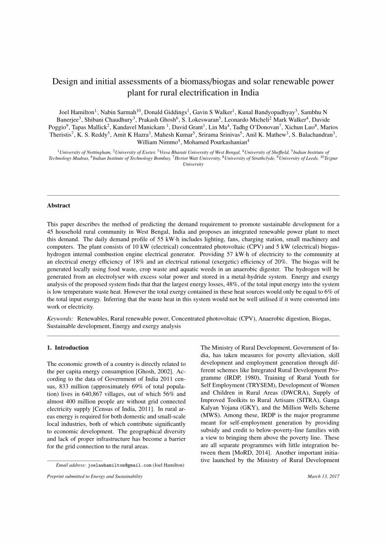
Design and initial assessments of a biomass/biogas and solar renewable powerplant for rural electrification in India
Joel Hamilton1,, Nabin Sarmah10, Donald Giddings1, Gavin S Walker1, Kunal Bandyopadhyay3, Sambhu NBanerjee3, Shibani Chaudhury3, Prakash Ghosh6, S. Lokeswaran5, Leonardo Micheli2 Mark Walker4, Davide
Poggio9, Tapas Mallick2, Kandavel Manickam 1, David Grant1, Lin Ma4, Tadhg O’Donovan7, Xichun Luo8, MariosTheristis7, K. S. Reddy5, Amit K Hazra3, Mahesh Kumar5, Srirama Srinivas5, Anil K. Mathew3, S. Balachandran3,
William Nimmo4, Mohamed Pourkashanian4
1University of Nottingham, 2University of Exeter, 3Visva Bharati University of West Bengal, 4University of She�eld, 5Indian Institute ofTechnology Madras, 6Indian Institute of Technology Bombay, 7Heriot Watt University, 8University of Strathclyde, 9University of Leeds, 10Tezpur
University
Abstract
This paper describes the method of predicting the demand requirement to promote sustainable development for a45 household rural community in West Bengal, India and proposes an integrated renewable power plant to meetthis demand. The daily demand profile of 55 kW·h includes lighting, fans, charging station, small machinery andcomputers. The plant consists of 10 kW (electrical) concentrated photovoltaic (CPV) and 5 kW (electrical) biogas-hydrogen internal combustion engine electrical generator. Providing 57 kW·h of electricity to the community atan electrical energy e�ciency of 18% and an electrical rational (exergetic) e�ciency of 20%. The biogas will begenerated locally using food waste, crop waste and aquatic weeds in an anaerobic digester. The hydrogen will begenerated from an electrolyser with excess solar power and stored in a metal-hydride system. Energy and exergyanalysis of the proposed system finds that that the largest energy losses, 48%, of the total input energy into the systemis low temperature waste heat. However the total exergy contained in these heat sources would only be equal to 6% ofthe total input exergy. Inferring that the waste heat in this system would not be well utilised if it were converted intowork or electricity.
Keywords: Renewables, Rural renewable power, Concentrated photovoltaic (CPV), Anaerobic digestion, Biogas,Sustainable development, Energy and exergy analysis
1. Introduction
The economic growth of a country is directly related tothe per capita energy consumption [Ghosh, 2002]. Ac-cording to the data of Government of India 2011 cen-sus, 833 million (approximately 69% of total popula-tion) lives in 640,867 villages, out of which 56% andalmost 400 million people are without grid connectedelectricity supply [Census of India, 2011]. In rural ar-eas energy is required for both domestic and small-scalelocal industries, both of which contribute significantlyto economic development. The geographical diversityand lack of proper infrastructure has become a barrierfor the grid connection to the rural areas.
Email address: [email protected] (Joel Hamilton)
The Ministry of Rural Development, Government of In-dia, has taken measures for poverty alleviation, skilldevelopment and employment generation through dif-ferent schemes like Integrated Rural Development Pro-gramme (IRDP, 1980), Training of Rural Youth forSelf Employment (TRYSEM), Development of Womenand Children in Rural Areas (DWCRA), Supply ofImproved Toolkits to Rural Artisans (SITRA), GangaKalyan Yojana (GKY), and the Million Wells Scheme(MWS). Among these, IRDP is the major programmemeant for self-employment generation by providingsubsidy and credit to below-poverty-line families witha view to bringing them above the poverty line. Theseare all separate programmes with little integration be-tween them [MoRD, 2014]. Another important initia-tive launched by the Ministry of Rural Development
Preprint submitted to Energy and Sustainability March 13, 2017
(MoRD), Government of India in June 2011 was Na-tional Rural Livelihoods Mission (NRLM). The Mis-sion, partly aided by the World Bank, aims to create e�-cient livelihood development for the rural poor throughsustainable enhancements and improved access to finan-cial services [NRLM, 2014].
In spite of having such activities by the Governmentof India, basic infrastructural facilities in rural Indialike electricity, education, transport and healthcare arestill far from satisfactory. In 2011, only 55.3% of ru-ral household had access to electricity [Census of In-dia, 2011] (Energy Statistics 2013). The Human De-velopment Report 2011 quotes a percentage point gapbetween urban and rural areas of 17% in literacy, 19%in child immunisation and 38 in institutional delivery(giving birth within an institution rather than at home),[Gandhi, 2011].
Per capita annual grid connected electricity consump-tion in India during 2011 is 288 kW·h in urban areasand 96 kW·h in rural areas. Though this is higher thanThe World Energy Outlook (WEO) analysis of the In-ternational Energy Agency (IEA) (2012) which consid-ers 250 kW·h and 500 kW·h as the minimum annualconsumption levels for a household of five in rural andurban areas respectively.
This lack of facilities has crippled the socio-economicdevelopment of the rural masses; who are dependent to alarge extent on natural resources for making their liveli-hood and wellbeing. The quality of life of these peo-ple living in rural India can be improved by widespreadelectrification, which can infuse visible changes in theirlivelihood. As the natural resources like plant biomass,agricultural by-products and solar radiation are in abun-dance in rural areas, e�cient management of these re-sources in a sustainable manner can provide holisticdevelopment of rural communities. Electrification canhelp improve facilities in terms of education, health-care, lifestyle and rural enterprises; thereby alleviatingpoverty and ushering in an era of self-su�ciency andbetter competitiveness to take on the challenges of therest of the world.
Decentralised hybrid power plants with di↵erent re-newable technologies can provide e�cient, cheap andsustainable options for rural electrification [Bajpai andDash, 2012] and [Ghosh, 2002]. The integration of a va-riety of renewable sources coupled with storage to com-plement each other can provide a sustainable develop-ment solution all year round.
India had 20,556 MW of renewable power generation
capacity by 30th June 2011 which was approximately11% of the total power generation capacity of the coun-try. There is an average intensity of solar radiationof 200 MW·km�2. Through the Jawaharlal Nehru Na-tional Solar Mission (JNNSM) it is envisaged that Indiawill have an installed solar capacity of 20,000 MW by2020, 100,000 MW by 2030 and 200,000 MW by 2050.[Sharma et al., 2012]
The following research is part of a collaborative group,called BioCPV, with the objective of providing a sus-tainable development solution to rural India through re-newable power. This research outlines the need forrural development in India and then describes the de-mographics of a particular community in Santiniketan,West Bengal, India. With this information a demandprofile is forecast and a technology selection process tomeet these needs is described. The initial design calcu-lations for the proposed technologies are presented andfollowed with an energy (first law) and exergy (secondlaw) analysis of the proposed system to identify areasfor optimisation.
2. Description of Need for Micro Electrical Genera-
tion Plant
Two rural tribal villages, Kaligung and Pearson-Palli,adjacent to Visva-Bharati, Santiniketan have been se-lected because the majority of the tribal people do nothave access to electricity owing to their socio-economicconditions. Although there is a grid connection in thevillage, the supply is weak, only providing a few hoursof electricity per day and not all the houses are con-nected through this grid. The villages are comprised of179 households with a population of approximately 821.Most the families in the village live below the povertyline. Out of the total population, 52% are women and10% are children. The average income of each house-hold is approximately INR 2500/month.
Basic facilities such as drinking water and sanitation arenot available which leads to an unhygienic lifestyle. Thehouses are typical for an Indian village made from bam-boo or wood and mud. There is a basic health centre inthe village which provides primary health care throughan arrangement with university, doctors and local healthworkers. Most of this care currently takes place out-doors. However for more serious illness, villagers visitthe Block Primary Health Centre (BPHC) or UniversityHospital (3 and 2 km away respectively).
2
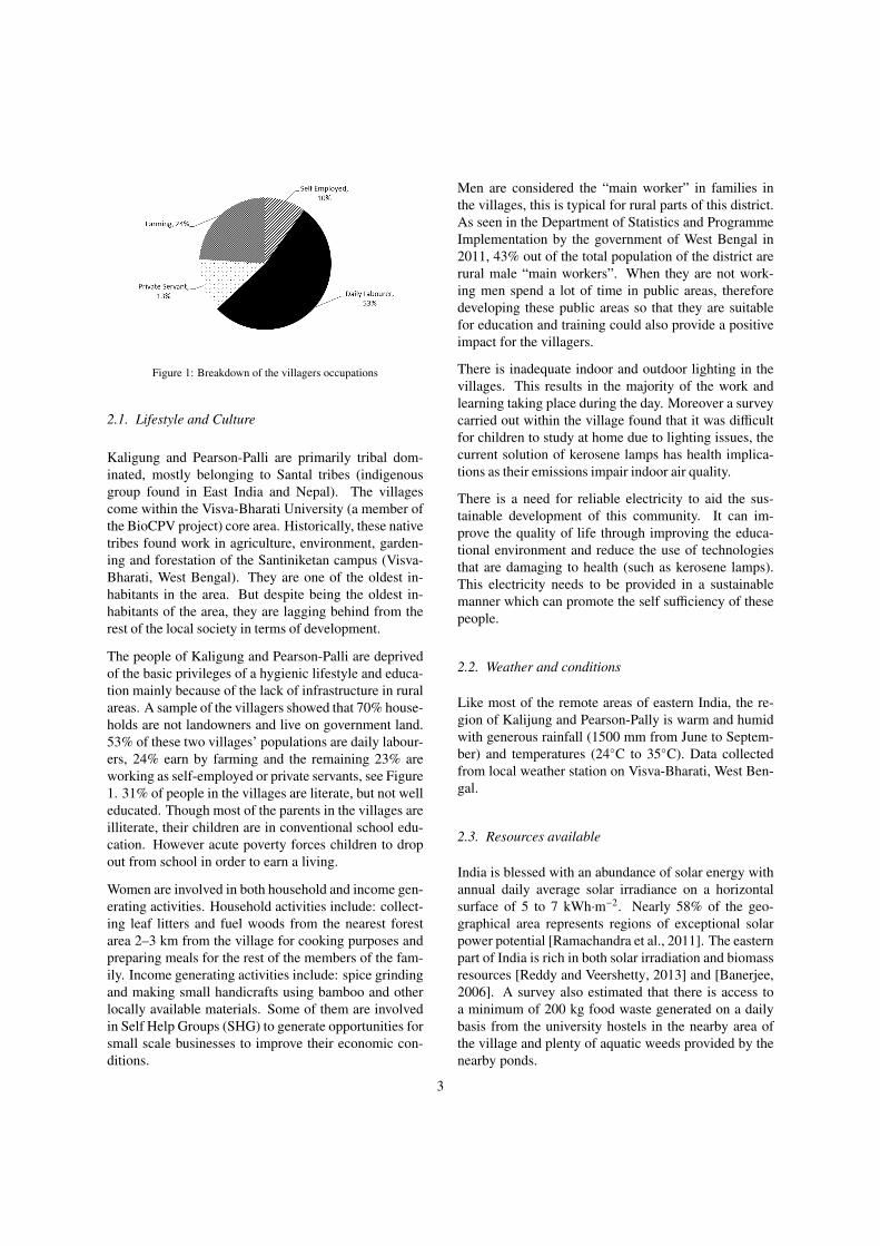
Figure 1: Breakdown of the villagers occupations
2.1. Lifestyle and Culture
Kaligung and Pearson-Palli are primarily tribal dom-inated, mostly belonging to Santal tribes (indigenousgroup found in East India and Nepal). The villagescome within the Visva-Bharati University (a member ofthe BioCPV project) core area. Historically, these nativetribes found work in agriculture, environment, garden-ing and forestation of the Santiniketan campus (Visva-Bharati, West Bengal). They are one of the oldest in-habitants in the area. But despite being the oldest in-habitants of the area, they are lagging behind from therest of the local society in terms of development.
The people of Kaligung and Pearson-Palli are deprivedof the basic privileges of a hygienic lifestyle and educa-tion mainly because of the lack of infrastructure in ruralareas. A sample of the villagers showed that 70% house-holds are not landowners and live on government land.53% of these two villages’ populations are daily labour-ers, 24% earn by farming and the remaining 23% areworking as self-employed or private servants, see Figure1. 31% of people in the villages are literate, but not welleducated. Though most of the parents in the villages areilliterate, their children are in conventional school edu-cation. However acute poverty forces children to dropout from school in order to earn a living.
Women are involved in both household and income gen-erating activities. Household activities include: collect-ing leaf litters and fuel woods from the nearest forestarea 2–3 km from the village for cooking purposes andpreparing meals for the rest of the members of the fam-ily. Income generating activities include: spice grindingand making small handicrafts using bamboo and otherlocally available materials. Some of them are involvedin Self Help Groups (SHG) to generate opportunities forsmall scale businesses to improve their economic con-ditions.
Men are considered the “main worker” in families inthe villages, this is typical for rural parts of this district.As seen in the Department of Statistics and ProgrammeImplementation by the government of West Bengal in2011, 43% out of the total population of the district arerural male “main workers”. When they are not work-ing men spend a lot of time in public areas, thereforedeveloping these public areas so that they are suitablefor education and training could also provide a positiveimpact for the villagers.
There is inadequate indoor and outdoor lighting in thevillages. This results in the majority of the work andlearning taking place during the day. Moreover a surveycarried out within the village found that it was di�cultfor children to study at home due to lighting issues, thecurrent solution of kerosene lamps has health implica-tions as their emissions impair indoor air quality.
There is a need for reliable electricity to aid the sus-tainable development of this community. It can im-prove the quality of life through improving the educa-tional environment and reduce the use of technologiesthat are damaging to health (such as kerosene lamps).This electricity needs to be provided in a sustainablemanner which can promote the self su�ciency of thesepeople.
2.2. Weather and conditions
Like most of the remote areas of eastern India, the re-gion of Kalijung and Pearson-Pally is warm and humidwith generous rainfall (1500 mm from June to Septem-ber) and temperatures (24�C to 35�C). Data collectedfrom local weather station on Visva-Bharati, West Ben-gal.
2.3. Resources available
India is blessed with an abundance of solar energy withannual daily average solar irradiance on a horizontalsurface of 5 to 7 kWh·m�2. Nearly 58% of the geo-graphical area represents regions of exceptional solarpower potential [Ramachandra et al., 2011]. The easternpart of India is rich in both solar irradiation and biomassresources [Reddy and Veershetty, 2013] and [Banerjee,2006]. A survey also estimated that there is access toa minimum of 200 kg food waste generated on a dailybasis from the university hostels in the nearby area ofthe village and plenty of aquatic weeds provided by thenearby ponds.
3

3. Community Power Demand Rationale
The following section describes the process for design-ing a small rural distributed renewable power plant. Theprocess requires a demand estimation and a detailedoverview of the technologies available allowing appro-priate selection. The section is followed with the designconsiderations and sizing calculations for each technol-ogy within the plant.
3.1. Demand Estimation
The World Energy Outlook analysis for the minimumelectricity consumption of a 5 person household is cal-culated using the assumption that following technolo-gies could be used: floor fan, a mobile telephone, andtwo compact fluorescent lamp (CFL) bulbs in rural ar-eas, and might include an e�cient refrigerator, a sec-ond mobile telephone, and another appliance, such asa small television or a computer, in urban areas. Elec-tric lighting is seen to be an influential technology toprovide development, from 2001 to 2011 the shares ofhouseholds in rural areas using electricity as their primesource of lighting changed from 43.5% to 55.3%, andin urban areas from 87.6% to 92.7% (Census of India,2011).
In light of these findings and studies of the local needstogether with the desire to provide sustainable devel-opment through improving the educational environmentand overall quality of life, the following items in Table1 have been selected for the demand profile.
Previous work with these communities carried out byVisva-Bharati, West Bengal found that successful adop-tion of change requires a holistic approach where thevillagers are involved throughout the project, trainingand education are provided and that everything is com-patible with their customs and traditions.
The following subsections describe the method for cal-culating the predicted demand.
Ventilation - Fans
Guidelines in the United Kingdom suggest 70 m2 is re-quired for primary or middle school class of 30 students[NUT, 2015]. A typical ceiling fan such as Vent-AxiaReversible Hi-Line + requires 60 W at full load and sug-gests in tropical climates that they should be placed 3m apart (and 6 m in temperate climates) [Vent-Axia,2015]. There are currently 104 students at the school
which are accommodated by 2 large rooms (approxi-mately 11 m x 5 m) and one small one (3 m x 4 m). Forthe purposes of repeatable demand profiling and as thenumber of students can vary, and the building may haveadditional rooms built on to it, the remaining analysis isbased on the guidelines mentioned earlier. Therefore theschool would require 3 classrooms allowing for a com-fortable learning environment for 90 children. Each 70m2 classroom can be allocated 2 fans depending on di-mensions. An assembly hall which can house activitiesand exercise classes as well is assumed to be the size of3 classrooms and would require 6 fans. Another roomthe same size as a classroom used as an o�ce for theteachers and sta↵ would require a further 2 fans. Thistotals 14 fans, however it will be very unlikely that allthe fans were on maximum load at the same time. Forthe purposes of load estimating an average of 10 fans at60 W each has been assumed.
Lighting
The e�cacy of compact florescent light bulb (CFL) =55 lm·W�1 [NREL, 2013]. The lighting requirementsfor a bright o�ce space requiring perception of detailis 200 lx and for dull workspaces not requiring percep-tion of detail 100 lx is needed [HSE, 1997]. By defini-tion
(1)e f f icacy =lumen
electrical power
And
(2)lux =lumenarea
Therefore using Equations 1 and 2 the lit area dependingon the lighting requirements can be found using Equa-tion 3
(3)area =e f f icacy ⇥ electrical power
lux
Using this information a 15 W CFL should provide4.125 m2 of bright workspace and 8.25 m2 of dullworkspace. Therefore 40 ⇥ 15 W CFLs are consideredfor public lighting, providing a bright area of 165 m2
and a dull area 330 m2. Taking natural light into con-sideration as well, the estimate of 40 bulbs provides anaverage load of public lighting to meet the daytime andevening needs.
4

Table 1: Appliance itinerary to create demand profile, including typical energy consumption and quantity required
Energy Per Item (W) Quantity Total Energy (kW)School / Public light bulb 15 40 0.75Fan 60 10 0.6Domestic light bulb 10 90 0.9Lantern / Phone charging 10 100 1Desktop PC 100 10 1Small Machinery 200 8 1.6
Likewise the same analysis can be used to determinethat 10 W CFLs in a domestic setting can provide theequivalent of 2.75 m2 of bright workspace and 5.5 m2
of dull workspace. Assuming that 2 rooms per house-hold require lighting, then 90 ⇥ 10 W CFL bulbs arerequired.
Lantern and Phone Charging
Lantern and phone charging was based on modern highpowered USB chargers outputting approximately 10 Wfor mobile phone charging for example the InnergieADP 21AW D. Since a large number of battery pow-ered devices can be charged by these it was assumedto be suitable for lanterns as well. It was assumed thatthere would be 2 lanterns per household and 10 phonesin the community resulting in a quantity of 100 ⇥ 10 Wdevices requiring charge.
Desktop PC
The power demand for a typical PC found on the marketis 100 W based on a basic specification of an HP 110-352na Desktop PC at 65 W and a typical monitor suchas the HP ENVY 24 60.5 cm at 26 W to 54 W [HP,2015]. It was assumed the school could have an averagePC load of 10 PCs.
Small Machinery
Small machinery such as spice grinders and sewing ma-chines were estimated at 200 W based on a range avail-able in the market. A quantity of 8 was estimated allow-ing a gentle introduction of the technology, so that thosewho want to work together with the machinery can andthose who prefer the traditional methods can maintaintheir current approach.
3.2. Demand Profile
Figure 2 shows the expected demand profile of the vil-lage over 24 hours. The demand is divided in to a day
Figure 2: Maximum predicted demand profile elected for the commu-nity on a typical day irrespective of the season
load which is from 09:00 to 17:00 and an evening loadfrom 17:00 to 21:00. public area lighting, fans, comput-ers and the charging station are assumed to be used allday from 09:00 to 21:00. This is a result of the commu-nity buildings being used as a school during the day andthen a community centre. The small machinery load isassumed to only take place during the day, this is mainlybecause they are noisy.
3.3. System Requirements
This demand profiling analysis shown in Figure 2 andTable 1 has found that there is a minimum system re-quirement of 4.8 kW of electricity during the day (09:00to 17:00) and 4.1 kW in the evening (17:00 to 21:00).Totalling 55 kW·h per day of electrical supply to thevillage. An additional 26 kW·h has been allocated forsystem ancillaries (12 kW·h), 14 kW·h solar trackersand 7 kW·h for hydrogen production (1 kW for the 7hours of CPV operation). Therefore there is an mini-mum electrical generation requirement of 88 kW·h perday.
4. Appropriate Generation Technologies
The main available renewable resources are solar andbiomass.
5
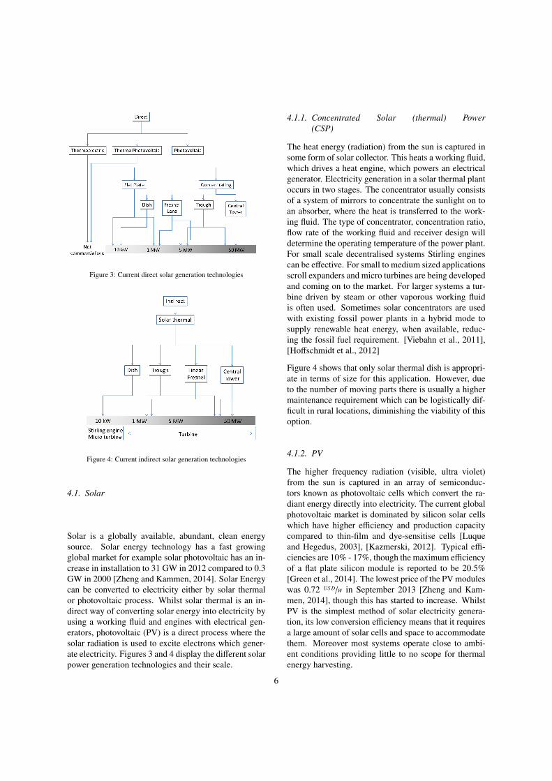
Figure 3: Current direct solar generation technologies
Figure 4: Current indirect solar generation technologies
4.1. Solar
Solar is a globally available, abundant, clean energysource. Solar energy technology has a fast growingglobal market for example solar photovoltaic has an in-crease in installation to 31 GW in 2012 compared to 0.3GW in 2000 [Zheng and Kammen, 2014]. Solar Energycan be converted to electricity either by solar thermalor photovoltaic process. Whilst solar thermal is an in-direct way of converting solar energy into electricity byusing a working fluid and engines with electrical gen-erators, photovoltaic (PV) is a direct process where thesolar radiation is used to excite electrons which gener-ate electricity. Figures 3 and 4 display the di↵erent solarpower generation technologies and their scale.
4.1.1. Concentrated Solar (thermal) Power(CSP)
The heat energy (radiation) from the sun is captured insome form of solar collector. This heats a working fluid,which drives a heat engine, which powers an electricalgenerator. Electricity generation in a solar thermal plantoccurs in two stages. The concentrator usually consistsof a system of mirrors to concentrate the sunlight on toan absorber, where the heat is transferred to the work-ing fluid. The type of concentrator, concentration ratio,flow rate of the working fluid and receiver design willdetermine the operating temperature of the power plant.For small scale decentralised systems Stirling enginescan be e↵ective. For small to medium sized applicationsscroll expanders and micro turbines are being developedand coming on to the market. For larger systems a tur-bine driven by steam or other vaporous working fluidis often used. Sometimes solar concentrators are usedwith existing fossil power plants in a hybrid mode tosupply renewable heat energy, when available, reduc-ing the fossil fuel requirement. [Viebahn et al., 2011],[Ho↵schmidt et al., 2012]
Figure 4 shows that only solar thermal dish is appropri-ate in terms of size for this application. However, dueto the number of moving parts there is usually a highermaintenance requirement which can be logistically dif-ficult in rural locations, diminishing the viability of thisoption.
4.1.2. PV
The higher frequency radiation (visible, ultra violet)from the sun is captured in an array of semiconduc-tors known as photovoltaic cells which convert the ra-diant energy directly into electricity. The current globalphotovoltaic market is dominated by silicon solar cellswhich have higher e�ciency and production capacitycompared to thin-film and dye-sensitise cells [Luqueand Hegedus, 2003], [Kazmerski, 2012]. Typical e�-ciencies are 10% - 17%, though the maximum e�ciencyof a flat plate silicon module is reported to be 20.5%[Green et al., 2014]. The lowest price of the PV moduleswas 0.72 US D/W in September 2013 [Zheng and Kam-men, 2014], though this has started to increase. WhilstPV is the simplest method of solar electricity genera-tion, its low conversion e�ciency means that it requiresa large amount of solar cells and space to accommodatethem. Moreover most systems operate close to ambi-ent conditions providing little to no scope for thermalenergy harvesting.
6
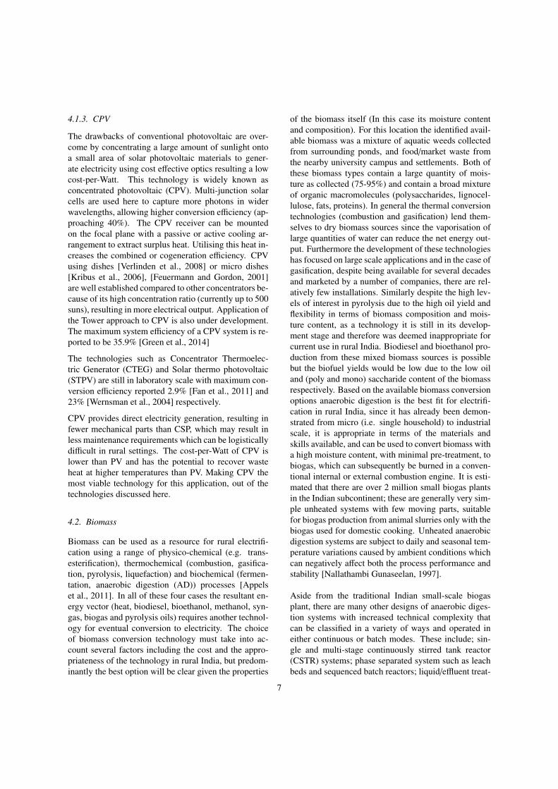
4.1.3. CPV
The drawbacks of conventional photovoltaic are over-come by concentrating a large amount of sunlight ontoa small area of solar photovoltaic materials to gener-ate electricity using cost e↵ective optics resulting a lowcost-per-Watt. This technology is widely known asconcentrated photovoltaic (CPV). Multi-junction solarcells are used here to capture more photons in widerwavelengths, allowing higher conversion e�ciency (ap-proaching 40%). The CPV receiver can be mountedon the focal plane with a passive or active cooling ar-rangement to extract surplus heat. Utilising this heat in-creases the combined or cogeneration e�ciency. CPVusing dishes [Verlinden et al., 2008] or micro dishes[Kribus et al., 2006], [Feuermann and Gordon, 2001]are well established compared to other concentrators be-cause of its high concentration ratio (currently up to 500suns), resulting in more electrical output. Application ofthe Tower approach to CPV is also under development.The maximum system e�ciency of a CPV system is re-ported to be 35.9% [Green et al., 2014]
The technologies such as Concentrator Thermoelec-tric Generator (CTEG) and Solar thermo photovoltaic(STPV) are still in laboratory scale with maximum con-version e�ciency reported 2.9% [Fan et al., 2011] and23% [Wernsman et al., 2004] respectively.
CPV provides direct electricity generation, resulting infewer mechanical parts than CSP, which may result inless maintenance requirements which can be logisticallydi�cult in rural settings. The cost-per-Watt of CPV islower than PV and has the potential to recover wasteheat at higher temperatures than PV. Making CPV themost viable technology for this application, out of thetechnologies discussed here.
4.2. Biomass
Biomass can be used as a resource for rural electrifi-cation using a range of physico-chemical (e.g. trans-esterification), thermochemical (combustion, gasifica-tion, pyrolysis, liquefaction) and biochemical (fermen-tation, anaerobic digestion (AD)) processes [Appelset al., 2011]. In all of these four cases the resultant en-ergy vector (heat, biodiesel, bioethanol, methanol, syn-gas, biogas and pyrolysis oils) requires another technol-ogy for eventual conversion to electricity. The choiceof biomass conversion technology must take into ac-count several factors including the cost and the appro-priateness of the technology in rural India, but predom-inantly the best option will be clear given the properties
of the biomass itself (In this case its moisture contentand composition). For this location the identified avail-able biomass was a mixture of aquatic weeds collectedfrom surrounding ponds, and food/market waste fromthe nearby university campus and settlements. Both ofthese biomass types contain a large quantity of mois-ture as collected (75-95%) and contain a broad mixtureof organic macromolecules (polysaccharides, lignocel-lulose, fats, proteins). In general the thermal conversiontechnologies (combustion and gasification) lend them-selves to dry biomass sources since the vaporisation oflarge quantities of water can reduce the net energy out-put. Furthermore the development of these technologieshas focused on large scale applications and in the case ofgasification, despite being available for several decadesand marketed by a number of companies, there are rel-atively few installations. Similarly despite the high lev-els of interest in pyrolysis due to the high oil yield andflexibility in terms of biomass composition and mois-ture content, as a technology it is still in its develop-ment stage and therefore was deemed inappropriate forcurrent use in rural India. Biodiesel and bioethanol pro-duction from these mixed biomass sources is possiblebut the biofuel yields would be low due to the low oiland (poly and mono) saccharide content of the biomassrespectively. Based on the available biomass conversionoptions anaerobic digestion is the best fit for electrifi-cation in rural India, since it has already been demon-strated from micro (i.e. single household) to industrialscale, it is appropriate in terms of the materials andskills available, and can be used to convert biomass witha high moisture content, with minimal pre-treatment, tobiogas, which can subsequently be burned in a conven-tional internal or external combustion engine. It is esti-mated that there are over 2 million small biogas plantsin the Indian subcontinent; these are generally very sim-ple unheated systems with few moving parts, suitablefor biogas production from animal slurries only with thebiogas used for domestic cooking. Unheated anaerobicdigestion systems are subject to daily and seasonal tem-perature variations caused by ambient conditions whichcan negatively a↵ect both the process performance andstability [Nallathambi Gunaseelan, 1997].
Aside from the traditional Indian small-scale biogasplant, there are many other designs of anaerobic diges-tion systems with increased technical complexity thatcan be classified in a variety of ways and operated ineither continuous or batch modes. These include; sin-gle and multi-stage continuously stirred tank reactor(CSTR) systems; phase separated system such as leachbeds and sequenced batch reactors; liquid/e✏uent treat-
7
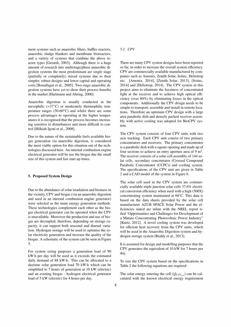
ment systems such as anaerobic filters, ba✏es reactors,anaerobic sludge blankets and membrane bioreactors,and a variety of systems that combine the above re-actor types [Gerardi, 2003]. Although there is a hugeamount of research into multistage/phase anaerobic di-gestion systems the most predominant are single stage(partially or completely) mixed systems due to theirsimpler, robust designs and lower capital and operatingcosts [Bouallagui et al., 2005]. Two-stage anaerobic di-gestion systems have yet to show their process benefitsin the market [Hartmann and Ahring, 2006].
Anaerobic digestion is usually conducted in themesophilic (⇡37�C) or moderately thermophilic tem-perature ranges (50-60�C) and whilst there are someprocess advantages to operating at the higher temper-atures it is recognised that the process becomes increas-ing sensitive to disturbances and more di�cult to con-trol [Hilkiah Igoni et al., 2008].
Due to the nature of the sustainable fuels available bio-gas generation via anaerobic digestion, is consideredthe most viable option for this situation out of the tech-nologies discussed here. An internal combustion engineelectrical generator will be use the biogas due the smallsize of this system and fast start up times.
5. Proposed System Design
Due to the abundance of solar irradiation and biomass inthe vicinity, CPV and biogas (via an anaerobic digestionand used in an internal combustion engine generator)were selected as the main energy generation methods.These technologies complement each other as the bio-gas electrical generator can be operated when the CPVis unavailable. Moreover the production and use of bio-gas are decoupled; therefore, depending on storage ca-pacity, it can support both seasonal and diurnal varia-tion. Hydrogen storage will be used to optimise the so-lar electricity generation and increase the quality of thebiogas. A schematic of the system can be seen in Figure5.
For system sizing purposes a generation load of 90kW·h per day will be used as it exceeds the estimateddaily demand of 88 kW·h. This can be allocated to adaytime solar generation load 70 kW·h which can besimplified to 7 hours of generation at 10 kW (electric)and an evening biogas - hydrogen electrical generatorload of 5 kW (electric) for 4 hours per day.
5.1. CPV
There are many CPV system designs have been reportedso far, in order to increase the overall system e�ciency.CPV are commercially available manufactured by com-panies such as Amonix, Zenith Solar, Soitec, Heliotropetc. [Amonix, 2014], [Zenith Solar, 2013], [Soitec,2014] and [Heliotrop, 2014]. The CPV system in thisproject aims to eliminate the fuzziness of concentratedlight at the receiver and to achieve high optical e�-ciency (over 80%) by eliminating losses in the opticalcomponents. Additionally the CPV design needs to besimple to transport, assemble and install in remote loca-tions. Therefore an optimum CPV design with a largearea parabolic dish and densely packed receiver assem-bly with active cooling was adopted for BioCPV sys-tem.
The CPV system consists of four CPV units with twoaxis tracking. Each CPV unit consist of two primaryconcentrators and receivers. The primary concentratoris a parabolic dish with a square opening and made up offour sections to achieve an entry aperture area of 9 m2.The receiver consists of a solar cell assembly of 144 so-lar cells, secondary concentrator (Crossed CompoundParabolic Concentrator (CCPC)) and cooling system.The specifications of the CPV unit are given in Table2 and a CAD model of the system in Figure 6.
The solar cell used in the CPV system are commer-cially available triple junction solar cells 37.6% electri-cal conversion e�ciency when used with a high (500X)concentrating system maintained at 60�C. This data isbased on the data sheets provided by the solar cellmanufacturer AZUR SPACE Solar Power and the ef-ficiencies stated are inline with the NREL report ti-tled “Opportunities and Challenges for Development ofa Mature Concentrating Photovoltaic Power Industry”[Kurtz, 2012]. A novel cooling system was developedfor e�cient heat recovery from the CPV units, whichwill be used in the Anaerobic Digestion system and hy-drogen storage system [Reddy et al., 2013].
It is assumed for design and modelling purposes that theCPV generates the equivalent of 10 kW for 7 hours perday.
To size the CPV system based on the specifications inTable 2 the following equations are required:
The solar energy entering the cell (QCPVcell ) can be cal-culated with the known electrical energy requirement
8
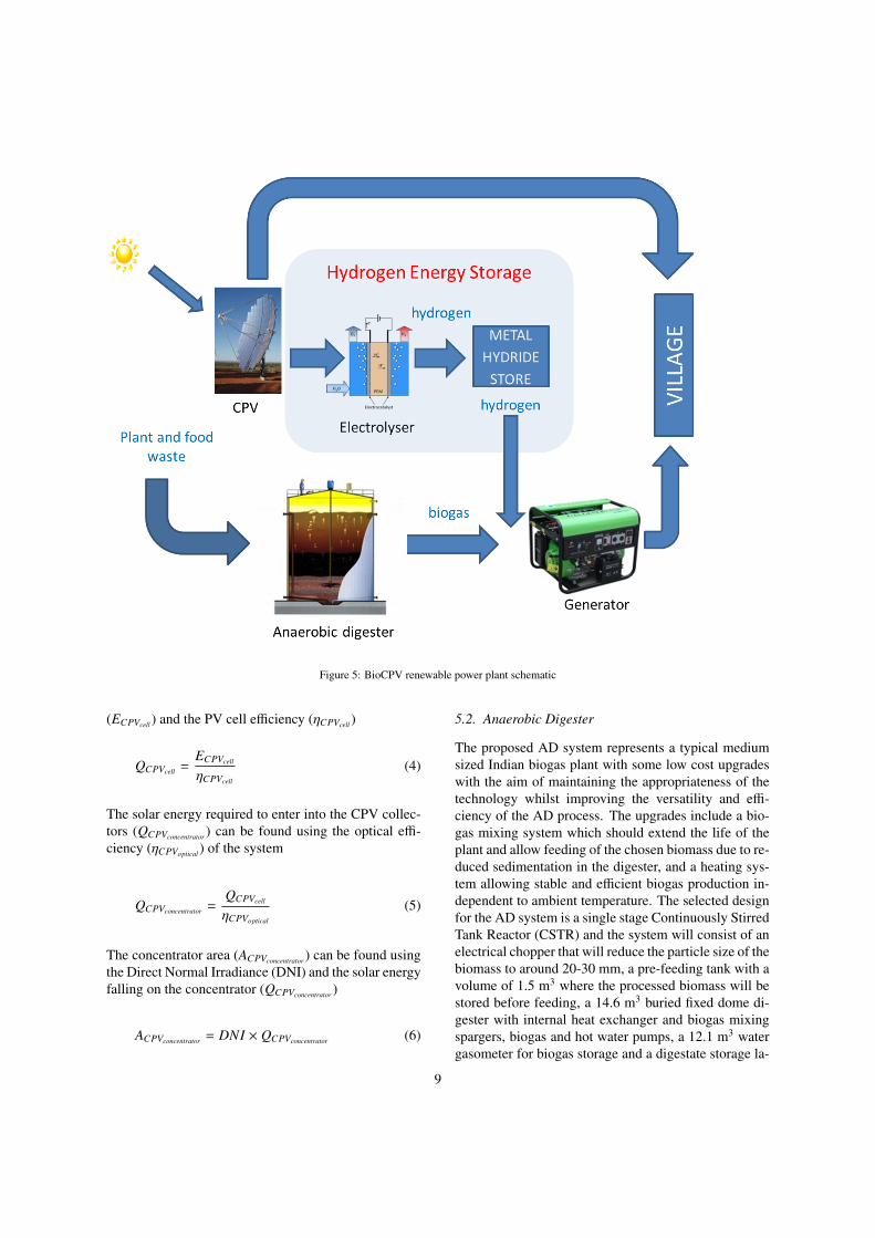
Figure 5: BioCPV renewable power plant schematic
(ECPVcell ) and the PV cell e�ciency (⌘CPVcell )
(4)QCPVcell =ECPVcell
⌘CPVcell
The solar energy required to enter into the CPV collec-tors (QCPVconcentrator ) can be found using the optical e�-ciency (⌘CPVoptical ) of the system
(5)QCPVconcentrator =QCPVcell
⌘CPVoptical
The concentrator area (ACPVconcentrator ) can be found usingthe Direct Normal Irradiance (DNI) and the solar energyfalling on the concentrator (QCPVconcentrator )
(6)ACPVconcentrator = DNI ⇥ QCPVconcentrator
5.2. Anaerobic Digester
The proposed AD system represents a typical mediumsized Indian biogas plant with some low cost upgradeswith the aim of maintaining the appropriateness of thetechnology whilst improving the versatility and e�-ciency of the AD process. The upgrades include a bio-gas mixing system which should extend the life of theplant and allow feeding of the chosen biomass due to re-duced sedimentation in the digester, and a heating sys-tem allowing stable and e�cient biogas production in-dependent to ambient temperature. The selected designfor the AD system is a single stage Continuously StirredTank Reactor (CSTR) and the system will consist of anelectrical chopper that will reduce the particle size of thebiomass to around 20-30 mm, a pre-feeding tank with avolume of 1.5 m3 where the processed biomass will bestored before feeding, a 14.6 m3 buried fixed dome di-gester with internal heat exchanger and biogas mixingspargers, biogas and hot water pumps, a 12.1 m3 watergasometer for biogas storage and a digestate storage la-
9
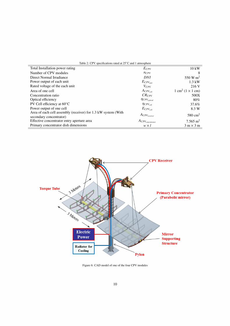
Table 2: CPV specifications rated at 25�C and 1 atmosphere
Total Installation power rating ECPV 10 kWNumber of CPV modules nCPV 8Direct Normal Irradiance DNI 550 W·m2
Power output of each unit ECPVunit 1.3 kWRated voltage of the each unit VCPV 216 VArea of one cell ACPVcell 1 cm2 (1 ⇥ 1 cm)Concentration ratio CRCPV 500XOptical e�ciency ⌘CPVoptical 80%PV Cell e�ciency at 60�C ⌘CPVcell 37.6%Power output of one cell ECPVcell 8.3 WArea of each cell assembly (receiver) for 1.3 kW system (Withsecondary concentrator)
ACPVreceiver 580 cm2
E↵ective concentrator entry aperture area ACPVconcentrator 7.565 m2
Primary concentrator dish dimensions w ⇥ l 3 m ⇥ 3 m
Figure 6: CAD model of one of the four CPV modules
10

Table 3: Anaerobic digester design specifications
Design STRTank volume VAD 15.6 m3
Tank height HAD 2.7 mTank diameter DAD 2.7 mHydraulic Retention Time HRT 30 daysOrganic Loading Rate OLR 4 kg·VS· m�3·day�1
Operational temperature TAD 37 �CThermal conductivity of tank walls UAD 1 W·m�2·�C�1
Pre-mixing tank volume VPre�mix 1.5 m3
Pre-mixing tank operational temperature TPre�mix Ambient
Figure 7: CAD model of the anaerobic digestion system
11

goon. See Figure 7 and Table 3 for the design layoutand specifications.
Design Calculations for Anaerobic Digester
The following describes the preliminary design calcula-tions required for an anaerobic digester.
Biomass Requirement
Total biogas calorific energy required from AD system,QAD is 76 kWh·day�1
(7)QAD = 76 kWh·day�1 = 273.6 MJ·day�1
and
(8)LHVCH4 = 50 MJ·kg�1
therefore,
(9)mCH4 =QAD
LHVCH4
(10)mCH4 = 5.472 kg·day�1
or at Standard Temperature and Pressure (STP) the vol-ume of methane required, VCH4 ,
(11)VCH4 = 7.77 m3·day�1
Since biogas is approximately 60% methane by vol-ume the daily biogas requirement is 12.95 m3·day�1
(STP).
Using Water Hyacinth (Eichhornia crassipes) as a modelbiomass for calculation purposes and using data from[Chanakya et al., 1992]
BMP (Biochemical methane potential) of biomass,PCH4
(12)PCH4 = 0.21 m3CH4·kg�1
VS added
Volatile solids (VS) concentration, CVS
(13)CVS = 0.079 kgVS ·kg�1wet
Assume the e↵ectiveness of the process, ↵AD
(14)↵AD = 0.9
(i.e. we expect to get around 90% of the BMP in thecontinuous process).
To calculate the biomass requirement to provide the re-quired amount of biogas
(15)mbiomass =QCH4
↵ADPCH4CVS
(16)mbiomass = 520.5 kg·day�1
Digester Sizing
The size of an anaerobic digestion system can either belimited by hydraulic or organic conditions dependingon the nature of the biomass.
Hydraulic conditions
The volumetric flow through the AD system must besuch that the microorganisms are not washed out. Thisapplies especially to the methanogenic organisms thatare crucial to the anaerobic digestion process but havea relatively low growth rate. Therefore it is common toset a lower limit on the HRT (hydraulic retention time),tR, defined by;
(17)tR =VHRT⇢biomass
mbiomass
Common values of HRT are between 15 and 60 daysand as a design constraint we have specified;
(18)tR � 30 days
Organic Loading
The organic loading rate (OLR), mOLR, must be suchthat intermediate species are not accumulated in theanaerobic digester. This can occur when the OLR is toohigh such that the hydrolysis and fermentative organ-isms, which are fast growing and tolerant to changes inpH, produce volatile fatty acids (VFA) at a rate greaterthan that which can be consumed by the acetogenic
12
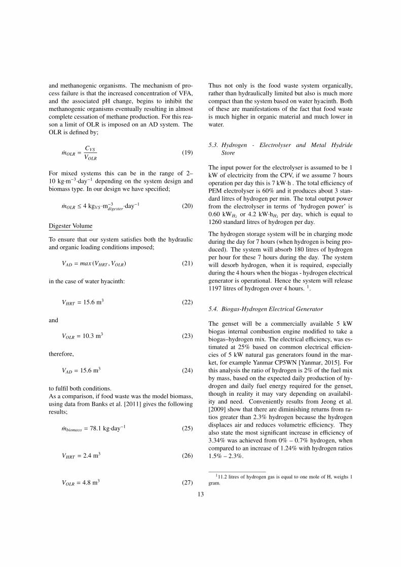
and methanogenic organisms. The mechanism of pro-cess failure is that the increased concentration of VFA,and the associated pH change, begins to inhibit themethanogenic organisms eventually resulting in almostcomplete cessation of methane production. For this rea-son a limit of OLR is imposed on an AD system. TheOLR is defined by;
(19)mOLR =CVS
VOLR
For mixed systems this can be in the range of 2–10 kg·m�3·day�1 depending on the system design andbiomass type. In our design we have specified;
(20)mOLR 4 kgVS ·m�3digester·day�1
Digester Volume
To ensure that our system satisfies both the hydraulicand organic loading conditions imposed;
(21)VAD = max (VHRT ,VOLR)
in the case of water hyacinth:
(22)VHRT = 15.6 m3
and
(23)VOLR = 10.3 m3
therefore,
(24)VAD = 15.6 m3
to fulfil both conditions.As a comparison, if food waste was the model biomass,using data from Banks et al. [2011] gives the followingresults;
(25)mbiomass = 78.1 kg·day�1
(26)VHRT = 2.4 m3
(27)VOLR = 4.8 m3
Thus not only is the food waste system organically,rather than hydraulically limited but also is much morecompact than the system based on water hyacinth. Bothof these are manifestations of the fact that food wasteis much higher in organic material and much lower inwater.
5.3. Hydrogen - Electrolyser and Metal HydrideStore
The input power for the electrolyser is assumed to be 1kW of electricity from the CPV, if we assume 7 hoursoperation per day this is 7 kW·h . The total e�ciency ofPEM electrolyser is 60% and it produces about 3 stan-dard litres of hydrogen per min. The total output powerfrom the electrolyser in terms of ‘hydrogen power’ is0.60 kWH2 or 4.2 kW·hH2 per day, which is equal to1260 standard litres of hydrogen per day.
The hydrogen storage system will be in charging modeduring the day for 7 hours (when hydrogen is being pro-duced). The system will absorb 180 litres of hydrogenper hour for these 7 hours during the day. The systemwill desorb hydrogen, when it is required, especiallyduring the 4 hours when the biogas - hydrogen electricalgenerator is operational. Hence the system will release1197 litres of hydrogen over 4 hours. 1.
5.4. Biogas-Hydrogen Electrical Generator
The genset will be a commercially available 5 kWbiogas internal combustion engine modified to take abiogas–hydrogen mix. The electrical e�ciency, was es-timated at 25% based on common electrical e�cien-cies of 5 kW natural gas generators found in the mar-ket, for example Yanmar CP5WN [Yanmar, 2015]. Forthis analysis the ratio of hydrogen is 2% of the fuel mixby mass, based on the expected daily production of hy-drogen and daily fuel energy required for the genset,though in reality it may vary depending on availabil-ity and need. Conveniently results from Jeong et al.[2009] show that there are diminishing returns from ra-tios greater than 2.3% hydrogen because the hydrogendisplaces air and reduces volumetric e�ciency. Theyalso state the most significant increase in e�ciency of3.34% was achieved from 0% – 0.7% hydrogen, whencompared to an increase of 1.24% with hydrogen ratios1.5% – 2.3%.
111.2 litres of hydrogen gas is equal to one mole of H, weighs 1gram.
13
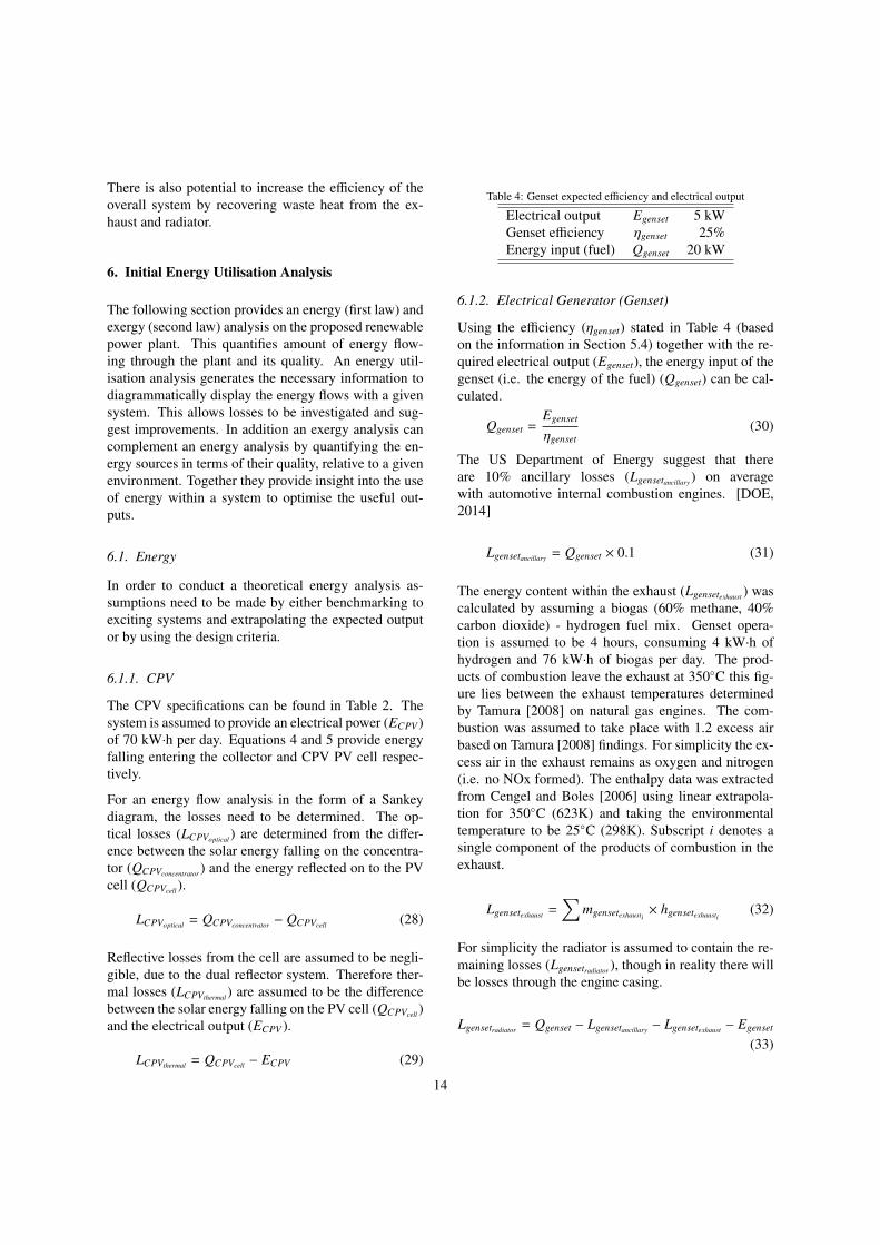
There is also potential to increase the e�ciency of theoverall system by recovering waste heat from the ex-haust and radiator.
6. Initial Energy Utilisation Analysis
The following section provides an energy (first law) andexergy (second law) analysis on the proposed renewablepower plant. This quantifies amount of energy flow-ing through the plant and its quality. An energy util-isation analysis generates the necessary information todiagrammatically display the energy flows with a givensystem. This allows losses to be investigated and sug-gest improvements. In addition an exergy analysis cancomplement an energy analysis by quantifying the en-ergy sources in terms of their quality, relative to a givenenvironment. Together they provide insight into the useof energy within a system to optimise the useful out-puts.
6.1. Energy
In order to conduct a theoretical energy analysis as-sumptions need to be made by either benchmarking toexciting systems and extrapolating the expected outputor by using the design criteria.
6.1.1. CPV
The CPV specifications can be found in Table 2. Thesystem is assumed to provide an electrical power (ECPV )of 70 kW·h per day. Equations 4 and 5 provide energyfalling entering the collector and CPV PV cell respec-tively.
For an energy flow analysis in the form of a Sankeydiagram, the losses need to be determined. The op-tical losses (LCPVoptical ) are determined from the di↵er-ence between the solar energy falling on the concentra-tor (QCPVconcentrator ) and the energy reflected on to the PVcell (QCPVcell ).
(28)LCPVoptical = QCPVconcentrator � QCPVcell
Reflective losses from the cell are assumed to be negli-gible, due to the dual reflector system. Therefore ther-mal losses (LCPVthermal ) are assumed to be the di↵erencebetween the solar energy falling on the PV cell (QCPVcell )and the electrical output (ECPV ).
(29)LCPVthermal = QCPVcell � ECPV
Table 4: Genset expected e�ciency and electrical output
Electrical output Egenset 5 kWGenset e�ciency ⌘genset 25%Energy input (fuel) Qgenset 20 kW
6.1.2. Electrical Generator (Genset)
Using the e�ciency (⌘genset) stated in Table 4 (basedon the information in Section 5.4) together with the re-quired electrical output (Egenset), the energy input of thegenset (i.e. the energy of the fuel) (Qgenset) can be cal-culated.
Qgenset =Egenset
⌘genset(30)
The US Department of Energy suggest that thereare 10% ancillary losses (Lgensetancillary ) on averagewith automotive internal combustion engines. [DOE,2014]
(31)Lgensetancillary = Qgenset ⇥ 0.1
The energy content within the exhaust (Lgensetexhaust ) wascalculated by assuming a biogas (60% methane, 40%carbon dioxide) - hydrogen fuel mix. Genset opera-tion is assumed to be 4 hours, consuming 4 kW·h ofhydrogen and 76 kW·h of biogas per day. The prod-ucts of combustion leave the exhaust at 350�C this fig-ure lies between the exhaust temperatures determinedby Tamura [2008] on natural gas engines. The com-bustion was assumed to take place with 1.2 excess airbased on Tamura [2008] findings. For simplicity the ex-cess air in the exhaust remains as oxygen and nitrogen(i.e. no NOx formed). The enthalpy data was extractedfrom Cengel and Boles [2006] using linear extrapola-tion for 350�C (623K) and taking the environmentaltemperature to be 25�C (298K). Subscript i denotes asingle component of the products of combustion in theexhaust.
(32)Lgensetexhaust =X
mgensetexhausti⇥ hgensetexhausti
For simplicity the radiator is assumed to contain the re-maining losses (Lgensetradiator ), though in reality there willbe losses through the engine casing.
Lgensetradiator = Qgenset � Lgensetancillary � Lgensetexhaust � Egenset
(33)
14
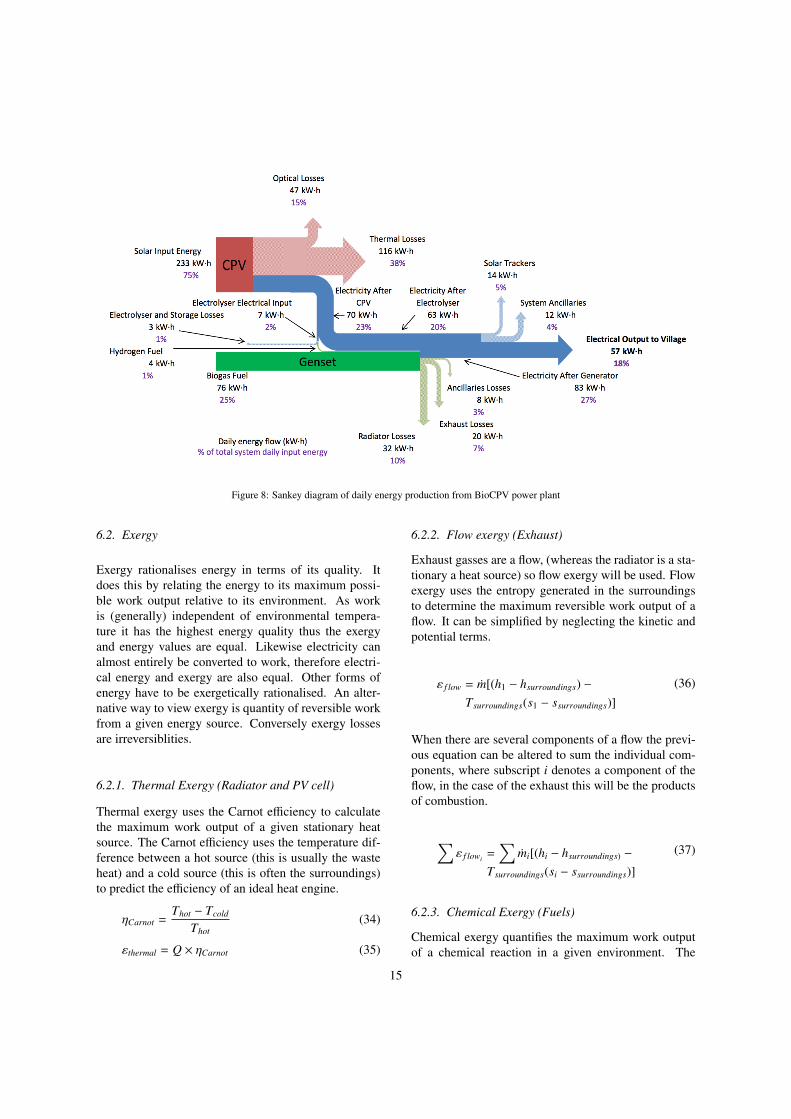
Figure 8: Sankey diagram of daily energy production from BioCPV power plant
6.2. Exergy
Exergy rationalises energy in terms of its quality. Itdoes this by relating the energy to its maximum possi-ble work output relative to its environment. As workis (generally) independent of environmental tempera-ture it has the highest energy quality thus the exergyand energy values are equal. Likewise electricity canalmost entirely be converted to work, therefore electri-cal energy and exergy are also equal. Other forms ofenergy have to be exergetically rationalised. An alter-native way to view exergy is quantity of reversible workfrom a given energy source. Conversely exergy lossesare irreversiblities.
6.2.1. Thermal Exergy (Radiator and PV cell)
Thermal exergy uses the Carnot e�ciency to calculatethe maximum work output of a given stationary heatsource. The Carnot e�ciency uses the temperature dif-ference between a hot source (this is usually the wasteheat) and a cold source (this is often the surroundings)to predict the e�ciency of an ideal heat engine.
⌘Carnot =Thot � Tcold
Thot(34)
"thermal = Q ⇥ ⌘Carnot (35)
6.2.2. Flow exergy (Exhaust)
Exhaust gasses are a flow, (whereas the radiator is a sta-tionary a heat source) so flow exergy will be used. Flowexergy uses the entropy generated in the surroundingsto determine the maximum reversible work output of aflow. It can be simplified by neglecting the kinetic andpotential terms.
(36)" f low = m[(h1 � hsurroundings) �Tsurroundings(s1 � ssurroundings)]
When there are several components of a flow the previ-ous equation can be altered to sum the individual com-ponents, where subscript i denotes a component of theflow, in the case of the exhaust this will be the productsof combustion.
(37)X" f lowi
=X
mi[(hi � hsurroundings) �Tsurroundings(si � ssurroundings)]
6.2.3. Chemical Exergy (Fuels)
Chemical exergy quantifies the maximum work outputof a chemical reaction in a given environment. The
15

chemical exergy of fuels has been tabulated by Bejan[1997] at 25�C and 1 atmosphere. This conveniently lieswithin the conditions expected for the BioCPV powerplant environment, and is compatible with the data forthe CPV system which is rated to the same conditions.Only the methane content of the biogas has been con-sidered for the exergetic value of the fuel.
• Hydrogen = 235.2 kJ· mol�1
• Methane = 830.2 kJ· mol�1
[Bejan, 1997]
To determine the input (fuel) exergy of the genset forthe total period of operation
(38)E(kJ) = E(kJ · mol�1) ⇥1000
m(kg · kmol�1)⇥ m(kg)
or for instantaneous (flow) exergy
(39)E(kW) = E(kJ · mol�1) ⇥1000
m(kg · kmol�1)⇥ m(kg · s�1)
6.2.4. Radiative exergy
This section extrapolates the technique described by Pe-tela [2010] exergetic analysis of a PV cell to a CPV sys-tem.
Petela [2010] calculates the total thermal exergy fromthe sun falling on a PV cell as
"CPVconcentrator = FS unEarth�
3APV ⇥
⇣3T 4
S un + T 4environment � 4TenvironementT 3
S un
⌘
(40)
To extrapolate to the 8 CPV modules being used in thisanalysis an e↵ective solar collector area needs to be cal-culated. This is equivalent to flat area to collect the sameout of solar energy as the CPV concentrator.
(41)Ae f f ective =QCPVconcentrator
FS unEarth ⇥ � ⇥ T 4S un
Table 5: Data for radiative exergy calculations
� Stephan-Boltzmanncoe�cient 5.67 ⇥ 10�8
J·s�1·m�2·K�4
FS un�EarthSun-Earth factor(dimensionless) 2.16�5
TS unSun surfaceTemperature 5800 K
TenvironmentEnvironmental
temperature 298 K
Ae f f ectiveCalculated e↵ective
area of collector 23 m2
"CPVconcentrator = FS unEarth�
3Ae f f ective ⇥ nCPV
⇥⇣3T 4
S un+T 4environment�4TenvironementT 3
S un
⌘
(42)
7. Results and Discussion
The surveys and anthropological investigations indi-cated that improving the environment for education andtraining would provide the foundation for sustainabledevelopment in the selected community. Due to alack of electrical infrastructure there is inadequate light-ing both in public areas such as the school and theirhomes. The current solutions include kerosene lampswhich have adverse health implications when used in-doors. There is no provision for thermal comfort suchas fans which can significantly aid a learning environ-ment.
To address the development needs of the village a dailyelectrical demand requirement of 55 kW·h, shown inFigure 2 based on: 7.2 kW·h of public lighting, 3.6kW·h of domestic lighting, 7.2 kW·h of fans, 12 kW·h ofcharging appliances such as mobile phones, torches andlanterns, 12 kW·h of computers and 12.8 kW·h of smallmachinery. This selection of technologies should im-prove the learning environment in the public areas andalleviate some of the labour intensive income generatingactivities of the community.
The technologies selected are based on the main renew-able energy sources being solar and biomass. Electricitygeneration will be provided by 10 kW (electric) concen-trated photovoltaic (CPV) during the day and a 5 kW(electric) biogas-hydrogen internal combustion electri-cal generator during the evening. The biogas will beprovided by an anaerobic digestion system and the hy-drogen from the excess electricity from the CPV via an
16
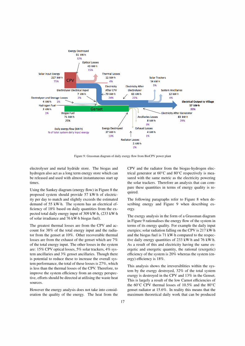
Figure 9: Grassman diagram of daily exergy flow from BioCPV power plant
electrolyser and metal hydride store. The biogas andhydrogen also act as a long term energy store which canbe released and used with almost instantaneous start uptimes.
Using the Sankey diagram (energy flow) in Figure 8 theproposed system should provide 57 kW·h of electric-ity per day to match and slightly exceeds the estimateddemand of 55 kW·h. The system has an electrical ef-ficiency of 18% based on daily quantities from the ex-pected total daily energy input of 309 kW·h, (233 kW·hof solar irradiance and 76 kW·h biogas fuel).
The greatest thermal losses are from the CPV and ac-count for 38% of the total energy input and the radia-tor from the genset at 10%. Other recoverable thermallosses are from the exhaust of the genset which are 7%of the total energy input. The other losses in the systemare: 15% CPV optical losses, 5% solar trackers, 4% sys-tem ancillaries and 3% genset ancillaries. Though thereis potential to reduce these to increase the overall sys-tem performance, the total of these losses is 27%, whichis less than the thermal losses of the CPV. Therefore, toimprove the system e�ciency from an energy perspec-tive, e↵orts should be directed at utilising the waste heatsources.
However the energy analysis does not take into consid-eration the quality of the energy. The heat from the
CPV and the radiator from the biogas-hydrogen elec-trical generator at 60�C and 80�C respectively is mea-sured with the same metric as the electricity poweringthe solar trackers. Therefore an analysis that can com-pare these quantities in terms of energy quality is re-quired.
The following paragraphs refer to Figure 8 when de-scribing energy and Figure 9 when describing ex-ergy.
The exergy analysis in the form of a Grassman diagramin Figure 9 rationalises the energy flow of the system interms of its energy quality. For example the daily inputexergies; solar radiation falling on the CPV is 217 kW·hand the biogas fuel is 71 kW·h compared to the respec-tive daily energy quantities of 233 kW·h and 76 kW·h.As a result of this and electricity having the same ex-ergetic and energetic quantity, the rational (exergetic)e�ciency of the system is 20% whereas the system (en-ergy) e�ciency is 18%.
This analysis shows the irreversiblities within the sys-tem by the exergy destroyed, 32% of the total systemexergy is destroyed in the CPV and 13% in the Genset.This is largely a result of the low Carnot e�ciencies ofthe 60�C CPV thermal losses of 10.5% and the 80�Cgenset radiator at 15.6%. In reality this means that themaximum theoretical daily work that can be produced
17
from 116 kW·h of thermal energy in the CPV is 12kW·h. Likewise the 32 kW·h of daily thermal energyin the radiator of the genset could only produce 5 kW·hof work. The exhaust of the genset is a flow so althoughits temperature is 350�C, its energy of 20 kW·h onlycontains 4 kW·h of exergy.
From an exergy perspective the greatest losses are theoptical losses from the CPV which amounts to 15% ofthe total system exergy, as well the electrical loss of thesystem ancillaries 4% and the solar trackers 5%. Incomparison the thermal losses from the CPV are 4%and the genset radiator is 2%. This may seem like itwould be more valuable to try to reduce these largerlosses but it will not recuperate the 45% of total sys-tem exergy input destroyed. The destroyed exergy is aresult of the low temperatures of the CPV and gensetradiator and indicates that the amount of work that isgenerated from these outputs is low. There are severaloptions which could use them more appropriately andimprove the system e�ciency and rational e�ciency.Such as direct utilisation e.g. hot water, heat poweredrefrigeration and water purification.
Though this research is focused on a specific location itsapproach can be applied to other rural community set-tings and the findings may be applicable to other CPVand biogas power generation systems.
8. Conclusion
This paper addresses a number of socio-economic as-pects of the selected village. Supplying sustainableand renewable electricity to the households is expectedto increase the quality of life through improving theeducational environment for the children and reducingthe manual labour load often burdened by the women.Small scale handwork industries such a craft makingand spice grinding can be operated electrically, with thepotential to work during the night as well. Lighting andfans in the school will improve comfort and concentra-tion, together with lighting in the home, making it pos-sible for children to study at night. The implementa-tion of a charging station for torches can improve theoverall safety of the village. The food waste and otherbiomass sources will be used as feedstock for an anaero-bic digester, providing a sustainable fuel and acting as asource of education for sustainability in general.
A 10 kW (electric) CPV combined with a 5 kW (elec-tric) biogas - hydrogen generator will supply the elec-tricity needs of the community. The energy and exergy
analysis has shown that the greatest potential to improvethe system e�ciency is through utilising the waste ther-mal energy in the CPV. This amounts for 38% of the to-tal input energy into the system. There is also potentialto recover a further 10% of the total input energy fromthe radiator of the genset. However the exergy analysisshowed that there is little work potential in these wasteheat sources as they are at low temperatures, 60�C and80�C respectively. Investigations into alternative usesof low temperature heat are required to make use of thiswaste energy to improve the system e�ciency.
9. Acknowledgements
This work has been carried out as a part of BioCPVproject jointly funded by DST, India (Ref No:DST/SEED/INDO-UK/002/2011) and EPSRC, UK,(Ref No: EP/J000345/1). Authors acknowledge boththe funding agencies for the support. The authors alsoacknowledge the support of their respective universi-ties which include: University of Exeter, Indian Instituteof Technology Bombay, Indian Institute of TechnologyMadras, University of Nottingham, Herriot Watt Uni-versity, Visva-Bharati (West Bengal) and University ofLeeds.
10. References
Amonix, 2014. Solar Power Concentrated Photovoltaic Systems.http://amonix.com/, Accessed: 2014-08-05.
Appels, L., Lauwers, J., Degreve, J., Helsen, L., Lievens, B., Willems,K., Van Impe, J., Dewil, R., 2011. Anaerobic digestion in globalbio-energy production: Potential and research challenges. Renew-able and Sustainable Energy Reviews 15 (9), 4295–4301.
Bajpai, P., Dash, V., 2012. Hybrid renewable energy systems forpower generation in stand-alone applications: A review. Renew-able and Sustainable Energy Reviews 16 (5), 2926–2939.
Banerjee, R., 2006. Comparison of options for distributed generationin India. Energy Policy 34 (1), 101–111.
Banks, C. J., Chesshire, M., Heaven, S., Arnold, R., 2011. Anaerobicdigestion of source-segregated domestic food waste: Performanceassessment by mass and energy balance. Bioresource Technology102 (2), 612–620.
Bejan, A., 1997. Advanced Engineering Thermodynamics second edi-tion. John Wiley & Sons, Inc., New York.
Bouallagui, H., Touhami, Y., Ben Cheikh, R., Hamdi, M., 2005.Bioreactor performance in anaerobic digestion of fruit and veg-etable wastes. Process Biochemistry 40 (3-4), 989–995.
Cengel, Boles, 2006. Thermodynamics: An engineering approach.Mc Graw-Hill, New York.
Chanakya, H., Borgaonkar, S., Rajan, M., Wahi, M., 1992. Two-phaseanaerobic digestion of water hyacinth or urban garbage. Biore-source Technology 42 (2), 123–131.
DOE, 2014. Fuel Economy where energy goes,http://www.fueleconomy.gov/feg/atv.shtml, Accessed 03-04-2014.
18

Fan, H., Singh, R., Akbarzadeh, A., 2011. Electric Power Generationfrom Thermoelectric Cells Using a Solar Dish Concentrator. Jour-nal of Electronic Materials 40 (5), 1311–1320.
Feuermann, D., Gordon, J. M., 2001. High-concentration photovoltaicdesigns based on miniature parabolic dishes. Solar Energy 70 (5),423–430.
Gandhi, A. (Ed.), 2011. India human development report, 2011: to-wards social inclusion, 1st Edition. Institute of Applied ManpowerResearch, Planning Commission, Govt. of India : Oxford Univer-sity Press, New Delhi.
Gerardi, M. H., 2003. Types of Anaerobic Digesters, in The Micro-biology of Anaerobic Digesters. Wastewater Microbiology Series.John Wiley & Sons, Inc., Hoboken, NJ, USA.
Ghosh, S., 2002. Electricity consumption and economic growth in In-dia. Energy Policy 30 (2), 125–129.
Green, M. A., Emery, K., Hishikawa, Y., Warta, W., Dunlop, E. D.,2014. Solar cell e�ciency tables (version 43): Solar cell e�-ciency tables. Progress in Photovoltaics: Research and Applica-tions 22 (1), 1–9.
Hartmann, H., Ahring, B., 2006. Strategies for the anaerobic diges-tion of the organic fraction of municipal solid waste: an overview.Water Science & Technology 53 (8), 7.
Heliotrop, 2014. Heliotrop - Innovative and low cost CPV solar sys-tems. http://www.heliotrop.fr/en-index.php, Accessed:2014-08-05.
Hilkiah Igoni, A., Ayotamuno, M., Eze, C., Ogaji, S., Probert, S.,2008. Designs of anaerobic digesters for producing biogas frommunicipal solid-waste. Applied Energy 85 (6), 430–438.
Ho↵schmidt, B., Alexopoulos, S., Rau, C., Sattler, J., Anthrakidis,A., Boura, C., O’Connor, B., Hilger, P., 2012. 3.18 - Concentrat-ing Solar Power. In: Sayigh, A. (Ed.), Comprehensive RenewableEnergy. Elsevier, Oxford, pp. 595 – 636.
HP, 2015. HP Online Store, http://store.hp.com/UKStore, Accessed14-01-2015.
HSE, 1997. Lighting at Work Web-Friendly Version of HSG38,http://www.hse.gov.uk/pubns/priced/hsg38.pdf, Accessed 04-01-2015).
Jeong, C., Kim, T., Lee, K., Song, S., Chun, K. M., 2009. Generatinge�ciency and emissions of a spark-ignition gas engine generatorfuelled with biogas–hydrogen blends. International Journal of Hy-drogen Energy 34 (23), 9620–9627.
Kazmerski, L., 2012. 1.03 - Solar Photovoltaics Technology: NoLonger an Outlier. In: Sayigh, A. (Ed.), Comprehensive Renew-able Energy. Elsevier, Oxford, pp. 13 – 30.
Kribus, A., Kaftori, D., Mittelman, G., Hirshfeld, A., Flitsanov, Y.,Dayan, A., 2006. A miniature concentrating photovoltaic and ther-mal system. Energy Conversion and Management 47 (20), 3582–3590.
Kurtz, S., 2012. Opportunities and Challenges for Development ofa Mature Concentrating Photovoltaic Power Industry (Revision).Tech. Rep. NREL/TP-5200-43208, 935595.
Luque, A., Hegedus, S. (Eds.), 2003. Handbook of photovoltaic sci-ence and engineering. Wiley, Hoboken, NJ.
MoRD, 2014. Ministry of Rural Development (Government of India),http://rural.nic.in/, Accessed 05-09-2014.
Nallathambi Gunaseelan, V., 1997. Anaerobic digestion of biomassfor methane production: A review. Biomass and Bioenergy 13 (1-2), 83–114.
NREL, 2013. NREL: National Residential E�ciency MeasuresDatabase - Retrofit Measures for Light Bulbs. http://www.
nrel.gov/ap/retrofits/measures.cfm?gId=5&ctId=30,Accessed: 2014-10-07.
NRLM, 2014. Aajeevika - National Rural Livelihoods Mission(NRLM), http://aajeevika.gov.in/, Accessed 05 September 2014.
NUT, 2015. Space Requirements in Classrooms: NUT Health
and Safety Guidance, https://www.teachers.org.uk/files/space-requirements-in-classrooms.doc, Accessed 27-09-2015.
Petela, R., 2010. Engineering Thermodynamics of Thermal Radiation,1st Edition. McGraw-Hill.
Ramachandra, T., Jain, R., Krishnadas, G., 2011. Hotspots of solar po-tential in India. Renewable and Sustainable Energy Reviews 15 (6),3178–3186.
Reddy, K. S., Lokeswaran, S., Agarwal, P., Mallick, T., 2013. Numeri-cal Analysis of Micro Channel Heat Sink Cooling System for SolarConcentrating Photovoltaic Module. In: Ghosh, P. C. (Ed.), 4th In-ternational Conference on Advances in Energy Research. Mumbai,India.
Reddy, K. S., Veershetty, G., 2013. Viability analysis of solarparabolic dish stand-alone power plant for Indian conditions. Ap-plied Energy 102, 908–922.
Sharma, N. K., Tiwari, P. K., Sood, Y. R., 2012. Solar energy in India:Strategies, policies, perspectives and future potential. Renewableand Sustainable Energy Reviews 16 (1), 933–941.
Soitec, 2014. Soitec - Revolutionary semiconductor materials forenergy and electronics. http://www.soitec.com/en/index.php, Accessed: 2014-08-05.
Tamura, M., 2008. An Investigation of a Natural Gas HCCI Enginefor 5kW Class Co-generation System. In: IGRC Paris 2008. Inter-national Gas Union Research Conference.
Vent-Axia, 2015. Reversible Hi Line Vent Axia, http://www.vent-axia.com/range/reversible-hi-line.html, Accessed 27-09-2015.
Verlinden, P., Lewandowski, A., Kendall, H., Carter, S., Cheah, K.,Varfolomeev, I., Watts, D., Volk, M., Thomas, I., Wakeman, P.,Neumann, A., Gizinski, P., Modra, D., Turner, D., Lasich, J., 2008.Update on two-year performance of 120 kWp concentrator PV sys-tems using multi-junction III-V solar cells and parabolic dish re-flective optics. IEEE, pp. 1–6.
Viebahn, P., Lechon, Y., Trieb, F., 2011. The potential role of con-centrated solar power (CSP) in Africa and Europe—A dynamicassessment of technology development, cost development and lifecycle inventories until 2050. Energy Policy 39 (8), 4420 – 4430.
Wernsman, B., Siergiej, R., Link, S., Mahorter, R., Palmisiano, M.,Wehrer, R., Schultz, R., Schmuck, G., Messham, R., Murray, S.,Murray, C., Newman, F., Taylor, D., DePoy, D., Rahmlow, T.,2004. Greater Than 20% Radiant Heat Conversion E�ciency ofa Thermophotovoltaic Radiator/Module System Using ReflectiveSpectral Control. IEEE Transactions on Electron Devices 51 (3),512–515.
Yanmar, 2015. Yanmar mCHP Catalogue, http://www.yanmar-es.com/uploads/files/349226-YAN-Catalog-Apr17˙FINAL˙DIGITAL˙med.pdf, Accessed 24-02-2016.
Zenith Solar, 2013. Zenith Solar. http://www.zenithsolar.com/solar-engineering.aspx, Accessed: 2014-08-05.
Zheng, C., Kammen, D. M., 2014. An innovation-focused roadmapfor a sustainable global photovoltaic industry. Energy Policy 67,159–169.
19
Related Documents