Investigating the significance of adversarial attacks and their ...

Investigating the significance of adversarial attacksand their relation to interpretability for

radar-based human activity recognition systemsUtku Ozbulak1, 5,∗ Baptist Vandersmissen1,∗ Azarakhsh Jalalvand1, 4 Ivo Couckuyt2

Arnout Van Messem3, 5 Wesley De Neve1, 5

1Department of Electronics and Information Systems, Ghent University, Belgium2Department of Information Technology, Ghent University–imec, Belgium

3Department of Applied Mathematics, Computer Science and Statistics, Ghent University, Belgium4Department of Mechanical and Aerospace Engineering, Princeton University, USA

5Center for Biotech Data Science, Ghent University Global Campus, Republic of Korea

Abstract—Given their substantial success in addressing awide range of computer vision challenges, Convolutional NeuralNetworks (CNNs) are increasingly being used in smart homeapplications, with many of these applications relying on theautomatic recognition of human activities. In this context, low-power radar devices have recently gained in popularity asrecording sensors, given that the usage of these devices allowsmitigating a number of privacy concerns, a key issue whenmaking use of conventional video cameras. Another concernthat is often cited when designing smart home applications isthe resilience of these applications against cyberattacks. It is,for instance, well-known that the combination of images andCNNs is vulnerable against adversarial examples, mischievousdata points that force machine learning models to generate wrongclassifications during testing time. In this paper, we investigatethe vulnerability of radar-based CNNs to adversarial attacks, andwhere these radar-based CNNs have been designed to recognizehuman gestures. Through experiments with four unique threatmodels, we show that radar-based CNNs are susceptible toboth white- and black-box adversarial attacks. We also exposethe existence of an extreme adversarial attack case, where itis possible to change the prediction made by the radar-basedCNNs by only perturbing the padding of the inputs, withouttouching the frames where the action itself occurs. Moreover,we observe that gradient-based attacks exercise perturbationnot randomly, but on important features of the input data.We highlight these important features by making use of Grad-CAM, a popular neural network interpretability method, herebyshowing the connection between adversarial perturbation andprediction interpretability.

* Equal contribution.Corresponding author: Utku Ozbulak – [email protected]. Accepted for publication on Computer Vision and Image Un-

derstanding, Special issue on Adversarial Deep Learning in Biometrics &Forensics, Elsevier, 2020.

DOI: https://doi.org/10.1016/j.cviu.2020.103111.

I. INTRODUCTION

Recent advancements in the field of computer vision, naturallanguage processing, and audio analysis enabled the deploy-ment of intelligent systems in homes in the form of assistivetechnologies. These so-called smart homes come with a widerange of functionality such as voice- and gesture-controlledappliances, security systems, and health-related applications.Naturally, multiple sensors are needed in these smart homesto capture the actions performed by household residents andto act upon them.

Sensors for smart home applications — Microphones andvideo cameras are currently two of the most commonly usedsensors in smart homes. The research in the domain ofvideo-oriented computer vision is extensive, and the combinedusage of a video camera and computer vision enables awide range of assistive technologies, including applicationsrelated to security (e.g., intruder detection) and applicationsincorporating gesture-controlled functionalities [54]. However,one of the major drawbacks of using video cameras is theirprivacy intrusiveness [33]. These privacy-related concerns are,at an increasing rate, being covered by media articles [41].Furthermore, a largely overlooked aspect of video-assistedtechnologies in smart homes is that video cameras are ableto capture both smart home residents and visitors. Therefore,residents of smart homes need to be aware of the statutoryrestrictions on privacy invasion.

Low-power radar devices, as complementary sensors, arecapable of alleviating the privacy concerns raised over theusage of video cameras. In that regard, the main advantagesof radar devices over video cameras are as follows: (1)better privacy preservation, (2) a higher effectiveness in poorcapturing conditions (e.g., low light, presence of smoke), and

arX

iv:2

101.

1056

2v1

[cs

.CV

] 2

6 Ja

n 20

21

(3) through-the-wall sensing [55].Frequency-modulated continuous-wave (FMCW) radars

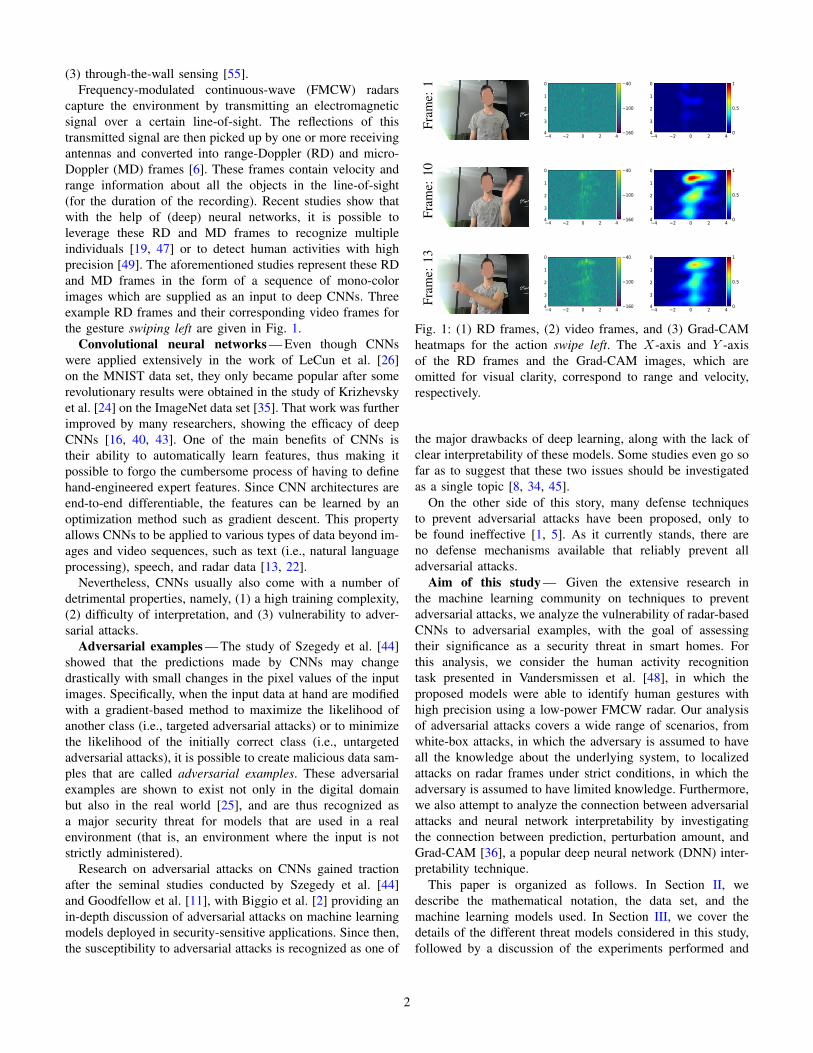
capture the environment by transmitting an electromagneticsignal over a certain line-of-sight. The reflections of thistransmitted signal are then picked up by one or more receivingantennas and converted into range-Doppler (RD) and micro-Doppler (MD) frames [6]. These frames contain velocity andrange information about all the objects in the line-of-sight(for the duration of the recording). Recent studies show thatwith the help of (deep) neural networks, it is possible toleverage these RD and MD frames to recognize multipleindividuals [19, 47] or to detect human activities with highprecision [49]. The aforementioned studies represent these RDand MD frames in the form of a sequence of mono-colorimages which are supplied as an input to deep CNNs. Threeexample RD frames and their corresponding video frames forthe gesture swiping left are given in Fig. 1.

Convolutional neural networks — Even though CNNswere applied extensively in the work of LeCun et al. [26]on the MNIST data set, they only became popular after somerevolutionary results were obtained in the study of Krizhevskyet al. [24] on the ImageNet data set [35]. That work was furtherimproved by many researchers, showing the efficacy of deepCNNs [16, 40, 43]. One of the main benefits of CNNs istheir ability to automatically learn features, thus making itpossible to forgo the cumbersome process of having to definehand-engineered expert features. Since CNN architectures areend-to-end differentiable, the features can be learned by anoptimization method such as gradient descent. This propertyallows CNNs to be applied to various types of data beyond im-ages and video sequences, such as text (i.e., natural languageprocessing), speech, and radar data [13, 22].

Nevertheless, CNNs usually also come with a number ofdetrimental properties, namely, (1) a high training complexity,(2) difficulty of interpretation, and (3) vulnerability to adver-sarial attacks.

Adversarial examples — The study of Szegedy et al. [44]showed that the predictions made by CNNs may changedrastically with small changes in the pixel values of the inputimages. Specifically, when the input data at hand are modifiedwith a gradient-based method to maximize the likelihood ofanother class (i.e., targeted adversarial attacks) or to minimizethe likelihood of the initially correct class (i.e., untargetedadversarial attacks), it is possible to create malicious data sam-ples that are called adversarial examples. These adversarialexamples are shown to exist not only in the digital domainbut also in the real world [25], and are thus recognized asa major security threat for models that are used in a realenvironment (that is, an environment where the input is notstrictly administered).

Research on adversarial attacks on CNNs gained tractionafter the seminal studies conducted by Szegedy et al. [44]and Goodfellow et al. [11], with Biggio et al. [2] providing anin-depth discussion of adversarial attacks on machine learningmodels deployed in security-sensitive applications. Since then,the susceptibility to adversarial attacks is recognized as one of

Fram

e:1

4 2 0 2 44

3

2

1

0

160

100

40

4 2 0 2 44

3

2

1

0

0

0.5

1

Fram

e:10

4 2 0 2 44

3

2

1

0

160

100

40

4 2 0 2 44

3

2

1

0

0

0.5

1

Fram

e:13

4 2 0 2 44

3

2

1

0

160

100

40

4 2 0 2 44

3

2

1

0

0

0.5

1

Fig. 1: (1) RD frames, (2) video frames, and (3) Grad-CAMheatmaps for the action swipe left. The X-axis and Y -axisof the RD frames and the Grad-CAM images, which areomitted for visual clarity, correspond to range and velocity,respectively.

the major drawbacks of deep learning, along with the lack ofclear interpretability of these models. Some studies even go sofar as to suggest that these two issues should be investigatedas a single topic [8, 34, 45].

On the other side of this story, many defense techniquesto prevent adversarial attacks have been proposed, only tobe found ineffective [1, 5]. As it currently stands, there areno defense mechanisms available that reliably prevent alladversarial attacks.

Aim of this study — Given the extensive research inthe machine learning community on techniques to preventadversarial attacks, we analyze the vulnerability of radar-basedCNNs to adversarial examples, with the goal of assessingtheir significance as a security threat in smart homes. Forthis analysis, we consider the human activity recognitiontask presented in Vandersmissen et al. [48], in which theproposed models were able to identify human gestures withhigh precision using a low-power FMCW radar. Our analysisof adversarial attacks covers a wide range of scenarios, fromwhite-box attacks, in which the adversary is assumed to haveall the knowledge about the underlying system, to localizedattacks on radar frames under strict conditions, in which theadversary is assumed to have limited knowledge. Furthermore,we also attempt to analyze the connection between adversarialattacks and neural network interpretability by investigatingthe connection between prediction, perturbation amount, andGrad-CAM [36], a popular deep neural network (DNN) inter-pretability technique.

This paper is organized as follows. In Section II, wedescribe the mathematical notation, the data set, and themachine learning models used. In Section III, we cover thedetails of the different threat models considered in this study,followed by a discussion of the experiments performed and

2

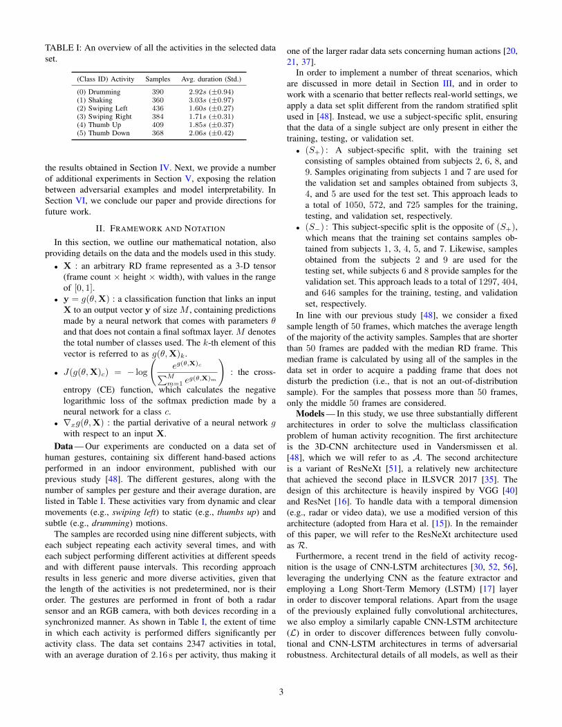
TABLE I: An overview of all the activities in the selected dataset.

(Class ID) Activity Samples Avg. duration (Std.)

(0) Drumming 390 2.92s (±0.94)(1) Shaking 360 3.03s (±0.97)(2) Swiping Left 436 1.60s (±0.27)(3) Swiping Right 384 1.71s (±0.31)(4) Thumb Up 409 1.85s (±0.37)(5) Thumb Down 368 2.06s (±0.42)

the results obtained in Section IV. Next, we provide a numberof additional experiments in Section V, exposing the relationbetween adversarial examples and model interpretability. InSection VI, we conclude our paper and provide directions forfuture work.

II. FRAMEWORK AND NOTATION

In this section, we outline our mathematical notation, alsoproviding details on the data and the models used in this study.• X : an arbitrary RD frame represented as a 3-D tensor

(frame count × height × width), with values in the rangeof [0, 1].

• y = g(θ,X) : a classification function that links an inputX to an output vector y of size M , containing predictionsmade by a neural network that comes with parameters θand that does not contain a final softmax layer. M denotesthe total number of classes used. The k-th element of thisvector is referred to as g(θ,X)k.

• J(g(θ,X)c) = − log

(eg(θ,X)c∑M

m=1 eg(θ,X)m

): the cross-

entropy (CE) function, which calculates the negativelogarithmic loss of the softmax prediction made by aneural network for a class c.

• ∇xg(θ,X) : the partial derivative of a neural network gwith respect to an input X.

Data — Our experiments are conducted on a data set ofhuman gestures, containing six different hand-based actionsperformed in an indoor environment, published with ourprevious study [48]. The different gestures, along with thenumber of samples per gesture and their average duration, arelisted in Table I. These activities vary from dynamic and clearmovements (e.g., swiping left) to static (e.g., thumbs up) andsubtle (e.g., drumming) motions.

The samples are recorded using nine different subjects, witheach subject repeating each activity several times, and witheach subject performing different activities at different speedsand with different pause intervals. This recording approachresults in less generic and more diverse activities, given thatthe length of the activities is not predetermined, nor is theirorder. The gestures are performed in front of both a radarsensor and an RGB camera, with both devices recording in asynchronized manner. As shown in Table I, the extent of timein which each activity is performed differs significantly peractivity class. The data set contains 2347 activities in total,with an average duration of 2.16 s per activity, thus making it

one of the larger radar data sets concerning human actions [20,21, 37].

In order to implement a number of threat scenarios, whichare discussed in more detail in Section III, and in order towork with a scenario that better reflects real-world settings, weapply a data set split different from the random stratified splitused in [48]. Instead, we use a subject-specific split, ensuringthat the data of a single subject are only present in either thetraining, testing, or validation set.• (S+) : A subject-specific split, with the training set

consisting of samples obtained from subjects 2, 6, 8, and9. Samples originating from subjects 1 and 7 are used forthe validation set and samples obtained from subjects 3,4, and 5 are used for the test set. This approach leads toa total of 1050, 572, and 725 samples for the training,testing, and validation set, respectively.

• (S−) : This subject-specific split is the opposite of (S+),which means that the training set contains samples ob-tained from subjects 1, 3, 4, 5, and 7. Likewise, samplesobtained from the subjects 2 and 9 are used for thetesting set, while subjects 6 and 8 provide samples for thevalidation set. This approach leads to a total of 1297, 404,and 646 samples for the training, testing, and validationset, respectively.

In line with our previous study [48], we consider a fixedsample length of 50 frames, which matches the average lengthof the majority of the activity samples. Samples that are shorterthan 50 frames are padded with the median RD frame. Thismedian frame is calculated by using all of the samples in thedata set in order to acquire a padding frame that does notdisturb the prediction (i.e., that is not an out-of-distributionsample). For the samples that possess more than 50 frames,only the middle 50 frames are considered.

Models — In this study, we use three substantially differentarchitectures in order to solve the multiclass classificationproblem of human activity recognition. The first architectureis the 3D-CNN architecture used in Vandersmissen et al.[48], which we will refer to as A. The second architectureis a variant of ResNeXt [51], a relatively new architecturethat achieved the second place in ILSVCR 2017 [35]. Thedesign of this architecture is heavily inspired by VGG [40]and ResNet [16]. To handle data with a temporal dimension(e.g., radar or video data), we use a modified version of thisarchitecture (adopted from Hara et al. [15]). In the remainderof this paper, we will refer to the ResNeXt architecture usedas R.

Furthermore, a recent trend in the field of activity recog-nition is the usage of CNN-LSTM architectures [30, 52, 56],leveraging the underlying CNN as the feature extractor andemploying a Long Short-Term Memory (LSTM) [17] layerin order to discover temporal relations. Apart from the usageof the previously explained fully convolutional architectures,we also employ a similarly capable CNN-LSTM architecture(L) in order to discover differences between fully convolu-tional and CNN-LSTM architectures in terms of adversarialrobustness. Architectural details of all models, as well as their

3

performance on the selected dataset, can be found in thesupplementary materials.

With 8.1 million trainable parameters, the employedResNeXt model (R) is significantly more complex thanthe 3D-CNN model (A), which contains approximately 647thousand trainable parameters. Consequently, the size of thetwo models is also considerably different: ResNeXt occupiesabout 32.9MB of memory, whereas 3D-CNN only takes about2.9MB. Although the space occupied by each of the modelsdoes not make a significant difference for many of the currentcommercial products, on the same hardware, the 3D-CNNmodel is up to 7 times faster than the ResNeXt model interms of inference speed. When considering edge-computingand real-time applications in the context of smart homes, thismeans that deploying the ResNeXt model will naturally costmore than deploying the 3D-CNN model.

By employing fully-convolutional models that are signifi-cantly different in terms of both architecture and the numberof trainable parameters, we are able to study the impact ofadversarial examples generated by an advanced model on asimpler model, and vice versa. Moreover, by evaluating theadversarial examples generated by these fully-convolutionalmodels on the CNN-LSTM model, we are able to analyze theeffectiveness of non-LSTM adversarial examples on LSTMarchitectures.

The accuracies of A, R, and L are provided in Table IV inthe supplementary materials, as obtained for the evaluationsplits. As can be observed from this table, although thenumber of trainable parameters is significantly different foreach architecture, they achieve comparable results. Note thatthe models trained on the evaluation splits S{−,+} achieveslightly lower test and validation accuracies than the modelspresented in our previous work. This can be attributed to thereduced amount of training data we intentionally assigned tothese splits, with the goal of covering a wide range of threatmodels (see Section III). Throughout this paper, we adoptthe notation ADataset split in order to describe a trained model.For instance, AS+

means that the model is of architecture Aand that this model has been trained on the training set ofS+. As will be described in the next section, our approachtowards selecting models and creating evaluation splits makesit possible to evaluate a wide range of white- and black-boxattack scenarios.

III. THREAT MODEL

In this section, we discuss the threat models evaluated inthis paper. To that end, recall that activities performed insmart homes cause either a global response, meaning thatthe assistance of a third party is required (e.g., calling thepolice to prevent an intruder from entering a home or callingan ambulance for a health-related emergency situation), ora local, in-house response, meaning that the request of ahousehold resident is related to a functionality confined to thehouse (e.g., turning on the lights). In this study, we evaluatethreat scenarios concerning an adversarial attack to the neuralnetwork that is part of the decision making mechanism,

Increasing

difficulty

Decreasing

knowledge

Increasing

complexity

Confidencereduction

Misclassification

Targetedmisclassification

Localized attack

Training dataand

model

Onlytrainedmodel

Onlytraining

data

Onlyarchitecture

Surrogate

White-box Black-box

WB B:1 B:2attack

Padding

B:3

Fig. 2: Threat configurations and their taxonomy for adversar-ial examples. Scenarios evaluated in this study are highlightedwith their abbreviation.

which may affect both in-house and out-house functionalities.Naturally, there are also other types of security-related topicsthat need to be analyzed when a smart home system requestsaid from outside the house. Such topics are mainly related tohome network security and are deemed out of scope for thisstudy.

Given the context described above, an activity and a cor-responding flow of events taking place in a smart homeenvironment are visualized in Fig. 9 in the supplementarymaterials, as well as in the graphical abstract of this paper. Weconsider three entry points for a possible adversarial attack: (1)when the radar frames are generated, (2) when radar framesare being transferred from the detector to the on-site server,and (3) right before the inference phase, where frames are sentas an input to the underlying CNN.

In order to be consistent with past research that studiedadversarial examples, we use a taxonomy similar to the oneoutlined in Papernot et al. [32]. In this context, the twomain aspects of a threat model are (1) the knowledge of theadversary about the underlying system and (2) the complexityof the attack. Multiple levels of (1) and (2) are shown in Fig. 2,with the labels within the figure also illustrating the differentscenarios assessed in this paper. Among all possible combina-tions of the attacks listed in Fig. 2, we only evaluate the twomost restrictive cases, which are targeted misclassification andtargeted misclassification with a localized attack. A detaileddescription of all attacks can be found in the supplementarymaterials.

Based on the different types of attacks and the level ofknowledge of the adversary about the underlying system, weevaluate the following scenarios as threat models:

• White-box threat model (WB) : The adversary hasaccess to the underlying trained model (including thetrained weights) that performs the classification whena radar activity is performed (e.g., adversarial examplesgenerated by AS+

and tested on AS+).

• Black-box threat models : The adversary does not haveaccess to the underlying trained model (including thetrained weights), but the adversary does have access to

4

the following specifications of the underlying decision-making system:

– Scenario 1 (B:1) : The adversary has access to (1)the architecture of the underlying model that per-forms the classification (without the trained weights)and (2) data from a similar distribution that theunderlying model was trained with (e.g., adversarialexamples generated by AS+

and tested on AS− ).– Scenario 2 (B:2) : The adversary has access to the

training data used to train the underlying model, butnot to the exact specifics of this model such as theweights, layers, and nodes (e.g., adversarial examplesgenerated by AS+

and tested on RS+).

– Scenario 3 (B:3) : The adversary neither has accessto the underlying model nor the training data used totrain this model. However, the adversary has accessto data obtained from a similar distribution and amodel that is akin to the underlying model (e.g.,adversarial examples generated by AS+

and testedon RS− ).

In the upcoming section, we evaluate the threat modelsdescribed above using various adversarial attacks.

IV. THREAT MODEL EVALUATION

In this section, we analyze the robustness of radar-basedCNNs against adversarial examples using the threat modelsdescribed in Section III. To that end, we investigate thesignificance of commonly used adversarial attacks, as wellas additional attacks that are only possible because of theexistence of the temporal domain in the employed input.

A. Evaluating Common Adversarial Attacks for Radar Data

Since the inception of adversarial attacks against machinelearning models, a wide range of attack methods has beenproposed in the literature, with each attack method focusing ona different aspect of the adversarial optimization. Fast GradientSign (FGS) [11] is a fast way of generating adversarialexamples without any iteration. Adversarial Patch [3] producesvisible patches that, when added to the input, reliably changethe prediction of the model. Basic Iterative Method (BIM) [25]is an extension of FGS that generates adversarial examplesin an iterative manner. Universal Perturbation, as proposedby Moosavi-Dezfooli et al. [29], shows that it is possible togenerate adversarial examples with a pre-selected perturbationpattern. Finally, the Carlini-Wagner Attack (CW) [4] producesdurable adversarial examples that are resistant to defensesystems. Next to these, there are also other black-box attacksthat do not use a surrogate model to produce adversarialexamples [14, 18].

Recently published studies typically aim for improving thestrength of the produced adversarial examples, making it easierto evade deployed defense systems [28]. In the literature, BIMand CW are often selected as methods to evaluate newlyproposed defense mechanisms against adversarial examples,given the diversity of their properties. Similarly, we use BIM

and CW in order to investigate the vulnerability of radar-basedCNNs.

Basic Iterative Method — This attack is an extension ofFGS, which uses the signature of the cross-entropy loss inorder to generate adversarial examples. On the one hand, BIMis seen as a method for generating weak adversarial examplesthat heavily perturb the input. On the other hand, BIM is highlyefficient because it generates adversarial examples much fasterthan CW. It is defined as follows:

Xn+1 = ClipX,ε(Xn − α sign(∇xJ(g(θ,Xn)c))) , (1)

where the Clip function ensures that the adversarial exampleXn+1 is a valid input (i.e., an image) and where α denotes theperturbation multiplier. In this study, we use α = 15× 10−4,meaning that a single iteration of perturbation will changevalues by half a pixel value (i.e., 0.5/255), reporting resultsbased on the use of this perturbation multiplier.

Carlini-Wagner Attack — The Carlini-Wagner attack isproposed as a method to generate strong adversarial examples[4]. This attack uses multi-target optimization and maximizesthe prediction likelihood of both the target class and second-most-likely class in order to deceive the underlying machinelearning model. CW is criticized for its high computationalcomplexity, which is primarily due to its extensive search forstrong perturbations [10]. It is defined as follows:

miminize ||X− (X + δ)||22 + `(X + δ) , (2)

`(X′) = max(

max{g(θ,X′)i : i 6= c} − g(θ,X′)c,−κ)(3)

where δ is the perturbation added to the image and ` a lossfunction. This equation aims at maximizing the predictionlikelihood of the target class c and the second-most likelyclass i, with κ controlling the logit difference between bothclasses. We adhere to the study of Carlini and Wagner [4] andset κ = 20.

Constraints on Adversarial Attacks — During the genera-tion of adversarial examples, when not considering constraintsfor the generated adversarial examples, (1) the optimizationmay result in an adversarial example that does not representa valid input for the targeted neural network or (2) theattack may not be representative of a real-world scenario. Inorder to avoid such scenarios, we impose a box constraint,a time constraint, and a discretization constraint on the wayadversarial examples are generated. A detailed description ofthese constraints can be found in the supplementary materials.

Experiments — In Table II, we present the experimentalresults obtained in terms of white-box and black-box transfer-ability success, for the adversarial examples created with BIMand CW. Specifically, Table II details the success rate obtainedfor 1000 adversarial examples that originate from unseen datapoints by their respective models during training time, as wellas median L2 and L∞ distances between adversarial examplesand their initial data points, giving an idea of the minimumamount of perturbation necessary to change the prediction of amodel by both attacks. Since we use the L2 and L∞ distances

5

TABLE II: Median value (interquartile range) of the L2 and L∞ distances obtained for 1000 adversarial optimizations, as wellas their success rate, for the models and data sets described in Section II. For easier comprehension, the threat models arelisted from most permissive to least permissive. L∞ values less than 0.003 are rolled up to 0.003 (this is approximately thesmallest amount of perturbation required to change a pixel value by 1, so to make discretization possible).

Threatmodel

Sourcemodel

Targetmodel

BIM CW

L2 L∞ Success % L2 L∞ Success %

WBA{S+,S−} A{S+,S−}

0.79 0.003100%

0.50 0.0297%

(0.72) (0.003) (0.42) (0.02)

R{S+,S−} R{S+,S−}0.19 0.003

100%0.17 0.01

99%(0.11) (0.003) (0.11) (0.02)

BB:1A{S+,S−} A{S−,S+}

2.27 0.00679%

0.72 0.0254%

(3.17) (0.011) (1.17) (0.09)

R{S+,S−} R{S−,S+}0.24 0.006

35%0.20 0.01

31%(0.08) (0.003) (0.17) (0.03)

BB:2A{S+,S−} R{S+,S−}

2.24 0.00935%

0.92 0.0330%

(4.77) (0.012) (0.97) (0.11)

R{S+,S−} A{S+,S−}0.24 0.006

28%0.22 0.03

27%(0.12) (0.003) (0.18) (0.02)

BB:3A{S+,S−} R{S−,S+}

3.12 0.01230%

0.87 0.0321%

(5.14) (0.07) (1.03) (0.13)

R{S+,S−} A{S−,S+}0.22 0.006

19%0.21 0.02

18%(0.10) (0.005) (0.27) (0.04)

between adversarial examples when they transfer successfullyfrom a source model to a target model, we also provide theinterquartile range in order to gain insight into the spread ofthe L2 and L∞ distances. We use median and interquartilerange over mean and standard deviation in order to mitigate theinfluence of outliers when the success rate of the attacks is low.Based on this experiment, we make the following observations:

• Unsurprisingly, the success rate of the adversarial attacksdecreases as the knowledge of the adversary on the un-derlying system decreases. As opposed to this trend, theminimal required perturbation to change the prediction ofthe target model often increases as the knowledge of theadversary decreases.

• More often than not, adversarial attacks with BIM aremore successful than the ones with CW, even thoughthe latter is considered a more advanced attack. Usingadditional experiments, we observed this can be primarilyattributed to the time constraint imposed on the optimiza-tion. Since CW is computationally more expensive thanBIM, given its extensive search for a minimum amountof perturbation, generating an adversarial example withCW within the time limit imposed becomes challenging.

• Although BIM is more successful in generating adversar-ial examples than CW, the adversarial examples generatedby BIM come with much stronger perturbations in termsof L2 distance than those generated by CW. On theother hand, thanks to the sign(·) function flattening thegradients to an equal level, adversarial examples createdwith BIM come with much less perturbation in termsof L∞ distance. This finding for radar data is also inline with the observations we have made in the image

domain [31].• Even though ResNeXt models are able to find adversarial

examples with less perturbation, the time limit set on thegeneration of adversarial examples also affects ResNeXtmodels more than 3D-CNN models, since it takes themlonger to perform a prediction, as well as to calculate thegradients for adversarial example generation, ultimatelyresulting in lower success rates.

• For all black-box cases, the ResNeXt architecture is ableto find adversarial examples with much less perturbationthan 3D-CNN. Our initial interpretation of this findingwas that the adversarial examples generated from strongermodels transfer with less perturbation when attackingsimilar or weaker models. However, recent results in thearea of adversarial research suggest that residual modelsthat contain skip-connections allow the generation ofadversarial examples with much less perturbation [50].Our experiments also confirm this observation.

• Experimental results obtained for the CNN-LSTM ar-chitecture (presented in Table V in the supplementarymaterials) show that adversarial examples generated byfully convolutional architectures are capable of adver-sarial transferability. Moreover, we observed that theCNN-LSTM architecture employed in this study providesno additional security compared to fully convolutionalmodels. A detailed discussion of these results is presentedin the supplementary materials.

Detailed visual examples of the degree of perturbationneeded and the perturbation visibility can be found in Fig. 10in the supplementary materials.

6

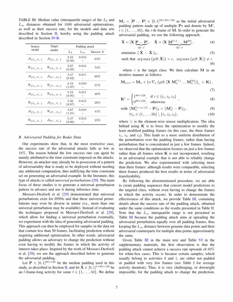
TABLE III: Median value (interquartile range) of the L2 andL∞ distances obtained for 1000 adversarial optimizations,as well as their success rate, for the models and data setsdescribed in Section II, hereby using the padding attackdescribed in Section IV-B.

Sourcemodel

Targetmodel

Padding attack

L2 L∞ Success %

A{S+,S−} A{S+,S−}3.34 0.012

84%(0.56) −

R{S+,S−} R{S+,S−}3.07 0.012

74%(0.28) −

A{S+,S−} A{S−,S+}3.47 0.011

68%(0.82) −

R{S+,S−} R{S−,S+}4.19 0.010

51%(1.07) −

A{S+,S−} R{S+,S−}5.19 0.011

48%(0.95) −

R{S+,S−} A{S+,S−}5.56 0.012

28%(0.87) −

A{S+,S−} R{S−,S+}4.67 0.010

41%(1.21) −

R{S+,S−} A{S−,S+}5.47 0.012

25%(0.80) −

B. Adversarial Padding for Radar Data

Our experiments show that, in the most restrictive case,the success rate of the adversarial attacks falls as low as18%. The reason behind the low success rate can again bemainly attributed to the time constraint imposed on the attacks.However, an attacker may already be in possession of a patternof adversariality that is ready to be deployed without needingany additional computation, thus nullifying the time constraintset on generating an adversarial example. In the literature, thistype of attacks is called universal perturbations [29]. The mainfocus of these studies is to generate a universal perturbationpattern in advance and use it during inference time.

Moosavi-Dezfooli et al. [29] demonstrated that universalperturbations exist for DNNs and that these universal pertur-bations may even be diverse in nature (i.e., more than oneuniversal perturbation may be available). Instead of evaluatingthe techniques proposed in Moosavi-Dezfooli et al. [29],which allow for finding a universal perturbation eventually,we experiment with the idea of generating adversarial padding.This approach can then be employed for samples in the data setthat contain less than 50 frames, facilitating prediction withoutrequiring additional optimization. In other words, adversarialpadding allows an adversary to change the prediction withouteven having to modify the frames in which the activity ofinterest takes place. Inspired by the work of Moosavi-Dezfooliet al. [29], we use the approach described below to generatethe adversarial padding.

Let P ∈ [0, 1]80×126 be the median padding used in thisstudy, as described in Section II, and let X ∈ [0, 1]`×80×126 bean `-frame-long activity for some ` ∈ {1, . . . , 50}. We define

M1 = [P . . . P] ∈ [0, 1]50×80×126 as the initial adversarialpadding pattern made up of multiple Ps and denote by Mi,i ∈ {1, . . . , 50}, the i-th frame of M. In order to generate theadversarial padding, we use the following approach:

X = [X P . . .P︸ ︷︷ ︸50−`

] , X = [X M`+1 . . .M50︸ ︷︷ ︸50−`

] , (4)

minimize || X − X ||2 , (5)

such that arg max(g(θ, X)

)= c, arg max

(g(θ, X)

)6= c

(6)

where c is the target class. We then calculate M in aniterative manner as follows:

Mn+1 = Mn +(α∇x

(g(θ, [X M`+1

n . . .M50n ]))c� K

),

(7)

Ki =

{180×126, if i ∈ {i1, i2, i3}080×126, otherwise

, (8)

with ||M{i1,i2,i3}n −P||2 < ||Miun −P||2 , (9)

∀iu ∈ {1, . . . , 50} \ {i1, i2, i3} , (10)

where � is the element-wise tensor multiplication. The ideabehind using K is to force the optimization to modify theleast modified padding frames (in this case, the three framesi1, i2, and i3). This leads to a more uniform distribution ofthe perturbation over the padding frames, rather than havingperturbation that is concentrated in just a few frames. Indeed,we observed that the optimization focuses on just a few framesrather than all frames when K is not incorporated, resultingin an adversarial example that is not able to reliably changethe prediction. We also experimented with selecting morethan three frames: although results were comparable, selectingthree frames produced the best results in terms of adversarialtransferability.

By following the aforementioned procedure, we are ableto create padding sequences that convert model predictions tothe targeted class, without even having to change the framesin which the activity occurs. In order to demonstrate theeffectiveness of this attack, we provide Table III, containingdetails about the success rate of the padding attack, obtainedunder the same conditions as the results presented in Table II.Note that the L∞ interquartile range is not presented inTable III because the padding attack aims at spreading theadversarial perturbation equally over all padding frames, thuskeeping the L∞ distance between genuine data points and theiradversarial counterparts for multiple data points approximatelythe same.

Given Table III in the main text and Table VI in thesupplementary materials, the first observation is that thepadding attack cannot achieve a success rate upwards of 80%for white-box cases. This is because certain samples, whichusually belong to activities 0 and 1, are either not paddedor padded with very few frames (see Table I for averageactivity duration). Thus, it is very challenging, or downrightimpossible, for the padding attack to change the prediction.

7

Trivially, the shorter activities are more affected by the paddingattack. Furthermore, we can observe that the padding attackachieves higher success rates in most black-box cases than theattacks presented in Table II, albeit by incorporating strongerperturbations.

Our experiments show that it is indeed possible to exploitthe structure of data sets that contain a temporal dimensionwith special attacks similar to the above-described paddingattack. In this case, we demonstrated the possibility of chang-ing a model prediction by only perturbing the frames wherethe activity does not take place. Moreover, the adversarialpadding generated by our padding attack only needs to becomputed once and can then be used multiple times, thusallowing it to be incorporated in scenarios where the attackerhas limited time for performing a malicious attack. In thesupplementary materials, we provide a detailed illustration ofadversarial padding in Fig. 11, showing how remarkably hardit is to spot adversarial padding using the bare eye.

In the next section, we discuss a number of interestingobservations related to model interpretability, as made duringour analysis of adversarial attacks on radar-based CNNs.

V. RELATION OF ADVERSARIAL ATTACKS TOINTERPRETABILITY

A major criticism regarding DNNs is their lack of in-terpretability; it is often challenging (if not impossible) tounderstand the reasoning behind the decisions made by aneural network-based model. In order to overcome this issueand to increase the trustworthiness of DNNs, several tech-niques have been proposed. These can broadly be dividedinto the following two groups: (1) perturbation-based forwardpropagation methods [38, 53] and (2) back-propagation-basedapproaches [36, 39, 57]. The main goal of these techniques isto highlight those parts of the input that are important for theprediction made by a neural network. When the input consistsof a natural image, this analysis is often done subjectively,unless the evaluated data comes with, for example, weakly-supervised localization labels, which can then be used for eval-uating the correctness of the selected interpretability technique.In our case, different from natural images, the input consistsof a sequence of RD frames that are significantly harder tointerpret by humans. However, different from prediction usinga single image, radar data also bring useful features, such asallowing for a frame-by-frame analysis.

A first peculiar observation we made during the experimentspresented in Section IV is that CW focuses on only introduc-ing perturbation in certain frames, rather than spreading outthe perturbation equally. In Fig. 4, we present the amountof perturbation added by CW to each frame in the formof boxplots. Note that padding frames at the end receiveconsiderably less perturbation than the frames containing theaction. We hypothesize that frames that are the recipient ofstronger perturbations are important frames, making it possibleto distinguish actions from one another.

In order to confirm this hypothesis, we perform an ex-haustive experiment on measuring the importance of a frame.

· · ·

Radar data

4 2 0 2 44

3

2

1

0

160

100

40

4 2 0 2 44

3

2

1

0

160

100

40

CN

NM

odel

y0y1...y5

Fig. 3: Visual representation of the frame replacement opera-tion as explained in Section V.

1 5 10 15 20 25 30 35 40 45 50Frames

0

0.1

0.2

0.3

L 2 p

ertu

rbat

ion

-0.20

0.33

0.66

1

Logi

t cha

nge

Fig. 4: A boxplot representation of added perturbation, as gen-erated by CW, displayed for individual frames of adversarialexamples that transfer from AS+

to AS− . The amount of addedperturbation is plotted against the median frame importance,as calculated by the experiment detailed in Section V.

1 5 10 15 20 25 30 35 40 45 50

Frames

0

0.4

0.8

1.2

Gra

d-C

AM

mag

nitu

de

(No

rmal

ized

)

-0.2

0

0.33

0.66

1

Log

it c

hang

e

Fig. 5: Mean Grad-CAM magnitude (normalized) is plottedagainst the mean frame importance, as calculated by theexperiment detailed in Section V.

As illustrated in Fig. 3, we replace individual frames, oneat a time, by the median frame we described in Section II,subsequently performing a forward pass. Since this medianframe is used throughout the training procedure to pad thedata, it is not an out-of-distribution sample, thus not favoringone class over another. By doing so, for each data point, wemeasure the change in the prediction logit for the correct class50 times (for each frame individually) and plot the mediandifference in Fig. 4, showing the relation between the perturba-tion amount per frame and the logit change when those framesare replaced. Specifically, the red line represents the medianlogit change and the shaded area represents the interquartilerange. As can be observed, the frames favored by adversarialattacks in terms of added perturbation are also the ones thatcontribute more to the prediction, confirming our hypothesis.In the supplementary materials, an extended version of thisexperiment, conducted on each class individually, can be foundin Fig. 12.

8

Following this experiment, we investigate the applicabilityof CNN interpretability techniques to radar data. Amongdifferent interpretability techniques, Grad-CAM [36] standsout, thanks to its superior weakly-supervised localizationresults obtained on ImageNet. Another reason for selectingthis method is that its approach is based on backpropagation,meaning that the input is not perturbed. We especially wantto avoid methods based on input perturbation because, unlikenatural images, small changes in RD frames may lead to largechanges in terms of correctness of the data (i.e., being a validdata point). In our setting, Grad-CAM is defined as follows:

Grad–CAM =∑k

(ReLU

(∑i

∑j

∇xLpi,j)Lpk

), (11)

where Lp denotes the output of the forward pass after the p-th layer (i.e., discriminative features) and ∇xLp denotes thegradient obtained with a backward pass from the same layerwith respect to the input (i.e., weighted gradient). Differentfrom adversarial attacks, as well as vanilla and guided back-propagation, Grad-CAM does not use the gradients of the firstlayer, thus arguably allowing for a more robust explanatoryapproach. Because the input is not a single image but a se-quence of frames, Grad-CAM produces class activation mapsfor each frame individually. An example set of video frames,their corresponding radar frames, and the obtained Grad-CAM heatmaps can be found in Fig. 1. In the supplementarymaterials, an extended version of the same activity sequenceis provided in Fig. 14. These qualitative results show that theheatmaps usually highlight (1) those frames where the mostimportant part of the activity occurs and (2) those locationswhere the radar activity is the largest.

Apart from the qualitative results provided in Fig. 1, whichare heavily criticized in Lipton [27] and Ghorbani et al. [9],we now aim at performing a quantitative evaluation of thecorrectness of the produced Grad-CAM activation frames.We calculate the median magnitude of the produced Grad-CAM frames, which are normalized between 0 and 1, andcompare it to the previously presented frame importance datain Fig. 5, where the blue line represents the median Grad-CAMmagnitude and the red line the median frame importance.The bands around the lines correspond to the respectiveinterquartile ranges. In the supplementary materials, the sametype of illustration on a per-class basis is provided in Fig. 13.

Given Fig. 5, we again observe a correlation between theimportance of frames and their corresponding Grad-CAMactivations. Both experiments, as presented in Fig. 4 andFig. 5, show strong correlation between their respective data.In particular, the higher the magnitude of the positive Grad-CAM heatmap, the larger the change in the prediction willbe when replacing the underlying frame with the paddingframe. Consequently, our experiments confirm that the outputof Grad-CAM can indeed be used to assess the relative im-portance of each radar frame for the prediction made. Indeed,the frames that contribute the most to a prediction are also theones that are naturally perturbed more than the others during

an adversarial optimization, pointing to a strong connectionbetween adversarial optimization and model interpretability.

VI. CONCLUSIONS AND FUTURE WORK

In this study, we evaluated multiple scenarios in whichadversarial attacks are performed on CNNs trained with asequence of range-Doppler images obtained from a low-power FMCW radar sensor, with the goal of performinggesture recognition. Our analysis showed that these modelsare vulnerable not only to commonly used attacks, but alsoto unique attacks that take advantage of how the data set iscrafted. In order to demonstrate a unique attack that leveragesknowledge about the data set, we proposed a padding attackthat creates a padding sequence that changes the predictionsmade by CNNs.

An often mentioned drawback of CNNs is their lack ofinterpretability. By taking advantage of the data selected forthis study, we were able to show the connection between theperturbation exercised by adversarial attacks and the impor-tance of individual frames. Moreover, we were also able todemonstrate that it is possible to identify important framesusing Grad-CAM, thus showing (1) the relation between adver-sarial optimization and interpretability, and (2) a quantitativemethod to evaluate interpretability techniques.

In future research, we aim to analyze multiple shortcom-ings of radar sensors against so-called real-world adversarialexamples [25, 42], as well as black-box attacks that do not usesurrogate models [7, 12, 46]. In the case of activity detection,real-world adversarial examples may occur when radar sensorsare employed in environments exhibiting poor recording con-ditions, such as environments that contain reflective materials(e.g., metal objects), or similarly, when the subject itself carriesany reflective material. Moreover, it would be of interest toinvestigate the influence of multiple moving subjects in thesame recording environment on adversariality.

ACKNOWLEDGEMENTS

We would like to thank the anonymous reviewers for theirvaluable and insightful comments. We believe their commentssignificantly improved the quality of this manuscript.

The research activities described in this paper were fundedby Ghent University Global Campus, Ghent University, imec,Flanders Innovation & Entrepreneurship (VLAIO), the Fundfor Scientific Research-Flanders (FWO-Flanders), and the EU.

REFERENCES

[1] Athalye, A., Carlini, N., Wagner, D., 2018. Obfus-cated Gradients Give A False Sense Of Security: Cir-cumventing Defenses To Adversarial Examples. CoRRabs/1802.00420.

[2] Biggio, B., Corona, I., Maiorca, D., Nelson, B., Srndic,N., Laskov, P., Giacinto, G., Roli, F., 2013. EvasionAttacks Against Machine Learning At Test Time, in:Joint European conference on machine learning andknowledge discovery in databases, Springer. pp. 387–402.

9

[3] Brown, T.B., Mane, D., Roy, A., Abadi, M., Gilmer, J.,2017. Adversarial Patch. CoRR abs/1712.09665.

[4] Carlini, N., Wagner, D.A., 2016. Towards Evaluating TheRobustness of Neural Networks. CoRR abs/1608.04644.

[5] Carlini, N., Wagner, D.A., 2017. Adversarial ExamplesAre Not Easily Detected: Bypassing Ten Detection Meth-ods. CoRR abs/1705.07263.

[6] Chen, V.C., Tahmoush, D., Miceli, W.J., 2014. RadarMicro-Doppler Signatures: Processing And Applications.Radar, Sonar & Navigation, Institution of Engineeringand Technology.

[7] Cheng, S., Dong, Y., Pang, T., Su, H., Zhu, J., 2019. Im-proving Black-box Adversarial Attacks with a Transfer-based Prior, in: Advances in Neural Information Process-ing Systems, pp. 10932–10942.

[8] Etmann, C., Lunz, S., Maass, P., Schonlieb, C.B., 2019.On The Connection Between Adversarial RobustnessAnd Saliency Map Interpretability. arXiv preprintarXiv:1905.04172 .

[9] Ghorbani, A., Abid, A., Zou, J., 2017. Interpretation OfNeural Networks Is Fragile. CoRR abs/1710.10547.

[10] Goodfellow, I., McDaniel, P., Papernot, N., 2018. MakingMachine Learning Robust Against Adversarial Inputs.Communications of the ACM 61, 56–66.

[11] Goodfellow, I., Shlens, J., Szegedy, C., 2014. Ex-plaining and Harnessing Adversarial Examples. CoRRabs/1412.6572.

[12] Gragnaniello, D., Marra, F., Poggi, G., Verdoliva, L.,2019. Perceptual quality-preserving black-box at-tack against deep learning image classifiers. CoRRabs/1902.07776.

[13] Graves, A., Mohamed, A.r., Hinton, G., 2013. SpeechRecognition With Deep Recurrent Neural Networks, in:2013 IEEE international conference on acoustics, speechand signal processing, IEEE. pp. 6645–6649.

[14] Guo, C., Gardner, J.R., You, Y., Wilson, A.G., Wein-berger, K.Q., 2019. Simple Black-box Adversarial At-tacks. CoRR abs/1905.07121.

[15] Hara, K., Kataoka, H., Satoh, Y., 2018. Can Spatiotem-poral 3D CNNs Retrace the History of 2D CNNs andImageNet?, in: Proceedings of the IEEE conference onComputer Vision and Pattern Recognition, pp. 6546–6555.

[16] He, K., Zhang, X., Ren, S., Sun, J., 2016. Deep ResidualLearning For Image Recognition, in: Proceedings ofthe IEEE conference on computer vision and patternrecognition, pp. 770–778.

[17] Hochreiter, S., Schmidhuber, J., 1997. Long short-termmemory. Neural computation 9, 1735–1780.

[18] Ilyas, A., Engstrom, L., Athalye, A., Lin, J., 2018.Black-box Adversarial Attacks with Limited Queries andInformation. CoRR abs/1804.08598.

[19] Jalalvand, A., Vandersmissen, B., De Neve, W., Mannens,E., 2019. Radar Signal Processing For Human Identifi-cation By Means Of Reservoir Computing Networks, in:IEEE Radar Conference, pp. 1–6.

[20] Jokanovic, B., Amin, M., Ahmad, F., 2016. Radar FallMotion Detection Using Deep Learning, in: 2016 IEEEradar conference (RadarConf), IEEE. pp. 1–6.

[21] Kim, Y., Moon, T., 2015. Human Detection and ActivityClassification Based on Micro-Doppler Signatures UsingDeep Convolutional Neural Networks. IEEE geoscienceand remote sensing letters 13, 8–12.

[22] Kim, Y., Toomajian, B., 2016. Hand Gesture Recogni-tion Using Micro-Doppler Signatures With ConvolutionalNeural Network. IEEE Access 4, 7125–7130.

[23] Kingma, D.P., Ba, J., 2014. Adam: A Method ForStochastic Optimization. CoRR abs/1412.6980.

[24] Krizhevsky, A., Sutskever, I., Hinton, G.E., 2012. Ima-geNet classification with deep convolutional neural net-works, in: Advances in neural information processingsystems, pp. 1097–1105.

[25] Kurakin, A., Goodfellow, I., Bengio, S., 2016. Ad-versarial Examples In The Physical World. CoRRabs/1607.02533.

[26] LeCun, Y., Bottou, L., Bengio, Y., Haffner, P., 1998.Gradient-Based Learning Applied To Document Recog-nition. Proceedings of the IEEE 86, 2278–2324.

[27] Lipton, Z.C., 2016. The Mythos Of Model Interpretabil-ity. arXiv preprint arXiv:1606.03490 .

[28] Madry, A., Makelov, A., Schmidt, L., Tsipras, D., Vladu,A., 2017. Towards Deep Learning Models Resistant ToAdversarial Attacks. CoRR abs/1706.06083.

[29] Moosavi-Dezfooli, S.M., Fawzi, A., Fawzi, O., Frossard,P., 2017. Universal Adversarial Perturbations, in: Pro-ceedings of the IEEE conference on computer vision andpattern recognition, pp. 1765–1773.

[30] Nair, N., Thomas, C., Jayagopi, D.B., 2018. HumanActivity Recognition Using Temporal Convolutional Net-work, in: Proceedings of the 5th international Workshopon Sensor-based Activity Recognition and Interaction,pp. 1–8.

[31] Ozbulak, U., Gasparyan, M., De Neve, W., Van Messem,A., 2020. Perturbation analysis of gradient-based adver-sarial attacks. Pattern Recognition Letters .

[32] Papernot, N., McDaniel, P.D., Jha, S., Fredrikson, M.,Celik, Z.B., Swami, A., 2015. The Limitations Of DeepLearning In Adversarial Settings. CoRR abs/1511.07528.

[33] Rajpoot, Q.M., Jensen, C.D., 2015. Video Surveillance:Privacy Issues And Legal Compliance, in: Promoting So-cial Change and Democracy through Information Tech-nology. IGI global, pp. 69–92.

[34] Ross, A.S., Doshi-Velez, F., 2018. Improving The Adver-sarial Robustness And Interpretability Of Deep NeuralNetworks By Regularizing Their Input Gradients, in:Thirty-second AAAI conference on artificial intelligence.

[35] Russakovsky, O., Deng, J., Su, H., Krause, J., Satheesh,S., Ma, S., Huang, Z., Karpathy, A., Khosla, A., Bern-stein, M., Berg, A.C., Fei-Fei, L., 2015. ImageNetLarge Scale Visual Recognition Challenge. InternationalJournal of Computer Vision 115, 211–252.

[36] Selvaraju, R.R., Das, A., Vedantam, R., Cogswell, M.,

10

Parikh, D., Batra, D., 2016. Grad-Cam: Why Did YouSay That? Visual Explanations From Deep Networks ViaGradient-Based Localization. CVPR 2016 .

[37] Seyfioglu, M.S., Ozbayoglu, A.M., Gurbuz, S.Z., 2018.Deep Convolutional Autoencoder for Radar-Based Clas-sification of Similar Aided and Unaided Human Activ-ities. IEEE Transactions on Aerospace and ElectronicSystems 54, 1709–1723.

[38] Shrikumar, A., Greenside, P., Kundaje, A., 2017. Learn-ing Important Features Through Propagating ActivationDifferences. CoRR abs/1704.02685.

[39] Simonyan, K., Vedaldi, A., Zisserman, A., 2014. DeepInside Convolutional Networks: Visualising Image Clas-sification Models And Saliency Maps, in: Workshop,Proceedings of 2th International Conference on LearningRepresentations (ICLR).

[40] Simonyan, K., Zisserman, A., 2014. Very Deep Convo-lutional Networks For Large-Scale Image Recognition.CoRR abs/1409.1556.

[41] Staples, P., 2019. Thinking About Buying A Smart HomeDevice? Heres What You Need To Know About Security.https://www.forbes.com. Accessed: 2019-07-26.

[42] Sun, L., Tan, M., Zhou, Z., 2018. A Survey of PracticalAdversarial Example Attacks. Cybersecurity 1, 9.

[43] Szegedy, C., Vanhoucke, V., Ioffe, S., Shlens, J., Wojna,Z., 2016. Rethinking The Inception Architecture ForComputer Vision, in: Proceedings of the IEEE conferenceon computer vision and pattern recognition, pp. 2818–2826.

[44] Szegedy, C., Zaremba, W., Sutskever, I., Bruna, J., Erhan,D., Goodfellow, I., Fergus, R., 2013. Intriguing Proper-ties Of Neural Networks. CoRR abs/1312.6199.

[45] Tao, G., Ma, S., Liu, Y., Zhang, X., 2018. AttacksMeet Interpretability: Attribute-Steered Detection Of Ad-versarial Samples, in: Advances in Neural InformationProcessing Systems, pp. 7717–7728.

[46] Tu, C.C., Ting, P., Chen, P.Y., Liu, S., Zhang, H.,Yi, J., Hsieh, C.J., Cheng, S.M., 2019. Autozoom:Autoencoder-based zeroth order optimization method forattacking black-box neural networks, in: Proceedings ofthe AAAI Conference on Artificial Intelligence, pp. 742–749.

[47] Vandersmissen, B., Knudde, N., Jalalvand, A., Couckuyt,I., Bourdoux, A., De Neve, W., Dhaene, T., 2018. IndoorPerson Identification Using A Low-Power Fmcw Radar.IEEE Transactions on Geoscience and Remote Sensing56, 3941–3952.

[48] Vandersmissen, B., Knudde, N., Jalalvand, A., Couckuyt,I., Dhaene, T., De Neve, W., 2019. Indoor HumanActivity Recognition Using High-Dimensional SensorsAnd Deep Neural Networks. Neural Computing andApplications , 1–15.

[49] Wang, S., Song, J., Lien, J., Poupyrev, I., Hilliges, O.,2016. Interacting With Soli: Exploring Fine-GrainedDynamic Gesture Recognition In The Radio-FrequencySpectrum, in: Proceedings of the 29th Annual Sympo-

sium on User Interface Software and Technology, ACM.pp. 851–860.

[50] Wu, D., Wang, Y., Xia, S.T., Bailey, J., Ma, X., 2020.Skip Connections Matter: On the Transferability of Ad-versarial Examples Generated with ResNets, in: Interna-tional Conference on Learning Representations.

[51] Xie, S., Girshick, R., Dollar, P., Tu, Z., He, K., 2017.Aggregated Residual Transformations for Deep NeuralNetworks, in: Proceedings of the IEEE conference oncomputer vision and pattern recognition, pp. 1492–1500.

[52] Yao, L., Qian, Y., 2018. DT-3DResNet-LSTM: An Ar-chitecture for Temporal Activity Recognition in Videos,in: Pacific Rim Conference on Multimedia, Springer. pp.622–632.

[53] Zeiler, M.D., Fergus, R., 2014. Visualizing And Under-standing Convolutional Networks, in: European confer-ence on computer vision, Springer. pp. 818–833.

[54] Zhang, H.B., Zhang, Y.X., Zhong, B., Lei, Q., Yang, L.,Du, J.X., Chen, D.S., 2019. A Comprehensive SurveyOf Vision-Based Human Action Recognition Methods.Sensors 19, 1005.

[55] Zhao, M., Li, T., Abu Alsheikh, M., Tian, Y., Zhao, H.,Torralba, A., Katabi, D., 2018a. Through-Wall HumanPose Estimation Using Radio Signals, in: Proceedings ofthe IEEE Conference on Computer Vision and PatternRecognition, pp. 7356–7365.

[56] Zhao, Y., Yang, R., Chevalier, G., Xu, X., Zhang, Z.,2018b. Deep Residual Bidir-LSTM for Human ActivityRecognition Using Wearable Sensors. MathematicalProblems in Engineering 2018.

[57] Zhou, B., Khosla, A., Lapedriza, A., Oliva, A., Torralba,A., 2016. Learning Deep Features For DiscriminativeLocalization, in: Proceedings of the IEEE conference oncomputer vision and pattern recognition, pp. 2921–2929.

11

Supplementary materials for:Investigating the significance of adversarial attacks and their relation to

interpretability for radar-based human activity recognition systems

DETAILED ARCHITECTURAL DESCRIPTIONS

(3× 3× 3) Conv

(3× 3× 3) Conv

(3× 3× 3) Conv

(3× 3× 3) Conv

Linear

Linear

ELU+Dropout

ELU+Dropout

ELU+Dropout

ELU+Dropout

ELU+Dropout

Pooling

Pooling

Pooling

Pooling

Input

Output

(1× 50× 80× 126)

(8× 50× 80× 126)

(8× 16× 40× 63)

(16× 16× 40× 63)

(16× 8× 20× 31)

(32× 8× 20× 31)

(32× 4× 10× 15)

(64× 4× 10× 15)

(64× 2× 10× 15)

(128× 1)

(6× 1)

Architecture: ATrainable parameters:∼ 6.4× 105

Size: ∼ 2.5MB

Fig. 6: Detailed description for architecture A.

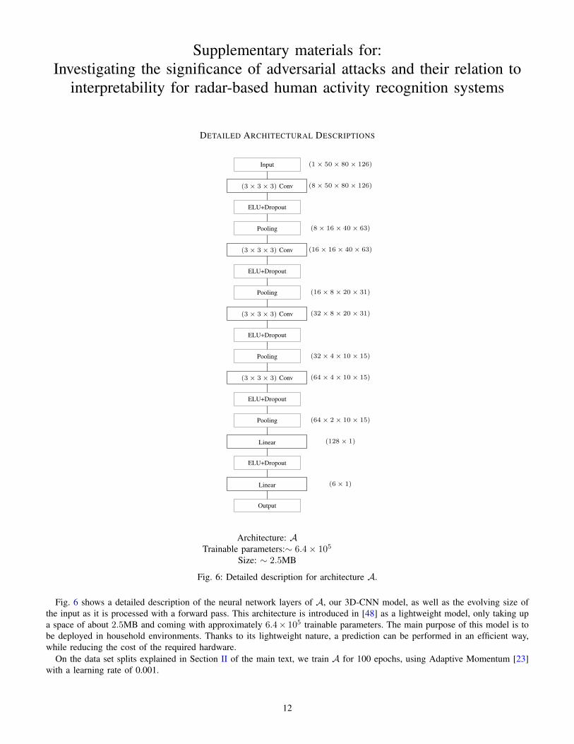
Fig. 6 shows a detailed description of the neural network layers of A, our 3D-CNN model, as well as the evolving size ofthe input as it is processed with a forward pass. This architecture is introduced in [48] as a lightweight model, only taking upa space of about 2.5MB and coming with approximately 6.4× 105 trainable parameters. The main purpose of this model is tobe deployed in household environments. Thanks to its lightweight nature, a prediction can be performed in an efficient way,while reducing the cost of the required hardware.

On the data set splits explained in Section II of the main text, we train A for 100 epochs, using Adaptive Momentum [23]with a learning rate of 0.001.

12

(3× 3× 3) Conv

ResNext Bottleneck

ResNext Bottleneck

ResNext Bottleneck

ResNext Bottleneck

Linear

Batch Normalization

ReLU

ReLU+Dropout

Pooling

Pooling

Input

Output

(1× 50× 80× 126)

(64× 25× 40× 63)

(64× 13× 20× 32)

(256× 13× 20× 32)

(512× 7× 10× 16)

(1024× 4× 5× 8)

(2048× 2× 3× 4)

(2048× 1)

(6× 1)

Architecture: RTrainable parameters:∼ 8.1× 106

Size: ∼ 32.9MB

Fig. 7: Detailed description for architecture R.

TABLE IV: Validation and testing accuracy of the architectures A, R, and L for each class, as obtained for the respectiveevaluation splits described in Section II of the main text.

A R L

Class Validation Test Validation Test Validation Test

(0) 57% 67% 60% 67% 75% 79%(1) 88% 86% 80% 81% 58% 72%(2) 83% 79% 77% 78% 85% 77%(3) 76% 79% 76% 71% 62% 55%(4) 55% 68% 54% 69% 55% 52%(5) 70% 69% 59% 63% 60% 65%

Total 72% 74% 67% 72% 66% 67%

Fig. 7 shows a detailed description of the second model used in our study (R). This model is a variant of the ResNeXtmodel [51], so to be able to handle data with a temporal dimension (e.g., video and radar data), and where this variant hasbeen presented in Hara et al. [15]. The architecture shown in Fig. 7, which contains four ResNeXt Bottleneck layers (moredetailed information about such layers can be found in Xie et al. [51]), is significantly more complex compared to the modelpresented in Fig. 6. Indeed, this model contains approximately 8.1×106 trainable parameters (roughly 12 times more than A).Moreover, this model is also larger in terms of size, taking up a space of about 32.9MB. To add, a single prediction made bythe ResNeXt model takes about 9 times longer than a single prediction made by the 3D-CNN model, thus possibly introducingsignificant time delays when it is deployed on similar hardware. The aforementioned considerations make it challenging for theResNeXt model to be deployed in household environments with cheap hardware, not only because of its size, but also becauseof the time required to make a prediction. Nevertheless, we selected this model in order to be able to make a comparison, in

13

(3× 3× 3) Conv

ResNext Bottleneck

ResNext Bottleneck

ResNext Bottleneck

ResNext Bottleneck

Linear

Batch Normalization

ReLU

ReLU+Dropout

Pooling

Pooling

Input

LSTM

Output

(1× 50× 80× 126)

(50× 64× 40× 63)

(50× 64× 20× 32)

(50× 64× 20× 32)

(50× 256× 20× 32)

(50× 512× 10× 16)

(50× 1024× 5× 8)

(50× 2048× 1× 1)

(1024× 1)

(6× 1)

Architecture: LTrainable parameters:∼ 17.8× 106

Size: ∼ 214MB

Fig. 8: Detailed description for architecture L.

terms of adversarial vulnerability, between a simple model that can be easily deployed and a larger model that is more capable.On the data set splits explained in Section II of the main text, we train R for 50 epochs, using Adaptive Momentum [23]

with a learning rate of 1e−5.Fig. 8 shows a detailed description of the third and the last model L used in our study. The architecture of L is similar

to that of R. However, L comes with a simple but crucial difference: it is a CNN-LSTM architecture that uses convolutionsas feature extractors and that leverages an LSTM layer to discover the underlying relations along the temporal dimension. Assuch, the convolution operations are only performed on individual frames and not along the temporal dimension. This allowsthe employed LSTM to discover temporal relations and make judgements based on the information stored over an extendedperiod of time. The down side of this model is its greater complexity in terms of storage and inference time. Due to theaddition of an LSTM layer, the size of the model significantly increases compared to R, containing ∼ 17.8 × 106 trainableparameters and taking a space of about 214MB. As a result, both a forward pass (prediction) and a backward pass (training)take significantly longer than in the case of A and R. These properties pose an important challenge when employing suchmodels using low-cost and low-power equipment in smart homes.

The best performing model for this architecture is the one we trained on the data set splits explained in Section II of themain text, for 30 epochs, hereby using Adaptive Momentum [23] with a learning rate of 0.00001.

Per-class accuracy of all three models observed for unseen data (i.e., validation and testing) is provided in Table IV. As canbe seen, even though all of the employed models are vastly different in terms of architecture as well as trainable parameters,they achieve roughly similar results for the task at hand, making them suitable for a study on adversarial research.

VISUAL SUMMARY OF THE EVALUATED SCENARIO

Fig. 9 contains a visual description of the flow of events for the scenario evaluated in the main text. To that end, when anyaction is performed in a household environment, a radar sensor (in this case an FMCW radar device) is able to detect this

14

(1) Action

4 2 0 2 44

3

2

1

0

160

100

40

4 2 0 2 44

3

2

1

0

160

100

40

4 2 0 2 44

3

2

1

0

160

100

40

4 2 0 2 44

3

2

1

0

160

100

40

FMC

WD

etec

tor

(2) Radar detection (3) Radar activity

On-site Server(4) Evaluation

CNNDecision

Mechanism

(5) Out-house functionality

(5) In-house functionality

�

4 2 0 2 44

3

2

1

0

0

0.5

1

4 2 0 2 44

3

2

1

0

0

0.5

1

4 2 0 2 44

3

2

1

0

0

0.5

1

4 2 0 2 44

3

2

1

0

0

0.5

1

Interpretability evaluation

Adversarial attack

Adversarial

attack

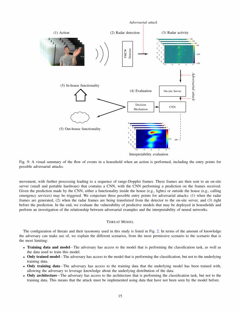
Fig. 9: A visual summary of the flow of events in a household when an action is performed, including the entry points forpossible adversarial attacks.

movement, with further processing leading to a sequence of range-Doppler frames. These frames are then sent to an on-siteserver (small and portable hardware) that contains a CNN, with the CNN performing a prediction on the frames received.Given the prediction made by the CNN, either a functionality inside the house (e.g., lights) or outside the house (e.g., callingemergency services) may be triggered. We conjecture three possible entry points for adversarial attacks: (1) when the radarframes are generated, (2) when the radar frames are being transferred from the detector to the on-site server, and (3) rightbefore the prediction. In the end, we evaluate the vulnerability of predictive models that may be deployed in households andperform an investigation of the relationship between adversarial examples and the interpretability of neural networks.

THREAT MODEL

The configuration of threats and their taxonomy used in this study is listed in Fig. 2. In terms of the amount of knowledgethe adversary can make use of, we explain the different scenarios, from the most permissive scenario to the scenario that isthe most limiting:

• Training data and model – The adversary has access to the model that is performing the classification task, as well asthe data used to train this model.

• Only trained model – The adversary has access to the model that is performing the classification, but not to the underlyingtraining data.

• Only training data – The adversary has access to the training data that the underlying model has been trained with,allowing the adversary to leverage knowledge about the underlying distribution of the data.

• Only architecture – The adversary has access to the architecture that is performing the classification task, but not to thetraining data. This means that the attack must be implemented using data that have not been seen by the model before.

15

TABLE V: Median value (interquartile range) of the L2 and L∞ distances obtained for 1000 adversarial optimizations, as wellas their success rate, for L and data sets described in Section II of the main text. For easier comprehension, the threat modelsare listed from most permissive to least permissive. L∞ values less than 0.003 are rolled up to 0.003 (this is approximatelythe smallest amount of perturbation required to change a pixel value by 1, so to make discretization possible).

Threatmodel

Sourcemodel

Targetmodel

BIM CW

L2 L∞ Success % L2 L∞ Success %

WB L{S+,S−} L{S+,S−}0.26 0.003

100%0.30 0.01

84%(0.29) (0.003) (0.30) (0.01)

BB:1 L{S+,S−} L{S−,S+}0.32 0.003

13%0.33 0.01

11%(0.16) (0.003) (0.47) (0.02)

BB:2A{S+,S−} L{S+,S−}

1.96 0.00935%

0.71 0.0232%

(2.15) (0.006) (1.09) (0.001)

R{S+,S−} L{S+,S−}0.28 0.006

38%0.27 0.03

34%(0.31) (0.003) (0.23) (0.02)

BB:3A{S+,S−} L{S−,S+}

2.07 0.01226%

0.84 0.0323%

(1.45) (0.011) (0.93) (0.07)

R{S+,S−} L{S−,S+}0.36 0.009

24%0.28 0.02

19%(0.52) (0.007) (0.17) (0.03)

• Surrogate – The adversary has access to a model (i.e., a surrogate) that has been trained with similar data that theunderlying system has been trained with. This allows the adversary to leverage knowledge about a model that has beentrained on data that are similar in terms of distribution to the training data of the underlying system.

The attacks originating from the first two cases are usually referred to as white-box attacks, which means that the attackerhas access to the underlying system, whereas the last three cases are referred to as black-box attacks, which means the attackerdoes not have access to the underlying system. In the main text, we analyzed a white-box scenario, as well as several black-boxscenarios.

For the same threat configuration, attacks that can be performed based on the knowledge of the adversary discussed abovecan be listed from easier to harder in the following way:• Confidence reduction – Reduce the output confidence of the prediction.• Misclassification – Change the prediction from a correct one to an (unspecified) incorrect one.• Targeted misclassification – Force the prediction to become a specified class that is different from the correct one.• Targeted misclassification with a localized attack – Force the prediction to become a specified class that is different

from the correct one and, while doing so, limit the attack (i.e., the perturbation) to selected regions of the input.

CONSTRAINTS ON ADVERSARIAL ATTACKS

For the evaluation performed in the main text, we imposed the following constraints on the generation of adversarial examples:• Box constraint – In order to ensure that the generated adversarial example is a valid image, its values are constrained as

follows: Xn ∈ [0, 1], with 0 denoting black and 1 denoting white. However, different from the image domain, the radardata we use in this study always contain a portion of noise, which limits the values even further when the radar signal isconverted to a sequence of RD frames. Thus, for the radar signal, we select the box constraint as Xn ∈ [0.31, 0.83], with0.31 and 0.83 representing the smallest and the largest value present in our data set, respectively.

• Time constraint – Threat scenarios that are tackled in this study consider data obtained from sensors manipulated by anadversary. However, we only assume the adversary to be capable of manipulating the frames (i.e., adversarial attacks). Indoing so, we assume there is no delay between frame capturing and the transfer of these frames to the underlying model.As a result, in order to work with a realistic attack scenario, we assume there is a limited amount of time available toimplement perturbations. In particular, we restrict the amount of time available for adversarial optimization to one second.This limitation approximately corresponds to 200 optimization iterations for BIM and 72 iterations for the CW attack ona single Titan-X GPU for model A.

• Discretization – As described above, the input data are bounded between 0.31 and 0.83. However, when the input isrepresented as a grayscale image, these values must be represented as integers between 0 and 255. Thus, if a value doesnot have a direct integer correspondance, it is rounded to the closest integer. Studies that investigate adversarial examplesoften disregard the discretization property of the produced adversarial examples, hereby providing results for images thatare impossible to represent in reality. This topic is discussed in more detail in Carlini and Wagner [4]. In this study, wemake sure that the generated adversarial examples can be represented as valid grayscale images.

16

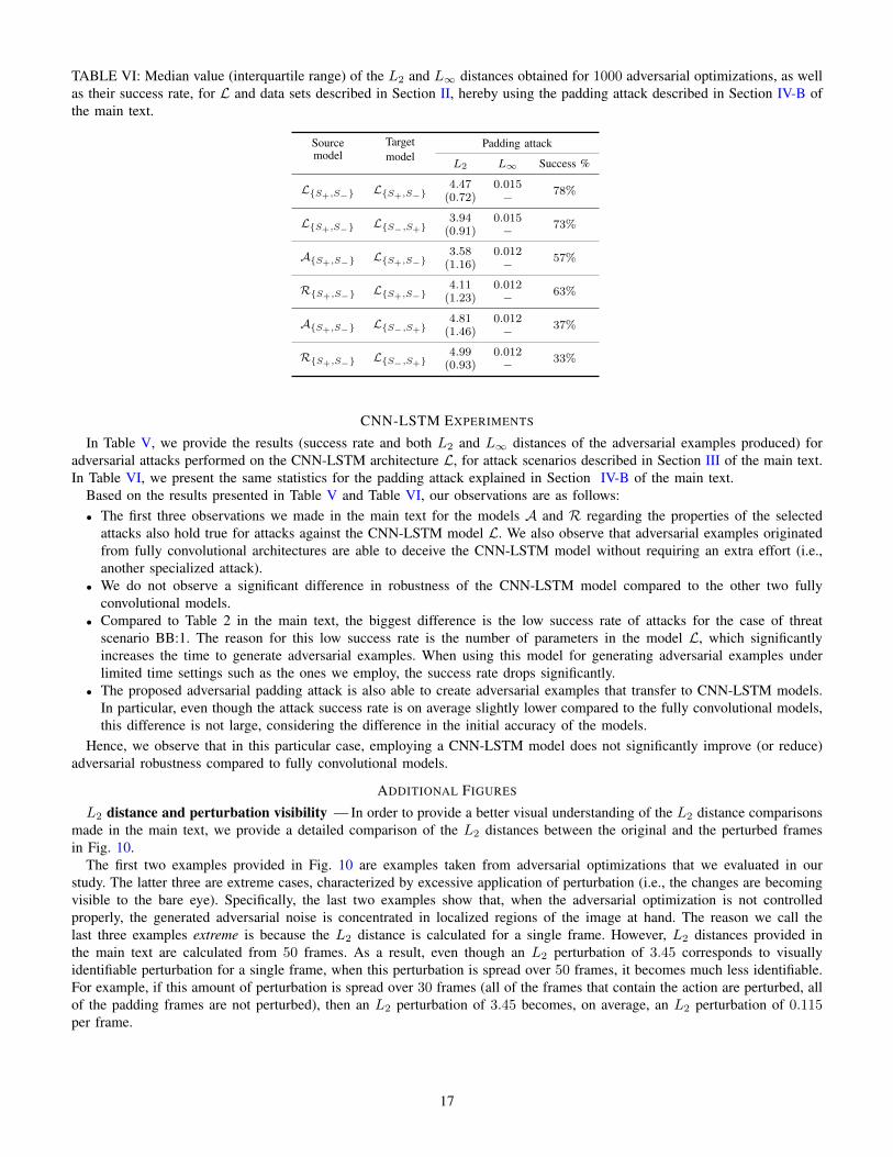
TABLE VI: Median value (interquartile range) of the L2 and L∞ distances obtained for 1000 adversarial optimizations, as wellas their success rate, for L and data sets described in Section II, hereby using the padding attack described in Section IV-B ofthe main text.

Sourcemodel

Targetmodel

Padding attack

L2 L∞ Success %

L{S+,S−} L{S+,S−}4.47 0.015

78%(0.72) −

L{S+,S−} L{S−,S+}3.94 0.015

73%(0.91) −

A{S+,S−} L{S+,S−}3.58 0.012

57%(1.16) −

R{S+,S−} L{S+,S−}4.11 0.012

63%(1.23) −

A{S+,S−} L{S−,S+}4.81 0.012

37%(1.46) −

R{S+,S−} L{S−,S+}4.99 0.012

33%(0.93) −

CNN-LSTM EXPERIMENTS

In Table V, we provide the results (success rate and both L2 and L∞ distances of the adversarial examples produced) foradversarial attacks performed on the CNN-LSTM architecture L, for attack scenarios described in Section III of the main text.In Table VI, we present the same statistics for the padding attack explained in Section IV-B of the main text.

Based on the results presented in Table V and Table VI, our observations are as follows:• The first three observations we made in the main text for the models A and R regarding the properties of the selected

attacks also hold true for attacks against the CNN-LSTM model L. We also observe that adversarial examples originatedfrom fully convolutional architectures are able to deceive the CNN-LSTM model without requiring an extra effort (i.e.,another specialized attack).

• We do not observe a significant difference in robustness of the CNN-LSTM model compared to the other two fullyconvolutional models.

• Compared to Table 2 in the main text, the biggest difference is the low success rate of attacks for the case of threatscenario BB:1. The reason for this low success rate is the number of parameters in the model L, which significantlyincreases the time to generate adversarial examples. When using this model for generating adversarial examples underlimited time settings such as the ones we employ, the success rate drops significantly.

• The proposed adversarial padding attack is also able to create adversarial examples that transfer to CNN-LSTM models.In particular, even though the attack success rate is on average slightly lower compared to the fully convolutional models,this difference is not large, considering the difference in the initial accuracy of the models.

Hence, we observe that in this particular case, employing a CNN-LSTM model does not significantly improve (or reduce)adversarial robustness compared to fully convolutional models.

ADDITIONAL FIGURES

L2 distance and perturbation visibility — In order to provide a better visual understanding of the L2 distance comparisonsmade in the main text, we provide a detailed comparison of the L2 distances between the original and the perturbed framesin Fig. 10.

The first two examples provided in Fig. 10 are examples taken from adversarial optimizations that we evaluated in ourstudy. The latter three are extreme cases, characterized by excessive application of perturbation (i.e., the changes are becomingvisible to the bare eye). Specifically, the last two examples show that, when the adversarial optimization is not controlledproperly, the generated adversarial noise is concentrated in localized regions of the image at hand. The reason we call thelast three examples extreme is because the L2 distance is calculated for a single frame. However, L2 distances provided inthe main text are calculated from 50 frames. As a result, even though an L2 perturbation of 3.45 corresponds to visuallyidentifiable perturbation for a single frame, when this perturbation is spread over 50 frames, it becomes much less identifiable.For example, if this amount of perturbation is spread over 30 frames (all of the frames that contain the action are perturbed, allof the padding frames are not perturbed), then an L2 perturbation of 3.45 becomes, on average, an L2 perturbation of 0.115per frame.

17

Original Frame Perturbed Frame

L2

Dis

tanc

e:0

4 2 0 2 4Velocity (m/s)

4

3

2

1

0

Rang

e (m

)160

100

40

4 2 0 2 4Velocity (m/s)

4

3

2

1

0

Rang

e (m

)

160

100

40

L2

Dis

tanc

e:0.

054

4 2 0 2 4Velocity (m/s)

4

3

2

1

0

Rang

e (m

)

160

100

40

4 2 0 2 4Velocity (m/s)

4

3

2

1

0

Rang

e (m

)

160

100

40

L2

Dis

tanc

e:0.

869

4 2 0 2 4Velocity (m/s)

4

3

2

1

0

Rang

e (m

)

160

100

40

4 2 0 2 4Velocity (m/s)

4

3

2

1

0

Rang

e (m

)

160

100

40

L2

Dis

tanc

e:1.

638

4 2 0 2 4Velocity (m/s)

4

3

2

1

0

Rang

e (m

)

160

100

40

4 2 0 2 4Velocity (m/s)

4

3

2

1

0

Rang

e (m

)

160

100

40

L2

Dis

tanc

e:2.

919

4 2 0 2 4Velocity (m/s)

4

3

2

1

0

Rang

e (m

)

160

100

40

4 2 0 2 4Velocity (m/s)

4

3

2

1

0

Rang

e (m

)

160

100

40

L2

Dis

tanc

e:3.

457

4 2 0 2 4Velocity (m/s)

4

3

2

1

0

Rang

e (m

)

160

100

40

4 2 0 2 4Velocity (m/s)

4

3

2

1

0

Rang

e (m

)

160

100

40

Fig. 10: (1) L2 distances, (2) original frames, and (3) perturbed frames are given in order to improve the visual understandingof various degrees of perturbation.

18

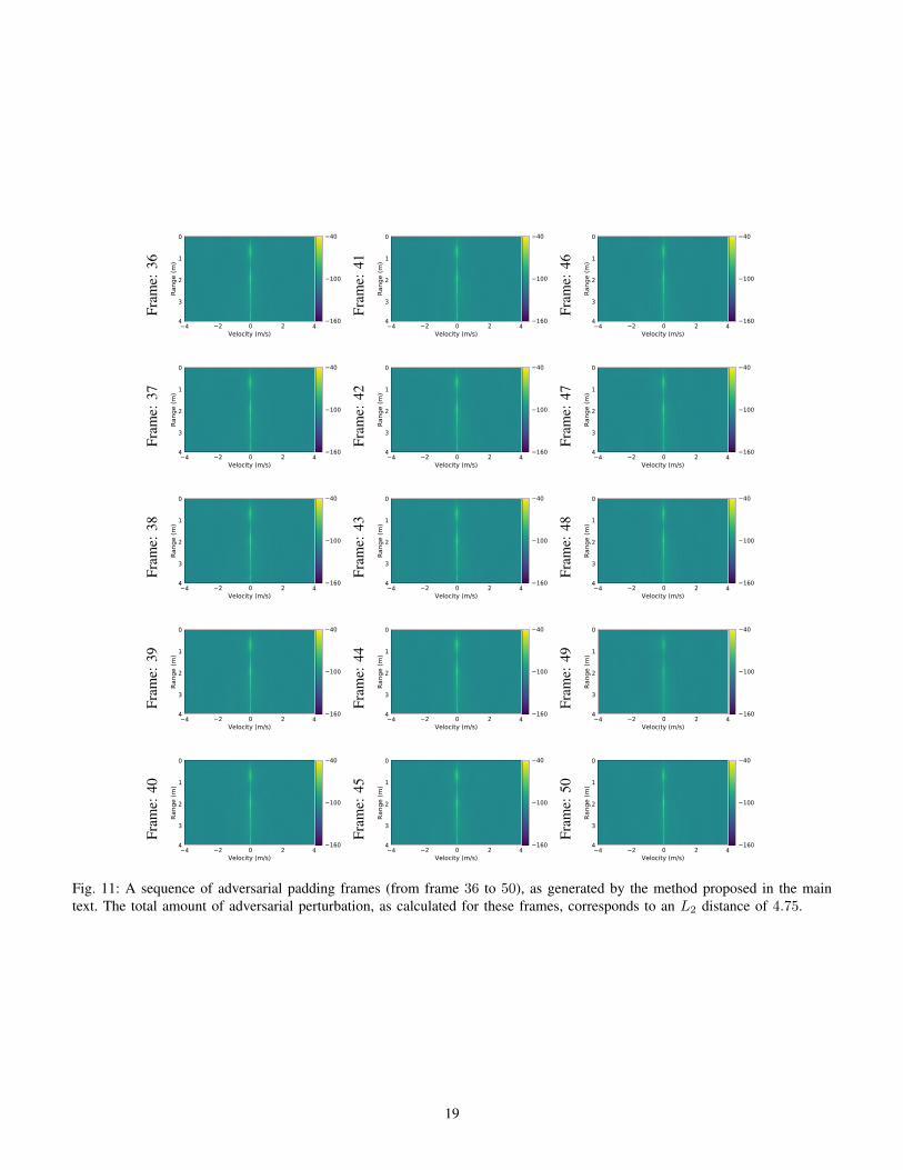
Fram

e:36

4 2 0 2 4Velocity (m/s)

4

3

2

1

0

Rang

e (m

)

160

100

40

Fram

e:41

4 2 0 2 4Velocity (m/s)

4

3

2

1

0

Rang

e (m

)

160

100

40

Fram

e:46

4 2 0 2 4Velocity (m/s)

4

3

2

1

0

Rang

e (m

)

160

100

40

Fram

e:37

4 2 0 2 4Velocity (m/s)

4

3

2

1

0

Rang

e (m

)

160

100

40Fr

ame:

42

4 2 0 2 4Velocity (m/s)

4

3

2

1

0Ra

nge

(m)

160

100

40

Fram

e:47

4 2 0 2 4Velocity (m/s)

4

3

2

1

0

Rang

e (m

)

160

100

40

Fram

e:38

4 2 0 2 4Velocity (m/s)

4

3

2

1

0

Rang

e (m

)

160

100

40

Fram

e:43

4 2 0 2 4Velocity (m/s)

4

3

2

1

0

Rang

e (m

)

160

100

40

Fram

e:48

4 2 0 2 4Velocity (m/s)

4

3

2

1

0

Rang

e (m

)160

100

40

Fram

e:39

4 2 0 2 4Velocity (m/s)

4

3

2

1

0

Rang

e (m

)

160

100

40

Fram

e:44

4 2 0 2 4Velocity (m/s)

4

3

2

1

0

Rang

e (m

)

160

100

40

Fram

e:49

4 2 0 2 4Velocity (m/s)

4

3

2

1

0

Rang

e (m

)

160

100

40

Fram

e:40

4 2 0 2 4Velocity (m/s)

4

3

2

1

0

Rang

e (m

)

160

100

40

Fram

e:45

4 2 0 2 4Velocity (m/s)

4

3

2

1

0

Rang

e (m

)

160

100

40

Fram

e:50

4 2 0 2 4Velocity (m/s)

4

3

2

1

0

Rang

e (m

)

160

100

40

Fig. 11: A sequence of adversarial padding frames (from frame 36 to 50), as generated by the method proposed in the maintext. The total amount of adversarial perturbation, as calculated for these frames, corresponds to an L2 distance of 4.75.

19

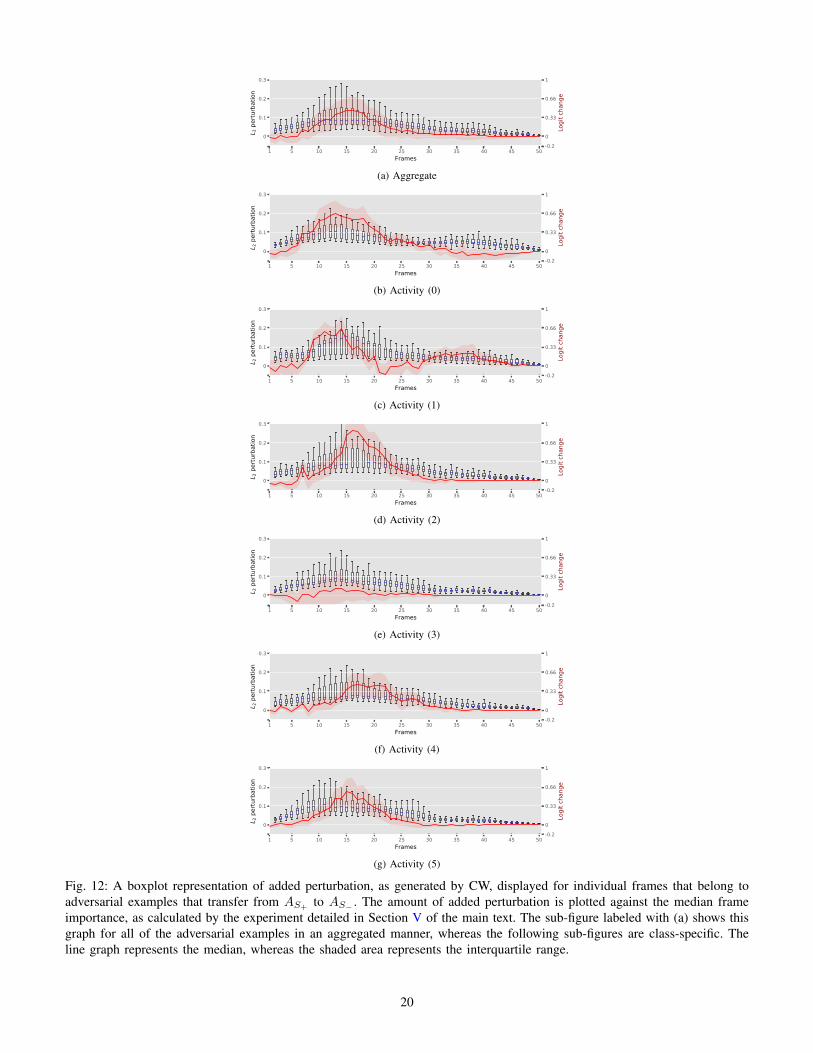
1 5 10 15 20 25 30 35 40 45 50Frames

0

0.1

0.2

0.3

L 2 p

ertu

rbat

ion

-0.20

0.33

0.66

1

Logi

t cha

nge

(a) Aggregate

1 5 10 15 20 25 30 35 40 45 50Frames

0

0.1

0.2

0.3

L 2 p

ertu

rbat

ion

-0.20

0.33

0.66

1

Logi

t cha

nge

(b) Activity (0)

1 5 10 15 20 25 30 35 40 45 50Frames

0

0.1

0.2

0.3

L 2 p

ertu

rbat

ion

-0.20

0.33

0.66

1

Logi

t cha

nge

(c) Activity (1)

1 5 10 15 20 25 30 35 40 45 50Frames

0

0.1

0.2

0.3

L 2 p

ertu

rbat

ion

-0.20

0.33

0.66

1

Logi

t cha

nge

(d) Activity (2)

1 5 10 15 20 25 30 35 40 45 50Frames

0

0.1

0.2

0.3

L 2 p

ertu

rbat

ion

-0.20

0.33

0.66

1

Logi

t cha

nge

(e) Activity (3)

1 5 10 15 20 25 30 35 40 45 50Frames

0

0.1

0.2

0.3

L 2 p

ertu

rbat

ion

-0.20

0.33

0.66

1

Logi

t cha

nge

(f) Activity (4)

1 5 10 15 20 25 30 35 40 45 50Frames

0

0.1

0.2

0.3

L 2 p

ertu

rbat

ion

-0.20

0.33

0.66

1

Logi

t cha

nge

(g) Activity (5)

Fig. 12: A boxplot representation of added perturbation, as generated by CW, displayed for individual frames that belong toadversarial examples that transfer from AS+

to AS− . The amount of added perturbation is plotted against the median frameimportance, as calculated by the experiment detailed in Section V of the main text. The sub-figure labeled with (a) shows thisgraph for all of the adversarial examples in an aggregated manner, whereas the following sub-figures are class-specific. Theline graph represents the median, whereas the shaded area represents the interquartile range.

20

1 5 10 15 20 25 30 35 40 45 50

Frames

0

0.4

0.8

1.2

Gra

d-C

AM

mag

nitu

de

(No

rmal

ized

)

-0.2

0

0.33

0.66

1

Log

it c

hang

e

(a) Aggregate

1 5 10 15 20 25 30 35 40 45 50

Frames

0

0.4

0.8

1.2

Gra

d-C

AM

mag

nitu

de

(No

rmal

ized

)-0.2

0

0.33

0.66

1

Log

it c

hang

e

(b) Activity (0)

1 5 10 15 20 25 30 35 40 45 50

Frames

0

0.4

0.8

1.2

Gra

d-C

AM

mag

nitu

de

(No

rmal

ized

)

-0.2

0

0.33

0.66

1

Log

it c

hang

e

(c) Activity (1)

1 5 10 15 20 25 30 35 40 45 50

Frames

0

0.4

0.8

1.2

Gra

d-C

AM

mag

nitu

de

(No

rmal

ized

)

-0.2

0

0.33

0.66

1

Log

it c

hang

e

(d) Activity (2)

1 5 10 15 20 25 30 35 40 45 50

Frames

0

0.4

0.8

1.2

Gra

d-C

AM

mag

nitu

de

(No

rmal

ized

)

-0.2

0

0.33

0.66

1

Log

it c

hang

e

(e) Activity (3)

1 5 10 15 20 25 30 35 40 45 50

Frames

0

0.4

0.8

1.2

Gra

d-C

AM

mag

nitu

de

(No

rmal

ized

)

-0.2

0

0.33

0.66

1

Log

it c

hang

e

(f) Activity (4)

1 5 10 15 20 25 30 35 40 45 50

Frames

0

0.4

0.8

1.2

Gra

d-C

AM

mag

nitu

de

(No

rmal

ized

)

-0.2

0

0.33

0.66

1

Log

it c

hang

e

(g) Activity (5)

Fig. 13: (blue) A line graph representation of Grad-CAM magnitudes (normalized between 0 and 1), displayed for individualframes that belong to genuine data points of adversarial examples that transfer from AS+

to AS− . This graph is plotted againstthe median frame importance (red), as calculated by the experiment detailed in Section V of the main text. The sub-figurelabeled with (a) shows this graph for all of the adversarial examples in an aggregated manner, whereas the following sub-figuresare class-specific. The line graph represents the median, whereas the shaded area represents the interquartile range.

21

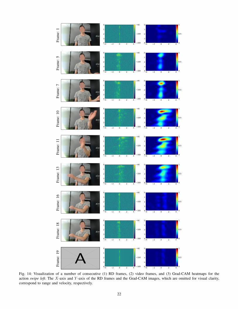
Fram

e:1

4 2 0 2 44

3

2

1

0

160

100

40

4 2 0 2 44

3

2

1

0

0

0.5

1

Fram

e:5

4 2 0 2 44

3

2

1

0

160

100

40

4 2 0 2 44

3

2

1

0

0

0.5

1

Fram

e:7

4 2 0 2 44

3

2

1

0

160

100

40

4 2 0 2 44

3

2

1

0

0

0.5

1

Fram

e:10

4 2 0 2 44

3

2

1

0

160

100

40

4 2 0 2 44

3

2

1

0

0

0.5

1

Fram

e:11

4 2 0 2 44

3

2

1

0

160

100

40

4 2 0 2 44

3

2

1

0

0

0.5

1

Fram

e:13

4 2 0 2 44

3

2

1

0

160

100

40

4 2 0 2 44

3

2

1

0

0

0.5

1

Fram

e:16

4 2 0 2 44

3

2

1

0

160

100

40

4 2 0 2 44

3

2

1

0

0

0.5

1

Fram

e:18

4 2 0 2 44

3

2

1

0

160

100

40

4 2 0 2 44

3

2

1

0

0

0.5

1

Fram

e:19 A

4 2 0 2 44

3

2

1

0

160

100

40

4 2 0 2 44

3

2

1

0

0

0.5

1

Fig. 14: Visualization of a number of consecutive (1) RD frames, (2) video frames, and (3) Grad-CAM heatmaps for theaction swipe left. The X-axis and Y -axis of the RD frames and the Grad-CAM images, which are omitted for visual clarity,correspond to range and velocity, respectively.

22