1 International Journal of Science and Business | www.ijsab.com Investigating The Relationship Between Gross Domestic Product (GDP) and Household Consumption Expenditure (HCE) In Two SAARC Countries: Nepal and Pakistan Md. Saiful Islam 1 & Dr. Shaikh Mostak Ahammad 2 Abstract This study examines the matter of trends (level and slope), cycle and irregular components in the Gross Domestic Product (GDP) and Household Consumption Expenditure (HCE) of two SAARC (South Asian Association for Regional Cooperation) countries: Nepal and Pakistan. SAARC countries produce GDP (PPP) US$ 9.9 trillion and GDP (Nominal) US$ 2.9 trillion and constitute 9.12% of global economy as of 2015. The mentioned two countries from this region are selected due to their importance in the SAARC region and their challenges during last few decades i.e. Political crisis and natural disasters. In this study the multivariate unobserved components model is used to decompose the GDP and HCE and examine the relationships between these two variables of Nepal and Pakistan. The time period of this study is 1970-2014 and Kushnirs statistical data is employed. The maximum likelihood smoother is employed in the trend plus stochastic cycle methodology of Koopman et al. (2009) to estimate the model. It is found here that there have no deficiencies in the diagnostics of normality, auxiliary, prediction, and forecast. And residual diagnostics also present that it is nicely fitted with this model. Empirical results clearly show that there have strong correlations between the GDP and HCE in irregular components in both the countries of Nepal and Pakistan. Finally, in both slope and cycle, the correlations between GDP and HCE of Nepal and Pakistan are found perfectly positive in the short and long run. Keywords: GDP, Household Consumption Expenditure, UC Model, SAARC, Economy 1 Master of Business Administration (MBA), Department of Accounting, Hajee Mohammad Danesh Science and Technology University, Dinajpur, Bangladesh. 2 Associate Professor, Department of Accounting, Hajee Mohammad Danesh Science and Technology University, Dinajpur, Bangladesh. Volume:1, Issue-2, Page: 1-36 2017 ISSN 2520-4750 International Journal of Science and Business

Investigating The Relationship Between Gross Domestic Product (GDP) and Household Consumption Expenditure (HCE) In Two SAARC Countries: Nepal and Pakistan
Apr 05, 2017
Welcome message from author
This document is posted to help you gain knowledge. Please leave a comment to let me know what you think about it! Share it to your friends and learn new things together.
Transcript
1 International Journal of Science and Business | www.ijsab.com
Investigating The Relationship Between Gross Domestic Product (GDP)
and Household Consumption Expenditure (HCE) In Two SAARC
Countries: Nepal and Pakistan
Md. Saiful Islam1 & Dr. Shaikh Mostak Ahammad
2
Abstract
This study examines the matter of trends (level and slope), cycle and irregular components in
the Gross Domestic Product (GDP) and Household Consumption Expenditure (HCE) of two
SAARC (South Asian Association for Regional Cooperation) countries: Nepal and Pakistan.
SAARC countries produce GDP (PPP) US$ 9.9 trillion and GDP (Nominal) US$ 2.9 trillion
and constitute 9.12% of global economy as of 2015. The mentioned two countries from this
region are selected due to their importance in the SAARC region and their challenges during
last few decades i.e. Political crisis and natural disasters. In this study the multivariate
unobserved components model is used to decompose the GDP and HCE and examine the
relationships between these two variables of Nepal and Pakistan. The time period of this
study is 1970-2014 and Kushnirs statistical data is employed. The maximum likelihood
smoother is employed in the trend plus stochastic cycle methodology of Koopman et al.
(2009) to estimate the model. It is found here that there have no deficiencies in the
diagnostics of normality, auxiliary, prediction, and forecast. And residual diagnostics also
present that it is nicely fitted with this model. Empirical results clearly show that there have
strong correlations between the GDP and HCE in irregular components in both the countries
of Nepal and Pakistan. Finally, in both slope and cycle, the correlations between GDP and
HCE of Nepal and Pakistan are found perfectly positive in the short and long run.
Keywords: GDP, Household Consumption Expenditure, UC Model, SAARC, Economy
1 Master of Business Administration (MBA), Department of Accounting, Hajee Mohammad
Danesh Science and Technology University, Dinajpur, Bangladesh.
2 Associate Professor, Department of Accounting, Hajee Mohammad Danesh Science and
Technology University, Dinajpur, Bangladesh.
Volume:1, Issue-2, Page: 1-36 2017
ISSN 2520-4750
International Journal of Science and Business
2 International Journal of Science and Business | www.ijsab.com
1. Introduction
Gross Domestic Product (GDP) is one of the most widely used measures of an economy’s
output or production-total values of goods and services produces within a country’s borders
in a specific time period-monthly, quarterly or annually and Household Consumption
Expenditure (HCE) shows how much money people spend on goods and services. So the
measurement and relations of GDP and HCE is very important as there have inner
relationship between these two variables. GDP is an accurate indication of an economy’s
size, while GDP per capita has a close correlation with the trend in living standards over time,
and the GDP growth rate is probably the single best indicator of economic growth. The GDP
is able to give an overall picture of the state of the economy to that of a satellite in space that
can survey the weather across an entire continent. GDP enables policymakers and central
banks to judge whether the economy is contracting or expanding, whether it needs a boost or
restraint and if threat such as recession or inflation looms on the horizon. Similarly HCE is an
important economic factor because is usually coincides with the overall household consumer
confidence in a nation’s economy. High consumer confidence indicators usually relate to
higher level of household consumption in the economic market. Consumer confidence
provides governments and businesses with an analysis on consumer perception. Businesses
can use household consumption data in their supply and demand economic calculations.
Supply and demand helps businesses produce goods and services at the most favorable
consumer price points. Businesses which can achieve the equilibrium price will sell the
maximum amount of goods with the highest available profit margin. Household consumption
helps companies determine which products have the most value in their economic
marketplace. Businesses can also use information fulfill consumer needs and develop new
products.
Consumption is normally the largest GDP component. Many persons judge the economic
performance of their country mainly in terms of consumption level and dynamics. GDP is
sometimes measured as a sum of all domestic and foreign effective demand for national
goods. Household consumption is one of the elements of domestic demand. The other
elements are government and firm expenditure. Demand for household consumption is not
only attracted by national goods but also by imports, which reduce the GDP sum. An increase
in effective demand for household consumption will increase GDP, provided national
producers can meet the quality/price requirements of buyers. This is not surprising that
household consumption constitutes largest share of GDP. Household consumption is 60% and
70% of GDP in US and Germany respectively. As such the pace at which G7 consumption
3 International Journal of Science and Business | www.ijsab.com
growth will revive is critical to the speed of world GDP growth. Higher GDP volatility-as
recently experienced-is associated with a sizeable reduction in consumption growth.
The South Asian Association for regional Cooperation abbreviated as SAARC was founded
in Dhaka on the 8th
of December 1985. Its secretariat is based in Kathmandu. Its member
states are eight at present including Afghanistan, Bangladesh, Bhutan, India, Nepal, the
Maldives, Pakistan and Sri Lanka. It is regional intergovernmental organization and
geopolitical union in South Asia aiming to promote development, economics and regional
integration among the member countries. It launched the South Asian Free Trade Area
abbreviated as SAPTA. SAARC compromises 3% of world’s area, 9.12% of the global
economy, and 9.21% of world’s GDP (PPP) from which the studied two countries Nepal and
Pakistan constitutes 0.98% of world GDP. Current study indicates that Nepal has faster
economic growth as well as household consumption than Pakistan. As there is a large
reservoir of political goodwill between Nepal and Pakistan and they have significant impact
on SAARC as well as global economy, it is important to assess the GDP and HCE
relationships between these two countries and forecast the future trends of GDP growth and
HCE status.
On the basis of this matter, this study examines the relationships between GDP and HCE of
Nepal and Pakistan using data from 1970 to 2014. These two SAARC countries have been
selected considering the importance, mutual understanding, economic background and
growth status over the last few decades. The GDP of these two countries constitute 10.60% of
SAARC GDP and 0.98% of world’s GDP. Household consumption of these two countries is
60-70% of GDP over the years. The GDP of Pakistan is amounted $982 billion (PPP) and
$285 billion (nominal) and ranked 26th
PPP and 36th
nominal in the world with the growth
rate of 4.71% in 2016.The GDP of Nepal is amounted $21 billion (nominal) with a growth
rate of 5.1%. The household consumption expenditure of Pakistan is amounted $215 billion
and of Nepal is amounted $17 billion which are a large part of the overall expenditure of
SAARC countries.
The main objective of this study is to apply the multivariate unobserved components model in
examining the relationships between the GDP and HCE of Nepal and Pakistan over the last
few decades. The second objective of this study is to find the trend, cycle and irregular
components in the GDP and HCE of these two countries. The main objective of using the
unobserved components model is that it is a flexible econometric tool that is used to
decompose the evaluation of time series data into trends, cycle and irregular components,
which is not possible to observe directly from the dataset. Long run direction of the economy
4 International Journal of Science and Business | www.ijsab.com
is represented by the trends, which is referred as permanent component, the fluctuation of the
short run economic activity is represented by the cycle, referred a transitory component. And
irregular component shows the nature of the unobserved factor. To forecast for the future is
another advantage of the UC model. The outliers and structural breaks can also be
investigated by the UC model.
The stochastic characteristics of this model improves traditional interpretations and provides
an important econometric tool for performing richer statistical analysis for the evaluation
behavior of the relationships between GDP and HCE of Nepal and Pakistan. Besides the
literature review shows that a large number of studies are occurred for examining the GDP
and HCE relationships and also the using of UC model by various writers. The findings of
this study also strengthen the using of structural time series model to the analysis of
relationships between GDP and HCE of Nepal and Pakistan.
The remainder of this study is presented as follows. The objectives of the study are discussed
in section 2. The literature review of the study is discussed in section 3. Section 4 presents
empirical unobserved components model in a long run trend, short run deviation (cycle) and
irregular components. Section 5 details the details data used this study. Section 6 reports the
empirical results of the study. Section 7 reports about discussion of the study. Finally, Section
8 describes the conclusions of the study.
2. Objective of the study
The main objective of the study is to apply multivariate unobserved components model in
examining the relationships between Gross Domestic Product (GDP) and Household
Consumption Expenditure (HCE) and their interdependencies to each other in an economy.
Other objectives of the study are to find out and understand certain things about the
relationships between Gross Domestic Product (GDP) and Household Consumption
Expenditure (HCE). These include the following:
a) To find out the trend, cycle and irregular components in GDP and HCE over the
studied period of Nepal and Pakistan.
b) To test the prediction of GDP and HCE in upcoming years based on the current and
past situations and forecast GDP and HCE.
c) To know the correlation between GDP and HCE over the period of time.
d) To measure the impact of HCE on GDP as the largest part.
e) To check whether any deficiency is existed in the diagnostic of normality, auxiliary,
prediction and forecast.
5 International Journal of Science and Business | www.ijsab.com
3. Literature Review
Gross Domestic Product (GDP) and Household Consumption Expenditure (HCE) are
important elements of the economy of a country. Significant contributions by GDP and HCE
to the economy have been seen and a relationship is existed between these two things as they
are changing in nature. HCE changing and other house related activities are estimated to
account 50-80% of GDP in a country. There have a significant number of investigations on
the relationship between GDP and HCE in Nepal and Pakistan. For example, Tapsin and
Hepsag (2014) studied about the household consumption expenditure and stated that
household consumption expenditures are primary indicators of economy well-being. In also
constitutes two third of the gross domestic product. Consumption theories are also analyzed
by Keynes’ absolute income hypothesis, Friedman’s permanent income hypothesis (1957),
Modigliani and Brumberg’s life cycle income hypothesis (1950), Dusenberry’s relative
income hypothesis (1949). Bastagli and Hills (2013) observed household consumption
patterns and dictates total potential consumption relating to economic growth. Crossley et al.
(2009) conducted a research on household consumption through recessions and provided
their observation that the household consumption have been affected by the recessions and
lower GDP. Household consumption is both the largest component of GDP and the
component most immediately connected to the welfare to individuals and households.
Anghelache (2011) states about the correlation between GDP and the final consumption. It
states that the evolution of the GDP is highly influenced by the evolution of the HCE.
Ceritoglu (2013) states about the household expectations and household consumption
expenditures. According to this paper the household expectations have a direct role on their
consumption and saving behavior in addition to their indirect influence through the income
channel.
A significant number of studies use Unobserved Components (UC) Model to capture the
permanent components (Trend) and transitory components (cycle) from the time series data.
For example Brintha et al. (2014) conducted an investigation relating to annual national
coconut production in Sri Lanka. The reason of accepting UC model by them was that the UC
model does not make use of the stationary assumption. Besides it breaks down response
series into components such as trends, cycles and regression effects which could be useful
especially in forecasting the production of perennial crops. Ferrara and Koopman (2010)
conducted a research on common business and housing market cycles in the euro area. They
used unobserved components model here considering the fact that it is able to assess the
common euro area housing cycle to evaluate its relationship with the economic cycle.
6 International Journal of Science and Business | www.ijsab.com
Carvalho et al. (2005) conducted a research on convergence in the trends and cycles in the
euro-zone income. It stated that multivariate UC time series model are fitted to annual post
war observations on real time per capita in countries in the euro-zone. Leamer (2007) pointed
out that by using the contributions to GDP growth during the 8 phases of recession covering
the whole period, the business cycle is in fact a consumer cycle mainly driven by residential
investment. Consequently the author argues that residential investment can be seen as an
early warning of oncoming recession. Carvalho and Harvey (2005) conducted a research on
growth, cycles and convergence in the US regional time series and stated here that the UC
time series model is fitted on the real income per capita in eight regions of the United States.
Villamoran (2007) conducted a research on multivariate data analysis. Sinclair and Mitra
(2008) studied about output fluctuation in G-7 using UC model successfully.
The world bank states that Household Consumption Expenditure (Formerly private
consumption) is the market value of all goods and services including durable products (Such
as cars, washing machines, and home computers) purchased by households. It excludes
purchases of dwellings but includes inputted rent for owner occupied dwellings. It also
includes payments and fees to governments to obtain permit and licenses. Here Household
Consumption Expenditure includes the expenditures of nonprofit institutions serving
households, even when reported separately by the country. This item also includes any
statistical discrepancy in the use of resources relative to supply of resources. We have been
experiencing from various studies that the increase in GDP of Nepal results in increased
household consumption. The GDP of the country has increased significantly in the urban
areas. This in turn leads to an increased demand for the household which further has
increased the household consumption expenditure. It is believed that the GDP growth has a
direct relation with the household consumption along with various other factors which result
in the appreciation of the household consumption. The researches show that GDP value of
Nepal represents 0.03% of the world economy. GDP of Nepal averaged 5.12 USD Billion
from 1960 until 2015, reaching an all-time high of 20.88 USD billion in 2015 and a record
low of 0.50 US Billion in 1963. Over the past 39 years the value of HCE has fluctuated
greatly and in relation to the trend of GDP. A significant researches show that Pakistan will
most likely miss its projected GDP growth rate of 5.1% and it is reflected in the household
consumption also as it increases slowly and sometimes falls. Evidences show that household
consumption is an important and growing sector in Pakistan. Pakistan spends 202 billion
dollars on household consumption in a year. Pakistan Bureau of Statistics states that housing
accounts for approximately 70%-80% of GDP and its growing over the years as the growing
7 International Journal of Science and Business | www.ijsab.com
need for urban planning. So we have been experiencing a positive relationship between GDP
and HCE in Pakistan also. Thus having almost same circumstances in the two mentioned
areas, the relationship between GDP and HCE has been seen same. A positive relationship is
existed here and the researches show that also. So this study intends to observe the
relationship between GDP and HCE in two SAARC countries Nepal and Pakistan using
multivariate unobserved components model.
4. Empirical Models
This study is about the relationship between Gross Domestic Product (GDP) and Household
Consumption Expenditure (HCE) in two SAARC countries-Nepal and Pakistan-by using a
multivariate UC model as described in some mentioned studies such as Brintha et al (2014),
Ferrara and Koopman (2010) and Leamer (2007).
The used multivariate UC model that disintegrates GDP and HCE into trends (µt) which is
the long run component in the series and indicates the general direction in which the series
are moving, cycles and interventions (wt) is given bellow:
Yt=µt+ t+w1+𝜀t𝜀t~ 𝑁𝐼𝐷 (0,∑𝜀)t=1,………..,T, (1)
With the variables of log GDP and HCE that was obtained from time series observations,
here, yt is a 2x1 vector corresponding to the countries Nepal GDP (lgdpn) and Pakistan GDP
(lgdpp)and Nepal HCE (lhcen) and Pakistan HCE (lhcep), with t=1 for 1970 and t=T=45 for
2014. µtis a 2x1 vector representing smooth trend component, t denotes 2x1 vector of the
stochastic cycle component, and t denotes 2x1 vector of the unobserved irregular
component term, which is normally distributed with a mean of 0 and 2×2 covariance matrix
∑ .
The smooth trend µt component in yt is defined bellow:
µ1=µt-1+βt-1+ 1 t~ NID(0, ∑ ), t=1,………,T, (2)
𝛽t=𝛽t-1+ t t~ 𝑁𝐼𝐷 (0, ) t=1,……….,T, (3)
Where, the slope of the trend component (µt) is βt, which is a 2x1 vector with t=1 for 1970
and t=T=45 for 2014. The level disturbance t and the slope disturbance t are uncorrelated
with each other. Each of the ∑ and ∑ is a 2x2 covariance matrix. When ∑ is not 0 but ∑
is 0 yt is called a “random walk plus drift”; however a deterministic linear trend is
generated when ∑ and ∑ are both 0. When ∑ is 0 but ∑ is not 0, the trend is called a
“smooth trend”. This model is often referred to as the integrated random walk (IRW). In this
8 International Journal of Science and Business | www.ijsab.com
chapter the integrated random walk (IRW) smoother is applied. Stated from Carvalho and
Harvey (2005), this model often allows a clearer separation into trend and cycle.
The short term movement has been represented by multivariate cyclical component and is
defined as follows:
1* * *
1
cos sin
sin cost c c t t
c ct t t
k
n kI
, t=1,……,T, (4)
Where t and *
t are cyclical components of 2x1 vectors with t=1 for 1970 and t=T=45 for
2014, and t and *
t are 2x1 vectors of disturbances i.e.
'' * *( ) ( )t t t tE k k E k k ∑k and '* *( )t tE k k =0 (5)
Here, ∑k is a 2x2 covariance matrix. The fluctuations of cycles are defined by the cyclical
frequency c which will satisfy 0≤ c≤𝜋. The dumping factor on the cycle amplitude is 𝜌
which satisfies 0≤𝜌 < 1. The period related to frequency is important nature of the cycle. The
period of the cycle is given as 2𝜋/ c. Here one stochastic cycle is considered. The
covariance matrix of t is given by:
∑ =(1-𝜌2)-1
∑k (6)
In equation 1.1, to capture outlier and structural breaks, intervention dummies have been used
by including wt, which is a 2x1 vector of interventions. Parameter matrix could specify
some elements to zero that denote particular equations can produce certain variables. Here, an
outlier is a temporary event of irregular disturbance which is structured by taking the value of
1 at the time of the outlier, and zero otherwise. A structural break is a permanent change in
the level of the time series which shifts it up or down permanently.
By using the maximum likelihood (exact score) approach, the measurement of the
unobserved components model can be formulated. At the time of making the estimation the
fitted model will be checked for serial correlation, normality and heteroskedasticity by using
standard time series diagnostics. Also to detect any deficiencies of this model, graphs of
residual diagnostics, auxiliary residuals, prediction tests and forecasting are used.
9 International Journal of Science and Business | www.ijsab.com
5. Data
The used dataset is yearly data on the logarithm of the Gross Domestic Product of Nepal
(lgdpn) and Pakistan (lgdpp) and logarithm of the Household Consumption Expenditure of
Nepal (lhcen) and Pakistan (lhcep) from 1970-2014. It was obtained from the Kushnirs
statistical dataset (http://www.kushnirs.org).
The GDP of Nepal (lgdpn) showed an upward trend smoothly with little fluctuations before
reaching the highest point in 2014 and HCE of Nepal (lhcen) showed an upward trend with
no outlier before reaching the highest point in 2010. The GDP of Pakistan (lgdpp) showed an
upward trend with some fluctuations and HCE of Pakistan (lhcep) showed same trend with a
level break in 1987 before reaching the highest point in 2014.
6. Empirical Results
Using the maximum likelihood approach models (1.1) and (1.7) can be used as mentioned in
Harvey (1989). Using a smoothing algorithm, the smooth trend and the stochastic cycle
components can be extracted as mentioned in Koopman (1992). The empirical results
obtained by using the STAMP 8.2 package of Koopman et al. (2009) indicate strong
convergence.
Table 1 reports some diagnostics and goodness-of-fit statistics such as N ( 2
2x ) (the normality
test following a 2 distribution with two degrees of freedom), H14 (F14, 14) (the
heteroskedasticity) test following an F distribution with (14, 14) degrees of freedom, Q(10,
5)(the Ljung Box statistics based on the first 10 autocorrelations, which is tested against a
2distribution with five degrees of freedom), and Rd
2 (coefficient of determination). The
mentioned statistics do not show any deficiencies in the estimated model.
Table 1: Diagnostics and goodness-of-fit statistics
Statistics lgdpn lhcen lgdpp lhcep
N ( 2
2x ) 1.2782 (0.5278) 0.93718 (0.6259) 12.576 (0.0019) 13.304 (0.0013)
H14 (F14,14) 1.1353 (0.4078) 1.0838 (0.4412) 0.17016 (0.9990) 0.13716 (0.9997)
Q (10, 5) 7.0742 (0.2152) 10.038 (0.0742) 7.7388 (0.1712) 10.064 (0.0734)
Rd2 -0.54423 -0.44919 0.014075 0.056376
Note: Values in parenthesis are p-values
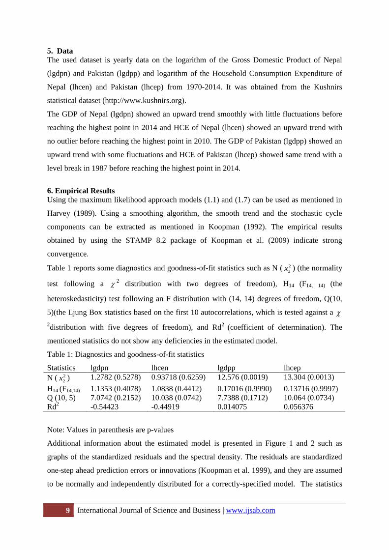
Additional information about the estimated model is presented in Figure 1 and 2 such as
graphs of the standardized residuals and the spectral density. The residuals are standardized
one-step ahead prediction errors or innovations (Koopman et al. 1999), and they are assumed
to be normally and independently distributed for a correctly-specified model. The statistics
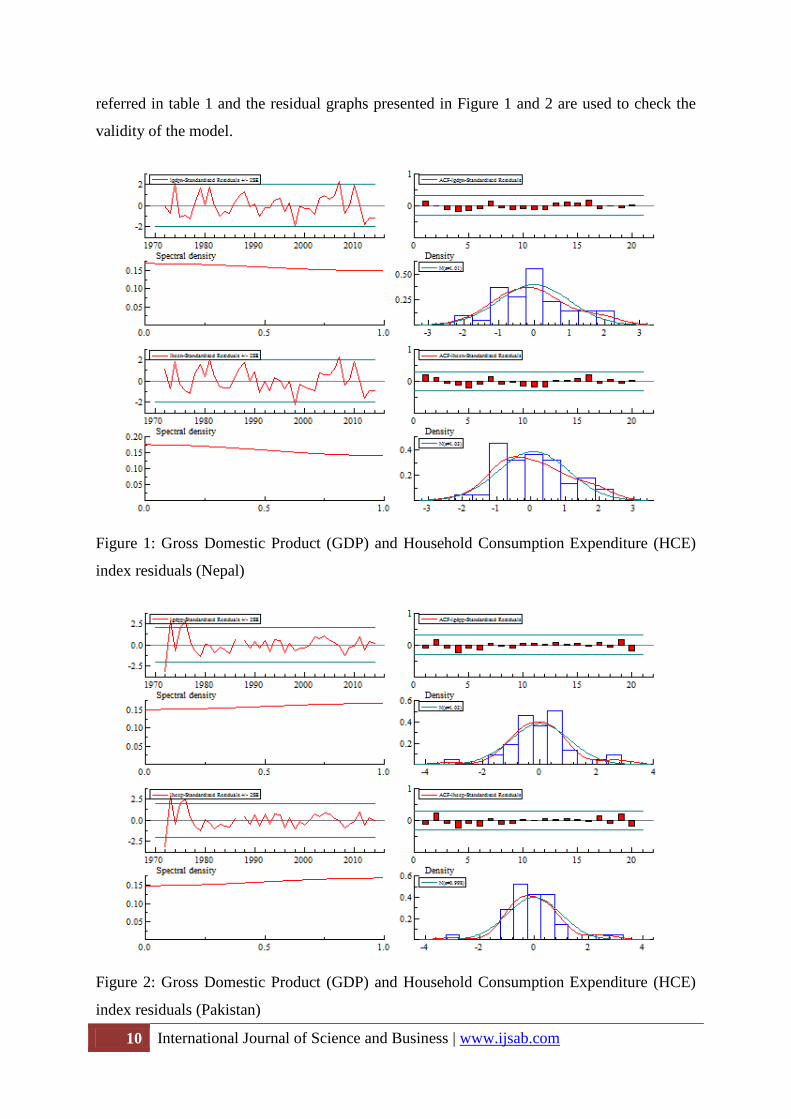
10 International Journal of Science and Business | www.ijsab.com
referred in table 1 and the residual graphs presented in Figure 1 and 2 are used to check the
validity of the model.
Figure 1: Gross Domestic Product (GDP) and Household Consumption Expenditure (HCE)
index residuals (Nepal)
Figure 2: Gross Domestic Product (GDP) and Household Consumption Expenditure (HCE)
index residuals (Pakistan)
11 International Journal of Science and Business | www.ijsab.com
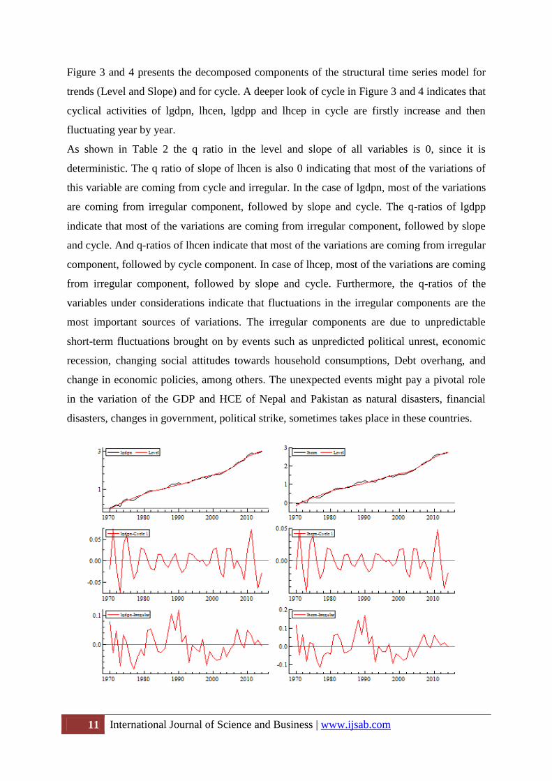
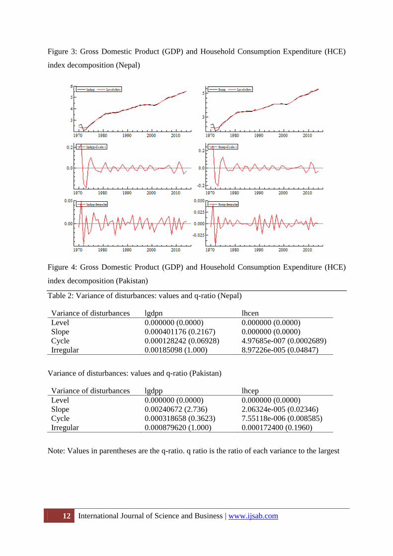
Figure 3 and 4 presents the decomposed components of the structural time series model for
trends (Level and Slope) and for cycle. A deeper look of cycle in Figure 3 and 4 indicates that
cyclical activities of lgdpn, lhcen, lgdpp and lhcep in cycle are firstly increase and then
fluctuating year by year.
As shown in Table 2 the q ratio in the level and slope of all variables is 0, since it is
deterministic. The q ratio of slope of lhcen is also 0 indicating that most of the variations of
this variable are coming from cycle and irregular. In the case of lgdpn, most of the variations
are coming from irregular component, followed by slope and cycle. The q-ratios of lgdpp
indicate that most of the variations are coming from irregular component, followed by slope
and cycle. And q-ratios of lhcen indicate that most of the variations are coming from irregular
component, followed by cycle component. In case of lhcep, most of the variations are coming
from irregular component, followed by slope and cycle. Furthermore, the q-ratios of the
variables under considerations indicate that fluctuations in the irregular components are the
most important sources of variations. The irregular components are due to unpredictable
short-term fluctuations brought on by events such as unpredicted political unrest, economic
recession, changing social attitudes towards household consumptions, Debt overhang, and
change in economic policies, among others. The unexpected events might pay a pivotal role
in the variation of the GDP and HCE of Nepal and Pakistan as natural disasters, financial
disasters, changes in government, political strike, sometimes takes place in these countries.
12 International Journal of Science and Business | www.ijsab.com
Figure 3: Gross Domestic Product (GDP) and Household Consumption Expenditure (HCE)
index decomposition (Nepal)
Figure 4: Gross Domestic Product (GDP) and Household Consumption Expenditure (HCE)
index decomposition (Pakistan)
Table 2: Variance of disturbances: values and q-ratio (Nepal)
Variance of disturbances lgdpn lhcen
Level 0.000000 (0.0000) 0.000000 (0.0000)
Slope 0.000401176 (0.2167) 0.000000 (0.0000)
Cycle 0.000128242 (0.06928) 4.97685e-007 (0.0002689)
Irregular 0.00185098 (1.000) 8.97226e-005 (0.04847)
Variance of disturbances: values and q-ratio (Pakistan)
Variance of disturbances lgdpp lhcep
Level 0.000000 (0.0000) 0.000000 (0.0000)
Slope 0.00240672 (2.736) 2.06324e-005 (0.02346)
Cycle 0.000318658 (0.3623) 7.55118e-006 (0.008585)
Irregular 0.000879620 (1.000) 0.000172400 (0.1960)
Note: Values in parentheses are the q-ratio. q ratio is the ratio of each variance to the largest
13 International Journal of Science and Business | www.ijsab.com
Table 3: Parameters of cycle
Parameters Nepal (Values) Pakistan (Values)
Number of order (n) 2 2
Period ( 2 / c ) in years 4.40822 4.29134
Frequency ( c ) 1.42533 1.46416
Dumping factor ( ) 0.66866 0.77723
Table 4: State vector analysis in the final state at time 2014 (Nepal)
lgdpn lhcen
Level 3.00299 [0.00] 2.74556 [0.00]
Slope 0.05448 [0.08] 0.05159 [0.08]
Cycle amplitude 0.04877 0.03203
Note: Values in brackets are p-values
State vector analysis in the final state at time 2014 (Pakistan)
lgdpn lhcen
Level 5.54940 [0.00] 5.41802 [0.00]
Slope 0.09589 [0.16] 0.09834 [0.16]
Cycle amplitude 0.05477 0.05477
Interventions
Level break 1987
Coefficient -0.07243 [0.00064]
Note: Values in brackets are p-values
Table 3 presents descriptive information on the cyclical parameters of the model. The results
show that the cycle has a period of 4.41 years (Nepal) and 4.29 years (Pakistan) and a
dumping factor of 0.669 (Nepal), 0.777(Pakistan). These findings indicate that the cycle
exhibits a high degree of persistence, and that the series are stationary, since the dumping
factor of cycle is less than 1 in both countries.
Table 4 reports the maximum likelihood estimates of the final state vector and intervention
dummies.
The level values of lgdpn and lgdpp are 3.00299, 5.54940 respectively, which are statistically
significant, while the anti-log analysis of the levels produces the values of 20.15 and 202.98
respectively. And the level values of lhcen and lhcep are 2.74556 and 5.41802 respectively,
while the anti-log analysis of the levels produces the values of 15.57 and 162.91 respectively.
The slope yields a yearly growth rate of about 5.44 and 9.59% for lgdpn and lgdpp
respectively and 5.16 and 9.83% for lhcen and lhcep respectively. The growth rate of both
14 International Journal of Science and Business | www.ijsab.com
countries is statistically significant. It is also observed that the amplitude of cycle as a
percentage of the trend is 4.88 and 5.48% for lgdpn and lgdpp respectively and 3.20 and
5.48% for lhcei and lhcep respectively.
Pakistan’s high growth rate might be the initiatives taken by the Pakistan government such as
strong service sector, concentrating on manufacturing and agriculture sector, effective
planning by the concerned authority and removing corruption and mismanagement in a better
way than Nepal. The amplitude of cycle as a percentage of the trend for Pakistan indicates
that Pakistan takes more time to respond against the short run shocks of gross domestic
product and household consumption expenditure than Nepal and also it takes more time to
come closer to the equilibrium level.
Table 5: Normality test ( 2 test) for auxiliary residuals: irregular, level and slope (Nepal)
Lgdpn lhcen
Irregular Level Slope Irregular Level Slope
Skewness 0.79343 5.0452 0.12087 1.7183 4.6175 0.12322
(0.37) (0.02) (0.73) (0.19) (0.03) (0.73)
Kurtosis 0.12891 0.52337 0.086676 0.15595 0.69642 0.077161
(0.72) (0.47) (0.77) (0.69) (0.40) (0.78)
Bowman- 0.92234 5.5686 0.20754 1.8743 5.314 0.20039
Shenton (0.63) (0.06) (0.90) (0.39) (0.07) (0.90)
Normality test ( 2 test) for auxiliary residuals: irregular, level and slope (Pakistan)
Lgdpp lhcep
Irregular Level Slope Irregular Level Slope
Skewness 0.33235 0.10068 4.4279 0.054125 0.12259 5.2559
(0.56) (0.75) (0.04) (0.82) (0.73) (0.02)
Kurtosis 0.60622 0.95109 0.038936 0.30302 1.0674 0.00040836
(0.44) (0.33) (0.84) (0.58) (0.30) (0.98)
Bowman- 0.93857 1.0518 4.4669 0.35714 1.19 5.2563
Shenton (0.63) (0.59) (0.11) (0.84) (0.55) (0.07)
Note: Values in parentheses are p-values
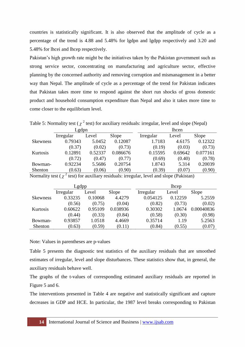
Table 5 presents the diagnostic test statistics of the auxiliary residuals that are smoothed
estimates of irregular, level and slope disturbances. These statistics show that, in general, the
auxiliary residuals behave well.
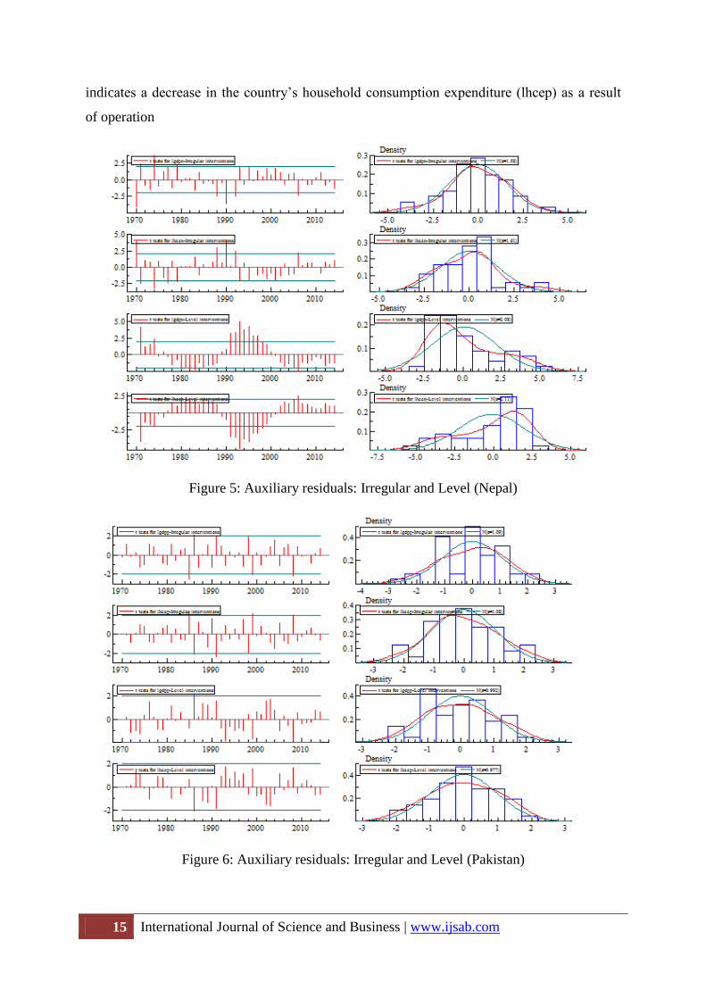
The graphs of the t-values of corresponding estimated auxiliary residuals are reported in
Figure 5 and 6.
The interventions presented in Table 4 are negative and statistically significant and capture
decreases in GDP and HCE. In particular, the 1987 level breaks corresponding to Pakistan
15 International Journal of Science and Business | www.ijsab.com
indicates a decrease in the country’s household consumption expenditure (lhcep) as a result
of operation
Figure 5: Auxiliary residuals: Irregular and Level (Nepal)
Figure 6: Auxiliary residuals: Irregular and Level (Pakistan)
16 International Journal of Science and Business | www.ijsab.com
brasstacks (the largest of its kind in south asia) conducted by India in 1987 and Pakistani
mobilization in response raised tensions and fears that it could lead to another war between
these two neighbors, as a result of Siachen conflict, further clashes erupted in the glacial area
in 1987 as Pakistan sought, without success, to oust India from its stronghold, and Political
crisis in that year by returning Benazir from exile to lead PPP in campaign for fresh elections.
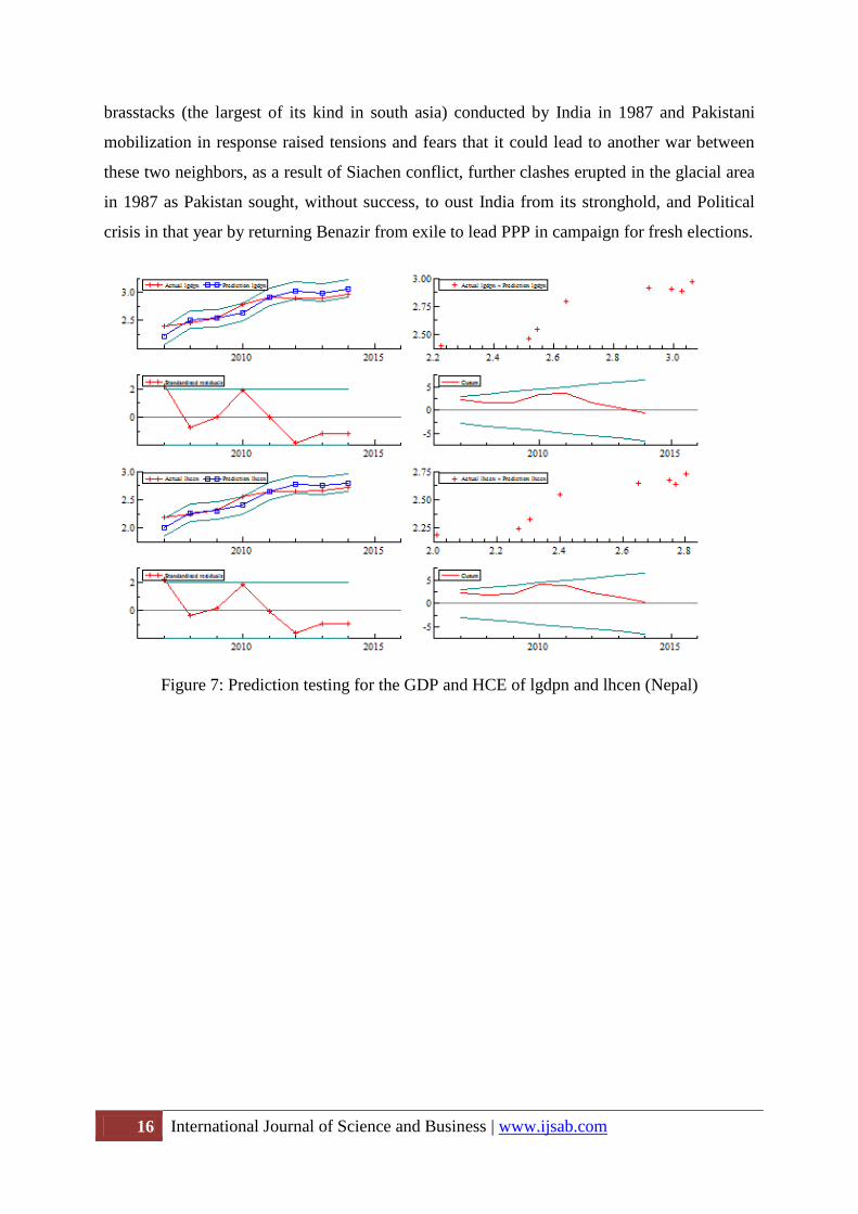
Figure 7: Prediction testing for the GDP and HCE of lgdpn and lhcen (Nepal)
17 International Journal of Science and Business | www.ijsab.com
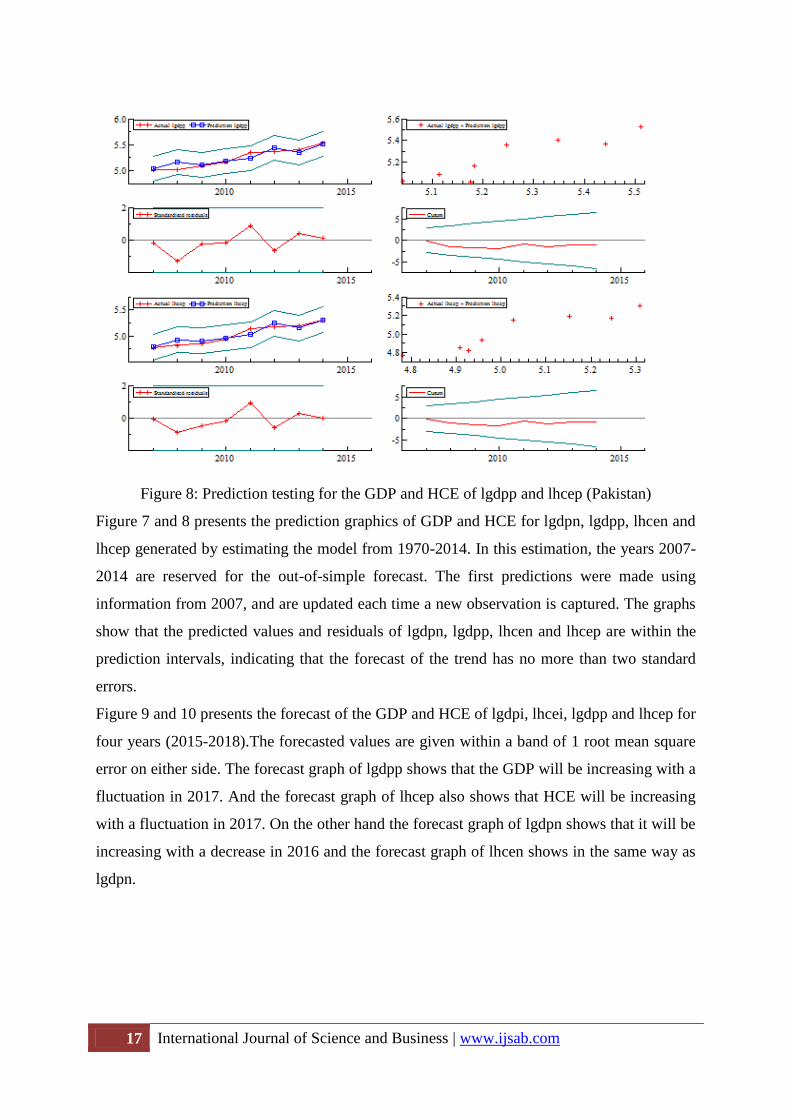
Figure 8: Prediction testing for the GDP and HCE of lgdpp and lhcep (Pakistan)
Figure 7 and 8 presents the prediction graphics of GDP and HCE for lgdpn, lgdpp, lhcen and
lhcep generated by estimating the model from 1970-2014. In this estimation, the years 2007-
2014 are reserved for the out-of-simple forecast. The first predictions were made using
information from 2007, and are updated each time a new observation is captured. The graphs
show that the predicted values and residuals of lgdpn, lgdpp, lhcen and lhcep are within the
prediction intervals, indicating that the forecast of the trend has no more than two standard
errors.
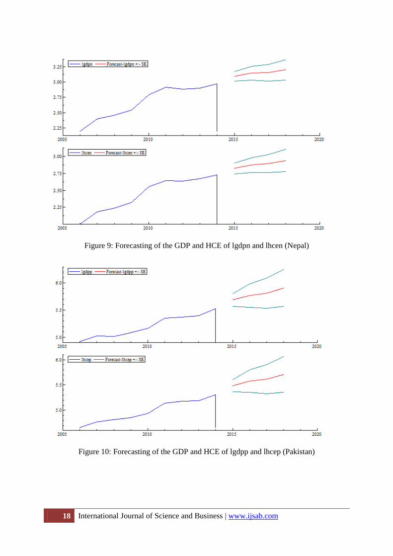
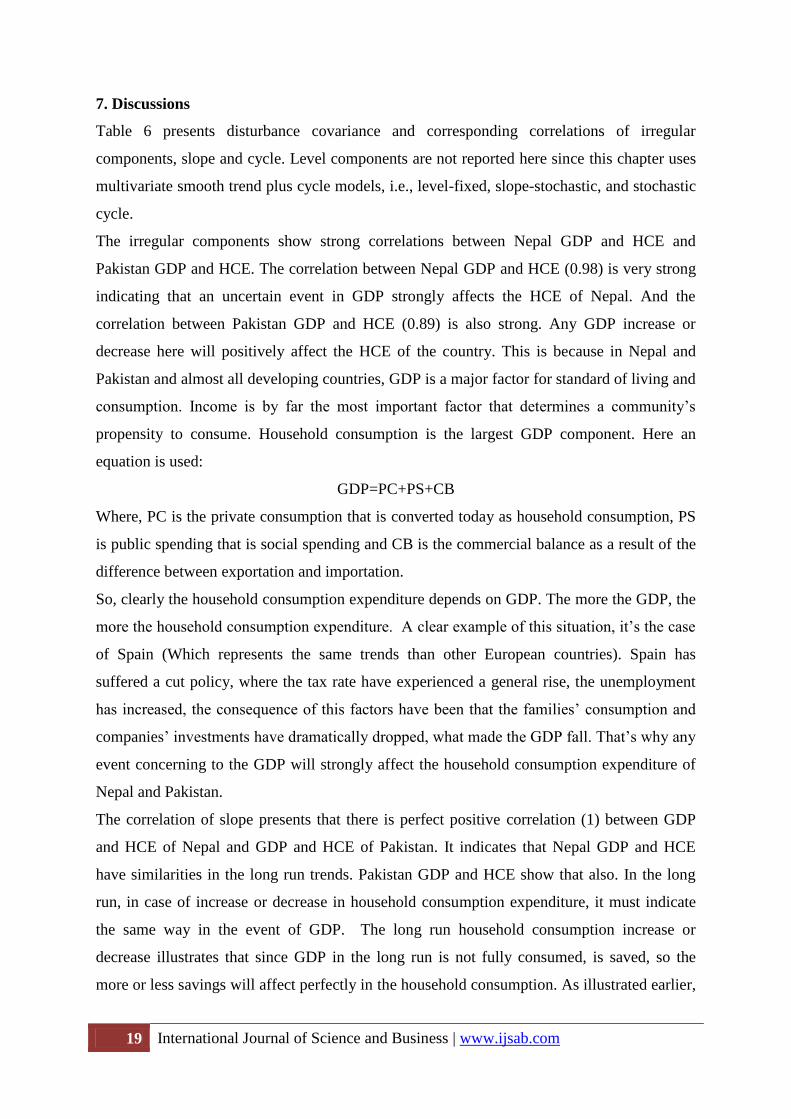
Figure 9 and 10 presents the forecast of the GDP and HCE of lgdpi, lhcei, lgdpp and lhcep for
four years (2015-2018).The forecasted values are given within a band of 1 root mean square
error on either side. The forecast graph of lgdpp shows that the GDP will be increasing with a
fluctuation in 2017. And the forecast graph of lhcep also shows that HCE will be increasing
with a fluctuation in 2017. On the other hand the forecast graph of lgdpn shows that it will be
increasing with a decrease in 2016 and the forecast graph of lhcen shows in the same way as
lgdpn.
18 International Journal of Science and Business | www.ijsab.com
Figure 9: Forecasting of the GDP and HCE of lgdpn and lhcen (Nepal)
Figure 10: Forecasting of the GDP and HCE of lgdpp and lhcep (Pakistan)
19 International Journal of Science and Business | www.ijsab.com
7. Discussions
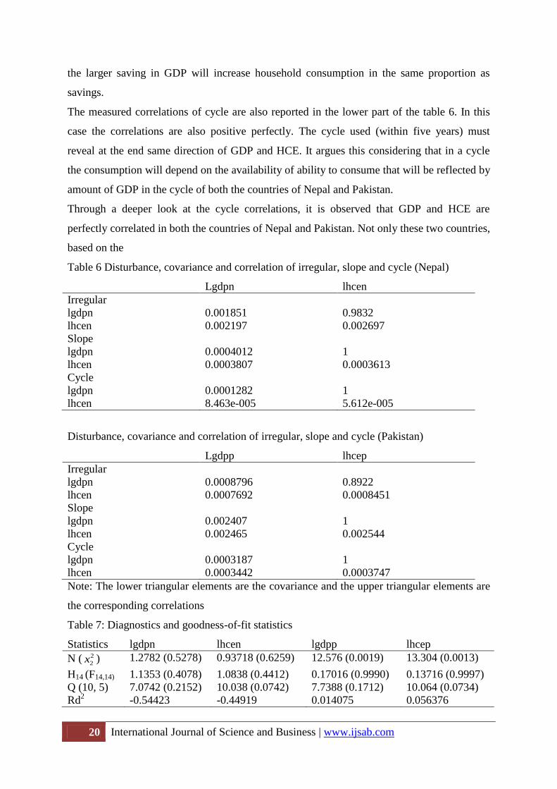
Table 6 presents disturbance covariance and corresponding correlations of irregular
components, slope and cycle. Level components are not reported here since this chapter uses
multivariate smooth trend plus cycle models, i.e., level-fixed, slope-stochastic, and stochastic
cycle.
The irregular components show strong correlations between Nepal GDP and HCE and
Pakistan GDP and HCE. The correlation between Nepal GDP and HCE (0.98) is very strong
indicating that an uncertain event in GDP strongly affects the HCE of Nepal. And the
correlation between Pakistan GDP and HCE (0.89) is also strong. Any GDP increase or
decrease here will positively affect the HCE of the country. This is because in Nepal and
Pakistan and almost all developing countries, GDP is a major factor for standard of living and
consumption. Income is by far the most important factor that determines a community’s
propensity to consume. Household consumption is the largest GDP component. Here an
equation is used:
GDP=PC+PS+CB
Where, PC is the private consumption that is converted today as household consumption, PS
is public spending that is social spending and CB is the commercial balance as a result of the
difference between exportation and importation.
So, clearly the household consumption expenditure depends on GDP. The more the GDP, the
more the household consumption expenditure. A clear example of this situation, it’s the case
of Spain (Which represents the same trends than other European countries). Spain has
suffered a cut policy, where the tax rate have experienced a general rise, the unemployment
has increased, the consequence of this factors have been that the families’ consumption and
companies’ investments have dramatically dropped, what made the GDP fall. That’s why any
event concerning to the GDP will strongly affect the household consumption expenditure of
Nepal and Pakistan.
The correlation of slope presents that there is perfect positive correlation (1) between GDP
and HCE of Nepal and GDP and HCE of Pakistan. It indicates that Nepal GDP and HCE
have similarities in the long run trends. Pakistan GDP and HCE show that also. In the long
run, in case of increase or decrease in household consumption expenditure, it must indicate
the same way in the event of GDP. The long run household consumption increase or
decrease illustrates that since GDP in the long run is not fully consumed, is saved, so the
more or less savings will affect perfectly in the household consumption. As illustrated earlier,
20 International Journal of Science and Business | www.ijsab.com
the larger saving in GDP will increase household consumption in the same proportion as
savings.
The measured correlations of cycle are also reported in the lower part of the table 6. In this
case the correlations are also positive perfectly. The cycle used (within five years) must
reveal at the end same direction of GDP and HCE. It argues this considering that in a cycle
the consumption will depend on the availability of ability to consume that will be reflected by
amount of GDP in the cycle of both the countries of Nepal and Pakistan.
Through a deeper look at the cycle correlations, it is observed that GDP and HCE are
perfectly correlated in both the countries of Nepal and Pakistan. Not only these two countries,
based on the
Table 6 Disturbance, covariance and correlation of irregular, slope and cycle (Nepal)
Lgdpn lhcen
Irregular
lgdpn 0.001851 0.9832
lhcen 0.002197 0.002697
Slope
lgdpn 0.0004012 1
lhcen 0.0003807 0.0003613
Cycle
lgdpn 0.0001282 1
lhcen 8.463e-005 5.612e-005
Disturbance, covariance and correlation of irregular, slope and cycle (Pakistan)
Lgdpp lhcep
Irregular
lgdpn 0.0008796 0.8922
lhcen 0.0007692 0.0008451
Slope
lgdpn 0.002407 1
lhcen 0.002465 0.002544
Cycle
lgdpn 0.0003187 1
lhcen 0.0003442 0.0003747
Note: The lower triangular elements are the covariance and the upper triangular elements are
the corresponding correlations
Table 7: Diagnostics and goodness-of-fit statistics
Statistics lgdpn lhcen lgdpp lhcep
N ( 2
2x ) 1.2782 (0.5278) 0.93718 (0.6259) 12.576 (0.0019) 13.304 (0.0013)
H14 (F14,14) 1.1353 (0.4078) 1.0838 (0.4412) 0.17016 (0.9990) 0.13716 (0.9997)
Q (10, 5) 7.0742 (0.2152) 10.038 (0.0742) 7.7388 (0.1712) 10.064 (0.0734)
Rd2 -0.54423 -0.44919 0.014075 0.056376
21 International Journal of Science and Business | www.ijsab.com
Note: Values in parenthesis are p-values
observation it can be said that it will be occurred in all countries as there have no options to
consume more than the amount of GDP.
The estimated cycle of this model has a period of 4.41 years (Nepal) and 4.29 years
(Pakistan), with a frequency of 1.43 (Nepal) and 1.46 (Pakistan), and a dumping factor of
0.67 (Nepal) and 0.78 (Pakistan). The empirical results are also satisfactory since there is no
major deviation from the model.
8. Conclusions
This study begins with the aim of examining the relationships between Gross Domestic
Product (GDP) and Household Consumption Expenditure (HCE) in two SAARC countries:
Nepal and Pakistan. The mentioned two countries are selected from SAARC organization due
to several reasons. SAARC (The South Asian Association for Regional Cooperation) is an
economic and political organization of eight countries in south Asia. In terms of population, it
is the largest of any regional organizations. The agreed five areas for cooperation involve
agriculture and rural development first. And it involves greatly the GDP and HCE in their
activities. Nepal and Pakistan have great influence on SAARC and face such difficulties as
political crisis, natural disasters etc. during the last few decades. It is thought that these two
countries can reveal the whole picture of all SAARC countries. The multivariate unobserved
components model is used to decompose the GDP and HCE of Nepal and Pakistan into
trends, cycle, interventions and irregular components. This approach provides some results
about the relationship between GDP and HCE of Nepal and Pakistan. Smooth trend plus
stochastic cycle components are considered for the specifications of this model, i.e., level-
fixed, slope-stochastic, stochastic cycle and irregular components. It is indicated by the
empirical results of this chapter that the time series of the relationship between GDP and
HCE in Nepal and Pakistan are best fitted by smooth trend plus stochastic cycle model, since
there are no deficiencies in the diagnostic statistics. Also interventions dummies have been
included, which accurately captured shocks.
The findings of this chapter are that the irregular components show a strong correlation
between GDP and HCE of both the countries of Nepal and Pakistan. This is because HCE is
the largest component of GDP. Household consumption, savings and public spending is
occurred from GDP of a country. That’s why strong positive correlation between GDP and
HCE indicate any change in GDP will affect positively HCE of Nepal and Pakistan.
22 International Journal of Science and Business | www.ijsab.com
Considering the slope, the correlation between GDP and HCE is perfectly positive. This
indicates in the long run, the GDP and HCE behave in the same way as the GDP is not
terminated quickly, rather is is save from time to time. So the amount of saving is a major
factor in household consumption. The more or less in savings will result the HCE more or
less. For this reason the same direction must be found in GDP and HCE in the long run in
both Nepal and Pakistan.
And in the cycle component (within five years), the correlations are found perfectly positive
that indicates that the ending of a cycle provides the same direction of GDP and HCE of
Nepal and Pakistan. In a cycle the amount of saved GDP in a country directs the HCE of the
country. Considering the fluctuations in the cycle years, it does not affect the aggregate
amount of GDP, thus does not affect the household consumption expenditure. So, the GDP
trend and HCE trend will be the same in both Nepal and Pakistan. Finally, this chapter
exposes the forecasted values of GDP and HCE of Nepal and Pakistan from 2015 to 2018. It
shows that the value of GDP of Nepal will be increasing with a decrease in 2016 and HCE of
Nepal also will be increasing with a decrease in 2016. The GDP of Pakistan will be
increasing with a fluctuation in 2017 and HCE of Pakistan will also be increasing with a
fluctuation of 2017.
References
23 International Journal of Science and Business | www.ijsab.com
Anghelache, C. (2011). Analysis of the correlation between GDP and the final consumption.
Theoretical and Applied Economics, Vol. 9 (562), 129-138.
Bastagli, F. and Hills, J. (2013). What gives? Household consumption patterns and the “Big
Trade Off” with public consumption. Center for Analysis of Social Exclusion, case-
170.
Brintha, N.K.K., Samita, S., Abeynayake, N.R., Idirisinghe, I.M.S.K., and Kumarathunga, A.
M. D. P. (2014). Use of unobserved components model for forecasting non-stationary
time series: A case of annual national coconut production in Sri Lanka. Tropical
Agricultural Research, Vol. 25 (4), 523-531.
Carvalho, V.M., and Harvey, A.C. (2005).Convergence in the trends and cycles of euro-zone
income. Journal of Applied Econometrics, Vol. 20, 275-289.
Carvalho, V.M., and Harvey, A.C. (2005).Growth, cycles and convergence in US regional
time series. International Journal of Forecasting, Vol. 21, 667-686.
Ceritoglu, E. (2013). Household expectations and household consumption expenditures: The
case of Turkey. Turkiye Cumhuriyet Merkez Bankasi, working paper no. 13/10.
Chen, X., Kontonikas, A. and Montagnoli, A. (2012). Asset prices, Credit and the business
cycle.
Crossley, T., Low, H. and O’Dea, C. (2009). Household consumptions through recent
recession. IFS Working Paper, W 11/18.
Duesenberry, J.S. (1949). Income saving and the theory of consumer behavior. The Review of
Economics and Statistics, Vol. 33 (3).
Ferrara, L. and Koopman, S. J. (2010).Common business and housing market cycles in the
euro area from a multivariate decomposition. Banque De Franch.
Friedman, M. (1957). A theory of the consumption function. National Bureau of Economic
Research (NBER Books).
Modigliani, F. (2005). The life cycle theory of consumption. Research Program in
Development Studies and Center for Health and Wellbeing.
Sinclair, T. and Mitra, S. (2008). Output fluctuations in the G-7: An unobserved components
approach. Institute of International Economic Policy Working Paper Series, The
George Washington University.
Tapsin, G. and Hepsag, A. (2014). An analysis of household consumption expenditures in
EA-18. European Scientific Journal,Vol. 10 (16), ISSN: 1857-7881 (Print) e- ISSN
1857-7431.
24 International Journal of Science and Business | www.ijsab.com
Villamoran, E. P. (2007). Multivariate data analysis: Multiple regression applied in
educational research. 10th
National Convention on Statistics (NCS), October 1,2.
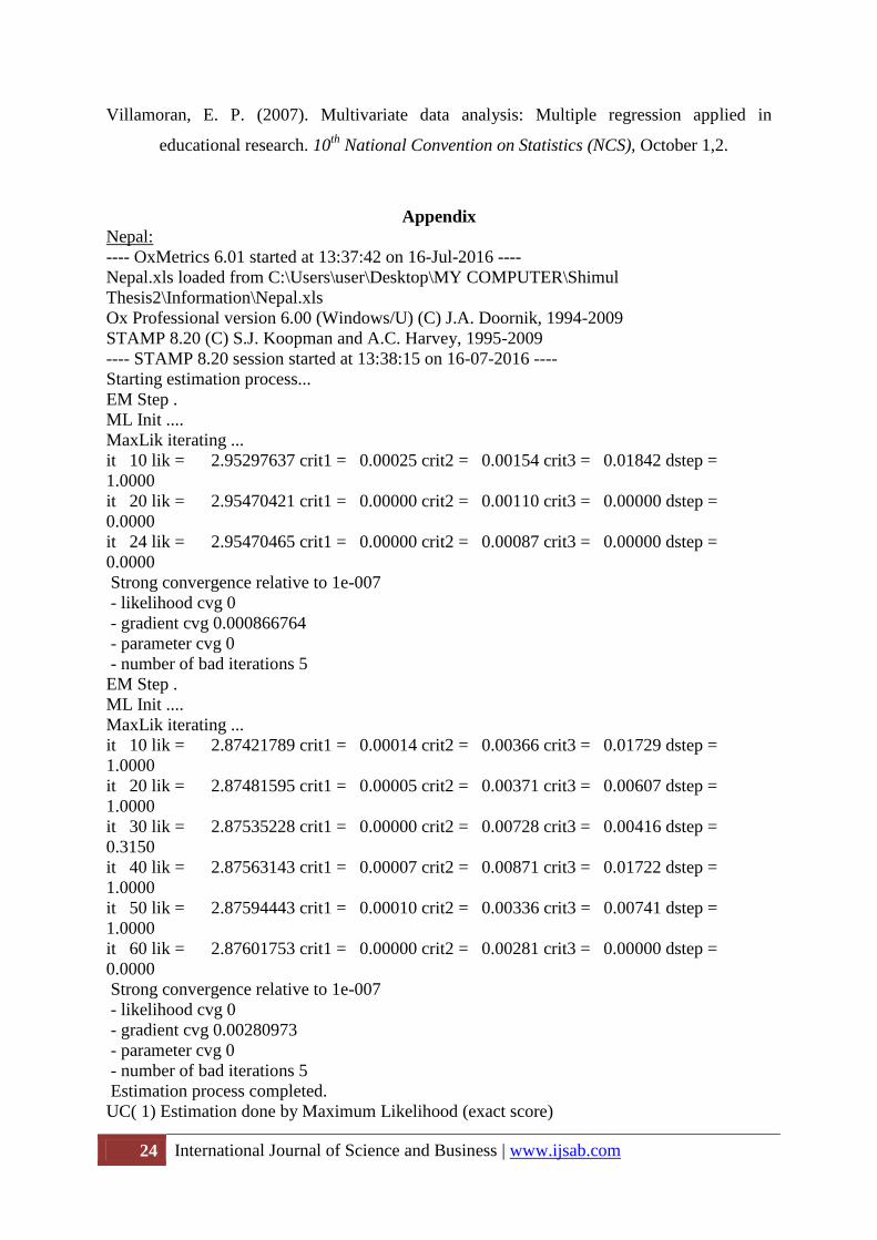
Appendix
Nepal:
---- OxMetrics 6.01 started at 13:37:42 on 16-Jul-2016 ----
Nepal.xls loaded from C:\Users\user\Desktop\MY COMPUTER\Shimul
Thesis2\Information\Nepal.xls
Ox Professional version 6.00 (Windows/U) (C) J.A. Doornik, 1994-2009
STAMP 8.20 (C) S.J. Koopman and A.C. Harvey, 1995-2009
---- STAMP 8.20 session started at 13:38:15 on 16-07-2016 ----
Starting estimation process...
EM Step .
ML Init ....
MaxLik iterating ...
it 10 lik = 2.95297637 crit1 = 0.00025 crit2 = 0.00154 crit3 = 0.01842 dstep =
1.0000
it 20 lik = 2.95470421 crit1 = 0.00000 crit2 = 0.00110 crit3 = 0.00000 dstep =
0.0000
it 24 lik = 2.95470465 crit1 = 0.00000 crit2 = 0.00087 crit3 = 0.00000 dstep =
0.0000
Strong convergence relative to 1e-007
- likelihood cvg 0
- gradient cvg 0.000866764
- parameter cvg 0
- number of bad iterations 5
EM Step .
ML Init ....
MaxLik iterating ...
it 10 lik = 2.87421789 crit1 = 0.00014 crit2 = 0.00366 crit3 = 0.01729 dstep =
1.0000
it 20 lik = 2.87481595 crit1 = 0.00005 crit2 = 0.00371 crit3 = 0.00607 dstep =
1.0000
it 30 lik = 2.87535228 crit1 = 0.00000 crit2 = 0.00728 crit3 = 0.00416 dstep =
0.3150
it 40 lik = 2.87563143 crit1 = 0.00007 crit2 = 0.00871 crit3 = 0.01722 dstep =
1.0000
it 50 lik = 2.87594443 crit1 = 0.00010 crit2 = 0.00336 crit3 = 0.00741 dstep =
1.0000
it 60 lik = 2.87601753 crit1 = 0.00000 crit2 = 0.00281 crit3 = 0.00000 dstep =
0.0000
Strong convergence relative to 1e-007
- likelihood cvg 0
- gradient cvg 0.00280973
- parameter cvg 0
- number of bad iterations 5
Estimation process completed.
UC( 1) Estimation done by Maximum Likelihood (exact score)
25 International Journal of Science and Business | www.ijsab.com
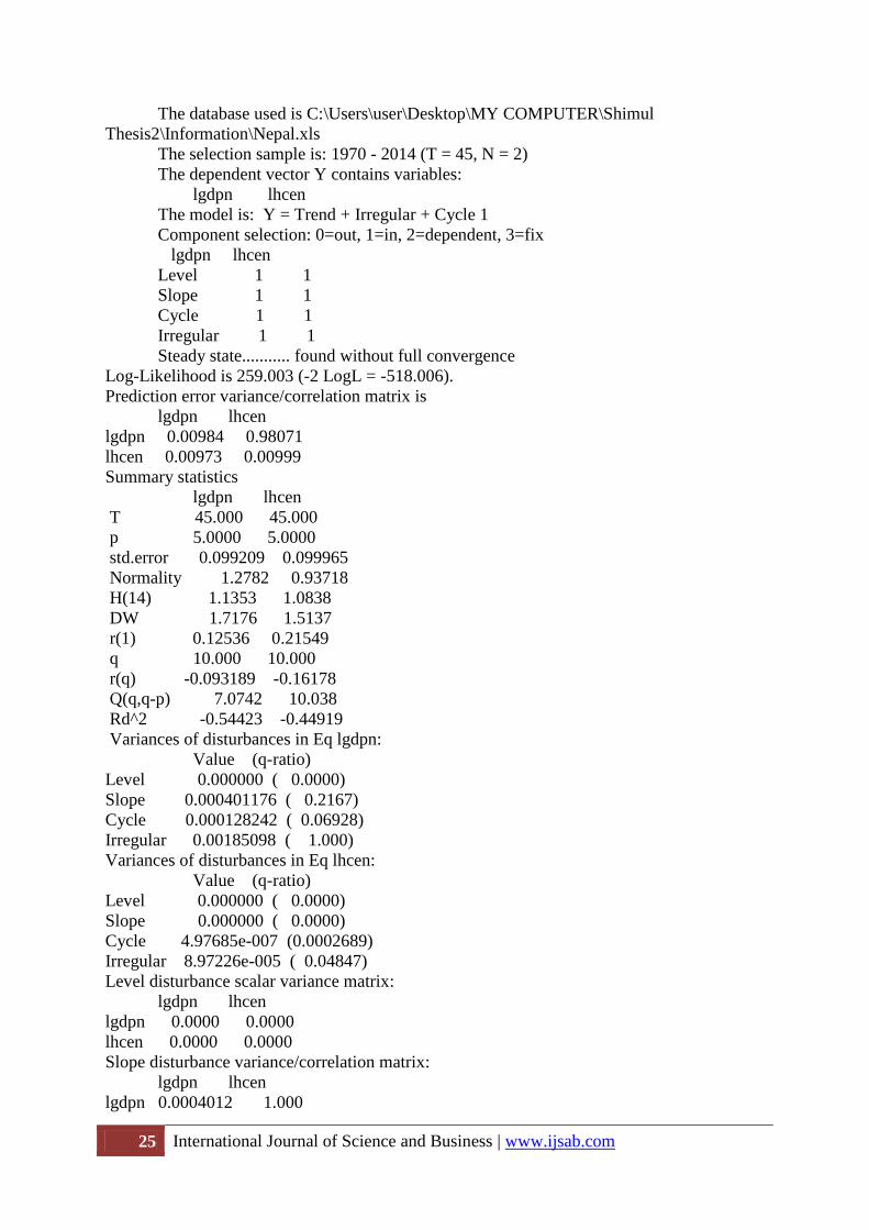
The database used is C:\Users\user\Desktop\MY COMPUTER\Shimul
Thesis2\Information\Nepal.xls
The selection sample is: 1970 - 2014 (T = 45, N = 2)
The dependent vector Y contains variables:
lgdpn lhcen
The model is: Y = Trend + Irregular + Cycle 1
Component selection: 0=out, 1=in, 2=dependent, 3=fix
lgdpn lhcen
Level 1 1
Slope 1 1
Cycle 1 1
Irregular 1 1
Steady state........... found without full convergence
Log-Likelihood is 259.003 (-2 LogL = -518.006).
Prediction error variance/correlation matrix is
lgdpn lhcen
lgdpn 0.00984 0.98071
lhcen 0.00973 0.00999
Summary statistics
lgdpn lhcen
T 45.000 45.000
p 5.0000 5.0000
std.error 0.099209 0.099965
Normality 1.2782 0.93718
H(14) 1.1353 1.0838
DW 1.7176 1.5137
r(1) 0.12536 0.21549
q 10.000 10.000
r(q) -0.093189 -0.16178
Q(q,q-p) 7.0742 10.038
Rd^2 -0.54423 -0.44919
Variances of disturbances in Eq lgdpn:
Value (q-ratio)
Level 0.000000 ( 0.0000)
Slope 0.000401176 ( 0.2167)
Cycle 0.000128242 ( 0.06928)
Irregular 0.00185098 ( 1.000)
Variances of disturbances in Eq lhcen:
Value (q-ratio)
Level 0.000000 ( 0.0000)
Slope 0.000000 ( 0.0000)
Cycle 4.97685e-007 (0.0002689)
Irregular 8.97226e-005 ( 0.04847)
Level disturbance scalar variance matrix:
lgdpn lhcen
lgdpn 0.0000 0.0000
lhcen 0.0000 0.0000
Slope disturbance variance/correlation matrix:
lgdpn lhcen
lgdpn 0.0004012 1.000
26 International Journal of Science and Business | www.ijsab.com
lhcen 0.0003807 0.0003613
Cycle disturbance variance/correlation matrix:
lgdpn lhcen
lgdpn 0.0001282 0.9975
lhcen 8.463e-005 5.612e-005
Irregular disturbance variance/correlation matrix:
lgdpn lhcen
lgdpn 0.001851 0.9832
lhcen 0.002197 0.002697
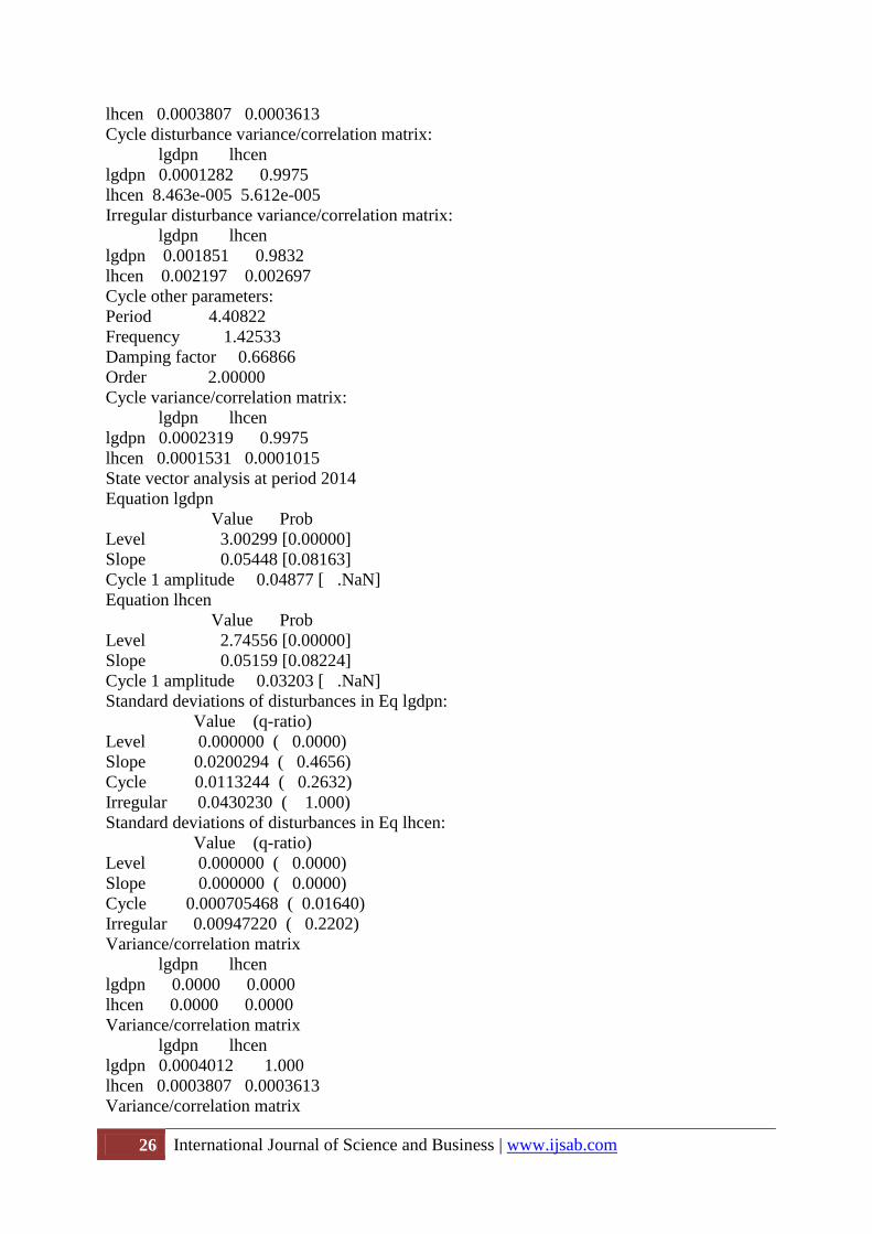
Cycle other parameters:
Period 4.40822
Frequency 1.42533
Damping factor 0.66866
Order 2.00000
Cycle variance/correlation matrix:
lgdpn lhcen
lgdpn 0.0002319 0.9975
lhcen 0.0001531 0.0001015
State vector analysis at period 2014
Equation lgdpn
Value Prob
Level 3.00299 [0.00000]
Slope 0.05448 [0.08163]
Cycle 1 amplitude 0.04877 [ .NaN]
Equation lhcen
Value Prob
Level 2.74556 [0.00000]
Slope 0.05159 [0.08224]
Cycle 1 amplitude 0.03203 [ .NaN]
Standard deviations of disturbances in Eq lgdpn:
Value (q-ratio)
Level 0.000000 ( 0.0000)
Slope 0.0200294 ( 0.4656)
Cycle 0.0113244 ( 0.2632)
Irregular 0.0430230 ( 1.000)
Standard deviations of disturbances in Eq lhcen:
Value (q-ratio)
Level 0.000000 ( 0.0000)
Slope 0.000000 ( 0.0000)
Cycle 0.000705468 ( 0.01640)
Irregular 0.00947220 ( 0.2202)
Variance/correlation matrix
lgdpn lhcen
lgdpn 0.0000 0.0000
lhcen 0.0000 0.0000
Variance/correlation matrix
lgdpn lhcen
lgdpn 0.0004012 1.000
lhcen 0.0003807 0.0003613
Variance/correlation matrix
27 International Journal of Science and Business | www.ijsab.com
lgdpn lhcen
lgdpn 0.0002319 0.9975
lhcen 0.0001531 0.0001015
Variance/correlation matrix
lgdpn lhcen
lgdpn 0.001851 0.9832
lhcen 0.002197 0.002697
State vector anti-log analysis at period 2014
It is assumed that time series is in logs.
Equation lgdpn
Value Prob
Level (anti-log) 20.14568 [0.00000]
Level (bias corrected) 20.15869 [ .NaN]
Slope (yearly %growth) 5.44778 [0.08163]
Cycle 1 amplitude (%trend) 4.87659 [ .NaN]
Equation lhcen
Value Prob
Level (anti-log) 15.57338 [0.00000]
Level (bias corrected) 15.58297 [ .NaN]
Slope (yearly %growth) 5.15853 [0.08224]
Cycle 1 amplitude (%trend) 3.20263 [ .NaN]
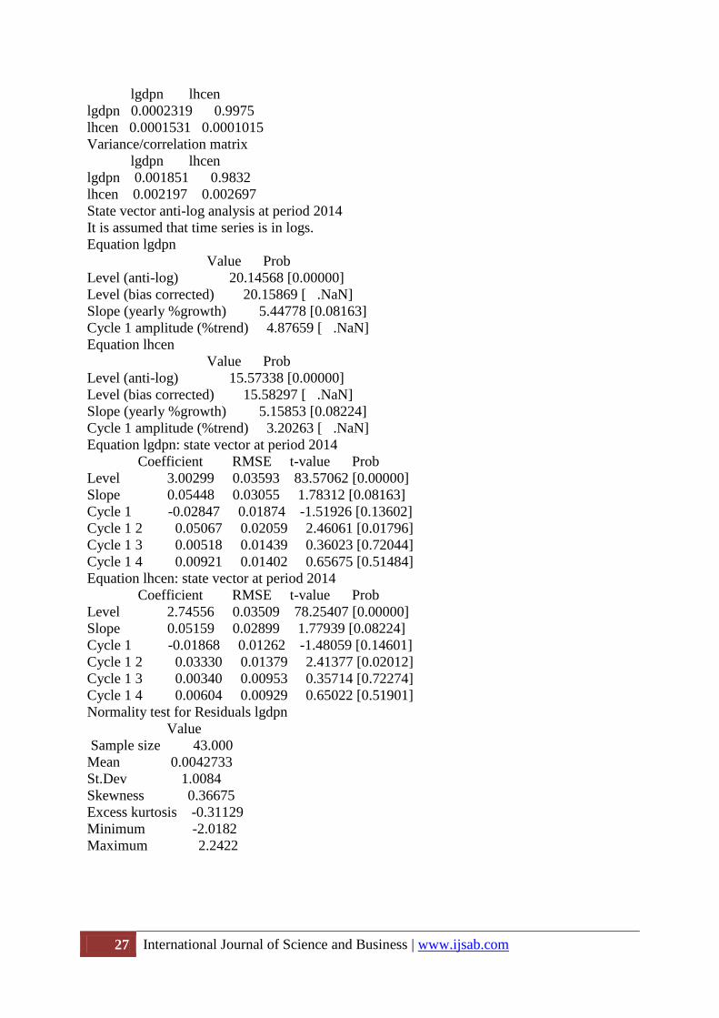
Equation lgdpn: state vector at period 2014
Coefficient RMSE t-value Prob
Level 3.00299 0.03593 83.57062 [0.00000]
Slope 0.05448 0.03055 1.78312 [0.08163]
Cycle 1 -0.02847 0.01874 -1.51926 [0.13602]
Cycle 1 2 0.05067 0.02059 2.46061 [0.01796]
Cycle 1 3 0.00518 0.01439 0.36023 [0.72044]
Cycle 1 4 0.00921 0.01402 0.65675 [0.51484]
Equation lhcen: state vector at period 2014
Coefficient RMSE t-value Prob
Level 2.74556 0.03509 78.25407 [0.00000]
Slope 0.05159 0.02899 1.77939 [0.08224]
Cycle 1 -0.01868 0.01262 -1.48059 [0.14601]
Cycle 1 2 0.03330 0.01379 2.41377 [0.02012]
Cycle 1 3 0.00340 0.00953 0.35714 [0.72274]
Cycle 1 4 0.00604 0.00929 0.65022 [0.51901]
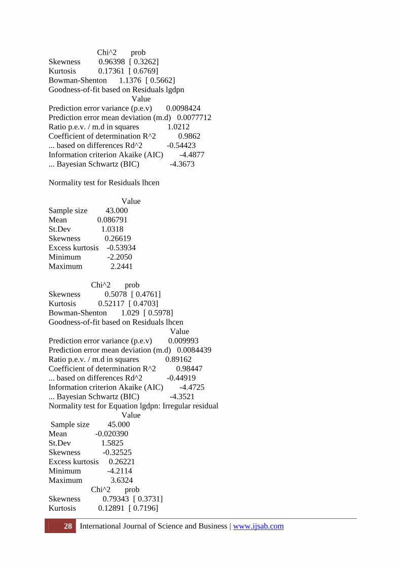
Normality test for Residuals lgdpn
Value
Sample size 43.000
Mean 0.0042733
St.Dev 1.0084
Skewness 0.36675
Excess kurtosis -0.31129
Minimum -2.0182
Maximum 2.2422
28 International Journal of Science and Business | www.ijsab.com
Chi^2 prob
Skewness 0.96398 [ 0.3262]
Kurtosis 0.17361 [ 0.6769]
Bowman-Shenton 1.1376 [ 0.5662]
Goodness-of-fit based on Residuals lgdpn
Value
Prediction error variance (p.e.v) 0.0098424
Prediction error mean deviation (m.d) 0.0077712
Ratio p.e.v. / m.d in squares 1.0212
Coefficient of determination R^2 0.9862
... based on differences Rd^2 -0.54423
Information criterion Akaike (AIC) -4.4877
... Bayesian Schwartz (BIC) -4.3673
Normality test for Residuals lhcen
Value
Sample size 43.000
Mean 0.086791
St.Dev 1.0318
Skewness 0.26619
Excess kurtosis -0.53934
Minimum -2.2050
Maximum 2.2441
Chi^2 prob
Skewness 0.5078 [ 0.4761]
Kurtosis 0.52117 [ 0.4703]
Bowman-Shenton 1.029 [ 0.5978]
Goodness-of-fit based on Residuals lhcen
Value
Prediction error variance (p.e.v) 0.009993
Prediction error mean deviation (m.d) 0.0084439
Ratio p.e.v. / m.d in squares 0.89162
Coefficient of determination R^2 0.98447
... based on differences Rd^2 -0.44919
Information criterion Akaike (AIC) -4.4725
... Bayesian Schwartz (BIC) -4.3521
Normality test for Equation lgdpn: Irregular residual
Value
Sample size 45.000
Mean -0.020390
St.Dev 1.5825
Skewness -0.32525
Excess kurtosis 0.26221
Minimum -4.2114
Maximum 3.6324
Chi^2 prob
Skewness 0.79343 [ 0.3731]
Kurtosis 0.12891 [ 0.7196]
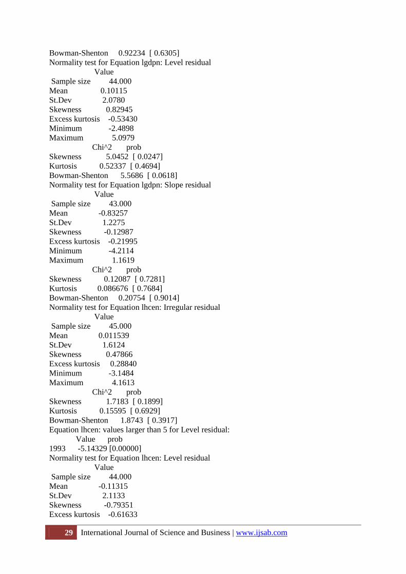
29 International Journal of Science and Business | www.ijsab.com
Bowman-Shenton 0.92234 [ 0.6305]
Normality test for Equation lgdpn: Level residual
Value
Sample size 44.000
Mean 0.10115
St.Dev 2.0780
Skewness 0.82945
Excess kurtosis -0.53430
Minimum -2.4898
Maximum 5.0979
Chi^2 prob
Skewness 5.0452 [ 0.0247]
Kurtosis 0.52337 [ 0.4694]
Bowman-Shenton 5.5686 [ 0.0618]
Normality test for Equation lgdpn: Slope residual
Value
Sample size 43.000
Mean -0.83257
St.Dev 1.2275
Skewness -0.12987
Excess kurtosis -0.21995
Minimum -4.2114
Maximum 1.1619
Chi^2 prob
Skewness 0.12087 [ 0.7281]
Kurtosis 0.086676 [ 0.7684]
Bowman-Shenton 0.20754 [ 0.9014]
Normality test for Equation lhcen: Irregular residual
Value
Sample size 45.000
Mean 0.011539
St.Dev 1.6124
Skewness 0.47866
Excess kurtosis 0.28840
Minimum -3.1484
Maximum 4.1613
Chi^2 prob
Skewness 1.7183 [ 0.1899]
Kurtosis 0.15595 [ 0.6929]
Bowman-Shenton 1.8743 [ 0.3917]
Equation lhcen: values larger than 5 for Level residual:
Value prob
1993 -5.14329 [0.00000]
Normality test for Equation lhcen: Level residual
Value
Sample size 44.000
Mean -0.11315
St.Dev 2.1133
Skewness -0.79351
Excess kurtosis -0.61633
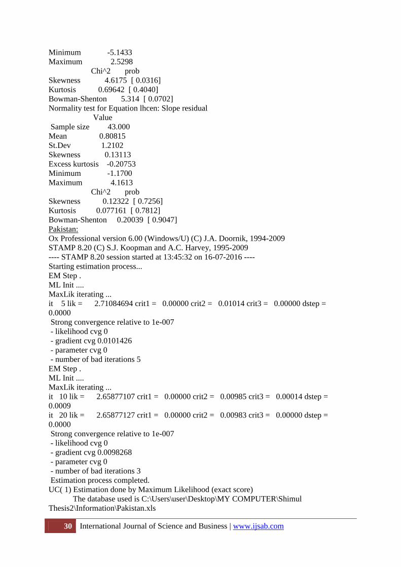
30 International Journal of Science and Business | www.ijsab.com
Minimum -5.1433
Maximum 2.5298
Chi^2 prob
Skewness 4.6175 [ 0.0316]
Kurtosis 0.69642 [ 0.4040]
Bowman-Shenton 5.314 [ 0.0702]
Normality test for Equation lhcen: Slope residual
Value
Sample size 43.000
Mean 0.80815
St.Dev 1.2102
Skewness 0.13113
Excess kurtosis -0.20753
Minimum -1.1700
Maximum 4.1613
Chi^2 prob
Skewness 0.12322 [ 0.7256]
Kurtosis 0.077161 [ 0.7812]
Bowman-Shenton 0.20039 [ 0.9047]
Pakistan:
Ox Professional version 6.00 (Windows/U) (C) J.A. Doornik, 1994-2009
STAMP 8.20 (C) S.J. Koopman and A.C. Harvey, 1995-2009
---- STAMP 8.20 session started at 13:45:32 on 16-07-2016 ----
Starting estimation process...
EM Step .
ML Init ....
MaxLik iterating ...
it 5 lik = 2.71084694 crit1 = 0.00000 crit2 = 0.01014 crit3 = 0.00000 dstep =
0.0000
Strong convergence relative to 1e-007
- likelihood cvg 0
- gradient cvg 0.0101426
- parameter cvg 0
- number of bad iterations 5
EM Step .
ML Init ....
MaxLik iterating ...
it 10 lik = 2.65877107 crit1 = 0.00000 crit2 = 0.00985 crit3 = 0.00014 dstep =
0.0009
it 20 lik = 2.65877127 crit1 = 0.00000 crit2 = 0.00983 crit3 = 0.00000 dstep =
0.0000
Strong convergence relative to 1e-007
- likelihood cvg 0
- gradient cvg 0.0098268
- parameter cvg 0
- number of bad iterations 3
Estimation process completed.
UC( 1) Estimation done by Maximum Likelihood (exact score)
The database used is C:\Users\user\Desktop\MY COMPUTER\Shimul
Thesis2\Information\Pakistan.xls
31 International Journal of Science and Business | www.ijsab.com
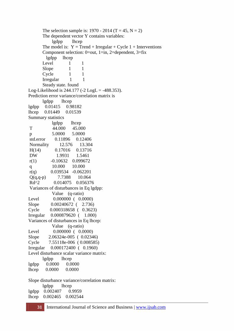
The selection sample is: 1970 - 2014 (T = 45, N = 2)
The dependent vector Y contains variables:
lgdpp lhcep
The model is: Y = Trend + Irregular + Cycle 1 + Interventions
Component selection: 0=out, 1=in, 2=dependent, 3=fix
lgdpp lhcep
Level 1 1
Slope 1 1
Cycle 1 1
Irregular 1 1
Steady state. found
Log-Likelihood is 244.177 (-2 LogL = -488.353).
Prediction error variance/correlation matrix is
lgdpp lhcep
lgdpp 0.01415 0.98182
lhcep 0.01449 0.01539
Summary statistics
lgdpp lhcep
T 44.000 45.000
p 5.0000 5.0000
std.error 0.11896 0.12406
Normality 12.576 13.304
H(14) 0.17016 0.13716
DW 1.9931 1.5461
r(1) -0.10632 0.099672
q 10.000 10.000
r(q) 0.039534 -0.062201
Q(q,q-p) 7.7388 10.064
Rd^2 0.014075 0.056376
Variances of disturbances in Eq lgdpp:
Value (q-ratio)
Level 0.000000 ( 0.0000)
Slope 0.00240672 ( 2.736)
Cycle 0.000318658 ( 0.3623)
Irregular 0.000879620 ( 1.000)
Variances of disturbances in Eq lhcep:
Value (q-ratio)
Level 0.000000 ( 0.0000)
Slope 2.06324e-005 ( 0.02346)
Cycle 7.55118e-006 ( 0.008585)
Irregular 0.000172400 ( 0.1960)
Level disturbance scalar variance matrix:
lgdpp lhcep
lgdpp 0.0000 0.0000
lhcep 0.0000 0.0000
Slope disturbance variance/correlation matrix:
lgdpp lhcep
lgdpp 0.002407 0.9959
lhcep 0.002465 0.002544
32 International Journal of Science and Business | www.ijsab.com
Cycle disturbance variance/correlation matrix:
lgdpp lhcep
lgdpp 0.0003187 0.9960
lhcep 0.0003442 0.0003747
Irregular disturbance variance/correlation matrix:
lgdpp lhcep
lgdpp 0.0008796 0.8922
lhcep 0.0007692 0.0008451
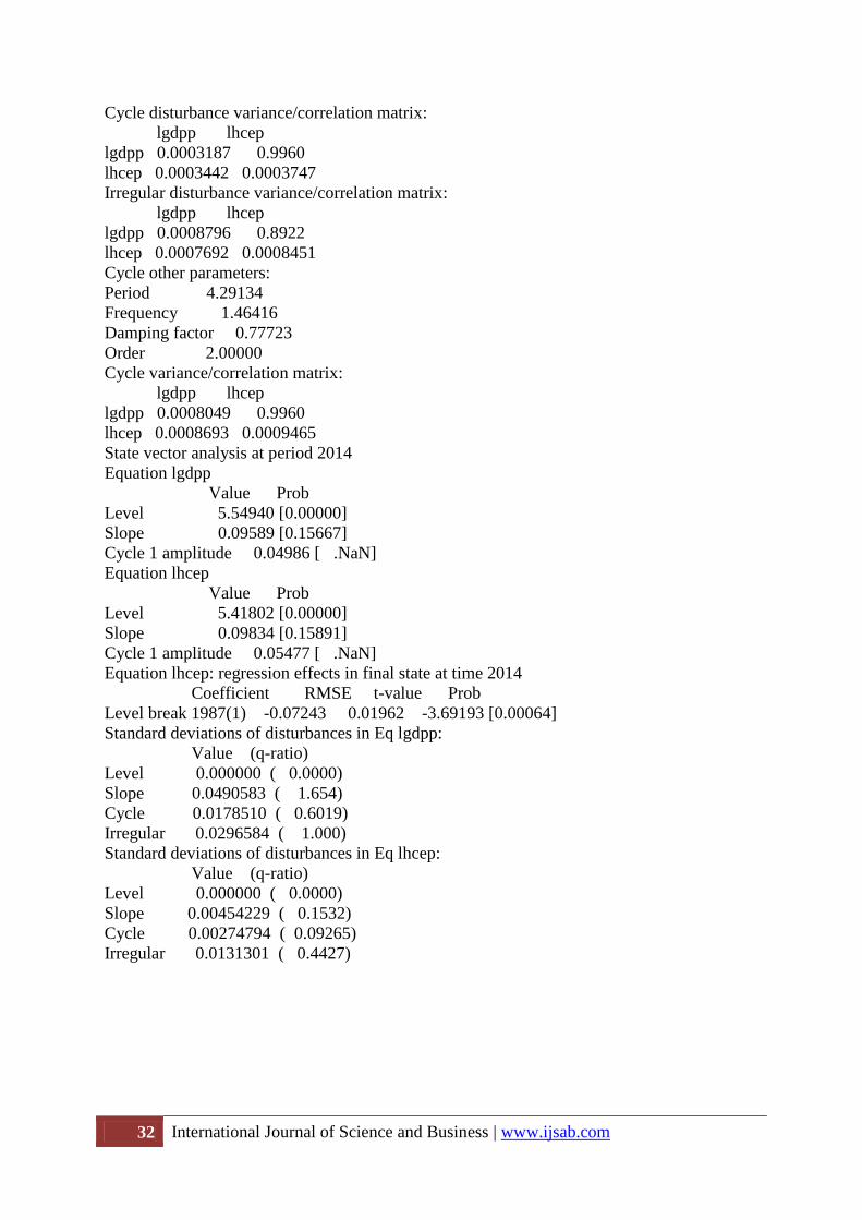
Cycle other parameters:
Period 4.29134
Frequency 1.46416
Damping factor 0.77723
Order 2.00000
Cycle variance/correlation matrix:
lgdpp lhcep
lgdpp 0.0008049 0.9960
lhcep 0.0008693 0.0009465
State vector analysis at period 2014
Equation lgdpp
Value Prob
Level 5.54940 [0.00000]
Slope 0.09589 [0.15667]
Cycle 1 amplitude 0.04986 [ .NaN]
Equation lhcep
Value Prob
Level 5.41802 [0.00000]
Slope 0.09834 [0.15891]
Cycle 1 amplitude 0.05477 [ .NaN]
Equation lhcep: regression effects in final state at time 2014
Coefficient RMSE t-value Prob
Level break 1987(1) -0.07243 0.01962 -3.69193 [0.00064]
Standard deviations of disturbances in Eq lgdpp:
Value (q-ratio)
Level 0.000000 ( 0.0000)
Slope 0.0490583 ( 1.654)
Cycle 0.0178510 ( 0.6019)
Irregular 0.0296584 ( 1.000)
Standard deviations of disturbances in Eq lhcep:
Value (q-ratio)
Level 0.000000 ( 0.0000)
Slope 0.00454229 ( 0.1532)
Cycle 0.00274794 ( 0.09265)
Irregular 0.0131301 ( 0.4427)
33 International Journal of Science and Business | www.ijsab.com
Variance/correlation matrix
lgdpp lhcep
lgdpp 0.0000 0.0000
lhcep 0.0000 0.0000
Variance/correlation matrix
lgdpp lhcep
lgdpp 0.002407 0.9959
lhcep 0.002465 0.002544
Variance/correlation matrix
lgdpp lhcep
lgdpp 0.0008049 0.9960
lhcep 0.0008693 0.0009465
Variance/correlation matrix
lgdpp lhcep
lgdpp 0.0008796 0.8922
lhcep 0.0007692 0.0008451
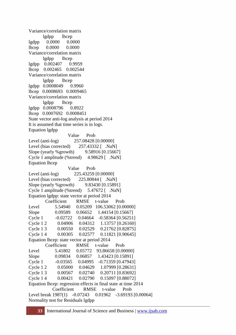
State vector anti-log analysis at period 2014
It is assumed that time series is in logs.
Equation lgdpp
Value Prob
Level (anti-log) 257.08428 [0.00000]
Level (bias corrected) 257.43332 [ .NaN]
Slope (yearly %growth) 9.58916 [0.15667]
Cycle 1 amplitude (%trend) 4.98629 [ .NaN]
Equation lhcep
Value Prob
Level (anti-log) 225.43259 [0.00000]
Level (bias corrected) 225.80844 [ .NaN]
Slope (yearly %growth) 9.83430 [0.15891]
Cycle 1 amplitude (%trend) 5.47672 [ .NaN]
Equation lgdpp: state vector at period 2014
Coefficient RMSE t-value Prob
Level 5.54940 0.05209 106.53062 [0.00000]
Slope 0.09589 0.06652 1.44154 [0.15667]
Cycle 1 -0.02722 0.04664 -0.58364 [0.56251]
Cycle 1 2 0.04906 0.04312 1.13757 [0.26160]
Cycle 1 3 0.00550 0.02529 0.21762 [0.82875]
Cycle 1 4 0.00305 0.02577 0.11821 [0.90645]
Equation lhcep: state vector at period 2014
Coefficient RMSE t-value Prob
Level 5.41802 0.05772 93.86658 [0.00000]
Slope 0.09834 0.06857 1.43423 [0.15891]
Cycle 1 -0.03565 0.04995 -0.71359 [0.47943]
Cycle 1 2 0.05000 0.04629 1.07999 [0.28631]
Cycle 1 3 0.00567 0.02740 0.20711 [0.83692]
Cycle 1 4 0.00421 0.02790 0.15097 [0.88072]
Equation lhcep: regression effects in final state at time 2014
Coefficient RMSE t-value Prob
Level break 1987(1) -0.07243 0.01962 -3.69193 [0.00064]
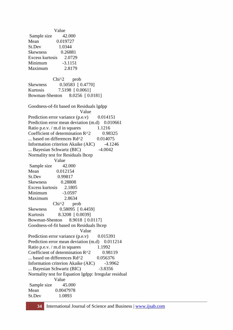
Normality test for Residuals lgdpp
34 International Journal of Science and Business | www.ijsab.com
Value
Sample size 42.000
Mean 0.019727
St.Dev 1.0344
Skewness 0.26881
Excess kurtosis 2.0729
Minimum -3.1151
Maximum 2.8179
Chi^2 prob
Skewness 0.50583 [ 0.4770]
Kurtosis 7.5198 [ 0.0061]
Bowman-Shenton 8.0256 [ 0.0181]
Goodness-of-fit based on Residuals lgdpp
Value
Prediction error variance (p.e.v) 0.014151
Prediction error mean deviation (m.d) 0.010661
Ratio p.e.v. / m.d in squares 1.1216
Coefficient of determination R^2 0.98325
... based on differences Rd^2 0.014075
Information criterion Akaike (AIC) -4.1246
... Bayesian Schwartz (BIC) -4.0042
Normality test for Residuals lhcep
Value
Sample size 42.000
Mean 0.012154
St.Dev 0.99817
Skewness 0.28808
Excess kurtosis 2.1805
Minimum -3.0597
Maximum 2.8634
Chi^2 prob
Skewness 0.58095 [ 0.4459]
Kurtosis 8.3208 [ 0.0039]
Bowman-Shenton 8.9018 [ 0.0117]
Goodness-of-fit based on Residuals lhcep
Value
Prediction error variance (p.e.v) 0.015391
Prediction error mean deviation (m.d) 0.011214
Ratio p.e.v. / m.d in squares 1.1992
Coefficient of determination R^2 0.98119
... based on differences Rd^2 0.056376
Information criterion Akaike (AIC) -3.9962
... Bayesian Schwartz (BIC) -3.8356
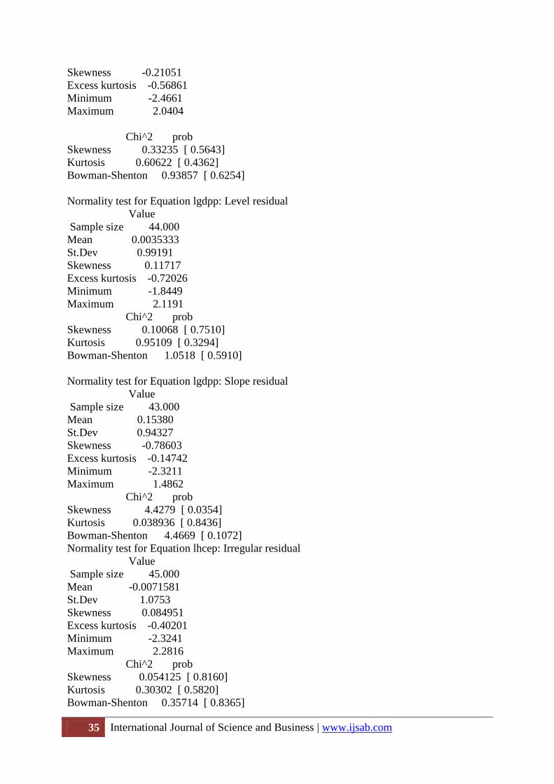
Normality test for Equation lgdpp: Irregular residual
Value
Sample size 45.000
Mean 0.0047978
St.Dev 1.0893
35 International Journal of Science and Business | www.ijsab.com
Skewness -0.21051
Excess kurtosis -0.56861
Minimum -2.4661
Maximum 2.0404
Chi^2 prob
Skewness 0.33235 [ 0.5643]
Kurtosis 0.60622 [ 0.4362]
Bowman-Shenton 0.93857 [ 0.6254]
Normality test for Equation lgdpp: Level residual
Value
Sample size 44.000
Mean 0.0035333
St.Dev 0.99191
Skewness 0.11717
Excess kurtosis -0.72026
Minimum -1.8449
Maximum 2.1191
Chi^2 prob
Skewness 0.10068 [ 0.7510]
Kurtosis 0.95109 [ 0.3294]
Bowman-Shenton 1.0518 [ 0.5910]
Normality test for Equation lgdpp: Slope residual
Value
Sample size 43.000
Mean 0.15380
St.Dev 0.94327
Skewness -0.78603
Excess kurtosis -0.14742
Minimum -2.3211
Maximum 1.4862
Chi^2 prob
Skewness 4.4279 [ 0.0354]
Kurtosis 0.038936 [ 0.8436]
Bowman-Shenton 4.4669 [ 0.1072]
Normality test for Equation lhcep: Irregular residual
Value
Sample size 45.000
Mean -0.0071581
St.Dev 1.0753
Skewness 0.084951
Excess kurtosis -0.40201
Minimum -2.3241
Maximum 2.2816
Chi^2 prob
Skewness 0.054125 [ 0.8160]
Kurtosis 0.30302 [ 0.5820]
Bowman-Shenton 0.35714 [ 0.8365]
36 International Journal of Science and Business | www.ijsab.com
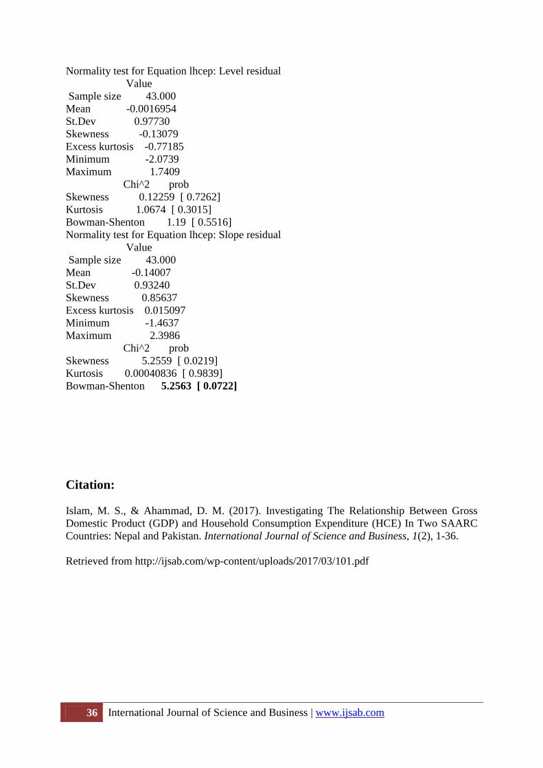
Normality test for Equation lhcep: Level residual
Value
Sample size 43.000
Mean -0.0016954
St.Dev 0.97730
Skewness -0.13079
Excess kurtosis -0.77185
Minimum -2.0739
Maximum 1.7409
Chi^2 prob
Skewness 0.12259 [ 0.7262]
Kurtosis 1.0674 [ 0.3015]
Bowman-Shenton 1.19 [ 0.5516]
Normality test for Equation lhcep: Slope residual
Value
Sample size 43.000
Mean -0.14007
St.Dev 0.93240
Skewness 0.85637
Excess kurtosis 0.015097
Minimum -1.4637
Maximum 2.3986
Chi^2 prob
Skewness 5.2559 [ 0.0219]
Kurtosis 0.00040836 [ 0.9839]
Bowman-Shenton 5.2563 [ 0.0722]
Citation:
Islam, M. S., & Ahammad, D. M. (2017). Investigating The Relationship Between Gross
Domestic Product (GDP) and Household Consumption Expenditure (HCE) In Two SAARC
Countries: Nepal and Pakistan. International Journal of Science and Business, 1(2), 1-36.
Retrieved from http://ijsab.com/wp-content/uploads/2017/03/101.pdf
37 International Journal of Science and Business | www.ijsab.com
<meta name="citation_title" content=" Investigating The Relationship
Between Gross Domestic Product (GDP) and Household Consumption Expenditure
(HCE) In Two SAARC Countries: Nepal and Pakistan.">
<meta name="citation_author" content=" Islam, M. S.">
<meta name="citation_author" content=" Ahammad, D. M.">
<meta name="citation_date" content="2017/03/30">
<meta name="citation_journal_title" content="International Journal of
Science and Business">
<meta name="citation_volume" content="1">
<meta name="citation_issue" content="2">
<meta name="citation_firstpage" content="1">
<meta name="citation_lastpage" content="36">
<meta name="citation_issn" content="ISSN 2520-4750">
<meta name="citation_publisher" content=" International Journal of Science
and Business (IJSB)">
<meta name="citation_pdf_url" content=" http://ijsab.com/wp-
content/uploads/2017/03/101.pdf ">
Related Documents