INVESTIGATING THE INFLUENCE OF FABRICATION PARAMETERS ON THE DIAMETER AND MECHANICAL PROPERTIES OF POLYSULFONE ULTRAFILTRATION HOLLOW-FIBRE MEMBRANES MSc. Eng. Mechanical Thesis Presented to the Faculty of Engineering Mechanical and Mechatronic Engineering Department of the University of Stellenbosch By: Ali Rugbani Supervised by: Prof Kristiaan Schreve University of Stellenbosch 2009

Welcome message from author
This document is posted to help you gain knowledge. Please leave a comment to let me know what you think about it! Share it to your friends and learn new things together.
Transcript
INVESTIGATING THE INFLUENCE OF
FABRICATION PARAMETERS ON THE
DIAMETER AND MECHANICAL PROPERTIES
OF POLYSULFONE ULTRAFILTRATION
HOLLOW-FIBRE MEMBRANES
MSc. Eng. Mechanical Thesis
Presented to the Faculty of Engineering
Mechanical and Mechatronic Engineering Department
of the University of Stellenbosch
By:
Ali Rugbani
Supervised by:
Prof Kristiaan Schreve
University of Stellenbosch
2009

DECLARATION
By submitting this thesis electronically, I declare that the entirety of the work
contained therein is my own, original work, that I am the owner of the copyright
thereof (unless to the extent explicitly otherwise stated) and that I have not previously
in its entirety or in part submitted it for obtaining any qualification.
Signature:
Name:
Date:
Copyright © 2009 Stellenbosch University
All rights reserved
i
ABSTRACT
Polysulfone hollow-fibre membranes were fabricated via the dry-wet solution
spinning technique. The objective was to demonstrate the influence of the various
fabrication parameters on the diameter and mechanical properties of the hollow-fibre
membranes and to optimize the spinning process by controlling these parameters with
a computer control system. The effects of the operation parameters were investigated
using an experimental design based on a fractional factorial method (Taguchi’s design
of experiments). The parameters that were considered are the spinneret size, dope
solution temperature, bore fluid temperature, coagulation bath temperature, dope
extrusion rate, bore flow rate and the take-up speed. A new pilot solution spinning
plant was installed and upgraded, and a computer control system, based on LabView,
was developed to control, monitor and log the experimental data. The diameter of the
hollow-fibres were determined using a scanning electron microscope (SEM) while the
mechanical properties were measured using a tensile tester. The effects of diameter
size and wall thickness of the hollow-fibres on the performance of the membranes
were studied.
The results showed the significance of the fabrication parameters that dominate the
diameter and strength of the hollow-fibres.
Keywards: Hollow-fibre membrane; Spinning; Taguchi’s method; Take-up speed;
Extrusion rate; Spinneret size; Bore flow; Dope extrusion rate; LabView.
ii
OPSOMMING
Polisulfoon holvesel membrane is met ‘n droë-nat oplossingspin proses vervaardig.
Die doel hiermee was om die invloed van verskeie vervaardigingsparameters op die
deursnee en meganiese eienskappe van die holvesel membrane te demonstreer asook
om die spin proses te optimeer deur gerekenariseerde beheer van die aanleg. ‘n
Eksperimentele ontwerp, gebaseer op ‘n gedeeltelike faktoriaal metode (Taguchi se
eksperimentele ontwerp) is gebruik om die invloed van die vervaardigingsparameters
te ondersoek. Die parameters wat oorweeg is, is spindop grootte, materiaal
temperatuur, boorvloeistof temperatuur, stolbad temperatuur, materiaal ekstrusie
tempo and opwen spoed. ‘n Nuwe oplossingspin loodsaanleg was geïnstalleer en
opgegradeer en ‘n rekenaar beheerstelsel, gebaseer op LabView, is ontwikkel om die
aanleg te beheer, moniteer en eksperimentele data te stoor. Die deursnee van die
holvesel is gemeet met ‘n skanderingelektron mikroskoop (SEM) terwyl die
meganiese eienskappe bepaal is met ‘n trektoets apparaat. Die effek van die deursnee
en wanddikte van die holvesels op die werkverrigting van die membrane is ook
bestudeer.
Die resultate toon watter vervaardigingsparameters is beduidend vir die deursnee en
sterkte van die holvesels.
Sleutelwoorde: Holvesel membrane; spin; Taguchi se metode; opwen spoed; esktrusie
tempo; spindop grootte; boorvloei; materiaal ekstrusie tempo; LabView.

iii
DEDICATION
I dedicate this thesis to the pillars of my life, my parents.

iv
ACKNOWLEDGEMENTS
I would like to express my deep and sincere appreciation to the strong influence of my
supervisor Prof Kristiaan Schreve for his valuable advice, support and encouragement
throughout this study.
I also would like to express my gratitude to Prof Ron Sanderson. His able guidance
has been an inspiration and has instilled professionalism in me.
A special thank goes to Dr Ian Goldie. I have benefited from his helpful comments
and useful suggestions about my research. Thanks to Dr Margie Hurndall, for the time
she spent editing my thesis.
I had a wonderful time working with Prof Li and Dr Yun at Tianjin Polytechnic
University in China, and appreciate their help with the equipments and the
opportunity to work in their lab in Jun through August 2007.
I express my gratitude to my family. They provided me with continuous support,
encouragement and help.
Lastly, I am extremely appreciative of the National Bureau of Research and
Development of Libya for funding this research.

v
TABLE OF CONTENTS Page
Table of contents........................................................................................................ v
List of figures............................................................................................................. ix
List of tables .............................................................................................................. xi
Abbreviations ...........................................................................................................xii
CHAPTER 1: INTRODUCTION AND OBJECTIVES............. ......................... 2
1.1 Introduction.............................................................................................2
1.2 Membrane history...................................................................................3
1.3 Membranes..............................................................................................3
1.3.1 Membranes classification .....................................................3
1.3.2 Types of membranes.............................................................4
1.3.2.1 Symmetric or isotropic (homogeneous) membranes5
1.3.2.2 Asymmetric or anisotropic (heterogeneous)
membranes............................................................................ 5
1.4 Membrane systems.................................................................................5
1.4.1 Hollow-fibre membranes......................................................5
1.5 Objectives ...............................................................................................7
1.6 Layout of document ...............................................................................7
CHAPTER 2: THEORETICAL BACKGROUND.................. .......................... 10
2.1 Fabrication of hollow-fibre membranes..............................................10
2.2 Methods of spinning hollow-fibres .....................................................12
2.2.1 Wet spinning........................................................................12
2.2.2 Dry spinning ........................................................................13
2.2.3 Melt spinning.......................................................................13
2.3 Spinning parameters.............................................................................13
2.3.1 Type of polymer..................................................................13
2.3.2 Types of solvents and additives in polymer solution........14
2.3.3 Dope solution extrusion rate...............................................15
vi
2.3.4 Air gap condition (length, humidity, pressure, temperature)
..............................................................................................16
2.3.5 Take-up speed......................................................................17
2.3.6 Coagulation bath temperature.............................................17
2.3.7 Bore type..............................................................................18
2.3.8 Viscosity of the spinning solution......................................18
2.3.9 Type of spinneret.................................................................19
2.4 Characterization of hollow-fibres........................................................21
2.4.1 Membrane morphology.......................................................21
2.4.2 Hollow-fibre diameters and hollowness ............................21
2.4.3 Membrane performance......................................................22
2.5 Commercial hollow-fibre manufacturers............................................23
2.6 Computer control of the hollow-fibre fabrication apparatus.............24
CHAPTER 3: EXPERIMENTAL APPARATUS AND PROCEDURES ... ... 26
3.1 Description of the experimental apparatus .........................................26
3.2 Installing the membrane fabrication plant ..........................................29
3.3 Materials and methods .........................................................................29
3.3.1 Materials ..............................................................................29
3.3.2 Dry/wet solution spinning procedure.................................30
3.3.3 Hollow-fibre post-processing.............................................31
3.4 Characterization of membrane samples ..............................................31
3.4.1 SEM imaging and analysis .................................................31
3.4.2 Mechanical testing ..............................................................32
3.5 Design and planning of experiments...................................................34
3.5.1 Design of experiments using the Taguchi method............34
3.5.2 Planning of experiments .....................................................35
3.5.3 First stage: factors’ preliminary investigation test ............35
3.5.4 Second stage: relation prediction .......................................38
3.5.5 Third stage: confirmation experiments..............................41
3.6 Membrane performance characterization ...........................................42
3.6.1 Test cell preparation............................................................42
3.6.2 Cell test apparatus ...............................................................42
3.6.3 Test procedure .....................................................................43
vii
CHAPTER 4: COMPUTER CONTROL SYSTEM (LABVIEW
IMPLEMENTATION) ................................................................................. 45
4.1 Introduction...........................................................................................45
4.2 Computer control system.....................................................................45
4.2.1 Control system requirements..............................................45
4.2.2 Programming the spinning control system ........................47
4.2.2.1 Spinning control software capabilities .............. 51
4.2.2.2 Spinning control flow chart ............................... 53
4.2.2.3 User interface...................................................... 54
4.3 Diameter control module .....................................................................55
CHAPTER 5: RESULTS AND DISCUSSION................................................... 57
5.1 Introduction...........................................................................................57
5.2 First stage ..............................................................................................57
5.2.1 Analysis of experimental data ............................................57
5.2.2 Analysis on the relative factor importance........................59
5.3 Second stage .........................................................................................61
5.3.1 Analysis of S1 experimental data.......................................62
5.3.1.1 Analysis on the relative factor importance ....... 63
5.3.1.2 Regression model ............................................... 64
5.3.2 Analysis of S2 experimental data.......................................65
5.3.2.1 Analysis on the relative factor importance ....... 67
5.3.2.2 Regression model ............................................... 68
5.4 Third stage ............................................................................................69
5.4.1 Take-up speed......................................................................69
5.4.2 Bore flow rate ......................................................................71
5.4.3 Air gap length ......................................................................73
5.4.4 Dope extrusion rate .............................................................75
5.5 Hollow-fibre membrane characterization ...........................................77
5.5.1 Tensile..................................................................................77
5.5.1.1 Analysis on the relative factor importance ....... 79
5.5.2 Membrane separation performance....................................79
CHAPTER 6: CONCLUSIONS............................................................................ 83

viii
APPENDIX A: SEM IMAGES ............................................................................. 94
APPENDIX B: DOE CALCULATIONS...........................................................106
APPENDIX C: INVESTIGATION OF FACTORS INTERACTION... .......113
APPENDIX D: RESULTS OF THE CONFIRMATION EXPERIMENTS 115
APPENDIX E: RESULTS OF THE TENSILE TEST....................................117
APPENDIX F: RESULTS OF MEMBRANE FLUX ......................................125
ix
LIST OF FIGURES
Page
Figure 1: Application range of MF, UF, NF and RO [19]. ..............................................4
Figure 2: Hollow-fibre membrane module [1]. ................................................................6
Figure 3: Structured view of double-element type module .............................................6
Figure 4: Schematic of the various types of hollow-fibre membranes [20]. ................10
Figure 5: Tube-in-orifice spinneret [27]. ........................................................................11
Figure 6: Schematic of a hollow-fibre spinning apparatus [27]. ...................................12
Figure 7: Cross sectional view of a 3-C shaped spinneret.............................................19
Figure 8: Triple-orifice spinneret [69]. ...........................................................................20
Figure 9: Schematic showing three streams in a membrane module. ...........................22
Figure 10: Schematic representation of the hollow-fibre spinning apparatus, adapted
from [91]. ..........................................................................................................................26
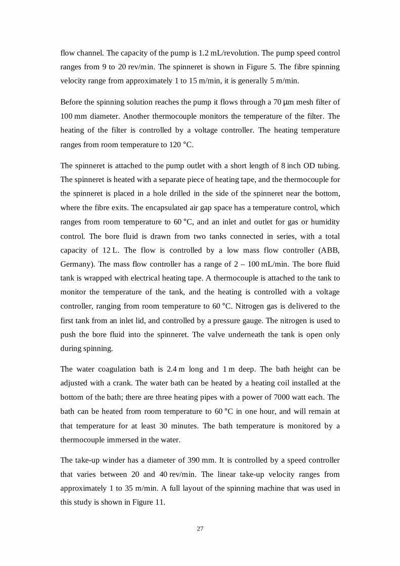
Figure 11: Hollow-fibre spinning machine as used in this study. .................................28
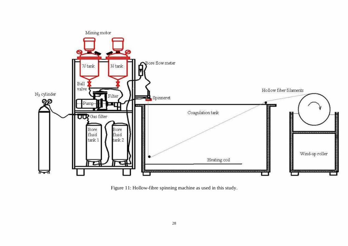
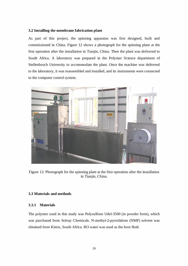
Figure 12: Photograph for the spinning plant at the first operation after the installation
in Tianjin, China. ..............................................................................................................29
Figure 13: Samples ready for SEM .................................................................................32
Figure 14: Flow chart of orthogonal array experimental design. ..................................35
Figure 15: Dimensions of the two used spinnerets, (S1 and S2). ..................................36
Figure 16: SEM image of cross-section of hollow-fibre when BF is too low. .............39
Figure 17: Hollow-fibre cells prepared for testing.........................................................42
Figure 18: Hollow-fibre pilot test plant used in this study. ...........................................43
Figure 19: Photograph of the computer control system.................................................46
Figure 20: Heating control module. ................................................................................47
Figure 21: Base motor speed control module. ................................................................48
Figure 22: Computer display module (pressure, flow rate, counting, etc.). .................48
Figure 23: Schematic diagram of the computer controlled output signals. ..................49
Figure 24: Schematic diagram of the acquired input signals.........................................50
Figure 25: Block diagram: Calculating the extrusion rate and spinning take-up speeds.
...........................................................................................................................................52
Figure 26: Flow chart of the spinning control system....................................................53
Figure 27: User interface of the LabView software. ......................................................54
x
Figure 28: Block diagram of the prediction model. .......................................................55
Figure 29: Effect of factors on the diameter size............................................................59
Figure 30: Factor effects on ID, using S1. ......................................................................62
Figure 31: Factor effects on OD, using S1. ....................................................................62
Figure 32: The results of the regression model, for S1 experiments.............................65
Figure 33: Effect of factors on ID, using S2...................................................................66
Figure 34: Effect of factors on OD, using S2. ................................................................66
Figure 35: The results of the regression model for S2 experiments..............................68
Figure 36: SEM images of cross-sections (150x magnification) of fibre prepared using
take-up speeds of a) minimum, b) 1.5x, c) 2x, d) 2.5x, e) 3x and f) 3.5x.....................70
Figure 37: ID and OD experimental measurements versus predicted values at different
relative take-up speeds. ....................................................................................................71
Figure 38: SEM images of cross-sections (150x magnification) of fibre prepared using
bore flow rates of a) 2 mL/min, b) 3 mL/min, c) 4 mL/min and d) 5 mL/min.............72
Figure 39: ID and OD, experimental measurements versus predicted calculations at
different BF. ......................................................................................................................73
Figure 40: SEM images of cross-sections (150x magnification) of fibre prepared using
air gap distances of a) 5 mm, b) 8 mm, c) 15 mm and d) 20 mm..................................74
Figure 41: ID and OD, experimental measurements versus predicted calculations for
different air gap distances. ...............................................................................................75
Figure 42: SEM images of cross-sections (150x magnification) of fibre prepared using
dope rates of a) 4.6 mL/min, b) 6 mL/min, c) 7.8 mL/min and d) 9.3 mL/min. ..........76
Figure 43: ID and OD, experimental measurements versus predicted calculations at
different DER....................................................................................................................77
Figure 44: Effect of factors on tensile stress, using S1. .................................................78
Figure 45: Effect of factors on tensile stress, using S2. .................................................78
Figure 46: Flux rate change with wall thickness at fixed OD. ......................................80
Figure 47: Flux rate change with wall thickness at fixed ID for samples prepared
using different take-up speeds. ........................................................................................80
xi
LIST OF TABLES
Page
Table 1: Factors and level values used in stage 1 of the experiments...........................37
Table 2: Orthogonal array L18 table ...............................................................................38
Table 3: Factors and levels when using S1.....................................................................40
Table 4: Factors and levels when using S2.....................................................................40
Table 5: Orthogonal array L8 table .................................................................................41
Table 6: Values for each factor used during the tests ....................................................41
Table 7: ANOVA results, L18.........................................................................................60
Table 8: ANOVA results for ID, using S1......................................................................63
Table 9: ANOVA results for OD, using S1 ....................................................................64
Table 10: ANOVA results for ID, using S2....................................................................67
Table 11: ANOVA results for OD, using S2 ..................................................................67
Table 12: ANOVA results of the tensile strength...........................................................79
xii
ABBREVIATIONS
2D : Two-dimensional.
3D : Three-dimensional.
Ag : Air gap length.
ANOVA: Analysis of variance.
BF : Bore fluid flow rate.
CA : Cellulose acetate.
CTA : Cellulose triacetate.
DAQ : Data acquisition card.
DER : Dope extrusion rate.
DOE : Design of experiments.
HF : Hollow-fibre.
ID : Inner diameter.
MF : Microfiltration.
NF : Nanofiltration.
NMP : 1-methyl-2-pyrrolidone.
OA : Orthogonal array.
OD : Outer diameter.
PA : Polyamide.
PEG : Polyethylene glycol.
PES : Polyethersulfone.
PS : Polysulfone.
PVDF : Polyvinylidene fluoride.
PVP : Polyvinyl pyrrolidone.
QC : Quality control.
RO : Reverse osmosis.
rpm : Revolutions per minute.
RT : Residence time.
SQ : Sum of squares.
SW : Spiral-wound.
Tup : Take-up speed.
UF : Ultrafiltration.

CHAPTER 1
INTRODUCTION AND OBJECTIVES
2
CHAPTER 1: INTRODUCTION AND OBJECTIVES
1.1 Introduction
Today membrane separation is one of the best available technologies for water
desalination and treatment, although scientists are still trying to improve the
membrane performance and reduce costs.
Membranes can treat moderately saline to saline water. The removal effectiveness
(percentage of removal of common minerals, including hardness, salts and suspended
solids) mainly depends on the membrane type, the applied pressure, and the amount
and properties of each contaminant [1].
The science of manufacturing a membrane separation system involves a multitude of
formulation variables. In this regard, membrane research involves a study of these
variables and their reciprocal actions in order to generate an understanding of the
science involved, and to subsequently exercise control over tailor-making membranes
with the desired properties.
Spinning of hollow-fibres is a highly complicated process that requires a good
understanding of the fabrication parameters that influence the hollow-fibre properties,
such as their fibre diameter, porosity, etc. Controlling these parameters during
membrane fabrication should lead to membranes with the required characteristics.
In this project, attention will be primarily focused on determining and controlling the
factors that influence the geometry and performance of asymmetric polysulfone (PS)
hollow-fibre membranes fabricated by the dry–wet spinning technique. It was
envisaged that the results could be used to contribute to optimizing the hollow-fibre
membrane spinning machine that was to be built (with the contribution of Tianjin
University, China) as part of a wider project.
Experiments were designed following the Taguchi method, the purpose of which was
to measure the fibre diameters and determine the effects of varying the spinning
parameters, and the significance of the respective parameters on the membrane
product.
3
1.2 Membrane history
Reverse osmosis RO is a relatively new separation process in relation to thermal
processes. In the early 1970s the first desalination membrane process was
commercially used after Sidney Loeb and Srinivasa Sourirajan from UCLA
(California) produced a functional synthetic RO membrane from cellulose acetate
(CA). These membranes were in the form of sheets, in plate-and-frame and spiral-
wound configurations, or formed by deposition on porous tubular supports. They
exhibited reasonable permeate flux and salt rejection, and operated under realistic
pressures [2]. Since then, much work has been done to study the morphological
structure and the properties of the filtration membranes, fabricated with various
polymeric materials, essentially CA and its derivatives [3-11], polyamides [11-14]
and polysulphones [13, 15-17].
1.3 Membranes
Membranes can be identified according to their classification and type as follows.
1.3.1 Membranes classification
There are different types of membranes, classified according to the size of the
particles that can pass through the pores and according to their separation technique
into the following groups [18].
• Microfiltration (MF)
Removes particles down to 0.1 microns in size.
• Ultrafiltration (UF)
Removes particles from 0.01 to 0.1 microns in size.
• Nanofiltration (NF)
Removes most organic compounds.
• Reverse Osmosis (RO)
Removes dissolved salts and metal ions.
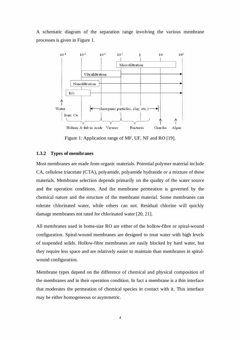
The pore size in the membrane becomes smaller in the order MF > UF > NF > RO,
and consequently also the size of the particles that can be separated by the respective
process [19].
4
A schematic diagram of the separation range involving the various membrane
processes is given in Figure 1.
Figure 1: Application range of MF, UF, NF and RO [19].
1.3.2 Types of membranes
Most membranes are made from organic materials. Potential polymer material include
CA, cellulose triacetate (CTA), polyamide, polyamide hydraside or a mixture of these
materials. Membrane selection depends primarily on the quality of the water source
and the operation conditions. And the membrane permeation is governed by the
chemical nature and the structure of the membrane material. Some membranes can
tolerate chlorinated water, while others can not. Residual chlorine will quickly
damage membranes not rated for chlorinated water [20, 21].
All membranes used in home-size RO are either of the hollow-fibre or spiral-wound
configuration. Spiral-wound membranes are designed to treat water with high levels
of suspended solids. Hollow-fibre membranes are easily blocked by hard water, but
they require less space and are relatively easier to maintain than membranes in spiral-
wound configuration.
Membrane types depend on the difference of chemical and physical composition of
the membranes and in their operation condition. In fact a membrane is a thin interface
that moderates the permeation of chemical species in contact with it. This interface
may be either homogeneous or asymmetric.
5
1.3.2.1 Symmetric or isotropic (homogeneous) membranes
Symmetric membranes can be regarded as having a uniform composition and
structure throughout the membrane thickness, with a relatively constant pore size,
randomly distributed between interconnected pores [22].
1.3.2.2 Asymmetric or anisotropic (heterogeneous) membranes
Asymmetric membranes consist of multi-layers. Typically, an asymmetric membrane
has a dense, thin layer that performs the separation. This skin layer is supported by an
open and much thicker microporous layer. Asymmetric membranes provide higher
permeability than the symmetric membranes for the same thickness [22].
1.4 Membrane systems
The most important component of a water treatment system is the membrane
assembly. The membrane assembly consists of a pressure vessel containing the
membrane modules. The membranes must be strong enough to withstand whatever
pressure is applied to them. Membranes are made in a variety of configurations: plate-
and-frame, tubular, spiral-wound (SW) and hollow-fibre (HF) of which the latter two
are the most common configurations [23].
1.4.1 Hollow-fibre membranes
The hollow-fibre membrane is an important improvement of the tubular membrane.
Hollow-fibre membranes offer three primary advantages over flat-sheet membranes.
• First, hollow-fibres exhibit higher productivity per unit volume due to their
high packing density.
• Second, they are self supporting, with no thick supporting layer.
• Thirdly, high recovery in individual units is achieved. The hollow-fibre
geometry allows a high membrane surface area to be contained in a compact
module. This means that large volumes can be filtered, while utilizing minimal
space, and requiring low power consumption.
Hollow-fibre membranes can be designed for circulation, dead-end, or single-pass
operations. The fibres range in diameter from 3 mm to 0.5 mm for the so called
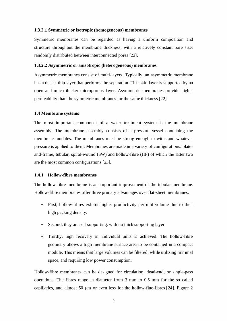
capillaries, and almost 50 µm or even less for the hollow-fine-fibres [24]. Figure 2
6
shows a hollow-fibre module that operates from the inside to the outside during
filtration. This means that the process fluid (reject) flows through the centre of the
hollow-fibre and the permeate passes through the fibre wall to the outside of the
membrane fibres [25].
Figure 2: Hollow-fibre membrane module [1].
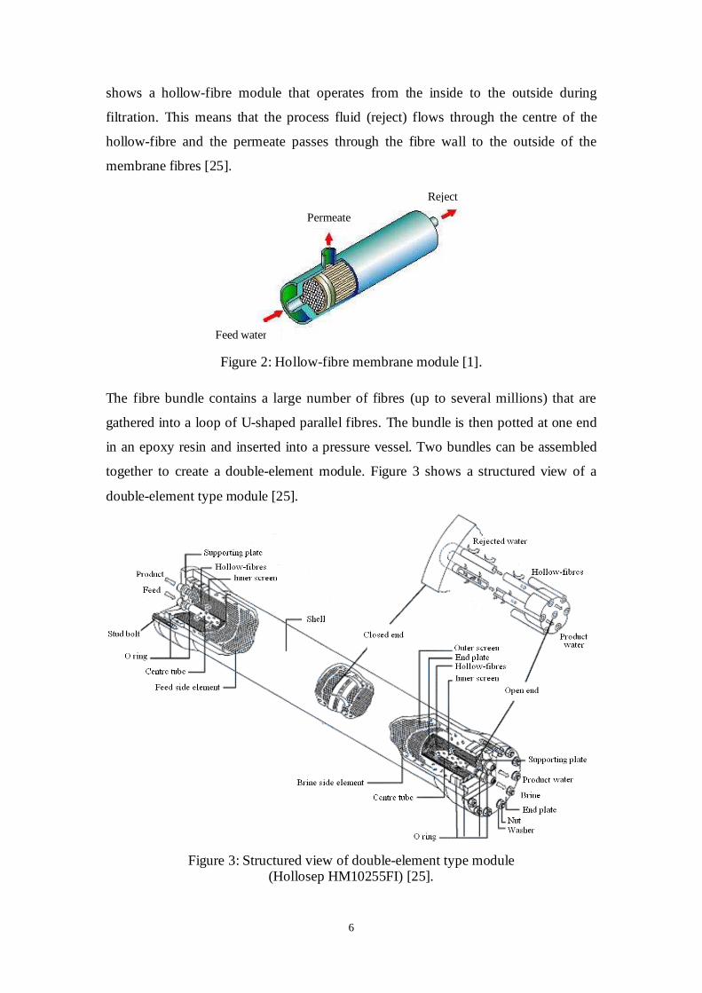
The fibre bundle contains a large number of fibres (up to several millions) that are
gathered into a loop of U-shaped parallel fibres. The bundle is then potted at one end
in an epoxy resin and inserted into a pressure vessel. Two bundles can be assembled
together to create a double-element module. Figure 3 shows a structured view of a
double-element type module [25].
Figure 3: Structured view of double-element type module (Hollosep HM10255FI) [25].
Reject
Permeate
Feed water
7
1.5 Objectives
The main objective of this study is the control and optimization of the hollow-fibre
spinning process, for the purpose of achieving the most suitable working conditions to
produce hollow-fibres with different diameter sizes and wall thicknesses. In order to
achieve this, the following were the specific objectives:
o Create a user friendly computer control system implementing LabView
software to fully control the hollow-fibre spinning process.
o Study the effect of the membrane fabrication parameters on the size
and performance of the hollow-fibres using factorial design.
o Create a model that can be used to predict the diameter size of the
hollow-fibres.
The first objective involved measuring, and then reading and importing the values of
the process parameters to the computer environment software (LabView). Having the
machine controlled with LabView computer software, by connecting all the
instruments with suitable data collection cards and transducers, permits carful
gathering of the required data to be controlled. The second objective involved
analyzing the acquired data in order to study the effects of the different process
variables and their significance on the geometry of the hollow-fibre by carrying out
series of experiments. The third objective involved creating a prediction model that is
used to optimize the spinning process for the most suitable working conditions in
order to produce hollow-fibres with an intended purpose.
The author acknowledges Tianjin Polytechnic, China, for building the spinning
apparatus that was subsequently used in this study.
1.6 Layout of document
Chapter 1 includes a brief introduction, and the objectives of the study.
Chapter 2 presents a background to techniques used in manufacturing hollow-
fibre membranes. A literature review of the effects of the various spinning parameters
on the membrane properties is included.
Chapter 3 describes the installation of the spinning apparatus used during the
study, and the running procedure. The materials used in this study and the procedures
8
followed to characterize the hollow-fibres are also presented. The design of
experiments is discussed in detail.
In Chapter 4 the implementation of the computer control system is described
in detail, and the user interface and the hardware and software used in this study are
discussed.
Chapter 5 presents the results of the factorial design that were conducted to
investigate the influence of the various fabrication parameters. The inside/outside
diameter and wall thickness of the fibres, fibre morphology, and mechanical strength
are reported on. Then the significances of the spinning factors are discussed in efforts
to determine the most favourable operation conditions.
Chapter 6 offers the conclusions drawn after conducting the factorial design of
experiments (DOE). It concludes with recommendations for improvement of the
spinning plant, and also fibre analysis.
Appendix A presents the SEM images of the fibres obtained from each
experiment. Appendix B presents the calculation and results of the DOE. Appendix C
includes investigation of the interaction between the factors. Appendix D lists the
results of the confirmation experiments. Appendix E includes the results of the tensile
tests. Appendix F includes fabrication settings for membrane samples and the results
of their flux performance.

CHAPTER 2
THEORETICAL BACKGROUND
10
CHAPTER 2: THEORETICAL BACKGROUND
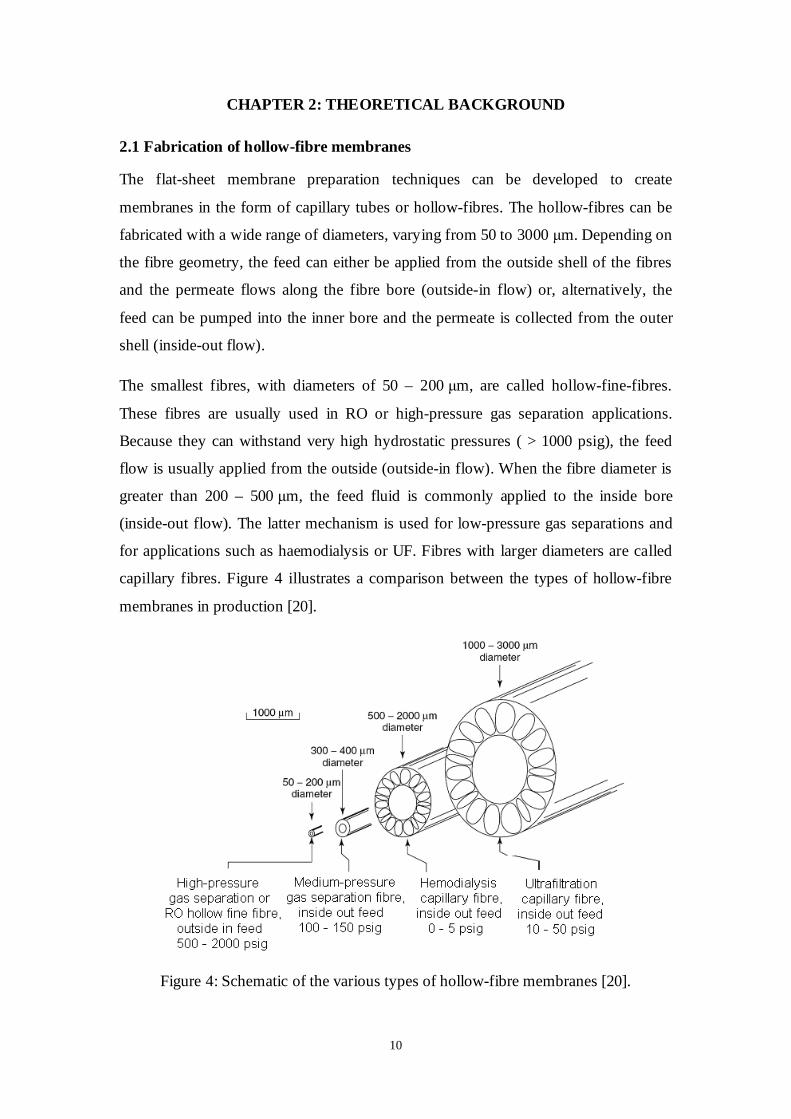
2.1 Fabrication of hollow-fibre membranes
The flat-sheet membrane preparation techniques can be developed to create
membranes in the form of capillary tubes or hollow-fibres. The hollow-fibres can be
fabricated with a wide range of diameters, varying from 50 to 3000 µm. Depending on
the fibre geometry, the feed can either be applied from the outside shell of the fibres
and the permeate flows along the fibre bore (outside-in flow) or, alternatively, the
feed can be pumped into the inner bore and the permeate is collected from the outer
shell (inside-out flow).
The smallest fibres, with diameters of 50 – 200 µm, are called hollow-fine-fibres.
These fibres are usually used in RO or high-pressure gas separation applications.
Because they can withstand very high hydrostatic pressures ( > 1000 psig), the feed
flow is usually applied from the outside (outside-in flow). When the fibre diameter is
greater than 200 – 500 µm, the feed fluid is commonly applied to the inside bore
(inside-out flow). The latter mechanism is used for low-pressure gas separations and
for applications such as haemodialysis or UF. Fibres with larger diameters are called
capillary fibres. Figure 4 illustrates a comparison between the types of hollow-fibre
membranes in production [20].
Figure 4: Schematic of the various types of hollow-fibre membranes [20].
11
There are several factors that contribute to a successful high-performance membrane
module. First, a suitable membrane material, with the appropriate chemical,
mechanical and subsequent permeation properties must be selected. There are several
other specific factors applicable for optimal membrane module performance, such as
operating temperature and pressure.
Most cellulosic and synthetic fibres are fabricated by “spinning”. This involves
pumping a thick viscous fluid through the tiny hole of an extruder “called a spinneret”
to form continuous filaments of semi-solid polymer [26].
The spinning solution is prepared by converting the fibre-forming polymer from its
solid state into a viscous fluid state. They must first be melted, if they are
thermoplastic syntactic that soften and melt when heated, or dissolved in a suitable
solvent, if they are non-thermoplastic [27].
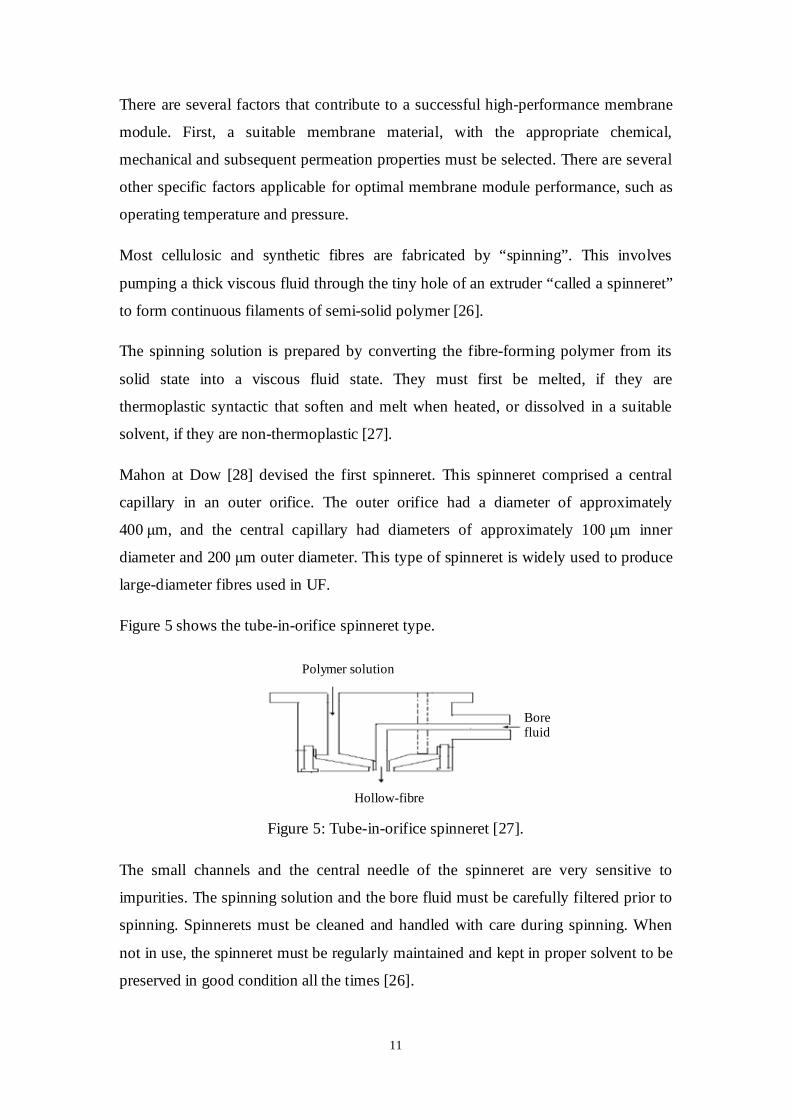
Mahon at Dow [28] devised the first spinneret. This spinneret comprised a central
capillary in an outer orifice. The outer orifice had a diameter of approximately
400 µm, and the central capillary had diameters of approximately 100 µm inner
diameter and 200 µm outer diameter. This type of spinneret is widely used to produce
large-diameter fibres used in UF.
Figure 5 shows the tube-in-orifice spinneret type.
Figure 5: Tube-in-orifice spinneret [27].
The small channels and the central needle of the spinneret are very sensitive to
impurities. The spinning solution and the bore fluid must be carefully filtered prior to
spinning. Spinnerets must be cleaned and handled with care during spinning. When
not in use, the spinneret must be regularly maintained and kept in proper solvent to be
preserved in good condition all the times [26].
Polymer solution
Bore fluid
Hollow-fibre
12
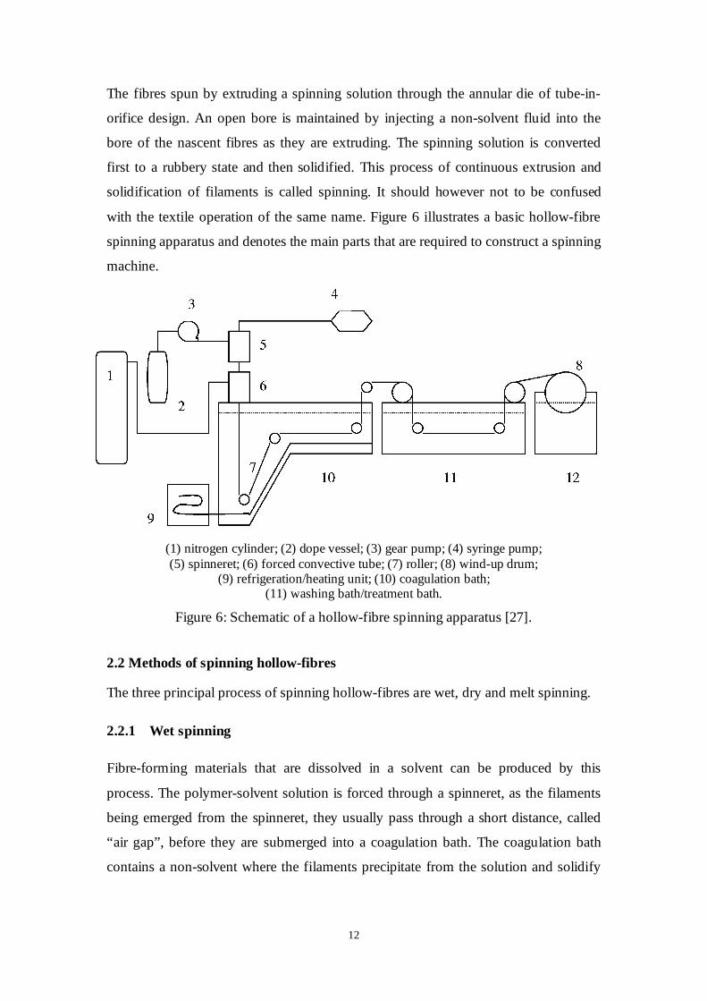
The fibres spun by extruding a spinning solution through the annular die of tube-in-
orifice design. An open bore is maintained by injecting a non-solvent fluid into the
bore of the nascent fibres as they are extruding. The spinning solution is converted
first to a rubbery state and then solidified. This process of continuous extrusion and
solidification of filaments is called spinning. It should however not to be confused
with the textile operation of the same name. Figure 6 illustrates a basic hollow-fibre
spinning apparatus and denotes the main parts that are required to construct a spinning
machine.
(1) nitrogen cylinder; (2) dope vessel; (3) gear pump; (4) syringe pump; (5) spinneret; (6) forced convective tube; (7) roller; (8) wind-up drum;
(9) refrigeration/heating unit; (10) coagulation bath; (11) washing bath/treatment bath.
Figure 6: Schematic of a hollow-fibre spinning apparatus [27].
2.2 Methods of spinning hollow-fibres
The three principal process of spinning hollow-fibres are wet, dry and melt spinning.
2.2.1 Wet spinning
Fibre-forming materials that are dissolved in a solvent can be produced by this
process. The polymer-solvent solution is forced through a spinneret, as the filaments
being emerged from the spinneret, they usually pass through a short distance, called
“air gap”, before they are submerged into a coagulation bath. The coagulation bath
contains a non-solvent where the filaments precipitate from the solution and solidify
13
[26]. Relatively large and porous haemodialysis and UF fibres are produced using this
process [20].
2.2.2 Dry spinning
Hollow-fibre can be produced from many common polymer materials, such as acetate,
triacetate, acrylic, polypropylene (PP) and spandex, by using the dry spinning process.
The solution is formed by dissolving the polymer in an appropriate solvent. As the hot
solution emerges from the spinneret the solvent starts to evaporate, solidification can
be enhanced by a stream of air. Draying is eliminated as there is no coagulation and
precipitation in the dry spinning process [26].
2.2.3 Melt spinning
In melt spinning the solid polymer used as a fibre-forming material is heated and
melted to form viscous liquid, for the purpose of pumping the melt through the
spinneret. Then the emerging filament starts to solidify as it comes in contact with
cold air without evaporation or precipitation of any solvent or other material. Nylon,
polyester and saran are produced in this manner [26].
Furthermore, better physical properties can be achieved by applying stretching while
the extruded fibres are in the process of solidifying or, in some cases, even after the
solidification. Stretching pulls the molecules and orients them in a more ordered
arrangement, reflecting considerably stronger fibres [26].
2.3 Spinning parameters
A large variety of membranes with different structures, properties, and hence
performance, can be obtained by varying the membrane material and conditions of
membrane preparation. All the interrelated factors pertaining to both membrane
material and preparation must be considered during the optimization of the hollow-
fibre spinning process.
2.3.1 Type of polymer
Membranes can be made from a wide and ever increasing range of polymers. Many
different polymers have been used (and investigated) in the processes of dry-wet and
melt spinning, e.g. PES [29] and Polyvinylidene Fluoride (PVDF) [30]. Some other
14
possible choices for the ultra-filtration membranes are Polysulfone (PS),
Polyethersulfone (PES), Polyvinylidene Fluoride (PVDF) [31] and Polyacryl Nitrile
(PAN) [31-34]. Wang spun PS hollow-fibres for UF using 3-C shaped spinnerets [35].
Hao et. al. used the same type of spinneret to spin CA for ultra-low-pressure RO
membranes [36].
2.3.2 Types of solvents and additives in polymer solution
For any particular polymer, one or more solvents may be suitable to create the
spinning solution. It must be taken into consideration that both the solvent and
nonsolvent must be completely miscible with each other to ensure that the polymer
solution remains in a uniform and stable state.
The addition of a nonsolvent to a polymer solution may positively or negatively affect
the formation of the dense skin layer of the subsequent hollow-fibre. For example,
during the drying process in the dry-wet phase inversion process, the local polymer
concentration increases due to the evaporation of the solvent and/or additive from the
surface layer of the fibre. If the boiling point of the solvent is higher than that of the
additive then the local solvating power will increase as a result of rapid vaporization
of the nonsolvent additive. As a result, a membrane with a dense, thick skin layer will
be formed. Conversely, a faster loss of solvent molecules from the surface tends to
result in the formation of a thin, porous skin layer [37].
The rates of evaporation of the additives depend on their volatilities as well as
temperature of the polymer solution and the atmospheric condition. Some additives,
such as ethanol, methanol, propanol, butanol, pentanol, ethylene glycol, diethelyene
glycol, have good volatility, and are completely miscible with water and N,N-
dimethylacetamide (DMAc). Their use has been systematically investigated by a
number of authors [38-40]. Other low molecular weight nonsolvents like water,
ethylene glycol and diethylene glycol, have also been widely used [37, 40-42].
Yeow et al. [31] have compared the morphology of PVDF membranes cast with four
different solvents that have been reported to be good solvents for PVDF namely,
DMAc, N,N-dimethylformamide (DMF), 1-methyl-2-pyrrolidone (NMP), and triethyl
phosphate (TEP). They mainly focused on the resulting membrane morphology by
comparing the effects of the use of different additives (ethanol, glycerol, LiCl,
15
LiClO4, and water) in the PVDF/DMAc system, at different dope temperatures.
Moreover, Yeow [43] reported that an increase in the quantity of the additive LiClO4
in a polymer dope increases the membrane’s mean pore size. Wienk et al. [29]
reported on the use of the hydrophilic polymer polyvinyl pyrrolidone (PVP) as an
additive in the membrane forming polymer solution of PES.
In general, adding high molecular weight additives such as PVP, PEG and
polyethylene oxide (PEO) has been reported to favour the formation of hollow-fibre
macrovoids in the membranes [44-46]. The addition of these additives results in an
increase in the solution viscosity, which increases with an increase in the additive
molecular mass. The use of high molecular weight hydrophilic polymers such as PVP
and PEO also results in an increase in permeability of the resultant membranes [29].
The addition of LiCl has been reported to reduce the mechanical strength of the fibre,
although, it does enhance the permeation performance [47, 48]. However, Wang et al.
[39] managed to retain membrane mechanical strength by cointroducing 1-propanol.
Because of its good water affinity, the presence of LiCl tends to encourage water
inflow and enhance the coagulation rate, therefore, yielding stronger membranes.
2.3.3 Dope solution extrusion rate
The dope extrusion rate is one of the most important factors that must be considered
during spinning of hollow-fibre membranes, due to its contribution to the structure of
these membranes. Idris et al. [27] studied the effect of varying the extrusion rate by
setting the extrusion rate to two levels: 2.5 mL/min as the lower level limit and
4.0 mL/min as the upper limit. They found that the bore fluid properties and the dope
extrusion rate have the most significant influence on the performance of the
membrane.
Puri [49] has reported the importance of fine-tuning the rheological properties of a
spinning dope, in terms of spinnability and membrane performance. Spinnability
relates to the stability of the filament during spinning and to the consistency of the
product. By comparing membranes produced at different extrusion rates for each trial,
but using the same bore fluid, it is observed that rejection rates of the membrane is
changed after changing the extrusion rate.
16
2.3.4 Air gap condition (length, humidity, pressure, temperature)
The air gap condition also has a significant influence on the membrane morphology
and performance. This topic has been widely studied. Chung and Hu [50] found that
an increase in air gap distance results in a hollow-fibre with a thinner layer of finger-
like voids and a significantly lower permeance in the case of PES hollow-fibre
membranes. Miao et al. [51] claimed that by spinning fibres from an air gap distance
of 14.4 cm to 16.1 cm, the hollow-fibres will not have a ring of finger-like structure
close to the outer skin due to the effect of moisture-induced phase-separation and
stress-induced orientation.
Chau et al. [52] found that an optimum PS UF membrane could be made using an air
gap of 7 cm. Using an air gap of 13 cm, Ismail et al. [53] managed to produce super-
selective PS hollow-fibres for gas separation. In general, increasing the length of the
air gap will result in a longer time that the fibres are exposed to the ambient
conditions, which will allow adequate skin formation The exposure time should
however not be too long as the mechanical properties and performance of the
membranes are adversely affected when the evaporation period is too long. According
to Sharpe et al. [54] the residence time (RT) in a forced convection air gap chamber
can be approximately determined by dividing the air gap height by the fibre velocity:
v
HRT = (1)
where:
RT: the residence time (sec)
H: air gap height (m)
v: fibre velocity (m/s).
The fibre velocity is calculated by dividing the solution extrusion rate by the cross-
sectional area of the spinneret annulus:
( )22
4
IDOD
DERv
−=
π (2)
where:
DER: dope extrusion rate
OD and ID: the outer and inner diameters of the spinneret annulus,
respectively.
17
However, this is only true if hollow-fibres are not drawn to their final dimensions.
Sharpe et al. [54] increased the selectivity and decreased the flux of membranes by
increasing the RT from 0.237 to 0.426 s as the skin matures and forms properly.
Generally, at low residence time, skin formation tends to be incomplete.
It should however be noted that the spinning velocity is not an independent variable
because, due to the effect of the gravity forces in the air gap, stretching of the
spinning solution will take place [29]. The influence of gravity force on the fibre
becomes significant when the length of the air gap is large and when the viscosity of
the dope solution is low. Wienk et al. [29] have shown that when the length of the air
gap increases, the diameter of the fibre decreases. Also, if the length of the air gap is
large, the take-up speed of the fibre has to be high to keep up with the extruded fibre.
2.3.5 Take-up speed
Strict control of the fibre wall properties, such as porosity and asymmetry, requires
the spinning of hollow-fibre membranes at relatively slow spinning speeds. For
instance, PP hollow-fibres can be spun with take-up speeds as low as 76.6 cm/min
[55], whereas Kim et al. [56] wet-spun hollow-fibres at speeds of only 10 – 35 m/min.
The spinning rate, in addition to the following cold drawing, significantly influences
the properties of the fibres. Usually, high-performance fibres can be obtained by
increasing both crystallinity and orientation. The morphological transformations and
chain-orientation procedures cause the high modulus and tensile strength of semi-
crystalline commercial synthetic fibres. For example, spinning polyester at about
3000 m/min and then off-line drawing at a draw ratio of about 2:1 will produce as
high a strength as if it was spun at about 6000 m/min [57].
2.3.6 Coagulation bath temperature
The coagulation bath temperature, together with the air gap length, has a significant
influence on the molecular weight cut-off (MWCO) of UF membranes, and hence on
membrane performance. Yeow [43] studied the effects of coagulation bath
temperature on the resulting membrane permeation properties and pore size
distribution. Results revealed that an increase in coagulation temperature is
advantageous in producing membranes with higher permeation rates. Such
18
membranes also exhibited a greater mean pore radius compared to those produced at
lower coagulation temperatures.
Generally, if the temperature of the water bath is high then the diffusion coefficients
will be high, which will allow faster growth of nuclei. Therefore, pore sizes are
expected to be larger at a higher temperature [29].
2.3.7 Bore type
The bore fluid (also called core fluid) is another factor that affects the quality of
hollow-fibre membranes. The selected bore fluid must provide a highly open lumen
on the inside of the hollow-fibres without affecting the phase separation processes
occurring at the outside surface [58]. The bore fluid undoubtedly alters the
morphological structure near the inner diameter of the hollow-fibres. In other words,
the morphology near the inner fibre diameter depends on the bore fluid type.
Idris [27], selected and compared two types of bore fluids, pure water and a 20 wt%
potassium acetate solution, and found water to be the better bore fluid. Ismail [59] has
shown that good results for PS membranes were achieved by using 20 wt% potassium
acetate solution. Cabasso et al. [60] produced good PS RO membranes by using
DMAc:H2O 3:1 as a bore fluid. For CA membranes, Shieh and Chung [61] reported
that the use of water and a mixture of 1:4 water/NMP as the bore fluid to be the better
coagulant [27].
2.3.8 Viscosity of the spinning solution
It has been found that solution viscosity is one of the most important parameters in
hollow-fibre fabrication [7, 8, 10, 12, 13, 60, 62-64]. Increasing or decreasing the
spinning solution viscosity directly influences its spinability and the subsequent
morphological structure of the fibre, and hence the hollow-fibre’s performance and
properties.
An increase in polymer concentration in the spinning solution will obviously increase
its viscosity, whereas an increase in solvent percentage in the spinning solution will
cause a decrease in its viscosity [65]. On the one hand, when spinning at low solution
viscosity, the inner bore of filaments will be too small or difficult to form, and the
hollow-fibre will collapse under the action of surface tension forces, and in the other
19
hand, spinning high viscosity solution will hinder the nonsolvent penetration during
the immersion step, and hence the formation of cavities in the membrane. The nascent
fibres will suffer from twisting deformation and breakage when extruded through the
spinneret [66].
Friedrich et al. [15] proved that the occurrence of cavities in the hollow-fibres is
enhanced by changing the solvent type to reduce the solution viscosity, for PVDF
polymer solutions of equal concentration. Jae-Jin Kim et al. [67] melt spun fibres at
temperatures above 458 K and found that, due to the low solution viscosity the fibre
melt could not maintain its hollow form, and collapsed. They concluded that when
spinning hollow-fibres at lower temperatures the resulting structures will be more
oriented than when spun at higher temperatures. That occurs because the viscosity of
polymer melt solution increases when the temperature decreased, and therefore, the
stress increases as the polymer solution passes through the spinneret holes.
2.3.9 Type of spinneret
The spinnerets used in the production of most manufactured fibres may have several
hundred of holes, to overcome the low productivity of one orifice, especially in the
dry-wet spinning method. The multihole spinnerets of a tube-in-orifice type require a
high degree of design precision and can most easily cause eccentricity. The delivery
of identical volumes of the spinning solution to each orifice is another problem that
may be encountered.
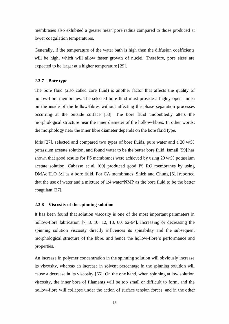
Figure 7 shows a cross-sectional view of a 3C-shaped spinneret.
Figure 7: Cross sectional view of a 3-C shaped spinneret.
The spinning solution is extruded through the three holes in the spinneret and it
rapidly coalesces to complete the circular shape of the hollow-fibre. There is no need
20
for bore fluid injection to create the core, because the air is drawn through the
unwelded gaps before the solution coalesces. Contrary to the tube-in-orifice spinneret
type, a hollow-fibre spun using the 3C-shaped spinneret is not eccentric. Although it
is easy to machine this type of spinneret, it does require highly accurate design
precision and machining [36].
Wang [35] used 3C-shaped orifices to spin PS hollow-fibre membranes for UF. Hao
et al. [36] reported the results of their studies on the spinning of CA for ultra low-
pressure RO hollow-fibre membranes spun by the dry-wet technique and elaborated
on the variable parameters involved in the spinning process.
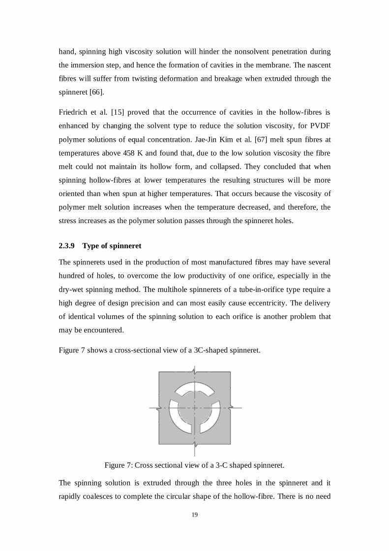
The triple-orifice spinneret is another spinneret type designed to produce double-
layered hollow-fibres, see Figure 8. This spinneret type was first described by Kusuki
et al. at Ube [68], and Kopp et al. at Memtec [69]. When spinning with this type of
spinneret, two casting solutions can be tailored together by adjusting the ratio of the
inner/outer extrusion rate. Using this type of spinneret it is possible to create hollow-
fibre membranes with respective outer and inner layers of various thicknesses.
Figure 8: Triple-orifice spinneret [69].
Zhang et al. [37] used the dry-wet process to produce asymmetric PS hollow-fibre
membranes by co-extrusion through a triple-orifice spinneret. The fabrication
conditions, water permeability and the morphological structure of the hollow-fibre
membranes were investigated. The hollow-fibres had a dense outer skin layer but a
more porous inner layer.
Bore fluid
Outer layer dope
Inner layer dope
Inner layer dope
21
2.4 Characterization of hollow-fibres
2.4.1 Membrane morphology
There are a few techniques that are used to determine the morphology of hollow-
fibres. The simplest type of microscopy is optical microscopy (OM), which uses
visible light and a system of lenses to magnify images of small samples. There are
other microscopy techniques with exponentially greater magnifications than OM. A
scanning electron microscope (SEM) produces high-resolution images of a sample
surface with a three-dimensional appearance, and is useful for determining the surface
structure of a membrane sample. Many researches have carried out investigations of
membrane structures using SEM techniques [27, 30, 36, 37, 42, 45, 48, 61, 70-78].
2.4.2 Hollow-fibre diameters and hollowness
The hollowness of the hollow-fibre is the ratio between the inner and the outer
diameters of the hollow-fibre, which can be defined as:
h = ID2/OD2 (3)
where:
h: the hollowness
ID: final (product) inside diameter
OD: final (product) outside diameter.
The value of h variable represents the ratio of the area of the hole to the total area of
the fibre [57], hence, h ranges from 0 for solid fibres to 1 for hollow-fibres with an
infinitely thin wall.
The polymer cost and the membrane performance are directly proportional to the
cross sectional area of the hollow-fibres, (i.e. proportional to 1 – h).
De Rovere et al. [18] showed how the ratio ID/OD is affected by the bore flow rate.
According to their results, there is only a small decrease in compression resistance
and a small increase in elastic loss as hollowness increases.
The ID and OD of PP hollow-fibres can be predicted by using the continuity
equations of the polymer dope solution and bore fluid fabricated by melt spinning
[18]. Regarding the wall thickness, Ekiner and Vassilatos [79] recommend that the
22
value for the outer diameter to inner diameter ratio should be 2. It is to be noted that
the flux across the membrane is inversely proportional to the wall thickness of the
fibres, which means that a thin fibre wall is favourable, as far as the resistance to burst
is achieved since the burst pressure depends on the ratio of the inside diameter to the
outside diameter [80].
2.4.3 Membrane performance
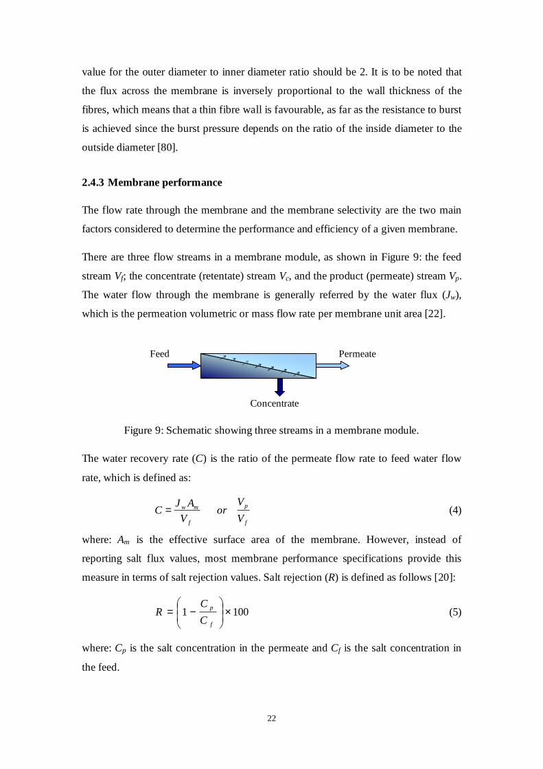
The flow rate through the membrane and the membrane selectivity are the two main
factors considered to determine the performance and efficiency of a given membrane.
There are three flow streams in a membrane module, as shown in Figure 9: the feed
stream Vf; the concentrate (retentate) stream Vc, and the product (permeate) stream Vp.
The water flow through the membrane is generally referred by the water flux (Jw),
which is the permeation volumetric or mass flow rate per membrane unit area [22].
Figure 9: Schematic showing three streams in a membrane module.
The water recovery rate (C) is the ratio of the permeate flow rate to feed water flow
rate, which is defined as:
f
p
f
mw
V
Vor
V
AJC = (4)
where: Am is the effective surface area of the membrane. However, instead of
reporting salt flux values, most membrane performance specifications provide this
measure in terms of salt rejection values. Salt rejection (R) is defined as follows [20]:
1001 ×
−=
f
p
C
CR (5)
where: Cp is the salt concentration in the permeate and Cf is the salt concentration in
the feed.
Permeate Feed
Concentrate
23
2.5 Commercial hollow-fibre manufacturers
Commencing in the late 1950s, at the Dow Chemical Company, Mahon and co-
workers in the United States investigated the spinning of fine CA fibres with a low
water flux (0.35 – 0.68 lmh) [28]. The later commercialization by Dow, Monsanto,
Du Pont, and others, represents one of the major events in membrane separation
technology.
Thereafter, the Permasep HF from DuPont company was a leading product, until
HOLLOSEP (Toyobo, Japan) became the only alternative for the direct replacement
of Permasep [81]. Toyobo’s CTA hollow-fibre membranes for brackish water and sea
water treatment have diameters of 160 µm and 163 µm, respectively. Sekino et al.
[82] have described the uses of these hollow-fibre membranes.
Many other manufacturers are now developing and producing commercial hollow-
fibre membranes for a wide range of separation operations and filtration purposes.
Toray is currently working on technology for the design and manufacture of large-size
(20 cmΦ × 2 m) MF modules installed with hollow-fibre PVDF membranes. They are
also manufacturing UF modules installed with hollow-fibre PAN membranes, and
actively developing drinking water production membrane processes [34].
MOTIMO manufactures modules of hollow-fibre UF and MF membranes [33].
Although they use range of materials, including PS, PES and PAN, MOTIMO's
particular technical advantage lies with the development of their PVDF modules.
Mitsubishi [83] produces hollow-fibre membranes with pores size of 0.1 µm for water
purification, using the melt spinning and drawing processes.
The Asahi Corporation’s UF hollow-fibre membrane consists of a tough, smooth,
double-skinned fibre, with a dense internal layer. The UF membrane is manufactured
with a uniformly tight skin on both the inside and outside of the fibre. Both skins of
the membrane have the same MWCO [84].
A good review of the early development of hollow-fibre membranes is given by Baum
et al.[85]. More recent developments are reviewed by Moch [86] and McKelvey et
al. [87].

24
2.6 Computer control of the hollow-fibre fabrication apparatus
The availability of user-friendly graphical programming languages has increased
rapidly over the last few years. Such languages allow rapid program development by
utilizing computers. The use of computers for acquiring and analyzing data and for
instrumentation control has also increased rapidly.
Optimization and control of the spinning process requires feedback information,
ideally provided in real time operation. It is essential that the entire spinning machine
be made computer controlled, as precise setting of the extrusion pump heating and
take-up speed, etc. is required in order to achieve a controlled spinning operation. The
powerful LabVIEW graphical programming environment was developed primarily to
offer good synchronized control and data acquisition for the entire system. It can be
adapted to a wide range of instrumentation control and optimization applications that
facilitate good instrumentation control and monitoring on the various instrumentation
of the spinning machine. Many authors have implemented the LabVIEW control
systems to control, analyze and optimize various processes [88-90].
CHAPTER 3
EXPERIMENTAL APPARATUS AND
PROCEDURES
26
CHAPTER 3: EXPERIMENTAL APPARATUS AND PROCEDURES
3.1 Description of the experimental apparatus
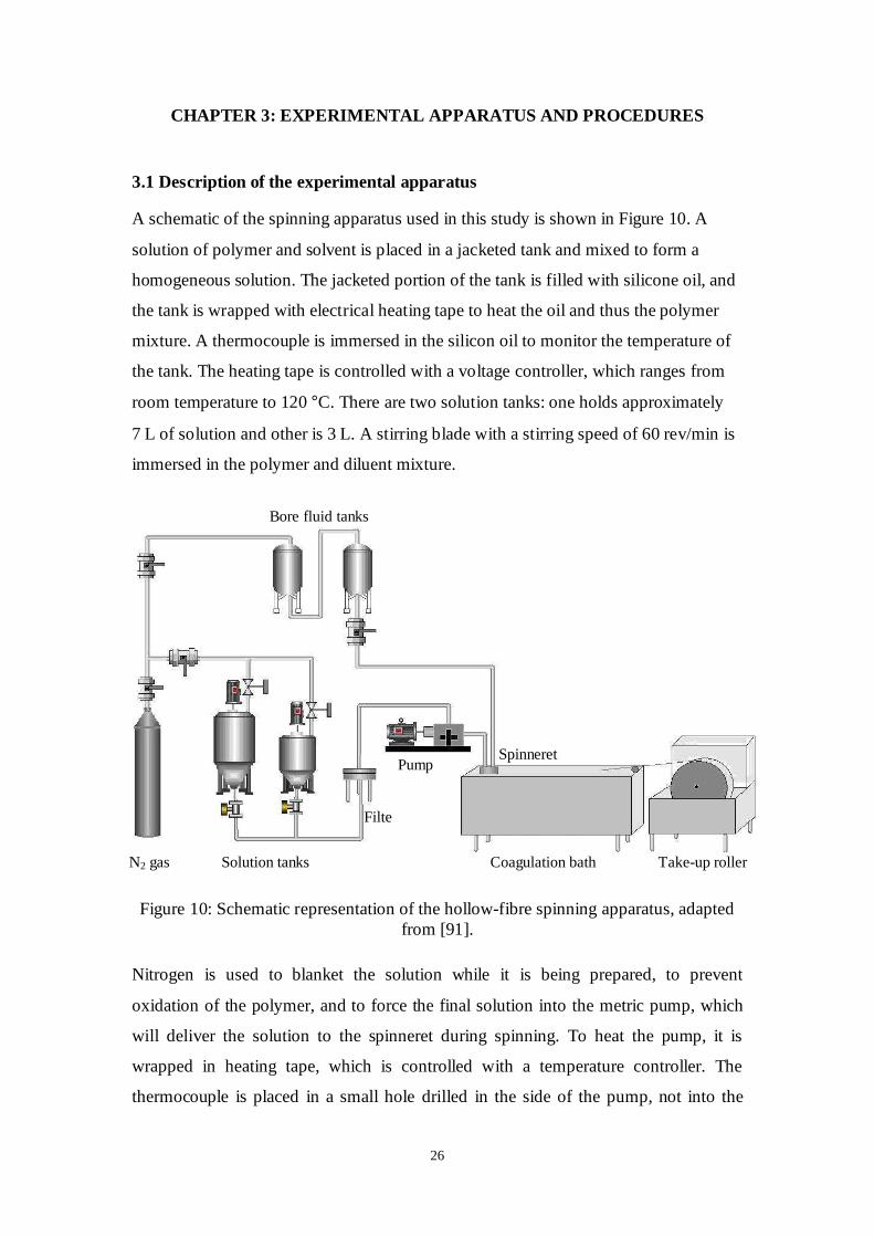
A schematic of the spinning apparatus used in this study is shown in Figure 10. A
solution of polymer and solvent is placed in a jacketed tank and mixed to form a
homogeneous solution. The jacketed portion of the tank is filled with silicone oil, and
the tank is wrapped with electrical heating tape to heat the oil and thus the polymer
mixture. A thermocouple is immersed in the silicon oil to monitor the temperature of
the tank. The heating tape is controlled with a voltage controller, which ranges from
room temperature to 120 °C. There are two solution tanks: one holds approximately
7 L of solution and other is 3 L. A stirring blade with a stirring speed of 60 rev/min is
immersed in the polymer and diluent mixture.
Figure 10: Schematic representation of the hollow-fibre spinning apparatus, adapted from [91].
Nitrogen is used to blanket the solution while it is being prepared, to prevent
oxidation of the polymer, and to force the final solution into the metric pump, which
will deliver the solution to the spinneret during spinning. To heat the pump, it is
wrapped in heating tape, which is controlled with a temperature controller. The
thermocouple is placed in a small hole drilled in the side of the pump, not into the
Take-up roller
Bore fluid tanks
Solution tanks
Pump
Filter
N2 gas Coagulation bath
Spinneret
27
flow channel. The capacity of the pump is 1.2 mL/revolution. The pump speed control
ranges from 9 to 20 rev/min. The spinneret is shown in Figure 5. The fibre spinning
velocity range from approximately 1 to 15 m/min, it is generally 5 m/min.
Before the spinning solution reaches the pump it flows through a 70 µm mesh filter of
100 mm diameter. Another thermocouple monitors the temperature of the filter. The
heating of the filter is controlled by a voltage controller. The heating temperature
ranges from room temperature to 120 °C.
The spinneret is attached to the pump outlet with a short length of 8 inch OD tubing.
The spinneret is heated with a separate piece of heating tape, and the thermocouple for
the spinneret is placed in a hole drilled in the side of the spinneret near the bottom,
where the fibre exits. The encapsulated air gap space has a temperature control, which
ranges from room temperature to 60 °C, and an inlet and outlet for gas or humidity
control. The bore fluid is drawn from two tanks connected in series, with a total
capacity of 12 L. The flow is controlled by a low mass flow controller (ABB,
Germany). The mass flow controller has a range of 2 – 100 mL/min. The bore fluid
tank is wrapped with electrical heating tape. A thermocouple is attached to the tank to
monitor the temperature of the tank, and the heating is controlled with a voltage
controller, ranging from room temperature to 60 °C. Nitrogen gas is delivered to the
first tank from an inlet lid, and controlled by a pressure gauge. The nitrogen is used to
push the bore fluid into the spinneret. The valve underneath the tank is open only
during spinning.
The water coagulation bath is 2.4 m long and 1 m deep. The bath height can be
adjusted with a crank. The water bath can be heated by a heating coil installed at the
bottom of the bath; there are three heating pipes with a power of 7000 watt each. The
bath can be heated from room temperature to 60 °C in one hour, and will remain at
that temperature for at least 30 minutes. The bath temperature is monitored by a
thermocouple immersed in the water.
The take-up winder has a diameter of 390 mm. It is controlled by a speed controller
that varies between 20 and 40 rev/min. The linear take-up velocity ranges from
approximately 1 to 35 m/min. A full layout of the spinning machine that was used in
this study is shown in Figure 11.
28
Figure 11: Hollow-fibre spinning machine as used in this study.
29
3.2 Installing the membrane fabrication plant
As part of this project, the spinning apparatus was first designed, built and
commissioned in China. Figure 12 shows a photograph for the spinning plant at the
first operation after the installation in Tianjin, China. Then the plant was delivered to
South Africa. A laboratory was prepared in the Polymer Science department of
Stellenbosch University to accommodate the plant. Once the machine was delivered
to the laboratory, it was reassembled and installed, and its instruments were connected
to the computer control system.
Figure 12: Photograph for the spinning plant at the first operation after the installation in Tianjin, China.
3.3 Materials and methods
3.3.1 Materials
The polymer used in this study was Polysulfone Udel-3500 (in powder form), which
was purchased from Solvay Chemicals. N-methyl-2-pyrrolidone (NMP) solvent was
obtained from Kimix, South Africa. RO water was used as the bore fluid.
30
Before starting the experiments, the pump was calibrated by setting the pump control
dial at a certain level using the programmed LabView control software, counting the
revolutions per minute of the outer pump gear, and measuring the output flow volume
over a certain period of time.
3.3.2 Dry/wet solution spinning procedure
A 5 L dope solution of 18:82 PS:NMP is placed in the tank and mixed into a
homogeneous solution for 12 hours at 80 °C. The solution is then degassed by leaving
it overnight at 60 °C. The mixer and the tank temperature are controlled by the
LabView software.
The bore fluid tank is filled with 12 L of RO water, and heated to the desired
temperature. The pump, filter, spinneret and the coagulation bath are also heated by
setting the temperature in the LabView software to the desired experiment settings.
Once the solution is prepared and degassed, and the set temperatures are reached, the
spinning process can commence. Nitrogen gas is pumped to the bore and the solution
tanks at 2 bar. The valve underneath the solution tank is opened and the solution is
drained from the tank into the metering pump.
The valve underneath the bore fluid tank is also opened to allow the bore fluid to be
delivered to the spinneret’s inner needle, forced by the nitrogen pressure. The pressure
of nitrogen gas is controlled by a needle valve and monitored by the LabView using a
pressure gauge. A nitrogen pressure of 2.5 bar was used.
The spinning of hollow-fibre is started by setting the knob of the metric pump at the
desired dope extrusion rate; the metric pump pushes the spinning solution through the
70 µm mesh filter and delivers it to the spinneret. Dope extrusion rate (DER) ranges
of 4 to 9 mL/min were used.
The hollow-fibre filaments then begin to extrude from the spinneret, passing the air
gape zone and entering the coagulation bath. The filaments start to float on the surface
of the water, so they are held under the water by three pulleys submerged in the bath,
keeping 3.1 m of the hollow-fibre length under the water.
31
The take-up winder (diameter of 390 mm) is started, by adjusting its speed knob on
the LabView. The winder and has its own bath to keep the fabricated hollow-fibre wet
during the spinning process. The fibre bundles are removed from the winder drum by
cutting all the fibres. The bundle length will be approximately equal to the winder’s
circumference (1.22 m).
3.3.3 Hollow-fibre post-processing
After conducting each fabrication run a batch of hollow fibres is taken from the take-
up drum and placed in a water bath overnight to extract the solvent. To complete the
extraction the batches are then placed in horizontal glass cylinders full of methanol
(99%). These cylinders are 15 cm in diameter, and specially designed to store the
fibres. To ensure complete extraction, the methanol had to be changed at least three
times, and allowing eight hours for the methanol solvent exchange each time.
3.4 Characterization of membrane samples
3.4.1 SEM imaging and analysis
On completion of the extraction, small samples of hollow fibres (about 2 mm in
length) were taken from each batch and immediately immersed in liquid nitrogen.
After about 40 seconds they were removed and carefully fractured, to get clean cross-
sections. The samples then were allowed to warm to room temperature and the
methanol content evaporated. The samples were left to dry overnight to ensure
complete evaporation of the methanol content prior to SEM analysis. Four samples
were taken from each hollow-fibre sample.
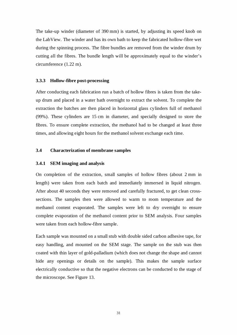
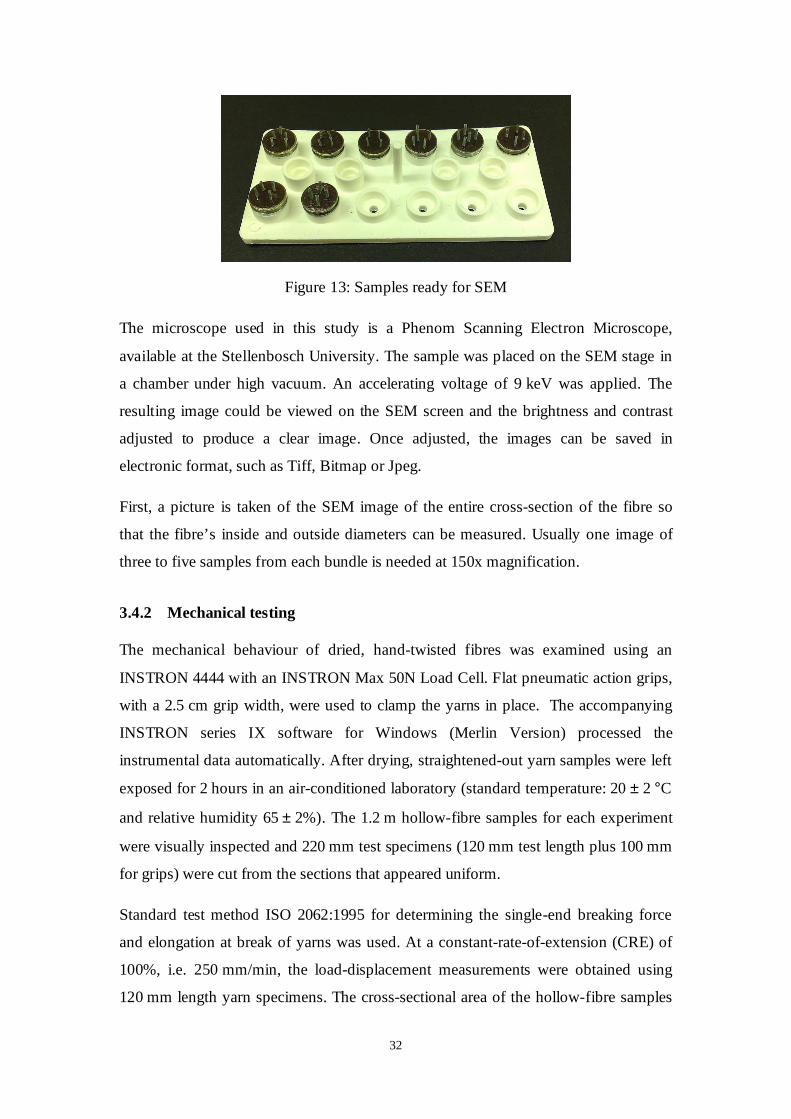
Each sample was mounted on a small stub with double sided carbon adhesive tape, for
easy handling, and mounted on the SEM stage. The sample on the stub was then
coated with thin layer of gold-palladium (which does not change the shape and cannot
hide any openings or details on the sample). This makes the sample surface
electrically conductive so that the negative electrons can be conducted to the stage of
the microscope. See Figure 13.
32
Figure 13: Samples ready for SEM
The microscope used in this study is a Phenom Scanning Electron Microscope,
available at the Stellenbosch University. The sample was placed on the SEM stage in
a chamber under high vacuum. An accelerating voltage of 9 keV was applied. The
resulting image could be viewed on the SEM screen and the brightness and contrast
adjusted to produce a clear image. Once adjusted, the images can be saved in
electronic format, such as Tiff, Bitmap or Jpeg.
First, a picture is taken of the SEM image of the entire cross-section of the fibre so
that the fibre’s inside and outside diameters can be measured. Usually one image of
three to five samples from each bundle is needed at 150x magnification.
3.4.2 Mechanical testing
The mechanical behaviour of dried, hand-twisted fibres was examined using an
INSTRON 4444 with an INSTRON Max 50N Load Cell. Flat pneumatic action grips,
with a 2.5 cm grip width, were used to clamp the yarns in place. The accompanying
INSTRON series IX software for Windows (Merlin Version) processed the
instrumental data automatically. After drying, straightened-out yarn samples were left
exposed for 2 hours in an air-conditioned laboratory (standard temperature: 20 ± 2 °C
and relative humidity 65 ± 2%). The 1.2 m hollow-fibre samples for each experiment
were visually inspected and 220 mm test specimens (120 mm test length plus 100 mm
for grips) were cut from the sections that appeared uniform.
Standard test method ISO 2062:1995 for determining the single-end breaking force
and elongation at break of yarns was used. At a constant-rate-of-extension (CRE) of
100%, i.e. 250 mm/min, the load-displacement measurements were obtained using
120 mm length yarn specimens. The cross-sectional area of the hollow-fibre samples
33
was calculated from the SEM images. Careful attention was paid to minimize
stretching of the fibre before testing and while placing the sample in the grips. The
test conditions were as follows:
Number of test specimens: 5 per sample
Sample length between the grips: 120 mm
Cross-head speed: 2 cm/min.
Percentage elongation and tensile strength at break were automatically calculated by
the computerized Instron for each of the samples according to the following
equations.
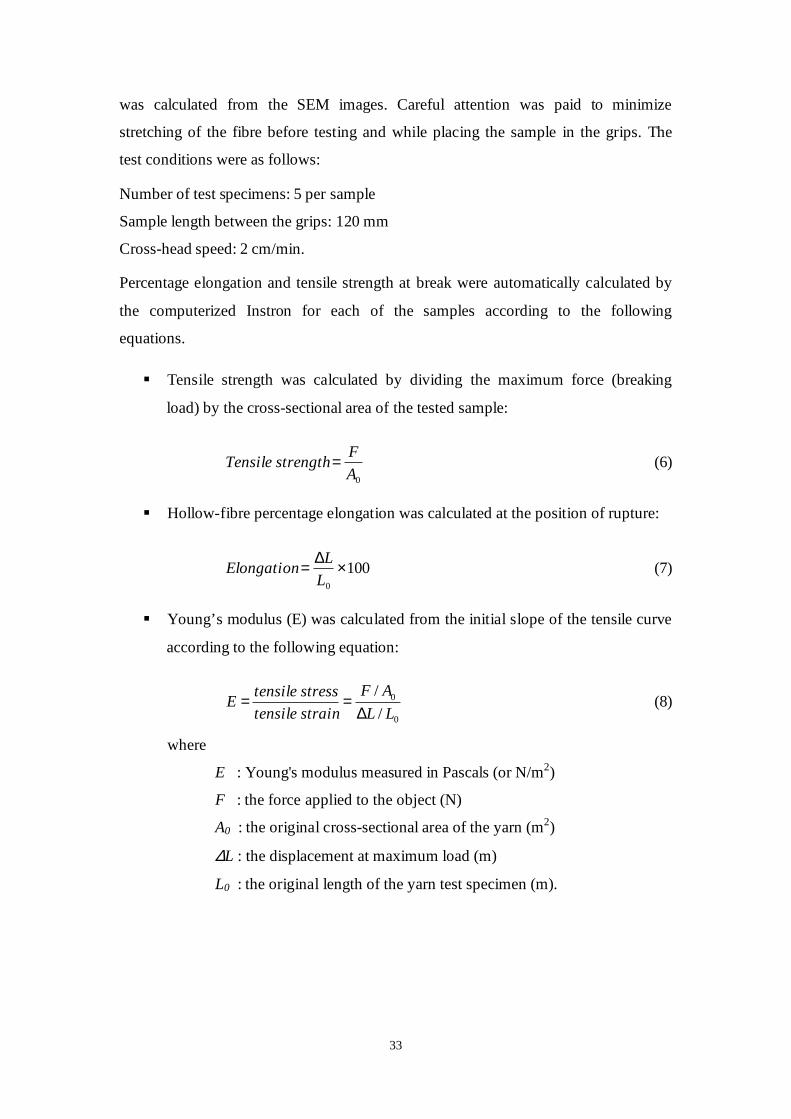
Tensile strength was calculated by dividing the maximum force (breaking
load) by the cross-sectional area of the tested sample:
0A
FstrengthTensile = (6)
Hollow-fibre percentage elongation was calculated at the position of rupture:
1000
×∆=L
LElongation (7)
Young’s modulus (E) was calculated from the initial slope of the tensile curve
according to the following equation:
0
0
/
/
LL
AF
straintensile
stresstensileE
∆== (8)
where
E : Young's modulus measured in Pascals (or N/m2)
F : the force applied to the object (N)
A0 : the original cross-sectional area of the yarn (m2)
∆L : the displacement at maximum load (m)
L0 : the original length of the yarn test specimen (m).
34
3.5 Design and planning of experiments
3.5.1 Design of experiments using the Taguchi method
This section describes the orthogonal array (OA) based on Taguchi’s method that was
used to study the effects of the operation parameters on the fibre diameter, wall
thickness and strength. Taguchi techniques, developed by Taguchi and Konishi [92],
are utilized widely in engineering analysis to optimize performance characteristics
within a combination of design parameters.
The Taguchi method is a tool for systematic experimental design that uses an OA in
which effects of several factors are studied efficiently and simultaneously, by running
tests at various levels of the factors. Taguchi has developed a number of orthogonal
arrays to perform the experiment design. Each array can be used to suit certain
experimental situations, and the choice of an array depends on the number of factors
to be investigated and number of levels for each factor. The results can be analyzed by
a standard method that he devised. [93].
Utilizing the orthogonal array described by Taguchi’s approach, and determining the
effects of the various factors by computing simple averages, offers simplicity of data
analysis. Combining this analysis method offered by Taguchi and the traditional
experimental design techniques produces consistency and reproducibility, which is
difficult to find in other statistical methods [27, 52]. Based on this OA, Taguchi’s
technique employs a special design to examine all the parameters with a small number
of experiments only, which leads to a reduction in the number of experiments and
may decrease the time and cost involved.
Taguchi experimentation results are primarily used to search for the optimum
fabrication conditions, find the factors that contribute to the results and their
significance, and predict the factor values at the optimum fabrication condition.
Taguchi introduced the use of the signal-to-noise (S/N) ratio approach to identify the
quality characteristics for the response. The S/N ratio characteristics are classified into
three types: the smaller-the-better, the nominal-the-best, and the larger-the-better.
[94]. In this study, the smaller-the-better for the S/N quality characteristic was chosen
to study the diameter size problem, as the purpose is to reduce the diameter size.
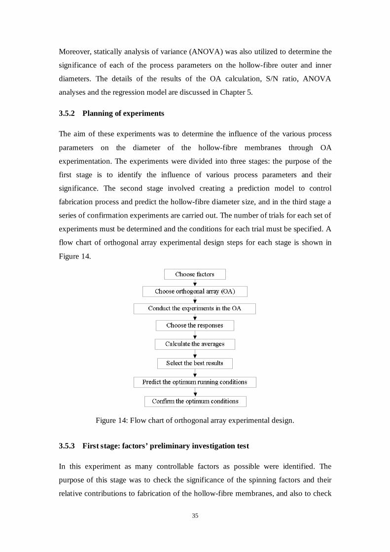
35
Moreover, statically analysis of variance (ANOVA) was also utilized to determine the
significance of each of the process parameters on the hollow-fibre outer and inner
diameters. The details of the results of the OA calculation, S/N ratio, ANOVA
analyses and the regression model are discussed in Chapter 5.
3.5.2 Planning of experiments
The aim of these experiments was to determine the influence of the various process
parameters on the diameter of the hollow-fibre membranes through OA
experimentation. The experiments were divided into three stages: the purpose of the
first stage is to identify the influence of various process parameters and their
significance. The second stage involved creating a prediction model to control
fabrication process and predict the hollow-fibre diameter size, and in the third stage a
series of confirmation experiments are carried out. The number of trials for each set of
experiments must be determined and the conditions for each trial must be specified. A
flow chart of orthogonal array experimental design steps for each stage is shown in
Figure 14.
Figure 14: Flow chart of orthogonal array experimental design.
3.5.3 First stage: factors’ preliminary investigation test
In this experiment as many controllable factors as possible were identified. The
purpose of this stage was to check the significance of the spinning factors and their
relative contributions to fabrication of the hollow-fibre membranes, and also to check
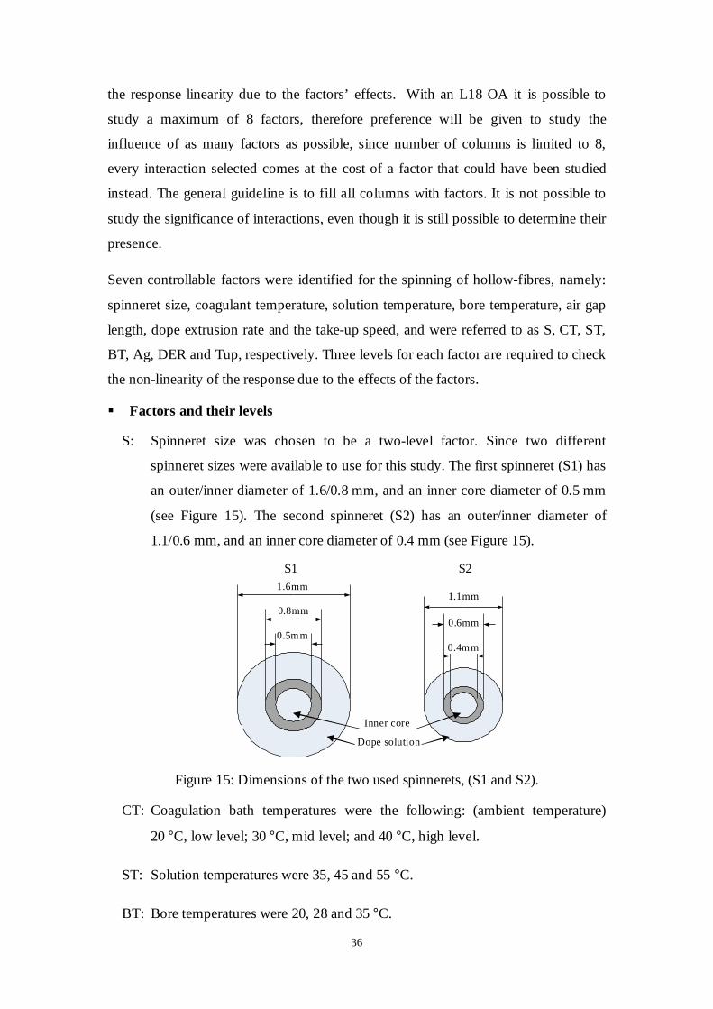
36
the response linearity due to the factors’ effects. With an L18 OA it is possible to
study a maximum of 8 factors, therefore preference will be given to study the
influence of as many factors as possible, since number of columns is limited to 8,
every interaction selected comes at the cost of a factor that could have been studied
instead. The general guideline is to fill all columns with factors. It is not possible to
study the significance of interactions, even though it is still possible to determine their
presence.
Seven controllable factors were identified for the spinning of hollow-fibres, namely:
spinneret size, coagulant temperature, solution temperature, bore temperature, air gap
length, dope extrusion rate and the take-up speed, and were referred to as S, CT, ST,
BT, Ag, DER and Tup, respectively. Three levels for each factor are required to check
the non-linearity of the response due to the effects of the factors.
Factors and their levels
S: Spinneret size was chosen to be a two-level factor. Since two different
spinneret sizes were available to use for this study. The first spinneret (S1) has
an outer/inner diameter of 1.6/0.8 mm, and an inner core diameter of 0.5 mm
(see Figure 15). The second spinneret (S2) has an outer/inner diameter of
1.1/0.6 mm, and an inner core diameter of 0.4 mm (see Figure 15).
Figure 15: Dimensions of the two used spinnerets, (S1 and S2).
CT: Coagulation bath temperatures were the following: (ambient temperature)
20 °C, low level; 30 °C, mid level; and 40 °C, high level.
ST: Solution temperatures were 35, 45 and 55 °C.
BT: Bore temperatures were 20, 28 and 35 °C.
0.5mm
0.8mm
1.6mm1.1mm
0.6mm
0.4mm
Inner core
Dope solution
S1 S2
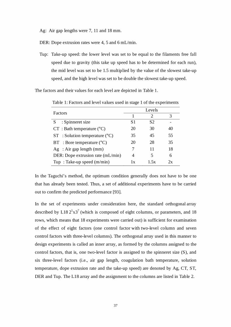
37
Ag: Air gap lengths were 7, 11 and 18 mm.
DER: Dope extrusion rates were 4, 5 and 6 mL/min.
Tup: Take-up speed: the lower level was set to be equal to the filaments free fall
speed due to gravity (this take up speed has to be determined for each run),
the mid level was set to be 1.5 multiplied by the value of the slowest take-up
speed, and the high level was set to be double the slowest take-up speed.
The factors and their values for each level are depicted in Table 1.
Table 1: Factors and level values used in stage 1 of the experiments
Levels Factors
1 2 3 S : Spinneret size S1 S2 -
CT : Bath temperature (°C) 20 30 40
ST : Solution temperature (°C) 35 45 55
BT : Bore temperature (°C) 20 28 35
Ag : Air gap length (mm) 7 11 18 DER: Dope extrusion rate (mL/min) 4 5 6
Tup : Take-up speed (m/min) 1x 1.5x 2x
In the Taguchi’s method, the optimum condition generally does not have to be one
that has already been tested. Thus, a set of additional experiments have to be carried
out to confirm the predicted performance [93].
In the set of experiments under consideration here, the standard orthogonal array
described by L18 21x37 (which is composed of eight columns, or parameters, and 18
rows, which means that 18 experiments were carried out) is sufficient for examination
of the effect of eight factors (one control factor with two-level column and seven
control factors with three-level columns). The orthogonal array used in this manner to
design experiments is called an inner array, as formed by the columns assigned to the
control factors, that is, one two-level factor is assigned to the spinneret size (S), and
six three-level factors (i.e., air gap length, coagulation bath temperature, solution
temperature, dope extrusion rate and the take-up speed) are denoted by Ag, CT, ST,
DER and Tup. The L18 array and the assignment to the columns are listed in Table 2.
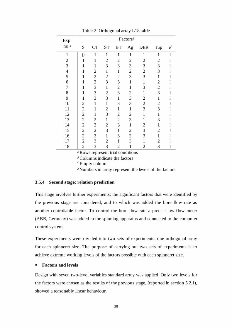
38
Table 2: Orthogonal array L18 table
Factorsb Exp. no.a S CT ST BT Ag DER Tup ec
1 1d 1 1 1 1 1 1 1 2 1 1 2 2 2 2 2 2 3 1 1 3 3 3 3 3 3 4 1 2 1 1 2 2 3 3 5 1 2 2 2 3 3 1 1 6 1 2 3 3 1 1 2 2 7 1 3 1 2 1 3 2 3 8 1 3 2 3 2 1 3 1 9 1 3 3 1 3 2 1 2 10 2 1 1 3 3 2 2 1 11 2 1 2 1 1 3 3 2 12 2 1 3 2 2 1 1 3 13 2 2 1 2 3 1 3 2 14 2 2 2 3 1 2 1 3 15 2 2 3 1 2 3 2 1 16 2 3 1 3 2 3 1 2 17 2 3 2 1 3 1 2 3 18 2 3 3 2 1 2 3 1
a Rows represent trial conditions b Columns indicate the factors c Empty column d Numbers in array represent the levels of the factors
3.5.4 Second stage: relation prediction
This stage involves further experiments; the significant factors that were identified by
the previous stage are considered, and to which was added the bore flow rate as
another controllable factor. To control the bore flow rate a precise low-flow meter
(ABB, Germany) was added to the spinning apparatus and connected to the computer
control system.
These experiments were divided into two sets of experiments: one orthogonal array
for each spinneret size. The purpose of carrying out two sets of experiments is to
achieve extreme working levels of the factors possible with each spinneret size.
Factors and levels
Design with seven two-level variables standard array was applied. Only two levels for
the factors were chosen as the results of the previous stage, (reported in section 5.2.1),
showed a reasonably linear behaviour.
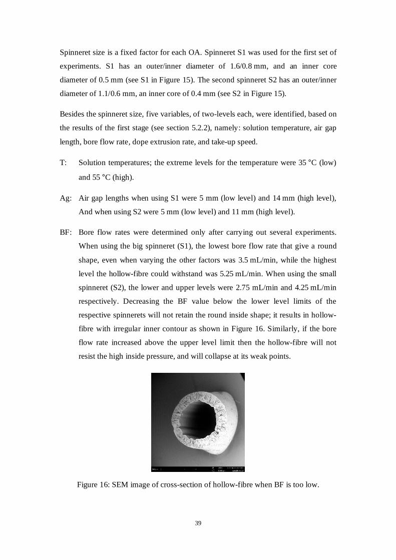
39
Spinneret size is a fixed factor for each OA. Spinneret S1 was used for the first set of
experiments. S1 has an outer/inner diameter of 1.6/0.8 mm, and an inner core
diameter of 0.5 mm (see S1 in Figure 15). The second spinneret S2 has an outer/inner
diameter of 1.1/0.6 mm, an inner core of 0.4 mm (see S2 in Figure 15).
Besides the spinneret size, five variables, of two-levels each, were identified, based on
the results of the first stage (see section 5.2.2), namely: solution temperature, air gap
length, bore flow rate, dope extrusion rate, and take-up speed.
T: Solution temperatures; the extreme levels for the temperature were 35 °C (low)
and 55 °C (high).
Ag: Air gap lengths when using S1 were 5 mm (low level) and 14 mm (high level),
And when using S2 were 5 mm (low level) and 11 mm (high level).
BF: Bore flow rates were determined only after carrying out several experiments.
When using the big spinneret (S1), the lowest bore flow rate that give a round
shape, even when varying the other factors was 3.5 mL/min, while the highest
level the hollow-fibre could withstand was 5.25 mL/min. When using the small
spinneret (S2), the lower and upper levels were 2.75 mL/min and 4.25 mL/min
respectively. Decreasing the BF value below the lower level limits of the
respective spinnerets will not retain the round inside shape; it results in hollow-
fibre with irregular inner contour as shown in Figure 16. Similarly, if the bore
flow rate increased above the upper level limit then the hollow-fibre will not
resist the high inside pressure, and will collapse at its weak points.
Figure 16: SEM image of cross-section of hollow-fibre when BF is too low.
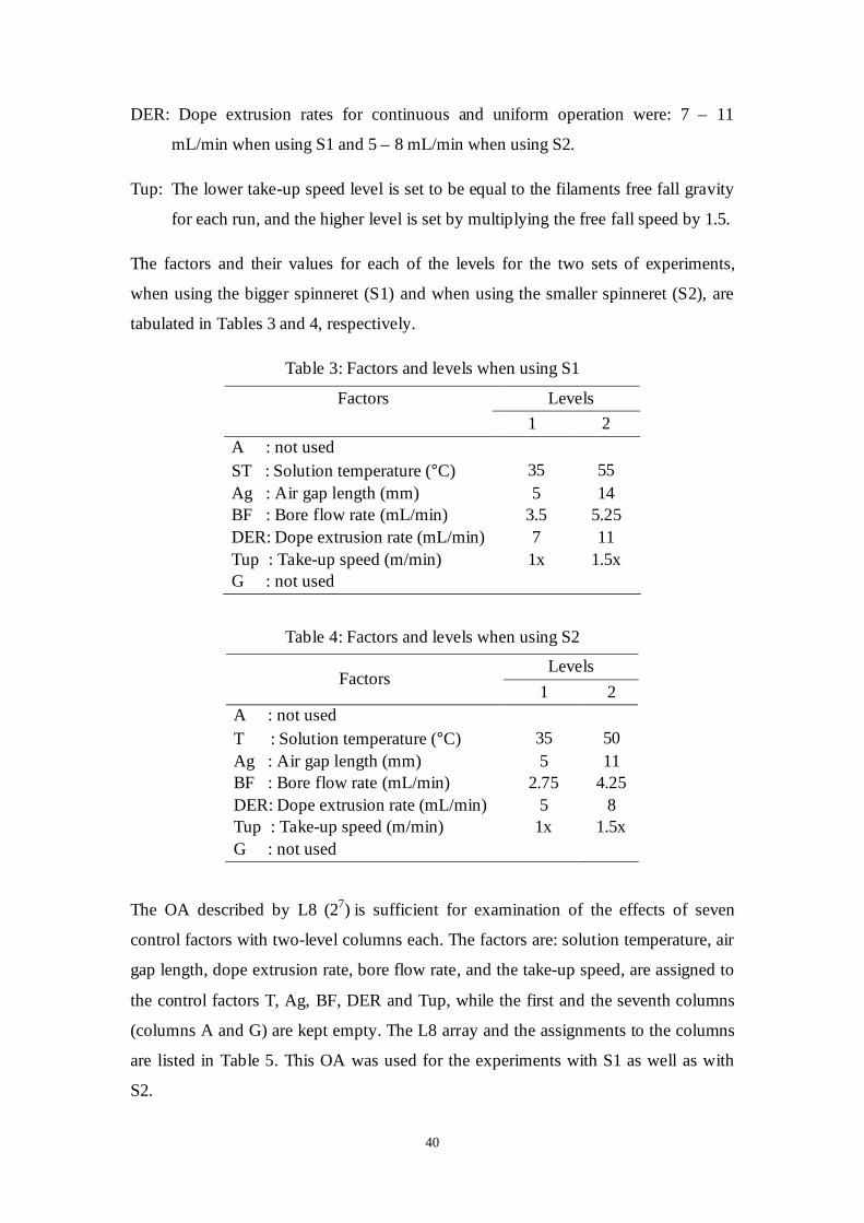
40
DER: Dope extrusion rates for continuous and uniform operation were: 7 – 11
mL/min when using S1 and 5 – 8 mL/min when using S2.
Tup: The lower take-up speed level is set to be equal to the filaments free fall gravity
for each run, and the higher level is set by multiplying the free fall speed by 1.5.
The factors and their values for each of the levels for the two sets of experiments,
when using the bigger spinneret (S1) and when using the smaller spinneret (S2), are
tabulated in Tables 3 and 4, respectively.
Table 3: Factors and levels when using S1
Factors Levels
1 2 A : not used ST : Solution temperature (°C) 35 55 Ag : Air gap length (mm) 5 14 BF : Bore flow rate (mL/min) 3.5 5.25 DER: Dope extrusion rate (mL/min) 7 11 Tup : Take-up speed (m/min) 1x 1.5x G : not used
Table 4: Factors and levels when using S2
Levels Factors
1 2 A : not used T : Solution temperature (°C) 35 50 Ag : Air gap length (mm) 5 11 BF : Bore flow rate (mL/min) 2.75 4.25 DER: Dope extrusion rate (mL/min) 5 8 Tup : Take-up speed (m/min) 1x 1.5x G : not used
The OA described by L8 (27) is sufficient for examination of the effects of seven
control factors with two-level columns each. The factors are: solution temperature, air
gap length, dope extrusion rate, bore flow rate, and the take-up speed, are assigned to
the control factors T, Ag, BF, DER and Tup, while the first and the seventh columns
(columns A and G) are kept empty. The L8 array and the assignments to the columns
are listed in Table 5. This OA was used for the experiments with S1 as well as with
S2.
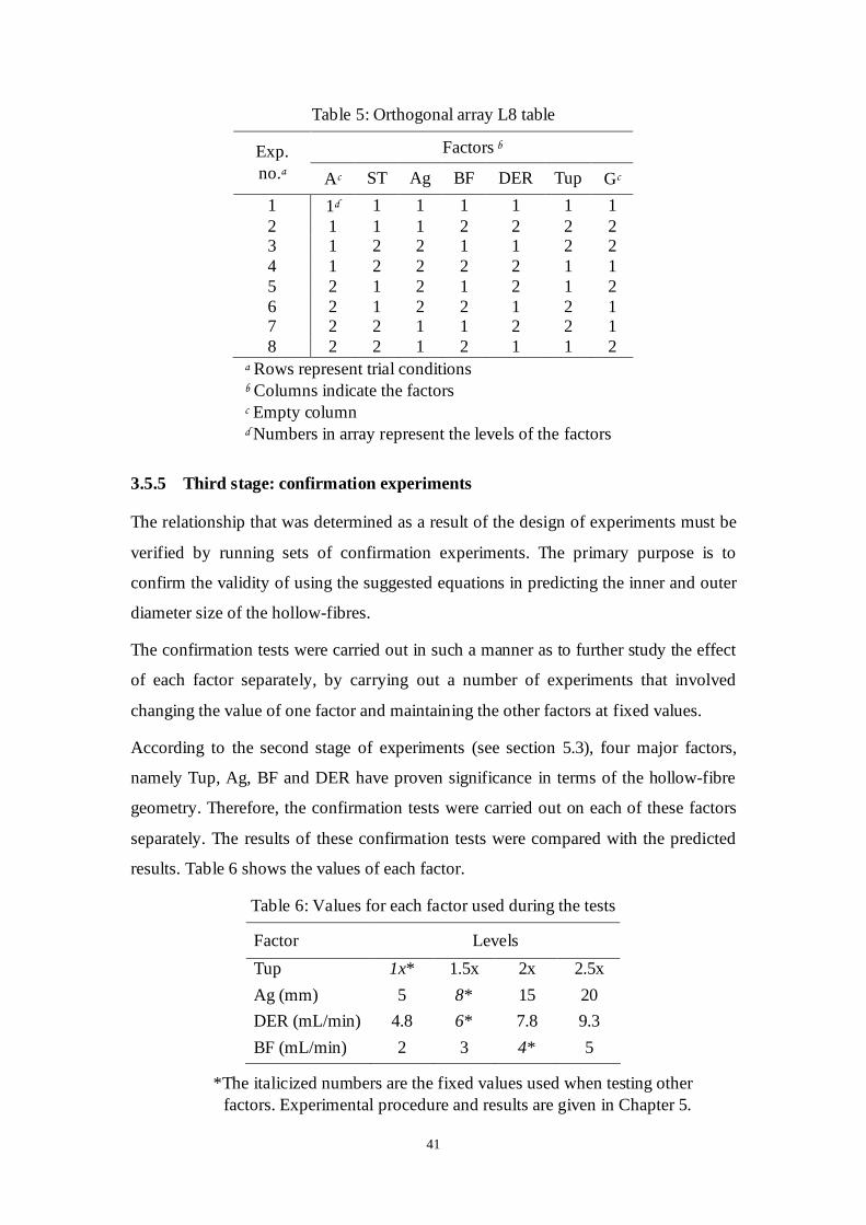
41
Table 5: Orthogonal array L8 table
Factors b Exp. no.a Ac ST Ag BF DER Tup Gc
1 1d 1 1 1 1 1 1 2 1 1 1 2 2 2 2 3 1 2 2 1 1 2 2 4 1 2 2 2 2 1 1 5 2 1 2 1 2 1 2 6 2 1 2 2 1 2 1 7 2 2 1 1 2 2 1 8 2 2 1 2 1 1 2
a Rows represent trial conditions b Columns indicate the factors c Empty column d Numbers in array represent the levels of the factors
3.5.5 Third stage: confirmation experiments
The relationship that was determined as a result of the design of experiments must be
verified by running sets of confirmation experiments. The primary purpose is to
confirm the validity of using the suggested equations in predicting the inner and outer
diameter size of the hollow-fibres.
The confirmation tests were carried out in such a manner as to further study the effect
of each factor separately, by carrying out a number of experiments that involved
changing the value of one factor and maintaining the other factors at fixed values.
According to the second stage of experiments (see section 5.3), four major factors,
namely Tup, Ag, BF and DER have proven significance in terms of the hollow-fibre
geometry. Therefore, the confirmation tests were carried out on each of these factors
separately. The results of these confirmation tests were compared with the predicted
results. Table 6 shows the values of each factor.
Table 6: Values for each factor used during the tests
Factor Levels
Tup 1x* 1.5x 2x 2.5x
Ag (mm) 5 8* 15 20
DER (mL/min) 4.8 6* 7.8 9.3
BF (mL/min) 2 3 4* 5
*The italicized numbers are the fixed values used when testing other factors. Experimental procedure and results are given in Chapter 5.
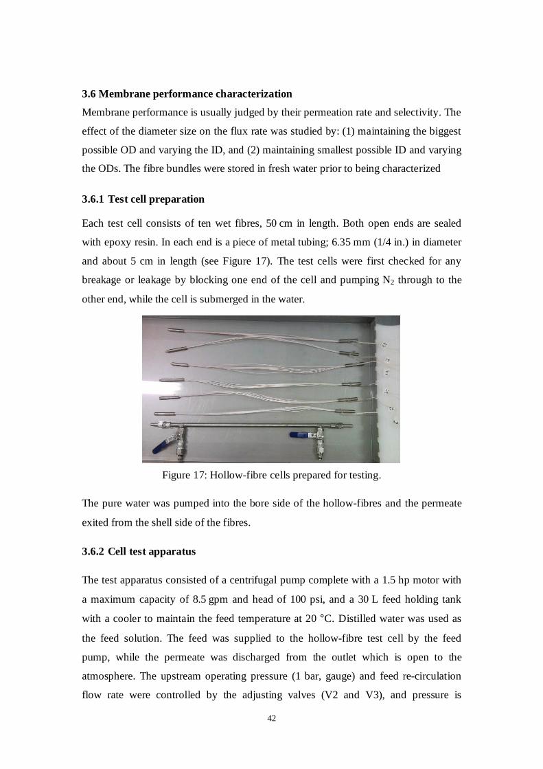
42
3.6 Membrane performance characterization
Membrane performance is usually judged by their permeation rate and selectivity. The
effect of the diameter size on the flux rate was studied by: (1) maintaining the biggest
possible OD and varying the ID, and (2) maintaining smallest possible ID and varying
the ODs. The fibre bundles were stored in fresh water prior to being characterized
3.6.1 Test cell preparation
Each test cell consists of ten wet fibres, 50 cm in length. Both open ends are sealed
with epoxy resin. In each end is a piece of metal tubing; 6.35 mm (1/4 in.) in diameter
and about 5 cm in length (see Figure 17). The test cells were first checked for any
breakage or leakage by blocking one end of the cell and pumping N2 through to the
other end, while the cell is submerged in the water.
Figure 17: Hollow-fibre cells prepared for testing.
The pure water was pumped into the bore side of the hollow-fibres and the permeate
exited from the shell side of the fibres.
3.6.2 Cell test apparatus
The test apparatus consisted of a centrifugal pump complete with a 1.5 hp motor with
a maximum capacity of 8.5 gpm and head of 100 psi, and a 30 L feed holding tank
with a cooler to maintain the feed temperature at 20 °C. Distilled water was used as
the feed solution. The feed was supplied to the hollow-fibre test cell by the feed
pump, while the permeate was discharged from the outlet which is open to the
atmosphere. The upstream operating pressure (1 bar, gauge) and feed re-circulation
flow rate were controlled by the adjusting valves (V2 and V3), and pressure is
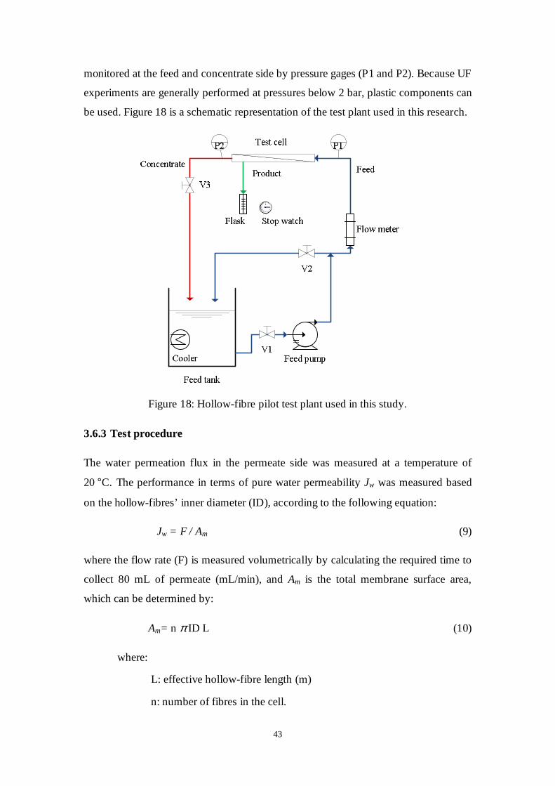
43
monitored at the feed and concentrate side by pressure gages (P1 and P2). Because UF
experiments are generally performed at pressures below 2 bar, plastic components can
be used. Figure 18 is a schematic representation of the test plant used in this research.
Figure 18: Hollow-fibre pilot test plant used in this study.
3.6.3 Test procedure
The water permeation flux in the permeate side was measured at a temperature of
20 °C. The performance in terms of pure water permeability Jw was measured based
on the hollow-fibres’ inner diameter (ID), according to the following equation:
Jw = F / Am (9)
where the flow rate (F) is measured volumetrically by calculating the required time to
collect 80 mL of permeate (mL/min), and Am is the total membrane surface area,
which can be determined by:
Am= n π ID L (10)
where:
L: effective hollow-fibre length (m)
n: number of fibres in the cell.

CHAPTER 4
COMPUTER CONTROL SYSTEM
(LABVIEW IMPLEMENTATION)
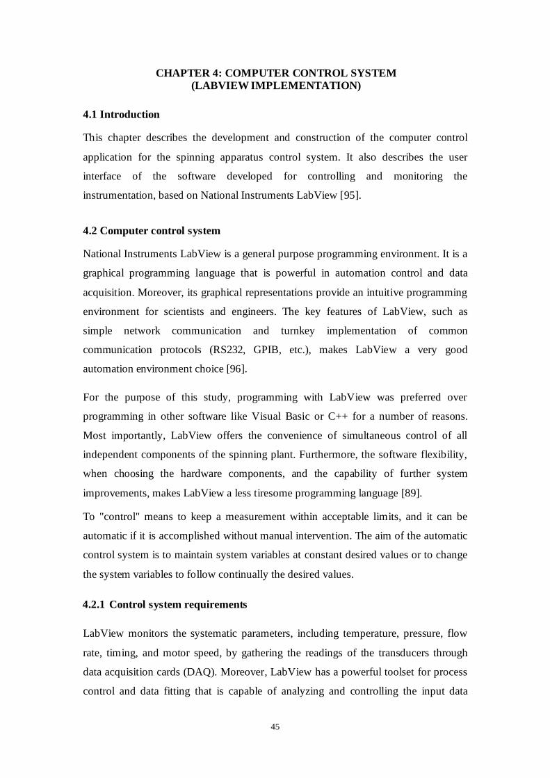
45
CHAPTER 4: COMPUTER CONTROL SYSTEM (LABVIEW IMPLEMENTATION)
4.1 Introduction
This chapter describes the development and construction of the computer control
application for the spinning apparatus control system. It also describes the user
interface of the software developed for controlling and monitoring the
instrumentation, based on National Instruments LabView [95].
4.2 Computer control system
National Instruments LabView is a general purpose programming environment. It is a
graphical programming language that is powerful in automation control and data
acquisition. Moreover, its graphical representations provide an intuitive programming
environment for scientists and engineers. The key features of LabView, such as
simple network communication and turnkey implementation of common
communication protocols (RS232, GPIB, etc.), makes LabView a very good
automation environment choice [96].
For the purpose of this study, programming with LabView was preferred over
programming in other software like Visual Basic or C++ for a number of reasons.
Most importantly, LabView offers the convenience of simultaneous control of all
independent components of the spinning plant. Furthermore, the software flexibility,
when choosing the hardware components, and the capability of further system
improvements, makes LabView a less tiresome programming language [89].
To "control" means to keep a measurement within acceptable limits, and it can be
automatic if it is accomplished without manual intervention. The aim of the automatic
control system is to maintain system variables at constant desired values or to change
the system variables to follow continually the desired values.
4.2.1 Control system requirements
LabView monitors the systematic parameters, including temperature, pressure, flow
rate, timing, and motor speed, by gathering the readings of the transducers through
data acquisition cards (DAQ). Moreover, LabView has a powerful toolset for process
control and data fitting that is capable of analyzing and controlling the input data
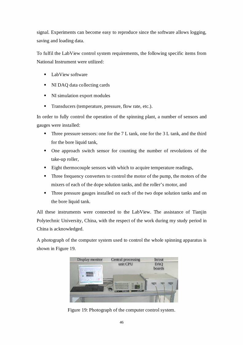
46
signal. Experiments can become easy to reproduce since the software allows logging,
saving and loading data.
To fulfil the LabView control system requirements, the following specific items from
National Instrument were utilized:
LabView software
NI DAQ data collecting cards
NI simulation export modules
Transducers (temperature, pressure, flow rate, etc.).
In order to fully control the operation of the spinning plant, a number of sensors and
gauges were installed:
Three pressure sensors: one for the 7 L tank, one for the 3 L tank, and the third
for the bore liquid tank,
One approach switch sensor for counting the number of revolutions of the
take-up roller,
Eight thermocouple sensors with which to acquire temperature readings,
Three frequency converters to control the motor of the pump, the motors of the
mixers of each of the dope solution tanks, and the roller’s motor, and
Three pressure gauges installed on each of the two dope solution tanks and on
the bore liquid tank.
All these instruments were connected to the LabView. The assistance of Tianjin
Polytechnic University, China, with the respect of the work during my study period in
China is acknowledged.
A photograph of the computer system used to control the whole spinning apparatus is
shown in Figure 19.
Figure 19: Photograph of the computer control system.
Display monitor Central processing unit CPU
In/out DAQ
boards
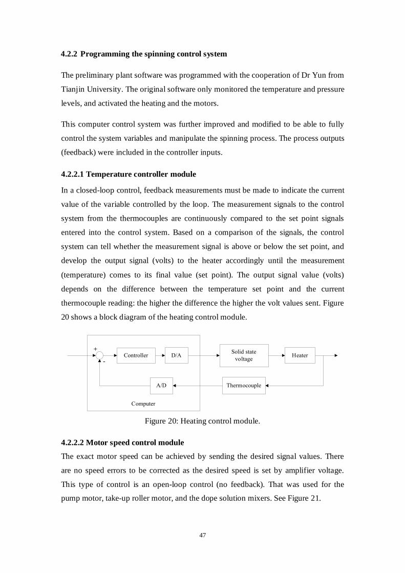
47
4.2.2 Programming the spinning control system
The preliminary plant software was programmed with the cooperation of Dr Yun from
Tianjin University. The original software only monitored the temperature and pressure
levels, and activated the heating and the motors.
This computer control system was further improved and modified to be able to fully
control the system variables and manipulate the spinning process. The process outputs
(feedback) were included in the controller inputs.
4.2.2.1 Temperature controller module
In a closed-loop control, feedback measurements must be made to indicate the current
value of the variable controlled by the loop. The measurement signals to the control
system from the thermocouples are continuously compared to the set point signals
entered into the control system. Based on a comparison of the signals, the control
system can tell whether the measurement signal is above or below the set point, and
develop the output signal (volts) to the heater accordingly until the measurement
(temperature) comes to its final value (set point). The output signal value (volts)
depends on the difference between the temperature set point and the current
thermocouple reading: the higher the difference the higher the volt values sent. Figure
20 shows a block diagram of the heating control module.
Computer
Controller D/ASolid state
voltageHeater
Thermocouple A/D
Figure 20: Heating control module.
4.2.2.2 Motor speed control module
The exact motor speed can be achieved by sending the desired signal values. There
are no speed errors to be corrected as the desired speed is set by amplifier voltage.
This type of control is an open-loop control (no feedback). That was used for the
pump motor, take-up roller motor, and the dope solution mixers. See Figure 21.
+
-
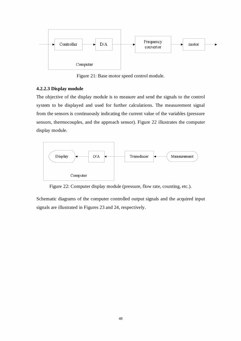
48
Figure 21: Base motor speed control module.
4.2.2.3 Display module
The objective of the display module is to measure and send the signals to the control
system to be displayed and used for further calculations. The measurement signal
from the sensors is continuously indicating the current value of the variables (pressure
sensors, thermocouples, and the approach sensor). Figure 22 illustrates the computer
display module.
Figure 22: Computer display module (pressure, flow rate, counting, etc.).
Schematic diagrams of the computer controlled output signals and the acquired input
signals are illustrated in Figures 23 and 24, respectively.
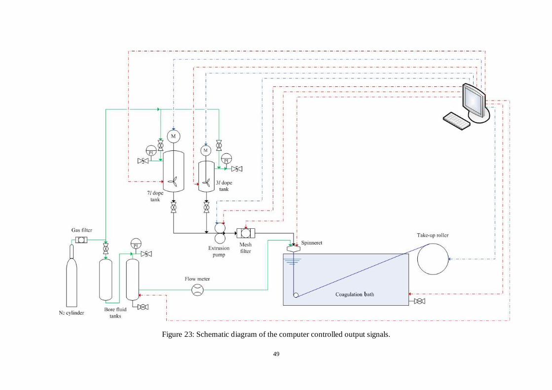
49
Figure 23: Schematic diagram of the computer controlled output signals.
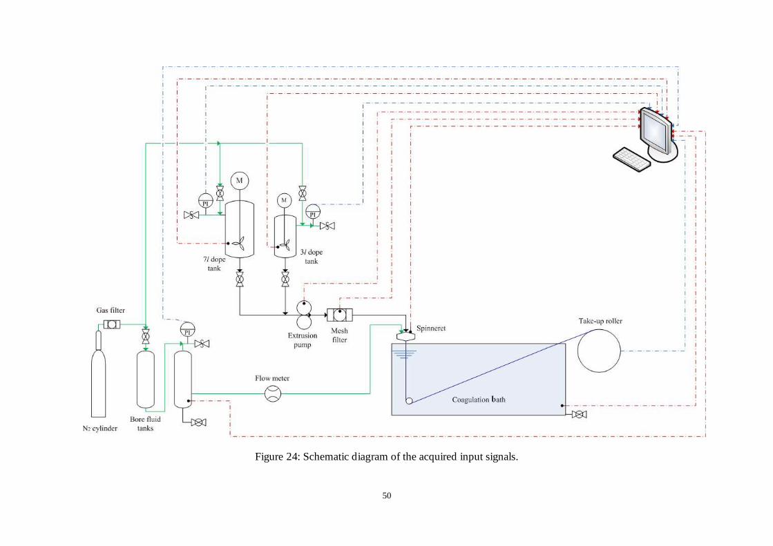
50
Figure 24: Schematic diagram of the acquired input signals.
51
4.2.2.1 Spinning control software capabilities
The spinning control software was developed and improved as required for the plant
to operate adequately. For instance, initially there was no option to save or load the
operation conditions and data, and some important indicators were missing, such as
the take-up speed and the extrusion rate. Displaying all the spinning parameters and
controls, and adding the current date and the time elapsed in a user friendly
environment is a great improvement to the software.
Including these crucial features allow the user to more easily monitor and control the
process, by providing the possibility to save and log the spinning conditions in an
Excel sheet, or print a technical report. More importantly, it provides the possibility to
input the spinneret details (inside/outside diameter) in order to be able to make some
important calculations, which are:
Extrusion rate
The capacity of the pump is 1.2 mL/revolution. The rpm of the motor is multiplied by
the pump gear ratio to get the rpm of the pump, and then multiplying it by the pump
capacity to get the extrusion flow rate (mL/min) of the pump. See the block diagram
illustrated in Figure 25.
Spinning velocity
The linear spinning velocity of the fibre was determined by dividing this extrusion
flow rate by the annular area of the spinneret through which the homogeneous
solution flows.
Take-up speed
The rpm of the roller motor is multiplied by the roller gear ratio to get the rpm of the
roller.
Speed ratio
The spinning speed ratio can be determined by dividing the take-up speed by the
spinning velocity.
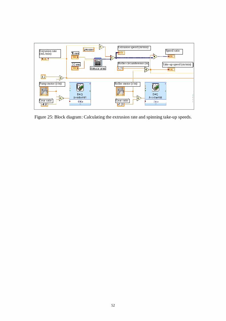
52
Figure 25: Block diagram: Calculating the extrusion rate and spinning take-up speeds.
Extrusion rate (mL/min)
Extrusion speed (m/min)
Roller circumference (m) Take-up speed (m/min)
Speed ratio
Roller motor (r/m)
Gear ratio Gear ratio
Pump motor (r/m)
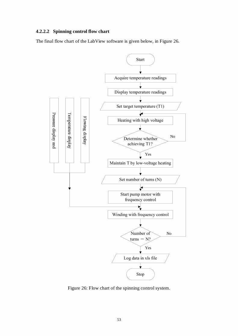
53
4.2.2.2 Spinning control flow chart
The final flow chart of the LabView software is given below, in Figure 26.
Start
Stop
Acquire temperature readings
Display temperature readings
Set target temperature (T1)
Determine whether
achieving T1?
Heating with high voltage
Maintain T by low-voltage heating
Set number of turns (N)
Start pump motor with
frequency control
Winding with frequency control
Number of
turns = N?
Log data in xls file
Figure 26: Flow chart of the spinning control system.
No
No
Yes
Yes
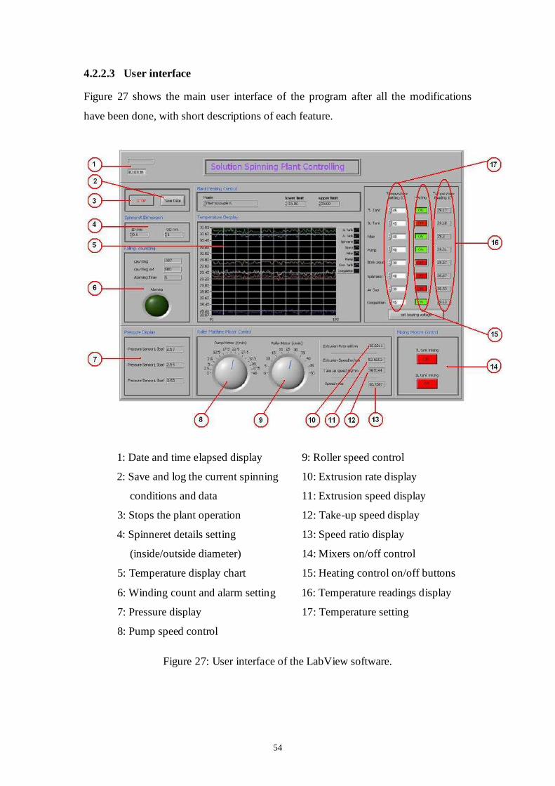
54
4.2.2.3 User interface
Figure 27 shows the main user interface of the program after all the modifications
have been done, with short descriptions of each feature.
1: Date and time elapsed display
2: Save and log the current spinning
conditions and data
3: Stops the plant operation
4: Spinneret details setting
(inside/outside diameter)
5: Temperature display chart
6: Winding count and alarm setting
7: Pressure display
8: Pump speed control
9: Roller speed control
10: Extrusion rate display
11: Extrusion speed display
12: Take-up speed display
13: Speed ratio display
14: Mixers on/off control
15: Heating control on/off buttons
16: Temperature readings display
17: Temperature setting
Figure 27: User interface of the LabView software.
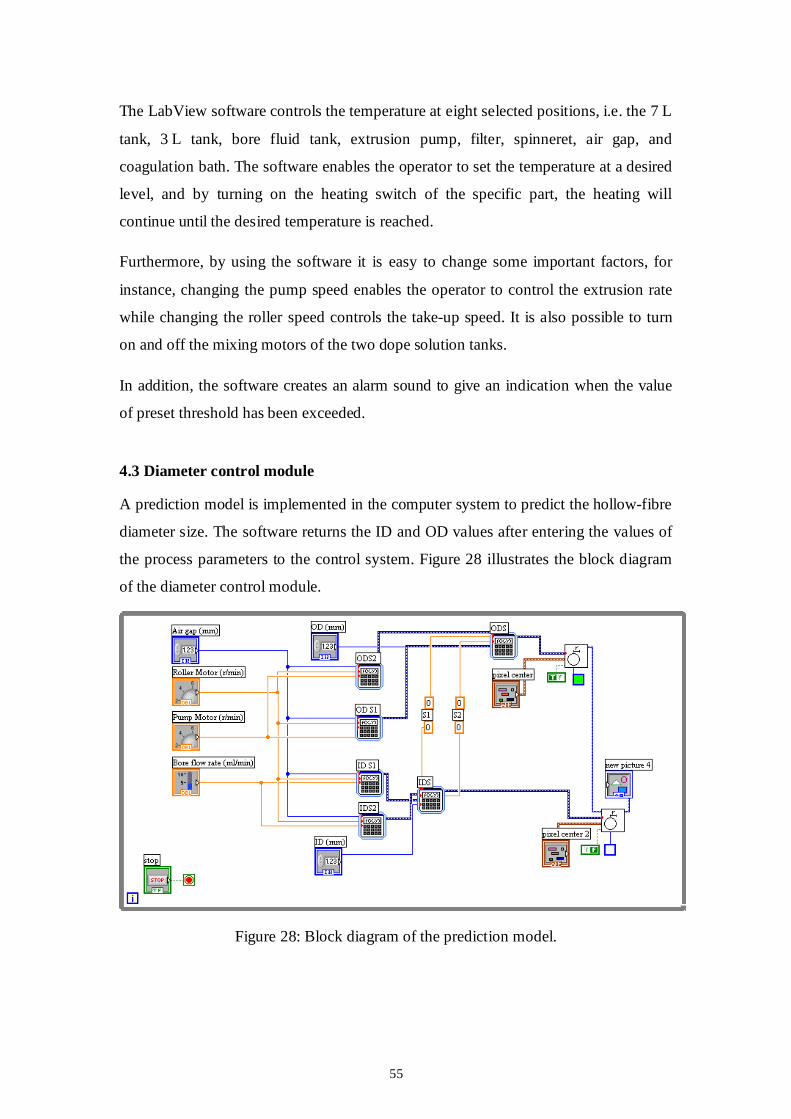
55
The LabView software controls the temperature at eight selected positions, i.e. the 7 L
tank, 3 L tank, bore fluid tank, extrusion pump, filter, spinneret, air gap, and
coagulation bath. The software enables the operator to set the temperature at a desired
level, and by turning on the heating switch of the specific part, the heating will
continue until the desired temperature is reached.
Furthermore, by using the software it is easy to change some important factors, for
instance, changing the pump speed enables the operator to control the extrusion rate
while changing the roller speed controls the take-up speed. It is also possible to turn
on and off the mixing motors of the two dope solution tanks.
In addition, the software creates an alarm sound to give an indication when the value
of preset threshold has been exceeded.
4.3 Diameter control module
A prediction model is implemented in the computer system to predict the hollow-fibre
diameter size. The software returns the ID and OD values after entering the values of
the process parameters to the control system. Figure 28 illustrates the block diagram
of the diameter control module.
Figure 28: Block diagram of the prediction model.

CHAPTER 5
RESULTS AND DISCUSSION
57
CHAPTER 5: RESULTS AND DISCUSSION
5.1 Introduction
As described in Chapter 3, the spinning experiments were divided into three stages.
The first stage involved a preliminary investigation, the purpose of which was to
identify the significance of the factors. The second stage involved creating a
prediction model, the purpose of which was to control and predict the diameter size
and wall thickness of the hollow-fibre. In the third stage, a series of confirmation
experiments were carried out. The results of each stage are listed, analysed and
discussed in this chapter.
5.2 First stage
Here seven parameters were considered, namely: the spinneret size, coagulation bath
temperature, solution temperature, bore temperature, air gap length, dope extrusion
rate and the take-up speed, and they were denoted by the letters S, CT, ST, BT, Ag,
DER and Tup, respectively. Three levels were assigned for each factor (see Table 1).
According to the levels combination given by the orthogonal array L18 (see Table 2),
a total of 18 experiments were carried out.
The response is the diameters of the hollow-fibre. The inner and the outer diameters
of the samples were determined from SEM images of the entire cross-section of the
sample, as described in Section 3.4.1. The built-in measurement tool in the SEM
apparatus was used to measure the hollow-fibre diameter. Measurements were taken
for four samples from each run. Table A-1 in Appendix A shows the SEM images and
the resulting measurements of the inner and the outer diameters.
5.2.1 Analysis of experimental data
In order to determine the influence of each selected factor on the response, the S/N
ratio approach was utilized to measure the deviations from the average response. The
S/N ratio approach was used instead of the average response value to convert the
experimental results into a value for the evaluation characteristic in the optimum
parameter analysis.
Since the smaller fibre diameter is favourable, the S/N ratio was chosen according to
the smaller-the-better criterion. Therefore, the best combination of the process
58
∑=
=n
iiD
nSQ
1
21
( )SQi log10 ×−=η
∑=
=n
iin 1
1 ηη
parameters is the one with the lowest S/N ratio. The S/N ratio for the smaller-the-
better target for the responses is denoted by η, and defined by:
(11)
where:
SQ: mean square deviation of the response.
In the smaller-the-better quality characteristic the target is to minimize the response,
therefore, deviation is measured from zero. Hence, SQ is expressed as:
(12)
where:
Di: the diameter value for the i th measurement
n: number of measurements.
The average diameter values (at least three samples were measured for each
experimental trial) and their corresponding values of the SQ and S/N ratios are listed
in Table B-1. The average S/N ratio for each factor level can be calculated in the
following way: for example, the Ag maintained itself at level Ag1 in six experiments
(1, 6, 7, 11, 14, and 18); the average S/N of factor level Ag1 is denoted by ηAg1 and is
given by:
ηAg1 = (η1 + η6 + η7 + η11 + η14 + η18) (13)
The average response for levels Ag2 and Ag3 of Ag, as well as those for the various
levels of the other factors, can be obtained in a similar way. And the overall mean
value of the 18 experiments is defined by:
(14)
where:
η: the overall mean S/N
n: number of experiments
ηi: S/N value of the i th experiment.
The diameter values corresponding to the process parameters of the L18 orthogonal
array of Taguchi and their η values are listed in Table B-2, in Appendix B.
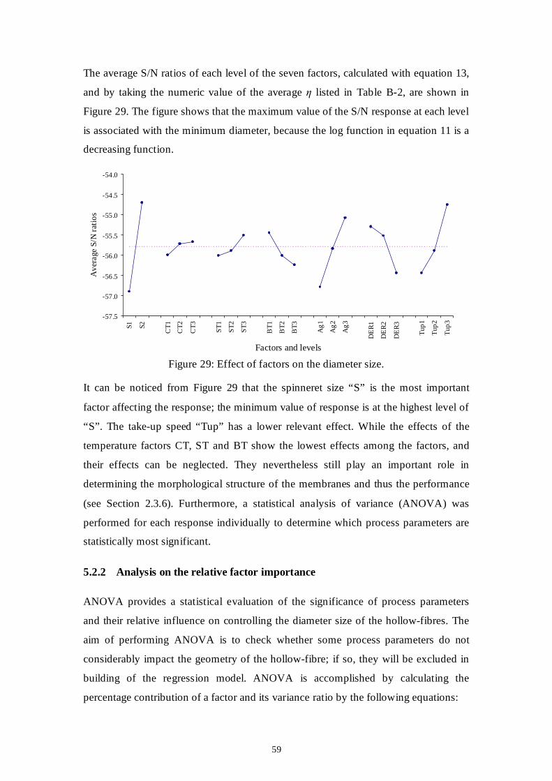
59
The average S/N ratios of each level of the seven factors, calculated with equation 13,
and by taking the numeric value of the average η listed in Table B-2, are shown in
Figure 29. The figure shows that the maximum value of the S/N response at each level
is associated with the minimum diameter, because the log function in equation 11 is a
decreasing function.
-57.5
-57.0
-56.5
-56.0
-55.5
-55.0
-54.5
-54.0
S1
S2
CT
1
CT
2
CT
3
ST
1
ST
2
ST
3
BT
1
BT
2
BT
3
Ag
1
Ag
2
Ag
3
DE
R1
DE
R2
DE
R3
Tu
p1
Tu
p2
Tu
p3
Factors and levels
Ave
rage
S/N
rat
ios
Figure 29: Effect of factors on the diameter size.
It can be noticed from Figure 29 that the spinneret size “S” is the most important
factor affecting the response; the minimum value of response is at the highest level of
“S”. The take-up speed “Tup” has a lower relevant effect. While the effects of the
temperature factors CT, ST and BT show the lowest effects among the factors, and
their effects can be neglected. They nevertheless still play an important role in
determining the morphological structure of the membranes and thus the performance
(see Section 2.3.6). Furthermore, a statistical analysis of variance (ANOVA) was
performed for each response individually to determine which process parameters are
statistically most significant.
5.2.2 Analysis on the relative factor importance
ANOVA provides a statistical evaluation of the significance of process parameters
and their relative influence on controlling the diameter size of the hollow-fibres. The
aim of performing ANOVA is to check whether some process parameters do not
considerably impact the geometry of the hollow-fibre; if so, they will be excluded in
building of the regression model. ANOVA is accomplished by calculating the
percentage contribution of a factor and its variance ratio by the following equations:
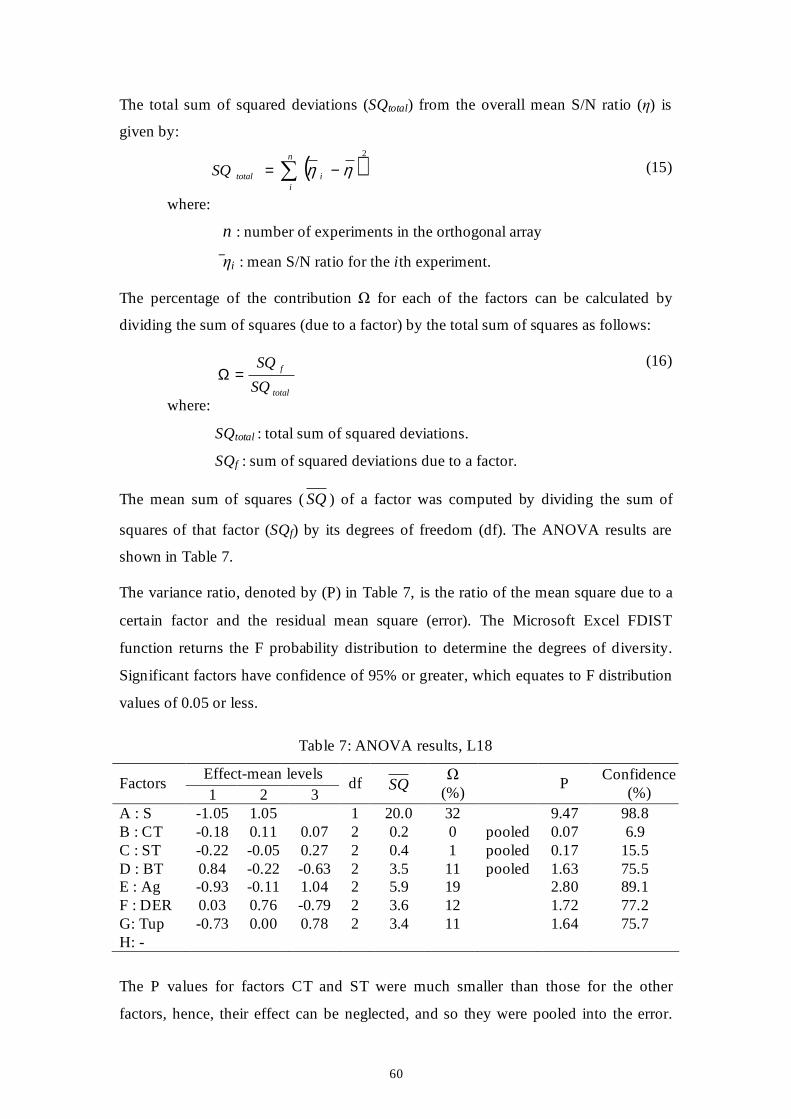
60
( )2
∑ −=n
iitotalSQ ηη
total
f
SQ
SQ=Ω
The total sum of squared deviations (SQtotal) from the overall mean S/N ratio (η) is
given by:
(15)
where:
n : number of experiments in the orthogonal array
ηi : mean S/N ratio for the i th experiment.
The percentage of the contribution Ω for each of the factors can be calculated by
dividing the sum of squares (due to a factor) by the total sum of squares as follows:
(16)
where:
SQtotal : total sum of squared deviations.
SQf : sum of squared deviations due to a factor.
The mean sum of squares (SQ) of a factor was computed by dividing the sum of
squares of that factor (SQf) by its degrees of freedom (df). The ANOVA results are
shown in Table 7.
The variance ratio, denoted by (P) in Table 7, is the ratio of the mean square due to a
certain factor and the residual mean square (error). The Microsoft Excel FDIST
function returns the F probability distribution to determine the degrees of diversity.
Significant factors have confidence of 95% or greater, which equates to F distribution
values of 0.05 or less.
Table 7: ANOVA results, L18
Effect-mean levels Factors
1 2 3 df SQ
Ω (%)
P Confidence
(%) A : S -1.05 1.05 1 20.0 32 9.47 98.8 B : CT -0.18 0.11 0.07 2 0.2 0 pooled 0.07 6.9 C : ST -0.22 -0.05 0.27 2 0.4 1 pooled 0.17 15.5 D : BT 0.84 -0.22 -0.63 2 3.5 11 pooled 1.63 75.5 E : Ag -0.93 -0.11 1.04 2 5.9 19 2.80 89.1 F : DER 0.03 0.76 -0.79 2 3.6 12 1.72 77.2 G: Tup -0.73 0.00 0.78 2 3.4 11 1.64 75.7 H: -
The P values for factors CT and ST were much smaller than those for the other
factors, hence, their effect can be neglected, and so they were pooled into the error.
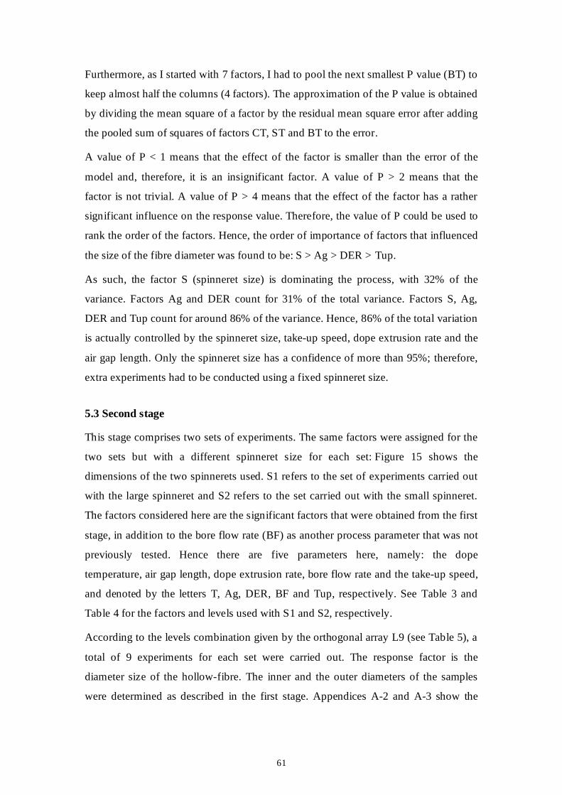
61
Furthermore, as I started with 7 factors, I had to pool the next smallest P value (BT) to
keep almost half the columns (4 factors). The approximation of the P value is obtained
by dividing the mean square of a factor by the residual mean square error after adding
the pooled sum of squares of factors CT, ST and BT to the error.
A value of P < 1 means that the effect of the factor is smaller than the error of the
model and, therefore, it is an insignificant factor. A value of P > 2 means that the
factor is not trivial. A value of P > 4 means that the effect of the factor has a rather
significant influence on the response value. Therefore, the value of P could be used to
rank the order of the factors. Hence, the order of importance of factors that influenced
the size of the fibre diameter was found to be: S > Ag > DER > Tup.
As such, the factor S (spinneret size) is dominating the process, with 32% of the
variance. Factors Ag and DER count for 31% of the total variance. Factors S, Ag,
DER and Tup count for around 86% of the variance. Hence, 86% of the total variation
is actually controlled by the spinneret size, take-up speed, dope extrusion rate and the
air gap length. Only the spinneret size has a confidence of more than 95%; therefore,
extra experiments had to be conducted using a fixed spinneret size.
5.3 Second stage
This stage comprises two sets of experiments. The same factors were assigned for the
two sets but with a different spinneret size for each set: Figure 15 shows the
dimensions of the two spinnerets used. S1 refers to the set of experiments carried out
with the large spinneret and S2 refers to the set carried out with the small spinneret.
The factors considered here are the significant factors that were obtained from the first
stage, in addition to the bore flow rate (BF) as another process parameter that was not
previously tested. Hence there are five parameters here, namely: the dope
temperature, air gap length, dope extrusion rate, bore flow rate and the take-up speed,
and denoted by the letters T, Ag, DER, BF and Tup, respectively. See Table 3 and
Table 4 for the factors and levels used with S1 and S2, respectively.
According to the levels combination given by the orthogonal array L9 (see Table 5), a
total of 9 experiments for each set were carried out. The response factor is the
diameter size of the hollow-fibre. The inner and the outer diameters of the samples
were determined as described in the first stage. Appendices A-2 and A-3 show the
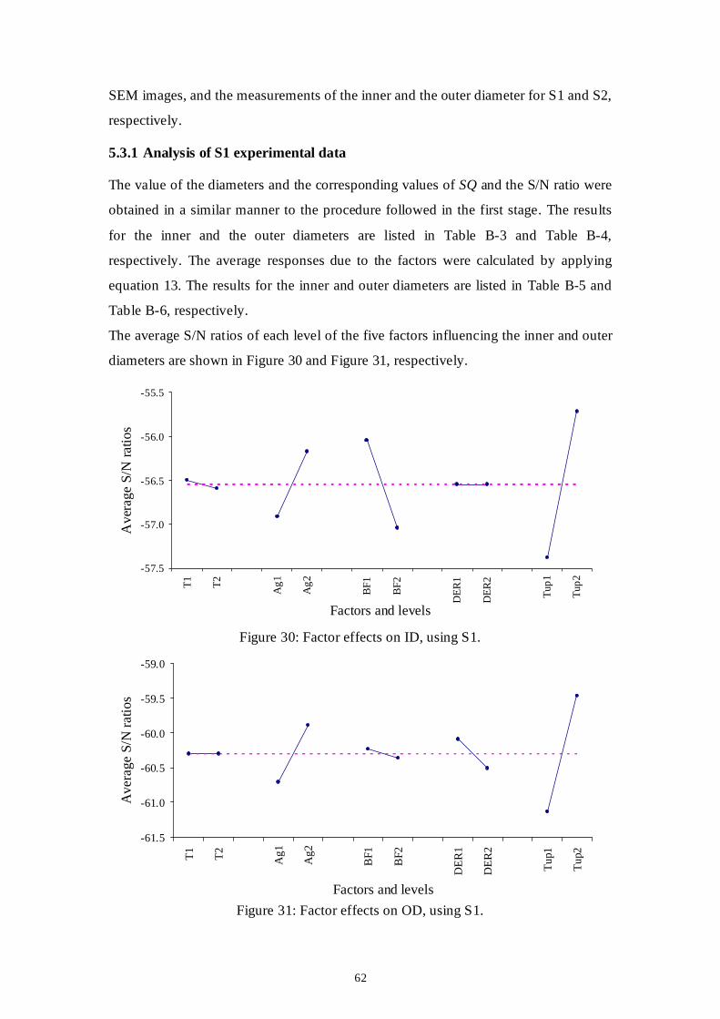
62
SEM images, and the measurements of the inner and the outer diameter for S1 and S2,
respectively.
5.3.1 Analysis of S1 experimental data
The value of the diameters and the corresponding values of SQ and the S/N ratio were
obtained in a similar manner to the procedure followed in the first stage. The results
for the inner and the outer diameters are listed in Table B-3 and Table B-4,
respectively. The average responses due to the factors were calculated by applying
equation 13. The results for the inner and outer diameters are listed in Table B-5 and
Table B-6, respectively.
The average S/N ratios of each level of the five factors influencing the inner and outer
diameters are shown in Figure 30 and Figure 31, respectively.
-57.5
-57.0
-56.5
-56.0
-55.5
T1
T2
Ag
1
Ag
2
BF
1
BF
2
DE
R1
DE
R2
Tup
1
Tup
2
Factors and levels
Ave
rag
e S
/N r
atio
s
Figure 30: Factor effects on ID, using S1.
-61.5
-61.0
-60.5
-60.0
-59.5
-59.0
T1
T2
Ag
1
Ag
2
BF
1
BF
2
DE
R1
DE
R2
Tu
p1
Tu
p2
Factors and levels
Ave
rag
e S
/N r
atio
s
Figure 31: Factor effects on OD, using S1.
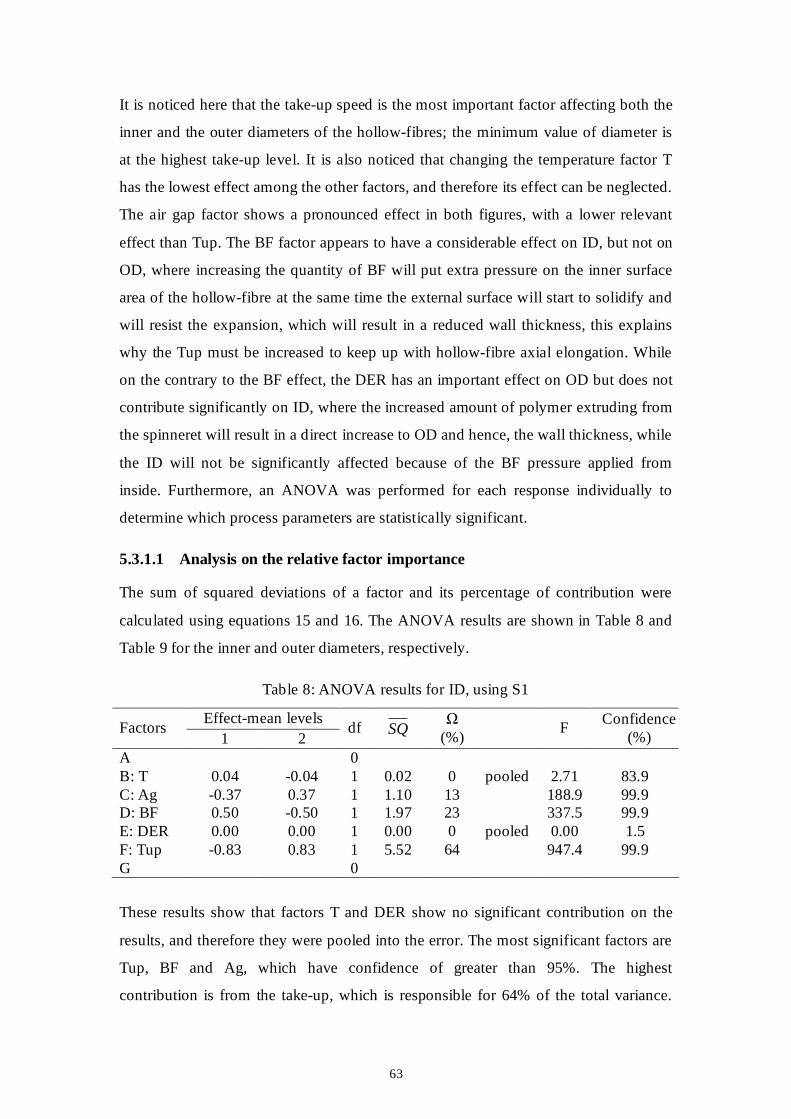
63
It is noticed here that the take-up speed is the most important factor affecting both the
inner and the outer diameters of the hollow-fibres; the minimum value of diameter is
at the highest take-up level. It is also noticed that changing the temperature factor T
has the lowest effect among the other factors, and therefore its effect can be neglected.
The air gap factor shows a pronounced effect in both figures, with a lower relevant
effect than Tup. The BF factor appears to have a considerable effect on ID, but not on
OD, where increasing the quantity of BF will put extra pressure on the inner surface
area of the hollow-fibre at the same time the external surface will start to solidify and
will resist the expansion, which will result in a reduced wall thickness, this explains
why the Tup must be increased to keep up with hollow-fibre axial elongation. While
on the contrary to the BF effect, the DER has an important effect on OD but does not
contribute significantly on ID, where the increased amount of polymer extruding from
the spinneret will result in a direct increase to OD and hence, the wall thickness, while
the ID will not be significantly affected because of the BF pressure applied from
inside. Furthermore, an ANOVA was performed for each response individually to
determine which process parameters are statistically significant.
5.3.1.1 Analysis on the relative factor importance
The sum of squared deviations of a factor and its percentage of contribution were
calculated using equations 15 and 16. The ANOVA results are shown in Table 8 and
Table 9 for the inner and outer diameters, respectively.
Table 8: ANOVA results for ID, using S1
Effect-mean levels Factors
1 2 df SQ
Ω (%)
F Confidence
(%) A 0 B: T 0.04 -0.04 1 0.02 0 pooled 2.71 83.9 C: Ag -0.37 0.37 1 1.10 13 188.9 99.9 D: BF 0.50 -0.50 1 1.97 23 337.5 99.9 E: DER 0.00 0.00 1 0.00 0 pooled 0.00 1.5 F: Tup -0.83 0.83 1 5.52 64 947.4 99.9 G 0
These results show that factors T and DER show no significant contribution on the
results, and therefore they were pooled into the error. The most significant factors are
Tup, BF and Ag, which have confidence of greater than 95%. The highest
contribution is from the take-up, which is responsible for 64% of the total variance.
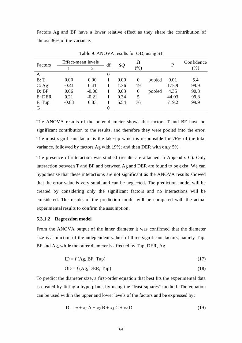
64
Factors Ag and BF have a lower relative effect as they share the contribution of
almost 36% of the variance.
Table 9: ANOVA results for OD, using S1
Effect-mean levels Factors
1 2 df SQ
Ω (%)
P Confidence
(%) A 0 B: T 0.00 0.00 1 0.00 0 pooled 0.01 5.4 C: Ag -0.41 0.41 1 1.36 19 175.9 99.9 D: BF 0.06 -0.06 1 0.03 0 pooled 4.35 90.8 E: DER 0.21 -0.21 1 0.34 5 44.03 99.8 F: Tup -0.83 0.83 1 5.54 76 719.2 99.9 G 0
The ANOVA results of the outer diameter shows that factors T and BF have no
significant contribution to the results, and therefore they were pooled into the error.
The most significant factor is the take-up which is responsible for 76% of the total
variance, followed by factors Ag with 19%; and then DER with only 5%.
The presence of interaction was studied (results are attached in Appendix C). Only
interaction between T and BF and between Ag and DER are found to be exist. We can
hypothesize that these interactions are not significant as the ANOVA results showed
that the error value is very small and can be neglected. The prediction model will be
created by considering only the significant factors and no interactions will be
considered. The results of the prediction model will be compared with the actual
experimental results to confirm the assumption.
5.3.1.2 Regression model
From the ANOVA output of the inner diameter it was confirmed that the diameter
size is a function of the independent values of three significant factors, namely Tup,
BF and Ag, while the outer diameter is affected by Tup, DER, Ag.
ID = f (Ag, BF, Tup) (17)
OD = f (Ag, DER, Tup) (18)
To predict the diameter size, a first-order equation that best fits the experimental data
is created by fitting a hyperplane, by using the "least squares" method. The equation
can be used within the upper and lower levels of the factors and be expressed by:
D = m + x1 A + x2 B + x3 C + x4 D (19)
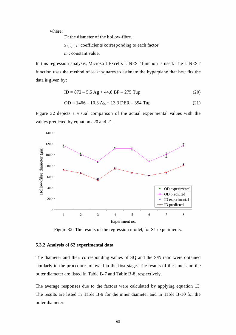
65
where: D: the diameter of the hollow-fibre.
x1, 2, 3, 4 : coefficients corresponding to each factor.
m : constant value.
In this regression analysis, Microsoft Excel’s LINEST function is used. The LINEST
function uses the method of least squares to estimate the hyperplane that best fits the
data is given by:
ID = 872 – 5.5 Ag + 44.8 BF – 275 Tup (20)
OD = 1466 – 10.3 Ag + 13.3 DER – 394 Tup (21)
Figure 32 depicts a visual comparison of the actual experimental values with the
values predicted by equations 20 and 21.
0
200
400
600
800
1000
1200
1400
1 2 3 4 5 6 7 8
Experiment no.
Hol
low
-fib
re d
iam
eter
( µm)
OD experimentalOD predictedID experimentalID predicted
Figure 32: The results of the regression model, for S1 experiments.
5.3.2 Analysis of S2 experimental data
The diameter and their corresponding values of SQ and the S/N ratio were obtained
similarly to the procedure followed in the first stage. The results of the inner and the
outer diameter are listed in Table B-7 and Table B-8, respectively.
The average responses due to the factors were calculated by applying equation 13.
The results are listed in Table B-9 for the inner diameter and in Table B-10 for the
outer diameter.
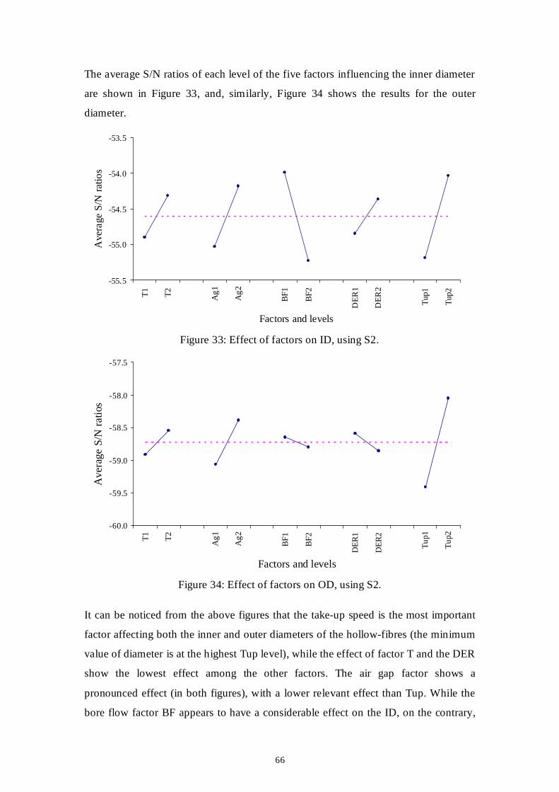
66
The average S/N ratios of each level of the five factors influencing the inner diameter
are shown in Figure 33, and, similarly, Figure 34 shows the results for the outer
diameter.
-55.5
-55.0
-54.5
-54.0
-53.5T
1
T2
Ag
1
Ag
2
BF
1
BF
2
DE
R1
DE
R2
Tup
1
Tup
2
Factors and levels
Ave
rage
S/N
rat
ios
Figure 33: Effect of factors on ID, using S2.
-60.0
-59.5
-59.0
-58.5
-58.0
-57.5
T1
T2
Ag
1
Ag
2
BF
1
BF
2
DE
R1
DE
R2
Tu
p1
Tu
p2
Factors and levels
Ave
rag
e S
/N r
atio
s
Figure 34: Effect of factors on OD, using S2.
It can be noticed from the above figures that the take-up speed is the most important
factor affecting both the inner and outer diameters of the hollow-fibres (the minimum
value of diameter is at the highest Tup level), while the effect of factor T and the DER
show the lowest effect among the other factors. The air gap factor shows a
pronounced effect (in both figures), with a lower relevant effect than Tup. While the
bore flow factor BF appears to have a considerable effect on the ID, on the contrary,
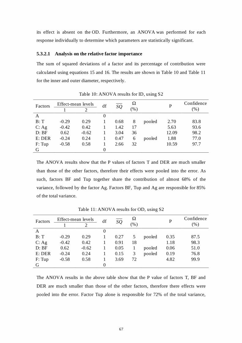
67
its effect is absent on the OD. Furthermore, an ANOVA was performed for each
response individually to determine which parameters are statistically significant.
5.3.2.1 Analysis on the relative factor importance
The sum of squared deviations of a factor and its percentage of contribution were
calculated using equations 15 and 16. The results are shown in Table 10 and Table 11
for the inner and outer diameter, respectively.
Table 10: ANOVA results for ID, using S2
Effect-mean levels Factors 1 2
df SQ Ω
(%) P
Confidence (%)
A 0 B: T -0.29 0.29 1 0.68 8 pooled 2.70 83.8 C: Ag -0.42 0.42 1 1.42 17 5.63 93.6 D: BF 0.62 -0.62 1 3.04 36 12.09 98.2 E: DER -0.24 0.24 1 0.47 6 pooled 1.88 77.0 F: Tup -0.58 0.58 1 2.66 32 10.59 97.7 G 0
The ANOVA results show that the P values of factors T and DER are much smaller
than those of the other factors, therefore their effects were pooled into the error. As
such, factors BF and Tup together share the contribution of almost 68% of the
variance, followed by the factor Ag. Factors BF, Tup and Ag are responsible for 85%
of the total variance.
Table 11: ANOVA results for OD, using S2
Effect-mean levels Factors 1 2
df SQ Ω
(%) P
Confidence (%)
A 0 B: T -0.29 0.29 1 0.27 5 pooled 0.35 87.5 C: Ag -0.42 0.42 1 0.91 18 1.18 98.3 D: BF 0.62 -0.62 1 0.05 1 pooled 0.06 51.0 E: DER -0.24 0.24 1 0.15 3 pooled 0.19 76.8 F: Tup -0.58 0.58 1 3.69 72 4.82 99.9 G 0
The ANOVA results in the above table show that the P value of factors T, BF and
DER are much smaller than those of the other factors, therefore there effects were
pooled into the error. Factor Tup alone is responsible for 72% of the total variance,
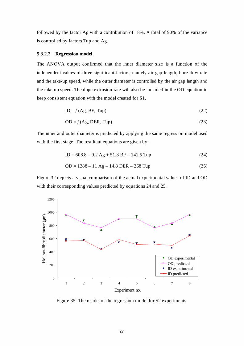
68
followed by the factor Ag with a contribution of 18%. A total of 90% of the variance
is controlled by factors Tup and Ag.
5.3.2.2 Regression model
The ANOVA output confirmed that the inner diameter size is a function of the
independent values of three significant factors, namely air gap length, bore flow rate
and the take-up speed, while the outer diameter is controlled by the air gap length and
the take-up speed. The dope extrusion rate will also be included in the OD equation to
keep consistent equation with the model created for S1.
ID = f (Ag, BF, Tup) (22)
OD = f (Ag, DER, Tup) (23)
The inner and outer diameter is predicted by applying the same regression model used
with the first stage. The resultant equations are given by:
ID = 608.8 – 9.2 Ag + 51.8 BF – 141.5 Tup (24)
OD = 1388 – 11 Ag – 14.8 DER – 268 Tup (25)
Figure 32 depicts a visual comparison of the actual experimental values of ID and OD
with their corresponding values predicted by equations 24 and 25.
0
200
400
600
800
1000
1200
1 2 3 4 5 6 7 8
Experiment no.
Hol
low
-fib
re d
iam
ete
r ( µm
)
OD experimentalOD predictedID experimentalID predicted
Figure 35: The results of the regression model for S2 experiments.
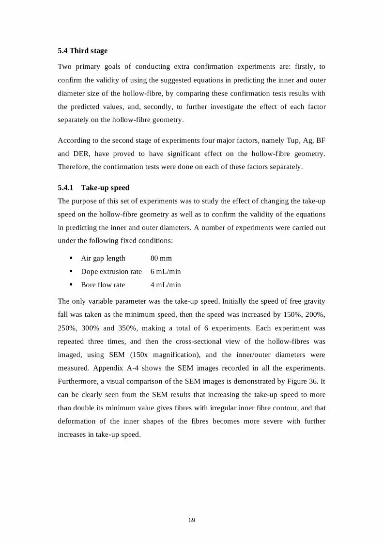
69
5.4 Third stage
Two primary goals of conducting extra confirmation experiments are: firstly, to
confirm the validity of using the suggested equations in predicting the inner and outer
diameter size of the hollow-fibre, by comparing these confirmation tests results with
the predicted values, and, secondly, to further investigate the effect of each factor
separately on the hollow-fibre geometry.
According to the second stage of experiments four major factors, namely Tup, Ag, BF
and DER, have proved to have significant effect on the hollow-fibre geometry.
Therefore, the confirmation tests were done on each of these factors separately.
5.4.1 Take-up speed
The purpose of this set of experiments was to study the effect of changing the take-up
speed on the hollow-fibre geometry as well as to confirm the validity of the equations
in predicting the inner and outer diameters. A number of experiments were carried out
under the following fixed conditions:
Air gap length 80 mm
Dope extrusion rate 6 mL/min
Bore flow rate 4 mL/min
The only variable parameter was the take-up speed. Initially the speed of free gravity
fall was taken as the minimum speed, then the speed was increased by 150%, 200%,
250%, 300% and 350%, making a total of 6 experiments. Each experiment was
repeated three times, and then the cross-sectional view of the hollow-fibres was
imaged, using SEM (150x magnification), and the inner/outer diameters were
measured. Appendix A-4 shows the SEM images recorded in all the experiments.
Furthermore, a visual comparison of the SEM images is demonstrated by Figure 36. It
can be clearly seen from the SEM results that increasing the take-up speed to more
than double its minimum value gives fibres with irregular inner fibre contour, and that
deformation of the inner shapes of the fibres becomes more severe with further
increases in take-up speed.
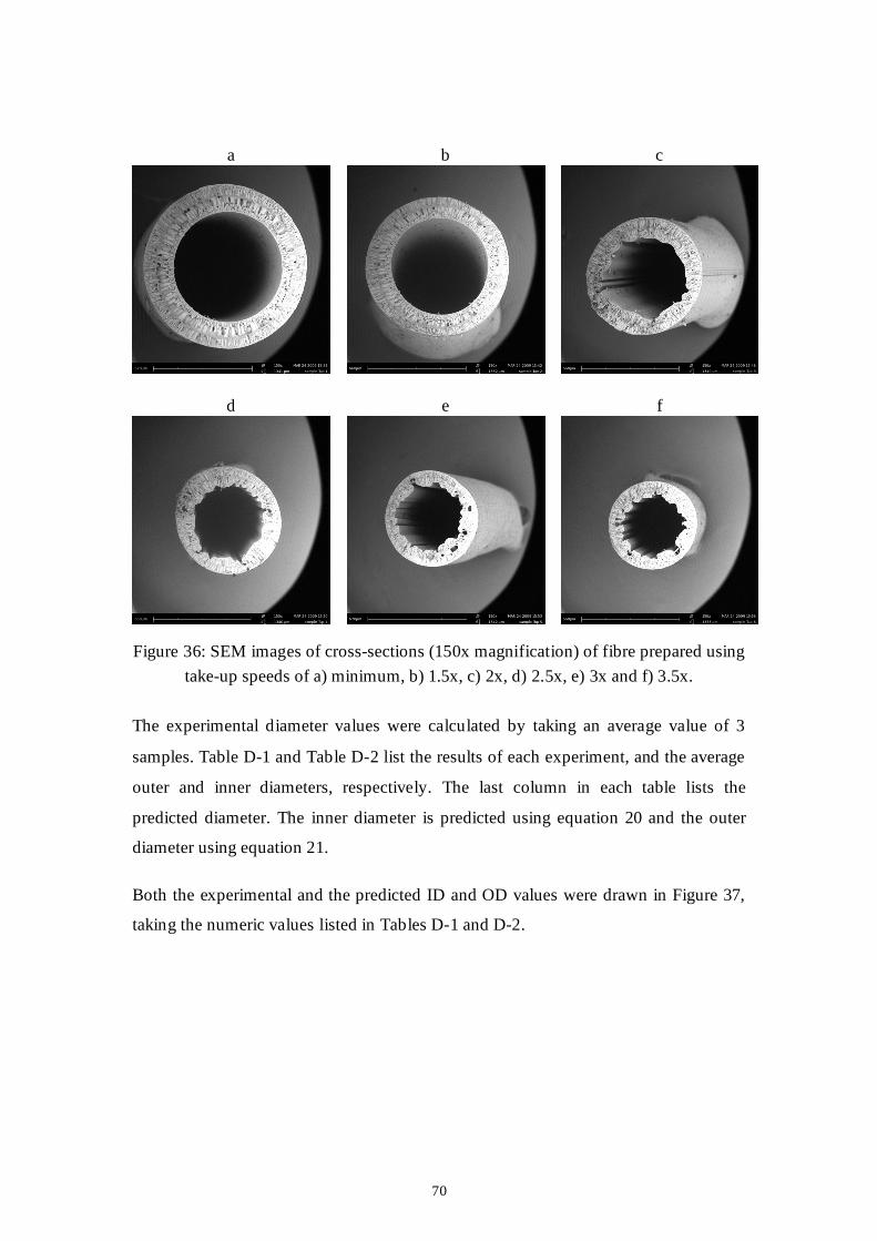
70
a
b
c
d
e
f
Figure 36: SEM images of cross-sections (150x magnification) of fibre prepared using
take-up speeds of a) minimum, b) 1.5x, c) 2x, d) 2.5x, e) 3x and f) 3.5x.
The experimental diameter values were calculated by taking an average value of 3
samples. Table D-1 and Table D-2 list the results of each experiment, and the average
outer and inner diameters, respectively. The last column in each table lists the
predicted diameter. The inner diameter is predicted using equation 20 and the outer
diameter using equation 21.
Both the experimental and the predicted ID and OD values were drawn in Figure 37,
taking the numeric values listed in Tables D-1 and D-2.
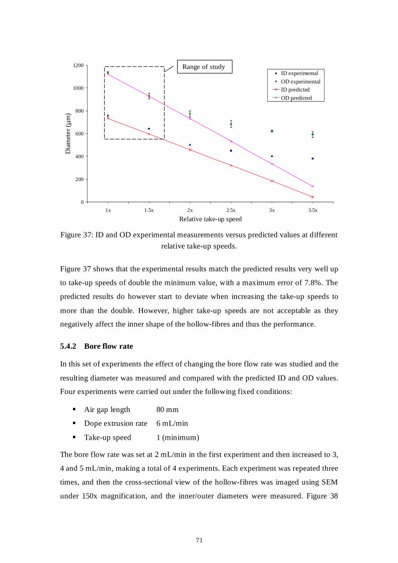
71
0
200
400
600
800
1000
1200
1x 1.5x 2x 2.5x 3x 3.5x
Relative take-up speed
Dia
met
er
( µm)
ID experimental
OD experimental
ID predicted
OD predicted
Figure 37: ID and OD experimental measurements versus predicted values at different
relative take-up speeds.
Figure 37 shows that the experimental results match the predicted results very well up
to take-up speeds of double the minimum value, with a maximum error of 7.8%. The
predicted results do however start to deviate when increasing the take-up speeds to
more than the double. However, higher take-up speeds are not acceptable as they
negatively affect the inner shape of the hollow-fibres and thus the performance.
5.4.2 Bore flow rate
In this set of experiments the effect of changing the bore flow rate was studied and the
resulting diameter was measured and compared with the predicted ID and OD values.
Four experiments were carried out under the following fixed conditions:
Air gap length 80 mm
Dope extrusion rate 6 mL/min
Take-up speed 1 (minimum)
The bore flow rate was set at 2 mL/min in the first experiment and then increased to 3,
4 and 5 mL/min, making a total of 4 experiments. Each experiment was repeated three
times, and then the cross-sectional view of the hollow-fibres was imaged using SEM
under 150x magnification, and the inner/outer diameters were measured. Figure 38
Range of study
72
shows SEM images of one sample from each experiment. See Appendix A-5 for all
the SEM images.
a
b
c
d
Figure 38: SEM images of cross-sections (150x magnification) of fibre prepared using bore flow rates of a) 2 mL/min, b) 3 mL/min, c) 4 mL/min and d) 5 mL/min.
The SEM images shown in Figure 38 prove that the ID is influenced by the value of
the bore flow rate; however, no major change in OD is noticed, it is therefore a way of
changing the wall thickness. Table D-3 and Table D-4 list the experimental results
and the average outer and inner diameters, respectively, of each experiment.
Equations 20 and 21 were applied to predict the ID and OD respectively.
The values of ID and OD (both experimental and predicted values) are shown in
Figure 39. The predicted OD is represented by a horizontal line, where the OD value
does not change by changing the bore flow rate. That is because the effect of the bore
flow rate factor BF on OD was neglected, and thus it was absent in equation 20.
However, the experimental OD values also do not show substantial deviation. In
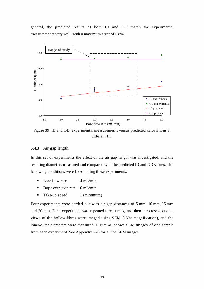
73
general, the predicted results of both ID and OD match the experimental
measurements very well, with a maximum error of 6.8%.
400
600
800
1000
1200
1.5 2.0 2.5 3.0 3.5 4.0 4.5 5.0
Bore flow rate (ml /min)
Dia
met
er
( µm)
ID experimental
OD experimental
ID predicted
OD predicted
Figure 39: ID and OD, experimental measurements versus predicted calculations at
different BF.
5.4.3 Air gap length
In this set of experiments the effect of the air gap length was investigated, and the
resulting diameters measured and compared with the predicted ID and OD values. The
following conditions were fixed during these experiments:
Bore flow rate 4 mL/min
Dope extrusion rate 6 mL/min
Take-up speed 1 (minimum)
Four experiments were carried out with air gap distances of 5 mm, 10 mm, 15 mm
and 20 mm. Each experiment was repeated three times, and then the cross-sectional
views of the hollow-fibres were imaged using SEM (150x magnification), and the
inner/outer diameters were measured. Figure 40 shows SEM images of one sample
from each experiment. See Appendix A-6 for all the SEM images.
Range of study
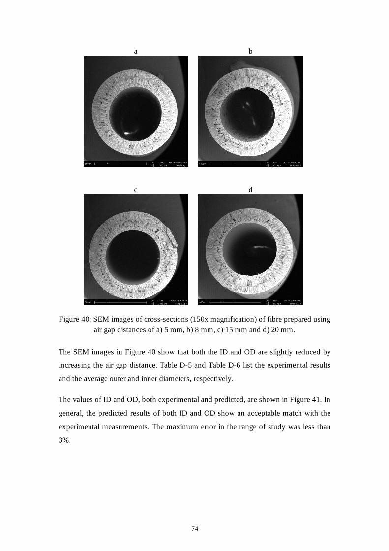
74
a
b
c
d
Figure 40: SEM images of cross-sections (150x magnification) of fibre prepared using
air gap distances of a) 5 mm, b) 8 mm, c) 15 mm and d) 20 mm.
The SEM images in Figure 40 show that both the ID and OD are slightly reduced by
increasing the air gap distance. Table D-5 and Table D-6 list the experimental results
and the average outer and inner diameters, respectively.
The values of ID and OD, both experimental and predicted, are shown in Figure 41. In
general, the predicted results of both ID and OD show an acceptable match with the
experimental measurements. The maximum error in the range of study was less than
3%.
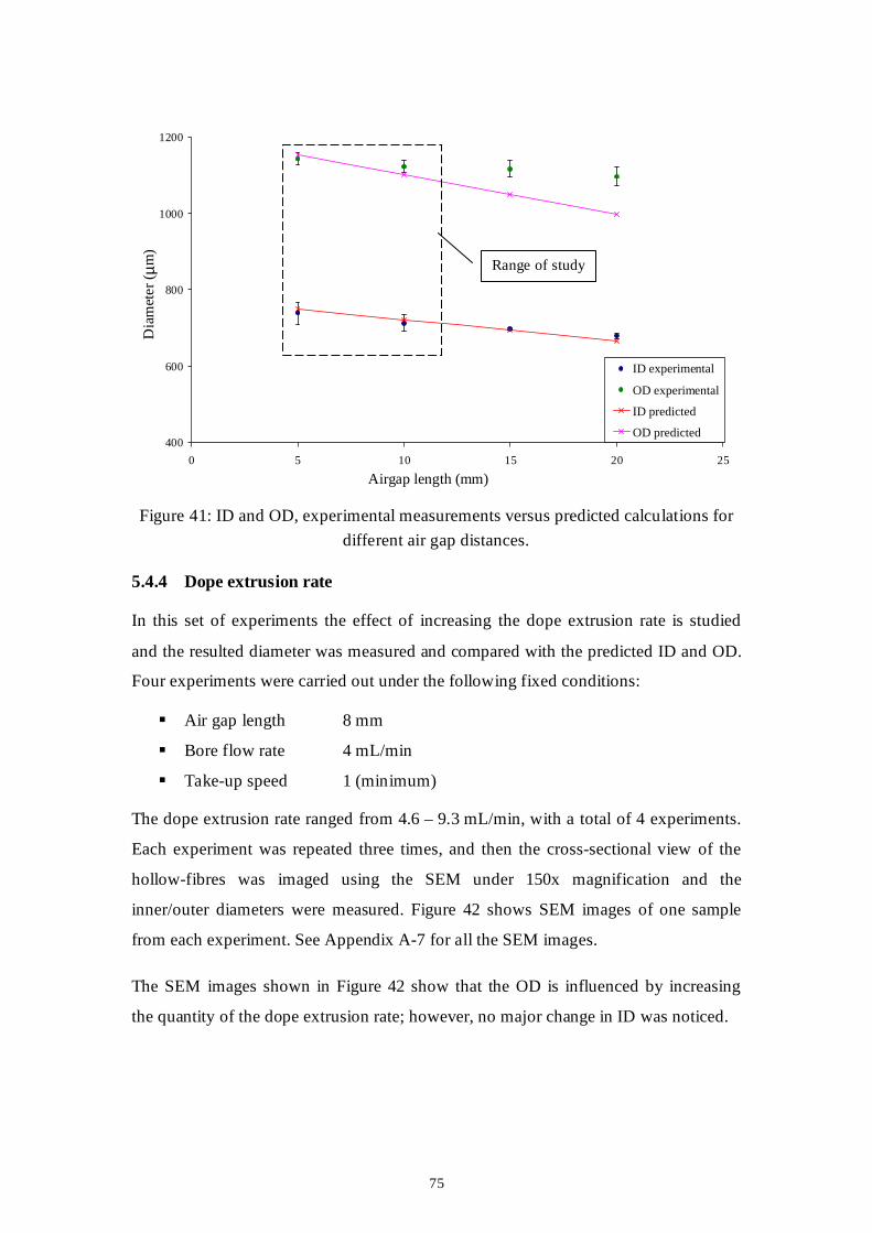
75
400
600
800
1000
1200
0 5 10 15 20 25
Airgap length (mm)
Dia
met
er
( µm)
ID experimental
OD experimental
ID predicted
OD predicted
Figure 41: ID and OD, experimental measurements versus predicted calculations for
different air gap distances.
5.4.4 Dope extrusion rate
In this set of experiments the effect of increasing the dope extrusion rate is studied
and the resulted diameter was measured and compared with the predicted ID and OD.
Four experiments were carried out under the following fixed conditions:
Air gap length 8 mm
Bore flow rate 4 mL/min
Take-up speed 1 (minimum)
The dope extrusion rate ranged from 4.6 – 9.3 mL/min, with a total of 4 experiments.
Each experiment was repeated three times, and then the cross-sectional view of the
hollow-fibres was imaged using the SEM under 150x magnification and the
inner/outer diameters were measured. Figure 42 shows SEM images of one sample
from each experiment. See Appendix A-7 for all the SEM images.
The SEM images shown in Figure 42 show that the OD is influenced by increasing
the quantity of the dope extrusion rate; however, no major change in ID was noticed.
Range of study
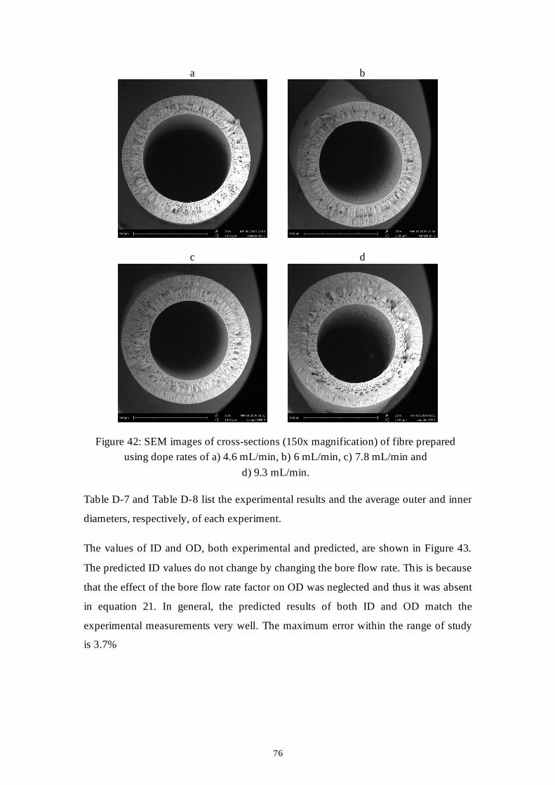
76
a
b
c
d
Figure 42: SEM images of cross-sections (150x magnification) of fibre prepared
using dope rates of a) 4.6 mL/min, b) 6 mL/min, c) 7.8 mL/min and
d) 9.3 mL/min.
Table D-7 and Table D-8 list the experimental results and the average outer and inner
diameters, respectively, of each experiment.
The values of ID and OD, both experimental and predicted, are shown in Figure 43.
The predicted ID values do not change by changing the bore flow rate. This is because
that the effect of the bore flow rate factor on OD was neglected and thus it was absent
in equation 21. In general, the predicted results of both ID and OD match the
experimental measurements very well. The maximum error within the range of study
is 3.7%
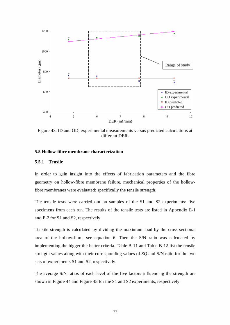
77
400
600
800
1000
1200
4 5 6 7 8 9 10
DER (ml /min)
Dia
me
ter
( µm)
ID experimentalOD experimental
ID predictedOD predicted
Figure 43: ID and OD, experimental measurements versus predicted calculations at
different DER.
5.5 Hollow-fibre membrane characterization
5.5.1 Tensile
In order to gain insight into the effects of fabrication parameters and the fibre
geometry on hollow-fibre membrane failure, mechanical properties of the hollow-
fibre membranes were evaluated; specifically the tensile strength.
The tensile tests were carried out on samples of the S1 and S2 experiments: five
specimens from each run. The results of the tensile tests are listed in Appendix E-1
and E-2 for S1 and S2, respectively
Tensile strength is calculated by dividing the maximum load by the cross-sectional
area of the hollow-fibre, see equation 6. Then the S/N ratio was calculated by
implementing the bigger-the-better criteria. Table B-11 and Table B-12 list the tensile
strength values along with their corresponding values of SQ and S/N ratio for the two
sets of experiments S1 and S2, respectively.
The average S/N ratios of each level of the five factors influencing the strength are
shown in Figure 44 and Figure 45 for the S1 and S2 experiments, respectively.
Range of study
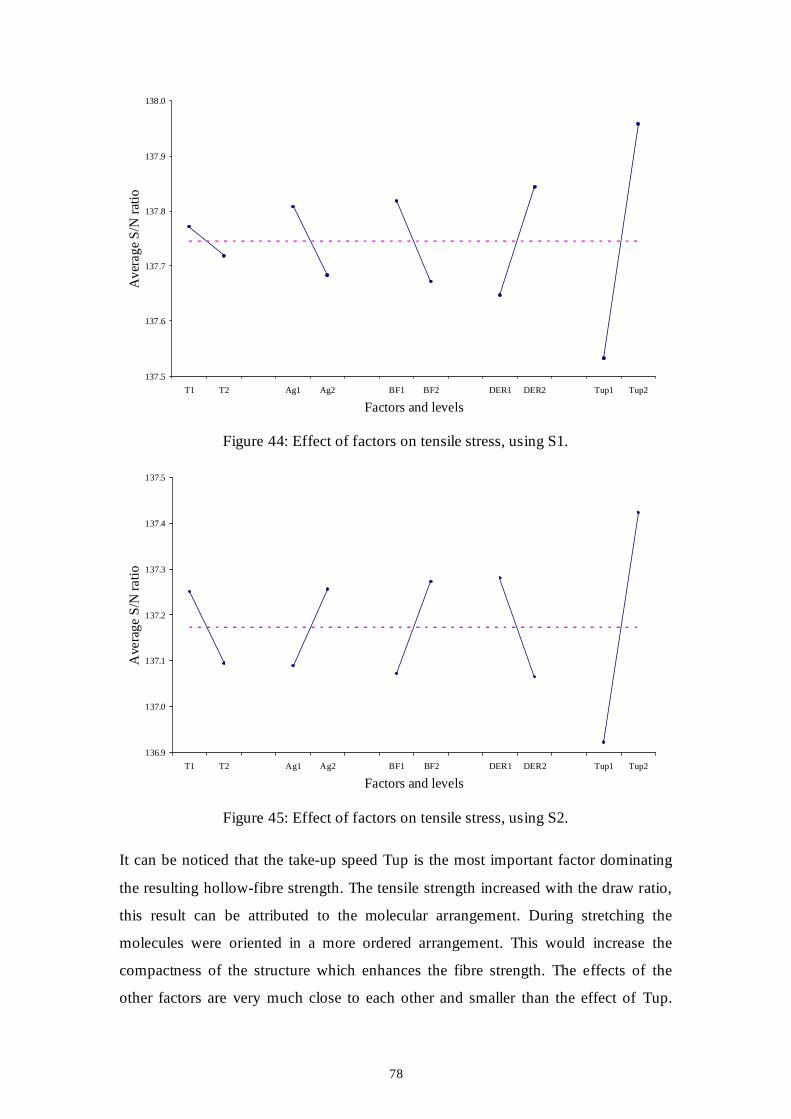
78
137.5
137.6
137.7
137.8
137.9
138.0
T1 T2 Ag1 Ag2 BF1 BF2 DER1 DER2 Tup1 Tup2
Factors and levels
Ave
rag
e S
/N r
atio
Figure 44: Effect of factors on tensile stress, using S1.
136.9
137.0
137.1
137.2
137.3
137.4
137.5
T1 T2 Ag1 Ag2 BF1 BF2 DER1 DER2 Tup1 Tup2
Factors and levels
Ave
rag
e S
/N r
atio
Figure 45: Effect of factors on tensile stress, using S2.
It can be noticed that the take-up speed Tup is the most important factor dominating
the resulting hollow-fibre strength. The tensile strength increased with the draw ratio,
this result can be attributed to the molecular arrangement. During stretching the
molecules were oriented in a more ordered arrangement. This would increase the
compactness of the structure which enhances the fibre strength. The effects of the
other factors are very much close to each other and smaller than the effect of Tup.
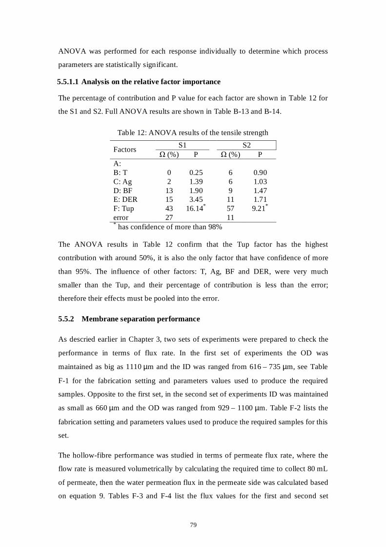
79
ANOVA was performed for each response individually to determine which process
parameters are statistically significant.
5.5.1.1 Analysis on the relative factor importance
The percentage of contribution and P value for each factor are shown in Table 12 for
the S1 and S2. Full ANOVA results are shown in Table B-13 and B-14.
Table 12: ANOVA results of the tensile strength
S1 S2 Factors
Ω (%) P Ω (%) P A: B: T 0 0.25
6 0.90
C: Ag 2 1.39 6 1.03 D: BF 13 1.90 9 1.47 E: DER 15 3.45 11 1.71 F: Tup 43 16.14* 57 9.21* error 27 11 * has confidence of more than 98%
The ANOVA results in Table 12 confirm that the Tup factor has the highest
contribution with around 50%, it is also the only factor that have confidence of more
than 95%. The influence of other factors: T, Ag, BF and DER, were very much
smaller than the Tup, and their percentage of contribution is less than the error;
therefore their effects must be pooled into the error.
5.5.2 Membrane separation performance
As descried earlier in Chapter 3, two sets of experiments were prepared to check the
performance in terms of flux rate. In the first set of experiments the OD was
maintained as big as 1110 µm and the ID was ranged from 616 – 735 µm, see Table
F-1 for the fabrication setting and parameters values used to produce the required
samples. Opposite to the first set, in the second set of experiments ID was maintained
as small as 660 µm and the OD was ranged from 929 – 1100 µm. Table F-2 lists the
fabrication setting and parameters values used to produce the required samples for this
set.
The hollow-fibre performance was studied in terms of permeate flux rate, where the
flow rate is measured volumetrically by calculating the required time to collect 80 mL
of permeate, then the water permeation flux in the permeate side was calculated based
on equation 9. Tables F-3 and F-4 list the flux values for the first and second set
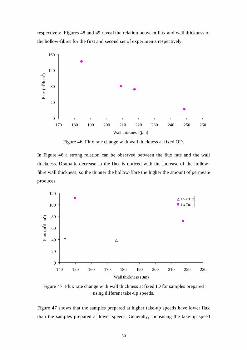
80
respectively. Figures 48 and 49 reveal the relation between flux and wall thickness of
the hollow-fibres for the first and second set of experiments respectively.
0
40
80
120
160
170 180 190 200 210 220 230 240 250 260
Wall thickness (µm)
Flu
x (m
3 /h.m
2 )
Figure 46: Flux rate change with wall thickness at fixed OD.
In Figure 46 a strong relation can be observed between the flux rate and the wall
thickness. Dramatic decrease in the flux is noticed with the increase of the hollow-
fibre wall thickness, so the thinner the hollow-fibre the higher the amount of permeate
produces.
0
20
40
60
80
100
120
140 150 160 170 180 190 200 210 220 230
Wall thickness (µm)
Flu
x (m
3 /h.m
2 )
1.5 x Tup
1 x Tup
Figure 47: Flux rate change with wall thickness at fixed ID for samples prepared
using different take-up speeds.
Figure 47 shows that the samples prepared at higher take-up speeds have lower flux
than the samples prepared at lower speeds. Generally, increasing the take-up speed

81
considerably decreases the flux rate. That could be attributed to the effect of
stretching the hollow-fibre. Where stretching the fibres will deform the shape of the
pores on the hollow-fibre surface and even close them, which results in a reduction in
the permeation rate through the membrane surface.

CHAPTER 6
CONCLUSIONS
83
CHAPTER 6: CONCLUSIONS
Polysulfone hollow-fibre membranes were fabricated using the dry-wet solution
spinning technique. A new solution spinning plant was installed as a part of wider
project. The plant was fully controlled with a specially devised computer control
system, which was developed to control, measure and then read and import data into a
real-time computer environment software (LabView). Using the user friendly
interface of the control system it was possible to monitor, print, log and save the
spinning conditions in an excel sheet, or to load earlier experimental conditions.
The acquired data were analyzed and used to study the significance on the fibre
diameter and the flux performance of the fibres. The influences of the various process
parameters, including spinneret size, dope extrusion rate, bore flow rate and the take-
up speed, were investigated using an experimental design based on a fractional
factorial method (Taguchi’s design of experiments). The experiments commenced
with a preliminary investigation using an L18 array, and were then refined into two
sets of L8 arrays. The diameters of the hollow-fibres were measured using a scanning
electron microscope (SEM), while the mechanical properties were determined using a
tensile tester.
Experimental results showed that hollow-fibre diameter and wall thickness could be
controlled by controlling the fabrication parameters, being the effect of the major
factors as follows:
• The use of a spinneret with an appropriate size was found to be the most
important parameter affecting the diameter size and the wall thickness of the
hollow-fibres. Hollow-fibres with large diameter size were fabricated using a
larger spinneret.
• Changing the temperatures had the smallest effect (among the factors considered
here), and therefore its effect was neglected in creating the prediction model. This
was done although it is known that the temperature plays an important role in the
creation of the resultant membrane morphology.
• The take-up speed was the second most important factor; affected both the inner
and the outer diameters of the hollow-fibres.
84
• The air gap factor had a pronounced effect on both the ID and OD of the fibres,
but had a lower relevant effect than the take-up speed. The influence of the
gravity force on the nascent fibre is more profound as the length of the air gap is
larger, which results in fibres with smaller diameters.
• The bore fluid flow rate had a considerable effect on ID, but not on OD:
increasing the rate of bore flow puts extra pressure on the inner surface area of
the hollow-fibre, and, simultaneously, the external surface started to solidify, and
resist expansion, which resulting in a reduced wall thickness.
• Opposite to the bore flow rate effect, the dope extrusion rate had a significant
effect on the OD, but did not contribute significantly to ID, where the increased
amount of polymer extruding from the spinneret will result in a direct increase to
OD and hence, the wall thickness, while the ID will not be significantly affected
because of the bore pressure applied from inside.
Two regression models were created to predict the diameter size of the hollow-fibre
membrane fabricated under certain selected conditions for the two spinnerets used
here. The equation that predicts the ID size was found to be a function of the
following factors: take-up speed, air gap length and bore flow rate. The equation that
predicts the OD size was found to be a function of: take-up speed, air gap length and
dope extrusion rate.
The prediction model was confirmed after conducting four sets of experiments, and
comparing the predicted results with the actual measurements. There were a very
good match between the predicted diameter and experimental diameters, with a
maximum error of 7%.
Results of cell tests on the membrane modules revealed that the permeate flux rate
through the membrane was strongly dependent on the wall thickness of the hollow-
fibre. A decrease in flux was noticed with an increase in the hollow-fibre wall
thickness. It was also noticed that the fabrication parameter settings affect the
membrane performance. Fibres prepared at higher take-up speeds had lower fluxes
than samples prepared at slower speeds. Generally, increasing the take-up speed
considerably decreased the flux rate: stretching the fibres deforms the shape of the
85
pores on the hollow-fibre surface, and even closes them, which results in a reduction
in the permeation rate.
Results of tensile strength tests revealed that the strongest fibres were produced when
using higher take-up speeds, as stretching the fibres during the fabrication orients the
molecular chains in a more ordered arrangement which enhances the strength.

REFERENCES
87
REFERENCES
1. Membrane technology overview. [cited 2007 April 14]; Available from: http://www.zenon.com/resources/introduction_to_membranes/.
2. Samueli, H. Membrane history. [cited 2007 May 5]; Available from: http://www.engineer.ucla.edu/history/osmosis.html.
3. Bloch, R. and M.A. Frommer, The mechanism for formation of 'skinned' membranes. I. Structure and properties of membranes cast from binary solutions. Desalination, 1970, 7(2): p. 259-264.
4. Cohen, C., G.B. Tanny, and S. Prager, Diffusion-controlled formationof porous structure in terantry polymer systems. Journal of Membrane Science, 1979, 17(3): p. 477-489.
5. Frommer, M.A., I. Feiner, O. Kedem, and R. Bloch, The mechanism for formation of 'skinned' membranes. II. Equilibrium properties and osmotic flows determining membran structure. Desalination, 1970, 7(3): p. 393-402.
6. Frommer, M.A. and D. Lancet, The mechanism of membrane formation: membrane structures and their relation to preparation conditions, in reverse osmosis membrane research, H. Lonsdale and H.E. Podall, Editors. 1972, Plenum press: New York.
7. Frommer, M.A. and R.M. Messalem, Mechanism of membrane formation. VI. Convective flows and large void formaion during membrane precipitation. Industrial Chemistry Research, 1973, 12(4): p. 328-333.
8. Guillotin, M., C. Lemoyne, C. Noel, and L. Monnerie, Physicochemiccal process occuring during the formation of cellulose diacetate membrane. Research of criteria for optimizing membrane performance. IV. Cellulose diacetate-aceton-additive casting solutions. Desalination, 1977, 21: p. 165-181.
9. Reuvers, A.J., F.W. Altena, and C.A. Smolders, Demixing and gelation behavior of ternary cellulose acetate solutions. Journal of Membrane Science, 1986, 24(4): p. 793-804.
10. Shen, T.C. and I. Cabasso, Ethyl Cellulose anisotropic membranes, in Macromolecular Solutions, R.B. Seymour and G.A. Stahl, Editors. 1982, Pergamon: New York. p. 108.
11. So, M.T., F.R. Eirich, H. Strathmann, and R.W. Baker, Preparation of asymmetric Loeb-Sourirajan membranes. Journal of Membrane Science, 1973, 11(3): p. 201-205.
12. Strathmann, H., Production of microporous media by phase inversion process, in Material Science and Sunthetic Membranes, D.R. Lloyd, Editor. 1985, American Chemical Society: Washington DC. p. 165.
13. Strathmann, H., Preparation of microporous membrane by phase inversion process, in Membranes and Membrane Processes, E. Drioli and M. Nakagaki, Editors. 1986, Plenum: New York. p. 115.
14. Yao, C.W., R.P. Burford, A.G. Fane, and C.J.D. Fell, Effect of coagulation conditions on structure and properties of membranes from aliphatic polymides. Journal of Membrane Science, 1988, 38(2): p. 113-125.
15. Friedrich, G., A. Driancourt, C. Noel, and L. Monnerie, Asymetric reverse osmosis and ultrafiltration membranes prepared from sulfonated polysulfone. Desalination, 1981, 36(1): p. 39-62.
88
16. Strathmann, H., Synthetic mambranes and their preparation, in Syntheric Membranes: Science, Engineering and Applications, P.M. Bungay, H.K. Lonsdale, and M.N.d. Pinho, Editors. 2004, NATO Science Dordrecht.
17. Wijmans, J.G., J. Kant, M.H.V. Mulder, and C.A. Smolders, Phase separation phenomena in solutions of polysulfone mixtures of a solvent and a nonsolvent: relationship with membrane formation. Polymer, 1985, 26(10): p. 1539-1545.
18. Rove`re, A.D. and R.L. Shambaugh, Melt-spun hollow-fibers for Use in nonwoven structures. Industrial Engineering Chemistry, 2001, 40: p. 176-187.
19. Qaisrani, T.M., MF Process an introduction. 2006, Universität Linz - Institut für Verfahrenstechnik. p. 1-9.
20. Baker, R.W., Membrane technology and applications. 2nd ed. 2004, California: John Wiley & Sons Ltd.
21. Kemmer, F.N., The NALCO water handbook. 2nd ed. Nalco Chemical Company, ed. H.B. Crawford and R.T. Margolies. 1988, New York: McGraw-Hill.
22. Baker, R.W., Overview of membrane science technology. Membrane Technology and Applications, ed. 2nd. 2004, California: John Wiley & Sons Ltd.
23. Reverse Osmosis. [cited 2007 April 29]; Available from: http://en.wikipedia.org/wiki/Reverse_osmosis.
24. ROMICON. Hollow fiber membrane overview. [cited 2007 May 7]; Available from: http://www.kochmembrane.com/prod_hf.html.
25. Hollosep features. [cited 2007 Nov. 22]; Available from: http://www.toyobo.co.jp/e/seihin/ro/tokucho.htm.
26. Manufacturing: synthetic and cellulosic fiber formation technology. [cited 2007 Mar. 13]; Available from: http://www.fibersource.com/f-tutor/techpag.htm.
27. Idris, A., A.F. Ismail, M.Y. Noordin, and S.J. ShiltonIdris, Optimization of cellulose acetate hollow-fiber reverse osmosis membrane production using Taguchi method. Journal of Membrane Science, 2002, 205: p. 223-237.
28. Mahon, H.I., Permeability separatory apparatus and membrane element, method of making the same and process utilizing the same. 1966, Dow Chemical Co.: United States.
29. Wienk, I.M., F.H.A.O. Scholtenhuis, T.v.d. Boomgaard, and C.A. Smolders, Spinning of hollow fiber ultra-filtration membranes from a polymer blend. Journal of Membrane Science, 1995, 106: p. 233-243.
30. Yeow, M.L., Y.T. Liu, and K. Li, Morphological study of Poly(vinylidene fluoride) asymmetric membranes: Effects of the solvent, additive, and dope temperature. Journal of Applied Polymer Science, 2004, 92: p. 1782-1789.
31. Yeow, M.L., Y.T. Liu, and K. Li, Isothermal phase diagrams and phase-inversion behavior of Poly(vinylidene fluoride)/solvents/additives/water systems. Journal of Applied Polymer Science, 2003, 90: p. 2150-2155.
32. KMS hollow-fiber filtration technology. [cited 2007 May 7]; Available from: http://www.kochmembrane.com/prod_hf.html,.
33. Hollow-fiber membrane & modules. [cited 2007 Nov. 20]; Available from: http://www.motimo.com.cn/en/hollow.htm.
34. Water treatment technology. [cited 2007 Nov. 20]; Available from: http://www.toray.com/technology/html/tec_a038.html.
89
35. Wang, Z., Technology of water treatment. 1989, 15: p. 302-306.
36. Hao, J.H., H. Dai, P. Yang, and Z. Wang, Spinning of cellulose acetate hollow-fiber by dry-wet technique of 3C-shaped spinneret. Journal of Applied Polymer Science, 1996, 62: p. 129-133.
37. Zhang, Y., Q. Du, Y. Wu, P. Wang, and J. Wu, Fabrication of polysulfone asymmetric hollow-fiber membranes by coextrusion through a Triple-Orifice spinneret. Journal of Applied Polymer Science, 2004, 94: p. 259-266.
38. Paulsena, F.G., S.S. Shojaieb, and W.B. Krantz, Effect of evaporation step on macrovoid defect formation in wet-cast polymeric membranes. Journal of Membrane Science, 1994, 91(3): p. 265-282.
39. Wang, D., K. Li, and W. Teo, Porous PVDF asymmetric hollow fiber membranes prepared with the use of small molecular additives. Journal of Membrane Science, 2000 178: p. 13-23.
40. Wang, D., K. Li, and W.K. Teo, Phase separation in Polyetherimide/solvent/nonsolvent systems and membrane formation. Journal of Applied Polymer Science, 1999, 71: p. 1789–1796.
41. Qin, J. and T.-S. Chung, Effect of dope flow rate on the morphology, separation performance, thermal and mechanical properties of ultrafiltration hollow fibre membranes. Journal of Membrane Science, 1999, 157: p. 35-51.
42. Khayet, M. and T. Matsuura, Preparation and characterization of polyvinylidene fluoride membranes for membrane distillation. Industrial Engineering Chemistry, 2001, 40: p. 5710-5718.
43. Yeowa, M.L., Y. Liu, and K. Li, Preparation of porous PVDF hollow fibre membrane via a phase inversion method using lithium perchlorate (LiClO4) as an additive. Journal of Membrane Science, 2005 258 p. 16-22.
44. Bottino, A., G. Capannelli, S. Munari, and A. Turturro, High performance ultrafiltration membranes cast from LiCl doped solutions. Desalination, 1988, 68: p. 167-177.
45. Deshmukh, S.P. and K. Li, Effect of ethanol composition in water coagulation bath on morphology of PVDF hollow-fibre membranes. Journal of Membrane Science, 1998, 150: p. 75-85.
46. Wang, D., K. Li, and W.K. Teo, Preparation and characterization of polyvinylidene fluoride (PVDF) hollow fiber membranes. Journal of Membrane Science, 1999, 163: p. 211-220.
47. Munari, S., A. Bottino, G. Camera-Roda, and G. Capannelli, Preparation of ultrafiltration membranes. State of the art. Desalination, 1990, 77: p. 85-100.
48. Tomaszewska, M., Preparation and properties of flat-sheet membranes from poly(vinylidene fluoride) for membrane distillation. Desalination, 1996, 104: p. 1-11.
49. Puri, P.S., Fabrication of hollow fiber gas separation membranes. Gas Separation & Purification, 1990, 4: p. 29-36.
50. Chung, T.S. and X. Hu, Effects of air gap distance on the morphology and thermal properties of polyethersulfone hollow fibers. Journal of Applied Polymer Science, 1997, 66: p. 1067-1077.
51. Miao, X., S. Sourirajan, H. Zhang, and W. Lau, Production of hollow fiber ultra-filtration membranes: effects of (internal coagulant) flow rate (WFR) and length of air gap. Separation Science and Technology, 1996, 31(2): p. 141-172.
90
52. Chau, J.L., S.S. Wang, and C.L. Guo, Pilot production of pulysulfone hollow fiber for ultra-filtration using orthogonal array experimentation. Industrial Chemistry Research, 1995, 34: p. 803-919.
53. Ismail, A.F., I.R. Dunkin, S.L. Gallivan, and S.J. Shilton, Production of superselective polysulfone hollow fiber membranes for gas separation. Polymer, 1999, 40: p. 6499-6506.
54. Sharpe, I.D., A.F. Ismail, and S.J. Shilton, A study of extrusion shear and forced convection residence time in the spinning of polysulfone hollow fiber membranes for gas separation. Separation and Purification Technology, 1999, 17(2): p. 101-109.
55. Kim, J.-J., T.-S. Jang, Y.-D. Kwon, U.Y. Kim, and S.S. Kim, Structural study of microporous polypropylene hollow fiber membranes made by the melt-spinning and cold-stretching method. Journal of Membrane Science, 1994, 93(3): p. 209-215.
56. Kim, J., Y. Park, J. Jegal, and K. Lee, The effects of spinning conditions on the structure formation and the dimension of the Hollow-fiber membranes and their relationship with the permeability in dry-wet spinning technology. Journal of Applied Polymer Science, 1995, 57(13): p. 1637-1644.
57. Rovere, A.D., B.P. Grady, and R.L. Shambaugh, The influence of processing parameters on the properties of melt-spun Polypropylene hollow-fibers. Journal of Applied Polymer Science, 2002, 83: p. 1759-1772.
58. Pesek, S.C. and W.J. Koros, Aqueous quenched asymmetric polysulfone hollow fiber prepared by dry/wet phase separation. Journal of Membrane Science, 1994, 88(1): p. 1-19.
59. Ismail, A.F., Novel studies of molecular orientation in synthetic polymeric membranes for gas separation. 1997, University of Strathclyde: Glasgow.
60. Cabasso, I., K.Q. Robert, E. Klein, and J.K. Smith, Porosity and pore size determination in polysulfone hollow fibers. Journal of Applied Polymer Science, 1977, 21(7): p. 1883-1900.
61. Shieh, J.J. and T.S. Chung, Effect of liquid-liquid demixing on the membrane morphology, gas permeation, thermal and mechanical properties of Cellulose Acetate hollow fibers. Journal of Membrane Science 1998, 140(1): p. 67-79.
62. Friedrich, G., A. Driancourt, C. Noel, and L. Monnerie, Asymetric reverse osmosis and ultrafiltration membranes prepared from sulfonated polysulfone. Desalination, 1985, 36.
63. Strathmann, H. and K. Kock, The formation mechanism of phase inversion membranes. Desalination, 1977, 21(3): p. 241-255.
64. Strathmann, H., K. Kock, P. Amar, and R.W. Baker, The formation mechanism of asymmetric membranes. Desalination, 1975, 16(2): p. 179-203.
65. Munari, S., A. Bottino, and G. Capannelli, Casting and performance of polyvinylidene fluoride based membranes. Journal of Membrane Science, 1983, 16: p. 181-193.
66. Bottino, A., G. Camera-Rodab, G. Capannelli, and S. Munari, The formation of microporous polyvinylidene difluoride membranes by phase separation. Journal of Membrane Science, 1991, 57: p. 1-20.
67. Kim, J.J., J.R. Hwang, U.Y. Kim, and S.S. Kim, Operation parameters of melt spinning of polypropylene hollow fiber membranes. Journal of Membrane Science, 1995, 108(1-2): p. 25-36.
91
68. Kusuki, Y., T. Yoshinaga, and H. Shimazaki, Aromatic polyimide double layered hollow filamentary membrane and process for producing same. 1992, Ube Industries, Ltd. (Ube, JP): United States.
69. Kopp, C.V., R.J.W. Streeton, and P.S. Khoo, Extrusion head for forming polymeric hollow fiber. 1994: United States.
70. Jian, K. and E. Pintauro, Asymmetric PVDF hollow-fiber membranes for organic/water pervaporation separations. Journal of Membrane Science, 1997, 135: p. 41-53.
71. Arthanareeswaran, G., T.K.S. Devi, and D. Mohan, Development, characterization and separation performance of organic-inorganic membranes Part II. Effect of additives. Separation and Purification Technology, 2009: p. 11.
72. Chung, T.-S., J.-J. Qin, and J. Gu, Effect of shear rate within the spinneret on morphology, separation performance and mechanical properties of ultra"ltration polyethersulfone hollow "ber membranes. Chemical Engineering Science, 2000, 55: p. 1077-1091.
73. Matsuyama, H., K. Hayashi, T. Maki, M. Teramoto, and N. Kubota, Effect of polymer density on polyethylene hollow fiber membrane formation via thermally induced phase separation. Journal of Applied Polymer Science, 2004, 93: p. 471-474.
74. Chou, W.L. and M.C. Yang, Effect of take-up speed on physical properties and permeation performance of cellulose acetate hollow-fibers. Journal of Membrane Science, 2005, 250: p. 259-267.
75. Childress, A.E., P. Le-Clech, J.L. Daugherty, C. Chen, and G.L. Leslie, Mechanical analysis of hollow fiber membrane integrity in water reuse applications. Desalination, 2005, 180: p. 5-14.
76. Smolders, C.A., A.J. Reuvers, R.M. Boom, and I.M. Wienk, Microstructures in phase-inversion membranes. Part 1. Formation of macrovoids. Journal of Membrane Sctence, 1992, 73: p. 259-275.
77. Pranzas, P.K., et al., Online SAXS investigations of polymeric hollow fibre membranes. Analytical and Bioanalytical Chemistry, 2003, 376: p. 602-607.
78. Yeow, M.L., Y. Liu, and K. Li, Preparation of porous PVDF hollow fibre membrane via a phase inversion method using lithium perchlorate (LiClO4) as an additive. Journal of Membrane Science, 2005, 258: p. 16-22.
79. Ekiner, O.M. and G. Vassilatos, Polyamide hollow-iber for hydrogen/methane separation-spinning and properties. Journal of Membrane Science, 1990, 53(3): p. 259-273.
80. Mattson, R.J. and V.J. Tomsic, Improved water quality. Chemical Engineering Progress, 1969, 66(1): p. 62-68.
81. Gorenflo, A., J.A. Redondo, and F. Reverberi, Basic options and two case studies for retrofitting hollow fiber elements by spiral-wound RO technology. Desalination 2005, 178: p. 247-260.
82. Sekino, M., K. Matsunaga, K. Gotoh, Y. Yanaga, and H. Nikko, Reverse osmosis modules for water desalination. Chemical Engineering Progress, 1985, 81(12): p. 52-56.
83. Hollow-fiber membrane filters "Sterapore". [cited 2007 Nov. 20]; Available from: http://www.mrc.co.jp/mre/english/sterapore/sterapore_01.html.
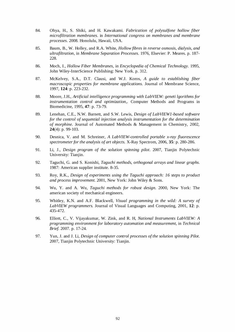
92
84. Ohya, H., S. Shiki, and H. Kawakami. Fabrication of polysulfone hollow fiber microfiltration membranes. in International congress on membranes and membrane processes. 2008. Honolulu, Hawaii, USA.
85. Baum, B., W. Holley, and R.A. White, Hollow fibres in reverse osmosis, dialysis, and ultrafiltration, in Membrane Separation Processes. 1976, Elsevier: P. Meares. p. 187-228.
86. Moch, I., Hollow Fiber Membranes, in Encyclopedia of Chemical Technology. 1995, John Wiley-InterScience Publishing: New York. p. 312.
87. McKelvey, S.A., D.T. Clausi, and W.J. Koros, A guide to establishing fiber macroscopic properties for membrane applications. Journal of Membrane Science, 1997, 124: p. 223-232.
88. Moore, J.H., Artificial intelligence programming with LabVIEW: geneti lgorithms for instrumentation control and optimization,. Computer Methods and Programs in Biomedicine, 1995, 47: p. 73-79.
89. Lenehan, C.E., N.W. Barnett, and S.W. Lewis, Design of LabVIEW1-based software for the control of sequential injection analysis instrumentation for the determination of morphine. Journal of Automated Methods & Management in Chemistry, 2002, 24(4): p. 99-103.
90. Desnica, V. and M. Schreiner, A LabVIEW-controlled portable x-ray fluorescence spectrometer for the analysis of art objects. X-Ray Spectrom, 2006, 35: p. 280-286.
91. Li, J., Design program of the solution spinning pilot. 2007, Tianjin Polytechnic University: Tianjin.
92. Taguchi, G. and S. Konishi, Taguchi methods, orthogonal arrays and linear graphs. 1987: American supplier institute. 8-35.
93. Roy, R.K., Design of experiments using the Taguchi approach: 16 steps to product and process improvement. 2001, New York: John Wiley & Sons.
94. Wu, Y. and A. Wu, Taguchi methods for robust design. 2000, New York: The american society of mechanical engineers.
95. Whitley, K.N. and A.F. Blackwell, Visual programming in the wild: A survey of LabVIEW programmers. Journal of Visual Languages and Computing, 2001, 12: p. 435-472.
96. Elliott, C., V. Vijayakumar, W. Zink, and R. H, National Instruments LabVIEW: A programming environment for laboratory automation and measurement, in Technical Brief. 2007. p. 17-24.
97. Yun, J. and J. Li, Design of computer control processes of the solution spinning Pilot. 2007, Tianjin Polytechnic University: Tianjin.

APPENDICES
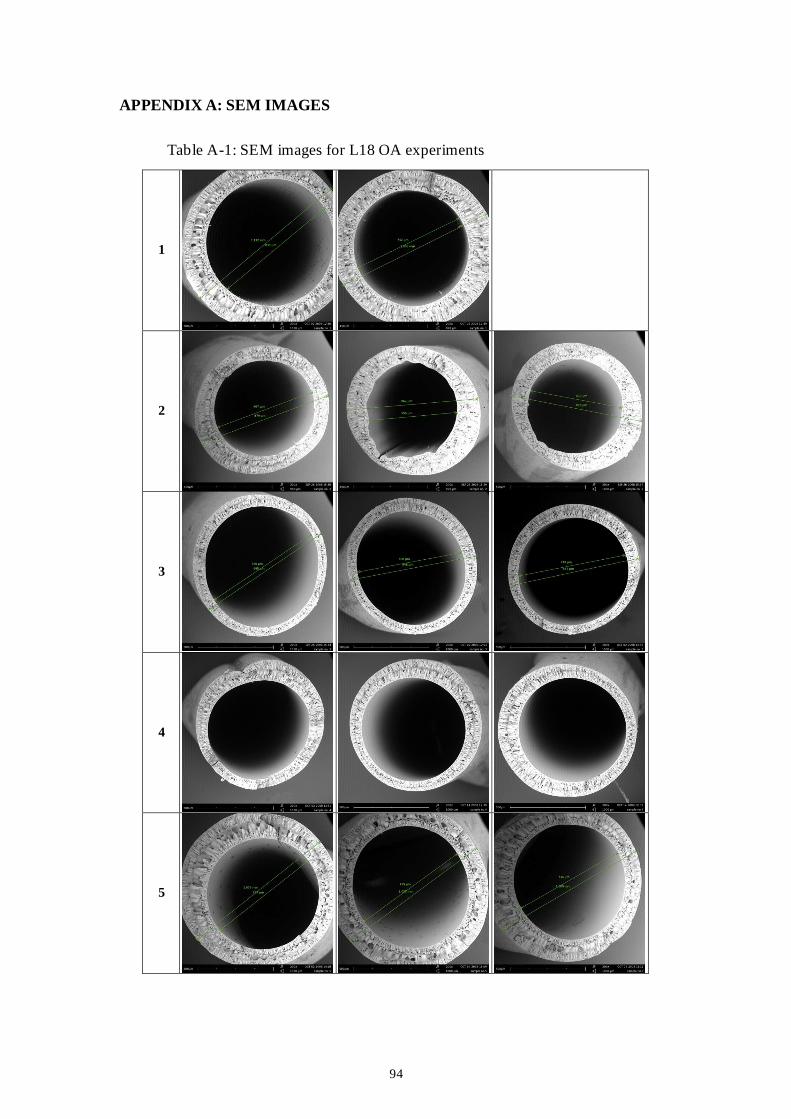
94
APPENDIX A: SEM IMAGES
Table A-1: SEM images for L18 OA experiments
1
2
3
4
5
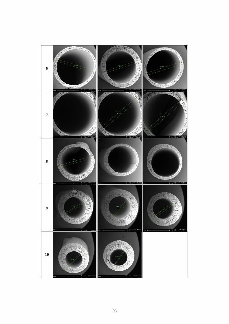
95
6
7
8
9
10
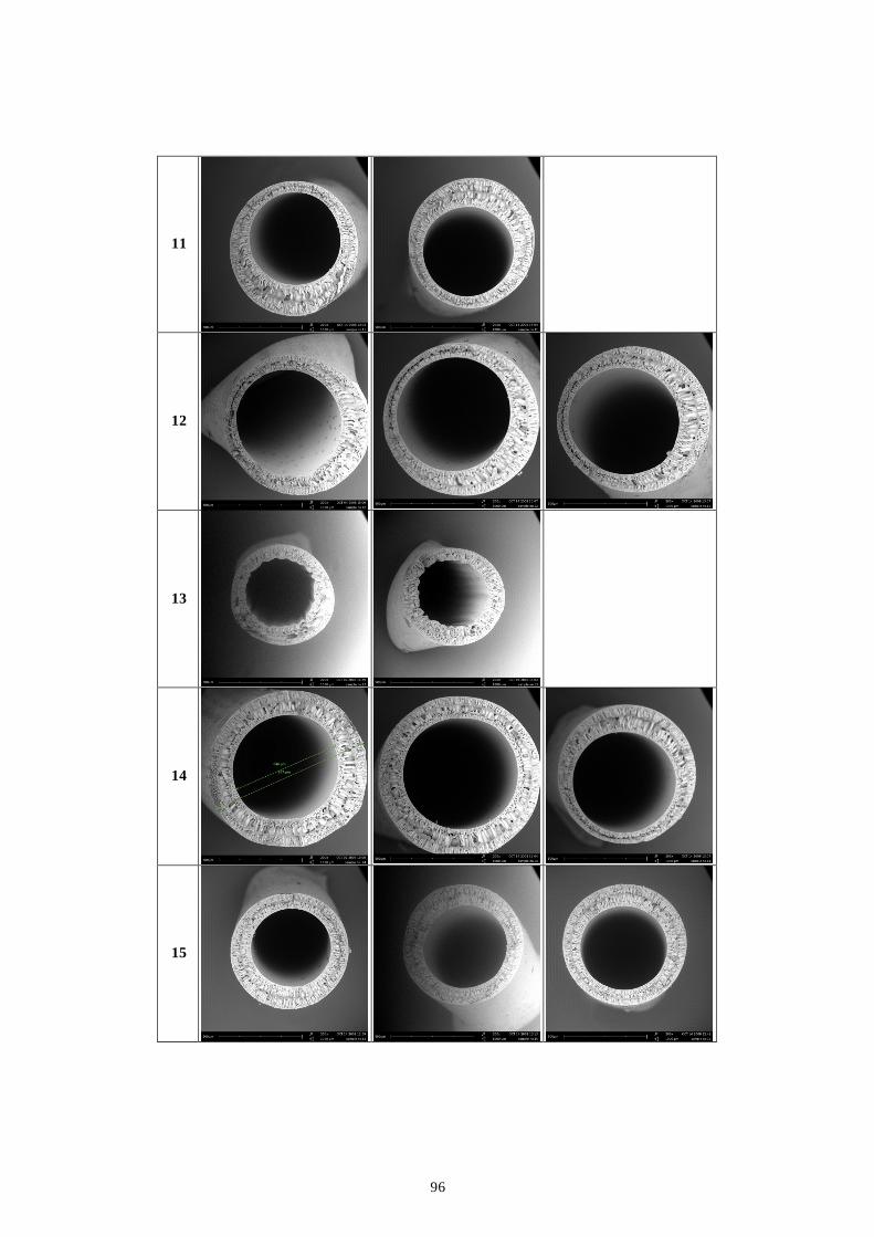
96
11
12
13
14
15
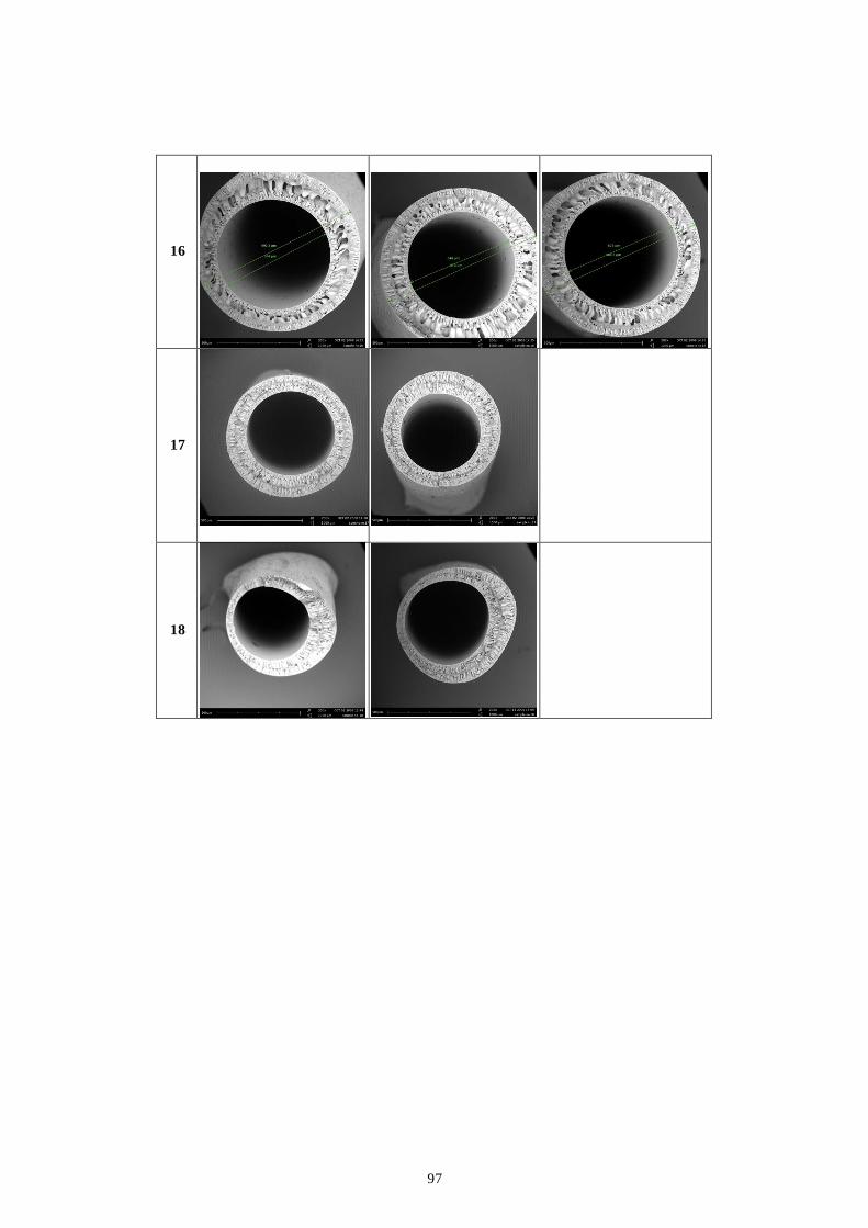
97
16
17
18
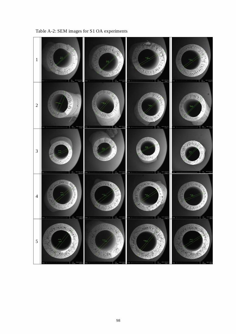
98
Table A-2: SEM images for S1 OA experiments
1
2
3
4
5
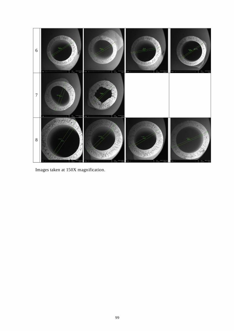
99
6
7
8
Images taken at 150X magnification.
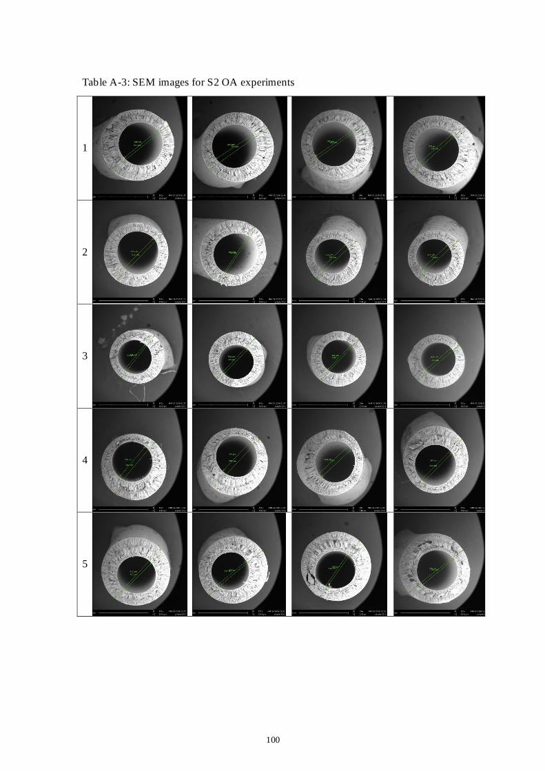
100
Table A-3: SEM images for S2 OA experiments
1
2
3
4
5
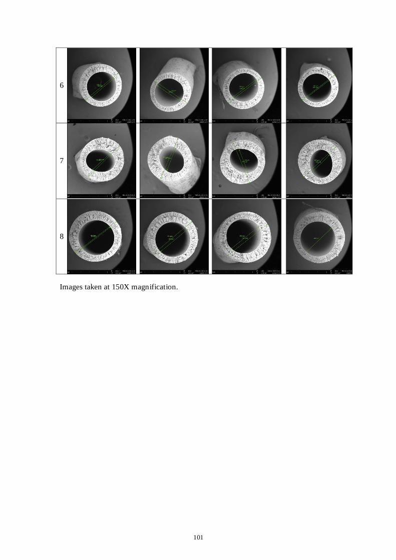
101
6
7
8
Images taken at 150X magnification.
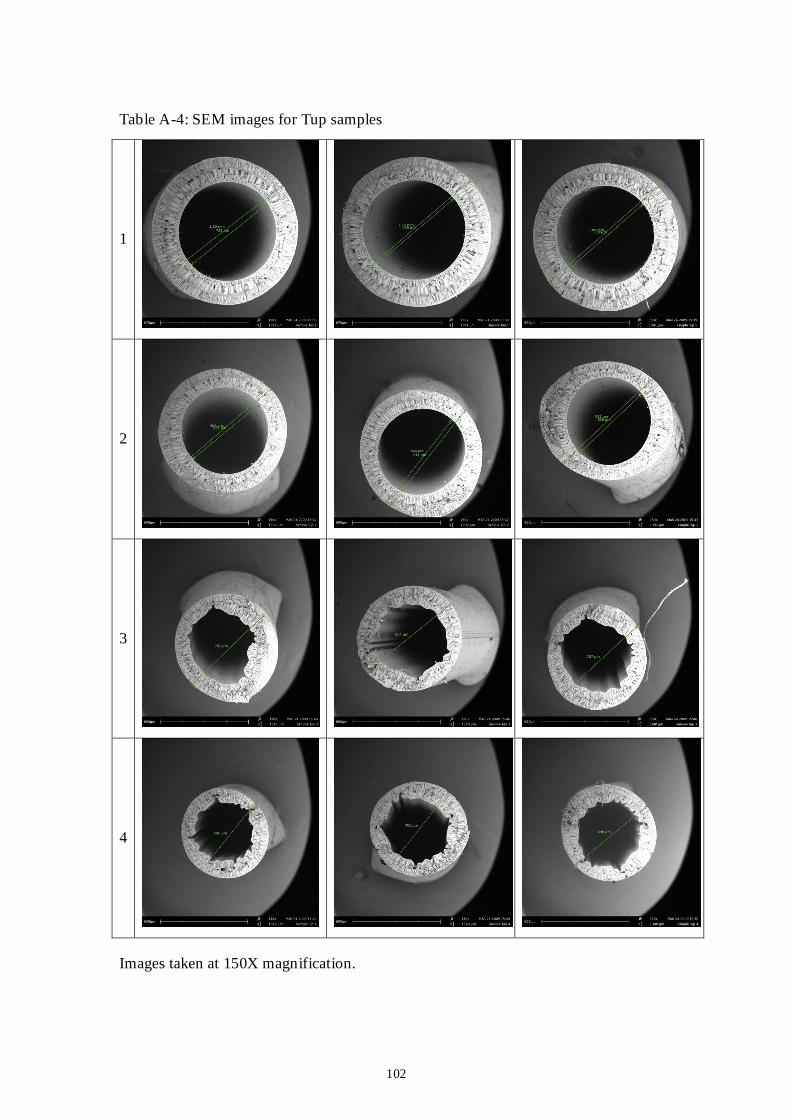
102
Table A-4: SEM images for Tup samples
1
2
3
4
Images taken at 150X magnification.
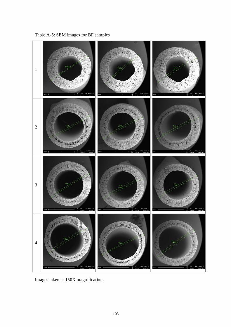
103
Table A-5: SEM images for BF samples
1
2
3
4
Images taken at 150X magnification.
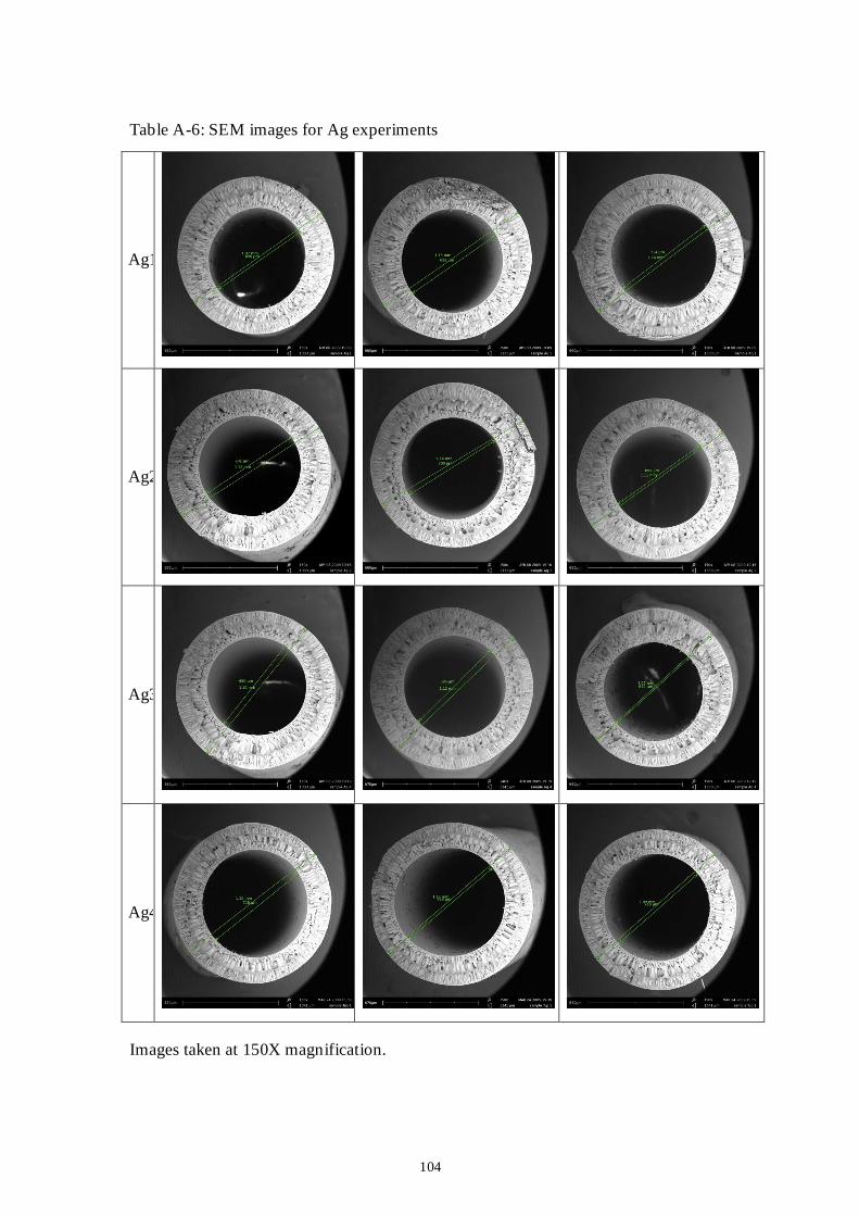
104
Table A-6: SEM images for Ag experiments
Ag1
Ag2
Ag3
Ag4
Images taken at 150X magnification.
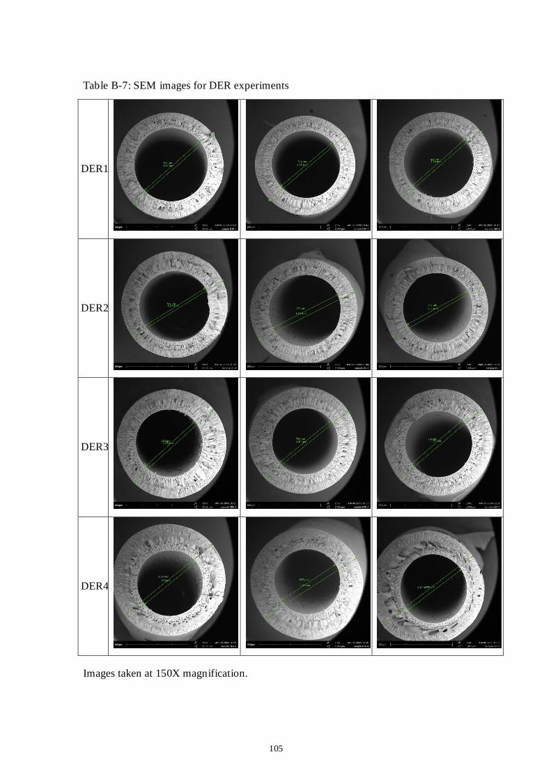
105
Table B-7: SEM images for DER experiments
DER1
DER2
DER3
DER4
Images taken at 150X magnification.
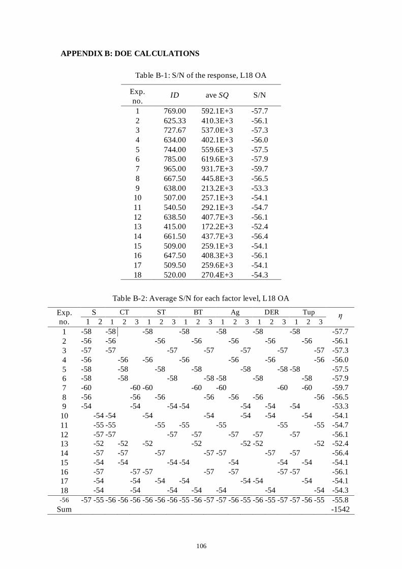
106
APPENDIX B: DOE CALCULATIONS
Table B-1: S/N of the response, L18 OA
Exp. no.
ID ave SQ S/N
1 769.00 592.1E+3 -57.7 2 625.33 410.3E+3 -56.1 3 727.67 537.0E+3 -57.3 4 634.00 402.1E+3 -56.0 5 744.00 559.6E+3 -57.5 6 785.00 619.6E+3 -57.9 7 965.00 931.7E+3 -59.7 8 667.50 445.8E+3 -56.5 9 638.00 213.2E+3 -53.3 10 507.00 257.1E+3 -54.1 11 540.50 292.1E+3 -54.7 12 638.50 407.7E+3 -56.1 13 415.00 172.2E+3 -52.4 14 661.50 437.7E+3 -56.4 15 509.00 259.1E+3 -54.1 16 647.50 408.3E+3 -56.1 17 509.50 259.6E+3 -54.1 18 520.00 270.4E+3 -54.3
Table B-2: Average S/N for each factor level, L18 OA
S CT ST BT Ag DER Tup Exp. no. 1 2 1 2 3 1 2 3 1 2 3 1 2 3 1 2 3 1 2 3
η
1 -58 -58 -58 -58 -58 -58 -58 -57.7 2 -56 -56 -56 -56 -56 -56 -56 -56.1 3 -57 -57 -57 -57 -57 -57 -57 -57.3 4 -56 -56 -56 -56 -56 -56 -56 -56.0 5 -58 -58 -58 -58 -58 -58 -58 -57.5 6 -58 -58 -58 -58 -58 -58 -58 -57.9 7 -60 -60 -60 -60 -60 -60 -60 -59.7 8 -56 -56 -56 -56 -56 -56 -56 -56.5 9 -54 -54 -54 -54 -54 -54 -54 -53.3 10 -54 -54 -54 -54 -54 -54 -54 -54.1 11 -55 -55 -55 -55 -55 -55 -55 -54.7 12 -57 -57 -57 -57 -57 -57 -57 -56.1 13 -52 -52 -52 -52 -52 -52 -52 -52.4 14 -57 -57 -57 -57 -57 -57 -57 -56.4 15 -54 -54 -54 -54 -54 -54 -54 -54.1 16 -57 -57 -57 -57 -57 -57 -57 -56.1 17 -54 -54 -54 -54 -54 -54 -54 -54.1 18 -54 -54 -54 -54 -54 -54 -54 -54.3 -56 -57 -55 -56 -56 -56 -56 -56 -56 -55 -56 -57 -57 -56 -55 -56 -55 -57 -57 -56 -55 -55.8
Sum -1542
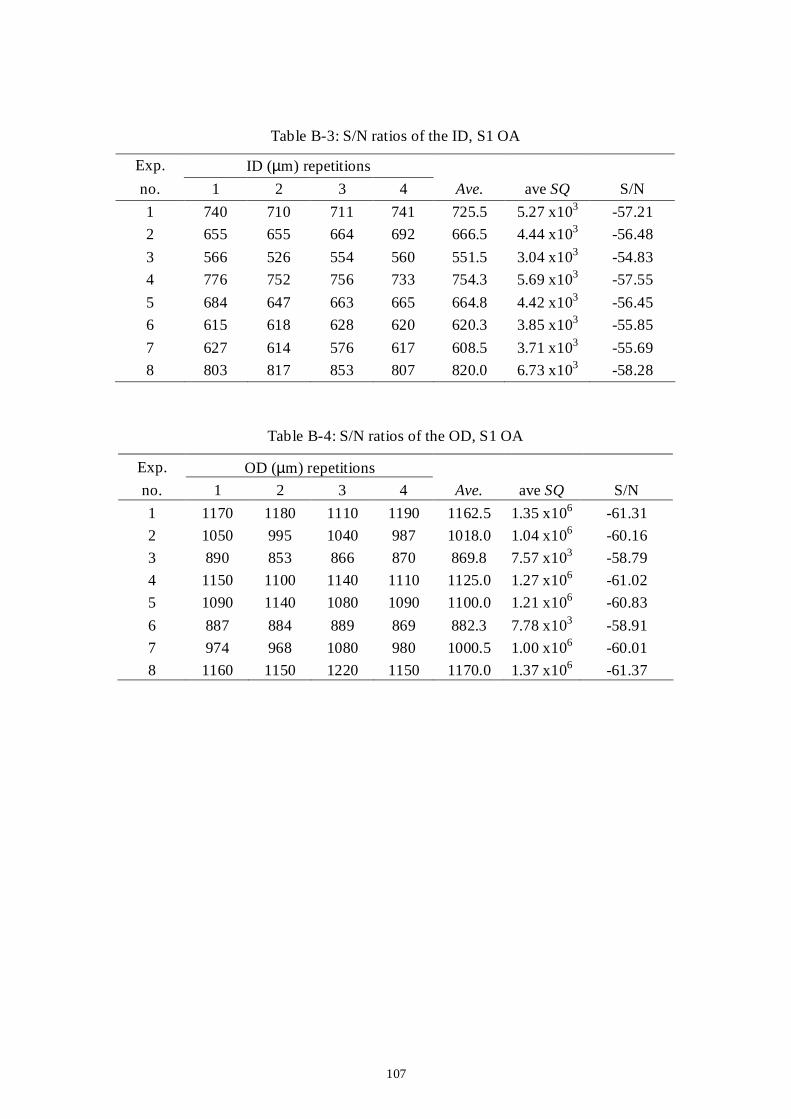
107
Table B-3: S/N ratios of the ID, S1 OA
Exp. ID (µm) repetitions
no. 1 2 3 4 Ave. ave SQ S/N
1 740 710 711 741 725.5 5.27 x10³ -57.21
2 655 655 664 692 666.5 4.44 x10³ -56.48
3 566 526 554 560 551.5 3.04 x10³ -54.83
4 776 752 756 733 754.3 5.69 x10³ -57.55
5 684 647 663 665 664.8 4.42 x10³ -56.45
6 615 618 628 620 620.3 3.85 x10³ -55.85
7 627 614 576 617 608.5 3.71 x10³ -55.69
8 803 817 853 807 820.0 6.73 x10³ -58.28
Table B-4: S/N ratios of the OD, S1 OA
Exp. OD (µm) repetitions
no. 1 2 3 4 Ave. ave SQ S/N
1 1170 1180 1110 1190 1162.5 1.35 x10⁶ -61.31
2 1050 995 1040 987 1018.0 1.04 x10⁶ -60.16
3 890 853 866 870 869.8 7.57 x10³ -58.79
4 1150 1100 1140 1110 1125.0 1.27 x10⁶ -61.02
5 1090 1140 1080 1090 1100.0 1.21 x10⁶ -60.83
6 887 884 889 869 882.3 7.78 x10³ -58.91
7 974 968 1080 980 1000.5 1.00 x10⁶ -60.01
8 1160 1150 1220 1150 1170.0 1.37 x10⁶ -61.37
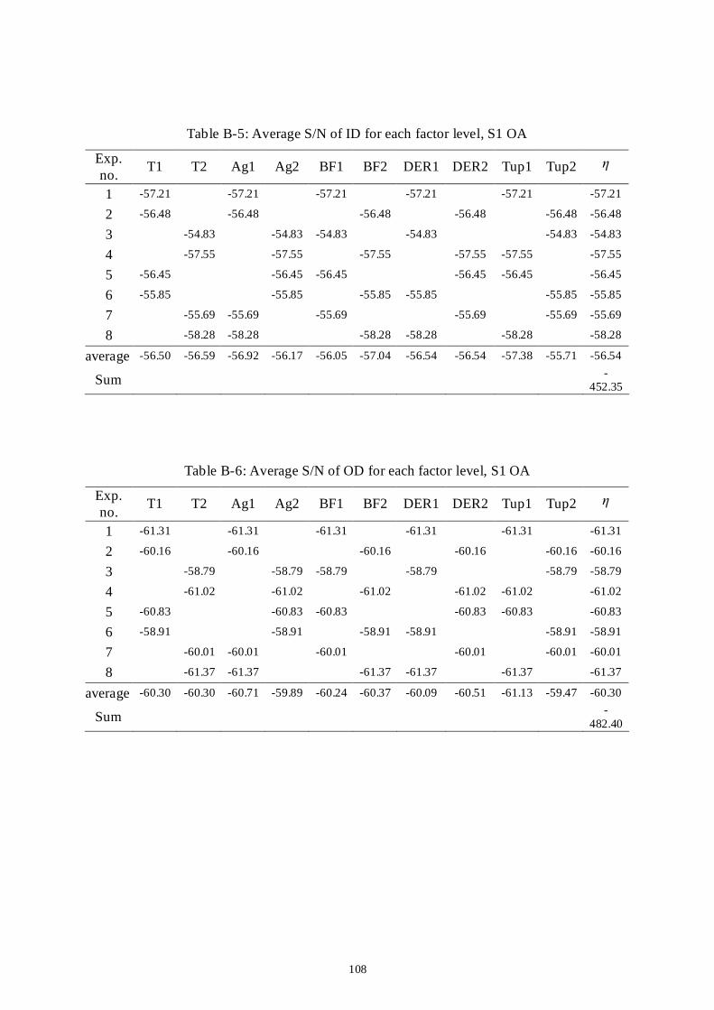
108
Table B-5: Average S/N of ID for each factor level, S1 OA
Exp. no.
T1 T2 Ag1 Ag2 BF1 BF2 DER1 DER2 Tup1 Tup2 η
1 -57.21 -57.21 -57.21 -57.21 -57.21 -57.21
2 -56.48 -56.48 -56.48 -56.48 -56.48 -56.48
3 -54.83 -54.83 -54.83 -54.83 -54.83 -54.83
4 -57.55 -57.55 -57.55 -57.55 -57.55 -57.55
5 -56.45 -56.45 -56.45 -56.45 -56.45 -56.45
6 -55.85 -55.85 -55.85 -55.85 -55.85 -55.85
7 -55.69 -55.69 -55.69 -55.69 -55.69 -55.69
8 -58.28 -58.28 -58.28 -58.28 -58.28 -58.28
average -56.50 -56.59 -56.92 -56.17 -56.05 -57.04 -56.54 -56.54 -57.38 -55.71 -56.54
Sum -452.35
Table B-6: Average S/N of OD for each factor level, S1 OA
Exp. no.
T1 T2 Ag1 Ag2 BF1 BF2 DER1 DER2 Tup1 Tup2 η
1 -61.31 -61.31 -61.31 -61.31 -61.31 -61.31
2 -60.16 -60.16 -60.16 -60.16 -60.16 -60.16
3 -58.79 -58.79 -58.79 -58.79 -58.79 -58.79
4 -61.02 -61.02 -61.02 -61.02 -61.02 -61.02
5 -60.83 -60.83 -60.83 -60.83 -60.83 -60.83
6 -58.91 -58.91 -58.91 -58.91 -58.91 -58.91
7 -60.01 -60.01 -60.01 -60.01 -60.01 -60.01
8 -61.37 -61.37 -61.37 -61.37 -61.37 -61.37
average -60.30 -60.30 -60.71 -59.89 -60.24 -60.37 -60.09 -60.51 -61.13 -59.47 -60.30
Sum -482.40
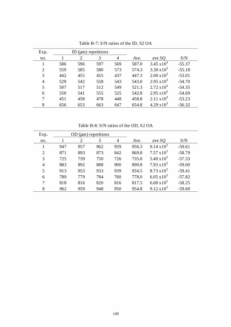
109
Table B-7: S/N ratios of the ID, S2 OA
Exp. ID (µm) repetitions no. 1 2 3 4 Ave. ave SQ S/N 1 586 596 597 569 587.0 3.45 x10³ -55.37 2 559 585 580 573 574.3 3.30 x10³ -55.18 3 442 455 455 437 447.3 2.00 x10³ -53.01 4 529 542 558 543 543.0 2.95 x10³ -54.70 5 507 517 512 549 521.3 2.72 x10³ -54.35 6 550 541 555 525 542.8 2.95 x10³ -54.69 7 451 458 478 448 458.8 2.11 x10³ -53.23 8 656 653 663 647 654.8 4.29 x10³ -56.32
Table B-8: S/N ratios of the OD, S2 OA
Exp. OD (µm) repetitions no. 1 2 3 4 Ave. ave SQ S/N 1 947 957 962 959 956.3 9.14 x10³ -59.61 2 871 893 873 842 869.8 7.57 x10³ -58.79 3 725 739 750 726 735.0 5.40 x10³ -57.33 4 883 892 888 900 890.8 7.93 x10³ -59.00 5 913 953 933 939 934.5 8.73 x10³ -59.41 6 789 779 784 760 778.0 6.05 x10³ -57.82 7 818 816 820 816 817.5 6.68 x10³ -58.25 8 962 959 948 950 954.8 9.12 x10³ -59.60
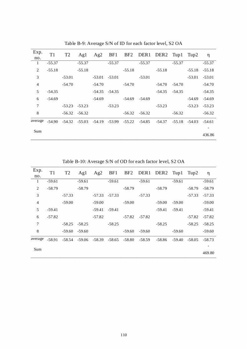
110
Table B-9: Average S/N of ID for each factor level, S2 OA
Exp. no.
T1 T2 Ag1 Ag2 BF1 BF2 DER1 DER2 Tup1 Tup2 η
1 -55.37 -55.37 -55.37 -55.37 -55.37 -55.37
2 -55.18 -55.18 -55.18 -55.18 -55.18 -55.18
3 -53.01 -53.01 -53.01 -53.01 -53.01 -53.01
4 -54.70 -54.70 -54.70 -54.70 -54.70 -54.70
5 -54.35 -54.35 -54.35 -54.35 -54.35 -54.35
6 -54.69 -54.69 -54.69 -54.69 -54.69 -54.69
7 -53.23 -53.23 -53.23 -53.23 -53.23 -53.23
8 -56.32 -56.32 -56.32 -56.32 -56.32 -56.32
average -54.90 -54.32 -55.03 -54.19 -53.99 -55.22 -54.85 -54.37 -55.18 -54.03 -54.61
Sum -
436.86
Table B-10: Average S/N of OD for each factor level, S2 OA
Exp. no.
T1 T2 Ag1 Ag2 BF1 BF2 DER1 DER2 Tup1 Tup2 η
1 -59.61 -59.61 -59.61 -59.61 -59.61 -59.61
2 -58.79 -58.79 -58.79 -58.79 -58.79 -58.79
3 -57.33 -57.33 -57.33 -57.33 -57.33 -57.33
4 -59.00 -59.00 -59.00 -59.00 -59.00 -59.00
5 -59.41 -59.41 -59.41 -59.41 -59.41 -59.41
6 -57.82 -57.82 -57.82 -57.82 -57.82 -57.82
7 -58.25 -58.25 -58.25 -58.25 -58.25 -58.25
8 -59.60 -59.60 -59.60 -59.60 -59.60 -59.60
average -58.91 -58.54 -59.06 -58.39 -58.65 -58.80 -58.59 -58.86 -59.40 -58.05 -58.73
Sum -
469.80
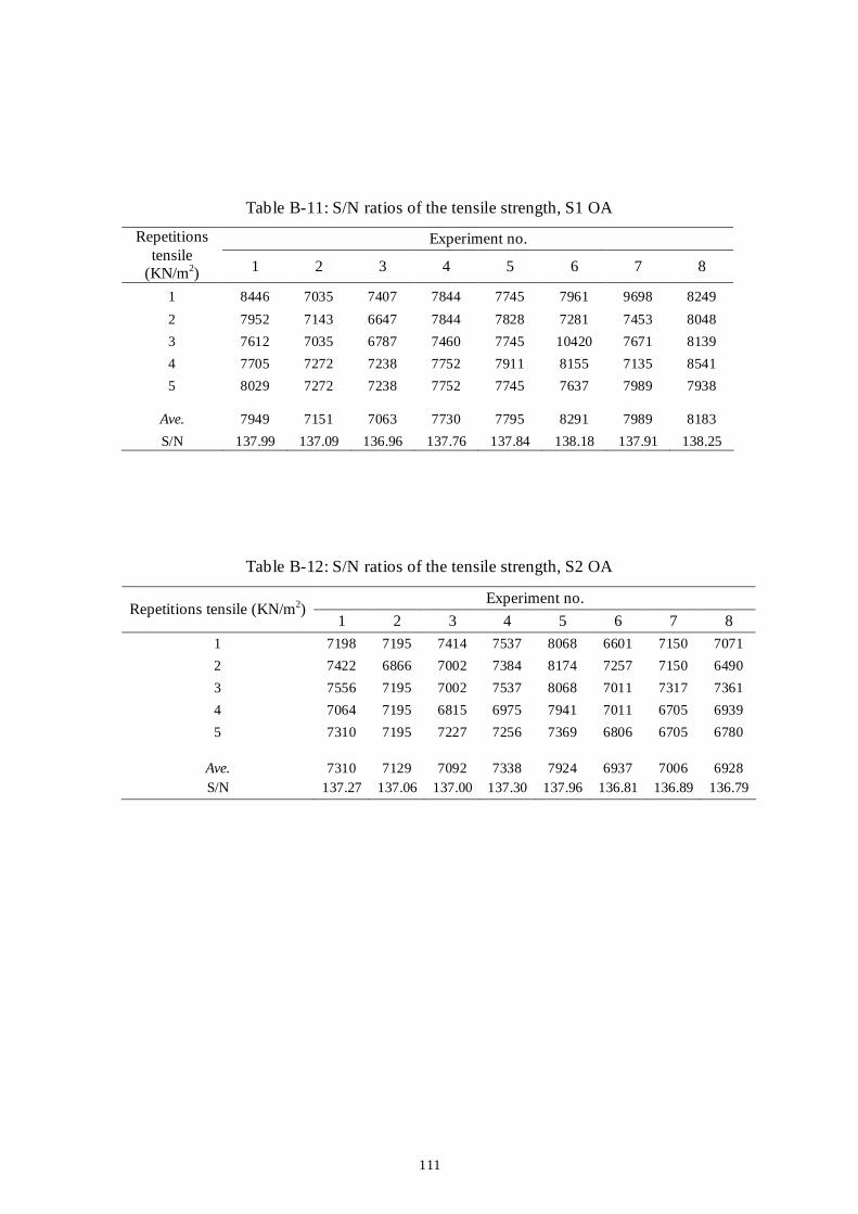
111
Table B-11: S/N ratios of the tensile strength, S1 OA
Experiment no. Repetitions tensile
(KN/m2) 1 2 3 4 5 6 7 8
1 8446 7035 7407 7844 7745 7961 9698 8249
2 7952 7143 6647 7844 7828 7281 7453 8048
3 7612 7035 6787 7460 7745 10420 7671 8139
4 7705 7272 7238 7752 7911 8155 7135 8541
5 8029 7272 7238 7752 7745 7637 7989 7938
Ave. 7949 7151 7063 7730 7795 8291 7989 8183
S/N 137.99 137.09 136.96 137.76 137.84 138.18 137.91 138.25
Table B-12: S/N ratios of the tensile strength, S2 OA
Experiment no. Repetitions tensile (KN/m2)
1 2 3 4 5 6 7 8
1 7198 7195 7414 7537 8068 6601 7150 7071
2 7422 6866 7002 7384 8174 7257 7150 6490
3 7556 7195 7002 7537 8068 7011 7317 7361
4 7064 7195 6815 6975 7941 7011 6705 6939
5 7310 7195 7227 7256 7369 6806 6705 6780
Ave. 7310 7129 7092 7338 7924 6937 7006 6928 S/N 137.27 137.06 137.00 137.30 137.96 136.81 136.89 136.79
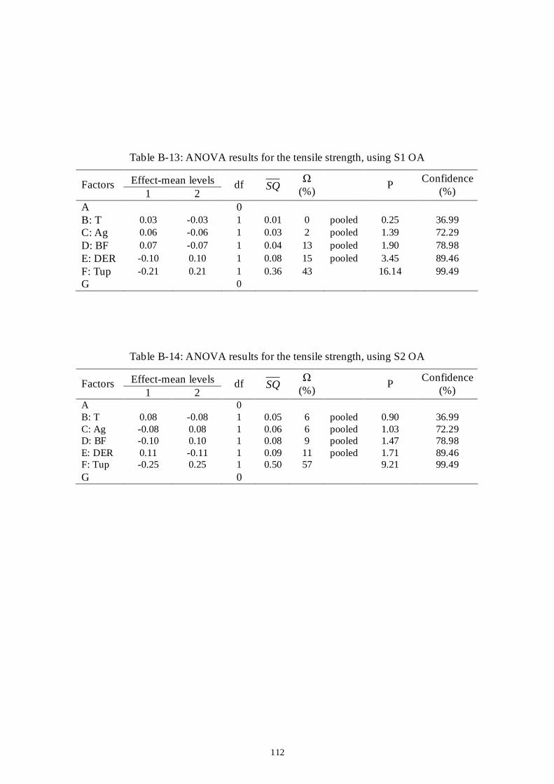
112
Table B-13: ANOVA results for the tensile strength, using S1 OA
Effect-mean levels Factors 1 2
df SQ Ω
(%) P
Confidence (%)
A 0 B: T 0.03 -0.03 1 0.01 0 pooled 0.25 36.99 C: Ag 0.06 -0.06 1 0.03 2 pooled 1.39 72.29 D: BF 0.07 -0.07 1 0.04 13 pooled 1.90 78.98 E: DER -0.10 0.10 1 0.08 15 pooled 3.45 89.46 F: Tup -0.21 0.21 1 0.36 43 16.14 99.49 G 0
Table B-14: ANOVA results for the tensile strength, using S2 OA
Effect-mean levels Factors 1 2
df SQ Ω
(%) P
Confidence (%)
A 0 B: T 0.08 -0.08 1 0.05 6 pooled 0.90 36.99 C: Ag -0.08 0.08 1 0.06 6 pooled 1.03 72.29 D: BF -0.10 0.10 1 0.08 9 pooled 1.47 78.98 E: DER 0.11 -0.11 1 0.09 11 pooled 1.71 89.46 F: Tup -0.25 0.25 1 0.50 57 9.21 99.49 G 0
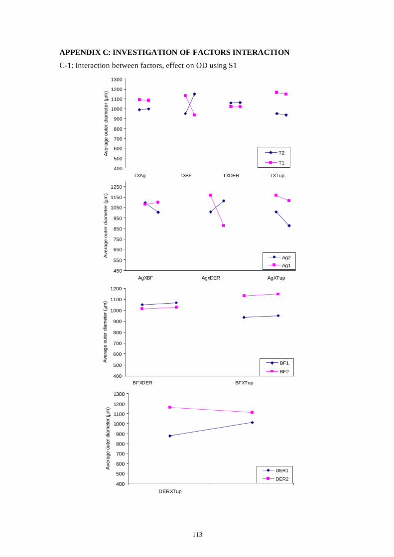
113
APPENDIX C: INVESTIGATION OF FACTORS INTERACTION
C-1: Interaction between factors, effect on OD using S1
400
500
600
700
800
900
1000
1100
1200
1300
TXAg TXBF TXDER TXTup
Ave
rage
out
er d
iam
eter
( µm
)
T2
T1
450
550
650
750
850
950
1050
1150
1250
AgXBF AgxDER AgXTup
Ave
rag
e o
ute
r d
iam
ete
r ( µ
m)
Ag2
Ag1
400
500
600
700
800
900
1000
1100
1200
BFXDER BFXTup
Ave
rag
e ou
ter
dia
met
er
( µm
)
BF1
BF2
400
500
600
700
800
900
1000
1100
1200
1300
DERXTup
Ave
rage
out
er d
iam
eter
( µm
)
DER1
DER2
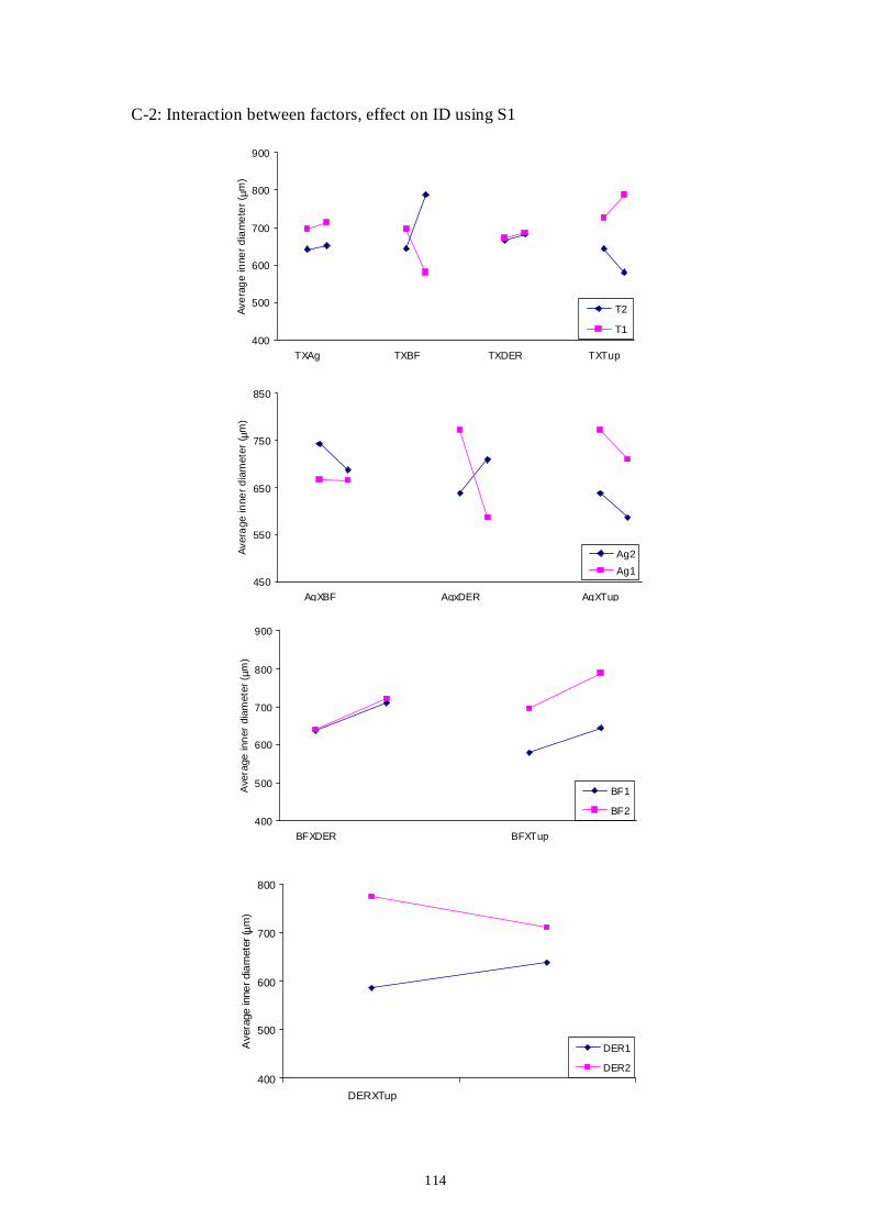
114
C-2: Interaction between factors, effect on ID using S1
400
500
600
700
800
900
TXAg TXBF TXDER TXTup
Ave
rag
e in
ner
dia
me
ter
( µm
)
T2
T1
450
550
650
750
850
AgXBF AgxDER AgXTup
Ave
rage
inne
r d
iam
eter
(µm
)
Ag2
Ag1
400
500
600
700
800
900
BFXDER BFXTup
Ave
rage
inn
er d
iam
eter
(µm
)
BF1
BF2
400
500
600
700
800
DERXTup
Ave
rage
inne
r di
am
eter
( µm
)
DER1
DER2
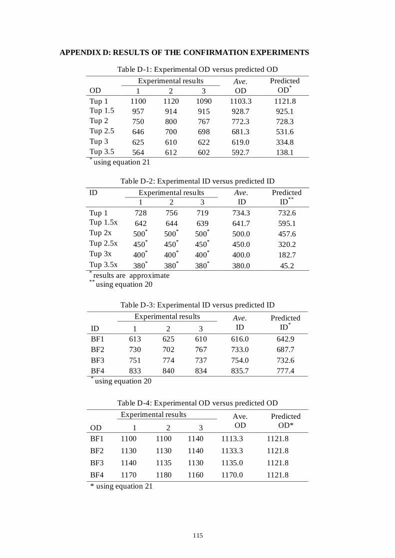
115
APPENDIX D: RESULTS OF THE CONFIRMATION EXPERIMENTS
Table D-1: Experimental OD versus predicted OD
Experimental results OD 1 2 3
Ave. OD
Predicted OD*
Tup 1 1100 1120 1090 1103.3 1121.8 Tup 1.5 957 914 915 928.7 925.1 Tup 2 750 800 767 772.3 728.3 Tup 2.5 646 700 698 681.3 531.6 Tup 3 625 610 622 619.0 334.8 Tup 3.5 564 612 602 592.7 138.1 * using equation 21
Table D-2: Experimental ID versus predicted ID
ID Experimental results 1 2 3
Ave. ID
Predicted ID**
Tup 1 728 756 719 734.3 732.6 Tup 1.5x 642 644 639 641.7 595.1 Tup 2x 500* 500* 500* 500.0 457.6 Tup 2.5x 450* 450* 450* 450.0 320.2 Tup 3x 400* 400* 400* 400.0 182.7 Tup 3.5x 380* 380* 380* 380.0 45.2 * results are approximate ** using equation 20
Table D-3: Experimental ID versus predicted ID
Experimental results
ID 1 2 3
Ave. ID
Predicted ID*
BF1 613 625 610 616.0 642.9 BF2 730 702 767 733.0 687.7
BF3 751 774 737 754.0 732.6 BF4 833 840 834 835.7 777.4 * using equation 20
Table D-4: Experimental OD versus predicted OD
Experimental results
OD 1 2 3
Ave. OD
Predicted OD*
BF1 1100 1100 1140 1113.3 1121.8
BF2 1130 1130 1140 1133.3 1121.8
BF3 1140 1135 1130 1135.0 1121.8
BF4 1170 1180 1160 1170.0 1121.8
* using equation 21
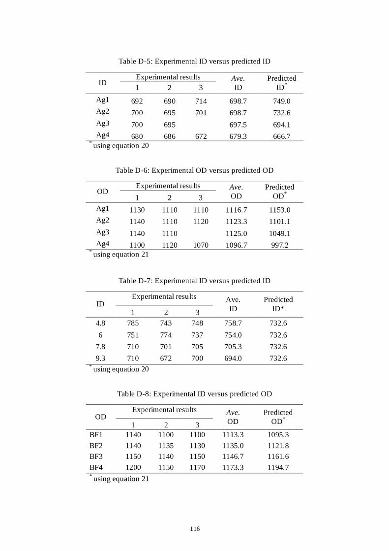
116
Table D-5: Experimental ID versus predicted ID
Experimental results ID
1 2 3 Ave. ID
Predicted ID*
Ag1 692 690 714 698.7 749.0 Ag2 700 695 701 698.7 732.6 Ag3 700 695 697.5 694.1 Ag4 680 686 672 679.3 666.7
* using equation 20
Table D-6: Experimental OD versus predicted OD
Experimental results OD
1 2 3
Ave. OD
Predicted OD*
Ag1 1130 1110 1110 1116.7 1153.0 Ag2 1140 1110 1120 1123.3 1101.1 Ag3 1140 1110 1125.0 1049.1 Ag4 1100 1120 1070 1096.7 997.2
* using equation 21
Table D-7: Experimental ID versus predicted ID
Experimental results ID
1 2 3
Ave. ID
Predicted ID*
4.8 785 743 748 758.7 732.6
6 751 774 737 754.0 732.6
7.8 710 701 705 705.3 732.6
9.3 710 672 700 694.0 732.6 * using equation 20
Table D-8: Experimental ID versus predicted OD
Experimental results OD
1 2 3
Ave. OD
Predicted OD*
BF1 1140 1100 1100 1113.3 1095.3
BF2 1140 1135 1130 1135.0 1121.8
BF3 1150 1140 1150 1146.7 1161.6
BF4 1200 1150 1170 1173.3 1194.7 * using equation 21

117
APPENDIX E: RESULTS OF THE TENSILE TEST
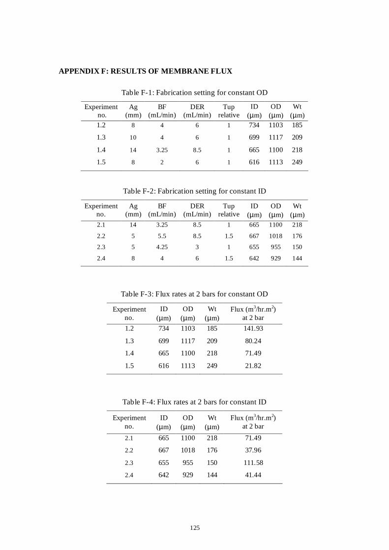
125
APPENDIX F: RESULTS OF MEMBRANE FLUX
Table F-1: Fabrication setting for constant OD
Experiment no.
Ag (mm)
BF (mL/min)
DER (mL/min)
Tup relative
ID (µm)
OD (µm)
Wt (µm)
1.2 8 4 6 1 734 1103 185
1.3 10 4 6 1 699 1117 209
1.4 14 3.25 8.5 1 665 1100 218
1.5 8 2 6 1 616 1113 249
Table F-2: Fabrication setting for constant ID
Experiment no.
Ag (mm)
BF (mL/min)
DER (mL/min)
Tup relative
ID (µm)
OD (µm)
Wt (µm)
2.1 14 3.25 8.5 1 665 1100 218
2.2 5 5.5 8.5 1.5 667 1018 176
2.3 5 4.25 3 1 655 955 150
2.4 8 4 6 1.5 642 929 144
Table F-3: Flux rates at 2 bars for constant OD
Experiment no.
ID (µm)
OD (µm)
Wt (µm)
Flux (m3/hr.m2) at 2 bar
1.2 734 1103 185 141.93
1.3 699 1117 209 80.24
1.4 665 1100 218 71.49
1.5 616 1113 249 21.82
Table F-4: Flux rates at 2 bars for constant ID
Experiment no.
ID (µm)
OD (µm)
Wt (µm)
Flux (m3/hr.m2) at 2 bar
2.1 665 1100 218 71.49
2.2 667 1018 176 37.96
2.3 655 955 150 111.58
2.4 642 929 144 41.44
Related Documents