Investigating spatio-temporal similarities in the epidemiology of childhood leukaemia and diabetes

PEDIATRIC EPIDEMIOLOGY

Investigating spatio-temporal similarities in the epidemiologyof childhood leukaemia and diabetes

Samuel O. M. Manda Æ Richard G. Feltbower ÆMark S. Gilthorpe

Received: 16 March 2009 / Accepted: 16 September 2009 / Published online: 26 September 2009

� Springer Science+Business Media B.V. 2009

Abstract Childhood acute lymphoblastic leukaemia

(ALL) and Type 1 diabetes (T1D) share some common

epidemiological features, including rising incidence rates

and links with an infectious aetiology. Previous work has

shown a significant positive correlation in incidence

between the two conditions both at the international and

small-area level. The aim was to extend the methodology

by including shared spatial and temporal trends using a

more extensive dataset among individuals diagnosed with

ALL and T1D in Yorkshire (UK) aged 0–14 years from

1978–2003. Cases with ALL and T1D were ascertained

from 2 high quality population-based disease registers

covering the Yorkshire region of the UK and linked to an

electoral ward from the 1991 UK census. A Bayesian

model was fitted where similarities and differences in risk

profiles of the two diseases were captured by the shared

and disease-specific components using a shared-component

model, with space-time interactions. The extended model

revealed a positive correlation of at least 0.70 between

diseases across all time periods, and an increasing risk

across time for both diseases, which was more evident for

T1D. Furthermore, both diseases exhibited lower rates in

the more urban county of West Yorkshire and higher rates

in the more rural northern and eastern part of the region. A

differential effect of T1D over ALL was found in the

south-eastern part of the region, which had a more pro-

nounced association with population mixing than with

population density or deprivation. Our approach has dem-

onstrated the utility in modelling temporally and spatially

varying disease incidence patterns across small geograph-

ical areas. The findings suggest searching for environ-

mental factors that exhibit similar geographical-temporal

variation in prevalence may help in the development and

testing of plausible aetiological hypotheses. Furthermore,

identifying environmental exposures specific to the south-

eastern part of the region, especially locally varying risk

factors which may differentially affect the development of

T1D and ALL, may also be fruitful.

Keywords Leukemia � Type 1 diabetes � Infection �Epidemiology � Children � Bayesian � Hierarchical �Temporal-spatial

Introduction

Childhood acute lymphoblastic leukaemia (ALL) and Type

1 diabetes (T1D) share some common epidemiological

features, including rising incidence rates [1–4] and potential

links with an infectious aetiology [5, 6]. Previous work has

shown a significant positive correlation in incidence

between the two conditions both at the international [7] and

small-area level [8]. For the latter, we considered a Bayesian

hierarchical joint spatial analysis investigating the variation

in the occurrence of these diseases across electoral wards in

the Yorkshire region in the north of England using data from

two co-terminus population-based registers, limited to a

S. O. M. Manda (&)

Biostatistics Unit, South African Medical Research Council,

1 Soutpansberg Road, Pretoria, South Africa

e-mail: [email protected]

R. G. Feltbower

Paediatric Epidemiology Group, Centre for Epidemiology and

Biostatistics, University of Leeds, Worsley Building,

Leeds LS2 9NL, UK

M. S. Gilthorpe

Biostatistics Unit, Centre for Epidemiology and Biostatistics,

University of Leeds, Worsley Building, Leeds LS2 9NL, UK

123

Eur J Epidemiol (2009) 24:743–752

DOI 10.1007/s10654-009-9391-2

period around the 1991 UK decadal census (1986–1998).

Specifically, we examined the spatial association between

the two conditions by including unstructured and spatially

structured area-level random components, which were

assigned a multivariate normal prior distribution, and we

assessed how the level of the spatial correlation differed

after adjusting for ecological factors previously associated

with disease risk (deprivation, population density and pop-

ulation mixing/migration).

In the current work, we present a novel extension to this

methodology by including a time-varying component to

take account of the change in incidence over time of ALL

and T1D, and we used a more extensive dataset for indi-

viduals diagnosed from 1978–2003. In particular, we aimed

to conduct a joint spatio-temporal analysis of the variation

of risk of childhood (ages 0–14 years) ALL and T1D in

Yorkshire by incorporating this time-varying component

[9]. Rather than using a multivariate normal prior to ana-

lyse the spatial association between the two diseases, we

investigated a shared-component model with temporal

dimensions. This was implemented using a Bayesian

hierarchical model, where we examined space- and time-

effects within an ecological framework to assess the

plausibility for a common aetiology between these two

diseases, thus enabling us to determine the extent of vari-

ation exhibited through shared unobserved environmental

risk factors. The proposed model allowed for both shared

local space and time dependence, in addition to disease-

specific components. This model also enabled us to

investigate persistence of disease patterns over time and

highlight unusual features of the data, both of which are

additional advantages over a purely spatial analysis [9, 10].

The analysis was underpinned by the unique availability of

high quality population-based disease register data on

childhood cancer [11] and diabetes [12] covering the same

period and study region.

Materials and methods

Case data

Information on individuals diagnosed with childhood (ages

0–14 years) ALL and T1D in the former Yorkshire

Regional Health Authority between 1978 and 2003 was

extracted from two co-terminus population-based disease

registers [11, 12]. Both registers accrue data on new

patients from multiple sources of ascertainment. Each

individual’s postcode at diagnosis was linked to an elec-

toral ward (n = 532) in existence at the time of the 1991

census. Both registers have extremely high levels of

completeness, through extensive cross-checks with multi-

ple sources of ascertainment. For example, capture-

recapture methods have shown that the diabetes register is

99.5% complete [12, 13].

We also derived three socio-demographic factors pre-

viously linked to disease onset [8]. These included:

(a) population mixing, reflecting the diversity of origins of

incomers into each Ward and calculated for the childhood

(0–14 years) population; (b) person-based childhood pop-

ulation density, which was calculated as a population

weighted average of the population density (persons per

hectare) for each census enumeration district, which then

was aggregated to electoral ward to provide a person-based

measure of population density; and (c) deprivation, mea-

sured using the Townsend Score, standardized to all Wards

in Yorkshire with the following variables contributing to

the index—unemployment, household overcrowding, car

ownership and housing tenure. Since these values were

fixed near the mid-point of the analysis (1991), they were

excluded from the temporal modeling but examined in

relation to the resulting smoothed spatial effects.

The spatial-temporal model

Our approach is an extension to that described previously

[8] whereby a Bayesian model was modified to include

correlated spatial terms using a multivariate normal struc-

ture. In the present study, similarities and differences in

risk profiles of the two diseases were captured by the

shared and disease-specific components using a shared-

component model, with space-time interactions [9, 10].

We supposed that the region under consideration was

divided into I contiguous sub-regions; in our case, these were

electoral wards for the Yorkshire region. Furthermore, we

assumed that data were collected at T successive discrete-

time periods. Now, let Oit1 and Oit2 represent the observed

number of cases from two diseases in area i at time period t,

which were five periods from 1978 to 2003, with period 1988

to 1993 being 6 years long; the other periods were 5 years

long (1 B t B T = 5; 1 B i B I = 532, in our case). It was

assumed that the observed counts followed Poisson distri-

butions with mean, litj = EitjRitj, where Eitj and Ritj were the

known expected number of cases and the unknown relative

risk, respectively, in area i at period t for disease j (j = 1, 2).

Expected counts were derived from average age-sex specific

incidence rates for the region and the entire period 1978–2003.

The maximum likelihood estimate of the relative risk of

disease j in area i at time-point t is the usual standardised

incidence (morbidity) ratio (SIR) Ritj ¼ Oitj=Eitj. It is

widely acknowledged that these crude risk ratios are mis-

leading, particularly when the diseases are rare or the areas

are small. Thus, more reliable estimates of relative risks for

rare diseases or small areas can be obtained by borrowing

information from neighbouring areas. A commonly used

744 S. O. M. Manda et al.

123

model for spatial smoothing of relative risks is the one

introduced by Besag et al. [14], abbreviated as the BYM

model. The basic BYM model decomposes the log of

disease-specific area-level relative risks into the sum of two

random effects: one that is unstructured (heterogeneous),

the other that is spatially structured (dependent). A char-

acterisation of these components of the BYM models is

detailed in ‘‘Appendix’’, where areas with common border

define neighbourhood in space.

In our previous analysis [8], a Bayesian hierarchical

joint spatial model was used to investigate the variation in

the occurrence of ALL and T1D in Yorkshire. The spatial

effects of the two diseases were assigned a multivariate

normal distribution. For this earlier work, we used the

techniques presented by Langford et al. [15] and Leyland

et al. [16] based on a multiple membership prior within a

multilevel structure, but differed in that our approach was

Bayesian. We have subsequently extended the methodol-

ogy by including time varying components to take into

account both the change in incidence of both diseases and a

more extensive dataset for individuals diagnosed from

1978–2003. Rather than using a multivariate normal prior

to assess spatial correlations, we used a shared-component

model [17, 18], though now extended to include temporal

effects, to determine the extent of the variation exhibited

through shared unobserved environmental risk factors in

space and time. Thus, following Richardson et al. [9], we

proposed a modification of (1) to include both main shared

spatial, temporal and space-time interaction effects, and

disease-specific effects within the framework of the BYM

model. These extensions permitted an investigation into

persistence of disease patterns over time and to highlight

unusual features of the data. These were additional

advantages over a purely spatial analysis [9]. These mod-

ifications are presented in ‘‘Appendix’’.

For a Bayesian model to be properly specified, all

unknown parameters whether fixed or random must be

given prior distributions. Where prior knowledge is avail-

able, this should be reflected in the prior distributions,

otherwise prior ignorance is assumed on the distributions of

parameters. We required priors that combine the BYM

framework to link risk in space at every time period and

time series techniques to link risk in time at every area. For

the purpose of this application, the shared spatial random

effects ui were given a CAR Normal W ; r2u

� �prior dis-

tribution to capture local dependence in space. Similarly,

we assumed that the disease 2 (T1D) specific spatial ran-

dom effects follow a conditional autoregressive normal

prior distribution: hi�CAR Normal W ; r2h

� �.

In order to capture local dependence in time, the shared

temporal trends wt were given a first order random walk

prior, which is simply a one dimensional version of the CAR

Normal prior distribution. Thus wt�CAR Normal D; r2w

� �

where the weight matrix D defines the temporal neighbours

of period t as periods t - 1 and t ? 1 for periods t = 2, 3, 4,

otherwise periods t = 1 and t = 5 have single neighbouring

periods t ? 1 and t - 1, respectively. The same first order

random walk prior was used to define the specific time trend

ct such that ct�CAR Normal D; r2c

� �.

In this analysis, we follow Richardson et al. [9] in fixing

the shared-temporal differential gradient x = 1 to improve

identifiability when using only five time periods for esti-

mating the temporal patterns. For the remaining scaling

parameter, an independent Normal (0, 5) prior distribution

was assigned to its logarithm, log j. All precision param-

eters were assigned independent hyper-prior Gamma (0.5,

0.0005) distributions. The inverse of covariance matrix

R-1 was assigned a Wishart (Q, 2) prior distribution, where

the scale parameter Q was assigned informative values as

described previously [8]. A complete specification of the

priors is in ‘‘Appendix’’.

Presently, we are unable to include period-specific data

on the three factors, population mixing; population density

and deprivation, as they are not available. In our pre-

liminary analyses when we included 1988–1993 data for

the other periods, the effects of the three contextual factors

were exceedingly high during the period, which we sus-

pected arose as an artefact of the data since these were

measured around the period 1991.

We fitted four variations of the joint spatio-temporal

model (3). The first two included only temporal trends

(Model A) or spatial trends (Model B) separately, thereby

demonstrating the impact of considering trends but only in

one dimension. We then included space-time interaction

terms (Model C), thereby demonstrating the impact of

considering trends in both dimensions. Model D was an

extension to Model C where heterogeneity terms were

added. Models C and D thus provided much greater flexi-

bility to identify salient patterns inherent in the data [9]. All

models were fitted to the data using full Bayesian estima-

tion within the WinBUGS software [19]. For each of the

four models, three independent chains were run for 40,000

iterations, and convergence was assessed by examining

trace plots as well as Brooks-Gelman Rubin diagnostics. A

burn-in period of 20,000 iterations was more than ade-

quate. The results reported were based on the remaining

20,000 posterior samples, keeping every 10th in order to

reduce serial correlation among samples of variance chains.

The performance of the four models was assessed using

the Deviance Information Criterion (DIC) [20], defined as

DIC ¼ Dþ pD where D is the posterior mean of the

deviance and measures model fit; pD is the effective

number of model parameters and measures model com-

plexity. The DIC works on similar principles as the non-

Investigating spatio-temporal similarities in the epidemiology 745

123

Bayesian Akaike Information Criterion (AIC), where the

model with a smaller DIC provides better support to the

data.

Results

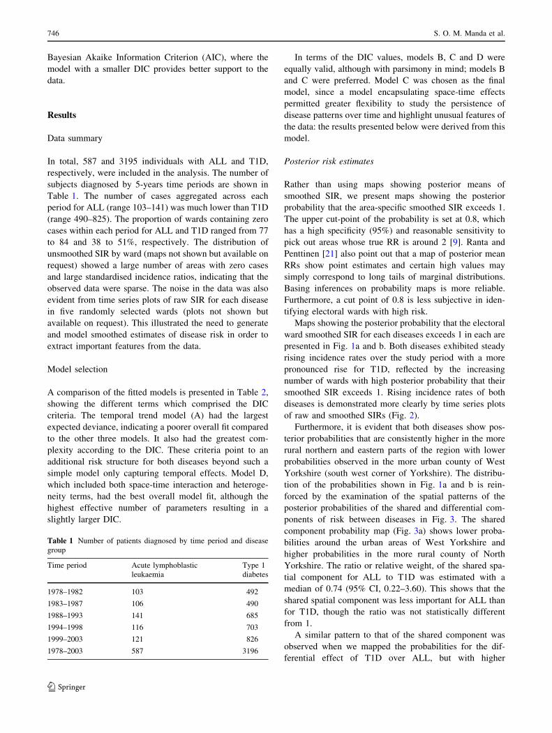
Data summary

In total, 587 and 3195 individuals with ALL and T1D,

respectively, were included in the analysis. The number of

subjects diagnosed by 5-years time periods are shown in

Table 1. The number of cases aggregated across each

period for ALL (range 103–141) was much lower than T1D

(range 490–825). The proportion of wards containing zero

cases within each period for ALL and T1D ranged from 77

to 84 and 38 to 51%, respectively. The distribution of

unsmoothed SIR by ward (maps not shown but available on

request) showed a large number of areas with zero cases

and large standardised incidence ratios, indicating that the

observed data were sparse. The noise in the data was also

evident from time series plots of raw SIR for each disease

in five randomly selected wards (plots not shown but

available on request). This illustrated the need to generate

and model smoothed estimates of disease risk in order to

extract important features from the data.

Model selection

A comparison of the fitted models is presented in Table 2,

showing the different terms which comprised the DIC

criteria. The temporal trend model (A) had the largest

expected deviance, indicating a poorer overall fit compared

to the other three models. It also had the greatest com-

plexity according to the DIC. These criteria point to an

additional risk structure for both diseases beyond such a

simple model only capturing temporal effects. Model D,

which included both space-time interaction and heteroge-

neity terms, had the best overall model fit, although the

highest effective number of parameters resulting in a

slightly larger DIC.

In terms of the DIC values, models B, C and D were

equally valid, although with parsimony in mind; models B

and C were preferred. Model C was chosen as the final

model, since a model encapsulating space-time effects

permitted greater flexibility to study the persistence of

disease patterns over time and highlight unusual features of

the data: the results presented below were derived from this

model.

Posterior risk estimates

Rather than using maps showing posterior means of

smoothed SIR, we present maps showing the posterior

probability that the area-specific smoothed SIR exceeds 1.

The upper cut-point of the probability is set at 0.8, which

has a high specificity (95%) and reasonable sensitivity to

pick out areas whose true RR is around 2 [9]. Ranta and

Penttinen [21] also point out that a map of posterior mean

RRs show point estimates and certain high values may

simply correspond to long tails of marginal distributions.

Basing inferences on probability maps is more reliable.

Furthermore, a cut point of 0.8 is less subjective in iden-

tifying electoral wards with high risk.

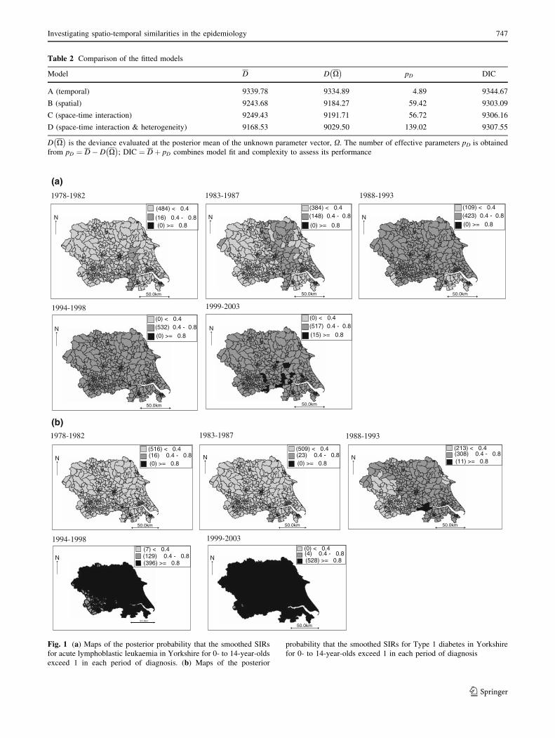
Maps showing the posterior probability that the electoral

ward smoothed SIR for each diseases exceeds 1 in each are

presented in Fig. 1a and b. Both diseases exhibited steady

rising incidence rates over the study period with a more

pronounced rise for T1D, reflected by the increasing

number of wards with high posterior probability that their

smoothed SIR exceeds 1. Rising incidence rates of both

diseases is demonstrated more clearly by time series plots

of raw and smoothed SIRs (Fig. 2).

Furthermore, it is evident that both diseases show pos-

terior probabilities that are consistently higher in the more

rural northern and eastern parts of the region with lower

probabilities observed in the more urban county of West

Yorkshire (south west corner of Yorkshire). The distribu-

tion of the probabilities shown in Fig. 1a and b is rein-

forced by the examination of the spatial patterns of the

posterior probabilities of the shared and differential com-

ponents of risk between diseases in Fig. 3. The shared

component probability map (Fig. 3a) shows lower proba-

bilities around the urban areas of West Yorkshire and

higher probabilities in the more rural county of North

Yorkshire. The ratio or relative weight, of the shared spa-

tial component for ALL to T1D was estimated with a

median of 0.74 (95% CI, 0.22–3.60). This shows that the

shared spatial component was less important for ALL than

for T1D, though the ratio was not statistically different

from 1.

A similar pattern to that of the shared component was

observed when we mapped the probabilities for the dif-

ferential effect of T1D over ALL, but with higher

Table 1 Number of patients diagnosed by time period and disease

group

Time period Acute lymphoblastic

leukaemia

Type 1

diabetes

1978–1982 103 492

1983–1987 106 490

1988–1993 141 685

1994–1998 116 703

1999–2003 121 826

1978–2003 587 3196


123

50.0km 50.0km

(0) >= 0.8

(384) < 0.4(148) 0.4 - 0.8

(0) >= 0.8

(484) < 0.4

50.0km

50.0km

(109) < 0.4(423) 0.4 - 0.8(0) >= 0.8

(0) < 0.4(532) 0.4 - 0.8(0) >= 0.8

50.0km

(0) < 0.4(517) 0.4 - 0.8(15) >= 0.8

1978-1982 1983-1987 1988-1993

1994-1998 1999-2003

50.0km 50.0km

(16) 0.4 - 0.8(0) >= 0.8

(516) < 0.4(23) 0.4 - 0.8(0) >= 0.8

(509) < 0.4

1978-1982 1983-1987

50.0km

(308) 0.4 - 0.8(11) >= 0.8

(213) < 0.4

(129) 0.4 - 0.8(396) >= 0.8

(7) < 0.4

50.0km

N(4) 0.4 - 0.8(528) >= 0.8

(0) < 0.4

1988-1993

1999-2003

(a)

(b)

(16) 0.4 - 0.8

50.0km

N

N

NN N

N

N N

N

1994-1998

Fig. 1 (a) Maps of the posterior probability that the smoothed SIRs

for acute lymphoblastic leukaemia in Yorkshire for 0- to 14-year-olds

exceed 1 in each period of diagnosis. (b) Maps of the posterior

probability that the smoothed SIRs for Type 1 diabetes in Yorkshire

for 0- to 14-year-olds exceed 1 in each period of diagnosis

Table 2 Comparison of the fitted models

Model D D X� �

pD DIC

A (temporal) 9339.78 9334.89 4.89 9344.67

B (spatial) 9243.68 9184.27 59.42 9303.09

C (space-time interaction) 9249.43 9191.71 56.72 9306.16

D (space-time interaction & heterogeneity) 9168.53 9029.50 139.02 9307.55

D X� �

is the deviance evaluated at the posterior mean of the unknown parameter vector, X. The number of effective parameters pD is obtained

from pD ¼ D� D X� �

; DIC ¼ Dþ pD combines model fit and complexity to assess its performance


123

probabilities present around the south-eastern part of the

region below the Humber estuary (Fig. 3b). The posterior

probability associated with the overall spatial distribution

of diabetes (Fig. 3c) shows that wards in the more urban

county of West Yorkshire had lower probabilities than in

the other parts of the region, while higher probabilities

were observed in the more rural eastern parts of the

region.

Inspection of the geographical variation in levels of risk

associated with each of the three contextual factors

(deprivation, population density and population mixing)

using Model C showed that lower rates of both childhood

ALL and T1D were present in areas with high deprivation,

population density and mixing. The same inverse associa-

tion was observed between the three contextual factors and

the shared and differential components.

We formally quantified the observed inverse relation-

ships between each of the three contextual variables and

shared and differential components by deriving correla-

tions using posterior samples of the smoothed SIRs. We

also quantified the correlations between the smoothed RRs

of the two diseases for each time period using the posterior

samples (Table 3), whereas previously we explicitly

included parameters to quantify the correlation between the

two diseases for the entire study period as a whole [8].

There was a significant positive correlation (0.74, 0.74,

0.74, 0.73 and 0.74, respectively, in periods 1–5) between

the two diseases, indicating that they may share common

environmental risk factors.

The shared component was significantly inversely

associated with population mixing, population density and

0.4

0.6

0.8

1

1.2

1.4

1.6

1978

-198

2

1983

-198

7

1988

-199

3

1994

-199

8

1999

-200

3

Period

SIR

Raw_T1D_SIR

Smoothed_T1D_SIR

Raw_ALL_SIR

Smoothed_ALL_SIR

Fig. 2 Plots of raw and smoothed Yorkshire-wide average temporal

SIRs for both diseases

50.0km

N(121) < 0.4

(411) 0.4 - 0.8(0) >= 0.8

50.0km

N

50.0km

N

(183) < 0.4

(341) 0.4 - 0.8

(8) >= 0.8

(158) < 0.4

(339) 0.4 - 0.8(35) >= 0.8

(a) (b)

(c)

Fig. 3 (a) Map of the posterior probability that the shared spatial

component smoothed SIR in Yorkshire for 0- to 14-year-olds, 1978–

2003, exceeds 1. (b) Map of the posterior probability that the spatial

smoothed SIR for Type 1 diabetes differential over lymphoblastic

leukaemia in Yorkshire for 0- to 14-year-olds, 1978–2003, exceeds 1.

(c) Map of the posterior probability that the overall smoothed SIR for

Type 1 diabetes in Yorkshire for 0- to 14-year olds, 1978–2003


123

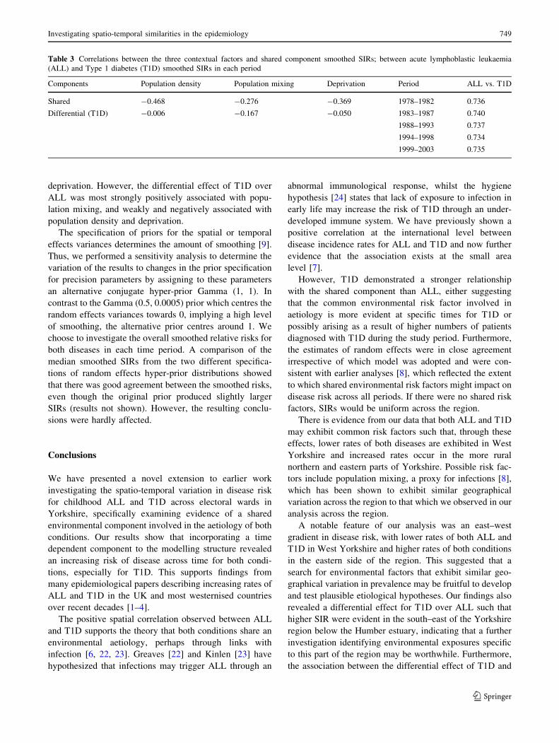
deprivation. However, the differential effect of T1D over

ALL was most strongly positively associated with popu-

lation mixing, and weakly and negatively associated with

population density and deprivation.

The specification of priors for the spatial or temporal

effects variances determines the amount of smoothing [9].

Thus, we performed a sensitivity analysis to determine the

variation of the results to changes in the prior specification

for precision parameters by assigning to these parameters

an alternative conjugate hyper-prior Gamma (1, 1). In

contrast to the Gamma (0.5, 0.0005) prior which centres the

random effects variances towards 0, implying a high level

of smoothing, the alternative prior centres around 1. We

choose to investigate the overall smoothed relative risks for

both diseases in each time period. A comparison of the

median smoothed SIRs from the two different specifica-

tions of random effects hyper-prior distributions showed

that there was good agreement between the smoothed risks,

even though the original prior produced slightly larger

SIRs (results not shown). However, the resulting conclu-

sions were hardly affected.

Conclusions

We have presented a novel extension to earlier work

investigating the spatio-temporal variation in disease risk

for childhood ALL and T1D across electoral wards in

Yorkshire, specifically examining evidence of a shared

environmental component involved in the aetiology of both

conditions. Our results show that incorporating a time

dependent component to the modelling structure revealed

an increasing risk of disease across time for both condi-

tions, especially for T1D. This supports findings from

many epidemiological papers describing increasing rates of

ALL and T1D in the UK and most westernised countries

over recent decades [1–4].

The positive spatial correlation observed between ALL

and T1D supports the theory that both conditions share an

environmental aetiology, perhaps through links with

infection [6, 22, 23]. Greaves [22] and Kinlen [23] have

hypothesized that infections may trigger ALL through an

abnormal immunological response, whilst the hygiene

hypothesis [24] states that lack of exposure to infection in

early life may increase the risk of T1D through an under-

developed immune system. We have previously shown a

positive correlation at the international level between

disease incidence rates for ALL and T1D and now further

evidence that the association exists at the small area

level [7].

However, T1D demonstrated a stronger relationship

with the shared component than ALL, either suggesting

that the common environmental risk factor involved in

aetiology is more evident at specific times for T1D or

possibly arising as a result of higher numbers of patients

diagnosed with T1D during the study period. Furthermore,

the estimates of random effects were in close agreement

irrespective of which model was adopted and were con-

sistent with earlier analyses [8], which reflected the extent

to which shared environmental risk factors might impact on

disease risk across all periods. If there were no shared risk

factors, SIRs would be uniform across the region.

There is evidence from our data that both ALL and T1D

may exhibit common risk factors such that, through these

effects, lower rates of both diseases are exhibited in West

Yorkshire and increased rates occur in the more rural

northern and eastern parts of Yorkshire. Possible risk fac-

tors include population mixing, a proxy for infections [8],

which has been shown to exhibit similar geographical

variation across the region to that which we observed in our

analysis across the region.

A notable feature of our analysis was an east–west

gradient in disease risk, with lower rates of both ALL and

T1D in West Yorkshire and higher rates of both conditions

in the eastern side of the region. This suggested that a

search for environmental factors that exhibit similar geo-

graphical variation in prevalence may be fruitful to develop

and test plausible etiological hypotheses. Our findings also

revealed a differential effect for T1D over ALL such that

higher SIR were evident in the south–east of the Yorkshire

region below the Humber estuary, indicating that a further

investigation identifying environmental exposures specific

to this part of the region may be worthwhile. Furthermore,

the association between the differential effect of T1D and

Table 3 Correlations between the three contextual factors and shared component smoothed SIRs; between acute lymphoblastic leukaemia

(ALL) and Type 1 diabetes (T1D) smoothed SIRs in each period

Components Population density Population mixing Deprivation Period ALL vs. T1D

Shared -0.468 -0.276 -0.369 1978–1982 0.736

Differential (T1D) -0.006 -0.167 -0.050 1983–1987 0.740

1988–1993 0.737

1994–1998 0.734

1999–2003 0.735


123

population mixing was more pronounced than population

density or deprivation, suggesting that other risk factors

may exist within the south-eastern parts of the region

which differentially affect the development of diabetes and

ALL.

We found a much greater positive correlation between

the diseases than in [8]. This may be partly due to sup-

pression such that when incorporating temporal smoothing,

we have ‘explained’ some of the ‘noise’ in the association,

resulting in stronger residual associations than before. It

may also be due to the modelling of the correlation struc-

tures. Previously, we had explicitly modelled these in a

multivariate normal model which needed prior elicitation

for possible values. It is well known that these priors are

problematic to elicit and specify. On the other hand, we

have now empirically computed the associations using the

posterior samples of the smoothed relative risks.

Future work is planned using latent variable analysis

(LVA) [25] to model unobserved exposures such as

infections, using measured covariates such as population

mixing, density and deprivation. Structural equation mod-

elling, which encompasses LVA, can then be applied to test

etiological hypotheses whilst adjusting appropriately for

confounders and explanatory factors [25]. This approach

would be particularly useful in dealing with the correlation

between population density, deprivation and migration,

factors previously linked to both ALL and T1D.

A further extension of the work is planned by including

potential risk factors such as deprivation, population den-

sity and population migration in the model for each period.

This will enable us to use time-varying fixed effects and

determine the amount of spatial and temporal variation

present after accounting for known and measured spatial

and temporal risk factors.

Acknowledgments We thank the Office for National Statistics for

the provision of population data and special migration statistics. We

are grateful to Margaret Buchan, Carolyn Stephenson, and Sheila

Jones for data collection and the co-operation of all pediatricians,

pediatric oncologists, physicians, Diabetes Specialist Nurses and

General Practitioners in Yorkshire. We thank the Candlelighters Trust

and Leeds Teaching Hospitals NHS Trust for supporting the costs of

running the cancer and diabetes registers. This diabetes registry work

was also undertaken by the University of Leeds who received funding

from the Department of Health. The views expressed in the publi-

cation are those of the authors and not necessarily those of the

Department of Health.

Appendix

The two diseases spatial temporal model

In the presence of longitudinal data for two diseases, an

extension of the BYM model is given by:

logðRit1Þ ¼ a0t1 þ bTt1xit þ uit1 þ vit1

logðRit2Þ ¼ a0t2 þ bT 0

t2 xit þ uit2 þ vit2

ð1Þ

where a0tj is an intercept term on the log relative risk scale

for disease j at time t; xit is a covariate risk vector with the

corresponding disease-specific coefficient parameter vector

btj at time t; and uitj and vitj represent unstructured and

spatially structured random effects, respectively, in area i at

time t for disease j. The unstructured random effects are

assumed to follow a normal distribution with time varying

variance such that uitj�N 0; r2tj

� �for j = 1, 2. The

spatially structured effects are modelled by the intrinsic

conditional autoregressive normal (CAR Normal) prior

[14, 26], which specifies a conditional distribution for a

specific spatially structured effect vitj as:

f ðvitjjvktj; k 6¼ iÞ ¼ N

Pk2Hi

WiktjvktjPk2Hi

Wiktj;

k2tjP

k2HiWiktj

!ð2Þ

at time t for disease j, where Hi is the set of areas adjacent

to area i; Wiktj is the weight reflecting spatial dependence

between area i and k at time t for disease j and k2tj is the

(conditional) structured variance. For simplicity, we

assume that the weighting factor Wiktj is constant over

time and disease, which seems reasonable as we do not

expect the influence of neighbouring areas to change over

time and to be different between the two diseases,

i.e. Wiktj = Wik. The most common and simplest

adjacent specification is to set Wik = 1 if areas i and k

are neighbours that share a common boundary and Wik = 0

otherwise. Thus, for disease j at time t, a CAR Normal

prior specifies the conditional distribution of each area-

specific effect vitj, given all the other v’s, to be a normal

distribution with mean equal to the average of the v’s of its

neighbours, and variance inversely proportional to the

number of neighbours; the more neighbours an area has,

the greater the precision for that area effect. This scenario

is reasonable for population density, as urban areas are

likely to have more neighbours that sparsely populated

rural areas. For brevity, following [14, 26], a conditional

autoregressive normal prior on the spatially structured

effects will be denoted by

vitj�CAR Normal W ; k2tj

� �

where W is simply the neighbourhood adjacency weight

matrix.

A common and specific spatial-temporal model

The spatio-temporal model we consider to estimate relative

risks of the two diseases in space and time is


123

logðRit1Þ ¼ a01 þ bTt1xit þ /ijþ wtxþ fit þ eit1

logðRit2Þ ¼ a02 þ bTt2xit þ

/i

jþ wt

xþ fit þ hi þ ct þ eit2

ð3Þ

where now a0j is the overall risk for disease j (j = 1, 2),

ui and wt are the main shared spatial and temporal

effects, respectively; hi and ct represent disease 2 (T1D)

specific spatial and temporal components, which capture

the differential effect between the two diseases; fit are

the shared space-time interaction effects, capturing

departure from space and time main effects, which may

highlight space-time clusters of risk, and eitj are the

disease-specific heterogeneous effects, capturing possible

extra-Poisson variation not explained by terms included

above. Thus, the shared-temporal factor model (3) par-

titions the risk profile for the two diseases into disease-

specific components and shared spatial and time com-

ponents. Parameters j and x are included to allow for a

differential gradient on the main shared spatial and

temporal components, respectively. The ratio j2 com-

pares the risk of disease 1 (ALL) to the risk of disease 2

(T1D) associated with the main shared spatial component

and the ratio x2 compares the risk associated with the

main temporal effect.

Ideally, in model (3) we could have split the main shared

spatial components into unstructured and structured effects

or the main shared temporal component into unstructured

and structured time trends or similarly the diseases-specific

components. This could have resulted into 8 9 5 = 40

extra random effects, as well as the space-time interaction

terms. This seems overly complex and could lead to

identifiability problems, so we decided to minimise the

number of random effects. We could have also included

specific components for disease 1, but such a symmetric

formulation can result in identifiability problems [9].

Prior specification

There are various choices of prior distributions for the

space-time interaction effects, fit. They can simply be

taken to be independent for every period and time with a

constant variance over time, as in [9], or, depending on the

length of the time periods, can evolve smoothly over time

with a polynomial temporal trend as in [27, 28]. Alterna-

tively, they can be allowed to vary independently or be

spatially structured for every period, with variances that are

either independently and identically distributed or tempo-

rally structured as proposed in Nobre et al. [10]. In the

present study, we define only five periods, too few to show

any reliable space-time jumps in risk. Thus, we assume a

spatially structured prior distribution at every period for the

shared interaction term, fit �CAR Normal W ; r2ft

� �(i.e. a

time-independent prior but linked in space) with variances

that are allowed to change smoothly over time,log r21t ¼

log r21ðt�1Þ þ et, where et �N 0;r2

e

� �. The pair of disease-

specific heterogeneity terms ðeit1; eit2ÞT are also assumed to

evolve smoothly over time according to a first-order

autoregressive (AR(1)) multivariate normal prior distribu-

tion with covariance matrix R to allow for correlations

between the ALL and T1D risks in each space-time unit.

Thus, ðei11; ei12ÞT �MVNð0;RÞ and ðeit1; eit2ÞT �MVN

ðeiðt�1Þ1; eiðt�1Þ2Þ;R� �

; t ¼ 2; . . .; 5. Since we are using the

CAR Normal prior, with sum-to-zero constraints on the

random effect terms, we assign a flat prior on the overall

disease risk terms, a0j.

References

1. Draper GJ, Kroll ME, Stiller CA. Childhood cancer. In: Doll R,

Fraumeni JF, Muir CS, editors. Cancer surveys vol 19/20: trends

in cancer incidence and mortality. New York: Cold Spring Har-

bor Laboratory; 1994. p. 493–517.

2. Linet MS, Ries LA, Smith MA, Tarone RE, Devesa SS. Cancer

surveillance series: recent trends in childhood cancer incidence

and mortality in the United States. J Natl Cancer Inst. 1999;91:

1051–8.

3. Onkamo P, Vaananen S, Karvonen M, Tuomilehto J. Worldwide

increase in incidence of type I diabetes—the analysis of the data

on published incidence trends. Diabetologia. 1999;42:1395–403.

4. Green A, Patterson CC. Trends in the incidence of childhood-onset

diabetes in Europe 1989–1998. Diabetologia. 2001;44(Suppl 3):

B3–8.

5. Greaves M. Childhood leukemia. BMJ. 2002;324:283–7.

6. EURODIAB Substudy 2 Study Group. Infections and vaccinations

as risk factors for childhood type 1 (insulin dependent) diabetes

mellitus: a multi-centre case-control investigation. Diabetologia.

2000;43:47–53.

7. Feltbower RG, McKinney PA, Greaves MF, Parslow RC,

Bodansky HJ. International parallels in leukaemia and diabetes

epidemiology. Arch Dis Child. 2004;89:54–6.

8. Feltbower RG, Manda SOM, Gilthorpe MS, Greaves MF, Par-

slow RC, Kinsey SE, et al. Detecting small-area similarities in the

epidemiology of childhood acute lymphoblastic leukemia and

diabetes mellitus, Type 1: a Bayesian approach. Am J Epidemiol.

2005;161:1168–80.

9. Richardson S, Abellan JJ, Best N. Bayesian spatio-temporal

analysis of joint patterns of male and female lung cancer risks in

Yorkshire (UK). Stat Methods Med Res. 2006;15:385–407.

10. Nobre AA, Schmidt AM, Lopes HF. Spatio-temporal models for

mapping the incidence of malaria in Para. Environmetrics. 2005;16:

291–304.

11. McKinney PA, Parslow RC, Lane SA, et al. Epidemiology of

childhood brain tumors in Yorkshire, UK 1974–1995: changing

patterns of occurrence. Br J Cancer. 1998;78:974–9.

12. Feltbower RG, McKinney PA, Parslow RC, Stephenson CR,

Bodansky HJ. Type 1 diabetes in Yorkshire, UK: time trends in

0–14 and 15–29 year olds, age at onset and age-period-cohort

modeling. Diabetic Med. 2003;20:437–41.

13. Feltbower RG, McNally RJ, Kinsey SE, Lewis IJ, Picton SV,

Proctor SJ, et al. Epidemiology of leukaemia and lymphoma in


123

children and young adults from the north of England, 1990–2002.

Eur J Cancer. 2009;45:420–7.

14. Besag J, York J, Mollie A. Bayesian image restoration, with two

applications in spatial statistics. Ann Inst Statist Math. 1991;43:

1–59.

15. Leyland AH, Langford IH, Rabash J, Goldstein H. Multivariate

spatial models for event data. Stat Med. 2000;19:2469–78.

16. Langford IH, Leyland AH, Rasbash J, Goldstein H. Multilevel

modeling of the geographical distributions of diseases. J R Stat

Soc C. 1999;48:253–68.

17. Knorr-Held L, Best NG. A shared component model for detecting

joint and selective clustering of two diseases. J R Stat Soc A. 2001;

164:73–85.

18. Held L, Natario I, Fenton SE, Rue H, Becker N. Towards joint

disease mapping. Stat Methods Med Res. 2006;14:61–82.

19. Spiegelhalter D, Thomas A, Best N, Lunn D. BUGS: Bayesian

inference using Gibbs sampling, version 1.4. Cambridge: MRC

Biostatistics Unit; 2003.

20. Spiegelhalter DJ, Best NG, Carlin BP, van der Linde A. Bayesian

measures of model complexity and fit (with discussion). J R Stat

Soc B. 2002;64:583–640.

21. Ranta J, Penttinen A. Probabilistic small area risk assessment

using GIS-based data: a case study of Finnish childhood diabetes.

Stat Med. 2000;19:2345–59.

22. Greaves M. Etiology of acute leukemia. Lancet. 1997;349:344–9.

23. Kinlen L. Evidence for an infective cause of childhood leukemia:

comparison of a Scottish new town with nuclear reprocessing

sites in Britain. Lancet. 1988;2:1323–7.

24. Wills-Karp M, Santeliz J, Karp CL. The germless theory of allergic

disease: revisiting the hygiene hypothesis. Nat Rev Immunol.

2001;1:69–75.

25. Kline RB. Principles of structural equation modelling. LEA;

2005.

26. Mollie A. Bayesian mapping of disease. In: Gilks WR, Rich-

ardson S, Spiegelhater DJ, editors. Markov chain Monte Carlo in

practice. London: Chapman & Hall; 1996. p. 359–79.

27. Waller LA, Carlin BP, Xia H, Gelfand AE. Hierachical spatio-

temporal mapping of disease rates. J Am Stat Assoc. 1997;92:

607–17.

28. Gill P. Spatio-temporal modelling and mapping of teenage birth rates.

[Online], available: http://people.ok.ubc.ca/gillpara/research/Poster.

pdf. Accessed 13 Dec 2006.


123

http://people.ok.ubc.ca/gillpara/research/Poster.pdf

http://people.ok.ubc.ca/gillpara/research/Poster.pdf

Investigating spatio-temporal similarities in the epidemiology of childhood leukaemia and diabetes

Documents