Simulation - Lectures Yee Whye Teh Part A Simulation TT 2013 Part A Simulation. TT 2013. Yee Whye Teh. 1 / 98 Administrivia Lectures: Wednesdays and Fridays 12-1pm Weeks 1-4. Lecture Room, 1 South Parks Road. Departmental problem classes: Wednesdays 4-5pm Weeks 3-6. Seminar Room, 1 South Parks Road. Hand in problem sheet solutions by Monday Weeks 3-5 noon in 1 South Parks Road. Week 6 is revision/consultation. Webpage: http://www.stats.ox.ac.uk/%7Eteh/simulation.html This course builds upon the notes of Mattias Winkel, Geoff Nicholls, and Arnaud Doucet. Part A Simulation. TT 2013. Yee Whye Teh. 2 / 98 Outline Introduction Inversion Method Transformation Methods Rejection Sampling Importance Sampling Normalised Importance Sampling Markov Chain Monte Carlo Metropolis-Hastings Part A Simulation. TT 2013. Yee Whye Teh. 3 / 98 Outline Introduction Inversion Method Transformation Methods Rejection Sampling Importance Sampling Normalised Importance Sampling Markov Chain Monte Carlo Metropolis-Hastings Part A Simulation. TT 2013. Yee Whye Teh. 4 / 98

Welcome message from author
This document is posted to help you gain knowledge. Please leave a comment to let me know what you think about it! Share it to your friends and learn new things together.
Transcript
Simulation - Lectures
Yee Whye Teh
Part A Simulation
TT 2013
Part A Simulation. TT 2013. Yee Whye Teh. 1 / 98
Administrivia
! Lectures: Wednesdays and Fridays 12-1pm Weeks 1-4.Lecture Room, 1 South Parks Road.
! Departmental problem classes: Wednesdays 4-5pm Weeks 3-6.Seminar Room, 1 South Parks Road.
! Hand in problem sheet solutions byMonday Weeks 3-5 noon in 1 South Parks Road.
! Week 6 is revision/consultation.
! Webpage: http://www.stats.ox.ac.uk/%7Eteh/simulation.html
! This course builds upon the notes of Mattias Winkel, Geo! Nicholls,and Arnaud Doucet.
Part A Simulation. TT 2013. Yee Whye Teh. 2 / 98
Outline
Introduction
Inversion Method
Transformation Methods
Rejection Sampling
Importance Sampling
Normalised Importance Sampling
Markov Chain Monte Carlo
Metropolis-Hastings
Part A Simulation. TT 2013. Yee Whye Teh. 3 / 98
Outline
Introduction
Inversion Method
Transformation Methods
Rejection Sampling
Importance Sampling
Normalised Importance Sampling
Markov Chain Monte Carlo
Metropolis-Hastings
Part A Simulation. TT 2013. Yee Whye Teh. 4 / 98
Monte Carlo Simulation Methods
! Computational tools for the simulation of random variables.
! These simulation methods, aka Monte Carlo methods, are used inmany fields including statistical physics, computational chemistry,statistical inference, genetics, finance etc.
! The Metropolis algorithm was named the top algorithm of the 20thcentury by a committee of mathematicians, computer scientists &physicists.
! With the dramatic increase of computational power, Monte Carlomethods are increasingly used.
Part A Simulation. TT 2013. Yee Whye Teh. 5 / 98
Objectives of the Course
! Introduce the main tools for the simulation of random variables:! inversion method,! transformation method,! rejection sampling,! importance sampling,! Markov chain Monte Carlo including Metropolis-Hastings.
! Understand the theoretical foundations and convergence properties ofthese methods.
! Learn to derive and implement specific algorithms for given randomvariables.
Part A Simulation. TT 2013. Yee Whye Teh. 6 / 98
Computing Expectations
! Assume you are interested in computing
! = E ("(X )) =!
!"(x)F (dx)
where X is a random variable (r.v.) taking values in ! withdistribution F and " : ! ! R.
! It is impossible to compute ! exactly in most realistic applications.
! Example: ! = Rd , X " N (µ,") and "(x) = I
"
#dk=1 x
2k # #
#
.
! Example: ! = Rd , X " N (µ,") and "(x) = I (x1 < 0, ..., xd < 0) .
Part A Simulation. TT 2013. Yee Whye Teh. 7 / 98
Example: Queuing Systems
! Customers arrive at a shop and queue to be served. Their requestsrequire varying amount of time.
! The manager cares about customer satisfaction and not excessivelyexceeding the 9am-5pm working day of his employees.
! Mathematically we could set up stochastic models for the arrivalprocess of customers and for the service time based on pastexperience.
! Question: If the shop assistants continue to deal with all customersin the shop at 5pm, what is the probability that they will have servedall the customers by 5.30pm?
! If we call X the number of customers in the shop at 5.30pm then theprobability of interest is
P (X = 0) = E (I(X = 0)) .
! For realistic models, we typically do not know analytically thedistribution of X .
Part A Simulation. TT 2013. Yee Whye Teh. 8 / 98
Example: Particle in a Random Medium
! A particle (Xt)t=1,2,... evolves according to a stochastic model on! = Rd .
! At each time step t, it is absorbed with probability 1$ G (Xt) whereG : ! ! [0, 1].
! Question: What is the probability that the particle has not yet beenabsorbed at time T ?
! The probability of interest is
P (not absorbed at time T ) = E [G (X1)G (X2) · · ·G (XT )] .
! For realistic models, we cannot compute this probability.
Part A Simulation. TT 2013. Yee Whye Teh. 9 / 98
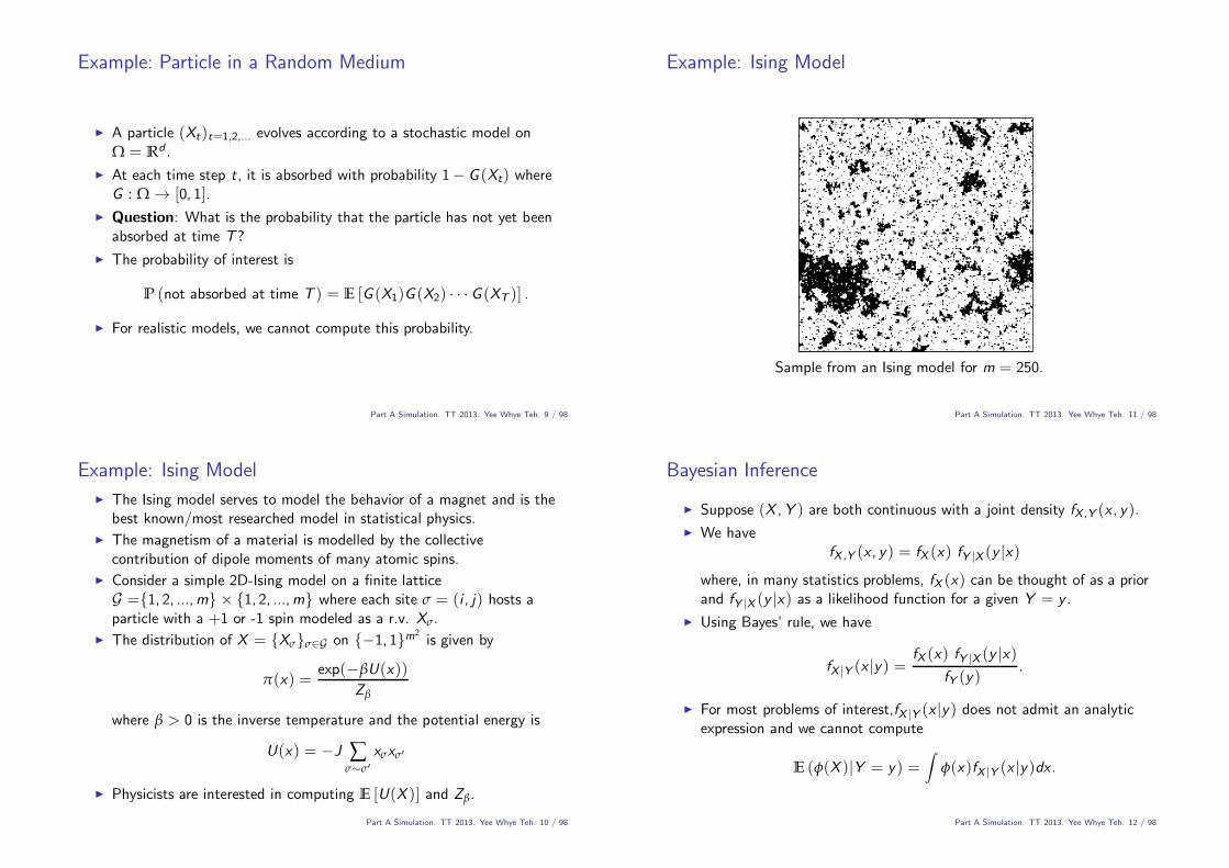
Example: Ising Model
! The Ising model serves to model the behavior of a magnet and is thebest known/most researched model in statistical physics.
! The magnetism of a material is modelled by the collectivecontribution of dipole moments of many atomic spins.
! Consider a simple 2D-Ising model on a finite latticeG ={1, 2, ...,m} % {1, 2, ...,m} where each site $ = (i , j) hosts aparticle with a +1 or -1 spin modeled as a r.v. X$.
! The distribution of X = {X$}$&G on {$1, 1}m2is given by
%(x) =exp($&U(x))
Z&
where & > 0 is the inverse temperature and the potential energy is
U(x) = $J #$"$'
x$x$'
! Physicists are interested in computing E [U(X )] and Z&.
Part A Simulation. TT 2013. Yee Whye Teh. 10 / 98
Example: Ising Model
Sample from an Ising model for m = 250.
Part A Simulation. TT 2013. Yee Whye Teh. 11 / 98
Bayesian Inference
! Suppose (X ,Y ) are both continuous with a joint density fX ,Y (x , y ).
! We havefX ,Y (x , y ) = fX (x) fY |X (y |x)
where, in many statistics problems, fX (x) can be thought of as a priorand fY |X (y |x) as a likelihood function for a given Y = y .
! Using Bayes’ rule, we have
fX |Y (x |y ) =fX (x) fY |X (y |x)
fY (y ).
! For most problems of interest,fX |Y (x |y ) does not admit an analyticexpression and we cannot compute
E ("(X )|Y = y ) =!
"(x)fX |Y (x |y )dx .
Part A Simulation. TT 2013. Yee Whye Teh. 12 / 98
Monte Carlo Integration
! Monte Carlo methods can be thought of as a stochastic way toapproximate integrals.
! Let X1, ...,Xn be a sample of independent copies of X and build theestimator
!n =1
n
n
#i=1
"(Xi ),
for the expectationE ("(X )) .
! Monte Carlo algorithm
- Simulate independent X1, ...,Xn from F .- Return !n = 1
n #ni=1 "(Xi ).
Part A Simulation. TT 2013. Yee Whye Teh. 13 / 98
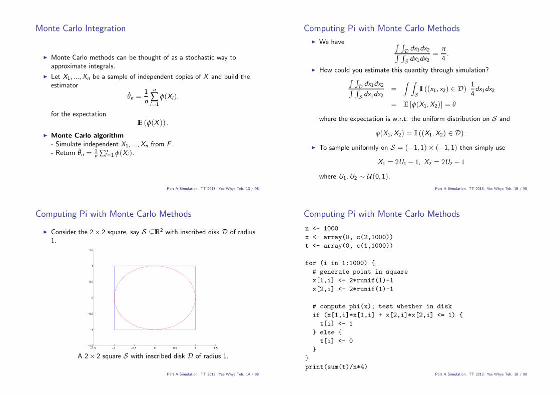
Computing Pi with Monte Carlo Methods
! Consider the 2% 2 square, say S (R2 with inscribed disk D of radius1.
−1.5 −1 −0.5 0 0.5 1 1.5−1.5
−1
−0.5
0
0.5
1
1.5
A 2% 2 square S with inscribed disk D of radius 1.
Part A Simulation. TT 2013. Yee Whye Teh. 14 / 98
Computing Pi with Monte Carlo Methods
! We have $ $
D dx1dx2$ $
S dx1dx2=
%
4.
! How could you estimate this quantity through simulation?$ $
D dx1dx2$ $
S dx1dx2=
! !
SI ((x1, x2) & D)
1
4dx1dx2
= E ["(X1,X2)] = !
where the expectation is w.r.t. the uniform distribution on S and
"(X1,X2) = I ((X1,X2) & D) .
! To sample uniformly on S = ($1, 1)% ($1, 1) then simply use
X1 = 2U1 $ 1, X2 = 2U2 $ 1
where U1,U2 " U(0, 1).Part A Simulation. TT 2013. Yee Whye Teh. 15 / 98
Computing Pi with Monte Carlo Methods
n <- 1000
x <- array(0, c(2,1000))t <- array(0, c(1,1000))
for (i in 1:1000) {
# generate point in square
x[1,i] <- 2*runif(1)-1
x[2,i] <- 2*runif(1)-1
# compute phi(x); test whether in disk
if (x[1,i]*x[1,i] + x[2,i]*x[2,i] <= 1) {
t[i] <- 1
} else {t[i] <- 0
}
}
print(sum(t)/n*4)Part A Simulation. TT 2013. Yee Whye Teh. 16 / 98
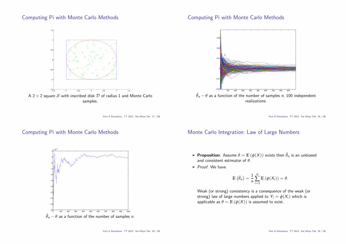
Computing Pi with Monte Carlo Methods
−1.5 −1 −0.5 0 0.5 1 1.5−1.5
−1
−0.5
0
0.5
1
1.5
A 2% 2 square S with inscribed disk D of radius 1 and Monte Carlosamples.
Part A Simulation. TT 2013. Yee Whye Teh. 17 / 98
Computing Pi with Monte Carlo Methods
0 100 200 300 400 500 600 700 800 900 1000−18
−16
−14
−12
−10
−8
−6
−4
−2
0
2x 10⁻³
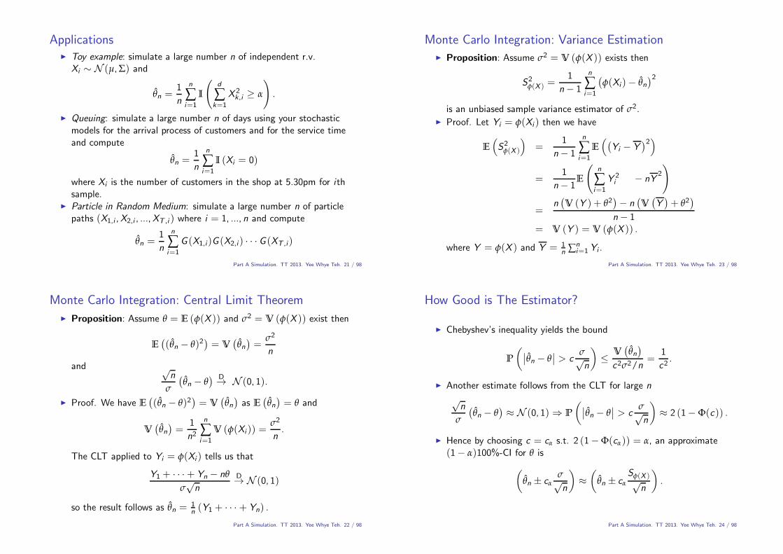
!n $ ! as a function of the number of samples n.
Part A Simulation. TT 2013. Yee Whye Teh. 18 / 98
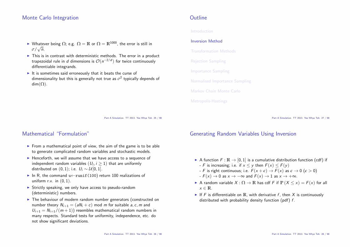
Computing Pi with Monte Carlo Methods
100 200 300 400 500 600 700 800 900−0.02
−0.01
0
0.01
0.02
0.03
!n $ ! as a function of the number of samples n, 100 independentrealizations.
Part A Simulation. TT 2013. Yee Whye Teh. 19 / 98
Monte Carlo Integration: Law of Large Numbers
! Proposition: Assume ! = E ("(X )) exists then !n is an unbiasedand consistent estimator of !.
! Proof: We have
E%
!n&
=1
n
n
#i=1
E ("(Xi )) = !.
Weak (or strong) consistency is a consequence of the weak (orstrong) law of large numbers applied to Yi = "(Xi ) which isapplicable as ! = E ("(X )) is assumed to exist.
Part A Simulation. TT 2013. Yee Whye Teh. 20 / 98
Applications! Toy example: simulate a large number n of independent r.v.
Xi " N (µ,") and
!n =1
n
n
#i=1
I
'd
#k=1
X 2k,i # #
(
.
! Queuing: simulate a large number n of days using your stochasticmodels for the arrival process of customers and for the service timeand compute
!n =1
n
n
#i=1
I (Xi = 0)
where Xi is the number of customers in the shop at 5.30pm for ithsample.
! Particle in Random Medium: simulate a large number n of particlepaths (X1,i ,X2,i , ...,XT ,i ) where i = 1, ..., n and compute
!n =1
n
n
#i=1
G (X1,i)G (X2,i ) · · ·G (XT ,i)
Part A Simulation. TT 2013. Yee Whye Teh. 21 / 98
Monte Carlo Integration: Central Limit Theorem
! Proposition: Assume ! = E ("(X )) and $2 = V ("(X )) exist then
E%
(!n $ !)2&
= V%
!n&
=$2
n
and )n
$
%
!n $ !& D! N (0, 1).
! Proof. We have E%
(!n $ !)2&
= V%
!n&
as E%
!n&
= ! and
V%
!n&
=1
n2
n
#i=1
V ("(Xi )) =$2
n.
The CLT applied to Yi = "(Xi ) tells us that
Y1 + · · ·+ Yn $ n!
$)n
D! N (0, 1)
so the result follows as !n = 1n (Y1 + · · ·+ Yn) .
Part A Simulation. TT 2013. Yee Whye Teh. 22 / 98
Monte Carlo Integration: Variance Estimation
! Proposition: Assume $2 = V ("(X )) exists then
S2"(X ) =
1
n$ 1
n
#i=1
%
"(Xi )$ !n&2
is an unbiased sample variance estimator of $2.! Proof. Let Yi = "(Xi ) then we have
E
"
S2"(X )
#
=1
n$ 1
n
#i=1
E
"%
Yi $ Y&2#
=1
n$ 1E
'n
#i=1
Y 2i $ nY
2
(
=n%
V (Y ) + !2&
$ n%
V%
Y&
+ !2&
n$ 1= V (Y ) = V ("(X )) .
where Y = "(X ) and Y = 1n #
ni=1Yi .
Part A Simulation. TT 2013. Yee Whye Teh. 23 / 98
How Good is The Estimator?
! Chebyshev’s inequality yields the bound
P
)**!n $ !
** > c
$)n
+
*V%
!n&
c2$2/n=
1
c2.
! Another estimate follows from the CLT for large n
)n
$
%
!n $ !&
+ N (0, 1) , P
)**!n $ !
** > c
$)n
+
+ 2 (1$ $(c)) .
! Hence by choosing c = c# s.t. 2 (1$ $(c#)) = #, an approximate(1$ #)100%-CI for ! is
)
!n ± c#$)n
+
+)
!n ± c#S"(X ))
n
+
.
Part A Simulation. TT 2013. Yee Whye Teh. 24 / 98
Monte Carlo Integration
! Whatever being !; e.g. ! = R or ! = R1000, the error is still in$/
)n.
! This is in contrast with deterministic methods. The error in a producttrapezoidal rule in d dimensions is O(n$2/d) for twice continuouslydi!erentiable integrands.
! It is sometimes said erroneously that it beats the curse ofdimensionality but this is generally not true as $2 typically depends ofdim(!).
Part A Simulation. TT 2013. Yee Whye Teh. 25 / 98
Mathematical “Formulation”
! From a mathematical point of view, the aim of the game is to be ableto generate complicated random variables and stochastic models.
! Henceforth, we will assume that we have access to a sequence ofindependent random variables (Ui , i # 1) that are uniformlydistributed on (0, 1); i.e. Ui " U [0, 1].
! In R, the command u-runif(100) return 100 realizations ofuniform r.v. in (0, 1).
! Strictly speaking, we only have access to pseudo-random(deterministic) numbers.
! The behaviour of modern random number generators (constructed onnumber theory Ni+1 = (aNi + c) mod m for suitable a, c ,m andUi+1 = Ni+1/(m+ 1)) resembles mathematical random numbers inmany respects. Standard tests for uniformity, independence, etc. donot show significant deviations.
Part A Simulation. TT 2013. Yee Whye Teh. 26 / 98
Outline
Introduction
Inversion Method
Transformation Methods
Rejection Sampling
Importance Sampling
Normalised Importance Sampling
Markov Chain Monte Carlo
Metropolis-Hastings
Part A Simulation. TT 2013. Yee Whye Teh. 27 / 98
Generating Random Variables Using Inversion
! A function F : R ! [0, 1] is a cumulative distribution function (cdf) if- F is increasing; i.e. if x * y then F (x) * F (y )- F is right continuous; i.e. F (x + ') ! F (x) as ' ! 0 (' > 0)- F (x) ! 0 as x ! $% and F (x) ! 1 as x ! +%.
! A random variable X : ! ! R has cdf F if P (X * x) = F (x) for allx & R.
! If F is di!erentiable on R, with derivative f , then X is continuouslydistributed with probability density function (pdf) f .
Part A Simulation. TT 2013. Yee Whye Teh. 28 / 98
Generating Random Variables Using Inversion
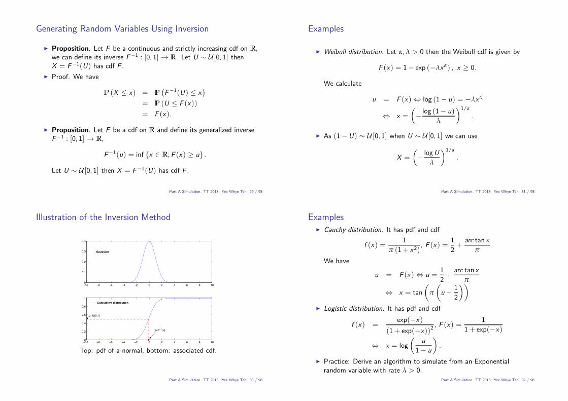
! Proposition. Let F be a continuous and strictly increasing cdf on R,we can define its inverse F$1 : [0, 1] ! R. Let U " U [0, 1] thenX = F$1(U) has cdf F .
! Proof. We have
P (X * x) = P%
F$1(U) * x&
= P (U * F (x))
= F (x).
! Proposition. Let F be a cdf on R and define its generalized inverseF$1 : [0, 1] ! R,
F$1(u) = inf {x & R;F (x) # u} .
Let U " U [0, 1] then X = F$1(U) has cdf F .
Part A Simulation. TT 2013. Yee Whye Teh. 29 / 98
Illustration of the Inversion Method
−10 −8 −6 −4 −2 0 2 4 6 8 100
0.1
0.2
0.3
0.4
−10 −8 −6 −4 −2 0 2 4 6 8 100
0.2
0.4
0.6
0.8
1
Gaussian
Cumulative distribution
u~U(0,1)
x=F−1(u)
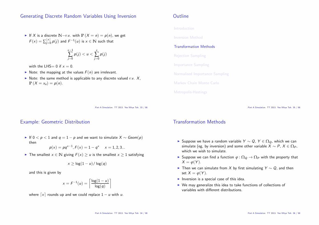
Top: pdf of a normal, bottom: associated cdf.
Part A Simulation. TT 2013. Yee Whye Teh. 30 / 98
Examples
! Weibull distribution. Let #,( > 0 then the Weibull cdf is given by
F (x) = 1$ exp ($(x#) , x # 0.
We calculate
u = F (x) . log (1$ u) = $(x#
. x =
)
$ log (1$ u)(
+1/#
.
! As (1$U) " U [0, 1] when U " U [0, 1] we can use
X =
)
$ logU
(
+1/#
.
Part A Simulation. TT 2013. Yee Whye Teh. 31 / 98
Examples! Cauchy distribution. It has pdf and cdf
f (x) =1
% (1+ x2), F (x) =
1
2+
arc tan x
%
We have
u = F (x) . u =1
2+
arc tan x
%
. x = tan
)
%
)
u $ 1
2
++
! Logistic distribution. It has pdf and cdf
f (x) =exp($x)
(1+ exp($x))2, F (x) =
1
1+ exp($x)
. x = log
)u
1$ u
+
.
! Practice: Derive an algorithm to simulate from an Exponentialrandom variable with rate ( > 0.
Part A Simulation. TT 2013. Yee Whye Teh. 32 / 98
Generating Discrete Random Variables Using Inversion
! If X is a discrete N$r.v. with P (X = n) = p(n), we get
F (x) = #/x0j=0 p(j) and F$1(u) is x & N such that
x$1
#j=0
p(j) < u <
x
#j=0
p(j)
with the LHS= 0 if x = 0.
! Note: the mapping at the values F (n) are irrelevant.
! Note: the same method is applicable to any discrete valued r.v. X ,P (X = xn) = p(n).
Part A Simulation. TT 2013. Yee Whye Teh. 33 / 98
Example: Geometric Distribution
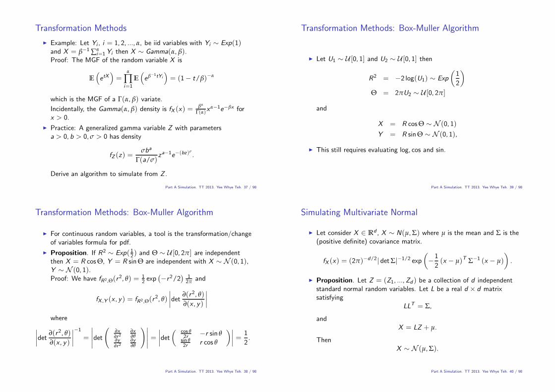
! If 0 < p < 1 and q = 1$ p and we want to simulate X " Geom(p)then
p(x) = pqx$1,F (x) = 1$ qx x = 1, 2, 3...
! The smallest x & N giving F (x) # u is the smallest x # 1 satisfying
x # log(1$ u)/ log(q)
and this is given by
x = F$1(u) =
,log(1$ u)log(q)
-
where 1x2 rounds up and we could replace 1$ u with u.
Part A Simulation. TT 2013. Yee Whye Teh. 34 / 98
Outline
Introduction
Inversion Method
Transformation Methods
Rejection Sampling
Importance Sampling
Normalised Importance Sampling
Markov Chain Monte Carlo
Metropolis-Hastings
Part A Simulation. TT 2013. Yee Whye Teh. 35 / 98
Transformation Methods
! Suppose we have a random variable Y " Q, Y & !Q , which we cansimulate (eg, by inversion) and some other variable X " P , X & !P ,which we wish to simulate.
! Suppose we can find a function ) : !Q ! !P with the property thatX = )(Y ).
! Then we can simulate from X by first simulating Y " Q, and thenset X = )(Y ).
! Inversion is a special case of this idea.
! We may generalize this idea to take functions of collections ofvariables with di!erent distributions.
Part A Simulation. TT 2013. Yee Whye Teh. 36 / 98
Transformation Methods
! Example: Let Yi , i = 1, 2, ..., #, be iid variables with Yi " Exp(1)and X = &$1 #
#i=1Yi then X " Gamma(#, &).
Proof: The MGF of the random variable X is
E
"
etX#
=#
&i=1
E
"
e&$1tYi
#
= (1$ t/&)$#
which is the MGF of a '(#, &) variate.
Incidentally, the Gamma(#, &) density is fX (x) =&#
'(#)x#$1e$&x for
x > 0.
! Practice: A generalized gamma variable Z with parametersa > 0, b > 0, $ > 0 has density
fZ (z) =$ba
'(a/$)za$1e$(bz)$
.
Derive an algorithm to simulate from Z .
Part A Simulation. TT 2013. Yee Whye Teh. 37 / 98
Transformation Methods: Box-Muller Algorithm
! For continuous random variables, a tool is the transformation/changeof variables formula for pdf.
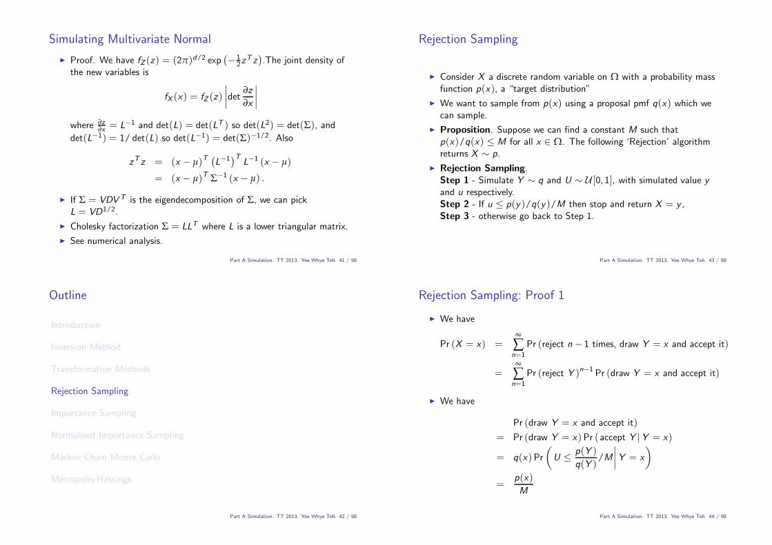
! Proposition. If R2 " Exp( 12) and ( " U [0, 2%] are independentthen X = R cos (, Y = R sin( are independent with X " N (0, 1),Y " N (0, 1).Proof: We have fR2,((r
2, !) = 12 exp
%
$r2/2&
12% and
fX ,Y (x , y ) = fR2,((r2, !)
****det
*(r2, !)*(x , y )
****
where
****det
*(r2, !)*(x , y )
****
$1
=
*****det
'*x*r2
*x*!
*y*r2
*y*!
(*****=
****det
) cos !2r $r sin !
sin !2r r cos !
+****=
1
2.
Part A Simulation. TT 2013. Yee Whye Teh. 38 / 98
Transformation Methods: Box-Muller Algorithm
! Let U1 " U [0, 1] and U2 " U [0, 1] then
R2 = $2 log(U1) " Exp
)1
2
+
( = 2%U2 " U [0, 2%]
and
X = R cos ( " N (0, 1)
Y = R sin( " N (0, 1),
! This still requires evaluating log, cos and sin.
Part A Simulation. TT 2013. Yee Whye Teh. 39 / 98
Simulating Multivariate Normal
! Let consider X & Rd , X " N(µ,") where µ is the mean and " is the(positive definite) covariance matrix.
fX (x) = (2%)$d/2| det "|$1/2 exp
)
$1
2(x $ µ)T "$1 (x $ µ)
+
.
! Proposition. Let Z = (Z1, ...,Zd ) be a collection of d independentstandard normal random variables. Let L be a real d % d matrixsatisfying
LLT = ",
andX = LZ + µ.
ThenX " N (µ,").
Part A Simulation. TT 2013. Yee Whye Teh. 40 / 98
Simulating Multivariate Normal
! Proof. We have fZ (z) = (2%)d/2 exp%
$ 12z
T z&
.The joint density ofthe new variables is
fX (x) = fZ (z)
****det
*z
*x
****
where *z*x = L$1 and det(L) = det(LT ) so det(L2) = det("), and
det(L$1) = 1/ det(L) so det(L$1) = det(")$1/2. Also
zT z = (x $ µ)T%
L$1&T
L$1 (x $ µ)
= (x $ µ)T "$1 (x $ µ) .
! If " = VDV T is the eigendecomposition of ", we can pickL = VD1/2.
! Cholesky factorization " = LLT where L is a lower triangular matrix.
! See numerical analysis.
Part A Simulation. TT 2013. Yee Whye Teh. 41 / 98
Outline
Introduction
Inversion Method
Transformation Methods
Rejection Sampling
Importance Sampling
Normalised Importance Sampling
Markov Chain Monte Carlo
Metropolis-Hastings
Part A Simulation. TT 2013. Yee Whye Teh. 42 / 98
Rejection Sampling
! Consider X a discrete random variable on ! with a probability massfunction p(x), a “target distribution”
! We want to sample from p(x) using a proposal pmf q(x) which wecan sample.
! Proposition. Suppose we can find a constant M such thatp(x)/q(x) * M for all x & !. The following ‘Rejection’ algorithmreturns X " p.
! Rejection Sampling.Step 1 - Simulate Y " q and U " U [0, 1], with simulated value y
and u respectively.Step 2 - If u * p(y )/q(y )/M then stop and return X = y ,Step 3 - otherwise go back to Step 1.
Part A Simulation. TT 2013. Yee Whye Teh. 43 / 98
Rejection Sampling: Proof 1
! We have
Pr (X = x) =%
#n=1
Pr (reject n$ 1 times, draw Y = x and accept it)
=%
#n=1
Pr (reject Y )n$1 Pr (draw Y = x and accept it)
! We have
Pr (draw Y = x and accept it)
= Pr (draw Y = x)Pr (accept Y |Y = x)
= q(x)Pr
)
U * p(Y )q(Y )
/M
****Y = x
+
=p(x)M
Part A Simulation. TT 2013. Yee Whye Teh. 44 / 98
! The probability of having a rejection is
Pr (reject Y ) = #x&!
Pr (draw Y = x and reject it)
= #x&!
q(x)Pr
)
U # p(Y )q(Y )
/M
****Y = x
+
= #x&!
q(x)
)
1$ p(x)q(x)M
+
= 1$ 1
M
! Hence we have
Pr (X = x) =%
#n=1
Pr (reject Y )n$1 Pr (draw Y = x and accept it)
=%
#n=1
)
1$ 1
M
+n$1 p(x)M
= p(x).
! Note the number of accept/reject trials has a geometric distributionof success probability 1/M, so the mean number of trials is M.
Part A Simulation. TT 2013. Yee Whye Teh. 45 / 98
Rejection Sampling: Proof 2
! Here is an alternative proof given for a continuous scalar variable X ,the rejection algorithm still works but p, q are now pdfs.
! We accept the proposal Y whenever (U,Y ) " pU,Y wherepU,Y (u, y ) = q(y )I(0,1)(u) satisfies U * p(Y )/Mq(Y ).
! We have
Pr (X * x) = Pr (Y * x |U * p(Y )/Mq(Y ))
=Pr (Y * x ,U * p(Y )/Mq(Y ))
Pr (U * p(Y )/Mq(Y ))
=
$ x
$%
$ p(y )/Mq(y )0 pU,Y (u, y )dudy
$ %
$%
$ p(y )/Mq(y )0 pU,Y (u, y )dudy
=
$ x
$%
$ p(y )/Mq(y )0 q(y )dudy
$ %
$%
$ p(y )/Mq(y )0 q(y )dudy
=! x
$%p(y )dy .
Part A Simulation. TT 2013. Yee Whye Teh. 46 / 98
Example: Beta Density! Assume you have for #, & # 1
p(x) ='(# + &)'(#)'(&)
x#$1(1$ x)&$1, 0 < x < 1
which is upper bounded on [0, 1].! We propose to use as a proposal q(x) = I(0,1)(x) the uniform density
on [0, 1].! We need to find a bound M s.t. p(x)/Mq(x) = p(x)/M * 1. The
smallest M is M = max0<x<1 p(x) and we obtain by solving forp'(x) = 0
M =' (# + &)
' (#) ' (&)
)# $ 1
# + & $ 2
+#$1) & $ 1
# + & $ 2
+&$1
. /0 1
M '
which givesp(y )Mq(y )
=y #$1(1$ y )&$1
M ' .
Part A Simulation. TT 2013. Yee Whye Teh. 47 / 98
Dealing with Unknown Normalising Constants
! In most practical scenarios, we only know p(x) and q(x) up to somenormalising constants; i.e.
p(x) = p(x)/Zp and q(x) = q(x)/Zq
where p(x), q(x) are known but Zp =$
!p(x)dx , Zq =
$
!q(x)dx
are unknown/expensive to compute.
! Rejection can still be used: Indeed p(x)/q(x) * M for all x & ! i!p(x)/q(x) * M ', with M ' = ZpM/Zq.
! Practically, this means we can ignore the normalising constants fromthe start: if we can find M ' to bound p(x)/q(x) then it is correct toaccept with probability p(x)/M 'q(x) in the rejection algorithm. Inthis case the mean number N of accept/reject trials will equalZqM
'/Zp (that is, M again).
Part A Simulation. TT 2013. Yee Whye Teh. 48 / 98
Simulating Gamma Random Variables
! We want to simulate a random variable X "Gamma(#, &) whichworks for any # # 1 (not just integers);
p(x) =x#$1 exp($&x)
Zpfor x > 0, Zp = '(#)/&#
so p(x) = x#$1 exp($&x) will do as our unnormalised target.
! When # = a is a positive integer we can simulate X " Gamma(a, &)by adding a independent Exp(&) variables, Yi " Exp(&),X = #
ai=1Yi .
! Hence we can sample densities ’close’ in shape to Gamma(#, &) sincewe can sample Gamma(/#0, &). Perhaps this, or something like it,would make an envelope/proposal density?
Part A Simulation. TT 2013. Yee Whye Teh. 49 / 98
! Let a = /#0 and let’s try to use Gamma(a, b) as the envelope, soY " Gamma(a, b) for integer a # 1 and some b > 0. The density ofY is
q(x) =xa$1 exp($bx)
Zqfor x > 0, Zq = '(a)/ba
so q(x) = xa$1 exp($bx) will do as our unnormalised envelopefunction.
! We have to check whether the ratio p(x)/q(x) is bounded over R
wherep(x)/q(x) = x#$a exp($(& $ b)x).
! Consider (a) x ! 0 and (b) x ! %. For (a) we need a * # soa = /#0 is indeed fine. For (b) we need b < & (not b = & since weneed the exponential to kill o! the growth of x#$a).
Part A Simulation. TT 2013. Yee Whye Teh. 50 / 98
! Given that we have chosen a = /#0 and b < & for the ratio to bebounded, we now compute the bound.
!ddx (p(x)/q(x)) = 0 at x = (# $ a)/(& $ b) (and this must be amaximum at x # 0 under our conditions on a and b), so p/q * M
for all x # 0 if
M =
)# $ a
& $ b
+#$a
exp($(# $ a)).
! Accept Y at step 2 of Rejection Sampler if U * p(Y )/Mq(Y ) wherep(Y )/Mq(Y ) = Y #$a exp($(& $ b)Y )/M.
Part A Simulation. TT 2013. Yee Whye Teh. 51 / 98
Simulating Gamma Random Variables: Best choice of b
! Any 0 < b < & will do, but is there a best choice of b?
! Idea: choose b to minimize the expected number of simulations of Yper sample X output.
! Since the number N of trials is Geometric, with success probabilityZp/(MZq), the expected number of trials is E(N) = ZqM/Zp. NowZp = '(#)&$# where ' is the Gamma function related to thefactorial.
! Practice: Show that the optimal b solves ddb (b
$a(& $ b)$#+a) = 0 sodeduce that b = &(a/#) is the optimal choice.
Part A Simulation. TT 2013. Yee Whye Teh. 52 / 98
Simulating Normal Random Variables
! Let p(x) = (2%)$12 exp($ 1
2x2) and q(x) = 1/%(1+ x2). We have
p(x)q(x)
= (1+ x2) exp
)
$1
2x2+
* 2/)e = M
which is attained at ±1.
! Hence the probability of acceptance is
P
)
U * p(x)Mq(x)
+
=Zp
MZq=
)2%
2)e
%=
2
e
2%+ 0.66
and the mean number of trials to success is approximately1/0.66 + 1.52.
Part A Simulation. TT 2013. Yee Whye Teh. 53 / 98
Rejection Sampling in High Dimension
! Consider
p(x1, ..., xd ) = exp
'
$1
2
d
#k=1
x2k
(
and
q(x1, ..., xd ) = exp
'
$ 1
2$2
d
#k=1
x2k
(
! For $ > 1, we have
p(x1, ..., xd )q(x1, ..., xd )
= exp
'
$1
2
%
1$ $$2& d
#k=1
x2k
(
* 1 = M.
! The acceptance probability of a proposal for $ > 1 is
P
)
U * p(X1, ...,Xd )Mq(X1, ...,Xd )
+
=Zp
MZq= $$d .
! The acceptance probability goes exponentially fast to zero with d .
Part A Simulation. TT 2013. Yee Whye Teh. 54 / 98
Outline
Introduction
Inversion Method
Transformation Methods
Rejection Sampling
Importance Sampling
Normalised Importance Sampling
Markov Chain Monte Carlo
Metropolis-Hastings
Part A Simulation. TT 2013. Yee Whye Teh. 55 / 98
Importance Sampling
! Importance sampling (IS) can be thought, among other things, as astrategy for recycling samples.
! It is also useful when we need to make an accurate estimate of theprobability that a random variable exceeds some very high threshold.
! In this context it is referred to as a variance reduction technique.
! There is a slight variation on the basic set up: we can generatesamples from q but we want to estimate an expectation Ep(f (X )) ofa function f under p.(Previously, it was “we want samples distributed according to p”.)
! In IS, we avoid sampling the target distribution p. Instead, we takesamples distributed according to q and reweight them.
Part A Simulation. TT 2013. Yee Whye Teh. 56 / 98
Importance Sampling Identity! Proposition. Let q and p be pdf on !. Assume
p(x) > 0 , q(x) > 0, then for any function " : ! ! R we have
Ep("(X )) = Eq("(X )w(X ))
where w : ! ! R+ is the importance weight function
w(x) =p(x)q(x)
.
! Proof: We have
Ep("(X )) =!
!"(x)p(x)dx
=!
!"(x)
p(x)q(x)
q(x)dx
=!
!"(x)w(x)q(x)dx
= Eq("(X )w(X )).
! Similar proof holds in the discrete case.
Part A Simulation. TT 2013. Yee Whye Teh. 57 / 98
Importance Sampling Estimator
! Proposition. Let q and p be pdf on !. Assumep(x)"(x) 3= 0 , q(x) > 0 and let " : ! ! R such that! = Ep("(X )) exists. Let Y1, ...,Yn be a sample of independentrandom variables distributed according to q then the estimator
!ISn =1
n
n
#i=1
"(Yi)w(Yi )
is unbiased and consistent.
! Proof. Unbiasedness follows directly fromEp("(X )) = Eq("(Yi )w(Yi )) and Yi " q. Weak (or strong)consistency is a consequence of the weak (or strong) law of largenumbers applied to Zi = "(Yi )w(Yi ) which is applicable as ! isassumed to exist.
Part A Simulation. TT 2013. Yee Whye Teh. 58 / 98
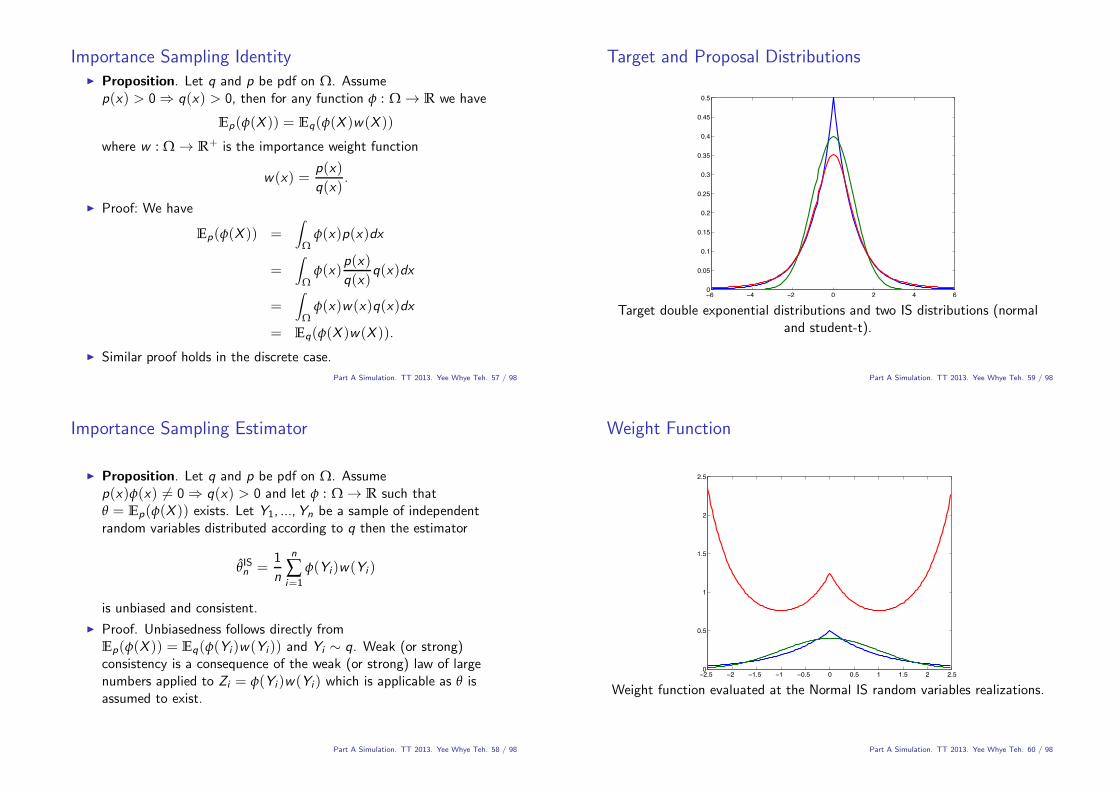
Target and Proposal Distributions
−6 −4 −2 0 2 4 60
0.05
0.1
0.15
0.2
0.25
0.3
0.35
0.4
0.45
0.5
Target double exponential distributions and two IS distributions (normaland student-t).
Part A Simulation. TT 2013. Yee Whye Teh. 59 / 98
Weight Function
−2.5 −2 −1.5 −1 −0.5 0 0.5 1 1.5 2 2.50
0.5
1
1.5
2
2.5
Weight function evaluated at the Normal IS random variables realizations.
Part A Simulation. TT 2013. Yee Whye Teh. 60 / 98
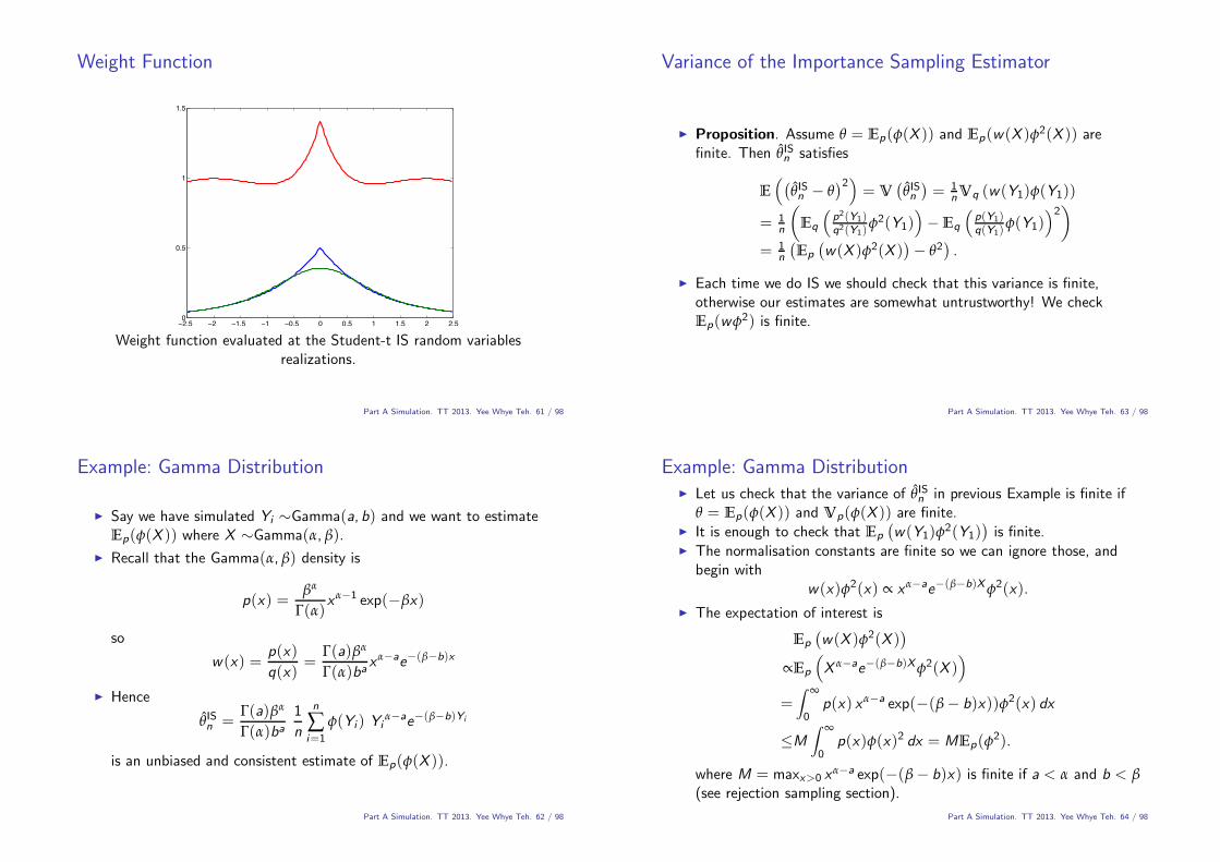
Weight Function
−2.5 −2 −1.5 −1 −0.5 0 0.5 1 1.5 2 2.50
0.5
1
1.5
Weight function evaluated at the Student-t IS random variablesrealizations.
Part A Simulation. TT 2013. Yee Whye Teh. 61 / 98
Example: Gamma Distribution
! Say we have simulated Yi "Gamma(a, b) and we want to estimateEp("(X )) where X "Gamma(#, &).
! Recall that the Gamma(#, &) density is
p(x) =&#
'(#)x#$1 exp($&x)
so
w(x) =p(x)q(x)
='(a)&#
'(#)bax#$ae$(&$b)x
! Hence
!ISn ='(a)&#
'(#)ba1
n
n
#i=1
"(Yi ) Yi#$ae$(&$b)Yi
is an unbiased and consistent estimate of Ep("(X )).
Part A Simulation. TT 2013. Yee Whye Teh. 62 / 98
Variance of the Importance Sampling Estimator
! Proposition. Assume ! = Ep("(X )) and Ep(w(X )"2(X )) arefinite. Then !ISn satisfies
E
"%
!ISn $ !&2#
= V%
!ISn&
= 1nVq (w(Y1)"(Y1))
= 1n
)
Eq
"p2(Y1)q2(Y1)
"2(Y1)#
$ Eq
"p(Y1)q(Y1)
"(Y1)#2+
= 1n
%
Ep
%
w(X )"2(X )&
$ !2&
.
! Each time we do IS we should check that this variance is finite,otherwise our estimates are somewhat untrustworthy! We checkEp(w"2) is finite.
Part A Simulation. TT 2013. Yee Whye Teh. 63 / 98
Example: Gamma Distribution! Let us check that the variance of !ISn in previous Example is finite if
! = Ep("(X )) and Vp("(X )) are finite.! It is enough to check that Ep
%
w(Y1)"2(Y1)&
is finite.! The normalisation constants are finite so we can ignore those, and
begin withw(x)"2(x) ) x#$ae$(&$b)X"2(x).
! The expectation of interest is
Ep
%
w(X )"2(X )&
)Ep
"
X #$ae$(&$b)X"2(X )#
=! %
0p(x) x#$a exp($(& $ b)x))"2(x) dx
*M
! %
0p(x)"(x)2 dx = MEp("
2).
where M = maxx>0 x#$a exp($(& $ b)x) is finite if a < # and b < &
(see rejection sampling section).
Part A Simulation. TT 2013. Yee Whye Teh. 64 / 98
! Since ! = Ep("(X )) and Vp("(X )) are finite, we haveEp("2(X )) < % if these conditions on a, b are satisfied. If not, wecannot conclude as it depends on ".
! These same (su"cient) conditions apply to our rejection sampler forGamma(#, &).
! For IS it is enough just for M to exist—we do not have to work outits value.
Part A Simulation. TT 2013. Yee Whye Teh. 65 / 98
Choice of the Importance Sampling Distribution! While p is given, q needs to cover p" (i.e.
p(x)"(x) 3= 0 , q(x) > 0) and be simple to sample.! The requirement V
%
!ISn&
< % further constrains our choice: we needEp
%
w(X )"2(X )&
< %.! If Vp("(X )) is known finite then, it may be easy to get a su"cient
condition for Ep
%
w(X )"2(X )&
< %; e.g. w(x) * M. Furtheranalysis will depend on ".
! What is the choice qopt of q that actually minimizes the variance ofthe IS estimator? Consider " : ! ! R+ then
qopt (x) =p(x)"(x)
Ep ("(X )), V(!ISn ) = 0.
! This optimal zero-variance estimator cannot be implemented as
w(x) = p(x)/qopt (x) = Ep ("(X )) /"(x)
where Ep ("(X )) is the thing we are trying to estimate! This canhowever be used as a guideline to select q.
Part A Simulation. TT 2013. Yee Whye Teh. 66 / 98
Importance Sampling for Rare Event Estimation
! One important class of applications of IS is to problems in which weestimate the probability for a rare event.
! In such scenarios, we may be able to sample from p directly but thisdoes not help us. If, for example, X " p withP(X > x0) = Ep (I[X > x0]) = ! say, with ! 4 1, we may not getany samples Xi > x0 and our estimate !n = #i I(Xi > x0)/n issimply zero.
! Generally, we have
E%
!n&
= !, V%
!n&
=!(1$ !)
n
but the relative variance
V%
!n&
!2=
(1$ !)!n
!!0! %.
! By using IS, we can actually reduce the variance of our estimator.
Part A Simulation. TT 2013. Yee Whye Teh. 67 / 98
Importance Sampling for Rare Event Estimation
! Let X " N (µ, $2) be a scalar normal random variable and we wantto estimate ! = P(X > x0) for some x0 5 µ + 3$. We canexponentially tilt the pdf of X towards larger values so that we getsome samples in the target region, and then correct for our tilting viaIS.
! If p(x) is pdf of X then q(x) = p(x)etx/Mp(t) is called anexponentially tilted version of p where Mp(t) = Ep(etX ) is themoment generating function of X .
! For p(x) the normal density,
q(x) ) e$(x$µ)2/2$2etx = e$(x$µ$t$2)2/2$2
eµt+t2$2/2
so we have
q(x) = N (x ;µ + t$2, $2), Mp(t) = eµt+t2$2/2.
Part A Simulation. TT 2013. Yee Whye Teh. 68 / 98
Importance Sampling for Rare Event Estimation
! The IS weight function is p(x)/q(x) = e$txMp(t) so
w(x) = e$t(x$µ$t$2/2).
! We take samples Yi " N (µ + t$2, $2), compute wi = w(Yi ) andform our IS estimator for ! = P(X > x0)
!ISn =1
n
n
#i=1
wiIYi>x0
since "(Yi ) = IYi>x0.
! We have not said how to choose t. The point here is that we wantsamples in the region of interest. We choose the mean of the tilteddistribution so that it equals x0, this ensure we have samples in theregion of interest; that is µ + t$2 = x0, or t = (x0 $ µ)/$2.
Part A Simulation. TT 2013. Yee Whye Teh. 69 / 98
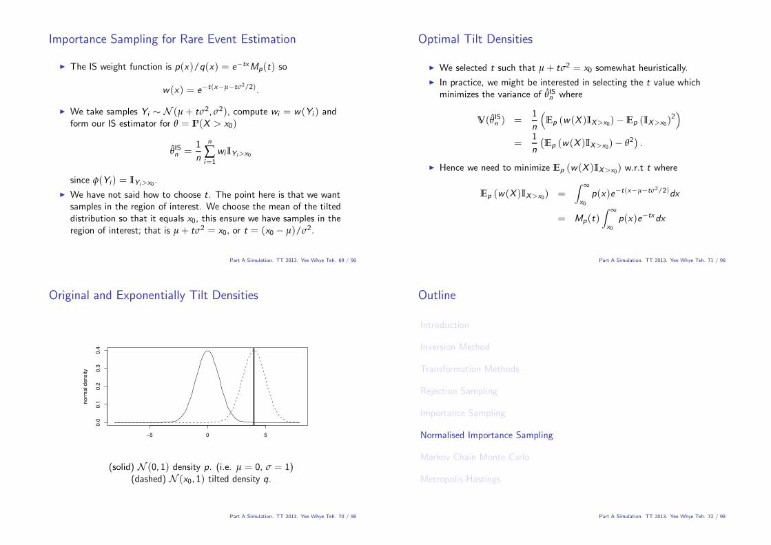
Original and Exponentially Tilt Densities
−5 0 5
0.0
0.1
0.2
0.3
0.4
norm
al d
ensi
ty
(solid) N (0, 1) density p. (i.e. µ = 0, $ = 1)(dashed) N (x0, 1) tilted density q.
Part A Simulation. TT 2013. Yee Whye Teh. 70 / 98
Optimal Tilt Densities
! We selected t such that µ + t$2 = x0 somewhat heuristically.
! In practice, we might be interested in selecting the t value whichminimizes the variance of !ISn where
V(!ISn ) =1
n
"
Ep (w(X )IX>x0)$ Ep (IX>x0)2#
=1
n
%
Ep (w(X )IX>x0)$ !2&
.
! Hence we need to minimize Ep (w(X )IX>x0) w.r.t t where
Ep (w(X )IX>x0) =! %
x0
p(x)e$t(x$µ$t$2/2)dx
= Mp(t)! %
x0p(x)e$txdx
Part A Simulation. TT 2013. Yee Whye Teh. 71 / 98
Outline
Introduction
Inversion Method
Transformation Methods
Rejection Sampling
Importance Sampling
Normalised Importance Sampling
Markov Chain Monte Carlo
Metropolis-Hastings
Part A Simulation. TT 2013. Yee Whye Teh. 72 / 98
Normalised Importance Sampling! In most practical scenarios,
p(x) = p(x)/Zp and q(x) = q(x)/Zq
where p(x), q(x) are known but Zp =$
!p(x)dx , Zq =
$
!q(x)dx
are unknown or di"cult to compute.! The previous IS estimator is not applicable as it requires evaluating
w(x) = p(x)/q(x).! An alternative IS estimator can be proposed based on the following
alternative IS identity.! Proposition. Let q and p be pdf on !. Assume
p(x) > 0 , q(x) > 0, then for any function " : ! ! R we have
Ep("(X )) =Eq("(X )w(X ))
Eq(w(X ))
where w : ! ! R+ is the importance weight function
w(x) = p(x)/q(x).
Part A Simulation. TT 2013. Yee Whye Teh. 73 / 98
Normalised Importance Sampling
! Proof: We have
Ep("(X )) =!
!"(x)p(x)dx
=
$
!"(x) p(x)
q(x)q(x)dx$
!p(x)q(x)q(x)dx
=
$
!"(x)w(x)q(x)dx$
!w(x)q(x)dx
=Eq("(X )w(X ))
Eq(w(X )).
! Remark: Even if we are interested in a simple function ", we do needp(x) > 0 , q(x) > 0 to hold instead of p(x)"(x) 3= 0 , q(x) > 0for the previous IS identity.
Part A Simulation. TT 2013. Yee Whye Teh. 74 / 98
Normalised Importance Sampling Pseudocode
1. Inputs:
! Function to draw samples from q! Function w (x) = p(x)/q(x)! Function "! Number of samples n
2. For i = 1, . . . , n:2.1 Draw yi " q.2.2 Compute wi = w (yi ).
3. Return#
ni=1 wi"(yi )
#ni=1 wi
.
Part A Simulation. TT 2013. Yee Whye Teh. 75 / 98
Normalised Importance Sampling Estimator
! Proposition. Let q and p be pdf on !. Assumep(x) > 0 , q(x) > 0 and let " : ! ! R such that ! = Ep("(X ))exists. Let Y1, ...,Yn be a sample of independent random variablesdistributed according to q then the estimator
!NISn =
1n #
ni=1 "(Yi )w(Yi )1n #
ni=1 w(Yi )
=#
ni=1 "(Yi )w(Yi )
#ni=1 w(Yi )
is consistent.
! Remark: It is easy to show that An = 1n #
ni=1 "(Yi )w(Yi ) (resp.
Bn = 1n #
ni=1 w(Yi )) is an unbiased and consistent estimator of
A = Eq ("(Y )w(Y )) (resp. B = Eq (w(Y ))). However !NISn , which
is a ratio of estimates, is biased for finite n.
Part A Simulation. TT 2013. Yee Whye Teh. 76 / 98
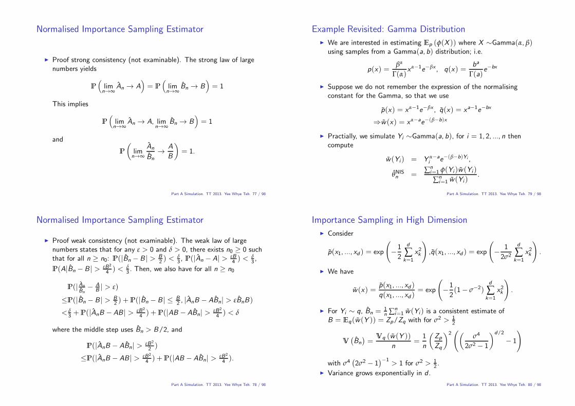
Normalised Importance Sampling Estimator
! Proof strong consistency (not examinable). The strong law of largenumbers yields
P
"
limn!%
An ! A#
= P
"
limn!%
Bn ! B#
= 1
This implies
P
"
limn!%
An ! A, limn!%
Bn ! B#
= 1
and
P
)
limn!%
An
Bn
! A
B
+
= 1.
Part A Simulation. TT 2013. Yee Whye Teh. 77 / 98
Normalised Importance Sampling Estimator
! Proof weak consistency (not examinable). The weak law of largenumbers states that for any + > 0 and , > 0, there exists n0 # 0 suchthat for all n # n0: P(|Bn $ B | > B
2 ) <,3 , P(|An $ A| > +B
4 ) < ,3 ,
P(A|Bn $ B | > +B2
4 ) < ,3 . Then, we also have for all n # n0
P(| An
Bn$ A
B | > +)
*P(|Bn $ B | > B2 ) + P(|Bn $ B | * B
2 , |AnB $ ABn| > +BnB)
<,3 + P(|AnB $ AB | > +B2
4 ) + P(|AB $ ABn| > +B2
4 ) < ,
where the middle step uses Bn > B/2, and
P(|AnB $ ABn| > +B2
2 )
*P(|AnB $ AB | > +B2
4 ) + P(|AB $ ABn| > +B2
4 ).
Part A Simulation. TT 2013. Yee Whye Teh. 78 / 98
Example Revisited: Gamma Distribution
! We are interested in estimating Ep ("(X )) where X "Gamma(#, &)using samples from a Gamma(a, b) distribution; i.e.
p(x) =&#
'(#)x#$1e$&x , q(x) =
ba
'(a)e$bx
! Suppose we do not remember the expression of the normalisingconstant for the Gamma, so that we use
p(x) = x#$1e$&x , q(x) = xa$1e$bx
,w(x) = x#$ae$(&$b)x
! Practially, we simulate Yi "Gamma(a, b), for i = 1, 2, ..., n thencompute
w(Yi ) = Y #$ai e$(&$b)Yi ,
!NISn =
#ni=1 "(Yi )w(Yi )
#ni=1 w(Yi )
.
Part A Simulation. TT 2013. Yee Whye Teh. 79 / 98
Importance Sampling in High Dimension
! Consider
p(x1, ..., xd ) = exp
'
$1
2
d
#k=1
x2k
(
,q(x1, ..., xd ) = exp
'
$ 1
2$2
d
#k=1
x2k
(
.
! We have
w(x) =p(x1, ..., xd )q(x1, ..., xd )
= exp
'
$1
2(1$ $$2)
d
#k=1
x2k
(
.
! For Yi " q, Bn = 1n #
ni=1 w(Yi ) is a consistent estimate of
B = Eq(w(Y )) = Zp/Zq with for $2>
12
V%
Bn
&
=Vq (w(Y ))
n=
1
n
)Zp
Zq
+2')
$4
2$2 $ 1
+d/2
$ 1
(
with $4%
2$2 $ 1&$1
> 1 for $2>
12 .
! Variance grows exponentially in d .
Part A Simulation. TT 2013. Yee Whye Teh. 80 / 98
Outline
Introduction
Inversion Method
Transformation Methods
Rejection Sampling
Importance Sampling
Normalised Importance Sampling
Markov Chain Monte Carlo
Metropolis-Hastings
Part A Simulation. TT 2013. Yee Whye Teh. 81 / 98
Markov chain Monte Carlo Methods
! Our aim is to estimate Ep("(X )) for p(x) some pmf (or pdf) definedfor x & !.
! Up to this point we have based our estimates on iid draws from eitherp itself, or some proposal distribution with pmf q.
! In MCMC we simulate a correlated sequence X0,X1,X2, .... whichsatisfies Xt " p (or at least Xt converges to p in distribution) andrely on the usual estimate "n = n$1 #
n$1t=0 "(Xt).
! We will suppose the space of states of X is finite (and thereforediscrete).
! But it should be kept in mind that MCMC methods are applicable tocountably infinite and continuous state spaces, and in fact one of themost versatile and widespread classes of Monte Carlo algorithmscurrently.
Part A Simulation. TT 2013. Yee Whye Teh. 82 / 98
Markov chains
! From Part A Probability.
! Let {Xt}%t=0 be a homogeneous Markov chain of random variables on
! with starting distribution X0 " p(0) and transition probability
Pi ,j = P(Xt+1 = j |Xt = i).
! Denote by P(n)i ,j the n-step transition probabilities
P(n)i ,j = P(Xt+n = j |Xt = i)
and by p(n)(i) = P(Xn = i).
! Recall that P is irreducible if and only if, for each pair of states
i , j & ! there is n such that P(n)i ,j > 0. The Markov chain is aperiodic
if P (n)i ,j is non zero for all su"ciently large n.
Part A Simulation. TT 2013. Yee Whye Teh. 83 / 98
Markov chains
! Here is an example of a periodic chain:! = {1, 2, 3, 4}, p(0) = (1, 0, 0, 0), and transition matrix
P =
3
445
0 1/2 0 1/21/2 0 1/2 00 1/2 0 1/2
1/2 0 1/2 0
6
778
,
since P(n)1,1 = 0 for n odd.
! Exercise: show that if P is irreducible and Pi ,i > 0 for some i & !
then P is aperiodic.
Part A Simulation. TT 2013. Yee Whye Teh. 84 / 98
Markov chains and Reversible Markov chains
! Recall that the pmf %(i), i & !, #i&! %(i) = 1 is a stationarydistribution of P if %P = %. If p(0) = % then
p(1)(j) = #i&!
p(0)(i)Pi ,j ,
so p(1)(j) = %(j) also. Iterating, p(t) = % for each t = 1, 2, ... in thechain, so the distribution of Xt " p(t) doesn’t change with t, it isstationary.
! In a reversible Markov chain we cannot distinguish the direction ofsimulation from inspection of a realization of the chain and itsreversal, even with knowledge of the transition matrix.
! Most MCMC algorithms are based on reversible Markov chains.
Part A Simulation. TT 2013. Yee Whye Teh. 85 / 98
Reversible Markov chains
! Denote by P 'i ,j = P(Xt$1 = j |Xt = i) the transition matrix for the
time-reversed chain.
! It seems clear that a Markov chain will be reversible if and only ifP = P ', so that any particular transition occurs with equal probabilityin forward and reverse directions.
! Theorem.(I) If there is a probability mass function %(i), i & ! satisfying%(i) # 0, #i&! %(i) = 1 and
“Detailed balance”: %(i)Pi ,j = %(j)Pj ,i for all pairs i , j & !,
then % = %P so % is stationary for P .(II) If in addition p(0) = % then P ' = P and the chain is reversiblewith respect to %.
Part A Simulation. TT 2013. Yee Whye Teh. 86 / 98
Reversible Markov chains
! Proof of (I): sum both sides of detailed balance equation over i & !.Now #i Pj ,i = 1 so #i %(i)Pi ,j = %(j).
! Proof of (II), we have % a stationary distribution of P soP(Xt = i) = %(i) for all t = 1, 2, ... along the chain. Then
P 'i ,j = P(Xt$1 = j |Xt = i)
= P(Xt = i |Xt$1 = j)P(Xt$1 = j)
P(Xt = i)(Bayes rule)
= Pj ,i%(j)/%(i) (stationarity)
= Pi ,j (detailed balance).
Part A Simulation. TT 2013. Yee Whye Teh. 87 / 98
Reversible Markov chains
! Why bother with reversibility? If we can find a transition matrix P
satisfying p(i)Pi ,j = p(j)Pj ,i for all i , j then pP = p so ‘our’ p is astationary distribution. Given P it is far easier to verify detailedbalance, than to check p = pP directly.
! We will be interested in using simulation of {Xt}n$1t=0 in order to
estimate Ep("(X )). The idea will be to arrange things so that thestationary distribution of the chain is % = p: if X0 " p (ie start thechain in its stationary distribution) then Xt " p for all t and we getsome useful samples.
! The ‘obvious’ estimator is
"n =1
n
n$1
#t=0
"(Xt),
but we may be concerned that we are averaging correlated quantities.
Part A Simulation. TT 2013. Yee Whye Teh. 88 / 98
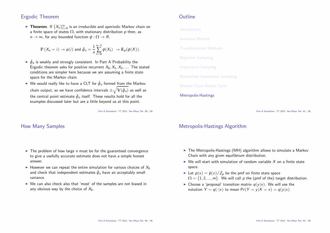
Ergodic Theorem
! Theorem. If {Xt}%t=0 is an irreducible and aperiodic Markov chain on
a finite space of states !, with stationary distribution p then, asn ! %, for any bounded function " : ! ! R ,
P (Xn = i) ! p(i) and "n =1
n
n$1
#t=0
"(Xt) ! Ep("(X )).
! "n is weakly and strongly consistent. In Part A Probability theErgodic theorem asks for positive recurrent X0,X1,X2, .... The statedconditions are simpler here because we are assuming a finite statespace for the Markov chain.
! We would really like to have a CLT for "n formed from the Markov
chain output, so we have confidence intervals ±9
V("n) as well as
the central point estimate "n itself. These results hold for all theexamples discussed later but are a little beyond us at this point.
Part A Simulation. TT 2013. Yee Whye Teh. 89 / 98
How Many Samples
! The problem of how large n must be for the guaranteed convergenceto give a usefully accurate estimate does not have a simple honestanswer.
! However we can repeat the entire simulation for various choices of X0
and check that independent estimates "n have an acceptably smallvariance.
! We can also check also that ’most’ of the samples are not biased inany obvious way by the choice of X0.
Part A Simulation. TT 2013. Yee Whye Teh. 90 / 98
Outline
Introduction
Inversion Method
Transformation Methods
Rejection Sampling
Importance Sampling
Normalised Importance Sampling
Markov Chain Monte Carlo
Metropolis-Hastings
Part A Simulation. TT 2013. Yee Whye Teh. 91 / 98
Metropolis-Hastings Algorithm
! The Metropolis-Hastings (MH) algorithm allows to simulate a MarkovChain with any given equilibrium distribution.
! We will start with simulation of random variable X on a finite statespace.
! Let p(x) = p(x)/Zp be the pmf on finite state space! = {1, 2, ...,m}. We will call p the (pmf of the) target distribution.
! Choose a ‘proposal’ transition matrix q(y |x). We will use thenotation Y " q(·|x) to mean Pr(Y = y |X = x) = q(y |x).
Part A Simulation. TT 2013. Yee Whye Teh. 92 / 98
Metropolis-Hastings Algorithm
1. Set the initial state x0, e.g. by drawing from an initial distributionp(0).
2. For t = 0, . . . , n$ 1:2.1 Let x = xt .2.2 Draw y " q(·|x) and u " U [0, 1].2.3 If
u * #(y |x) where #(y |x) = min
:
1,p(y)q(x |y)p(x)q(y |x)
;
set xt+1 = y , otherwise set xt+1 = x .
Part A Simulation. TT 2013. Yee Whye Teh. 93 / 98
Metropolis-Hastings Algorithm! Theorem. The transition matrix P of the Markov chain generated by
the M-H algorithm satisfies p = pP .! Proof: Since p is a pmf, we just check detailed balance. The case
x = y is trivial. If Xt = x , then the probability to come out withXt+1 = y for y 3= x is the probability to propose y at step 1 timesthe probability to accept it at step 2. Hence we havePx ,y = P(Xt+1 = y |Xt = x) = q(y |x)#(y |x) and
p(x)Px ,y = p(x)q(y |x)#(y |x)
= p(x)q(y |x)min
:
1,p(y )q(x |y )p(x)q(y |x)
;
= min {p(x)q(y |x), p(y )q(x |y )}
= p(y )q(x |y )min
:p(x)q(y |x)p(y )q(x |y ) , 1)
;
= p(y )q(x |y )#(x |y )= p(y )Py ,x .
Part A Simulation. TT 2013. Yee Whye Teh. 94 / 98
Metropolis-Hastings Algorithm
! To run the MH algorithm, we need to specify X0 = x0 and a proposalq(y |x).
! We only need to know the target p up to a normalizing constant as #depends only p(y )/p(x) = p(y )/p(x).
! If the Markov chain simulated by the MH algorithm is irreducible andaperiodic then the ergodic theorem applies.
! Verifying aperiodicity is usually straightforward, since the MCMCalgorithm may reject the candidate state y , so Px ,x > 0 for at leastsome states x & !. In order to check irreducibility we need to checkthat q can take us anywhere in ! (so q itself is an irreducibletransition matrix), and then that the acceptance step doesn’t trap thechain (as might happen if #(y |x) is zero too often).
Part A Simulation. TT 2013. Yee Whye Teh. 95 / 98
Example: Simulating a Discrete Distribution
! We will use MH to simulate X " p on ! = {1, 2, ...,m} with
p(i) = i so Zp = #mi=1 i =
m(m+1)2 .
! One simple proposal distribution is Y " q on ! such thatq(i) = 1/m.
! This proposal scheme is clearly irreducible (we can get from A to B ina single hop).
! If xt = x , then xt+1 is determined in the following way.
1. Simulate y " U{1, 2, ...,m} and u " U [0, 1].2. If
u * min
:
1,p(y)q(x |y)p(x)q(y |x)
;
= min<
1,y
x
=
set xt+1 = y , otherwise set xt+1 = x .
Part A Simulation. TT 2013. Yee Whye Teh. 96 / 98
Example: Simulating a Poisson Distribution
! We want to simulate p(x) = e$((x/x ! ) (x/x !
! For the proposal we use
q(y |x) =:
12 for y = x ± 10 otherwise,
i.e. toss a coin and add or substract 1 to x to obtain y .! If xt = x , then xt+1 is determined in the following way.
1. Simulate V " U [0, 1] and set y = x + 1 if V * 12 and y = x $ 1
otherwise.2. Simulate U " U [0, 1].
3. Let #(y |x) = min<
1, p(y )q(x |y )p(x)q(y |x)
=
then
#(y |x) =
>
?@
?A
min"
1, (x+1
#
if y = x + 1
min%
1, x(&
if y = x $ 1 # 00 if y = $1.
and if u * #(y |x), set xt+1 = y , otherwise set xt+1 = x .
Part A Simulation. TT 2013. Yee Whye Teh. 97 / 98
Estimating Normalizing Constants
! Assume we are interested in estimating Zp.
! If we have an irreducible and aperiodic Markov chain then the ergodictheorem tells us that "n = 1
n #n$1t=0 "(Xt) ! Ep("(X )) so for
"(x) = Ix '(x), Ep("(X )) = p(x ')
pn(x') =
1
n
n$1
#t=0
Ix '(Xt) ! p(x ').
! For any x ' s.t. p(x ') > 0, we have
p(x ') =p(x ')Zp
. Zp =p(x ')p(x ')
.
! Hence a consistent estimate of Zp is
Zp,n =p(x ')pn(x ')
.
Part A Simulation. TT 2013. Yee Whye Teh. 98 / 98
Related Documents