Inverse trigonometric functions (Sect. 7.6) Today: Derivatives and integrals. Review: Definitions and properties. Derivatives. Integrals. Last class: Definitions and properties. Domains restrictions and inverse trigs. Evaluating inverse trigs at simple values. Few identities for inverse trigs.

Welcome message from author
This document is posted to help you gain knowledge. Please leave a comment to let me know what you think about it! Share it to your friends and learn new things together.
Transcript
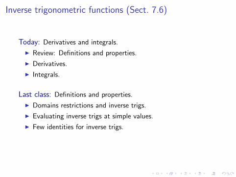
Inverse trigonometric functions (Sect. 7.6)
Today: Derivatives and integrals.
I Review: Definitions and properties.
I Derivatives.
I Integrals.
Last class: Definitions and properties.
I Domains restrictions and inverse trigs.
I Evaluating inverse trigs at simple values.
I Few identities for inverse trigs.

Review: Definitions and properties
Remark: On certain domains the trigonometric functions areinvertible.
1
y y = sin(x)
x− π / 2 π / 2
−1
1
y
x
y = cos(x)
π0 π / 2
−1
π / 2 x
y = tan(x)y
− π / 2
0 x
y y = csc(x)
− π / 2 π / 2
−1
1
y
x
1
−1
0 π / 2 π
y = sec(x)
π / 2
y
x0
y = cot(x)
π

Review: Definitions and properties
Remark: The graph of the inverse function is a reflection of theoriginal function graph about the y = x axis.
y = arcsin(x)
x
π / 2
− π / 2
1−1
y y = arccos(x)
0
π / 2
π
y
x−1 1
y
x
− π / 2
π / 2
y = arctan(x)
y = arccsc(x)y
−1 0 1
π / 2
− π / 2
x
y = arcsec(x)
−1 10
π / 2
π
y
x
y
0
π / 2
π
x
y = arccot(x)

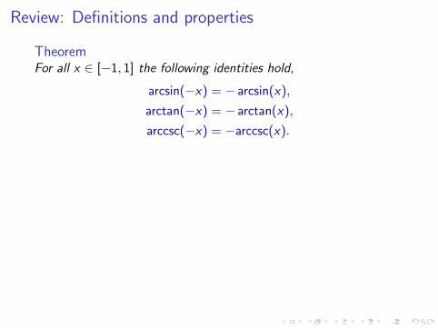
Review: Definitions and properties
TheoremFor all x ∈ [−1, 1] the following identities hold,
arccos(x) + arccos(−x) = π, arccos(x) + arcsin(x) =π
2.
Proof:
arccos(−x)
θ
1
y
(θ)x = cos(π−θ)−x = cos
π − θ
θ
x
arccos(x) arccos(x)
θ
1
y
(θ)x = cos x
π/2 − θ
(π/2−θ)x = sin
arcsin(x)

Review: Definitions and properties
TheoremFor all x ∈ [−1, 1] the following identities hold,
arccos(x) + arccos(−x) = π, arccos(x) + arcsin(x) =π
2.
Proof:
arccos(−x)
θ
1
y
(θ)x = cos(π−θ)−x = cos
π − θ
θ
x
arccos(x)
arccos(x)
θ
1
y
(θ)x = cos x
π/2 − θ
(π/2−θ)x = sin
arcsin(x)

Review: Definitions and properties
TheoremFor all x ∈ [−1, 1] the following identities hold,
arccos(x) + arccos(−x) = π, arccos(x) + arcsin(x) =π
2.
Proof:
arccos(−x)
θ
1
y
(θ)x = cos(π−θ)−x = cos
π − θ
θ
x
arccos(x) arccos(x)
θ
1
y
(θ)x = cos x
π/2 − θ
(π/2−θ)x = sin
arcsin(x)
Review: Definitions and properties
TheoremFor all x ∈ [−1, 1] the following identities hold,
arcsin(−x) = − arcsin(x),
arctan(−x) = − arctan(x),
arccsc(−x) = −arccsc(x).
Proof:y = arcsin(x)
x
π / 2
− π / 2
1−1
y y
x
− π / 2
π / 2
y = arctan(x) y = arccsc(x)y
−1 0 1
π / 2
− π / 2
x

Review: Definitions and properties
TheoremFor all x ∈ [−1, 1] the following identities hold,
arcsin(−x) = − arcsin(x),
arctan(−x) = − arctan(x),
arccsc(−x) = −arccsc(x).
Proof:y = arcsin(x)
x
π / 2
− π / 2
1−1
y
y
x
− π / 2
π / 2
y = arctan(x) y = arccsc(x)y
−1 0 1
π / 2
− π / 2
x

Review: Definitions and properties
TheoremFor all x ∈ [−1, 1] the following identities hold,
arcsin(−x) = − arcsin(x),
arctan(−x) = − arctan(x),
arccsc(−x) = −arccsc(x).
Proof:y = arcsin(x)
x
π / 2
− π / 2
1−1
y y
x
− π / 2
π / 2
y = arctan(x)
y = arccsc(x)y
−1 0 1
π / 2
− π / 2
x

Review: Definitions and properties
TheoremFor all x ∈ [−1, 1] the following identities hold,
arcsin(−x) = − arcsin(x),
arctan(−x) = − arctan(x),
arccsc(−x) = −arccsc(x).
Proof:y = arcsin(x)
x
π / 2
− π / 2
1−1
y y
x
− π / 2
π / 2
y = arctan(x) y = arccsc(x)y
−1 0 1
π / 2
− π / 2
x

Inverse trigonometric functions (Sect. 7.6)
Today: Derivatives and integrals.
I Review: Definitions and properties.
I Derivatives.
I Integrals.

Derivatives of inverse trigonometric functions
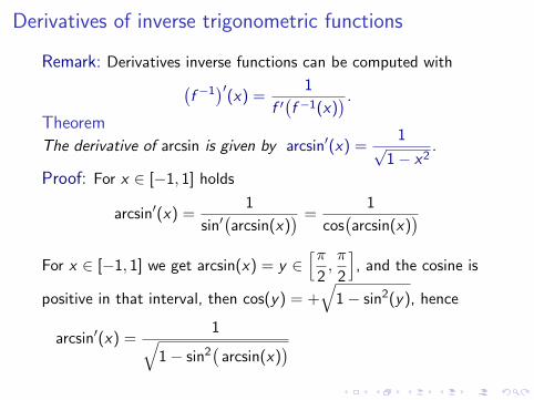
Remark: Derivatives inverse functions can be computed with(f −1
)′(x) =
1
f ′(f −1(x)
) .
Theorem
The derivative of arcsin is given by arcsin′(x) =1√
1− x2.
Proof: For x ∈ [−1, 1] holds
arcsin′(x) =1
sin′(arcsin(x)
) =1
cos(arcsin(x)
)For x ∈ [−1, 1] we get arcsin(x) = y ∈
[π
2,π
2
], and the cosine is
positive in that interval, then cos(y) = +√
1− sin2(y), hence
arcsin′(x) =1√
1− sin2(arcsin(x)
) ⇒ arcsin′(x) =1√
1− x2.

Derivatives of inverse trigonometric functions
Remark: Derivatives inverse functions can be computed with(f −1
)′(x) =
1
f ′(f −1(x)
) .
Theorem
The derivative of arcsin is given by arcsin′(x) =1√
1− x2.
Proof: For x ∈ [−1, 1] holds
arcsin′(x) =1
sin′(arcsin(x)
)
=1
cos(arcsin(x)
)For x ∈ [−1, 1] we get arcsin(x) = y ∈
[π
2,π
2
], and the cosine is
positive in that interval, then cos(y) = +√
1− sin2(y), hence
arcsin′(x) =1√
1− sin2(arcsin(x)
) ⇒ arcsin′(x) =1√
1− x2.

Derivatives of inverse trigonometric functions
Remark: Derivatives inverse functions can be computed with(f −1
)′(x) =
1
f ′(f −1(x)
) .
Theorem
The derivative of arcsin is given by arcsin′(x) =1√
1− x2.
Proof: For x ∈ [−1, 1] holds
arcsin′(x) =1
sin′(arcsin(x)
) =1
cos(arcsin(x)
)
For x ∈ [−1, 1] we get arcsin(x) = y ∈[π
2,π
2
], and the cosine is
positive in that interval, then cos(y) = +√
1− sin2(y), hence
arcsin′(x) =1√
1− sin2(arcsin(x)
) ⇒ arcsin′(x) =1√
1− x2.

Derivatives of inverse trigonometric functions
Remark: Derivatives inverse functions can be computed with(f −1
)′(x) =
1
f ′(f −1(x)
) .
Theorem
The derivative of arcsin is given by arcsin′(x) =1√
1− x2.
Proof: For x ∈ [−1, 1] holds
arcsin′(x) =1
sin′(arcsin(x)
) =1
cos(arcsin(x)
)For x ∈ [−1, 1] we get arcsin(x) = y ∈
[π
2,π
2
],
and the cosine is
positive in that interval, then cos(y) = +√
1− sin2(y), hence
arcsin′(x) =1√
1− sin2(arcsin(x)
) ⇒ arcsin′(x) =1√
1− x2.

Derivatives of inverse trigonometric functions
Remark: Derivatives inverse functions can be computed with(f −1
)′(x) =
1
f ′(f −1(x)
) .
Theorem
The derivative of arcsin is given by arcsin′(x) =1√
1− x2.
Proof: For x ∈ [−1, 1] holds
arcsin′(x) =1
sin′(arcsin(x)
) =1
cos(arcsin(x)
)For x ∈ [−1, 1] we get arcsin(x) = y ∈
[π
2,π
2
], and the cosine is
positive in that interval,
then cos(y) = +√
1− sin2(y), hence
arcsin′(x) =1√
1− sin2(arcsin(x)
) ⇒ arcsin′(x) =1√
1− x2.

Derivatives of inverse trigonometric functions
Remark: Derivatives inverse functions can be computed with(f −1
)′(x) =
1
f ′(f −1(x)
) .
Theorem
The derivative of arcsin is given by arcsin′(x) =1√
1− x2.
Proof: For x ∈ [−1, 1] holds
arcsin′(x) =1
sin′(arcsin(x)
) =1
cos(arcsin(x)
)For x ∈ [−1, 1] we get arcsin(x) = y ∈
[π
2,π
2
], and the cosine is
positive in that interval, then cos(y) = +√
1− sin2(y),
hence
arcsin′(x) =1√
1− sin2(arcsin(x)
) ⇒ arcsin′(x) =1√
1− x2.
Derivatives of inverse trigonometric functions
Remark: Derivatives inverse functions can be computed with(f −1
)′(x) =
1
f ′(f −1(x)
) .
Theorem
The derivative of arcsin is given by arcsin′(x) =1√
1− x2.
Proof: For x ∈ [−1, 1] holds
arcsin′(x) =1
sin′(arcsin(x)
) =1
cos(arcsin(x)
)For x ∈ [−1, 1] we get arcsin(x) = y ∈
[π
2,π
2
], and the cosine is
positive in that interval, then cos(y) = +√
1− sin2(y), hence
arcsin′(x) =1√
1− sin2(arcsin(x)
)
⇒ arcsin′(x) =1√
1− x2.

Derivatives of inverse trigonometric functions
Remark: Derivatives inverse functions can be computed with(f −1
)′(x) =
1
f ′(f −1(x)
) .
Theorem
The derivative of arcsin is given by arcsin′(x) =1√
1− x2.
Proof: For x ∈ [−1, 1] holds
arcsin′(x) =1
sin′(arcsin(x)
) =1
cos(arcsin(x)
)For x ∈ [−1, 1] we get arcsin(x) = y ∈
[π
2,π
2
], and the cosine is
positive in that interval, then cos(y) = +√
1− sin2(y), hence
arcsin′(x) =1√
1− sin2(arcsin(x)
) ⇒ arcsin′(x) =1√
1− x2.

Derivatives of inverse trigonometric functions
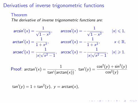
TheoremThe derivative of inverse trigonometric functions are:
arcsin′(x) =1√
1− x2, arccos′(x) = − 1√
1− x2, |x | 6 1,
arctan′(x) =1
1 + x2, arccot′(x) = − 1
1 + x2, x ∈ R,
arcsec′(x) =1
|x |√
x2 − 1, arccsc′(x) = − 1
|x |√
x2 − 1, |x | > 1.
Proof: arctan′(x) =1
tan′(arctan(x)
) , tan′(y) =cos2(y) + sin2(y)
cos2(y)
tan′(y) = 1 + tan2(y), y = arctan(x), ⇒ arctan′(x) =1
1 + x2.

Derivatives of inverse trigonometric functions
TheoremThe derivative of inverse trigonometric functions are:
arcsin′(x) =1√
1− x2, arccos′(x) = − 1√
1− x2, |x | 6 1,
arctan′(x) =1
1 + x2, arccot′(x) = − 1
1 + x2, x ∈ R,
arcsec′(x) =1
|x |√
x2 − 1, arccsc′(x) = − 1
|x |√
x2 − 1, |x | > 1.
Proof: arctan′(x) =1
tan′(arctan(x)
) ,
tan′(y) =cos2(y) + sin2(y)
cos2(y)
tan′(y) = 1 + tan2(y), y = arctan(x), ⇒ arctan′(x) =1
1 + x2.

Derivatives of inverse trigonometric functions
TheoremThe derivative of inverse trigonometric functions are:
arcsin′(x) =1√
1− x2, arccos′(x) = − 1√
1− x2, |x | 6 1,
arctan′(x) =1
1 + x2, arccot′(x) = − 1
1 + x2, x ∈ R,
arcsec′(x) =1
|x |√
x2 − 1, arccsc′(x) = − 1
|x |√
x2 − 1, |x | > 1.
Proof: arctan′(x) =1
tan′(arctan(x)
) , tan′(y) =cos2(y) + sin2(y)
cos2(y)
tan′(y) = 1 + tan2(y), y = arctan(x), ⇒ arctan′(x) =1
1 + x2.

Derivatives of inverse trigonometric functions
TheoremThe derivative of inverse trigonometric functions are:
arcsin′(x) =1√
1− x2, arccos′(x) = − 1√
1− x2, |x | 6 1,
arctan′(x) =1
1 + x2, arccot′(x) = − 1
1 + x2, x ∈ R,
arcsec′(x) =1
|x |√
x2 − 1, arccsc′(x) = − 1
|x |√
x2 − 1, |x | > 1.
Proof: arctan′(x) =1
tan′(arctan(x)
) , tan′(y) =cos2(y) + sin2(y)
cos2(y)
tan′(y) = 1 + tan2(y),
y = arctan(x), ⇒ arctan′(x) =1
1 + x2.
Derivatives of inverse trigonometric functions
TheoremThe derivative of inverse trigonometric functions are:
arcsin′(x) =1√
1− x2, arccos′(x) = − 1√
1− x2, |x | 6 1,
arctan′(x) =1
1 + x2, arccot′(x) = − 1
1 + x2, x ∈ R,
arcsec′(x) =1
|x |√
x2 − 1, arccsc′(x) = − 1
|x |√
x2 − 1, |x | > 1.
Proof: arctan′(x) =1
tan′(arctan(x)
) , tan′(y) =cos2(y) + sin2(y)
cos2(y)
tan′(y) = 1 + tan2(y), y = arctan(x),
⇒ arctan′(x) =1
1 + x2.

Derivatives of inverse trigonometric functions
TheoremThe derivative of inverse trigonometric functions are:
arcsin′(x) =1√
1− x2, arccos′(x) = − 1√
1− x2, |x | 6 1,
arctan′(x) =1
1 + x2, arccot′(x) = − 1
1 + x2, x ∈ R,
arcsec′(x) =1
|x |√
x2 − 1, arccsc′(x) = − 1
|x |√
x2 − 1, |x | > 1.
Proof: arctan′(x) =1
tan′(arctan(x)
) , tan′(y) =cos2(y) + sin2(y)
cos2(y)
tan′(y) = 1 + tan2(y), y = arctan(x), ⇒ arctan′(x) =1
1 + x2.

Derivatives of inverse trigonometric functions
Proof: arcsec′(x) =1
sec′(arcsec(x)
) ,
for |x | > 1.
Then y = arcsec(x) satisfies y ∈ [0, π]− {π/2}. Recall,
sec′(y) =( 1
cos(y)
)′=
sin(y)
cos2(y), sin(y) = +
√1− cos2(y),
sec′(y) =
√1− cos2(y)
cos2(y)=
1
| cos(y)|
√1− cos2(y)
| cos(y)|,
sec′(y) =1
| cos(y)|
√1
cos2(y)− 1 = | sec(y)|
√sec2(y)− 1.
We conclude: arcsec′(x) =1
|x |√
x2 − 1.

Derivatives of inverse trigonometric functions
Proof: arcsec′(x) =1
sec′(arcsec(x)
) , for |x | > 1.
Then y = arcsec(x) satisfies y ∈ [0, π]− {π/2}.
Recall,
sec′(y) =( 1
cos(y)
)′=
sin(y)
cos2(y), sin(y) = +
√1− cos2(y),
sec′(y) =
√1− cos2(y)
cos2(y)=
1
| cos(y)|
√1− cos2(y)
| cos(y)|,
sec′(y) =1
| cos(y)|
√1
cos2(y)− 1 = | sec(y)|
√sec2(y)− 1.
We conclude: arcsec′(x) =1
|x |√
x2 − 1.

Derivatives of inverse trigonometric functions
Proof: arcsec′(x) =1
sec′(arcsec(x)
) , for |x | > 1.
Then y = arcsec(x) satisfies y ∈ [0, π]− {π/2}. Recall,
sec′(y) =( 1
cos(y)
)′
=sin(y)
cos2(y), sin(y) = +
√1− cos2(y),
sec′(y) =
√1− cos2(y)
cos2(y)=
1
| cos(y)|
√1− cos2(y)
| cos(y)|,
sec′(y) =1
| cos(y)|
√1
cos2(y)− 1 = | sec(y)|
√sec2(y)− 1.
We conclude: arcsec′(x) =1
|x |√
x2 − 1.

Derivatives of inverse trigonometric functions
Proof: arcsec′(x) =1
sec′(arcsec(x)
) , for |x | > 1.
Then y = arcsec(x) satisfies y ∈ [0, π]− {π/2}. Recall,
sec′(y) =( 1
cos(y)
)′=
sin(y)
cos2(y),
sin(y) = +√
1− cos2(y),
sec′(y) =
√1− cos2(y)
cos2(y)=
1
| cos(y)|
√1− cos2(y)
| cos(y)|,
sec′(y) =1
| cos(y)|
√1
cos2(y)− 1 = | sec(y)|
√sec2(y)− 1.
We conclude: arcsec′(x) =1
|x |√
x2 − 1.

Derivatives of inverse trigonometric functions
Proof: arcsec′(x) =1
sec′(arcsec(x)
) , for |x | > 1.
Then y = arcsec(x) satisfies y ∈ [0, π]− {π/2}. Recall,
sec′(y) =( 1
cos(y)
)′=
sin(y)
cos2(y), sin(y) = +
√1− cos2(y),
sec′(y) =
√1− cos2(y)
cos2(y)=
1
| cos(y)|
√1− cos2(y)
| cos(y)|,
sec′(y) =1
| cos(y)|
√1
cos2(y)− 1 = | sec(y)|
√sec2(y)− 1.
We conclude: arcsec′(x) =1
|x |√
x2 − 1.

Derivatives of inverse trigonometric functions
Proof: arcsec′(x) =1
sec′(arcsec(x)
) , for |x | > 1.
Then y = arcsec(x) satisfies y ∈ [0, π]− {π/2}. Recall,
sec′(y) =( 1
cos(y)
)′=
sin(y)
cos2(y), sin(y) = +
√1− cos2(y),
sec′(y) =
√1− cos2(y)
cos2(y)
=1
| cos(y)|
√1− cos2(y)
| cos(y)|,
sec′(y) =1
| cos(y)|
√1
cos2(y)− 1 = | sec(y)|
√sec2(y)− 1.
We conclude: arcsec′(x) =1
|x |√
x2 − 1.

Derivatives of inverse trigonometric functions
Proof: arcsec′(x) =1
sec′(arcsec(x)
) , for |x | > 1.
Then y = arcsec(x) satisfies y ∈ [0, π]− {π/2}. Recall,
sec′(y) =( 1
cos(y)
)′=
sin(y)
cos2(y), sin(y) = +
√1− cos2(y),
sec′(y) =
√1− cos2(y)
cos2(y)=
1
| cos(y)|
√1− cos2(y)
| cos(y)|,
sec′(y) =1
| cos(y)|
√1
cos2(y)− 1 = | sec(y)|
√sec2(y)− 1.
We conclude: arcsec′(x) =1
|x |√
x2 − 1.

Derivatives of inverse trigonometric functions
Proof: arcsec′(x) =1
sec′(arcsec(x)
) , for |x | > 1.
Then y = arcsec(x) satisfies y ∈ [0, π]− {π/2}. Recall,
sec′(y) =( 1
cos(y)
)′=
sin(y)
cos2(y), sin(y) = +
√1− cos2(y),
sec′(y) =
√1− cos2(y)
cos2(y)=
1
| cos(y)|
√1− cos2(y)
| cos(y)|,
sec′(y) =1
| cos(y)|
√1
cos2(y)− 1
= | sec(y)|√
sec2(y)− 1.
We conclude: arcsec′(x) =1
|x |√
x2 − 1.

Derivatives of inverse trigonometric functions
Proof: arcsec′(x) =1
sec′(arcsec(x)
) , for |x | > 1.
Then y = arcsec(x) satisfies y ∈ [0, π]− {π/2}. Recall,
sec′(y) =( 1
cos(y)
)′=
sin(y)
cos2(y), sin(y) = +
√1− cos2(y),
sec′(y) =
√1− cos2(y)
cos2(y)=
1
| cos(y)|
√1− cos2(y)
| cos(y)|,
sec′(y) =1
| cos(y)|
√1
cos2(y)− 1 = | sec(y)|
√sec2(y)− 1.
We conclude: arcsec′(x) =1
|x |√
x2 − 1.

Derivatives of inverse trigonometric functions
Proof: arcsec′(x) =1
sec′(arcsec(x)
) , for |x | > 1.
Then y = arcsec(x) satisfies y ∈ [0, π]− {π/2}. Recall,
sec′(y) =( 1
cos(y)
)′=
sin(y)
cos2(y), sin(y) = +
√1− cos2(y),
sec′(y) =
√1− cos2(y)
cos2(y)=
1
| cos(y)|
√1− cos2(y)
| cos(y)|,
sec′(y) =1
| cos(y)|
√1
cos2(y)− 1 = | sec(y)|
√sec2(y)− 1.
We conclude: arcsec′(x) =1
|x |√
x2 − 1.

Derivatives of inverse trigonometric functions
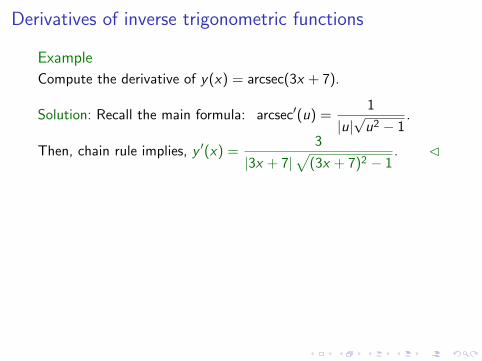
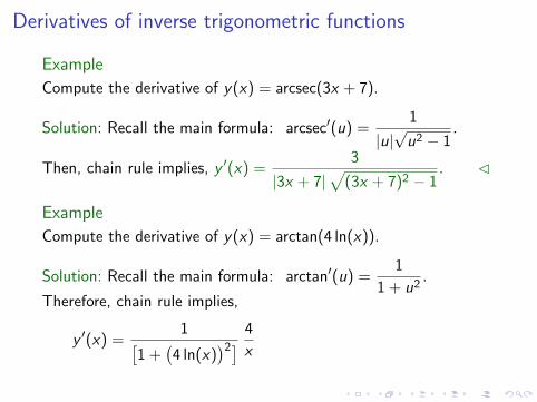
Example
Compute the derivative of y(x) = arcsec(3x + 7).
Solution: Recall the main formula: arcsec′(u) =1
|u|√
u2 − 1.
Then, chain rule implies, y ′(x) =3
|3x + 7|√
(3x + 7)2 − 1. C
Example
Compute the derivative of y(x) = arctan(4 ln(x)).
Solution: Recall the main formula: arctan′(u) =1
1 + u2.
Therefore, chain rule implies,
y ′(x) =1[
1 +(4 ln(x)
)2] 4
x⇒ y ′ =
4
x[1 + 16 ln2(x)
] . C

Derivatives of inverse trigonometric functions
Example
Compute the derivative of y(x) = arcsec(3x + 7).
Solution: Recall the main formula: arcsec′(u) =1
|u|√
u2 − 1.
Then, chain rule implies,
y ′(x) =3
|3x + 7|√
(3x + 7)2 − 1. C
Example
Compute the derivative of y(x) = arctan(4 ln(x)).
Solution: Recall the main formula: arctan′(u) =1
1 + u2.
Therefore, chain rule implies,
y ′(x) =1[
1 +(4 ln(x)
)2] 4
x⇒ y ′ =
4
x[1 + 16 ln2(x)
] . C
Derivatives of inverse trigonometric functions
Example
Compute the derivative of y(x) = arcsec(3x + 7).
Solution: Recall the main formula: arcsec′(u) =1
|u|√
u2 − 1.
Then, chain rule implies, y ′(x) =3
|3x + 7|√
(3x + 7)2 − 1. C
Example
Compute the derivative of y(x) = arctan(4 ln(x)).
Solution: Recall the main formula: arctan′(u) =1
1 + u2.
Therefore, chain rule implies,
y ′(x) =1[
1 +(4 ln(x)
)2] 4
x⇒ y ′ =
4
x[1 + 16 ln2(x)
] . C

Derivatives of inverse trigonometric functions
Example
Compute the derivative of y(x) = arcsec(3x + 7).
Solution: Recall the main formula: arcsec′(u) =1
|u|√
u2 − 1.
Then, chain rule implies, y ′(x) =3
|3x + 7|√
(3x + 7)2 − 1. C
Example
Compute the derivative of y(x) = arctan(4 ln(x)).
Solution: Recall the main formula: arctan′(u) =1
1 + u2.
Therefore, chain rule implies,
y ′(x) =1[
1 +(4 ln(x)
)2] 4
x⇒ y ′ =
4
x[1 + 16 ln2(x)
] . C
Derivatives of inverse trigonometric functions
Example
Compute the derivative of y(x) = arcsec(3x + 7).
Solution: Recall the main formula: arcsec′(u) =1
|u|√
u2 − 1.
Then, chain rule implies, y ′(x) =3
|3x + 7|√
(3x + 7)2 − 1. C
Example
Compute the derivative of y(x) = arctan(4 ln(x)).
Solution: Recall the main formula: arctan′(u) =1
1 + u2.
Therefore, chain rule implies,
y ′(x) =1[
1 +(4 ln(x)
)2] 4
x
⇒ y ′ =4
x[1 + 16 ln2(x)
] . C

Derivatives of inverse trigonometric functions
Example
Compute the derivative of y(x) = arcsec(3x + 7).
Solution: Recall the main formula: arcsec′(u) =1
|u|√
u2 − 1.
Then, chain rule implies, y ′(x) =3
|3x + 7|√
(3x + 7)2 − 1. C
Example
Compute the derivative of y(x) = arctan(4 ln(x)).
Solution: Recall the main formula: arctan′(u) =1
1 + u2.
Therefore, chain rule implies,
y ′(x) =1[
1 +(4 ln(x)
)2] 4
x⇒ y ′ =
4
x[1 + 16 ln2(x)
] . C

Inverse trigonometric functions (Sect. 7.6)
Today: Derivatives and integrals.
I Review: Definitions and properties.
I Derivatives.
I Integrals.

Integrals of inverse trigonometric functions
Remark: The formulas for the derivatives of inverse trigonometricfunctions imply the integration formulas.
TheoremFor any constant a 6= 0 holds,∫
dx√a2 − x2
= arcsin(x
a
)+ c , |x | < a,∫
dx
a2 + x2=
1
aarctan
(x
a
)+ c , x ∈ R,∫
dx
x√
x2 − a2=
1
aarcsec
(∣∣∣xa
∣∣∣) + c , |x | > a > 0.
Proof: (For arcsine only.) y(x) = arcsin(x
a
)+ c , then
y ′(x) =1√
1− x2
a2
1
a=
|a|√a2 − x2
1
a⇒ y ′(x) =
1√a2 − x2

Integrals of inverse trigonometric functions
Remark: The formulas for the derivatives of inverse trigonometricfunctions imply the integration formulas.
TheoremFor any constant a 6= 0 holds,∫
dx√a2 − x2
= arcsin(x
a
)+ c , |x | < a,∫
dx
a2 + x2=
1
aarctan
(x
a
)+ c , x ∈ R,∫
dx
x√
x2 − a2=
1
aarcsec
(∣∣∣xa
∣∣∣) + c , |x | > a > 0.
Proof: (For arcsine only.)
y(x) = arcsin(x
a
)+ c , then
y ′(x) =1√
1− x2
a2
1
a=
|a|√a2 − x2
1
a⇒ y ′(x) =
1√a2 − x2

Integrals of inverse trigonometric functions
Remark: The formulas for the derivatives of inverse trigonometricfunctions imply the integration formulas.
TheoremFor any constant a 6= 0 holds,∫
dx√a2 − x2
= arcsin(x
a
)+ c , |x | < a,∫
dx
a2 + x2=
1
aarctan
(x
a
)+ c , x ∈ R,∫
dx
x√
x2 − a2=
1
aarcsec
(∣∣∣xa
∣∣∣) + c , |x | > a > 0.
Proof: (For arcsine only.) y(x) = arcsin(x
a
)+ c ,
then
y ′(x) =1√
1− x2
a2
1
a=
|a|√a2 − x2
1
a⇒ y ′(x) =
1√a2 − x2

Integrals of inverse trigonometric functions
Remark: The formulas for the derivatives of inverse trigonometricfunctions imply the integration formulas.
TheoremFor any constant a 6= 0 holds,∫
dx√a2 − x2
= arcsin(x
a
)+ c , |x | < a,∫
dx
a2 + x2=
1
aarctan
(x
a
)+ c , x ∈ R,∫
dx
x√
x2 − a2=
1
aarcsec
(∣∣∣xa
∣∣∣) + c , |x | > a > 0.
Proof: (For arcsine only.) y(x) = arcsin(x
a
)+ c , then
y ′(x)
=1√
1− x2
a2
1
a=
|a|√a2 − x2
1
a⇒ y ′(x) =
1√a2 − x2

Integrals of inverse trigonometric functions
Remark: The formulas for the derivatives of inverse trigonometricfunctions imply the integration formulas.
TheoremFor any constant a 6= 0 holds,∫
dx√a2 − x2
= arcsin(x
a
)+ c , |x | < a,∫
dx
a2 + x2=
1
aarctan
(x
a
)+ c , x ∈ R,∫
dx
x√
x2 − a2=
1
aarcsec
(∣∣∣xa
∣∣∣) + c , |x | > a > 0.
Proof: (For arcsine only.) y(x) = arcsin(x
a
)+ c , then
y ′(x) =1√
1− x2
a2
1
a
=|a|√
a2 − x2
1
a⇒ y ′(x) =
1√a2 − x2

Integrals of inverse trigonometric functions
Remark: The formulas for the derivatives of inverse trigonometricfunctions imply the integration formulas.
TheoremFor any constant a 6= 0 holds,∫
dx√a2 − x2
= arcsin(x
a
)+ c , |x | < a,∫
dx
a2 + x2=
1
aarctan
(x
a
)+ c , x ∈ R,∫
dx
x√
x2 − a2=
1
aarcsec
(∣∣∣xa
∣∣∣) + c , |x | > a > 0.
Proof: (For arcsine only.) y(x) = arcsin(x
a
)+ c , then
y ′(x) =1√
1− x2
a2
1
a=
|a|√a2 − x2
1
a
⇒ y ′(x) =1√
a2 − x2

Integrals of inverse trigonometric functions
Remark: The formulas for the derivatives of inverse trigonometricfunctions imply the integration formulas.
TheoremFor any constant a 6= 0 holds,∫
dx√a2 − x2
= arcsin(x
a
)+ c , |x | < a,∫
dx
a2 + x2=
1
aarctan
(x
a
)+ c , x ∈ R,∫
dx
x√
x2 − a2=
1
aarcsec
(∣∣∣xa
∣∣∣) + c , |x | > a > 0.
Proof: (For arcsine only.) y(x) = arcsin(x
a
)+ c , then
y ′(x) =1√
1− x2
a2
1
a=
|a|√a2 − x2
1
a⇒ y ′(x) =
1√a2 − x2

Integrals of inverse trigonometric functions
Example
Evaluate I =
∫6√
3− 4(x − 1)2dx .
Solution: Substitute: u = 2(x − 1), then du = 2 dx ,
I =
∫6√
3− u2
du
2= 3
∫du√
3− u2.
Recall:
∫dx√
a2 − u2= arcsin
(u
a
)+ c . Then, for a =
√3,
I = 3 arcsin( u√
3
)+ c ⇒ I = 3 arcsin
(2(x − 1)√3
)+ c . C

Integrals of inverse trigonometric functions
Example
Evaluate I =
∫6√
3− 4(x − 1)2dx .
Solution: Substitute: u = 2(x − 1),
then du = 2 dx ,
I =
∫6√
3− u2
du
2= 3
∫du√
3− u2.
Recall:
∫dx√
a2 − u2= arcsin
(u
a
)+ c . Then, for a =
√3,
I = 3 arcsin( u√
3
)+ c ⇒ I = 3 arcsin
(2(x − 1)√3
)+ c . C

Integrals of inverse trigonometric functions
Example
Evaluate I =
∫6√
3− 4(x − 1)2dx .
Solution: Substitute: u = 2(x − 1), then du = 2 dx ,
I =
∫6√
3− u2
du
2= 3
∫du√
3− u2.
Recall:
∫dx√
a2 − u2= arcsin
(u
a
)+ c . Then, for a =
√3,
I = 3 arcsin( u√
3
)+ c ⇒ I = 3 arcsin
(2(x − 1)√3
)+ c . C

Integrals of inverse trigonometric functions
Example
Evaluate I =
∫6√
3− 4(x − 1)2dx .
Solution: Substitute: u = 2(x − 1), then du = 2 dx ,
I =
∫6√
3− u2
du
2
= 3
∫du√
3− u2.
Recall:
∫dx√
a2 − u2= arcsin
(u
a
)+ c . Then, for a =
√3,
I = 3 arcsin( u√
3
)+ c ⇒ I = 3 arcsin
(2(x − 1)√3
)+ c . C

Integrals of inverse trigonometric functions
Example
Evaluate I =
∫6√
3− 4(x − 1)2dx .
Solution: Substitute: u = 2(x − 1), then du = 2 dx ,
I =
∫6√
3− u2
du
2= 3
∫du√
3− u2.
Recall:
∫dx√
a2 − u2= arcsin
(u
a
)+ c . Then, for a =
√3,
I = 3 arcsin( u√
3
)+ c ⇒ I = 3 arcsin
(2(x − 1)√3
)+ c . C

Integrals of inverse trigonometric functions
Example
Evaluate I =
∫6√
3− 4(x − 1)2dx .
Solution: Substitute: u = 2(x − 1), then du = 2 dx ,
I =
∫6√
3− u2
du
2= 3
∫du√
3− u2.
Recall:
∫dx√
a2 − u2= arcsin
(u
a
)+ c .
Then, for a =√
3,
I = 3 arcsin( u√
3
)+ c ⇒ I = 3 arcsin
(2(x − 1)√3
)+ c . C

Integrals of inverse trigonometric functions
Example
Evaluate I =
∫6√
3− 4(x − 1)2dx .
Solution: Substitute: u = 2(x − 1), then du = 2 dx ,
I =
∫6√
3− u2
du
2= 3
∫du√
3− u2.
Recall:
∫dx√
a2 − u2= arcsin
(u
a
)+ c . Then, for a =
√3,
I = 3 arcsin( u√
3
)+ c ⇒ I = 3 arcsin
(2(x − 1)√3
)+ c . C

Integrals of inverse trigonometric functions
Example
Evaluate I =
∫6√
3− 4(x − 1)2dx .
Solution: Substitute: u = 2(x − 1), then du = 2 dx ,
I =
∫6√
3− u2
du
2= 3
∫du√
3− u2.
Recall:
∫dx√
a2 − u2= arcsin
(u
a
)+ c . Then, for a =
√3,
I = 3 arcsin( u√
3
)+ c
⇒ I = 3 arcsin(2(x − 1)√
3
)+ c . C

Integrals of inverse trigonometric functions
Example
Evaluate I =
∫6√
3− 4(x − 1)2dx .
Solution: Substitute: u = 2(x − 1), then du = 2 dx ,
I =
∫6√
3− u2
du
2= 3
∫du√
3− u2.
Recall:
∫dx√
a2 − u2= arcsin
(u
a
)+ c . Then, for a =
√3,
I = 3 arcsin( u√
3
)+ c ⇒ I = 3 arcsin
(2(x − 1)√3
)+ c . C

Integrals of inverse trigonometric functions
Example
Evaluate I =
∫6
t[ln2(t) + ln(t4) + 8
] dt.
Solution: Recall: ln(t4) = 4 ln(t), Try to complete the square.
I =
∫6
t[ln2(t) + 4 ln(t) + 8
] dt,
I =
∫6
t[ln2(t) + 2(2 ln(t)) + 4− 4 + 8
] dt
I =
∫6
t[(
ln(t) + 2)2
+ 4] dt
This looks like the derivative of the arctangent.

Integrals of inverse trigonometric functions
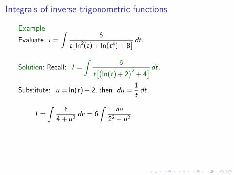
Example
Evaluate I =
∫6
t[ln2(t) + ln(t4) + 8
] dt.
Solution: Recall: ln(t4) = 4 ln(t),
Try to complete the square.
I =
∫6
t[ln2(t) + 4 ln(t) + 8
] dt,
I =
∫6
t[ln2(t) + 2(2 ln(t)) + 4− 4 + 8
] dt
I =
∫6
t[(
ln(t) + 2)2
+ 4] dt
This looks like the derivative of the arctangent.

Integrals of inverse trigonometric functions
Example
Evaluate I =
∫6
t[ln2(t) + ln(t4) + 8
] dt.
Solution: Recall: ln(t4) = 4 ln(t), Try to complete the square.
I =
∫6
t[ln2(t) + 4 ln(t) + 8
] dt,
I =
∫6
t[ln2(t) + 2(2 ln(t)) + 4− 4 + 8
] dt
I =
∫6
t[(
ln(t) + 2)2
+ 4] dt
This looks like the derivative of the arctangent.

Integrals of inverse trigonometric functions
Example
Evaluate I =
∫6
t[ln2(t) + ln(t4) + 8
] dt.
Solution: Recall: I =
∫6
t[(
ln(t) + 2)2
+ 4] dt.
Substitute: u = ln(t) + 2, then du =1
tdt,
I =
∫6
4 + u2du = 6
∫du
22 + u2= 6
1
2arctan
(u
2
)+ c .
I = 3 arctan(1
2(ln(t)+2)
)+c ⇒ I = 3 arctan
(ln(√
t)+1)+c .C

Integrals of inverse trigonometric functions
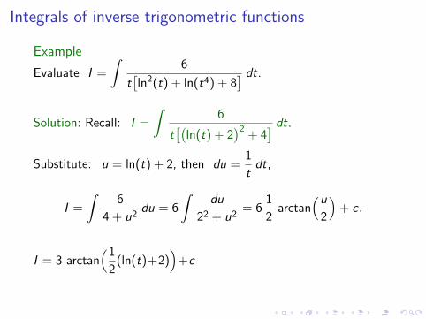
Example
Evaluate I =
∫6
t[ln2(t) + ln(t4) + 8
] dt.
Solution: Recall: I =
∫6
t[(
ln(t) + 2)2
+ 4] dt.
Substitute: u = ln(t) + 2,
then du =1
tdt,
I =
∫6
4 + u2du = 6
∫du
22 + u2= 6
1
2arctan
(u
2
)+ c .
I = 3 arctan(1
2(ln(t)+2)
)+c ⇒ I = 3 arctan
(ln(√
t)+1)+c .C

Integrals of inverse trigonometric functions
Example
Evaluate I =
∫6
t[ln2(t) + ln(t4) + 8
] dt.
Solution: Recall: I =
∫6
t[(
ln(t) + 2)2
+ 4] dt.
Substitute: u = ln(t) + 2, then du =1
tdt,
I =
∫6
4 + u2du = 6
∫du
22 + u2= 6
1
2arctan
(u
2
)+ c .
I = 3 arctan(1
2(ln(t)+2)
)+c ⇒ I = 3 arctan
(ln(√
t)+1)+c .C

Integrals of inverse trigonometric functions
Example
Evaluate I =
∫6
t[ln2(t) + ln(t4) + 8
] dt.
Solution: Recall: I =
∫6
t[(
ln(t) + 2)2
+ 4] dt.
Substitute: u = ln(t) + 2, then du =1
tdt,
I =
∫6
4 + u2du
= 6
∫du
22 + u2= 6
1
2arctan
(u
2
)+ c .
I = 3 arctan(1
2(ln(t)+2)
)+c ⇒ I = 3 arctan
(ln(√
t)+1)+c .C
Integrals of inverse trigonometric functions
Example
Evaluate I =
∫6
t[ln2(t) + ln(t4) + 8
] dt.
Solution: Recall: I =
∫6
t[(
ln(t) + 2)2
+ 4] dt.
Substitute: u = ln(t) + 2, then du =1
tdt,
I =
∫6
4 + u2du = 6
∫du
22 + u2
= 61
2arctan
(u
2
)+ c .
I = 3 arctan(1
2(ln(t)+2)
)+c ⇒ I = 3 arctan
(ln(√
t)+1)+c .C

Integrals of inverse trigonometric functions
Example
Evaluate I =
∫6
t[ln2(t) + ln(t4) + 8
] dt.
Solution: Recall: I =
∫6
t[(
ln(t) + 2)2
+ 4] dt.
Substitute: u = ln(t) + 2, then du =1
tdt,
I =
∫6
4 + u2du = 6
∫du
22 + u2= 6
1
2arctan
(u
2
)+ c .
I = 3 arctan(1
2(ln(t)+2)
)+c ⇒ I = 3 arctan
(ln(√
t)+1)+c .C
Integrals of inverse trigonometric functions
Example
Evaluate I =
∫6
t[ln2(t) + ln(t4) + 8
] dt.
Solution: Recall: I =
∫6
t[(
ln(t) + 2)2
+ 4] dt.
Substitute: u = ln(t) + 2, then du =1
tdt,
I =
∫6
4 + u2du = 6
∫du
22 + u2= 6
1
2arctan
(u
2
)+ c .
I = 3 arctan(1
2(ln(t)+2)
)+c
⇒ I = 3 arctan(ln(√
t)+1)+c .C

Integrals of inverse trigonometric functions
Example
Evaluate I =
∫6
t[ln2(t) + ln(t4) + 8
] dt.
Solution: Recall: I =
∫6
t[(
ln(t) + 2)2
+ 4] dt.
Substitute: u = ln(t) + 2, then du =1
tdt,
I =
∫6
4 + u2du = 6
∫du
22 + u2= 6
1
2arctan
(u
2
)+ c .
I = 3 arctan(1
2(ln(t)+2)
)+c ⇒ I = 3 arctan
(ln(√
t)+1)+c .C

Hyperbolic functions (Sect. 7.7)
I Circular and hyperbolic functions.
I Definitions and identities.
I Derivatives of hyperbolic functions.
I Integrals of hyperbolic functions.

Circular and hyperbolic functions
Remark: Trigonometric functions are also called circular functions.
(θ)
y
x1
θ
cos (θ)
sin
The circle x2 + y2 = 1 can beparametrized by the functions
x = cos(θ),
y = sin(θ).
Since these functions satisfy
cos2(θ) + sin2(θ) = 1.
Remark: The parametrization is not unique. Another solution is
x = cos(nθ), y = sin(nθ), n ∈ N.

Circular and hyperbolic functions
Remark: Trigonometric functions are also called circular functions.
(θ)
y
x1
θ
cos (θ)
sin
The circle x2 + y2 = 1 can beparametrized by the functions
x = cos(θ),
y = sin(θ).
Since these functions satisfy
cos2(θ) + sin2(θ) = 1.
Remark: The parametrization is not unique.
Another solution is
x = cos(nθ), y = sin(nθ), n ∈ N.

Circular and hyperbolic functions
Remark: Trigonometric functions are also called circular functions.
(θ)
y
x1
θ
cos (θ)
sin
The circle x2 + y2 = 1 can beparametrized by the functions
x = cos(θ),
y = sin(θ).
Since these functions satisfy
cos2(θ) + sin2(θ) = 1.
Remark: The parametrization is not unique. Another solution is
x = cos(nθ), y = sin(nθ), n ∈ N.

Circular and hyperbolic functions
Remark:Hyperbolic functions are a parametrization of a hyperbola.
y(u)
y
x1
x(u)
The hyperbola x2 − y2 = 1 canbe parametrized by the functions
x = f (u), y = g(u),
satisfying the condition
f 2(u)− g2(u) = 1.
Remark: A solution is x =1
2
[h(u) +
1
h(u)
], y =
1
2
[h(u)− 1
h(u)
],
x2 − y2 =1
4
[h2 +
1
h2+ 2− h2 − 1
h2+ 2
]= 1.

Circular and hyperbolic functions
Remark:Hyperbolic functions are a parametrization of a hyperbola.
y(u)
y
x1
x(u)
The hyperbola x2 − y2 = 1 canbe parametrized by the functions
x = f (u), y = g(u),
satisfying the condition
f 2(u)− g2(u) = 1.
Remark: A solution is x =1
2
[h(u) +
1
h(u)
], y =
1
2
[h(u)− 1
h(u)
],
x2 − y2 =
1
4
[h2 +
1
h2+ 2− h2 − 1
h2+ 2
]= 1.

Circular and hyperbolic functions
Remark:Hyperbolic functions are a parametrization of a hyperbola.
y(u)
y
x1
x(u)
The hyperbola x2 − y2 = 1 canbe parametrized by the functions
x = f (u), y = g(u),
satisfying the condition
f 2(u)− g2(u) = 1.
Remark: A solution is x =1
2
[h(u) +
1
h(u)
], y =
1
2
[h(u)− 1
h(u)
],
x2 − y2 =1
4
[h2 +
1
h2+ 2
− h2 − 1
h2+ 2
]= 1.

Circular and hyperbolic functions
Remark:Hyperbolic functions are a parametrization of a hyperbola.
y(u)
y
x1
x(u)
The hyperbola x2 − y2 = 1 canbe parametrized by the functions
x = f (u), y = g(u),
satisfying the condition
f 2(u)− g2(u) = 1.
Remark: A solution is x =1
2
[h(u) +
1
h(u)
], y =
1
2
[h(u)− 1
h(u)
],
x2 − y2 =1
4
[h2 +
1
h2+ 2− h2 − 1
h2+ 2
]
= 1.

Circular and hyperbolic functions
Remark:Hyperbolic functions are a parametrization of a hyperbola.
y(u)
y
x1
x(u)
The hyperbola x2 − y2 = 1 canbe parametrized by the functions
x = f (u), y = g(u),
satisfying the condition
f 2(u)− g2(u) = 1.
Remark: A solution is x =1
2
[h(u) +
1
h(u)
], y =
1
2
[h(u)− 1
h(u)
],
x2 − y2 =1
4
[h2 +
1
h2+ 2− h2 − 1
h2+ 2
]= 1.

Circular and hyperbolic functions
Remarks:
I The hyperbola x2 − y2 = 1 can be parametrized by
x =1
2
[h(u) +
1
h(u)
], y =
1
2
[h(u)− 1
h(u)
],
where h is any non-zero continuous function satisfying
limu→∞
h(u) = ∞, limu→−∞
h(u) = 0, h(0) = 1.
I The hyperbolic trigonometric functions correspond to
h(u) = eu.
DefinitionThe hyperbolic trigonometric functions are defined by
cosh(u) =eu + e−u
2, sinh(u) =
eu − e−u
2.

Circular and hyperbolic functions
Remarks:
I The hyperbola x2 − y2 = 1 can be parametrized by
x =1
2
[h(u) +
1
h(u)
], y =
1
2
[h(u)− 1
h(u)
],
where h is any non-zero continuous function satisfying
limu→∞
h(u) = ∞,
limu→−∞
h(u) = 0, h(0) = 1.
I The hyperbolic trigonometric functions correspond to
h(u) = eu.
DefinitionThe hyperbolic trigonometric functions are defined by
cosh(u) =eu + e−u
2, sinh(u) =
eu − e−u
2.

Circular and hyperbolic functions
Remarks:
I The hyperbola x2 − y2 = 1 can be parametrized by
x =1
2
[h(u) +
1
h(u)
], y =
1
2
[h(u)− 1
h(u)
],
where h is any non-zero continuous function satisfying
limu→∞
h(u) = ∞, limu→−∞
h(u) = 0,
h(0) = 1.
I The hyperbolic trigonometric functions correspond to
h(u) = eu.
DefinitionThe hyperbolic trigonometric functions are defined by
cosh(u) =eu + e−u
2, sinh(u) =
eu − e−u
2.

Circular and hyperbolic functions
Remarks:
I The hyperbola x2 − y2 = 1 can be parametrized by
x =1
2
[h(u) +
1
h(u)
], y =
1
2
[h(u)− 1
h(u)
],
where h is any non-zero continuous function satisfying
limu→∞
h(u) = ∞, limu→−∞
h(u) = 0, h(0) = 1.
I The hyperbolic trigonometric functions correspond to
h(u) = eu.
DefinitionThe hyperbolic trigonometric functions are defined by
cosh(u) =eu + e−u
2, sinh(u) =
eu − e−u
2.

Circular and hyperbolic functions
Remarks:
I The hyperbola x2 − y2 = 1 can be parametrized by
x =1
2
[h(u) +
1
h(u)
], y =
1
2
[h(u)− 1
h(u)
],
where h is any non-zero continuous function satisfying
limu→∞
h(u) = ∞, limu→−∞
h(u) = 0, h(0) = 1.
I The hyperbolic trigonometric functions correspond to
h(u) = eu.
DefinitionThe hyperbolic trigonometric functions are defined by
cosh(u) =eu + e−u
2, sinh(u) =
eu − e−u
2.

Hyperbolic functions (Sect. 7.7)
I Circular and hyperbolic functions.
I Definitions and identities.
I Derivatives of hyperbolic functions.
I Integrals of hyperbolic functions.
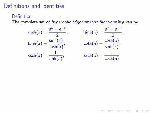
Definitions and identities
DefinitionThe complete set of hyperbolic trigonometric functions is given by
cosh(x) =ex + e−x
2, sinh(x) =
ex − e−x
2,
tanh(x) =sinh(x)
cosh(x), coth(x) =
cosh(x)
sinh(x),
csch(x) =1
sinh(x), sech(x) =
1
cosh(x).
Remarks:
I These functions satisfy identities similar but not equal tothose satisfied by circular trigonometric functions.
I We have seen one of these identities:
cosh2(x)− sinh2(x) = 1.

Definitions and identities
TheoremThe following identities hold,
cosh2(x)− sinh2(x) = 1,
sinh(2x) = 2 sinh(x) cosh(x), cosh(2x) = cosh2(x) + sinh2(x),
cosh2(x) =1
2
[1 + cosh(2x)
], sinh2(x) =
1
2
[−1 + cosh(2x)
].
Proof: (Only double angle formula for sinh.)
sinh(2x) =1
2
[e2x − 1
e2x
]=
1
2
[(ex
)2−
( 1
ex
)2].
Recalling the formula a2 − b2 = (a + b)(a− b),
sinh(2x) =2
4
[ex +
1
ex
][ex − 1
ex
]= 2 cosh(x) sinh(x).

Definitions and identities
TheoremThe following identities hold,
cosh2(x)− sinh2(x) = 1,
sinh(2x) = 2 sinh(x) cosh(x), cosh(2x) = cosh2(x) + sinh2(x),
cosh2(x) =1
2
[1 + cosh(2x)
], sinh2(x) =
1
2
[−1 + cosh(2x)
].
Proof: (Only double angle formula for sinh.)
sinh(2x) =1
2
[e2x − 1
e2x
]
=1
2
[(ex
)2−
( 1
ex
)2].
Recalling the formula a2 − b2 = (a + b)(a− b),
sinh(2x) =2
4
[ex +
1
ex
][ex − 1
ex
]= 2 cosh(x) sinh(x).

Definitions and identities
TheoremThe following identities hold,
cosh2(x)− sinh2(x) = 1,
sinh(2x) = 2 sinh(x) cosh(x), cosh(2x) = cosh2(x) + sinh2(x),
cosh2(x) =1
2
[1 + cosh(2x)
], sinh2(x) =
1
2
[−1 + cosh(2x)
].
Proof: (Only double angle formula for sinh.)
sinh(2x) =1
2
[e2x − 1
e2x
]=
1
2
[(ex
)2−
( 1
ex
)2].
Recalling the formula a2 − b2 = (a + b)(a− b),
sinh(2x) =2
4
[ex +
1
ex
][ex − 1
ex
]= 2 cosh(x) sinh(x).

Definitions and identities
TheoremThe following identities hold,
cosh2(x)− sinh2(x) = 1,
sinh(2x) = 2 sinh(x) cosh(x), cosh(2x) = cosh2(x) + sinh2(x),
cosh2(x) =1
2
[1 + cosh(2x)
], sinh2(x) =
1
2
[−1 + cosh(2x)
].
Proof: (Only double angle formula for sinh.)
sinh(2x) =1
2
[e2x − 1
e2x
]=
1
2
[(ex
)2−
( 1
ex
)2].
Recalling the formula a2 − b2 = (a + b)(a− b),
sinh(2x) =2
4
[ex +
1
ex
][ex − 1
ex
]
= 2 cosh(x) sinh(x).

Definitions and identities
TheoremThe following identities hold,
cosh2(x)− sinh2(x) = 1,
sinh(2x) = 2 sinh(x) cosh(x), cosh(2x) = cosh2(x) + sinh2(x),
cosh2(x) =1
2
[1 + cosh(2x)
], sinh2(x) =
1
2
[−1 + cosh(2x)
].
Proof: (Only double angle formula for sinh.)
sinh(2x) =1
2
[e2x − 1
e2x
]=
1
2
[(ex
)2−
( 1
ex
)2].
Recalling the formula a2 − b2 = (a + b)(a− b),
sinh(2x) =2
4
[ex +
1
ex
][ex − 1
ex
]= 2 cosh(x) sinh(x).

Definitions and identities
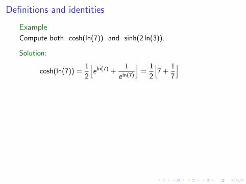
Example
Compute both cosh(ln(7)) and sinh(2 ln(3)).
Solution:
cosh(ln(7)) =1
2
[e ln(7) +
1
e ln(7)
]=
1
2
[7 +
1
7
]=
1
2
50
7.
We conclude that cosh(ln(7)) =25
7.
sinh(2 ln(3)) =1
2
[e2 ln(3) − 1
e2 ln(3)
]=
1
2
[e ln(9) − 1
e ln(9)
]
sinh(2 ln(3)) =1
2
[9− 1
9
]=
1
2
80
9⇒ sinh(2 ln(3)) =
40
9.C

Definitions and identities
Example
Compute both cosh(ln(7)) and sinh(2 ln(3)).
Solution:
cosh(ln(7))
=1
2
[e ln(7) +
1
e ln(7)
]=
1
2
[7 +
1
7
]=
1
2
50
7.
We conclude that cosh(ln(7)) =25
7.
sinh(2 ln(3)) =1
2
[e2 ln(3) − 1
e2 ln(3)
]=
1
2
[e ln(9) − 1
e ln(9)
]
sinh(2 ln(3)) =1
2
[9− 1
9
]=
1
2
80
9⇒ sinh(2 ln(3)) =
40
9.C

Definitions and identities
Example
Compute both cosh(ln(7)) and sinh(2 ln(3)).
Solution:
cosh(ln(7)) =1
2
[e ln(7) +
1
e ln(7)
]
=1
2
[7 +
1
7
]=
1
2
50
7.
We conclude that cosh(ln(7)) =25
7.
sinh(2 ln(3)) =1
2
[e2 ln(3) − 1
e2 ln(3)
]=
1
2
[e ln(9) − 1
e ln(9)
]
sinh(2 ln(3)) =1
2
[9− 1
9
]=
1
2
80
9⇒ sinh(2 ln(3)) =
40
9.C
Definitions and identities
Example
Compute both cosh(ln(7)) and sinh(2 ln(3)).
Solution:
cosh(ln(7)) =1
2
[e ln(7) +
1
e ln(7)
]=
1
2
[7 +
1
7
]
=1
2
50
7.
We conclude that cosh(ln(7)) =25
7.
sinh(2 ln(3)) =1
2
[e2 ln(3) − 1
e2 ln(3)
]=
1
2
[e ln(9) − 1
e ln(9)
]
sinh(2 ln(3)) =1
2
[9− 1
9
]=
1
2
80
9⇒ sinh(2 ln(3)) =
40
9.C

Definitions and identities
Example
Compute both cosh(ln(7)) and sinh(2 ln(3)).
Solution:
cosh(ln(7)) =1
2
[e ln(7) +
1
e ln(7)
]=
1
2
[7 +
1
7
]=
1
2
50
7.
We conclude that cosh(ln(7)) =25
7.
sinh(2 ln(3))
=1
2
[e2 ln(3) − 1
e2 ln(3)
]=
1
2
[e ln(9) − 1
e ln(9)
]
sinh(2 ln(3)) =1
2
[9− 1
9
]=
1
2
80
9⇒ sinh(2 ln(3)) =
40
9.C

Definitions and identities
Example
Compute both cosh(ln(7)) and sinh(2 ln(3)).
Solution:
cosh(ln(7)) =1
2
[e ln(7) +
1
e ln(7)
]=
1
2
[7 +
1
7
]=
1
2
50
7.
We conclude that cosh(ln(7)) =25
7.
sinh(2 ln(3)) =1
2
[e2 ln(3) − 1
e2 ln(3)
]
=1
2
[e ln(9) − 1
e ln(9)
]
sinh(2 ln(3)) =1
2
[9− 1
9
]=
1
2
80
9⇒ sinh(2 ln(3)) =
40
9.C

Definitions and identities
Example
Compute both cosh(ln(7)) and sinh(2 ln(3)).
Solution:
cosh(ln(7)) =1
2
[e ln(7) +
1
e ln(7)
]=
1
2
[7 +
1
7
]=
1
2
50
7.
We conclude that cosh(ln(7)) =25
7.
sinh(2 ln(3)) =1
2
[e2 ln(3) − 1
e2 ln(3)
]=
1
2
[e ln(9) − 1
e ln(9)
]
sinh(2 ln(3)) =1
2
[9− 1
9
]
=1
2
80
9⇒ sinh(2 ln(3)) =
40
9.C

Definitions and identities
Example
Compute both cosh(ln(7)) and sinh(2 ln(3)).
Solution:
cosh(ln(7)) =1
2
[e ln(7) +
1
e ln(7)
]=
1
2
[7 +
1
7
]=
1
2
50
7.
We conclude that cosh(ln(7)) =25
7.
sinh(2 ln(3)) =1
2
[e2 ln(3) − 1
e2 ln(3)
]=
1
2
[e ln(9) − 1
e ln(9)
]
sinh(2 ln(3)) =1
2
[9− 1
9
]=
1
2
80
9
⇒ sinh(2 ln(3)) =40
9.C

Definitions and identities
Example
Compute both cosh(ln(7)) and sinh(2 ln(3)).
Solution:
cosh(ln(7)) =1
2
[e ln(7) +
1
e ln(7)
]=
1
2
[7 +
1
7
]=
1
2
50
7.
We conclude that cosh(ln(7)) =25
7.
sinh(2 ln(3)) =1
2
[e2 ln(3) − 1
e2 ln(3)
]=
1
2
[e ln(9) − 1
e ln(9)
]
sinh(2 ln(3)) =1
2
[9− 1
9
]=
1
2
80
9⇒ sinh(2 ln(3)) =
40
9.C

Hyperbolic functions (Sect. 7.7)
I Circular and hyperbolic functions.
I Definitions and identities.
I Derivatives of hyperbolic functions.
I Integrals of hyperbolic functions.

Derivatives of hyperbolic functions
TheoremThe following equations hold,
sinh′(x) = cosh(x) cosh′(x) = sinh(x)
tanh′(x) =1
cosh2(x)coth′(x) = − 1
sinh2(x)
sech′(x) = − sinh(x)
cosh2(x)csch′(x) = − cosh(x)
sinh2(x).
Proof: (Only for sinh.)
sinh′(x) =1
2
(ex − e−x
)′=
1
2
(ex − e−x (−1)
)sinh′(u) =
1
2
(ex + e−x
)⇒ sinh′(x) = cosh(x).

Derivatives of hyperbolic functions
TheoremThe following equations hold,
sinh′(x) = cosh(x) cosh′(x) = sinh(x)
tanh′(x) =1
cosh2(x)coth′(x) = − 1
sinh2(x)
sech′(x) = − sinh(x)
cosh2(x)csch′(x) = − cosh(x)
sinh2(x).
Proof: (Only for sinh.)
sinh′(x) =1
2
(ex − e−x
)′
=1
2
(ex − e−x (−1)
)sinh′(u) =
1
2
(ex + e−x
)⇒ sinh′(x) = cosh(x).

Derivatives of hyperbolic functions
TheoremThe following equations hold,
sinh′(x) = cosh(x) cosh′(x) = sinh(x)
tanh′(x) =1
cosh2(x)coth′(x) = − 1
sinh2(x)
sech′(x) = − sinh(x)
cosh2(x)csch′(x) = − cosh(x)
sinh2(x).
Proof: (Only for sinh.)
sinh′(x) =1
2
(ex − e−x
)′=
1
2
(ex − e−x (−1)
)
sinh′(u) =1
2
(ex + e−x
)⇒ sinh′(x) = cosh(x).

Derivatives of hyperbolic functions
TheoremThe following equations hold,
sinh′(x) = cosh(x) cosh′(x) = sinh(x)
tanh′(x) =1
cosh2(x)coth′(x) = − 1
sinh2(x)
sech′(x) = − sinh(x)
cosh2(x)csch′(x) = − cosh(x)
sinh2(x).
Proof: (Only for sinh.)
sinh′(x) =1
2
(ex − e−x
)′=
1
2
(ex − e−x (−1)
)sinh′(u) =
1
2
(ex + e−x
)
⇒ sinh′(x) = cosh(x).

Derivatives of hyperbolic functions
TheoremThe following equations hold,
sinh′(x) = cosh(x) cosh′(x) = sinh(x)
tanh′(x) =1
cosh2(x)coth′(x) = − 1
sinh2(x)
sech′(x) = − sinh(x)
cosh2(x)csch′(x) = − cosh(x)
sinh2(x).
Proof: (Only for sinh.)
sinh′(x) =1
2
(ex − e−x
)′=
1
2
(ex − e−x (−1)
)sinh′(u) =
1
2
(ex + e−x
)⇒ sinh′(x) = cosh(x).

Derivatives of hyperbolic functions
Example
Compute the derivative of the function y(x) = etanh(3x).
Solution:y ′(x) = etanh(3x) tanh′(3x) 3.
We only need to remember the first two formulas in the Theoremabove, since
tanh′(x) =( sinh(x)
cosh(x)
)′=
sinh′(x) cosh(x)− sinh(x) cosh′(x)
cosh2(x)
tanh′(x) =cosh2(x)− sinh2(x)
cosh2(x)=
1
cosh2(x).
We conclude that y ′(x) =3etanh(3x)
cosh2(3x). C

Derivatives of hyperbolic functions
Example
Compute the derivative of the function y(x) = etanh(3x).
Solution:y ′(x) = etanh(3x) tanh′(3x) 3.
We only need to remember the first two formulas in the Theoremabove,
since
tanh′(x) =( sinh(x)
cosh(x)
)′=
sinh′(x) cosh(x)− sinh(x) cosh′(x)
cosh2(x)
tanh′(x) =cosh2(x)− sinh2(x)
cosh2(x)=
1
cosh2(x).
We conclude that y ′(x) =3etanh(3x)
cosh2(3x). C

Derivatives of hyperbolic functions
Example
Compute the derivative of the function y(x) = etanh(3x).
Solution:y ′(x) = etanh(3x) tanh′(3x) 3.
We only need to remember the first two formulas in the Theoremabove, since
tanh′(x) =( sinh(x)
cosh(x)
)′
=sinh′(x) cosh(x)− sinh(x) cosh′(x)
cosh2(x)
tanh′(x) =cosh2(x)− sinh2(x)
cosh2(x)=
1
cosh2(x).
We conclude that y ′(x) =3etanh(3x)
cosh2(3x). C

Derivatives of hyperbolic functions
Example
Compute the derivative of the function y(x) = etanh(3x).
Solution:y ′(x) = etanh(3x) tanh′(3x) 3.
We only need to remember the first two formulas in the Theoremabove, since
tanh′(x) =( sinh(x)
cosh(x)
)′=
sinh′(x) cosh(x)− sinh(x) cosh′(x)
cosh2(x)
tanh′(x) =cosh2(x)− sinh2(x)
cosh2(x)=
1
cosh2(x).
We conclude that y ′(x) =3etanh(3x)
cosh2(3x). C

Derivatives of hyperbolic functions
Example
Compute the derivative of the function y(x) = etanh(3x).
Solution:y ′(x) = etanh(3x) tanh′(3x) 3.
We only need to remember the first two formulas in the Theoremabove, since
tanh′(x) =( sinh(x)
cosh(x)
)′=
sinh′(x) cosh(x)− sinh(x) cosh′(x)
cosh2(x)
tanh′(x) =cosh2(x)− sinh2(x)
cosh2(x)
=1
cosh2(x).
We conclude that y ′(x) =3etanh(3x)
cosh2(3x). C

Derivatives of hyperbolic functions
Example
Compute the derivative of the function y(x) = etanh(3x).
Solution:y ′(x) = etanh(3x) tanh′(3x) 3.
We only need to remember the first two formulas in the Theoremabove, since
tanh′(x) =( sinh(x)
cosh(x)
)′=
sinh′(x) cosh(x)− sinh(x) cosh′(x)
cosh2(x)
tanh′(x) =cosh2(x)− sinh2(x)
cosh2(x)=
1
cosh2(x).
We conclude that y ′(x) =3etanh(3x)
cosh2(3x). C

Derivatives of hyperbolic functions
Example
Compute the derivative of the function y(x) = etanh(3x).
Solution:y ′(x) = etanh(3x) tanh′(3x) 3.
We only need to remember the first two formulas in the Theoremabove, since
tanh′(x) =( sinh(x)
cosh(x)
)′=
sinh′(x) cosh(x)− sinh(x) cosh′(x)
cosh2(x)
tanh′(x) =cosh2(x)− sinh2(x)
cosh2(x)=
1
cosh2(x).
We conclude that y ′(x) =3etanh(3x)
cosh2(3x). C
Hyperbolic functions (Sect. 7.7)
I Circular and hyperbolic functions.
I Definitions and identities.
I Derivatives of hyperbolic functions.
I Integrals of hyperbolic functions.

Integrals of hyperbolic functions
TheoremFor every real constant c the following expressions hold,∫
sinh(x) dx = cosh(x) + c ,
∫cosh(x) dx = sinh(x) + c ,∫
sech2(x) dx = tanh(x) + c ,
∫csch2(x) dx = − coth(x) + c ,
Proof: The derivative of each right-hand side above is theintegrand in each left-hand side
Remark: There are many other integration formulas, but the onesabove are the most frequently used.

Integrals of hyperbolic functions
Example
Evaluate I =
∫6 cosh(3x − ln(2)) dx .
Solution: We try the substitution u = 3x − ln(2), then du = 3 dx .
I =
∫6 cosh(u)
du
3= 2
∫cosh(u) du = 2 sinh(u) + c .
We conclude that I = 2 sinh(3x − ln(2)) + c . C
Remark: If needed, one can rewrite the sinh above as
sinh(3x − ln(2)) =1
2
(e3x−ln(2) − e−3x+ln(2)
)sinh(3x − ln(2)) =
1
2
( e3x
e ln(2)− e−3x e ln(2)
)=
e3x
4− e−3x .

Integrals of hyperbolic functions
Example
Evaluate I =
∫6 cosh(3x − ln(2)) dx .
Solution: We try the substitution u = 3x − ln(2),
then du = 3 dx .
I =
∫6 cosh(u)
du
3= 2
∫cosh(u) du = 2 sinh(u) + c .
We conclude that I = 2 sinh(3x − ln(2)) + c . C
Remark: If needed, one can rewrite the sinh above as
sinh(3x − ln(2)) =1
2
(e3x−ln(2) − e−3x+ln(2)
)sinh(3x − ln(2)) =
1
2
( e3x
e ln(2)− e−3x e ln(2)
)=
e3x
4− e−3x .

Integrals of hyperbolic functions
Example
Evaluate I =
∫6 cosh(3x − ln(2)) dx .
Solution: We try the substitution u = 3x − ln(2), then du = 3 dx .
I =
∫6 cosh(u)
du
3= 2
∫cosh(u) du = 2 sinh(u) + c .
We conclude that I = 2 sinh(3x − ln(2)) + c . C
Remark: If needed, one can rewrite the sinh above as
sinh(3x − ln(2)) =1
2
(e3x−ln(2) − e−3x+ln(2)
)sinh(3x − ln(2)) =
1
2
( e3x
e ln(2)− e−3x e ln(2)
)=
e3x
4− e−3x .

Integrals of hyperbolic functions
Example
Evaluate I =
∫6 cosh(3x − ln(2)) dx .
Solution: We try the substitution u = 3x − ln(2), then du = 3 dx .
I =
∫6 cosh(u)
du
3
= 2
∫cosh(u) du = 2 sinh(u) + c .
We conclude that I = 2 sinh(3x − ln(2)) + c . C
Remark: If needed, one can rewrite the sinh above as
sinh(3x − ln(2)) =1
2
(e3x−ln(2) − e−3x+ln(2)
)sinh(3x − ln(2)) =
1
2
( e3x
e ln(2)− e−3x e ln(2)
)=
e3x
4− e−3x .

Integrals of hyperbolic functions
Example
Evaluate I =
∫6 cosh(3x − ln(2)) dx .
Solution: We try the substitution u = 3x − ln(2), then du = 3 dx .
I =
∫6 cosh(u)
du
3= 2
∫cosh(u) du
= 2 sinh(u) + c .
We conclude that I = 2 sinh(3x − ln(2)) + c . C
Remark: If needed, one can rewrite the sinh above as
sinh(3x − ln(2)) =1
2
(e3x−ln(2) − e−3x+ln(2)
)sinh(3x − ln(2)) =
1
2
( e3x
e ln(2)− e−3x e ln(2)
)=
e3x
4− e−3x .

Integrals of hyperbolic functions
Example
Evaluate I =
∫6 cosh(3x − ln(2)) dx .
Solution: We try the substitution u = 3x − ln(2), then du = 3 dx .
I =
∫6 cosh(u)
du
3= 2
∫cosh(u) du = 2 sinh(u) + c .
We conclude that I = 2 sinh(3x − ln(2)) + c . C
Remark: If needed, one can rewrite the sinh above as
sinh(3x − ln(2)) =1
2
(e3x−ln(2) − e−3x+ln(2)
)sinh(3x − ln(2)) =
1
2
( e3x
e ln(2)− e−3x e ln(2)
)=
e3x
4− e−3x .

Integrals of hyperbolic functions
Example
Evaluate I =
∫6 cosh(3x − ln(2)) dx .
Solution: We try the substitution u = 3x − ln(2), then du = 3 dx .
I =
∫6 cosh(u)
du
3= 2
∫cosh(u) du = 2 sinh(u) + c .
We conclude that I = 2 sinh(3x − ln(2)) + c . C
Remark: If needed, one can rewrite the sinh above as
sinh(3x − ln(2)) =1
2
(e3x−ln(2) − e−3x+ln(2)
)
sinh(3x − ln(2)) =1
2
( e3x
e ln(2)− e−3x e ln(2)
)=
e3x
4− e−3x .
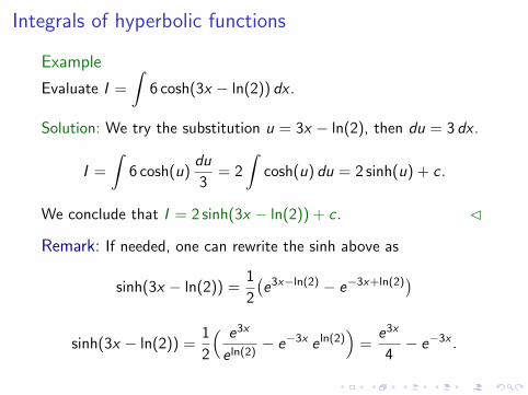
Integrals of hyperbolic functions
Example
Evaluate I =
∫6 cosh(3x − ln(2)) dx .
Solution: We try the substitution u = 3x − ln(2), then du = 3 dx .
I =
∫6 cosh(u)
du
3= 2
∫cosh(u) du = 2 sinh(u) + c .
We conclude that I = 2 sinh(3x − ln(2)) + c . C
Remark: If needed, one can rewrite the sinh above as
sinh(3x − ln(2)) =1
2
(e3x−ln(2) − e−3x+ln(2)
)sinh(3x − ln(2)) =
1
2
( e3x
e ln(2)− e−3x e ln(2)
)=
e3x
4− e−3x .

Integrals of hyperbolic functions
Example
Evaluate the integral I =
∫8x
sinh(3x2)
cosh3(3x2)dx .
Solution: Recall that cosh′(x) = sinh(x). We then try thesubstitution
u = cosh(3x2), du = sinh(3x2) 6x dx .
I =
∫8
1
u3
du
6=
4
3
∫u−3 du =
4
3
u−2
(−2)+ c = −2
3
1
u2+ c
If we substitute back u = cosh(3x2), we obtain
I = −2
3
1
cosh2(3x2)+ c . C
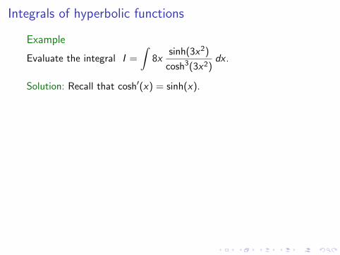
Integrals of hyperbolic functions
Example
Evaluate the integral I =
∫8x
sinh(3x2)
cosh3(3x2)dx .
Solution: Recall that cosh′(x) = sinh(x).
We then try thesubstitution
u = cosh(3x2), du = sinh(3x2) 6x dx .
I =
∫8
1
u3
du
6=
4
3
∫u−3 du =
4
3
u−2
(−2)+ c = −2
3
1
u2+ c
If we substitute back u = cosh(3x2), we obtain
I = −2
3
1
cosh2(3x2)+ c . C
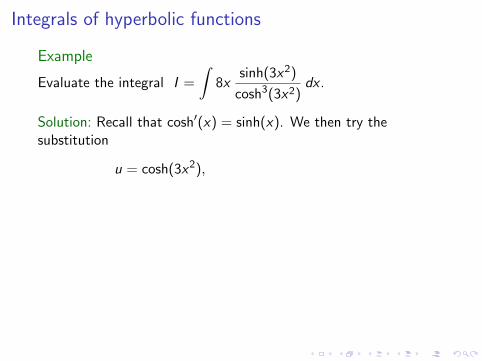
Integrals of hyperbolic functions
Example
Evaluate the integral I =
∫8x
sinh(3x2)
cosh3(3x2)dx .
Solution: Recall that cosh′(x) = sinh(x). We then try thesubstitution
u = cosh(3x2),
du = sinh(3x2) 6x dx .
I =
∫8
1
u3
du
6=
4
3
∫u−3 du =
4
3
u−2
(−2)+ c = −2
3
1
u2+ c
If we substitute back u = cosh(3x2), we obtain
I = −2
3
1
cosh2(3x2)+ c . C

Integrals of hyperbolic functions
Example
Evaluate the integral I =
∫8x
sinh(3x2)
cosh3(3x2)dx .
Solution: Recall that cosh′(x) = sinh(x). We then try thesubstitution
u = cosh(3x2), du = sinh(3x2) 6x dx .
I =
∫8
1
u3
du
6=
4
3
∫u−3 du =
4
3
u−2
(−2)+ c = −2
3
1
u2+ c
If we substitute back u = cosh(3x2), we obtain
I = −2
3
1
cosh2(3x2)+ c . C

Integrals of hyperbolic functions
Example
Evaluate the integral I =
∫8x
sinh(3x2)
cosh3(3x2)dx .
Solution: Recall that cosh′(x) = sinh(x). We then try thesubstitution
u = cosh(3x2), du = sinh(3x2) 6x dx .
I =
∫8
1
u3
du
6
=4
3
∫u−3 du =
4
3
u−2
(−2)+ c = −2
3
1
u2+ c
If we substitute back u = cosh(3x2), we obtain
I = −2
3
1
cosh2(3x2)+ c . C

Integrals of hyperbolic functions
Example
Evaluate the integral I =
∫8x
sinh(3x2)
cosh3(3x2)dx .
Solution: Recall that cosh′(x) = sinh(x). We then try thesubstitution
u = cosh(3x2), du = sinh(3x2) 6x dx .
I =
∫8
1
u3
du
6=
4
3
∫u−3 du
=4
3
u−2
(−2)+ c = −2
3
1
u2+ c
If we substitute back u = cosh(3x2), we obtain
I = −2
3
1
cosh2(3x2)+ c . C

Integrals of hyperbolic functions
Example
Evaluate the integral I =
∫8x
sinh(3x2)
cosh3(3x2)dx .
Solution: Recall that cosh′(x) = sinh(x). We then try thesubstitution
u = cosh(3x2), du = sinh(3x2) 6x dx .
I =
∫8
1
u3
du
6=
4
3
∫u−3 du =
4
3
u−2
(−2)+ c
= −2
3
1
u2+ c
If we substitute back u = cosh(3x2), we obtain
I = −2
3
1
cosh2(3x2)+ c . C

Integrals of hyperbolic functions
Example
Evaluate the integral I =
∫8x
sinh(3x2)
cosh3(3x2)dx .
Solution: Recall that cosh′(x) = sinh(x). We then try thesubstitution
u = cosh(3x2), du = sinh(3x2) 6x dx .
I =
∫8
1
u3
du
6=
4
3
∫u−3 du =
4
3
u−2
(−2)+ c = −2
3
1
u2+ c
If we substitute back u = cosh(3x2), we obtain
I = −2
3
1
cosh2(3x2)+ c . C

Integrals of hyperbolic functions
Example
Evaluate the integral I =
∫8x
sinh(3x2)
cosh3(3x2)dx .
Solution: Recall that cosh′(x) = sinh(x). We then try thesubstitution
u = cosh(3x2), du = sinh(3x2) 6x dx .
I =
∫8
1
u3
du
6=
4
3
∫u−3 du =
4
3
u−2
(−2)+ c = −2
3
1
u2+ c
If we substitute back u = cosh(3x2), we obtain
I = −2
3
1
cosh2(3x2)+ c . C

Integration techniques (Supp. Material 8-IT)
I Substitution rule.
I Completing the square.
I Trigonometric identities.
I Polynomial division.
I Multiplying by 1.

Substitution rule
TheoremFor every differentiable functions f , u : R → R holds,∫
f (u(x)) u′(x) dx =
∫f (y) dy .
Proof: This is the integral form of the chain rule for derivatives.Let F be a primitive of f , that is, F ′ = f . Then(
F (u))′
= F ′(u) u′ = f (u) u′.
Integrate the equation above,∫f (u(x)) u′(x) dx =
∫d(F (u))
dx(x) dx = F (u(x)).
Denoting y = u(x), we get∫f (u(x)) u′(x) dx = F (y) =
∫F ′(y) dy =
∫f (y) dy .

Substitution rule
TheoremFor every differentiable functions f , u : R → R holds,∫
f (u(x)) u′(x) dx =
∫f (y) dy .
Proof: This is the integral form of the chain rule for derivatives.
Let F be a primitive of f , that is, F ′ = f . Then(F (u)
)′= F ′(u) u′ = f (u) u′.
Integrate the equation above,∫f (u(x)) u′(x) dx =
∫d(F (u))
dx(x) dx = F (u(x)).
Denoting y = u(x), we get∫f (u(x)) u′(x) dx = F (y) =
∫F ′(y) dy =
∫f (y) dy .

Substitution rule
TheoremFor every differentiable functions f , u : R → R holds,∫
f (u(x)) u′(x) dx =
∫f (y) dy .
Proof: This is the integral form of the chain rule for derivatives.Let F be a primitive of f ,
that is, F ′ = f . Then(F (u)
)′= F ′(u) u′ = f (u) u′.
Integrate the equation above,∫f (u(x)) u′(x) dx =
∫d(F (u))
dx(x) dx = F (u(x)).
Denoting y = u(x), we get∫f (u(x)) u′(x) dx = F (y) =
∫F ′(y) dy =
∫f (y) dy .

Substitution rule
TheoremFor every differentiable functions f , u : R → R holds,∫
f (u(x)) u′(x) dx =
∫f (y) dy .
Proof: This is the integral form of the chain rule for derivatives.Let F be a primitive of f , that is, F ′ = f .
Then(F (u)
)′= F ′(u) u′ = f (u) u′.
Integrate the equation above,∫f (u(x)) u′(x) dx =
∫d(F (u))
dx(x) dx = F (u(x)).
Denoting y = u(x), we get∫f (u(x)) u′(x) dx = F (y) =
∫F ′(y) dy =
∫f (y) dy .

Substitution rule
TheoremFor every differentiable functions f , u : R → R holds,∫
f (u(x)) u′(x) dx =
∫f (y) dy .
Proof: This is the integral form of the chain rule for derivatives.Let F be a primitive of f , that is, F ′ = f . Then(
F (u))′
= F ′(u) u′
= f (u) u′.
Integrate the equation above,∫f (u(x)) u′(x) dx =
∫d(F (u))
dx(x) dx = F (u(x)).
Denoting y = u(x), we get∫f (u(x)) u′(x) dx = F (y) =
∫F ′(y) dy =
∫f (y) dy .

Substitution rule
TheoremFor every differentiable functions f , u : R → R holds,∫
f (u(x)) u′(x) dx =
∫f (y) dy .
Proof: This is the integral form of the chain rule for derivatives.Let F be a primitive of f , that is, F ′ = f . Then(
F (u))′
= F ′(u) u′ = f (u) u′.
Integrate the equation above,∫f (u(x)) u′(x) dx =
∫d(F (u))
dx(x) dx = F (u(x)).
Denoting y = u(x), we get∫f (u(x)) u′(x) dx = F (y) =
∫F ′(y) dy =
∫f (y) dy .

Substitution rule
TheoremFor every differentiable functions f , u : R → R holds,∫
f (u(x)) u′(x) dx =
∫f (y) dy .
Proof: This is the integral form of the chain rule for derivatives.Let F be a primitive of f , that is, F ′ = f . Then(
F (u))′
= F ′(u) u′ = f (u) u′.
Integrate the equation above,
∫f (u(x)) u′(x) dx =
∫d(F (u))
dx(x) dx = F (u(x)).
Denoting y = u(x), we get∫f (u(x)) u′(x) dx = F (y) =
∫F ′(y) dy =
∫f (y) dy .

Substitution rule
TheoremFor every differentiable functions f , u : R → R holds,∫
f (u(x)) u′(x) dx =
∫f (y) dy .
Proof: This is the integral form of the chain rule for derivatives.Let F be a primitive of f , that is, F ′ = f . Then(
F (u))′
= F ′(u) u′ = f (u) u′.
Integrate the equation above,∫f (u(x)) u′(x) dx =
∫d(F (u))
dx(x) dx
= F (u(x)).
Denoting y = u(x), we get∫f (u(x)) u′(x) dx = F (y) =
∫F ′(y) dy =
∫f (y) dy .

Substitution rule
TheoremFor every differentiable functions f , u : R → R holds,∫
f (u(x)) u′(x) dx =
∫f (y) dy .
Proof: This is the integral form of the chain rule for derivatives.Let F be a primitive of f , that is, F ′ = f . Then(
F (u))′
= F ′(u) u′ = f (u) u′.
Integrate the equation above,∫f (u(x)) u′(x) dx =
∫d(F (u))
dx(x) dx = F (u(x)).
Denoting y = u(x), we get∫f (u(x)) u′(x) dx = F (y) =
∫F ′(y) dy =
∫f (y) dy .

Substitution rule
TheoremFor every differentiable functions f , u : R → R holds,∫
f (u(x)) u′(x) dx =
∫f (y) dy .
Proof: This is the integral form of the chain rule for derivatives.Let F be a primitive of f , that is, F ′ = f . Then(
F (u))′
= F ′(u) u′ = f (u) u′.
Integrate the equation above,∫f (u(x)) u′(x) dx =
∫d(F (u))
dx(x) dx = F (u(x)).
Denoting y = u(x), we get
∫f (u(x)) u′(x) dx = F (y) =
∫F ′(y) dy =
∫f (y) dy .

Substitution rule
TheoremFor every differentiable functions f , u : R → R holds,∫
f (u(x)) u′(x) dx =
∫f (y) dy .
Proof: This is the integral form of the chain rule for derivatives.Let F be a primitive of f , that is, F ′ = f . Then(
F (u))′
= F ′(u) u′ = f (u) u′.
Integrate the equation above,∫f (u(x)) u′(x) dx =
∫d(F (u))
dx(x) dx = F (u(x)).
Denoting y = u(x), we get∫f (u(x)) u′(x) dx = F (y)
=
∫F ′(y) dy =
∫f (y) dy .

Substitution rule
TheoremFor every differentiable functions f , u : R → R holds,∫
f (u(x)) u′(x) dx =
∫f (y) dy .
Proof: This is the integral form of the chain rule for derivatives.Let F be a primitive of f , that is, F ′ = f . Then(
F (u))′
= F ′(u) u′ = f (u) u′.
Integrate the equation above,∫f (u(x)) u′(x) dx =
∫d(F (u))
dx(x) dx = F (u(x)).
Denoting y = u(x), we get∫f (u(x)) u′(x) dx = F (y) =
∫F ′(y) dy
=
∫f (y) dy .

Substitution rule
TheoremFor every differentiable functions f , u : R → R holds,∫
f (u(x)) u′(x) dx =
∫f (y) dy .
Proof: This is the integral form of the chain rule for derivatives.Let F be a primitive of f , that is, F ′ = f . Then(
F (u))′
= F ′(u) u′ = f (u) u′.
Integrate the equation above,∫f (u(x)) u′(x) dx =
∫d(F (u))
dx(x) dx = F (u(x)).
Denoting y = u(x), we get∫f (u(x)) u′(x) dx = F (y) =
∫F ′(y) dy =
∫f (y) dy .

Substitution rule
Example
Evaluate I =
∫3x etan(2x2)
[1 + cos(4x2)]dx .
Solution: The argument in the tangent function is has an x2,and in the integral appears the factor x dx . We try the substitution
u = tan(2x2), du =1
cos2(2x2)(4x) dx .
This substitution will simplify the integration if cos2(2x2) can berelated to [1 + cos(4x2)]. And this is the case, since
cos2(θ) =1
2
(1 + cos(2θ)
), θ = 2x2,
I =
∫3x etan(2x2)
[1 + cos(4x2)]dx =
∫3x etan(2x2)
2 cos2(2x2)dx =
3
2
∫eu du
4.

Substitution rule
Example
Evaluate I =
∫3x etan(2x2)
[1 + cos(4x2)]dx .
Solution: The argument in the tangent function is has an x2,
and in the integral appears the factor x dx . We try the substitution
u = tan(2x2), du =1
cos2(2x2)(4x) dx .
This substitution will simplify the integration if cos2(2x2) can berelated to [1 + cos(4x2)]. And this is the case, since
cos2(θ) =1
2
(1 + cos(2θ)
), θ = 2x2,
I =
∫3x etan(2x2)
[1 + cos(4x2)]dx =
∫3x etan(2x2)
2 cos2(2x2)dx =
3
2
∫eu du
4.

Substitution rule
Example
Evaluate I =
∫3x etan(2x2)
[1 + cos(4x2)]dx .
Solution: The argument in the tangent function is has an x2,and in the integral appears the factor x dx .
We try the substitution
u = tan(2x2), du =1
cos2(2x2)(4x) dx .
This substitution will simplify the integration if cos2(2x2) can berelated to [1 + cos(4x2)]. And this is the case, since
cos2(θ) =1
2
(1 + cos(2θ)
), θ = 2x2,
I =
∫3x etan(2x2)
[1 + cos(4x2)]dx =
∫3x etan(2x2)
2 cos2(2x2)dx =
3
2
∫eu du
4.

Substitution rule
Example
Evaluate I =
∫3x etan(2x2)
[1 + cos(4x2)]dx .
Solution: The argument in the tangent function is has an x2,and in the integral appears the factor x dx . We try the substitution
u = tan(2x2),
du =1
cos2(2x2)(4x) dx .
This substitution will simplify the integration if cos2(2x2) can berelated to [1 + cos(4x2)]. And this is the case, since
cos2(θ) =1
2
(1 + cos(2θ)
), θ = 2x2,
I =
∫3x etan(2x2)
[1 + cos(4x2)]dx =
∫3x etan(2x2)
2 cos2(2x2)dx =
3
2
∫eu du
4.

Substitution rule
Example
Evaluate I =
∫3x etan(2x2)
[1 + cos(4x2)]dx .
Solution: The argument in the tangent function is has an x2,and in the integral appears the factor x dx . We try the substitution
u = tan(2x2), du =1
cos2(2x2)(4x) dx .
This substitution will simplify the integration if cos2(2x2) can berelated to [1 + cos(4x2)]. And this is the case, since
cos2(θ) =1
2
(1 + cos(2θ)
), θ = 2x2,
I =
∫3x etan(2x2)
[1 + cos(4x2)]dx =
∫3x etan(2x2)
2 cos2(2x2)dx =
3
2
∫eu du
4.

Substitution rule
Example
Evaluate I =
∫3x etan(2x2)
[1 + cos(4x2)]dx .
Solution: The argument in the tangent function is has an x2,and in the integral appears the factor x dx . We try the substitution
u = tan(2x2), du =1
cos2(2x2)(4x) dx .
This substitution will simplify the integration if cos2(2x2) can berelated to [1 + cos(4x2)].
And this is the case, since
cos2(θ) =1
2
(1 + cos(2θ)
), θ = 2x2,
I =
∫3x etan(2x2)
[1 + cos(4x2)]dx =
∫3x etan(2x2)
2 cos2(2x2)dx =
3
2
∫eu du
4.

Substitution rule
Example
Evaluate I =
∫3x etan(2x2)
[1 + cos(4x2)]dx .
Solution: The argument in the tangent function is has an x2,and in the integral appears the factor x dx . We try the substitution
u = tan(2x2), du =1
cos2(2x2)(4x) dx .
This substitution will simplify the integration if cos2(2x2) can berelated to [1 + cos(4x2)]. And this is the case,
since
cos2(θ) =1
2
(1 + cos(2θ)
), θ = 2x2,
I =
∫3x etan(2x2)
[1 + cos(4x2)]dx =
∫3x etan(2x2)
2 cos2(2x2)dx =
3
2
∫eu du
4.

Substitution rule
Example
Evaluate I =
∫3x etan(2x2)
[1 + cos(4x2)]dx .
Solution: The argument in the tangent function is has an x2,and in the integral appears the factor x dx . We try the substitution
u = tan(2x2), du =1
cos2(2x2)(4x) dx .
This substitution will simplify the integration if cos2(2x2) can berelated to [1 + cos(4x2)]. And this is the case, since
cos2(θ) =1
2
(1 + cos(2θ)
),
θ = 2x2,
I =
∫3x etan(2x2)
[1 + cos(4x2)]dx =
∫3x etan(2x2)
2 cos2(2x2)dx =
3
2
∫eu du
4.

Substitution rule
Example
Evaluate I =
∫3x etan(2x2)
[1 + cos(4x2)]dx .
Solution: The argument in the tangent function is has an x2,and in the integral appears the factor x dx . We try the substitution
u = tan(2x2), du =1
cos2(2x2)(4x) dx .
This substitution will simplify the integration if cos2(2x2) can berelated to [1 + cos(4x2)]. And this is the case, since
cos2(θ) =1
2
(1 + cos(2θ)
), θ = 2x2,
I =
∫3x etan(2x2)
[1 + cos(4x2)]dx =
∫3x etan(2x2)
2 cos2(2x2)dx =
3
2
∫eu du
4.

Substitution rule
Example
Evaluate I =
∫3x etan(2x2)
[1 + cos(4x2)]dx .
Solution: The argument in the tangent function is has an x2,and in the integral appears the factor x dx . We try the substitution
u = tan(2x2), du =1
cos2(2x2)(4x) dx .
This substitution will simplify the integration if cos2(2x2) can berelated to [1 + cos(4x2)]. And this is the case, since
cos2(θ) =1
2
(1 + cos(2θ)
), θ = 2x2,
I =
∫3x etan(2x2)
[1 + cos(4x2)]dx
=
∫3x etan(2x2)
2 cos2(2x2)dx =
3
2
∫eu du
4.

Substitution rule
Example
Evaluate I =
∫3x etan(2x2)
[1 + cos(4x2)]dx .
Solution: The argument in the tangent function is has an x2,and in the integral appears the factor x dx . We try the substitution
u = tan(2x2), du =1
cos2(2x2)(4x) dx .
This substitution will simplify the integration if cos2(2x2) can berelated to [1 + cos(4x2)]. And this is the case, since
cos2(θ) =1
2
(1 + cos(2θ)
), θ = 2x2,
I =
∫3x etan(2x2)
[1 + cos(4x2)]dx =
∫3x etan(2x2)
2 cos2(2x2)dx
=3
2
∫eu du
4.

Substitution rule
Example
Evaluate I =
∫3x etan(2x2)
[1 + cos(4x2)]dx .
Solution: The argument in the tangent function is has an x2,and in the integral appears the factor x dx . We try the substitution
u = tan(2x2), du =1
cos2(2x2)(4x) dx .
This substitution will simplify the integration if cos2(2x2) can berelated to [1 + cos(4x2)]. And this is the case, since
cos2(θ) =1
2
(1 + cos(2θ)
), θ = 2x2,
I =
∫3x etan(2x2)
[1 + cos(4x2)]dx =
∫3x etan(2x2)
2 cos2(2x2)dx =
3
2
∫eu du
4.

Substitution rule
Example
Evaluate I =
∫3x etan(2x2)
[1 + cos(4x2)]dx .
Solution: Recall: I =3
2
∫eu du
4, with u = tan(2x2).
I =3
8
∫eu du =
3
8eu + c .
We now substitute back with u = tan(2x2),
I =3
8etan(2x2) + c .
C

Substitution rule
Example
Evaluate I =
∫3x etan(2x2)
[1 + cos(4x2)]dx .
Solution: Recall: I =3
2
∫eu du
4, with u = tan(2x2).
I =3
8
∫eu du
=3
8eu + c .
We now substitute back with u = tan(2x2),
I =3
8etan(2x2) + c .
C

Substitution rule
Example
Evaluate I =
∫3x etan(2x2)
[1 + cos(4x2)]dx .
Solution: Recall: I =3
2
∫eu du
4, with u = tan(2x2).
I =3
8
∫eu du =
3
8eu + c .
We now substitute back with u = tan(2x2),
I =3
8etan(2x2) + c .
C

Substitution rule
Example
Evaluate I =
∫3x etan(2x2)
[1 + cos(4x2)]dx .
Solution: Recall: I =3
2
∫eu du
4, with u = tan(2x2).
I =3
8
∫eu du =
3
8eu + c .
We now substitute back with u = tan(2x2),
I =3
8etan(2x2) + c .
C

Substitution rule
Example
Evaluate I =
∫3x etan(2x2)
[1 + cos(4x2)]dx .
Solution: Recall: I =3
2
∫eu du
4, with u = tan(2x2).
I =3
8
∫eu du =
3
8eu + c .
We now substitute back with u = tan(2x2),
I =3
8etan(2x2) + c .
C

Integration techniques (Supp. Material 8-IT)
I Substitution rule.
I Completing the square.
I Trigonometric identities.
I Polynomial division.
I Multiplying by 1.

Completing the square
Example
Evaluate I =
∫dx
(x + 3)√
x2 + 6x + 4.
Solution: The idea is to rewrite the function inside the square root:
x2 + 6x + 4 = x2 + 2(6
2
)x + 4 = x2 + 2(3x) + 4
x2 + 6x + 4 = [x2 + 2(3x) + 9]− 9 + 4 = (x + 3)2 − 5.
I =
∫dx
(x + 3)√
(x + 3)2 − 5u = x + 3, du = dx
I =
∫du
u√
u2 − 5=
1√5
arcsec( |u|√
5
)+ c .
We obtain I =1√5
arcsec( |x + 3|√
5
)+ c . C

Completing the square
Example
Evaluate I =
∫dx
(x + 3)√
x2 + 6x + 4.
Solution: The idea is to rewrite the function inside the square root:
x2 + 6x + 4
= x2 + 2(6
2
)x + 4 = x2 + 2(3x) + 4
x2 + 6x + 4 = [x2 + 2(3x) + 9]− 9 + 4 = (x + 3)2 − 5.
I =
∫dx
(x + 3)√
(x + 3)2 − 5u = x + 3, du = dx
I =
∫du
u√
u2 − 5=
1√5
arcsec( |u|√
5
)+ c .
We obtain I =1√5
arcsec( |x + 3|√
5
)+ c . C

Completing the square
Example
Evaluate I =
∫dx
(x + 3)√
x2 + 6x + 4.
Solution: The idea is to rewrite the function inside the square root:
x2 + 6x + 4 = x2 + 2(6
2
)x + 4
= x2 + 2(3x) + 4
x2 + 6x + 4 = [x2 + 2(3x) + 9]− 9 + 4 = (x + 3)2 − 5.
I =
∫dx
(x + 3)√
(x + 3)2 − 5u = x + 3, du = dx
I =
∫du
u√
u2 − 5=
1√5
arcsec( |u|√
5
)+ c .
We obtain I =1√5
arcsec( |x + 3|√
5
)+ c . C

Completing the square
Example
Evaluate I =
∫dx
(x + 3)√
x2 + 6x + 4.
Solution: The idea is to rewrite the function inside the square root:
x2 + 6x + 4 = x2 + 2(6
2
)x + 4 = x2 + 2(3x) + 4
x2 + 6x + 4 = [x2 + 2(3x) + 9]− 9 + 4 = (x + 3)2 − 5.
I =
∫dx
(x + 3)√
(x + 3)2 − 5u = x + 3, du = dx
I =
∫du
u√
u2 − 5=
1√5
arcsec( |u|√
5
)+ c .
We obtain I =1√5
arcsec( |x + 3|√
5
)+ c . C

Completing the square
Example
Evaluate I =
∫dx
(x + 3)√
x2 + 6x + 4.
Solution: The idea is to rewrite the function inside the square root:
x2 + 6x + 4 = x2 + 2(6
2
)x + 4 = x2 + 2(3x) + 4
x2 + 6x + 4 = [x2 + 2(3x) + 9]− 9 + 4
= (x + 3)2 − 5.
I =
∫dx
(x + 3)√
(x + 3)2 − 5u = x + 3, du = dx
I =
∫du
u√
u2 − 5=
1√5
arcsec( |u|√
5
)+ c .
We obtain I =1√5
arcsec( |x + 3|√
5
)+ c . C

Completing the square
Example
Evaluate I =
∫dx
(x + 3)√
x2 + 6x + 4.
Solution: The idea is to rewrite the function inside the square root:
x2 + 6x + 4 = x2 + 2(6
2
)x + 4 = x2 + 2(3x) + 4
x2 + 6x + 4 = [x2 + 2(3x) + 9]− 9 + 4 = (x + 3)2 − 5.
I =
∫dx
(x + 3)√
(x + 3)2 − 5u = x + 3, du = dx
I =
∫du
u√
u2 − 5=
1√5
arcsec( |u|√
5
)+ c .
We obtain I =1√5
arcsec( |x + 3|√
5
)+ c . C

Completing the square
Example
Evaluate I =
∫dx
(x + 3)√
x2 + 6x + 4.
Solution: The idea is to rewrite the function inside the square root:
x2 + 6x + 4 = x2 + 2(6
2
)x + 4 = x2 + 2(3x) + 4
x2 + 6x + 4 = [x2 + 2(3x) + 9]− 9 + 4 = (x + 3)2 − 5.
I =
∫dx
(x + 3)√
(x + 3)2 − 5
u = x + 3, du = dx
I =
∫du
u√
u2 − 5=
1√5
arcsec( |u|√
5
)+ c .
We obtain I =1√5
arcsec( |x + 3|√
5
)+ c . C

Completing the square
Example
Evaluate I =
∫dx
(x + 3)√
x2 + 6x + 4.
Solution: The idea is to rewrite the function inside the square root:
x2 + 6x + 4 = x2 + 2(6
2
)x + 4 = x2 + 2(3x) + 4
x2 + 6x + 4 = [x2 + 2(3x) + 9]− 9 + 4 = (x + 3)2 − 5.
I =
∫dx
(x + 3)√
(x + 3)2 − 5u = x + 3,
du = dx
I =
∫du
u√
u2 − 5=
1√5
arcsec( |u|√
5
)+ c .
We obtain I =1√5
arcsec( |x + 3|√
5
)+ c . C

Completing the square
Example
Evaluate I =
∫dx
(x + 3)√
x2 + 6x + 4.
Solution: The idea is to rewrite the function inside the square root:
x2 + 6x + 4 = x2 + 2(6
2
)x + 4 = x2 + 2(3x) + 4
x2 + 6x + 4 = [x2 + 2(3x) + 9]− 9 + 4 = (x + 3)2 − 5.
I =
∫dx
(x + 3)√
(x + 3)2 − 5u = x + 3, du = dx
I =
∫du
u√
u2 − 5=
1√5
arcsec( |u|√
5
)+ c .
We obtain I =1√5
arcsec( |x + 3|√
5
)+ c . C

Completing the square
Example
Evaluate I =
∫dx
(x + 3)√
x2 + 6x + 4.
Solution: The idea is to rewrite the function inside the square root:
x2 + 6x + 4 = x2 + 2(6
2
)x + 4 = x2 + 2(3x) + 4
x2 + 6x + 4 = [x2 + 2(3x) + 9]− 9 + 4 = (x + 3)2 − 5.
I =
∫dx
(x + 3)√
(x + 3)2 − 5u = x + 3, du = dx
I =
∫du
u√
u2 − 5
=1√5
arcsec( |u|√
5
)+ c .
We obtain I =1√5
arcsec( |x + 3|√
5
)+ c . C

Completing the square
Example
Evaluate I =
∫dx
(x + 3)√
x2 + 6x + 4.
Solution: The idea is to rewrite the function inside the square root:
x2 + 6x + 4 = x2 + 2(6
2
)x + 4 = x2 + 2(3x) + 4
x2 + 6x + 4 = [x2 + 2(3x) + 9]− 9 + 4 = (x + 3)2 − 5.
I =
∫dx
(x + 3)√
(x + 3)2 − 5u = x + 3, du = dx
I =
∫du
u√
u2 − 5=
1√5
arcsec( |u|√
5
)+ c .
We obtain I =1√5
arcsec( |x + 3|√
5
)+ c . C

Completing the square
Example
Evaluate I =
∫dx
(x + 3)√
x2 + 6x + 4.
Solution: The idea is to rewrite the function inside the square root:
x2 + 6x + 4 = x2 + 2(6
2
)x + 4 = x2 + 2(3x) + 4
x2 + 6x + 4 = [x2 + 2(3x) + 9]− 9 + 4 = (x + 3)2 − 5.
I =
∫dx
(x + 3)√
(x + 3)2 − 5u = x + 3, du = dx
I =
∫du
u√
u2 − 5=
1√5
arcsec( |u|√
5
)+ c .
We obtain I =1√5
arcsec( |x + 3|√
5
)+ c . C

Completing the square
Remark: Sometimes completing the square is not needed.
Example
Evaluate I =
∫(x + 3) dx√x2 + 6x + 4
.
Solution: Since the factor (x + 3) is in the numerator, instead ofthe denominator, substitution will work:
u = x2 + 6x + 4, du = (2x + 6) dx = 2(x + 3) dx .
I =
∫1√u
du
2=
1
2
∫u−1/2 du =
1
2
(2u1/2
)+ c .
We conclude that I =√
x2 + 6x + 4 + c . C

Completing the square
Remark: Sometimes completing the square is not needed.
Example
Evaluate I =
∫(x + 3) dx√x2 + 6x + 4
.
Solution: Since the factor (x + 3) is in the numerator, instead ofthe denominator,
substitution will work:
u = x2 + 6x + 4, du = (2x + 6) dx = 2(x + 3) dx .
I =
∫1√u
du
2=
1
2
∫u−1/2 du =
1
2
(2u1/2
)+ c .
We conclude that I =√
x2 + 6x + 4 + c . C

Completing the square
Remark: Sometimes completing the square is not needed.
Example
Evaluate I =
∫(x + 3) dx√x2 + 6x + 4
.
Solution: Since the factor (x + 3) is in the numerator, instead ofthe denominator, substitution will work:
u = x2 + 6x + 4, du = (2x + 6) dx = 2(x + 3) dx .
I =
∫1√u
du
2=
1
2
∫u−1/2 du =
1
2
(2u1/2
)+ c .
We conclude that I =√
x2 + 6x + 4 + c . C

Completing the square
Remark: Sometimes completing the square is not needed.
Example
Evaluate I =
∫(x + 3) dx√x2 + 6x + 4
.
Solution: Since the factor (x + 3) is in the numerator, instead ofthe denominator, substitution will work:
u = x2 + 6x + 4,
du = (2x + 6) dx = 2(x + 3) dx .
I =
∫1√u
du
2=
1
2
∫u−1/2 du =
1
2
(2u1/2
)+ c .
We conclude that I =√
x2 + 6x + 4 + c . C

Completing the square
Remark: Sometimes completing the square is not needed.
Example
Evaluate I =
∫(x + 3) dx√x2 + 6x + 4
.
Solution: Since the factor (x + 3) is in the numerator, instead ofthe denominator, substitution will work:
u = x2 + 6x + 4, du = (2x + 6) dx
= 2(x + 3) dx .
I =
∫1√u
du
2=
1
2
∫u−1/2 du =
1
2
(2u1/2
)+ c .
We conclude that I =√
x2 + 6x + 4 + c . C

Completing the square
Remark: Sometimes completing the square is not needed.
Example
Evaluate I =
∫(x + 3) dx√x2 + 6x + 4
.
Solution: Since the factor (x + 3) is in the numerator, instead ofthe denominator, substitution will work:
u = x2 + 6x + 4, du = (2x + 6) dx = 2(x + 3) dx .
I =
∫1√u
du
2=
1
2
∫u−1/2 du =
1
2
(2u1/2
)+ c .
We conclude that I =√
x2 + 6x + 4 + c . C

Completing the square
Remark: Sometimes completing the square is not needed.
Example
Evaluate I =
∫(x + 3) dx√x2 + 6x + 4
.
Solution: Since the factor (x + 3) is in the numerator, instead ofthe denominator, substitution will work:
u = x2 + 6x + 4, du = (2x + 6) dx = 2(x + 3) dx .
I =
∫1√u
du
2
=1
2
∫u−1/2 du =
1
2
(2u1/2
)+ c .
We conclude that I =√
x2 + 6x + 4 + c . C

Completing the square
Remark: Sometimes completing the square is not needed.
Example
Evaluate I =
∫(x + 3) dx√x2 + 6x + 4
.
Solution: Since the factor (x + 3) is in the numerator, instead ofthe denominator, substitution will work:
u = x2 + 6x + 4, du = (2x + 6) dx = 2(x + 3) dx .
I =
∫1√u
du
2=
1
2
∫u−1/2 du
=1
2
(2u1/2
)+ c .
We conclude that I =√
x2 + 6x + 4 + c . C

Completing the square
Remark: Sometimes completing the square is not needed.
Example
Evaluate I =
∫(x + 3) dx√x2 + 6x + 4
.
Solution: Since the factor (x + 3) is in the numerator, instead ofthe denominator, substitution will work:
u = x2 + 6x + 4, du = (2x + 6) dx = 2(x + 3) dx .
I =
∫1√u
du
2=
1
2
∫u−1/2 du =
1
2
(2u1/2
)+ c .
We conclude that I =√
x2 + 6x + 4 + c . C

Completing the square
Remark: Sometimes completing the square is not needed.
Example
Evaluate I =
∫(x + 3) dx√x2 + 6x + 4
.
Solution: Since the factor (x + 3) is in the numerator, instead ofthe denominator, substitution will work:
u = x2 + 6x + 4, du = (2x + 6) dx = 2(x + 3) dx .
I =
∫1√u
du
2=
1
2
∫u−1/2 du =
1
2
(2u1/2
)+ c .
We conclude that I =√
x2 + 6x + 4 + c . C

Integration techniques (Supp. Material 8-IT)
I Substitution rule.
I Completing the square.
I Trigonometric identities.
I Polynomial division.
I Multiplying by 1.

Trigonometric identities
Example
Evaluate I =
∫ [sec(x) + tan(x)
]2dx .
Solution: This problem can be solved using trigonometric identitiesfor sine and cosine functions only.
f (x) =[sec(x) + tan(x)
]2=
[ 1
cos(x)+
sin(x)
cos(x)
]2=
(1 + sin(x))2
cos2(x).
f (x) =1 + 2 sin(x) + sin2(x)
cos2(x)=
1
cos2(x)+
2 sin(x)
cos2(x)+
sin2(x)
cos2(x).
sin2(x)
cos2(x)=
1− cos2(x)
cos2(x)=
1
cos2(x)− 1.
Trigonometric identities
Example
Evaluate I =
∫ [sec(x) + tan(x)
]2dx .
Solution: This problem can be solved using trigonometric identitiesfor sine and cosine functions only.
f (x) =[sec(x) + tan(x)
]2
=[ 1
cos(x)+
sin(x)
cos(x)
]2=
(1 + sin(x))2
cos2(x).
f (x) =1 + 2 sin(x) + sin2(x)
cos2(x)=
1
cos2(x)+
2 sin(x)
cos2(x)+
sin2(x)
cos2(x).
sin2(x)
cos2(x)=
1− cos2(x)
cos2(x)=
1
cos2(x)− 1.

Trigonometric identities
Example
Evaluate I =
∫ [sec(x) + tan(x)
]2dx .
Solution: This problem can be solved using trigonometric identitiesfor sine and cosine functions only.
f (x) =[sec(x) + tan(x)
]2=
[ 1
cos(x)+
sin(x)
cos(x)
]2
=(1 + sin(x))2
cos2(x).
f (x) =1 + 2 sin(x) + sin2(x)
cos2(x)=
1
cos2(x)+
2 sin(x)
cos2(x)+
sin2(x)
cos2(x).
sin2(x)
cos2(x)=
1− cos2(x)
cos2(x)=
1
cos2(x)− 1.

Trigonometric identities
Example
Evaluate I =
∫ [sec(x) + tan(x)
]2dx .
Solution: This problem can be solved using trigonometric identitiesfor sine and cosine functions only.
f (x) =[sec(x) + tan(x)
]2=
[ 1
cos(x)+
sin(x)
cos(x)
]2=
(1 + sin(x))2
cos2(x).
f (x) =1 + 2 sin(x) + sin2(x)
cos2(x)=
1
cos2(x)+
2 sin(x)
cos2(x)+
sin2(x)
cos2(x).
sin2(x)
cos2(x)=
1− cos2(x)
cos2(x)=
1
cos2(x)− 1.

Trigonometric identities
Example
Evaluate I =
∫ [sec(x) + tan(x)
]2dx .
Solution: This problem can be solved using trigonometric identitiesfor sine and cosine functions only.
f (x) =[sec(x) + tan(x)
]2=
[ 1
cos(x)+
sin(x)
cos(x)
]2=
(1 + sin(x))2
cos2(x).
f (x) =1 + 2 sin(x) + sin2(x)
cos2(x)
=1
cos2(x)+
2 sin(x)
cos2(x)+
sin2(x)
cos2(x).
sin2(x)
cos2(x)=
1− cos2(x)
cos2(x)=
1
cos2(x)− 1.

Trigonometric identities
Example
Evaluate I =
∫ [sec(x) + tan(x)
]2dx .
Solution: This problem can be solved using trigonometric identitiesfor sine and cosine functions only.
f (x) =[sec(x) + tan(x)
]2=
[ 1
cos(x)+
sin(x)
cos(x)
]2=
(1 + sin(x))2
cos2(x).
f (x) =1 + 2 sin(x) + sin2(x)
cos2(x)=
1
cos2(x)+
2 sin(x)
cos2(x)+
sin2(x)
cos2(x).
sin2(x)
cos2(x)=
1− cos2(x)
cos2(x)
=1
cos2(x)− 1.

Trigonometric identities
Example
Evaluate I =
∫ [sec(x) + tan(x)
]2dx .
Solution: This problem can be solved using trigonometric identitiesfor sine and cosine functions only.
f (x) =[sec(x) + tan(x)
]2=
[ 1
cos(x)+
sin(x)
cos(x)
]2=
(1 + sin(x))2
cos2(x).
f (x) =1 + 2 sin(x) + sin2(x)
cos2(x)=
1
cos2(x)+
2 sin(x)
cos2(x)+
sin2(x)
cos2(x).
sin2(x)
cos2(x)=
1− cos2(x)
cos2(x)=
1
cos2(x)− 1.

Trigonometric identities
Example
Evaluate I =
∫ [sec(x) + tan(x)
]2dx .
Solution: Recall: f (x) =[sec(x) + tan(x)
]2,
f (x) =1
cos2(x)+
2 sin(x)
cos2(x)+
sin2(x)
cos2(x)and
sin2(x)
cos2(x)=
1
cos2(x)− 1.
f (x) =2
cos2(x)+
2 sin(x)
cos2(x)− 1.
I =
∫2 dx
cos2(x)+
∫2 sin(x) dx
cos2(x)−
∫dx .
u = cos(x),
du = − sin(x) dx .
I = 2 tan(x)− 2
∫du
u2− x + c ⇒ I = 2 tan(x) +
2
cos(x)− x + c .

Trigonometric identities
Example
Evaluate I =
∫ [sec(x) + tan(x)
]2dx .
Solution: Recall: f (x) =[sec(x) + tan(x)
]2,
f (x) =1
cos2(x)+
2 sin(x)
cos2(x)+
sin2(x)
cos2(x)and
sin2(x)
cos2(x)=
1
cos2(x)− 1.
f (x) =2
cos2(x)+
2 sin(x)
cos2(x)− 1.
I =
∫2 dx
cos2(x)+
∫2 sin(x) dx
cos2(x)−
∫dx .
u = cos(x),
du = − sin(x) dx .
I = 2 tan(x)− 2
∫du
u2− x + c
⇒ I = 2 tan(x) +2
cos(x)− x + c .

Trigonometric identities
Example
Evaluate I =
∫ [sec(x) + tan(x)
]2dx .
Solution: Recall: f (x) =[sec(x) + tan(x)
]2,
f (x) =1
cos2(x)+
2 sin(x)
cos2(x)+
sin2(x)
cos2(x)and
sin2(x)
cos2(x)=
1
cos2(x)− 1.
f (x) =2
cos2(x)+
2 sin(x)
cos2(x)− 1.
I =
∫2 dx
cos2(x)+
∫2 sin(x) dx
cos2(x)−
∫dx .
u = cos(x),
du = − sin(x) dx .
I = 2 tan(x)− 2
∫du
u2− x + c ⇒ I = 2 tan(x) +
2
cos(x)− x + c .

Integration techniques (Supp. Material 8-IT)
I Substitution rule.
I Completing the square.
I Trigonometric identities.
I Polynomial division.
I Multiplying by 1.

Polynomial division
Example
Evaluate I =
∫4x2 − 7
2x + 3dx .
Solution: The degree of the polynomial in the numerator is greateror equal the degree of the polynomial in the denominator.In this case it is convenient to do the division:
2x − 3
2x + 3)
4x2 − 7− 4x2 − 6x
− 6x − 76x + 9
2
⇒ 4x2 − 7
2x + 3= 2x − 3 +
2
2x + 3.
I =
∫(2x−3) dx +
∫2 dx
2x + 3⇒ I = x2−3x +ln(2x +3)+ c .

Polynomial division
Example
Evaluate I =
∫4x2 − 7
2x + 3dx .
Solution: The degree of the polynomial in the numerator is greateror equal the degree of the polynomial in the denominator.
In this case it is convenient to do the division:
2x − 3
2x + 3)
4x2 − 7− 4x2 − 6x
− 6x − 76x + 9
2
⇒ 4x2 − 7
2x + 3= 2x − 3 +
2
2x + 3.
I =
∫(2x−3) dx +
∫2 dx
2x + 3⇒ I = x2−3x +ln(2x +3)+ c .

Polynomial division
Example
Evaluate I =
∫4x2 − 7
2x + 3dx .
Solution: The degree of the polynomial in the numerator is greateror equal the degree of the polynomial in the denominator.In this case it is convenient to do the division:
2x − 3
2x + 3)
4x2 − 7− 4x2 − 6x
− 6x − 76x + 9
2
⇒ 4x2 − 7
2x + 3= 2x − 3 +
2
2x + 3.
I =
∫(2x−3) dx +
∫2 dx
2x + 3⇒ I = x2−3x +ln(2x +3)+ c .

Polynomial division
Example
Evaluate I =
∫4x2 − 7
2x + 3dx .
Solution: The degree of the polynomial in the numerator is greateror equal the degree of the polynomial in the denominator.In this case it is convenient to do the division:
2x − 3
2x + 3)
4x2 − 7− 4x2 − 6x
− 6x − 76x + 9
2
⇒ 4x2 − 7
2x + 3= 2x − 3 +
2
2x + 3.
I =
∫(2x−3) dx +
∫2 dx
2x + 3
⇒ I = x2−3x +ln(2x +3)+ c .

Polynomial division
Example
Evaluate I =
∫4x2 − 7
2x + 3dx .
Solution: The degree of the polynomial in the numerator is greateror equal the degree of the polynomial in the denominator.In this case it is convenient to do the division:
2x − 3
2x + 3)
4x2 − 7− 4x2 − 6x
− 6x − 76x + 9
2
⇒ 4x2 − 7
2x + 3= 2x − 3 +
2
2x + 3.
I =
∫(2x−3) dx +
∫2 dx
2x + 3⇒ I = x2−3x +ln(2x +3)+ c .

Integration techniques (Supp. Material 8-IT)
I Substitution rule.
I Completing the square.
I Trigonometric identities.
I Polynomial division.
I Multiplying by 1.

Multiplying by 1
Example
Evaluate I =
∫dx
1 + sin(x).
Solution:
I =
∫1(
1 + sin(x)) (
1− sin(x))(
1− sin(x)) dx =
∫ (1− sin(x)
)(1− sin2(x)
) dx .
I =
∫ (1− sin(x)
)cos2(x)
dx =
∫dx
cos2(x)−
∫sin(x)
cos2(x)dx .
Since tan′(x) =1
cos2(x)and u = cos(x) implies du = − sin(x) dx ,
I = tan(x) +
∫du
u2= tan(x)− 1
u+ c = tan(x)− 1
cos(x)+ c .
We conclude that I = tan(x)− sec(x) + c . C

Multiplying by 1
Example
Evaluate I =
∫dx
1 + sin(x).
Solution:
I =
∫1(
1 + sin(x)) (
1− sin(x))(
1− sin(x)) dx
=
∫ (1− sin(x)
)(1− sin2(x)
) dx .
I =
∫ (1− sin(x)
)cos2(x)
dx =
∫dx
cos2(x)−
∫sin(x)
cos2(x)dx .
Since tan′(x) =1
cos2(x)and u = cos(x) implies du = − sin(x) dx ,
I = tan(x) +
∫du
u2= tan(x)− 1
u+ c = tan(x)− 1
cos(x)+ c .
We conclude that I = tan(x)− sec(x) + c . C

Multiplying by 1
Example
Evaluate I =
∫dx
1 + sin(x).
Solution:
I =
∫1(
1 + sin(x)) (
1− sin(x))(
1− sin(x)) dx =
∫ (1− sin(x)
)(1− sin2(x)
) dx .
I =
∫ (1− sin(x)
)cos2(x)
dx =
∫dx
cos2(x)−
∫sin(x)
cos2(x)dx .
Since tan′(x) =1
cos2(x)and u = cos(x) implies du = − sin(x) dx ,
I = tan(x) +
∫du
u2= tan(x)− 1
u+ c = tan(x)− 1
cos(x)+ c .
We conclude that I = tan(x)− sec(x) + c . C

Multiplying by 1
Example
Evaluate I =
∫dx
1 + sin(x).
Solution:
I =
∫1(
1 + sin(x)) (
1− sin(x))(
1− sin(x)) dx =
∫ (1− sin(x)
)(1− sin2(x)
) dx .
I =
∫ (1− sin(x)
)cos2(x)
dx
=
∫dx
cos2(x)−
∫sin(x)
cos2(x)dx .
Since tan′(x) =1
cos2(x)and u = cos(x) implies du = − sin(x) dx ,
I = tan(x) +
∫du
u2= tan(x)− 1
u+ c = tan(x)− 1
cos(x)+ c .
We conclude that I = tan(x)− sec(x) + c . C

Multiplying by 1
Example
Evaluate I =
∫dx
1 + sin(x).
Solution:
I =
∫1(
1 + sin(x)) (
1− sin(x))(
1− sin(x)) dx =
∫ (1− sin(x)
)(1− sin2(x)
) dx .
I =
∫ (1− sin(x)
)cos2(x)
dx =
∫dx
cos2(x)−
∫sin(x)
cos2(x)dx .
Since tan′(x) =1
cos2(x)and u = cos(x) implies du = − sin(x) dx ,
I = tan(x) +
∫du
u2= tan(x)− 1
u+ c = tan(x)− 1
cos(x)+ c .
We conclude that I = tan(x)− sec(x) + c . C

Multiplying by 1
Example
Evaluate I =
∫dx
1 + sin(x).
Solution:
I =
∫1(
1 + sin(x)) (
1− sin(x))(
1− sin(x)) dx =
∫ (1− sin(x)
)(1− sin2(x)
) dx .
I =
∫ (1− sin(x)
)cos2(x)
dx =
∫dx
cos2(x)−
∫sin(x)
cos2(x)dx .
Since tan′(x) =1
cos2(x)
and u = cos(x) implies du = − sin(x) dx ,
I = tan(x) +
∫du
u2= tan(x)− 1
u+ c = tan(x)− 1
cos(x)+ c .
We conclude that I = tan(x)− sec(x) + c . C

Multiplying by 1
Example
Evaluate I =
∫dx
1 + sin(x).
Solution:
I =
∫1(
1 + sin(x)) (
1− sin(x))(
1− sin(x)) dx =
∫ (1− sin(x)
)(1− sin2(x)
) dx .
I =
∫ (1− sin(x)
)cos2(x)
dx =
∫dx
cos2(x)−
∫sin(x)
cos2(x)dx .
Since tan′(x) =1
cos2(x)and u = cos(x)
implies du = − sin(x) dx ,
I = tan(x) +
∫du
u2= tan(x)− 1
u+ c = tan(x)− 1
cos(x)+ c .
We conclude that I = tan(x)− sec(x) + c . C

Multiplying by 1
Example
Evaluate I =
∫dx
1 + sin(x).
Solution:
I =
∫1(
1 + sin(x)) (
1− sin(x))(
1− sin(x)) dx =
∫ (1− sin(x)
)(1− sin2(x)
) dx .
I =
∫ (1− sin(x)
)cos2(x)
dx =
∫dx
cos2(x)−
∫sin(x)
cos2(x)dx .
Since tan′(x) =1
cos2(x)and u = cos(x) implies du = − sin(x) dx ,
I = tan(x) +
∫du
u2= tan(x)− 1
u+ c = tan(x)− 1
cos(x)+ c .
We conclude that I = tan(x)− sec(x) + c . C

Multiplying by 1
Example
Evaluate I =
∫dx
1 + sin(x).
Solution:
I =
∫1(
1 + sin(x)) (
1− sin(x))(
1− sin(x)) dx =
∫ (1− sin(x)
)(1− sin2(x)
) dx .
I =
∫ (1− sin(x)
)cos2(x)
dx =
∫dx
cos2(x)−
∫sin(x)
cos2(x)dx .
Since tan′(x) =1
cos2(x)and u = cos(x) implies du = − sin(x) dx ,
I = tan(x) +
∫du
u2
= tan(x)− 1
u+ c = tan(x)− 1
cos(x)+ c .
We conclude that I = tan(x)− sec(x) + c . C

Multiplying by 1
Example
Evaluate I =
∫dx
1 + sin(x).
Solution:
I =
∫1(
1 + sin(x)) (
1− sin(x))(
1− sin(x)) dx =
∫ (1− sin(x)
)(1− sin2(x)
) dx .
I =
∫ (1− sin(x)
)cos2(x)
dx =
∫dx
cos2(x)−
∫sin(x)
cos2(x)dx .
Since tan′(x) =1
cos2(x)and u = cos(x) implies du = − sin(x) dx ,
I = tan(x) +
∫du
u2= tan(x)− 1
u+ c
= tan(x)− 1
cos(x)+ c .
We conclude that I = tan(x)− sec(x) + c . C

Multiplying by 1
Example
Evaluate I =
∫dx
1 + sin(x).
Solution:
I =
∫1(
1 + sin(x)) (
1− sin(x))(
1− sin(x)) dx =
∫ (1− sin(x)
)(1− sin2(x)
) dx .
I =
∫ (1− sin(x)
)cos2(x)
dx =
∫dx
cos2(x)−
∫sin(x)
cos2(x)dx .
Since tan′(x) =1
cos2(x)and u = cos(x) implies du = − sin(x) dx ,
I = tan(x) +
∫du
u2= tan(x)− 1
u+ c = tan(x)− 1
cos(x)+ c .
We conclude that I = tan(x)− sec(x) + c . C

Multiplying by 1
Example
Evaluate I =
∫dx
1 + sin(x).
Solution:
I =
∫1(
1 + sin(x)) (
1− sin(x))(
1− sin(x)) dx =
∫ (1− sin(x)
)(1− sin2(x)
) dx .
I =
∫ (1− sin(x)
)cos2(x)
dx =
∫dx
cos2(x)−
∫sin(x)
cos2(x)dx .
Since tan′(x) =1
cos2(x)and u = cos(x) implies du = − sin(x) dx ,
I = tan(x) +
∫du
u2= tan(x)− 1
u+ c = tan(x)− 1
cos(x)+ c .
We conclude that I = tan(x)− sec(x) + c . C

Multiplying by 1
Example
Evaluate I =
∫sec(x) dx .
Solution: This problem can be solved using trigonometric identitiesfor sine and cosine functions only.
I =
∫dx
cos(x)=
∫1
cos(x)
(1
cos2(x)+ sin(x)
cos2(x)
)(
1cos2(x)
+ sin(x)cos2(x)
) dx
I =
∫ (1
cos2(x)+ sin(x)
cos2(x)
)(
1cos(x) + sin(x)
cos(x)
) dx and
( 1
cos(x)
)′=
sin(x)
cos2(x),( sin(x)
cos(x)
)′=
1
cos2(x).
I =
∫ (1
cos(x) + sin(x)cos(x)
)′(1
cos(x) + sin(x)cos(x)
) dx ⇒ I = ln( 1
cos(x)+
sin(x)
cos(x)
)+ c .

Multiplying by 1
Example
Evaluate I =
∫sec(x) dx .
Solution: This problem can be solved using trigonometric identitiesfor sine and cosine functions only.
I =
∫dx
cos(x)
=
∫1
cos(x)
(1
cos2(x)+ sin(x)
cos2(x)
)(
1cos2(x)
+ sin(x)cos2(x)
) dx
I =
∫ (1
cos2(x)+ sin(x)
cos2(x)
)(
1cos(x) + sin(x)
cos(x)
) dx and
( 1
cos(x)
)′=
sin(x)
cos2(x),( sin(x)
cos(x)
)′=
1
cos2(x).
I =
∫ (1
cos(x) + sin(x)cos(x)
)′(1
cos(x) + sin(x)cos(x)
) dx ⇒ I = ln( 1
cos(x)+
sin(x)
cos(x)
)+ c .

Multiplying by 1
Example
Evaluate I =
∫sec(x) dx .
Solution: This problem can be solved using trigonometric identitiesfor sine and cosine functions only.
I =
∫dx
cos(x)=
∫1
cos(x)
(1
cos2(x)+ sin(x)
cos2(x)
)(
1cos2(x)
+ sin(x)cos2(x)
) dx
I =
∫ (1
cos2(x)+ sin(x)
cos2(x)
)(
1cos(x) + sin(x)
cos(x)
) dx and
( 1
cos(x)
)′=
sin(x)
cos2(x),( sin(x)
cos(x)
)′=
1
cos2(x).
I =
∫ (1
cos(x) + sin(x)cos(x)
)′(1
cos(x) + sin(x)cos(x)
) dx ⇒ I = ln( 1
cos(x)+
sin(x)
cos(x)
)+ c .

Multiplying by 1
Example
Evaluate I =
∫sec(x) dx .
Solution: This problem can be solved using trigonometric identitiesfor sine and cosine functions only.
I =
∫dx
cos(x)=
∫1
cos(x)
(1
cos2(x)+ sin(x)
cos2(x)
)(
1cos2(x)
+ sin(x)cos2(x)
) dx
I =
∫ (1
cos2(x)+ sin(x)
cos2(x)
)(
1cos(x) + sin(x)
cos(x)
) dx
and
( 1
cos(x)
)′=
sin(x)
cos2(x),( sin(x)
cos(x)
)′=
1
cos2(x).
I =
∫ (1
cos(x) + sin(x)cos(x)
)′(1
cos(x) + sin(x)cos(x)
) dx ⇒ I = ln( 1
cos(x)+
sin(x)
cos(x)
)+ c .

Multiplying by 1
Example
Evaluate I =
∫sec(x) dx .
Solution: This problem can be solved using trigonometric identitiesfor sine and cosine functions only.
I =
∫dx
cos(x)=
∫1
cos(x)
(1
cos2(x)+ sin(x)
cos2(x)
)(
1cos2(x)
+ sin(x)cos2(x)
) dx
I =
∫ (1
cos2(x)+ sin(x)
cos2(x)
)(
1cos(x) + sin(x)
cos(x)
) dx and
( 1
cos(x)
)′=
sin(x)
cos2(x),( sin(x)
cos(x)
)′=
1
cos2(x).
I =
∫ (1
cos(x) + sin(x)cos(x)
)′(1
cos(x) + sin(x)cos(x)
) dx ⇒ I = ln( 1
cos(x)+
sin(x)
cos(x)
)+ c .

Multiplying by 1
Example
Evaluate I =
∫sec(x) dx .
Solution: This problem can be solved using trigonometric identitiesfor sine and cosine functions only.
I =
∫dx
cos(x)=
∫1
cos(x)
(1
cos2(x)+ sin(x)
cos2(x)
)(
1cos2(x)
+ sin(x)cos2(x)
) dx
I =
∫ (1
cos2(x)+ sin(x)
cos2(x)
)(
1cos(x) + sin(x)
cos(x)
) dx and
( 1
cos(x)
)′=
sin(x)
cos2(x),( sin(x)
cos(x)
)′=
1
cos2(x).
I =
∫ (1
cos(x) + sin(x)cos(x)
)′(1
cos(x) + sin(x)cos(x)
) dx
⇒ I = ln( 1
cos(x)+
sin(x)
cos(x)
)+ c .

Multiplying by 1
Example
Evaluate I =
∫sec(x) dx .
Solution: This problem can be solved using trigonometric identitiesfor sine and cosine functions only.
I =
∫dx
cos(x)=
∫1
cos(x)
(1
cos2(x)+ sin(x)
cos2(x)
)(
1cos2(x)
+ sin(x)cos2(x)
) dx
I =
∫ (1
cos2(x)+ sin(x)
cos2(x)
)(
1cos(x) + sin(x)
cos(x)
) dx and
( 1
cos(x)
)′=
sin(x)
cos2(x),( sin(x)
cos(x)
)′=
1
cos2(x).
I =
∫ (1
cos(x) + sin(x)cos(x)
)′(1
cos(x) + sin(x)cos(x)
) dx ⇒ I = ln( 1
cos(x)+
sin(x)
cos(x)
)+ c .
Related Documents