POSIVA OY Olkiluoto FI-27160 EURAJOKI, FINLAND Tel +358-2-8372 31 Fax +358-2-8372 3809 Ilmo Kukkonen Arto Korpisalo Teemu Koskinen November 2011 Working Report 2011-79 Inverse Temperature Gradient Method for Estimating Thermal Conductivity in Drillholes

Welcome message from author
This document is posted to help you gain knowledge. Please leave a comment to let me know what you think about it! Share it to your friends and learn new things together.
Transcript
P O S I V A O Y
O l k i l u o t o
F I -27160 EURAJOKI , F INLAND
Tel +358-2-8372 31
Fax +358-2-8372 3809
I lmo Kukkonen
Arto Korp i sa lo
Teemu Kosk inen
November 2011
Work ing Repor t 2011 -79
Inverse Temperature Gradient Methodfor Estimating Thermal Conductivity in Drillholes
November 2011
Working Reports contain information on work in progress
or pending completion.
I lmo Kukkonen
Arto Korp isa lo
Geo log ian tu tk imuskeskus
Teemu Kosk inen
St ips Oy
Work ing Report 2011 -79
Inverse Temperature Gradient Methodfor Estimating Thermal Conductivity in Drillholes
INVERSE TEMPERATURE GRADIENT METHOD FOR ESTIMATING THERMAL CONDUCTIVITY IN DRILLHOLES ABSTRACT The inverse temperature gradient method is based on Fourier’s first law of heat conduction. Assuming the heat flow to be known apparent thermal conductivity can be calculated from measured temperature gradient data and the results can be applied for studies of heterogeneity and scales of variation of thermal conductivity. We present theoretical and experimental results on the method. Theoretical finite difference modeling was done with a 2D model including an inclined 10 m thick layer of higher conductivity. Drillhole measurements were simulated by picking model results along vertical and inclined drillhole paths corresponding to typical drilling geometries. The results obtained using thermal conductivity and heat flow values representative for the Olkiluoto case suggest that the method can be used for local estimation of conductivity variations in drillholes. Using conductivity contrasts of 2.8 vs. 3.2 Wm-1K-1 and heat flow of 40 mWm-2 yields gradient variations are of the order of 1 mK/m. In order to record such small variations in a borehole the temperature data must have a very good temperature resolution and be recorded at very short reading intervals. The method was tested using novel temperature data in drillhole OL-KR46 in Olkiluoto. The borehole is dominated by pegmatitic granite, veined gneiss and tonalitic-granodioritic-granitic gneiss. High resolution temperature data (1 mK in temperature, 0.02 m reading interval) was recorded as a continuous log with a memory logger probe. The data density allows detection of local gradient variations with accuracy of about 0.15 mK/m and apparent conductivity variations of the order of 0.1 Wm-1K-1 over 1 m intervals. The determined apparent conductivity logs indicate local conductivity variations with an amplitude of about 0.1 – 0.5 Wm-1K-1 in scales ranging from tens of cm to several meters. The drill core conductivity data from OL-KR46 are in agreement with apparent conductivity logs but do not fit exactly. It can be attributed to the anisotropy and heterogeneity of rock in the scale of cm to meters. Apparent thermal conductivity logs show both minima and maxima at sections of pegmatitic granite. It is caused by the anisotropy and heterogeneity as well as overlapping ranges of thermal conductivity of pegmatitic granite and migmatitic gneisses. Keywords: Thermal conductivity, temperature gradient, temperature logging, Fourier’s law, nuclear waste disposal, Olkiluoto
LÄMMÖNJOHTAVUUDEN MÄÄRITTÄMINEN KAIRAREI’ISSÄ LÄMPÖTILAGRADIENTIN KÄÄNTEISARVON AVULLA TIIVISTELMÄ Lämmönjohtavuuden paikallista vaihtelua voidaan tutkia Fourierin ensimmäinen läm-mönjohtumislain mukaisesti lämpötilagradientin käänteisarvon ja lämpövuon avulla. Tällöin lämpövuo on tunnettava tai se on oletettava tunnetuksi ja lämpötilagradientti on mitattava. Menetelmän avulla laskettavaa näennäistä lämmönjohtavuutta voidaan käyt-tää lämmönjohtavuuden heterogeenisyyden ja sen vaihtelun mittakaavojen tutkimiseen kairarei’istä. Tässä työssä esitetään teoreettisia ja empiirisiä tuloksia menetelmästä. Teoreettista lämmönsiirtomallinnusta tehtiin äärellisen erotuksen menetelmällä käyttäen 500 m x 500 m kokoista 2D-mallia, jossa on kalteva paremmin johtava 10 m paksu kerros. Reikämittauksia simuloitiin poimimalla mallista tuloksia pitkin tyypillisiä kai-raustilanteita vastaavia polkuja. Tulokset, jotka laskettiin käyttäen Olkiluodon olo-suhteita vastaavia lämmönjohtavuusarvoja osoittavat, että menetelmää voidaan käyttää johtavuuden paikalliseen estimointiin. Johtavuusarvoilla 2.8 Wm-1K-1 ja 3.2 Wm-1K-1
sekä lämpövuon arvolla 41 mWm-2 lasketut lämpötilagradientin vaihtelut ovat luokkaa 1 mK/m. Jotta näin pieniä gradienttivaihteluita voidaan havaita kairareikämittauksissa, lämpötilamittaukset on tehtävä erittäin hyvällä lämpötilaresoluutiolla ja pienellä mittauspistevälillä. Menetelmää sovellettiin käytännössä Olkiluodon kairareikään OL-KR46. Reiän geo-logiaa hallitsevat pegmatiittinen graniitti, suonigneissi ja tonalliittis-trondhjemiittinen gneissi. Korkean resoluution lämpötiladata (1 mK, pisteväli 0.02 m) mitattiin jatkuvana luotauksena käyttäen muistikortille rekisteröivää anturia. Lämpötila- ja paikkaresoluutio tekevät mahdolliseksi havaita paikallisia gradienttimuutoksia noin 0.15 mK/m tarkkuudella ja johtavuusvaihteluita noin 0.1 Wm-1K-1 tarkkuudella 1 m paksuisissa kerroksissa. Määritetyissä näennäisen johtavuuden profiileissa on vaihteluita, joiden amplitudi on 0.1 – 0.5 Wm-1K-1 ja vaihtelun mittakaava on tyypillisesti kymmenistä senttimetreistä useisiin metreihin. OL-KR46:n kairasydännäytteistä mitatut lämmön-johtavuuden arvot ovat sopusoinnussa näennäisen johtavuuden profiilien kanssa, mutta eivät kuitenkaan sovi niihin täydellisesti. Se johtuu lämmönjohtavuuden aniso-trooppisuudesta ja kallion heterogeenisyydestä cm- ja metrimittakaavoissa. Näennäisen johtavuuden käyrillä on sekä minimeitä että maksimeita pegmatiittisen graniitin koh-dalla, minkä aiheuttavat gneissien kivilajien anisotrooppisuus, kivilajien yleinen heterogeenisyys sekä ja kivilajien lämmönjohtavuuden vaihtelualueiden osittainen päällekkäisyys. Avainsanat: Lämmönjohtavuus, lämpötilagradientti, lämpötilaluotaus, Fourierin laki, ydinjätteiden loppusijoitus, Olkiluoto

1
TABLE OF CONTENTS ABSTRACT TIIVISTELMÄ
PREFACE ....................................................................................................................... 2 1 INTRODUCTION .................................................................................................... 3 2 MEASUREMENTS OF HEAT FLOW IN INCLINED DRILLHOLES ........................ 5 3 MEASUREMENTS IN DRILLHOLE OL-KR46 ...................................................... 16 4 DISCUSSION AND CONCLUSIONS .................................................................... 27 REFERENCES ............................................................................................................. 29
2
PREFACE This study has been carried out at the Geological Survey of Finland (GTK) on contract for Posiva Oy. On behalf of the client, the supervising of the work was done by Kimmo Kemppainen, Aimo Hautojärvi, Jere Lahdenperä (Posiva Oy), and Erik Johansson (Saanio & Riekkola Oy). The measurements were done by Arto Korpisalo (GTK) and Teemu Koskinen (Stips Oy), and interpretation and reporting by Ilmo Kukkonen (GTK).
3
1 INTRODUCTION The present work is about thermal properties of rocks in Olkiluoto. The study site is planned to become the final disposal site of spent nuclear fuel in Finland. Extensive research and development of methods on rock thermal property investigations have been carried out in several projects since the 1990’s using both laboratory measurements of drill core samples (Kjørholt 1992, Kukkonen and Lindberg 1995, 1998, Kukkonen, 2000, Kukkonen et al. 2011a) as well as in situ measurements using the specially developed Posivas’s downhole tools TERO56 and TERO76 (Kukkonen and Suppala 1999, Kukkonen et al. 2005, 2006, 2007). An important question on the thermal properties of rocks is related to the spatial variation of heterogeneity of thermal conductivity and the scales of variation. In case of high degree of heterogeneity present over a broad range of scale, neither laboratory measurements nor in situ measurements are completely representative. Thermal properties may be estimated with other information and parameters, such as lithology and selected physical property data, given a sufficiently unique dependence with thermal parameters exist. At present, representative data on thermal conductivity, specific heat capacity, and diffusivity of Olkiluoto rock types is available (Kukkonen et al. 2011a). Variogram analyses of thermal conductivity data measured on drill cores suggested that conductivity variation includes a considerable random component even at very short distances and the range of conductivity variogram, i.e. maximum correlation distance of conductivity values, is only about 7 m (Posiva 2011). This is due to rapid rock type variation in the formation characterized by migmatitic gneisses and pegmatitic granite. In this study we have attempted to apply an inverse approach to the investigation of heterogeneity of conductivity with the aid of Fourier’s first law of heat conduction:
zTq��
� � (1)
In Eq. 1 q is heat flow density (typically in units of mWm-2), � is thermal conductivity (Wm-1K-1) and �T/�z is the temperature gradient (mKm-1). Assuming 1D geometry, and a constant heat flow density in the medium, variations in temperature gradient are inversely correlated with thermal conductivity variations. The 1D case is an ‘end-member’ producing maximum variations in gradient due to conductivity. Where thermal conductivity is present in 2D and 3D structures, the effect becomes more complicated due to channelling of heat into domains of higher conductivity. In this work we show results of 2D effects simulated numerically. Previously the method has been discussed and applied in sedimentary rocks by Conaway and Beck (1977). Channelling of heat flow in inclined structures in crystalline rocks were studied by e.g. Kukkonen and Safanda (1996) and Kukkonen et al. (2011b). Our aim in the present study is to investigate, whether temperature gradient variations in a drillhole could be used to reveal the heterogeneity and variations in thermal conductivity in the conditions of Olkiluoto. Naturally, the concept is complicated by the above mentioned 2D and 3D variations in conductivity, and particularly by advective

4
heat transfer by flowing fluid in the drillhole and fractures. Nevertheless, empirical evidence tells that temperature gradient variations in deep holes are at least locally controlled by conductivity variations (e.g. Kukkonen et al. 2011b). Thus, we investigate here how spatially detailed and continuous information on temperature gradient measured in drillholes could be used to delineate the main zones of interest for later laboratory and in situ measurements. As a case history we study the drillhole OL-KR46 using novel high resolution temperature data measured in this study as well as other logging data from the hole and laboratory measurements of drill core adopted from previous works.
5
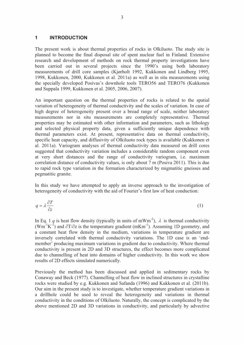
2 MEASUREMENTS OF HEAT FLOW IN INCLINED DRILLHOLES Diamond drillholes are usually non-vertical due to the driller’s aim to maximize penetrated stratigraphy and to minimize drilling meters. Therefore holes are oriented approximately perpendicular to lithological boundaries. In Olkiluoto the boundaries dip at an angle of about 20-40 degrees and the drillholes have a dip of about 60-80 degrees. The temperature gradient along drillhole is directly obtained from the measured temperature data. In geothermal studies a major derivative from measured data is the vertical component of temperature gradient (geothermal gradient) and the heat flow density, both corrected for drillhole deviation from vertical (qVA = qD sin � where � is the drillhole dip). In such a correction, the total heat flow vector is assumed to be vertical. However, the heat flow vector is vertical only in a horizontally layered or homogeneous 1D earth. In 2D and 3D media the direction of the heat flow vector is affected by the thermal conductivity variations. Heat flow prefers pathways of higher conductivity, which results in the phenomenon of channelling of heat flow into layers with higher conductivity. The principal relations of different heat flow components are qualitatively depicted in Figure 1.
Figure 1. Relations between total heat flow vector, its components and projections in a dipping layer and the measurement geometry in an inclined drillhole. Thermal conductivity �1 > �2.

6
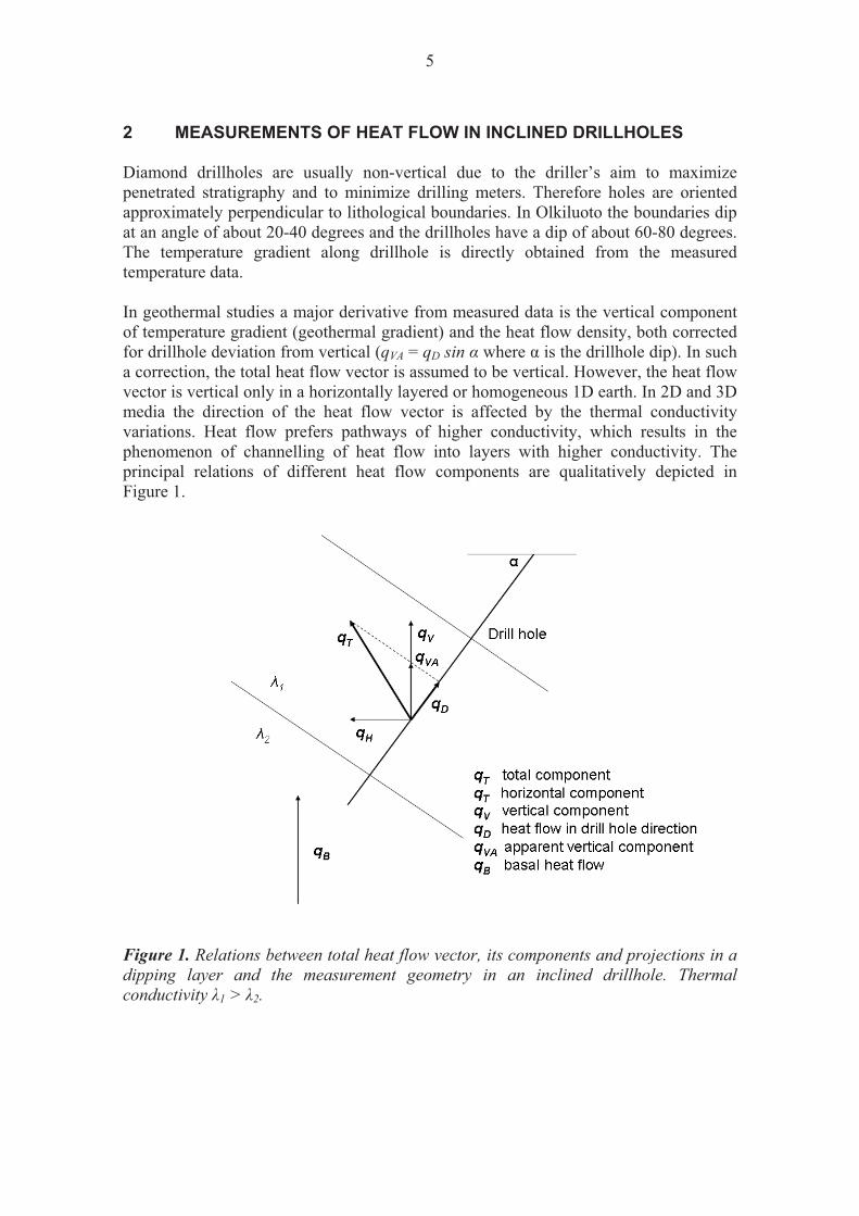
Due to the channelling of heat (also called refraction of heat) the total heat total vector (qT) turns towards the up-dip direction of the high conductivity layer. The direction is generally unknown if only drillhole data is available. Temperature and thermal conductivity data determined in a drillhole provide information only on the component qD of heat flow density in the direction of the hole. Depending on the true orientation of the total heat flow vector, the magnitude of the qD component may differ from the true vertical component qV and the basal (or background) heat flow qB. Particularly, the simple geometrical correction for borehole deviation may result in a significant difference between the vertical heat flow estimate qVA and the true values of qV and qT (Fig. 1). These 2D effects depend on the thermal conductivity contrast (�1 vs. �2), dip of the layer and the inclination of the drillhole. In the following we use numerical heat transfer models to study these effects in detail. The 2D finite difference modelling applies a 500 m x 500 m medium with 1 m x 1 m discretization. There is a 10 m thick inclined (dip 27°) layer of higher conductivity embedded in a homogeneous environment. Thermal conductivity of the high conductivity layer is varied between 3.2 and 8 W m-1K-1, and the surrounding medium conductivity is 2.8 W m-1K-1. A constant temperature boundary condition (5°C) was applied on the upper, and a constant heat flow density (40 mWm-2) on the lower boundary, respectively. All models were calculated for steady-state conditions using the code Processing Shemat (Clauser 2003).
Figure 2. Thermal conductivity structure applied in the numerical modelling. Results were simulated for the drillhole geometries shown.
7
Figure 3. Horizontal (above) and vertical (below) components of heat flow calculated with the model in Fig. 2. Thermal conductivity of the dipping layer is 3.2 W m-1K-1 and of the medium 2.8 W m-1K-1, respectively. Heat flow values are positive towards up and right.

8
-0.01
0.00
0.01
0.02
0.03
0.04
0.05
-10
-5
0
5
10
15
20
230 240 250 260 270
Heat flow (Wm-2)
Dip qT (deg)
Depth (m)
Conductivity 3.2 and 2.8, hole incl. 63°
Dip qTqTqHqVqVA
Conductivity 3.2 and 2.8, hole incl. 63°
-10
-5
0
5
10
15
20
230 240 250 260 270
Depth (m)
Gra
d (m
K/m
)
0
2
4
6
8
10
12
14
Con
duct
ivity
(Wm
-1K
-1)
Grad along holeInv. cond
Figure 4.Thermal modelling results picked along a drillhole with an inclination of 63º and cutting the high conductivity layer perpendicularly. Upper panel: components of heat flow and dip angle of total heat flow vector; lower panel: temperature gradient along borehole and inverted apparent thermal conductivity. Thermal conductivity of the high conductivity layer is 3.2 Wm-1K-1 and medium 2.8 Wm-1K-1. Note that qV, qT and qVA are practically identical in the applied scale of presentation.
9
Conductivity 3.2 and 2.8, hole incl. 90°
-10
-5
0
5
10
15
20
230 240 250 260 270
Depth (m)
Dip
qT
(deg
)
-0.01
0.00
0.01
0.02
0.03
0.04
0.05
Hea
t flo
w (W
m-2
)
Dip qqTqVqHqVA
Conductivity 3.2 and 2.8, hole incl. 90°
-10
-5
0
5
10
15
20
230 240 250 260 270
Depth (m)
Gra
d (m
K/m
)
0
2
4
6
8
10
12
14
Con
duct
ivity
(Wm
-1K
-1)
Grad along holeInv. cond
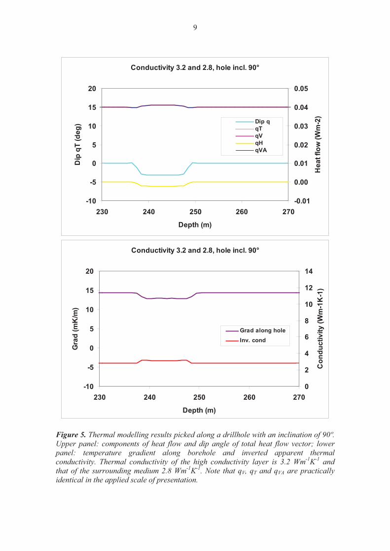
Figure 5. Thermal modelling results picked along a drillhole with an inclination of 90º. Upper panel: components of heat flow and dip angle of total heat flow vector; lower panel: temperature gradient along borehole and inverted apparent thermal conductivity. Thermal conductivity of the high conductivity layer is 3.2 Wm-1K-1 and that of the surrounding medium 2.8 Wm-1K-1. Note that qV, qT and qVA are practically identical in the applied scale of presentation.
10
Conductivity 4.0 and 2.8, hole incl. 63°
-20
-10
0
10
20
30
40
230 240 250 260 270
Depth (m)
Dip
qT
(deg
)
-0.01
0.00
0.01
0.02
0.03
0.04
0.05
Hea
t flo
w (W
m-2
)Dip qTqTqVqHqVA
Conductivity 4.0 and 2.8, hole incl. 63°
02468
101214161820
230 240 250 260 270
Depth (m)
Gra
d (m
K/m
)
0
2
4
6
8
10
12
14
Con
duct
ivity
(Wm
-1K
-1)
Grad along holeInv. cond
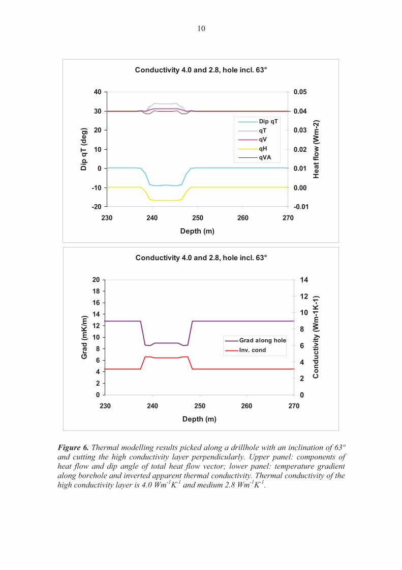
Figure 6. Thermal modelling results picked along a drillhole with an inclination of 63º and cutting the high conductivity layer perpendicularly. Upper panel: components of heat flow and dip angle of total heat flow vector; lower panel: temperature gradient along borehole and inverted apparent thermal conductivity. Thermal conductivity of the high conductivity layer is 4.0 Wm-1K-1 and medium 2.8 Wm-1K-1.
11
Conductivity 4.0 and 2.8, hole incl. 90°
-20
-15
-10
-5
0
5
10
15
20
230 240 250 260 270
Depth (m)
Dip
qT
(deg
)
-0.01
0.00
0.01
0.02
0.03
0.04
0.05
Hea
t flo
w (W
m-2
)Dip qTqTqHqVqVA
Conductivity 4.0 and 2.8, hole incl. 90°
02468
101214161820
230 240 250 260 270
Depth (m)
Gra
dien
t (m
K/m
)
0.00
2.00
4.00
6.00
8.00
10.00
12.00
14.00
Hea
t flo
w (W
m-2
)
Grad along hole
Inv cond
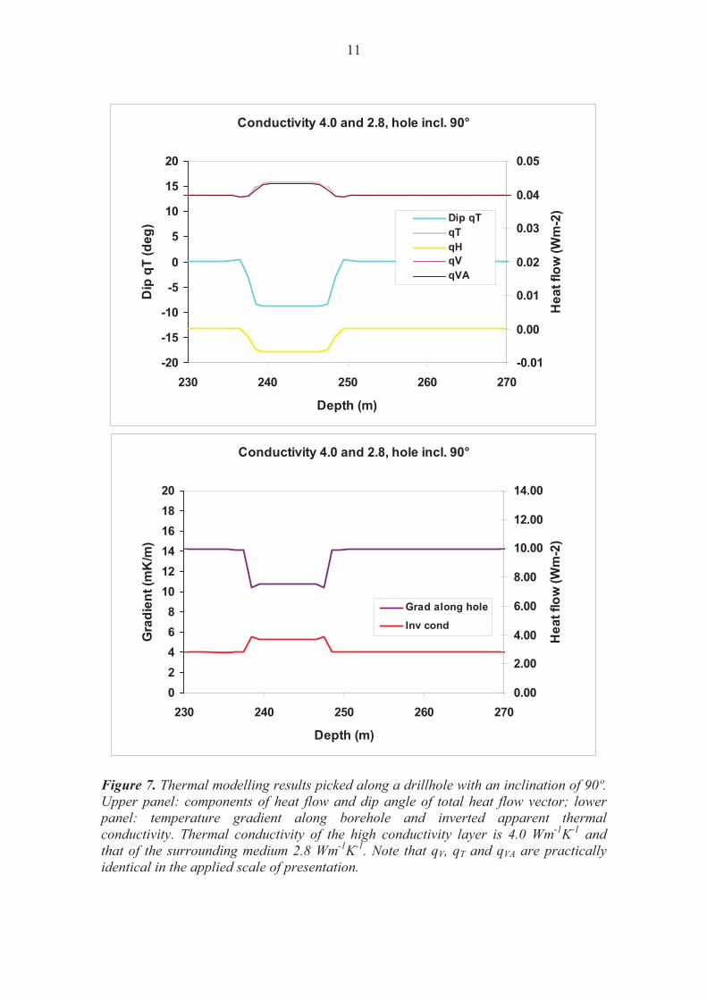
Figure 7. Thermal modelling results picked along a drillhole with an inclination of 90º. Upper panel: components of heat flow and dip angle of total heat flow vector; lower panel: temperature gradient along borehole and inverted apparent thermal conductivity. Thermal conductivity of the high conductivity layer is 4.0 Wm-1K-1 and that of the surrounding medium 2.8 Wm-1K-1. Note that qV, qT and qVA are practically identical in the applied scale of presentation.

12
Conductivity 8.0 and 2.8, hole incl. 63°
-40
-30
-20
-10
0
10
20
230 240 250 260 270
Depth (m)
Dip
qT
(deg
)
-0.04
-0.02
0.00
0.02
0.04
0.06
0.08
Hea
t flo
w (W
m-2
)
Dip qqTqVqHqVA
Conductivity 8.0 and 2.8, hole incl. 63°
0
2
4
6
8
10
12
14
230 240 250 260 270
Depth (m)
Gra
dien
t (m
K/m
)
0
2
4
6
8
10
12
14
Con
duct
ivity
(Wm
-1K
-1)
Grad along hole
Inv cond
Figure 8. Thermal modelling results picked along a drillhole with an inclination of 63º and cutting the high conductivity layer perpendicularly. Upper panel: components of heat flow and dip angle of total heat flow vector; lower panel: temperature gradient along borehole and inverted apparent thermal conductivity. Thermal conductivity of the high conductivity layer is 8.0 Wm-1K-1 and medium 2.8 Wm-1K-1.
13
Conductivity 8.0 and 2.8, hole incl. 90°
-40
-35
-30
-25
-20
-15
-10
-5
0
5
230 240 250 260 270
Depth (m)
Dip
qT
(deg
)
-0.04
-0.02
0.00
0.02
0.04
0.06
0.08
Hea
t flo
w (W
m-2
)
Dip qTqTqVqHqVA
Conductivity 8.0 and 2.8, hole incl. 90°
02468
101214161820
230 240 250 260 270
Depth (m)
Gra
dien
t (m
K/m
)
0
2
4
6
8
10
12
14
Con
duct
ivity
(Wm
-1K
-1)
Grad along hole
Inv. cond
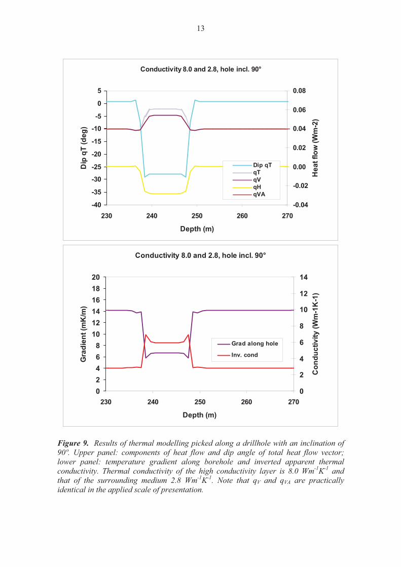
Figure 9. Results of thermal modelling picked along a drillhole with an inclination of 90º. Upper panel: components of heat flow and dip angle of total heat flow vector; lower panel: temperature gradient along borehole and inverted apparent thermal conductivity. Thermal conductivity of the high conductivity layer is 8.0 Wm-1K-1 and that of the surrounding medium 2.8 Wm-1K-1. Note that qV and qVA are practically identical in the applied scale of presentation.
14
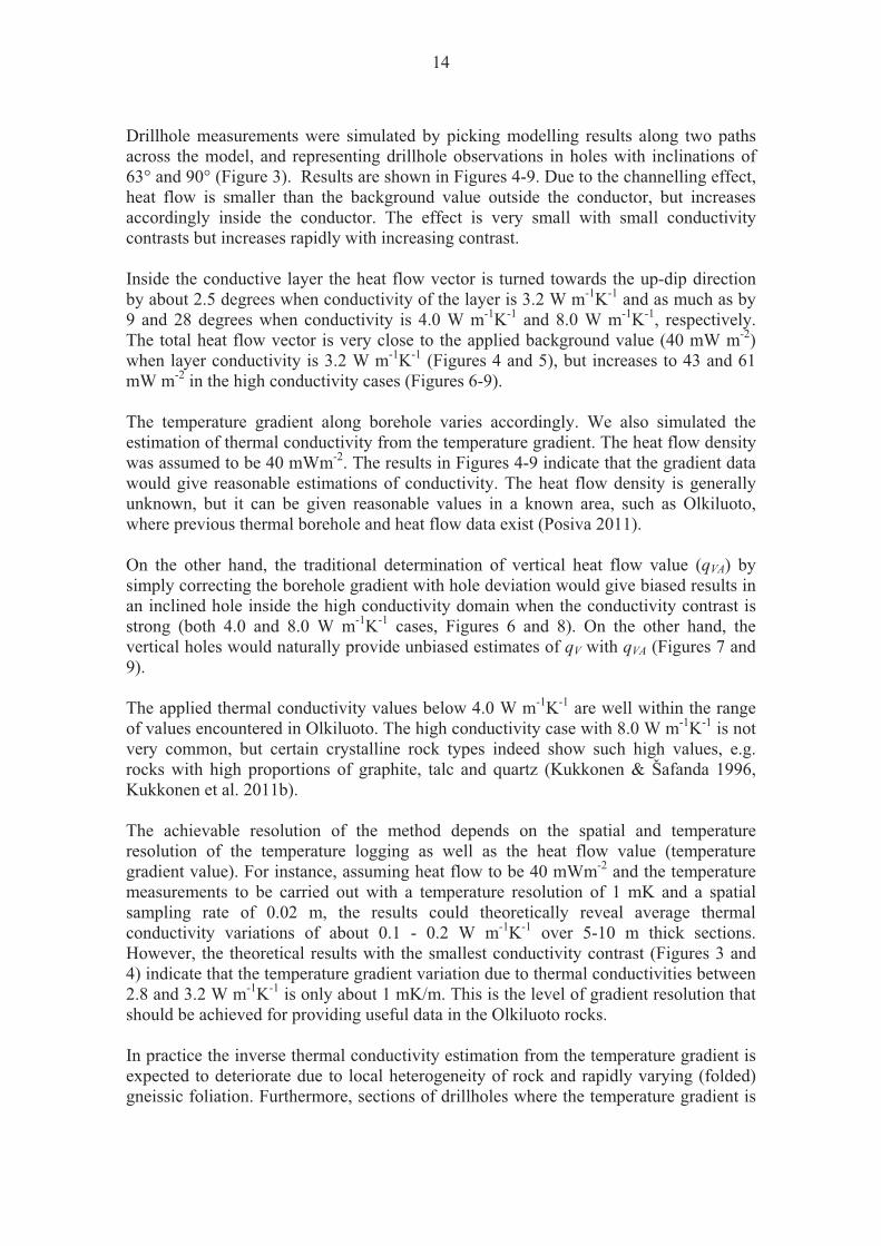
Drillhole measurements were simulated by picking modelling results along two paths across the model, and representing drillhole observations in holes with inclinations of 63° and 90° (Figure 3). Results are shown in Figures 4-9. Due to the channelling effect, heat flow is smaller than the background value outside the conductor, but increases accordingly inside the conductor. The effect is very small with small conductivity contrasts but increases rapidly with increasing contrast. Inside the conductive layer the heat flow vector is turned towards the up-dip direction by about 2.5 degrees when conductivity of the layer is 3.2 W m-1K-1 and as much as by 9 and 28 degrees when conductivity is 4.0 W m-1K-1 and 8.0 W m-1K-1, respectively. The total heat flow vector is very close to the applied background value (40 mW m-2) when layer conductivity is 3.2 W m-1K-1 (Figures 4 and 5), but increases to 43 and 61 mW m-2 in the high conductivity cases (Figures 6-9). The temperature gradient along borehole varies accordingly. We also simulated the estimation of thermal conductivity from the temperature gradient. The heat flow density was assumed to be 40 mWm-2. The results in Figures 4-9 indicate that the gradient data would give reasonable estimations of conductivity. The heat flow density is generally unknown, but it can be given reasonable values in a known area, such as Olkiluoto, where previous thermal borehole and heat flow data exist (Posiva 2011). On the other hand, the traditional determination of vertical heat flow value (qVA) by simply correcting the borehole gradient with hole deviation would give biased results in an inclined hole inside the high conductivity domain when the conductivity contrast is strong (both 4.0 and 8.0 W m-1K-1 cases, Figures 6 and 8). On the other hand, the vertical holes would naturally provide unbiased estimates of qV with qVA (Figures 7 and 9). The applied thermal conductivity values below 4.0 W m-1K-1 are well within the range of values encountered in Olkiluoto. The high conductivity case with 8.0 W m-1K-1 is not very common, but certain crystalline rock types indeed show such high values, e.g. rocks with high proportions of graphite, talc and quartz (Kukkonen & Šafanda 1996, Kukkonen et al. 2011b). The achievable resolution of the method depends on the spatial and temperature resolution of the temperature logging as well as the heat flow value (temperature gradient value). For instance, assuming heat flow to be 40 mWm-2 and the temperature measurements to be carried out with a temperature resolution of 1 mK and a spatial sampling rate of 0.02 m, the results could theoretically reveal average thermal conductivity variations of about 0.1 - 0.2 W m-1K-1 over 5-10 m thick sections. However, the theoretical results with the smallest conductivity contrast (Figures 3 and 4) indicate that the temperature gradient variation due to thermal conductivities between 2.8 and 3.2 W m-1K-1 is only about 1 mK/m. This is the level of gradient resolution that should be achieved for providing useful data in the Olkiluoto rocks. In practice the inverse thermal conductivity estimation from the temperature gradient is expected to deteriorate due to local heterogeneity of rock and rapidly varying (folded) gneissic foliation. Furthermore, sections of drillholes where the temperature gradient is
15
very small or zero are encountered in bedrock in the uppermost 100 m. It is due to a transient state of subsurface temperature field by a palaeoclimatic effect which has increased the ground surface temperatures during the last two centuries. In addition, advective heat transfer by flow of fluid in the hole and free thermal convection of borehole fluid in sufficiently large diameter holes may also disturb the conductivity estimation.

16
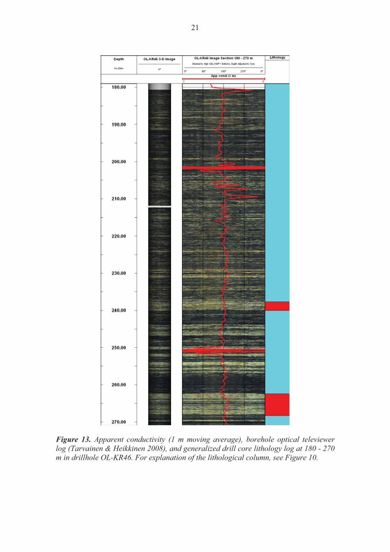
3 MEASUREMENTS IN DRILLHOLE OL-KR46 The inverse gradient method was tested using novel temperature data on the 594 m deep drillhole OL-KR46 in Olkiluoto. The drillhole penetrates mainly veined gneiss, pegmatitic granite and tonalitic-granodioritic-granitic gneiss. The hole dip is 70 degrees. The hole diameter is 56 mm (Toropainen 2007). Temperature data was logged on Oct 12, 2010, using a memory logger probe manufactured by Antares GmbH, Germany. The probe is capable of temperature readings at a pre-programmable rate and with a resolution of 1 mK. The probe was installed at the lower end of the logging cable on a motorized winch of the TERO logging equipment. The logging was carried out in downward direction to the depth of 580 m as a continuous log with a speed of 1.1 – 1.4 m/min (about 2 cm/s). Temperature was sampled at every 1 s. The winch was stopped at every 50 m for depth and temperature control. Final temperature-depth data was obtained by correlating the temperature-time data from the probe and the depth-time data from the winch. The resulting final reading interval in depth is 0.02 m. The overall results are shown in Fig. 10. Temperature gradient was calculated with different averaging windows of 1 – 10 m using a heat flow density value of 40.7 mWm-2 equal to the average determined for OL-KR46 (Posiva 2011). The apparent conductivities are mostly in the range of 2.7 – 3.2 Wm-1K-1 excluding zones disturbed by either the stopping of the winch or by hydrogeological flow effects in the hole. Therefore, variation of conductivity seems to be rather small in OL-KR46. The standard error of the gradient is about 0.15 mK/m for calculated 1 m intervals and about one and two orders of magnitude smaller for 5 m and 10 intervals, respectively. The corresponding uncertainty of apparent thermal conductivity (1 m intervals) is about 0.1 Wm-1K-1. Thus, from the mathematical point of view the data has sufficient resolution for conductivity estimation. When compared with lithological data it can be seen that the generalized lithology log is too coarse for detailed comparison with the apparent conductivity logs. Therefore, the results were also compared with optical televiewer data which provides a high spatial resolution and reveals the rock types (Figures 11-18). In the image logs the veined gneiss is seen as a dark foliated rock and the pegmatitic granite as yellowish-light grey, non-oriented coarse-grained rock. The texture of tonalitic-granodioritic-granitic gneiss resembles veined gneiss but contains more material represented by light tints. Laboratory measurements indicated that the average thermal conductivity of pegmatitic granite (3.20 Wm-1K-1 is slightly higher than that of veined gneiss (2.83 Wm-1K-1) or tonalitic-granodioritic-granitic gneiss (2.78 Wm-1K-1) (Kukkonen et al. 2011a). Thus, the sections of pegmatitic granite could be expected to show as modest highs in the apparent conductivity curves. The apparent conductivity results sometimes follow this expectation but sometimes show also lower values of conductivity for pegmatitic granite. We attribute this to the fact that the conductivity histograms of the three rock types determined from laboratory measurements actually overlap, and single samples may show both high and low values. In addition, the gneisses are thermally anisotropic and the orientation of the foliation further affects the results. Pegmatitic granite shows

17
also coarse texture variations and spatial variations in the content of feldspars and quartz which also affect the conductivity variations. Laboratory measurements exist for 28 drill core samples from OL-KR46. The laboratory measurements at 380-485 m (Figures 10 and 15-17) are generally in a good agreement with the apparent conductivity logs. However, in details the data do not match perfectly with the logs due to the above mentioned anisotropy and heterogeneity. The differences are nevertheless usually smaller than 0.5 Wm-1K-1.

18
Figure 10. Results from drillhole OL-KR46. Columns from left: temperature data, calculated temperature gradients (moving averages with 1, 5 and 10 m windows), corresponding apparent conductivities calculated with the average heat flow in 40.7 mWm-2, generalized lithology (blue: veined gneiss, red: pegmatitic granite, yellow: tonalitic-granodioritic-granitic gneiss, pale yellow: quartzitic gneiss) and gamma-gamma density log. Laboratory conductivities are from Kukkonen et al. (2011a) and lithology and density logs from Tarvainen & Heikkinen (2008).
19
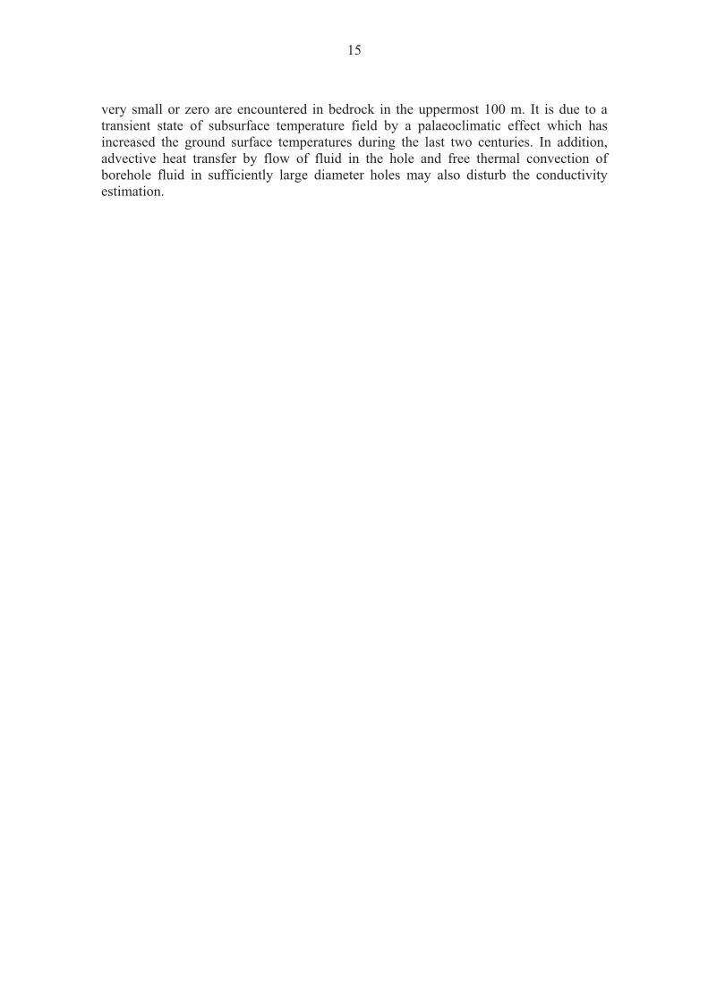
Figure 11. Apparent conductivity (1 m moving average), borehole optical televiewer log (Tarvainen & Heikkinen 2008), and generalized drill core lithology log at 55-120 m in drillhole OL-KR46. For explanation of the lithological column, see Figure 10.
20
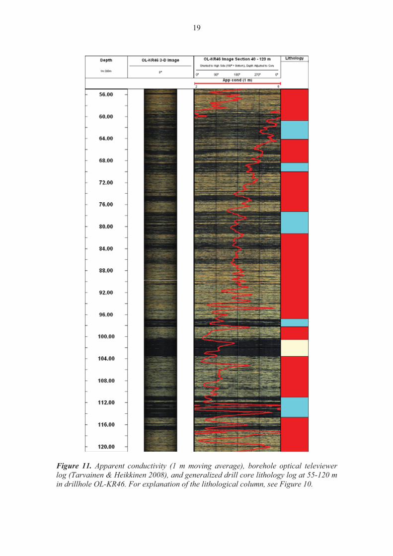
Figure 12. Apparent conductivity (1 m moving average), borehole optical televiewer log (Tarvainen & Heikkinen 2008), and generalized drill core lithology log at 120 - 180 m in drillhole OL-KR46. For explanation of the lithological column, see Figure 10.
21
Figure 13. Apparent conductivity (1 m moving average), borehole optical televiewer log (Tarvainen & Heikkinen 2008), and generalized drill core lithology log at 180 - 270 m in drillhole OL-KR46. For explanation of the lithological column, see Figure 10.
22
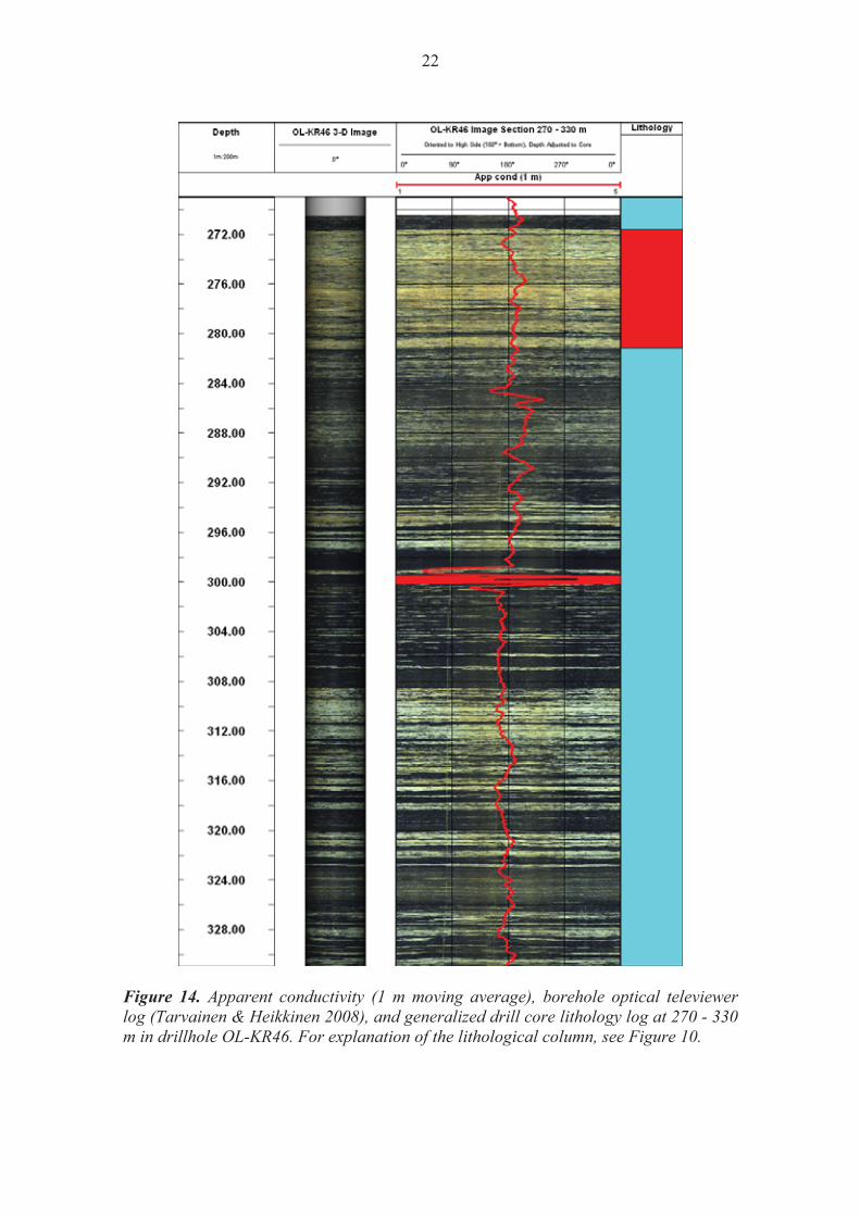
Figure 14. Apparent conductivity (1 m moving average), borehole optical televiewer log (Tarvainen & Heikkinen 2008), and generalized drill core lithology log at 270 - 330 m in drillhole OL-KR46. For explanation of the lithological column, see Figure 10.

23
Figure 15. Apparent conductivity (1 m moving average), measured drill core conductivities, borehole optical televiewer log (Tarvainen & Heikkinen 2008), and generalized drill core lithology log at 380-470 m in drillhole OL-KR46. For explanation of the lithological column, see Figure 10.

24
Figure 16. Apparent conductivity (1 m moving average), measured drill core conductivities and borehole optical televiewer log, and generalized drill core lithology log at 380-470 m in drillhole OL-KR46. For explanation of the lithological column, see Figure 10.
25
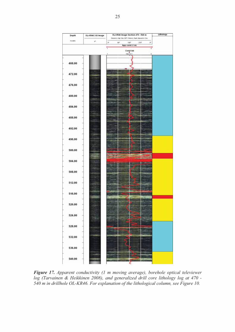
Figure 17. Apparent conductivity (1 m moving average), borehole optical televiewer log (Tarvainen & Heikkinen 2008), and generalized drill core lithology log at 470 - 540 m in drillhole OL-KR46. For explanation of the lithological column, see Figure 10.
26
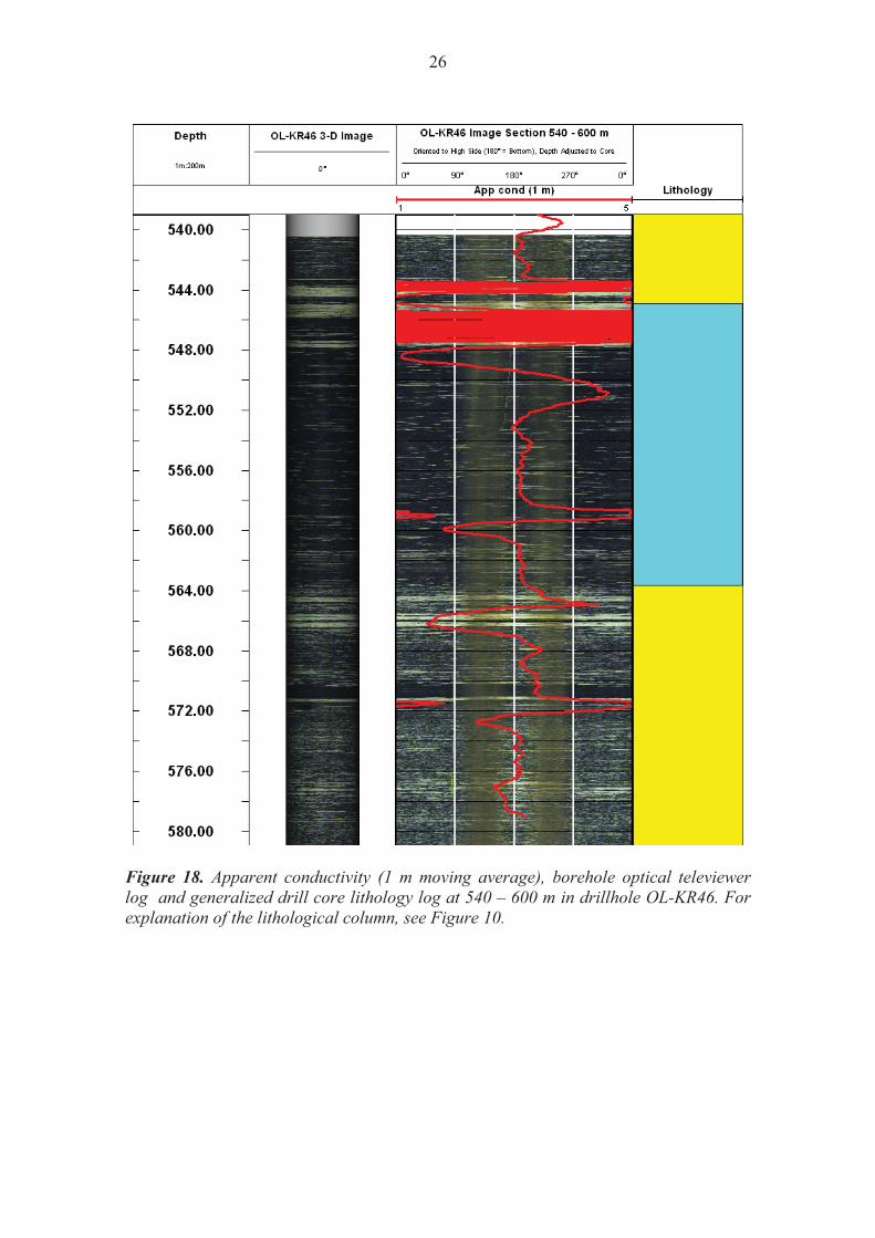
Figure 18. Apparent conductivity (1 m moving average), borehole optical televiewer log and generalized drill core lithology log at 540 – 600 m in drillhole OL-KR46. For explanation of the lithological column, see Figure 10.

27
4 DISCUSSION AND CONCLUSIONS The inverse gradient method is based Fourier’s first law of heat conduction. Assuming that the heat flow density is locally constant, thermal conductivity variations can be inverted for apparent thermal conductivity values from measured temperature gradient data. In inclined boreholes penetrating dipping rock layers, channelling of heat affects the thermal regime and generates a deviation of the heat flow vector from vertical. Conduction effects were simulated with a 500 m x 500 m 2D finite difference model including a 10 m thick dipping layer of higher conductivity. The deviation of heat flow vector from vertical is practically negligible with small conductivity contrasts but increases quickly with increasing conductivity of the inclined layer. The results also show that typical conventions applied in geothermal heat flow studies in inclined holes may result in biased estimates of vertical heat flow inside an inclined high conductivity rock layer. However, the effect does not harm the apparent conductivity estimation with the inverse gradient technique. The present results indicate that theoretically the method is able to reveal thermal conductivity variations of sufficiently continuous rock layers. Results of theoretical simulations encourage applying the method in the conditions of Olkiluoto, where rock thermal conductivities are in the range of 2 - 4 Wm-1K-1 and heat flow is about 40 mWm-2. How the scale of heterogeneity of thermal conductivity would actually modify the results was not modelled in the present study and must be left for future studies. In Olkiluoto spatial variations of thermal conductivity take place in scales ranging from centimeters to tens of metres. The inverse gradient method assumes inherently that only conductive heat transfer takes place. In practice, many non-conductive disturbances may deteriorate the results, such as flow of fluid in the drillhole between two fracture systems. Further, free thermal convection of fluid may take place in large diameter water-filled holes. The onset of free convection depends mainly on the borehole diameter and temperature gradient. The critical temperature gradient value Gc, above which convection takes place (Hales, 1937), can be calculated from
4
16dg
kBC
TgGf
c ���
�� (2)
where g is the acceleration of gravity, T is absolute temperature, � is the coefficient of thermal expansion, k is the diffusivity, � the kinematic viscosity, Cf is the specific heat of fluid (4183 J K–1 kg–1 for water at 20°C), and B is a constant which has the value 216 for a tube whose length is great compared with its diameter (d). The critical geothermal gradient for free convection in a 56 mm (vertical) drillhole is about 26 mK/m, but only about 8 mK/m in a 76 mm hole, respectively. Convection cells are about as tall as the borehole diameter, and as a result the temperature logs would be disturbed by a small ‘noise’ component in the mK level. Therefore, free convection may need to be taken into account because the resolution requirement of the inverse gradient method is in the same mK range. The diameter of OL-KR46 is 56 mm and it is likely not affected by free convection.
28
The method was applied in practice with data measured in the drillhole OL-KR46 in Olkiluoto. Temperature logs were obtained with a high resolution memory logger probe carried downhole at the end of logging cable installed on a motorized winch. A continuous log was obtained with a logging speed of about 2 cm/s. During logging the winch was stopped at about 50 m intervals and the results show that the temperature readings were lagging behind by up to a few cK. This results in a minor convolution of temperature anomalies but does not affect the general results as long as the logging speed is kept constant and as low as possible. The results are also influenced by the downward diffusing ground surface temperature variations. Due to the palaeoclimatic increase in ground temperature during the past 100-200 years the temperature gradient has decreased in the uppermost 100 m of the bedrock which results in too high values of inverted apparent conductivity. The temperature-depth curve could of course be straightened by fitting an appropriate function in the data to remove the long wavelength effect. In sections where the surface temperature increase has resulted in a zero temperature gradient the inverse gradient method becomes meaningless. The apparent conductivity logs calculated from the OL-KR46 data are in agreement with drill core results, although they do not fit exactly. We attribute this to the anisotropy and heterogeneity of rock in the scale of cm to meters. Due to overlapping thermal conductivity histograms of pegmatitic granite and the migmatitic gneisses the results actually indicate that the thermal conductivity of pegmatitic granite may locally be either lower or higher than the gneisses. The inverse gradient method does not replace laboratory and in situ TERO measurements of thermal conductivity but provides an additional tool in studying the heterogeneity and spatial variation of thermal conductivity. The method is best suited for detecting local variations and the scales of such variations. However, it is not useful for determination of absolute values of conductivity, as the heat flow must be assumed to be known at least locally.
29
REFERENCES Clauser, C. (Ed.), 2003. Numerical simulation of reactive flow in hot aquifers. SHEMAT and Processing SHEMAT. Springer, Berlin, 332 pp. Conaway, J.G. & Beck A.E. 1977. Continuous logging of temperature gradients. Tectonophysics, 41, 1-7. Hales, A.L., 1937. Convection currents in geysers. Mon. Not. R. Astron. Soc., Geophys. Suppl., 4, 122–131. Kjørholt, H. 1992. Thermal properties of rocks. Teollisuuden Voima Oy, TVO/Site investigations, work report 92-56, 13 p. Kukkonen, I., 2000. Thermal properties of the Olkiluoto mica gneiss: results of laboratory measurements. Posiva Oy, Working Report 2000-40, 28 p. Kukkonen I. & Lindberg A. 1995. Thermal conductivity of rocks at the TVO investigation sites Olkiluoto, Romuvaara and Kivetty. Nuclear Waste Commission of Finnish Power Companies, Report YJT-98-08, 29 p. Kukkonen, I. & Lindberg, A. 1998. Thermal properties of rocks at the investigation sites: measured and calculated thermal conductivity, specific heat capacity and thermal diffusivity. Posiva Oy, Working Report 98-09e, 29 p. Kukkonen, I.T. & Šafanda, J. 1996. Palaeoclimate and structure: the most important factors controlling subsurface temperatures in crystalline rocks. A case history from Outokumpu, eastern Finland. Geophysical Journal International, 126, 101-112. Kukkonen, I. and Suppala, I. 1999. Measurement of thermal conductivity and diffusivity in situ: Literature survey and theoretical modelling of measurements. Posiva Oy, Report 99-1, 69 p. Kukkonen, I., Suppala, I., Korpisalo, A. and Koskinen, T., 2005. TERO borehole logging device and test measurements of rock thermal properties in Olkiluoto. Posiva Oy, Report 2005-09, 96 p. Kukkonen, I., Suppala, I., Korpisalo, A. and Lehtimäki, J., 2006. TERO thermal property measurements in boreholes KAV01 and KLX06 in Oskarshamn. Posiva Oy, Working Report 2006-82, 26 p. Kukkonen, I., Suppala, I., Korpisalo, A. and Koskinen, T., 2007. Drillhole logging device TERO76 for determination of rock thermal properties. Posiva Oy, Report 2007-01, 38 p. Kukkonen, I., Kivekäs L., Vuoriainen, S. & Kääriä, M., 2011a. Thermal properties of rocks in Olkiluoto: Results of laboratory measurements 1994-2010. Posiva Oy, Working Report 2011, 96 p.

30
Kukkonen, I.T, Rath, V., Kivekäs ,L. Šafanda ,J. & �ermak ,V., 2011b. Geothermal Studies of the Outokumpu Deep Drill Hole, Finland: Vertical variation in heat flow and palaeoclimatic implications. Physics of the Earth and Planetary Interiors, 188, 9–25. Posiva 2011. Olkiluoto Site Description 2010. Posiva Oy, Working Report 2011-xx (in prep.).
Related Documents
![FSO Detection Using Differential Signaling in Outdoor ... · temperature gradient measurement) as in [16]. The temperature gradient was measured using 20 temperature sensors positioned](https://static.cupdf.com/doc/110x72/60b3e025ce38416d9367fa8a/fso-detection-using-differential-signaling-in-outdoor-temperature-gradient-measurement.jpg)


