Inverse scattering perturbation theory for the nonlinear ... · PDF fileJosselin Garnier and Konstantinos Kalimeris ... (Some figures may appear in colour only in the online ... allow

Inverse scattering perturbation theory for the nonlinear Schrödinger equation with non-

vanishing background

This article has been downloaded from IOPscience. Please scroll down to see the full text article.

2012 J. Phys. A: Math. Theor. 45 035202

(http://iopscience.iop.org/1751-8121/45/3/035202)

Download details:

IP Address: 129.199.97.143

The article was downloaded on 20/12/2011 at 08:11

Please note that terms and conditions apply.

View the table of contents for this issue, or go to the journal homepage for more

Home Search Collections Journals About Contact us My IOPscience

IOP PUBLISHING JOURNAL OF PHYSICS A: MATHEMATICAL AND THEORETICAL

J. Phys. A: Math. Theor. 45 (2012) 035202 (13pp) doi:10.1088/1751-8113/45/3/035202

Inverse scattering perturbation theory for thenonlinear Schrodinger equation with non-vanishingbackground

Josselin Garnier and Konstantinos Kalimeris

Laboratoire de Probabilites et Modeles Aleatoires, site Chevalerat, case 7012,Universite Paris VII, 75251 Paris Cedex 13, France

E-mail: [email protected] and [email protected]

Received 4 August 2011, in final form 30 October 2011Published 19 December 2011Online at stacks.iop.org/JPhysA/45/035202

AbstractIn this paper, a perturbation theory for the nonlinear Schrodinger equation withnon-vanishing boundary conditions based on the inverse scattering transformis presented. It is applied to study the stability of the soliton propagation on acontinuous-wave background. It is shown that the soliton is rather robust withrespect to dispersive perturbations but it can be strongly affected by damping.In particular, it is shown that adiabatic approaches can underestimate the decayof the soliton energy.

PACS numbers: 42.65.−R, 47.20.Ky

(Some figures may appear in colour only in the online journal)

1. Introduction

It is well known that the one-dimensional nonlinear Schrodinger (NLS) equation can model thewave dynamics in the deep ocean [20] and pulse propagation in optical fibers [1]. This analogyhas recently found an imaginative and insightful development. Indeed, the understanding ofthe infamous hydrodynamic rogue waves on the surface of the ocean [7] is not straightforwardas very few observations are available. The discovery that optical rogue waves can be generatedin optical systems [22] has opened the way to new research directions, as it is now possibleto produce and study optical rogue waves in laboratories. Furthermore, the analysis of specialsolutions of the NLS equation that could describe rogue waves has attracted a lot of attention.

The bright soliton solution for the NLS equation with vanishing boundary conditions wasexhibited by Zakharov and is now well known [19]. Using the inverse scattering transform,soliton solutions with non-vanishing boundary conditions were first investigated in [16]. It isalso possible to find this solution using more direct approaches based on a direct algebraicansatz [3] or the Backlund transform [13]. This solution is nowadays better known under thename of Ma soliton [18]. In the notation of equation (2.1), it is a wave solution periodic int and localized in x. When the background wave goes to zero, one recovers the standard bright

1751-8113/12/035202+13$33.00 © 2012 IOP Publishing Ltd Printed in the UK & the USA 1

J. Phys. A: Math. Theor. 45 (2012) 035202 J Garnier and K Kalimeris

soliton of the NLS equation. The Ma soliton can be seen as a particular class of a more generalfamily of solutions that describes periodic wave solutions in both t and x [3]. Note that theAkhmediev breathers are another particular class of this general family of solutions [4]. Thesebreathers are localized in t and periodic in x and they can be used to describe a nonlinearstage of the modulational instability. The Peregrine solution [21] is a rational solution of theNLS equation, which can be seen as a limiting case of both a one-parameter family of Masolitons or a one-parameter family of Akhmediev breathers (when the periods go to infinity).The Peregrine solution was observed in [17] and it is a very good candidate for a ‘wave thatappears from nowhere and disappears without a trace’ [2], that is, a rogue wave. The Masolitons provide one way to study the Peregrine solution.

It is of theoretical and practical interest to understand the stability of the Ma soliton underdifferent types of perturbations [9]. In the hydrodynamic context, one should take into accountfinite depth, bottom friction, dissipation and other effects present in the ocean [6, 23]. Inthe nonlinear fiber optics context, the NLS equation is a simplified model of a more generalequation that should take into account high-order dispersion and nonlinear effects [8, 24] anddamping [6, 14].

The stability of the solutions of the NLS equation with non-vanishing boundary conditionshas already been investigated using numerical or analytical tools. Background modulationalinstability and Raman self-scattering were numerically investigated in [5]. In this paper, weare not concerned with the possible modulational instability of the background but we focusour attention to the stability of the Ma soliton with respect to different types of perturbations.An adiabatic approach was used to study the stability of the soliton in [10]. In this approach, itis assumed that the solution keeps its form and that its parameters slowly evolve. The adiabaticevolutions of the soliton parameters are identified by using the evolution equations of a fewconserved integrals, such as the total energy. In our paper, we develop a perturbation theorybased on the inverse scattering transform to study the evolution of the soliton. The principleof such a method for a small perturbation of an integrable system was described in [15]. Thismethod was successfully applied to the NLS equation with vanishing boundary conditions inthe case of both deterministic and random perturbations [11, 12].

In this paper, we develop the perturbation theory for the solution of the NLS equation withnon-vanishing boundary conditions and pay particular attention to the case of the Ma soliton.This theory can be applied to analyze the effect of different dispersive, diffusive (damping),or nonlinear perturbations to the soliton propagation. As we will see, the perturbed inversescattering transform approach reveals that the evolution of the soliton can be different thanthat predicted by the adiabatic approach. In particular, radiation can play a significant role inthe evolution of the conserved integrals. We will show that the Ma soliton is rather robust withrespect to dispersive perturbations, but can be strongly affected by damping terms. Althoughthe total energy is not greatly affected by damping, the soliton energy can decay significantly.These theoretical predictions are confirmed by numerical simulations.

2. The nonlinear Schrodinger equation with non-vanishing boundary conditions

In this section, we recall two of the one-soliton solutions of one-dimensional NLS equation

ivt + vxx + 2|v|2v = 0, (2.1)

with non-vanishing boundary conditions. The simple transformation v(x, t) = e2iν20 (t−t0 )q(x, t)

in (2.1) gives

iqt + qxx + 2(|q|2 − ν2

0

)q = 0, (2.2)

and we consider the non-vanishing boundary conditions limx→±∞ q(x, t) = ν0.

2

J. Phys. A: Math. Theor. 45 (2012) 035202 J Garnier and K Kalimeris

The general form of the Ma soliton, as it is known in the literature [18] (with shifted timeand space), was firstly discovered in [16]1, using the inverse scattering transform and is givenby the following expression:

q(x, t) = ν0 + 2ηη cos(4νηt + θ ) + iν sin(4νηt + θ )

ν0 cos(4νηt + θ ) − ν cosh(2ηx + ψ), (2.3)

where ψ, θ are real numbers and η, ν and ν0 are positive parameters, for which η =√

ν2 − ν20 .

For ψ = θ = 0, we obtain the usual form of the Ma soliton

q(x, t) = ν0 + 2ηη cos(4νηt) + iν sin(4νηt)

ν0 cos(4νηt) − ν cosh(2ηx). (2.4)

The limit of (2.4) at η → 0 gives the Peregrine soliton [21], which is a rational solution of(2.2) and has the following expression:

p(x, t) = ν0

(1 − 4 + 16iν2

0 t

1 + 4ν20 x2 + 16ν4

0 t2

). (2.5)

3. Inverse scattering transform

3.1. The spectral problems

Following [16] the generalized eigenvalue problem associated with (2.2) is

ux = D(λ; x, t)u, D(λ; x, t) = −iλσ3 + Q(x, t), (3.1a)

ut = F(λ; x, t)u, F(λ; x, t) = −i(2λ2 − |q(x, t)|2 + ν20 )σ3 + 2λQ(x, t) + iσ3Qx(x, t),

(3.1b)

where

σ3 =(

1 00 −1

)and Q(x, t) =

(0 q(x, t)

−q(x, t) 0

),

and the bar stands for the complex conjugate. The compatibility condition uxt = utx yields theequation Dt − Fx + DF − FD = 0, which is equivalent to (2.2).

The Jost functions �±(x, t; λ, ζ ; η, ν, ν0) are defined as the 2 × 2 matrices which satisfythe ordinary differential equation (ODE) (3.1a) with the boundary conditions

�±(x, t; λ, ζ ; η, ν, ν0) → T (λ, ζ )J(ζx), x → ±∞, (3.2)

where

T (λ, ζ ) =(−iν0 λ − ζ

λ − ζ −iν0

), J(ζx) =

(e−iζx 0

0 eiζx

)and ζ =

√λ2 + ν2

0 .

From the above problem one can see thatd

dx(Det(�±)) = Tr(−iλσ3 + Q(x, t)) = −iλTr(σ3) = 0.

Using conditions (3.2), we obtain

d(λ, ζ ) := Det(�±) = 2ζ (λ − ζ ). (3.3)

We define the scattering matrix S by the following relation:

�−(x, t; λ, ζ ; η, ν, ν0) = �+(x, t; λ, ζ ; η, ν, ν0)S(t; λ, ζ ; η, ν, ν0) (3.4)

1 There is a sign error in equation (6.10) in the original paper [16]. The exact expression is (2.3).

3

J. Phys. A: Math. Theor. 45 (2012) 035202 J Garnier and K Kalimeris

and Det(S) = 1, for every x and t. Using equations (3.1)–(3.4), one can derive an ODE for thefunction S(t; λ, ζ ) from which we obtain the following expression:

S(t; λ, ζ ) = e−2iλζσ3tS0(λ, ζ ) e2iλζσ3t, S0(λ, ζ ) = S(t; λ, ζ )|t=0. (3.5)

In order to consider the analytic properties in the spectral plane we use the transformed Jostfunctions ± = T −1�± which now satisfy the ODE

rx = T −1(DT − Tx)r (r = T −1u)

and the conditions

±(x, t; λζ ) → J(ζx), as x → ±∞.

Equation (3.4) remains invariant under this transformation, i.e. − = +S.For an initial profile that converges sufficiently rapidly to ν0 as x → ±∞ we can obtain

the following theorem, as was stated in [16].

Theorem 3.1. Let ±1 and ±

2 be the columns of ± and S = (S11 S12S21 S22

). The functions

−1 (λ, ζ , x, t) eiζx, +

2 (λ, ζ , x, t) e−iζx and S11(λ, ζ ) are analytic on λ, when Im ζ > 0.The functions −

2 (λ, ζ , x, t) e−iζx, +1 (λ, ζ , x, t) eiζx and S22(λ, ζ ) are analytic on λ, when

Im ζ < 0.

Furthermore, if we assume that the function f (x) = q(x, 0) − ν0 has a compact support,

then all of the above functions are analytic in λ if ζ �= 0. Here we consider ζ =√

λ2 + ν20 as

a single valued function by introducing two Riemann surfaces.

3.2. Integrals

On the one hand, asymptotic expansions of the functions listed in theorem 3.1, around |ζ | = ∞,in their domain of analyticity, allow us to construct two 2 × 2 systems of integral equationsfor the Jost functions, (equations (4.4) and (4.5) in [16]). On the other hand, the ODE (3.1a)allows us to construct the following integral representation for the Jost functions:

�±(x, t; λ, ζ ) = T (λ, ζ )J(ζx) −∫ ±∞

xK±(x, s, t)T (λ, ζ )J(ζx) ds. (3.6)

Substitution of the integral representation (3.6) into the previously mentioned integralequations yields two 2 × 2 systems of integral equations where Jost functions are eliminated,which give the Gel’fand–Levitan integral equations

K±(x, y, t) + H±(x + y, t) =∫ ±∞

xK±(x, s, t)H±(y + s) ds, y > x, (3.7)

where

H± = (H±

2 , H±1

), H±

j (z) = 1

4π

∫�±

j

e−(−1) j iζ z

ζρ j(λ, ζ )T (λ, ζ ) dλ

(δ2 j

δ1 j

),

where δij stands for the Kronecker delta. ρ1(λ, ζ ) = S21(λ,ζ )

S11(λ,ζ )and ρ2(λ, ζ ) = S12(λ,ζ )

S22(λ,ζ ), for some

appropriate contours{�±

j

}2j=1 on the λ-plane, see [16]. From the (+) equations above, one

can obtain that 2K+12(x, x, t) = q(x, t) − ν0.

The following symmetries are valid and will be useful in the following subsection:

S(λ, ζ ) = σ2S(λ, ζ )σ2, K±(x, y, t) = σ2K±(x, y, t)σ2, ρ1(λ, ζ ) = −ρ2(λ, ζ ),

where σ2 = (0 −ii 0

).

4

J. Phys. A: Math. Theor. 45 (2012) 035202 J Garnier and K Kalimeris

Moreover, the fact that the functions �±(x, t; λ,−ζ ) satisfy equation (3.1a), the definitionof S(t; λ, ζ ) in (3.4) implies that S11(t; λ, ζ ) = S22(t; λ,−ζ ) and S12(t; λ, ζ ) = S21(t; λ,−ζ ).Hence,

S11(t; λ, ζ ) = S11(t; λ,−ζ ). (3.8)

3.3. Solitons

From (3.5) we find that ρ1(λ, ζ , t) = ρ1(λ, ζ , 0) e4iλζ t . So if we consider the discrete part ofthe functions H±(z, t) one has to find the zeros of ρ1(λ, ζ , t) or equivalently S11(λ, ζ , 0)—letus note them {(λ j, ζ j)}n

j=1. Then, the definition of H+1 (z, t) gives the following representation:

H+1 (z, t) =

n∑j=1

(c j(t)c j(t)

)eiζ j z, Im (ζ j) > 0, (3.9)

where

c j(t) = i

2(λ j − ζ j)b(λ j, ζ j) e4iλ jζ jt, c j(t) = −1

2ν0b(λ j, ζ j) e4iλ jζ jt,

and

b(λ, ζ ) = S21(λ, ζ )

ζdS11(λ,ζ )

dλ

.

The form of function H+1 (z, t) suggests to take the following representation:(

K+12(x, y, t)

K+22(x, y, t)

)=

n∑j=1

(K+

j (x, t)K+

j (x, t)

)eiζ jy. (3.10)

Applying the representations (3.9) and (3.10), of functions H+(z, t) and K+(x, y, t),respectively, to the (+) integral equation (3.7), one obtains two n × n linear systems ofalgebraic equations which give the functions

{K+

j (x, t), K+j (x, t)

}n

j=1.

The symmetry relation (3.8) shows that the zeros of S11 go in pairs, apart from the casethat λ j ∈ R. Furthermore, from the definition of b(λ, ζ ) we obtain that b(λ, ζ ) = b(λ,−ζ ).Following the previous procedure, we take the pairs of zeros {(λ j, ζ j) = ((−1) jν, η)}2

j=1 with

the constraint ν =√

η2 − ν20 and by letting b(λ j, ζ j) = 2η

ν, j = 1, 2, we obtain

K+(x, x, t) = η

ν0 cos(4νηt) − ν cosh(2ηx)

×(

ν0 cos(4νηt) − νe−2ηx η cos(4νηt) + iν sin(4νηt)−η cos(4νηt) + iν sin(4νηt) ν0 cos(4νηt) − νe−2ηx

)(3.11)

and K(x, y, t) = K(x, x, t) eη(x−y). Consequently, we obtain the Ma soliton given in (2.4). Anarbitrary choice for b(λ, ζ ) will give, in the same way, the more general form (time and spaceshifted) of the Ma soliton given in equation (2.3).

4. The Jost functions

4.1. The Jost functions for the Ma soliton

Applying the expression we obtained for K+(x, y, t) in (3.11) to the integral representation ofthe Jost functions in (3.6), we obtain the following expressions for �+ = (

�+1 ,�+

2

):

5

J. Phys. A: Math. Theor. 45 (2012) 035202 J Garnier and K Kalimeris

�+1 (x, t) = − e−iζx

ζ − iη

1

ν0 cos(4νηt) − ν cosh(2ηx)

×(

iν20λ cos(4νηt) − iν[(λ − ζ )(ν cos(4νηt) + iη sin(4νηt)) + ν0(ζ cosh(2ηx) − iη sinh(2ηx))]

ν0λ(λ − ζ ) cos(4νηt) + ν[ν0(ν cos(4νηt) − iη sin(4νηt)) + (λ − ζ )(ζ cosh(2ηx) − iη sinh(2ηx))]

)(4.1)

and

�+2 (x, t) = − eiζx

ζ + iη

1

ν0 cos(4νηt) − ν cosh(2ηx)

×(

ν0λ(λ − ζ ) cos(4νηt) + ν[ν0(ν cos(4νηt) + iη sin(4νηt)) + (λ − ζ )(ζ cosh(2ηx) + iη sinh(2ηx))]iν2

0λ cos(4νηt) − iν[(λ − ζ )(ν cos(4νηt) − iη sin(4νηt)) + ν0(ζ cosh(2ηx) + iη sinh(2ηx))]

).

(4.2)

The Jost functions �− are given from the �+ under the substitution η → −η. Moreover, theequation �− = �+S yields the following expression:

S(λ, ζ , t) =

⎛⎜⎜⎝

ζ − iη

ζ + iη0

0ζ + iη

ζ − iη

⎞⎟⎟⎠. (4.3)

Functions ± are given by equation ± = T −1�± and we obtain the following expressions:

+1 (x, t) = e−iζx

ν0 cos(4νηt) − ν cosh(2ηx)

×

⎛⎜⎝

ν0

ζ(ζ + iη) cos(4νηt) − ν

ζ − iη(ζ cosh(2ηx) − iη sinh(2ηx))

− iη

ζ

1

ζ − iη(ηλ cos(4νηt) − iνζ sin(4νηt))

⎞⎟⎠ (4.4)

and

+2 (x, t) = eiζx

ν0 cos(4νηt) − ν cosh(2ηx)

×

⎛⎜⎝ − iη

ζ

1

ζ + iη(ηλ cos(4νηt) + iνζ sin(4νηt))

ν0

ζ(ζ − iη) cos(4νηt) − ν

ζ + iη(ζ cosh(2ηx) + iη sinh(2ηx))

⎞⎟⎠ . (4.5)

The functions − are given by the + under the substitution η → −η. Note that ± → J(ζx)

as x → ±∞.

4.2. The Jost functions for the Peregrine soliton

In the case of the Peregrine soliton (2.5) we can obtain the expressions of the relative spectralfunctions by taking the limit η → 0 on the equations of the previous subsection, i.e.

K(x, x, t) = − 2ν0

1 + 4ν20 x2 + 16ν4

0 t2

(2ν0x 1 + 4iν2

0 t−1 + 4iν2

0 t 2ν0x

)(4.6)

and K(x, y, t) = K(x, x, t). The Jost functions �+ = (�+

1 ,�+2

)are given by

�+1 (x, t)= e−iζx

⎛⎜⎜⎜⎝

−iν0

{1 − i

ζ

2ν0

1 + 4ν20 x2 + 16ν4

0 t2

[2ν0x + i

λ − ζ

ν0(1 + 4iν2

0 t)

]}

(λ − ζ )

{1 − i

ζ

2ν0

1 + 4ν20 x2 + 16ν4

0 t2

[2ν0x − i

λ + ζ

ν0(1 − 4iν2

0 t)

]}⎞⎟⎟⎟⎠ (4.7)

6

J. Phys. A: Math. Theor. 45 (2012) 035202 J Garnier and K Kalimeris

and

�+2 (x, t)= eiζx

⎛⎜⎜⎜⎝(λ − ζ )

{1 + i

ζ

2ν0

1 + 4ν20 x2 + 16ν4

0 t2

[2ν0x + i

λ + ζ

ν0(1 + 4iν2

0 t)

]}

−iν0

{1 + i

ζ

2ν0

1 + 4ν20 x2 + 16ν4

0 t2

[2ν0x − i

λ − ζ

ν0(1 − 4iν2

0 t)

]}⎞⎟⎟⎟⎠. (4.8)

Mentioning that �+ → T J as x → ±∞, we conclude that the Jost functions �− are identicalto the �+ functions. This means that S(λ, ζ ) that satisfies the equation �− = �+S is theidentity matrix, which means that the Peregrine soliton is a zero-radiation solution but it doesnot provide any eigenvalue, i.e. S11(λ, ζ ) �= 0.

Functions = ± are given by equation = T −1� and we obtain the followingexpressions:

(x, t) =

⎛⎜⎜⎜⎝

e−iζx

(1 − 2ν2

0

ζ 2

1 + 2iζx

1 + 4ν20 x2 + 16ν4

0 t2

)eiζx 2iν0

ζ 2

λ+4iν20 ζ t

1+4ν20 x2+16ν4

0 t2

e−iζx 2iν0

ζ 2

λ − 4iν20ζ t

1 + 4ν20 x2 + 16ν4

0 t2eiζx

(1 − 2ν2

0ζ 2

1−2iζx1+4ν2

0 x2+16ν40 t2

)⎞⎟⎟⎟⎠ . (4.9)

Alternatively,

(x, t) = J(ζx) + 1

ζ 2

2ν0

1 + 4ν20 x2 + 16ν4

0 t2

(−e−iζxν0 (1 + 2iζx) eiζx(iλ − 4ν20ζ t)

e−iζx(iλ + 4ν20ζ t) −eiζxν0 (1 − 2iζx)

).

(4.10)

5. Perturbation theory

In this section, we consider a perturbation theory for the perturbed NLS equation

qt = S[q] + εR[q], (5.1)

where

S[q] = iqxx + 2i(|q|2 − ν2

0

)q

is the right-hand side (rhs) of the unperturbed NLS equation (2.2), R[q] is a perturbation and ε

is a (small) dimensionless parameter that characterizes the amplitude of the perturbation. Weassume that the perturbation R[q] does not affect the background. We work in a way similar to[15] in order to obtain the evolution of the eigenvalues of the spectral problem in the presenceof small perturbations.

5.1. Variational derivative

Equations (3.1a) can be rewritten as(iσ3

∂

∂x+ Q(x, t)

)u = λu, Q =

(0 −iq(x, t)

−iq(x, t) 0

). (5.2)

By taking the variational derivative of (5.2) we obtain(iσ3

∂

∂x+ Q(x; t)− λI

)δu{q; x, t, λ}

δq(x′)= −δQ(x; t)

δq(x′)u{q; x, t, λ} + δλ{q}

δq(x′)u{q; x, t, λ}. (5.3)

When λ belongs to the continuous spectrum, we obtain the following problem for the variationalderivative of the Jost functions:(

iσ3∂

∂x+ Q(x; t) − λI

)δ�±{q; x, t, λ}

δq(x′)= iδ(x − x′)�±{q; x, t, λ}

(0 10 0

), (5.4)

7

J. Phys. A: Math. Theor. 45 (2012) 035202 J Garnier and K Kalimeris

with the conditions δ�±{q;x,t,λ}δq(x′ ) → 0 as x → ±∞. These conditions are valid because we

consider the problem on the continuous spectrum.Hence, one has to find Green’s function associated with equation (5.2). Using the fact that

the columns of the Jost functions are independent solutions of the associated homogeneousproblem along with the previous conditions we find that

δ�±{q; x, t, λ}δq(x′)

= �(±(x′ − x))

d(λ, ζ )�±(x)

(φ±

21(x′)φ±

22(x′) φ±

22(x′)2

−φ±21(x

′)2 −φ±21(x

′)φ±22(x

′)

), (5.5)

where d(λ, ζ ) is given in (3.3) and �(y) is the Heaviside function �(y) = {0, y<0,

1, y>0.. Here we

do not write explicitly the time t on the rhs of the equation, considering it as a parameter. Wewill keep this notation throughout this section.

Taking the variational derivative of equation (3.4) we obtainδ�−(x)

δq(x′)= δ�+(x)

δq(x′)S + �+(x)

δS

δq(x′),

for all x ∈ R. Taking the limit x → +∞, we obtainδS

δq(x′)= lim

x→+∞

{(�+(x))−1 δ�−(x)

δq(x′)

}.

Equation (5.5) yields

δS

δq(x′)= 1

d(λ, ζ )lim

x→+∞{(�+(x))−1�−(x)}(

φ−21(x

′)φ−22(x

′) φ−22(x

′)2

−φ−21(x

′)2 −φ−21(x

′)φ−22(x

′)

).

Using the fact that the quantity (�+(x))−1�−(x) is equal to S and independent of x we obtain

δS

δq(x)= 1

d(λ, ζ )(�+(x))−1�−(x)

(φ−

21(x)φ−22(x) φ−

22(x)2

−φ−21(x)2 −φ−

21(x)φ−22(x)

)

and consequently

δS

δq(x)= 1

d(λ, ζ )

(φ−

21(x)φ+22(x) φ−

22(x)φ+22(x)

−φ−21(x)φ+

21(x) −φ−22(x)φ+

21(x)

). (5.6)

If λ = iν, ν > 0 is a discrete eigenvalue, i.e. S11(iν) = 0, then we obtain the followingidentity:

δν

δq(x)= i

S′11(iν)

δS

δq(x)

∣∣∣∣λ=iν

, (5.7)

where the prime stands for the derivative with respect to λ and consequentlyδν

δq(x)= 1

d(iν, iη)

i

S′11(iν)

φ−21(x)φ+

22(x)

∣∣∣∣λ=iν,ζ=iη

. (5.8)

In the same way, we obtain the analog of (5.4), (5.5), (5.6) and (5.8) for the function q,(iσ3

∂

∂x+ Q(x; t) − λI

)δ�±{q; x, t, λ}

δq(x′)= iδ(x − x′)�±{q; x, t, λ}

(0 01 0

), (5.9)

δ�±{q; x, t, λ}δq(x′)

= H(±(x′ − x))

d(λ, ζ )�±(x)

(φ±

11(x′)φ±

12(x′) φ±

12(x′)2

−φ±11(x

′)2 −φ±11(x

′)φ±12(x

′)

), (5.10)

δS

δq(x)= 1

d(λ, ζ )

(φ−

11(x)φ+12(x) φ−

12(x)φ+12(x)

−φ−11(x)φ+

11(x) −φ−12(x)φ+

11(x)

), (5.11)

and, if S11(iν) = 0, then we obtainδν

δq(x)= 1

d(iν, iη)

i

S′11(iν)

φ−11(x)φ+

12(x)

∣∣∣∣λ=iν,ζ=iη

. (5.12)

8

J. Phys. A: Math. Theor. 45 (2012) 035202 J Garnier and K Kalimeris

5.2. Evolution of the discrete spectrum

Let F{q} be a functional that depends on q(x, t), x, t ∈ R. Its time derivative is given by

dF{q}dt

=∫ +∞

−∞

[δF

δq(x)

dq

dt+ δF

δq(x)

dq

dt

]dx. (5.13)

Applying this to the perturbed NLS equation (5.1) we obtain that

dF{q}dt

=∫ +∞

−∞

(δF

δq(x)S[q] + δF

δq(x)S[q]

)dx + ε

∫ +∞

−∞

(δF

δq(x)R[q] + δF

δq(x)R[q]

)dx.

(5.14)

If λ = iν, ν > 0 is a discrete eigenvalue, then using the fact that the eigenvalues of theunperturbed NLS are time independent we obtain the following identity:∫ +∞

−∞

(δν

δq(x)S[q] + δν

δq(x)S[q]

)dx = dν

dt

∣∣∣∣ε=0

= 0

and consequently the formula that describes the evolution of these eigenvalues is

dν

dt= ε

∫ +∞

−∞

(δν

δq(x)R[q] + δν

δq(x)R[q]

)dx, (5.15)

where δνδq(x)

and δνδq(x)

are given by (5.8) and (5.12).From now on we develop a first-order perturbation theory. In this case, we can substitute

into the rhs of (5.15) the corresponding expression with the unperturbed solution q(x, t) andthis gives the evolution equation of the parameter ν to first order in ε.

6. Evolution of the Ma soliton under small perturbations

In what follows we will explicitly write the evolution of the eigenvalue, under the followingperturbations, which do not affect the background:

(i) R[q] = qxx

(ii) R[q] = qxxx

(iii) R[q] = iqxxxx.

By making use of equations (4.1), (4.2), (4.3), (3.3) and the fact that �− is given by �+

under the substitution η → −η, equations (5.8) and (5.12) becomeδν

δq(x)= ην

2

ν0 − ν cosh(2ηx − i4νηt) − η sinh(2ηx − i4νηt)

[ν0 cos(4νηt) − ν cosh(2ηx)]2 (6.1)

andδν

δq(x)= ην

2

ν0 − ν cosh(2ηx − i4νηt) + η sinh(2ηx − i4νηt)

[ν0 cos(4νηt) − ν cosh(2ηx)]2 . (6.2)

6.1. Diffusive perturbations

We compute the evolution of the parameter ν, given by (5.15), when R[q] = qxx. Equations(6.1), (6.2) and the solution (2.4) give

dν

dt= 4η5ν2ε

∫ +∞

−∞

−3ν + 2ν0 cos(4νηt) cosh(2ηx) + ν cosh(4ηx)

[ν0 cos(4νηt) − ν cosh(2ηx)]4 dx. (6.3)

Consequently,

dν

dt= − 4η4ν

3[ν2 − ν2

0 cos2(4νηt)]εD(η, t), (6.4)

9

J. Phys. A: Math. Theor. 45 (2012) 035202 J Garnier and K Kalimeris

where

D(η, t) = 2ν2 + ν20 cos2(4νηt)

ν2 − ν20 cos2(4νηt)

+6ν2ν0 tan−1

(√ν+ν0 cos(4νηt)ν−ν0 cos(4νηt)

)cos(4νηt)[

ν2 − ν20 cos2(4νηt)

]3/2

and we recall that ν =√

η2 + ν20 . Moreover using that dη

dt = νη

dνdt , we obtain

dη

dt= − 4η3ν2

3[ν2 − ν2

0 cos2(4νηt)]εD(η, t). (6.5)

The rhs is negative valued which shows that damping induces a decay of the soliton parameter.One can compute the order ε evolution of the total energy Etot, using the following formula:

Etot =∫ +∞

−∞

(|q(x, t)|2 − ν20

)dx,

∂Etot

∂t= −2ε

∫ +∞

−∞|qx(x, t)|2 dx. (6.6)

Straightforward computations give, to leading order ε,∫ +∞

−∞|qx(x, t)|2 dx = 8η3

3D(η, t). (6.7)

Using the fact that the energy of the soliton is

Esol =∫ +∞

−∞

(|q(x, t)|2 − ν20

)dx = 4η,

we find∂Etot

∂t= ∂Esol

∂t

ν2 − ν20 cos2(4ηνt)

ν2. (6.8)

This shows that the decay of the soliton energy is larger than the decay of the total energy.Therefore, an adiabatic approach based on the identification of the soliton parameter via thedecay of the total energy and the hypothesis that the wave solution has the form of solitonwould underestimate the decay of the solution [10]. Note, however, that the adiabatic approachgives the right prediction when ν0 → 0, that is the classical case of the bright soliton solutionof the NLS equation with vanishing boundary condition.

6.2. Dispersive perturbations

When R[q] = qxxx, straightforward calculations yield

dν

dt= 6η6ν2ε

∫ +∞

−∞

×[−11ν2 + 2ν2

0 cos2(4νηt) + 8νν0 cos(4νηt) cosh(2ηx) + ν2 cosh(4ηx)]

sinh(2ηx)

[ν0 cos(4νηt) − ν cosh(2ηx)]5 dx,

(6.9)

which givesdν

dt= dη

dt= 0.

This shows that the Ma soliton is stable with respect to third-order dispersion.When R[q] = iqxxxx we obtain

dν

dt= 4η6ν2ε

∫ +∞

−∞

ν0 [ν − ν0 cos(4νηt) cosh(2ηx)] sin(4νηt) + i[ν2 − ν2

0 cos2(4νηt)]

sinh(2ηx)

[ν0 cos(4νηt) − ν cosh(2ηx)]7{4νν2

0 cos2(4νηt)[−5 + 11 cosh(4ηx)] + ν3[115 − 76 cosh(4ηx) + cosh(8ηx)]

+ 4ν0 cos(4νηt) cosh(2ηx)[2ν20 cos2(4νηt) − 29ν2 + 11ν2 cosh(2ηx)]

}dx. (6.10)

10

J. Phys. A: Math. Theor. 45 (2012) 035202 J Garnier and K Kalimeris

0 1 2 3 4 50

1

2

3

4

max

x |q(t

,x)|

t t

x

0 1 2 3 4 5

−5

0

5

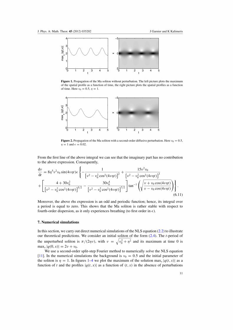
Figure 1. Propagation of the Ma soliton without perturbation. The left picture plots the maximumof the spatial profile as a function of time, the right picture plots the spatial profiles as a functionof time. Here ν0 = 0.5, η = 1.

0 1 2 3 4 50

1

2

3

4

max

x |q(t

,x)|

t t

x

0 1 2 3 4 5

−5

0

5

Figure 2. Propagation of the Ma soliton with a second-order diffusive perturbation. Here ν0 = 0.5,η = 1 and ε = 0.02.

From the first line of the above integral we can see that the imaginary part has no contributionto the above expression. Consequently,

dν

dt= 8η5ν2ν0 sin(4νηt)ε

{− 1[

ν2 − ν20 cos2(4νηt)

]2 + 15ν2ν0[ν2 − ν2

0 cos2(4νηt)]3

+[

4 + 30ν20[

ν2 − ν20 cos2(4νηt)

]5/2 − 30ν40[

ν2 − ν20 cos2(4νηt)

]7/2

]tan−1

(√ν + ν0 cos(4νηt)

ν − ν0 cos(4νηt)

)}.

(6.11)

Moreover, the above rhs expression is an odd and periodic function; hence, its integral overa period is equal to zero. This shows that the Ma soliton is rather stable with respect tofourth-order dispersion, as it only experiences breathing (to first order in ε).

7. Numerical simulations

In this section, we carry out direct numerical simulations of the NLS equation (2.2) to illustrateour theoretical predictions. We consider an initial soliton of the form (2.4). The t-period of

the unperturbed soliton is π/(2ην), with ν =√

ν20 + η2 and its maximum at time 0 is

maxx |q(0, x)| = 2ν + ν0.We use a second-order split-step Fourier method to numerically solve the NLS equation

[11]. In the numerical simulations the background is ν0 = 0.5 and the initial parameter ofthe soliton is η = 1. In figures 1–4 we plot the maximum of the solution maxx |q(t, x)| as afunction of t and the profiles |q(t, x)| as a function of (t, x) in the absence of perturbations

11

J. Phys. A: Math. Theor. 45 (2012) 035202 J Garnier and K Kalimeris

0 1 2 3 4 50

1

2

3

4

max

x |q(t

,x)|

t t

x

0 1 2 3 4 5

−5

0

5

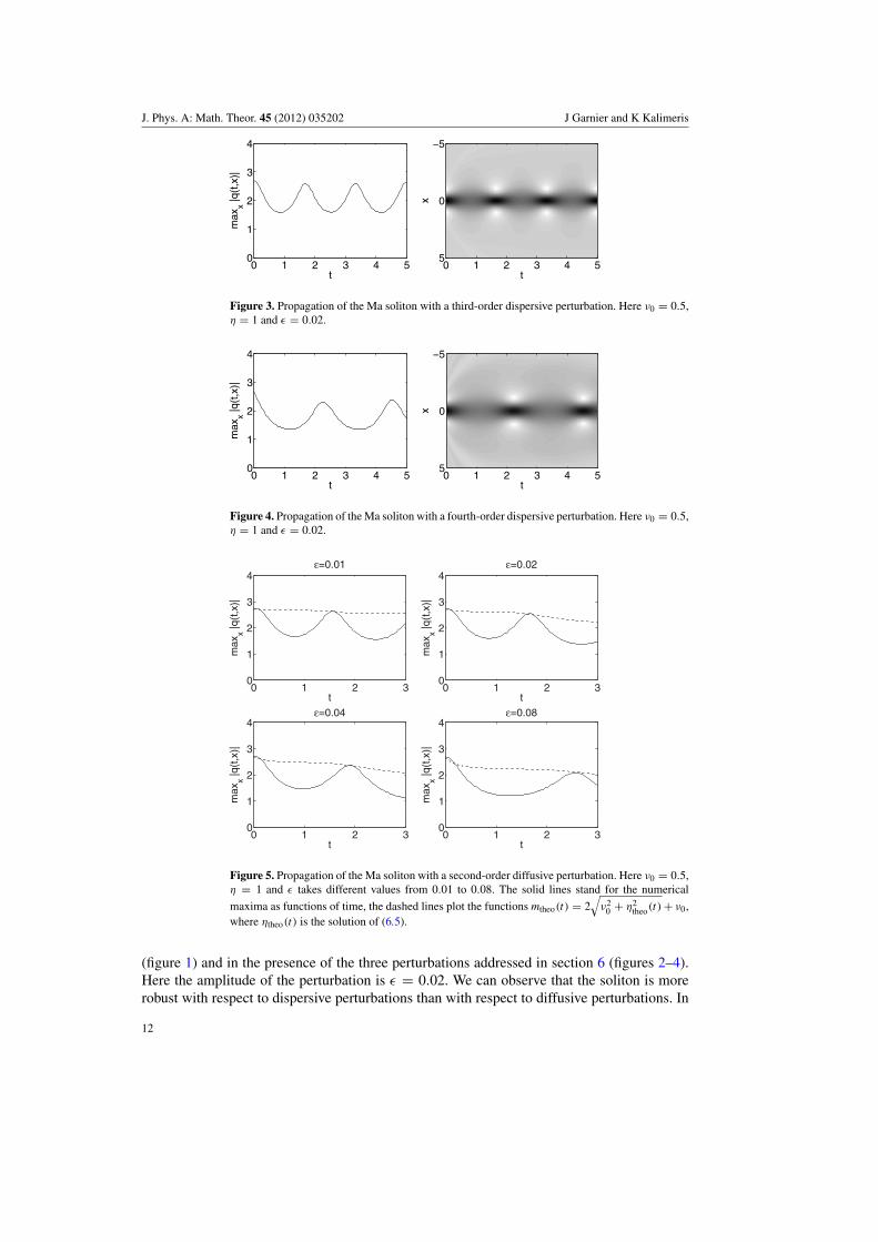
Figure 3. Propagation of the Ma soliton with a third-order dispersive perturbation. Here ν0 = 0.5,η = 1 and ε = 0.02.

0 1 2 3 4 50

1

2

3

4

max

x |q(t

,x)|

t t

x

0 1 2 3 4 5

−5

0

5

Figure 4. Propagation of the Ma soliton with a fourth-order dispersive perturbation. Here ν0 = 0.5,η = 1 and ε = 0.02.

0 1 2 30

1

2

3

4

max

x |q(t

,x)|

t

ε=0.01

0 1 2 30

1

2

3

4

max

x |q(t

,x)|

t

ε=0.02

0 1 2 30

1

2

3

4

max

x |q(t

,x)|

t

ε=0.04

0 1 2 30

1

2

3

4

max

x |q(t

,x)|

t

ε=0.08

Figure 5. Propagation of the Ma soliton with a second-order diffusive perturbation. Here ν0 = 0.5,η = 1 and ε takes different values from 0.01 to 0.08. The solid lines stand for the numerical

maxima as functions of time, the dashed lines plot the functions mtheo(t) = 2√

ν20 + η2

theo(t) + ν0,where ηtheo(t) is the solution of (6.5).

(figure 1) and in the presence of the three perturbations addressed in section 6 (figures 2–4).Here the amplitude of the perturbation is ε = 0.02. We can observe that the soliton is morerobust with respect to dispersive perturbations than with respect to diffusive perturbations. In

12

J. Phys. A: Math. Theor. 45 (2012) 035202 J Garnier and K Kalimeris

particular, we can observe a nice periodic behavior in figure 3 in the case of a third-orderdispersion, as predicted by the theory. The same holds true in the case of a fourth-orderdispersion (figure 4) although the period has changed compared to the unperturbed case.Finally, we can observe a decay of the soliton and a continuous increase of its period in thecase of a diffusive perturbation, which is also in agreement with the theoretical predictions. Tobe complete, we must add that the stability of the soliton also becomes affected by dispersiveperturbations when ε � 0.1. Our theory is therefore valid only for weak perturbations.

More quantitatively, we can numerically integrate the ODE (6.5) to find ηtheo(t), take care

of mtheo(t) = 2νtheo(t) + ν0 = 2√

ν20 + η2

theo(t) + ν0 and compare with the maximum of thesolution after one oscillation. The results are reported in figure 5 for different values of ε,which again shows good agreement.

References

[1] Agrawal G P 2006 Nonlinear Fiber Optics (San Diego, CA: Academic)[2] Akhmediev N, Ankievicz A and Taki M 2009 Waves that appear from nowhere and disappear without a trace

Phys. Lett. A 373 675–8[3] Akhmediev N N, Eleonskii V M and Kulagin N E 1987 Exact first-order solutions of the nonlinear Schrodinger

equation Teor. Mat. Fiz. 72 183–96Akhmediev N N, Eleonskii V M and Kulagin N E 1987 Theor. Math. Phys. 72 809–18

[4] Akhmediev N and Korneed V I 1986 Modulational instability and periodic solutions of the nonlinear Schrodingerequation Theor. Math. Phys. 69 1089–93

[5] Akhmediev N N and Wabnitz S 1992 Phase detecting of solitons by mixing with a continuous-wave backgroundin an optical fiber J. Opt. Soc. Am. B 9 236–42

[6] Ankievicz A, Devine N and Akhmediev N 2009 Are rogue waves robust against perturbations? Phys. Lett.A 373 3997–4000

[7] Draper L 1965 Freak ocean waves Mar. Obs. 35 193–5[8] Dudley J M, Genty G and Coen S 2006 Supercontinuum generation in photonic crystal fiber Rev. Mod.

Phys. 78 1135–84[9] Dudley J M, Finot C, Millot G, Garnier J, Genty G, Agafontsev D and Dias F 2010 Extreme events in optics:

challenges of the MANUREVA project Eur. Phys. J. Spec. Top. 185 125–33[10] Gagnon L 1993 Solitons on a continuous-wave background an collision between two dark pulses: some analytical

results J. Opt. Soc. Am. B 10 469–74[11] Garnier J 1998 Asymptotic transmission of solitons through random media SIAM J. Appl. Math. 58 1969–95[12] Gredeskul S A and Kivshar Y U 1992 Propagation and scattering of nonlinear waves in disordered systems

Phys. Rep. 216 1–61[13] Hadachira H, McLaughlin D W, Moloney J V and Newell A C 1988 Solitary waves as fixed points of infinite-

dimensional maps for an optical bistable ring cavity: analysis J. Math. Phys. 29 63–86[14] Haelterman M, Trillo S and Wabnitz S 1992 Dissipative modulation instability in a nonlinear dispersive ring

cavity Opt. Commun. 91 401–7[15] Karpman V I 1978 Soliton evolution in the presence of perturbation Phys. Scr. 20 462–78[16] Kawata T and Inoue H 1978 Inverse scattering method for the nonlinear evolution equations under nonvanishing

conditions J. Phys. Soc. Japan 4 1722–9[17] Kibler B, Hammani K, Fatome J, Finot C, Millot G, Dias F, Genty G, Akhmediev N and Dudley J M 2010

Peregrine soliton in optical fibre optics Nature Phys. 6 790–5[18] Ma Y-C 1979 The perturbed plane-wave solutions of the cubic Schrodinger equation Stud. Appl. Math. 60 43–58[19] Novikov S P, Manakov S V, Pitaevskii L P and Zakharov V E 1984 Theory of Solitons: The Inverse Scattering

Method (New York: Consultants Bureau)[20] Osborne A R 2009 Nonlinear Ocean Waves (New York: Academic)[21] Peregrine D H 1983 Water waves, nonlinear Schrodinger equations and their solutions J. Aust. Math. Soc. Ser.

B 25 16–43[22] Solli D R, Ropers C, Koonath P and Jalali B 2007 Optical rogue waves Nature 450 1054–7[23] Voronovich V V, Shrira V I and Thomas G 2008 Can bottom friction suppress ‘freak wave’ formation? J. Fluid

Mech. 604 263–96[24] Xu Z Y, Li L, Li Z H and Zhou G S 2003 Modulation instability and solitons on a cw background in an optical

fiber with high-order effects Phys. Rev. E 67 026603

13