Inverse modeling of simplified hygrothermal building models to predict and characterize indoor climates

at SciVerse ScienceDirect

Building and Environment 68 (2013) 87e99

Contents lists available

Building and Environment

journal homepage: www.elsevier .com/locate/bui ldenv

Inverse modeling of simplified hygrothermal building models topredict and characterize indoor climates

Rick Kramer*, Jos van Schijndel, Henk SchellenDepartment of the Built Environment, Eindhoven University of Technology, Den Dolech 2, 5612 AZ Eindhoven, The Netherlands

a r t i c l e i n f o

Article history:Received 23 April 2013Received in revised form31 May 2013Accepted 2 June 2013

Keywords:Inverse modelingParameter identificationSimplified building modelIndoor climate predictionMonumental buildings

* Corresponding author. Tel.: þ31 40 247 5613.E-mail addresses: [email protected] (R. Kramer), a.

Schijndel), [email protected] (H. Schellen).

0360-1323/$ e see front matter � 2013 Elsevier Ltd.http://dx.doi.org/10.1016/j.buildenv.2013.06.001

a b s t r a c t

Computational research on monumental buildings yields three problems regarding currently useddetailed building models: tedious modeling, relatively long simulation run times, difficulties to char-acterize a building by its model parameters. A new simplified hygrothermal building model in state spaceform is presented with an inverse modeling technique to identify its parameters. Based on a literaturereview, 10 thermal models and 5 hygric models were developed. An optimization routine was used to fitthe output of the models to long term hourly measurements of a typical monumental building zone andto a fictive indoor climate that was simulated by a validated simulation tool. The model performance wasassessed by three criteria and the best models were selected. The validation of the selected thermal andhygric models consisted of fitting the models’ output to indoor climate measurements of four monu-mental building zones, a residual analysis and parameter analysis. The results show that the simplifiedhygrothermal model is capable of reproducing most indoor climates accurately. Moreover, the state spacemodel results in fast simulations: 100 years with hourly samples was simulated in 0.45 s on an ordinarycomputer (i5-processor). Characterization and validation of the parameter values are challenging andrequires additional measurements and research.

� 2013 Elsevier Ltd. All rights reserved.

1. Introduction

Monumental buildings and their collections are important as-sets that form our cultural heritage. Unfortunately, they areexposed to all kinds of agents of deterioration, including incorrecttemperature and incorrect relative humidity [1]. A certain indoorclimate quality for the preservation of the collection and thebuilding is required [2]. So, research is performed to relate physicalprocesses of deterioration to the indoor climate [3]. Moreover, it isimportant to consider the building itself [4]: Moisture is the largestissue in historic buildings and needs constant attention [5] andshould therefore be included in research. Excess moisture may leadto condensation, result in wood rot [6] and also causes moldgrowth, which depends on temperature and relative humidity [7].Finally, the effects of climate change on cultural heritage areresearched [8,9]: building simulations are performed with hourlyclimate data for the years 2000 until 2100. This research revealsthat moisture is important to include and will become even moreimportant in the future.

[email protected] (J. van

All rights reserved.

Computational modeling and simulation play a vital role inperforming the aforementioned research on the built cultural her-itage, both in the spatial domain as in the time domain. Increasingcomputational power accelerates developments in building per-formance simulations [10]: the level of details and time scales usednowadays was considered impossible a few years ago. However,three problems are identifiedwith respect to current techniques formodeling monumental buildings: (i) detailed modeling of thebuildings requires much effort since monumental buildings are oldand protected: Blueprints are hard to find and destructive methodsto obtain building material properties are often not allowed; (ii)simulation run times are long due to long simulation periods (up to100 years with time step 1 h) and detailed physical models; (iii)detailed models obstruct an easy characterization of the building.

A simplified building zone model with physical meaning isdesired that is capable of simulating temperature and humidity, inwhich the parameters are identified frommeasurements by inversemodeling. The simplified model is needed for the prediction ofindoor temperature and indoor humidity and for building charac-terization. Inverse modeling implies many repetitive simulations inorder to find the optimum parameters. Therefore, we focus onLinear Time Invariant models, specifically state space models, toensure simulation speed.

Nomenclature

A state matrixB input matrixC output matrixCi effective indoor air capacitance [J/K]Cint effective interior capacitance [J/K]Cw effective envelope capacitance [J/K]D transition matrix3 residuals [�C] or [Pa]fI effective irradiance area [m2]fit goodness of fit [%]Gfast conductance from indoor air to outdoor air [W/K]Gi conductance from indoor air to envelope [W/K]Gint conductance from indoor air to interior [W/K]Gw conductance from envelope to outdoor air [W/K]Irrad solar irradiation [W/m2]mae mean absolute error [�C] or [Pa]mse mean squared error [�C2] or [Pa2]

ODE ordinary differential equationPe outdoor air vapor pressure [Pa]Pfixed fixed vapor pressure [Pa]Pi indoor air vapor pressure [Pa]Pisim simulated indoor air vapor pressure [Pa]Psat saturation pressure [Pa]Pvapor vapor pressure [Pa]RH relative humidity [e] or [%]SG solar gain factor windows [-]Te outdoor air temperature [�C]Tfixed fixed temperature [�C]Ti indoor air temperature [�C]Tint interior temperature [�C]Tisim simulated indoor air temperature [�C]Tw envelope temperature [�C]U input vectorX state vectory output vector

R. Kramer et al. / Building and Environment 68 (2013) 87e9988

The article is structured as follows. Section 2 elaborates on themethodology, Section 3 presents the results: 3.1 deals with statespace performance, 3.2 with simplified model development andassessment, and Section 3.3 deals with model validation. Section 4provides a discussion and Section 5 presents the conclusions.

2. Methodology

2.1. Literature review

Although simplified building models are researched intensively,a literature review was missing. Therefore, a literature review wasperformed to research the state-of-the-art on simplified buildingmodeling and inverse building modeling, generally referred to assystem identification. Mainly, the search engine of Science Directwas used with the following key words: building model, simplifiedbuilding model, lumped building model, linear parametric buildingmodel, neural network building model, inverse building modeling,building parameter identification. Black box models are researchedintensively [11], white box models apply mostly to one buildingcomponent [12], validation is often performed in laboratory con-ditions [13] or in case of real buildings, data include short mea-surement periods [14]. Literature shows that a simplified linearhygrothermal model, with physical meaning, used for inversemodeling of a building zone, validated with long term measure-ments is missing. The outcome of this literature research is re-ported comprehensively in Kramer et al. [15].

2.2. Data acquisition

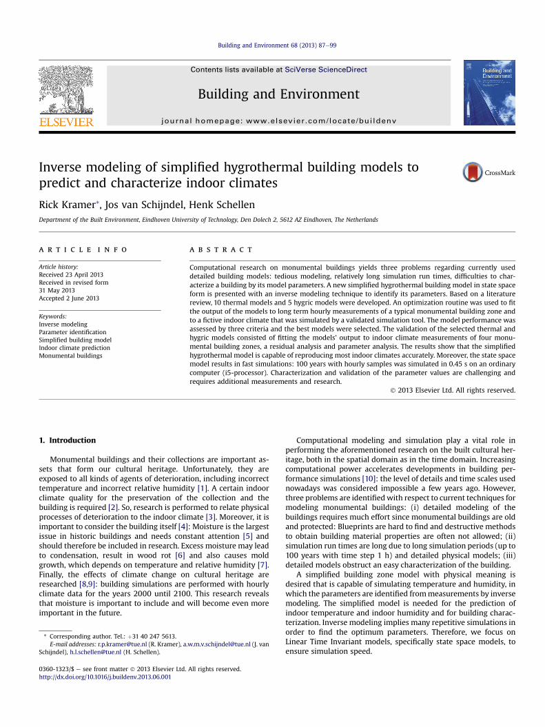
The Building Physics of Monuments group of the University ofTechnology Eindhoven has performed many long term measure-ments in monumental buildings [16]. The measurements includetemperature, relative humidity, surface temperatures, carbon di-oxide concentrations and thermographic images. The monitoredbuildings include castles, churches, cathedrals, museums and othermonumental buildings. These case studies are presented on thePhysics of Monuments webpage [17]. The selected buildings usedfor the results in this study are presented in Fig. 1.

The following indoor climate data were used for model devel-opment: a fictive building zone that was modeled and simulatedwith HAMBase [18], and measurements of Amerongen Castle’sking’s chamber. For model validation, the following indoor climate

measurements were used: Amerongen Castle’s washing room,Gaasbeek Castle’s gothic chamber, Keukenhof Castle’s attic and St.Bavo’s Cathedral’s south transept. Measured outdoor climate datawere provided by the Royal Netherlands Meteorological Institute:temperature, relative humidity and global irradiance on the hori-zontal plane.

Amerongen Castle is situated in the center of the Netherlands. Itis a 17th century building, surrounded by a moat, with massivewalls varying from 0.7 to 1.5m thick. The building covers five floors.The main building materials are brick, wood and slate roofcovering. The king’s chamber is located on the second floor and haswindows oriented to the south and to the east. The indoor climate isfree floating. One adjacent room is not free floating but has limitedheating with setpoint 10 �C. The washing room is located in thebasement and has windows oriented to the south and to the west.The indoor climate is free floating. An important aspect is that thewashing room is adjacent to the moat and has been flooded in thepast due to flooding of the river Rhine affecting the indoor climate’shumidity.

Gaasbeek Castle is situated in Belgium. It was built around 1240AD. Since the year 1924 AD, the castle functions partly as amuseum.The average annual number of visitors is 70.000. The gothicchamber is situated at the second floor and is part of the museumaccessible to public during tours. The room is free floating andwindows are oriented to the southeast.

Keukenhof Castle is situated five kilometers from the west coastof the Netherlands. The room of interest for this research is theattic. From measurements, it turns out that the attic overheatsduring summer days. Therefore the attic is an interesting room touse for validation purposes. The overheating is due to sun irradi-ance on the thin roof covering.

St. Bavo’s Cathedral is situated in Belgium. The measurementswere performed in the south transept. Fig. 1 [bottom-right] showsthe exterior and the glazing in the south transept’s façade. Theinfluence of solar irradiance and themassive constructionmake themeasurement data particularly valuable for model validation.

The indoor temperature and the relative humidity weremeasured by using combined digital humidity and temperaturesensors. The relative humidity sensors have an absolute accuracy of�2% RH from 10 to 90% RH, and the temperature sensors have anaccuracy of �0.5 �C from 0 to 40 �C [19]. The sensors inside thebuildings were placed at a height of 1e2 m above floor level. Toobtain uniform room conditions, sensors were placed at the best

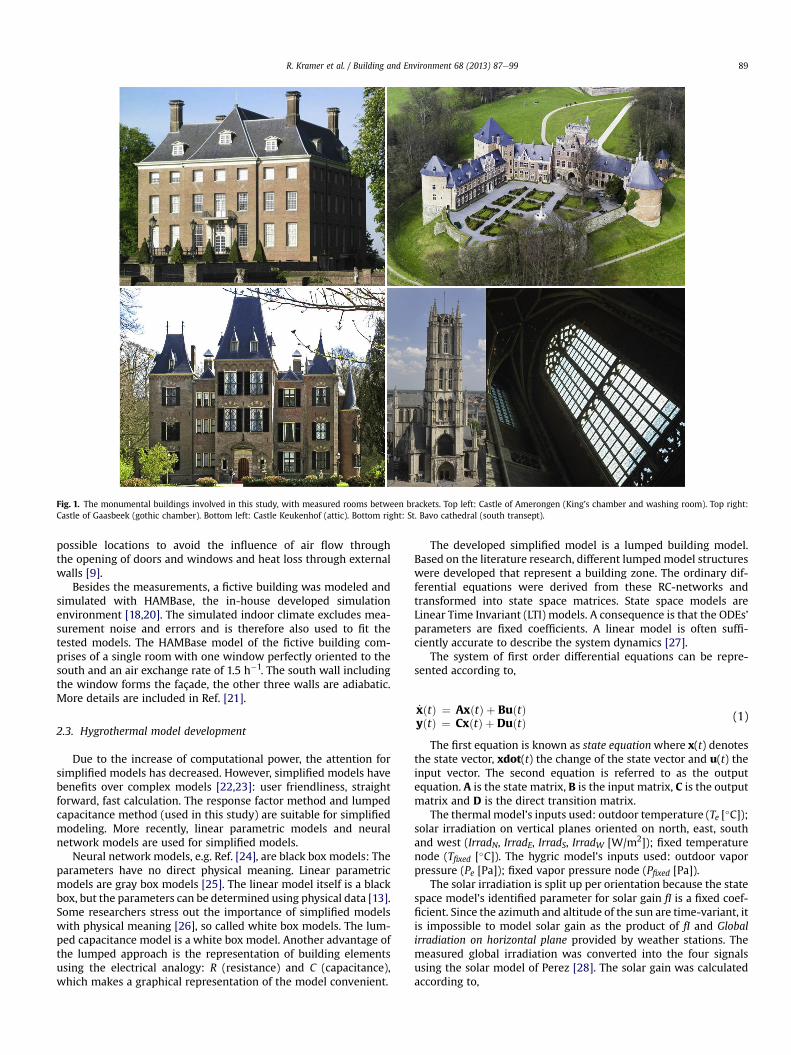
Fig. 1. The monumental buildings involved in this study, with measured rooms between brackets. Top left: Castle of Amerongen (King’s chamber and washing room). Top right:Castle of Gaasbeek (gothic chamber). Bottom left: Castle Keukenhof (attic). Bottom right: St. Bavo cathedral (south transept).

R. Kramer et al. / Building and Environment 68 (2013) 87e99 89

possible locations to avoid the influence of air flow throughthe opening of doors and windows and heat loss through externalwalls [9].

Besides the measurements, a fictive building was modeled andsimulated with HAMBase, the in-house developed simulationenvironment [18,20]. The simulated indoor climate excludes mea-surement noise and errors and is therefore also used to fit thetested models. The HAMBase model of the fictive building com-prises of a single room with one window perfectly oriented to thesouth and an air exchange rate of 1.5 h�1. The south wall includingthe window forms the façade, the other three walls are adiabatic.More details are included in Ref. [21].

2.3. Hygrothermal model development

Due to the increase of computational power, the attention forsimplified models has decreased. However, simplified models havebenefits over complex models [22,23]: user friendliness, straightforward, fast calculation. The response factor method and lumpedcapacitance method (used in this study) are suitable for simplifiedmodeling. More recently, linear parametric models and neuralnetwork models are used for simplified models.

Neural network models, e.g. Ref. [24], are black box models: Theparameters have no direct physical meaning. Linear parametricmodels are gray box models [25]. The linear model itself is a blackbox, but the parameters can be determined using physical data [13].Some researchers stress out the importance of simplified modelswith physical meaning [26], so called white box models. The lum-ped capacitance model is a white box model. Another advantage ofthe lumped approach is the representation of building elementsusing the electrical analogy: R (resistance) and C (capacitance),which makes a graphical representation of the model convenient.

The developed simplified model is a lumped building model.Based on the literature research, different lumpedmodel structureswere developed that represent a building zone. The ordinary dif-ferential equations were derived from these RC-networks andtransformed into state space matrices. State space models areLinear Time Invariant (LTI) models. A consequence is that the ODEs’parameters are fixed coefficients. A linear model is often suffi-ciently accurate to describe the system dynamics [27].

The system of first order differential equations can be repre-sented according to,

_xðtÞ ¼ AxðtÞ þ BuðtÞyðtÞ ¼ CxðtÞ þ DuðtÞ (1)

The first equation is known as state equationwhere x(t) denotesthe state vector, xdot(t) the change of the state vector and u(t) theinput vector. The second equation is referred to as the outputequation. A is the state matrix, B is the input matrix, C is the outputmatrix and D is the direct transition matrix.

The thermal model’s inputs used: outdoor temperature (Te [�C]);solar irradiation on vertical planes oriented on north, east, southand west (IrradN, IrradE, IrradS, IrradW [W/m2]); fixed temperaturenode (Tfixed [�C]). The hygric model’s inputs used: outdoor vaporpressure (Pe [Pa]); fixed vapor pressure node (Pfixed [Pa]).

The solar irradiation is split up per orientation because the statespace model’s identified parameter for solar gain fI is a fixed coef-ficient. Since the azimuth and altitude of the sun are time-variant, itis impossible to model solar gain as the product of fI and Globalirradiation on horizontal plane provided by weather stations. Themeasured global irradiation was converted into the four signalsusing the solar model of Perez [28]. The solar gain was calculatedaccording to,

Fig. 2. Optimization process.

Fig. 3. Genetic Algorithm, PatternSearch and fmincon were used to find the optimum.After every optimization, bounds were checked to ensure that the parameter valuesdid not coincide with boundary conditions.

R. Kramer et al. / Building and Environment 68 (2013) 87e9990

SG ¼ fI!� Irrad���! ¼

2664fINfIEfISfIW

3775 �

2664IrNIrEIrSIrW

3775 (2)

The input Pe of the hygric model was calculated from mea-surements RHe and Te according to [29],

Pvapor ¼ PsatðTÞ$RH (3)

in which Psat was calculated for T � 0 �C according to

Psat ¼ 611$e17:08$T=ð234:18þTÞ (4)

and for T < 0 �C calculated according to

Psat ¼ 611$e22:44$T=ð272:44þTÞ (5)

RHisim was calculated analogous from Pisim and Tisim. So, theoutput of the thermal model (Tisim) was used together with theoutput of the hygric model (Pisim) to calculate the indoor relativehumidity (RHisim). Consequently, the errors in the indoor relativehumidity are influenced by both the thermal and hygric models’errors. Nevertheless, relative humidity was used since it is morecomprehensible and more meaningful than vapor pressure.

Other climate data as precipitation and wind, were excluded tokeep the amount of parameters at a minimum. This is a veryimportant aspect: more parameters lead to a higher uncertainty inparameter estimation [27].

2.4. Inverse modeling

Inverse modeling is the inverse of traditional modeling. Intraditional modeling, the system is known and the output is un-known. By modeling the system, the output can be simulated. Ininverse modeling, the output is known, e.g. measured, but little isknown about the systems parameters. The goal is to find theparameter set that minimizes the error between the simulationresult and the measurements, according to

bqN ¼ argminq1N

XNk¼1

ε2ðt; qÞ (6)

with bqN being the estimated parameters based on a data set with Nsamples, ε(t,q) being the simulation error depending on the timeand parameter value. If the solution space includes multipleminima, the goal is to find the global minimum, called globaloptimization.

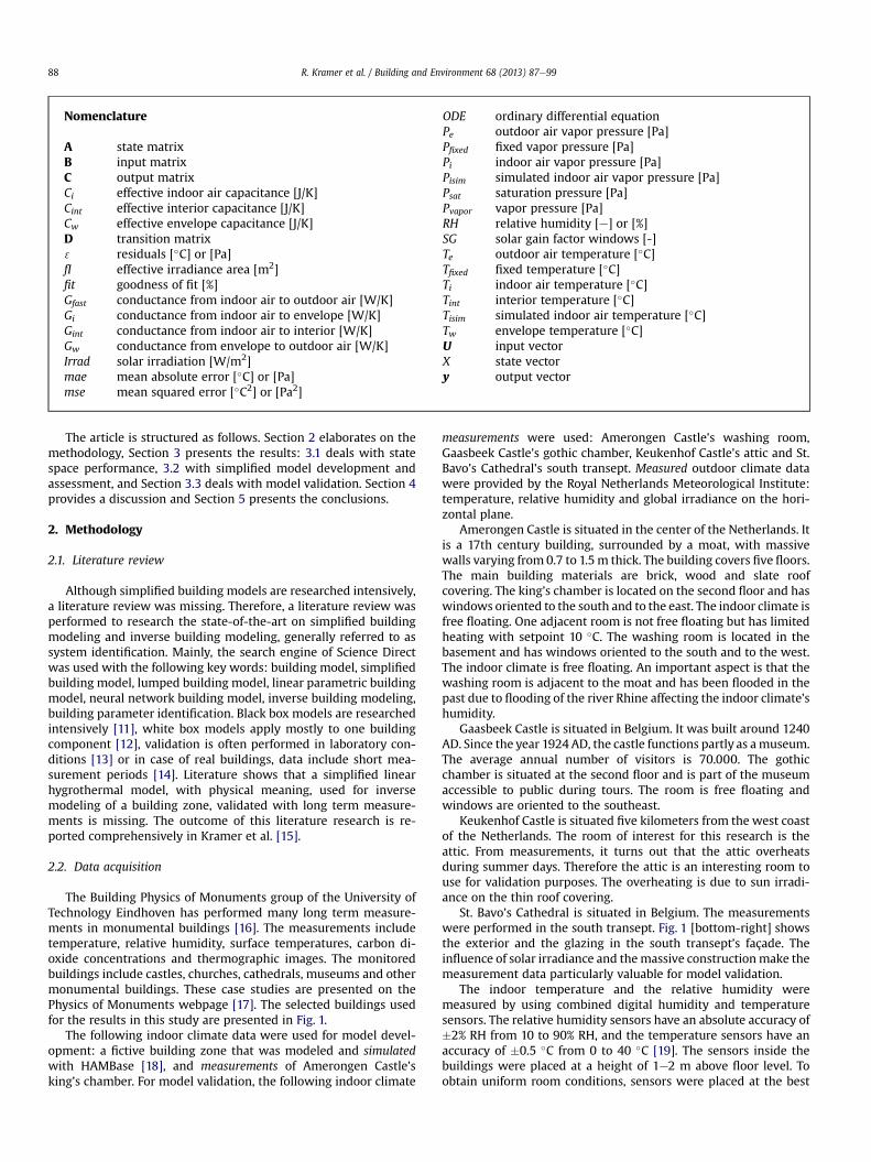
To maximize the speed of the optimization process, see Fig. 2, allcalculations that do not need to be repeated were executed in theinitialization step: preparing climate data, including measurementdata, set constraints and set initial values. The function file includesthe model and simulates the model with the given parameter setand calculates the objective function by comparing the simulationresult to measurements. The objective function is passed to theGlobal Optimization Algorithm that calculates the new parameterset that is likely to decrease the objective function.

The optimization process as presented in Fig. 2 was sequen-tially executed with different solvers. Although Genetic Algo-rithms gain popularity by researchers [11,30e34], it is known thatsuch Evolutionary Algorithms only find a near-optimum solution.However, Genetic Algorithm is computationally efficient and canhandle large solution spaces. Therefore, GA was used to find anapproximate solution and set the identified parameter values asthe new initial values [35,36]. Then the new initial values wereused with the PatternSearch algorithm to search the global

solution space thoroughly. Again, the identified parameter valueswere set as new initial values. Eventually, the new initial valueswere used with fmincon, a local solver, to check the solution orimprove it (fmincon finds the optimum more precisely than theother algorithms). This is illustrated in Fig. 3. These algorithms areincluded in MATLAB’s Global Optimization Toolbox and Optimi-zation Toolbox.

2.5. Performance validation

The validation consisted of applying the model to four monu-mental building zones, a residual analysis and a parameter analysis.To quantify the model’s accuracy, three performance criteria wereused: the mean squared error (mse), the mean absolute error (mae)and goodness of fit (fit). The mse is calculated according to,

mse ¼ 1N

XNk¼1

�y’ � y

�2(7)

where y’ is the measured signal, y is the simulated signal and N thenumber of samples. The mae was calculated according to,

mae ¼ 1N

XNk¼1

���y’ � y��� (8)

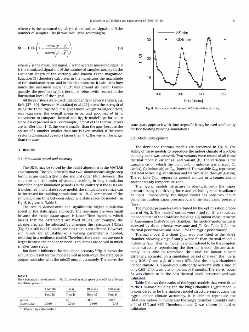
Fig. 4. State space model versus ode23 simulation accuracy.

R. Kramer et al. / Building and Environment 68 (2013) 87e99 91

where y’ is the measured signal, y is the simulated signal and N thenumber of samples. The fit was calculated according to,

fit ¼ 100$

0@1� norm�y’ � y

�norm

�y’ � y’

1A (9)

where y’ is the measured signal, y’ is the averagemeasured signal, yis the simulated signal and N the number of samples. norm(y) is theEuclidean length of the vector y, also known as the magnitude.Equation (9) therefore calculates in the numerator the magnitudeof the simulation error, and in the denominator, it calculates howmuch the measured signal fluctuates around its mean. Conse-quently, the goodness of fit criterion is robust with respect to thefluctuation level of the signal.

All three criteriawere used independently in several studies, e.g.Refs. [37e39]. However, Mustafaraj et al. [25] stress the strength ofusing the three together: mse gives more weight to larger errors,mae expresses the overall mean error, and goodness of fit isconvenient to compare thermal and hygric model’s performancesince it is expressed in %. For example, if most of the thermal errorsare smaller than 1 �C, the mse is smaller than the mae, because thesquare of a number smaller than one is even smaller. If the errorvector is dominated by errors larger than 1 �C, themsewill be largerthan the mae.

3. Results

3.1. Simulation speed and accuracy

The ODEs may be solved by the ode23 algorithm in the MATLABenvironment. The ‘23’ indicates that two simultaneous single-stepformulas are used: a 2nd order and 3rd order [40]. However, thestep size is in the order of seconds resulting in long simulationtimes for longer simulation periods. On the contrary, if the ODEs aretransformed into a state space model, the simulation step size canbe increased for building simulations to 1 h. A comparison of thesimulation run time between ode23 and state space for model 1 inFig. 5, is given in Table 1.

The results demonstrate the significantly higher simulationspeed of the state space approach. The run-times are very smallbecause the model (state space) is Linear Time Invariant, whichmeans that the parameters are fixed values. For example, theglazing area can be adjusted by changing the resistance 1/Gfast(Fig. 5). It still is a LTI model and run-time is not affected. However,sun blinds are adjustable, so a varying parameter is needed,resulting in a nonlinear model. Therefore, the run-times are muchlarger because the nonlinear model’s equations are solved in muchsmaller time steps.

But does it influence the simulation accuracy? Fig. 4 shows thesimulation result for themodel solved in bothways. The state spaceoutput coincides with the ode23 output accurately. Therefore, the

Table 1The calculation time of model 1 (Fig. 5), solved as state space or ode23 for differentsimulation periods.

1 Month 1 Year 10 Years 100 Years

Time [s] Time [s] Time [s] Time [s]

ode23 5 89 9̴00a 9̴000a

State space 0.016 0.016 0.050 0.45

a Obtained by extrapolation.

state space approachwith time steps of 1 hmay be used confidentlyfor free floating building simulations.

3.2. Model development

The developed thermal models are presented in Fig. 5. Theability of these models to reproduce the indoor climate of a wholebuilding zone was assessed. Two variants were tested of all thesethermal models: variant (a) and variant (b). The variation is thecapacitance on which the input solar irradiance was placed: Cw(walls), Ci (indoor air) or Cint (interior). The variable Gfast representsfast heat losses, e.g. ventilation and transmission through glazing.The variable Tfixed represents ground contact or a connection toanother steady temperature zone.

The hygric models’ structure is identical, with the vaporpressure being the driving force and excluding solar irradianceas input. Consequently, the hygric model has only two inputsbeing the outdoor vapor pressure Pe and the fixed vapor pressurePfixed.

The models parameters were tuned by the optimization proce-dure of Fig. 3. The models’ output were fitted to: (i) a simulatedindoor climate of the HAMBase building; (ii) indoor measurementsof Amerongen Castle’s king’s chamber. The models’ performance isassessed by three criteria: mse, mae and fit. See Table 2 for thethermal performance and Table 3 for the hygric performance.

Thermal model 2 without Tfixed was also fitted to the king’schamber, showing a significantly worse fit than thermal model 2including Tfixed. Thermal model 3a is considered to be the simplestmodel structure reproducing the thermal indoor climate accu-rately. It is able to reproduce the HAMBase indoor climateextremely accurate: on a simulation period of a year, the mse isonly 0.05 �C and a fit of almost 97%. Also the king’s chamber’sindoor climate is reproduced sufficiently accurate with a mse ofonly 0.63 �C for a simulation period of 8 months. Therefore, model3a was chosen to be the best thermal model structure and wasvalidated.

Table 3 shows the results of the hygric models that were fittedto the HAMBase building and the king’s chamber. Hygric model 2is considered to be the simplest model structure reproducing thehygric indoor climate accurately. It is able to reproduce theHAMBase indoor humidity and the king’s chamber humidity witha fit of 81% and 86%. Therefore, model 2 was chosen for furthervalidation.

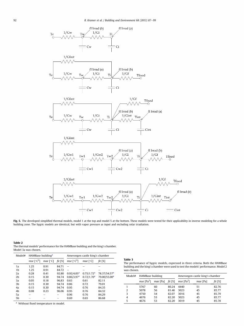
Fig. 5. The developed simplified thermal models, model 1 at the top and model 5 at the bottom. These models were tested for their applicability in inverse modeling for a wholebuilding zone. The hygric models are identical, but with vapor pressure as input and excluding solar irradiation.

Table 2The thermalmodels’ performance for the HAMBase building and the king’s chamber.Model 3a was chosen.

Model# HAMBase buildinga Amerongen castle king’s chamber

mse [�C2] mae [�C] fit [%] mse [�C2] mae [�C] fit [%]

1a 1.25 0.91 84.71 e e e

1b 1.25 0.91 84.72 e e e

2a 0.28 0.41 92.80 0.92/4.05a 0.75/1.72a 78.37/54.57a

2b 0.15 0.30 94.74 0.86/3.97a 0.72/1.70a 79.00/55.00a

3a 0.05 0.18 96.83 0.63 0.61 82.113b 0.15 0.30 94.74 0.86 0.72 79.014a 0.15 0.30 94.74 0.95 0.76 84.354b 0.08 0.23 96.06 0.95 0.76 84.325a e e e 0.96 0.76 84.295b e e e 0.69 0.65 86.68

a Without fixed temperature in model.

Table 3The performance of hygric models, expressed in three criteria. Both the HAMBasebuilding and the king’s chamberwere used to test themodels’ performance. Model 2was chosen.

Model# HAMBase building Amerongen castle king’s chamber

mse [Pa2] mae [Pa] fit [%] mse [Pa2] mae [Pa] fit [%]

1 5767 60 80.24 4440 51 82.762 5078 56 81.46 3023 45 85.773 4750 54 82.07 3016 45 85.794 4676 53 82.20 3023 45 85.775 4676 53 82.20 3019 45 85.78

R. Kramer et al. / Building and Environment 68 (2013) 87e9992

0 1000 2000 3000 40005

10

15Ti

[°C

]

time [hours]

meassim

0 1000 2000 3000 4000

50

70

90

RH

[%]

time [hours]

meas sim

3050 3150 3250

12

13

14

time [hours]

3050 3150 3250

70

75

80

time [hours]

Fig. 6. The thermal model (top) and hygric model (bottom) fitted to Amerongen Castle’s washing room.

R. Kramer et al. / Building and Environment 68 (2013) 87e99 93

The ODEs of the selected thermal and hygric models are,

CwTdTwdt ¼ GwT ðTe�TwÞ�GiT ðTw�TiÞ

CiTdTidt ¼ GiT ðTw�TiÞ�GfT

�Ti�Tf

��GintT ðTi�TintÞþGfastT ðTe�TiÞ

CintTdTintdt ¼ GintTðTi�TintÞþ fI

!� Irrad���!CwP

dPwdt ¼ GwPðPe�PwÞ�GiPðPw�PiÞ

CiPdPidt ¼ GiPðPw�PiÞþGfastPðPe�PiÞ

(10)

The models were aggregated in state space form, see AppendixA for the state space matrices.

0 1000 2000 3000

5

15

25

Ti [°

C]

time [hours]

0 1000 2000 3000

45

65

85

RH

[%]

time [hours]

Fig. 7. The thermal model (top) and hygric model (bo

3.3. Validation

3.3.1. Case studiesThe simplified hygrothermal model was fitted to indoor climate

measurements of four monumental building zones: AmerongenCastle’s washing room, Gaasbeek Castle’s gothic chamber, Keu-kenhof Castle’s Attic and St. Bavo’s Cathedral’s south transept. Asmentioned before, the hygric model’s input Pe was calculated frommeasured Te and RHe. Accordingly, the hygric model’s output is Pisim.Because RH is more comprehensible, RHisim was calculated fromTisim and Pisim. The Figs. 6e9 show the results of the inversemodeling procedure in time plots: the entire simulation period atthe left side and a detail view at the right side.

Fig. 10 shows the simulation errors of the thermal and hygricbuilding model of the washing room, gothic chamber, attic and

4000

meassim

4000

meassim

1750 1850 1950

17

20

23

time [hours]

1750 1850 1950

50

55

60

time [hours]

ttom) fitted to Gaasbeek Castle’s gothic chamber.

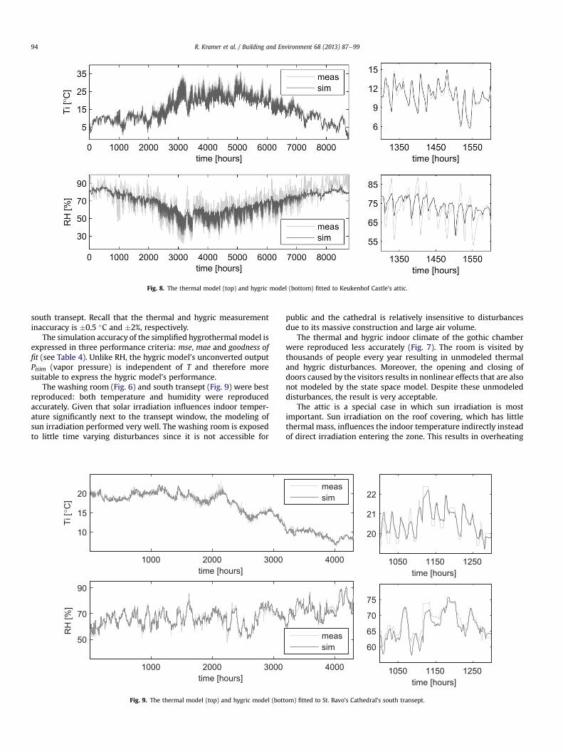
Fig. 8. The thermal model (top) and hygric model (bottom) fitted to Keukenhof Castle’s attic.

R. Kramer et al. / Building and Environment 68 (2013) 87e9994

south transept. Recall that the thermal and hygric measurementinaccuracy is �0.5 �C and �2%, respectively.

The simulation accuracy of the simplified hygrothermalmodel isexpressed in three performance criteria: mse, mae and goodness offit (see Table 4). Unlike RH, the hygric model’s unconverted outputPisim (vapor pressure) is independent of T and therefore moresuitable to express the hygric model’s performance.

The washing room (Fig. 6) and south transept (Fig. 9) were bestreproduced: both temperature and humidity were reproducedaccurately. Given that solar irradiation influences indoor temper-ature significantly next to the transept window, the modeling ofsun irradiation performed very well. The washing room is exposedto little time varying disturbances since it is not accessible for

1000 2000 3000

10

15

20

Ti [°

C]

time [hours]

1000 2000 3000

50

70

90

RH

[%]

time [hours]

Fig. 9. The thermal model (top) and hygric model (bott

public and the cathedral is relatively insensitive to disturbancesdue to its massive construction and large air volume.

The thermal and hygric indoor climate of the gothic chamberwere reproduced less accurately (Fig. 7). The room is visited bythousands of people every year resulting in unmodeled thermaland hygric disturbances. Moreover, the opening and closing ofdoors caused by the visitors results in nonlinear effects that are alsonot modeled by the state space model. Despite these unmodeleddisturbances, the result is very acceptable.

The attic is a special case in which sun irradiation is mostimportant. Sun irradiation on the roof covering, which has littlethermal mass, influences the indoor temperature indirectly insteadof direct irradiation entering the zone. This results in overheating

4000

meassim

4000

meassim

1050 1150 1250

20

21

22

time [hours]

1050 1150 1250

60

65

70

75

time [hours]

om) fitted to St. Bavo’s Cathedral’s south transept.

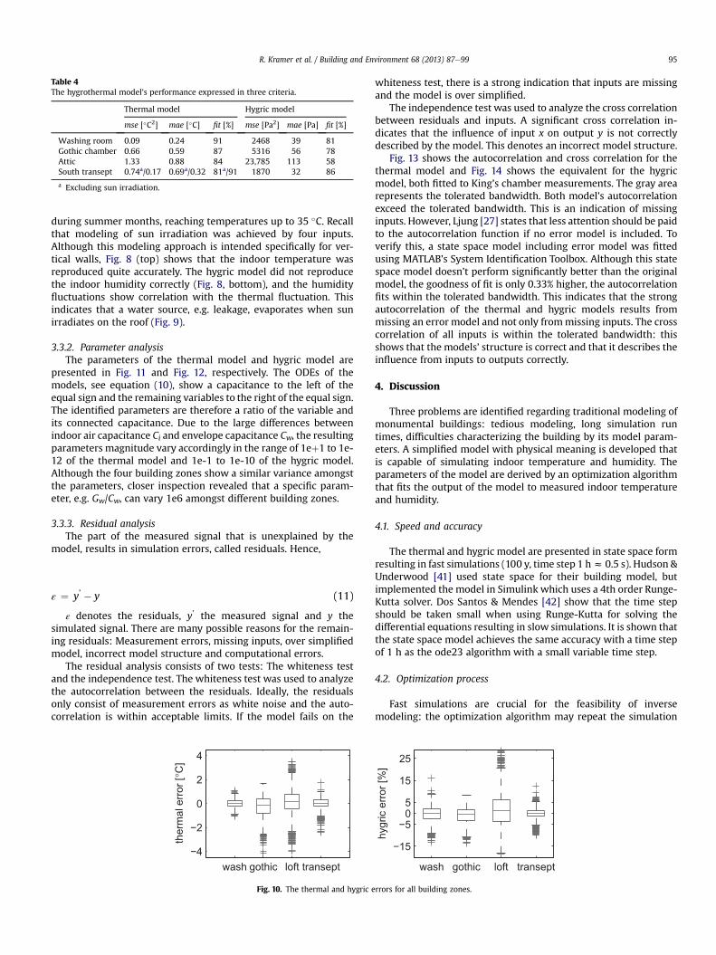
Table 4The hygrothermal model’s performance expressed in three criteria.

Thermal model Hygric model

mse [�C2] mae [�C] fit [%] mse [Pa2] mae [Pa] fit [%]

Washing room 0.09 0.24 91 2468 39 81Gothic chamber 0.66 0.59 87 5316 56 78Attic 1.33 0.88 84 23,785 113 58South transept 0.74a/0.17 0.69a/0.32 81a/91 1870 32 86

a Excluding sun irradiation.

R. Kramer et al. / Building and Environment 68 (2013) 87e99 95

during summer months, reaching temperatures up to 35 �C. Recallthat modeling of sun irradiation was achieved by four inputs.Although this modeling approach is intended specifically for ver-tical walls, Fig. 8 (top) shows that the indoor temperature wasreproduced quite accurately. The hygric model did not reproducethe indoor humidity correctly (Fig. 8, bottom), and the humidityfluctuations show correlation with the thermal fluctuation. Thisindicates that a water source, e.g. leakage, evaporates when sunirradiates on the roof (Fig. 9).

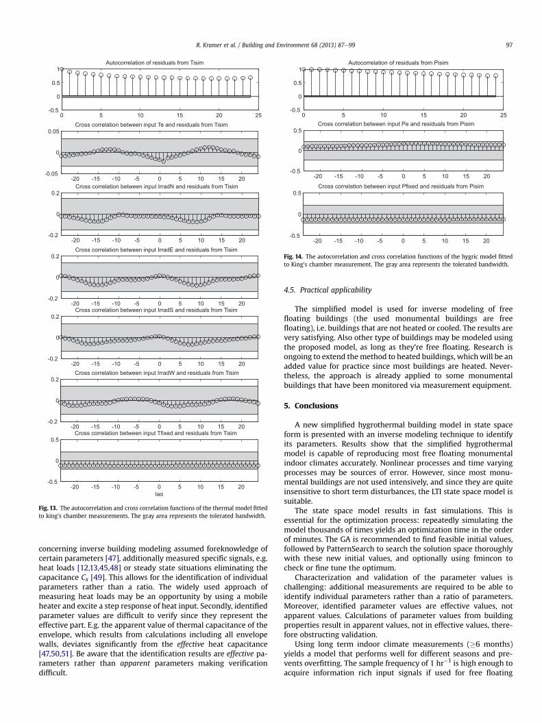
3.3.2. Parameter analysisThe parameters of the thermal model and hygric model are

presented in Fig. 11 and Fig. 12, respectively. The ODEs of themodels, see equation (10), show a capacitance to the left of theequal sign and the remaining variables to the right of the equal sign.The identified parameters are therefore a ratio of the variable andits connected capacitance. Due to the large differences betweenindoor air capacitance Ci and envelope capacitance Cw, the resultingparameters magnitude vary accordingly in the range of 1eþ1 to 1e-12 of the thermal model and 1e-1 to 1e-10 of the hygric model.Although the four building zones show a similar variance amongstthe parameters, closer inspection revealed that a specific param-eter, e.g. Gw/Cw, can vary 1e6 amongst different building zones.

3.3.3. Residual analysisThe part of the measured signal that is unexplained by the

model, results in simulation errors, called residuals. Hence,

ε ¼ y’ � y (11)

ε denotes the residuals, y’ the measured signal and y thesimulated signal. There are many possible reasons for the remain-ing residuals: Measurement errors, missing inputs, over simplifiedmodel, incorrect model structure and computational errors.

The residual analysis consists of two tests: The whiteness testand the independence test. The whiteness test was used to analyzethe autocorrelation between the residuals. Ideally, the residualsonly consist of measurement errors as white noise and the auto-correlation is within acceptable limits. If the model fails on the

wash gothic loft transept−4

−2

0

2

4

ther

mal

erro

r [°C

]

Fig. 10. The thermal and hygric e

whiteness test, there is a strong indication that inputs are missingand the model is over simplified.

The independence test was used to analyze the cross correlationbetween residuals and inputs. A significant cross correlation in-dicates that the influence of input x on output y is not correctlydescribed by the model. This denotes an incorrect model structure.

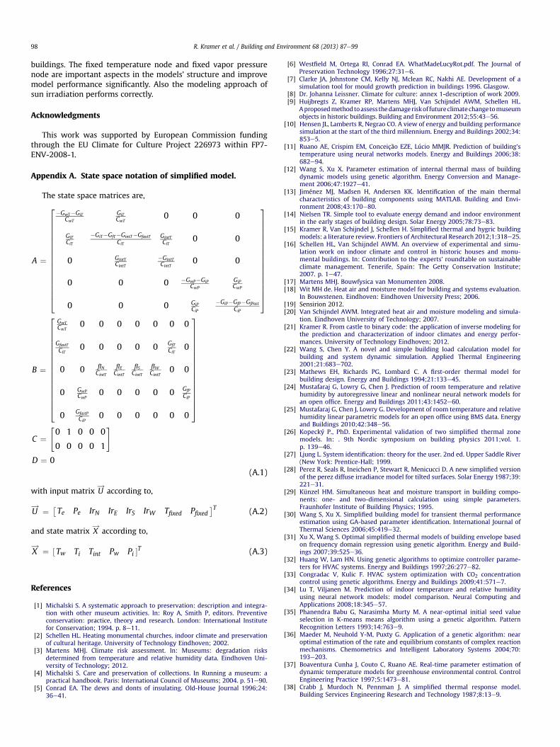
Fig. 13 shows the autocorrelation and cross correlation for thethermal model and Fig. 14 shows the equivalent for the hygricmodel, both fitted to King’s chamber measurements. The gray arearepresents the tolerated bandwidth. Both model’s autocorrelationexceed the tolerated bandwidth. This is an indication of missinginputs. However, Ljung [27] states that less attention should be paidto the autocorrelation function if no error model is included. Toverify this, a state space model including error model was fittedusing MATLAB’s System Identification Toolbox. Although this statespace model doesn’t perform significantly better than the originalmodel, the goodness of fit is only 0.33% higher, the autocorrelationfits within the tolerated bandwidth. This indicates that the strongautocorrelation of the thermal and hygric models results frommissing an error model and not only frommissing inputs. The crosscorrelation of all inputs is within the tolerated bandwidth: thisshows that the models’ structure is correct and that it describes theinfluence from inputs to outputs correctly.

4. Discussion

Three problems are identified regarding traditional modeling ofmonumental buildings: tedious modeling, long simulation runtimes, difficulties characterizing the building by its model param-eters. A simplified model with physical meaning is developed thatis capable of simulating indoor temperature and humidity. Theparameters of the model are derived by an optimization algorithmthat fits the output of the model to measured indoor temperatureand humidity.

4.1. Speed and accuracy

The thermal and hygric model are presented in state space formresulting in fast simulations (100 y, time step 1 hz 0.5 s). Hudson &Underwood [41] used state space for their building model, butimplemented the model in Simulink which uses a 4th order Runge-Kutta solver. Dos Santos & Mendes [42] show that the time stepshould be taken small when using Runge-Kutta for solving thedifferential equations resulting in slow simulations. It is shown thatthe state space model achieves the same accuracy with a time stepof 1 h as the ode23 algorithm with a small variable time step.

4.2. Optimization process

Fast simulations are crucial for the feasibility of inversemodeling: the optimization algorithm may repeat the simulation

wash gothic loft transept

−15

−505

15

25

hygr

ic e

rror [

%]

rrors for all building zones.

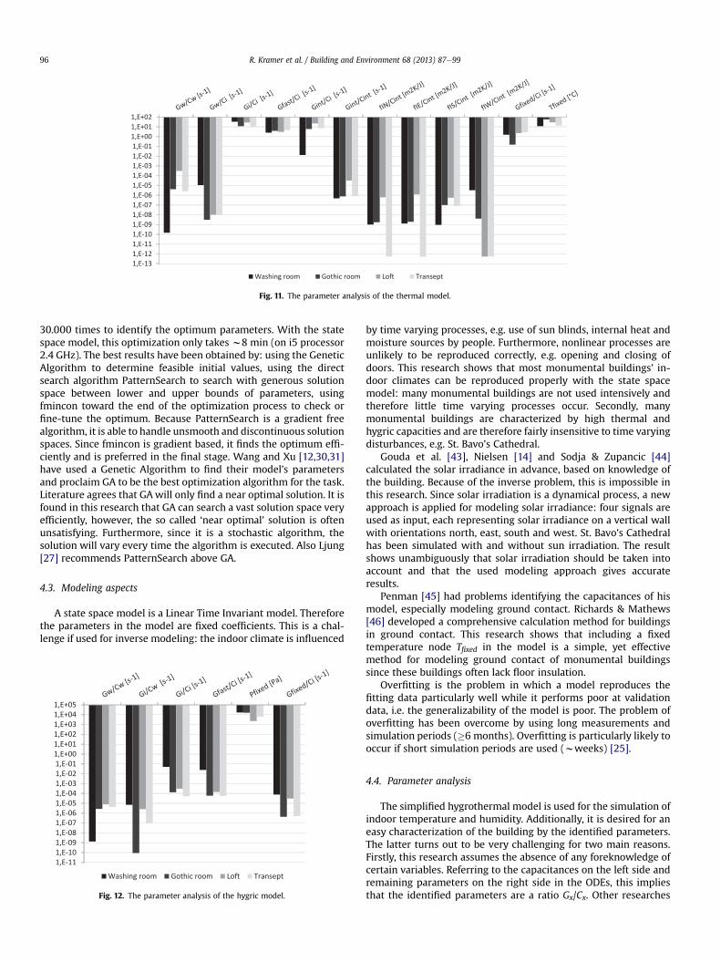
Fig. 11. The parameter analysis of the thermal model.

R. Kramer et al. / Building and Environment 68 (2013) 87e9996

30.000 times to identify the optimum parameters. With the statespace model, this optimization only takes w8 min (on i5 processor2.4 GHz). The best results have been obtained by: using the GeneticAlgorithm to determine feasible initial values, using the directsearch algorithm PatternSearch to search with generous solutionspace between lower and upper bounds of parameters, usingfmincon toward the end of the optimization process to check orfine-tune the optimum. Because PatternSearch is a gradient freealgorithm, it is able to handle unsmooth and discontinuous solutionspaces. Since fmincon is gradient based, it finds the optimum effi-ciently and is preferred in the final stage. Wang and Xu [12,30,31]have used a Genetic Algorithm to find their model’s parametersand proclaim GA to be the best optimization algorithm for the task.Literature agrees that GAwill only find a near optimal solution. It isfound in this research that GA can search a vast solution space veryefficiently, however, the so called ‘near optimal’ solution is oftenunsatisfying. Furthermore, since it is a stochastic algorithm, thesolution will vary every time the algorithm is executed. Also Ljung[27] recommends PatternSearch above GA.

4.3. Modeling aspects

A state space model is a Linear Time Invariant model. Thereforethe parameters in the model are fixed coefficients. This is a chal-lenge if used for inverse modeling: the indoor climate is influenced

Fig. 12. The parameter analysis of the hygric model.

by time varying processes, e.g. use of sun blinds, internal heat andmoisture sources by people. Furthermore, nonlinear processes areunlikely to be reproduced correctly, e.g. opening and closing ofdoors. This research shows that most monumental buildings’ in-door climates can be reproduced properly with the state spacemodel: many monumental buildings are not used intensively andtherefore little time varying processes occur. Secondly, manymonumental buildings are characterized by high thermal andhygric capacities and are therefore fairly insensitive to time varyingdisturbances, e.g. St. Bavo’s Cathedral.

Gouda et al. [43], Nielsen [14] and Sodja & Zupancic [44]calculated the solar irradiance in advance, based on knowledge ofthe building. Because of the inverse problem, this is impossible inthis research. Since solar irradiation is a dynamical process, a newapproach is applied for modeling solar irradiance: four signals areused as input, each representing solar irradiance on a vertical wallwith orientations north, east, south and west. St. Bavo’s Cathedralhas been simulated with and without sun irradiation. The resultshows unambiguously that solar irradiation should be taken intoaccount and that the used modeling approach gives accurateresults.

Penman [45] had problems identifying the capacitances of hismodel, especially modeling ground contact. Richards & Mathews[46] developed a comprehensive calculation method for buildingsin ground contact. This research shows that including a fixedtemperature node Tfixed in the model is a simple, yet effectivemethod for modeling ground contact of monumental buildingssince these buildings often lack floor insulation.

Overfitting is the problem in which a model reproduces thefitting data particularly well while it performs poor at validationdata, i.e. the generalizability of the model is poor. The problem ofoverfitting has been overcome by using long measurements andsimulation periods (�6 months). Overfitting is particularly likely tooccur if short simulation periods are used (wweeks) [25].

4.4. Parameter analysis

The simplified hygrothermal model is used for the simulation ofindoor temperature and humidity. Additionally, it is desired for aneasy characterization of the building by the identified parameters.The latter turns out to be very challenging for two main reasons.Firstly, this research assumes the absence of any foreknowledge ofcertain variables. Referring to the capacitances on the left side andremaining parameters on the right side in the ODEs, this impliesthat the identified parameters are a ratio Gx/Cx. Other researches

0 5 10 15 20 25-0.5

0

0.5

1Autocorrelation of residuals from Pisim

-20 -15 -10 -5 0 5 10 15 20-0.5

0

0.5Cross correlation between input Pe and residuals from Pisim

-20 -15 -10 -5 0 5 10 15 20-0.5

0

0.5Cross correlation between input Pfixed and residuals from Pisim

Fig. 14. The autocorrelation and cross correlation functions of the hygric model fittedto King’s chamber measurement. The gray area represents the tolerated bandwidth.

-20 -15 -10 -5 0 5 10 15 20-0.05

0

0.05Cross correlation between input Te and residuals from Tisim

-20 -15 -10 -5 0 5 10 15 20-0.2

0

0.2Cross correlation between input IrradN and residuals from Tisim

-20 -15 -10 -5 0 5 10 15 20-0.2

0

0.2Cross correlation between input IrradE and residuals from Tisim

-20 -15 -10 -5 0 5 10 15 20-0.2

0

0.2Cross correlation between input IrradS and residuals from Tisim

-20 -15 -10 -5 0 5 10 15 20-0.2

0

0.2Cross correlation between input IrradW and residuals from Tisim

-20 -15 -10 -5 0 5 10 15 20-0.5

0

0.5Cross correlation between input Tfixed and residuals from Tisim

0 5 10 15 20 25-0.5

0

0.5

1Autocorrelation of residuals from Tisim

Fig. 13. The autocorrelation and cross correlation functions of the thermal model fittedto king’s chamber measurements. The gray area represents the tolerated bandwidth.

R. Kramer et al. / Building and Environment 68 (2013) 87e99 97

concerning inverse building modeling assumed foreknowledge ofcertain parameters [47], additionally measured specific signals, e.g.heat loads [12,13,45,48] or steady state situations eliminating thecapacitance Cx [49]. This allows for the identification of individualparameters rather than a ratio. The widely used approach ofmeasuring heat loads may be an opportunity by using a mobileheater and excite a step response of heat input. Secondly, identifiedparameter values are difficult to verify since they represent theeffective part. E.g. the apparent value of thermal capacitance of theenvelope, which results from calculations including all envelopewalls, deviates significantly from the effective heat capacitance[47,50,51]. Be aware that the identification results are effective pa-rameters rather than apparent parameters making verificationdifficult.

4.5. Practical applicability

The simplified model is used for inverse modeling of freefloating buildings (the used monumental buildings are freefloating), i.e. buildings that are not heated or cooled. The results arevery satisfying. Also other type of buildings may be modeled usingthe proposed model, as long as they’re free floating. Research isongoing to extend themethod to heated buildings, which will be anadded value for practice since most buildings are heated. Never-theless, the approach is already applied to some monumentalbuildings that have been monitored via measurement equipment.

5. Conclusions

A new simplified hygrothermal building model in state spaceform is presented with an inverse modeling technique to identifyits parameters. Results show that the simplified hygrothermalmodel is capable of reproducing most free floating monumentalindoor climates accurately. Nonlinear processes and time varyingprocesses may be sources of error. However, since most monu-mental buildings are not used intensively, and since they are quiteinsensitive to short term disturbances, the LTI state space model issuitable.

The state space model results in fast simulations. This isessential for the optimization process: repeatedly simulating themodel thousands of times yields an optimization time in the orderof̴ minutes. The GA is recommended to find feasible initial values,followed by PatternSearch to search the solution space thoroughlywith these new initial values, and optionally using fmincon tocheck or fine tune the optimum.

Characterization and validation of the parameter values ischallenging: additional measurements are required to be able toidentify individual parameters rather than a ratio of parameters.Moreover, identified parameter values are effective values, notapparent values. Calculations of parameter values from buildingproperties result in apparent values, not in effective values, there-fore obstructing validation.

Using long term indoor climate measurements (�6 months)yields a model that performs well for different seasons and pre-vents overfitting. The sample frequency of 1 hr�1 is high enough toacquire information rich input signals if used for free floating

R. Kramer et al. / Building and Environment 68 (2013) 87e9998

buildings. The fixed temperature node and fixed vapor pressurenode are important aspects in the models’ structure and improvemodel performance significantly. Also the modeling approach ofsun irradiation performs correctly.

Acknowledgments

This work was supported by European Commission fundingthrough the EU Climate for Culture Project 226973 within FP7-ENV-2008-1.

Appendix A. State space notation of simplified model.

The state space matrices are,

A ¼

266666666666666664

�GwT�GiTCwT

GiTCwT

0 0 0

GiTCiT

�GiT�GfT�GintT�GfastT

CiT

GintTCiT

0 0

0 GintTCintT

�GintTCintT

0 0

0 0 0 �GwP�GiPCwP

GiPCwP

0 0 0 GiPCiP

�GiP�GfP�GfPast

CiP

377777777777777775

B ¼

266666666666666664

GwTCwT

0 0 0 0 0 0 0

GfastT

CiT0 0 0 0 0 GfT

CiT0

0 0 fINCintT

fIECintT

fISCintT

fIWCintT

0 0

0 GwPCwP

0 0 0 0 0 GfP

CiP

0 GfastP

CiP0 0 0 0 0 0

377777777777777775C ¼

"0 1 0 0 0

0 0 0 0 1

#D ¼ 0

(A.1)

with input matrix U!

according to,

U! ¼

Te Pe IrN IrE IrS IrW Tfixed Pfixed�T (A.2)

and state matrix X!

according to,

X! ¼ ½ Tw Ti Tint Pw Pi �T (A.3)

References

[1] Michalski S. A systematic approach to preservation: description and integra-tion with other museum activities. In: Roy A, Smith P, editors. Preventiveconservation: practice, theory and research. London: International Institutefor Conservation; 1994. p. 8e11.

[2] Schellen HL. Heating monumental churches, indoor climate and preservationof cultural heritage. University of Technology Eindhoven; 2002.

[3] Martens MHJ. Climate risk assessment. In: Museums: degradation risksdetermined from temperature and relative humidity data. Eindhoven Uni-versity of Technology; 2012.

[4] Michalski S. Care and preservation of collections. In Running a museum: apractical handbook. Paris: International Council of Museums; 2004. p. 51e90.

[5] Conrad EA. The dews and donts of insulating. Old-House Journal 1996;24:36e41.

[6] Westfield M, Ortega RI, Conrad EA. WhatMadeLucyRot.pdf. The Journal ofPreservation Technology 1996;27:31e6.

[7] Clarke JA, Johnstone CM, Kelly NJ, Mclean RC, Nakhi AE. Development of asimulation tool for mould growth prediction in buildings 1996. Glasgow.

[8] Dr. Johanna Leissner. Climate for culture: annex 1-description of work 2009.[9] Huijbregts Z, Kramer RP, Martens MHJ, Van Schijndel AWM, Schellen HL.

Aproposedmethodtoassess thedamageriskof futureclimatechangetomuseumobjects in historic buildings. Building and Environment 2012;55:43e56.

[10] Hensen JL, Lamberts R, Negrao CO. A view of energy and building performancesimulation at the start of the third millennium. Energy and Buildings 2002;34:853e5.

[11] Ruano AE, Crispim EM, Conceição EZE, Lúcio MMJR. Prediction of building’stemperature using neural networks models. Energy and Buildings 2006;38:682e94.

[12] Wang S, Xu X. Parameter estimation of internal thermal mass of buildingdynamic models using genetic algorithm. Energy Conversion and Manage-ment 2006;47:1927e41.

[13] Jiménez MJ, Madsen H, Andersen KK. Identification of the main thermalcharacteristics of building components using MATLAB. Building and Envi-ronment 2008;43:170e80.

[14] Nielsen TR. Simple tool to evaluate energy demand and indoor environmentin the early stages of building design. Solar Energy 2005;78:73e83.

[15] Kramer R, Van Schijndel J, Schellen H. Simplified thermal and hygric buildingmodels: a literature review. Frontiers of Architectural Research 2012;1:318e25.

[16] Schellen HL, Van Schijndel AWM. An overview of experimental and simu-lation work on indoor climate and control in historic houses and monu-mental buildings. In: Contribution to the experts’ roundtable on sustainableclimate management. Tenerife, Spain: The Getty Conservation Institute;2007. p. 1e47.

[17] Martens MHJ. Bouwfysica van Monumenten 2008.[18] Wit MH de. Heat air and moisture model for building and systems evaluation.

In Bouwstenen. Eindhoven: Eindhoven University Press; 2006.[19] Sensirion 2012.[20] Van Schijndel AWM. Integrated heat air and moisture modeling and simula-

tion. Eindhoven University of Technology; 2007.[21] Kramer R. From castle to binary code: the application of inverse modeling for

the prediction and characterization of indoor climates and energy perfor-mances. University of Technology Eindhoven; 2012.

[22] Wang S, Chen Y. A novel and simple building load calculation model forbuilding and system dynamic simulation. Applied Thermal Engineering2001;21:683e702.

[23] Mathews EH, Richards PG, Lombard C. A first-order thermal model forbuilding design. Energy and Buildings 1994;21:133e45.

[24] Mustafaraj G, Lowry G, Chen J. Prediction of room temperature and relativehumidity by autoregressive linear and nonlinear neural network models foran open office. Energy and Buildings 2011;43:1452e60.

[25] Mustafaraj G, Chen J, Lowry G. Development of room temperature and relativehumidity linear parametric models for an open office using BMS data. Energyand Buildings 2010;42:348e56.

[26] Kopecký P., PhD. Experimental validation of two simplified thermal zonemodels. In: . 9th Nordic symposium on building physics 2011;vol. 1.p. 139e46.

[27] Ljung L. System identification: theory for the user. 2nd ed. Upper Saddle River(New York: Prentice-Hall; 1999.

[28] Perez R, Seals R, Ineichen P, Stewart R, Menicucci D. A new simplified versionof the perez diffuse irradiance model for tilted surfaces. Solar Energy 1987;39:221e31.

[29] Künzel HM. Simultaneous heat and moisture transport in building compo-nents: one- and two-dimensional calculation using simple parameters.Fraunhofer Institute of Building Physics; 1995.

[30] Wang S, Xu X. Simplified building model for transient thermal performanceestimation using GA-based parameter identification. International Journal ofThermal Sciences 2006;45:419e32.

[31] Xu X, Wang S. Optimal simplified thermal models of building envelope basedon frequency domain regression using genetic algorithm. Energy and Build-ings 2007;39:525e36.

[32] Huang W, Lam HN. Using genetic algorithms to optimize controller parame-ters for HVAC systems. Energy and Buildings 1997;26:277e82.

[33] Congradac V, Kulic F. HVAC system optimization with CO2 concentrationcontrol using genetic algorithms. Energy and Buildings 2009;41:571e7.

[34] Lu T, Viljanen M. Prediction of indoor temperature and relative humidityusing neural network models: model comparison. Neural Computing andApplications 2008;18:345e57.

[35] Phanendra Babu G, Narasimha Murty M. A near-optimal initial seed valueselection in K-means means algorithm using a genetic algorithm. PatternRecognition Letters 1993;14:763e9.

[36] Maeder M, Neuhold Y-M, Puxty G. Application of a genetic algorithm: nearoptimal estimation of the rate and equilibrium constants of complex reactionmechanisms. Chemometrics and Intelligent Laboratory Systems 2004;70:193e203.

[37] Boaventura Cunha J, Couto C, Ruano AE. Real-time parameter estimation ofdynamic temperature models for greenhouse environmental control. ControlEngineering Practice 1997;5:1473e81.

[38] Crabb J, Murdoch N, Pennman J. A simplified thermal response model.Building Services Engineering Research and Technology 1987;8:13e9.

R. Kramer et al. / Building and Environment 68 (2013) 87e99 99

[39] Frausto HU, Pieters JG, Deltour JM. Modelling greenhouse temperature bymeans of auto regressive models. Biosystems Engineering 2003;84:147e57.

[40] Bogacki P, Shampine LF. A 3(2) pair of RungeeKutta formulas. AppliedMathematics Letters 1989;2:321e5.

[41] Hudson G, Underwood CP. A simple building modelling procedure for MAT-LAB/Simulink. In: Proceedings of the 6th international conference on buildingperformance simulation, Kyoto 1999. p. 777e83.

[42] Dos Santos GH, Mendes N. Analysis of numerical methods and simulationtime step effects on the prediction of building thermal performance. AppliedThermal Engineering 2004;24:1129e42.

[43] Gouda MM, Danaher S, Underwood CP. Building thermal model reductionusing nonlinear constrained optimization. Building and Environment2002;37:1255e65.

[44] Sodja A, Zupan�ci�c B. Modelling thermal processes in buildings using an object-oriented approach and modelica. Simulation Modelling Practice and Theory2009;17:1143e59.

[45] Penman JM. Second order system identification in the thermal response of aworking school. Building and Environment 1990;25:105e10.

[46] Richards PG, Mathews EH. A thermal design tool for buildings in groundcontact. Building and Environment 1994;29:73e82.

[47] Mathews EH, Rousseau PG, Richards PG, Lombard C. A procedure to estimatethe effective heat storage capability of a building. Building and Environment1991;26:179e88.

[48] Lundin M, Andersson S, Östin R. Development and validation of a methodaimed at estimating building performance parameters. Energy and Buildings2004;36:905e14.

[49] Norlén U. Estimating thermal parameters of outdoor test cells. Building andEnvironment 1990;25:17e24.

[50] Antonopoulos KA, Koronaki E. Apparent and effective thermal capacitance ofbuildings. Energy 1998;23:183e92.

[51] Antonopoulos K a, Koronaki E. Envelope and indoor thermal capacitance ofbuildings. Applied Thermal Engineering 1999;19:743e56.