Inventory-Routing Problem in Sea Freight: Direct versus Transshipment Model

Inventory-Routing Problem in Sea Freight:

Direct versus Transshipment Model

Mabel Chou ∗, Miao Song† and Chung-Piaw Teo ‡

July 30, 2003

Abstract

In this paper, we present a problem in international shipping which combines the ship routingproblem with inventory considerations. A fleet of ships is responsible for the transportation of agiven commodity between a supply port and the demand ports. Their routes should be selected sothat the total transportation cost and the inventory cost is minimized. Although a generic mixed-integer programming model can be used to model the problem, the complexity and size of the modelpreclude it from practical use as it is impossible to solve the large scale MIP problem in reasonabletime. Moreover, the optimal solutions obtained from the MIP model are usually complicated andsensitive to data, i.e., nervous to the input of the model. Therefore, we turn to heuristics forgood practical solutions. We consider two routing strategies often used in the shipping industry -the multiple ports of call (direct) and the hub-and-spoke (transshipment) system. We show thatour problem for the multiple ports of call system can be viewed as a combination of the travelingsalesman problem and the traveling repairman problem, and can be readily solved by extensionof classical local search heuristic. For the hub-and-spoke system, we used insights from classicalone-warehouse multi-retailer system to model the inventory cost in the system. We compare theperformance of the two systems using sample ports in the Asia Pacific region.

1. Introduction

With the increased product specialization and globalization, shipping industry has experienced asteady growth during the past decades. At the same time, ocean carriers compete to offer betterservice at cheaper price. As a result, operation became one of the key competitive advantages, inwhich optimization based approaches are expected to play an important role. This study is motivatedby a real problem faced by a logistics subsidiary in a large shipping company. Its client owns threemines in Australia. Since the ores from the mines are consumed as raw material by some factories inAsia, this company set up several warehouses in strategically selected ports, to satisfy the demand fromthe factories. The ores must be transported from the mine ports (henceforth called supply ports) tothe warehouse ports (henceforth called demand ports) by a fleet of ships. As an illustration, see Figure

∗Department of Decision Sciences, National University of Singapore and The Logistics Institute - Asia Pacific. E-mail:[email protected]

†The Logistics Institute - Asia Pacific. E-mail:[email protected]‡Department of Decision Sciences, National University of Singapore and The Logistics Institute - Asia Pacific. E-

mail:[email protected]

1

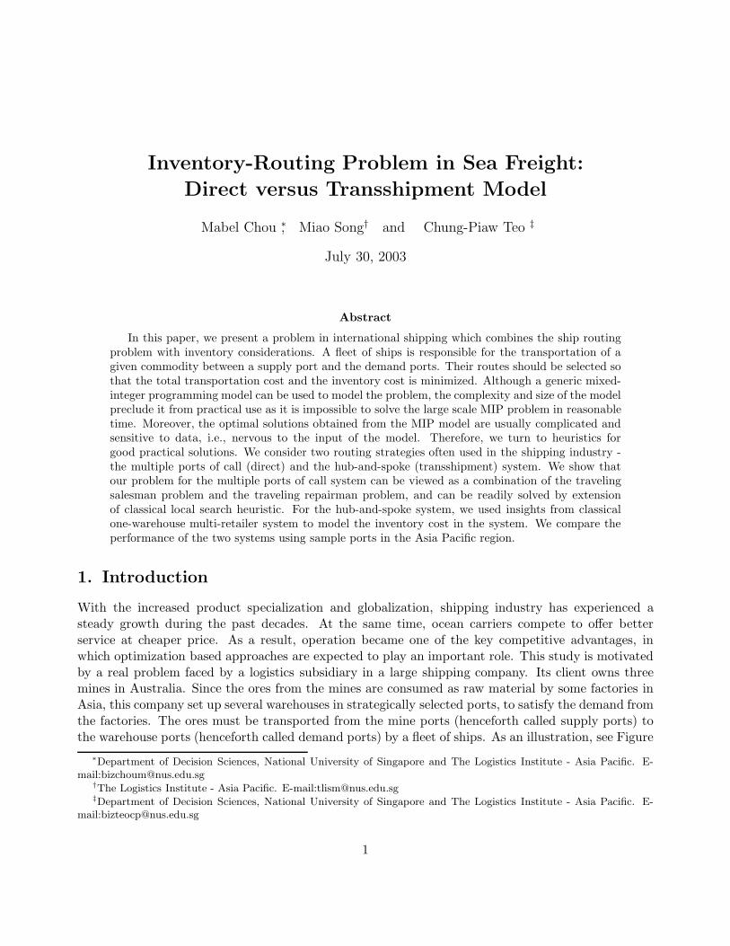
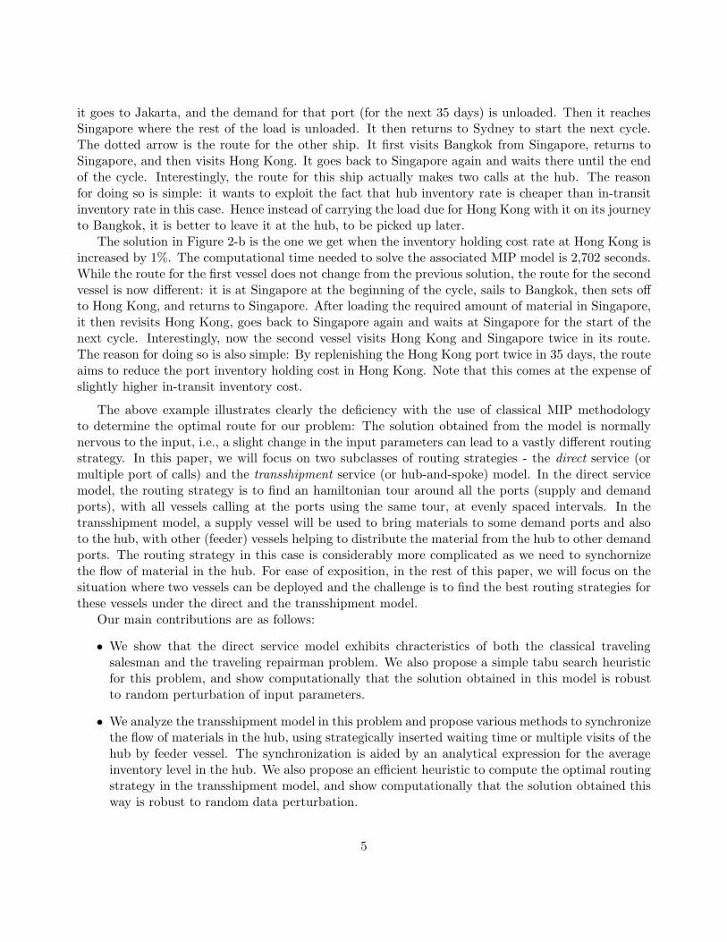
1 for the location of the supply port (in Australia) and the demand ports in the Asia Pacific region.All these ports (except for the port of Singapore, which is included for transshipment consideration)hold inventory, and the inventory holding costs may differ from port to port. The challenge is to helpthe client to determine the least cost logistics strategy to move the ores from the supply ports to thedemand ports. In this way, we need a model to determine the optimal shipping routes to minimizethe associated transportation and inventory cost charged to the client.

Figure 1: Some of the Main Ports in Southeast Asia and Australia

One of the fundamental questions in this problem is whether the company should move the rawmaterials into the demand ports directly from the supply port, or whether the transshipment operationusing a hub such as Singapore can help to reduce the total cost to the shipper. From the carrier’sperspective, the transshipment system is certainly much more preferred: It provides better utilizationof the assets. The large linehaul ships can be used to serve the route between the supply port andregional hubs, while smaller ones can be used for the feeder routes. As a result, the large ships nolonger visit those ports whose inbound/outbound volume is relatively low. However, the benefits oftransshipment operation for the shipper is less apparent. According to an article by Damas [15],shippers have often complained that they do not really have a choice in their cargo routing strategy,

2

since the routes are primarily determined based on carrier’s economics of operations alone. In fact,when interviewed, several of the shippers commented that if given a choice, they will choose directservice, as transshipment creates a potential problem like missed feeders. Furthermore, schedulereliability in the transshipment service is often touted as an important determinant for the selectionof direct versus transshipment mode of operation.

In this paper, our goal is to understand the benefits of transshipment oepration from the shipper’sperspective. We study the following questions:

• What is the optimal routing strategy for the direct service model, when the vessel brings rawmaterial directly form the supply port to the demand ports, without intermediate storage?

• What is the optimal routing strategy for the transshipment model, when the raw materials aredistributed using a hub and spoke system?

• Under what condition will the transshipment model be better than the direct service model?

We have a given homogeneous fleet of ships V that can be deployed. Let S denote the supplyport, and P the set of demand ports. Let H denote the transportation hubs. At a hub, the goodson one ship can be discharged from that ship and reloaded to another one. That is, both loadingand discharging operations can be carried out at a hub while a pure supply (resp. demand) portcan perform loading (resp. unloading) operation. We also assume that demand rate (demand perunit time) Di at the demand port i are deterministic, and that the production rate at the supplyport equals the aggregate demand rate, i.e., the supply and demand rate within the whole system isbalanced. For ease of exposition, let

Ri ={

Di if i is a demand port−

∑j∈P Dj if i = S

Let tij denote the sailing time from port i to port j. Let CLi denote the loading/discharging cost

per unit of the commodity at port i, i ∈ P, and CLs and CL

h the loading/unloading charges at thesupply port and the hub respectively.

Our cost model is built upon using the following cost parameters:

Hm The in-transit inventory and transportation cost per unit of the commodity per dayHh The hub inventory cost per unit of the commodity per day in hubHs The supply port inventory cost per unit of the commodity per day in the supply portHi The inventory holding cost per unit of the commodity per day at demand port i, i ∈ P.

The in-transit inventory and transportation cost rate Hm is the inventory holding cost incurredfor the commodities on the ship, the cost of transportation, plus other operational cost proportionalto the load on ship while the vessel is on the move (for example, the cost for the extra fuel burnedwith more load on ship), and the cost of insurance. Throughout the rest of this paper, we assume,unless otherwise stated, that

Assumption 1. Hs ≤ mini∈P Hi ≤ maxi∈P Hi ≤ min(Hh,Hm).

3

There are other associated cost components such as port chagres, fixed transportation cost (volumeindependent cost) incurred for each leg of the schedule etc. However, as will be evident later, manyof these additional costs associated with the schedule either reduces to a constant in the average costmodel, or are usually small compared to the inventory and transportation cost components whenvolume of shipment is large. We can thus ignored the impact of these cost components in our model.

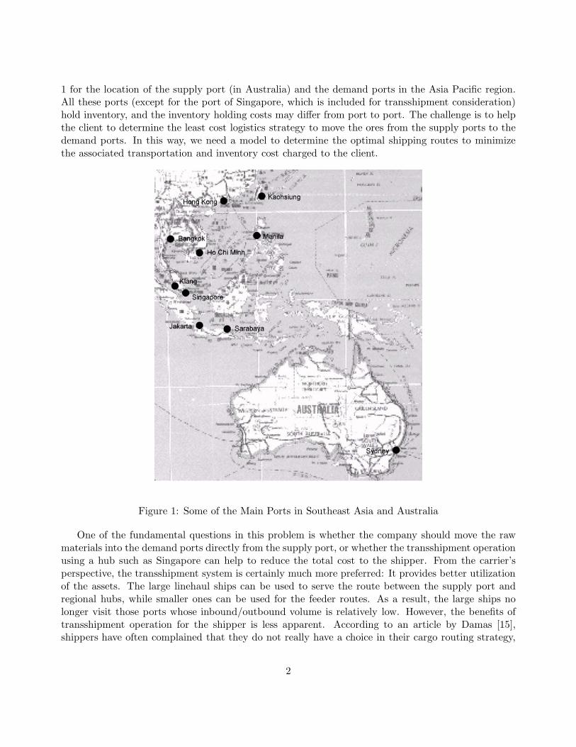
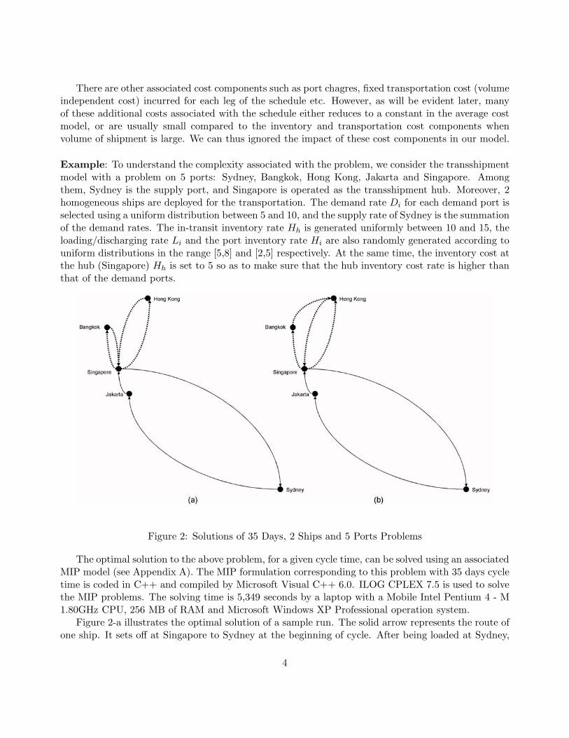
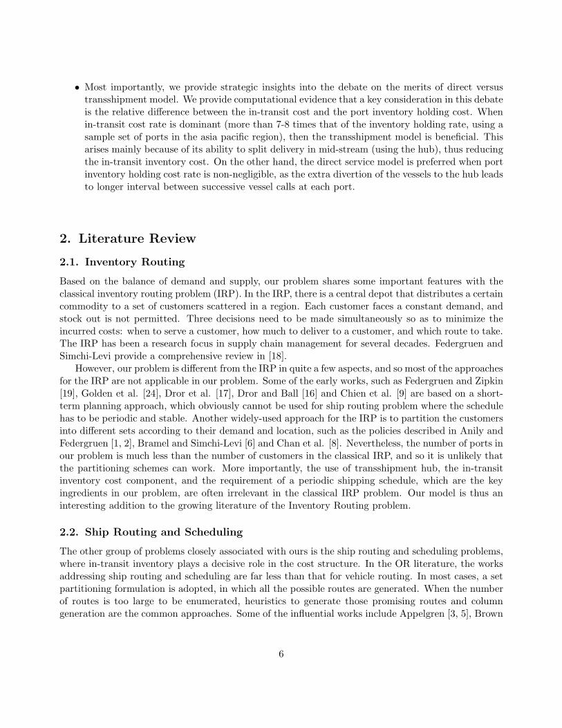
Example: To understand the complexity associated with the problem, we consider the transshipmentmodel with a problem on 5 ports: Sydney, Bangkok, Hong Kong, Jakarta and Singapore. Amongthem, Sydney is the supply port, and Singapore is operated as the transshipment hub. Moreover, 2homogeneous ships are deployed for the transportation. The demand rate Di for each demand port isselected using a uniform distribution between 5 and 10, and the supply rate of Sydney is the summationof the demand rates. The in-transit inventory rate Hh is generated uniformly between 10 and 15, theloading/discharging rate Li and the port inventory rate Hi are also randomly generated according touniform distributions in the range [5,8] and [2,5] respectively. At the same time, the inventory cost atthe hub (Singapore) Hh is set to 5 so as to make sure that the hub inventory cost rate is higher thanthat of the demand ports.

Figure 2: Solutions of 35 Days, 2 Ships and 5 Ports Problems

The optimal solution to the above problem, for a given cycle time, can be solved using an associatedMIP model (see Appendix A). The MIP formulation corresponding to this problem with 35 days cycletime is coded in C++ and compiled by Microsoft Visual C++ 6.0. ILOG CPLEX 7.5 is used to solvethe MIP problems. The solving time is 5,349 seconds by a laptop with a Mobile Intel Pentium 4 - M1.80GHz CPU, 256 MB of RAM and Microsoft Windows XP Professional operation system.

Figure 2-a illustrates the optimal solution of a sample run. The solid arrow represents the route ofone ship. It sets off at Singapore to Sydney at the beginning of cycle. After being loaded at Sydney,

4

it goes to Jakarta, and the demand for that port (for the next 35 days) is unloaded. Then it reachesSingapore where the rest of the load is unloaded. It then returns to Sydney to start the next cycle.The dotted arrow is the route for the other ship. It first visits Bangkok from Singapore, returns toSingapore, and then visits Hong Kong. It goes back to Singapore again and waits there until the endof the cycle. Interestingly, the route for this ship actually makes two calls at the hub. The reasonfor doing so is simple: it wants to exploit the fact that hub inventory rate is cheaper than in-transitinventory rate in this case. Hence instead of carrying the load due for Hong Kong with it on its journeyto Bangkok, it is better to leave it at the hub, to be picked up later.

The solution in Figure 2-b is the one we get when the inventory holding cost rate at Hong Kong isincreased by 1%. The computational time needed to solve the associated MIP model is 2,702 seconds.While the route for the first vessel does not change from the previous solution, the route for the secondvessel is now different: it is at Singapore at the beginning of the cycle, sails to Bangkok, then sets offto Hong Kong, and returns to Singapore. After loading the required amount of material in Singapore,it then revisits Hong Kong, goes back to Singapore again and waits at Singapore for the start of thenext cycle. Interestingly, now the second vessel visits Hong Kong and Singapore twice in its route.The reason for doing so is also simple: By replenishing the Hong Kong port twice in 35 days, the routeaims to reduce the port inventory holding cost in Hong Kong. Note that this comes at the expense ofslightly higher in-transit inventory cost.

The above example illustrates clearly the deficiency with the use of classical MIP methodologyto determine the optimal route for our problem: The solution obtained from the model is normallynervous to the input, i.e., a slight change in the input parameters can lead to a vastly different routingstrategy. In this paper, we will focus on two subclasses of routing strategies - the direct service (ormultiple port of calls) and the transshipment service (or hub-and-spoke) model. In the direct servicemodel, the routing strategy is to find an hamiltonian tour around all the ports (supply and demandports), with all vessels calling at the ports using the same tour, at evenly spaced intervals. In thetransshipment model, a supply vessel will be used to bring materials to some demand ports and alsoto the hub, with other (feeder) vessels helping to distribute the material from the hub to other demandports. The routing strategy in this case is considerably more complicated as we need to synchornizethe flow of material in the hub. For ease of exposition, in the rest of this paper, we will focus on thesituation where two vessels can be deployed and the challenge is to find the best routing strategies forthese vessels under the direct and the transshipment model.

Our main contributions are as follows:

• We show that the direct service model exhibits chracteristics of both the classical travelingsalesman and the traveling repairman problem. We also propose a simple tabu search heuristicfor this problem, and show computationally that the solution obtained in this model is robustto random perturbation of input parameters.

• We analyze the transshipment model in this problem and propose various methods to synchronizethe flow of materials in the hub, using strategically inserted waiting time or multiple visits of thehub by feeder vessel. The synchronization is aided by an analytical expression for the averageinventory level in the hub. We also propose an efficient heuristic to compute the optimal routingstrategy in the transshipment model, and show computationally that the solution obtained thisway is robust to random data perturbation.

5

• Most importantly, we provide strategic insights into the debate on the merits of direct versustransshipment model. We provide computational evidence that a key consideration in this debateis the relative difference between the in-transit cost and the port inventory holding cost. Whenin-transit cost rate is dominant (more than 7-8 times that of the inventory holding rate, using asample set of ports in the asia pacific region), then the transshipment model is beneficial. Thisarises mainly because of its ability to split delivery in mid-stream (using the hub), thus reducingthe in-transit inventory cost. On the other hand, the direct service model is preferred when portinventory holding cost rate is non-negligible, as the extra divertion of the vessels to the hub leadsto longer interval between successive vessel calls at each port.

2. Literature Review

2.1. Inventory Routing

Based on the balance of demand and supply, our problem shares some important features with theclassical inventory routing problem (IRP). In the IRP, there is a central depot that distributes a certaincommodity to a set of customers scattered in a region. Each customer faces a constant demand, andstock out is not permitted. Three decisions need to be made simultaneously so as to minimize theincurred costs: when to serve a customer, how much to deliver to a customer, and which route to take.The IRP has been a research focus in supply chain management for several decades. Federgruen andSimchi-Levi provide a comprehensive review in [18].

However, our problem is different from the IRP in quite a few aspects, and so most of the approachesfor the IRP are not applicable in our problem. Some of the early works, such as Federgruen and Zipkin[19], Golden et al. [24], Dror et al. [17], Dror and Ball [16] and Chien et al. [9] are based on a short-term planning approach, which obviously cannot be used for ship routing problem where the schedulehas to be periodic and stable. Another widely-used approach for the IRP is to partition the customersinto different sets according to their demand and location, such as the policies described in Anily andFedergruen [1, 2], Bramel and Simchi-Levi [6] and Chan et al. [8]. Nevertheless, the number of ports inour problem is much less than the number of customers in the classical IRP, and so it is unlikely thatthe partitioning schemes can work. More importantly, the use of transshipment hub, the in-transitinventory cost component, and the requirement of a periodic shipping schedule, which are the keyingredients in our problem, are often irrelevant in the classical IRP problem. Our model is thus aninteresting addition to the growing literature of the Inventory Routing problem.

2.2. Ship Routing and Scheduling

The other group of problems closely associated with ours is the ship routing and scheduling problems,where in-transit inventory plays a decisive role in the cost structure. In the OR literature, the worksaddressing ship routing and scheduling are far less than that for vehicle routing. In most cases, a setpartitioning formulation is adopted, in which all the possible routes are generated. When the numberof routes is too large to be enumerated, heuristics to generate those promising routes and columngeneration are the common approaches. Some of the influential works include Appelgren [3, 5], Brown

6

et al. [7], Fisher et al. [20], Lai et al. [25], Papadakis and Perakis [29], Rana and Vickson [30, 31] andRonen [32]. The readers can refer to Christiansen and Fagerholt [11] for a detailed survey.

To the best of our knowledge, the ship routing problem combined with inventory management hasbeen largely ignored in the literature. One of the pioneering researches is done by Miller [28]. Someliquid bulk chemicals are shipped to warehouses all over the world so as to maintain the minimuminventory levels. A fleet of bulk tankers are used for the delivery, and each of them are allowed todelivery multiple commodities. An interactive, computer-aided system is developed for the problem,which uses heuristics to improve the decisions. Larson [26] also proposed a problem that combinesship routing with inventory control. In the problem, the municipal sewage sludge is transportedfrom city-operated wastewater treatment plants to an ocean dumping site. This research focuses onthe design of a logistics system and the decision for the fleet sizing from the strategic perspective.The recent works of Christiansen and Nygreen [12, 13] and Christiansen [10] discuss a ship routingproblem with inventory constraint and time window. The inventory of ammonia is balanced in allthe production and consumption harbors throughout the world, that is, the inventory level at eachharbor is kept above a lower bound and below an upper bound. Inventory cost is thus not explicitlymodeled in their approach, and is not affected by the shipping routes selected. The objective is todecide the routes for a fleet of homogeneous ships, which minimize the transportation cost in thisprocess. Given a planning horizon, the problem can be decomposed into ship subproblems and harborsubproblems. The Dantzig-Wolfe column generation approach is used to solve the master problem,and the subprograms are solved by dynamic programming algorithms for shortest path problems. Inaddition, integral solutions are obtained by a branch-and-bound search.

Note that mathematical programming techniques have often been used to solve vehicle routingproblem to optimality, but the excessive computational effort associated with this approach doesnot lend itself well to practical use, especially on large scale instances. Fortunately, for the shiprouting problem, the number of ports considered are normally small (compared to traditional vehiclerouting problem), and the central challenge here lies in integrating inventory, transportation, and portoperations concerns into the model.

2.3. Economics of Transshipment

The debate between transshipment and direct service is normally considered from the perspective of thecarriers. Traditionally, maritime economists, ports and shipping lines have considered transshipmentto be more expensive than direct call services, mainly by virtue of extra feeder costs (feeder ship costare much higher per TEU-mile) and transshipment hub charges (see Wu and Kleywegt [34] for a reviewof charges during port visit). Furthermore, according to MDS Transmodal [27], the costs of makinga port call are relatively small compared to the cost of the transshipment, provided the size of thecontainer exchange is significant. Through careful investigation into container size economies, a studyby Gilman [22] has also concluded that direct calls at Benelux, German and UK ports, irrespective ofship size, would be far cheaper than a hub-and-spoke based transshipment operation.

However, the industry, at least the major carriers, appears to be moving in the opposite direction.Transshipment services are now widely used on major trade routes. According to industry statistics,about 23% of all port container handling movements in 2001 come from transshipment, compared tojust 12% in 1980 (Damas [15]). This is mainly due to the following reason (Baird [4]): The increase inship sizes has forced carriers to seek higher levels of return from their assets. This has led to removal of

7

calls to ports with lower trade cargo volume, justifying the needs for transshipment services. Frankel[21] have also made the observation that the objectives of transshipment are not restricted to totalcost reduction, but also to improve just-in-time delivery of cargo, reduce in-transit inventory, andmake the total origin-to-destination movement of containerized cargo more seamless. Transshipmentis thus not just a logistics convenience measure, but also an opportunity for adding value to thegoods transshipped. This has indeed spurred several new developments in the industry. The Port ofSingapore Authority (PSA), for instance, recognized the importance of the value-added propositionof transshipment hub. It has recently launched a new service called N2N Mobile Hub, which allowscustomers to use PSA yard as temporary storage space for their containers. This helps to eliminateunnecessary transport costs and time delays incurred in trucking containers away from the port toexternal yards or warehouses. Containers under the N2N hub concept arrive at PSA’s yard with noonward carrier nominees and no set destination. Customers are allowed to route the containers tofinal destinations based on demand requirement. This reaps significant advantage in risk pooling ofinventory, as the cargo final destination can be delayed until the containers reach PSA port.

While there are various streams of research in the literature that attempt to understand the issuesin the direct versus transshipment debate (see, for instance, Baird [4] with a thorough cost analysisand comparison of the two models), most of the study uses mainly empirical data to justify theirconclusions. In general, very few qualitative insights and understanding on the debate has beenobtained. An exception is a study by Wijnolst [33], which claimed that the hub-feeder system couldonly be competitive if there was a substantial percentage of containers on the deep sea vessel that arenot feedered (about 35-45%), but remain in the mainport for onward distribution by land. The studyconcluded that without this base cargo, double handling costs involved in feeder containers and theadditional transport cost would outweigh the benefits of ultra large container carriers. Unfortunately,no detailed cost breakdown was presented to justify this conclusion (see Baird [4]).

3. Direct Service Model

The direct service, or the multiple ports of call system is one of the most widely used routing systemin the shipping industry. A direct port-to-port service exists for any port pair, and every ship visits allthe ports following the same route. Raw materials are thus loaded onto the ship at the supply port,and are only unloaded at the designated demand ports. In this section, we consider a special case ofthe multiple ports of call system, in which (i) all the ports are visited exactly once by each ship. Thatis, the route is a Hamiltonian cycle. Moreover, (ii) all the ships deployed take the same route andload/discharge the same quantity at the same port, and the time interval between any consecutivearrivals at any port is the same. These restrictions, however, will not severely limits the quality of thesolutions obtained, due to the following reasons:

• It is not optimal to visit a demand port more than once between every successive visit to thesupply port. Otherwise, the amount unloaded at the second visit to the demand port can beunloaded at the port during the first visit. This results in savings because the in-transit inventoryrate is higher than port inventory holding rate.

• The supply port is assumed to be far from all the demand ports, as is in our sea freight example.Whenever a ship goes back to the supply port, it should have already emptied its load at the

8

demand ports. It is costly to make long trips back to the supply port with an empty vessel, andhence it is desirable for the ship to visit all the demand ports between every successive visit tothe supply port.

Since the cycle time here is decided by the Hamiltonian route, the average cost occurred during acycle should be minimize so as to optimize the long run operation cost. We refer to this problem asthe multiple ports of call problem (MP). In this section, we show that this problem is a combinationof the Ttraveling Salesman Problem (from port inventory optimization) and the Traveling RepairmanProblem (from in-transit inventory optimization).

3.1. Cost Model

The total cost of the MP includes the fixed transportation cost per day, the loading/discharging cost,the port inventory cost, and the in-transit inventory cost. According to out objective to minimize theaverage cost, the first two items here become a constant. The last two cost components correspondtwo classical problems in discrete optimization: the TSP and the TRP.

3.1.1. The TSP Component

The traveling salesman problem (TSP) is one of the most famous problems in discrete optimization. Ina graph G = (V,E) with vertices V and edges E, a traveling time l(u, v) is assigned to any edge (u, v),(u, v) ∈ E that connects vertex u and v. The TSP is to find out the tour with the shortest travelingtime so that any vertex v, v ∈ V is visited exactly once. In other words, the TSP is to minimize thelength of the Hamiltonian cycle for graph G. As a well-known NP-hard problem, it is one of the mostwidely studied problem in computer science and operations research, and a great amount of heuristicsand approximation algorithms have been proposed. However, the worst case bound of the TSP evenwith the triangle inequality has not been improved since the 3/2 bound suggested by Christofides [14]in 1976.

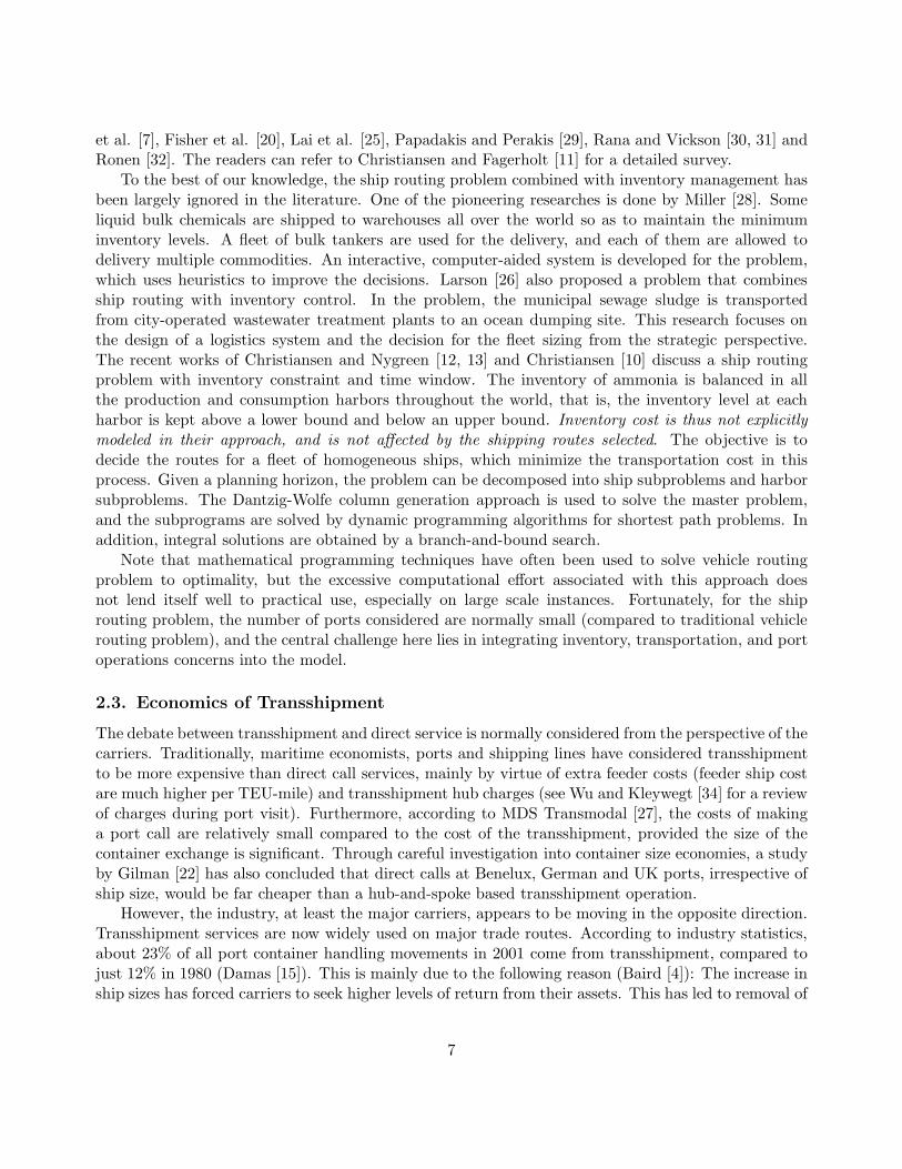
In our problem, given a Hamiltonian cycle, the cycle time n can be calculated by summing upthe transportation time for each leg. According to the equal loading/discharging and equal arrivalinterval assumptions, a port i is visited every n/|V| days, and n|Ri|/|V| units are loaded/discharged.The inventory level of supply and demand ports are shown in Figure 3. Obviously, the averageinventory cost is

12

∑i∈P∪{S}

1|V|Hi|Ri|n =

n

2|V|∑

i∈P∪{S}Hi|Ri|, (1)

which is a constant times the cycle time n. Therefore, to minimize the inventory cost is to minimizethe transportation time, which is exactly the TSP.

In the shipping schedule, the ships can choose to wait at some ports. However, as shown in (1),waiting can only increase the port inventory cost for it increases the cycle time.

3.1.2. The TRP Component

The traveling repairman problem (TRP), also called the minimum latency problem (MLP) is a variantof the TSP. While the TSP seeks to minimize the traveling time for the salesman, the TRP tries tominimize the weighted sum of the waiting times for all the customers. The TRP also considers a graph

9

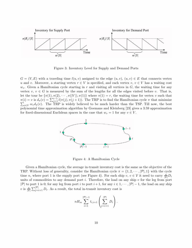
Figure 3: Inventory Level for Supply and Demand Ports

G = (V,E) with a traveling time l(u, v) assigned to the edge (u, v), (u, v) ∈ E that connects vertexu and v. Moreover, a starting vertex r ∈ V is specified, and each vertex v, v ∈ V has a waiting costwv. Given a Hamiltonian cycle starting in r and visiting all vertices in G, the waiting time for anyvertex v, v ∈ G is measured by the sum of the lengths for all the edges visited before v. That is,let the tour be {π(1), π(2), · · · , π(|V |), π(1)} where π(1) = r, the waiting time for vertex v such thatπ(i) = v is dπ(v) =

∑i−1j=1 l(π(j), π(j + 1)). The TRP is to find the Hamiltonian cycle π that minimize∑

v∈V wvdπ(v). The TRP is widely believed to be much harder than the TSP. Till now, the bestpolynomial time approximation algorithm by Goemans and Kleinberg [23] gives a 3.59 approximationfor fixed-dimensional Euclidean spaces in the case that wv = 1 for any v ∈ V .

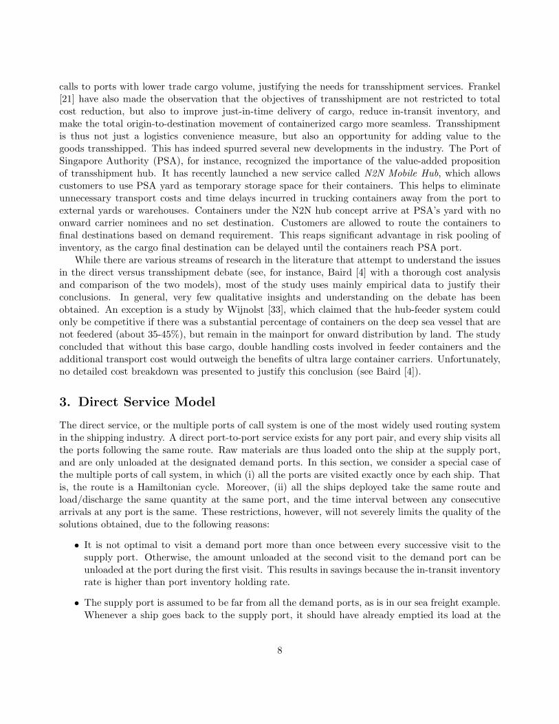
Figure 4: A Hamiltonian Cycle

Given a Hamiltonian cycle, the average in-transit inventory cost is the same as the objective of theTRP. Without loss of generality, consider the Hamiltonian cycle π = {1, 2, · · · , |P|, 1} with the cycletime n, where port 1 is the supply port (see Figure 4). For each ship v, v ∈ V it need to carry n

|V|Di

units of commodities to any demand port i. Therefore, the load on any ship v for the leg from port|P| to port 1 is 0; for any leg from port i to port i + 1, for any i ∈ 1, · · · , |P| − 1, the load on any shipv is n

|V|∑|P|

j=i+1 Di. As a result, the total in-transit inventory cost is

nHm

|P|−1∑i=1

ti,i+1

|P|∑

j=i+1

Di

.

10

That is, the average in-transit inventory cost is

Hm

|P|−1∑i=1

ti,i+1

|P|∑

j=i+1

Di

= Hm

|P|∑i=2

Di

i−1∑

j=1

ti,i+1

. (2)

Let us consider a TRP problem with each port to be a vertex and each leg to be an edge. The startingvertex is the supply port; the waiting cost for any vertex i except for the starting vertex is set to beDi; the traveling time from vertex i to vertex j is equal to Tij . In that case, (2) is exactly the objectivefunction for the TRP. Therefore, to minimize the average in-transit inventory cost is equavalent to theTRP.

Am important observation of (2) is that the in-transit inventory cost is not changed if waitingoccurs at the empty leg. Waiting at any other leg can only increase the in-trasit inventory cost.Combined with the result from the TSP compenent, there is no need to delay the shipping schedulein the multiple ports of call system. Note also that the in-transit inventory cost is not affected by thenumber of vessels deployed, as long as the route used by each vessel is identical.

3.2. MIP Formulation

According to the above analysis, the MP is to minimize a objective function which combines the TSPwith the TRP subject to the constraints of a Hamiltonian cycle. Let us define the variables

xij The binary variable to represent whether the arc from port i, i ∈ P to port j, j ∈ P \ {i}is included in the route

yij The load on each ship for the arc from port i, i ∈ P to port j, j ∈ P \ {i}n The cycle time.

Firstly, a Hamiltonian route must be constructed, that is,∑

j∈P\{i} xij = 1, ∀i ∈ P∑j∈P\{i} xji = 1, ∀i ∈ P∑i∈S

∑j∈S\{i} xij ≤ |S| − 1, ∀S ⊂ P, S �= Φ

xij ∈ {0, 1}. ∀i ∈ P, j ∈ P \ {i}

Therefore, the cycle time n is defined as

n =∑i∈P

∑j∈P\{i}

tijxij.

Based on the route, we can get the load on ship for each leg:∑

j∈P\{i} yij −∑

j∈P\{i} yji = Ri, ∀i ∈ Pyij ≤ Mxij, ∀i ∈ P, j ∈ P \ {i}yij ≥ 0, ∀i ∈ P, j ∈ P \ {i}

in which M denotes a very large number. The objective function comes from (2) and (3), that is,

n

2|V|2∑i∈P

Hi|Ri| + Hm

∑i∈P

∑j∈P\{i}

tijyij.

11

As a result, our MIP formulation becomes

min n2|V|

∑i∈P Hi|Ri| + V

∑i∈P

∑j∈P\{i} Tijyij

s.t.∑

j∈P\{i} xij = 1, ∀i ∈ P∑j∈P\{i} xji = 1, ∀i ∈ P∑i∈S

∑j∈S\{i} xij ≤ |S| − 1, ∀S ⊂ P, S �= Φ∑

j∈P\{i} yij −∑

j∈P\{i} yji = Ri, ∀i ∈ Pyij ≤ Mxij, ∀i ∈ P, j ∈ P \ {i}n =

∑i∈P

∑j∈P\{i} Tijxij,

xij ∈ {0, 1}, ∀i ∈ P, j ∈ P \ {i}yij ≥ 0. ∀i ∈ P, j ∈ P \ {i}

(3)

3.3. Transposition Heuristic

Obviously, (3) has an exponential number of constraints due to the subtour elimination. Therefore,it is impossible to solve a large-scale problem with this formulation. For example, the computationaltime needed to solve (3) using CPLEX 7.5 exceeds 1 hour for a 15 port problem. Therefore, we mustturn to heuristics so as to solve the problem efficiently.

The computational complexity to compute the average cost for a given route is O(|P|), that is, it iseasy to judge whether a new route improves the objective value. Therefore, most of the improvementheuristics for the TSP can be used for the MP. Since our transit time is not symmetric in most cases,we use the transposition heuristic which performs well for the asymmetric TSP. Note that the 2-optheuristic can also be utilized for our problem. According to our experiments, Its performance is asgood as that of the transposition heuristic, but not better.

Given a Hamiltonian cycle, a transposition is to exchange two ports along the cycle. For instance,given an initial route

{π(1), · · · , π(i − 1), π(i), π(i + 1), · · · , π(j − 1), π(j), π(j + 1), · · · , π(P), π(1)}

a transposition of π(i) and π(j) gives a new route

{π(1), · · · , π(i − 1), π(j), π(i + 1), · · · , π(j − 1), π(i), π(j + 1), · · · , π(P), π(1)},

which is illustrated in Figure 5. The transposition heuristic starts from an arbitrary initial route,improves the route by transpositions and terminates when no better solution can be found by anytransposition.

Transposition Heuristic for the MP

Step 1: Let π the given initial route. Compute z(π) the average cost of the MP for π and z(π−1) theaverage cost of the MP for the inverse route of π. Set π∗ := π, z∗ := min(z(π), z(π−1)), i := 1 andj := 2.

Step 2: Let π be the route given by π∗ with the transposition of π∗(i) and π∗(j). Compute theaverage cost of the MP for π and the inverse route of π, that is, z(π) and z(π−1) respectively. Ifz∗ > min(z(π), z(π−1)), go to Step 3. Otherwise, go to Step 4.

12

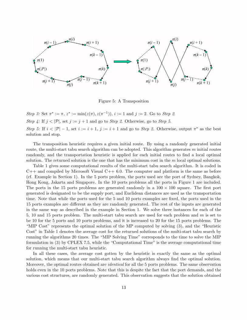
Figure 5: A Transposition

Step 3: Set π∗ := π, z∗ := min(z(π), z(π−1)), i := 1 and j := 2. Go to Step 2.

Step 4: If j < |P|, set j := j + 1 and go to Step 2. Otherwise, go to Step 5.

Step 5: If i < |P| − 1, set i := i + 1, j := i + 1 and go to Step 2. Otherwise, output π∗ as the bestsolution and stop.

The transposition heuristic requires a given initial route. By using a randomly generated initialroute, the multi-start tabu search algorithm can be adopted. This algorithm generates m initial routesrandomly, and the transportation heuristic is applied for each initial routes to find a local optimalsolution. The returned solution is the one that has the minimum cost in the m local optimal solutions.

Table 1 gives some computational results of the multi-start tabu search algorithm. It is coded inC++ and compiled by Microsoft Visual C++ 6.0. The computer and platform is the same as before(cf. Example in Section 1). In the 5 ports problem, the ports used are the port of Sydney, Bangkok,Hong Kong, Jakarta and Singapore. In the 10 ports problems all the ports in Figure 1 are included.The ports in the 15 ports problems are generated randomly in a 100 × 100 square. The first portgenerated is designated to be the supply port, and Euclidean distances are used as the transportationtime. Note that while the ports used for the 5 and 10 ports examples are fixed, the ports used in the15 ports examples are different as they are randomly generated. The rest of the inputs are generatedin the same way as described in the example in Section 1. We solve three instances for each of the5, 10 and 15 ports problem. The multi-start tabu search are used for each problem and m is set tobe 10 for the 5 ports and 10 ports problems, and it is increased to 20 for the 15 ports problems. The“MIP Cost” represents the optimal solution of the MP computed by solving (3), and the “HeuristicCost” in Table 1 denotes the average cost for the returned solutions of the multi-start tabu search byrunning the algorithms 20 times. The “MIP Solving Time” corresponds to the time to solve the MIPformulation in (3) by CPLEX 7.5, while the “Computational Time” is the average computational timefor running the multi-start tabu heuristic.

In all these cases, the average cost gotten by the heuristic is exactly the same as the optimalsolution, which means that our multi-start tabu search algorithm always find the optimal solution.Moreover, the optimal routes obtained are identical for all the 5 ports problems. The same observationholds even in the 10 ports problems. Note that this is despite the fact that the port demands, and thevarious cost structures, are randomly generated. This observation suggests that the solution obtained

13

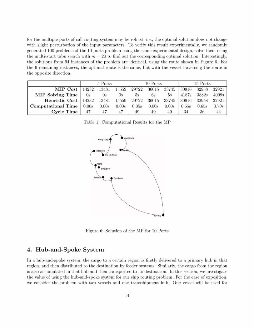
for the multiple ports of call routing system may be robust, i.e., the optimal solution does not changewith slight perturbation of the input parameters. To verify this result experimentally, we randomlygenerated 100 problems of the 10 ports problem using the same experimental design, solve them usingthe multi-start tabu search with m = 20 to find out the corresponding optimal solution. Interestingly,the solutions from 94 instances of the problem are identical, using the route shown in Figure 6. Forthe 6 remaining instances, the optimal route is the same, but with the vessel traversing the route inthe opposite direction.

5 Ports 10 Ports 15 PortsMIP Cost 14232 13481 15559 29722 36015 33745 30916 32958 32921

MIP Solving Time 0s 0s 0s 5s 6s 5s 4187s 3882s 4009sHeuristic Cost 14232 13481 15559 29722 36015 33745 30916 32958 32921

Computational Time 0.00s 0.00s 0.00s 0.05s 0.00s 0.00s 0.65s 0.65s 0.70sCycle Time 47 47 47 49 49 49 34 36 44

Table 1: Computational Results for the MP

Figure 6: Solution of the MP for 10 Ports

4. Hub-and-Spoke System

In a hub-and-spoke system, the cargo to a certain region is firstly delivered to a primary hub in thatregion, and then distributed to the destination by feeder systems. Similarly, the cargo from the regionis also accumulated in that hub and then transported to its destination. In this section, we investigatethe value of using the hub-and-spoke system for our ship routing problem. For the ease of exposition,we consider the problem with two vessels and one transshipment hub. One vessel will be used for

14

bringing the commodity from the supply port to certain demand ports, and to the hub for furtherdistribution to other demand ports, using the second vessel. We call these vessels the supply vesseland the feeder vessel respectively1. As in the case of the direct service model, we may assume that thesupply vessel visits the same set of ports (and the hub) once between successive visits to the supplyport. We need to, however, (i) address the routing strategy for the feeder vessel. Furthermore, (ii)unlike the direct service case, we need to address how waiting time can be strategically inserted intoeach leg of the routes in order to synchronize the flow of material from the supply vessel to the feedervessel.

We first consider the simplest strategy for the feeder route: Single Cycle routing strategy. Here,the feeder vessel service all its route in a cyclic fashion, visiting each of the port once and exactlyonce between each successive visit to the hub. We should distinguish this from the Multi-Cyclerouting strategy, where the feeder vessel may return to the hub to pick up more commodity withinone the the cycle. Figure 2-a and 2-b show examples of the multi-cycle feeder strategy. In the caseof Figure 2-a, each of the demand port is visited exactly once within each cycle. We call this theMulti-Disjoint-Cycle strategy. We first analyze the transshipment operation using the single cyclestrategy, and show later how the multi-cycle strategy can be used to improve upon the model. Notethat since the physical trnasportation time between the supply and the feeder route may not match,it is also important that waiting time must be inserted strategically for the supply and feeder vessel,at the supply port and the hub respectively. We call this the Transshipment Synchronizationproblem.

4.1. Hub Inventory Model (Single Cycle)

Suppose that one ship brings s units of the commodity to the hub every ts days (called supply interval)and the other ship picks up d units from the hub every td days (feeder interval), in which s/ts = d/td =Γ, the total demand rate for ports served by the feeder vessel. As long as the supply/feeder intervals donot change, any shift in the arrival time of the two routes at the port will not change the transportationcost and inventory holding cost at supply/demand ports, but will only affect the inventory managementat the hub. Therefore, we can consider the hub inventory problem separately, with only informationon ts and td.

Let T be the least common multiplier of ts and td, T = λsts = λdtd. Obviously, the arrival time ofsupply and feeder vessels, as well as the inventory level at the hub, will repeat themselves after T . Asa result, we only need to minimize the average inventory cost in T days. Let Ts = {tsi |tsi = ts0 + its, i =0, · · · , λs − 1} be the set of arrival time for supply vessel, and Td = {tdi |tdi = td0 + itd, i = 0, · · · , λd − 1}the set of arrival time for feeder vessel. Here ts0 ∈ {0, · · · , ts − 1} and td0 ∈ {0, · · · , td − 1}. Hence, theamount of supply at time t, denoted by S(t), is s if t ∈ Ts and 0 otherwise; and the amount of demandat time t, D(t) is d if t ∈ Td and 0 otherwise. Moreover, we let It, t = 0, . . . , T − 1, denote the netinventory position at the hub at time t. We have

I0 = IT−1 + S(0) − D(0),It = It−1 + S(t) − D(t), ∀t = 1, · · · , T − 1It ≥ 0. ∀t = 0, · · · , T − 1

(4)

1Although our algorithm and formulation in this section deals with the situation with one supply and feeder vessel,they can be easily extended to the cases with multiple supply and/or feeder vessels, provided the route taken for eachsupply (resp. feeder) vessel is the same.

15

To synchronize the transshipment activities, we need to choose I0, ts0, t

d0 to minimize the total inventory∑T−1

t=0 It. By periodicity of the supply and feeder intervals, we can assume that the first arrival timeof supply in the T days, ts0 is equal to 0.

Proposition 1. In the optimal solution, both the supply and demand will arrive at a certain time t,0 ≤ t ≤ T − 1.

Proof. For any feeder arrival time tdi ∈ Td, we define a set T<i which represents the set of supply arrival

time before tdi , that is, T<i = {t|t ∈ Ts, t < tdi }. Let

k∗ = min{tdi − t : i = 0, . . . , λd − 1, t ∈ T<i }.

Consider a feasible solution of the hub inventory problem, with inventory It and the arrival timesets Ts and Td. Suppose that there does not exist a time t at which both the feeder and the supplyvessel arrive, that is, k∗ > 0. According to the definition of k∗ and the fact that ts0 = 0, td0 ≥ k∗.Therefore, we can shift the arrival time of feeder vessel k∗ days ahead, and get another feasible solutionwith

t′si = tsi , ∀i = 0, · · · , λs − 1t′di = tdi − k∗, ∀i = 0, · · · , λd − 1

I ′t ={

It − d if tdi − k∗ ≤ t < tdi , tdi ∈ Td

It otherwise. ∀t = 0, · · · , T − 1

In this new solution, both the supply and the feeder vessel must arrive at some time t, 0 ≤ t ≤ T − 1,and the sum of the inventory level is reduced by λd×k∗×d. Therefore, any solution without a commonarrival time for feeder and supply vessel can be improved by synchronizing the arrivals of feeder andsupply vessel, which proves the proposition.

Theorem 2. The optimal inventory level in the transshipment hub is given by

Γ(

12(ts + td) − g.c.d.(ts, td)

),

in which g.c.d.(.) denotes the function to find out the greatest common divider of the input.

Proof. Without loss of generality, we may assume that ts ≥ td. Otherwise, by inverting the role ofsupply and feeder intervals in the following argument, we can establish the same result in the casewhen td ≥ ts.

By Proposition 1, we may assume that ts0 = td0 = 0. We only need to determine the correspondingoptimal I0. Instead of monitoring the inventory level at the hub, we examine the echelon inventorylevel, that is, we include also the inventory at all demand ports served by the feeder route. Note thatthese ports have aggregate demand rate of Γ. With feeder interval of td, the average inventory levelat these ports is thus given by 1

2Γtd = d2 .

Note that the echelon inventory level fluctuates between I0 and I0 + s, with average echeloninventory I0 + s/2. The average inventory level at the hub is thus given by

I0 +12(s − d) = I0 +

12Γ(ts − td).

16

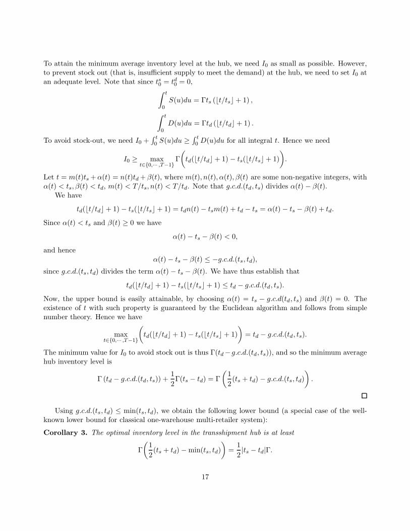
To attain the minimum average inventory level at the hub, we need I0 as small as possible. However,to prevent stock out (that is, insufficient supply to meet the demand) at the hub, we need to set I0 atan adequate level. Note that since ts0 = td0 = 0,∫ t

0S(u)du = Γts (�t/ts� + 1) ,

∫ t

0D(u)du = Γtd (�t/td� + 1) .

To avoid stock-out, we need I0 +∫ t0 S(u)du ≥

∫ t0 D(u)du for all integral t. Hence we need

I0 ≥ maxt∈{0,··· ,T−1}

Γ(

td(�t/td� + 1) − ts(�t/ts� + 1))

.

Let t = m(t)ts + α(t) = n(t)td + β(t), where m(t), n(t), α(t), β(t) are some non-negative integers, withα(t) < ts, β(t) < td, m(t) < T/ts, n(t) < T/td. Note that g.c.d.(td, ts) divides α(t) − β(t).

We have

td(�t/td� + 1) − ts(�t/ts� + 1) = tdn(t) − tsm(t) + td − ts = α(t) − ts − β(t) + td.

Since α(t) < ts and β(t) ≥ 0 we have

α(t) − ts − β(t) < 0,

and henceα(t) − ts − β(t) ≤ −g.c.d.(ts, td),

since g.c.d.(ts, td) divides the term α(t) − ts − β(t). We have thus establish that

td(�t/td� + 1) − ts(�t/ts� + 1) ≤ td − g.c.d.(td, ts).

Now, the upper bound is easily attainable, by choosing α(t) = ts − g.c.d(td, ts) and β(t) = 0. Theexistence of t with such property is guaranteed by the Euclidean algorithm and follows from simplenumber theory. Hence we have

maxt∈{0,··· ,T−1}

(td(�t/td� + 1) − ts(�t/ts� + 1)

)= td − g.c.d.(td, ts).

The minimum value for I0 to avoid stock out is thus Γ(td− g.c.d.(td, ts)), and so the minimum averagehub inventory level is

Γ (td − g.c.d.(td, ts)) +12Γ(ts − td) = Γ

(12(ts + td) − g.c.d.(ts, td)

).

Using g.c.d.(ts, td) ≤ min(ts, td), we obtain the following lower bound (a special case of the well-known lower bound for classical one-warehouse multi-retailer system):

Corollary 3. The optimal inventory level in the transshipment hub is at least

Γ(

12(ts + td) − min(ts, td)

)=

12|ts − td|Γ.

17

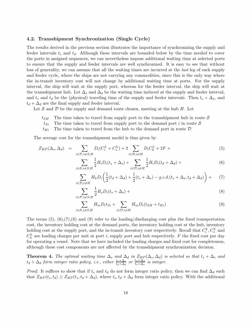
4.2. Transshipment Synchronization (Single Cycle)

The results derived in the previous section illustrates the importance of synchronizing the supply andfeeder intervals ts and td. Although these intervals are bounded below by the time needed to coverthe ports in assigned sequences, we can nevertheless impose additional waiting time at selected portsto ensure that the supply and feeder intervals are well synchronized. It is easy to see that withoutloss of generality, we can assume that all the waiting times are incurred at the last leg of each supplyand feeder cycle, where the ships are not carrying any commodities, since this is the only way wherethe in-transit inventory cost will not change by additional waiting time at ports. For the supplyinterval, the ship will wait at the supply port, whereas for the feeder interval, the ship will wait atthe transshipment hub. Let ∆s and ∆d be the waiting time induced at the supply and feeder interval,and ts and td be the (physical) traveling time of the supply and feeder intervals. Then ts + ∆s, andtd + ∆d are the final supply and feeder interval.

Let S and D be the supply and demand route chosen, meeting at the hub H. Let

tSH The time taken to travel from supply port to the transshipment hub in route StSi The time taken to travel from supply port to the demand port i in route StHi The time taken to travel from the hub to the demand port in route D.

The average cost for the transshipment model is thus given by

ZHP (∆s,∆d) =∑

i∈P,i�=S,H

Di(CLi + CL

s ) + 2∑

i∈D,i�=H

DiCLh + 2F + (5)

∑i∈S,i�=S,H

12HiDi(ts + ∆s) +

∑i∈D,i�=H

12HiDi(td + ∆d) + (6)

∑i∈D,i�=H

HhDi

(12(td + ∆d) +

12(ts + ∆s) − g.c.d.(ts + ∆s, td + ∆d)

)+ (7)

∑i∈P,i�=S,H

12HsDi(ts + ∆s) + (8)

∑i∈S,i�=S,H

HmDitSi +∑

i∈D,i�=H

HmDi(tSH + tHi) (9)

The terms (5), (6),(7),(8) and (9) refer to the loading/discharging cost plus the fixed transportationcost, the inventory holding cost at the demand ports, the inventory holding cost at the hub, inventoryholding cost at the supply port, and the in-transit inventory cost respectively. Recall that CL

i , CLs and

CLh are loading charges per unit at port i, supply port and hub respectively. F the fixed cost per day

for operating a vessel. Note that we have included the loading charges and fixed cost for completeness,although these cost components are not affected by the transshipment synchronization decision.

Theorem 4. The optimal waiting time ∆s and ∆d in ZHP (∆s,∆d) is selected so that ts + ∆s andtd + ∆d form integer ratio policy, i.e., either ts+∆s

td+∆dor td+∆d

ts+∆sis integer.

Proof. It suffices to show that if ts and td do not form integer ratio policy, then we can find ∆d suchthat ZHP (ts, td) ≥ ZHP (ts, td + ∆d), where ts, td + ∆d form integer ratio policy. With the additional

18

waiting time, the term (6) increases by

∑i∈D,i�=H

12HiDi∆d.

Let td = αp, ts = βp, where p = g.c.d.(ts, td). By assumption, α, β > 1. Now, g.c.d.(ts, td + ∆d) =min(ts, td + ∆d).

• Case a: ts ≥ td. In this case, we can choose ∆ such that ts ≥ td+∆d. We have g.c.d.(ts, td+∆d) =αp + ∆d. The hub inventory term (7) decreases by

∑i∈D,i�=H

HHDi

((α − 1)p +

∆d

2

)>

∑i∈D,i�=H

12HiDi∆d.

The rest of the terms in the cost function are not affected by the change in td + ∆d. Hence wehave the desired result.

• Case b: ts ≤ td. let k = td mod ts, k ≥ 1. We can choose ∆d = ts − k, so that ts, td + ∆d formsinteger ratio policy. Note that p divides ts, td and td + ∆d. Hence p divides k, i.e. k ≥ p. Wehave g.c.d.(ts, td + ∆d) = ts ≥ ∆d + p. The hub inventory term (7) decreases by

∑i∈D,i�=H

12HHDi∆d ≥

∑i∈D,i�=H

12HiDi∆d.

The rest of the terms in the cost function are not affected by the change in td + ∆d. Again, wehave the desired result.

Based on Theorem 4, we can find an efficient algorithm to find out the optimal waiting time:

• Case a: ts = td. Any positive ∆s or ∆d must increase the port inventory cost, that is, (6) and(8). Moreover, the hub inventory cost cannot be decreased for (7) = 0 when ts = td. Therefore,we have ∆s = ∆d = 0.

• Case b: ts > td. According to the solution when ts = td, we only need to consider the situationsuch that ∆s ≥ 0 and 0 ≤ ∆d ≤ ts−td. Therefore, we have ts+∆s ≥ td+∆d. Because of Theorem4, the cost associated with the cycle times can be represented in the form α(ts +∆s)+β(td +∆d),in which

α =∑

i∈S,i�=S,H12HiDi +

∑i∈D,i�=H

12HHDi +

∑i∈P,i�=H,i�=S

12HsDi,

β =∑

i∈D,i�=H12 (Hi − Hh)Di.

Since α ≥ 0 and β ≤ 0, the optimal waiting time must be ∆s = 0 and ∆d = ts − td.

19

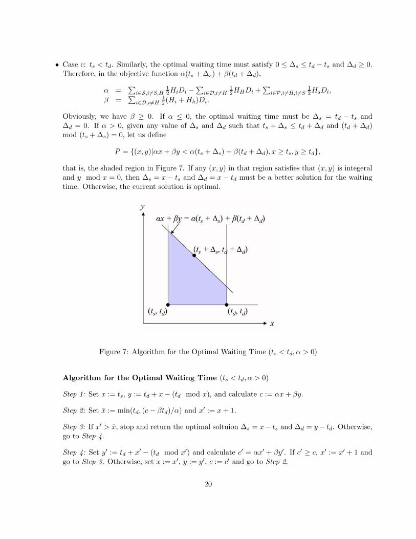
• Case c: ts < td. Similarly, the optimal waiting time must satisfy 0 ≤ ∆s ≤ td − ts and ∆d ≥ 0.Therefore, in the objective function α(ts + ∆s) + β(td + ∆d),

α =∑

i∈S,i�=S,H12HiDi −

∑i∈D,i�=H

12HHDi +

∑i∈P,i�=H,i�=S

12HsDi,

β =∑

i∈D,i�=H12 (Hi + Hh)Di.

Obviously, we have β ≥ 0. If α ≤ 0, the optimal waiting time must be ∆s = td − ts and∆d = 0. If α > 0, given any value of ∆s and ∆d such that ts + ∆s ≤ td + ∆d and (td + ∆d)mod (ts + ∆s) = 0, let us define

P = {(x, y)|αx + βy < α(ts + ∆s) + β(td + ∆d), x ≥ ts, y ≥ td},

that is, the shaded region in Figure 7. If any (x, y) in that region satisfies that (x, y) is integeraland y mod x = 0, then ∆s = x − ts and ∆d = x − td must be a better solution for the waitingtime. Otherwise, the current solution is optimal.

Figure 7: Algorithm for the Optimal Waiting Time (ts < td, α > 0)

Algorithm for the Optimal Waiting Time (ts < td, α > 0)

Step 1: Set x := ts, y := td + x − (td mod x), and calculate c := αx + βy.

Step 2: Set x̄ := min(td, (c − βtd)/α) and x′ := x + 1.

Step 3: If x′ > x̄, stop and return the optimal soltuion ∆s = x− ts and ∆d = y − td. Otherwise,go to Step 4.

Step 4: Set y′ := td + x′ − (td mod x′) and calculate c′ = αx′ + βy′. If c′ ≥ c, x′ := x′ + 1 andgo to Step 3. Otherwise, set x := x′, y := y′, c := c′ and go to Step 2.

20

Obviously, the worst computational complexity for this algorithm is O(td − ts). Since every portexcept for the hub can only be visited once, ts and td cannot be very large numbers, and so theoptimal waiting time can be calculated efficiently.

4.3. Synchronization using Multi-Disjoint Cycle

The previous section outlined a method to strategically insert waiting time for the vessels in orderto synchronize the inventory flow from supply to feeder vessel. This is not the only means to reducethe inventory cost at the hub. Another strategy, in the case when the hub inventory cost is lowerthan the in-transit inventory cost, and when supply cycle is much longer than the feeder cycle, is touse the feeder vessel to make repeated calls at the hub in between each call by the supply vessel atthe hub. Note that the use of multi-cycle strategy creates complex material flow pattern in the hub.Fortunately, using our approach for the single cycle case, we can embed the search for multi-disjointcycle into our transposition heuristic to obtain improvement for the hub-and-spoke problem. This isobtained by trying to break down the feeder route from a single cycle into multiple disjoint cycles,while making sure that the additional traveling time does not exceed the waiting time inserted intothe feeder route for hub synchronization.

More formally, given an initial single cycle route, πD = {H,π(1), · · · , π(k),H}, with k demandports on the single feeder cycle, we can generate a new multi cycle route π′

D = {H,π(1), · · · , π(j),H, π(j+1), · · · , π(k),H} for each j ∈ {1, · · · , k − 1} and π(j) �= H. Suppose the schedule for the feeder vesselin the route πD includes waiting of ∆d days. The route π′

D is acceptable if and only if

Tπ(j)H + THπ(j+1) − Tπ(j)π(j+1) ≤ ∆d. (10)

For the route π′D, the allowable delay time is decreased to ∆d − Tπ(j)H + THπ(j+1) − Tπ(j)π(j+1). The

revisit of H changed the cost by

(Hh(T + Tπ(j)H) + HmTHπ(j+1) − Hm(T + Tπ(j)π(j+1))

) k∑i=j+1

Di. (11)

Here T is the transportation time for the route {H,π(1), · · · , π(j)}. Note that the route π′D is better

than the route πD provided the term in (11) is negative.By repeating the above cycle breaking heuristic, we can turn a single cycle route into multiple

disjoint cycle route using a single feeder vessel. Let c(πD) denote the cost of the best multi-disjointcycle route obtained with the initial route πD.

4.4. Transposition Heuristic

According to the above analysis, it is impossible to compute the optimal solution of the MP by solvingan optimization model. It has nonlinear objective function and requires the partition of the ports.At the same time, the routes are Hamiltonian tours of all the ports the ship visits. However, thecalculation for the average cost with given routes is very efficient. Similar to the MP, given the routesfor the hub-and-spoke system, the in-transit inventory cost and the loading/discharging cost can becalculated in O(|P|). The algorithm for the optimal waiting time gives the evidence that the portinventory cost can be computed in O(|P| + |ts − td|). Moreover, the fixed transportation cost is a

21

constant when considering the average cost. As a result, we can adopt a local search algorithm, whichterminates when no improvement is available in the neighborhood.

The transposition heuristic is also applicable here. Let us consider the hub as two separate ports.If H and H ′ denote the two ports corresponding to the hub, we have a new set of ports P ′ = P∪{H ′}.Given a Hamiltonian tour π of P ′,

{H,π(1), · · · , π(m),H ′, π(m + 2), · · · , π(|P|),H},

in which π(0) = π(|P| + 1) = H and π(m + 1) = H ′. It corresponds to the two routes in thehub-and-spoke system

π0 = {H,π(1), · · · , π(m),H} and π1 = {H,π(m + 2), · · · , π(|P|),H}.

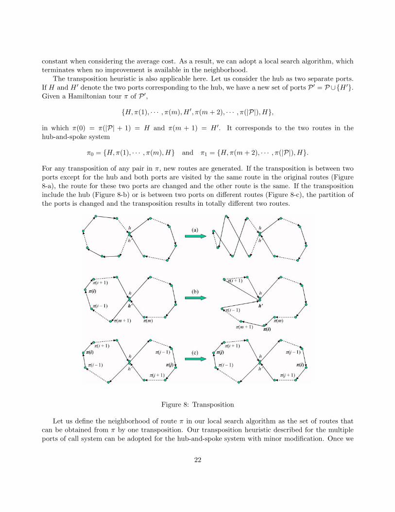
For any transposition of any pair in π, new routes are generated. If the transposition is between twoports except for the hub and both ports are visited by the same route in the original routes (Figure8-a), the route for these two ports are changed and the other route is the same. If the transpositioninclude the hub (Figure 8-b) or is between two ports on different routes (Figure 8-c), the partition ofthe ports is changed and the transposition results in totally different two routes.

Figure 8: Transposition

Let us define the neighborhood of route π in our local search algorithm as the set of routes thatcan be obtained from π by one transposition. Our transposition heuristic described for the multipleports of call system can be adopted for the hub-and-spoke system with minor modification. Once we

22

obtain the supply and feeder routes, we can next determine the optimal waiting time to be insertedinto the supply and feeder routes to minimize the inventory at the hub. We next compute c(πD), thebest multi-disjoint cycle route obtained with an initial feeder route πD.

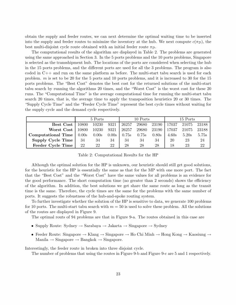
The computational results of the algorithm are displayed in Table 2. The problems are generatedusing the same approached in Section 3. In the 5 ports problems and the 10 ports problems, Singaporeis selected as the transshipment hub. The locations of the ports are considered when selecting the hubin the 15 ports problems, and the different ports are used for all the 3 problems. The program is alsocoded in C++ and run on the same platform as before. The multi-start tabu search is used for eachproblem. m is set to be 20 for the 5 ports and 10 ports problems, and it is increased to 30 for the 15ports problems. The “Best Cost” denotes the best cost for the returned solutions of the multi-starttabu search by running the algorithms 20 times, and the “Worst Cost” is the worst cost for these 20runs. The “Computational Time” is the average computational time for running the multi-start tabusearch 20 times, that is, the average time to apply the transposition heuristics 20 or 30 times. The“Supply Cycle Time” and the “Feeder Cycle Time” represent the best cycle times without waiting forthe supply cycle and the demand cycle respectively.

5 Ports 10 Ports 15 PortsBest Cost 10800 10230 9321 26257 29680 23190 17037 21075 23188

Worst Cost 10800 10230 9321 26257 29680 23190 17037 21075 23188Computational Time 0.00s 0.00s 0.00s 0.75s 0.75s 0.80s 4.60s 5.20s 5.75s

Supply Cycle Time 34 34 34 34 34 34 20 23 24Feeder Cycle Time 22 22 22 28 28 28 18 23 22

Table 2: Computational Results for the HP

Although the optimal solution for the HP is unknown, our heuristic should still get good solutions,for the heuristic for the HP is essentially the same as that for the MP with one more port. The factthat the “Best Cost” and the “Worst Cost” have the same values for all problems is an evidence forthe good performance. The short computation time (no greater than 2 seconds) shows the efficiencyof the algorithm. In addition, the best solutions we get share the same route as long as the transittime is the same. Therefore, the cycle times are the same for the problems with the same number ofports. It suggests the robustness of the hub-and-spoke routing system.

To further investigate whether the solution of the HP is sensitive to data, we generate 100 problemsfor 10 ports. The multi-start tabu search with m = 50 is used to solve these problem. All the solutionsof the routes are displayed in Figure 9.

The optimal routs of 94 problems are that in Figure 9-a. The routes obtained in this case are

• Supply Route: Sydney → Sarabaya → Jakarta → Singapore → Sydney

• Feeder Route: Singapore → Klang → Singapore → Ho Chi Minh → Hong Kong → Kaosiung →Manila → Singapore → Bangkok → Singapore.

Interestingly, the feeder route in broken into three disjoint cycle.The number of problems that using the routes in Figure 9-b and Figure 9-c are 5 and 1 respectively.

23

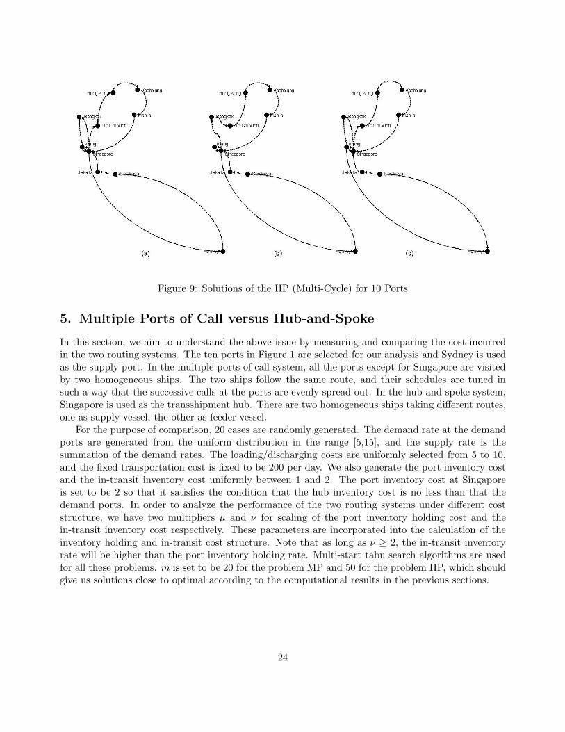
Figure 9: Solutions of the HP (Multi-Cycle) for 10 Ports

5. Multiple Ports of Call versus Hub-and-Spoke

In this section, we aim to understand the above issue by measuring and comparing the cost incurredin the two routing systems. The ten ports in Figure 1 are selected for our analysis and Sydney is usedas the supply port. In the multiple ports of call system, all the ports except for Singapore are visitedby two homogeneous ships. The two ships follow the same route, and their schedules are tuned insuch a way that the successive calls at the ports are evenly spread out. In the hub-and-spoke system,Singapore is used as the transshipment hub. There are two homogeneous ships taking different routes,one as supply vessel, the other as feeder vessel.

For the purpose of comparison, 20 cases are randomly generated. The demand rate at the demandports are generated from the uniform distribution in the range [5,15], and the supply rate is thesummation of the demand rates. The loading/discharging costs are uniformly selected from 5 to 10,and the fixed transportation cost is fixed to be 200 per day. We also generate the port inventory costand the in-transit inventory cost uniformly between 1 and 2. The port inventory cost at Singaporeis set to be 2 so that it satisfies the condition that the hub inventory cost is no less than that thedemand ports. In order to analyze the performance of the two routing systems under different coststructure, we have two multipliers µ and ν for scaling of the port inventory holding cost and thein-transit inventory cost respectively. These parameters are incorporated into the calculation of theinventory holding and in-transit cost structure. Note that as long as ν ≥ 2, the in-transit inventoryrate will be higher than the port inventory holding rate. Multi-start tabu search algorithms are usedfor all these problems. m is set to be 20 for the problem MP and 50 for the problem HP, which shouldgive us solutions close to optimal according to the computational results in the previous sections.

24

MP HP # MP worse than HPµ ν TC Inv. Tra. TC Inv. Tra.1 2 9799 2869 2675 11397 4187 2469 01 4 15149 2869 2675 16047 4404 2373 01 6 20499 2869 2675 20621 4404 2341 71 8 25849 2869 2675 25170 4586 2306 191 10 31200 2869 2675 29692 4628 2293 201 15 44575 2869 2675 40909 4884 2263 201 20 57951 2869 2675 52123 4990 2254 20

Table 3: Multiple Ports of Call versus Hub-and-Spoke

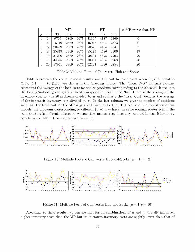
Table 3 presents the computational results, and the cost for each cases when (µ, ν) is equal to(1,2), (1,4), . . ., to (1,20) are shown in the following figures. The “Total Cost” for each systemsrepresents the average of the best costs for the 20 problems corresponding to the 20 cases. It includesthe loasing/unloading charges and fixed transportation cost. The “Inv. Cost” is the average of theinventory cost for the 20 problems divided by µ and similarly the “Tra. Cost” denotes the averageof the in-transit inventory cost divided by ν. In the last column, we give the number of problemssuch that the total cost for the MP is greater than that for the HP. Because of the robustness of ourmodels, the problems corresponding to different (µ, ν) may have the same optimal routes even if thecost structure is different. Therefore, we have the same average inventory cost and in-transit inventorycost for some different combinations of µ and ν.

Figure 10: Multiple Ports of Call versus Hub-and-Spoke (µ = 1, ν = 2)

Figure 11: Multiple Ports of Call versus Hub-and-Spoke (µ = 1, ν = 10)

According to these results, we can see that for all combinations of µ and ν, the HP has muchhigher inventory costs than the MP but its in-transit inventory costs are slightly lower than that of

25

the MP. Therefore, when the in-transit inventory cost is much higher than the port inventory cost,the hub-and-spoke system should have lower cost than that of the multiple ports of call.

For example, when the in-transit inventory cost is roughly 10 times of the port inventory cost,the improvement in the average cost is around 10% in our problems. However, when the in-transitinventory cost is not dominant in the total cost, the multiple ports of call system should have betterperformance. Even when the inventory cost and the in-transit inventory cost is almost the same, thecost for multiple ports of cost is close to 90% of the cost for hub-and-spoke.

An important fact is that the in-transit inventory cost is always higher than the port inventorycost. The port inventory cost mainly consists of the handling cost and the financial cost. Thesetwo components also occur for the in-transit inventory, and the handling cost can only be higher. Forexample, the in-transit inventory may incure higher insurance cost. Moreover, as mentioned in Section1, the in-transit inventory cost also includes the transportation cost that is in proportion to the loadon ship. In addition, there is also the opportunity cost for occupying the ship capacity. Therefore,although the 10 times higher in-transit inventory sounds outrageous, it happens in the real world.For those low value commodities, the inventory holding cost should be much lower than the in-transitinventory cost. The ores in our problem is a good example of such commodities.

6. Conclusion and Future Work

In this paper, we discuss a ship routing problem combined with inventory control. Firstly, a MIPformulation based on the time expanded network is proposed. Although the formulation gives astandard approach for this class of the problems, its solution is too complex and too sensitive to datato be implemented in practice. Therefore, we focus on the two routing systems: the multiple portsof call and the hub-and-spoke system, and propose good heuristics to find out the optimal routes forthese systems. Using the computational results of the algorithms, the costs incurred in these twosystems are investigated. The utilization of the hub-and-spoke system is justified from the perspectiveof cost effectiveness, when the in-transit inventory cost dominate the total cost.

In our model, only one supply port is considered. Although our algorithm can be applied directlyfor the problems with multiple supply ports in the multiple ports of call, the optimal waiting timein the hub-and-spoke system is not so straightforward. In addition, the existence of multiple supplyports may decrease the in-transit inventory cost, and so it is hard to tell whether the hub-and-spokesystem can be more cost effective even with high in-transit inventory cost.

Another natural extension is to investigate the problem with stochastic demand. Our computa-tional results suggest that the optimal routes may change when the demand and supply rates vary.Therefore, it must be an interesting problem to find out how much safety stock to keep at the differentports including the hub and whether the increased port inventory cost may change the optimal routesin the two routing systems.

References

[1] Anily, S., Federgruen, A. (1990): One warehouse multiple retailer systems with vehicle routingcosts., Management Science 36, 92-114.

26

[2] Anily, S., Federgruen, A. (1990): Rejoinder to “comments on one warehouse multiple retailersystems with vehicle routing costs”., Management Science 37, 1497-1499.

[3] Appelgren, L.H. (1969): A column generation algorithm for a ship scheduling problem., Trans-portation Science 3, 53-68.

[4] Baird, A.J. (2002): The economics of transshipment., Chapter 36, The Handbook of MaritimeEconomics and Business., Costas Th. Grammenos Ed., 832-859.

[5] Appelgren, L.H. (1971): Integer programming methods for a vessel scheduling problem., Trans-portation Science 5, 64-78.

[6] Bramel, J., Simchi-Levi, D. (1995): A location based heuristic for general routing problems.,Operations research 43, 649-660.

[7] Brown, B.B., Graves, G.W., Ronen, D. (1987): Scheduling ocean transportation of crude oil.,Management Science 33(3), 335-346.

[8] Chan, L.M.A., Federgruen, A., Simchi-Levi, D. (1998): Probabilistic analysis and practical algo-rithms for inventory-routing models., Operations Research 46(1), 96-106.

[9] Chien, T., Balakrishnan, A., Wong R. (1989): An integrated inventory allocation and vehiclerouting problem., Transportation Science 23, 67-76.

[10] Christiansen, M. (1999): Decomposition of a combined inventory and time constrained ship rout-ing problem., Transportation Science 33(1), 3-16.

[11] Christiansen, M., Fagerholt K. (2003): Ship routing and scheduling - status and trends., Workingpaper, Norwegian University of Science and Technology.

[12] Christiansen, M., Nygreen B. (1998a): A method for solving ship routing problems with inventoryconstraints., Annals of Operations Research 81, 357-378.

[13] Christiansen, M., Nygreen B. (1998b): Modelling path flows for a combined ship routing andinventory management problem., Annals of Operations Research 82, 391-412.

[14] Christofides, N. (1976): Worst-case analysis of a new heuristic for the traveling salesman problem.,Report 388, Graduate School of Industrial Administration, Carnegie-Mellon University.

[15] Damas, P. (2001): Transship or direct: a real choice?, American Shipper, June.

[16] Dror, M., Ball, M. (1987): Inventory/routing: reduction from an annual to a short period prob-lem., Naval Research Logistics Quarterly 34, 891-905.

[17] Dror, M., Ball, M., Golden, B. (1985): Computational comparison of algorithms for the inventoryrouting problem., Annals of Operations Research 4, 3-23.

[18] Federgruen, A., Simchi-Levi, D. (1995): Analysis of vehicle routing and inventory-routing prob-lems., Handbooks in Operations Research and Managment Science 8, Network Routing., M.O. Ball,T.L. Magnanti, C.L. Monma and G.L. Nemhauser, Eds., North-Holland, Amsterdam, 297-373.

27

[19] Federgruen, A., Zipkin, P. (1984): A combined vehicle routing and inventory allocation problem.,Operations Research 32, 1019-1036.

[20] Fisher, M.L., Rosenwein, M.B. (1989): An interactive optimization system for bulk-cargo shipscheduling., Naval Research Logistics 36, 27-42.

[21] Frankel, E.G. (2002): The challenge of container transshipment in the Caribbean., InternationalAssociation of Maritime Economist Conference, Panama.

[22] Gilman, S. (1999): The size economies and network efficiency of large containerships., Interna-tional Journal of Maritime Economics, 1(1), July-September, 39-59.

[23] Goemans, M.X., Kleinberg, J.(1996): An improved approximation ratio for the minimum latencyproblem., Proceedings of the 7th Annual ACM-SIAM Symposium on Discrete Algorithms, 152-158.

[24] Golden, B., Assad, A., Dahl, R. (1984): Analysis of a Large scale vehicle routing problem withan inventory component., Large Scale Systems 7, 181-190.

[25] Lai, K.K., Lam, K., Chan, W.K. (1995): Shipping container logistics and allocation., Journal ofOperational Research Society 46, 687-697.

[26] Larson, R. (1988): Transporting sludge to the 106 mile site: an inventory/routing model for fleetsizing and logistics system design., Transportation Science 22, 186-198.

[27] MDS Transmodal (1994): The future of Southampton Docks: Dibden Bay port development.,Unpublished report for Hampshire County Council, May.

[28] Miller, D.M. (1987): An interactive, computer-aided ship scheduling system., European Journalof Operational Research 32, 363-379.

[29] Papadakis, N.A., Perakis, A.N. (1989): A nonlinear approach to the multiorigin, multidestinationfleet deployment problem., Naval Research Logistics 36, 515-528.

[30] Rana, K., Vickson R.G. (1988): A model and solution algorithm for optimal routing of a time-chartered containership., Transporation Science 22(2), 83-95.

[31] Rana, K., Vickson R.G. (1991): Routing container ships using Lagrangean relaxation and decom-position., Transportation Science 25(3), 201-214.

[32] Ronen, D. (1986): Short-term scheduling of vessels for shipping bulk or semi-bulk commoditiesoriginating in a single area., Operations Research 34(1), 164-173.

[33] Wijnolst, N. (2000): Ships, larger and larger: containerships of 18000 TEU - impacts on operatorsand ports., Dynamar Liner Shipping 2020 Workshop, London, 13-29.

[34] Wu, G. and Kleywegt, A. (2002): Models of cost incurred by ocean carriers during port visits.,TLI-AP White Paper Series.

28

Appendix A:

We will describe an MIP formulation for a more general routing problem, where the ships deployedmay not be homogeneous, and there are limited capacity in ports for loading/unloading operation.

Problem DefinitionSuppose that we have a fleet of ships V to be responsible for the transportation. There are some

supply ports PS , that is, ports corresponding to the mines, and some demand ports P which are portsfor the warehouses. Moreover, among these supply and demand ports, some of these ports H can beused as transportation hubs. At a hub, the goods on one ship can be discharged from that ship andreloaded to another one. That is, both loading and discharging can be carried out at a hub whilea pure supply port can only load some commodities to the ships and a pure demand port can onlydischarge some commodities from the ships. We assume the cycle time is given in this section, andthe shipping schedule will repeat itself in each cycle. In sum, our index sets include

V The set of shipsT The set of time, T = {0, · · · , n} where n is the cycle timeP The set of ports, P = PS ∪ PPS The set of ports corresponding to minesP The set of ports corresponding to warehousesH The set of ports which can be hubs, H ⊆ P.

We also assume that both the supply rate Si at the supply ports and the demand rate Di at thedemand ports are deterministic. For the hubs, these rates can be equal to 0. Moreover, we define therate Ri, which is equal to Si for any supply port i and −Di for any demand port i. To make our problemmore realistic, we impose the capacities for the ships, the port inventory and the loading/dischargingquantity. In addition, the transit time between any ports for any ship should be given as long as thatservice is available. These inputs are summarized in the following table:

Si The quantity of the commodity produced per day at port i, i ∈ PS

Di The quantity of the commodity consumed per day at port i, i ∈ PRi The supply/demand rate at port i, i ∈ PCv The capacity of ship v, v ∈ VCI

i The inventory capacity of port i, i ∈ PCL

i The maximum quantity that can be loaded/discharged per day at port i, i ∈ PT v

ij The sailing time from port i, i ∈ P to port j, j ∈ P \ {i} for ship v, v ∈ V.

For the transportation costs, we firstly consider a fixed cost per day for every ship, which corre-sponds to the cost for the crews, the insurance and etc. The in-transit inventory cost is the inventoryholding cost for the commodities on ship plus other cost proportional to the load on ship, for example,the cost for the extra fuel burned with more load on ship. In addition, the loading/discharging costis also taken into account in the transportation cost. At the same time, the inventory holding cost isconsidered for the port inventory. All these cost parameter are displayed in the following table:

F v The fixed cost per day for ship v, v ∈ VV v The in-transit inventory cost per unit of the commodity per day for v, v ∈ VLi The loading/discharging cost per unit of the commodity at port i, i ∈ PHi The inventory holding cost per unit of the commodity per day at port i, i ∈ P.

29

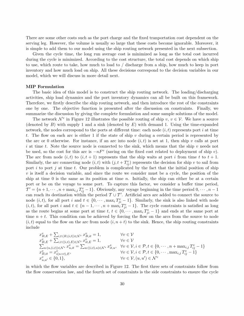
There are some other costs such as the port charge and the fixed tranportation cost dependent on theserving leg. However, the volume is usually so large that these costs become ignorable. Moreover, itis simple to add them to our model using the ship routing network presented in the next subsection.

Given the cycle time, the long run average cost is minimized as long as the total cost incurredduring the cycle is minimized. According to the cost structure, the total cost depends on which shipto use, which route to take, how much to load to / discharge from a ship, how much to keep in portinventory and how much load on ship. All these decisions correspond to the decision variables in ourmodel, which we will discuss in more detail next.

MIP FormulationThe basic idea of this model is to construct the ship routing network. The loading/discharging

activities, ship load dynamics and the port inventory dynamics can all be built on this framework.Therefore, we firstly describe the ship routing network, and then introduce the rest of the constraintsone by one. The objective function is presented after the discussion on constraints. Finally, wesummarize the discussion by giving the complete formulation and some sample solutions of the model.

The network N v in Figure 12 illustrates the possible routing of ship v, v ∈ V. We have a source(denoted by B) with supply 1 and a sink (denoted by E) with demand 1. Using the time-expandednetwork, the nodes correspond to the ports at different time: each node (i, t) represents port i at timet. The flow on each arc is either 1 if the state of ship v during a certain period is represented bythe arc or 0 otherwise. For instance, if an arc into node (i, t) is set at 1, then ship v calls at porti at time t. Note the source node is connected to the sink, which means that the ship v needs notbe used, so the cost for this arc is −nF v (saving on the fixed cost related to deployment of ship v).The arc from node (i, t) to (i, t + 1) represents that the ship waits at port i from time t to t + 1.Similarly, the arc connecting node (i, t) with (j, t + T v

ij) represents the decision for ship v to sail fromport i to port j at time t. Our problem is complicated by the fact that the initial position of shipv is itself a decision variable, and since the route we consider must be a cycle, the position of theship at time 0 is the same as its position at time n. Initially, the ship can either be at a certainport or be on the voyage to some port. To capture this factor, we consider a buffer time period,T ′ = {n + 1, · · · , n + maxi,j T v

ij − 1}. Obviously, any voyage beginning in the time period 0, · · · , n − 1can reach its destination within the period T ∪ T ′. Artificial arcs are added to connect the source tonode (i, t), for all port i and t ∈ {0, · · · ,maxi T

vji − 1}. Similarly, the sink is also linked with node

(i, t), for all port i and t ∈ {n − 1, · · · , n + maxi Tvji − 1}. The cycle constraints is satisfied as long

as the route begins at some port at time t, t ∈ {0, · · · ,maxi Tvji − 1} and ends at the same port at

time n + t. This condition can be achieved by forcing the flow on the arcs from the source to node(i, t) equal to the flow on the arc from node (i, n + t) to the sink. Hence, the ship routing constraintsinclude

xvB,E +

∑i,t:(B,(i,t))∈N v xv

B,it = 1, ∀v ∈ Vxv

B,E +∑

i,t:((i,t),E)∈N v xvit,E = 1, ∀v ∈ V∑

u:(u,(i,t))∈N v xvu,it =

∑u:((i,t),u)∈N v xs

it,u, ∀v ∈ V, i ∈ P, t ∈ {0, · · · , n + maxi,j T vij − 1}

xvB,it = xv

i(n+t),E , ∀v ∈ V, i ∈ P, t ∈ {0, · · · ,maxi,j T vij − 1}

xvu,u′ ∈ {0, 1}, ∀v ∈ V, (u, u′) ∈ N v

in which the flow variables are described in Figure 12. The first three sets of constraints follow fromthe flow conservation law, and the fourth set of constraints is the side constraints to ensure the cycle

30

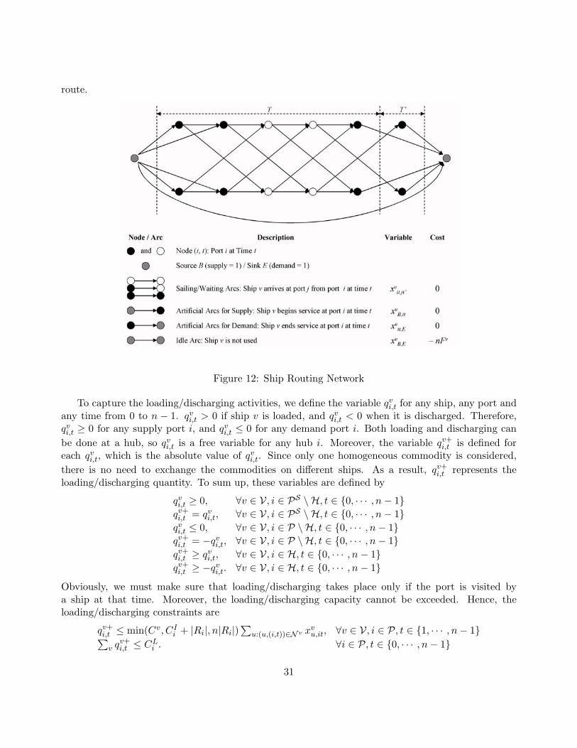
route.

Figure 12: Ship Routing Network

To capture the loading/discharging activities, we define the variable qvi,t for any ship, any port and

any time from 0 to n − 1. qvi,t > 0 if ship v is loaded, and qv

i,t < 0 when it is discharged. Therefore,qvi,t ≥ 0 for any supply port i, and qv

i,t ≤ 0 for any demand port i. Both loading and discharging canbe done at a hub, so qv

i,t is a free variable for any hub i. Moreover, the variable qv+i,t is defined for

each qvi,t, which is the absolute value of qv

i,t. Since only one homogeneous commodity is considered,there is no need to exchange the commodities on different ships. As a result, qv+

i,t represents theloading/discharging quantity. To sum up, these variables are defined by

qvi,t ≥ 0, ∀v ∈ V, i ∈ PS \ H, t ∈ {0, · · · , n − 1}

qv+i,t = qv

i,t, ∀v ∈ V, i ∈ PS \ H, t ∈ {0, · · · , n − 1}qvi,t ≤ 0, ∀v ∈ V, i ∈ P \H, t ∈ {0, · · · , n − 1}

qv+i,t = −qv

i,t, ∀v ∈ V, i ∈ P \H, t ∈ {0, · · · , n − 1}qv+i,t ≥ qv

i,t, ∀v ∈ V, i ∈ H, t ∈ {0, · · · , n − 1}qv+i,t ≥ −qv

i,t. ∀v ∈ V, i ∈ H, t ∈ {0, · · · , n − 1}

Obviously, we must make sure that loading/discharging takes place only if the port is visited bya ship at that time. Moreover, the loading/discharging capacity cannot be exceeded. Hence, theloading/discharging constraints are

qv+i,t ≤ min(Cv, CI

i + |Ri|, n|Ri|)∑

u:(u,(i,t))∈N v xvu,it, ∀v ∈ V, i ∈ P, t ∈ {1, · · · , n − 1}∑

v qv+i,t ≤ CL

i . ∀i ∈ P, t ∈ {0, · · · , n − 1}

31

The cycle time constraint requires that the load on ship at time n is equal to that at time 0. LetQv

t be the load on ship v at any time t, t = {0, · · · , n − 1}, we have the constraints

Qv0 = Qv

n−1 +∑

i qvi,0, ∀v ∈ V

Qvt = Qv

t−1 +∑

i qvi,t, ∀v ∈ V, t ∈ {1, · · · , n − 1}

0 ≤ Qvt ≤ Cv. ∀v ∈ V, t ∈ {0, · · · , n − 1}

Similarly, let Ii,t be the inventory level at port i at any time t, t = {0, · · · , n− 1}. The port inventorydynamics are described by these constraints:

Ii,0 = Ii,n−1 −∑

v qvi,0 + Ri, ∀i ∈ P

Ii,t = Ii,t−1 −∑

v qvi,t + Ri, ∀i ∈ P, t ∈ {1, · · · , n − 1}

0 ≤ Ii,t ≤ CIi . ∀i ∈ P, t ∈ {1, · · · , n − 1}

The objective is to minimize the transportation cost as well as the inventory cost. The fixedtransportation cost, the fixed transportation cost for each leg and the port charge are all included in thearc cost of the ship routing network. For any ship v, the sum of these costs is (nF v −nF vxv

B,E). SincenF v is a constant, it can be removed from the objective function. The rest of the total transportationcost includes the in-transit inventory cost and the loading/discharging cost. For a ship v, the sum ofthese two terms is

∑t V vQv

t +∑

i,t Liqv+i,t . Moreover, we also have the inventory holding cost

∑i,t HiIi,t.

Therefore, we get our objective function

−∑

v

nF vxvB,E +

∑v,t

V vQvt +

∑v,i,t

Liqv+i,t +

∑i,t

HiIi,t.

The Complete FormulationTo sum up, the decision variables in this model include

xvu,u′ The ship routing network flow variable for arc (u, u′), (u, u′) ∈ N v for ship v, v ∈ V

qvi,t The loading/discharging of ship v, v ∈ V at port i, i ∈ P at time t, t ∈ {0, · · · , n − 1}

qv+i,t The loading/discharging quantity correpsonding to qv

i,t

Qvt The quantity of the commodity on ship v, v ∈ V at time t, t ∈ {0, · · · , n − 1}

Ii,t The inventory at port i, i ∈ P at time t, t ∈ {0, · · · , n − 1}.

32

Putting the objective function and the constraints together, the MIP formulation is

min −∑

v nF vxvB,E +

∑v,t V vQv

t +∑

v,i,t Liqv+i,t +

∑i,t HiIi,t

s.t. xvB,E +

∑i,t:(B,(i,t))∈N v xv

B,it = 1, ∀v ∈ Vxv

B,E +∑

i,t:((i,t),E)∈N v xvit,E = 1, ∀v ∈ V∑

u:(u,(i,t))∈N v xvu,it =

∑u:((i,t),u)∈N v xs

it,u, ∀v ∈ V, i ∈ P, t ∈ {0, · · · , n + maxi,j T vij − 1}

xvB,it = xv

i(n+t),E , ∀v ∈ V, i ∈ P, t ∈ {0, · · · ,maxi,j T vij − 1}

qv+i,t ≤ min(Cv, CI

i + |Ri|, n|Ri|)∑

u:(u,(i,t))∈N v xvu,it, ∀v ∈ V, i ∈ P, t ∈ {1, · · · , n − 1}∑

v qv+i,t ≤ CL

i . ∀i ∈ P, t ∈ {0, · · · , n − 1}Qv

0 = Qvn−1 +

∑i q

vi,0, ∀v ∈ V

Qvt = Qv

t−1 +∑

i qvi,t, ∀v ∈ V, t ∈ {1, · · · , n − 1}

Ii,0 = Ii,n−1 −∑

v qvi,0 + Ri, ∀i ∈ P

Ii,t = Ii,t−1 −∑

v qvi,t + Ri, ∀i ∈ P, t ∈ {1, · · · , n − 1}

qv+i,t = qv

i,t, ∀v ∈ V, i ∈ PS \ H, t ∈ {0, · · · , n − 1}qv+i,t = −qv

i,t, ∀v ∈ V, i ∈ P \ H, t ∈ {0, · · · , n − 1}qv+i,t ≥ qv

i,t, ∀v ∈ V, i ∈ H, t ∈ {0, · · · , n − 1}qv+i,t ≥ −qv

i,t, ∀v ∈ V, i ∈ H, t ∈ {0, · · · , n − 1}xv

u,u′ ∈ {0, 1}, ∀v ∈ V, (u, u′) ∈ N v

qvi,t ≥ 0, ∀v ∈ V, i ∈ PS \ H, t ∈ {0, · · · , n − 1}

qvi,t ≤ 0, ∀v ∈ V, i ∈ P \ H, t ∈ {0, · · · , n − 1}

0 ≤ Qvt ≤ Cv. ∀v ∈ V, t ∈ {0, · · · , n − 1}

0 ≤ Ii,t ≤ CIi . ∀i ∈ P, t ∈ {1, · · · , n − 1}

(12)

33