INVENTORY PINCH DECOMPOSITION AND GLOBAL OPTIMIZATION METHODS

Welcome message from author
This document is posted to help you gain knowledge. Please leave a comment to let me know what you think about it! Share it to your friends and learn new things together.
Transcript
INVENTORY PINCH DECOMPOSITION
AND GLOBAL OPTIMIZATION METHODS

PLANNING AND SCHEDULING OF CONTINUOUS
PROCESSES VIA INVENTORY PINCH DECOMPOSITION
AND GLOBAL OPTIMIZATION ALGORITHMS
By PEDRO A. CASTILLO CASTILLO,
M.A.Sc. Chemical Engineering
A Thesis Submitted to the School of Graduate Studies
in Partial Fulfillment of the Requirements for the Degree
Doctor of Philosophy
McMaster University
© Copyright by Pedro A. Castillo Castillo, March 2020

Ph. D. Thesis – Pedro A. Castillo
Castillo
McMaster University – Chemical Engineering
ii
DOCTOR OF PHILOSOPHY (2020) McMaster University
(Chemical Engineering) Hamilton, Ontario
TITLE: Planning and Scheduling of Continuous Processes
Via Inventory Pinch Decomposition and Global
Optimization Algorithms
AUTHOR: Pedro A. Castillo Castillo
M.A.Sc. Chemical Engineering (McMaster
University)
SUPERVISOR: Professor Vladimir Mahalec
NUMBER OF PAGES: x, 216

Ph. D. Thesis – Pedro A. Castillo
Castillo
McMaster University – Chemical Engineering
iii
Lay Abstract
Optimal planning and scheduling of production systems are two very important tasks in
industrial practice. Their objective is to ensure optimal utilization of raw materials and
equipment to reduce production costs. In order to compute realistic production plans and
schedules, it is often necessary to replace simplified linear models with nonlinear ones
including discrete decisions (e.g., “yes/no”, “on/off”). To compute a global optimal
solution for this type of problems in reasonable time is a challenge due to their intrinsic
nonlinear and combinatorial nature.
The main goal of this thesis is the development of efficient algorithms to solve large-scale
planning and scheduling problems. The key contributions of this work are the
development of: i) a heuristic technique to compute near-optimal solutions rapidly, and ii)
a deterministic global optimization algorithm. Both approaches showed results and
performances better or equal to those obtained by commercial software and previously
published methods.

Ph. D. Thesis – Pedro A. Castillo
Castillo
McMaster University – Chemical Engineering
iv
Abstract
In order to compute more realistic production plans and schedules, techniques using
nonlinear programming (NLP) and mixed-integer nonlinear programming (MINLP) have
gathered a lot of attention from the industry and academy. Efficient solution of these
problems to a proven 𝜀-global optimality remains a challenge due to their combinatorial,
nonconvex, and large dimensionality attributes.
The key contributions of this work are: 1) the generalization of the inventory pinch
decomposition method to scheduling problems, and 2) the development of a deterministic
global optimization method.
An inventory pinch is a point at which the cumulative total demand touches its
corresponding concave envelope. The inventory pinch points delineate time intervals
where a single fixed set of operating conditions is most likely to be feasible and close to
the optimum. The inventory pinch method decomposes the original problem in three
different levels. The first one deals with the nonlinearities, while subsequent levels
involve only linear terms by fixing part of the solution from previous levels. In this
heuristic method, infeasibilities (detected via positive value of slack variables) are
eliminated by adding at the first level new period boundaries at the point in time where
infeasibilities are detected.
The global optimization algorithm presented in this work utilizes both piecewise
McCormick (PMCR) and Normalized Multiparametric Disaggregation (NMDT), and
employs a dynamic partitioning strategy to refine the estimates of the global optimum.
Another key element is the parallelized bound tightening procedure.
Case studies include gasoline blend planning and scheduling, and refinery planning. Both
inventory pinch method and the global optimization algorithm show promising results
and their performance is either better or on par with other published techniques and
commercial solvers, as exhibited in a number of test cases solved during the course of this
work.

Ph. D. Thesis – Pedro A. Castillo
Castillo
McMaster University – Chemical Engineering
v
Preface
Chapters 2–8 contain multi-authored work previously published in peer-reviewed
scientific journals. My individual contributions to each of those chapters consisted of the
following:
• Implementing the corresponding mathematical models in GAMS.
• Developing the steps of the solution algorithms.
• Implementing the algorithms (MPIP, MPIP-C, and deterministic global
optimization method) using GAMS, Python, and MATLAB.
• Running the examples and gathering numerical results.
• Analyzing the numerical results.
• Writing the initial draft and final version of each manuscript.
Contributions from Dr. Vladimir Mahalec in Chapters 2–8 included:
• Providing insightful discussions about planning and scheduling problems,
potential solution strategies, and during the analysis of the numerical results.
• Approving numerical data used in the examples.
• Proofreading and editing each manuscript.
Contributions from Dr. Pedro M. Castro in Chapters 6 and 7 included:
• Providing insightful discussions about piecewise linear relaxations, bound
tightening techniques, and during the analysis of the numerical results.
• Proofreading and editing each manuscript.

Ph. D. Thesis – Pedro A. Castillo
Castillo
McMaster University – Chemical Engineering
vi
Acknowledgments
I would like to thank my supervisor Dr. Vladimir Mahalec for all his support, guidance,
and patience during the last five years. Dr. Mahalec is a great professor and a person that
really cares about his students beyond their academic performance. Since the beginning,
he always encouraged me to be the best version of myself. I would like to thank him for
the time and expertise he provided me, which were key elements to make each step of my
journey a success. My sincere gratitude and utmost respect to him.
I would also like to thank my thesis committee: Dr. Christopher L. E. Swartz, from the
Chemical Engineering department, and Dr. Antoine Deza, from the Computing and
Software department. I really appreciated their advice, questions, and suggestions during
our committee meetings. In addition, I would like to thank Dr. Pedro M. Castro for
collaborating with me and Dr. Vladimir Mahalec during the development of our global
optimization algorithm.
My sincere thanks to the always supportive and amazing administrative staff in the
Chemical Engineering department: Ms. Michelle Whalen, Ms. Kristina Trollip, Ms. Lynn
Falkiner, and Ms. Cathie Roberts.
For their financial support, I would like to show my gratitude to the Chemical
Engineering department, the McMaster Advanced Control Consortium, the International
Ontario Graduate Scholarship (OGS) Program, and the Engineering Research Council of
Canada (NSERC).
Thank you to all the people that were part of my life during this time, especially to my
friends from my research group, the Chemical Engineering department, the Organization
of Latin American Students (OLAS), McMaster University, Hamilton and Toronto. I will
never forget the time we spent together discussing optimization techniques, going to
scientific conferences, playing sports all year round, going to Toronto FC matches,
enjoying the good times, and supporting each other in difficult moments.
Finally, I would like to say thank you to my family, especially to my parents. They were
my main motivation and their love and support were invaluable to me. Thank you to my
grandparents for all their blessings. Thank you to my brothers, aunts, my uncle, and all
my cousins, always putting a smile on my face when I went back to visit them and during
our telephone calls.
“It is more important to ask the right questions than it is to have the right answers”

Ph. D. Thesis – Pedro A. Castillo
Castillo
McMaster University – Chemical Engineering
vii
Table of Contents
Lay Abstract .......................................................................................................................... iii
Abstract ................................................................................................................................. iv
Preface ..................................................................................................................................... v
Acknowledgments ................................................................................................................. vi
Table of Contents ................................................................................................................. vii
List of Abbreviations ............................................................................................................ ix
Declaration of Academic Achievement ................................................................................. x
Chapter 1: Introduction ......................................................................................................... 1
1.1. Supply chain optimization ....................................................................................... 2
1.2. Planning and scheduling of oil refinery operations ................................................. 4
1.3. The inventory pinch approach for production planning and scheduling ................. 8
1.4. Deterministic global optimization techniques ....................................................... 10
1.5. Objectives of the thesis .......................................................................................... 13
1.6. Thesis Outline ........................................................................................................ 13
1.7. References .............................................................................................................. 15
Chapter 2: Inventory Pinch Based, Multiscale Models for Integrated Planning and
Scheduling-Part I: Gasoline Blend Planning ..................................................................... 23
Chapter 3: Inventory Pinch Based, Multiscale Models for Integrated Planning and
Scheduling-Part II: Gasoline Blend Scheduling ................................................................ 46
Chapter 4: Inventory Pinch-Based Multi-Scale Model for Refinery Production
Planning ................................................................................................................................. 71
Chapter 5: Improved Continuous-Time Model for Gasoline Blend Scheduling ............ 79
Chapter 6: Inventory Pinch Gasoline Blend Scheduling Algorithm Combining
Discrete- and Continuous-Time Models ........................................................................... 101
Chapter 7: Global Optimization Algorithm for Large-Scale Refinery Planning Models
with Bilinear Terms ............................................................................................................ 119
Chapter 8: Global Optimization of Nonlinear Blend-Scheduling Problems ................. 140
Chapter 9: Global Optimization of MIQCPs with Dynamic Piecewise Relaxations .... 156
Chapter 10: Concluding Remarks .................................................................................... 184

Ph. D. Thesis – Pedro A. Castillo
Castillo
McMaster University – Chemical Engineering
viii
10.1. Key Findings and Contributions ............................................................ 185
10.2. Future Work Outlook ............................................................................. 186
Appendix A: Supporting Information for Chapters 2 and 3 .......................................... 188
Appendix B: Supporting Information for Chapters 5, 6, and 8 ..................................... 192
Appendix C: Supporting Information for Chapter 7 and 9 ........................................... 199

Ph. D. Thesis – Pedro A. Castillo
Castillo
McMaster University – Chemical Engineering
ix
List of Abbreviations
CATP Cumulative average total production
CCR Continuous catalytic reforming unit
CDU Crude distillation unit
CTD Cumulative total demand
DHT Diesel hydrotreating unit
FBBT Feasibility-based bound tightening
FCC Fluid catalytic cracking unit
GAMS General algebraic modeling system
GOHT Gasoil hydrotreating unit
HC Hydrocracking unit
LP Linear programming
MILP Mixed-integer linear programming
MINLP Mixed-integer nonlinear programming
MPIP Multiperiod inventory pinch
MPIP-C Multiperiod inventory pinch with continuous-time scheduling model
NHT Naphtha hydrotreating unit
NLP Nonlinear programming
NMDT Normalized multiparametric disaggregation technique
OBBT Optimality-based bound tightening
PMCR Piecewise McCormick relaxation
RHT Residue hydrotreating unit

Ph. D. Thesis – Pedro A. Castillo
Castillo
McMaster University – Chemical Engineering
x
Declaration of Academic Achievement
I, Pedro Alejandro Castillo Castillo, declare that my contributions to this research work
are the following:
i) I provided the main ideas to develop the algorithms introduced in this work,
ii) I implemented the required mathematical models in GAMS,
iii) I implemented the proposed algorithms (MPIP, MPIP-C, and deterministic
global optimization method) using Python, GAMS, and MATLAB,
iv) I developed a Python script to use Dia Diagram Editor as a graphical user
interface to model production processes as nodes in a network,
v) I solved the case studies presented in this work and gathered the numerical
results, and
vi) I wrote the initial draft and final version of each manuscript presented here.
In addition, I declare that Dr. Vladimir Mahalec and Dr. Pedro M. Castro provided ideas
and guidance to enhance such algorithms, proofread and edited the manuscripts in which
each one of them collaborated.
Sincerely,
Pedro Alejandro Castillo Castillo

Ph. D. Thesis – Pedro A. Castillo
Castillo
McMaster University – Chemical Engineering
1
1. Chapter 1: Introduction
Planning and scheduling of production systems are two activities in supply chain
optimization that increase profit margins of the plant sites by utilizing raw materials,
intermediate components, storage capacity, and production equipment in the best way
possible along a given time horizon, considering current market conditions and forecasts.
Planning and scheduling software-based tools have become necessary for most
companies, especially those that operate on economic markets with fast dynamics, face
strict environmental regulations, and/or have low profit margins (e.g., commodity
producers) [1].
Current trend in planning and scheduling techniques is to increase the accuracy of the
mathematical models employed to represent processing units and operational policies
(taking into account their scalability), as well as the development of advanced algorithms
to efficiently solve these models to optimality.
It is often the case that the nature of the production process is inherently nonlinear, and
operational policies usually rely on discrete decisions (e.g., “yes/no”, “on/off”).
Therefore, to compute more realistic production plans and schedules, techniques using
nonlinear programming (NLP) and mixed-integer nonlinear programming (MINLP) are
required. The challenges associated with nonlinear planning and scheduling problems are
the following:
1. Possible nonconvexities, which can introduce multiple local and global optima
▪ Traditional gradient-based optimization methods can stop at a local
optimum. Global optimization techniques are thus needed to understand
the quality of the solution and make better decisions.
2. Potential need of a large number of partitions to represent the time domain, which
can result in a model containing thousands or more variables
▪ The larger the number of time periods or time slots, the larger the number
of nonconvex terms and discrete variables, thus the higher computational
cost involved to solve the problem to optimality.
This thesis summarizes a project focused on the development of two algorithms to solve
planning and scheduling problems: a heuristic decomposition approach based on the
inventory pinch concept, and a deterministic global optimization method based on
dynamic partitioning of piecewise linear relaxations and optimality-based bound
tightening.

Ph. D. Thesis – Pedro A. Castillo
Castillo
McMaster University – Chemical Engineering
2
In this Chapter, different concepts used throughout this report are briefly described. In
addition, the objectives and outline of this thesis are presented.
1.1. Supply chain optimization
A supply chain consists of all different entities and activities necessary to produce and
distribute a product to the final customer. These activities include procurement of raw
materials, transformation and/or purification of the raw materials into intermediate and
final products, storage and distribution of intermediate and final products, and demand
forecasting and satisfaction. The physical elements of a supply chain include warehouses,
distribution centers, production sites, retailers, etc. Supply chain optimization consists of
determining the best possible flow of materials and information among these elements
that maximize the performance of the supply chain. The performance of the supply chain
is defined according to the company’s goals; e.g., increase profit, market share, customer
satisfaction, and/or decrease costs, lead time, etc.
Different type of decisions in the supply chain optimization problem can be identified
based on business functionalities, timeframe, geographical scope, and hierarchical levels.
The most common classification is shown in Figure 1. There are three basic decision
levels: strategic, tactical and operational [2–6]. Long-term strategic level defines the
structure and capacity of the supply chain considering a time horizon of several months or
years. Medium-term tactical level assigns production and distribution targets to the
different facilities usually on a weekly or monthly basis. Short-term operational level
determines the assignment and sequencing of tasks to equipment units for the next few
hours or days. These three levels are interconnected because the decisions made at one of
them directly affect others [2, 5, 6].
In the automation pyramid (Figure 2) there are two more layers below the short-term
operational level (i.e., scheduling level): real-time optimization and control. The control
layer involves all the sensors, actuators, and equipment required to meet and follow
process setpoints, as well as safety and alarm systems. The frequency of the calculations
required by the control layer is on the order of seconds or even less. The real-time
optimization (RTO) level provides setpoints to the control layer every few hours. The
RTO setpoints correspond to a steady-state of the process that is optimal for the current
production targets and/or market conditions.

Ph. D. Thesis – Pedro A. Castillo
Castillo
McMaster University – Chemical Engineering
3
Figure 1. Supply chain planning tasks classified based on business functionalities and
time scope
Figure 2. Automation pyramid
Strategic Planning
Production
planning
Distribution
planning
Demand
planning
Requirements
planning
Production
scheduling
Transport
planning
Demand
fulfillment
Tim
e sc
ale
Flow of goods
Procurement Production Distribution Sales
Ordering
materials
Long Term: Months – Years Strategic Level
Medium Term: Weeks – Months Tactical Level
Short Term: Hours – Days Operational Level

Ph. D. Thesis – Pedro A. Castillo
Castillo
McMaster University – Chemical Engineering
4
Computational tools based on mathematical programming and simulation techniques have
become very common in modern industry for supply chain optimization. Mathematical
models derived from engineering first principles (i.e., material and energy balances,
thermodynamic relationships, reaction kinetics, etc.) or from historical plant data (i.e.,
data-driven models) are used to represent supply chain elements. These models also
include operational constraints such as maximum and minimum production, storage, and
transportation capacities, product demand, product specifications, availability of raw
materials, inventory policies, etc. A model must be robust, reliable, and relatively easy to
maintain. Model formulation is key to be able to compute realistic and optimal solutions
(i.e., plans and schedules) in a reasonable amount of time (depending on the application).
Given the complexity of modeling an entire supply chain, as well as the high
computational cost required to solve such model to optimality, supply chain optimization
is usually carried out by solving smaller optimization problems. It is very common to use
the scheme shown in Figure 1 (plus geographical scope) to define these smaller problems.
For production planning and scheduling problems, formulations can be classified based
on the process type (continuous, batch) and the time representation employed (discrete,
continuous, and their variants). Models can be classified as well according to their
mathematical structure (linear, nonlinear, mixed-integer, etc.). Extensive reviews can be
found in the literature [7–9]. Another key aspect is the algorithm used to solve the
optimization problem. The solution algorithms can be classified as deterministic,
stochastic, and heuristic methods. Based on their optimality guarantees, they are classified
into local and global optimization methods.
Research efforts have been directed to integrate several decision levels. By taking into
account the interactions between them, the efficiency of the supply chain can be
increased. Model formulations and solution algorithms that exploit the structure of the
integrated problems have been developed in the last decades [10–13], but there is still an
ongoing research work in this area.
In section 1.2, an overview of advances and challenges in planning and scheduling of oil
refinery operations is presented.
1.2. Planning and scheduling of oil refinery operations
Crude oil is a mixture of different hydrocarbons and, to a lesser extent, other organic and
inorganic compounds. Most common types of hydrocarbons found in crude oil are
alkanes, naphthenes, and aromatics. Crude oils from different reservoirs have different

Ph. D. Thesis – Pedro A. Castillo
Castillo
McMaster University – Chemical Engineering
5
attributes (i.e., quality properties or qualities), e.g., density, aromatics, sulfur, and metals
content, etc. Oil refineries transform crude oil into more valuable products such as
liquefied petroleum gas, gasoline, diesel, jet fuel, and other hydrocarbon products which
can be used as either fuels or feedstocks for other chemical processes. The petroleum
refining industry is still the largest source of energy products in the world [14].
A petroleum refinery plant is commonly divided into three main sections: crude oil
unloading and blending, production units, and blending and shipping of final products
[15, 16]. The crude oil is transported to the plant by tankers or through pipelines, where it
is unloaded into storage tanks. From these storage tanks, crude oils are then transferred
into charging tanks where they are mixed. The crude oil mix is fed to the crude
distillation units (CDUs) where the crude mix is separated into different fractions based
on their boiling temperature range. The crude oil fractions go through a
hydrodesulfurization process to remove most of their sulfur content (because sulfur can
poison the catalysts of downstream units). Subsequently, the crude oil fractions go
through corresponding chemical processes: i) Catalytic reforming converts low-octane
naphthas into high-octane reformate, ii) hydrocracking employs hydrogen to break long-
chain hydrocarbons into simpler compounds (mostly diesel and jet fuel), and iii) fluid
catalytic cracking transforms heavy crude oil fractions into higher value products (mostly
gasoline and light olefins). Finally, the intermediate products are blended into final
products, which are shipped through pipelines or distributed by tanker trucks. The final
products must meet associated minimum and maximum quality specifications. Figure 3
shows a simplified scheme of an oil refinery plant with one CDU, one continuous
catalytic reformer (CCR), one hydrocracker (HC), one fluid catalytic cracker (FCC), four
different hydrotreaters (NHT, DHT, GOHT, RHT), and the gasoline and diesel blending
sections. Given the complexity of the processes involved and their interconnections, a lot
of work in the literature has been dedicated to oil refinery planning and scheduling
problems.

Ph. D. Thesis – Pedro A. Castillo
Castillo
McMaster University – Chemical Engineering
6
Figure 3. Simplified scheme of an oil refinery plant
Production planning in petroleum industries started to use linear programming in the
1950s [17]. Nonlinear models have gathered more attention since the late 1990s because
of the technological advances in nonlinear optimization solvers. The general modelling
framework for a processing unit in a refinery [18] considers i) the flowrate of each
product stream as a function of the feed flowrate, the feed properties, and unit operating
conditions, and ii) the properties of each product stream as a function of the feed
properties, and unit operating conditions. Particular frameworks for storage tanks,
blenders, and pipelines in a refinery system have been developed too [19, 20]. Discrete-
time formulations are usually employed for planning models [20–24]. The time periods in
which the planning horizon is discretized are denoted as big-bucket periods [2, 14]
because the goal of planning models is to provide production and inventory targets for
each time period, not to exactly define the start and end times of all the tasks involved to
meet those targets. Mathematical models based on engineering first principles and/or
empirical correlations, as well as artificial neural networks, have been developed for
crude distillation units [25–28], hydrocracking units [29], and fluid catalytic cracking

Ph. D. Thesis – Pedro A. Castillo
Castillo
McMaster University – Chemical Engineering
7
units [30–32]. Currently, there exist a renewed interest in data-driven models due to the
improvements in big-data applications [21, 33, 34].
Current research trend is to formulate planning models that consider more upstream and
downstream operations in the supply chain (i.e., enterprise-wide optimization) [14, 35,
36], integrate more scheduling decisions [2, 10, 12, 13, 37, 38], and that take into account
the uncertainty in demand, supply, and price forecasts [39–42], while keeping the model
computationally tractable or developing efficient solution algorithms tailored to model
formulations. More recently, pinch analysis for production planning has been developed
[43–45]. This topic is described in section 1.3.
Production scheduling in oil refineries is usually carried out by scheduling the three
refinery sections separately [15, 46–49], but solution strategies that account for their
interdependence have recently been published [37, 50–52]. Compared to planning
models, scheduling models include more constraints associated with operational policies
and logistics. These constraints often involve discrete decisions (e.g., yes-no, on-off);
therefore, most refinery scheduling formulations are mixed-integer linear models.
Solution strategies for this type of models rely on the branch-and-bound methodology.
Scheduling decisions are the following: i) To specify the number of tasks required to meet
production and inventory targets, ii) to associate those tasks to specific units, iii) to select
the appropriate operating modes of the units, and iv) to determine the sequence of these
tasks that incurs in the less number of product changeovers in the tanks with low or null
demurrages (see Figure 4). Discrete-time and continuous-time models have been
developed for refinery scheduling problems [18, 53–55].
Current research trend is to develop scheduling formulations with reduced number of
discrete variables [56, 57], that provide a tight relaxation [58], and that take into
consideration mode transitions in the processing units [53]. By formulating scheduling
models of tractable size with strong relaxations, the solution of the refinery-wide
scheduling problem can be simplified and longer scheduling horizons can be considered.
Also, integration of planning and scheduling decisions is an ongoing research topic.

Ph. D. Thesis – Pedro A. Castillo
Castillo
McMaster University – Chemical Engineering
8
Figure 4. Scheduling decisions: task assignment, unit assignment, selection of operating
mode, and task sequencing
1.3. The inventory pinch approach for production planning and
scheduling
Pinch analysis was first introduced by Bodo Linhoff during the late 1970’s to calculate
the minimum amount of heat and cold utilities required in a heat exchanger network [59,
60]. The concept was quickly adapted to the general case of energy consumption
minimization and it constitutes one of the first process integration techniques [61, 62].
The general idea is to determine the hot and cold composite curves based on the energy
available at the different temperatures present in the process network, and then identify
the point at which the two curves are separated by the minimum temperature difference
allowed (∆𝑇𝑚𝑖𝑛). The reason why the two curves should not touch is because as ∆𝑇𝑚𝑖𝑛
tends to zero, the heat exchanger area required increases to infinity. Once the two curves
are separated by ∆𝑇𝑚𝑖𝑛 , the minimum external hot and cold utility requirements (or
energy targets) can be easily determined (see Figure 5). To achieve these targets, three
rules must be followed: i) heat must not be transferred across the pinch, ii) there must be
no external cooling above the pinch, and iii) there must be no external heating below the
pinch.

Ph. D. Thesis – Pedro A. Castillo
Castillo
McMaster University – Chemical Engineering
9
Figure 5. Pinch point in energy consumption minimization
Pinch analysis techniques have been developed for a wide range of applications: water
network synthesis [63–65], carbon-constrained energy sector planning [66], and financial
management [67]. Pinch analysis has been used in production planning too. Singhvi and
Shenoy [44, 43] used the demand and production composite curves to define how much
product is necessary to be produced between pinch points. In this case, pinch points are
defined as the points where the two composite curves touch (i.e., there is no minimum
separation equivalent to ∆𝑇𝑚𝑖𝑛).
Castillo et al. [45] developed a different approach to use pinch analysis in production
planning. Castillo et al. [45] defined an inventory pinch point as the point where the
cumulative total demand (CDT) curve and the cumulative average total production
(CATP) curve touch (see Figure 6). The CTD curve is constructed based on the demand
data. The CATP curve is defined by the minimum number of straight-line segments
whose initial and last points touch the CTD curve; except for the first segment, which
starts at the initial total inventory available at the beginning of the planning horizon. The
inventory pinch points delineate time periods where constant operating conditions are
likely to be feasible [45].

Ph. D. Thesis – Pedro A. Castillo
Castillo
McMaster University – Chemical Engineering
10
Figure 6. CTD and CATP curves, and inventory pinch points
Castillo et al. [45] developed an iterative approach:
1. To optimize operating conditions for pinch-delineated periods, and
2. To eliminate infeasibilities if they are encountered.
The inventory pinch approach is very useful when the number of pinch-delineated periods
is smaller than the original time discretization of the planning problem. This
dimensionality reduction makes the problem formulation smaller, thus requiring less
computational effort to solve it to optimality. It also produces optimal or near-optimal
solutions with operating conditions that remain constant as much as possible, which is
something desirable from an operational point of view. Chapters 2, 3, and 5 contain more
details on this methodology.
The inventory pinch approach is a heuristic technique which does not guarantees globally
optimal solutions. In section 1.4, a brief review of rigorous global optimization methods
is presented.
1.4. Deterministic global optimization techniques
Deterministic global optimization focuses on developing and improving mathematical
theories, algorithms, and computational tools in order to find a global minimum of the

Ph. D. Thesis – Pedro A. Castillo
Castillo
McMaster University – Chemical Engineering
11
objective function 𝑓 subject to the set of constraints 𝑆 by computing lower and upper
bounds of the objective function 𝑓 that are valid for the whole feasible region 𝑆. The goal
of deterministic global optimization is to compute an 𝜀 -global optimal solution with
theoretical guarantees, where 𝜀 > 0 refers to the desired relative difference between the
upper and lower bounds.
Consider a minimization problem. To compute lower bounds, deterministic global
optimization algorithms relax the original nonconvex nonlinear problem into either a
linear (LP), a mixed-integer linear (MILP), or a convex nonlinear program (NLP). The
relaxation can be derived using one or a combination of the following methodologies:
convex envelopes [68–70], piecewise linear relaxations [71–73], αBB underestimators
[74, 75], the reformulation-linearization technique [76], outer-approximation [77, 78], by
removing integrality constraints, and other techniques. To iteratively improve the
relaxation (i.e., make it tighter or closer to the original model), one can rely on spatial
branch-and-bound [71] (see Figure 7), cutting planes [79], bound tightening [80, 81],
interval elimination strategies [82], and further partitioning in piecewise relaxations [83].
To compute upper bounds (i.e., feasible solutions), information from the relaxation is
often used by single/multistart NLP strategies and other heuristic techniques.
Figure 7. Sketch of a nonconvex function 𝑓(𝑥) (blue curve) and some possible
relaxations 𝑓𝑅(𝑥) (red curves). By partitioning the domain of variable 𝑥, the relaxations
become closer to the original function, and the best possible solution (red dot) increases.
Bound tightening (or range reduction) techniques reduce the domain of the variables
involved in nonlinear terms. There are two main categories: Feasibility-based bound
tightening (FBBT), and optimality-based bound tightening (OBBT). FBBT is an iterative
procedure that employs the model constraints and interval arithmetic to imply bounds on
Ph. D. Thesis – Pedro A. Castillo
Castillo
McMaster University – Chemical Engineering
12
the variables [84]. Although FBBT is not the most effective method to reduce the bounds
of the variables, it does not require too much computational effort and it is very common
in most global optimization algorithms. On the other hand, OBBT involves solving one
minimization and one maximization problem for each variable [80]. The minimization
problem yields a lower bound of the variable, and the maximization problem gives an
upper bound. These optimization problems can be solved sequentially [85] or in parallel
[86].
In a branch-and-bound algorithm, it has been shown that is useful to apply OBBT at each
node instead of only at the root node, in order to reduce the number of nodes to explore
and the final optimality gap [87]. Since OBBT is very effective but requires significant
computational effort, accelerating and approximation techniques have been proposed for
OBBT in a branch-and-bound framework [88].
A different strategy is to not use a branch-and-bound framework at all. In this case,
piecewise linear relaxations are employed and the number of partitions is increased in
each iteration [83, 86]. By increasing the number of partitions, the relaxation becomes
tighter. However, increasing the number of partitions results in larger MILP models and
the difficulty to solve them to optimality (due to the addition of extra binary variables). In
order to tighten the relaxation and avoid a rapid increase in model size, OBBT can be
applied before increasing the number of partitions. By reducing the domain of the
variables, the same number of partitions will yield a tighter relaxation. Given the large
number of variables involved in bilinear terms (and that each variable requires two
optimization problems), parallel implementation of OBBT is necessary to develop
efficient algorithms.
Global commercial solvers employ a variety of all the previous discussed techniques and
methodologies. BARON [89] relies heavily on spatial branch-and-bound and linear
relaxations, but newer versions are moving towards a more significant use of piecewise
linear relaxations. ANTIGONE [90] relies more on OBBT, cutting planes, and piecewise
linear relaxations. Currently, there is no commercial solver that will outperform the others
if using a wide variety of test examples for comparison. In general, for bilinear programs,
most of the research on global optimization has been done on formulating tighter MINLP
model formulations, improving piecewise relaxation techniques, and novel algorithmic
developments. Applications of global optimization methods to refinery planning are
described in Chapters 6 and 7.

Ph. D. Thesis – Pedro A. Castillo
Castillo
McMaster University – Chemical Engineering
13
1.5. Objectives of the thesis
The focus of this thesis is the development of efficient algorithms to solve planning and
scheduling problems that can be formulated as mixed-integer nonlinear programs, with
nonlinearities strictly due to bilinear and/or quadratic terms. More specifically:
1. The generalization of the inventory pinch decomposition method to scheduling
problems, and
2. The development of a deterministic global optimization method based on dynamic
partitioning of piecewise linear relaxations and optimality-based bound tightening.
Thus, this thesis work explores both heuristic and rigorous optimization approaches, their
particular advantages and disadvantages, and how can they complement each other.
1.6. Thesis Outline
Chapter 1: Introduction. This chapter summarizes the literature review and the
fundamental principles related to this project. It also includes the research objectives and
the thesis outline.
Chapter 2: “Inventory Pinch Based, Multiscale Models for Integrated Planning
and Scheduling-Part I: Gasoline Blend Planning”. This chapter presents more details
about the inventory pinch concept for production planning, and it describes the
multiperiod inventory pinch (MPIP) algorithm for blend planning problems. MPIP is a
heuristic technique that decomposes the planning problem into two levels. The 1st level
optimizes blend recipes, and the 2nd level computes blend plan. Both levels are
formulated using discrete-time representation. This work has been published in the AIChE
Journal.
Chapter 3: “Inventory Pinch Based, Multiscale Models for Integrated Planning
and Scheduling-Part II: Gasoline Blend Scheduling”. This chapter describes the MPIP
algorithm for blend scheduling problems. For this type of problems, MPIP employs a
three level decomposition. The 1st and 2nd levels are constructed as in Chapter 2, while the
3rd level is a multiperiod MILP model with fixed blend recipes. All three levels are
formulated using discrete-time representation. This work has been published in the AIChE
Journal.
Chapter 4: “Inventory Pinch-Based Multi-Scale Model for Refinery Production
Planning”. In this chapter, the MPIP algorithm from Chapter 2 is applied to a refinery

Ph. D. Thesis – Pedro A. Castillo
Castillo
McMaster University – Chemical Engineering
14
planning problem. In this example, the inventory pinch points are defined for each
blending pool, e.g., gasoline and diesel.
Chapter 5: “Improved Continuous-Time Model for Gasoline Blend Scheduling”.
This chapter presents a continuous-time blend scheduling model that includes more
operational constraints than previously published model, but it requires smaller number of
binary variables. This work has been published in the Computers & Chemical Journal.
Chapter 6: “Inventory Pinch Gasoline Blend Scheduling Algorithm Combining
Discrete- and Continuous-Time Models”. This chapter introduces the MPIP-C algorithm
which is an improved version of the MPIP method. By employing the continuous-time
blend scheduling model from Chapter 5, MPIP-C requires smaller execution times than
MPIP and computes better solutions (less switching operations). This work has been
published in the Computers & Chemical Journal.
Chapter 7: “Global Optimization Algorithm for Large-Scale Refinery Planning
Models with Bilinear Terms”. This chapter describes the deterministic global
optimization algorithm designed for mixed-integer bilinear programs. This algorithm
computes estimates of the global solution by solving MILP relaxations of the original
model derived using either Piecewise McCormick or Normalized Multiparametric
Disaggregation. The estimates of the global solution are refined by increasing the number
of partitions and reducing the domain of the variables involved in bilinear terms. This
work has been published in the Industrial & Engineering Chemistry Research Journal.
Chapter 8: “Global Optimization of Nonlinear Blend-Scheduling Problems”. This
chapter presents the results obtained for nonlinear blend-scheduling problems using both
MPIP-C and the global optimization algorithm from Chapter 7. This work has been
published in the Engineering Journal.
Chapter 9: “Global Optimization of MIQCPs with Dynamic Piecewise
Relaxations”. This chapter describes an enhanced version of the algorithm presented in
Chapter 7. This global optimization algorithm aims to reduce as much as possible the
domain of the variables involved in bilinear terms by using optimality-based bound
tightening more extensively. The algorithm also increases or decreases the number of
partitions depending on the last iteration execution time, optimality gap improvement,
and average domain reduction. The algorithm switches from piecewise McCormick to
Normalized Multiparametric Disaggregation when the number of partitions is greater or
equal to 10. This work has been published in the Journal of Global Optimization.
Chapter 10: Concluding Remarks. The final chapter explores main conclusions,
major contributions and future work for this research project.

Ph. D. Thesis – Pedro A. Castillo
Castillo
McMaster University – Chemical Engineering
15
Appendix A, B, and C: Supporting information for Chapters 2 to 9.
1.7. References
1. Papageorgiou, L.G.: Supply chain optimisation for the process industries:
Advances and opportunities. Comput. Chem. Eng. (2009).
doi:10.1016/j.compchemeng.2009.06.014
2. Maravelias, C.T., Sung, C.: Integration of production planning and scheduling:
Overview, challenges and opportunities. Comput. Chem. Eng. 33, 1919–1930
(2009). doi:10.1016/j.compchemeng.2009.06.007
3. Fleischmann, B., Meyr, H.: Supply Chain Operations Planning Hierarchy,
Modeling and Advanced Planning Systems.
4. Fleischmann, B., Meyr, H., Wagner, M.: Advanced Planning. In: Stadtler, H.,
Kilger, C., and Meyr, H. (eds.) Supply Chain Management and Advanced
Planning: Concepts, Models, Software, and Case Studies. pp. 71–95. Springer
Berlin Heidelberg, Berlin, Heidelberg (2015)
5. Shobrys, D.E., White, D.C.: Planning, scheduling and control systems: why can
they not work together. Comput. Chem. Eng. 24, 163–173 (2000)
6. Noz, E.M., Capón-García, E., Laínez-Aguirre, J.M., Esp Na, A., Puigjaner, L.:
Supply chain planning and scheduling integration using Lagrangian decomposition
in a knowledge management environment. Comput. Chem. Eng. 72, 52–67 (2015).
doi:10.1016/j.compchemeng.2014.06.002
7. Floudas, C.A., Lin, X.: Continuous-time versus discrete-time approaches for
scheduling of chemical processes: a review. Comput. Chem. Eng. 28, 2109–2129
(2004)
8. Sundaramoorthy, A., Maravelias, C.T.: Computational study of network-based
mixed-integer programming approaches for chemical production scheduling. Ind.
Eng. Chem. Res. 50, 5023–5040 (2011)
9. Harjunkoski, I., Maravelias, C.T., Bongers, P., Castro, P.M., Engell, S.,
Grossmann, I.E., Hooker, J., Méndez, C., Sand, G., Wassick, J.: Scope for
industrial applications of production scheduling models and solution methods.
Comput. Chem. Eng. 62, 161–193 (2014)
10. Li, Z., Ierapetritou, M.G.: Production planning and scheduling integration through
augmented Lagrangian optimization. Comput. Chem. Eng. (2010).
doi:10.1016/j.compchemeng.2009.11.016

Ph. D. Thesis – Pedro A. Castillo
Castillo
McMaster University – Chemical Engineering
16
11. Li, Z., Ierapetritou, M.G.: Integrated production planning and scheduling using a
decomposition framework. Chem. Eng. Sci. (2009). doi:10.1016/j.ces.2009.04.047
12. Terrazas-Moreno, S., Trotter, P.A., Grossmann, I.E.: Temporal and spatial
Lagrangean decompositions in multi-site, multi-period production planning
problems with sequence-dependent changeovers. Comput. Chem. Eng. (2011).
doi:10.1016/j.compchemeng.2011.01.004
13. Terrazas-Moreno, S., Grossmann, I.E.: A multiscale decomposition method for the
optimal planning and scheduling of multi-site continuous multiproduct plants.
Chem. Eng. Sci. (2011). doi:10.1016/j.ces.2011.03.017
14. Shah, N.K., Li, Z., Ierapetritou, M.G.: Petroleum refining operations: Key issues,
advances, and opportunities. Ind. Eng. Chem. Res. (2011). doi:10.1021/ie1010004
15. Jia, Z., Ierapetritou, M.: Efficient short-term scheduling of refinery operations
based on a continuous time formulation. In: Computers and Chemical Engineering
(2004)
16. Méndez, C.A., Grossmann, I.E., Harjunkoski, I., Kaboré, P.: A simultaneous
optimization approach for off-line blending and scheduling of oil-refinery
operations. Comput. Chem. Eng. 30, 614–634 (2006)
17. Bodington, C.E., Baker, T.E.: A History of Mathematical Programming in the
Petroleum Industry. Interfaces (Providence). 20, 117–127 (1990).
doi:10.1287/inte.20.4.117
18. Pinto, J.M., Joly, M., Moro, L.F.L.: Planning and scheduling models for refinery
operations. Comput. Chem. Eng. (2000). doi:10.1016/S0098-1354(00)00571-8
19. Neiro, S.M.S., Pinto, J.M.: A general modeling framework for the operational
planning of petroleum supply chains. In: Computers and Chemical Engineering
(2004)
20. Neiro, S.M.S., Pinto, J.M.: Multiperiod optimization for production planning of
petroleum refineries. Chem. Eng. Commun. (2005).
doi:10.1080/00986440590473155
21. Alhajri, I., Elkamel, A., Albahri, T., Douglas, P.L.: A nonlinear programming
model for refinery planning and optimisation with rigorous process models and
product quality specifications. Int. J. Oil, Gas Coal Technol. J. Oil, Gas Coal
Technol. 1, 283–307 (2008)
22. Pongsakdi, A., Rangsunvigit, P., Siemanond, K., Bagajewicz, M.J.: Financial risk
management in the planning of refinery operations. Int. J. Prod. Econ. (2006).
doi:10.1016/j.ijpe.2005.04.007

Ph. D. Thesis – Pedro A. Castillo
Castillo
McMaster University – Chemical Engineering
17
23. Leiras, A., Hamacher, S., Elkamel, A.: Petroleum refinery operational planning
using robust optimization. Eng. Optim. (2010). doi:10.1080/03052151003686724
24. Zhen, G., Lixin, T., Hui, J., Nannan, X.: An Optimization Model for the Production
Planning of Overall Refinery*. Chinese J. Chem. Eng. 16, 67–70 (2008)
25. Menezes, B.C., Kelly, J.D., Grossmann, I.E.: Improved swing-cut modeling for
planning and scheduling of oil-refinery distillation units. Ind. Eng. Chem. Res.
(2013). doi:10.1021/ie4025775
26. Kumar, V., Sharma, A., Chowdhury, I.R., Ganguly, S., Saraf, D.N.: A crude
distillation unit model suitable for online applications. Fuel Process. Technol.
(2001). doi:10.1016/S0378-3820(01)00195-3
27. Dave, D.J., Dabhiya, M.Z., Satyadev, S.V.K., Ganguly, S., Saraf, D.N.: Online
tuning of a steady state crude distillation unit model for real time applications. In:
Journal of Process Control (2003)
28. Alattas, A.M., Grossmann, I.E., Palou-Rivera, I.: Integration of nonlinear crude
distillation unit models in refinery planning optimization. Ind. Eng. Chem. Res.
(2011). doi:10.1021/ie200151e
29. Alhajree, I., Zahedi, G., Manan, Z.A., Zadeh, S.M.: Modeling and optimization of
an industrial hydrocracker plant. J. Pet. Sci. Eng. (2011).
doi:10.1016/j.petrol.2011.07.019
30. Li, W., Hui, C.W., Li, A.: Integrating CDU, FCC and product blending models into
refinery planning. Comput. Chem. Eng. (2005).
doi:10.1016/j.compchemeng.2005.05.010
31. Kangas, I., Nikolopoulou, C., Attiya, M.: Modeling & Optimization of the FCC
Unit to Maximize Gasoline Production and Reduce Carbon Dioxide Emissions in
the Presence of CO 2 Emissions Trading Scheme. (2013)
32. Long, J., Mao, M.S., Zhao, G.Y.: Refinery Planning Optimization Integrating
Rigorous Fluidized Catalytic Cracking Unit Models. Pet. Sci. Technol. (2015).
doi:10.1080/10916466.2015.1076846
33. Li, J., Boukouvala, F., Xiao, X., Floudas, C.A., Zhao, B., Du, G., Su, X., Liu, H.:
Data‐Driven Mathematical Modeling and Global Optimization Framework for
Entire Petrochemical Planning Operations. AIChE J. (2016)
34. Cuiwen, C., Xingsheng, G., Zhong, X.: A data-driven rolling-horizon online
scheduling model for diesel production of a real-world refinery. AIChE J. (2013).
doi:10.1002/aic.13895
35. Grossmann, I.E.: Advances in mathematical programming models for enterprise-

Ph. D. Thesis – Pedro A. Castillo
Castillo
McMaster University – Chemical Engineering
18
wide optimization. Comput. Chem. Eng. (2012).
doi:10.1016/j.compchemeng.2012.06.038
36. Grossmann, I.E.: Challenges in the application of mathematical programming in
the enterprise-wide optimization of process industries. Theor. Found. Chem. Eng.
(2014). doi:10.1134/S0040579514050182
37. Mouret, S., Grossmann, I.E., Pestiaux, P.: A new Lagrangian decomposition
approach applied to the integration of refinery planning and crude-oil scheduling.
Comput. Chem. Eng. (2011). doi:10.1016/j.compchemeng.2011.03.026
38. Shah, N.K., Ierapetritou, M.G.: Integrated production planning and scheduling
optimization of multisite, multiproduct process industry. Comput. Chem. Eng.
(2012). doi:10.1016/j.compchemeng.2011.08.007
39. Li, W., Hui, C.-W., Li, P., Li, A.-X.: Refinery Planning under Uncertainty.
doi:10.1021/ie049737d
40. Yang, Y., Barton, P.I.: Integrated crude selection and refinery optimization under
uncertainty. AIChE J. (2016). doi:10.1002/aic.15075
41. Al-Othman, W.B.E., Lababidi, H.M.S., Alatiqi, I.M., Al-Shayji, K.: Supply chain
optimization of petroleum organization under uncertainty in market demands and
prices. Eur. J. Oper. Res. (2008). doi:10.1016/j.ejor.2006.06.081
42. LUO, C., RONG, G.: A Strategy for the Integration of Production Planning and
Scheduling in Refineries under Uncertainty. Chinese J. Chem. Eng. (2009).
doi:10.1016/S1004-9541(09)60042-2
43. Singhvi, A., Madhavan, K.P., Shenoy, U. V: Pinch analysis for aggregate
production planning in supply chains. Comput. Chem. Eng. 28, 993–999 (2004).
doi:10.1016/j.compchemeng.2003.09.006
44. Singhvi, A., Shenoy, U.V.: Aggregate Planning in Supply Chains by Pinch
Analysis. Chem. Eng. Res. Des. (2002). doi:10.1205/026387602760312791
45. Castillo, P.A.C., Mahalec, V., Kelly, J.D.: Inventory pinch algorithm for gasoline
blend planning. AIChE J. 59, 3748–3766 (2013)
46. Wu, N.Q., Bai, L.P., Zhou, M.C.: An Efficient Scheduling Method for Crude Oil
Operations in Refinery with Crude Oil Type Mixing Requirements. IEEE Trans.
Syst. Man, Cybern. Syst. (2016). doi:10.1109/TSMC.2014.2332138
47. Reddy, P.C.P., Karimi, I.A., Srinivasan, R.: A new continuous-time formulation
for scheduling crude oil operations. Chem. Eng. Sci. (2004).
doi:10.1016/j.ces.2004.01.009
48. Li, J., Xiao, X., Floudas, C.A.: Integrated gasoline blending and order delivery

Ph. D. Thesis – Pedro A. Castillo
Castillo
McMaster University – Chemical Engineering
19
operations: Part I. Short‐term scheduling and global optimization for single and
multi‐period operations. AIChE J. (2016)
49. Li, J., Karimi, I.A., Srinivasan, R.: Recipe determination and scheduling of
gasoline blending operations. AIChE J. (2010). doi:10.1002/aic.11970
50. Luo, C., Rong, G.: Hierarchical approach for short-term scheduling in refineries.
Ind. Eng. Chem. Res. (2007). doi:10.1021/ie061354n
51. Shah, N.K., Sahay, N., Ierapetritou, M.G.: Efficient Decomposition Approach for
Large-Scale Refinery Scheduling. Ind. Eng. Chem. Res. (2015).
doi:10.1021/ie504835b
52. Shah, N.K., Ierapetritou, M.G.: Lagrangian decomposition approach to scheduling
large-scale refinery operations. Comput. Chem. Eng. (2015).
doi:10.1016/j.compchemeng.2015.04.021
53. Shi, L., Jiang, Y., Wang, L., Huang, D.: Refinery production scheduling involving
operational transitions of mode switching under predictive control system. Ind.
Eng. Chem. Res. (2014). doi:10.1021/ie500233k
54. Karuppiah, R., Furman, K.C., Grossmann, I.E.: Global optimization for scheduling
refinery crude oil operations. Comput. Chem. Eng. (2008).
doi:10.1016/j.compchemeng.2007.11.008
55. Gao, X., Jiang, Y., Chen, T., Huang, D.: Optimizing scheduling of refinery
operations based on piecewise linear models. Comput. Chem. Eng. (2015).
doi:10.1016/j.compchemeng.2015.01.022
56. Kolodziej, S.P., Grossmann, I.E., Furman, K.C., Sawaya, N.W.: A discretization-
based approach for the optimization of the multiperiod blend scheduling problem.
Comput. Chem. Eng. (2013). doi:10.1016/j.compchemeng.2013.01.016
57. Mouret, S., Grossmann, I.E., Pestiaux, P.: A novel priority-slot based continuous-
time formulation for crude-oil scheduling problems. Ind. Eng. Chem. Res. (2009).
doi:10.1021/ie8019592
58. Castro, P.M.: New MINLP formulation for the multiperiod pooling problem.
AIChE J. (2015). doi:10.1002/aic.15018
59. Linnhoff, B., Flower, J.R.: Synthesis of heat exchanger networks: I. Systematic
generation of energy optimal networks. AIChE J. 24, 633–642 (1978).
doi:10.1002/aic.690240411
60. Linnhoff, B., Hindmarsh, E.: The pinch design method for heat exchanger
networks. Chem. Eng. Sci. 38, 745–763 (1983). doi:https://doi.org/10.1016/0009-
2509(83)80185-7

Ph. D. Thesis – Pedro A. Castillo
Castillo
McMaster University – Chemical Engineering
20
61. Smith, R.: State of the art in process integration. Appl. Therm. Eng. 20, 1337–1345
(2000). doi:https://doi.org/10.1016/S1359-4311(00)00010-7
62. Klemeš, J.J., Kravanja, Z.: Forty years of Heat Integration: Pinch Analysis (PA)
and Mathematical Programming (MP). Curr. Opin. Chem. Eng. 2, 461–474 (2013).
doi:https://doi.org/10.1016/j.coche.2013.10.003
63. Foo, D.C.Y.: State-of-the-Art Review of Pinch Analysis Techniques for Water
Network Synthesis. Ind. Eng. Chem. Res. 48, 5125–5159 (2009).
doi:10.1021/ie801264c
64. Tan, Y.L., Manan, Z.A., Foo, D.C.Y.: Retrofit of Water Network with
Regeneration Using Water Pinch Analysis. Process Saf. Environ. Prot. 85, 305–
317 (2007). doi:https://doi.org/10.1205/psep06040
65. Jacob, J., Kaipe, H., Couderc, F., Paris, J.: Water network analysis in pulp and
paper processes by pinch and linear programming techniques. Chem. Eng.
Commun. 189, 184–206 (2002). doi:10.1080/00986440211836
66. Tan, R.R., Foo, D.C.Y.: Pinch analysis approach to carbon-constrained energy
sector planning. Energy. 32, 1422–1429 (2007).
doi:https://doi.org/10.1016/j.energy.2006.09.018
67. Zhelev, T.K.: On the integrated management of industrial resources incorporating
finances. J. Clean. Prod. 13, 469–474 (2005).
doi:https://doi.org/10.1016/j.jclepro.2003.09.004
68. McCormick, G.P.: Computability of global solutions to factorable nonconvex
programs: Part I—Convex underestimating problems. Math. Program. 10, 147–175
(1976)
69. Liberti, L., Pantelides, C.C.: Convex Envelopes of Monomials of Odd Degree. J.
Glob. Optim. 25, 157–168 (2003). doi:10.1023/A:1021924706467
70. Meyer, C.A., Floudas, C.A.: Convex envelopes for edge-concave functions. Math.
Program. 103, 207–224 (2005). doi:10.1007/s10107-005-0580-9
71. Quesada, I., Grossmann, I.E.: Global optimization of bilinear process networks
with multicomponent flows. Comput. Chem. Eng. (1995). doi:10.1016/0098-
1354(94)00123-5
72. Misener, R., Thompson, J.P., Floudas, C.A.: APOGEE: Global optimization of
standard, generalized, and extended pooling problems via linear and logarithmic
partitioning schemes. Comput. Chem. Eng. 35, 876–892 (2011)
73. Teles, J.P., Castro, P.M., Matos, H.A.: Multi-parametric disaggregation technique
for global optimization of polynomial programming problems. J. Glob. Optim.

Ph. D. Thesis – Pedro A. Castillo
Castillo
McMaster University – Chemical Engineering
21
(2013). doi:10.1007/s10898-011-9809-8
74. Androulakis, I.P., Maranas, C.D., Floudas, C.A.: c BB: A Global Optimization
Method for General Constrained Nonconvex Problems. J. Glob. Optim. 7, 337–363
(1995)
75. Adjiman, C.S., Androulakis, I.P., Maranas, C.D., Floudas, C.A.: A GLOBAL
OPTIMIZATION METHODs aBB, FOR PROCESS DESIGN. Comput. chem.
Engng. 20, 419–424 (1996)
76. Sherali, H.D., Alameddine, A.: A new reformulation-linearization technique for
bilinear programming problems. J. Glob. Optim. 2, 379–410 (1992)
77. Duran, M.A., Grossmann, I.E.: An outer-approximation algorithm for a class of
mixed-integer nonlinear programs. Math. Program. 36, 307–339 (1986)
78. Bergamini, M.L., Grossmann, I., Scenna, N., Aguirre, P.: An improved piecewise
outer-approximation algorithm for the global optimization of MINLP models
involving concave and bilinear terms. Comput. Chem. Eng. (2008).
doi:10.1016/j.compchemeng.2007.03.011
79. Karuppiah, R., Furman, K.C., Grossmann, I.E.: Global Optimization for
Scheduling Refinery Crude Oil Operations. (2007)
80. Castro, P.M., Grossmann, I.E.: Optimality-based bound contraction with
multiparametric disaggregation for the global optimization of mixed-integer
bilinear problems. J. Glob. Optim. (2014). doi:10.1007/s10898-014-0162-6
81. Yang, Y., Barton, P.I.: Refinery optimization integrated with a nonlinear crude
distillation unit model. In: IFAC-PapersOnLine (2015)
82. Faria, D.C., Bagajewicz, M.J.: A new approach for global optimization of a class
of MINLP problems with applications to water management and pooling problems.
AIChE J. 58, 2320–2335 (2012)
83. Castro, P.M.: Normalized multiparametric disaggregation: an efficient relaxation
for mixed-integer bilinear problems. J. Glob. Optim. (2016). doi:10.1007/s10898-
015-0342-z
84. Belotti, P., Cafieri, S., Lee, J., Liberti, L.: Feasibility-Based Bounds Tightening via
Fixed Points. In: Wu, W. and Daescu, O. (eds.) Combinatorial Optimization and
Applications: 4th International Conference, COCOA 2010, Kailua-Kona, HI, USA,
December 18-20, 2010, Proceedings, Part I. pp. 65–76. Springer Berlin Heidelberg,
Berlin, Heidelberg (2010)
85. Nagarajan, H., Lu, M., Yamangil, E., Bent, R.: Tightening McCormick Relaxations
for Nonlinear Programs via Dynamic Multivariate Partitioning. In: Rueher, M.

Ph. D. Thesis – Pedro A. Castillo
Castillo
McMaster University – Chemical Engineering
22
(ed.) Principles and Practice of Constraint Programming: 22nd International
Conference, CP 2016, Toulouse, France, September 5-9, 2016, Proceedings. pp.
369–387. Springer International Publishing, Cham (2016)
86. Castillo Castillo, P., Castro, P.M., Mahalec, V.: Global Optimization Algorithm for
Large-Scale Refinery Planning Models with Bilinear Terms. Ind. Eng. Chem. Res.
56, 530–548 (2017). doi:10.1021/acs.iecr.6b01350
87. Castro, P.M.: Spatial Branch-and-Bound Algorithm for MIQCPs featuring
Multiparametric Disaggregation.
88. Gleixner, A.M., Berthold, T., Müller, B., Weltge, S.: Three enhancements for
optimization-based bound tightening. J. Glob. Optim. (2017). doi:10.1007/s10898-
016-0450-4
89. Tawarmalani, M., Sahinidis, N. V.: A polyhedral branch-and-cut approach to
global optimization. In: Mathematical Programming (2005)
90. Misener, R., Floudas, C.A.: ANTIGONE: algorithms for continuous/integer global
optimization of nonlinear equations. J. Glob. Optim. 59, 503–526 (2014)

Ph. D. Thesis – Pedro A. Castillo
Castillo
McMaster University – Chemical Engineering
23
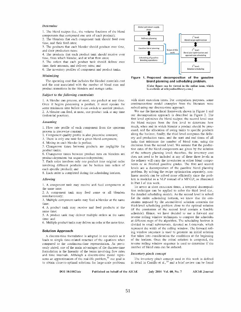
2. Chapter 2: Inventory Pinch Based, Multiscale Models for Integrated
Planning and Scheduling-Part I: Gasoline Blend Planning
This chapter has been published in the AIChE Journal. Complete citation:
Castillo Castillo, P. A., & Mahalec, V. (2014). Inventory pinch based, multiscale models
for integrated planning and scheduling‐part I: Gasoline blend planning.” AIChE Journal,
60(6), 2158–2178. Wiley Online Library, doi: 10.1002/aic.14423
Permission from © American Institute of Chemical Engineers.

Ph. D. Thesis – Pedro A. Castillo
Castillo
McMaster University – Chemical Engineering
24
In Chapter 2, the inventory pinch concept for production planning is revisited and the
multiperiod inventory pinch (MPIP) algorithm is introduced for blend planning problems.
MPIP relies on a two level decomposition of the original problem. At the 1st level, the
blend recipes are determined by solving a multiperiod NLP model with periods delineated
by inventory pinch points. The 2nd level is a multiperiod MILP model (with original
number of periods defined by the planner) with fixed blend recipes. Both levels are
formulated using discrete-time representation. One of the key features of the MPIP
approach is that produces solutions with less variations in blend recipes.
The MPIP for blend planning is the base for the MPIP algorithm for blend scheduling
presented in Chapter 3.

Ph. D. Thesis – Pedro A. Castillo
Castillo
McMaster University – Chemical Engineering
25

Ph. D. Thesis – Pedro A. Castillo
Castillo
McMaster University – Chemical Engineering
26

Ph. D. Thesis – Pedro A. Castillo
Castillo
McMaster University – Chemical Engineering
27

Ph. D. Thesis – Pedro A. Castillo
Castillo
McMaster University – Chemical Engineering
28

Ph. D. Thesis – Pedro A. Castillo
Castillo
McMaster University – Chemical Engineering
29

Ph. D. Thesis – Pedro A. Castillo
Castillo
McMaster University – Chemical Engineering
30

Ph. D. Thesis – Pedro A. Castillo
Castillo
McMaster University – Chemical Engineering
31

Ph. D. Thesis – Pedro A. Castillo
Castillo
McMaster University – Chemical Engineering
32

Ph. D. Thesis – Pedro A. Castillo
Castillo
McMaster University – Chemical Engineering
33

Ph. D. Thesis – Pedro A. Castillo
Castillo
McMaster University – Chemical Engineering
34

Ph. D. Thesis – Pedro A. Castillo
Castillo
McMaster University – Chemical Engineering
35

Ph. D. Thesis – Pedro A. Castillo
Castillo
McMaster University – Chemical Engineering
36

Ph. D. Thesis – Pedro A. Castillo
Castillo
McMaster University – Chemical Engineering
37

Ph. D. Thesis – Pedro A. Castillo
Castillo
McMaster University – Chemical Engineering
38

Ph. D. Thesis – Pedro A. Castillo
Castillo
McMaster University – Chemical Engineering
39

Ph. D. Thesis – Pedro A. Castillo
Castillo
McMaster University – Chemical Engineering
40

Ph. D. Thesis – Pedro A. Castillo
Castillo
McMaster University – Chemical Engineering
41
Ph. D. Thesis – Pedro A. Castillo
Castillo
McMaster University – Chemical Engineering
42

Ph. D. Thesis – Pedro A. Castillo
Castillo
McMaster University – Chemical Engineering
43

Ph. D. Thesis – Pedro A. Castillo
Castillo
McMaster University – Chemical Engineering
44

Ph. D. Thesis – Pedro A. Castillo
Castillo
McMaster University – Chemical Engineering
45

Ph. D. Thesis – Pedro A. Castillo
Castillo
McMaster University – Chemical Engineering
46
3. Chapter 3: Inventory Pinch Based, Multiscale Models for Integrated
Planning and Scheduling-Part II: Gasoline Blend Scheduling
This chapter has been published in the AIChE Journal. Complete citation:
Castillo Castillo, P. A., & Mahalec, V. (2014). Inventory pinch based, multiscale models
for integrated planning and scheduling‐part II: Gasoline blend scheduling. AIChE
Journal, 60(7), 2475–2497. Wiley Online Library, doi: 10.1002/aic.14444
Permission from © American Institute of Chemical Engineers.

Ph. D. Thesis – Pedro A. Castillo
Castillo
McMaster University – Chemical Engineering
47
In Chapter 3, the multiperiod inventory pinch (MPIP) algorithm is introduced for blend
scheduling problems. In this case, MPIP decomposes the original problem into three
levels. The 1st and 2nd levels are constructed based on the methodology presented in
Chapter 2, with some modifications to the 2nd level MILP model to include a few
scheduling decisions. The 3rd level is a multiperiod MILP model (with original number of
periods defined by the scheduler) with fixed blend recipes. All three levels are formulated
using discrete-time representation. Due to their large size, the 3rd level model is solved
using a rolling horizon strategy.

Ph. D. Thesis – Pedro A. Castillo
Castillo
McMaster University – Chemical Engineering
48

Ph. D. Thesis – Pedro A. Castillo
Castillo
McMaster University – Chemical Engineering
49

Ph. D. Thesis – Pedro A. Castillo
Castillo
McMaster University – Chemical Engineering
50
Ph. D. Thesis – Pedro A. Castillo
Castillo
McMaster University – Chemical Engineering
51

Ph. D. Thesis – Pedro A. Castillo
Castillo
McMaster University – Chemical Engineering
52

Ph. D. Thesis – Pedro A. Castillo
Castillo
McMaster University – Chemical Engineering
53

Ph. D. Thesis – Pedro A. Castillo
Castillo
McMaster University – Chemical Engineering
54

Ph. D. Thesis – Pedro A. Castillo
Castillo
McMaster University – Chemical Engineering
55

Ph. D. Thesis – Pedro A. Castillo
Castillo
McMaster University – Chemical Engineering
56

Ph. D. Thesis – Pedro A. Castillo
Castillo
McMaster University – Chemical Engineering
57

Ph. D. Thesis – Pedro A. Castillo
Castillo
McMaster University – Chemical Engineering
58

Ph. D. Thesis – Pedro A. Castillo
Castillo
McMaster University – Chemical Engineering
59

Ph. D. Thesis – Pedro A. Castillo
Castillo
McMaster University – Chemical Engineering
60

Ph. D. Thesis – Pedro A. Castillo
Castillo
McMaster University – Chemical Engineering
61

Ph. D. Thesis – Pedro A. Castillo
Castillo
McMaster University – Chemical Engineering
62

Ph. D. Thesis – Pedro A. Castillo
Castillo
McMaster University – Chemical Engineering
63

Ph. D. Thesis – Pedro A. Castillo
Castillo
McMaster University – Chemical Engineering
64

Ph. D. Thesis – Pedro A. Castillo
Castillo
McMaster University – Chemical Engineering
65

Ph. D. Thesis – Pedro A. Castillo
Castillo
McMaster University – Chemical Engineering
66

Ph. D. Thesis – Pedro A. Castillo
Castillo
McMaster University – Chemical Engineering
67

Ph. D. Thesis – Pedro A. Castillo
Castillo
McMaster University – Chemical Engineering
68

Ph. D. Thesis – Pedro A. Castillo
Castillo
McMaster University – Chemical Engineering
69

Ph. D. Thesis – Pedro A. Castillo
Castillo
McMaster University – Chemical Engineering
70

Ph. D. Thesis – Pedro A. Castillo
Castillo
McMaster University – Chemical Engineering
71
4. Chapter 4: Inventory Pinch-Based Multi-Scale Model for Refinery
Production Planning
This chapter has been published in the proceedings of the 24th European Symposium on
Computer Aided Process Engineering (ESCAPE):
Castillo Castillo, P. A., & Mahalec, V. (2014). Inventory pinch based multi-scale model
for refinery production planning. In J. J. Klemeš, P. S. Varbanov, & P. Y. Liew (Eds.),
Computer Aided Chemical Engineering (Vol. 33, pp. 283-288). Budapest, Hungary:
Elsevier. doi: 10.1016/B978-0-444-63456-6.50048-X
Permission from © Elsevier Ltd. All rights reserved.

Ph. D. Thesis – Pedro A. Castillo
Castillo
McMaster University – Chemical Engineering
72
The first three sections of Chapter 4 are an overview of Chapter 2. Section 4 presents an
example of the MPIP algorithm from Chapter 2 applied to a refinery planning problem.
Compared to the gasoline blending problem, the refinery planning problem considers
different product pools (e.g., gasoline, diesel, kerosene). Therefore, the inventory pinch
points are determined based on the cumulative product demand curves of each pool.

Ph. D. Thesis – Pedro A. Castillo
Castillo
McMaster University – Chemical Engineering
73

Ph. D. Thesis – Pedro A. Castillo
Castillo
McMaster University – Chemical Engineering
74

Ph. D. Thesis – Pedro A. Castillo
Castillo
McMaster University – Chemical Engineering
75

Ph. D. Thesis – Pedro A. Castillo
Castillo
McMaster University – Chemical Engineering
76

Ph. D. Thesis – Pedro A. Castillo
Castillo
McMaster University – Chemical Engineering
77

Ph. D. Thesis – Pedro A. Castillo
Castillo
McMaster University – Chemical Engineering
78

Ph. D. Thesis – Pedro A. Castillo
Castillo
McMaster University – Chemical Engineering
79
5. Chapter 5: Improved Continuous-Time Model for Gasoline Blend
Scheduling
This chapter has been published in the Computers and Chemical Engineering Journal.
Complete citation:
Castillo Castillo, P. A., & Mahalec, V. (2016). Improved continuous-time model for
gasoline blend scheduling. Computers & Chemical Engineering, 84, 627–646. Elsevier
Ltd., doi: 10.1016/j.compchemeng.2015.08.003
Permission from © Elsevier Ltd. All rights reserved.

Ph. D. Thesis – Pedro A. Castillo
Castillo
McMaster University – Chemical Engineering
80
In Chapter 5, the development of a continuous-time blend scheduling model is presented.
As the problem size grows (e.g., more blenders, products, orders, and/or longer
scheduling horizon), this model requires smaller number of binary variables than previous
published model, while including more logistic constraints found in real practice.
Although not all the examples were solved to proven optimality, the feasible solutions
found were better than those previously reported in the literature.
This continuous-time blend scheduling model is used in Chapter 6 to improve the
performance of the MPIP algorithm presented in Chapter 3.

Ph. D. Thesis – Pedro A. Castillo
Castillo
McMaster University – Chemical Engineering
81

Ph. D. Thesis – Pedro A. Castillo
Castillo
McMaster University – Chemical Engineering
82

Ph. D. Thesis – Pedro A. Castillo
Castillo
McMaster University – Chemical Engineering
83

Ph. D. Thesis – Pedro A. Castillo
Castillo
McMaster University – Chemical Engineering
84

Ph. D. Thesis – Pedro A. Castillo
Castillo
McMaster University – Chemical Engineering
85

Ph. D. Thesis – Pedro A. Castillo
Castillo
McMaster University – Chemical Engineering
86

Ph. D. Thesis – Pedro A. Castillo
Castillo
McMaster University – Chemical Engineering
87

Ph. D. Thesis – Pedro A. Castillo
Castillo
McMaster University – Chemical Engineering
88

Ph. D. Thesis – Pedro A. Castillo
Castillo
McMaster University – Chemical Engineering
89

Ph. D. Thesis – Pedro A. Castillo
Castillo
McMaster University – Chemical Engineering
90

Ph. D. Thesis – Pedro A. Castillo
Castillo
McMaster University – Chemical Engineering
91

Ph. D. Thesis – Pedro A. Castillo
Castillo
McMaster University – Chemical Engineering
92

Ph. D. Thesis – Pedro A. Castillo
Castillo
McMaster University – Chemical Engineering
93

Ph. D. Thesis – Pedro A. Castillo
Castillo
McMaster University – Chemical Engineering
94

Ph. D. Thesis – Pedro A. Castillo
Castillo
McMaster University – Chemical Engineering
95

Ph. D. Thesis – Pedro A. Castillo
Castillo
McMaster University – Chemical Engineering
96

Ph. D. Thesis – Pedro A. Castillo
Castillo
McMaster University – Chemical Engineering
97

Ph. D. Thesis – Pedro A. Castillo
Castillo
McMaster University – Chemical Engineering
98

Ph. D. Thesis – Pedro A. Castillo
Castillo
McMaster University – Chemical Engineering
99

Ph. D. Thesis – Pedro A. Castillo
Castillo
McMaster University – Chemical Engineering
100

Ph. D. Thesis – Pedro A. Castillo
Castillo
McMaster University – Chemical Engineering
101
6. Chapter 6: Inventory Pinch Gasoline Blend Scheduling Algorithm
Combining Discrete- and Continuous-Time Models
This chapter has been published in the Computers and Chemical Engineering Journal.
Complete citation:
Castillo Castillo, P. A., & Mahalec, V. (2016). Inventory pinch gasoline blend scheduling
algorithm combining discrete- and continuous-time models. Computers & Chemical
Engineering, 84, 611–626. Elsevier Ltd., doi: 10.1016/j.compchemeng.2015.08.005
Permission from © Elsevier Ltd. All rights reserved.

Ph. D. Thesis – Pedro A. Castillo
Castillo
McMaster University – Chemical Engineering
102
In Chapter 6, the MPIP-C algorithm is introduced. It combines the solution strategy
described in Chapter 3 with the continuous-time blend scheduling model from Chapter 5.
The continuous-time blend scheduling model enables MPIP-C algorithm to solve the 3rd
level for the entire time horizon (instead of subintervals as in Chapter 3). The execution
times required by MPIP-C are almost one order of magnitude shorter than those required
by MPIP algorithm. It is demonstrated as well that MPIP-C can handle nonlinear blending
rules.
Chapter 6 marks a milestone within my Ph.D. project. The MPIP-C method is a heuristic
approach that provides optimal or near-optimal solutions in a few seconds for linear and
nonlinear blend scheduling problems, and with a reduced number of blend recipes. This
fulfills one of the general objectives of this work.

Ph. D. Thesis – Pedro A. Castillo
Castillo
McMaster University – Chemical Engineering
103

Ph. D. Thesis – Pedro A. Castillo
Castillo
McMaster University – Chemical Engineering
104

Ph. D. Thesis – Pedro A. Castillo
Castillo
McMaster University – Chemical Engineering
105

Ph. D. Thesis – Pedro A. Castillo
Castillo
McMaster University – Chemical Engineering
106

Ph. D. Thesis – Pedro A. Castillo
Castillo
McMaster University – Chemical Engineering
107

Ph. D. Thesis – Pedro A. Castillo
Castillo
McMaster University – Chemical Engineering
108

Ph. D. Thesis – Pedro A. Castillo
Castillo
McMaster University – Chemical Engineering
109

Ph. D. Thesis – Pedro A. Castillo
Castillo
McMaster University – Chemical Engineering
110

Ph. D. Thesis – Pedro A. Castillo
Castillo
McMaster University – Chemical Engineering
111

Ph. D. Thesis – Pedro A. Castillo
Castillo
McMaster University – Chemical Engineering
112

Ph. D. Thesis – Pedro A. Castillo
Castillo
McMaster University – Chemical Engineering
113

Ph. D. Thesis – Pedro A. Castillo
Castillo
McMaster University – Chemical Engineering
114

Ph. D. Thesis – Pedro A. Castillo
Castillo
McMaster University – Chemical Engineering
115

Ph. D. Thesis – Pedro A. Castillo
Castillo
McMaster University – Chemical Engineering
116

Ph. D. Thesis – Pedro A. Castillo
Castillo
McMaster University – Chemical Engineering
117

Ph. D. Thesis – Pedro A. Castillo
Castillo
McMaster University – Chemical Engineering
118

Ph. D. Thesis – Pedro A. Castillo
Castillo
McMaster University – Chemical Engineering
119
7. Chapter 7: Global Optimization Algorithm for Large-Scale Refinery
Planning Models with Bilinear Terms
This chapter has been published in the Industrial & Engineering Chemistry Research
Journal. Complete citation:
Castillo Castillo, P. A., Castro, P. M., & Mahalec, V. (2017). Global optimization
algorithm for large-scale refinery planning models with bilinear terms. Industrial &
Engineering Chemistry Research, 56(2), 530–548. American Chemical Society, doi:
10.1021/acs.iecr.6b01350
Permission from © American Chemical Society.

Ph. D. Thesis – Pedro A. Castillo
Castillo
McMaster University – Chemical Engineering
120
Chapters 2–6 show the development steps of a heuristic algorithm (i.e., MPIP-C). In
Chapter 7, a deterministic global optimization algorithm for mixed-integer bilinear
programs is presented. This method computes estimates of the global solution by solving
an MILP relaxation of the original model. The relaxation is derived using either
Piecewise McCormick or Normalized Multiparametric Disaggregation. By increasing the
number of partitions, and reducing the domain of the variables, the estimates of the global
solution are improved. The case study used in Chapter 6 is an oil refinery planning
problem.

Ph. D. Thesis – Pedro A. Castillo
Castillo
McMaster University – Chemical Engineering
121

Ph. D. Thesis – Pedro A. Castillo
Castillo
McMaster University – Chemical Engineering
122

Ph. D. Thesis – Pedro A. Castillo
Castillo
McMaster University – Chemical Engineering
123

Ph. D. Thesis – Pedro A. Castillo
Castillo
McMaster University – Chemical Engineering
124

Ph. D. Thesis – Pedro A. Castillo
Castillo
McMaster University – Chemical Engineering
125

Ph. D. Thesis – Pedro A. Castillo
Castillo
McMaster University – Chemical Engineering
126

Ph. D. Thesis – Pedro A. Castillo
Castillo
McMaster University – Chemical Engineering
127

Ph. D. Thesis – Pedro A. Castillo
Castillo
McMaster University – Chemical Engineering
128

Ph. D. Thesis – Pedro A. Castillo
Castillo
McMaster University – Chemical Engineering
129

Ph. D. Thesis – Pedro A. Castillo
Castillo
McMaster University – Chemical Engineering
130

Ph. D. Thesis – Pedro A. Castillo
Castillo
McMaster University – Chemical Engineering
131

Ph. D. Thesis – Pedro A. Castillo
Castillo
McMaster University – Chemical Engineering
132

Ph. D. Thesis – Pedro A. Castillo
Castillo
McMaster University – Chemical Engineering
133

Ph. D. Thesis – Pedro A. Castillo
Castillo
McMaster University – Chemical Engineering
134

Ph. D. Thesis – Pedro A. Castillo
Castillo
McMaster University – Chemical Engineering
135

Ph. D. Thesis – Pedro A. Castillo
Castillo
McMaster University – Chemical Engineering
136

Ph. D. Thesis – Pedro A. Castillo
Castillo
McMaster University – Chemical Engineering
137

Ph. D. Thesis – Pedro A. Castillo
Castillo
McMaster University – Chemical Engineering
138

Ph. D. Thesis – Pedro A. Castillo
Castillo
McMaster University – Chemical Engineering
139

Ph. D. Thesis – Pedro A. Castillo
Castillo
McMaster University – Chemical Engineering
140
8. Chapter 8: Global Optimization of Nonlinear Blend-Scheduling
Problems
This chapter has been published in the Engineering Journal (open access). Complete
citation:
Castillo Castillo, P. A., Castro, P. M., & Mahalec, V. (2017). Global optimization of
nonlinear blend-scheduling problems. Engineering, 3(2), 188–201. Elsevier Ltd., doi:
10.1016/J.ENG.2017.02.005

Ph. D. Thesis – Pedro A. Castillo
Castillo
McMaster University – Chemical Engineering
141
In Chapter 8, the heuristic and rigorous optimization techniques from the previous two
Chapters are used to solve nonlinear blend-scheduling problems. MPIP-C is faster
computing feasible near-optimal solutions than the global optimization method. The
lower bound on the blend cost computed by MPIP-C is larger than the initial one
computed by the global optimization algorithm. These results show the importance of the
MPIP-C technique and how it can improve a deterministic global optimization algorithm.

Ph. D. Thesis – Pedro A. Castillo
Castillo
McMaster University – Chemical Engineering
142

Ph. D. Thesis – Pedro A. Castillo
Castillo
McMaster University – Chemical Engineering
143

Ph. D. Thesis – Pedro A. Castillo
Castillo
McMaster University – Chemical Engineering
144

Ph. D. Thesis – Pedro A. Castillo
Castillo
McMaster University – Chemical Engineering
145

Ph. D. Thesis – Pedro A. Castillo
Castillo
McMaster University – Chemical Engineering
146

Ph. D. Thesis – Pedro A. Castillo
Castillo
McMaster University – Chemical Engineering
147

Ph. D. Thesis – Pedro A. Castillo
Castillo
McMaster University – Chemical Engineering
148

Ph. D. Thesis – Pedro A. Castillo
Castillo
McMaster University – Chemical Engineering
149

Ph. D. Thesis – Pedro A. Castillo
Castillo
McMaster University – Chemical Engineering
150

Ph. D. Thesis – Pedro A. Castillo
Castillo
McMaster University – Chemical Engineering
151

Ph. D. Thesis – Pedro A. Castillo
Castillo
McMaster University – Chemical Engineering
152
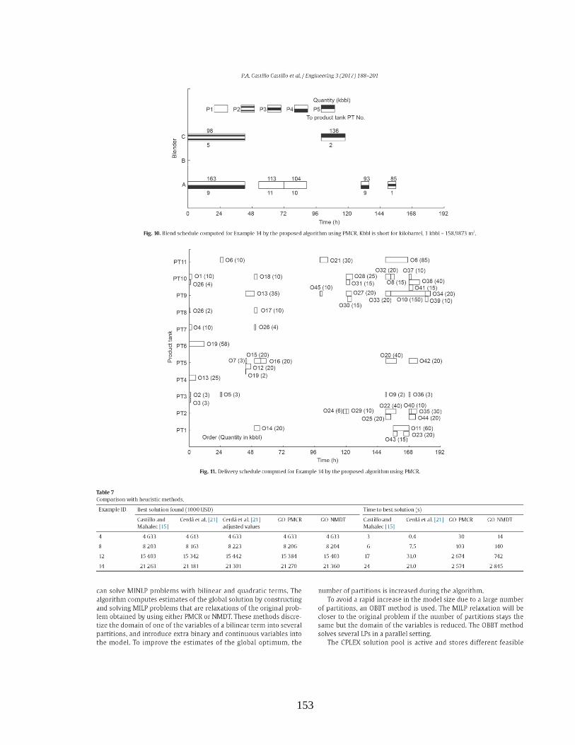
Ph. D. Thesis – Pedro A. Castillo
Castillo
McMaster University – Chemical Engineering
153

Ph. D. Thesis – Pedro A. Castillo
Castillo
McMaster University – Chemical Engineering
154

Ph. D. Thesis – Pedro A. Castillo
Castillo
McMaster University – Chemical Engineering
155
Ph. D. Thesis – Pedro A. Castillo
Castillo
McMaster University – Chemical Engineering
156
9. Chapter 9: Global Optimization of MIQCPs with Dynamic Piecewise
Relaxations
This chapter has been published online in the Journal of Global Optimization. Complete
citation:
Castillo Castillo, P. A., Castro, P. M., & Mahalec, V. (2017). Global optimization of
MIQCPs with dynamic piecewise relaxations. Journal of Global Optimization. doi:
10.1007/s10898-018-0612-7.

Ph. D. Thesis – Pedro A. Castillo
Castillo
McMaster University – Chemical Engineering
157
In Chapter 9, an improved version of the algorithm described in Chapter 7 is presented.
Compared to the method detailed in Chapter 7, this new version of the algorithm uses
optimality-based bound tightening not only when a new upper bound is found, but
whenever the domain of the variables is significantly reduced. In addition, the algorithm
also increases or decreases the number of partitions depending on the last iteration
performance, which is defined by the required execution time, optimality gap
improvement, and average domain reduction. Finally, the algorithm can switch from
piecewise McCormick to Normalized Multiparametric Disaggregation when the number
of partitions is greater or equal to 10.
The test examples include the refinery planning problems from Chapter 6, and 3
scheduling problems of a hydro energy system. The results show that this version of the
algorithm is superior to that from Chapter 6.

Ph. D. Thesis – Pedro A. Castillo
Castillo
McMaster University – Chemical Engineering
158

Ph. D. Thesis – Pedro A. Castillo
Castillo
McMaster University – Chemical Engineering
159

Ph. D. Thesis – Pedro A. Castillo
Castillo
McMaster University – Chemical Engineering
160

Ph. D. Thesis – Pedro A. Castillo
Castillo
McMaster University – Chemical Engineering
161

Ph. D. Thesis – Pedro A. Castillo
Castillo
McMaster University – Chemical Engineering
162

Ph. D. Thesis – Pedro A. Castillo
Castillo
McMaster University – Chemical Engineering
163

Ph. D. Thesis – Pedro A. Castillo
Castillo
McMaster University – Chemical Engineering
164

Ph. D. Thesis – Pedro A. Castillo
Castillo
McMaster University – Chemical Engineering
165

Ph. D. Thesis – Pedro A. Castillo
Castillo
McMaster University – Chemical Engineering
166

Ph. D. Thesis – Pedro A. Castillo
Castillo
McMaster University – Chemical Engineering
167

Ph. D. Thesis – Pedro A. Castillo
Castillo
McMaster University – Chemical Engineering
168

Ph. D. Thesis – Pedro A. Castillo
Castillo
McMaster University – Chemical Engineering
169

Ph. D. Thesis – Pedro A. Castillo
Castillo
McMaster University – Chemical Engineering
170

Ph. D. Thesis – Pedro A. Castillo
Castillo
McMaster University – Chemical Engineering
171

Ph. D. Thesis – Pedro A. Castillo
Castillo
McMaster University – Chemical Engineering
172

Ph. D. Thesis – Pedro A. Castillo
Castillo
McMaster University – Chemical Engineering
173

Ph. D. Thesis – Pedro A. Castillo
Castillo
McMaster University – Chemical Engineering
174

Ph. D. Thesis – Pedro A. Castillo
Castillo
McMaster University – Chemical Engineering
175

Ph. D. Thesis – Pedro A. Castillo
Castillo
McMaster University – Chemical Engineering
176

Ph. D. Thesis – Pedro A. Castillo
Castillo
McMaster University – Chemical Engineering
177

Ph. D. Thesis – Pedro A. Castillo
Castillo
McMaster University – Chemical Engineering
178

Ph. D. Thesis – Pedro A. Castillo
Castillo
McMaster University – Chemical Engineering
179

Ph. D. Thesis – Pedro A. Castillo
Castillo
McMaster University – Chemical Engineering
180

Ph. D. Thesis – Pedro A. Castillo
Castillo
McMaster University – Chemical Engineering
181

Ph. D. Thesis – Pedro A. Castillo
Castillo
McMaster University – Chemical Engineering
182
Ph. D. Thesis – Pedro A. Castillo
Castillo
McMaster University – Chemical Engineering
183
Ph. D. Thesis – Pedro A. Castillo
Castillo
McMaster University – Chemical Engineering
184
10. Chapter 10: Concluding Remarks
This thesis has focused on the development of efficient algorithms to solve production
planning and scheduling problems. Two approaches were considered: i) a heuristic
algorithm based on the inventory pinch concept to compute near-optimal solutions in
short execution times, and ii) a rigorous deterministic global optimization algorithm based
on increasing number of partitions of piecewise linear relaxations. The main case studies
included gasoline blend planning and scheduling, and refinery planning.
The inventory pinch algorithm decomposes the problem into three levels: 1) optimization
of operating conditions and blend recipes, 2) computation of an approximate schedule,
and 3) detailed scheduling. At the first level, a discrete-time NLP model is formulated,
where periods are delineated by the inventory pinch points for various product pools (e.g.
gasoline and diesel). This reduces drastically the number of periods and enables use of
nonlinear, more accurate refinery models. The second level is solved via discrete-time
MILP model where periods are delineated by scheduler based on the demand and supply
data, and the minimum time requirements to complete major tasks (i.e. blend runs,
product tank service). The third level uses a discrete-time MILP scheduling model (MPIP
algorithm) or a continuous-time MILP scheduling model (MPIP-C) to determine the exact
times to carry out the necessary tasks. The second and third levels are linear models since
the nonlinear constraints are handled at the first level, and the optimal conditions found at
such level are fixed in the other levels. The algorithm minimizes the total cost which is
defined as the cost of raw materials, switching cost, and demurrage cost. The algorithm
eliminates infeasibilities by iteratively re-optimizing operating conditions and blend
recipes at the first level.
The deterministic global optimization algorithm relies on discretizing the bilinear or
quadratic terms dynamically using either piecewise McCormick (PMCR) or normalized
multiparametric disaggregation (NMDT). The resulting MILP model is solved using
CPLEX and several feasible solutions are stored in CPLEX’s solution pool and employed
as starting points for a local nonlinear solver (e.g. CONOPT). These nonlinear models are
solved in parallel. Then, the estimate of the global solution and the best feasible solution
are updated. If the relative difference between these two (i.e. the optimality gap) is
smaller than the tolerance, then the algorithm stops; otherwise, it continues by reducing
the range of the variables or increasing the number of partitions for the next iteration. The
domain of the variables involved in nonlinear terms is reduced using an optimality-based
bound tightening (OBBT) method. This OBBT method consists in solving two
optimization problems for each variable: a maximization and a minimization of the range

Ph. D. Thesis – Pedro A. Castillo
Castillo
McMaster University – Chemical Engineering
185
of the variable subject to the MILP relaxation constraints. Parallelization of this step is
required to avoid long execution times.
10.1. Key Findings and Contributions
The research objectives presented in Chapter 1 have been achieved, and the key
contributions of this work include:
10.1.1. The development of a heuristic technique for blend planning and scheduling
problems: the multiperiod inventory pinch algorithm MPIP. This method
computes blend plans and schedules with reduced number of different blend
recipes by reducing the number of time periods using the inventory pinch
points. The inventory pinch points are defined by the cumulative total demand
along the planning/scheduling horizon. MPIP employs discrete-time uniform-
grid MILP scheduling model. Results in Chapter 2 and 3 show that MPIP
computes the same or better solutions than three commercial solvers trying to
solve the original full-space model. In Chapter 4, MPIP is used to solve a
refinery planning problem.
10.1.2. In Chapter 2, results indicate that the solutions computed by the MPIP
planning algorithm are optimal when the objective function of the second level
contains only variables that are aggregated at the first level; and they are near-
optimal when the objective function of the second level contains a penalty
term associated with variables that are not aggregated at the first level, and this
penalty term is significantly smaller than the cost of raw materials.
10.1.3. The formulation of a continuous-time unit-specific slot-based MILP
scheduling model with reduced number of binary variables for gasoline
blending operations. In Chapter 5, it is shown that the addition of a lower
bound on the blend cost reduces the execution times required to solve blend
scheduling problems to optimality.
10.1.4. The development of the multiperiod inventory pinch algorithm MPIP-C for
scheduling problems. MPIP-C has all the features of MPIP but it employs a
continuous-time unit-specific slot-based MILP scheduling model. As shown in
Chapter 6 and 8, MPIP-C computes solutions in shorter execution times than
three commercial solvers, and around the same times as another published
heuristic strategy.
10.1.5. The development of a deterministic global optimization algorithm for MINLP
problems where nonlinearities are strictly bilinear and/or quadratic terms. The
algorithm is based on dynamic partitioning of piecewise linear relaxations

Ph. D. Thesis – Pedro A. Castillo
Castillo
McMaster University – Chemical Engineering
186
(PMCR and NMDT) and optimality-based bound tightening. Chapter 7, 8, and
9 show that the algorithm performs on par with two commercial global
solvers, and even better in some examples.
10.2. Future Work Outlook
The MPIP and MPIP-C algorithms have shown promising results for short-term planning
and scheduling problems where 1) the cost associated with the raw materials is bigger
than the cost associated with switching tasks, and 2) the problem can be decomposed into
2 or 3 decision levels. However, the performance of these heuristic algorithms depends on
the ability of the modeler to define the constraints that will be included at each level.
Therefore, it is necessary to develop a systematic approach to generate the mathematical
models for each level based on the original problem formulation and with minimal
additional input from the planner/scheduler. Such development will simplify the
application and implementation of these two inventory pinch-based algorithms to a wider
variety of planning and scheduling problems, as well as its integration with global
optimization algorithms (to find feasible solutions).
A possible next step for the MPIP method is to employ it for solving and linking long-
and medium-term planning problems. The questions to be answered include:
1. What granularity of the product demand data to use? Different data granularities
(e.g., daily and hourly data) could yield different inventory pinch points.
2. What are the best linking decisions between the long- and medium-term plans?
These will depend on the selected case study. For example, for an oil refinery,
these can be the total amount of crude oil to purchase, the crude distillation unit
throughput, or the final inventory levels.
The deterministic global optimization algorithm from Chapter 9 can be further enhanced.
One of the major issues of the current implementation is when the optimality-based
bound tightening (OBBT) method is not run and the number of partitions in the relaxed
model is increased. In this situation, the MILP solver might explore many of the nodes
that were fathomed in the previous iteration. To avoid this unnecessary calculations, it is
necessary to retrieve the branch-and-bound tree information from the MILP solver.
Another issue of the deterministic global optimization algorithm is that there is no
specific rule to select the variable of a bilinear term to be partitioned. The current rule is
to pick the variables that will lead to the smallest MILP relaxation. The proposed method
is to make this a dynamic selection during the algorithm run. Let’s consider the bilinear

Ph. D. Thesis – Pedro A. Castillo
Castillo
McMaster University – Chemical Engineering
187
term 𝑥1𝑥2, where 𝑥2 is the partitioned variable at the beginning of the algorithm. Once the
domain of 𝑥2 cannot be reduced by OBBT, and there is no significant improvement in the
best possible solution, 𝑥1 becomes the partitioned variable.
In the dynamic partitioning scheme employed by the deterministic global optimization
algorithm, the number of partitions of all partitioned variables increase by the same
factor. A topic that can be investigated is if this factor can be different for each
partitioned variable, and how to determine it. This can lead to smaller MILP relaxations.
One possible approach to decrease the time required for solving the MILP relaxations is
to employ a mathematical decomposition strategy. Either Benders or Lagrangean
decomposition methods could prove to be useful given the block structure of the
constraints associated with Piecewise McCormick and Normalized Multiparametric
Disaggregation.

Ph. D. Thesis – Pedro A. Castillo
Castillo
McMaster University – Chemical Engineering
188
Appendix A: Supporting Information for Chapters 2 and 3
Table A.1. Components data (properties, cost, supply rates and inventory limits)
Components ALK BUT HCL HCN LCN LNP RFT
ARO (%vol aromatics) 0 0 0 25 18 2.974 74.9
BEN (%vol benzene) 0 0 0 0.5 1 0.595 7.5
MON 93.7 90 79.8 75.8 81.6 66 90.8
OLF (%vol olefin) 0 0 0 14 27 0 0
RON 95 93.8 82.3 86.7 93.2 67.8 103
RVP (psi) 5.15 138 22.335 2.378 13.876 19.904 3.622
SPG 0.703 0.584 0.695 0.791 0.744 0.677 0.818
SUL (%vol sulfur) 0 0 0 0.485 0.078 0.013 0
Cost ($/bbl) 29.2 11.5 20 22 25 19.7 24.5
Minimum Inventory (×103 bbl) 5 5 5 5 5 5 5
Maximum Inventory (×103 bbl) 150 75 50 50 150 100 150
Initial Inventory (×103 bbl)
Cases 1 – 14 30 20 20 10 30 20 50
Supply Rate (×103 bbl/day)
Cases 1 – 7 18 5 3 5 25 20 44

Ph. D. Thesis – Pedro A. Castillo
Castillo
McMaster University – Chemical Engineering
189
Table A.2. Supply rate of components along planning horizon, cases 8 – 14
Component ALK BUT HCL HCN LCN LNP RFT
L2-period ×103 bbl/day
1 25 7 0 3 27 20 45
2 25 7 0 3 27 20 45
3 25 7 0 3 27 20 45
4 20 5 3 5 25 18 40
5 15 3 7 9 20 22 35
6 15 3 7 9 20 22 35
7 15 3 7 9 20 22 35
8 20 5 3 5 25 18 40
9 20 5 3 5 25 18 40
10 25 7 0 3 27 22 45
11 25 7 0 3 27 22 45
12 25 7 0 3 27 22 45
13 20 5 3 5 25 18 40
14 20 5 3 5 25 18 40

Ph. D. Thesis – Pedro A. Castillo
Castillo
McMaster University – Chemical Engineering
190
Table A.3. Minimum and maximum quality specifications of the products
Specification Minimum Maximum
Product U87 U91 U93 U87 U91 U93
ARO (%vol aromatics) 0 0 0 60 60 60
BEN (%vol benzene) 0 0 0 5.9 5.9 5.9
MON 81.5 85.7 87.5 - - -
OLF (%vol olefin) 0 0 0 24.2 24.2 24.2
RON 91.4 94.5 97.5 - - -
RVP (psi) 0 0 0 15.6 15.6 15.6
SPG 0.73 0.73 0.73 0.81 0.81 0.81
SUL (%vol sulfur) 0 0 0 0.1 0.1 0.1
Table A.4. Product storage tank data
Product
tank
Storable
products
Product
transition
penalty
(×103 $)
Minimum
hold up
(×103 bbl)
Maximum
hold up
(×103 bbl)
Maximum
delivery
rate (×103
bbl/h)
Initial
inventory
(×103 bbl)
Initial
product
Tk-101 U87 - 10 70 10 40 U87
Tk-102 U91 - 10 70 10 70 U91
Tk-103 U93 - 10 70 10 30 U93
Tk-104 U87, U91, U93 14.5 0 40 10 30 U87
Tk-105 U87, U91, U93 14.5 0 40 10 40 U91
Tk-106 U87, U91, U93 14.5 0 40 10 30 U91

Ph. D. Thesis – Pedro A. Castillo
Castillo
McMaster University – Chemical Engineering
191
Table A.5. Demand profiles (×103 bbl) and cost coefficient profile for the product inventory slack
variables (2nd level MILP model)
Dem
an
d
pro
file
Pro
du
ct
L2-period
1 2 3 4 5 6 7 8 9 10 11 12 13 14
1
U87 60 50 50 80 50 60 60 50 75 50 50 50 80 100
U91 50 80 70 30 50 0 40 30 30 50 40 40 30 50
U93 30 30 0 0 40 40 0 35 30 0 0 40 30 40
2
U87 80 80 60 80 80 100 90 0 0 50 50 30 60 100
U91 50 50 50 30 30 50 50 30 30 50 0 50 60 50
U93 30 30 35 30 35 0 30 35 30 0 30 40 30 0
3
U87 70 70 50 70 70 60 60 60 50 70 120 0 50 70
U91 50 50 50 30 30 50 50 30 30 50 50 30 30 50
U93 30 30 45 30 40 0 0 35 30 0 30 35 0 30
4
U87 70 50 50 120 100 30 30 50 75 110 50 50 50 90
U91 50 80 70 30 50 0 0 30 50 50 0 40 30 0
U93 30 30 45 0 40 40 0 35 30 30 30 0 30 30
5
U87 60 50 50 70 90 80 130 50 0 30 50 50 50 80
U91 50 80 70 50 50 30 30 30 30 30 0 40 30 0
U93 30 30 45 0 30 40 30 30 30 30 30 0 30 40
6
U87 100 70 80 100 40 30 40 110 0 50 70 100 0 50
U91 50 80 70 50 30 30 30 50 30 30 30 35 30 30
U93 30 30 45 30 0 30 30 30 30 0 0 30 30 30
Cost coefficients for product slack variables
U87, U91,
U93
1.8
×106
1.7
×106
1.6
×1
06
1.5
×105
1.4
×105
1.3
×105
1.2
×105
1.1
×104
1
×103
9
×102
8
×102
5
×102
1
×102
5
×101

Ph. D. Thesis – Pedro A. Castillo
Castillo
McMaster University – Chemical Engineering
192
Appendix B: Supporting Information for Chapters 5, 6, and 8
Table B.1. Demand data
Product Demand (kbbl) Maximum Delivery Rate
Dordermax (kbbl/h)
Example 12 The rest 3 4 7-8 9 12 14 3 4 7-8 9 12 14
Order
O1 P1 P1 10 10 10 10 10 10 5 5 5 5 5 5
O2 P2 P2 3 3 3 3 3 3 3 3 3 3 3 3
O3 P2 P2 3 3 3 3 3 3 3 3 3 3 3 3
O4 P1 P1 10 10 10 10 10 10 5 5 5 5 5 5
O5 P2 P2 3 3 3 3 3 3 3 3 3 3 3 3
O6 P1 P1 10 10 10 10 10 10 5 5 5 5 5 5
O7 P2 P2 3 3 3 3 3 3 3 3 3 3 3 3
O8 P1 P1 100 100 100 100 100 100 5 5 5 5 5 5
O9 P2 P2 3 3 3 3 3 3 3 3 3 3 3 3
O10 P4 P4 150 150 150 150 100 150 5 5 5 5 5 5
O11 P3 P3 20 20 60 60 60 60 5 5 5 5 5 5
O12 P2 P2 30 30 20 20 20 20 5 5 5 5 5 5
O13 P4 P4 - 60 60 60 60 60 - 5 5 5 5 5
O14 P3 P3 - 10 15 20 15 20 - 5 5 5 5 5
O15 P2 P2 - 20 20 20 20 20 - 4 4 4 4 4
O16 P2 P2 - - 20 20 20 20 - - 5 5 5 5
O17 P1 P1 - - 10 10 10 10 - - 5 5 5 5
O18 P1 P1 - - 10 10 10 10 - - 5 5 5 5
O19 P2 P2 - - 60 60 60 60 - - 5 5 5 5
O20 P2 P2 - - 40 40 40 40 - - 5 5 5 5
O21 P5 P1 - - - 30 30 30 - - - 5 5 5
O22 P5 P5 - - - 40 40 40 - - - 5 5 5
O23 P3 P3 - - - 20 20 20 - - - 5 5 5
O24 P5 P5 - - - - 6 6 - - - - 3 3
O25 P5 P5 - - - - 20 20 - - - - 5 5
O26 P3 P1 - - - - 30 10 - - - - 4 4
O27 P3 P4 - - - - 20 20 - - - - 4 5
O28 P4 P1 - - - - 3 25 - - - - 3 5
O29 P4 P5 - - - - 15 10 - - - - 3 5
O30 P1 P4 - - - - 15 15 - - - - 3 5
O31 P2 P1 - - - - 15 15 - - - - 5 5
O32 P5 P1 - - - - 20 20 - - - - 2 5
O33 P1 P4 - - - - 20 20 - - - - 5 5
O34 P3 P4 - - - - 20 20 - - - - 5 5
O35 P3 P5 - - - - 30 30 - - - - 5 5
O36 - P2 - - - - - 3 - - - - - 3
O37 - P1 - - - - - 10 - - - - - 5
O38 - P1 - - - - - 40 - - - - - 5
O39 - P4 - - - - - 10 - - - - - 5
O40 - P5 - - - - - 10 - - - - - 5
O41 - P1 - - - - - 15 - - - - - 5
O42 - P2 - - - - - 20 - - - - - 3
O43 - P3 - - - - - 15 - - - - - 5
O44 - P5 - - - - - 20 - - - - - 4
O45 - P4 - - - - - 10 - - - - - 5

Ph. D. Thesis – Pedro A. Castillo
Castillo
McMaster University – Chemical Engineering
193
Table B.2. Delivery windows Delivery Window [TOstart, TOend] (h)
Example 3 4 7-8 9 12 14
Order
O1 [0,24] [0,24] [0,24] [0,24] [0,24] [0,24]
O2 [0,24] [0,24] [0,24] [0,24] [0,24] [0,24]
O3 [0,24] [0,24] [0,24] [0,24] [0,24] [0,24]
O4 [0,24] [0,24] [0,24] [0,24] [0,24] [0,24]
O5 [24,48] [24,48] [24,48] [24,48] [24,48] [24,48]
O6 [24,48] [24,48] [24,48] [24,48] [24,48] [24,48]
O7 [24,48] [24,48] [24,48] [24,48] [24,48] [24,48]
O8 [118,190] [118,190] [118,190] [118,190] [118,190] [118,190]
O9 [144,168] [144,168] [144,168] [144,168] [144,168] [144,168]
O10 [150.5,185.5] [150.5,185.5] [150.5,185.5] [150.5,185.5] [150.5,185.5] [150.5,185.5]
O11 [144,168] [144,168] [144,168] [144,168] [144,168] [144,168]
O12 [24,48] [24,48] [24,48] [24,48] [24,48] [24,48]
O13 - [0,56] [0,56] [0,56] [0,56] [0,56]
O14 - [48,72] [48,72] [48,72] [48,72] [48,72]
O15 - [0,72] [0,72] [0,72] [0,72] [0,72]
O16 - - [48,72] [48,72] [48,72] [48,72]
O17 - - [48,72] [48,72] [48,72] [48,72]
O18 - - [48,72] [48,72] [48,72] [48,72]
O19 - - [0,50] [0,50] [0,50] [0,50]
O20 - - [144, 168] [144,168] [144,168] [144,168]
O21 - - - [96,120] [96,120] [96,120]
O22 - - - [144,168] [144,168] [144,168]
O23 - - - [144,168] [144,168] [144,168]
O24 - - - - [96,120] [96,120]
O25 - - - - [144,168] [144,168]
O26 - - - - [144,168] [0,76]
O27 - - - - [72,96] [120,144]
O28 - - - - [72,96] [120,144]
O29 - - - - [96,120] [120,144]
O30 - - - - [96,120] [120,144]
O31 - - - - [96,120] [120,144]
O32 - - - - [96,120] [144,168]
O33 - - - - [0,76] [144,168]
O34 - - - - [120,144] [168,192]
O35 - - - - [120,144] [168,192]
O36 - - - - - [168,192]
O37 - - - - - [168,192]
O38 - - - - - [168,192]
O39 - - - - - [168,192]
O40 - - - - - [168,192]
O41 - - - - - [168,192]
O42 - - - - - [168,192]
O43 - - - - - [144,168]
O44 - - - - - [168,192]
O45 - - - - - [96,120]

Ph. D. Thesis – Pedro A. Castillo
Castillo
McMaster University – Chemical Engineering
194
Table B.3. Product and component tank data
Product or
Component Tank
Initial
Product
Initial
Stock Vini
(kbbl)
Max.
Capacity
Vmax
(kbbl)
Storable Products (Set JP) Max. Delivery Rate
Dprmax (kbbl/h)
Example 3, 4,
7, 8 9, 14 12 3, 4 7-8 9 12 14
Tk1 P3 30.00 150 P2, P3 P2, P3, P5 P2, P3, P5 20 20 30 30 30
Tk2 P3 0.00 150 P2, P3 P2, P3, P5 P2, P3, P5 20 20 30 30 30
Tk3 P2 14.08 150 P2, P3 P2, P3, P5 P2, P3, P5 20 20 30 30 30
Tk4 P4 25.00 200 P2- P4 P2- P4 P2- P5 20 20 30 30 30
Tk5 P2 28.49 200 P2, P3 P2, P5 P2, P3, P5 20 20 30 30 30
Tk6 P2 57.59 150 P2, P3 P2, P5 P2, P3, P5 20 20 30 30 30
Tk7 P1 13.79 200 P1, P4 P1, P4 P1, P4 20 20 30 30 30
Tk8 P1 12.36 150 P1, P4 P1, P4 P1, P4 20 20 30 30 30
Tk9 P4 23.96 200 P1, P4 P1, P4 P1, P4 20 20 30 30 30
Tk10 P1 60.00 150 P1, P4 P1, P4 P1, P4 20 20 30 30 30
Tk11 P1 12.36 150 P1, P4 P1, P4 P1, P4 20 20 30 30 30
C1 C1 26.46 250 - - - - - - - -
C2 C2 67.90 300 - - - - - - - -
C3 C3 59.44 300 - - - - - - - -
C4 C4 44.44 300 - - - - - - - -
C5 C5 10.59 200 - - - - - - - -
C6 C6 19.53 250 - - - - - - - -
C7 C7 46.91 250 - - - - - - - -
C8 C8 49.47 250 - - - - - - - -
C9 C9 44.58 250 - - - - - - - -

Ph. D. Thesis – Pedro A. Castillo
Castillo
McMaster University – Chemical Engineering
195
Table B.4. Product and component property specification (ON, RVPI, SI)
Comp./ Quality ON RVPI SI
Product Example 4, 7, 8 9, 12, 14 4, 7, 8 9, 12, 14 4, 7, 8 9, 12, 14
C1
Qbc
86.50 86.50 140.47 140.47 80.00 80.00
C2 103.66 103.66 68.92 68.92 40.00 40.00
C3 111.35 111.35 87.68 87.68 0.00 0.00
C4 113.93 113.93 51.47 51.47 5.00 5.00
C5 94.50 94.50 175.59 175.59 0.00 0.00
C6 118.16 118.16 19.91 19.91 0.08 0.08
C7 144.68 144.68 12.55 12.55 7.50 7.50
C8 150.66 150.66 110.59 110.59 2.00 2.00
C9 92.50 92.50 436.34 436.34 30.00 30.00
P1
[Qprmin, Qpr
max]
[110.45, +] [110.45, +] [15, 170] [15, 170] [0, 45] [0, 45]
P2 [111.95, +] [111.95, +] [15, 170] [15, 170] [0, 50] [0, 50]
P3 [108.97, +] [108.97, +] [15, 170] [15, 170] [0, 44] [0, 44]
P4 [103.24, +] [103.24, +] [15, 170] [15, 170] [0, 50] [0, 50]
P5 - [115.01, +] - [15, 170] - [0, 48]
Table B.5. Product and component property specification (BI, AI, OI)
Comp./ Quality BI AI OI
Product Example 4, 7, 8 9, 12, 14 4, 7, 8 9, 12, 14 4 7, 8 9, 12, 14
C1
Qbc
0.78 0.78 25.00 25.00 1.00 1.00 1.00
C2 0.98 0.98 31.70 31.70 23.80 23.80 23.80
C3 1.20 1.20 48.00 48.00 0.85 0.85 0.85
C4 0.00 0.00 0.00 0.00 0.00 0.00 0.00
C5 0.10 0.10 0.00 0.00 0.40 0.40 0.40
C6 0.01 0.01 0.00 0.00 0.72 0.72 0.72
C7 0.01 0.01 0.05 0.05 0.00 0.00 0.00
C8 0.25 0.25 19.20 19.20 0.15 0.15 0.15
C9 0.09 0.09 24.00 24.00 0.06 0.06 0.06
P1
[Qprmin, Qpr
max]
[0, 0.86] [0, 0.86] [0, 35.00] [0, 35.00] [0, 20.00] [0, 20.00] [0, 20.00]
P2 [0, 0.92] [0, 0.92] [0, 36.00] [0, 36.00] [0, 18.00] [0, 18.00] [0, 18.00]
P3 [0, 0.94] [0, 0.94] [0, 42.00] [0, 42.00] [0, 20.00] [0, 20.00] [0, 20.00]
P4 [0, 0.90] [0, 0.90] [0, 40.00] [0, 40.00] [0, 18.00] [0, 18.00] [0, 18.00]
P5 - [0, 0.93] - [0, 40.00] - - [0, 20.00]

Ph. D. Thesis – Pedro A. Castillo
Castillo
McMaster University – Chemical Engineering
196
Table B.6. Product and component property specification (BI, AI, OI)
Comp.
/ Quality SGI FI OXI
Produc
t Example 4, 7, 8 9, 12, 14 4, 7, 8 9, 12, 14 4 7, 8 9 12, 14
C1
Qbc
1.49 1.49 3.45 3.45 0.25 0.25 0.25 0.25
C2 1.33 1.33 6.25 6.25 0.75 0.75 0.75 0.75
C3 1.22 1.22 2.36 2.36 2.00 2.00 2.00 2.00
C4 1.58 1.58 3.56 3.56 1.25 1.25 1.25 1.25
C5 1.50 1.50 1.96 1.96 0.08 0.08 0.08 0.08
C6 1.44 1.44 3.65 3.65 0.00 0.00 0.00 0.00
C7 1.15 1.15 2.96 2.96 0.00 0.00 0.00 0.00
C8 1.35 1.35 5.46 5.46 18.20 18.20 18.20 18.20
C9 1.61 1.61 7.95 7.95 0.85 0.85 0.85 0.85
P1
[Qprmin,
Qprmax]
[1.19,
1.67]
[1.19,
1.67]
[1.4,
7.60]
[1.4,
7.60]
[0,
1.85]
[0,
2.80]
[0,
2.80]
[0,
2.80]
P2
[1.20,
1.67]
[1.20,
1.67]
[1.4,
7.25]
[1.4,
7.25]
[0,
1.90]
[0,
2.75]
[4,
7.25]
[0,
2.75]
P3
[1.18,
1.67]
[1.18,
1.67]
[1.4,
7.20]
[1.4,
7.20]
[0,
2.10]
[0,
2.90]
[0,
2.90]
[0,
2.90]
P4
[1.19,
1.67]
[1.19,
1.67]
[1.4,
7.50]
[1.4,
7.50]
[0,
2.00]
[0,
2.70]
[0,
2.70]
[0,
2.70]
P5 -
[1.20,
1.67] -
[1.4,
7.40] - -
[0,
3.00]
[0,
3.00]
Table B.7. Composition constraints (components C1, C2, C3)
Component C1 C2 C3
Product Example 3, 4, 7, 8 9, 12, 14 3, 4, 7, 8 9, 12, 14 3, 4, 7, 8 9, 12, 14
P1 [rmin, rmax]
[0, 0.22] [0, 0.22] [0.10, 1] [0.10, 1] [0, 1] [0, 1]
P2 [0, 0.24] [0, 0.24] [0.10, 1] [0.10, 1] [0, 1] [0, 1]
P3 [0, 0.25] [0, 0.25] [0.10, 1] [0.10, 1] [0, 1] [0, 1]
P4 [0, 0.24] [0, 0.24] [0.10, 1] [0.10, 1] [0, 1] [0, 1]
P5 - [0, 0.30] - [0.15, 1] - [0, 1]
Table B.8. Composition constraints (components C4, C5, C6)
Component C4 C5 C6
Product Example 3, 4, 7 8 9, 12 14 3, 4, 7, 8 9, 12, 14 3, 4, 7, 8 9, 12, 14
P1 [rmin, rmax] [0, 0.40] [0, 0.40] [0, 0.40] [0, 0.40] [0, 0.25] [0, 0.25] [0, 0.20] [0, 0.20]
P2 [0, 0.45] [0, 0.45] [0, 0.45] [0, 0.45] [0, 0.25] [0, 0.25] [0, 0.22] [0, 0.22]
P3 [0, 0.43] [0, 0.43] [0, 0.43] [0, 0.43] [0, 0.25] [0, 0.25] [0, 0.18] [0, 0.18]
P4 [0, 0.44] [0, 0.44] [0, 0.44] [0, 0.44] [0, 0.25] [0, 0.25] [0, 0.20] [0, 0.20]
P5 - - [0, 0.40] [0, 0.40] - [0, 0.25] - [0, 0.20]
Table B.9. Composition constraints (components C7, C8, C9)
Component C7 C8 C9
Product Example 3, 4, 7, 8 9, 12, 14 3, 4, 7, 8 9, 12, 14 3, 4, 7, 8 9, 12, 14
P1 [rmin, rmax] [0, 0.25] [0, 0.25] [0, 0.30] [0, 0.30] [0, 0.15] [0, 0.15]
P2 [0, 0.25] [0, 0.25] [0, 0.30] [0, 0.30] [0, 0.18] [0, 0.18]
P3 [0, 0.25] [0, 0.25] [0, 0.30] [0, 0.30] [0, 0.20] [0, 0.20]
P4 [0, 0.25] [0, 0.25] [0, 0.30] [0, 0.30] [0, 0.16] [0, 0.16]
P5 - [0, 0.25] - [0, 0.30] - [0, 0.17]

Ph. D. Thesis – Pedro A. Castillo
Castillo
McMaster University – Chemical Engineering
197
Table B.10. Blender data
ctblend and CVblend at
time 0 (kbbl)
Minimum & Maximum Blending Rate,
Fblendmin and Fblend
max (kbbl/h)
Allowable Product
(set BP) Ble
nder
Exa
mple 3, 4, 7 8, 9, 12 14
3, 4 7 8, 9 12 14
3,
4, 7 8
9,
12 14
A 0 0 0
1.5-20 1.5-25 1.5-25 1.5-30 1.5-30
P1-
P4
P1
-
P4
P1
-
P5
P1
-
P5
B - 0 0
- - 1.5-25 1.5-30 1.5-30
-
P1
-
P4
P1
-
P5
P1
-
P5
C - - 0
- - - - 1.5-25
- - -
P1
-
P5
Minimum Blend Run Length ctblendmin (h)
P1 P2 P3 P4 P5
Ble
nder
Exa
mple 3, 4, 7 8, 9, 12 14
3,
4,
7
8, 9, 12 14 3, 4, 7 8, 9, 12 14
3,
4,
7
8,
9,
12
14 9,
12 14
A 6 6 6 6 6 6 6 6 6 6 6 6 5 5
B - 6 6 - 6 6 - 6 6 - 6 6 5 5
C - - 6 - - 6 - - 6 - - 6 - 5
Table B.11. Supply profiles of blend components
Feed Flow Rate to Component Tank Fbc (kbbl/h)
Example Supply
profile α
Duration
(h)
End time
FTbcend (h)
C1 C2 C3 C4 C5 C6 C7 C8 C9
3, 4 1 100 100 1.2 0.8 1.2 1.2 0.5 0.8 0.0 0.0 1.0
2 92 192 0.8 0.6 0.6 0.8 0.5 0.6 0.5 0.5 0.0
7 1 80 80 1.2 0.8 1.2 1.2 0.7 0.8 0.0 0.0 1.0
2 70 150 0.8 0.6 0.6 0.8 0.5 0.6 0.5 0.5 0.0
3 42 192 0.0 0.0 0.0 0.0 0.0 0.0 0.0 0.0 0.0
8 1 80 80 1.2 0.8 1.2 1.2 0.5 0.8 0.0 0.0 1.0
2 70 150 0.8 0.6 0.6 0.8 0.5 0.6 0.5 0.5 0.0
3 42 192 0.0 0.0 0.0 0.0 0.0 0.0 0.0 0.0 0.0
9 1 80 80 1.0 0.5 1.0 1.0 0.5 0.5 0.0 0.0 1.0
2 70 150 0.8 0.6 0.6 0.8 0.5 0.6 0.5 0.5 0.0
3 42 192 0.0 0.0 0.0 0.0 0.0 0.0 0.0 0.0 0.0
12 1 50 50 1.0 0.5 1.0 1.0 0.8 0.5 0.0 0.0 1.0
2 50 100 0.8 0.6 0.6 0.8 0.5 0.6 0.5 0.5 0.0
3 50 150 0.5 0.5 0.5 0.5 0.5 0.5 0.0 0.0 0.5
4 42 192 0.0 0.0 0.0 0.0 0.0 0.0 0.0 0.0 0.0
14 1 50 50 1.0 0.5 1.0 1.0 0.7 0.5 0.5 0.5 1.0
2 50 100 0.8 0.6 0.6 0.8 0.5 0.6 0.5 0.5 0.0
3 50 150 0.5 0.5 0.5 0.5 0.5 0.5 0.0 0.0 0.5
4 42 192 0.0 0.0 0.0 0.0 0.0 0.0 0.0 0.0 0.0

Ph. D. Thesis – Pedro A. Castillo
Castillo
McMaster University – Chemical Engineering
198
Table B.12. Economic data
Component C1 C2 C3 C4 C5 C6 C7 C8 C9 Scheduling
Horizon H (h)
Cost c1 ($/bbl) 20 24 30 25 22 27 50 50 22.5 192
Swing tank Tk1 Tk2 Tk3 Tk4 Tk5 Tk6 Tk7 Tk8 Tk9 Tk10 Tk11
Transition Cost c3
(k$/instance) 14.5 14.5 14.5 19 19 14.5 19 14.5 19 14.5 14.5
Transition Cost in blender c2
(k$/instance) Penalty coefficients for slack variables
20 c6(n) = {[ (N – n) / N ]^2}·(1000 – 100) +100
Demurrage Cost c5 (k$/h) c7(n) = 0.5·c6(n)
2.5 c8 = 1000

Ph. D. Thesis – Pedro A. Castillo
Castillo
McMaster University – Chemical Engineering
199
Appendix C: Supporting Information for Chapter 7 and 9
Table C.1. Supply and demand data for scenario #1 (kbbl)
Day 1 2 3 4 5 6 7
RG 40 40 40 50 40 80 80
PG 30 30 40 20 20 20 20
K1 10 10 10 10 10 15 10
D1 10 10 10 10 10 10 10
D2 10 30 30 30 20 10 20
CO1 30 30 0 0 0 0 0
CO2 0 50 70 0 80 0 70
CO3 40 0 40 50 0 80 70
CO4 0 30 0 0 30 0 0
CO5 0 0 0 30 0 30 0
Table C.2. Supply and demand data for scenario #2 (kbbl)
Day 1 2 3 4 5 6 7
RG 40 40 0 50 40 80 80
PG 30 30 40 20 20 0 20
K1 10 0 10 10 10 15 10
D1 10 10 10 0 10 10 10
D2 0 30 30 30 20 0 20
CO1 0 30 0 30 20 0 0
CO2 40 50 50 0 70 40 0
CO3 40 0 40 50 0 80 40
CO4 0 30 0 0 30 0 20
CO5 0 0 0 40 0 0 0

Ph. D. Thesis – Pedro A. Castillo
Castillo
McMaster University – Chemical Engineering
200
Table C.3. Supply and demand data for scenario #3 (kbbl)
Day 1 2 3 4 5 6 7
RG 40 40 50 80 0 30 90
PG 0 30 60 50 0 30 50
K1 0 10 10 10 10 0 20
D1 10 10 10 0 0 20 20
D2 20 0 30 30 0 30 20
CO1 30 0 30 0 20 0 0
CO2 50 60 70 0 0 60 20
CO3 60 40 80 20 0 40 0
CO4 30 30 0 0 0 0 0
CO5 30 0 0 0 0 0 0

Ph. D. Thesis – Pedro A. Castillo
Castillo
McMaster University – Chemical Engineering
201
Table C.4. Quality data of crude oils CO1 and CO2 (parameter qco(s1,qp,s))
Crude
oil
Quality
property
CDU outlet streams (cuts)
cdu_pf
_ln
cdu_atm
_hn
cdu_atm_
kero
cdu_atm
_ds
cdu_atm
_ago
cdu_vcm
_lgo
cdu_vcm
_hgo
cdu_vcm
_rsd
CO1 sg 0.64 0.75 0.84 0.90 0.93 0.96 1.02 1.07
CO1 sul 0.00 0.09 0.68 1.93 2.61 3.29 4.69 6.08
CO1 ron 71.20 44.80 0.00 0.00 0.00 0.00 0.00 0.00
CO1 mon 69.70 43.10 0.00 0.00 0.00 0.00 0.00 0.00
CO1 arom 0.00 11.51 12.87 0.00 0.00 0.00 0.00 0.00
CO1 rvp 5.80 5.80 0.00 0.00 0.00 0.00 0.00 0.00
CO1 cin 0.00 0.00 34.80 37.80 35.75 33.70 21.95 10.20
CO1 pour 256.00 332.00 345.00 409.00 451.50 494.00 539.00 584.00
CO2 sg 0.67 0.76 0.81 0.85 0.88 0.91 0.94 0.98
CO2 sul 0.00 0.00 0.02 0.22 0.42 0.62 0.96 1.29
CO2 ron 71.80 44.68 0.00 0.00 0.00 0.00 0.00 0.00
CO2 mon 70.30 43.08 0.00 0.00 0.00 0.00 0.00 0.00
CO2 arom 0.00 16.38 20.22 0.00 0.00 0.00 0.00 0.00
CO2 rvp 3.50 3.50 0.00 0.00 0.00 0.00 0.00 0.00
CO2 cin 0.00 0.00 43.70 54.00 55.35 56.70 51.35 46.00
CO2 pour 256.00 332.00 398.00 477.00 520.00 563.00 563.00 563.00
Units: sul (% wt.), rvp (psig), arom (% vol.), pour (˚R)

Ph. D. Thesis – Pedro A. Castillo
Castillo
McMaster University – Chemical Engineering
202
Table C.5. Quality data of crude oils CO3 and CO4 (parameter qco(s1,qp,s))
Crude
oil
Quality
property
CDU outlet streams (cuts)
cdu_pf
_ln
cdu_atm
_hn
cdu_atm_
kero
cdu_atm
_ds
cdu_atm
_ago
cdu_vcm
_lgo
cdu_vcm
_hgo
cdu_vcm
_rsd
CO3 sg 0.67 0.76 0.82 0.86 0.88 0.91 0.95 0.99
CO3 sul 0.00 0.00 0.02 0.22 0.43 0.63 0.99 1.35
CO3 ron 72.00 44.90 0.00 0.00 0.00 0.00 0.00 0.00
CO3 mon 70.40 43.10 0.00 0.00 0.00 0.00 0.00 0.00
CO3 arom 0.00 7.86 15.56 0.00 0.00 0.00 0.00 0.00
CO3 rvp 4.20 4.20 0.00 0.00 0.00 0.00 0.00 0.00
CO3 cin 0.00 0.00 40.50 53.40 54.90 56.40 48.95 41.50
CO3 pour 256.00 332.00 393.00 473.00 518.50 564.00 558.50 553.00
CO4 sg 0.66 0.75 0.82 0.89 0.93 0.97 1.01 1.04
CO4 sul 0.02 0.07 0.33 1.45 2.40 3.34 4.58 5.81
CO4 ron 69.50 46.80 0.00 0.00 0.00 0.00 0.00 0.00
CO4 mon 68.00 45.30 0.00 0.00 0.00 0.00 0.00 0.00
CO4 arom 0.63 14.21 10.84 24.94 28.06 31.18 31.38 31.58
CO4 rvp 3.70 3.70 0.00 0.00 0.00 0.00 0.00 0.00
CO4 cin 0.00 0.00 38.40 40.20 20.10 0.00 0.00 0.00
CO4 pour 256.00 332.00 389.00 413.00 456.50 500.00 552.50 605.00
Units: sul (% wt.), rvp (psig), arom (% vol.), pour (˚R)

Ph. D. Thesis – Pedro A. Castillo
Castillo
McMaster University – Chemical Engineering
203
Table C.6. Quality data of crude oil CO5 (parameter qco(s1,qp,s))
Crude
oil
Quality
property
CDU outlet streams (cuts)
cdu_pf
_ln
cdu_atm
_hn
cdu_atm_
kero
cdu_atm
_ds
cdu_atm
_ago
cdu_vcm
_lgo
cdu_vcm
_hgo
cdu_vcm
_rsd
CO5 sg 0.65 0.75 0.81 0.86 0.90 0.94 1.01 1.07
CO5 sul 0.03 0.21 0.93 2.32 3.16 4.00 5.87 7.74
CO5 ron 70.20 47.50 0.00 0.00 0.00 0.00 0.00 0.00
CO5 mon 69.40 46.00 0.00 0.00 0.00 0.00 0.00 0.00
CO5 arom 0.00 14.60 25.80 0.00 0.00 0.00 0.00 0.00
CO5 rvp 0.50 1.00 0.00 0.00 0.00 0.00 0.00 0.00
CO5 cin 0.00 0.00 0.00 54.00 55.35 56.70 51.35 46.00
CO5 pour 256.00 332.00 415.00 471.00 554.50 638.00 671.00 704.00
Units: sul (% wt.), rvp (psig), arom (% vol.), pour (˚R)

Ph. D. Thesis – Pedro A. Castillo
Castillo
McMaster University – Chemical Engineering
204
Table C.7. Fixed values for quality properties – part 1 (parameter qfix(s,qp,n) for all n)
Stream Quality property
sg ron mon rvp arom sul cin Pour
Alkylate 0.7030 95.0 91.7 6.6 0.0 0.0000 0 0
All n-butane
streams 0.5840 93.8 90.0 138.0 0.0 0.0000 0 0
nht_hn C 39.8 39.5 0.8 13.1 C
dht_n 0.7732 55.0 54.0 1.3 22.0 0.0120
dht_ds C C 54 458
goht_hc_n 0.7732 55.0 54.0 1.3 22.0 0.0221
goht_hc_ds 0.8473 0.0520 54 450
hc_feed C C 550
goht_fcc_n 0.7732 55.0 54.0 1.3 22.0 0.0221
goht_fcc_ds 0.8473 0.0520 54 450
fcc_feed C C 550
rht_n 0.7732 55.0 54.0 1.3 22.0 0.0471
rht_ds 0.8473 0.1108 54 450
FuelOil C C 510
reformateA 0.8180 102.0 90.3 6.6 40.0 0.0000
reformateB 0.8180 93.0 83.4 4.4 40.0 0.0000
hcgm_ln 0.6601 82.4 79.5 13.0 2.0 0.0005
hcgm_hn 0.7658 53.5 53.1 0.5 10.0 0.0010
hckm_ln 0.6641 84.0 80.8 13.0 2.0 0.0005
hckm_hn 0.7345 61.9 61.7 1.0 7.0 0.0010
hckm_kero 0.8144 18.5 C 394
hcdm_ln 0.6673 85.3 81.8 13.0 2.0 0.0005
hcdm_hn 0.7644 65.4 64.9 0.8 6.0 0.0010
hcdm_diesel 0.8360 C 51 405
C = Computed within the model
Units: sul (% wt.), rvp (psig), arom (% vol.), pour (˚R)

Ph. D. Thesis – Pedro A. Castillo
Castillo
McMaster University – Chemical Engineering
205
Table C.8. Fixed values for quality properties – part 2 (parameter qfix(s,qp,n) for all n)
Stream Quality property
sg ron mon rvp arom Sul cin pour
fccA_n 0.7440 91.5 80.7 6.4 0.0 C
fccA_lco 0.9240 C 51 460
fccA_hco 0.9710 C 51 480
fccB_n 0.7450 92.3 81.3 6.4 0.0 C
fccB_lco 0.9350 C 51 430
fccB_hco 1.0450 C 51 450
C = Computed within the model
Units: sul (% wt.), rvp (psig), arom (% vol.), pour (˚R)
Table C.9. Fixed yields for hydrotreaters (parameter YieldHTU(u,s))
Unit Outlet stream Yield (% vol.)
nht nht_nbut 0.08
nht_hn 100.01
dht
dht_nbut 0.02
dht_n 0.08
dht_ds 99.90
goht_hc
goht_hc_nbut 0.09
goht_hc_n 0.88
goht_hc_ds 7.19
hc_feed 92.31
goht_fcc
goht_fcc_nbut 0.09
goht_fcc_n 0.88
goht_fcc_ds 7.19
fcc_feed 92.31
rht
rht_nbut 0.50
rht_n 2.46
rht_ds 7.34
FuelOil 88.68

Ph. D. Thesis – Pedro A. Castillo
Castillo
McMaster University – Chemical Engineering
206
Table C.10. Fixed yields for processing units (parameter YieldPU(u,s))
Unit Outlet stream Yield (% vol.)
reformerA refA_nbut 7.42
reformateA 70.69
reformerB refB_nbut 4.44
reformateB 80.99
hc_gm
hcgm_nbut 6.83
hcgm_ln 33.30
hcgm_hn 70.76
hc_km
hckm_nbut 4.30
hckm_ln 19.76
hckm_hn 35.02
hckm_kero 54.79
hc_dm
hcdm_nbut 2.78
hcdm_ln 10.85
hcdm_hn 29.37
hcdm_diesel 70.88
fccA
fccA_nbut 2.19
fccA_n 58.03
fccA_lco 17.39
fccA_hco 7.62
fccA_coke 5.00
fccB
fccB_nbut 2.37
fccB_n 62.75
fccB_lco 10.43
fccB_hco 4.57
fccB_coke 6.63
Table C.11. Sulfur removal factor (parameter SRFfix(u,s))
Unit Outlet stream SRFfix(u,s)
hc_km hckm_kero 0.008
hc_dm hcdm_diesel 0.020
fccA
fccA_n 0.130
fccA_lco 0.500
fccA_hco 0.750
fccB
fccB_n 0.100
fccB_lco 0.750
fccB_hco 0.900

Ph. D. Thesis – Pedro A. Castillo
Castillo
McMaster University – Chemical Engineering
207
Table C.12. Initial quality of storage tanks (parameter qini(s,qp))
Tank Outlet stream Quality property
sg ron mon rvp arom sul cin pour
tank_srhn srhn 0.750 65 63 1 7 0
tank_hcln hcln 0.667 85.3 81.8 13 2 0
tank_hchn hchn 0.764 65.4 64.9 0.8 6 0.0001
tank_srln srln 0.670 78 68 5 20 0
tank_fccnA fccnA 0.744 90 80 3 20 0.0001
tank_fccnB fccnB 0.745 92 82 3 20 0.0001
tank_refA refA 0.818 102 90.3 6.6 40 0
tank_refB refB 0.818 93 83.4 4.4 40 0
tank_srk srk 0.814 20 0.3 47 400
tank_hck hck 0.814 20 0.3 47 400
tank_ds ds1 0.828 20 0.001 47 470
tank_hcds hcds 0.836 20 0.001 47 470
tank_lcoA lcoA 0.924 20 0.001 47 470
tank_hcoA hcoA 0.971 20 0.001 47 470
tank_lcoB lcoB 0.935 20 0.001 47 470
tank_hcoB hcoB 1.045 20 0.001 47 470
tank_srds srds 0.830 20 0.002 47 470
Units: sul (% wt.), rvp (psig), arom (% vol.), pour (˚R)
Table C.13. Minimum and maximum feed flow rates to the units (kbbl/day)
Unit VFmin(u) VFmax(u)
cdu 72 120
nht 1 40
dht 1 40
goht_hc 1 40
goht_fcc 1 40
rht 0 60
reformerA 4 40
reformerB 4 40
fccA 4 40
fccB 4 40
hc_gm 4 40
hc_km 4 40
hc_dm 4 40 For all mixers and splitters: VFmin(u) = 0, VFmax(u) = 40 kbbl/day.

Ph. D. Thesis – Pedro A. Castillo
Castillo
McMaster University – Chemical Engineering
208
Table C.14. Initial, minimum, and maximum inventory levels (kbbl)
Tank Vini(t) Vmin(t) Vmax(t)
tank_CO1 100 10 200
tank_CO2 50 10 200
tank_CO3 80 10 200
tank_CO4 30 10 200
tank_CO5 10 10 200
tank_rgas 100 20 200
tank_pgas 20 20 200
tank_kero 20 20 200
tank_D1 40 20 200
tank_D2 40 20 200
tank_srhn 5 5 50
tank_hcln 68 5 100
tank_nbut 25 5 100
tank_hchn 74 5 100
tank_srln 16 5 50
tank_refA 27 5 100
tank_refB 24 5 100
tank_fccnA 35 5 100
tank_fccnB 26 5 100
tank_ds 35 5 100
tank_lcoA 32 5 100
tank_hcoA 19 5 100
tank_lcoB 26 5 100
tank_hcoB 30 5 100
tank_hcds 5 5 100
tank_srk 19 5 100
tank_hck 20 5 100
tank_srds 20 5 50

Ph. D. Thesis – Pedro A. Castillo
Castillo
McMaster University – Chemical Engineering
209
Table C.15. Tank, mixer, and unit subsets
ID Tanks Description
T1 tank_CO1, tank_CO2, tank_CO3,
tank_CO4, tank_CO5 No quality computation
T2
tank_rgas, tank_pgas, tank_kero,
tank_D1, tank_D2, tank_nbut,
tank_hcln, tank_hchn, tank_refA,
tank_refB
Quality of the outlet stream is equal to the quality of
the inlet stream
T3 tank_srln, tank_srhn, tank_srk,
tank_srds
Quality properties are computed with blending
equations
T4
tank_ds, tank_hcds, tank_lcoA,
tank_hcoA, tank_lcoB, tank_hcoB,
tank_srds, tank_hck, tank_fccA,
tank_fccB
Only sulfur content is computed with blending
equations, all the other properties of the outlet stream
are equal to those of the inlet stream
ID Mixers Description
MX1 mixer6_coke No quality computation
MX2 mixer1_nbut Quality of the outlet stream is set equal to a specified
value
MX3 mixer2_naphtha, mixer3_diesel,
mixer4_hcln, mixer5_hchn
Quality of the outlet stream is equal to the quality of
the main inlet stream
MX4 mixer_nht, mixer_ds_ago,
mixer_tgo_hc, mixer_tgo_fcc
Quality properties are computed with blending
equations
ID Units Description
CDU cdu Crude distillation units
HTU nht, dht, goth_fcc, goth_hc, rht Hydrotreating units
MU reformerA, reformerB, fccA, fccB,
hc_gm, hc_km, hc_dm Units representing an operating mode
PU reformerA, reformerB, fccA, fccB,
hc_gm, hc_km, hc_dm
Processing units (reformer, fluid catalytic cracker,
hydrocracker)
RU REFORMER, HYDROCRACKER,
FLUID_CATALYTIC_CRACKER Physical unit with different operating modes

Ph. D. Thesis – Pedro A. Castillo
Castillo
McMaster University – Chemical Engineering
210
Values used for remaining parameters
Parameters HTSmin(u) and HTSmax(u) are equal to 0.8 and 0.998, respectively, for all
hydrotreaters (i.e. uHTU).
Parameter RSRmax(u) is equal to 50 ton/day for all hydrotreaters (i.e. uHTU).
Parameters VRmin(t) and VRmax(t) are equal to 0 and 300 kbbl/day, respectively, for all
storage tanks.
Parameters VFTRmin(ru) and VFTRmax(ru) are equal to 4 and 40 kbbl/day, respectively, for
all units ruRU. Parameter VFmin(u) is equal to 4 kbbl for all units uPU.
Parameters VBRmin(b) and VBRmax(b) are equal to 10 and 120 kbbl/day, respectively, for
all blenders. Parameter Vblendmin(s) is equal to 3 kbbl for all products s:(b,s)BO.
Quality blending equations for storage tanks
The equations in this subsection are the actual form of eq. 31 shown in the paper for each
type of tank. There are four classes of tanks considered. There are tanks that only require
the volumetric balance (i.e. mathematical model given by eqs. 27-30 from the paper)
since it is assumed that 1) the tank has a single inlet, 2) the quality of the inlet stream is
known and it does not change with time, 3) the quality of the initial material in the tank is
the same as that of the inlet stream, and 4) the quality of the outlet stream is used in the
next unit, thus it is not necessary to include it here. These type of tanks are assigned to
set T1.
Set T2 includes the tanks for which we assume that the quality of the outlet stream is
equal to the quality of the inlet stream. Therefore, eq. 31 for a tank from set T2 is
replaced by eq. C1.
( ) ( )nqpsqnqpsq ,,1,, = SQTOTIT2 ),(:,),(:,)1,(:1,, qpsqpstsstsnt
(C1)
Set T3 consists of the tanks that include the quality balance equations for all the possible
quality properties. Thus, eq. 31 for tanks belonging to set T3 is replaced by eqs. C2-C15.
( ) ( ) ( )nsVFlownqpsqnqpsQVFlow ,,,,, = SQTIT3 ),(:,),(:,, qpsqpstsnt
(C2)
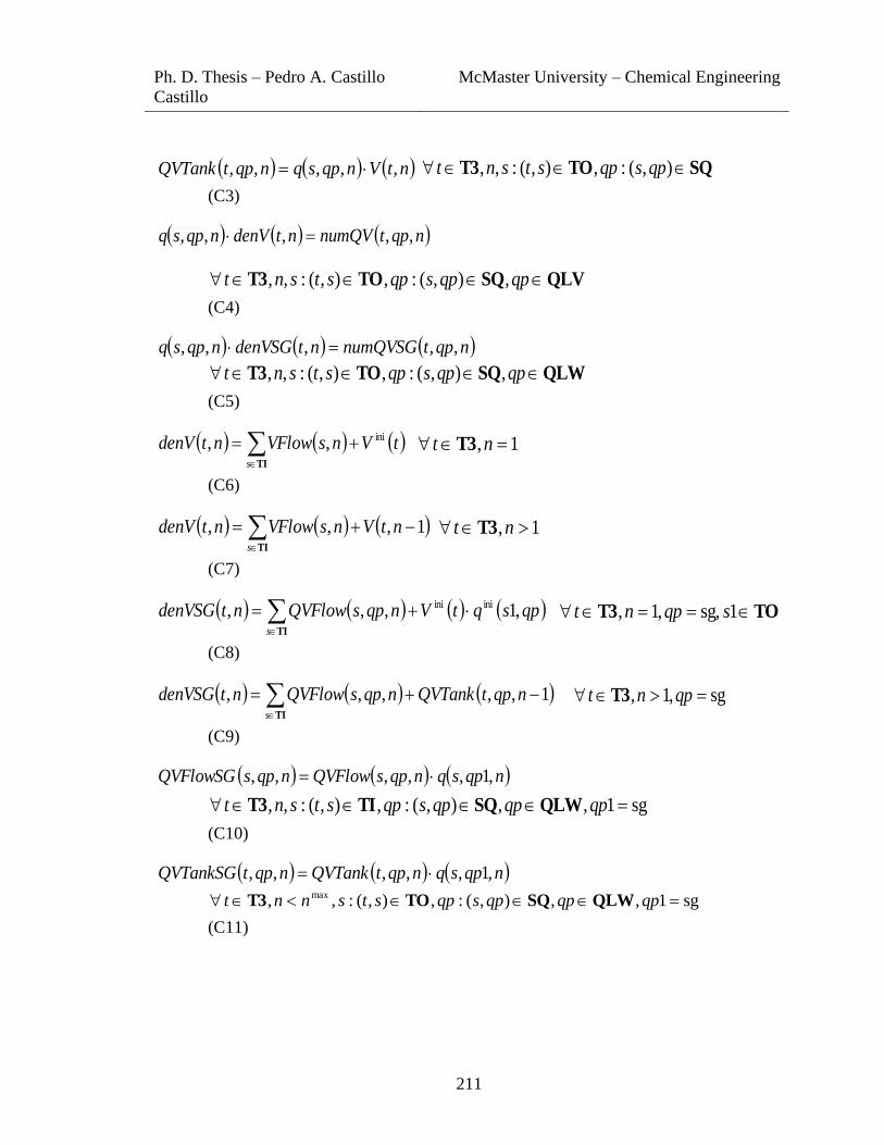
Ph. D. Thesis – Pedro A. Castillo
Castillo
McMaster University – Chemical Engineering
211
( ) ( ) ( )ntVnqpsqnqptQVTank ,,,,, = SQTOT3 ),(:,),(:,, qpsqpstsnt
(C3)
( ) ( ) ( )nqptnumQVntdenVnqpsq ,,,,, =
QLVSQTOT3 qpqpsqpstsnt ,),(:,),(:,,
(C4)
( ) ( ) ( )nqptnumQVSGntdenVSGnqpsq ,,,,, =
QLWSQTOT3 qpqpsqpstsnt ,),(:,),(:,,
(C5)
( ) ( ) ( )tVnsVFlowntdenVs
ini,, += TI
1, = nt T3
(C6)
( ) ( ) ( )1,,, −+=
ntVnsVFlowntdenVs TI
1, nt T3
(C7)
( ) ( ) ( ) ( )qpsqtVnqpsQVFlowntdenVSGs
,1,,, iniini += TI
TOT3 == 1sg,,1, sqpnt
(C8)
( ) ( ) ( )1,,,,, −+=
nqptQVTanknqpsQVFlowntdenVSGs TI
sg,1, = qpnt T3
(C9)
( ) ( ) ( )nqpsqnqpsQVFlownqpsQVFlowSG ,1,,,,, =
sg1,,),(:,),(:,, = qpqpqpsqpstsnt QLWSQTIT3
(C10)
( ) ( ) ( )nqpsqnqptQVTanknqptQVTankSG ,1,,,,, =
sg1,,),(:,),(:,, max = qpqpqpsqpstsnnt QLWSQTOT3
(C11)

Ph. D. Thesis – Pedro A. Castillo
Castillo
McMaster University – Chemical Engineering
212
( ) ( ) ( ) ( )qpsqtVnqpsQVFlownqptnumQVs
,1,,,, iniini += TI
QLVSQTOT3 = qpqpsqpsnt ,),1(:,1,1,
(C12)
( ) ( ) ( )1,,,,,, −+=
nqptQVTanknqpsQVFlownqptnumQVs TI
QLVSQT3 qpqpsqpnt ,),1(:,1,
(C13)
( ) ( ) ( ) ( ) ( )1,1,1,,,, iniiniini qpsqqpsqtVnqpsQVFlowSGnqptnumQVSGs
+= TI
sg1,,),1(:,1,1, == qpqpqpsqpsnt QLWSQTOT3
(C14)
( ) ( ) ( )1,,,,,, −+=
nqptQVTankSGnqpsQVFlowSGnqptnumQVSGs TI
QLWSQT3 qpqpsqpnt ,),1(:,1,
(C15)
Finally, the tanks that only require the quality balance equations for the sulfur content
property (‘sul’), and assume all the other properties of the outlet stream to be equal to the
inlet stream, conform the set T4. Therefore, eq. 31 for tanks from set T4 is replaced by
eqs. C16-C25.
( ) ( ) ( )nsVFlownqpsqnqpsQVFlow ,,,,, = }sulsg,{,),(:,, qpstsnt TIT4
(C16)
( ) ( ) ( )ntVnqpsqnqptQVTank ,,,,, = }sulsg,{,),(:,, qpstsnt TOT4
(C17)
( ) ( ) ( )nqptnumQVSGntdenVSGnqpsq ,,,,, = sul,),(:,, = qpstsnt TOT4
(C18)
( ) ( ) ( ) ( )qpsqtVnqpsQVFlowntdenVSGs
,1,,, iniini += TI
TOT4 == 1sg,,1, sqpnt
(C19)

Ph. D. Thesis – Pedro A. Castillo
Castillo
McMaster University – Chemical Engineering
213
( ) ( ) ( )1,,,,, −+=
nqptQVTanknqpsQVFlowntdenVSGs TI
sg,1, = qpnt T4
(C20)
( ) ( ) ( )nqpsqnqpsQVFlownqpsQVFlowSG ,1,,,,, =
sg1,sul,),(:,, == qpqpstsnt TIT4
(C21)
( ) ( ) ( )nqpsqnqptQVTanknqptQVTankSG ,1,,,,, =
sg1,sul,),(:,, max == qpqpstsnnt TOT4
(C22)
( ) ( ) ( ) ( ) ( )1,1,1,,,, iniiniini qpsqqpsqtVnqpsQVFlowSGnqptnumQVSGs
+= TI
sg1,sul,1,1, === qpqpsnt TOT4
(C23)
( ) ( ) ( )1,,,,,, −+=
nqptQVTankSGnqpsQVFlowSGnqptnumQVSGs TI
sul,1, = qpnt T4
(C24)
( ) ( )nqpsqnqpsq ,,1,, =
sul,),(:,),(:,)1,(:1,, qpqpsqpstsstsnt SQTOTIT4
(C25)
Output flow and quality constraints for mixers
Eq. 34 from the paper takes the form given by eq. C26 for all mixers.
( ) ( )nuVFnsVFlow ,, = UOMX ),(:,, susun
(C26)
Eq. 35 from the paper is replaced according to the mixer type. The general set of mixers
MX is divided into the following subsets: MX1, MX2, MX3 and MX4. MX1 are the
mixers for which we only need a material balance around them; i.e. their mathematical
model is composed by eqs. 32-33 from the paper and eq. C26.
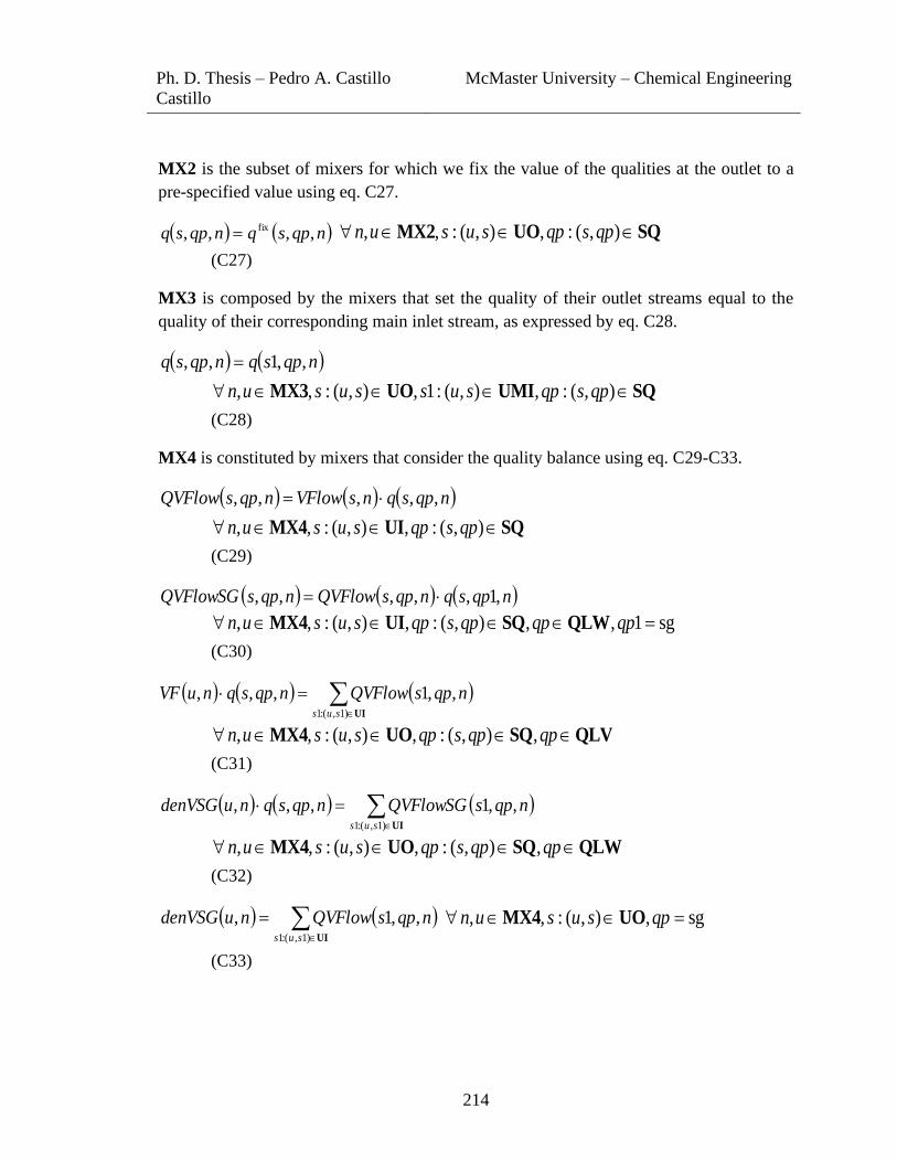
Ph. D. Thesis – Pedro A. Castillo
Castillo
McMaster University – Chemical Engineering
214
MX2 is the subset of mixers for which we fix the value of the qualities at the outlet to a
pre-specified value using eq. C27.
( ) ( )nqpsqnqpsq ,,,, fix= SQUOMX2 ),(:,),(:,, qpsqpsusun
(C27)
MX3 is composed by the mixers that set the quality of their outlet streams equal to the
quality of their corresponding main inlet stream, as expressed by eq. C28.
( ) ( )nqpsqnqpsq ,,1,, =
SQUMIUOMX3 ),(:,),(:1,),(:,, qpsqpsussusun
(C28)
MX4 is constituted by mixers that consider the quality balance using eq. C29-C33.
( ) ( ) ( )nqpsqnsVFlownqpsQVFlow ,,,,, =
SQUIMX4 ),(:,),(:,, qpsqpsusun
(C29)
( ) ( ) ( )nqpsqnqpsQVFlownqpsQVFlowSG ,1,,,,, =
sg1,,),(:,),(:,, = qpqpqpsqpsusun QLWSQUIMX4
(C30)
( ) ( ) ( )
=UI)1,(:1
,,1,,,sus
nqpsQVFlownqpsqnuVF
QLVSQUOMX4 qpqpsqpsusun ,),(:,),(:,,
(C31)
( ) ( ) ( )
=UI)1,(:1
,,1,,,sus
nqpsQVFlowSGnqpsqnudenVSG
QLWSQUOMX4 qpqpsqpsusun ,),(:,),(:,,
(C32)
( ) ( )
=UI)1,(:1
,,1,sus
nqpsQVFlownudenVSG sg,),(:,, = qpsusun UOMX4
(C33)

Ph. D. Thesis – Pedro A. Castillo
Castillo
McMaster University – Chemical Engineering
215
Output flow and quality constraints for hydrotreaters
Eq. 34 from the paper takes the form given by eq. C34 for all hydrotreaters.
( ) ( ) ( )nuVFsuYieldnsVFlow HTU ,,, = UOHTU ),(:,, susun
(C34)
For all the hydrotreaters, eq. 35 from the paper is replaced by eqs. C35-C41.
( ) ( ) ( )nsVFlownqpsqnsMFlow ,,,, = sg,),(:,, = qpsusun UOUIHTU
(C35)
( ) ( ) ( ) ( ) ( )nuRSnsMFlownqpsqnsMFlownqpsqsussus
,,,,,1,,1),(:)1,(:1
+= UOUI
sul,, = qpun HTU
(C36)
( ) ( ) ( )nLuRSRnuRS max, HTU un,
(C37)
( )( ) ( ) ( ) ( )( ) ( )nqpsquHTSnqpsqnqpsquHTS ,,1,,,,1 minmax −−
sul,),(:,, = qpsusun UOSHTU
(C38)
( ) ( )nqpsqnqpsq ,,198.0,, = sg,),(:,)1,(:1,, = qpsussusun UOSUIHTU
(C39)
( ) ( )nqpsqnqpsq ,,,, fix= SQUOSUOHTU ),(:,/),(:,, qpsqpsusun
(C40) ( ) ( )nqpsqnqpsq ,,,, fix=
sulsg,,),(:,),(:,, qpqpsqpsusun SQUOSHTU
(C41)

Ph. D. Thesis – Pedro A. Castillo
Castillo
McMaster University – Chemical Engineering
216
Output flow and quality constraints for other processing units
(reformer, hydrocracker, fluid catalytic cracker)
Eq. 34 from the paper takes the form given by eq. C42 for the processing units from set
PU.
( ) ( ) ( )nuVFsuYieldnsVFlow PU ,,, = UOPU ),(:,, susun
(C42)
For all the units from set PU, eq. 35 from the paper is replaced by eqs. C43-C44.
( ) ( ) ( )nqpsqsuSRFnqpsq ,,1,,, fix = sul,),(:,, = qpsusun UOPU
(C43)
( ) ( )nqpsqnqpsq ,,,, fix= sul,),(:,),(:,, qpqpsqpsusun SQUOPU
(C44)
Bilinear terms
The bilinear terms appear in eqs. C2-C5, C10-C11, C16-C18, C21-C22, C29-C32, and
C35-C36.
Related Documents