Inventory Management

Chapter 16. Inventory Management

[Page 729]Inventory analysis is one of the most popular topics in management science. One reason is that almost all types of business organizations have inventory. Although we tend to think of inventory only in terms of stock on a store shelf, it can take on a variety of forms, such as partially finished products at different stages of a manufacturing process, raw materials, resources, labor, or cash. In addition, the purpose of inventory is not always simply to meet customer demand. For example, companies frequently stock large inventories of raw materials as a hedge against strikes. Whatever form inventory takes or whatever its purpose, it often represents a significant cost to a business firm. It is estimated that the average annual cost of manufactured goods inventory in the United States is approximately 30% of the total value of the inventory. Thus, if a company has $10.0 million worth of products in inventory, the cost of holding the inventory (including insurance, obsolescence, depreciation, interest, opportunity costs, storage costs, etc.) would be approximately $3.0 million. If the amount of inventory could be reduced by half to $5.0 million, then $1.5 million would be saved in inventory costs, a significant cost reduction.

In this chapter we describe the classic economic order quantity models, which represent the most basic and fundamental form of inventory analysis. These models provide a means for determining how much to order (the order quantity) and when to place an order so that inventory- related costs are minimized. The underlying assumption of these models is that demand is known with certainty and is constant. In addition, we will describe models for determining the order size and reorder points (when to place an order) when demand is uncertain.

[Page 729 ( continued )]

Elements of Inventory Management

Inventory is defined as a stock of items kept on hand by an organization to use to meet customer demand. Virtually every type of organization maintains some form of inventory. A department store carries inventories of all the retail items it sells; a nursery has inventories of different plants, trees, and flowers; a rental car agency has inventories of cars ; and a major league baseball team maintains an inventory of players on its minor league teams . Even a family household will maintain inventories of food, clothing, medical supplies , personal hygiene products, and so on.Inventory is a stock of items kept on hand to meet demand .

The Role of Inventory

A company or an organization keeps stocks of inventory for a variety of important reasons. The most prominent is holding finished goods inventories to meet customer demand for a product, especially in a retail operation. However, customer demand can also be in the form of a secretary going to a storage closet to get a printer cartridge or paper, or a carpenter getting a board or nail from a storage shed. A level of inventory is normally maintained that will meet anticipated or expected customer demand. However, because demand is usually not known with certainty , additional amounts of inventory, called safety , or buffer , stocks , are often kept on hand to meet unexpected variations in excess of expected demand.Additional stocks of inventories are sometimes built up to meet seasonal or cyclical demand. Companies will produce items when demand is low to meet high seasonal demand for which their production capacity is insufficient. For example, toy manufacturers produce large inventories during the summer and fall to meet anticipated demand during the Christmas season . Doing so enables them to maintain a relatively smooth production flow throughout the year. They would not normally have the production capacity or logistical support to produce enough to meet all of the Christmas demand during that season. Correspondingly, retailers might find it necessary to keep large stocks of inventory on their shelves to meet peak seasonal demand, such as at Christmas, or for display purposes to attract buyers .

[Page 730]A company will often purchase large amounts of inventory to take advantage of price discounts , as a hedge against anticipated future price increases , or because it can get a lower price by purchasing in volume. For example, Wal-Mart has long been known to purchase an entire manufacturer's stock of soap powder or other retail items because it can get a very low price, which it subsequently passes on to its customers. Companies will often purchase large stocks of items when a supplier liquidates to get a low price. In some cases, large orders will be made simply because the cost of an order may be very high, and it is more cost-effective to have higher inventories than to make a lot of orders.

Many companies find it necessary to maintain in-process inventories at different stages in a manufacturing process to provide independence between operations and to avoid work stoppages or delays. Inventories of raw materials and purchased parts are kept on hand so that the production process will not be delayed as a result of missed or late deliveries or shortages from a supplier. Work-in-process inventories are kept between stages in the manufacturing process so that production can continue smoothly if there are temporary machine breakdowns or other work stoppages. Similarly, a stock of finished parts or products allows customer demand to be met in the event of a work stoppage or problem with the production process.

Demand

A crucial component and the basic starting point for the management of inventory is customer demand. Inventory exists for the purpose of meeting the demand of customers. Customers can be inside the organization, such as a machine operator waiting for a part or a partially completed product to work on, or outside the organization, such as an individual purchasing groceries or a new stereo. As such, an essential determinant of effective

inventory management is an accurate forecast of demand. For this reason the topics of forecasting (Chapter 15) and inventory management are directly interrelated.

In general, the demand for items in inventory is classified as dependent or independent. Dependent demand items are typically component parts, or materials, used in the process of producing a final product. For example, if an automobile company plans to produce 1,000 new cars, it will need 5,000 wheels and tires (including spares ). In this case the demand for wheels is dependent on the production of cars; that is, the demand for one item is a function of demand for another item.Dependent demand items are used internally to produce a final product .

Alternatively, cars are an example of an independent demand item. In general, independent demand items are final or finished products that are not a function of, or dependent upon, internal production activity. Independent demand is usually external, and, thus, beyond the direct control of the organization. In this chapter we will focus on the management of inventory for independent demand items.Independent demand items are final products demanded by an external customer .

Inventory Costs

There are three basic costs associated with inventory: carrying (or holding) costs, ordering costs, and shortage costs. Carrying costs are the costs of holding items in storage. These vary with the level of inventory and occasionally with the length of time an item is held; that is, the greater the level of inventory over time, the higher the carrying cost(s). Carrying costs can include the cost of losing the use of funds tied up in inventory; direct storage costs, such as rent, heating, cooling, lighting, security, refrigeration, record keeping, and logistics; interest on loans used to purchase inventory; depreciation; obsolescence as markets for products in inventory diminish; product deterioration and spoilage; breakage ; taxes; and pilferage.Inventory costs include carrying, ordering , and shortage costs .

[Page 731]Carrying costs are normally specified in one of two ways. The most general form is to assign total carrying costs, determined by summing all the individual costs mentioned previously, on a per-unit basis per time period, such as a month or a year. In this form, carrying costs would commonly be expressed as a per-unit dollar amount on an annual basis (for example, $10 per year). Alternatively, carrying costs are sometimes expressed as a percentage of the value of an item or as a percentage of average inventory value. It is generally estimated that carrying costs range from 10% to 40% of the value of a manufactured item.

Ordering costs are the costs associated with replenishing the stock of inventory being held. These are normally expressed as a dollar amount per order and are independent of the order

size . Thus, ordering costs vary with the number of orders made (i.e., as the number of orders increases, the ordering cost increases). Costs incurred each time an order is made can include requisition costs, purchase orders, transportation and shipping, receiving, inspection, handling and placing in storage, and accounting and auditing.Ordering costs generally react inversely to carrying costs. As the size of orders increases, fewer orders are required, thus reducing annual ordering costs. However, ordering larger amounts results in higher inventory levels and higher carrying costs. In general, as the order size increases, annual ordering costs decrease and annual carrying costs increase.

Shortage costs , also referred to as stockout costs , occur when customer demand cannot be met because of insufficient inventory on hand. If these shortages result in a permanent loss of sales for items demanded but not provided, shortage costs include the loss of profits. Shortages can also cause customer dissatisfaction and a loss of goodwill that can result in a permanent loss of customers and future sales. In some instances the inability to meet customer demand or lateness in meeting demand results in specified penalties in the form of price discounts or rebates. When demand is internal, a shortage can cause work stoppages in the production process and create delays, resulting in downtime costs and the cost of lost production (including indirect and direct production costs).Costs resulting from immediate or future lost sales because demand could not be met are more difficult to determine than carrying or ordering costs. As a result, shortage costs are frequently subjective estimates and many times no more than educated guesses.

Shortages occur because it is costly to carry inventory in stock. As a result, shortage costs have an inverse relationship to carrying costs; as the amount of inventory on hand increases, the carrying cost increases, while shortage costs decrease.

The objective of inventory management is to employ an inventory control system that will indicate how much should be ordered and when orders should take place to minimize the sum of the three inventory costs described here.The purpose of inventory management is to determine how much and when to order .

Inventory Control Systems

An inventory system is a structure for controlling the level of inventory by determining how much to order (the level of replenishment) and when to order. There are two basic types of inventory systems: a continuous (or fixedorder quantity ) system and a periodic (or fixedtime period ) system . The primary difference between the two systems is that in a continuous system, an order is placed for the same constant amount whenever the inventory on hand decreases to a certain level, whereas in a periodic system, an order is placed for a variable amount after an established passage of time.Continuous Inventory Systems

In a continuous inventory system , alternatively referred to as a perpetual system or a fixedorder quantity system , a continual record of the inventory level for every item is maintained . Whenever the inventory on hand decreases to a predetermined level, referred to as the reorder

point , a new order is placed to replenish the stock of inventory. The order that is placed is for a "fixed" amount that minimizes the total inventory carrying, ordering, and shortage costs. This fixed order quantity is called the economic order quantity ; its determination will be discussed in greater detail in a later section.

[Page 732]In a continuous inventory system, a constant amount is ordered when inventory declines to a predetermined level .

A positive feature of a continuous system is that the inventory level is closely and continuously monitored so that management always knows the inventory status. This is especially advantageous for critical inventory items such as replacement parts or raw materials and supplies . However, the cost of maintaining a continual record of the amount of inventory on hand can also be a disadvantage of this type of system.

A simple example of a continuous inventory system is a ledger-style checkbook that many of us use on a daily basis. Our checkbook comes with 300 checks; after the 200th check has been used (and there are 100 left), there is an order form for a new batch of checks that has been inserted by the printer. This form, when turned in at the bank, initiates an order for a new batch of 300 checks from the printer. Many office inventory systems use "reorder" cards that are placed within stacks of stationery or at the bottom of a case of pens or paper clips to signal when a new order should be placed. If you look behind the items on a hanging rack in a Kmart store, you will see a card indicating that it is time to place an order for this item, for an amount indicated on the card.

A more sophisticated example of a continuous inventory system is a computerized checkout system with a laser scanner, used by many supermarkets and retail stores. In this system a laser scanner reads the Universal Product Code (UPC), or bar code, off the product package, and the transaction is instantly recorded and the inventory level updated. Such a system is not only quick and accurate, but it also provides management with continuously updated information on the status of inventory levels. Although not as publicly visible as supermarket systems, many manufacturing companies, suppliers, and distributors also use bar code systems and handheld laser scanners to inventory materials, supplies, equipment, in-process parts, and finished goods.

Because continuous inventory systems are much more common than periodic systems, models that determine fixed order quantities and the time to order will receive most of our attention in this chapter.

Periodic Inventory Systems

In a periodic inventory system , also referred to as a fixedtime period system or periodic review system , the inventory on hand is counted at specific time intervalsfor example, every week or at the end of each month. After the amount of inventory in stock is determined, an order is placed for an amount that will bring inventory back up to a desired level. In this system the inventory level is not monitored at all during the time interval between orders, so it has the advantage of requiring little or no record keeping. However, it has the disadvantage of less direct control. This typically results in larger inventory levels for a periodic inventory system than in a continuous

system, to guard against unexpected stockouts early in the fixed period. Such a system also requires that a new order quantity be determined each time a periodic order is made.In a periodic inventory system , an order is placed for a variable amount after a fixed passage of time.

Periodic inventory systems are often found at a college or university bookstore. Textbooks are normally ordered according to a periodic system, wherein a count of textbooks in stock (for every course) is made after the first few weeks or month during the semester or quarter. An order for new textbooks for the next semester is then made according to estimated course enrollments for the next term (i.e., demand) and the number remaining in stock. Smaller retail stores, drugstores, grocery stores, and offices often use periodic systems; the stock level is checked every week or month, often by a vendor, to see how much (if anything) should be ordered.

[Page 733]

Time Out: For Ford Harris

The earliest published derivation of the classic economic lot size model is credited to Ford Harris of Westinghouse Corporation in 1915. His equation determined a minimum sum of inventory costs and setup costs, given demand that was known and constant and a rate of production that was assumed to be higher than demand.

Economic Order Quantity Models

You will recall that in a continuous or fixedorder quantity system, when inventory reaches a specific level, referred to as the reorder point , a fixed amount is ordered. The most widely used and traditional means for determining how much to order in a continuous system is the economic order quantity (EOQ) model, also referred to as the economic lot size model.EOQ is a continuous inventory system .

The function of the EOQ model is to determine the optimal order size that minimizes total inventory costs. There are several variations of the EOQ model, depending on the assumptions made about the inventory system. In this and following sections we will describe three model versions: the basic EOQ model, the EOQ model with noninstantaneous receipt, and the EOQ model with shortages.

[Page 733 ( continued )]

The Basic EOQ Model

The simplest form of the economic order quantity model on which all other model versions are based is called the basic EOQ model. It is essentially a single formula for determining the optimal order size that minimizes the sum of carrying costs and ordering costs. The model formula is derived under a set of simplifying and restrictive assumptions, as follows :

Demand is known with certainty and is relatively constant over time. No shortages are allowed. Lead time for the receipt of orders is constant. The order quantity is received all at once.

EOQ is the optimal order quantity that will minimize total inventory costs .

Assumptions of the EOQ model include constant demand, no shortages, constant lead time, and instantaneous order receipt .

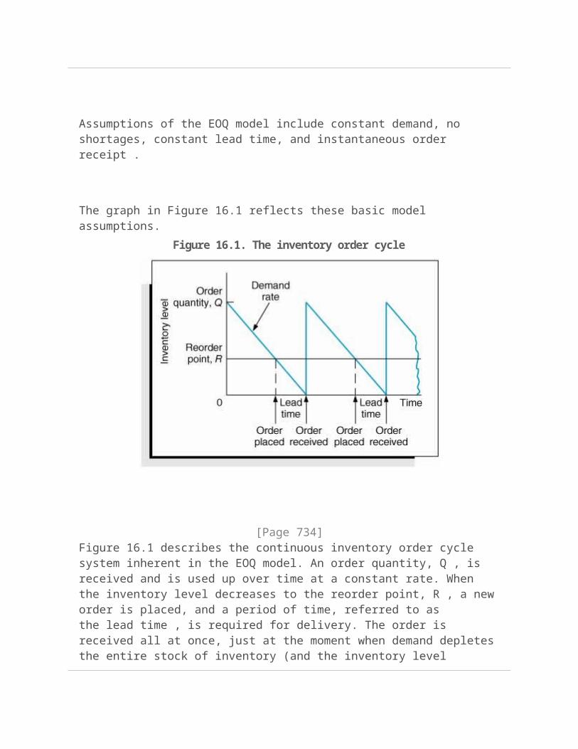
The graph in Figure 16.1 reflects these basic model assumptions.

Figure 16.1. The inventory order cycle

[Page 734]Figure 16.1 describes the continuous inventory order cycle system inherent in the EOQ model. An order quantity, Q , is received and is used up over time at a constant rate. When the inventory level decreases to the reorder point, R , a new order is placed, and a period of time, referred to as the lead time , is required for delivery. The order is received all at once, just at the moment when demand depletes the entire stock of inventory (and the inventory level reaches zero), thus allowing no shortages. This cycle is continuously repeated for the same order quantity, reorder point, and lead time.As we mentioned earlier, Q is the order size that minimizes the sum of carrying costs and holding costs. These two costs react inversely to each other in response to an increase in the order size. As the order size increases, fewer orders are required, causing the ordering cost to decline, whereas the average amount of inventory on hand increases , resulting in an increase in carrying costs. Thus, in effect, the optimal order quantity represents a compromise between these two conflicting costs.Carrying Cost

Carrying cost is usually expressed on a per-unit basis for some period of time (although it is sometimes given as a percentage of average inventory). Traditionally, the carrying cost is referred to on an annual basis (i.e., per year).

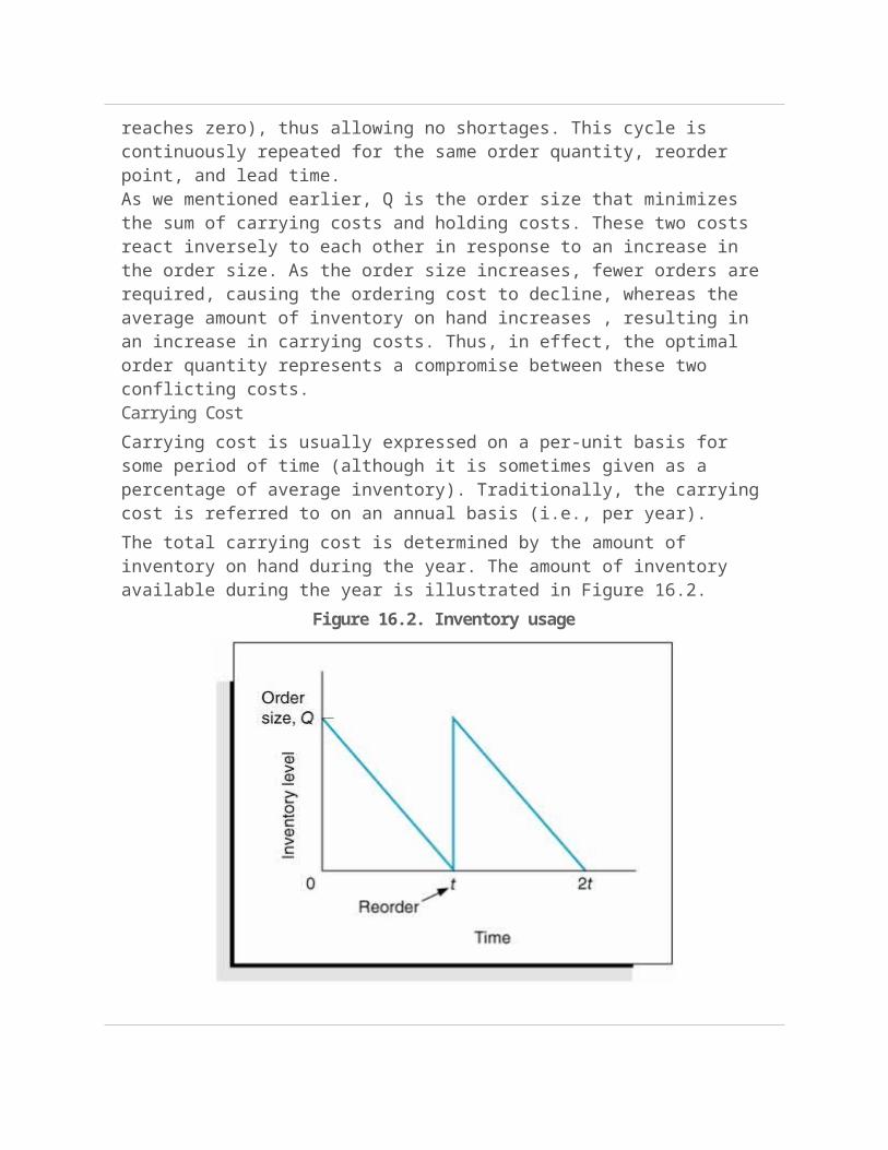
The total carrying cost is determined by the amount of inventory on hand during the year. The amount of inventory available during the year is illustrated in Figure 16.2.

Figure 16.2. Inventory usage

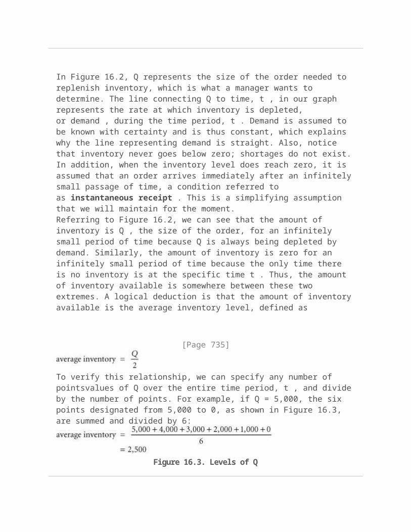
In Figure 16.2, Q represents the size of the order needed to replenish inventory, which is what a manager wants to determine. The line connecting Q to time, t , in our graph represents the rate at which inventory is depleted, or demand , during the time period, t . Demand is assumed to be known with certainty and is thus constant, which explains why the line representing demand is straight. Also, notice that inventory never goes below zero; shortages do not exist. In addition, when the inventory level does reach zero, it is assumed that an order arrives immediately after an infinitely small passage of time, a condition referred to as instantaneous receipt . This is a simplifying assumption that we will maintain for the moment.Referring to Figure 16.2, we can see that the amount of inventory is Q , the size of the order, for an infinitely small period of time because Q is always being depleted by demand. Similarly, the amount of inventory is zero for an infinitely small period of time because the only time there is no inventory is at the specific time t . Thus, the amount of inventory available is somewhere between these two extremes. A logical deduction is that the amount of inventory available is the average inventory level, defined as

[Page 735]

To verify this relationship, we can specify any number of pointsvalues of Q over the entire time period, t , and divide by the number of points. For example, if Q = 5,000, the six points designated from 5,000 to 0, as shown in Figure 16.3, are summed and divided by 6:

Figure 16.3. Levels of Q

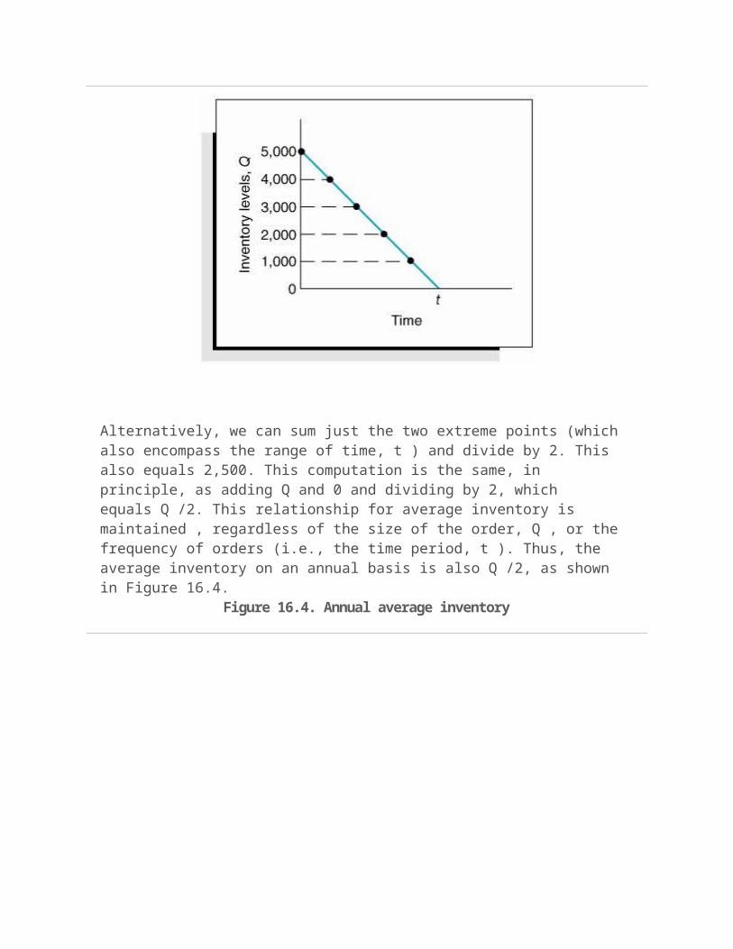
Alternatively, we can sum just the two extreme points (which also encompass the range of time, t ) and divide by 2. This also equals 2,500. This computation is the same, in principle, as adding Q and 0 and dividing by 2, which equals Q /2. This relationship for average inventory is maintained , regardless of the size of the order, Q , or the frequency of orders (i.e., the time period, t ). Thus, the average inventory on an annual basis is also Q /2, as shown in Figure 16.4.

Figure 16.4. Annual average inventory

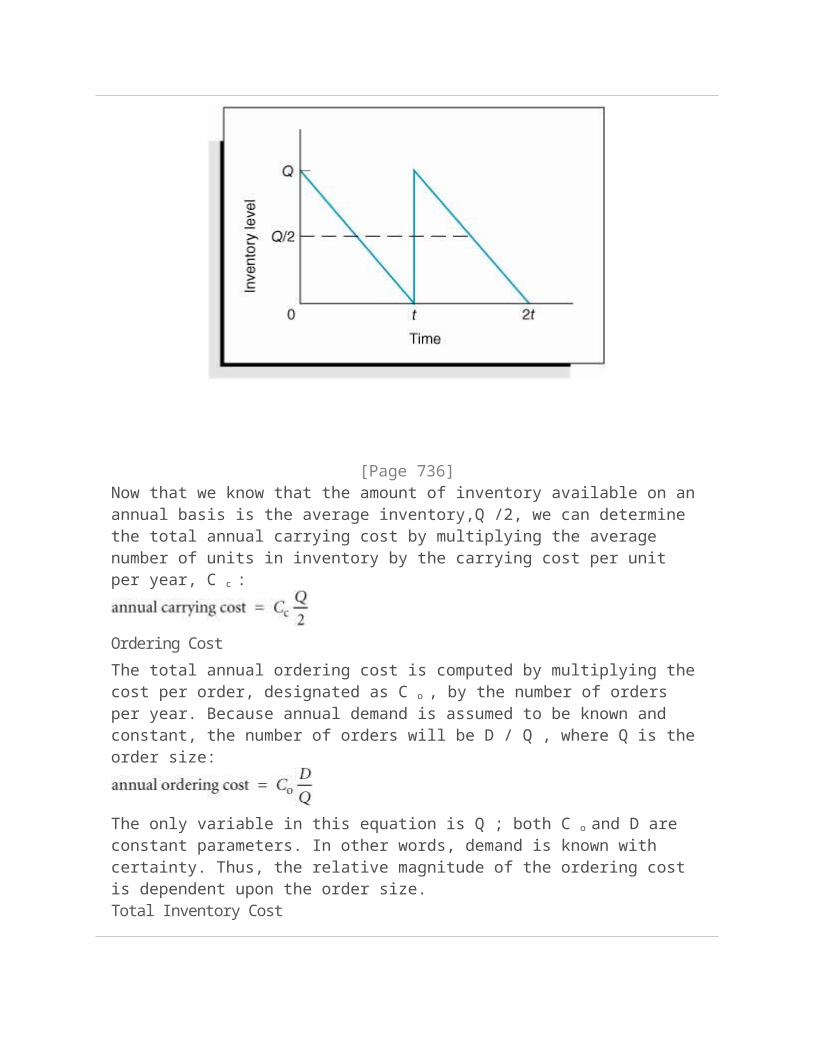
[Page 736]Now that we know that the amount of inventory available on an annual basis is the average inventory,Q /2, we can determine the total annual carrying cost by multiplying the average number of units in inventory by the carrying cost per unit per year, C c :

Ordering Cost

The total annual ordering cost is computed by multiplying the cost per order, designated as C o , by the number of orders per year. Because annual demand is assumed to be known and constant, the number of orders will be D / Q , where Q is the order size:

The only variable in this equation is Q ; both C o and D are constant parameters. In other words, demand is known with certainty. Thus, the relative magnitude of the ordering cost is dependent upon the order size.Total Inventory Cost

The total annual inventory cost is simply the sum of the ordering and carrying costs:

These cost functions are shown in Figure 16.5. Notice the inverse relationship between ordering cost and carrying cost, resulting in a convex total cost curve.

Figure 16.5. The EOQ cost model

Observe the general upward trend of the total carrying cost curve. As the order size Q (shown on the horizontal axis) increases, the total carrying cost (shown on the vertical axis) increases. This is logical because larger orders will result in more units carried in inventory. Next, observe the ordering cost curve in Figure 16.5. As the order size, Q , increases, the ordering cost decreases (just the opposite of what occurred with the carrying cost). This is logical because an increase in the size of the orders will result in fewer orders being placed each year. Because one cost increases as the other decreases, the result of summing the two costs is a convex total cost curve.

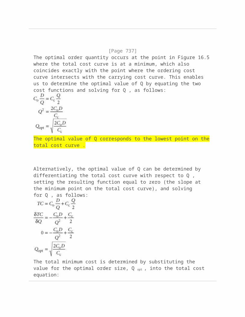
[Page 737]The optimal order quantity occurs at the point in Figure 16.5 where the total cost curve is at a minimum, which also coincides exactly with the point where the ordering cost curve intersects with the carrying cost curve. This enables us to determine the optimal value of Q by equating the two cost functions and solving for Q , as follows:

The optimal value of Q corresponds to the lowest point on the total cost curve .

Alternatively, the optimal value of Q can be determined by differentiating the total cost curve with respect to Q , setting the resulting function equal to zero (the slope at the minimum point on the total cost curve), and solving for Q , as follows:

The total minimum cost is determined by substituting the value for the optimal order

size, Q opt , into the total cost equation:

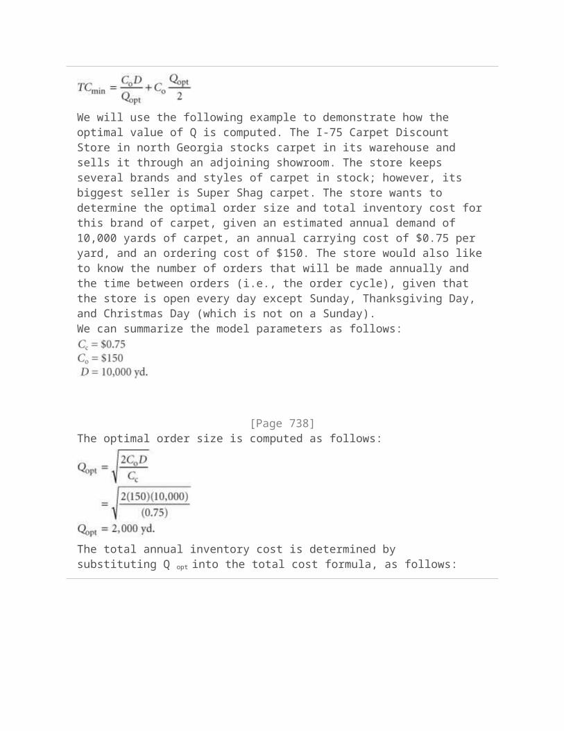
We will use the following example to demonstrate how the optimal value of Q is computed. The I-75 Carpet Discount Store in north Georgia stocks carpet in its warehouse and sells it through an adjoining showroom. The store keeps several brands and styles of carpet in stock; however, its biggest seller is Super Shag carpet. The store wants to determine the optimal order size and total inventory cost for this brand of carpet, given an estimated annual demand of 10,000 yards of carpet, an annual carrying cost of $0.75 per yard, and an ordering cost of $150. The store would also like to know the number of orders that will be made annually and the time between orders (i.e., the order cycle), given that the store is open every day except Sunday, Thanksgiving Day, and Christmas Day (which is not on a Sunday).We can summarize the model parameters as follows:

[Page 738]The optimal order size is computed as follows:

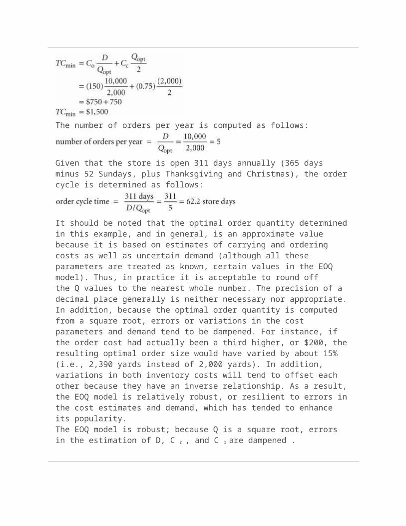
The total annual inventory cost is determined by substituting Q opt into the total cost formula, as follows:

The number of orders per year is computed as follows:

Given that the store is open 311 days annually (365 days minus 52 Sundays, plus Thanksgiving and Christmas), the order cycle is determined as follows:

It should be noted that the optimal order quantity determined in this example, and in general, is an approximate value because it is based on estimates of carrying and ordering costs as well as uncertain demand (although all these parameters are treated as known, certain values in the EOQ model). Thus, in practice it is acceptable to round off the Q values to the nearest whole number. The precision of a decimal place generally is neither necessary nor appropriate. In addition, because the optimal order quantity is computed from a square root, errors or variations in the cost parameters and demand tend to be dampened. For instance, if the order cost had actually been a third higher, or $200, the resulting optimal order size would have varied by about 15% (i.e., 2,390 yards instead of 2,000 yards). In addition, variations in both inventory costs will tend to offset each other because they have an inverse relationship. As a result, the EOQ model is relatively robust, or resilient to errors in the cost estimates and demand, which has tended to enhance its popularity.The EOQ model is robust; because Q is a square root, errors in the estimation of D, C c , and C o are dampened .

EOQ Analysis Over Time

One aspect of inventory analysis that can be confusing is the time frame encompassed by the analysis. Therefore, we will digress for just a moment to discuss this aspect of EOQ analysis.

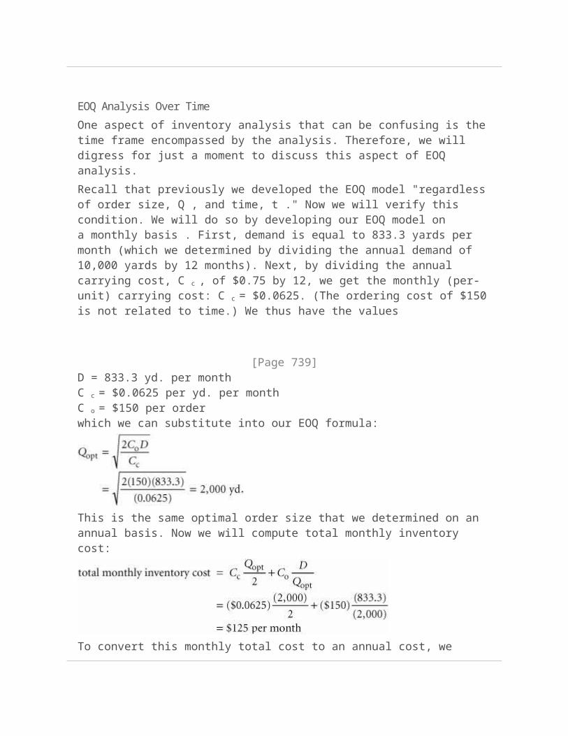
Recall that previously we developed the EOQ model "regardless of order size, Q , and time, t ." Now we will verify this condition. We will do so by developing our EOQ model on a monthly basis . First, demand is equal to 833.3 yards per month (which we determined by dividing the annual demand of 10,000 yards by 12 months). Next, by dividing the annual carrying cost, C c , of $0.75 by 12, we get the monthly (per-unit) carrying cost: C c = $0.0625. (The ordering cost of $150 is not related to time.) We thus have the values

[Page 739]D = 833.3 yd. per monthC c = $0.0625 per yd. per monthC o = $150 per orderwhich we can substitute into our EOQ formula:

This is the same optimal order size that we determined on an annual basis. Now we will compute total monthly inventory cost:

To convert this monthly total cost to an annual cost, we multiply it by 12 (months):

total annual inventory cost = ($125)(12) = $1,500

This brief example demonstrates that regardless of the time period encompassed by EOQ analysis, the economic order quantity ( Q opt ) is the same.

The EOQ Model with Noninstantaneous Receipt

A variation of the basic EOQ model is achieved when the assumption that orders are received all at once is relaxed . This version of the EOQ model is known as the noninstantaneous receipt model , also referred to as the gradual usage , or production lot size , model . In this EOQ variation, the order quantity is received gradually over time and the inventory level is depleted at the same time it is being replenished. This is a situation most commonly found when the inventory user is also the producer, as, for example, in a manufacturing operation where a part is produced to use in a larger assembly. This situation can also occur when orders are delivered gradually over time or the retailer and producer of a product are one and the same. The noninstantaneous receipt model is illustrated graphically in Figure 16.6, which highlights the difference between this variation and the basic EOQ model.

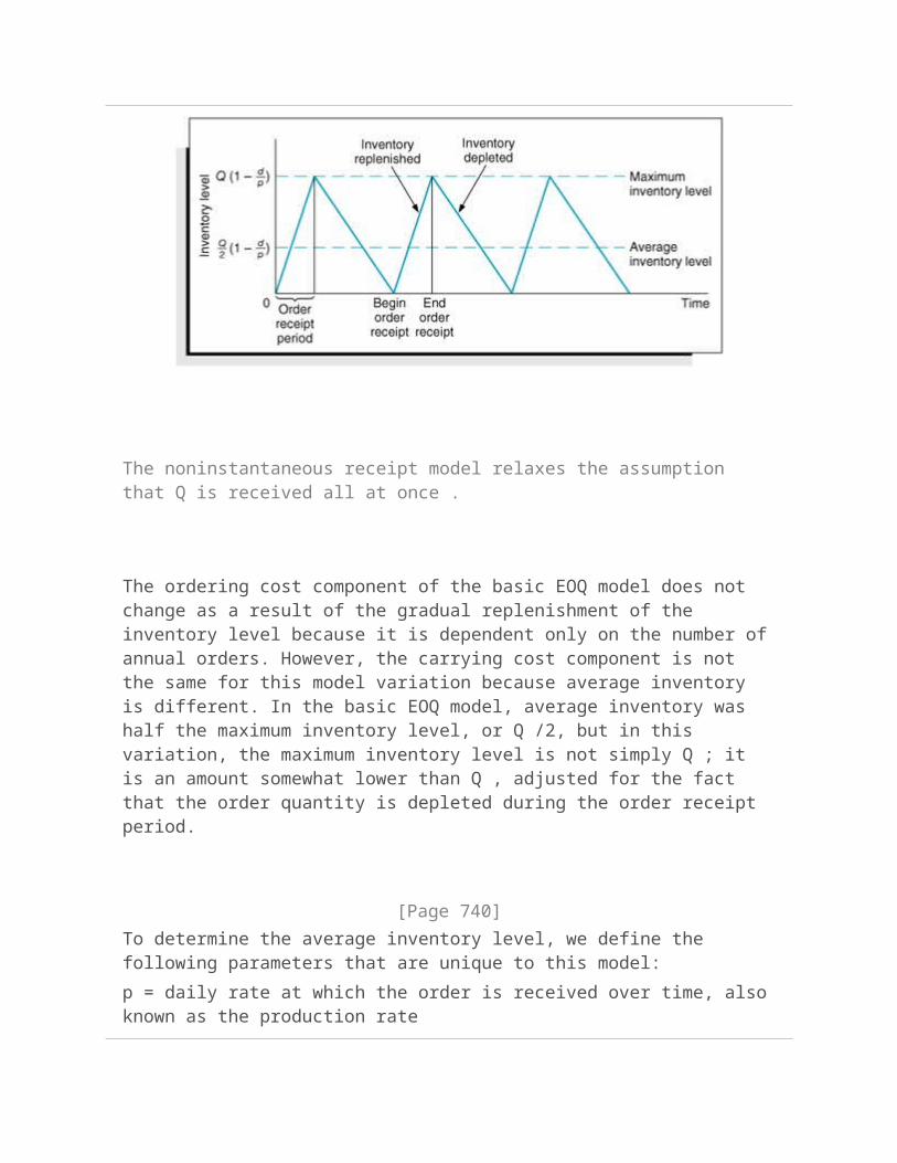
Figure 16.6. The EOQ model with noninstantaneous order receipt

(This item is displayed on page 740 in the print version)

The noninstantaneous receipt model relaxes the assumption that Q is received all at once .

The ordering cost component of the basic EOQ model does not change as a result of the gradual replenishment of the inventory level because it is dependent only on the number of annual orders. However, the carrying cost component is not the same for this model variation because average inventory is different. In the basic EOQ model, average inventory was half the maximum inventory level, or Q /2, but in this variation, the maximum inventory level is not simply Q ; it is an amount somewhat lower than Q , adjusted for the fact that the order quantity is depleted during the order receipt period.

[Page 740]To determine the average inventory level, we define the following parameters that are unique to this model:

p = daily rate at which the order is received over time, also known as the production rated = the daily rate at which inventory is demandedThe demand rate cannot exceed the production rate because we are still assuming that no shortages are possible, and if d = p , then there is no order size because items are used as fast as they are produced. Thus, for this model, the production rate must exceed the demand rate, or p > d .Observing Figure 16.6, the time required to receive an order is the order quantity divided by the rate at which the order is received, or Q/p . For example, if the order size is 100 units and the production rate, p , is 20 units per day, the order will be received in 5 days. The amount of inventory that will be depleted or used up during this time period is determined by multiplying by the demand rate, or(Q/p)d . For example, if it takes 5 days to receive the order and during this time inventory is depleted at the rate of 2 units per day, then a total of

10 units is used. As a result, the maximum amount of inventory that is on hand is the order size minus the amount depleted during the receipt period, computed as follows and shown earlier in Figure 16.6:

Because this is the maximum inventory level, the average inventory level is determined by dividing this amount by 2, as follows:

[Page 741]The total carrying cost, using this function for average inventory, is

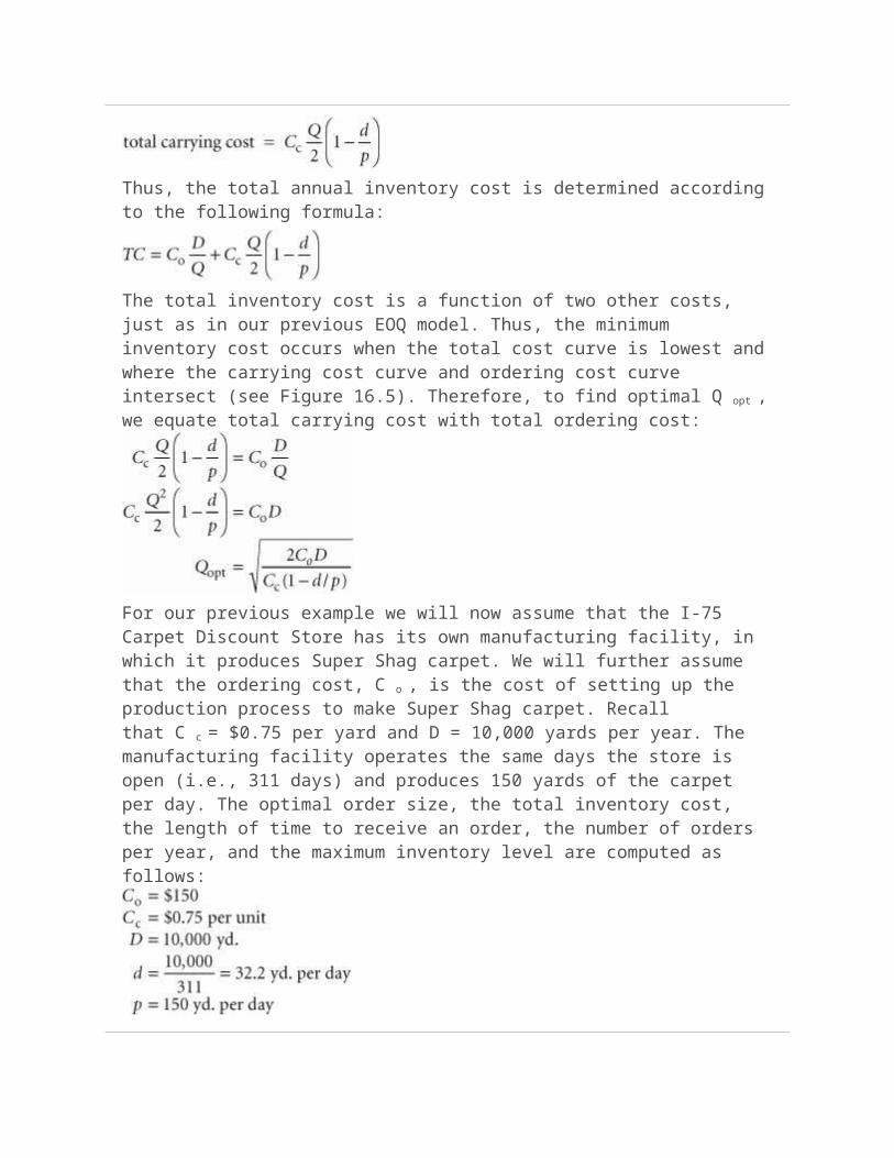
Thus, the total annual inventory cost is determined according to the following formula:

The total inventory cost is a function of two other costs, just as in our previous EOQ model. Thus, the minimum inventory cost occurs when the total cost curve is lowest and where the carrying cost curve and ordering cost curve intersect (see Figure 16.5). Therefore, to find optimal Q opt , we equate total carrying cost with total ordering cost:

For our previous example we will now assume that the I-75 Carpet Discount Store has its own manufacturing facility, in which it produces Super Shag carpet. We will further assume that the ordering cost, C o , is the cost of setting up the production process to make Super Shag carpet. Recall that C c = $0.75 per yard and D = 10,000 yards per year. The manufacturing facility operates the same days the store is open (i.e., 311 days) and produces

150 yards of the carpet per day. The optimal order size, the total inventory cost, the length of time to receive an order, the number of orders per year, and the maximum inventory level are computed as follows:

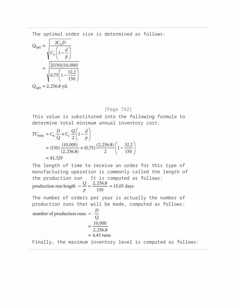
The optimal order size is determined as follows:

[Page 742]This value is substituted into the following formula to determine total minimum annual inventory cost:

The length of time to receive an order for this type of manufacturing operation is commonly called the length of the production run . It is computed as follows:

The number of orders per year is actually the number of production runs that will be made, computed as follows:

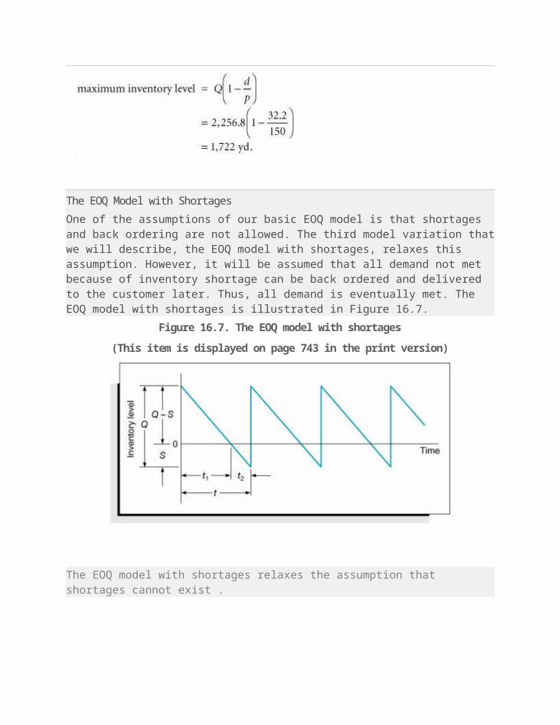
Finally, the maximum inventory level is computed as follows:

The EOQ Model with Shortages

One of the assumptions of our basic EOQ model is that shortages and back ordering are not allowed. The third model variation that we will describe, the EOQ model with shortages, relaxes this assumption. However, it will be assumed that all demand not met because of inventory shortage can be back ordered and delivered to the customer later. Thus, all demand is eventually met. The EOQ model with shortages is illustrated in Figure 16.7.

Figure 16.7. The EOQ model with shortages

(This item is displayed on page 743 in the print version)

The EOQ model with shortages relaxes the assumption that shortages cannot exist .

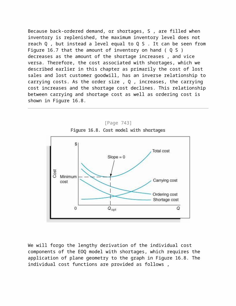
Because back-ordered demand, or shortages, S , are filled when inventory is replenished, the maximum inventory level does not reach Q , but instead a level equal to Q S . It can be seen from Figure 16.7 that the amount of inventory on hand ( Q S ) decreases as the amount of the shortage increases , and vice versa. Therefore, the cost associated with shortages, which we described earlier in this chapter as primarily the cost of lost sales and lost customer goodwill, has an

inverse relationship to carrying costs. As the order size , Q , increases, the carrying cost increases and the shortage cost declines. This relationship between carrying and shortage cost as well as ordering cost is shown in Figure 16.8.

[Page 743]Figure 16.8. Cost model with shortages

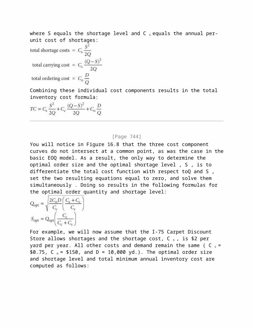
We will forgo the lengthy derivation of the individual cost components of the EOQ model with shortages, which requires the application of plane geometry to the graph in Figure 16.8. The individual cost functions are provided as follows , where S equals the shortage level and C s equals the annual per-unit cost of shortages:

Combining these individual cost components results in the total inventory cost formula:

[Page 744]You will notice in Figure 16.8 that the three cost component curves do not intersect at a common point, as was the case in the basic EOQ model. As a result, the only way to determine the optimal order size and the optimal shortage level , S , is to differentiate the total cost function with respect toQ and S , set the two resulting equations equal to zero, and solve them simultaneously . Doing so results in the following formulas for the optimal order quantity and shortage level:

For example, we will now assume that the I-75 Carpet Discount Store allows shortages and the shortage cost, C s , is $2 per yard per year. All other costs and demand remain the same ( C c = $0.75, C o = $150, and D = 10,000 yd.). The optimal order size and shortage level and total minimum annual inventory cost are computed as follows:

Several additional parameters of the EOQ model with shortages can be computed for this example, as follows:

[Page 745]The time between orders, identified as t in Figure 16.7, is computed as follows:

The time during which inventory is on hand, t 1 in Figure 16.7, and the time during which there is a shortage, t 2 in Figure 16.7, during each order cycle can be computed using the following formulas:

Management Science Application: Determining Inventory Ordering Policy at Dell

Dell Inc., the world's largest computer-systems company, bypasses retailers and sells directly to customers via phone or the Internet. After an order is processed , it is sent to one of its assembly plants in Austin, Texas, where the product is built, tested , and packaged within 8 hours.

Dell carries very little components inventory itself. Technology changes occur so fast that holding inventory can be a huge liability; some components lose 0.5% to 2.0% of their value per week. In addition, many of Dell's suppliers are located in Southeast Asia, and their shipping times to Austin range from 7 days for air transport to 30 days for water and ground transport. To compensate for these factors, Dell's suppliers keep inventory in small warehouses called "revolvers" (for revolving inventory), which are a few miles from Dell's assembly plants. Dell keeps very little inventory at its own plants, so it withdraws inventory from the revolvers every few hours, while most Dell's suppliers deliver to their revolvers three times per week.

The cost of carrying inventory by Dell's suppliers is ultimately reflected in the final price of a computer. Thus, in order to maintain a competitive price advantage in the market, Dell strives to help its suppliers reduce inventory costs. Dell has a vendor-managed inventory (VMI) arrangement with its suppliers, which decide how much to order and when to send their orders to the revolvers. Dell's suppliers order in batches (to offset ordering costs), using

a continuous ordering system with a batch order size, Q , and a reorder point, R , where R is the sum of the inventory on order and a safety stock. The order size estimate, based on long- term data and forecasts, is held constant. Dell sets target inventory levels for its supplierstypically 10 days of inventoryand keeps track of how much suppliers deviate from these targets and reports this information back to suppliers so that they can make adjustments accordingly .

Source: R. Kapuscinski, R. Zhang, P. Carbonneau, R. Moore, and B. Reeves, "Inventory Decisions in Dell's Supply Chain," Interfaces 34, no. 3 (MayJune 2004): 191205.

EOQ Analysis with QM for Windows

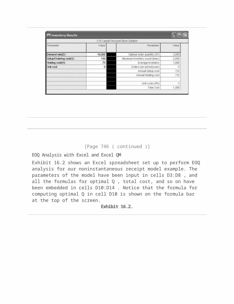
QM for Windows has modules for all the EOQ models we have presented, including the basic model, the noninstantaneous receipt model, and the model with shortages. To demonstrate the capabilities of this program, we will use our basic EOQ example, for which the solution output summary is shown in Exhibit 16.1.

Exhibit 16.1.

[Page 746 ( continued )]

EOQ Analysis with Excel and Excel QM

Exhibit 16.2 shows an Excel spreadsheet set up to perform EOQ analysis for our noninstantaneous receipt model example. The parameters of the model have been input in cells D3:D8 , and all the formulas for optimal Q , total cost, and so on have been embedded in cells D10:D14 . Notice that the formula for computing optimal Q in cell D10 is shown on the formula bar at the top of the screen.

Exhibit 16.2.

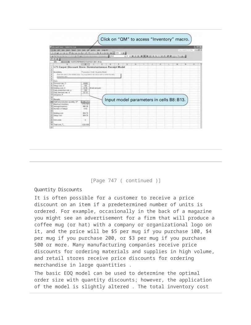
In Chapter 1 we introduced Excel QM, a set of spreadsheet macros that we have also used in several other chapters. Excel QM includes a set of spreadsheet macros for "Inventory" that includes EOQ analysis. After Excel QM is activated, the "Excel QM" menu is accessed by clicking on "QM" on the menu bar at the top of the spreadsheet. Clicking on "Inventory" from this menu results in a Spreadsheet Initialization window, in which you enter the problem title and the form of holding (or carrying) cost. Clicking on "OK" will result in the spreadsheet shown in Exhibit 16.3. Initially, this spreadsheet will have example values in the data cells B8:B13 . Thus, the first step in using this macro is to type in cells B8:B13 the data for the noninstantaneous receipt model for our I-75 Carpet Discount Store problem. The model results are computed automatically in cells B16:B26 from formulas already embedded in the spreadsheet.

[Page 747]Exhibit 16.3.

[Page 747 ( continued )]

Quantity Discounts

It is often possible for a customer to receive a price discount on an item if a predetermined number of units is ordered. For example, occasionally in the back of a magazine you might see an advertisement for a firm that will produce a coffee mug (or hat) with a company or organizational logo on it, and the price will be $5 per mug if you purchase 100, $4 per mug if you purchase 200, or $3 per mug if you purchase 500 or more. Many manufacturing companies receive price discounts for ordering materials and supplies in high volume, and retail stores receive price discounts for ordering merchandise in large quantities .

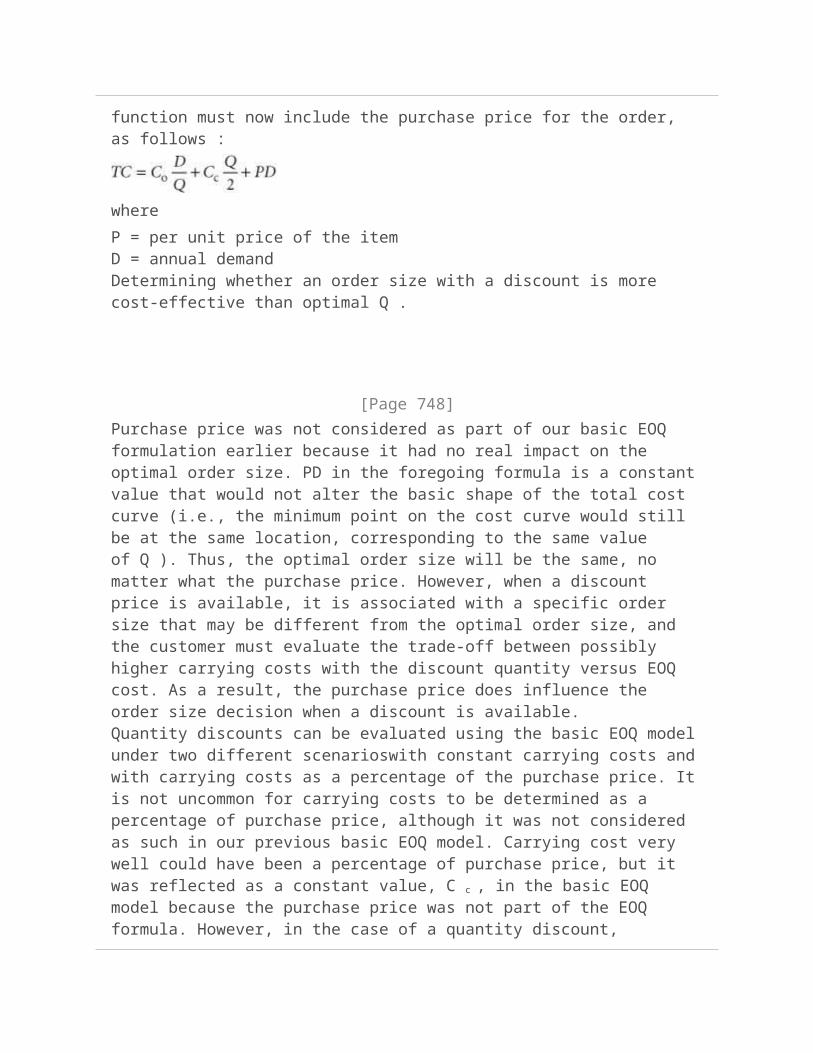
The basic EOQ model can be used to determine the optimal order size with quantity discounts; however, the application of the model is slightly altered . The total inventory cost function must now include the purchase price for the order, as follows :

where

P = per unit price of the itemD = annual demandDetermining whether an order size with a discount is more cost-effective than optimal Q .

[Page 748]Purchase price was not considered as part of our basic EOQ formulation earlier because it had no real impact on the optimal order size. PD in the foregoing formula is a constant value that would not alter the basic shape of the total cost curve (i.e., the minimum point on the cost curve would still be at the same location, corresponding to the same value of Q ). Thus, the optimal order size will be the same, no matter what the purchase price. However, when a discount price is available, it is associated with a specific order size that may be different from the optimal order size, and the customer must evaluate the trade-off between possibly higher carrying costs with the discount quantity versus EOQ cost. As a result, the purchase price does influence the order size decision when a discount is available.Quantity discounts can be evaluated using the basic EOQ model under two different scenarioswith constant carrying costs and with carrying costs as a percentage of the purchase price. It is not uncommon for carrying costs to be determined as a percentage of purchase price, although it was not considered as such in our previous basic EOQ model. Carrying cost very well could have been a percentage of purchase price, but it was reflected as a constant value, C c , in the basic EOQ model because the purchase price was not part of the EOQ formula. However, in the case of a quantity discount, carrying cost will vary with the change in price if it is computed as a percentage of purchase price.Quantity discounts are evaluated with constant C c and as a percentage of price .

Quantity Discounts with Constant Carrying Costs

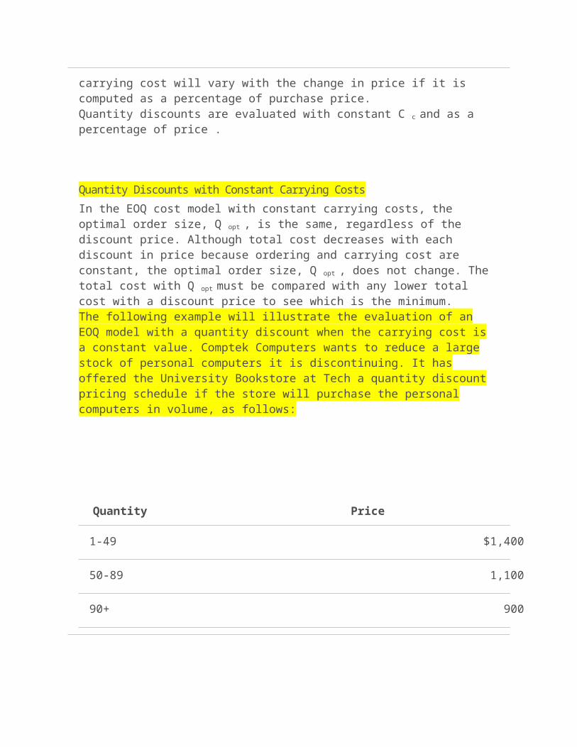
In the EOQ cost model with constant carrying costs, the optimal order size, Q opt , is the same, regardless of the discount price. Although total cost decreases with each discount in price because ordering and carrying cost are constant, the optimal order size, Q opt , does not change. The total cost with Q opt must be compared with any lower total cost with a discount price to see which is the minimum.The following example will illustrate the evaluation of an EOQ model with a quantity discount when the carrying cost is a constant value. Comptek Computers wants to reduce a large stock of personal computers it is discontinuing. It has offered the University Bookstore at Tech a quantity discount pricing schedule if the store will purchase the personal computers in volume, as follows:

Quantity Price

1-49 $1,400

50-89 1,100

90+ 900

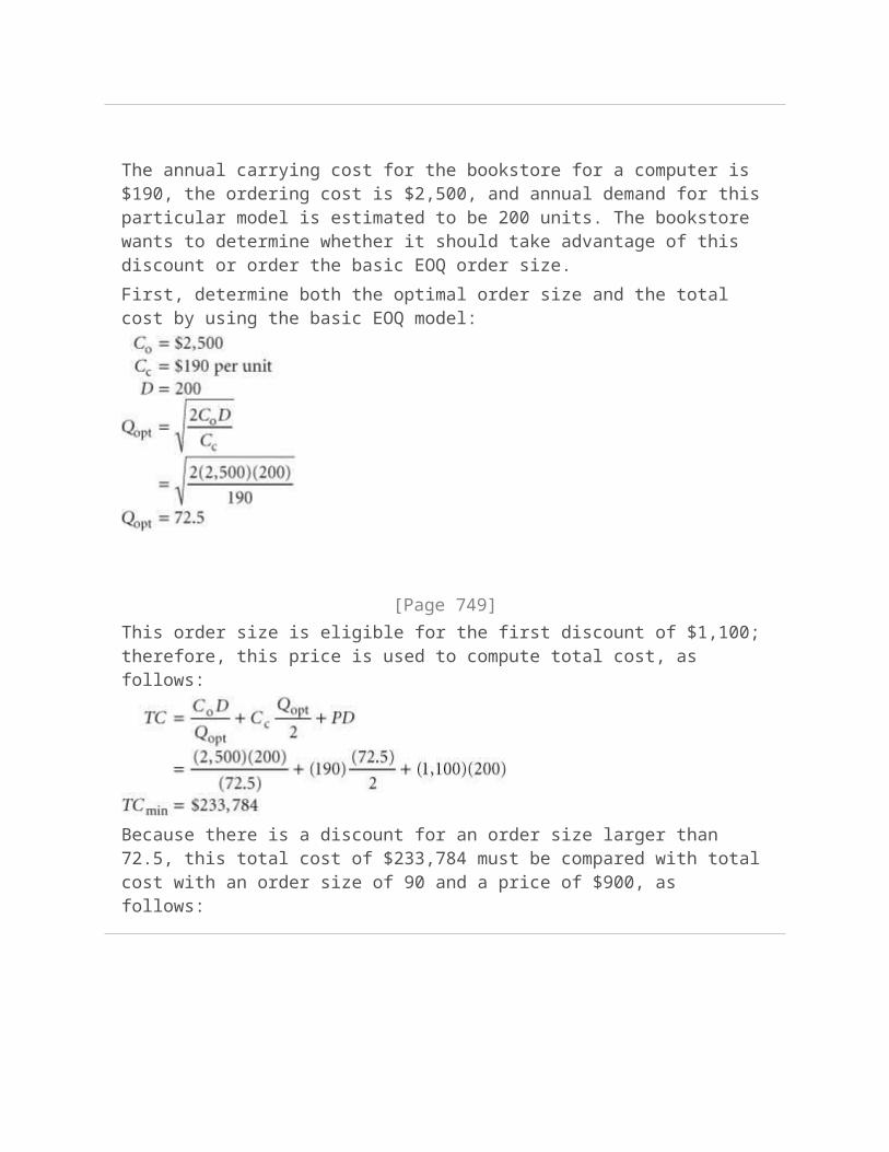
The annual carrying cost for the bookstore for a computer is $190, the ordering cost is $2,500, and annual demand for this particular model is estimated to be 200 units. The bookstore wants to determine whether it should take advantage of this discount or order the basic EOQ order size.

First, determine both the optimal order size and the total cost by using the basic EOQ model:

[Page 749]This order size is eligible for the first discount of $1,100; therefore, this price is used to compute total cost, as follows:

Because there is a discount for an order size larger than 72.5, this total cost of $233,784 must be compared with total cost with an order size of 90 and a price of $900, as follows:

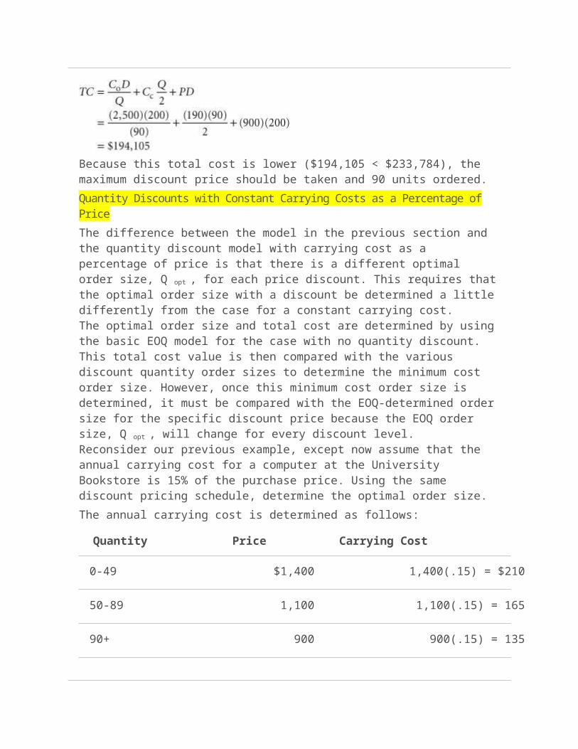
Because this total cost is lower ($194,105 < $233,784), the maximum discount price should be taken and 90 units ordered.

Quantity Discounts with Constant Carrying Costs as a Percentage of Price

The difference between the model in the previous section and the quantity discount model with carrying cost as a percentage of price is that there is a different optimal order size, Q opt , for each price discount. This requires that the optimal order size with a discount be determined a little differently from the case for a constant carrying cost.The optimal order size and total cost are determined by using the basic EOQ model for the case with no quantity discount. This total cost value is then compared with the various discount quantity order sizes to determine the minimum cost order size. However, once this minimum cost order size is determined, it must be compared with the EOQ-determined order size for the specific discount price because the EOQ order size, Q opt , will change for every discount level.Reconsider our previous example, except now assume that the annual carrying cost for a computer at the University Bookstore is 15% of the purchase price. Using the same discount pricing schedule, determine the optimal order size.

The annual carrying cost is determined as follows:

Quantity Price Carrying Cost

0-49 $1,400 1,400(.15) = $210

50-89 1,100 1,100(.15) = 165

90+ 900 900(.15) = 135

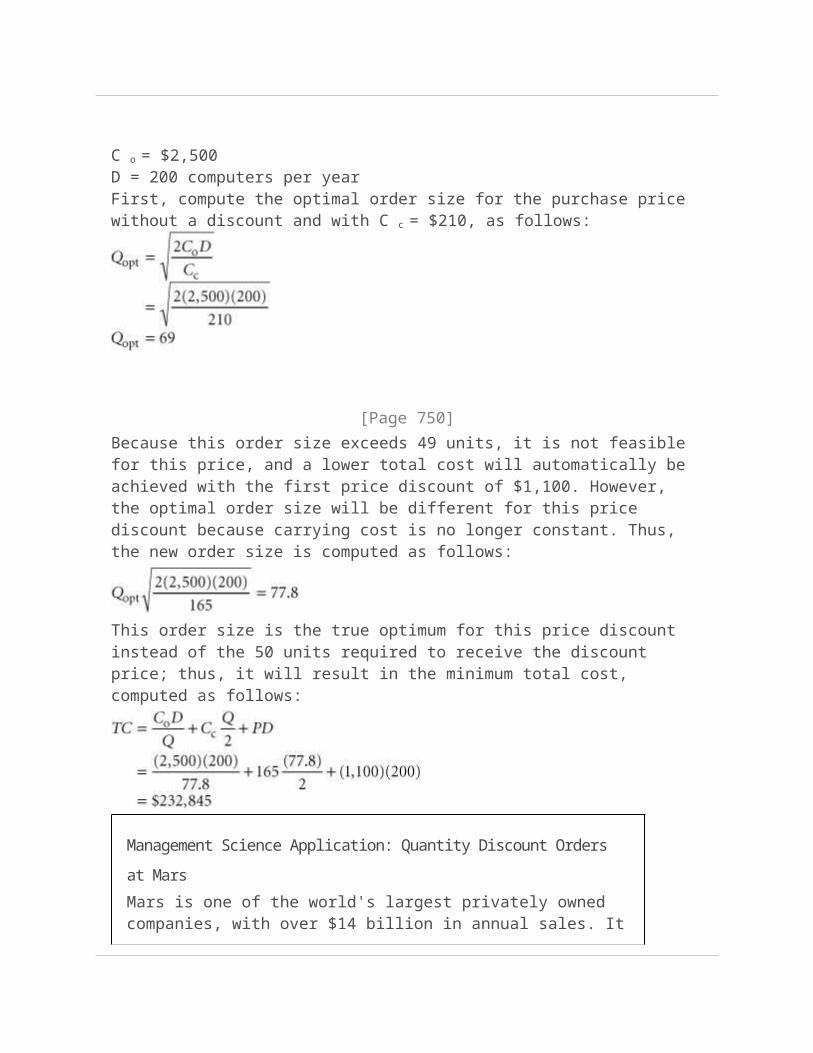
C o = $2,500D = 200 computers per yearFirst, compute the optimal order size for the purchase price without a discount and with C c = $210, as follows:

[Page 750]Because this order size exceeds 49 units, it is not feasible for this price, and a lower total cost will automatically be achieved with the first price discount of $1,100. However, the optimal order size will be different for this price discount because carrying cost is no longer constant. Thus, the new order size is computed as follows:

This order size is the true optimum for this price discount instead of the 50 units required to receive the discount price; thus, it will result in the minimum total cost, computed as follows:

Management Science Application: Quantity Discount Orders at Mars

Mars is one of the world's largest privately owned companies, with over $14 billion in annual sales. It has grown from making and selling buttercream candies door-to-door to a global business spanning 100 countries that includes food, pet care, beverage vending, and electronic payment systems. It produces such well-known products as Mars candies, M&M's, Snickers, and Uncle Ben's rice.

Mars relies on a small number of suppliers for each of the huge number of materials it uses in its products. One way that Mars purchases materials from its suppliers is through online electronic auctions, in which Mars buyers negotiate bids for orders from suppliers. The most important purchases are those of high value and large volume, for which the suppliers provide quantity discounts. The suppliers provide a pricing schedule that includes quantity ranges associated with each price level. Such quantity-discount auctions are tailored (by online brokers ) for industries in which volume discounts are common, such as bulk chemicals and agricultural commodities.

A Mars buyer selects the bids that minimize total purchasing costs, subject to several rules: There must be a minimum and maximum number of suppliers so that Mars is not dependent on too few suppliers nor loses quality control by having too many; there must be a maximum amount purchased from each supplier to limit the influence of any one supplier; and a minimum amount must be ordered to avoid economically inefficient orders (i.e., less than a full tuckload).

Source: G. Hohner, J. Rich, E. Ng, A. Davenport, J. Kalagnanam, H. Lee, and C. An, "Combinatorial and Quantity-Discount Procurement Auctions Benefit Mars, Incroporated and Its Suppliers,"Interfaces 33, no. 1 (JanuaryFebruary 2003): 2335.

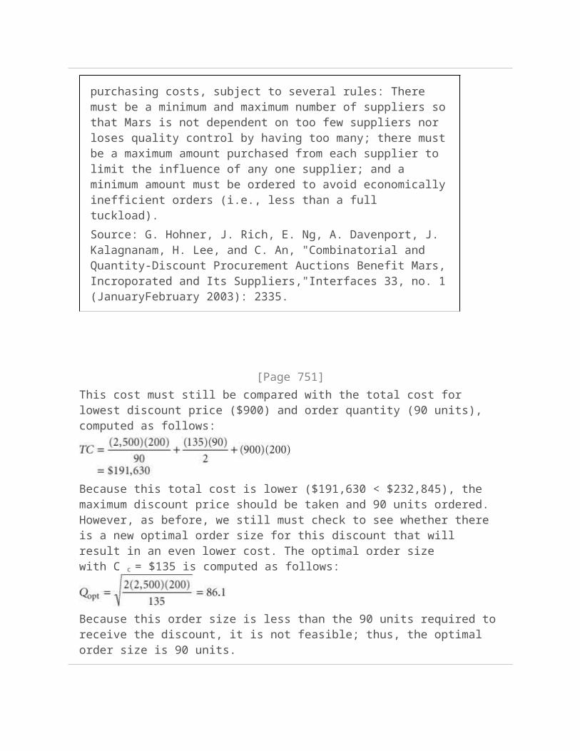
[Page 751]This cost must still be compared with the total cost for lowest discount price ($900) and order quantity (90 units), computed as follows:

Because this total cost is lower ($191,630 < $232,845), the maximum discount price should be taken and 90 units ordered. However, as before, we still must check to see whether there is a new optimal order size for this discount that will result in an even lower cost. The optimal order size with C c = $135 is computed as follows:

Because this order size is less than the 90 units required to receive the discount, it is not feasible; thus, the optimal order size is 90 units.

Quantity Discount Model Solution with QM for Windows

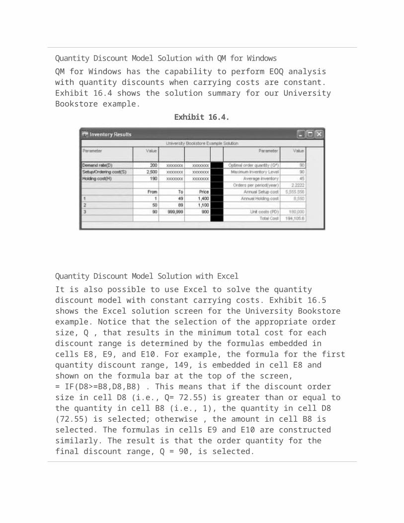
QM for Windows has the capability to perform EOQ analysis with quantity discounts when carrying costs are constant. Exhibit 16.4 shows the solution summary for our University Bookstore example.

Exhibit 16.4.

Quantity Discount Model Solution with Excel

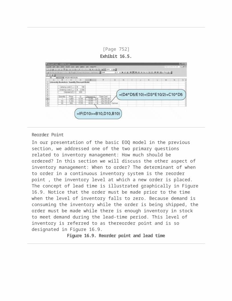
It is also possible to use Excel to solve the quantity discount model with constant carrying costs. Exhibit 16.5 shows the Excel solution screen for the University Bookstore example. Notice that the selection of the appropriate order size, Q , that results in the minimum total cost for each discount range is determined by the formulas embedded in cells E8, E9, and E10. For example, the formula for the first quantity discount range, 149, is embedded in cell E8 and shown on the formula bar at the top of the screen, = IF(D8>=B8,D8,B8) . This means that if the discount order size in cell D8 (i.e., Q= 72.55) is greater than or equal to the

quantity in cell B8 (i.e., 1), the quantity in cell D8 (72.55) is selected; otherwise , the amount in cell B8 is selected. The formulas in cells E9 and E10 are constructed similarly. The result is that the order quantity for the final discount range, Q = 90, is selected.

[Page 752]Exhibit 16.5.

Reorder Point

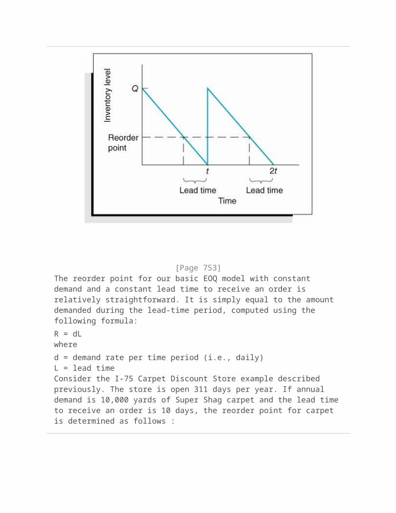
In our presentation of the basic EOQ model in the previous section, we addressed one of the two primary questions related to inventory management: How much should be ordered? In this section we will discuss the other aspect of inventory management: When to order? The determinant of when to order in a continuous inventory system is the reorder point , the inventory level at which a new order is placed.The concept of lead time is illustrated graphically in Figure 16.9. Notice that the order must be made prior to the time when the level of inventory falls to zero. Because demand is consuming the inventory while the order is being shipped, the order must be made while there is enough inventory in stock to meet demand during the lead-time period. This level of inventory is referred to as thereorder point and is so designated in Figure 16.9.

Figure 16.9. Reorder point and lead time

[Page 753]The reorder point for our basic EOQ model with constant demand and a constant lead time to receive an order is relatively straightforward. It is simply equal to the amount demanded during the lead-time period, computed using the following formula:

R = dLwhere

d = demand rate per time period (i.e., daily)L = lead timeConsider the I-75 Carpet Discount Store example described previously. The store is open 311 days per year. If annual demand is 10,000 yards of Super Shag carpet and the lead time to receive an order is 10 days, the reorder point for carpet is determined as follows :

Thus, when the inventory level falls to approximately 321 yards of carpet, a new order is placed. Notice that the reorder point is not related to the optimal order quantity or any of the inventory costs.

Safety Stocks

In our previous example for determining the reorder point, an order is made when the inventory level reaches the reorder point. During the lead time, the remaining inventory in stock is depleted as a constant demand rate, such that the new order quantity arrives at exactly the same moment as the inventory level reaches zero in Figure 16.9. Realistically, however, demandand to a lesser extent lead timeis uncertain. The inventory level might be depleted at a slower or faster rate during lead time. This is depicted in Figure 16.10 for uncertain demand and a constant lead time.

Figure 16.10. Inventory model with uncertain demand

Notice in the second order cycle that a stockout occurs when demand exceeds the available inventory in stock. As a hedge against stockouts when demand is uncertain, a safety (or buffer) stock of inventory is frequently added to the demand during lead time. The addition of a safety stock is shown in Figure 16.11.

[Page 754]Figure 16.11. Inventory model with safety stock

[Page 754 ( continued )]

Determining Safety Stock By Using Service Levels

There are several approaches to determining the amount of the safety stock needed. One of the most popular methods is to establish a safety stock that will meet a specified service level . The service level is the probability that the amount of inventory on hand during the lead time is sufficient to meet expected demand (i.e., the probability that a stockout will not occur). The word service is used because the higher the probability that inventory will be on hand, the more likely that customer demand will be met (i.e., the customer can be served ). For example, a service level of 90% means that there is a .90 probability that demand will be met during the lead time period and a .10 probability that a stockout will occur. The specification of the service level is typically a policy decision based on a number of factors, including costs for the "extra" safety stock and present and future lost sales if customer demand cannot be met.The service level is the probability that the inventory available during the lead time will meet demand.

Reorder Point with Variable Demand

To compute the reorder point with a safety stock that will meet a specific service level, we

will assume that the individual demands during each day of lead time are uncertain and independent and can be described by a normal probability distribution. The average demand for the lead-time period is the sum of the average daily demands for the days of the lead time, which is also the product of the average daily demand multiplied by the lead time. Likewise, the variance of the distribution is the sum of the daily variances for the number of days in the lead-time period. Using these parameters, the reorder point to meet a specific service level can be computed as follows :

where

= average daily demand

L = lead time

s d= the standard deviation of daily demand

Z = number of standard deviations corresponding to the service level probability

= safety stock

[Page 755]

The term   in this formula for reorder point is the square root of the sum of the daily variances during lead time:

The reorder point relative to the service level is shown in Figure 16.12. The service level is the shaded area, or probability, to the left of the reorder point, R .

Figure 16.12. Reorder point for a service level

The I-75 Carpet Discount Store sells Super Shag carpet. The average daily customer demand for the carpet stocked by the store is normally distributed, with a mean daily demand of 30 yards and a standard deviation of 5 yards of carpet per day. The lead time for receiving a new order of carpet is 10 days. The store wants a reorder point and safety stock for a service level of 95%, with the probability of a stockout equal to 5%:

 = 30 yd. per day, L = 10 days, s d = 5 yd. per dayFor a 95% service level, the value of Z (from Table A.1 in Appendix A) is 1.65. The reorder point is computed as follows:

The safety stock is the second term in the reorder point formula:

Determining the Reorder Point Using Excel

Excel can be used to determine the reorder point with variable demand. Exhibit 16.6 shows an Excel spreadsheet set up to compute the reorder point for our I-75 Carpet Discount Store example. Notice that the formula for computing the reorder point in cell E7 is shown on the formula bar at the top of the spreadsheet.

[Page 756]Exhibit 16.6.

Reorder Point with Variable Lead Time

In the model in the previous section for determining the reorder point, we assumed a variable demand rate and a constant lead time. In the case where demand is constant and the lead time varies, we can use a similar formula, as follows:

R = d   + Zd s L

where

d = constant daily demand

= average lead time

s L= standard deviation of lead time

d s L= standard deviation of demand during lead time

Zd s L= safety stock

For our previous example of the I-75 Carpet Discount Store, we will now assume that daily demand for Super Shag carpet is a constant 30 yards. Lead time is normally distributed, with a mean of 10 days and a standard deviation of 3 days. The reorder point and safety stock corresponding to a 95% service level are computed as follows:

d = 30 yd. per day

= 10 days

s L= 3 days

Z = 1.65 for a 95% service level

R = d   + Zd s L = (30)(10) + (1.65)(30)(3) = 300 + 148.5 = 448.5 yd.

Reorder Point with Variable Demand and Lead Time

The final reorder point case we will consider is the case in which both demand and lead time are variables . The reorder point formula for this model is as follows.

where

= average daily demand

= average lead time

= standard deviation of demand during lead time

= safety stock

[Page 757]

Management Science Application: Establishing Inventory Safety Stocks at Kellogg's

Kellogg's is the world's largest cereal producer and a leading maker of convenience foods , with worldwide sales in 1999 of almost $7 billion. The company started with a single product, Kellogg's Corn Flakes, in 1906, and over the years has developed a product line of other cereals, including Rice Krispies and Corn Pops, as well as convenience foods, such as Pop-Tarts and Nutri-Grain cereal bars. Kellogg's operates 5 plants in the United States and Canada and 7 distribution centers, and it contracts with 15 co-packers to

produce or pack some Kellogg's products. Kellogg's must coordinate the production, packaging, inventory, and distribution of roughly 80 cereal products alone at these various facilities.

For more than a decade , Kellogg's has been using a model called the Kellogg Planning System (KPS) to plan its weekly production, inventory, and distribution decisions. The data used in the model are subject to much uncertainty, and the greatest uncertainty is in product demand. Demand in the first few weeks of a planning horizon is based on customer orders and is fairly accurate; however, demand in the third and fourth weeks may be significantly different from marketing forecasts. However, Kellogg's primary goal is to meet customer demand, and in order to achieve this goal, Kellogg's employs safety stocks as a buffer against uncertain demand. The safety stock for a product at a specific production facility in week t is the sum of demands for weeks t and t + 1. However, for a product that is being promoted in an advertising campaign, the safety stock is the sum of forecasted demand for a 4-week horizon or longer. KPS has saved Kellogg's many millions of dollars since the mid-1990s. The tactical version of KPS recently helped the company consolidate production capacity, with estimated projected savings of almost $40 million.

Source: G. Brown, J. Keegan, B. Vigus, and K. Wood, "The Kellogg Company Optimizes Production, Inventory, and Distribution," Interfaces 31, no. 6 (NovemberDecember 2001): 115.

Again we will consider the I-75 Carpet Discount Store example, used previously. In this case, daily demand is normally distributed, with a mean of 30 yards and a standard deviation of 5 yards. Lead time is also assumed to be normally distributed, with a mean of 10 days and a standard deviation of 3 days. The reorder point and safety stock for a 95% service level are computed as follows:

[Page 758]Thus, the reorder point is 450.8 yards, with a safety stock of 150.8 yards. Notice that this reorder point encompasses the largest safety stock of our three reorder point examples, which would be anticipated, given the increased variability resulting from variable demand and lead time.

Order Quantity for a Periodic Inventory System

Previously we defined a continuous, or fixedorder quantity, inventory system as one in which the order quantity was constant and the time between orders varied. So far, this type of inventory system has been the primary focus of our discussion. The less common periodic , or fixedtime period ,inventory system is one in which the time between orders is constant and the order size varies. A drugstore is one example of a business that sometimes uses a fixed-period inventory system. Drugstores stock a number of personal hygiene and health- related products, such as shampoo, toothpaste, soap, bandages, cough medicine, and aspirin. Normally, the vendors that provide these items to the store will make periodic visitsfor example, every few weeks or every monthand count the stock of inventory on hand for their products. If the inventory is exhausted or at some predetermined reorder point, a new order will be placed for an amount that will bring the inventory level back up to the desired level. The drugstore managers will generally not monitor the inventory level between vendor visits but instead rely on the vendor to take inventory at the time of the scheduled visit.A periodic inventory system uses variable order sizes at fixed time intervals .

A limitation of this type of inventory system is that inventory can be exhausted early in the time period between visits, resulting in a stockout that will not be remedied until the next scheduled order. Alternatively, in a fixedorder quantity system, when inventory reaches a reorder point, an

order is made that minimizes the time during which a stockout might exist. As a result of this drawback, a larger safety stock is normally required for the fixed-interval system.

A periodic inventory system normally requires a larger safety stock .

Order Quantity with Variable Demand

If the demand rate and lead time are constant, then the fixed-period model will have a fixed order quantity that will be made at specified time intervals, which is the same as the fixed quantity (EOQ) model under similar conditions. However, as we have already explained, the fixed-period model reacts significantly differently from the fixedorder quantity model when demand is a variable.

The order size for a fixed-period model, given variable daily demand that is normally distributed, is determined by the following formula:

where

= average demand rate

t b= the fixed time between orders

L = lead time

s d= standard deviation of demand

= safety stock

I = inventory in stock

The first term in the preceding formula, d ( t b + L ), is the average demand during the order cycle time plus the lead time. It reflects the amount of inventory that will be needed to protect against shortages during the entire time from this order to the next and the lead time, until the order is

received. The second term,   , is the safety stock for a specific service level, determined in much the same way as previously described for a reorder point. The final term, I , is the amount of inventory on hand when the inventory level is checked and an order is made. We will demonstrate the computation of Q with an example.

[Page 759]The Corner Drug Store stocks a popular brand of sunscreen. The average demand for the sunscreen is 6 bottles per day, with a standard deviation of 1.2 bottles. A vendor for the sunscreen producer checks the drugstore stock every 60 days, and during a particular visit the drugstore had 8 bottles in stock. The lead time to receive an order is 5 days. The order size for this order period that will enable the drugstore to maintain a 95% service level is computed as follows :

Determining the Order Quantity for the Fixed-Period Model with Excel

Exhibit 16.7 shows an Excel spreadsheet set up to compute the order quantity for the fixed-period model with variable demand for our Corner Drug Store example. Notice that the formula for the order quantity in cell D10 is shown on the formula bar at the top of the spreadsheet.

Exhibit 16.7.

Summary

In this chapter the classical economic order quantity model has been presented. The basic form of the EOQ model we discussed included simplifying assumptions regarding order receipt, no shortages, and constant demand known with certainty . By relaxing some of these assumptions, we were able to create increasingly complex but realistic models. These EOQ variations included the reorder point model, the noninstantaneous receipt model, the model with shortages, and models with safety stocks. The techniques for inventory analysis presented in this chapter are not widely used to analyze other types of problems. Conversely, however, many of the techniques presented in this text are used for inventory analysis (in addition to the methods presented in these chapters). The wide use of management science techniques for inventory analysis attests to the importance of inventory

to all types of organizations.

[Page 760]

[Page 760 ( continued )]

References

Buchan, J., and Koenigsberg, E. Scientific Inventory Management . Upper Saddle River, NJ: Prentice Hall,

1963.

Buffa, E. S., and Miller, J. G. Production-Inventory Systems: Planning and Control , 3rd ed. Homewood,

IL: Irwin, 1979.

Churchman, C. W., Ackoff, R. L., and Arnoff, E. L.Introduction to Operations Research . New York: John

Wiley & Sons, 1957.

Hadley, G., and Whitin, T. M. Analysis of Inventory Systems. Upper Saddle River, NJ: Prentice Hall, 1963.

Johnson, L. A., and Montgomery, D. C. Operations Research in Production Planning, Scheduling and

Inventory Control . New York: John Wiley & Sons, 1974.

Magee, J. F., and Boodman, D. M. Production Planning and Inventory Control , 2nd ed. New York:

McGraw-Hill, 1967.

Starr, M. K., and Miller, D. W. Inventory Control: Theory and Practice . Upper Saddle River, NJ: Prentice

Hall, 1962.

Wagner, H. M. Statistical Management of Inventory Systems. New York: John Wiley & Sons, 1962.

Whitin, T. M. The Theory of Inventory Management . Princeton, NJ: Princeton University Press, 1957.