INVENTORY CONTROL IN THE RETAIL SECTOR: A CASE STUDY OF CANADIAN TIRE PACIFIC ASSOCIATES by BRIAN ANTHONY KAPALKA B.Sc.(C.E.), The University of Manitoba, 1992 B.Sc., The University of Manitoba, 1992 A THESIS SUBMITTED IN PARTIAL FULFILLMENT OF THE REQUIREMENTS FOR THE DEGREE OF MASTER OF SCIENCE (BUSINESS ADMINISTRATION) in THE FACULTY OF GRADUATE STUDIES (Department of Commerce and Business Administration) We accept this thesis as conforming to the required standard THE UNIVERSITY OF BRITISH COLUMBIA April 1995 ® Brian Anthony Kapalka, 1995

Welcome message from author
This document is posted to help you gain knowledge. Please leave a comment to let me know what you think about it! Share it to your friends and learn new things together.
Transcript
I N V E N T O R Y C O N T R O L IN T H E R E T A I L S E C T O R A C A S E STUDY O F C A N A D I A N TIRE PACIFIC ASSOCIATES
by
BRIAN A N T H O N Y K A P A L K A
BSc(CE) The University of Manitoba 1992 BSc The University of Manitoba 1992
A THESIS SUBMITTED IN PARTIAL F U L F I L L M E N T OF
T H E REQUIREMENTS FOR T H E D E G R E E OF
MASTER OF SCIENCE (BUSINESS ADMINISTRATION)
in
T H E F A C U L T Y OF G R A D U A T E STUDIES
(Department of Commerce and Business Administration)
We accept this thesis as conforming to the required standard
T H E UNIVERSITY OF BRITISH COLUMBIA
April 1995
reg Brian Anthony Kapalka 1995
In presenting t h i s thesis i n p a r t i a l f u l f i l l m e n t of the requirements for an advanced degree at the University of B r i t i s h Columbia I agree that the Library s h a l l make i t f r e e l y a v a i l a b l e for reference and study I further agree that permission for extensive copying of t h i s thesis for scholarly purposes may be granted by the head of my department or by h i s or her representatives I t i s understood that copying or pub l i c a t i o n of t h i s thesis for f i n a n c i a l gain s h a l l not be allowed without my written permission
Department of Cotv^errg- ftni)gt ^osmecs AAnmna-WoAor
The University of B r i t i s h Columbia Vancouver Canada
Date ZS A y r A 9 9 5
Abstract
Canadian Tire Pacific Associates owns and operates 21 retail stores in the lower
mainland of British Columbia and a central warehouse in Burnaby In this thesis we formulate
a single-product single-location model of its inventory system as a first step in developing an
integrated interactive inventory control system Specifically we formulate a Markov chain
model for a periodic review system with a deterministic lead time and lost sales The model
utilizes empirical demand data to calculate the long-run average cost of inventory for a given
(sS) policy We then develop a heuristic that locates a near optimal policy quickly The
heuristic incorporates a constraint on the customer service level makes use of an updating
technique for the transition probability matrix and is based on assumptions regarding the
properties of the solution space Next we create a prototype of the interface that enables
managers to use the model interactively Finally we compare the existing inventory policy to
the optimal policy for each of 420 products sold at one of the stores This thesis finds that
Canadian Tire Pacific Associates is currently holding excessively large in-store inventory and
that it could reduce its cost of inventory by approximately 40 to 50 We estimate that
implementing optimal inventory control in the stores would result in annual savings of between
$55 and $7 million
ii
Table of Contents
Abstract ii
Table of Contents iii
List of Tables v
List of Figures vi
Acknowledgement vii
I INTRODUCTION 1
II T H E INVENTORY SYSTEM A T CANADIAN TIRE PACIFIC ASSOCIATES 8 A Background 8 B The Problem 11 C The Project 15 D The Demand Data 17 E The Cost Data 18
III M O D E L FORMULATION 20 A Terminology 20 B Assumptions 21 C A Markov Chain Model 22 D The Transition Probability Matrix 25 E The Steady State Probabilities 27 F The Cost of Inventory 29 G The Customer Service Level 31 H A Methodology for Evaluating an (sS) Policy 34
IV A N ALGORITHM FOR OBTAINING T H E OPTIMAL (sS) POLICY 35 A Introduction 35 B A Grid Search 36 C A Technique for Updating the Transition Probability Matrix 41
A new policy (s+mS) 41 A new policy (sS+m) 42 The modified algorithm 43
D A Lower Bound on S 45 E A Heuristic Search 48
V T H E INTERFACE 52
iii
VI RESULTS A N D SENSITIVITY ANALYSIS 55 A Comparison of Current Policies to Optimal Policies 55 B Sensitivity Analysis on the Ordering Cost and Holding Rate 62 C Sensitivity Analysis on the Demand Probability Mass Function 65
VII CONCLUSION 70
Afterword 73
Bibliography 74
Appendix A A Portion of the Sales File for Product 200001 a 30-amp
Inline Fuse 76
Appendix B Sample Distribution Files 77
Appendix C A Proof that the Limiting Distribution is Independent of the
Initial State 79
Appendix D A Measure for the Steady State Customer Service Level 83
Appendix E The Calculation of the Conditional Expected Demand Not Satisfied
During a Period of T Consecutive Days 86
Appendix F Justification of the Updating Technique for the New Policy (s+mS) 87
Appendix G Justification of the Updating Technique for the New Policy (sS+m) 92
Appendix H A Hypothetical Consultation 97
Appendix I The Source Code for the Interface Module 104
Appendix J The Source Code for the Main Module 119
Appendix K Current and Optimal Policies for Product Category 20 at Store 6 131
iv
List o f Tables
Table 1 Location and particulars of the 21 stores 10
Table 2 Execution times of the algorithms for product 200001 a 30-amp inline fuse 39
Table 3 Execution times of the algorithms for product 206917 a 6
solder connector 40
Table 4 Products with insufficient existing policies 56
Table 5 Products with the largest potential absolute savings 60
Table 6 A comparison of optimal policies to true optimal policies 63
Table 7 The cost of existing policies and the relative savings of the optimal policies under various scenarios 64
Table 8 True optimal and optimal policies for each demand scenario 66
v
List of Figures
Figure 1 A typical sample path of the process with a 4-day review period
and a 2-day lead time 24
Figure 2 The flow chart of the grid search algorithm 38
Figure 3 The flow chart of the grid search algorithm utilizing the updating
technique for the transition probability matrix 44
Figure 4 An evaluation of the lower bound Sm i n 47
Figure 5 The flow chart of the heuristic algorithm 50
Figure 6 The distribution of savings of optimal policies in (a) dollars and
(b) percentage of current cost 59
Figure A-1 The title screen 97
Figure A-2 The main menu 98
Figure A-3 Calculating the optimal policy and evaluating the current policy 99
Figure A-4 Displaying the results 100
Figure A-5 Entering an alternate policy 101
Figure A-6 The particulars of the alternate policy 102
Figure A-7 The main menu revisited 103
vi
Acknowledgement
The completion of this thesis was made possible by the encouragement and assistance
of a number of people
I would like to express my sincere appreciation to my thesis supervisor Professor
Martin Puterman for all of his many efforts on my behalf His help advice patience charity
and tolerance were very much appreciated
I would like to acknowledge Professor Hong Chen and Professor Garland Chow for their
time and input as members of my thesis committee In addition I must acknowledge the
assistance of PhD student Kaan Katircioglu for his insight and help on this project
I offer many thanks to Professor Tom Ross for his kindness and friendship during the
past few years especially during the writing of this work I must also thank his family for
adopting me on many holidays I still owe thanks to Professor Slobodan Simonovic at the
University of Manitoba for influencing me to attend graduate school in the first place and for
helping me to obtain funding
I cannot thank my parents enough for their never-ending support both emotional and
financial Also to my friends especially Cathy Dave Lisa Steve and the Philbuds thanks
for giving me a life off campus and for picking up many a tab - the next one is on me
I would like to give special thanks to my good friend and fellow MSc student Paul
Crookshanks for allowing me to bounce ideas off of him and for being such a procrastinator
that despite my finishing a year late I only lost by two days
Financial assistance received from the Natural Science and Engineering Research
Council (NSERC) and from Canadian Tire Pacific Associates was greatly appreciated
vii
I INTRODUCTION
The importance of inventory management has grown significantly over the years
especially since the turn of this century In colonial times large inventories were viewed as
signs of wealth and therefore merchants and policy makers were not overly concerned with
controlling inventory However during the economic collapse of the 1930s managers began
to perceive the risks associated with holding large inventories As a result managers
emphasized rapid rates of inventory turnover (Silver and Peterson 1985) Following the
Second World War Arrow Harris and Marschak (1951) and Dvoretzky Kiefer and
Wolfowitz (1952ab) laid the basis for future developments in mathematical inventory theory
Shortly thereafter new inventory control methodologies were widely applied in the private
manufacturing sector More recently when inflation and interest rates soared during the 1970s
many organizations were forced to rethink their inventory strategies yet again Today the
control of inventory is a problem common to all organizations in any sector of the economy
Sir Graham Day chairman of Britains Cadbury-Schweppes P C L expressed this sentiment
when he stated I believe the easiest money any business having any inventory can save lies
with the minimization of that inventory (Day 1992) Lee and Nahmias (1993) and Silver and
Peterson (1985) provide a more detailed history of inventory management and control
Most inventory problems in the retail sector involve the control and management of a
large number of different products Ideally the inventory policies should be determined for all
products on a system-wide basis however because the number of products is often in the tens
of thousands formulating a model to do so is impractical Therefore single-product models
are frequently used in practice to determine policies for products separately (Lee and Nahmias
1993) Lee and Nahmias (1993) and Silver and Peterson (1985) provide a good overview of
1
single-product single-location models for a more complete review of the literature we refer
to them
The degree of complexity of a single-product model depends largely on the assumptions
made regarding the demand cost structure and physical characteristics of the inventory system
For example demand can be either deterministic meaning it is known with absolute certainty
or stochastic meaning it is unknown but follows a known probability distribution
Deterministic models tend to be relatively simple yet useful such as the basic EOQ model
However future demand is seldom known with certainty in practice and therefore the use of
these simple models is limited As a result the majority of research in inventory has focused
on stochastic demand models (Lee and Nahmias 1993)
Because the objective of most inventory models is to minimize the cost of inventory
assumptions regarding the structure of the cost are very important also Generally speaking
the cost of inventory has four components the purchaseproduction cost the orderingsetup
cost the holding cost and the shortage cost1 Each of these costs can be fixed proportional
nonlinear or some complex combination of these Further because nearly all inventory
problems require decisions be made sequentially over a period of time the costs can be either
discounted or averaged In the former case a discount factor is included in the cost function
in order to account for the time value of money However since most inventory problems are
on-going the long-run average cost is usually minimized (Lee and Nahmias 1993) In
practice this is achieved by minimizing the expected cost per time period under steady state
conditions
Finally the physical characteristics of the system are important in determining the
1 The cost of a stockout is often very difficult to estimate in practice As a result service levels are frequently used in its place When this is done a constraint is included in the model
2
complexity of the model For example the review process can be either continuous in which
case the inventory is reviewed continuously and orders are placed as soon as the stock reaches
a certain level or periodic in which case the inventory is reviewed at regular intervals and
orders can be placed only at those fixed times Also excess demand can be fully backordered
as is common in many manufacturing and wholesale systems completely lost as is common
in most retail environments or some combination of the two Lead time assumptions are also
important models with lead times are more complex than those in which the supply of
inventory is assumed to be instantaneous
Although the literature is dominated by single-product models (Lee and Nahmias 1993)
much recent work has focused on extending those models to multiple-product problems
However multiple-product models are inherently more complex than the simple-product
models In fact no efficient algorithms are currently available for determining fully optimal
strategies for most multiple-product problems (Federgruen 1993) As a result research has
focused on the development of easily computable approximation techniques Muckstadt and
Roundy (1993) provide a good overview of multiple-product andor multiple-location models
with deterministic demand although emphasis is placed on models for production and
distribution Federgruen (1993) extends the discussion to consider these models under uncertain
demand and also provides a complete list of references on the subject Silver and Peterson
(1985) discuss models for coordinated replenishments for both deterministic and stochastic
demand
In this thesis we examine the inventory system at Canadian Tire Pacific Associates
owner of 21 retail stores and a central warehouse Although this is a multiple-product
multiple-location single-warehouse problem and strictly speaking should be modelled as such
we analyze the inventory problem on a product-by-product and store-by-store basis We believe
3
that this simpler single-product single-location model captures the essentials of the problem for
two reasons First the coordination of replenishments for products andor locations is most
advantageous when significant savings are possible because of high first order costs and low
marginal costs for placing subsequent orders However because of the large number of
products and the physical distribution system in this problem trucks are dispatched to stores
on a regular basis Therefore the benefits of coordinating replenishments for this problem are
negligible Second we believe that controlling in-store inventory alone can result in substantial
savings to Canadian Tire Pacific Associates Further given the excessive amount of inventory
in the warehouse a single-location model assuming an infinite warehouse capacity is reasonable
Of course should inventory control in the warehouse become a priority a more elaborate model
would be required
More specifically we consider a periodic review single-product inventory model with
stationary independent stochastic demand a deterministic lead time and an infinite planning
horizon The probability mass function for the demand is based on empirical sales data
collected over a period of approximately ten months The cost of inventory includes a
proportional holding cost and a fixed ordering cost neither of which is discounted All excess
demand is completely lost The objective of the model is to minimize the long-run average cost
per unit time subject to a service level constraint on the fraction of demand satisfied directly
from in-store inventory In order to obtain meaningful cost comparisons the model calculates
the expected annual cost of inventory
For inventory problems like the one described above optimal (sS) policies can be
computed by Markovian decision process methods such as successive approximations or policy
iteration or by stationary Markovian methods However each of these methods generate
calculations that are complex and time consuming Therefore much research interest lies in
4
developing techniques to find approximate (sS) policies with little computational effort The
majority of the approximation techniques begin with an exact formulation of the problem and
then manipulate the problem by relaxations restrictions projections or cost approximations
(Federgruen 1993) Porteus (1985) presents three approximation techniques and compares
them to fourteen others for a periodic review single-product inventory model in which
shortages are fully backordered and a shortage cost is incurred Federgruen Groenevelt and
Tijms (1984) present an algorithm for finding approximate (sS) policies for a continuous review
model with backordering and a service level constraint Also Tijms and Groenevelt (1984)
present simple approximations for periodic review systems with lost sales and service level
constraints All three works find that the approximation techniques perform well However
the techniques are evaluated for a variety of demand parameters that all result in policies with
a value of S in the range of 50 to 200 Given the slower moving products at Canadian Tire 2
it is unclear how well such approximation techniques would perform Therefore we do not
attempt to apply or modify any of these approximation methods
Exact optimal policies for this problem can be obtained by formulating a constrained
Markov decision process and solving it However the data generating requirements and the
lack of a good upper bound on S make this formulation impractical Therefore we formulate
a Markov chain model for fixed values of s and S and then employ a search technique to find
the optimal values for s and S In order to improve the performance of the model we develop
a heuristic search that locates near optimal policies relatively quickly
The remaining chapters of this thesis are organized as follows In Chapter II an
overview of the existing inventory system at Canadian Tire is presented along with a description
2 For example very few of the products analyzed have optimal values of S exceeding 20 with the largest value of S equalling 69
5
of the problem Next a multi-phase project designed to develop a fully integrated interactive
inventory control system is described with the scope of the research reported in this thesis
completing the first phase of the project Finally a description of the demand and cost data is
given
In Chapter III we formulate a Markov chain model that can be used to calculate the cost
and service level associated with a given (sS) policy Based on several simplifying
assumptions the Markov chain is formulated and the equations for the corresponding transition
probability matrix are developed Then given the limiting probability distribution of the chain
the equations for the steady state annual cost of inventory and the corresponding service level
are obtained The chapter concludes with a brief summary of the model
In Chapter IV an algorithm that searches for the optimal (sS) policy is developed As
a starting point a simple grid search algorithm is developed and evaluated on the basis of
execution time In order to improve the algorithms speed a technique for updating the
transition probability matrix is presented and the improvement in the algorithm is noted Next
a theoretical lower bound on S is obtained although the corresponding reduction in the
execution time is minimal Finally based on two assumptions regarding the shape of the
feasible space a heuristic search is developed which improves the speed of the algorithm
significantly
In Chapter V a prototype of the inventory control systems interface is created In its
present form the interface allows managers to evaluate inventory policies interactively The
manager can set review parameters compare optimal policies and current policies and evaluate
alternate policies The chapter concludes by recommending specific options be including in
future versions to make the system more automated and user-friendly
In Chapter VI optimal policies for all products in one product category sold at one store
6
are compared to existing policies on the basis of expected annual costs and customer service
levels The analysis suggests that existing policies result in a large excess inventory and that
implementing the optimal policies would reduce the annual cost of inventory by approximately
50 A sensitivity analysis on the cost estimates is performed and suggests that the model is
not sensitive to relative errors of approximately 20 in the cost estimates Finally a sensitivity
analysis on the demand probability mass function is performed The analysis indicates that the
model is sensitive at least in terms of the customer service level to slight changes in the tail
of the demand distributions of low-demand products
Finally in Chapter VII the results of the analysis are summarized and future work is
outlined In order to incorporate recent changes in the review procedures at several stores the
model must be modified to allow for the duration of the review period to exceed the lead time
We recommend that the second phase of the project proceed specifically that a data collection
and storage scheme be designed and that a forecasting model be developed Because of the
substantial savings that can be realized by reducing inventory only at the stores inventory
control at the warehouse should also be investigated
7
II T H E I N V E N T O R Y S Y S T E M A T C A N A D I A N TIRE
A Background
Canadian Tire Pacific Associates owns and operates 21 retail stores in the lower
mainland of British Columbia The stores carry approximately 30000 active products3 that
are divided into 80 product categories The merchandise comprises primarily automotive parts
and accessories home hardware housewares and sporting goods Canadian Tire Pacific
Associates also owns a central warehouse in Burnaby at which inventory is received from
Toronto Inventory is then shipped periodically from the warehouse via truck to the local
stores In 1992 total sales at the stores exceeded $99 million and the value of inventory was
estimated to be $28 million of which approximately half was stored in the warehouse
On selected days of each week a stores inventory records are reviewed automatically
and orders for products are placed to the warehouse as required Management uses the term
flushing to describe the process of reviewing the inventory and producing the tickets for stock
owing and the term picking to describe the physical act of filling the order at the warehouse4
Whether or not an order is placed for a product depends upon its current inventory level its
target level and its minimum fill 5 If the target level less the current level exceeds the
minimum fill an order is placed to bring the stock up to the target level From the moment
3 Active products are those that are regularly restocked Canadian Tire Pacific Associates can choose from up to 50000 products
4 Note that the number of picks per week is equal to the number of times per week that the inventory records are reviewed At the beginning of this study eighteen stores had two picks per week while the remaining three stores had only one
5 The target level is the maximum number of items that should be on the shelf at one time and the minimum fill is the minimum number of items that should be ordered
8
the order is placed to the moment the product is reshelved takes between two to four days
depending on the store On average 11000 items are shipped from the warehouse at each
flush
Although a products minimum fill is the same for all stores its target level depends
upon the size of the store Based upon its sales volume and retail space a store is classified
as being one of five sizes small (S) medium (M) large (L) jumbo (J) and extra jumbo
(EJ) 6 Each product has associated with it a target level for each size of store
Consequently all stores of the same size have identical inventory policies Table 1 lists the
location size number of picks per week sales and floor space of each store as of October
1993
Periodically the inventory manager reviews the policies and when deemed necessary
adjusts them In this way the manager can account for seasonality in demand changes in mean
demand and any shortcomings of previous policies At the present time the review process
is not automated nor performed on-line The inventory manager uses Hxl5 computer
printouts with five products to a sheet to study the relevant information and on which to note
any changes Afterward the changes are recorded in the system and the new policies take
effect
Currently the inventory policies are based on rules of thumb developed through the
years and not on a statistical analysis of demand nor on a calculation of the cost of inventory
These rules of thumb incorporate a marketing philosophy which at times dominates the
inventory strategy The prevailing philosophy holds that a large in-store inventory instills
6 During the course of this study stores were resized several times At one point the entire class of medium stores was eliminated leaving only four sizes of stores On another occasion the store in Chilliwack was changed from being a small store to a large store
9
Table 1 Location and particulars of the 21 stores
Store Location Store Size
Picks Per Week
1992 Sales ($)
Floor Space (ft2)
1 Chilliwack S 2 2901969 6678
2 Coquitlam M 2 4015303 6510
3 Langley EJ 2 8138673 15422
4 Scott Road EJ 2 7307820 15064
5 Maple Ridge L 2 4102110 6678
6 Kingsway L 2 4153736 6574
7 Richmond EJ 2 8175105 14961
8 North Vancouver M 2 3856571 6534
9 Guildford M 2 3714372 6567
10 Burnaby M 2 3532752 6983
11 New Westminster S 1 2417992 6470
12 Abbotsford EJ 2 7899398 15303
13 Hastings J 2 4647794 9849
14 King Edward EJ 2 3825372 25492
15 White Rock L 2 3960262 6870
16 Main amp Mountain S 1 2705602 6431
17 Heather J 2 4161227 9427
18 King George J 2 4606817 9640
19 Cambie J 2 5855022 9091
20 Lougheed M 1 3114180 6615
21 Burrard J 2 6553310 10608
10
consumer confidence which in turn leads to increased sales In other words if a customer
perceives that Canadian Tire is in the hardware business he or she will choose to shop there
when meeting future needs However management has adopted this philosophy without any
analysis of the cost of holding excess inventory Only recently has management begun to
question the cost-effectiveness of allocating inventory based on these rules of thumb
Speculating that existing inventory practices might be deficient Mr Don Graham the
vice-president of Canadian Tire Pacific Associates commissioned a pilot study to examine the
inventory system and to propose alternate strategies7 The study using a steady state model
to represent a simplified inventory system suggested that existing policies lead to overly high
inventory levels More importantly the study outlined a methodology that would enable
management to determine inventory levels based on observed demand The pilot study
recommended that a more detailed model of the inventory system be formulated that the
methodology be expanded to incorporate the cost of inventory and that an algorithm be
developed that would quickly identify the optimal inventory policies
B The Problem
At the time of the pilot study management was concerned primarily with its inability
to distinguish between stores of the same size As mentioned in the previous section a
stores size is based solely on its sales volume and floor space and under existing practices
all stores of the same size have identical inventory policies for every product Management
realized that demand for some products might be a function of variables other than size such
7 The pilot study was performed by Martin Puterman a professor of Management Science and Kaan Katircioglu a doctoral student in Management Science both at the University of British Columbia The results of the study were presented at a U B C Transportation and Logistics Workshop on March 25 1993
11
as location For example the demand for sump pumps is likely to be very different in suburban
areas than in urban ones However management was unable to allocate more sump pumps to
large suburban stores than to large urban stores This inability led management to seek a
tool that would allow for a more effective allocation of inventory between stores of the same
size
By the end of the pilot study however management was less concerned with
reallocating inventory within a size of store than with reallocating inventory between sizes
of stores and with reducing overall inventory According to management assigning individual
inventory policies to each store appeared to be operationally infeasible Firstly management
believed that having individual policies would lead to confusion in the warehouse and to
increased shipping errors Exactly why this would occur is unclear the warehouse would
simply continue to fill orders from tickets that make no reference to the policy in place
Secondly and perhaps more tenably the computer technology at Canadian Tire Pacific
Associates did not allow for policies to vary across all stores Both the database used to store
the inventory data and the printouts used by the inventory manager allowed for only five
different policies per product all with the same minimum fill Moving to individual policies
would have required an overhaul of the existing information system Although management
saw this overhaul as inevitable it did not see the overhaul as imminent Therefore
management switched the focus of the study to developing a tool that would help reduce overall
inventory levels andor reallocate inventory more effectively between groups of stores
The subtle change in the studys objective prompted an important question how should
the stores be grouped The current practice of grouping stores based on size is problematic
for two reasons First as discussed above additional factors of demand such as location
cannot be taken into account Second grouping inherently results in a misallocation of
12
inventory when some stores within a group have differing numbers of picks per week For
example the medium-sized Lougheed store which has one pick per week requires higher
inventory levels to achieve a given customer service level than the other medium stores
which all have two picks per week8 In fact in terms of customer service levels it might
be more appropriate to group the Lougheed store with the large stores having two picks per
week Ideally this artificial grouping of stores will be abandoned when the computer system
is upgraded and policies can then be set on a store by store basis
As the project proceeded management grew somewhat uneasy with the concept of using
an analytical tool to evaluate and set inventory policies According to both the pilot study and
the preliminary results of this study significantly reducing inventory would greatly reduce costs
while still providing a high level of customer service However management held that because
the model cannot take into account intangibles such as marketing considerations such a drastic
reduction in inventory would be very inappropriate In this light management viewed the
optimal policies as lower bounds for inventory levels these policies would have to be
modified upwards in order to be practical Therefore management contended that any
methodology or software produced during this study should provide the means to evaluate and
compare a number of alternate policies
Regardless of exactly how the tool is to be used there is currently a lack of historical
sales data from which to analyze the inventory system and determine optimal policies No sales
data had ever been collected prior to the pilot study and only a relatively small amount has
been collected since In order to proceed with any analysis of the inventory system a
8 If demand is a function of size then the Lougheed store must meet the same demand with one fewer pick per week This would lead to either increased probabilities of stockouts at the Lougheed store or higher inventory levels at all the other medium stores
13
substantial amount of additional data would be needed The existing information system at
Canadian Tire Pacific Associates does allow for sales data to be captured however the system
is limited by the amount of data it can capture at one time and by its storage capacity In order
to collect the amount of data required management would have to upgrade the system and
develop some kind of data collection scheme coupled with a data compression technique The
collection scheme must allow for characteristics of demand such as trends and seasonality to
be identified and the compression technique must allow for sales data for over 30000 products
to be stored for each store
Because many of the products sold by Canadian Tire have nonstationary demand as a
result of seasonality andor trend the inventory tool must be able to forecast demand for the
coming period Products such as sporting goods and outdoor equipment exhibit patterns of
demand that are very seasonal For example sales of snow shovels increase through the fall
peak in the winter and drop to zero by late spring At the same time some products might
become either more or less fashionable over time resulting in changes in mean demand
Setting inventory policies for any of these products based on observed demand would result in
insufficient stock if demand increased during the period or in excess stock if demand decreased
Therefore the tool must be able to forecast the demand for the period for which the policy is
intended
Toward the end of the project management began discussing the integration of the
interactive inventory tool with the existing system to form a new inventory control system The
new system would utilize a modified point of sales system to collect sales data continually
Based on the latest available data the system would forecast demand for the coming period and
calculate the optimal policies for every product at every store The system would then provide
all relevant information on-line for the inventory manager to review The manager could weigh
14
other information such as marketing considerations and examine alternate policies to determine
the effect on cost Finally the preferred policy would be set in place with the touch of a key
and information on the next product or store would be presented for review
C The Project
Development of the inventory control system envisioned by management requires the
completion of five tasks 1) the design of a data collection system that generates and stores the
necessary sales data 2) the development of a forecasting method that provides accurate
estimates of demand distributions 3) the formulation of a model that calculates the cost of
inventory and the customer service level for an inventory policy 4) the development of an
algorithm that finds the optimal policy for a product at a store and 5) the creation of an
interface that allows interactive and on-line consultation Ultimately the above components
would have to be integrated and incorporated in a manner that would ensure the compatibility
and reliability of the system
The scope of the research reported in this thesis completes the first phase of the project
specifically we formulate an inventory model develop an algorithm and create a prototype of
the interface Because of the changing environment at Canadian Tire Pacific Associates minor
modifications to both the model and the algorithm developed herein might be necessary to
reflect future changes in operational procedures Upon completion of phase one the interface
will be interactive allowing managers to select the store product and review scenario and then
to compare optimal policies with existing policies or with alternate policies Although the
prototype will be delivered to Canadian Tire Pacific Associates for ih-house testing at the end
of this phase the interface will require modification in subsequent phases as feedback from
management is received and as the system is brought on-line
15
In order to assess more fully the potential savings of implementing the inventory control
system this thesis includes a comparison of optimal policies9 and existing policies The
expected annual cost of inventory for an entire product category is calculated for both the
optimal policies and the existing policies Based on an analysis of these costs the potential
savings of implementing the optimal policies are extrapolated Further the thesis examines the
sensitivity of the model to variations in the estimates of demand and costs
Originally results from all 21 stores were to be included in the above analysis
However just prior to the analysis management changed the review procedure at several
stores the result of which being that three picks per week are now performed at those stores
Because one of the main assumptions of the model specifically that the length of the lead time
does not exceed the duration of the review period is violated under this new review procedure
those stores cannot be included in the analysis Therefore the analysis is based solely on the
results from store six the large store located on Kingsway Avenue10
For the purpose of the analysis sales data for product category 20 automotive and
electrical accessories were collected from all 21 stores This product category was selected
because the distribution of demand for products within it is non-seasonal and because few of
the products are ever placed on sale11 The lack of trend or seasonality eliminates the need
for forecasting demand the optimal policies can be determined based directly on observed
demand
9 That is those policies obtained from the model
1 0 Store six is one of the only stores whose review procedure is not expected to change from two picks per week
1 1 Products that were on sale at any time during the period were not included in the data set
16
D The Demand Data
In total sales data for 520 products of which 458 are active products were collected
over a 307-day period from October 10 1992 to August 18 199312 The data was supplied
by Canadian Tire Pacific Associates in the form of a 10 MB text file with one line per day per
product recording sales from the stores13 Each line had the following format
Columns 1-6 part number Columns 7-9 Julian date14
Columns 10-18 cost of the item (to three decimal places) Columns 19-124 sales for stores 1 through 21 (5 columns per store)
In order to facilitate the analysis the file was sorted into 458 sales files with each of
these files containing the history of daily sales for one of the products Two changes were
made to the format of these files to improve readability 1) a column was added between the
product number and the Julian date and 2) all leading zeros were dropped Appendix A
contains a partial printout of the sales file for a typical product Finally a distribution file
summarizing the daily sales was created from each of the sales files Each distribution file
contains the products number the products cost and the number of days during which various
quantities of the product were sold at each store
Prior to the analysis the distribution files for a large number of products were
examined and based on the shapes of the histograms the products were divided into three
groups The first group low-demand comprises products that have demand on only a few
days with the daily demand seldom exceeding three items The second group medium-
1 2 Of the active products only 420 are sold at store 6
1 3 Strictly speaking a line was written to the file only on days on which at least one store registered a sale of the product
1 4 According to the Julian calendar days are numbered sequentially from 1 to 365 (366 during leap-years) beginning with the first of January
17
demand comprises products that have demand on approximately half of the days with the daily
demand seldom exceeding more than six items Finally the last group high-demand
comprises products that have demand on most days occasionally upwards of twenty items and
whose demand histograms resemble Poisson distributions The majority of the products
examined fell into the low and medium-demand groups only a few high-demand products
were observed Appendix B contains a printout of the distribution file for a typical product
in each group
For most products no theoretical distribution appeared to model the demand well
Demand for low and medium-demand products followed a non-standard distribution with
a mass at zero and a relatively small tail Although some theoretical distributions such as the
mixed-Poisson can be made to resemble this it was unclear how well they would perform
Further the effects of sampling errors from such non-standard distributions were unknown
On the other hand the standard Poisson distribution did appear to model high-demand
products well however only a few products fell into that group Therefore in the absence of
a good theoretical candidate the empirical demand function was chosen for the analysis The
empirical function was readily available from the distribution files and offered the best
estimate of the true underlying function
E The Cost Data
Along with the sales data management supplied estimates relating to the costs of holding
and ordering inventory Management estimates that the cost of holding an item in inventory
for one year is 30 of the items cost Incorporated in this holding rate are a number of costs
such as the opportunity cost of money invested and the costs incurred in running a store
Because it is the annual cost of inventory that is of interest either the compounded daily
18
holding rate or the simple daily holding rate can be used to determine the costs incurred during
a review period however the method of calculating and extrapolating the holding costs must
be consistent For the sake of simplicity a simple daily holding rate is used
In order to estimate the cost of ordering inventory management analyzed the various
tasks that result from an order being placed Using the average time required to fill and then
reshelve an order management obtained an estimate of the direct labour costs involved To
this management added an estimate of the cost of transporting an order from the warehouse to
the store Finally the estimate was adjusted slightly upward to account for the cost of breakage
and errors Based on the analysis management estimates the cost of placing an order for a
product to be $0085 regardless of the size of the order
19
III M O D E L F O R M U L A T I O N
A Terminology
In the previous chapter several terms were introduced to describe the inventory system
at Canadian Tire Pacific Associates These terms though perfectly adequate are not widely
used in the academic literature to describe inventory management problems Therefore in
order to avoid confusion and be consistent with the literature the following terms are used
throughout this thesis
The length of time between successive moments at which the
inventory position is reviewed15
The time at which a reorder decision is made
The length of time between the moment at which a decision to
place an order is made and the moment at which the order is
physically on the shelf
An operating policy in a periodic review inventory model in
which (i) the inventory position is reviewed every T days (ii) a
replenishment order is placed at a review only when the inventory
level x is at or below the reorder level s (gt 0) and (iii) a
replenishment order is placed for S-x units (S gt s)1 6
Lost Sales - The situation in which any demand during a stockout is lost
Review Period -
Decision Epoch
Lead Time -
(sS) Policy
1 5 With respect to the terminology used at Canadian Tire Pacific Associates a review period equals the number of days between flushes
1 6 With respect to the terminology used at Canadian Tire Pacific Associates S represents the target level and s represents the difference between the target level and the minimum fill
20
B Assumptions
In to order make the model of the inventory system mathematically manageable several
simplifying assumptions are made However we believe that the following assumptions do not
significantly reduce the accuracy of the model
1) Demand can be approximated very closely by sales during the period in which the data
is collected Generally inventory levels at the stores are very high and the number of
lost sales is assumed to be negligible In fact the inventory levels for a number of
products were tracked over time during the pilot study and not a single incidence of
stockout was observed Because all products appear to have similar excess inventory
it seems reasonable to assume that virtually all demand resulted in sales
2) The demands in successive periods are independent identically distributed random
variables Preliminary tests (Fishers exact tests) suggested no dependence between
sales on consecutive days and plots of sales over time indicated no seasonal pattern
3) Demand is independent across products That is we assume that sales of one product
do not affect nor can they be predicted from sales of another product
4) Unmet demand results in lost sales with no penalty other than the loss of the sale
5) The duration of the review period for a store is an integer value and is fixed over a
planning period For stores with two picks per week we assume that the inventory
is reviewed every four days rather than on a four day - three day cycle
6) The decision epoch is the start of a review period Review periods begin at midnight
at which time the inventory is reviewed and orders are placed instantaneously
7) The duration of the lead time for a store is deterministic and integer-valued In reality
the lead time for some stores was stochastic but management felt the variation could be
controlled and virtually eliminated
21
8) The lead time does not exceed the review period In other words items ordered at a
decision epoch arrive and are shelved before the next decision epoch In practice this
did not always occur
9) Orders arrive at the end of the lead time and are on the shelf to start the next day
10) Holding costs are incurred daily for all inventory held at the start of the day
11) The warehouse has an infinite capacity that is all orders to the warehouse are filled
Because of the high inventory levels in the warehouse stockouts in the warehouse are
very unlikely
C A Markov Chain Model
Consider the situation in which an (sS) policy is applied to an inventory system based
on the above assumptions Inventory is reviewed at the decision epoch for each of the periods
labelled t = 0 12 and replenishment occurs at the end of the lead time provided an order
was placed Demand during day d in period t is a random variable whose probability mass
function is independent of the day and period The function is given by
f^ik) = Pr ltd = k = ak for k = 0 1 2
where ak gt 0 and E ak = 1 Let T denote the duration of a review period and L denote the
length of the lead time Next define D T ( as the total demand during period t D L as the total
demand during the lead time in period t and D T L as the difference between D T and DLt
Assuming that successive demands pound f pound 2 are independent the probability mass function of
1 7 The aggregated demand variables are given by
^ = XXd and DT_Ut=J d= d= d=L+l
22
each aggregated demand variable can be obtained by convolving the probability mass function
of t d l s Finally let X denote the inventory on hand at the beginning of period t just prior to
the review
The process X is a discrete time stochastic process with the finite discrete state space
0 1 S A typical sample path of the process with a review period of four days and a
lead time of two days is depicted in Figure 1 As period t begins X units are on hand The
inventory is reviewed and because X is less than s an order is placed for (S-X) units Over
the next two days a demand of D L r occurs and the inventory drops accordingly With the
arrival of the order the inventory level increases by (S-X) at the start of the third day of the
period Over the remaining two days a demand of D T L is observed bring the inventory level
down to X + 1 Note that in this example an order would not be placed in period t+l because
X r + i exceeds s
The stock levels at the beginning of two consecutive review periods are related by the
balance equation
_K- DLy+ (s - v - DT-LX ixtlts ( 1 )
t + l ~ (Xt - DTtY ifXtgts
where the positive operator is interpreted as
= max a 0
1 8 For example the probability mass function of D T bdquo denoted fD T ( is the T-th fold convolution of f t Mathematically the function can be obtained using the recursive relation
and the identity f1^ = f5(
23
-2 I 8
gt o
r
CO
o a
CM
X
00
24
Because X + 1 depends only on Xt the process X satisfies the Markov property
PrXt+l=jX0 = i0Xt_l=it_vXt = i) = PrXt+1=jXt = i
and therefore is a discrete time Markov chain Further because the probability mass function
of the random variable pound is independent of t and thus so too are the probability mass functions
of the aggregated demand the Markov chain is stationary19
D The Transition Probability Matrix
The stationary transition probability p(gt is defined as the probability of X + 1 being in state
j given that X is in state i independent of the period t In the inventory model p-- represents
the probability of starting the next review period with j items on the shelf given there are i units
on hand at the start of the current period By convention the transition probabilities are
arranged in an (S + l)x(S + 1) matrix P such that (P)y = p- Thus the (i + l)st row of P contains
the probability distribution for the stock on hand at the beginning of the next period given that
there are i units on hand at the start of the current period The matrix P is known as the
transition probability matrix Note that since we are concerned with a steady state analysis we
need not consider the possibility of initial stock levels greater than S once the inventory level
is below S it can never again exceed S
The transition probability ptj is calculated by expanding (1) to include all possible
instances of demand that allow for a change in inventory from i units at the beginning of a
period to j units at the beginning of the next period For example suppose the inventory policy
(510) is in place 2 items are on hand at the start of the current review period and 7 items are
1 9 Henceforth the subscripts t and d are omitted from the daily and aggregate demand variables for the sake of brevity
25
on hand at the start of the next period Then only three scenarios are possible
1) No items are sold during the lead time (meaning that the stock level increases to 10
after replenishment) and 3 items are sold during the remainder of the period
2) One item is sold during the lead time and 2 items are sold during the remainder of
the period
3) Two items are sold during the lead time (though demand could exceed 2) and 1 item
is sold during the remainder of the period
The transition probability p 2 7 is the sum of the probabilities of the various scenarios and is
computed by
p2J = PrDL=0PrDT_L = 3] + PrDL = l] Pr[DT_L=2 + PrDL2] PrDT_L = l]
In general the transition probabilities for the inventory model are calculated as follows
Case 1 The lead time is less than the review period
For 0 lt lt s
Pij
i-l pound [PrDL=kPrDT_LgtS-k] + PrDLgtiPrDT_LgtS-i if j = 0
i - l
^[PriD^^PrlD^S-j-kn+PHD^PriD^S-j-i if 0 lt j ltL S-i (2) k=0 s-j
E [PrDL=kPrDT_L = S-j-k] if S-i ltj^S k=0
26
For s lt i lt S
PrDTzi]
0 p = PrDT=i-j)
ifj = 0 ifOltjzi ifiltjltS
(3)
Case 2 The lead time equals the review period
For 0 lt i lt s
Pa
0 PrDTzi) PrDT = S-j
ifOltLJlt S-i ifj = S-i if S-i ltj plusmn S
(4)
For s lt i lt S use (3)
E The Steady State Probabilities
Provided 1) there is a positive probability of non-zero demand during a review period
and 2) there is a positive probability of zero demand during a review period20 then the
Markov chain described by (1) has a limiting probability distribution ir = (ir0 TTu irs)
where 0 lt IT lt 1 for j = 0 1 S and E 7ry = 1 Further this limiting distribution is
independent of the initial state In other words the probability of finding the Markov chain in
a particular state in the long-run converges to a nonnegative number no matter in which state
the chain began at time 0 The limiting distribution is the unique nonnegative solution of the
equations
2 0 That is 0 lt PrD x = 0 lt 1 Given the nature of the problem this assumption is not very restrictive
27
^ = E ^ - far j = 0 l S (5)
s and pound nk = 1 (6)
For the proof that the limiting distribution is independent of the initial state and is obtained from
(5) and (6) the reader is directed to Appendix C
In terms of the inventory problem 7ry is the steady state probability of having j units of
inventory on hand at the decision epoch However some subsequent calculations are made
easier if the steady state probability of having j units of inventory on the shelf just after
replenishment is known Instead of reformulating the Markov chain these probabilities can be
obtained by shifting the limiting distribution TT Much in the same way that the transition
probabilities are calculated the shifted limiting distribution t] is obtained by accounting for
all possible instances of demand that allow for the shifted inventory position For example
suppose that the policy (510) has the limiting distribution TT In order to have say 8 units on
hand immediately after replenishment one of the following must occur
1) Ten items are on hand at the decision epoch and 2 items are sold during the lead time
2) Nine items are on hand at the decision epoch and 1 item is sold during the lead time
3) Eight items are on hand at the decision epoch and nothing is sold during the lead time
4) Either 2 3 4 or 5 items are on hand at the decision epoch and 2 items are sold during
the lead time
The steady state probability of having 8 units on hand just after replenishment is calculated as
n 8 = n10PrDL = 2] +iz9PrDL = l] +n8PrDL = 0 +[iz5 + iz4 + iz3]PrDL = 2 +n2PrDLgt2
28
In general the shifted steady state probabilities are given by
s pound nPrDLgti ifj = 0
i=s+l S
pound PrDL = i-j] ifl plusmnjltS-s i=max(s+l)
S = pound 7tjirZ)L = i-+7i 5 FrD i ^5 ifj = 5-5
i=max(s+l)
^ 7 1 ^ ^ = 1-7+ pound TtiFrZgti=5-y+iis_PrD1^S-7 ifS-sltjltS i=max(gt+l) i=S-j+l
(7)
F The Cost of Inventory
For this problem the cost of inventory has two components (i) a fixed ordering cost
cf incurred whenever an order is placed and (ii) a holding cost cv incurred daily for each item
held in inventory The expected cost of inventory for a review period can be calculated by
summing the costs associated with each inventory position under steady state conditions
Because a simple holding rate is used this cost is simply adjusted by number of review periods
in a year to obtain the expected annual cost of inventory
The ordering cost for a review period is relatively straight forward to calculate either
an order is placed in which case the order cost is incurred or no order is placed in which case
no cost is incurred According to the rules of the inventory policy orders are placed only if
the stock on hand at the beginning of a review period is less than or equal to s Further the
probability that the review period begins with the inventory in one of these positions is equal
to the sum of the first (s + 1) steady state probabilities Therefore the expected ordering cost
29
for a review period is given by
E[OC] = cfY n y=o
Unlike the simple structure of the ordering cost the holding cost is incurred daily for
each item held in inventory Therefore the daily holding costs associated with all possible
inventory positions must be weighted and summed to obtain the holding cost for the review
period In order to make the calculations less complicated a shifted review period beginning
immediately after replenishment and ending just prior to the next replenishment is considered
Define e(0 to be the expected number of items on hand to start day i of the shifted
review period and let g(i f) denote the expected number of items on hand to start day i given
that there were j items immediately following replenishment21 The function g(z j) is the sum
of the probabilities of possible demand weighted by the resulting stock levels that is
g(ij) = j^kPriD^j-k)
To obtain the expected number of items on hand to start day i independent of j the above
function is summed over all possible values of j and weighted by the corresponding steady state
probabilities yielding
s j ed) = pound r 5 gt P r Z ) = - pound
7=0 k=
2 1 In other words g(if) is the expected number of items on hand to start day i given e(0)=v
30
The expected holding cost for a review period is then given by
T
E[HC] = $gt v e(0 i=i
i=l =0 k=l
where c v equals the simple daily holding rate multiplied by the cost of the item
Although differently defined review periods are used to calculate the above expected
costs the costs can still be summed to obtain the expected cost of inventory for a review
period The expected costs are calculated based on steady state conditions and therefore
represent the costs expected to be incurred during any T consecutive days Summing the above
two expected costs and multiplying the sum by the number of review periods in a year yields
the expected annual cost of inventory
E[AC] = mdash[E[OC]+E[HC]]
T S j 1 ( g ) 365
j=0 i=l j=0 fc=l
G The Customer Service Level
There are many ways to define customer service and the most appropriate definition
depends upon the nature of the business and the perspective of management Two commonly
used definitions are 1) the proportion of periods in which all demand is met and 2) the
proportion of demand satisfied immediately from inventory Although the former definition is
often used because of its simplicity the latter definition is closer to what one commonly means
by service (Lee and Nahmias 1993) A third definition also relevant in retail environments
31
is the probability that lost sales do not exceed some critical number Other definitions such
as probability that backorders are filled within a certain amount of time are more applicable
to industrial and manufacturing settings where backlogging demand is common
Given the retail environment with the possibility of lost sales that exists at Canadian Tire
Pacific Associates management is concerned primarily with the fraction of sales that are lost
For example management views the situation in which demand exceeds stock by one unit every
period more favourably than that in which the same demand exceeds stock by three units every
other period For this reason the proportion of demand satisfied immediately from inventory
is the most appropriate measure of customer service
The customer service level for a single review period CSLRP is given by
r bdquo T _ Demand satisfied during RP Total demand during RP
Because we are interested in the long-run behaviour of the system a measure of the steady state
customer service C S L must be obtained As shown in Appendix D the correct measure is
poundpoundpound _ E[Demand satisfied during RP] E[Total demand during RP]
which can be rewritten as
pound pound pound _ j _ E[Demand not satisfied during RP] ^ E[Total demand during RP]
Because of the steady state conditions the above customer service level can be estimated
from any period of T consecutive days As was done for one of the cost calculations the T-day
period beginning just after replenishment is considered Suppose that there are j units of
inventory on hand immediately following replenishment Then the conditional customer service
32
level is
CSL j = 1 E[(DT-j)l
E[DT] (10)
The denominator in the second term is merely the expect demand during the period
E[DT] = 7gt (11)
where p is the mean of the random daily demand variable pound The numerator which is the
conditional expected demand that is not satisfied during the T-day period expands to
7-1
E[(DT-j)+] = T u - j + YU-k)PrDT = k] k=0
(12)
The reader is directed to Appendix E for a mathematical justification of (12) In order to obtain
the unconditional expected demand not satisfied (12) is applied to all possible values of j and
a weighted sum of the terms is calculated The result is given by
E[Demand not satisfied] = Y j =0
y-i Ti - j + 1pound(j-k)PrDT = k
S j-1
= - E[I] + Y0-k)Pr[DT=k) =0 it=0
(13)
where E[I] denotes the steady state inventory level Finally the customer service level is
obtained by the substituting (11) and (13) into (9) yielding
CSL = 1
s j-l
Ti - E[I] + Jgty Y(J-k)PrDT=k]
m n J2VjTU-k)PrDT=k Eil J=Q fc=o
(14)
33
H A Methodology for Evaluating an (sS) Policy
In this section a brief methodology summarizing the main results of the model is
presented The methodology can be applied to evaluate a given (sS) policy in terms of its cost
and its resulting customer service level Given the probability mass function of the daily
demand f the duration of the review period T the length of the lead time L the fixed cost
of placing an order cf and the daily unit cost of holding inventory cv
1) Calculate the aggregated demand probability mass functions fDT fDL and f D x L as the T-th
fold L-th fold and (T-L)th fold convolutions of f respectively
2) Generate the transition probability matrix using either equation (2) or (4) and equation (3)
3) Calculate the limiting distribution TT from (5) and (6)
4) Obtain the L-day shifted limiting distribution rj using (7)
5) Calculate the expected annual cost of inventory using (8)
6) Determine the customer service level using (14)
34
IV A N A L G O R I T H M F O R OBTAINING T H E O P T I M A L (sS) P O L I C Y
A Introduction
The methodology developed in the previous chapter can be used to calculate the cost and
service level associated with a given (sS) policy In this chapter an algorithm that finds the
feasible policy yielding the lowest cost is developed A policy is feasible if it satisfies both the
basic condition 0 lt s lt S and the imposed constraint on the customer service level2 2 In
order to find the optimal policy the algorithm must combine the methodology for evaluating
a single policy with a search technique
Search techniques are evaluated in terms of two somewhat antithetic criteria On the one
hand the search should locate the optimal solution or at least a near optimal solution on
the other hand the search should take as little time as possible Many search techniques
guarantee optimality provided the objective function and constraints exhibit certain properties
such as convexity However even if such a search technique also guarantees its termination
in polynomial time the search might take too long to be practical Alternatively some search
techniques provide reasonable though sub-optimal solutions very quickly These techniques
often called heuristics must be evaluated in terms of both their speed and the accuracy of their
solutions The choice of a heuristic over a search that guarantees optimality depends upon the
nature of the feasible space the need for accuracy and the cost of time
Given the complexity of the cost and customer service level functions it is very difficult
to show theoretically for what if any combinations of demand and costs the feasible space is
convex However a plot of the objective function for a single product may be obtained by
2 2 Management specified that each policy must provide a customer service level of at least 975 Therefore the algorithm must incorporate the constraint CSL gt 0975
35
evaluating the costs for a number of policies within a grid When the service level constraint
is included in these plots maps of the feasible space are obtained Examination of the
maps for several products suggests that the space is convex over most regions however
maps for some products reveal some regions of non-convexity Unfortunately there is no
way of knowing the degree of non-convexity for other products other stores or different costs
estimates without a more rigorous survey of the feasible space Therefore if one of the
techniques that guarantee optimality under the condition of convexity is employed the search
would have to be evaluated as a heuristic Instead as a first step to finding a practical search
technique a crude search that guarantees optimality under virtually all conditions is
investigated
B A Grid Search
The simplest search technique that guarantees optimality merely evaluates all policies in
the grid defined by 0 lt s lt S and 0 lt Sm i n lt S lt S m a x where Sm i n and S m a x are
some predefined values That is the grid search is a brute force method that examines every
policy within the grid 2 3 Although the number of policies that must be examined is large the
grid search is guaranteed to find the optimal policy provided that S o p t is contained in the grid
that is provided Sm i n lt S o p t lt Sm a x The grid search algorithm proceeds by generating the
transition probability matrix for the policy (0Smin) and then evaluating the service level
associated with that policy If the policy is feasible24 the cost associated with the policy is
2 3 The total number of policies evaluated is the sum of the first Sm a x integers less the sum of the first Smin-1 integers Numerically [(l2)(Sm a x)(Sm a x+l) - (l2)(Smin-l)(Smin)] policies are examined
2 4 That is if the service level is adequate
36
calculated and compared to the current lowest cost The procedure continues until all points
in the grid have been examined and the optimal policy has been found A flow chart of the grid
search algorithm is shown in Figure 2
In order to assess the grid search the algorithm was coded and compiled into an
executable program The program was run for two products (a medium-demand product and
a high-demand product) and with four values of Sm a x In each run Sm i n was taken to be zero
The following times were recorded for each trial
T P M - the amount of time spent generating the transition probability matrix
GAUSS - the amount of time spent solving for the steady state probabilities
COSTS - the amount of time spent calculating the expected annual costs
SERVICE - the amount of time spent determining the customer service levels
T O T A L - the total execution time of the program
The columns entitled Grid Search in Tables 2 and 3 summarize the results of the trials All
times are recorded in seconds as required by a 486DX33 MHz personal computer with an
empty buffer memory
Three results are evident from the tables First the vast majority of the execution time
is spent generating transition probability matrices and then solving for the steady state
probabilities with the time being split almost equally between the two tasks Second the total
execution time of the algorithm increases exponentially as Sm a x increases For product 206917
doubling S^ from 30 to 60 led to an increase in the execution time of more than 2100 (from
172 seconds to 3661 seconds) Third the grid search algorithm as it stands does not appear
to be adequate for the problem at hand Given the large number of products that must be
evaluated the algorithm is much too slow to be implementable
37
Calculate the demand probability functions
Initialize s = 0 S = Smin] cost = 10A5
s = s+1
Calculate the probability transition matrix for (sS)
Evaluate policy (sS) Is service level ^ 0975
No
No Yes
Is cost lt cost
Yes
s = s S = S cost = cost
Is s = S-l
Yes
Is S = Smax No
Yes
Print results (sS) cost
s = 0 S = S+1
Figure 2 The flow chart of the grid search algorithm
38
Table 2 Execution times of the algorithms for product 200001 a 30-amp inline fuse
(in seconds)
-max Subroutine Grid Search Grid Search
Updating T P M Heuristic
10 T P M 006 010 001
GAUSS 010 006 001
COST 005 005 001
SERVICE 001 001 001
T O T A L 050 035 027
20 T P M 126 021 010
GAUSS 119 160 023
COST 027 026 001
SERVICE 017 016 001
T O T A L 318 236 055
30 T P M 703 096 010
GAUSS 757 801 093
COST 079 085 001
SERVICE 047 042 001
T O T A L 1664 1137 126
40 T P M 2257 163 015
GAUSS 2958 3003 206
COST 313 329 001
SERVICE 092 083 011
T O T A L 5871 3851 285
39
Table 3 Execution times of the algorithms for product 206917 a 6 solder connector
(in seconds)
bull-max Subroutine Grid Search Grid Search
Updating T P M Heuristic
30 T P M 717 067 006
GAUSS 762 880 093
COST 098 087 010
SERVICE 016 021 006
T O T A L 1720 1176 220
40 T P M 2390 157 022
GAUSS 2861 2911 209
COST 219 227 006
SERVICE 080 088 011
T O T A L 5827 3790 362
50 T P M 6691 413 010
GAUSS 7994 8201 472
COST 568 577 016
SERVICE 212 197 005
T O T A L 15840 10041 654
60 T P M 15509 894 040
GAUSS 18607 18951 876
COST 1367 1353 038
SERVICE 350 359 022
T O T A L 36614 22794 1120
40
C A Technique for Updating the Transition Probability Matrix
As was noted in the previous section approximately half of the execution time of the grid
search algorithm is spent generating transition probability matrices Furthermore the amount
of time increases exponentially as Sm a x increases This increase is exponential for two reasons
first the number of transition matrices that must be calculated is a function of S^ squared and
second the average size of the matrices and hence the average number of calculations per
matrix increases with Sm a x For example when S m a x equals 30 the transition probability matrix
must be generated 465 times with the largest matrix having dimensions (31x31) When Sm a x
equals 40 the matrix must be generated 820 times with 355 of the matrices having dimensions
larger than (31x31) The performance of the algorithm could be improved considerably if
either the number of matrices that must be generated or the number of calculations per matrix
is reduced This section introduces a technique that accomplishes the latter by updating the
transition probability matrix for a new policy instead of generating it anew for each policy
A new policy (s+mS)
Suppose the policy (sS) has associated with it the (S + l)x(S + l) transition probability
matrix P and the policy (s+mS) where m is any integer satisfying 0 lt s+m lt S has
associated with it the (S + l)x(S + 1) transition probability matrix J Then T can be obtained by
recalculating only m rows of P Recall that the equations for generating a transition
probability matrix are divided into two sets based upon the row being calculated equations (2)
or (4) for rows 0 through s and (3) for rows (s + 1) through S The equations themselves are
independent of s only the limits defining the cases contain s Therefore only the m rows
that are affected by the change in the limits need to be recalculated The following updating
technique can be used to obtain 7
41
1) If m gt 0 rows i = (s + 1) (s+2) (s+m) are recalculated using (2) or (4)
2) If m lt 0 rows i = (s-1) (s-2) (s-m) are recalculated using (3)
3) All other rows of T are identical to those of P
The reader is directed to Appendix F for a mathematical justification of the technique
A new policy (sS+m)
Suppose the policy (sS) has associated with it the (S + l)x(S + l) transition probability
matrix P and the policy (sS+m) where m is any positive integer has associated with it the
(S+m+l)x(S+m+l) transition probability matrix P Then T can be obtained by modifying
each row of P and adding m additional rows and columns The updating technique is not as
simple as that for a new policy (s+mS) for two reasons the dimensions of P and T differ and
the equations for generating a transition probability matrix contain S Nevertheless an updating
technique that requires much less computing time than generating the matrix anew can be
developed The following technique can be used to obtain P
1) For rows i from 0 through s
For columns j from 0 through m recalculate using (2) or (4)
For columns j from (m+1) through (S+m) enter the (j-m)th column entry of P
2) For rows i from (s + 1) through S
For columns j from 0 through S enter the corresponding value from P
For columns j from (S + 1) through (S+m) enter 0
3) For rows i from (S + 1) through (S+m) recalculate using (3)
The above technique is justified mathematically in Appendix G
42
The modified algorithm
The updating technique can be easily incorporated into the grid search algorithm with
only a slight change in the manner in which s is incremented Figure 3 shows the flow chart
of the new algorithm As before the algorithm was coded and compiled into an executable
program and the various execution times were recorded The results are listed in Tables 2 and
3 under the columns Grid Search Updating TPM
Updating the transition probability matrix does improve the performance of the
algorithm The time required to generate the transition probability matrices is reduced by
approximately 90 This translates to a reduction in total execution time of approximately
30 Not surprisingly the reductions are greater for large values of Sm a x However despite
this seemly significant improvement a decrease of only approximately 08 seconds is obtained
when S^ equals 20 Further when S ^ equals 30 the algorithm requires over 11 seconds
which is still much too high
The execution time is now dominated by the time required to solve for the steady state
probabilities The steady state probabilities could be solved by using approximation techniques
which are faster than solving the systems exactly however because the probabilities are often
very small numbers the approximation techniques would be unable to provide the required
accuracy The only remaining way to decrease the execution time is to reduce the number of
policies that are evaluated during the search This can be done by either reducing the size of
the grid being searched or reducing the number of policies being evaluated within the grid The
following section introduces a method of reducing the size of the grid by obtaining a lower
bound for S namely Sm i n
43
s = s+k
Calculate the demand probability functions
Initialize s = 0 S = Smin| cost = 105
k= 1
Update the probability transition matrix for (sS)
Evaluate policy (sS) Is service level ^ 0975
No
No
iNo
Yes
Is cost lt cost
Yes
s = s S = S cost = cost
Ifk= 1 iss = S-l If k =-1 is s = 0
Yes
Is S = Smax No
Yes
Print results (sS) cost
If k=l s=s+l S = S+1
Figure 3 The flow chart of the grid search algorithm utilizing the updating technique for the transition probability matrix
44
D A Lower Bound on S
As mentioned earlier the size of the grid is specified by the number of policies within
the domain defined by 0 lt s lt S and 0 lt Smin lt S lt Smax Thus the size of the grid
and hence the total amount of computation time can be reduced by obtaining tight bounds on
S Unfortunately because of the extreme non-linearity of the objection function and the service
level constraint obtaining a mathematical upper bound on S is very difficult and beyond the
scope of this work This section introduces a method for obtaining a lower bound on S25
For a given value of S an upper bound on the customer service level can be found as
follows Suppose that there are S units of inventory on the shelf at the beginning of every
review period regardless of demand No (sS) policy can provide a higher level of customer
service because there exists a positive probability of beginning a review period with less than
S units on the shelf Thus the customer service level associated with starting each review
period with S units on the shelf is an upper bound on the customer service level for any (sS)
policy From (10) this level is
E[(DT-SY] CSL 5 = 1 - T mdash mdash - ( 1 5 gt
E[DT]
Replacing j with S in (12) and then substituting (12) and (11) into (15) yields
CSL 15 = mdash- - J2(S-k)PrDT = k] (16)
To obtain Smin use (16) to find the largest value of S with a customer service level less than
0975
There are two criteria for a good lower bound on S the bound must be no larger than
This method was proposed by Kaan Katircioglu
45
S o p t and it must be very close to So p t These criteria ensure that the optimal policy will be
contained in the search grid and that the size of the grid is reduced by as much as possible
Based on these criteria the above method of obtaining a lower bound is assessed A value for
S m i n is obtained for each of the products in product category 20 and compared with the
corresponding value of S o p t 2 6 The results are illustrated in Figure 4 which shows the number
of occurrences of various Sm i n and S o p t combinations Note that a point lying on the 45deg line
represents a perfect bound while a point lying close to the S o p t axis represents a very loose
bound The absence of any points above the 45deg line indicates that the first criterion is satisfied
in each instance the method did not generate a value of Sm i n exceeding the corresponding value
of So p t Moreover the bounds are reasonably tight for 85 of the products analyzed that
is for those products with S o p t equal to 10 or less27 However as S o p t increases the bounds
become steadily worse Because values of S o p t are likely to be larger for these products at the
ten Jumbo and Extra Jumbo stores and for other products with higher demand the lower bounds
are not expected to be very tight in general
Although obtaining the bound Sm i n does reduce the size of the grid the corresponding
reduction in the execution time of the algorithm is miriimal For example if S^ equals 60 and
a value of 30 is obtained for Sm i n the program would still require approximately 215 seconds
to search the grid (compared to the 228 seconds required without a lower bound on S) Because
the execution time increases exponentially with So p t a tight upper bound on S would likely have
a more significant impact on reducing the execution time of the algorithm Further research
on this issue is required
2 6 The optimal policy for each product was obtained using a grid search with an extremely large upper bound
2 7 On average Sm i n is approximately half of S o p t for these products
46
47
The only remaining approach to improving the algorithm is to modify the search so that
fewer policies within the grid are evaluated Toward this goal assumptions can be made with
respect to the feasible space and a heuristic search can be developed based on these
assumptions
E A Heuristic Search
As mentioned previously in this chapter a map of the feasible space for each of
several products was obtained Upon closer examination the maps illustrate two patterns
without exception for a given value of S both the cost and the customer service level increase
as s increases The following intuitive argument is offered as a possible explanation for the
observed behaviour When S is held constant increasing s results in more instances in which
an order is placed upon review Hence the average stock level would increase which in turn
would lead to an increase in the cost and the customer service level28 With this in mind a
heuristic search based on the following assumptions is developed for a given value of S both
the cost and the customer service level are monotonically increasing functions of s
In general the heuristic proceeds as follows Having just incremented S by one the
customer service level of the policy (sS) is evaluated If the policy is feasible s is decreased
until the lowest value of s producing a feasible policy is found If the policy is not feasible
s is increased until either the cost exceeds the current lowest cost for a feasible policy a
feasible policy is obtained or s equals S-l In the event that a feasible policy is found the cost
2 8 In order to prove that the customer service level increases as s increases it would be sufficient to show that the probability of placing an order increases as s increases Such a result might be possible if assumptions regarding the demand function are made Further if both the probability of placing an order and the average stock level increase then both the ordering cost and the holding cost would increase No proofs are offered here
48
of the policy is calculated if the cost of the policy is less than the current lowest cost the new
policy becomes the current best Finally S is increased by one and the process repeats
provided S does not exceed some predefined value Sm a x The flow chart of the algorithm
incorporating the heuristic search is shown in Figure 5 Note that the algorithm begins by
attempting to improve on the lower bound Sm i n the policy (Sm i n-lSm i n) is evaluated and if it
is not feasible S m i n is increased by one The improvement continues until a feasible policy is
found
As previously mentioned a heuristic search must be evaluated in terms of both its speed
and the accuracy of its solutions To evaluate the heuristic on the basis of speed the same
approach used to evaluate the previous algorithms is employed The columns entitled
Heuristic in Tables 2 and 3 contain the various execution times of the heuristic The heuristic
is a vast improvement over the previous search techniques the reduction in execution time is
enormous and becomes more so as S m a x increases For a S m a x of 20 the reduction is
approximately 75 of the time required by the grid search algorithm29 and for a S m a x of 60
that reduction soars to over 95 More importantly the heuristic can search a grid with a
of 40 in under 4 seconds or a grid with a S m a x of 60 in under 12 seconds These low execution
times should be sufficient to allow for a large number of products to be analyzed in a
reasonable amount of time
In order to further assess the practicability of the heuristic the total time required by the
heuristic to find solutions for the entire product category was determined and compared to the
corresponding time for the grid search algorithm With a priori knowledge of the optimal
solutions conservative yet reasonable values of S m a x were selected and used by both of the
2 9 Hereafter grid search algorithm refers to the algorithm utilizing the grid search the updating technique and the lower bound Sm i n
49
Calculate the demand probability functions
Calculate Smin S = Smin s = S-l
S = S+l s = S-l t
Update the probability transition matrix for (sS)
No Is service level pound 0975 Yes
No Is service level ^ 0975
Yes
Is cost lt cost No
Yes
Is s lt S-l No
Yes
s = s+l
Update the probability transition matrix for (sS)
Is service level pound 0975
Yes
Is cost lt cost No
Yes
s = s S = S cost = cost
s = s-l
No
Update the probability transition matrix for (sS)
S = S+l
Is s 2 0 Yes
Update the probability transition matrix for (sS)
Is service level pound 0975
No
s = s+l
No
No
Is S = Smax
^Yes
Is cost lt cost
Yes
s = s S = S cost = cost
Print results (sS) cost
Figure 5 The flow chart of the heuristic algorithm
50
algorithms30 The grid search algorithm required approximately 9 hours and 41 minutes to
find the solutions while the heuristic required only slightly more than 23 minutes Based on
speed the heuristic is preferable to the grid search algorithm
Finally to evaluate the heuristic based on the accuracy of its solutions its solutions were
compared to the previously obtained optimal policies Without exception the heuristic
algorithm found the optimal policy Although there is no guarantee that the heuristic will find
the optimal solution for different products or different demand functions the heuristic appears
to work extremely well Based on the fast execution time and the apparent accuracy of the
solutions the heuristic will be used in the development of the inventory tool
3 0 For the test the following values of Sm a x were used 20 (273 products) 30 (19) 50 (23) 100 (3) and 125 (2)
51
V T H E I N T E R F A C E
With the model formulated and the algorithm developed the only remaining task in the
development of the prototype is the creation the interface In fact two interfaces are created
one that displays results in terms of minimum fills and target levels and one that displays
results in terms of reorder points and target levels To be consistent with the previous chapters
the latter interface is described here31
In its present form the interface allows the manager to set review parameters to
compare optimal and current policies and to evaluate alternate policies From the main menu
the manager selects the product store duration of the review period length of the lead time
and value of Sm a x Once the parameters are set the system calculates the optimal policy and
then evaluates the current policy displaying results as they are obtained In particular the
reorder point target level expected annual cost and expected customer service level are
displayed for each policy If a current policy meets the desired customer service level the
expected annual savings of the optimal policy are displayed in terms of both dollars and
percentage of current cost otherwise the value of the current customer service level is
displayed in red to indicate that it is deficient Finally the manager can choose to evaluate
alternate policies or to return to the main menu
Although the prototype is far from the ultimate integrated inventory control system it
is still valuable to management As mentioned in Chapter II inventory policies at Canadian
Tire Pacific Associates are currently based on rules of thumb that incorporate marketing
3 1 Because significant changes to the interface are expected as feedback from management is received and as the system is brought on-line only a brief description of the present interface is given
52
strategies The prototype provides management with a means of determining the proportion of
the cost of inventory that is not attributable to meeting customer demand For example
consider a hypothetical consultation in which the manager chooses to analyze product 200001
a 30-amp inline fuse at store 6 The prototype displays to the manager the current policy of
(1214) which provides a customer service level of 1000 at an annual cost of $748 and the
optimal policy of (39) which provides a customer service level of 977 at an annual cost of
only $319 If for some reason the manager feels the optimal policy is undesirable he or she
can investigate the additional cost of holding excess inventory Suppose the manager chooses
to evaluate the policy (610) The prototype evaluates the policy and displays the results the
customer service level is 998 and the annual cost is $441 With the alternate policy
virtually all demand is satisfied and the cost of inventory is still reduced by over 40 Thus
the manager ascertains that approximately 40 of the current cost of inventory for this product
is directly attributable to marketing considerations Using the prototype in this way
management can begin to understand better the nature of its inventory costs A description and
graphical depiction of the above hypothetical consultation are presented in Appendix H
As for the technical details of the system the prototype can run on any computer using
the DOS operating system having approximately 420K of available conventional memory and
attached to a V G A or SVGA monitor Further the prototype can be used on a machine without
a math coprocessor however performance is slower The prototype consists of two modules
linked together into one executable program The interface module contains the various
interactive subroutines and the main module contains the methodology of the model and the
logic of the heuristic search Both modules are coded in Fortran and compiled using Microsoft
Fortran 50 which provides many extensions to standard Fortran The source codes for the
interface module and the main module are listed in Appendix I and Appendix J
53
respectively
In addition to the above technical specifications the program requires the presence of
certain files in certain directories The program uses the distribution files mentioned in
Chapter II to read the unit costs and the empirical demand functions Each product has a
unique distribution file the name of which is the six digit product number followed by the
extension dst The text file containing the existing policies at each store must be located in
the same directory as the distribution files Finally the file tmsrbfon which contains the
font used by the interface must be located in the directory from which the program is executed
In its future versions the system should be more automated and more user-friendly
Rather than having the manager choose an upper bound for the search the algorithm should
incorporate a method of determining Sm a x For this to happen either a theoretical upper bound
must be obtained or a heuristic for terminating the search must be developed Also the amount
of time spent waiting for calculations to be performed can be reduced by reading the optimal
and current policies and their associated costs and customer service levels from a file or
database This solution file could be created any time prior to the consultation by running
the system in a batch mode The interface should allow the manager to change cost estimates
and service level values view results graphically and print results and summary documents
Finally the system should provide an option for automatically incrementing the product andor
store during a consultation This option would enable a manager to review quickly the
inventory policy of a product at each store
54
VI R E S U L T S AND SENSITIVITY ANALYSIS
A Comparison of Current Policies to Optimal Policies
In order to estimate the potential savings of implementing optimal policies the solutions
obtained in the Chapter IV are analyzed in more detail For each product the current policy
is evaluated and then compared to the optimal policy with respect to cost and customer service
level Finally the potential savings of the optimal policies are extrapolated to all products and
all stores
Of the 420 products examined each of 37 products has an existing policy that fails to
provide the desired customer service level of 975 However most of these policies just
fail to do so only 4 policies provide a customer service level of less than 90 Table 4
provides a list of these 37 products each with its current customer service level its current
annual cost and the additional cost of its optimal policy3 2 Two comments regarding Table
4 are in order First the current customer service level for product 203312 an amber
driveway marker is listed at a misleading 303 Examination of the demand distribution
reveals that this product was sold on only 1 of the 307 days during which sales data were
collected and on that day 13 of the markers were sold Clearly this data point constitutes
either an error or an unusual event the current policy of (34) does not allow for more than 4
items to be sold per review period Second the additional cost of the optimal policy for each
of 5 products is negative In other words for each of these products the current policy which
fails to provide the desired customer service level costs more than the optimal policy which
3 2 This is the difference between the expected annual cost of the optimal policy and the annual cost of the current policy It is the minimum additional cost required to increase the customer service level to at least 975
55
Table 4 Products with insufficient existing policies
Product Current CSL ()
Current Annual Cost ($)
Additional Cost of the Optimal Policy ($)
206932 974 204 -051
204570 973 222 -025
203053 973 248 009
206550 972 118 042
206547 972 105 035
206565 972 146 056
203702 972 340 157
206876 972 155 061
205752 972 330 153
205922 972 108 036
206857 972 180 073
205393 972 190 -003
201513 971 345 015
203405 970 255 037
203069 968 295 -048
203071 967 321 -001
205635 967 390 029
203914 966 460 160
204601 962 252 061
203326 960 144 014
202003 958 876 437
206516 958 112 029
206517 958 283 120
206350 958 333 147
205932 958 180 066
203936 952 598 294
56
Product Current CSL ()
Current Annual Cost ($)
Additional Cost of the Optimal Policy ($)
206932 974 204 -051
203939 948 413 193
203977 945 1216 1242
206551 945 132 077
205389 934 598 047
203590 927 1223 607
206567 919 122 070
203591 905 1228 834
205390 887 291 074
203318 833 136 084
206393 776 319 289
203312 303 237 511
provides at least the desired customer service level For the 36 products the total additional
cost of the optimal policies is $542033
Of the remaining 383 products most have an existing policy that provides a customer
service level well above 975 When the customer service levels are rounded to one decimal
each of 253 products has a customer service level of 1000 and each of 347 products has a
customer service level of at least 990 In contrast each of only 58 products has an optimal
policy that yields a customer service level of at least 99034 For each of 37 products the
3 3 The cost associated with product 203312 is not included in the total
3 4 Optimal policies do not have customer service levels of exactly 975 because the function is discrete For low-demand products a unit step in s or S results in a relatively large change in the customer service level
57
current policy is identical to the optimal policy
The extremely high level of service provided by most policies allows for substantial
savings in the cost of inventory With current policies the estimated annual cost of inventory
for all 420 products is $420743 whereas the expected annual cost of the optimal policies is
only $186884 This amounts to a savings of approximately $2340 or over 55 of the current
cost of inventory
In order to further assess the savings the difference between the costs of the current
policies and the costs of the optimal policies are examined in more detail For each of the 383
products whose existing policy provides a customer service level above 975 the difference
between the estimated annual cost of the existing policy and the expected annual cost of the
optimal policy is calculated The resulting histograms of the savings in (a) dollars and (b)
percentage of current cost are shown in Figure 6 The particulars for the current and optimal
policies for all 420 products are provided in Appendix K
As evident from Figure 6(a) the majority of the expected savings in absolute terms
comes from only six products In order to examine these products more closely the current
and optimal policies along with the associated costs and savings for each of the six products
are listed in Table 5 Each current policy is very different than its corresponding optimal
policy resulting in excessive inventory for each product In fact over half of the total expected
savings could be realized by implementing the optimal policy just for each of these six products
Interestingly five of the six products are sealed beam headlights
58
90
10 - 20 30 - 40 50 - 60 70 - 80 90- 100
Savings ()
(b)
Figure 6 The distribution of savings of optimal policies in (a) dollars and (b) percentage of current cost
59
Table 5 Products with the largest potential absolute savings
PRODUCT
CURRENT OPTIMAL SAVINGS
PRODUCT s S Cost ($)
C S L
()
s S Cost ($)
C S L () ($) ()
2036801 194 200 64014 1000 37 48 bull 9245 975 54769 856
2036772 94 100 23652 1000 18 22 3850 978 19802 837
2036723 78 90 23043 1000 19 23 4454 975 18589 807
2030944 145 175 19522 1000 34 45 3727 975 15795 809
2036425 48 60 10491 1000 13 17 2682 977 7809 744
2036556 68 80 7265 1000 14 22 1699 975 5566 766
1 H6054 rectangular sealed beam headlight 2 H4656 rectangular sealed beam headlight 3 6053 rectangular sealed beam headlight 4 9004 halogen bulb 5 4652 rectangular sealed beam headlight 6 6104 7 sealed beam headlight
Although Figure 6(a) seems to indicate that the majority of the current policies are close
in cost to the optimal policies this is very misleading For example suppose the optimal policy
for a product costs $1 and that the current policy costs $2 In absolute terms the optimal
policy saves only $1 but in relative terms the optimal policy saves 50 of the current cost
When savings are viewed in this manner as in Figure 6(b) it is clear that substantial savings
can be realized for the majority of the products In fact both the mode and the mean of the
savings are between 40 and 50 of the current costs
In order to extrapolate the above savings to obtain the potential savings for product
category 20 at all 21 stores the differences between stores must be considered During the
60
pilot study the current policy for each of several products at each size of store was evaluated
The study suggested that medium and large stores have a similar amount of excess
inventory and that jumbo and extra jumbo stores have much more excess inventory One
could reasonably expect that the additional excess inventory allows for higher savings to be
realized at the jumbo and extra jumbo stores Thus because 18 of the 21 stores are
medium or larger the expected 40-50 savings at store 6 can be viewed as a lower bound
on the potential savings to Canadian Tire Pacific Associates from implementing optimal policies
for product category 20 in all its stores
Finally in order to obtain the overall potential savings the expected savings from
product category 20 must be extrapolated to all product categories Ideally the proportion of
inventory comprising each product category and the relative savings that can be realized for
each category would be used to obtain a good estimate of the overall potential savings
However as this information is not known only a crude extrapolation is possible Thus the
analysis proceeds under the assumption that a 40-50 savings can be realized in each product
category35
Before an estimate of the total potential savings in absolute terms can be obtained the
proportion of the current inventory to which the savings apply must be determined Up to this
point the analysis has been concerned solely with reducing inventory at the stores However
it is inappropriate to perform further analysis without considering the entire inventory system
including the central warehouse Because the lead time for orders from Toronto is highly
variable and considerably greater than those at individual stores Canadian Tire Pacific
3 5 During the pilot study the current policies for a paint brush and an ironing board were evaluated and found to result in excess inventory similar to that of product category 20 Although this in no way justifies the assumption it does lend some support
61
Associates must keep a fairly high safety stock at the warehouse Without knowing the
proportion of inventory serving as the safety stock it is inappropriate to assume any reduction
in inventory at the warehouse is possible Therefore the relative savings of implementing
optimal policies is applied only to the inventory held in the stores36 Of the estimated $28
million in inventory approximately half is held in the stores therefore the 40-50 savings
translates to a savings of approximately $55 to $7 million per year
B Sensitivity Analysis on the Ordering Cost and Holding Rate
The above analysis was based on estimates of the ordering cost and the annual unit
holding rate37 provided by management As described in Chapter II these estimates
incorporate a number of costs that are difficult to quantify or that are speculative Therefore
there is some question as to the accuracy of the estimates In this section errors of +$0015
in the ordering cost and +5 in the holding cost are assumed in order to determine the
sensitivity of the model to errors in these variables38
The analysis proceeds as follows Based on an ordering cost of $0080 and a holding
rate of 30 the optimal policies from the previous section were obtained39 Then assuming
3 6 Of course this assumes that the excess inventory currently held in the stores is not required as part of the safety stock Based on the large amount of inventory at the warehouse this assumption seems reasonable
3 7 Hereafter simply referred to as the holding rate
3 8 An error of +$0015 in the ordering cost implies an actual ordering cost of $0070 a relative error of approximately 21 and an error of -$0015 implies an actual ordering cost of $0100 a relative error of 15 An error of +5 in the holding rate implies an actual rate of 25 a relative error of 20 and an error of -5 implies an actual holding rate of 35 a relative error of approximately 17
3 9 These policies are referred to as optimal policies for the duration of this chapter
62
the actual ordering cost andor holding rate are different from managements estimates the
heuristic is used to obtain the true optimal policies Finally the optimal policies are
evaluated based on the actual ordering cost and holding rate and then compared to the true
optimal policies For each possible combination of ordering cost and holding rate three
numbers are recorded the number of products with an optimal policy that differs from its
true optimal policy the total cost of implementing the optimal policies given the actual
ordering cost and holding rate and the difference between the cost of implementing the
optimal policies and the cost of implementing the true optimal policies The results of the
analysis are summarized in Table 6
Table 6 A comparison of optimal policies to true optimal policies
Actual Ordering Cost
$0070 $0085 $0100
25 5 products $155439
$002
51 products $160590
$092
88 products $165464
$449
Actual Holding Rate
30 54 products
$181470 $182
48 products $192026
$088
35 79 products
$207270 $574
48 products $212940
$136
2 products $218312
$000
4 0 The table should be read as follows If the actual ordering cost is $0070 and the actual holding rate is 25 then each of 5 products has an optimal policy that is different from its true optimal policy The total cost of implementing the optimal policies is $155439 which is $002 more than implementing the true optimal policies
63
The model appears to be quite insensitive to relative errors in the order of 20 Under
the worst case scenario when one of the variables is over-estimated and the other is undershy
estimated the optimal policies result in a total cost of inventory which is only approximately
3 higher than the cost of the true optimal policies Further because demand is not changed
by errors in these estimates each of the optimal policies still provides a customer service
level of at least 975 under all of the scenarios Finally although the cost of the optimal
policies varies significantly for the different scenarios the relative savings remain virtually
constant Table 7 lists the cost of existing policies and in parenthesis the relative savings of
the optimal policies for each of the different combinations of ordering cost and holding rate
The cost of the existing policies varies in the same manner as that of the optimal policies the
relative savings for each of the scenarios remains around 55 Therefore even in the presence
of such errors in the ordering cost and holding rate the projected savings of implementing the
optimal policies would be unchanged
Table 7 The cost of existing policies and the relative savings of the optimal policies under various scenarios
Actual Ordering Cost
$0070 $0085 $0100
25 $350153 (56)
$358464 (55)
$366764 (55)
Actual Holding Rate
30 $412438 (56)
$429048 (55)
35 $474725 (56)
$483026 (56)
$491320 (56)
64
C Sensitivity Analysis on the Demand Probability Mass Function
In this section the sensitivity of the model to slight changes in the demand probability
mass function is investigated As described in Chapter II the demand function used in the
model is based solely on observed sales however this empirical function is only one possible
instance of the underlying true demand function For example had the data been collected
over a period both starting and finishing one month earlier many of the empirical functions
would be slightly different Consequently depending upon the degree to which the empirical
functions vary and the sensitivity of the model to these variations the optimal policies from
the model might be inaccurate For example recall the case of the amber driveway marker
only thirteen markers were sold and all were sold on the same day Because the empirical
demand function is used the model calculates an optimal policy of (1213) clearly this
policy is impractical Although this example is extreme it does indicate the danger of using
unrealistic empirical demand functions41
As discussed in Chapter II three classes of products were identified namely low
medium and high-demand products For this analysis the same method of classification
is used Two products are selected from each of these groups and two new distribution files
are created for each of the six products For each product one of the files contains two
additional days of data with each day having a demand equal to the maximum observed demand
for that product In the second file only one additional day of data is added but the demand
on that day is two more than the maximum observed demand The situations that could give
4 1 Certainly a rigorous analysis to determine both the extent of variation in the empirical demand functions and the effect of using the empirical functions needs to be performed However such an analysis is beyond the scope of this thesis only a brief analysis that might suggest the degree to which the model is sensitive is performed here
65
rise to such changes in the demand data are termed Scenario 1 and Scenario 2 respectively42
The analysis proceeds in a manner similar to the one in the previous section Given the
demand that was originally observed the optimal policies were obtained Now assuming the
true demand function corresponds to the demand under Scenario 1 the true optimal policy
for each product is calculated Then each optimal policy is re-evaluated using the true
demand function and compared to the true optimal policy The analysis is then repeated
assuming the true demand function corresponds to the demand under Scenario 2 Table 8
lists the results for each product and scenario
Table 8 True optimal and optimal policies for each demand scenario
Product 202101 (low demand)
Scenario s s Cost ($) C S L ()
1 True optimal 1 2 470 993
Optimal 1 2 470 993
2 True optimal 2 3 663 976
Optimal 1 2 461 875
Product 203507 (low demand)
Scenario s S Cost ($) C S L ()
1 True optimal 0 3 334 981
Optimal 0 2 258 972
2 True optimal 2 3 508 980
Optimal 0 2 273 702
4 2 To be clear the scenarios are defined as follows Scenario 1 The addition of two days each with a demand of max Scenario 2 The addition of one day with a demand of max+2
where max is the maximum observed daily demand for each product in the sample period
66
Product 201032 (medium demand)
Scenario s S Cost ($) C S L ()
1 True optimal 6 12 1377 976
Optimal 6 11 1338 973
2 True optimal 6 13 1426 977
Optimal 6 11 1338 970
Product 203039 (medium demand)
Scenario s S Cost ($) CSL ()
1 True optimal 5 19 256 975
Optimal 5 16 251 969
2 True optimal 5 20 258 976
Optimal 5 16 249 968
Product 203677 (high demand)
Scenario s S Cost ($) CSL ()
1 True optimal 18 23 3981 977
Optimal 18 22 3817 972
2 True optimal 18 23 3995 978
Optimal 18 22 3831 973
Product 203680 (high demand)
Scenario s S Cost ($) CSL ()
1 True optimal 38 49 9498 976
Optimal 37 48 9175 971
2 True optimal 37 49 9484 975
Optimal 37 48 9206 972
67
The model is most sensitive to changes or errors in the demand functions of low-
demand products When only one additional day of demand for max+2 units is added to the
data the optimal policy for each of the low-demand products results in a very low customer
service level In fact for one of the products the customer service level drops to almost 70
The increase in demand does lower the customer service level for each of the other the
products but that decrease is slight
The above analysis indicates the need for some kind of smoothing or modelling of the
demand data especially for low-demand products The inherent variation between two
instances of a true demand function could very well result in more pronounced changes than
those resulting from either of the above scenarios Therefore it is likely that many optimal
policies especially those for low-demand products would actually provide a much lower or
much higher customer service level than expected However by smoothing the data the
variation between instances of a true demand function can be reduced and the desired
customer service levels can be achieved
For example suppose that the demand for a product is stationary that the average
demand during the previous period was unusually low and that the optimal policy for this
period is based on the demand during the previous period Because the demand is stationary
the probability that the demand during this period is higher than that during the past period is
more than 50 In other words the probability that the demand during this period is higher
than that for which the optimal policy provides the desired expected customer service level
is greater than 05 Thus expected customer service level for this period is actually less than
that specified Now suppose instead that the optimal policy is based on smoothed data which
reflects very closely the expected demand The probability that the demand during this period
is higher than that for which the optimal policy provides the desired expected customer service
68
level is virtually 05 Thus as a result of smoothing the data the specified customer service
level should be expected
69
VII C O N C L U S I O N
In this thesis we developed a single-product single-location model of the inventory
system at Canadian Tire Pacific Associates Specifically we formulated a Markov chain model
to determine the long-run average cost of inventory for fixed values of s and S and then
developed a heuristic search to find near optimal policies quickly Also as a first step toward
developing an integrated interactive inventory control system we created a prototype of the
interface
According to the analysis performed here Canadian Tire Pacific Associates is currently
holding an excessively large inventory in its stores This study finds that Canadian Tire Pacific
Associates could reduce the cost of inventory for product category 20 at store 6 by
approximately 50 and still maintain customer service levels of at least 975 Further the
mean and modal values of savings for these products are between 40 and 50 Given the
similar excess inventory at the other stores and in all product categories we believe that savings
in this range are possible for all products and stores We estimate that the application of
inventory control as described in this thesis would result in annual savings of $55 to $7
million
Given the large potential savings to Canadian Tire Pacific Associates we recommend
that management proceed with the next phase of the project Specifically we recommend that
the model algorithm and interface be refined further that a forecasting model be developed
and that a data collection and storage scheme be designed
In order to reflect operational changes at Canadian Tire Pacific Associates subsequent
to the formulation of the model modifications must be made to allow for the lead time to
exceed the review period Several of the stores now have three picks per week and as a
70
result orders placed for these stores at one decision epoch do not arrive until after the next
decision epoch Because this violates one of the models assumptions the model must be
modified accordingly Note however that with three picks per week and a review period
of four days orders from only the previous decision epoch are ever outstanding at the current
decision epoch
Also the model should be refined to reflect the fact that the review period is not fixed
over the planning period In its present form the model assumes a fixed review period
however inventory at stores with two picks per week is actually reviewed on a four day -
three day cycle and inventory at stores with three picks per week is reviewed on a three day
- two day - two day cycle Rather than obtaining the steady state costs for fixed review period
the model should calculate the steady state cost for a period of one week during which multiple
replenishments occur Although the solutions are not expected to differ significantly as a result
of the change the model would reflect the actual process more accurately
Further work is also required on the search technique for locating near optimal
policies Although the heuristic search described in this thesis appears to work well the
decision maker must provide an upper bound on S prior to the search In practice this upper
bound is generally not known in advance Thus if the heuristic is to be used either a tight
theoretical bound must be found or a termination heuristic must be developed Alternatively
a new heuristic search could be developed based on additional or different assumptions
regarding the properties of the feasible space For example although some regions of non-
convexity were found for some products much of the feasible space appeared to be convex
A heuristic that assumes a convex feasible space would not require an upper bound on S and
might perform very well However before such a heuristic is implemented further work is
necessary to determine the degree of non-convexity for a variety of demand functions and
71
ordering and holding costs
In addition to making the above modifications we recommend that Canadian Tire Pacific
Associates begin work on the remaining two components of the inventory control system First
in order to allow for products with seasonal demand the system requires a forecasting model
to provide accurate estimates of demand for the coming period Second the system needs a
data collection and storage module that systematically collects sales data for each active
product and for each store and then updates the corresponding demand distributions Because
approximately 25 of demand is expected to result in lost sales under the optimal policies the
sales data will have to be adjusted accordingly in the future Also because the model appears
to be sensitive to slight changes in the demand distribution for low-demand products the
module should incorporate a technique for smoothing the empirical distributions for these
products Further work should be undertaken to determine the extent of variation in the
empirical distributions and the most appropriate smoothing technique However because of
the large amount of data required to forecast seasonal demand and because of the current lack
of historical data we recommend that management proceed immediately with the design of a
data collection scheme
Finally two additional issues that are beyond the scope of the next phase should be
addressed at some point First a monitoring system will be required once inventory control
is implemented in the stores The monitoring system will ensure that optimal policies perform
as expected and will indicated whether or not demand is adversely affected by the lower levels
of in-store inventory Second given the degree to which in-store inventory can be reduced
inventory control in the warehouse should be investigated Because approximately half of the
existing inventory is held in the warehouse the additional savings from reducing system-wide
inventory could be great
72
Afterword
Just prior to the completion of the work described in this thesis Mr Don Graham
principle owner of Canadian Tire Pacific Associates sold his shares in the company Shortly
thereafter the results of this thesis were presented to the new management group
Unfortunately the new management did not consider development of an inventory control
system to be a priority Nonetheless the prototype was delivered to Canadian Tire Pacific
Associates for possible in-house testing however at the time of this writing - almost one year
after the meeting - Canadian Tire Pacific Associates has not decided to continue with the
project
73
Bibliography
Arrow K A T E Harris and J Marschak (1951) Optimal inventory policy Econometrica 19 250-272
Day G (1992) In a speech to the Empire Club of Canada Toronto quoted in When the JIT fits The Globe and Mail October 20 1992 B24 and in Puterman (1994)
Dvoretzky A J Kiefer and J Wolfowitz (1952a) The inventory problem I Case of known distributions of demand Econometrica 20 187-222
Dvoretzky A J Kiefer and J Wolfowitz (1952b) The inventory problem II Case of unknown distributions of demand Econometrica 20 450-466
Federgruen A (1993) Centralized Planning Models in SC Graves A H G Rinnooy Kan and P H Zipkin (eds) Logistics of Production and Inventory Handbooks in Operations Research and Management Science vol 4 North-Holland Amsterdam
Federgruen A H Groenevelt and H C Tijms (1984) Coordinated replenishments in a multi-item inventory system with compound Poisson demands and constant lead times Management Sci 30 344-357
Lee H L and S Nahmias (1993) Single-Product Single-Location Models in SC Graves A H G Rinnooy Kan and PH Zipkin (eds) Logistics of Production and Inventory Handbooks in Operations Research and Management Science vol 4 North-Holland Amsterdam
Muckstadt J A and R O Roundy (1993) Analysis of Multistage Production Systems in SC Graves A H G Rinnooy Kan and PH Zipkin (eds) Logistics of Production and Inventory Handbooks in Operations Research and Management Science vol 4 North-Holland Amsterdam
Porteus E L (1985) Numerical Comparisons of Inventory Policies for Periodic Review Systems Oper Res 33 134-152
Puterman M L (1994) Markov Decision Processes Discrete Stochastic Dynamic Programming Wiley New York
Silver E A and R Peterson (1985) Decision Systems for Inventory Management and Production Planning 2nd edition Wiley New York
Taylor H M and S Karlin (1994) An Introduction to Stochastic Modeling revised edition Academic Press San Diego
74
Tijms H C and H Groenevelt (1984) Simple approximations for the reorder point in periodic and continuous review (sS) inventory systems with service level constraints European J Oper Res 17 175-190
75
Appendix A
A Portion of the Sales File for Product 200001 a 30-amp Inline Fuse
200001 283 1190 0 0 2 0 0 1 1 0 0 0 0 0 0 0 0 0 0 2 0 0 0 200001 284 1190 2 0 1 0 0 1 0 0 0 0 0 0 0 0 0 0 0 0 0 0 0 200001 285 1190 0 0 4 0 0 0 0 1 1 0 0 0 0 0 0 0 0 0 0 0 0 200001 286 1190 0 1 0 0 0 0 0 0 0 0 1 0 0 0 0 0 0 0 0 1 0 200001 287 1190 0 0 2 0 0 0 0 0 0 1 0 0 0 0 0 0 2 0 0 0 0 200001 288 1190 0 0 0 0 0 0 0 1 0 1 0 0 1 0 0 0 0 1 1 0 2 200001 289 1190 0 0 1 0 0 0 1 0 1 0 0 0 0 0 0 0 0 0 0 0 0 200001 290 1190 0 2 0 0 0 0 0 1 0 0 0 0 0 0 0 0 0 0 0 0 0 200001 291 1190 0 0 2 0 0 0 0 0 0 0 0 0 0 1 1 1 0 1 0 0 1 200001 292 1190 0 0 0 0 0 0 0 0 0 0 1 0 0 0 0 0 0 0 0 0 1 200001 294 1190 0 0 0 1 0 0 0 0 1 3 0 0 0 0 0 0 0 0 0 0 1 200001 295 1190 0 0 0 0 1 0 0 0 1 0 0 0 0 0 0 0 0 0 0 0 1 200001 296 1190 0 0 0 1 1 0 0 0 0 0 0 1 0 0 0 0 0 0 0 0 0 200001 297 1190 0 0 0 0 0 0 0 0 0 0 0 0 0 0 0 1 0 0 0 0 0 200001 298 1190 0 0 1 2 0 0 0 0 0 1 0 0 0 0 0 0 0 0 0 1 0 200001 299 1190 0 0 1 0 0 0 1 0 1 0 0 2 0 0 0 0 0 2 1 1 0 200001 300 1190 0 0 1 0 0 0 0 1 0 0 0 0 0 2 2 0 0 0 0 3 0 200001 301 1190 0 0 1 1 0 0 0 0 0 1 0 1 0 0 0 0 0 0 0 0 0 200001 303 1190 0 0 0 0 0 0 0 0 0 0 0 1 0 1 0 0 0 0 0 0 0 200001 304 1190 1 0 0 0 0 0 0 0 1 0 0 2 0 0 0 0 0 0 0 0 0 200001 305 1190 0 0 0 0 1 0 0 0 1 0 0 0 0 0 0 0 0 2 0 0 0 200001 306 1190 1 1 1 1 0 1 1 1 1 0 0 0 0 0 1 0 2 0 0 1 0 200001 308 1190 0 0 0 1 0 1 0 0 0 2 0 1 0 0 0 0 1 1 1 0 0 200001 309 1190 1 3 0 0 0 0 1 0 0 1 0 0 0 1 0 0 1 0 0 1 0 200001 310 1190 0 0 2 0 0 0 0 0 0 1 0 0 0 1 0 0 0 0 0 0 0 200001 311 1190 0 0 0 0 0 0 0 0 1 0 0 0 0 1 0 1 0 0 0 1 0 200001 312 1190 0 1 1 0 0 0 0 0 0 0 0 0 0 2 1 0 0 0 0 0 0 200001 313 1190 1 0 1 0 0 0 0 0 0 1 0 0 0 0 0 0 0 1 0 2 0 200001 314 1190 0 0 0 0 0 0 1 0 1 0 0 0 1 0 0 0 0 0 1 0 1 200001 315 1190 0 0 2 0 0 0 1 0 0 0 0 0 0 0 0 0 1 0 0 0 0 200001 316 1190 0 0 0 0 1 0 1 0 0 0 0 1 1 0 0 0 0 0 0 0 1 200001 317 1190 2 0 0 1 0 0 0 0 0 0 5 1 0 0 0 1 0 0 0 0 0 200001 318 1190 0 0 0 0 0 0 0 0 3 0 0 0 0 0 0 0 0 0 0 0 1 200001 319 1190 0 0 0 0 1 0 0 0 1 0 0 1 0 0 0 1 0 0 0 0 0 200001 320 1190 0 0 0 0 0 0 0 0 0 0 0 0 0 0 1 0 0 0 0 1 0 200001 321 1190 0 0 0 1 0 0 1 0 0 0 0 0 0 0 1 0 0 1 0 1 1 200001 322 1190 1 0 0 0 0 0 0 0 1 0 0 0 0 0 0 0 0 0 0 0 0 200001 323 1190 0 0 0 1 0 0 0 0 0 0 0 0 0 2 0 0 0 0 0 0 0 200001 324 1190 0 0 2 0 0 0 0 0 0 1 0 0 0 0 1 0 0 2 1 1 0 200001 325 1190 0 0 0 1 0 0 0 0 0 0 0 0 0 1 0 0 0 0 0 0 3 200001 326 1190 0 0 1 0 1 0 0 0 2 0 0 1 0 0 0 1 0 1 0 0 1 200001 328 1190 0 0 1 0 0 0 0 0 0 0 0 0 0 0 0 0 0 1 1 0 0 200001 329 1190 0 0 0 0 1 0 0 0 0 0 0 0 1 1 0 0 0 0 0 0 0 200001 330 1190 0 0 1 0 0 0 0 0 0 0 3 0 0 0 0 0 0 0 0 0 0 200001 331 1190 0 0 0 0 1 1 0 0 0 1 0 0 1 0 0 0 1 1 0 0 0 200001 332 1190 0 0 0 0 0 0 0 0 0 0 0 1 1 0 0 0 1 0 0 0 0 200001 333 1190 0 1 0 0 0 0 0 0 0 0 0 0 0 0 0 0 1 1 0 0 0 200001 334 1190 0 0 2 0 0 1 0 0 0 0 0 1 0 0 0 0 0 0 0 0 0 200001 335 1190 0 1 0 0 0 1 1 0 0 0 0 0 0 0 0 0 0 1 0 0 0 200001 336 1190 0 0 0 1 0 0 3 0 0 0 0 0 2 0 0 0 0 0 0 0 0
(253 subsequent lines omitted)
76
Appendix B
Sample Distribution Files
a) A low-demand product - an automobile back-up alarm
PRODUCT NUMBER 202101 PRICE $ 684
DMD
3 0 0 0 0 0 0 0 0 0 0 0 0 0 0 0 0 0 1 0 0 0
N 2 0 0 0 0 0 0 0 0 0 0 0 1 1 0 0 0 1 2 2 0 1
1 5 3 8 12 5 7 11 6 11 5 4 11 10 19 4 2 5 14 5 6 4
0 302 304 299 295 302 300 296 301 296 302 303 295 296 288 303 305 301 290 300 301 302
STORE 1 2 3 4 5 6 7 8 9 10 11 12 13 14 15 16 17 18 19 20 21
b) A medium-demand product - a 168 bulb
PRODUCT NUMBER 203039 PRICE $ 51
DMD
16 0 0 0 0 0 0 0 0 0 0 0 1 0 0 0 0 0 0 0 0 0
15 0 0 0 0 0 0 0 0 0 0 0 0 0 0 0 0 0 0 0 0 0
14 0 0 0 0 0 0 0 0 0 0 0 0 1 0 0 0 0 0 0 0 0
13 0 0 0 0 0 0 0 0 0 0 0 0 0 0 0 0 0 0 0 0 0
12 0 0 0 1 1 0 0 0 0 0 0 0 0 0 0 0 0 0 0 0 0
11 0 0 0 0 1 0 0 0 0 0 0 0 0 0 0 0 0 0 0 0 0
10 1 0 0 0 0 0 0 1 1 0 0 1 0 1 0 1 1 0 0 0 0
9 0 0 2 5 0 0 1 0 0 0 0 0 0 1 0 0 0 1 0 0 0
8 0 0 2 5 0 0 2 0 1 1 3 0 1 3 0 0 1 1 0 0 1
7 2 1 3 1 0 0 1 0 2 3 1 1 4 1 1 0 2 1 1 1 1
6 4 7 1 10 3 1 3 2 1 3 5 2 7 4 1 0 1 1 3 3 4
5 1 7 7 17 0 2 11 1 5 4 1 2 6 9 6 2 6 9 4 4 1
4 5 10 10 16 5 5 19 10 13 8 11 9 13 10 12 7 5 15 5 8 3
3 10 12 13 27 4 6 24 11 10 13 14 9 23 14 18 8 14 18 14 12 14
2 14 30 36 43 16 16 43 32 38 39 39 34 47 36 41 21 19 39 20 34 24
1 30 56 68 56 37 30 70 48 67 61 44 75 62 63 48 28 52 61 63 53 47
0 240 184 165 126 240 247 133 202 169 175 189 173 143 165 180 240 206 161 197 192 212
STORE 1 2 3 4 5 6 7 8 9 10 11 12 13 14 15 16 17 18 19 20 21
77
c) A high-demand product - a H4651 rectangular sealed beam headlight
PRODUCT NUMBER 203677 PRICE $ 857
DMD
14 0 0 0 0 0 0 1 0 0 0 0 0 0 0 0 0 0 0 0 0 0
13 0 0 1 0 0 0 1 0 0 0 0 0 0 0 0 0 0 0 0 0 0
12 0 0 2 3 0 0 1 0 0 0 0 1 1 1 0 0 0 0 2 0 0
11 0 1 3 1 0 0 4 1 0 0 0 0 0 0 0 0 1 0 0 0 1
10 0 0 4 4 1 0 2 0 0 0 0 0 0 2 0 0 0 0 0 0 1
9 0 3 14 11 0 1 7 1 0 2 0 8 0 1 0 0 0 2 1 0 0
8 0 4 12 16 1 0 18 4 3 5 0 2 1 4 2 1 1 0 0 1 3
7 1 2 12 13 1 6 19 3 5 9 0 11 2 5 4 0 2 3 3 1 4
6 2 9 22 21 6 10 29 12 10 11 4 24 3 7 10 4 7 11 6 3 14
5 7 13 35 33 8 16 29 19 18 8 3 26 15 26 15 12 9 14 13 11 19
4 19 35 34 43 32 30 41 31 32 47 11 42 20 33 30 31 20 31 22 21 31
3 32 63 49 54 42 60 51 40 51 35 33 55 39 51 39 38 39 57 58 40 54
2 46 59 56 55 73 63 61 65 63 61 63 54 68 85 65 53 72 69 70 77 63
1 109 79 42 40 80 64 32 80 74 77 99 55 97 57 83 93 80 75 81 97 73
0 91 39 21 13 63 57 11 51 51 52 94 29 61 35 59 75 76 45 51 56 44
STORE 1 2 3 4 5 6 7 8 9 10 11 12 13 14 15 16 17 18 19 20 21
78
Appendix C
A Proof that the Limiting Probability Distribution is Independent of the Initial State
In this appendix we show that provided 0 lt PrDT = 0 lt 1 the Markov chain
corresponding to an inventory model with a (sS) policy has a limiting probability distribution
7T where 0 lt TTJ lt 1 for y = 0 1 S that is independent of the initial state Further the
limiting distribution is the unique nonnegative solution of the equations
Tt P = TI (AD
s and J gt = 1 (A 2)
i=0
where P is the (S + l) x (S + l) transition probability matrix whose first n rows (and columns)
correspond to the n recurrent states in the chain and whose remaining rows (and columns) if
any correspond to transient states43 Prior to the proof several preliminary results are
obtained
RESULT 1 The Markov chain has exactly one positive recurrent class and perhaps some
transient states
First note that in the absence of any absorbing states a Markov chain with a discrete
finite state space must have at least one positive recurrent class containing at least two states
Now consider the Markov chain for an inventory model with a (sS) policy
a) State i gt s cannot be absorbing because there is a positive probability of reaching
j lt i (Since PrDT gt 0 gt 0)
4 3 Note that since the rows and columns of P are reordered the elements of it must be reordered accordingly
79
b) State lt s cannot be absorbing because by the rules of the ordering policy and
the assumption that PrDT = 0 gt 0 there is a positive probability reaching S
Therefore the chain has no absorbing states and must have at least one positive recurrent class
Next consider the subset of states A = i | i lt s Because the state space is finite
and PrDT gt 0 gt 0 the process must return to at least one state in A in other words at least
one state in A must be recurrent Let k G A be a member of a recurrent class dt Because
of the ordering policy and the assumption that PrDT = 0 gt 0 k -raquo S Also by definition
there must be a positive probability of returning to k from S S -gt k Therefore S G 3w
Further because S is reachable from all states in A i G A is either transient with i -raquo dt or
recurrent with pound iR
Now consider the subset of states B = | j gt s Because PrDT gt 0 gt 0 the
chain will eventually reach a state i G A If i is transient then j must be transient also with
y -gt 3 if i G 9 then j is either transient with j -gt dt or recurrent with j E dt Thus the
Markov chain has exactly one recurrent class and perhaps some transient states
RESULT 2 The limiting probability distribution ir for the Markov chain corresponding to the
nxn submatrix Pm = [Ptj] i j G dt is independent of the initial state and is the
unique nonnegative solution of the equations
TC-Prr = re (A3)
and J2 K = 1 ( A 4 )
jt=i
where the rows and columns of are numbered from 1 to n rather than
Since if i j i and j must be in the same equivalence class
80
according to their associated states
First note that both the original Markov chain and the one corresponding to the
submatrix P R R are aperiodic because PrDT = 0 gt 0 Therefore given that 9 is a positive
recurrent aperiodic class the limiting distribution ir is uniquely determined by (A3) and (A4)
(Taylor and Karlin 1994 Theorem 44 p213) Further because there are no absorbing states
or other recurrent classes in the original chain the process must eventually enter the recurrent
class 9 regardless of the initial state Therefore in the limit the probability of being in state
i G 9 is independent of the initial state
RESULT 3 The limiting probability distribution for the transient states is the null vector
independent of the initial state
This result follows directly from the definition of a transient state
PROOF Suppose the states are reordered such that the first n rows (and columns) of P
correspond to the n recurrent states of the Markov chain Then P can be partitioned into four
submatrices
PRK - the n x n submatrix [Py] i j E 9
P T T - the (S + 1-I) x (S + l-n) submatrix [Py] i j g 9
P T R - the (S + l-n) x n submatrix [Py] i pound 9 j G 9
P R T - the n x (S + l-n) submatrix [Py] i G 9 j pound 9t By definition this is a matrix
of zeros
(Al) can then be rewritten as
81
(ltR TtT) P P L TR TT
I-P RR 0
p I-P TR 1 TT
(TtR TCT)
(0- 0T)
where irR denotes the limiting probability distribution for the n recurrent states and irT denotes
the distribution for the remaining S + l-n transient states Solving for TT t gives
TCr-0 + itT-(I-PTI) = 0T
itT-(I-PJJ) = 0 r
i c r = (I-P^-Oj
Since (I - PTT)1 always exists (Puterman 1994 Proposition A3 p 593) irT = 0X which is
in agreement with Result 3 Now solving for 7rR yields
(A2) can be rewritten as
bullRPRR 1 1R (A5)
(A6) S + l
k + L k =1
k=l k=n+
k=i
where ir contains the appropriately reordered steady state probabilities Since (A5) and (A6)
are equivalent to (A3) and (A4) respectively Result 2 holds Therefore the Markov chain
corresponding to an inventory model with a (sS) policy has a limiting distribution that is
independent of the initial state and is the unique nonnegative solution to (Al) and (A2)
82
Appendix D
A Measure for the Steady State Customer Service Level
In this appendix we show that the appropriate measure for the steady state customer
service level is given by
_ E[Demand satisfied during RP] E[Total demand during RP]
Consider the following two measures of the steady state customer service level
Measure 1 Suppose the customer service level is calculated only after n review periods have
passed Denoting DS as the demand satisfied in review period i and DT as the total demand
in period i the customer service level after n periods CSL(n) is
DS + DS0 + + DSbdquo CSLn) = - -
DT + DT + + DT
Dividing both the numerator and denominator by n taking the limit as n -raquo oo and applying
the Law of Large Numbers yields
CSL = lim CSL(n) n-degdeg
- [DS + DS + + DS] = l i m ^ J 1 1
raquo~ - [DT + DT + + DT]
E[DS]
E[DT]
83
Measure 2 Suppose the customer service level is calculated for each of n review periods and
then averaged Thus the customer service level after n periods CSL(n) is given by
CSL(n) = -DS DS
DT DT DT_
Taking the limit as n -gt oo yields
CSL = lim CSL(n)
lim mdash DSl DS2
DT DT DT_
DS
DT
Now consider the scenario in which there is one item on the shelf to begin each review
period and in which demand is stochastic with PrDT = 2 = Vi and PrD x = 100 = Vi
According to Measure 1 the customer service level is
CSL - = ^ W + ^ W = plusmn bdquo 002 E[DT) 1 (2) + 1(100) 51
while according to Measure 2 the customer service level is
CSL = E DS DT
1(1) + i(-Ls
22) + 2 100
51 200
026
Clearly from managements point of view the first measure is more indicative of the
actual level of service being provided The problem with the second measure is that equal
84
weight is given to each ratio regardless of the magnitude of the numbers For example with
respect to Measure 2 the events LSLR = 12 and LSLR = 50100 are identical however
with respect to lost sales the second event is much worse than the first Therefore the proper
measure for the steady state customer service level is Measure 1
85
Appendix E
The Calculation of the Conditional Expected Demand Not Satisfied During a Period of T Consecutive Days
Denoting D x as the demand during a period of T consecutive days and j as the inventory
on hand at the beginning of the period the conditional expected demand not satisfied during the
period E[(DT-y)+] is calculated as follows
E[(DT-j)+] = pound ltk-j)Pr[DT = k k=j+l
= pound (k-j)PrDT = k] + J2(k-j)PrDT = k] - pound (fc-)VJgtr = fc k=j+l k=0 k=0
= J2(k-j)Pr[DT=k -J2(k-j)PrDT = k] k=0 k=0
= YkPrDT=k) - J2jPrDT=k - Yk-j)PrDT=k) Jfc=0 k=Q k=0
= Ti - j - Y(k-j)PrDT=k 7-1
= Tx - j + YltJ-k)PrDT = k jt=0
where fx is the mean daily demand
86
Appendix F
Justification of the Updating Technique for the New Policy (s+mS)
Let the probability transition matrix corresponding to the policy (sS) be denoted by the
(S + l)x(S + l) matrix P with elements py Define s = s+m where m is an integer satisfying
the condition 0 lt s+m lt S Let the probability transition matrix of the new policy (sS)
be denoted by the (S + 1)X(S + 1) matrix 7gt with elements py Using the equations developed
in Chapter III the elements of P are found as follows
CASE 1 The lead time is less than the review period
A m gt 0
For 0 lt i lt s
( i-i pound [PrDL=kPrDT_LgtS-k]] + PrDLziPrDT_LplusmnS-i k=0
i-l 53 [PrDL=kPrDT_L = S-j-k]] + PrDLziPr[DT_L = S-j-i) k=0 s-j
52 [Pr[DL = kPrDT_L = S-j-kn k=0
ifj = 6
ifOltjz S-i
if S-i ltj ltS
a) 0 lt lt s
Pij
= lt Pij
Pij
= pij
b) s lt i lt s This does not simplify but it is identical to (2)
87
For s lt i lt S
PrDTgt i
p = lt PrDT = i-j
0
Pfj ifj = 0
= lt Pij ifOltjlti
Pij if i ltj plusmn S
= pij
B m lt 0
ifj = 0
if 0 ltj lt i
if i ltj plusmn S
For 0 lt i lt s
i-l 53 [PrDL=kPrDT_LplusmnS-k]] + PrDLgtiPrDT_LplusmnS-i
i-l E [PrZgti = fciVZ)7W=S--fc] +PrD tgtiP-D 7 t = S-7-
p y laquoy = o
P i j ifOltjS-i
vPij ifS-iltjS
ifj = 0
ifOltjltS-i
if S-i ltjltS
For s lt i lt S
fPrJgtrgt- 17=0 = PrDT = i-j] ifOltjlti
0 ifiltjplusmnS
88
a) s lt lt s This does not simplify but it is identical to (3)
b) s lt i lt S
PrDTgti
= bull PrDT = i-j]
0
17=0
if0ltjplusmni
ifiltjS
= Pt
ifj = 0
if0ltjlti
ifiltjplusmnS
= Pi
CASE 2 The lead time is equals the review period
A m gt 0
For 0 lt i lt s
0 if0ltjlt S-i
PrDTgti ifj = S-i
PrDT=S-j] ifS-iltjltS
a) 0 lt i lt s
= bull y Pij
Pij
ifOplusmnjltS-i
ifj = S-i
ifS-iltjS
= Pij
b) s lt i lt s This does not simplify but it is identical to (4)
89
For s lt i lt S
PrDTgti)
Pr[DT=i-j
0
laquof 7=0
ifOltjplusmni
if i ltj lt S
Pa
Pij
if 7 = 0
if 0 lty lt i
ifiltjltS
B w lt 0
For 0 lt t lt s
ro PrJrgt PrDT = S-j
ifOzjltS-i
ifj = S-i
if S-i ltj lt S
Pij
ifOzjltS-i
ifj = S-i
if S-i ltj ltS
= Pi
For s lt i lt S
PrDTgti
= PrDT = i-j
0
i 7 = o ifOltjplusmni
ifiltjltS
a) s lt i lt s This does not simplify but it is identical to (3)
90
PrDTzi ifj = 0
PrDT = i-j] ifOltjplusmni
0 ifiltjltS
Py ifj = 0
ptj ifOltjplusmni
Pij if iltj plusmnS
Appendix G
Justification of the Updating Technique for the New Policy (sS+m)
Let the probability transition matrix corresponding to the policy (sS) be denoted by the
(S + l)x(S + l) matrix P with elements p(gt Define S = S+m where m is any non-negative
integer Let the probability transition matrix of the new policy (sS) be denoted by the
(S+m+l)x(S+m + l) matrix IP with elements ptj Then using the equations developed in
Chapter III the elements of 7 are found as follows
CASE 1 The lead time is less than the review period
For 0 lt i lt s
pound [PrDL=kPrDT_LplusmnS-k] + PrDLi)PrDT^Sgt- k=0
i-l pound [Pr[DL = kPrDT_L = S-j-k- +Pr[DLiPrDT_L = S-j-i Jt=0
s-i Y [Pr[DL=kPrDT_L = S-j-k] k=0
i - l
ifj=0
ifOltjltS-i
ifS-iltjltS
pound [PrDL = kPrDT_LS-k + Pr[DLi)PrDT_LplusmnS-i) if j = 0 fc=0
i - l = pound [PrDL=kPrDT_L = (S+m)-j-k] + PrDLgtiPr[DT_L = (S+m)-j-i ifOltj lt (J5+m)-i
if (S+m)-iltj lt(S+m)
k=0
i - l
pound (Sm)-j
pound [PrDL = kPrDT_L = (S+m)-j-k]] k=0
92
I-l
53 [PrDL = kPrDT_LgtS-k] + PrDLziPrDT_LS-i ifj = 0 k=0
i-l
Y[PrDL = kPrDT_L = S-(j-m)-k] + Pr[DLziPrDT_L = S-(j-m)-i] ifOltjzS+m-i k=0 S-(j-m)
53 [PrDL = kPrDT_L = S-(j-m)-k]] if S+m-i ltj lt S+m
i - l
53 [PrDL = kPrDT_LzS-k] + PrDLziPrDT_LzS-i] ifj = 0 =0
i - l
13 [Pr[DL = kPrDT_L = S-(j-m)-k] + Pr[DLziPr[DT_L = S-(j-m)-i ifOltjz S+m-i k=o and 0 z j-m
Pi(j-m)
Pi(j-m)
if 0 ltj lt S+m-i and 0ltj-mltS-i
if S+m-i ltj lt S+m and S-i lt j-m zS
i - l
Y [PrDL = k)PrDT_LzS-k] + PrDLi)PrDT_LplusmnS-i ifj = 0
k=0 i - l
53 [PrDL = kPrDT_L = S-(j-m)-k] + PrDLziPrDT_L = S-(j-m)-i ifOltjzm k=0
Piij-m)
Piij-m)
if mltj lt S+m-i
if S+m-i ltj lt S+m
i - l
YlPrDL = kPr[DT_L^S-k + PrDLi)PrDT_LS-i) ifj = 0
i - l
53 [PrDL = kPrDT_L = S-j-k] + PrDLgtiPrDT_L = S-j-i ifOltj i m k=0
Pi if mltj ltS
which for 0 lt j lt m is identical to (2)
93
For s lt i lt S
Pu =
PrDTgti
PrDT = i-j]
0
if0ltjlti
ifiltjltS
a) s lt i lt S
PrDTgti 7=0
PrDT = i -j) if0ltjlti
0 if i ltj lt S
0 ifSltjltSgt
ifj=0
if 0 ltj lt i
if i ltj plusmn S
0 ifSltjltS
ifOltjltS
0 ifSltjltSgt
b) S lt i lt S This does not simplify but it is identical to (3)
CASE 2 The lead time equals the review period
For 0 lt i lt s
0 ifO lt jltS-i
PrDTgti ifj=S-i
PrDT=S-j ifS-iltjltS
94
0 ifOplusmnjlt(S+m)-i
PrDT ifj = (S+m)-i
PrDT = (S+m) -j) if (S+m)-i ltj ltL (S+m)
0 if 0 lt jltS+m-i
PrDTzi] if j = S+m-i
PrDT = S-(j-m) if S+m-i ltj lt S+m
0 if 0 ltj lt S+m-i and 0 ^ j-m
Pi(j-m) if 0ltjlt S+m-i and 0ltj-mltS-i bull
Pi(j-m) if j = S+m-i and j-m = S-i
Pi(j-m) if S+m-i ltj z S+m and S-i lt j-m ^S
0 if 0 zj ltm
Pi(j-m) if mlt jlt S+m-i lt
Piij-m) if j = S+m-i
if S+m-i ltj lt S+m
1deg if 0 ltj ltm
[PiV-m) ifmltjltS
which for 0 lt i lt s is identical to (3)
For s lt lt S
PrDTzi
= PrDT = i-j)
0
ifj = 0
if 0 ltj ltL i
ifKjzS1
95
a) s lt i lt S
PrDTzi
PrDT = i-j]
0
0
17=0
if0ltjplusmni
ifiltjS
ifSltjltSgt
Pij 7=0
Pij if0ltjii
Pij if i ltj ltL S
0 ifSltjltS
Pij ifOzjiS
0 ifSltjltS
b) S lt i lt S This does not simplify but it is identical to (3)
96
Appendix H
A Hypothetical Consultation
In this appendix the interface during a hypothetical consultation is depicted The figures
accurately represent the various screens that are presented to the manager with the exception
that all lines and text are really white on a blue background During the consultation described
below only the choices made by the manager are hypothetical all the results are real
The title screen as depicted in Figure A - l appears initially upon execution of the
program In order to proceed to the main menu the manager presses the enter key
O I C S
Optimat Inventory Control System
For the exclusive use of
Canadian Tire Pacific Associates
Developed at The Faculty of Commerce
and Business Administration The University of British Columbia
Brian Kapalka Kaan Katircioghi Marty Puterman
Press ltEntergt to continue
Figure A - l The title screen
97
Main Menu 1 Select data directory
ctircdatadst
2 Select product and store combination Product 200001
3 Select scenario Review Period 4 Lead Time 3
4 Select search parameter Smax 25
5 Execute program
6 Exit to DOS
Please enter the desired option 5
Figure A-2 The main menu
Figure A-2 depicts the main menu of the program it is from here that the manager
enters all the review parameters If the manager wishes to change one of the parameters from
its default value he or she selects the appropriate number and enters the correct information
in the window presented The new settings will then be shown in place of the default values
In this example the relevant data files are located in the default directory ctiredatadst and
the manager has selected the productstore combination of product 200001 and store 6 Further
the manager has selected a review scenario of a 4-day review period and a 3-day lead time and
an upper search limit of 25 Finally in order to proceed with the analysis the manager
executes the main module of the program by selecting option 5
98
Product 200001 - Store 6 RP = 4 days L T = 3 days
OPTIMAL POLICY Reorder Point Target Level Service Level Annual Cost
CURRENT POLICY Reorder Point Target Level Service Level Annual Cost
Workingplease wait
Figure A-3 Calculating the optimal policy and evaluating the current policy
Once the main module of the program is executed the screen depicted in Figure A-3
appears While this screen is displayed the system determines the optimal policy and evaluates
the current policy As demonstrated in the previous chapter the amount of time required to
determine the optimal policy depends on the value of S^ chosen45 Further for a product
with a very large current policy the time required to evaluate the current policy is often more
than that required to determine the optimal policy (assuming a reasonable value of Sm a x)
4 5 Actually for a given value of Sm a x the amount of time required when using the graphical interface is slightly more than that recorded in chapter III
99
Product 200001 - Store 6 RP = 4 days
OPTIMAL POLICY Reorder Point 3 Target Level 2 9 Service Level 977 Annual Cost Xl$ Annual Savings 429
(574)
LT raquo 3 days
CURRENT POLICY Reorder Point Target Level Service Level Annual Cost
12 14 1000
748
Would you like to evaluate a different policy (yn)
Figure A-4 Displaying the results
Once the optimal policy is determined and the current policy is evaluated the results are
displayed as shown in Figure A-4 For this example the optimal policy of (39) provides a
customer service level of 977 at an annual cost of $319 In comparison the current policy
of (1214) provides a customer service level of 1000 at an annual cost of $748 Further
because the current policy meets the desired customer service level the expected annual savings
of the optimal policy are calculated the optimal policy would save $429 per year or 547
of the current cost Finally when asked if he or she would like to evaluate a different policy
the manager answers yes
100
Product 200001 - Store 6 RP = 4 days LT = 3 days
OPTIMAL POLICY CURRENT POLICY Reorder Point 3 Reorder Point 12 Target Level 9 Target Level 14 Service Level 977 Service Level 1000 Annual Cost 319 Annual Cost 748 Annual Savings 429
(574)
ALTERNATE POLICY New Reorder Point 5
New Target Level 10
Figure A-5 Entering an alternate policy
Having requested that a different policy be evaluated the manager is prompted for the
new reorder point and target level as shown in Figure A-5 The manager can enter any valid
policy that is any policy satisfying the basic condition 0 lt s lt S Here the manager
chooses to evaluate the policy (610) which is somewhere between the optimal policy and
the current policy
101
Product 200001 - Store 6 RP - 4 days L T = 3 days
OPTIMAL POLICY Reorder Point 3 Target Level 9 Service Level 977
319 Annual Cost
Annual Savings 429 (574)
CURRENT POLICY Reorder Point Target Level Service Level Annual Cost
12 14 1000
748
ALTERNATE POLICY Reorder Point 5 Target Level 10
Service Level Annual Cost
99 5 393
Would you like to evaluate a different policy (yn)
Figure A-6 The particulars of the alternate policy
Once the new policy has been entered the system evaluates the policy and presents the
results as depicted in Figure A-6 In this case the new policy of (610) provides a customer
service level of 998 at an annual cost of $441 Because this policy is expected to meet
virtually all of the demand the difference between the cost of the current policy and the cost
of this policy is directly attributable to the cost of the marketing strategy Thus approximately
40 of the cost of inventory for product 200001 at store 6 is due to excess stock for the
purpose of marketing Finally if the manager wishes to evaluate yet another policy he or she
would answer yes to the question and repeat the process Here the manager chooses not
to evaluate another policy
102
Main Menu 1 Select data directory
ctiredatadst
2 Select product and store combination Product 200001 Store 6
3 Select scenario Review Period 4 Lead Time 3
4 Select search parameter Smax 25
5 Execute program
6 Exit to DOS
Please enter the desired option 6
Figure A-7 The main menu revisited
Having answered no to the previous question the manager is returned to the main
menu as shown in Figure A -7 Now the manager might decide to evaluate another product
at store 6 or to evaluate the same product at a different store Alternatively the manager might
decide to examine the implications of a different review scenario by changing those parameters
and proceeding with the analysis Here the manager chooses to end the consultation by
selecting option 6
103
Appendix I
The Source Code for the Interface Module
include fgraphfi include fgraphfd
dimension f(070200) p(02000200) pi(0200) spi(0200) real mu integer 2 dummy newx newy maxx maxy integer rp bigs smalls smax store target(21) character 1 more character 6 prod prev size(3) character 40 dir character 44 str
record rccoord curpos
common initial dir prod store smax common ptm f p rp It bigs smalls common vector pi spi common costs fc vc eac cac clevel mu common coord maxx maxy common video size
data dirctiredatadst7 prod2000017 prev 7 data store6 rp4 lt3 smax25
call graphicsmode() dummy = setfont( size(l)) ic = 0
do while( ic ne 6 ) more = call menu() read( (il) err =10) ic select case ( ic )
case ( 1 ) call refresh() call border 1() call settextposition( 12 22 curpos ) call outtext( Enter directory containing DST files ) call input( 15 21 40 ) read( (a40)) dir
104
case ( 2 ) store = 0 do while( store It 1 or store gt 21 )
call refreshO call border2() call settextposition( 11 19 curpos ) str = Enter the product and store to be analyzed call outtext( str ) call settextposition( 14 25 curpos) call outtext( Six-digit product code ) call settextposition( 16 25 curpos ) call outtext( Store number ) call input( 14 49 6 ) read( (a6)) prod call clearinput( 14 49 6 ) call input( 16 39 2 ) read( (i2) err=20) store
20 end do
case ( 3 ) rp = 0 It = 1 do while( iocheck gt 0 or It gt rp )
call refresh() call border2() call settextposition( 11 23 curpos ) call outtext( Enter the scenario to be examined ) call settextposition( 14 28 curpos ) call outtext( Review period (days) ) call settextposition( 16 28 curpos ) call outtext( Lead time (days) ) call input( 14 50 1 ) read( (il) iostat=iocheck err=30) rp call clearinput( 14 50 1 ) call input( 16 50 1 ) read( (il) iostat=iocheck err=30) It
30 end do
case ( 4 ) smax 0 do while( smax le 0 )
call refresh() call border 1() call settextposition( 12 22 curpos) call outtext( Enter the upper limit of the search ) call settextposition( 15 33 curpos ) call outtext( Maximum S )
105
40
call input( 15 45 3 ) read( (i3) err=40) smax
end do
case ( 5 ) call openfiles( iflag ) if( iflag eq 0 ) then
call titles( prod store rp It) call opt() do while( prev ne prod )
read(71000) prev (target(i) i = 1 21 ) mf end do bigs = target(store) smalls = - 1 new = bigs - mf call policy( new ) call current( more ) do while( more eq Y or more eq y )
bigs = 0 new = 1 do while( iocheck gt 0 or new ge bigs )
call setviewport( newx( int2( 100 ) ) newy( int2( 700 ) + newx( int2( 900 )) newy( int2( 940 ) ) )
call clearscreen( $gviewport) call setviewport( 0 0 maxx maxy ) call settextposition( 23 30 curpos ) call outtext( New Reorder Point ) call settextposition( 25 30 curpos ) call outtext( New Target Level ) call input( 23 50 3 ) read( (i3) iostat=iocheck err=50) new call clearinput( 23 50 3 ) call input( 25 50 3 ) read( (i3) iostat=iocheck err=50) bigs
50 end do smalls = - 1 call policy( new ) call alternate( more )
end do end if
10 end select end do
dummy = setvidepmode( $defaultmode ) 1000 format( a6 lx 21( i5 ) i4 )
106
subroutine graphicsmode()
include fgraphfd
integer 2 dummy maxx maxy maxc maxr character 6 size(3)
record videoconfig my screen
common coord maxx maxy common video size
call getvideoconfig( myscreen )
select case ( myscreen adapter )
case( $vga $ovga $mcga ) dummy = setvideomode( $vresl6color ) size(l) = h26wl6 size(2) = h20wl2 size(3) = hl6w9
case default stop Error cannot set graphics mode
end select
call getvideoconfig( myscreen ) maxx = myscreen numxpixels - 1 maxy = myscreen numypixels - 1 maxc = myscreen numtextcols maxr = myscreen numtextrows call titlescreen()
end
subroutine titlescreen()
include fgraphfd
integer dummy4 integer 2 dummy maxx maxy newx newy character 1 dum character 6 size(3) character 25 str
107
record rccoord record xycoord
curpos xy
common coord common video
maxx maxy size
dummy = setbkcolor( $blue ) dummy = settextcolor( 15 ) dummy = registerfonts( tmsrbfon ) call refresh() dummy4 = setcolor( int2( 15 ) ) dummy = setfont( size(l) ) dummy = getgtextextent( O I C ) call moveto( ( maxx - dummy ) 2 newy( int2( 150 )) xy ) call outgtext( O I C ) dummy = setfont( size(2)) dummy = getgtextextent( OPTIMAL INVENTORY CONTROL ) call moveto( ( maxx - dummy ) 2 newy( int2( 200 ) ) xy ) call outgtext( OPTIMAL INVENTORY CONTROL ) dummy = getgtextextent( For the exclusive use of ) call moveto( ( maxx - dummy ) 2 newy( int2( 340 ) ) xy ) call outgtext( For the exclusive use of ) dummy = getgtextextent( Canadian Tire Pacific Associates ) call moveto( ( maxx - dummy ) 2 newy( int2( 400 )) xy ) call outgtext( Canadian Tire Pacific Associates ) call moveto( newx( int2( 100 )) newy( int2( 600 )) xy ) call outgtext( Developed at ) call moveto( newx( int2( 100 ) ) newy( int2( 670 ) ) xy ) call outgtext( The Faculty of Commerce ) call moveto( newx( int2( 100 )) newy( int2( 710 )) xy ) call outgtext( and Business Administration ) call moveto( newx( int2( 100 )) newy( int2( 760 )) xy ) call outgtext( University of British Columbia ) call moveto( newx( int2( 650 ) ) newy( int2( 670 )) xy ) call outgtext( Marty Puterman ) call moveto( newx( int2( 650 )) newy( int2( 715 )) xy ) call outgtext( Kaan Katircioglu ) call moveto( newx( int2( 650 )) newy( int2( 760 )) xy ) call outgtext( Brian Kapalka ) call settextposition( 27 28 curpos ) str = Press lt Enter gt to continue call outtext( str ) call settextposition( 15 100 curpos ) read( (al)) dum
end
108
subroutine menu()
include fgraphfd
dimension f(070200) p(02000200) integer 2 dummy temp newx newy maxx maxy integer store rp bigs smalls smax dummy4 character 6 prod size(3) str character 40 dir
record rccoord curpos record xycoord xy
common initial common ptm common coord common video
dir prod store smax f p rp It bigs smalls maxx maxy size
call refresh() dummy4 = setcolor( int2( 15 ) ) dummy = rectangle( $gborder newx( int2( 150 ) ) newy( int2( 110 ) )
+ newx( int2( 850 ) ) newy( int2( 890 ) ) ) dummy = getgtextextent( MAIN M E N U ) dummy4 = setcolor( int2( 1 ) ) temp = rectangle( $gfillinterior int2( ( maxx - dummy ) I 2) newy( int2( 100 ) )
+ int2( ( maxx + dummy ) I 2) newy( int2( 120 ) ) ) dummy4 = setcolor( int2( 15 ) ) call moveto( ( maxx - dummy ) 2 newy( int2( 90 )) xy ) call outgtext( MAIN M E N U ) call settextposition( 7 20 curpos )
call outtext( 1 Select data directory ) call settextposition( 8 28 curpos ) call outtext( dir ) call settextposition( 10 20 curpos )
call outtext( 2 Select product and store combination ) call settextposition( 11 28 curpos ) call outtext( Product ) call settextposition( 11 37 curpos) call outtext( prod ) call settextposition( 12 28 curpos ) call outtext( Store ) if( store It 10 ) then
write(str(il)) store else
write(str (12)) store
109
end if call settextposition( 12 37 curpos ) call outtext( str ) call settextposition( 14 20 curpos )
call outtext( 3 Select scenario ) call settextposition( 15 28 curpos ) call outtext( Review Period ) call settextposition( 15 43 curpos ) write(str(il)) rp call outtext( str ) call settextposition( 16 28 curpos ) call outtext( Lead Time ) call settextposition( 16 43 curpos ) write(str(il)) It call outtext( str ) call settextposition( 18 20 curpos )
call outtext( 4 Select search parameter ) call settextposition( 19 28 curpos ) call outtext( Smax ) if( smax It 10 ) then
write(str(il)) smax else if( smax It 100 ) then
write(str(i2)) smax else
write(str(i3)) smax end if call settextposition( 19 35 curpos ) call outtext( str ) call settextposition( 21 20 curpos )
call outtext( 5 Execute program ) call settextposition( 23 20 curpos ) call outtext( 6 Exit to DOS ) call settextposition( 26 24 curpos )
call outtext( Please enter the desired option ) call input( 26 57 1 )
end
110
subroutine openfiles( iflag)
include fgraphfd
integer store smax character 6 character 40 character 43 character 53
prod dir strl str2
record rccoord curpos
common initial dir prod store smax
if( dir eq a or dir eq A ) then open( 1 file = a7proddst status = old err=10 ) open( 7 file = a class20txt status=old err=10 )
else if( dir eq b or dir eq B ) then open( 1 file = b7proddst status=old err=10 ) open( 7 file = bxlass20txt status = old err=10 )
else if( dir eq c or dir eq C ) then open( 1 file = c7proddst status = old err=10 ) open( 7 file = cxlass20txt status = old err=10 )
open( 1 file = dir7proddst status = old err =10 ) open( 7 file = dir7class20txt status = old err=10 )
end if
iflag = 0
call clearscreen( $clearscreen ) call refresh() call border2() call settextposition( 11 23 curpos ) call outtext( ERROR Unable to access data files ) call settextposition( 14 14 curpos ) strl = The program could not open either the file write(str2 (a43a6a4)) strl prod dst call outtext( str2 ) str2 = or the file class20txt in the directory call settextposition( 15 14 curpos ) call outtext( str2 ) call settextposition( 16 14 curpos ) call outtext( dir) call settextposition( 18 28 curpos ) call outtext( Press lt Enter gt to continue )
else
return
111
iflag = 1 call settextposition( 20 90 curpos ) read( (al)) str
end
subroutine titles( prod store rp It)
include fgraphfd
integer 2 integer character 6 character 29
dummy temp maxx maxy newx newy store rp prod size(3) str
record rccoord record xycoord
curpos xy
common coord common video
maxx maxy size
call clearscreen( $gclearscreen ) call refresh() dummy = setfont( size(l)) write(str (a9a6alli2)) Product prod - Store store dummy = getgtextextent( str ) call moveto( ( maxx - dummy ) 2 newy( int2( 100 ) ) xy ) call outgtext( str ) call moveto( ( maxx - dummy ) 2 newy( int2( 200 )) xy ) temp = lineto( ( maxx + dummy ) 2 newy( int2( 200 ) ) ) dummy = setfont( size(3) ) write(str (a5ilal7ila5)) RP = rp days L T = It days dummy = getgtextextent( str ) call moveto( ( maxx - dummy ) 2 newy( int2( 150 )) xy ) call outgtext( str )
dummy = setfont( size(2) ) dummy = getgtextextent( OPTIMAL POLICY ) call moveto( newx( int2( 25 ) ) + maxx 4 - dummy 2 newy( int2( 250 ) ) xy ) call outgtext( OPTIMAL POLICY ) call settextposition( 11 12 curpos ) call outtext( Reorder Point ) call settextposition( 12 12 curpos ) call outtext( Target Level ) call settextposition( 14 12 curpos ) call outtext( Service Level )
112
call settextposition( 15 12 curpos ) call outtext( Annual Cost ) dummy = getgtextextent( CURRENT POLICY ) call moveto( maxx - newx( int2( 25 ) ) - maxx 4 - dummy 2
+ newy( int2( 250 ) ) xy ) call outgtext( CURRENT POLICY ) call settextposition( 11 48 curpos ) call outtext( Reorder Point ) call settextposition( 12 48 curpos ) call outtext( Target Level ) call settextposition( 14 48 curpos ) call outtext( Service Level ) call settextposition( 15 48 curpos ) call outtext( Annual Cost ) call settextposition( 17 29 curpos ) call outtext( Working please wait )
end
subroutine current( more )
include fgraphfd
dimension integer 2 integer character 1 character 6 character 7 character 52
f(070200) p(02000200) dummy maxx maxy newy rp bigs smalls more size(3) str str2
record xycoord xy record rccoord curpos
common ptm common costs common video common coord
f p rp It bigs smalls fc vc eac cac clevel mu size maxx maxy
write(str(i3)) smalls call settextposition( 11 67 curpos ) call outtext( str ) write(str(i3)) bigs call settextposition( 12 67 curpos ) call outtext( str ) write(str(f51al)) clevel 100
113
call settextposition( 14 64 curpos ) if( clevel It 0975) dummy = settextcolor( 4 ) call outtext( str ) if( clevel It 0975) dummy = settextcolor( 15 ) write(str(f62)) cac call settextposition( 15 64 curpos ) call outtext( str ) call settextposition( 17 28 curpos ) call outtext( ) if( eac le cac ) then
icol = 12 save = cac - eac pet = save cac 100 write(str(alf41a2)) ( pet ) call settextposition( 18 28 curpos ) call outtext( str )
else icol = 48 save = eac - cac end if call settextposition( 17 icol curpos ) call outtext( Annual Savings ) write(str(f62)) save call settextposition( 17 icol + 16 curpos ) call outtext( str ) do while( more ne Y and more ne y and more ne N
+ and more ne n ) call settextposition( 27 67 curpos ) call outtext( ) call settextposition( 27 12 curpos) str2 = Would you like to evaluate a different policy (yn) call outtext( str2 ) call input( 27 67 1 ) read( (al)) more
end do if( more eq Y or more eq y ) then dummy = setfont( size(2)) dummy = getgtextextent( A L T E R N A T E POLICY ) call moveto( ( maxx - dummy ) 2 newy( int2( 640 )) xy ) call outgtext(ALTERNATE POLICY)
end if close( 7 )
end
114
subroutine alternate( more )
include fgraphfd
dimension f(070200) p(02000200) real mu integer rp bigs smalls integer 2 dummy newx newy maxx maxy character 1 more character 6 str character 52 str2
record rccoord curpos
common ptm f p rp It bigs smalls common costs fc vc eac cac clevel mu common coord maxx maxy
call setviewport( newx( int2( 100 )) newy( int2( 700 )) newx( int2( 900 )) + newy( int2( 940 ) ) ) call clearscreen( $gviewport) call setviewport( 0 0 maxx maxy ) call settextposition( 23 12 curpos ) call outtext( Reorder Point ) write(str(i3)) smalls call settextposition( 23 30 curpos ) call outtext( str ) call settextposition( 24 12 curpos ) call outtext( Target Level ) write(str(i3)) bigs call settextposition( 24 30 curpos ) call outtext( str ) call settextposition( 23 48 curpos ) call outtext( Service Level ) write(str(f51al)) clevel 100 call settextposition( 23 64 curpos ) if( clevel It 0975) dummy = settextcolor( 4 ) call outtext( str ) if( clevel It 0975) dummy = settextcolor( 15 ) call settextposition( 24 48 curpos) call outtext( Annual Cost ) write(str(f62)) cac call settextposition( 24 64 curpos ) call outtext( str ) more =
115
do while( more ne Y and more ne y and more ne N and more ne n call settextposition( 27 65 curpos ) call outtext( ) call settextposition( 27 12 curpos ) str2 = Would you like to evaluate a different policy (yn) call outtext( str2 ) call input( 27 67 1 ) read( (al)) more
end do
end
subroutine refresh()
include fgraphfd
integer dummy4 integer 2 dummy2 newx newy maxx maxy
common coord maxx maxy
call clearscreen( $gclearscreen ) dummy4 = setcolor( int2( 15 ) ) dummy2 = rectangle( $gborder newx( int2( 50 )) newy( int2( 50 ) )
+ newx( int2( 950 ) ) newy( int2( 950 ) ) )
end
subroutine input( iy ix length )
include fgraphfd
integer 2 dummy2 maxx maxy integer dummy4
record rccoord curpos common coord maxx maxy
dummy4 = setcolor( int2( 4 ) ) dummy2 = rectangle( $gborder ( maxx i x 8 0 ) - 1 5 ( maxy iy 30 ) - 22
+ ( maxx (ix + length ) 80 ) + 2 ( maxy iy 30 ) + 5 ) call settextposition( iy ix curpos ) dummy4 = setcolor( int2( 15 ) )
end
116
subroutine clearinput( iy ix length )
include fgraphfd
integer 2 dummy2 maxx maxy integer dummy4
common coord maxx maxy
dummy4 = setcolor( int2( 1 ) ) dummy2 = rectangle( $gborder (maxx ix 80 ) - 15 ( maxy iy 30 ) -
+ ( maxx ( ix + length ) 80 ) + 2 ( maxy iy 30 ) + 5 ) dummy4 = setcolor( int2( 15 ) )
end
subroutine borderl()
include fgraphfd
integer 2 dummy2 maxx maxy
common coord maxx maxy
dummy2 = rectangle( $gborder ( maxx 1080 ) maxy 1 2 3 0 - 7 + ( maxx 70 80 ) ( maxy 18 30 ) )
end
subroutine border2()
include fgraphfd
integer 2 dummy2 maxx maxy
common coord maxx maxy
dummy2 = rectangle( $gborder ( maxx 1080 ) maxy 1 1 3 0 - 7 + ( maxx 70 80 ) ( maxy 19 30 ) )
end
117
integer 2 function newx( xcoord )
integer 2 xcoord maxx maxy real 4 tempx
common coord maxx maxy
tempx = maxx 1000 tempx = xcoord tempx + 05 newx = tempx
end
integer 2 function newy( ycoord )
integer 2 ycoord maxx maxy real 4 tempy
common coord maxx maxy
tempy = maxy 1000 tempy = ycoord tempy + 05 newy = tempy
end
118
Appendix J
The Source Code for the Main Module
include fgraphfi
subroutine opt()
include fgraphfd
dimension dimension real integer character 1 character 6 character 40
f(070200) p(02000200) pi(0200) spi(0200) temppi(0200) tempspi(0200) mean mu store rp smalls bigs smin smax ssopt bsopt q t prod str dir
record rccoord curpos
common initial common ptm
dir prod store smax f p rp It bigs smalls
common vector pi spi common costs fc vc eac cac clevel mu
do 10 i = 0 7 do 10 j = 0 200
10 f(ij) = 0 f(00) = 1 fsum = 0
read in demand distribution
j = store 10 k = mod( store 10 ) q = char( j + 48 ) t = char( k + 48 ) read(l1000) ( q i = 1 10 ) price read(l1100) read(l1200) max ( f(lmax) j = 1 store ) do 20 j = max-1 0 -1
20 read(l1200) k ( f(lj) i = 1 store ) close( 1 ) imax = 0 do while( imax eq 0 )
if( f(lmax) eq 0 ) then
119
max = max - 1 else
imax = 1 end if
end do
if( max ge 50 ) write(8 ) WARNING MAX EXCEEDS 50 ssopt = 0 bsopt = 0 eac = IelO fill = 0 fc = 0085 vc = ( 30 365 ) price
create the cumulative demand distribution and convolve the demand up to rp days
do 40 i = 0 max fsum = fsum + f(li) do 50 i = 0 max f(li) = f(li) fsum mu = mean( f max ) call conv( f rp max )
obtain an initial solution
call lbound( f rp mu max smin ) bigs - - smin smalls = - 1 call update 1( smin ) smalls = smalls - 1 call steady()
iterate for S = smin to smax
do while( bigs It smax ) iflag = 0 temp = service( mu ) if( temp ge 0975 ) then
do while( temp ge 0975 and smalls ge 0 ) slevel = temp do 60 i = 0 bigs
temppi(i) = pi(i) 60 tempspi(i) = spi(i)
if( smalls gt 0 ) then call update 1( smalls - 1 ) call steady() temp = service( mu )
40
50
120
else smalls = smalls - 1
end if end do call update 1( smalls + 1 ) do 70 i= 0 bigs
pi(i) = temppi(i) spi(i) = tempspi(i)
else do while( temp It 0975 and smalls It bigs-1 and iflag eq 0 )
tcost = cost( fc vc ) if( tcost ge eac ) iflag = 1 call update 1( smalls + 1 ) call steady() temp = service( mu )
end do slevel=temp if( smalls eq bigs-1 and slevel It 0975 ) iflag = 1
end if if( iflag eq 0 ) then
tcost = cost( fc vc ) if( tcost It eac ) then
eac = tcost fill = slevel ssopt smalls bsopt = bigs
end if end if call update2( bigs + 1 ) call steady()
end do
print optimal policy to the screen
write(str(i3)) ssopt call settextposition( 11 31 curpos ) call outtext( str ) write(str(i3)) bsopt call settextposition( 12 31 curpos ) call outtext( str ) write(str(f51al)) fill 100 call settextposition( 14 28 curpos) call outtext( str ) write(str(f62)) eac call settextposition( 15 28 curpos ) call outtext( str )
121
1000 format( 10(al) f82 ) 1100 format() 1200 format( i9 21(f50))
end
subroutine conv( f rp max )
convolves the demand up to 7 days
dimension f(070200) integer rp
do 10 i = 2 rp do 10 j = 0 i max do 10 k = 0 j
10 f(ij) = f(ij) + f(lk) f(i-lj-k)
end
subroutine lbound( f rp mu max smin )
calculates a lower bound for S
dimension real integer
f(070200) mu lost rp smin
smin = 0 if( mu gt 0 ) then
j = 0 fill = 0 do while( fill It 0975 )
smin = j lost = 0 do 10 k = 0 max
10 if( smin It k ) lost = lost + ( k - smin ) f(rpk) fill = 1 - lost ( rp mu )
j = J + 1 end do
end if
if( smin It 1 ) smin = 1
end
122
subroutine updatel( new )
updates the transition matrix for policy (sS) to one for (newS)
dimension f(070200) p(02000200) integer rp bs ss
common ptm f p rp It bs ss
consider new gt s
if( ( new - ss ) gt 0 ) then
do 10 i = ss + 1 new sum = 0 do 20 k = 0 i- l
20 sum = sum + f(ltk) tail( f rp - It bs - k ) p(i0) = sum + tail( f It i ) tail( f rp - It bs - i ) do 30 j = 1 bs-i
sum = 0 do 40 k = 0 i - l
40 sum = sum + f(ltk) f(rp-ltbs-j-k) 30 p(ij) = sum + tail( f It i ) f(rp-ltbs-j-i)
do 50 j = bs-i+1 bs sum = 0 do 60 k = 0 bs-j
60 sum = sum + f(ltk) f(rp-ltbs-j-k) 50 p(ij) = sum 10 continue
consider new lt s
else do 70 i =ss new + 1 -1
p(i0) = tail( f rp i ) do 80 j =1 i
80 p(ij) = f(rpi-j) do 90 j = i+1 bs
90 p(ij) = 0 70 continue
end if
ss = new
123
subroutine update2( new )
updates the transition matrix for policy (sS) to one for (snew)
dimension f(070200) p(02000200) integer rp bs ss
common ptm f p rp It bs ss
note it is assumed that new gt S
consider i lt = ss
do 10 i = 0 ss do 20 j = new new-bs+1 -1
20 p(ij) = p(ij-new+bs) sum = 0 do 30 k = 0 i- l
30 sum = sum + f(ltk) tail( f rp - It new - k ) p(i0) = sum + tail( f It i ) tail( f rp - It new - i ) do 40 j = 1 new-bs
sum = 0 do 50 k = 0 i- l
50 sum = sum + f(ltk) f(rp-ltnew-j-k) 40 p(ij) = sum + tail( f It i ) f(rp-ltnew-j-i) 10 continue
consider i gt ss
do 60 i = ss +1 bs do 60 j = bs +1 new
60 p(ij) = 0
do 70 i = bs + 1 new p(i0) = tail( f rp i ) do 80 j = 1 i
80 p(ij) = f(rpi-j) do 90 j = i+1 bs
90 p(ij) = 0 70 continue
bs = new
end
124
subroutine steady()
solves for the steady state probabilities
dimension dimension integer
f(070200) p(02000200) a(02000200) pi(0200) spi(0200) rp bs ss
common ptm common vector
f p rp It bs ss pi spi
20
do 10 i = 0 bs do 20 j = 0 bs a(ij) = p(ij) a(ii) = a(ii) - 1 pi(i) = 0
10 spi(i) = 0 call trans( a bs ) do 30 j = 0 bs
30 a(bsj) = 1 pi(bs) = 1 call gauss( a pi bs ) if( It eq rp ) then
do 40 j = 0 bs 40 spi(j) = piO)
else call shift()
end if
end
subroutine trans( a n )
transposes a square matrix
dimension a(02000200)
do 10 i = 0 n-l do 10 j = i+1 n
r = a(ij) c = a(ji) a(i j ) = c
10 a(ji) = r
125
subroutine gauss( a x n )
solves a system of linear equations
dimension a(02000200) x(0200)
tol = le-10
do 10 i = 0 n-1
k = i
d = abs( a(ii)) do 20 j = i + 1 n
c = abs( aGi)) if( c gt d ) then
k = j d = c
end if 20 continue
if( k ne i ) then do 30 j = i n
c = a(ij) a(ij) = a(kj)
30 a(kj) = c c = x(i) x(i) = x(k) x(k) = c
end if
if( abs( a(ii)) le tol) return
e = a(ii) do 40 j = i n
40 a(ij) = a(ij) e x(i) = x(i) e do 50 j = i+1 n
e = - a(ji) do 60 k = i n
60 a(jk) = a(jk) + e a(ik) 50 x(j) = x(j) + e x(i)
10 continue
if( abs( a(nn)) le tol) return
x(n) = x(n) a(nn)
126
a(nn) = 1 do 70 i = n 1 -1 do 70 j = i - l 0 -1
e = - a(ji) 70 x(j) = x(j) + e x(i)
end
subroutine shift()
calculates the steady-state probabilities for a shift of It days
dimension f(070200) p(02000200) pi(0200) spi(0200) integer rp bs ss
common ptm f p rp It bs ss common vector pi spi
do 10 i = 0 ss spi(bs-i) = spi(bs-i) + pi(i) tail( f It i ) do 20 j = bs-i+1 bs
20 spi(j) = spi(j) + pi(i) f(ltbs-j) 10 continue
do 30 i = ss + 1 bs spi(O) = spi(O) + pi(I) tail( f It i ) do 40 j = 1 i
40 spi(j) = spi(j) + pi(I) f(lti-j) 30 continue
end
subroutine policy( new )
evaluates the policy (newbigs)
dimension f(070200) p(02000200) real mu integer rp bigs smalls
common ptm f p rp It bigs smalls common costs fc vc eac cac clevel mu
call update 1( bigs) call update 1( new )
127
call steadyO cac = cost( fc vc ) clevel = service( mu )
end
real function mean( f max )
calculates the mean daily demand
dimension f(070200)
mean = 0 do 10 i = 1 max
10 mean = mean + i f(li)
end
20 10
function service( mu )
calculates 1 minus the ratio of expected demand not met to expected demand
dimension real integer
f(070200) p(02000200) pi(0200) spi(0200) mu rp bigs smalls
common ptm f p rp It bigs smalls common vector pi spi
service = 1
if( mu gt 0 ) then do 10 j = 0 bigs
sum = 0 do 20 k = 0 j-1 sum = sum + ( k - j ) f(rpk)
service = service - spi(j) ( rp mu - j - sum ) (rp mu) end if
end
128
function cost( fc vc )
calculates the annual expected inventory cost
dimension integer
f(070200) p(02000200) pi(0200) spi(0200) rp bigs smalls
common ptm common vector
f p rp It bigs smalls pi spi
10
stock = ei() cost = 0 do 10 i = 0 smalls cost = cost + fc pi(i) cost = cost + vc stock cost = cost 365 rp
end
20 10
function ei()
calculates the expected amount of inventory during the review period
dimension integer
common ptm common vector
ei = 0
f(070200) p(02000200) pi(0200) spi(0200) rp bigs smalls
f p rp It bigs smalls pi spi
do 10 i = 0 bigs sum = 0 do 20 d = 0 rp-1 do 20 k = 0 i- l sum = sum + ( i - k ) f(dk)
ei = ei + spi(i) sum
end
129
function tail( f i j )
evaluates Pr X(i) gt = j
dimension f(070200)
sum = 0 do 10 k = 0 j-1
10 sum = sum + f(ik) tail = 1 - sum
end
130
Appendix K
Current and Optimal Policies for Product Category 20 at Store 6
PRODUCT
CURRENT OPTIMAL SAVINGS
PRODUCT s S Cost ($)
CSL ()
s S Cost ($)
CSL () ($) ()
200001 12 14 748 1000 3 9 319 977 429 574
200002 4 5 652 999 2 4 420 985 232 356
200004 3 4 235 1000 1 3 143 986 092 391
200006 3 4 289 1000 1 3 169 997 120 415
200008 2 3 260 1000 0 4 184 978 076 292
200010 1 2 168 1000 0 1 089 986 079 470
200016 6 7 506 1000 2 6 233 987 273 540
200017 2 3 468 1000 0 3 299 981 169 361
200020 2 3 216 1000 0 1 078 986 138 639
200025 14 18 750 1000 3 11 339 977 411 548
200032 0 1 039 1000 0 1 039 1000 000 00
200047 3 4 126 1000 0 2 049 986 077 611
200048 5 6 289 1000 1 6 140 978 149 516
200049 3 4 202 1000 1 3 119 985 083 411
200050 3 4 128 1000 0 1 039 986 089 695
200052 4 5 393 999 1 8 224 977 169 430
201030 3 4 785 997 2 4 616 989 169 215
201032 21 26 3662 1000 6 11 1342 978 2320 634
201036 3 4 404 1000 1 3 238 981 166 411
201038 25 45 1874 1000 9 23 897 975 977 521
201045 0 1 282 986 0 1 282 986 000 00
201502 1 2 148 993 1 3 123 997 025 169
201503 2 3 199 1000 1 4 131 997 068 342
201505 3 4 350 997 1 6 178 975 172 491
201506 4 5 642 1000 1 4 360 980 282 439
131
PRODUCT
CURRENT OPTIMAL SAVINGS
PRODUCT s S Cost ($)
CSL ()
s S Cost ($)
CSL () ($) ()
201507 7 8 728 1000 2 7 312 979 416 571
201508 3 4 220 1000 0 1 055 1000 165 750
201509 3 4 229 1000 0 1 064 986 165 721
201510 3 4 220 1000 0 1 055 1000 165 750
201511 3 4 220 1000 0 1 055 1000 165 750
201512 4 5 334 1000 1 4 153 989 181 542
201513 3 4 345 971 3 5 360 982 -015 -43
201514 3 4 350 1000 1 3 212 985 138 394
201521 6 8 376 1000 1 6 180 977 196 521
201522 5 7 366 1000 2 6 224 984 142 388
201523 10 12 649 1000 3 9 305 980 344 530
201525 8 10 555 1000 2 8 256 980 299 539
201526 3 4 331 994 1 7 178 978 153 462
201530 12 15 713 1000 3 10 329 977 384 539
201531 20 25 957 1000 5 14 429 980 528 552
201532 8 10 468 1000 2 7 224 988 244 521
201533 8 10 514 1000 2 9 251 975 263 512
201534 4 5 452 999 1 9 210 978 242 535
201550 13 16 674 1000 2 10 273 977 401 595
201551 6 8 433 1000 2 7 235 983 198 457
201552 3 4 229 1000 1 4 128 997 101 441
201553 25 35 2515 1000 9 19 1166 975 1349 536
201554 10 20 865 1000 5 14 593 976 272 314
201555 10 20 563 1000 2 9 266 976 297 528
201556 2 3 281 997 1 3 213 985 068 242
201558 3 4 349 999 1 3 216 975 133 381
201564 3 4 294 999 1 4 152 982 142 483
201566 4 5 407 1000 1 5 174 977 233 572
201568 4 5 399 1000 1 5 172 978 227 569
132
PRODUCT
CURRENT OPTIMAL SAVINGS
PRODUCT s S Cost ($)
CSL ()
s S Cost ($)
CSL () ($) ()
201570 4 6 276 1000 1 5 160 978 116 420
201572 23 28 1061 1000 5 17 444 975 617 582
201573 3 4 388 998 1 6 179 979 209 539
201575 4 6 482 999 2 6 325 984 157 326
201577 15 18 1198 1000 4 14 550 977 648 541
201578 25 35 1671 1000 9 20 838 977 833 499
201579 8 10 741 1000 2 10 386 976 355 479
201580 16 26 1185 1000 6 14 643 977 542 457
201581 7 10 606 999 3 8 390 977 216 356
201582 10 20 547 1000 3 9 305 976 242 442
201586 8 10 545 1000 3 9 291 983 254 466
201589 3 4 295 1000 1 4 151 990 144 488
202005 1 2 1212 998 0 3 1195 976 017 14
202006 0 1 876 958 0 2 1313 978 -437 -499
202036 2 3 876 997 1 3 718 986 158 180
202037 2 3 935 989 2 3 935 989 000 00
202055 1 2 1463 993 1 2 1463 993 000 00
202072 0 1 351 986 0 1 351 986 000 00
202073 1 2 1669 999 0 2 1245 978 424 254
202100 3 4 2422 999 1 4 1809 981 613 253
202101 2 3 663 1000 1 2 458 996 205 309
202105 1 2 1212 977 1 2 1212 977 000 00
202106 8 10 2657 1000 0 2 425 978 2232 840
202107 1 2 559 1000 0 1 279 1000 280 501
202900 80 90 2594 1000 21 43 913 976 1681 648
202901 10 14 614 1000 3 15 372 977 242 394
202907 6 8 350 998 3 7 236 979 114 326
202916 110 130 2295 1000 32 69 912 975 1383 603
202918 30 40 1336 1000 7 23 581 975 755 565
133
PRODUCT
CURRENT OPTIMAL SAVINGS
PRODUCT s S Cost ($)
CSL ()
s S Cost ($)
CSL () ($) ()
202921 8 10 594 997 4 11 359 977 235 396
202925 30 40 842 1000 9 24 423 976 419 498
202930 8 10 285 1000 2 7 143 976 142 498
203001 2 3 173 980 1 6 103 979 070 405
203003 10 20 300 1000 2 8 153 977 147 490
203004 2 3 162 1000 0 5 101 977 061 377
203008 3 4 195 976 2 7 167 976 028 144
203010 10 20 388 991 7 20 333 977 055 142
203012 20 30 605 1000 7 23 362 976 243 402
203013 2 3 157 985 1 4 123 977 034 217
203017 26 36 682 1000 6 20 327 979 355 521
203018 10 12 448 1000 2 6 190 980 258 576
203019 4 6 307 996 2 7 211 978 096 313
203020 4 5 257 995 2 5 171 981 086 335
203024 130 140 2771 1000 29 64 858 975 1913 690
203031 10 20 520 1000 4 11 314 976 206 396
203032 10 12 518 1000 3 12 286 976 232 448
203033 20 24 886 1000 4 13 356 977 530 598
203039 30 40 629 1000 5 16 245 979 384 610
203040 3 4 292 982 2 6 197 980 095 325
203044 14 24 620 1000 3 12 294 977 326 526
203045 3 5 184 1000 1 3 117 986 067 364
203047 3 4 160 1000 0 2 063 978 097 606
203053 3 5 248 973 3 6 257 980 -009 -36
203056 5 7 370 1000 2 6 227 982 143 386
203057 2 3 286 999 1 4 185 992 101 353
203058 6 8 437 1000 2 8 248 978 189 432
203059 4 6 448 1000 2 4 313 986 135 301
203060 6 8 391 999 2 11 241 977 150 384
134
PRODUCT
CURRENT OPTIMAL SAVINGS
PRODUCT s S Cost ($)
CSL ()
s S Cost ($)
CSL () ($) ()
203061 3 4 280 990 2 6 179 988 101 361
203064 8 10 473 999 3 9 257 979 216 457
203065 4 6 229 992 2 8 189 976 040 175
203066 6 8 530 1000 2 6 298 977 232 438
203067 4 6 339 995 2 8 221 976 118 348
203068 50 60 2003 1000 11 27 711 976 1292 645
203069 4 6 295 968 3 10 247 975 048 163
203070 18 20 1005 1000 4 14 391 976 614 611
203071 2 3 321 967 2 4 320 984 001 03
203072 6 8 313 1000 2 6 180 984 133 425
203076 2 3 268 1000 1 2 199 996 069 257
203081 10 20 529 1000 3 9 295 976 234 442
203082 6 8 725 1000 2 9 451 977 274 378
203083 10 20 1046 1000 5 11 662 982 384 367
203085 12 16 1779 1000 1 3 350 992 1429 803
203086 12 16 2150 1000 2 6 688 980 1462 680
203091 12 14 2001 1000 3 9 897 976 1104 552
203093 13 16 3057 1000 3 6 1039 980 2018 660
203094 145 175 19522 1000 34 45 3727 975 15795 809
203095 10 12 721 1000 3 13 330 977 391 542
203096 3 4 673 999 1 4 463 979 210 312
203097 30 40 4961 1000 7 14 1467 976 3494 704
203098 1 2 490 1000 0 1 245 1000 245 500
203099 6 8 2164 1000 2 5 1145 979 1019 471
203202 1 2 531 1000 0 1 268 986 263 495
203312 3 4 237 303 12 13 748 986 -511 -2156
203313 4 5 329 1000 0 2 137 986 192 584
203314 4 6 378 1000 0 4 172 978 206 545
203315 6 7 908 990 5 6 786 977 122 134
135
PRODUCT
CURRENT OPTIMAL SAVINGS
PRODUCT s S Cost ($)
CSL ()
s s Cost ($)
CSL () ($) ()
203316 4 6 349 999 2 4 243 980 106 304
203317 1 2 124 977 1 2 124 977 000 00
203318 1 2 136 833 2 4 220 985 -084 -618
203319 3 4 247 1000 0 3 116 981 131 530
203321 4 6 312 1000 1 2 124 981 188 603
203322 3 5 289 1000 1 3 175 986 114 394
203323 3 4 295 993 2 4 239 985 056 190
203324 1 2 102 986 0 2 102 986 000 00
203325 4 5 251 997 1 3 156 975 095 378
203326 1 2 144 960 1 3 158 979 -014 -97
203327 4 5 292 978 3 6 290 981 002 07
203400 6 8 511 999 3 4 294 976 217 425
203403 8 10 689 981 7 11 643 978 046 67
203404 6 8 506 1000 1 4 214 982 292 577
203405 2 3 255 970 2 4 292 984 -037 -145
203406 3 4 312 1000 1 2 169 978 143 458
203409 2 3 514 1000 0 1 176 986 338 658
203410 2 3 488 1000 0 1 163 1000 325 666
203413 3 4 331 1000 0 126 986 205 619
203414 3 4 313 1000 0 1 078 1000 235 751
203415 3 4 320 1000 0 1 080 1000 240 750
203416 3 4 329 1000 0 1 089 986 240 729
203417 3 4 262 1000 0 1 065 1000 197 752
203418 3 4 402 1000 0 1 107 986 295 734
203419 3 4 394 1000 0 1 098 1000 296 751
203421 2 3 608 980 2 3 608 980 000 00
203454 4 5 1229 997 1 3 736 975 493 401
203460 2 3 450 979 0 4 438 978 012 27
203463 2 3 452 988 1 3 408 982 044 97
136
PRODUCT
CURRENT OPTIMAL SAVINGS
PRODUCT s S Cost ($)
CSL ()
s S Cost ($)
CSL () ($) ()
203472 5 6 806 982 4 6 805 981 001 01
203473 10 12 1109 1000 3 5 478 980 631 569
203474 10 12 1087 1000 2 5 402 981 685 630
203477 1 2 255 999 0 2 183 978 072 282
203478 1 2 253 978 1 2 253 978 000 00
203483 6 7 1271 1000 2 4 651 977 620 488
203484 4 5 926 1000 1 4 535 981 391 422
203488 3 4 221 1000 1 3 130 984 091 412
203503 3 4 705 1000 0 3 343 976 362 513
203506 2 3 490 993 0 2 329 986 161 329
203507 4 6 905 1000 0 2 252 986 653 722
203509 2 3 604 996 1 2 411 977 193 320
203510 3 4 811 1000 1 3 492 983 319 393
203512 1 2 596 990 1 2 596 990 000 00
203520 4 6 687 999 2 4 469 981 218 317
203521 4 5 1953 1000 1 3 959 982 994 509
203523 1 2 200 1000 0 1 100 1000 100 500
203525 2 3 300 1000 0 1 100 1000 200 667
203527 4 6 626 1000 1 3 316 977 310 495
203532 2 3 517 1000 0 3 332 981 185 358
203533 2 3 495 1000 0 1 170 986 325 657
203566 2 3 434 976 2 3 434 976 000 00
203590 1 2 1223 927 2 3 1830 987 -607 -496
203591 1 2 1228 905 2 4 2062 983 -834 -679
203596 1 2 1496 997 1 2 1496 997 000 00
203597 1 2 1503 1000 0 2 1123 986 380 253
203598 2 3 2235 999 1 2 1485 987 750 336
203599 1 2 1495 996 1 2 1495 996 000 00
203601 3 4 540 996 2 4 419 988 121 224
137
PRODUCT
CURRENT OPTIMAL SAVINGS
PRODUCT s S Cost ($)
CSL ()
s s Cost ($)
CSL () ($) ()
203604 8 20 1349 1000 4 10 765 977 584 433
203609 9 10 5761 1000 3 5 2472 979 3289 571
203610 7 8 3209 1000 3 6 1877 978 1332 415
203611 2 3 1216 997 1 3 1011 986 205 169
203618 2 3 649 1000 0 3 416 976 233 359
203626 1 2 458 981 1 2 458 981 000 00
203641 6 7 1613 998 3 6 1098 981 515 319
203642 48 60 10491 1000 13 17 2682 977 7809 744
203650 1 2 350 1000 0 2 258 986 092 263
203655 68 80 7265 1000 14 22 1699 975 5566 766
203672 78 90 23043 1000 19 23 4454 975 18589 807
203675 2 3 973 992 1 4 941 981 032 33
203676 24 30 6012 1000 3 6 1120 981 4892 814
203677 94 100 23652 1000 18 22 3850 978 19802 837
203678 9 10 3232 1000 4 7 1794 980 1438 445
203679 8 14 5780 1000 4 6 2694 978 3086 534
203680 194 200 64014 1000 37 48 9245 975 54769 856
203681 10 16 5157 1000 3 4 1633 979 3524 683
203683 3 4 1750 1000 1 4 1207 982 543 310
203696 2 3 2486 997 1 3 2085 986 401 161
203698 1 2 1590 981 1 2 1590 981 000 00
203699 4 5 4116 998 2 4 2919 982 1197 291
203702 1 2 340 972 0 4 497 986 -157 -462
203703 2 3 545 1000 1 2 378 997 167 306
203704 2 3 506 996 1 2 344 978 162 320
203705 3 5 812 1000 1 2 403 996 409 504
203712 2 3 699 1000 0 2 348 986 351 502
203717 2 3 585 1000 0 3 374 976 211 361
203740 1 2 394 1000 0 1 197 1000 197 500
138
PRODUCT
CURRENT OPTIMAL SAVINGS
PRODUCT s S Cost ($)
CSL ()
s S Cost ($)
CSL () ($) ()
203877 4 5 712 1000 1 2 327 993 385 541
203879 2 3 447 996 1 2 305 978 142 318
203906 1 2 456 1000 0 2 337 986 119 261
203907 1 2 457 981 1 2 457 981 000 00
203911 1 2 451 986 0 2 451 986 000 00
203914 1 2 460 966 1 3 620 982 -160 -348
203916 3 4 1395 1000 1 2 723 990 672 482
203919 3 4 1417 1000 1 3 867 983 550 388
203921 1 2 334 981 1 2 334 981 000 00
203931 5 6 1065 998 3 4 749 976 316 297
203932 10 12 1909 1000 3 8 956 979 953 499
203935 4 5 1747 1000 2 3 1062 980 685 392
203936 1 2 598 952 2 3 892 981 -294 -492
203937 0 1 306 986 0 1 306 986 000 00
203938 2 3 623 990 1 3 543 980 080 128
203939 1 2 413 948 1 4 606 978 -193 -467
203942 2 3 850 997 1 3 696 986 154 181
203943 2 3 839 997 1 2 568 975 271 323
203954 1 2 865 1000 0 1 432 1000 433 501
203961 7 8 2524 1000 2 4 1114 983 1410 559
203977 0 1 1216 945 0 3 2458 981 -1242 -1021
204001 2 3 1595 1000 0 3 1047 976 548 344
204004 1 2 729 977 1 2 729 977 000 00
204510 2 3 106 1000 0 2 053 986 053 500
204511 3 4 152 979 3 4 152 979 000 00
204513 2 3 106 995 1 2 077 981 029 274
204570 2 3 222 973 1 6 197 976 025 113
204573 4 5 289 990 3 5 244 985 045 156
204600 1 2 231 1000 0 1 120 986 111 481
139
PRODUCT
CURRENT OPTIMAL SAVINGS
PRODUCT s S Cost ($)
CSL ()
s s Cost ($)
CSL () ($) ()
204601 1 2 252 962 1 3 313 980 -061 -242
204603 2 3 354 996 1 3 268 983 086 243
204604 2 3 336 986 1 4 302 976 034 101
204649 3 4 675 1000 1 2 364 996 311 461
204663 3 4 321 988 2 5 243 982 078 243
204665 1 2 305 1000 0 1 153 1000 152 498
204666 1 2 245 1000 0 1 122 1000 123 502
204667 0 1 122 1000 0 1 122 1000 000 00
204668 1 2 094 1000 0 1 052 986 042 447
204808 4 5 277 1000 0 2 088 978 189 682
205350 1 2 308 996 1 2 308 996 000 00
205375 2 3 241 991 1 3 193 978 048 199
205376 2 3 244 1000 1 3 181 998 063 258
205377 3 4 226 1000 0 4 119 978 107 473
205378 2 3 227 1000 0 4 156 978 071 313
205379 3 4 263 1000 1 3 161 986 102 388
205380 3 4 359 1000 1 3 210 996 149 415
205381 1 2 252 998 0 3 221 976 031 123
205382 3 4 492 998 1 5 369 979 123 250
205383 3 4 244 997 1 5 160 975 084 344
205384 4 5 802 1000 2 3 509 986 293 365
205385 3 4 336 994 2 4 264 984 072 214
205389 4 5 598 934 4 8 645 976 -047 -79
205390 2 3 291 887 3 4 365 977 -074 -254
205392 2 3 245 991 1 3 201 979 044 180
205393 1 2 190 972 1 3 187 985 003 16
205394 1 2 190 1000 0 2 138 986 052 274
205395 1 2 162 999 0 2 114 978 048 296
205397 3 4 238 999 1 4 145 981 093 391
140
PRODUCT
CURRENT OPTIMAL SAVINGS
PRODUCT s S Cost ($)
CSL ()
s S Cost ($)
CSL () ($) ()
205398 2 3 140 976 2 3 140 976 000 00
205635 1 2 390 967 1 3 419 982 -029 -74
205752 0 1 330 972 0 2 483 986 -153 -464
205905 0 1 166 986 0 1 166 986 000 00
205922 0 1 108 972 0 2 144 986 -036 -333
205925 1 2 259 998 0 3 228 976 031 120
205932 0 1 180 958 0 2 246 978 -066 -367
206018 1 2 214 1000 0 1 107 1000 107 500
206019 1 2 202 1000 0 1 101 1000 101 500
206101 1 2 087 1000 0 1 048 986 039 448
206118 2 3 334 1000 1 2 245 995 089 266
206119 4 6 691 1000 1 3 356 978 335 485
206121 1 2 243 999 0 2 175 978 068 280
206350 0 1 333 958 0 2 480 978 -147 -441
206383 0 1 320 1000 0 1 320 1000 000 00
206393 0 1 319 776 1 2 608 975 -289 -906
206405 3 5 201 1000 1 4 134 987 067 333
206406 6 8 557 1000 2 6 312 991 245 440
206407 1 2 307 999 0 3 283 981 024 78
206408 1 2 330 996 1 2 330 996 000 00
206409 1 2 322 997 1 2 322 997 000 00
206410 6 8 573 1000 1 3 228 992 345 602
206411 6 8 601 1000 1 4 259 980 342 569
206414 10 12 1386 1000 3 6 634 977 752 543
206415 10 12 894 1000 1 5 285 976 609 681
206417 10 20 561 1000 3 9 310 976 251 447
206418 3 4 307 999 1 4 186 979 121 394
206454 4 6 377 998 2 5 266 979 111 294
206455 4 6 490 1000 1 6 307 976 183 373
141
PRODUCT
CURRENT OPTIMAL SAVINGS
PRODUCT s S Cost ($)
CSL ()
s s Cost ($)
CSL () ($) ()
206456 4 6 512 1000 1 7 334 978 178 348
206458 4 6 481 1000 1 7 330 978 151 314
206459 4 6 198 1000 0 5 102 977 096 485
206504 1 2 621 999 0 2 458 978 163 262
206511 2 3 320 1000 1 2 233 996 087 272
206515 0 1 087 1000 0 1 087 1000 000 00
206516 0 1 112 958 0 2 141 978 -029 -259
206517 0 1 283 958 0 2 403 978 -120 -424
206530 0 1 096 986 0 1 096 986 000 00
206547 0 1 105 972 0 2 140 986 -035 -333
206550 0 1 118 972 0 2 160 986 -042 -356
206551 0 1 132 945 0 3 209 981 -077 -583
206552 0 1 133 1000 0 1 133 1000 000 00
206553 2 379 998 1 3 262 987 117 309
206565 0 1 146 972 0 2 202 986 -056 -384
206567 0 1 122 919 0 4 192 978 -070 -574
206572 0 1 122 986 0 1 122 986 000 00
206573 1 2 255 990 1 3 246 995 009 35
206576 1 2 296 993 1 2 296 993 000 00
206610 1 2 385 1000 0 1 192 1000 193 501
206812 0 1 095 986 0 1 095 986 000 00
206856 2 3 348 999 1 3 250 993 098 282
206857 0 1 180 972 0 2 253 986 -073 -406
206858 0 1 150 986 0 1 150 986 000 00
206872 0 1 122 1000 0 1 122 1000 000 00
206876 0 1 155 972 0 2 216 986 -061 -394
206901 3 4 099 1000 0 2 040 978 059 596
206902 6 8 246 1000 1 6 116 976 130 528
206903 4 6 163 1000 1 5 095 984 068 417
142
PRODUCT
CURRENT OPTIMAL SAVINGS
PRODUCT s S Cost ($)
CSL ()
s S Cost ($)
CSL () ($) ()
206904 4 6 142 996 2 7 111 975 031 218
206905 10 14 313 1000 2 9 158 986 155 495
206906 8 10 297 1000 1 6 122 979 175 589
206907 8 10 315 1000 1 9 135 975 180 571
206908 12 14 510 1000 2 10 187 979 323 633
206909 3 5 124 1000 1 4 082 989 042 339
206910 3 5 120 995 2 5 100 988 020 167
206911 3 5 176 999 1 6 109 984 067 381
206912 3 5 169 994 1 9 123 977 046 272
206913 2 3 089 1000 0 3 046 981 043 483
206914 2 3 089 996 1 3 065 982 024 270
206915 2 3 117 997 1 4 075 990 042 359
206916 35 45 856 1000 7 22 358 977 498 582
206917 65 75 1450 1000 8 30 419 975 1031 711
206918 15 25 463 1000 4 14 262 977 201 434
206919 33 45 798 1000 7 21 344 975 454 569
206920 12 22 366 1000 2 13 193 976 173 473
206921 14 24 429 1000 3 15 236 975 193 450
206922 8 10 416 1000 3 11 202 980 214 514
206923 14 24 430 1000 3 13 232 979 198 460
206924 10 12 426 1000 3 11 194 984 232 545
206925 6 8 260 1000 1 8 126 976 134 515
206926 6 8 186 985 5 9 162 975 024 129
206928 9 12 443 995 5 12 301 975 142 321
206930 25 30 823 1000 6 16 352 975 471 572
206932 3 4 204 974 2 7 153 976 051 250
206940 4 6 157 1000 1 5 093 981 064 408
206941 13 15 593 1000 3 16 238 977 355 599
206942 8 10 318 1000 2 10 158 976 160 503
143
PRODUCT
CURRENT OPTIMAL SAVINGS
PRODUCT s S Cost ($)
CSL ()
s S Cost ($)
CSL () ($) ()
206943 14 24 443 1000 3 17 250 976 193 436
206944 11 14 481 1000 2 11 206 981 275 572
206945 1 2 074 999 0 3 048 981 026 351
206946 14 24 408 1000 3 17 230 977 178 436
206947 18 28 506 1000 4 19 270 975 236 466
206948 18 28 521 1000 3 18 257 976 264 507
206949 14 24 430 1000 3 12 228 975 202 470
206950 2 3 070 1000 0 2 035 986 035 500
206951 5 6 145 1000 0 3 048 981 097 669
206952 5 6 116 1000 0 1 027 986 089 767
206953 5 6 154 1000 0 3 051 976 103 669
206955 2 3 144 1000 0 5 091 980 053 368
206964 3 5 198 994 1 9 133 976 065 328
206965 2 3 173 996 1 5 093 990 080 462
206996 8 10 454 1000 2 9 216 978 238 524
206997 8 10 367 1000 1 9 174 978 193 526
206998 6 8 261 1000 1 3 107 986 154 590
206999 1 2 117 998 0 3 086 976 031 265
207145 6 8 269 1000 1 10 136 976 133 494
207146 5 6 219 1000 0 7 087 975 132 603
207147 5 6 129 1000 0 2 037 986 092 713
207148 5 6 134 1000 0 2 040 978 094 701
207501 6 8 969 1000 3 6 634 984 335 346
207502 10 12 1364 1000 3 6 622 982 742 544
207503 3 4 622 975 2 6 577 975 045 72
207504 10 12 528 998 4 13 315 975 213 403
207505 10 12 472 1000 2 7 204 978 268 568
207506 6 8 376 1000 1 6 181 978 195 519
207507 6 8 391 1000 1 4 180 979 211 540
144
PRODUCT
CURRENT OPTIMAL SAVINGS
PRODUCT s S Cost ($)
CSL ()
s S Cost ($)
CSL () ($) ()
207508 13 16 715 1000 3 9 319 977 396 554
207509 17 20 903 1000 3 8 325 975 578 640
207510 2 3 180 990 1 3 151 980 029 161
207511 10 12 1162 1000 3 8 567 979 595 512
207512 25 125 211 1000 0 1 008 1000 203 962
207521 17 20 1597 1000 4 9 613 978 984 616
207522 25 125 156 1000 0 1 006 1000 150 962
207541 16 26 1586 1000 4 12 661 977 925 583
207561 26 36 1835 1000 4 15 602 976 1233 672
207581 10 20 850 1000 2 9 368 977 482 567
207591 12 15 740 1000 3 10 349 978 391 528
207592 9 15 779 1000 4 9 474 978 305 392
207593 6 12 1650 1000 2 5 733 981 917 556
207594 6 8 476 1000 2 5 270 977 206 433
207595 4 6 173 999 2 4 124 985 049 283
207596 6 8 271 1000 1 5 130 976 141 520
207597 6 8 290 1000 1 6 140 978 150 517
207598 4 6 203 1000 0 2 065 978 138 680
145
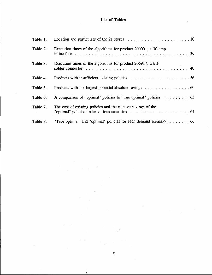
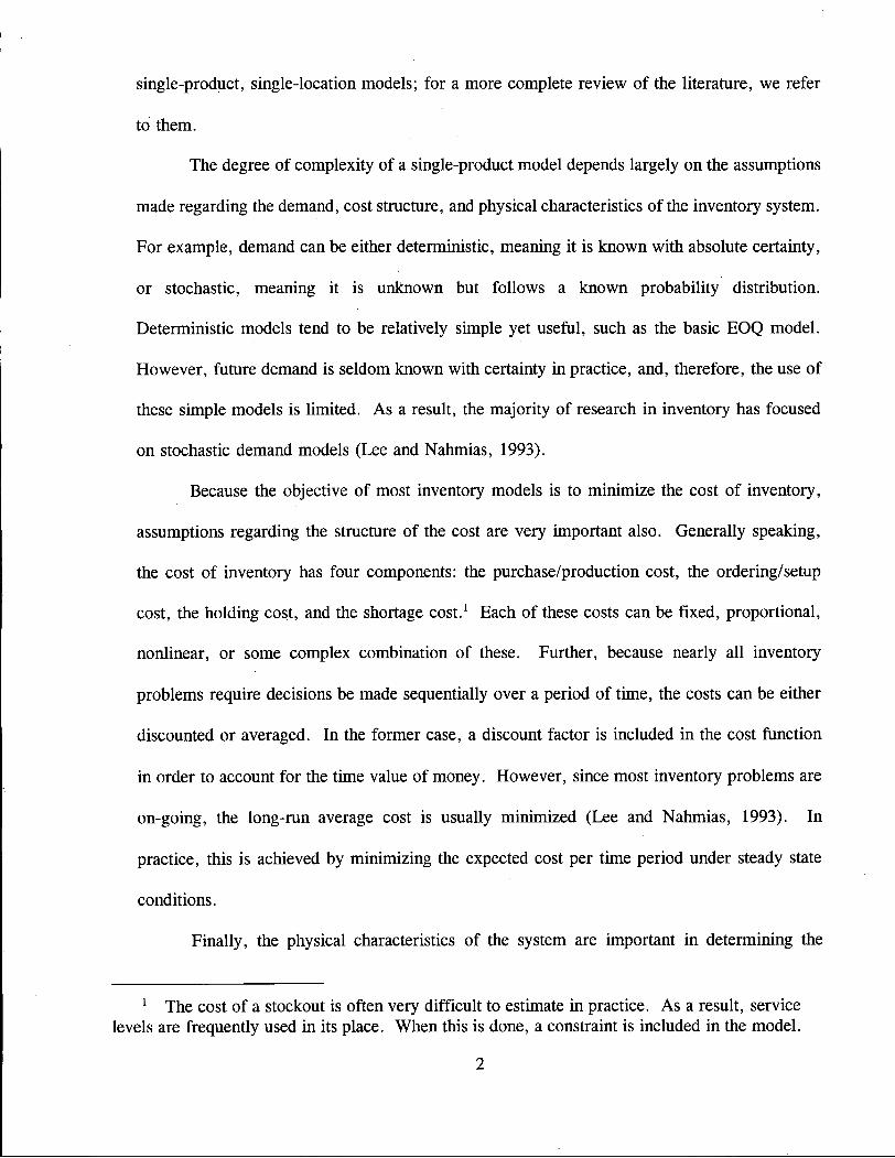
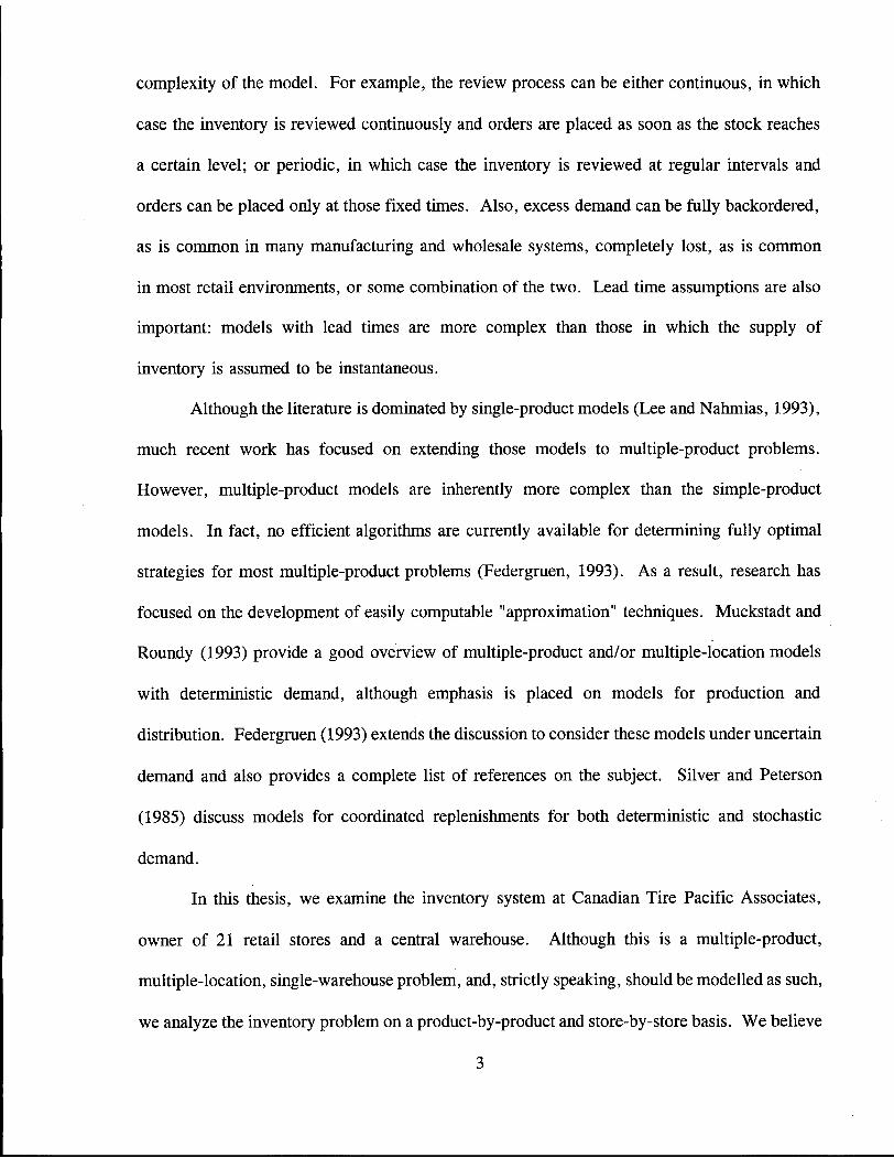


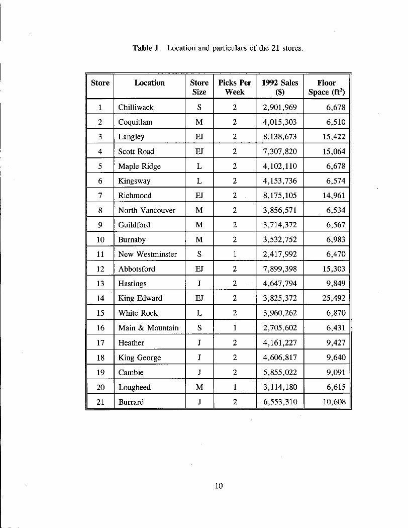


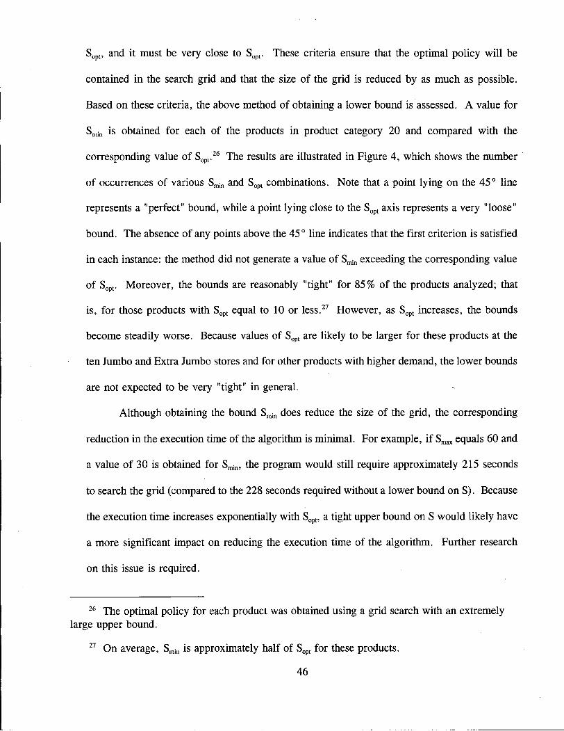


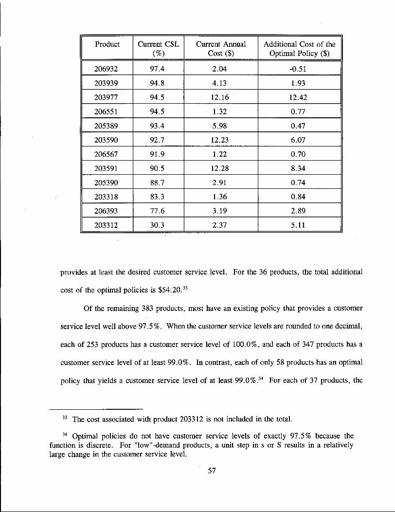

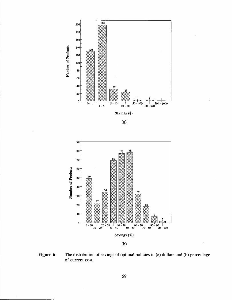


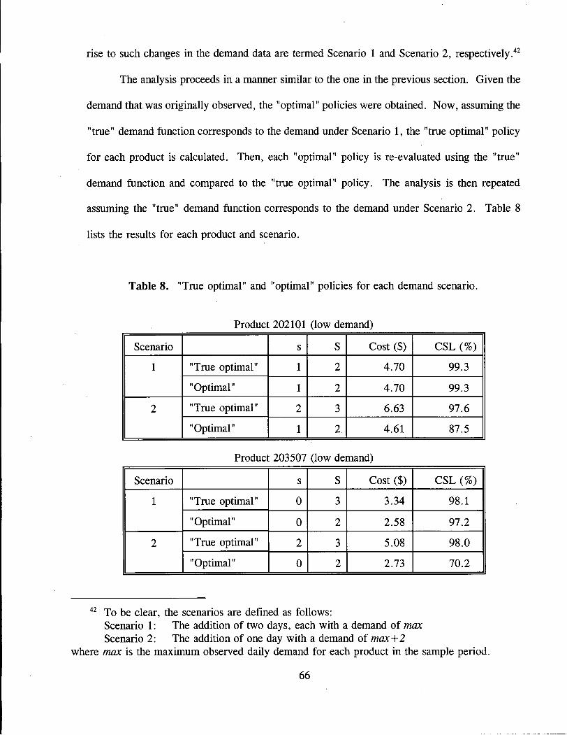
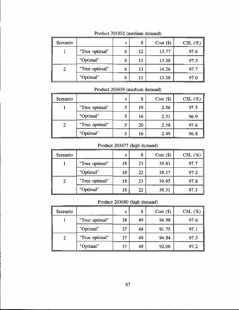


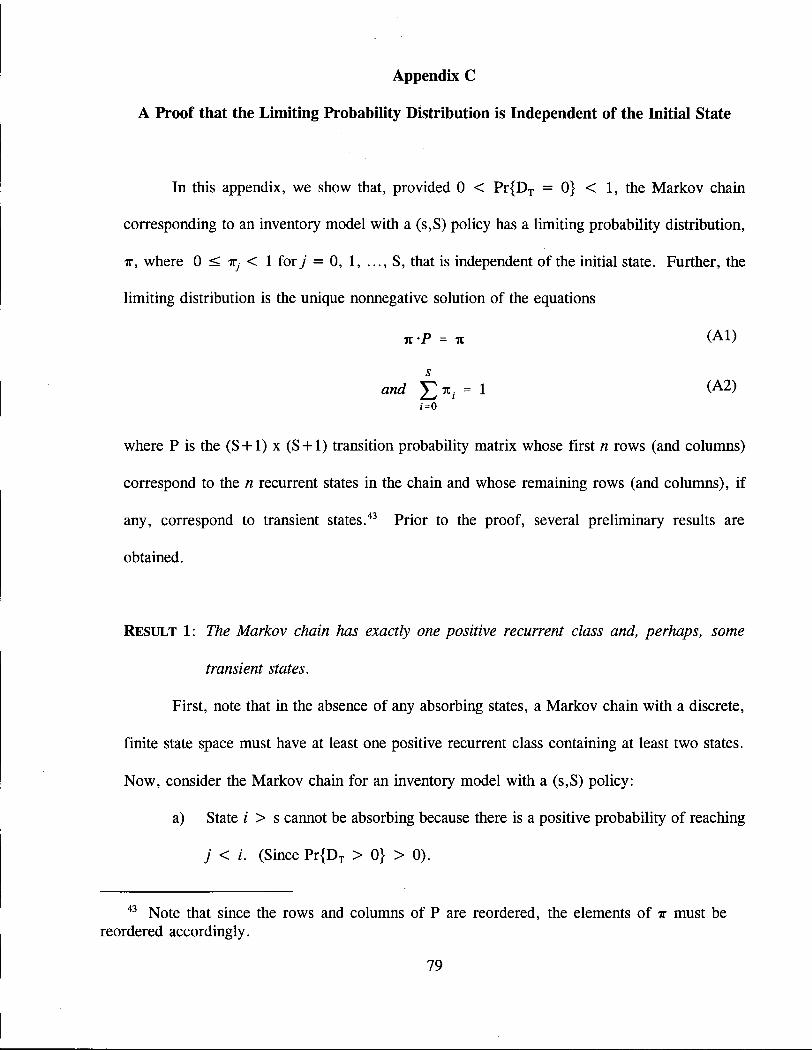


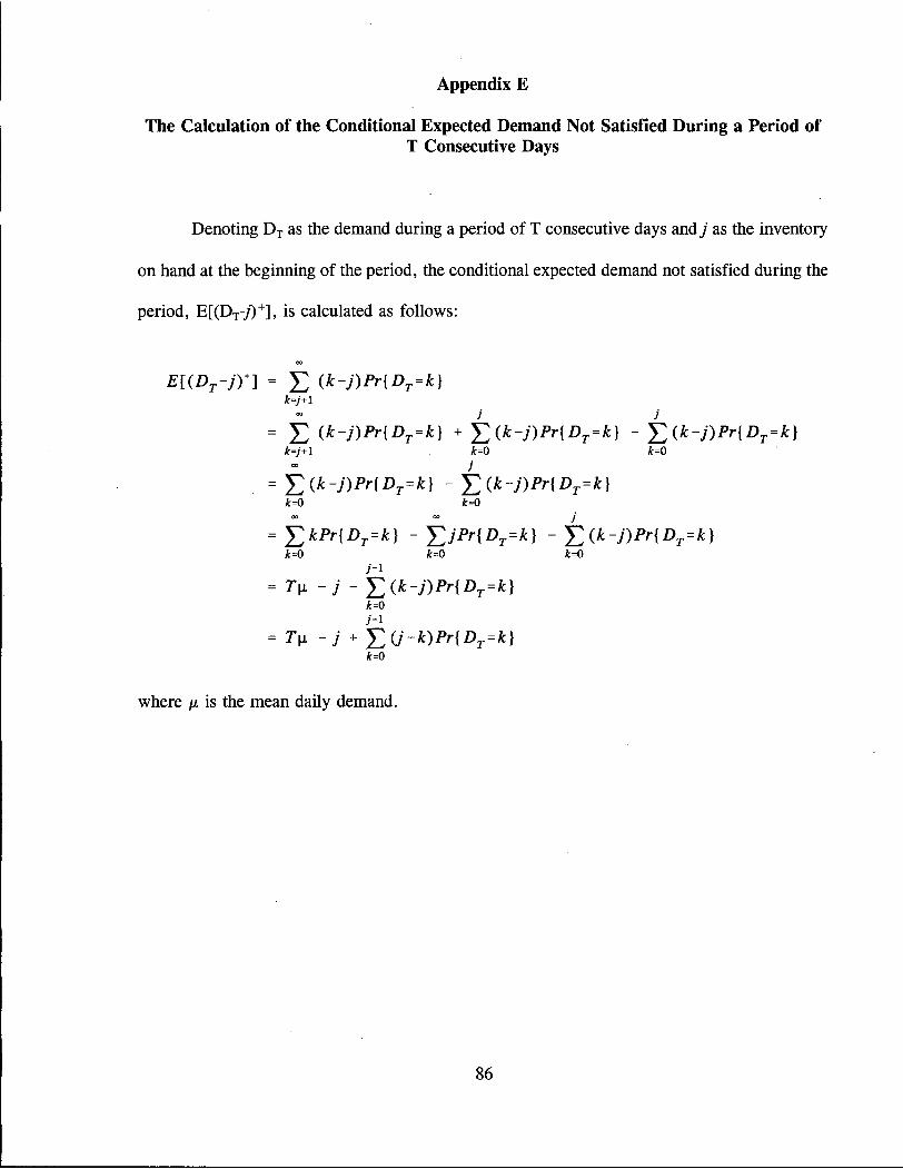


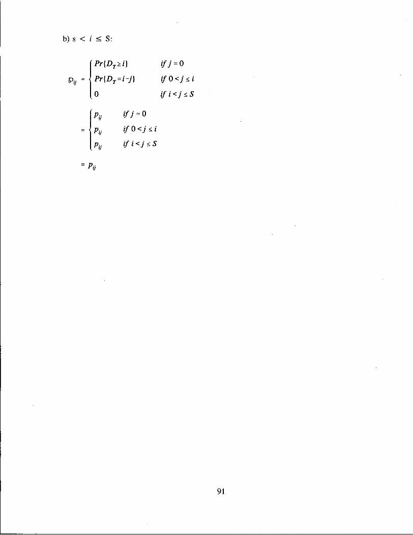


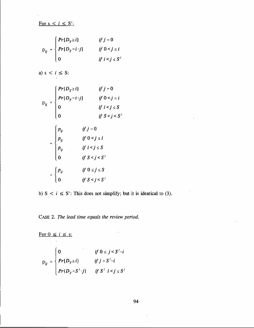
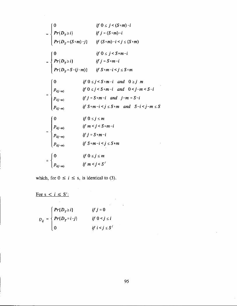


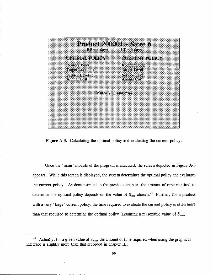


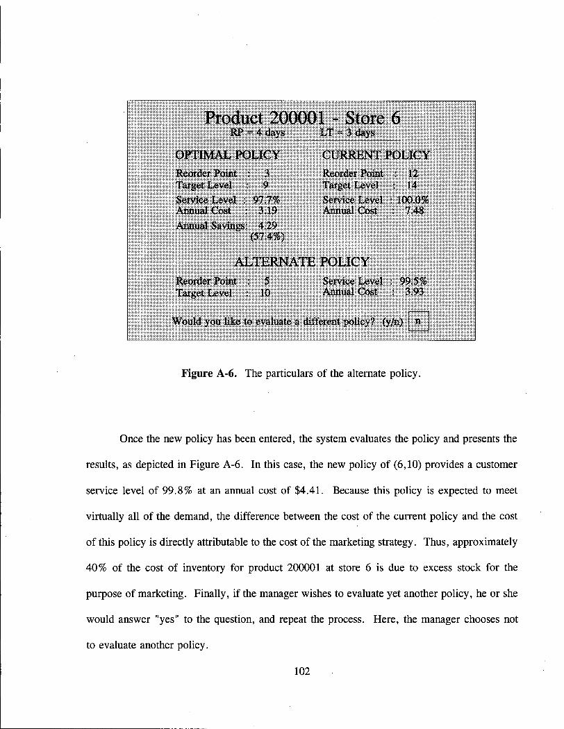
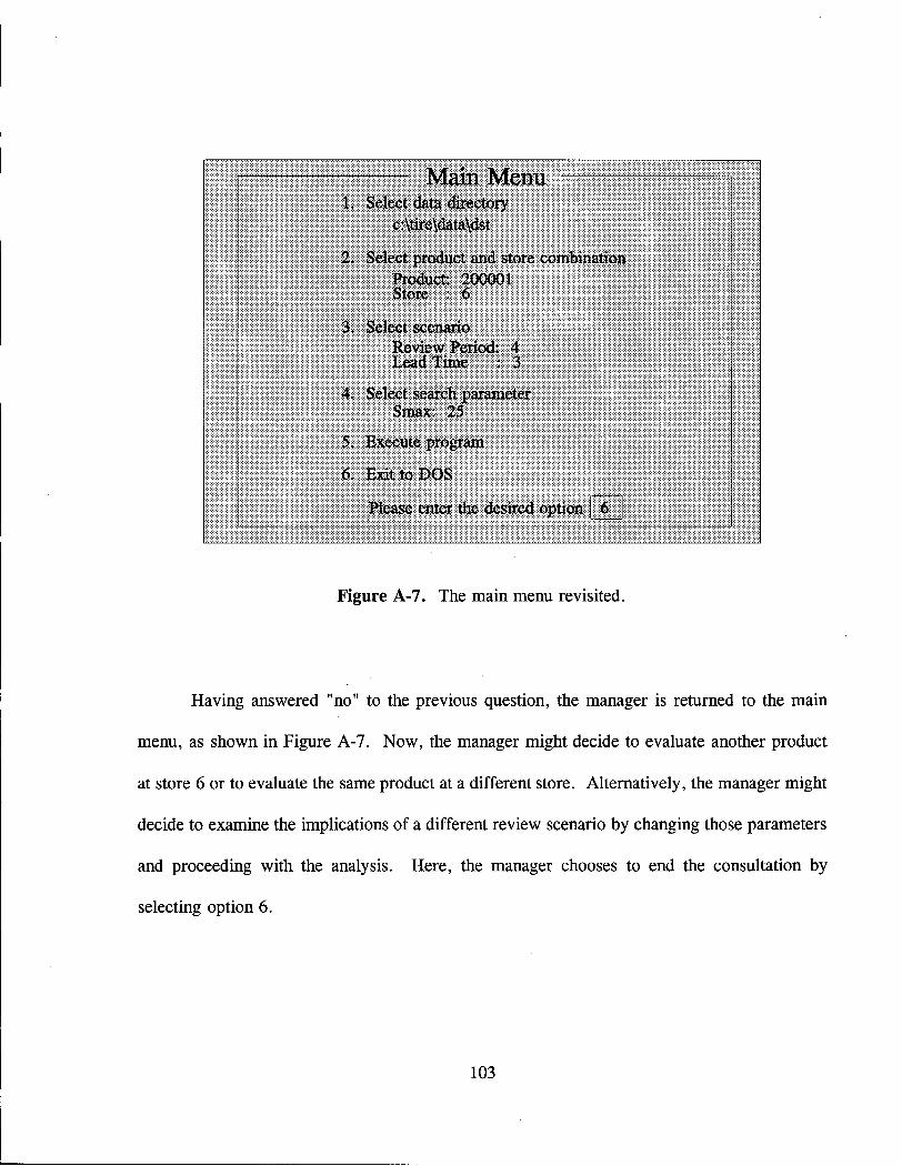
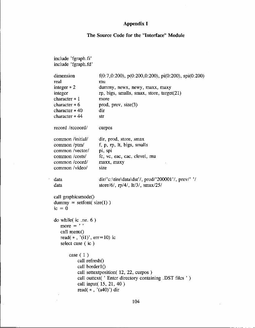

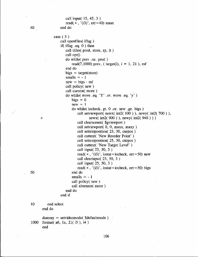


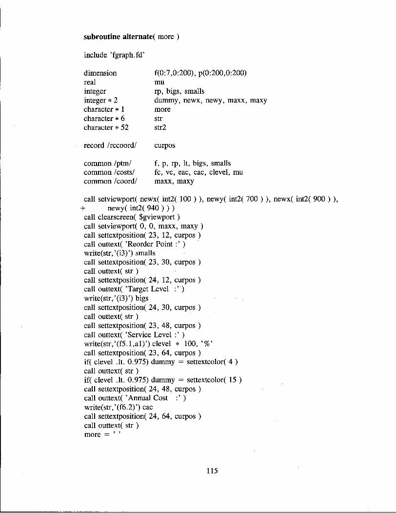


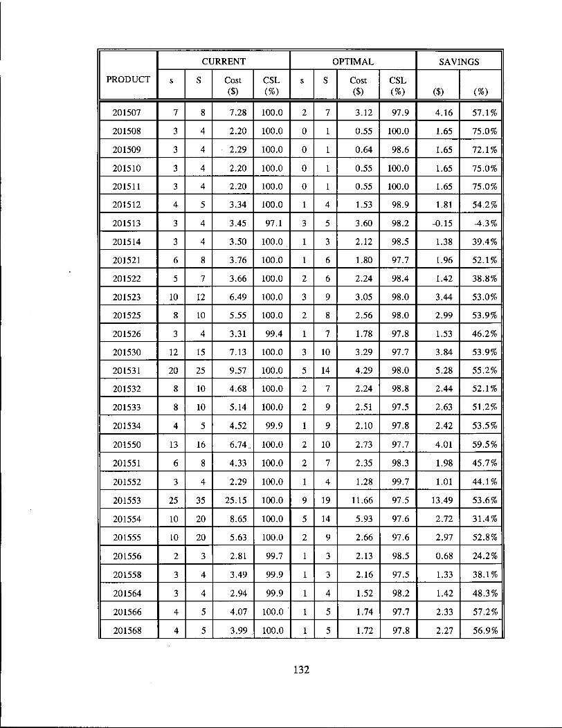


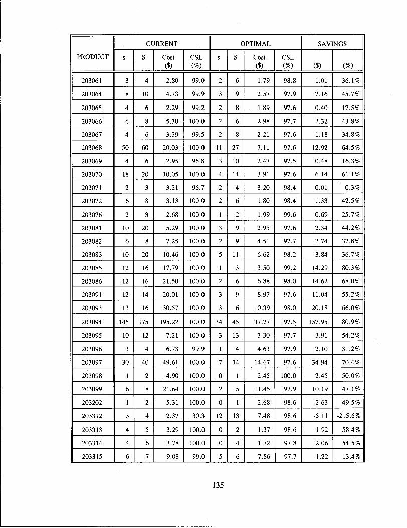

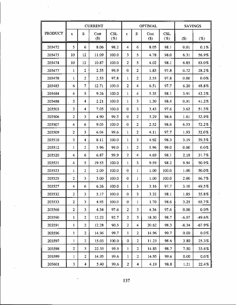

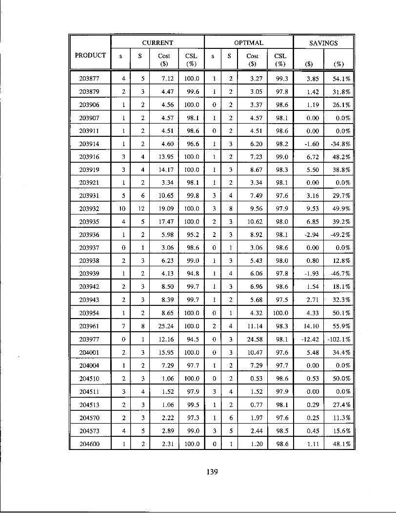


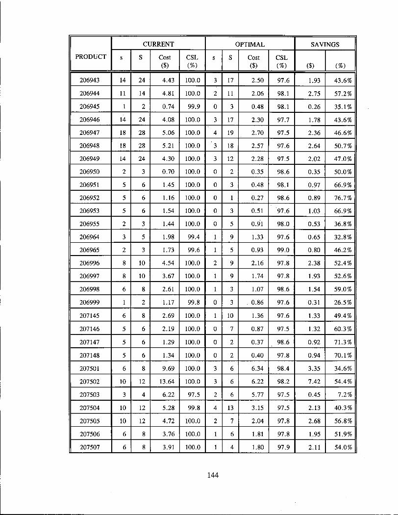

Related Documents


