Presented by Josephine Njuguna Department of Finance, Risk Management and Banking INV2601 DISCUSSION CLASS SEMESTER 1

Welcome message from author
This document is posted to help you gain knowledge. Please leave a comment to let me know what you think about it! Share it to your friends and learn new things together.
Transcript

Presented by Josephine Njuguna
Department of Finance, Risk Management and Banking
INV2601 DISCUSSION CLASSSEMESTER 1
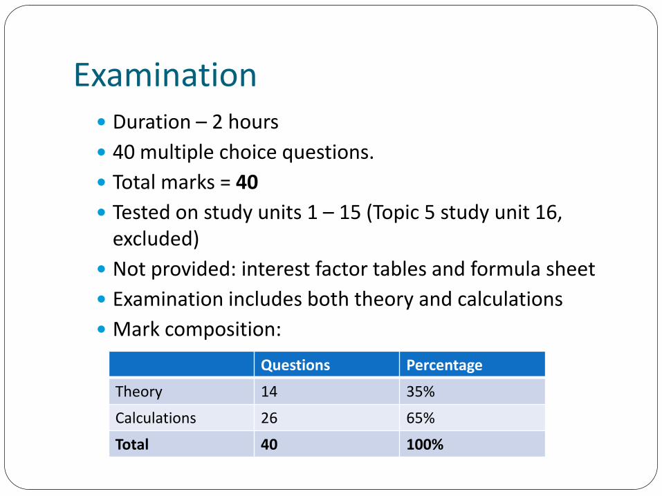
Examination Duration – 2 hours
40 multiple choice questions.
Total marks = 40
Tested on study units 1 – 15 (Topic 5 study unit 16, excluded)
Not provided: interest factor tables and formula sheet
Examination includes both theory and calculations
Mark composition:
Questions Percentage
Theory 14 35%
Calculations 26 65%
Total 40 100%
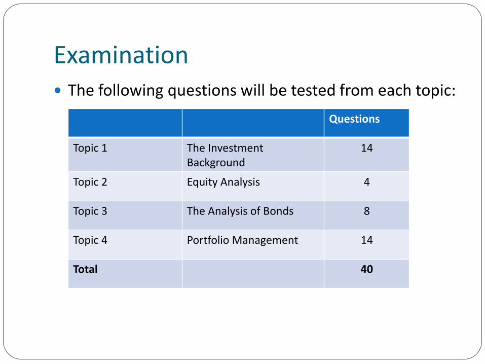
Examination The following questions will be tested from each topic:
Questions
Topic 1 The Investment Background
14
Topic 2 Equity Analysis 4
Topic 3 The Analysis of Bonds 8
Topic 4 Portfolio Management 14
Total 40
TOPIC 1
THE INVESTMENT BACKGROUND
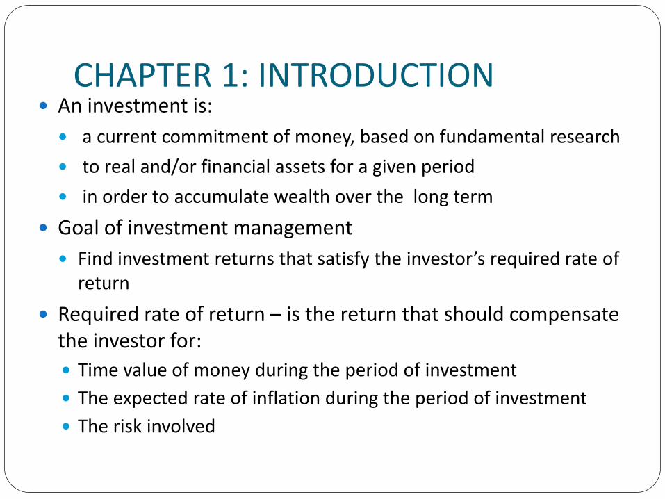
CHAPTER 1: INTRODUCTION An investment is:
a current commitment of money, based on fundamental research
to real and/or financial assets for a given period
in order to accumulate wealth over the long term
Goal of investment management
Find investment returns that satisfy the investor’s required rate of return
Required rate of return – is the return that should compensate the investor for:
Time value of money during the period of investment
The expected rate of inflation during the period of investment
The risk involved
Required Rate of Return
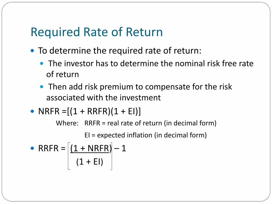
To determine the required rate of return:
The investor has to determine the nominal risk free rate of return
Then add risk premium to compensate for the risk associated with the investment
NRFR =[(1 + RRFR)(1 + EI)]Where: RRFR = real rate of return (in decimal form)
EI = expected inflation (in decimal form)
RRFR = (1 + NRFR) – 1
(1 + EI)
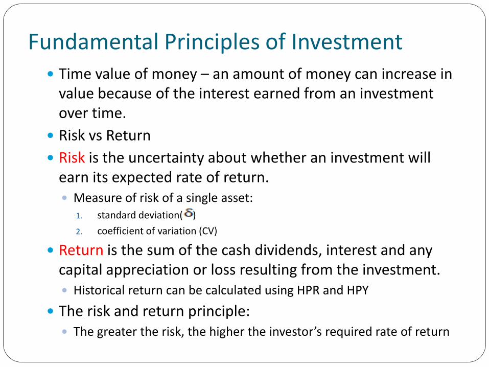
Fundamental Principles of Investment Time value of money – an amount of money can increase in
value because of the interest earned from an investment over time.
Risk vs Return
Risk is the uncertainty about whether an investment will earn its expected rate of return. Measure of risk of a single asset:
1. standard deviation( )
2. coefficient of variation (CV)
Return is the sum of the cash dividends, interest and any capital appreciation or loss resulting from the investment. Historical return can be calculated using HPR and HPY
The risk and return principle: The greater the risk, the higher the investor’s required rate of return
Example - HPR and HPY
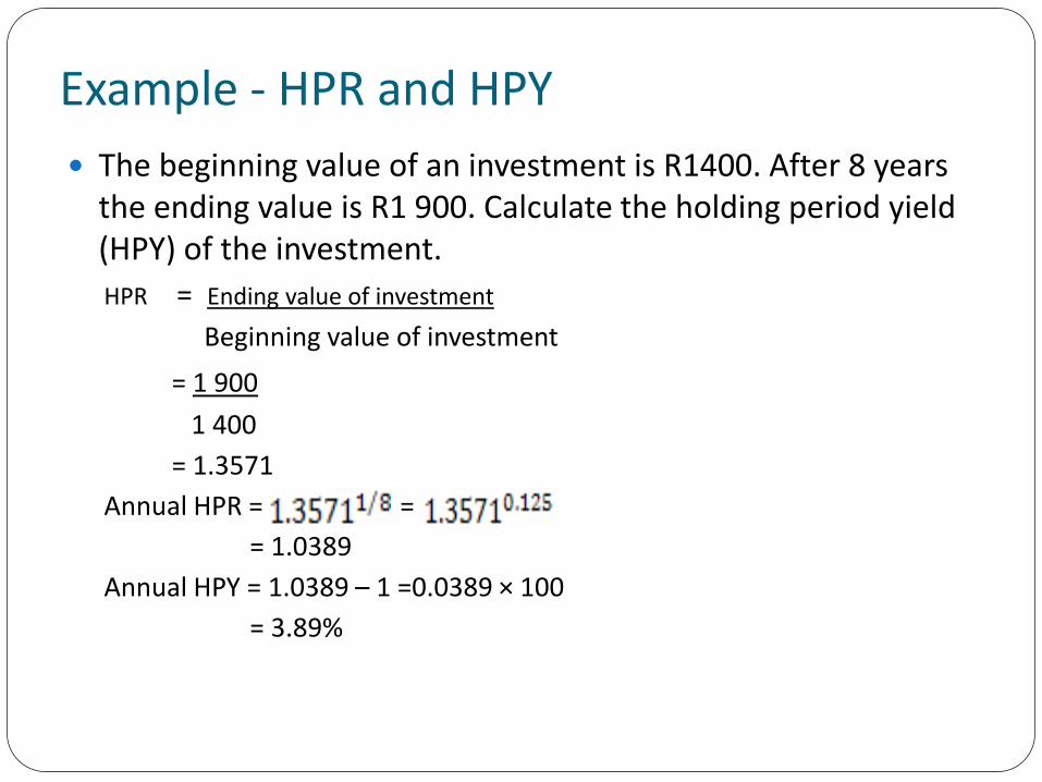
The beginning value of an investment is R1400. After 8 years the ending value is R1 900. Calculate the holding period yield (HPY) of the investment.
HPR = Ending value of investment
Beginning value of investment
= 1 900
1 400
= 1.3571
Annual HPR = =
= 1.0389
Annual HPY = 1.0389 – 1 =0.0389 × 100
= 3.89%
Example - HPR, HPY and Real Rate of Return
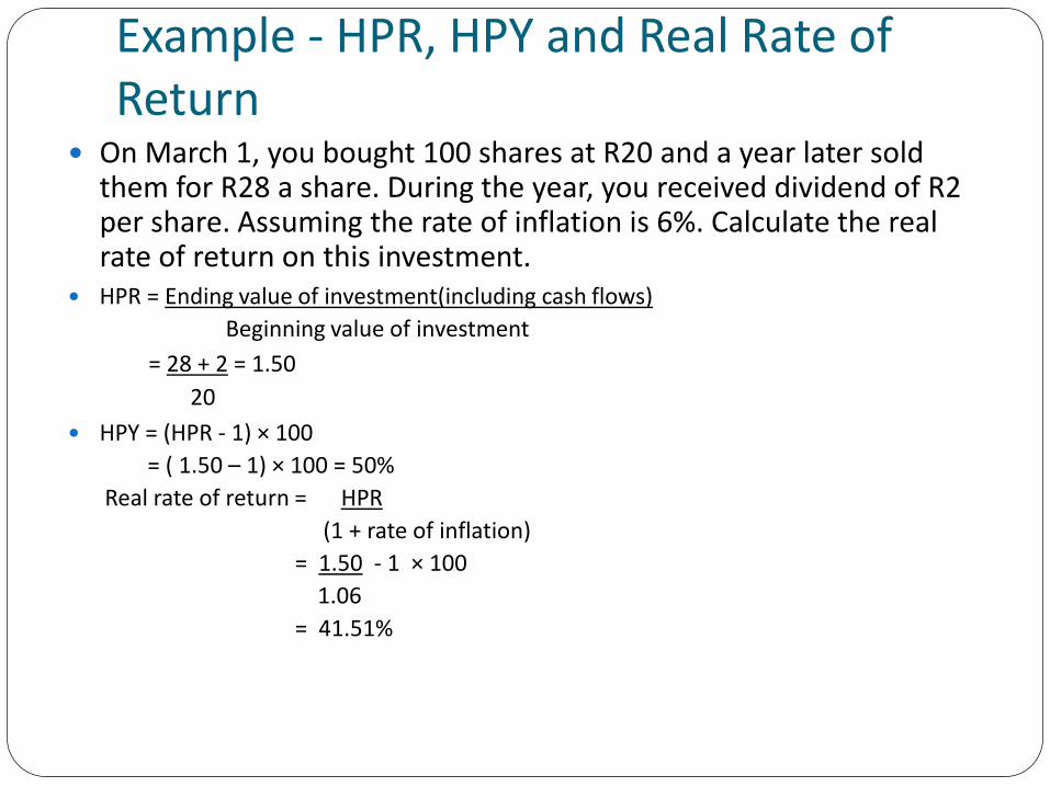
On March 1, you bought 100 shares at R20 and a year later sold them for R28 a share. During the year, you received dividend of R2 per share. Assuming the rate of inflation is 6%. Calculate the real rate of return on this investment.
HPR = Ending value of investment(including cash flows)
Beginning value of investment
= 28 + 2 = 1.50
20
HPY = (HPR - 1) × 100
= ( 1.50 – 1) × 100 = 50%
Real rate of return = HPR
(1 + rate of inflation)
= 1.50 - 1 × 100
1.06
= 41.51%
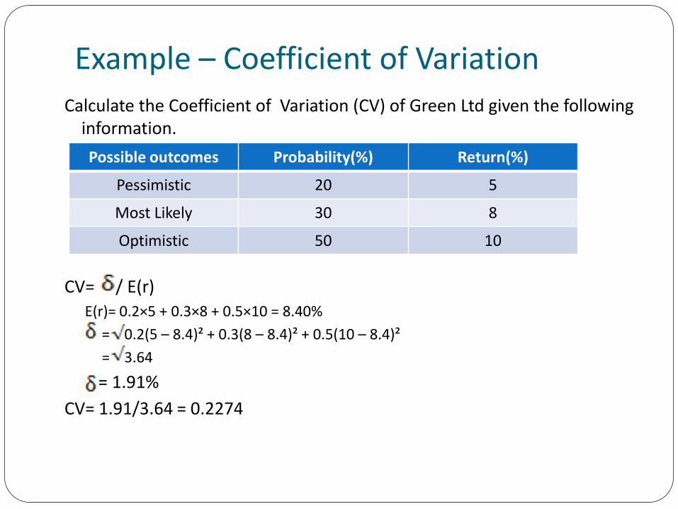
Example – Coefficient of VariationCalculate the Coefficient of Variation (CV) of Green Ltd given the following
information.
CV= / E(r)
E(r)= 0.2×5 + 0.3×8 + 0.5×10 = 8.40%
= 0.2(5 – 8.4)² + 0.3(8 – 8.4)² + 0.5(10 – 8.4)²
= 3.64
= 1.91%
CV= 1.91/3.64 = 0.2274
Possible outcomes Probability(%) Return(%)
Pessimistic 20 5
Most Likely 30 8
Optimistic 50 10
CHAPTER 2: CHARACTERISTICS OF A WELL FUNCTIONING MARKET
Availability of information
Liquidity and price continuity
Transaction costs
Informational efficiency• A large number of competing, profit-maximising, independent
participants analyze and value securities
• New information arrives randomly
• Competing investors attempt to adjust prices rapidly to reflect new information
Primary and Secondary Markets
Primary markets – sells newly issued securities of companies(‘new issues’) and is also involved in initial public offerings(IPOs).
Secondary market – supports the primary market by: i) giving investors liquidity, price continuity and depth
ii)providing information about current prices and yields
Third market - Over the counter trading of listed shares (OTC) by a broker. This market may be used by investors to trade shares that are either suspended on the exchange or while the exchange is closed.
Fourth market – direct trading of securities between two parties with no intermediary.
Type of Transactions Market orders – orders to buy or sell securities at the best
prevailing price. ‘sell at best’ or ‘buy at best’. Provide liquidity
Limit orders - specify the buy or sell price
Short sales - the sale of shares the investor does not own with the intention of buying them back at a lower price at a later stage. He would have to borrow them from another investor, sell them in the
market and subsequently replace them at (hopefully) a price lower than the price at which he sold them.
The investor who lends the shares receives the proceeds as collateral and can invest this in short-term, risk-free securities.
Stop loss – conditional market order that directs the trade should the share price decline to a predetermined level
Stop buy order – used by short seller who want to minimise any loss if the share increases in value
CHAPTER 3: INTRODUCTION Investment theory – explains the way in which
investors specify and measure risk and return in the valuation process
The efficient market theory is an important component of the investment theory
Investors are faced with systematic and unsystematic risk
Two important theories about risk and return
Capital asset pricing model (CAPM)
Arbitrage pricing model (APT)
Efficient Market Theory An efficient market – is one in which: Prices of securities adjust rapidly to the arrival of new
information. Current prices of securities reflect all information about a security.
Investments with higher expected returns have higher expected risk
Forms of the efficient market hypothesis Weak form – current security prices reflect all security market
information
Semi-strong form – security prices adjust rapidly to all public information
Strong form – security prices fully reflect all information (public and private sources)
Investment Theory THE SECURITY MARKET LINE (SML)
Reflects the best combination of risk and return on alternative investments
A portfolio consists of a risk-free asset and combinations of alternative risky assets can be constructed
= linear proportion of the standard deviation of the risky asset portfolio.
SML risk is measured by means of beta (systematic risk)
Markowitz Efficient Frontier Represent that set of portfolios that have the maximum
return for every given level of risk or the minimum risk for every level of return. Also known as efficient portfolios. Contains only portfolios
Individual assets cannot have their risk reduced by diversification.
No portfolio dominates any other portfolio
Adding a risk free asset leads to creation of the capital market line(CML) It is a risk-return for efficient portfolios
NB: CML risk is measured by means of the standard deviation (total risk)
Total risk = systematic risk + unsystematic risk
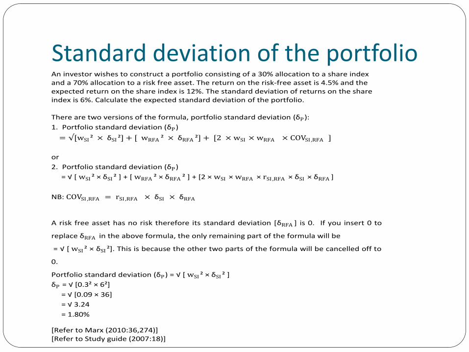
Standard deviation of the portfolioAn investor wishes to construct a portfolio consisting of a 30% allocation to a share index and a 70% allocation to a risk free asset. The return on the risk-free asset is 4.5% and the expected return on the share index is 12%. The standard deviation of returns on the share index is 6%. Calculate the expected standard deviation of the portfolio. There are two versions of the formula, portfolio standard deviation (δP):
1. Portfolio standard deviation (δP)
= √[wSI ² × δSI ²] + [ wRFA ² × δRFA ²] + [2 × wSI × wRFA × COVSI ,RFA ]
or
2. Portfolio standard deviation (δP)
= √ * wSI ² × δSI ² ] + [ wRFA ² × δRFA ² ] + [2 × wSI × wRFA × rSI ,RFA × δSI × δRFA ]
NB: COVSI ,RFA = rSI ,RFA × δSI × δRFA
A risk free asset has no risk therefore its standard deviation [δRFA ] is 0. If you insert 0 to
replace δRFA in the above formula, the only remaining part of the formula will be
= √ * wSI ² × δSI ²]. This is because the other two parts of the formula will be cancelled off to
0.
Portfolio standard deviation (δP) = √ * wSI ² × δSI ² ]
δP = √ *0.3² × 6²+
= √ *0.09 × 36+
= √ 3.24
= 1.80%
[Refer to Marx (2010:36,274)] [Refer to Study guide (2007:18)]
Asset Pricing Models Two most common theories are CAPM and APT
If you can measure risk, you should be able to determine the required rate of return
Investors are risk averse; thus for any increase in risk they require an increase in the required rate of return
CAPM – the return an investor should require from a risky asset assuming that he is exposed only to the asset’s systematic risk as measured by beta.
Rationale – for any level of risk, the SML indicates the return that should be earned by using the market portfolio and the risk-free asset
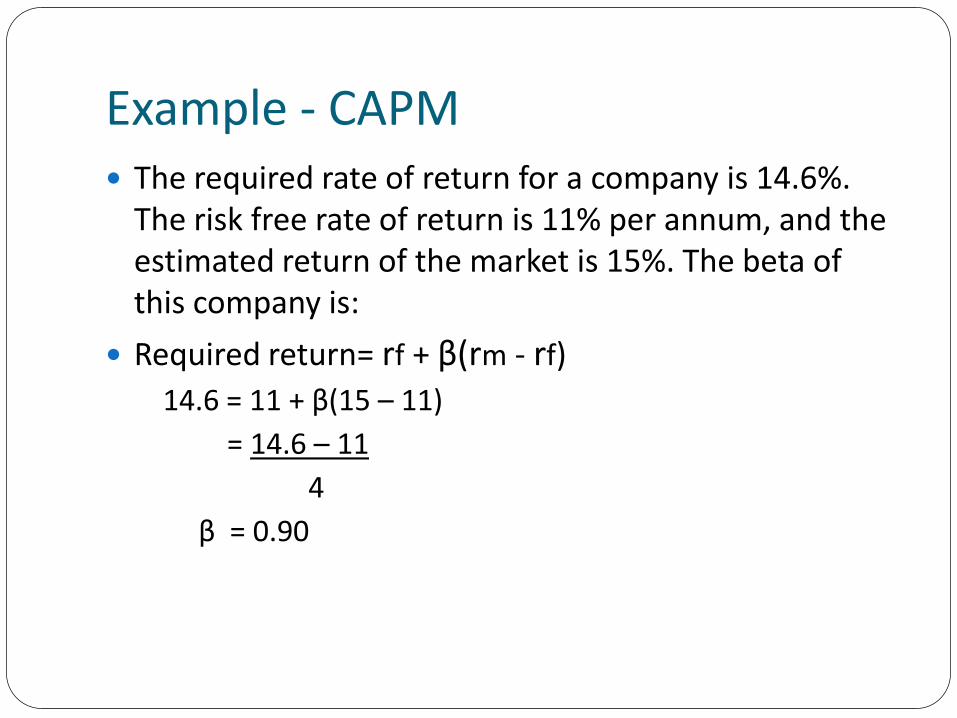
Example - CAPM The required rate of return for a company is 14.6%.
The risk free rate of return is 11% per annum, and the estimated return of the market is 15%. The beta of this company is:
Required return= rf + β(rm - rf)
14.6 = 11 + β(15 – 11)
= 14.6 – 11
4
β = 0.90
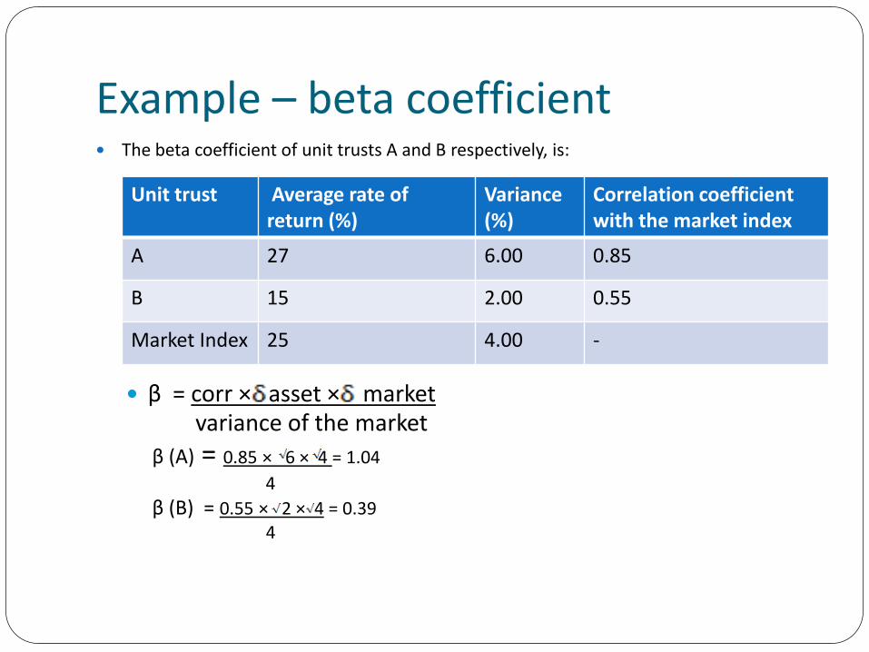
Example – beta coefficient The beta coefficient of unit trusts A and B respectively, is:
β = corr × asset × market variance of the market
β (A) = 0.85 × 6 × 4 = 1.04
4
β (B) = 0.55 × 2 × 4 = 0.394
Unit trust Average rate of return (%)
Variance(%)
Correlation coefficientwith the market index
A 27 6.00 0.85
B 15 2.00 0.55
Market Index 25 4.00 -
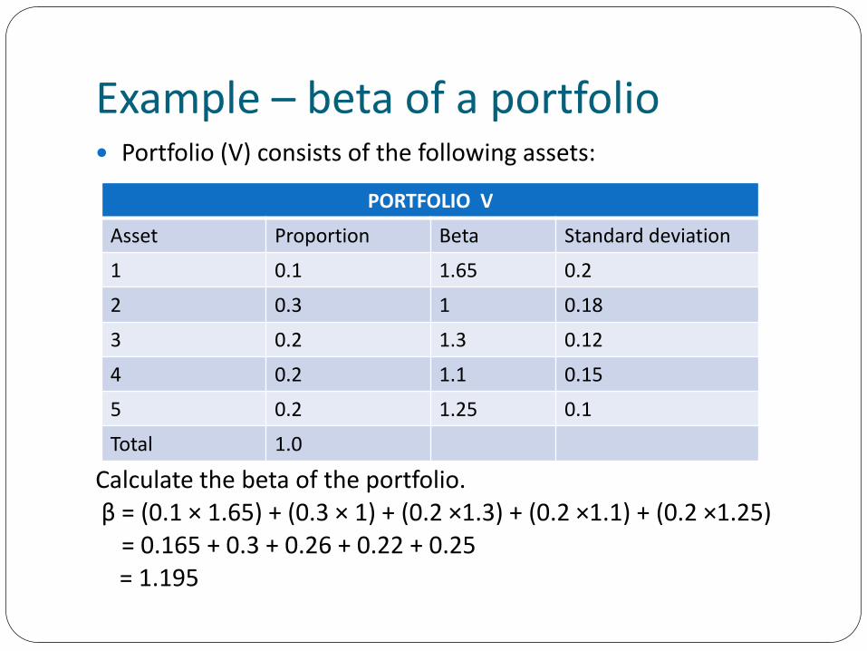
Example – beta of a portfolio Portfolio (V) consists of the following assets:
Calculate the beta of the portfolio.β = (0.1 × 1.65) + (0.3 × 1) + (0.2 ×1.3) + (0.2 ×1.1) + (0.2 ×1.25)
= 0.165 + 0.3 + 0.26 + 0.22 + 0.25= 1.195
PORTFOLIO V
Asset Proportion Beta Standard deviation
1 0.1 1.65 0.2
2 0.3 1 0.18
3 0.2 1.3 0.12
4 0.2 1.1 0.15
5 0.2 1.25 0.1
Total 1.0
Using CAPM to assess an asset An investment in an asset can be assessed by means of
CAPM to determine whether an asset is over or undervalued
Estimated rate of return – is the actual holding period rate of return that the investor anticipates Estimated rate of return > required rate of return The share is undervalued
Estimated rate of return < required rate of return The share is overvalued
Highly efficient market – all assets should plot on the SML Less efficient market – assets may at times be mispriced
due to investors being unaware of all the relevant information
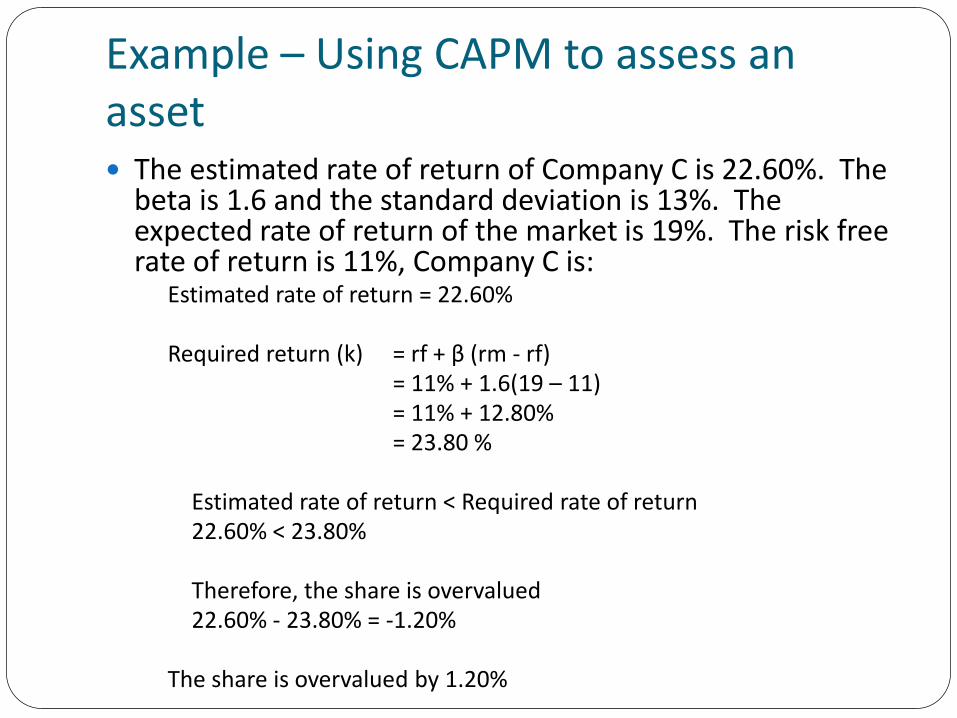
Example – Using CAPM to assess an asset The estimated rate of return of Company C is 22.60%. The
beta is 1.6 and the standard deviation is 13%. The expected rate of return of the market is 19%. The risk free rate of return is 11%, Company C is:
Estimated rate of return = 22.60%
Required return (k) = rf + β (rm - rf)= 11% + 1.6(19 – 11)= 11% + 12.80%= 23.80 %
Estimated rate of return < Required rate of return 22.60% < 23.80%
Therefore, the share is overvalued22.60% - 23.80% = -1.20%
The share is overvalued by 1.20%
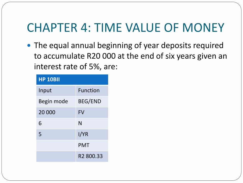
CHAPTER 4: TIME VALUE OF MONEY The equal annual beginning of year deposits required
to accumulate R20 000 at the end of six years given an interest rate of 5%, are:
HP 10BII
Input Function
Begin mode BEG/END
20 000 FV
6 N
5 I/YR
PMT
R2 800.33
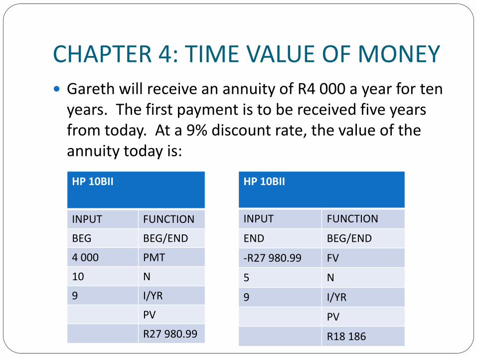
CHAPTER 4: TIME VALUE OF MONEY Gareth will receive an annuity of R4 000 a year for ten
years. The first payment is to be received five years from today. At a 9% discount rate, the value of the annuity today is:
HP 10BII
INPUT FUNCTION
BEG BEG/END
4 000 PMT
10 N
9 I/YR
PV
R27 980.99
HP 10BII
INPUT FUNCTION
END BEG/END
-R27 980.99 FV
5 N
9 I/YR
PV
R18 186
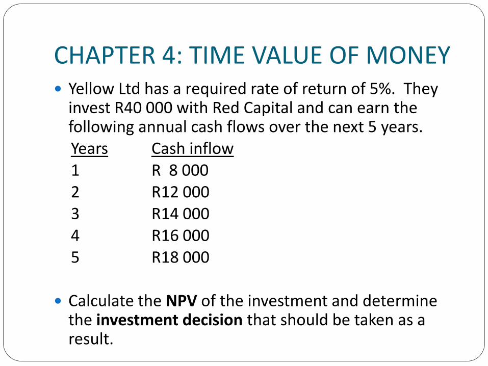
CHAPTER 4: TIME VALUE OF MONEY Yellow Ltd has a required rate of return of 5%. They
invest R40 000 with Red Capital and can earn the following annual cash flows over the next 5 years.Years Cash inflow1 R 8 0002 R12 0003 R14 0004 R16 0005 R18 000
Calculate the NPV of the investment and determine the investment decision that should be taken as a result.
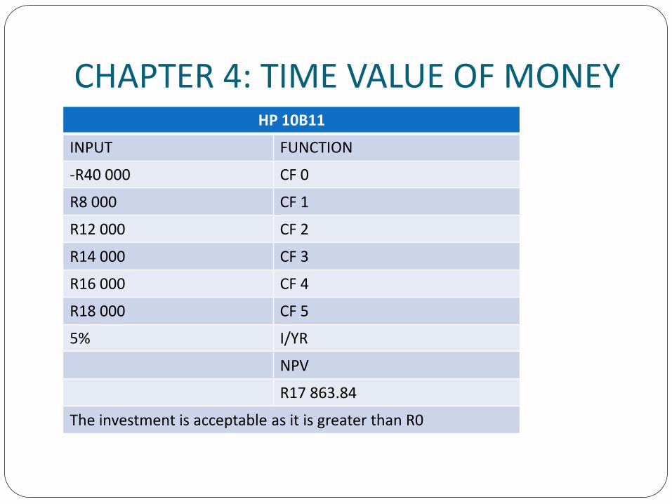
CHAPTER 4: TIME VALUE OF MONEYHP 10B11
INPUT FUNCTION
-R40 000 CF 0
R8 000 CF 1
R12 000 CF 2
R14 000 CF 3
R16 000 CF 4
R18 000 CF 5
5% I/YR
NPV
R17 863.84
The investment is acceptable as it is greater than R0
CHAPTER 5: VALUATION PRINCIPLES AND PRACTICES Valuation – process of finding the intrinsic value of an
asset. Also called fair value or estimated value of an asset It plays an important role in investment decision making Buy : intrinsic value > market value Earning positive returns
Don’t buy : intrinsic value < market value
Valuation concepts Par value, market value, book value and intrinsic value
Required inputs Cash flows, timing and discount rate
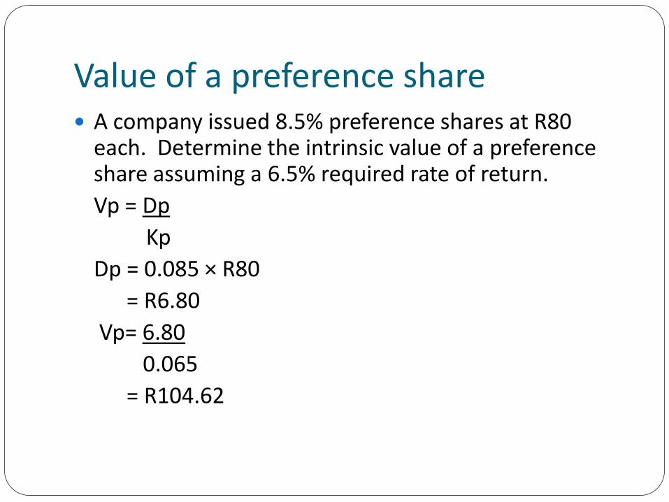
Value of a preference share A company issued 8.5% preference shares at R80
each. Determine the intrinsic value of a preference share assuming a 6.5% required rate of return.
Vp = Dp
Kp
Dp = 0.085 × R80
= R6.80
Vp= 6.80
0.065
= R104.62
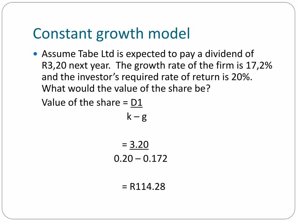
Constant growth model Assume Tabe Ltd is expected to pay a dividend of
R3,20 next year. The growth rate of the firm is 17,2% and the investor’s required rate of return is 20%. What would the value of the share be?
Value of the share = D1
k – g
= 3.20
0.20 – 0.172
= R114.28
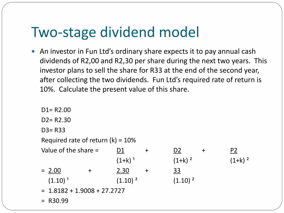
Two-stage dividend model An investor in Fun Ltd’s ordinary share expects it to pay annual cash
dividends of R2,00 and R2,30 per share during the next two years. This investor plans to sell the share for R33 at the end of the second year, after collecting the two dividends. Fun Ltd’s required rate of return is 10%. Calculate the present value of this share.
D1= R2.00
D2= R2.30
D3= R33
Required rate of return (k) = 10%
Value of the share = D1 + D2 + P2
(1+k) ¹ (1+k) ² (1+k) ²
= 2.00 + 2.30 + 33
(1.10) ¹ (1.10) ² (1.10) ²
= 1.8182 + 1.9008 + 27.2727
= R30.99
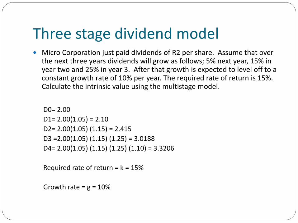
Three stage dividend model Micro Corporation just paid dividends of R2 per share. Assume that over
the next three years dividends will grow as follows; 5% next year, 15% in year two and 25% in year 3. After that growth is expected to level off to a constant growth rate of 10% per year. The required rate of return is 15%. Calculate the intrinsic value using the multistage model.
D0= 2.00
D1= 2.00(1.05) = 2.10
D2= 2.00(1.05) (1.15) = 2.415
D3 =2.00(1.05) (1.15) (1.25) = 3.0188
D4= 2.00(1.05) (1.15) (1.25) (1.10) = 3.3206
Required rate of return = k = 15%
Growth rate = g = 10%
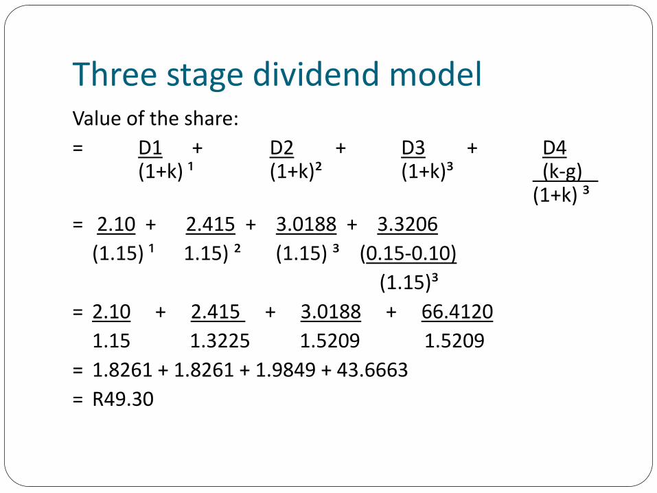
Three stage dividend modelValue of the share:
= D1 + D2 + D3 + D4(1+k) ¹ (1+k)² (1+k)³ (k-g)
(1+k) ³
= 2.10 + 2.415 + 3.0188 + 3.3206
(1.15) ¹ 1.15) ² (1.15) ³ (0.15-0.10)
(1.15)³
= 2.10 + 2.415 + 3.0188 + 66.4120
1.15 1.3225 1.5209 1.5209
= 1.8261 + 1.8261 + 1.9849 + 43.6663
= R49.30
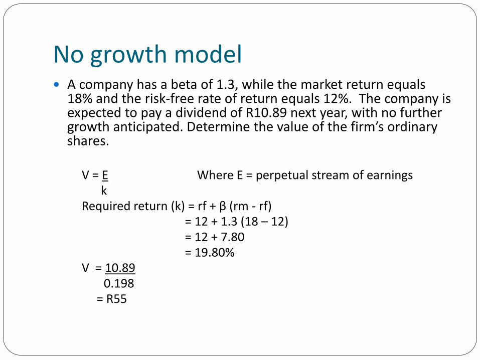
No growth model A company has a beta of 1.3, while the market return equals
18% and the risk-free rate of return equals 12%. The company is expected to pay a dividend of R10.89 next year, with no further growth anticipated. Determine the value of the firm’s ordinary shares.
V = E Where E = perpetual stream of earningsk
Required return (k) = rf + β (rm - rf)= 12 + 1.3 (18 – 12)= 12 + 7.80= 19.80%
V = 10.890.198
= R55
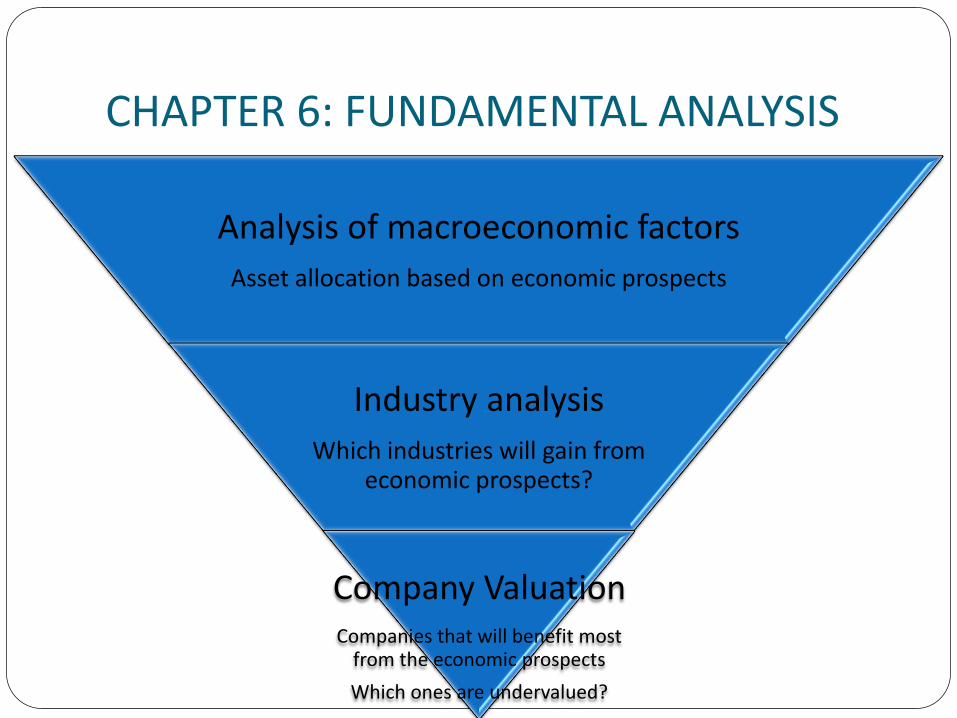
CHAPTER 6: FUNDAMENTAL ANALYSIS
Analysis of macroeconomic factors
Asset allocation based on economic prospects
Industry analysis
Which industries will gain from economic prospects?
Company ValuationCompanies that will benefit most
from the economic prospects
Which ones are undervalued?
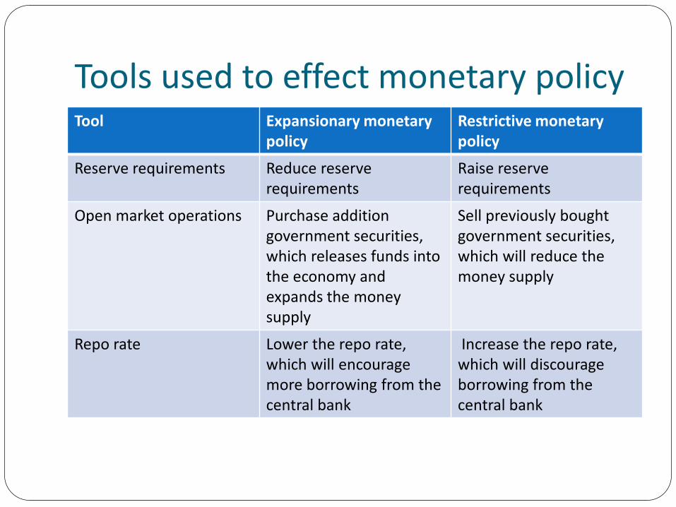
Tools used to effect monetary policyTool Expansionary monetary
policyRestrictive monetary policy
Reserve requirements Reduce reserve requirements
Raise reserve requirements
Open market operations Purchase addition government securities, which releases funds into the economy and expands the money supply
Sell previously boughtgovernment securities, which will reduce the money supply
Repo rate Lower the repo rate, which will encourage more borrowing from the central bank
Increase the repo rate, which will discourage borrowing from the central bank
TOPIC 2
EQUITY ANALYSIS
CHAPTER 8: COMPANY ANALYSIS Ratio analysis
Liquidity ratios
Financial leverage ratios
Asset management ratios
Profitability ratios
Market value ratios
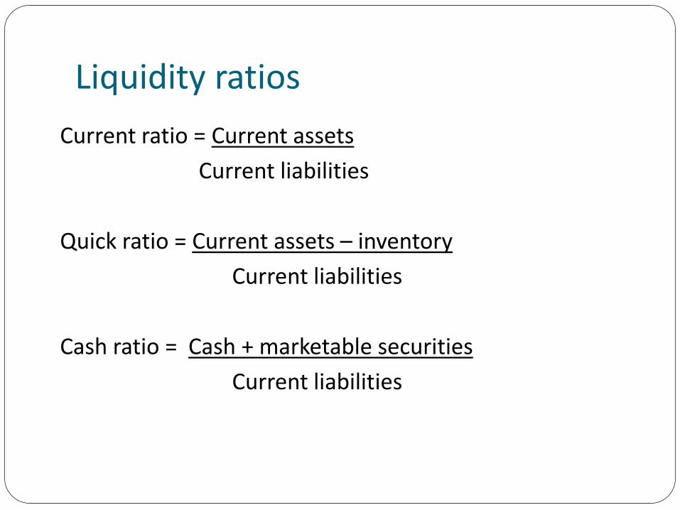
Liquidity ratios
Current ratio = Current assets
Current liabilities
Quick ratio = Current assets – inventory
Current liabilities
Cash ratio = Cash + marketable securities
Current liabilities
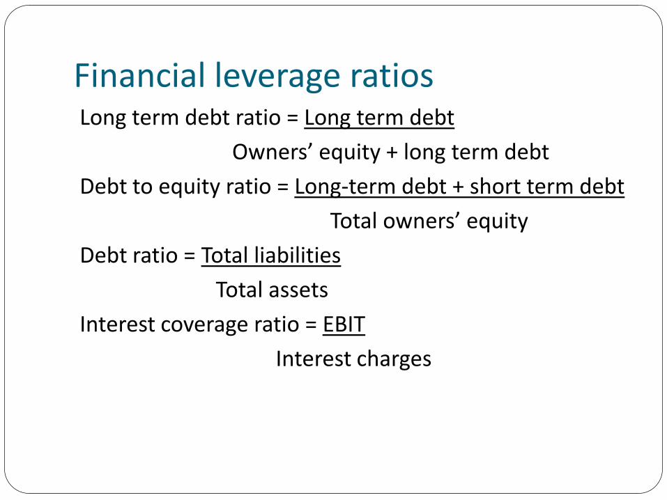
Financial leverage ratiosLong term debt ratio = Long term debt
Owners’ equity + long term debt
Debt to equity ratio = Long-term debt + short term debt
Total owners’ equity
Debt ratio = Total liabilities
Total assets
Interest coverage ratio = EBIT
Interest charges
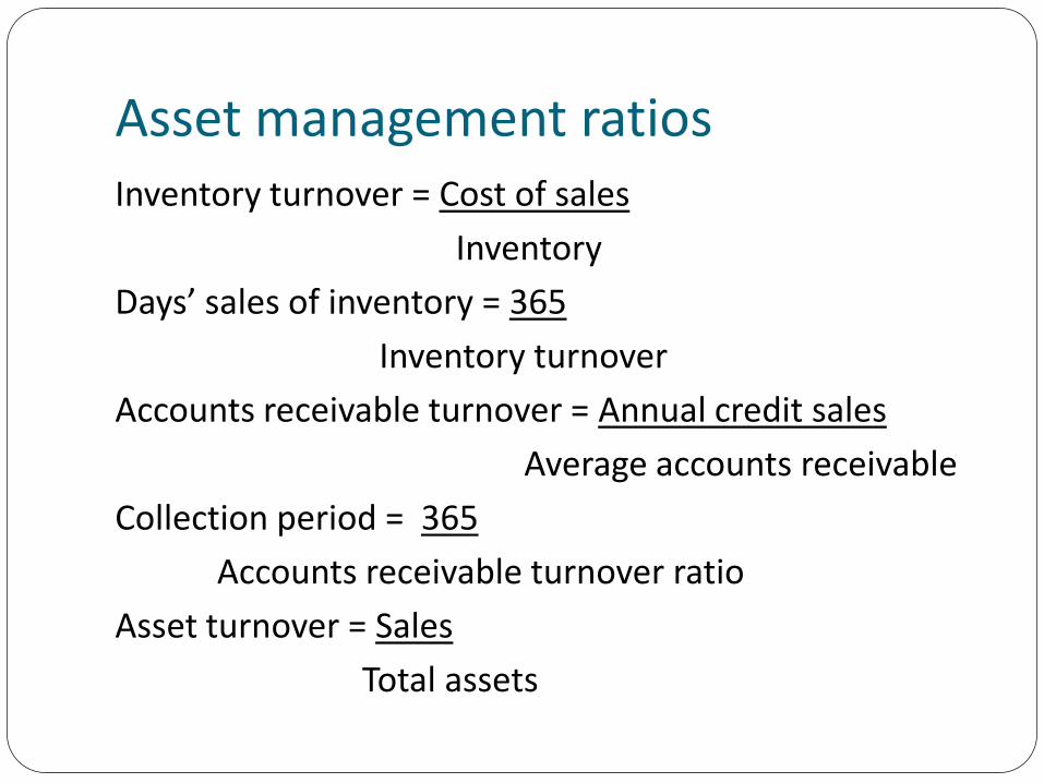
Asset management ratiosInventory turnover = Cost of sales
Inventory
Days’ sales of inventory = 365
Inventory turnover
Accounts receivable turnover = Annual credit sales
Average accounts receivable
Collection period = 365
Accounts receivable turnover ratio
Asset turnover = Sales
Total assets
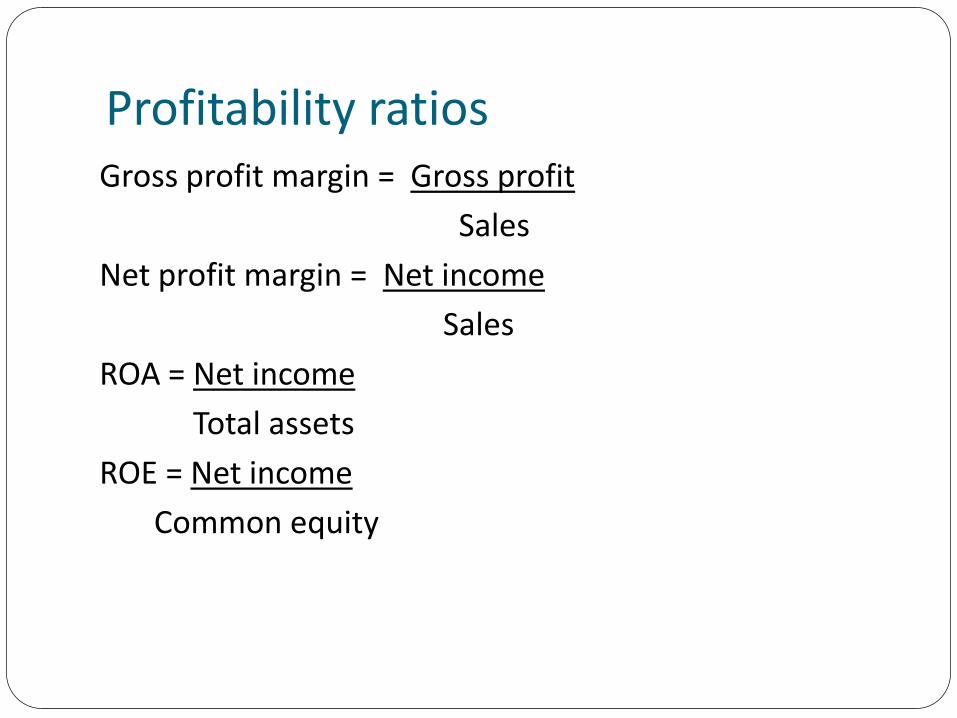
Profitability ratiosGross profit margin = Gross profit
Sales
Net profit margin = Net income
Sales
ROA = Net income
Total assets
ROE = Net income
Common equity
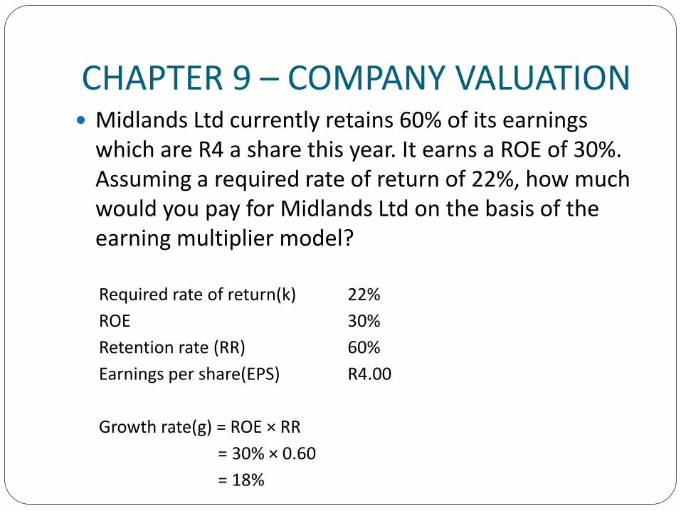
CHAPTER 9 – COMPANY VALUATION Midlands Ltd currently retains 60% of its earnings
which are R4 a share this year. It earns a ROE of 30%. Assuming a required rate of return of 22%, how much would you pay for Midlands Ltd on the basis of the earning multiplier model?
Required rate of return(k) 22%
ROE 30%
Retention rate (RR) 60%
Earnings per share(EPS) R4.00
Growth rate(g) = ROE × RR
= 30% × 0.60
= 18%
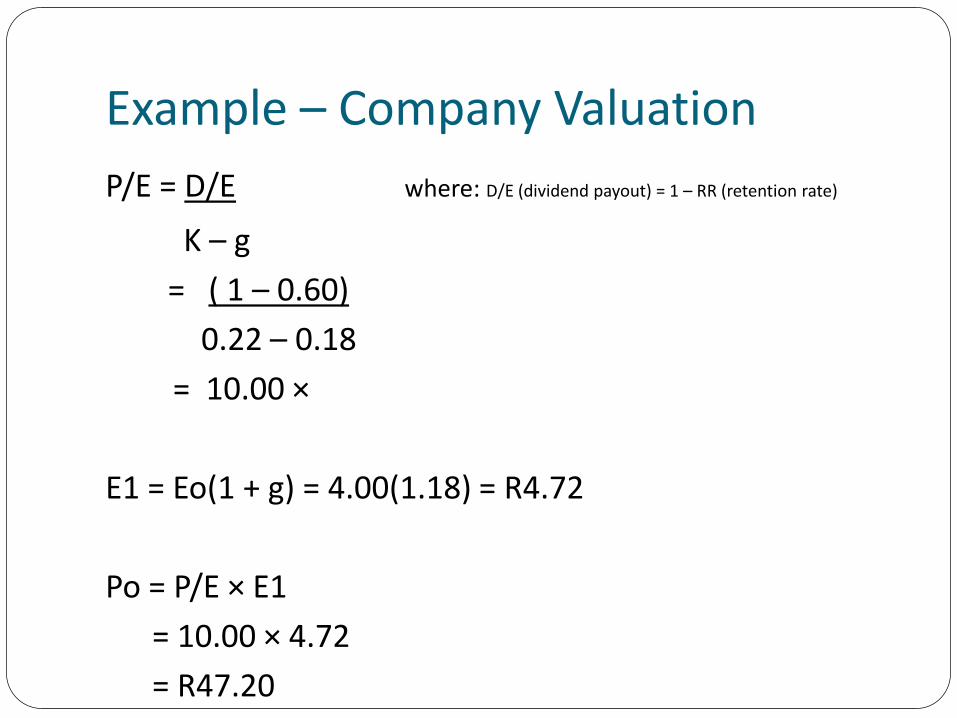
Example – Company Valuation
P/E = D/E where: D/E (dividend payout) = 1 – RR (retention rate)
K – g
= ( 1 – 0.60)
0.22 – 0.18
= 10.00 ×
E1 = Eo(1 + g) = 4.00(1.18) = R4.72
Po = P/E × E1
= 10.00 × 4.72
= R47.20
TOPIC 3
THE ANALYSIS OF BONDS
CHAPTER 11: BOND FUNDAMENTALS Bonds are issued in the capital market (financial
market for long term debt obligations and equity securities)
Bonds provide an alternative to direct lending as a source of funding
Basics of bonds
Principal value
Coupon rate
Term to maturity
Market value
Yield to maturity
Bond Risk Exposures Interest rate risk – effect of changes in the prevailing
market rate on the return on a bond (price risk and reinvestment risk)
Price risk – arises when a bond is sold before maturity
Reinvestment risk – arises from the market rate being different from the yield to maturity
Credit risk – risk that creditworthiness of a bond issuer will deteriorate. It is sub-divided into the following: Default risk – possibility that issuer will fail to meet its obligations
regarding timely payment of coupons and principal
Credit spread risk – risk that the credit spread will increase
Downgrade risk – risk that a rating agency assigns a lower rating to a bond causing a rise in yield and drop in price
Bond Risk Exposures Yield curve risk – arises from a non parallel shift in the
yield curve
Liquidity risk – risk of having to sell a bond at a price below fair value due to lack of liquidity
Call risk
Applies to callable bonds
It is the risk that the bond is eventually called from the holder by the issuer when the market rate falls
Call protection reduces call risk
Non-callable bonds have no call risk
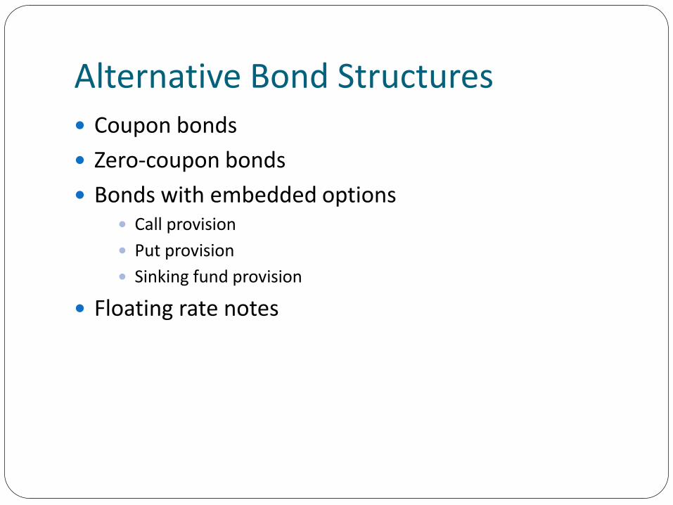
Alternative Bond Structures Coupon bonds
Zero-coupon bonds
Bonds with embedded options Call provision
Put provision
Sinking fund provision
Floating rate notes
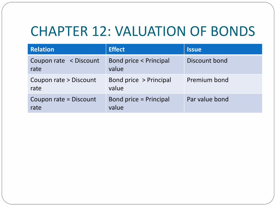
CHAPTER 12: VALUATION OF BONDSRelation Effect Issue
Coupon rate < Discount rate
Bond price < Principalvalue
Discount bond
Coupon rate > Discount rate
Bond price > Principal value
Premium bond
Coupon rate = Discountrate
Bond price = Principalvalue
Par value bond
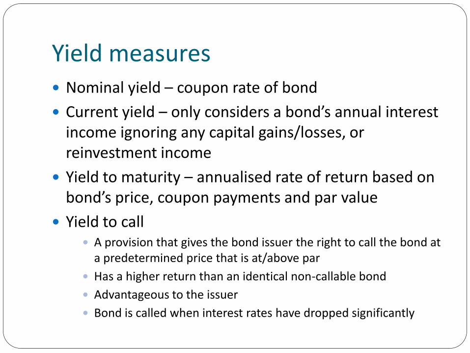
Yield measures Nominal yield – coupon rate of bond
Current yield – only considers a bond’s annual interest income ignoring any capital gains/losses, or reinvestment income
Yield to maturity – annualised rate of return based on bond’s price, coupon payments and par value
Yield to call A provision that gives the bond issuer the right to call the bond at
a predetermined price that is at/above par
Has a higher return than an identical non-callable bond
Advantageous to the issuer
Bond is called when interest rates have dropped significantly
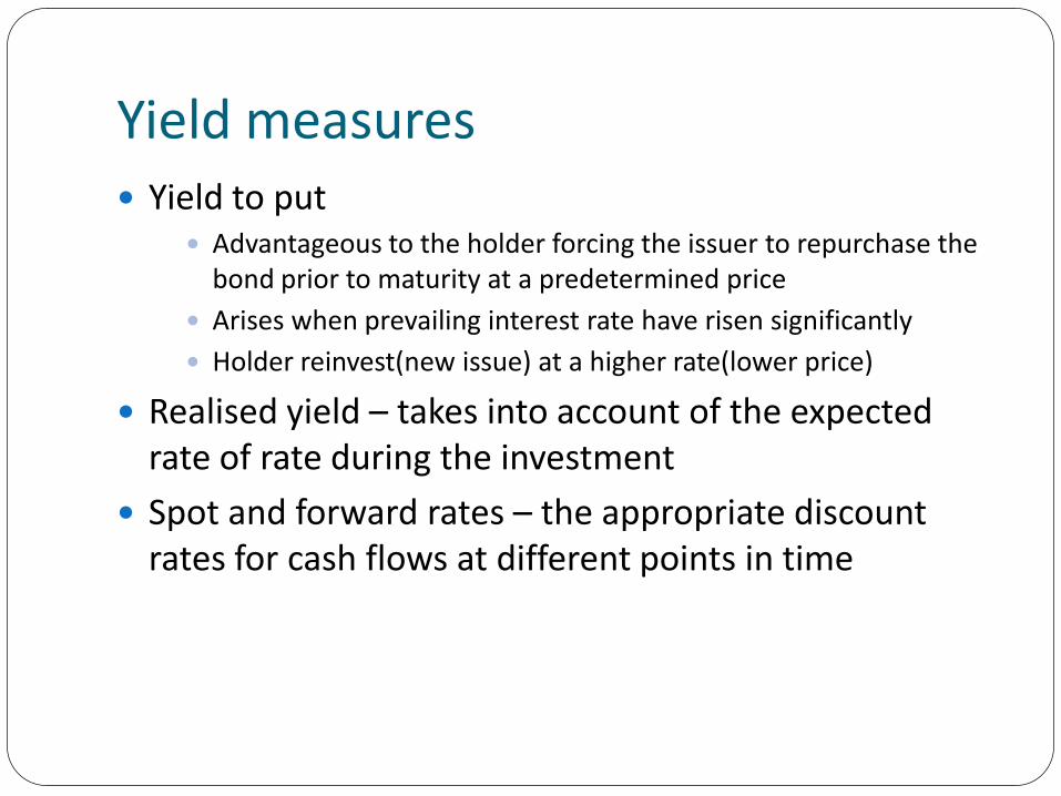
Yield measures Yield to put
Advantageous to the holder forcing the issuer to repurchase the bond prior to maturity at a predetermined price
Arises when prevailing interest rate have risen significantly
Holder reinvest(new issue) at a higher rate(lower price)
Realised yield – takes into account of the expected rate of rate during the investment
Spot and forward rates – the appropriate discount rates for cash flows at different points in time
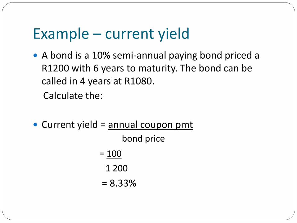
Example – current yield A bond is a 10% semi-annual paying bond priced a
R1200 with 6 years to maturity. The bond can be called in 4 years at R1080.
Calculate the:
Current yield = annual coupon pmt
bond price
= 100
1 200
= 8.33%
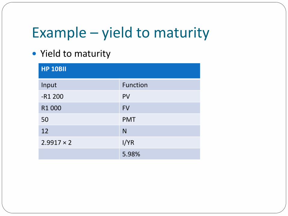
Example – yield to maturity Yield to maturity
HP 10BII
Input Function
-R1 200 PV
R1 000 FV
50 PMT
12 N
2.9917 × 2 I/YR
5.98%
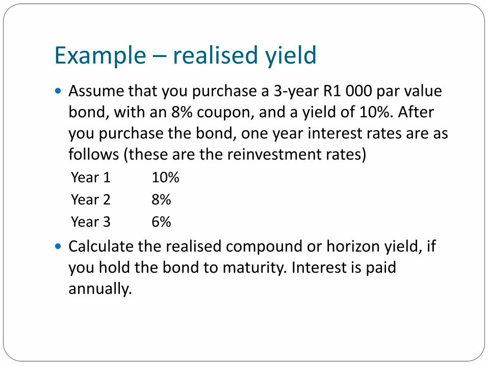
Example – realised yield Assume that you purchase a 3-year R1 000 par value
bond, with an 8% coupon, and a yield of 10%. After you purchase the bond, one year interest rates are as follows (these are the reinvestment rates)
Year 1 10%
Year 2 8%
Year 3 6%
Calculate the realised compound or horizon yield, if you hold the bond to maturity. Interest is paid annually.
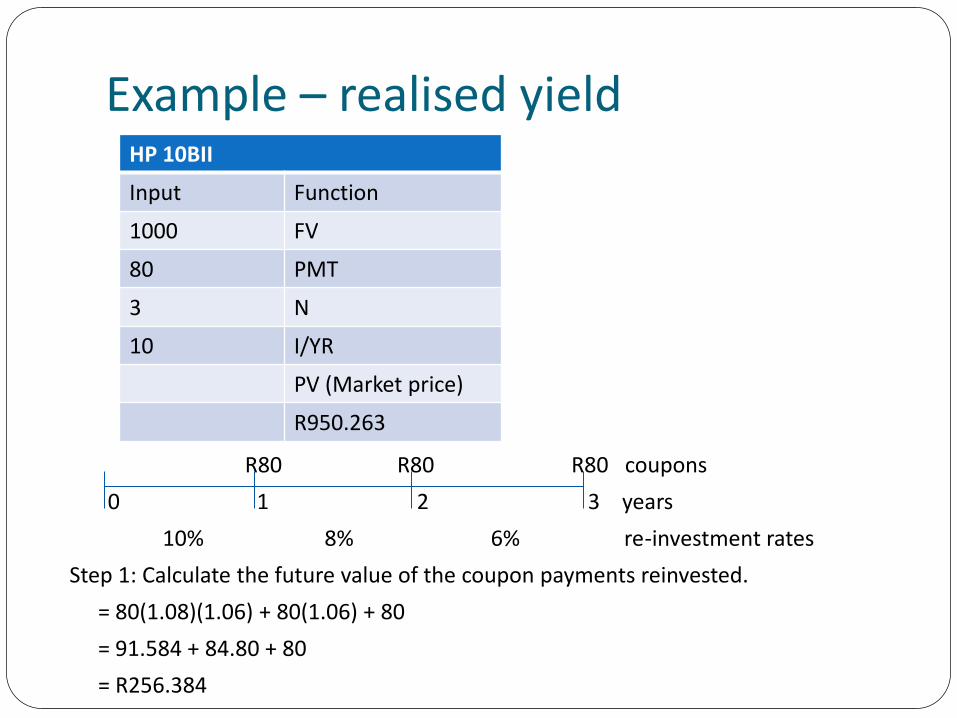
Example – realised yield
R80 R80 R80 coupons
0 1 2 3 years
10% 8% 6% re-investment rates
Step 1: Calculate the future value of the coupon payments reinvested.
= 80(1.08)(1.06) + 80(1.06) + 80
= 91.584 + 84.80 + 80
= R256.384
HP 10BII
Input Function
1000 FV
80 PMT
3 N
10 I/YR
PV (Market price)
R950.263
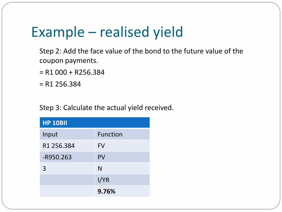
Example – realised yieldStep 2: Add the face value of the bond to the future value of the coupon payments.
= R1 000 + R256.384
= R1 256.384
Step 3: Calculate the actual yield received.
HP 10BII
Input Function
R1 256.384 FV
-R950.263 PV
3 N
I/YR
9.76%
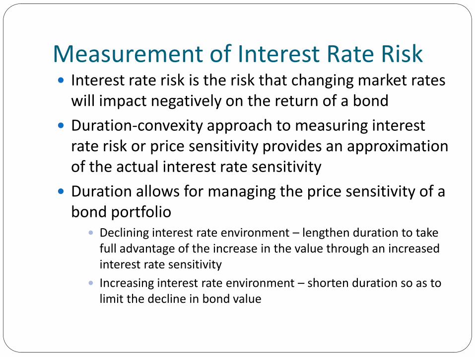
Measurement of Interest Rate Risk Interest rate risk is the risk that changing market rates
will impact negatively on the return of a bond
Duration-convexity approach to measuring interest rate risk or price sensitivity provides an approximation of the actual interest rate sensitivity
Duration allows for managing the price sensitivity of a bond portfolio Declining interest rate environment – lengthen duration to take
full advantage of the increase in the value through an increased interest rate sensitivity
Increasing interest rate environment – shorten duration so as to limit the decline in bond value
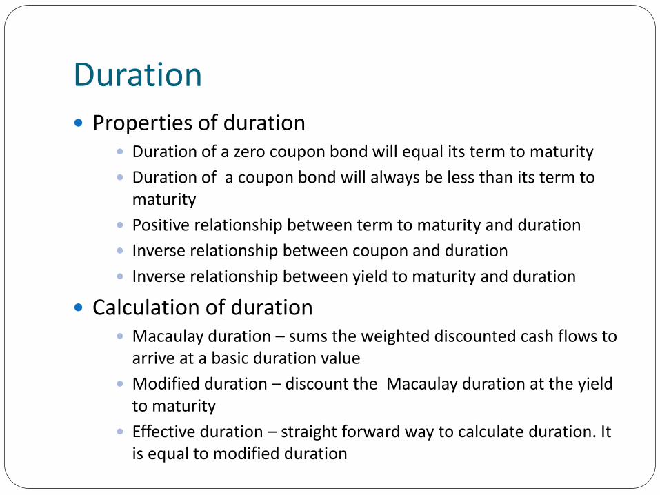
Duration Properties of duration
Duration of a zero coupon bond will equal its term to maturity
Duration of a coupon bond will always be less than its term to maturity
Positive relationship between term to maturity and duration
Inverse relationship between coupon and duration
Inverse relationship between yield to maturity and duration
Calculation of duration Macaulay duration – sums the weighted discounted cash flows to
arrive at a basic duration value
Modified duration – discount the Macaulay duration at the yield to maturity
Effective duration – straight forward way to calculate duration. It is equal to modified duration
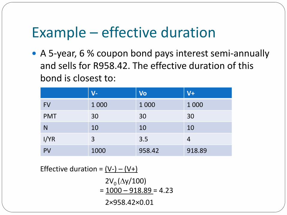
Example – effective duration A 5-year, 6 % coupon bond pays interest semi-annually
and sells for R958.42. The effective duration of this bond is closest to:
Effective duration = (V-) – (V+)
2V0 ( y/100)= 1000 – 918.89 = 4.23
2×958.42×0.01
V- Vo V+
FV 1 000 1 000 1 000
PMT 30 30 30
N 10 10 10
I/YR 3 3.5 4
PV 1000 958.42 918.89
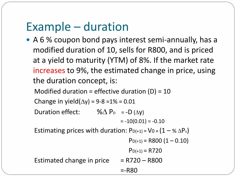
Example – duration A 6 % coupon bond pays interest semi-annually, has a
modified duration of 10, sells for R800, and is priced at a yield to maturity (YTM) of 8%. If the market rate increases to 9%, the estimated change in price, using the duration concept, is:Modified duration = effective duration (D) = 10
Change in yield( y) = 9-8 =1% = 0.01
Duration effect: % PD = -D ( y)
= -10(0.01) = -0.10
Estimating prices with duration: PD(+1) = V0 × (1 – % PD)
PD(+1) = R800 (1 – 0.10)
PD(+1) = R720
Estimated change in price = R720 – R800
=-R80
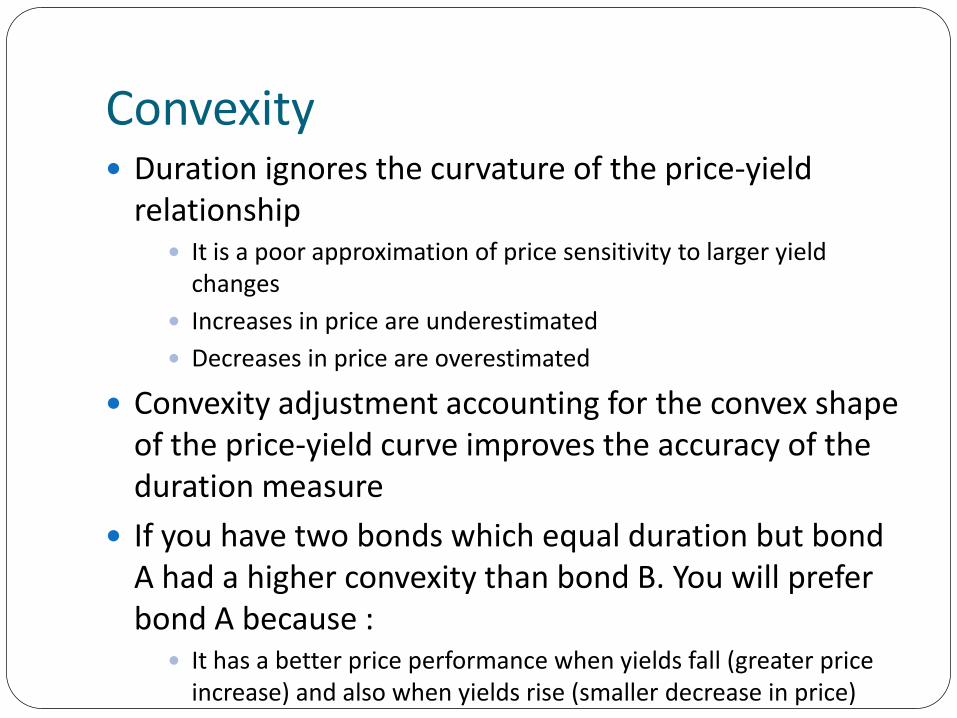
Convexity Duration ignores the curvature of the price-yield
relationship It is a poor approximation of price sensitivity to larger yield
changes
Increases in price are underestimated
Decreases in price are overestimated
Convexity adjustment accounting for the convex shape of the price-yield curve improves the accuracy of the duration measure
If you have two bonds which equal duration but bond A had a higher convexity than bond B. You will prefer bond A because : It has a better price performance when yields fall (greater price
increase) and also when yields rise (smaller decrease in price)
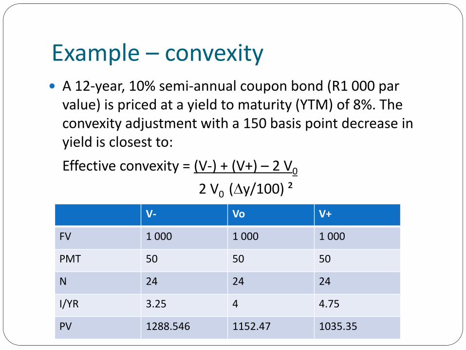
Example – convexity A 12-year, 10% semi-annual coupon bond (R1 000 par
value) is priced at a yield to maturity (YTM) of 8%. The convexity adjustment with a 150 basis point decrease in yield is closest to:
Effective convexity = (V-) + (V+) – 2 V0
2 V0 ( y/100) ²
V- Vo V+
FV 1 000 1 000 1 000
PMT 50 50 50
N 24 24 24
I/YR 3.25 4 4.75
PV 1288.546 1152.47 1035.35
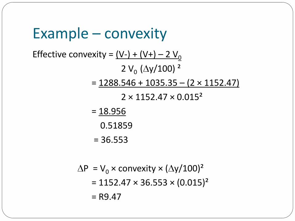
Example – convexityEffective convexity = (V-) + (V+) – 2 V0
2 V0 ( y/100) ²
= 1288.546 + 1035.35 – (2 × 1152.47)
2 × 1152.47 × 0.015²
= 18.956
0.51859
= 36.553
P = V0 × convexity × ( y/100)²
= 1152.47 × 36.553 × (0.015)²
= R9.47

TOPIC 4
PORTFOLIO MANAGEMENT
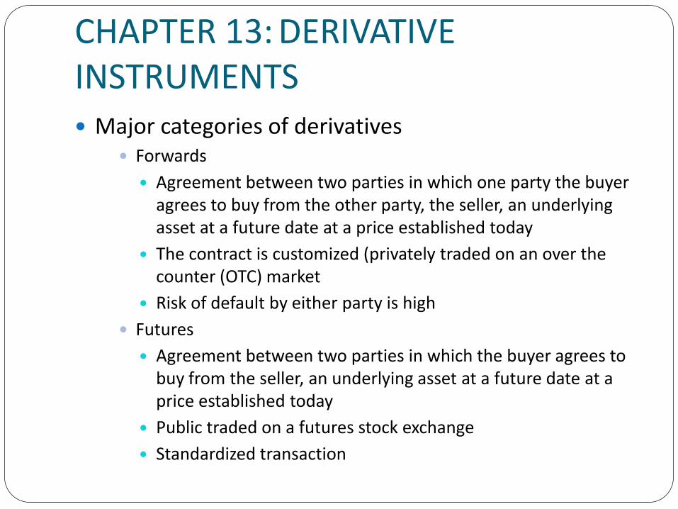
CHAPTER 13: DERIVATIVE INSTRUMENTS Major categories of derivatives
Forwards
Agreement between two parties in which one party the buyer agrees to buy from the other party, the seller, an underlying asset at a future date at a price established today
The contract is customized (privately traded on an over the counter (OTC) market
Risk of default by either party is high
Futures
Agreement between two parties in which the buyer agrees to buy from the seller, an underlying asset at a future date at a price established today
Public traded on a futures stock exchange
Standardized transaction
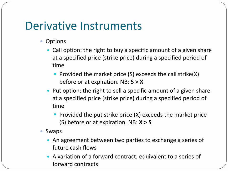
Derivative Instruments Options
Call option: the right to buy a specific amount of a given share at a specified price (strike price) during a specified period of time
Provided the market price (S) exceeds the call strike(X) before or at expiration. NB: S > X
Put option: the right to sell a specific amount of a given share at a specified price (strike price) during a specified period of time
Provided the put strike price (X) exceeds the market price (S) before or at expiration. NB: X > S
Swaps
An agreement between two parties to exchange a series of future cash flows
A variation of a forward contract; equivalent to a series of forward contracts
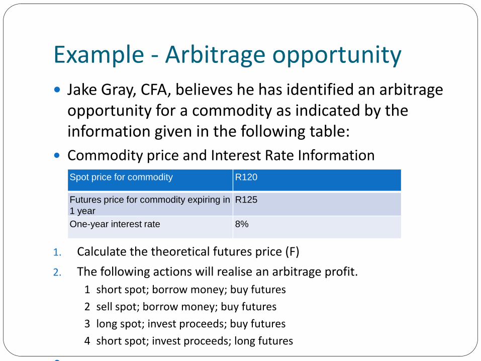
Example - Arbitrage opportunity Jake Gray, CFA, believes he has identified an arbitrage
opportunity for a commodity as indicated by the information given in the following table:
Commodity price and Interest Rate Information
1. Calculate the theoretical futures price (F)
2. The following actions will realise an arbitrage profit.
1 short spot; borrow money; buy futures
2 sell spot; borrow money; buy futures
3 long spot; invest proceeds; buy futures
4 short spot; invest proceeds; long futures
Spot price for commodity R120
Futures price for commodity expiring in
1 year
R125
One-year interest rate 8%
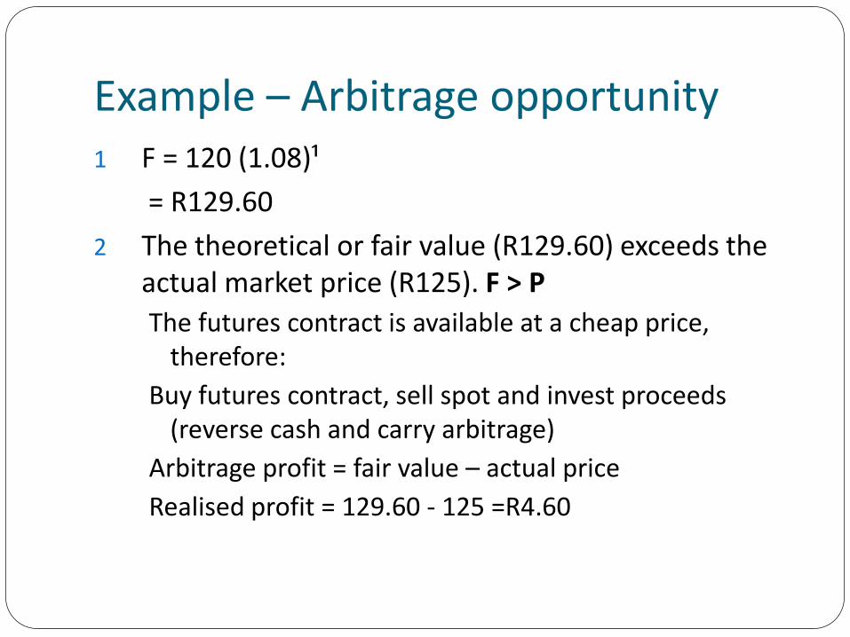
Example – Arbitrage opportunity1 F = 120 (1.08)¹
= R129.60
2 The theoretical or fair value (R129.60) exceeds the actual market price (R125). F > P
The futures contract is available at a cheap price, therefore:
Buy futures contract, sell spot and invest proceeds (reverse cash and carry arbitrage)
Arbitrage profit = fair value – actual price
Realised profit = 129.60 - 125 =R4.60
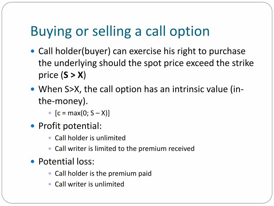
Buying or selling a call option Call holder(buyer) can exercise his right to purchase
the underlying should the spot price exceed the strike price (S > X)
When S>X, the call option has an intrinsic value (in-the-money). [c = max(0; S – X)]
Profit potential: Call holder is unlimited
Call writer is limited to the premium received
Potential loss: Call holder is the premium paid
Call writer is unlimited
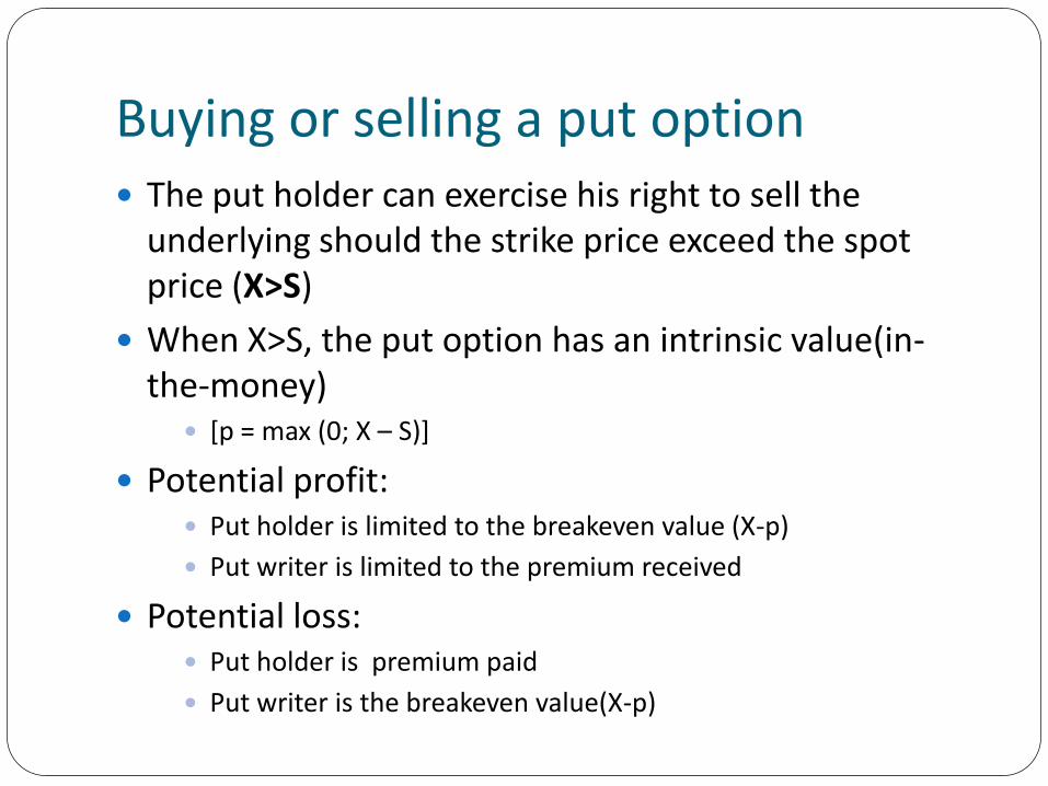
Buying or selling a put option The put holder can exercise his right to sell the
underlying should the strike price exceed the spot price (X>S)
When X>S, the put option has an intrinsic value(in-the-money) [p = max (0; X – S)]
Potential profit: Put holder is limited to the breakeven value (X-p)
Put writer is limited to the premium received
Potential loss: Put holder is premium paid
Put writer is the breakeven value(X-p)
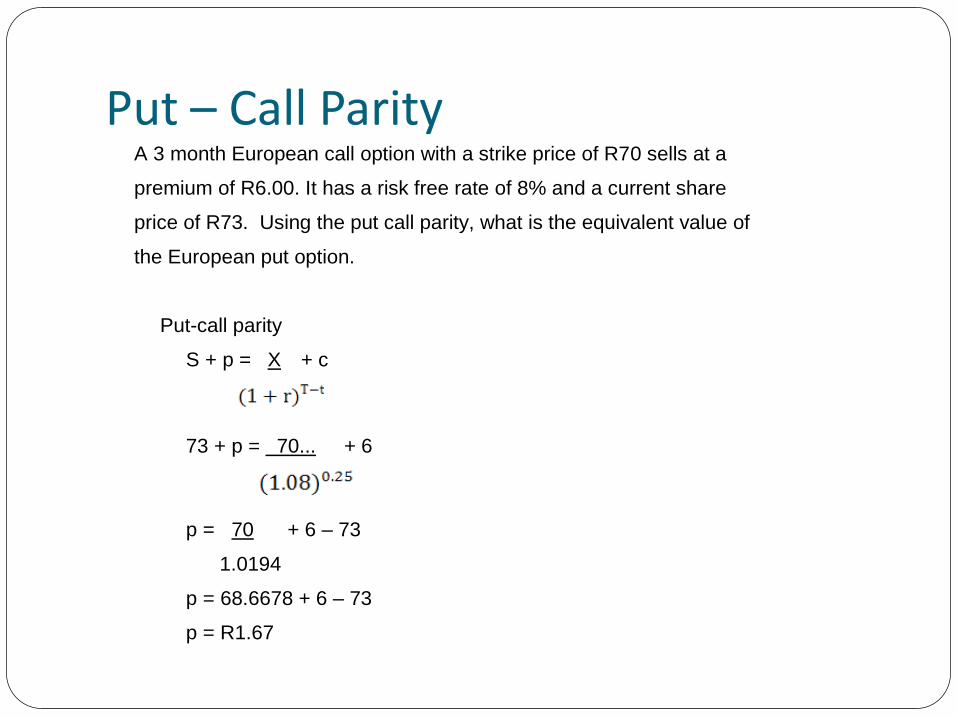
Put – Call ParityA 3 month European call option with a strike price of R70 sells at a
premium of R6.00. It has a risk free rate of 8% and a current share
price of R73. Using the put call parity, what is the equivalent value of
the European put option.
Put-call parity
S + p = X + c
73 + p = 70... + 6
p = 70 + 6 – 73
1.0194
p = 68.6678 + 6 – 73
p = R1.67
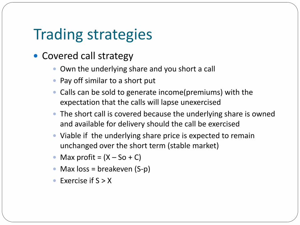
Trading strategies Covered call strategy
Own the underlying share and you short a call
Pay off similar to a short put
Calls can be sold to generate income(premiums) with the expectation that the calls will lapse unexercised
The short call is covered because the underlying share is owned and available for delivery should the call be exercised
Viable if the underlying share price is expected to remain unchanged over the short term (stable market)
Max profit = (X – So + C)
Max loss = breakeven (S-p)
Exercise if S > X
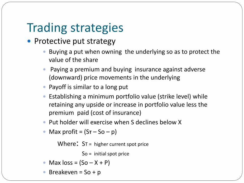
Trading strategies Protective put strategy
Buying a put when owning the underlying so as to protect the value of the share
Paying a premium and buying insurance against adverse (downward) price movements in the underlying
Payoff is similar to a long put
Establishing a minimum portfolio value (strike level) while retaining any upside or increase in portfolio value less the premium paid (cost of insurance)
Put holder will exercise when S declines below X
Max profit = (ST – So – p)
Where: ST = higher current spot price
So = initial spot price
Max loss = (So – X + P)
Breakeven = So + p
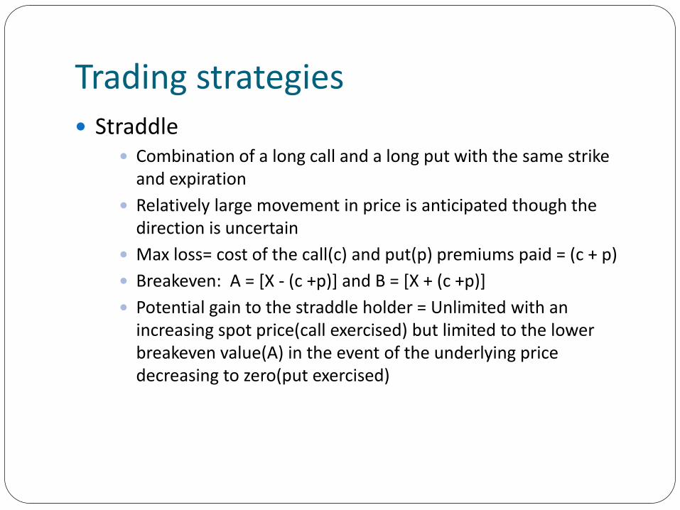
Trading strategies Straddle
Combination of a long call and a long put with the same strike and expiration
Relatively large movement in price is anticipated though the direction is uncertain
Max loss= cost of the call(c) and put(p) premiums paid = (c + p)
Breakeven: A = [X - (c +p)] and B = [X + (c +p)]
Potential gain to the straddle holder = Unlimited with an increasing spot price(call exercised) but limited to the lower breakeven value(A) in the event of the underlying price decreasing to zero(put exercised)
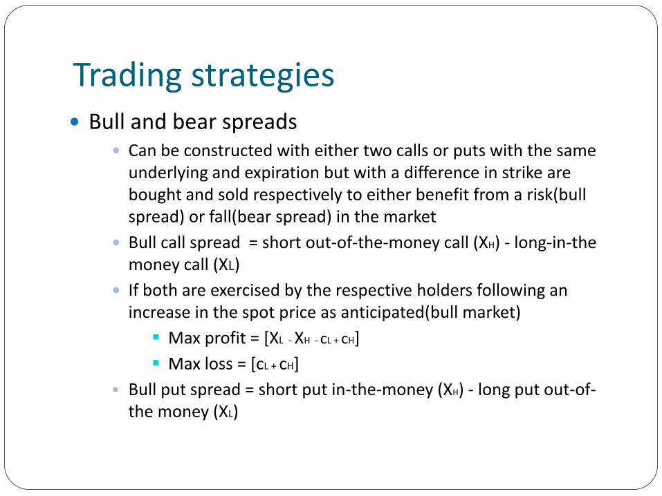
Trading strategies Bull and bear spreads
Can be constructed with either two calls or puts with the same underlying and expiration but with a difference in strike are bought and sold respectively to either benefit from a risk(bull spread) or fall(bear spread) in the market
Bull call spread = short out-of-the-money call (XH) - long-in-the money call (XL)
If both are exercised by the respective holders following an increase in the spot price as anticipated(bull market)
Max profit = [XL - XH - cL + cH]
Max loss = [cL + cH]
Bull put spread = short put in-the-money (XH) - long put out-of-the money (XL)
CHAPTER 14:PORTFOLIO MANAGEMENT Life cycle phase of an individual investor
Accumulation phase
Consolidation phase
Spending phase
Objectives of the investor Capital preservation
Capital appreciation
Current income
Constraints Liquidity and time horizon
Tax concerns
Legal and regulatory factors
Unique needs and personal preferences
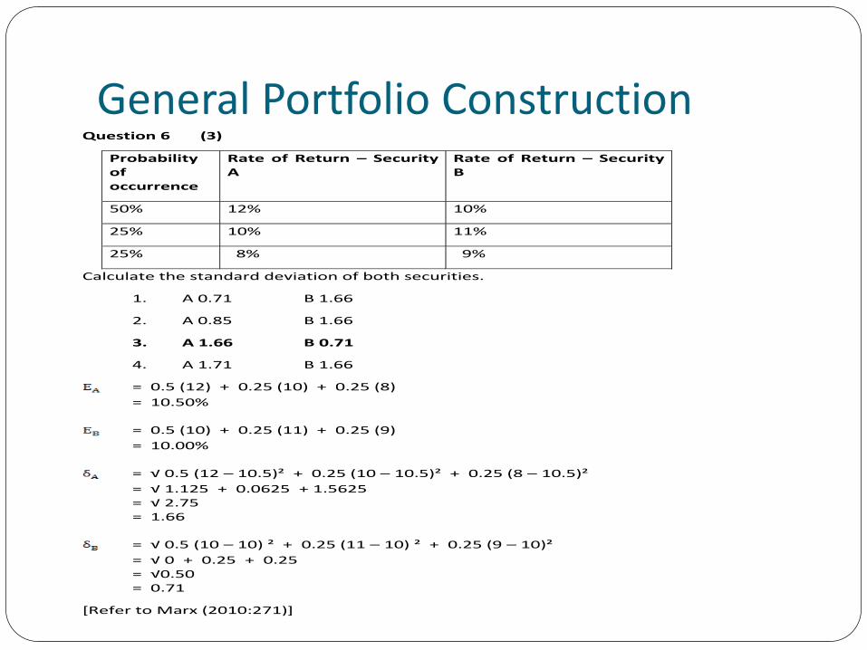
General Portfolio ConstructionQuestion 6 (3)
Probability of occurrence
Rate of Return – Security A
Rate of Return – Security B
50% 12% 10%
25% 10% 11%
25% 8% 9%
Calculate the standard deviation of both securities.
1. A 0.71 B 1.66
2. A 0.85 B 1.66
3. A 1.66 B 0.71
4. A 1.71 B 1.66
= 0.5 (12) + 0.25 (10) + 0.25 (8)
= 10.50%
= 0.5 (10) + 0.25 (11) + 0.25 (9)
= 10.00%
= √ 0.5 (12 – 10.5)² + 0.25 (10 – 10.5)² + 0.25 (8 – 10.5)²
= √ 1.125 + 0.0625 + 1.5625 = √ 2.75 = 1.66
= √ 0.5 (10 – 10) ² + 0.25 (11 – 10) ² + 0.25 (9 – 10)²
= √ 0 + 0.25 + 0.25 = √0.50 = 0.71
[Refer to Marx (2010:271)]
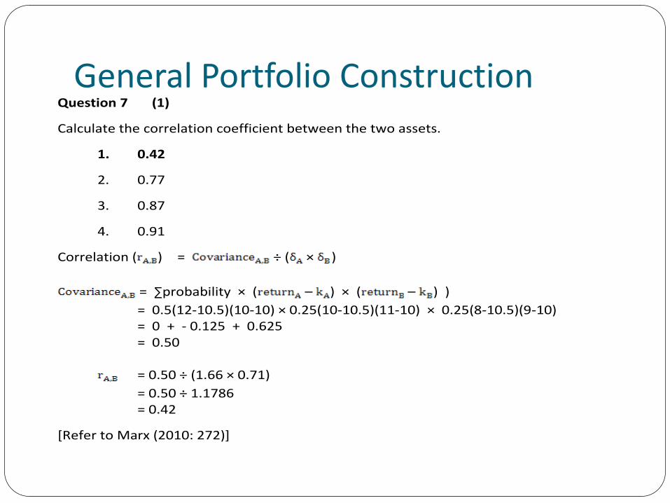
General Portfolio ConstructionQuestion 7 (1)
Calculate the correlation coefficient between the two assets.
1. 0.42
2. 0.77
3. 0.87
4. 0.91
Correlation ( ) = ÷ ( × )
= ∑probability × ( – ) × ( – ) )
= 0.5(12-10.5)(10-10) × 0.25(10-10.5)(11-10) × 0.25(8-10.5)(9-10) = 0 + - 0.125 + 0.625 = 0.50 = 0.50 ÷ (1.66 × 0.71)
= 0.50 ÷ 1.1786 = 0.42
[Refer to Marx (2010: 272)]
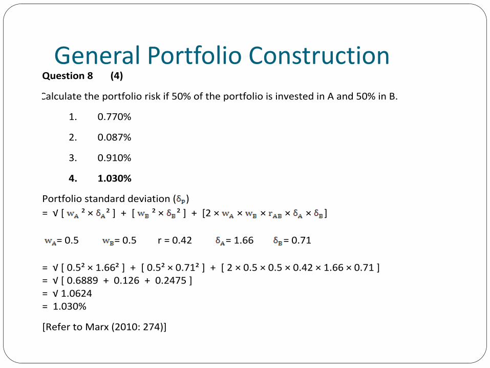
General Portfolio ConstructionQuestion 8 (4)
Calculate the portfolio risk if 50% of the portfolio is invested in A and 50% in B.
1. 0.770%
2. 0.087%
3. 0.910%
4. 1.030%
Portfolio standard deviation ( )
= √ * ² × ² ] + [ ² × ² ] + [2 × × × × × ]
= 0.5 = 0.5 r = 0.42 = 1.66 = 0.71
= √ * 0.5² × 1.66² + + * 0.5² × 0.71² + + * 2 × 0.5 × 0.5 × 0.42 × 1.66 × 0.71 + = √ * 0.6889 + 0.126 + 0.2475 + = √ 1.0624 = 1.030%
[Refer to Marx (2010: 274)]
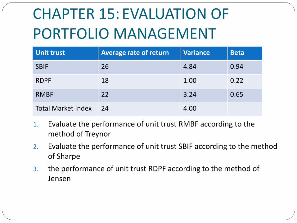
CHAPTER 15: EVALUATION OF PORTFOLIO MANAGEMENT
1. Evaluate the performance of unit trust RMBF according to the method of Treynor
2. Evaluate the performance of unit trust SBIF according to the method of Sharpe
3. the performance of unit trust RDPF according to the method of Jensen
Unit trust Average rate of return Variance Beta
SBIF 26 4.84 0.94
RDPF 18 1.00 0.22
RMBF 22 3.24 0.65
Total Market Index 24 4.00
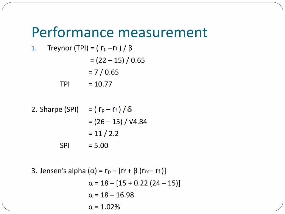
Performance measurement1. Treynor (TPI) = ( rp –rf ) / β
= (22 – 15) / 0.65
= 7 / 0.65
TPI = 10.77
2. Sharpe (SPI) = ( rp – rf ) /
= (26 – 15) / √4.84
= 11 / 2.2
SPI = 5.00
3. Jensen’s alpha (α) = rp – [rf + β (rm– rf )]
α = 18 – [15 + 0.22 (24 – 15)]
α = 18 – 16.98
α = 1.02%

Good luck in your exam!!
Related Documents


![FAC1502+Discussion+Class+Slides+2012+ +First+Semester[1]](https://static.cupdf.com/doc/110x72/544e61ecb1af9f23638b4db5/fac1502discussionclassslides2012-firstsemester1.jpg)