Introductory concepts for control engineeering

Introductory concepts forcontrol engineeering

José Ruiz Ascencio

Vocabulary

• Input u(t)

• Plant H(s), G(s), dy/dt + a*y = u

• Output y(t)

• State x(t)

• Feedback

• Controller

• Setpoint, reference, command

•

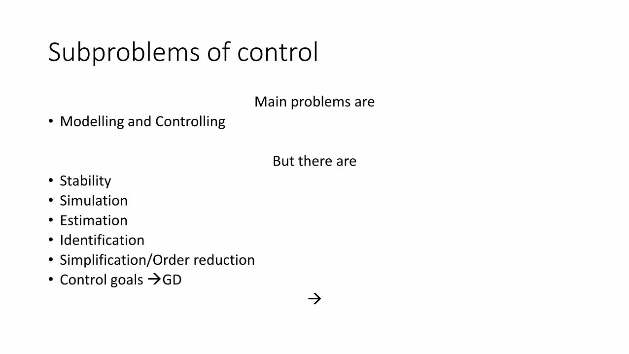
Subproblems of control

Main problems are

• Modelling and Controlling

But there are

• Stability

• Simulation

• Estimation

• Identification

• Simplification/Order reduction

• Control goalsGD

Benefits of feedback

• A system with feedback will be robust:• Behavior will depend less on the plant and more on the feedback and the

controller

• Feedback can be used to give the system a reference model• Specified dynamics, different from those of the plant

• E.g. making it behave like a second order system, when the plant isactually of higher order

• Linear, when the plant is not.

• CONTINUE w-GD-28

Recap

• Modelling• First principles by means of ODE’s, physics.

• Identification• Transient (e.g step) response.• Frequency response

• Simulation (3-step) of an ODE in Simulink (or other)

• Experimental• Requires collecting data, plus some theory

• Today• Data driven modelling through the state evolution function

ⅆ𝑦

ⅆ𝑡+ 𝑎𝑦 = 𝑢

Simulink simulations of PID control

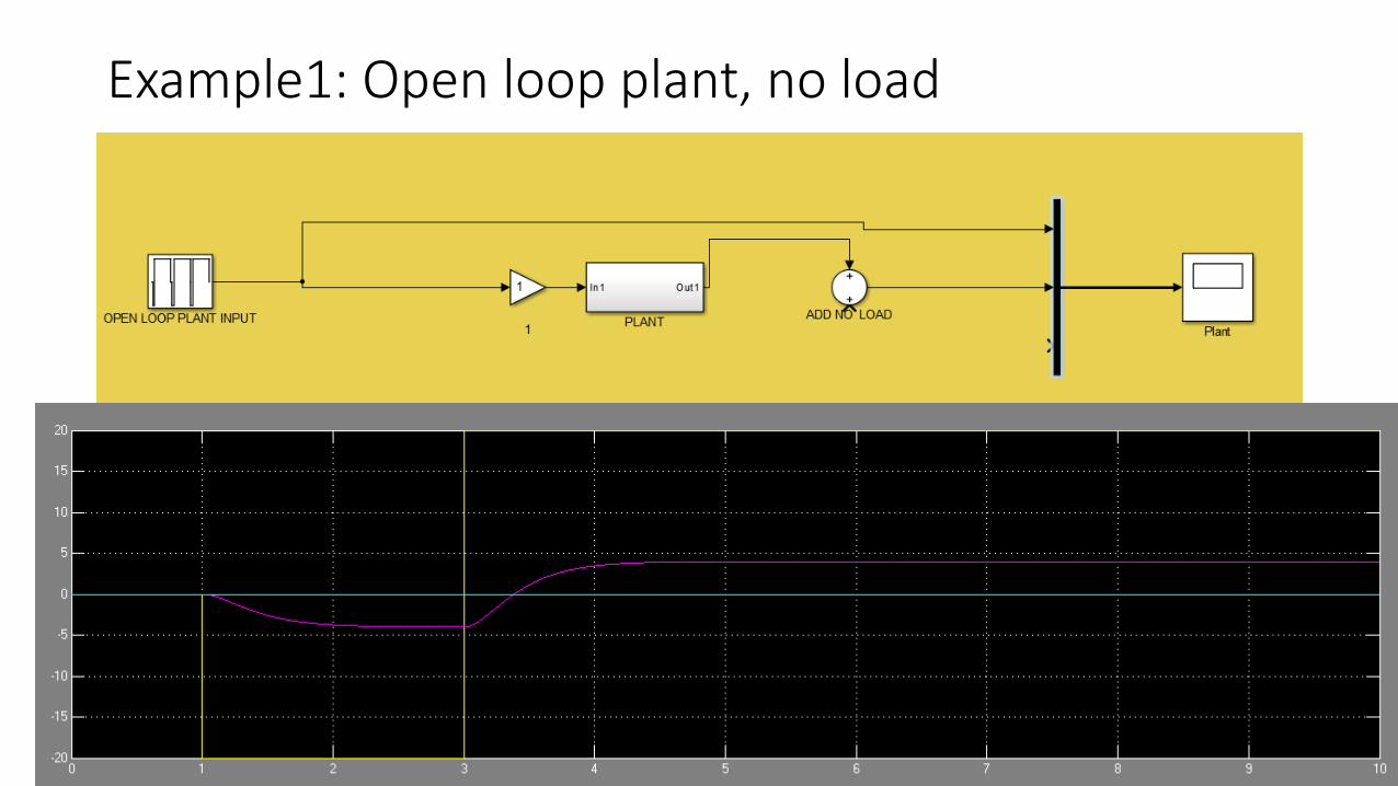
Example1: Open loop plant, no load

Example1: Open loop w/gain, when load appears

Signal traces• Yellow Setpoint

• Pink Output

• Blue Load

• Red Error

• Green Control (plant input)

Example1: Bang-bang control

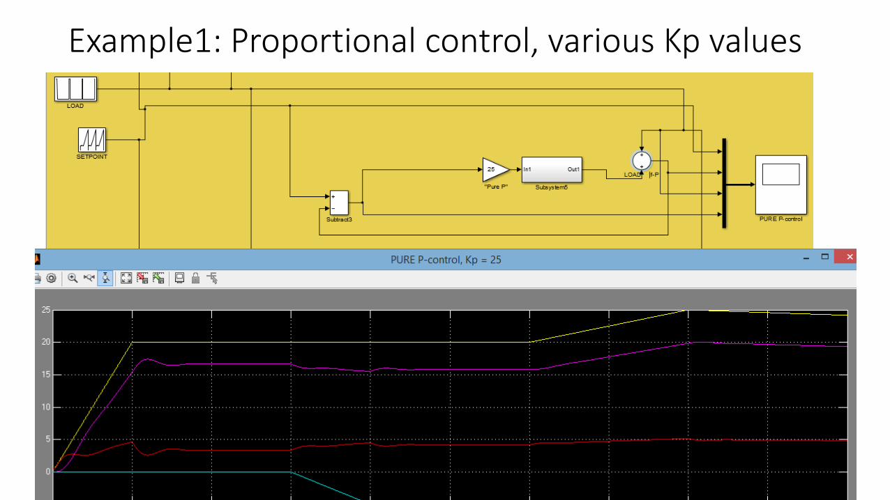
Example1: Proportional control, various Kp values

Example1: Proportional control, Kp = 60, 120

Example1: From P to PD control. Dampened with Kd?

Example1: PD Control, Kp = 120, Kd = 12, 24

This “anticipation” effect is nota good idea, and the overshootis worse…

Example1: PID control

Long-tem control behaviour, Proportional (Green) vs Integral (Red) components

Data driven modelling and control• Since all the signals that appear are functions of time,

• e.g. u(t), y(t), x(t), we will drop the (t), excepto where necessary to make a point.

• Let’s (=*equating objects of different nature)

•y[t1, t2] =* y(t), t ϵ [t1, t2]• For a deterministic and causal system

•y[t1, t2] = F{x(t1), y[t1, t2] }•y(t1) = f(x(t1), u(t1))

Data driven modelling and control• The state evolution function

•x(t2) = φ[x(t1), u[t1, t2) ] for a time invariant system

•x(t + T) = φ[x(t), u[t, t+T) ] sampled uniformly at T.

• Key simplification: admit only staircase inputs:

•u[t1, t2) =* u(t1)• That is the way computers work, so it is not a limitation.

Approximation of state evolution function

• We use Nomura’s algorithm, but backpropagation neural network or ANFIS (neurofuzzy algorithm) or any Arbitrary Function Approximator in N dimensions will give the same result.

• Although Nomura’s algorithm is slower, this implementation is very goodfor teaching purposes.

H. Nomura, I. Hayashi, N. Wakami,A learning method of fuzzy inference rules by descent method, IEEE International Conference on Fuzzy Systems. San Diego, CA, USA, 8-12 March 1992.

Data acquisition

• Inputs are “staircased” (sampled with zero-order hold)

• Outputs are sampled synchronously for acquisition

• Antecedents are delayed to correspond with consequents

First-order data samples of system

t u(t) x(t) x(t + T)

First-order samples and tuned surface: Input is not rich enough

Samples are more dispersed, will give better tunng. They are notconfined to the plane, which means order is greater than one.

Test fuzzy model with a different input, no random component (forclarity), compare against original system.

Modelling via approximation of the stateevolution function• The first-order fuzzy model approximates the plant reasonably well,

even though:

• The system order is (approximately) two (plus a small delay).

• Tha samples are not well distributed

• When we tune a second or greater -order model, it is imposible to plot the surface, so we have to trust the tuning error as an indicator.