Introduction to Volume Rendering Jon Johansson Academic Information and Communication Technologies November 30, 2005

Introduction to Volume Rendering Jon Johansson Academic Information and Communication Technologies November 30, 2005 Jon Johansson Academic Information.
Dec 26, 2015
Welcome message from author
This document is posted to help you gain knowledge. Please leave a comment to let me know what you think about it! Share it to your friends and learn new things together.
Transcript

Introduction to Volume Rendering
Introduction to Volume Rendering
Jon JohanssonAcademic Information and Communication Technologies
November 30, 2005
Jon JohanssonAcademic Information and Communication Technologies
November 30, 2005

Volume DataVolume Data
• Volumes of data can be measured or generated
• measured: CT, MRI, Ultrasound• modeled: atmospheric models, air flow
over wing• The big question:
If your data is represented as a solid volume of points, how do you see the internal structure?
• Volumes of data can be measured or generated
• measured: CT, MRI, Ultrasound• modeled: atmospheric models, air flow
over wing• The big question:
If your data is represented as a solid volume of points, how do you see the internal structure?

Volume DataVolume Data
• we have looked at some techniques to extract geometric objects within a volume of data
• these techniques fall under the heading “Volume Visualization”
• many data sets for volume rendering are composed of a Cartesian grid with data values at each node
• we have looked at some techniques to extract geometric objects within a volume of data
• these techniques fall under the heading “Volume Visualization”
• many data sets for volume rendering are composed of a Cartesian grid with data values at each node

Volume DataVolume Data
• AVS/Express sample data set hydrogen.fld
• three-dimensional, uniform volume with byte data (integers [0, 255])
• grid dimensions: – 64x64x64 262,122
points– 633 voxels (volume
elements)
• transparent isosurfaces can show how the field behaves quite nicely
• AVS/Express sample data set hydrogen.fld
• three-dimensional, uniform volume with byte data (integers [0, 255])
• grid dimensions: – 64x64x64 262,122
points– 633 voxels (volume
elements)
• transparent isosurfaces can show how the field behaves quite nicely

Volume DataVolume Data
• the data values are separated by constant spacing on a Cartesian grid
• the connections are regular, forming hexahedrons (cubes in this case actually)
• the smallest connected volumes are called Voxels (volume elements)
• the data values are separated by constant spacing on a Cartesian grid
• the connections are regular, forming hexahedrons (cubes in this case actually)
• the smallest connected volumes are called Voxels (volume elements)

Volume DataVolume Data

Volume DataVolume Data
• a voxel typically has data values associated with the corner points
• to find a data value at an arbitrary location in the voxel we need to interpolate
• commonly use tri-linear interpolation
• some data sets will have a single data value for the volume (referred to as cell data)
• a voxel typically has data values associated with the corner points
• to find a data value at an arbitrary location in the voxel we need to interpolate
• commonly use tri-linear interpolation
• some data sets will have a single data value for the volume (referred to as cell data)

Volume DataVolume Data
• we are now going to look at rendering volumetric data directly instead of constructing geometric primitives
• treat the volume as being composed of semitransparent material– transmits and absorbs light– light is scattered by the particles
• we are now going to look at rendering volumetric data directly instead of constructing geometric primitives
• treat the volume as being composed of semitransparent material– transmits and absorbs light– light is scattered by the particles

Volume DataVolume Data
• we can see into the volume depending on how transparent the material is:– transparency → fraction of light that passes through a
surface or an object; = 1 all light passes– opacity → fraction of light that is absorbed at a
surface or an object; opacity = 1 no light passes– opacity = 1 – transparency
• transparency commonly refers to visible light• it can actually refer to any type of radiation: e.g..
flesh is transparent to X-rays, while bone is not, allowing the use of medical X-ray machines

Volume DataVolume Data

Volume RenderingVolume Rendering• techniques for volume rendering
– ray casting• J. T. Kajiya, B. P. V. Herzen, "Ray Tracing Volume Densities,"
Computer Graphics, 1984, Vol. 18, No. 3, pp. 165-174 – splatting
• Westover, L., “Splatting: A Parallel, Feed-Forward Volume Rendering Algorithm”. PhD Dissertation, July 1991
– hardware texture memory• Brian Cabral , Nancy Cam , Jim Foran, “Accelerated volume
rendering and tomographic reconstruction using texture mapping hardware”, Proceedings of the 1994 symposium on Volume visualization, p.91-98, October 17-18, 1994, Tysons Corner, Virginia, United States
– shear-warp factorization• Philippe Lacroute and Marc Levoy, “Fast Volume Rendering Using a
Shear-Warp Factorization of the Viewing Transformation”, Proc. SIGGRAPH '94, Orlando, Florida, July, 1994, pp. 451-458
• techniques for volume rendering – ray casting
• J. T. Kajiya, B. P. V. Herzen, "Ray Tracing Volume Densities," Computer Graphics, 1984, Vol. 18, No. 3, pp. 165-174
– splatting• Westover, L., “Splatting: A Parallel, Feed-Forward Volume
Rendering Algorithm”. PhD Dissertation, July 1991
– hardware texture memory• Brian Cabral , Nancy Cam , Jim Foran, “Accelerated volume
rendering and tomographic reconstruction using texture mapping hardware”, Proceedings of the 1994 symposium on Volume visualization, p.91-98, October 17-18, 1994, Tysons Corner, Virginia, United States
– shear-warp factorization• Philippe Lacroute and Marc Levoy, “Fast Volume Rendering Using a
Shear-Warp Factorization of the Viewing Transformation”, Proc. SIGGRAPH '94, Orlando, Florida, July, 1994, pp. 451-458

Ray CastingRay Casting
• a widely used ray casting technique is based on the model of Blinn and Kajiya
• in order to find the color of a pixel in the image:– send a ray R through the volume
• the material has a density D(x,y,z) = D(t) varying in space
• parameterize movement along the ray by t [t1, t2]
– at each point there is an illumination I(x,y,z) = I(t) from any light sources
– determining the illumination function is difficult since it depends on how light is attenuated by the material in the volume
• in many calculations I(x,y,z) = I(t) = constant

Ray CastingRay Casting

Ray CastingRay Casting
• the attenuation of radiation due to the density along the ray can be calculated as
• the attenuation of radiation due to the density along the ray can be calculated as
• the intensity of light arriving at the eye along the ray due to all points between t1 and t2 is then
• the intensity of light arriving at the eye along the ray due to all points between t1 and t2 is then
2
1
expt
tdssD
dtPtDtIdssDBt
t
t
t
2
1 1
)(cosexp

Ray CastingRay Casting
• to take away from this, in this ray casting calculation we want to find the intensity of light for a pixel in our image– calculate the attenuation of light along the ray:
integrate along the ray through the volume– calculate the intensity of light reaching the image
location – integrate along the ray again– to include lighting effects we need to calculate the
amount of light from the sources reaching each point along the ray – more integration
– multiple scattering effects – lots more integrations

Ray CastingRay Casting
• in order to do the integrations along the rays we need to find values of the scalar field at arbitrary positions in a voxel
• use Trilinear Interpolation– 4 1-D interps in x– 2 1-D interps in y– 1 1-D interps in z
• in order to do the integrations along the rays we need to find values of the scalar field at arbitrary positions in a voxel
• use Trilinear Interpolation– 4 1-D interps in x– 2 1-D interps in y– 1 1-D interps in z

Volume Rendering – HardwareVolume Rendering – Hardware
• volume rendering seems like it might benefit from hardware acceleration
• VolumePro by TeraRecon– PCI card for PCs– real-time 3D volume rendering
of volumes up to 512x512x512
• there are other solutions as well of course
• volume rendering seems like it might benefit from hardware acceleration
• VolumePro by TeraRecon– PCI card for PCs– real-time 3D volume rendering
of volumes up to 512x512x512
• there are other solutions as well of course

Volume Rendering – SoftwareVolume Rendering – Software
• many visualization packages have volume rendering capability
• AVS/Express – Advanced Visual Systems
• VTK (Visualization Toolkit) – Kitware
• VolView – based on VTK from Kitware– commercial system which focuses on volume
rendering– has support for the VolumePro card
• many visualization packages have volume rendering capability
• AVS/Express – Advanced Visual Systems
• VTK (Visualization Toolkit) – Kitware
• VolView – based on VTK from Kitware– commercial system which focuses on volume
rendering– has support for the VolumePro card

Volume RenderingVolume Rendering
• the entire body of 3D data must be processed each time an image is drawn or displayed
• imaginary "rays" are cast through the data, picking up color and opacity as they traverse it
• the rays are then projected onto a computer screen or display surface
• to make the image move or to manipulate it interactively, the data is re-processed in rapid succession, fast enough for interactive frame rates – this needs fast hardware.

Volume RenderingVolume Rendering
• in order to render a 3D volume into a 2D image we need to:– cast the rays through the volume – assign color and opacity values to the sample
points – calculate gradients and assign lighting to the
image – sum up all the color and opacity values to
create the image
• in order to render a 3D volume into a 2D image we need to:– cast the rays through the volume – assign color and opacity values to the sample
points – calculate gradients and assign lighting to the
image – sum up all the color and opacity values to
create the image

Computed Tomography (CT)Computed Tomography (CT)
• Computed Tomography (CT) or Computed Axial Tomography (CAT)
• uses a combination of X-rays and computer technology to produce cross-sectional images of the body
• an x-ray tube rotates in a circle around the patient, making many pictures as it rotates
• final slice images are generated utilizing the basic principle that the internal structure of the body can be reconstructed from multiple X-ray projections
• physicians can then examine “slices” through different organs and show detailed images of any part of the body
Computed Tomography (CT)Computed Tomography (CT)
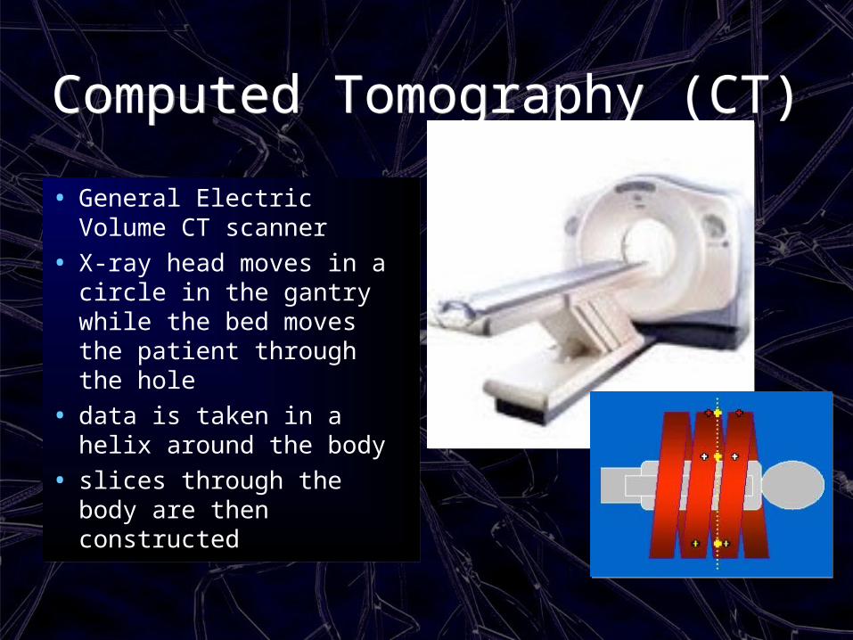
• General Electric Volume CT scanner
• X-ray head moves in a circle in the gantry while the bed moves the patient through the hole
• data is taken in a helix around the body
• slices through the body are then constructed
• General Electric Volume CT scanner
• X-ray head moves in a circle in the gantry while the bed moves the patient through the hole
• data is taken in a helix around the body
• slices through the body are then constructed

Computed Tomography (CT)Computed Tomography (CT)
• image sizes are at most 1024x1024 pixels or less – actual physical resolution depends on a sample size
• scanners can now provide 0.5 mm slice widths for small samples (more usually use 1-10 mm)
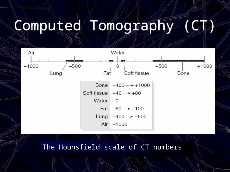
• can distinguish a tissue density difference of 1 percent• CT densities (grey levels) in the range [-1024, 3071]
Hounsfield Units (HU)– Air: -1000 HU (black)– Fat: -50– Water: 0 HU– muscle: +40– Bone: 1000 – 3000 HU (white)
• rescale to [0, 4095] to use unsigned ints
• image sizes are at most 1024x1024 pixels or less – actual physical resolution depends on a sample size
• scanners can now provide 0.5 mm slice widths for small samples (more usually use 1-10 mm)
• can distinguish a tissue density difference of 1 percent• CT densities (grey levels) in the range [-1024, 3071]
Hounsfield Units (HU)– Air: -1000 HU (black)– Fat: -50– Water: 0 HU– muscle: +40– Bone: 1000 – 3000 HU (white)
• rescale to [0, 4095] to use unsigned ints
1000
water
waterobjectHU
Computed Tomography (CT)Computed Tomography (CT)
The Hounsfield scale of CT numbersThe Hounsfield scale of CT numbers

Computed Tomography (CT)Computed Tomography (CT)
• the human eye can’t actually distinguish between 4000 different shades of grey
• “Window Width” (contrast) covers the HU of all the tissues of interest
• “Window Level” (brightness) represents the central HU of all the numbers within the window width
• a visually useful grey scale is achieved by setting the WW and WL to suitable values
• tissues with CT numbers outside the range are displayed as either black or white

Computed Tomography (CT)Computed Tomography (CT)
• in a CT chest exam:– to highlight the soft
tissue, set:• WW = 350
• WL = +40
– to highlight the lung fields (mostly air)
• WW = 1500
• WL = -600
• in a CT chest exam:– to highlight the soft
tissue, set:• WW = 350
• WL = +40
– to highlight the lung fields (mostly air)
• WW = 1500
• WL = -600

Other Volume Data SourcesOther Volume Data Sources
• lots of bio-medical measurement sources– Magnetic Resonance Imaging (MRI) – Positron Emission Tomography (PET) – Single Photon Emission Computed
Tomography (SPECT, ECT) – Ultrasound Imaging – 2-D and 3-D Microscopy Imaging (Light,
Electron, Confocal, Atomic Force)
• lots of bio-medical measurement sources– Magnetic Resonance Imaging (MRI) – Positron Emission Tomography (PET) – Single Photon Emission Computed
Tomography (SPECT, ECT) – Ultrasound Imaging – 2-D and 3-D Microscopy Imaging (Light,
Electron, Confocal, Atomic Force)
Other Volume Data SourcesOther Volume Data Sources
• measurements– seismic data– atmospheric data
• scientific modeling– plasma physics– atmospheric modeling– geophysical earth models
• plenty of others
• measurements– seismic data– atmospheric data
• scientific modeling– plasma physics– atmospheric modeling– geophysical earth models
• plenty of others

Medical Data - DICOMMedical Data - DICOM
• Digital Imaging and Communications in Medicine (DICOM)
• main objective of this standard is to create a vendor independent platform for the communication of medical images and related data
• http://medical.nema.org/dicom/
• Digital Imaging and Communications in Medicine (DICOM)
• main objective of this standard is to create a vendor independent platform for the communication of medical images and related data
• http://medical.nema.org/dicom/

Medical Data - DICOMMedical Data - DICOM
• a set of rules that allow medical images to be exchanged between instruments, computers, and hospitals
• a DICOM file contains:– a header
• stores information about the patient's name, the type of scan, image dimensions, etc.
– all of the image data • which can contain information in three dimensions

Example – CT scanExample – CT scan
• VolView from Kitware– based on the Visualization Toolkit
• look at sample data from the University of North Carolina• Description: CT study of a cadaver head
– Dimensions: 113 slices of 256 x 256 pixels,voxel grid is rectangular, andX:Y:Z aspect ratio of each voxel is 1:1:2
– Files: 113 binary files, one file per slice– File format: 16-bit integers (Mac byte ordering), file contains no
header– Data source: acquired on a General Electric CT Scanner and
provided courtesy of North Carolina Memorial Hospital
Example – CT scanExample – CT scan
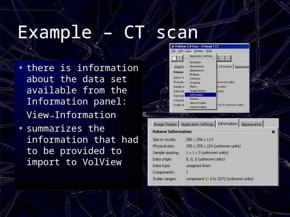
• there is information about the data set available from the Information panel:
View→Information
• summarizes the information that had to be provided to import to VolView
• there is information about the data set available from the Information panel:
View→Information
• summarizes the information that had to be provided to import to VolView
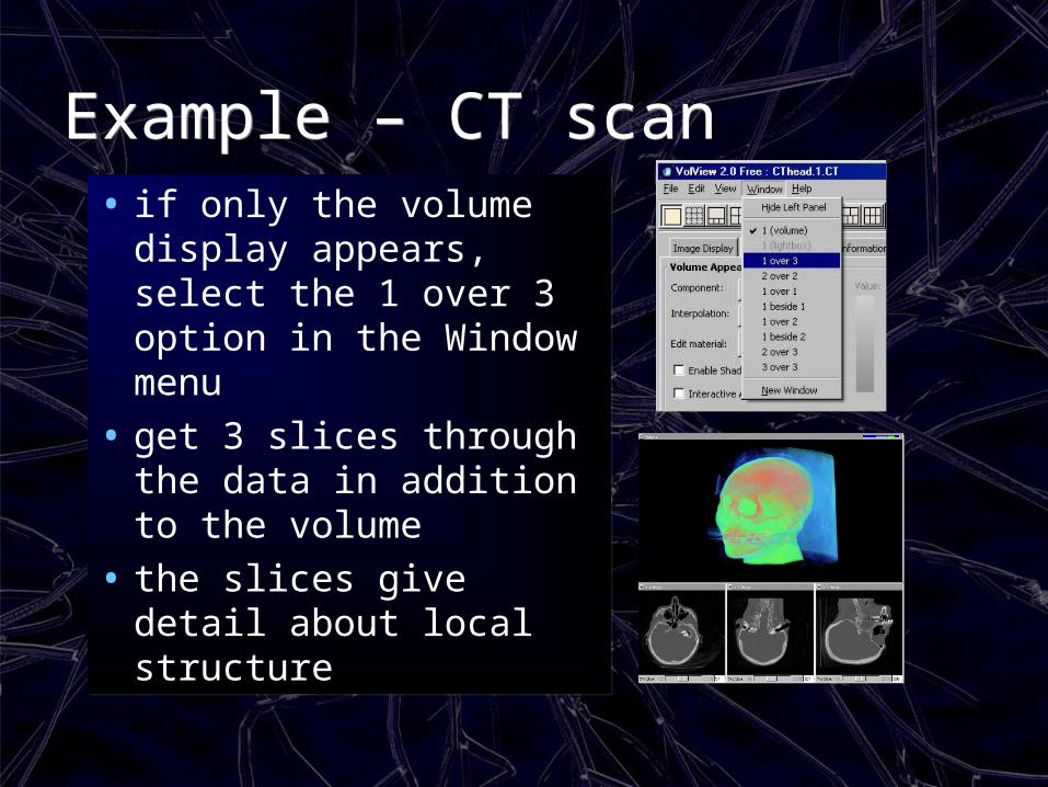
Example – CT scanExample – CT scan• if only the volume display
appears, select the 1 over 3 option in the Window menu
• get 3 slices through the data in addition to the volume
• the slices give detail about local structure
• if only the volume display appears, select the 1 over 3 option in the Window menu
• get 3 slices through the data in addition to the volume
• the slices give detail about local structure

Example – CT scanExample – CT scan
• select Y-Z image from the upper left corner for the Volume window
• the Y-Z slice then occupies the large window
• sliders along the bottom of each window allow a view of a slice at any depth
• select Y-Z image from the upper left corner for the Volume window
• the Y-Z slice then occupies the large window
• sliders along the bottom of each window allow a view of a slice at any depth
Example – CT scanExample – CT scan
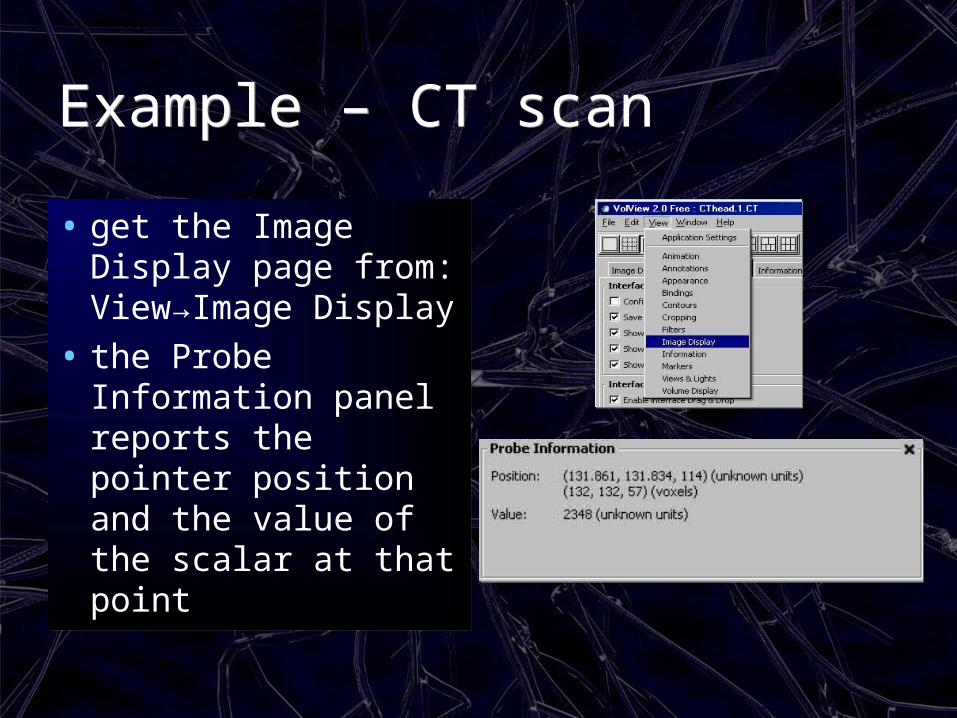
• get the Image Display page from: View→Image Display
• the Probe Information panel reports the pointer position and the value of the scalar at that point
• get the Image Display page from: View→Image Display
• the Probe Information panel reports the pointer position and the value of the scalar at that point
Example – CT scanExample – CT scan
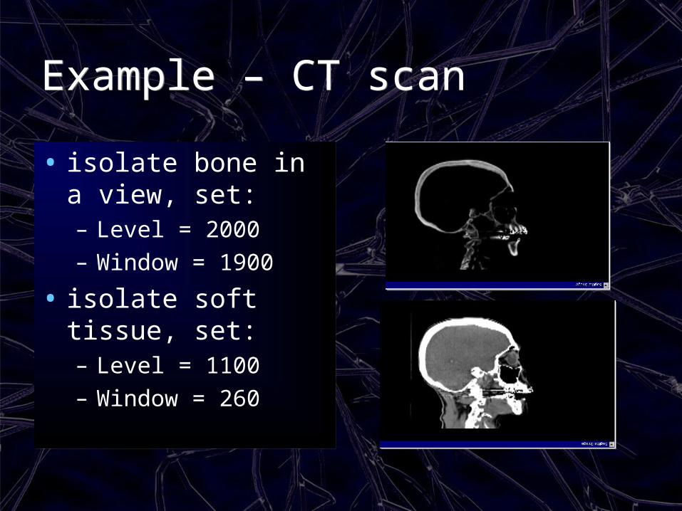
• isolate bone in a view, set:– Level = 2000– Window = 1900
• isolate soft tissue, set:– Level = 1100– Window = 260
• isolate bone in a view, set:– Level = 2000– Window = 1900
• isolate soft tissue, set:– Level = 1100– Window = 260

Example – CT scanExample – CT scan
• choose Volume under the Window menu to get rid of the slice windows
• choose Appearance under the View menu
• the Appearance page controls how the rendering will look
• lots of power here to give us what we want
• choose Volume under the Window menu to get rid of the slice windows
• choose Appearance under the View menu
• the Appearance page controls how the rendering will look
• lots of power here to give us what we want
Example – CT scanExample – CT scan
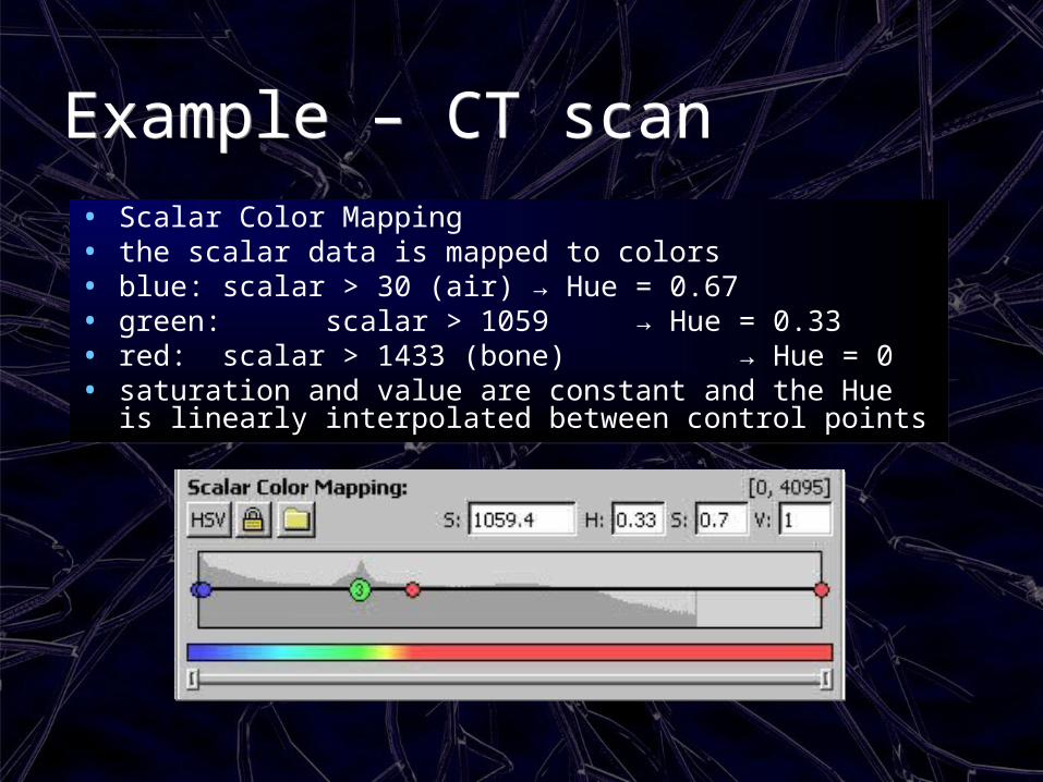
• Scalar Color Mapping• the scalar data is mapped to colors• blue: scalar > 30 (air) → Hue = 0.67 • green: scalar > 1059 → Hue = 0.33• red: scalar > 1433 (bone) → Hue = 0• saturation and value are constant and the Hue is linearly
interpolated between control points
• Scalar Color Mapping• the scalar data is mapped to colors• blue: scalar > 30 (air) → Hue = 0.67 • green: scalar > 1059 → Hue = 0.33• red: scalar > 1433 (bone) → Hue = 0• saturation and value are constant and the Hue is linearly
interpolated between control points

Example – CT scanExample – CT scan
• Scalar Opacity Mapping
• scalar values are given an opacity
• scalar = 0 → opacity = 0
• scalar > 1406 → opacity = 0.2
• Scalar Opacity Mapping
• scalar values are given an opacity
• scalar = 0 → opacity = 0
• scalar > 1406 → opacity = 0.2

Example – CT scanExample – CT scan
• we are seeing the red (less transparent) bone through greenish (more transparent) soft tissue
• we are seeing the red (less transparent) bone through greenish (more transparent) soft tissue

Example – CT scanExample – CT scan
• Gradient Opacity Mapping• at each point in the volume a gradient is
calculated• the gradient magnitude is mapped to the opacity
ramp
• Gradient Opacity Mapping• at each point in the volume a gradient is
calculated• the gradient magnitude is mapped to the opacity
ramp
opacity=0
opacity=1

Example – CT scanExample – CT scan
• places of rapid change in the scalar field are opaque
• areas of constant field are transparent
• we see the boundaries– air → tissue– tissue → bone
• a way to get “surfaces”
• places of rapid change in the scalar field are opaque
• areas of constant field are transparent
• we see the boundaries– air → tissue– tissue → bone
• a way to get “surfaces”

Example – CT scanExample – CT scan
• now adjust color settings
• select the folder icon in the Scalar Color Mapping area
• select the White option to set the color to solid white
• all the scalar data is now mapped to white
• now adjust color settings
• select the folder icon in the Scalar Color Mapping area
• select the White option to set the color to solid white
• all the scalar data is now mapped to white

Example – CT scanExample – CT scan• add a node to the center of
the editing area by left clicking there
• click on the left node to select it and make the color brown (~H=0.05, S=0.76, V=0.92)
• click close to the left node to add another brown node and move it to a scalar value S=725
• move the middle white node to S=810
• add a node to the center of the editing area by left clicking there
• click on the left node to select it and make the color brown (~H=0.05, S=0.76, V=0.92)
• click close to the left node to add another brown node and move it to a scalar value S=725
• move the middle white node to S=810

Example – CT scanExample – CT scan• Modify the Scalar Opacity Mappings to look like this
(points numbered from left to right):• 1 → S = 0, O = 0• 2 → S = 561, O = 0• 3 → S = 620, O = 0.357• 4 → S = 930, O = 0.357• 5 → S = 1194, O = 0.5
• Modify the Scalar Opacity Mappings to look like this (points numbered from left to right):
• 1 → S = 0, O = 0• 2 → S = 561, O = 0• 3 → S = 620, O = 0.357• 4 → S = 930, O = 0.357• 5 → S = 1194, O = 0.5

Example – CT scanExample – CT scan

Example – CT scanExample – CT scan
• the Appearance panel in VolView 2.0 is the most complex interface
• it defines the core parameters that affect the volume rendered image
• this is where the control is for effectively visualizing data!
• the Appearance panel in VolView 2.0 is the most complex interface
• it defines the core parameters that affect the volume rendered image
• this is where the control is for effectively visualizing data!

ConclusionConclusion
• Volume rendering is a powerful tool for visualization and can assist in understanding volumetric data sets
• useful to add to the toolkit to compliment the geometric techniques that we’ve seen earlier.
• Volume rendering is a powerful tool for visualization and can assist in understanding volumetric data sets
• useful to add to the toolkit to compliment the geometric techniques that we’ve seen earlier.
Related Documents