Introduction to Transportation Engineering Prof. …textofvideo.nptel.ac.in/105105107/lec17.pdfLet us start with some common terminologies. We have already discussed that the normal

Introduction to Transportation Engineering Prof. Bhargab Maitra

Department of Civil Engineering Indian Institute of Technology, Kharagpur

Lecture - 17 Horizontal Alignment - IV

(Refer Slide Time: 00:01:00 min)

Horizontal Alignment part IV. Among different design elements we have already discussed about horizontal curves the forces acting on a vehicle, when a vehicle is negotiating horizontal curves, the need for superelevation, the basis for design of superelevation under mixed traffic operation, the different approaches as mentioned in AASHTO for distribution of ‘e’ and ‘f’ superelevation and sight friction factor and also different methods for attainment of superelevation their advantages disadvantages. We have also discussed about the need for providing adequate setback distance and the basis for calculation of setback distance under different conditions. Today we shall discuss about transition curve.

1


After completing this lesson the student will be able to understand basic elements and terminologies related to transition control different terminologies which are commonly used for transition control, the student will be able to understand the need for providing transition curve, why we need to provide transition curve or what are the advantages and also the basis for using spiral transition curve, why a spiral curve is normally recommended as horizontal transition curve. The student will also be able to understand the IRC approach Indian Roads Congress approach for design of the length of transition curve, how the transition curve length is designed as per the approach recommended by the IRC Indian Roads Congress. (Refer Slide Time: 00:03:36 min)

2

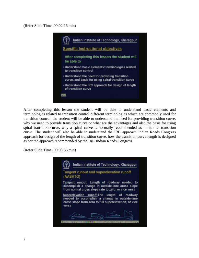
Let us start with some common terminologies. We have already discussed that the normal cambered section is like this. Now, when we are trying to provide superelevation we gradually turn the outer edge, assume the method for rotation of pavement with respect to the central line, rotation of the outer edge with respect to the central line so over a length we rotate it and you find a cross section when the outer edge is rotated and leveled. so this change is done over a length of curve and that part is known as tangent runout. So tangent run out is the length of roadway needed to accomplish a change in outside-lane cross slope from normal cross slope as indicated here this is normal cross slope to 0. This is the cross slope where the outer edge is flat so the slope is 0. So the length of the curve suppose if it is done over a length that length is known as the tangent runout. Now further rotation is done to make it uniform, uniform slope equal to the cross slope of the camber and then it is further rotated to have the required superelevation. So this is stage three and this is stage 4. Now again this change is done over a length so this length where the outer edge from 0 is rotated to attain the full superelevation as shown here is known as superelevation runoff. So superelevation runoff is the length of roadway needed to accomplish a change in outside-lane cross slope from 0 as shown here to full superelevation or vice versa. That is what is known as tangent runout and superelevation runoff. (Refer Slide Time 00:07:09 min)

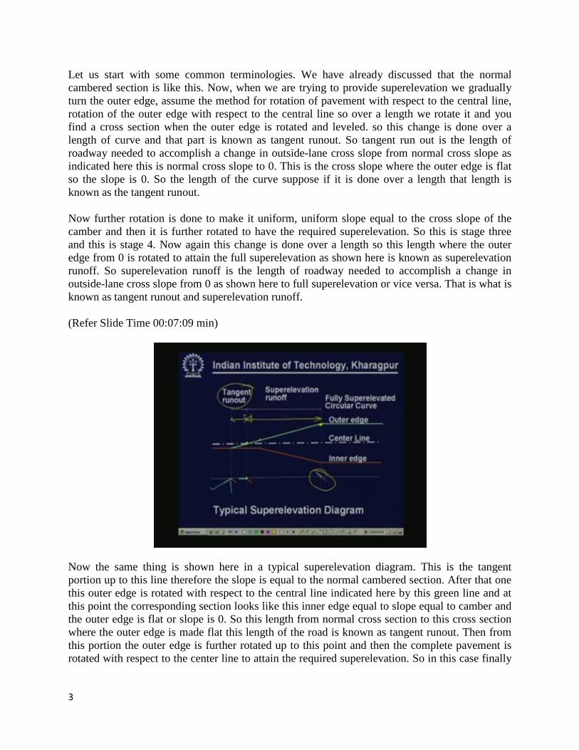
Now the same thing is shown here in a typical superelevation diagram. This is the tangent portion up to this line therefore the slope is equal to the normal cambered section. After that one this outer edge is rotated with respect to the central line indicated here by this green line and at this point the corresponding section looks like this inner edge equal to slope equal to camber and the outer edge is flat or slope is 0. So this length from normal cross section to this cross section where the outer edge is made flat this length of the road is known as tangent runout. Then from this portion the outer edge is further rotated up to this point and then the complete pavement is rotated with respect to the center line to attain the required superelevation. So in this case finally

3

at the beginning of circular curve the section looks like this. so this portion of the length is known as the superelevation runoff. (Refer Slide Time: 00:09:18 min)

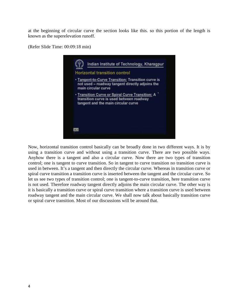
Now, horizontal transition control basically can be broadly done in two different ways. It is by using a transition curve and without using a transition curve. There are two possible ways. Anyhow there is a tangent and also a circular curve. Now there are two types of transition control; one is tangent to curve transition. So in tangent to curve transition no transition curve is used in between. It’s a tangent and then directly the circular curve. Whereas in transition curve or spiral curve transition a transition curve is inserted between the tangent and the circular curve. So let us see two types of transition control; one is tangent-to-curve transition, here transition curve is not used. Therefore roadway tangent directly adjoins the main circular curve. The other way is it is basically a transition curve or spiral curve transition where a transition curve is used between roadway tangent and the main circular curve. We shall now talk about basically transition curve or spiral curve transition. Most of our discussions will be around that.

4


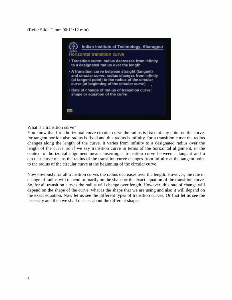
What is a transition curve? You know that for a horizontal curve circular curve the radius is fixed at any point on the curve. for tangent portion also radius is fixed and this radius is infinity. for a transition curve the radius changes along the length of the curve. it varies from infinity to a designated radius over the length of the curve. so if we say transition curve in terms of the horizontal alignment, in the context of horizontal alignment means inserting a transition curve between a tangent and a circular curve means the radius of the transition curve changes from infinity at the tangent point to the radius of the circular curve at the beginning of the circular curve. Now obviously for all transition curves the radius decreases over the length. However, the rate of change of radius will depend primarily on the shape or the exact equation of the transition curve. So, for all transition curves the radius will change over length. However, this rate of change will depend on the shape of the curve, what is the shape that we are using and also it will depend on the exact equation. Now let us see the different types of transition curves. Or first let us see the necessity and then we shall discuss about the different shapes.

5

(Refer slide Time 00:13:26 min)

We have already discussed the forces which are normally acting on a vehicle when a vehicle is negotiating a horizontal curve. On tangent portion the centrifugal force is 0 because the radius is infinity. There may be significant amount of centrifugal force basically W by g into V square by R that will be the amount of the centrifugal force which will act outward and starting from the circular curve the radius is say RC radius of the circular curve therefore there may be a significant amount of centrifugal force depending on the radius of the circular curve and this is certainly a value which is much higher than 0. So on tangent the centrifugal force is 0 and on circular curve it is a finite amount which is a significant amount rather we can say. Now just think of a vehicle which is negotiating a circular curve. So as long as it is on tangent the centrifugal force is 0. The moment it is on circular curve there is a significant amount of centrifugal force and the change is almost sudden because the radius is changing suddenly from infinity to the radius of the circular curve. If a transition curve is used in between, or if a transition curve is inserted in between then the radius will change gradually from infinity to the radius of the circular curve over a length. Therefore centrifugal force also will be introduced gradually and there will be no jerk on vehicle when the vehicle is negotiating a horizontal curve. Therefore the first advantage is introducing gradually the centrifugal force between the tangent and the beginning of the circular curve avoiding a sudden jerk on the vehicle, this is number one advantage. Number 2; vehicles are steered manually. Drivers will use the steering to turn the vehicle. Now as long as it is a tangent there is practically or theoretically there is no need of steering movement because it is a straight road theoretically and the moment is on circular curve then the wheel side is to be turned making it compatible to the curvature or the radius of the circular curve. Now this change again cannot be done instantly because change of direction is also done manually by the driver so it’s a manual operation. Therefore suddenly from the straight to turning the wheels at a required degree that cannot be done instantly it has to be done over a length. It is done gradually and therefore it is done over a length and this natural path of driving

6

is also in transition. So if we insert a transition curve in between the tangent and the circular curve then it will be compatible with the natural path of driving. What we can say is it is an easy to follow path for drivers. So a transition curve will ensure the easy to follow path for drivers. (Refer Slide Time: 00:18:13 min)

Number 3; when a vehicle is negotiating a curve horizontal curve there is a possibility of lateral shift and encroachment on adjoining traffic lanes. We shall come back to this topic again when we discuss about the AASHTO guidelines in the subsequent lesson. But there is a possibility of encroachment on adjoining traffic length. Now if we provide a transition curve then that minimizes the possibility of encroachment on adjoining traffic lanes and thereby tend to promote uniformity in speed. Number 4; you are already familiar about the need and the method of providing superelevation attainment of superelevation. Now superelevation or the rotation of pavement from normal cambered section to the required cross slope making it compatible to the requirement of superelevation that cannot be done instantaneously. Again that is to be done over a length; it has to be done gradually. The rotation of pavement also is to be done gradually. Therefore if the transition curve is provided then this superelevation can be introduced easily over a length of road. That is another advantage number 4. Number 5; also it is required to widen the roads on curves. This part we have not discussed so far and that will be discussed rather later. But it is necessary to widen the road on curves. Now that widening like superelevation also should not be done or cannot be done instantaneously. That means it is again to be done over a length of road. Therefore if we provide transition curve then that will help us to attain the extra widening over a length of the road and gradually. Last point is it will improve the aesthetic appearance of the road if a transition curve is introduced. So, if a transition curves is introduced therefore that will also improve the aesthetic appearance. These are basically the principle advantages of providing transition curve and reasons why we provide transition curve when designing the horizontal alignment.

7


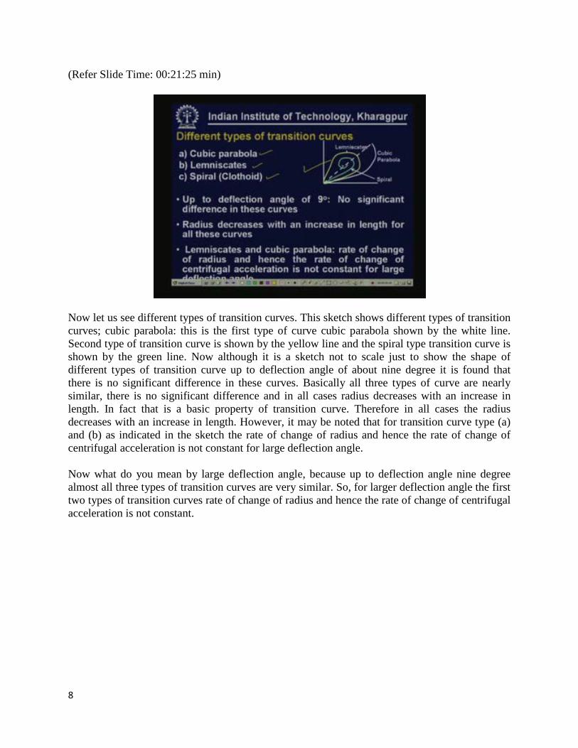
Now let us see different types of transition curves. This sketch shows different types of transition curves; cubic parabola: this is the first type of curve cubic parabola shown by the white line. Second type of transition curve is shown by the yellow line and the spiral type transition curve is shown by the green line. Now although it is a sketch not to scale just to show the shape of different types of transition curve up to deflection angle of about nine degree it is found that there is no significant difference in these curves. Basically all three types of curve are nearly similar, there is no significant difference and in all cases radius decreases with an increase in length. In fact that is a basic property of transition curve. Therefore in all cases the radius decreases with an increase in length. However, it may be noted that for transition curve type (a) and (b) as indicated in the sketch the rate of change of radius and hence the rate of change of centrifugal acceleration is not constant for large deflection angle. Now what do you mean by large deflection angle, because up to deflection angle nine degree almost all three types of transition curves are very similar. So, for larger deflection angle the first two types of transition curves rate of change of radius and hence the rate of change of centrifugal acceleration is not constant.

8


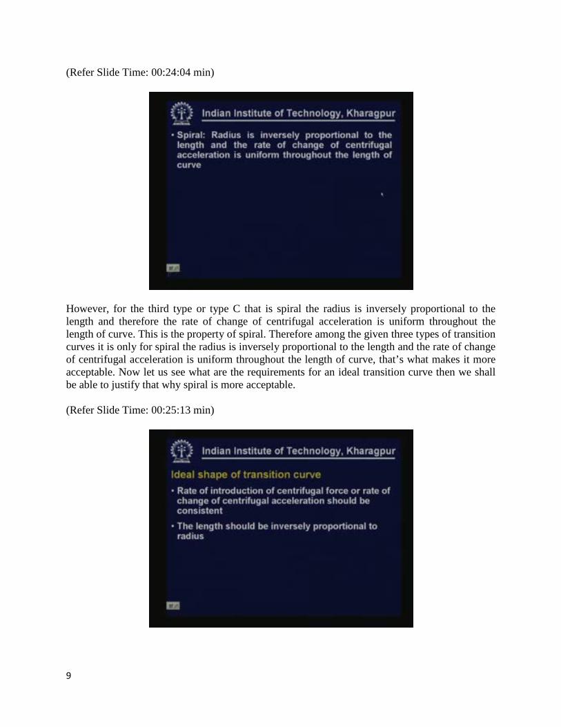
However, for the third type or type C that is spiral the radius is inversely proportional to the length and therefore the rate of change of centrifugal acceleration is uniform throughout the length of curve. This is the property of spiral. Therefore among the given three types of transition curves it is only for spiral the radius is inversely proportional to the length and the rate of change of centrifugal acceleration is uniform throughout the length of curve, that’s what makes it more acceptable. Now let us see what are the requirements for an ideal transition curve then we shall be able to justify that why spiral is more acceptable. (Refer Slide Time: 00:25:13 min)

9

Now, ideal shape of transition curve should be such that the rate of introduction of centrifugal force or in other way rate of change of centrifugal acceleration should be consistent, that’s what is a requirement. This indirectly means that the length should be inversely proportional to radius. Because if the length is inversely proportional to radius then rate of introduction of centrifugal force or rate of change of centrifugal acceleration should be consistent. (Refer Slide Time: 00:26:09 min)

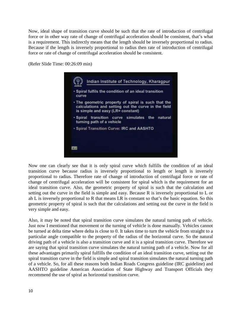
Now one can clearly see that it is only spiral curve which fulfills the condition of an ideal transition curve because radius is inversely proportional to length or length is inversely proportional to radius. Therefore rate of change of introduction of centrifugal force or rate of change of centrifugal acceleration will be consistent for spiral which is the requirement for an ideal transition curve. Also, the geometric property of spiral is such that the calculation and setting out the curve in the field is simple and easy. Because R is inversely proportional to L or ah L is inversely proportional to R that means LR is constant so that’s the basic equation. So this geometric property of spiral is such that the calculations and setting out the curve in the field is very simple and easy. Also, it may be noted that spiral transition curve simulates the natural turning path of vehicle. Just now I mentioned that movement or the turning of vehicle is done manually. Vehicles cannot be turned at delta time where delta is close to 0. It takes time to turn the vehicle from straight to a particular angle compatible to the property of the radius of the horizontal curve. So the natural driving path of a vehicle is also a transition curve and it is a spiral transition curve. Therefore we are saying that spiral transition curve simulates the natural turning path of a vehicle. Now for all these advantages primarily spiral fulfills the condition of an ideal transition curve, setting out the spiral transition curve in the field is simple and spiral transition simulates the natural turning path of a vehicle. So, for all these reasons both Indian Roads Congress guideline (IRC guideline) and AASHTO guideline American Association of State Highway and Transport Officials they recommend the use of spiral as horizontal transition curve.

10

(Refer Slide Time 00:29:11 min)

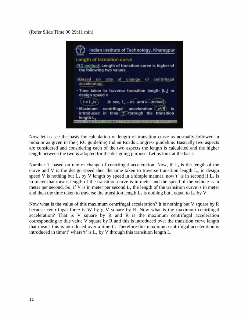
Now let us see the basis for calculation of length of transition curve as normally followed in India or as given in the (IRC guideline) Indian Roads Congress guideline. Basically two aspects are considered and considering each of the two aspects the length is calculated and the higher length between the two is adopted for the designing purpose. Let us look at the basis. Number 1; based on rate of change of centrifugal acceleration. Now, if Ls is the length of the curve and V is the design speed then the time taken to traverse transition length Ls in design speed V is nothing but Ls by V length by speed in a simple manner. now‘t’ is in second if Ls is in meter that means length of the transition curve is in meter and the speed of the vehicle is in meter per second. So, if V is in meter per second Ls the length of the transition curve is in meter and then the time taken to traverse the transition length Ls is nothing but t equal to Ls by V. Now what is the value of this maximum centrifugal acceleration? It is nothing but V square by R because centrifugal force is W by g V square by R. Now what is the maximum centrifugal acceleration? That is V square by R and R is the maximum centrifugal acceleration corresponding to this value V square by R and this is introduced over the transition curve length that means this is introduced over a time‘t’. Therefore this maximum centrifugal acceleration is introduced in time‘t’ where‘t’ is Ls by V through this transition length L.

11


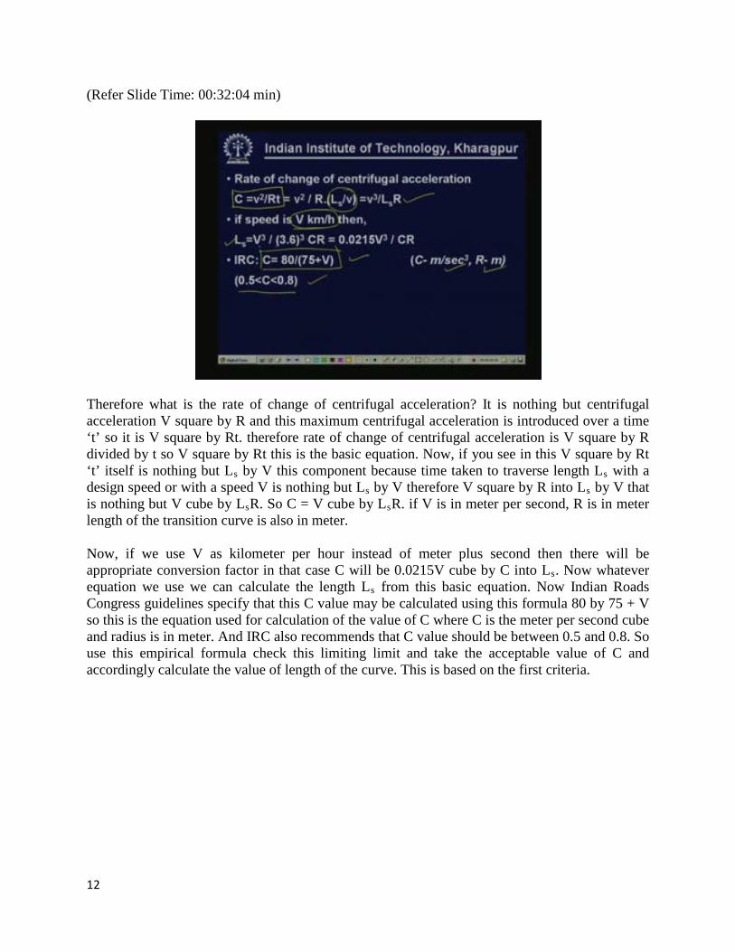
Therefore what is the rate of change of centrifugal acceleration? It is nothing but centrifugal acceleration V square by R and this maximum centrifugal acceleration is introduced over a time ‘t’ so it is V square by Rt. therefore rate of change of centrifugal acceleration is V square by R divided by t so V square by Rt this is the basic equation. Now, if you see in this V square by Rt ‘t’ itself is nothing but Ls by V this component because time taken to traverse length Ls with a design speed or with a speed V is nothing but Ls by V therefore V square by R into Ls by V that is nothing but V cube by LsR. So C = V cube by LsR. if V is in meter per second, R is in meter length of the transition curve is also in meter. Now, if we use V as kilometer per hour instead of meter plus second then there will be appropriate conversion factor in that case C will be 0.0215V cube by C into Ls. Now whatever equation we use we can calculate the length Ls from this basic equation. Now Indian Roads Congress guidelines specify that this C value may be calculated using this formula 80 by 75 + V so this is the equation used for calculation of the value of C where C is the meter per second cube and radius is in meter. And IRC also recommends that C value should be between 0.5 and 0.8. So use this empirical formula check this limiting limit and take the acceptable value of C and accordingly calculate the value of length of the curve. This is based on the first criteria.

12


Now the second criterion is based on the rate of change of superelevation. As we have all ready discussed superelevation should be introduced gradually over a length, that is the superelevation runoff also we have defined so at certain rate this superelevation should be introduced. Now when we are talking about rate of change of superelevation it means the longitudinal grade developed at the pavement edge compared to through grade along the central line and this rate of change why we limit it because this rate of change should not cause discomfort to travelers or make the road appear unsightly. Considering this aspect IRC says that there should be a lower limit for the rate of change of superelevation. it should be done at a rate faster than one in one fifty for roads in plain and rolling terrain and the limiting value is one in sixty for mountainous and steep terrain. Now considering this rate of change whatever transition curve length we will obtain our actual transition curve length should not be lesser than that value. In that case rate of introduction of superelevation will be faster than these recommended values and this is a situation which is not acceptable. It must not be done at a rate faster than this. So, if we say 1 in 150 if you know the superelevation rate we can calculate the length accordingly and it should not be more than that. Obviously the required length depends on the method of rotation. Because the actual amount of elevation what is to be done for the outer edge that will depend on the method of rotation of pavement that means whether the rotation is with respect to the central line or whether it is the rotation with respect to the inner edge of the pavement. We have discussed both the methods. So obviously the amount of superelevation what is to be attained or the amount of elevation what is to be done that will depend on the method of rotation.

13


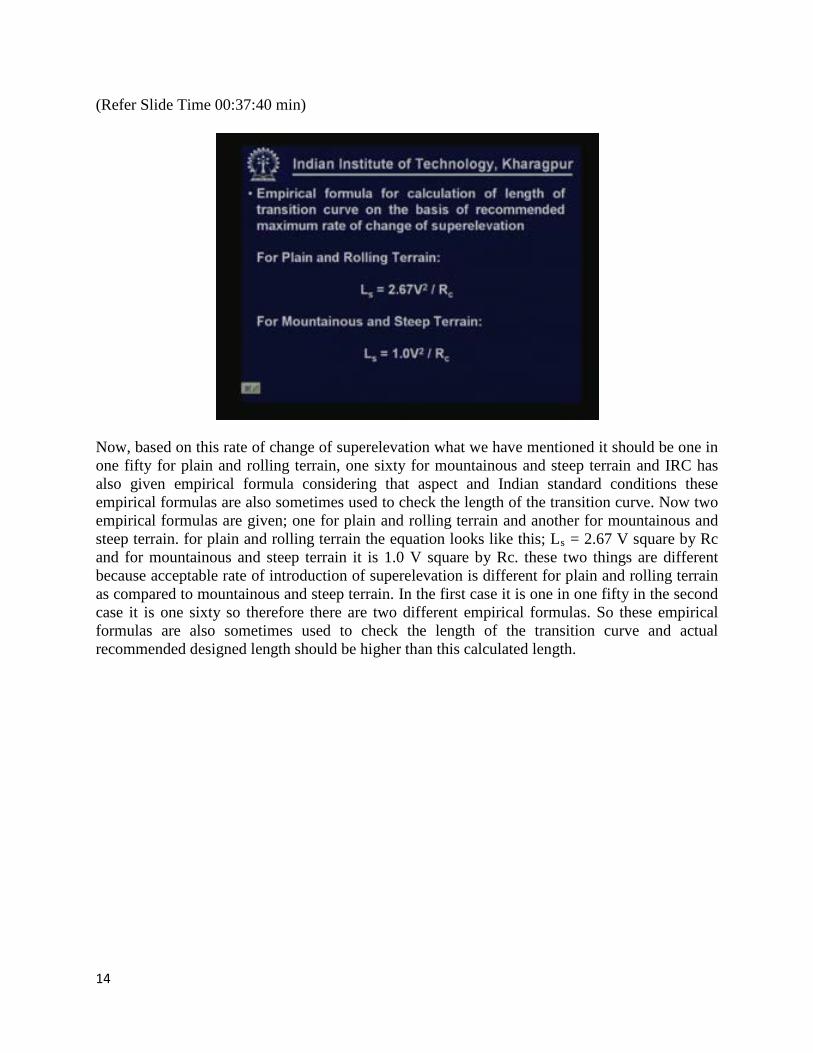
Now, based on this rate of change of superelevation what we have mentioned it should be one in one fifty for plain and rolling terrain, one sixty for mountainous and steep terrain and IRC has also given empirical formula considering that aspect and Indian standard conditions these empirical formulas are also sometimes used to check the length of the transition curve. Now two empirical formulas are given; one for plain and rolling terrain and another for mountainous and steep terrain. for plain and rolling terrain the equation looks like this; Ls = 2.67 V square by Rc and for mountainous and steep terrain it is 1.0 V square by Rc. these two things are different because acceptable rate of introduction of superelevation is different for plain and rolling terrain as compared to mountainous and steep terrain. In the first case it is one in one fifty in the second case it is one sixty so therefore there are two different empirical formulas. So these empirical formulas are also sometimes used to check the length of the transition curve and actual recommended designed length should be higher than this calculated length.

14


Let us quickly see the different elements of combined circular and transition curve. We have tried to show that here. This yellow portion is actually the tangent portion, these green lines are transition curves and the circular curve is shown by the red line. We have tried to indicate different elements. These things are also available in any standard textbook. in each case at both ends of circular curves the transition curves are introduced so this green line is the length of the transition curve, the red line shows the length of the circular curve, this ES this distance is known as the apex distance, these are the two tangent points and this is the amount of shift what is normally designated as ‘s’ so that is the shift and this is the point which is known as Horizontal Intersection Point because earlier this was one tangent, this was another tangent so this HIP is also used Horizontal Intersection Point.

15


Now let us see some of the other properties also. This angle delta is known as total deviation angle, this is thetas here and also at this end because transition curve is introduced at both ends of circular curve. This thetas is known as deviation angle of transition curve whereas this angle delta c is known as deviation and central angle of the circular arc. Remember that this red line is actually the circular arc. These are some of the elements of a combined transition curve and circular curve. The red portion is the circular curve, the green line shows the transition curves and these are the tangent points, this is horizontal intersection point and so on. Now obviously all elements can be calculated. There are standard textbooks. All these materials are available. I am only mentioning the shift because it is often required to calculate the shift. as I have indicated this is the shift this is nothing but Ls square by 24 Rc. This is the equation that is commonly used or what is used to calculate the shift Ls is the length of the transition curve and Rc is the radius of the circular curve. So it is Ls square divided by 24 Rc.

16


Now let us take an example problem. Design the length of transition curve for a two lane highway so it is a two lane highway having circular curve of 250m radius and the design speed is 70 Km/h. So, as per IRC we are doing the calculations. So we have to calculate it following two different approaches and the higher of those two values is to be taken. Now based on rate of change of centrifugal acceleration what is the l recommended C for that? C is 80 by 75 + V, this V is nothing but 70 Km/h so put that we calculate V as 0.55, we check that this calculated C is in between 0.5 and 0.8 therefore this rate of change of centrifugal acceleration is acceptable. Now using this calculated C we calculate the length. Since we are using V in kilometer per hour therefore we are using this formula with conversion factor point 0 two one five V cube by CR. V is 70, C we know 0.55 calculated, R is two fifty meter radius circular curve put that we calculate it as 53.6 m say let us call it as 55 m. now based on allowable rate of change of superelevation for mixed traffic operation superelevation is designed considering 75% of the design speed therefore it is V square by 225R and as indicated here the calculated value is 0.087 which is more than the permissible value.

17


What is the maximum permissible value? Permissible value for superelevation in the plain and rolling terrain is 7% that means e acceptable is basically 0.07. So we have to check it against the side friction factor taking the original equilibrium equation e + f = V square by 127R, earlier we calculated e considering 75% of the design speed and in this case it is V square by 127R considering the complete design speed so we calculate the ‘f’ and we find that the required f which means it is acceptable. So this 7% superelevation is acceptable. Now pavement width let us assume it is 7.5m therefore total raise if we consider total raise of outer edge with respect to central line, that means we are assuming that here the pavement is rotated with respect to center line this is very important then in that case the total raise of outer edge will be this superelevation rate seven percent multiplied by B by 2. Why it is B by 2, here this is capital E by 2 and because the pavement is rotated with respect to center line therefore this is E by 2 the raise is also E by 2 because it is rotated with respect to the center line. So this amount this raise is nothing but capital E by 2 which is nothing but E into B by 2 therefore it is 0.07 into 7.5 by 2 so it is 0.26 m. so what is the length required considering the rate of 1 in 150? It is 0.26 into 150 so it is 39 m. Therefore what should be the design length? It should be the maximum of these two and that should be used so maximum of these two is about 55 m.

18


Now we have seen that the transition length depends on the design speed as it was evident in that equation how we have calculated the length of the transition curve, it also depends on the circular curve radius and also because the acceptable values are the rate of change of superelevation is 1 in 150 for plain terrain and 1 in 160 for mountainous terrain therefore it depends on the terrain also. Hence considering terrain, considering design speed and considering different curve radius the required length of transition curves under different conditions have also been calculated and given in tabular form in the IRC code. (Refer Slide Time: 00:49:15 min)

19

Where transition curve cannot be provided for some practical reasons also we know that it is advantageous to provide transition curve but if transition curve cannot be provided then two-third of the superelevation will be attained on straight section itself before the start of the circular curve and balance one-third on the circular curve itself so that way we shall introduce the required superelevation. It is two-third before the beginning of the circular curve and one-third within the circular curve length. This also will make it compatible with the requirement of drivers and considering the natural path of driving. (Refer Slide Time: 00:50:09 min)

Here are some question sets: 1) What are the advantages of providing transition curves in horizontal alignment? 2) Why spiral is used as an ideal shape of transition curves in horizontal alignment 3) Explain the basis for calculation of the length of horizontal curves as per the recommendations of Indian Roads Congress. Try to answer these questions.

20


Now let me try to answer the questions of lessons 3.9. The first question was: Explain various stages and alternative approaches for attainment of superelevation. Basically there are two stages; first stage is elimination of crown of cambered section, this is the normal cambered section so first stage is to have uniform slope equal to camber that was elimination of the crown of cambered section then further rotation of pavement to attain the full superelevation. So this line is rotated again further to have the required superelevation. Now the first stage can be done in two alternative approaches. outer edge is rotated about the crown, keeping this point constant the outer edge is gradually rotated like this so here the disadvantage is that lesser cross slope lesser than the required camber so there could be drainage problem for a small portion where the slope is lesser than the camber so alternative approach is to shift the crown gradually which was another thing but here there won’t be any drainage problem but there will be negative superelevation and also the crown is shifted so vehicles have a tendency to follow the crown so it may not be very convenient considering the safety so each method has its own advantage and disadvantage.

21


The second stage is rotation of pavement to attain full superelevation. That means after removing crown we have a uniform section like this. So now, to have the required superelevation this is to be rotated. Now this can be rotated with respect to central line that is the first method rotation about the center line that is may be making it like this so in that case the earthwork is balanced but the lower edge or the inner edge is depressed so there could be drainage problem in this area. So the second method is rotation about the inner edge so you fix the inner edge and then rotate the pavement to have the required superelevation. Here the vertical profile of the center line is also changed which is another disadvantage and earthwork is also not balanced. Sometimes there is another method which is also followed in a limited way rotation about the outer edge for a given special situation. And each method has its own advantages and disadvantages. So sight specific decision is to be made.

22


Now the next question was: define curve resistance. This was not discussed but I thought you should try to answer this question because it is all ready known to you. Automobiles are steered by turning the front wheels so the movement is something like this. These are the wheels which are may be turned like this to negotiate a curve. Now vehicles which are driven by the rear wheels on horizontal curves the direction of rotation of rear and front wheels are different because rear wheels are like this, so front wheels are only rotated. hence what is happening is the tractive force what is given by the rear wheel is actually T, say this is T which is given by the rear wheels but tractive force which is available in the direction of movement is nothing but this is making it compatible with this direction so this is nothing but T cos alpha if this turning angle is alpha. So the whole T is not available in the direction of movement it is only the T cos alpha that amount is available in the direction of movement. So what is happening is it is basically because of this curve this is happening so there is a loss of tractive force.

23


What is that amount? The amount is T – T cos alpha or T into 1 – cos alpha which is a function of the turning angle alpha. That means this is happening only in curves so because of the curve this amount of loss is occurring. Therefore this is known as curve resistance. Thus curve resistance is nothing but loss of tractive force due to turning of vehicles on horizontal curves. Now obviously for vehicles with front driving wheels this problem does not exist and it will be severe for heavy vehicles because most of the heavy vehicles have rear driving wheels. Therefore there is more curve resistance on sharper curves because this angle alpha will be different as it depends on alpha so alpha is more for sharper curves so there is more curve resistance. Also, it is worthwhile to mention that this problem of curve resistance is acute on hill roads because it is not only the sharp horizontal curves but also there are steep gradients so the problem becomes more acute for hill roads. We shall come back to this topic on how to consider this aspect and design when we talk about vertical alignment. There is something called grade compensation so we will discuss this in that topic.

24


Now the last question was; Calculate set-back distance for radius of curve 400 m length of horizontal curve 200 m required sight distance is 300 m so here you can see very clearly that this is a case where the required sight distance is basically more than the length of the curve. So what is happening is in this case alpha by 2 can be considered as 180 L by 2 phi R – d so it is calculated as 14.39. (Refer Slide Time: 00:58:04 min)

Next in this case you can see the set-back distance is nothing but CF this can be calculated as CG + GF. Now what is CG? CG is nothing but OB is R – d OC is R so OC – OG. Now what is OG? OG is nothing but OB cos alpha by 2 that means CG is nothing but R – R – d cos alpha by 2 plus

25

if we have to calculate the total set-back distance this GF component is to be added. Now GF is nothing but S – L by 2 which is nothing but AB sin alpha by 2 so that’s what is added. We have already discussed the theoretical basis for that.

26

Introduction to Transportation Engineering Prof. …textofvideo.nptel.ac.in/105105107/lec17.pdfLet us start with some common terminologies. We have already discussed that the normal

Documents