Introduction to Time Series Analysis Handout 2: Stationary ...mayoral.iae-csic.org/timeseries2019/handout2_arma.pdf · Introduction to Time Series Analysis Handout 2: Stationary Processes.

Introduction to Time Series Analysis

Handout 2: Stationary Processes. Wold Decomposition and ARMA processes

Laura Mayoral

IAE and BGSEIDEA, Winter 2019

• This lecture introduces the basic linear models for stationary processes.

• Most economic variables are non-stationary.

• However, stationary linear models are used as building blocks in more complicated nonlinear and/or non-stationary models.

Roadmap

§ The Wold decomposition

§ From the Wold decomposition to theARMA representation

§ MA processes and invertibility

§ AR processes, stationarity and causality

§ ARMA, invertibility and causality.

Wold theorem in words:

Any stationary process {Zt} can be expressed as a sum of two components:

- a stochastic component: a linearcombination of lags of a white noise process.

- a deterministic component, uncorrelated with the latter stochastic component.

The Wold Decomposition

If {Zt} is a nondeterministic stationary time series, then:

€

Zt = ψ jj=0

∞

∑ at−j +Vt = Ψ(L )at +Vt ,

where

1. ψ0 = 1 and ψ j2

j=0

∞

∑ <∞,

2. at = Zt - P(Zt | Zt -1,Zt -2 ,...), where P(. | .) denotes linear projection.3. {at} is WN(0,σ 2 ), with σ 2 > 0,3. Cov(as , Vt ) = 0 for all s and t,4. The ψ i 's and the a 's are unique.5. {Vt} is deterministic.

The Wold Decomposition

• This theorem implies that any stationary process can be written as a linear combination of a lagged values of a white noise process (this is the MA(∞) representation).

• By inverting the corresponding polynomial, we can obtain a representation of Zt that depends on past values of the variable and the contemporaneous value of the white noise.

• This is the AR(∞) representation of Zt.

• We will see that the AR representation can be estimated using standard methods: OLS!

• Problem: we might need to estimate a lot of parameters.

• ARMA models: they are an approximation to former representations that tries to be more parsimonious (=less parameters)

Importance of the Wold Decomposition

)L(p

)L(q)L(F

Q»Y

Under general conditions the infinite lag polynomial of the WoldDecomposition can be approximated by the ratio of two finite lag polynomials:

Therefore

€

Zt = Ψ(L)at ≈Θq (L)Φp (L)

at ,

Φp (L)Zt =Θq (L)at

(1−φ1L − ...−φpLp )Zt = (1+ θ1L + ...+ θqL

q )at

Zt −φ1Zt−1 − ...−φpZt− p = at + θ1at−1 + ...+ θqat−q

AR(p) MA(q)

Birth of ARMA(p,q) models

MA(q) processes

Let

€

at{ } a zero-mean white noise process ),0( 2ata σ→

€

Zt = µ + at +θat−1 →MA(1)

- Expectation

- Variance

Autocovariance€

E(Zt ) = µ + E(at ) +θE(at−1) = µ

€

Var(Zt ) = E(Zt − µ)2 = E(at +θat−1)2 =

= E(at2 +θ 2at−1

2 + 2θatat−1) =σ a2(1+θ 2)

€

1st. orderE(Zt − µ)(Zt−1 − µ) = E(at +θat−1)(at−1 +θat−2) =

= E(atat−1 +θat−12 +θatat−2 +θ 2at−1at−2) = θσ a

2

Moving Average of order 1, MA(1)

-Autocovariance of higher order

- Autocorrelation

€

E(Zt − µ)(Zt− j − µ) = E(at +θat−1)(at− j +θat− j−1) =

= E(atat− j +θat−1at− j +θatat− j−1 +θ 2at−1at− j−1) = 0 j >1

€

ρ1 =γ1γ 0

=θσ 2

(1+ θ 2)σ 2 =θ

1+ θ 2

ρ j = 0 j >1

Partial autocorrelation

€

ρ1 =γ1γ 0

=θσ 2

(1+ θ 2)σ 2 =θ

1+ θ 2

ρ j = 0 j >1

StationarityMA(1) process is always covariance-stationary because

22 )1()()( σθµ +== tt ZVarZE

ErgodicityMA(1) process is ergodic for first and second moments because

€

γ j =σ 2(1+θ 2) + θσ 2

j=0

∞

∑ < ∞

If were Gaussian, then would be ergodic for all moments

€

at

€

Zt

MA(1): Stationarity and Ergodicity

MA(q) processes

qtqtttt aaaaZ −−− +++++= θθθµ 2211

A process is MA(q) if it can be written as a linear combination of q lags of a white noise process.

First and Second moments of a MA(q)

€

E(Zt ) = µ

γ 0 = var(Zt ) = (1+ θ12 + θ2

2 ++ θq2)σ a

2

γ j = E(at + θ1at−1 ++ θqat−q )(at− j + θ1at− j−1 ++ θqat− j−q )

γ j =(θ j + θ j+1θ1 + θ j+2θ2 ++ θqθq− j )σ

2 for j ≤ q0 for j > q

' ( )

ρ j =γ j

γ 0

=θ j + θ j+1θ1 + θ j+2θ2 ++ θqθq− j

θi2

i=1

q

∑

Example MA(2)

ρ1 =θ1 + θ1θ2

1+ θ12 + θ2

2 ρ2 =θ2

1+ θ12 + θ2

2 ρ3 = ρ4 = = ρk = 0

- AMA(q) process is said to be invertible if there exists a sequence of constants and

- In other words, Zt is invertible if it admits and autoregressive representation.

€

{π j} such that |π jj= 0

∞

∑ |<∞

€

at = π jj=0

∞

∑ Zt− j, t=0,±1,...

Invertibility: definition

Theorem:Let {Zt} be a MA(q). Then {Zt} is invertible if and only if

The coefficients {pj} are determined by the relation:€

θ(x) ≠ 0 for all x∈C such that | x |≤1.

€

π (x) = π jj=0

∞

∑ x j =1

θ (x), | x |≤1.

Necessary and Sufficient Conditions for Invertibility

MA processes are not uniquely identified

€

1) ρ1 =θ

1+θ 2

2) ρ *1 =1/θ

1+ (1/θ)2 =θ

1+θ 2

Consider the autocorrelation function of these two MA(1) processes:

€

Zt = µ + at +θat−1

€

Z *t = µ + a*t +(1/θ)a*t−1

The autocorrelation functions are:

MA processes are not uniquely identified, II

§ Then, these two processes show identical correlation pattern: The MA coefficient is not uniquely identified.

§ In other words: any MA(1) process has two representations (one with MA parameter larger than 1, and the other, with MA parameter smaller than 1).

MA processes are not uniquely identified, III

•This means that each MA(1) has two representations: one that is invertible, another one that is not.

•We prefer representations that are invertible sowe will choose the representation with q<1.

Z

MA processes are not uniquely identified, IV

•The same problem is present for MA(q) processes.

•In this case, one needs to look at the roots of the MA(q) polynomial: roots smaller than 1 imply non-invertibity.

•There is always an invertible representation, obtained by inverting the root that is smaller than 1.

Z

Exercise

Consider a MA(1) process with a MA coefficient equal to 1.3

1) Is it stationary? Is it ergodic?

2) is it invertible? If it is not, suggest an alternative representation that has identical autocorrelation structure and is invertible

Zt = µ + ψ jat− j ψ0 =1j=0

∞

∑

MA(infinite)

This is the most general MA process.

It contains and infinite number of lags of a white noise process.

€

E(Zt ) = µ, Var(Zt ) =σ a2 ψ i

2

i= 0

∞

∑

γ j = E (Zt −µ)(Zt− j −µ)[ ] =σ 2 ψ iψ i+ ji= 0

∞

∑

ρ j =

ψiψ i+ ji= 0

∞

∑

ψ i2

i= 0

∞

∑

MA(infinite): moments

Notice that in order to define the second order moments we need

The process is covariance-stationaryprovided the former condition holds.€

ψi2

i= 0

∞

∑ <∞

MA(infinite): stationarity condition

Some interesting results

Proposition 1.

Proposition 2.

∞<⇒∞< ∑∑∞

=

∞

= 0

2

0 ii

ii ψψ

(absolutelysummable)

€

ψ ii= 0

∞

∑ <∞⇒ γ ii= 0

∞

∑ <∞

(squaresummable)

Ergodic for second moments

Proof 1. ¥<Þ¥< åå¥

=

¥

= 0

2

0 ii

ii yy

€

If ψ ii= 0

∞

∑ <∞⇒ ∃ N <∞ such that ψ i <1 ∀i ≥ N

ψi2 < ψ i ∀i ≥ N⇒ ψi

2

i=N

∞

∑ < ψ ii=N

∞

∑

Now,

ψi2

i= 0

∞

∑ = ψ i2

i= 0

N−1

∑ + ψ i2

i=N

∞

∑ < ψ i2

i= 0

N−1

∑ + |ψi |i=N

∞

∑(1) (2)

(1) It is finite because N is finite(2) It is finite because is absolutely summableThe picture can't be displayed.

then

Proof 2.

M

MM

jji

i ii

jjii

jji

ii

j j ijiij

ijii

ijiij

ijiij

<

∞<<<=

==≤

≤=

=

∑

∑ ∑∑

∑∑∑ ∑∑

∑∑

∑

∞

=+

∞

=

∞

=

∞

=+

∞

=+

∞

=

∞

=

∞

=

∞

=+

∞

=+

∞

=+

∞

=+

0

22

0 0

2

0

2

0 00 0

2

0

2

0

2

0

2

0

2

assumptionby because ψ

σψσψψσ

ψψσψψσγ

ψψσψψσγ

ψψσγ

AR(p) processes

€

Zt = c + φZt−1 + at

AR(1) process

An autoregressive process Z is a function of its own past and a contemporaneous value of a white noice sequence

€

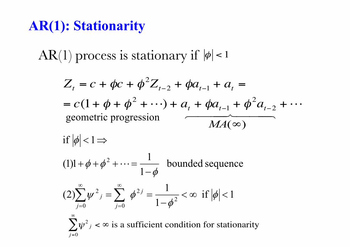
Zt = c + φc + φ 2Zt−2 + φat−1 + at =

= c(1+ φ + φ 2 +) + at + φat−1 + φ 2at−2 +geometric progression

)( ∞MA

1 if 1

1)2(

sequence bounded 1

11)1(

1 if

22

00

2

2

<¥<-

==

-=+++

Þ<

åå¥

=

¥

=

ff

fy

fff

f

j

jjj

!

€

ψ 2j

j=0

∞

∑ < ∞ is a sufficient condition for stationarity

AR(1): Stationarity

AR(1) process is stationary if 1<φ

Mean of a stationary AR(1)

€

Zt =c

1−φ+ at + φat−1 + φ 2at−2 +

µ = E(Zt ) =c

1−φ

Variance of a stationary AR(1)

€

γ 0 = 1+ φ 2 + φ 4 +( )σ 2 =1

1−φ 2σ a

2

AR(1): First and second order moments

Autocovariance of a stationary AR(1)

- You need to solve a system of equations:

€

γ j = E Zt −µ( ) Zt− j −µ( )[ ] = E φ Zt−1 −µ( ) + at( ) Zt− j −µ( )[ ] =

= φE Zt−1 −µ( ) Zt− j −µ( ) + at Zt− j −µ( )[ ] = φγ j−1

11 ³= - jjj fgg

Autocorrelation of a stationary AR(1)

€

ρ j =γ j

γ o= φ

γ j−1

γ 0= φρ j−1 j ≥1

ρ j = φ 2ρ j−2 = φ 3ρ j−3 = = φ jρ0 = φ j

PACF: from Yule-Walker equations

€

φ11 = ρ 1̀ = φ

φ22 =

1 ρ1ρ1 ρ21 ρ1ρ1 1

=ρ2 − ρ1

2

1− ρ12 =

φ 2 −φ 2

1− ρ12 = 0

φkk = 0 k ≥ 2

AR(1): Partial autocorrelation function

A stationary AR(1) process is ergodic for first and second moments.

Show this as an exercise.

AR(1): Ergodicity

ttt aZZ += -11f

€

Iterating we obtain

Zt = at + φ1at + ...+ φ1kat -k + φ1Zt -k -1.

If φ1 <1 we showed that

Zt = φ1jat− j

j=0

∞

∑

Consider the AR(1) process,

€

This cannot be done if φ1 ≥1, (no mean - square convergence) However, in this case one could write

Zt = φ1−1Zt+1 −φ1

−1at+1

Then, Zt = − φ1− jat+ j

j=0

∞

∑

and this is a stationary representation of Zt .

Causality and Stationarity

11 <f 11 <f

11 <f

However, this stationary representation depends on future values of

It is customary to restrict attention to AR(1) processes with

Such processes are called stationary but also CAUSAL, or future-indepent AR representations.

11 <f€

at

Causality and Stationarity, II

Definition: An AR(p) process defined by the equation

is said to be causal, or a causal function of {at}, if there exists a sequence of constants

and- A necessary and sufficient condition for causality is

tatZ)L(p =f

€

{ψ j} such that |ψ jj=0

∞

∑ |< ∞

€

Zt = ψ jj=0

∞

∑ at− j, t=0,±1,...

€

φ(x) ≠ 0 for all x∈C such that | x |≤1.

Causality and Stationarity, III

€

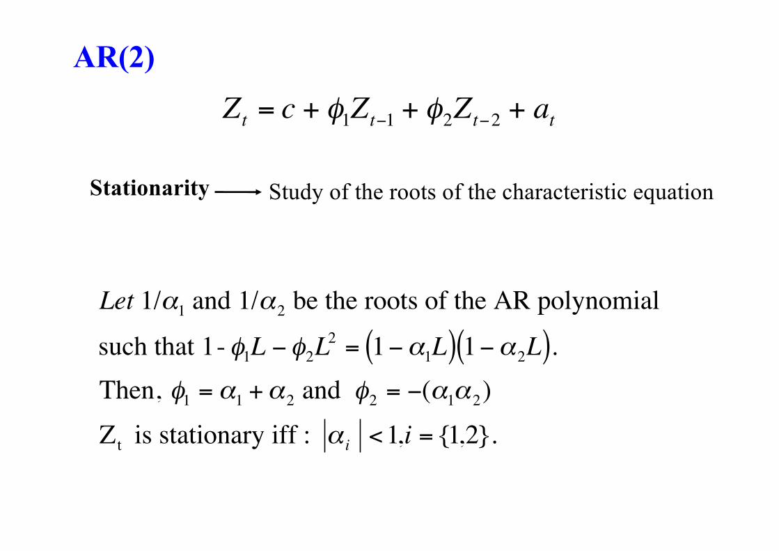
Zt = c + φ1Zt−1 + φ2Zt−2 + at

Stationarity Study of the roots of the characteristic equation

€

Let 1/α1 and 1/α2 be the roots of the AR polynomial

such that 1- φ1L −φ2L2 = 1−α1L( ) 1−α2L( ).

Then, φ1 = α1 +α2 and φ2 = −(α1α2)

Zt is stationary iff : α i <1,i = {1,2}.

AR(2)

Mean of AR(2)

€

E(Zt ) = c + φ1E(Zt ) + φ2E(Zt )⇒

E(Zt ) = µ =c

1−φ1 −φ2

Variance

€

γ 0 = E(Zt −µ)2 = φ1E(Zt−1 −µ)(Zt −µ)+ φ2E(Zt−2 −µ) Zt −µ( ) + E(Zt −µ)atγ 0 = φ1γ−1 + φ2γ−2 +σ 2

a

γ 0 = φ1ρ1γ 0 + φ2ρ2γ 0 +σ 2a

γ 0 =σ 2

a

1−φ1ρ1 −φ2ρ2

First and Second order moments

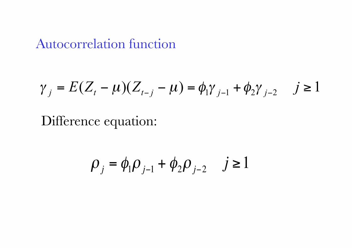
Autocorrelation function

1))(( 2211 ≥+=−−= −−− jZZE jjjttj γφγφµµγ

€

ρ j = φ1ρ j−1 + φ2ρ j−2 j ≥1

Difference equation:

€

ρ j = φ1ρ j−1 + φ2ρ j−2 j ≥1

12213

22

21

2

2

11

02112

12011

31

121

ρφρφρ

φφ

φρ

φφ

ρ

ρφρφρ

ρφρφρ

+==

##$

##%

&

+−

=

−=

→$%&

+==

+==

j

jj

Partial autocorrelations: from Yule-Walker equations

€

φ11 = ρ1 =φ1

1−φ2; φ22 =

ρ2 − ρ12

1− ρ12 ; φ33 = 0

Partial Autocorrelations

(complex roots)

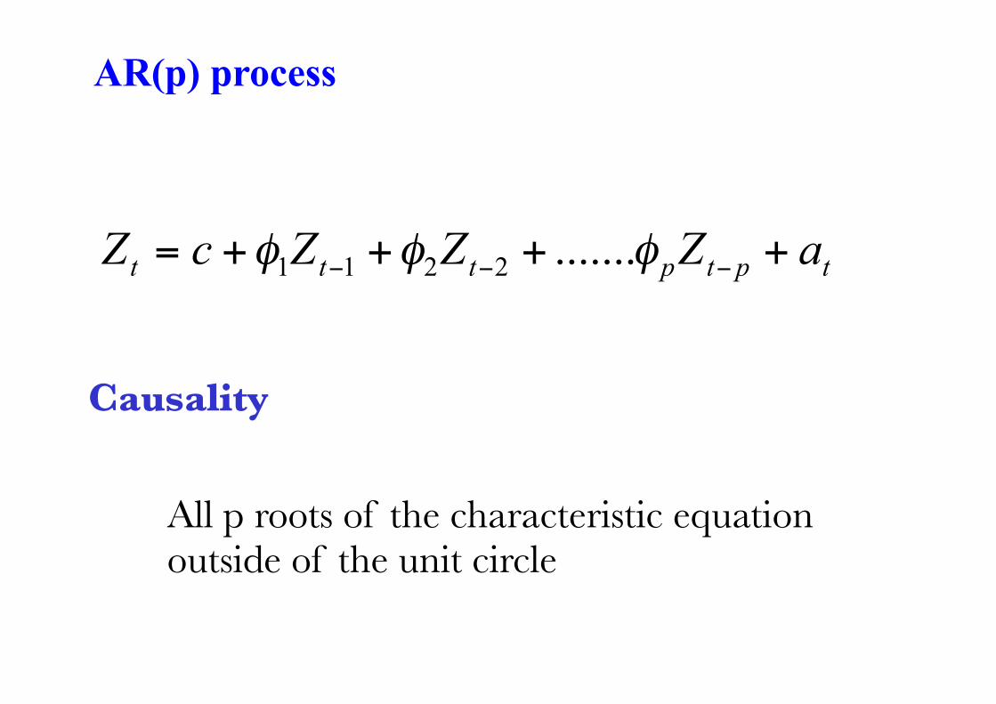
tptpttt aZZZcZ ++++= −−− φφφ .......2211

Causality

All p roots of the characteristic equation outside of the unit circle

AR(p) process

Autocorrelation Function

€

ρk = φ1ρk−1 + φ2ρk−2 + ......φpρk− p

ρ1 = φ1ρ0 + φ2ρ1 + ......φpρp−1

ρ2 = φ1ρ11 + φ2ρ0 + ......φpρp−2

ρp = φ1ρp−1 + φ2ρp−2 + ......φpρ0

%

&

' '

(

' '

System of equations.The first pautocorrelations:p unknowns and p equations

ACF decays as mixture of exponentials and/or damped sine waves, Depending on real/complex roots

PACF

€

φkk = 0 for k > p

Second order moments

Relationship between AR(p) and MA(q)

Stationary AR(p)

€

Φp (L)Zt = at Φp (L) = (1−φ1L −φ2L2 − ....φpL

p )1

Φp (L)=Ψ(L)⇒Φp (L)Ψ(L) =1

Zt =1

Φp (L)at =Ψ(L)at Ψ(L) = (1+ψ1L +ψ2L

2 + ....)

€ €

Relationship between AR(p) and MA(q), II

€

€

Zt =Θq (L)at Θq (L) = (1−θ1L −θ2L2 − ....θqL

q )1

Θq (L)=Π(L)⇒Θq (L)Π(L) =1

Π(L)Zt =1

Θq (L)Zt = at Π(L) = (1+π1L +π 2L

2 + ....)

Invertible MA(q)

€

ARMA(p,q) Processes

ttp

q

ttq

pt

q

tqtp

aLaLL

aZLL

ZL

xx

xx

aLZL

)()()(

ZtionrepresentaMA Pure

)()(

)( tion representa AR Pure

10)( of roots ty Stationari

10)( of roots ity Invertibil

)()(

t

p

Y=F

Q=®

=Q

F=P®

>=F®

>=Q®

Q=F

ARMA(p,q)

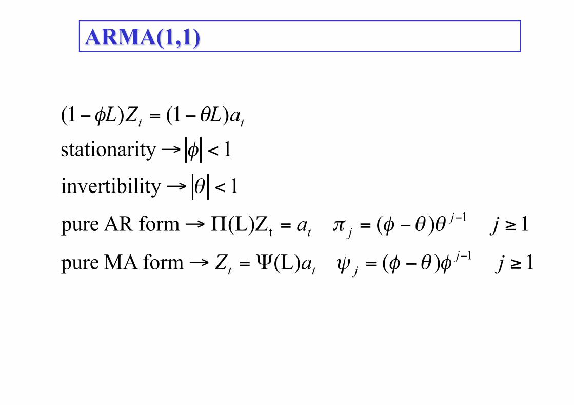
ARMA(1,1)

1)((L)form MApure

1)((L)Zform AR pure

1ityinvertibil

1 ty stationari

)1()1(

1

1t

≥−=Ψ=→

≥−==Π→

<→

<→

−=−

−

−

jaZ

ja

aLZL

jjtt

jjt

tt

φθφψ

θθφπ

θ

φ

θφ

ACF of ARMA(1,1)

€

ZtZt−k = φZt−1Zt−k + atZt−k −θat−1Zt−k

taking expectations

€

γ k = φγ k−1 + E(atZt−k ) −θE(at−1Zt−k )

€

k = 0 E(atZt ) =σ2a E(at−1Zt ) = (φ −θ )σa2

γ 0 = φγ1 +σa2 −θ (φ −θ )σa

2

k =1 γ1 = φγ 0 −θσa2

k ≥ 2 γ k = φγ k−1!"#

10 and for solveunknowns 2 and equations 2 of system

γγ

you get this system of equations

€

ρk =

1 k = 0(φ −θ) 1−φθ( )1+θ 2 − 2φθ

k =1

φρk−1 k ≥ 2

'

( ) )

* ) )

PACF

decay lexponentia)1,1()1( ARMAMA ⊂

ACF