Introduction to Thermo-Fluids Systems Design

Welcome message from author
This document is posted to help you gain knowledge. Please leave a comment to let me know what you think about it! Share it to your friends and learn new things together.
Transcript

JWST229-fm JWST229-McDonald Printer: Yet to Come August 16, 2012 11:29 Trim: 244mm × 168mm
Introduction to Thermo-FluidsSystems Design
i

JWST229-fm JWST229-McDonald Printer: Yet to Come August 16, 2012 11:29 Trim: 244mm × 168mm
Introduction toThermo-FluidsSystems Design
Andre G. McDonald, Ph.D., P.ENG.University of Alberta, Canada
Hugh L. Magande, M.B.A., M.S.E.M.Rinnai America Corporation, USA
A John Wiley & Sons, Ltd., Publication
iii

JWST229-fm JWST229-McDonald Printer: Yet to Come August 16, 2012 11:29 Trim: 244mm × 168mm
This edition first published 2012.C© 2012 Andre G. McDonald and Hugh L. Magande.
Registered officeJohn Wiley & Sons Ltd, The Atrium, Southern Gate, Chichester, West Sussex, PO19 8SQ, United Kingdom
For details of our global editorial offices, for customer services and for information about how to applyfor permission to reuse the copyright material in this book please see our website at www.wiley.com.
The right of the author to be identified as the author of this work has been asserted in accordance with theCopyright, Designs and Patents Act 1988.
All rights reserved. No part of this publication may be reproduced, stored in a retrieval system, ortransmitted, in any form or by any means, electronic, mechanical, photocopying, recording or otherwise,except as permitted by the UK Copyright, Designs and Patents Act 1988, without the prior permission ofthe publisher.
Wiley also publishes its books in a variety of electronic formats. Some content that appears in print maynot be available in electronic books.
Designations used by companies to distinguish their products are often claimed as trademarks. All brandnames and product names used in this book are trade names, service marks, trademarks or registeredtrademarks of their respective owners. The publisher is not associated with any product or vendormentioned in this book. This publication is designed to provide accurate and authoritative information inregard to the subject matter covered. It is sold on the understanding that the publisher is not engaged inrendering professional services. If professional advice or other expert assistance is required, the servicesof a competent professional should be sought.
DISCLAIMER
The contents of this textbook are meant to supply information on the design of thermo-fluids systems.The book is not meant to be the sole resource used in any design project. The examples and solutionspresented are not to be construed as complete engineered design solutions for any particular problem orproject. The authors and publisher are not attempting to render any type of engineering or otherprofessional services. Should these services be required, an appropriate professional engineer should beconsulted. The authors and publisher assume no liability or responsibility for any uses made of thematerial contained and described herein.
Library of Congress Cataloging-in-Publication Data
McDonald, Andre G.Introduction to thermo-fluids systems design / Andre G. McDonald, Ph. D., P. Eng., Hugh L. Magande,
M.B.A., M.S.E.M.pages cm
Includes bibliographical references and index.ISBN 978-1-118-31363-3 (cloth)
1. Heat exchangers–Fluid dynamics. 2. Fluids–Thermal properties. I. Magande, Hugh L. II. Title.TJ263.M38 2013621.402′2–dc23
2012023753
A catalogue record for this book is available from the British Library.
ISBN: 9781118313633
Set in 10/12.5pt Palatino by Aptara Inc., New Delhi, India.
iv
JWST229-fm JWST229-McDonald Printer: Yet to Come August 1, 2012 7:44 Trim: 244mm × 168mm
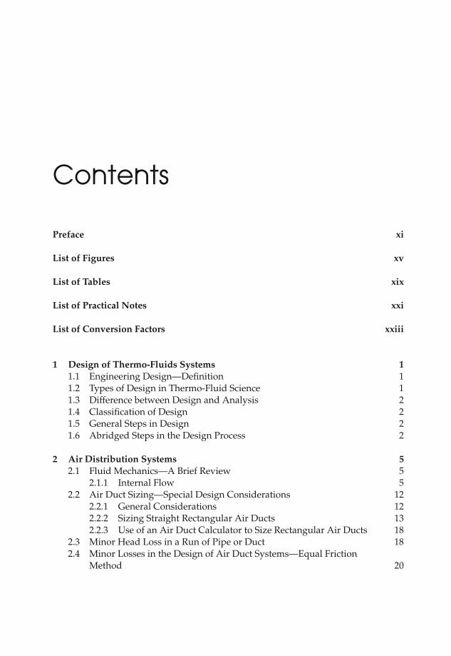
Contents
Preface xi
List of Figures xv
List of Tables xix
List of Practical Notes xxi
List of Conversion Factors xxiii
1 Design of Thermo-Fluids Systems 11.1 Engineering Design—Definition 11.2 Types of Design in Thermo-Fluid Science 11.3 Difference between Design and Analysis 21.4 Classification of Design 21.5 General Steps in Design 21.6 Abridged Steps in the Design Process 2
2 Air Distribution Systems 52.1 Fluid Mechanics—A Brief Review 5
2.1.1 Internal Flow 52.2 Air Duct Sizing—Special Design Considerations 12
2.2.1 General Considerations 122.2.2 Sizing Straight Rectangular Air Ducts 132.2.3 Use of an Air Duct Calculator to Size Rectangular Air Ducts 18
2.3 Minor Head Loss in a Run of Pipe or Duct 182.4 Minor Losses in the Design of Air Duct Systems—Equal Friction
Method 20
v
JWST229-fm JWST229-McDonald Printer: Yet to Come August 1, 2012 7:44 Trim: 244mm × 168mm
vi Contents
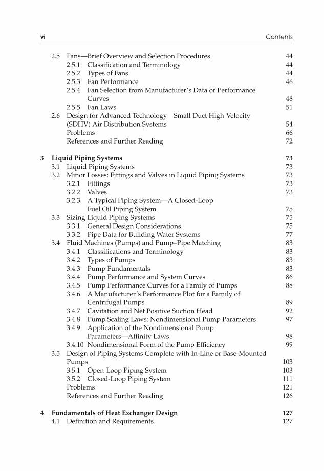
2.5 Fans—Brief Overview and Selection Procedures 442.5.1 Classification and Terminology 442.5.2 Types of Fans 442.5.3 Fan Performance 462.5.4 Fan Selection from Manufacturer’s Data or Performance
Curves 482.5.5 Fan Laws 51
2.6 Design for Advanced Technology—Small Duct High-Velocity(SDHV) Air Distribution Systems 54Problems 66References and Further Reading 72
3 Liquid Piping Systems 733.1 Liquid Piping Systems 733.2 Minor Losses: Fittings and Valves in Liquid Piping Systems 73
3.2.1 Fittings 733.2.2 Valves 733.2.3 A Typical Piping System—A Closed-Loop
Fuel Oil Piping System 753.3 Sizing Liquid Piping Systems 75
3.3.1 General Design Considerations 753.3.2 Pipe Data for Building Water Systems 77
3.4 Fluid Machines (Pumps) and Pump–Pipe Matching 833.4.1 Classifications and Terminology 833.4.2 Types of Pumps 833.4.3 Pump Fundamentals 833.4.4 Pump Performance and System Curves 863.4.5 Pump Performance Curves for a Family of Pumps 883.4.6 A Manufacturer’s Performance Plot for a Family of
Centrifugal Pumps 893.4.7 Cavitation and Net Positive Suction Head 923.4.8 Pump Scaling Laws: Nondimensional Pump Parameters 973.4.9 Application of the Nondimensional Pump
Parameters—Affinity Laws 983.4.10 Nondimensional Form of the Pump Efficiency 99
3.5 Design of Piping Systems Complete with In-Line or Base-MountedPumps 1033.5.1 Open-Loop Piping System 1033.5.2 Closed-Loop Piping System 111Problems 121References and Further Reading 126
4 Fundamentals of Heat Exchanger Design 1274.1 Definition and Requirements 127

JWST229-fm JWST229-McDonald Printer: Yet to Come August 1, 2012 7:44 Trim: 244mm × 168mm
Contents vii
4.2 Types of Heat Exchangers 1274.2.1 Double-Pipe Heat Exchangers 1274.2.2 Compact Heat Exchangers 1294.2.3 Shell-and-Tube Heat Exchangers 129
4.3 The Overall Heat Transfer Coefficient 1304.3.1 The Thermal Resistance Network for Plane Walls—
Brief Review 1324.3.2 Thermal Resistance from Fouling—The Fouling Factor 136
4.4 The Convection Heat Transfer Coefficients—Forced Convection 1384.4.1 Nusselt Number—Fully Developed Internal Laminar Flows 1394.4.2 Nusselt Number—Developing Internal Laminar Flows—
Correlation Equation 1394.4.3 Nusselt Number—Turbulent Flows in Smooth Tubes:
Dittus–Boelter Equation 1414.4.4 Nusselt Number—Turbulent Flows in Smooth Tubes:
Gnielinski’s Equation 1414.5 Heat Exchanger Analysis 142
4.5.1 Preliminary Considerations 1424.5.2 Axial Temperature Variation in the Working Fluids—Single
Phase Flow 1434.6 Heat Exchanger Design and Performance Analysis: Part 1 147
4.6.1 The Log-Mean Temperature Difference Method 1474.6.2 The Effectiveness-Number of Transfer Units
Method: Introduction 1484.6.3 The Effectiveness-Number of Transfer Units Method: ε-NTU
Relations 1494.6.4 Comments on the Number of Transfer Units and the Capacity
Ratio (c) 1514.6.5 Procedures for the ε-NTU Method 1564.6.6 Heat Exchanger Design Considerations 157
4.7 Heat Exchanger Design and Performance Analysis: Part 2 1574.7.1 External Flow over Bare Tubes in Cross Flow—Equations and
Charts 1574.7.2 External Flow over Tube Banks—Pressure Drop 1624.7.3 External Flow over Finned-Tubes in Cross Flow—Equations
and Charts 1754.8 Manufacturer’s Catalog Sheets for Heat Exchanger Selection 202
Problems 208References and Further Reading 211
5 Applications of Heat Exchangers in Systems 2135.1 Operation of a Heat Exchanger in a Plasma Spraying System 2135.2 Components and General Operation of a Hot Water
Heating System 216

JWST229-fm JWST229-McDonald Printer: Yet to Come August 1, 2012 7:44 Trim: 244mm × 168mm
viii Contents
5.3 Boilers for Water 2175.3.1 Types of Boilers 2175.3.2 Operation and Components of a Typical Boiler 2185.3.3 Water Boiler Sizing 2205.3.4 Boiler Capacity Ratings 2245.3.5 Burner Fuels 226
5.4 Design of Hydronic Heating Systems c/w Baseboardsor Finned-Tube Heaters 2275.4.1 Zoning and Types of Systems 2275.4.2 One-Pipe Series Loop System 2275.4.3 Two-Pipe Systems 2295.4.4 Baseboard and Finned-Tube Heaters 233
5.5 Design Considerations for Hot Water Heating Systems 236Problems 258References and Further Reading 265
6 Performance Analysis of Power Plant Systems 2676.1 Thermodynamic Cycles for Power Generation—Brief Review 267
6.1.1 Types of Power Cycles 2676.1.2 Vapor Power Cycles—Ideal Carnot Cycle 2686.1.3 Vapor Power Cycles—Ideal Rankine Cycle for Steam
Power Plants 2686.1.4 Vapor Power Cycles—Ideal Regenerative Rankine Cycle for
Steam Power Plants 2696.2 Real Steam Power Plants—General Considerations 2716.3 Steam-Turbine Internal Efficiency and Expansion Lines 2726.4 Closed Feedwater Heaters (Surface Heaters) 2806.5 The Steam Turbine 282
6.5.1 Steam-Turbine Internal Efficiency and Exhaust End Losses 2826.5.2 Casing and Shaft Arrangements of Large Steam Turbines 284
6.6 Turbine-Cycle Heat Balance and Heat and Mass Balance Diagrams 2866.7 Steam-Turbine Power Plant System Performance Analysis
Considerations 2886.8 Second-Law Analysis of Steam-Turbine Power Plants 3006.9 Gas-Turbine Power Plant Systems 307
6.9.1 The Ideal Brayton Cycle for Gas-Turbine Power PlantSystems 307
6.9.2 Real Gas-Turbine Power Plant Systems 3096.9.3 Regenerative Gas-Turbine Power Plant Systems 3126.9.4 Operation and Performance of Gas-Turbine Power
Plants—Practical Considerations 3136.10 Combined-Cycle Power Plant Systems 324
6.10.1 The Waste Heat Recovery Boiler 325Problems 332References and Further Reading 338
JWST229-fm JWST229-McDonald Printer: Yet to Come August 1, 2012 7:44 Trim: 244mm × 168mm
Contents ix
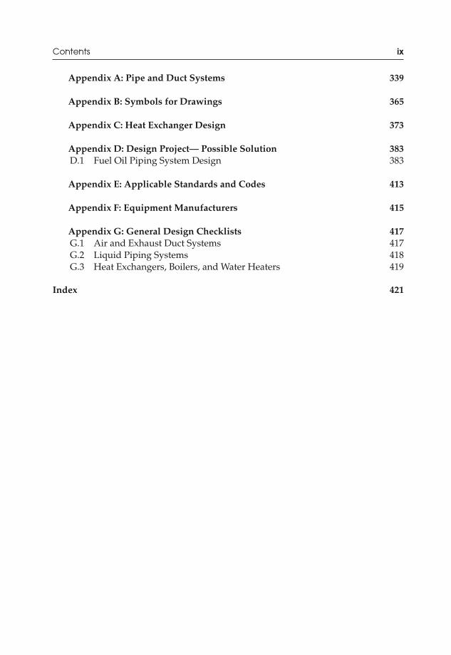
Appendix A: Pipe and Duct Systems 339
Appendix B: Symbols for Drawings 365
Appendix C: Heat Exchanger Design 373
Appendix D: Design Project— Possible Solution 383D.1 Fuel Oil Piping System Design 383
Appendix E: Applicable Standards and Codes 413
Appendix F: Equipment Manufacturers 415
Appendix G: General Design Checklists 417G.1 Air and Exhaust Duct Systems 417G.2 Liquid Piping Systems 418G.3 Heat Exchangers, Boilers, and Water Heaters 419
Index 421

JWST229-fm JWST229-McDonald Printer: Yet to Come August 1, 2012 7:44 Trim: 244mm × 168mm
Preface
Design courses and projects in contemporary undergraduate curricula have focusedmainly on topics in solid mechanics. This has left graduating junior engineers withlimited knowledge and experience in the design of components and systems in thethermo-fluids sciences. ABB Automation in their handbook on Energy Efficient Designof Auxiliary Systems in Fossil-Fuel Power Plants has mentioned that this lack of trainingin thermo-fluids systems design will limit our ability to produce high-performancesystems. This deficiency in contemporary undergraduate curricula has resulted inan urgent need for course materials that underline the application of fundamentalconcepts in the design of thermo-fluids components and systems.
Owing to the urgent need for course materials in this area, this textbook has been de-veloped to bridge the gap between the fundamental concepts of fluid mechanics, heattransfer, and thermodynamics and the practical design of thermo-fluids componentsand systems. To achieve this goal, this textbook is focused on the design of internalfluid flow systems, coiled heat exchangers, and performance analysis of power plantsystems. This requires prerequisite knowledge of internal fluid flow, conduction heattransfer, convection heat transfer with emphasis on forced convection in tubes andover cylinders, analysis of constant area fins, and thermodynamic power cycles, inparticular, the Rankine and Brayton cycles. The fundamental concepts are used astools in an exhaustive design process to solve various practical problems presentedin the examples. For junior design engineers with limited practical experience, useof fundamental concepts of which they have previous knowledge will help them toincrease their confidence and decision-making capabilities.
The complete design or modification of modern equipment and systems will re-quire knowledge of current industry practices. While relying on and demonstrat-ing the application of fundamental principles, this textbook highlights the use ofmanufacturers’ catalogs to select equipment and practical rules to guide decision-making in the design process. Some of these practical rules are included in thetext as Practical Notes, to underline their importance in current practice and pro-vide additional information. While great emphasis is placed upon the use of theserules, an effort was made to ensure that the reader understands the fundamental
xi
JWST229-fm JWST229-McDonald Printer: Yet to Come August 1, 2012 7:44 Trim: 244mm × 168mm
xii Preface
concepts that support these guidelines. It is strongly believed that this will also en-able the design engineer to make quick and accurate decisions in situations wherethe guidelines may not be applicable.
The topics covered in the text are arranged so that each topic builds on the previousconcepts. It is important to convey to the reader that, in the design process, topics arenot stand-alone items and they must come together to produce a successful design.There are three main topical areas, arranged in six chapters.
Introductory material on the design process is presented in Chapter 1. Since the bookfocuses on the detailed, technical design of thermo-fluids components and systems,the chapter ends with an abridged version of the full design process.
Chapters 2 and 3 deal with the design of air duct and liquid piping systems, respec-tively. It is in these initial chapters that a brief review of internal fluid flow is presented.System layout, component sizing, and equipment selection are also covered.
An introduction to heat exchanger design and analysis is presented in Chapter 4. Thischapter presents the most fundamental material in the textbook. Extensive charts areused to design and analyze the performance of bare-tube and finned-tube coiled heatexchangers. The chapter ends with a description of excerpts from a manufacturer’scatalog used to select heating coil models that are used in high-velocity duct systems.
Chapter 5 continues the discussion of heat exchangers by focusing on the sizing andselection of various heat exchangers such as boilers, water heaters, and finned-tubebaseboard heaters. Various rules and data are presented to guide the selection anddesign process.
Chapter 6 focuses on the analysis of power plant systems. Here, the reader is in-troduced to a review of thermodynamic power cycles and various practical consid-erations in the analysis of steam-turbine and gas-turbine power generation systems.Combined-cycle systems and waste heat recovery boilers are also presented.
There are seven Appendices at the end of this book. They contain a wide varietyof charts, tables, and catalog sheets that the design engineer will find useful duringpractice. Also included in the appendices are: a possible solution of a design project,the names of organizations that provide applicable codes and standards, and thenames of some manufacturers and suppliers of equipment used in thermo-fluidssystems.
The writing of this textbook was inspired, in part, by the difficulty to find ap-propriate textbooks that presented a detailed practical approach to the design ofthermo-fluids components and systems in industrial environments. It is hoped thatthe readers and design engineers, in particular, will find it useful in practice as areference during design projects and analysis.
The authors have made no effort to claim complete originality of the text. We havebeen motivated by the work of many others that have been appropriately referencedthroughout the textbook.
While we feel that this textbook will be a valuable resource for design engineers inindustry, it is offered as a guide, and as such, judgement is required when using thetext to design systems or for application to specific installations. The authors and thepublisher are not responsible for any uses made of this text.

JWST229-fm JWST229-McDonald Printer: Yet to Come August 1, 2012 7:44 Trim: 244mm × 168mm
Preface xiii
We express our deepest gratitude to and acknowledge the advice, critiques, andsuggestions that we received from, our advisory committee of professors, profes-sional engineers, and students. These individuals include Dr. Roger Toogood, P. Eng.;Mr. Mark Ackerman, P. Eng.; Mr. Curt Stout, P. Eng.; Dr. Larry Kostiuk, P. Eng.;Mr. Dave DeJong, P. Eng.; Mr. Michael Ross; and Mr. David Therrien.
A.G. McDonaldH.L. Magande

JWST229-fm JWST229-McDonald Printer: Yet to Come August 1, 2012 7:44 Trim: 244mm × 168mm
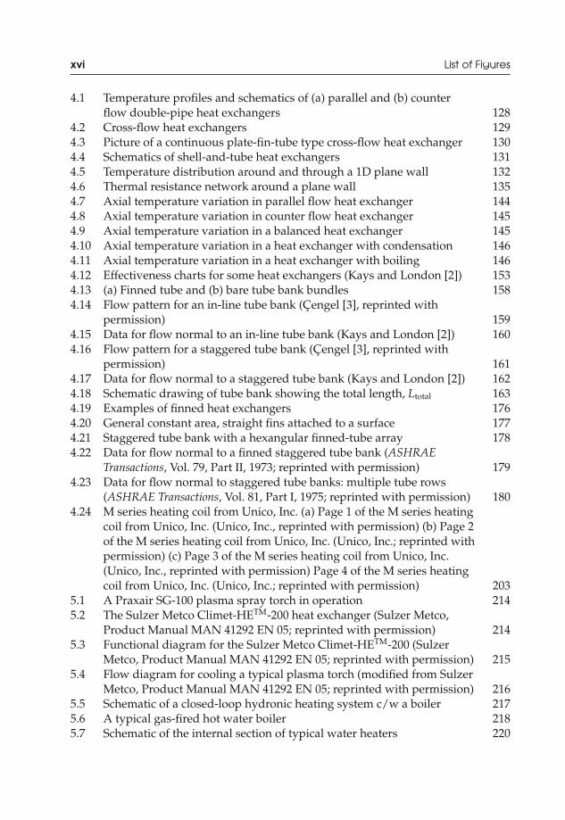
List of Figures
1.1 General steps in the design process 32.1 Duct shapes and aspect ratios 132.2 Photo of a typical air duct calculator 192.3 A ductwork system to transport air (ASHRAE Handbook, Fundamentals
Volume, 2005; reprinted with permission) 212.4 Axial fans 452.5 Centrifugal fans 452.6 Classification of centrifugal fans based on blade types 462.7 Typical performance curves of centrifugal fans 472.8 Forward-curved centrifugal fan performance curves (Morrison
Products, Inc.; reprinted with permission) 493.1 Some typical industrial valves 743.2 A typical fuel oil piping system complete with a pump set (ASHRAE
Handbook, Fundamentals Volume, 2005; reprinted with permission) 753.3 Plastic pipe (Schedule 80) friction loss chart (ASHRAE Handbook,
Fundamentals Volume, 2005; reprinted with permission) 793.4 Pipes supported on hangers 793.5 Pipes and an in-line pump mounted on brackets 813.6 Types of industrial pumps: (a) three-lobe rotary pump; (b) two-screw
pump; (c) in-line centrifugal pump; (d) vertical mutistage submersiblepump (Hydraulic Institute, Parsippany, NJ, www.pumps.org; reprintedwith permission) 84
3.7 Schematic of a Hpump versus V curve for a centrifugal pump 863.8 Schematic of a ηpump versus V curve 873.9 Schematic of a system curve intersecting a pump performance curve 883.10 Performance curves for a family of geometrically similar pumps 893.11 Pump performance plot (Taco, Inc.; reprinted with permission) 893.12 A typical open-loop condenser piping system for water 1043.13 Diagrams of closed-loop piping systems 112
xv
JWST229-fm JWST229-McDonald Printer: Yet to Come August 1, 2012 7:44 Trim: 244mm × 168mm
xvi List of Figures
4.1 Temperature profiles and schematics of (a) parallel and (b) counterflow double-pipe heat exchangers 128
4.2 Cross-flow heat exchangers 1294.3 Picture of a continuous plate-fin-tube type cross-flow heat exchanger 1304.4 Schematics of shell-and-tube heat exchangers 1314.5 Temperature distribution around and through a 1D plane wall 1324.6 Thermal resistance network around a plane wall 1354.7 Axial temperature variation in parallel flow heat exchanger 1444.8 Axial temperature variation in counter flow heat exchanger 1454.9 Axial temperature variation in a balanced heat exchanger 1454.10 Axial temperature variation in a heat exchanger with condensation 1464.11 Axial temperature variation in a heat exchanger with boiling 1464.12 Effectiveness charts for some heat exchangers (Kays and London [2]) 1534.13 (a) Finned tube and (b) bare tube bank bundles 1584.14 Flow pattern for an in-line tube bank (Cengel [3], reprinted with
permission) 1594.15 Data for flow normal to an in-line tube bank (Kays and London [2]) 1604.16 Flow pattern for a staggered tube bank (Cengel [3], reprinted with
permission) 1614.17 Data for flow normal to a staggered tube bank (Kays and London [2]) 1624.18 Schematic drawing of tube bank showing the total length, Ltotal 1634.19 Examples of finned heat exchangers 1764.20 General constant area, straight fins attached to a surface 1774.21 Staggered tube bank with a hexangular finned-tube array 1784.22 Data for flow normal to a finned staggered tube bank (ASHRAE
Transactions, Vol. 79, Part II, 1973; reprinted with permission) 1794.23 Data for flow normal to staggered tube banks: multiple tube rows
(ASHRAE Transactions, Vol. 81, Part I, 1975; reprinted with permission) 1804.24 M series heating coil from Unico, Inc. (a) Page 1 of the M series heating
coil from Unico, Inc. (Unico, Inc., reprinted with permission) (b) Page 2of the M series heating coil from Unico, Inc. (Unico, Inc.; reprinted withpermission) (c) Page 3 of the M series heating coil from Unico, Inc.(Unico, Inc., reprinted with permission) Page 4 of the M series heatingcoil from Unico, Inc. (Unico, Inc.; reprinted with permission) 203
5.1 A Praxair SG-100 plasma spray torch in operation 2145.2 The Sulzer Metco Climet-HETM-200 heat exchanger (Sulzer Metco,
Product Manual MAN 41292 EN 05; reprinted with permission) 2145.3 Functional diagram for the Sulzer Metco Climet-HETM-200 (Sulzer
Metco, Product Manual MAN 41292 EN 05; reprinted with permission) 2155.4 Flow diagram for cooling a typical plasma torch (modified from Sulzer
Metco, Product Manual MAN 41292 EN 05; reprinted with permission) 2165.5 Schematic of a closed-loop hydronic heating system c/w a boiler 2175.6 A typical gas-fired hot water boiler 2185.7 Schematic of the internal section of typical water heaters 220
JWST229-fm JWST229-McDonald Printer: Yet to Come August 1, 2012 7:44 Trim: 244mm × 168mm
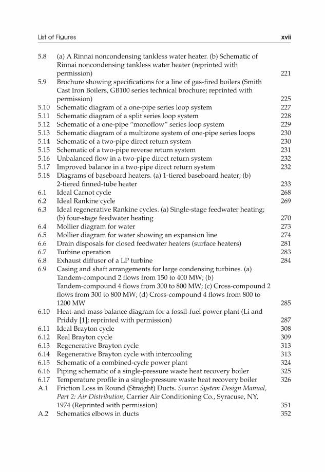
List of Figures xvii
5.8 (a) A Rinnai noncondensing tankless water heater. (b) Schematic ofRinnai noncondensing tankless water heater (reprinted withpermission) 221
5.9 Brochure showing specifications for a line of gas-fired boilers (SmithCast Iron Boilers, GB100 series technical brochure; reprinted withpermission) 225
5.10 Schematic diagram of a one-pipe series loop system 2275.11 Schematic diagram of a split series loop system 2285.12 Schematic of a one-pipe “monoflow” series loop system 2295.13 Schematic diagram of a multizone system of one-pipe series loops 2305.14 Schematic of a two-pipe direct return system 2305.15 Schematic of a two-pipe reverse return system 2315.16 Unbalanced flow in a two-pipe direct return system 2325.17 Improved balance in a two-pipe direct return system 2325.18 Diagrams of baseboard heaters. (a) 1-tiered baseboard heater; (b)
2-tiered finned-tube heater 2336.1 Ideal Carnot cycle 2686.2 Ideal Rankine cycle 2696.3 Ideal regenerative Rankine cycles. (a) Single-stage feedwater heating;
(b) four-stage feedwater heating 2706.4 Mollier diagram for water 2736.5 Mollier diagram for water showing an expansion line 2746.6 Drain disposals for closed feedwater heaters (surface heaters) 2816.7 Turbine operation 2836.8 Exhaust diffuser of a LP turbine 2846.9 Casing and shaft arrangements for large condensing turbines. (a)
Tandem-compound 2 flows from 150 to 400 MW; (b)Tandem-compound 4 flows from 300 to 800 MW; (c) Cross-compound 2flows from 300 to 800 MW; (d) Cross-compound 4 flows from 800 to1200 MW 285
6.10 Heat-and-mass balance diagram for a fossil-fuel power plant (Li andPriddy [1]; reprinted with permission) 287
6.11 Ideal Brayton cycle 3086.12 Real Brayton cycle 3096.13 Regenerative Brayton cycle 3136.14 Regenerative Brayton cycle with intercooling 3136.15 Schematic of a combined-cycle power plant 3246.16 Piping schematic of a single-pressure waste heat recovery boiler 3256.17 Temperature profile in a single-pressure waste heat recovery boiler 326A.1 Friction Loss in Round (Straight) Ducts. Source: System Design Manual,
Part 2: Air Distribution, Carrier Air Conditioning Co., Syracuse, NY,1974 (Reprinted with permission) 351
A.2 Schematics elbows in ducts 352

JWST229-fm JWST229-McDonald Printer: Yet to Come August 1, 2012 7:44 Trim: 244mm × 168mm
xviii List of Figures
A.3 Copper tubing friction loss (open and closed piping systems) (CarrierCorp.; reprinted with permission) 353
A.4 Commercial steel pipe (Schedule 40) friction loss. (a) Open pipingsystems (Carrier Corp.; reprinted with permission); (b) closed pipingsystems (Carrier Corp.; reprinted with permission) 354
A.5 Bell & Gosset pump catalog (ITT Bell & Gossett; reprinted withpermission) 356
C.1 j-factor versus ReG charts for in-line tube banks. Transient tests(2 charts): (a) For Xt = 1.50 and XL = 1.25; (b) For Xt = 1.25 andXL = 1.25.(Kays, W. and London, A. (1964) Compact Heat Exchangers, 2nd edn,McGraw-Hill, Inc., New York) 375
C.2 j-factor versus ReG charts for staggered tube banks. Transient tests(6 charts): (a) For Xt = 1.50 and XL = 1.25; (b) For Xt = 1.25 andXL = 1.25; (c) For Xt = 1.50 and XL = 1.0; (d) For Xt = 1.5 and XL = 1.5;(e) For Xt = 2 and XL = 1; (f) For Xt = 2.5 and XL = 0.75.(Kays, W. and London, A. (1964) Compact Heat Exchangers, 2nd edn,McGraw-Hill, Inc., New York) 376
C.3 j-factor versus RexL charts for staggered tube banks (finned tubes):(a) five rows of tubes (ASHRAE Transactions, vol. 79, Part II, 1973;reprinted with permission); (b) multiple rows of tubes (ASHRAETransactions, vol. 81, Part I, 1975; reprinted with permission) 380
C.4 j-factor versus ReG charts for staggered tube banks (finned tubes).(a) Tube outer diameter = 0.402 in.; (b) tube outer diameter = 0.676 in.(Kays, W. and London, A. (1964) Compact Heat Exchangers, 2nd edn,McGraw-Hill, Inc., New York) 381
JWST229-fm JWST229-McDonald Printer: Yet to Come August 1, 2012 7:44 Trim: 244mm × 168mm
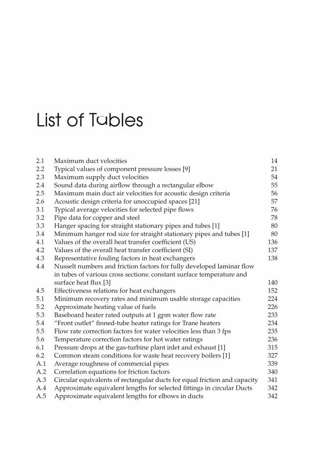
List of Tables
2.1 Maximum duct velocities 142.2 Typical values of component pressure losses [9] 212.3 Maximum supply duct velocities 542.4 Sound data during airflow through a rectangular elbow 552.5 Maximum main duct air velocities for acoustic design criteria 562.6 Acoustic design criteria for unoccupied spaces [21] 573.1 Typical average velocities for selected pipe flows 763.2 Pipe data for copper and steel 783.3 Hanger spacing for straight stationary pipes and tubes [1] 803.4 Minimum hanger rod size for straight stationary pipes and tubes [1] 804.1 Values of the overall heat transfer coefficient (US) 1364.2 Values of the overall heat transfer coefficient (SI) 1374.3 Representative fouling factors in heat exchangers 1384.4 Nusselt numbers and friction factors for fully developed laminar flow
in tubes of various cross sections: constant surface temperature andsurface heat flux [3] 140
4.5 Effectiveness relations for heat exchangers 1525.1 Minimum recovery rates and minimum usable storage capacities 2245.2 Approximate heating value of fuels 2265.3 Baseboard heater rated outputs at 1 gpm water flow rate 2335.4 “Front outlet” finned-tube heater ratings for Trane heaters 2345.5 Flow rate correction factors for water velocities less than 3 fps 2355.6 Temperature correction factors for hot water ratings 2366.1 Pressure drops at the gas-turbine plant inlet and exhaust [1] 3156.2 Common steam conditions for waste heat recovery boilers [1] 327A.1 Average roughness of commercial pipes 339A.2 Correlation equations for friction factors 340A.3 Circular equivalents of rectangular ducts for equal friction and capacity 341A.4 Approximate equivalent lengths for selected fittings in circular Ducts 342A.5 Approximate equivalent lengths for elbows in ducts 342
xix

JWST229-fm JWST229-McDonald Printer: Yet to Come August 1, 2012 7:44 Trim: 244mm × 168mm
xx List of Tables
A.6 Data for copper pipes 343A.7 Data for schedule 40 steel pipes 344A.8 Data for schedule 80 steel pipes 345A.9 Data for class 150 cast iron pipes 346A.10 Data for glass pipes 346A.11 Data for PVC plastic pipes 347A.12 Typical average velocities for selected pipe flowsa 348A.13 Erosion limits: maximum design fluid velocities for water flow in
small tubes 348A.14 Loss coefficients for pipe fittings 349A.15 Typical pipe data format 350A.16 Typical pump schedule format 350B.1 Airmoving devices and ductwork symbols 365B.2 Piping symbols 367B.3 Symbols for piping specialities 368B.4 Additional/alternate valve symbols 369B.5 Fittings 370B.6 Radiant Panel Symbols 372C.1 Representative values of the overall heat transfer coefficients (US) 373C.2 Representative values of the overall heat transfer coefficients (SI) 374C.3 Representative fouling factors in heat exchangers 374

JWST229-fm JWST229-McDonald Printer: Yet to Come August 1, 2012 7:44 Trim: 244mm × 168mm
List of Practical Notes
2.1 Total Static Pressure Available at a Plenum or Produced by a Fan 202.2 Diffuser Discharge Air Volume Flow Rates
in SDHV Systems 563.1 Link Seals 753.2 Piping Systems Containing Air 763.3 Higher Pipe Friction Losses and Velocities 773.4 Piping System Supported by Brackets 813.5 Manufacturers’ Pump Performance Curves 883.6 “To-the-point” Design 903.7 Oversizing Pumps 903.8 NPSH 933.9 Bypass Lines 1043.10 Regulation and Control of Flow Rate
across a Pump 1043.11 In-Line and Base-Mounted Pumps 1053.12 Flanged or Screwed Pipe Fittings? 1134.1 Industrial Flows 1424.2 Flow in Rough Pipes 1424.3 Condensers and Boilers 1474.4 Real Heat Exchangers 1494.5 Heat Transfer from Staggered Tube Banks 1614.6 Coil Arrangement in Air-to-Water
Heat Exchangers 1644.7 Pressure Drop Over Tube Banks 1644.8 L and M values 1795.1 Condensing Boilers 2195.2 Typical OSF Values 2225.3 Domestic Water Data for Edmonton, Alberta, Canada 2235.4 Hot Water Temperatures from Faucets 2235.5 Temperature Data for Sizing Finned-Tube Heaters 235
xxi

JWST229-fm JWST229-McDonald Printer: Yet to Come August 1, 2012 7:44 Trim: 244mm × 168mm
xxii List of Practical Notes
6.1 Optimizing the Number of Feedwater Heaters 2716.2 DCA and TTD Values 2816.3 Stages of a Steam Turbine 2826.4 Exhaust End Loss 2846.5 Units of the Net Heat Rate (NHR) 2886.6 How Does One Initiate Operation of a Power Plant System? 2896.7 Reference Pressure and Temperature for Availability Analysis 3026.8 Combustion Air and Cracking in a Burner 309

JWST229-fm JWST229-McDonald Printer: Yet to Come August 1, 2012 7:44 Trim: 244mm × 168mm
List of Conversion Factors
Dimension Conversion
Energy 1 Btu = 778.28 lbf ft1 kWh = 3412.14 Btu1 hp h = 2545 Btu1 therm = 105 Btu (natural gas)
Force 1 lbf = 32.2 lbm ft/s2 = 16 ozf1 dyne = 2.248 × 10⁻⁶ lbf
Length 1 ft = 12 in.1 yard = 3 ft1 in. = 25.4 mm1 mile = 5280 ft
Mass 1 slug = 32.2 lbm1 lbm = 16 ounces (oz)1 ton mass = 2000 lbm
Power 1 kW = 3412.14 Btu/h1 hp = 550 lbf ft/s1 hp (boiler) = 33475 Btu/h1 ton refrigeration = 12000 Btu/h
Pressure 1 atm = 14.7 psia1 psia = 2.0 in Hg at 32◦F
Temperature T(R) = T(◦F) + 460T(◦F) = 1.8T(◦C) + 32
Viscosity (dynamic) 1 lbm/(ft s) = 1488 centipoises (cp)
Viscosity (kinematic) 1 ft2/s = 929 stokes (St)
Volume 1 British gallon = 1.2 US gallon1 ft3 = 7.48 US gallons1 US gallon = 128 fluid ounces
Volume Flow Rate 35.315 ft3/s = 15850 gal/min (gpm) = 2118.9 ft3/min (cfm)
xxiii

JWST229-c01 JWST229-McDonald Printer: Yet to Come July 27, 2012 9:6 Trim: 244mm × 168mm
1Design of Thermo-FluidsSystems
1.1 Engineering Design—Definition
Process of devising a system, subsystem, component, or process to meet desiredneeds.
1.2 Types of Design in Thermo-Fluid Science
(i) Process Design: The manipulation of physical and/or chemical processes to meetdesired needs.
Example: (a) Introduce boiling or condensation to increase heat transfer rates.(ii) System Design: The process of defining the components and their assembly to
function to meet a specified requirement.Examples: (a) Steam turbine power plant system consisting of turbines, pumps,
pipes, and heat exchangers.(b) Hot water heating system, complete with boilers.
(iii) Subsystem Design: The process of defining and assembling a small group of com-ponents to do a specified function.
Example: Pump/piping system of a large power plant. The pump/pipingsystem is a subsystem of the larger power plant system used to transport waterto and from the boiler or steam generator.
(iv) Component Design: Development of a piece of equipment or device.
Introduction to Thermo-Fluids Systems Design, First Edition. Andre G. McDonald and Hugh L. Magande.C© 2012 Andre G. McDonald and Hugh L. Magande. Published 2012 by John Wiley & Sons, Ltd.
1
JWST229-c01 JWST229-McDonald Printer: Yet to Come July 27, 2012 9:6 Trim: 244mm × 168mm
2 Introduction to Thermo-Fluids Systems Design
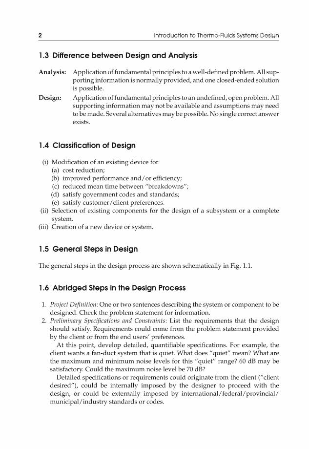
1.3 Difference between Design and Analysis
Analysis: Application of fundamental principles to a well-defined problem. All sup-porting information is normally provided, and one closed-ended solutionis possible.
Design: Application of fundamental principles to an undefined, open problem. Allsupporting information may not be available and assumptions may needto be made. Several alternatives may be possible. No single correct answerexists.
1.4 Classification of Design
(i) Modification of an existing device for(a) cost reduction;(b) improved performance and/or efficiency;(c) reduced mean time between “breakdowns”;(d) satisfy government codes and standards;(e) satisfy customer/client preferences.
(ii) Selection of existing components for the design of a subsystem or a completesystem.
(iii) Creation of a new device or system.
1.5 General Steps in Design
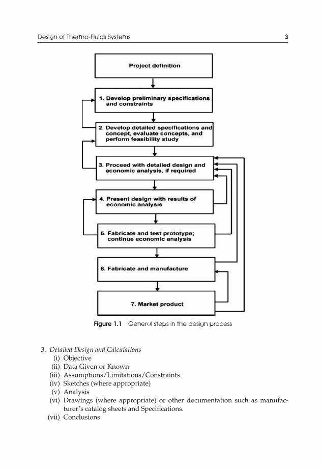
The general steps in the design process are shown schematically in Fig. 1.1.
1.6 Abridged Steps in the Design Process
1. Project Definition: One or two sentences describing the system or component to bedesigned. Check the problem statement for information.
2. Preliminary Specifications and Constraints: List the requirements that the designshould satisfy. Requirements could come from the problem statement providedby the client or from the end users’ preferences.
At this point, develop detailed, quantifiable specifications. For example, theclient wants a fan-duct system that is quiet. What does “quiet” mean? What arethe maximum and minimum noise levels for this “quiet” range? 60 dB may besatisfactory. Could the maximum noise level be 70 dB?
Detailed specifications or requirements could originate from the client (“clientdesired”), could be internally imposed by the designer to proceed with thedesign, or could be externally imposed by international/federal/provincial/municipal/industry standards or codes.
JWST229-c01 JWST229-McDonald Printer: Yet to Come July 27, 2012 9:6 Trim: 244mm × 168mm
Design of Thermo-Fluids Systems 3
Figure 1.1 General steps in the design process
3. Detailed Design and Calculations(i) Objective
(ii) Data Given or Known(iii) Assumptions/Limitations/Constraints(iv) Sketches (where appropriate)(v) Analysis
(vi) Drawings (where appropriate) or other documentation such as manufac-turer’s catalog sheets and Specifications.
(vii) Conclusions

JWST229-c02 JWST229-McDonald Printer: Yet to Come July 28, 2012 13:33 Trim: 244mm × 168mm
2Air Distribution Systems
2.1 Fluid Mechanics—A Brief Review
2.1.1 Internal Flow
Flow is laminar: smooth streamlines; highly ordered motion.Or
Flow is turbulent: velocity fluctuates with time; highly disordered motion.Use the Reynolds number to characterize the flow regime:
ReD = ρVave Dμ
= Vave Dυ
= inertial forcesviscous forces
. (2.1)
Note: For noncircular pipes or ducts, ReD is based on the hydraulic diameter, Dh:
Dh = 4Ac
p, (2.2)
where Ac is the cross-sectional area and p is the perimeter wetted by the fluid.For square ducts,
Dh = 4(L × L)L + L + L + L
= 4L2
4L= L . (2.3)
For rectangular ducts,
Dh = 4(L × w)2L + 2w
= 2LwL + w
. (2.4)
It is important to note that, for volume flow rate calculations, Dh should not beused to find the cross-sectional area. Use the true cross-sectional area.
Introduction to Thermo-Fluids Systems Design, First Edition. Andre G. McDonald and Hugh L. Magande.C© 2012 Andre G. McDonald and Hugh L. Magande. Published 2012 by John Wiley & Sons, Ltd.
5

JWST229-c02 JWST229-McDonald Printer: Yet to Come July 28, 2012 13:33 Trim: 244mm × 168mm
6 Introduction to Thermo-Fluids Systems Design
Therefore, for a rectangular duct,
V = Vave Ac = Vave(Lw). (2.5)
But
V = Vave Ac �= Vave
(π D2
h
4
). (2.6)
Criteria for Flow Characterization
Re ≤ 2300 Laminar flow (2.7)
2300 ≤ Re ≤ 4000 Transitional flow: laminar to turbulent flow (2.8)
Re ≥ 4000 Fully turbulent flow. (2.9)
For engineering design analysis, use a critical Reynolds number, Recr:
Recr = 2300 (2.10)
Re < Recr For laminar flow (2.11)
Re > Recr For turbulent flow. (2.12)
2.1.2 Frictional Losses in Internal Flow—Head Losses
For fully developed laminar flow, the volume flow rate is related to the pressure dropvia Poiseuille’s law:
V = π D4�P128 μL
. (2.13)
So,
V ∝ �P and Vave ∝ �P. (2.14)
From these relationships, it can be seen that an increase in the average velocitywithin the duct/pipe system will result in an increased pressure drop within theduct/pipe owing to the higher frictional losses.
Head losses are the frictional losses that occur in ducts/pipes due to flow. There aretwo types of head losses:
Major head losses, Hl: These are due to viscous effects in fully developed flow inconstant area pipes or ducts.

JWST229-c02 JWST229-McDonald Printer: Yet to Come July 28, 2012 13:33 Trim: 244mm × 168mm
Air Distribution Systems 7
Minor head losses, Hlm: These are due to entrances, fittings, valves, and area changes.In addition, for ductwork this could be caused by filters, cooling or heating coils,and volume dampers, to name a few.
Given the point above, the total head loss is determined by
HlT = Hl + Hlm. (2.15)
Head losses are expressed in units of meter, feet, or inches of fluid. Head lossexpressed in terms of units of length of water is preferred by practicing engineers inindustry.
Under some conditions, the total head loss in a pipe/duct system is directly relatedto the pressure drop in the length of pipe/duct. Consider the energy equation (withoutfluid machines included in the pipe/duct section):
(p1
ρg+ V2
1
2g+ z1
)−
(p2
ρg+ V2
2
2g+ z2
)= HlT, (2.16)
where points 1 and 2 are points selected at the beginning and end points of the lengthof pipe/duct. The average pipe/duct velocity is V.
For a constant area pipe/duct, V1 = V2. For a horizontal pipe/duct, z1 = z2.Hence,
p1
ρg− p2
ρg= �p
ρg= HlT, (2.17)
where �p is the pressure drop across the length of pipe/duct.
2.1.3 Major Head Loss in a Run of Pipe or Duct—Pipe/Duct Sizing
In general, the following expression for head loss applies:
Hl = fLD
V2
2g, (2.18)
where f is Darcy friction factor.For laminar flows,
flaminar = 64ReD
. (2.19)
So, flaminar depends on the Reynolds number only.
JWST229-c02 JWST229-McDonald Printer: Yet to Come July 28, 2012 13:33 Trim: 244mm × 168mm
8 Introduction to Thermo-Fluids Systems Design
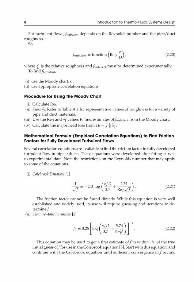
For turbulent flows, fturbulent depends on the Reynolds number and the pipe/ductroughness, e.
So,
fturbulent = function(
ReD,
eD
), (2.20)
where eD is the relative roughness and fturbulent must be determined experimentally.
To find fturbulent,
(i) use the Moody chart, or(ii) use appropriate correlation equations.
Procedure for Using the Moody Chart
(i) Calculate ReD.(ii) Find e
D . Refer to Table A.1 for representative values of roughness for a variety ofpipe and duct materials.
(iii) Use the ReD and eD values to find estimates of fturbulent from the Moody chart.
(iv) Calculate the major head loss from Hl = f LD
V2
2g .
Mathematical Formula (Empirical Correlation Equations) to Find FrictionFactors for Fully Developed Turbulent Flows
Several correlation equations are available to find the friction factor in fully developedturbulent flow in pipes/ducts. These equations were developed after fitting curvesto experimental data. Note the restrictions on the Reynolds number that may applyto some of the equations.
(i) Colebrook Equation [1]
1√f
= −2.0 log(
ε/D3.7
+ 2.51ReD
√f
). (2.21)
The friction factor cannot be found directly. While this equation is very wellestablished and widely used, its use will require guessing and iterations to de-termine f.
(ii) Swamee–Jain Formulae [2]
f0 = 0.25
[log
(ε/D3.7
+ 5.74
Re0.9D
)]−2
. (2.22)
This equation may be used to get a first estimate of f to within 1% of the trueinitial guess of f for use in the Colebrook equation [3]. Start with this equation, andcontinue with the Colebrook equation until sufficient convergence in f occurs.
JWST229-c02 JWST229-McDonald Printer: Yet to Come July 28, 2012 13:33 Trim: 244mm × 168mm
Air Distribution Systems 9
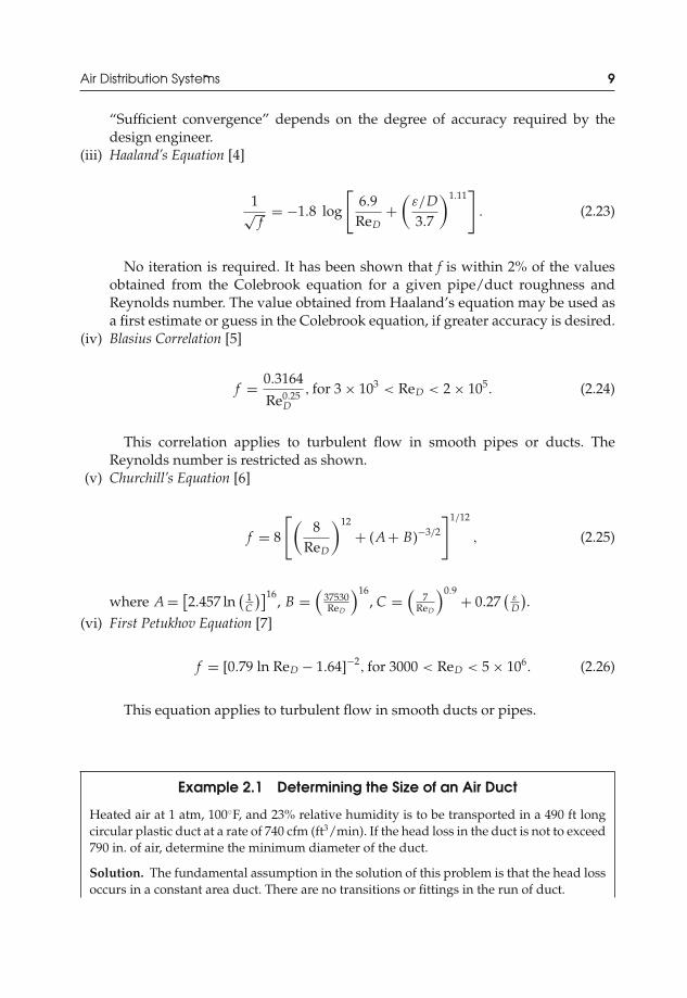
“Sufficient convergence” depends on the degree of accuracy required by thedesign engineer.
(iii) Haaland’s Equation [4]
1√f
= −1.8 log
[6.9
ReD+
(ε/D3.7
)1.11]
. (2.23)
No iteration is required. It has been shown that f is within 2% of the valuesobtained from the Colebrook equation for a given pipe/duct roughness andReynolds number. The value obtained from Haaland’s equation may be used asa first estimate or guess in the Colebrook equation, if greater accuracy is desired.
(iv) Blasius Correlation [5]
f = 0.3164
Re0.25D
, for 3 × 10³ < ReD < 2 × 10⁵. (2.24)
This correlation applies to turbulent flow in smooth pipes or ducts. TheReynolds number is restricted as shown.
(v) Churchill’s Equation [6]
f = 8
[(8
ReD
)12
+ (A+ B)−3/2
]1/12
, (2.25)
where A = [2.457 ln
( 1C
)]16, B =
(37530ReD
)16, C =
(7
ReD
)0.9+ 0.27
(εD
).
(vi) First Petukhov Equation [7]
f = [0.79 ln ReD − 1.64]−2, for 3000 < ReD < 5 × 10⁶. (2.26)
This equation applies to turbulent flow in smooth ducts or pipes.
Example 2.1 Determining the Size of an Air Duct
Heated air at 1 atm, 100◦F, and 23% relative humidity is to be transported in a 490 ft longcircular plastic duct at a rate of 740 cfm (ft3/min). If the head loss in the duct is not to exceed790 in. of air, determine the minimum diameter of the duct.
Solution. The fundamental assumption in the solution of this problem is that the head lossoccurs in a constant area duct. There are no transitions or fittings in the run of duct.
JWST229-c02 JWST229-McDonald Printer: Yet to Come July 28, 2012 13:33 Trim: 244mm × 168mm
10 Introduction to Thermo-Fluids Systems Design
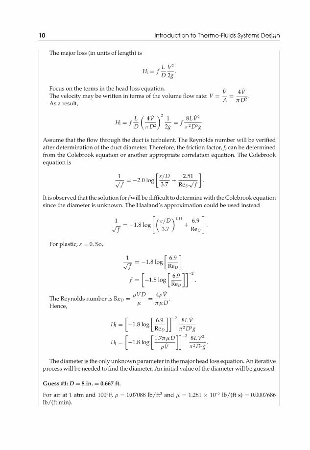
The major loss (in units of length) is
Hl = fLD
V2
2g.
Focus on the terms in the head loss equation.The velocity may be written in terms of the volume flow rate: V = V
A= 4V
π D2.
As a result,
Hl = fLD
(4Vπ D2
)21
2g= f
8LV2
π 2 D5g.
Assume that the flow through the duct is turbulent. The Reynolds number will be verifiedafter determination of the duct diameter. Therefore, the friction factor, f, can be determinedfrom the Colebrook equation or another appropriate correlation equation. The Colebrookequation is
1√f
= −2.0 log[
ε/D3.7
+ 2.51ReD
√f
].
It is observed that the solution for f will be difficult to determine with the Colebrook equationsince the diameter is unknown. The Haaland’s approximation could be used instead
1√f
= −1.8 log
[(ε/D3.7
)1.11
+ 6.9ReD
].
For plastic, ε = 0. So,
1√f
= −1.8 log[
6.9ReD
]
f =[−1.8 log
[6.9ReD
]]−2
.
The Reynolds number is ReD = ρVDμ
= 4ρVπμD
.Hence,
Hl =[−1.8 log
[6.9ReD
]]−2 8LVπ 2 D5g
Hl =[−1.8 log
[1.7πμD
ρV
]]−2 8LV2
π 2 D5g.
The diameter is the only unknown parameter in the major head loss equation. An iterativeprocess will be needed to find the diameter. An initial value of the diameter will be guessed.
Guess #1: D = 8 in. = 0.667 ft.
For air at 1 atm and 100◦F, ρ = 0.07088 lb/ft3 and μ = 1.281 × 10⁻⁵ lb/(ft s) = 0.0007686lb/(ft min).
JWST229-c02 JWST229-McDonald Printer: Yet to Come July 28, 2012 13:33 Trim: 244mm × 168mm
Air Distribution Systems 11
Therefore,
Hl =⎡⎣−1.8 log
⎡⎣1.7π (0.0007686 lb/ft/min) (0.667 ft)(
0.07088 lb/ft3) (
740 ft3/min
)⎤⎦
⎤⎦
−28 (490 ft)
(740 ft3
/min)2
π 2 (0.667 ft)5(
32.2 ft/s2)
×(
1 min60 s
)2
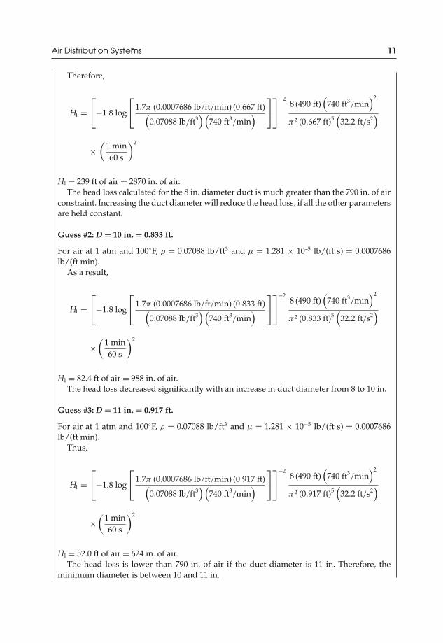
Hl = 239 ft of air = 2870 in. of air.The head loss calculated for the 8 in. diameter duct is much greater than the 790 in. of air
constraint. Increasing the duct diameter will reduce the head loss, if all the other parametersare held constant.
Guess #2: D = 10 in. = 0.833 ft.
For air at 1 atm and 100◦F, ρ = 0.07088 lb/ft3 and μ = 1.281 × 10⁻⁵ lb/(ft s) = 0.0007686lb/(ft min).
As a result,
Hl =⎡⎣−1.8 log
⎡⎣1.7π (0.0007686 lb/ft/min) (0.833 ft)(
0.07088 lb/ft3) (
740 ft3/min
)⎤⎦
⎤⎦
−28 (490 ft)
(740 ft3
/min)2
π 2 (0.833 ft)5(
32.2 ft/s2)
×(
1 min60 s
)2
Hl = 82.4 ft of air = 988 in. of air.The head loss decreased significantly with an increase in duct diameter from 8 to 10 in.
Guess #3: D = 11 in. = 0.917 ft.
For air at 1 atm and 100◦F, ρ = 0.07088 lb/ft3 and μ = 1.281 × 10⁻⁵ lb/(ft s) = 0.0007686lb/(ft min).
Thus,
Hl =⎡⎣−1.8 log
⎡⎣1.7π (0.0007686 lb/ft/min) (0.917 ft)(
0.07088 lb/ft3) (
740 ft3/min
)⎤⎦
⎤⎦
−28 (490 ft)
(740 ft3
/min)2
π 2 (0.917 ft)5(
32.2 ft/s2)
×(
1 min60 s
)2
Hl = 52.0 ft of air = 624 in. of air.The head loss is lower than 790 in. of air if the duct diameter is 11 in. Therefore, the
minimum diameter is between 10 and 11 in.
JWST229-c02 JWST229-McDonald Printer: Yet to Come July 28, 2012 13:33 Trim: 244mm × 168mm
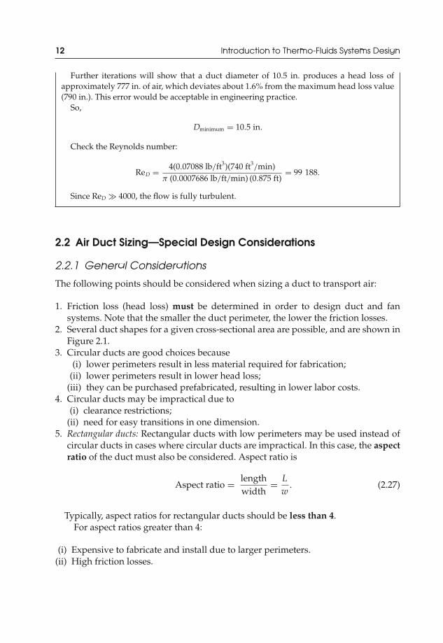
12 Introduction to Thermo-Fluids Systems Design
Further iterations will show that a duct diameter of 10.5 in. produces a head loss ofapproximately 777 in. of air, which deviates about 1.6% from the maximum head loss value(790 in.). This error would be acceptable in engineering practice.
So,
Dminimum = 10.5 in.
Check the Reynolds number:
ReD = 4(0.07088 lb/ft3)(740 ft3/min)
π (0.0007686 lb/ft/min) (0.875 ft)= 99 188.
Since ReD 4000, the flow is fully turbulent.
2.2 Air Duct Sizing—Special Design Considerations
2.2.1 General Considerations
The following points should be considered when sizing a duct to transport air:
1. Friction loss (head loss) must be determined in order to design duct and fansystems. Note that the smaller the duct perimeter, the lower the friction losses.
2. Several duct shapes for a given cross-sectional area are possible, and are shown inFigure 2.1.
3. Circular ducts are good choices because(i) lower perimeters result in less material required for fabrication;
(ii) lower perimeters result in lower head loss;(iii) they can be purchased prefabricated, resulting in lower labor costs.
4. Circular ducts may be impractical due to(i) clearance restrictions;
(ii) need for easy transitions in one dimension.5. Rectangular ducts: Rectangular ducts with low perimeters may be used instead of
circular ducts in cases where circular ducts are impractical. In this case, the aspectratio of the duct must also be considered. Aspect ratio is
Aspect ratio = lengthwidth
= Lw
. (2.27)
Typically, aspect ratios for rectangular ducts should be less than 4.For aspect ratios greater than 4:
(i) Expensive to fabricate and install due to larger perimeters.(ii) High friction losses.

JWST229-c02 JWST229-McDonald Printer: Yet to Come July 28, 2012 13:33 Trim: 244mm × 168mm
Air Distribution Systems 13
Figure 2.1 Duct shapes and aspect ratios
2.2.2 Sizing Straight Rectangular Air Ducts
The Circular Equivalent Method presents a practical approach to size rectangularducts. First, determine the diameter of a round duct that satisfies the airflow require-ment at an acceptable velocity and frictional loss. Charts may be used to facilitatethe selection of an appropriate round duct diameter, rather than using the correlationequations presented in Example 2.1. For applications requiring low noise, velocitieslower than about 1200 ft/min are desired (low-velocity systems). Table 2.1 presentsan exhaustive list of maximum duct velocities for low-velocity systems [9]. Tables orcharts may then be used to select equivalent rectangular ducts, based on the roundduct diameter. Since many configurations of equivalent rectangular duct dimensionswill be available for a given round duct diameter, the final choice of rectangular ductdimensions will depend on the following:
(i) Architectural barriers and limitations.(ii) Location of structural members.
(iii) Noise constraint: Higher flow velocities produce more noise in the ductwork(typical).
(iv) Aspect ratio: Lower aspect ratio ducts require less material for fabrication andwill produce less head loss (typical).

JWST229-c02 JWST229-McDonald Printer: Yet to Come July 28, 2012 13:33 Trim: 244mm × 168mm
14 Introduction to Thermo-Fluids Systems Design
Table 2.1 Maximum duct velocities
Low-Velocity Systems
Schools, Theaters,Designation Private Residences Public Buildings Industrial Buildings
Maximum Velocities (fpm)
Main ducts 800–1200 1100–1600 1300–2200Branch ducts 700–1000 800–1300 1000–1800Branch risers 650–800 800–1200 1000–1600
Typical Velocities (fpm)a
Throwaway filter 200–800Heating coil 400–500 (200 min, 1500 max)Cooling coil 500–600
Source: Howell, Sauer, and Coad [9].aDuctulator, Trane US Inc., La Crosse, Wisconsin.
Example 2.2 Sizing a Rectangular Air Duct
Size an appropriate rectangular air duct under the following conditions from Example 2.1:
(a) Heated air at 1 atm, 100◦F, and 23% RH(b) Flow rate of 740 cfm(c) Head loss of 790 in. of air over 490 ft of duct(d) Duct material is plastic tubing (ε ≈ 0)
Solution. Figure A.1 can be used to find the diameter of the circular duct equivalent basedon the air volume flow rate and friction loss. Figure A.1 applies to clean, round, smooth,galvanized metal duct.
This problem provides the friction loss in units of in of air. However, the friction losschart of Figure A.1 uses friction loss as inch water gage (in. wg) per 100 ft of equivalentlength of duct. Therefore, the head loss of 790 in. of air (Ha) should be converted to headloss in terms of inches water gage (Hw) for use with the friction loss chart. From fluidstatics,
ρairgHa = ρwatergHw.
Thus,
Hw = ρair
ρwaterHa = SGair Ha.
JWST229-c02 JWST229-McDonald Printer: Yet to Come July 28, 2012 13:33 Trim: 244mm × 168mm
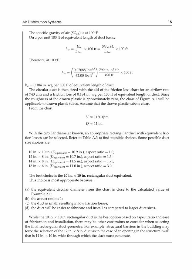
Air Distribution Systems 15
The specific gravity of air (SGair) is at 100◦F.On a per unit 100 ft of equivalent length of duct basis,
hw = Hw
Lduct× 100 ft = SGair Ha
Lduct× 100 ft.
Therefore, at 100◦F,
hw =(
0.07088 lb/ft3
62.00 lb/ft3
)790 in. of air
490 ft× 100 ft
hw = 0.184 in. wg per 100 ft of equivalent length of duct.The circular duct is then sized with the aid of the friction loss chart for an airflow rate
of 740 cfm and a friction loss of 0.184 in. wg per 100 ft of equivalent length of duct. Sincethe roughness of the drawn plastic is approximately zero, the chart of Figure A.1 will beapplicable to drawn plastic tubes. Assume that the drawn plastic tube is clean.
From the chart:
V ≈ 1180 fpm
D ≈ 11 in.
With the circular diameter known, an appropriate rectangular duct with equivalent fric-tion losses can be selected. Refer to Table A.3 to find possible choices. Some possible ductsize choices are
10 in. × 10 in. (Dequivalent = 10.9 in.), aspect ratio = 1.0;12 in. × 8 in. (Dequivalent = 10.7 in.), aspect ratio = 1.5;14 in. × 8 in. (Dequivalent = 11.5 in.), aspect ratio = 1.75;18 in. × 6 in. (Dequivalent = 11.0 in.), aspect ratio = 3.0.
The best choice is the 10 in. × 10 in. rectangular duct equivalent.This choice is most appropriate because
(a) the equivalent circular diameter from the chart is close to the calculated value ofExample 2.1;
(b) the aspect ratio is 1;(c) the duct is small, resulting in low friction losses;(d) the duct will be easier to fabricate and install as compared to larger duct sizes.
While the 10 in. × 10 in. rectangular duct is the best option based on aspect ratio and easeof fabrication and installation, there may be other constraints to consider when selectingthe final rectangular duct geometry. For example, structural barriers in the building mayforce the selection of the 12 in. × 8 in. duct as in the case of an opening in the structural wallthat is 14 in. × 10 in. wide through which the duct must penetrate.
JWST229-c02 JWST229-McDonald Printer: Yet to Come July 28, 2012 13:33 Trim: 244mm × 168mm
16 Introduction to Thermo-Fluids Systems Design
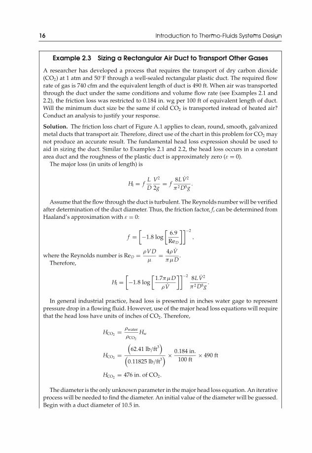
Example 2.3 Sizing a Rectangular Air Duct to Transport Other Gases
A researcher has developed a process that requires the transport of dry carbon dioxide(CO2) at 1 atm and 50◦F through a well-sealed rectangular plastic duct. The required flowrate of gas is 740 cfm and the equivalent length of duct is 490 ft. When air was transportedthrough the duct under the same conditions and volume flow rate (see Examples 2.1 and2.2), the friction loss was restricted to 0.184 in. wg per 100 ft of equivalent length of duct.Will the minimum duct size be the same if cold CO2 is transported instead of heated air?Conduct an analysis to justify your response.
Solution. The friction loss chart of Figure A.1 applies to clean, round, smooth, galvanizedmetal ducts that transport air. Therefore, direct use of the chart in this problem for CO2 maynot produce an accurate result. The fundamental head loss expression should be used toaid in sizing the duct. Similar to Examples 2.1 and 2.2, the head loss occurs in a constantarea duct and the roughness of the plastic duct is approximately zero (ε = 0).
The major loss (in units of length) is
Hl = fLD
V2
2g= f
8LV2
π 2 D5g.
Assume that the flow through the duct is turbulent. The Reynolds number will be verifiedafter determination of the duct diameter. Thus, the friction factor, f, can be determined fromHaaland’s approximation with ε = 0:
f =[−1.8 log
[6.9ReD
]]−2
,
where the Reynolds number is ReD = ρVDμ
= 4ρVπμD
.Therefore,
Hl =[−1.8 log
[1.7πμD
ρV
]]−2 8LV2
π 2 D5g.
In general industrial practice, head loss is presented in inches water gage to representpressure drop in a flowing fluid. However, use of the major head loss equations will requirethat the head loss have units of inches of CO2. Therefore,
HCO2 = ρwater
ρCO2
Hw
HCO2 =(
62.41 lb/ft3)
(0.11825 lb/ft3
) × 0.184 in.
100 ft× 490 ft
HCO2 = 476 in. of CO2.
The diameter is the only unknown parameter in the major head loss equation. An iterativeprocess will be needed to find the diameter. An initial value of the diameter will be guessed.Begin with a duct diameter of 10.5 in.

JWST229-c02 JWST229-McDonald Printer: Yet to Come July 28, 2012 13:33 Trim: 244mm × 168mm
Air Distribution Systems 17
Guess #1: D = 10.5 in. = 0.875 ft.
For CO2 at 1 atm and 50◦F, ρ = 0.11825 lb/ft3 and μ = 9.564 × 10⁻⁶ lb/(ft s) = 0.0005738lb/(ft min).
So,
Hl =⎡⎣−1.8 log
⎡⎣1.7π (0.0005738 lb/ft/min) (0.875 ft)(
0.11825 lb/ft3) (
740 ft3/min
)⎤⎦
⎤⎦
−28 (490 ft)
(740 ft3
/min)2
π 2 (0.875 ft)5(
32.2 ft/s2)
×(
1 min60 s
)2
Hl = 55 ft of CO2 = 665 in. of CO2.The head loss calculated for the 10.5 in. diameter duct is greater than the 476 in. of CO2
constraint. Increasing the duct diameter will reduce the head loss, if all the other parametersare held constant.
Guess #2: D = 11 in. = 0.917 ft.
Hl =⎡⎣−1.8 log
⎡⎣1.7π (0.0005738 lb/ft/min) (0.917 ft)(
0.11825 lb/ft3) (
740 ft3/min
)⎤⎦
⎤⎦
−28 (490 ft)
(740 ft3
/min)2
π 2 (0.917 ft)5(
32.2 ft/s2)
×(
1 min60 s
)2
Hl = 44 ft of air = 531 in. of CO2.The head loss decreased further with an increase in duct diameter.
Guess #3: D = 11.5 in. = 0.958 ft.
Hl =⎡⎣−1.8 log
⎡⎣1.7π (0.0005738 lb/ft/min) (0.958 ft)(
0.11825 lb/ft3) (
740 ft3/min
)⎤⎦
⎤⎦
−28 (490 ft)
(740 ft3
/min)2
π 2 (0.958 ft)5(
32.2 ft/s2)
×(
1 min60 s
)2
Hl = 36 ft of CO2 = 430 in. of CO2.The head loss is lower than 476 in. of CO2 if the duct diameter is 11.5 in. Therefore, the
minimum diameter is between 11 and 11.5 in.Take the circular duct diameter to be 11.5 in., which produces a head loss of approximately
430 in. of CO2, which deviates about 10% from the maximum head loss value (476 in.). Thiserror would be acceptable in engineering practice.
Therefore,
Dminimum = 11.5 in.

JWST229-c02 JWST229-McDonald Printer: Yet to Come July 28, 2012 13:33 Trim: 244mm × 168mm
18 Introduction to Thermo-Fluids Systems Design
Check the Reynolds number:
ReD = 4(0.11825 lb/ft3)(740 ft3/min)
π (0.0005738 lb/ft/min) (0.958 ft)= 202683.
Since ReD 4000, the flow is fully turbulent.The diameter of the circular duct estimated for the transport of CO2 is no more than 1 in.
larger than the diameter of the duct used to transport air. This represents a difference of nomore than 10%. Further, this error would be lower because the actual duct size would beslightly lower than 11.5 in. Under these circumstances, the 11 in. circular duct selected fromthe friction loss chart of Figure A.1 in Example 2.2 could be used in this application withoutthe generation of significant head loss to undermine the performance of the system. Theactual head loss, in inches water gage, would be 0.205 in. wg per 100 ft of equivalent lengthof duct, which corresponds to 531 in. of CO2 in 490 ft of duct.
Table A.3 and the circular equivalent method can be used to find the rectangular ductsize. So, a possible choice could be 14 in. × 8 in. (Dequivalent = 11.5 in.). In this case, the aspectratio is 1.75, which is lower than 4. This duct size and geometry was one of the possiblechoices that were presented in Example 2.2.
This exercise demonstrates that the error generated through the use of the friction losscharts that are based on air for gases may be small. Provided that these small errors areacceptable, the chart may be used to size ducts that transport a variety of gases, as well asair at various temperatures.
2.2.3 Use of an Air Duct Calculator to Size Rectangular Air Ducts
The air duct calculator is a device used to size circular and rectangular ducts.Figure 2.2 shows a typical air duct calculator. With any one of the following fourparameters known, the other three are found from a single setting of the calculator:
(i) Friction loss (head loss)(ii) Duct velocity (for round duct)
(iii) Round duct diameter(iv) Dimensions for rectangular duct
2.3 Minor Head Loss in a Run of Pipe or Duct
Minor losses occur when a fluid passes through (i) fittings, (ii) bends, (iii) valves,(iv) abrupt area changes, (v) other devices or components in the flow path thatadd resistance to flow (filters, strainers, cooling/heating coils, louvers, dampers,flowmeters), and (vi) entrances and exits.
In long air duct or liquid piping systems, these minor losses may be small comparedto the major losses in the constant area straight runs of duct or pipe.
In shorter air duct or liquid piping systems, these losses are significant.

JWST229-c02 JWST229-McDonald Printer: Yet to Come July 28, 2012 13:33 Trim: 244mm × 168mm
Air Distribution Systems 19
Figure 2.2 Photo of a typical air duct calculator
Minor losses are defined as
Hlm = KV2
2g(in units of length), (2.28)
where K is the loss coefficient.
JWST229-c02 JWST229-McDonald Printer: Yet to Come July 28, 2012 13:33 Trim: 244mm × 168mm
20 Introduction to Thermo-Fluids Systems Design
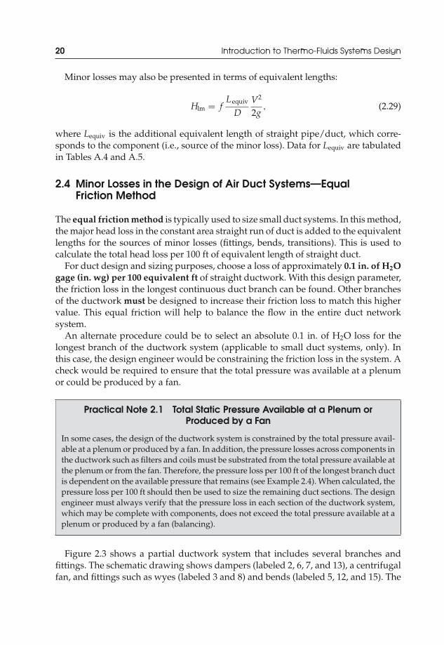
Minor losses may also be presented in terms of equivalent lengths:
Hlm = fLequiv
DV2
2g, (2.29)
where Lequiv is the additional equivalent length of straight pipe/duct, which corre-sponds to the component (i.e., source of the minor loss). Data for Lequiv are tabulatedin Tables A.4 and A.5.
2.4 Minor Losses in the Design of Air Duct Systems—EqualFriction Method
The equal friction method is typically used to size small duct systems. In this method,the major head loss in the constant area straight run of duct is added to the equivalentlengths for the sources of minor losses (fittings, bends, transitions). This is used tocalculate the total head loss per 100 ft of equivalent length of straight duct.
For duct design and sizing purposes, choose a loss of approximately 0.1 in. of H2Ogage (in. wg) per 100 equivalent ft of straight ductwork. With this design parameter,the friction loss in the longest continuous duct branch can be found. Other branchesof the ductwork must be designed to increase their friction loss to match this highervalue. This equal friction will help to balance the flow in the entire duct networksystem.
An alternate procedure could be to select an absolute 0.1 in. of H2O loss for thelongest branch of the ductwork system (applicable to small duct systems, only). Inthis case, the design engineer would be constraining the friction loss in the system. Acheck would be required to ensure that the total pressure was available at a plenumor could be produced by a fan.
Practical Note 2.1 Total Static Pressure Available at a Plenum orProduced by a Fan
In some cases, the design of the ductwork system is constrained by the total pressure avail-able at a plenum or produced by a fan. In addition, the pressure losses across components inthe ductwork such as filters and coils must be substrated from the total pressure available atthe plenum or from the fan. Therefore, the pressure loss per 100 ft of the longest branch ductis dependent on the available pressure that remains (see Example 2.4). When calculated, thepressure loss per 100 ft should then be used to size the remaining duct sections. The designengineer must always verify that the pressure loss in each section of the ductwork system,which may be complete with components, does not exceed the total pressure available at aplenum or produced by a fan (balancing).
Figure 2.3 shows a partial ductwork system that includes several branches andfittings. The schematic drawing shows dampers (labeled 2, 6, 7, and 13), a centrifugalfan, and fittings such as wyes (labeled 3 and 8) and bends (labeled 5, 12, and 15). The

JWST229-c02 JWST229-McDonald Printer: Yet to Come July 28, 2012 13:33 Trim: 244mm × 168mm
Air Distribution Systems 21
Figure 2.3 A ductwork system to transport air (ASHRAE Handbook, Fundamentals Vol-ume, 2005; reprinted with permission)
flow rates and sizes of each duct section are also shown. Fire dampers are shown inareas where the ducts penetrate a firewall. This is required by Section 705.11 of theInternational Building Code [10], Section 607 of the International Mechanical Code[11], and the National Fire Protection Association (NFPA) Standard 90A [12].
As mentioned in Practical Note 2.1, components in the ductwork system will gen-erate air pressure losses during transport. These losses must be considered in order tosize the fan or plenum and balance the pressure losses in the system. Table 2.2 presentssome typical pressure loss values across several components. The list is not extensiveor exhaustive. Therefore, the design engineer may need to consult the manufacturerto obtain detailed information for specific components.
Table 2.2 Typical values of component pressure losses [9]
Component Static Pressure Loss (in. wg)
Supply plenum 0.50Supply grille (diffuser) 0.05Raised floor perforations 0.05High-efficiency particulate air (HEPA) filter 0.7030/30 prefilters 0.30Bag filters 0.80Return plenum 0.05Cooling coil 0.35
Source: Howell, Sauer, and Coad [9].

JWST229-c02 JWST229-McDonald Printer: Yet to Come July 28, 2012 13:33 Trim: 244mm × 168mm
22 Introduction to Thermo-Fluids Systems Design
It is important to note that the construction and installation of fittings and com-ponents into a ductwork system will affect the total static pressure that is generatedwithin the system. Duct construction standards provided by organizations such as theSheet Metal and Air Conditioning Contractors National Association, Inc. (SMACNA)[13] are useful in that they allow contractors to construct the ductwork in accordancewith the design documents and specifications. However, the onus rests on the designengineer to present clear guidance regarding the types of fittings and componentsthat are required.
Example 2.4 Sizing a Simple Air Duct System
The layout of a simple low-velocity (maximum velocity = 1000 ft/min) duct system ispresented below. Size an appropriate rectangular air duct for this system, if the plenum canonly provide 0.18 in. wg of static pressure. The client will install a diffuser that is rated for0.03 in. wg at the exit of the duct system.
Possible Solution
Definition
Size an appropriate rectangular air duct for the given system. Select a suitable material.
Preliminary Specifications and Constraints
(i) The working fluid will be air.(ii) The duct system must be attached to an air plenum and have two 90◦ elbows.
(iii) The air exits the system at 500 cfm.(iv) The plenum can only provide 0.18 in. wg of static pressure.
Detailed Design
Objective
To size a rectangular air duct. The size and material of the duct will be determined.
JWST229-c02 JWST229-McDonald Printer: Yet to Come July 28, 2012 13:33 Trim: 244mm × 168mm
Air Distribution Systems 23
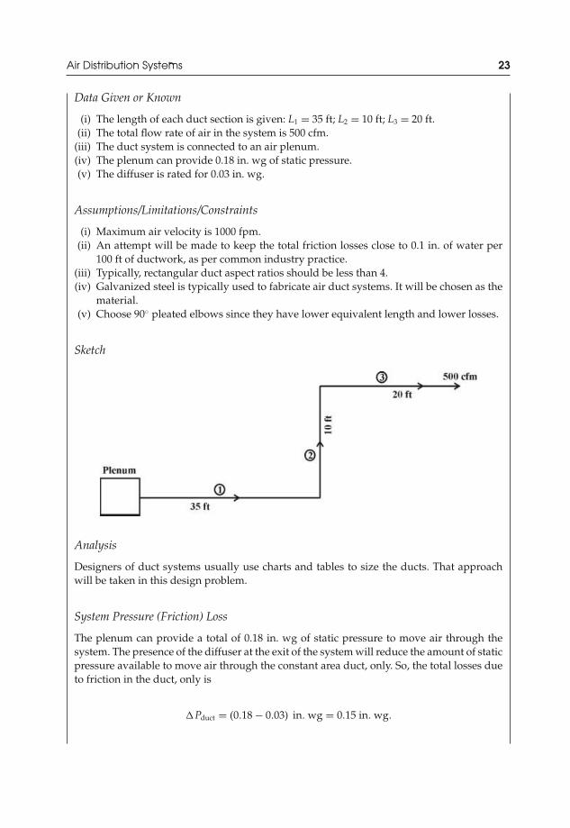
Data Given or Known
(i) The length of each duct section is given: L1 = 35 ft; L2 = 10 ft; L3 = 20 ft.(ii) The total flow rate of air in the system is 500 cfm.
(iii) The duct system is connected to an air plenum.(iv) The plenum can provide 0.18 in. wg of static pressure.(v) The diffuser is rated for 0.03 in. wg.
Assumptions/Limitations/Constraints
(i) Maximum air velocity is 1000 fpm.(ii) An attempt will be made to keep the total friction losses close to 0.1 in. of water per
100 ft of ductwork, as per common industry practice.(iii) Typically, rectangular duct aspect ratios should be less than 4.(iv) Galvanized steel is typically used to fabricate air duct systems. It will be chosen as the
material.(v) Choose 90◦ pleated elbows since they have lower equivalent length and lower losses.
Sketch
Analysis
Designers of duct systems usually use charts and tables to size the ducts. That approachwill be taken in this design problem.
System Pressure (Friction) Loss
The plenum can provide a total of 0.18 in. wg of static pressure to move air through thesystem. The presence of the diffuser at the exit of the system will reduce the amount of staticpressure available to move air through the constant area duct, only. So, the total losses dueto friction in the duct, only is
�Pduct = (0.18 − 0.03) in. wg = 0.15 in. wg.

JWST229-c02 JWST229-McDonald Printer: Yet to Come July 28, 2012 13:33 Trim: 244mm × 168mm
24 Introduction to Thermo-Fluids Systems Design
The equivalent length of the ductwork is the sum of the actual total length (straight runs)of the duct, plus the equivalent lengths for the 90◦ abrupt entrance from the large plenumand the two 90◦ bends:
Le,total = L1 + L2 + L3 + Le,entrance + 2Le,90◦ elbow.
To choose the appropriate equivalent length for the fittings, the circular duct diameter isrequired. However, the purpose of this design is to determine the duct diameter. So, assumethat the duct diameter is 10 in., and verify this assumption at the end of the design. Someiteration may be required.
The equivalent lengths are found from Table A.4 for a 10 in. diameter circular galvanizedduct: Le,entrance = 25 ft and Le,90◦ elbow = 13 ft.
Therefore,
Le,total = 35 ft + 10 ft + 20 ft + 25 ft + 2(13 ft) = 116 ft.
The total friction loss in the main run of the ductwork is restricted to 0.15 in. wg. Hence,the pressure loss in the ductwork is
�P = 0.15 in. of water116 ft
× 100 ft of ductwork = 0.13 in. wg per 100 ft of duct.
Note that the loss is close to 0.1 in. wg per 100 ft of ductwork.
Duct Size
With the friction loss and the airflow rate (500 cfm) known, the chart for friction in round,straight galvanized steel ducts can be used to select the appropriate duct diameter, andspecify the flow velocity (Figure A.1).
Thus, Dcircular = 10.2 in. and V = 890 fpm. Note that V = 890 fpm < 1000 fpm.Since the circular diameter is known, an appropriate rectangular duct with equivalent
friction losses can be chosen from Table A.3.
Possible Choices and TheirAspect Ratios. RectangularSize (in. × in.)
CircularDiameter (in.) Aspect Ratio
10 × 9 10.4 1.111 × 8 10.2 1.413 × 7 10.3 1.915 × 6 10.1 2.516 × 6 10.4 2.7

JWST229-c02 JWST229-McDonald Printer: Yet to Come July 28, 2012 13:33 Trim: 244mm × 168mm
Air Distribution Systems 25
Drawings
No additional drawings are required.
Conclusions
A rectangular galvanized sheet metal duct with dimensions of 10 in. × 9 in. is chosen. Thesize is chosen because of the following reasons:
(i) Dcircular ∼ 10.2 in.(ii) Aspect ratio is close to 1.
(iii) Duct is small. So, friction losses will be low.(iv) Ductwork will be easier to fabricate compared to the other choices.
Other constraints (e.g., structural or architectural), if provided, would need to be consid-ered when making the final selection of duct geometry.
Note that, though more expensive, the bellmouth entrance could have been chosen toreduce losses at the entrance of the duct system at the plenum.
Example 2.5 System Design: Designing a Simple Air Duct System
Miss Cherry is the proprietor of a local massage-beauty-relaxation spa. She has solicitedthe services of an engineer to size a rectangular duct system to deliver air to three privaterooms in her establishment. It is expected that the air will be delivered from the droppedceiling height directly from openings in the ductwork. Miss Cherry has some knowledge ofmechanical design, and has provided the following sketch, complete with air requirementsper room.
A new Greenheck fan will be located on top of the roof, and the new duct system will beconnected to this fan. The roof is 3 ft above the dropped ceiling. The wall partitions shownin the sketch do not extend beyond the dropped ceiling. Layout an appropriate rectangularduct system to deliver the air to the private rooms.
JWST229-c02 JWST229-McDonald Printer: Yet to Come July 28, 2012 13:33 Trim: 244mm × 168mm
26 Introduction to Thermo-Fluids Systems Design
Possible Solution
Definition
Size an appropriate rectangular air duct system for the given space.
Preliminary Specifications and Constraints
(i) The working fluid will be air.(ii) The three rooms in the establishment have the following air requirements: 250, 125,
and 450 cfm.(iii) The duct system must be attached to an existing rooftop fan.(iv) The length of the ductwork is constrained by the dimensions of the room.
Detailed Design
Objective
To design a rectangular air duct system. The size and material of the duct will be determined.
Data Given or Known
(i) Air will be delivered from the dropped ceiling height directly from openings in theductwork. This implies that no duct elbows will be needed to deliver the air to thespace. No diffusers will be attached at the duct exit.
(ii) All the dimensions of the rooms were provided by the client.(iii) The air requirements for the three rooms were given as 250, 125, and 450 cfm. The total
air requirement is 825 cfm.(iv) The roof is 3 ft above the dropped ceiling.(v) The wall partitions do not extend beyond the dropped ceiling.
Assumptions/Limitations/Constraints
(i) Total friction losses available for the ductwork should be about 0.1 in. of water per100 ft of ductwork, as per industry standard. In this case, it is assumed that the fan orplenum will be sized after the ductwork system since no technical information on theGreenheck fan was provided.
(ii) Typically, rectangular duct aspect ratios should be less than 4, as per industry standard.(iii) Galvanized steel is typically used to fabricate air duct systems. It will be chosen as the
material.(iv) Where appropriate, branch fittings will be 45◦ wyes or mitered 90◦ elbows with turning
vanes. This will reduce the minor loss equivalent lengths.(v) Losses due to duct size reductions will be ignored since they are small compared to
other losses.(vi) The entrance to the duct system from the fan will be a bellmouth to reduce frictional
losses.(vii) This is a massage-beauty-relaxation spa. Therefore, a low-velocity ductwork system
would probably be required by the client. The air velocity in the duct should not exceed1200 fpm (assuming a private residence).
JWST229-c02 JWST229-McDonald Printer: Yet to Come July 28, 2012 13:33 Trim: 244mm × 168mm
Air Distribution Systems 27
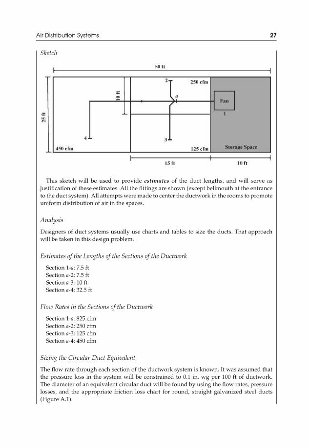
Sketch
This sketch will be used to provide estimates of the duct lengths, and will serve asjustification of these estimates. All the fittings are shown (except bellmouth at the entranceto the duct system). All attempts were made to center the ductwork in the rooms to promoteuniform distribution of air in the spaces.
Analysis
Designers of duct systems usually use charts and tables to size the ducts. That approachwill be taken in this design problem.
Estimates of the Lengths of the Sections of the Ductwork
Section 1-a: 7.5 ftSection a-2: 7.5 ftSection a-3: 10 ftSection a-4: 32.5 ft
Flow Rates in the Sections of the Ductwork
Section 1-a: 825 cfmSection a-2: 250 cfmSection a-3: 125 cfmSection a-4: 450 cfm
Sizing the Circular Duct Equivalent
The flow rate through each section of the ductwork system is known. It was assumed thatthe pressure loss in the system will be constrained to 0.1 in. wg per 100 ft of ductwork.The diameter of an equivalent circular duct will be found by using the flow rates, pressurelosses, and the appropriate friction loss chart for round, straight galvanized steel ducts(Figure A.1).

JWST229-c02 JWST229-McDonald Printer: Yet to Come July 28, 2012 13:33 Trim: 244mm × 168mm
28 Introduction to Thermo-Fluids Systems Design
Therefore,
Section 1-a: 13 in. diameter, 900 fpmSection a-2: 8.25 in. diameter, 690 fpmSection a-3: 6.50 in. diameter, 580 fpmSection a-4: 10.25 in. diameter, 800 fpm
Note that the velocities of the air in each section of the ductwork system are less than the1200 fpm maximum that is allowed for low-velocity duct systems.
Sizing the Rectangular Duct Equivalent
The equal friction and capacity chart (Table A.3) will be used to select an appropriaterectangular duct equivalent for the circular ducts. The aspect ratio will be 4 or lower.
Accordingly,
Section 1-a: 12 in. × 12 in. (13.1 in. diameter; aspect ratio = 1)Section a-2: 8 in. × 7 in. (8.2 in. diameter; aspect ratio = 1.1)Section a-3: 6 in. × 6 in. (6.6 in. diameter; aspect ratio = 1)Section a-4: 10 in. × 9 in. (10.4 in. diameter; aspect ratio = 1.1)
Drawings
The final drawing shows the layout and size of the ducts.
Conclusions
The rectangular ductwork system has been sized. Galvanized sheet metal will be used tofabricate the system. The aspect ratios are low (1.1 or lower) to reduce friction losses andfacilitate fabrication. The air velocities in each section of the duct are less than 1200 fpm.If the total available pressure from the fan was known, then the pressure drops throughthe sections of the system would need to be calculated to ensure that the total pressure
JWST229-c02 JWST229-McDonald Printer: Yet to Come July 28, 2012 13:33 Trim: 244mm × 168mm
Air Distribution Systems 29
would not be exceeded. If the fan or plenum was to be sized, then the pressure drop in thelongest (main) branch would be needed. Dampers will probably be needed to balance theairflow in the system. The following final duct sizes are recommended to facilitate furtherthe fabrication of the system and reduce the aspect ratios.
Section 1-a: 12 in. × 12 in.Section a-2: 8 in. × 8 in.Section a-3: 6 in. × 6 in.Section a-4: 10 in. × 10 in.
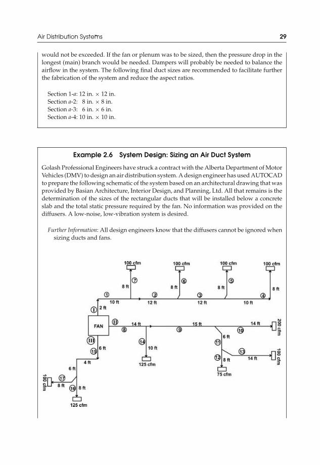
Example 2.6 System Design: Sizing an Air Duct System
Golash Professional Engineers have struck a contract with the Alberta Department of MotorVehicles (DMV) to design an air distribution system. A design engineer has used AUTOCADto prepare the following schematic of the system based on an architectural drawing that wasprovided by Basian Architecture, Interior Design, and Planning, Ltd. All that remains is thedetermination of the sizes of the rectangular ducts that will be installed below a concreteslab and the total static pressure required by the fan. No information was provided on thediffusers. A low-noise, low-vibration system is desired.
Further Information: All design engineers know that the diffusers cannot be ignored whensizing ducts and fans.

JWST229-c02 JWST229-McDonald Printer: Yet to Come July 28, 2012 13:33 Trim: 244mm × 168mm
30 Introduction to Thermo-Fluids Systems Design
Possible Solution
Definition
Size an appropriate rectangular air duct system for the air distribution system.
Preliminary Specifications and Constraints
(i) The working fluid will be air.(ii) A low-noise, low-vibration system is required.
(iii) The duct lengths and airflow rates through the sections are constrained to the valuesshown in the drawing.
Detailed Design
Objective
To design a rectangular air duct system. The size and material of the duct will be determined.
Data Given or Known
(i) An architectural drawing has been provided.(ii) All the duct lengths were provided by the architect.
(iii) All the airflow rates were provided by the architect.(iv) The system will be installed below a concrete slab.
Assumptions/Limitations/Constraints
(i) Friction losses within the ductwork should be about 0.1 in. of water per 100 ft ofductwork, as per industry standard. In this case, the fan will be sized after the ductworksystem has been sized since no technical information was provided.
(ii) Typically, rectangular duct aspect ratios should be less than 4, as per industry standard.(iii) Galvanized steel is typically used to fabricate air duct systems. However, since the
client wishes to install the ducts below a concrete slab, smooth stainless steel will bechosen to provide strength and corrosion resistance.
(iv) Where appropriate, branch fittings will be 45◦ wyes or mitered 90◦ elbows with turningvanes. This will reduce the minor loss equivalent lengths.
(v) The entrance to the duct system from the fan will be a bellmouth to reduce frictionallosses.
(vi) A low-noise, low-vibration ductwork system is required by the client. Therefore, theair velocity in the duct should not exceed 1200 fpm. If the DMV wishes to install theducts in an industrial setting, then the velocity limit could be as high as 2200 fpm.However, since limited information was provided, a conservative maximum velocitywill be chosen to ensure that the system will meet the client’s requirement of low-noise,low-vibration under most circumstances.
(vii) Assume that the diffuser pressure loss is on the order of 0.05 in. wg. This is a typicalorder of magnitude value for diffusers. In practice, the pressure drop across the diffuserwill depend on the airflow rate (in cfm) and the air velocity (in. fpm).

JWST229-c02 JWST229-McDonald Printer: Yet to Come July 28, 2012 13:33 Trim: 244mm × 168mm
Air Distribution Systems 31
Sketch
A complete architectural drawing was provided. The sections of the duct have also beenlabeled for the engineer.
Analysis
Designers of duct systems usually use charts and tables to size the ducts. That approachwill be taken in this design problem.
Flow Rates in the Sections of the Ductwork
Section 1: 400 cfmSection 2: 300 cfmSection 3: 200 cfmSection 4: 100 cfmSection 5: 100 cfmSection 6: 100 cfmSection 7: 100 cfmSection 8: 500 cfmSection 9: 375 cfmSection 10: 200 cfmSection 11: 175 cfmSection 12: 75 cfmSection 13: 100 cfmSection 14: 125 cfmSection 15: 225 cfmSection 16: 125 cfmSection 17: 100 cfm
Sizing the Circular Duct Equivalent
The flow rate through each section of the ductwork system is known. It was assumedthat the pressure loss in the system will be constrained to 0.1 in. wg per 100 ft of duct-work. Note that since no information was given regarding the total pressure availablefrom the fan, the design engineer will opt to use this industry standard. The approximatediameter of an equivalent circular duct will be found by using the flow rates, pressurelosses, and the appropriate friction loss chart for round, straight galvanized steel ducts(Figure A.1).
So,
Section 1: 9.9 in. diameter, 780 fpmSection 2: 8.9 in. diameter, 710 fpmSection 3: 7.5 in. diameter, 650 fpmSection 4: 5.9 in. diameter, 540 fpmSection 5: 5.9 in. diameter, 540 fpmSection 6: 5.9 in. diameter, 540 fpm

JWST229-c02 JWST229-McDonald Printer: Yet to Come July 28, 2012 13:33 Trim: 244mm × 168mm
32 Introduction to Thermo-Fluids Systems Design
Section 7: 5.9 in. diameter, 540 fpmSection 8: 10.3 in. diameter, 810 fpmSection 9: 9.5 in. diameter, 760 fpmSection 10: 7.5 in. diameter, 650 fpmSection 11: 7.2 in. diameter, 620 fpmSection 12: 5.2 in. diameter, 500 fpmSection 13: 5.9 in. diameter, 540 fpmSection 14: 6.3 in. diameter, 560 fpmSection 15: 7.9 in. diameter, 670 fpmSection 16: 6.3 in. diameter, 560 fpmSection 17: 5.9 in. diameter, 540 fpm
Note that the velocities of the air in each section of the ductwork system are less than1200 fpm, as required for a low-velocity, low-noise, low-vibration duct system.
Sizing the Rectangular Duct Equivalent
The equal friction and capacity chart (Table A.3) will be used to select an appropriaterectangular duct equivalent for the circular ducts. The aspect ratio will be 4 or lower.
So,
Section 1: 10 in. × 8 in. (aspect ratio: 1.25)Section 2: 8 in. × 8 in. (aspect ratio: 1.00)Section 3: 8 in. × 6 in. (aspect ratio: 1.33)Section 4: 6 in. × 6 in. (aspect ratio: 1.00)∗
Section 5: 6 in. × 6 in. (aspect ratio: 1.00)∗
Section 6: 6 in. × 6 in. (aspect ratio: 1.00)∗
Section 7: 6 in. × 6 in. (aspect ratio: 1.00)∗
Section 8: 10 in. × 10 in. (aspect ratio: 1.00)∗∗
Section 9: 10 in. × 8 in. (aspect ratio: 1.25)∗∗
Section 10: 8 in. × 6 in. (aspect ratio: 1.00)Section 11: 8 in. × 6 in. (aspect ratio: 1.00)∗∗
Section 12: 6 in. × 6 in. (aspect ratio: 1.00)∗
Section 13: 6 in. × 6 in. (aspect ratio: 1.00)∗
Section 14: 6 in. × 6 in. (aspect ratio: 1.00)∗
Section 15: 10 in. × 6 in. (aspect ratio: 1.67)∗
Section 16: 6 in. × 6 in. (aspect ratio: 1.00)∗
Section 17: 6 in. × 6 in. (aspect ratio: 1.00)∗
∗Note: The smallest size available from Table A.3 is 6 in. × 6 in. This is gives an equivalentdiameter of 6.6 in. At this diameter, the pressure loss will be lower than the design equivalentdiameters of 5.9 in. and 6.3 in., resulting in a smaller fan. The increase in material is small.This should be acceptable from a cost and installation perspective.
∗∗Note: The equivalent diameter is exceeded slightly. This decision was made to keep theaspect ratio low.

JWST229-c02 JWST229-McDonald Printer: Yet to Come July 28, 2012 13:33 Trim: 244mm × 168mm
Air Distribution Systems 33
Total Static Pressure Required from the Fan
For this problem, all the circular duct sizes were determined with a friction loss of 0.1 in.wg per 100 ft of ductwork. This friction loss can be used to estimate the total static pressurerequired by the fan. The total equivalent length (straight duct + equivalent lengths of thefittings) of the longest branch should be used.
From visual inspection of the drawing supplied by the design engineer, it appears asthough either branch I-1-2-3-4 or branch II-8-9-11-13 will be the longest branch in thissystem. The lengths should be calculated.
For branch I-1-2-3-4,
Le,total = Lstraight + Lent + L90 + L tee,thru + Lcontract + Lwye,thru + Lcontract + Lwye,thru
+ Lcontract + L90
Le,total = 54 ft + 10 ft + 8 ft + 7 ft + 3 ft + 6 ft + 3 ft + 5 ft + 3 ft + 5 ft
Le,total = 104 ft.
For branch II-8-9-11-13,
Le,total = Lstraight + Lent + L tee,thru + Lcontract + Lwye,branch + Lwye,branch
Le,total = 49 ft + 10 ft + 7 ft + 3 ft + 12 ft + 10 ft
Le,total = 91 ft.
Therefore, branch I-1-2-3-4 is the longest branch in this air distribution system.It should be noted that in some cases the Le/D ratio (Table A.4) was used to estimate the
equivalent lengths. The duct diameter must be converted to feet to use this ratio.The pressure drop in the duct is
�Pduct = 0.1 in. of water100 ft
× 104 ft of ductwork = 0.104 in. wg.
The total static pressure required from the fan is
�Pfan = �Pduct + �Pdiffuser = (0.104 + 0.05) in. wg
�Pfan = 0.16 in. wg.
If the fan is able to move air through the longest duct branch with this total static pressure,then it will be able to move air through all the other smaller branches in the air distributionsystem.
Drawings
The duct sizes determined by the design engineer can be included on the architecturaldrawing.

JWST229-c02 JWST229-McDonald Printer: Yet to Come July 28, 2012 13:33 Trim: 244mm × 168mm
34 Introduction to Thermo-Fluids Systems Design
Conclusions
The rectangular ductwork system has been sized. Stainless steel will be used to fabricatethe system. The aspect ratios are small (1.67 or lower) to reduce friction losses and facilitatefabrication. Some sections were slightly oversized to maintain a low aspect ratio. This willreduce slightly the static pressure required from the fan. The air velocities in each section ofthe duct are less than 1200 fpm. With the total available pressure from the fan known, thepressure drops through the other branches of the system can be calculated to ensure thatthe total pressure would not be exceeded. Dampers will probably be needed to balance theairflow in the system.
Example 2.7 Design of a Kitchen Exhaust System—Applicationof Codes
La Ronde Jambalaya Grill and Restaurant has decided to install a variety of cooking ap-pliances, including a deep fat fryer for chicken, grills for beef burger patties, and gas-firedoven ranges. The appliances will be installed along a wall in a one-story building and willrequire approximately 14 ft of wall space. The depth and height of the appliances range fromabout 2 to 4 ft. The NFPA Standard 96 requires that all cooking equipment used in processesthat generate smoke and vapors containing grease be equipped with an exhaust system[14]. To that end, the management team of the restaurant has hired a mechanical engineer todesign and layout the required exhaust system. There is a fire-rated roof-ceiling assembly inthe building, which, according to NFPA Standard 96, requires special consideration duringinstallation of the exhaust system. Of all the components that will be required, including ahood, ductwork, and exhaust fan, the client has clearly stated that a wall-mounted canopytype hood would fit within the architectural esthetic of the kitchen. Through consultation

JWST229-c02 JWST229-McDonald Printer: Yet to Come July 28, 2012 13:33 Trim: 244mm × 168mm
Air Distribution Systems 35
with NFPA Standard 96, the International Mechanical Code, and the American Society ofHeating, Refrigerating, and Air-Conditioning Engineers (ASHRAE) Standard 154 [15], de-sign the exhaust system for the appliances based on the drawings of the building sectionsprovided by the client.
Further Information: It is expected that the mechanical engineer will specify a hood andexhaust fan from manufacturers’ catalog(s) and will present excerpts for review, ifavailable.
JWST229-c02 JWST229-McDonald Printer: Yet to Come July 28, 2012 13:33 Trim: 244mm × 168mm
36 Introduction to Thermo-Fluids Systems Design
Possible Solution
Definition
Design an appropriate exhaust duct system for this kitchen application.
Preliminary Specifications and Constraints
(i) The working fluid will be an exhaust gas mixture from the appliances.(ii) The building has one story and a fire-rated roof-ceiling assembly.
(iii) NFPA Standard 96 requires the use of an exhaust system in this type of kitchenapplication.
(iv) The International Mechanical Code and ASHRAE Standard 154 should be consulted.(v) A wall-mounted canopy type hood, ductwork, and an exhaust fan will be required.
Detailed Design
Objective
To design a duct system to remove odors, latent heat, and combustion by-products. Thesize and material of the duct will be determined. The fan and hood will be selected.
Data Given or Known
(i) An architectural drawing has been provided, complete with dimensions.(ii) The types and sizes of the appliances have been provided by the client.
(iii) A 14 ft wall space has been allocated for the appliances that will be located under thehood.
Assumptions/Limitations/Constraints
(i) The friction losses in the ductwork should be about 0.1 in. of water per 100 ft ofductwork to mitigate noise and vibration. In this case, the fan will be sized after theductwork system has been designed.
(ii) Circular ducts will be used. This will facilitate installation and reduce pressure lossand noise.
(iii) Type I exhaust ducts and hoods are those that are installed where cooking appliancesproduce grease or smoke, such as with fryers and oven ranges. According to Section506.3.1.1 of the International Mechanical Code, for Type I exhaust ducts, steel of notless than No. 16 gage (0.0575 in. thick) or stainless steel of not less than No. 18 gage(0.044 in. thick) must be used to construct the duct system. Since excessive amountsof water will likely not be present to induce corrosion or other chemical reactions, No.16 galvanized steel shall be used as the duct material. This is permitted by Sections7.5.1.1 and A.7.5.1 of NFPA Standard 96.
(iv) Where appropriate, 90◦ elbows will possess long radii. This will reduce the minor lossequivalent lengths.
(v) The exit from the duct system to the fan will be a bellmouth to reduce frictional losses.(vi) Assume that the kitchen is an industrial setting.

JWST229-c02 JWST229-McDonald Printer: Yet to Come July 28, 2012 13:33 Trim: 244mm × 168mm
Air Distribution Systems 37
(vii) Section 8.2.1.1 of NFPA Standard 96 and Section 506.3.4 of the International MechanicalCode require that the exhaust gas velocity in the ductwork be at least 500 fpm. In orderto maintain a low-noise, low-vibration ductwork system, the gas velocity should notexceed 2200 fpm in the main duct and 1800 fpm in the branch duct. Therefore, a targetmaximum velocity of 1800 fpm will be chosen for the duct system for a conservativedesign approach. A note to Section 5.3.1 of ASHRAE Standard 154 also suggestsgeneral design velocities up to 1800 fpm for commercial exhaust systems for cookingoperations.
(viii) Additional pressure losses will occur when the exhaust gas enters the duct from thehood, passes through the grease filters, and is ejected from the fan against externalprevailing winds. Assume that the losses at the entrance of the duct are similar to thatencountered in a bellmouth entrance (Le/D = 12). The losses across the filters willbe assumed to be the same as those across 30/30 filters (0.30 in. wg). The losses dueto wind currents may be between 0.1 and 0.5 in. wg. For a conservative design andequipment sizing, assume the loss to be 0.5 in. wg.
Sketch
A complete architectural drawing was provided. A sketch of the ductwork is shown in thedrawing.
Analysis
The ductwork and fan will need to be sized. Reference will be made to the sketch of theductwork.
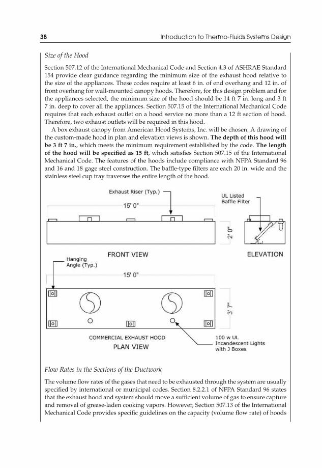
JWST229-c02 JWST229-McDonald Printer: Yet to Come July 28, 2012 13:33 Trim: 244mm × 168mm
38 Introduction to Thermo-Fluids Systems Design
Size of the Hood
Section 507.12 of the International Mechanical Code and Section 4.3 of ASHRAE Standard154 provide clear guidance regarding the minimum size of the exhaust hood relative tothe size of the appliances. These codes require at least 6 in. of end overhang and 12 in. offront overhang for wall-mounted canopy hoods. Therefore, for this design problem and forthe appliances selected, the minimum size of the hood should be 14 ft 7 in. long and 3 ft7 in. deep to cover all the appliances. Section 507.15 of the International Mechanical Coderequires that each exhaust outlet on a hood service no more than a 12 ft section of hood.Therefore, two exhaust outlets will be required in this hood.
A box exhaust canopy from American Hood Systems, Inc. will be chosen. A drawing ofthe custom-made hood in plan and elevation views is shown. The depth of this hood willbe 3 ft 7 in., which meets the minimum requirement established by the code. The lengthof the hood will be specified as 15 ft, which satisfies Section 507.15 of the InternationalMechanical Code. The features of the hoods include compliance with NFPA Standard 96and 16 and 18 gage steel construction. The baffle-type filters are each 20 in. wide and thestainless steel cup tray traverses the entire length of the hood.
Flow Rates in the Sections of the Ductwork
The volume flow rates of the gases that need to be exhausted through the system are usuallyspecified by international or municipal codes. Section 8.2.2.1 of NFPA Standard 96 statesthat the exhaust hood and system should move a sufficient volume of gas to ensure captureand removal of grease-laden cooking vapors. However, Section 507.13 of the InternationalMechanical Code provides specific guidelines on the capacity (volume flow rate) of hoods

JWST229-c02 JWST229-McDonald Printer: Yet to Come July 28, 2012 13:33 Trim: 244mm × 168mm
Air Distribution Systems 39
for appliances that are defined as heavy duty, medium duty, or light duty. Section 3 ofASHRAE Standard 154 provides full definitions of the duty levels of the appliances. For thisdesign problem, Section 4.2 of ASHRAE Standard 154 defines the gas-fired ranges as heavy-duty appliances and the deep fat fryer and grills as medium-duty appliances. Accordingto Section 507.13 of the International Mechanical Code, type I wall-mounted canopy hoodsshould exhaust at least 400 cfm per linear ft of hood for heavy-duty appliances and 300 cfmper linear ft of hood for medium-duty appliances. The same code section requires that theminimum exhaust flow rate required by the heaviest duty appliance covered by the hoodshould apply to the entire hood. Therefore, 500 cfm per linear ft of hood will be used todesign the exhaust duct system and select the fan.
Therefore, for the hood in question, the exhaust gas volume flow rate will be
V = 500 cfm1 ft hood
× 15 ft hood = 7500 cfm.
For each section of the ductwork system, the volume flow rates are
Section a-b: 3750 cfm (for each side of the symmetrical system),Section b-c: 7500 cfm.
Sizing the Circular Duct
The flow rate through each section of the ductwork system is known. It was assumed thatthe pressure loss in the system will be guided by a value of 0.1 in. wg per 100 ft of ductworkand the target maximum velocity will be 1800 fpm. Note that since the designer will sizeand select a fan as a part of this problem solution, this industry standard will be used. Theapproximate diameter of the circular ducts will be found by using the flow rates, pressurelosses, and the appropriate friction loss chart for round, straight galvanized steel ducts(Figure A.1).
Thus,
Section a-b: 22 in. diameter, 1500 fpm, 0.14 in. wg per 100 ftSection b-c: 30 in. diameter, 1550 fpm, 0.10 in. wg per 100 ft
Note that the velocities of the exhaust gas in each section of the ductwork system are lessthan 1800 fpm, as required for a low-velocity, low-noise, low-vibration duct system.
It is likely that the horizontal portion of Section a-b will be 30 in. to accommodate instal-lation and attachment to the 30 in. duct of Section b-c.
Total External Static Pressure Required from the Fan
The friction loss for each section can be used to estimate the pressure loss in the duct. Theequivalent length (straight duct + equivalent lengths of the fittings) of the longest branchshould be used. The longest branch is section a-b-c.
For section a-b,
Le,a−b = Lstraight + Lent + L tee,branch.

JWST229-c02 JWST229-McDonald Printer: Yet to Come July 28, 2012 13:33 Trim: 244mm × 168mm
40 Introduction to Thermo-Fluids Systems Design
The exhaust outlet is located about 3 ft from the edge of the hood to facilitate centeringthe outlets. Therefore, the horizontal length of straight duct is approximately 4 ft. Therefore,Lstraight = 4 ft.
So,
Le,a−b = 4 ft + 22 ft + 73 ft
Le,a−b = 99 ft.
It should be noted that the use of a 90◦ bend instead of a tee fitting would have reducedthe losses significantly. If a 5-piece or 3-piece 90◦ bend was chosen, the radius of curvaturewould need to be 1.5 times the duct diameter. For a 22 in. diameter duct, the radius ofcurvature would need to be 33 in. For the 30 in. duct, it would need to be 45 in. Given thata 30 in. diameter duct may be used for the horizontal portion of section a-b, the 90◦ bendwould likely not be feasible or easy to install given the 40 in. space that is available betweenthe top of the hood and the finished ceiling (see final drawing). Therefore, the tee fittingmight be the most likely fitting that would be installed.
For section b-c,
Le,b−c = Lstraight + L tee,branch.
Section 4.2.1 of NFPA Standard 96 requires a minimum 18 in. clearance from the fanto the roof if the roof were made of combustible material. To facilitate installation, a 2 ftclearance will be provided, which will be added to the 3 ft length over which section b-cpenetrates the attic space for connection with section a-b. Therefore, the length of sectionb-c is approximately 5 ft.
So,
Le,b−c = 5 ft + 100 ft
Le,b−c = 105 ft.
It should be noted that in some cases the Le/D ratio (Table A.4) was used to estimate theequivalent lengths. The duct diameter must be converted to feet to use this ratio.
The pressure drop in the duct is
�Pduct = 0.14 in. of water100 ft
× 99 ft of ductwork
+ 0.10 in. of water100 ft
× 105 ft of ductwork = 0.244 in. wg.
The total static pressure required from the fan is
�Pfan = �Pduct + �Pfilter + �Pwind = (0.244 + 0.30 + 0.5) in. wg
�Pfan = 1.1 in. wg.
A Greenheck tubular centrifugal belt drive roof upblast fan will be selected for thisapplication. The specifications are marked in the catalog sheet. The fan should be able to

JWST229-c02 JWST229-McDonald Printer: Yet to Come July 28, 2012 13:33 Trim: 244mm × 168mm
Air Distribution Systems 41
move 7500 cfm of exhaust gas over 1.1 in. wg of external static pressure. The fan that canproduce 1.5 in. wg of external static pressure will meet the design requirements. From theselection table for the Greenheck TCBRU-2-22 line of fans, a 1542 rpm speed and a 4.64hp motor is selected.
Source: Greenheck Fan, Corp. (reprinted with permission)

JWST229-c02 JWST229-McDonald Printer: Yet to Come July 28, 2012 13:33 Trim: 244mm × 168mm
42 Introduction to Thermo-Fluids Systems Design
Drawings
The duct sizes determined by the design engineer are included on the architectural drawingthat was supplied by the client. Further details on the required clearances are also shown.
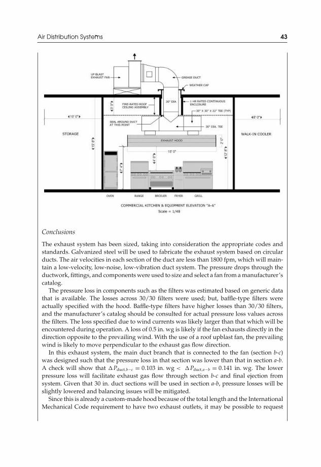
JWST229-c02 JWST229-McDonald Printer: Yet to Come July 28, 2012 13:33 Trim: 244mm × 168mm
Air Distribution Systems 43
Conclusions
The exhaust system has been sized, taking into consideration the appropriate codes andstandards. Galvanized steel will be used to fabricate the exhaust system based on circularducts. The air velocities in each section of the duct are less than 1800 fpm, which will main-tain a low-velocity, low-noise, low-vibration duct system. The pressure drops through theductwork, fittings, and components were used to size and select a fan from a manufacturer’scatalog.
The pressure loss in components such as the filters was estimated based on generic datathat is available. The losses across 30/30 filters were used; but, baffle-type filters wereactually specified with the hood. Baffle-type filters have higher losses than 30/30 filters,and the manufacturer’s catalog should be consulted for actual pressure loss values acrossthe filters. The loss specified due to wind currents was likely larger than that which will beencountered during operation. A loss of 0.5 in. wg is likely if the fan exhausts directly in thedirection opposite to the prevailing wind. With the use of a roof upblast fan, the prevailingwind is likely to move perpendicular to the exhaust gas flow direction.
In this exhaust system, the main duct branch that is connected to the fan (section b-c)was designed such that the pressure loss in that section was lower than that in section a-b.A check will show that �Pduct,b−c = 0.103 in. wg < �Pduct,a−b = 0.141 in. wg. The lowerpressure loss will facilitate exhaust gas flow through section b-c and final ejection fromsystem. Given that 30 in. duct sections will be used in section a-b, pressure losses will beslightly lowered and balancing issues will be mitigated.
Since this is already a custom-made hood because of the total length and the InternationalMechanical Code requirement to have two exhaust outlets, it may be possible to request

JWST229-c02 JWST229-McDonald Printer: Yet to Come July 28, 2012 13:33 Trim: 244mm × 168mm
44 Introduction to Thermo-Fluids Systems Design
the fabrication of circular exhaust outlets on the hood to avoid the use of transitions fromsquare outlets to round ducts.
Codes and standards have placed other requirements on the system, some of which havebeen addressed in this design. Section 8.1.2.1 of NFPA Standard 96 requires that the fanmotor be located outside of the exhaust gas stream. The catalog sheet from the GreenheckFan, Corp. shows that the in-line upblast exhaust fan selected meets this requirement. Asexhaust air is moved from the kitchen, the air must be replaced by another fan or appropriatemakeup air unit, in accordance with Section 508.1 of the International Mechanical Code.Section 8.3.1 of NFPA Standard 96 requires that an adequate quantity of air be suppliedsuch that negative pressures in the cooking area do not exceed 0.02 in. wg. Section 6 ofASHRAE Standard 154 provides details on delivery of the replacement or makeup air.While outside the scope of this present design problem, consideration of the makeup airsystem would be required since it is required by code. Finally, Section 5.7 of ASHRAEStandard 154 requires that the exhaust system become immediately operational wheneverthe appliances are on through use of direct or indirect interlocks. Heat-sensitive switchescould be used for automatic operation of the exhaust system. A detailed control systemdesign would be required.
2.5 Fans—Brief Overview and Selection Procedures
2.5.1 Classification and Terminology
A fan is a fluid machine that is used to move and induce flow of a gas (gas pumps).Rotational mechanical energy is imparted upon the gas, causing an increase in gaspressure. The increased pressure and energy of the gas is used to overcome frictionaland component losses in the system to which the fan is connected. The pressuredifference of the gas that is generated across the inlet and discharge of the fan willusually be reported in inches water gage. Fans that generate pressure differencesin excess of 30 in. wg are known as compressors. Most fans that are used in othersystems such as those found in commercial or residential buildings tend to gener-ate pressure differences less than 15 in. wg. These types of fans are introduced inSection 2.5.2. The Fan Application Manual published by Carrier Corporation [16] is aresource that may be consulted for detailed information on fans.
2.5.2 Types of Fans
(a) Axial Fans: In an axial fan, gas flow enters and leaves the fan in a straight line.The fluid flows through the impeller and parallel to the driveshaft, which isused to rotate the fan blade (impeller). Motors may be connected directly tothe impeller for direct-drive motor arrangements. Alternatively, the impellershaft may be connected to the motor via a drive pulley to a belt drive arrange-ment. Several types of axial fans are available, including propeller, tubeaxial, andvaneaxial fans. These types of fans are shown pictorially in Figure 2.4. A pro-peller fan is used to propel air into an open ambient, and is devoid of a housing

JWST229-c02 JWST229-McDonald Printer: Yet to Come July 28, 2012 13:33 Trim: 244mm × 168mm
Air Distribution Systems 45
Figure 2.4 Axial fans
enclosure. A tubeaxial or vaneaxial fan is a propeller fan that is enclosed within aducted system.
(b) Centrifugal Fans: Centrifugal fans are fabricated such that an impeller wheel, thatis complete with blades, rotates within an enclosure or fan housing as illustratedin Figure 2.5. Air enters the fan axially, through one or both sides (through the“eye”), and is propelled radially through the impeller and discharge outlet. Thefan may be connected directly to a motor (direct-drive) or connected to the motor
Figure 2.5 Centrifugal fans

JWST229-c02 JWST229-McDonald Printer: Yet to Come July 28, 2012 13:33 Trim: 244mm × 168mm
46 Introduction to Thermo-Fluids Systems Design
Figure 2.6 Classification of centrifugal fans based on blade types
via a belt drive (belt-driven). Centrifugal fans may be classified based on thedesign of the fan blades as forward-curved (curved in the direction of rotationof the fan) or backward-curved (curved in the direction opposite to the rotationof fan) as shown in Figure 2.6. Some fans with backward-curved blades mayhave those blades in the shape of airfoils (shape of a wing). These airfoil fansincrease operational efficiency due to the streamlined flow of the gas over theblades. However, they are more expensive than typical backward-curved fans thatpossess simpler blades. The orientation of the blades in centrifugal fans will havean impact on the performance of the fan. In particular, forward-curved fans areusually used in low-pressure (less than 5 in. wg) systems found in residential andlight commercial applications. For applications that require high pressures andhigh efficiency, backward-curved fans may be the more suitable choice, thoughthey could also be used in low-to-medium-pressure applications.
2.5.3 Fan Performance
The design, installation, and inclusion of components in a duct system will producepressure losses that the fan must overcome in order to move the gas through thesystem. Once the design of the ductwork system is complete, the design engineer willdetermine the maximum amount of flow (in cfm) and the total pressure loss (in in.wg) that will be experienced by the moving gas. That total volume flow rate of gas andstatic pressure must be supplied by the fan. Given that the static pressure required bythe ductwork system is external to fan and housing, the pressure difference requiredis usually referred to as external static pressure.
Manufacturers will present catalogs that specify the performance of their line offans based in the total volume flow rate of gas that can be delivered (usually air)and the external static pressure that the fan can provide. This data may be providedin either tabular or graphical forms. When in graphical form, curves of the externalstatic pressure versus the volume flow rate for a fan operating at different speedsare known as performance curves. Figure 2.7 shows typical performance curves for
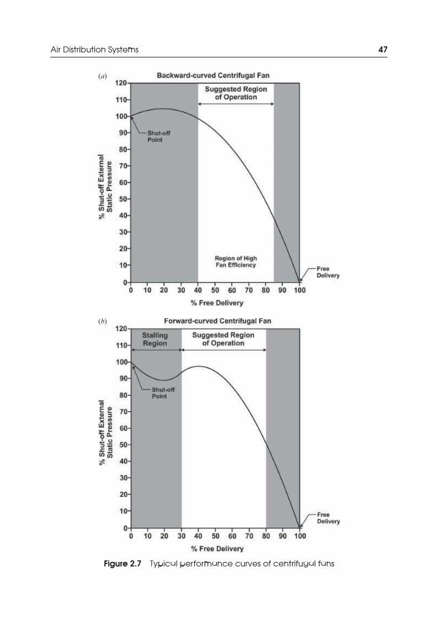
JWST229-c02 JWST229-McDonald Printer: Yet to Come July 28, 2012 13:33 Trim: 244mm × 168mm
Air Distribution Systems 47
(a)
(b)
Figure 2.7 Typical performance curves of centrifugal fans

JWST229-c02 JWST229-McDonald Printer: Yet to Come July 28, 2012 13:33 Trim: 244mm × 168mm
48 Introduction to Thermo-Fluids Systems Design
backward-curved and forward-curved centrifugal fans. The figure shows that noflow occurs when the external static pressure is maximum (i.e., maximum resistanceto flow). This point on the curve is known as the shut-off point. The point on thecurves at which the external static pressure is a minimum and the volume flow rateis a maximum (i.e., no resistance to flow) is known as free delivery. Shut-off and freedelivery will be explored in greater detail in Chapter 3.
The shapes of the performance curves shown in Figure 2.7 are specific to the typeof centrifugal fan. Backward-curved and airfoil fans usually have a curve with aparabolic shape, with external static pressure increasing from the shut-off point toa maximum pressure and decreasing steeply to free delivery. Forward-curved fansusually have the performance curve shown in Figure 2.7, in which the static pressuredecreases, then increases as the volume flow increases shortly after the shut-off point.Operation of the fan in this “dip” section of the curve will result in unsteady pressureand flow, lower efficiency, and high noise. Operation of the fan in this stalling regionshould be avoided. Close to free delivery, pulsations in flow, pressure, and air speedwill occur. Therefore, operation of the fan close to free delivery should also be avoided.Figure 2.7 shows the suggested region of operation of the fans as a percentage of thefree delivery volume flow rate. This range was selected after conducting a surveyof several performance curves from different manufacturers. The design engineershould consult the manufacturer for details on the fan that is selected for use in thedesign system.
2.5.4 Fan Selection from Manufacturer’s Dataor Performance Curves
Figure 2.8 shows a typical set of manufacturer’s performance curves for fans operatingat different speeds (in revolutions per minute, rpm). The torque provided by themotor, which is directly proportional to the motor brake horsepower, is also shown.The combination of maximum volume flow rate and external static pressure requiredby the ductwork system will produce a point on the appropriate performance curveknown as the system operating point. This point and the performance curve are usedto make the fan selection.
The following points pertaining to the performance curves shown in Figure 2.8should be noted:
(a) Fan Housing Size: The dimensions and a schematic of the fan housing are shownin the insert at the upper right corner of the graph. The diameter of the inlet tothe eye is 8.81 in. Not shown are the actual diameter and width of the impellerwheel. The 10–7 designation indicates that the wheel diameter is 10 in. and thewidth is 7 in.
(b) Motor Arrangement: This is a direct-drive fan motor arrangement.

JWST229-c02 JWST229-McDonald Printer: Yet to Come July 28, 2012 13:33 Trim: 244mm × 168mm
Air Distribution Systems 49
Figure 2.8 Forward-curved centrifugal fan performance curves (Morrison Products,Inc.; reprinted with permission)
(c) Fan Speed: The speed of the fan ranges from 800 to 1200 rpm, producing differentcurves for each speed.
(d) Motor Torque: The torque provided by the motor is shown in ounce feet (oz ft) andounce-inch (oz in). The torque and speed can be used to determine the motor brakehorsepower. The minimum motor torque available is 5 oz ft and the maximumtorque is 70 oz ft.
Example 2.8 Selecting a Fan for a Designed System
Select a centrifugal fan from a manufacturer’s performance curves if the total air requirementis 1400 cfm and the minimum external static pressure required by the system is 0.75 in. wgat 70◦F. Specify the fan motor size, that is, the brake horsepower (bhp).
Solution. A forward-curved centrifugal fan would be suitable for this application sincethe external static pressure required is low and less than 5 in. wg. The operating point inthis problem would be located on the performance curve at an air volume flow rate of 1400cfm and an external static pressure of 0.75 in. wg. The manufacturer’s performance curveshown shows the operating point located on the performance curve for the fan that rotatesat 1100 rpm.

JWST229-c02 JWST229-McDonald Printer: Yet to Come July 28, 2012 13:33 Trim: 244mm × 168mm
50 Introduction to Thermo-Fluids Systems Design
Source: Morrison Products, Inc. (reprinted with permission)
The details of the fan housing and wheel are provided with the curves. The fanspeed must be 1100 rpm. It is important to note that the operating point falls withinthe recommended region of operation shown in Figure 2.7. Operating points that fallbelow 570 cfm (30% of free delivery) or above 1520 cfm (80% of free delivery) shouldnot be matched with this fan operating at 1100 rpm.
The operating point falls between the 35 and 40 oz ft torque curves. Since the 35 oz fttorque curve is to the left of the operating point, it should not be chosen. The exacttorque requirement is 37 oz ft. However, to avoid motor overloading and damage, 40oz ft of torque is chosen. Motor overloading will be explored further in Chapter 3. InImperial units, the ounce (oz) presented in the unit of torque is ounce-force (ozf), and16 ozf is equal to 1 lbf (pound-force). In terms of brake horsepower, the motor size,based on 40 ozf ft of torque at 1100 rpm, is
bhp = Tω
bhp = (40 ozf ft)(
1100revmin
)(2π rad1 rev
)(1 lbf
16 ozf
) (1 min60 s
)(1 hp
550 lbf-ft/s
)
bhp = 0.53 hp.
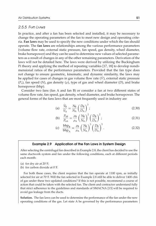
JWST229-c02 JWST229-McDonald Printer: Yet to Come July 28, 2012 13:33 Trim: 244mm × 168mm
Air Distribution Systems 51
2.5.5 Fan Laws
In practice, and after a fan has been selected and installed, it may be necessary tochange the operating parameters of the fan to meet new design and operating crite-ria. Fan laws may be used to specify the new conditions under which the fan shouldoperate. The fan laws are relationships among the various performance parameters(volume flow rate, external static pressure, fan speed, gas density, wheel diameter,brake horsepower) and they can be used to determine new values of selected parame-ters as a result of changes in any of the other remaining parameters. Derivation of thelaws will not be detailed here. The laws were derived by utilizing the BuckinghamPi theory and applying the method of repeating variables [17, 18] to develop nondi-mensional ratios of the performance parameters. Provided that the fan type doesnot change to ensure geometric, kinematic, and dynamic similarity, the laws maybe applied for cases of changes in gas volume flow rate (V), external static pressure(Ps), fan speed (N), gas density (ρ), type of gas and wheel diameter (D), and brakehorsepower (bhp).
Consider two fans (fan A and fan B) or consider a fan at two different states ofvolume flow rate, fan speed, gas density, wheel diameter, and brake horsepower. Thegeneral forms of the fans laws that are most frequently used in industry are
(a)VB
VA= NB
NA
(DB
DA
)3
; (2.30)
(b)PsB
PsA= ρB
ρA
(NB
NA
)2 (DB
DA
)2
; (2.31)
(c)bhpB
bhpA= ρB
ρA
(NB
NA
)3 (DB
DA
)5
. (2.32)
Example 2.9 Application of the Fan Laws in System Design
After selecting the centrifugal fan described in Example 2.8, the client has decided to use thesame ductwork system and fan under the following conditions, each at different periodseach month:
(a) for dry air at 20◦F;(b) for carbon dioxide at 0◦F.
For both these cases, the client requires that the fan operate at 1100 rpm, as initiallyselected for air at 70◦F. Will the fan selected in Example 2.8 still be able to deliver 1400 cfmof gas under these two updated conditions? If this is not possible, recommend a course ofaction that could be taken with the selected fan. The client and contractor understand fullythat strict adherence to the guidelines and standards of SMACNA [13] will be required toavoid gas leakage from the ducts.
Solution. The fan laws can be used to determine the performance of the fan under the newoperating conditions of the gas. Let state A be governed by the performance parameters
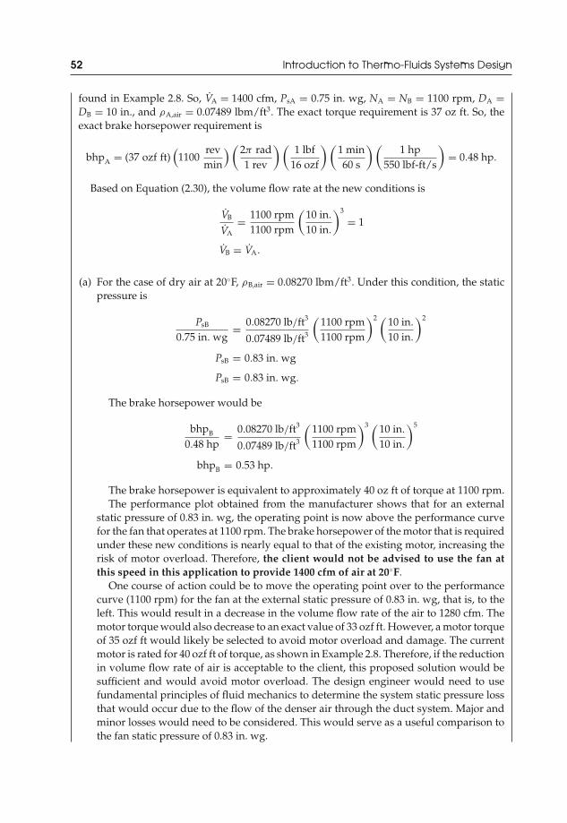
JWST229-c02 JWST229-McDonald Printer: Yet to Come July 28, 2012 13:33 Trim: 244mm × 168mm
52 Introduction to Thermo-Fluids Systems Design
found in Example 2.8. So, VA = 1400 cfm, PsA = 0.75 in. wg, NA = NB = 1100 rpm, DA =DB = 10 in., and ρA,air = 0.07489 lbm/ft3. The exact torque requirement is 37 oz ft. So, theexact brake horsepower requirement is
bhpA = (37 ozf ft)(
1100revmin
) (2π rad1 rev
)(1 lbf
16 ozf
)(1 min60 s
)(1 hp
550 lbf-ft/s
)= 0.48 hp.
Based on Equation (2.30), the volume flow rate at the new conditions is
VB
VA= 1100 rpm
1100 rpm
(10 in.
10 in.
)3
= 1
VB = VA.
(a) For the case of dry air at 20◦F, ρB,air = 0.08270 lbm/ft3. Under this condition, the staticpressure is
PsB
0.75 in. wg= 0.08270 lb/ft3
0.07489 lb/ft3
(1100 rpm1100 rpm
)2 (10 in.
10 in.
)2
PsB = 0.83 in. wg
PsB = 0.83 in. wg.
The brake horsepower would be
bhpB
0.48 hp= 0.08270 lb/ft3
0.07489 lb/ft3
(1100 rpm1100 rpm
)3 (10 in.
10 in.
)5
bhpB = 0.53 hp.
The brake horsepower is equivalent to approximately 40 oz ft of torque at 1100 rpm.The performance plot obtained from the manufacturer shows that for an external
static pressure of 0.83 in. wg, the operating point is now above the performance curvefor the fan that operates at 1100 rpm. The brake horsepower of the motor that is requiredunder these new conditions is nearly equal to that of the existing motor, increasing therisk of motor overload. Therefore, the client would not be advised to use the fan atthis speed in this application to provide 1400 cfm of air at 20◦F.
One course of action could be to move the operating point over to the performancecurve (1100 rpm) for the fan at the external static pressure of 0.83 in. wg, that is, to theleft. This would result in a decrease in the volume flow rate of the air to 1280 cfm. Themotor torque would also decrease to an exact value of 33 ozf ft. However, a motor torqueof 35 ozf ft would likely be selected to avoid motor overload and damage. The currentmotor is rated for 40 ozf ft of torque, as shown in Example 2.8. Therefore, if the reductionin volume flow rate of air is acceptable to the client, this proposed solution would besufficient and would avoid motor overload. The design engineer would need to usefundamental principles of fluid mechanics to determine the system static pressure lossthat would occur due to the flow of the denser air through the duct system. Major andminor losses would need to be considered. This would serve as a useful comparison tothe fan static pressure of 0.83 in. wg.
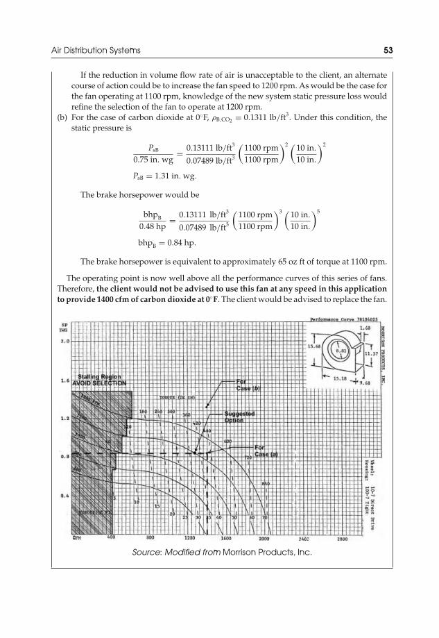
JWST229-c02 JWST229-McDonald Printer: Yet to Come July 28, 2012 13:33 Trim: 244mm × 168mm
Air Distribution Systems 53
If the reduction in volume flow rate of air is unacceptable to the client, an alternatecourse of action could be to increase the fan speed to 1200 rpm. As would be the case forthe fan operating at 1100 rpm, knowledge of the new system static pressure loss wouldrefine the selection of the fan to operate at 1200 rpm.
(b) For the case of carbon dioxide at 0◦F, ρB,CO2 = 0.1311 lb/ft3. Under this condition, thestatic pressure is
PsB
0.75 in. wg= 0.13111 lb/ft3
0.07489 lb/ft3
(1100 rpm1100 rpm
)2 (10 in.
10 in.
)2
PsB = 1.31 in. wg.
The brake horsepower would be
bhpB
0.48 hp= 0.13111 lb/ft3
0.07489 lb/ft3
(1100 rpm1100 rpm
)3 (10 in.
10 in.
)5
bhpB = 0.84 hp.
The brake horsepower is equivalent to approximately 65 oz ft of torque at 1100 rpm.
The operating point is now well above all the performance curves of this series of fans.Therefore, the client would not be advised to use this fan at any speed in this applicationto provide 1400 cfm of carbon dioxide at 0◦F. The client would be advised to replace the fan.
Source: Modified from Morrison Products, Inc.

JWST229-c02 JWST229-McDonald Printer: Yet to Come July 28, 2012 13:33 Trim: 244mm × 168mm
54 Introduction to Thermo-Fluids Systems Design
2.6 Design for Advanced Technology—Small Duct High-Velocity(SDHV) Air Distribution Systems
Small duct, high-velocity (SDHV) air distribution systems are those in which small-sized duct branches and high velocities are used to transport air through the systemand to the spaces. This type of system can be used when space restrictions are presentin a building such that large ducts cannot be accommodated. The SDHV systems maybe used during the retrofit of older residential buildings that were not constructedwith conventional duct systems. Due to the small sizes of the ducts required, extensivedemolition may not be required and the interior and exterior appearance of thebuilding may be preserved. The SDHV air distribution system is not a new technology.However, the use of this type of system is becoming popular in residential buildingapplications.
In SDHV air distribution systems, duct sizes can be as low as 2 in. in diameter, inwhich flexible ductwork would be used. Table 2.3 shows the supply air velocities thattypify SDHV air distribution systems based on the air volume flow rate. The supplyductwork provides air from the fan or blower to the spaces or the applications. Acomparison of the velocities presented in Tables 2.1 and 2.3 show that for residentialapplications with main duct airflow rates between 1000 and 3000 cfm, an SDHV airdistribution system may be defined as a system in which the supply air velocity isbetween approximately 1200 and 2500 fpm. For industrial (commercial) buildings, thevelocity range would be 2200–2500 fpm. Any velocity greater than 2500 fpm wouldforce classification of the system as a high-velocity duct system. It should be notedthat as the air returns from the space back to the fan or blower, the return air ductsare low-velocity ducts.
The small ducts and high velocities required by SDHV air distribution systemswill produce higher external static pressures. The higher velocities will producehigher pressure losses through the ductwork system and across components such as
Table 2.3 Maximum supply duct velocities
High-Velocity Systems (Main Branches)
Airflow Rate in Duct (cfm) Maximum Velocity (fpm)
1000–3000 25003000–6000 30006000–10000 3500
10000–15000 400015000–25000 450025000–40000 500040000–60000 6000
Source: Howell, Sauer, and Coad [9].

JWST229-c02 JWST229-McDonald Printer: Yet to Come July 28, 2012 13:33 Trim: 244mm × 168mm
Air Distribution Systems 55
heating/cooling coils. This will result in larger power (bhp and torque) requirementsby the fan or blower that is used to move the air. The design engineer needs toensure that the increased requirements of the fan or blower are met since under-sized fans or blowers will produce lower air volume flows rates, which may un-dermine the performance of the installed components and the design criteria maynot be satisfied. To that end, Section 3.11 of the Air-Conditioning, Heating, andRefrigeration Institute (AHRI) Standard 210/240-2005 [19] requires that a coolingproduct contain a blower that produces at least 1.2 in. wg of external static pres-sure when operating at the certified airflow rate of 220–350 cfm per rated ton ofcooling. One ton of cooling is equivalent to 12000 Btu/h of energy. In this case, theminimum external static pressure requirement of the fan or blower is specified bythe standard, and it should be utilized in the design of the ductwork and selectionof equipment.
Noise may be an issue to address during operation of SDHV air distribution sys-tems. ASHRAE have led the development of criteria that are used to stipulate ac-ceptable noise levels for spaces, equipment, and air duct systems. These criteria arespecific to the application and use of the space, and are based on values of the noisecriteria (NC). NC values are established after conducting acoustic tests at differentsound frequencies. The maximum sound pressure (power) level in decibels (dB) thatis achieved during the tests will represent the value for the NC rating. Table 2.4shows results from a sound test of an 8 in. × 8 in. rectangular elbow with 7 circulararc turning vanes. The air velocity was 3000 fpm. Since the maximum pressure levelis approximately 55 dB (at 500 Hz), the NC rating for the elbow is NC-55. Higher NCvalues indicate higher levels of noise.
NC can be used to guide and justify decisions during the design of air distributionsystems. Further constraints on air velocities, similar to those provided in Tables 2.1and 2.3, can be established based on acceptable NC for spaces. Table 2.5 presentsrecommended maximum velocities that are required to achieve specified acousticdesign criteria for main ducts. In order to achieve the same NC values listed in the
Table 2.4 Sound data during airflow through arectangular elbow
Frequency (Hz) Sound Pressure Level (dB)
125 50250 53500 55
1000 522000 514000 468000 40
Source: ASHRAE [20].

JWST229-c02 JWST229-McDonald Printer: Yet to Come July 28, 2012 13:33 Trim: 244mm × 168mm
56 Introduction to Thermo-Fluids Systems Design
Table 2.5 Maximum main duct air velocities for acoustic design criteria
Maximum Velocity (fpm)
Duct Location Noise Criteria (NC) Rectangular Duct Circular Duct
In shaft or abovedrywall ceiling
45 3500 500035 2500 350025 1700 2500
Above suspendedacoustic ceiling
45 2500 450035 1750 300025 1200 2000
In occupied space 45 2000 390035 1450 260025 950 1700
Source: ASHRAE [20].
table, the velocities in branch ducts should be 80% of the values listed [20]. Whereapplicable, for duct runouts from the branch ducts to outlets such as diffuser boots,the velocities should be 50% or less of those in the main duct. Table 2.6 followswith the recommended design guidelines for sound in unoccupied spaces. The ta-bles may be used in conjunction with other design criteria to make and justify ductsystem design decisions. The design engineer should consult with an acoustical en-gineer regarding acoustical critical spaces such as concert and recital halls or TV andradio studios.
There will be cases where modifications of the design of the ductwork will noteliminate excess noise. In such cases, the design engineer will need to take additionalsteps. Noise control protocols may include the use of acoustical liners in the ducts,nonmetallic insulated flexible duct, and/or duct silencers (sound attenuators, soundtraps, or mufflers). These solutions may add further pressure loss to the duct systemand they should be considered when sizing and selecting appropriate fans.
Practical Note 2.2 Diffuser Discharge Air Volume Flow Ratesin SDHV Systems
The velocities at air supply outlets such as diffusers in SDHV air distribution systems maybe in excess of the constraints established by Table 2.5 for duct runouts. This becomesamplified when the air volume flow rates through the diffusers are high and the duct sizeis small. To mitigate this problem, designers and contractors will constrain the air volumeflow rate through the duct runouts and diffusers at approximately 40–70 cfm. While thisconstraint will establish the need for multiple diffusers in a space, the constraints on noiselevels and velocities will be met successfully.

JWST229-c02 JWST229-McDonald Printer: Yet to Come July 28, 2012 13:33 Trim: 244mm × 168mm
Air Distribution Systems 57
Table 2.6 Acoustic design criteria for unoccupied spaces [21]
Type of Space Noise Criteria (NC)
Private residences, apartments, condominia 25–35
Hotels and motelsIndividual rooms or suites; meeting and
banquet rooms25–35
Halls, corridors, lobbies, service and supportareas
35–45
Office buildingsExecutive and private offices, conference
rooms25–35
Teleconferencing rooms 25 (max)Open-plan offices 30–40Circulation and public lobbies 40–45
Hospitals and clinicsPrivate rooms 25–35Wards 30–40Operating rooms 25–35Corridors, public areas 30–40
Laboratories (with fume hoods)Testing or research, minimal speech
communication45–55
Research, extensive telephone usage, speechcommunication
40–50
Group teaching 35–45Places of worship 25–35
SchoolsClassrooms, less than 750 ft2 40 (max)Classrooms, more than 750 ft2 35 (max)
Libraries 30–40
CourtroomsUnamplified speech 25–35Amplified speech 30–40
Performing arts spacesDrama theaters and music teaching studios 25 (max)Music practicing rooms 25–35
School and university gymnasia and natatoria 40–50

JWST229-c02 JWST229-McDonald Printer: Yet to Come July 28, 2012 13:33 Trim: 244mm × 168mm
58 Introduction to Thermo-Fluids Systems Design
Example 2.10 Designing a Simple SDHV Air Distribution System
Miss Cherry wishes to modify the air duct system that was designed in Example 2.5 to thatof an SDHV air distribution system. In this case, she has requested that all the ducts becircular to deliver air to three private rooms in her establishment. Instead of delivering airfrom the dropped ceiling height directly from openings in the ductwork, she has requestedthat diffusers be used. The original sketch of the floor plan, complete with air requirementsper room, is shown below.
Miss Cherry has also decided to include a finned-tube heating coil and a Camfil Farr 30/30medium efficiency pleated air filter in the main duct to heat the air that will be delivered toher rooms. It is expected that the pressure drop across the coil will be approximately 0.25in. wg. A new fan, which will be located on top of the roof, will be required. In compliancewith Section 1209 of the 2006 International Building Code, the roof is 3 ft above the droppedceiling. The wall partitions shown on the sketch do not extend beyond the dropped ceiling.Layout an appropriate SDHV air distribution system based on circular ducts. Size and selecta fan.
Possible Solution
Definition
Size and layout an appropriate circular SDHV air distribution system for the given space.Select a fan.
Preliminary Specifications and Constraints
(i) The working fluid will be air.(ii) The system should be based on small circular ducts and high air velocities.
JWST229-c02 JWST229-McDonald Printer: Yet to Come July 28, 2012 13:33 Trim: 244mm × 168mm
Air Distribution Systems 59
(iii) The three rooms in the establishment have the following air requirements: 250, 125,and 450 cfm.
(iv) A finned-tube heating coil is required by the client, which will induce air pressuredrop in then system.
(v) A Camfil Farr 30/30 medium efficiency pleated air filter will be installed.(vi) A new rooftop fan is required.
(vii) The length of the ductwork is constrained by the dimensions of the room.(viii) The attic space between the roof and the dropped ceiling is 3 ft.
Detailed Design
Objective
To design a circular SDHV air distribution system that is complete with a selected fan.
Data Given or Known
(i) Air will now be delivered from diffusers connected to ductwork.(ii) All the dimensions of the rooms were provided by the client.
(iii) The air requirements for the three rooms were given as 250, 125, and 450 cfm. The totalair requirement is 825 cfm.
(iv) The finished ceiling is 3 ft above the dropped ceiling.(v) The wall partitions do not extend beyond the dropped ceiling.
(vi) A finned-tube heating coil with an air pressure drop of 0.25 in. wg will beinstalled.
(vii) A Camfil Farr 30/30 medium efficiency pleated air filter will be installed.
Assumptions/Limitations/Constraints
(i) Section 3.11 of the AHRI Standard 210/240-2005 requires that a cooling productcontain a blower that produces at least 1.2 in. wg of external static pressure whenoperating at the certified airflow rate of 220–350 cfm per rated ton of cooling. In thisdesign problem, the client (Miss Cherry) is heating the air. Also, the design problempreamble statement does not specify if cooling will be required and the tonnage ofcooling that would be needed. This presents some uncertainty in the possible designsolution. However, it is expected that Miss Cherry may need cooling during thesummer months and she may wish to use the same duct-fan system that is proposedhere. Therefore, a conservative design approach would be to assume that the fan orblower will provide at least 1.2 in. wg of external static pressure to provide the clientwith some flexibility.
(ii) Galvanized steel is typically used to fabricate air duct systems. It will be chosen asthe material.
(iii) Where appropriate, branch fittings will be 45◦ wyes or 90◦ elbows with long smoothradii. This will reduce the minor loss equivalent lengths.
(iv) Converging transitions (duct size reductions) will be at 20◦ angles to reducelosses.

JWST229-c02 JWST229-McDonald Printer: Yet to Come July 28, 2012 13:33 Trim: 244mm × 168mm
60 Introduction to Thermo-Fluids Systems Design
(v) The entrance to the duct system from the fan will be a bellmouth to reduce frictionallosses.
(vi) Assume that the dropped ceiling is a suspended acoustic ceiling.(vii) This is a massage-beauty-relaxation spa. Therefore, it will be assumed that the space
will be similar to a private residence, apartment, or condominia. So, based on Table2.6, the noise criterion will be restricted to 35.
(viii) Based on the NC restriction and Table 2.5, the maximum air velocity in the mainducts will be 3000 fpm since the ducts will be located above a suspended acousticceiling.
(ix) Restrict the flow rate through each diffuser to 70 cfm or less.
Sketch
This sketch will be used to provide estimates of the duct lengths, and will serve as justi-fication of these estimates. All the fittings are shown (except the bellmouth fitting at theentrance to the duct system). Typically, high-velocity diffusers are placed at the perimeterof the structure (close to the walls) to minimize the direct discharge of high-speed air onthe occupants. Therefore, every attempt was made to center the ductwork and locate thediffusers close to the walls. An attempt was also made to promote uniform distribution ofair in the spaces.
Flexible duct was also used to connect the galvanized smooth duct to the diffusers.Given the corrugated nature of flexible duct, Section 3.23 of the SMACNA HVAC ductconstruction standards requires that a minimum length be used. This will minimize bothpressure losses in the duct system and fan sizes. As a practical guide, flexible duct lengthsshould not exceed 3 ft whenever possible. In this solution, the lengths were constrainedto 2 ft.
Analysis
Designers of duct systems usually use charts and tables to size the ducts. That approachwill be taken in this design problem.

JWST229-c02 JWST229-McDonald Printer: Yet to Come July 28, 2012 13:33 Trim: 244mm × 168mm
Air Distribution Systems 61
Estimates of the Lengths of the Main and Branch Sections of the Ductwork
Section a-b: 7.5 ftSection b-e: 7.5 ftSection b-h: 10 ftSection b-o: 40 ft
Flow Rates in the Sections of the Ductwork
Section a-b: 825 cfmSection b-c: 190 cfmSection c-d: 130 cfmSection d-e: 70 cfmSection b-f: 185 cfmSection f-g: 125 cfmSection g-h: 65 cfmSection b-i: 450 cfmSection i-j: 385 cfmSection j-k: 320 cfmSection k-l: 260 cfmSection l-m: 195 cfmSection m-n: 130 cfmSection n-o: 65 cfm
Sizing the Circular Duct
The flow rate through each section of the ductwork system is known. Given that the pressuredrop in this SDHV air distribution system is expected to be large, the maximum velocitiesthat are expected for each section will be used to guide the sizing of the duct, in lieu of thefriction loss. The diameter of the circular ducts will be found by using the flow rates, airvelocities, and the appropriate friction loss chart for round, straight galvanized steel ducts(Figure A.1). The NC will be used to confirm the final duct sizes based on the expectedperformance of the system.
For this design problem, the following maximum velocities are expected to maintain amaximum noise criterion of 35:
1. Main duct: 3000 fpm2. Branch duct: 2400 fpm3. Duct runouts (flexible ducts): 1500 fpm
Based on the sketch, the 2-ft-long flexible ducts should deliver 60, 65, or 70 cfm of air tothe diffusers. So, based on the airflow rates,
Flexible duct: 60 cfm, 3 in. diameter, 1210 fpm, friction loss ≈ 1.0 in. wg per 100 ftFlexible duct: 65 cfm, 3 in. diameter, 1310 fpm, friction loss ≈ 1.2 in. wg per 100 ftFlexible duct: 70 cfm, 3 in. diameter, 1450 fpm, friction loss ≈ 1.4 in. wg per 100 ft.
The friction loss chart for round, straight galvanized steel ducts shown in Figure A.1applies to smooth, galvanized steel ducts. Corrugated flexible ducts will have higher friction
JWST229-c02 JWST229-McDonald Printer: Yet to Come July 28, 2012 13:33 Trim: 244mm × 168mm
62 Introduction to Thermo-Fluids Systems Design
loss than smooth ducts for a given airflow rate. However, the short lengths of the ductswill make the error in the static pressure loss negligible. The Carrier Corporation [22] hasprovided a friction loss chart similar to that shown in Figure A.1 for flexible ducts with 3in. and 4 in. diameters.
For the main and branch ducts,
Section a-b: 8 in. diameter, 2350 fpm, friction loss = 1.0 in. wg per 100 ft (main duct)Section b-c: 4 in. diameter, 2150 fpm, friction loss = 1.9 in. wg per 100 ft (branch duct)Section c-d: 4 in. diameter, 1450 fpm, friction loss = 1.0 in. wg per 100 ft (branch duct)Section d-e: 3 in. diameter, 1450 fpm, friction loss = 1.4 in. wg per 100 ft (branch duct)Section b-f: 4 in. diameter, 2020 fpm, friction loss = 1.8 in. wg per 100 ft (branch duct)Section f-g: 4 in. diameter, 1380 fpm, friction loss = 0.9 in. wg per 100 ft (branch duct)Section g-h: 3 in. diameter, 1310 fpm, friction loss = 1.2 in. wg per 100 ft (branch duct)Section b-i: 6 in. diameter, 2300 fpm, friction loss = 1.4 in. wg per 100 ft (main duct)Section i-j: 6 in. diameter, 2000 fpm, friction loss = 1.1 in. wg per 100 ft (main duct)Section j-k: 6 in. diameter, 1680 fpm, friction loss = 0.8 in. wg per 100 ft (main duct)Section k-l: 5 in. diameter, 1850 fpm, friction loss = 1.2 in. wg per 100 ft (main duct)Section l-m: 5 in. diameter, 1425 fpm, friction loss = 0.7 in. wg per 100 ft (main duct)Section m-n: 4 in. diameter, 1450 fpm, friction loss = 1.0 in. wg per 100 ft (main duct)Section n-o: 3 in. diameter, 1310 fpm, friction loss = 1.2 in. wg per 100 ft (main duct).
The velocities are lower than the maximum values prescribed for main and branch ductsand duct runouts in order to achieve NC less than 35. However, in comparison to low-velocity air distribution systems, where friction losses are approximately 0.1 in. wg per100 ft, the friction losses are an order of magnitude higher at approximately 1.0 in. wgper 100 ft.
Sizing and Selecting a Fan
For this problem, the friction loss varies in each section of the ductwork system whereflexible ducts are attached. These friction loss values should be used to estimate the totalexternal static pressure required by the fan. The total equivalent length (straight duct +equivalent lengths of the fittings) of the longest branch should be used. The additionalpressure losses across the heating coil and the filter should be included.
From visual inspection of the drawing, the longest branch in this system is a-b-j-k-l-m-n-o-diffuser (from the fan at a to the diffuser at o). The equivalent length is
Le,total = Lstraight + Lent + 2L tee,thru,8′′ + Lcontract,8′′-6′′ + L90 + 2L tee,thru,6′′ + 3L tee,thru,5′′ + L tee,thru,4′′
L tee,branch,3′′ + Lcontract,6′′-5′′ + Lcontract,5′′-4′′ + Lcontract,4′′-3′′
Le,total = (7.5 ft + 40 ft + 2 ft) + 8 ft + 2 (5 ft) + 3 ft + 4.5 ft + 2 (4 ft) + 3 (3.5 ft) + 3 ft
10 ft + 2 ft + 2 ft + 1.5 ft
Le,total = 112 ft.
JWST229-c02 JWST229-McDonald Printer: Yet to Come July 28, 2012 13:33 Trim: 244mm × 168mm
Air Distribution Systems 63
It should be noted that in some cases the Le/D ratio (Table A.4) was used to esti-mate the equivalent lengths. The duct diameter must be converted to feet to use thisratio.
The total equivalent length should be used with the friction loss to determine the totalexternal static pressure loss due to the duct and fittings. As mentioned earlier, the frictionloss at each section of the main duct where flexible ducts are attached will be different.The length of these sections will also differ. Specifying exact duct section lengths betweenthe flexible duct connections may not be useful since field installation will usually requiremodifications to the exact connection points. Therefore, an average friction loss for themain duct will be used with the total equivalent length of duct to find the static pressuredrop. The friction loss in the main duct varies from 0.7 to 1.4 in wg per 100 ft of equiva-lent length of duct. The average friction loss is 1.1 in. wg per 100 ft of equivalent lengthof duct.
The pressure drop in the duct is
�Pduct = 1.1 in. of water100 ft
× 112 ft of ductwork = 1.23 in. wg.
The total static pressure required from the fan is
�Pfan = �Pduct + �Pcoils + �Pfilter + �Pdiffuser,
�Pfan = (1.23 + 0.25 + 0.30 + 0.05) in. wg,
�Pfan = 1.83 in. wg.
Table 2.2 provided typical values of the static pressure losses through the filter and thediffuser. If the fan is able to move air through the longest duct branch with this total staticpressure, then it will be able to move air through all the other smaller branches in the airdistribution system. At this point, it is important to note that the total external static pressureof the fan is in excess of 1.2 in. wg, which is the minimum external static pressure requiredby Section 3.11 of the AHRI Standard 210/240-2005 when a cooling product is used in theSDHV air distribution system.
A Greenheck tubular centrifugal belt drive roof supply fan will be selected for thisapplication. The performance curves and specifications are shown in the catalog sheet. Thefan should provide 825 cfm of air over 1.83 in. wg of external static pressure. From theperformance curves for the Greenheck TCBRS-1-09 line of fans, a 2545 rpm speed and a3/4 hp motor is selected.
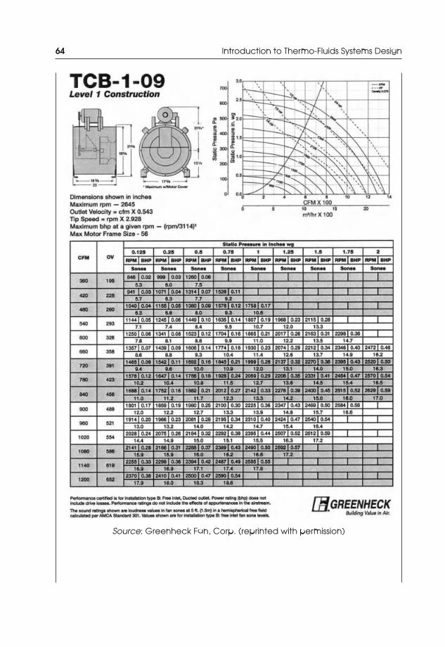
JWST229-c02 JWST229-McDonald Printer: Yet to Come July 28, 2012 13:33 Trim: 244mm × 168mm
64 Introduction to Thermo-Fluids Systems Design
Source: Greenheck Fan, Corp. (reprinted with permission)

JWST229-c02 JWST229-McDonald Printer: Yet to Come July 28, 2012 13:33 Trim: 244mm × 168mm
Air Distribution Systems 65
Drawings
The final drawing shows the layout and size of the ducts.
Conclusions
The SDHV air distribution system based circular ducts has been designed. Galvanized sheetmetal will be used to fabricate the system. A suitable fan has also been selected. The airvelocity in each section of the duct and the air volume flow rate was used to size the ducts.The NC used was a performance metric to support final duct size selections. Dampers willprobably be needed to balance the airflow in the system.
Flow across the filter and heating coil will need to occur at a velocity that is much lowerthan 2350 fpm, which is the velocity in the main duct section that is connected to the fan.This will prevent damage to the filter and mitigate pressure losses across the heating coil.It may be common to find filters complete with the fan assembly, in which the filter staticpressure loss would be included with the static pressure that is internal to the fan and itshousing. The section of duct that houses the heating coil would likely be larger to reducethe flow velocity across the coil. This will likely be possible because the outlet orifice of thefan is 183/8 in., which is much larger than the diameter of the duct that is connected to thefan (8 in.).
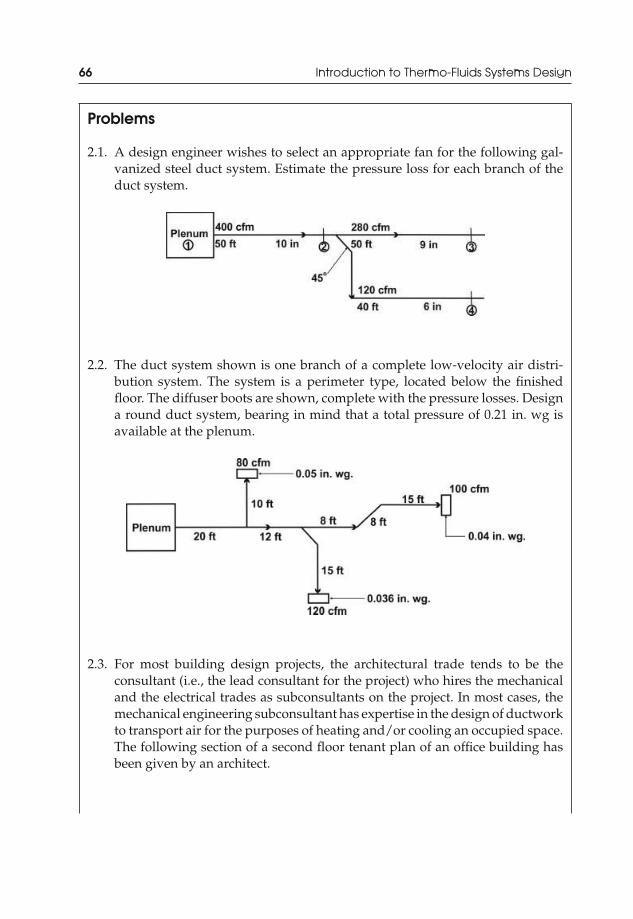
JWST229-c02 JWST229-McDonald Printer: Yet to Come July 28, 2012 13:33 Trim: 244mm × 168mm
66 Introduction to Thermo-Fluids Systems Design
Problems
2.1. A design engineer wishes to select an appropriate fan for the following gal-vanized steel duct system. Estimate the pressure loss for each branch of theduct system.
2.2. The duct system shown is one branch of a complete low-velocity air distri-bution system. The system is a perimeter type, located below the finishedfloor. The diffuser boots are shown, complete with the pressure losses. Designa round duct system, bearing in mind that a total pressure of 0.21 in. wg isavailable at the plenum.
2.3. For most building design projects, the architectural trade tends to be theconsultant (i.e., the lead consultant for the project) who hires the mechanicaland the electrical trades as subconsultants on the project. In most cases, themechanical engineering subconsultant has expertise in the design of ductworkto transport air for the purposes of heating and/or cooling an occupied space.The following section of a second floor tenant plan of an office building hasbeen given by an architect.

JWST229-c02 JWST229-McDonald Printer: Yet to Come July 28, 2012 13:33 Trim: 244mm × 168mm
Air Distribution Systems 67
For the offices shown in the plan above (complete with the occupant andwork function), the architect has requested the design of a ductwork systemto provide air at 75◦F to heat the occupied spaces. A HVAC engineer hasdetermined the amount of air required to maintain the space temperature,and they are shown in the following table.
Office Space
Heating AirRequirement
(cfm)
Office 204 310Office 205 450Office 206 170Office 207 500
However, the engineer missed the fact that ASHRAE Standard 62 requiresthat 20 cfm per person of fresh outdoor air must be provided.
(a) To ensure an esthetically pleasing finish in the space, the architect hasrequested the design of a ductwork system based on round ducts. Because
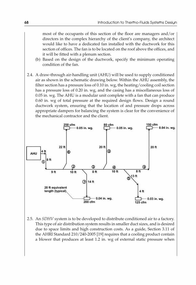
JWST229-c02 JWST229-McDonald Printer: Yet to Come July 28, 2012 13:33 Trim: 244mm × 168mm
68 Introduction to Thermo-Fluids Systems Design
most of the occupants of this section of the floor are managers and/ordirectors in the complex hierarchy of the client’s company, the architectwould like to have a dedicated fan installed with the ductwork for thissection of offices. The fan is to be located on the roof above the offices, andit will be fitted with a plenum section.
(b) Based on the design of the ductwork, specify the minimum operatingcondition of the fan.
2.4. A draw-through air-handling unit (AHU) will be used to supply conditionedair as shown in the schematic drawing below. Within the AHU assembly, thefilter section has a pressure loss of 0.10 in. wg, the heating/cooling coil sectionhas a pressure loss of 0.20 in. wg, and the casing has a miscellaneous loss of0.05 in. wg. The AHU is a modular unit complete with a fan that can produce0.60 in. wg of total pressure at the required design flows. Design a roundductwork system, ensuring that the location of and pressure drops acrossappropriate dampers for balancing the system is clear for the convenience ofthe mechanical contractor and the client.
2.5. An SDHV system is to be developed to distribute conditioned air to a factory.This type of air distribution system results in smaller duct sizes, and is desireddue to space limits and high construction costs. As a guide, Section 3.11 ofthe AHRI Standard 210/240-2005 [19] requires that a cooling product containa blower that produces at least 1.2 in. wg of external static pressure when
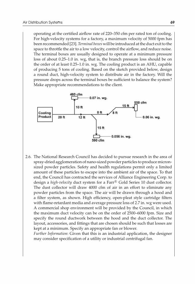
JWST229-c02 JWST229-McDonald Printer: Yet to Come July 28, 2012 13:33 Trim: 244mm × 168mm
Air Distribution Systems 69
operating at the certified airflow rate of 220–350 cfm per rated ton of cooling.For high-velocity systems for a factory, a maximum velocity of 5000 fpm hasbeen recommended [23]. Terminal boxes will be introduced at the duct exit to thespace to throttle the air to a low velocity, control the airflow, and reduce noise.The terminal boxes are usually designed to operate at a minimum pressureloss of about 0.25–1.0 in. wg, that is, the branch pressure loss should be onthe order of at least 0.25–1.0 in. wg. The cooling product is an AHU, capableof producing 5 tons of cooling. Based on the sketch provided below, designa round duct, high-velocity system to distribute air in the factory. Will thepressure drops across the terminal boxes be sufficient to balance the system?Make appropriate recommendations to the client.
2.6. The National Research Council has decided to pursue research in the area ofspray-dried agglomeration of nano-sized powder particles to produce micron-sized powder particles. Safety and health regulations permit only a limitedamount of these particles to escape into the ambient air of the space. To thatend, the Council has contracted the services of Alliance Engineering Corp. todesign a high-velocity duct system for a Farr R© Gold Series 10 dust collector.The dust collector will draw 4000 cfm of air in an effort to eliminate anypowder particles from the space. The air will be drawn through a hood anda filter system, as shown. High efficiency, open-pleat style cartridge filterswith flame-retardant media and average pressure loss of 2.7 in. wg were used.A commercial shop environment will be provided by the Council, in whichthe maximum duct velocity can be on the order of 2500–6000 fpm. Size andspecify the round ductwork between the hood and the duct collector. Thelayout, accessories, and fittings that are chosen should be such that losses arekept at a minimum. Specify an appropriate fan or blower.Further Information: Given that this is an industrial application, the designermay consider specification of a utility or industrial centrifugal fan.

JWST229-c02 JWST229-McDonald Printer: Yet to Come July 28, 2012 13:33 Trim: 244mm × 168mm
70 Introduction to Thermo-Fluids Systems Design
2.7. Refer to Problem 2.2 and redesign the system with rectangular ducts.
2.8. Refer to Problem 2.4 and redesign the system with rectangular ducts. Specifya fan from a manufacturer’s catalog.
2.9. Hot combustion gases from a large burner are being considered to heat coldwater in a heat exchanger. To facilitate operation and maintenance of the twounits, they have been separated and installed individually. The client failedto provide specific information regarding the heat exchanger and conductverification of the presence of electronics and electrical boards on the unit. Asper the 2006 NFPA Standard 31, Section 4.3.6, oil-burning equipment must beinstalled so that a minimum 3 ft separation is maintained from any electricalpanel-board. The design strategy will be to connect a duct to the burner androute it to the bottom of the heat exchanger. It is expected that 25000 lb/hof corrosive combustion gases at 600◦F will be transported through the ductafter combustion with a low air/fuel ratio. The duct will be routed throughthe concrete slab of the floor in a trench to provide insulation, support, andprotection. Design and layout a low-velocity rectangular duct system.Further Information: For the system designed, the maximum length of straightduct will depend on the fact that the burner blower cannot provide more than0.35 in. wg of pressure.
2.10. Refer to Problem 2.5. The client has decided to upgrade the factory space thatis serviced by the SDHV system such that it will be classified as a clean roomspace for use in fabrication of microelectronic devices. To that end, the clientwishes to replace the existing terminal boxes with replaceable terminal ceilingfilter modules based on HEPA or ultra-low penetration air (ULPA) technology.Specify and select an appropriate fan from a manufacturer’s catalog for thisapplication. Details on the recommendation of filter modules should be pro-vided for review by the client. Specify dampers, where required, to balance
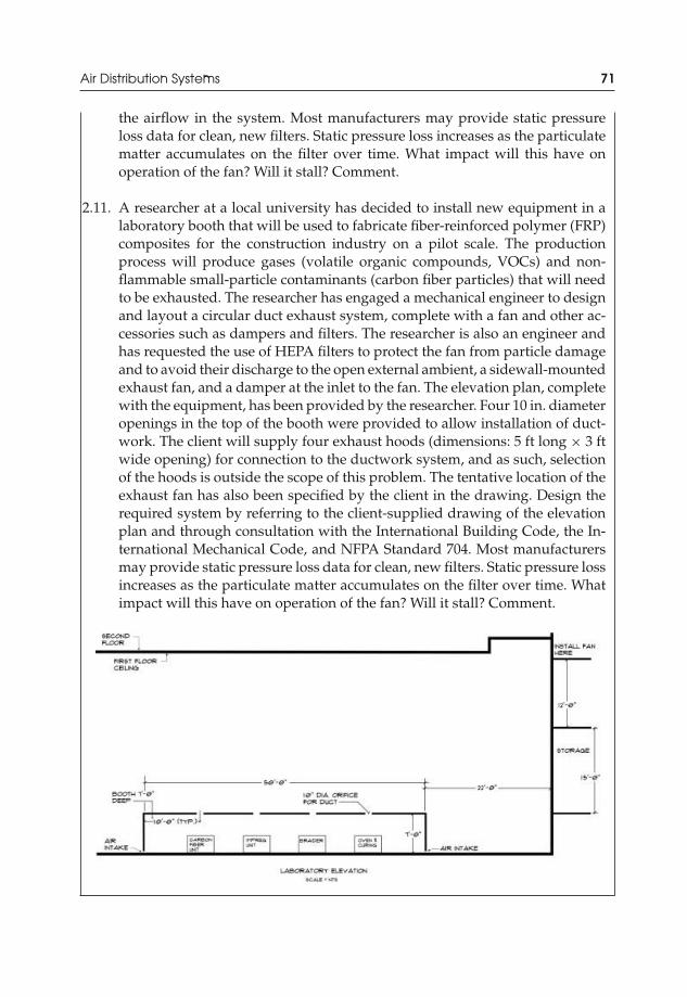
JWST229-c02 JWST229-McDonald Printer: Yet to Come July 28, 2012 13:33 Trim: 244mm × 168mm
Air Distribution Systems 71
the airflow in the system. Most manufacturers may provide static pressureloss data for clean, new filters. Static pressure loss increases as the particulatematter accumulates on the filter over time. What impact will this have onoperation of the fan? Will it stall? Comment.
2.11. A researcher at a local university has decided to install new equipment in alaboratory booth that will be used to fabricate fiber-reinforced polymer (FRP)composites for the construction industry on a pilot scale. The productionprocess will produce gases (volatile organic compounds, VOCs) and non-flammable small-particle contaminants (carbon fiber particles) that will needto be exhausted. The researcher has engaged a mechanical engineer to designand layout a circular duct exhaust system, complete with a fan and other ac-cessories such as dampers and filters. The researcher is also an engineer andhas requested the use of HEPA filters to protect the fan from particle damageand to avoid their discharge to the open external ambient, a sidewall-mountedexhaust fan, and a damper at the inlet to the fan. The elevation plan, completewith the equipment, has been provided by the researcher. Four 10 in. diameteropenings in the top of the booth were provided to allow installation of duct-work. The client will supply four exhaust hoods (dimensions: 5 ft long × 3 ftwide opening) for connection to the ductwork system, and as such, selectionof the hoods is outside the scope of this problem. The tentative location of theexhaust fan has also been specified by the client in the drawing. Design therequired system by referring to the client-supplied drawing of the elevationplan and through consultation with the International Building Code, the In-ternational Mechanical Code, and NFPA Standard 704. Most manufacturersmay provide static pressure loss data for clean, new filters. Static pressure lossincreases as the particulate matter accumulates on the filter over time. Whatimpact will this have on operation of the fan? Will it stall? Comment.
JWST229-c02 JWST229-McDonald Printer: Yet to Come July 28, 2012 13:33 Trim: 244mm × 168mm
72 Introduction to Thermo-Fluids Systems Design
References and Further Reading
[1] Colebrook, C. (1939) Turbulent flow in pipes, with particular reference to the transitionbetween the smooth and rough pipe laws. Journal of the Institute of Civil Engineers London,11, 133–156.
[2] Swamee, P. and Jain, A. (1976) Explicit equations for pipe-flow problems. Proceedings ofthe ASCE, Journal of the Hydraulics Division, 102 (HY5), 657–664.
[3] Miller, R. (1996) Flow Measurement Engineering Handbook, 3rd edn, McGraw-Hill, Inc., NewYork.
[4] Haaland, S. (1983) Simple and explicit formulas for the friction factor in turbulent pipeflow, Journal of Fluids Engineering, 105, 89–90.
[5] Blasius, H. (1912) Das Aehnlichkeitsgesetz bei Reibungsvorgangen. Zeitschrift des VereinesDeutscher Ingenieure, 56, 639–643.
[6] Churchill, S. (1977) Friction-factor equation spans all fluid-flow regimes. Chemical Engi-neering, 84, 91–92.
[7] Petukhov, B. (1970) Heat transfer and friction in turbulent pipe flow with variable physicalproperties, in Advances in Heat Transfer, vol. 6 (eds T. Irvine and J. Hartnett), AcademicPress, New York.
[8] Moody, L. (1944) Friction factors for pipe flows. Transactions of the ASME, 66, 671–684.[9] Howell, R., Sauer Jr. H., and Coad, W. (2005) Principles of Heating, Ventilating, and Air-
Conditioning, American Society of Heating, Refrigerating, and Air-Conditioning Engi-neers, Inc., Atlanta, GA.
[10] International Code Council, Inc. (2006) International Building Code, Country Club Hills, IL.[11] International Code Council, Inc. (2006) International Mechanical Code, Country Club Hills,
IL.[12] National Fire Protection Association (2012) Standard for the Installation of Air-conditioning
and Ventilating Systems, Standard 90A, Quincy, MA.[13] Sheet Metal and Air Conditioning Contractors National Association, Inc. (1985) HVAC
Duct Construction Standards: Metal and Flexible, Vienna, VA.[14] National Fire Protection Association (2011) Standard for Ventilation Control and Fire Protec-
tion of Commercial Cooking Operations, Standard 96, Quincy, MA.[15] American Society of Heating, Refrigerating, and Air-Conditioning Engineers (2011) Ven-
tilation for Commercial Cooking Operations, Standard 154-2011, Atlanta, GA.[16] Carrier Corporation (1991) Fan Application Manual, Syracuse, NY.[17] Pritchard, P. (2011) Fox and McDonald’s Introduction to Fluid Mechanics, 8th edn, John Wiley
& Sons, Hoboken, NJ.[18] Cengel, Y. and Cimbala, J. (2010) Fluid Mechanics: Fundamentals and Applications, 2nd edn,
McGraw Hill Companies, Inc., New York.[19] Air-Conditioning, Heating, and Refrigeration Institute (formerly Air-Conditioning and
Refrigeration Institute) (2005) Standard for Performance Rating of Unitary Air-Conditioningand Air-Source Heat Pump Equipment, Standard 210/240, Arlington, VA.
[20] American Society of Heating, Refrigerating, and Air-Conditioning Engineers, ASHRAE(2011) Heating, Ventilating, and Air-Conditioning Applications, Atlanta, GA.
[21] Kingsbury, H. (1995) Review and revision of room noise criteria. Noise Control EngineeringJournal, 43, 65–72.
[22] Carrier Corporation (1972) System Design Manual: Part 2 – Air Distribution, Chart 8, Syra-cuse, NY.
[23] Carrier Air Conditioning Co. (1974) System Design Manual, Part 2: Air Distribution, Syra-cuse, NY.
JWST229-c03 JWST229-McDonald Printer: Yet to Come July 28, 2012 13:48 Trim: 244mm × 168mm
3Liquid Piping Systems
3.1 Liquid Piping Systems
Piping systems are used to transport diverse liquids for a variety of different appli-cations. These applications may range from water service for buildings to complextwo-phase flow systems in industrial plants. The design of these systems requiresconsideration of several groups of specialties and accessories that will be needed fora functional system. This chapter will focus on fittings and accessories, pipe materi-als, fluid machines, and design considerations necessary for the successful design ofpractical piping systems for various applications.
3.2 Minor Losses: Fittings and Valves in Liquid Piping Systems
3.2.1 Fittings
Fittings are used to extend pipe lengths, expand the pipe network, or perform aselected function. Examples of fittings specific to liquid piping systems are plugs,unions, wyes, valves, tees, caps, ferrules, elbows, nipples, reducers, sleeves, couplings,adapters, fasteners, compression fittings, and bulkhead fittings, to name a few. Allthese add resistance to fluid flow. Tabulated K values (loss coefficients) are availablefor these and other fittings.
3.2.2 Valves
Valves are used to control the flow rate of fluid in piping systems. For valves, lower Kvalues occur when they are fully open; thus, frictional losses will be low. The K valueswill increase as the valve is closed. A similar trend will apply to Lequiv values. Thereare many types of valves. Some of these valves and their drawing symbols are shownin Figure 3.1. Additional information and typical K values for valves are provided in
Introduction to Thermo-Fluids Systems Design, First Edition. Andre G. McDonald and Hugh L. Magande.C© 2012 Andre G. McDonald and Hugh L. Magande. Published 2012 by John Wiley & Sons, Ltd.
73
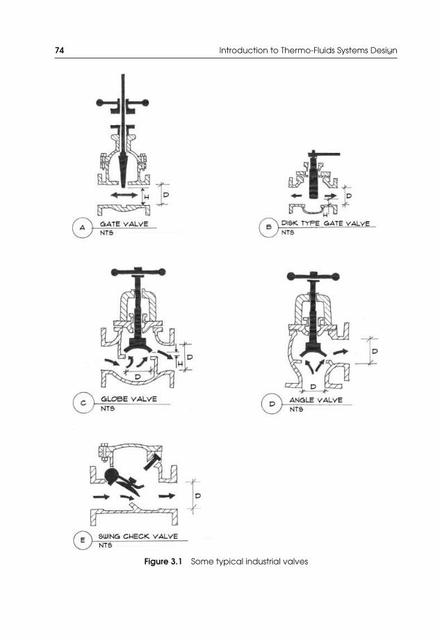
JWST229-c03 JWST229-McDonald Printer: Yet to Come July 28, 2012 13:48 Trim: 244mm × 168mm
74 Introduction to Thermo-Fluids Systems Design
Figure 3.1 Some typical industrial valves

JWST229-c03 JWST229-McDonald Printer: Yet to Come July 28, 2012 13:48 Trim: 244mm × 168mm
Liquid Piping Systems 75
Figure 3.2 A typical fuel oil piping system complete with a pump set (ASHRAE Hand-book, Fundamentals Volume, 2005; reprinted with permission)
Table A.14. Manufacturer’s catalogs should be consulted to find other valves and/orpipe fittings and their K or Lequiv values.
3.2.3 A Typical Piping System—A Closed-LoopFuel Oil Piping System
The schematic drawing shown in Figure 3.2 depicts a typical fuel oil piping systemc/w a pump set. Note all the fittings and valves. Note also the symbols used fordifferent equipment. Additional symbols are provided in Appendix B. The designengineer should be familiar with this type of drawing for piping systems.
Practical Note 3.1 Link Seals
Absent are link seals to protect the pipes that penetrate the concrete walls. The seals areused to fill voids between the pipe and the barrier through which it passes.
3.3 Sizing Liquid Piping Systems
3.3.1 General Design Considerations
Sizing liquid piping follows a similar procedure to that outlined in Example 2.1of Chapter 2. Consider the following additional points when sizing and designingpiping systems.
(A) Pipe Materials: Is the fluid corrosive? Are there particulates in the fluid (e.g., oilsand liquid slurries) that will erode the pipe? Is the fluid temperature high?
(B) Pipe Thickness: Is higher pipe strength required for high stress (high pressure)applications?
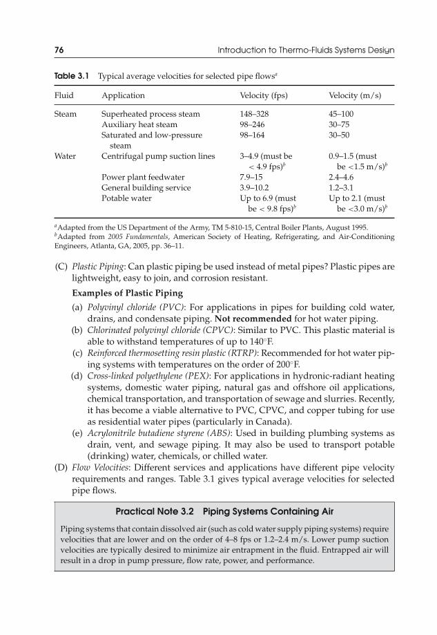
JWST229-c03 JWST229-McDonald Printer: Yet to Come July 28, 2012 13:48 Trim: 244mm × 168mm
76 Introduction to Thermo-Fluids Systems Design
Table 3.1 Typical average velocities for selected pipe flowsa
Fluid Application Velocity (fps) Velocity (m/s)
Steam Superheated process steam 148–328 45–100Auxiliary heat steam 98–246 30–75Saturated and low-pressure
steam98–164 30–50
Water Centrifugal pump suction lines 3–4.9 (must be< 4.9 fps)b
0.9–1.5 (mustbe <1.5 m/s)b
Power plant feedwater 7.9–15 2.4–4.6General building service 3.9–10.2 1.2–3.1Potable water Up to 6.9 (must
be < 9.8 fps)bUp to 2.1 (must
be <3.0 m/s)b
aAdapted from the US Department of the Army, TM 5-810-15, Central Boiler Plants, August 1995.bAdapted from 2005 Fundamentals, American Society of Heating, Refrigerating, and Air-ConditioningEngineers, Atlanta, GA, 2005, pp. 36–11.
(C) Plastic Piping: Can plastic piping be used instead of metal pipes? Plastic pipes arelightweight, easy to join, and corrosion resistant.
Examples of Plastic Piping
(a) Polyvinyl chloride (PVC): For applications in pipes for building cold water,drains, and condensate piping. Not recommended for hot water piping.
(b) Chlorinated polyvinyl chloride (CPVC): Similar to PVC. This plastic material isable to withstand temperatures of up to 140◦F.
(c) Reinforced thermosetting resin plastic (RTRP): Recommended for hot water pip-ing systems with temperatures on the order of 200◦F.
(d) Cross-linked polyethylene (PEX): For applications in hydronic-radiant heatingsystems, domestic water piping, natural gas and offshore oil applications,chemical transportation, and transportation of sewage and slurries. Recently,it has become a viable alternative to PVC, CPVC, and copper tubing for useas residential water pipes (particularly in Canada).
(e) Acrylonitrile butadiene styrene (ABS): Used in building plumbing systems asdrain, vent, and sewage piping. It may also be used to transport potable(drinking) water, chemicals, or chilled water.
(D) Flow Velocities: Different services and applications have different pipe velocityrequirements and ranges. Table 3.1 gives typical average velocities for selectedpipe flows.
Practical Note 3.2 Piping Systems Containing Air
Piping systems that contain dissolved air (such as cold water supply piping systems) requirevelocities that are lower and on the order of 4–8 fps or 1.2–2.4 m/s. Lower pump suctionvelocities are typically desired to minimize air entrapment in the fluid. Entrapped air willresult in a drop in pump pressure, flow rate, power, and performance.

JWST229-c03 JWST229-McDonald Printer: Yet to Come July 28, 2012 13:48 Trim: 244mm × 168mm
Liquid Piping Systems 77
3.3.2 Pipe Data for Building Water Systems
As seen in Example 2.1 of Chapter 2, pipe and duct sizing can be laborious, requir-ing many iterations of complex correlation equations. In practice for building watersystems, charts and tables are used to simplify the process of liquid pipe sizing. Ofimportance is pipe material selection, determination of pipe diameter, and installationspecifications. While the focus is on building water systems, the procedures outlinedhere will apply directly to other types of piping systems such as wastewater/sludgesystems, food processing systems, and chemical liquid systems.
(A) Pipe Materials for Building Water Systems: Type L copper tubing is widely used.Schedule 40 steel is used in steam heating systems. Schedule 80 steel, which isthicker than Schedule 40 steel, is used in high-pressure steam lines. PEX may alsobe used in cold or hot water systems in lieu of copper. It is not recommended forhigh-pressure steam lines. Table 3.2 shows some data for copper and steel pipes.Consult Tables A.6 through A.11 for more extensive information for a variety ofmaterials, and refer to it often.
(B) Pipe Sizing Considerations—Determination of Pipe Diameters: Pipes in closed-loopbuilding systems should be designed to limit friction losses to 3 ft of water per100 ft of pipe. This will reduce the final pump size and cost.
In addition, pipe velocities should be less than 10 fps or 3 m/s to reduce noise andpipe material erosion. Typically, volume flow rates in the pipes are known, whichmakes determination of the pipe diameter easier.
Practical Note 3.3 Higher Pipe Friction Losses and Velocities
The design engineer should bear in mind that the aforementioned points are guidelines.Flexibility exists in order to optimize the performance of a given system design. For example,higher friction losses may be acceptable for shorter run of pipes or for cases where smallerpipe sizes are mandatory by the client or application. Higher pipe velocities may be requiredfor fluid systems that transport solid sediments. This ensures that the sediments do not clogthe pipes by sticking to the pipe wall. However, for small diameter pipes, erosion becomes aconcern when large velocities are used. For example, in stainless steel tubes, erosion becomesa concern when velocities are larger than 15 fps (consult Table A.13 for additional data). Alldeviations from the established guidelines should be justified by the design engineer.
After selection of the pipe friction loss and velocity, an appropriate chart may beused to determine the pipe diameter. One such chart for plastic piping systems isshown in Figure 3.3. Consult Appendix A for additional and more extensive charts.
(A) Pipe Installation: Pipes are typically hung between the slab and the dropped(finished) ceiling and are supported by pipe hangers. The hangers are fastenedaround the pipe and their support rods are anchored to the ceiling. Figure 3.4

JWST229-c03 JWST229-McDonald Printer: Yet to Come July 28, 2012 13:48 Trim: 244mm × 168mm
78 Introduction to Thermo-Fluids Systems Design
Table 3.2 Pipe data for copper and steel
Diameter (in.)
Material Nominal Inner Outer
Weight per LinearFoot of Pipe and
Water (lb)Gallons of Waterper Linear Foot
CopperType L 3/8 0.430 0.500 0.26 0.008Type L 1/2 0.545 0.625 0.39 0.012Type L 3/4 0.785 0.875 0.67 0.025Type L 1 1.025 1.125 1.01 0.043Type L 11/4 1.265 1.375 1.43 0.065Type L 11/2 1.505 1.625 1.91 0.093Type L 2 1.985 2.125 3.09 0.161Type L 21/2 2.465 2.625 4.55 0.248Type L 3 2.945 3.125 6.29 0.354Type L 31/2 3.425 3.625 8.29 0.479Type L 4 3.905 4.125 10.58 0.622
SteelSchedule 40 1/4 0.364 0.540 0.475 0.005Schedule 40 1/2 0.622 0.840 0.992 0.016Schedule 40 3/4 0.824 1.050 1.372 0.028Schedule 40 1 1.049 1.315 2.055 0.045Schedule 40 11/4 1.380 1.660 2.929 0.077Schedule 40 11/2 1.610 1.900 3.602 0.106Schedule 40 2 2.067 2.375 5.114 0.174Schedule 40 21/2 2.469 2.875 7.873 0.248Schedule 40 3 3.068 3.500 10.781 0.383Schedule 40 31/2 3.548 4.000 13.397 0.513Schedule 40 4 4.026 4.500 16.316 0.660
Schedule 80 1/2 0.546 0.840 1.189 0.012Schedule 80 3/4 0.742 1.050 1.686 0.026Schedule 80 1 0.957 1.315 2.483 0.037Schedule 80 11/4 1.278 1.660 3.551 0.067Schedule 80 11/2 1.500 1.900 4.396 0.092Schedule 80 2 1.939 2.375 6.302 0.154Schedule 80 21/2 2.323 2.875 9.491 0.220Schedule 80 3 2.900 3.500 13.122 0.344Schedule 80 31/2 3.364 4.000 16.225 0.458Schedule 80 4 3.826 4.500 19.953 0.597

JWST229-c03 JWST229-McDonald Printer: Yet to Come July 28, 2012 13:48 Trim: 244mm × 168mm
Liquid Piping Systems 79
Figure 3.3 Plastic pipe (Schedule 80) friction loss chart (ASHRAE Handbook, Funda-mentals Volume, 2005; reprinted with permission)
shows pipes supported on hangers. The weights per foot of piping filled withwater are used to determine the spacing of the pipe hangers and the sizing ofthe support rods. Shown below (Tables 3.3 and 3.4) is data adapted from anErico (Solon, OH, USA) catalog for steel and copper hangers for water or steamservice.
Important Note: The hanger data presented in Tables 3.3 and 3.4 do not apply whenspan calculations are made or where concentrated loads from pipe accessories arepresent between the supports. Changes in pipe direction will require additional sup-port. Section 308 of the International Plumbing Code provides further details on pipehanger spacings.
Figure 3.4 Pipes supported on hangers

JWST229-c03 JWST229-McDonald Printer: Yet to Come July 28, 2012 13:48 Trim: 244mm × 168mm
80 Introduction to Thermo-Fluids Systems Design
Table 3.3 Hanger spacing for straight stationary pipes and tubes [1]
Steel Pipe (ft) Copper Pipe (ft)
Water Service Steam Service Water Service Steam ServiceNominal PipeDiameter (in.)
1/4 7 8 5 53/8 7 8 5 61/2 7 8 5 63/4 7 9 5 71 7 9 6 811/4 7 9 7 911/2 9 12 8 102 10 13 8 1121/2 11 14 9 133 12 15 10 1431/2 13 16 11 154 14 17 12 165 16 19 13 186 17 21 14 208 19 24 16 2310 20 26 18 2512 23 30 19 2814 25 3216 27 3518 28 3720 30 3924 32 4230 33 44
Table 3.4 Minimum hanger rod size for straight stationarypipes and tubes [1]
Nominal Pipe Diameter(in.) Minimum Rod Size (in.)
1/4–2 3/821/2–31/2 1/24–5 5/86 3/48–12 7/814–18 120–24 11/4
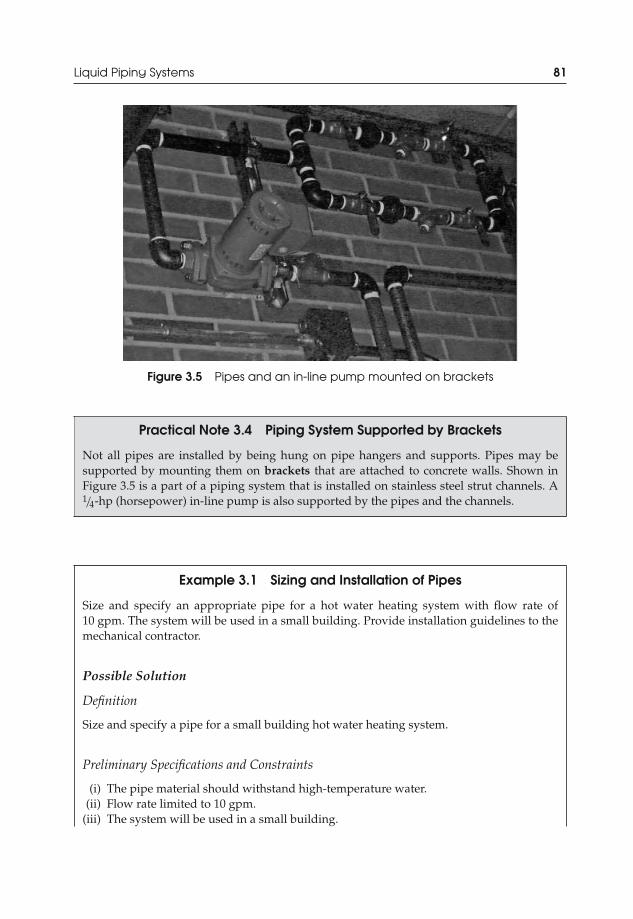
JWST229-c03 JWST229-McDonald Printer: Yet to Come July 28, 2012 13:48 Trim: 244mm × 168mm
Liquid Piping Systems 81
Figure 3.5 Pipes and an in-line pump mounted on brackets
Practical Note 3.4 Piping System Supported by Brackets
Not all pipes are installed by being hung on pipe hangers and supports. Pipes may besupported by mounting them on brackets that are attached to concrete walls. Shown inFigure 3.5 is a part of a piping system that is installed on stainless steel strut channels. A1/4-hp (horsepower) in-line pump is also supported by the pipes and the channels.
Example 3.1 Sizing and Installation of Pipes
Size and specify an appropriate pipe for a hot water heating system with flow rate of10 gpm. The system will be used in a small building. Provide installation guidelines to themechanical contractor.
Possible Solution
Definition
Size and specify a pipe for a small building hot water heating system.
Preliminary Specifications and Constraints
(i) The pipe material should withstand high-temperature water.(ii) Flow rate limited to 10 gpm.
(iii) The system will be used in a small building.
JWST229-c03 JWST229-McDonald Printer: Yet to Come July 28, 2012 13:48 Trim: 244mm × 168mm
82 Introduction to Thermo-Fluids Systems Design
Detailed Design
Objective
To size and specify an appropriate pipe.
Data Given or Known
(i) The water flow rate is 10 gpm.
Assumptions/Limitations/Constraints
(i) Choose type L copper tubing. This is most common in building piping systems, is usedreadily for hot water heating systems, and is widely available to contractors.
(ii) Limit the pipe friction losses to 3 ft of water per 100 ft of pipe, as per industry standard.(iii) Limit the water velocity to 6 fps. The erosion limit of water in small copper tubes is
6 fps. Further, this velocity limit is within the range for general building service (4–10fps).
Sketch
A drawing is not needed.
Analysis
Figure A.3 presents a copper tubing friction loss chart. From this chart, some possible pipesizes, velocities, and friction losses are
Option a: 1 in. nominal, 11/8; in. OD, 4 fps, 7 ft of water per 100 ft of pipeOption b: 11/4 in. nominal, 13/8 in. OD, 2.7 fps, 2.5 ft of water per 100 ft of pipeOption c: 11/2 in. nominal, 15/8 in. OD, 1.7 fps, 1.2 ft of water per 100 ft of pipe
Option a is immediately discarded because the friction loss exceeds 3 ft of water per 100 ftof pipe.
Drawings
No drawings are required.
Conclusions
Options b and c meet the design requirements and satisfy the constraints. Since smallerpipes will result in lower material and installation costs, option b is chosen.
Therefore, choose
Copper type L, 11/4 in. nominal, 13/8 in. OD
Installation Guidelines and Specifications
Tables 3.3 and 3.4 should be consulted to prepare the installation specifications:
The contractor shall use copper hangers and rods. The hangers shall be spaced 7 ft apart.The rod size shall be 3/8 in.

JWST229-c03 JWST229-McDonald Printer: Yet to Come July 28, 2012 13:48 Trim: 244mm × 168mm
Liquid Piping Systems 83
Copper hangers were chosen to eliminate any thermal expansion coefficient differencesbetween the pipe and the hanger. This could generate severe stresses on the pipes. Also, sim-ilar pipe and hanger material will eliminate the possibility of corrosion (galvanic/dissimilarmetal corrosion).
3.4 Fluid Machines (Pumps) and Pump–Pipe Matching
3.4.1 Classifications and Terminology
Pumps serve to move liquids. The pump adds energy to the fluid to keep it moving,to overcome head losses, and/or to build pressure on the fluid to overcome elevationhead in the line. As the fluid passes through the pump and energy is added, thedischarge pressure of the exiting fluid becomes greater than the pressure of the inletfluid. There are many types of pumps available on the market. The Pump Handbook[2] should be consulted for detailed information on pumps.
3.4.2 Types of Pumps
(a) Gas pumps: These pumps move gases. Examples of these types of pumps are fansand compressors.
(b) Positive displacement pumps: These pumps pressurize the fluid by contracting orchanging their boundaries to force fluid to flow. Suction is achieved when theboundaries of the pump expand or the volume of the pump becomes larger.Examples of positive displacement pumps include the human heart, flexible-tubeperistaltic pumps, and double-screw pumps. These pumps are capable of creatinga significant vacuum pressure at their inlets, even when dry, and are able to liftfluids from long distances below the pump. These pumps are also called self-priming pumps.
(c) Dynamic pumps: Rotating blades are used to supply energy to the fluid. The bladesimpart momentum to the fluid. Fluid enters the eye of the impeller, is flung fromthe impeller blades into the scroll case (volute) of the pump where the fluid ispressurized. The fluid exits at high pressure.
Figure 3.6 shows schematic cross-sectional drawings of some typical pumpsencountered in engineering practice. Figure 3.6a and 3.6b show examples of posi-tive displacement pumps and Figure 3.6c shows an example of a dynamic pump(centrifugal pump).
3.4.3 Pump Fundamentals
There are several fundamental parameters that need to be mentioned before proceed-ing to pump sizing and selection.
(a) Pump Capacity: Volume flow rate of fluid through the pump:
V = mρ
. (3.1)

JWST229-c03 JWST229-McDonald Printer: Yet to Come July 28, 2012 13:48 Trim: 244mm × 168mm
84 Introduction to Thermo-Fluids Systems Design
(a)
(c) (d)
(b)Three-lobe rotary pump Two screw pump
In-line centrifugal pump Vertical multi-stage submersible pump
Figure 3.6 Types of industrial pumps: (a) three-lobe rotary pump; (b) two-screw pump;(c) in-line centrifugal pump; (d) vertical mutistage submersible pump (Hydraulic Insti-tute, Parsippany, NJ, www.pumps.org; reprinted with permission)

JWST229-c03 JWST229-McDonald Printer: Yet to Come July 28, 2012 13:48 Trim: 244mm × 168mm
Liquid Piping Systems 85
(b) Pump Net Head: Used to increase the fluid energy (usually in units of length)An expression for the pump net head can be found by considering the energy
equation.Thus, the pump specific work is
wpump =(
p2
ρ+ V2
2
2+ gz2
)−
(p1
ρ+ V2
1
2+ gz1
)+ hlT, (3.2)
where points 1 and 2 are points in the pipe system chosen by the engineer.Dividing by g gives the pump net head (in units of length):
Hpump = wpump
g=
(p2
ρg+ V2
2
2g+ z2
)−
(p1
ρg+ V2
1
2g+ z1
)+ HlT. (3.3)
If a control volume were drawn around the pump only, the following could beassumed:
HlT = 0 (applies to pipe head loss, only); point 1 is the pump inlet; point 2 is thepump outlet; z2 = z1 (horizontally mounted pump); D2 = D1 (assuming suctionand discharge pipe diameters are equal); V2 = V1 (no area changes yields equalvelocities).
Therefore,
Hpump = p2
ρg− p1
ρg= p2 − p1
ρg= poutlet − pinlet
ρg= �prise
ρg. (3.4)
The energy required to generate a pressure rise across the pump is directlyrelated to the pump net head.
(c) Water Horsepower: Power delivered directly to the fluid by the pump:
Wwater horsepower = mgHpump = ρgVHpump. (3.5)
(d) Brake Horsepower (bhp): External power supplied to the pump by a mechanicalshaft or an electrical motor.
For a rotating shaft that supplies the bhp:
bhp = Wpump,shaft = ωTshaft, (3.6)
where ω is the rotational speed and Tshaft is the torque generated by the shaft.(e) Pump efficiency: Ratio of useful power to supplied power:
ηpump = Wwater horsepower
bhp= ρgVHpump
ωTshaft. (3.7)
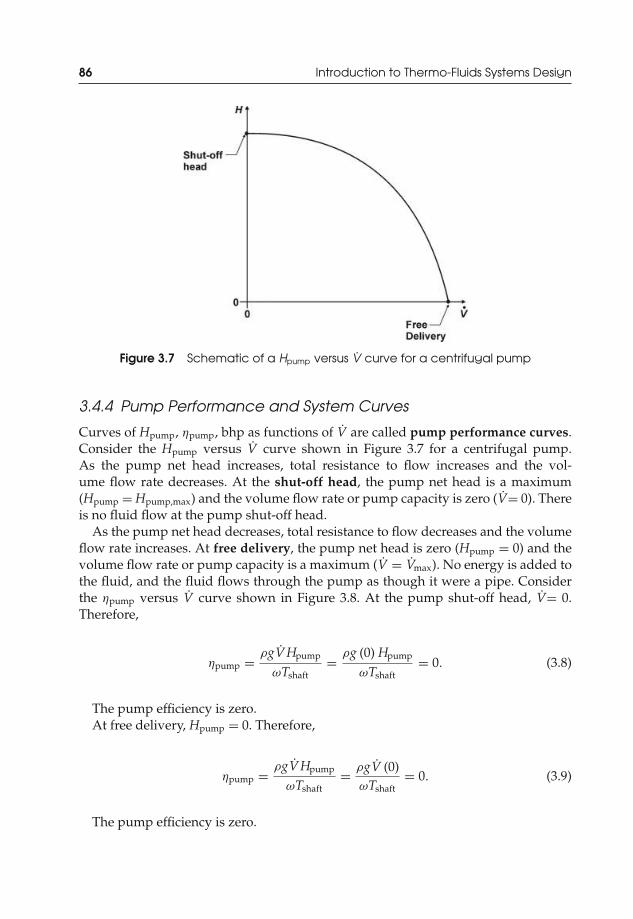
JWST229-c03 JWST229-McDonald Printer: Yet to Come July 28, 2012 13:48 Trim: 244mm × 168mm
86 Introduction to Thermo-Fluids Systems Design
Figure 3.7 Schematic of a Hpump versus V curve for a centrifugal pump
3.4.4 Pump Performance and System Curves
Curves of Hpump, ηpump, bhp as functions of V are called pump performance curves.Consider the Hpump versus V curve shown in Figure 3.7 for a centrifugal pump.As the pump net head increases, total resistance to flow increases and the vol-ume flow rate decreases. At the shut-off head, the pump net head is a maximum(Hpump = Hpump,max) and the volume flow rate or pump capacity is zero (V= 0). Thereis no fluid flow at the pump shut-off head.
As the pump net head decreases, total resistance to flow decreases and the volumeflow rate increases. At free delivery, the pump net head is zero (Hpump = 0) and thevolume flow rate or pump capacity is a maximum (V = Vmax). No energy is added tothe fluid, and the fluid flows through the pump as though it were a pipe. Considerthe ηpump versus V curve shown in Figure 3.8. At the pump shut-off head, V= 0.Therefore,
ηpump = ρgVHpump
ωTshaft= ρg (0) Hpump
ωTshaft= 0. (3.8)
The pump efficiency is zero.At free delivery, Hpump = 0. Therefore,
ηpump = ρgVHpump
ωTshaft= ρgV (0)
ωTshaft= 0. (3.9)
The pump efficiency is zero.

JWST229-c03 JWST229-McDonald Printer: Yet to Come July 28, 2012 13:48 Trim: 244mm × 168mm
Liquid Piping Systems 87
Figure 3.8 Schematic of a ηpump versus V curve
The best efficiency point (BEP) of the pump is the maximum pump efficiency(ηpump,max). Note that the performance curve will show the pump capacity that pro-duces the BEP.
When selecting a pump, the design engineer needs to determine the total amountof head that is required to overcome all the losses in the piping system, build up thepressures required by the design, overcome elevation differences, and increase thefluid velocity (as required) across selected points in the system.
Thus, between two points, 1 and 2, the required head for the system is
Hpump,required =(
p2
ρg+ V2
2
2g+ z2
)−
(p1
ρg+ V2
1
2g+ z1
)+ HlT. (3.10)
The pump performance curve shows the amount of head that is available(Hpump,available) and can be delivered by a specific pump. The pump head requiredmust be calculated, and the performance curve must be checked to determine ifthe selected pump can provide the required head. Calculated values of the requiredpump head (Hpump,required) at different pump capacities (flow rates) can be plottedalongside the performance curve. These curves of Hpump,required versus V are calledsystem curves. The point of intersection between the pump performance curve andthe system curve is the operating point of the pipe system.
Therefore, at the operating point,
Hpump,available = Hpump,required. (3.11)
This indicates that the selected pump can provide the total head required by thesystem.
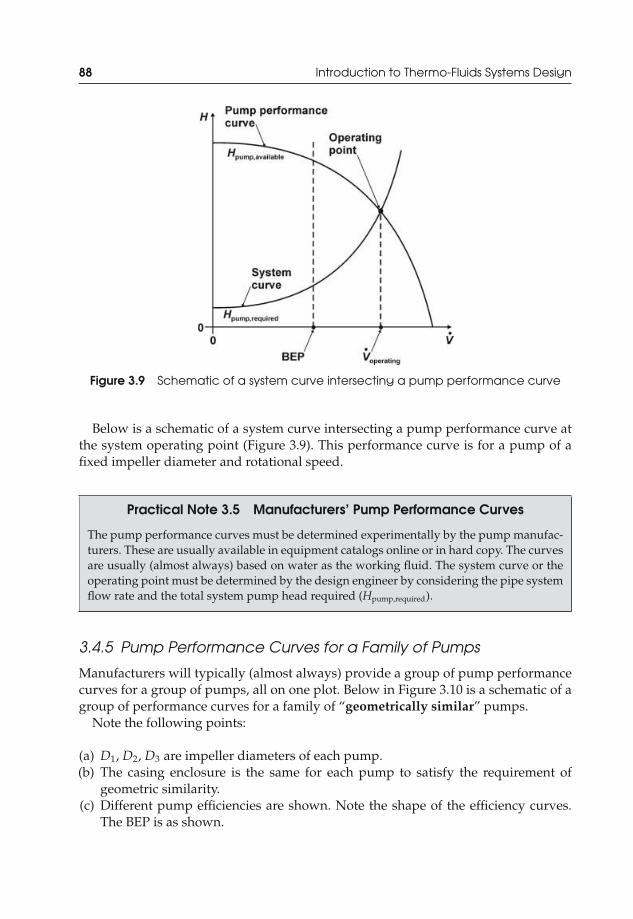
JWST229-c03 JWST229-McDonald Printer: Yet to Come July 28, 2012 13:48 Trim: 244mm × 168mm
88 Introduction to Thermo-Fluids Systems Design
Figure 3.9 Schematic of a system curve intersecting a pump performance curve
Below is a schematic of a system curve intersecting a pump performance curve atthe system operating point (Figure 3.9). This performance curve is for a pump of afixed impeller diameter and rotational speed.
Practical Note 3.5 Manufacturers’ Pump Performance Curves
The pump performance curves must be determined experimentally by the pump manufac-turers. These are usually available in equipment catalogs online or in hard copy. The curvesare usually (almost always) based on water as the working fluid. The system curve or theoperating point must be determined by the design engineer by considering the pipe systemflow rate and the total system pump head required (Hpump,required).
3.4.5 Pump Performance Curves for a Family of Pumps
Manufacturers will typically (almost always) provide a group of pump performancecurves for a group of pumps, all on one plot. Below in Figure 3.10 is a schematic of agroup of performance curves for a family of “geometrically similar” pumps.
Note the following points:
(a) D1, D2, D3 are impeller diameters of each pump.(b) The casing enclosure is the same for each pump to satisfy the requirement of
geometric similarity.(c) Different pump efficiencies are shown. Note the shape of the efficiency curves.
The BEP is as shown.

JWST229-c03 JWST229-McDonald Printer: Yet to Come July 28, 2012 13:48 Trim: 244mm × 168mm
Liquid Piping Systems 89
Figure 3.10 Performance curves for a family of geometrically similar pumps
(d) These curves will be determined experimentally by the manufacturer for a specificliquid. Typically, the liquid is water.
3.4.6 A Manufacturer’s Performance Plot for a Familyof Centrifugal Pumps
Figure 3.11 shows a real pump performance plot from a catalog provided by Taco Inc.Additional pump performance plots are provided in Appendix A for Bell and Gosset
Figure 3.11 Pump performance plot (Taco, Inc.; reprinted with permission)
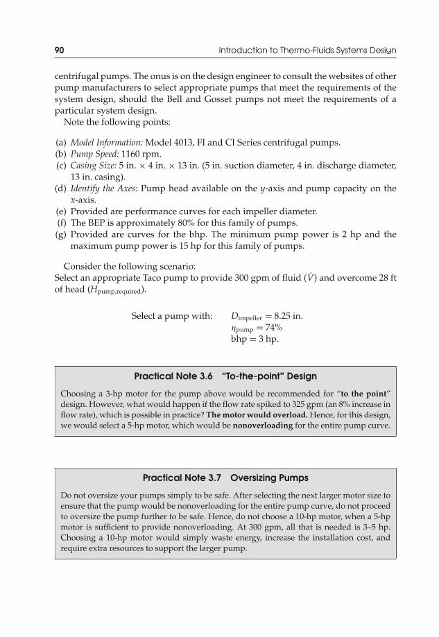
JWST229-c03 JWST229-McDonald Printer: Yet to Come July 28, 2012 13:48 Trim: 244mm × 168mm
90 Introduction to Thermo-Fluids Systems Design
centrifugal pumps. The onus is on the design engineer to consult the websites of otherpump manufacturers to select appropriate pumps that meet the requirements of thesystem design, should the Bell and Gosset pumps not meet the requirements of aparticular system design.
Note the following points:
(a) Model Information: Model 4013, FI and CI Series centrifugal pumps.(b) Pump Speed: 1160 rpm.(c) Casing Size: 5 in. × 4 in. × 13 in. (5 in. suction diameter, 4 in. discharge diameter,
13 in. casing).(d) Identify the Axes: Pump head available on the y-axis and pump capacity on the
x-axis.(e) Provided are performance curves for each impeller diameter.(f) The BEP is approximately 80% for this family of pumps.(g) Provided are curves for the bhp. The minimum pump power is 2 hp and the
maximum pump power is 15 hp for this family of pumps.
Consider the following scenario:Select an appropriate Taco pump to provide 300 gpm of fluid (V) and overcome 28 ftof head (Hpump,required).
Select a pump with: Dimpeller = 8.25 in.ηpump = 74%bhp = 3 hp.
Practical Note 3.6 “To-the-point” Design
Choosing a 3-hp motor for the pump above would be recommended for “to the point”design. However, what would happen if the flow rate spiked to 325 gpm (an 8% increase inflow rate), which is possible in practice? The motor would overload. Hence, for this design,we would select a 5-hp motor, which would be nonoverloading for the entire pump curve.
Practical Note 3.7 Oversizing Pumps
Do not oversize your pumps simply to be safe. After selecting the next larger motor size toensure that the pump would be nonoverloading for the entire pump curve, do not proceedto oversize the pump further to be safe. Hence, do not choose a 10-hp motor, when a 5-hpmotor is sufficient to provide nonoverloading. At 300 gpm, all that is needed is 3–5 hp.Choosing a 10-hp motor would simply waste energy, increase the installation cost, andrequire extra resources to support the larger pump.
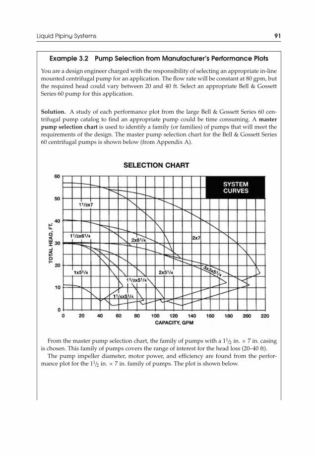
JWST229-c03 JWST229-McDonald Printer: Yet to Come July 28, 2012 13:48 Trim: 244mm × 168mm
Liquid Piping Systems 91
Example 3.2 Pump Selection from Manufacturer’s Performance Plots
You are a design engineer charged with the responsibility of selecting an appropriate in-linemounted centrifugal pump for an application. The flow rate will be constant at 80 gpm, butthe required head could vary between 20 and 40 ft. Select an appropriate Bell & GossettSeries 60 pump for this application.
Solution. A study of each performance plot from the large Bell & Gossett Series 60 cen-trifugal pump catalog to find an appropriate pump could be time consuming. A masterpump selection chart is used to identify a family (or families) of pumps that will meet therequirements of the design. The master pump selection chart for the Bell & Gossett Series60 centrifugal pumps is shown below (from Appendix A).
From the master pump selection chart, the family of pumps with a 11/2 in. × 7 in. casingis chosen. This family of pumps covers the range of interest for the head loss (20–40 ft).
The pump impeller diameter, motor power, and efficiency are found from the perfor-mance plot for the 11/2 in. × 7 in. family of pumps. The plot is shown below.

JWST229-c03 JWST229-McDonald Printer: Yet to Come July 28, 2012 13:48 Trim: 244mm × 168mm
92 Introduction to Thermo-Fluids Systems Design
From the performance plot, and for V= 80 gpm and Hpump = 40 ft (to cover the entirerange of interest):
Dimpeller = 7.0 in.ηpump ≈ 55%bhp ≈ 2 hp.
For this family of pumps, the BEP is approximately 56%. The efficiency of the selectedpump is close to the maximum efficiency.
“To-the-point” design would require the selection of a 11/2-hp motor for this pump. Toavoid motor overloading, a 2-hp motor was chosen instead.
3.4.7 Cavitation and Net Positive Suction Head
Suction into a pump may occur as reduced pressure and high velocity is created topromote the movement of fluid into the pump. The inlet pressures on the suction sideof the pump may be significantly lower than the discharge pressures, and may belower than atmospheric pressure. In some cases in liquid pumps, the inlet pressure tothe pump may become lower than the vapor pressure of the liquid at the operatingtemperature. When this occurs, the liquid will vaporize to form bubbles. Pressuredrop across the pump inlet passage or losses in the pump impeller may also decreasethe pump inlet pressure to values lower than the vapor pressure of the fluid.
Hence, vapor bubbles will form in liquid pumps if
Pinlet < Pvapor,liquid. (3.12)
JWST229-c03 JWST229-McDonald Printer: Yet to Come July 28, 2012 13:48 Trim: 244mm × 168mm
Liquid Piping Systems 93
In a liquid pump, these vapor-filled bubbles are called cavitation bubbles. In thehigh-pressure regions of the pump, these cavitation bubbles will collapse, resultingin damage to the pump and reduction in pump performance. Other negative conse-quences of cavitation include
(a) noise;(b) vibration;(c) pump efficiency reduction;(d) pitting and erosion of pump impeller, casing, and blades due to high-pressure
explosion of the bubbles.
The presence of vapor in the impeller can also result in a loss of pump pressurerise. A study of Equation (3.4) shows that, due to the low density of the vapor, thepressure rise across the pump will be small. In effect, for a vapor-filled impeller, atotal loss of pump performance will occur.
It is necessary to ensure that Pinlet > Pvapor,liquid to avoid cavitation and pumpperformance loss. NPSH can be used to verify if this requirement will be met.
Therefore, in units of length,
NPSH =(
pρg
+ V2
2g
)pump,inlet
− Pvapor
ρg. (3.13)
Pump manufacturers will provide the NPSH required (NPSHR) on the performanceplots for a family of pumps (NPSHR vs. V), and is determined experimentally by themanufacturer. This NPSHR value must be compared with the calculated NPSH.
Thus, to avoid cavitation,
NPSHR < NPSH. (3.14)
The NPSH must be calculated by the design engineer for comparison with theNPSHR to ensure that sufficient NPSH is available.
Practical Note 3.8 NPSH
It is common to see NPSH referred to as net positive suction head available (NPSHA). TheNPSHA is always calculated.
Example 3.3 Net Positive Suction Head
A centrifugal Peerless Pump R© Type 4AE11 is tested at 1750 rpm using the flow system shown.The water level in the inlet reservoir is 3.5 ft above the pump centerline; the inlet line consistsof 6 ft of 4-in. diameter Class 150 cast-iron pipe, a standard elbow, and a fully open gate
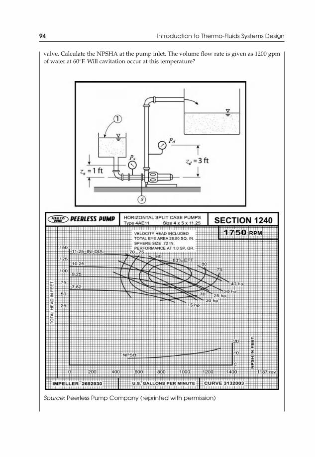
JWST229-c03 JWST229-McDonald Printer: Yet to Come July 28, 2012 13:48 Trim: 244mm × 168mm
94 Introduction to Thermo-Fluids Systems Design
valve. Calculate the NPSHA at the pump inlet. The volume flow rate is given as 1200 gpmof water at 60◦F. Will cavitation occur at this temperature?
Source: Peerless Pump Company (reprinted with permission)

JWST229-c03 JWST229-McDonald Printer: Yet to Come July 28, 2012 13:48 Trim: 244mm × 168mm
Liquid Piping Systems 95
Solution. The NPSHA is
NPSHA =(
ps
ρg+ V2
s
2g
)pump,inlet
− Pvapor
ρg.
The energy equation will be used to find the pump inlet pressure, ps:
P1
ρg+ α1
V21
2g+ z1 = ps
ρg+ αs
V2s
2g+ zs + HlT.
Point 1 is the free surface of the water in the reservoir. Thus, V1 ≈ 0 and P1 = Patm.Therefore,
ps
ρg= Patm
ρg− αs
V2s
2g+ (z1 − zs) − HlT.
Assume that the pipe flow is turbulent. That is, αs ≈ 1. The Reynolds number will needto be verified. Hence,
ps
ρg= Patm
ρg− V2
s
2g+ (z1 − zs) − HlT.
Then,
NPSHA = Patm
ρg− V2
s
2g+ (z1 − zs) − HlT + V2
s
2g− Pvapor
ρg
NPSHA = Patm − Pvapor
ρg+ (z1 − zs) − HlT.
Find the total head loss in the pipe. Note that since the diameter of the pipe does notchange, the law of conservation of mass requires that the pipe average velocity be constant.Therefore,
HlT = Hl + Hlm =(
fLD
+∑
K)
V2s
2g.
For the 4-in. nominal diameter pipe, it will be assumed that the system is assembled withflanged fittings. The loss coefficients are shown in Table A.14 (or other sources) and areshown below. Note that the values for the 4-in. diameter pipe were used:
90◦ regular elbow: Kelbow = 0.3Open gate valve: Kgate = 0.16Sharp-edged inlet: Kinlet = 0.5.
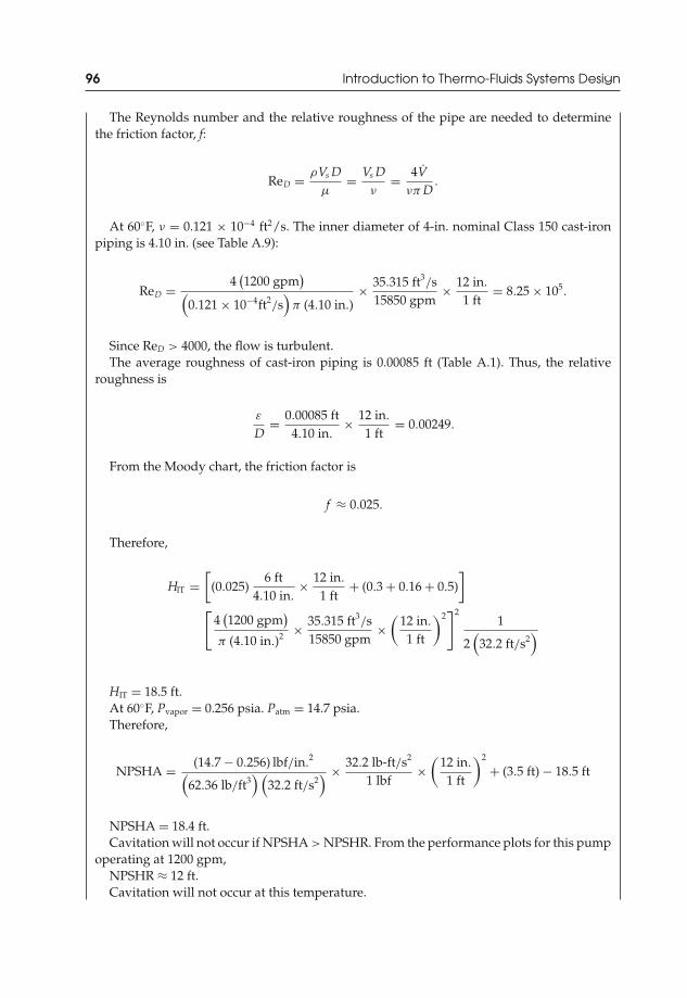
JWST229-c03 JWST229-McDonald Printer: Yet to Come July 28, 2012 13:48 Trim: 244mm × 168mm
96 Introduction to Thermo-Fluids Systems Design
The Reynolds number and the relative roughness of the pipe are needed to determinethe friction factor, f:
ReD = ρVs Dμ
= Vs Dν
= 4Vνπ D
.
At 60◦F, ν = 0.121 × 10⁻⁴ ft2/s. The inner diameter of 4-in. nominal Class 150 cast-ironpiping is 4.10 in. (see Table A.9):
ReD = 4(1200 gpm
)(
0.121 × 10⁻⁴ft2/s
)π (4.10 in.)
× 35.315 ft3/s
15850 gpm× 12 in.
1 ft= 8.25 × 10⁵.
Since ReD > 4000, the flow is turbulent.The average roughness of cast-iron piping is 0.00085 ft (Table A.1). Thus, the relative
roughness is
ε
D= 0.00085 ft
4.10 in.× 12 in.
1 ft= 0.00249.
From the Moody chart, the friction factor is
f ≈ 0.025.
Therefore,
HlT =[
(0.025)6 ft
4.10 in.× 12 in.
1 ft+ (0.3 + 0.16 + 0.5)
][
4(1200 gpm
)π (4.10 in.)2 × 35.315 ft3
/s15850 gpm
×(
12 in.
1 ft
)2]2
1
2(
32.2 ft/s2)
HlT = 18.5 ft.At 60◦F, Pvapor = 0.256 psia. Patm = 14.7 psia.Therefore,
NPSHA = (14.7 − 0.256) lbf/in.2(
62.36 lb/ft3) (
32.2 ft/s2) × 32.2 lb-ft/s2
1 lbf×
(12 in.
1 ft
)2
+ (3.5 ft) − 18.5 ft
NPSHA = 18.4 ft.Cavitation will not occur if NPSHA > NPSHR. From the performance plots for this pump
operating at 1200 gpm,NPSHR ≈ 12 ft.Cavitation will not occur at this temperature.

JWST229-c03 JWST229-McDonald Printer: Yet to Come July 28, 2012 13:48 Trim: 244mm × 168mm
Liquid Piping Systems 97
Comment
The following expression for the NPSHA was derived specifically for this problem:
NPSHA = Patm − Pvapor
ρg+ (z1 − zs) − HlT.
From this equation, it is observed that shorter suction pipes will result in lower headloss (HlT), which will increase NPSHA. This will reduce the possibility of the occurrence ofcavitation.
The amount of fluid in the tank and the static pressure head will have an effect on theNPSHA and cavitation. The static pressure head will increase as (z1–zs) increases. As thestatic pressure head increases, the NPSHA will increase, and the possibility of cavitationwill be reduced.
3.4.8 Pump Scaling Laws: Nondimensional Pump Parameters
Dimensional analysis, the Buckingham Pi () theorem, and the method of repeatingvariables can be used to generate nondimensional pump parameters that includethe pump head, pump capacity, and pump bhp.
For a typical pump, the following functional forms will apply:
gHpump = f(V, D, ε, ω, ρ, μ
)(3.15)
bhp = f(V, D, ε, ω, ρ, μ
), (3.16)
where ε is the relative roughness and D is the diameter of the pump impeller.The resulting dimensionless groups produce nondimensional pump parame-
ters with special names. Following are the six nondimensional pump parameters ofinterest:
(a)ρωD2
μ= Re = Reynold’s number, (3.17)
where ωD is the characteristic velocity.
(b)ε
D= Relative roughness (3.18)
(c)gHpump
ω2 D2 = CH = Head coefficient (3.19)
(d)V
ωD3 = CQ = Capacity coefficient (3.20)
(e)bhp
ρω3 D5 = CP = Power coefficient (3.21)
(f)g × NPSHR
ω2 D2 = CNPSH = Suction head coefficient. (3.22)

JWST229-c03 JWST229-McDonald Printer: Yet to Come July 28, 2012 13:48 Trim: 244mm × 168mm
98 Introduction to Thermo-Fluids Systems Design
3.4.9 Application of the Nondimensional PumpParameters—Affinity Laws
Pumps that are geometrically similar may considered to be equivalent. Pump equiv-alence implies that the nondimensional pump parameters are equal for differentpumps or for different states of the same pump.
Consider two pumps (pump A and pump B) or consider a pump at two differ-ent states of volume flow rate, speed, pump head, bhp, etc. The pump equivalenceequations are:
(a)VA
ωA D3A
= VB
ωB D3B
= CQ,A = CQ,B (3.23)
(b)ρAωA D2
A
μA= ρBωB D2
B
μB= ReA = ReB (3.24)
(c)εA
DA= εB
DB(3.25)
(d)gHpump,A
ω2A D2
A
= gHpump,B
ω2B D2
B
= CH,A = CH,B (3.26)
(e)bhpA
ρAω3A D5
A
= bhpB
ρBω3B D5
B
= CP,A = CP,B. (3.27)
The pump equivalence equations can be expressed as ratios in order to scale pumpsof different sizes or determine the parameters at different states for the same pump.Thus, for different pumps,
(a)VB
VA= ωB
ωA
(DB
DA
)3
(3.28)
(b)HB
HA=
(ωB
ωA
)2 (DB
DA
)2
(3.29)
(c)bhpB
bhpA= ρB
ρA
(ωB
ωA
)3 (DB
DA
)5
. (3.30)
The aforementioned equations are known as the affinity laws. The affinity laws alsoapply to a given pump moving the same liquid. For this case, ρA = ρB and DA = DB.In general, ω = 2πN, where N is the number of revolutions per minute of the pumpimpeller.

JWST229-c03 JWST229-McDonald Printer: Yet to Come July 28, 2012 13:48 Trim: 244mm × 168mm
Liquid Piping Systems 99
Hence, for the same pump that has experienced a speed change from NA to NB,
(a)VB
VA= NB
NA(3.31)
(b)HB
HA=
(NB
NA
)2
(3.32)
(c)bhpB
bhpA=
(NB
NA
)3
. (3.33)
3.4.10 Nondimensional Form of the Pump Efficiency
Dimensional analysis can also be used to establish a nondimensional form of thepump efficiency. Consider the following analysis:
ηpump = Wwater horsepower
bhp= ρgVHpump
bhp(3.34)
Remember:gHpump
ω2 D2 = CH,V
ωD3 = CQ,bhp
ρω3 D5 = CP
Therefore,
ηpump = ρ(ωD3CQ
) (ω2 D2CH
)ρω3 D5CP
= CQCH
CP. (3.35)
Example 3.4 Manipulating the Affinity Laws
When operated at N = 1170 rpm, a centrifugal pump, with impeller diameter, D = 8 in., hasshut-off head Ho = 25.0 ft of water. At the same operating speed, best efficiency occurs atV = 300 gpm, where the head is H = 21.9 ft of water. Specify the discharge and head for thepump when it is operated at 1750 rpm at both the shut-off and BEPs.
Solution. The pump remains the same, so the two flow conditions are geometrically similar.If no cavitation occurs, the flows will also be kinematically similar.
Let condition 1 be at 1170 rpm and condition 2 be at 1750 rpm.For the flow rates (discharge),
CQ1 = CQ2
V1
ω1 D31
= V2
ω2 D32
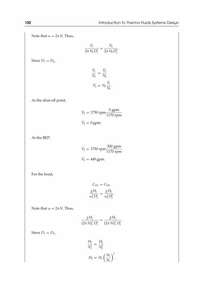
JWST229-c03 JWST229-McDonald Printer: Yet to Come July 28, 2012 13:48 Trim: 244mm × 168mm
100 Introduction to Thermo-Fluids Systems Design
Note that ω = 2πN. Thus,
V1
2π N1 D31
= V2
2π N2 D32
.
Since D1 = D2,
V1
N1= V2
N2
V2 = N2V1
N1.
At the shut-off point,
V2 = 1750 rpm0 gpm
1170 rpm
V2 = 0 gpm.
At the BEP:
V2 = 1750 rpm300 gpm1170 rpm
V2 = 449 gpm.
For the head,
CH1 = CH2
gH1
ω21 D2
1
= gH2
ω22 D2
2
.
Note that ω = 2πN. Thus,
gH1
(2π N)21 D2
1
= gH2
(2π N)22 D2
2
.
Since D1 = D2,
H1
N21
= H2
N22
H2 = H1
(N2
N1
)2
.

JWST229-c03 JWST229-McDonald Printer: Yet to Come July 28, 2012 13:48 Trim: 244mm × 168mm
Liquid Piping Systems 101
At the shut-off point,
H2 = 25.0 ft(
1750 rpm1170 rpm
)2
H2 = 55.9 ft.
At the BEP,
H2 = 21.9 ft(
1750 rpm1170 rpm
)2
H2 = 49.0 ft.
Example 3.5 Selecting a Pump Using Equivalent Performance Plots
Bell & Gossett manufacture 3 in. × 3 in. × 51/4 in. pumps that operate at 1750 rpm. Unfortu-nately, a design project requires a 1750 rpm pump that would provide 70 gpm of kerosenefor a total head of 10 ft of kerosene, if it were to operate at 1150 rpm. Select an appropriatepump from the available Bell & Gossett performance curves. Prepare a pump schedule forthe purposes of installation by the mechanical contractor.
Solution. Appendix A shows performance plots from the Bell & Gossett Series 60 centrifugalpump catalog. The performance plot for the 3 in. × 3 in. × 51/4 in. family of pumps is shownbelow.
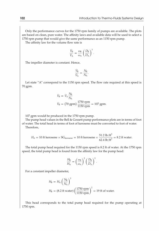
JWST229-c03 JWST229-McDonald Printer: Yet to Come July 28, 2012 13:48 Trim: 244mm × 168mm
102 Introduction to Thermo-Fluids Systems Design
Only the performance curves for the 1750 rpm family of pumps are available. The plotsare based on clean, pure water. The affinity laws and available data will be used to select a1750 rpm pump that would give the same performance as an 1150 rpm pump.
The affinity law for the volume flow rate is
VB
VA= ωB
ωA
(DB
DA
)3
.
The impeller diameter is constant. Hence,
VB
VA= NB
NA.
Let state “A” correspond to the 1150 rpm speed. The flow rate required at this speed is70 gpm.
VB = VANB
NA
VB = (70 gpm
) 1750 rpm1150 rpm
= 107 gpm.
107 gpm would be produced in the 1750 rpm pump.The pump head values in the Bell & Gossett pump performance plots are in terms of foot
of water. The total head in terms of foot of kerosene must be converted to foot of water.Therefore,
HA = 10 ft kerosene × SGkerosene = 10 ft kerosene × 51.2 lb/ft3
62.4 lb/ft3 = 8.2 ft water.
The total pump head required for the 1150 rpm speed is 8.2 ft of water. At the 1750 rpmspeed, the total pump head is found from the affinity law for the pump head:
HB
HA=
(ωB
ωA
)2 (DB
DA
)2
.
For a constant impeller diameter,
HB = HA
(NB
NA
)2
HB = (8.2 ft water)(
1750 rpm1150 rpm
)2
= 19 ft of water.
This head corresponds to the total pump head required for the pump operating at1750 rpm.
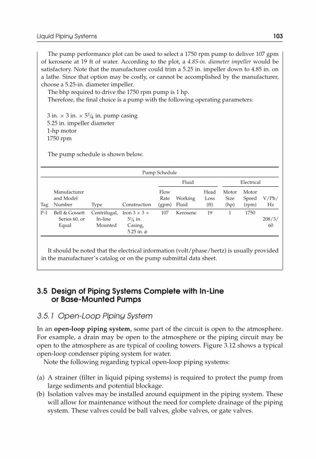
JWST229-c03 JWST229-McDonald Printer: Yet to Come July 28, 2012 13:48 Trim: 244mm × 168mm
Liquid Piping Systems 103
The pump performance plot can be used to select a 1750 rpm pump to deliver 107 gpmof kerosene at 19 ft of water. According to the plot, a 4.85-in. diameter impeller would besatisfactory. Note that the manufacturer could trim a 5.25 in. impeller down to 4.85 in. ona lathe. Since that option may be costly, or cannot be accomplished by the manufacturer,choose a 5.25-in. diameter impeller.
The bhp required to drive the 1750 rpm pump is 1 hp.Therefore, the final choice is a pump with the following operating parameters:
3 in. × 3 in. × 51/4 in. pump casing5.25 in. impeller diameter1-hp motor1750 rpm
The pump schedule is shown below.
Pump Schedule
Fluid Electrical
Tag
Manufacturerand ModelNumber Type Construction
FlowRate
(gpm)WorkingFluid
HeadLoss(ft)
MotorSize(hp)
MotorSpeed(rpm)
V/Ph/Hz
P-1 Bell & GossettSeries 60, orEqual
Centrifugal,In-lineMounted
Iron 3 × 3 ×51/4 in.Casing,5.25 in. φ
107 Kerosene 19 1 1750208/3/
60
It should be noted that the electrical information (volt/phase/hertz) is usually providedin the manufacturer’s catalog or on the pump submittal data sheet.
3.5 Design of Piping Systems Complete with In-Lineor Base-Mounted Pumps
3.5.1 Open-Loop Piping System
In an open-loop piping system, some part of the circuit is open to the atmosphere.For example, a drain may be open to the atmosphere or the piping circuit may beopen to the atmosphere as are typical of cooling towers. Figure 3.12 shows a typicalopen-loop condenser piping system for water.
Note the following regarding typical open-loop piping systems:
(a) A strainer (filter in liquid piping systems) is required to protect the pump fromlarge sediments and potential blockage.
(b) Isolation valves may be installed around equipment in the piping system. Thesewill allow for maintenance without the need for complete drainage of the pipingsystem. These valves could be ball valves, globe valves, or gate valves.
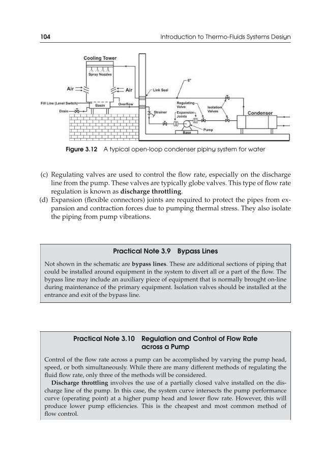
JWST229-c03 JWST229-McDonald Printer: Yet to Come July 28, 2012 13:48 Trim: 244mm × 168mm
104 Introduction to Thermo-Fluids Systems Design
Figure 3.12 A typical open-loop condenser piping system for water
(c) Regulating valves are used to control the flow rate, especially on the dischargeline from the pump. These valves are typically globe valves. This type of flow rateregulation is known as discharge throttling.
(d) Expansion (flexible connectors) joints are required to protect the pipes from ex-pansion and contraction forces due to pumping thermal stress. They also isolatethe piping from pump vibrations.
Practical Note 3.9 Bypass Lines
Not shown in the schematic are bypass lines. These are additional sections of piping thatcould be installed around equipment in the system to divert all or a part of the flow. Thebypass line may include an auxiliary piece of equipment that is normally brought on-lineduring maintenance of the primary equipment. Isolation valves should be installed at theentrance and exit of the bypass line.
Practical Note 3.10 Regulation and Control of Flow Rateacross a Pump
Control of the flow rate across a pump can be accomplished by varying the pump head,speed, or both simultaneously. While there are many different methods of regulating thefluid flow rate, only three of the methods will be considered.
Discharge throttling involves the use of a partially closed valve installed on the dis-charge line of the pump. In this case, the system curve intersects the pump performancecurve (operating point) at a higher pump head and lower flow rate. However, this willproduce lower pump efficiencies. This is the cheapest and most common method offlow control.
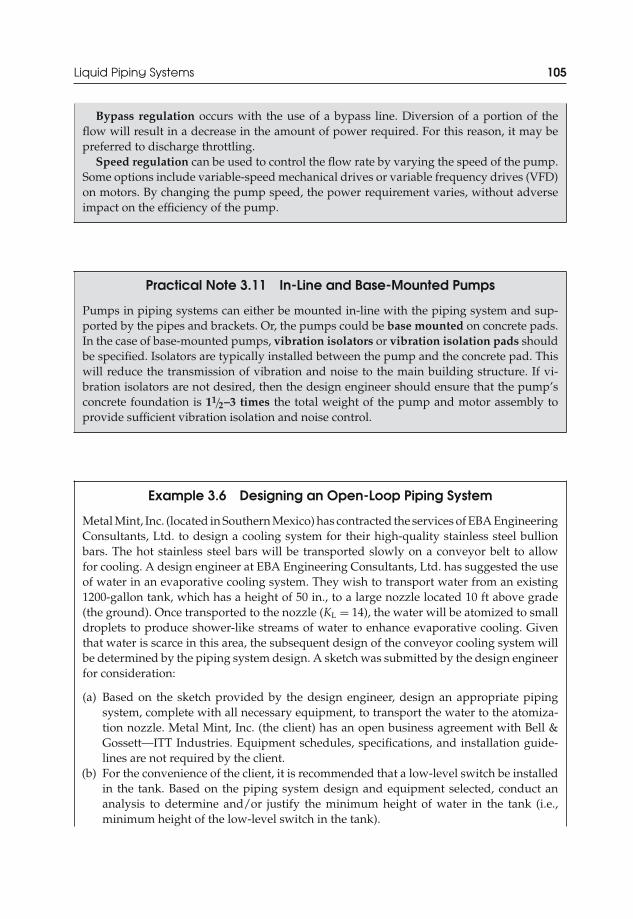
JWST229-c03 JWST229-McDonald Printer: Yet to Come July 28, 2012 13:48 Trim: 244mm × 168mm
Liquid Piping Systems 105
Bypass regulation occurs with the use of a bypass line. Diversion of a portion of theflow will result in a decrease in the amount of power required. For this reason, it may bepreferred to discharge throttling.
Speed regulation can be used to control the flow rate by varying the speed of the pump.Some options include variable-speed mechanical drives or variable frequency drives (VFD)on motors. By changing the pump speed, the power requirement varies, without adverseimpact on the efficiency of the pump.
Practical Note 3.11 In-Line and Base-Mounted Pumps
Pumps in piping systems can either be mounted in-line with the piping system and sup-ported by the pipes and brackets. Or, the pumps could be base mounted on concrete pads.In the case of base-mounted pumps, vibration isolators or vibration isolation pads shouldbe specified. Isolators are typically installed between the pump and the concrete pad. Thiswill reduce the transmission of vibration and noise to the main building structure. If vi-bration isolators are not desired, then the design engineer should ensure that the pump’sconcrete foundation is 11/2–3 times the total weight of the pump and motor assembly toprovide sufficient vibration isolation and noise control.
Example 3.6 Designing an Open-Loop Piping System
Metal Mint, Inc. (located in Southern Mexico) has contracted the services of EBA EngineeringConsultants, Ltd. to design a cooling system for their high-quality stainless steel bullionbars. The hot stainless steel bars will be transported slowly on a conveyor belt to allowfor cooling. A design engineer at EBA Engineering Consultants, Ltd. has suggested the useof water in an evaporative cooling system. They wish to transport water from an existing1200-gallon tank, which has a height of 50 in., to a large nozzle located 10 ft above grade(the ground). Once transported to the nozzle (KL = 14), the water will be atomized to smalldroplets to produce shower-like streams of water to enhance evaporative cooling. Giventhat water is scarce in this area, the subsequent design of the conveyor cooling system willbe determined by the piping system design. A sketch was submitted by the design engineerfor consideration:
(a) Based on the sketch provided by the design engineer, design an appropriate pipingsystem, complete with all necessary equipment, to transport the water to the atomiza-tion nozzle. Metal Mint, Inc. (the client) has an open business agreement with Bell &Gossett—ITT Industries. Equipment schedules, specifications, and installation guide-lines are not required by the client.
(b) For the convenience of the client, it is recommended that a low-level switch be installedin the tank. Based on the piping system design and equipment selected, conduct ananalysis to determine and/or justify the minimum height of water in the tank (i.e.,minimum height of the low-level switch in the tank).
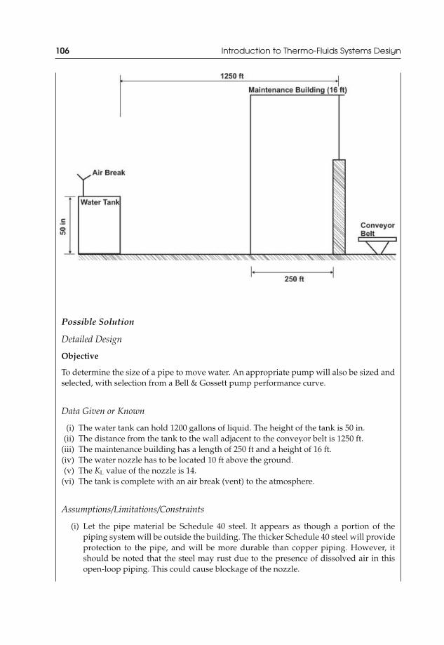
JWST229-c03 JWST229-McDonald Printer: Yet to Come July 28, 2012 13:48 Trim: 244mm × 168mm
106 Introduction to Thermo-Fluids Systems Design
Possible Solution
Detailed Design
Objective
To determine the size of a pipe to move water. An appropriate pump will also be sized andselected, with selection from a Bell & Gossett pump performance curve.
Data Given or Known
(i) The water tank can hold 1200 gallons of liquid. The height of the tank is 50 in.(ii) The distance from the tank to the wall adjacent to the conveyor belt is 1250 ft.
(iii) The maintenance building has a length of 250 ft and a height of 16 ft.(iv) The water nozzle has to be located 10 ft above the ground.(v) The KL value of the nozzle is 14.
(vi) The tank is complete with an air break (vent) to the atmosphere.
Assumptions/Limitations/Constraints
(i) Let the pipe material be Schedule 40 steel. It appears as though a portion of thepiping system will be outside the building. The thicker Schedule 40 steel will provideprotection to the pipe, and will be more durable than copper piping. However, itshould be noted that the steel may rust due to the presence of dissolved air in thisopen-loop piping. This could cause blockage of the nozzle.
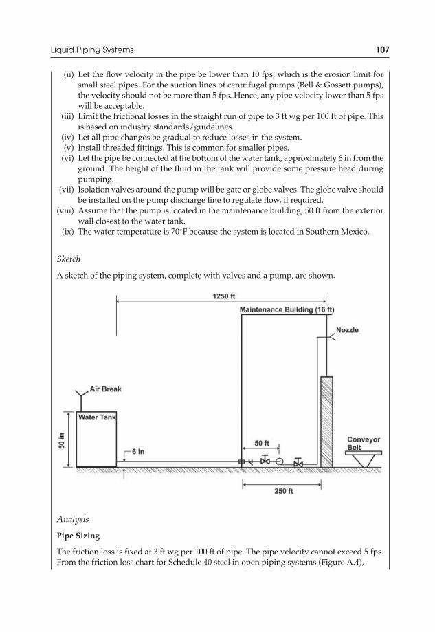
JWST229-c03 JWST229-McDonald Printer: Yet to Come July 28, 2012 13:48 Trim: 244mm × 168mm
Liquid Piping Systems 107
(ii) Let the flow velocity in the pipe be lower than 10 fps, which is the erosion limit forsmall steel pipes. For the suction lines of centrifugal pumps (Bell & Gossett pumps),the velocity should not be more than 5 fps. Hence, any pipe velocity lower than 5 fpswill be acceptable.
(iii) Limit the frictional losses in the straight run of pipe to 3 ft wg per 100 ft of pipe. Thisis based on industry standards/guidelines.
(iv) Let all pipe changes be gradual to reduce losses in the system.(v) Install threaded fittings. This is common for smaller pipes.
(vi) Let the pipe be connected at the bottom of the water tank, approximately 6 in from theground. The height of the fluid in the tank will provide some pressure head duringpumping.
(vii) Isolation valves around the pump will be gate or globe valves. The globe valve shouldbe installed on the pump discharge line to regulate flow, if required.
(viii) Assume that the pump is located in the maintenance building, 50 ft from the exteriorwall closest to the water tank.
(ix) The water temperature is 70◦F because the system is located in Southern Mexico.
Sketch
A sketch of the piping system, complete with valves and a pump, are shown.
Analysis
Pipe Sizing
The friction loss is fixed at 3 ft wg per 100 ft of pipe. The pipe velocity cannot exceed 5 fps.From the friction loss chart for Schedule 40 steel in open piping systems (Figure A.4),
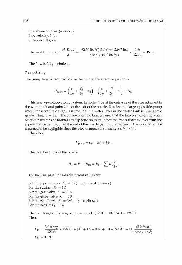
JWST229-c03 JWST229-McDonald Printer: Yet to Come July 28, 2012 13:48 Trim: 244mm × 168mm
108 Introduction to Thermo-Fluids Systems Design
Pipe diameter: 2 in. (nominal)Pipe velocity: 3 fpsFlow rate: 30 gpm.
Reynolds number :ρVDinner
μ= (62.30 lb/ft3) (3.0 ft/s) (2.067 in.)
6.556 × 10⁻⁴ lb/ft/s× 1 ft
12 in.= 49105.
The flow is fully turbulent.
Pump Sizing
The pump head is required to size the pump. The energy equation is
Hpump =(
p2
ρg+ V2
2
2g+ z2
)−
(p1
ρg+ V2
1
2g+ z1
)+ HlT.
This is an open-loop piping system. Let point 1 be at the entrance of the pipe attached tothe water tank and point 2 be at the exit of the nozzle. To select the largest possible pump(most conservative design), assume that the water level in the water tank is 6 in. abovegrade. Thus, z1 = 6 in. The air break on the tank ensures that the free surface of the waterreservoir remains at normal atmospheric pressure. Since the free surface is level with thepipe entrance, p1 = patm. At the exit of the nozzle, p2 = patm. Changes in the velocity will beassumed to be negligible since the pipe diameter is constant. So, V2 ≈ V1.
Therefore,
Hpump = (z2 − z1) + HlT.
The total head loss in the pipe is
HlT = Hl + Hlm = Hl +∑
KLV2
2g.
For the 2 in. pipe, the loss coefficient values are:
For the pipe entrance: KL = 0.5 (sharp-edged entrance)For the strainer: KL = 1.5For the gate valve: KL = 0.16For the globe valve: KL = 6.9For the 90◦ elbows: KL = 0.95 (regular elbows)For the nozzle: KL = 14.
The total length of piping is approximately (1250 + 10–0.5) ft = 1260 ft.Thus,
HlT = 3.0 ft wg100 ft
× 1260 ft + [0.5 + 1.5 + 0.16 + 6.9 + 2 (0.95) + 14](3.0 ft/s)2
2(32.2 ft/s2)HlT = 41 ft.

JWST229-c03 JWST229-McDonald Printer: Yet to Come July 28, 2012 13:48 Trim: 244mm × 168mm
Liquid Piping Systems 109
Hence,
Hpump = (10 − 0.5) ft + 41 ft
Hpump = 50.5 ft ≈ 51 ft.
The flow rate is 30 gpm. From the performance plots for the Bell & Gossett Series 60in-line mounted centrifugal pumps, select the following pump:
11/2 × 11/2 × 7 in. casing7.0 in. impeller diameter11/2-hp motor1750 rpm
Or, choose Bell & Gossett Series 60 pump Model 618T, which is in stock.
Drawings
Conclusion
The piping system and pump has been sized and designed. The following points should benoted:
(i) A gate and globe valve are used as isolation valves. The globe valve on the dischargeline of the pump may be used to control the flow rate, if needed. Another option couldbe to use a VFD to control the pump via the motor.
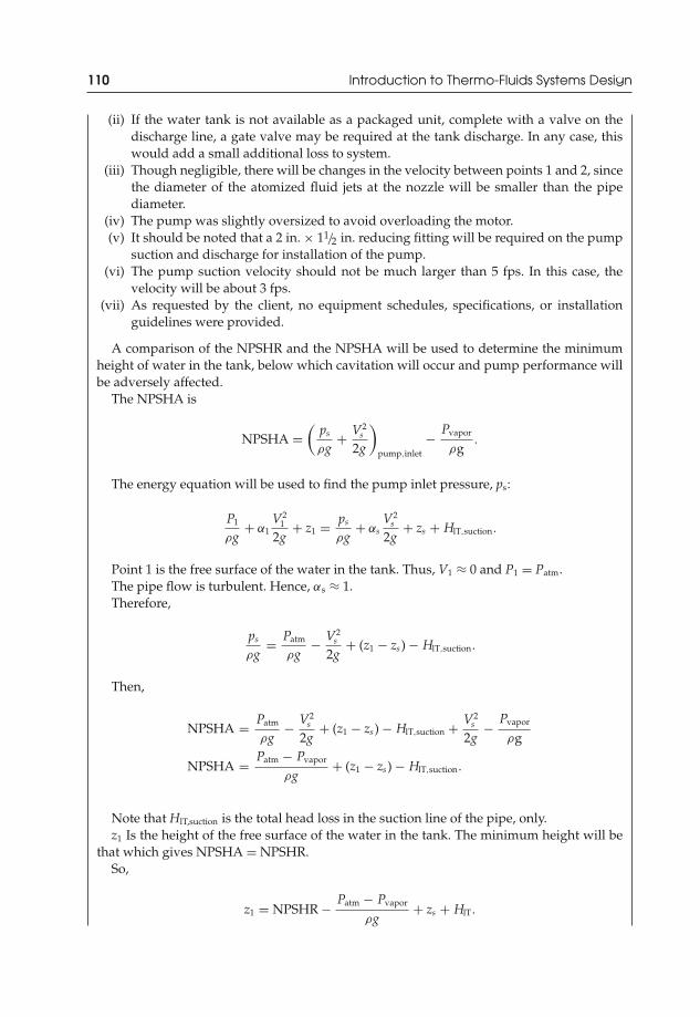
JWST229-c03 JWST229-McDonald Printer: Yet to Come July 28, 2012 13:48 Trim: 244mm × 168mm
110 Introduction to Thermo-Fluids Systems Design
(ii) If the water tank is not available as a packaged unit, complete with a valve on thedischarge line, a gate valve may be required at the tank discharge. In any case, thiswould add a small additional loss to system.
(iii) Though negligible, there will be changes in the velocity between points 1 and 2, sincethe diameter of the atomized fluid jets at the nozzle will be smaller than the pipediameter.
(iv) The pump was slightly oversized to avoid overloading the motor.(v) It should be noted that a 2 in. × 11/2 in. reducing fitting will be required on the pump
suction and discharge for installation of the pump.(vi) The pump suction velocity should not be much larger than 5 fps. In this case, the
velocity will be about 3 fps.(vii) As requested by the client, no equipment schedules, specifications, or installation
guidelines were provided.
A comparison of the NPSHR and the NPSHA will be used to determine the minimumheight of water in the tank, below which cavitation will occur and pump performance willbe adversely affected.
The NPSHA is
NPSHA =(
ps
ρg+ V2
s
2g
)pump,inlet
− Pvapor
ρg.
The energy equation will be used to find the pump inlet pressure, ps:
P1
ρg+ α1
V21
2g+ z1 = ps
ρg+ αs
V2s
2g+ zs + HlT,suction.
Point 1 is the free surface of the water in the tank. Thus, V1 ≈ 0 and P1 = Patm.The pipe flow is turbulent. Hence, αs ≈ 1.Therefore,
ps
ρg= Patm
ρg− V2
s
2g+ (z1 − zs) − HlT,suction.
Then,
NPSHA = Patm
ρg− V2
s
2g+ (z1 − zs) − HlT,suction + V2
s
2g− Pvapor
ρg
NPSHA = Patm − Pvapor
ρg+ (z1 − zs) − HlT,suction.
Note that HlT,suction is the total head loss in the suction line of the pipe, only.z1 Is the height of the free surface of the water in the tank. The minimum height will be
that which gives NPSHA = NPSHR.So,
z1 = NPSHR − Patm − Pvapor
ρg+ zs + HlT.

JWST229-c03 JWST229-McDonald Printer: Yet to Come July 28, 2012 13:48 Trim: 244mm × 168mm
Liquid Piping Systems 111
From the performance plot of the 11/2 × 11/2 × 7 in. casing pump, and at 30 gpm, theNPSHR is approximately 3 ft. At 70◦F, Pvapor = 0.363 psia. Patm = 14.7 psia. Based on thepump casing size, assume that the centerline of the pump is 1 ft above grade. Therefore,zs = 1 ft.
The head loss in the suction line of the pipe is
HlT = Hl,suction +∑
KLV2
2g.
The total length of suction piping is approximately 1050 ft.Hence,
HlT = 3.0 ft wg100 ft
× 1050 ft + [0.5 + 1.5 + 0.16](3.0 ft/s)2
2(
32.2 ft/s2)
HlT = 32 ft
and
z1 = 3 ft − (14.7 − 0.363) lbf/in.2(
62.3 lb/ft3) (
32.2 ft/s2) × 32.2 lb/ft/s2
1 lbf×
(12 in.
1 ft
)2
+ 1 ft + 32 ft
z1 ≈ 2.86 ft = 2 ft 10 in.
According to this calculation, cavitation will only occur if the free surface of the fluid isless than 2 ft 10 in. above grade. Therefore, the designer may choose any appropriate heightabove 2 ft 10 in. to mount the low-level switch. If this is not possible, and the low-levelswitch must be installed close to the base of the tank, the client may consider mounting thetank on a support that is at least 2 ft 10 in. high. This will generate the same static pressurehead required to avoid cavitation. If mounting the tank is not an option, the client is advisedto consider another tank with height greater than 50 in.
3.5.2 Closed-Loop Piping System
In a closed-loop piping system, there are no points open to the ambient. Figure 3.13shows schematic drawings of two-pipe and four-pipe closed-loop piping systems.
Note the following regarding typical closed-loop piping systems:
(a) Filters are optional for this system. They may be included in the design if it isdeemed necessary to protect equipment.
(b) An expansion tank is required for closed-loop piping systems. There should beonly one expansion tank in each loop of a piping system.Expansion tanks:
(i) Protect the system from damage due to volume changes induced by temper-ature variations.
(ii) Create a point of constant pressure in the system.

JWST229-c03 JWST229-McDonald Printer: Yet to Come July 28, 2012 13:48 Trim: 244mm × 168mm
112 Introduction to Thermo-Fluids Systems Design
Figure 3.13 Diagrams of closed-loop piping systems
(iii) Provide a collecting space for entrapped air. Entrapped air is undesirable inthe water systems since it makes the flow noisy and produces unwanted pipevibrations—water hammer.
(c) Air separators for air elimination from the closed-loop piping system are required.Air will enter the closed-loop piping system when makeup water from external

JWST229-c03 JWST229-McDonald Printer: Yet to Come July 28, 2012 13:48 Trim: 244mm × 168mm
Liquid Piping Systems 113
sources is introduced. Devices such as a vortex air separator create a high-speedfluid vortex in its center. This low-pressure region enhances the release of airbubbles from the liquid, which is released through an automatic vent or otherdevice.
(d) Pressure regulators, isolation, control, and/or three-way valves, flow meters, andthermocouples may also be required.
Practical Note 3.12 Flanged or Screwed Pipe Fittings?
Flanged pipe is generally specified for aboveground service for air, water, sewage, oil, andother fluids where rigid, restrained joints are needed. It may be used for larger, heavierpipes and fluids. It is also widely used in industrial piping systems, water treatment plants,sewage treatment plants, and for other interior piping. American Water Works Association(AWWA) standards restrict the use of flanged joints underground due to the rigidity of thejoints.
Example 3.7 Designing a Closed-Loop Piping System
A consulting engineering firm received the following sketch of a water piping system fromthe Ministry of Defense in Ottawa.
Source: Modified from McQuiston et al. [4]
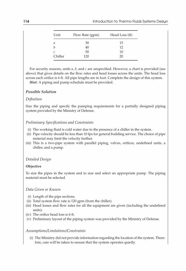
JWST229-c03 JWST229-McDonald Printer: Yet to Come July 28, 2012 13:48 Trim: 244mm × 168mm
114 Introduction to Thermo-Fluids Systems Design
Unit Flow Rate (gpm) Head Loss (ft)
a 30 15b 40 12c 50 10Chiller 120 20
For security reasons, units a, b, and c are unspecified. However, a chart is provided (seeabove) that gives details on the flow rates and head losses across the units. The head lossacross each orifice is 6 ft. All pipe lengths are in foot. Complete the design of this system.
Hint: A piping and pump schedule must be provided.
Possible Solution
Definition
Size the piping and specify the pumping requirements for a partially designed pipingsystem provided by the Ministry of Defense.
Preliminary Specifications and Constraints
(i) The working fluid is cold water due to the presence of a chiller in the system.(ii) Pipe velocity should be less than 10 fps for general building service. The choice of pipe
material may limit the velocity further.(iii) This is a two-pipe system with parallel piping, valves, orifices, undefined units, a
chiller, and a pump.
Detailed Design
Objective
To size the pipes in the system and to size and select an appropriate pump. The pipingmaterial must be selected.
Data Given or Known
(i) Length of the pipe sections.(ii) Total system flow rate is 120 gpm (from the chiller).
(iii) Head losses and flow rates for all the equipment are given (including the undefinedunits).
(iv) The orifice head loss is 6 ft.(v) Preliminary layout of the piping system was provided by the Ministry of Defense.
Assumptions/Limitations/Constraints
(i) The Ministry did not provide information regarding the location of the system. There-fore, care will be taken to ensure that the system operates quietly.
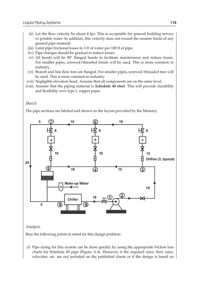
JWST229-c03 JWST229-McDonald Printer: Yet to Come July 28, 2012 13:48 Trim: 244mm × 168mm
Liquid Piping Systems 115
(ii) Let the flow velocity be about 4 fps. This is acceptable for general building serviceor potable water. In addition, this velocity does not exceed the erosion limits of anygeneral pipe material.
(iii) Limit pipe frictional losses to 3 ft of water per 100 ft of pipe.(iv) Pipe changes should be gradual to reduce losses.(v) All bends will be 90o flanged bends to facilitate maintenance and reduce losses.
For smaller pipes, screwed/threaded bends will be used. This is more common inindustry.
(vi) Branch and line flow tees are flanged. For smaller pipes, screwed/threaded tees willbe used. This is more common in industry.
(vii) Negligible elevation head. Assume that all components are on the same level.(viii) Assume that the piping material is Schedule 40 steel. This will provide durability
and flexibility over type L copper pipes.
Sketch
The pipe sections are labeled and shown on the layout provided by the Ministry.
Analysis
Bear the following points in mind for this design problem:
(i) Pipe sizing for this system can be done quickly by using the appropriate friction losscharts for Schedule 40 pipe (Figure A.4). However, if the required sizes, flow rates,velocities, etc. are not included on the published charts or if the design is based on
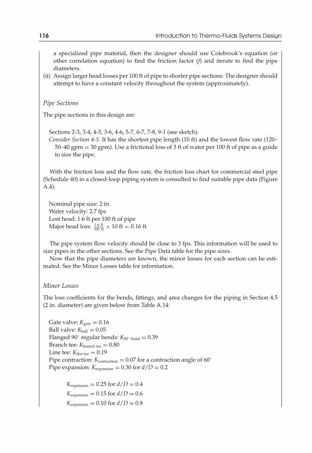
JWST229-c03 JWST229-McDonald Printer: Yet to Come July 28, 2012 13:48 Trim: 244mm × 168mm
116 Introduction to Thermo-Fluids Systems Design
a specialized pipe material, then the designer should use Colebrook’s equation (orother correlation equation) to find the friction factor (f) and iterate to find the pipediameters.
(ii) Assign larger head losses per 100 ft of pipe to shorter pipe sections. The designer shouldattempt to have a constant velocity throughout the system (approximately).
Pipe Sections
The pipe sections in this design are:
Sections 2-3, 3-4, 4-5, 3-6, 4-6, 5-7, 6-7, 7-8, 9-1 (see sketch).Consider Section 4-5. It has the shortest pipe length (10 ft) and the lowest flow rate (120–
50–40 gpm = 30 gpm). Use a frictional loss of 3 ft of water per 100 ft of pipe as a guideto size the pipe.
With the friction loss and the flow rate, the friction loss chart for commercial steel pipe(Schedule 40) in a closed-loop piping system is consulted to find suitable pipe data (FigureA.4):
Nominal pipe size: 2 in.Water velocity: 2.7 fpsLost head: 1.6 ft per 100 ft of pipeMajor head loss: 1.6 ft
100 ft × 10 ft = 0.16 ft
The pipe system flow velocity should be close to 3 fps. This information will be used tosize pipes in the other sections. See the Pipe Data table for the pipe sizes.
Now that the pipe diameters are known, the minor losses for each section can be esti-mated. See the Minor Losses table for information.
Minor Losses
The loss coefficients for the bends, fittings, and area changes for the piping in Section 4.5(2 in. diameter) are given below from Table A.14:
Gate valve: Kgate = 0.16Ball valve: Kball = 0.05Flanged 90◦ regular bends: K90◦ bend = 0.39Branch tee: Kbranch tee = 0.80Line tee: Kline tee = 0.19Pipe contraction: Kcontraction = 0.07 for a contraction angle of 60◦
Pipe expansion: Kexpansion = 0.30 for d/D = 0.2
Kexpansion = 0.25 for d/D = 0.4
Kexpansion = 0.15 for d/D = 0.6
Kexpansion = 0.10 for d/D = 0.8

JWST229-c03 JWST229-McDonald Printer: Yet to Come July 28, 2012 13:48 Trim: 244mm × 168mm
Liquid Piping Systems 117
Minor Loss:
1 flanged 90◦ bend: K90◦ bend = 0.391 line tee: Kline tee = 0.191 pipe contraction from a 3 in. diameter in Section 3–4 to a 2 in. diameter in Section 4-5:
Kcontraction = 0.07
Therefore,
Hlm =∑
KLV2
ave
2g= (0.39 + 0.19 + 0.07)
⎡⎣ (2.8 ft/s)2
2(
32.2 ft/s2)
⎤⎦ = 0.079 ft.
The total head loss in the Section 4-5 is
HlT = Hl + Hlm = 0.16 ft + 0.079 ft = 0.24 ft.
A similar procedure is followed for the other pipe sections. The results are shown in thetables below.
Minor Losses
PipeSectionNo.
GateValves
BallValves
90◦
RegularBends
Tees-Branch Tees-Line
GradualExpansion(KL = vary)
GradualContrac-tion (KL =0.07)
TotalMinorLoss(ft)
2-3 0.05 (one) 0.3 (three) 0.64 (one) 0.323-4 0.19 (one) 0.07 (one) 0.044-5 0.39 (one) 0.19 (one) 0.07 (one) 0.083-6 0.35 (one) 0.05 (one) 0.39 (one) 0.80 (one) KL = 0.10 0.274-6 0.35 (one) 0.05 (one) 0.80 (two) 0.235-7 0.35 (one) 0.05 (one) 0.80 (one) 0.156-7 0.19 (one) KL = 0.10 0.077-8 0.30 (two) 0.14 (two) 0.189-1 0.30 (one) 0.30 (one) 0.12
Pipe Data
PipeSectionNo.
PipeLength
(ft)
FlowRate
(gpm)Lost Head(ft/100 ft)
FluidVelocity
(ft/s)NominalSize (in.)
MinorLosses
(ft)
TotalHead
Loss (ft)2-3 15 120 1.4 3.6 31/2 0.32 0.533-4 10 70 1.3 3 3 0.04 0.174-5 10 30 1.6 2.8 2 0.08 0.243-6 28 50 1.8 3.2 21/2 0.27 0.774-6 18 40 1.3 2.7 21/2 0.23 0.465-7 18 30 1.6 2.8 2 0.15 0.446-7 10 90 1.9 3.8 3 0.07 0.267-8 35 120 1.4 3.6 31/2 0.18 0.679-1 18 120 1.4 3.6 31/2 0.12 0.37
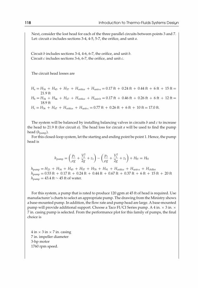
JWST229-c03 JWST229-McDonald Printer: Yet to Come July 28, 2012 13:48 Trim: 244mm × 168mm
118 Introduction to Thermo-Fluids Systems Design
Next, consider the lost head for each of the three parallel circuits between points 3 and 7.Let: circuit a includes sections 3-4, 4-5, 5-7, the orifice, and unit a.
Circuit b includes sections 3-4, 4-6, 6-7, the orifice, and unit b.Circuit c includes sections 3-6, 6-7, the orifice, and unit c.
The circuit head losses are
Ha = H34 + H45 + H57 + Horifice + Hunit-a = 0.17 ft + 0.24 ft + 0.44 ft + 6 ft + 15 ft =21.9 ft
Hb = H34 + H46 + H67 + Horifice + Hunit-b = 0.17 ft + 0.46 ft + 0.26 ft + 6 ft + 12 ft =18.9 ft
Hc = H36 + H67 + Horifice + Hunit-c = 0.77 ft + 0.26 ft + 6 ft + 10 ft = 17.0 ft.
The system will be balanced by installing balancing valves in circuits b and c to increasethe head to 21.9 ft (for circuit a). The head loss for circuit a will be used to find the pumphead (hpump).
For this closed-loop system, let the starting and ending point be point 1. Hence, the pumphead is
hpump =(
p1
ρg+ V2
1
2g+ z1
)−
(p1
ρg+ V2
1
2g+ z1
)+ HlT = HlT
hpump = H23 + H34 + H45 + H57 + H78 + H91 + Horifice + Hunit-a + Hchiller
hpump = 0.53 ft + 0.17 ft + 0.24 ft + 0.44 ft + 0.67 ft + 0.37 ft + 6 ft + 15 ft + 20 fthpump = 43.4 ft ∼ 45 ft of water.
For this system, a pump that is rated to produce 120 gpm at 45 ft of head is required. Usemanufacturer’s charts to select an appropriate pump. The drawing from the Ministry showsa base-mounted pump. In addition, the flow rate and pump head are large. A base-mountedpump will provide additional support. Choose a Taco FI/CI Series pump. A 4 in. × 3 in. ×7 in. casing pump is selected. From the performance plot for this family of pumps, the finalchoice is
4 in × 3 in × 7 in. casing7 in. impeller diameter3-hp motor1760 rpm speed.

JWST229-c03 JWST229-McDonald Printer: Yet to Come July 28, 2012 13:48 Trim: 244mm × 168mm
Liquid Piping Systems 119
The pump performance curve is shown below.
Source: Taco, Inc. (reprinted with permission)
Drawings
The drawing below shows the pipe sizes required.

JWST229-c03 JWST229-McDonald Printer: Yet to Come July 28, 2012 13:48 Trim: 244mm × 168mm
120 Introduction to Thermo-Fluids Systems Design
Conclusions
The piping system has been designed. All the pipe sizes are known, and the piping materialhas been selected. A pump has been specified and selected. It should be noted that for thepipe sizes in this design, threaded fittings could have been used. In that case, the losseswould have increased. It should also be noted that 4 × 31/2 in. and 31/2 × 3 in. reducingfittings will be required on the pump suction and discharge, respectively, for installation ofthe pump.
The Pipe Data and Pump Schedule are shown below.
Pipe Data
PipeSectionNo.
PipeLength
(ft)
FlowRate
(gpm)
LostHead
(ft/100ft)
FluidVelocity
(ft/s)NominalSize (in.)
MinorLosses
(ft)
TotalHead
Loss (ft)
2-3 15 120 1.4 3.6 31/2 0.32 0.533-4 10 70 1.3 3 3 0.04 0.174-5 10 30 1.6 2.8 2 0.08 0.243-6 28 50 1.8 3.2 21/2 0.27 0.774-6 18 40 1.3 2.7 21/2 0.23 0.465-7 18 30 1.6 2.8 2 0.15 0.446-7 10 90 1.9 3.8 3 0.07 0.267-8 35 120 1.4 3.6 31/2 0.18 0.679-1 18 120 1.4 3.6 31/2 0.12 0.37
Pump Schedule
Fluid Electrical
Tag
Manufacturerand ModelNumber Type Construction
FlowRate(gpm)
WorkingFluid
HeadLoss(ft)
MotorSize(hp)
MotorSpeed(rpm)
V/Ph/Hz
P-1 Taco, FI/CISeries, Model3007, or equal
Centrifugal,base-mounted
Cast iron4 × 3 × 7 in.Casing, 7 in.φ
120 Water 45 3 1760 208/3/60
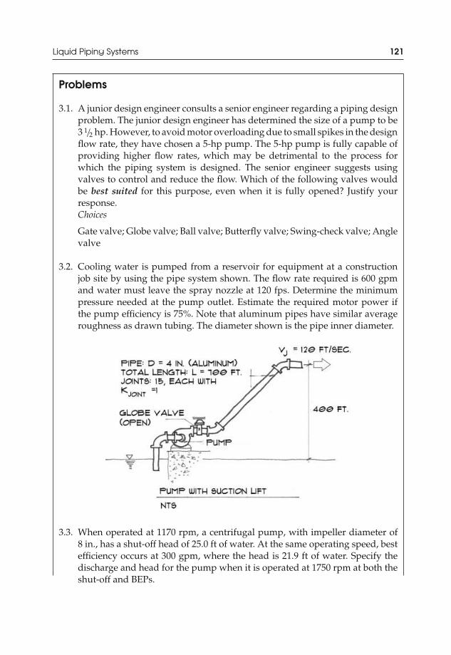
JWST229-c03 JWST229-McDonald Printer: Yet to Come July 28, 2012 13:48 Trim: 244mm × 168mm
Liquid Piping Systems 121
Problems
3.1. A junior design engineer consults a senior engineer regarding a piping designproblem. The junior design engineer has determined the size of a pump to be3 1/2 hp. However, to avoid motor overloading due to small spikes in the designflow rate, they have chosen a 5-hp pump. The 5-hp pump is fully capable ofproviding higher flow rates, which may be detrimental to the process forwhich the piping system is designed. The senior engineer suggests usingvalves to control and reduce the flow. Which of the following valves wouldbe best suited for this purpose, even when it is fully opened? Justify yourresponse.Choices
Gate valve; Globe valve; Ball valve; Butterfly valve; Swing-check valve; Anglevalve
3.2. Cooling water is pumped from a reservoir for equipment at a constructionjob site by using the pipe system shown. The flow rate required is 600 gpmand water must leave the spray nozzle at 120 fps. Determine the minimumpressure needed at the pump outlet. Estimate the required motor power ifthe pump efficiency is 75%. Note that aluminum pipes have similar averageroughness as drawn tubing. The diameter shown is the pipe inner diameter.
3.3. When operated at 1170 rpm, a centrifugal pump, with impeller diameter of8 in., has a shut-off head of 25.0 ft of water. At the same operating speed, bestefficiency occurs at 300 gpm, where the head is 21.9 ft of water. Specify thedischarge and head for the pump when it is operated at 1750 rpm at both theshut-off and BEPs.
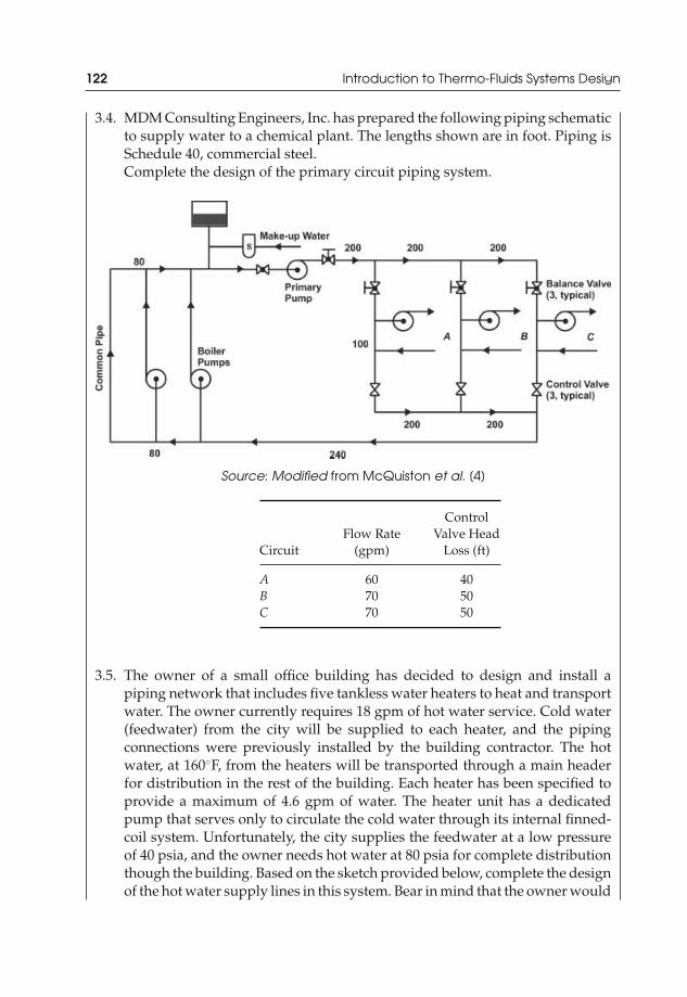
JWST229-c03 JWST229-McDonald Printer: Yet to Come July 28, 2012 13:48 Trim: 244mm × 168mm
122 Introduction to Thermo-Fluids Systems Design
3.4. MDM Consulting Engineers, Inc. has prepared the following piping schematicto supply water to a chemical plant. The lengths shown are in foot. Piping isSchedule 40, commercial steel.Complete the design of the primary circuit piping system.
Source: Modified from McQuiston et al. [4]
CircuitFlow Rate
(gpm)
ControlValve Head
Loss (ft)
A 60 40B 70 50C 70 50
3.5. The owner of a small office building has decided to design and install apiping network that includes five tankless water heaters to heat and transportwater. The owner currently requires 18 gpm of hot water service. Cold water(feedwater) from the city will be supplied to each heater, and the pipingconnections were previously installed by the building contractor. The hotwater, at 160◦F, from the heaters will be transported through a main headerfor distribution in the rest of the building. Each heater has been specified toprovide a maximum of 4.6 gpm of water. The heater unit has a dedicatedpump that serves only to circulate the cold water through its internal finned-coil system. Unfortunately, the city supplies the feedwater at a low pressureof 40 psia, and the owner needs hot water at 80 psia for complete distributionthough the building. Based on the sketch provided below, complete the designof the hot water supply lines in this system. Bear in mind that the owner would

JWST229-c03 JWST229-McDonald Printer: Yet to Come July 28, 2012 13:48 Trim: 244mm × 168mm
Liquid Piping Systems 123
like to maintain flexibility to expand the system in the future to its maximumcapabilities.Further Information: In practice, the lengths of the hot water supply piping thatconnect directly to the heaters are small in comparison to that of the mainsupply header.
3.6. A heating coil is a heat exchanger that can be used to transfer energy from hot 50%ethylene glycol solution to air for the purposes of space heating. A proposalhas been submitted that will focus on the development of a heating coil thatcontains one row with six loops of coils. Each loop will be 24 in. long and theywill be connected to each other by way of 180◦ smooth return bends. The 50%ethylene glycol solution will be supplied at 200◦F and 5 gpm to the heating coilcomponent. A dedicated pump will be required for this component. Designthe piping system in the heating coil and specify any major accessories thatwill be required.
3.7. A plant manager has hired a recent graduate of a mechanical engineeringprogram to consider the design of a piping system to supply kerosene to threeburners that will be located outdoors. Burner “A” will require 10 gpm of fuel,burner “B,” 20 gpm, and burner “C,” 25 gpm. For convenience, the managerwill purchase a vented outdoor fuel oil storage tank to supply enough kerosenefor 8 hours of operation. They wish to install the discharge pipe connection atthe base of the tank to take advantage of the fuel static pressure head and tofacilitate pipe installation. It is understood that codes will need to be verified.The fuel oil storage tank and piping should be supplied with sufficient heattracing to maintain the kerosene temperature at about 68◦F. Given that thefuel will be atomized and combusted completely in the burner, there will beno need for return piping from the burners to the storage tank. Design theburner kerosene supply piping system that will meet the requirements of themanager.
Further Information: Consultation with NFPA 31 may provide guidance tojustify some design decisions.

JWST229-c03 JWST229-McDonald Printer: Yet to Come July 28, 2012 13:48 Trim: 244mm × 168mm
124 Introduction to Thermo-Fluids Systems Design
3.8. A pipe-pump assembly is being considered by a farmer for use in irrigating afield during summer. There is an underground water well that is 250 ft deep.The well is an open-hole type in which the free surface of water is about 8 ftbelow grade. To ensure that one of the pumps will operate for only a few hoursper day, the farmer will fill a 2500-gallon tank in 4 hours, which will provideenough water for 2 days of farm operation. The tank cannot be more than10 ft long and should come complete with valved piping connections whoselocations will be specified by the farmer. The tank can be located anywherein the line that the farmer deems fit. Due to location of the field and well, apump must be located no more than 600 ft from the well. The pipe will beconnected to an existing irrigation system that is 750 ft from the well andis 10 ft long. The farmer’s land is flat, from the well to the field. Design themain piping system to meet the water requirements of the farmer. Specify themaximum depth of the pipe inlet in the well for the purposes of installation bythe farmer.
Further Information: The design engineer may consider the use of a footvalve (a type of check valve), complete with a strainer at the inlet to thepiping system. This will ensure that the pumps are properly primed,that is, completely filled with water before the start of pumping. Otheralternatives are available.
3.9. An engineer has presented a piping system layout that includes a pump,condenser, and cooling tower for a building cooling application. Size thepiping and specify the pump required if the total volume flow rate of water is450 gpm, the pressure drop in the condenser is 15 ft of water gage, the verticaldistance from the pump centerline to the top of the cooling tower is 45 ft, thehorizontal distance from the condenser to the tower is 70 ft, and the pumpis 15 ft below the tower basin. All the necessary accessories are shown in thesketch provided by the engineer.

JWST229-c03 JWST229-McDonald Printer: Yet to Come July 28, 2012 13:48 Trim: 244mm × 168mm
Liquid Piping Systems 125
3.10. Independent Living Developments Inc. has recently awarded a project for thefirst phase of the detailed design of a system to deliver potable water froma bore-well to a 2-floor, 12-apartment residence to a mechanical engineeringconsulting firm. In this first phase of the project, the client has requested thatthe design be restricted to include elements associated with the extractionof water from a bore-well in sufficient quantity to meet the needs of theirproposed residential complex and to deliver it at a pressure of 100 psia at theinlet to each floor riser. This phase of the project is not to include any aspectsof the design of the bore-well or the layout of the internal plumbing systems ofthe building. Detailed drawings of items such as connections and penetrationsare not required at this time. The proposed construction site is a rectangularplot of land with an area of 1/2-acre that has road access on one side and landon the other three sides. The footprint of the 12-apartment complex is plannedto be 60 ft × 120 ft. Any existing building structures on the plot of land havebeen slated for demolition. The complex will be located in an area where theaverage outdoor temperature in winter is −4◦F, and in the summer, 80◦F. Theapartment complex will have a basement, which will serve as a storage areaand mechanical room and will have a foundation that is 6 ft below grade anda clear height of 8 ft to meet the requirements of the International BuildingCode. The first floor has eight 2-bedroom apartments (floor area 800–1000 ft2
each and height 10 ft) and the second floor has four 3-bedroom apartments(floor area 1000–1200 ft2 each and height 10 ft). There is an existing bore-welllocated 50 ft from the proposed building. Standard draw down and recoverytests that were conducted at the well depth of 100 ft showed that the well couldsupport continuous extraction of water at 10 gpm. Through consultation withthe local utility company, it was found that each person uses approximately60 gallons of water per day. In order to guarantee the availability of sufficientamounts of water, the client has requested the use of a water storage tank.With reference and adherence to the International Building Code and theInternational Plumbing Code (or Uniform Plumbing Code), design the pipingsystem required to deliver water from the well to the floors of the complex (upto and including the floor risers). The designer should ensure that necessarycomponents such as pumps, pipes, valves, piping accessories, the tank and itssize, to name a few, are clearly specified.
Further Information: The design engineer may consider the use of a footvalve (a type of check valve), complete with a strainer at the inlet to thepiping system. This will ensure that the pumps are properly primed,that is, completely filled with water before the start of pumping. Otheralternatives may include a submersible pump complete with a footvalve.
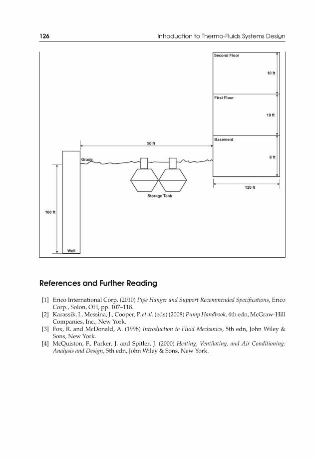
JWST229-c03 JWST229-McDonald Printer: Yet to Come July 28, 2012 13:48 Trim: 244mm × 168mm
126 Introduction to Thermo-Fluids Systems Design
References and Further Reading
[1] Erico International Corp. (2010) Pipe Hanger and Support Recommended Specifications, EricoCorp., Solon, OH, pp. 107–118.
[2] Karassik, I., Messina, J., Cooper, P. et al. (eds) (2008) Pump Handbook, 4th edn, McGraw-HillCompanies, Inc., New York.
[3] Fox, R. and McDonald, A. (1998) Introduction to Fluid Mechanics, 5th edn, John Wiley &Sons, New York.
[4] McQuiston, F., Parker, J. and Spitler, J. (2000) Heating, Ventilating, and Air Conditioning:Analysis and Design, 5th edn, John Wiley & Sons, New York.

JWST229-c04 JWST229-McDonald Printer: Yet to Come July 31, 2012 12:14 Trim: 244mm × 168mm
4Fundamentals of HeatExchanger Design
4.1 Definition and Requirements
Heat exchangers are devices that facilitate energy transfer between two fluids atdifferent temperatures while keeping them from mixing with each other. Fundamentalknowledge of heat conduction and heat convection are required for heat exchangerdesign and/or selection. Examples of heat exchangers include (i) car radiator; (ii)hydronic baseboard heaters; (iii) condensers; (iv) superheaters; (v) boilers; and (vi)regenerators/recurperators.
4.2 Types of Heat Exchangers
4.2.1 Double-Pipe Heat Exchangers
In this type of heat exchanger, one fluid flows through a pipe and the other fluidflows through an annular space that encloses the pipe. There are two types of flowsin double-pipe heat exchangers: parallel flow and counter flow. Figure 4.1 showsschematics of double-pipe heat exchangers:
Parallel flow: Both fluids enter and exit at the same point (ie. fluids flow in the samedirection). For very long systems, the temperatures of the two fluids will eventuallybecome equal at the exit.Counter flow: The fluids enter and leave at opposite ends (ie. fluids flow in oppositedirections). The flows are in opposite directions. A larger temperature difference existsover the length of this heat exchanger compared to the parallel flow heat exchanger.
Introduction to Thermo-Fluids Systems Design, First Edition. Andre G. McDonald and Hugh L. Magande.C© 2012 Andre G. McDonald and Hugh L. Magande. Published 2012 by John Wiley & Sons, Ltd.
127

JWST229-c04 JWST229-McDonald Printer: Yet to Come July 31, 2012 12:14 Trim: 244mm × 168mm
(a)
(b)
Fig
ure
4.1
Tem
pe
ratu
rep
rofil
es
an
dsc
he
ma
tics
of
(a)
pa
ralle
lan
d(b
)c
ou
nte
rflo
wd
ou
ble
-pip
eh
ea
te
xch
an
ge
rs
128
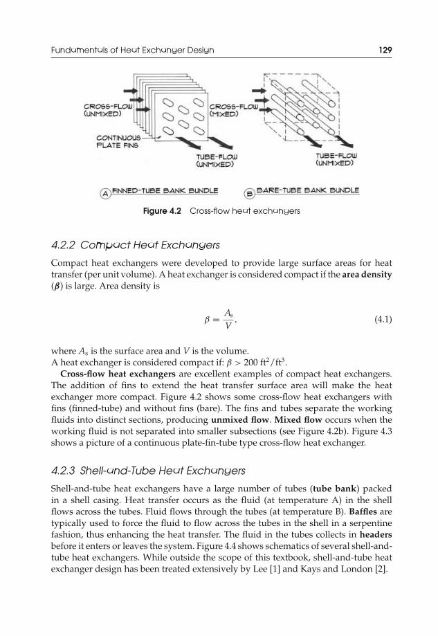
JWST229-c04 JWST229-McDonald Printer: Yet to Come July 31, 2012 12:14 Trim: 244mm × 168mm
Fundamentals of Heat Exchanger Design 129
Figure 4.2 Cross-flow heat exchangers
4.2.2 Compact Heat Exchangers
Compact heat exchangers were developed to provide large surface areas for heattransfer (per unit volume). A heat exchanger is considered compact if the area density(β) is large. Area density is
β = As
V, (4.1)
where As is the surface area and V is the volume.A heat exchanger is considered compact if: β > 200 ft2/ft3.
Cross-flow heat exchangers are excellent examples of compact heat exchangers.The addition of fins to extend the heat transfer surface area will make the heatexchanger more compact. Figure 4.2 shows some cross-flow heat exchangers withfins (finned-tube) and without fins (bare). The fins and tubes separate the workingfluids into distinct sections, producing unmixed flow. Mixed flow occurs when theworking fluid is not separated into smaller subsections (see Figure 4.2b). Figure 4.3shows a picture of a continuous plate-fin-tube type cross-flow heat exchanger.
4.2.3 Shell-and-Tube Heat Exchangers
Shell-and-tube heat exchangers have a large number of tubes (tube bank) packedin a shell casing. Heat transfer occurs as the fluid (at temperature A) in the shellflows across the tubes. Fluid flows through the tubes (at temperature B). Baffles aretypically used to force the fluid to flow across the tubes in the shell in a serpentinefashion, thus enhancing the heat transfer. The fluid in the tubes collects in headersbefore it enters or leaves the system. Figure 4.4 shows schematics of several shell-and-tube heat exchangers. While outside the scope of this textbook, shell-and-tube heatexchanger design has been treated extensively by Lee [1] and Kays and London [2].

JWST229-c04 JWST229-McDonald Printer: Yet to Come July 31, 2012 12:14 Trim: 244mm × 168mm
130 Introduction to Thermo-Fluids Systems Design
Figure 4.3 Picture of a continuous plate-fin-tube type cross-flow heat exchanger
4.3 The Overall Heat Transfer Coefficient
The rate of heat transfer across the surfaces in a heat exchanger will be governed, inpart, by the thermal resistance to heat transfer across those surfaces. Determinationof the thermal resistance will require simplified heat conduction and heat convec-tion analyses.
In heat exchangers, heat transfer occurs primarily by conduction and convection.The schematic drawing below shows these modes of heat transfer through an idealplane wall:

JWST229-c04 JWST229-McDonald Printer: Yet to Come July 31, 2012 12:14 Trim: 244mm × 168mm
Fundamentals of Heat Exchanger Design 131
(a)
(b)
(c) (d)
Figure 4.4 Schematics of shell-and-tube heat exchangers
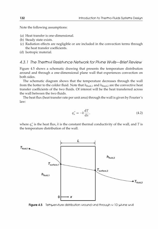
JWST229-c04 JWST229-McDonald Printer: Yet to Come July 31, 2012 12:14 Trim: 244mm × 168mm
132 Introduction to Thermo-Fluids Systems Design
Note the following assumptions:
(a) Heat transfer is one-dimensional.(b) Steady state exists.(c) Radiation effects are negligible or are included in the convection terms through
the heat transfer coefficients.(d) Isotropic material.
4.3.1 The Thermal Resistance Network for Plane Walls—Brief Review
Figure 4.5 shows a schematic drawing that presents the temperature distributionaround and through a one-dimensional plane wall that experiences convection onboth sides.
The schematic diagram shows that the temperature decreases through the wallfrom the hotter to the colder fluid. Note that hfluid,1 and hfluid,2 are the convective heattransfer coefficients of the two fluids. Of interest will be the heat transferred acrossthe wall between the two fluids.
The heat flux (heat transfer rate per unit area) through the wall is given by Fourier’slaw:
q ′′x = −k
dTdx
, (4.2)
where q ′′x is the heat flux, k is the constant thermal conductivity of the wall, and T is
the temperature distribution of the wall.
Figure 4.5 Temperature distribution around and through a 1D plane wall
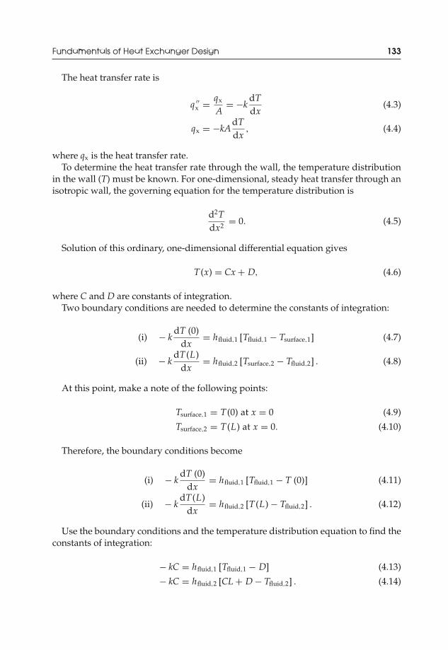
JWST229-c04 JWST229-McDonald Printer: Yet to Come July 31, 2012 12:14 Trim: 244mm × 168mm
Fundamentals of Heat Exchanger Design 133
The heat transfer rate is
q ′′x = qx
A= −k
dTdx
(4.3)
qx = −kAdTdx
, (4.4)
where qx is the heat transfer rate.To determine the heat transfer rate through the wall, the temperature distribution
in the wall (T) must be known. For one-dimensional, steady heat transfer through anisotropic wall, the governing equation for the temperature distribution is
d2Tdx2 = 0. (4.5)
Solution of this ordinary, one-dimensional differential equation gives
T(x) = Cx + D, (4.6)
where C and D are constants of integration.Two boundary conditions are needed to determine the constants of integration:
(i) − kdT (0)
dx= hfluid,1 [Tfluid,1 − Tsurface,1] (4.7)
(ii) − kdT(L)
dx= hfluid,2 [Tsurface,2 − Tfluid,2] . (4.8)
At this point, make a note of the following points:
Tsurface,1 = T(0) at x = 0 (4.9)
Tsurface,2 = T(L) at x = 0. (4.10)
Therefore, the boundary conditions become
(i) − kdT (0)
dx= hfluid,1 [Tfluid,1 − T (0)] (4.11)
(ii) − kdT(L)
dx= hfluid,2 [T(L) − Tfluid,2] . (4.12)
Use the boundary conditions and the temperature distribution equation to find theconstants of integration:
− kC = hfluid,1 [Tfluid,1 − D] (4.13)
− kC = hfluid,2 [CL + D − Tfluid,2] . (4.14)
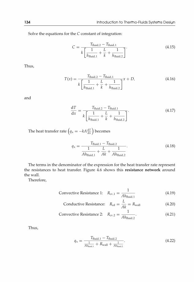
JWST229-c04 JWST229-McDonald Printer: Yet to Come July 31, 2012 12:14 Trim: 244mm × 168mm
134 Introduction to Thermo-Fluids Systems Design
Solve the equations for the C constant of integration:
C = Tfluid,2 − Tfluid,1
k[
1hfluid,1
+ Lk
+ 1hfluid,2
] . (4.15)
Thus,
T(x) = Tfluid,2 − Tfluid,1
k[
1hfluid,1
+ Lk
+ 1hfluid,2
] x + D, (4.16)
and
dTdx
= Tfluid,2 − Tfluid,1
k[
1hfluid,1
+ Lk
+ 1hfluid,2
] . (4.17)
The heat transfer rate(
qx = −kA dTdx
)becomes
qx = Tfluid,1 − Tfluid,2
1Ahfluid,1
+ LAk
+ 1Ahfluid,2
. (4.18)
The terms in the denominator of the expression for the heat transfer rate representthe resistances to heat transfer. Figure 4.6 shows this resistance network aroundthe wall.
Therefore,
Convective Resistance 1: Rcv,1 = 1Ahfluid,1
(4.19)
Conductive Resistance: Rcd = LAk
= Rwall (4.20)
Convective Resistance 2: Rcv,2 = 1Ahfluid,2
. (4.21)
Thus,
qx = Tfluid,1 − Tfluid,21
Ahfluid,1+ Rwall + 1
Ahfluid,2
. (4.22)
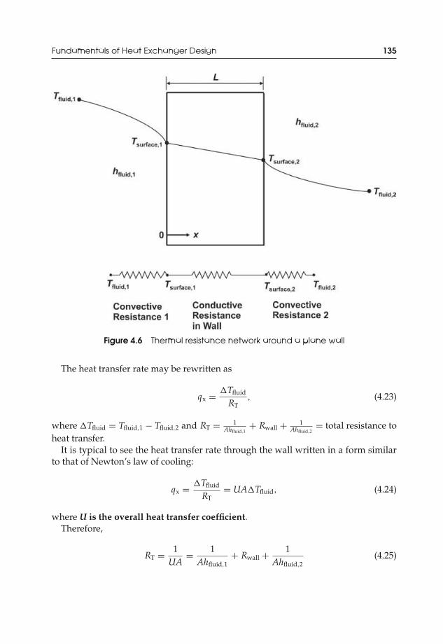
JWST229-c04 JWST229-McDonald Printer: Yet to Come July 31, 2012 12:14 Trim: 244mm × 168mm
Fundamentals of Heat Exchanger Design 135
Figure 4.6 Thermal resistance network around a plane wall
The heat transfer rate may be rewritten as
qx = �Tfluid
RT, (4.23)
where �Tfluid = Tfluid,1 − Tfluid,2 and RT = 1Ahfluid,1
+ Rwall + 1Ahfluid,2
= total resistance toheat transfer.
It is typical to see the heat transfer rate through the wall written in a form similarto that of Newton’s law of cooling:
qx = �Tfluid
RT= UA�Tfluid, (4.24)
where U is the overall heat transfer coefficient.Therefore,
RT = 1UA
= 1Ahfluid,1
+ Rwall + 1Ahfluid,2
(4.25)

JWST229-c04 JWST229-McDonald Printer: Yet to Come July 31, 2012 12:14 Trim: 244mm × 168mm
136 Introduction to Thermo-Fluids Systems Design
and
1U
= 1hfluid,1
+ Rwall A+ 1hfluid,2
. (4.26)
It should be noted at this point that the area, A is the surface area of the wall. Itshould also be noted that the expression for the wall resistance (Rwall) will be differentfor plane walls and cylindrical walls (pipes, tubes):
For plane walls: Rwall = LAk
. (4.27)
For cylindrical walls: Rwall = 12πkL
ln(
ro
ri
). (4.28)
For cylindrical walls, ro is outer wall thickness, ri is the inner wall thickness, andA = 2πrL.
Later in this chapter, it will be shown that determination of the overall heat transfercoefficient is essential to the design of heat exchangers. Tables 4.1 and 4.2 provide somerepresentative values for some types of heat exchangers. Note that heat exchangersare defined based on the working fluids.
4.3.2 Thermal Resistance from Fouling—The Fouling Factor
An additional resistance may be encountered on heat exchanger tubes or plates thathave been in operation for prolonged periods of time. Materials or other contaminantsmay deposit on the surface, restricting heat transfer. This deposition of material
Table 4.1 Values of the overall heat transfer coefficient (US)
Type of Heat Exchanger U, Btu/(h ft2 ◦F)
Water-to-water 150–300Water-to-oil 18–60Water-to-gasoline or kerosene 55–180Feedwater heaters 180–1500Steam-to-light fuel oil 35–70Steam-to-heavy fuel oil 10–35Steam condenser 180–1060Freon condenser (water cooled) 55–180Ammonia condenser (water cooled) 140–250Alcohol condensers (water cooled) 45–125Gas-to-gas 2–7Water-to-air in finned tubes (water in tubes) 5–10 (air); 70–150 (water)Steam-to-air in finned tubes (steam in tubes) 5–50 (air); 70–705 (water)

JWST229-c04 JWST229-McDonald Printer: Yet to Come July 31, 2012 12:14 Trim: 244mm × 168mm
Fundamentals of Heat Exchanger Design 137
Table 4.2 Values of the overall heat transfer coefficient (SI)
Type of Heat Exchanger U (W/(m2 ◦C))
Water-to-water 850–1700Water-to-oil 100–350Water-to-gasoline or kerosene 300–1000Feedwater heaters 1000–8500Steam-to-light fuel oil 200–400Steam-to-heavy fuel oil 50–200Steam condenser 1000–6000Freon condenser (water cooled) 300–1000Ammonia condenser (water cooled) 800–1400Alcohol condensers (water cooled) 250–700Gas-to-gas 10–40Water-to-air in finned tubes (water in tubes) 30–60 (air); 400–850 (water)Steam-to-air in finned tubes (steam in tubes) 30–300 (air); 400–4000 (water)
Source: Cengel [3].
or contaminants on the heat exchanger surfaces is known as fouling. Fouling willdeteriorate the performance of the heat exchanger by adding an additional resistance.
Some sources of fouling include
(i) precipitation of salts from hard water;(ii) chemical reactions which form solid deposits;
(iii) biological species growing on surfaces;(iv) sedimentation of solid deposits;(v) corrosion, which forms low thermal conductivity metal oxides on the heat ex-
changer surfaces.
The design engineer must make allowances to account for fouling, where applica-ble. In this case, the designer must consider the fouling factor, Rf, or the additionalresistance due to fouling in the calculation of the overall heat transfer coefficient.
Therefore, with fouling, the overall heat transfer coefficient becomes
1U
= 1hfluid,1
+ Rf,1 + Rwall A+ Rf,2 + 1hfluid,2
, (4.29)
where Rf,1 is the fouling resistance on the side of the wall in contact with fluid 1 andRf,2 is the fouling resistance on the side of the wall in contact with fluid 2.
Table 4.3 provides some representative values of fouling factors for some workingfluids.

JWST229-c04 JWST229-McDonald Printer: Yet to Come July 31, 2012 12:14 Trim: 244mm × 168mm
138 Introduction to Thermo-Fluids Systems Design
Table 4.3 Representative fouling factors in heat exchangers
Fluid Rf (ft2 h ◦F)/Btu
Gas oil 0.00051Transformer oil 0.00102Lubrication oil 0.00102Heat transfer oil 0.00102Hydraulic oil 0.00102Fuel oil 0.0051Hydrogen 0.00999Engine exhaust 0.00999Steam (oil-free) 0.00051Steam with oil traces 0.0010Cooling fluid vapors with oil traces 0.00199Organic solvent vapors 0.0010Alcohol vapors 0.00057Refrigerants (vapor) 0.0023Compressed air 0.00199Natural gas 0.0010Distilled water, seawater, river water, boiler feedwater: below 122◦F 0.00057Distilled water, seawater, river water, boiler feedwater: above 122◦F 0.0011Refrigerants (liquid) 0.0011Cooling fluid 0.0010Organic heat transfer fluids 0.0010Salts 0.00051Liquefied petroleum gas (LPG), liquefied natural gas (LNG) 0.0010MEA and DEA (Amines) solutions 0.00199DEG and TEG (glycols) solutions 0.00199Vegetable oils 0.0030
4.4 The Convection Heat Transfer Coefficients—Forced Convection
Determination of the convective heat transfer coefficients, hfluid,1 and hfluid,2, is neededto calculate values of the overall heat transfer coefficient. The heat transfer coefficientis a parameter (not a property) that depends on the surface geometry, fluid velocity,fluid properties, and temperatures of the solid surface and fluid.
Heat transfer coefficients are typically nondimensionalized as the Nusselt number.The Nusselt number is defined as
Nu = hδ
kfluid, (4.30)
where δ is a characteristic length.For heat exchangers with circular tubes, δ = D. For noncircular tubes, the hydraulic
diameter is used. The hydraulic diameter is Dh = 4AP .

JWST229-c04 JWST229-McDonald Printer: Yet to Come July 31, 2012 12:14 Trim: 244mm × 168mm
Fundamentals of Heat Exchanger Design 139
Therefore,
Nu = h Dkfluid
. (4.31)
Fundamental Note: The thermal conductivity (k) in the Nusselt number is that of thefluid at a mean temperature (Tm). This mean temperature is typically the average ofthe inlet and outlet temperatures of the fluid in the tube.
4.4.1 Nusselt Number—Fully Developed Internal Laminar Flows
For fully-developed (hydrodynamic and thermal boundary layers have merged) lam-inar flows in channels (circular tubes, square ducts, and pipes), the Nusselt numberswill be different for constant surface temperature (Ts = constant) and constant surfaceheat flux (q ′′
s = constant) conditions. Table 4.4 shows values of the Nusselt numberfor a variety of channel geometries.
4.4.2 Nusselt Number—Developing Internal LaminarFlows—Correlation Equation
A correlation equation exists for the case of internal laminar flows with fully de-veloped velocity profiles (hydrodynamic boundary layers have merged) and devel-oping temperature profiles (thermal boundary layers have not merged). Note thata correlation equation is an equation that was partially developed analytically, andexperimental data was used to develop the final form of the equation.
For developing temperature profiles,
L tube ≤ L t,laminar,
where Lt,laminar ≈ 0.05 Re PrD = thermal entry length and Pr = c pμ
kfluid= Prandtl number.
Therefore, the correlation equation is [4]
Nu = 3.66 +0.065
(DL
)Re Pr
1 + 0.04[(
DL
)Re Pr
]2/3 . (4.32)
This correlation equation is applied to the following:
(i) Entrance region of the tube.(ii) Uniform surface temperature.
(iii) Fully developed velocity profile in laminar flows. This correlation equation willgive good approximations for hydrodynamically developing laminar flows.
(iv) Developing temperature profiles in laminar flow.(v) Fluid properties that are at the mean temperature of the bulk fluid.

JWST229-c04 JWST229-McDonald Printer: Yet to Come July 31, 2012 12:14 Trim: 244mm × 168mm
140 Introduction to Thermo-Fluids Systems Design
Table 4.4 Nusselt numbers and friction factors for fully developed laminar flow in tubes ofvarious cross sections: constant surface temperature and surface heat flux [3]
Nusselt Number, NuDh
Pipe GeometryL/H ratio
or θ
Ts =constant
q ′′s =
constantFrictionFactor, f
— 3.66 4.36 64.00/Re
L/H ratio1 2.98 3.61 56.92/Re2 3.39 4.12 62.20/Re3 3.96 4.79 68.36/Re4 4.44 5.33 72.92/Re6 5.14 6.05 78.80/Re8 5.60 6.49 82.32/Re∞ 7.54 8.24 96.00/Re
L/H ratio1 3.66 4.36 64.00/Re2 3.74 4.56 67.28/Re4 3.79 4.88 72.96/Re8 3.72 5.09 76.60/Re
16 3.65 5.18 78.16/Re
�
10◦ 1.61 2.45 50.80/Re30◦ 2.26 2.91 52.28/Re60◦ 2.47 3.11 53.32/Re90◦ 2.34 2.98 52.60/Re
120◦ 2.00 2.68 50.96/Re
In some cases, the temperature of the fluid in contact with the surface of the tubemay differ greatly from that of the bulk fluid in the rest of the tube. In that case,viscosity differences in the fluid will affect the Nusselt number. The appropriatecorrelation equation to use is [5]:
Nu = 1.86(
Re PrDL
)1/3 (μbulk fluid
μsurface fluid
)0.14
, (4.33)
where μsurface fluid is the viscosity of the fluid at the surface temperature.

JWST229-c04 JWST229-McDonald Printer: Yet to Come July 31, 2012 12:14 Trim: 244mm × 168mm
Fundamentals of Heat Exchanger Design 141
This correlation equation is applied to
(i) 0.48 < Pr < 16700;(ii) 0.0044 <
μbulk fluidμsurface fluid
< 9.75.
4.4.3 Nusselt Number—Turbulent Flows in Smooth Tubes:Dittus–Boelter Equation
For fully developed turbulent flows in smooth tubes, the Dittus–Boelter correlationequation [6] may be used to determine the Nusselt number.
Therefore,
Nu = 0.023Re0.8Prn. (4.34)
Note: n = 0.4 for heating the fluid flowing in the tube.n = 0.3 for cooling the fluid flowing in the tube.
This correlation equation is applied to
(i) fully developed turbulent flow;(ii) smooth tubes;
(iii) ReD > 10000;(iv) 0.7 < Pr < 160;(v) L
D > 60.
In some cases, the temperature of the fluid in contact with the surface of the tubemay differ greatly from that of the bulk fluid in the rest of the tube. In that case,viscosity differences in the fluid will affect the Nusselt number. The appropriatecorrelation equation to use is [5]:
Nu = 0.027Re0.8Pr1/3(
μbulk fluid
μsurface fluid
)0.14
, (4.35)
where μsurface fluid is the viscosity of the fluid at the surface temperature.This correlation equation is applied to
(i) 0.7 < Pr < 17600;(ii) ReD > 10000.
4.4.4 Nusselt Number—Turbulent Flows in Smooth Tubes:Gnielinski’s Equation
For fully developed turbulent flows in smooth tubes, Gnielinski’s correlation equation[7] may be used as an alternative to the Dittus–Boelter correlation equation to deter-mine the Nusselt number. Though more complex, Gnielinski’s correlation equation
JWST229-c04 JWST229-McDonald Printer: Yet to Come July 31, 2012 12:14 Trim: 244mm × 168mm
142 Introduction to Thermo-Fluids Systems Design
will give more accurate values of the Nusselt number, especially at lower Reynoldsnumber flows (ReD > 2300).
Therefore,
Nu =
(f8
)(ReD − 1000) Pr
1.0 + 12.7(
f8
)0.5 (Pr2/3 − 1
)[
1 +(
DL
)2/3]
, (4.36)
where f is the Darcy friction factor. Consult Chapter 2 for correlation equations forthe friction factor.
Note: For fully developed flow, DL ≈ 0.
This correlation equation is applied to
(i) developing or fully developed turbulent flow;(ii) smooth tubes;
(iii) 2300 < ReD < 5 × 10⁶;(iv) 0.5 < Pr < 2000;(v) 0 < D
L < 1.
Practical Note 4.1 Industrial Flows
For most industrial applications involving flow through tubes in heat exchangers, the flowis turbulent.
Practical Note 4.2 Flow in Rough Pipes
In practice, the Dittus–Boelter and Gnielinski’s correlation equations are also used withrough surfaces. This is due to a lack of appropriate, simple equations for rough tubes.
4.5 Heat Exchanger Analysis
4.5.1 Preliminary Considerations
Heat exchanger analysis involves the determination of the size (area, volume, lengthof tubes, where applicable) of the heat exchanger required to transfer a specifiedamount of heat and the quantification of the performance of the heat exchanger.
Some fundamental assumptions are as follows:
(i) Heat exchangers are steady-flow devices. That is, the system is in steady state.(ii) All fluid and thermal properties are constant.
JWST229-c04 JWST229-McDonald Printer: Yet to Come July 31, 2012 12:14 Trim: 244mm × 168mm
Fundamentals of Heat Exchanger Design 143
(iii) The overall heat transfer coefficient (U) is constant.(iv) There is no heat exchange between the heat exchanger and the surroundings.(v) All heat exchange occurs between the fluids through the solid surfaces.
On the basis of these assumptions, the first law of thermodynamics may be writ-ten as
Qhot = Qcold, (4.37)
where Qhot is the heat transfer rate from the hot fluid and Qcold is the heat transferrate to the cold fluid.
For flowing fluids,
Qhot = mhcph(Th,in − Th,out) (4.38)
Qcold = mccpc(Tc,out − Tc,in), (4.39)
where the subscripts “in” and “out” represent the fluid entering and leaving the heatexchanger system, respectively.
Therefore,
Qhot = Qcold = mhcph(Th,in − Th,out) = mccpc(Tc,out − Tc,in). (4.40)
In heat exchanger analysis, the heat capacity rates are used.
Ch = mhcph and Cc = mccpc. (4.41)
Thus,
Ch(Th,in − Th,out) = Cc(Tc,out − Tc,in). (4.42)
4.5.2 Axial Temperature Variation in the Working Fluids—SinglePhase Flow
As heat is transferred along the length of the heat exchanger, the temperature of theworking fluids will change along the length of heat exchanger (axial direction). So,the temperature of the hot fluid may decrease from the inlet to the outlet of the heatexchanger while the temperature of the cold fluid may increase from the inlet to theoutlet as heat is transferred.
Single-pass parallel flow heat exchangerc
In this case, the working fluids enter and exit at the same end. At the exit point,the temperatures of the hot and cold fluids approach equality, since the temperaturedifference (�T) becomes smaller (see Figure 4.7).

JWST229-c04 JWST229-McDonald Printer: Yet to Come July 31, 2012 12:14 Trim: 244mm × 168mm
144 Introduction to Thermo-Fluids Systems Design
Figure 4.7 Axial temperature variation in parallel flow heat exchanger
Single-pass counter flow heat exchanger
In this case, the working fluids enter and leave at opposite ends. It requires longerheat exchangers to achieve equality of the temperatures at the exit points of any of thefluids. This improves the ability of counter flow heat exchangers to transfer more heatcompared to parallel flow heat exchangers since �T remains larger (see Figure 4.8).
Single-pass counter flow heat exchanger with �T = constant
In this single-pass counter flow heat exchanger case, the temperature difference be-tween the hot and cold fluids are maintained constant along the length of the heatexchanger (see Figure 4.9). For this to occur, the specific heat rates must be equal.
Thus,
Ch = Cc = mhcph = mccpc (“balanced” heat exchanger). (4.43)
Then,
(Th,in − Th,out) = (Tc,out − Tc,in) (4.44)
(Th,in − Tc,out) = (Th,out − Tc,in) = �T = constant. (4.45)
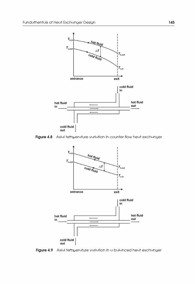
JWST229-c04 JWST229-McDonald Printer: Yet to Come July 31, 2012 12:14 Trim: 244mm × 168mm
Fundamentals of Heat Exchanger Design 145
Figure 4.8 Axial temperature variation in counter flow heat exchanger
Figure 4.9 Axial temperature variation in a balanced heat exchanger

JWST229-c04 JWST229-McDonald Printer: Yet to Come July 31, 2012 12:14 Trim: 244mm × 168mm
146 Introduction to Thermo-Fluids Systems Design
Figure 4.10 Axial temperature variation in a heat exchanger with condensation
Fundamental Note: The temperatures of the hot fluid (including Th,in and Th,out) mustbe greater than the temperatures of the cold fluid (including Tc,in and Tc,out) for heattransfer in accordance with the second law of thermodynamics.
Condensation in counter flow or parallel heat exchangers
In this case, a phase change occurs in one of the working fluids. The hot fluid willcondense by transferring heat to the cold fluid. Since this is a phase change situation,the temperature of the hot fluid will remain constant. As the cold fluid becomes hotter,its temperature will approach that of the hot fluid (see Figure 4.10).
Boiling in counter flow or parallel heat exchangers
In this case, a phase change occurs in one of the working fluids. The cold fluid will boildue to the transfer of heat from the hot fluid. Since this is a phase change situation, thetemperature of the cold fluid will remain constant. As the hot fluid becomes colder,its temperature will approach that of the cold fluid (see Figure 4.11).
Figure 4.11 Axial temperature variation in a heat exchanger with boiling

JWST229-c04 JWST229-McDonald Printer: Yet to Come July 31, 2012 12:14 Trim: 244mm × 168mm
Fundamentals of Heat Exchanger Design 147
Practical Note 4.3 Condensers and Boilers
Condensers and boilers are heat exchangers in which condensation and boiling phasechanges occur, respectively. Pinch point analysis and other Nusselt number correlationequations for phase changes should be used for heat exchangers with phase changes.
4.6 Heat Exchanger Design and Performance Analysis: Part 1
Heat exchanger design or sizing refers to the specification of the construction andflow arrangement of the heat exchanger.
This may involve determination of the following:
(i) Heat transfer surface area (A)(ii) Tube diameters (D)
(iii) Tube lengths (L)(iv) Number of tubes (n)
The objective of the design will be to provide a heat exchanger that will providea specified outlet temperature of the working fluids or transfer a specified amountof heat.
Heat exchanger performance analysis serves to determine the outlet temperatures(Tout) of the working fluids and/or the amount of heat (Q) exchanged by the heatexchanger. As a design engineer, it may be necessary to analyze the performance of anewly designed or existing heat exchanger within a system.
4.6.1 The Log-Mean Temperature Difference Method
This method may be used to determine the size (heat transfer surface area), theoutlet temperatures of the working fluid, or the heat transfer rate of/within the heatexchanger. This method can be used to find the amount of heat exchanged in the heatexchanger by using Newton’s law of cooling:
Q = UA�Tlm, (4.46)
where U is the overall heat transfer coefficient, A is the heat exchanger surface area,and �Tlm is the log-mean temperature difference (LMTD).
This method works best in heat exchanger design and sizing problems when allthe inlet and outlet temperatures of the working fluids are known.
In heat exchanger performance analysis where all the temperatures of the workingfluids are not known and the outlet temperatures must be determined, the LMTDmethod becomes iterative, tedious, and long. In this course, emphasis will be placedon the more powerful effectiveness-number of transfer units (ε-NTU) method forboth heat exchanger design and performance analysis.
JWST229-c04 JWST229-McDonald Printer: Yet to Come July 31, 2012 12:14 Trim: 244mm × 168mm
148 Introduction to Thermo-Fluids Systems Design
4.6.2 The Effectiveness-Number of Transfer Units Method:Introduction
This method was developed by Kays and London [2] to allow for easier design andperformance analysis of heat exchangers without exhaustive iterations. The methodis more straightforward than the LMTD method.
The dimensionless heat transfer effectiveness (ε) is defined as
ε = QQmax
= actual heat transfer ratemaximum possible heat transfer rate
. (4.47)
This expression may be considered as the efficiency of the heat exchanger to ex-change energy between the fluid streams.
The maximum heat transfer rate (Qmax) will occur over the maximum possibletemperature difference. The maximum possible temperature difference is
�Tmax = Th,in − Tc,in. (4.48)
In real heat exchangers, the maximum heat transfer and maximum temperaturedifference will occur in the working fluid with smaller heat capacity. The fluid withthe smaller heat capacity will experience faster temperature changes, will store lessenergy, and will transfer heat faster.
Therefore,
Qmax = mcp,min (Th,in − Tc,in) = Cmin (Th,in − Tc,in) . (4.49)
The working fluid with the lower heat capacity (cp,min) or lower heat capacity rate(Cmin) could be either hot or cold.
Hence,
Cmin = Cc or Cmin = Ch. (4.50)
The effectiveness becomes
ε = Cc
Cmin
(Tc,out − Tc,in)(Th,in − Tc,in)
or
ε = Ch
Cmin
(Th,in − Th,out)(Th,in − Tc,in)
. (4.51)
The actual heat transfer rate is
Q = εQmax = εCmin (Th,in − Tc,in) . (4.52)

JWST229-c04 JWST229-McDonald Printer: Yet to Come July 31, 2012 12:14 Trim: 244mm × 168mm
Fundamentals of Heat Exchanger Design 149
Practical Note 4.4 Real Heat Exchangers
Typically, the inlet temperatures of the working fluids, the mass or volume flow rates, andthe heat capacities are known in real heat exchanger applications and design. The heattransfer rate and the outlet temperatures of the working fluids are usually unknown.
4.6.3 The Effectiveness-Number of Transfer Units Method:ε-NTU Relations
A variety of ε-NTU relations have been developed to facilitate heat exchanger designand performance analysis. The derivation of the ε-NTU relation for a simple double-pipe parallel flow heat exchanger is shown below. For other types of heat exchangers,the derivations become complicated. As a result, designers rely on referenced relationequations or charts.
Derivation of the ε-NTU relation for a simple double-pipe parallel flowheat exchanger
Consider a single-pass parallel-flow heat exchanger with a schematic drawing shownbelow:
Take an infinitesimal section of the system for analysis
dQ = −mhcphdTh (4.53)
dQ = +mccpcdTc (4.54)
Rearrangement gives
dTh = − dQmhcph
; dTc = + dQmccpc
(4.55)
Substract the differential temperatures:
dTh − dTc = −dQ[
1mhcph
+ 1mccpc
]. (4.56)
The differential heat transfer rate is governed by Newton’s Law of Cooling:
dQ = U(Th − Tc)dA (4.57)
JWST229-c04 JWST229-McDonald Printer: Yet to Come July 31, 2012 12:14 Trim: 244mm × 168mm
150 Introduction to Thermo-Fluids Systems Design
Substitution:
dTh − dTc = −U (Th − Tc) dA[
1mhcph
+ 1mccpc
](4.58)
Or
d (Th − Tc)Th − Tc
= −UdA[
1mhcph
+ 1mccpc
](4.59)
Integrate between the inlet and outlet of the heat exchanger:
ln (Th,out − Tc,out) − ln (Th,in − Tc,in) = −UA[
1mhcph
+ 1mccpc
](4.60)
ln[
Th,out − Tc,out
Th,in − Tc,in
]= −UA
[1
mhcph+ 1
mccpc
]. (4.61)
Remember: Ch = mhcph and Cc = mccpc.Therefore,
ln[
Th,out − Tc,out
Th,in − Tc,in
]= −UA
Cc
[1 + Cc
Ch
]. (4.62)
From the expressions for heat transfer rate,
Ch (Th,in − Th,out) = Cc (Tc,out − Tc,in)
Th,out = Th,in − Cc
Ch(Tc,out − Tc,in) . (4.63)
Substitution:
ln
⎡⎢⎢⎣
Th,in − Cc
Ch(Tc,out − Tc,in) − Tc,out
Th,in − Tc,in
⎤⎥⎥⎦ = −UA
Cc
[1 + Cc
Ch
](4.64)
ln
⎡⎢⎢⎣
Th,in − Tc,in − Cc
Ch(Tc,out − Tc,in) + Tc,in − Tc,out
Th,in − Tc,in
⎤⎥⎥⎦ = −UA
Cc
[1 + Cc
Ch
](4.65)
ln[
1 −(
1 + Cc
Ch
)Tc,out − Tc,in
Th,in − Tc,in
]= −UA
Cc
[1 + Cc
Ch
]. (4.66)
Remember that the effectiveness is defined as
ε = Cc
Cmin
Tc,out − Tc,in
Th,in − Tc,in.
JWST229-c04 JWST229-McDonald Printer: Yet to Come July 31, 2012 12:14 Trim: 244mm × 168mm
Fundamentals of Heat Exchanger Design 151
Therefore,
Tc,out − Tc,in
Th,in − Tc,in= ε
Cmin
Cc. (4.67)
Then,
ln[
1 −(
1 + Cc
Ch
)ε
Cmin
Cc
]= −UA
Cc
[1 + Cc
Ch
]. (4.68)
Solve for ε:
εCmin
Cc=
1 − exp[−UA
Cc
(1 + Cc
Ch
)](
1 + Cc
Ch
) . (4.69)
Cmin can be either Cc or Ch. Let Cmin be Cc and Cmax be Ch.Thus, effectiveness is
ε =1 − exp
[− UA
Cmin
(1 + Cmin
Cmax
)](
1 + Cmin
Cmax
) . (4.70)
Let the number of transfer units and the capacity ratio be
NTU = UACmin
and c = Cmin
Cmax. (4.71)
Therefore,
ε = 1 − exp [−NTU (1 + c)](1 + c)
for double-pipe, parallel flow heat exchangers.
(4.72)
Table 4.5 and the charts of Figure 4.12 provide additional ε-NTU relations for othertypes of heat exchangers.
4.6.4 Comments on the Number of Transfer Units andthe Capacity Ratio (c)
(i) The following are some general points regarding the number of transfer unitsand the capacity ratio (c).

JWST229-c04 JWST229-McDonald Printer: Yet to Come July 31, 2012 12:14 Trim: 244mm × 168mm
152 Introduction to Thermo-Fluids Systems Design
Table 4.5 Effectiveness relations for heat exchangers
Heat Exchanger Type Effectiveness Relation
Double pipe: parallel flow ε = 1 − exp [−NTU (1 + c)]1 + c
Double pipe: counter flowε = 1 − exp [−NTU (1 − c)]
1 − c exp [−NTU (1 − c)]for c < 1
ε = NTU1 + NTU
for c = 1
Shell-and-tube: one-shell pass andan even number of tube passes ε1 = 2
⎡⎣1 + c + √
1 + c21 + exp
[−NTU1
√1 + c2
]1 − exp
[−NTU1
√1 + c2
]⎤⎦
−1
Shell-and-tube: N shell passes and2N, 4N . . . tube passes
ε =
(1 − ε1c1 − ε1
)N
− 1(
1 − ε1c1 − ε1
)N
− c
ε1 and NTU1 are for one-shell pass
Cross-flow (single-pass): bothfluids unmixed ε = 1 − exp
[NTU0.22
c
[exp
(−cNTU0.78) − 1]]
Cross-flow (single-pass): bothmixed ε =
[1
1 − exp (−NTU)+ c
1 − exp (−cNTU)− 1
NTU
]−1
Cross-flow (single-pass): Cmax
mixed; Cmin unmixed ε = 1c
(1 − exp
[1 − c
[1 − exp (−NTU)
]])Cross-flow (single-pass): Cmin
mixed; Cmax unmixed ε = 1 − exp[−1
c
[1 − exp (−cNTU)
]]
All heat exchangers with c = 0(boiling or condensation)
ε = 1 − exp(−NTU)
(ii) The NTU = UACmin
is a measure of the heat transfer surface area of the heat ex-changer. It is directly proportional to the surface area. Larger NTU values indi-cate larger heat exchanger surface areas. With larger surface areas, fabricationcosts will increase. For NTU values larger than 10, economic factors should drivethe fabrication of such heat exchangers.
(iii) The ε-NTU relation charts shown in Section 4.6.3 show that the effectivenessincreases rapidly for smaller values of NTU. For NTU greater than 1.5, increasesin ε are small. The design engineer may be hard pressed to justify larger heatexchanger and larger NTU values. Therefore, NTU values are typically lowerthan 3 to 5 (depending on the heat exchanger configuration).

JWST229-c04 JWST229-McDonald Printer: Yet to Come July 31, 2012 12:14 Trim: 244mm × 168mm
Fundamentals of Heat Exchanger Design 153
(a)
(c)
(e) (f)
(d)
(b)
Figure 4.12 Effectiveness charts for some heat exchangers (Kays and London [2])

JWST229-c04 JWST229-McDonald Printer: Yet to Come July 31, 2012 12:14 Trim: 244mm × 168mm
154 Introduction to Thermo-Fluids Systems Design
(iv) NTU is also a measure of the ability of the heat exchanger to transfer energy.Higher NTU values indicate higher heat transfer rates.
(v) For the special case of c = CminCmax
= 0, Cmax → ∞. This means that one of the work-ing fluids absorbs or rejects heat without a temperature change. This is mosttypical of a phase change situation (condensation or boiling). This case producesthe maximum possible ε for a given NTU value and heat exchanger configura-tion. Boilers, condensers, and refrigeration systems are examples of equipment/systems in which this will occur.
Example 4.1 Heating Water in a Counter Flow Heat Exchanger
A counter flow double-pipe heat exchanger is used to heat water from 70◦F to 180◦F foruse in a specialized self-service laundromat. The water will flow at a rate of 20 gpm. Theheating is to be accomplished by hot, compressed geothermal brine available at 320◦F at aflow rate of 35 gpm. The inner tube is thin-walled and has a diameter of 5/8 in. If the overallheat transfer coefficient of the heat exchanger is 110 Btu/(h ft2 ◦F), determine the length ofthe heat exchanger required to achieve the desired heating.
Solution. Several assumptions are relevant and will serve to guide the analysis:
(i) Steady state operation of the heat exchanger.(ii) Constant fluid and thermal properties.
(iii) There is no fouling. So, the fouling resistance is zero.(iv) The heat exchanger is well insulated. There is no heat loss from the device.(v) The brine solution is sufficiently dilute to assume that its properties are equal to those
of pure water.
The total length of the heat exchanger is found from the surface area:
A = npDtube L .
For this single-pipe heat exchanger, n = 1.Therefore,
L = Aπ Dtube
.

JWST229-c04 JWST229-McDonald Printer: Yet to Come July 31, 2012 12:14 Trim: 244mm × 168mm
Fundamentals of Heat Exchanger Design 155
The area is needed. The ε-NTU method can be used in the analysis of the heat exchanger.The NTU is
NTU = UACmin
.
The area is
A = CminNTUU
.
Consider each term in the area equation. To find Cmin, the average temperatures will beused. In this case, the average cold fluid temperature is
Tc = Tc,in + Tc,out
2= 70◦F + 180◦F
2= 125◦F.
Find the cold-water properties at 125◦F and the hot water properties at 320◦F. The heatcapacity rates are:
Cc = mccpc = ρcVccpc =(
61.63 lb/ft3) (
20 gpm)
(0.999 Btu/(lb R))
(35.315 ft3
/s15850 gpm
)
= 2.74 Btu/(s R) = Cmin
Ch = mhcph = ρhVhcph =(
56.65 lb/ft3) (
35 gpm)
(1.036 Btu/(lb R))
(35.315 ft3
/s15850 gpm
)
= 4.58 Btu/(s R) = Cmax
Find the NTU. The capacity ratio is
c = Cmin
Cmax= Cc
Ch= 2.74 Btu/(s R)
4.58 Btu/(s R)= 0.599.
The effectiveness is
ε = Cc
Cmin
Tc,out − Tc,in
Th,in − Tc,in= Tc,out − Tc,in
Th,in − Tc,in= (180 − 70) ◦F
(320 − 70) ◦F= 0.44 = 44%.
This is a counter flow heat exchanger problem. So, with c and ε known, the charts ofFigure 4.12 or the equations in Table 4.5 can be used to find the NTU. From the charts,
NTU ≈ 0.70.
The effectiveness equation for a double-pipe counter flow heat exchanger with c < 1gives
ε = 1 − exp [−NTU (1 − c)]1−c exp [−NTU (1 − c)]
= 1 − exp [−0.401 NTU]1 − 0.599 exp [−0.401 NTU]
= 0.44.

JWST229-c04 JWST229-McDonald Printer: Yet to Come July 31, 2012 12:14 Trim: 244mm × 168mm
156 Introduction to Thermo-Fluids Systems Design
Therefore,
NTU = 0.68.
With the NTU known, the area can be determined.
A = (2.74 Btu/(s R)) (0.68)
110 Btu/(h ft2 R)× 3600 s
1 h= 60.98 ft2
Thus,
L = 60.98 ft2
π (0.625 in.)× 12 in.
1 ft
L = 373 ft.
4.6.5 Procedures for the ε-NTU Method
The ε-NTU method can be used in both heat exchanger design and performance analy-sis problems in a direct, straightforward manner, without the need for iterations/trial-and-error.
(A) Consider the design of a heat exchanger to find the heat transfer surface area, A.In a design problem, the following may/will be known:
Th,in;Th,out;Tc,in; mc; mh.
The ε-NTU solution method approach is as follows:(i) Compute ε and c from available data.
(ii) Determine the NTU from an appropriate relation or chart.(iii) Compute A from NTU = UA
Cmin.
(iv) For circular tubes, the total tube length is found from A = nπDtubeL.(B) Consider a performance analysis of a heat exchanger to find Tc,out;Th,out;Q. In a
performance analysis, the following may/will be known:
A; U; mc; mh ; Th,in; Tc,in.
The ε-NTU solution method approach is as follows:(i) Calculate the NTU from given data.
(ii) Use relations or charts to find ε using the NTU and c.(iii) Calculate one of the outlet temperatures with ε = Cc
Cmin
(Tc,out−Tc,in)(Th,in−Tc,in) or ε =
ChCmin
(Th,in−Th,out)(Th,in−Tc,in) .
(iv) Calculate Q and the other outlet temperature.
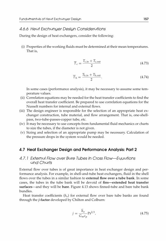
JWST229-c04 JWST229-McDonald Printer: Yet to Come July 31, 2012 12:14 Trim: 244mm × 168mm
Fundamentals of Heat Exchanger Design 157
4.6.6 Heat Exchanger Design Considerations
During the design of heat exchangers, consider the following:
(i) Properties of the working fluids must be determined at their mean temperatures.That is,
T c = Tc,in + Tc,out
2(4.73)
Th = Th,in + Th,out
2. (4.74)
In some cases (performance analysis), it may be necessary to assume some tem-perature values.
(ii) Correlation equations may be needed for the heat transfer coefficients to find theoverall heat transfer coefficient. Be prepared to use correlation equations for theNusselt numbers for internal and external flows.
(iii) The design engineer is responsible for the selection of an appropriate heat ex-changer construction, tube material, and flow arrangement. That is, one-shell-pass, two-tube-passes-copper tube, etc.
(iv) It may be necessary to use concepts from fundamental fluid mechanics or chartsto size the tubes, if the diameter is not given.
(v) Sizing and selection of an appropriate pump may be necessary. Calculation ofthe pressure drops in the system would be needed.
4.7 Heat Exchanger Design and Performance Analysis: Part 2
4.7.1 External Flow over Bare Tubes in Cross Flow—Equationsand Charts
External flow over tubes is of great importance in heat exchanger design and per-formance analysis. For example, in shell-and-tube heat exchangers, fluid in the shellflows over the tubes in a similar fashion to external flow over a tube bank. In somecases, the tubes in the tube bank will be devoid of fins—extended heat transfersurfaces—and they will be bare. Figure 4.13 shows finned-tube and bare tube bankbundles.
Heat transfer coefficients (ho) for external flow over bare tube banks are foundthrough the j-factor developed by Chilton and Colburn:
j = ho
GmcpPr2/3, (4.75)
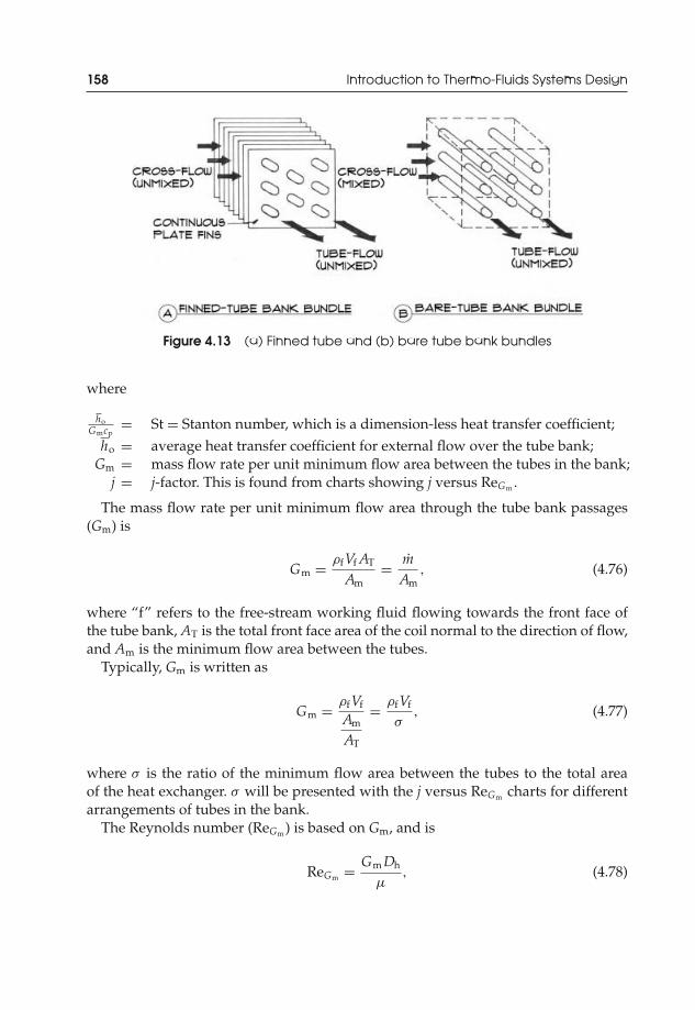
JWST229-c04 JWST229-McDonald Printer: Yet to Come July 31, 2012 12:14 Trim: 244mm × 168mm
158 Introduction to Thermo-Fluids Systems Design
Figure 4.13 (a) Finned tube and (b) bare tube bank bundles
where
hoGmcp
= St = Stanton number, which is a dimension-less heat transfer coefficient;ho = average heat transfer coefficient for external flow over the tube bank;
Gm = mass flow rate per unit minimum flow area between the tubes in the bank;j = j-factor. This is found from charts showing j versus ReGm .
The mass flow rate per unit minimum flow area through the tube bank passages(Gm) is
Gm = ρfVf AT
Am= m
Am, (4.76)
where “f” refers to the free-stream working fluid flowing towards the front face ofthe tube bank, AT is the total front face area of the coil normal to the direction of flow,and Am is the minimum flow area between the tubes.
Typically, Gm is written as
Gm = ρfVf
Am
AT
= ρfVf
σ, (4.77)
where σ is the ratio of the minimum flow area between the tubes to the total areaof the heat exchanger. σ will be presented with the j versus ReGm charts for differentarrangements of tubes in the bank.
The Reynolds number (ReGm ) is based on Gm, and is
ReGm = Gm Dh
μ, (4.78)

JWST229-c04 JWST229-McDonald Printer: Yet to Come July 31, 2012 12:14 Trim: 244mm × 168mm
Fundamentals of Heat Exchanger Design 159
Figure 4.14 Flow pattern for an in-line tube bank (Cengel [3], reprinted with permission)
where Dh is the hydraulic diameter of the flow passage space between the tubes inthe bank, and is found from j versus ReGm charts.
Charts of j versus ReGm for In-line Tube Bank Arrangements
Figure 4.14 shows the pattern of fluid flow through a bank of tubes arrangedin line.
Charts of j versus ReGm must be prepared experimentally. Figure 4.15 shows sucha chart for flow through an in-line tube bank. The chart and those presented inAppendix C were developed with experimental data from Kays and London [2], andare approximate. The design engineer is encouraged to consult Reference [2] for moredetailed information.
The following observations are made regarding Figure 4.15:
(i) This chart was developed from transient tests. So, the number of rows of tubesis variable, and must be determined through the design process. In addition,curves of this type have wider application.
(ii) A curve of the friction factor (f ) versus ReGm is provided at the top of thechart.
(iii) A curve of the j-factor versus ReGm is provided at the bottom of the chart.(iv) D is the tube outer diameter, and is given as 0.375 in.(v) Xt is the traverse tube-pitch ratio, xt
D .

JWST229-c04 JWST229-McDonald Printer: Yet to Come July 31, 2012 12:14 Trim: 244mm × 168mm
160 Introduction to Thermo-Fluids Systems Design
DATATube outside diameter: 0.375 in.
Hydraulic diameter, Dh: 0.0248 ft
Free-flow area/Frontal area, σ: 0.333
Heat transfer area/Total volume, α: 53.6 ft2/ft3
Figure 4.15 Data for flow normal to an in-line tube bank (Kays and London [2])
(vi) XL is the longitudinal tube-pitch ratio, xLD .
(vii) σ is given.(viii) α is the ratio of the total heat transfer area on the external side of the tubes
(outer surface area) to the total volume of the exchanger.(ix) Dh is given.
Additional charts are provided in Appendix C. Refer to the appendix for a moreextensive listing of charts.
Charts of j versus ReGm for Staggered Tube Bank Arrangements
Figure 4.16 shows the pattern of fluid flow through a bank of tubes arranged in astaggered fashion.
Figure 4.17 shows a chart for flow through staggered tube banks.
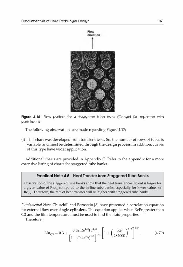
JWST229-c04 JWST229-McDonald Printer: Yet to Come July 31, 2012 12:14 Trim: 244mm × 168mm
Fundamentals of Heat Exchanger Design 161
Figure 4.16 Flow pattern for a staggered tube bank (Cengel [3], reprinted withpermission)
The following observations are made regarding Figure 4.17:
(i) This chart was developed from transient tests. So, the number of rows of tubes isvariable, and must be determined through the design process. In addition, curvesof this type have wider application.
Additional charts are provided in Appendix C. Refer to the appendix for a moreextensive listing of charts for staggered tube banks.
Practical Note 4.5 Heat Transfer from Staggered Tube Banks
Observation of the staggered tube banks show that the heat transfer coefficient is larger fora given value of ReGm compared to the in-line tube banks, especially for lower values ofReGm . Therefore, the rate of heat transfer will be higher with staggered tube banks.
Fundamental Note: Churchill and Bernstein [8] have presented a correlation equationfor external flow over single cylinders. The equation applies when RePr greater than0.2 and the film temperature must be used to find the fluid properties.
Therefore,
Nucyl = 0.3 + 0.62 Re1/2Pr1/3[1 + (0.4/Pr)2/3
]1/4
[1 +
(Re
282000
)5/8]4/5
. (4.79)

JWST229-c04 JWST229-McDonald Printer: Yet to Come July 31, 2012 12:14 Trim: 244mm × 168mm
162 Introduction to Thermo-Fluids Systems Design
DATATube outside diameter: 0.375 in.
Hydraulic diameter, Dh: 0.0249 ft
Free-flow area/Frontal area, σ: 0.333
Note: Minimum free-flow area is in the spaces transverse to the flow
Heat transfer area/Total volume, α: 53.6 ft2/ft3
Figure 4.17 Data for flow normal to a staggered tube bank (Kays and London [2])
This correlation equation cannot be used for a bank of tubes since the fluid flowsover the tubes will have an influence on each other. However, this equation may applyto the case of a single row of circular tubes oriented such that the flow over them willnot be affected by the presence of others.
4.7.2 External Flow over Tube Banks—Pressure Drop
Pressure drop for external flow over bare and finned-tubes in tube banks is givenempirically as [2]
�Pbank = G2m
2ρi
[(Ki + 1 − σ 2) + 2
(ρi
ρe− 1
)+ f
AT
Ac
ρi
ρmean− (
1 − σ 2 − Ke) ρi
ρe
],
(4.80)
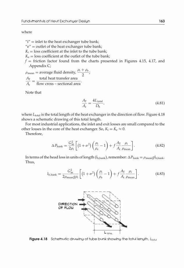
JWST229-c04 JWST229-McDonald Printer: Yet to Come July 31, 2012 12:14 Trim: 244mm × 168mm
Fundamentals of Heat Exchanger Design 163
where
“i” = inlet to the heat exchanger tube bank;“e” = outlet of the heat exchanger tube bank;Ki = loss coefficient at the inlet to the tube bank;Ke = loss coefficient at the outlet of the tube bank;f = friction factor found from the charts presented in Figures 4.15, 4.17, and
Appendix C;
ρmean = average fluid density,ρi + ρe
2;
AT
Ac= total heat transfer area
flow cross – sectional area.
Note that
AT
Ac= 4L total
Dh, (4.81)
where Ltotal is the total length of the heat exchanger in the direction of flow. Figure 4.18shows a schematic drawing of this total length.
For most industrial applications, the inlet and exit losses are small compared to theother losses in the core of the heat exchanger. So, Ki = Ke ≈ 0.
Therefore,
�Pbank = G2m
2ρi
[(1 + σ 2) (
ρi
ρe− 1
)+ f
AT
Ac
ρi
ρmean
]. (4.82)
In terms of the head loss in units of length (lh,bank), remember: �Pbank = ρmeanglh,bank.Thus,
lh,bank = G2m
2ρmeangρi
[(1 + σ 2) (
ρi
ρe− 1
)+ f
AT
Ac
ρi
ρmean
]. (4.83)
Figure 4.18 Schematic drawing of tube bank showing the total length, Ltotal

JWST229-c04 JWST229-McDonald Printer: Yet to Come July 31, 2012 12:14 Trim: 244mm × 168mm
164 Introduction to Thermo-Fluids Systems Design
Practical Note 4.6 Coil Arrangement in Air-to-WaterHeat Exchangers
For most small applications that involve air-to-water heat exchangers, where airflowsover a tube bank and water flows in the tubes, the number of rows of tubes is usu-ally 4 to 6. While oversizing the heat exchanger may be necessary due to equipmentavailability or design requirements, the design engineer should be aware that increasednumber of tubes in a tube bank will require greater powers from a fan (for air) or apump (for liquids) to move the fluid through the bank. If the number of rows becomelarger than 6, the design engineer may wish to increase the center-to-center spacing (lon-gitudinal tube pitch) between the tube rows to reduce pressure losses. An even num-ber of rows is usually preferred to ensure that the tube entrance and exit points are onthe same side and level of the heat exchanger. This will approach a counter flow heatexchanger system.
Practical Note 4.7 Pressure Drop Over Tube Banks
The equations presented earlier for the determination of the pressure drop and head loss forexternal flow over the tube bank apply to both bare tube and finned-tube heat exchangers.Finned-tube heat exchangers are more widely used in industry.
Example 4.2 Design of a Heating Coil Heat Exchanger
Mr. Chin has hired a junior design engineer to design a small heating coil for his fresh air in-take duct line. Mr. Chin is a frugal entrepreneur, and has requested a bare-tube type heatingcoil arrangement. The HVAC engineer has presented the following duty and specificationsfor the coil:
(i) Heat fresh air from 50◦F to about 100◦F.(ii) Duct airflow rate is 2000 cfm.
(iii) Entering hot water temperature is about 150◦F.(iv) This is a low-velocity duct section.(v) Water connections must be on the same end of the coil system to facilitate easy instal-
lation and to approach a counter flow heat exchanger system.(vi) One large inlet and exit header is required. The tubes will be attached to the headers.
Further Information: This design problem should address and present the following points:
(i) Exit water temperature(ii) Heating coil configuration and number of coils
(iii) Final dimensions of the heat exchanger (length, width, and depth)(iv) Pressure loss for the airflow through the coil bank(v) Head loss in the waterside of the tube
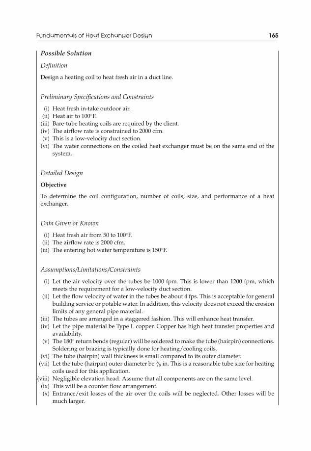
JWST229-c04 JWST229-McDonald Printer: Yet to Come July 31, 2012 12:14 Trim: 244mm × 168mm
Fundamentals of Heat Exchanger Design 165
Possible Solution
Definition
Design a heating coil to heat fresh air in a duct line.
Preliminary Specifications and Constraints
(i) Heat fresh in-take outdoor air.(ii) Heat air to 100◦F.
(iii) Bare-tube heating coils are required by the client.(iv) The airflow rate is constrained to 2000 cfm.(v) This is a low-velocity duct section.
(vi) The water connections on the coiled heat exchanger must be on the same end of thesystem.
Detailed Design
Objective
To determine the coil configuration, number of coils, size, and performance of a heatexchanger.
Data Given or Known
(i) Heat fresh air from 50 to 100◦F.(ii) The airflow rate is 2000 cfm.
(iii) The entering hot water temperature is 150◦F.
Assumptions/Limitations/Constraints
(i) Let the air velocity over the tubes be 1000 fpm. This is lower than 1200 fpm, whichmeets the requirement for a low-velocity duct section.
(ii) Let the flow velocity of water in the tubes be about 4 fps. This is acceptable for generalbuilding service or potable water. In addition, this velocity does not exceed the erosionlimits of any general pipe material.
(iii) The tubes are arranged in a staggered fashion. This will enhance heat transfer.(iv) Let the pipe material be Type L copper. Copper has high heat transfer properties and
availability.(v) The 180◦ return bends (regular) will be soldered to make the tube (hairpin) connections.
Soldering or brazing is typically done for heating/cooling coils.(vi) The tube (hairpin) wall thickness is small compared to its outer diameter.
(vii) Let the tube (hairpin) outer diameter be 3/8 in. This is a reasonable tube size for heatingcoils used for this application.
(viii) Negligible elevation head. Assume that all components are on the same level.(ix) This will be a counter flow arrangement.(x) Entrance/exit losses of the air over the coils will be neglected. Other losses will be
much larger.

JWST229-c04 JWST229-McDonald Printer: Yet to Come July 31, 2012 12:14 Trim: 244mm × 168mm
166 Introduction to Thermo-Fluids Systems Design
Sketch
A complete drawing will be provided after the design to show the tube flow circuitry in theheating coil.
Analysis
Determine the overall heat transfer coefficient (U )
The ε-NTU method will be used in this design. To determine the effectiveness and NTU,the overall heat transfer coefficient (U) must be determined first. The overall heat transfercoefficient is
1U
= 1hi
+ Rfi + Rwall A+ Rfo + 1ho
.
The wall resistance is
Rwall = 12πkL
ln(
ro
ri
).
It was assumed that the wall thickness is small. Therefore, ro ≈ ri. So, Rwall ≈ 0. Thus,
1U
= 1hi
+ Rfi + Rfo + 1ho
.
The heat transfer coefficient for flow in the tube (hairpin) is found from the Dittus–Boeltercorrelation equation. Note that, though more complex, the Gnielinski correlation could havebeen used:
Nu = hi Di
k= 0.023Re0.8
DiPr0.3.
The inlet and outlet temperatures of the working fluids will needed to find appropriateproperties for the determination of ReD and Pr.
Given: Ta,i = 50◦F, Tw,i = 150◦FTa,o = 100◦F, Tw,o = unknown.
An educated guess of Tw,o will be needed. Water has a very high specific heat capacitycompared to air. Therefore, the water temperature changes slowly as heat is transferred. Ingeneral,
cp,w
cp,a≈ 4.
Therefore, if �Tair = (100 – 50)◦F = 50◦F, then �Twater ≈ 10◦F. Let Tw,o = (150 – 10)◦F =140◦F.
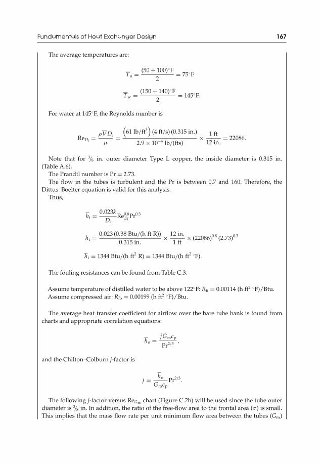
JWST229-c04 JWST229-McDonald Printer: Yet to Come July 31, 2012 12:14 Trim: 244mm × 168mm
Fundamentals of Heat Exchanger Design 167
The average temperatures are:
Ta = (50 + 100)◦F2
= 75◦F
Tw = (150 + 140)◦F2
= 145◦F.
For water at 145◦F, the Reynolds number is
ReDi = ρVDi
μ=
(61 lb/ft3
)(4 ft/s) (0.315 in.)
2.9 × 10⁻⁴ lb/(fts)× 1 ft
12 in.= 22086.
Note that for 3/8 in. outer diameter Type L copper, the inside diameter is 0.315 in.(Table A.6).
The Prandtl number is Pr = 2.73.The flow in the tubes is turbulent and the Pr is between 0.7 and 160. Therefore, the
Dittus–Boelter equation is valid for this analysis.Thus,
hi = 0.023kDi
Re0.8Di
Pr0.3
hi = 0.023 (0.38 Btu/(h ft R))0.315 in.
× 12 in.
1 ft× (22086)0.8 (2.73)0.3
hi = 1344 Btu/(h ft2 R) = 1344 Btu/(h ft2 ◦F).
The fouling resistances can be found from Table C.3.
Assume temperature of distilled water to be above 122◦F: Rfi = 0.00114 (h ft2 ◦F)/Btu.Assume compressed air: Rfo = 0.00199 (h ft2 ◦F)/Btu.
The average heat transfer coefficient for airflow over the bare tube bank is found fromcharts and appropriate correlation equations:
ho = jGmcp
Pr2/3 ,
and the Chilton–Colburn j-factor is
j = ho
GmcpPr2/3.
The following j-factor versus ReGm chart (Figure C.2b) will be used since the tube outerdiameter is 3/8 in. In addition, the ratio of the free-flow area to the frontal area (σ ) is small.This implies that the mass flow rate per unit minimum flow area between the tubes (Gm)
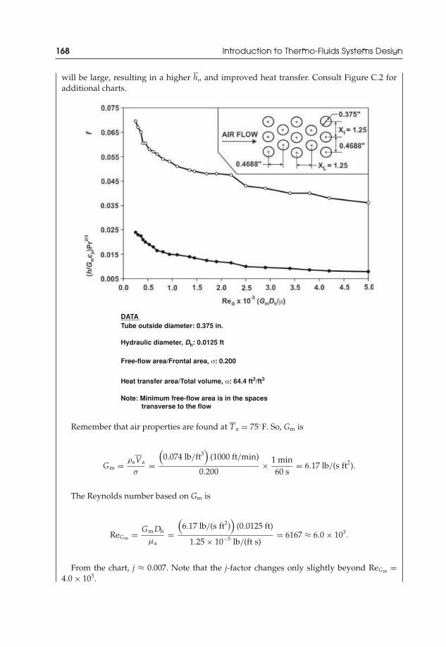
JWST229-c04 JWST229-McDonald Printer: Yet to Come July 31, 2012 12:14 Trim: 244mm × 168mm
168 Introduction to Thermo-Fluids Systems Design
will be large, resulting in a higher ho and improved heat transfer. Consult Figure C.2 foradditional charts.
DATATube outside diameter: 0.375 in.
Hydraulic diameter, Dh: 0.0125 ft
Free-flow area/Frontal area, σ: 0.200
Heat transfer area/Total volume, α: 64.4 ft2/ft3
Note: Minimum free-flow area is in the spaces transverse to the flow
Remember that air properties are found at Ta = 75◦F. So, Gm is
Gm = ρaVa
σ=
(0.074 lb/ft3
)(1000 ft/min)
0.200× 1 min
60 s= 6.17 lb/(s ft2).
The Reynolds number based on Gm is
ReGm = Gm Dh
μa=
(6.17 lb/(s ft2)
)(0.0125 ft)
1.25 × 10⁻⁵ lb/(ft s)= 6167 ≈ 6.0 × 10³.
From the chart, j ≈ 0.007. Note that the j-factor changes only slightly beyond ReGm =4.0 × 10³.

JWST229-c04 JWST229-McDonald Printer: Yet to Come July 31, 2012 12:14 Trim: 244mm × 168mm
Fundamentals of Heat Exchanger Design 169
Therefore,
ho =(0.007)
(6.17 lb/(s ft2)
)(0.24 Btu/(lb ◦F))
(0.73)2/3 × 3600 s1 h
ho = 46.0 Btu/(h ft2 ◦F).
As expected, the heat transfer coefficient of the liquid water is higher than that ofgaseous air.
The overall heat transfer coefficient is
1U
= 1
1344 Btu/(h ft2 ◦F)+ 0.00114 (h ft2 ◦F)/Btu + 0.00199 (h ft2 ◦F)/Btu + 1
46.0 (h ft2 ◦F)/Btu
1U
= 0.0256 (h ft2 ◦F)/Btu
U = 39 Btu/(h ft2 ◦F).
Determine the configuration, number of coils, and dimensions of the heat exchanger. Find thetotal surface area of the tubes by using the ε-NTU method.
NTU = UACmin
A = CminNTUU
The minimum heat capacity is needed. For air,
Ca =macpa =ρaVacpa = (0.074 lb/ft3)(2000 ft3/min) (0.24 Btu/(lb ◦F)) = 35.5 Btu/(min ◦F) = Cc.
For water, the law of conservation of energy can be used:
Cw = Ch = CcTa,o − Ta,i
Tw,i − Tw,o= (35.5 Btu/(min ◦F))
[100◦F − 50◦F150◦F − 140◦F
]= 177.5 Btu/(min ◦F).
Therefore, Ca = Cc = Cmin and Cw = Ch = Cmax.The capacity ratio is
c = Cmin
Cmax= 35.5 Btu/(min ◦F)
177.5 Btu/(min ◦F)
c = 0.20.
The effectiveness is
ε = Cc
Cmin
(Ta,o − Ta,i)(Tw,i − Ta,i)
= (Ta,o − Ta,i)(Tw,i − Ta,i)
= 100◦F − 50◦F150◦F − 50◦F
ε = 0.50.
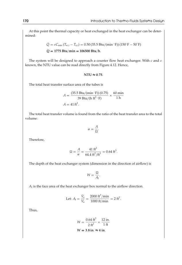
JWST229-c04 JWST229-McDonald Printer: Yet to Come July 31, 2012 12:14 Trim: 244mm × 168mm
170 Introduction to Thermo-Fluids Systems Design
At this point the thermal capacity or heat exchanged in the heat exchanger can be deter-mined:
Q = εCmin (Tw,i − Ta,i) = 0.50 (35.5 Btu/(min ◦F)) (150◦F − 50◦F)
Q = 1775 Btu/min = 106500 Btu/h.
The system will be designed to approach a counter flow heat exchanger. With c and ε
known, the NTU value can be read directly from Figure 4.12. Hence,
NTU ≈ 0.75.
The total heat transfer surface area of the tubes is
A = (35.5 Btu/(min ◦F)) (0.75)
39 Btu/(h ft2 ◦F)× 60 min
1 h
A = 41 ft2.
The total heat transfer volume is found from the ratio of the heat transfer area to the totalvolume:
α = A�
.
Therefore,
� = Aα
= 41 ft2
64.4 ft2/ft3 = 0.64 ft3
.
The depth of the heat exchanger system (dimension in the direction of airflow) is
W = �
Af.
Af is the face area of the heat exchanger box normal to the airflow direction.
Let: Af = Va
Va= 2000 ft3
/min1000 ft/min
= 2 ft2.
Thus,
W = 0.64 ft3
2 ft2 × 12 in.
1 ft
W = 3.8 in. ≈ 4 in.
JWST229-c04 JWST229-McDonald Printer: Yet to Come July 31, 2012 12:14 Trim: 244mm × 168mm
Fundamentals of Heat Exchanger Design 171
From the j-factor versus ReGm chart, the longitudinal tube pitch is 0.4688 in. The numberof tube rows is
Nr = WxL
= 3.8 in.
0.4688 in.
Nr = 8.1 ≈ 8 tube rows.
Determine the number of tubes per row. The cross-sectional area for the tube can be foundfrom the mass flow rate equation (for water):
mw = ρwVw Atube.
The tube area is Atube = Ntubeπ D2
i4 . The mass flow rate can be determined from the defini-
tion of the heat capacity rate, Ch = mwcp,w.Therefore,
Ch
cp,w= ρwVw Ntube
π D2i
4
Ntube = 4Ch
cp,wρwVwπ D2i
Ntube = 4 (177.5 Btu/(min ◦F))
(1.0 Btu/(lb ◦F))(
61 lb/ft3)
(4 ft/s) π (0.315 in.)2×
(12 in.
1 ft
)2
× 1 min60 s
Ntube = 22.4 tubes per row ≈ 22 tubes per row.
The total number of tubes along the length of the heat exchanger will be 176 tubes(8 rows × 22 tubes per row). If each row has 22 tubes, the height of the heating coil is
H = Ntubext = (22)(0.4688 in.)
H = 10.3 in. ≈ 11 in.
The length of the heat exchanger is found by considering an alternate definition of theface area normal to the direction of airflow:
Af = LH.
The heat exchanger length is
L = Af
H= 2 ft2
10.3 in.×
(12 in.
1 ft
)2
L = 27.96 in. ≈ 28 in.
The total length of the tubes in the heat exchanger is 410 ft (28 in. per tube × 176 tubes).

JWST229-c04 JWST229-McDonald Printer: Yet to Come July 31, 2012 12:14 Trim: 244mm × 168mm
172 Introduction to Thermo-Fluids Systems Design
Pressure loss of air across the tube coils
The pressure drop of the air across the tube coil bank is given by
�Pbank = G2m
2ρa,i
[(1 + σ 2) (
ρa,i
ρa,o− 1
)+ f
AT
Ac
ρa,i
ρmean
].
Remember: Gm = 6.17 lb/(s ft2) and ReGm = 6167 ≈ 6.0 × 10³.From the j-factor versus ReGm chart, the friction factor (f ) is
f ≈ 0.035.
The area ratio is
AT
Ac= 4W
Dh= 4 (4 in.)
0.0125 ft× 1 ft
12 in.= 106.7.
The mean density (ρmean) is
ρmean = ρa,i + ρa,o
2= (0.078 + 0.071) lb/ft3
2= 0.075 lb/ft3
.
Therefore,
�Pbank =(
6.17 lb/(s ft2))2
2(
0.078 lb/ft3)
[(1 + 0.202) (
0.078 lb/ft3
0.071 lb/ft3 − 1
)+ (0.035) (106.7)
0.078 lb/ft3
0.075 lb/ft3
]
�Pbank = 972.8 lb/(ft s2) × 1 lbf
32.2 (lb ft)/s2 = 30.2 lbf/ft2 = 30.2 psf.
In practice, the pressure drop is reported in inches of water. Thus,
�Pbank = 972.8 lb/(ft s2) × 1
0.075 lb/ft3 × 1
32.2 ft/s2 = 402.8 ft of air
�Pbank = 402.8 ft of air × SGair,75◦F = 402.8 ft of air × 0.075 lb/ft3
62 lb/ft3 × 12 in.
1 ft
�Pbank = 5.9 in. of water = 5.9 in. wg.
Note: This is a very large pressure drop across the tube coils. This is due to the large airflowrate and velocity, large value of Gm, and small values of xL and σ .
Pressure loss of water in the tube coils
Determination of the pressure loss of the water in the tubes is needed to find the pumppower required to move the fluid through the heat exchanger system. The total head loss is
HlT =(
fL tube
Di+ K
)V
2w
2g.
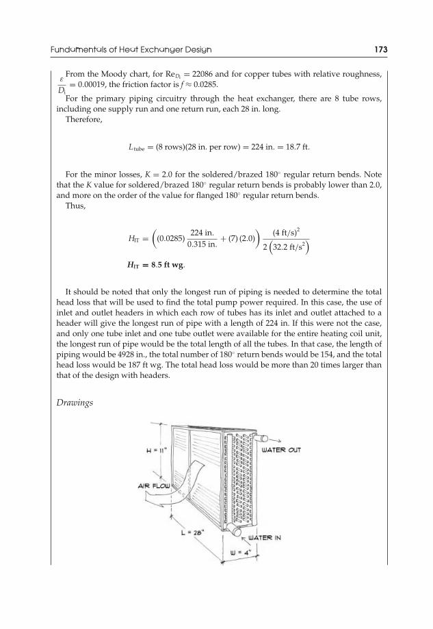
JWST229-c04 JWST229-McDonald Printer: Yet to Come July 31, 2012 12:14 Trim: 244mm × 168mm
Fundamentals of Heat Exchanger Design 173
From the Moody chart, for ReDi = 22086 and for copper tubes with relative roughness,ε
Di= 0.00019, the friction factor is f ≈ 0.0285.
For the primary piping circuitry through the heat exchanger, there are 8 tube rows,including one supply run and one return run, each 28 in. long.
Therefore,
L tube = (8 rows)(28 in. per row) = 224 in. = 18.7 ft.
For the minor losses, K = 2.0 for the soldered/brazed 180◦ regular return bends. Notethat the K value for soldered/brazed 180◦ regular return bends is probably lower than 2.0,and more on the order of the value for flanged 180◦ regular return bends.
Thus,
HlT =(
(0.0285)224 in.
0.315 in.+ (7) (2.0)
)(4 ft/s)2
2(
32.2 ft/s2)
HlT = 8.5 ft wg.
It should be noted that only the longest run of piping is needed to determine the totalhead loss that will be used to find the total pump power required. In this case, the use ofinlet and outlet headers in which each row of tubes has its inlet and outlet attached to aheader will give the longest run of pipe with a length of 224 in. If this were not the case,and only one tube inlet and one tube outlet were available for the entire heating coil unit,the longest run of pipe would be the total length of all the tubes. In that case, the length ofpiping would be 4928 in., the total number of 180◦ return bends would be 154, and the totalhead loss would be 187 ft wg. The total head loss would be more than 20 times larger thanthat of the design with headers.
Drawings

JWST229-c04 JWST229-McDonald Printer: Yet to Come July 31, 2012 12:14 Trim: 244mm × 168mm
174 Introduction to Thermo-Fluids Systems Design
Conclusions
A heating coil heat exchanger with a bare-tube bank has been designed. The followingpoints should be noted:
(i) The ReGm value that was used with the j-factor versus ReGm chart was slightly off thecurve. The error incurred was small.
(ii) The pressure drop of the air across the tube bank and the number of rows of tubeswere large. The tubes were too close, since σ = 0.200. σ = 0.333 may have been a betterchoice for improvement of the design.
(iii) A pressure drop of 5.9 in. wg on the air side is too large. This pressure drop should belimited to an order of 1 in. wg across the tube bank, if possible. Increasing xL and σ
would reduce the pressure drop.
A heat exchanger design data sheet is shown below.
Heat Exchanger Design Data Sheet
Type Counter Flow
Section: Tube BankWorking fluid AirVolume flow rate 2000 cfmInlet temperature 50◦FOutlet temperature 100◦FPressure drop 5.9 in. wg
Section: TubeTube material CopperWorking fluid WaterVelocity 4 ft/sTube inner diameter 0.315 in.Tube outer diameter 0.375 in.Number of tube rows 8Number of tubes per row 22Tube spacing (xt × xL) 0.4688 in. × 0.4688 in.Total tube length 410 ftInlet temperature 150◦FOutlet temperature 140◦FHead loss 8.5 ft wg
Heat Exchanger ParametersThermal capacity 106500 Btu/hEffectiveness 0.50Capacity ratio 0.20Overall heat transfer coefficient 39 Btu/(h ft2 ◦F)Number of transfer units (NTU) 0.75Heat exchanger dimensions (L × H × W) 28 in. × 11 in. × 4 in.
JWST229-c04 JWST229-McDonald Printer: Yet to Come July 31, 2012 12:14 Trim: 244mm × 168mm
Fundamentals of Heat Exchanger Design 175
4.7.3 External Flow over Finned-Tubes in Cross Flow—Equationsand Charts
External flow over finned-tube tube banks is more prevalent in industrial applica-tions. The addition of fins extends the heat transfer surface area of the bare tubes inthe bank.
A staggered arrangement of the tubes, coupled with continuous fins across thelength of the tube bank and heat exchanger will increase the heat transfer capabilityof the exchanger. Figure 4.19 shows some examples of finned heat exchangers thatmay be encountered by the design engineer in industry.
Of importance in the design and performance analysis of heat exchangers is thedetermination of the overall heat transfer coefficient (U). To determine the overallheat transfer coefficient for finned-tubes, consider the following assumptions andobservations:
(i) Constant area, straight fins (e.g., continuous fins, plate-fin-tube geometry).(ii) The base of the fin transfers heat also. Figure 4.20 shows a schematic of general
constant area, straight fins attached to a surface (the base).(iii) So, the combined fin/base surface effectiveness, ηs, is used in heat exchanger
calculations, instead of the fin efficiency, η.(iv) The fins are very thin. So, l t. This is typical of fins used in industrial heat
exchangers.(v) The fins are rigidly and perfectly attached to the base. So, there is no contact
resistance to heat transfer between the fin and the base.(vi) The heat transfer coefficient, fluid properties, and thermal properties are
constant.(vii) The temperature distribution is uniform and steady (steady state) through the
fin. So, the Biot number is small compared to unity(Bi = hδ
k � 1). This assump-
tion will hold for very thin fins (δ = t or δ = t/2) and/or high fin materialthermal conductivities (k), which can be easily incorporated into any design.Low heat transfer coefficients (h) reduce Bi also. This is less desirable from a findesign/performance perspective.
Without derivation, the overall heat transfer coefficient for finned-tube heat ex-changers is
1UFT
= 1hoηso
+ Rfo + Rfi(Ai/Ao
) + 1
hiηsi
(Ai/Ao
) , (4.84)
where “o” refers to the working fluid outside the tube in the tube bank, and “i” refersto the working fluid inside the tubes.
For most industrial applications, the tubes are completely filled with fluid. So,ηsi = 1.
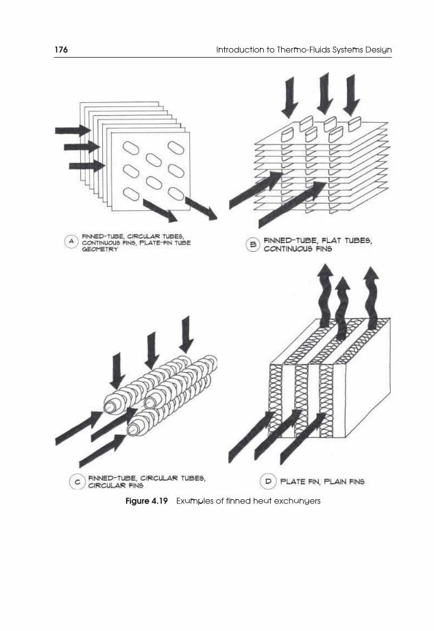
JWST229-c04 JWST229-McDonald Printer: Yet to Come July 31, 2012 12:14 Trim: 244mm × 168mm
176 Introduction to Thermo-Fluids Systems Design
Figure 4.19 Examples of finned heat exchangers
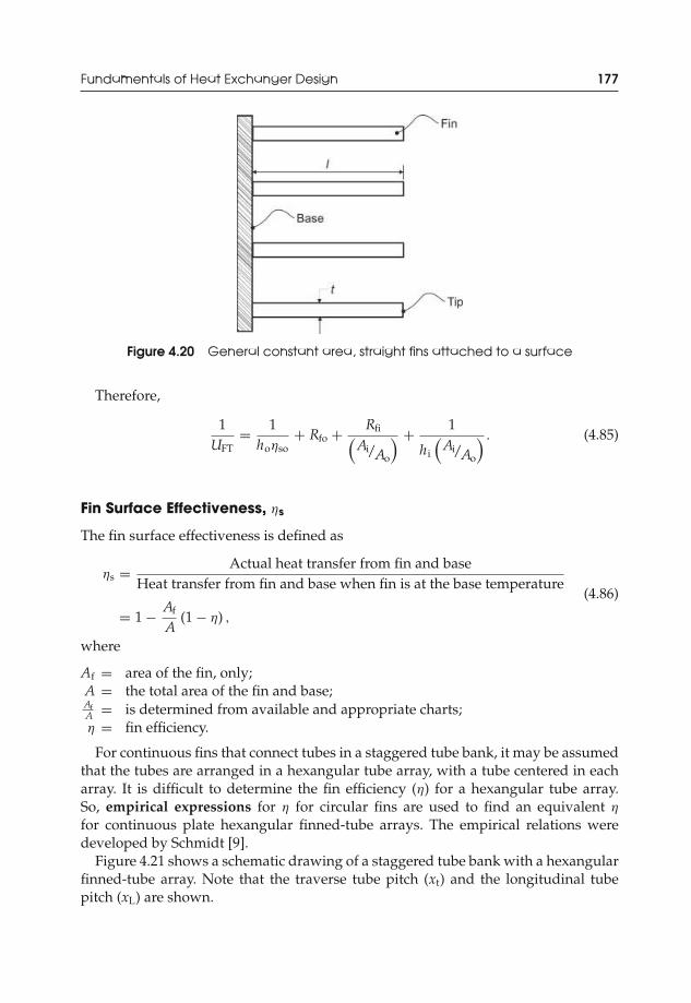
JWST229-c04 JWST229-McDonald Printer: Yet to Come July 31, 2012 12:14 Trim: 244mm × 168mm
Fundamentals of Heat Exchanger Design 177
Figure 4.20 General constant area, straight fins attached to a surface
Therefore,
1UFT
= 1hoηso
+ Rfo + Rfi(Ai/Ao
) + 1
hi
(Ai/Ao
) . (4.85)
Fin Surface Effectiveness, ηs
The fin surface effectiveness is defined as
ηs = Actual heat transfer from fin and baseHeat transfer from fin and base when fin is at the base temperature
= 1 − Af
A(1 − η) ,
(4.86)
where
Af = area of the fin, only;A = the total area of the fin and base;AfA = is determined from available and appropriate charts;η = fin efficiency.
For continuous fins that connect tubes in a staggered tube bank, it may be assumedthat the tubes are arranged in a hexangular tube array, with a tube centered in eacharray. It is difficult to determine the fin efficiency (η) for a hexangular tube array.So, empirical expressions for η for circular fins are used to find an equivalent η
for continuous plate hexangular finned-tube arrays. The empirical relations weredeveloped by Schmidt [9].
Figure 4.21 shows a schematic drawing of a staggered tube bank with a hexangularfinned-tube array. Note that the traverse tube pitch (xt) and the longitudinal tubepitch (xL) are shown.
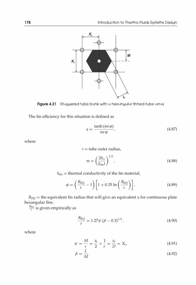
JWST229-c04 JWST229-McDonald Printer: Yet to Come July 31, 2012 12:14 Trim: 244mm × 168mm
178 Introduction to Thermo-Fluids Systems Design
Figure 4.21 Staggered tube bank with a hexangular finned-tube array
The fin efficiency for this situation is defined as
η = tanh (mrφ)mrφ
, (4.87)
where
r = tube outer radius,
m =(
2ho
kfint
)1/2
, (4.88)
kfin = thermal conductivity of the fin material,
φ =(
REQ
r− 1
) [1 + 0.35 ln
(REQ
r
)], (4.89)
REQ = the equivalent fin radius that will give an equivalent η for continuous platehexangular fins.
REQ
r is given empirically as
REQ
r= 1.27ψ (β − 0.3)1/2
, (4.90)
where
ψ = Mr
= xt
2× 1
r= xt
D= Xt, (4.91)
β = LM
. (4.92)
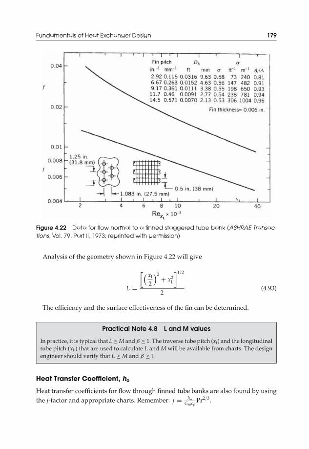
JWST229-c04 JWST229-McDonald Printer: Yet to Come July 31, 2012 12:14 Trim: 244mm × 168mm
Fundamentals of Heat Exchanger Design 179
Figure 4.22 Data for flow normal to a finned staggered tube bank (ASHRAE Transac-tions, Vol. 79, Part II, 1973; reprinted with permission)
Analysis of the geometry shown in Figure 4.22 will give
L =
[( xt
2
)2+ x2
L
]1/2
2. (4.93)
The efficiency and the surface effectiveness of the fin can be determined.
Practical Note 4.8 L and M values
In practice, it is typical that L ≥ M and β ≥ 1. The traverse tube pitch (xt) and the longitudinaltube pitch (xL) that are used to calculate L and M will be available from charts. The designengineer should verify that L ≥ M and β ≥ 1.
Heat Transfer Coefficient, ho
Heat transfer coefficients for flow through finned tube banks are also found by usingthe j-factor and appropriate charts. Remember: j = ho
GmcpPr2/3.
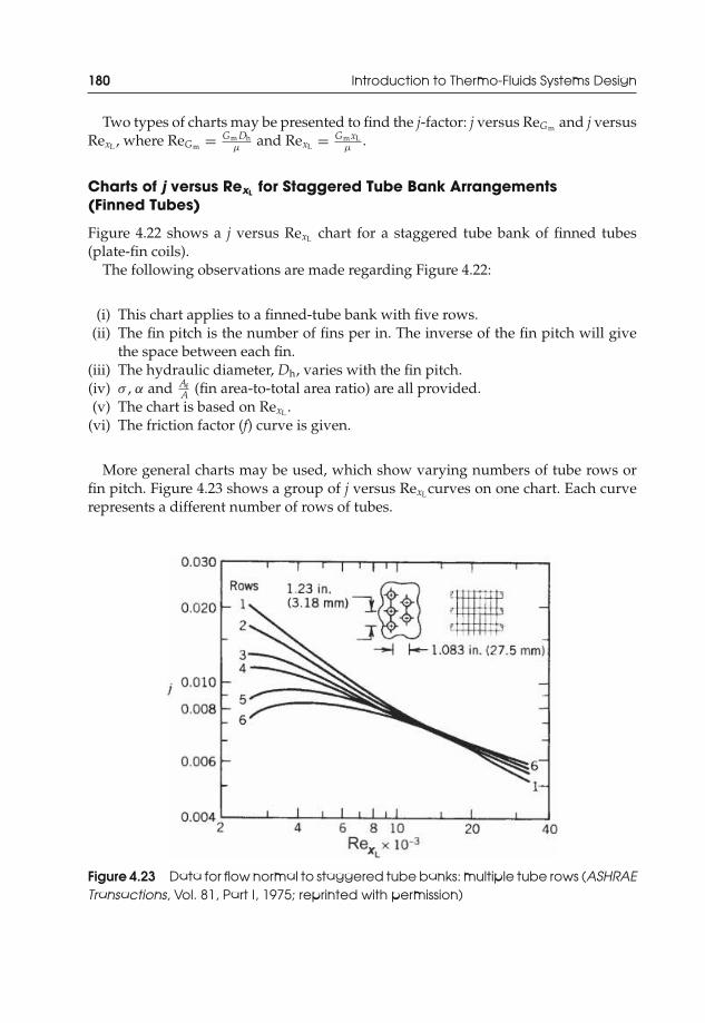
JWST229-c04 JWST229-McDonald Printer: Yet to Come July 31, 2012 12:14 Trim: 244mm × 168mm
180 Introduction to Thermo-Fluids Systems Design
Two types of charts may be presented to find the j-factor: j versus ReGm and j versusRexL , where ReGm = Gm Dh
μand RexL = GmxL
μ.
Charts of j versus RexL for Staggered Tube Bank Arrangements(Finned Tubes)
Figure 4.22 shows a j versus RexL chart for a staggered tube bank of finned tubes(plate-fin coils).
The following observations are made regarding Figure 4.22:
(i) This chart applies to a finned-tube bank with five rows.(ii) The fin pitch is the number of fins per in. The inverse of the fin pitch will give
the space between each fin.(iii) The hydraulic diameter, Dh, varies with the fin pitch.(iv) σ , α and Af
A (fin area-to-total area ratio) are all provided.(v) The chart is based on RexL .
(vi) The friction factor (f) curve is given.
More general charts may be used, which show varying numbers of tube rows orfin pitch. Figure 4.23 shows a group of j versus RexL curves on one chart. Each curverepresents a different number of rows of tubes.
Figure 4.23 Data for flow normal to staggered tube banks: multiple tube rows (ASHRAETransactions, Vol. 81, Part I, 1975; reprinted with permission)

JWST229-c04 JWST229-McDonald Printer: Yet to Come July 31, 2012 12:14 Trim: 244mm × 168mm
Fundamentals of Heat Exchanger Design 181
The following observations are made regarding Figure 4.23. Additional charts areavailable in Appendix C:
(i) This chart applies to various numbers of tube rows.(ii) There are large deviations in the j-factor for low values of RexL .
(iii) At about RexL≈ 8000, the j-factor becomes approximately independent of thenumber of rows.
(iv) Hence, for RexL> 8000, any chart or curve may be used independently of thenumber of rows for other specified data such as tube diameter, fin pitch, σ , α,and Af
A .
Example 4.3 Design of a Heating Coil Heat Exchangerc/w Finned Tubes
Mr. Chin is concerned about the large pressure drops across the bare tube bank, and hasdecided that he would prefer a small heating coil c/w finned tubes for his fresh air in-takeduct line. A HVAC engineer had presented the following duty for the coil:
(i) Heat fresh air from 50 to about 100◦F.(ii) Duct airflow rate is 2000 cfm.
(iii) Entering hot water temperature is about 150◦F.(iv) This is a low-velocity duct section.(v) Water connections must be on the same end of the coil system to facilitate easy instal-
lation and to approach a counter flow heat exchanger system.
Further Information: This design problem should address and present the following points:
(i) Exit water temperature(ii) Heating coil configuration, number of coils, fin pitch
(iii) Final dimensions of the heat exchanger (length, width, and depth)(iv) Pressure loss for the airflow through the coil bank(v) Head loss in the waterside of the tube
Possible Solution
Definition
Design a heating coil complete with finned tubes to heat fresh air in a duct line.
Preliminary Specifications and Constraints
Same as Example 4.2, in addition to
(i) finned-tube heating coils required by the client.

JWST229-c04 JWST229-McDonald Printer: Yet to Come July 31, 2012 12:14 Trim: 244mm × 168mm
182 Introduction to Thermo-Fluids Systems Design
Detailed Design
Objective
To determine the coil configuration, number of coils, size, and performance of a heat ex-changer that has finned tubes.
Data Given or Known
(i) Same as Example 4.2.
Assumptions/Limitations/Constraints
(i) Same as Example 4.2, in addition to/except.(ii) Let the tube outside diameter be 0.676 in. After studying the data in Table A.6, assume
that the tube thickness is 0.04 in.(iii) The tubes longitudinal pitch is 1.75 in. A large pitch is chosen (close to 1 in.) to reduce
possible pressure losses on the air side.(iv) Let the fin material be aluminum. This material is typically used in industry for the
fabrication of fins for heating or cooling coils. Copper could also be used.(v) Assume 7.75 fins per inch.
Sketch
A sketch has been provided with the problem preamble. The sketch will be modified toshow the tube flow circuitry after the design.
Analysis
Determine the overall heat transfer coefficient (UFT)
The ε-NTU method will be used in this design. To determine the effectiveness and NTU,the overall heat transfer coefficient (UFT) must be determined first. The overall heat transfercoefficient for finned tubes is
1UFT
= 1hi (Ai/Ao)
+ Rfi
(Ai/Ao)+ Rfo + 1
hoηso.
The heat transfer coefficient for flow in the tube is found from the Dittus–Boelter corre-lation equation:
Nu = hi Di
k= 0.023Re0.8
DiPr0.3.
Appropriate properties for the determination of ReD and Pr will be found at 145◦F (seeExample 4.2). The inner diameter of the copper tube is approximately 0.596 in.
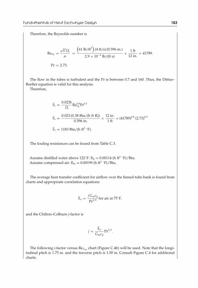
JWST229-c04 JWST229-McDonald Printer: Yet to Come July 31, 2012 12:14 Trim: 244mm × 168mm
Fundamentals of Heat Exchanger Design 183
Therefore, the Reynolds number is
ReDi = ρVDi
μ=
(61 lb/ft3
)(4 ft/s) (0.596 in.)
2.9 × 10⁻⁴ lb/(ft s)× 1 ft
12 in.= 41789.
Pr = 2.73.
The flow in the tubes is turbulent and the Pr is between 0.7 and 160. Thus, the Dittus–Boelter equation is valid for this analysis.
Therefore,
hi = 0.023kDi
Re0.8Di
Pr0.3
hi = 0.023 (0.38 Btu/(h ft R))0.596 in.
× 12 in.
1 ft× (41789)0.8 (2.73)0.3
hi = 1183 Btu/(h ft2 ◦F).
The fouling resistances can be found from Table C.3.
Assume distilled water above 122◦F: Rfi = 0.00114 (h ft2 ◦F)/Btu.Assume compressed air: Rfo = 0.00199 (h ft2 ◦F)/Btu.
The average heat transfer coefficient for airflow over the finned-tube bank is found fromcharts and appropriate correlation equations:
ho = jGmcp
Pr2/3 for air at 75◦F,
and the Chilton–Colburn j-factor is
j = ho
GmcpPr2/3.
The following j-factor versus ReGm chart (Figure C.4b) will be used. Note that the longi-tudinal pitch is 1.75 in. and the traverse pitch is 1.50 in. Consult Figure C.4 for additionalcharts.
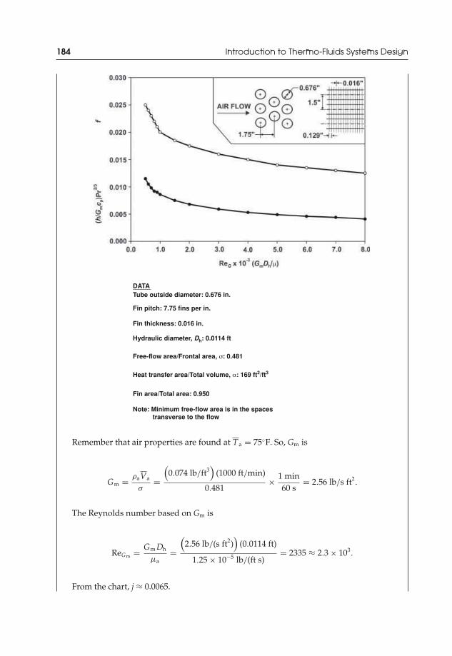
JWST229-c04 JWST229-McDonald Printer: Yet to Come July 31, 2012 12:14 Trim: 244mm × 168mm
184 Introduction to Thermo-Fluids Systems Design
DATATube outside diameter: 0.676 in.
Hydraulic diameter, Dh: 0.0114 ft
Free-flow area/Frontal area, σ: 0.481
Heat transfer area/Total volume, α: 169 ft2/ft3
Fin area/Total area: 0.950
Fin thickness: 0.016 in.
Fin pitch: 7.75 fins per in.
Note: Minimum free-flow area is in the spaces transverse to the flow
Remember that air properties are found at Ta = 75◦F. So, Gm is
Gm = ρaVa
σ=
(0.074 lb/ft3
)(1000 ft/min)
0.481× 1 min
60 s= 2.56 lb/s ft2
.
The Reynolds number based on Gm is
ReGm = Gm Dh
μa=
(2.56 lb/(s ft2)
)(0.0114 ft)
1.25 × 10⁻⁵ lb/(ft s)= 2335 ≈ 2.3 × 10³.
From the chart, j ≈ 0.0065.
JWST229-c04 JWST229-McDonald Printer: Yet to Come July 31, 2012 12:14 Trim: 244mm × 168mm
Fundamentals of Heat Exchanger Design 185
Therefore,
ho =(0.0065)
(2.56 lb/(s ft2)
)(0.24 Btu/(lb ◦F))
(0.73)2/3 × 3600 s1 h
ho = 17.7 Btu/(h ft2 ◦F).
As expected, the heat transfer coefficient of the liquid water is higher than that of gaseousair.
The fin surface effectiveness is
ηso = 1 − Afin
A(1 − ηo) .
The fin efficiency is
ηo = tan h (mrφ)mrφ
.
For aluminum, kfin = 100 Btu/(h ft ◦F). For the fins, the thickness is t = 0.016 in., asobtained from the j-factor versus ReGm chart. Thus,
m =(2ho
)1/2
(kfint)1/2 =
⎡⎢⎢⎣ 2
(17.7 Btu/(h ft2 ◦F)
)(100 Btu/(h ft ◦F)) (0.016 in.)
(1 ft
12 in.
)⎤⎥⎥⎦
1/2
= 16.3 ft−1
The tube outer radius is
r = 0.676 in.
2× 1 ft
12 in.= 0.0282 ft.
Find φ.
φ =(
REQ
r− 1
)[1 + 0.35 ln
(REQ
r
)]REQ
r= 1.27ψ (β − 0.3)1/2
ψ = Mr
= xt
2× 1
r= xt
Do= Xt = 1.50 in.
0.676 in.= 2.22
β = LM
M = xt
2= 1.50 in.
2= 0.75 in.
L =
[( xt
2
)2+ x2
L
]1/2
2=
[(1.50 in.
2
)2
+ (1.75 in.)2
]1/2
2= 0.952 in.

JWST229-c04 JWST229-McDonald Printer: Yet to Come July 31, 2012 12:14 Trim: 244mm × 168mm
186 Introduction to Thermo-Fluids Systems Design
Thus,
β = 0.952 in.
0.750 in.= 1.27.
Note that L ≥ M and β ≥ 1, as observed in practice.Therefore,
REQ
r= 1.27 (2.22) (1.27 − 0.3)1/2 = 2.78.
φ = (2.78 − 1) [1 + 0.35 ln (2.78)] = 2.42.
The fin efficiency is
ηo =tanh
(16.3 ft−1 × 0.0282 ft × 2.42
)16.3 ft−1 × 0.0282 ft × 2.42
= 0.724.
Thus, the fin effectiveness is
ηso = 1 − 0.950 (1 − 0.724) = 0.737.
Find the AiAo
ratio. Remember that α = Ao�
. From the j-factor versus ReGm chart, α =169 ft2/ft3. Assume that the tubes fill the volume bounded by xtxLLtube. Hence,
Ai
�≈ π Di L tube
xtxL L tube= π Di
xtxL
Ai
Ao≈
(Ai
�
)(
Ao
�
) ≈π Di
xtxL
α= π Di
αxtxL
Ai
Ao≈ π (0.596 in.)(
169 ft2/ft3
)(1.50 in.) (1.75 in.)
× 12 in.
1 ft= 0.0507.
The overall heat transfer coefficient is
1UFT
= 1(1183 Btu/(h ft2 ◦F)
)(0.0507)
+(
0.001140.0507
+ 0.00199)
(h ft2 ◦F)/Btu
+ 1(17.7 (h ft2 ◦F)/Btu
)(0.737)
1U
= 0.118 (h ft2 ◦F)/Btu
U = 8.49 Btu/(h ft2 ◦F)
JWST229-c04 JWST229-McDonald Printer: Yet to Come July 31, 2012 12:14 Trim: 244mm × 168mm
Fundamentals of Heat Exchanger Design 187
Determine the configuration, number of coils, and dimensions of the heat exchanger. Find thetotal surface area of the tubes by using the ε-NTU method:
Ao = CminNTUU
.
From Example 4.2,
Ca = Cc = Cmin = 35.5 Btu/(min ◦F)
Cw = Ch = Cmax = 177.5 Btu/(min ◦F)
c = 0.20
ε = 0.50
Q = 1775 Btu/min = 106500 Btu/h
NTU ≈ 0.75.
The heat transfer surface area is
Ao = (35.5 Btu/(min ◦F)) (0.75)
8.49 Btu/(h ft2 ◦F)× 60 min
1 h
Ao = 188 ft2.
This value for the heat transfer surface area includes the extended surface area of the fins.The total heat transfer volume is found from the ratio of the heat transfer area to the total
volume:
α = Ao
�.
Therefore,
� = Ao
α= 188 ft2
169 ft2/ft3 = 1.11 ft3
.
The depth of the heat exchanger system (dimension in the direction of airflow) is
W = �
Af.
Af is the face area normal to the airflow direction, and is equal to 2 ft2.Therefore,
W = 1.11 ft3
2 ft2 × 12 in.
1 ft
W = 6.7 in. ≈ 7 in.
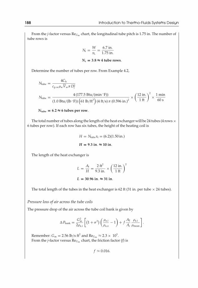
JWST229-c04 JWST229-McDonald Printer: Yet to Come July 31, 2012 12:14 Trim: 244mm × 168mm
188 Introduction to Thermo-Fluids Systems Design
From the j-factor versus ReGm chart, the longitudinal tube pitch is 1.75 in. The number oftube rows is
Nr = WxL
= 6.7 in.
1.75 in.
Nr = 3.8 ≈ 4 tube rows.
Determine the number of tubes per row. From Example 4.2,
Ntube = 4Ch
cp,wρwVwπ D2i
Ntube = 4 (177.5 Btu/(min ◦F))
(1.0 Btu/(lb ◦F))(
61 lb/ft3)
(4 ft/s) π (0.596 in.)2×
(12 in.
1 ft
)2
× 1 min60 s
Ntube = 6.2 ≈ 6 tubes per row.
The total number of tubes along the length of the heat exchanger will be 24 tubes (4 rows ×6 tubes per row). If each row has six tubes, the height of the heating coil is
H = Ntubext = (6.2)(1.50 in.)
H = 9.3 in. ≈ 10 in.
The length of the heat exchanger is
L = Af
H= 2 ft2
9.3 in.×
(12 in.
1 ft
)2
L = 30.96 in. ≈ 31 in.
The total length of the tubes in the heat exchanger is 62 ft (31 in. per tube × 24 tubes).
Pressure loss of air across the tube coils
The pressure drop of the air across the tube coil bank is given by
�Pbank = G2m
2ρa,i
[(1 + σ 2) (
ρa,i
ρa,o− 1
)+ f
AT
Ac
ρa,i
ρmean
].
Remember: Gm = 2.56 lb/s ft2 and ReGm ≈ 2.3 × 10³.From the j-factor versus ReGm chart, the friction factor (f) is
f ≈ 0.016.

JWST229-c04 JWST229-McDonald Printer: Yet to Come July 31, 2012 12:14 Trim: 244mm × 168mm
Fundamentals of Heat Exchanger Design 189
The area ratio is
AT
Ac= 4W
Dh= 4 (6.7 in.)
0.0114 ft× 1 ft
12 in.= 195.9.
From Example 4.2, the mean density (ρmean) is ρmean = 0.075 lb/ft3. From the j-factorversus ReGm chart, σ = 0.481.
Therefore,
�Pbank = (2.56 lb/(s ft2))2
2(0.078 lb/ft3)
[(1 + 0.4812) (
0.078 lb/ft3
0.071 lb/ft3 − 1
)+ (0.016) (195.9)
0.078 lb/ft3
0.075 lb/ft3
]
�Pbank = 142 lb/ft s2 × 1 lbf
32.2 lb ft/s2 = 4.4 lbf/ft2 = 4.4 psf.
In practice, the pressure drop is reported in inches of water. Therefore,
�Pbank = 142 lb/ft s2 × 1
0.075 lb/ft3 × 1
32.2 ft/s2 = 58.8 ft of air
�Pbank = 58.8 ft of air × SGair,75◦F = 58.8 ft of air × 0.075 lb/ft3
62 lb/ft3 × 12 in.
1 ft
�Pbank = 0.85 in. of water = 0.85 in. wg.
Pressure loss of water in the tube coils
Determination of the pressure loss of the water in the tubes is needed to find the pumppower required to move the fluid through the heat exchanger system. The total head loss is
HlT =(
fL tube
Di+ K
)V
2w
2g.
From the Moody chart, for ReDi = 41789 and for copper tubes with relative roughness,ε
Di= 0.0001, the friction factor is f ≈ 0.022.For the primary piping circuitry through the heat exchanger, there are four tube rows,
including 1 supply run and 1 return run, each 31 in. long.Therefore,
L tube = (4 rows)(31 in. per row) = 124 in. = 10.3 ft.
For the minor losses, K = 2.0 for the soldered/brazed 180◦ return bends.Hence,
HlT =(
(0.022)124 in.
0.596 in.+ (3) (2.0)
)(4 ft/s)2
2(
32.2 ft/s2)
H lT = 2.6 ft wg.
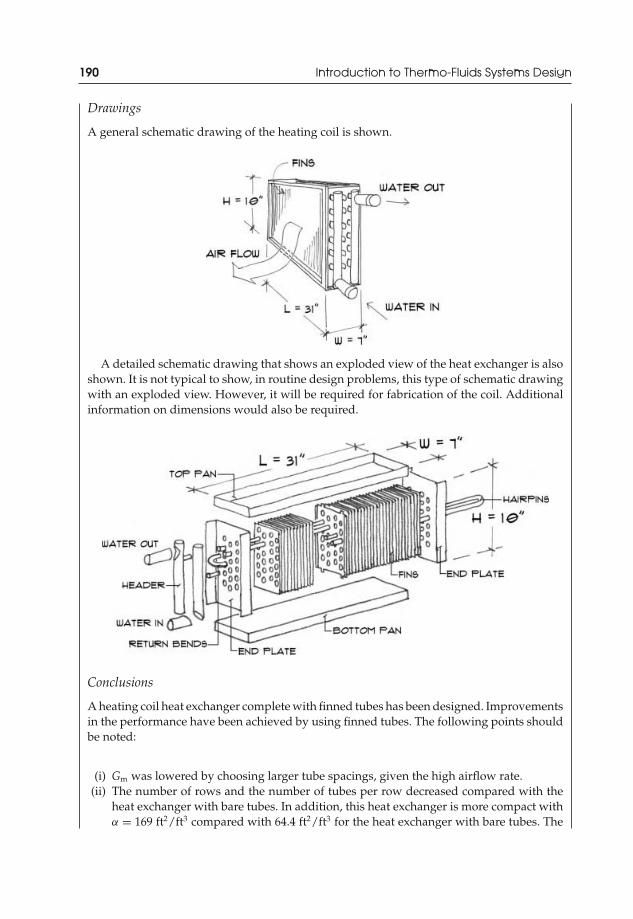
JWST229-c04 JWST229-McDonald Printer: Yet to Come July 31, 2012 12:14 Trim: 244mm × 168mm
190 Introduction to Thermo-Fluids Systems Design
Drawings
A general schematic drawing of the heating coil is shown.
A detailed schematic drawing that shows an exploded view of the heat exchanger is alsoshown. It is not typical to show, in routine design problems, this type of schematic drawingwith an exploded view. However, it will be required for fabrication of the coil. Additionalinformation on dimensions would also be required.
Conclusions
A heating coil heat exchanger complete with finned tubes has been designed. Improvementsin the performance have been achieved by using finned tubes. The following points shouldbe noted:
(i) Gm was lowered by choosing larger tube spacings, given the high airflow rate.(ii) The number of rows and the number of tubes per row decreased compared with the
heat exchanger with bare tubes. In addition, this heat exchanger is more compact withα = 169 ft2/ft3 compared with 64.4 ft2/ft3 for the heat exchanger with bare tubes. The

JWST229-c04 JWST229-McDonald Printer: Yet to Come July 31, 2012 12:14 Trim: 244mm × 168mm
Fundamentals of Heat Exchanger Design 191
total length of tube required decreased from 410 ft in the bare tube heat exchangerdesign to 62 ft in the finned-tube heat exchanger.
(iii) The calculated value of Nr was 3.8. It was assumed that Nr was equal to 4. However,the calculated value of Ntube was 6.2. It was assumed that Ntube was equal to 6. Whileit is typical to increase to the next whole number for more conservative designs, thecompromise between Nr and Ntube should mitigate any significant error.
(iv) Lower pressure drop of the air across the tube bank was achieved. In particular, thepressure drop was on the order of 1 in. wg.
(v) The use of headers in this design resulted in low total head loss in the heating coilpiping.
A heat exchanger design data sheet is shown in the following table.
Heat Exchanger Design Data Sheet
Type Counter Flow
Section: Tube BankWorking fluid AirVolume flow rate 2000 cfmInlet temperature 50◦FOutlet temperature 100◦FPressure drop 0.85 in. wg
Section: TubeTube material CopperWorking fluid WaterVelocity 4 ft/sTube inner diameter 0.596 in.Tube outer diameter 0.676 in.Number of tube rows 4Number of tubes per row 6Tube spacing (xt × xL) 1.50 in. × 1.75 in.Total tube length 62 ftInlet temperature 150◦FOutlet temperature 140◦FHead loss 2.6 ft wgFin material AluminumFin pitch 7.75 fins per in.Fin thickness 0.016 in.
Heat Exchanger ParametersThermal capacity 106500 Btu/hEffectiveness 0.50Capacity ratio 0.20Overall heat transfer coefficient 8.49 Btu/(h ft2 ◦F)Number of transfer units (NTU) 0.75Heat exchanger dimensions (L × H × W) 31 in. × 10 in. × 7 in.

JWST229-c04 JWST229-McDonald Printer: Yet to Come July 31, 2012 12:14 Trim: 244mm × 168mm
192 Introduction to Thermo-Fluids Systems Design
Example 4.4 Performance of an Oil Cooler
An oil cooler has been designed for use in a factory. The cooler has one tube inlet and onetube outlet into and out of a tube bank, respectively, to form an oil recycling system. Clean,unused engine oil is circulated through 1/2-in. tubes that are connected with continuous-plate fins with a fin pitch of 8 fins per in. Cool air is forced over the tubes. The systemoperates under the following conditions:
(i) Four rows of tubes(ii) Six tubes per row
(iii) Width is 26 in.(iv) Fin thickness is 0.006 in.(v) Entering air temperature is 65◦F
(vi) Coil face velocity is 650 ft/min(vii) Entering engine oil temperature is 150◦F
The design engineer who designed the original system used the following chart to aid inthe design:
Source: ASHRAE Transactions, Vol. 79, Part II, 1973 (Reprinted with permission)
Analyze the performance of the oil cooler and comment on the design.
Possible Solution
Definition
Analyze the performance of a finned-tube oil cooler (heat exchanger).
JWST229-c04 JWST229-McDonald Printer: Yet to Come July 31, 2012 12:14 Trim: 244mm × 168mm
Fundamentals of Heat Exchanger Design 193
Preliminary Specifications and Constraints
(i) The oil cooler is a heat exchanger with one tube inlet and one tube outlet.(ii) The working fluid in the tubes is clean, unused engine oil.
(iii) The working fluid outside the tubes is cool air.(iv) The tubes have a nominal diameter of 1/2 in.(v) This is a finned-tube heat exchanger with a fin pitch of 8 fins per in.
(vi) Additional specifications are given in the problem preamble.
Detailed Design
Objective
To determine the thermal capacity, outlet temperatures, and pressure drops in a finned-tubeoil cooler.
Data Given or Known
(i) The working fluid in the tubes is clean, unused engine oil.(ii) The working fluid outside the tubes is cool air.
(iii) The tubes have a nominal diameter of 1/2 in.(iv) This is a finned-tube heat exchanger with a fin pitch of 8 fins per in. and fin thickness
of 0.006 in.(v) There are four rows of tubes with six tubes per row.
(vi) The width of the oil cooler is 26 in.(vii) The coil velocity (of air) is 650 fpm.
(viii) The entering air temperature is 65◦F.(ix) The entering engine oil temperature is 150◦F.(x) A j-factor vs RexL chart was provided.
Assumptions/Limitations/Constraints
(i) Let the tube material be Type L copper. Copper has high heat transfer properties.(ii) Let the fin material be aluminum. This material is typically for the fabrication of fins
for heating or cooling coils.(iii) Let the flow velocity of engine oil in the copper tubes be 3 fps. This velocity is lower
than the erosion limit of copper with unused engine oil (≈7 fps calculated for “OtherLiquids” from Table A.13). A low tube velocity is desired since engine oil is highlyviscous at lower temperatures. As the engine oil cools, its viscosity will increase, andit will require higher pump power to move through the coils.
(iv) The tube thickness is approximately 0.04 in (see Table A.6). It will be assumed thatthe tube wall thickness is negligible compared to the inner and outer diameters.
(v) The return bends will be soldered 180◦ return bends (regular).(vi) There is negligible elevation head. Assume that all the components are on the same
level.(vii) Entrance and exit losses of the air over the coils will be negligible compared to other
losses across the coils.(viii) This is a counter flow arrangement. The inlet and exit of the coils are on the same side
of the cooler.

JWST229-c04 JWST229-McDonald Printer: Yet to Come July 31, 2012 12:14 Trim: 244mm × 168mm
194 Introduction to Thermo-Fluids Systems Design
Sketch
A sketch is not needed for this performance analysis.
Performance Analysis
Determine the overall heat transfer coefficient (UFT)
The ε-NTU method will be used in this performance problem. To determine the effectivenessand NTU, the overall heat transfer coefficient (UFT) must be determined first. The overallheat transfer coefficient for finned tubes is
1UFT
= 1hi (Ai/Ao)
+ Rfi
(Ai/Ao)+ Rfo + 1
hoηso.
Appropriate engine oil properties for the determination of ReD and Pr will be found at150◦F. Note that the average temperature should be used, rather than the entering tem-perature. This will introduce a small error in the analysis. This will be verified. The innerdiameter of the copper tube is approximately 0.545 in. (Table A.6).
The Reynolds number is
ReDi = ρVDi
μ=
(53.73 lb/ft3
)(3 ft/s) (0.545 in.)
3.833 × 10⁻² lb/(fts)× 1 ft
12 in.= 191.
The Prandtl number is
Pr = 848.3.
Assuming a constant surface heat flux from the tubes, and since the flow is laminar, theNusselt number and heat transfer coefficient for flow in the tube is
Nu = hi Di
k= 4.36
hi = 4.36kDi
hi = 4.36 (0.08046 Btu/(h ft R))0.545 in.
× 12 in.
1 ft= 7.724 Btu/(h ft R) = 7.724 Btu/(h ft ◦F).
The fouling resistances can be found from Table C.3.
For clean, unused engine oil: Rfi = 0.Assume compressed air: Rfo = 0.00199 (h ft2 ◦F)/Btu.
The average heat transfer coefficient for airflow over the finned-tube bank is found fromcharts and appropriate correlation equations:
ho = jGmcp
Pr2/3 for air at 65◦F,
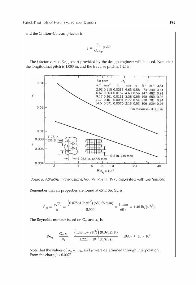
JWST229-c04 JWST229-McDonald Printer: Yet to Come July 31, 2012 12:14 Trim: 244mm × 168mm
Fundamentals of Heat Exchanger Design 195
and the Chilton–Colburn j-factor is
j = ho
GmcpPr2/3.
The j-factor versus ReGm chart provided by the design engineer will be used. Note thatthe longitudinal pitch is 1.083 in. and the traverse pitch is 1.25 in.
Source: ASHRAE Transactions, Vol. 79, Part II, 1973 (reprinted with permission).
Remember that air properties are found at 65◦F. So, Gm is
Gm = ρaVa
σ=
(0.07561 lb/ft3
)(650 ft/min)
0.555× 1 min
60 s= 1.48 lb/(s ft2).
The Reynolds number based on Gm and xL is
RexL = GmxL
μa=
(1.48 lb/(s ft2)
)(0.09025 ft)
1.221 × 10⁻⁵ lb/(ft s)= 10939 ≈ 11 × 103.
Note that the values of ρa, σ , Dh, and μ were determined through interpolation.From the chart, j ≈ 0.0073.
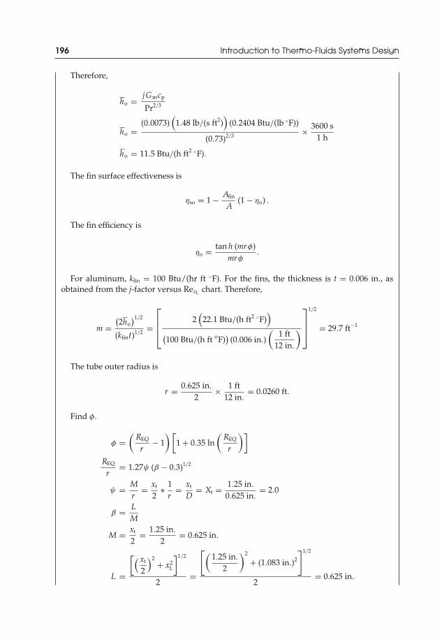
JWST229-c04 JWST229-McDonald Printer: Yet to Come July 31, 2012 12:14 Trim: 244mm × 168mm
196 Introduction to Thermo-Fluids Systems Design
Therefore,
ho = jGmcp
Pr2/3
ho =(0.0073)
(1.48 lb/(s ft2)
)(0.2404 Btu/(lb ◦F))
(0.73)2/3 × 3600 s1 h
ho = 11.5 Btu/(h ft2 ◦F).
The fin surface effectiveness is
ηso = 1 − Afin
A(1 − ηo) .
The fin efficiency is
ηo = tan h (mrφ)mrφ
.
For aluminum, kfin = 100 Btu/(hr ft ◦F). For the fins, the thickness is t = 0.006 in., asobtained from the j-factor versus RexL chart. Therefore,
m =(2ho
)1/2
(kfint)1/2 =
⎡⎢⎢⎣ 2
(22.1 Btu/(h ft2 ◦F)
)(100 Btu/(h ft oF)
)(0.006 in.)
(1 ft
12 in.
)⎤⎥⎥⎦
1/2
= 29.7 ft−1
The tube outer radius is
r = 0.625 in.
2× 1 ft
12 in.= 0.0260 ft.
Find φ.
φ =(
REQ
r− 1
)[1 + 0.35 ln
(REQ
r
)]REQ
r= 1.27ψ (β − 0.3)1/2
ψ = Mr
= xt
2∗ 1
r= xt
D= Xt = 1.25 in.
0.625 in.= 2.0
β = LM
M = xt
2= 1.25 in.
2= 0.625 in.
L =
[( xt
2
)2+ x2
L
]1/2
2=
[(1.25 in.
2
)2
+ (1.083 in.)2
]1/2
2= 0.625 in.
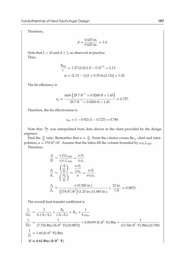
JWST229-c04 JWST229-McDonald Printer: Yet to Come July 31, 2012 12:14 Trim: 244mm × 168mm
Fundamentals of Heat Exchanger Design 197
Therefore,
β = 0.625 in.
0.625 in.= 1.0.
Note that L ≥ M and β ≥ 1, as observed in practice.Thus,
REQ
r= 1.27 (2.0) (1.0 − 0.3)1/2 = 2.13.
φ = (2.13 − 1) [1 + 0.35 ln (2.13)] = 1.43.
The fin efficiency is
ηo =tanh
(29.7 ft−1 × 0.0260 ft × 1.43
)29.7 ft−1 × 0.0260 ft × 1.43
= 0.727.
Therefore, the fin effectiveness is
ηso = 1 − 0.921 (1 − 0.727) = 0.749.
Note that AfinA was interpolated from data shown in the chart provided by the design
engineer.Find the Ai
Aoratio. Remember that α = Ao
�. From the j-factor versus RexL chart and inter-
polation, α = 174 ft2/ft3. Assume that the tubes fill the volume bounded by xtxLLtube.Therefore,
Ai
�≈ π Di L tube
xtxL L tube= π Di
xtxL
Ai
Ao≈
(Ai
�
)(
Ao
�
) ≈π Di
xtxL
α= π Di
αxtxL
Ai
Ao≈ π (0.545 in.)(
174 ft2/ft3
)(1.25 in.) (1.083 in.)
× 12 in.
1 ft= 0.0872.
The overall heat transfer coefficient is
1UFT
= 1hi (Ai/Ao)
+ Rfi
(Ai/Ao)+ Rfo + 1
hoηso
1UFT
= 1
(7.724 Btu/(h ft2 ◦F)) (0.0872)+ 0.00199 (h ft2 ◦F)/Btu + 1
(11.5(h ft2 ◦F)/Btu) (0.749)
1U
= 1.60 (h ft2 ◦F)/Btu
U = 0.62 Btu/(h ft2 ◦F).
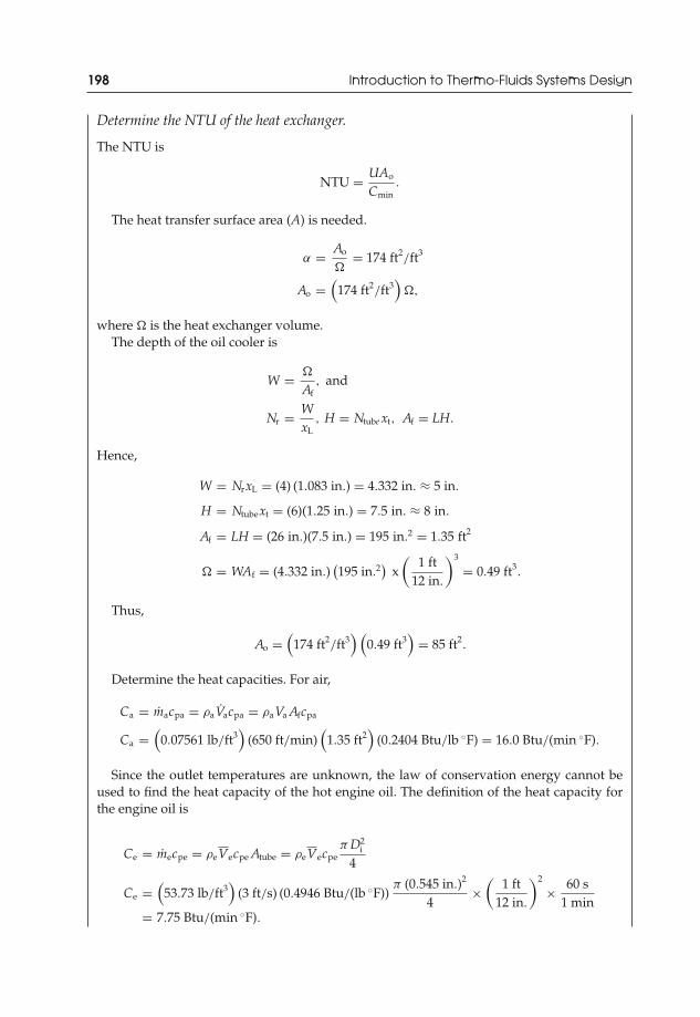
JWST229-c04 JWST229-McDonald Printer: Yet to Come July 31, 2012 12:14 Trim: 244mm × 168mm
198 Introduction to Thermo-Fluids Systems Design
Determine the NTU of the heat exchanger.
The NTU is
NTU = UAo
Cmin.
The heat transfer surface area (A) is needed.
α = Ao
�= 174 ft2
/ft3
Ao =(
174 ft2/ft3
)�,
where � is the heat exchanger volume.The depth of the oil cooler is
W = �
Af, and
Nr = WxL
, H = Ntube xt, Af = LH.
Hence,
W = NrxL = (4) (1.083 in.) = 4.332 in. ≈ 5 in.
H = Ntubext = (6)(1.25 in.) = 7.5 in. ≈ 8 in.
Af = LH = (26 in.)(7.5 in.) = 195 in.2 = 1.35 ft2
� = WAf = (4.332 in.)(195 in.2
)x
(1 ft
12 in.
)3
= 0.49 ft3.
Thus,
Ao =(
174 ft2/ft3
) (0.49 ft3
)= 85 ft2
.
Determine the heat capacities. For air,
Ca = macpa = ρaVacpa = ρaVa Afcpa
Ca =(
0.07561 lb/ft3)
(650 ft/min)(
1.35 ft2)
(0.2404 Btu/lb ◦F) = 16.0 Btu/(min ◦F).
Since the outlet temperatures are unknown, the law of conservation energy cannot beused to find the heat capacity of the hot engine oil. The definition of the heat capacity forthe engine oil is
Ce = mecpe = ρeVecpe Atube = ρeVecpeπ D2
i
4
Ce =(
53.73 lb/ft3)
(3 ft/s) (0.4946 Btu/(lb ◦F))π (0.545 in.)2
4×
(1 ft
12 in.
)2
× 60 s1 min
= 7.75 Btu/(min ◦F).

JWST229-c04 JWST229-McDonald Printer: Yet to Come July 31, 2012 12:14 Trim: 244mm × 168mm
Fundamentals of Heat Exchanger Design 199
Therefore, Ca = Cc = Cmax and Ce = Ch = Cmin.It should be noted that since there is only one inlet tube connection in this heat exchanger,
it was not necessary to include Ntube in the calculation of Atube.The NTU is
NTU =(
0.62 Btu/(h ft2 ◦F)) (
85 ft2)
7.75 Btu/(min ◦F)× 1 h
60 minNTU = 0.113.
Determine the thermal capacity and outlet temperatures
The thermal capacity and the outlet temperatures can be determined after determination ofthe effectiveness of the oil cooler.
The capacity ratio is
c = Cmin
Cmax= 7.75 Btu/(min ◦F)
16.0 Btu/(min ◦F)= 0.484
c = 0.484.
Therefore,
ε = 1 − exp [−NTU (1 − c)]1 − c exp [−NTU (1 − c)]
ε = 1 − exp [− (0.113) (1 − 0.484)]1 − (0.484) exp [− (0.113) (1 − 0.484)]
ε = 0.104 = 10.4%
The outlet temperature of the air can be determined:
ε = Ca
Cmin
(Ta,o − Ta,i)(Te,i − Ta,i)
Ta,o = Ta,i + εCmin
Ca(Te,i − Ta,i) = 65◦F + (0.104)
7.75 Btu/(min ◦F)16 Btu/(min ◦F)
(150 − 65) ◦F
T a,o = 69.3◦F = 70◦F.
The thermal capacity of the oil cooler is
Q = macpa (Ta,o − Ta,i) = ρaVa Afcpa (Ta,o − Ta,i)
Q = (0.07561 lb/ft3)(650 ft/min)(1.35 ft2) (0.2404 Btu/(lb ◦F)) (70 − 65)◦F × 60 min1 h
Q = 4785 Btu/h.
The outlet temperature of the engine oil can be determined:
Q = mecpe (Te,i − Te,o) = Ce (Te,i − Te,o)
Te,o = Te,i − QCe
= 150◦F − 4785 Btu/h7.75 Btu/(min ◦F)
× 1 h60 min
T e,o = 139.7◦F = 140◦F.
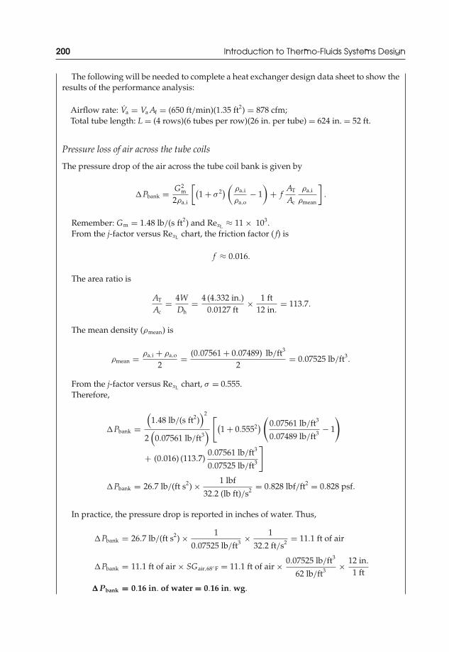
JWST229-c04 JWST229-McDonald Printer: Yet to Come July 31, 2012 12:14 Trim: 244mm × 168mm
200 Introduction to Thermo-Fluids Systems Design
The following will be needed to complete a heat exchanger design data sheet to show theresults of the performance analysis:
Airflow rate: Va = Va Af = (650 ft/min)(1.35 ft2) = 878 cfm;Total tube length: L = (4 rows)(6 tubes per row)(26 in. per tube) = 624 in. = 52 ft.
Pressure loss of air across the tube coils
The pressure drop of the air across the tube coil bank is given by
�Pbank = G2m
2ρa,i
[(1 + σ 2) (
ρa,i
ρa,o− 1
)+ f
AT
Ac
ρa,i
ρmean
].
Remember: Gm = 1.48 lb/(s ft2) and RexL ≈ 11 × 103.From the j-factor versus RexL chart, the friction factor ( f) is
f ≈ 0.016.
The area ratio is
AT
Ac= 4W
Dh= 4 (4.332 in.)
0.0127 ft× 1 ft
12 in.= 113.7.
The mean density (ρmean) is
ρmean = ρa,i + ρa,o
2= (0.07561 + 0.07489) lb/ft3
2= 0.07525 lb/ft3
.
From the j-factor versus RexL chart, σ = 0.555.Therefore,
�Pbank =(
1.48 lb/(s ft2))2
2(
0.07561 lb/ft3)
[(1 + 0.5552) (
0.07561 lb/ft3
0.07489 lb/ft3 − 1
)
+ (0.016) (113.7)0.07561 lb/ft3
0.07525 lb/ft3
]
�Pbank = 26.7 lb/(ft s2) × 1 lbf
32.2 (lb ft)/s2 = 0.828 lbf/ft2 = 0.828 psf.
In practice, the pressure drop is reported in inches of water. Thus,
�Pbank = 26.7 lb/(ft s2) × 1
0.07525 lb/ft3 × 1
32.2 ft/s2 = 11.1 ft of air
�Pbank = 11.1 ft of air × SGair,68◦F = 11.1 ft of air × 0.07525 lb/ft3
62 lb/ft3 × 12 in.
1 ft
�Pbank = 0.16 in. of water = 0.16 in. wg.
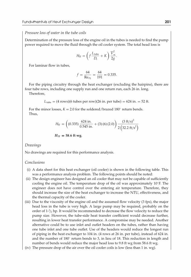
JWST229-c04 JWST229-McDonald Printer: Yet to Come July 31, 2012 12:14 Trim: 244mm × 168mm
Fundamentals of Heat Exchanger Design 201
Pressure loss of water in the tube coils
Determination of the pressure loss of the engine oil in the tubes is needed to find the pumppower required to move the fluid through the oil cooler system. The total head loss is
HlT =(
fL tube
Di+ K
)V
2w
2g.
For laminar flow in tubes,
f = 64ReDi
= 64191
= 0.335.
For the piping circuitry through the heat exchanger (excluding the hairpins), there arefour tube rows, including one supply run and one return run, each 26 in. long.
Therefore,
L tube = (4 rows)(6 tubes per row)(26 in. per tube) = 624 in. = 52 ft.
For the minor losses, K = 2.0 for the soldered/brazed 180◦ return bends.Thus,
HlT =(
(0.335)624 in.
0.545 in.+ (3) (6) (2.0)
)(3 ft/s)2
2(
32.2 ft/s2)
H lT = 58.6 ft wg.
Drawings
No drawings are required for this performance analysis.
Conclusions
(i) A data sheet for this heat exchanger (oil cooler) is shown in the following table. Thiswas a performance analysis problem. The following points should be noted:
(ii) The design engineer has designed an oil cooler that may not be capable of sufficientlycooling the engine oil. The temperature drop of the oil was approximately 10◦F. Theengineer does not have control over the entering air temperature. Therefore, theyshould increase the size of the heat exchanger to increase the NTU, effectiveness, andthe thermal capacity of the cooler.
(iii) Due to the viscosity of the engine oil and the assumed flow velocity (3 fps), the majorhead loss in the tube is very high. A large pump may be required, probably on theorder of 1-1/2 hp. It would be recommended to decrease the flow velocity to reduce thepump size. However, the tube-side heat transfer coefficient would decrease further,resulting in lower heat transfer performance. A compromise may be needed. Anotheralternative could be to use inlet and outlet headers on the tubes, rather than havingone tube inlet and one tube outlet. Use of the headers would reduce the longest runof piping in the heat exchanger to 104 in. (4 rows at 26 in. per tube), instead of 624 in.and the number of 180◦ return bends to 3, in lieu of 18. This reduction in length andnumber of bends would reduce the major head loss to 9.8 ft wg from 58.6 ft wg.
(iv) The pressure drop of the air over the oil cooler coils is low (less than 1 in. wg).
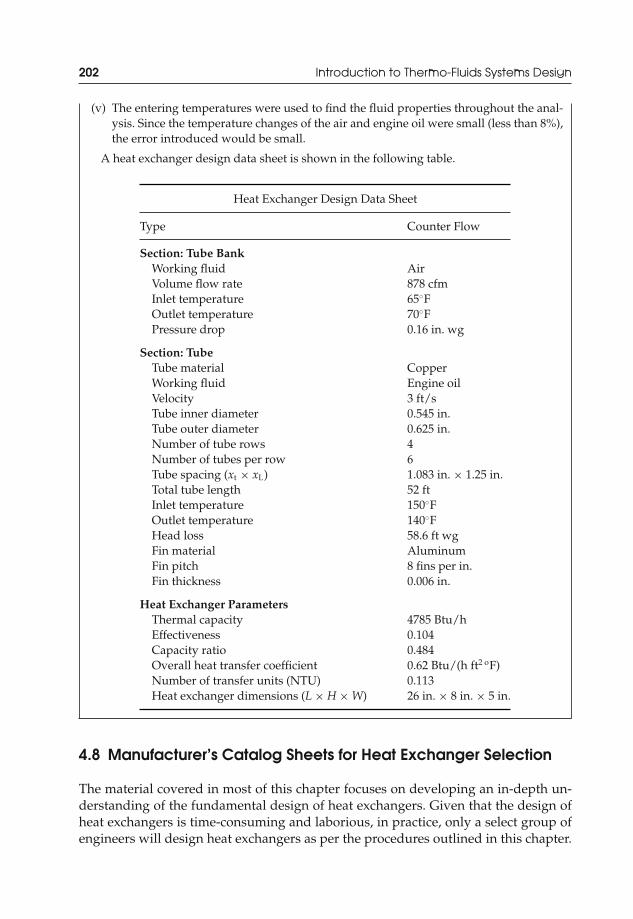
JWST229-c04 JWST229-McDonald Printer: Yet to Come July 31, 2012 12:14 Trim: 244mm × 168mm
202 Introduction to Thermo-Fluids Systems Design
(v) The entering temperatures were used to find the fluid properties throughout the anal-ysis. Since the temperature changes of the air and engine oil were small (less than 8%),the error introduced would be small.
A heat exchanger design data sheet is shown in the following table.
Heat Exchanger Design Data Sheet
Type Counter Flow
Section: Tube BankWorking fluid AirVolume flow rate 878 cfmInlet temperature 65◦FOutlet temperature 70◦FPressure drop 0.16 in. wg
Section: TubeTube material CopperWorking fluid Engine oilVelocity 3 ft/sTube inner diameter 0.545 in.Tube outer diameter 0.625 in.Number of tube rows 4Number of tubes per row 6Tube spacing (xt × xL) 1.083 in. × 1.25 in.Total tube length 52 ftInlet temperature 150◦FOutlet temperature 140◦FHead loss 58.6 ft wgFin material AluminumFin pitch 8 fins per in.Fin thickness 0.006 in.
Heat Exchanger ParametersThermal capacity 4785 Btu/hEffectiveness 0.104Capacity ratio 0.484Overall heat transfer coefficient 0.62 Btu/(h ft2 oF)Number of transfer units (NTU) 0.113Heat exchanger dimensions (L × H × W) 26 in. × 8 in. × 5 in.
4.8 Manufacturer’s Catalog Sheets for Heat Exchanger Selection
The material covered in most of this chapter focuses on developing an in-depth un-derstanding of the fundamental design of heat exchangers. Given that the design ofheat exchangers is time-consuming and laborious, in practice, only a select group ofengineers will design heat exchangers as per the procedures outlined in this chapter.

JWST229-c04 JWST229-McDonald Printer: Yet to Come July 31, 2012 12:14 Trim: 244mm × 168mm
Fundamentals of Heat Exchanger Design 203
Figure 4.24 M series heating coil from Unico, Inc.: (a) page 1 of the M series heatingcoil from Unico, Inc. (Unico, Inc., reprinted with permission); (b) page 2 of the M seriesheating coil from Unico, Inc. (Unico, Inc.; reprinted with permission); (c) page 3 of theM series heating coil from Unico, Inc. (Unico, Inc., reprinted with permission); (d) page4 of the M series heating coil from Unico, Inc. (Unico, Inc.; reprinted with permission)

JWST229-c04 JWST229-McDonald Printer: Yet to Come July 31, 2012 12:14 Trim: 244mm × 168mm
204 Introduction to Thermo-Fluids Systems Design
Figure 4.24 (Continued)

JWST229-c04 JWST229-McDonald Printer: Yet to Come July 31, 2012 12:14 Trim: 244mm × 168mm
Fundamentals of Heat Exchanger Design 205
Figure 4.24 (Continued)

JWST229-c04 JWST229-McDonald Printer: Yet to Come July 31, 2012 12:14 Trim: 244mm × 168mm
206 Introduction to Thermo-Fluids Systems Design
Figure 4.24 (Continued)

JWST229-c04 JWST229-McDonald Printer: Yet to Come July 31, 2012 12:14 Trim: 244mm × 168mm
Fundamentals of Heat Exchanger Design 207
Most design engineers will use manufacturer’s catalog sheets to select a heat ex-changer. The designer would calculate the required thermal capacity, and with otherparameters, an appropriate heat exchanger for the application would be selected. Inpractice, the size (physical dimensions) of the heat exchanger is typically a majorfactor that drives the final selection of a unit.
Figure 4.24 shows four sheets of a heat exchanger selection bulletin for a heat-ing coil model used in high-velocity duct systems. In the bulletin, the manufacturerpresents an overview of their M series heating coil heat exchanger (Figure 4.24a). Inthis overview, the manufacturer describes the construction of the unit, provides a listof the parts, and shows a drawing of the unit. Detailed drawings and specificationson the heating coil and the construction are also provided (Figure 4.24b). The man-ufacturer understands that each design will require different thermal capacities, andhas provided three different models of hot water heating coils, HW-2430 and HW-3660 (Figure 4.24c). Each model is subdivided based on the flow rate of air across theheating coils and the minimum number of outlets from the duct system. The designengineer should note that to determine the heat transfer performance (i.e., thermalcapacity) of the unit, the water flow rate and entering water temperature will need tobe known. The final page of the bulletin (Figure 4.24d) shows pressure drops in andacross the coils for different pipe velocities and airflow rates, respectively.
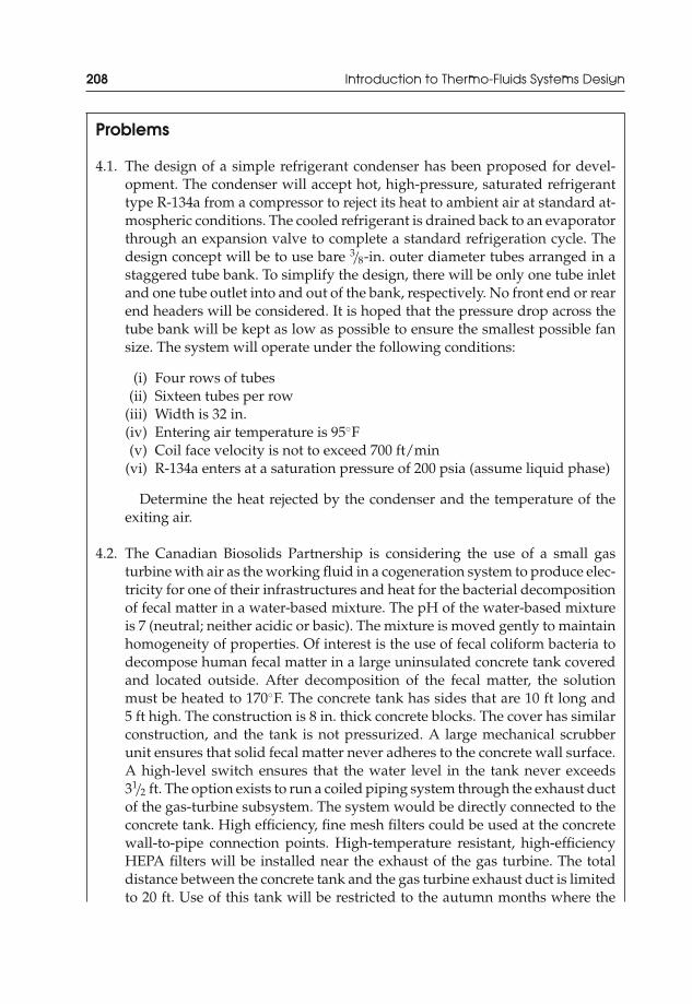
JWST229-c04 JWST229-McDonald Printer: Yet to Come July 31, 2012 12:14 Trim: 244mm × 168mm
208 Introduction to Thermo-Fluids Systems Design
Problems
4.1. The design of a simple refrigerant condenser has been proposed for devel-opment. The condenser will accept hot, high-pressure, saturated refrigeranttype R-134a from a compressor to reject its heat to ambient air at standard at-mospheric conditions. The cooled refrigerant is drained back to an evaporatorthrough an expansion valve to complete a standard refrigeration cycle. Thedesign concept will be to use bare 3/8-in. outer diameter tubes arranged in astaggered tube bank. To simplify the design, there will be only one tube inletand one tube outlet into and out of the bank, respectively. No front end or rearend headers will be considered. It is hoped that the pressure drop across thetube bank will be kept as low as possible to ensure the smallest possible fansize. The system will operate under the following conditions:
(i) Four rows of tubes(ii) Sixteen tubes per row
(iii) Width is 32 in.(iv) Entering air temperature is 95◦F(v) Coil face velocity is not to exceed 700 ft/min
(vi) R-134a enters at a saturation pressure of 200 psia (assume liquid phase)
Determine the heat rejected by the condenser and the temperature of theexiting air.
4.2. The Canadian Biosolids Partnership is considering the use of a small gasturbine with air as the working fluid in a cogeneration system to produce elec-tricity for one of their infrastructures and heat for the bacterial decompositionof fecal matter in a water-based mixture. The pH of the water-based mixtureis 7 (neutral; neither acidic or basic). The mixture is moved gently to maintainhomogeneity of properties. Of interest is the use of fecal coliform bacteria todecompose human fecal matter in a large uninsulated concrete tank coveredand located outside. After decomposition of the fecal matter, the solutionmust be heated to 170◦F. The concrete tank has sides that are 10 ft long and5 ft high. The construction is 8 in. thick concrete blocks. The cover has similarconstruction, and the tank is not pressurized. A large mechanical scrubberunit ensures that solid fecal matter never adheres to the concrete wall surface.A high-level switch ensures that the water level in the tank never exceeds31/2 ft. The option exists to run a coiled piping system through the exhaust ductof the gas-turbine subsystem. The system would be directly connected to theconcrete tank. High efficiency, fine mesh filters could be used at the concretewall-to-pipe connection points. High-temperature resistant, high-efficiencyHEPA filters will be installed near the exhaust of the gas turbine. The totaldistance between the concrete tank and the gas turbine exhaust duct is limitedto 20 ft. Use of this tank will be restricted to the autumn months where the

JWST229-c04 JWST229-McDonald Printer: Yet to Come July 31, 2012 12:14 Trim: 244mm × 168mm
Fundamentals of Heat Exchanger Design 209
average outdoor temperature is approximately 55◦F and wind speeds arelow. Ground temperatures are between 40 and 48◦F. The given schematicdrawing provides additional information. Not all accessories are shown.Design an appropriate heat exchanger subsystem in this cogeneration systemto provide enough energy to heat the fecal water to the required temperature.
4.3. Rinnai US has recently developed a new hydronic air handling unit (AHUSeries 37AHA) to heat air in residential buildings. It is expected that hot waterfrom a tankless water heater will be pumped through a finned-tube heatingcoil installed in the main branch (20 in. × 18 in.) of a ductwork system. Ahomeowner has calculated that 96000 Btu/h will be needed to heat theirhome as desired. Air will enter the duct at approximately 70◦F and shouldleave at 150◦F. Water will enter the coil system at 180◦F. Design the hot waterheating coil for this application.
4.4. A superheater is a counter flow heat exchanger used in power plant systems totransfer heat from hot exhaust flue gases to saturated steam to increase its tem-perature before entrance to a steam turbine. The tubes containing saturatedsteam are usually arranged in-line and may be fabricated from low carbonsteel, chrome-moly, stainless steel, super-alloys or other types of heat-resistantalloys. The tubes tend to be devoid of extended surfaces. A superheater willbe required to produce steam at a rate of 1000000 lb/h at 1900 psia and 1000◦F.The hot exhaust flue gas enters the superheater at 2000◦F at a rate of 1230000
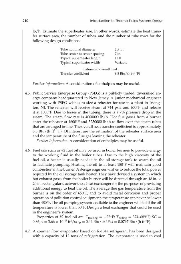
JWST229-c04 JWST229-McDonald Printer: Yet to Come July 31, 2012 12:14 Trim: 244mm × 168mm
210 Introduction to Thermo-Fluids Systems Design
lb/h. Estimate the superheater size. In other words, estimate the heat trans-fer surface area, the number of tubes, and the number of tube rows for thefollowing design conditions:
Tube nominal diameter 21/2 in.Tube center to center spacing 7 in.Typical superheater length 12 ftTypical superheater width Variable
Estimated overall heatTransfer coefficient 8.8 Btu/(h ft2 ◦F)
Further Information: A consideration of enthalpies may be useful.
4.5. Public Service Enterprise Group (PSEG) is a publicly traded, diversified en-ergy company headquartered in New Jersey. A junior mechanical engineerworking with PSEG wishes to size a reheater for use in a plant in Irving-ton, NJ. The reheater will receive steam at 744 psia and 600◦F and releaseit at 1000◦F. Due to losses in the tubing, there is a 7% pressure drop in thesteam. The steam flow rate is 4000000 lb/h. Hot flue gases from a burnerenter the reheater at 1600◦F and 5250000 lb/h to flow over the steam tubesthat are arranged in-line. The overall heat transfer coefficient is approximately8.5 Btu/(h ft2 ◦F). Of interest are the estimation of the reheater surface areaand the temperature of the flue gas leaving the reheater.
Further Information: A consideration of enthalpies may be useful.
4.6. Fuel oils such as #2 fuel oil may be used in boiler burners to provide energyto the working fluid in the boiler tubes. Due to the high viscosity of thefuel oil, a heater is usually needed in the oil storage tank to warm the oilto facilitate pumping. Heating the oil to at least 150◦F will maintain goodcombustion in the burner. A design engineer wishes to reduce the total powerrequired by the oil storage tank heater. They have devised a system in whichhot exhaust gases from the boiler burner will be directed through an 18 in. ×20 in. rectangular ductwork to a heat exchanger for the purposes of providingadditional energy to heat the oil. The average flue gas temperature from theburner is on the order of 650◦F, and to avoid metal corrosion and properoperation of pollution control equipment, the temperature can never be lowerthan 480◦F. The oil pumping system available to the engineer will fail if the oiltemperature is lower than 50◦F. Design a heat exchanger that could be usedin the engineer’s system.
Properties of #2 fuel oil are: Tfreezing = −22◦F; Tboiling = 374–689◦F; SG =0.86; ν = 3.66 × 10⁻⁵ ft2/s; cp = 0.44 Btu/lb-◦F; k = 0.0797 Btu/(h ft ◦F).
4.7. A counter flow evaporator based on R-134a refrigerant has been designedwith a capacity of 12 tons of refrigeration. The evaporator is used to cool

JWST229-c04 JWST229-McDonald Printer: Yet to Come July 31, 2012 12:14 Trim: 244mm × 168mm
Fundamentals of Heat Exchanger Design 211
50 vol% ethylene glycol solution (cp = 0.775 Btu/(lb ◦F) that enters the heatexchanger at 55◦F with a mass flow rate of 20000 lb/h. The R-134a enters theheat exchanger at 35◦F with a quality of 0.1 and leaves with a quality of 0.65.Estimate the exit temperature of the ethylene glycol solution, the mass flowrate of the refrigerant, and the increase in efficiency of the heat exchanger ifthe surface area of the evaporator were doubled.
Further Information: The R-134a refrigerant has experienced a phase change.
4.8. A low-velocity residential air duct is to be equipped with a manufacturer’sheating module. It is expected that the module will temper dry air by heatingit from 40◦F to 80◦F. Hot water from a boiler package is available. Due toinefficiencies in the boiler, the exit water temperatures will range from 140◦Fto 180◦F. Select a manufacturer’s heating module to heat the air and preparean equipment schedule for the client’s contract documents. The air duct sizewill depend on the size of the module unit that is selected by the mechanicalengineer.
References and Further Reading
[1] Lee, H. (2010) Thermal Design: Heat Sinks, Thermoelectrics, Heat Pipes, Compact Heat Exchang-ers, and Solar Cells, John Wiley & Sons, Inc., Hoboken.
[2] Kays, W. and London, A. (1964) Compact Heat Exchangers, 2nd edn, McGraw-Hill, Inc.,New York.
[3] Cengel, Y. (2007) Heat and Mass Transfer: A Practical Approach, 3rd edn, McGraw-Hill, Inc.,New York, p. 469.
[4] Edwards, D., Denny, V., and Mills, A. (1979) Transfer Processes, 2nd edn, HemispherePublishing Corp., New York.
[5] Sieder, E. and Tate, G. (1936) Heat transfer and pressure drop of liquids in tubes, IndustrialEngineering Chemistry, 28, 1429–1435.
[6] Dittus, F. and Boelter, L. (1930) University of California Publications on Engineering, 2, 433.[7] Gnielinski, V. (1976) New equations for heat and mass transfer in turbulent pipe and
channel flow, International Chemical Engineering, 16, 359–368.[8] Churchill, S. and Bernstein, M. (1977) A correlating equation for forced convection from
gases and liquids to a circular cylinder in cross flow, Journal of Heat Transfer, 99, 300–306.[9] Schmidt, T. (1945–1946) La production calorifique des surfaces munies d’ailettes, Annexe
du Bulletin de L’Institut International du Froid, Annexe G-5.[10] McQuiston, F., Parker, J., and Spitler, J. (2000) Heating, Ventilating, and Air Conditioning:
Analysis and Design, 5th edn, John Wiley & Sons, Inc., New York, pp. 489–503.[11] Wolverine Tube Inc. (2009) Wolverine Tube Heat Transfer Data Book, Wolverine Tube Inc.,
Huntsville, pp. 45–56.

JWST229-c05 JWST229-McDonald Printer: Yet to Come August 1, 2012 11:14 Trim: 244mm × 168mm
5Applications of HeatExchangers in Systems
The fundamental design of heat exchangers can be a complex and laborious process,requiring the use of multiple charts and correlation equations. To that end, equip-ment manufacturers have invested millions of dollars into conducting performancetests and securing appropriate government certification of their equipment. This per-formance data is usually available in catalogs from the manufacturers. This greatlyreduces the work required by design engineers during larger system designs thatinclude heat exchangers.
This chapter focuses on the practical applications of heat exchangers in thermo-fluids systems. Particular attention will be given to a cooling system for a high-temperature plasma spray torch and hot water heating systems.
5.1 Operation of a Heat Exchanger in a Plasma Spraying System
Plasma spraying is a high-temperature process used to melt and accelerate powderedparticles in order to fabricate protective coatings on machine and industrial parts.Figure 5.1 shows a picture of a plasma torch in operation, the small plasma jet shown,can reach temperatures between 10000 and 20000 K. As a consequence of the highplasma jet temperatures, a system is needed to cool the torch electrodes and housingto prevent overheating.
Figure 5.2 shows a heat exchanger that could be used to provide chilled water tothe torch. In addition, Figure 5.3 shows a functional diagram of the heat exchanger.The functional diagram shows all the functional parts of the heat exchanger. Ofspecial interest is the distilled/deionized water storage tank (label 7 in Figure 5.3).In this application, it is paramount to have chilled deionized water in contact withthe components of the torch. If the cooling water is hard or ionized, electricity fromthe torch could flow through the cooling water, with dangerous consequences. A
Introduction to Thermo-Fluids Systems Design, First Edition. Andre G. McDonald and Hugh L. Magande.C© 2012 Andre G. McDonald and Hugh L. Magande. Published 2012 by John Wiley & Sons, Ltd.
213

JWST229-c05 JWST229-McDonald Printer: Yet to Come August 1, 2012 11:14 Trim: 244mm × 168mm
214 Introduction to Thermo-Fluids Systems Design
Figure 5.1 A Praxair SG-100 plasma spray torch in operation
heat exchanger module (label 3 in Figure 5.3) is needed for the exchange of heatbetween the heated deionized water and the cold plant/building or chiller water,which typically contains ions or other chemical contaminants.
A flow diagram is usually presented to show the flow of water (the working fluid) inthe cooling system that includes the heat exchanger. Figure 5.4 shows a flow diagram
Figure 5.2 The Sulzer Metco Climet-HETM-200 heat exchanger ( Sulzer Metco, ProductManual MAN 41292 EN 05; reprinted with permission)

JWST229-c05 JWST229-McDonald Printer: Yet to Come August 1, 2012 11:14 Trim: 244mm × 168mm
Applications of Heat Exchangers in Systems 215
Figure 5.3 Functional diagram for the Sulzer Metco Climet-HETM-200 (Sulzer Metco,Product Manual MAN 41292 EN 05; reprinted with permission)
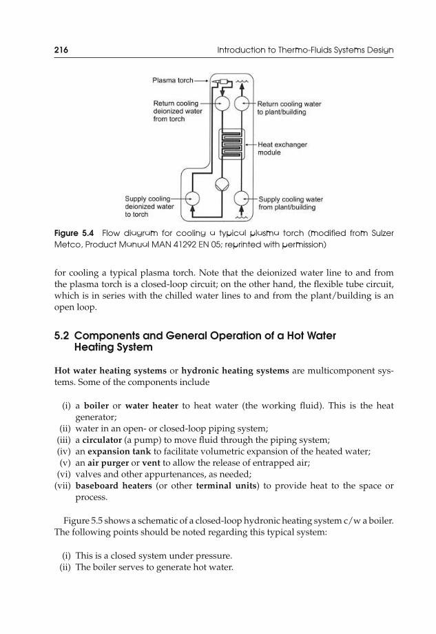
JWST229-c05 JWST229-McDonald Printer: Yet to Come August 1, 2012 11:14 Trim: 244mm × 168mm
216 Introduction to Thermo-Fluids Systems Design
Figure 5.4 Flow diagram for cooling a typical plasma torch (modified from SulzerMetco, Product Manual MAN 41292 EN 05; reprinted with permission)
for cooling a typical plasma torch. Note that the deionized water line to and fromthe plasma torch is a closed-loop circuit; on the other hand, the flexible tube circuit,which is in series with the chilled water lines to and from the plant/building is anopen loop.
5.2 Components and General Operation of a Hot WaterHeating System
Hot water heating systems or hydronic heating systems are multicomponent sys-tems. Some of the components include
(i) a boiler or water heater to heat water (the working fluid). This is the heatgenerator;
(ii) water in an open- or closed-loop piping system;(iii) a circulator (a pump) to move fluid through the piping system;(iv) an expansion tank to facilitate volumetric expansion of the heated water;(v) an air purger or vent to allow the release of entrapped air;
(vi) valves and other appurtenances, as needed;(vii) baseboard heaters (or other terminal units) to provide heat to the space or
process.
Figure 5.5 shows a schematic of a closed-loop hydronic heating system c/w a boiler.The following points should be noted regarding this typical system:
(i) This is a closed system under pressure.(ii) The boiler serves to generate hot water.
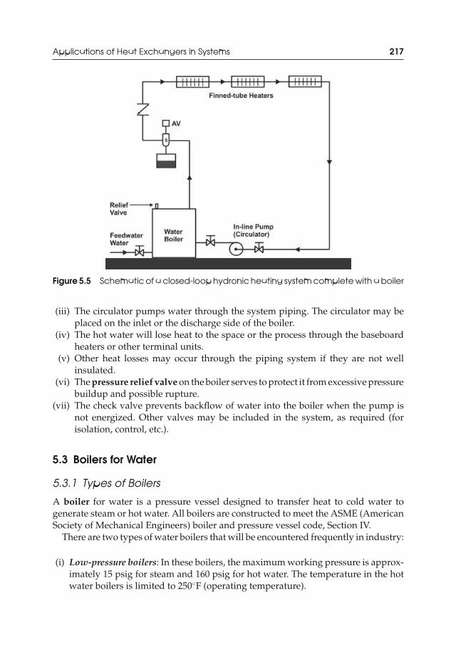
JWST229-c05 JWST229-McDonald Printer: Yet to Come August 1, 2012 11:14 Trim: 244mm × 168mm
Applications of Heat Exchangers in Systems 217
Figure 5.5 Schematic of a closed-loop hydronic heating system complete with a boiler
(iii) The circulator pumps water through the system piping. The circulator may beplaced on the inlet or the discharge side of the boiler.
(iv) The hot water will lose heat to the space or the process through the baseboardheaters or other terminal units.
(v) Other heat losses may occur through the piping system if they are not wellinsulated.
(vi) The pressure relief valve on the boiler serves to protect it from excessive pressurebuildup and possible rupture.
(vii) The check valve prevents backflow of water into the boiler when the pump isnot energized. Other valves may be included in the system, as required (forisolation, control, etc.).
5.3 Boilers for Water
5.3.1 Types of Boilers
A boiler for water is a pressure vessel designed to transfer heat to cold water togenerate steam or hot water. All boilers are constructed to meet the ASME (AmericanSociety of Mechanical Engineers) boiler and pressure vessel code, Section IV.
There are two types of water boilers that will be encountered frequently in industry:
(i) Low-pressure boilers: In these boilers, the maximum working pressure is approx-imately 15 psig for steam and 160 psig for hot water. The temperature in the hotwater boilers is limited to 250◦F (operating temperature).

JWST229-c05 JWST229-McDonald Printer: Yet to Come August 1, 2012 11:14 Trim: 244mm × 168mm
218 Introduction to Thermo-Fluids Systems Design
(ii) Medium- and high-pressure boilers: These boilers will operate above 15 psig forsteam and above 160 psig, but less than 250◦F for hot water.
5.3.2 Operation and Components of a Typical Boiler
Figure 5.6 shows a schematic of a typical gas-fired hot water boiler. Note that thearrangement of the components can vary.
Of interest are the following additional components that expand the operation of atypical boiler:
(i) A drain valve complete with a hose bib or pipe cock. This is used to drain theboiler to allow for maintenance/repairs or to prevent flooding.
(ii) Water feed line. This line supplies fresh plant or building water to the boiler. Forhomes or small commercial buildings, the feedwater may be supplied by thelocal municipality.
(iii) Burners c/w with a gas valve. The burners supply the heat required. Open flameswill heat the water contained in the boiler tubes (water tube) or storage tank (firetube). Natural gas, oil, wood, or coal are examples of fuels that may be used.
(iv) Aquastat. The aquastat is a thermostat that is used to measure the water temper-ature and control the burners by modulating the fuel flow rate (through the gasvalve).
Figure 5.6 A typical gas-fired hot water boiler

JWST229-c05 JWST229-McDonald Printer: Yet to Come August 1, 2012 11:14 Trim: 244mm × 168mm
Applications of Heat Exchangers in Systems 219
(v) Vent or chimney. This serves to channel combustion flue gases from the burnersto the atmosphere. As the burners (enclosed in the combustion chamber) heatthe fluid inside the heat exchanger, combustion gases are formed. The vent istherefore connected to the combustion chamber to facilitate routing of the fluegases to atmosphere.
Practical Note 5.1 Condensing Boilers
The typical boiler system described in Section 5.3.2 is a conventional, noncondensing boiler.In this type of boiler, the combustion flue gases are exhausted from the combustion chamberat high temperatures on the order of 350–400◦F. This results in significant waste of energy.Currently, condensing boilers are being specified by design engineers and design-buildcontractors, in lieu of conventional, noncondensing boilers. In a condensing boiler, thetemperature of the flue gases may be lowered to 140◦F through the use of a secondary heatexchanger to preheat the return water. A larger primary heat exchanger, which providesa larger condensing surface area, may be used instead of a secondary heat exchanger toreduce the flue gas temperature (fully condensing boiler). The design engineer should notethat reducing the flue gas temperature to 140◦F results in the formation of condensate. Thiscould pose a serious corrosion issue if not properly drained from the system. Additionally,the condensate should be neutralized prior to disposal into the building’s plumbing drainsystem. The abovementioned issue should be considered in all designs, selections, andconsultations. Regarding efficiency of the condensing boiler, it is increased with lowerreturn water temperatures to the boiler heat exchanger. The water return temperature tothe boiler should not exceed 113–122◦F [1] to improve efficiency.
Water heaters are also used extensively in industry to provide hot water (not steam),especially in residential buildings or small process applications. The operation of gas-fired water heaters is similar to that of boilers. Figure 5.7 shows a schematic of theinternal sections of typical water heaters. The figure shows that the water heaters caneither be electric or gas fired. In the electric water heater, heating elements are placedat different levels in the tank. In both water heater configurations, dip tubes are usedto supply cold feedwater to the tank. The dip tube is placed near the bottom of thetank since colder water has a higher density than heated water, and will thus fall tothe bottom of the tank. In addition, the dip tube has several small orifices. As thewater exits the orifices at high velocity, this promotes mixing in the tank to enhanceheating and uniform tank water temperature. The hot water outlet that supplies hotwater to the building or process will be installed close to the top of the tank. This willensure that only hot water will be supplied.
Tankless water heaters are also being used to supply hot water for a variety ofdifferent residential and commercial applications. In some of these systems (condens-ing), direct heat from a burner flame and flue gases are used to heat water flowing overfinned copper tubes in a counterflow heat exchanger arrangement. The high efficiencyof the heat exchanger design eliminates the need for large water tanks. This reduces
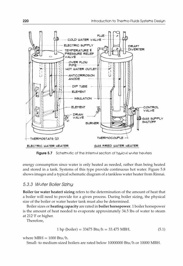
JWST229-c05 JWST229-McDonald Printer: Yet to Come August 1, 2012 11:14 Trim: 244mm × 168mm
220 Introduction to Thermo-Fluids Systems Design
Figure 5.7 Schematic of the internal section of typical water heaters
energy consumption since water is only heated as needed, rather than being heatedand stored in a tank. Systems of this type provide continuous hot water. Figure 5.8shows images and a typical schematic diagram of a tankless water heater from Rinnai.
5.3.3 Water Boiler Sizing
Boiler (or water heater) sizing refers to the determination of the amount of heat thata boiler will need to provide for a given process. During boiler sizing, the physicalsize of the boiler or water heater tank must also be determined.
Boiler sizes or heating capacity are rated in boiler horsepower. 1 boiler horsepoweris the amount of heat needed to evaporate approximately 34.5 lbs of water to steamat 212◦F or higher.
Therefore,
1 hp (boiler) = 33475 Btu/h = 33.475 MBH, (5.1)
where MBH = 1000 Btu/h.Small- to medium-sized boilers are rated below 10000000 Btu/h or 10000 MBH.
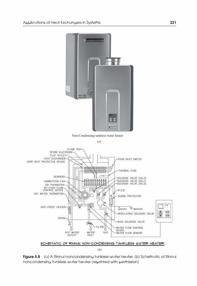
JWST229-c05 JWST229-McDonald Printer: Yet to Come August 1, 2012 11:14 Trim: 244mm × 168mm
Applications of Heat Exchangers in Systems 221
Non-Condensing tankless water heater
(a)
(b)
Figure 5.8 (a) A Rinnai noncondensing tankless water heater. (b) Schematic of Rinnainoncondensing tankless water heater (reprinted with permission)

JWST229-c05 JWST229-McDonald Printer: Yet to Come August 1, 2012 11:14 Trim: 244mm × 168mm
222 Introduction to Thermo-Fluids Systems Design
To determine the heating capacity of a boiler or water heater, the amount of heatrequired by the application must first be determined. That will determine the size ofthe boiler or water heater. For example, consider the heating of a space (residentialor commercial) and domestic water. The thermal size of the boiler or water heater isfound from
Qboiler = Qspace × OSF + Ghρcp (Tout − Tin)η
, (5.2)
where
Qboiler = thermal size of the boiler;Qspace = energy required to maintain the space at a set temperature. This will be the
total heat transferred through the baseboard heaters;OSF = oversizing factor. Consider this as a safety factor, which ranges between
1.05 and 1.25;Gh = recovery rate. The recovery rate is the volume flow rate of hot water that is
required to ensure that a sufficient amount of hot water is available at therequired outlet temperatures for domestic use. Charts are used to find Gh;
Tout = outlet temperature of the hot water from the boiler or water heater;Tin = inlet temperature of cold water from the plant/building or from the munic-
ipal line that enters the boiler or water heater; andη = efficiency of the boiler or water heater. Boiler efficiencies may range between
70% and 85%. For fully condensing boilers, the efficiency may be above 90%.
It is important to note that in Equation (5.2), the total thermal size of the boiler isthe total heat required to heat the space and to supply hot water for domestic use.For other applications, the onus is on the design engineer to determine the amount ofheat required by the application or process in order to size the boiler appropriately.Equation (5.2) may be modified to determine the thermal size of a boiler or waterheater that will provide hot water for an industrial process. In this case, Qspace = 0and Gh = V.
Practical Note 5.2 Typical OSF Values
Residential houses and apartments are typically heavily occupied (more people per unitarea who are cooking and constantly using hot water.) and will require OSF values from1.05 to 1.1. Commercial buildings or schools that are lightly occupied or unoccupied (lesspeople per unit area) will require OSF values from 1.1 to 1.25. Higher OSF values enablefaster achievement of the set temperatures because the water boiler and/or water heaterwill have excess capacity to respond to demand faster. When no domestic water is required,the OSF may be considered as the efficiency of the boiler.
JWST229-c05 JWST229-McDonald Printer: Yet to Come August 1, 2012 11:14 Trim: 244mm × 168mm
Applications of Heat Exchangers in Systems 223
Practical Note 5.3 Domestic Water Data for Edmonton,Alberta, Canada
Water supplied by the City of Edmonton has temperatures on the order of 40–48◦F (4–9◦C).The water pressure will range between 35 and 100 psig (240–700 kPa gage). Typical waterconsumption is on the order of 60 gal per person per day (225 L per person per day) [2].
The physical size of the boiler or water heater is represented as the volume of thehot water tank. The tank size (for domestic use) is given by
�tank = �capacity
FusableN, (5.3)
where
�tank = required size of the boiler or water heater tank (volume);�capacity = usable storage capacity required per person (L/person or gal/person).
This is the amount of hot water that the tank should provide per person orother unit, such as an apartment. Charts are used to find �capacity;
Fusable = fraction of the tank water that has the minimum required temperature.Normally, Fusable ranges between 60% and 80%. Remember that heating ofcold water may occur from the bottom of the tank (as in the case of gas-firedboilers or water heaters). Heat will be conducted from the bottom to thetop of the tank, which will not occur instantaneously. Therefore, the watertemperature will not be uniform at the set temperature throughout the tankvolume; and
N = number of units (e.g., persons, beds, apartments, etc.).
Practical Note 5.4 Hot Water Temperatures from Faucets
Division B, Section 7.2.6.1 of the 2006 Alberta Building Code [2] requires that hot water besupplied at temperatures higher than 113◦F (45◦C). To prevent burning (scalding), Section7.2.6.7 requires that hot water from faucets must be limited to 130◦F (54◦C). For domesticuse, hot water boilers and water heaters should not produce water with temperatures higherthan 140◦F (Section 501.6 of the International Plumbing Code). For other jurisdictions, theappropriate codes should be consulted. To limit the possibility of legionella growth, tankwater should be kept at a minimum of 140◦F. If lower water temperatures are required, athermostatic mixing valve should be employed.
Table 5.1 shows some typical values of the minimum recovery rates and the corre-sponding minimum usable storage capacities for a variety of residential and industrialapplications.
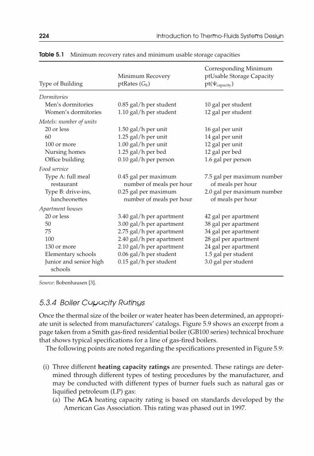
JWST229-c05 JWST229-McDonald Printer: Yet to Come August 1, 2012 11:14 Trim: 244mm × 168mm
224 Introduction to Thermo-Fluids Systems Design
Table 5.1 Minimum recovery rates and minimum usable storage capacities
Type of BuildingMinimum RecoveryptRates (Gh)
Corresponding MinimumptUsable Storage Capacitypt(�capacity)
DormitoriesMen’s dormitories 0.85 gal/h per student 10 gal per studentWomen’s dormitories 1.10 gal/h per student 12 gal per student
Motels: number of units20 or less 1.50 gal/h per unit 16 gal per unit60 1.25 gal/h per unit 14 gal per unit100 or more 1.00 gal/h per unit 12 gal per unitNursing homes 1.25 gal/h per bed 12 gal per bedOffice building 0.10 gal/h per person 1.6 gal per person
Food serviceType A: full meal
restaurant0.45 gal per maximum
number of meals per hour7.5 gal per maximum number
of meals per hourType B: drive-ins,
luncheonettes0.25 gal per maximum
number of meals per hour2.0 gal per maximum number
of meals per hour
Apartment houses20 or less 3.40 gal/h per apartment 42 gal per apartment50 3.00 gal/h per apartment 38 gal per apartment75 2.75 gal/h per apartment 34 gal per apartment100 2.40 gal/h per apartment 28 gal per apartment130 or more 2.10 gal/h per apartment 24 gal per apartmentElementary schools 0.06 gal/h per student 1.5 gal per studentJunior and senior high
schools0.15 gal/h per student 3.0 gal per student
Source: Bobenhausen [3].
5.3.4 Boiler Capacity Ratings
Once the thermal size of the boiler or water heater has been determined, an appropri-ate unit is selected from manufacturers’ catalogs. Figure 5.9 shows an excerpt from apage taken from a Smith gas-fired residential boiler (GB100 series) technical brochurethat shows typical specifications for a line of gas-fired boilers.
The following points are noted regarding the specifications presented in Figure 5.9:
(i) Three different heating capacity ratings are presented. These ratings are deter-mined through different types of testing procedures by the manufacturer, andmay be conducted with different types of burner fuels such as natural gas orliquified petroleum (LP) gas:(a) The AGA heating capacity rating is based on standards developed by the
American Gas Association. This rating was phased out in 1997.
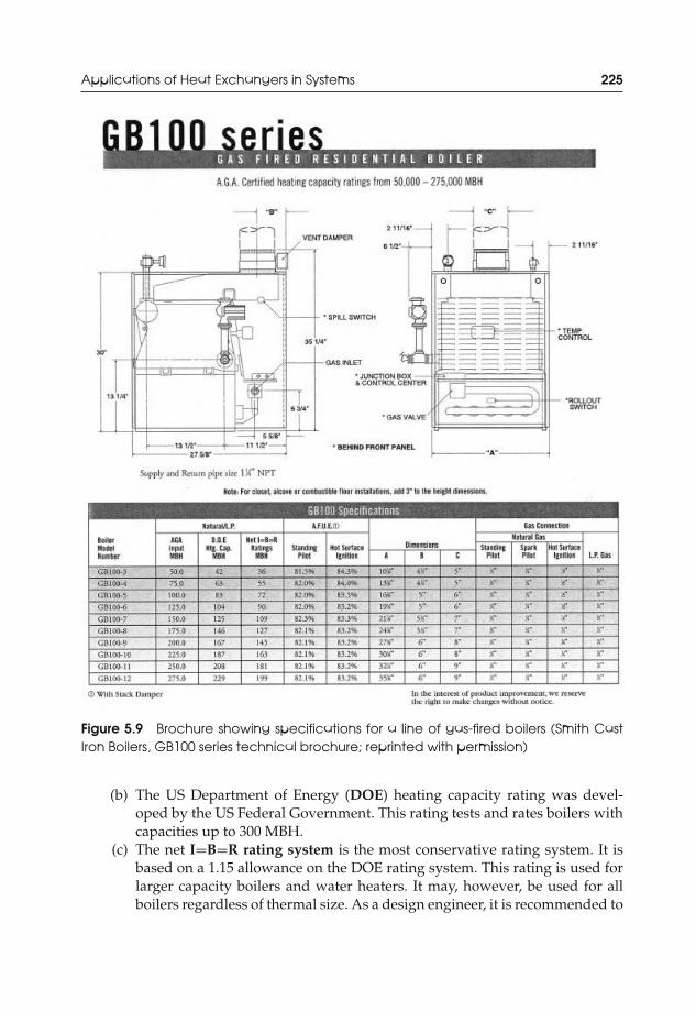
JWST229-c05 JWST229-McDonald Printer: Yet to Come August 1, 2012 11:14 Trim: 244mm × 168mm
Applications of Heat Exchangers in Systems 225
Figure 5.9 Brochure showing specifications for a line of gas-fired boilers (Smith CastIron Boilers, GB100 series technical brochure; reprinted with permission)
(b) The US Department of Energy (DOE) heating capacity rating was devel-oped by the US Federal Government. This rating tests and rates boilers withcapacities up to 300 MBH.
(c) The net I=B=R rating system is the most conservative rating system. It isbased on a 1.15 allowance on the DOE rating system. This rating is used forlarger capacity boilers and water heaters. It may, however, be used for allboilers regardless of thermal size. As a design engineer, it is recommended to
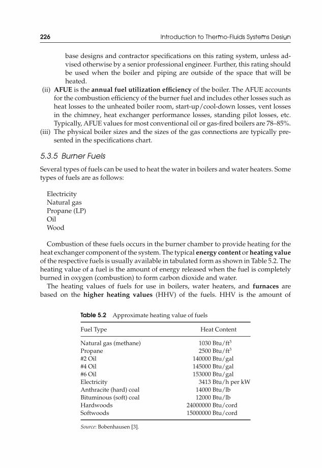
JWST229-c05 JWST229-McDonald Printer: Yet to Come August 1, 2012 11:14 Trim: 244mm × 168mm
226 Introduction to Thermo-Fluids Systems Design
base designs and contractor specifications on this rating system, unless ad-vised otherwise by a senior professional engineer. Further, this rating shouldbe used when the boiler and piping are outside of the space that will beheated.
(ii) AFUE is the annual fuel utilization efficiency of the boiler. The AFUE accountsfor the combustion efficiency of the burner fuel and includes other losses such asheat losses to the unheated boiler room, start-up/cool-down losses, vent lossesin the chimney, heat exchanger performance losses, standing pilot losses, etc.Typically, AFUE values for most conventional oil or gas-fired boilers are 78–85%.
(iii) The physical boiler sizes and the sizes of the gas connections are typically pre-sented in the specifications chart.
5.3.5 Burner Fuels
Several types of fuels can be used to heat the water in boilers and water heaters. Sometypes of fuels are as follows:
ElectricityNatural gasPropane (LP)OilWood
Combustion of these fuels occurs in the burner chamber to provide heating for theheat exchanger component of the system. The typical energy content or heating valueof the respective fuels is usually available in tabulated form as shown in Table 5.2. Theheating value of a fuel is the amount of energy released when the fuel is completelyburned in oxygen (combustion) to form carbon dioxide and water.
The heating values of fuels for use in boilers, water heaters, and furnaces arebased on the higher heating values (HHV) of the fuels. HHV is the amount of
Table 5.2 Approximate heating value of fuels
Fuel Type Heat Content
Natural gas (methane) 1030 Btu/ft3
Propane 2500 Btu/ft3
#2 Oil 140000 Btu/gal#4 Oil 145000 Btu/gal#6 Oil 153000 Btu/galElectricity 3413 Btu/h per kWAnthracite (hard) coal 14000 Btu/lbBituminous (soft) coal 12000 Btu/lbHardwoods 24000000 Btu/cordSoftwoods 15000000 Btu/cord
Source: Bobenhausen [3].

JWST229-c05 JWST229-McDonald Printer: Yet to Come August 1, 2012 11:14 Trim: 244mm × 168mm
Applications of Heat Exchangers in Systems 227
energy released after complete combustion of fuel and complete condensation ofwater. Lower heating value (LHV) is the amount of energy released after completecombustion of the fuel, but with water as a vapor.
5.4 Design of Hydronic Heating Systems c/w Baseboardsor Finned-Tube Heaters
5.4.1 Zoning and Types of Systems
Space heating in a residential or commercial building may be accomplished with theuse of piping system arrangements, which include a water boiler or water heater,circulators, valves, expansion tanks, and baseboard heaters. These types of hydronicheating systems may include multiple-pipe circuits to provide heating to differentzones of the space or building. A zone is an area of the space or building that iscontrolled by a single thermostat.
5.4.2 One-Pipe Series Loop System
Figure 5.10 shows a schematic diagram of a one-pipe series loop system. As the figureshows, this is a closed-loop system with a single pipeline routed from and to theboiler. The line also includes several heaters.
Figure 5.10 Schematic diagram of a one-pipe series loop system
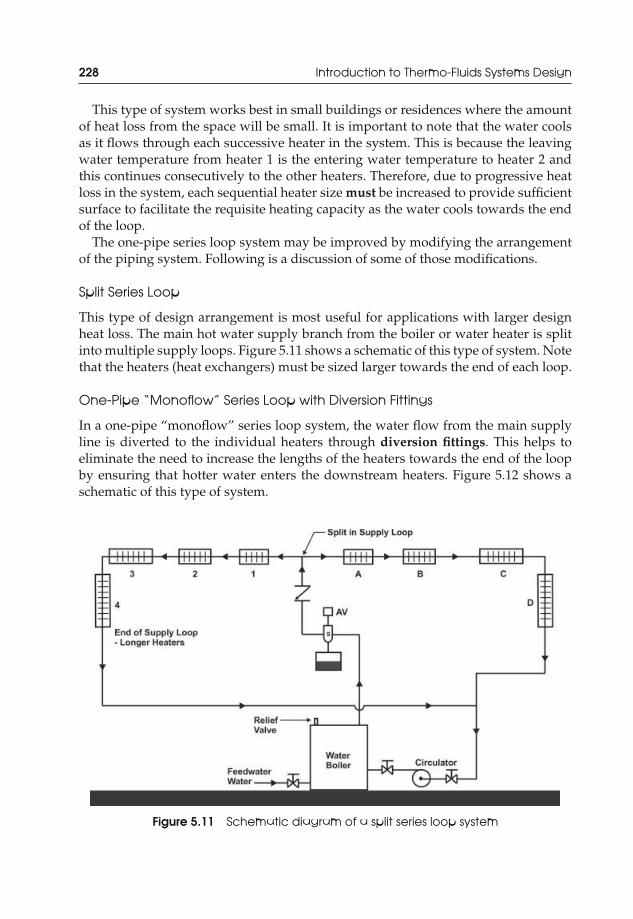
JWST229-c05 JWST229-McDonald Printer: Yet to Come August 1, 2012 11:14 Trim: 244mm × 168mm
228 Introduction to Thermo-Fluids Systems Design
This type of system works best in small buildings or residences where the amountof heat loss from the space will be small. It is important to note that the water coolsas it flows through each successive heater in the system. This is because the leavingwater temperature from heater 1 is the entering water temperature to heater 2 andthis continues consecutively to the other heaters. Therefore, due to progressive heatloss in the system, each sequential heater size must be increased to provide sufficientsurface to facilitate the requisite heating capacity as the water cools towards the endof the loop.
The one-pipe series loop system may be improved by modifying the arrangementof the piping system. Following is a discussion of some of those modifications.
Split Series Loop
This type of design arrangement is most useful for applications with larger designheat loss. The main hot water supply branch from the boiler or water heater is splitinto multiple supply loops. Figure 5.11 shows a schematic of this type of system. Notethat the heaters (heat exchangers) must be sized larger towards the end of each loop.
One-Pipe “Monoflow” Series Loop with Diversion Fittings
In a one-pipe “monoflow” series loop system, the water flow from the main supplyline is diverted to the individual heaters through diversion fittings. This helps toeliminate the need to increase the lengths of the heaters towards the end of the loopby ensuring that hotter water enters the downstream heaters. Figure 5.12 shows aschematic of this type of system.
Figure 5.11 Schematic diagram of a split series loop system

JWST229-c05 JWST229-McDonald Printer: Yet to Come August 1, 2012 11:14 Trim: 244mm × 168mm
Applications of Heat Exchangers in Systems 229
Figure 5.12 Schematic of a one-pipe “monoflow” series loop system
Multiple one-pipe series circuits can be used to provide heat to different zones ofa large space or building. To improve the performance of the system, the supply linefor each circuit is manifold to the main hot water supply line. In addition, diversionfittings may be used with each heater. Figure 5.13 shows a schematic of a largemultizone heating system of one-pipe series loops.
5.4.3 Two-Pipe Systems
Two-pipe systems were developed to eliminate the need for larger downstreamheaters due to water temperature drops. In these types of systems, each heater pos-sesses its own return line that is connected to a main return line. There are two maintypes of two-pipe systems.
Two-Pipe Direct Return System
Figure 5.14 shows a schematic of this type of system. In this system, return water fromeach heater is returned directly to a main return line that is piped back to the boiler.
Use of this system minimizes the amount of piping required. However, for thedownstream heaters, pipe pressure losses will be greater. The fluid may not flowthrough the heaters, and the heaters will be starved of heat. This is an example of anunbalanced flow system.

JWST229-c05 JWST229-McDonald Printer: Yet to Come August 1, 2012 11:14 Trim: 244mm × 168mm
230 Introduction to Thermo-Fluids Systems Design
Figure 5.13 Schematic diagram of a multizone system of one-pipe series loops
Figure 5.14 Schematic of a two-pipe direct return system
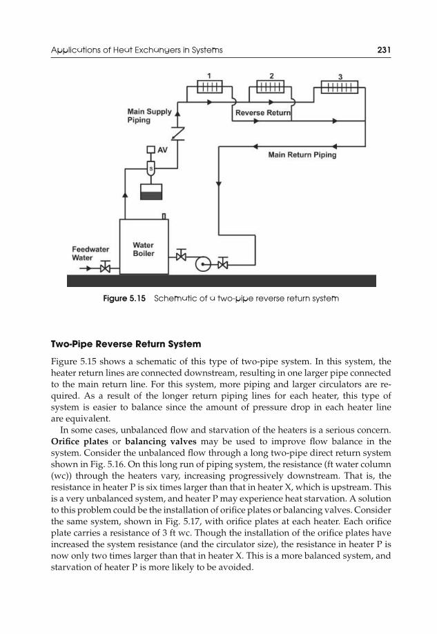
JWST229-c05 JWST229-McDonald Printer: Yet to Come August 1, 2012 11:14 Trim: 244mm × 168mm
Applications of Heat Exchangers in Systems 231
Figure 5.15 Schematic of a two-pipe reverse return system
Two-Pipe Reverse Return System
Figure 5.15 shows a schematic of this type of two-pipe system. In this system, theheater return lines are connected downstream, resulting in one larger pipe connectedto the main return line. For this system, more piping and larger circulators are re-quired. As a result of the longer return piping lines for each heater, this type ofsystem is easier to balance since the amount of pressure drop in each heater lineare equivalent.
In some cases, unbalanced flow and starvation of the heaters is a serious concern.Orifice plates or balancing valves may be used to improve flow balance in thesystem. Consider the unbalanced flow through a long two-pipe direct return systemshown in Fig. 5.16. On this long run of piping system, the resistance (ft water column(wc)) through the heaters vary, increasing progressively downstream. That is, theresistance in heater P is six times larger than that in heater X, which is upstream. Thisis a very unbalanced system, and heater P may experience heat starvation. A solutionto this problem could be the installation of orifice plates or balancing valves. Considerthe same system, shown in Fig. 5.17, with orifice plates at each heater. Each orificeplate carries a resistance of 3 ft wc. Though the installation of the orifice plates haveincreased the system resistance (and the circulator size), the resistance in heater P isnow only two times larger than that in heater X. This is a more balanced system, andstarvation of heater P is more likely to be avoided.
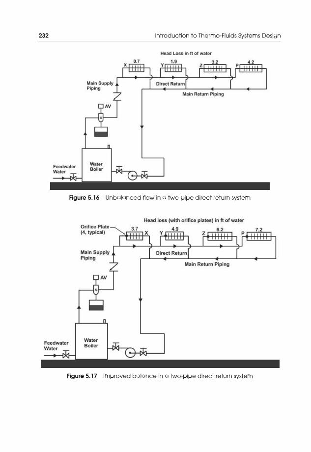
JWST229-c05 JWST229-McDonald Printer: Yet to Come August 1, 2012 11:14 Trim: 244mm × 168mm
232 Introduction to Thermo-Fluids Systems Design
Figure 5.16 Unbalanced flow in a two-pipe direct return system
Figure 5.17 Improved balance in a two-pipe direct return system

JWST229-c05 JWST229-McDonald Printer: Yet to Come August 1, 2012 11:14 Trim: 244mm × 168mm
Applications of Heat Exchangers in Systems 233
1-tiered baseboard heater 2-tiered finned-tube heater(a) (b)
Figure 5.18 Diagrams of baseboard heaters. (a) 1-tiered baseboard heater; (b) 2-tiered finned-tube heater
5.4.4 Baseboard and Finned-Tube Heaters
Baseboard and finned-tube heaters are finned-tube heat exchangers used to heatspaces through buoyancy-driven free convection mechanisms. These heaters typicallyconsist of a copper water pipe with aluminum fins attached to increase the heattransfer surface area. Most units will have 25–60 fins per foot of piping. The depthof the heaters will range from 3 to 6 in. and the height may range from 6 to 24 in.Baseboard heaters are small in height, ranging from 6 to 12 in. Finned-tube heatersare larger than baseboard heaters, with heights of 8–24 in. Baseboard heaters aretypically 1-tiered, with one finned-tube pipe. Finned-tube heaters are typically atleast 2-tiered, with two rows of finned-tube pipes. Figure 5.18 shows two types ofheaters, baseboard and finned-tube.
Manufacturer’s catalogs must be consulted to select the heaters that will be installedby the mechanical contractor. Tables 5.3 and 5.4 provide ratings and specifications for
Table 5.3 Baseboard heater rated outputs at 1 gpm water flow rate
Average WaterTemperature (◦F)
Rated Output (Btu/h)per foot of pipe
220 840215 810210 770200 710190 640180 580170 510160 450
Source: Slant/ Fin Corporation.
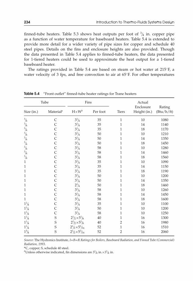
JWST229-c05 JWST229-McDonald Printer: Yet to Come August 1, 2012 11:14 Trim: 244mm × 168mm
234 Introduction to Thermo-Fluids Systems Design
finned-tube heaters. Table 5.3 shows heat outputs per foot of 3/4 in. copper pipeas a function of water temperature for baseboard heaters. Table 5.4 is extended toprovide more detail for a wider variety of pipe sizes for copper and schedule 40steel pipes. Details on the fins and enclosure heights are also provided. Thoughthe data presented in Table 5.4 applies to finned-tube heaters, the data presentedfor 1-tiered heaters could be used to approximate the heat output for a 1-tieredbaseboard heater.
The ratings provided in Table 5.4 are based on steam or hot water at 215◦F, awater velocity of 3 fps, and free convection to air at 65◦F. For other temperatures
Table 5.4 “Front outlet” finned-tube heater ratings for Trane heaters
Tube Fins
Size (in.) Materiala H×Wb Per foot Tiers
ActualEnclosure
Height (in.)Rating
(Btu/h/ft)
3/4 C 31/4 35 1 10 10803/4 C 31/4 35 1 14 11403/4 C 31/4 35 1 18 11703/4 C 31/4 50 1 10 12103/4 C 31/4 50 1 14 13503/4 C 31/4 50 1 18 14503/4 C 31/4 58 1 10 12803/4 C 31/4 58 1 14 14603/4 C 31/4 58 1 18 15601 C 31/4 35 1 10 10901 C 31/4 35 1 14 11501 C 31/4 35 1 18 11901 C 31/4 50 1 10 12001 C 31/4 50 1 14 13501 C 21/4 50 1 18 14601 C 31/4 58 1 10 12601 C 31/4 58 1 14 14501 C 31/4 58 1 18 160011/4 C 31/4 35 1 10 110011/4 C 31/4 50 1 10 120011/4 C 31/4 58 1 10 125011/4 S 21/2×51/8 40 1 16 130011/4 S 21/2×51/8 40 2 16 198011/4 S 21/2×51/16 52 1 16 151013/4 S 21/2×53/16 52 2 16 2060
Source: The Hydronics Institute, I=B=R Ratings for Boilers, Baseboard Radiation, and Finned Tube (Commercial)Radiation, 1993.aC, copper; S, schedule 40 steel.bUnless otherwise indicated, fin dimensions are 31/4 in.×31/4 in.

JWST229-c05 JWST229-McDonald Printer: Yet to Come August 1, 2012 11:14 Trim: 244mm × 168mm
Applications of Heat Exchangers in Systems 235
Table 5.5 Flow rate correction factors for watervelocities less than 3 fps
Water Velocity (fps) Correction Factor (CF)
3.0 1.0002.5 0.9922.0 0.9841.5 0.9731.0 0.9570.5 0.9310.25 0.905
Source: The Hydronics Institute, I=B=R Ratings for Boilers,Baseboard Radiation, and Finned Tube (Commercial) Radiation,1993.
and/or velocities, correction factors are used to determine the actual heat output ofthe heaters. The actual heat output is
Qactual = Qrating × CT × CF, (5.4)
where
Qactual = actual heat transferred from the heater at water temperatures other than215◦F and velocities other than 3 fps;
Qrating = heat output rating obtained from Table 5.4;CT = temperature correction factor. This is found from tables or charts;CF = velocity correction factor. This is found from tables or charts.
Tables 5.5 and 5.6 give CF and CT values, respectively. For the CF values presentedin Table 5.5, if the flow velocities are larger than 3 fps, CF = 1.00.
Practical Note 5.5 Temperature Data for Sizing Finned-Tube Heaters
Some manufacturers may provide data on the inlet temperatures to the heaters that will givea specific heat output. As the inlet temperatures decrease, their data will show a decreasein heat output. In addition, the temperature change (�T) may be provided to determine theoutlet temperature.
The length of the heater is found from
Lheater = Qdesign
Qactual= Qdesign
Qrating × CT × CF, (5.5)
where Qdesign is the total amount of heat that needs to be supplied by the heater.

JWST229-c05 JWST229-McDonald Printer: Yet to Come August 1, 2012 11:14 Trim: 244mm × 168mm
236 Introduction to Thermo-Fluids Systems Design
Table 5.6 Temperature correction factors for hot water ratings
Average HeaterTemperature (◦F) Correction Factor (CT)
100 0.15120 0.26150 0.45170 0.61175 0.65180 0.69185 0.73190 0.78195 0.82200 0.86205 0.91210 0.95215 1.00220 1.05230 1.14240 1.25
Source: The Hydronics Institute, I=B=R Ratings for Boilers, Baseboard Radia-tion, and Finned Tube (Commercial) Radiation, 1993.
5.5 Design Considerations for Hot Water Heating Systems
The following are several points that should be borne in mind during the design ofhot water heating systems:
(i) Study the architectural drawings or other relevant information for the spaceor process that requires hot water. For architectural drawings, these should befurnished by the architect.
(ii) Obtain the heat requirement (heating loads) for each space for building heatingapplications. A Heating, Ventilating, and Air-conditioning (HVAC) engineershould provide the heating loads for each space. For processes, determine theheat requirement by using appropriate formula.
(iii) Size the boiler or hot water heater (heat capacity and tank volume or volumeflow rate). In some jurisdictions (e.g., California and Vermont), the use of asingle boiler or hot water heater for domestic water and space heating is strictlyprohibited. In that case, a dual use hot water boiler (combi system) may beconsidered. In that case, the boiler/water heater must have two distinct sectionsfor heating water, one for domestic water use and one for space heating.
(iv) The International Plumbing Code (Section 501.2) requires the maximum hotwater temperature for domestic use (drinking, showers) to be 140◦F. Authoritieshaving juridiction may specify minimum hot water temperatures for domestic
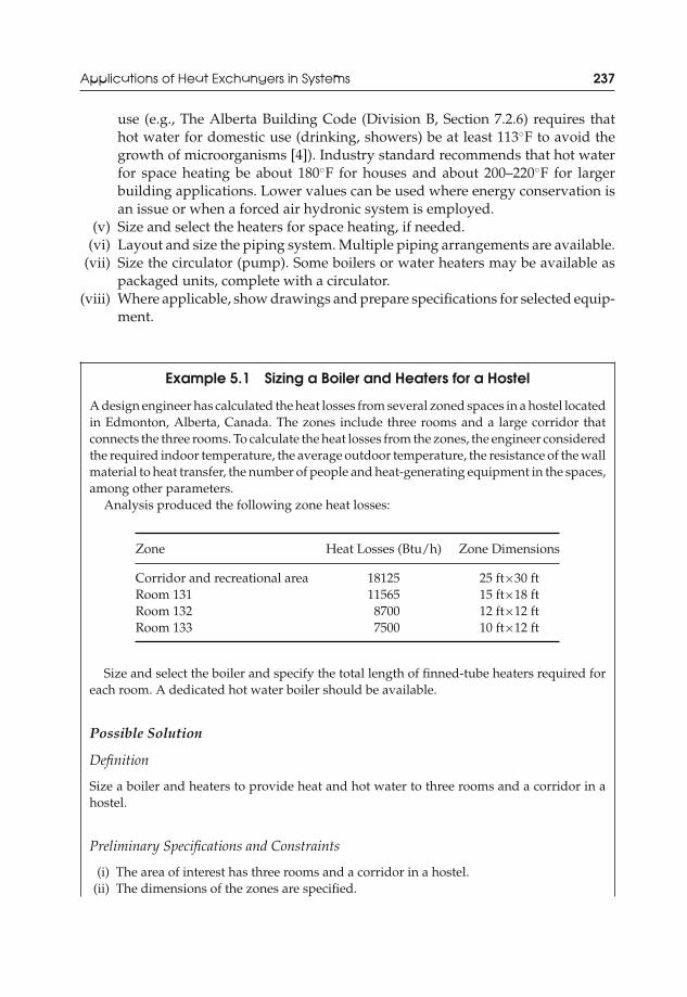
JWST229-c05 JWST229-McDonald Printer: Yet to Come August 1, 2012 11:14 Trim: 244mm × 168mm
Applications of Heat Exchangers in Systems 237
use (e.g., The Alberta Building Code (Division B, Section 7.2.6) requires thathot water for domestic use (drinking, showers) be at least 113◦F to avoid thegrowth of microorganisms [4]). Industry standard recommends that hot waterfor space heating be about 180◦F for houses and about 200–220◦F for largerbuilding applications. Lower values can be used where energy conservation isan issue or when a forced air hydronic system is employed.
(v) Size and select the heaters for space heating, if needed.(vi) Layout and size the piping system. Multiple piping arrangements are available.
(vii) Size the circulator (pump). Some boilers or water heaters may be available aspackaged units, complete with a circulator.
(viii) Where applicable, show drawings and prepare specifications for selected equip-ment.
Example 5.1 Sizing a Boiler and Heaters for a Hostel
A design engineer has calculated the heat losses from several zoned spaces in a hostel locatedin Edmonton, Alberta, Canada. The zones include three rooms and a large corridor thatconnects the three rooms. To calculate the heat losses from the zones, the engineer consideredthe required indoor temperature, the average outdoor temperature, the resistance of the wallmaterial to heat transfer, the number of people and heat-generating equipment in the spaces,among other parameters.
Analysis produced the following zone heat losses:
Zone Heat Losses (Btu/h) Zone Dimensions
Corridor and recreational area 18125 25 ft×30 ftRoom 131 11565 15 ft×18 ftRoom 132 8700 12 ft×12 ftRoom 133 7500 10 ft×12 ft
Size and select the boiler and specify the total length of finned-tube heaters required foreach room. A dedicated hot water boiler should be available.
Possible Solution
Definition
Size a boiler and heaters to provide heat and hot water to three rooms and a corridor in ahostel.
Preliminary Specifications and Constraints
(i) The area of interest has three rooms and a corridor in a hostel.(ii) The dimensions of the zones are specified.

JWST229-c05 JWST229-McDonald Printer: Yet to Come August 1, 2012 11:14 Trim: 244mm × 168mm
238 Introduction to Thermo-Fluids Systems Design
(iii) The heat losses from the spaces were specified by the design engineer.(iv) Limited space is available for mechanical equipment and units.
Detailed Design
Objective
Size a boiler to provide hot water and space heating to a three-room/corridor space in ahostel. Specify the boiler and the lengths of the heaters for space heating.
Data Given or Known
(i) Three rooms in a hostel(ii) One large corridor
(iii) Dimensions are given in the following table:
Zone Zone Dimensions
Corridor 25 ft×30 ftRoom 131 15 ft×18 ftRoom 132 12 ft×12 ftRoom 133 10 ft×12 ft
(iv) Heat losses from the spaces are provided in the following table:
Zone Heat Losses (Btu/h)
Corridor 18125Room 131 11565Room 132 8700Room 133 7500
Assumptions/Limitations/Constraints
(i) Assume that the spaces will be heavily occupied. Therefore, the boiler OSF is 1.10.(ii) The average outlet temperature of water from the boiler will be 200◦F. Industry stan-
dard recommends that hot water for space heating be about 180◦F for houses andabout 200–220◦F for larger building applications. The assumed outlet temperature isslightly higher than that recommended for houses or hostels.
(iii) The average inlet temperature of the water into the boiler is 40◦F. For Edmonton, inletwater temperature is about 40–48◦F.
(iv) The boiler efficiency will be at least 80%. Selection of a manufacturer’s unit will givea precise value.
(v) The heater tube size will be 3/4 in. The tubes will be Type L copper to promote heattransfer.

JWST229-c05 JWST229-McDonald Printer: Yet to Come August 1, 2012 11:14 Trim: 244mm × 168mm
Applications of Heat Exchangers in Systems 239
(vi) The flow velocity in the tube will not exceed 6 fps to prevent erosion of the coppertubes. Assume a water velocity of 1.5 fps. This low velocity should increase heattransfer to the space, while keeping the circulator size small.
(vii) All properties of the water used for sizing the boiler will be taken at an averagetemperature.
(viii) The pipelines that connect the heaters in each room will be properly insulated by themechanical contractor. The design engineer should provide details in the Specifica-tions section of the contract documents.
Sketch
No sketch is needed.
Analysis
Heater Sizing
Finned-tube heaters will be used in this application. The architect has specified that space islimited for mechanical equipment and units. Therefore, heaters with the smallest enclosureheights will be chosen. Therefore, choose the Trane 1-tier finned-tube heaters with 58 finsper foot of tube, an enclosure height of 10 in., and a rating of 1280 Btu/(h ft). Tube diameteris 3/4 in., and the material is copper.
For this application, a simple one-pipe series loop system will be chosen. A two-pipedirect return system could have been chosen.
The heater length is given by
Lheater = Qdesign
Qrating × CT × CF.
Each space will need to be considered individually when sizing the heaters because therewill be a temperature drop in the water as it proceeds from one heater to the next in theseries loop system. This decrease in inlet temperatures to the heaters will result in a changein the temperature correction factors (CT). Since the corridor is the space with the largestheat load requirement, the heaters in this space will be the first to receive hot water fromthe boiler.
For the corridor:For a hot water temperature of 200◦F, CT = 0.86. For tube velocities of 1.5 fps, CF = 0.973.Therefore,
Lcorridor = 18125 Btu/h(1280 Btu/(h ft)) (0.86) (0.973)
= 16.9 ft ≈ 17 ft.
Since the corridor is large, install three heaters each with 6-ft length around the perimeterof the corridor.
The exit temperature of the water from the heater is found from
Q = ρwaterVcp,water (Tin − Tout) = ρwaterπ D2
i Vwater
4cp,water (Tin − Tout) .
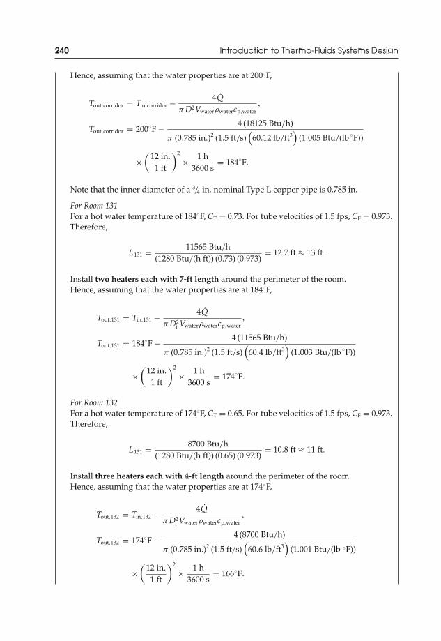
JWST229-c05 JWST229-McDonald Printer: Yet to Come August 1, 2012 11:14 Trim: 244mm × 168mm
240 Introduction to Thermo-Fluids Systems Design
Hence, assuming that the water properties are at 200◦F,
Tout,corridor = Tin,corridor − 4Qπ D2
i Vwaterρwatercp,water,
Tout,corridor = 200◦F − 4 (18125 Btu/h)
π (0.785 in.)2 (1.5 ft/s)(
60.12 lb/ft3)
(1.005 Btu/(lb ◦F))
×(
12 in.
1 ft
)2
× 1 h3600 s
= 184◦F.
Note that the inner diameter of a 3/4 in. nominal Type L copper pipe is 0.785 in.
For Room 131For a hot water temperature of 184◦F, CT = 0.73. For tube velocities of 1.5 fps, CF = 0.973.Therefore,
L131 = 11565 Btu/h(1280 Btu/(h ft)) (0.73) (0.973)
= 12.7 ft ≈ 13 ft.
Install two heaters each with 7-ft length around the perimeter of the room.Hence, assuming that the water properties are at 184◦F,
Tout,131 = Tin,131 − 4Qπ D2
i Vwaterρwatercp,water,
Tout,131 = 184◦F − 4 (11565 Btu/h)
π (0.785 in.)2 (1.5 ft/s)(
60.4 lb/ft3)
(1.003 Btu/(lb ◦F))
×(
12 in.
1 ft
)2
× 1 h3600 s
= 174◦F.
For Room 132For a hot water temperature of 174◦F, CT = 0.65. For tube velocities of 1.5 fps, CF = 0.973.Therefore,
L131 = 8700 Btu/h(1280 Btu/(h ft)) (0.65) (0.973)
= 10.8 ft ≈ 11 ft.
Install three heaters each with 4-ft length around the perimeter of the room.Hence, assuming that the water properties are at 174◦F,
Tout,132 = Tin,132 − 4Qπ D2
i Vwaterρwatercp,water,
Tout,132 = 174◦F − 4 (8700 Btu/h)
π (0.785 in.)2 (1.5 ft/s)(
60.6 lb/ft3)
(1.001 Btu/(lb ◦F))
×(
12 in.
1 ft
)2
× 1 h3600 s
= 166◦F.
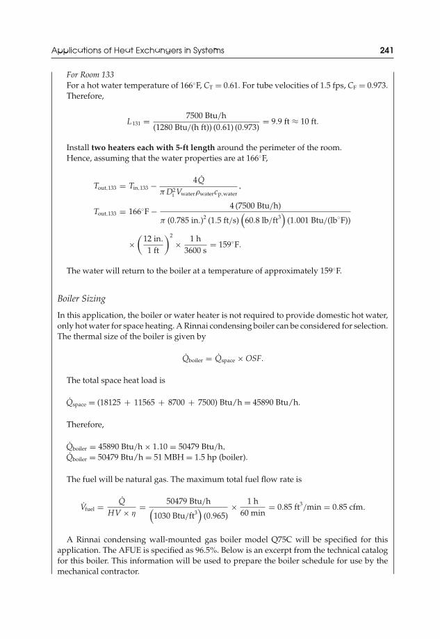
JWST229-c05 JWST229-McDonald Printer: Yet to Come August 1, 2012 11:14 Trim: 244mm × 168mm
Applications of Heat Exchangers in Systems 241
For Room 133For a hot water temperature of 166◦F, CT = 0.61. For tube velocities of 1.5 fps, CF = 0.973.Therefore,
L131 = 7500 Btu/h(1280 Btu/(h ft)) (0.61) (0.973)
= 9.9 ft ≈ 10 ft.
Install two heaters each with 5-ft length around the perimeter of the room.Hence, assuming that the water properties are at 166◦F,
Tout,133 = Tin,133 − 4Qπ D2
i Vwaterρwatercp,water,
Tout,133 = 166◦F − 4 (7500 Btu/h)
π (0.785 in.)2 (1.5 ft/s)(
60.8 lb/ft3)
(1.001 Btu/(lb◦F))
×(
12 in.
1 ft
)2
× 1 h3600 s
= 159◦F.
The water will return to the boiler at a temperature of approximately 159◦F.
Boiler Sizing
In this application, the boiler or water heater is not required to provide domestic hot water,only hot water for space heating. A Rinnai condensing boiler can be considered for selection.The thermal size of the boiler is given by
Qboiler = Qspace × OSF.
The total space heat load is
Qspace = (18125 + 11565 + 8700 + 7500) Btu/h = 45890 Btu/h.
Therefore,
Qboiler = 45890 Btu/h × 1.10 = 50479 Btu/h,
Qboiler = 50479 Btu/h = 51 MBH = 1.5 hp (boiler).
The fuel will be natural gas. The maximum total fuel flow rate is
Vfuel = QHV × η
= 50479 Btu/h(1030 Btu/ft3
)(0.965)
× 1 h60 min
= 0.85 ft3/min = 0.85 cfm.
A Rinnai condensing wall-mounted gas boiler model Q75C will be specified for thisapplication. The AFUE is specified as 96.5%. Below is an excerpt from the technical catalogfor this boiler. This information will be used to prepare the boiler schedule for use by themechanical contractor.
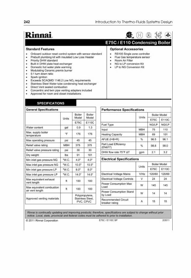
JWST229-c05 JWST229-McDonald Printer: Yet to Come August 1, 2012 11:14 Trim: 244mm × 168mm
242 Introduction to Thermo-Fluids Systems Design

JWST229-c05 JWST229-McDonald Printer: Yet to Come August 1, 2012 11:14 Trim: 244mm × 168mm
Applications of Heat Exchangers in Systems 243
Source: Rinnai America Corp. (reprinted with permission)
JWST229-c05 JWST229-McDonald Printer: Yet to Come August 1, 2012 11:14 Trim: 244mm × 168mm
244 Introduction to Thermo-Fluids Systems Design
Drawings
Not needed.
Conclusions
The boiler has been sized. The lengths of the heaters have also been specified. The lengthsof the heaters are smaller than the total length of the walls.
While a condensing boiler was chosen, a conventional boiler could have been selectedinstead. The designer will need to make a final selection based on the preferences of theclient, need for routine equipment maintenance, and costs (fixed and operating).
The water is returned to the boiler at 159◦F. Industry standard recommends that hot waterfor space heating be about 180◦F for houses. For some of the heaters, the return temperatureis lower than the minimum temperature required. Therefore, the heaters may need to belarger to provide the required amount of heat.
It should be noted that while the AFUE is specified as 96.5%, this efficiency will decreasewhen higher temperature water returns to the condensing boiler. Larger �T between theboiler supply water temperature and return water temperature will improve condensingboiler efficiency. It is well-known that in order to extract more heat from the flue gasesin the boiler heat exchanger and increase the boiler efficiency, the water return temper-ature should not exceed 113–122◦F [1]. To that end, a return water temperature of 110◦Fcould be chosen. In that case, the water temperature at the outlet of the finned-tube heaterthat serves Room 133 will be 110◦F. Therefore, the water that exits the boiler will havea temperature of approximately 152◦F. For energy efficient buildings, the heat loads areusually smaller. Therefore, it may not be necessary that water for space heating be 180◦For higher.
With smaller loads, the flow rate of the fuel supplied to the boiler can be reduced afterinitial start of the system. Since the water will return to the boiler at 159◦F, a lower amountof energy will be required to heat it to 200◦F. Further, given that the heating capacity ofthe Rinnai model Q75C (69000 Btu/h with natural gas) condensing boiler is much higherthan the energy requirement for this application (50479 Btu/h), the fuel flow rate can bemodulated to meet the lower requirements. In less sosphisticated systems, a control systemmay be installed to modulate the fuel flow; but since the Q75C is a modulating boiler,such adjustment will be automatic. Another option could be to purchase more than onesmaller boilers and schedule their operation in order to meet the heating requirements ofthe client.
It should be noted that the boiler will be slightly oversized in this application. The OSFused was 1.10 (equivalent to 91% efficiency). However, the AFUE of the selected boiler isabout 96%.
Orifice plates or balancing valves may be required to balance the losses through thissystem. This will ensure that the heaters in Room 133 will not be “starved” of hot water dueto large pressure drops.
A two-pipe direct return system could have been specified for the finned-tube heatersinstead of the one-pipe series loop system that was selected. In this case, there would be noneed to verify the inlet temperatures to the heaters, assuming no heat loss from the pipesoutside the finned-tube heater units.

JWST229-c05 JWST229-McDonald Printer: Yet to Come August 1, 2012 11:14 Trim: 244mm × 168mm
Applications of Heat Exchangers in Systems 245
Data Sheets and Equipment Schedules
Below are a data sheet and a schedule of the major equipment.
1-Tiered Finned-Tube Heater Data
Tube Fins
Zone Size (in.) Material H×W (in.×in.) Per FootHeight
(in.)
TotalLength
(ft)
Corridor 3/4 copper 31/4×31/4 58 10 17Room 131 3/4 copper 31/4×31/4 58 10 13Room 132 3/4 copper 31/4×31/4 58 10 11Room 133 3/4 copper 31/4×31/4 58 10 10
Boiler Schedule
Fuel Dimensions
Tag
Manufacturerand ModelNumber
BoilerThermalSize Boiler Type
FlowRate(cfm)
FuelType
HHV(Btu/ft3) Width Height Depth
B-1 RinnaimodelQ75C,or equal
69000Btu/h(capacity)
Condensing;wall-mounted
0.85 Naturalgas
1030 19.7′ ′ 25.6′ ′ 15.6′ ′
Example 5.2 Design of a Water Heating System fora Chemical Plant
A chemical engineer would like to use warm, liquid ethyl alcohol (CH3CH2OH)to convert 2-bromo-3-methylbutane (CH3CHBrCH(CH3)2) to 2-ethoxy-2-methylbutane(CH3CH2C(CH3)2OCH2CH3). For this process, the concentration of the ethyl alcohol shouldbe 40% vol. and the temperature should be 100◦F. Pure ethyl alcohol (at 68◦F) from a storagetank will be mixed in mixing tank 1 (see sketch) with water from a hot water heater or boiler.The warm, dilute ethyl alcohol will be mixed with 2-bromo-3-methylbutane in mixing tank2 (see sketch) to produce 2-ethoxy-2-methylbutane. A requirement of the chemical processsets the ethyl alcohol storage tank at 4 ft or less from the mixing tanks. An unlimited,constant supply of pure ethyl alcohol is available for the storage tank. The following sketchprovides additional information on the existing system and the chemical process. Not allaccessories are shown.
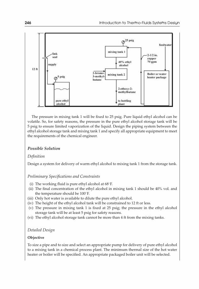
JWST229-c05 JWST229-McDonald Printer: Yet to Come August 1, 2012 11:14 Trim: 244mm × 168mm
246 Introduction to Thermo-Fluids Systems Design
The pressure in mixing tank 1 will be fixed to 25 psig. Pure liquid ethyl alcohol can bevolatile. So, for safety reasons, the pressure in the pure ethyl alcohol storage tank will be5 psig to ensure limited vaporization of the liquid. Design the piping system between theethyl alcohol storage tank and mixing tank 1 and specify all appropriate equipment to meetthe requirements of the chemical engineer.
Possible Solution
Definition
Design a system for delivery of warm ethyl alcohol to mixing tank 1 from the storage tank.
Preliminary Specifications and Constraints
(i) The working fluid is pure ethyl alcohol at 68◦F.(ii) The final concentration of the ethyl alcohol in mixing tank 1 should be 40% vol. and
the temperature should be 100◦F.(iii) Only hot water is available to dilute the pure ethyl alcohol.(iv) The height of the ethyl alcohol tank will be constrained to 12 ft or less.(v) The pressure in mixing tank 1 is fixed at 25 psig; the pressure in the ethyl alcohol
storage tank will be at least 5 psig for safety reasons.(vi) The ethyl alcohol storage tank cannot be more than 4 ft from the mixing tanks.
Detailed Design
Objective
To size a pipe and to size and select an appropriate pump for delivery of pure ethyl alcoholto a mixing tank in a chemical process plant. The minimum thermal size of the hot waterheater or boiler will be specified. An appropriate packaged boiler unit will be selected.

JWST229-c05 JWST229-McDonald Printer: Yet to Come August 1, 2012 11:14 Trim: 244mm × 168mm
Applications of Heat Exchangers in Systems 247
Data Given or Known
(i) Chemicals in the process are known. Of interest is the pure ethyl alcohol.(ii) The pressures in the ethyl alcohol storage tank and mixing tank 1 are 5 psig and 25
psig, respectively.(iii) The ethyl alcohol must be mixed with hot water to a final concentration of 40% vol.
and 100◦F.(iv) Pure ethyl alcohol in the storage tank is available at 68◦F.(v) A hot water heater or boiler will be available to provide 70 gpm of hot water.
(vi) The hot water pipe size is 21/2 in. and the pipe material is copper.(vii) Pure liquid ethyl alcohol can be volatile.
(viii) The ethyl alcohol storage tank cannot be more than 4 ft from the mixing tanks.
Assumptions/Limitations/Constraints
(i) This system uses volatile chemicals. Assume that this system is located in a chemicalplant and noise from pipe flow may not be an issue.
(ii) For transportation of ethyl alcohol between the storage tank and mixing tank 1, assumethat the piping material is PEX (cross-linked polyethylene). This should ensure thatlimited reactions occur between the piping material and the working ethyl alcoholfluid.
(iii) Assume that the sizes of the PEX piping is equivalent to that of Schedule 40 PVCplastic piping.
(iv) For the purpose of sizing the PEX piping, the friction loss chart for Schedule 40 steelwill be used. If available, the chart for plastic piping can be used.
(v) Let the flow velocity be about 6 fps or less. Without information on the erosion limitof PEX, a velocity lower than the erosion limit of soft metals such as aluminum ischosen. This is a conservative choice to avoid system failure.
(vi) Limit pipe frictional losses to 7 ft of water per 100 ft of pipe. This is more thanthe standard of 3 ft of water per 100 ft of pipe. Larger head losses are accept-able since the system will be located in a plant and the length of pipe will beshort (no more than 12 ft). The viscosity of ethyl alcohol is larger than that ofwater, but the two viscosities are on the same order of magnitude for a giventemperature.
(vii) All fittings will be screwed.(viii) Assume that the ethyl alcohol storage tank height is 4 ft. This will ensure proper
maintenance by a 5 ft 6 in. person. In addition, this height is well below the maximumheight of the building of 12 ft.
(ix) Since the supply flow rate of the pure ethyl alcohol to the storage tank is unknown,assume that the storage tank is always nearly full (a constant, unlimited supply isavailable). To prevent spills, assume that the tank is always full to a height of 3 ft. Ahigh-level limit switch could be installed to control the fill height.
(x) To permit easy access, assume that the discharge pipe connection to the storage tankis 6 in. from the finished floor.
(xi) The pump will be an in-line pump mounted on brackets and mounted to the backwall.
(xii) Ball valves will be used to isolate the pump to facilitate maintenance.

JWST229-c05 JWST229-McDonald Printer: Yet to Come August 1, 2012 11:14 Trim: 244mm × 168mm
248 Introduction to Thermo-Fluids Systems Design
(xiii) The pipe connection to mixing tank 1 will be above the free surface of the liquid inthe tank. This will eliminate minor losses at the pipe exit.
(xiv) Mixing tank 1 is 8 ft above the finished floor. This will provide a 4 ft clearance betweenthe top of the mixing tank and the ceiling.
(xv) In Edmonton, the inlet temperature of the feed water to the boiler is about 40◦F.
Sketch
The following drawing shows a possible layout of the piping between the ethyl alcoholstorage tank and mixing tank 1. Note the locations of the pipe connections to the tanks andthe valves.
Analysis
Determine the Pipe Size Required
The pipe size will be determined by considering the flow rate of pure ethyl alcohol that isrequired and the maximum allowed head loss (7 ft of water per 100 ft of pipe).
Use the volume flow rate of water into mixing tank 1 and the final concentration (basedon volume) of ethyl alcohol to determine the volume flow rate of ethyl alcohol into mixingtank 1.
Therefore,
Vethyl
Vethyl + Vwater= 0.40.
Thus,
Vethyl = 0.400.60
Vwater = 0.400.60
(70 gpm
) = 47 gpm.
JWST229-c05 JWST229-McDonald Printer: Yet to Come August 1, 2012 11:14 Trim: 244mm × 168mm
Applications of Heat Exchangers in Systems 249
Use the friction loss chart for Schedule 40 steel for open piping systems (Figure A.4) witha flow rate of 47 gpm and a maximum head loss of 7 ft of water per 100 ft of pipe to estimatethe pipe size.
Therefore,
Dpipe = 2 in. nominal.
For this pipe diameter, the head loss is approximately 6.9 ft of water per 100 ft of pipe andthe pipe velocity is approximately 4.8 fps. The head loss and pipe velocity are below themaximum values of the design constraints. If the friction loss chart for Schedule 80 plasticpiping was used (Figure 3.3), a nominal 2 in. pipe that transports 47 gpm of alcohol wouldgenerate head loss of approximately 5.5 ft of water per 100 ft of pipe.
Determine the Minimum Pump Size Required
The energy equation will be used to determine the pump head required:
hpump = HlT +[
p2
ρg+ α2
V2ave,2
2g+ z2
]−
[p1
ρg+ α1
V2ave,1
2g+ z1
].
Let point 1 be at the inlet to the pipe from the ethyl alcohol storage tank and point 2 bein the fluid jet at the exit of the pipe in mixing tank 1. Therefore, Vave,1 = Vave,2 = 4.8 fps. Itis assumed that the ethyl alcohol fluid jet into mixing tank 1 has the same diameter as thepipe to ensure that the jet velocity is equal to the pipe velocity.
At point 1
p1 = ps-tank + ρgh, where h is the height of fluid in the tank above the pipe connectionh = 3 ft – 6 in. = 2 ft 6 in.z1 = 0.
At point 2
p2 = pm-tank,
z2 = 12 ft – 4 ft – 6 in. = 7 ft 6 in.
The energy equation becomes
hpump = HlT +[
p2
ρg+ z2
]−
[p1
ρg+ z1
]
hpump = HlT +[
pm−tank
ρg+ z2
]−
[ps−tank + ρgh
ρg
]
hpump = HlT +[
pm−tank
ρg+ z2
]−
[ps−tank
ρg+ h
]
hpump = HlT +[
pm−tank − ps−tank
ρg
]+ [z2 − h] .

JWST229-c05 JWST229-McDonald Printer: Yet to Come August 1, 2012 11:14 Trim: 244mm × 168mm
250 Introduction to Thermo-Fluids Systems Design
The total head loss is the sum of the major head loss and the minor head losses.The major head loss is
HlM = 6.9 ft water100 ft pipe
× Lpipe = 6.9 ft water100 ft pipe
× (7.5 ft + 4 ft) = 0.79 ft water.
For the minor head losses, the loss coefficients for the bends, fittings, and valves are givenbelow for a 2 in. diameter pipe,
Ball valve: Kball = 0.05Check valve: Kcheck = 2.1Screwed 90◦ regular bends: K90 deg bend = 0.95Pipe entrance, sharp-edged: Kentrance = 0.50 .
Remember that it was assumed that an in-line pump will be selected. No 90◦ bends atthe pump are expected for this arrangement.
Therefore,
Hlm =∑
KLV2
ave
2g= (0.50 + 2 (0.95) + 2 (0.05) + 2.1)
⎡⎣ (4.8 ft/s)2
2(
32.2 ft/s2)
⎤⎦= 1.65 ft ethyl alcohol.
Multiply by the specific gravity of ethyl alcohol (SGethyl = 0.794) to convert the units to ftof water.
Hlm = 1.65 ft ethyl alcohol×SGethyl = (1.65×0.794) ft water = 1.31 ft water.
The total head loss is
HlT = Hl + Hlm = 0.79 ft + 1.31 ft = 2.10 ft water.
The pump head is
hpump = 2.10 ft water +⎡⎣ 25 lbf/in.2 − 5 lbf/in.2(
49.3 lbm/ft3) (
32.2 ft/s2)
⎤⎦ × (12 in.)2
1 ft2 × 32.2(lbm ft)/s2
1 lbf
+ [7.5 ft − 2.5 ft] ,
hpump = 2.10 ft water + 58.4 ft ethyl alcohol + 5 ft ethyl alcoholhpump = 2.10 ft water + 58.4 ft ethyl alcohol×(SGethyl) + 5 ft ethyl alcohol×(SGethyl).
In terms of ft of water, the pump head required is
hpump = 53 ft water.

JWST229-c05 JWST229-McDonald Printer: Yet to Come August 1, 2012 11:14 Trim: 244mm × 168mm
Applications of Heat Exchangers in Systems 251
The discharge of the pump should be 47 gpm. For this application, a pump that is rated 47gpm at 53 ft of head is required. Readily available are the pump performance curves of Series60 Bell & Gossett in-line centrifugal pumps. The master selection chart is shown below:
The operating point would fall in the contour of the 11/2 in.×7 in. pump casing. Choosethe 11/2 in.×11/2 in.×7 in. family of pumps.

JWST229-c05 JWST229-McDonald Printer: Yet to Come August 1, 2012 11:14 Trim: 244mm × 168mm
252 Introduction to Thermo-Fluids Systems Design
The final choice is a pump with the following operating parameters:
11/2 in. × 11/2 in. × 7 in. pump casing7.0 in. impeller diameter11/2 hp motor1750 rpm.
Boiler Sizing
This boiler serves only to provide hot water to a chemical process. The thermal size of theboiler is
Qboiler = mwatercp,water (Tout,boiler − Tin,boiler) .
The efficiency of the boiler is not considered at this point until an appropriate unit isfinally selected.
In terms of volume flow rate,
Qboiler = ρwaterVwatercp,water (Tout,boiler − Tin,boiler) .
The outlet temperature of the water from the boiler is still unknown. The heat transferredfrom the hot water will be equal to the heat absorbed by the ethyl alcohol in mixing tank 1to achieve the tank temperature of 100◦F. Therefore,
q = mwatercp,water (Tout,boiler − Ttank) = methylcp,ethyl(Ttank − Tethyl,storage
)q = ρwaterVwatercp,water (Tout,boiler − Ttank) = ρethylVethylcp,ethyl
(Ttank − Tethyl,storage
).
Hence,
Tout,boiler = Ttank + ρethylVethylcp,ethyl(Ttank − Tethyl,storage
)ρwaterVwatercp,water
.
Assume that the properties of ethyl alcohol are at 68◦F and those of water are at 100◦F.Then,
JWST229-c05 JWST229-McDonald Printer: Yet to Come August 1, 2012 11:14 Trim: 244mm × 168mm
Applications of Heat Exchangers in Systems 253
Tout,boiler = 100◦F
+(
49.3 lb/ft3) (
47 gal/min)
(0.678 Btu/(lb ◦F)) (100 − 68) ◦ F(
35.315 ft3/264.17 gal
)(
62 lb/ft3) (
70 gal/min)
(0.999 Btu/(lb ◦F))(
35.315 ft3/264.17 gal
)
Tout,boiler = 112◦F.
The properties of water that will be used to size the boiler will be taken at an averagetemperature. For the boiler, the average temperature is
Tave,boiler = Tout,boiler + Tin,boiler
2.
In Edmonton, the inlet temperature of the feed water to the boiler is about 40◦F.Assume Tin,boiler = 40◦F.Thus,
Tave,boiler = 112◦F + 100◦F2
= 106◦F.
Then,
Qboiler ≈(
61.86 lb/ft3) (
70 gal/min)
(0.999 Btu/(lb ◦F)) (112 − 40) ◦ F × 35.315 ft3
264.17 gal× 60 min
1 h.
The minimum thermal size of the hot water boiler is
Qboiler ≈ 2.29 × 10⁶ Btu/h = 2290 MBH = 68 hp (boiler).
A Cleaver-Brooks commercial package boiler will be selected for this application(www.cbboilers.com/commercial_boilers.htm). Sometimes, the efficiencies of the boilersmay not be provided in the manufacturer’s boiler book. However, Cleaver-Brooks uses anominal boiler efficiency of 82% in fuel consumption calculations. Therefore,
Qboiler ≈ 84 hp (boiler).
A Cleaver-Brooks model 4WG packaged hot water boiler will be specified for this appli-cation. Below is an excerpt from the technical catalog of the boiler book. This informationwill be used to prepare the boiler schedule for use by the mechanical contractor.

JWST229-c05 JWST229-McDonald Printer: Yet to Come August 1, 2012 11:14 Trim: 244mm × 168mm
254 Introduction to Thermo-Fluids Systems Design
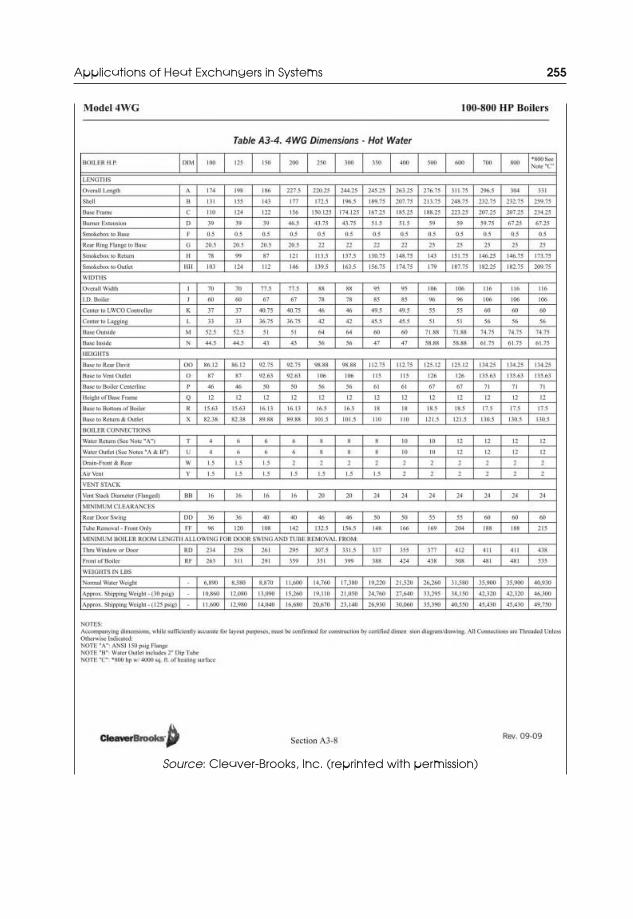
JWST229-c05 JWST229-McDonald Printer: Yet to Come August 1, 2012 11:14 Trim: 244mm × 168mm
Applications of Heat Exchangers in Systems 255
Source: Cleaver-Brooks, Inc. (reprinted with permission)
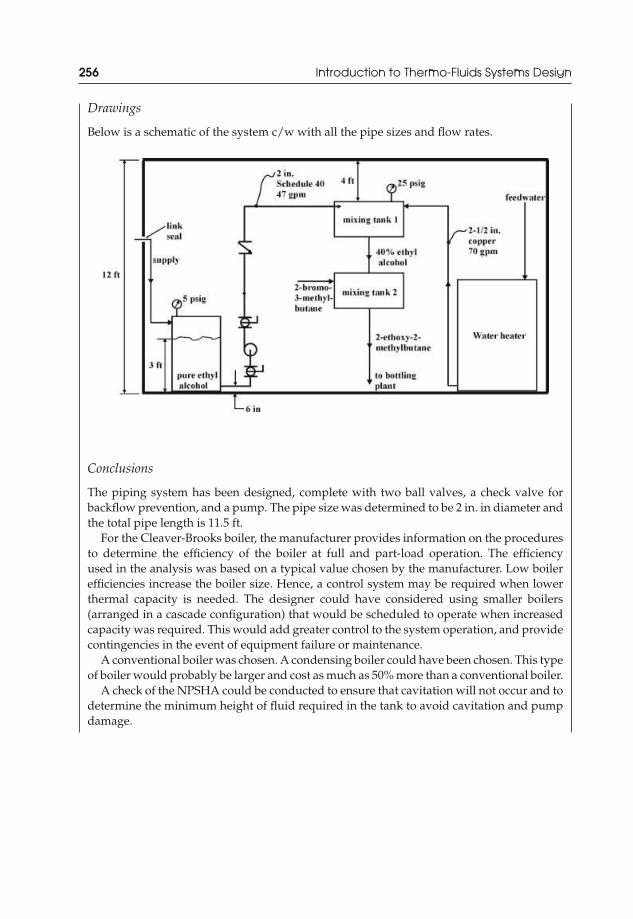
JWST229-c05 JWST229-McDonald Printer: Yet to Come August 1, 2012 11:14 Trim: 244mm × 168mm
256 Introduction to Thermo-Fluids Systems Design
Drawings
Below is a schematic of the system c/w with all the pipe sizes and flow rates.
Conclusions
The piping system has been designed, complete with two ball valves, a check valve forbackflow prevention, and a pump. The pipe size was determined to be 2 in. in diameter andthe total pipe length is 11.5 ft.
For the Cleaver-Brooks boiler, the manufacturer provides information on the proceduresto determine the efficiency of the boiler at full and part-load operation. The efficiencyused in the analysis was based on a typical value chosen by the manufacturer. Low boilerefficiencies increase the boiler size. Hence, a control system may be required when lowerthermal capacity is needed. The designer could have considered using smaller boilers(arranged in a cascade configuration) that would be scheduled to operate when increasedcapacity was required. This would add greater control to the system operation, and providecontingencies in the event of equipment failure or maintenance.
A conventional boiler was chosen. A condensing boiler could have been chosen. This typeof boiler would probably be larger and cost as much as 50% more than a conventional boiler.
A check of the NPSHA could be conducted to ensure that cavitation will not occur and todetermine the minimum height of fluid required in the tank to avoid cavitation and pumpdamage.
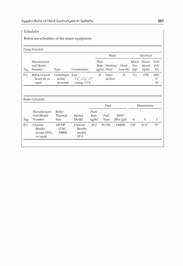
JWST229-c05 JWST229-McDonald Printer: Yet to Come August 1, 2012 11:14 Trim: 244mm × 168mm
Applications of Heat Exchangers in Systems 257
Schedules
Below are schedules of the major equipment.
Pump Schedule
Fluid Electrical
Tag
Manufacturerand ModelNumber Type Construction
FlowRate
(gpm)WorkingFluid
HeadLoss (ft)
MotorSize(hp)
MotorSpeed(rpm)
Volt/pH/Hz
P-1 Bell & GossettSeries 60, orequal
Centrifugal,in-linemounted
Iron11/2
′ ′×11/2′ ′×7′ ′
casing, 7.0"φ
47 Ethylalcohol
53 11/2 1750 208/3/60
Boiler Schedule
Fuel Dimensions
Tag
ManufacturerAnd ModelNumber
BoilerThermalSize
BurnerModel
FlowRate(gph)
FuelType
HHV(Btu/gal) A X I
B-1 Cleaver-Brooksmodel 4WG,or equal
100 HP(3347MBH)
Cleaver-BrooksmodelFP-3
29.2 #2 OIL 140000 174′ ′ 82.4′ ′ 70′ ′
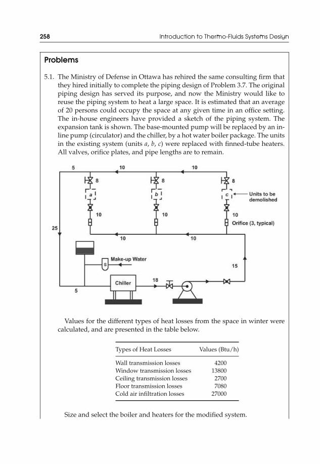
JWST229-c05 JWST229-McDonald Printer: Yet to Come August 1, 2012 11:14 Trim: 244mm × 168mm
258 Introduction to Thermo-Fluids Systems Design
Problems
5.1. The Ministry of Defense in Ottawa has rehired the same consulting firm thatthey hired initially to complete the piping design of Problem 3.7. The originalpiping design has served its purpose, and now the Ministry would like toreuse the piping system to heat a large space. It is estimated that an averageof 20 persons could occupy the space at any given time in an office setting.The in-house engineers have provided a sketch of the piping system. Theexpansion tank is shown. The base-mounted pump will be replaced by an in-line pump (circulator) and the chiller, by a hot water boiler package. The unitsin the existing system (units a, b, c) were replaced with finned-tube heaters.All valves, orifice plates, and pipe lengths are to remain.
Values for the different types of heat losses from the space in winter werecalculated, and are presented in the table below.
Types of Heat Losses Values (Btu/h)
Wall transmission losses 4200Window transmission losses 13800Ceiling transmission losses 2700Floor transmission losses 7080Cold air infiltration losses 27000
Size and select the boiler and heaters for the modified system.
JWST229-c05 JWST229-McDonald Printer: Yet to Come August 1, 2012 11:14 Trim: 244mm × 168mm
Applications of Heat Exchangers in Systems 259
5.2. The City of Edmonton has solicited the services of a mechanical engineer-ing consulting firm to design a heating system for a public pool located inthe City. The pool will be 20 ft wide and 15 ft long. It will be 4 ft deep atone end, varying linearly along the length of the pool to a depth of 10 ft.The pool water is to be heated to 77◦F in the month of May. The focus ofthe design will be to provide a system that can heat the water from an initialtemperature, after winter closure. The 2006 Alberta Building Code, DivisionB, Section 7.3.3.9 requires that the slope of the bottom of public swimmingpools be no more than 1:3. Section 7.3.3.39 of the same code also requires thatthe turnover period (recirculation period) of the pool water shall not exceed4 hours. Design a heating system that is complete with one or more boilerpackages. The maximum length of the piping system may be 25–50 ft fromthe pool. Reference to the 2006 Alberta Building Code may be useful.
5.3. A tankless water heater is required to heat water to 140◦F for domestic use.The water flow rate should be fixed between 2 and 4 gpm. Select and specify(present a schedule) a manufacturer’s tankless water heater. Determine theminimum amount of fuel that will be needed for this application.
5.4. Manufacturers of tankless water heaters will usually recommend that theirunits be vented vertically or horizontally over short runs of pipe. In verticalventing, the vent will protrude about 6 in. upward from the top of the unit and,through a regular 90◦ bend, will penetrate the interior wall to exhaust to theexterior. In the case of a client living in a condominium, this type of installationwas not permitted by the bylaws of the condominium board. As a result,the length of the vent was extended so that venting could be accomplishedthrough a wall that was a horizontal distance, L from the tankless water heaterunit. The designer noted that one manufacturer’s vent model was a concentrictubular venting system in which there was a 21/2 in. inner metal tube vent forhot exhaust gases and a 4 in. outer PVC tube for fresh air from outside forcombustion. The fan installed with the unit moves 50 cfm of air and exhaustgases through the respective sections of the vent. The average outdoor airtemperature is –22◦F and the exhaust gases exit the finned copper tubes of theheat exchanger bank at about 200◦F. Estimate the length of the vent if the airshould enter the combustion chamber at a minimum temperature of 40◦F.
5.5. Campbell, Thompson, and Stewart Architects Ltd. have provided the follow-ing floor plan to a mechanical consulting engineer.
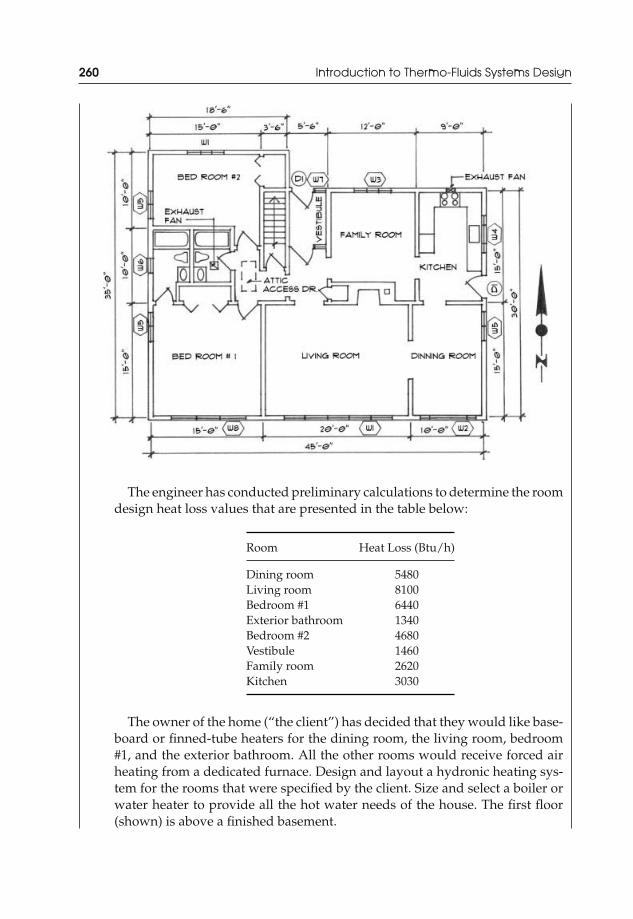
JWST229-c05 JWST229-McDonald Printer: Yet to Come August 1, 2012 11:14 Trim: 244mm × 168mm
260 Introduction to Thermo-Fluids Systems Design
The engineer has conducted preliminary calculations to determine the roomdesign heat loss values that are presented in the table below:
Room Heat Loss (Btu/h)
Dining room 5480Living room 8100Bedroom #1 6440Exterior bathroom 1340Bedroom #2 4680Vestibule 1460Family room 2620Kitchen 3030
The owner of the home (“the client”) has decided that they would like base-board or finned-tube heaters for the dining room, the living room, bedroom#1, and the exterior bathroom. All the other rooms would receive forced airheating from a dedicated furnace. Design and layout a hydronic heating sys-tem for the rooms that were specified by the client. Size and select a boiler orwater heater to provide all the hot water needs of the house. The first floor(shown) is above a finished basement.
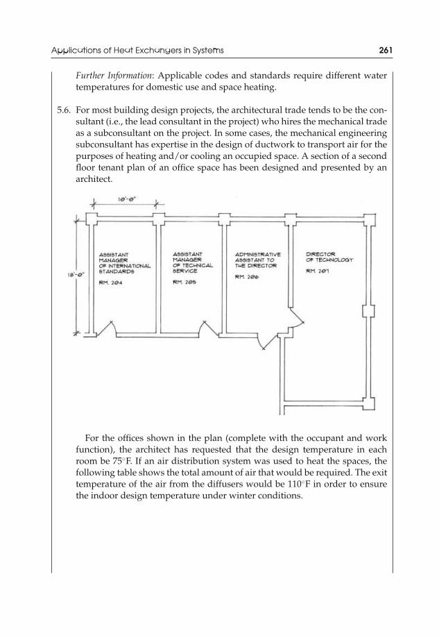
JWST229-c05 JWST229-McDonald Printer: Yet to Come August 1, 2012 11:14 Trim: 244mm × 168mm
Applications of Heat Exchangers in Systems 261
Further Information: Applicable codes and standards require different watertemperatures for domestic use and space heating.
5.6. For most building design projects, the architectural trade tends to be the con-sultant (i.e., the lead consultant in the project) who hires the mechanical tradeas a subconsultant on the project. In some cases, the mechanical engineeringsubconsultant has expertise in the design of ductwork to transport air for thepurposes of heating and/or cooling an occupied space. A section of a secondfloor tenant plan of an office space has been designed and presented by anarchitect.
For the offices shown in the plan (complete with the occupant and workfunction), the architect has requested that the design temperature in eachroom be 75◦F. If an air distribution system was used to heat the spaces, thefollowing table shows the total amount of air that would be required. The exittemperature of the air from the diffusers would be 110◦F in order to ensurethe indoor design temperature under winter conditions.
JWST229-c05 JWST229-McDonald Printer: Yet to Come August 1, 2012 11:14 Trim: 244mm × 168mm
262 Introduction to Thermo-Fluids Systems Design
Office Space Heating Air Requirement
Office 204 330 cfmOffice 205 470 cfmOffice 206 190 cfmOffice 207 520 cfm
However, instead of an air distribution system, the client has requested thata finned-tube heating system, complete with a dedicated condensing boiler bedesigned and installed. Comment on any trade-offs between boiler efficiencyand heater lengths.
Further Information: The length of a standard door is 3 ft.
5.7. WoodBridge ClimateCare, located in Toronto, has solicited the services ofGTA Designs Inc. in Brampton, Ontario to design and layout the ductworksystem that will provide heated air to the space shown in the drawing below.A dedicated furnace, complete with a fan will be purchased and installedbelow the space in an open-concept basement. The ducts will be hung fromthe ceiling of the basement, and appropriate flexible connections of shortlength will be made from the ducts to the diffusers shown in the drawing.Only supply air ducts will be required, since return air will be drawn intothe fan from the open basement space. GTA Designs Inc. has conducted aheat load analysis, and the heat required to maintain each room/area in thespace at 77◦F is shown in the table below. Given the low winter outdoor airtemperature in Toronto proper, the air will exit the diffuser grilles at 125◦F tomaintain the desired indoor space temperature. Design a supply air ductworksystem, based on round ducts, to meet the most stringent demands for heatedair. At this stage of the design, consideration of system balancing and furnaceselection is not required.
Room/Area Heating Load (Btu/h)
Eating area 12800Stairs 1000Private wash room (PWR) 1000Family room 6600Dining 6050Foyer 1200Living room 7050
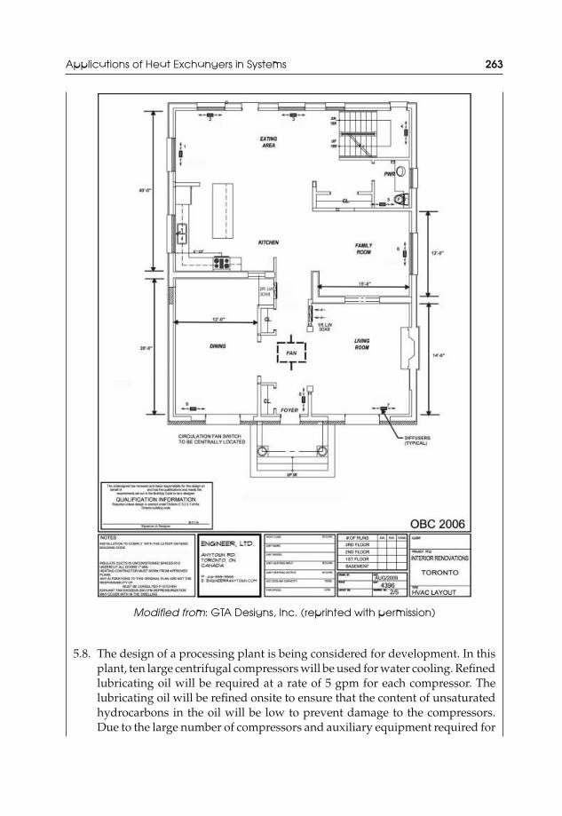
JWST229-c05 JWST229-McDonald Printer: Yet to Come August 1, 2012 11:14 Trim: 244mm × 168mm
Applications of Heat Exchangers in Systems 263
Modified from: GTA Designs, Inc. (reprinted with permission)
5.8. The design of a processing plant is being considered for development. In thisplant, ten large centrifugal compressors will be used for water cooling. Refinedlubricating oil will be required at a rate of 5 gpm for each compressor. Thelubricating oil will be refined onsite to ensure that the content of unsaturatedhydrocarbons in the oil will be low to prevent damage to the compressors.Due to the large number of compressors and auxiliary equipment required for
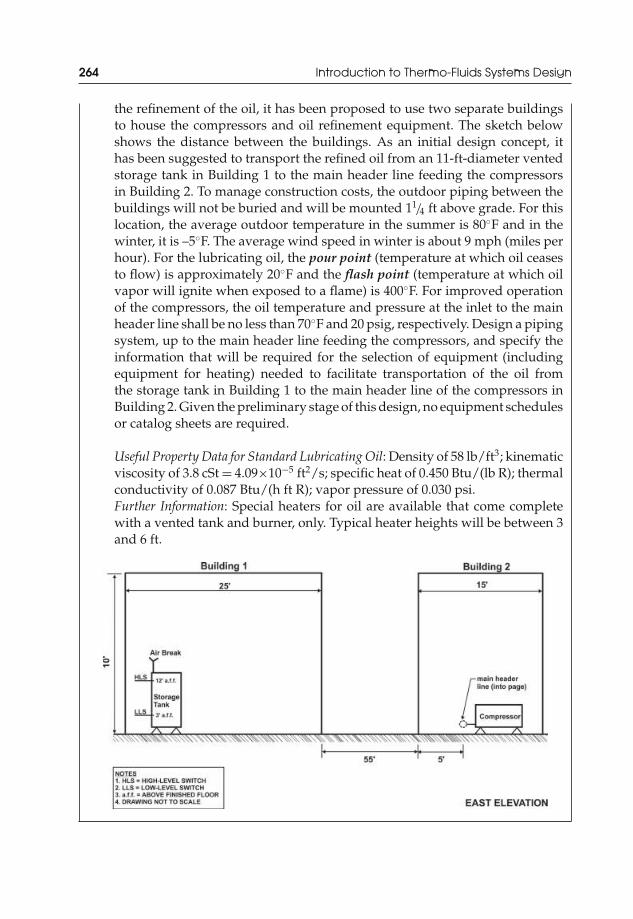
JWST229-c05 JWST229-McDonald Printer: Yet to Come August 1, 2012 11:14 Trim: 244mm × 168mm
264 Introduction to Thermo-Fluids Systems Design
the refinement of the oil, it has been proposed to use two separate buildingsto house the compressors and oil refinement equipment. The sketch belowshows the distance between the buildings. As an initial design concept, ithas been suggested to transport the refined oil from an 11-ft-diameter ventedstorage tank in Building 1 to the main header line feeding the compressorsin Building 2. To manage construction costs, the outdoor piping between thebuildings will not be buried and will be mounted 11/4 ft above grade. For thislocation, the average outdoor temperature in the summer is 80◦F and in thewinter, it is –5◦F. The average wind speed in winter is about 9 mph (miles perhour). For the lubricating oil, the pour point (temperature at which oil ceasesto flow) is approximately 20◦F and the flash point (temperature at which oilvapor will ignite when exposed to a flame) is 400◦F. For improved operationof the compressors, the oil temperature and pressure at the inlet to the mainheader line shall be no less than 70◦F and 20 psig, respectively. Design a pipingsystem, up to the main header line feeding the compressors, and specify theinformation that will be required for the selection of equipment (includingequipment for heating) needed to facilitate transportation of the oil fromthe storage tank in Building 1 to the main header line of the compressors inBuilding 2. Given the preliminary stage of this design, no equipment schedulesor catalog sheets are required.
Useful Property Data for Standard Lubricating Oil: Density of 58 lb/ft3; kinematicviscosity of 3.8 cSt = 4.09×10⁻⁵ ft2/s; specific heat of 0.450 Btu/(lb R); thermalconductivity of 0.087 Btu/(h ft R); vapor pressure of 0.030 psi.Further Information: Special heaters for oil are available that come completewith a vented tank and burner, only. Typical heater heights will be between 3and 6 ft.

JWST229-c05 JWST229-McDonald Printer: Yet to Come August 1, 2012 11:14 Trim: 244mm × 168mm
Applications of Heat Exchangers in Systems 265
References and Further Reading
[1] Natural Resources Canada (2004) Heating with Gas, Home Heating and Cooling Series, Nat-ural Resources Canada, Ottawa.
[2] Epcor, Corp. (2009) Edmonton Water Utilities Statistics, Epcor, Corp., Edmonton.[3] Bobenhausen, W. (1994) Simplified Design of HVAC Systems, John Wiley and Sons, Inc., New
York.[4] National Research Council of Canada (2006) Alberta Building Code, Division B, vol. 2, part
7, Plumbing Services and Health, Ottawa, pp. 7-9–7-10.

JWST229-c06 JWST229-McDonald Printer: Yet to Come July 31, 2012 12:36 Trim: 244mm × 168mm
6Performance Analysis ofPower Plant Systems
Power plant systems are used to generate electrical power and heat. Power plants aremulticomponent systems with turbines, compressors, steam boilers (steam genera-tors), condensers, other heat exchangers, pumps, and combustion burners, to namea few. Although this type of system operates on a thermodynamic (power) cycle toproduce electrical power, other fundamental concepts from fluid mechanics (pipe andduct sizing, pump sizing) and heat exchanger design (design of condensers, feedwa-ter heaters, reheaters) may be needed. Due to the multicomponent nature of powerplant systems, their design can be laborious, especially when control system design isincluded. In addition, significant analysis must be conducted to determine the mosteconomical power plant that will yield the greatest efficiency and performance todeliver a required amount of power. In performance analysis of power plant systems,the design engineer will analyze existing power plants and their components to makerecommendations for improvement of the systems.
6.1 Thermodynamic Cycles for Power Generation—Brief Review
6.1.1 Types of Power Cycles
The thermodynamic (power) cycles are categorized into two groups: gas cycles andvapor cycles.
In a gas (power) cycle, the working fluid remains as a gas throughout the entirecycle. An example is a gas-turbine system based on the Brayton cycle with air orcombustion gas as the working fluid.
In a vapor (power) cycle, the working fluid is a gas in one part of the cycle and isa liquid in another part of the system. An example is a steam-turbine system based
Introduction to Thermo-Fluids Systems Design, First Edition. Andre G. McDonald and Hugh L. Magande.C© 2012 Andre G. McDonald and Hugh L. Magande. Published 2012 by John Wiley & Sons, Ltd.
267
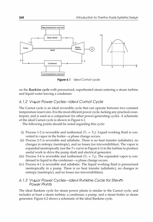
JWST229-c06 JWST229-McDonald Printer: Yet to Come July 31, 2012 12:36 Trim: 244mm × 168mm
268 Introduction to Thermo-Fluids Systems Design
Figure 6.1 Ideal Carnot cycle
on the Rankine cycle with pressurized, superheated steam entering a steam turbineand liquid water leaving a condenser.
6.1.2 Vapor Power Cycles—Ideal Carnot Cycle
The Carnot cycle is an ideal reversible cycle that can operate between two constanttemperature reservoirs. It is the most efficient power cycle, lacking any practical coun-terpart, and is used as a comparison for other power-generating cycles. A schematicof the ideal Carnot cycle is shown in Figure 6.1.
The following points should be noted regarding this cycle:
(i) Process 1-2 is reversible and isothermal (T1 = T2). Liquid working fluid is con-verted to vapor in the boiler—a phase change occurs.
(ii) Process 2-3 is reversible and adiabatic. There is no heat transfer (adiabatic), nochanges in entropy (isentropic), and no losses (no irreversibilities). The vapor isexpanded isentropically (see the T-s curve in Figure 6.1) in the turbine to produceuseful work to drive the pump shaft and electrical generator.
(iii) Process 3-4 is reversible and isothermal (T3 = T4). The expanded vapor is con-densed to liquid in the condenser—a phase change occurs.
(iv) Process 4-1 is reversible and adiabatic. The liquid working fluid is pressurizedisentropically in a pump. There is no heat transfer (adiabatic), no changes inentropy (isentropic), and no losses (no irreversibilities).
6.1.3 Vapor Power Cycles—Ideal Rankine Cycle for SteamPower Plants
The ideal Rankine cycle for steam power plants is similar to the Carnot cycle, andincludes at least a steam turbine, a condenser, a pump, and a steam boiler or steamgenerator. Figure 6.2 shows a schematic of the ideal Rankine cycle.

JWST229-c06 JWST229-McDonald Printer: Yet to Come July 31, 2012 12:36 Trim: 244mm × 168mm
Performance Analysis of Power Plant Systems 269
Figure 6.2 Ideal Rankine cycle
In the Rankine cycle for steam power plants, the condenser may be a large shell-and-tube heat exchanger supplied with cooling water to permit steam condensation. Asshown in Figure 6.2, steam condensation terminates at the saturated liquid state (point4 on the saturation curve), which is different from the Carnot cycle (see Figure 6.1).The steam generator (boiler) may include a burner in which fuel is combusted toprovide the heat needed for steam generation. A simple liquid pump, with reducedpump power requirements, can be used. For smaller pumps, a dedicated motor couldbe used to drive them (motor-driven pump); for larger pumps, an auxiliary steamturbine could be used to drive them (turbine-driven pump). It will be shown laterthrough second-law analysis that losses in the boiler are high (see the T-s diagram ofFigure 6.2). This makes the Rankine cycle much less efficient than the Carnot cycle.
6.1.4 Vapor Power Cycles—Ideal Regenerative Rankine Cycle forSteam Power Plants
Regeneration can be included in the ideal Rankine cycle to preheat the liquid thatenters the boiler. Hot steam is bled from an intermediate section of the steam turbineand used to heat the liquid water. The heating occurs in feedwater heaters (regener-ators). As a result of this preheating, less heat is lost at the condenser, and the overallcycle efficiency increases. Figure 6.3 shows schematics of a single-stage regenerativeRankine cycle and a four-stage regenerative Rankine cycle. In the single-stage regen-erative Rankine cycle, one feedwater heater is present; in the four-stage regenerativeRankine cycle, four feedwater heaters are used.
Figure 6.3 shows two types of feedwater heaters: open feedwater heaters andclosed feedwater heaters.
In open feedwater heaters (contact feedwater heaters), direct mixing of steamwith liquid water occurs. This will increase the efficiency of heating. However, propercontrol of heating is difficult and a special feedwater pump may be needed, which

JWST229-c06 JWST229-McDonald Printer: Yet to Come July 31, 2012 12:36 Trim: 244mm × 168mm
270 Introduction to Thermo-Fluids Systems Design
(a)
(b)
Single-stage feedwater heating
4-stage feedwater heating
Figure 6.3 Ideal regenerative Rankine cycles. (a) Single-stage feedwater heating; (b)four-stage feedwater heating

JWST229-c06 JWST229-McDonald Printer: Yet to Come July 31, 2012 12:36 Trim: 244mm × 168mm
Performance Analysis of Power Plant Systems 271
may increase first costs (installation/initial construction costs) and operation costs ofthe plant.
In closed feedwater heaters (surface heaters), there is no direct mixing of steamand liquid water. All heat transfer occurs though the heat transfer surface area (maybe tubular). This type of feedwater heater may be more desirable for steam powerplants because the heat exchanger can be designed (tube size, arrangement, numberof fins, etc.) to provide some control over the transfer of heat. In addition, only thecondensate pump may be required to move the liquid through the tube line thatpasses through the feedwater heaters.
Practical Note 6.1 Optimizing the Number of Feedwater Heaters
Many feedwater heaters could be included in a regenerative Rankine cycle-based steampower plant. It is the responsibility of the design engineer to optimize the number offeedwater heaters to produce the greatest system efficiency at the most acceptable andreasonable cost (installation and operating costs).
Fundamental Note: A reheat stage may be added to the cycle between two dif-ferent stages of the steam turbine. Moisture in the steam can reduce the efficiencyand undermine the performance of the turbine during expansion. In addition, withless steam to expand, the work output of the turbine will be reduced. Reheating par-tially expanded steam in a reheater (complete with a burner) to facilitate completeexpansion in the intermediate-pressure (IP) or low-pressure (LP) stage of the cyclewill increase the performance and life of the turbine.
6.2 Real Steam Power Plants—General Considerations
Real steam power plants based on the Rankine cycle will differ from the ideal Rankinecycle due to losses throughout the system. The following general points should beconsidered for real steam power plants:
(i) The actual cycle efficiency will depend on the efficiencies of the components inthe system (turbine, pump, condenser, boiler/steam generator) and losses in thepipes and fittings. A second-law analysis may be more appropriate for this typeof practical, multicomponent system.
(ii) There may be multiple feedwater heaters to improve the efficiency of the plant.(iii) Feedwater pumps tend to be larger (larger pump horsepowers). So, they are
typically driven by auxiliary steam-turbine units rather than electric motors.(iv) Steam may be extracted to preheat combustion air that is used in the boiler
burners or in supplementary burners for the feedwater heaters. Energy fromthe combustion gases that exit the boiler stack may also be used to preheat thecombustion air.

JWST229-c06 JWST229-McDonald Printer: Yet to Come July 31, 2012 12:36 Trim: 244mm × 168mm
272 Introduction to Thermo-Fluids Systems Design
6.3 Steam-Turbine Internal Efficiency and Expansion Lines
For an isentropic, adiabatic expansion in a turbine, the turbine internal efficiencywould be 100%, and sin = sout. However, due to losses in real turbines, the expansionis not isentropic and sin �= sout. So, the entropy of steam at the inlet to the turbine isnot equal to the entropy of expanded steam that exhausts from the turbine.
The internal efficiency of the turbine is given as
ηi = hin − hout
hin − hout,s, (6.1)
where hout,s = enthalpy of steam at the turbine exit with the same entropy as that ofhin at the turbine inlet.
If the internal efficiency of the turbine is known and the objective is the determi-nation of the real work output of the turbine, the real enthalpy of the steam at theturbine exhaust (hout) would be needed. Equation (6.1) could be used to find hout.
In the case of steam bleeding for feedwater or process heating, the enthalpies of thesteam bled off from the turbine at IPs would be needed to determine the turbine work.In the case of multistage feedwater heating, the determination of all the enthalpiesof the bled steam could be time consuming if the quality of steam is first determinedto find these enthalpies. Instead, it is typical to use the Mollier diagram for water toplot straight expansion lines between hin and hout to find the enthalpies of the steambled from the turbine at IPs between the inlet and outlet pressures of the turbine.Figure 6.4 shows the Mollier diagram for water. The diagram presents entropy on thex-axis, enthalpy on the y-axis, and lines of pressure, temperature, and quality. Thediagram only applies to superheated steam or steam in which the quality is greaterthan 50%. The Mollier diagram for water can become very busy. Care should be takento read the diagram carefully.
Consider the simple plant with one stage of contact feedwater heating and onesteam turbine that is shown in Figure 6.3a. The turbine internal efficiency is 85%.The inlet pressure to the turbine is P1 = 300 psia (saturated vapor). Steam at 60 psiais bled from the turbine for heating in the contact (open) feedwater heater (P2 =60 psia). Steam is exhausted from the turbine at 1 psia to the condenser (P3 = 1psia ≈ 2.0 in. Hg. abs.). The Mollier diagram can be used to find the enthalpy atpoint 2.
The following steps may be employed:
(i) Find hin = h1 from appropriate thermodynamic tables for steam. At this point,only the pressure was given. Therefore, the Mollier diagram cannot be used tofind h1.
Therefore, h1 = 1203.3 Btu/lb for P1 = 300 psia and T1 = 417.4◦F. The entropyis s1 = 1.51 Btu/(lb R).
(ii) Identify point 1 on the Mollier diagram (see Figure 6.5).

JWST229-c06 JWST229-McDonald Printer: Yet to Come July 31, 2012 12:36 Trim: 244mm × 168mm
Performance Analysis of Power Plant Systems 273
Figure 6.4 Mollier diagram for water

JWST229-c06 JWST229-McDonald Printer: Yet to Come July 31, 2012 12:36 Trim: 244mm × 168mm
274 Introduction to Thermo-Fluids Systems Design
Figure 6.5 Mollier diagram for water showing an expansion line

JWST229-c06 JWST229-McDonald Printer: Yet to Come July 31, 2012 12:36 Trim: 244mm × 168mm
Performance Analysis of Power Plant Systems 275
(iii) Find h3s. This is the enthalpy at the exhaust of the turbine for an isentropicexpansion from 300 to 1 psia. On the Mollier diagram, follow the s1 = s3s =1.51Btu/(lb R) line down from 300 to 1 psia, and identify the enthalpy.
Hence, h3s ≈ 850 Btu/lb.(iv) The turbine internal efficiency can be used to find the real enthalpy of the steam
at the turbine exhaust (h3).
Remember: ηi = h1 − h3
h1 − h3s.
Therefore,
h3 = h1 − ηi (h1 − h3 s)
h3 = 1203.3 Btu/lb − (0.85)(1203.3 − 850) Btu/lb
h3 ≈ 903 Btu/lb at 1 psia
(v) Identify point 3 on the Mollier diagram (see Figure 6.5).(vi) Connect a straight line between points 1 and 3.
(vii) Point 2 will lie along this straight, expansion line at 60 psia.(viii) From the Mollier diagram, h2 ≈ 1095 Btu/lb at 60 psia.
(ix) Use the expansion line between the inlet (point 1) and the outlet (point 3) of theturbine to find the enthalpies of the extracted steam at the specified pressuresfor multiple feedwater heaters.
Example 6.1 First-Law Efficiencies of the Rankine Cycle
A steam power plant is being considered for development. It is expected that saturatedsteam at 300 psia will enter the turbine and exhaust at 1 psia to the condenser. It is proposedto extract some of the steam at 60 psia for the purpose of feedwater heating. Calculate thefirst-law cycle efficiencies of the plant with and without steam extraction.
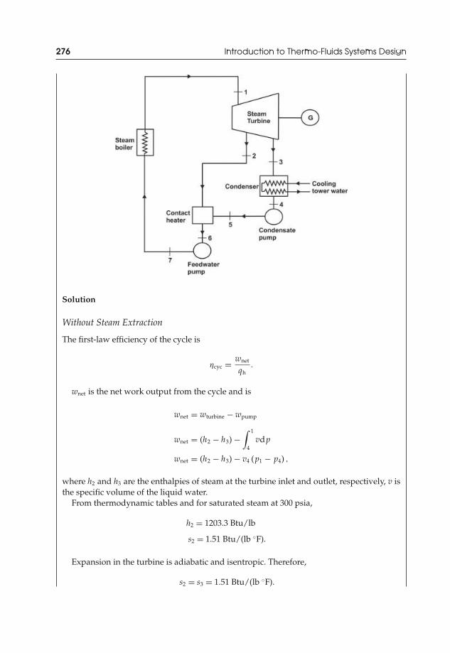
JWST229-c06 JWST229-McDonald Printer: Yet to Come July 31, 2012 12:36 Trim: 244mm × 168mm
276 Introduction to Thermo-Fluids Systems Design
Solution
Without Steam Extraction
The first-law efficiency of the cycle is
ηcyc = wnet
qh.
wnet is the net work output from the cycle and is
wnet = wturbine − wpump
wnet = (h2 − h3) −∫ 1
4vdp
wnet = (h2 − h3) − v4 (p1 − p4) ,
where h2 and h3 are the enthalpies of steam at the turbine inlet and outlet, respectively, v isthe specific volume of the liquid water.
From thermodynamic tables and for saturated steam at 300 psia,
h2 = 1203.3 Btu/lb
s2 = 1.51 Btu/(lb ◦F).
Expansion in the turbine is adiabatic and isentropic. Therefore,
s2 = s3 = 1.51 Btu/(lb ◦F).

JWST229-c06 JWST229-McDonald Printer: Yet to Come July 31, 2012 12:36 Trim: 244mm × 168mm
Performance Analysis of Power Plant Systems 277
The Mollier diagram can be used to estimate h3 at p3 = 1 psia and s3 = 1.51 Btu/(lb ◦F).From Figure 6.4,
h3 ≈ 850 Btu/lb.
If a Mollier diagram is not readily available, h3 can be determined by considering thequality of the expanded steam exiting the turbine. The quality of the steam is
xquality = s3 − sf3
sfg3= (1.51 − 0.133) Btu/(lb ◦F)
1.85 Btu/(lb ◦F)= 0.744.
With the quality known, the enthalpy at point 3 is
h3 = hf3 + xqualityhfg3
h3 = 69.72 Btu/lb + (0.744)(1035.7 Btu/lb)h3 = 841 Btu/lb ≈ 850 Btu/lb.
Assuming that there are no losses in the system,
p4 = 1 psiap1 = 300 psiav4 = 0.01614 ft3/lb (obtained from thermodynamic tables)h4 = 69.72 Btu/lb (obtained from thermodynamic tables).
Therefore,
wnet = (1203.3 − 850) Btu/lb − 0.01614ft3
lb× (300 − 1)
lbfin2
× 32.2 lb/ft/s2
1 lbf
×(
12 in.
1 ft
)2
× 1 Btu/lb
25037 ft2/s2
wnet = 352.4 Btu/lb.
Heat (qh) is supplied at the boiler to vaporize the liquid water to steam. This occursbetween points 1 and 2. Thus,
qh = h2 − h1.
The enthalpy of the liquid at the inlet to the boiler is
h1 = h4 − wpump = h4 − [−v4(p1 − p4)].
JWST229-c06 JWST229-McDonald Printer: Yet to Come July 31, 2012 12:36 Trim: 244mm × 168mm
278 Introduction to Thermo-Fluids Systems Design
Hence,
qh = h2 − h4 − [v4(p1 − p4)]
qh = (1203.3 − 69.72) Btu/lb − 0.01614ft3
lb× (300 − 1)
lbfin.2
× 32.2 lb/ft/s2
1 lbf
×(
12 in.
1 ft
)2
× 1 Btu/lb
25037 ft2/s2
qh = 1132.7 Btu/lb.
The first-law cycle efficiency is
ηcyc = 352.4 Btu/lb1132.7 Btu/lb
ηcyc = 31.1%.
With Steam Extraction
The first-law efficiency of the cycle is still
ηcyc = wnet
qh.
The use of regenerative feedwater heaters makes the problem more complicated sincesteam is bled from the turbine at an intermediate stage. Each point in the cycle will beanalyzed.
Point 1: Steam at 300 psia. Use tables.
h1 = 1203.3 Btu/lb and s1 = 1.51 Btu/(lb ◦F).
Point 2: Steam at 60 psia after isentropic expansion. Use the Mollier diagram.
h2 ≈ 1075 Btu/lb and s2 = 1.51 Btu/(lb ◦F).
Point 3: Steam at 1 psia after isentropic expansion. Use the Mollier diagram.
h3 ≈ 850 Btu/lb and s3 = 1.51 Btu/(lb ◦F).
Point 4: Liquid water at 1 psia. Use tables.
h4 = 69.72 Btu/lb, s4 = 0.133 Btu/(lb ◦F), and v4 = 0.01614 ft3/lb

JWST229-c06 JWST229-McDonald Printer: Yet to Come July 31, 2012 12:36 Trim: 244mm × 168mm
Performance Analysis of Power Plant Systems 279
Point 5: Liquid water at the condensate pump exit:
h5 = h4 − wcon.pump = h4 − [−v4(p5 − p4)]
h5 = 69.72 Btu/lb + 0.01614ft3
lb× (60 − 1)
lbfin.2
× 32.2 lb/ft/s2
1 lbf
×(
12 in.
1 ft
)2
× 1 Btu/lb
25037 ft2/s2
h5 = 69.9 Btu/lb.
Note that p5 = 60 psia to match p2 = 60 psia. This will prevent backflow of liquid into thedischarge line of the condensate pump.
Point 6: Liquid water at the open feedwater heater exit. Use tables.At this point, the pressure is 60 psia. The enthalpy, h6, is a sum of the enthalpies of the
fluid masses from the condensate pump and the bleed line (line 2) from the turbine.Therefore,
�m6h6 = �m2h2 + �m5h5.
The mass is �m6 = �m2 + �m5.Then,
�m6h6 = �m2h2 + (�m6 − �m2)h5
h6 = �m2
�m6h2 +
(1 − �m2
�m6
)h5.
From tables, h6 = 262.2 Btu/lb and v6 = 0.01738 ft3/lb.The mass flow ratio, �m2
�m6, is
262.2 Btu/lb = �m2
�m6(1075 Btu/lb) +
(1 − �m2
�m6
)(69.9 Btu/lb)
�m2
�m6= 0.191.
Point 7: Liquid Water at the Feedwater Pump Exit:
h7 = h6 − wfeed.pump = h6 − [−v6(p7 − p1)]
h7 = 262.2 Btu/lb + 0.01738ft3
lb× (300 − 60)
lbfin.2
× 32.2 lb/ft/s2
1 lbf
×(
12 in.
1 ft
)2
× 1 Btu/lb
25037 ft2/s2
h7 = 262.97 Btu/lb.

JWST229-c06 JWST229-McDonald Printer: Yet to Come July 31, 2012 12:36 Trim: 244mm × 168mm
280 Introduction to Thermo-Fluids Systems Design
All the enthalpies are known. The turbine work output is
wturbine = h1 − �m2
�m6h2 −
(1 − �m2
�m6
)h3
wturbine = 1203.3 Btu/lb − (0.191) (1075 Btu/lb) − (1 − 0.191) (850 Btu/lb)
wturbine = 310.3 Btu/lb.
The total pump work is
wpump = wcon.pump + wfeed.pump
wpump =(
1 − �m2
�m6
)(h5 − h4) + (h7 − h6)
wpump = (1 − 0.191) (69.9 − 69.72) Btu/lb + (262.97 − 262.2) Btu/lb
wpump = −0.916 Btu/lb.
Note that the negative sign indicates that the system inputs energy to drive the pumps.The heat supplied at the boiler is
qh = h1 − h7 = (1203.3 − 262.97) Btu/lb = 940.3 Btu/lb.
The first-law cycle efficiency is
ηcyc = (310.3 − 0.916) Btu/lb940.3 Btu/lb
ηcyc = 32.9%.
With regeneration, the first-law cycle efficiency is increased.
6.4 Closed Feedwater Heaters (Surface Heaters)
In closed feedwater heaters (typically, shell-and-tube heat exchangers), condensatewater (feedwater) flows through tubes in the heater, and energy is absorbed fromcondensing steam in the shell. The closed feedwater heater may have three mainheat exchanger zones: the desuperheating zone, the condensing zone, and the draincooling zone. In the desuperheating zone, superheated steam will be cooled to about50◦F above the saturation temperature before entering the condensing zone. The liquidcondensate may be cooled in a drain cooler to recover additional energy. Figure 6.6shows two types of drain disposals for closed feedwater heaters. Liquid water fromthe drain cooler may be pumped to the main water that is routed toward the boiler(Figure 6.6a) or it may be throttled back to a LP heater or to the condenser (Figure 6.6b).Some feedwater heater designs may be devoid of drain coolers. In which case, theliquid condensate will leave the feedwater at the saturation temperature.

JWST229-c06 JWST229-McDonald Printer: Yet to Come July 31, 2012 12:36 Trim: 244mm × 168mm
Performance Analysis of Power Plant Systems 281
Figure 6.6 Drain disposals for closed feedwater heaters (surface heaters)
To analyze the plant system completely, the enthalpies of the water exiting thepiping system and the feedwater heater will be needed. To find the enthalpies, thewater temperatures will be needed. Figure 6.6 shows that the temperature of theinlet water to the feedwater pipe is denoted as Tx and for the exiting pipe water, thetemperature is denoted as Ty.
Two methods are available to find Tx and Ty: the drain cooler approach (DCA) andthe terminal temperature difference (TTD).
For the case of drain cooling, the DCA isDCA = Tdrain − Tx, (6.2)
whereTdrain = temperature of the water leaving the feedwater heater drain cooler;
Tx = inlet temperature of the water to the feedwater heater pipe.
For the TTD,TTD = Tsat − Ty, (6.3)
whereTsat = saturation temperature at the operating pressure of the condensing zone;Ty = exit temperature of the water from the feedwater heater pipe.
Practical Note 6.2 DCA and TTD Values
The performance of a feedwater heater is specified by the values of DCA and TTD. LowerDCA and TTD indicate greater heat transfer. In practice, the DCA will range from 10◦F to20◦F for an internal drain cooler. The TTD will range from −3◦F to 10◦F. Negative valuesof TTD are possible for feedwater heaters with desuperheating zones. As the superheatedsteam exchanges heat with the feedwater exiting the heater, the exit water temperaturemay exceed the saturation temperature at the operating pressure of the condensing zone toproduce a negative TTD value. Typically, though, TTD values will be on the order of 2◦F to10◦F, with 2◦F being a practical lower limit for a feedwater heater without a desuperheatingzone. A desuperheating zone may not be necessary for extraction steam with less than 100◦Fsuperheat.
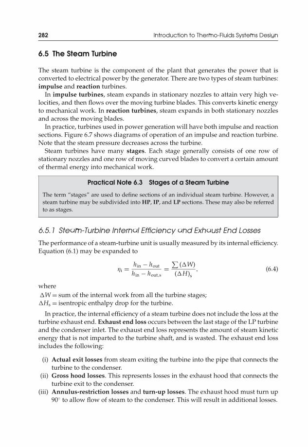
JWST229-c06 JWST229-McDonald Printer: Yet to Come July 31, 2012 12:36 Trim: 244mm × 168mm
282 Introduction to Thermo-Fluids Systems Design
6.5 The Steam Turbine
The steam turbine is the component of the plant that generates the power that isconverted to electrical power by the generator. There are two types of steam turbines:impulse and reaction turbines.
In impulse turbines, steam expands in stationary nozzles to attain very high ve-locities, and then flows over the moving turbine blades. This converts kinetic energyto mechanical work. In reaction turbines, steam expands in both stationary nozzlesand across the moving blades.
In practice, turbines used in power generation will have both impulse and reactionsections. Figure 6.7 shows diagrams of operation of an impulse and reaction turbine.Note that the steam pressure decreases across the turbine.
Steam turbines have many stages. Each stage generally consists of one row ofstationary nozzles and one row of moving curved blades to convert a certain amountof thermal energy into mechanical work.
Practical Note 6.3 Stages of a Steam Turbine
The term “stages” are used to define sections of an individual steam turbine. However, asteam turbine may be subdivided into HP, IP, and LP sections. These may also be referredto as stages.
6.5.1 Steam-Turbine Internal Efficiency and Exhaust End Losses
The performance of a steam-turbine unit is usually measured by its internal efficiency.Equation (6.1) may be expanded to
ηi = hin − hout
hin − hout,s=
∑(�W)
(�H)s, (6.4)
where�W = sum of the internal work from all the turbine stages;�Hs = isentropic enthalpy drop for the turbine.
In practice, the internal efficiency of a steam turbine does not include the loss at theturbine exhaust end. Exhaust end loss occurs between the last stage of the LP turbineand the condenser inlet. The exhaust end loss represents the amount of steam kineticenergy that is not imparted to the turbine shaft, and is wasted. The exhaust end lossincludes the following:
(i) Actual exit losses from steam exiting the turbine into the pipe that connects theturbine to the condenser.
(ii) Gross hood losses. This represents losses in the exhaust hood that connects theturbine exit to the condenser.
(iii) Annulus-restriction losses and turn-up losses. The exhaust hood must turn up90◦ to allow flow of steam to the condenser. This will result in additional losses.

JWST229-c06 JWST229-McDonald Printer: Yet to Come July 31, 2012 12:36 Trim: 244mm × 168mm
Performance Analysis of Power Plant Systems 283
Figure 6.7 Turbine operation
Figure 6.8 shows a schematic of exhaust diffuser of a LP turbine. Note that thesteam turns up and is constrained in an annulus before discharge to the condenser.
The exhaust end loss depends heavily on the absolute steam velocity at the laststage of the turbine. The exhaust end loss can be reduced by reducing the abso-lute steam velocity by (i) increasing the last stage blade length and (ii) increasingthe number of steam flows. So, larger exhaust ends will improve the steam-turbineperformance. As always, the design engineer must make a reasonable compromise
JWST229-c06 JWST229-McDonald Printer: Yet to Come July 31, 2012 12:36 Trim: 244mm × 168mm
284 Introduction to Thermo-Fluids Systems Design
Figure 6.8 Exhaust diffuser of an LP turbine
between increased size for increased performance with the additional costs that willbe incurred.
Because of the exhaust end losses, the steam conditions (in particular, the enthalpy)at the exit of the LP turbine and the inlet of the condenser will be different. The steamconditions at the exit of the last stage of the LP turbine are referred to as those atthe expansion-line-end point (ELEP). Steam conditions at the condenser inlet arethose at the used-energy-end point (UEEP). The exhaust end losses (loss in the steamkinetic energy) are such that the enthalpy at the UEEP (condenser inlet) will be largerthan the enthalpy at the ELEP (LP turbine outlet).
Therefore,
Exhaust end loss = hi,condenser − he,turbine = UEEP − ELEP. (6.5)
Practical Note 6.4 Exhaust End Loss
Typically, the exhaust end loss is approximately 1–3% of the LP turbine work output atfull-load operation. Full-load operation refers to the maximum amount of power that theturbine is designed to produce. Part-load operation may occur during periods of low powerdemand.
6.5.2 Casing and Shaft Arrangements of Large Steam Turbines
The physical size of steam turbines depends, in part, on the amount of power that theyare required to deliver. Their capacities range from a few kilowatts to over 1000000 kW(1000 MW). The inlet pressures to the turbine may be as high as supercritical pressures,and the temperatures may be over 1000◦F. Generator drive speeds are typically 3600and 1800 rpm; geared units can be 10000 rpm or higher. Figure 6.9 shows examples

JWST229-c06 JWST229-McDonald Printer: Yet to Come July 31, 2012 12:36 Trim: 244mm × 168mm
Performance Analysis of Power Plant Systems 285
Tandem-compound 2 flows from 150 to 400 MW
(a)
(b)
(c)
Tandem-compound 4 flows from 300 to 800 MW
Cross-compound 2 flows from 300 to 800 MW
Figure 6.9 Casing and shaft arrangements for large condensing turbines. (a) Tandem-compound 2 flows from 150 to 400 MW; (b) Tandem-compound 4 flows from 300 to 800MW; (c) Cross-compound 2 flows from 300 to 800 MW; (d) Cross-compound 4 flows from800 to 1200 MW

JWST229-c06 JWST229-McDonald Printer: Yet to Come July 31, 2012 12:36 Trim: 244mm × 168mm
286 Introduction to Thermo-Fluids Systems Design
(d)
Cross-compound 4 flows from 800 to 1200 MW
Figure 6.9 (Continued )
of casing and shaft arrangements for large condensing turbines. The figure showsthat the cross-compound arrangements produce large amounts of power. They aretypically only considered for high-capacity machines.
6.6 Turbine-Cycle Heat Balance and Heat and MassBalance Diagrams
The law of conservation of energy and mass can be used to show the flow of steam andenergy in a steam-turbine power cycle. Heat and mass balances are used to determinethe performance/output of the system. A heat and mass balance diagram shows adiagrammatic representation of mass flows, pressures, temperatures, enthalpies, andcycle arrangement of the components.
Consider an actual steam-turbine cycle for a conventional fossil-fuel power plant.The plant has one stage of steam reheat between the HP and IP turbines and sevenstages of regenerative feedwater heating. The initial pressure to the HP turbine is3515 psia and the initial temperature is 1000◦F. The condenser pressure is set to 2.5 in.Hg. abs. ≈ 1.2 psia. After an analysis of the system, a heat and mass balance diagramwas generated. Figure 6.10 shows the details of the diagram.
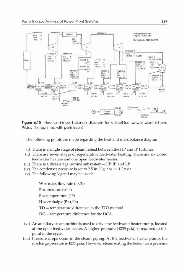
JWST229-c06 JWST229-McDonald Printer: Yet to Come July 31, 2012 12:36 Trim: 244mm × 168mm
Performance Analysis of Power Plant Systems 287
Figure 6.10 Heat-and-mass balance diagram for a fossil-fuel power plant (Li andPriddy [1]; reprinted with permission)
The following points are made regarding the heat and mass balance diagram:
(i) There is a single stage of steam reheat between the HP and IP turbines.(ii) There are seven stages of regenerative feedwater heating. There are six closed
feedwater heaters and one open feedwater heater.(iii) There is a three-stage turbine subsystem—HP, IP, and LP.(iv) The condenser pressure is set to 2.5 in. Hg. abs. ≈ 1.2 psia.(v) The following legend may be used:
W = mass flow rate (lb/h)
P = pressure (psia)
F = temperature (◦F)
H = enthalpy (Btu/lb)
TD = temperature difference in the TTD method
DC = temperature difference for the DCA
(vi) An auxiliary steam turbine is used to drive the feedwater heater pump, locatedat the open feedwater heater. A higher pressure (4235 psia) is required at thispoint in the cycle.
(vii) Pressure drops occur in the steam piping. At the feedwater heater pump, thedischarge pressure is 4235 psia. However, steam exiting the boiler has a pressure

JWST229-c06 JWST229-McDonald Printer: Yet to Come July 31, 2012 12:36 Trim: 244mm × 168mm
288 Introduction to Thermo-Fluids Systems Design
of 3515 psia (as required by the plant). A pressure drop of 720 psia or 17% hasoccurred in the boiler. A pressure drop also occurred across the reheater.
(viii) The exhaust end loss can be determined. Based on the UEEP and ELEP, theexhaust end loss is 11.5 Btu/lb.
(ix) The net generator output or the turbogenerator net output supplied by thegenerator is shown as 726171 kW (power in kW).
(x) The net heat rate (NHR) is also shown (7823 Btu/kWh). This is the ratio of thetotal heat input to the turbogenerator net output.
The net generator output includes the network from the cycle, the exhaust end loss,and the efficiencies of the generator and the turbine–generator mechanical coupling.So, for the plant,
Wgen = ηcouplingηgeneratormsteam(wcycle − LOSSexhaust
). (6.6)
Typically, ηcoupling = 100% and ηgenerator = 95%–98.5%.The NHR is the ratio of the total heat input (from all sources: boiler, reheater, etc.)
to the net generator output.For electric motor-driven feedwater pumps,
NHR = total heat inputgenerator output − electric power for feedwater pumps
. (6.7)
For shaft-driven or auxiliary turbine-driven feedwater pumps,
NHR = total heat inputnet generator output
. (6.8)
It can be seen from Equations (6.7) and (6.8) that lower values of NHR indicateimproved performance of the power plant since low heat inputs produce high netgenerator outputs.
Practical Note 6.5 Units of the Net Heat Rate (NHR)
The NHR must be reported in Btu/kWh.
6.7 Steam-Turbine Power Plant System Performance AnalysisConsiderations
Real steam-turbine power plants may become complex with complicated piping ar-rangements and many different components. The following points may be consideredwhen analyzing the performance of or designing a power plant system:
JWST229-c06 JWST229-McDonald Printer: Yet to Come July 31, 2012 12:36 Trim: 244mm × 168mm
Performance Analysis of Power Plant Systems 289
(i) An appropriate (real) vapor cycle typically consists of a multistage regenerativeRankine cycle with interstage reheating at the turbine.
(ii) Multiple feedwater heaters are usually included to improve the plant efficiency.The total number must be optimized by considering improvements in the plantefficiency and the increased installation and operating costs.
(iii) One stage of reheat is typical. Multiple stages of reheat are not economical.(iv) Steam is usually expanded to about 1 psia ≈ 2.0 in. Hg. abs. in the steam turbine
before condensation in the condenser. This will increase the work output fromthe turbine subsystem.
(v) The net cycle output should be reported in Btu/h or kW.(vi) During design and determination of the performance of a steam-turbine power
plant, the design engineer must consider the(a) main steam pressure and temperature inlet to the steam turbine;(b) reheat steam temperature and pressure;(c) boiler, reheater, and pipe pressure drops;(d) condenser pressure;(e) number of feedwater heaters (stages of regenerative feedwater heating);(f) type of feedwater heaters (open or closed feedwater heaters);(g) heat drain disposal scheme. Will the feedwater heaters drain to other LP
feedwater heaters or directly to the condenser? Will drain coolers be used?(h) DCA;(i) heater TTD;(j) steam extraction for auxiliary turbines;
(k) steam extraction for industrial use and heating;(l) exhaust end loss at the LP turbine.
Practical Note 6.6 How Does One Initiate Operation of a PowerPlant System?
Black-start is the process of restoring a power plant station to operation without relying onexternal energy sources such as from an electric grid. Batteries may be used to start smallauxiliary (diesel) generators. These are used to provide power to run the working fluidthrough bypass lines to ensure flow. For steam power plants, steam may be generated tothe required pressure and temperature by burning the fuel. Blowers for forcing combustiongases over the boiler heat exchanger surfaces would receive power from the generators.
The hot, pressurized steam would flow to the steam turbine to initiate power generation.Hydroelectric plants can also be designated as black-start sources.
Example 6.2 Performance Analysis of a Steam-Turbine Power Plant
In a steam-turbine power plant, steam enters a two-stage turbine at 1250 psia and 950◦F.There are two extraction points at 100 and 25 psia to two stages of regenerative feedwater

JWST229-c06 JWST229-McDonald Printer: Yet to Come July 31, 2012 12:36 Trim: 244mm × 168mm
290 Introduction to Thermo-Fluids Systems Design
heating. The turbine internal efficiency is 90% and the pump efficiency is 85%. The boilerpressure drop is 21%. The steam flow rate at the turbine inlet is 1300000 lb/h. Estimate theperformance of this plant.
Further Information: This performance analysis should address and present the follow-ing points:
(i) Net turbogenerator output(ii) First-law efficiency of the plant
(iii) NHR(iv) A heat and mass balance diagram
Solution. The performance of this plant will include information on the (i) net turbogen-erator output of the plant, (ii) first-law efficiency of the plant, (iii) NHR, and (iv) a heatbalance diagram showing the mass flow rates, pressures, temperatures, and enthalpies ofthe working fluid at different points in the cycle.
Assumptions: (i) The steam finally exhausts to the condenser at 1 psia (typical).(ii) The exhaust end loss is 3% of the output of the steam turbine.
Study Each Point in the Cycle
Point 1: Superheated steam at 1250 psia and 950◦F. Consult tables.With interpolation, h1 = 1469 Btu/lb and s1 = 1.60 Btu/(lb R)
Point 2: Saturated steam at 100 psia after expansion in the HP turbine.The entropies at points 1 and 2 are equal for an isentropic expansion: s1s = s2s = 1.60
Btu/(lb R).
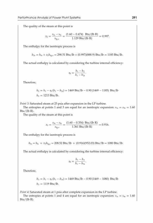
JWST229-c06 JWST229-McDonald Printer: Yet to Come July 31, 2012 12:36 Trim: 244mm × 168mm
Performance Analysis of Power Plant Systems 291
The quality of the steam at this point is
x2 = s2s − sfs
sfg,s= (1.60 − 0.474) Btu/(lb R)
1.129 Btu/(lb R)= 0.997.
The enthalpy for the isentropic process is
h2s = hfs + x2hfg,s = 298.51 Btu/lb + (0.997)(888.9) Btu/lb = 1185 Btu/lb.
The actual enthalpy is calculated by considering the turbine internal efficiency:
ηt = h1 − h2
h1 − h2s.
Therefore,
h2 = h1 − ηt (h1 − h2s) = 1469 Btu/lb − 0.90 (1469 − 1185) Btu/lb
h2 = 1213 Btu/lb.
Point 3: Saturated steam at 25 psia after expansion in the LP turbine.The entropies at points 1 and 3 are equal for an isentropic expansion: s1s = s3s = 1.60
Btu/(lb R).The quality of the steam at this point is
x3 = s3s − sfs
sfg,s= (1.60 − 0.354) Btu/(lb R)
1.361 Btu/(lb R)= 0.916.
The enthalpy for the isentropic process is
h3s = hfs + x3hfg,s = 208.52 Btu/lb + (0.916)(952.03) Btu/lb = 1080 Btu/lb.
The actual enthalpy is calculated by considering the turbine internal efficiency:
ηt = h1 − h3
h1 − h3s.
Therefore,
h3 = h1 − ηt (h1 − h3s) = 1469 Btu/lb − 0.90 (1469 − 1080) Btu/lb
h3 = 1119 Btu/lb.
Point 4: Saturated steam at 1 psia after complete expansion in the LP turbine.The entropies at points 1 and 4 are equal for an isentropic expansion: s1s = s4s = 1.60
Btu/(lb R).
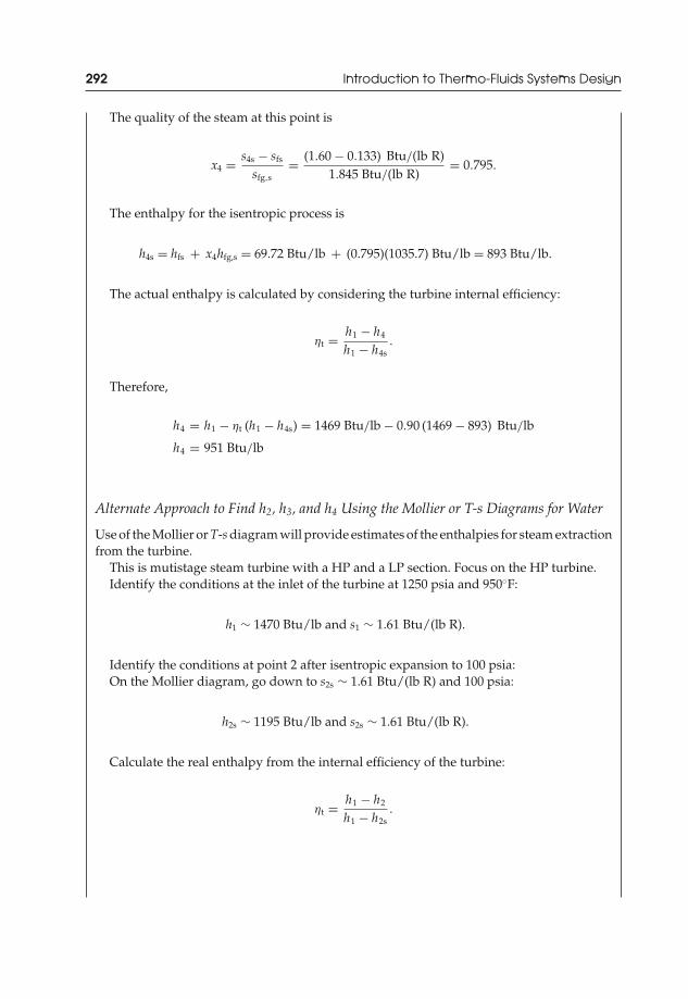
JWST229-c06 JWST229-McDonald Printer: Yet to Come July 31, 2012 12:36 Trim: 244mm × 168mm
292 Introduction to Thermo-Fluids Systems Design
The quality of the steam at this point is
x4 = s4s − sfs
sfg,s= (1.60 − 0.133) Btu/(lb R)
1.845 Btu/(lb R)= 0.795.
The enthalpy for the isentropic process is
h4s = hfs + x4hfg,s = 69.72 Btu/lb + (0.795)(1035.7) Btu/lb = 893 Btu/lb.
The actual enthalpy is calculated by considering the turbine internal efficiency:
ηt = h1 − h4
h1 − h4s.
Therefore,
h4 = h1 − ηt (h1 − h4s) = 1469 Btu/lb − 0.90 (1469 − 893) Btu/lb
h4 = 951 Btu/lb
Alternate Approach to Find h2, h3, and h4 Using the Mollier or T-s Diagrams for Water
Use of the Mollier or T-s diagram will provide estimates of the enthalpies for steam extractionfrom the turbine.
This is mutistage steam turbine with a HP and a LP section. Focus on the HP turbine.Identify the conditions at the inlet of the turbine at 1250 psia and 950◦F:
h1 ∼ 1470 Btu/lb and s1 ∼ 1.61 Btu/(lb R).
Identify the conditions at point 2 after isentropic expansion to 100 psia:On the Mollier diagram, go down to s2s ∼ 1.61 Btu/(lb R) and 100 psia:
h2s ∼ 1195 Btu/lb and s2s ∼ 1.61 Btu/(lb R).
Calculate the real enthalpy from the internal efficiency of the turbine:
ηt = h1 − h2
h1 − h2s.

JWST229-c06 JWST229-McDonald Printer: Yet to Come July 31, 2012 12:36 Trim: 244mm × 168mm
Performance Analysis of Power Plant Systems 293
Therefore,
h2 = h1 − ηt (h1 − h2s) = 1470 Btu/lb − 0.90 (1470 − 1195) Btu/lb
h2 ∼ 1223 Btu/lb.
Note that this value deviates about 0.8% from that found after calculating the quality.Connect points 1 and 2 on the Mollier diagram with a straight line. The steam at point 2 issuperheated (see Mollier diagram). The temperature is T2 ∼ 390◦F.
Note: The Mollier diagram also shows the amount of superheat of the steam. At point2, the steam has approximately 65◦F superheat. This constant superheat is the temperaturedifference between the saturation temperature at the operating pressure (100 psia) and theactual temperature. Thus, T2 ∼ 328◦F + 65◦F ∼ 393◦F.
For this problem, the inlet conditions to the LP turbine are the same as the exit conditionsfrom the HP turbine, and will be used as the starting point of the expansion line for the LPturbine. Identify the conditions at point 4 after isentropic expansion to 1 psia:
On the Mollier diagram, go down to s4s ∼ 1.61 Btu/lb-R and 1 psia.
h4s ∼ 895 Btu/lb and s4s ∼ 1.61 Btu/(lb R)
Calculate the real enthalpy from the internal efficiency of the turbine:
ηt = h1 − h4
h1 − h4s.
Therefore,
h4 = h1 − ηt (h1 − h4s) = 1470 Btu/lb-0.90 (1470 − 895) Btu/lb
h4 ∼ 953 Btu/lb = ELEP.
This is at 1 psia. Identify this point on the Mollier diagram. Point 4 lies below the saturationline. Therefore, the saturation temperature at this point is found from the steam tables at 1psia. Hence, T4 = 101.69◦F.
Connect points 2 and 4 on the Mollier diagram with a straight line. Identify the conditionsat point 3 (25 psia), along the line.
Therefore,
h3 ∼ 1130 Btu/lb and T3 = 240◦F (from the steam tables).
This value of the enthalpy at point 3 deviates about 1% from that found after calculatingthe quality.Point 5: Saturated water at 1 psia. Consult tables.
h5 = 69.72 Btu/lb and v5 = 0.01614 ft3/lb.
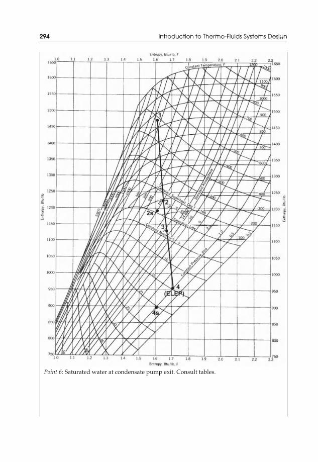
JWST229-c06 JWST229-McDonald Printer: Yet to Come July 31, 2012 12:36 Trim: 244mm × 168mm
294 Introduction to Thermo-Fluids Systems Design
Point 6: Saturated water at condensate pump exit. Consult tables.
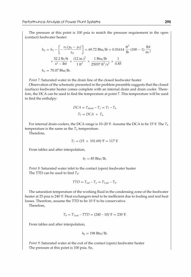
JWST229-c06 JWST229-McDonald Printer: Yet to Come July 31, 2012 12:36 Trim: 244mm × 168mm
Performance Analysis of Power Plant Systems 295
The pressure at this point is 100 psia to match the pressure requirement in the open(contact) feedwater heater:
h6 = h5 −[−v5 (p6 − p5)
ηp
]= 69.72 Btu/lb + 0.01614
ft3
lb(100 − 1)
lbfin.2
×32.2 lb/fts2 − lbf
× (12 in.)2
1 ft2 × 1 Btu/lb
25037 ft2/s2
× 10.85
h6 = 70.07 Btu/lb.
Point 7: Saturated water in the drain line of the closed feedwater heaterObservation of the schematic presented in the problem preamble suggests that the closed
(surface) feedwater heater comes complete with an internal drain and drain cooler. There-fore, the DCA can be used to find the temperature at point 7. This temperature will be usedto find the enthalpy:
DCA = Tdrain – Tx = T7 – T6
T7 = DCA + T6.
For internal drain coolers, the DCA range is 10–20◦F. Assume the DCA to be 15◦F. The T6
temperature is the same as the T4 temperature.Therefore,
T7 = (15 + 101.69)◦F = 117◦F.
From tables and after interpolation,
h7 = 85 Btu/lb.
Point 8: Saturated water inlet to the contact (open) feedwater heaterThe TTD can be used to find T8:
TTD = Tsat – Ty = T3,sat – T8.
The saturation temperature of the working fluid in the condensing zone of the feedwaterheater at 25 psia is 240◦F. Heat exchangers tend to be inefficient due to fouling and real heatlosses. Therefore, assume the TTD to be 10◦F to be conservative.
Therefore,
T8 = T3,sat – TTD = (240 – 10)◦F = 230◦F.
From tables and after interpolation,
h8 = 198 Btu/lb.
Point 9: Saturated water at the exit of the contact (open) feedwater heaterThe pressure at this point is 100 psia. So,

JWST229-c06 JWST229-McDonald Printer: Yet to Come July 31, 2012 12:36 Trim: 244mm × 168mm
296 Introduction to Thermo-Fluids Systems Design
h9 = 298.5 Btu/lb and v9 = 0.01774 ft3/lb.Point 10: Saturated water from the pumpThe water in the pipes that pass through the boiler will experience a 21% pressure drop.
Therefore, p10 must be greater than 1250 psia to compensate for this loss. Hence, p10 = 1583psia:
h10 = h9 −[−v9 (p10 − p9)
ηp
]= 298.5 Btu/lb + 0.01774
ft3
lb(1583 − 100)
lbfin.2
×32.2 lb/fts2 − lbf
× (12 in.)2
1 ft2 × 1 Btu/lb
25037 ft2/s2
× 10.85
h10 = 304.23 Btu/lb
The total turbine work is the sum of the HP and LP turbine work outputs:
wt = wHP + wLP.
The HP and LP turbine work outputs are
wHP = m1h1 − m2h2 − mLPh2
wHP = m1h1 − m2h2 − (m3 + m4) h2
wLP = (m3 + m4) h2 − m3h3 − m4h4 = (h2 − h3) m3 + (h2 − h4) m4.
The mass flow rates at each section of the turbine are needed. Conduct a mass balance:
m9 = m2 + m8
m1 = m2 + m3 + m4
m5 = m3 + m4
m1 = m9 = m10 = 1300000 lb/h
m3 = m7
m5 = m6 = m8.
Energy balance across the open feedwater heater: m9h9 = m2h2 + m8h8.Therefore,
m2 + m8 = 1300000 lb/h
(1300000 lb/h)(298.5 Btu/lb) = m2(1223 Btu/lb) + m8(198 Btu/lb)
These are two equations with two unknowns:
m2 = 127384 lb/h
m8 = 1172616 lb/h
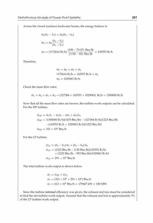
JWST229-c06 JWST229-McDonald Printer: Yet to Come July 31, 2012 12:36 Trim: 244mm × 168mm
Performance Analysis of Power Plant Systems 297
Across the closed (surface) feedwater heater, the energy balance is
m3(h3 − h7) = m8(h8 − h6)
m3 = m8(h8 − h6)(h3 − h7)
m3 = (1172616 lb/h)(198 − 70.07) Btu/lb(1130 − 85) Btu/lb
= 143553 lb/h.
Therefore,
m5 = m8 = m3 + m4
1172616 lb/h = 143553 lb/h + m4
m4 = 1029063 lb/h.
Check the mass flow rates:
m1 = m2 + m3 + m4 = (127384 + 143553 + 1029063) lb/h = 1300000 lb/h.
Now that all the mass flow rates are known, the turbine work outputs can be calculated.For the HP turbine,
wHP = m1h1 − m2h2 − (m3 + m4) h2
wHP = (1300000 lb/h)(1470 Btu/lb) − (127384 lb/h)(1223 Btu/lb)
−(143553 lb/h + 1029063 lb/h)(1223 Btu/lb)
wHP = 321 × 106 Btu/h.
For the LP turbine,
wLP = (h2 − h3) m3 + (h2 − h4) m4
wLP = (1223 Btu/lb − 1130 Btu/lb)(143553 lb/h)+ (1223 Btu/lb − 953 Btu/lb)(1029063 lb/h)
wLP = 291 × 106 Btu/h.
The total turbine work output is shown below.
wt = wHP + wLP
wt = (321 × 106 + 291 × 106) Btu/h
wt = 612 × 106 Btu/h = 179447 kW = 180 MW.
Since the turbine internal efficiency was given, the exhaust end loss must be consideredto find the net turbine work output. Assume that the exhaust end loss is approximately 3%of the LP turbine work output.

JWST229-c06 JWST229-McDonald Printer: Yet to Come July 31, 2012 12:36 Trim: 244mm × 168mm
298 Introduction to Thermo-Fluids Systems Design
Therefore,
wt,loss = 0.03 wLP = 0.03(291 × 106 Btu/h) = 8.7 × 10⁶ Btu/h
The net turbine work output is
wt,net = (612 × 106 – 8.7 × 10⁶) Btu/h = 603 × 106 Btu/h = 176722 kW = 177 MW.
The enthalpy of the steam entering the condenser is larger than that exiting the turbine.The UEEP is
UEEP = h4,condenser = h4,turbine + wt,loss
m4= 953 Btu/lb + 8.7 × 10⁶ Btu/h
1029063 lb/h= 962 Btu/lb.
The total pump work is
wp = m6v5 (p6 − p5)
ηp+ m10
v9 (p10 − p9)ηp
wp = (1172616 lb/h)
(0.01614
ft3
lb
)(100 − 1)
lbfin.2
× 32.2 lb/fts2 − lbf
× (12 in.)2
1 ft2
× 1 Btu/lb
25037 ft2/s2
× 10.85
+ (1300000 lb/h) 0.01774ft3
lb(1583 − 100)
lbfin.2
×32.2 lb/fts2 − lbf
× (12 in.)2
1 ft2 × 1 Btu/lb
25037 ft2/s2
× 10.85
wp = 7.85 × 10⁶ Btu/h = 2304 kW = 2.30 MW.
The net output of the cycle is
wnet = wt,net – wp = 603 × 106 Btu/h – 7.85 × 10⁶ Btu/h
wnet = 595 × 106 Btu/h = 175 × 103 kW = 175 MW.
The heat supplied to the working fluid is
qh = m1(h1 – h10)
qh = (1300000 lb/h)(1470 – 304.23) Btu/lb
qh = 1516 × 106 Btu/h = 444 × 103 kW = 444 MW.
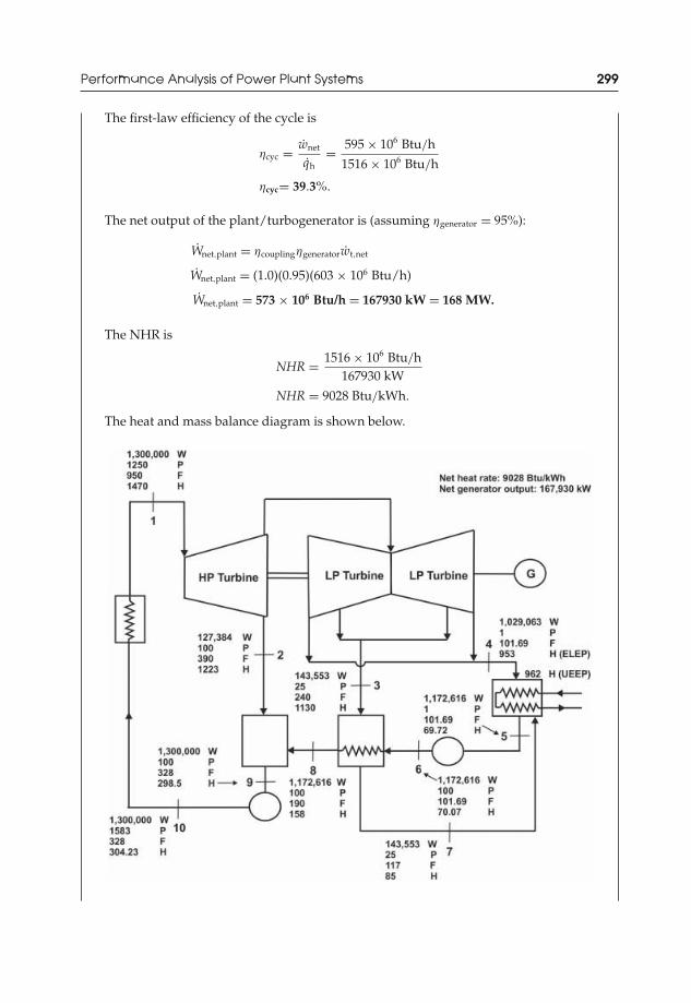
JWST229-c06 JWST229-McDonald Printer: Yet to Come July 31, 2012 12:36 Trim: 244mm × 168mm
Performance Analysis of Power Plant Systems 299
The first-law efficiency of the cycle is
ηcyc = wnet
qh= 595 × 106 Btu/h
1516 × 106 Btu/h
ηcyc= 39.3%.
The net output of the plant/turbogenerator is (assuming ηgenerator = 95%):
Wnet,plant = ηcouplingηgeneratorwt,net
Wnet,plant = (1.0)(0.95)(603 × 106 Btu/h)
Wnet,plant = 573 × 106 Btu/h = 167930 kW = 168 MW.
The NHR is
NHR = 1516 × 106 Btu/h167930 kW
NHR = 9028 Btu/kWh.
The heat and mass balance diagram is shown below.
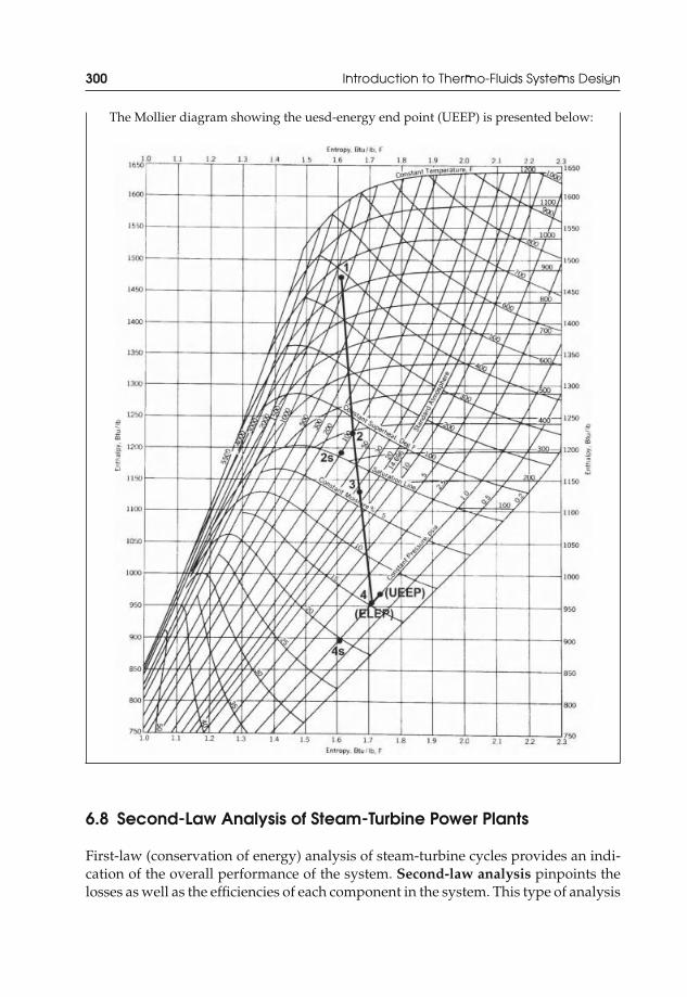
JWST229-c06 JWST229-McDonald Printer: Yet to Come July 31, 2012 12:36 Trim: 244mm × 168mm
300 Introduction to Thermo-Fluids Systems Design
The Mollier diagram showing the uesd-energy end point (UEEP) is presented below:
6.8 Second-Law Analysis of Steam-Turbine Power Plants
First-law (conservation of energy) analysis of steam-turbine cycles provides an indi-cation of the overall performance of the system. Second-law analysis pinpoints thelosses as well as the efficiencies of each component in the system. This type of analysis

JWST229-c06 JWST229-McDonald Printer: Yet to Come July 31, 2012 12:36 Trim: 244mm × 168mm
Performance Analysis of Power Plant Systems 301
is useful for identifying components with large losses to target areas that need furtherimprovement.
Second-law analysis is based on the concept of availability (exergy, available en-ergy, useful energy). Availability is reversible work produced when the cycle workingfluid changes to the state that is in thermal and mechanical equilibrium with the envi-ronment or surroundings. In other words, availability can be considered as a propertythat measures the capacity of the working fluid to do work under environmentalconditions.
Therefore,
a = �wrev, (6.9)
wherea = availability;
wrev = reversible work.
Assuming no kinetic and potential energies, the first law gives
�Wrev = �mihi − �mehe − �Qrev, (6.10)
wheresubscript “i” = the initial state;subscript “e” = the end state;
Qrev = heat transferred.
The second law gives
�misi − �mese − �Qrev
T0= 0, (6.11)
where T0 is reference temperature of the surrounding environment.Therefore,
�Qrev = T0 (�misi − �mese) . (6.12)
Then,
�Wrev = (�mihi − �mehe) − T0 (�misi − �mese) . (6.13)
For steady state, steady processes, �mi = �me = �m. So,
�wrev = �Wrev
�m= (hi − he) − T0 (si − se) . (6.14)
With the environment as a reference and the definition of availability,
a = (h − h0) − T0 (s − s0) . (6.15)

JWST229-c06 JWST229-McDonald Printer: Yet to Come July 31, 2012 12:36 Trim: 244mm × 168mm
302 Introduction to Thermo-Fluids Systems Design
Practical Note 6.7 Reference Pressure and Temperature forAvailability Analysis
Conditions for the reference environment are typically taken at P0 = 14.7 psia and T0 = 77◦F.
The reversible work is the maximum amount of work that can be produced in aprocess, and is usually greater than the actual work output of the real process for thesame end states. So, across a component operating between states 1 and 2,
�wrev = a1 − a2. (6.16)
The difference between the reversible and the actual work is the lost work oravailability loss due to irreversibility.
Therefore,
�I = �wrev − �wact, (6.17)or
Aloss = Ainput − Aoutput. (6.18)
With the input and output availabilities known, the second-law efficiency of thesteam-turbine plant and effectiveness of the components can be determined. Theeffectiveness is a measure of the quality of component design or performance. Thesecond-law efficiency of a plant or a component is
ε = Aoutput
Ainput. (6.19)
A second-law analysis contributes significantly to understanding of the perfor-mance of a plant. Unlike the first-law efficiency, the second-law efficiency takes intoaccount the availability loss and availability destruction across a component. So, ε istypically lower than η.
Example 6.3 Second-Law Analysis of a Steam-Turbine Power Plant
A simple steam-turbine power plant system operates at steady-state, steady-flow conditions.Steam property data are given. Calculate the second-law efficiency for this power-generatingsystem. Calculate the effectiveness of each component.
State P (psia) T (◦F) h (Btu/lb) s (Btu/lb-R)
1 320 Saturated vapor 1204.3 1.50602 1 895.3 1.60313 1 Saturated vapor 69.73 0.132664 320 70.92 0.13290

JWST229-c06 JWST229-McDonald Printer: Yet to Come July 31, 2012 12:36 Trim: 244mm × 168mm
Performance Analysis of Power Plant Systems 303
Hard coal is used in the boiler burner. The burner efficiency is approximately 82%.
Solution
System Effectiveness
The second-law efficiency of the system is
ε = Aoutput
Ainput.
For this system, availability output is
Aoutput = wst − wp.
This is the actual work output from the system.The availability input is
Ainput = qh,fuel.
This is the total heat input to the system. This occurs at the boiler burner, and representsthe total heat available from the fuel.
Therefore,
ε = wst − wp
qh,fuel.
The steam-turbine work output is
wst = h1 – h2 = (1204.3 – 895.3) Btu/lb = 309 Btu/lb.

JWST229-c06 JWST229-McDonald Printer: Yet to Come July 31, 2012 12:36 Trim: 244mm × 168mm
304 Introduction to Thermo-Fluids Systems Design
The pump work is
wp = h4 – h3 = (70.92 – 69.73) Btu/lb = 1.19 Btu/lb.
The total heat available from the fuel is
qh,fuel = mfaf = mf(HVf).
The fuel consumption per pound of steam is mf. Note that the fuel availability is theheating value of the fuel (HVf). For more conservative analyses, the lower heating valuewill be used.
Table 5.2 gives the higher heating value of hard coal as HVf = 14000 Btu/lb coal. The fuelconsumption per pound of steam is
mf = h1 − h4
ηburner (HVf)= (1204.3 − 70.92) Btu/lb steam
0.82 (14000 Btu/lb coal)= 0.0987 lb coal/lb steam.
Therefore,
qh,fuel = (0.0987 lb coal/lb steam)(14000 Btu/lb coal)
qh,fuel = 1382.2 Btu/lb steam.
The second-law efficiency of the system is
ε = (309 − 1.19) Btu/lb steam1382.2 Btu/lb steam
ε = 22%.
For comparison, the first-law efficiency is
ηcyc = wst − wp
qh,boiler= wst − wp
h1 − h4
ηcyc = (309 − 1.19) Btu/lb steam(1204.3 − 70.92) Btu/lb steam
= 27%.
As expected, ε > η.
Component Effectiveness—Boiler/Steam Generator
The second-law efficiency of the boiler is
εboiler = Aoutput
Ainput
εboiler = a1 − a4
mf (HVf).

JWST229-c06 JWST229-McDonald Printer: Yet to Come July 31, 2012 12:36 Trim: 244mm × 168mm
Performance Analysis of Power Plant Systems 305
Find the availabilities at points 1 and 4. Assume that environmental conditions are atP0 = 14.7 psia and T0 = 77◦F.
Therefore,
a1 = (h1 – h0) – T0(s1 – s0)
a1 = (1204.3 – 45.09) Btu/lb – (537 R)(1.5060 – 0.08775) Btu/(lb R)
a1 = 397.3 Btu/lb,
and
a4 = (h4 – h0) – T0(s4 – s0)
a4 = (70.92 – 45.09) Btu/lb – (537 R)(0.13290 – 0.08775) Btu/lb-R
a4 = 1.585 Btu/lb.
Hence,
εboiler = (397.3 − 1.585) Btu/lb1382.2 Btu/lb
εboiler = 29%.
The effectiveness of the boiler is very low. In order to improve the overall effectivenessof the system, the performance of the boiler will need to be improved. The availability lossin the boiler is
�I = Aloss = Ainput − Aoutput = (1382.2 − 397.3 + 1.585) Btu/lb
�I = Aloss = 986.5 Btu/lb.
Of the 1382.2 Btu/lb of energy available from the fuel, 986.5 Btu/lb is lost during operationof the boiler/steam generator.
Component Effectiveness—Steam Turbine
The second-law efficiency of the steam turbine is
εst = Aoutput
Ainput
εst = wst
a1 − a2= h1 − h2
a1 − a2.
Find the availability at point 2. Assume that environmental conditions are at P0 = 14.7psia and T0 = 77◦F.
Therefore,
a2 = (h2 – h0) – T0(s2 – s0)
a2 = (895.3 – 45.09) Btu/lb – (537 R)(1.6031 – 0.08775) Btu/(lb R)
a2 = 36.47 Btu/lb.

JWST229-c06 JWST229-McDonald Printer: Yet to Come July 31, 2012 12:36 Trim: 244mm × 168mm
306 Introduction to Thermo-Fluids Systems Design
Hence,
εst = 309 Btu/lb(397.3 − 36.47) Btu/lb
εst = 86%.
The effectiveness of the steam turbine is the internal efficiency of the unit. So,
ηi = εst = 86%.
The availability loss in the steam turbine is
�I = Aloss = Ainput − Aoutput = (a1 − a2) − wst = (360.8 − 309) Btu/lb
�I = Aloss = 51.8 Btu/lb.
Component Effectiveness—Condenser
The condenser is a heat exchanger. The effectiveness is determined by considering theavailability input from the condensing steam and the availability received by the coolingwater in the heat exchanger tubes (availability output).
Therefore,
εc = Aoutput,cooling water
Ainput,steam.
For this problem, the inlet and exit conditions of the cooling water are not known, andwould be needed to proceed further.
Component Effectiveness—Pump
The second-law efficiency of the pump is
εp = Aoutput
Ainput
εst = a4 − a3
wp= a4 − a3
h4 − h3.
Find the availability at point 3. Assume that environmental conditions are at P0 = 14.7psia and T0 = 77◦F.
Therefore,
a3 = (h3 – h0) – T0(s3 – s0)
a3 = (69.73 – 45.09) Btu/lb – (537 R)(0.13266 – 0.08775) Btu/(lb R)
a3 = 0.5233 Btu/lb.
JWST229-c06 JWST229-McDonald Printer: Yet to Come July 31, 2012 12:36 Trim: 244mm × 168mm
Performance Analysis of Power Plant Systems 307
Hence,
εp = (1.585 − 0.5233) Btu/lb1.19 Btu/lb
εst = 89%.
The availability loss in the pump is
�I = Aloss = Ainput − Aoutput = (a3 − a4) − wp = −1.06 Btu/lb − (−1.19 Btu/lb)
�I = Aloss = 0.13 Btu/lb.
From this analysis, it is clear that the boiler/steam generator is the most inefficientcomponent of the system.
6.9 Gas-Turbine Power Plant Systems
Power plant systems that operate solely with gases as the working fluid are said tooperate on a gas (power) cycle. For typical gas-turbine power plant systems, air or acombustion gas mixture is the working fluid.
6.9.1 The Ideal Brayton Cycle for Gas-Turbine PowerPlant Systems
The simple gas-turbine power plant cycle is based on the Brayton cycle. Figure 6.11shows a schematic of the cycle. Air enters the system and is compressed in a com-pressor, which is then mixed with fuel and burned in a combustor/burner. The hot,compressed products of combustion are expanded in a turbine to produce work todrive the compressor and a generator. The combustion gases are exhausted from thesystem after expansion in the turbine.
The following points are noted regarding Figure 6.11:
(i) Process 1-2 is an isentropic (constant entropy) compression of air in the compres-sor (see T-s diagram of Figure 6.11). The air pressure increases.
(ii) Process 2-3 is a constant pressure heat addition in a combustor or burner. Fuel ismixed with air and burned.
(iii) Process 3-4 is an isentropic expansion of the hot, compressed gas mixture inthe gas turbine. The gas pressure decreases and work output occurs. The gas istypically expanded to atmospheric pressure.
This process and working fluid do not follow a thermodynamic cycle like the steam-turbine power plant system. The composition of the working fluid changes due to

JWST229-c06 JWST229-McDonald Printer: Yet to Come July 31, 2012 12:36 Trim: 244mm × 168mm
308 Introduction to Thermo-Fluids Systems Design
Figure 6.11 Ideal Brayton cycle
fuel mixing and combustion in the burner. In order to analyze a gas-turbine powerplant system, several simplifying assumptions are typically made:
(i) The working fluid is considered as air having a fixed composition. The air is anideal gas with constant specific heats. This assumption is justified beyond thecombustor/burner if the air/fuel ratio is high. In this case, a larger amount of airis present during combustion.
(ii) The combustion process is one that occurs after the mixing of fuel with air. Thedirect mixing and burning of this air/fuel mixture improves the heat transfer, butthe mass of the working fluid will change. The combustion process is assumedto be a heat transfer process from an external source. This is followed by anassumption of constant mass flow rate throughout the system.
(iii) The inlet and exhaust processes can be replaced by constant pressure processes.This will form a complete gas turbine cycle. Typically, air will enter the compres-sor at 14.7 psia, and will leave the turbine at 14.7 psia.
(iv) To ensure ideality of the cycle, all the processes are internally reversible.
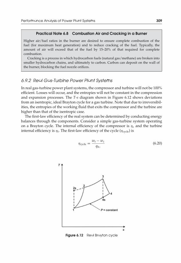
JWST229-c06 JWST229-McDonald Printer: Yet to Come July 31, 2012 12:36 Trim: 244mm × 168mm
Performance Analysis of Power Plant Systems 309
Practical Note 6.8 Combustion Air and Cracking in a Burner
Higher air/fuel ratios in the burner are desired to ensure complete combustion of thefuel (for maximum heat generation) and to reduce cracking of the fuel. Typically, theamount of air will exceed that of the fuel by 15–20% of that required for completecombustion.
Cracking is a process in which hydrocarbon fuels (natural gas/methane) are broken intosmaller hydrocarbon chains, and ultimately to carbon. Carbon can deposit on the wall ofthe burner, blocking the fuel nozzle orifices.
6.9.2 Real Gas-Turbine Power Plant Systems
In real gas-turbine power plant systems, the compressor and turbine will not be 100%efficient. Losses will occur, and the entropies will not be constant in the compressionand expansion processes. The T-s diagram shown in Figure 6.12 shows deviationsfrom an isentropic, ideal Brayton cycle for a gas turbine. Note that due to irreversibil-ities, the entropies of the working fluid that exits the compressor and the turbine arehigher than that of the isentropic case.
The first-law efficiency of the real system can be determined by conducting energybalances through the components. Consider a simple gas-turbine system operatingon a Brayton cycle. The internal efficiency of the compressor is ηc and the turbineinternal efficiency is ηt. The first-law efficiency of the cycle (ηcycle) is
ηcycle = wt − wc
qh,(6.20)
Figure 6.12 Real Brayton cycle
JWST229-c06 JWST229-McDonald Printer: Yet to Come July 31, 2012 12:36 Trim: 244mm × 168mm
310 Introduction to Thermo-Fluids Systems Design
wherewt = total turbine output;wc = energy input required to drive the compressor;qh = total heated added to the system (at the burner and/or a reheater).
The total turbine output is
wt = ηtcp (T3 − T4s) , (6.21)
where cp = specific heat of the combustion gas mixture and T4s is the temperatureafter isentropic expansion in the ideal case.
The input required to drive the compressor is
wc = 1ηc
cp (T2s − T1) , (6.22)
where T2s is the temperature after isentropic compression in the ideal case.Consider the total turbine output in detail:
wt = ηtcp
(1 − T4s
T3
)T3. (6.23)
For the ideal isentropic processes between points 1-2 and 3-4,
T2s
T1= T3
T4s=
(P2s
P1
)(k−1)/k
=(
P3
P4s
)(k−1)/k
= r (k−1)/kp , (6.24)
where
k = cp
cv= specific heat ratio;
rp = pressure ratio.
Therefore,
wt = ηtcpT3
(1 − 1
r (k−1)/kp
). (6.25)
A similar analysis can be conducted for the compressor. This analysis gives
wc = 1ηc
cpT1
(r (k−1)/k
p − 1)
. (6.26)
If the total heat input occurs at the burner, the heat input to the system is
qh = cp (T3 − T2) . (6.27)
Let : qh = cpT1
(T3
T1− T2
T1
). (6.28)
JWST229-c06 JWST229-McDonald Printer: Yet to Come July 31, 2012 12:36 Trim: 244mm × 168mm
Performance Analysis of Power Plant Systems 311
In practice, the inlet temperatures to the gas turbine (T3) and the compressor (T1)will be known. An expression for T2 will be needed to determine the heat transferredto the working fluid in the burner.
The compressor internal efficiency may be expressed as
ηc = h2s − h1
h2 − h1. (6.29)
If the properties of the working fluid are assumed to be constant so that cp =constant,
ηc = T2s − T1
T2 − T1, (6.30)
T2 = T2s − T1
ηc+ T1, (6.31)
T2
T1= 1
ηc
(T2s
T1− 1
)+ 1. (6.32)
Remember: T2sT1
= r (k−1)/kp .
Therefore,
T2
T1= 1
ηc
(r (k−1)/k
p − 1)
+ 1, (6.33)
and
qh = cpT1
[T3
T1− r (k−1)/k
p − 1ηc
− 1
](6.34)
qh = cpT1
ηc
[ηc
(T3
T1− 1
)− r (k−1)/k
p + 1]
. (6.35)
Hence, the first-law efficiency of the cycle becomes
ηcycle =ηtcpT3
(1 − 1
r (k−1)/kp
)− 1
ηccpT1
(r (k−1)/k
p − 1)
cpT1
ηc
[ηc
(T3
T1− 1
)− r (k−1)/k
p + 1] (6.36)
ηcycle =ηtηcT3
(1 − 1
r (k−1)/kp
)− T1
(r (k−1)/k
p − 1)
T1
[ηc
(T3
T1− 1
)− r (k−1)/k
p + 1] (6.37)
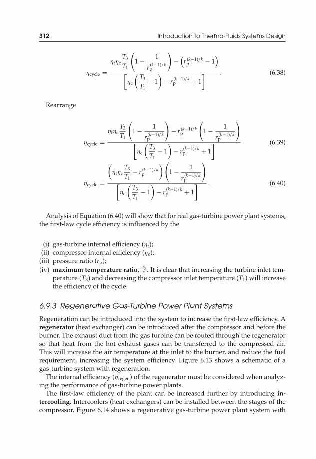
JWST229-c06 JWST229-McDonald Printer: Yet to Come July 31, 2012 12:36 Trim: 244mm × 168mm
312 Introduction to Thermo-Fluids Systems Design
ηcycle =ηtηc
T3
T1
(1 − 1
r (k−1)/kp
)−
(r (k−1)/k
p − 1)
[ηc
(T3
T1− 1
)− r (k−1)/k
p + 1] . (6.38)
Rearrange
ηcycle =ηtηc
T3
T1
(1 − 1
r (k−1)/kp
)− r (k−1)/k
p
(1 − 1
r (k−1)/kp
)[ηc
(T3
T1− 1
)− r (k−1)/k
p + 1] (6.39)
ηcycle =
(ηtηc
T3
T1− r (k−1)/k
p
) (1 − 1
r (k−1)/kp
)[ηc
(T3
T1− 1
)− r (k−1)/k
p + 1] . (6.40)
Analysis of Equation (6.40) will show that for real gas-turbine power plant systems,the first-law cycle efficiency is influenced by the
(i) gas-turbine internal efficiency (ηt);(ii) compressor internal efficiency (ηc);
(iii) pressure ratio (rp);(iv) maximum temperature ratio, T3
T1. It is clear that increasing the turbine inlet tem-
perature (T3) and decreasing the compressor inlet temperature (T1) will increasethe efficiency of the cycle.
6.9.3 Regenerative Gas-Turbine Power Plant Systems
Regeneration can be introduced into the system to increase the first-law efficiency. Aregenerator (heat exchanger) can be introduced after the compressor and before theburner. The exhaust duct from the gas turbine can be routed through the regeneratorso that heat from the hot exhaust gases can be transferred to the compressed air.This will increase the air temperature at the inlet to the burner, and reduce the fuelrequirement, increasing the system efficiency. Figure 6.13 shows a schematic of agas-turbine system with regeneration.
The internal efficiency (ηregen) of the regenerator must be considered when analyz-ing the performance of gas-turbine power plants.
The first-law efficiency of the plant can be increased further by introducing in-tercooling. Intercoolers (heat exchangers) can be installed between the stages of thecompressor. Figure 6.14 shows a regenerative gas-turbine power plant system with

JWST229-c06 JWST229-McDonald Printer: Yet to Come July 31, 2012 12:36 Trim: 244mm × 168mm
Performance Analysis of Power Plant Systems 313
Figure 6.13 Regenerative Brayton cycle
intercooling. Additional reheating via a burner installed in the two-stage gas-turbineassembly is shown.
6.9.4 Operation and Performance of Gas-Turbine PowerPlants—Practical Considerations
The first-law efficiency of the plant presents an indication of the overall performance.Gas-turbine first-law efficiencies are typically on the order of 40% (for plants withregeneration). Second-law analysis would be required to determine the efficiencies ofthe plant components, and to identify components that need improvement.
The gas-turbine unit sizes will range from about 2000 to 100000 kW. Most largeunits are designed to operate at 3000 or 3600 rpm. Gas turbines have relatively lowinitial costs. So, they are frequently used for emergency service and to provide extrapower during peak (electrical) load periods (high electricity demand periods).
Figure 6.14 Regenerative Brayton cycle with intercooling

JWST229-c06 JWST229-McDonald Printer: Yet to Come July 31, 2012 12:36 Trim: 244mm × 168mm
314 Introduction to Thermo-Fluids Systems Design
Natural gas (methane) is the most suitable fuel for gas turbines because limitedfuel preparation is required. In lieu of natural gas, #2 oil may be used. If heavier oilsare considered, they must be heated to reduce their viscosities to facilitate pipingand atomization in the burner. Atomization in the burner results in the formation ofdroplets of fuel, which are easier to burn since the surface area of droplets are large.
Gas-turbine power plant systems have high back work ratios. The back work ratiois the ratio of the compressor work required to the turbine work output. Typically,about two-thirds of the gas-turbine output is used to drive the compressor. Theremainder is used for power generation. Gas turbines tend to be larger than steamturbines for an equivalent power output to the generator because of the large backwork ratios of gas-turbine power plant systems.
Gas-turbine systems can operate at part-load conditions. Full-load operation isthe maximum operation (as specified by the design and the manufacturer) of the gasturbine. As the load decreases to accommodate part-load conditions, the turbine NHRincreases. For part-load operation, it is typical to keep the gas flow rate constant at themaximum capacity for which the system was designed. Reduction in the fuel flowrate will reduce the turbine inlet temperature (lower energy from combustion), andthe work/power output.
In modern gas turbines, the turbine inlet temperatures can be as high as 2600◦F.Higher temperatures are known to accelerate creeping and corrosion of turbineblades. However, the development of protective thermal-sprayed coatings for theblades has enabled the temperature increase. The coatings are usually a bilayer of aNi/Co alloy and yttria-stabilized zirconia, with the zirconia exposed to the ambientto provide high-temperature and corrosion protection.
Manufactured gas-turbine units will come complete with design ratings that arebased on standard, outdoor site conditions. The International Standards Organization(ISO) site conditions are most typically used and referenced: T = 59◦F, P = 14.7 psia,and relative humidity of 60%. Some gas-turbine manufacturers have referenced theirstandard designs to the conditions established by the National Electric ManufacturersAssociation (NEMA): T = 80◦F and P = 14.17 psia.
The first-law efficiency of the gas turbine will increase with a decrease in ambienttemperature. A 5% increase in the first-law efficiency will occur for a temperaturedrop from 59◦F to 0◦F. As the temperature decreases, the air density will also increase.For a constant speed, the air mass flow rate in the compressor will increase by about12% for a temperature drop from 59◦F to 0◦F [1].
Pressure losses in the system will affect the power output and efficiency of thegas-turbine power plant. Typically, and based on the arrangement of the gas-turbinepower plant system, standard inlet losses are 2 in. of water and exhaust losses are4 in. of water. These standard losses are due to duct arrangements and standardunits installed in the ductwork. Inclusion of other auxiliary units—filters, silencers,dampers, waste heat recovery boilers, regenerators, etc.—will increase the inlet andexhaust end pressure drops. Table 6.1 shows some pressure drop values for somecommon units that may be installed at the inlet or exhaust of the plant. These pressuredrops are in addition to the standard losses.

JWST229-c06 JWST229-McDonald Printer: Yet to Come July 31, 2012 12:36 Trim: 244mm × 168mm
Performance Analysis of Power Plant Systems 315
Table 6.1 Pressure drops at the gas-turbine plant inletand exhaust [1]
Inlet Losses Inch of Water
Air filter (protects the air compressor) 0.5Low-level silencer (for noise reduction) 1.5High-level silencer (for noise reduction) 3.5Evaporative air cooler (for water removal) 0.8Exhaust end losses Inch of waterWaste heat boiler for combined systems 10–14Bypass duct for combined systems 6Regenerative air heater (total) 8Open damper 1
Example 6.4 Real Gas-Turbine Power Plant with Part Loads
A gas-turbine plant is in development for the purpose of power generation. The manu-facturer has designed the system as per ISO site conditions for a regenerative gas-turbinemodel.
The compressor, turbine, and regenerator efficiencies are noted to be 85%, 88%, and 70%,respectively. Pressure loss in the burner is 6%. The pressure ratio of the compressor willbe 4 and the inlet temperature of the turbine cannot exceed 2500◦F. The airflow rate willbe 1896000 lb/h. Consulting engineers have decided to use an inlet air filter and low-levelsilencer and an open damper beyond the regenerator in the exhaust duct. Auxiliary powerrequired by the plant for operations will be 7%.
Analyze the performance of the gas-turbine power plant under full-load conditions.Identify the component in the system that requires the most improvement. Determinethe part-load fuel consumption percentage, plant efficiency, and NHR for a 60% part-loadoperating condition.
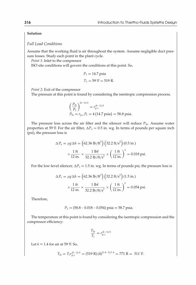
JWST229-c06 JWST229-McDonald Printer: Yet to Come July 31, 2012 12:36 Trim: 244mm × 168mm
316 Introduction to Thermo-Fluids Systems Design
Solution
Full Load Conditions
Assume that the working fluid is air throughout the system. Assume negligible duct pres-sure losses. Study each point in the plant cycle.
Point 1: Inlet to the compressorISO site conditions will govern the conditions at this point. So,
P1 = 14.7 psia
T1 = 59◦F = 519 R.
Point 2: Exit of the compressorThe pressure at this point is found by considering the isentropic compression process.
(P2s
P1
)(k−1)/k
= r (k−1)/kp,c
P2s = rp,c P1 = 4(14.7 psia
) = 58.8 psia.
The pressure loss across the air filter and the silencer will reduce P2s. Assume waterproperties at 59◦F. For the air filter, �Pa = 0.5 in. wg. In terms of pounds per square inch(psi), the pressure loss is
�Pa = ρg�h =(
62.36 lb/ft3) (
32.2 ft/s2)
(0.5 in.)
× 1 ft12 in.
× 1 lbf
32.2 lb/ft/s2 ×(
1 ft12 in.
)2
= 0.018 psi.
For the low-level silencer, �Ps = 1.5 in. wg. In terms of pounds psi, the pressure loss is
�Ps = ρg�h =(
62.36 lb/ft3) (
32.2 ft/s2)
(1.5 in.)
× 1 ft12 in.
× 1 lbf
32.2 lb/ft/s2 ×(
1 ft12 in.
)2
= 0.054 psi.
Therefore,
P2 = (58.8 – 0.018 – 0.054) psia = 58.7 psia.
The temperature at this point is found by considering the isentropic compression and thecompressor efficiency:
T2s
T1= r (k−1)/k
p,c
Let k ≈ 1.4 for air at 59◦F. So,
T2s = T1r (k−1)/kp,c = (519 R) (4)(1.4−1)/1.4 = 771 R = 311◦F.

JWST229-c06 JWST229-McDonald Printer: Yet to Come July 31, 2012 12:36 Trim: 244mm × 168mm
Performance Analysis of Power Plant Systems 317
The real temperature, T2, is found from the definition of the compressor efficiency. Assumeconstant specific heats of air:
ηc = T2s − T1
T2 − T1
T2 = T1 + T2s − T1
ηc= 519 R + (771 − 519) R
0.85
T2 = 816 R = 356◦F.Point 3: Inlet to the gas turbineThere is a 6% pressure drop across the burner. All the losses in the regenerator will be
considered in the exhaust end pressure loss.Therefore,
P3 = (1 – 0.06)P2 = 0.94(58.7 psia)
P3 = 55.2 psia
T3 = 2500◦F = 2960 R.
Point 4: Exit of the gas turbineDue to losses in the regenerator (�Preg) and the open damper (�Pd), the pressure of
the gas mixture leaving the turbine must be greater than the ambient pressure to preventbackflow into the gas turbine.
The total exhaust end pressure loss is
�PT = �Preg + �Pd = (8 + 1) in. wg. = 9 in. wg.
In terms of psi:
�PT =(
62.36 lb/ft3) (
32.2 ft/s2)
(9.0 in.) × 1 ft12 in.
× 1 lbf
32.2 lb/ft/s2 ×(
1 ft12 in.
)2
= 0.33 psi
Therefore,
P4 = 14.7 psia + 0.33 psia = 15.0 psia.
The pressure ratio of the turbine is
rp,t = 55.2 psia15.0 psia
= 3.67.
The temperature of the exhaust gas is found by considering the isentropic expansion ofthe gas mixture in the turbine and the turbine efficiency:
T3
T4s= r (k−1)/k
p,t
T4s = T3
r (k−1)/kp,t
.

JWST229-c06 JWST229-McDonald Printer: Yet to Come July 31, 2012 12:36 Trim: 244mm × 168mm
318 Introduction to Thermo-Fluids Systems Design
Assume that the gas mixture has properties of air at 2500◦F. So, k ≈ 1.3.
T4s = 2960 R
(3.67)(1.3−1)/1.3 = 2193 R = 1733◦F.
The real exhaust gas temperature is found by using the definition of the turbine efficiency:
ηt = T3 − T4
T3 − T4s
T4 = T3 − ηt (T3 − T4s) = 2960 R − 0.88 (2960 − 2193) R
T4 = 2285 R = 1825◦F.Point x: Exit of the regenerator (compressed air to burner)Assume no pressure drop in the regenerator between points 2 and x. So,P2 = Px = 58.7 psia.The temperature is found by considering the efficiency of the regenerator:
ηreg = hx − h2
h4 − hy≈ hx − h2
h4 − h2≈ Tx − T2
T4 − T2.
Note that T4–T2 is the temperature difference that will give the maximum heat transferin the regenerator. As Ty becomes equal to T2, the performance of the regenerator (a heatexchanger) improves. Tx–T2 is the temperature difference that will give the actual heattransfer in the regenerator.
Therefore,
Tx = T2 + ηreg (T4 − T2) = 816 R + (0.70) (2285 − 816) R
Tx = 1844 R = 1384◦F.
Point y: Exit of the regenerator (exhaust gas from the turbine)This point is after the regenerator. So, the turbine exhaust gas pressure will be reduced
by the losses in the regenerator. So,Py = P4 − �Pgen
Py = 15.0 psia −(
62.36 lb/ft3) (
32.2 ft/s2)
(8 in.) × 1 ft12 in.
× 1 lbf
32.2 lb/ft/s2 ×(
1 ft12 in.
)2
Py = 14.71 psia.The temperature is found by conducting an energy balance across the regenerator.
The subscript “a” represents the compressed air and subscript “g” represents exhaustgas mixture.
macp (Tx − T2) = mgcp(T4 − Ty
)
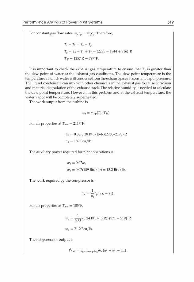
JWST229-c06 JWST229-McDonald Printer: Yet to Come July 31, 2012 12:36 Trim: 244mm × 168mm
Performance Analysis of Power Plant Systems 319
For constant gas flow rates: macp = mgcp. Therefore,
Tx − T2 = T4 − Ty
Ty = T4 − Tx + T2 = (2285 − 1844 + 816) R
Ty = 1257 R = 797◦F.
It is important to check the exhaust gas temperature to ensure that Ty is greater thanthe dew point of water at the exhaust gas conditions. The dew point temperature is thetemperature at which water will condense from the exhaust gases at constant vapor pressure.The liquid condensate can mix with other chemicals in the exhaust gas to cause corrosionand material degradation of the exhaust stack. The relative humidity is needed to calculatethe dew point temperature. However, in this problem and at the exhaust temperature, thewater vapor will be completely superheated.
The work output from the turbine is
wt = ηtcp(T3–T4s).
For air properties at Tave = 2117◦F,
wt = 0.88(0.28 Btu/lb-R)(2960–2193) R
wt = 189 Btu/lb.
The auxiliary power required for plant operations is
wa = 0.07wt
wa = 0.07(189 Btu/lb) = 13.2 Btu/lb.
The work required by the compressor is
wc = 1ηc
cp (T2s − T1) .
For air properties at Tave = 185◦F,
wc = 10.85
(0.24 Btu/(lb R)) (771 − 519) R
wc = 71.2 Btu/lb.
The net generator output is
Wnet = ηgenηcouplingma (wt − wc − wa) .

JWST229-c06 JWST229-McDonald Printer: Yet to Come July 31, 2012 12:36 Trim: 244mm × 168mm
320 Introduction to Thermo-Fluids Systems Design
Assume: ηgen = 95% and ηcoupling = 100%. So,
Wnet = (0.95) (1.00) (1896000 lb/h) (189 − 71.2 − 13.2) Btu/lb
Wnet = 1.89 × 10⁸ Btu/h = 552 41 kW = 55.2 MW.
The back work ratio is
Back work ratio = wc
wt= 71.2 Btu/lb
189 Btu/lb
Back work ratio = 0.38The heat added at the burner is
qh = cp(T3 − Tx).
For air properties at Tave = 1942◦F,
qh = (0.286 Btu/(lb R))(2960 − 1844) R
qh = 319.2 Btu/lb.
In kilowatts,
qh = maqh
qh = (1896000 lb/h)(319.2 Btu/lb)
qh = 6.05 × 10⁸ Btu/h = 177354 kW = 177.4 MW.
The first-law efficiency of the plant is
ηcyc = Wnet
qh= 55241 kW
177354 kW
ηcyc = 31.2%.
The plant NHR is
NHR = heat inputgenerator output
NHR = 6.05 × 10⁸ Btu/h55241 kW
NHR = 10952 Btu/kWh.
Note that the low cycle efficiency results in a high NHR.Below is a heat and mass balance diagram for this problem.

JWST229-c06 JWST229-McDonald Printer: Yet to Come July 31, 2012 12:36 Trim: 244mm × 168mm
Performance Analysis of Power Plant Systems 321
A second-law analysis must be conducted to identify the component of the plant thatneeds the most improvement. Some of the efficiencies are already known.
For the compressor: εc = 85%For the turbine: εt = 88%For the regenerator: εreg = 70%.
For the burner (a heat exchanger), the effectiveness is the ratio of the availability increasein the working fluid (gas mixture) to the availability supplied to the burner. The availabilitysupplied to the burner is the heat added (qh).
Therefore,
εb = a3 − ax
qh= (h3 − hx) − T0 (s3 − sx)
h3 − hx= 1 − T0 (s3 − sx)
h3 − hx.
Remember that for constant cp, s3 − sx ≈ cpln T3Tx
− R ln P3Px
. Thus,
εb = 1 −T0
[cpln
T3
Tx− R ln
P3
Px
]h3 − hx
.
Let T0 = 77◦F = 537 R, and
εb = 1 −(537 R)
[(0.286 Btu/(lb R)) ln
2960 R1844 R
− (0.0686 Btu/lb-R) ln55.2 psia58.7 psia
]319.2 Btu/lb
εb = 76.5%.
Based on the analysis, the burner and the regenerator require the most improvement. Inpractice, regenerator efficiencies are usually lower than 85%.
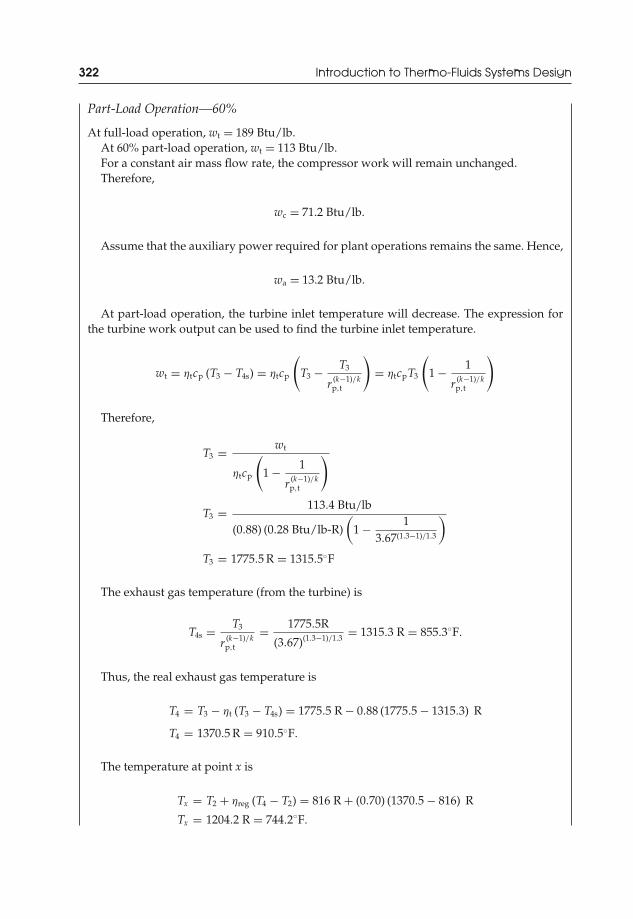
JWST229-c06 JWST229-McDonald Printer: Yet to Come July 31, 2012 12:36 Trim: 244mm × 168mm
322 Introduction to Thermo-Fluids Systems Design
Part-Load Operation—60%
At full-load operation, wt = 189 Btu/lb.At 60% part-load operation, wt = 113 Btu/lb.For a constant air mass flow rate, the compressor work will remain unchanged.Therefore,
wc = 71.2 Btu/lb.
Assume that the auxiliary power required for plant operations remains the same. Hence,
wa = 13.2 Btu/lb.
At part-load operation, the turbine inlet temperature will decrease. The expression forthe turbine work output can be used to find the turbine inlet temperature.
wt = ηtcp (T3 − T4s) = ηtcp
(T3 − T3
r (k−1)/kp,t
)= ηtcpT3
(1 − 1
r (k−1)/kp,t
)
Therefore,
T3 = wt
ηtcp
(1 − 1
r (k−1)/kp,t
)
T3 = 113.4 Btu/lb
(0.88) (0.28 Btu/lb-R)(
1 − 13.67(1.3−1)/1.3
)
T3 = 1775.5 R = 1315.5◦F
The exhaust gas temperature (from the turbine) is
T4s = T3
r (k−1)/kp,t
= 1775.5R
(3.67)(1.3−1)/1.3 = 1315.3 R = 855.3◦F.
Thus, the real exhaust gas temperature is
T4 = T3 − ηt (T3 − T4s) = 1775.5 R − 0.88 (1775.5 − 1315.3) R
T4 = 1370.5 R = 910.5◦F.
The temperature at point x is
Tx = T2 + ηreg (T4 − T2) = 816 R + (0.70) (1370.5 − 816) R
Tx = 1204.2 R = 744.2◦F.

JWST229-c06 JWST229-McDonald Printer: Yet to Come July 31, 2012 12:36 Trim: 244mm × 168mm
Performance Analysis of Power Plant Systems 323
The heat added at the burner for a 60% part-load operation is
qh = cp(T3–Tx)
qh = (0.26 Btu/(lb –R))(1775.5 – 1204.2) R
qh = 148.5 Btu/lb.
The first-law efficiency of the plant at 60% part-load operation is
ηcyc = wnet
qh= wt − wc − wa
qh= (113.4 − 71.2 − 13.2) Btu/lb
148.5 Btu/lb
ηcyc = 19.5%.
The plant NHR is
NHR = heat inputgenerator output
.
The heat input in Btu/h is
qh = maqh
qh = (1896000 lb/h)(148.5 Btu/lb)
qh = 2.82 × 10⁸ Btu/h.
The net generator output for a 60% part-load situation is
Wnet = ηgenηcouplingma (wt − wc − wa) .
Assume: ηgen = 95% and ηcoupling = 100%. So,
Wnet = (0.95) (1.00) (1896000 lb/h) (113.4 − 71.2 − 13.2) Btu/lb
Wnet = 5.22 × 10⁷ Btu/h = 15309 kW = 15.3 MW.
Thus,
NHR = 2.82 × 10⁸ Btu/h15309 kW
NHR = 18421 Btu/kWh.
As the efficiency decreases for part-load operation, the NHR increases.
Fuel Requirements
Assume that #2 oil is used for the power plant burner.At full-load operation,
Vfuel = qh
HVf= 6.05 × 10⁸ Btu/h
140000 Btu/gal
Vfuel = 4321 gph.

JWST229-c06 JWST229-McDonald Printer: Yet to Come July 31, 2012 12:36 Trim: 244mm × 168mm
324 Introduction to Thermo-Fluids Systems Design
At 60% part-load operation:
Vfuel = qh
HVf= 2.82 × 10⁸ Btu/h
140000 Btu/gal
Vfuel = 2014 gph.
The part-load fuel consumption percentage is
2014 gph4321 gph
= 47%.
6.10 Combined-Cycle Power Plant Systems
The efficiency and output of a power plant can be increased by combining differenttypes of cycles for power generation. The combined-cycle plant may consist of one ormore complete gas-turbine units and a steam-turbine unit. The efficiency of this typeof combined-cycle power plant system may exceed 50%.
Figure 6.15 shows a schematic of a combined-cycle power plant with one gas-turbine unit and one steam-turbine unit (Brayton–Rankine combined-cycle powerplant).
In this power plant, electrical power is generated by the gas turbine. The hot exhaustgas mixture is discharged to a waste heat recovery boiler, where steam is generatedfor the steam-turbine unit. The cooled exhaust gas is discharged from the boiler stack.In this way, a greater amount of the fuel supplied at the gas-turbine burner is usedfor electrical power generation.
The power plant shown in Figure 6.15 is very simple. Typically, regeneration maybe included in the gas turbine (with regenerators) and steam turbine (with feedwaterheaters). There may also be intercooling in multistage compressors of the gas-turbine
Figure 6.15 Schematic of a combined-cycle power plant
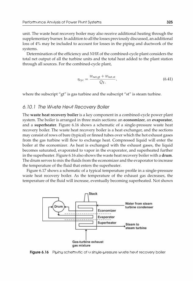
JWST229-c06 JWST229-McDonald Printer: Yet to Come July 31, 2012 12:36 Trim: 244mm × 168mm
Performance Analysis of Power Plant Systems 325
unit. The waste heat recovery boiler may also receive additional heating through thesupplementary burner. In addition to all the losses previously discussed, an additionalloss of 4% may be included to account for losses in the piping and ductwork of thesystems.
Determination of the efficiency and NHR of the combined-cycle plant considers thetotal net output of all the turbine units and the total heat added to the plant stationthrough all sources. For the combined-cycle plant,
ηcyc = wnet,gt + wnet,st
QT,, (6.41)
where the subscript “gt” is gas turbine and the subscript “st” is steam turbine.
6.10.1 The Waste Heat Recovery Boiler
The waste heat recovery boiler is a key component in a combined-cycle power plantsystem. The boiler is arranged in three main sections: an economizer, an evaporator,and a superheater. Figure 6.16 shows a schematic of a single-pressure waste heatrecovery boiler. The waste heat recovery boiler is a heat exchanger, and the sectionsmay consist of rows of bare (typical) or finned tubes over which the hot exhaust gasesfrom the gas turbine will flow to exchange heat. Compressed liquid will enter theboiler at the economizer. As heat is exchanged with the exhaust gases, the liquidbecomes saturated, evaporated to vapor in the evaporator, and superheated furtherin the superheater. Figure 6.16 also shows the waste heat recovery boiler with a drum.The drum serves to mix the fluids from the economizer and the evaporator to increasethe temperature of the fluid that enters the superheater.
Figure 6.17 shows a schematic of a typical temperature profile in a single-pressurewaste heat recovery boiler. As the temperature of the exhaust gas decreases, thetemperature of the fluid will increase, eventually becoming superheated. Not shown
Figure 6.16 Piping schematic of a single-pressure waste heat recovery boiler
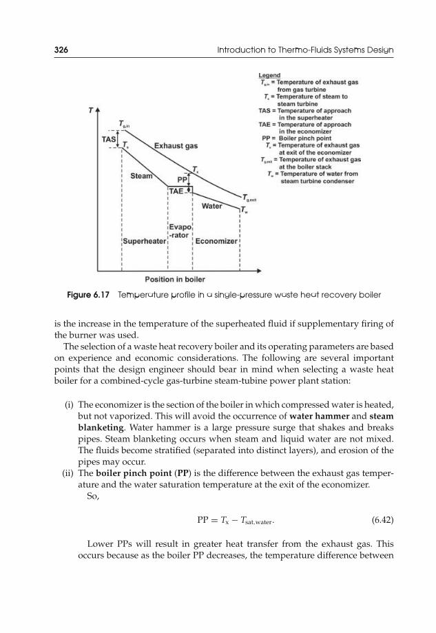
JWST229-c06 JWST229-McDonald Printer: Yet to Come July 31, 2012 12:36 Trim: 244mm × 168mm
326 Introduction to Thermo-Fluids Systems Design
Figure 6.17 Temperature profile in a single-pressure waste heat recovery boiler
is the increase in the temperature of the superheated fluid if supplementary firing ofthe burner was used.
The selection of a waste heat recovery boiler and its operating parameters are basedon experience and economic considerations. The following are several importantpoints that the design engineer should bear in mind when selecting a waste heatboiler for a combined-cycle gas-turbine steam-tubine power plant station:
(i) The economizer is the section of the boiler in which compressed water is heated,but not vaporized. This will avoid the occurrence of water hammer and steamblanketing. Water hammer is a large pressure surge that shakes and breakspipes. Steam blanketing occurs when steam and liquid water are not mixed.The fluids become stratified (separated into distinct layers), and erosion of thepipes may occur.
(ii) The boiler pinch point (PP) is the difference between the exhaust gas temper-ature and the water saturation temperature at the exit of the economizer.
So,
PP = Tx − Tsat,water. (6.42)
Lower PPs will result in greater heat transfer from the exhaust gas. Thisoccurs because as the boiler PP decreases, the temperature difference between
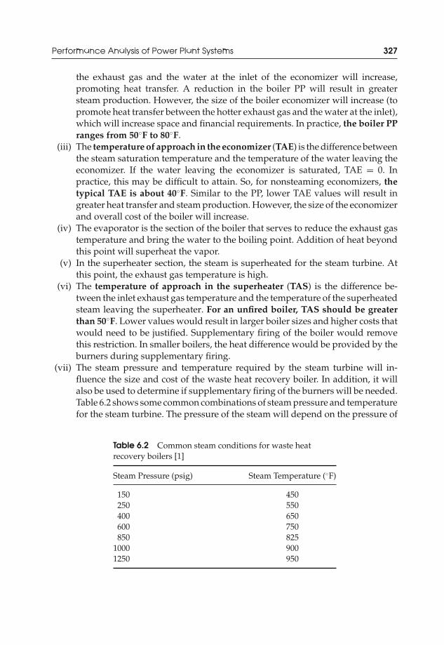
JWST229-c06 JWST229-McDonald Printer: Yet to Come July 31, 2012 12:36 Trim: 244mm × 168mm
Performance Analysis of Power Plant Systems 327
the exhaust gas and the water at the inlet of the economizer will increase,promoting heat transfer. A reduction in the boiler PP will result in greatersteam production. However, the size of the boiler economizer will increase (topromote heat transfer between the hotter exhaust gas and the water at the inlet),which will increase space and financial requirements. In practice, the boiler PPranges from 50◦F to 80◦F.
(iii) The temperature of approach in the economizer (TAE) is the difference betweenthe steam saturation temperature and the temperature of the water leaving theeconomizer. If the water leaving the economizer is saturated, TAE = 0. Inpractice, this may be difficult to attain. So, for nonsteaming economizers, thetypical TAE is about 40◦F. Similar to the PP, lower TAE values will result ingreater heat transfer and steam production. However, the size of the economizerand overall cost of the boiler will increase.
(iv) The evaporator is the section of the boiler that serves to reduce the exhaust gastemperature and bring the water to the boiling point. Addition of heat beyondthis point will superheat the vapor.
(v) In the superheater section, the steam is superheated for the steam turbine. Atthis point, the exhaust gas temperature is high.
(vi) The temperature of approach in the superheater (TAS) is the difference be-tween the inlet exhaust gas temperature and the temperature of the superheatedsteam leaving the superheater. For an unfired boiler, TAS should be greaterthan 50◦F. Lower values would result in larger boiler sizes and higher costs thatwould need to be justified. Supplementary firing of the boiler would removethis restriction. In smaller boilers, the heat difference would be provided by theburners during supplementary firing.
(vii) The steam pressure and temperature required by the steam turbine will in-fluence the size and cost of the waste heat recovery boiler. In addition, it willalso be used to determine if supplementary firing of the burners will be needed.Table 6.2 shows some common combinations of steam pressure and temperaturefor the steam turbine. The pressure of the steam will depend on the pressure of
Table 6.2 Common steam conditions for waste heatrecovery boilers [1]
Steam Pressure (psig) Steam Temperature (◦F)
150 450250 550400 650600 750850 825
1000 9001250 950

JWST229-c06 JWST229-McDonald Printer: Yet to Come July 31, 2012 12:36 Trim: 244mm × 168mm
328 Introduction to Thermo-Fluids Systems Design
the compressed liquid from the pump (condensate or feedwater heater pump).Losses or leakage will reduce this pressure. The temperature of the superheatedsteam will develop in the waste heat recovery boiler.
(viii) The amount of steam produced by the waste heat recovery boiler will dependon the mass flow rate of exhaust gas and conditions of both the exhaust gas andsteam. Conservation of energy across the superheater and evaporator could beused to find the mass flow rate ratio. Alternatively, conservation of energy acrossthe entire boiler (superheater to economizer) could be used to find the mass flowratio. In fact, the energy balance could be conducted across any section of theboiler where the conditions are known or can be easily determined. So, acrossthe superheater and evaporator,
mgascp,gas(Tg,in − Tx
) = msteam (hsteam,out − hwater,in) (6.43)
msteam
mgas= cp,gas
(Tg,in − Tx
)(hsteam,out − hwater,in)
. (6.44)
(ix) The allowable back pressure is an important parameter that must be consid-ered. This is the pressure of the gas mixture at the exhaust nozzles of the gasturbine. This pressure controls the size of the free flow area of the hot gas be-tween the boiler tubes. High back pressures from the gas turbine will reducethe size of the boiler. However, the work output of the gas turbine will decreasewith increasing back pressures since the exhaust pressure from the gas turbineis high. The output of the gas turbine will decrease at a rate of 0.3% for everyinch of water increase in back pressure. Typically, the back pressure ranges from10 to 15 in. of water gage [1].
(x) The stack allows for final expulsion of the exhaust gases to the open atmosphere.Low temperatures of the exhaust gas from the stack indicate high heat transferrates in the boiler. However, that may also result in a large and expensive boiler.As a minimum, the temperature of the exhaust gas mixture should be higherthan the dew point temperature. This will prevent condensation in the stackand the economizer, which will result in corrosion.
Example 6.5 Performance of a Waste Heat Recovery Boiler
An applications engineer has proposed the following flow diagram and determined the tem-perature profiles for a single-pressure waste heat recovery boiler subsystem in a combined-cycle power plant system:

JWST229-c06 JWST229-McDonald Printer: Yet to Come July 31, 2012 12:36 Trim: 244mm × 168mm
Performance Analysis of Power Plant Systems 329
To simplify the plant load control system, the engineer has decided to use an unfired wasteheat recovery boiler. Estimate the steam production rate and the stack gas exit temperature.
Data
Parameter Value
Exhaust gas flow rate 2255670 lb/hExhaust gas temperature 914.3◦FSteam pressure 1250 psiaBoiler water inlet temperature 326.4◦F
Solution. Let the subscript “g” refer to the exhaust gas and “s” refer to steam. Refer tothe temperature profile for additional terms. In this problem, some of the conditions ofthe steam are given. To estimate the steam production rate (ms), conduct an energy (heatbalance) balance across the superheater and the evaporator, where steam will be produced

JWST229-c06 JWST229-McDonald Printer: Yet to Come July 31, 2012 12:36 Trim: 244mm × 168mm
330 Introduction to Thermo-Fluids Systems Design
in the pipes. Heat transferred by the cooling exhaust gas will be directly transferred to thesaturated liquid water to convert it to steam.
Therefore,
mgcp,g(Tg,in − Tx
) = ms (hs − hwater) .
The definition of the boiler PP can be used to find Tx. Assume that PP = 60◦F.
PP = Tx – Tsat,water
Tx = PP + Tsat,water.
The saturated water temperature at 1250 psia is found from the steam tables and inter-polation: Tsat,water = 572.2◦F.
Therefore,
Tx = 60◦F + 572.2◦F = 632.2◦F.
For steam at 1250 psia, the common temperature is 950◦F (see Table 6.2). The enthalpyfor steam at 1250 psia and 950◦F is found from the steam tables and interpolation: hs = 1469Btu/lb.
The enthalpy for water at 1250 psia is found from the steam tables and interpolation:hwater = 579 Btu/lb.
The steam production rate is
ms = mgcp,g(Tg,in − Tx
)(hs − hwater)
.
Assuming that the exhaust gas has the properties of air: cp,g = 0.240 Btu/(lb R),
ms = (2255670 lb/h) (0.240 Btu/(lb R)) (914.3 + 460 − 632.2 − 460) R(1469 Btu/lb − 579 Btu/lb)
ms= 171593 lb/h.
The stack gas exit temperature is found by conducting an energy (heat) balance across theeconomizer section of the boiler. Note that the energy balance could have been conductedacross the superheater to the economizer section. Try it!
mgcp,g(Tx − Tg,exit
) = ms (hwater,1250 − hwater,inlet) ,
where hwater,1250 is the enthalpy of the saturated water at 1250 psia in the economizer pipesection of the boiler and hwater,inlet is the enthalpy of the saturated water at 326.4◦F, inlet tothe economizer.
Therefore,
Tg,exit = Tx − ms (hwater,1250 − hwater,inlet)mgcp,g
.

JWST229-c06 JWST229-McDonald Printer: Yet to Come July 31, 2012 12:36 Trim: 244mm × 168mm
Performance Analysis of Power Plant Systems 331
From the steam tables and after interpolation: hwater,inlet = 297.1 Btu/lb.
Tg,exit = (632.2 + 460) R − (171593 lb/h) (579 − 297.1) Btu/lb(2255670 lb/h) (0.24 Btu/(lbR))
Tg,exit= 1002.8 R = 542.9◦F.
In this case, the water vapor in the exhaust gas is not superheated. The saturation pressureof water at Tg,exit = 542.9◦F is approximately Psat = 963 psia. Assume that the relativehumidity of the exhaust gas is 30%. Then, the vapor pressure of the water is
Pv = φPsat
Pv = (0.30)(963 psia
) = 289 psia.
The dew point temperature is
Tdp = Tsat,Pv ≈ 415◦F.
Since Tg,exit > Tdp, no condensation of water vapor will occur, and corrosion of the boilerstack will be avoided.

JWST229-c06 JWST229-McDonald Printer: Yet to Come July 31, 2012 12:36 Trim: 244mm × 168mm
332 Introduction to Thermo-Fluids Systems Design
Problems
6.1. Epcor has contracted General Electric Energy to build and install a combinedgas-turbine–steam-turbine power plant system. A senior engineer would liketo reuse an existing recovery waste heat boiler as the heat exchanger interfacebetween the two turbine subsystems. Due to age, the efficiency of this boiler is45%, and will produce steam with a quality of 0.77 for the steam turbine. Twojunior design engineers object, stating that this existing recovery waste heatboiler could significantly undermine the performance of the steam-turbinesubsystem. Are their concerns justified?
6.2. An engineer at Westinghouse has been charged with the responsibility ofdesigning a gas-turbine system to deliver 40 MW of power to a small ruralcommunity. The load requirements vary from 5 to 40 MW over the course of agiven day. To meet the daily load variations, the engineer has decided to varythe gas mass flow rate. The client objects to this plan, stating that this wouldundermine the performance of the compressor and turbine components of thesystem, given that these components are fluid machines like a pump or a fan.Are their concerns justified? Comment.
6.3. The demand to utility networks is not usually constant and steam-turbinegenerating units do not always operate at full-load capacity to produce max-imum power. To achieve part-load operation, a throttle governing method,complete with a throttle valve may be used to control steam consumption bythe turbine. Other appropriate methods may involve bypass governing withthe use of bypass lines. A single-stage steam-turbine power plant operateswith steam generator (steam boiler) exit conditions of 1000 psia, 900◦F, and850000 lb/h of steam. The condenser working pressure is restricted to 3 in.Hg. abs., and the line that connects the steam turbine exit to the condenseris relatively short. The turbine internal efficiency is 0.89 and the pump effi-ciency is 92%. It is expected that a 14% pressure drop will occur in the steamboiler, and due to the design of the plant and its auxiliaries, a pressure dropof 48 psi gage will occur in the line that connects the steam boiler and steamturbine. These pressure drops are independent of steam flow rate. The linesare wrapped in high-quality fiberglass, which has a high-temperature rangeof 1000◦F. Determine the plant net output needed to satisfy 40% part-loadoperation and the first-law efficiency under these same operating conditions.
Note: Do not present a heat and mass balance diagram
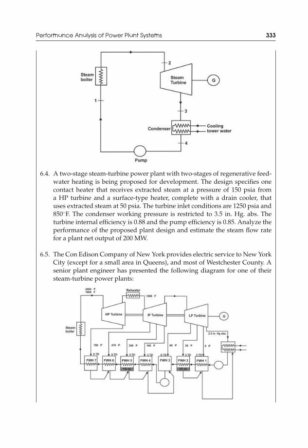
JWST229-c06 JWST229-McDonald Printer: Yet to Come July 31, 2012 12:36 Trim: 244mm × 168mm
Performance Analysis of Power Plant Systems 333
6.4. A two-stage steam-turbine power plant with two-stages of regenerative feed-water heating is being proposed for development. The design specifies onecontact heater that receives extracted steam at a pressure of 150 psia froma HP turbine and a surface-type heater, complete with a drain cooler, thatuses extracted steam at 50 psia. The turbine inlet conditions are 1250 psia and850◦F. The condenser working pressure is restricted to 3.5 in. Hg. abs. Theturbine internal efficiency is 0.88 and the pump efficiency is 0.85. Analyze theperformance of the proposed plant design and estimate the steam flow ratefor a plant net output of 200 MW.
6.5. The Con Edison Company of New York provides electric service to New YorkCity (except for a small area in Queens), and most of Westchester County. Asenior plant engineer has presented the following diagram for one of theirsteam-turbine power plants:

JWST229-c06 JWST229-McDonald Printer: Yet to Come July 31, 2012 12:36 Trim: 244mm × 168mm
334 Introduction to Thermo-Fluids Systems Design
Since this is an existing system, it is known that the HP turbine, IP turbine,and LP turbine internal efficiencies are 90%, 92%, and 89%, respectively. Thepump efficiency is 90% and the generator efficiency is 98%. The feedwaterpump drive is motor driven. There is a 7% reheater pressure loss and a 16%boiler pressure loss. Only FWH 2 and FWH 5 have drain cooling. The steamflow rate is 4 × 10⁶ lb/h. In an effort to improve company-wide operations,Management has requested a performance analysis of all existing plants. Pre-pare an analysis of the aforementioned plant for submission to Management.
6.6. The Con Edison Company of New York provides electric service to New YorkCity (except for a small area in Queens), and most of Westchester County. Asenior plant engineer has presented the following diagram for one of theirsteam-turbine power plants:
Since this is an existing system, it is known that the HP turbine, IP turbine,and LP turbine internal efficiencies are 90%, 92%, and 89%, respectively. Thepump efficiency is 90%, the generator efficiency is 98%, and the burner effi-ciency is 87%. Anthracite coal is used in the boiler burner and natural gas isused in the reheater burner. The feedwater pump drive is motor driven. Thereis a 7% reheater pressure loss and a 16% boiler pressure loss. Only FWH 2 andFWH 5 have drain cooling. The steam flow rate is 4 × 10⁶ lb/h. In an effort toimprove company-wide operations, Management has requested an analysisof all existing plants to identify components in each plant that may need im-provement. Prepare the analysis of the aforementioned plant for submissionto Management.
6.7. A gas-turbine power plant operates on a regenerative Brayton cycle with airas the working fluid into the compressor.

JWST229-c06 JWST229-McDonald Printer: Yet to Come July 31, 2012 12:36 Trim: 244mm × 168mm
Performance Analysis of Power Plant Systems 335
The following conditions were provided:
Compressor inlet conditions P1 = 14.7 psiaT1 = 60◦F
Turbine inlet temperature T3 = 2000◦FPressure ratio 4Compressor efficiency 0.85Turbine efficiency 0.88Regenerator efficiency 0.70Gas flow rate 360000 lb/h
Calculate the net cycle output and the thermal efficiency (first-law effi-ciency). Assume that no pressure drops occur in the system.
6.8. The schematic diagram of a closed-cycle gas-turbine system is shown be-low. The system is directly coupled with a high-temperature gas-cooled re-actor. The working fluid is helium, and since no combustion is involved, thehelium has a constant composition. Since helium is expensive, the flow rate islimited to 100000 lb/h. Estimate the performance of this plant.
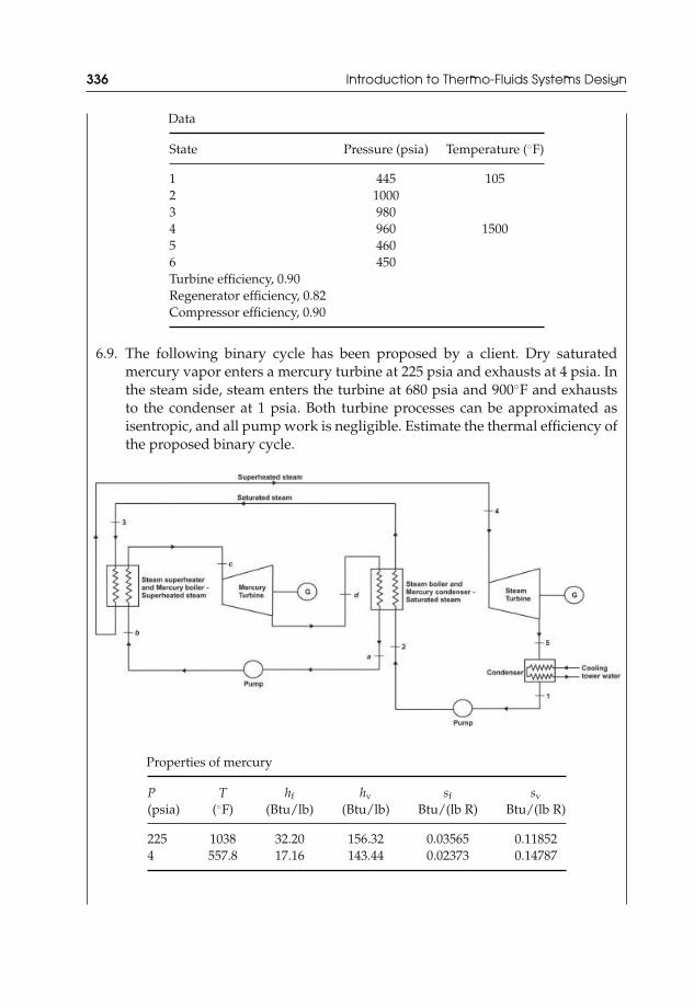
JWST229-c06 JWST229-McDonald Printer: Yet to Come July 31, 2012 12:36 Trim: 244mm × 168mm
336 Introduction to Thermo-Fluids Systems Design
Data
State Pressure (psia) Temperature (◦F)
1 445 1052 10003 9804 960 15005 4606 450Turbine efficiency, 0.90Regenerator efficiency, 0.82Compressor efficiency, 0.90
6.9. The following binary cycle has been proposed by a client. Dry saturatedmercury vapor enters a mercury turbine at 225 psia and exhausts at 4 psia. Inthe steam side, steam enters the turbine at 680 psia and 900◦F and exhauststo the condenser at 1 psia. Both turbine processes can be approximated asisentropic, and all pump work is negligible. Estimate the thermal efficiency ofthe proposed binary cycle.
Properties of mercury
P T hf hv sf sv
(psia) (◦F) (Btu/lb) (Btu/lb) Btu/(lb R) Btu/(lb R)
225 1038 32.20 156.32 0.03565 0.118524 557.8 17.16 143.44 0.02373 0.14787

JWST229-c06 JWST229-McDonald Printer: Yet to Come July 31, 2012 12:36 Trim: 244mm × 168mm
Performance Analysis of Power Plant Systems 337
6.10. A combined-cycle system consists mainly of a gas turbine, a waste heat re-covery boiler, and a steam turbine that will be operated in the summer. Aschematic and some system conditions are given below:
Gas Turbine
Gas flow rate 400000 lb/hPressure ratio 9Turbine inlet temperature 2100◦FCompressor efficiency 85%Turbine efficiency 90%Burner efficiency 95%
Boiler and Steam Turbine
Steam pressure and temperature 600 psia, 700◦FTurbine internal efficiency 80%Pump efficiency 78%
Considering all component inefficiencies, estimate the first-law efficiency,plant output, and NHR of this combined-cycle system. A heat and mass bal-ance diagram is not required.
6.11. A single-pressure waste heat recovery boiler is being considered in acombined-cycle system design. The boiler is expected to provide steam at1250 psia and 950◦F at an inlet water temperature of 274◦F. Calculate thesteam flow rate and stack gas temperature for the following conditions:
Exhaust gas flow rate 1.68 × 10⁶ lb/hExhaust gas temperature 960◦FSupplementary heat addition rate 26.57 × 10⁶ Btu/h at superheater
Conduct an analysis to comment on the acceptability of the value of thestack gas temperature with respect to longevity of the exhaust stack.
JWST229-c06 JWST229-McDonald Printer: Yet to Come July 31, 2012 12:36 Trim: 244mm × 168mm
338 Introduction to Thermo-Fluids Systems Design
6.12. Baltimore Gas and Electric (BGE) has recently installed a reheater for use ina plant in Prince Georges County, MD. The reheater will receive steam at 850psia and 700◦F and release it at 1200◦F. Because of losses in the tubing, thereis a 12% pressure drop in the steam. The steam flow rate is 2000000 lb/h.Hot flue gases from a burner enter the reheater at 1900◦F and 3500000 lb/h toflow over the steam tubes that are arranged in-line. The overall heat transfercoefficient is approximately 8.5 Btu/(h ft2 ◦F). Estimate the effectiveness ofthe reheater by using the ε-NTU and by conducting a second-law analysis.Specify all assumptions and comment on the results of the calculations.
6.13. It is well known that exhaust end losses between the LP steam turbine exit andthe condenser inlet will result in different values of enthalpy at the two points.In other words, the ELEP will differ from the UEEP. Conduct an analysisto show that the exhaust end loss represents the amount of steam kineticenergy that is lost between the turbine exit and the condenser inlet. Presentall applicable assumptions and explain the results of the analysis.
6.14. Syncrude Canada Ltd. has contracted the services of a consulting firm to as-sess the performance of a small steam-turbine plant. This existing plant has asingle-stage steam turbine and one stage of closed feedwater heating, whichcomes complete with drain cooling. It has been specified that the full-loadsteam mass flow rate is 255000 lb/h. The turbine inlet conditions are 1000psia and 900◦F. Steam is extracted from the turbine at 200 psia for feedwa-ter heating. Losses in the plant system result in a turbine internal efficiencyof 86%, a pump efficiency of 70%, and a total boiler pressure drop of 60psia. An auxiliary power requirement of 8% will be derived from the steamturbine to maintain plant operations. Using practical knowledge of steam-turbine plants (where applicable), conduct an appropriate analysis to preparea heat-and-mass balance diagram for full-load operation of the plant. Was adesuperheating zone of tubes installed in the feedwater heat exchanger?
References and Further Reading
[1] Li, K. and Priddy, A. (1985) Power Plant System Design, John Wiley & Sons, Ltd, New York.[2] Mollier, R. (1906) Neue Tabellen und Diagramme fur Wasserdampf, Springer-Verlag, Berlin.[3] Mollier, R. (1927) The Mollier Steam Tables and Diagrams, Extended to the Critical Pressure
(English edition adapted and extended from the third German edition by H. Moss), Pitmanand Sons, London.

JWST229-bapp01 JWST229-McDonald Printer: Yet to Come July 28, 2012 13:37 Trim: 244mm × 168mm
Appendix APipe and Duct Systems
Table A.1 Average roughness of commercial pipes
ε
New Material ft mm
Riveted steel 0.003–0.03 0.9–9.0Concrete 0.001–0.01 0.3–3.0Wood stave 0.0006–0.003 0.18–0.9Cast iron 0.00085 0.26Galvanized iron 0.0005 0.15Asphalted cast iron 0.0004 0.12Commercial steel 0.00015 0.046Drawn tubing 0.000005 0.0015Glass “Smooth” “Smooth”
Source: Fox, R. and McDonald, A. (1998) Introduction to Fluid Mechanics, 5th edn, John Wiley & Sons, Inc.,New York
Introduction to Thermo-Fluids Systems Design, First Edition. Andre G. McDonald and Hugh L. Magande.C© 2012 Andre G. McDonald and Hugh L. Magande. Published 2012 by John Wiley & Sons, Ltd.
339

JWST229-bapp01 JWST229-McDonald Printer: Yet to Come July 28, 2012 13:37 Trim: 244mm × 168mm
340 Appendix A
Table A.2 Correlation equations for friction factors
Swamee-Jain formulae fo = 0.25
[log
(ε/D3.7
+ 5.74
Re0.9D
)]−2
Colebrook equation1√
f= −2.0 log
(ε/D3.7
+ 2.51ReD
√f
)
Haaland’s approximation1√
f= −1.8 log
[6.9ReD
+(
ε/D3.7
)1.11]
Blasius correlation for smooth pipes f = 0.316
Re0.25D
,
for ReD ≤ 105
Churchill’s equation f = 8
[(8
ReD
)12
+ (A+ B)−3/2
]1/12
,
A =[
2.457 ln(
1C
)]16
,
B =(
37530ReD
)16
,
C =(
7ReD
)0.9
+ 0.27( ε
D
)First Petukhov equation forturbulent flow in smooth tubes
f = [0.79 ln Re − 1.64]−2,for 3000 < Re < 5 × 10⁶
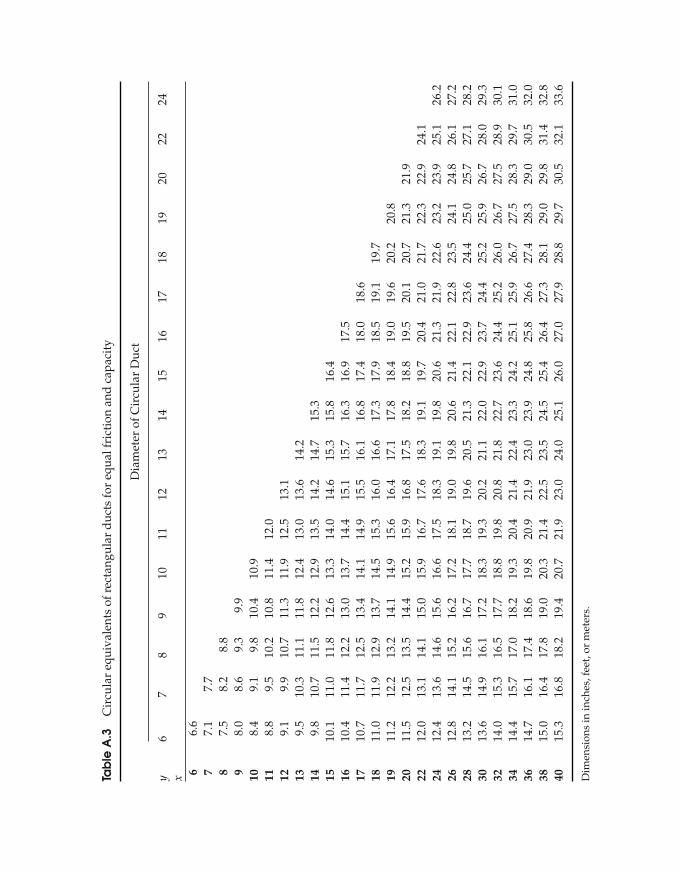
JWST229-bapp01 JWST229-McDonald Printer: Yet to Come July 28, 2012 13:37 Trim: 244mm × 168mm
Tab
leA
.3C
ircu
lar
equi
vale
nts
ofre
ctan
gula
rd
ucts
for
equa
lfri
ctio
nan
dca
paci
ty
Dia
met
erof
Cir
cula
rD
uct
y x6
78
910
1112
1314
1516
1718
1920
2224
66.
67
7.1
7.7
87.
58.
28.
89
8.0
8.6
9.3
9.9
108.
49.
19.
810
.410
.911
8.8
9.5
10.2
10.8
11.4
12.0
129.
19.
910
.711
.311
.912
.513
.113
9.5
10.3
11.1
11.8
12.4
13.0
13.6
14.2
149.
810
.711
.512
.212
.913
.514
.214
.715
.315
10.1
11.0
11.8
12.6
13.3
14.0
14.6
15.3
15.8
16.4
1610
.411
.412
.213
.013
.714
.415
.115
.716
.316
.917
.517
10.7
11.7
12.5
13.4
14.1
14.9
15.5
16.1
16.8
17.4
18.0
18.6
1811
.011
.912
.913
.714
.515
.316
.016
.617
.317
.918
.519
.119
.719
11.2
12.2
13.2
14.1
14.9
15.6
16.4
17.1
17.8
18.4
19.0
19.6
20.2
20.8
2011
.512
.513
.514
.415
.215
.916
.817
.518
.218
.819
.520
.120
.721
.321
.922
12.0
13.1
14.1
15.0
15.9
16.7
17.6
18.3
19.1
19.7
20.4
21.0
21.7
22.3
22.9
24.1
2412
.413
.614
.615
.616
.617
.518
.319
.119
.820
.621
.321
.922
.623
.223
.925
.126
.226
12.8
14.1
15.2
16.2
17.2
18.1
19.0
19.8
20.6
21.4
22.1
22.8
23.5
24.1
24.8
26.1
27.2
2813
.214
.515
.616
.717
.718
.719
.620
.521
.322
.122
.923
.624
.425
.025
.727
.128
.230
13.6
14.9
16.1
17.2
18.3
19.3
20.2
21.1
22.0
22.9
23.7
24.4
25.2
25.9
26.7
28.0
29.3
3214
.015
.316
.517
.718
.819
.820
.821
.822
.723
.624
.425
.226
.026
.727
.528
.930
.134
14.4
15.7
17.0
18.2
19.3
20.4
21.4
22.4
23.3
24.2
25.1
25.9
26.7
27.5
28.3
29.7
31.0
3614
.716
.117
.418
.619
.820
.921
.923
.023
.924
.825
.826
.627
.428
.329
.030
.532
.038
15.0
16.4
17.8
19.0
20.3
21.4
22.5
23.5
24.5
25.4
26.4
27.3
28.1
29.0
29.8
31.4
32.8
4015
.316
.818
.219
.420
.721
.923
.024
.025
.126
.027
.027
.928
.829
.730
.532
.133
.6
Dim
ensi
ons
inin
ches
,fee
t,or
met
ers.
341
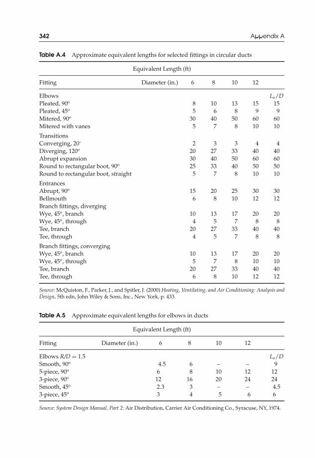
JWST229-bapp01 JWST229-McDonald Printer: Yet to Come July 28, 2012 13:37 Trim: 244mm × 168mm
342 Appendix A
Table A.4 Approximate equivalent lengths for selected fittings in circular ducts
Equivalent Length (ft)
Fitting Diameter (in.) 6 8 10 12
Elbows Le/DPleated, 90o 8 10 13 15 15Pleated, 45o 5 6 8 9 9Mitered, 90o 30 40 50 60 60Mitered with vanes 5 7 8 10 10
TransitionsConverging, 20◦ 2 3 3 4 4Diverging, 120o 20 27 33 40 40Abrupt expansion 30 40 50 60 60Round to rectangular boot, 90o 25 33 40 50 50Round to rectangular boot, straight 5 7 8 10 10
EntrancesAbrupt, 90o 15 20 25 30 30Bellmouth 6 8 10 12 12Branch fittings, divergingWye, 45o, branch 10 13 17 20 20Wye, 45o, through 4 5 7 8 8Tee, branch 20 27 33 40 40Tee, through 4 5 7 8 8
Branch fittings, convergingWye, 45o, branch 10 13 17 20 20Wye, 45o, through 5 7 8 10 10Tee, branch 20 27 33 40 40Tee, through 6 8 10 12 12
Source: McQuiston, F., Parker, J., and Spitler, J. (2000) Heating, Ventilating, and Air Conditioning: Analysis andDesign, 5th edn, John Wiley & Sons, Inc., New York, p. 433.
Table A.5 Approximate equivalent lengths for elbows in ducts
Equivalent Length (ft)
Fitting Diameter (in.) 6 8 10 12
Elbows R/D = 1.5 Le/DSmooth, 90o 4.5 6 – – 95-piece, 90o 6 8 10 12 123-piece, 90o 12 16 20 24 24Smooth, 45o 2.3 3 – – 4.53-piece, 45o 3 4 5 6 6
Source: System Design Manual, Part 2: Air Distribution, Carrier Air Conditioning Co., Syracuse, NY, 1974.

JWST229-bapp01 JWST229-McDonald Printer: Yet to Come July 28, 2012 13:37 Trim: 244mm × 168mm
Appendix A 343
Table A.6 Data for copper pipes
Weight perLinear Foot of Gallons of
Pipe and Water perWater (lb) Linear Foot
Diameter (in.)
Material Nominal Inner Outer
CopperType L 1/4 0.315 0.375 0.16 0.004Type L 3/8 0.430 0.500 0.26 0.008Type L 1/2 0.545 0.625 0.39 0.012Type L 5/8 0.666 0.750 0.512 0.018Type L 3/4 0.785 0.875 0.67 0.025Type L 1 1.025 1.125 1.01 0.043Type L 11/4 1.265 1.375 1.43 0.065Type L 11/2 1.505 1.625 1.91 0.093Type L 2 1.985 2.125 3.09 0.161Type L 21/2 2.465 2.625 4.55 0.248Type L 3 2.945 3.125 6.29 0.354Type L 31/2 3.425 3.625 8.29 0.479Type L 4 3.905 4.125 10.58 0.622Type L 5 4.875 5.125 15.70 0.970Type L 6 5.845 6.125 21.81 1.394Type L 8 7.725 8.125 39.58 2.435Type L 10 9.625 10.125 61.61 3.780Type L 12 11.565 12.125 85.89 5.457
Type K 1/4 0.305 0.375 0.177 0.004Type K 3/8 0.402 0.500 0.275 0.007Type K 1/2 0.527 0.625 0.438 0.011Type K 5/8 0.652 0.750 0.563 0.017Type K 3/4 0.745 0.875 0.829 0.023Type K 1 0.995 1.125 1.176 0.040Type K 11/4 1.245 1.375 1.570 0.063Type K 11/2 1.481 1.625 2.109 0.089Type K 2 1.959 2.125 3.364 0.157Type K 21/2 2.435 2.625 4.927 0.242Type K 3 2.907 3.125 6.870 0.345Type K 31/2 3.385 3.625 9.051 0.467Type K 4 3.857 4.125 11.564 0.607Type K 5 4.805 5.125 17.532 0.942Type K 6 5.741 6.125 25.132 1.345Type K 8 7.583 8.125 45.494 2.346Type K 10 9.449 10.125 70.689 3.643Type K 12 11.315 12.125 101.355 5.224
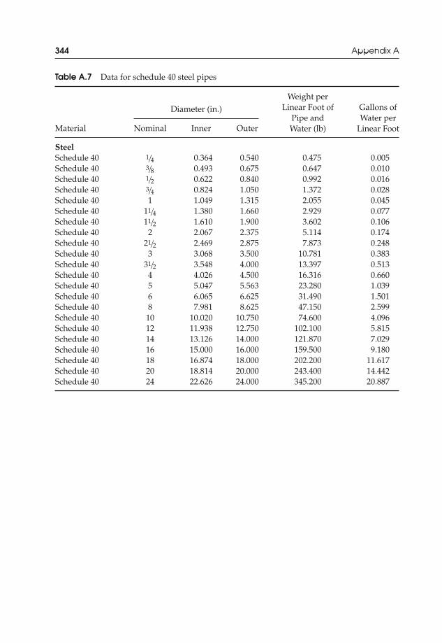
JWST229-bapp01 JWST229-McDonald Printer: Yet to Come July 28, 2012 13:37 Trim: 244mm × 168mm
344 Appendix A
Table A.7 Data for schedule 40 steel pipes
Weight perLinear Foot of Gallons of
Pipe and Water perWater (lb) Linear Foot
Diameter (in.)
Material Nominal Inner Outer
SteelSchedule 40 1/4 0.364 0.540 0.475 0.005Schedule 40 3/8 0.493 0.675 0.647 0.010Schedule 40 1/2 0.622 0.840 0.992 0.016Schedule 40 3/4 0.824 1.050 1.372 0.028Schedule 40 1 1.049 1.315 2.055 0.045Schedule 40 11/4 1.380 1.660 2.929 0.077Schedule 40 11/2 1.610 1.900 3.602 0.106Schedule 40 2 2.067 2.375 5.114 0.174Schedule 40 21/2 2.469 2.875 7.873 0.248Schedule 40 3 3.068 3.500 10.781 0.383Schedule 40 31/2 3.548 4.000 13.397 0.513Schedule 40 4 4.026 4.500 16.316 0.660Schedule 40 5 5.047 5.563 23.280 1.039Schedule 40 6 6.065 6.625 31.490 1.501Schedule 40 8 7.981 8.625 47.150 2.599Schedule 40 10 10.020 10.750 74.600 4.096Schedule 40 12 11.938 12.750 102.100 5.815Schedule 40 14 13.126 14.000 121.870 7.029Schedule 40 16 15.000 16.000 159.500 9.180Schedule 40 18 16.874 18.000 202.200 11.617Schedule 40 20 18.814 20.000 243.400 14.442Schedule 40 24 22.626 24.000 345.200 20.887
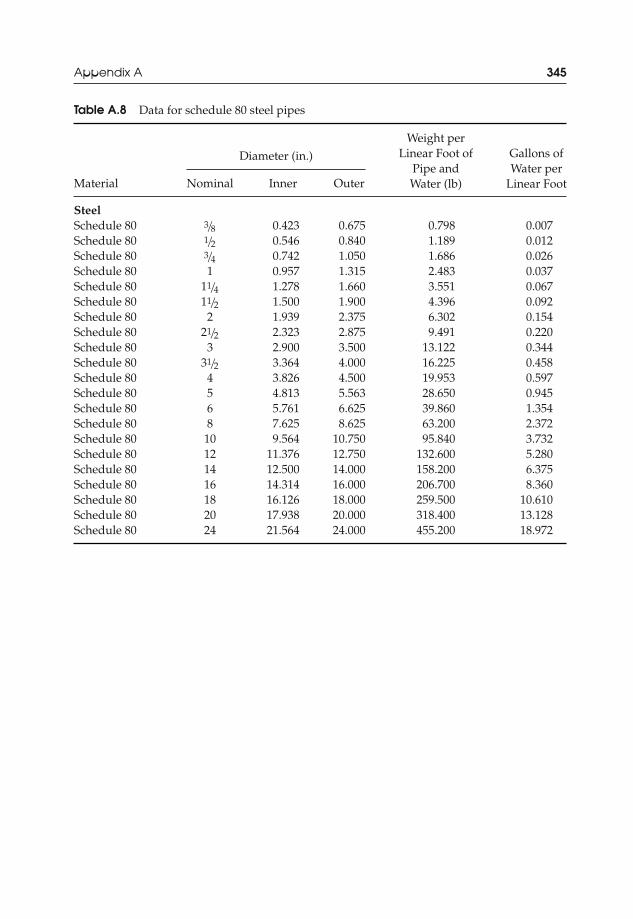
JWST229-bapp01 JWST229-McDonald Printer: Yet to Come July 28, 2012 13:37 Trim: 244mm × 168mm
Appendix A 345
Table A.8 Data for schedule 80 steel pipes
Weight perLinear Foot of Gallons of
Pipe and Water perWater (lb) Linear Foot
Diameter (in.)
Material Nominal Inner Outer
SteelSchedule 80 3/8 0.423 0.675 0.798 0.007Schedule 80 1/2 0.546 0.840 1.189 0.012Schedule 80 3/4 0.742 1.050 1.686 0.026Schedule 80 1 0.957 1.315 2.483 0.037Schedule 80 11/4 1.278 1.660 3.551 0.067Schedule 80 11/2 1.500 1.900 4.396 0.092Schedule 80 2 1.939 2.375 6.302 0.154Schedule 80 21/2 2.323 2.875 9.491 0.220Schedule 80 3 2.900 3.500 13.122 0.344Schedule 80 31/2 3.364 4.000 16.225 0.458Schedule 80 4 3.826 4.500 19.953 0.597Schedule 80 5 4.813 5.563 28.650 0.945Schedule 80 6 5.761 6.625 39.860 1.354Schedule 80 8 7.625 8.625 63.200 2.372Schedule 80 10 9.564 10.750 95.840 3.732Schedule 80 12 11.376 12.750 132.600 5.280Schedule 80 14 12.500 14.000 158.200 6.375Schedule 80 16 14.314 16.000 206.700 8.360Schedule 80 18 16.126 18.000 259.500 10.610Schedule 80 20 17.938 20.000 318.400 13.128Schedule 80 24 21.564 24.000 455.200 18.972
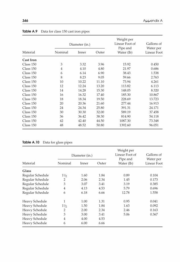
JWST229-bapp01 JWST229-McDonald Printer: Yet to Come July 28, 2012 13:37 Trim: 244mm × 168mm
346 Appendix A
Table A.9 Data for class 150 cast iron pipes
Weight perLinear Foot of Gallons of
Pipe and Water perWater (lb) Linear Foot
Diameter (in.)
Material Nominal Inner Outer
Cast IronClass 150 3 3.32 3.96 15.92 0.450Class 150 4 4.10 4.80 21.97 0.686Class 150 6 6.14 6.90 38.43 1.538Class 150 8 8.23 9.05 59.66 2.763Class 150 10 10.22 11.10 73.94 4.261Class 150 12 12.24 13.20 113.82 6.113Class 150 14 14.28 15.30 148.05 8.320Class 150 16 16.32 17.40 185.30 10.867Class 150 18 18.34 19.50 228.69 13.723Class 150 20 20.36 21.60 277.44 16.913Class 150 24 24.34 25.80 391.31 24.171Class 150 30 30.30 32.00 589.19 37.458Class 150 36 36.42 38.30 814.90 54.118Class 150 42 42.40 44.50 1087.30 73.348Class 150 48 48.52 50.80 1392.60 96.051
Table A.10 Data for glass pipes
Weight perLinear Foot of Gallons of
Pipe and Water perWater (lb) Linear Foot
Diameter (in.)
Material Nominal Inner Outer
GlassRegular Schedule 11/2 1.60 1.84 0.89 0.104Regular Schedule 2 2.06 2.34 1.45 0.173Regular Schedule 3 3.07 3.41 3.19 0.385Regular Schedule 4 4.13 4.53 5.79 0.696Regular Schedule 6 6.18 6.66 12.78 1.558
Heavy Schedule 1 1.00 1.31 0.95 0.041Heavy Schedule 11/2 1.50 1.84 1.63 0.092Heavy Schedule 2 2.00 2.34 2.46 0.163Heavy Schedule 3 3.00 3.41 5.06 0.367Heavy Schedule 4 4.00 4.53Heavy Schedule 6 6.00 6.66

JWST229-bapp01 JWST229-McDonald Printer: Yet to Come July 28, 2012 13:37 Trim: 244mm × 168mm
Appendix A 347
Table A.11 Data for PVC plastic pipes
Weight perLinear Foot of Gallons of
Pipe and Water perWater (lb) Linear Foot
Diameter (in.)
Material Nominal Inner Outer
PVC PlasticSchedule 40 1/8 0.269 0.405 0.068 0.003Schedule 40 1/4 0.364 0.540 0.119 0.005Schedule 40 3/8 0.493 0.675 0.183 0.010Schedule 40 1/2 0.622 0.840 0.282 0.016Schedule 40 3/4 0.784 1.050 0.429 0.025Schedule 40 1 1.049 1.315 0.669 0.045Schedule 40 11/4 1.380 1.660 1.047 0.078Schedule 40 11/2 1.610 1.900 1.360 0.106Schedule 40 2 2.067 2.375 2.095 0.174Schedule 40 21/2 2.469 2.875 3.092 0.249Schedule 40 3 3.068 3.500 4.533 0.384Schedule 40 31/2 3.548 4.000 5.878 0.514Schedule 40 4 4.026 4.500 7.409 0.661Schedule 40 5 5.047 5.563 11.430 1.039Schedule 40 6 6.065 6.625 15.489 1.501Schedule 40 8 7.981 8.625 26.880 2.599Schedule 40 10 10.018 10.750 41.605 4.095Schedule 40 12 11.938 12.750 58.523 5.815
Schedule 80 1/8 0.215 0.405 0.071 0.002Schedule 80 1/4 0.302 0.540 0.125 0.004Schedule 80 3/8 0.423 0.675 0.190 0.007Schedule 80 1/2 0.546 0.840 0.251 0.012Schedule 80 3/4 0.742 1.050 0.481 0.022Schedule 80 1 0.957 1.315 0.693 0.037Schedule 80 11/4 1.278 1.660 1.082 0.067Schedule 80 11/2 1.500 1.900 1.404 0.092Schedule 80 2 1.939 2.375 2.163 0.153Schedule 80 21/2 2.323 2.875 3.184 0.220Schedule 80 3 2.900 3.500 4.664 0.343Schedule 80 31/2 3.364 4.000 6.045 0.462Schedule 80 4 3.826 4.500 7.616 0.597Schedule 80 5 4.780 5.563 11.996 0.932Schedule 80 6 5.761 6.625 16.318 1.354Schedule 80 8 7.625 8.625 27.823 2.372Schedule 80 10 9.564 10.750 42.994 3.732Schedule 80 12 11.376 12.750 60.365 5.280
Source: Some data from Erico International Corp., Pipe Hanger and Support Recommended Specifications, EricoCorp., Solon, OH, 2010, pp. 114–117.
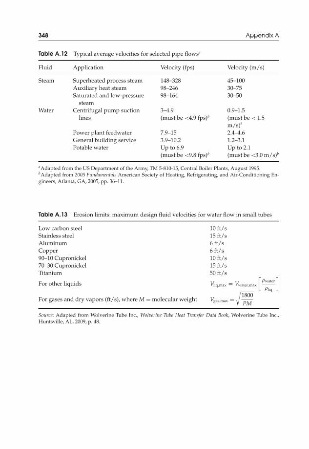
JWST229-bapp01 JWST229-McDonald Printer: Yet to Come July 28, 2012 13:37 Trim: 244mm × 168mm
348 Appendix A
Table A.12 Typical average velocities for selected pipe flowsa
Fluid Application Velocity (fps) Velocity (m/s)
Steam Superheated process steam 148–328 45–100Auxiliary heat steam 98–246 30–75Saturated and low-pressure
steam98–164 30–50
Water Centrifugal pump suctionlines
3–4.9(must be <4.9 fps)b
0.9–1.5(must be < 1.5m/s)b
Power plant feedwater 7.9–15 2.4–4.6General building service 3.9–10.2 1.2–3.1Potable water Up to 6.9
(must be <9.8 fps)bUp to 2.1(must be <3.0 m/s)b
aAdapted from the US Department of the Army, TM 5-810-15, Central Boiler Plants, August 1995.bAdapted from 2005 Fundamentals American Society of Heating, Refrigerating, and Air-Conditioning En-gineers, Atlanta, GA, 2005, pp. 36–11.
Table A.13 Erosion limits: maximum design fluid velocities for water flow in small tubes
Low carbon steel 10 ft/sStainless steel 15 ft/sAluminum 6 ft/sCopper 6 ft/s90–10 Cupronickel 10 ft/s70–30 Cupronickel 15 ft/sTitanium 50 ft/s
For other liquids Vliq,max = Vwater,max
[ρwater
ρliq
]
For gases and dry vapors (ft/s), where M = molecular weight Vgas,max =√
1800PM
Source: Adapted from Wolverine Tube Inc., Wolverine Tube Heat Transfer Data Book, Wolverine Tube Inc.,Huntsville, AL, 2009, p. 48.
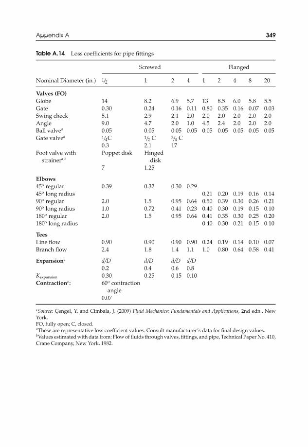
JWST229-bapp01 JWST229-McDonald Printer: Yet to Come July 28, 2012 13:37 Trim: 244mm × 168mm
Appendix A 349
Table A.14 Loss coefficients for pipe fittings
Screwed Flanged
Nominal Diameter (in.) 1/2 1 2 4 1 2 4 8 20
Valves (FO)Globe 14 8.2 6.9 5.7 13 8.5 6.0 5.8 5.5Gate 0.30 0.24 0.16 0.11 0.80 0.35 0.16 0.07 0.03Swing check 5.1 2.9 2.1 2.0 2.0 2.0 2.0 2.0 2.0Angle 9.0 4.7 2.0 1.0 4.5 2.4 2.0 2.0 2.0Ball valvea 0.05 0.05 0.05 0.05 0.05 0.05 0.05 0.05 0.05Gate valvea 1/4C 1/2 C 3/4 C
0.3 2.1 17Foot valve with
strainera ,bPoppet disk Hinged
disk7 1.25
Elbows45o regular 0.39 0.32 0.30 0.2945o long radius 0.21 0.20 0.19 0.16 0.1490o regular 2.0 1.5 0.95 0.64 0.50 0.39 0.30 0.26 0.2190o long radius 1.0 0.72 0.41 0.23 0.40 0.30 0.19 0.15 0.10180o regular 2.0 1.5 0.95 0.64 0.41 0.35 0.30 0.25 0.20180o long radius 0.40 0.30 0.21 0.15 0.10
TeesLine flow 0.90 0.90 0.90 0.90 0.24 0.19 0.14 0.10 0.07Branch flow 2.4 1.8 1.4 1.1 1.0 0.80 0.64 0.58 0.41
Expansionc d/D d/D d/D d/D0.2 0.4 0.6 0.8
Kexpansion 0.30 0.25 0.15 0.10Contractionc: 60o contraction
angle0.07
cSource: Cengel, Y. and Cimbala, J. (2009) Fluid Mechanics: Fundamentals and Applications, 2nd edn., NewYork.FO, fully open; C, closed.aThese are representative loss coefficient values. Consult manufacturer’s data for final design values.bValues estimated with data from: Flow of fluids through valves, fittings, and pipe, Technical Paper No. 410,Crane Company, New York, 1982.
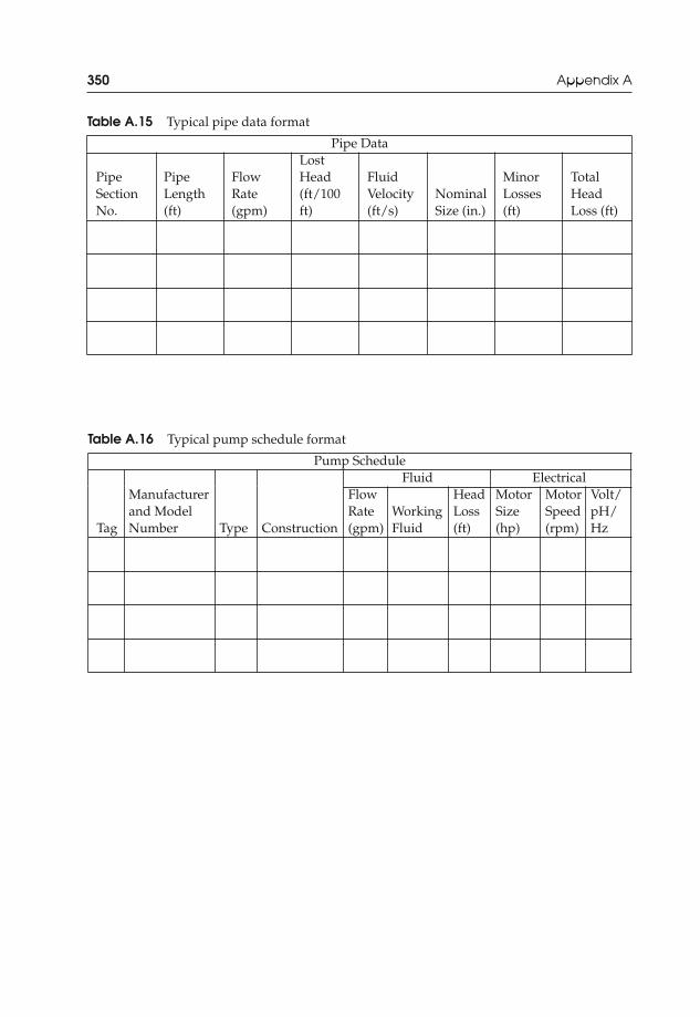
JWST229-bapp01 JWST229-McDonald Printer: Yet to Come July 28, 2012 13:37 Trim: 244mm × 168mm
350 Appendix A
Table A.15 Typical pipe data format
Pipe Data
PipeSectionNo.
PipeLength(ft)
FlowRate(gpm)
LostHead(ft/100ft)
FluidVelocity(ft/s)
NominalSize (in.)
MinorLosses(ft)
TotalHeadLoss (ft)
Table A.16 Typical pump schedule format
Pump ScheduleFluid Electrical
Tag
Manufacturerand ModelNumber Type Construction
FlowRate(gpm)
WorkingFluid
HeadLoss(ft)
MotorSize(hp)
MotorSpeed(rpm)
Volt/pH/Hz

JWST229-bapp01 JWST229-McDonald Printer: Yet to Come July 28, 2012 13:37 Trim: 244mm × 168mm
Appendix A 351
Figure A.1 Friction Loss in Round (Straight) Ducts. Source: System Design Manual,Part 2: Air Distribution, Carrier Air Conditioning Co., Syracuse, NY, 1974 (Reprinted withpermission)
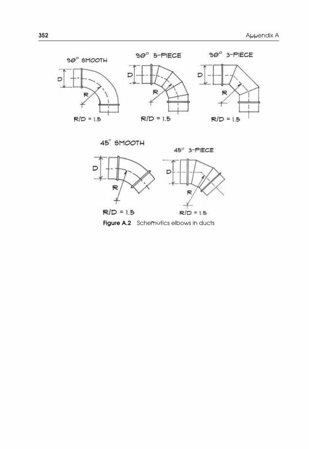
JWST229-bapp01 JWST229-McDonald Printer: Yet to Come July 28, 2012 13:37 Trim: 244mm × 168mm
352 Appendix A
Figure A.2 Schematics elbows in ducts

JWST229-bapp01 JWST229-McDonald Printer: Yet to Come July 28, 2012 13:37 Trim: 244mm × 168mm
Appendix A 353
Figure A.3 Copper tubing friction loss (open and closed piping systems) (Carrier Corp.;reprinted with permission)
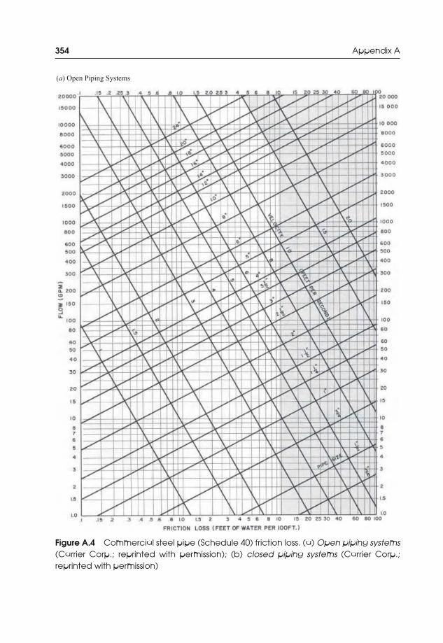
JWST229-bapp01 JWST229-McDonald Printer: Yet to Come July 28, 2012 13:37 Trim: 244mm × 168mm
354 Appendix A
(a) Open Piping Systems
Figure A.4 Commercial steel pipe (Schedule 40) friction loss. (a) Open piping systems(Carrier Corp.; reprinted with permission); (b) closed piping systems (Carrier Corp.;reprinted with permission)

JWST229-bapp01 JWST229-McDonald Printer: Yet to Come July 28, 2012 13:37 Trim: 244mm × 168mm
Appendix A 355
(b) Closed Piping Systems
Figure A.4 (Continued)
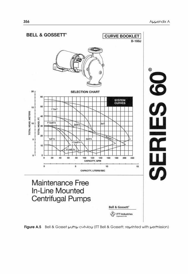
JWST229-bapp01 JWST229-McDonald Printer: Yet to Come July 28, 2012 13:37 Trim: 244mm × 168mm
356 Appendix A
Figure A.5 Bell & Gosset pump catalog (ITT Bell & Gossett; reprinted with permission)

JWST229-bapp01 JWST229-McDonald Printer: Yet to Come July 28, 2012 13:37 Trim: 244mm × 168mm
Appendix A 357
Figure A.5 (Continued)

JWST229-bapp01 JWST229-McDonald Printer: Yet to Come July 28, 2012 13:37 Trim: 244mm × 168mm
358 Appendix A
Figure A.5 (Continued)
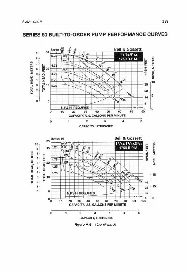
JWST229-bapp01 JWST229-McDonald Printer: Yet to Come July 28, 2012 13:37 Trim: 244mm × 168mm
Appendix A 359
Figure A.5 (Continued)

JWST229-bapp01 JWST229-McDonald Printer: Yet to Come July 28, 2012 13:37 Trim: 244mm × 168mm
360 Appendix A
Figure A.5 (Continued)

JWST229-bapp01 JWST229-McDonald Printer: Yet to Come July 28, 2012 13:37 Trim: 244mm × 168mm
Appendix A 361
Figure A.5 (Continued)
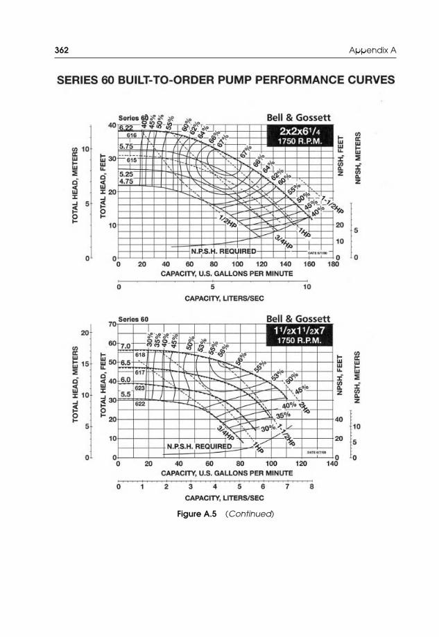
JWST229-bapp01 JWST229-McDonald Printer: Yet to Come July 28, 2012 13:37 Trim: 244mm × 168mm
362 Appendix A
Figure A.5 (Continued)

JWST229-bapp01 JWST229-McDonald Printer: Yet to Come July 28, 2012 13:37 Trim: 244mm × 168mm
Appendix A 363
Figure A.5 (Continued)

JWST229-bapp02 JWST229-McDonald Printer: Yet to Come July 28, 2012 9:46 Trim: 244mm × 168mm
Appendix BSymbols for Drawings
Table B.1 Air moving devices and ductwork symbols
Air Movement
Fans
Axial flow fan
Centrifugal fan
Propeller fan
Intake roof ventilator (supply)
Exhaust roof ventilator
Ductwork
Direction of flow
Change of elevation [rise (R), drop (D)]R
Vertical or horizontal access doorsAD
Acoustical lining (sound insulation)
Cowl, gooseneck, and flashing
(continued)
Introduction to Thermo-Fluids Systems Design, First Edition. Andre G. McDonald and Hugh L. Magande.C© 2012 Andre G. McDonald and Hugh L. Magande. Published 2012 by John Wiley & Sons, Ltd.
365

JWST229-bapp02 JWST229-McDonald Printer: Yet to Come July 28, 2012 9:46 Trim: 244mm × 168mm
366 Appendix B
Table B.1 (Continued)
Ductwork (cont.)
Flexible connection
Flexible duct
Sound attenuatorSA
Mixing terminal unit TUCH
M - 1
Reheat terminal unit TURH - 1
Variable air volume terminal unit TUVAV - 1
Turning vanes
Fire and/or smoke detectors
Source: HVAC Duct Construction Standards: Metal and Flexible, Sheet Metaland Air Conditioning Contractors National Association, Inc., Vienna, VA,1985.

JWST229-bapp02 JWST229-McDonald Printer: Yet to Come July 28, 2012 9:46 Trim: 244mm × 168mm
Table B.2 Piping symbols
Piping
Heating
High-pressure steam HPSMedium-pressure steam MPSLow-pressure steam LPSHigh-pressure condensate HPCMedium-pressure condensate MPCLow-pressure condensate LPCBoiler blowdown BBDPumped condensate PCVacuum pump discharge VPDMakeup water MUAtmospheric vent ATVFuel oil discharge FODFuel oil gage FOGFuel oil suction (supply) FOSFuel oil return FORLow-temperature hot water supply HWSMedium-temperature hot water supply MTWSHigh-temperature hot water supply HTWSLow-temperature hot water return HWRMedium-temperature hot water return MTWRHigh-temperature hot water return HTWRCompressed air AVacuum (air) VACExisting piping (NAME)Piping to be removed XX (NAME) XX
Air Conditioning and Refrigeration
Refrigerant discharge RDRefrigerant suction (supply) RSBrine supply BBrine return BRCondenser water supply CCondenser water return CRChilled water supply CWSChilled water return CWRFill line FILLHumidification line HDrain DHot/chilled water supply HCSHot/chilled water return HCRRefrigerant liquid RLHeat pump water supply HPWSHeat pump water return HPWR
367

JWST229-bapp02 JWST229-McDonald Printer: Yet to Come July 28, 2012 9:46 Trim: 244mm × 168mm
Table B.3 Symbols for piping specialities
Piping Specialities
Automatic air vent (AV) AV
Manual air vent (MV) MV
Air separator S
Alignment guide
Intermediate anchor
Main anchor
Ball joint
Expansion joint (with drawing number) EJ - 1
Flexible connector
Orifice flowmeter
Venturi flowmeter
Flow switch FS
Hanger rodH
Hanger spring H
Liquid–liquid heat exchanger
Pipe pitch [rise (R), drop (D)] R
Pressure gage and cock
Pressure switchPS
Pump (indicate use and drawing number)CW-1
Pump suction diffuserPSD
Strainer
Blow off strainer
Duplex strainer
Tank (indicate use)FO
Thermometer
368
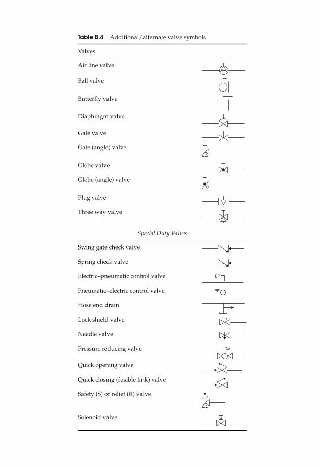
JWST229-bapp02 JWST229-McDonald Printer: Yet to Come July 28, 2012 9:46 Trim: 244mm × 168mm
Table B.4 Additional/alternate valve symbols
Valves
Air line valve
Ball valve
Butterfly valve
Diaphragm valve
Gate valve
Gate (angle) valve
Globe valve
Globe (angle) valve
Plug valve
Three way valve
Special Duty Valves
Swing gate check valve
Spring check valve
Electric–pneumatic control valve EP
Pneumatic–electric control valve PE
Hose end drain
Lock shield valve
Needle valve
Pressure reducing valve
Quick opening valve
Quick closing (fusible link) valve
Safety (S) or relief (R) valve
Solenoid valve S
369
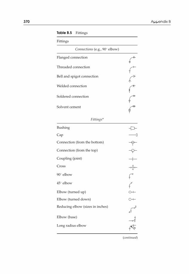
JWST229-bapp02 JWST229-McDonald Printer: Yet to Come July 28, 2012 9:46 Trim: 244mm × 168mm
370 Appendix B
Table B.5 Fittings
Fittings
Connections (e.g., 90◦ elbow)
Flanged connection
Threaded connection
Bell and spigot connection
Welded connection
Soldered connection
Solvent cement
Fittings*
Bushing
Cap
Connection (from the bottom)
Connection (from the top)
Coupling (joint)
Cross
90◦ elbow
45◦ elbow
Elbow (turned up)
Elbow (turned down)
Reducing elbow (sizes in inches) 2
4
Elbow (base)
Long radius elbow LR
(continued)

JWST229-bapp02 JWST229-McDonald Printer: Yet to Come July 28, 2012 9:46 Trim: 244mm × 168mm
Appendix B 371
Table B.5 (Continued)
Fittings* (cont.)
Double branch elbow
Elbow (side outlet, outlet up)
Elbow (side outlet, outlet down)
Fittings*
Lateral
Concentric reducer
Eccentric (straight invert) reducer
Eccentric (straight crown) reducer
Tee
Tee (outlet up)
Tee (outlet down)
Reducing tee (sizes in inches) 2
46
Tee (side outlet, outlet up)
Tee (side outlet, outlet down)
Single sweep tee
Screwed union
Flanged union
aWhere applicable, the fittings are shown for threadedscrew connections.Source: ASHRAE Handbook, Fundamentals Volume, 2005.

JWST229-bapp02 JWST229-McDonald Printer: Yet to Come July 28, 2012 9:46 Trim: 244mm × 168mm
372 Appendix B
Table B.6 Radiant Panel Symbols
Radiant Panel Symbols
Hydronic heating element
Electric heating element
Radiant Ceiling Panels
Embedded
Above ceiling
Surface mounted
Suspended
Radiant Floor Panels
Slab on grade
Above subfloor
Below subfloor
Slab above subfloor
Radiant Wall Panels
Embedded
Surface mounted
Source: ASHRAE Handbook, Fundamentals Volume, 2005.

JWST229-bapp03 JWST229-McDonald Printer: Yet to Come July 31, 2012 11:45 Trim: 244mm × 168mm
Appendix CHeat Exchanger Design
Table C.1 Representative values of the overall heat transfer coefficients (US)
Type of Heat Exchanger U (Btu/(h ft2 ◦F))
Water-to-water 150–300Water-to-oil 18–60Water-to-gasoline or kerosene 55–180Feedwater heaters 180–1500Steam-to-light fuel oil 35–70Steam-to-heavy fuel oil 10–35Steam condenser 180–1060Freon condenser (water cooled) 55–180Ammonia condenser (water cooled) 140–250Alcohol condenser (water cooled) 45–125Gas-to-gas 2–7Water-to-air in finned tubes (water in tubes) 5–10 (air); 70–150 (water)Steam-to-air in finned tubes (steam in tubes) 5–50 (air); 70–705 (water)
Introduction to Thermo-Fluids Systems Design, First Edition. Andre G. McDonald and Hugh L. Magande.C© 2012 Andre G. McDonald and Hugh L. Magande. Published 2012 by John Wiley & Sons, Ltd.
373

JWST229-bapp03 JWST229-McDonald Printer: Yet to Come July 31, 2012 11:45 Trim: 244mm × 168mm
Table C.2 Representative values of the overall heat transfer coefficients (SI)
Type of Heat Exchanger U (W/(m2 ◦C))
Water-to-water 850–1700Water-to-oil 100–350Water-to-gasoline or kerosene 300–1000Feedwater heater 1000–8500Steam-to-light fuel oil 200–400Steam-to-heavy fuel oil 50–200Steam condenser 1000–6000Freon condenser (water cooled) 300–1000Ammonia condenser (water cooled) 800–1400Alcohol condenser (water cooled) 250–700Gas-to-gas 10–40Water-to-air in finned tubes (water in tubes) 30–60 (air); 400–850 (water)Steam-to-air in finned tubes (steam in tubes) 30–300 (air); 400–4000 (water)
Source: Cengel, Y.A. (2007) Heat and Mass Transfer: A Practical Approach, 3rd edn, McGraw-Hill, Inc., NewYork.
Table C.3 Representative fouling factors in heat exchangers
Fluid Rf ((ft2 h ◦F)/Btu)
Gas oil 0.00051Transformer oil 0.00102Lubrication oil 0.00102Heat transfer oil 0.00102Hydraulic oil 0.00102Fuel oil 0.0051Hydrogen 0.00999Engine exhaust 0.00999Steam (oil-free) 0.00051Steam with oil traces 0.0010Cooling fluid vapors with oil traces 0.00199Organic solvent vapors 0.0010Alcohol vapors 0.00057Refrigerants (vapor) 0.0023Compressed air 0.00199Natural gas 0.0010Distilled water, seawater, river water, boiler feedwater: below 122◦F 0.00057Distilled water, seawater, river water, boiler feedwater: above 122◦F 0.0011Refrigerants (liquid) 0.0011Cooling fluid 0.0010Organic heat transfer fluids 0.0010Salts 0.00051Liquefied petroleum gas (LPG), liquefied natural gas (LNG) 0.0010MEA and DEA (amines) solutions 0.00199DEG and TEG (glycols) solutions 0.00199Vegetable oils 0.0030
374

JWST229-bapp03 JWST229-McDonald Printer: Yet to Come July 31, 2012 11:45 Trim: 244mm × 168mm
(a)
(b)
Figure C.1 j-factor versus ReG charts for in-line tube banks. Transient tests (2 charts):(a) For Xt = 1.50 and XL = 1.25; (b) For Xt = 1.25 and XL = 1.25.(Kays, W. and London, A. (1964) Compact Heat Exchangers, 2nd edn, McGraw-Hill,Inc., New York)
375

JWST229-bapp03 JWST229-McDonald Printer: Yet to Come July 31, 2012 11:45 Trim: 244mm × 168mm
376 Appendix C
(a)
Figure C.2 j-factor versus ReG charts for staggered tube banks. Transient tests(6 charts): (a) For Xt = 1.50 and XL = 1.25; (b) For Xt = 1.25 and XL = 1.25; (c) ForXt = 1.50 and XL = 1.0; (d) For Xt = 1.5 and XL = 1.5; (e) For Xt = 2 and XL = 1; (f) ForXt = 2.5 and XL = 0.75.(Kays, W. and London, A. (1964) Compact Heat Exchangers, 2nd edn, McGraw-Hill,Inc., New York)

JWST229-bapp03 JWST229-McDonald Printer: Yet to Come July 31, 2012 11:45 Trim: 244mm × 168mm
(b)
(c)
Figure C.2 (Continued )
377

JWST229-bapp03 JWST229-McDonald Printer: Yet to Come July 31, 2012 11:45 Trim: 244mm × 168mm
(d)
(e)
Figure C.2 (Continued )
378

JWST229-bapp03 JWST229-McDonald Printer: Yet to Come July 31, 2012 11:45 Trim: 244mm × 168mm
Appendix C 379
(f)
Figure C.2 (Continued )
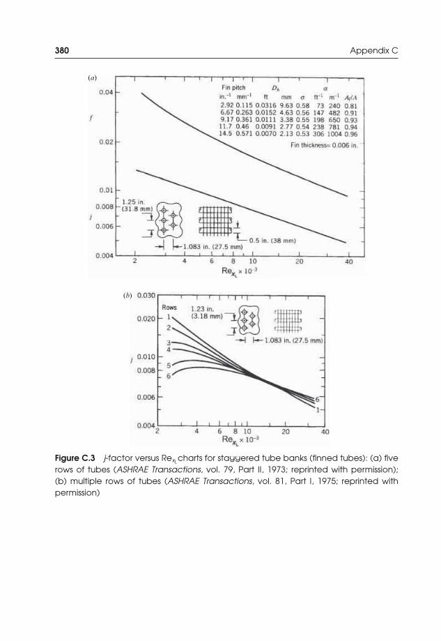
JWST229-bapp03 JWST229-McDonald Printer: Yet to Come July 31, 2012 11:45 Trim: 244mm × 168mm
380 Appendix C
(a)
(b)
Figure C.3 j-factor versus RexL charts for staggered tube banks (finned tubes): (a) fiverows of tubes (ASHRAE Transactions, vol. 79, Part II, 1973; reprinted with permission);(b) multiple rows of tubes (ASHRAE Transactions, vol. 81, Part I, 1975; reprinted withpermission)
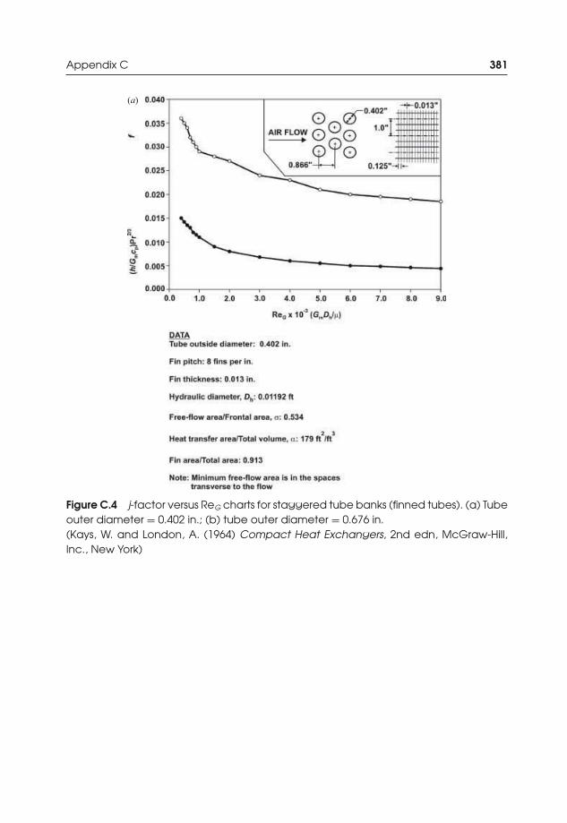
JWST229-bapp03 JWST229-McDonald Printer: Yet to Come July 31, 2012 11:45 Trim: 244mm × 168mm
Appendix C 381
(a)
Figure C.4 j-factor versus ReG charts for staggered tube banks (finned tubes). (a) Tubeouter diameter = 0.402 in.; (b) tube outer diameter = 0.676 in.(Kays, W. and London, A. (1964) Compact Heat Exchangers, 2nd edn, McGraw-Hill,Inc., New York)
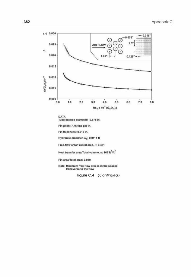
JWST229-bapp03 JWST229-McDonald Printer: Yet to Come July 31, 2012 11:45 Trim: 244mm × 168mm
382 Appendix C
(b)
Figure C.4 (Continued )

JWST229-bapp04 JWST229-McDonald Printer: Yet to Come July 28, 2012 13:3 Trim: 244mm × 168mm
Appendix DDesign Project—Possible Solution
D.1 Fuel Oil Piping System Design
A major part of electric power supply is from large steam power plants with steamproduced by the combustion of fossil fuels or from nuclear reactors. However, forthe supply of power to small communities, it may be economical to use engines toprovide electricity and heat. The expected load and daily power demand for a smallcommunity is provided by the utility company.
Time 0000–0500 h 0500–0700 h 0700–1800 h 1800–2200 h 2200–0000 hLoad (kW) 1650 3100 15200 3100 1650
Engines that operate on #2 oil or other light oil could be purchased. The combinedalternator-transmission efficiency for these engines is typically 90–98%. Motor Ship(October 2000) has shown that specific fuel consumption of slow-speed engines atpeak load varies from approximately 0.30–0.35 lb/(bhp h).
Design the complete fuel oil piping system to supply the engines that are requiredby this community.
Possible Solution
Definition
Design a complete fuel oil piping system for engines used to produce power for asmall community.
Introduction to Thermo-Fluids Systems Design, First Edition. Andre G. McDonald and Hugh L. Magande.C© 2012 Andre G. McDonald and Hugh L. Magande. Published 2012 by John Wiley & Sons, Ltd.
383

JWST229-bapp04 JWST229-McDonald Printer: Yet to Come July 28, 2012 13:3 Trim: 244mm × 168mm
384 Appendix D
Preliminary Specifications and Constraints
(i) Engines will be used to provide power to a small community.(ii) The daily power demand is shown below.
Time 0000–0500 h 0500–0700 h 0700–1800 h 1800–2200 h 2200–0000 hLoad (kW) 1650 3100 15200 3100 1650
(iii) The working fluid could be #2 fuel oil.(iv) The alternator-transmission efficiency of the engine is typically 90%.(v) Fuel consumption could be on the order of 0.30–0.35 lb/(bhp h) for slow-speed
engines.
Detailed Design
Objective
To size the pipes in the system and to size and select appropriate pumps. Pipingaccessories will also be specified.
Data Given or Known
(i) The daily power load requirements are known.(ii) The alternator-transmission efficiency of the engine is typically 90%.
(iii) Fuel consumption can range from 0.30 to 0.35 lb/(bhp h).
Assumptions/Limitations/Constraints
(i) Let the piping material be Schedule 40 steel. Steel is an acceptable material asper the National Fire Protection Association (NFPA) standard 30, section 27.4and NFPA 31, section 8.2.
(ii) Let the flow velocity be about 5 fps. The maximum erosion limit for #2 fuel oil isabout 12 fps. It was assumed that the specific gravity of #2 oil was approximately0.83 (Material Data Safety Sheet (MSDS) supplied by NOVA Chemicals, Calgary,AB).
(iii) Limit pipe frictional losses (major losses) to 5 ft of water per 100 ft of pipe.(iv) Pipe changes should be gradual to reduce losses.(v) All bends will be 90◦ threaded (screwed) regular bends.
(vi) All fittings and pipe accessories will be threaded to reduce losses.(vii) Negligible elevation head in the piping system between the engines. Assume
that all components are on the same level. Some fluid lifting may be needed onthe suction line between the pump and the fuel storage tank.
(viii) Assume that the viscosity (at 104◦F) and specific gravity (at 59◦F) of #2 fuel oilis 3.4 cSt and 0.83, respectively. Note that 3.4 cSt = 3.66 × 10⁻⁵ ft2/s (MaterialData Safety Sheet (MSDS) supplied by NOVA Chemicals, Calgary, AB).

JWST229-bapp04 JWST229-McDonald Printer: Yet to Come July 28, 2012 13:3 Trim: 244mm × 168mm
Appendix D 385
(ix) Assume the vapor pressure of the #2 fuel oil to be 1.5 mm Hg = 0.059 in. Hg =0.80 in. wg = 0.0290 psi at 68◦F (Material Data Safety Sheet (MSDS) suppliedby NOVA Chemicals, Calgary, AB).
(x) Assume the power requirement of the plant that will house the engines isabout 500 kW. According to ABB Automation (Smart Generation: Energy EfficientDesign of Auxiliary Systems in Fossil-fuel Power Plants), oil-fired power plantswill require 3.5–7.5% of the plant output at full load to run the plant auxiliaries.
(xi) Assume that the maximum efficiency of an engine will occur when it operatesat about 80% of its rated output.
(xii) The fuel storage tank(s) will be filled once every week. This can be modifiedbased on the desires of the client.
Sketch
There are many additional parameters that will be needed before a drawing or sketchcan be provided. A full drawing will be provided toward the end of the design. Asketch may be provided in Section “Analysis.”
Analysis
Bear the following points in mind for this design problem:
(i) Pipe sizing for this system can be done quickly by using the appropriate frictionloss charts for Schedule 40 pipe. However, if the required sizes, flow rates,velocities, etc., are not included on the published charts or if the design isbased on a specialized pipe material, then the designer should use Colebrook’sequation (or other correlation equation) to find the friction factor ( f ) and iterateto find the pipe diameters.
(ii) Lower fuel velocities will be used to keep head loss low, reduce pipe erosion,and provide longer, trouble-free service.
(iii) It is possible that the pump will need to lift oil from an underground oil storagetank. Underground storage will provide protection against accidental damageto the tanks. On the other hand, above ground tanks will be easier to maintainand problems will be easier to identify.
(iv) All attempts will be made to install the pump as close as possible to the fuel oilstorage tank.
(v) Shorter, larger suction pipes are usually recommended.(vi) Fuel oils will produce vapor that are flammable, posing a safety problem. In
addition, vapor formation in the pump and suction line can result in cavitation,noise, and reduced performance of the pump. The net positive suction heads(NPSH) should be calculated.
(vii) A strainer will be installed in the pump suction line to prevent or reduce theamount of solid particulates that enter the pump and engines.
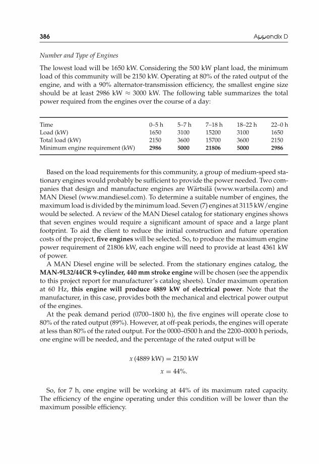
JWST229-bapp04 JWST229-McDonald Printer: Yet to Come July 28, 2012 13:3 Trim: 244mm × 168mm
386 Appendix D
Number and Type of Engines
The lowest load will be 1650 kW. Considering the 500 kW plant load, the minimumload of this community will be 2150 kW. Operating at 80% of the rated output of theengine, and with a 90% alternator-transmission efficiency, the smallest engine sizeshould be at least 2986 kW ≈ 3000 kW. The following table summarizes the totalpower required from the engines over the course of a day:
Time 0–5 h 5–7 h 7–18 h 18–22 h 22–0 hLoad (kW) 1650 3100 15200 3100 1650Total load (kW) 2150 3600 15700 3600 2150Minimum engine requirement (kW) 2986 5000 21806 5000 2986
Based on the load requirements for this community, a group of medium-speed sta-tionary engines would probably be sufficient to provide the power needed. Two com-panies that design and manufacture engines are Wartsila (www.wartsila.com) andMAN Diesel (www.mandiesel.com). To determine a suitable number of engines, themaximum load is divided by the minimum load. Seven (7) engines at 3115 kW/enginewould be selected. A review of the MAN Diesel catalog for stationary engines showsthat seven engines would require a significant amount of space and a large plantfootprint. To aid the client to reduce the initial construction and future operationcosts of the project, five engines will be selected. So, to produce the maximum enginepower requirement of 21806 kW, each engine will need to provide at least 4361 kWof power.
A MAN Diesel engine will be selected. From the stationary engines catalog, theMAN-9L32/44CR 9-cylinder, 440 mm stroke engine will be chosen (see the appendixto this project report for manufacturer’s catalog sheets). Under maximum operationat 60 Hz, this engine will produce 4889 kW of electrical power. Note that themanufacturer, in this case, provides both the mechanical and electrical power outputof the engines.
At the peak demand period (0700–1800 h), the five engines will operate close to80% of the rated output (89%). However, at off-peak periods, the engines will operateat less than 80% of the rated output. For the 0000–0500 h and the 2200–0000 h periods,one engine will be needed, and the percentage of the rated output will be
x (4889 kW) = 2150 kW
x = 44%.
So, for 7 h, one engine will be working at 44% of its maximum rated capacity.The efficiency of the engine operating under this condition will be lower than themaximum possible efficiency.
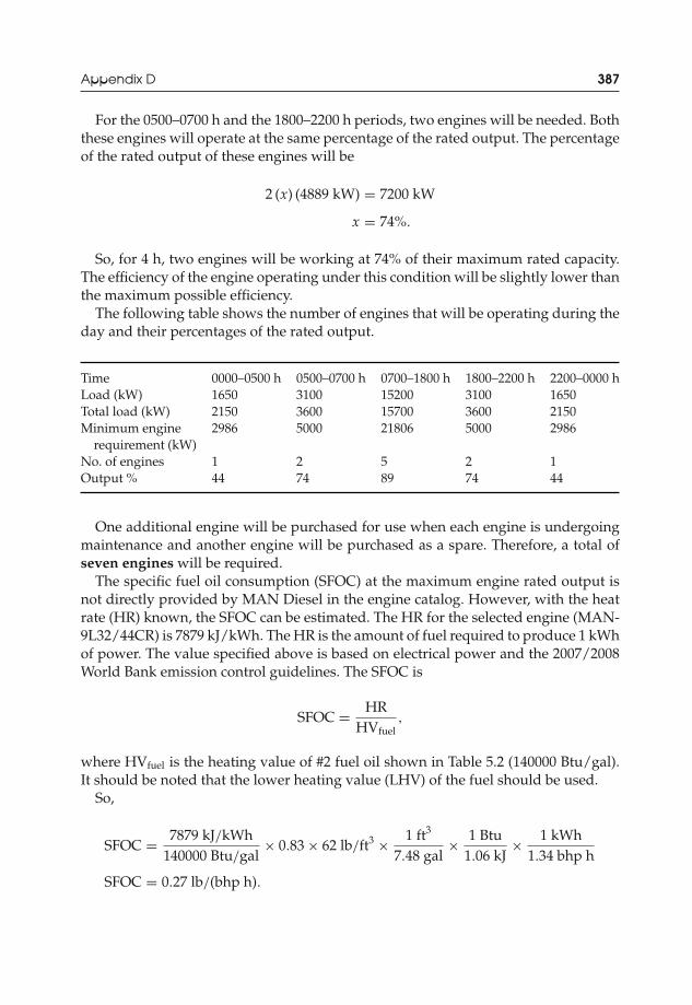
JWST229-bapp04 JWST229-McDonald Printer: Yet to Come July 28, 2012 13:3 Trim: 244mm × 168mm
Appendix D 387
For the 0500–0700 h and the 1800–2200 h periods, two engines will be needed. Boththese engines will operate at the same percentage of the rated output. The percentageof the rated output of these engines will be
2 (x) (4889 kW) = 7200 kW
x = 74%.
So, for 4 h, two engines will be working at 74% of their maximum rated capacity.The efficiency of the engine operating under this condition will be slightly lower thanthe maximum possible efficiency.
The following table shows the number of engines that will be operating during theday and their percentages of the rated output.
Time 0000–0500 h 0500–0700 h 0700–1800 h 1800–2200 h 2200–0000 hLoad (kW) 1650 3100 15200 3100 1650Total load (kW) 2150 3600 15700 3600 2150Minimum engine
requirement (kW)2986 5000 21806 5000 2986
No. of engines 1 2 5 2 1Output % 44 74 89 74 44
One additional engine will be purchased for use when each engine is undergoingmaintenance and another engine will be purchased as a spare. Therefore, a total ofseven engines will be required.
The specific fuel oil consumption (SFOC) at the maximum engine rated output isnot directly provided by MAN Diesel in the engine catalog. However, with the heatrate (HR) known, the SFOC can be estimated. The HR for the selected engine (MAN-9L32/44CR) is 7879 kJ/kWh. The HR is the amount of fuel required to produce 1 kWhof power. The value specified above is based on electrical power and the 2007/2008World Bank emission control guidelines. The SFOC is
SFOC = HRHVfuel
,
where HVfuel is the heating value of #2 fuel oil shown in Table 5.2 (140000 Btu/gal).It should be noted that the lower heating value (LHV) of the fuel should be used.
So,
SFOC = 7879 kJ/kWh140000 Btu/gal
× 0.83 × 62 lb/ft3 × 1 ft3
7.48 gal× 1 Btu
1.06 kJ× 1 kWh
1.34 bhp h
SFOC = 0.27 lb/(bhp h).

JWST229-bapp04 JWST229-McDonald Printer: Yet to Come July 28, 2012 13:3 Trim: 244mm × 168mm
388 Appendix D
Size of Fuel Oil Storage Tank
Now that the number of engines and their capacities are known (to provide themaximum demand), the total volume of fluid, the size of the tank, and the spec-ifications of the tank can be determined. The volume flow rate of fuel requiredwill be
� =(
0.35 lbbhp h
) (5 engines
) (4440 kWengine
) (1.341 bhp
1 kW
)⎛⎝ 1
(0.83)(
62.36 lb/ft3)⎞⎠
(264.17 gal
35.315 ft3
)(1 h
60 min
)
� = 25 gpm.
The volume of fluid required every week is
� =(
0.35 lbbhp h
) (5 engines
) (4440 kWengine
) (1.341 bhp
1 kW
)(1 week)
(168 h
1 week
)⎛⎝ 1
(0.83)(
62.36 lb/ft3)⎞⎠
� = 33820 ft3 = 252988 US gal.
For the five engines that will operate at 79% of their maximum rated output, only79% of the fuel will be used over the 1-week period (177092 gal). However, the finalsize of the storage tank will be selected based on this maximum volume. In thiscase, there will be enough fuel for approximately 2 days beyond the 1-week period(36141 gal per day).
Five above ground fuel storage tanks will be selected. Clemmer Steelcraft Tech-nologies (www.clemmertech.com) Model AGDW1581 tanks will be chosen. See theequipment schedule for additional information. The size of each tank is 52835 US gal.
It is expected that the total length of piping between the fuel storage tanks and thepump will be large. So, the pump size will be large. Consistently operating a largepump to move fluid to the engines may be costly and frequent maintenance may beneeded. Therefore, two fuel oil day tanks will be installed inside the plant. Theywill be filled to provide 12 h of oil, and a smaller pump will move fuel from the daytanks to the engines. Clemmer Steelcraft Technologies Model AGDW1573 tanks willbe chosen. See the equipment schedule for additional information. The size of eachtank is 9246 US gal. About 9035 US gal are needed per tank per day.

JWST229-bapp04 JWST229-McDonald Printer: Yet to Come July 28, 2012 13:3 Trim: 244mm × 168mm
Appendix D 389
Pipe Sizes
Charts can be used to determine the pipe sizes that will be needed for the fuel oilsystem. The total volume flow rate required for the five engines operating during themaximum load period is 25 gpm. Each engine will require 5 gpm.
At this point, a preliminary, tentative layout of the system would be useful.
Since day tanks (DT) are present in the plant, fuel from the outdoor storage tanks(ST) will be pumped at a rate of 50 gpm from the pipe manifold. This rate is double
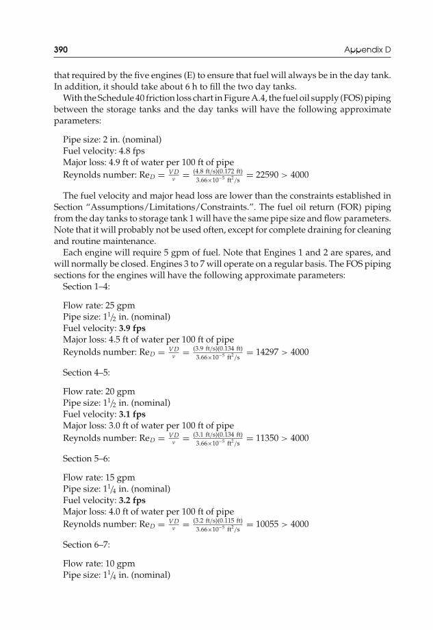
JWST229-bapp04 JWST229-McDonald Printer: Yet to Come July 28, 2012 13:3 Trim: 244mm × 168mm
390 Appendix D
that required by the five engines (E) to ensure that fuel will always be in the day tank.In addition, it should take about 6 h to fill the two day tanks.
With the Schedule 40 friction loss chart in Figure A.4, the fuel oil supply (FOS) pipingbetween the storage tanks and the day tanks will have the following approximateparameters:
Pipe size: 2 in. (nominal)Fuel velocity: 4.8 fpsMajor loss: 4.9 ft of water per 100 ft of pipeReynolds number: ReD = VD
ν= (4.8 ft/s)(0.172 ft)
3.66×10⁻⁵ ft2/s
= 22590 > 4000
The fuel velocity and major head loss are lower than the constraints established inSection “Assumptions/Limitations/Constraints.”. The fuel oil return (FOR) pipingfrom the day tanks to storage tank 1 will have the same pipe size and flow parameters.Note that it will probably not be used often, except for complete draining for cleaningand routine maintenance.
Each engine will require 5 gpm of fuel. Note that Engines 1 and 2 are spares, andwill normally be closed. Engines 3 to 7 will operate on a regular basis. The FOS pipingsections for the engines will have the following approximate parameters:
Section 1–4:
Flow rate: 25 gpmPipe size: 11/2 in. (nominal)Fuel velocity: 3.9 fpsMajor loss: 4.5 ft of water per 100 ft of pipeReynolds number: ReD = VD
ν= (3.9 ft/s)(0.134 ft)
3.66×10⁻⁵ ft2/s
= 14297 > 4000
Section 4–5:
Flow rate: 20 gpmPipe size: 11/2 in. (nominal)Fuel velocity: 3.1 fpsMajor loss: 3.0 ft of water per 100 ft of pipeReynolds number: ReD = VD
ν= (3.1 ft/s)(0.134 ft)
3.66×10⁻⁵ ft2/s
= 11350 > 4000
Section 5–6:
Flow rate: 15 gpmPipe size: 11/4 in. (nominal)Fuel velocity: 3.2 fpsMajor loss: 4.0 ft of water per 100 ft of pipeReynolds number: ReD = VD
ν= (3.2 ft/s)(0.115 ft)
3.66×10⁻⁵ ft2/s
= 10055 > 4000
Section 6–7:
Flow rate: 10 gpmPipe size: 11/4 in. (nominal)

JWST229-bapp04 JWST229-McDonald Printer: Yet to Come July 28, 2012 13:3 Trim: 244mm × 168mm
Appendix D 391
Fuel velocity: 2.1 fpsMajor loss: 1.8 ft of water per 100 ft of pipeReynolds number: ReD = VD
ν= (2.1 ft/s)(0.115 ft)
3.66×10⁻⁵ ft2/s
= 6598 > 4000
Section 7–8:
Flow rate: 5 gpmPipe size: 1 in. (nominal)Fuel velocity: 1.9 fpsMajor loss: 2.0 ft of water per 100 ft of pipeReynolds number: ReD = VD
ν= (1.9 ft/s)(0.0874 ft)
3.66×10⁻⁵ ft2/s
= 4538 > 4000
For sections 6–7 and 7–8 where the major head loss is low, balancing valves mayneed to be installed to increase the head loss in that section of the FOS piping to theengines. In that case, the loss coefficients of the valves will be calculated to facilitateselection by the contractor. All the pipe flows are fully turbulent.
The adjacent FOR piping sections from the engines will have the same pipe sizesand flow parameters.
Pipe Lengths and Major Head Losses
The lengths of the pipe sections for the supply and return lines will depend onthe installation distance between the tanks and engines. Of interest will also be thedistance of the tanks and engines from the walls of the building.
The National Fire Protection Association standards will be used to specify thedistances. NFPA 30 (Flammable and Combustible Liquids Code), section 22.4 requirethat outdoor aboveground storage tanks with capacities between 50001 and 100000gal be located at least 15 ft from the plant building (see the appendix to this projectreport). The same section of the code requires that each tank shall not be requiredto be separated by more than 3 ft. This part of the code refers to crude petroleum.However, it will be applied to #2 light fuel oil. Note that no attempt was made toclassify #2 fuel oil as a stable liquid. If that is the case, an 8-ft distance between thetanks and the building would satisfy the requirements of the code.
For consistency, a 3 ft distance will be placed between the engines, around thepumps, and between the day tanks. Note the following dimensions:
Storage tank (AGDW1581) Diameter = 14 ftLength = 53 ft
Day tank (AGDW1573) Diameter = 9 ftLength = 24 ft
Engine (MAN-9L32/44CR 9-cyl.) Length = 40 ftWidth = 9 ft
With these distances and equipment dimensions, the preliminary layout of thesystem, complete with lengths, becomes

JWST229-bapp04 JWST229-McDonald Printer: Yet to Come July 28, 2012 13:3 Trim: 244mm × 168mm
392 Appendix D
The longest run of fuel oil supply piping between the storage tanks (ST-5) andpump, P-1 is approximately,
LST-S = (78 + 61 + 15 + 6 + 3 + 4.5 + 4.5) ft = 172 ft.
The last 3 ft, and two 4.5 ft lengths were added based on the distance between theday tanks (3 ft) and half the diameter of the tank (4.5 ft).
The total major head loss for this section of supply piping is
HST-S = 4.9 ft100 ft
× 172 ft = 8.43 ft.

JWST229-bapp04 JWST229-McDonald Printer: Yet to Come July 28, 2012 13:3 Trim: 244mm × 168mm
Appendix D 393
For the return line between ST-1 and P-4,
LST-S = (6 + 73 + 74) ft = 153 ft.
The total major head loss for this section of return piping is
HST-S = 4.9 ft100 ft
× 153 ft = 7.50 ft.
The total major head loss that will be experienced by pump, P-2.FOS section between the day tanks (DT-1 and DT-2) and engine 3 (E-3):
4.5 ft100 ft
× (1.5 + 4.5 + 20 + 1.5 + 9 + 3 + 3 + 9 + 3 + 9 + 3 + 4.5) ft = 3.06 ft.
FOS section between E-3 and E-4,
3.0 ft100 ft
× (4.5 + 3 + 4.5) ft = 0.36 ft.
FOS section between E-4 and E-5,
4.0 ft100 ft
× (4.5 + 3 + 4.5) ft = 0.48 ft.
FOS section between E-5 and E-6,
1.8 ft100 ft
× (4.5 + 3 + 4.5) ft = 0.22 ft.
FOS section between E-6 and E-7,
2.0 ft100 ft
× (4.5 + 3 + 4.5) ft = 0.24 ft.
The total major head loss that will be experienced by pump, P-2 will be
HFOS-E = (3.06 + 0.36 + 0.48 + 0.22 + 0.24) ft = 4.36 ft.
The total major head loss that will be experienced by pump, P-3 will be approxi-mately
HFOR-E = 4.36 ft.
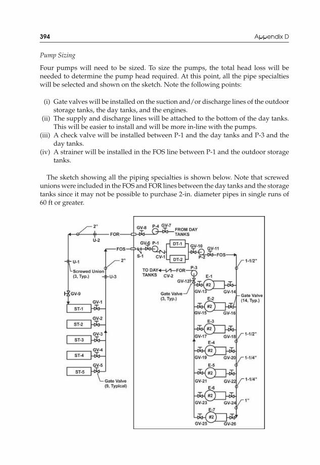
JWST229-bapp04 JWST229-McDonald Printer: Yet to Come July 28, 2012 13:3 Trim: 244mm × 168mm
394 Appendix D
Pump Sizing
Four pumps will need to be sized. To size the pumps, the total head loss will beneeded to determine the pump head required. At this point, all the pipe specialtieswill be selected and shown on the sketch. Note the following points:
(i) Gate valves will be installed on the suction and/or discharge lines of the outdoorstorage tanks, the day tanks, and the engines.
(ii) The supply and discharge lines will be attached to the bottom of the day tanks.This will be easier to install and will be more in-line with the pumps.
(iii) A check valve will be installed between P-1 and the day tanks and P-3 and theday tanks.
(iv) A strainer will be installed in the FOS line between P-1 and the outdoor storagetanks.
The sketch showing all the piping specialties is shown below. Note that screwedunions were included in the FOS and FOR lines between the day tanks and the storagetanks since it may not be possible to purchase 2-in. diameter pipes in single runs of60 ft or greater.

JWST229-bapp04 JWST229-McDonald Printer: Yet to Come July 28, 2012 13:3 Trim: 244mm × 168mm
Appendix D 395
Now that the pipe diameters are known, the minor losses for each section can beestimated. The loss coefficients (K) for the piping specialties are given below (consultTable A.14). Note that the pipe diameters were considered when reporting the losscoefficients.
Fuel oil supply piping between the storage tanks and pump, P-1:
Pipe Specialty NumberPipe Diameter
(in.)Pipe Velocity
(fps) KMinor
Loss (ft)
GV-5, GV-6 2 2 4.8 0.16 0.114U-3 1 2 4.8 0.08 0.029S-1 1 2 4.8 1.5 0.537CV-1 1 2 4.8 2.1 0.751Screwed 90◦ bend 3 2 4.8 0.95 1.02Line flow tee 4 2 4.8 0.90 1.29Branch flow tee 1 2 4.8 1.4 0.501Sharp-edged entrance 1 2 4.8 0.5 0.179Rounded exit 1 2 4.8 1.05 0.376Total 4.80
The total head loss for the fuel oil supply piping between the storage tanks andpump, P-1 is
HT,ST-S = (8.43 + 4.80) ft = 13.23 ft.
The pump head (in feet) is
HP-1 =(
p2
ρg+ V2
2
2g+ z2
)−
(p1
ρg+ V2
1
2g+ z1
)+ HT,ST−S.
Let point 1 be at the bottom of storage tank 5 and point 2 be at the bottom of theday tanks. So, V1 = V2 and z1 = z2.
HP-1 = p2 − p1
ρg+ HT,ST-S
To ensure that the pump will be sized adequately for all operation scenarios, it willbe assumed that the storage tank is empty and the day tank is filled to maximumcapacity. Assume that the tanks are vented to the atmosphere.
So,
p1 = patm
p2 = patm + ρgh = patm + ρgDtank.
Then,
HP-1 = Dtank + HT,ST-S
HP-1 = (9 + 13.23) ft = 22.23 ft ≈ 23 ft.

JWST229-bapp04 JWST229-McDonald Printer: Yet to Come July 28, 2012 13:3 Trim: 244mm × 168mm
396 Appendix D
The total flow rate through P-1 will be 50 gpm.
Fuel oil supply piping between the day tanks and the engines through pump, P-2:
Pipe Specialty NumberPipe Diameter
(in.)Pipe Velocity
(fps) KMinor
Loss (ft)
GV-10, GV-11 2 11/2 3.9 0.24 0.113Sharp-edged entrance 1 11/2 3.9 0.50 0.118Branch flow tee 1 11/2 3.9 1.8 0.425Screwed 90◦ bend 2 11/2 3.9 1.5 0.709Line flow tee 3 11/2 3.9 0.90 0.638Line flow tee 1 11/4 3.2 0.90 0.143Gradual Contraction 1 11/2 to 11/4 3.1 0.07 0.011Gradual Contraction 1 11/4 to 1 2.1 0.07 0.005Line flow tee 1 11/4 3.2 0.90 0.143Line flow tee 1 11/4 3.2 0.90 0.14390◦ bend 1 1 1.9 1.5 0.084GV-26 1 1 1.9 0.24 0.014Rounded exit 1 1 1.9 1.05 0.059Total 2.61
As mentioned earlier, the head loss may become very small as one gets farther awayfrom P-2. This will result in unbalanced flow through the pipeline. Check sections1–8 in this line and determine if balancing valves will be needed. Note that section1–4 is ignored because there is no other path for fluid flow between points 1 and 4 ifengines 1 and 2 are not operational.
Section Major Head Loss (ft) Minor Head Loss (ft) Total Head Loss (ft)
Section 1–4 3.06 2.00 5.06Section 4–5 0.36 0.154 0.514Section 5–6 0.48 0.143 0.623Section 6–7 0.22 0.148 0.368Section 7–8 0.24 0.157 0.397
The total head losses in sections 4–8 are close. So, no balancing valves will berecommended.
The total head loss for the fuel oil supply piping between the day tanks and pump,P-2 is
HT,FOS-E = (4.36 + 2.61) ft = 6.97 ft.
The pump head (in ft) is
HP-2 =(
p4
ρg+ V2
4
2g+ z4
)−
(p3
ρg+ V2
3
2g+ z3
)+ HT,FOS-E.
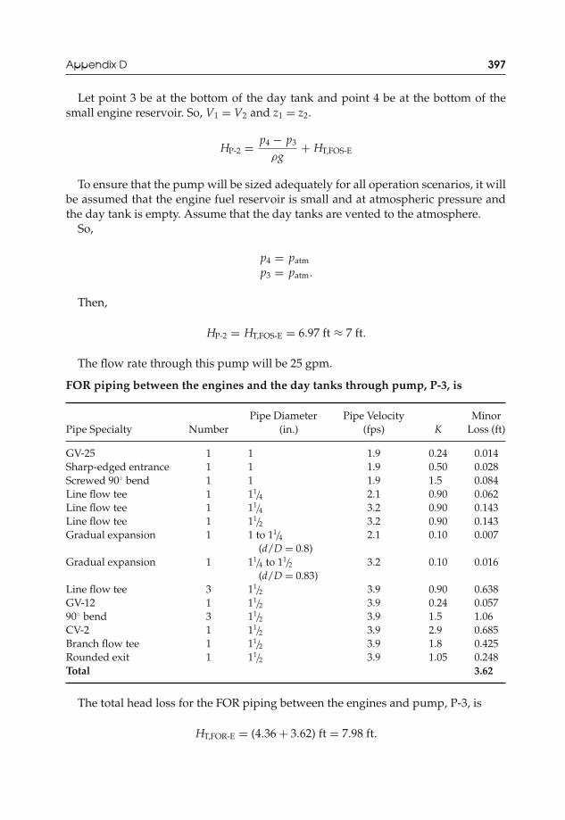
JWST229-bapp04 JWST229-McDonald Printer: Yet to Come July 28, 2012 13:3 Trim: 244mm × 168mm
Appendix D 397
Let point 3 be at the bottom of the day tank and point 4 be at the bottom of thesmall engine reservoir. So, V1 = V2 and z1 = z2.
HP-2 = p4 − p3
ρg+ HT,FOS-E
To ensure that the pump will be sized adequately for all operation scenarios, it willbe assumed that the engine fuel reservoir is small and at atmospheric pressure andthe day tank is empty. Assume that the day tanks are vented to the atmosphere.
So,
p4 = patm
p3 = patm.
Then,
HP-2 = HT,FOS-E = 6.97 ft ≈ 7 ft.
The flow rate through this pump will be 25 gpm.
FOR piping between the engines and the day tanks through pump, P-3, is
Pipe Specialty NumberPipe Diameter
(in.)Pipe Velocity
(fps) KMinor
Loss (ft)
GV-25 1 1 1.9 0.24 0.014Sharp-edged entrance 1 1 1.9 0.50 0.028Screwed 90◦ bend 1 1 1.9 1.5 0.084Line flow tee 1 11/4 2.1 0.90 0.062Line flow tee 1 11/4 3.2 0.90 0.143Line flow tee 1 11/2 3.2 0.90 0.143Gradual expansion 1 1 to 11/4
(d/D = 0.8)2.1 0.10 0.007
Gradual expansion 1 11/4 to 11/2
(d/D = 0.83)3.2 0.10 0.016
Line flow tee 3 11/2 3.9 0.90 0.638GV-12 1 11/2 3.9 0.24 0.05790◦ bend 3 11/2 3.9 1.5 1.06CV-2 1 11/2 3.9 2.9 0.685Branch flow tee 1 11/2 3.9 1.8 0.425Rounded exit 1 11/2 3.9 1.05 0.248Total 3.62
The total head loss for the FOR piping between the engines and pump, P-3, is
HT,FOR-E = (4.36 + 3.62) ft = 7.98 ft.

JWST229-bapp04 JWST229-McDonald Printer: Yet to Come July 28, 2012 13:3 Trim: 244mm × 168mm
398 Appendix D
The pump head (in feet) is
HP-3 =(
p6
ρg+ V2
6
2g+ z6
)−
(p5
ρg+ V2
5
2g+ z5
)+ HT,FOR-E.
Let point 5 be at the bottom of the E-7 and point 6 be at the bottom of the day tank.So, V1 = V2 and z1 = z2.
HP-3 = p6 − p5
ρg+ HT,FOR-E
To ensure that the pump will be sized adequately for all operation scenarios, it willbe assumed that the engine fuel reservoir is small and at atmospheric pressure andthe day tank is full to the maximum capacity. Assume that the day tanks are ventedto the atmosphere.
So,
p5 = patm
p6 = patm + ρgh = patm + ρgDtank.
Then,
HP-3 = Dtank + HT,FOR-E = (9 + 7.98) ft = 16.98 ft ≈ 17 ft.
The flow rate through this pump will be 25 gpm.
FOR piping between the day tanks and storage tank, ST-1 through P-4:
Pipe Specialty NumberPipe Diameter
(in.)Pipe Velocity
(fps) KMinor
Loss (ft)
GV-7, GV-8, GV-9 3 2 4.8 0.16 0.172Sharp-edged entrance 1 2 4.8 0.50 0.179Branch flow tee 1 2 4.8 1.4 0.500Screwed 90◦ bend 3 2 4.8 0.95 1.02U-2 2 2 4.8 0.08 0.057Rounded exit 1 2 4.8 1.05 0.376Total 2.30
The total head loss for the FOR piping between the day tanks and pump, P-4 is
HT,ST-R = (7.50 + 2.30) ft = 9.80 ft.
The pump head (in feet) is
HP-4 =(
p8
ρg+ V2
8
2g+ z8
)−
(p7
ρg+ V2
7
2g+ z7
)+ HT,ST-R.

JWST229-bapp04 JWST229-McDonald Printer: Yet to Come July 28, 2012 13:3 Trim: 244mm × 168mm
Appendix D 399
Let point 7 be at the bottom of the day tank and point 8 be at the bottom of the ST-1So, V1 = V2 and z1 = z2.
HP-4 = p8 − p7
ρg+ HT,ST-R
To ensure that the pump will be sized adequately for all operation scenarios, it willbe assumed that the day tank is empty and at atmospheric pressure and ST-1 is fullto the maximum capacity. Assume that the tanks are vented to the atmosphere.
So,
p7 = patm
p8 = patm + ρgh = patm = ρgDST-1.
Then,
HP-4 = DST-1 + HT,ST-R = (14 + 9.80) ft = 23.8 ft ≈ 24 ft.
The flow rate through this pump will be 50 gpm.
Pump Selection
For this fuel oil piping system, pumps rated with the following capacities are required:
P-1: 23 ft of head and 50 gpm;P-2: 7 ft of head and 25 gpm;P-3: 17 ft of head and 25 gpm;P-4: 24 ft of head and 50 gpm.
Use manufacturer’s charts to select an appropriate pump. A review of the variousBell & Gossett pumps shows that Series 60 in-line mounted pumps would be suitable.The pump performance plots are shown below.
From the Master Selection chart, the 2 in. × 2 in. × 51/4 in. casing pump will bechosen for P-1 and P-4. The 1 in. × 1 in. × 51/4 in. casing pump will be chosen for P-2and the 11/4 in. × 11/4 in. × 51/4 in. casing pump will be chosen for P-3.
From the performance plots (see below), the final choices are as follows.
P-1 and P-4: 2 in. × 2 in. × 51/4 in. casing5.25 in. impeller diameter3/4 hp motor1750 rpm speed

JWST229-bapp04 JWST229-McDonald Printer: Yet to Come July 28, 2012 13:3 Trim: 244mm × 168mm
400 Appendix D
The manufacturer’s cut sheet will show that a Series 60, 612T is the best optionin stock.
P-2: 1 in. × 1 in. × 51/4 in. casing3.75 in. impeller diameter1/4 hp motor1750 rpm speed
The manufacturer’s cut sheet will show that a Series 60, 601T is the best optionin stock.
P-3: 11/4 in. × 11/4 in. × 51/4 in. casing4.75 in. impeller diameter1/4 hp motor1750 rpm speed
The manufacturer’s cut sheet will show that a Series 60, 605T is the best option instock (see Figure A.5).
Note that “to-the-point” design was avoided, and slightly larger sizes and powerswere chosen.
60
501½x7
1½x6¼
1½x5¼
1¼x5¼
2x5¼
2x7
3x3x5¼
2x6¼
1x5¼
40
30
20
10
00 20 40 60 80 100 120 140
CAPACITY, GPM
SELECTION CHART
SYSTEMCURVES
TOTA
L H
EA
D, F
T.
160 180 200 220

JWST229-bapp04 JWST229-McDonald Printer: Yet to Come July 28, 2012 13:3 Trim: 244mm × 168mm
Appendix D 401
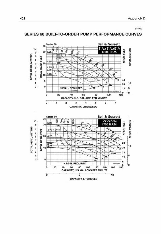
JWST229-bapp04 JWST229-McDonald Printer: Yet to Come July 28, 2012 13:3 Trim: 244mm × 168mm
402 Appendix D
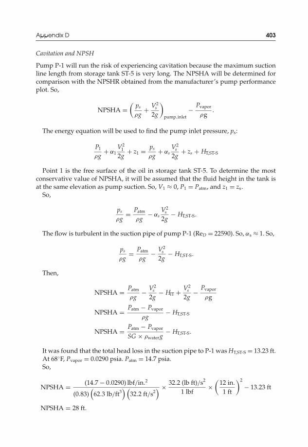
JWST229-bapp04 JWST229-McDonald Printer: Yet to Come July 28, 2012 13:3 Trim: 244mm × 168mm
Appendix D 403
Cavitation and NPSH
Pump P-1 will run the risk of experiencing cavitation because the maximum suctionline length from storage tank ST-5 is very long. The NPSHA will be determined forcomparison with the NPSHR obtained from the manufacturer’s pump performanceplot. So,
NPSHA =(
ps
ρg+ V2
s
2g
)pump,inlet
− Pvapor
ρg.
The energy equation will be used to find the pump inlet pressure, ps:
P1
ρg+ α1
V21
2g+ z1 = ps
ρg+ αs
V2s
2g+ zs + HT,ST-S
Point 1 is the free surface of the oil in storage tank ST-5. To determine the mostconservative value of NPSHA, it will be assumed that the fluid height in the tank isat the same elevation as pump suction. So, V1 ≈ 0, P1 = Patm, and z1 = zs.
So,
ps
ρg= Patm
ρg− αs
V2s
2g− HT,ST-S.
The flow is turbulent in the suction pipe of pump P-1 (ReD = 22590). So, αs ≈ 1. So,
ps
ρg= Patm
ρg− V2
s
2g− HT,ST-S.
Then,
NPSHA = Patm
ρg− V2
s
2g− HlT + V2
s
2g− Pvapor
ρg
NPSHA = Patm − Pvapor
ρg− HT,ST-S
NPSHA = Patm − Pvapor
SG × ρwaterg− HT,ST-S.
It was found that the total head loss in the suction pipe to P-1 was HT,ST-S = 13.23 ft.At 68◦F, Pvapor = 0.0290 psia. Patm = 14.7 psia.So,
NPSHA = (14.7 − 0.0290) lbf/in.2
(0.83)(
62.3 lb/ft3) (
32.2 ft/s2) × 32.2 (lb ft)/s2
1 lbf×
(12 in.
1 ft
)2
− 13.23 ft
NPSHA = 28 ft.
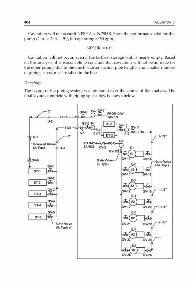
JWST229-bapp04 JWST229-McDonald Printer: Yet to Come July 28, 2012 13:3 Trim: 244mm × 168mm
404 Appendix D
Cavitation will not occur if NPSHA > NPSHR. From the performance plot for thispump (2 in. × 2 in. × 51/4 in.) operating at 50 gpm,
NPSHR ≈ 6 ft.
Cavitation will not occur, even if the farthest storage tank is nearly empty. Basedon this analysis, it is reasonable to conclude that cavitation will not be an issue forthe other pumps due to the much shorter suction pipe lengths and smaller numberof piping accessories installed in the lines.
Drawings
The layout of the piping system was prepared over the course of the analysis. Thefinal layout, complete with piping specialties, is shown below.

JWST229-bapp04 JWST229-McDonald Printer: Yet to Come July 28, 2012 13:3 Trim: 244mm × 168mm
Appendix D 405
A drawing detail of the piping connections to the day tanks will be neededto facilitate contractor installation. The manufacturer of the tank (Clemmer Steel-craft Technologies) should be contacted to determine if all the required connectionsare possible.
Equipment Schedules
Shown below are the schedules of the major equipment that will be specified for thefuel oil system. Minor equipment such as valves and unions will not be specifiedbeyond the contract drawings shown above.
Engine Schedule
Major Dimensions (ft)
Tag
Manufacturerand ModelNumber
MaximumOutput
(kW) CylinderBore &Stroke (ft)
MaximumSFOC
(lb/(bhp h)) C W H
E-1 toE-7
MAN diesel,MAN-9L32/44CR, orequal
4889 9 1.05 and1.44
0.30 40 9 17
Fuel Oil Tank Schedule
Dimensions (in.)
Tag
Manufacturerand ModelNumber
Volume(gal) Gage
Weight(lb) Diameter Length
ST-1 toST-5
Clemmersteelcraft,AGDW1581,or equal
52835 Doublewall
56000 158 630
DT-1,DT-2
Clemmersteelcraft,AGDW1573,or equal
9246 Singlewall
7330 99 281
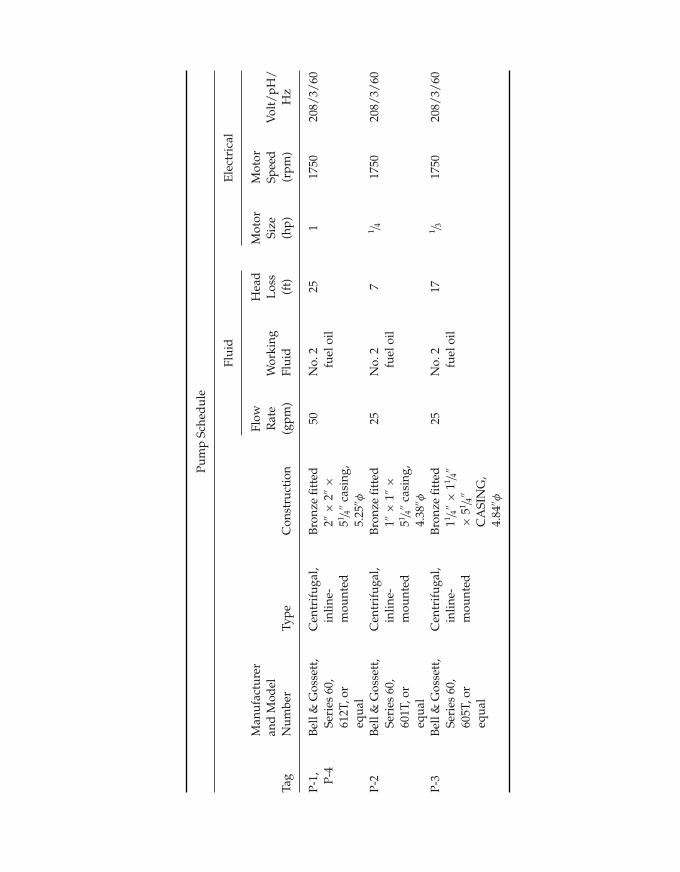
JWST229-bapp04 JWST229-McDonald Printer: Yet to Come July 28, 2012 13:3 Trim: 244mm × 168mm
Pum
pSc
hed
ule
Flui
dE
lect
rica
l
Tag
Man
ufac
ture
ran
dM
odel
Num
ber
Type
Con
stru
ctio
n
Flow
Rat
e(g
pm)
Wor
king
Flui
d
Hea
dL
oss
(ft)
Mot
orSi
ze(h
p)
Mot
orSp
eed
(rpm
)V
olt/
pH/
Hz
P-1, P-
4B
ell&
Gos
sett
,Se
ries
60,
612T
,or
equa
l
Cen
trif
ugal
,in
line-
mou
nted
Bro
nze
fitt
ed2′′
×2′′
×51 /
4′′ca
sing
,5.
25′′ φ
50N
o.2
fuel
oil
251
1750
208/
3/60
P-2
Bel
l&G
osse
tt,
Seri
es60
,60
1T,o
req
ual
Cen
trif
ugal
,in
line-
mou
nted
Bro
nze
fitt
ed1′′
×1′′
×51 /
4′′ca
sing
,4.
38′′ φ
25N
o.2
fuel
oil
71 /
417
5020
8/3/
60
P-3
Bel
l&G
osse
tt,
Seri
es60
,60
5T,o
req
ual
Cen
trif
ugal
,in
line-
mou
nted
Bro
nze
fitt
ed11 /
4′′×
11 /4′′
×51 /
4′′
CA
SIN
G,
4.84
′′ φ
25N
o.2
fuel
oil
171 /
317
5020
8/3/
60
406
JWST229-bapp04 JWST229-McDonald Printer: Yet to Come July 28, 2012 13:3 Trim: 244mm × 168mm
Appendix D 407
Conclusions
A fuel oil piping system has been designed to transport #2 fuel oil to several power-generating engines. The design of the system was based on the maximum amountof fuel that would be needed to meet the maximum/peak power load of a smallcommunity.
A conservative approach was taken in the design analysis. For example, pumpswere sized by considering empty or full fuel tanks in an attempt to remove the benefitsof hydrostatic head that would drive flow through the pipes. Slightly larger fuel oilstorage tanks, pumps, and engines were selected to ensure that the client had someflexibility to cover unexpected surges in power or flow rates. The client may considerthe use of a bypass line, complete with pumps of similar performance ratings as P-1and P-2 (label them P-1A and P-2A), to pump the fuel during times of maintenanceor failure of P-1 and P-2. Also, the friction loss chart for a closed Schedule 40 pipingsystem was used. Use of the friction loss chart for open Schedule 40 piping systemswould produce larger pipe sizes and slightly lower friction losses. This decision wasmade to keep the cost of pipe material low given the low impact on pump sizesthrough use of the smaller pipes.
No allocations have been made for flow control of the pumps. The client may wishto consider speed regulation through the use of a variable frequency drive on themotor or bypass regulation with the use of a bypass line. Discharge throttling is notrecommended due to the large system head loss that may occur. Some vaporizationof the oil may occur on the discharge side due to the high velocities generated duringthe throttling process, which may pose a safety hazard.
No allocation has been made to prime the pump should the storage tanks becomeempty. Complete draining of the storage tanks and pipelines should be avoided.Level switches may be installed or purchased with the storage tanks to form a part ofa control or low-level warning system. Vacuum pumping may be a suitable methodto prime the pump by removing air from the suction line, if needed. A gate valve(not to be used for flow control), downstream of the check valve on the discharge lineof P-1 would be needed. The valves on the discharge lines of the pumps should beclosed before initiating vacuum pumping.
While the design and the contract documents (drawings, schedules, etc.) providesufficient information to initiate construction, the contractor and architect may needto communicate with the mechanical engineer to finalize some points. For example,the size and layout of the plant building still needs to be determined and the engineerwill need to approve the selection and installation plan for piping and specialtiessuch as the valves and unions. These should comply with applicable standards suchas NFPA 30 and 31. Details regarding the fuel day tanks (DT-1 and DT-2) will need tobe determined. In particular, the piping connections will need to be determined oncethe final tanks are selected.
Though outside of the scope of the present project, control systems will be needed.For example, high-level (spill protection) and low-level switches (empty tank) will beneeded at the day tanks. These switches would be routed to a controller that operatesthe P-1 motor.
JWST229-bapp04 JWST229-McDonald Printer: Yet to Come July 28, 2012 13:3 Trim: 244mm × 168mm
408 Appendix D
Other items outside of the scope of this project are a fuel oil heating system andHVAC (heating, ventilation, and air-conditioning system) for the plant building. Theclient is advised to seek consultation for the design of a heating system to preventfreezing of the fuel in the pipes. Also, applicable building and ASHRAE (AmericanSociety of Heating, Refrigeration, and Air-Conditioning Engineers) codes require thatsufficient ventilation of exhaust gases from the engines and air conditioning of theplant building occur to meet safety and human health standards.
Though the efficiency of some of the engines are lowered due to operation at lowercapacities than the maximum possible engine capacity, the reduced maintenance,operations, and initial installation and purchase costs may outweigh the lost savings inincreased engine efficiency. In this case, a reasonable compromise was made betweensystem efficiency and long-term costs.
Specifications
This section is included to specify equipment or piping specialties that may havespecial requirements.
1. 2′′ fuel strainer
The 2′′ fuel strainer shall have a capacity of 50 gpm and have a 100 mesh element.
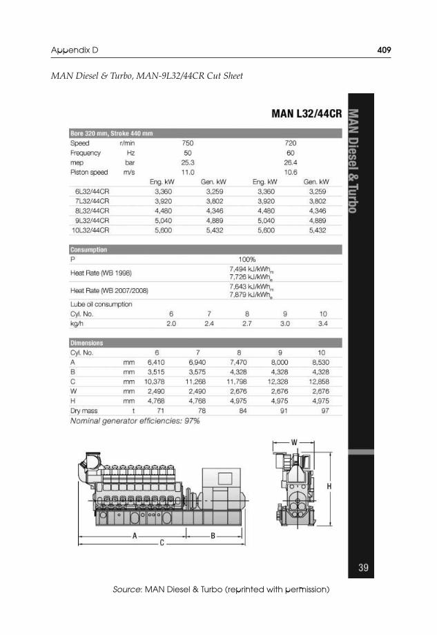
JWST229-bapp04 JWST229-McDonald Printer: Yet to Come July 28, 2012 13:3 Trim: 244mm × 168mm
Appendix D 409
MAN Diesel & Turbo, MAN-9L32/44CR Cut Sheet
Source: MAN Diesel & Turbo (reprinted with permission)

JWST229-bapp04 JWST229-McDonald Printer: Yet to Come July 28, 2012 13:3 Trim: 244mm × 168mm
410 Appendix D
Excerpts from the NFPA 30—Flammable and Combustible Liquids Code, 2008 Edition
Source: MAN Diesel & Turbo (reprinted with permission)
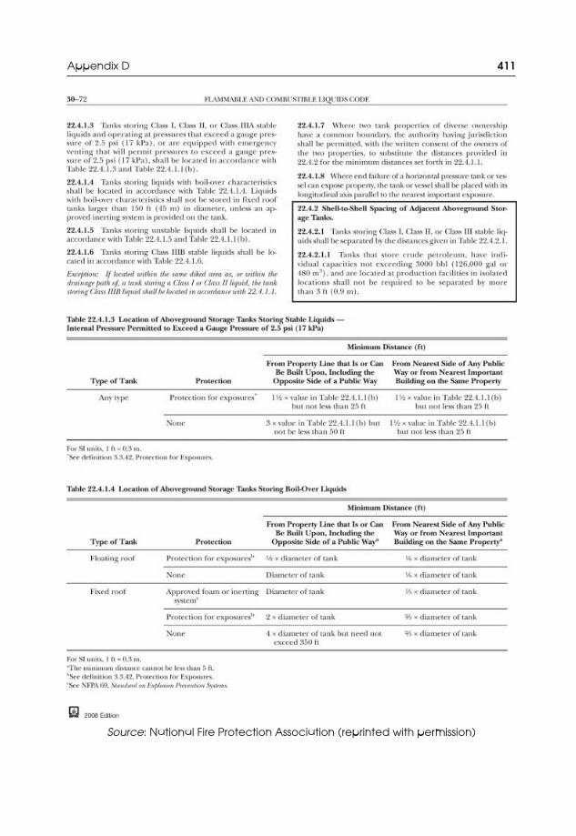
JWST229-bapp04 JWST229-McDonald Printer: Yet to Come July 28, 2012 13:3 Trim: 244mm × 168mm
Appendix D 411
Source: National Fire Protection Association (reprinted with permission)

JWST229-bapp05 JWST229-McDonald Printer: Yet to Come July 28, 2012 10:28 Trim: 244mm × 168mm
Appendix EApplicable Standardsand Codes
A standard is a set of technical definitions and guidelines that function as instructionsfor designers, manufacturers, operators, or users of equipment. Standards do not havethe force of law, and are voluntary guidelines. A standard becomes a code when ithas been adopted by one or more government agencies and is enforced by law, orwhen it has been incorporated into a business contract.
The following organizations provide codes and standards that may be useful inthe design, installation, and commissioning (process by which a system, equipment,facility or plant, which has been installed or is near completion, is tested to verify thatit functions according to its design objectives and/or specifications) of thermo-fluidssystems and equipment. Most of these organizations provide a variety of differenttypes of codes and/or standards that will be useful for the design, installation, andtesting of thermo-fluids systems and equipment.
Air Conditioning Contractors of America (ACCA)Air-Conditioning, Heating and Refrigeration Institute (AHRI) – Formerly (ARI)American Petroleum Institute (API)American Society of Heating, Refrigeration and Air-Conditioning Engineers
(ASHRAE)American Society for Testing and Materials (ASTM)American Society of Mechanical Engineers (ASME)American Water Works Association (AWWA)American National Standards Institute (ANSI)Canadian Standards Association (CSA)Gas Processors Association (GPA)Institute of Boiler and Radiator Manufacturers (I=B=R)International Association of Plumbing and Mechanical Officials (IAPMO)
Introduction to Thermo-Fluids Systems Design, First Edition. Andre G. McDonald and Hugh L. Magande.C© 2012 Andre G. McDonald and Hugh L. Magande. Published 2012 by John Wiley & Sons, Ltd.
413

JWST229-bapp05 JWST229-McDonald Printer: Yet to Come July 28, 2012 10:28 Trim: 244mm × 168mm
414 Appendix E
International Organization for Standardization (ISO)Municipal Building and Fire Codes (e.g., Alberta Building and Fire Codes,
Building Code of the City of New York)National Association of Corrosion Engineers (NACE)National Fire Protection Association (NFPA)Steel Boiler Institute (SBI)Sheet Metal and Air Conditioning Contractors National Association (SMACNA)Uniform Building Code StandardsUniform Mechanical Code (by IAPMO)Uniform Plumbing Code (by IAPMO)

JWST229-bapp06 JWST229-McDonald Printer: Yet to Come July 28, 2012 10:30 Trim: 244mm × 168mm
Appendix FEquipment Manufacturers
Currently, there are many manufacturers who provide equipment specified for use inthermo-fluids systems. Below is an abridged list of manufacturers whose equipmentmay be specified in a system design. Though organized in the groups shown, somemanufacturers may provide other equipment and services. The onus rests on thedesign engineer to check product lines of the manufacturers and suppliers listedbelow and conduct a thorough search to find other manufacturers and suppliers toprovide equipment that meets the required performance targets.
Air Distribution and Heating, Ventilating, and Air-ConditioningTrane (Ingersoll Rand); York (Johnson Controls); McQuay International (DaikinIndustries); Carrier Corporation (United Technologies); Engineered Air (EngA);EH Price, Ltd.; Mortex Products, Inc.; Goodman Manufacturing; FHP Manufac-turing (Bosch Thermotechnology); First Company Products; Rheem Manufactur-ing Company
Pumps and PipingITT Bell & Gossett; ITT Goulds Pumps; Taco, Inc.; Peerless Pump; Sulzer Pumps;ACME Pumps; Grundfos Pumps Corporation
Heat ExchangersUnico System, Inc.; ITT Standard; Armstrong, Ltd.; Sulzer Metco, Inc.; MortexProducts, Inc.
Boilers and Water HeatersRinnai America Corporation; Cleaver Brooks, Inc.; Smith Cast Iron Boilers;Lennox; Amtrol, Inc.; Tramont (fuel tanks); American Water Heaters; BoschThermotechnology; Navien America, Inc.; A. O. Smith Corporation; Rheem Man-ufacturing Company; Takagi
Condensing BoilersRinnai America Corporation; Triangle Tube; Weil-McLain; NY Thermal, Inc.;Viessmann Manufacturing Company, Inc.; Buderus (Bosch Thermotechnology);Lochinvar
Introduction to Thermo-Fluids Systems Design, First Edition. Andre G. McDonald and Hugh L. Magande.C© 2012 Andre G. McDonald and Hugh L. Magande. Published 2012 by John Wiley & Sons, Ltd.
415

JWST229-bapp07 JWST229-McDonald Printer: Yet to Come July 28, 2012 10:33 Trim: 244mm × 168mm
Appendix GGeneral Design Checklists
The training provided in this textbook has focused heavily on the design, develop-ment, and analysis of specific systems and components. Codes, standards, industryrules-of-thumb, client requirements, and engineering intuition have been incorpo-rated in the design analysis. The design checklists of this Appendix serves to provideadditional guidance with regard to other items that should be considered in thedesign analysis and included in the contract documents, such as the drawings andspecifications. While the checklists are not extensive, they should be useful to bothjunior design engineers as well as experienced practicing engineers.
G.1 Air and Exhaust Duct Systems
1. Have appropriate codes and standards from ASHRAE (American Society of Heat-ing, Refrigerating, and Air-Conditioning Engineers), AHRI (Air-Conditioning,Heating, and Refrigeration Institute), NFPA (National Fire Protection Associa-tion), and the local jurisdiction been considered?
2. Have adequate balancing dampers been provided at outlets (diffusers, terminalboxes) to restrict noise due to excessive pressure and/or air velocity?
3. Are fire damper and smoke damper locations, type, and flow restrictions indi-cated?
4. Are access doors at fire dampers, smoke dampers, turning vanes, humidifiers,heating/cooling coils, and other accessories requiring access properly specifiedand included on the contract drawing sheets or in the general notes?
5. Are flexible connections shown and specified?6. Is acoustical sound lining required in the duct? Is it properly located and specified?7. Will the arrangement of the ducts allow the transfer of excessive noise between
offices, spaces, and rooms of different function? Do large supply ducts pass overquiet rooms?
Introduction to Thermo-Fluids Systems Design, First Edition. Andre G. McDonald and Hugh L. Magande.C© 2012 Andre G. McDonald and Hugh L. Magande. Published 2012 by John Wiley & Sons, Ltd.
417
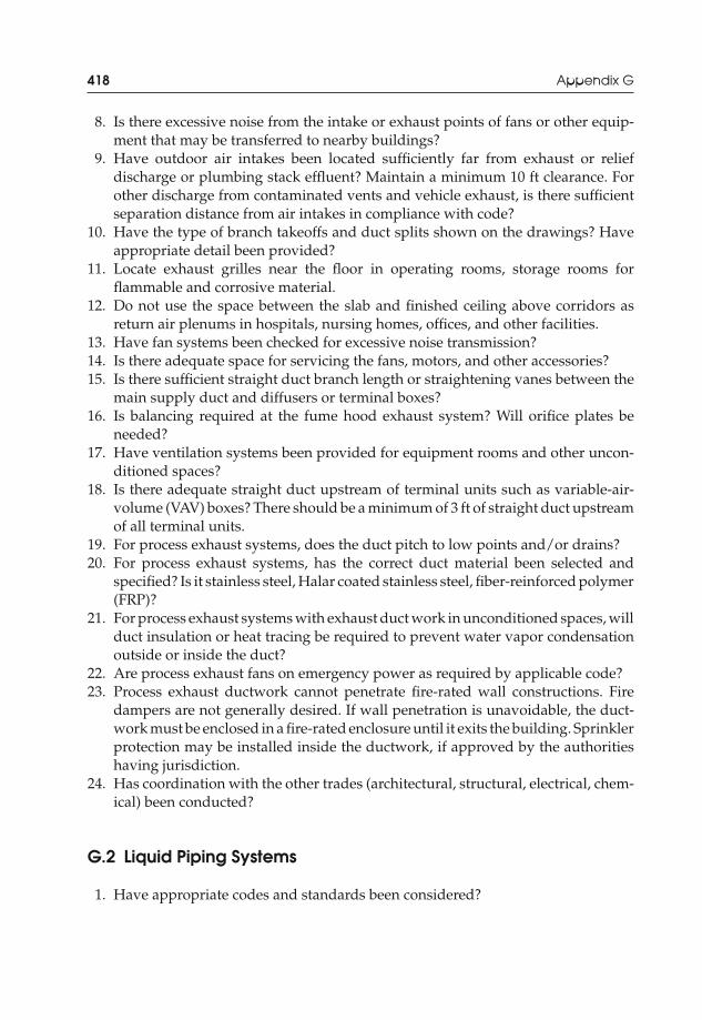
JWST229-bapp07 JWST229-McDonald Printer: Yet to Come July 28, 2012 10:33 Trim: 244mm × 168mm
418 Appendix G
8. Is there excessive noise from the intake or exhaust points of fans or other equip-ment that may be transferred to nearby buildings?
9. Have outdoor air intakes been located sufficiently far from exhaust or reliefdischarge or plumbing stack effluent? Maintain a minimum 10 ft clearance. Forother discharge from contaminated vents and vehicle exhaust, is there sufficientseparation distance from air intakes in compliance with code?
10. Have the type of branch takeoffs and duct splits shown on the drawings? Haveappropriate detail been provided?
11. Locate exhaust grilles near the floor in operating rooms, storage rooms forflammable and corrosive material.
12. Do not use the space between the slab and finished ceiling above corridors asreturn air plenums in hospitals, nursing homes, offices, and other facilities.
13. Have fan systems been checked for excessive noise transmission?14. Is there adequate space for servicing the fans, motors, and other accessories?15. Is there sufficient straight duct branch length or straightening vanes between the
main supply duct and diffusers or terminal boxes?16. Is balancing required at the fume hood exhaust system? Will orifice plates be
needed?17. Have ventilation systems been provided for equipment rooms and other uncon-
ditioned spaces?18. Is there adequate straight duct upstream of terminal units such as variable-air-
volume (VAV) boxes? There should be a minimum of 3 ft of straight duct upstreamof all terminal units.
19. For process exhaust systems, does the duct pitch to low points and/or drains?20. For process exhaust systems, has the correct duct material been selected and
specified? Is it stainless steel, Halar coated stainless steel, fiber-reinforced polymer(FRP)?
21. For process exhaust systems with exhaust duct work in unconditioned spaces, willduct insulation or heat tracing be required to prevent water vapor condensationoutside or inside the duct?
22. Are process exhaust fans on emergency power as required by applicable code?23. Process exhaust ductwork cannot penetrate fire-rated wall constructions. Fire
dampers are not generally desired. If wall penetration is unavoidable, the duct-work must be enclosed in a fire-rated enclosure until it exits the building. Sprinklerprotection may be installed inside the ductwork, if approved by the authoritieshaving jurisdiction.
24. Has coordination with the other trades (architectural, structural, electrical, chem-ical) been conducted?
G.2 Liquid Piping Systems
1. Have appropriate codes and standards been considered?
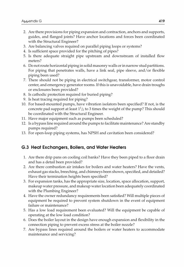
JWST229-bapp07 JWST229-McDonald Printer: Yet to Come July 28, 2012 10:33 Trim: 244mm × 168mm
Appendix G 419
2. Are there provisions for piping expansion and contraction, anchors and supports,guides, and flanged joints? Have anchor locations and forces been coordinatedwith the Structural Engineer?
3. Are balancing valves required on parallel piping loops or systems?4. Is sufficient space provided for the pitching of pipes?5. Is there adequate straight pipe upstream and downstream of installed flow
meters?6. Do not route horizontal piping in solid masonry walls or in narrow stud partitions.
For piping that penetrates walls, have a link seal, pipe sleeve, and/or flexiblepiping been used?
7. There should not be piping in electrical switchgear, transformer, motor controlcenter, and emergency generator rooms. If this is unavoidable, have drain troughsor enclosures been provided?
8. Is cathodic protection required for buried piping?9. Is heat tracing required for piping?
10. For based-mounted pumps, have vibration isolators been specified? If not, is theconcrete pad support at least 11/2 to 3 times the weight of the pump? This shouldbe coordinated with the Structural Engineer.
11. Have major equipment such as pumps been scheduled?12. Is a bypass line required around the pumps to facilitate maintenance? Are standby
pumps required?13. For open-loop piping systems, has NPSH and cavitation been considered?
G.3 Heat Exchangers, Boilers, and Water Heaters
1. Are there drip pans on cooling coil banks? Have they been piped to a floor drainand has a detail been provided?
2. Are there combustion air intakes for boilers and water heaters? Have the vents,exhaust gas stacks, breeching, and chimneys been shown, specified, and detailed?Have their termination heights been specified?
3. For expansion tanks, has the appropriate size, location, space allocation, support,makeup water pressure, and makeup water location been adequately coordinatedwith the Plumbing Engineer?
4. Have the owner redundancy requirements been satisfied? Will multiple pieces ofequipment be required to prevent system shutdown in the event of equipmentfailure or maintenance?
5. Has a low load requirement been evaluated? Will the equipment be capable ofoperating at the low load condition?
6. Does the boiler layout in the design have enough expansion and flexibility in theconnection piping to prevent excess stress at the boiler nozzle?
7. Are bypass lines required around the boilers or water heaters to accommodatemaintenance and servicing?

JWST229-bapp07 JWST229-McDonald Printer: Yet to Come July 28, 2012 10:33 Trim: 244mm × 168mm
420 Appendix G
8. Is there sufficient access to components in the boiler or water heater that mayneed servicing?
9. Has a check valve been installed on the boiler or water heater discharge pipelineto prevent backflow of cooled water into the unit?
10. Are water softeners required on the makeup line? Are they shown on thedrawings?
11. Is pressure regulation needed?12. Will the minimum required circulation through the boiler or water heater be
maintained?13. For water distribution systems, will they be reverse-return systems? If not, has
proper balancing been considered? Will balancing valves or orifice plates berequired?

JWST229-IND JWST229-McDonald Printer: Yet to Come August 1, 2012 16:41 Trim: 244mm × 168mm
Index
Affinity laws, 98Air distribution systems
low velocity, 13small duct high-velocity, 54
Air duct, 9–10, 12–14, 16, 18, 20–22, 29–30,54–55, 58, 211, 262
Air handling unit, 67Air purger, 216Air separators, 112Air/fuel ratio, 306Allowable back pressure, 326Aquastat, 218aspect ratio, 15Atomization, 105, 312Availability, 299, 319
Back work ratio, 312Balancing valves, 231Baseboard heater, 216Baseboard heaters, 233Bell and Gosset, 89Binary cycle, 333Blasius correlation, 9Boiler, 138, 209, 210, 216, 245, 266, 323
annual fuel utilization efficiency, 226drum, 323dual use, 236feedwater, 218heating capacity, 220heating capacity ratings, 224hose bib, 218
low-pressure, 217medium- and high-pressure, 218oversizing factor, 222pinch point (PP), 324pipe cock, 218sizing, 220stack, 269, 317, 322, 326, 335thermal size, 222waste heat recovery, 322
Boiling, 146Brayton cycle, 265, 305, 332Burner, 218
Capacity ratio, 151Carnot cycle, 266Cavitation, 93Chimney, 219, 226Churchill and Bernstein equation, 161Churchill’s equation, 9Circular equivalent method, 18Circulator, 216, 231, 257Colebrook equation, 8Combined-cycle plant, 322Compressor, 44, 305Condensation, 146Condenser, 103, 104, 136, 207, 266, 278, 287,
335Conduction, 127, 130Contact feedwater heater. See Feedwater
heaterConvection, 130
Introduction to Thermo-Fluids Systems Design, First Edition. Andre G. McDonald and Hugh L. Magande.C© 2012 Andre G. McDonald and Hugh L. Magande. Published 2012 by John Wiley & Sons, Ltd.
421
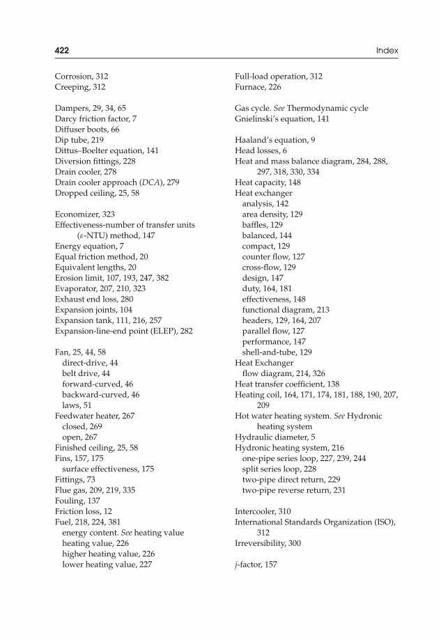
JWST229-IND JWST229-McDonald Printer: Yet to Come August 1, 2012 16:41 Trim: 244mm × 168mm
422 Index
Corrosion, 312Creeping, 312
Dampers, 29, 34, 65Darcy friction factor, 7Diffuser boots, 66Dip tube, 219Dittus–Boelter equation, 141Diversion fittings, 228Drain cooler, 278Drain cooler approach (DCA), 279Dropped ceiling, 25, 58
Economizer, 323Effectiveness-number of transfer units
(ε-NTU) method, 147Energy equation, 7Equal friction method, 20Equivalent lengths, 20Erosion limit, 107, 193, 247, 382Evaporator, 207, 210, 323Exhaust end loss, 280Expansion joints, 104Expansion tank, 111, 216, 257Expansion-line-end point (ELEP), 282
Fan, 25, 44, 58direct-drive, 44belt drive, 44forward-curved, 46backward-curved, 46laws, 51
Feedwater heater, 267closed, 269open, 267
Finished ceiling, 25, 58Fins, 157, 175
surface effectiveness, 175Fittings, 73Flue gas, 209, 219, 335Fouling, 137Friction loss, 12Fuel, 218, 224, 381
energy content. See heating valueheating value, 226higher heating value, 226lower heating value, 227
Full-load operation, 312Furnace, 226
Gas cycle. See Thermodynamic cycleGnielinski’s equation, 141
Haaland’s equation, 9Head losses, 6Heat and mass balance diagram, 284, 288,
297, 318, 330, 334Heat capacity, 148Heat exchanger
analysis, 142area density, 129baffles, 129balanced, 144compact, 129counter flow, 127cross-flow, 129design, 147duty, 164, 181effectiveness, 148functional diagram, 213headers, 129, 164, 207parallel flow, 127performance, 147shell-and-tube, 129
Heat Exchangerflow diagram, 214, 326
Heat transfer coefficient, 138Heating coil, 164, 171, 174, 181, 188, 190, 207,
209Hot water heating system. See Hydronic
heating systemHydraulic diameter, 5Hydronic heating system, 216
one-pipe series loop, 227, 239, 244split series loop, 228two-pipe direct return, 229two-pipe reverse return, 231
Intercooler, 310International Standards Organization (ISO),
312Irreversibility, 300
j-factor, 157
JWST229-IND JWST229-McDonald Printer: Yet to Come August 1, 2012 16:41 Trim: 244mm × 168mm
Index 423
Laminar flow, 6fully-developed, 139
LMTD method, 147Loss coefficient, 19
Mollier diagram, 270Moody chart, 8
National Electric Manufacturers Association(NEMA), 312
Net generator output, 286Net heat rate, 286, 288, 297, 318, 321Net positive suction head (NPSH), 93Noise criteria, 55Number of transfer units (NTU), 151Nusselt number, 138
Orifice plates, 231Overall heat transfer coefficient, 135, 138,
175, 194, 209, 335
Part-load conditions, 312Petukhov equation, 9Pipe
hangers, 77installation, 77materials, 75plastic, 76sizing, 77velocities, 76
Piping system, 73closed-loop, 111open-loop, 103
Plasma spraying, 213Plenum, 22Power plant system, 265Pressure loss, 23Pump
best efficiency point, 87brake horsepower, 85capacity, 83dynamic, 83efficiency, 85equivalence, 98free delivery, 86gas, 83master selection chart, 91
net head, 85performance curves, 86positive-displacement, 83set, 75shut-off head, 86system curve, 87water horsepower, 85
Rankine cycle, 266, 267, 269, 287Recovery rate, 222Regeneration, 267Regenerator, 310Regenerators. See Feedwater heaterReheater, 269Relative humidity, 9, 312, 317, 329Relative roughness, 8Resistance network, 134Reynolds number, 5Rinnai, 209, 220, 221, 241, 413
Second-law analysis, 298Second-law efficiency, 300, 301Steam blanketing, 324Steam generator, 265Strainer, 103Superheater, 209, 323, 325, 326, 327, 328, 335Surface heaters. See Feedwater heaterSwamee-Jain formulae, 8
Taco Pumps, 89Temperature correction factor, 235Terminal temperature difference (TTD), 279Thermal resistance, 130Thermodynamic cycle, 265Transitional flow, 6Tube bank
bare, 157in line, 159pressure drop, 162staggered, 160
Tube-pitch ratio, 159Turbine
impulse, 280internal efficiency, 270reaction, 280stages, 280steam, 280

JWST229-IND JWST229-McDonald Printer: Yet to Come August 1, 2012 16:41 Trim: 244mm × 168mm
424 Index
Turbogenerator net output. See Netgenerator output
Turbulent flow, 6
Unico, Inc., 203Usable storage capacity, 223Used-energy-end point (UEEP), 282
Valves, 73Vapor cycle. See Thermodynamic cycleVapor pressure, 92Variable frequency drive, 109
Velocity correction factor,235
Vent, 219
Water hammer, 112, 324Water heater, 209, 216, 220, 236, 258
tankless, 219
Zone, 227condensing, 278desuperheating, 278drain cooling, 278
Related Documents