Introduction to the Theory of Linear Operatorsjoye/spectral.pdf · Introduction to the Theory of Linear Operators Alain Joye Institut Fourier, Universit´e de Grenoble 1, BP 74, 38402

Introduction to the Theory of LinearOperators

Alain Joye

Institut Fourier, Universite de Grenoble 1,BP 74, 38402 Saint-Martin d’Heres Cedex, [email protected]

1 Introduction

The purpose of this first set of lectures about Linear Operator Theory isto provide the basics regarding the mathematical key features of unboundedoperators to readers that are not familiar with such technical aspects. Itis a necessity to deal with such operators if one wishes to study QuantumMechanics since such objects appear as soon as one wishes to consider, say,a free quantum particle in R. The topics covered by these lectures is quitebasic and can be found in numerous classical textbooks, some of which arelisted at the end of these notes. They have been selected in order to providethe reader with the minimal background allowing to proceed to the moreadvanced subjects that will be treated in subsequent lectures, and also ac-cording to their relevance regarding the main subject of this school on OpenQuantum Systems. Obviously, there is no claim about originality in the pre-sented material. The reader is assumed to be familiar with the theory ofbounded operators on Banach spaces and with some of the classical abstractTheorems in Functional Analysis.

2 Generalities about Unbounded Operators

Let us start by setting the stage, introducing the basic notions necessary tostudy linear operators. While we will mainly work in Hilbert spaces, we statethe general definitions in Banach spaces.

If B is a Banach space over C with norm ‖ · ‖ and T is a bounded linearoperator on B, i.e. T : B → B, its norm is given by

‖T‖ = supϕ 6=0

‖Tϕ‖‖ϕ‖

<∞.

Now, consider the position operator of Quantum Mechanics q = multx onL2(R), acting as (qϕ)(x) = xϕ(x). It readily seen to be unbounded sinceone can find a sequence of normalized functions ϕn ∈ L2(R), n ∈ N, suchthat ‖qϕn‖ → ∞ as n→∞, and, there are functions of L2(R) which are nolonger L2(R) when multiplied by the independent variable. We shall adoptthe following definition of (possibly unbounded) operators.

2 Alain Joye

Definition 2.1. A linear operator on B is a pair (A,D) where D ⊂ B is adense linear subspace of B and A : D → B is linear.

We will nevertheless often talk about the operator A and call the subspaceD the domain of A. It will sometimes be denoted by Dom(A).

Definition 2.2. If (A, D) is another linear operator such that D ⊃ D andAϕ = Aϕ for all ϕ ∈ D, the operator A defines an extension of A and onedenotes this fact by A ⊂ A

That the precise definition of the domain of a linear operator is importantfor the study of its properties is shown by the following

Example 2.1. : Let H be defined on L2[a, b], a < b finite, as the differential op-erator Hϕ(x) = −ϕ′′(x), where the prime denotes differentiation. Introducethe dense sets DD and DN in L2[a, b] by

DD =ϕ ∈ C2[a, b] |ϕ(a) = ϕ(b) = 0

(1)

DN =ϕ ∈ C2[a, b] |ϕ′(a) = ϕ′(b) = 0

. (2)

It is easily checked that 0 is an eigenvalue of (H,DN ) but not of (H,DD). Theboundary conditions appearing in (1), (2) respectively are called Dirichlet andNeumann boundary conditions respectively.

The notion of continuity naturally associated with bounded linear opera-tors is replaced for unbounded operators by that of closedness.

Definition 2.3. Let (A,D) be an operator on B. It is said to be closed if forany sequence ϕn ∈ D such that

ϕn → ϕ ∈ B and Aϕn → ψ ∈ B,

it follows that ϕ ∈ D and Aϕ = ψ.

Remark 2.1. i) In terms of the the graph of the operator A, denoted by Γ (A)and given by

Γ (A) = (ϕ,ψ) ∈ B × B |ϕ ∈ D, ψ = Aϕ ,

we have the equivalence

A closed ⇐⇒ Γ (A) closed (for the norm ‖(ϕ,ψ)‖2 = ‖ϕ‖2 + ‖ψ‖2).

ii) If D = B, then A is closed if and only if A is bounded, by the ClosedGraph Theorema.iii) If A is bounded and closed, then D = B so that it is possible to extendA to the whole of B as a bounded operator.iv) If A : D → D′ ⊂ B is one to one and onto, then A is closed is equivalent

aIf T : X → Y, where X and Y are two Banach spaces, then T is bounded iffthe graph of T is closed.

Introduction to the Theory of Linear Operators 3

to A−1 : D′ → D is closed. This last property can be seen by introducing theinverse graph of A, Γ ′(A) = (x, y) ∈ B × B | y ∈ D,x = Ay and noticingthat A closed iff Γ ′(A) is closed and Γ (A) = Γ ′(A−1).

The notion of spectrum of operators is a key issue for applications inQuantum Mechanics. Here are the relevant definitions.

Definition 2.4. The spectrum σ(A) of an operator (A,D) on B is definedby its complement σ(A)C = ρ(A), where the resolvent set of A is given by

ρ(A) = z ∈ C | (A− z) : D → B is one to one and onto, and(A− z)−1 : B → D is a bounded operator.

The operator R(z) = (A− z)−1 is called the resolvent of A.Actually, A− z is to be understood as A− z II , where II denotes the identityoperator.

Here are a few of the basic properties related to these notions.

Proposition 2.1. With the notations above,i) If σ(A) 6= C, then A is closed.ii) If z 6∈ σ(A) and u ∈ C is such that |u| < ‖R(z)‖−1, then z + u ∈ ρ(A).Thus, ρ(A) is open and σ(A) is closed.iii) The resolvent is an analytic map from ρ(A) to L(B), the set of boundedlinear operators on B, and the following identities hold for any z, w ∈ ρ(A),

R(z)−R(w) = (z − w)R(z)R(w) (3)dn

dznR(z) = n!Rn+1(z).

Remark 2.2. Identity (3) is called the first resolvent identity. As a conse-quence, we get that the resolvents at two different points of the resolvent setcommute, i.e.

[R(z), R(w)] = 0, ∀z, w ∈ ρ(A).

Proof. i) If z ∈ ρ(A), then R(z) is one to one and bounded thus closed andremark iv) above applies.ii) We need to show that R(z + u) exists and is bounded from B to D. Wehave on D

(A− z − u)ϕ = ( II − u(A− z)−1)(A− z)ϕ = ( II − uR(z))(A− z)ϕ,

where |u|‖R(z)‖ < 1 by assumption. Hence, the Neumann series∑n≥0

Tn = ( II − T )−1 where T : B → B is such that ‖T‖ < 1, (4)

shows that the natural candidate for (A − z − u)−1 is R(z)( II − uR(z))−1 :B → D. Then one checks that on B

4 Alain Joye

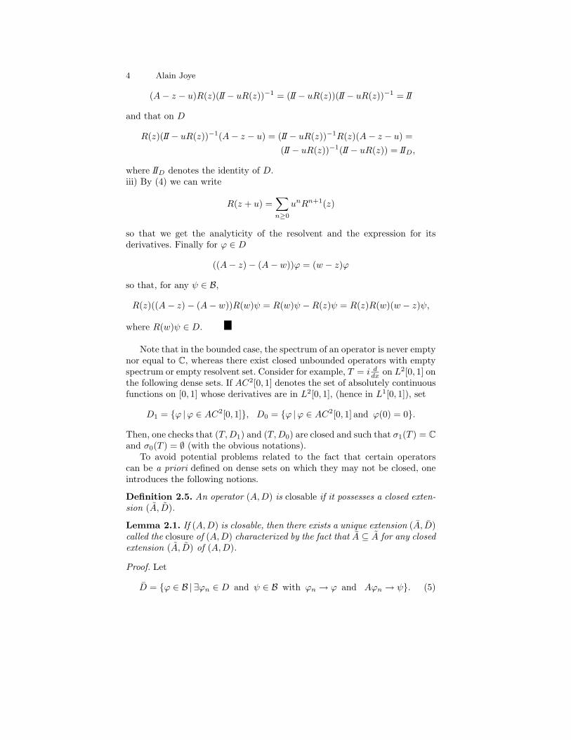
(A− z − u)R(z)( II − uR(z))−1 = ( II − uR(z))( II − uR(z))−1 = II

and that on D

R(z)( II − uR(z))−1(A− z − u) = ( II − uR(z))−1R(z)(A− z − u) =( II − uR(z))−1( II − uR(z)) = II D,

where II D denotes the identity of D.iii) By (4) we can write

R(z + u) =∑n≥0

unRn+1(z)

so that we get the analyticity of the resolvent and the expression for itsderivatives. Finally for ϕ ∈ D

((A− z)− (A− w))ϕ = (w − z)ϕ

so that, for any ψ ∈ B,

R(z)((A− z)− (A− w))R(w)ψ = R(w)ψ −R(z)ψ = R(z)R(w)(w − z)ψ,

where R(w)ψ ∈ D.

Note that in the bounded case, the spectrum of an operator is never emptynor equal to C, whereas there exist closed unbounded operators with emptyspectrum or empty resolvent set. Consider for example, T = i ddx on L2[0, 1] onthe following dense sets. If AC2[0, 1] denotes the set of absolutely continuousfunctions on [0, 1] whose derivatives are in L2[0, 1], (hence in L1[0, 1]), set

D1 = ϕ |ϕ ∈ AC2[0, 1], D0 = ϕ |ϕ ∈ AC2[0, 1] and ϕ(0) = 0.

Then, one checks that (T,D1) and (T,D0) are closed and such that σ1(T ) = Cand σ0(T ) = ∅ (with the obvious notations).

To avoid potential problems related to the fact that certain operatorscan be a priori defined on dense sets on which they may not be closed, oneintroduces the following notions.

Definition 2.5. An operator (A,D) is closable if it possesses a closed exten-sion (A, D).

Lemma 2.1. If (A,D) is closable, then there exists a unique extension (A, D)called the closure of (A,D) characterized by the fact that A ⊆ A for any closedextension (A, D) of (A,D).

Proof. Let

D = ϕ ∈ B | ∃ϕn ∈ D and ψ ∈ B with ϕn → ϕ and Aϕn → ψ. (5)


For any closed extension A of A and any ϕ ∈ D, we have ϕ ∈ D and Aϕ = ψis uniquely determined by ϕ. Let us define (A, D) by Aϕ = ψ, for all ϕ ∈ D.Then A is an extension of A and any closed extension A ⊆ A is such thatA ⊆ A. The graph Γ (A) of A satisfies Γ (A) = Γ (A), so that A is closed.

Note also that the closure of a closed operator coincide with the operatoritself. Also, before ending this section, note that there exist non closableoperators. Fortunately enough, such operators do not play an essential rolein Quantum Mechanics, as we will shortly see.

3 Adjoint, Symmetric and Self-adjoint Operators

The arena of Quantum Mechanics is a complex Hilbert space H where thenotion of scalar product 〈 · | · 〉 gives rise to a norm denoted by ‖ · ‖. Oper-ators that are self-adjoint with respect to that product play a particularlyimportant role, as they correspond to the observables of the theory. We shallassume the following convention regarding the positive definite sesquilinearform 〈 · | · 〉 on H × H: it is linear in the right variable and thus anti-linearin the left variable. We shall also always assume that our Hilbert space isseparable, i.e. it admits a countable basis, and we shall identify the dual H′

of H with H, since ∀l : H → C, ∃!ψ ∈ H such that l(·) = 〈ψ| ·〉.Let us make the first steps towards self-adjunction.

Definition 3.1. An operator (H,D) in H is said to be symmetric if ∀ϕ,ψ ∈D ⊆ H

〈ϕ|Hψ〉 = 〈Hϕ|ψ〉.

For example, the operators (− d2

dx2 , DD) and (− d2

dx2 , DN ) introduced aboveare symmetric, as shown by integration by parts.

Remark 3.1. If H is symmetric, its eigenvalues are real.

The next property is related to an earlier remark concerning the role ofnon closable operators in Quantum Mechanics.

Proposition 3.1. Any symmetric operator (H,D) is closable and its closureis symmetric.

This Proposition will allow us to consider that any symmetric operator isclosed from now on.

Proof. Let D ⊇ D as in (5) and χ ∈ D, ϕ ∈ D. We compute for any such χ,

〈ϕ|Hχ〉 = limn〈ϕn|Hχ〉 = lim

n〈Hϕn|χ〉 = 〈ψ|χ〉. (6)

As D is dense by assumption, the vector ψ is uniquely determined by thelinear, bounded form lψ : D → C such that lψ(χ) = 〈ψ|χ〉. In other words,

6 Alain Joye

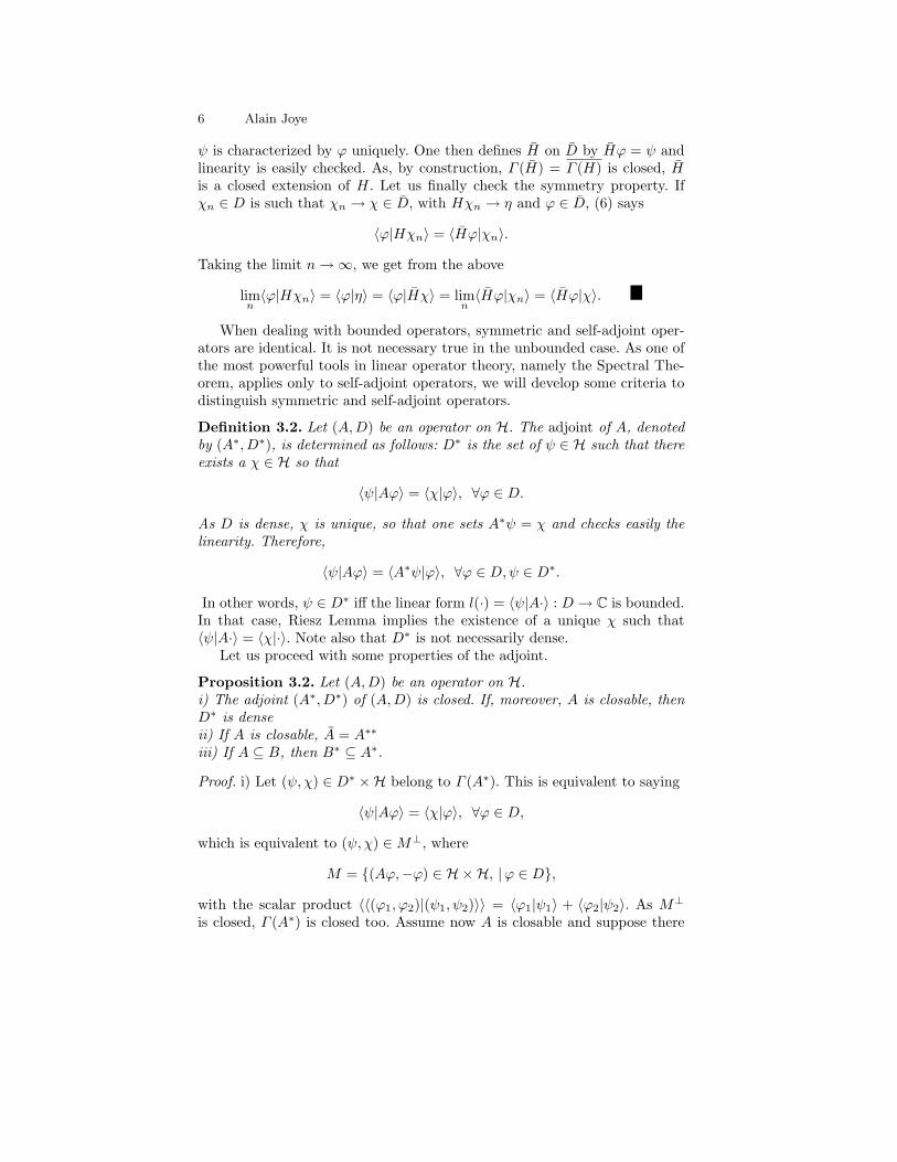
ψ is characterized by ϕ uniquely. One then defines H on D by Hϕ = ψ andlinearity is easily checked. As, by construction, Γ (H) = Γ (H) is closed, His a closed extension of H. Let us finally check the symmetry property. Ifχn ∈ D is such that χn → χ ∈ D, with Hχn → η and ϕ ∈ D, (6) says

〈ϕ|Hχn〉 = 〈Hϕ|χn〉.

Taking the limit n→∞, we get from the above

limn〈ϕ|Hχn〉 = 〈ϕ|η〉 = 〈ϕ|Hχ〉 = lim

n〈Hϕ|χn〉 = 〈Hϕ|χ〉.

When dealing with bounded operators, symmetric and self-adjoint oper-ators are identical. It is not necessary true in the unbounded case. As one ofthe most powerful tools in linear operator theory, namely the Spectral The-orem, applies only to self-adjoint operators, we will develop some criteria todistinguish symmetric and self-adjoint operators.

Definition 3.2. Let (A,D) be an operator on H. The adjoint of A, denotedby (A∗, D∗), is determined as follows: D∗ is the set of ψ ∈ H such that thereexists a χ ∈ H so that

〈ψ|Aϕ〉 = 〈χ|ϕ〉, ∀ϕ ∈ D.

As D is dense, χ is unique, so that one sets A∗ψ = χ and checks easily thelinearity. Therefore,

〈ψ|Aϕ〉 = 〈A∗ψ|ϕ〉, ∀ϕ ∈ D,ψ ∈ D∗.

In other words, ψ ∈ D∗ iff the linear form l(·) = 〈ψ|A·〉 : D → C is bounded.In that case, Riesz Lemma implies the existence of a unique χ such that〈ψ|A·〉 = 〈χ|·〉. Note also that D∗ is not necessarily dense.

Let us proceed with some properties of the adjoint.

Proposition 3.2. Let (A,D) be an operator on H.i) The adjoint (A∗, D∗) of (A,D) is closed. If, moreover, A is closable, thenD∗ is denseii) If A is closable, A = A∗∗

iii) If A ⊆ B, then B∗ ⊆ A∗.

Proof. i) Let (ψ, χ) ∈ D∗ ×H belong to Γ (A∗). This is equivalent to saying

〈ψ|Aϕ〉 = 〈χ|ϕ〉, ∀ϕ ∈ D,

which is equivalent to (ψ, χ) ∈M⊥, where

M = (Aϕ,−ϕ) ∈ H ×H, |ϕ ∈ D,

with the scalar product 〈〈(ϕ1, ϕ2)|(ψ1, ψ2)〉〉 = 〈ϕ1|ψ1〉 + 〈ϕ2|ψ2〉. As M⊥

is closed, Γ (A∗) is closed too. Assume now A is closable and suppose there


exists η ∈ H such that 〈ψ|η〉 = 0, for all ψ ∈ D∗. This implies that (η, 0) isorthogonal to Γ (A∗). But,

Γ (A∗)⊥ = M⊥⊥ = M.

Therefore, there exists ϕn ∈ D, such that ϕn → 0 and Aϕn → η. As A isclosable, η = A0 = 0, i.e. (D∗)⊥ = 0 and D∗ = (D∗)⊥⊥ = H.ii) Define a unitary operator V on H×H by

V (ϕ,ψ) = (ψ,−ϕ).

It has the property V (E⊥) = (V (E))⊥, for any linear subspace E ⊆ H×H.In particular, we have just seen

Γ (A∗) = (V (Γ (A)))⊥

so that

Γ (A) = (Γ (A)⊥)⊥ = ((V 2Γ (A))⊥)⊥

= (V (V (Γ (A))⊥))⊥ = (V (Γ (A∗)))⊥ = Γ (A∗∗),

i.e. A = A∗∗.iii) Follows readily from the definition.

When H is symmetric, we get from the definition and properties abovethat H∗ is a closed extension of H. This motivates the

Definition 3.3. An operator (H,D) is self-adjoint whenever it coincides withits adjoint (H∗, D∗). It is therefore closed.An operator (H,D) is essentially self-adjoint if it is symmetric and its closure(H, D) is self-adjoint.Therefore, we have in general for a symmetric operator,

H ⊆ H = H∗∗ ⊆ H∗, and H∗ = H∗ = H∗∗∗ = H∗.

In case H is essentially self-adjoint,

H ⊆ H = H∗∗ = H∗.

We now head towards our general criterion for (essential) self-adjointness.We need a few more

Definition 3.4. For (H,D) symmetric and denoting its adjoint by (H∗, D∗),the deficiency subspaces L± are defined by

L± = ϕ ∈ D∗ |H∗ϕ = ±iϕ = ϕ ∈ H | 〈Hψ|ϕ〉 = ±i〈ψ|ϕ〉 ∀ψ ∈ D= Ran(H ± i)⊥ = Ker(H∗ ∓ i).

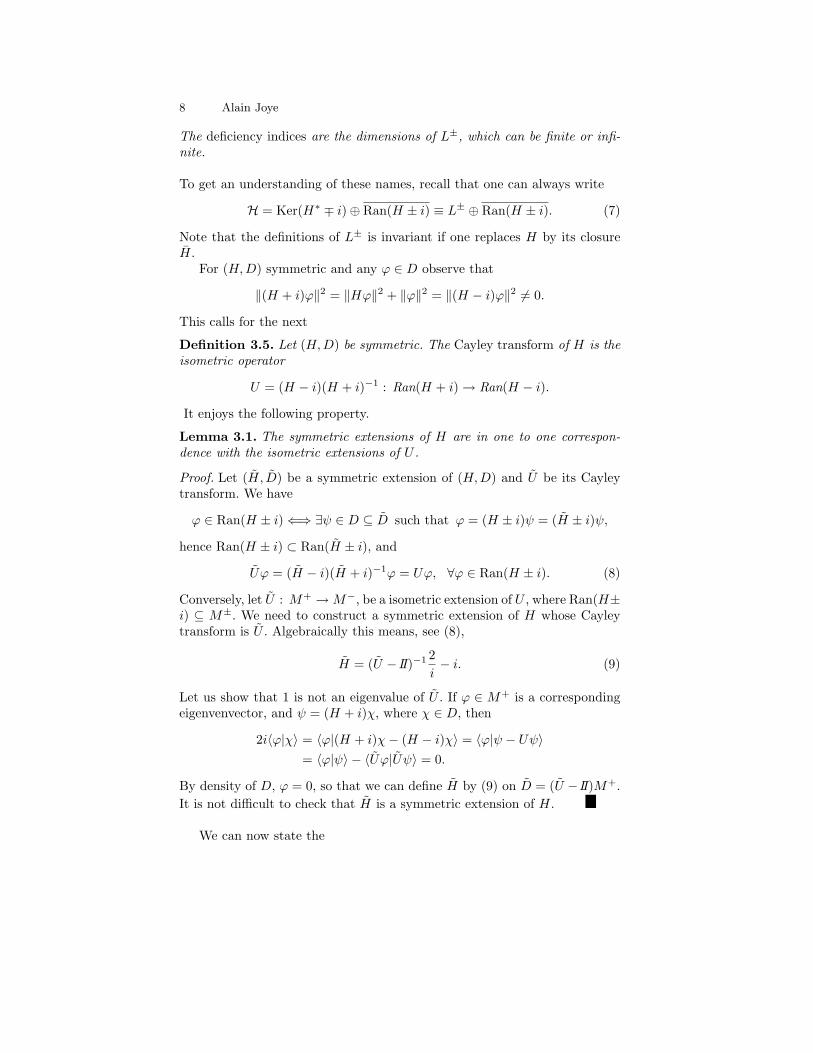
8 Alain Joye

The deficiency indices are the dimensions of L±, which can be finite or infi-nite.

To get an understanding of these names, recall that one can always write

H = Ker(H∗ ∓ i)⊕ Ran(H ± i) ≡ L± ⊕ Ran(H ± i). (7)

Note that the definitions of L± is invariant if one replaces H by its closureH.

For (H,D) symmetric and any ϕ ∈ D observe that

‖(H + i)ϕ‖2 = ‖Hϕ‖2 + ‖ϕ‖2 = ‖(H − i)ϕ‖2 6= 0.

This calls for the next

Definition 3.5. Let (H,D) be symmetric. The Cayley transform of H is theisometric operator

U = (H − i)(H + i)−1 : Ran(H + i) → Ran(H − i).

It enjoys the following property.

Lemma 3.1. The symmetric extensions of H are in one to one correspon-dence with the isometric extensions of U .

Proof. Let (H, D) be a symmetric extension of (H,D) and U be its Cayleytransform. We have

ϕ ∈ Ran(H ± i) ⇐⇒ ∃ψ ∈ D ⊆ D such that ϕ = (H ± i)ψ = (H ± i)ψ,

hence Ran(H ± i) ⊂ Ran(H ± i), and

Uϕ = (H − i)(H + i)−1ϕ = Uϕ, ∀ϕ ∈ Ran(H ± i). (8)

Conversely, let U : M+ →M−, be a isometric extension of U , where Ran(H±i) ⊆ M±. We need to construct a symmetric extension of H whose Cayleytransform is U . Algebraically this means, see (8),

H = (U − II )−1 2i− i. (9)

Let us show that 1 is not an eigenvalue of U . If ϕ ∈ M+ is a correspondingeigenvenvector, and ψ = (H + i)χ, where χ ∈ D, then

2i〈ϕ|χ〉 = 〈ϕ|(H + i)χ− (H − i)χ〉 = 〈ϕ|ψ − Uψ〉= 〈ϕ|ψ〉 − 〈Uϕ|Uψ〉 = 0.

By density of D, ϕ = 0, so that we can define H by (9) on D = (U − II )M+.It is not difficult to check that H is a symmetric extension of H.

We can now state the


Theorem 3.1. If (H,D) is symmetric on H, there exist self-adjoint exten-sions of H if and only if the deficiency indices are equal. Moreover, the fol-lowing statements are equivalent:1) H is essentially self-adjoint2) The deficiency indices are both zero3) H possesses exactly one self-adjoint extension.

Proof. 1)⇒ 3): Let J be a self-adjoint extension of H. Then H ⊆ J = J∗ andJ ⊇ H. Hence J = J∗ ⊆ H∗ = H, so that J = H.1)⇒ 2): We can assume that H is closed so H = H = H∗. For any ϕ ∈ L± =Ker(H∗ ∓ i),

0 = ‖(H∗∓ i)ϕ‖2 = ‖(H∓ i)ϕ‖2 = ‖Hϕ‖2 +‖ϕ‖2 ≥ ‖ϕ‖2, L± = 0. (10)

2) ⇒ 1): Consider (H + i) : D → Ran(H + i). By (10) above, this operatoris one to one, and we can define (H + i)−1 : Ran(H + i) → D. By the sameestimate it satisfies

‖(H + i)−1ψ‖2 ≤ ‖(H + i)(H + i)−1ψ‖2 = ‖ψ‖2.

As H can be assumed to be closed (i.e. H = H) and L+ = 0, we get thatRan(H + i) is closed so that H = Ran(H + i), due to (7). Therefore, for anyϕ ∈ D∗, there exists a ψ ∈ D such that (H∗ + i)ϕ = (H + i)ψ. As H ⊆ H∗,

(H∗ + i)(ϕ− ψ) = 0, i.e. ϕ− ψ ∈ Ker(H∗ + i) = 0,

we get that ϕ ∈ D and H = H∗, which is what we set out to prove.3) ⇒ 2): if K is a self-adjoint extension of H, its deficiency indices are zero(by 2)). Therefore, (see (7)), its Cayley transform V is a unitary extensionof U , the Cayley transform of H. In particular, V |L+ : L+ → L− is one toone and onto, so that the deficiency indices of H are equal. That yields thefirst part of the Theorem. Now assume these indices are not zero. By thepreceding Lemma, there exist an infinite number of symmetric extensions ofH, parametrized by all isometries from L+ to L−. In particular, there existextensions with zero deficiency indices, which by 2) and 1) are self-adjoint,contradicting the fact that K is the unique self-adjoint extension of H.

Remark 3.2. It is a good exercise to prove that in case (H,D) is symmetricand H ≥ 0, i.e. 〈ϕ|Hϕ〉 ≥ 0 for any ϕ ∈ D, then H is essentially self-adjointiff Ker(H∗ + 1) = 0.

As a first application, we give a key property of self-adjoint operators forthe role they play in the Quantum dogma concerning measure of observables.It is the following fact concerning their spectrum.

Theorem 3.2. Let H = H∗. Then, σ(H) ⊆ R and,

‖(H − z)−1‖ ≤ 1|=z|

, if z 6∈ R. (11)

10 Alain Joye

Moreover, for any z in the resolvent set of H,

(H − z)−1 = ((H − z)−1)∗. (12)

Proof. Let ϕ ∈ D, D being the domain of H and z = x + iy, with y 6= 0.Then

‖(H − x− iy)ϕ‖2 = ‖(H − x)ϕ‖2 + y2‖ϕ‖2 ≥ y2‖ϕ‖2. (13)

This implies

Ker(H − z) = Ker(H∗ − z) = 0 i.e. Ran(H − z) = H,

and H − z is invertible on Ran(H − z). (13) shows that (H − z) is boundedwith the required bound, and as the resolvent is closed, it can be extendedon H with the same bound. Equality (12) is readily checked.

As an application of the first part of Theorem 3.1, consider a symmetricoperator (H,D) which commutes with a conjugation C. More precisely:

C is anti-linear, C2 = II and ‖Cϕ‖ = ‖ϕ‖. Hence 〈ϕ|ψ〉 = 〈Cψ|Cϕ〉. More-over, C : D → D and CH = HC on D.

Under such circumstances, the deficiency indices of H are equal and thereexist self-adjoint extensions of H.

Indeed, one first deduces that C(D) = D. Then, for any ϕ+ ∈ L+ =Ker(H∗ − i) and ψ ∈ D, we compute

0 = 〈ϕ+|(H + i)ψ〉 = 〈Cϕ+|C(H + i)ψ〉 = 〈Cϕ+|(H − i)Cψ〉,

so that Cϕ+ ∈ Ran(H − i)⊥ = Ker(H∗ + i) = L−. In other words,C : L+ → L−, and one shows similarly that C : L− → L+. As C is iso-metric, the dimensions of L+ and L− are the same.

A particular case where this happens is that of the complex conjugationand a differential operator on Rn, with real valued coefficients.

An example of direct application of this criterion is the following. Considerthe symmetric operator Hϕ = iϕ′ on the domain C∞0 (0,∞) ⊂ L2(0,∞). Avector ψ ∈ D∗ iff there exists χ ∈ L2(0,∞) such that 〈ψ|Hϕ〉 = 〈χ|ϕ〉, forall ϕ ∈ C∞0 (0,∞). Expressing the scalar products this means∫

χ(x)ϕ(x)dx = −i∫ψ(x)ϕ′(x)dx = iDxTψ(ϕ),

where Tψ denotes the distribution associated with ψ. In other words, wehave ψ ∈ W 1,2(0,∞) = D∗ and H∗ψ = iψ in the weak sense. Elements ofKer(H∗ ∓ i) satisfy


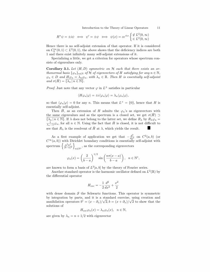
H∗ψ = ±iψ ⇐⇒ ψ′ = ±ψ ⇐⇒ ψ(x) = ce±x6∈ L2(0,∞)∈ L2(0,∞)

Hence there is no self-adjoint extension of that operator. If it is consideredon C∞0 (0, 1) ⊂ L2(0, 1), the above shows that the deficiency indices are both1 and there exist infinitely many self-adjoint extensions of it.

Specializing a little, we get a criterion for operators whose spectrum con-sists of eigenvalues only.

Corollary 3.1. Let (H,D) symmetric on H such that there exists an or-thonormal basis ϕnn∈N of H of eigenvectors of H satisfying for any n ∈ N,ϕn ∈ D and Hϕn = λnϕn, with λn ∈ R. Then H is essentially self-adjointand σ(H) = λn |n ∈ N.

Proof. Just note that any vector ϕ in L± satisfies in particular

〈Hϕn|ϕ〉 = ±i〈ϕn|ϕ〉 = λn〈ϕn|ϕ〉,

so that 〈ϕn|ϕ〉 = 0 for any n. This means that L+ = 0, hence that H isessentially self-adjoint.

Then H, as an extension of H admits the ϕn’s as eigenvectors withthe same eigenvalues and as the spectrum is a closed set, we get σ(H) ⊃λn |n ∈ N. If λ does not belong to the latter set, we define Rλ by Rλϕn =

1λn−λϕn, for all n ∈ N. Using the fact that H is closed, it is not difficult to

see that Rλ is the resolvent of H at λ, which yields the result.

As a first example of application we get that − d2

dx2 on C2(a, b) (orC∞(a, b)) with Dirichlet boundary conditions is essentially self-adjoint withspectrum

n2π2

(b−a)2

n∈N∗

, as the corresponding eigenvectors

ϕn(x) =(

2b− a

)1/2

sin(nπ(x− a)b− a

), n ∈ N∗,

are known to form a basis of L2[a, b] by the theory of Fourier series.Another standard operator is the harmonic oscillator defined on L2(R) by

the differential operator

Hosc = −12d2

dx2+x2

2

with dense domain S the Schwartz functions. This operator is symmetricby integration by parts, and it is a standard exercise, using creation andannihilation operators b† = (x − ∂x)/

√2, b = (x + ∂x)/

√2 to show that the

solutions ofHoscϕn(x) = λnϕn(x), n ∈ N,

are given by λn = n+ 1/2 with eigenvector

12 Alain Joye

ϕn(x) = cnHn(x)e−x2/2, with Hn(x) = (−1)nex

2 dn

dxne−x

2,

and cn = (2nn!√π)−1/2. These eigenvectors also form a basis of L2(R), so

that this operator is essentially self-adjoint with spectrum N+1/2. Note thatcannot work on C∞0 to apply this criterion here.

Another popular way to prove that an operator is self-adjoint is to com-pare it to another operator known to be self-adjoint and use a perturbativeargument to get self-adjointness of the former.

Let (H,D) be a self-adjoint operator onH and let (A,D(A)) be symmetricwith domain D(A) ⊇ D.

Definition 3.6. The operator A has a relative bound α ≥ 0 with respect toH if there exists c <∞ such that

‖Aϕ‖ ≤ α‖Hϕ‖+ c‖ϕ‖, ∀ϕ ∈ D. (14)

The infimum over such relative bounds is the relative bound of A w.r.t. H.

Remark 3.3. The definition of the relative bound is unchanged if we replace(14) by the slightly stronger condition

‖Aϕ‖2 ≤ α2‖Hϕ‖2 + c2‖ϕ‖2, ∀ϕ ∈ D.

Lemma 3.2. Let K : D → H be such that Kϕ = Hϕ + Aϕ. If 0 ≤ α < 1,is the relative bound of A w.r.t. H, K is closed and symmetric. Moreover,‖A(H + iλ)−1‖ < 1, if λ ∈ R has large enough modulus.

Proof. The symmetry of K is clear. Let us consider ϕn ∈ D such that ϕn → ϕand Kϕn → ψ. Then, by assumption,

‖Hϕn −Hϕm‖ ≤ ‖Kϕn −Kϕm‖+ ‖Aϕn −Aϕm‖≤ ‖Kϕn −Kϕm‖+ α‖Hϕn −Hϕm‖+ c‖ϕn − ϕm‖,

so that

‖Hϕn−Hϕm‖ ≤1

1− α‖Kϕn−Kϕm‖+

c

1− α‖ϕn−ϕm‖ → 0 as n,m→∞.

H being closed, we deduce from the above that ϕ ∈ D and Hϕn → Hϕ.Then, from (14), we get Aϕn−Aϕ→ 0 from which follows Kϕn → Kϕ = ψ.

The proof of the statement concerning the resolvent reads as follows. Letψ ∈ H, ϕ = (H + iλ)−1ψ and 0 ≤ α < β < 1. Then, for |λ| > 0 large enough

‖Aϕ‖2 ≤ (α‖Hϕ‖+ c‖ϕ‖)2 ≤ β2(‖Hϕ‖2 + λ2‖ϕ‖2

)= β2‖(H + iλ)ϕ‖2 = β2‖ψ‖2.

Hence ‖A(H + iλ)−1ψ‖ ≤ β‖ψ‖.This leads to the


Theorem 3.3. If H is self-adjoint and A is symmetric with relative boundα < 1 w.r.t. H, then K = H +A is self-adjoint on the same domain as thatof H.

Proof. Let |λ| be large enough. From the formal expressions

(H +A+ iλ)−1 − (H + iλ)−1 = −(H +A+ iλ)−1(A)(H + iλ)−1 ⇐⇒(H +A+ iλ)−1 = (H + iλ)−1( II +A(H + iλ)−1)−1

we see that the natural candidate for the resolvent of K is

Rλ = (H + iλ)−1∑n∈N

(−A(H + iλ)−1)n.

By assumption on |λ|, this sum converges in norm and Ran(Rλ) = D. Routinemanipulations show that (H + A + iλ)Rλ = Rλ(H + A + iλ) = II so thatRan(H+A+ iλ) = H. This implies that the deficiency indices of K = H+Aare both zero, and since it is closed, K is self-adjoint. Note that one uses thefact that dim ker(K∗ − iλ) is constant for λ > 0 and λ < 0.

4 Spectral Theorem

Let us start this section by the presentation of another example of self-adjointoperator, which will play a key role in the Spectral Theorem, we set out toprove here. Before getting to work, let us specify right away that we shall notprovide here a full proof of the version of the Spectral Theorem we chose.Some parts of it, of a purely analytical character, will be presented as factswhose detailed full proofs can be found in Davies’s book [D]. But we hope toconvey the main ideas of the proof in these notes.

Consider E ⊆ RN a Borel set and µ a Borel non-negative measure on E.Let H = L2(E, dµ) be the usual set of measurable functions f : E → C suchthat ‖f‖2 =

∫E|f(x)|2dµ <∞, with identification of functions that coincide

almost everywhere.Let a : E → R be measurable and such that the restriction of a to any

bounded set of E is bounded. We set

D = f ∈ H |∫E

(1 + a2(x))|f(x)|2dµ <∞,

which is dense, and we define the multiplication operator (A,D) by

(Af)(x) = a(x)f(x), ∀f ∈ D.

Lemma 4.1. (A,D) is self-adjoint and if L2c denotes the set of functions

of H which are zero outside a compact subset of E, then A is essentiallyself-adjoint on L2

c.

14 Alain Joye

Proof. A is clearly symmetric. If z 6∈ R, the bounded operator R(z) given by

(R(z)f)(x) = (a(x)− z)−1f(x)

is easily seen to be the inverse of (A − z). Hence, σ(A) 6= C, so that A isclosed. Moreover, the deficiency indices of A are both seen to be zero:

A∗f = if ⇔ ∀h ∈ D∫Ahfdµ = i

∫hfdµ

⇔∫

(a(x)− i)hfdµ = 0,

⇔ f = 0 µ a.e.

So that A is closed and essentially self-adjoint, hence self-adjoint.Concerning the last statement, we need to show that A is the closure of

its restriction to L2c . If f ∈ D and n ∈ N, we define

fn(x) =f(x) if x ∈ E, |x| ≤ n

0 otherwise.

Hence |fn(x)| ≤ |f(x)| and fn ∈ L2c ∈ D. By Lebesgue dominated conver-

gence Theorem, one checks that fn → f and Afn → Af as n→∞.

Lemma 4.2. The spectrum and resolvent of A are such that

σ(A) = essential range of a = λ ∈ R |µ(x | |a(x)− λ| < ε) > 0,∀ε > 0.

If λ 6∈ σ(A), then

‖(A− λ)−1‖ =1

dist (λ, σ(A)).

Proof. If λ is not in the essential range of a, it is readily checked that themultiplication operator by (a(x)− λ)−1 is bounded (outside of a set of zeroµ measure). Also one sees that this operator yields the inverse of a − λ forsuch λ’s, which, consequently, belong to ρ(A). Conversely, let us take λ inthe essential range of a and show that λ ∈ σ(A). We define sets of positive µmeasures by

Sm = x ∈ E | |λ− a(x)| < 2−m.

Let χm be the characteristic function of Sm, which is a non zero element ofL2(E, dµ). Then

‖(A−λ)χm‖2 =∫Sm

|χm|2|a(x)−λ|2dµ ≤ 2−2m

∫Sm

|χm|2dµ = 2−2m‖χm‖2,

which shows that (A − λ)−1 cannot be bounded. Finally, if λ is not in theessential range of a, we set

‖(a(·)− λ)−1‖∞ = essential supremum of (a(·)− λ)−1,


where we recall that for a measurable function f

‖f‖∞ = infK > 0 | |f(x)| ≤ K µ a.e..

We immediately get that ‖a(·)− λ‖∞ is an upper bound for the norm of theresolvent, as, for any ε > 0 there exists a set S ⊂ E of positive measure suchthat |(a(x)− λ)−1| ≥ K − ε, ∀x ∈ S. Considering the characteristic functionof this set, one sees that the upper bound is actually reached and correspondswith the distance of λ to the spectrum of A.

4.1 Functional Calculus

Let us now come to the steps leading to the Spectral Theorem. The generalsetting is as follows. One has a self-adjoint operator (H,D), D dense in aseparable Hilbert space H. We first want to define a functional calculus,allowing us to take functions of self-adjoint operators. If H is a multiplicationoperator by a real valued function h, as in the above example, then f(H), fora reasonable function f : R → C, is easily conceivable as the multiplicationby f h. We are going to define a function of an operator H in a quitegeneral setting by means of an explicit formula due to Helffer and Sjostrandand we will check that this formula has the properties we expect of suchan operation. Finally, we will also see that any operator can be seen as amultiplication operator on some L2(dµ) space.

Let us introduce the notation < z >= (1+|z|2)1/2 and the set of functionswe will work with. Let β ∈ R and Sβ be the set of complex valued C∞(R)functions such that there exists a cn so that

|f (n)(x)| =∣∣∣∣ dndxn f(x)

∣∣∣∣ ≤ cn < x >β−n, ∀x ∈ R ∀n ∈ N.

We set A = ∪β<0Sβ and we define norms ‖ · ‖n on A, for any n ≥ 1, by

‖f‖n =n∑r=0

∫ ∞

−∞|f (r)(x)| < x >r−1 dx.

This set of functions enjoys the following properties:A is an algebra for the multiplication of functions, it contains the rationalfunctions which decay to zero at ∞ and have non-vanishing denominator onthe real axis.Moreover, it is not difficult to see that

‖f‖n <∞ ⇒ f ′ ∈ L1(R), and f(x) → 0 as |x| → ∞

and that

‖f − fk‖n → 0, as k →∞ ⇒ supx∈R

|f(x)− fk(x)| → 0, as k →∞.

16 Alain Joye

Definition 4.1. A map which to any f ∈ E ⊂ L∞(R) associates f(H) ∈L(H) is a functional calculus if the following properties are true.

1. f 7→ f(H) is linear and multiplicative, (i.e. fg 7→ f(H)g(H))2. f(H) = (f(H))∗, ∀f ∈ E3. ‖f(H)‖ ≤ ‖f‖∞, ∀f ∈ E4. If w 6∈ R and rw(x) = (x− w)−1, then rw(H) = (H − w)−1

5. If f ∈ C∞0 (R) such that supp(f) ∩ σ(H) = ∅ then f(H) = 0.

For f ∈ C∞, we define its quasi-analytic extension f : C → C by

f(z) =

(n∑r=0

f (r)(x)(iy)r

r!

)σ(x, y)

with z = x + iy, n ≥ 1, σ(x, y) = τ(y/ < x >), where τ ∈ C∞0 is equal toone on [−1, 1], has support in [−2, 2]. We are naturally abusing notations asf is not analytic in general, but it is C∞. Its support is confined to the set|y| ≤ 2 < x > due to the presence of τ . Also, the projection on the x axis ofthe support of f is equal to the support of f . The choice of τ and n will turnout to have no importance for us.

Explicit computations yield

∂

∂zf(z) =

12

(∂

∂x+ i

∂

∂y

)f(z) = (15)(

n∑r=0

f (r)(x)(iy)r

r!

)(σx(x, y) + iσy(x, y))

2+ f (n+1)(x)

(iy)n

n!σ(x, y)

2.

As supp(σx(x, y)) and supp(σy(x, y)) are included in supp(τ ′(y/ < x >), i.e.in the set < x >≤ |y| ≤ 2 < x >, if x is fixed and y → 0,∣∣∣∣ ∂∂z f(z)

∣∣∣∣ = O(|y|n),

which justifies the name quasi-analytic extension as y goes to zero.

Definition 4.2. For any f ∈ A and any self-adjoint operator H on H theHelffer-Sjostrand formula for f(H) reads

f(H) =1π

∫C

∂

∂zf(z)(H − z)−1dxdy ∈ L(H). (16)

Remark 4.1. This formula allows to compute functions of operators by meansof their resolvent only. Therefore it holds for bounded as well as unboundedoperators. Moreover, being explicit, it can yield useful bounds in concretecases. Note also that it is linear in f .

We need to describe a little bit more in what sense this integral holds.


Lemma 4.3. The expression (16) converges in norm and the following boundholds

‖f(H)‖ ≤ cn‖f‖n+1, ∀f ∈ A and n ≥ 1. (17)

Proof. The integrand is bounded and C∞ on C \ R, therefore (16) convergesin norm as a limit of Riemann sums on any compact of C \ R. It remains todeal with the limit when these sets tend to the whole of C. Let us introducethe sets

U = (x, y) | < x >≤ |y| ≤ 2 < x > ⊇ supp τ ′(y/ < x >)V = (x, y) | 0 ≤ |y| ≤ 2 < x > ⊇ supp τ(y/ < x >).

We easily get by explicit computations that

|σx(x, y) + iσy(x, y)| ≤cχU (x, y)< x >

,

where χU is the characteristic function of the set U . Using the bound (11)on the resolvent, (15), and the fact that |y| '< x > on U , we can bound theintegrand of (16) by a constant times

n∑r=0

|f (r)(x)| < x >r−2 χU (x, y) + |f (n+1)(x)||y|n−1χV (x, y).

After integration on y at fixed x, the integrand of the remaining integral inx is bounded by a constant times

n∑r=0

|f (r)(x)| < x >r−1 +|f (n+1)(x)| < x >n,

hence the announced bound.We need a few more properties regarding formula (16) before we can show

it defines a functional calculus.

It is sometimes easier to deal with C∞0 functions rather then with func-tions of A. The following Lemma shows this is harmless.

Lemma 4.4. C∞0 (R) is dense in A for the norms ‖ · ‖n.

Proof. We use the classical technique of mollifiers. Let Φ ≥ 0 be smooth withthe same conditions of support as τ . Set Φm(x) = Φ(x/m) for all x ∈ R andfm = Φmf . Hence, fm ∈ A and support considerations yield

‖f − fm‖n+1 =n+1∑r=0

∫R

∣∣∣∣ drdxr (f(x)(1− Φm(x)))∣∣∣∣ < x >r−1 dx

≤ cn

n+1∑r=0

∫|x|>m

|f (r)(x)| < x >r−1 dx→ 0, as m→∞.

18 Alain Joye

The next Lemma will be useful several times in the sequel.

Lemma 4.5. If F ∈ C∞0 (C) and F (z) = O(y2) as y → 0 at fixed real x, then

1π

∫C

∂

∂zF (z)(H − z)−1dxdy = 0. (18)

Proof. Suppose suppF ⊂ |x| < N, |y| < N and let Ωδ, δ > 0 small suchthat Ωδ ⊂ |x| < N, δ < |y| < N. We want to apply Stokes Theorem to theabove integral. Recall that

∂

∂z=

12

(∂

∂x+ i

∂

∂y

),∂

∂z=

12

(∂

∂x− i

∂

∂y

)⇐⇒ dz = dx− idy, dz = dx+ idy

so that dz ∧ dz = 2idx ∧ dy = 2idxdy. Moreover, since ∂∂z (H − z)−1 = 0 by

analyticity,

d(F (z)(H − z)−1dz) =∂

∂z(F (z)(H − z)−1)dz ∧ dz

+∂

∂z(F (z)(H − z)−1)dz ∧ dz

=∂F

∂z(z)(H − z)−1dz ∧ dz.

Therefore, if I denotes (18), we get by Stokes Theorem

I = limδ→0

12πi

∫Ωδ

d(F (z)(H − z)−1dz) = limδ→0

12πi

∫∂Ωδ

F (z)(H − z)−1dz

= limδ→0

12πi

∫y=δ

y=−δ|x|<N

F (z)(H − z)−1dz.

Hence the bound

|I| ≤ limδ→0

12π

∫ N

−N(|F (x+ iδ|+ |F (x− iδ|)1

δdx = lim

δ→0O(δ) = 0,

where we used Taylor’s formula F (x, y) = y2

2 Fyy(x, θ(y, x)y) with θ(x, y) ∈(0, 1), so that |F (x, y)| ≤ c(x)y2.

Remark 4.2. It follows from the above proof that if f has compact support,we can write

f(H) = limδ→0

12πi

∫∂Ωδ

f(z)(H − z)−1dz.

Neglecting support considerations, if f was analytic, this is the way we wouldnaturally define f(H).

We can now show a comforting fact about our definition (16) of f(H).


Lemma 4.6. If f ∈ A and n ≥ 1, then f(H) is independent of σ and n.

Proof. By density of C∞0 in A for the norms ‖ · ‖n and Lemma 4.3, we canassume f ∈ C∞0 . Let fσ1,n and fσ2,n be associated with σ1 and σ2. Then

fσ1,n − fσ2,n =

(n∑r=0

f (r)(x)(iy)r

r!

)(τ1(y/ < x >)− τ2(y/ < x >)),

is identically zero for y small enough, so Lemma 4.5 applies. Similarly, ifm > n ≥ 1, with similar notations,

fσ,m − fσ,n =m∑

r=n+1

f (r)(x)(iy)r

r!σ(x, y) = O(y2), as y → 0, x fixed,

and Lemma 4.5 applies again.We are now in a position to show that formula (16) possesses the proper-

ties of a functional calculus.

Proposition 4.1. With the notations above,a) If f ∈ C∞0 and supp(f) ∩ σ(H) = ∅, then f(H) = 0.b) (fg)(H) = f(H)g(H), for all f, g ∈ A.c) f(H) = f(H)∗ and ‖f(H)‖ ≤ ‖f‖∞.d) rw(H) = (H − w)−1, w 6∈ R.

Proof. a) In that case, since the compact set supp(f) and the closed setσ(H) are disjoint, we can consider a finite number of contours γ1, · · · , γrsurrounding a region W disjoint from σ(H) containing the support of f . ByStokes Theorem again

f(H) =1π

∫C

∂

∂zf(z)(H − z)−1dxdy =

12πi

r∑j=1

∫γj

f(z)(H − z)−1dz ≡ 0,

by our choice of γj .b) Assume first f, g ∈ C∞0 , so that K =supp(f) and L =supp(g) are compact.

f(H)g(H) =1π2

∫K×L

∂

∂zf(z)

∂

∂wg(w)(H − z)−1(H − w)−1dxdydudv

=1π2

∫K×L

∂

∂zf(z)

∂

∂wg(w)

(H − w)−1 − (H − z)−1

w − zdxdydudv.

Then one uses the formula (easily proven using Stokes again)

1π

∫K

∂

∂zf(z)

dxdy

w − z= f(w),

the equivalent one for g and one gets, changing variables to z,

20 Alain Joye

f(H)g(H) =1π

∫K∩L

(g(z)

∂

∂zf(z) + f(z)

∂

∂zg(z)

)(H − z)−1dxdy

=1π

∫K∩L

∂

∂z(f(z)g(z))(H − z)−1dxdy.

It remains to see that if k(z) = f(z)g(z)−fg(z), the integral of ∂∂zk(z) against

the resolvent on C is zero. But this is again a consequence of Lemma 4.5,since k has compact support and explicit computations yield k(z) = O(y2)as y → 0 with x fixed. The generalization to functions of A is proven alongthe same lines as Lemma 4.4 with Lemma 4.3.c) The first point follows from (H − z)−1∗ = (H − z)−1, the convergence in

norm of (16) and the fact that ˜f(z) = f(z) if τ is even, which we can alwaysassume. For the second point, take f ∈ A and c > 0 such that ‖f‖∞ ≤ c.Defining g(x) = c − (c2 − |f(x)|2)1/2, one checks that g ∈ A as well. Theidentity ff − 2cg + g2 = 0 in the algebra A implies with the above

f(H)f(H)∗ − 2cg(H) + g(H)g(H)∗ = 0⇔ f(H)∗f(H) + (c− g(H))∗(c− g(H)) = c2.

Thus, for any ψ ∈ H, it follows

‖f(H)ψ‖2 ≤ ‖f(H)ψ‖2 + ‖(c− g(H))ψ‖2 ≤ c2‖ψ‖2,

where c ≥ ‖f‖∞ is arbitrary.d) Let us take n = 1 and assume =w > 0. We further choose

σ(x, y) = τ(λy/ < x >),

where λ ≥ 1 will be chosen large enough so that w does not belong to thesupport of σ and then kept fixed in the rest of the argument. The sole effectof this manipulation is to change the support of τ , but everything we havedone so far remains true for λ > 1 and fixed. Let us define, for m > 0 large,

Ωm = (x, y) | |x| < m and < x > /m < |y| < 2m.

Then, by definition and Stokes,

rw(H) = limm→∞

1π

∫Ωm

∂

∂zrw(z)(H − z)−1dxdy

= limm→∞

12πi

∫∂Ωm

rw(z)(H − z)−1dz, (19)

where, since n = 1,

rw(z) = (rw(x) + r′w(x)iy)σ(x, y).

At this point, we want to replace rw(z) by rw(z) in (19). Indeed, it can beshown using the above explicit formula that


limm→∞

∣∣∣∣∫∂Ωm

(rw(z)− rw(z))(H − z)−1dz

∥∥∥∥ = 0,

by support considerations and elementary estimates on the different piecesof ∂Ωm. Admitting this fact we have

rw(H) = limm→∞

12πi

∫∂Ωm

rw(z)(H − z)−1dz

= res(rw(z)(H − z)−1)|z=w = (H − w)−1,

due to the analyticity of the resolvent inside Ωm.We can now state the first Spectral Theorem for the set C∞(R) of con-

tinuous functions that vanish at infinity

C∞(R) = f ∈ C(R) | ∀ε > 0,∃K compact with |f(x)| < ε if x 6∈ K.

Theorem 4.1. There exists a unique linear map f 7→ f(H) from C∞ toL(H) which is a functional calculus.

Proof. Replacing C∞ by A we have existence. Now, C∞0 ⊂ A ⊂ C∞ and it isa classical fact that C∞0

‖·‖∞ = C∞, [RS]. Hence A is dense in C∞ in the supnorm. As ‖f(H)‖ ≤ ‖f‖∞ ∀f ∈ A, a density argument yields an extensionof the map to C∞ with convergence in norm. It is routine to check that allproperties listed in Proposition 4.1 remain true for f ∈ C∞. The uniquenessproperty is shown as follows. If there exists another functional calculus, then,by hypothesis, it must agree with ours on the set of functions R

R = n∑i=1

λirwi, where λi ∈ C, wi 6∈ R.

But, it is a classical result also that the set R satisfies the hypothesis of theStone-Weierstrass Theoremb and R = C∞, so that the two functional calcu-lus must coincide everywhere.

We shall pursue in two directions. We first want to show that any self-adjointoperator can be represented as a multiplication operator on some L2 space.Then we shall extend the functional calculus to bounded measurable func-tions.

4.2 L2 Spectral Representation

Let (H,D) be self-adjoint on H.

bLet X be locally compact and consider C∞(X). If B is a subalgebra of C∞(X)that separates points and satisfies f ∈ B ⇒ f ∈ B, then B is dense in C∞(X) for‖ · ‖∞

22 Alain Joye

Definition 4.3. A closed linear subspace L of H is said invariant under Hif (H − z)−1L ⊆ L for any z 6∈ R.

Remark 4.3. It is an exercise to show that if ϕ ∈ L ∩ D, then Hϕ ∈ L, asexpected.Also, for any λ ∈ R, Ker(H − λ) is invariant. If is is positive, the dimensionof this subspace is called the multiplicity of the eigenvalue λ.

Lemma 4.7. If L is invariant under H = H∗, then L⊥ is invariant also.Moreover, f(H)L ⊆ L, for all f ∈ C∞(R).

Proof. The first point is straightforward and the second follows from theapproximation of the integral representation (16) of f(H) for f ∈ A bya norm convergent limit of Riemann sums and by a density argument forf ∈ C∞(R).

Definition 4.4. For (H,D) self-adjoint on H, the cyclic subspace generatedby the vector v ∈ H is the subspace

L = span (H − z)−1v, z 6∈ R.

Remark 4.4. i) Cyclic subspaces are invariant under H, as easily checked.ii) If the vector v chosen to generate the cyclic subspace is an eigenvector,then, this subspace is Cv.iii) If the cyclic subspace corresponding to some vector v coincides with H,we say that v is a cyclic vector for H.iv) In the finite dimensional case, the matrix H has a cyclic vector v iff thespectrum of H is simple, i.e. all eigenvalues have multiplicity one.

These subspaces allow to structure the Hilbert space with respect to theaction of H.

Lemma 4.8. For (H,D) self-adjoint on H, there exists a sequence of orthog-onal cyclic subspaces Ln ⊂ H with cyclic vector vn such that H = ⊕Nn=1Ln,with N finite or not.

Proof. As H is assumed to be separable, there exists an orthonormal basisfjj∈N of H. Let L1 be the subspace corresponding to f1. By induction, letus assume orthogonal cyclic subspaces L1, L2, · · · , Ln are given. Let m(n) bethe smallest integer such that fm(n) 6∈ L1 ⊕ · · · ⊕ Ln and let gm(n) be thecomponent of fm(n) orthogonal to that subspace. We let Ln+1 be the cyclicsubspace generated by the vector gm(n). Then we have Ln+1 ⊥ Lr, for allr ≤ n and fm(n) ∈ L1⊕· · ·⊕Ln⊕Ln+1. Then either the induction continuesindefinitely and N = ∞, or at some point, such a m(n) does not exist andthe sum is finite.

The above allows us consider each H|Ln, n = 1, 2 · · · , N separately. Note,

however, that the decomposition is not canonical.


Theorem 4.2. Let (H,D) be self-adjoint on H, separable. Let S = σ(H) ⊂R. Then there exists a finite positive measure µ on S × N and a unitary op-erator U : H → L2 ≡ L2(S × N, dµ) such that if

h : S × N → R(x, n) 7→ x

, then ξ ∈ H belongs to D ⇐⇒ hUξ ∈ L2.

Moreover,

UHU−1ψ = hψ, ∀ψ ∈ U(D) ⊂ L2(S × N, dµ) andUf(H)U−1ψ = f(h)ψ, ∀ f ∈ C∞(R), ψ ∈ L2(S × N, dµ).

This Theorem will be a Corollary of the

Theorem 4.3. Let (H,D) be self-adjoint on H and S = σ(H) ⊂ R. Furtherassume that H admits a cyclic vector v. Then, there exists a finite positivemeasure µ on S and a unitary operator U : H → L2(S, dµ) ≡ L2 such that if

h : S → Rx 7→ x

, then ξ ∈ H belongs to D ⇐⇒ hUξ ∈ L2

andUHU−1ψ = hψ ∀ψ ∈ U(D) ⊂ L2(S, dµ).

Proof. (of Theorem 4.3). Let the linear functional Φ : C∞(R) → C be definedby

Φ(f) = 〈v|f(H)v〉.

The functional calculus shows that Φ(f) = Φ(f). And if 0 ≤ f ∈ C∞(R),then, with g =

√f , we have

Φ(f) = ‖g(H)v‖2 ≥ 0, i.e. Φ is positive.

Thus, by Riesz-Markov Theoremc, there exists a positive measure on R suchthat

〈v|f(H)v〉 =∫

Rf(x)dµ(x), ∀ f ∈ C∞(R).

Since in case supp (f) ∩ σ(H) = ∅, f(H) is zero, we deduce that supp (µ) ⊆S = σ(H). Also, note that f above belongs to L2(S, dµ), since∫

|f(x)|2dµ(x) = 〈v|f(H)∗f(H)v〉 ≤ ‖f2‖∞‖v‖2 <∞.

Consider the linear map T : C∞(R) → L2 such that Tf = f . It satisfies forany f, g ∈ C∞(R)

cIf X is a locally compact space, any positive linear functional l on C∞(X) isof the form l(f) =

RX

f dµ, where µ is a (regular) Borel measure with finite totalmass.

24 Alain Joye

〈Tg|Tf〉L2 =∫S

g(x)f(x)dµ(x) = Φ(gf)

= 〈v|g∗(H)f(H)v〉H = 〈g(H)v|f(H)v〉H.

DefiningM = f(H)v ∈ H | f ∈ C∞(R),

we have existence of an onto isomorphism U such that

U : M → C∞(R) ⊆ L2 such that Uf(H)v = f.

Now, M is dense in H since v is cyclic and C∞(R) is dense in L2, so that Uadmits a unitary extension from H to L2.

Let f1, f2, f ∈ C∞(R) and ψi = fi(H)v ∈ H. Then

〈ψ2|f(H)ψ1〉H = 〈f2(H)v|(ff1)(H)v〉H

=∫S

f2(x)f(x)f1(x)dµ(x) = 〈Uψ2|fUψ1〉L2 ,

where f denotes the obvious multiplication operator. In particular, if f(x) =rw(x) = (x− w)−1, we deduce that for all ξ ∈ L2 and all w 6∈ R

Urw(H)U−1ξ = U(H − w)−1U−1ξ = rwξ. (20)

Thus, U maps Ran(H −w) to Ran(rw), i.e. D and ξ ∈ L2 |xξ(x) ∈ L2 arein one to one correspondence.

If ξ ∈ L2 and ψ = rwξ, then ψ ∈ D(h), where D(h) is the domain of themultiplication operator by h : x 7→ x. Then, with (20)

UHU−1ψ = UHU−1rwξ = UHrw(H)U−1ξ = wrwξ+ ξ = xrwξ = hψ.

Proof. (of Theorem 4.2). We know H = ⊕nLn with cyclic subspaces Lnwith vectors vn. We will assume ‖vn‖ = 1/2n, ∀n ∈ N. By Theorem 4.2,there exist µn of mass

∫Sdµn = ‖vn‖2 = 2−2n and unitary operators

Un : Ln → L2(S, dµn) such that Hn = H|Lnis unitarily equivalent to

the multiplication by x on L2(S, dµn). Defining µ on S × N by imposingµ|S×n = µn and U by ⊕nUn, we get the result.

In case H = Cn and H = H∗ has simple eigenvalues λj with associ-ated eigenvectors ψj , the measure can be chosen as µ =

∑j δ(x − λj) and

L2 = L2(R, dµ) = Cn. Note also that µ =∑j ajδ(x− λj), where aj > 0 is as

good a measure as µ to represent Cn as L2(R, dµ).

Let us now extend our Spectral Theorem to B(R), the set of boundedBorel functions on R.


Definition 4.5. We say that fn ∈ B(R) is monotonically increasing tof ∈ B(R), if fn(x) increases monotonically to f(x) for any x ∈ R.

Thus, ‖fn‖ = supx∈R |fn(x)| is uniformly bounded in n.

Theorem 4.4. There exists a unique functional calculus f → f(H) fromB(R) to L(H) if one imposes s-limn→∞ fn(H) = f(H) if fn ∈ B(R) convergesmonotonically to f ∈ B(R).

Recall that s-lim means limit in the strong sense, i.e. s-limAn = A in L(H)is equivalent to limnAnϕ = Aϕ, in H, ∀ϕ ∈ H.

Proof. Consider existence first. By unitary equivalence, we identify H andL2(S×N, dµ) and H by multiplication by h : (x, n) 7→ x. We define f(H) forf ∈ B(R) by

f(H)ψ(x, n) = f(h(x, n))ψ(x, n) on L2(S × N, dµ),

which is easily shown to satisfy the properties of a functional calculus. Then,by the dominated convergence Theorem, if fn converges monotonically to f :

limn→∞

fn(H)ψ(x,m) = f(H)ψ(x,m).

Uniqueness is shown as follows. Consider two functional calculus with thementioned properties. Let C be the subset of B(R) on which they coincide.We know C∞(R) ⊂ C and C is closed by taking monotone limits. But thesmallest set of functions containing C∞(R) which is closed under monotonelimits is B(R), see [RS].

Remark 4.5. It all works the same if one considers functions fn that convergepointwise to f and such that supn ‖fn‖∞ <∞

We have the following Corollary concerning the resolvent.

Corollary 4.1. With the hypotheses and notations above, σ(H) is the essen-tial range of h in L2(S, dµ) and

‖(H − z)−1‖ =1

dist (z, σ(H))

Proof. This follows from Theorem 4.3 and our study of multiplication opera-tors.

Another instance where our previous study of multiplication operators isuseful is the case of constant coefficient differential operators on S(RN ), theset of Schwartz functions. Such an operator L is defined by a finite sum ofthe form

26 Alain Joye

L =∑α

aαDα, (21)

where

α = (α1, · · · , αN ) ∈ NN , aα ∈ C, Dαj =∂αj

∂xαj

j

, Dα = Dα1 · · ·DαN ,

and L acts on functions in S(RN ) ⊂ L2(RN ). This set of functions beinginvariant under Fourier transformation F , this operator is unitarily equivalentto

FLF−1 =∑α

aα(ik)α, on S(RN ) ⊂ L2(RN ).

The function∑α aα(ik)α is called the symbol of the differential operator. It

is not difficult to get the following

Proposition 4.2. Let L be the differential operator on Rn with constant co-efficients defined in (21). Then L is symmetric iff its symbol is real valued inRN . In that case, L is self-adjoint and

σ(L) = ∑α

aα(ik)α | k ∈ RN.

Let us finally introduce spectral projectors in the general case of un-bounded operators.

Theorem 4.5. Let (H,D) be self-adjoint on H and (a, b) an open interval.Let fn be an increasing sequence of non-negative continuous functions on Rwith support in (a, b) that converges to χ(a,b), the characteristic function of(a, b). Then

s- limnfn(H) = P(a,b),

a canonical orthogonal projector, independent of fn, that satisfies

P(a,b)H ⊂ HP(a,b), and P(a,b) = 0 ⇐⇒ (a, b) ∩ σ(H) = ∅

Proof. The existence of the limit is ensured by Theorem 4.4 and and itsproperties are immediate.

Remark 4.6. The fact that P(a,b) is a projector follows from the identityχ(a,b) = χ2

(a,b), which makes χ(a,b) a projector, when viewed as a multiplica-tion operator.These projectors are called spectral projectors and their range L(a,b) = P(a,b)Hare called spectral subspaces. These spectral subspaces satisfy

L(a,b) ' L2(E(a,b), dµ), where E(a,b) = (x, n) | a < h(x, n) < b,


and ' denotes the unitary equivalence constructed in Theorem 4.2It is also customary to represent a self-adjoint operator H by the Stieltjesintegral

H =∫ ∞

−∞λdE(λ),

where E(λ) = P (−∞, λ) is projection operator valued. Let us justify thisin case H has a cyclic vector, the general case following immediately. Bypolarization, it is enough to check that for ξ ∈ D

〈ξ|Hξ〉H =∫λd〈ξ|E(λ)ξ〉 =

∫λd‖E(λ)ξ‖2.

By unitary equivalence to L2(R, dµ), if ψ = Uξ

d‖E(λ)ξ‖2 = d

∫ ∞

−∞|χ(−∞,λ)(x)ψ(x)|2dµ(x)

= d

∫ λ

−∞|ψ(x)|2dµ(x) = |ψ(λ)|2dµ(λ).

Hence〈ξ|Hξ〉H =

∫λ|ψ(λ)|2dµ(λ) = 〈ψ|hψ〉L2 .

We close this Section about the Spectral Theorem by some results inperturbation theory of unbounded operators.

Definition 4.6. Let (H,D) and (Hn, Dn) be a sequence of self-adjoint oper-ators on H. We say that Hn → H in the norm resolvent sense if

limn→∞

‖(Hn + i)−1 − (H + i)−1‖ = 0.

The point i ∈ C plays no particular role as the following Lemma shows.

Lemma 4.9. If z = x+iy ∈ C\R, and g(x, y) = suph∈R |(h+ i)/(h− x− iy)|then, there exists a constant c such that

‖(Hn − z)−1 − (H − z)−1‖ ≤ cg(x, y)‖(Hn + i)−1 − (H + i)−1‖.

Proof. Once the identity

(Hn − z)−1 − (H − z)−1 = (22)(Hn + i)(Hn − z)−1((Hn + i)−1 − (H + i)−1)(H + i)(H − z)−1

is established, the Lemma is a consequence of the bound following from theSpectral Theorem

‖(H + i)(H − z)−1‖ ≤ g(x, y).

If one doesn’t take care of domain issues, (22) is straightforward. We refer to[D] for a careful proof of (22).

28 Alain Joye

Remark 4.7. If z ∈ ρ(H) ∩ ρ(Hn), the result is similar.

Theorem 4.6. If Hn → H in the norm resolvent sense, then

limn→∞

‖f(Hn)− f(H)‖ = 0, ∀f ∈ C∞.

Remark 4.8. The result is not generally true if f ∈ B(R). Consider spectralprojectors, for instance. See also Corollary 4.2 below.

Proof. If f ∈ A, the definition yields,

‖f(H)− f(Hn)‖ ≤1π

∫C

∣∣∣∣∣∂f(z)∂z

∣∣∣∣∣ ‖(Hn − z)−1 − (H − z)−1‖dxdy

≤ 4cπ

∫C

∣∣∣∣∣∂f(z)∂z

∣∣∣∣∣ g(x, y)dxdy ‖(Hn + i)−1 − (H + i)−1‖.

It is not difficult to see that the last integral is finite, due to the propertiesof ∂f(z)

∂z and of g(x, y). The convergence in norm is established for f ∈ A andthe extension of the result to f ∈ C∞(R) comes from the extension of thefunctional calculus to those f ’s and by density.

We have the following spectral consequences.

Corollary 4.2. If Hn → H in the norm resolvent sense, we have convergenceof the spectrum of Hn to that of H in the following sense:

λ ∈ R \ σ(H) ⇒ λ 6∈ σ(Hn), n large enoughλ ∈ σ(H) ⇒ ∃λn ∈ σ(Hn), such that lim

n→∞λn = λ.

Proof. If λ ∈ R\σ(H), there exists f ∈ C∞0 (R) whose support is disjoint fromσ(H) and which is equal to 1 in a neighborhood of λ. Then, Theorem 4.6implies ‖f(Hn)‖ → 0 and, in turn, the Spectral Theorem implies λ 6∈ σ(Hn)if ‖f(Hn)‖ < 1. Conversely, if λ ∈ σ(H), pick an ε > 0 and a f ∈ C∞0 (R)such that f(λ) = 1 and supp (f) ⊂ (λ − ε, λ + ε). From limn ‖f(Hn)‖ = 1follows that σ(Hn) ∩ (λ− ε, λ+ ε) 6= ∅, if n is as large as we wish.

5 Stone’s Theorem, Mean Ergodic Theorem and TrotterFormula

The Spectral Theorem allows to prove easily Stone’s Theorem, which charac-terizes one parameter evolution groups which we define below. Such groupsare those giving the time evolution of a wave function ψ in Quantum Me-chanics governed by the Schrodinger equation

i~∂

∂tψ(t) = Hψ(t), with ψ(0) = ψ0,

where H is the Hamiltonian.


Definition 5.1. A one-parameter evolution group on a Hilbert space is afamily U(t)t∈R of unitary operators satisfying U(t+ s) = U(t)U(s) for allt, s ∈ R and U(t) is strongly continuous in t on R.

Remark 5.1. It is easy to check that strong continuity at 0 is equivalent tostrong continuity everywhere and that weak continuity is equivalent to strongcontinuity in that setting.Actually, we have equivalence between the following statements: the mapt 7→ 〈ϕ|U(t)ψ〉 is measurable for all ϕ,ψ and U(t) is strongly continuous, see[RS] for a proof.

Theorem 5.1. Let (A,D) be self-adjoint on H and U(t) = eitA given byfunctional calculus. Thena) U(t)t∈R forms a one parameter evolution group and U(t) : D → D fort ∈ R.b) For any ψ ∈ D,

U(t)ψ − ψ

t→ iAψ as t→ 0.

c) Conversely,

limt→0

U(t)ψ − ψ

texists ⇒ ψ ∈ D.

Proof. a) follows from the Functional Calculus and the properties of x 7→ft(x) = eitx. Similarly b) is a consequence of the functional calculus (seeTheorem 4.4) applied to x 7→ gt(x) = (eitx − 1)/t and of the estimate |eix −1| ≤ |x|.c) Define

D(B) =ψ | lim

t→0

U(t)ψ − ψ

texists

, and Bψ = lim

t→0

U(t)ψ − ψ

iton D(B).

(23)One checks that B is symmetric and b) implies B ⊇ A. But A ⊆ B ⊆ B andA = A∗ is closed, thus A = B.

Remark 5.2. The formula (23) defines the so-called infinitesimal generator ofthe evolution group U(t).

The converse of that result is Stone’s Theorem.

Theorem 5.2. If U(t)t∈R forms a one parameter evolution group on H,then there exists (A,D) self-adjoint on H such that U(t) = eiAt.

Proof. The idea of the proof is to define A as the infinitesimal generator ona set of good vectors and show that A is essentially self-adjoint. Then oneshows that U(t) =iAt.

Let f ∈ C∞0 (R) and define

30 Alain Joye

ϕf =∫

Rf(t)U(t)ϕdt, ∀ϕ ∈ H.

Let D be the set of finite linear combinations of such ϕf , with different ϕand f .

1) D is dense: Let jε(x) = j(x/ε)/ε, where 0 ≤ j ∈ C∞0 with support in[−1, 1] and

∫j(x) dx = 1. Then, for any ϕ,

‖ϕjε − ϕ‖ =∥∥∥∥∫ jε(t)(U(t)ϕ− ϕ)dt

∥∥∥∥≤(∫ ∞

−∞jε(t)dt

)sup|t|≤ε

‖U(t)ϕ− ϕ‖ → 0 as ε→ 0.

2) Infinitesimal generator on D: Let ϕf ∈ D.

(U(s)− II )s

ϕf =∫

Rf(t)

U(t+ s)− U(t)s

ϕdt

=∫

R

f(τ − s)− f(τ)s

U(τ)ϕdτ

s→ 0−→ −

∫Rf ′(τ)U(τ)ϕdτ = ϕ−f ′ .

Hence, we set for ϕf ∈ D,

Aϕf =1iϕ−f ′ = lim

t→0

U(t)− II

itϕf

and it is easily checked that

U(t) : D → D, A : D → D, and U(t)Aϕf = AU(t)ϕf =1iϕ−f ′(·−t).

Moreover, for ϕf , ϕg ∈ D,

〈ϕg|Aϕf 〉 = lims→0

⟨ϕf |

U(s)− II

isϕg

⟩= lims→0

⟨U(−s)− II

−isϕf |ϕg

⟩= 〈Aϕf |ϕg〉,

so that A is symmetric.3) A is essentially self-adjoint: Assume there exists ψ ∈ D∗ = D(A∗) suchthat A∗ψ = iψ. Then, ∀ϕ ∈ D,

d

dt〈ψ|U(t)ϕ〉 = 〈ψ|iAU(t)ϕ〉 = i〈A∗ψ|U(t)ϕ〉 = 〈ψ|U(t)ϕ〉.

Hence, solving the differential equation,

〈ψ|U(t)ϕ〉 = 〈ψ|ϕ〉et.


As ‖U(t)‖ = 1, this implies 〈ψ|ϕ〉 = 0, so that ψ = 0 as D is dense. A similarreasoning holds for any χ ∈ Ker(A∗ + i), so that A is essentially self-adjointand A is self-adjoint.4) U(t) = eiAt: Let ϕ ∈ D ⊆ D = D(A). On the one hand,

eiAtϕ ∈ D andd

dteiAtϕ = iAeiAtϕ,

by b) Theorem 5.1. On the other hand, U(t)ϕ ∈ D ⊂ D for all t. Thus,introducing ψ(t) = U(t)ϕ− eiAtϕ; we compute

ψ′(t) = iAU(t)ϕ− iAeiAtϕ = iAψ(t), with ψ(0) = 0,

so that ddt‖ψ(t)‖2 ≡ 0, hence ψ(t) ≡ 0. As D is dense, eiAt ≡ U(t).

Examining the above proof, one deduces the following Corollary whichcan be useful in applications.

Corollary 5.1. Let (A,D) be self-adjoint on H et E ⊂ D be dense. If, forall t ∈ R, eitA : E → E, then (A|E , E) is essentially self-adjoint.

Remark 5.3. i) In the situation of the Corollary, one says that E is a core forA.ii) The solution to the following equation, in the strong sense,

d

dtϕ(t) = iAϕ(t), ∀t ∈ R ϕ(0) = ϕ0 ∈ D

is unique and is given by ϕ(t) = eiAtϕ0.

In case A is bounded, the evolution group generated by A can be obtainedfrom the power series of the exponential. This relation remains true in acertain sense when A is unbounded and self-adjoint. Indeed, if ϕ belongsto the dense set ∪M≥0P (−M,M)H, where P (−M,M) denotes the spectralprojectors of A, we get

N∑k=0

(itA)k

k!ϕ→ eitAϕ, as N →∞.

This formula makes sense due to the fact that ϕ ∈ ∩n≥0D(An), where D(An)is the domain of An. Stone’s Theorem provides a link between evolutiongroups and self-adjoint generators, therefore one can expect a relation be-tween essentially self-adjoint operators and the existence of sufficiently manyvectors for which the above formula makes sense.

32 Alain Joye

Definition 5.2. Let A be an operator on a Hilbert space H. A vector ϕ ∈∩n≥0D(An) is called an analytic vector if

∞∑k=0

‖Akϕ‖k!

tk <∞, for some t > 0.

The relation alluded to above is provided by the following criterion for essen-tial self-adjointness.

Theorem 5.3 (Nelson’s Analytic Vector Theorem). Let (A,D) be sym-metric on a Hilbert space H. If D contains a total set of analytic vectors, then(A,D) is essentially self-adjoint.

We refer the reader to [RS] for a proof and we proceed by providing alink between the discrete spectrum of the self-adjoint operator H with theevolution operator eitH it generates. This is the so-called

Theorem 5.4 (Mean Ergodic Theorem). Let Pλ be the spectral projectoron an eigenvalue λ of a self-adjoint operator H of domain D ∈ H. Then

Pλ = s− limt2−t1→∞

1t2 − t1

∫ t2

t1

eitHe−itλdt.

Proof. One can assume λ = 0 by considering H − λ if necessary.i) If ϕ ∈ P0H, then Hϕ = 0 and eitHϕ = ϕ, so that

1t2 − t1

∫ t2

t1

eitHϕdt = ϕ = P0ϕ, for any t1, t2.

ii) If ϕ ∈ Ran(H), i.e. ϕ = Hψ for some ψ ∈ D, then

eitHϕ = eitHHψ = −i ddteitHψ,

so that we can write

1t2 − t1

∫ t2

t1

eitHϕdt = − i

t2 − t1(eit2H − eit1H)ψ → 0 = P0ψ.

The result is thus proven for Ran(H) and Ran(P0). As the integral is uni-formly bounded, the result is true on Ran(H) as well and we conclude by

H = Ran(H)⊕Ker(H) = Ran(H)⊕ P0H,

which follows from H = H∗.

With a little more efforts, one can prove in the same vein


Theorem 5.5 (Von Neumann’s Mean Ergodic Theorem). If V is suchthat ‖V n‖ ≤ C, uniformly in n and P1 projects on Ker(V − II ), then

1N

N−1∑n=0

V nϕ→ P1ϕ, as N →∞.

Remark 5.4. 0) The projector P1 is not necessarily self-adjoint.i) The projection on Ker(V −λ) where |λ| = 1 is obtained by replacing V byV/λ in the Theorem.ii) It follows from the assumption that σ(V ) ⊆ z | |z| ≤ 1, since the spectralradius spr(V ) = limn→∞ ‖V n‖1/n = 1.iii) A proof can be found in [Y].

Another link between the spectrum of its generator and the behaviour ofan evolution group arises when a vector is transported away from its initialvalue at t = 0 by the evolution exponentially fast as |t| → ∞ .

Proposition 5.1. Let (H,D) be self-adjoint on H and assume there existsa normalized vector ϕ ∈ H such that, for any t ∈ R and for some positiveconstants A,B,

|〈ϕ|eitHϕ〉| ≤ Ae−B|t|.

Then σ(H) = R.

Proof. Taking ϕ as first vector in the decomposition provided in Lemma 4.8,we have by the Spectral Theorem, that on L2(dµ1), the restriction of L2(dµ)unitary equivalent to that first cyclic subspace,

ϕ ' 1, eitHϕ ' eitx1,

so that〈ϕ|eitHϕ〉 =

∫eitxdµ1(x) ≡ f(t).

This f admits a Fourier transform ω 7→ f(ω) which is analytic in a stripω | |=ω| < B. Therefore, we have dµ1(x) = f(x)dx and the support ofdµ1 = R. Hence, σ(H) ⊃ R.

Let us close this Section by a result concerning evolution groups generatedby sums of self-adjoint operators.

Theorem 5.6 (Trotter product formula). Let (A,DA), (B,DB) be self-adjoint and A+B be essentially self-adjoint on DA ∩DB. Then

ei(A+B)t = s- limn→∞

(eitA/neitB/n

)n, ∀ t ∈ R.

If, moreover, A and B are bounded from below,

e−(A+B)t = s- limn→∞

(e−tA/ne−tB/n

)n, ∀ t ≥ 0.

34 Alain Joye

Remark 5.5. The operator e−Ct, t ≥ 0 for C self-adjoint and bounded belowcan be defined via the Spectral Theorem applied to the function f defined asfollows: f(x) = e−x, if x ≥ x0 and f(x) = 0 otherwise, with x0 small enough.

Proof. (partial). We only consider the first assertion under the significantlysimplifying hypothesis that A+B is self-adjoint on D = DA∩DB . The secondassertion is proven along the same lines.

Let ψ ∈ D and consider

s−1(eisAeisB − II )ψ = s−1(eisA − II )ψ + s−1eisA(eisB − II )ψ → iAψ + iBψ

as s→ 0 and

s−1(eis(A+B) − II )ψ → i(A+B)ψ as s→ 0.

Thus, setting K(s) = s−1(eisAeisB − eis(A+B)), the vector K(s)ψ → 0 ass → 0 or s → ∞, for any ψ ∈ D. Due to the assumed self-adjointness ofA+B on D, A+B is closed so that D equipped with the norm

‖ψ‖A+B = ‖ψ‖+ ‖(A+B)ψ‖

is a Banach space. As K(s) : D → H is bounded for each finite s and tendsto zero strongly at 0 and ∞, we can apply the uniform boundedness principleor Banach-Steinhaus Theorem d to deduce the existence of a constant C sothat

‖K(s)ψ‖ ≤ C‖ψ‖A+B , ∀s ∈ R, ∀ψ ∈ D.Therefore, on any compact set of D in the ‖ · ‖A+B norm, K(s)ψ → 0 uni-formly as s → 0. We know from Theorem 5.1 that eis(A+B) : D → D andis strongly continuous, thus eis(A+B)ψ | s ∈ [−1, 1] is compact in D for‖ · ‖A+B , for ψ fixed.

Hencet−1(eitAeitB − eit(A+B))eis(A+B)ψ → 0

uniformly in s ∈ [−1, 1] as t→ 0. Therefore, writing((eitA/neitB/n

)n−(eit(A+B)/n

)n)ψ =

n−1∑k=0

(eitA/neitB/n

)k [eitA/neitB/n − eit(A+B)/n

] (eit(A+B)/n

)n−1−kψ,

we get that the RHS is bounded in norm by

|t|max|s|<t

∥∥∥∥∥(t

n

)−1 [eitA/neitB/n − eit(A+B)/n

]eis(A+B)ψ

∥∥∥∥∥ .dIf X and Y are two Banach spaces, and F is a family of bounded linear operators

from X to Y such that for each x ∈ X , ‖Tx‖Y |T ∈ F is bounded, then ‖T‖ |T ∈F is bounded.


Thus, if ψ ∈ D, we get(eitA/neitB/n

)nψ → eit(A+B)ψ, as n→∞.

The operators being bounded and D being dense, this finishes the proof.

6 One-Parameter Semigroups

This Section extends some results of the previous one in the sense that uni-tary groups discussed above are a particular case of semigroups. The settingused in this Section is that of a Banach space denoted by B. One parametersemigroups will be used in the study the time evolution of Open QuantumSystems.

Definition 6.1. Let S(t)t≥0 be a family of bounded operators defined on B.We say that S(t)t≥0 is a strongly continuous semigroup or C0 semigroupif1) S(0) = II2) S(t+ s) = S(t)S(s) for any s, t ≥ 03) S(t)ϕ is continuous as a function of t on [0,∞), for all ϕ ∈ B.

Remark 6.1. 3) is equivalent to requiring continuity at 0+ only.

Definition 6.2. The infinitesimal generator of the semigroup S(t)t≥0, isthe linear operator (A,D) defined by

D = ϕ ∈ B | limt→0+

t−1(S(t)− II )ϕ exists in B

Aϕ = limt→0+

(S(t)− II )ϕt

, ϕ ∈ D.

The main properties of semigroups and their generators are listed below.

Proposition 6.1. Let S(t)t≥0 be a semigroup of generator A. Thena) There exist ω ∈ R and M ≥ 1 such that ‖S(t)‖ ≤Meωt, for all t ≥ 0.b) The generator A is closed with dense domain D.c) For any t ≥ 0, ϕ ∈ D, we have

∫ t0S(τ)ϕdτ ∈ D and

A

(∫ t

0

S(τ)dτ)

= S(t)ϕ− ϕ.

d) For any t ≥ 0, S(t) : D → D and if ϕ ∈ D, t 7→ S(t)ϕ is in C1([0,∞))and

d

dtS(t)ϕ = AS(t)ϕ = S(t)Aϕ, t ≥ 0.

e) If S1(t)t≥0 and S2(t)t≥0 are two C0 semigroups with the same gener-ator A, then S1(t) ≡ S2(t).

36 Alain Joye

Proof. a) By the right continuity at 0 and the Banach-Steinhaus Theorem,there exists ε > 0 and M ≥ 1 such that ‖S(t)‖ ≤ M if t ∈ [0, ε]. For anygiven t ≥ 0, there exists n ∈ N and 0 ≤ δ < ε such that t = nε+ δ, hence

‖S(t)‖ = ‖S(δ)S(ε)n‖ ≤Mn+1 ≤MM t/ε ≡Meωt, with ω =lnMε

≥ 0.

c) For ϕ ∈ D, t ≥ 0 and any ε > 0,

(S(ε)− II )ϕε

∫ t

0

S(τ)ϕ =1ε

∫ t

0

(S(τ + ε)− S(τ))ϕdτ

=1ε

∫ t+ε

t

S(τ)ϕ− 1ε

∫ ε

0

S(τ)ϕ

which converges to S(t)ϕ− ϕ as ε→ 0.d) For ϕ ∈ D, t ≥ 0 and any ε > 0, we have

(S(ε)− II )ϕε

S(t)ϕ = S(t)(S(ε)− II )ϕ

εϕ→ S(t)Aϕ, as ε→ 0. (24)

Thus S(t)ϕ ∈ D and AS(t) = S(t)A on D. As a consequence of (24) , thefunction t 7→ S(t)ϕ has a right derivative given by S(t)Aϕ which is continuouson [0,∞). Therefore, a classical result of analysis shows that the derivativeat t ≥ 0 exists.b) Let ϕ and define ϕε for any ε > 0 by ϕε = 1

ε

∫ ε0S(τ)ϕdτ . The vector

ϕε ∈ D, by c) and ϕε → ϕ and ε → 0, so that D is dense. Closedness of Ais shown as follows. Let ϕnn∈N be a sequence of vectors in D, such thatϕn → ϕ and Aϕn → ψ, for some ϕ and ψ. For any n ∈ N and t > 0, d)implies by integration

S(t)ϕn − ϕn =∫ t

0

S(τ)Aϕndτ.

Taking limits n→∞ we get S(t)ϕ− ϕ =∫ t0S(τ)ψdτ , therefore

limt→0+

t−1S(t)ϕ− ϕ = ψ.

In other words, ψ ∈ D and ψ = Aϕ.e) Finally, for ϕ ∈ D, t > 0, we define, for τ ∈ [0, T ], ψ(τ) = S1(t− τ)S2(τ)ϕ.In view of c) we are allowed to differentiate w.r.t. τ and we get

d

dτψ(τ) = −S1(t− τ)AS2(τ)ϕ+ S1(t− τ)AS2(τ)ϕ = 0,

hence ψ(0) = ψ(t), i.e. S1(t)ϕ = S2(t)ϕ. The density of D concludes theproof.


Remark 6.2. If S(t)t≥0 is a semigroup that is continuous in norm, i.e. suchthat ‖S(t) − II ‖ → 0 as t → 0+, it is not difficult to show that (see e.g. [P])that there exists A ∈ L(B) such that S(t) = eAt for any t ≥ 0.

Definition 6.3. Semigroups characterized by the bound ‖S(t)‖ ≤ 1 for allt ≥ 0 are called contraction semigroups .

Remark 6.3. There is no loss of generality in studying contraction semigroupsin the sense that if the semigroup S(t)t≥0 satisfies the bound a) in theProposition above, we can consider the new C0 semigroup S1(t) = e−βtS(t)satisfying ‖S1(t)‖ ≤ M . At the price of a change of the norm of the Banachspace, we can turn it into a contraction semigroup. Let

|||ϕ||| = supt≥0

‖S1(t)ϕ‖,

such that ‖ϕ‖ ≤ |||ϕ||| ≤M‖ϕ‖ and |||S1(τ)ϕ||| ≤ |||ϕ|||.

The characterization of generators of C0 semigroups is given by the

Theorem 6.1 (Hille Yosida). Let (A,D) be a closed operator with densedomain. The following statements are equivalent:1) The operator A generates a C0 semigroup S(t)t≥0 satisfying

‖S(t)‖ ≤Meωt, t ≥ 0

2) The resolvent and resolvent set of A are such that for all λ > ω and alln ∈ N∗

ρ(A) ⊃ (ω,∞) and ‖(A− λ)−n‖ ≤ M

(λ− ω)n

3) The resolvent and resolvent set of A are such that for all n ∈ N∗

ρ(A) ⊃ λ ∈ C | <λ > ω and ‖(A− λ)−n‖ ≤ M

(<λ− ω)n, <λ > ω.

Remark 6.4. A proof of this Theorem can be found in [Y] or [P]. We simplynote here that A generates of a contraction semigroup, M = 1, ω = 0, if andonly if ‖(A−λ)−1‖ ≤ 1

<λ , <λ > 0. This is trivially true if A = iH in a Hilbertspace where H = H∗, as expected. Moreover, in that case, A and −A satisfythe bound, so that we can construct a group, as we already know, generatedby iH.

Let us specialize a little by considering contraction semigroups on aHilbert space H. We can characterize their generator by roughly saying thattheir real part in non-positive.

Definition 6.4. An operator (A,D) on a Hilbert space H is called dissipativeif for any ϕ ∈ D

〈ϕ|Aϕ〉+ 〈Aϕ|ϕ〉 = 2<(〈ϕ|Aϕ〉) ≤ 0.

38 Alain Joye

Proposition 6.2. Let A be the generator of a C0 semigroup S(t)t≥0 on H.Then S(t)t≥0 is a contraction semigroup iff A is dissipative.

Proof. Assume S(t) is a contraction semigroup and ϕ ∈ D. Consider f(t) =〈S(t)ϕ|S(t)ϕ〉. As a function of t, it is differentiable and 0 ≥ f ′(0) = 〈ϕ|Aϕ〉+〈Aϕ|ϕ〉. Conversely, if A is dissipative, as we have S(t) : D → D, we get forany t ≥ 0,

f ′(t) = 〈S(t)ϕ|S(t)Aϕ〉+ 〈AS(t)ϕ|S(t)ϕ〉 ≤ 0,

so f(t) is monotonically decreasing and ‖S(t)ϕ‖ ≤ ‖ϕ‖. As D is dense,S(t)t≥0 is a contraction semigroup.

Actually, the notion of dissipative operator can be generalized to theBanach space setting. Moreover, it is still true that dissipative operators andgenerators of C0 contraction semigroups are related. This is the content ofthe Lumer Phillips Theorem stated below.

Let B be a Banach space and let B′ be its dual. The value of l ∈ B′ atϕ ∈ B is denoted by 〈l, ϕ〉 ∈ C. Let us define for any ϕ ∈ B the duality setF (ϕ) ⊂ B′ by

F (ϕ) = l ∈ B′ | 〈l, ϕ〉 = ‖ϕ‖2 = ‖l‖2.By the Hahn-Banach Theorem, F (ϕ) 6= ∅ for any ϕ ∈ B.

Definition 6.5. An operator (A,D) on a Banach space B is called dissipativeif for any ϕ ∈ D, there exists l ∈ F (ϕ) such that <(〈l, Aϕ〉) ≤ 0.

The following characterization of dissipative operators avoiding direct du-ality considerations can be found in [P]:

Proposition 6.3. An operator (A,D) is dissipative if and only if

‖(λ II −A)ϕ‖ ≥ λ‖ϕ‖, for all ϕ ∈ D and all λ > 0.

The link between dissipativity and contraction semigroups is provided bythe

Theorem 6.2 (Lumer Phillips). Let (A,D) be an operator with dense do-main in a Banach space B.

a) If A is dissipative and there exists λ0 > 0 such that Ran(λ0 II −A) = B,then A is the generator of a C0 contraction semigroup.

b) If A is the generator of a C0 contraction semigroup on B, then Ran(λ II −A) = B for all λ > 0 and A is dissipative.

The proof of this result can be found in [P], for example.

We close this Section by considerations on the perturbation of semigroups,or more precisely, of their generators. We stick to our Banach space settingfor the end of the Section.

We first show that the property of being a generator is stable under per-turbation by bounded operators.


Theorem 6.3. Let A be the generator of a C0 semigroup S(t)t≥0 on Bwhich satisfies the bound 1) in Theorem 6.1. Then, if B is a bounded operator,the operator A+B generates a C0 semigroup V (t)t≥0 that satisfies the samebound with M 7→M and ω 7→ ω +M‖B‖. Moreover, if B is replaced by xB,the semigroup generated by A+xB is an entire function of the variable x ∈ C.

Proof. If A + B generates a contraction semigroup V (t), it must solve thefollowing differential equation on D(A+B) = D(A)

d

dtV (t) = (A+B)V (t).

Introducing S(t), the solution of that equation must solve

V (t) = S(t) +∫ t

0

S(t− s)BV (s)ds. (25)

Strictly speaking the above integral equation is true on D(A) only, but asD(A) is dense and all operators are bounded, (25) is true on B, as a strongintegral. We solve this equation by iteration

V (t) =∑n≥0

Sn(t), (26)

where

Sn+1(t) =∫ t

0

S(t− s)BSn(s)ds, n = 0, 1, . . . , and S0(t) = S(t).

All integrals are strongly continuous and we have the bounds

‖Sn(t)‖ ≤Mn+1‖B‖neωttn/n!

which are proven by an easy induction. The starting estimate is true by hy-pothesis on S(t). Thus we see that (26) is absolutely convergent and satisfies

‖V (t)‖ ≤Me(ω+M‖B‖)t.

To show that V (t) defined this way is actually generated by A + B, wemultiply (25) by e−λt and integrate over [0,∞], assuming <λ > ω +M‖B‖,to get

r(λ) =∫ ∞

0

e−λtV (t)dt

=∫ ∞

0

e−λtS(t)dt+(∫ ∞

0

e−λtS(t)dt)B

(∫ ∞

0

e−λtV (t)dt)

= −(A− λ)−1 − (A− λ)−1Br(λ).

40 Alain Joye

This yields (A+B−λ)r(λ) = − II and, as λ ∈ ρ(A+B) by our choice of λ, itfollows by computations we went through already that r(λ) = −(A+B−λ)−1.We finally use Hille Yoshida Theorem to conclude. For any k = 0, 1, 2, · · ·,

‖(A+B − λ)−k−1‖ =1k!

∥∥∥∥ dkdλk r(λ)∥∥∥∥ ≤ 1

k!

∫ ∞

0

tk|e−λt|‖V (t)‖dt

≤ M

k!

∫ ∞

0

tke−(<λ−ω−M‖B‖)tdt = M(<λ− ω −M‖B‖)−k−1,

which shows that the resolvent of A+B satisfies the estimate of the point 3)of Hille Yosida’s Theorem.

Finally, we note that V (t) has the form of a converging series in powersof B, which proves the last statement.

More general perturbations of generators of semigroups are allowed underthe supplementary hypothesis that both the unperturbed generator and theperturbation generate contraction semigroups.

Theorem 6.4. Let A and B be generators of contraction semigroups andassume B is relatively bounded w.r.t. A with relative bound smaller that 1/2.Then, A+B generates a contraction semigroup.

For a proof, see [K], for example.

References

[D] E. B. Davies, Spectral Theory and Differential operators, Cambridge UniversityPress, 1995.

[K] T. Kato, Perturbation Theory of Linear Operators, CIM, Springer 1981.[P] A. Pazy, Semigroups of Linear Operators and Applications to Partial Differen-

tial Equations, Springer, 1983.[RS] M. Reed, B. Simon, Methods of Modern Mathematical Physics, Vol 1-4, Aca-

demic Press, 1971-1978.[Y] K. Yosida, Functional Analysis, CIM, Springer 1980.

Introduction to the Theory of Linear Operatorsjoye/spectral.pdf · Introduction to the Theory of Linear Operators Alain Joye Institut Fourier, Universit´e de Grenoble 1, BP 74, 38402

Documents