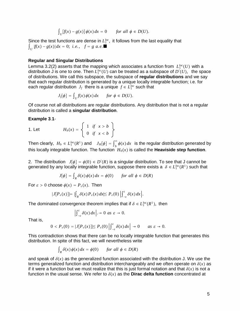
Introduction to the Theory of Distributionspauld/M545/6Distrib.pdf · Introduction to the Theory of Distributions Generalized functions or distributions are a generalization of the

Introduction to the Theory of Distributions

Generalized functions or distributions are a generalization of the notion of a function definedon Rn. Distributions are more general than the usual notion of pointwise defined functionsand they are even more general than LpU functions. Distributions have many convenientproperties with respect to the operations of analysis but in return for these convenientproperties we must give up the notion of a function that assumes it values pointwise or evenpointwise almost everywhere. Instead these functions assume their values only is a locallyaveraged sense (to be made precise later). This point of view is consistent, however, withmany physical applications and makes possible a coherent description of such things asimpulsive forces in mechanics and poles and dipoles in electromagnetic theory.Mathematically these objects are Dirac deltas and its derivatives and these may beaccomodated within the theory of distributions.

This development distributions will be based on the notion of duality. We begin with alinear space X that is contained in an inner product space, H, whose inner product wedenote by ⋅, ⋅H. Now suppose that X is equipped with a notion of convergence that isstronger than the one in H associated with its inner product; i.e., if xn is a sequence in Xthat converges in X then xn, viewed as a sequence in H, is still convergent. This is thesame thing as saying X is continuously embedded in H. Then for each x in X and every y inH, x,yH is a real number and if xn → x in X , then xn,yH → x,yH for every y in H. If X isproperly contained in H (i.e., X is not equal to H) then it may be that

xn → x, in X implies xn,yH → x,yH for every y in X’

where X′ is a linear space containing H but larger than H. In particular, if we choose

X = C0∞U, H = L2U and u,vH = ∫

Uuxvxdx

then, since X is very much smaller than H, the space X ′, the space of distributions on U, isvery much larger than H. We will now make these remarks precise.

1. Test FunctionsIn order to compute the locally averaged values of a distribution, the notion of a test functionis required. A function fx defined on an open set U ⊂ Rn is said to have compact supportif fx = 0 for x in the complement of a compact subset of U. In particular, if U = Rn, then fhas compact support if there is a positive constant, C such that fx = 0 for |x| > C. Wesay that fx is a test function if f has compact support and, in addition, f is infinitelydifferentiable on U. We use the notation f ∈ Cc

∞U or f ∈ DU to indicate that f is a testfunction on U.

The function

Tx =Kexp −1

1 − |x|2 if |x| < 1

0 if |x| ≥ 1, x ∈ Rn

where the constant K is chosen such that ∫Rn

Txdx = 1, is a test function on Rn. For thecase n = 1, this test function is pictured below

1

The Test Function T(x)

Note that Tx vanishes, together with all its derivatives as |x| → 1−, so Tx is infinitelydifferentiable and has compact support. .For n = 1 and > 0, let

Sx = 1 T x

and Pεx = T x .

Then Sx ≥ 0 and Pεx ≥ 0 for all x

Sx = 0 and Pεx = 0 for |x|>

∫R

Sxdx = 1 ∀ > 0, Sx → +∞ as → 0,

∫R

Pxdx → 0 as → 0, P0 = K/e ∀ > 0,

Evidently, Sx becomes thinner and higher as tends to zero but the area under thegraph is constantly equal to one. On the other hand, Pεx has constant height but growsthinner as tends to zero. These test functions can be used as the ”seeds” from which aninfinite variety of other test functions can be constructed by using a technique calledregularization to be discussed later.

Convergence in the space of test functionsClearly DU is a linear space of functions but it turns out to be impossible to define a normon the space. However, it will be sufficient to define the notion of convergence in this space.We say that the sequence φn ∈ DU converges to zero in DU if

1. there exists a single compact set M in U such that the support of every φn iscontained in M

2. for every multi-index, α, maxM |∂xαφn | → 0 as n → ∞ (φn and all its derivatives

tend uniformly to zero on M)

Then φn ∈ DU is said to converge to φ in DU if φn − φ converges to zero in DU.

2. Functionals on the space of test functionsA real valued function defined on the space of test functions is called a functional onDU. Consider the following examples, where φ denotes an arbitrary test function:

J1φ = φa for a ∈ U a fixed point in U

2

J2φ = ∫Vφxdx for V ⊂ U a fixed set

J3φ = φ ′a for a ∈ U fixed

J4φ = φ ′aφa for a ∈ U fixed.

Linear Functionals on DUEach of the examples above is a real valued function defined on the space of test functions,i.e., a functional. A functional on D is said to be a linear functional on D if

∀φ ,ψ ∈ DU, JC1φ + C2ψ = C1Jφ + C2Jψ, ∀C1, C2 ∈ R

The functionals J1, J2, and J3 are all linear, J4 is not linear.

Continuous Linear FunctionalsA linear functional J on D(U) is said to be continuous at zero if, for all sequencesφn ∈ DU converging to zero in DU, we have Jφn converging to zero as a sequenceof real numbers; i.e.,

φn → 0 in DU implies Jφn → 0 in R.

For linear functionals, continuity at any point is equivalent to continuity at every point.

Lemma 2.1 If J is a linear functional on D(U), then J is continuous at zero, if and only if J iscontinuous at every point in D(U); i.e.,

φn → 0 in DU implies Jφn → 0 in R.

if and only if

∀φ ∈ DU, φn → φ in DU implies |Jφn − Jφ|→ 0 in R.

examples

1. J1φ = φa for a ∈ R fixed is a continuous linear functional on D = DR1.

Let φn denote a sequence of test functions converging to zero in DR. Then there is aclosed bounded interval M such that for every n, φnx = 0 for x not in M. If a is not in Mthen J1φn = φna = 0 for every n so |Jφn − J0|= 0 → 0 in R. in this case. On the otherhand, if a ∈ M, then |Jφn − J0|= |φna| ≤ maxM |φnx| → 0 as n → ∞ so we haveconvergence in this case as well.

2. J2φ = ∫Vφxdx for V ⊂ U is a continuous linear functional on DU

Let φn denote a sequence of test functions converging to zero in DU. Then there is acompact set M ⊂ U such that for every n, φnx = 0 for x not in M. Let W = V ∩ M. If W isempty, then J2φn = 0 for every n so we have convergence in this case. If W is not emptythen

|J2φn |= |∫Wφnxdx|≤ maxW |φn | |W| ≤ maxM |φn | |W| → 0 as n → ∞

3

and we have convergence in this case as well.

3. DistributionsA continuous linear functional on the space of test functions DU will be called adistribution on U. We will denote the set of all distributions on U by D′U, or, when U isthe whole space, by D′. We will soon see the connection between distributions andgeneralized functions.

If we define C1J1 + C2J2φ to equal C1J1φ + C2J2φ for all test functions φ, thenD ′U is a linear space.

Lemma 3.1 D′U is a linear space over the reals.

For φ a test function in DU, and J a distribution on U, we will use the notationsJφ = ⟨J,φ⟩ interchangeably to denote the value of J acting on the test function φ, and werefer to this as the action of J. Although J is evaluated at functions in D rather than atpoints in U, we will still be able to show that distributions can be interpreted as ageneralization of the usual pointwise notion of functions.

Locally Integrable FunctionsA function fx defined on U is said to be locally integrable if, for every compact subsetM ⊂ U, there exists a constant K = KM, f such that

∫M

| fx|dx = K < ∞

We indicate this by writing f ∈ L1locU. Note that when U is Rn then f ∈ L1

locRn need not beabsolutely integrable, it only needs to be integrable on every compact set. This means, forexample, that all polynomials are in L1

locU although polynomials are certainly notintegrable on Rn.

Lemma 3.2 For f ∈ L1loc, define Jfφ = ∫

Ufxφxdx for φ ∈ DU.

Then1. Jf ∈ D′U.2. For f ,g ∈ L1

loc such that Jfφ = Jgφ, for all φ ∈ DU, f = g a.e.

Proof- To show 1, let φn denote a sequence of test functions converging to zero inDU. Then there is a compact set M ⊂ U such that for every n, φnx = 0 for x not in M.For f ∈ L1

loc, and

Jfφ = ∫U

fxφxdx for φ ∈ DU,

we have

|Jfφn |= |∫U

fxφnxdx|= |∫M

fxφnxdx|≤ maxM|φnx| |∫M

fx dx|= K maxM|φnx| → 0 as n →

To show 2, note that for f ,g ∈ L1loc such that Jfφ = Jgφ, for all φ ∈ DU, we have

4

∫Ufx − gxφxdx = 0 for all φ ∈ DU.

Since the test functions are dense in L1loc, it follows from the last equality that

∫U

|fx − gx|dx = 0; i.e. , f = g a.e.■

Regular and Singular DistributionsLemma 3.2(2) asserts that the mapping which associates a function from L1

locU with adistribution J is one to one. Then L1

locU can be treated as a subspace of D′U, the spaceof distributions. We call this subspace, the subspace of regular distributions and we saythat each regular distribution is generated by a unique locally integrable function; i.e. foreach regular distribution Jf there is a unique f ∈ L1

loc such that

Jfφ = ∫U

fxφxdx for φ ∈ DU.

Of course not all distributions are regular distributions. Any distribution that is not a regulardistribution is called a singular distribution.

Example 3.1-

1. Let Hbx =1 if x > b

0 if x < b

Then clearly, Hb ∈ L1locR1 and JHφ = ∫

b

∞φxdx is the regular distribution generated by

this locally integrable function. The function H0x is called the Heaviside step function.

2. The distribution Jφ = φ0 ∈ D′R is a singular distribution. To see that J cannot begenerated by any locally integrable function, suppose there exists a δ ∈ L1

locR1 such that

Jφ = ∫Rδxφxdx = φ0 for all φ ∈ DR

For > 0 choose φx = Px. Then

|JPx|= |∫RδxPxdx|≤ P0 ∫

−

δxdx .

The dominated convergence theorem implies that if δ ∈ L1locR1, then

∫−

δxdx .→ 0 as → 0.

That is,0 < P0 = |JPx|≤ P0 ∫

−

δxdx → 0 as → 0.

This contradiction shows that there can be no locally integrable function that generates thisdistribution. In spite of this fact, we will nevertheless write

∫Rδxφxdx = φ0 for all φ ∈ DR

and speak of δx as the generalized function associated with the distribution J. We use theterms generalized function and distribution interchangeably and we often operate on δx asif it were a function but we must realize that this is just formal notation and that δx is not afunction in the usual sense. We refer to δx as the Dirac delta function concentrated at

5

the origin. More generally, the distribution Jφ = φa for all φ ∈ DR, is written as

∫Rδx − aφxdx = φa for all φ ∈ DR

and is called the Dirac delta function concentrated at x = a. We refer toJφ = φa for all φ ∈ DR as the ”action” of the distribution and we refer to δx − a asthe generalized function associated with the distribution having this action. Although we willoften write equations like

∇2Gx = δx − a, x ∈ U,

all we mean by this is that

∫R∇2Gxφxdx = φa for all φ ∈ DR.

Problem 1 Each of the following distributions is defined by its action. Identify thegeneralized function for each of them.

(a) J1φ = a2φa (b) J2φ = −e−bφb + φ ′b

(c) J3φ = ∫a

bx2φxdx (d) J4φ = ∫

a

bφxdx

Problem 2 Describe the action on test functions for the following generalized functions.

(a) F1x = xδx (b) F2x = x δ ′x − a(c) F3x = δ3x (d) F4x = H0x − H0x − 1 sinπx

Equality and Values on an Open SetAlthough we are not entitled to treat generalized functions as if they have pointwise values,we are still able to talk about distributions that are zero on certain sets as well as definingwhat is meant by equality of distributions on open sets.Distributions J1 and J2 are said to be equal in the sense of distributions if

J1φ = J2φ for all φ ∈ DU;

If F1 and F2 are generalized functions, then F1 and F2 are said to be equal if

∫U

F1xφxdx = ∫U

F2xφxdx for all φ ∈ DU.

The support of a test function φx is defined as the smallest closed set K such that φxis identically zero off K. Then we can say that a distribution J vanishes on an open set, Ω,if Jφ = 0 for all test functions φ having support in Ω. For example, δx vanishes on theopen sets −∞, 0 and 0,∞. Two distributions, J1 and J2 , can be said to be equal on anopen set, Ω if J1 − J2 vanishes on the open set Ω.

We define the support of a distribution J to be the complement of the largest openset where J is zero. Then the support of the Dirac delta is just the point 0, and any regulardistribution generated by a function having compact support, K, is a distribution whosesupport is equal to K.

6

Differentiation of DistributionsLet Jf denote the regular distribution generated by the locally integrable function of onevariable, fx and consider the distribution generated by the derivative f ′x. The action ofthis distribution is described by

∫R

f ′xφxdx = fxφx |x=−∞x=∞ − ∫R

f xφ′xdx = 0 + ⟨Jf,−φ′ ⟩ ∀φ ∈ DR

Here we integrated by parts (formally) and used the fact that a test function has compactsupport to make the boundary term vanish. It is evident that the derivative generates adistribution Jf ′ whose action on the test function φx is the same as the action of Jf on−φ′x. This motivates the following definition.

distributional derivative For any J ∈ D′R, the derivative dJ/dx ∈ D′R is thedistribution whose action on test function φx is given by dJ/dxφ = J−φ′ ; i.e. ,

⟨dJ/dx,φx⟩ = ⟨J,−φ′x⟩ ∀φ ∈ DR

Equivalently, the distribution Jf generated by the generalized function fx has as itsdistributional derivative, the distribution Jf ′ generated by f ′x. For higher order derivatives,we have

⟨dkJ/dxk,φx⟩ = −1k ⟨J, φkx⟩ ∀φ ∈ DR.

More generally, for any J ∈ D′U, the derivative ∂xαJ ∈ D′U is the distribution whose

action on test function φx is given by ∂xαJφ = J−1 |α |∂x

αφ; i.e. ,

⟨∂xαJ,φx⟩ = −1 |α |⟨J,∂x

αφx⟩ ∀φ ∈ DR.

Here α = α1. . .αn denotes a multi-index , hence ∂xαJ = ∂x1

α1 . . . ∂xnαn J, and |α| = α1 +. . .+αn.

Equality of Mixed PartialsSuppose J is a distribution on open set U ⊂ R2. Then ∂xyJ = ∂yxJ. To see this write

⟨∂xyJ,φx,y⟩ = −12⟨J,∂xyφx,y⟩ ∀φ ∈ DR.⟨∂yxJ,φx,y⟩ = −12⟨J,∂yxφx,y⟩ ∀φ ∈ DR.

But for a test function, ∂yxφx,y = ∂xyφx,y, hence ∂xyJ = ∂yxJ. More generally, everydistribution is infinitely differentiable and the values of derivatives of higher order areindependent of the order of differentiation.

Example 3.2-1. Let JH denote the distribution generated by the locally integrable function H0x. Then

⟨dJH/dx,φx⟩ = ⟨JH,−φ′x⟩ = ∫0

∞−φ′xdx ∀φ ∈ DR

i.e.,∫

0

∞−φ′xdx = −φx |x=0

x=∞ = φ0.

Then

⟨dJH/dx,φx⟩ = φ0. ∀φ ∈ DR,

7

and since ⟨δx,φx⟩ = φ0, ∀φ ∈ DR, we conclude that dH0x/dx = δx in the senseof distributions.

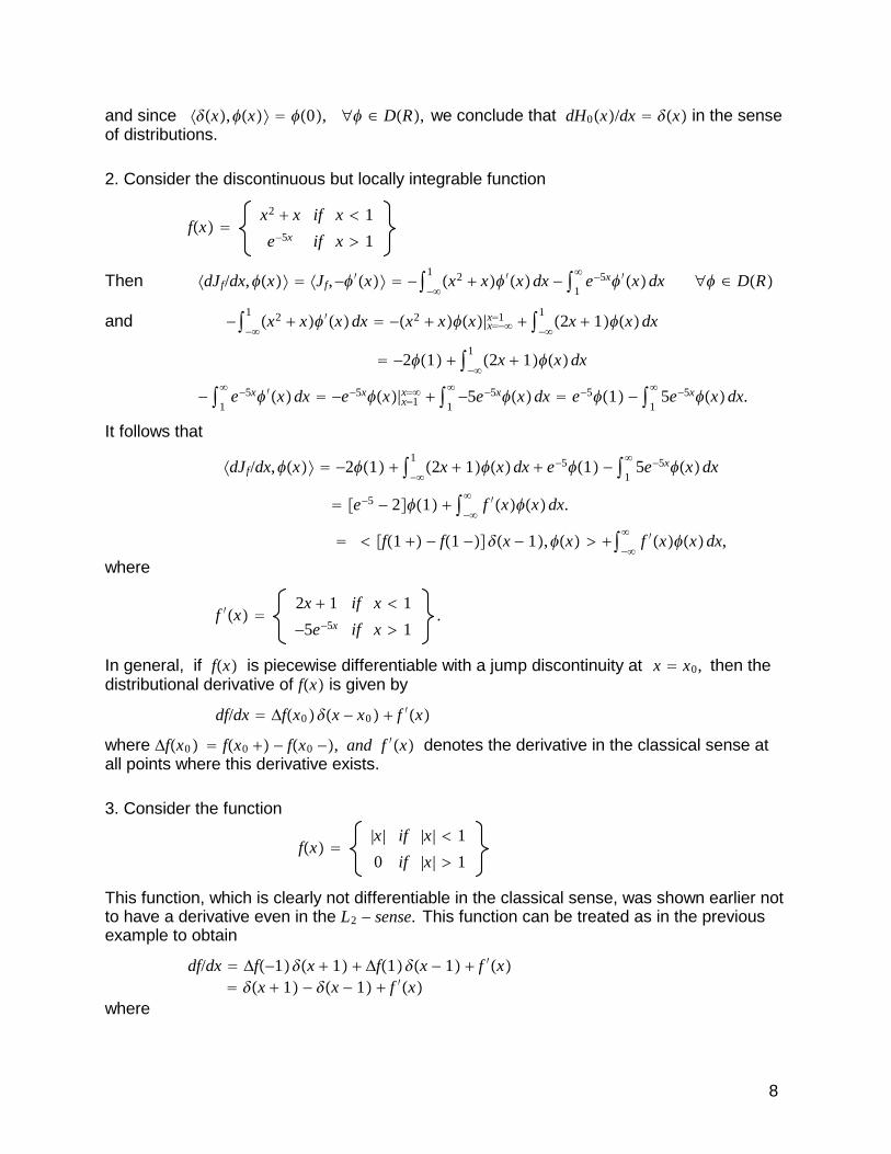
2. Consider the discontinuous but locally integrable function

fx =x2 + x if x < 1

e−5x if x > 1

Then ⟨dJf/dx,φx⟩ = ⟨Jf,−φ′x⟩ = − ∫−∞

1x2 + xφ′xdx − ∫

1

∞e−5xφ′xdx ∀φ ∈ DR

and − ∫−∞

1x2 + xφ′xdx = −x2 + xφx|x=−∞x=1 + ∫

−∞

12x + 1φxdx

= −2φ1 + ∫−∞

12x + 1φxdx

− ∫1

∞e−5xφ′xdx = −e−5xφx|x=1

x=∞ + ∫1

∞−5e−5xφxdx = e−5φ1 − ∫

1

∞5e−5xφxdx.

It follows that

⟨dJf/dx,φx⟩ = −2φ1 + ∫−∞

12x + 1φxdx + e−5φ1 − ∫

1

∞5e−5xφxdx

= e−5 − 2φ1 + ∫−∞

∞f ′xφxdx.

= < f1 + − f1 −δx − 1,φx > + ∫−∞

∞f ′xφxdx,

where

f ′x =2x + 1 if x < 1

−5e−5x if x > 1.

In general, if fx is piecewise differentiable with a jump discontinuity at x = x0, then thedistributional derivative of fx is given by

df/dx = Δfx0δx − x0 + f ′x

where Δfx0 = fx0 + − fx0 −, and f ′x denotes the derivative in the classical sense atall points where this derivative exists.

3. Consider the function

fx =|x| if |x| < 1

0 if |x| > 1

This function, which is clearly not differentiable in the classical sense, was shown earlier notto have a derivative even in the L2 − sense. This function can be treated as in the previousexample to obtain

df/dx = Δf−1δx + 1 + Δf1δx − 1 + f ′x= δx + 1 − δx − 1 + f ′x

where

8

f ′x =

−1 if −1 < x < 0

+1 if 0 < x < 1

0 if |x| > 1

Alternatively, using the definition of distributional derivative leads to

⟨dJf/dx,φx⟩ = ⟨Jf,−φ′x⟩ = ∫−1

0xφ′xdx − ∫

0

1xφ′xdx ∀φ ∈ DR

= xφx|x=−1x=0 − ∫

−1

0φxdx − xφx|x=0

x=1 + ∫0

1φxdx

i.e., ∫−∞

∞f ′xφxdx = φ−1 − φ1 + ∫

−1

1sgnxφxdx, ∀φ ∈ DR.

This implies f ′x = δx + 1 − δx − 1 + I1x sgnx Of courser this is the derivative in thedistributional sense.

4. Recall that the initial value problem

∂tux, t + a∂xux, t = 0, x ∈ R, t > 0ux, 0 = fx

has the solution ux, t = fx − at. In the case that the function fx is not sufficiently regularfor the existence of a classical solution, (i.e., if f is not at least differentiable in the classicalsense) we can say that u is a solution in the sense of distributions if, for every test functionφx, t ∈ DR × R+,

⟨∂tux, t + a∂xux, t,φx, t⟩ = 0.

e.g., suppose fx = I1x so that f ′x = δx + 1 − δx − 1 + 0 and then

∂t + a∂xfx − at =

= δx − at + 1 − δx − at − 1 + 0−a + aδx − at + 1 − δx − at − 1 + 0 = 0.

This is the same thing as the argument,

⟨∂tux, t + a∂xux, t,φx, t⟩

= −a⟨δx − at + 1 − δx − at − 1,φx, t⟩ + a ⟨δx − at + 1 − δx − at − 1,φx, t⟩

= −aφat − 1, t − φat + 1 + aφat − 1, t − φat + 1 = 0.

Note that ⟨δx − at − 1,φx, t⟩ = φat + 1, t is a special case of⟨δψx, t,φx, t⟩ = φxt, t or φx, tx, a result which is only true if ψx, t = C implies

one of the variables x, t can be expressed as a C∞ function of the other, x = xt or t = tx.In general, this type of composition is not defined. In this case, however, the verification thatux, t = fx − at solves the initial value problem is formally the same as in the case where fis smooth. For this discontinuous function f, however, the steps showing that ux, t solvesthe problem can only be justified within the framework of distribution theory.

The Hilbert-Sobolev Space of Order OneWe are going to define a new function space which will be of use in the weak formulation of

9

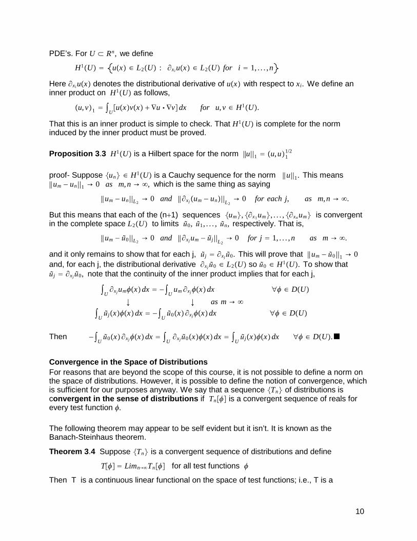
PDE’s. For U ⊂ Rn, we define

H1U = ux ∈ L2U : ∂xiux ∈ L2U for i = 1, . . . ,n

Here ∂xiux denotes the distributional derivative of ux with respect to xi. We define aninner product on H1U as follows,

u,v1 = ∫Uuxvx + ∇u ⋅ ∇vdx for u,v ∈ H1U.

That this is an inner product is simple to check. That H1U is complete for the norminduced by the inner product must be proved.

Proposition 3.3 H1U is a Hilbert space for the norm ||u||1 = u,u11/2

proof- Suppose un ∈ H1U is a Cauchy sequence for the norm ||u||1. This means||um − un ||1 → 0 as m,n → ∞, which is the same thing as saying

||um − un ||L2→ 0 and ||∂xjum − un||L2

→ 0 for each j, as m,n → ∞.

But this means that each of the (n+1) sequences um,∂x1um, . . . ,∂xnum is convergentin the complete space L2U to limits ũ0, ũ1, . . . , ũn, respectively. That is,

||um − ũ0 ||L2→ 0 and ||∂xjum − ũj ||L2

→ 0 for j = 1, . . . ,n as m → ∞.

and it only remains to show that for each j, ũj = ∂xjũ0. This will prove that ||um − ũ0 ||1 → 0and, for each j, the distributional derivative ∂xjũ0 ∈ L2U so ũ0 ∈ H1U. To show thatũj = ∂xjũ0, note that the continuity of the inner product implies that for each j,

∫U∂xjumφxdx = − ∫

Uum ∂xjφxdx ∀φ ∈ DU

↓ ↓ as m → ∞∫

Uũjxφxdx = − ∫

Uũ0x∂xjφxdx ∀φ ∈ DU

Then − ∫Uũ0x∂xjφxdx = ∫

U∂xjũ0xφxdx = ∫

Uũjxφxdx ∀φ ∈ DU.■

Convergence in the Space of DistributionsFor reasons that are beyond the scope of this course, it is not possible to define a norm onthe space of distributions. However, it is possible to define the notion of convergence, whichis sufficient for our purposes anyway. We say that a sequence Tn of distributions isconvergent in the sense of distributions if Tnφ is a convergent sequence of reals forevery test function φ.

The following theorem may appear to be self evident but it isn’t. It is known as theBanach-Steinhaus theorem.

Theorem 3.4 Suppose Tn is a convergent sequence of distributions and define

Tφ = Limn→∞Tnφ for all test functions φ

Then T is a continuous linear functional on the space of test functions; i.e., T is a

10

distribution.

Delta SequencesOne type of distributional sequence we are particularly interested in are the so called deltasequences.

Theorem 3.5 Suppose fn is a sequence of locally integrable functions such that forsuitable constants M and C, we have

1. fnx = 0 for |x| > Mn

2. ∫R

fnxdx = 1 ∀n

3. ∫R| fnx|dx ≤ C ∀n

Then the sequence Jn of distributions generated by the functions fnx converge toδx in the sense of distributions.

Proof-Suppose fn is a sequence of locally integrable functions with properties 1,2, and 3and let Jn denote the sequence of distributions generated by the functions fnx. For anarbitrary test function φx, it follows from 2 that

Jnφx = ∫R

fnxφxdx = φ0 + ∫R

fnxφxdx − φ0 ∫R

fnx dx

andJnφx − φ0 = ∫

Rfnx φx − φ0 dx.

Now properties 1 and 3 show that

|Jnφx − φ0| ≤ max|φx − φ0| : |x| < Mn ∫

R| fnx|dx

≤ Cmax|φx − φ0| : |x| < Mn → 0 as n → ∞.

We just showed

∀φ ∈ D Jnφx → φ0 as n → ∞; i.e. Jn → δx in D′■

Note that this is a result for distributions on R1.

Example 3.31. The following are all delta sequences.

fnx = nπ

11 + n2x2 , gnx =

−n if |x| < 12n

2n if 12n < x < 1

n

0 if |x| > 1n

hnx = S1/nx

Note that fn0 and hn0 both tend to plus infinity as n tends to infinity. This is consistentwith the commonly held impression that the delta function is zero everywhere except at zerowhere it has the value plus infinity. However, gnx is also a delta sequence and gn0 tendsto minus infinity as n tends to infinity. This illustrates the difficulty in assigning a pointwisevalue to a singular distribution.

11

2. Consider the following sequences of locally integrable functions.

Fnx = 12

+ 1π arctannx, fnx = n

π1

1 + n2x2 , gnx = −2n3

πx

1 + n2x22 .

Then F ′x = fnx and f n′ x = gnx. Moreover

limn→∞Fnx =

1 if x > 012 if x = 0

0 if x < 0

= H0x so ∫R

Fnφ → ∫0

∞φ

hence∫

Rfnφ = ∫

RF n

′ φ = ∫R−Fnφ′ → ∫

0

∞−φ′ = φ0 i.e. , fn → δx

and

∫R

gnφ = ∫R

f n′ φ = ∫

R− fnφ′ = ∫

R−Fn

′φ′ = ∫R

Fnφ"→ ∫0

∞−φ" = −φ ′0 i.e. , gn → δ′x

This is an illustration of the following result.

Theorem 3.6 Suppose Tn is a sequence of distributions converging to a limit T in thedistributional sense. Then

1. the derivatives T n′ form a sequence of distributions converging to the limit T ′ in

the distributional sense.2. the antiderivatives ∫x

T n form a sequence of distributions converging to thelimit ∫x

T in the distributional sense

A connection between pointwise and distributional convergence is contained in the followingcorollary of the dominated convergence theorem.

Theorem 3.7 Suppose fn is a sequence of locally integrable functions such that

| fn | ≤ g ∈ L1loc and fn → f pointwise almost everywhere.

Then the sequence of regular distributions, Jfn , converges in the distributional sense to Jf.

In example 3.3(2) it is straightforward to show that |Fnx| ≤ 1 and that Fnx convergespointwise to H0x. Then the distributional convergence of Fn to H0 follows and theorem 3.6can be applied as illustrated in example 3.3(2).

Applications to PDE’s

1). We are going to show first that for 0 < x,y < π, δx − y ∈ D′0,π, can be expanded interms of the eigenfunctions sinnx. Formally,

δx − y = ∑n=1∞ dny sinnx,

leads to

12

⟨δx − y, sinmx⟩ = ∑n=1∞ dny sinnx, sinmx

= ∑n=1∞ dny ∫

0

πsinnx sinmxdx = 1

2dmy.

But⟨δx − y, sinmx⟩ = sinmy

hencedmy = 2sinmy and δx − y = 2∑n=1

∞ sinny sinnx.

This result is only formal since expansion in terms of eigenfunctions was developed forfunctions in L20,π and has not been shown to extend to generalized functions. In fact, itdoes extend but this is what we must now show.

One way to show that this result extends to distributions, is to note that for each fixedy ∈ 0,π, the series

2∑n=1∞ 1

n2 sinny sinnx

converges uniformly for 0 ≤ x ≤ π, to a limit we will denote by Gx,y. It follows then fromtheorem 3.6 that

−∂xx 2∑n=1N 1

n2 sinny sinnx = 2∑n=1N sinny sinnx −∂xxGx,y as N ∞

where the convergence is in the sense of distributions on 0,π. Since the differentiatedseries is the series we found for δx − y, the validity of the series will be established if wecan show that − ∂xxGx,y = δx − y. To see this, note that any test functionφx ∈ D0,π can be expanded in a series of the form

φx = ∑n=1∞ φn sinnx = ∑n=1

∞ 2 ∫0

πφy sinnydy sinnx

= ∫0

πφy ∑n=1

∞ 2 sinnx sinny dy = ⟨φy,−∂xxGx,y⟩.

Since

⟨φy,−∂xxGx,y⟩ = φx for any test function φx ∈ D0,π,

it follows that −∂xxGx,y = δx − y.

2. For each fixed y ∈ 0,π, let Hx,y, t denote the (distributional) solution of

∂t − ∂xxHx,y, t = 0, 0 < x < π, t > 0

and Hx,y, 0 = δx − y,

H0,y, t = Hπ,y, t = 0.

Then, as we have seen previously, the solution to this problem is given by

Hx,y, t = ∑n=1∞ dnye−n2t sinnx = ∑n=1

∞ 2sinnye−n2t sinnx.

Here using the expansion for δx − y is rigorous not just formal.Now if u = ux, t solves

∂t − ∂xxux, t = 0, 0 < x < π, t > 0

13

and ux, 0 = fx, 0 < x < π,u0, t = uπ, t = 0, t > 0,

then ux, t = ∫0

πHx,y, t fydy.

To see this, simply note that u0, t = uπ, t = 0, follows fromH0,y, t = Hπ,y, t = 0, and in addition,

∂t − ∂xxux, t = ∫0

π∂t − ∂xxHx,y, t fydy = 0,

andux, 0 = ∫

0

πHx,y, 0 fydy = ∫

0

πδx − y fydy = fx.

Evidently, Hx,y, t is what we have previously called the Green’s function for the heatequation. Now we will see an equivalent alternative description of the Green’s function.

3. For each fixed y ∈ 0,π, and t > s > 0, let Hx,y, t − s denote the solution of

∂t − ∂xxHx,y, t − s = δx − yδt − s, 0 < x < π, t > s > 0and Hx,y, 0 = 0,

H0,y, t = Hπ,y, t = 0.

In this case, the solution to this problem can be written

Hx,y, t − s = ∑n=1∞ Hny, t − s sinnx

where

∂tHny, t − s + n2Hny, t − s = dnyδt − s, Hny, 0 = 0.

Then

Hny, t − s = dny ∫0

te−n2t−τ δτ − sdτ = 2 sinnye−n2t−s

andHx,y, t − s = 2∑n=1

∞ e−n2t−s sinny sinnx.

Now if u = ux, t solves

∂t − ∂xxux, t = Fx, t, 0 < x < π, t > 0and ux, 0 = 0, u0, t = uπ, t = 0,

then

ux, t = ∫0

t ∫0

πHx,y, t − sFy, sdy ds.

To see this, simply note that u0, t = uπ, t = 0, follows fromH0,y, t = Hπ,y, t = 0, and furthermore

∂t − ∂xxux, t = ∫0

t ∫0

π∂t − ∂xxHx,y, t − sFy, sdy ds

= ∫0

t ∫0

πδx − yδt − sFy, sdyds = Fx, t.

and

ux, 0 = ∫0

t ∫0

πHx,y, 0Fy, sdyds = 0.

14

Evidently, Hx,y, t − s is also what we have previously called the Green’s function for theheat equation, and we can characterize the Green’s function equivalently as Hx,y, t, the(distributional) solution of

∂t − ∂xxHx,y, t = 0, 0 < x < π, t > 0 and Hx,y, 0 = δx − y,

or as Hx,y, t − s, the solution in the distributional sense of

∂t − ∂xxHx,y, t = δx − yδt − s, 0 < x < π, t > s > 0 and Hx,y, 0 = 0.

4. The Distributional Fourier TransformIn order to extend the definition of the Fourier transform to generalized functions, we firstrecall that an infinitely differentiable function ux is said to be rapidly decreasing if

∀ integers m,n, |xmunx|→ 0, as |x| → ∞

Then the rapidly decreasing functions are smooth functions that tend to zero, together withtheir derivatives of all orders, as |x| tends to infinity, more rapidly than any negative power of|x|. We denote this class of functions by SR and note that the test functions, Cc

∞R arecontained in SR, and SR is contained in L2R and in L1R. Then every f ∈ SR has aFourier transform which can be shown to also belong to SR. Thus SR is another space,like L2R, which is symmetric with respect to the Fourier transform in the sense that bothf and F belong to the same space of functions.

Proposition 4.1 For each f ∈ SR, F = TF f ∈ SR and TF−1F = fx where the

equality here is in the pointwise sense..We now define the sense of convergence in SR. A sequence φn of rapidly decreasingfunctions is said to converge to zero in SR if, for all integers p and q,

maxx∈R xpφnqx → 0 as n → ∞

Then φn → φ in SR if φn − φ → 0 in SR. Since the space of rapidly decreasingfunctions has no norm, we cannot say that the Fourier transform is an isometry onSR. However, we have the following result.

Proposition 4.2 For fn ∈ SR, with Fn = TF fn ∈ SR , φn → φ in SR impliesFn → F = TFφ in SR.

Tempered DistributionsA linear functional T defined on SR is said to be a tempered distribution if, for everysequence φn of rapidly decreasing functions that is converging to zero in SR, it followsthat Tφn converges to zero as a sequence of real numbers. In this case we writeT ∈ S′R.

Note that convergence in the sense of test functions is stronger than convergence in thesense of rapidly decreasing functions. Then every J ∈ D′R is also a tempered distributionbut the converse is false.

15

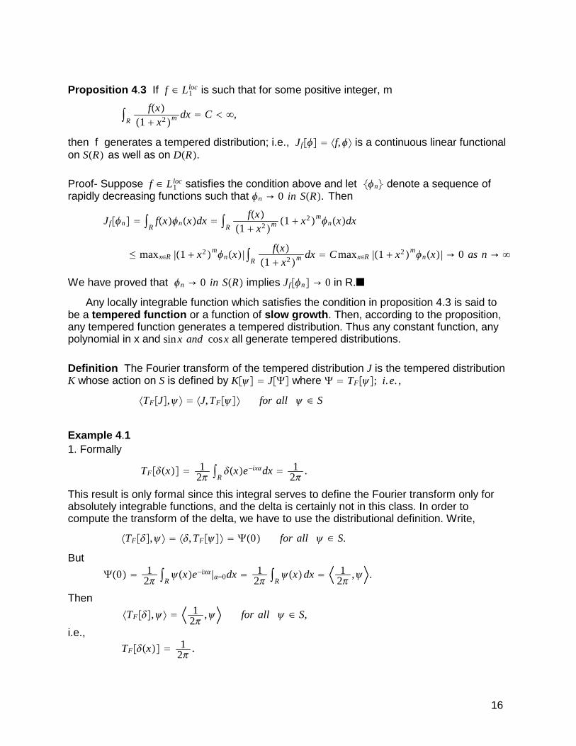
Proposition 4.3 If f ∈ L1loc is such that for some positive integer, m

∫R

fx1 + x2m dx = C < ∞,

then f generates a tempered distribution; i.e., Jfφ = ⟨f,φ⟩ is a continuous linear functionalon SR as well as on DR.

Proof- Suppose f ∈ L1loc satisfies the condition above and let φn denote a sequence of

rapidly decreasing functions such that φn → 0 in SR. Then

Jfφn = ∫R

fxφnxdx = ∫R

fx1 + x2m 1 + x2mφnxdx

≤ maxx∈R |1 + x2mφnx| ∫R

fx1 + x2m dx = Cmaxx∈R |1 + x2mφnx| → 0 as n → ∞

We have proved that φn → 0 in SR implies Jfφn → 0 in R.■

Any locally integrable function which satisfies the condition in proposition 4.3 is said tobe a tempered function or a function of slow growth. Then, according to the proposition,any tempered function generates a tempered distribution. Thus any constant function, anypolynomial in x and sinx and cosx all generate tempered distributions.

Definition The Fourier transform of the tempered distribution J is the tempered distributionK whose action on S is defined by Kψ = JΨ where Ψ = TFψ; i.e. ,

⟨TFJ,ψ⟩ = ⟨J,TFψ⟩ for all ψ ∈ S

Example 4.11. Formally

TFδx = 12π

∫Rδxe−ixαdx = 1

2π.

This result is only formal since this integral serves to define the Fourier transform only forabsolutely integrable functions, and the delta is certainly not in this class. In order tocompute the transform of the delta, we have to use the distributional definition. Write,

⟨TFδ,ψ⟩ = ⟨δ,TFψ⟩ = Ψ0 for all ψ ∈ S.

But

Ψ0 = 12π

∫Rψxe−ixα|α=0dx = 1

2π∫

Rψxdx = 1

2π,ψ .

Then

⟨TFδ,ψ⟩ = 12π

,ψ for all ψ ∈ S,

i.e.,

TFδx = 12π

.

16

2. The constant function fx = 1 ∀x, is a tempered function and generates a tempereddistribution which we will denote by I. Then for arbitrary ψ ∈ S,

⟨TFI,ψ⟩ = ⟨I,TFψ⟩ = ∫RΨαdα = ∫

RΨαeixαdα|x=0 = ψ0;

i.e.,⟨TFI,ψ⟩ = ψ0 for all ψ ∈ S.

This is equivalent to the assertion that TFI = δ.

3. Using these two results we now can see that

TFδnx = iαn 12π

, TFxnI = inδnα

TFδx − p = 12π

.e−ipα, TFeixpI = δx − p,

TFcospx = TFeixpI + e−ixpI/2 = δx − p + δx + p/2

TFsinpx = TFeixpI − e−ixpI/2i = δx − p − δx + p/2i

Applications to PDE’s1. For fixed y ∈ R, and s ≥ 0, consider the initial value problem

∂t − ∂xxHx,y, t − s = δx − yδt − s x ∈ R, t > s ≥ 0,Hx,y, t − s = 0 for s > t.

If Ĥα,y, t − s denotes the Fourier transform in x of Hx,y, t − s, then

ddtĤα,y, t − s + α2Ĥα,y, t − s = 1

2π.e−iyα δt − s,

Ĥα,y, t − s = 0 for s > t.

It follows that

Ĥα,y, t − s = ∫0

te−α2t−τ 1

2π.e−iyα δτ − sdτ = 1

2π.e−iyαe−α2t−s

Since TF−1 e−α2t−s = π

t − s e− x2

4t − s it follows that

Hx,y, t − s = 14πt − s

e−x − y2

4t − s , t > s ≥ 0.

This is the previously obtained fundamental solution for the heat equation on R × R+. Notethat similar arguments show that the solution of the initial value problem

∂t − ∂xxHx,y, t = 0 x ∈ R, t > 0,Hx,y, 0 = δx − y,

is given by Hx,y, t = 14πt

e−x − y2

4t , t > 0.

17

2. For fixed y ∈ R, and s ≥ 0, consider the initial value problem

∂tt − ∂xxWx,y, t − s = δx − yδt − s x ∈ R, t > s ≥ 0,Wx,y, t − s = 0 for s > t.

If Ŵα,y, t − s denotes the Fourier transform in x of Ŵx,y, t − s, then

d2

dt2 Ŵα,y, t − s + α2Ŵα,y, t − s = 12π

.e−iyα δt − s,

Ŵα,y, t − s = 0 for s > t.

There are various ways to solve this equation, one of them is to apply the Laplace transformin t to get

β2 + α2ŵα,y,β − s = 12π

.e−iyαe−βs

where

ŵα,y,β − s = £ Ŵα,y, t − s = Laplace transform in t of Ŵα,y, t − s

and£δt − s = ∫

0

∞e−βtδt − sdt = e−βs

Then

ŵα,y,β − s = 12π

.e−iyα ββ2 + α2

e−βs

β.

Now

TF−1 1

2π.e−iyα β

β2 + α2 = 12 e−β|x−y| and £−1 e−βA

β= H0t − A

hence Wx,y, t − s = 12 H0t − s − |x − y|.

This is the so called causal fundamental solution for the wave equation. Ifu = ux, t solves

∂tt − ∂xxux, t = Fx, t x ∈ R, t > 0,ux, 0 = ∂tux, 0 = 0 for x ∈ R

then ux, t = ∫0

t ∫R

Wx,y, t − sFy, sdy ds.

3. Using the Laplace transform, the solution of the initial boundary value problem,

∂tvx, t − ∂xxvx, t = 0, x > 0, t > 0,vx, 0 = 0, x > 0,

∂xv0, t = gt, t > 0,

is found to be

vx, t = ∫0

t −1πt − s

e− x2

4t − s gsds = − ∫0

tKx, t − sgsds.

while the solution of

18

∂twx, t − ∂xxwx, t = 0, x > 0, t > 0,wx, 0 = 0, x > 0,

w0, t = ft, t > 0,

is given by

wx, t = ∫0

t x

4πt − s3e− x2

4t − s gsds = ∫0

t∂xKx, t − sgsds.

The functions Kx, t, and hx, t = −∂xKx, t each satisfy

∂tux, t − ∂xxux, t = 0, x > 0, t > 0,

andLim t→0+ ux, t = 0, for x ≠ 0

This seems to violate the uniqueness of solutions to the pure initial value problem for theheat equation. However, Kx, t, and hx, t are distributional solutions of the initial valueproblem and neither of them is continuous in the closed upper half plane; i.e.,

Limx2=t→0 Kx, t = +∞ = Limx2=t→0 hx, t.

On the other hand, we can also show that

i) Lim t→0⟨Kx, t,φx⟩ = φ0 ∀φ ∈ DRii) Lim t→0⟨hx, t,φx⟩ = 2φ′0 ∀φ ∈ DR

This is equivalent to

i) ∂tKx, t − ∂xxKx, t = 0, in D′R, Kx, 0 = 2δxii) ∂thx, t − ∂xxhx, t = 0, in D′R, Kx, 0 = 2δ′x.

To see that i) holds, write

⟨Kx, t,φx⟩ = ∫R

1πt

e− x2

4t φxdx = 2π

∫R

e−z2φ z 4t dz

= 2π

∫R

e−z2φ z 4t − φ0dz + 2φ0

This leads to the result, Limt→0 ⟨Kx, t,φx⟩ = 2φ0, ∀φ ∈ DR.

5. Distributions SupplementWe wish to consider two questions in the theory of distributions:

i) given J ∈ D′R, find T ∈ D′R, such that xTx = Jxii) find J ∈ D′R, such that J ′x = 0

To answer the first question we need the following lemma.

19

Lemma 5.1- The test function φx satisfies

φ0 = 0 if and only if φx = xψx for some test function, ψx.

More generally, the test function φx satisfies

φm0 = 0 m = 0,1, . . . ,N − 1 if and only if φx = xNψx for some test function, ψx.

Proof- Clearly if φx = xψx, then φ0 = 0. Conversely, for any test function

φx = φ0 + ∫0

xφ′tdt,

and if φ0 = 0, then the substitution t = xs leads to

φx = ∫0

xφ′tdt = x ∫

0

1φ′xsds = xψx.

Clearly ψx is a test function if φx is a test function. The more general statement followsby a similar argument.■

Now, using lemma 5.1, we can show

Lemma 5.2- The general solution of i) is of the form Tx = T0x + Cδx, where T0 isany particular solution of i) and C is an arbitrary constant.

Proof- Note that the general solution of i) is necessarily of the form Tx = T0x + Kx,where T0 is any particular solution of i) and K is a distributional solution of xKx = 0. Thismeans that

0 = ⟨xKx,ψx⟩ = ⟨Kx,xψx⟩ for all test functions ψ.

Now it follows from lemma 1 that 0 = ⟨Kx,φx⟩ for all test functions such that φ0 = 0.Now any test function φx can be written in the form φx = φ0φ1x + φ0x, where φ0,φ1

denote test functions such that φ00 = 0 and φ10 = 1; e.g.,

φx = φ0φ1x + φx − φ0φ1x.

Then for arbitrary test function φx we can write

⟨Kx,φx⟩ = ⟨Kx,φ0φ1x + φ0x⟩ = φ0⟨K,φ1 ⟩ + ⟨K,φ0 ⟩ = Cφ0

which is to say, K = Cδ. More generally, similar arguments show that the generaldistributional solution of xNTx = Jx is of the form

Tx = T0x +∑n=0N−1 Cn δnx. ■

As an application of this result, consider the problem of finding the Fourier transform of thetempered function fx = Sgnx.Note that

TFddx

Sgnx = iαTFSgnx = iαFα.

But ddx

Sgnx = 2δx and TF2δx = 1π

20

hence

iαFα = 1π .

Then it follows from lemma 2 that Fα = − iπα + Cδα. Now it follows from previous

observations about the Fourier transform, that since fx is an odd real valued function of x,then Fα is an odd and purely imaginary valued function of α. Then the fact that δα isan even function of α implies that C = 0.

Similarly, the Fourier transform of the Heaviside step function can be obtained by a similarcomputation. We have

TFddx

Hx = iαTFHx = iαhα.

Alsoddx

Hx = δx and TFδx = 12π

Then

iαhα = 12π

,

and lemma 2 implies hα = − i2πα

+ Cδα. In order to determine the constant C, note

that

Hx + H−x = 1, hence TFHx + TFH−x = δα.

ButTFHx + TFH−x = hα + h−α = 2Cδα

which implies C = 1/2 and hα = 12 δα −

i2πα

.

In order to answer the question raised in ii), we need

Lemma 5.3- The test function φx satisfies

φx = ψ′x for some test function, ψx

if and only if ∫Rφxdx = 0.

Proof- If φx = ψ′x for some test function, ψx then

∫Rψ′xdx = ψ∞ − ψ−∞ = 0.

Conversely if ∫Rφxdx = 0, then

ψx = ∫−∞

xφsds satisfies ψ′x = φx.

In addition, ψ has compact support since ∫Rφxdx = 0 and φ has compact support. Then

ψ is a test function.■

21

Note that any test function can be written in the form φx = Aφ1x + φ0x where

A = ∫Rφxdx, ∫

Rφ0xdx = 0, and ∫

Rφ1xdx = 1.

e.g., φ = Aφ1 + φ − Aφ1.

Now, using this result we can show

Lemma 5.4- The distributional solution of u′x = 0 is the regular distribution generatedby the locally integrable function ux = C.

Proof- If u′x = 0 then

u′,ψ = − u,ψ′ = 0 for all test fucntions ψ.

i.e.,u,φ = 0 for all test functions φ = ψ′

By the previous result then

u,φ = ⟨u,Aφ1x + φ0x⟩

= A < u,φ1 > + < u,φ0 >

= C ∫Rφxdx where C = < u,φ1 >

This shows that

u,φ = ∫R

Cφxdx ∀φ ∈ D ■

22