Introduction to the Theory of Computation Some Notes for CIS262 Jean Gallier Department of Computer and Information Science University of Pennsylvania Philadelphia, PA 19104, USA e-mail: [email protected] c Jean Gallier Please, do not reproduce without permission of the author December 26, 2017

Welcome message from author
This document is posted to help you gain knowledge. Please leave a comment to let me know what you think about it! Share it to your friends and learn new things together.
Transcript
Introduction to the Theory of ComputationSome Notes for CIS262
Jean GallierDepartment of Computer and Information Science
University of PennsylvaniaPhiladelphia, PA 19104, USA
e-mail: [email protected]
c© Jean Gallier
Please, do not reproduce without permission of the author
December 26, 2017

2
Contents
1 Introduction 7
2 Basics of Formal Language Theory 92.1 Alphabets, Strings, Languages . . . . . . . . . . . . . . . . . . . . . . . . . . 92.2 Operations on Languages . . . . . . . . . . . . . . . . . . . . . . . . . . . . . 15
3 DFA’s, NFA’s, Regular Languages 193.1 Deterministic Finite Automata (DFA’s) . . . . . . . . . . . . . . . . . . . . . 203.2 The “Cross-product” Construction . . . . . . . . . . . . . . . . . . . . . . . 253.3 Nondeteterministic Finite Automata (NFA’s) . . . . . . . . . . . . . . . . . . 273.4 ǫ-Closure . . . . . . . . . . . . . . . . . . . . . . . . . . . . . . . . . . . . . . 303.5 Converting an NFA into a DFA . . . . . . . . . . . . . . . . . . . . . . . . . 323.6 Finite State Automata With Output: Transducers . . . . . . . . . . . . . . . 363.7 An Application of NFA’s: Text Search . . . . . . . . . . . . . . . . . . . . . 40
4 Hidden Markov Models (HMMs) 454.1 Hidden Markov Models (HMMs) . . . . . . . . . . . . . . . . . . . . . . . . . 454.2 The Viterbi Algorithm and the Forward Algorithm . . . . . . . . . . . . . . 58
5 Regular Languages, Minimization of DFA’s 675.1 Directed Graphs and Paths . . . . . . . . . . . . . . . . . . . . . . . . . . . 675.2 Labeled Graphs and Automata . . . . . . . . . . . . . . . . . . . . . . . . . 705.3 The Closure Definition of the Regular Languages . . . . . . . . . . . . . . . 725.4 Regular Expressions . . . . . . . . . . . . . . . . . . . . . . . . . . . . . . . 755.5 Regular Expressions and Regular Languages . . . . . . . . . . . . . . . . . . 765.6 Regular Expressions and NFA’s . . . . . . . . . . . . . . . . . . . . . . . . . 785.7 Applications of Regular Expressions . . . . . . . . . . . . . . . . . . . . . . . 865.8 Summary of Closure Properties of the Regular Languages . . . . . . . . . . . 875.9 Right-Invariant Equivalence Relations on Σ∗ . . . . . . . . . . . . . . . . . . 885.10 Finding minimal DFA’s . . . . . . . . . . . . . . . . . . . . . . . . . . . . . . 985.11 State Equivalence and Minimal DFA’s . . . . . . . . . . . . . . . . . . . . . 1005.12 The Pumping Lemma . . . . . . . . . . . . . . . . . . . . . . . . . . . . . . . 1115.13 A Fast Algorithm for Checking State Equivalence . . . . . . . . . . . . . . . 115
3
4 CONTENTS
6 Context-Free Grammars And Languages 1276.1 Context-Free Grammars . . . . . . . . . . . . . . . . . . . . . . . . . . . . . 1276.2 Derivations and Context-Free Languages . . . . . . . . . . . . . . . . . . . . 1286.3 Normal Forms for Context-Free Grammars . . . . . . . . . . . . . . . . . . . 1346.4 Regular Languages are Context-Free . . . . . . . . . . . . . . . . . . . . . . 1416.5 Useless Productions in Context-Free Grammars . . . . . . . . . . . . . . . . 1426.6 The Greibach Normal Form . . . . . . . . . . . . . . . . . . . . . . . . . . . 1446.7 Least Fixed-Points . . . . . . . . . . . . . . . . . . . . . . . . . . . . . . . . 1456.8 Context-Free Languages as Least Fixed-Points . . . . . . . . . . . . . . . . . 1476.9 Least Fixed-Points and the Greibach Normal Form . . . . . . . . . . . . . . 1516.10 Tree Domains and Gorn Trees . . . . . . . . . . . . . . . . . . . . . . . . . . 1566.11 Derivations Trees . . . . . . . . . . . . . . . . . . . . . . . . . . . . . . . . . 1606.12 Ogden’s Lemma . . . . . . . . . . . . . . . . . . . . . . . . . . . . . . . . . . 1626.13 Pushdown Automata . . . . . . . . . . . . . . . . . . . . . . . . . . . . . . . 1686.14 From Context-Free Grammars To PDA’s . . . . . . . . . . . . . . . . . . . . 1726.15 From PDA’s To Context-Free Grammars . . . . . . . . . . . . . . . . . . . . 1736.16 The Chomsky-Schutzenberger Theorem . . . . . . . . . . . . . . . . . . . . . 175
7 A Survey of LR-Parsing Methods 1777.1 LR(0)-Characteristic Automata . . . . . . . . . . . . . . . . . . . . . . . . . 1777.2 Shift/Reduce Parsers . . . . . . . . . . . . . . . . . . . . . . . . . . . . . . . 1867.3 Computation of FIRST . . . . . . . . . . . . . . . . . . . . . . . . . . . . . . 1887.4 The Intuition Behind the Shift/Reduce Algorithm . . . . . . . . . . . . . . . 1897.5 The Graph Method for Computing Fixed Points . . . . . . . . . . . . . . . . 1907.6 Computation of FOLLOW . . . . . . . . . . . . . . . . . . . . . . . . . . . . 1927.7 Algorithm Traverse . . . . . . . . . . . . . . . . . . . . . . . . . . . . . . . 1937.8 More on LR(0)-Characteristic Automata . . . . . . . . . . . . . . . . . . . . 1957.9 LALR(1)-Lookahead Sets . . . . . . . . . . . . . . . . . . . . . . . . . . . . . 1957.10 Computing FIRST, FOLLOW, etc. in the Presence of ǫ-Rules . . . . . . . . 1977.11 LR(1)-Characteristic Automata . . . . . . . . . . . . . . . . . . . . . . . . . 204
8 RAM Programs, Turing Machines 2098.1 Partial Functions and RAM Programs . . . . . . . . . . . . . . . . . . . . . 2098.2 Definition of a Turing Machine . . . . . . . . . . . . . . . . . . . . . . . . . . 2158.3 Computations of Turing Machines . . . . . . . . . . . . . . . . . . . . . . . . 2178.4 RAM-computable functions are Turing-computable . . . . . . . . . . . . . . 2208.5 Turing-computable functions are RAM-computable . . . . . . . . . . . . . . 2218.6 Computably Enumerable and Computable Languages . . . . . . . . . . . . . 2228.7 The Primitive Recursive Functions . . . . . . . . . . . . . . . . . . . . . . . 2238.8 The Partial Computable Functions . . . . . . . . . . . . . . . . . . . . . . . 229
9 Universal RAM Programs and the Halting Problem 2359.1 Pairing Functions . . . . . . . . . . . . . . . . . . . . . . . . . . . . . . . . . 235
CONTENTS 5
9.2 Equivalence of Alphabets . . . . . . . . . . . . . . . . . . . . . . . . . . . . . 2389.3 Coding of RAM Programs . . . . . . . . . . . . . . . . . . . . . . . . . . . . 2429.4 Kleene’s T -Predicate . . . . . . . . . . . . . . . . . . . . . . . . . . . . . . . 2509.5 A Simple Function Not Known to be Computable . . . . . . . . . . . . . . . 2529.6 A Non-Computable Function; Busy Beavers . . . . . . . . . . . . . . . . . . 254
10 Elementary Recursive Function Theory 25910.1 Acceptable Indexings . . . . . . . . . . . . . . . . . . . . . . . . . . . . . . . 25910.2 Undecidable Problems . . . . . . . . . . . . . . . . . . . . . . . . . . . . . . 26210.3 Listable (Recursively Enumerable) Sets . . . . . . . . . . . . . . . . . . . . . 26710.4 Reducibility and Complete Sets . . . . . . . . . . . . . . . . . . . . . . . . . 27210.5 The Recursion Theorem . . . . . . . . . . . . . . . . . . . . . . . . . . . . . 27610.6 Extended Rice Theorem . . . . . . . . . . . . . . . . . . . . . . . . . . . . . 28010.7 Creative and Productive Sets . . . . . . . . . . . . . . . . . . . . . . . . . . 283
11 Listable and Diophantine Sets; Hilbert’s Tenth 28711.1 Diophantine Equations; Hilbert’s Tenth Problem . . . . . . . . . . . . . . . . 28711.2 Diophantine Sets and Listable Sets . . . . . . . . . . . . . . . . . . . . . . . 29011.3 Some Applications of the DPRM Theorem . . . . . . . . . . . . . . . . . . . 294
12 The Post Correspondence Problem; Applications 29912.1 The Post Correspondence Problem . . . . . . . . . . . . . . . . . . . . . . . 29912.2 Some Undecidability Results for CFG’s . . . . . . . . . . . . . . . . . . . . . 30012.3 More Undecidable Properties of Languages . . . . . . . . . . . . . . . . . . . 303
13 Computational Complexity; P and NP 30513.1 The Class P . . . . . . . . . . . . . . . . . . . . . . . . . . . . . . . . . . . . 30513.2 Directed Graphs, Paths . . . . . . . . . . . . . . . . . . . . . . . . . . . . . . 30713.3 Eulerian Cycles . . . . . . . . . . . . . . . . . . . . . . . . . . . . . . . . . . 30813.4 Hamiltonian Cycles . . . . . . . . . . . . . . . . . . . . . . . . . . . . . . . . 30913.5 Propositional Logic and Satisfiability . . . . . . . . . . . . . . . . . . . . . . 31013.6 The Class NP, NP-Completeness . . . . . . . . . . . . . . . . . . . . . . . 31413.7 The Cook-Levin Theorem . . . . . . . . . . . . . . . . . . . . . . . . . . . . 319
14 Some NP-Complete Problems 33114.1 Statements of the Problems . . . . . . . . . . . . . . . . . . . . . . . . . . . 33114.2 Proofs of NP-Completeness . . . . . . . . . . . . . . . . . . . . . . . . . . . 34214.3 Succinct Certificates, coNP, and EXP . . . . . . . . . . . . . . . . . . . . . 355
15 Primality Testing is in NP 36115.1 Prime Numbers and Composite Numbers . . . . . . . . . . . . . . . . . . . . 36115.2 Methods for Primality Testing . . . . . . . . . . . . . . . . . . . . . . . . . . 36215.3 Modular Arithmetic, the Groups Z/nZ, (Z/nZ)∗ . . . . . . . . . . . . . . . . 365
6 CONTENTS
15.4 The Lucas Theorem; Lucas Trees . . . . . . . . . . . . . . . . . . . . . . . . 37415.5 Algorithms for Computing Powers Modulo m . . . . . . . . . . . . . . . . . 37915.6 PRIMES is in NP . . . . . . . . . . . . . . . . . . . . . . . . . . . . . . . . 381
Chapter 1
Introduction
The theory of computation is concerned with algorithms and algorithmic systems: theirdesign and representation, their completeness, and their complexity.
The purpose of these notes is to introduce some of the basic notions of the theory ofcomputation, including concepts from formal languages and automata theory, the theory ofcomputability, some basics of recursive function theory, and an introduction to complexitytheory. Other topics such as correctness of programs will not be treated here (there justisn’t enough time!).
The notes are divided into three parts. The first part is devoted to formal languagesand automata. The second part deals with models of computation, recursive functions, andundecidability. The third part deals with computational complexity, in particular the classesP and NP.
7
8 CHAPTER 1. INTRODUCTION
Chapter 2
Basics of Formal Language Theory
2.1 Alphabets, Strings, Languages
Our view of languages is that a language is a set of strings. In turn, a string is a finitesequence of letters from some alphabet. These concepts are defined rigorously as follows.
Definition 2.1. An alphabet Σ is any finite set.
We often write Σ = a1, . . . , ak. The ai are called the symbols of the alphabet.
Examples :
Σ = aΣ = a, b, cΣ = 0, 1Σ = α, β, γ, δ, ǫ, λ, ϕ, ψ, ω, µ, ν, ρ, σ, η, ξ, ζA string is a finite sequence of symbols. Technically, it is convenient to define strings as
functions. For any integer n ≥ 1, let
[n] = 1, 2, . . . , n,
and for n = 0, let[0] = ∅.
Definition 2.2. Given an alphabet Σ, a string over Σ (or simply a string) of length n isany function
u : [n]→ Σ.
The integer n is the length of the string u, and it is denoted as |u|. When n = 0, thespecial stringu : [0]→ Σ of length 0 is called the empty string, or null string , and is denoted as ǫ.
9
10 CHAPTER 2. BASICS OF FORMAL LANGUAGE THEORY
Given a string u : [n] → Σ of length n ≥ 1, u(i) is the i-th letter in the string u. Forsimplicity of notation, we denote the string u as
u = u1u2 . . . un,
with each ui ∈ Σ.
For example, if Σ = a, b and u : [3] → Σ is defined such that u(1) = a, u(2) = b, andu(3) = a, we write
u = aba.
Other examples of strings are
work, fun, gabuzomeuh
Strings of length 1 are functions u : [1]→ Σ simply picking some element u(1) = ai in Σ.Thus, we will identify every symbol ai ∈ Σ with the corresponding string of length 1.
The set of all strings over an alphabet Σ, including the empty string, is denoted as Σ∗.
Observe that when Σ = ∅, then∅∗ = ǫ.
When Σ 6= ∅, the set Σ∗ is countably infinite. Later on, we will see ways of ordering andenumerating strings.
Strings can be juxtaposed, or concatenated.
Definition 2.3. Given an alphabet Σ, given any two strings u : [m] → Σ and v : [n] → Σ,the concatenation u · v (also written uv) of u and v is the stringuv : [m+ n]→ Σ, defined such that
uv(i) =
u(i) if 1 ≤ i ≤ m,v(i−m) if m+ 1 ≤ i ≤ m+ n.
In particular, uǫ = ǫu = u. Observe that
|uv| = |u|+ |v|.
For example, if u = ga, and v = buzo, then
uv = gabuzo
It is immediately verified that
u(vw) = (uv)w.
2.1. ALPHABETS, STRINGS, LANGUAGES 11
Thus, concatenation is a binary operation on Σ∗ which is associative and has ǫ as an identity.
Note that generally, uv 6= vu, for example for u = a and v = b.
Given a string u ∈ Σ∗ and n ≥ 0, we define un recursively as follows:
u0 = ǫ
un+1 = unu (n ≥ 0).
Clearly, u1 = u, and it is an easy exercise to show that
unu = uun, for all n ≥ 0.
For the induction step, we have
un+1u = (unu)u by definition of un+1
= (uun)u by the induction hypothesis
= u(unu) by associativity
= uun+1 by definition of un+1.
Definition 2.4. Given an alphabet Σ, given any two strings u, v ∈ Σ∗ we define the followingnotions as follows:
u is a prefix of v iff there is some y ∈ Σ∗ such that
v = uy.
u is a suffix of v iff there is some x ∈ Σ∗ such that
v = xu.
u is a substring of v iff there are some x, y ∈ Σ∗ such that
v = xuy.
We say that u is a proper prefix (suffix, substring) of v iff u is a prefix (suffix, substring)of v and u 6= v.
For example, ga is a prefix of gabuzo,
zo is a suffix of gabuzo and
buz is a substring of gabuzo.
Recall that a partial ordering ≤ on a set S is a binary relation ≤ ⊆ S × S which isreflexive, transitive, and antisymmetric.
The concepts of prefix, suffix, and substring, define binary relations on Σ∗ in the obviousway. It can be shown that these relations are partial orderings.
Another important ordering on strings is the lexicographic (or dictionary) ordering.
12 CHAPTER 2. BASICS OF FORMAL LANGUAGE THEORY
Definition 2.5. Given an alphabet Σ = a1, . . . , ak assumed totally ordered such thata1 < a2 < · · · < ak, given any two strings u, v ∈ Σ∗, we define the lexicographic ordering as follows:
u v
(1) if v = uy, for some y ∈ Σ∗, or(2) if u = xaiy, v = xajz, ai < aj,with ai, aj ∈ Σ, and for some x, y, z ∈ Σ∗.
Note that cases (1) and (2) are mutually exclusive. In case (1) u is a prefix of v. In case(2) v 6 u and u 6= v.
For example
ab b, gallhager gallier.
It is fairly tedious to prove that the lexicographic ordering is in fact a partial ordering.
In fact, it is a total ordering , which means that for any two strings u, v ∈ Σ∗, eitheru v, or v u.
The reversal wR of a string w is defined inductively as follows:
ǫR = ǫ,
(ua)R = auR,
where a ∈ Σ and u ∈ Σ∗.
For example
reillag = gallierR.
It can be shown that
(uv)R = vRuR.
Thus,
(u1 . . . un)R = uRn . . . u
R1 ,
and when ui ∈ Σ, we have
(u1 . . . un)R = un . . . u1.
We can now define languages.
Definition 2.6. Given an alphabet Σ, a language over Σ (or simply a language) is anysubset L of Σ∗.
2.1. ALPHABETS, STRINGS, LANGUAGES 13
If Σ 6= ∅, there are uncountably many languages.
A Quick Review of Finite, Infinite, Countable, and Uncountable Sets
For details and proofs, see Discrete Mathematics, by Gallier.
Let N = 0, 1, 2, . . . be the set of natural numbers.
Recall that a set X is finite if there is some natural number n ∈ N and a bijection betweenX and the set [n] = 1, 2, . . . , n. (When n = 0, X = ∅, the empty set.)
The number n is uniquely determined. It is called the cardinality (or size) of X and isdenoted by |X|.
A set is infinite iff it is not finite.
Recall that any injection or surjection of a finite set to itself is in fact a bijection.
The above fails for infinite sets.
The pigeonhole principle asserts that there is no bijection between a finite set X and anyproper subset Y of X .
Consequence: If we think of X as a set of n pigeons and if there are only m < n boxes(corresponding to the elements of Y ), then at least two of the pigeons must share the samebox.
As a consequence of the pigeonhole principle, a set X is infinite iff it is in bijection witha proper subset of itself.
For example, we have a bijection n 7→ 2n between N and the set 2N of even naturalnumbers, a proper subset of N, so N is infinite.
A set X is countable (or denumerable) if there is an injection from X into N.
If X is not the empty set, then X is countable iff there is a surjection from N onto X .
It can be shown that a set X is countable if either it is finite or if it is in bijection withN.
We will see later that N×N is countable. As a consequence, the set Q of rational numbersis countable.
A set is uncountable if it is not countable.
For example, R (the set of real numbers) is uncountable.
Similarly
(0, 1) = x ∈ R | 0 < x < 1
is uncountable. However, there is a bijection between (0, 1) and R (find one!)
The set 2N of all subsets of N is uncountable.
14 CHAPTER 2. BASICS OF FORMAL LANGUAGE THEORY
If Σ 6= ∅, then the set Σ∗ of all strings over Σ is infinite and countable.
Suppose |Σ| = k with Σ = a1, . . . , ak.If k = 1 write a = a1, and then
a∗ = ǫ, a, aa, aaa, . . . , an, . . ..
We have the bijection n 7→ an from N to a∗.If k ≥ 2, then we can think of the string
u = ai1 · · · ainas a representation of the integer ν(u) in base k shifted by (kn − 1)/(k − 1),
ν(u) = i1kn−1 + i2k
n−2 + · · ·+ in−1k + in
=kn − 1
k − 1+ (i1 − 1)kn−1 + · · ·+ (in−1 − 1)k + in − 1.
(with ν(ǫ) = 0).
We leave it as an exercise to show that ν : Σ∗ → N is a bijection.
In fact, ν correspond to the enumeration of Σ∗ where u precedes v if |u| < |v|, and uprecedes v in the lexicographic ordering if |u| = |v|.
For example, if k = 2 and if we write Σ = a, b, then the enumeration begins with
ǫ, a, b, aa, ab, ba, bb.
On the other hand, if Σ 6= ∅, the set 2Σ∗
of all subsets of Σ∗ (all languages) is uncountable.
Indeed, we can show that there is no surjection from N onto 2Σ∗
.
First, we show that there is no surjection from Σ∗ onto 2Σ∗
.
We claim that if there is no surjection from Σ∗ onto 2Σ∗
, then there is no surjection fromN onto 2Σ
∗
either.
Assume by contradiction that there is a surjection g : N→ 2Σ∗
. But, if Σ 6= ∅, then Σ∗ isinfinite and countable, thus we have the bijection ν : Σ∗ → N. Then the composition
Σ∗ ν // Ng // 2Σ
∗
is a surjection, because the bijection ν is a surjection, g is a surjection, and the compositionof surjections is a surjection, contradicting the hypothesis that there is no surjection fromΣ∗ onto 2Σ
∗
.
To prove that that there is no surjection Σ∗ onto 2Σ∗
. We use a diagonalization argument.This is an instance of Cantor’s Theorem.
2.2. OPERATIONS ON LANGUAGES 15
Theorem 2.1. (Cantor) There is no surjection from Σ∗ onto 2Σ∗
.
Proof. Assume there is a surjection h : Σ∗ → 2Σ∗
, and consider the set
D = u ∈ Σ∗ | u /∈ h(u).
By definition, for any u we have u ∈ D iff u /∈ h(u). Since h is surjective, there is somew ∈ Σ∗ such that h(w) = D. Then, since by definition of D and since D = h(w), we have
w ∈ D iff w /∈ h(w) = D,
a contradiction. Therefore g is not surjective.
Therefore, if Σ 6= ∅, then 2Σ∗
is uncountable.
We will try to single out countable “tractable” families of languages.
We will begin with the family of regular languages , and then proceed to the context-freelanguages .
We now turn to operations on languages.
2.2 Operations on Languages
A way of building more complex languages from simpler ones is to combine them usingvarious operations. First, we review the set-theoretic operations of union, intersection, andcomplementation.
Given some alphabet Σ, for any two languages L1, L2 over Σ, the union L1 ∪ L2 of L1
and L2 is the language
L1 ∪ L2 = w ∈ Σ∗ | w ∈ L1 or w ∈ L2.
The intersection L1 ∩ L2 of L1 and L2 is the language
L1 ∩ L2 = w ∈ Σ∗ | w ∈ L1 and w ∈ L2.
The difference L1 − L2 of L1 and L2 is the language
L1 − L2 = w ∈ Σ∗ | w ∈ L1 and w /∈ L2.The difference is also called the relative complement .
A special case of the difference is obtained when L1 = Σ∗, in which case we define thecomplement L of a language L as
L = w ∈ Σ∗ | w /∈ L.
The above operations do not use the structure of strings. The following operations useconcatenation.
16 CHAPTER 2. BASICS OF FORMAL LANGUAGE THEORY
Definition 2.7. Given an alphabet Σ, for any two languages L1, L2 over Σ, the concatenationL1L2 of L1 and L2 is the language
L1L2 = w ∈ Σ∗ | ∃u ∈ L1, ∃v ∈ L2, w = uv.
For any language L, we define Ln as follows:
L0 = ǫ,Ln+1 = LnL (n ≥ 0).
The following properties are easily verified:
L∅ = ∅,∅L = ∅,
Lǫ = L,
ǫL = L,
(L1 ∪ ǫ)L2 = L1L2 ∪ L2,
L1(L2 ∪ ǫ) = L1L2 ∪ L1,
LnL = LLn.
In general, L1L2 6= L2L1.
So far, the operations that we have introduced, except complementation (since L = Σ∗−Lis infinite if L is finite and Σ is nonempty), preserve the finiteness of languages. This is notthe case for the next two operations.
Definition 2.8. Given an alphabet Σ, for any language L over Σ, the Kleene ∗-closure L∗
of L is the language
L∗ =⋃
n≥0
Ln.
The Kleene +-closure L+ of L is the language
L+ =⋃
n≥1
Ln.
Thus, L∗ is the infinite union
L∗ = L0 ∪ L1 ∪ L2 ∪ . . . ∪ Ln ∪ . . . ,
2.2. OPERATIONS ON LANGUAGES 17
and L+ is the infinite union
L+ = L1 ∪ L2 ∪ . . . ∪ Ln ∪ . . . .
Since L1 = L, both L∗ and L+ contain L.
In fact,
L+ = w ∈ Σ∗, ∃n ≥ 1,
∃u1 ∈ L · · · ∃un ∈ L, w = u1 · · ·un,
and since L0 = ǫ,
L∗ = ǫ ∪ w ∈ Σ∗, ∃n ≥ 1,
∃u1 ∈ L · · · ∃un ∈ L, w = u1 · · ·un.
Thus, the language L∗ always contains ǫ, and we have
L∗ = L+ ∪ ǫ.However, if ǫ /∈ L, then ǫ /∈ L+. The following is easily shown:
∅∗ = ǫ,L+ = L∗L,
L∗∗ = L∗,
L∗L∗ = L∗.
The Kleene closures have many other interesting properties.
Homomorphisms are also very useful.
Given two alphabets Σ,∆, a homomorphismh : Σ∗ → ∆∗ between Σ∗ and ∆∗ is a functionh : Σ∗ → ∆∗ such that
h(uv) = h(u)h(v) for all u, v ∈ Σ∗.
Letting u = v = ǫ, we get
h(ǫ) = h(ǫ)h(ǫ),
which implies that (why?)
18 CHAPTER 2. BASICS OF FORMAL LANGUAGE THEORY
h(ǫ) = ǫ.
If Σ = a1, . . . , ak, it is easily seen that h is completely determined by h(a1), . . . , h(ak)(why?)
Example: Σ = a, b, c, ∆ = 0, 1, and
h(a) = 01, h(b) = 011, h(c) = 0111.
For example
h(abbc) = 010110110111.
Given any language L1 ⊆ Σ∗, we define the image h(L1) of L1 as
h(L1) = h(u) ∈ ∆∗ | u ∈ L1.
Given any language L2 ⊆ ∆∗, we define theinverse image h−1(L2) of L2 as
h−1(L2) = u ∈ Σ∗ | h(u) ∈ L2.
We now turn to the first formalism for defining languages, Deterministic Finite Automata(DFA’s)
Chapter 3
DFA’s, NFA’s, Regular Languages
The family of regular languages is the simplest, yet interesting family of languages.
We give six definitions of the regular languages.
1. Using deterministic finite automata (DFAs).
2. Using nondeterministic finite automata (NFAs).
3. Using a closure definition involving, union, concatenation, and Kleene ∗.
4. Using regular expressions .
5. Using right-invariant equivalence relations of finite index (the Myhill-Nerode charac-terization).
6. Using right-linear context-free grammars .
We prove the equivalence of these definitions, often by providing an algorithm for con-verting one formulation into another.
We find that the introduction of NFA’s is motivated by the conversion of regular expres-sions into DFA’s.
To finish this conversion, we also show that every NFA can be converted into a DFA(using the subset construction).
So, although NFA’s often allow for more concise descriptions, they do not have moreexpressive power than DFA’s.
NFA’s operate according to the paradigm: guess a successful path, and check it in poly-nomial time.
This is the essence of an important class of hard problems known as NP, which will beinvestigated later.
19
20 CHAPTER 3. DFA’S, NFA’S, REGULAR LANGUAGES
We will also discuss methods for proving that certain languages are not regular (Myhill-Nerode, pumping lemma).
We present algorithms to convert a DFA to an equivalent one with a minimal number ofstates.
3.1 Deterministic Finite Automata (DFA’s)
First we define what DFA’s are, and then we explain how they are used to accept or rejectstrings. Roughly speaking, a DFA is a finite transition graph whose edges are labeled withletters from an alphabet Σ.
The graph also satisfies certain properties that make it deterministic. Basically, thismeans that given any string w, starting from any node, there is a unique path in the graph“parsing” the string w.
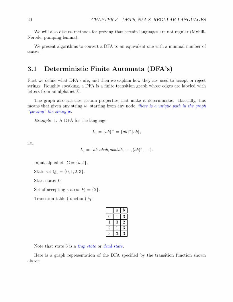
Example 1. A DFA for the language
L1 = ab+ = ab∗ab,
i.e.,
L1 = ab, abab, ababab, . . . , (ab)n, . . ..
Input alphabet: Σ = a, b.
State set Q1 = 0, 1, 2, 3.
Start state: 0.
Set of accepting states: F1 = 2.
Transition table (function) δ1:
a b
0 1 31 3 22 1 33 3 3
Note that state 3 is a trap state or dead state.
Here is a graph representation of the DFA specified by the transition function shownabove:
3.1. DETERMINISTIC FINITE AUTOMATA (DFA’S) 21
0 1 2
3
a
b
b
a
a
b
a, b
Figure 3.1: DFA for ab+
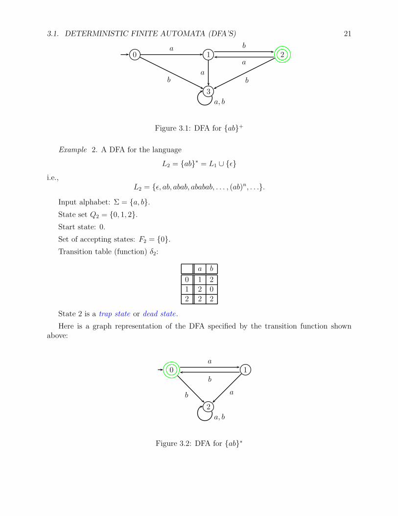
Example 2. A DFA for the language
L2 = ab∗ = L1 ∪ ǫi.e.,
L2 = ǫ, ab, abab, ababab, . . . , (ab)n, . . ..
Input alphabet: Σ = a, b.State set Q2 = 0, 1, 2.Start state: 0.
Set of accepting states: F2 = 0.Transition table (function) δ2:
a b
0 1 21 2 02 2 2
State 2 is a trap state or dead state.
Here is a graph representation of the DFA specified by the transition function shownabove:
0 1
2
b
a
b
a
a, b
Figure 3.2: DFA for ab∗
22 CHAPTER 3. DFA’S, NFA’S, REGULAR LANGUAGES
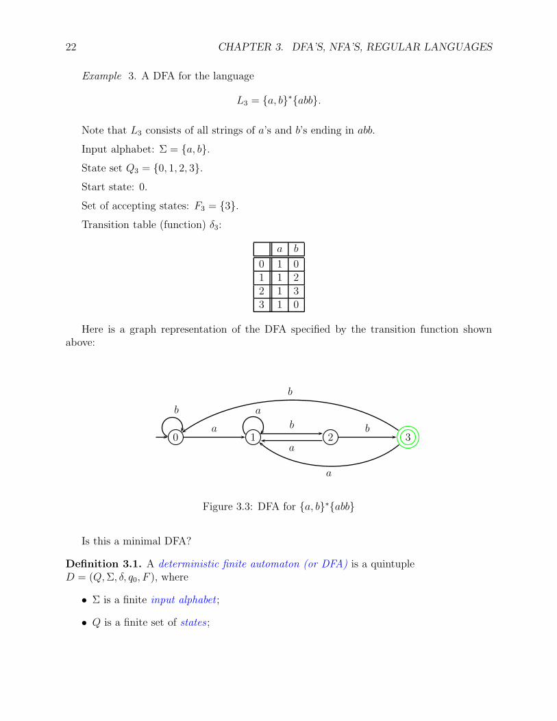
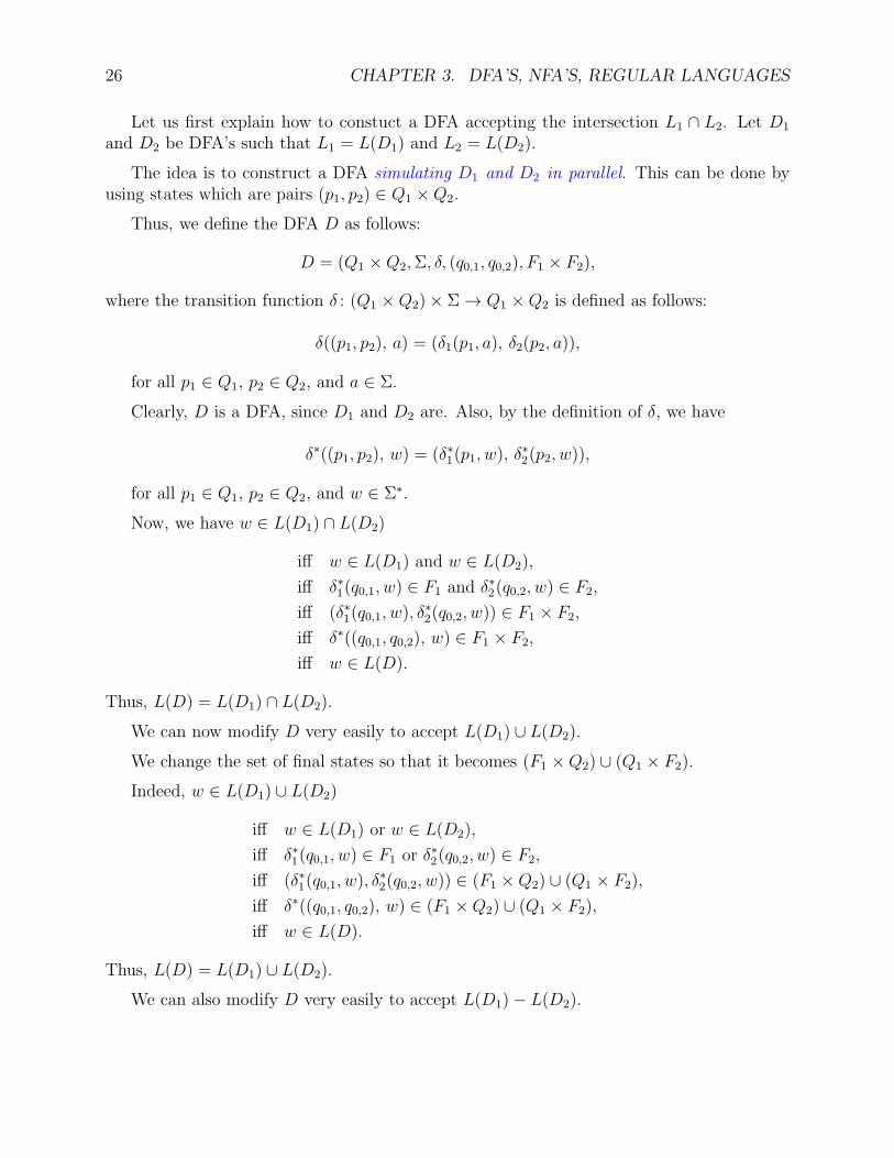
Example 3. A DFA for the language
L3 = a, b∗abb.
Note that L3 consists of all strings of a’s and b’s ending in abb.
Input alphabet: Σ = a, b.State set Q3 = 0, 1, 2, 3.Start state: 0.
Set of accepting states: F3 = 3.Transition table (function) δ3:
a b
0 1 01 1 22 1 33 1 0
Here is a graph representation of the DFA specified by the transition function shownabove:
0 1 2 3a b
a
b
b a
b
a
Figure 3.3: DFA for a, b∗abb
Is this a minimal DFA?
Definition 3.1. A deterministic finite automaton (or DFA) is a quintupleD = (Q,Σ, δ, q0, F ), where
• Σ is a finite input alphabet ;
• Q is a finite set of states ;
3.1. DETERMINISTIC FINITE AUTOMATA (DFA’S) 23
• F is a subset of Q of final (or accepting) states ;
• q0 ∈ Q is the start state (or initial state);
• δ is the transition function, a function
δ : Q× Σ→ Q.
For any state p ∈ Q and any input a ∈ Σ, the state q = δ(p, a) is uniquely determined.
Thus, it is possible to define the state reached from a given state p ∈ Q on input w ∈ Σ∗,following the path specified by w.
Technically, this is done by defining the extended transition function δ∗ : Q× Σ∗ → Q.
Definition 3.2. Given a DFA D = (Q,Σ, δ, q0, F ), the extended transition function δ∗ : Q×Σ∗ → Q is defined as follows:
δ∗(p, ǫ) = p,
δ∗(p, ua) = δ(δ∗(p, u), a),
where a ∈ Σ and u ∈ Σ∗.
It is immediate that δ∗(p, a) = δ(p, a) for a ∈ Σ.
The meaning of δ∗(p, w) is that it is the state reached from state p following the pathfrom p specified by w.
We can show (by induction on the length of v) that
δ∗(p, uv) = δ∗(δ∗(p, u), v) for all p ∈ Q and all u, v ∈ Σ∗
For the induction step, for u ∈ Σ∗, and all v = ya with y ∈ Σ∗ and a ∈ Σ,
δ∗(p, uya) = δ(δ∗(p, uy), a) by definition of δ∗
= δ(δ∗(δ∗(p, u), y), a) by induction
= δ∗(δ∗(p, u), ya) by definition of δ∗.
We can now define how a DFA accepts or rejects a string.
Definition 3.3. Given a DFA D = (Q,Σ, δ, q0, F ), the language L(D) accepted (or recog-nized) by D is the language
L(D) = w ∈ Σ∗ | δ∗(q0, w) ∈ F.
24 CHAPTER 3. DFA’S, NFA’S, REGULAR LANGUAGES
Thus, a string w ∈ Σ∗ is accepted iff the path from q0 on input w ends in a final state.
The definition of a DFA does not prevent the possibility that a DFA may have statesthat are not reachable from the start state q0, which means that there is no path from q0 tosuch states.
For example, in the DFA D1 defined by the transition table below and the set of finalstates F = 1, 2, 3, the states in the set 0, 1 are reachable from the start state 0, butthe states in the set 2, 3, 4 are not (even though there are transitions from 2, 3, 4 to 0, butthey go in the wrong direction).
a b
0 1 01 0 12 3 03 4 04 2 0
Since there is no path from the start state 0 to any of the states in 2, 3, 4, the states2, 3, 4 are useless as far as acceptance of strings, so they should be deleted as well as thetransitions from them.
Given a DFA D = (Q,Σ, δ, q0, F ), the above suggests defining the set Qr of reachable (oraccessible) states as
Qr = p ∈ Q | (∃u ∈ Σ∗)(p = δ∗(q0, u)).
The set Qr consists of those states p ∈ Q such that there is some path from q0 to p (alongsome string u).
Computing the set Qr is a reachability problem in a directed graph. There are variousalgorithms to solve this problem, including breadth-first search or depth-first search.
Once the set Qr has been computed, we can clean up the DFAD by deleting all redundantstates in Q−Qr and all transitions from these states.
More precisely, we form the DFA Dr = (Qr,Σ, δr, q0, Qr ∩ F ), where δr : Qr ×Σ→ Qr isthe restriction of δ : Q× Σ→ Q to Qr.
If D1 is the DFA of the previous example, then the DFA (D1)r is obtained by deletingthe states 2, 3, 4:
a b
0 1 01 0 1
It can be shown that L(Dr) = L(D) (see the homework problems).
3.2. THE “CROSS-PRODUCT” CONSTRUCTION 25
A DFA D such that Q = Qr is said to be trim (or reduced).
Observe that the DFA Dr is trim. A minimal DFA must be trim.
Computing Qr gives us a method to test whether a DFA D accepts a nonempty language.Indeed
L(D) 6= ∅ iff Qr ∩ F 6= ∅
We now come to the first of several equivalent definitions of the regular languages.
Regular Languages, Version 1
Definition 3.4. A language L is a regular language if it is accepted by some DFA.
Note that a regular language may be accepted by many different DFAs. Later on, wewill investigate how to find minimal DFA’s.
For a given regular language L, a minimal DFA for L is a DFA with the smallest number ofstates among all DFA’s accepting L. A minimal DFA for L must exist since every nonemptysubset of natural numbers has a smallest element.
In order to understand how complex the regular languages are, we will investigate theclosure properties of the regular languages under union, intersection, complementation, con-catenation, and Kleene ∗.
It turns out that the family of regular languages is closed under all these operations. Forunion, intersection, and complementation, we can use the cross-product construction whichpreserves determinism.
However, for concatenation and Kleene ∗, there does not appear to be any methodinvolving DFA’s only. The way to do it is to introduce nondeterministic finite automata(NFA’s), which we do a little later.
3.2 The “Cross-product” Construction
Let Σ = a1, . . . , am be an alphabet.
Given any two DFA’s D1 = (Q1,Σ, δ1, q0,1, F1) andD2 = (Q2,Σ, δ2, q0,2, F2), there is a very useful construction for showing that the union, theintersection, or the relative complement of regular languages, is a regular language.
Given any two languages L1, L2 over Σ, recall that
L1 ∪ L2 = w ∈ Σ∗ | w ∈ L1 or w ∈ L2,L1 ∩ L2 = w ∈ Σ∗ | w ∈ L1 and w ∈ L2,L1 − L2 = w ∈ Σ∗ | w ∈ L1 and w /∈ L2.
26 CHAPTER 3. DFA’S, NFA’S, REGULAR LANGUAGES
Let us first explain how to constuct a DFA accepting the intersection L1 ∩ L2. Let D1
and D2 be DFA’s such that L1 = L(D1) and L2 = L(D2).
The idea is to construct a DFA simulating D1 and D2 in parallel. This can be done byusing states which are pairs (p1, p2) ∈ Q1 ×Q2.
Thus, we define the DFA D as follows:
D = (Q1 ×Q2,Σ, δ, (q0,1, q0,2), F1 × F2),
where the transition function δ : (Q1 ×Q2)× Σ→ Q1 ×Q2 is defined as follows:
δ((p1, p2), a) = (δ1(p1, a), δ2(p2, a)),
for all p1 ∈ Q1, p2 ∈ Q2, and a ∈ Σ.
Clearly, D is a DFA, since D1 and D2 are. Also, by the definition of δ, we have
δ∗((p1, p2), w) = (δ∗1(p1, w), δ∗2(p2, w)),
for all p1 ∈ Q1, p2 ∈ Q2, and w ∈ Σ∗.
Now, we have w ∈ L(D1) ∩ L(D2)
iff w ∈ L(D1) and w ∈ L(D2),
iff δ∗1(q0,1, w) ∈ F1 and δ∗2(q0,2, w) ∈ F2,
iff (δ∗1(q0,1, w), δ∗2(q0,2, w)) ∈ F1 × F2,
iff δ∗((q0,1, q0,2), w) ∈ F1 × F2,
iff w ∈ L(D).
Thus, L(D) = L(D1) ∩ L(D2).
We can now modify D very easily to accept L(D1) ∪ L(D2).
We change the set of final states so that it becomes (F1 ×Q2) ∪ (Q1 × F2).
Indeed, w ∈ L(D1) ∪ L(D2)
iff w ∈ L(D1) or w ∈ L(D2),
iff δ∗1(q0,1, w) ∈ F1 or δ∗2(q0,2, w) ∈ F2,
iff (δ∗1(q0,1, w), δ∗2(q0,2, w)) ∈ (F1 ×Q2) ∪ (Q1 × F2),
iff δ∗((q0,1, q0,2), w) ∈ (F1 ×Q2) ∪ (Q1 × F2),
iff w ∈ L(D).
Thus, L(D) = L(D1) ∪ L(D2).
We can also modify D very easily to accept L(D1)− L(D2).
3.3. NONDETETERMINISTIC FINITE AUTOMATA (NFA’S) 27
We change the set of final states so that it becomes F1 × (Q2 − F2).
Indeed, w ∈ L(D1)− L(D2)
iff w ∈ L(D1) and w /∈ L(D2),
iff δ∗1(q0,1, w) ∈ F1 and δ∗2(q0,2, w) /∈ F2,
iff (δ∗1(q0,1, w), δ∗2(q0,2, w)) ∈ F1 × (Q2 − F2),
iff δ∗((q0,1, q0,2), w) ∈ F1 × (Q2 − F2),
iff w ∈ L(D).
Thus, L(D) = L(D1)− L(D2).
In all cases, if D1 has n1 states and D2 has n2 states, the DFA D has n1n2 states.
3.3 Nondeteterministic Finite Automata (NFA’s)
NFA’s are obtained from DFA’s by allowing multiple transitions from a given state on agiven input. This can be done by defining δ(p, a) as a subset of Q rather than a single state.It will also be convenient to allow transitions on input ǫ.
We let 2Q denote the set of all subsets of Q, including the empty set. The set 2Q is thepower set of Q.
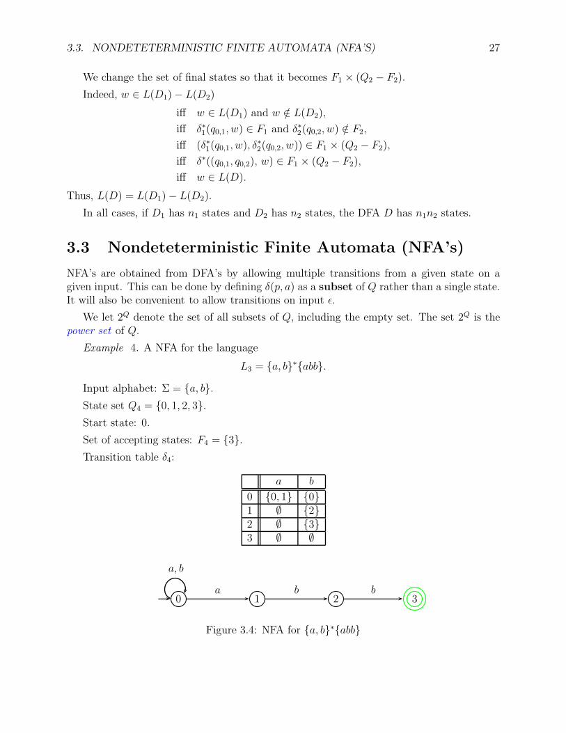
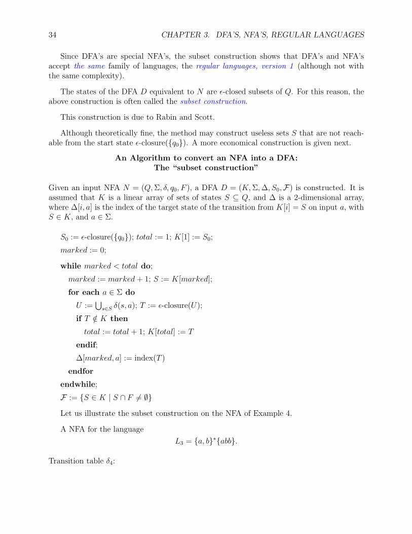
Example 4. A NFA for the language
L3 = a, b∗abb.
Input alphabet: Σ = a, b.State set Q4 = 0, 1, 2, 3.Start state: 0.
Set of accepting states: F4 = 3.Transition table δ4:
a b
0 0, 1 01 ∅ 22 ∅ 33 ∅ ∅
0 1 2 3a b b
a, b
Figure 3.4: NFA for a, b∗abb
28 CHAPTER 3. DFA’S, NFA’S, REGULAR LANGUAGES
Example 5. Let Σ = a1, . . . , an, letLin = w ∈ Σ∗ | w contains an odd number of ai’s,
and letLn = L1
n ∪ L2n ∪ · · · ∪ Ln
n.
The language Ln consists of those strings in Σ∗ that contain an odd number of someletter ai ∈ Σ.
Equivalently Σ∗ −Ln consists of those strings in Σ∗ with an even number of every letterai ∈ Σ.
It can be shown that every DFA accepting Ln has at least 2n states.
However, there is an NFA with 2n+ 1 states accepting Ln.
We define NFA’s as follows.
Definition 3.5. A nondeterministic finite automaton (or NFA) is a quintupleN = (Q,Σ, δ, q0, F ), where
• Σ is a finite input alphabet ;
• Q is a finite set of states ;
• F is a subset of Q of final (or accepting) states ;
• q0 ∈ Q is the start state (or initial state);
• δ is the transition function, a function
δ : Q× (Σ ∪ ǫ)→ 2Q.
For any state p ∈ Q and any input a ∈ Σ ∪ ǫ, the set of states δ(p, a) is uniquelydetermined. We write q ∈ δ(p, a).
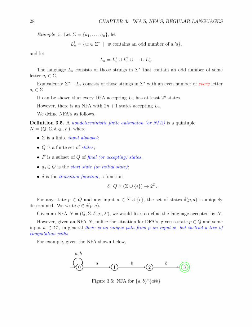
Given an NFA N = (Q,Σ, δ, q0, F ), we would like to define the language accepted by N .
However, given an NFA N , unlike the situation for DFA’s, given a state p ∈ Q and someinput w ∈ Σ∗, in general there is no unique path from p on input w, but instead a tree ofcomputation paths .
For example, given the NFA shown below,
0 1 2 3a b b
a, b
Figure 3.5: NFA for a, b∗abb
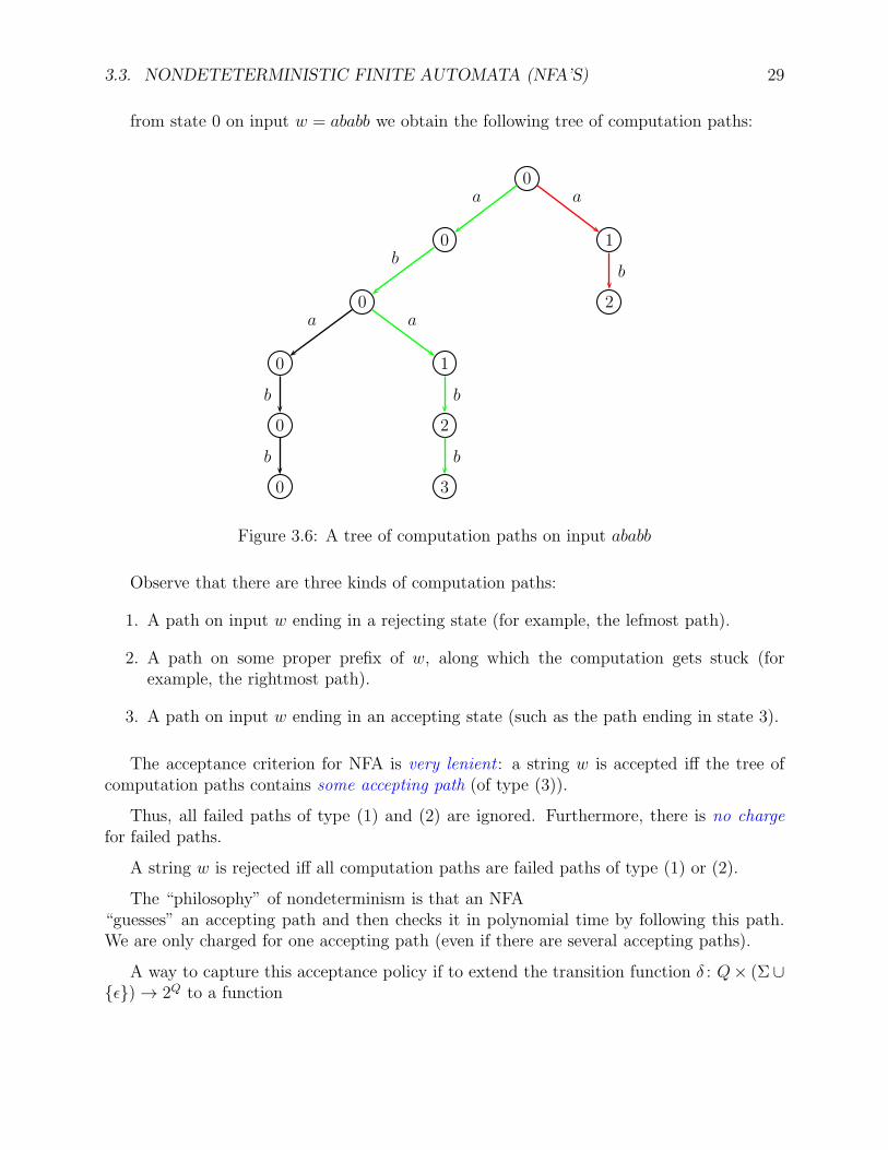
3.3. NONDETETERMINISTIC FINITE AUTOMATA (NFA’S) 29
from state 0 on input w = ababb we obtain the following tree of computation paths:
0
0
0
3
2
1
0
0
2
1
0a a
bb
a
b
b
a
b
b
Figure 3.6: A tree of computation paths on input ababb
Observe that there are three kinds of computation paths:
1. A path on input w ending in a rejecting state (for example, the lefmost path).
2. A path on some proper prefix of w, along which the computation gets stuck (forexample, the rightmost path).
3. A path on input w ending in an accepting state (such as the path ending in state 3).
The acceptance criterion for NFA is very lenient : a string w is accepted iff the tree ofcomputation paths contains some accepting path (of type (3)).
Thus, all failed paths of type (1) and (2) are ignored. Furthermore, there is no chargefor failed paths.
A string w is rejected iff all computation paths are failed paths of type (1) or (2).
The “philosophy” of nondeterminism is that an NFA“guesses” an accepting path and then checks it in polynomial time by following this path.We are only charged for one accepting path (even if there are several accepting paths).
A way to capture this acceptance policy if to extend the transition function δ : Q× (Σ∪ǫ)→ 2Q to a function
30 CHAPTER 3. DFA’S, NFA’S, REGULAR LANGUAGES
δ∗ : Q× Σ∗ → 2Q.
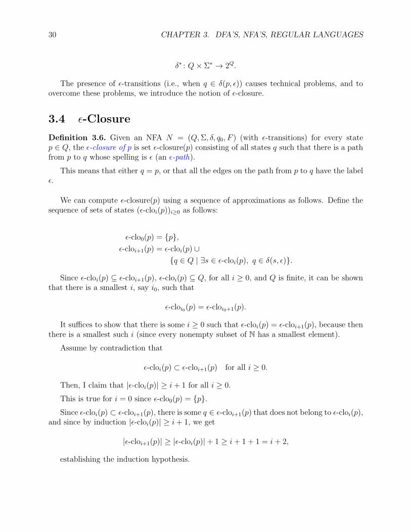
The presence of ǫ-transitions (i.e., when q ∈ δ(p, ǫ)) causes technical problems, and toovercome these problems, we introduce the notion of ǫ-closure.
3.4 ǫ-Closure
Definition 3.6. Given an NFA N = (Q,Σ, δ, q0, F ) (with ǫ-transitions) for every statep ∈ Q, the ǫ-closure of p is set ǫ-closure(p) consisting of all states q such that there is a pathfrom p to q whose spelling is ǫ (an ǫ-path).
This means that either q = p, or that all the edges on the path from p to q have the labelǫ.
We can compute ǫ-closure(p) using a sequence of approximations as follows. Define thesequence of sets of states (ǫ-cloi(p))i≥0 as follows:
ǫ-clo0(p) = p,ǫ-cloi+1(p) = ǫ-cloi(p) ∪
q ∈ Q | ∃s ∈ ǫ-cloi(p), q ∈ δ(s, ǫ).
Since ǫ-cloi(p) ⊆ ǫ-cloi+1(p), ǫ-cloi(p) ⊆ Q, for all i ≥ 0, and Q is finite, it can be shownthat there is a smallest i, say i0, such that
ǫ-cloi0(p) = ǫ-cloi0+1(p).
It suffices to show that there is some i ≥ 0 such that ǫ-cloi(p) = ǫ-cloi+1(p), because thenthere is a smallest such i (since every nonempty subset of N has a smallest element).
Assume by contradiction that
ǫ-cloi(p) ⊂ ǫ-cloi+1(p) for all i ≥ 0.
Then, I claim that |ǫ-cloi(p)| ≥ i+ 1 for all i ≥ 0.
This is true for i = 0 since ǫ-clo0(p) = p.Since ǫ-cloi(p) ⊂ ǫ-cloi+1(p), there is some q ∈ ǫ-cloi+1(p) that does not belong to ǫ-cloi(p),
and since by induction |ǫ-cloi(p)| ≥ i+ 1, we get
|ǫ-cloi+1(p)| ≥ |ǫ-cloi(p)|+ 1 ≥ i+ 1 + 1 = i+ 2,
establishing the induction hypothesis.
3.4. ǫ-CLOSURE 31
If n = |Q|, then |ǫ-clon(p)| ≥ n+ 1, a contradiction.
Therefore, there is indeed some i ≥ 0 such thatǫ-cloi(p) = ǫ-cloi+1(p), and for the least such i = i0, we have i0 ≤ n− 1.
It can also be shown that
ǫ-closure(p) = ǫ-cloi0(p),
by proving that
1. ǫ-cloi(p) ⊆ ǫ-closure(p), for all i ≥ 0.
2. ǫ-closure(p)i ⊆ ǫ-cloi0(p), for all i ≥ 0.
where ǫ-closure(p)i is the set of states reachable from p by an ǫ-path of length ≤ i.
When N has no ǫ-transitions, i.e., when δ(p, ǫ) = ∅ for all p ∈ Q (which means that δcan be viewed as a function δ : Q× Σ→ 2Q), we have
ǫ-closure(p) = p.
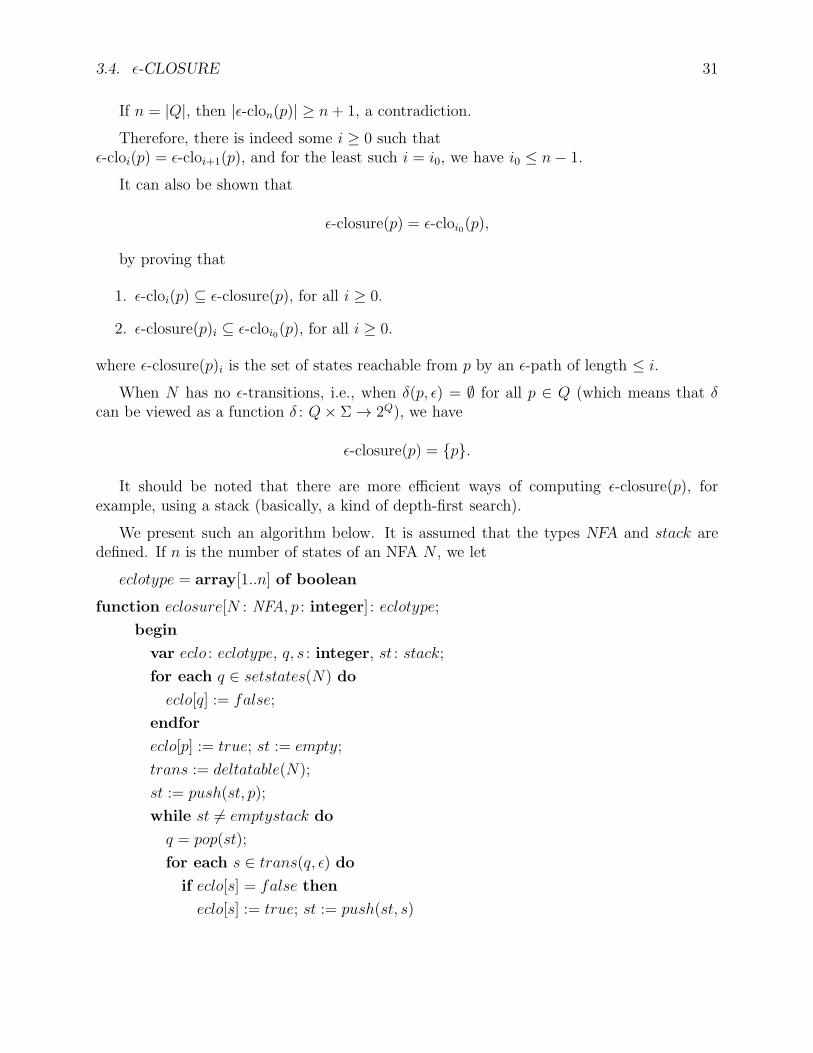
It should be noted that there are more efficient ways of computing ǫ-closure(p), forexample, using a stack (basically, a kind of depth-first search).
We present such an algorithm below. It is assumed that the types NFA and stack aredefined. If n is the number of states of an NFA N , we let
eclotype = array[1..n] of boolean
function eclosure[N : NFA, p : integer] : eclotype;
begin
var eclo : eclotype, q, s : integer, st : stack;
for each q ∈ setstates(N) do
eclo[q] := false;
endfor
eclo[p] := true; st := empty;
trans := deltatable(N);
st := push(st, p);
while st 6= emptystack do
q = pop(st);
for each s ∈ trans(q, ǫ) doif eclo[s] = false then
eclo[s] := true; st := push(st, s)
32 CHAPTER 3. DFA’S, NFA’S, REGULAR LANGUAGES
endif
endfor
endwhile;
eclosure := eclo
end
This algorithm can be easily adapted to compute the set of states reachable from a givenstate p (in a DFA or an NFA).
Given a subset S of Q, we define ǫ-closure(S) as
ǫ-closure(S) =⋃
s∈S
ǫ-closure(s),
with
ǫ-closure(∅) = ∅.When N has no ǫ-transitions, we have
ǫ-closure(S) = S.
We are now ready to define the extension δ∗ : Q × Σ∗ → 2Q of the transition functionδ : Q× (Σ ∪ ǫ)→ 2Q.
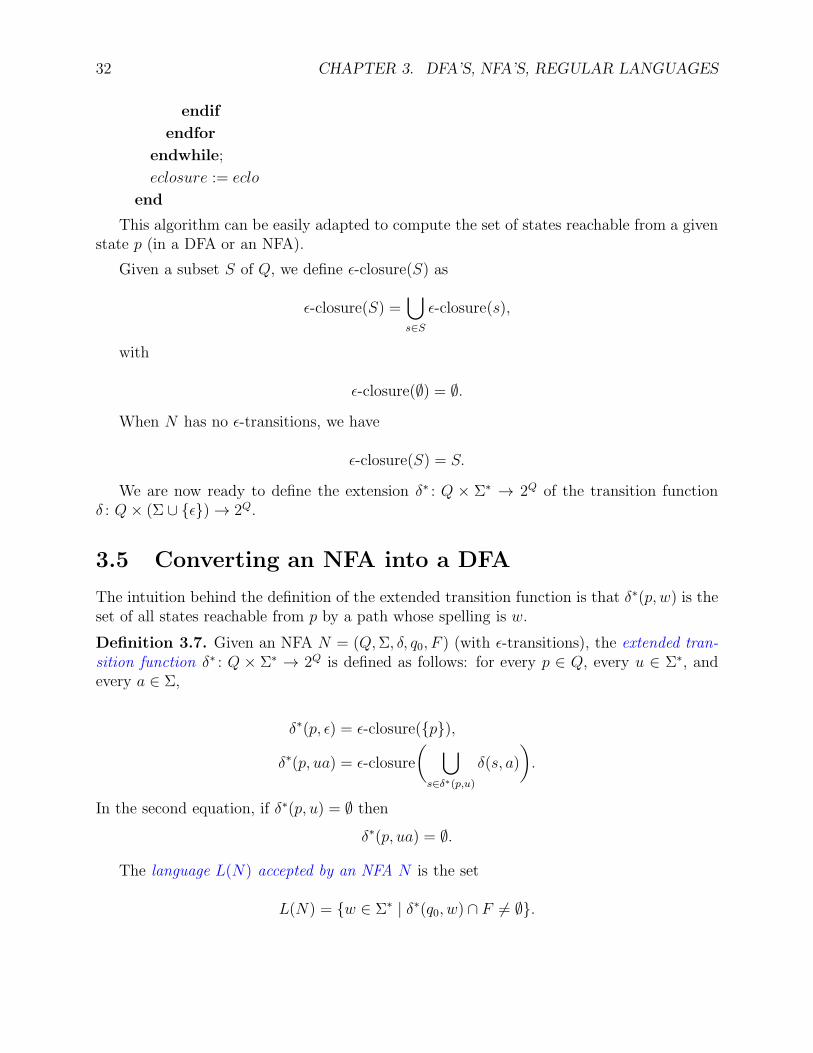
3.5 Converting an NFA into a DFA
The intuition behind the definition of the extended transition function is that δ∗(p, w) is theset of all states reachable from p by a path whose spelling is w.
Definition 3.7. Given an NFA N = (Q,Σ, δ, q0, F ) (with ǫ-transitions), the extended tran-sition function δ∗ : Q × Σ∗ → 2Q is defined as follows: for every p ∈ Q, every u ∈ Σ∗, andevery a ∈ Σ,
δ∗(p, ǫ) = ǫ-closure(p),
δ∗(p, ua) = ǫ-closure
( ⋃
s∈δ∗(p,u)
δ(s, a)
).
In the second equation, if δ∗(p, u) = ∅ thenδ∗(p, ua) = ∅.
The language L(N) accepted by an NFA N is the set
L(N) = w ∈ Σ∗ | δ∗(q0, w) ∩ F 6= ∅.
3.5. CONVERTING AN NFA INTO A DFA 33
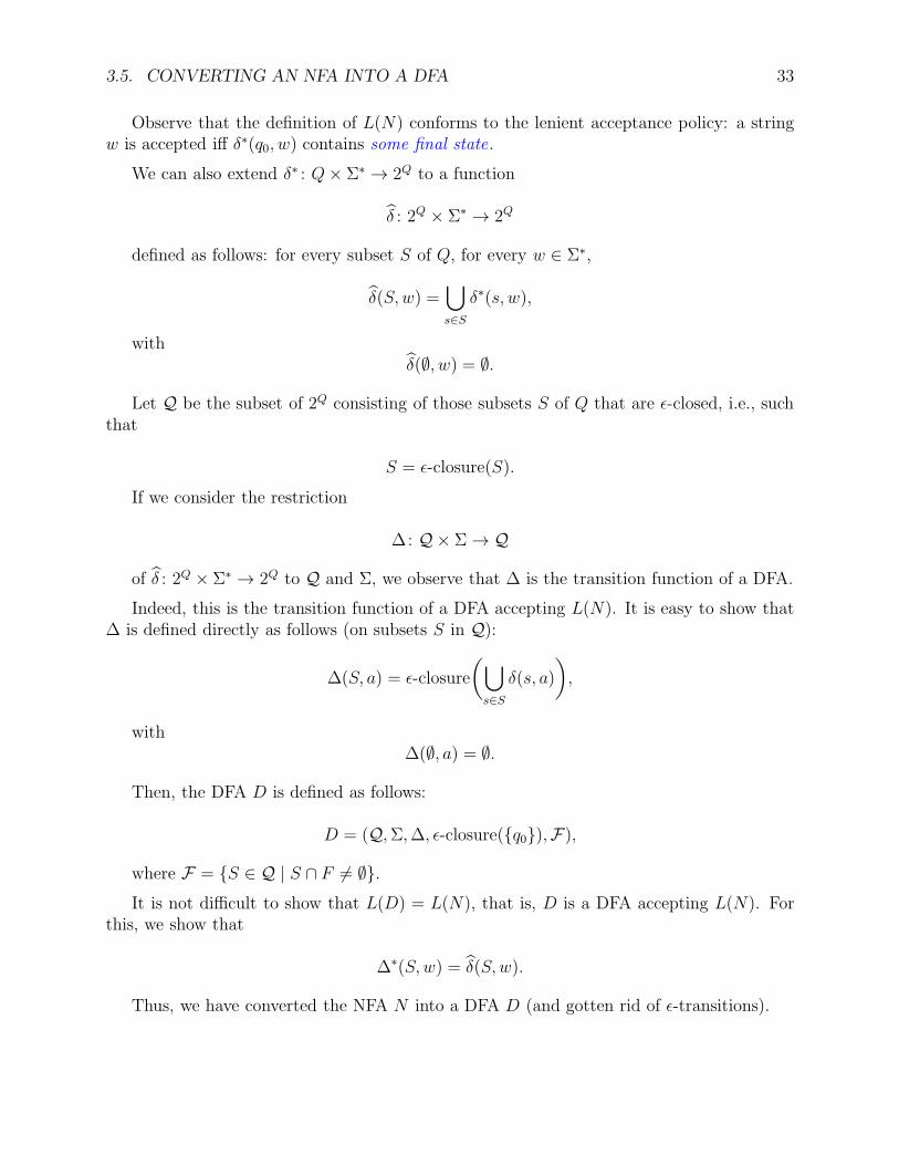
Observe that the definition of L(N) conforms to the lenient acceptance policy: a stringw is accepted iff δ∗(q0, w) contains some final state.
We can also extend δ∗ : Q× Σ∗ → 2Q to a function
δ : 2Q × Σ∗ → 2Q
defined as follows: for every subset S of Q, for every w ∈ Σ∗,
δ(S, w) =⋃
s∈S
δ∗(s, w),
withδ(∅, w) = ∅.
Let Q be the subset of 2Q consisting of those subsets S of Q that are ǫ-closed, i.e., suchthat
S = ǫ-closure(S).
If we consider the restriction
∆: Q× Σ→ Q
of δ : 2Q × Σ∗ → 2Q to Q and Σ, we observe that ∆ is the transition function of a DFA.
Indeed, this is the transition function of a DFA accepting L(N). It is easy to show that∆ is defined directly as follows (on subsets S in Q):
∆(S, a) = ǫ-closure
(⋃
s∈S
δ(s, a)
),
with∆(∅, a) = ∅.
Then, the DFA D is defined as follows:
D = (Q,Σ,∆, ǫ-closure(q0),F),
where F = S ∈ Q | S ∩ F 6= ∅.It is not difficult to show that L(D) = L(N), that is, D is a DFA accepting L(N). For
this, we show that
∆∗(S, w) = δ(S, w).
Thus, we have converted the NFA N into a DFA D (and gotten rid of ǫ-transitions).
34 CHAPTER 3. DFA’S, NFA’S, REGULAR LANGUAGES
Since DFA’s are special NFA’s, the subset construction shows that DFA’s and NFA’saccept the same family of languages, the regular languages, version 1 (although not withthe same complexity).
The states of the DFA D equivalent to N are ǫ-closed subsets of Q. For this reason, theabove construction is often called the subset construction.
This construction is due to Rabin and Scott.
Although theoretically fine, the method may construct useless sets S that are not reach-able from the start state ǫ-closure(q0). A more economical construction is given next.
An Algorithm to convert an NFA into a DFA:The “subset construction”
Given an input NFA N = (Q,Σ, δ, q0, F ), a DFA D = (K,Σ,∆, S0,F) is constructed. It isassumed that K is a linear array of sets of states S ⊆ Q, and ∆ is a 2-dimensional array,where ∆[i, a] is the index of the target state of the transition from K[i] = S on input a, withS ∈ K, and a ∈ Σ.
S0 := ǫ-closure(q0); total := 1; K[1] := S0;
marked := 0;
while marked < total do;
marked := marked + 1; S := K[marked];
for each a ∈ Σ do
U :=⋃
s∈S δ(s, a); T := ǫ-closure(U);
if T /∈ K then
total := total + 1; K[total] := T
endif;
∆[marked, a] := index(T )
endfor
endwhile;
F := S ∈ K | S ∩ F 6= ∅
Let us illustrate the subset construction on the NFA of Example 4.
A NFA for the language
L3 = a, b∗abb.
Transition table δ4:
3.5. CONVERTING AN NFA INTO A DFA 35
a b
0 0, 1 01 ∅ 22 ∅ 33 ∅ ∅
Set of accepting states: F4 = 3.
0 1 2 3a b b
a, b
Figure 3.7: NFA for a, b∗abb
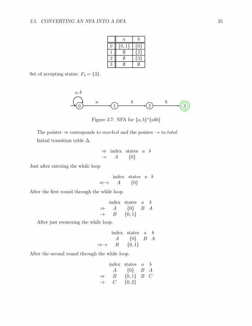
The pointer ⇒ corresponds to marked and the pointer → to total.
Initial transition table ∆.
⇒ index states a b→ A 0
Just after entering the while loop
index states a b⇒→ A 0
After the first round through the while loop.
index states a b⇒ A 0 B A→ B 0, 1
After just reentering the while loop.
index states a bA 0 B A
⇒→ B 0, 1After the second round through the while loop.
index states a bA 0 B A
⇒ B 0, 1 B C→ C 0, 2
36 CHAPTER 3. DFA’S, NFA’S, REGULAR LANGUAGES
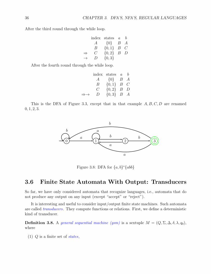
After the third round through the while loop.
index states a bA 0 B AB 0, 1 B C
⇒ C 0, 2 B D→ D 0, 3
After the fourth round through the while loop.
index states a bA 0 B AB 0, 1 B CC 0, 2 B D
⇒→ D 0, 3 B A
This is the DFA of Figure 3.3, except that in that example A,B,C,D are renamed0, 1, 2, 3.
0 1 2 3a b
a
b
b a
b
a
Figure 3.8: DFA for a, b∗abb
3.6 Finite State Automata With Output: Transducers
So far, we have only considered automata that recognize languages, i.e., automata that donot produce any output on any input (except “accept” or “reject”).
It is interesting and useful to consider input/output finite state machines. Such automataare called transducers . They compute functions or relations. First, we define a deterministickind of transducer.
Definition 3.8. A general sequential machine (gsm) is a sextuple M = (Q,Σ,∆, δ, λ, q0),where
(1) Q is a finite set of states ,
3.6. FINITE STATE AUTOMATA WITH OUTPUT: TRANSDUCERS 37
(2) Σ is a finite input alphabet ,
(3) ∆ is a finite output alphabet ,
(4) δ : Q× Σ→ Q is the transition function,
(5) λ : Q× Σ→ ∆∗ is the output function and
(6) q0 is the initial (or start) state.
If λ(p, a) 6= ǫ, for all p ∈ Q and all a ∈ Σ, then M is nonerasing . If λ(p, a) ∈ ∆ for allp ∈ Q and all a ∈ Σ, we say that M is a complete sequential machine (csm).
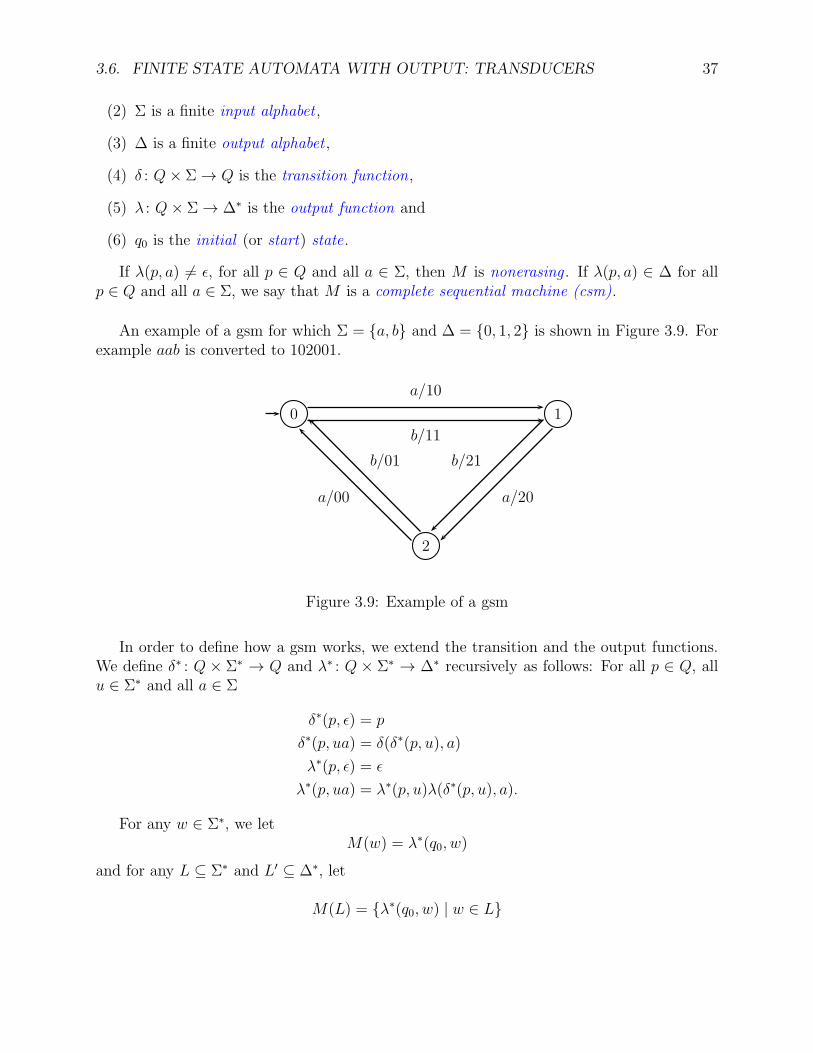
An example of a gsm for which Σ = a, b and ∆ = 0, 1, 2 is shown in Figure 3.9. Forexample aab is converted to 102001.
0 1
2
a/00
b/01
a/10
b/11
a/20
b/21
Figure 3.9: Example of a gsm
In order to define how a gsm works, we extend the transition and the output functions.We define δ∗ : Q × Σ∗ → Q and λ∗ : Q × Σ∗ → ∆∗ recursively as follows: For all p ∈ Q, allu ∈ Σ∗ and all a ∈ Σ
δ∗(p, ǫ) = p
δ∗(p, ua) = δ(δ∗(p, u), a)
λ∗(p, ǫ) = ǫ
λ∗(p, ua) = λ∗(p, u)λ(δ∗(p, u), a).
For any w ∈ Σ∗, we letM(w) = λ∗(q0, w)
and for any L ⊆ Σ∗ and L′ ⊆ ∆∗, let
M(L) = λ∗(q0, w) | w ∈ L
38 CHAPTER 3. DFA’S, NFA’S, REGULAR LANGUAGES
and
M−1(L′) = w ∈ Σ∗ | λ∗(q0, w) ∈ L′.
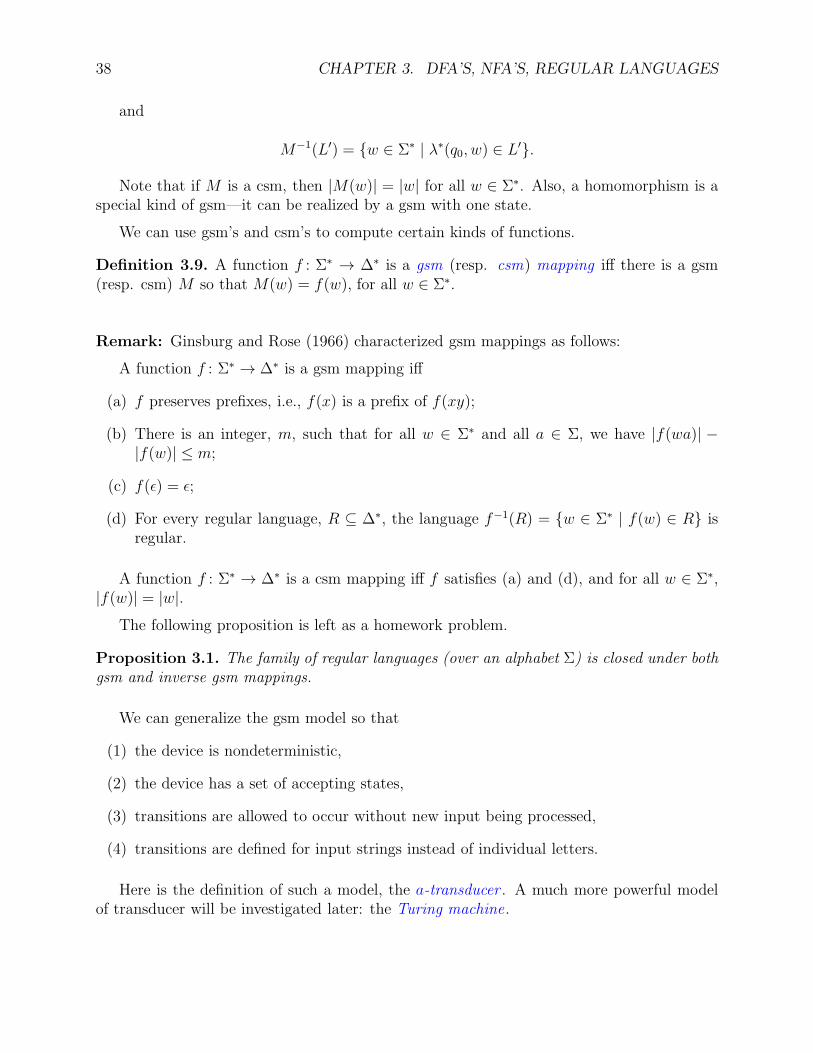
Note that if M is a csm, then |M(w)| = |w| for all w ∈ Σ∗. Also, a homomorphism is aspecial kind of gsm—it can be realized by a gsm with one state.
We can use gsm’s and csm’s to compute certain kinds of functions.
Definition 3.9. A function f : Σ∗ → ∆∗ is a gsm (resp. csm) mapping iff there is a gsm(resp. csm) M so that M(w) = f(w), for all w ∈ Σ∗.
Remark: Ginsburg and Rose (1966) characterized gsm mappings as follows:
A function f : Σ∗ → ∆∗ is a gsm mapping iff
(a) f preserves prefixes, i.e., f(x) is a prefix of f(xy);
(b) There is an integer, m, such that for all w ∈ Σ∗ and all a ∈ Σ, we have |f(wa)| −|f(w)| ≤ m;
(c) f(ǫ) = ǫ;
(d) For every regular language, R ⊆ ∆∗, the language f−1(R) = w ∈ Σ∗ | f(w) ∈ R isregular.
A function f : Σ∗ → ∆∗ is a csm mapping iff f satisfies (a) and (d), and for all w ∈ Σ∗,|f(w)| = |w|.
The following proposition is left as a homework problem.
Proposition 3.1. The family of regular languages (over an alphabet Σ) is closed under bothgsm and inverse gsm mappings.
We can generalize the gsm model so that
(1) the device is nondeterministic,
(2) the device has a set of accepting states,
(3) transitions are allowed to occur without new input being processed,
(4) transitions are defined for input strings instead of individual letters.
Here is the definition of such a model, the a-transducer . A much more powerful modelof transducer will be investigated later: the Turing machine.
3.6. FINITE STATE AUTOMATA WITH OUTPUT: TRANSDUCERS 39
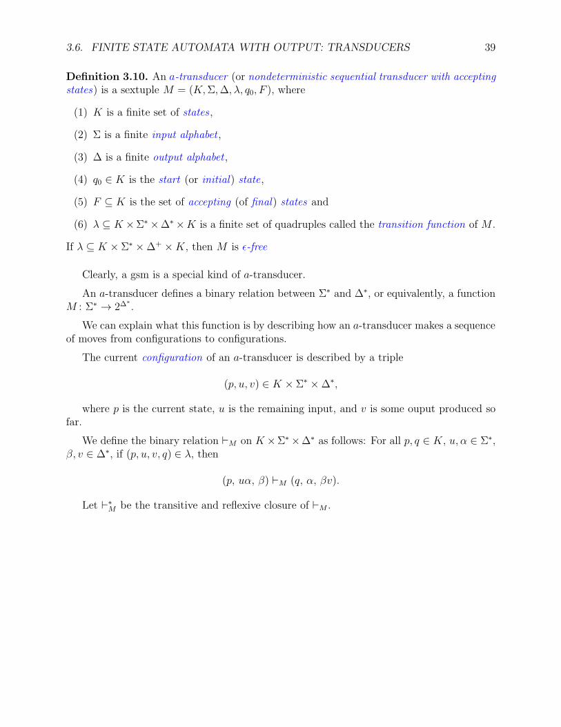
Definition 3.10. An a-transducer (or nondeterministic sequential transducer with acceptingstates) is a sextuple M = (K,Σ,∆, λ, q0, F ), where
(1) K is a finite set of states ,
(2) Σ is a finite input alphabet ,
(3) ∆ is a finite output alphabet ,
(4) q0 ∈ K is the start (or initial) state,
(5) F ⊆ K is the set of accepting (of final) states and
(6) λ ⊆ K ×Σ∗×∆∗×K is a finite set of quadruples called the transition function of M .
If λ ⊆ K × Σ∗ ×∆+ ×K, then M is ǫ-free
Clearly, a gsm is a special kind of a-transducer.
An a-transducer defines a binary relation between Σ∗ and ∆∗, or equivalently, a functionM : Σ∗ → 2∆
∗
.
We can explain what this function is by describing how an a-transducer makes a sequenceof moves from configurations to configurations.
The current configuration of an a-transducer is described by a triple
(p, u, v) ∈ K × Σ∗ ×∆∗,
where p is the current state, u is the remaining input, and v is some ouput produced sofar.
We define the binary relation ⊢M on K ×Σ∗×∆∗ as follows: For all p, q ∈ K, u, α ∈ Σ∗,β, v ∈ ∆∗, if (p, u, v, q) ∈ λ, then
(p, uα, β) ⊢M (q, α, βv).
Let ⊢∗M be the transitive and reflexive closure of ⊢M .

40 CHAPTER 3. DFA’S, NFA’S, REGULAR LANGUAGES
The function M : Σ∗ → 2∆∗
is defined such that for every w ∈ Σ∗,
M(w) = y ∈ ∆∗ | (q0, w, ǫ) ⊢∗M (f, ǫ, y), f ∈ F.
For any language L ⊆ Σ∗ let
M(L) =⋃
w∈L
M(w).
For any y ∈ ∆∗, let
M−1(y) = w ∈ Σ∗ | y ∈M(w)
and for any language L′ ⊆ ∆∗, let
M−1(L′) =⋃
y∈L′
M−1(y).
Remark: Notice that if w ∈M−1(L′), then there exists some y ∈ L′ such that w ∈M−1(y),i.e.,y ∈M(w). This does not imply that M(w) ⊆ L′, only that M(w) ∩ L′ 6= ∅.
One should realize that for any L′ ⊆ ∆∗ and any a-transducer, M , there is some a-transducer, M ′, (from ∆∗ to 2Σ
∗
) so that M ′(L′) =M−1(L′).
The following proposition is left as a homework problem:
Proposition 3.2. The family of regular languages (over an alphabet Σ) is closed under botha-transductions and inverse a-transductions.
3.7 An Application of NFA’s: Text Search
A common problem in the age of the Web (and on-line text repositories) is the following:
Given a set of words, called the keywords , find all the documents that contain one (orall) of those words.
Search engines are a popular example of this process. Search engines use inverted indexes(for each word appearing on the Web, a list of all the places where that word occurs is stored).
However, there are applications that are unsuited for inverted indexes, but are good forautomaton-based techniques.
Some text-processing programs, such as advanced forms of the UNIX grep command(such as egrep or fgrep) are based on automaton-based techniques.
The characteristics that make an application suitable for searches that use automata are:
3.7. AN APPLICATION OF NFA’S: TEXT SEARCH 41
(1) The repository on which the search is conducted is rapidly changing.
(2) The documents to be searched cannot be catalogued. For example, Amazon.com cre-ates pages “on the fly” in response to queries.
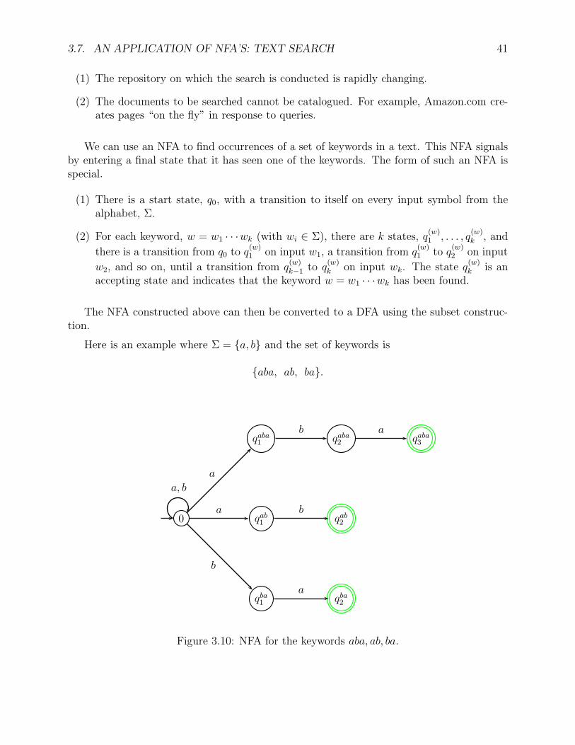
We can use an NFA to find occurrences of a set of keywords in a text. This NFA signalsby entering a final state that it has seen one of the keywords. The form of such an NFA isspecial.
(1) There is a start state, q0, with a transition to itself on every input symbol from thealphabet, Σ.
(2) For each keyword, w = w1 · · ·wk (with wi ∈ Σ), there are k states, q(w)1 , . . . , q
(w)k , and
there is a transition from q0 to q(w)1 on input w1, a transition from q
(w)1 to q
(w)2 on input
w2, and so on, until a transition from q(w)k−1 to q
(w)k on input wk. The state q
(w)k is an
accepting state and indicates that the keyword w = w1 · · ·wk has been found.
The NFA constructed above can then be converted to a DFA using the subset construc-tion.
Here is an example where Σ = a, b and the set of keywords is
aba, ab, ba.
0
qaba1 qaba2 qaba3
qab1 qab2
qba1 qba2
a
b a
a b
b
a
a, b
Figure 3.10: NFA for the keywords aba, ab, ba.
42 CHAPTER 3. DFA’S, NFA’S, REGULAR LANGUAGES
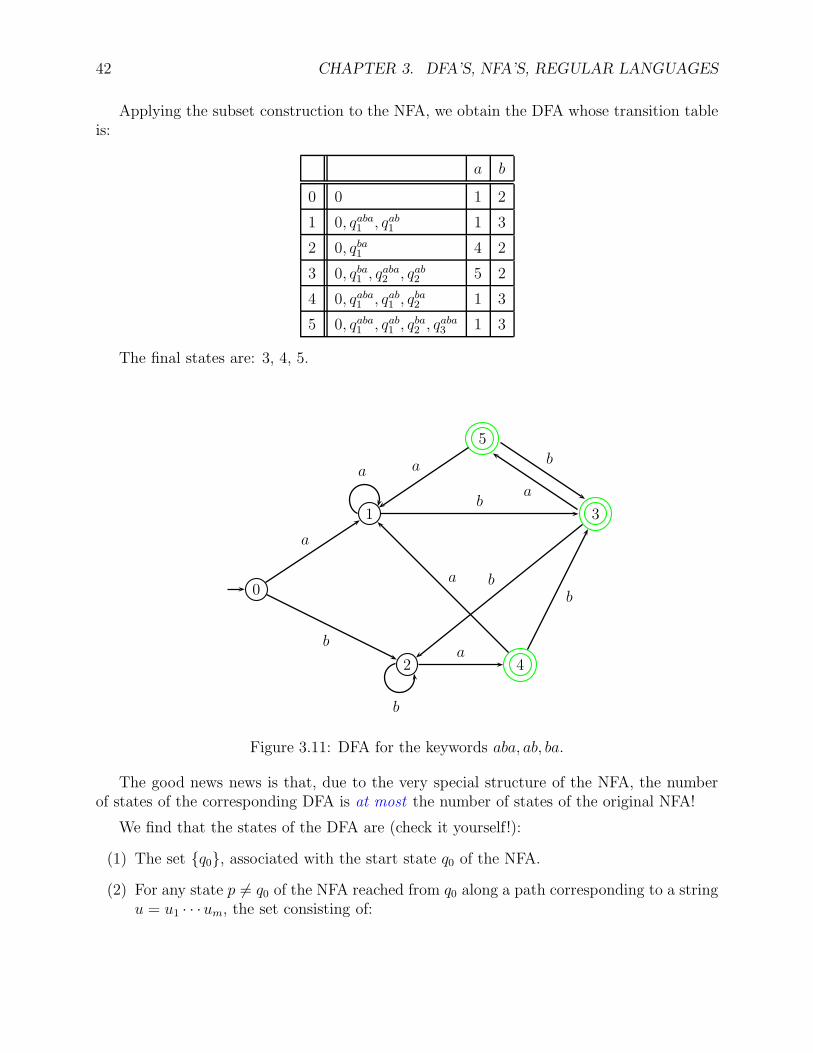
Applying the subset construction to the NFA, we obtain the DFA whose transition tableis:
a b
0 0 1 2
1 0, qaba1 , qab1 1 3
2 0, qba1 4 2
3 0, qba1 , qaba2 , qab2 5 2
4 0, qaba1 , qab1 , qba2 1 3
5 0, qaba1 , qab1 , qba2 , q
aba3 1 3
The final states are: 3, 4, 5.
0
1
2
3
4
5
a
b
b
a
ba
a
ba
b
a
b
Figure 3.11: DFA for the keywords aba, ab, ba.
The good news news is that, due to the very special structure of the NFA, the numberof states of the corresponding DFA is at most the number of states of the original NFA!
We find that the states of the DFA are (check it yourself!):
(1) The set q0, associated with the start state q0 of the NFA.
(2) For any state p 6= q0 of the NFA reached from q0 along a path corresponding to a stringu = u1 · · ·um, the set consisting of:
3.7. AN APPLICATION OF NFA’S: TEXT SEARCH 43
(a) q0
(b) p
(c) The set of all states q of the NFA reachable from q0 by following a path whosesymbols form a nonempty suffix of u, i.e., a string of the formujuj+1 · · ·um.
As a consequence, we get an efficient (w.r.t. time and space) method to recognize a setof keywords. In fact, this DFA recognizes leftmost occurrences of keywords in a text (we canstop as soon as we enter a final state).
44 CHAPTER 3. DFA’S, NFA’S, REGULAR LANGUAGES
Chapter 4
Hidden Markov Models (HMMs)
4.1 Hidden Markov Models (HMMs)
There is a variant of the notion of DFA with ouput, for example a transducer such asa gsm (generalized sequential machine), which is widely used in machine learning. Thismachine model is known as hidden Markov model , for short HMM . These notes are only anintroduction to HMMs and are by no means complete. For more comprehensive presentationsof HMMs, see the references at the end of this chapter.
There are three new twists compared to traditional gsm models:
(1) There is a finite set of states Q with n elements, a bijection σ : Q → 1, . . . , n, andthe transitions between states are labeled with probabilities rather that symbols froman alphabet. For any two states p and q in Q, the edge from p to q is labeled with aprobability A(i, j), with i = σ(p) and j = σ(q). The probabilities A(i, j) form an n×nmatrix A = (A(i, j)).
(2) There is a finite set O of size m (called the observation space) of possible outputs thatcan be emitted, a bijection ω : O → 1, . . . , m, and for every state q ∈ Q, there isa probability B(i, j) that output O ∈ O is emitted (produced), with i = σ(q) andj = ω(O). The probabilities B(i, j) form an n×m matrix B = (B(i, j)).
(3) Sequences of outputs O = (O1, . . . , OT ) (with Ot ∈ O for t = 1, . . . , T ) emitted bythe model are directly observable, but the sequences of states S = (q1, . . . , qT ) (withqt ∈ Q for t = 1, . . . , T ) that caused some sequence of output to be emitted are notobservable. In this sense the states are hidden, and this is the reason for calling thismodel a hidden Markov model.
Remark: We could define a state transition probability function A : Q × Q → [0, 1] byA(p, q) = A(σ(p), σ(q)), and a state observation probability function B : Q × O → [0, 1] byB(p, O) = B(σ(p), ω(O)). The function A conveys exactly the same amount of information
45
46 CHAPTER 4. HIDDEN MARKOV MODELS (HMMS)
as the matrix A, and the function B conveys exactly the same amount of information as thematrix B. The only difference is that the arguments of A are states rather than integers,so in that sense it is perhaps more natural. We can think of A as an implementation of A.Similarly, the arguments of B are states and outputs rather than integers. Again, we canthink of B as an implementation of B. Most of the literature is rather sloppy about this.We will use matrices.
Before going any further, we wish to address a notational issue that everyone who writesabout state-processes faces. This issue is a bit of a headache which needs to be resolved toavoid a lot of confusion.
The issue is how to denote the states, the ouputs, as well as (ordered) sequences of statesand sequences of output. In most problems, states and outputs have “meaningful” names.For example, if we wish to describe the evolution of the temperature from day to day, itmakes sense to use two states “Cold” and “Hot,” and to describe whether a given individualhas a drink by “D,” and no drink by “N.” Thus our set of states is Q = Cold,Hot, andour set of outputs is O = N,D.
However, when computing probabilities, we need to use matrices whose rows and columnsare indexed by positive integers, so we need a mechanism to associate a numerical index toevery state and to every output, and this is the purpose of the bijections σ : Q→ 1, . . . , nand ω : O → 1, . . . , m. In our example, we define σ by σ(Cold) = 1 and σ(Hot) = 2, andω by ω(N) = 1 and ω(D) = 2.
Some author circumvent (or do they?) this notational issue by assuming that the set ofoutputs is O = 1, 2, . . . , m, and that the set of states is Q = 1, 2, . . . , n. The disad-vantage of doing this is that in “real” situations, it is often more convenient to name theoutputs and the states with more meaningful names than 1, 2, 3 etc. With respect to this,Mitch Marcus pointed out to me that the task of naming the elements of the output alphabetcan be challenging, for example in speech recognition.
Let us now turn to sequences. For example, consider the sequence of six states (from theset Q = Cold,Hot),
S = (Cold,Cold,Hot,Cold,Hot,Hot).
Using the bijection σ : Cold,Hot → 1, 2 defined above, the sequence S is completelydetermined by the sequence of indices
σ(S) = (σ(Cold), σ(Cold), σ(Hot), σ(Cold), σ(Hot), σ(Hot)) = (1, 1, 2, 1, 2, 2).
More generally, we will denote a sequence of length T ≥ 1 of states from a set Q of sizen by
S = (q1, q2, . . . , qT ),
with qt ∈ Q for t = 1, . . . , T . Using the bijection σ : Q → 1, . . . , n, the sequence S iscompletely determined by the sequence of indices
σ(S) = (σ(q1), σ(q2), . . . , σ(qT )),
4.1. HIDDEN MARKOV MODELS (HMMS) 47
where σ(qt) is some index from the set 1, . . . , n, for t = 1, . . . , T . The problem now is,what is a better notation for the index denoted by σ(qt)?
Of course, we could use σ(qt), but this is a heavy notation, so we adopt the notationalconvention to denote the index σ(qt) by it.
1
Going back to our example
S = (q1, q2, q3, q4, q4, q6) = (Cold,Cold,Hot,Cold,Hot,Hot),
we have
σ(S) = (σ(q1), σ(q2), σ(q3), σ(q4), σ(q5), σ(q6)) = (1, 1, 2, 1, 2, 2),
so the sequence of indices (i1, i2, i3, i4, i5, i6) = (σ(q1), σ(q2), σ(q3), σ(q4), σ(q5), σ(q6)) is givenby
σ(S) = (i1, i2, i3, i4, i5, i6) = (1, 1, 2, 1, 2, 2).
So, the fourth index i4 is has the value 1.
We apply a similar convention to sequences of outputs. For example, consider the se-quence of six outputs (from the set O = N,D),
O = (N,D,N,N,N,D).
Using the bijection ω : N,D → 1, 2 defined above, the sequence O is completely deter-mined by the sequence of indices
ω(O) = (ω(N), ω(D), ω(N), ω(N), ω(N), ω(D)) = (1, 2, 1, 1, 1, 2).
More generally, we will denote a sequence of length T ≥ 1 of outputs from a set O of sizem by
O = (O1, O2, . . . , OT ),
with Ot ∈ O for t = 1, . . . , T . Using the bijection ω : O → 1, . . . , m, the sequence O iscompletely determined by the sequence of indices
ω(O) = (ω(O1), ω(O2), . . . , ω(OT )),
where ω(Ot) is some index from the set 1, . . . , m, for t = 1, . . . , T . This time, we adoptthe notational convention to denote the index ω(Ot) by ωt.
Going back to our example
O = (O1, O2, O3, O4, O5, O6) = (N,D,N,N,N,D),
1We contemplated using the notation σt for σ(qt) instead of it. However, we feel that this would deviatetoo much from the common practice found in the literature, which uses the notation it. This is not to saythat the literature is free of horribly confusing notation!
48 CHAPTER 4. HIDDEN MARKOV MODELS (HMMS)
we have
ω(O) = (ω(O1), ω(O2), ω(O3), ω(O4), ω(O5), ω(O6)) = (1, 2, 1, 1, 1, 2),
so the sequence of indices (ω1, ω2, ω3, ω4, ω5, ω6) = (ω(O1), ω(O2), ω(O3), ω(O4), ω(O5),ω(O6)) is given by
ω(O) = (ω1, ω2, ω3, ω4, ω5, ω6) = (1, 2, 1, 1, 1, 2).
Remark: What is very confusing is this: to assume that our state set is Q = q1, . . . , qn,and to denote a sequence of states of length T as S = (q1, q2, . . . , qT ). The symbol q1 in thesequence S may actually refer to q3 in Q, etc.
We feel that the explicit introduction of the bijections σ : Q → 1, . . . , n and ω : O →1, . . . , m, although not standard in the literature, yields a mathematically clean way todeal with sequences which is not too cumbersome, although this latter point is a matter oftaste.
HMM’s are among the most effective tools to solve the following types of problems:
(1) DNA and protein sequence alignment in the face of mutations and other kindsof evolutionary change.
(2) Speech understanding, also called Automatic speech recognition. When wetalk, our mouths produce sequences of sounds from the sentences that we want tosay. This process is complex. Multiple words may map to the same sound, words arepronounced differently as a function of the word before and after them, we all formsounds slightly differently, and so on. All a listener can hear (perhaps a computer sys-tem) is the sequence of sounds, and the listener would like to reconstruct the mapping(backward) in order to determine what words we were attempting to say. For example,when you “talk to your TV” to pick a program, say game of thrones , you don’t wantto get Jessica Jones.
(3) Optical character recognition (OCR). When we write, our hands map from anidealized symbol to some set of marks on a page (or screen). The marks are observable,but the process that generates them isn’t. A system performing OCR, such as a systemused by the post office to read addresses, must discover which word is most likely tocorrespond to the mark it reads.
Here is an example illustrating the notion of HMM.
Example 4.1. Say we consider the following behavior of some professor at some university.On a hot day (denoted by Hot), the professor comes to class with a drink (denoted D) withprobability 0.7, and with no drink (denoted N) with probability 0.3. On the other hand, on
4.1. HIDDEN MARKOV MODELS (HMMS) 49
a cold day (denoted Cold), the professor comes to class with a drink with probability 0.2,and with no drink with probability 0.8.
Suppose a student intrigued by this behavior recorded a sequence showing whether theprofessor came to class with a drink or not, say NNND. Several months later, the studentwould like to know whether the weather was hot or cold the days he recorded the drinkingbehavior of the professor.
Now the student heard about machine learning, so he constructs a probabilistic (hiddenMarkov) model of the weather. Based on some experiments, he determines the probabilityof going from a hot day to another hot day to be 0.75, the probability of going from a hotto a cold day to be 0.25, the probability of going from a cold day to another cold day to be0.7, and the probability of going from a cold day to a hot day to be 0.3. He also knows thatwhen he started his observations, it was a cold day with probability 0.45, and a hot day withprobability 0.55.
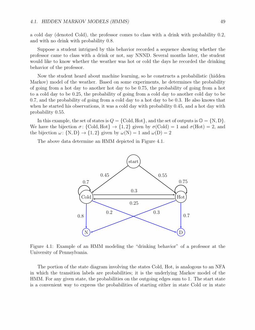
In this example, the set of states isQ = Cold,Hot, and the set of outputs isO = N,D.We have the bijection σ : Cold,Hot → 1, 2 given by σ(Cold) = 1 and σ(Hot) = 2, andthe bijection ω : N,D → 1, 2 given by ω(N) = 1 and ω(D) = 2
The above data determine an HMM depicted in Figure 4.1.
start
Cold Hot
N D
0.45 0.55
0.3
0.25
0.80.2 0.3
0.7
0.7 0.75
Figure 4.1: Example of an HMM modeling the “drinking behavior” of a professor at theUniversity of Pennsylvania.
The portion of the state diagram involving the states Cold, Hot, is analogous to an NFAin which the transition labels are probabilities; it is the underlying Markov model of theHMM. For any given state, the probabilities on the outgoing edges sum to 1. The start stateis a convenient way to express the probabilities of starting either in state Cold or in state
50 CHAPTER 4. HIDDEN MARKOV MODELS (HMMS)
Hot. Also, from each of the states Cold and Hot, we have emission probabilities of producingthe ouput N or D, and these probabilities also sum to 1.
We can also express these data using matrices. The matrix
A =
0.7 0.3
0.25 0.75
describes the transitions of the Makov model, the vector
π =
0.45
0.55
describes the probabilities of starting either in state Cold or in state Hot, and the matrix
B =
0.8 0.2
0.3 0.7
describes the emission probabilities. Observe that the rows of the matrices A and B sum to1. Such matrices are called row-stochastic matrices . The entries in the vector π also sum to1.
The student would like to solve what is known as the decoding problem. Namely, giventhe output sequence NNND, find the most likely state sequence of the Markov model thatproduces the output sequence NNND. Is it (Cold,Cold,Cold,Cold), or (Hot,Hot,Hot,Hot),or (Hot,Cold,Cold,Hot), or (Cold,Cold,Cold,Hot)? Given the probabilities of the HMM,it seems unlikely that it is (Hot,Hot,Hot,Hot), but how can we find the most likely one?
Let us consider another example taken from Stamp [19].
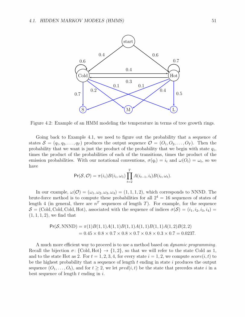
Example 4.2. Suppose we want to determine the average annual temperature at a particularlocation over a series of years in a distant past where thermometers did not exist. Since wecan’t go back in time, we look for indirect evidence of the temperature, say in terms of thesize of tree growth rings. For simplicity, assume that we consider the two temperatures Coldand Hot, and three different sizes of tree rings: small, medium and large, which we denoteby S, M, L.
In this example, the set of states is Q = Cold,Hot, and the set of outputs is O =S,M,L. We have the bijection σ : Cold,Hot → 1, 2 given by σ(Cold) = 1 andσ(Hot) = 2, and the bijection ω : S,M,L → 1, 2, 3 given by ω(S) = 1, ω(M) = 2,and ω(L) = 3. The HMM shown in Figure 4.2 is a model of the situation.
Suppose we observe the sequence of tree growth rings (S, M, S, L). What is the mostlikely sequence of temperatures over a four-year period which yields the observations (S, M,S, L)?
4.1. HIDDEN MARKOV MODELS (HMMS) 51
start
Cold Hot
S M L
0.4 0.6
0.4
0.3
0.70.2
0.1 0.10.4
0.5
0.6 0.7
Figure 4.2: Example of an HMM modeling the temperature in terms of tree growth rings.
Going back to Example 4.1, we need to figure out the probability that a sequence ofstates S = (q1, q2, . . . , qT ) produces the output sequence O = (O1, O2, . . . , OT ). Then theprobability that we want is just the product of the probability that we begin with state q1,times the product of the probabilities of each of the transitions, times the product of theemission probabilities. With our notational conventions, σ(qt) = it and ω(Ot) = ωt, so wehave
Pr(S,O) = π(i1)B(i1, ω1)
T∏
t=2
A(it−1, it)B(it, ωt).
In our example, ω(O) = (ω1, ω2, ω3, ω4) = (1, 1, 1, 2), which corresponds to NNND. Thebrute-force method is to compute these probabilities for all 24 = 16 sequences of states oflength 4 (in general, there are nT sequences of length T ). For example, for the sequenceS = (Cold,Cold,Cold,Hot), associated with the sequence of indices σ(S) = (i1, i2, i3, i4) =(1, 1, 1, 2), we find that
Pr(S,NNND) = π(1)B(1, 1)A(1, 1)B(1, 1)A(1, 1)B(1, 1)A(1, 2)B(2, 2)
= 0.45× 0.8× 0.7× 0.8× 0.7× 0.8× 0.3× 0.7 = 0.0237.
A much more efficient way to proceed is to use a method based on dynamic programming .Recall the bijection σ : Cold,Hot → 1, 2, so that we will refer to the state Cold as 1,and to the state Hot as 2. For t = 1, 2, 3, 4, for every state i = 1, 2, we compute score(i, t) tobe the highest probability that a sequence of length t ending in state i produces the outputsequence (O1, . . . , Ot), and for t ≥ 2, we let pred(i, t) be the state that precedes state i in abest sequence of length t ending in i.
52 CHAPTER 4. HIDDEN MARKOV MODELS (HMMS)
Recall that in our example, ω(O) = (ω1, ω2, ω3, ω4) = (1, 1, 1, 2), which corresponds toNNND. Initially, we set
score(j, 1) = π(j)B(j, ω1), j = 1, 2,
and since ω1 = 1 we get score(1, 1) = 0.45× 0.8 = 0.36, which is the probability of startingin state Cold and emitting N, and score(2, 1) = 0.55× 0.3 = 0.165, which is the probabilityof starting in state Hot and emitting N.
Next we compute score(1, 2) and score(2, 2) as follows. For j = 1, 2, for i = 1, 2, computetemporary scores
tscore(i, j) = score(i, 1)A(i, j)B(j, ω2);
then pick the best of the temporary scores,
score(j, 2) = maxitscore(i, j).
Since ω2 = 1, we get tscore(1, 1) = 0.36×0.7×0.8 = 0.2016, tscore(2, 1) = 0.165×0.25×0.8 =0.0330, and tscore(1, 2) = 0.36×0.3×0.3 = 0.0324, tscore(2, 2) = 0.165×0.75×0.3 = 0.0371.Then
score(1, 2) = maxtscore(1, 1), tscore(2, 1) = max0.2016, 0.0330 = 0.2016,
which is the largest probability that a sequence of two states emitting the output (N,N)ends in state Cold, and
score(2, 2) = maxtscore(1, 2), tscore(2, 2) = max0.0324, 0.0371 = 0.0371.
which is the largest probability that a sequence of two states emitting the output (N,N)ends in state Hot. Since the state that leads to the optimal score score(1, 2) is 1, we letpred(1, 2) = 1, and since the state that leads to the optimal score score(2, 2) is 2, we letpred(2, 2) = 2.
We compute score(1, 3) and score(2, 3) in a similar way. For j = 1, 2, for i = 1, 2,compute
tscore(i, j) = score(i, 2)A(i, j)B(j, ω3);
then pick the best of the temporary scores,
score(j, 3) = maxitscore(i, j).
Since ω3 = 1, we get tscore(1, 1) = 0.2016 × 0.7 × 0.8 = 0.1129, tscore(2, 1) = 0.0371 ×0.25× 0.8 = 0.0074, and tscore(1, 2) = 0.2016× 0.3× 0.3 = 0.0181, tscore(2, 2) = 0.0371×0.75× 0.3 = 0.0083. Then
score(1, 3) = maxtscore(1, 1), tscore(2, 1) = max0.1129, 0.074 = 0.1129,
4.1. HIDDEN MARKOV MODELS (HMMS) 53
which is the largest probability that a sequence of three states emitting the output (N,N,N)ends in state Cold, and
score(2, 3) = maxtscore(1, 2), tscore(2, 2) = max0.0181, 0.0083 = 0.0181,
which is the largest probability that a sequence of three states emitting the output (N,N,N)ends in state Hot. We also get pred(1, 3) = 1 and pred(2, 3) = 1. Finally, we computescore(1, 4) and score(2, 4) in a similar way. For j = 1, 2, for i = 1, 2, compute
tscore(i, j) = score(i, 3)A(i, j)B(j, ω4);
then pick the best of the temporary scores,
score(j, 4) = maxitscore(i, j).
Since ω4 = 2, we get tscore(1, 1) = 0.1129 × 0.7 × 0.2 = 0.0158, tscore(2, 1) = 0.0181 ×0.25× 0.2 = 0.0009, and tscore(1, 2) = 0.1129× 0.3× 0.7 = 0.0237, tscore(2, 2) = 0.0181×0.75× 0.7 = 0.0095. Then
score(1, 4) = maxtscore(1, 1), tscore(2, 1) = max0.0158, 0.0009 = 0.0158,
which is the largest probability that a sequence of four states emitting the output (N,N,N,D)ends in state Cold, and
score(2, 4) = maxtscore(1, 2), tscore(2, 2) = max0.0237, 0.0095 = 0.0237,
which is the largest probability that a sequence of four states emitting the output (N,N,N,D)ends in state Hot, and pred(1, 4) = 1 and pred(2, 4) = 1
Since maxscore(1, 4), score(2, 4) = max0.0158, 0.0237 = 0.0237, the state with themaximum score is Hot, and by following the predecessor list (also called backpointer list),we find that the most likely state sequence to produce the output sequence NNND is(Cold,Cold,Cold,Hot).
The stages of the computations of score(j, t) for i = 1, 2 and t = 1, 2, 3, 4 can be recordedin the following diagram called a lattice, or a trellis (which means lattice in French!):
Cold 0.36 0.2016 +3
0.0324
$$
0.2016 0.1129 +3
0.0181
(
0.1129 0.0158 +3
0.0237
(
0.0158
Hot 0.16500.0371
+3
0.033
;;0.0371
0.0083//
0.074
;;0.0181
0.0095//
0.0009
::0.0237
Double arrows represent the predecessor edges. For example, the predecessor pred(2, 3)of the third node on the bottom row labeled with the score 0.0181 (which corresponds to
54 CHAPTER 4. HIDDEN MARKOV MODELS (HMMS)
Hot), is the second node on the first row labeled with the score 0.2016 (which correspondsto Cold). The two incoming arrows to the third node on the bottom row are labeled withthe temporary scores 0.0181 and 0.0083. The node with the highest score at time t = 4 isHot, with score 0.0237 (showed in bold), and by following the double arrows backward fromthis node, we obtain the most likely state sequence (Cold,Cold,Cold,Hot).
The method we just described is known as the Viterbi algorithm. We now define HHM’sin general, and then present the Viterbi algorithm.
Definition 4.1. A hidden Markov model , for short HMM , is a quintupleM = (Q,O, π, A,B)where
• Q is a finite set of states with n elements, and there is a bijection σ : Q→ 1, . . . , n.
• O is a finite output alphabet (also called set of possible observations) with m observa-tions, and there is a bijection ω : O→ 1, . . . , m.
• A = (A(i, j)) is an n× n matrix called the state transition probability matrix , with
A(i, j) ≥ 0, 1 ≤ i, j ≤ n, andn∑
j=1
A(i, j) = 1, i = 1, . . . , n.
• B = (B(i, j)) is an n×m matrix called the state observation probability matrix (alsocalled confusion matrix ), with
B(i, j) ≥ 0, 1 ≤ i, j ≤ n, andm∑
j=1
B(i, j) = 1, i = 1, . . . , n.
A matrix satisfying the above conditions is said to be row stochastic. Both A and Bare row-stochastic.
We also need to state the conditions that makeM a Markov model. To do this rigorouslyrequires the notion of random variable and is a bit tricky (see the remark below), so we willcheat as follows:
(a) Given any sequence of states (q0, . . . , qt−2, p, q), the conditional probability that q is thetth state given that the previous states were q0, . . . , qt−2, p is equal to the conditionalprobability that q is the tth state given that the previous state at time t− 1 is p:
Pr(q | q0, . . . , qt−2, p) = Pr(q | p).
This is the Markov property . Informally, the “next” state q of the process at time tis independent of the “past” states q0, . . . , qt−2, provided that the “present” state p attime t− 1 is known.
4.1. HIDDEN MARKOV MODELS (HMMS) 55
(b) Given any sequence of states (q0, . . . , qi, . . . , qt), and given any sequence of outputs(O0, . . . , Oi, . . . , Ot), the conditional probability that the output Oi is emitted dependsonly on the state qi, and not any other states or any other observations:
Pr(Oi | q0, . . . , qi, . . . , qt, O0, . . . , Oi, . . . , Ot) = Pr(Oi | qi).
This is the output independence condition. Informally, the output function is near-sighted.
Examples of HMMs are shown in Figure 4.1, Figure 4.2, and Figure 4.3. Note that anouput is emitted when visiting a state, not when making a transition, as in the case of a gsm.So the analogy with the gsm model is only partial; it is meant as a motivation for HMMs.
The hidden Markov model was developed by L. E. Baum and colleagues at the Instituefor Defence Analysis at Princeton (including Petrie, Eagon, Sell, Soules, and Weiss) startingin 1966.
If we ignore the output components O and B, then we have what is called a Markovchain. A good interpretation of a Markov chain is the evolution over (discrete) time ofthe populations of n species that may change from one species to another. The probabilityA(i, j) is the fraction of the population of the ith species that changes to the jth species. Ifwe denote the populations at time t by the row vector x = (x1, . . . , xn), and the populationsat time t + 1 by y = (y1, . . . , yn), then
yj = A(1, j)x1 + · · ·+ A(i, j)xi + · · ·+ A(n, j)xn, 1 ≤ j ≤ n,
in matrix form, y = xA. The condition∑n
j=1A(i, j) = 1 expresses that the total populationis preserved, namely y1 + · · ·+ yn = x1 + · · ·+ xn.
Remark: This remark is intended for the reader who knows some probability theory, andit can be skipped without any negative effect on understanding the rest of this chapter.Given a probability space (Ω,F , µ) and any countable set Q (for simplicity we may assumeQ is finite), a stochastic discrete-parameter process with state space Q is a countable family(Xt)t∈N of random variables Xt : Ω → Q. We can think of t as time, and for any q ∈ Q, ofPr(Xt = q) as the probability that the process X is in state q at time t. If
Pr(Xt = q | X0 = q0, . . . , Xt−2 = qt−2, Xt−1 = p) = Pr(Xt = q | Xt−1 = p)
for all q0, , . . . , qt−2, p, q ∈ Q and for all t ≥ 1, and if the probability on the right-hand sideis independent of t, then we say that X = (Xt)t∈N is a time-homogeneous Markov chain, forshort, Markov chain. Informally, the “next” state Xt of the process is independent of the“past” states X0, . . . , Xt−2, provided that the “present” state Xt−1 is known.
Since for simplicity Q is assumed to be finite, there is a bijection σ : Q→ 1, . . . , n, andthen, the process X is completely determined by the probabilities
aij = Pr(Xt = q | Xt−1 = p), i = σ(p), j = σ(q), p, q ∈ Q,
56 CHAPTER 4. HIDDEN MARKOV MODELS (HMMS)
and if Q is a finite state space of size n, these form an n × n matrix A = (aij) called theMarkov matrix of the process X . It is a row-stochastic matrix.
The beauty of Markov chains is that if we write
π(i) = Pr(X0 = i)
for the initial probability distribution, then the joint probability distribution of X0, X1, . . .,Xt is given by
Pr(X0 = i0, X1 = i1, . . . , Xt = it) = π(i0)A(i0, i1) · · ·A(it−1, it).
The above expression only involves π and the matrix A, and makes no mention of the originalmeasure space. Therefore, it doesn’t matter what the probability space is!
Conversely, given an n × n row-stochastic matrix A, let Ω be the set of all countablesequences ω = (ω0, ω1, . . . , ωt, . . .) with ωt ∈ Q = 1, . . . , n for all t ∈ N, and let Xt : Ω→ Qbe the projection on the tth component, namely Xt(ω) = ωt.
2 Then it is possible to define aσ-algebra (also called a σ-field) B and a measure µ on B such that (Ω,B, µ) is a probabilityspace, and X = (Xt)t∈N is a Markov chain with corresponding Markov matrix A.
To define B, proceed as follows. For every t ∈ N, let Ft be the family of all unions ofsubsets of Ω of the form
ω ∈ Ω | (X0(ω) ∈ S0) ∧ (X1(ω) ∈ S1) ∧ · · · ∧ (Xt(ω) ∈ St),
where S0, S1, . . . , St are subsets of the state space Q = 1, . . . , n. It is not hard to showthat each Ft is a σ-algebra. Then let
F =⋃
t≥0
Ft.
Each set in F is a set of paths for which a finite number of outcomes are restricted to lie incertain subsets of Q = 1, . . . , n. All other outcomes are unrestricted. In fact, every subsetC in F is a countable union
C =⋃
i∈N
B(t)i
of sets of the form
B(t)i = ω ∈ Ω | ω = (q0, q1, . . . , qt, st+1, . . . .sj , . . . , ) | q0, q1, . . . , qt ∈ Q
= ω ∈ Ω | X0(ω) = q0, X1(ω) = q1, . . . , Xt(ω) = qt.2It is customary in probability theory to denote events by the letter ω. In the present case, ω denotes a
countable sequence of elements from Q. This notation has nothing do with the bijection ω : O→ 1, . . . ,moccurring in Definition 4.1.
4.1. HIDDEN MARKOV MODELS (HMMS) 57
The sequences in B(t)i are those beginning with the fixed sequence (q0, q1, . . . , qt). One can
show that F is a field of sets, but not necessarily a σ-algebra, so we form the smallestσ-algebra G containing F .
Using the matrix A we can define the measure ν(B(t)i ) as the product of the probabilities
along the sequence (q0, q1, . . . , qt). Then it can be shown that ν can be extended to a measureµ on G, and we let B be the σ-algebra obtained by adding to G all subsets of sets of measurezero. The resulting probability space (Ω,B, µ) is usually called the sequence space, and themeasure µ is called the tree measure. Then it is easy to show that the family of randomvariables Xt : Ω→ Q on the probability space(Ω,B, µ) is a time-homogeneous Markov chainwhose Markov matrix is the orginal matrix A. The above construction is presented in fulldetail in Kemeny, Snell, and Knapp[10] (Chapter 2, Sections 1 and 2).
Most presentations of Markov chains do not even mention the probability space overwhich the random variables Xt are defined. This makes the whole thing quite mysterious,since the probabilities Pr(Xt = q) are by definition given by
Pr(Xt = q) = µ(ω ∈ Ω | Xt(ω) = q),
which requires knowing the measure µ. This is more problematic if we start with a stochasticmatrix. What are the random variables Xt, what are they defined on? The above construc-tion puts things on firm grounds.
There are three types of problems that can be solved using HMMs:
(1) The decoding problem: Given an HMM M = (Q,O, π, A,B), for any observedoutput sequence O = (O1, O2, . . . , OT ) of length T ≥ 1, find a most likely sequenceof states S = (q1, q2, . . . , qT ) that produces the output sequence O. More precisely,with our notational convention that σ(qt) = it and ω(Ot) = ωt, this means finding asequence S such that the probability
Pr(S,O) = π(i1)B(i1, ω1)
T∏
t=2
A(it−1, it)B(it, ωt)
is maximal. This problem is solved effectively by the Viterbi algorithm that we outlinedbefore.
(2) The evaluation problem, also called the likelyhood problem: Given a finitecollection M1, . . . ,ML of HMM’s with the same output alphabet O, for any outputsequence O = (O1, O2, . . . , OT ) of length T ≥ 1, find which model Mℓ is most likely tohave generated O. More precisely, given any model Mk, we compute the probabilitytprobk that Mk could have produced O along any path. Then we pick an HMM Mℓ
for which tprobℓ is maximal. We will return to this point after having described theViterbi algoritm. A variation of the Viterbi algorithm called the forward algorithmeffectively solves the evaluation problem.
58 CHAPTER 4. HIDDEN MARKOV MODELS (HMMS)
(3) The training problem, also called the learning problem: Given a set O1, . . . ,Orof output sequences on the same output alpabet O, usually called a set of training data,given Q, find the “best” π,A, and B for an HMM M that produces all the sequencesin the training set, in the sense that the HMM M = (Q,O, π, A,B) is the most likelyto have produced the sequences in the training set. The technique used here is calledexpectation maximization, or EM . It is an iterative method that starts with an initialtriple π,A,B, and tries to impove it. There is such an algorithm known as the Baum-Welch or forward-backward algorithm, but it is beyond the scope of this introduction.
Let us now describe the Viterbi algorithm in more details.
4.2 The Viterbi Algorithm and the Forward Algorithm
Given an HMM M = (Q,O, π, A,B), for any observed output sequence O = (O1, O2, . . .,OT ) of length T ≥ 1, we want to find a most likely sequence of states S = (q1, q2, . . . , qT )that produces the output sequence O.
Using the bijections σ : Q → 1, . . . , n and ω : O → 1, . . . , m, we can work withsequences of indices, and recall that we denote the index σ(qt) associated with the tth stateqt in the sequence S by it, and the index ω(Ot) associated with the tth output Ot in thesequence O by ωt. Then we need to find a sequence S such that the probability
Pr(S,O) = π(i1)B(i1, ω1)
T∏
t=2
A(it−1, it)B(it, ωt)
is maximal.
In general, there are nT sequences of length T . This problem can be solved efficientlyby a method based on dynamic programming . For any t, 1 ≤ t ≤ T , for any state q ∈ Q,if σ(q) = j, then we compute score(j, t), which is the largest probability that a sequence(q1, . . . , qt−1, q) of length t ending with q has produced the output sequence (O1, . . . , Ot−1, Ot).
The point is that if we know score(k, t − 1) for k = 1, . . . , n (with t ≥ 2), then we canfind score(j, t) for j = 1, . . . , n, because if we write k = σ(qt−1) and j = σ(q) (recall thatωt = ω(Ot)), then the probability associated with the path (q1, . . . , qt−1, q) is
tscore(k, j) = score(k, t− 1)A(k, j)B(j, ωt).
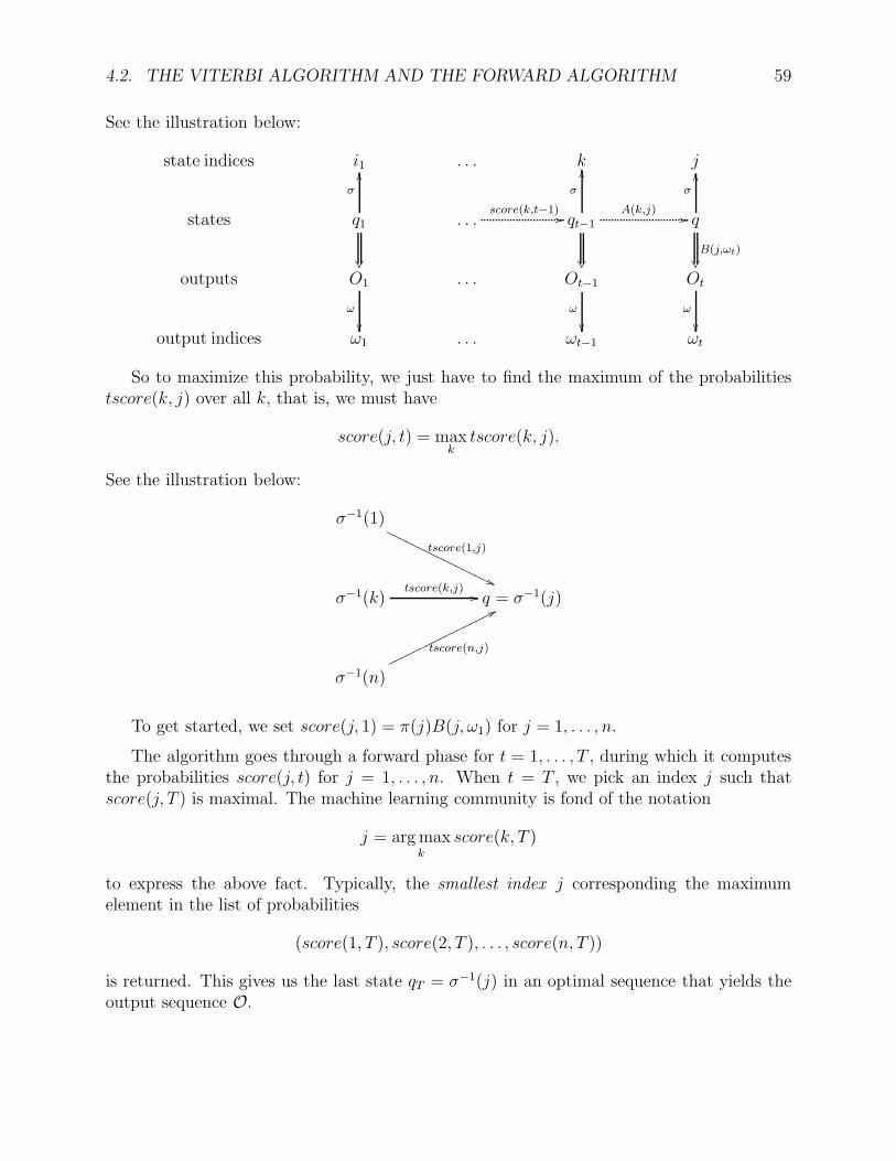
4.2. THE VITERBI ALGORITHM AND THE FORWARD ALGORITHM 59
See the illustration below:
state indices i1 . . . k j
states q1
σ
OO
. . .score(k,t−1) // qt−1
σ
OO
A(k,j) // q
σ
OO
B(j,ωt)
outputs O1
ω
. . . Ot−1
ω
Ot
ω
output indices ω1 . . . ωt−1 ωt
So to maximize this probability, we just have to find the maximum of the probabilitiestscore(k, j) over all k, that is, we must have
score(j, t) = maxktscore(k, j).
See the illustration below:
σ−1(1)
tscore(1,j)
''
σ−1(k)tscore(k,j) // q = σ−1(j)
σ−1(n)
tscore(n,j)
77♦♦♦♦♦♦♦♦♦♦♦♦♦♦♦♦♦
To get started, we set score(j, 1) = π(j)B(j, ω1) for j = 1, . . . , n.
The algorithm goes through a forward phase for t = 1, . . . , T , during which it computesthe probabilities score(j, t) for j = 1, . . . , n. When t = T , we pick an index j such thatscore(j, T ) is maximal. The machine learning community is fond of the notation
j = argmaxk
score(k, T )
to express the above fact. Typically, the smallest index j corresponding the maximumelement in the list of probabilities
(score(1, T ), score(2, T ), . . . , score(n, T ))
is returned. This gives us the last state qT = σ−1(j) in an optimal sequence that yields theoutput sequence O.
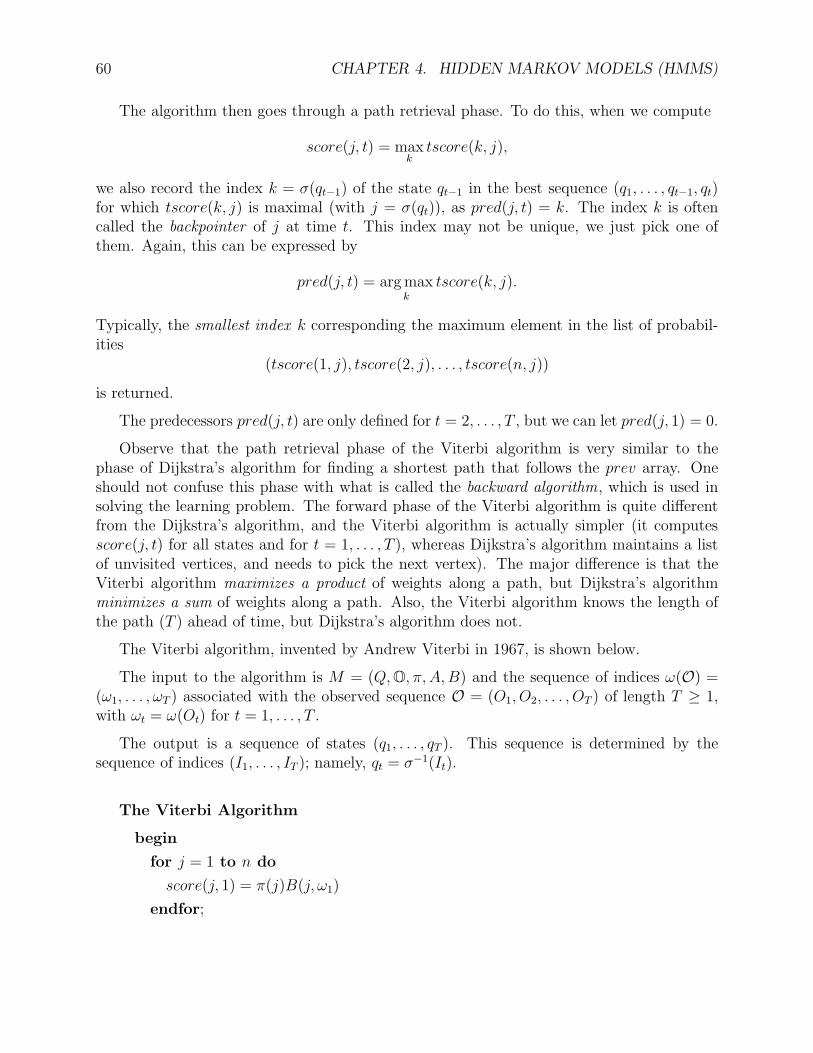
60 CHAPTER 4. HIDDEN MARKOV MODELS (HMMS)
The algorithm then goes through a path retrieval phase. To do this, when we compute
score(j, t) = maxktscore(k, j),
we also record the index k = σ(qt−1) of the state qt−1 in the best sequence (q1, . . . , qt−1, qt)for which tscore(k, j) is maximal (with j = σ(qt)), as pred(j, t) = k. The index k is oftencalled the backpointer of j at time t. This index may not be unique, we just pick one ofthem. Again, this can be expressed by
pred(j, t) = argmaxk
tscore(k, j).
Typically, the smallest index k corresponding the maximum element in the list of probabil-ities
(tscore(1, j), tscore(2, j), . . . , tscore(n, j))
is returned.
The predecessors pred(j, t) are only defined for t = 2, . . . , T , but we can let pred(j, 1) = 0.
Observe that the path retrieval phase of the Viterbi algorithm is very similar to thephase of Dijkstra’s algorithm for finding a shortest path that follows the prev array. Oneshould not confuse this phase with what is called the backward algorithm, which is used insolving the learning problem. The forward phase of the Viterbi algorithm is quite differentfrom the Dijkstra’s algorithm, and the Viterbi algorithm is actually simpler (it computesscore(j, t) for all states and for t = 1, . . . , T ), whereas Dijkstra’s algorithm maintains a listof unvisited vertices, and needs to pick the next vertex). The major difference is that theViterbi algorithm maximizes a product of weights along a path, but Dijkstra’s algorithmminimizes a sum of weights along a path. Also, the Viterbi algorithm knows the length ofthe path (T ) ahead of time, but Dijkstra’s algorithm does not.
The Viterbi algorithm, invented by Andrew Viterbi in 1967, is shown below.
The input to the algorithm is M = (Q,O, π, A,B) and the sequence of indices ω(O) =(ω1, . . . , ωT ) associated with the observed sequence O = (O1, O2, . . . , OT ) of length T ≥ 1,with ωt = ω(Ot) for t = 1, . . . , T .
The output is a sequence of states (q1, . . . , qT ). This sequence is determined by thesequence of indices (I1, . . . , IT ); namely, qt = σ−1(It).
The Viterbi Algorithm
begin
for j = 1 to n do
score(j, 1) = π(j)B(j, ω1)
endfor;
4.2. THE VITERBI ALGORITHM AND THE FORWARD ALGORITHM 61
(∗ forward phase to find the best (highest) scores ∗)for t = 2 to T do
for j = 1 to n do
for k = 1 to n do
tscore(k) = score(k, t− 1)A(k, j)B(j, ωt)
endfor;
score(j, t) = maxk tscore(k);
pred(j, t) = argmaxk tscore(k)
endfor
endfor;
(∗ second phase to retrieve the optimal path ∗)IT = argmaxj score(j, T );
qT = σ−1(IT );
for t = T to 2 by −1 do
It−1 = pred(It, t);
qt−1 = σ−1(It−1)
endfor
end
An illustration of the Viterbi algorithm applied to Example 4.1 was presented afterExample 4.3. If we run the Viterbi algorithm on the output sequence (S, M, S, L) ofExample 4.2, we find that the sequence (Cold,Cold,Cold,Hot) has the highest probability,0.00282, among all sequences of length four.
One may have noticed that the numbers involved, being products of probabilities, becomequite small. Indeed, underflow may arise in dynamic programming. Fortunately, thereis a simple way to avoid underflow by taking logarithms. We initialize the algorithm bycomputing
score(j, 1) = log[π(j)] + log[B(j, ω1)],
and in the step where tscore is computed we use the formula
tscore(k) = score(k, t− 1) + log[A(k, j)] + log[B(j, ωt)].
It immediately verified that the time complexity of the Viterbi algorithm is O(n2T ).
Let us now to turn to the second problem, the evaluation problem (or likelyhood problem).
This time, given a finite collection M1, . . . ,ML of HMM’s with the same output al-phabet O, for any observed output sequence O = (O1, O2, . . . , OT ) of length T ≥ 1, findwhich model Mℓ is most likely to have generated O. More precisely, given any model Mk,
62 CHAPTER 4. HIDDEN MARKOV MODELS (HMMS)
we compute the probability tprobk that Mk could have produced O along any sequence ofstates S = (q1, . . . , qT ). Then we pick an HMM Mℓ for which tprobℓ is maximal.
The probability tprobk that we are seeking is given by
tprobk = Pr(O)=
∑
(i1,...,iT )∈1,...,nT
Pr((qi1 , . . . , qiT ),O)
=∑
(i1,...,iT )∈1,...,nT
π(i1)B(i1, ω1)
T∏
t=2
A(it−1, it)B(it, ωt),
where 1, . . . , nT denotes the set of all sequences of length T consisting of elements fromthe set 1, . . . , n.
It is not hard to see that a brute-force computation requires 2TnT multiplications. For-tunately, it is easy to adapt the Viterbi algorithm to compute tprobk efficiently. Since weare not looking for an explicity path, there is no need for the second phase, and during theforward phase, going from t−1 to t, rather than finding the maximum of the scores tscore(k)for k = 1, . . . , n, we just set score(j, t) to the sum over k of the temporary scores tscore(k).At the end, tprobk is the sum over j of the probabilities score(j, T ).
The algorithm solving the evaluation problem known as the forward algorithm is shownbelow.
The input to the algorithm is M = (Q,O, π, A,B) and the sequence of indices ω(O) =(ω1, . . . , ωT ) associated with the observed sequence O = (O1, O2, . . . , OT ) of length T ≥ 1,with ωt = ω(Ot) for t = 1, . . . , T . The output is the probability tprob.
The Foward Algorithm
begin
for j = 1 to n do
score(j, 1) = π(j)B(j, ω1)
endfor;
for t = 2 to T do
for j = 1 to n do
for k = 1 to n do
tscore(k) = score(k, t− 1)A(k, j)B(j, ωt)
endfor;
score(j, t) =∑
k tscore(k)
endfor
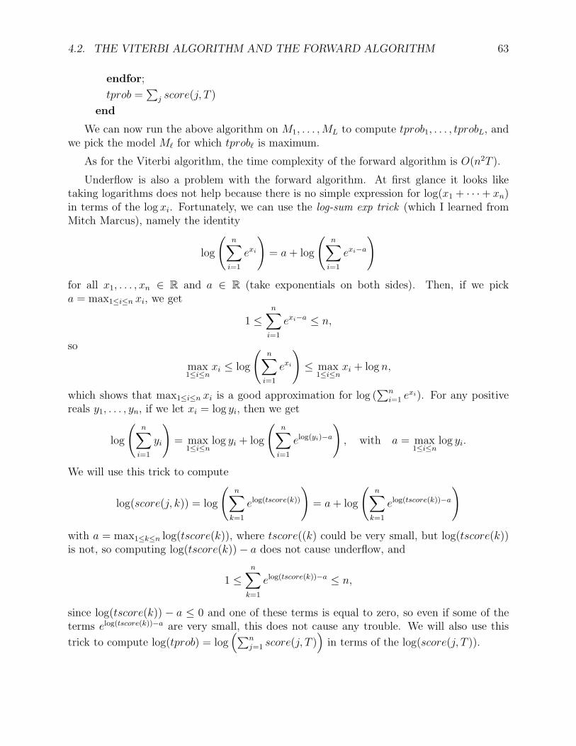
4.2. THE VITERBI ALGORITHM AND THE FORWARD ALGORITHM 63
endfor;
tprob =∑
j score(j, T )
end
We can now run the above algorithm on M1, . . . ,ML to compute tprob1, . . . , tprobL, andwe pick the model Mℓ for which tprobℓ is maximum.
As for the Viterbi algorithm, the time complexity of the forward algorithm is O(n2T ).
Underflow is also a problem with the forward algorithm. At first glance it looks liketaking logarithms does not help because there is no simple expression for log(x1 + · · ·+ xn)in terms of the log xi. Fortunately, we can use the log-sum exp trick (which I learned fromMitch Marcus), namely the identity
log
(n∑
i=1
exi
)= a+ log
(n∑
i=1
exi−a
)
for all x1, . . . , xn ∈ R and a ∈ R (take exponentials on both sides). Then, if we picka = max1≤i≤n xi, we get
1 ≤n∑
i=1
exi−a ≤ n,
so
max1≤i≤n
xi ≤ log
(n∑
i=1
exi
)≤ max
1≤i≤nxi + log n,
which shows that max1≤i≤n xi is a good approximation for log (∑n
i=1 exi). For any positive
reals y1, . . . , yn, if we let xi = log yi, then we get
log
(n∑
i=1
yi
)= max
1≤i≤nlog yi + log
(n∑
i=1
elog(yi)−a
), with a = max
1≤i≤nlog yi.
We will use this trick to compute
log(score(j, k)) = log
(n∑
k=1
elog(tscore(k))
)= a+ log
(n∑
k=1
elog(tscore(k))−a
)
with a = max1≤k≤n log(tscore(k)), where tscore((k) could be very small, but log(tscore(k))is not, so computing log(tscore(k))− a does not cause underflow, and
1 ≤n∑
k=1
elog(tscore(k))−a ≤ n,
since log(tscore(k)) − a ≤ 0 and one of these terms is equal to zero, so even if some of theterms elog(tscore(k))−a are very small, this does not cause any trouble. We will also use this
trick to compute log(tprob) = log(∑n
j=1 score(j, T ))in terms of the log(score(j, T )).
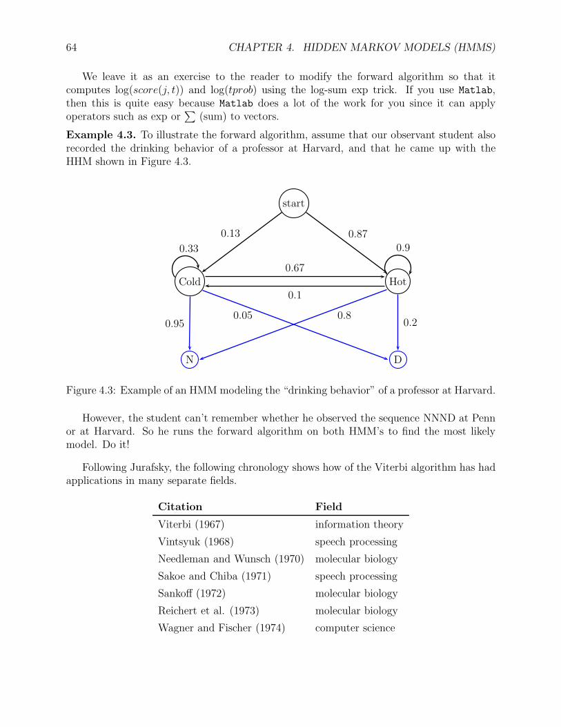
64 CHAPTER 4. HIDDEN MARKOV MODELS (HMMS)
We leave it as an exercise to the reader to modify the forward algorithm so that itcomputes log(score(j, t)) and log(tprob) using the log-sum exp trick. If you use Matlab,then this is quite easy because Matlab does a lot of the work for you since it can applyoperators such as exp or
∑(sum) to vectors.
Example 4.3. To illustrate the forward algorithm, assume that our observant student alsorecorded the drinking behavior of a professor at Harvard, and that he came up with theHHM shown in Figure 4.3.
start
Cold Hot
N D
0.13 0.87
0.67
0.1
0.950.05 0.8
0.2
0.33 0.9
Figure 4.3: Example of an HMM modeling the “drinking behavior” of a professor at Harvard.
However, the student can’t remember whether he observed the sequence NNND at Pennor at Harvard. So he runs the forward algorithm on both HMM’s to find the most likelymodel. Do it!
Following Jurafsky, the following chronology shows how of the Viterbi algorithm has hadapplications in many separate fields.
Citation Field
Viterbi (1967) information theory
Vintsyuk (1968) speech processing
Needleman and Wunsch (1970) molecular biology
Sakoe and Chiba (1971) speech processing
Sankoff (1972) molecular biology
Reichert et al. (1973) molecular biology
Wagner and Fischer (1974) computer science
4.2. THE VITERBI ALGORITHM AND THE FORWARD ALGORITHM 65
Readers who wish to learn more about HMMs should begin with Stamp [19], a greattutorial which contains a very clear and easy to read presentation. Another nice intro-duction is given in Rich [18] (Chapter 5, Section 5.11). A much more complete, yet ac-cessible, coverage of HMMs is found in Rabiner’s tutorial [16]. Jurafsky and Martin’sonline Chapter 9 (Hidden Markov Models) is also a very good and informal tutorial (seehttps://web.stanford.edu/ jurafsky/slp3/9.pdf).
A very clear and quite accessible presentation of Markov chains is given in Cinlar [4].Another thorough but a bit more advanced presentation is given in Bremaud [3]. Other pre-sentations of Markov chains can be found in Mitzenmacher and Upfal [13], and in Grimmettand Stirzaker [9].
Acknowledgments: I would like to thank Mitch Marcus, Jocelyn Qaintance, and JoaoSedoc, for scrutinizing my work and for many insightful comments.
66 CHAPTER 4. HIDDEN MARKOV MODELS (HMMS)
Chapter 5
Regular Languages and EquivalenceRelations, The Myhill-NerodeCharacterization, State Equivalence
5.1 Directed Graphs and Paths
It is often useful to view DFA’s and NFA’s as labeled directed graphs.
Definition 5.1. A directed graph is a quadruple G = (V,E, s, t), where V is a set of vertices,or nodes , E is a set of edges, or arcs , and s, t : E → V are two functions, s being called thesource function, and t the target function. Given an edge e ∈ E, we also call s(e) the origin(or source) of e, and t(e) the endpoint (or target) of e.
Remark : the functions s, t need not be injective or surjective. Thus, we allow “isolatedvertices.”
Example: Let G be the directed graph defined such that
E = e1, e2, e3, e4, e5, e6, e7, e8,
V = v1, v2, v3, v4, v5, v6, and
s(e1) = v1, s(e2) = v2, s(e3) = v3, s(e4) = v4,
s(e5) = v2, s(e6) = v5, s(e7) = v5, s(e8) = v5,
t(e1) = v2, t(e2) = v3, t(e3) = v4, t(e4) = v2,
t(e5) = v5, t(e6) = v5, t(e7) = v6, t(e8) = v6.
Such a graph can be represented by the following diagram:
67
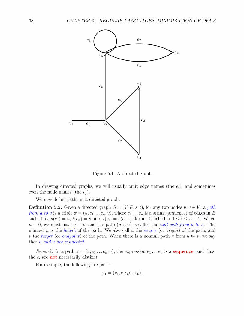
68 CHAPTER 5. REGULAR LANGUAGES, MINIMIZATION OF DFA’S
e7
e8
v1 v2
v3
v4
v5v6
e1
e2
e3
e4
e5
e6
Figure 5.1: A directed graph
In drawing directed graphs, we will usually omit edge names (the ei), and sometimeseven the node names (the vj).
We now define paths in a directed graph.
Definition 5.2. Given a directed graph G = (V,E, s, t), for any two nodes u, v ∈ V , a pathfrom u to v is a triple π = (u, e1 . . . en, v), where e1 . . . en is a string (sequence) of edges in Esuch that, s(e1) = u, t(en) = v, and t(ei) = s(ei+1), for all i such that 1 ≤ i ≤ n− 1. Whenn = 0, we must have u = v, and the path (u, ǫ, u) is called the null path from u to u. Thenumber n is the length of the path. We also call u the source (or origin) of the path, andv the target (or endpoint) of the path. When there is a nonnull path π from u to v, we saythat u and v are connected .
Remark : In a path π = (u, e1 . . . en, v), the expression e1 . . . en is a sequence, and thus,the ei are not necessarily distinct.
For example, the following are paths:
π1 = (v1, e1e5e7, v6),
5.1. DIRECTED GRAPHS AND PATHS 69
π2 = (v2, e2e3e4e2e3e4e2e3e4, v2),
andπ3 = (v1, e1e2e3e4e2e3e4e5e6e6e8, v6).
Clearly, π2 and π3 are of a different nature from π1. Indeed, they contain cycles. This isformalized as follows.
Definition 5.3. Given a directed graph G = (V,E, s, t), for any node u ∈ V a cycle (orloop) through u is a nonnull path of the form π = (u, e1 . . . en, u) (equivalently, t(en) = s(e1)).More generally, a nonnull path π = (u, e1 . . . en, v) contains a cycle iff for some i, j, with1 ≤ i ≤ j ≤ n, t(ej) = s(ei). In this case, letting w = t(ej) = s(ei), the path (w, ei . . . ej , w)is a cycle through w. A path π is acyclic iff it does not contain any cycle. Note that eachnull path (u, ǫ, u) is acyclic.
Obviously, a cycle π = (u, e1 . . . en, u) through u is also a cycle through every node t(ei).Also, a path π may contain several different cycles.
Paths can be concatenated as follows.
Definition 5.4. Given a directed graph G = (V,E, s, t), two paths π1 = (u, e1 . . . em, v)and π2 = (u′, e′1 . . . e
′n, v
′) can be concatenated provided that v = u′, in which case theirconcatenation is the path
π1π2 = (u, e1 . . . eme′1 . . . e
′n, v
′).
It is immediately verified that the concatenation of paths is associative, and that theconcatenation of the pathπ = (u, e1 . . . em, v) with the null path (u, ǫ, u) or with the null path (v, ǫ, v) is the path πitself.
The following fact, although almost trivial, is used all the time, and is worth stating indetail.
Proposition 5.1. Given a directed graph G = (V,E, s, t), if the set of nodes V containsm ≥ 1 nodes, then every path π of length at least m contains some cycle.
A consequence of Proposition 5.1 is that in a finite graph with m nodes, given any twonodes u, v ∈ V , in order to find out whether there is a path from u to v, it is enough toconsider paths of length ≤ m− 1.
Indeed, if there is path between u and v, then there is some path π of minimal length(not necessarily unique, but this doesn’t matter).
If this minimal path has length at least m, then by the Proposition, it contains a cycle.
However, by deleting this cycle from the path π, we get an even shorter path from u tov, contradicting the minimality of π.
We now turn to labeled graphs.
70 CHAPTER 5. REGULAR LANGUAGES, MINIMIZATION OF DFA’S
5.2 Labeled Graphs and Automata
In fact, we only need edge-labeled graphs.
Definition 5.5. A labeled directed graph is a tuple G = (V,E, L, s, t, λ), where V is a setof vertices, or nodes , E is a set of edges, or arcs , L is a set of labels , s, t : E → V are twofunctions, s being called the source function, and t the target function, and λ : E → L is thelabeling function. Given an edge e ∈ E, we also call s(e) the origin (or source) of e, t(e) theendpoint (or target) of e, and λ(e) the label of e.
Note that the function λ need not be injective or surjective. Thus, distinct edges mayhave the same label.
Example: Let G be the directed graph defined such that
E = e1, e2, e3, e4, e5, e6, e7, e8,V = v1, v2, v3, v4, v5, v6, L = a, b,and
s(e1) = v1, s(e2) = v2, s(e3) = v3, s(e4) = v4,
s(e5) = v2, s(e6) = v5, s(e7) = v5, s(e8) = v5,
t(e1) = v2, t(e2) = v3, t(e3) = v4, t(e4) = v2,
t(e5) = v5, t(e6) = v5, t(e7) = v6, t(e8) = v6
λ(e1) = a, λ(e2) = b, λ(e3) = a, λ(e4) = a,
λ(e5) = b, λ(e6) = a, λ(e7) = a, λ(e8) = b.
Such a labeled graph can be represented by the following diagram:
In drawing labeled graphs, we will usually omit edge names (the ei), and sometimes eventhe node names (the vj).
Paths, cycles, and concatenation of paths are defined just as before (that is, we ignorethe labels). However, we can now define the spelling of a path.
Definition 5.6. Given a labeled directed graph G = (V,E, L, s, t, λ) for any two nodesu, v ∈ V , for any path π = (u, e1 . . . en, v), the spelling of the path π is the string of labels
λ(e1) · · ·λ(en).
When n = 0, the spelling of the null path (u, ǫ, u) is the null string ǫ.
For example, the spelling of the path
π3 = (v1, e1e2e3e4e2e3e4e5e6e6e8, v6)
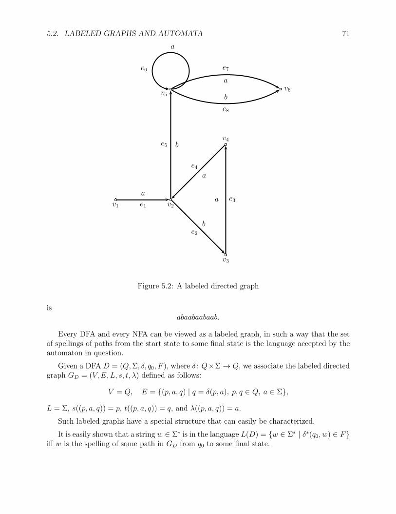
5.2. LABELED GRAPHS AND AUTOMATA 71
a
b
a
a
b
e7
a
e8
b
a
v1 v2
v3
v4
v5v6
e1
e2
e3
e4
e5
e6
Figure 5.2: A labeled directed graph
isabaabaabaab.
Every DFA and every NFA can be viewed as a labeled graph, in such a way that the setof spellings of paths from the start state to some final state is the language accepted by theautomaton in question.
Given a DFA D = (Q,Σ, δ, q0, F ), where δ : Q×Σ→ Q, we associate the labeled directedgraph GD = (V,E, L, s, t, λ) defined as follows:
V = Q, E = (p, a, q) | q = δ(p, a), p, q ∈ Q, a ∈ Σ,
L = Σ, s((p, a, q)) = p, t((p, a, q)) = q, and λ((p, a, q)) = a.
Such labeled graphs have a special structure that can easily be characterized.
It is easily shown that a string w ∈ Σ∗ is in the language L(D) = w ∈ Σ∗ | δ∗(q0, w) ∈ Fiff w is the spelling of some path in GD from q0 to some final state.
72 CHAPTER 5. REGULAR LANGUAGES, MINIMIZATION OF DFA’S
Similarly, given an NFA N = (Q,Σ, δ, q0, F ), where δ : Q× (Σ∪ ǫ)→ 2Q, we associatethe labeled directed graph GN = (V,E, L, s, t, λ) defined as follows: V = Q
E = (p, a, q) | q ∈ δ(p, a), p, q ∈ Q, a ∈ Σ ∪ ǫ,
L = Σ ∪ ǫ, s((p, a, q)) = p, t((p, a, q)) = q,
λ((p, a, q)) = a.
Remark : When N has no ǫ-transitions, we can let L = Σ.
Such labeled graphs have also a special structure that can easily be characterized.
Again, a string w ∈ Σ∗ is in the language L(N) = w ∈ Σ∗ | δ∗(q0, w) ∩ F 6= ∅ iff w isthe spelling of some path in GN from q0 to some final state.
5.3 The Closure Definition of the Regular Languages
Let Σ = a1, . . . , am be some alphabet. We would like to define a family of languages, R(Σ),by singling out some very basic (atomic) languages, namely the languages a1, . . . , am,the empty language, and the trivial language, ǫ, and then forming more complicatedlanguages by repeatedly forming union, concatenation and Kleene ∗ of previously constructedlanguages. By doing so, we hope to get a family of languages (R(Σ)) that is closed underunion, concatenation, and Kleene ∗. This means that for any two languages, L1, L2 ∈ R(Σ),we also have L1 ∪ L2 ∈ R(Σ) and L1L2 ∈ R(Σ), and for any language L ∈ R(Σ), we haveL∗ ∈ R(Σ). Furthermore, we would like R(Σ) to be the smallest family with these properties.How do we achieve this rigorously?
First, let us look more closely at what we mean by a family of languages. Recall that alanguage (over Σ) is any subset, L, of Σ∗. Thus, the set of all languages is 2Σ
∗
, the powerset of Σ∗. If Σ is nonempty, this is an uncountable set. Next, we define a family , L, oflanguages to be any subset of 2Σ
∗
. This time, the set of families of languages is 22Σ∗
. This
is a huge set. We can use the inclusion relation on 22Σ∗
to define a partial order on familiesof languages. So, L1 ⊆ L2 iff for every language, L, if L ∈ L1 then L ∈ L2.
We can now state more precisely what we are trying to do. Consider the followingproperties for a family of languages, L:
(1) We have a1, . . . , am, ∅, ǫ ∈ L, i.e., L contains the “atomic” languages.
(2a) For all L1, L2 ∈ L, we also have L1 ∪ L2 ∈ L.
(2b) For all L1, L2 ∈ L, we also have L1L2 ∈ L.
(2c) For all L ∈ L, we also have L∗ ∈ L.
5.3. THE CLOSURE DEFINITION OF THE REGULAR LANGUAGES 73
In other words, L is closed under union, concatenation and Kleene ∗.Now, what we want is the smallest (w.r.t. inclusion) family of languages that satisfies
properties (1) and (2)(a)(b)(c). We can construct such a family using an inductive definition.This inductive definition constructs a sequence of families of languages, (R(Σ)n)n≥0, calledthe stages of the inductive definition, as follows:
R(Σ)0 = a1, . . . , am, ∅, ǫ,R(Σ)n+1 = R(Σ)n ∪ L1 ∪ L2, L1L2, L
∗ | L1, L2, L ∈ R(Σ)n.
Then, we define R(Σ) by
R(Σ) =⋃
n≥0
R(Σ)n.
Thus, a language L belongs to R(Σ) iff it belongs Ln, for some n ≥ 0.
For example, if Σ = a, b, we have
R(Σ)1 = a, b, ∅, ǫ,a, b, a, ǫ, b, ǫ,ab, ba, aa, bb, a∗, b∗.
Some of the languages that will appear in R(Σ)2 are:
a, bb, ab, ba, abb, aabb, aa∗, aab∗, bb∗.
Observe that
R(Σ)0 ⊆ R(Σ)1 ⊆ R(Σ)2 ⊆ · · ·R(Σ)n ⊆ R(Σ)n+1 ⊆ · · · ⊆ R(Σ),
so that if L ∈ R(Σ)n, then L ∈ R(Σ)p, for all p ≥ n. Also, there is some smallest n forwhich L ∈ R(Σ)n (the birthdate of L!). In fact, all these inclusions are strict. Note that eachR(Σ)n only contains a finite number of languages (but some of the languages in R(Σ)n areinfinite, because of Kleene ∗).
Then we define the Regular languages, Version 2 , as the family R(Σ).
Of course, it is far from obvious that R(Σ) coincides with the family of languages acceptedby DFA’s (or NFA’s), what we call the regular languages, version 1. However, this is the case,and this can be demonstrated by giving two algorithms. Actually, it will be slightly moreconvenient to define a notation system, the regular expressions , to denote the languagesin R(Σ). Then, we will give an algorithm that converts a regular expression, R, into anNFA, NR, so that LR = L(NR), where LR is the language (in R(Σ)) denoted by R. Wewill also give an algorithm that converts an NFA, N , into a regular expression, RN , so thatL(RN ) = L(N).
But before doing all this, we should make sure that R(Σ) is indeed the family that weare seeking. This is the content of
74 CHAPTER 5. REGULAR LANGUAGES, MINIMIZATION OF DFA’S
Proposition 5.2. The family, R(Σ), is the smallest family of languages which contains theatomic languages a1, . . . , am, ∅, ǫ, and is closed under union, concatenation, andKleene ∗.
Proof. There are two things to prove.
(i) We need to prove that R(Σ) has properties (1) and (2)(a)(b)(c).
(ii) We need to prove that R(Σ) is the smallest family having properties (1) and(2)(a)(b)(c).
(i) Since
R(Σ)0 = a1, . . . , am, ∅, ǫ,it is obvious that (1) holds. Next, assume that L1, L2 ∈ R(Σ). This means that there aresome integers n1, n2 ≥ 0, so that L1 ∈ R(Σ)n1 and L2 ∈ R(Σ)n2 . Now, it is possible thatn1 6= n2, but if we let n = maxn1, n2, as we observed that R(Σ)p ⊆ R(Σ)q wheneverp ≤ q, we are guaranteed that both L1, L2 ∈ R(Σ)n. However, by the definition of R(Σ)n+1
(that’s why we defined it this way!), we have L1 ∪ L2 ∈ R(Σ)n+1 ⊆ R(Σ). The sameargument proves that L1L2 ∈ R(Σ)n+1 ⊆ R(Σ). Also, if L ∈ R(Σ)n, we immediately haveL∗ ∈ R(Σ)n+1 ⊆ R(Σ). Therefore, R(Σ) has properties (1) and (2)(a)(b)(c).
(ii) Let L be any family of languages having properties (1) and (2)(a)(b)(c). We need toprove that R(Σ) ⊆ L. If we can prove that R(Σ)n ⊆ L, for all n ≥ 0, we are done (sincethen, R(Σ) =
⋃n≥0R(Σ)n ⊆ L). We prove by induction on n that R(Σ)n ⊆ L, for all n ≥ 0.
The base case n = 0 is trivial, since L has (1), which says that R(Σ)0 ⊆ L. Assumeinductively that R(Σ)n ⊆ L. We need to prove that R(Σ)n+1 ⊆ L. Pick any L ∈ R(Σ)n+1.Recall that
R(Σ)n+1 = R(Σ)n ∪ L1 ∪ L2, L1L2, L∗ | L1, L2, L ∈ R(Σ)n.
If L ∈ R(Σ)n, then L ∈ L, since R(Σ)n ⊆ L, by the induction hypothesis. Otherwise, thereare three cases:
(a) L = L1 ∪ L2, where L1, L2 ∈ R(Σ)n. By the induction hypothesis, R(Σ)n ⊆ L, so, weget L1, L2 ∈ L; since L has 2(a), we have L1 ∪ L2 ∈ L.
(b) L = L1L2, where L1, L2 ∈ R(Σ)n. By the induction hypothesis, R(Σ)n ⊆ L, so, we getL1, L2 ∈ L; since L has 2(b), we have L1L2 ∈ L.
(c) L = L∗1, where L1 ∈ R(Σ)n. By the induction hypothesis, R(Σ)n ⊆ L, so, we get
L1 ∈ L; since L has 2(c), we have L∗1 ∈ L.
Thus, in all cases, we showed that L ∈ L, and so, R(Σ)n+1 ⊆ L, which proves the inductionstep.
5.4. REGULAR EXPRESSIONS 75
Note: a given language L may be built up in different ways. For example,
a, b∗ = (a∗b∗)∗.
Students should study carefully the above proof. Although simple, it is the prototype ofmany proofs appearing in the theory of computation.
5.4 Regular Expressions
The definition of the family of languages R(Σ) given in the previous section in terms ofan inductive definition is good to prove properties of these languages but is it not veryconvenient to manipulate them in a practical way. To do so, it is better to introduce asymbolic notation system, the regular expressions . Regular expressions are certain stringsformed according to rules that mimic the inductive rules for constructing the families R(Σ)n.The set of regular expressions R(Σ) over an alphabet Σ is a language defined on an alphabet∆ defined as follows.
Given an alphabet Σ = a1, . . . , am, consider the new alphabet
∆ = Σ ∪ +, ·, ∗, (, ), ∅, ǫ.
We define the family (R(Σ)n) of languages over ∆ as follows:
R(Σ)0 = a1, . . . , am, ∅, ǫ,R(Σ)n+1 = R(Σ)n ∪ (R1 +R2), (R1 ·R2), R
∗ |R1, R2, R ∈ R(Σ)n.
Then, we define R(Σ) asR(Σ) =
⋃
n≥0
R(Σ)n.
Note that every language R(Σ)n is finite.
For example, if Σ = a, b, we have
R(Σ)1 = a, b, ∅, ǫ,(a+ b), (b+ a), (a+ a), (b+ b), (a + ǫ), (ǫ+ a),
(b+ ǫ), (ǫ+ b), (a+ ∅), (∅+ a), (b+ ∅), (∅+ b),
(ǫ+ ǫ), (ǫ+ ∅), (∅+ ǫ), (∅+ ∅),(a · b), (b · a), (a · a), (b · b), (a · ǫ), (ǫ · a),(b · ǫ), (ǫ · b), (ǫ · ǫ), (a · ∅), (∅ · a),(b · ∅), (∅ · b), (ǫ · ∅), (∅ · ǫ), (∅ · ∅),a∗, b∗, ǫ∗, ∅∗.
76 CHAPTER 5. REGULAR LANGUAGES, MINIMIZATION OF DFA’S
Some of the regular expressions appearing in R(Σ)2 are:
(a+ (b · b)), ((a · b) + (b · a)), ((a · b) · b),((a · a) · (b · b)), (a · a∗), ((a · a) · b∗), (b · b)∗.
Definition 5.7. The set R(Σ) is the set of regular expressions (over Σ).
Proposition 5.3. The language R(Σ) is the smallest language which contains the symbolsa1, . . . , am, ∅, ǫ, from ∆, and such that (R1 + R2), (R1 · R2), and R
∗, also belong to R(Σ),when R1, R2, R ∈ R(Σ).
For simplicity of notation, we write
(R1R2)
instead of
(R1 ·R2).
Examples : R = (a+ b)∗, S = (a∗b∗)∗.
T = ((a + b)∗a)((a+ b) · · · (a+ b)︸ ︷︷ ︸n
).
5.5 Regular Expressions and Regular Languages
Every regular expression R ∈ R(Σ) can be viewed as the name, or denotation, of somelanguage L ∈ R(Σ). Similarly, every language L ∈ R(Σ) is the interpretation (or meaning)of some regular expression R ∈ R(Σ).
Think of a regular expression R as a program, and of L(R) as the result of the executionor evaluation, of R by L.
This can be made rigorous by defining a function
L : R(Σ)→ R(Σ).
This function is defined recursively as follows:
L[ai] = ai,L[∅] = ∅,L[ǫ] = ǫ,
L[(R1 +R2)] = L[R1] ∪ L[R2],
L[(R1R2)] = L[R1]L[R2],
L[R∗] = L[R]∗.
5.5. REGULAR EXPRESSIONS AND REGULAR LANGUAGES 77
Proposition 5.4. For every regular expression R ∈ R(Σ), the language L[R] is regular(version 2), i.e. L[R] ∈ R(Σ). Conversely, for every regular (version 2) language L ∈ R(Σ),there is some regular expression R ∈ R(Σ) such that L = L[R].
Proof. To prove that L[R] ∈ R(Σ) for all R ∈ R(Σ), we prove by induction on n ≥ 0 thatif R ∈ R(Σ)n, then L[R] ∈ R(Σ)n. To prove that L is surjective, we prove by induction onn ≥ 0 that if L ∈ R(Σ)n, then there is some R ∈ R(Σ)n such that L = L[R].
Note: the function L is not injective.
Example: If R = (a+ b)∗, S = (a∗b∗)∗, then
L[R] = L[S] = a, b∗.
For simplicity, we often denote L[R] as LR. As examples, we have
L[(((ab)b) + a)] = a, abbL[((((a∗b)a∗)b)a∗)] = w ∈ a, b∗ | w has
two b’sL[(((((a∗b)a∗)b)a∗)∗a∗)] = w ∈ a, b∗ | w has an
even # of b’sL[(((((((a∗b)a∗)b)a∗)∗a∗)b)a∗)] = w ∈ a, b∗ | w has an
odd # of b’s
Remark. IfR = ((a+ b)∗a)((a+ b) · · · (a+ b)︸ ︷︷ ︸
n
),
it can be shown that any minimal DFA accepting LR has 2n+1 states. Yet, both ((a+ b)∗a)and ((a + b) · · · (a + b)︸ ︷︷ ︸
n
) denote languages that can be accepted by “small” DFA’s (of size 2
and n+ 2).
Definition 5.8. Two regular expressions R, S ∈ R(Σ) are equivalent , denoted as R ∼= S, iffL[R] = L[S].
It is immediate that ∼= is an equivalence relation. The relation ∼= satisfies some (nice)identities. For example:
(((aa) + b) + c) ∼= ((aa) + (b+ c))
((aa)(b(cc))) ∼= (((aa)b)(cc))
(a∗a∗) ∼= a∗,
78 CHAPTER 5. REGULAR LANGUAGES, MINIMIZATION OF DFA’S
and more generally
((R1 +R2) +R3) ∼= (R1 + (R2 +R3)),
((R1R2)R3) ∼= (R1(R2R3)),
(R1 +R2) ∼= (R2 +R1),
(R∗R∗) ∼= R∗,
R∗∗ ∼= R∗.
There is an algorithm to test the equivalence of regular expressions, but its complexityis exponential. Such an algorithm uses the conversion of a regular expression to an NFA,and the subset construction for converting an NFA to a DFA. Then the problem of decidingwhether two regular expressions R and S are equivalent is reduced to testing whether twoDFA D1 and D2 accept the same languages (the equivalence problem for DFA’s). This lastproblem is equivalent to testing whether
L(D1)− L(D2) = ∅ and L(D2)− L(D1) = ∅.
But L(D1) − L(D2) (and similarly L(D2) − L(D1)) is accepted by a DFA obtained by thecross-product construction for the relative complement (with final states F1×F2 and F1×F2).Thus, in the end, the equivalence problem for regular expressions reduces to the problem oftesting whether a DFA D = (Q,Σ, δ, q0, F ) accepts the empty language, which is equivalentto Qr ∩ F = ∅. This last problem is a reachability problem in a directed graph which iseasily solved in polynomial time.
It is an open problem to prove that the problem of testing the equivalence of regularexpressions cannot be decided in polynomial time.
In the next two sections we show the equivalence of NFA’s and regular expressions, byproviding an algorithm to construct an NFA from a regular expression, and an algorithm forconstructing a regular expression from an NFA. This will show that the regular languagesVersion 1 coincide with the regular languages Version 2.
5.6 Regular Expressions and NFA’s
Proposition 5.5. There is an algorithm, which, given any regular expression R ∈ R(Σ),constructs an NFA NR accepting LR, i.e., such that LR = L(NR).
In order to ensure the correctness of the construction as well as to simplify the descriptionof the algorithm it is convenient to assume that our NFA’s satisfy the following conditions:
1. Each NFA has a single final state, t, distinct from the start state, s.
2. There are no incoming transitions into the the start state, s, and no outgoing transi-tions from the final state, t.
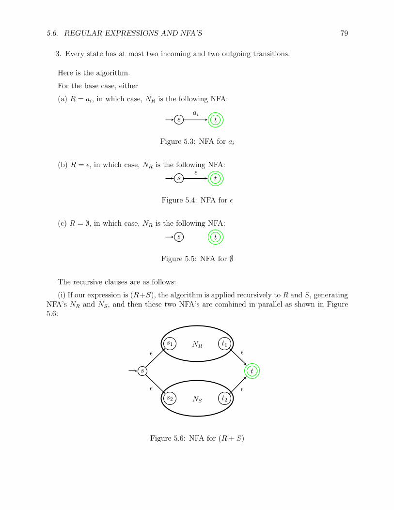
5.6. REGULAR EXPRESSIONS AND NFA’S 79
3. Every state has at most two incoming and two outgoing transitions.
Here is the algorithm.
For the base case, either
(a) R = ai, in which case, NR is the following NFA:
s tai
Figure 5.3: NFA for ai
(b) R = ǫ, in which case, NR is the following NFA:
s tǫ
Figure 5.4: NFA for ǫ
(c) R = ∅, in which case, NR is the following NFA:
s t
Figure 5.5: NFA for ∅
The recursive clauses are as follows:
(i) If our expression is (R+S), the algorithm is applied recursively to R and S, generatingNFA’s NR and NS, and then these two NFA’s are combined in parallel as shown in Figure5.6:
s
s2
s1
t2
t1
t
ǫ
ǫ
ǫ
ǫ
NS
NR
Figure 5.6: NFA for (R + S)
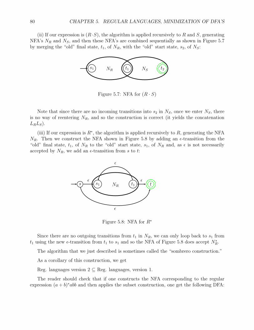
80 CHAPTER 5. REGULAR LANGUAGES, MINIMIZATION OF DFA’S
(ii) If our expression is (R ·S), the algorithm is applied recursively to R and S, generatingNFA’s NR and NS, and then these NFA’s are combined sequentially as shown in Figure 5.7by merging the “old” final state, t1, of NR, with the “old” start state, s2, of NS:
s1 t1 t2NR NS
Figure 5.7: NFA for (R · S)
Note that since there are no incoming transitions into s2 in NS, once we enter NS, thereis no way of reentering NR, and so the construction is correct (it yields the concatenationLRLS).
(iii) If our expression is R∗, the algorithm is applied recursively to R, generating the NFANR. Then we construct the NFA shown in Figure 5.8 by adding an ǫ-transition from the“old” final state, t1, of NR to the “old” start state, s1, of NR and, as ǫ is not necessarilyaccepted by NR, we add an ǫ-transition from s to t:
s s1 t1 tǫ ǫ
ǫ
ǫ
NR
Figure 5.8: NFA for R∗
Since there are no outgoing transitions from t1 in NR, we can only loop back to s1 fromt1 using the new ǫ-transition from t1 to s1 and so the NFA of Figure 5.8 does accept N∗
R.
The algorithm that we just described is sometimes called the “sombrero construction.”
As a corollary of this construction, we get
Reg. languages version 2 ⊆ Reg. languages, version 1.
The reader should check that if one constructs the NFA corresponding to the regularexpression (a+ b)∗abb and then applies the subset construction, one get the following DFA:
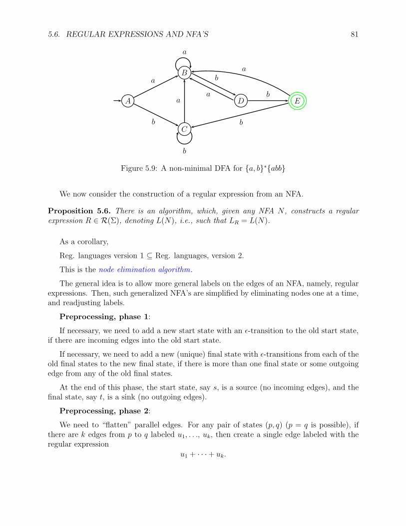
5.6. REGULAR EXPRESSIONS AND NFA’S 81
A
B
C
D E
a
b
a
b
a b
b
a
b
a
Figure 5.9: A non-minimal DFA for a, b∗abb
We now consider the construction of a regular expression from an NFA.
Proposition 5.6. There is an algorithm, which, given any NFA N , constructs a regularexpression R ∈ R(Σ), denoting L(N), i.e., such that LR = L(N).
As a corollary,
Reg. languages version 1 ⊆ Reg. languages, version 2.
This is the node elimination algorithm.
The general idea is to allow more general labels on the edges of an NFA, namely, regularexpressions. Then, such generalized NFA’s are simplified by eliminating nodes one at a time,and readjusting labels.
Preprocessing, phase 1:
If necessary, we need to add a new start state with an ǫ-transition to the old start state,if there are incoming edges into the old start state.
If necessary, we need to add a new (unique) final state with ǫ-transitions from each of theold final states to the new final state, if there is more than one final state or some outgoingedge from any of the old final states.
At the end of this phase, the start state, say s, is a source (no incoming edges), and thefinal state, say t, is a sink (no outgoing edges).
Preprocessing, phase 2:
We need to “flatten” parallel edges. For any pair of states (p, q) (p = q is possible), ifthere are k edges from p to q labeled u1, . . ., uk, then create a single edge labeled with theregular expression
u1 + · · ·+ uk.
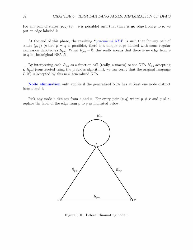
82 CHAPTER 5. REGULAR LANGUAGES, MINIMIZATION OF DFA’S
For any pair of states (p, q) (p = q is possible) such that there is no edge from p to q, weput an edge labeled ∅.
At the end of this phase, the resulting “generalized NFA” is such that for any pair ofstates (p, q) (where p = q is possible), there is a unique edge labeled with some regularexpression denoted as Rp,q. When Rp,q = ∅, this really means that there is no edge from pto q in the original NFA N .
By interpreting each Rp,q as a function call (really, a macro) to the NFA Np,q acceptingL[Rp,q] (constructed using the previous algorithm), we can verify that the original languageL(N) is accepted by this new generalized NFA.
Node elimination only applies if the generalized NFA has at least one node distinctfrom s and t.
Pick any node r distinct from s and t. For every pair (p, q) where p 6= r and q 6= r,replace the label of the edge from p to q as indicated below:
Rr,r
Rp,q
Rp,r Rr,q
p q
r
Figure 5.10: Before Eliminating node r
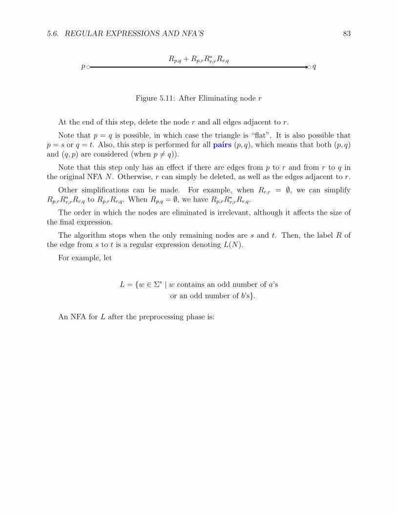
5.6. REGULAR EXPRESSIONS AND NFA’S 83
bc bcRp,q +Rp,rR
∗r,rRr,q
p q
Figure 5.11: After Eliminating node r
At the end of this step, delete the node r and all edges adjacent to r.
Note that p = q is possible, in which case the triangle is “flat”. It is also possible thatp = s or q = t. Also, this step is performed for all pairs (p, q), which means that both (p, q)and (q, p) are considered (when p 6= q)).
Note that this step only has an effect if there are edges from p to r and from r to q inthe original NFA N . Otherwise, r can simply be deleted, as well as the edges adjacent to r.
Other simplifications can be made. For example, when Rr,r = ∅, we can simplifyRp,rR
∗r,rRr,q to Rp,rRr,q. When Rp,q = ∅, we have Rp,rR
∗r,rRr,q.
The order in which the nodes are eliminated is irrelevant, although it affects the size ofthe final expression.
The algorithm stops when the only remaining nodes are s and t. Then, the label R ofthe edge from s to t is a regular expression denoting L(N).
For example, let
L = w ∈ Σ∗ | w contains an odd number of a’s
or an odd number of b’s.
An NFA for L after the preprocessing phase is:
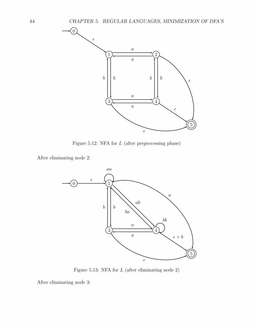
84 CHAPTER 5. REGULAR LANGUAGES, MINIMIZATION OF DFA’S
0
1 2
3 4
5
ǫ
a
a
bb
a
a
bb ǫ
ǫ
ǫ
Figure 5.12: NFA for L (after preprocessing phase)
After eliminating node 2:
0 1
3 4
5
ǫ
ab
babb
a
a
a
ǫ+ b
ǫ
aa
bb
Figure 5.13: NFA for L (after eliminating node 2)
After eliminating node 3:
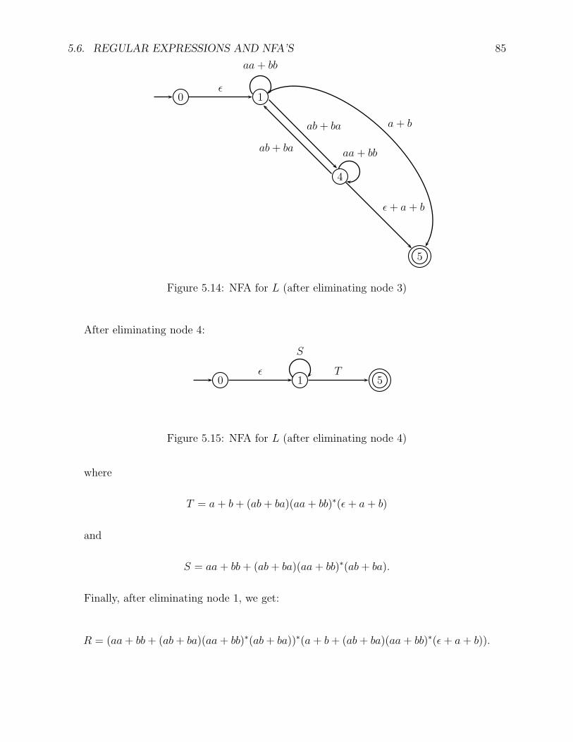
5.6. REGULAR EXPRESSIONS AND NFA’S 85
0 1
4
5
ǫ
ab+ ba
ab+ ba
a + b
ǫ+ a + b
aa + bb
aa + bb
Figure 5.14: NFA for L (after eliminating node 3)
After eliminating node 4:
0 1 5ǫ T
S
Figure 5.15: NFA for L (after eliminating node 4)
where
T = a + b+ (ab+ ba)(aa + bb)∗(ǫ+ a+ b)
and
S = aa + bb+ (ab+ ba)(aa + bb)∗(ab+ ba).
Finally, after eliminating node 1, we get:
R = (aa+ bb+ (ab+ ba)(aa + bb)∗(ab+ ba))∗(a + b+ (ab+ ba)(aa + bb)∗(ǫ+ a+ b)).
86 CHAPTER 5. REGULAR LANGUAGES, MINIMIZATION OF DFA’S
5.7 Applications of Regular Expressions:
Lexical analysis, Finding patterns in text
Regular expressions have several practical applications. The first important application isto lexical analysis .
A lexical analyzer is the first component of a compiler .
The purpose of a lexical analyzer is to scan the source program and break it into atomiccomponents, known as tokens , i.e., substrings of consecutive characters that belong togetherlogically.
Examples of tokens are: identifiers, keywords, numbers (in fixed point notation or floatingpoint notation, etc.), arithmetic operators (+, ·,−, ^), comparison operators (<,>,=, <>),assignment operator (:=), etc.
Tokens can be described by regular expressions. For this purpose, it is useful to enrichthe syntax of regular expressions, as in UNIX.
For example, the 26 upper case letters of the (roman) alphabet, A, . . . , Z, can be specifiedby the expression
[A-Z]
Similarly, the ten digits, 0, 1, . . . , 9, can be specified by the expression
[0-9]
The regular expression
R1 +R2 + · · ·+Rk
is denoted
[R1R2 · · ·Rk]
So, the expression
[A-Za-z0-9]
denotes any letter (upper case or lower case) or digit. This is called an alphanumeric.
If we define an identifier as a string beginning with a letter (upper case or lower case)followed by any number of alphanumerics (including none), then we can use the followingexpression to specify identifiers:
[A-Za-z][A-Za-z0-9]∗
There are systems, such as lex or flex that accept as input a list of regular expressionsdescribing the tokens of a programming language and construct a lexical analyzer for thesetokens.
5.8. SUMMARY OF CLOSURE PROPERTIES OF THE REGULAR LANGUAGES 87
Such systems are called lexical analyzer generators . Basically, they build a DFA fromthe set of regular expressions using the algorithms that have been described earlier.
Usually, it is possible associate with every expression some action to be taken when thecorresponding token is recognized
Another application of regular expressions is finding patterns in text.
Using a regular expression, we can specify a “vaguely defined” class of patterns.
Take the example of a street address. Most street addresses end with “Street”, or “Av-enue”, or “Road” or “St.”, or “Ave.”, or “Rd.”.
We can design a regular expression that captures the shape of most street addresses andthen convert it to a DFA that can be used to search for street addresses in text.
For more on this, see Hopcroft-Motwani and Ullman.
5.8 Summary of Closure Properties of the Regular Lan-
guages
The family of regular languages is closed under many operations. In particular, it is closedunder the following operations listed below. Some of the closure properties are left as ahomework problem.
(1) Union, intersection, relative complement.
(2) Concatenation, Kleene ∗, Kleene +.
(3) Homomorphisms and inverse homomorphisms.
(4) gsm and inverse gsm mappings, a-transductions and inverse a-transductions.
Another useful operation is substitution.
Given any two alphabets Σ,∆, a substitution is a function, τ : Σ→ 2∆∗
, assigning somelanguage, τ(a) ⊆ ∆∗, to every symbol a ∈ Σ.
A substitution τ : Σ → 2∆∗
is extended to a map τ : 2Σ∗ → 2∆
∗
by first extending τ tostrings using the following definition
τ(ǫ) = ǫ,τ(ua) = τ(u)τ(a),
where u ∈ Σ∗ and a ∈ Σ, and then to languages by letting
τ(L) =⋃
w∈L
τ(w),
88 CHAPTER 5. REGULAR LANGUAGES, MINIMIZATION OF DFA’S
for every language L ⊆ Σ∗.
Observe that a homomorphism is a special kind of substitution.
A substitution is a regular substitution iff τ(a) is a regular language for every a ∈ Σ.The proof of the next proposition is left as a homework problem.
Proposition 5.7. If L is a regular language and τ is a regular substitution, then τ(L) isalso regular. Thus, the family of regular languages is closed under regular substitutions.
5.9 Right-Invariant Equivalence Relations on Σ∗
The purpose of this section is to give one more characterization of the regular languages interms of certain kinds of equivalence relations on strings. Pushing this characterization a bitfurther, we will be able to show how minimal DFA’s can be found.
Let D = (Q,Σ, δ, q0, F ) be a DFA. The DFA D may be redundant, for example, if thereare states that are not accessible from the start state. The set Qr of accessible or reachablestates is the subset of Q defined as
Qr = p ∈ Q | ∃w ∈ Σ∗, δ∗(q0, w) = p.
If Q 6= Qr, we can “clean up” D by deleting the states in Q−Qr and restricting the transitionfunction δ to Qr. This way, we get an equivalent DFA Dr such that L(D) = L(Dr), whereall the states of Dr are reachable. From now on, we assume that we are dealing with DFA’ssuch that D = Dr, called trim, or reachable.
Recall that an equivalence relation ≃ on a set A is a relation which is reflexive, symmetric,and transitive. Given any a ∈ A, the set
b ∈ A | a ≃ b
is called the equivalence class of a, and it is denoted as [a]≃, or even as [a]. Recall thatfor any two elements a, b ∈ A, [a] ∩ [b] = ∅ iff a 6≃ b, and [a] = [b] iff a ≃ b. The set ofequivalence classes associated with the equivalence relation ≃ is a partition Π of A (alsodenoted as A/ ≃). This means that it is a family of nonempty pairwise disjoint sets whoseunion is equal to A itself. The equivalence classes are also called the blocks of the partitionΠ. The number of blocks in the partition Π is called the index of ≃ (and Π).
Given any two equivalence relations ≃1 and ≃2 with associated partitions Π1 and Π2,
≃1 ⊆≃2
iff every block of the partition Π1 is contained in some block of the partition Π2. Then, everyblock of the partition Π2 is the union of blocks of the partition Π1, and we say that ≃1 isa refinement of ≃2 (and similarly, Π1 is a refinement of Π2). Note that Π2 has at most asmany blocks as Π1 does.
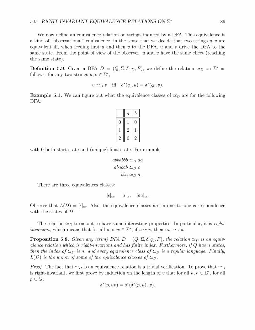
5.9. RIGHT-INVARIANT EQUIVALENCE RELATIONS ON Σ∗ 89
We now define an equivalence relation on strings induced by a DFA. This equivalence isa kind of “observational” equivalence, in the sense that we decide that two strings u, v areequivalent iff, when feeding first u and then v to the DFA, u and v drive the DFA to thesame state. From the point of view of the observer, u and v have the same effect (reachingthe same state).
Definition 5.9. Given a DFA D = (Q,Σ, δ, q0, F ), we define the relation ≃D on Σ∗ asfollows: for any two strings u, v ∈ Σ∗,
u ≃D v iff δ∗(q0, u) = δ∗(q0, v).
Example 5.1. We can figure out what the equivalence classes of ≃D are for the followingDFA:
a b
0 1 0
1 2 1
2 0 2
with 0 both start state and (unique) final state. For example
abbabbb ≃D aa
ababab ≃D ǫ
bba ≃D a.
There are three equivalences classes:
[ǫ]≃, [a]≃, [aa]≃.
Observe that L(D) = [ǫ]≃. Also, the equivalence classes are in one–to–one correspondencewith the states of D.
The relation ≃D turns out to have some interesting properties. In particular, it is right-invariant , which means that for all u, v, w ∈ Σ∗, if u ≃ v, then uw ≃ vw.
Proposition 5.8. Given any (trim) DFA D = (Q,Σ, δ, q0, F ), the relation ≃D is an equiv-alence relation which is right-invariant and has finite index. Furthermore, if Q has n states,then the index of ≃D is n, and every equivalence class of ≃D is a regular language. Finally,L(D) is the union of some of the equivalence classes of ≃D.
Proof. The fact that ≃D is an equivalence relation is a trivial verification. To prove that ≃D
is right-invariant, we first prove by induction on the length of v that for all u, v ∈ Σ∗, for allp ∈ Q,
δ∗(p, uv) = δ∗(δ∗(p, u), v).
90 CHAPTER 5. REGULAR LANGUAGES, MINIMIZATION OF DFA’S
Then, if u ≃D v, which means that δ∗(q0, u) = δ∗(q0, v), we have
δ∗(q0, uw) = δ∗(δ∗(q0, u), w) = δ∗(δ∗(q0, v), w) = δ∗(q0, vw),
which means that uw ≃D vw. Thus, ≃D is right-invariant. We still have to prove that ≃D
has index n. Define the function f : Σ∗ → Q such that
f(u) = δ∗(q0, u).
Note that if u ≃D v, which means that δ∗(q0, u) = δ∗(q0, v), then f(u) = f(v). Thus, thefunction f : Σ∗ → Q has the same value on all the strings in some equivalence class [u], so
it induces a function f : Π→ Q defined such that
f([u]) = f(u)
for every equivalence class [u] ∈ Π, where Π = Σ∗/ ≃ is the partition associated with≃D. This function is well defined since f(v) has the same value for all elements v in theequivalence class [u].
However, the function f : Π→ Q is injective (one-to-one), since f([u]) = f([v]) is equiva-
lent to f(u) = f(v) (since by definition of f we have f([u]) = f(u) and f([v]) = f(v)), whichby definition of f means that δ∗(q0, u) = δ∗(q0, v), which means precisely that u ≃D v, thatis, [u] = [v].
Since Q has n states, Π has at most n blocks. Moreover, since every state is accessible, forevery q ∈ Q, there is some w ∈ Σ∗ so that δ∗(q0, w) = q, which shows that f([w]) = f(w) = q.
Consequently, f is also surjective. But then, being injective and surjective, f is bijective andΠ has exactly n blocks.
Every equivalence class of Π is a set of strings of the form
w ∈ Σ∗ | δ∗(q0, w) = p,
for some p ∈ Q, which is accepted by the DFA
Dp = (Q,Σ, δ, q0, p)
obtained from D by changing F to p. Thus, every equivalence class is a regular language.Finally, since
L(D) = w ∈ Σ∗ | δ∗(q0, w) ∈ F=⋃
f∈F
w ∈ Σ∗ | δ∗(q0, w) = f
=⋃
f∈F
L(Df),
we see that L(D) is the union of the equivalence classes corresponding to the final states inF .
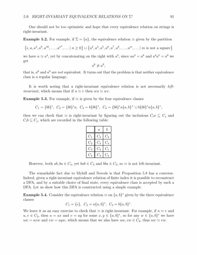
5.9. RIGHT-INVARIANT EQUIVALENCE RELATIONS ON Σ∗ 91
One should not be too optimistic and hope that every equivalence relation on strings isright-invariant.
Example 5.2. For example, if Σ = a, the equivalence relation ≃ given by the partition
ǫ, a, a4, a9, a16, . . . , an
2
, . . . | n ≥ 0∪a2, a3, a5, a6, a7, a8, . . . , am, . . . | m is not a square
we have a ≃ a4, yet by concatenating on the right with a5, since aa5 = a6 and a4a5 = a9 weget
a6 6≃ a9,
that is, a6 and a9 are not equivalent. It turns out that the problem is that neither equivalenceclass is a regular language.
It is worth noting that a right-invariant equivalence relation is not necessarily left-invariant , which means that if u ≃ v then wu ≃ wv.
Example 5.3. For example, if ≃ is given by the four equivalence classes
C1 = bb∗, C2 = bb∗a, C3 = bbb∗, C4 = bb∗aa, b+ ∪ bbb∗aa, b∗,
then we can check that ≃ is right-invariant by figuring out the inclusions Cia ⊆ Cj andCib ⊆ Cj , which are recorded in the following table:
a b
C1 C2 C3
C2 C4 C4
C3 C4 C1
C4 C4 C4
However, both ab, ba ∈ C4, yet bab ∈ C4 and bba ∈ C2, so ≃ is not left-invariant.
The remarkable fact due to Myhill and Nerode is that Proposition 5.8 has a converse.Indeed, given a right-invariant equivalence relation of finite index it is possible to reconstructa DFA, and by a suitable choice of final state, every equivalence class is accepted by such aDFA. Let us show how this DFA is constructed using a simple example.
Example 5.4. Consider the equivalence relation ≃ on a, b∗ given by the three equivalenceclasses
C1 = ǫ, C2 = aa, b∗, C3 = ba, b∗.We leave it as an easy exercise to check that ≃ is right-invariant. For example, if u ≃ v andu, v ∈ C2, then u = ax and v = ay for some x, y ∈ a, b∗, so for any w ∈ a, b∗ we haveuw = axw and vw = ayw, which means that we also have uw, vw ∈ C2, thus uw ≃ vw.
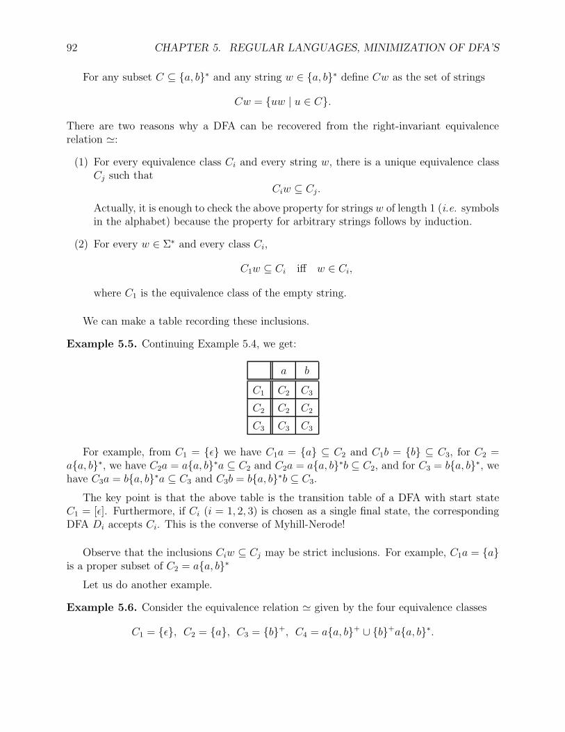
92 CHAPTER 5. REGULAR LANGUAGES, MINIMIZATION OF DFA’S
For any subset C ⊆ a, b∗ and any string w ∈ a, b∗ define Cw as the set of strings
Cw = uw | u ∈ C.
There are two reasons why a DFA can be recovered from the right-invariant equivalencerelation ≃:
(1) For every equivalence class Ci and every string w, there is a unique equivalence classCj such that
Ciw ⊆ Cj.
Actually, it is enough to check the above property for strings w of length 1 (i.e. symbolsin the alphabet) because the property for arbitrary strings follows by induction.
(2) For every w ∈ Σ∗ and every class Ci,
C1w ⊆ Ci iff w ∈ Ci,
where C1 is the equivalence class of the empty string.
We can make a table recording these inclusions.
Example 5.5. Continuing Example 5.4, we get:
a b
C1 C2 C3
C2 C2 C2
C3 C3 C3
For example, from C1 = ǫ we have C1a = a ⊆ C2 and C1b = b ⊆ C3, for C2 =aa, b∗, we have C2a = aa, b∗a ⊆ C2 and C2a = aa, b∗b ⊆ C2, and for C3 = ba, b∗, wehave C3a = ba, b∗a ⊆ C3 and C3b = ba, b∗b ⊆ C3.
The key point is that the above table is the transition table of a DFA with start stateC1 = [ǫ]. Furthermore, if Ci (i = 1, 2, 3) is chosen as a single final state, the correspondingDFA Di accepts Ci. This is the converse of Myhill-Nerode!
Observe that the inclusions Ciw ⊆ Cj may be strict inclusions. For example, C1a = ais a proper subset of C2 = aa, b∗
Let us do another example.
Example 5.6. Consider the equivalence relation ≃ given by the four equivalence classes
C1 = ǫ, C2 = a, C3 = b+, C4 = aa, b+ ∪ b+aa, b∗.
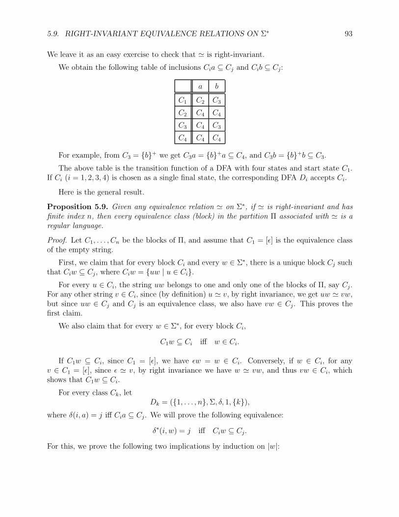
5.9. RIGHT-INVARIANT EQUIVALENCE RELATIONS ON Σ∗ 93
We leave it as an easy exercise to check that ≃ is right-invariant.
We obtain the following table of inclusions Cia ⊆ Cj and Cib ⊆ Cj:
a b
C1 C2 C3
C2 C4 C4
C3 C4 C3
C4 C4 C4
For example, from C3 = b+ we get C3a = b+a ⊆ C4, and C3b = b+b ⊆ C3.
The above table is the transition function of a DFA with four states and start state C1.If Ci (i = 1, 2, 3, 4) is chosen as a single final state, the corresponding DFA Di accepts Ci.
Here is the general result.
Proposition 5.9. Given any equivalence relation ≃ on Σ∗, if ≃ is right-invariant and hasfinite index n, then every equivalence class (block) in the partition Π associated with ≃ is aregular language.
Proof. Let C1, . . . , Cn be the blocks of Π, and assume that C1 = [ǫ] is the equivalence classof the empty string.
First, we claim that for every block Ci and every w ∈ Σ∗, there is a unique block Cj suchthat Ciw ⊆ Cj, where Ciw = uw | u ∈ Ci.
For every u ∈ Ci, the string uw belongs to one and only one of the blocks of Π, say Cj.For any other string v ∈ Ci, since (by definition) u ≃ v, by right invariance, we get uw ≃ vw,but since uw ∈ Cj and Cj is an equivalence class, we also have vw ∈ Cj. This proves thefirst claim.
We also claim that for every w ∈ Σ∗, for every block Ci,
C1w ⊆ Ci iff w ∈ Ci.
If C1w ⊆ Ci, since C1 = [ǫ], we have ǫw = w ∈ Ci. Conversely, if w ∈ Ci, for anyv ∈ C1 = [ǫ], since ǫ ≃ v, by right invariance we have w ≃ vw, and thus vw ∈ Ci, whichshows that C1w ⊆ Ci.
For every class Ck, letDk = (1, . . . , n,Σ, δ, 1, k),
where δ(i, a) = j iff Cia ⊆ Cj. We will prove the following equivalence:
δ∗(i, w) = j iff Ciw ⊆ Cj.
For this, we prove the following two implications by induction on |w|:
94 CHAPTER 5. REGULAR LANGUAGES, MINIMIZATION OF DFA’S
(a) If δ∗(i, w) = j, then Ciw ⊆ Cj , and
(b) If Ciw ⊆ Cj, then δ∗(i, w) = j.
The base case (w = ǫ) is trivial for both (a) and (b). We leave the proof of the inductionstep for (a) as an exercise and give the proof of the induction step for (b) because it is moresubtle. Let w = ua, with a ∈ Σ and u ∈ Σ∗. If Ciua ⊆ Cj, then by the first claim, we knowthat there is a unique block, Ck, such that Ciu ⊆ Ck. Furthermore, there is a unique block,Ch, such that Cka ⊆ Ch, but Ciu ⊆ Ck implies Ciua ⊆ Cka so we get Ciua ⊆ Ch. However,by the uniqueness of the block, Cj, such that Ciua ⊆ Cj, we must have Ch = Cj . By theinduction hypothesis, as Ciu ⊆ Ck, we have
δ∗(i, u) = k
and, by definition of δ, as Cka ⊆ Cj (= Ch), we have δ(k, a) = j, so we deduce that
δ∗(i, ua) = δ(δ∗(i, u), a) = δ(k, a) = j,
as desired. Then, using the equivalence just proved and the second claim, we have
L(Dk) = w ∈ Σ∗ | δ∗(1, w) ∈ k= w ∈ Σ∗ | δ∗(1, w) = k= w ∈ Σ∗ | C1w ⊆ Ck= w ∈ Σ∗ | w ∈ Ck = Ck,
proving that every block, Ck, is a regular language.
In general it is false that Cia = Cj for some block Cj, and we can only claim thatCia ⊆ Cj.
We can combine Proposition 5.8 and Proposition 5.9 to get the following characterizationof a regular language due to Myhill and Nerode:
Theorem 5.10. (Myhill-Nerode) A language L (over an alphabet Σ) is a regular language iffit is the union of some of the equivalence classes of an equivalence relation ≃ on Σ∗, whichis right-invariant and has finite index.
Theorem 5.10 can also be used to prove that certain languages are not regular. A generalscheme (not the only one) goes as follows: If L is not regular, then it must be infinite.Now, we argue by contradiction. If L was regular, then by Myhill-Nerode, there would besome equivalence relation ≃, which is right-invariant and of finite index, and such that L isthe union of some of the classes of ≃. Because Σ∗ is infinite and ≃ has only finitely manyequivalence classes, there are strings x, y ∈ Σ∗ with x 6= y so that
x ≃ y.
5.9. RIGHT-INVARIANT EQUIVALENCE RELATIONS ON Σ∗ 95
If we can find a third string, z ∈ Σ∗, such that
xz ∈ L and yz /∈ L,
then we reach a contradiction. Indeed, by right invariance, from x ≃ y, we get xz ≃ yz. But,L is the union of equivalence classes of ≃, so if xz ∈ L, then we should also have yz ∈ L,contradicting yz /∈ L. Therefore, L is not regular.
Then the scenario is this: to prove that L is not regular, first we check that L is infinite.If so, we try finding three strings x, y, z, where and x and y 6= x are prefixes of strings in Lsuch that
x ≃ y,
where ≃ is a right-invariant relation of finite index such that L is the union of equivalenceof L (which must exist by Myhill–Nerode since we are assuming by contradiction that L isregular), and where z is chosen so that
xz ∈ L and yz 6∈ L.
Example 5.7. For example, we prove that L = anbn | n ≥ 1 is not regular.Assuming for the sake of contradiction that L is regular, there is some equivalence relation
≃ which is right-invariant and of finite index and such that L is the union of some of theclasses of ≃. Since the sequence
a, aa, aaa, . . . , ai, . . .
is infinite and ≃ has a finite number of classes, two of these strings must belong to thesame class, which means that ai ≃ aj for some i 6= j. But since ≃ is right invariant, byconcatenating with bi on the right, we see that aibi ≃ ajbi for some i 6= j. However aibi ∈ L,and since L is the union of classes of ≃, we also have ajbi ∈ L for i 6= j, which is absurd,given the definition of L. Thus, in fact, L is not regular.
Here is another illustration of the use of the Myhill-Nerode Theorem to prove that alanguage is not regular.
Example 5.8. We claim that the language,
L′ = an! | n ≥ 1,
is not regular, where n! (n factorial) is given by 0! = 1 and (n+ 1)! = (n + 1)n!.
Assume L′ is regular. Then, there is some equivalence relation ≃ which is right-invariantand of finite index and such that L′ is the union of some of the classes of ≃. Since thesequence
a, a2, . . . , an, . . .
96 CHAPTER 5. REGULAR LANGUAGES, MINIMIZATION OF DFA’S
is infinite, two of these strings must belong to the same class, which means that ap ≃ aq forsome p, q with 1 ≤ p < q. As q! ≥ q for all q ≥ 0 and q > p, we can concatenate on the rightwith aq!−p and we get
apaq!−p ≃ aqaq!−p,
that is,
aq! ≃ aq!+q−p.
Since p < q we have q! < q! + q − p. If we can show that
q! + q − p < (q + 1)!
we will obtain a contradiction because then aq!+q−p /∈ L′, yet aq!+q−p ≃ aq! and aq! ∈ L′,contradicting Myhill-Nerode. Now, as 1 ≤ p < q, we have q − p ≤ q − 1, so if we can provethat
q! + q − p ≤ q! + q − 1 < (q + 1)!
we will be done. However, q! + q − 1 < (q + 1)! is equivalent to
q − 1 < (q + 1)!− q!,
and since (q + 1)!− q! = (q + 1)q!− q! = qq!, we simply need to prove that
q − 1 < q ≤ qq!,
which holds for q ≥ 1.
There is another version of the Myhill-Nerode Theorem involving congruences which isalso quite useful. An equivalence relation, ≃, on Σ∗ is left and right-invariant iff for allx, y, u, v ∈ Σ∗,
if x ≃ y then uxv ≃ uyv.
An equivalence relation, ≃, on Σ∗ is a congruence iff for all u1, u2, v1, v2 ∈ Σ∗,
if u1 ≃ v1 and u2 ≃ v2 then u1u2 ≃ v1v2.
It is easy to prove that an equivalence relation is a congruence iff it is left and right-invariant.
For example, assume that ≃ is a left and right-invariant equivalence relation, and assumethat
u1 ≃ v1 and u2 ≃ v2.
By right-invariance applied to u1 ≃ v1 , we get
u1u2 ≃ v1u2
5.9. RIGHT-INVARIANT EQUIVALENCE RELATIONS ON Σ∗ 97
and by left-invariance applied to u2 ≃ v2 we get
v1u2 ≃ v1v2.
By transitivity, we conclude that
u1u2 ≃ v1v2.
which shows that ≃ is a congruence.
Proving that a congruence is left and right-invariant is even easier.
There is a version of Proposition 5.8 that applies to congruences and for this we definethe relation ∼D as follows: For any (trim) DFA, D = (Q,Σ, δ, q0, F ), for all x, y ∈ Σ∗,
x ∼D y iff (∀q ∈ Q)(δ∗(q, x) = δ∗(q, y)).
Proposition 5.11. Given any (trim) DFA, D = (Q,Σ, δ, q0, F ), the relation ∼D is anequivalence relation which is left and right-invariant and has finite index. Furthermore, ifQ has n states, then the index of ∼D is at most nn and every equivalence class of ∼D is aregular language. Finally, L(D) is the union of some of the equivalence classes of ∼D.
Proof. We leave most of the proof of Proposition 5.11 as an exercise. The last two parts ofthe proposition are proved using the following facts:
(1) Since ∼D is left and right-invariant and has finite index, in particular, ∼D is right-invariant and has finite index, so by Proposition 5.9 every equivalence class of ∼D isregular.
(2) Observe that∼D ⊆≃D,
since the condition δ∗(q, x) = δ∗(q, y) holds for every q ∈ Q, so in particular for q = q0.But then, every equivalence class of ≃D is the union of equivalence classes of ∼D andsince, by Proposition 5.8, L is the union of equivalence classes of ≃D, we conclude thatL is also the union of equivalence classes of ∼D.
This completes the proof.
Using Proposition 5.11 and Proposition 5.9, we obtain another version of the Myhill-Nerode Theorem.
Theorem 5.12. (Myhill-Nerode, Congruence Version) A language L (over an alphabet Σ)is a regular language iff it is the union of some of the equivalence classes of an equivalencerelation ≃ on Σ∗, which is a congruence and has finite index.
We now consider an equivalence relation associated with a language L.
98 CHAPTER 5. REGULAR LANGUAGES, MINIMIZATION OF DFA’S
5.10 Finding minimal DFA’s
Given any language L (not necessarily regular), we can define an equivalence relation ρL onΣ∗ which is right-invariant, but not necessarily of finite index. The equivalence relation ρLis such that L is the union of equivalence classes of ρL. Furthermore, when L is regular, therelation ρL has finite index. In fact, this index is the size of a smallest DFA accepting L. Asa consequence, if L is regular, a simple modification of the proof of Proposition 5.9 appliedto ≃ = ρL yields a minimal DFA DρL accepting L.
Then, given any trim DFA D accepting L, the equivalence relation ρL can be translatedto an equivalence relation ≡ on states, in such a way that for all u, v ∈ Σ∗,
uρLv iff ϕ(u) ≡ ϕ(v),
where ϕ : Σ∗ → Q is the function (run the DFA D on u from q0) given by
ϕ(u) = δ∗(q0, u).
One can then construct a quotient DFA D/ ≡ whose states are obtained by merging allstates in a given equivalence class of states into a single state, and the resulting DFA D/ ≡is a mininal DFA. Even though D/ ≡ appears to depend on D, it is in fact unique, andisomorphic to the abstract DFA DρL induced by ρL.
The last step in obtaining the minimal DFA D/ ≡ is to give a constructive method tocompute the state equivalence relation ≡. This can be done by constructing a sequence ofapproximations ≡i, where each ≡i+1 refines ≡i. It turns out that if D has n states, thenthere is some index i0 ≤ n− 2 such that
≡j =≡i0 for all j ≥ i0 + 1,
and that
≡=≡i0 .
Furthermore, ≡i+1 can be computed inductively from ≡i. In summary, we obtain a iterativealgorithm for computing ≡ that terminates in at most n− 2 steps.
Definition 5.10. Given any language L (over Σ), we define the right-invariant equivalenceρL associated with L as the relation on Σ∗ defined as follows: for any two strings u, v ∈ Σ∗,
uρLv iff ∀w ∈ Σ∗(uw ∈ L iff vw ∈ L).
It is clear that the relation ρL is an equivalence relation, and it is right-invariant. Toshow right-invariance, argue as follows: if uρLv, then for any w ∈ Σ∗, since uρLv means that
uz ∈ L iff vz ∈ L
5.10. FINDING MINIMAL DFA’S 99
for all z ∈ Σ∗, in particular the above equivalence holds for all z of the form z = wy for anyarbitary y ∈ Σ∗, so we have
uwy ∈ L iff vwy ∈ Lfor all y ∈ Σ∗, which means that uwρLvw.
It is also clear that L is the union of the equivalence classes of strings in L. This isbecause if u ∈ L and uρLv, by letting w = ǫ in the definition of ρL, we get
u ∈ L iff v ∈ L,
and since u ∈ L, we also have v ∈ L. This implies that if u ∈ L then [u]ρL ⊆ L and so,
L =⋃
u∈L
[u]ρL.
Example 5.9. For example, consider the regular language
L = a ∪ bm | m ≥ 1.
We leave it as an exercise to show that the equivalence relation ρL consists of the fourequivalence classes
C1 = ǫ, C2 = a, C3 = b+, C4 = aa, b+ ∪ b+aa, b∗
encountered earlier in Example 5.6. Observe that
L = C2 ∪ C3.
When L is regular, we have the following remarkable result:
Proposition 5.13. Given any regular language L, for any (trim) DFA D = (Q,Σ, δ, q0, F )such that L = L(D), ρL is a right-invariant equivalence relation, and we have ≃D ⊆ ρL.Furthermore, if ρL has m classes and Q has n states, then m ≤ n.
Proof. By definition, u ≃D v iff δ∗(q0, u) = δ∗(q0, v). Since w ∈ L(D) iff δ∗(q0, w) ∈ F , thefact that uρLv can be expressed as
∀w ∈ Σ∗(uw ∈ L iff vw ∈ L)iff
∀w ∈ Σ∗(δ∗(q0, uw) ∈ F iff δ∗(q0, vw) ∈ F )iff
∀w ∈ Σ∗(δ∗(δ∗(q0, u), w) ∈ F iff δ∗(δ∗(q0, v), w) ∈ F ),
and if δ∗(q0, u) = δ∗(q0, v), this shows that uρLv. Since the number of classes of ≃D is n and≃D ⊆ ρL, the equivalence relation ρL has fewer classes than ≃D, and m ≤ n.
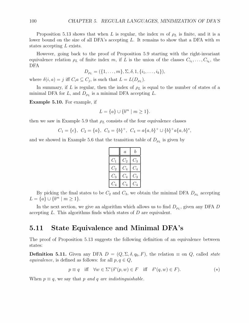
100 CHAPTER 5. REGULAR LANGUAGES, MINIMIZATION OF DFA’S
Proposition 5.13 shows that when L is regular, the index m of ρL is finite, and it is alower bound on the size of all DFA’s accepting L. It remains to show that a DFA with mstates accepting L exists.
However, going back to the proof of Proposition 5.9 starting with the right-invariantequivalence relation ρL of finite index m, if L is the union of the classes Ci1 , . . . , Cik , theDFA
DρL = (1, . . . , m,Σ, δ, 1, i1, . . . , ik),where δ(i, a) = j iff Cia ⊆ Cj, is such that L = L(DρL).
In summary, if L is regular, then the index of ρL is equal to the number of states of aminimal DFA for L, and DρL is a minimal DFA accepting L.
Example 5.10. For example, if
L = a ∪ bm | m ≥ 1.then we saw in Example 5.9 that ρL consists of the four equivalence classes
C1 = ǫ, C2 = a, C3 = b+, C4 = aa, b+ ∪ b+aa, b∗,and we showed in Example 5.6 that the transition table of DρL is given by
a b
C1 C2 C3
C2 C4 C4
C3 C4 C3
C4 C4 C4
By picking the final states to be C2 and C3, we obtain the minimal DFA DρL acceptingL = a ∪ bm | m ≥ 1.
In the next section, we give an algorithm which allows us to find DρL, given any DFA Daccepting L. This algorithms finds which states of D are equivalent.
5.11 State Equivalence and Minimal DFA’s
The proof of Proposition 5.13 suggests the following definition of an equivalence betweenstates:
Definition 5.11. Given any DFA D = (Q,Σ, δ, q0, F ), the relation ≡ on Q, called stateequivalence, is defined as follows: for all p, q ∈ Q,
p ≡ q iff ∀w ∈ Σ∗(δ∗(p, w) ∈ F iff δ∗(q, w) ∈ F ). (∗)When p ≡ q, we say that p and q are indistinguishable.
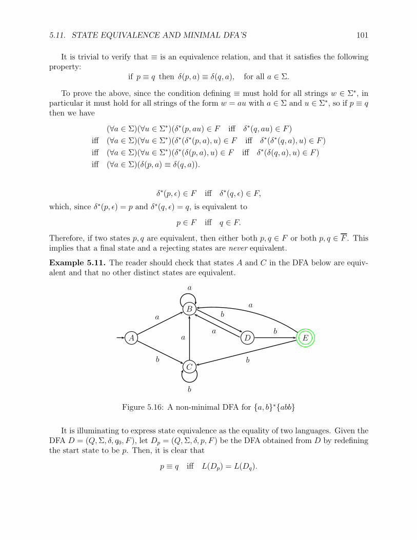
5.11. STATE EQUIVALENCE AND MINIMAL DFA’S 101
It is trivial to verify that ≡ is an equivalence relation, and that it satisfies the followingproperty:
if p ≡ q then δ(p, a) ≡ δ(q, a), for all a ∈ Σ.
To prove the above, since the condition defining ≡ must hold for all strings w ∈ Σ∗, inparticular it must hold for all strings of the form w = au with a ∈ Σ and u ∈ Σ∗, so if p ≡ qthen we have
(∀a ∈ Σ)(∀u ∈ Σ∗)(δ∗(p, au) ∈ F iff δ∗(q, au) ∈ F )iff (∀a ∈ Σ)(∀u ∈ Σ∗)(δ∗(δ∗(p, a), u) ∈ F iff δ∗(δ∗(q, a), u) ∈ F )iff (∀a ∈ Σ)(∀u ∈ Σ∗)(δ∗(δ(p, a), u) ∈ F iff δ∗(δ(q, a), u) ∈ F )iff (∀a ∈ Σ)(δ(p, a) ≡ δ(q, a)).
δ∗(p, ǫ) ∈ F iff δ∗(q, ǫ) ∈ F,which, since δ∗(p, ǫ) = p and δ∗(q, ǫ) = q, is equivalent to
p ∈ F iff q ∈ F.Therefore, if two states p, q are equivalent, then either both p, q ∈ F or both p, q ∈ F . Thisimplies that a final state and a rejecting states are never equivalent.
Example 5.11. The reader should check that states A and C in the DFA below are equiv-alent and that no other distinct states are equivalent.
A
B
C
D E
a
b
a
b
a b
b
a
b
a
Figure 5.16: A non-minimal DFA for a, b∗abb
It is illuminating to express state equivalence as the equality of two languages. Given theDFA D = (Q,Σ, δ, q0, F ), let Dp = (Q,Σ, δ, p, F ) be the DFA obtained from D by redefiningthe start state to be p. Then, it is clear that
p ≡ q iff L(Dp) = L(Dq).
102 CHAPTER 5. REGULAR LANGUAGES, MINIMIZATION OF DFA’S
This simple observation implies that there is an algorithm to test state equivalence.Indeed, we simply have to test whether the DFA’s Dp and Dq accept the same languageand this can be done using the cross-product construction. Indeed, L(Dp) = L(Dq) iffL(Dp)−L(Dq) = ∅ and L(Dq)−L(Dp) = ∅. Now, if (Dp×Dq)1−2 denotes the cross-productDFA with starting state (p, q) and with final states F × (Q− F ) and (Dp ×Dq)2−1 denotesthe cross-product DFA also with starting state (p, q) and with final states (Q− F )× F , weknow that
L((Dp ×Dq)1−2) = L(Dp)− L(Dq) and L((Dp ×Dq)2−1) = L(Dq)− L(Dp),
so all we need to do if to test whether (Dp × Dq)1−2 and (Dp × Dq)2−1 accept the emptylanguage. However, we know that this is the case iff the set of states reachable from (p, q)in (Dp ×Dq)1−2 contains no state in F × (Q− F ) and the set of states reachable from (p, q)in (Dp ×Dq)2−1 contains no state in (Q− F )× F .
Actually, the graphs of (Dp ×Dq)1−2 and (Dp ×Dq)2−1 are identical, so we only need tocheck that no state in (F × (Q−F ))∪ ((Q−F )×F ) is reachable from (p, q) in that graph.This algorithm to test state equivalence is not the most efficient but it is quite reasonable(it runs in polynomial time).
If L = L(D), Theorem 5.14 below shows the relationship between ρL and ≡ and, moregenerally, between the DFA, DρL , and the DFA, D/ ≡, obtained as the quotient of the DFAD modulo the equivalence relation ≡ on Q.
The minimal DFA D/ ≡ is obtained by merging the states in each block Ci of thepartition Π associated with ≡, forming states corresponding to the blocks Ci, and drawinga transition on input a from a block Ci to a block Cj of Π iff there is a transition q = δ(p, a)from any state p ∈ Ci to any state q ∈ Cj on input a.
The start state is the block containing q0, and the final states are the blocks consistingof final states.
Example 5.12. For example, consider the DFA D1 accepting L = ab, ba∗ shown in Figure5.17.
This is not a minimal DFA. In fact,
0 ≡ 2 and 3 ≡ 5.
Here is the minimal DFA for L:
The minimal DFA D2 is obtained by merging the states in the equivalence class 0, 2into a single state, similarly merging the states in the equivalence class 3, 5 into a singlestate, and drawing the transitions between equivalence classes. We obtain the DFA shownin Figure 5.18.
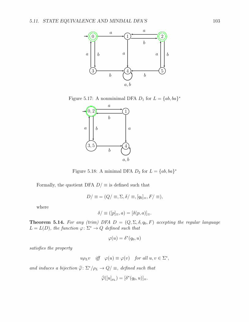
5.11. STATE EQUIVALENCE AND MINIMAL DFA’S 103
0 1 2
3 4 5
a
b
b
a
a
ba
b
a
b
a, b
Figure 5.17: A nonminimal DFA D1 for L = ab, ba∗
0, 2 1
3, 5 4
a
b
b aa
b
a, b
Figure 5.18: A minimal DFA D2 for L = ab, ba∗
Formally, the quotient DFA D/ ≡ is defined such that
D/ ≡= (Q/ ≡,Σ, δ/ ≡, [q0]≡, F/ ≡),
whereδ/ ≡ ([p]≡, a) = [δ(p, a)]≡.
Theorem 5.14. For any (trim) DFA D = (Q,Σ, δ, q0, F ) accepting the regular languageL = L(D), the function ϕ : Σ∗ → Q defined such that
ϕ(u) = δ∗(q0, u)
satisfies the property
uρLv iff ϕ(u) ≡ ϕ(v) for all u, v ∈ Σ∗,
and induces a bijection ϕ : Σ∗/ρL → Q/ ≡, defined such that
ϕ([u]ρL) = [δ∗(q0, u)]≡.
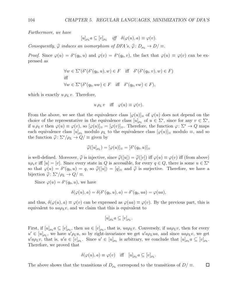
104 CHAPTER 5. REGULAR LANGUAGES, MINIMIZATION OF DFA’S
Furthermore, we have[u]ρLa ⊆ [v]ρL iff δ(ϕ(u), a) ≡ ϕ(v).
Consequently, ϕ induces an isomorphism of DFA’s, ϕ : DρL → D/ ≡.
Proof. Since ϕ(u) = δ∗(q0, u) and ϕ(v) = δ∗(q0, v), the fact that ϕ(u) ≡ ϕ(v) can be ex-pressed as
∀w ∈ Σ∗(δ∗(δ∗(q0, u), w) ∈ F iff δ∗(δ∗(q0, v), w) ∈ F )iff
∀w ∈ Σ∗(δ∗(q0, uw) ∈ F iff δ∗(q0, vw) ∈ F ),
which is exactly u ρL v. Therefore,
u ρL v iff ϕ(u) ≡ ϕ(v).
From the above, we see that the equivalence class [ϕ(u)]≡ of ϕ(u) does not depend on thechoice of the representative in the equivalence class [u]ρL of u ∈ Σ∗, since for any v ∈ Σ∗,if u ρL v then ϕ(u) ≡ ϕ(v), so [ϕ(u)]≡ = [ϕ(v)]≡. Therefore, the function ϕ : Σ∗ → Q mapseach equivalence class [u]ρL modulo ρL to the equivalence class [ϕ(u)]≡ modulo ≡, and sothe function ϕ : Σ∗/ρL → Q/ ≡ given by
ϕ([u]ρL) = [ϕ(u)]≡ = [δ∗(q0, u)]≡
is well-defined. Moreover, ϕ is injective, since ϕ([u]) = ϕ([v]) iff ϕ(u) ≡ ϕ(v) iff (from above)uρvv iff [u] = [v]. Since every state in Q is accessible, for every q ∈ Q, there is some u ∈ Σ∗
so that ϕ(u) = δ∗(q0, u) = q, so ϕ([u]) = [q]≡ and ϕ is surjective. Therefore, we have abijection ϕ : Σ∗/ρL → Q/ ≡.
Since ϕ(u) = δ∗(q0, u), we have
δ(ϕ(u), a) = δ(δ∗(q0, u), a) = δ∗(q0, ua) = ϕ(ua),
and thus, δ(ϕ(u), a) ≡ ϕ(v) can be expressed as ϕ(ua) ≡ ϕ(v). By the previous part, this isequivalent to uaρLv, and we claim that this is equivalent to
[u]ρLa ⊆ [v]ρL.
First, if [u]ρLa ⊆ [v]ρL , then ua ∈ [v]ρL, that is, uaρLv. Conversely, if uaρLv, then for everyu′ ∈ [u]ρL, we have u′ρLu, so by right-invariance we get u′aρLua, and since uaρLv, we getu′aρLv, that is, u′a ∈ [v]ρL . Since u′ ∈ [u]ρL is arbitrary, we conclude that [u]ρLa ⊆ [v]ρL .Therefore, we proved that
δ(ϕ(u), a) ≡ ϕ(v) iff [u]ρLa ⊆ [v]ρL.
The above shows that the transitions of DρL correspond to the transitions of D/ ≡.
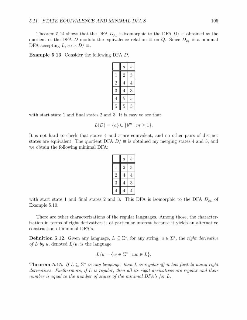
5.11. STATE EQUIVALENCE AND MINIMAL DFA’S 105
Theorem 5.14 shows that the DFA DρL is isomorphic to the DFA D/ ≡ obtained as thequotient of the DFA D modulo the equivalence relation ≡ on Q. Since DρL is a minimalDFA accepting L, so is D/ ≡.
Example 5.13. Consider the following DFA D,
a b
1 2 3
2 4 4
3 4 3
4 5 5
5 5 5
with start state 1 and final states 2 and 3. It is easy to see that
L(D) = a ∪ bm | m ≥ 1.
It is not hard to check that states 4 and 5 are equivalent, and no other pairs of distinctstates are equivalent. The quotient DFA D/ ≡ is obtained my merging states 4 and 5, andwe obtain the following minimal DFA:
a b
1 2 3
2 4 4
3 4 3
4 4 4
with start state 1 and final states 2 and 3. This DFA is isomorphic to the DFA DρL ofExample 5.10.
There are other characterizations of the regular languages. Among those, the character-ization in terms of right derivatives is of particular interest because it yields an alternativeconstruction of minimal DFA’s.
Definition 5.12. Given any language, L ⊆ Σ∗, for any string, u ∈ Σ∗, the right derivativeof L by u, denoted L/u, is the language
L/u = w ∈ Σ∗ | uw ∈ L.
Theorem 5.15. If L ⊆ Σ∗ is any language, then L is regular iff it has finitely many rightderivatives. Furthermore, if L is regular, then all its right derivatives are regular and theirnumber is equal to the number of states of the minimal DFA’s for L.
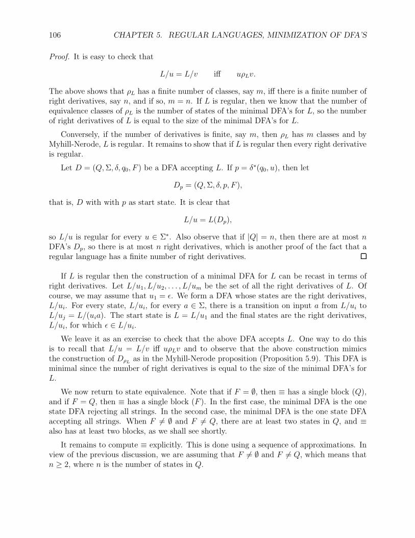
106 CHAPTER 5. REGULAR LANGUAGES, MINIMIZATION OF DFA’S
Proof. It is easy to check that
L/u = L/v iff uρLv.
The above shows that ρL has a finite number of classes, say m, iff there is a finite number ofright derivatives, say n, and if so, m = n. If L is regular, then we know that the number ofequivalence classes of ρL is the number of states of the minimal DFA’s for L, so the numberof right derivatives of L is equal to the size of the minimal DFA’s for L.
Conversely, if the number of derivatives is finite, say m, then ρL has m classes and byMyhill-Nerode, L is regular. It remains to show that if L is regular then every right derivativeis regular.
Let D = (Q,Σ, δ, q0, F ) be a DFA accepting L. If p = δ∗(q0, u), then let
Dp = (Q,Σ, δ, p, F ),
that is, D with with p as start state. It is clear that
L/u = L(Dp),
so L/u is regular for every u ∈ Σ∗. Also observe that if |Q| = n, then there are at most nDFA’s Dp, so there is at most n right derivatives, which is another proof of the fact that aregular language has a finite number of right derivatives.
If L is regular then the construction of a minimal DFA for L can be recast in terms ofright derivatives. Let L/u1, L/u2, . . . , L/um be the set of all the right derivatives of L. Ofcourse, we may assume that u1 = ǫ. We form a DFA whose states are the right derivatives,L/ui. For every state, L/ui, for every a ∈ Σ, there is a transition on input a from L/ui toL/uj = L/(uia). The start state is L = L/u1 and the final states are the right derivatives,L/ui, for which ǫ ∈ L/ui.
We leave it as an exercise to check that the above DFA accepts L. One way to do thisis to recall that L/u = L/v iff uρLv and to observe that the above construction mimicsthe construction of DρL as in the Myhill-Nerode proposition (Proposition 5.9). This DFA isminimal since the number of right derivatives is equal to the size of the minimal DFA’s forL.
We now return to state equivalence. Note that if F = ∅, then ≡ has a single block (Q),and if F = Q, then ≡ has a single block (F ). In the first case, the minimal DFA is the onestate DFA rejecting all strings. In the second case, the minimal DFA is the one state DFAaccepting all strings. When F 6= ∅ and F 6= Q, there are at least two states in Q, and ≡also has at least two blocks, as we shall see shortly.
It remains to compute ≡ explicitly. This is done using a sequence of approximations. Inview of the previous discussion, we are assuming that F 6= ∅ and F 6= Q, which means thatn ≥ 2, where n is the number of states in Q.
5.11. STATE EQUIVALENCE AND MINIMAL DFA’S 107
Definition 5.13. Given any DFA D = (Q,Σ, δ, q0, F ), for every i ≥ 0, the relation ≡i onQ, called i-state equivalence, is defined as follows: for all p, q ∈ Q,
p ≡i q iff ∀w ∈ Σ∗, |w| ≤ i (δ∗(p, w) ∈ F iff δ∗(q, w) ∈ F ).
When p ≡i q, we say that p and q are i-indistinguishable.
Since state equivalence ≡ is defined such that
p ≡ q iff ∀w ∈ Σ∗(δ∗(p, w) ∈ F iff δ∗(q, w) ∈ F ),
we note that testing the condition
δ∗(p, w) ∈ F iff δ∗(q, w) ∈ F
for all strings in Σ∗ is equivalent to testing the above condition for all strings of length atmost i for all i ≥ 0, i.e.
p ≡ q iff ∀i ≥ 0 ∀w ∈ Σ∗, |w| ≤ i (δ∗(p, w) ∈ F iff δ∗(q, w) ∈ F ).
Since ≡i is defined such that
p ≡i q iff ∀w ∈ Σ∗, |w| ≤ i (δ∗(p, w) ∈ F iff δ∗(q, w) ∈ F ),
we conclude thatp ≡ q iff ∀i ≥ 0 (p ≡i q).
This identity can also be expressed as
≡=⋂
i≥0
≡i .
If we assume that F 6= ∅ and F 6= Q, observe that ≡0 has exactly two equivalence classesF and Q− F , since ǫ is the only string of length 0, and since the condition
δ∗(p, ǫ) ∈ F iff δ∗(q, ǫ) ∈ F
is equivalent to the conditionp ∈ F iff q ∈ F.
It is also obvious from the definition of ≡i that
≡⊆ · · · ⊆ ≡i+1 ⊆≡i ⊆ · · · ⊆ ≡1 ⊆≡0 .
If this sequence was strictly decreasing for all i ≥ 0, the partition associated with ≡i+1 wouldcontain at least one more block than the partition associated with ≡i and since we start witha partition with two blocks, the partition associated with ≡i would have at least i+2 blocks.
108 CHAPTER 5. REGULAR LANGUAGES, MINIMIZATION OF DFA’S
But then, for i = n− 1, the partition associated with ≡n−1 would have at least n+1 blocks,which is absurd since Q has only n states. Therefore, there is a smallest integer, i0 ≤ n− 2,such that
≡i0+1 =≡i0 .
Thus, it remains to compute ≡i+1 from ≡i, which can be done using the following propo-sition: The proposition also shows that
≡=≡i0 .
Proposition 5.16. For any (trim) DFA D = (Q,Σ, δ, q0, F ), for all p, q ∈ Q, p ≡i+1 q iffp ≡i q and δ(p, a) ≡i δ(q, a), for every a ∈ Σ. Furthermore, if F 6= ∅ and F 6= Q, there is asmallest integer i0 ≤ n− 2, such that
≡i0+1 =≡i0 =≡ .
Proof. By the definition of the relation ≡i,
p ≡i+1 q iff ∀w ∈ Σ∗, |w| ≤ i+ 1 (δ∗(p, w) ∈ F iff δ∗(q, w) ∈ F ).
The trick is to observe that the condition
δ∗(p, w) ∈ F iff δ∗(q, w) ∈ F
holds for all strings of length at most i+ 1 iff it holds for all strings of length at most i andfor all strings of length between 1 and i+ 1. This is expressed as
p ≡i+1 q iff ∀w ∈ Σ∗, |w| ≤ i (δ∗(p, w) ∈ F iff δ∗(q, w) ∈ F )and
∀w ∈ Σ∗, 1 ≤ |w| ≤ i+ 1 (δ∗(p, w) ∈ F iff δ∗(q, w) ∈ F ).
Obviously, the first condition in the conjunction is p ≡i q, and since every string w suchthat 1 ≤ |w| ≤ i+1 can be written as au where a ∈ Σ and 0 ≤ |u| ≤ i, the second conditionin the conjunction can be written as
∀a ∈ Σ∀u ∈ Σ∗, |u| ≤ i (δ∗(p, au) ∈ F iff δ∗(q, au) ∈ F ).
However, δ∗(p, au) = δ∗(δ(p, a), u) and δ∗(q, au) = δ∗(δ(q, a), u), so that the above conditionis really
∀a ∈ Σ (δ(p, a) ≡i δ(q, a)).
Thus, we showed that
p ≡i+1 q iff p ≡i q and ∀a ∈ Σ (δ(p, a) ≡i δ(q, a)).
5.11. STATE EQUIVALENCE AND MINIMAL DFA’S 109
We claim that if ≡i+1 = ≡i for some i ≥ 0, then ≡i+j = ≡i for all j ≥ 1. This claimis proved by induction on j. For the base case j, the claim is that ≡i+1 = ≡i, which is thehypothesis.
Assume inductively that ≡i+j = ≡i for any j ≥ 1. Since p ≡i+j+1 q iff p ≡i+j q andδ(p, a) ≡i+j δ(q, a), for every a ∈ Σ, and since by the induction hypothesis ≡i+j = ≡i, weobtain p ≡i+j+1 q iff p ≡i q and δ(p, a) ≡i δ(q, a), for every a ∈ Σ, which is equivalent top ≡i+1 q, and thus ≡i+j+1 =≡i+1. But ≡i+1 =≡i, so ≡i+j+1 =≡i, establishing the inductionstep.
Since
≡=⋂
i≥0
≡i, ≡i+1 ⊆≡i,
and since we know that there is a smallest index say i0, such that ≡j =≡i0 , for all j ≥ i0+1,we have ≡=
⋂i0i=0 ≡i =≡i0 .
Using Proposition 5.16, we can compute ≡ inductively, starting from ≡0= (F,Q−F ), andcomputing ≡i+1 from ≡i, until the sequence of partitions associated with the ≡i stabilizes.
Note that if F = Q or F = ∅, then ≡ = ≡0, and the inductive characterization ofProposition 5.16 holds trivially.
There are a number of algorithms for computing ≡, or to determine whether p ≡ q forsome given p, q ∈ Q.
A simple method to compute ≡ is described in Hopcroft and Ullman. The basic idea isto propagate inequivalence, rather than equivalence.
The method consists in forming a triangular array corresponding to all unordered pairs(p, q), with p 6= q (the rows and the columns of this triangular array are indexed by thestates in Q, where the entries are below the descending diagonal). Initially, the entry (p, q)is marked iff p and q are not 0-equivalent, which means that p and q are not both in F ornot both in Q− F .
Then, we process every unmarked entry on every row as follows: for any unmarkedpair (p, q), we consider pairs (δ(p, a), δ(q, a)), for all a ∈ Σ. If any pair (δ(p, a), δ(q, a)) isalready marked, this means that δ(p, a) and δ(q, a) are inequivalent, and thus p and q areinequivalent, and we mark the pair (p, q). We continue in this fashion, until at the end of around during which all the rows are processed, nothing has changed. When the algorithmstops, all marked pairs are inequivalent, and all unmarked pairs correspond to equivalentstates.
Let us illustrates the above method.
Example 5.14. Consider the following DFA accepting a, b∗abb:
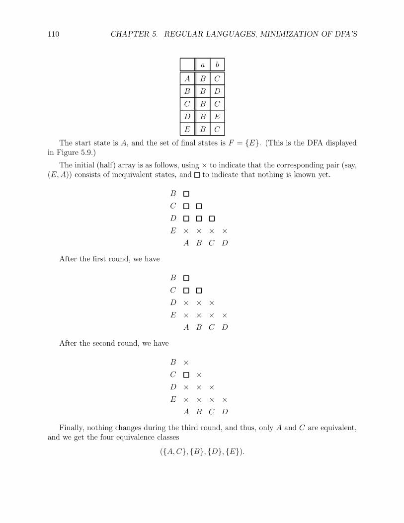
110 CHAPTER 5. REGULAR LANGUAGES, MINIMIZATION OF DFA’S
a b
A B C
B B D
C B C
D B E
E B C
The start state is A, and the set of final states is F = E. (This is the DFA displayedin Figure 5.9.)
The initial (half) array is as follows, using × to indicate that the corresponding pair (say,(E,A)) consists of inequivalent states, and to indicate that nothing is known yet.
B
C
D
E × × × ×A B C D
After the first round, we have
B
C
D × × ×E × × × ×
A B C D
After the second round, we have
B ×C ×D × × ×E × × × ×
A B C D
Finally, nothing changes during the third round, and thus, only A and C are equivalent,and we get the four equivalence classes
(A,C, B, D, E).
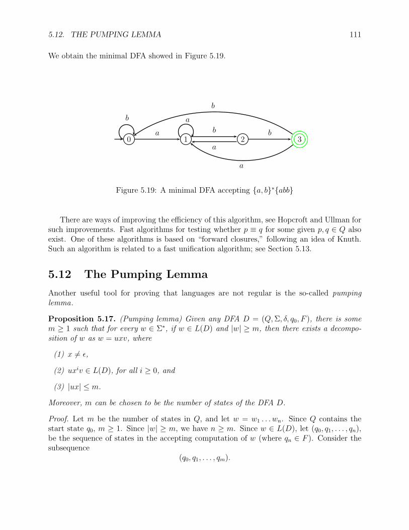
5.12. THE PUMPING LEMMA 111
We obtain the minimal DFA showed in Figure 5.19.
0 1 2 3a b
a
b
b a
b
a
Figure 5.19: A minimal DFA accepting a, b∗abb
There are ways of improving the efficiency of this algorithm, see Hopcroft and Ullman forsuch improvements. Fast algorithms for testing whether p ≡ q for some given p, q ∈ Q alsoexist. One of these algorithms is based on “forward closures,” following an idea of Knuth.Such an algorithm is related to a fast unification algorithm; see Section 5.13.
5.12 The Pumping Lemma
Another useful tool for proving that languages are not regular is the so-called pumpinglemma.
Proposition 5.17. (Pumping lemma) Given any DFA D = (Q,Σ, δ, q0, F ), there is somem ≥ 1 such that for every w ∈ Σ∗, if w ∈ L(D) and |w| ≥ m, then there exists a decompo-sition of w as w = uxv, where
(1) x 6= ǫ,
(2) uxiv ∈ L(D), for all i ≥ 0, and
(3) |ux| ≤ m.
Moreover, m can be chosen to be the number of states of the DFA D.
Proof. Let m be the number of states in Q, and let w = w1 . . . wn. Since Q contains thestart state q0, m ≥ 1. Since |w| ≥ m, we have n ≥ m. Since w ∈ L(D), let (q0, q1, . . . , qn),be the sequence of states in the accepting computation of w (where qn ∈ F ). Consider thesubsequence
(q0, q1, . . . , qm).
112 CHAPTER 5. REGULAR LANGUAGES, MINIMIZATION OF DFA’S
This sequence contains m + 1 states, but there are only m states in Q, and thus, we haveqi = qj, for some i, j such that 0 ≤ i < j ≤ m. Then, letting u = w1 . . . wi, x = wi+1 . . . wj,and v = wj+1 . . . wn, it is clear that the conditions of the proposition hold.
An important consequence of the pumping lemma is that if a DFA D has m states andif there is some string w ∈ L(D) such that |w| ≥ m, then L(D) is infinite.
Indeed, by the pumping lemma, w ∈ L(D) can be written as w = uxv with x 6= ǫ, and
uxiv ∈ L(D) for all i ≥ 0.
Since x 6= ǫ, we have |x| > 0, so for all i, j ≥ 0 with i < j we have
|uxiv| < |uxiv|+ (j − i)|x| = |uxjv|,which implies that uxiv 6= uxjv for all i < j, and the set of strings
uxiv | i ≥ 0 ⊆ L(D)
is an infinite subset of L(D), which is itself infinite.
As a consequence, if L(D) is finite, there are no strings w in L(D) such that |w| ≥ m.In this case, since the premise of the pumping lemma is false, the pumping lemma holdsvacuously; that is, if L(D) is finite, the pumping lemma yields no information.
Another corollary of the pumping lemma is that there is a test to decide whether a DFAD accepts an infinite language L(D).
Proposition 5.18. Let D be a DFA with m states, The language L(D) accepted by D isinfinite iff there is some string w ∈ L(D) such that m ≤ |w| < 2m.
If L(D) is infinite, there are strings of length ≥ m in L(D), but a prirori there is noguarantee that there are “short” strings w in L(D), that is, strings whose length is uniformlybounded by some function of m independent of D. The pumping lemma ensures that thereare such strings, and the function is m 7→ 2m.
Typically, the pumping lemma is used to prove that a language is not regular. Themethod is to proceed by contradiction, i.e., to assume (contrary to what we wish to prove)that a language L is indeed regular, and derive a contradiction of the pumping lemma. Thus,it would be helpful to see what the negation of the pumping lemma is, and for this, we firststate the pumping lemma as a logical formula. We will use the following abbreviations:
nat = 0, 1, 2, . . .,pos = 1, 2, . . .,A ≡ w = uxv,
B ≡ x 6= ǫ,
C ≡ |ux| ≤ m,
P ≡ ∀i : nat (uxiv ∈ L(D)).
5.12. THE PUMPING LEMMA 113
The pumping lemma can be stated as
∀D : DFA ∃m : pos ∀w : Σ∗
((w ∈ L(D) ∧ |w| ≥ m) ⊃ (∃u, x, v : Σ∗ A ∧B ∧ C ∧ P )
).
Recalling that
¬(A ∧ B ∧ C ∧ P ) ≡ ¬(A ∧ B ∧ C) ∨ ¬P ≡ (A ∧ B ∧ C) ⊃ ¬P
and¬(R ⊃ S) ≡ R ∧ ¬S,
the negation of the pumping lemma can be stated as
∃D : DFA ∀m : pos ∃w : Σ∗
((w ∈ L(D) ∧ |w| ≥ m) ∧ (∀u, x, v : Σ∗ (A ∧ B ∧ C) ⊃ ¬P )
).
Since¬P ≡ ∃i : nat (uxiv /∈ L(D)),
in order to show that the pumping lemma is contradicted, one needs to show that for someDFA D, for every m ≥ 1, there is some string w ∈ L(D) of length at least m, such that forevery possible decomposition w = uxv satisfying the constraints x 6= ǫ and |ux| ≤ m, thereis some i ≥ 0 such that uxiv /∈ L(D).
When proceeding by contradiction, we have a language L that we are (wrongly) assumingto be regular, and we can use any DFA D accepting L. The creative part of the argumentis to pick the right w ∈ L (not making any assumption on m ≤ |w|).
As an illustration, let us use the pumping lemma to prove that L1 = anbn | n ≥ 1 isnot regular. The usefulness of the condition |ux| ≤ m lies in the fact that it reduces thenumber of legal decomposition uxv of w. We proceed by contradiction. Thus, let us assumethat L1 = anbn | n ≥ 1 is regular. If so, it is accepted by some DFA D. Now, we wish tocontradict the pumping lemma. For every m ≥ 1, let w = ambm. Clearly, w = ambm ∈ L1
and |w| ≥ m. Then, every legal decomposition u, x, v of w is such that
w = a . . . a︸ ︷︷ ︸u
a . . . a︸ ︷︷ ︸x
a . . . ab . . . b︸ ︷︷ ︸v
where x 6= ǫ and x ends within the a’s, since |ux| ≤ m. Since x 6= ǫ, the string uxxv is ofthe form anbm where n > m, and thus uxxv /∈ L1, contradicting the pumping lemma.
Let us consider two more examples. let L2 = ambn | 1 ≤ m < n. We claim that L2
is not regular. Our first proof uses the pumping lemma. For any m ≥ 1, pick w = ambm+1.We have w ∈ L2 and |w| ≥ m so we need to contradict the pumping lemma. Every legaldecomposition u, x, v of w is such that
w = a . . . a︸ ︷︷ ︸u
a . . . a︸ ︷︷ ︸x
a . . . ab . . . b︸ ︷︷ ︸v
114 CHAPTER 5. REGULAR LANGUAGES, MINIMIZATION OF DFA’S
where x 6= ǫ and x ends within the a’s, since |ux| ≤ m. Since x 6= ǫ and x consists of a’s thestring ux2v = uxxv contains at least m+1 a’s and still m+1 b’s, so ux2v 6∈ L2, contradictingthe pumping lemma.
Our second proof uses Myhill-Nerode. Let ≃ be a right-invariant equivalence relation offinite index such that L2 is the union of classes of ≃. If we consider the infinite sequence
a, a2, . . . , an, . . .
since ≃ has a finite number of classes there are two strings am and an with m < n such that
am ≃ an.
By right-invariance by concatenating on the right with bn we obtain
ambn ≃ anbn,
and since m < n we have ambn ∈ L2 but anbn /∈ L2, a contradiction.
Let us now consider the language L3 = ambn | m 6= n. This time let us begin by usingMyhill-Nerode to prove that L3 is not regular. The proof is the same as before, we obtain
ambn ≃ anbn,
and the contradiction is that ambn ∈ L3 and anbn /∈ L3.
Let use now try to use the pumping lemma to prove that L3 is not regular. For anym ≥ 1 pick w = ambm+1 ∈ L3. As in the previous case, every legal decomposition u, x, v ofw is such that
w = a . . . a︸ ︷︷ ︸u
a . . . a︸ ︷︷ ︸x
a . . . ab . . . b︸ ︷︷ ︸v
where x 6= ǫ and x ends within the a’s, since |ux| ≤ m. However this time we have a problem,namely that we know that x is a nonempty string of a’s but we don’t know how many, sowe can’t guarantee that pumping up x will yield exactly the string am+1bm+1. We made thewrong choice for w. There is a choice that will work but it is a bit tricky.
Fortunately, there is another simpler approach. Recall that the regular languages areclosed under the boolean operations (union, intersection and complementation). Thus, L3
is not regular iff its complement L3 is not regular. Observe that L3 contains anbn | n ≥ 1,which we showed to be nonregular. But there is another problem, which is that L3 containsother strings besides strings of the form anbn, for example strings of the form bman withm,n > 0.
Again, we can take care of this difficulty using the closure operations of the regularlanguages. If we can find a regular language R such that L3∩R is not regular, then L3 itselfis not regular, since otherwise as L3 and R are regular then L3 ∩ R is also regular. In ourcase, we can use R = a+b+ to obtain
L3 ∩ a+b+ = anbn | n ≥ 1.
5.13. A FAST ALGORITHM FOR CHECKING STATE EQUIVALENCE 115
Since anbn | n ≥ 1 is not regular, we reached our final contradiction. Observe how we usethe language R to “clean up” L3 by intersecting it with R.
To complete a direct proof using the pumping lemma, the reader should try w =am!b(m+1)!.
The use of the closure operations of the regular languages is often a quick way of showingthat a language L is not regular by reducing the problem of proving that L is not regular tothe problem of proving that some well-known language is not regular.
5.13 A Fast Algorithm for Checking State Equivalence
Using a “Forward-Closure”
Given two states p, q ∈ Q, if p ≡ q, then we know that δ(p, a) ≡ δ(q, a), for all a ∈ Σ.This suggests a method for testing whether two distinct states p, q are equivalent. Startingwith the relation R = (p, q), construct the smallest equivalence relation R† containing Rwith the property that whenever (r, s) ∈ R†, then (δ(r, a), δ(s, a)) ∈ R†, for all a ∈ Σ. If weever encounter a pair (r, s) such that r ∈ F and s ∈ F , or r ∈ F and s ∈ F , then r ands are inequivalent, and so are p and q. Otherwise, it can be shown that p and q are indeedequivalent. Thus, testing for the equivalence of two states reduces to finding an efficientmethod for computing the “forward closure” of a relation defined on the set of states of aDFA.
Such a method was worked out by John Hopcroft and Richard Karp and published ina 1971 Cornell technical report. This method is based on an idea of Donald Knuth forsolving Exercise 11, in Section 2.3.5 of The Art of Computer Programming, Vol. 1, secondedition, 1973. A sketch of the solution for this exercise is given on page 594. As far as Iknow, Hopcroft and Karp’s method was never published in a journal, but a simple recursivealgorithm does appear on page 144 of Aho, Hopcroft and Ullman’s The Design and Analysisof Computer Algorithms, first edition, 1974. Essentially the same idea was used by Patersonand Wegman to design a fast unification algorithm (in 1978). We make a few definitions.
A relation S ⊆ Q×Q is a forward closure iff it is an equivalence relation and whenever(r, s) ∈ S, then (δ(r, a), δ(s, a)) ∈ S, for all a ∈ Σ. The forward closure of a relationR ⊆ Q×Q is the smallest equivalence relation R† containing R which is forward closed.
We say that a forward closure S is good iff whenever (r, s) ∈ S, then good(r, s), wheregood(r, s) holds iff either both r, s ∈ F , or both r, s /∈ F . Obviously, bad(r, s) iff ¬good(r, s).
Given any relation R ⊆ Q×Q, recall that the smallest equivalence relation R≈ containingR is the relation (R∪R−1)∗ (where R−1 = (q, p) | (p, q) ∈ R, and (R∪R−1)∗ is the reflexiveand transitive closure of (R∪R−1)). The forward closure of R can be computed inductivelyby defining the sequence of relations Ri ⊆ Q×Q as follows:
116 CHAPTER 5. REGULAR LANGUAGES, MINIMIZATION OF DFA’S
R0 = R≈
Ri+1 = (Ri ∪ (δ(r, a), δ(s, a)) | (r, s) ∈ Ri, a ∈ Σ)≈.
It is not hard to prove that Ri0+1 = Ri0 for some least i0, and that R† = Ri0 is thesmallest forward closure containing R. The following two facts can also been established.
(a) if R† is good, then
R† ⊆≡ . (5.1)
(b) if p ≡ q, then
R† ⊆≡,
that is, equation (5.1) holds. This implies that R† is good.
As a consequence, we obtain the correctness of our procedure: p ≡ q iff the forwardclosure R† of the relation R = (p, q) is good.
In practice, we maintain a partition Π representing the equivalence relation that we areclosing under forward closure. We add each new pair (δ(r, a), δ(s, a)) one at a time, andimmediately form the smallest equivalence relation containing the new relation. If δ(r, a)and δ(s, a) already belong to the same block of Π, we consider another pair, else we mergethe blocks corresponding to δ(r, a) and δ(s, a), and then consider another pair.
The algorithm is recursive, but it can easily be implemented using a stack. To manipulatepartitions efficiently, we represent them as lists of trees (forests). Each equivalence class Cin the partition Π is represented by a tree structure consisting of nodes and parent pointers,with the pointers from the sons of a node to the node itself. The root has a null pointer.Each node also maintains a counter keeping track of the number of nodes in the subtreerooted at that node.
Note that pointers can be avoided. We can represent a forest of n nodes as a list of npairs of the form (father , count). If (father , count) is the ith pair in the list, then father = 0iff node i is a root node, otherwise, father is the index of the node in the list which is theparent of node i. The number count is the total number of nodes in the tree rooted at theith node.
For example, the following list of nine nodes
((0, 3), (0, 2), (1, 1), (0, 2), (0, 2), (1, 1), (2, 1), (4, 1), (5, 1))
represents a forest consisting of the following four trees:
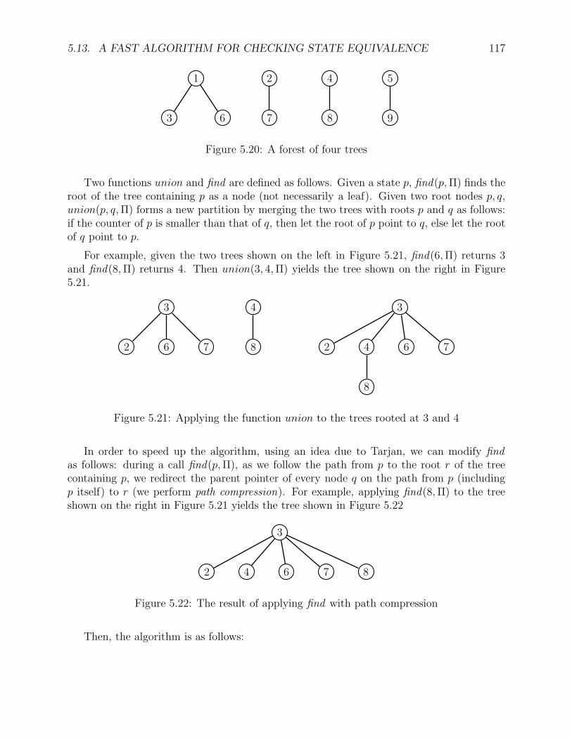
5.13. A FAST ALGORITHM FOR CHECKING STATE EQUIVALENCE 117
1
3 6
2
7
4
8
5
9
Figure 5.20: A forest of four trees
Two functions union and find are defined as follows. Given a state p, find(p,Π) finds theroot of the tree containing p as a node (not necessarily a leaf). Given two root nodes p, q,union(p, q,Π) forms a new partition by merging the two trees with roots p and q as follows:if the counter of p is smaller than that of q, then let the root of p point to q, else let the rootof q point to p.
For example, given the two trees shown on the left in Figure 5.21, find(6,Π) returns 3and find(8,Π) returns 4. Then union(3, 4,Π) yields the tree shown on the right in Figure5.21.
3
2 6 7
4
8
3
2 4 6 7
8
Figure 5.21: Applying the function union to the trees rooted at 3 and 4
In order to speed up the algorithm, using an idea due to Tarjan, we can modify findas follows: during a call find(p,Π), as we follow the path from p to the root r of the treecontaining p, we redirect the parent pointer of every node q on the path from p (includingp itself) to r (we perform path compression). For example, applying find(8,Π) to the treeshown on the right in Figure 5.21 yields the tree shown in Figure 5.22
3
2 4 6 7 8
Figure 5.22: The result of applying find with path compression
Then, the algorithm is as follows:
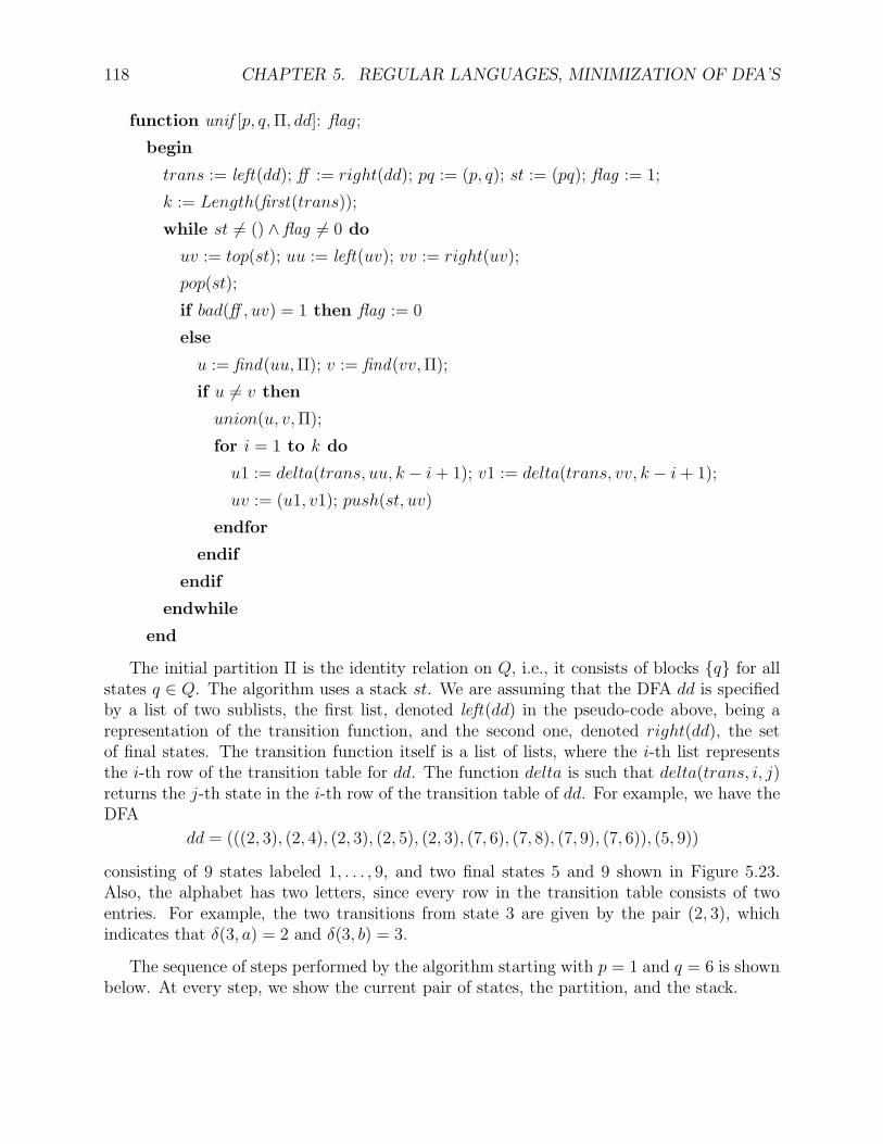
118 CHAPTER 5. REGULAR LANGUAGES, MINIMIZATION OF DFA’S
function unif [p, q,Π, dd]: flag ;
begin
trans := left(dd); ff := right(dd); pq := (p, q); st := (pq); flag := 1;
k := Length(first(trans));
while st 6= () ∧ flag 6= 0 do
uv := top(st); uu := left(uv); vv := right(uv);
pop(st);
if bad(ff , uv) = 1 then flag := 0
else
u := find(uu,Π); v := find(vv,Π);
if u 6= v then
union(u, v,Π);
for i = 1 to k do
u1 := delta(trans, uu, k − i+ 1); v1 := delta(trans, vv, k − i+ 1);
uv := (u1, v1); push(st, uv)
endfor
endif
endif
endwhile
end
The initial partition Π is the identity relation on Q, i.e., it consists of blocks q for allstates q ∈ Q. The algorithm uses a stack st. We are assuming that the DFA dd is specifiedby a list of two sublists, the first list, denoted left(dd) in the pseudo-code above, being arepresentation of the transition function, and the second one, denoted right(dd), the setof final states. The transition function itself is a list of lists, where the i-th list representsthe i-th row of the transition table for dd. The function delta is such that delta(trans, i, j)returns the j-th state in the i-th row of the transition table of dd. For example, we have theDFA
dd = (((2, 3), (2, 4), (2, 3), (2, 5), (2, 3), (7, 6), (7, 8), (7, 9), (7, 6)), (5, 9))
consisting of 9 states labeled 1, . . . , 9, and two final states 5 and 9 shown in Figure 5.23.Also, the alphabet has two letters, since every row in the transition table consists of twoentries. For example, the two transitions from state 3 are given by the pair (2, 3), whichindicates that δ(3, a) = 2 and δ(3, b) = 3.
The sequence of steps performed by the algorithm starting with p = 1 and q = 6 is shownbelow. At every step, we show the current pair of states, the partition, and the stack.
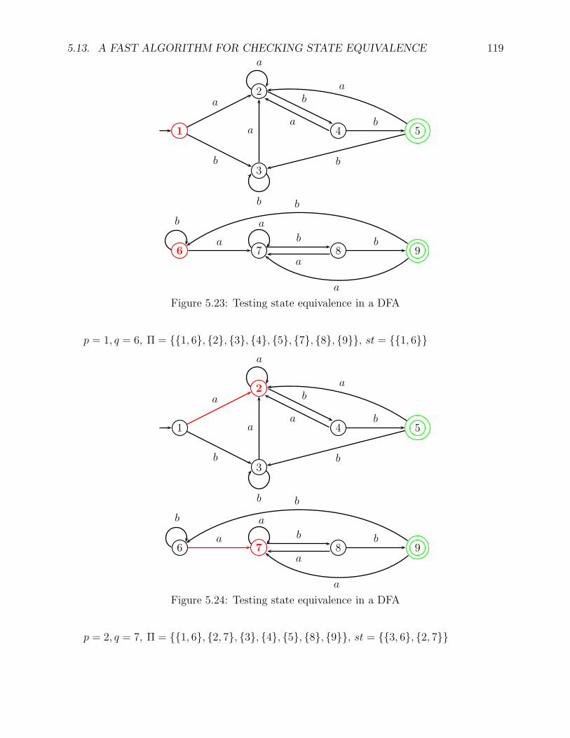
5.13. A FAST ALGORITHM FOR CHECKING STATE EQUIVALENCE 119
1
2
3
4 5
a
b
a
b
a b
b
a
b
a
6 7 8 9a b
a
b
b a
b
a
Figure 5.23: Testing state equivalence in a DFA
p = 1, q = 6, Π = 1, 6, 2, 3, 4, 5, 7, 8, 9, st = 1, 6
1
2
3
4 5
a
b
a
b
a b
b
a
b
a
6 7 8 9a b
a
b
b a
b
a
Figure 5.24: Testing state equivalence in a DFA
p = 2, q = 7, Π = 1, 6, 2, 7, 3, 4, 5, 8, 9, st = 3, 6, 2, 7
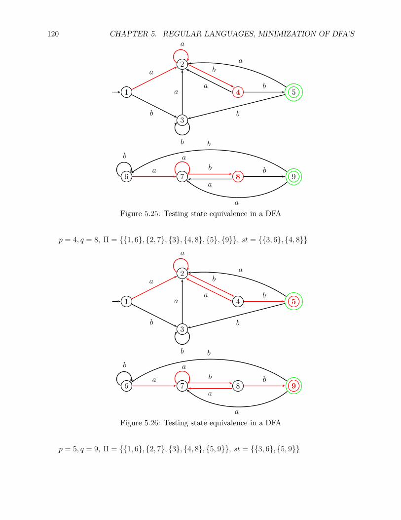
120 CHAPTER 5. REGULAR LANGUAGES, MINIMIZATION OF DFA’S
1
2
3
4 5
a
b
a
b
a b
b
a
b
a
6 7 8 9a b
a
b
b a
b
a
Figure 5.25: Testing state equivalence in a DFA
p = 4, q = 8, Π = 1, 6, 2, 7, 3, 4, 8, 5, 9, st = 3, 6, 4, 8
1
2
3
4 5
a
b
a
b
a b
b
a
b
a
6 7 8 9a b
a
b
b a
b
a
Figure 5.26: Testing state equivalence in a DFA
p = 5, q = 9, Π = 1, 6, 2, 7, 3, 4, 8, 5, 9, st = 3, 6, 5, 9
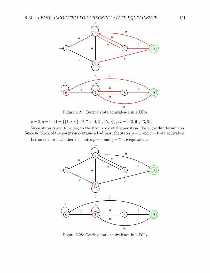
5.13. A FAST ALGORITHM FOR CHECKING STATE EQUIVALENCE 121
1
2
3
4 5
a
b
a
b
a b
b
a
b
a
6 7 8 9a b
a
b
b a
b
a
Figure 5.27: Testing state equivalence in a DFA
p = 3, q = 6, Π = 1, 3, 6, 2, 7, 4, 8, 5, 9, st = 3, 6, 3, 6Since states 3 and 6 belong to the first block of the partition, the algorithm terminates.
Since no block of the partition contains a bad pair, the states p = 1 and q = 6 are equivalent.
Let us now test whether the states p = 3 and q = 7 are equivalent.
1
2
3
4 5
a
b
a
b
a b
a
a
b
a
6 7 8 9a b
a
b
b a
b
a
Figure 5.28: Testing state equivalence in a DFA
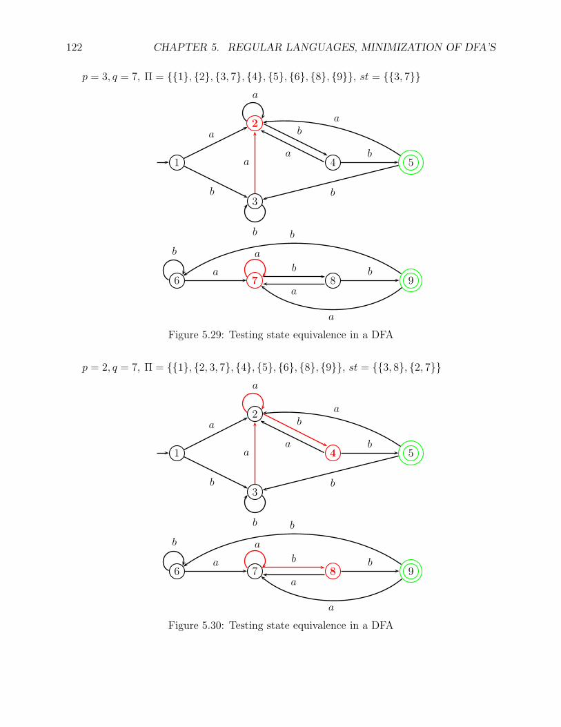
122 CHAPTER 5. REGULAR LANGUAGES, MINIMIZATION OF DFA’S
p = 3, q = 7, Π = 1, 2, 3, 7, 4, 5, 6, 8, 9, st = 3, 7
1
2
3
4 5
a
b
a
b
a b
b
a
b
a
6 7 8 9a b
a
b
b a
b
a
Figure 5.29: Testing state equivalence in a DFA
p = 2, q = 7, Π = 1, 2, 3, 7, 4, 5, 6, 8, 9, st = 3, 8, 2, 7
1
2
3
4 5
a
b
a
b
a b
b
a
b
a
6 7 8 9a b
a
b
b a
b
a
Figure 5.30: Testing state equivalence in a DFA
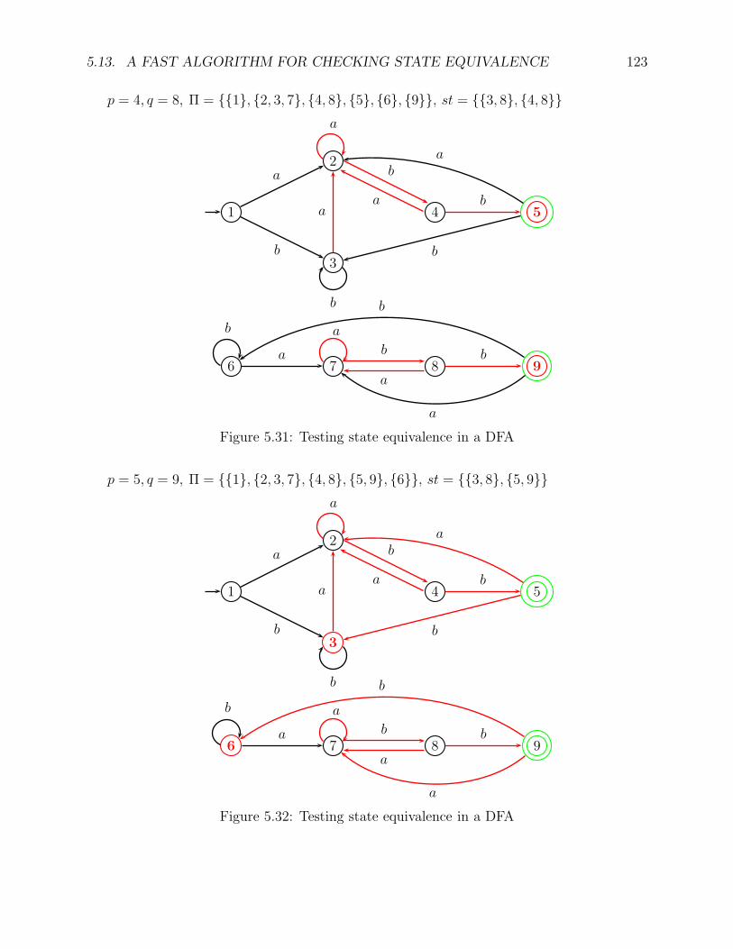
5.13. A FAST ALGORITHM FOR CHECKING STATE EQUIVALENCE 123
p = 4, q = 8, Π = 1, 2, 3, 7, 4, 8, 5, 6, 9, st = 3, 8, 4, 8
1
2
3
4 5
a
b
a
b
a b
b
a
b
a
6 7 8 9a b
a
b
b a
b
a
Figure 5.31: Testing state equivalence in a DFA
p = 5, q = 9, Π = 1, 2, 3, 7, 4, 8, 5, 9, 6, st = 3, 8, 5, 9
1
2
3
4 5
a
b
a
b
a b
b
a
b
a
6 7 8 9a b
a
b
b a
b
a
Figure 5.32: Testing state equivalence in a DFA
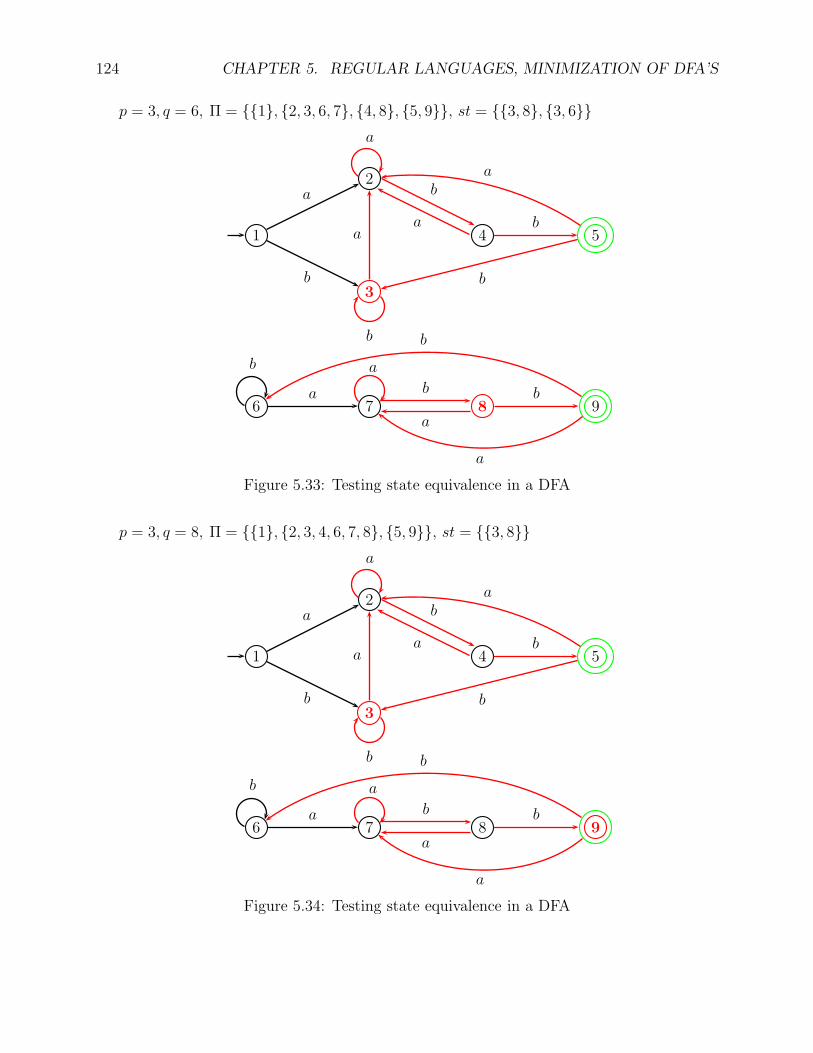
124 CHAPTER 5. REGULAR LANGUAGES, MINIMIZATION OF DFA’S
p = 3, q = 6, Π = 1, 2, 3, 6, 7, 4, 8, 5, 9, st = 3, 8, 3, 6
1
2
3
4 5
a
b
a
b
a b
b
a
b
a
6 7 8 9a b
a
b
b a
b
a
Figure 5.33: Testing state equivalence in a DFA
p = 3, q = 8, Π = 1, 2, 3, 4, 6, 7, 8, 5, 9, st = 3, 8
1
2
3
4 5
a
b
a
b
a b
b
a
b
a
6 7 8 9a b
a
b
b a
b
a
Figure 5.34: Testing state equivalence in a DFA
5.13. A FAST ALGORITHM FOR CHECKING STATE EQUIVALENCE 125
p = 3, q = 9, Π = 1, 2, 3, 4, 6, 7, 8, 5, 9, st = 3, 9Since the pair (3, 9) is a bad pair, the algorithm stops, and the states p = 3 and q = 7
are inequivalent.
126 CHAPTER 5. REGULAR LANGUAGES, MINIMIZATION OF DFA’S
Chapter 6
Context-Free Grammars,Context-Free Languages, Parse Treesand Ogden’s Lemma
6.1 Context-Free Grammars
A context-free grammar basically consists of a finite set of grammar rules. In order to definegrammar rules, we assume that we have two kinds of symbols: the terminals, which are thesymbols of the alphabet underlying the languages under consideration, and the nonterminals,which behave like variables ranging over strings of terminals. A rule is of the form A→ α,where A is a single nonterminal, and the right-hand side α is a string of terminal and/ornonterminal symbols. As usual, first we need to define what the object is (a context-freegrammar), and then we need to explain how it is used. Unlike automata, grammars are usedto generate strings, rather than recognize strings.
Definition 6.1. A context-free grammar (for short, CFG) is a quadruple G = (V,Σ, P, S),where
• V is a finite set of symbols called the vocabulary (or set of grammar symbols);
• Σ ⊆ V is the set of terminal symbols (for short, terminals);
• S ∈ (V − Σ) is a designated symbol called the start symbol ;
• P ⊆ (V − Σ)× V ∗ is a finite set of productions (or rewrite rules, or rules).
The set N = V −Σ is called the set of nonterminal symbols (for short, nonterminals). Thus,P ⊆ N × V ∗, and every production 〈A, α〉 is also denoted as A → α. A production of theform A→ ǫ is called an epsilon rule, or null rule.
127
128 CHAPTER 6. CONTEXT-FREE GRAMMARS AND LANGUAGES
Remark : Context-free grammars are sometimes defined as G = (VN , VT , P, S). Thecorrespondence with our definition is that Σ = VT and N = VN , so that V = VN ∪VT . Thus,in this other definition, it is necessary to assume that VT ∩ VN = ∅.
Example 1. G1 = (E, a, b, a, b, P, E), where P is the set of rules
E −→ aEb,
E −→ ab.
As we will see shortly, this grammar generates the language L1 = anbn | n ≥ 1, whichis not regular.
Example 2. G2 = (E,+, ∗, (, ), a, +, ∗, (, ), a, P, E), where P is the set of rules
E −→ E + E,
E −→ E ∗ E,E −→ (E),
E −→ a.
This grammar generates a set of arithmetic expressions.
6.2 Derivations and Context-Free Languages
The productions of a grammar are used to derive strings. In this process, the productionsare used as rewrite rules. Formally, we define the derivation relation associated with acontext-free grammar. First, let us review the concepts of transitive closure and reflexiveand transitive closure of a binary relation.
Given a set A, a binary relation R on A is any set of ordered pairs, i.e. R ⊆ A×A. Forshort, instead of binary relation, we often simply say relation. Given any two relations R, Son A, their composition R S is defined as
R S = (x, y) ∈ A× A | ∃z ∈ A, (x, z) ∈ R and (z, y) ∈ S.
The identity relation IA on A is the relation IA defined such that
IA = (x, x) | x ∈ A.
For short, we often denote IA as I. Note that
R I = I R = R
for every relation R on A. Given a relation R on A, for any n ≥ 0 we define Rn as follows:
R0 = I,
Rn+1 = Rn R.
6.2. DERIVATIONS AND CONTEXT-FREE LANGUAGES 129
It is obvious that R1 = R. It is also easily verified by induction that Rn R = R Rn.The transitive closure R+ of the relation R is defined as
R+ =⋃
n≥1
Rn.
It is easily verified that R+ is the smallest transitive relation containing R, and that(x, y) ∈ R+ iff there is some n ≥ 1 and some x0, x1, . . . , xn ∈ A such that x0 = x, xn = y,and (xi, xi+1) ∈ R for all i, 0 ≤ i ≤ n − 1. The transitive and reflexive closure R∗ of therelation R is defined as
R∗ =⋃
n≥0
Rn.
Clearly, R∗ = R+ ∪ I. It is easily verified that R∗ is the smallest transitive and reflexiverelation containing R.
Definition 6.2. Given a context-free grammar G = (V,Σ, P, S), the (one-step) derivationrelation =⇒G associated with G is the binary relation =⇒G ⊆ V ∗ × V ∗ defined as follows:for all α, β ∈ V ∗, we have
α =⇒G β
iff there exist λ, ρ ∈ V ∗, and some production (A→ γ) ∈ P , such that
α = λAρ and β = λγρ.
The transitive closure of =⇒G is denoted as+
=⇒G and the reflexive and transitive closure of=⇒G is denoted as
∗=⇒G.
When the grammar G is clear from the context, we usually omit the subscript G in =⇒G,+
=⇒G, and∗
=⇒G.
A string α ∈ V ∗ such that S∗
=⇒ α is called a sentential form, and a string w ∈ Σ∗ suchthat S
∗=⇒ w is called a sentence. A derivation α
∗=⇒ β involving n steps is denoted as
αn
=⇒ β.
Note that a derivation step
α =⇒G β
is rather nondeterministic. Indeed, one can choose among various occurrences of nontermi-nals A in α, and also among various productions A→ γ with left-hand side A.
For example, using the grammar G1 = (E, a, b, a, b, P, E), where P is the set of rules
E −→ aEb,
E −→ ab,
130 CHAPTER 6. CONTEXT-FREE GRAMMARS AND LANGUAGES
every derivation from E is of the form
E∗
=⇒ anEbn =⇒ anabbn = an+1bn+1,
orE
∗=⇒ anEbn =⇒ anaEbbn = an+1Ebn+1,
where n ≥ 0.
Grammar G1 is very simple: every string anbn has a unique derivation. This is usuallynot the case. For example, using the grammar G2 = (E,+, ∗, (, ), a, +, ∗, (, ), a, P, E),where P is the set of rules
E −→ E + E,
E −→ E ∗ E,E −→ (E),
E −→ a,
the string a+ a ∗ a has the following distinct derivations, where the boldface indicates whichoccurrence of E is rewritten:
E =⇒ E ∗ E =⇒ E+ E ∗ E=⇒ a+ E ∗ E =⇒ a+ a ∗ E =⇒ a+ a ∗ a,
and
E =⇒ E+ E =⇒ a + E
=⇒ a+ E ∗ E =⇒ a+ a ∗ E =⇒ a+ a ∗ a.
In the above derivations, the leftmost occurrence of a nonterminal is chosen at each step.Such derivations are called leftmost derivations . We could systematically rewrite the right-most occurrence of a nonterminal, getting rightmost derivations . The string a + a ∗ a alsohas the following two rightmost derivations, where the boldface indicates which occurrenceof E is rewritten:
E =⇒ E + E =⇒ E + E ∗ E=⇒ E + E ∗ a =⇒ E+ a ∗ a =⇒ a+ a ∗ a,
and
E =⇒ E ∗E =⇒ E ∗ a=⇒ E + E ∗ a =⇒ E+ a ∗ a =⇒ a+ a ∗ a.
The language generated by a context-free grammar is defined as follows.
6.2. DERIVATIONS AND CONTEXT-FREE LANGUAGES 131
Definition 6.3. Given a context-free grammar G = (V,Σ, P, S), the language generated byG is the set
L(G) = w ∈ Σ∗ | S +=⇒ w.
A language L ⊆ Σ∗ is a context-free language (for short, CFL) iff L = L(G) for somecontext-free grammar G.
It is technically very useful to consider derivations in which the leftmost nonterminal isalways selected for rewriting, and dually, derivations in which the rightmost nonterminal isalways selected for rewriting.
Definition 6.4. Given a context-free grammar G = (V,Σ, P, S), the (one-step) leftmostderivation relation =⇒
lmassociated with G is the binary relation =⇒
lm⊆ V ∗ × V ∗ defined as
follows: for all α, β ∈ V ∗, we have
α =⇒lm
β
iff there exist u ∈ Σ∗, ρ ∈ V ∗, and some production (A→ γ) ∈ P , such that
α = uAρ and β = uγρ.
The transitive closure of =⇒lm
is denoted as+=⇒lm
and the reflexive and transitive closure of
=⇒lm
is denoted as∗=⇒lm
. The (one-step) rightmost derivation relation =⇒rm
associated with
G is the binary relation =⇒rm⊆ V ∗ × V ∗ defined as follows: for all α, β ∈ V ∗, we have
α =⇒rm
β
iff there exist λ ∈ V ∗, v ∈ Σ∗, and some production (A→ γ) ∈ P , such that
α = λAv and β = λγv.
The transitive closure of =⇒rm
is denoted as+=⇒rm
and the reflexive and transitive closure of
=⇒rm
is denoted as∗=⇒rm
.
Remarks : It is customary to use the symbols a, b, c, d, e for terminal symbols, and thesymbols A,B,C,D,E for nonterminal symbols. The symbols u, v, w, x, y, z denote terminalstrings, and the symbols α, β, γ, λ, ρ, µ denote strings in V ∗. The symbols X, Y, Z usuallydenote symbols in V .
Given a context-free grammar G = (V,Σ, P, S), parsing a string w consists in finding outwhether w ∈ L(G), and if so, in producing a derivation for w. The following proposition istechnically very important. It shows that leftmost and rightmost derivations are “universal”.This has some important practical implications for the complexity of parsing algorithms.
132 CHAPTER 6. CONTEXT-FREE GRAMMARS AND LANGUAGES
Proposition 6.1. Let G = (V,Σ, P, S) be a context-free grammar. For every w ∈ Σ∗, for
every derivation S+
=⇒ w, there is a leftmost derivation S+=⇒lm
w, and there is a rightmost
derivation S+=⇒rm
w.
Proof. Of course, we have to somehow use induction on derivations, but this is a littletricky, and it is necessary to prove a stronger fact. We treat leftmost derivations, rightmostderivations being handled in a similar way.
Claim: For every w ∈ Σ∗, for every α ∈ V +, for every n ≥ 1, if αn
=⇒ w, then there is aleftmost derivation α
n=⇒lm
w.
The claim is proved by induction on n.
For n = 1, there exist some λ, ρ ∈ V ∗ and some production A → γ, such that α = λAρand w = λγρ. Since w is a terminal string, λ, ρ, and γ, are terminal strings. Thus, A is the
only nonterminal in α, and the derivation step α1
=⇒ w is a leftmost step (and a rightmoststep!).
If n > 1, then the derivation αn
=⇒ w is of the form
α =⇒ α1n−1=⇒ w.
There are two subcases.
Case 1. If the derivation step α =⇒ α1 is a leftmost step α =⇒lm
α1, by the induction
hypothesis, there is a leftmost derivation α1n−1=⇒lm
w, and we get the leftmost derivation
α =⇒lm
α1n−1=⇒lm
w.
Case 2. The derivation step α =⇒ α1 is a not a leftmost step. In this case, there mustbe some u ∈ Σ∗, µ, ρ ∈ V ∗, some nonterminals A and B, and some production B → δ, suchthat
α = uAµBρ and α1 = uAµδρ,
where A is the leftmost nonterminal in α. Since we have a derivation α1n−1=⇒ w of length
n− 1, by the induction hypothesis, there is a leftmost derivation
α1n−1=⇒lm
w.
Since α1 = uAµδρ where A is the leftmost terminal in α1, the first step in the leftmost
derivation α1n−1=⇒lm
w is of the form
uAµδρ =⇒lm
uγµδρ,
6.2. DERIVATIONS AND CONTEXT-FREE LANGUAGES 133
for some production A→ γ. Thus, we have a derivation of the form
α = uAµBρ =⇒ uAµδρ =⇒lm
uγµδρn−2=⇒lm
w.
We can commute the first two steps involving the productions B → δ and A → γ, and weget the derivation
α = uAµBρ =⇒lm
uγµBρ =⇒ uγµδρn−2=⇒lm
w.
This may no longer be a leftmost derivation, but the first step is leftmost, and we areback in case 1. Thus, we conclude by applying the induction hypothesis to the derivation
uγµBρn−1=⇒ w, as in case 1.
Proposition 6.1 implies that
L(G) = w ∈ Σ∗ | S +=⇒lm
w = w ∈ Σ∗ | S +=⇒rm
w.
We observed that if we consider the grammar G2 = (E,+, ∗, (, ), a, +, ∗, (, ), a, P, E),where P is the set of rules
E −→ E + E,
E −→ E ∗ E,E −→ (E),
E −→ a,
the string a + a ∗ a has the following two distinct leftmost derivations, where the boldfaceindicates which occurrence of E is rewritten:
E =⇒ E ∗ E =⇒ E+ E ∗ E=⇒ a+ E ∗ E =⇒ a+ a ∗ E =⇒ a+ a ∗ a,
and
E =⇒ E+ E =⇒ a + E
=⇒ a+ E ∗ E =⇒ a+ a ∗ E =⇒ a+ a ∗ a.When this happens, we say that we have an ambiguous grammars. In some cases, it ispossible to modify a grammar to make it unambiguous. For example, the grammar G2 canbe modified as follows.
Let G3 = (E, T, F,+, ∗, (, ), a, +, ∗, (, ), a, P, E), where P is the set of rules
E −→ E + T,
E −→ T,
T −→ T ∗ F,T −→ F,
F −→ (E),
F −→ a.
134 CHAPTER 6. CONTEXT-FREE GRAMMARS AND LANGUAGES
We leave as an exercise to show that L(G3) = L(G2), and that every string in L(G3) hasa unique leftmost derivation. Unfortunately, it is not always possible to modify a context-free grammar to make it unambiguous. There exist context-free languages that have nounambiguous context-free grammars. For example, the language
L3 = ambmcn | m,n ≥ 1 ∪ ambncn | m,n ≥ 1
is context-free, since it is generated by the following context-free grammar:
S → S1,
S → S2,
S1 → XC,
S2 → AY,
X → aXb,
X → ab,
Y → bY c,
Y → bc,
A→ aA,
A→ a,
C → cC,
C → c.
However, it can be shown that L3 has no unambiguous grammars. All this motivates thefollowing definition.
Definition 6.5. A context-free grammarG = (V,Σ, P, S) is ambiguous if there is some stringw ∈ L(G) that has two distinct leftmost derivations (or two distinct rightmost derivations).Thus, a grammar G is unambiguous if every string w ∈ L(G) has a unique leftmost derivation(or a unique rightmost derivation). A context-free language L is inherently ambiguous if everyCFG G for L is ambiguous.
Whether or not a grammar is ambiguous affects the complexity of parsing. Parsing algo-rithms for unambiguous grammars are more efficient than parsing algorithms for ambiguousgrammars.
We now consider various normal forms for context-free grammars.
6.3 Normal Forms for Context-Free Grammars, Chom-
sky Normal Form
One of the main goals of this section is to show that every CFG G can be converted to anequivalent grammar in Chomsky Normal Form (for short, CNF). A context-free grammar
6.3. NORMAL FORMS FOR CONTEXT-FREE GRAMMARS 135
G = (V,Σ, P, S) is in Chomsky Normal Form iff its productions are of the form
A→ BC,
A→ a, or
S → ǫ,
where A,B,C ∈ N , a ∈ Σ, S → ǫ is in P iff ǫ ∈ L(G), and S does not occur on theright-hand side of any production.
Note that a grammar in Chomsky Normal Form does not have ǫ-rules, i.e., rules of theform A→ ǫ, except when ǫ ∈ L(G), in which case S → ǫ is the only ǫ-rule. It also does nothave chain rules , i.e., rules of the form A→ B, where A,B ∈ N . Thus, in order to converta grammar to Chomsky Normal Form, we need to show how to eliminate ǫ-rules and chainrules. This is not the end of the story, since we may still have rules of the form A→ α whereeither |α| ≥ 3 or |α| ≥ 2 and α contains terminals. However, dealing with such rules is asimple recoding matter, and we first focus on the elimination of ǫ-rules and chain rules. Itturns out that ǫ-rules must be eliminated first.
The first step to eliminate ǫ-rules is to compute the set E(G) of erasable (or nullable)nonterminals
E(G) = A ∈ N | A +=⇒ ǫ.
The set E(G) is computed using a sequence of approximations Ei defined as follows:
E0 = A ∈ N | (A→ ǫ) ∈ P,Ei+1 = Ei ∪ A | ∃(A→ B1 . . . Bj . . . Bk) ∈ P, Bj ∈ Ei, 1 ≤ j ≤ k.
Clearly, the Ei form an ascending chain
E0 ⊆ E1 ⊆ · · · ⊆ Ei ⊆ Ei+1 ⊆ · · · ⊆ N,
and since N is finite, there is a least i, say i0, such that Ei0 = Ei0+1. We claim thatE(G) = Ei0 . Actually, we prove the following proposition.
Proposition 6.2. Given a context-free grammar G = (V,Σ, P, S), one can construct acontext-free grammar G′ = (V ′,Σ, P ′, S ′) such that:
(1) L(G′) = L(G);
(2) P ′ contains no ǫ-rules other than S ′ → ǫ, and S ′ → ǫ ∈ P ′ iff ǫ ∈ L(G);
(3) S ′ does not occur on the right-hand side of any production in P ′.
Proof. We begin by proving that E(G) = Ei0 . For this, we prove that E(G) ⊆ Ei0 andEi0 ⊆ E(G).
To prove that Ei0 ⊆ E(G), we proceed by induction on i. Since E0 = A ∈ N | (A →ǫ) ∈ P, we have A
1=⇒ ǫ, and thus A ∈ E(G). By the induction hypothesis, Ei ⊆
136 CHAPTER 6. CONTEXT-FREE GRAMMARS AND LANGUAGES
E(G). If A ∈ Ei+1, either A ∈ Ei and then A ∈ E(G), or there is some production(A → B1 . . . Bj . . . Bk) ∈ P , such that Bj ∈ Ei for all j, 1 ≤ j ≤ k. By the induction
hypothesis, Bj+
=⇒ ǫ for each j, 1 ≤ j ≤ k, and thus
A =⇒ B1 . . . Bj . . . Bk+
=⇒ B2 . . . Bj . . . Bk+
=⇒ Bj . . . Bk+
=⇒ ǫ,
which shows that A ∈ E(G).To prove that E(G) ⊆ Ei0 , we also proceed by induction, but on the length of a derivation
A+
=⇒ ǫ. If A1
=⇒ ǫ, then A→ ǫ ∈ P , and thus A ∈ E0 since E0 = A ∈ N | (A→ ǫ) ∈ P.If A
n+1=⇒ ǫ, then
A =⇒ αn
=⇒ ǫ,
for some production A→ α ∈ P . If α contains terminals of nonterminals not in E(G), it isimpossible to derive ǫ from α, and thus, we must have α = B1 . . . Bj . . . Bk, with Bj ∈ E(G),for all j, 1 ≤ j ≤ k. However, Bj
nj
=⇒ ǫ where nj ≤ n, and by the induction hypothesis,Bj ∈ Ei0 . But then, we get A ∈ Ei0+1 = Ei0 , as desired.
Having shown that E(G) = Ei0 , we construct the grammar G′. Its set of production P ′
is defined as follows. First, we create the production S ′ → S where S ′ /∈ V , to make surethat S ′ does not occur on the right-hand side of any rule in P ′. Let
P1 = A→ α ∈ P | α ∈ V + ∪ S ′ → S,and let P2 be the set of productions
P2 = A→ α1α2 . . . αkαk+1 | ∃α1 ∈ V ∗, . . . , ∃αk+1 ∈ V ∗, ∃B1 ∈ E(G), . . . , ∃Bk ∈ E(G)A→ α1B1α2 . . . αkBkαk+1 ∈ P, k ≥ 1, α1 . . . αk+1 6= ǫ.
Note that ǫ ∈ L(G) iff S ∈ E(G). If S /∈ E(G), then let P ′ = P1∪P2, and if S ∈ E(G), thenlet P ′ = P1 ∪ P2 ∪ S ′ → ǫ. We claim that L(G′) = L(G), which is proved by showing thatevery derivation using G can be simulated by a derivation using G′, and vice-versa. All theconditions of the proposition are now met.
From a practical point of view, the construction or Proposition 6.2 is very costly. Forexample, given a grammar containing the productions
S → ABCDEF,
A→ ǫ,
B → ǫ,
C → ǫ,
D → ǫ,
E → ǫ,
F → ǫ,
. . .→ . . . ,
6.3. NORMAL FORMS FOR CONTEXT-FREE GRAMMARS 137
eliminating ǫ-rules will create 26 − 1 = 63 new rules corresponding to the 63 nonemptysubsets of the set A,B,C,D,E, F. We now turn to the elimination of chain rules.
It turns out that matters are greatly simplified if we first apply Proposition 6.2 to theinput grammar G, and we explain the construction assuming that G = (V,Σ, P, S) satisfiesthe conditions of Proposition 6.2. For every nonterminal A ∈ N , we define the set
IA = B ∈ N | A +=⇒ B.
The sets IA are computed using approximations IA,i defined as follows:
IA,0 = B ∈ N | (A→ B) ∈ P,IA,i+1 = IA,i ∪ C ∈ N | ∃(B → C) ∈ P, andB ∈ IA,i.
Clearly, for every A ∈ N , the IA,i form an ascending chain
IA,0 ⊆ IA,1 ⊆ · · · ⊆ IA,i ⊆ IA,i+1 ⊆ · · · ⊆ N,
and since N is finite, there is a least i, say i0, such that IA,i0 = IA,i0+1. We claim thatIA = IA,i0 . Actually, we prove the following proposition.
Proposition 6.3. Given a context-free grammar G = (V,Σ, P, S), one can construct acontext-free grammar G′ = (V ′,Σ, P ′, S ′) such that:
(1) L(G′) = L(G);
(2) Every rule in P ′ is of the form A → α where |α| ≥ 2, or A → a where a ∈ Σ, orS ′ → ǫ iff ǫ ∈ L(G);
(3) S ′ does not occur on the right-hand side of any production in P ′.
Proof. First, we apply Proposition 6.2 to the grammar G, obtaining a grammar G1 =(V1,Σ, S1, P1). The proof that IA = IA,i0 is similar to the proof that E(G) = Ei0 . First,we prove that IA,i ⊆ IA by induction on i. This is staightforward. Next, we prove that
IA ⊆ IA,i0 by induction on derivations of the form A+
=⇒ B. In this part of the proof, weuse the fact that G1 has no ǫ-rules except perhaps S1 → ǫ, and that S1 does not occur on
the right-hand side of any rule. This implies that a derivation An+1=⇒ C is necessarily of the
form An
=⇒ B =⇒ C for some B ∈ N . Then, in the induction step, we have B ∈ IA,i0, andthus C ∈ IA,i0+1 = IA,i0.
We now define the following sets of rules. Let
P2 = P1 − A→ B | A→ B ∈ P1,and let
P3 = A→ α | B → α ∈ P1, α /∈ N1, B ∈ IA.We claim that G′ = (V1,Σ, P2 ∪ P3, S1) satisfies the conditions of the proposition. Forexample, S1 does not appear on the right-hand side of any production, since the productionsin P3 have right-hand sides from P1, and S1 does not appear on the right-hand side in P1.It is also easily shown that L(G′) = L(G1) = L(G).
138 CHAPTER 6. CONTEXT-FREE GRAMMARS AND LANGUAGES
Let us apply the method of Proposition 6.3 to the grammar
G3 = (E, T, F,+, ∗, (, ), a, +, ∗, (, ), a, P, E),
where P is the set of rules
E −→ E + T,
E −→ T,
T −→ T ∗ F,T −→ F,
F −→ (E),
F −→ a.
We get IE = T, F, IT = F, and IF = ∅. The new grammar G′3 has the set of rules
E −→ E + T,
E −→ T ∗ F,E −→ (E),
E −→ a,
T −→ T ∗ F,T −→ (E),
T −→ a,
F −→ (E),
F −→ a.
At this stage, the grammar obtained in Proposition 6.3 no longer has ǫ-rules (exceptperhaps S ′ → ǫ iff ǫ ∈ L(G)) or chain rules. However, it may contain rules A → α with|α| ≥ 3, or with |α| ≥ 2 and where α contains terminals(s). To obtain the Chomsky NormalForm. we need to eliminate such rules. This is not difficult, but notationally a bit messy.
Proposition 6.4. Given a context-free grammar G = (V,Σ, P, S), one can construct acontext-free grammar G′ = (V ′,Σ, P ′, S ′) such that L(G′) = L(G) and G′ is in ChomskyNormal Form, that is, a grammar whose productions are of the form
A→ BC,
A→ a, or
S ′ → ǫ,
where A,B,C ∈ N ′, a ∈ Σ, S ′ → ǫ is in P ′ iff ǫ ∈ L(G), and S ′ does not occur on theright-hand side of any production in P ′.
6.3. NORMAL FORMS FOR CONTEXT-FREE GRAMMARS 139
Proof. First, we apply Proposition 6.3, obtaining G1. Let Σr be the set of terminals occurringon the right-hand side of rules A→ α ∈ P1, with |α| ≥ 2. For every a ∈ Σr, let Xa be a newnonterminal not in V1. Let
P2 = Xa → a | a ∈ Σr.
Let P1,r be the set of productions
A→ α1a1α2 · · ·αkakαk+1,
where a1, . . . , ak ∈ Σr and αi ∈ N∗1 . For every production
A→ α1a1α2 · · ·αkakαk+1
in P1,r, let
A→ α1Xa1α2 · · ·αkXakαk+1
be a new production, and let P3 be the set of all such productions. Let P4 = (P1 − P1,r) ∪P2 ∪P3. Now, productions A→ α in P4 with |α| ≥ 2 do not contain terminals. However, wemay still have productions A→ α ∈ P4 with |α| ≥ 3. We can perform some recoding usingsome new nonterminals. For every production of the form
A→ B1 · · ·Bk,
where k ≥ 3, create the new nonterminals
[B1 · · ·Bk−1], [B1 · · ·Bk−2], · · · , [B1B2B3], [B1B2],
and the new productions
A→ [B1 · · ·Bk−1]Bk,
[B1 · · ·Bk−1]→ [B1 · · ·Bk−2]Bk−1,
· · · → · · · ,[B1B2B3]→ [B1B2]B3,
[B1B2]→ B1B2.
All the productions are now in Chomsky Normal Form, and it is clear that the same languageis generated.
Applying the first phase of the method of Proposition 6.4 to the grammar G′3, we get the
140 CHAPTER 6. CONTEXT-FREE GRAMMARS AND LANGUAGES
rules
E −→ EX+T,
E −→ TX∗F,
E −→ X(EX),
E −→ a,
T −→ TX∗F,
T −→ X(EX),
T −→ a,
F −→ X(EX),
F −→ a,
X+ −→ +,
X∗ −→ ∗,X( −→ (,
X) −→).
After applying the second phase of the method, we get the following grammar in ChomskyNormal Form:
E −→ [EX+]T,
[EX+] −→ EX+,
E −→ [TX∗]F,
[TX∗] −→ TX∗,
E −→ [X(E]X),
[X(E] −→ X(E,
E −→ a,
T −→ [TX∗]F,
T −→ [X(E]X),
T −→ a,
F −→ [X(E]X),
F −→ a,
X+ −→ +,
X∗ −→ ∗,X( −→ (,
X) −→).
For large grammars, it is often convenient to use the abbreviation which consists in group-ing productions having a common left-hand side, and listing the right-hand sides separated
6.4. REGULAR LANGUAGES ARE CONTEXT-FREE 141
by the symbol |. Thus, a group of productions
A→ α1,
A→ α2,
· · · → · · · ,A→ αk,
may be abbreviated asA→ α1 | α2 | · · · | αk.
An interesting corollary of the CNF is the following decidability result. There is analgorithm which, given a context-free grammar G, given any string w ∈ Σ∗, decides whetherw ∈ L(G). Indeed, we first convert G to a grammar G′ in Chomsky Normal Form. If w = ǫ,we can test whether ǫ ∈ L(G), since this is the case iff S ′ → ǫ ∈ P ′. If w 6= ǫ, letting n = |w|,note that since the rules are of the form A → BC or A → a, where a ∈ Σ, any derivationfor w has n− 1 + n = 2n− 1 steps. Thus, we enumerate all (leftmost) derivations of length2n− 1.
There are much better parsing algorithms than this naive algorithm. We now show thatevery regular language is context-free.
6.4 Regular Languages are Context-Free
The regular languages can be characterized in terms of very special kinds of context-freegrammars, right-linear (and left-linear) context-free grammars.
Definition 6.6. A context-free grammar G = (V,Σ, P, S) is left-linear iff its productionsare of the form
A→ Ba,
A→ a,
A→ ǫ.
where A,B ∈ N , and a ∈ Σ. A context-free grammar G = (V,Σ, P, S) is right-linear iff itsproductions are of the form
A→ aB,
A→ a,
A→ ǫ.
where A,B ∈ N , and a ∈ Σ.
The following proposition shows the equivalence between NFA’s and right-linear gram-mars.
142 CHAPTER 6. CONTEXT-FREE GRAMMARS AND LANGUAGES
Proposition 6.5. A language L is regular if and only if it is generated by some right-lineargrammar.
Proof. Let L = L(D) for some DFA D = (Q,Σ, δ, q0, F ). We construct a right-linear gram-mar G as follows. Let V = Q ∪ Σ, S = q0, and let P be defined as follows:
P = p→ aq | q = δ(p, a), p, q ∈ Q, a ∈ Σ ∪ p→ ǫ | p ∈ F.It is easily shown by induction on the length of w that
p∗
=⇒ wq iff q = δ∗(p, w),
and thus, L(D) = L(G).
Conversely, let G = (V,Σ, P, S) be a right-linear grammar. First, let G = (V ′,Σ, P ′, S) bethe right-linear grammar obtained from G by adding the new nonterminal E to N , replacingevery rule in P of the form A → a where a ∈ Σ by the rule A → aE, and adding therule E → ǫ. It is immediately verified that L(G′) = L(G). Next, we construct the NFAM = (Q,Σ, δ, q0, F ) as follows: Q = N ′ = N ∪ E, q0 = S, F = A ∈ N ′ | A→ ǫ, and
δ(A, a) = B ∈ N ′ | A→ aB ∈ P ′,for all A ∈ N and all a ∈ Σ. It is easily shown by induction on the length of w that
A∗
=⇒ wB iff B ∈ δ∗(A,w),and thus, L(M) = L(G′) = L(G).
A similar proposition holds for left-linear grammars. It is also easily shown that theregular languages are exactly the languages generated by context-free grammars whose rulesare of the form
A→ Bu,
A→ u,
where A,B ∈ N , and u ∈ Σ∗.
6.5 Useless Productions in Context-Free Grammars
Given a context-free grammar G = (V,Σ, P, S), it may contain rules that are useless fora number of reasons. For example, consider the grammar G3 = (E,A, a, b, a, b, P, E),where P is the set of rules
E −→ aEb,
E −→ ab,
E −→ A,
A −→ bAa.
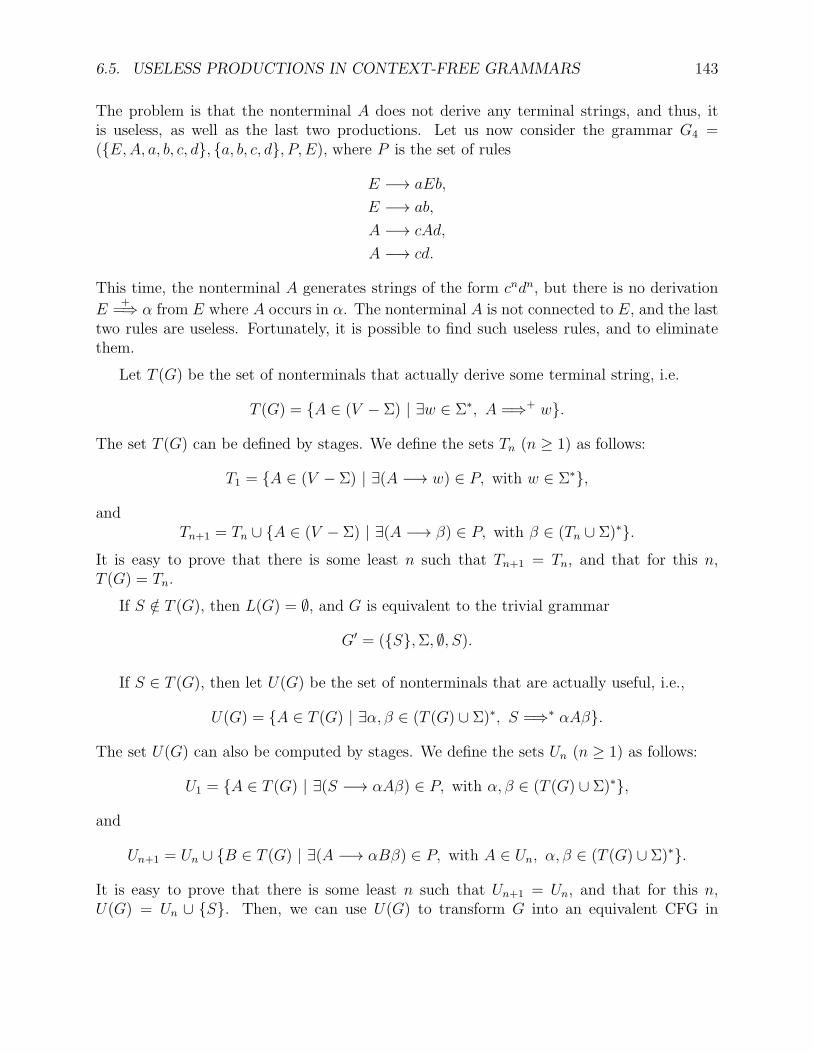
6.5. USELESS PRODUCTIONS IN CONTEXT-FREE GRAMMARS 143
The problem is that the nonterminal A does not derive any terminal strings, and thus, itis useless, as well as the last two productions. Let us now consider the grammar G4 =(E,A, a, b, c, d, a, b, c, d, P, E), where P is the set of rules
E −→ aEb,
E −→ ab,
A −→ cAd,
A −→ cd.
This time, the nonterminal A generates strings of the form cndn, but there is no derivation
E+
=⇒ α from E where A occurs in α. The nonterminal A is not connected to E, and the lasttwo rules are useless. Fortunately, it is possible to find such useless rules, and to eliminatethem.
Let T (G) be the set of nonterminals that actually derive some terminal string, i.e.
T (G) = A ∈ (V − Σ) | ∃w ∈ Σ∗, A =⇒+ w.
The set T (G) can be defined by stages. We define the sets Tn (n ≥ 1) as follows:
T1 = A ∈ (V − Σ) | ∃(A −→ w) ∈ P, with w ∈ Σ∗,
andTn+1 = Tn ∪ A ∈ (V − Σ) | ∃(A −→ β) ∈ P, with β ∈ (Tn ∪ Σ)∗.
It is easy to prove that there is some least n such that Tn+1 = Tn, and that for this n,T (G) = Tn.
If S /∈ T (G), then L(G) = ∅, and G is equivalent to the trivial grammar
G′ = (S,Σ, ∅, S).
If S ∈ T (G), then let U(G) be the set of nonterminals that are actually useful, i.e.,
U(G) = A ∈ T (G) | ∃α, β ∈ (T (G) ∪ Σ)∗, S =⇒∗ αAβ.
The set U(G) can also be computed by stages. We define the sets Un (n ≥ 1) as follows:
U1 = A ∈ T (G) | ∃(S −→ αAβ) ∈ P, with α, β ∈ (T (G) ∪ Σ)∗,
and
Un+1 = Un ∪ B ∈ T (G) | ∃(A −→ αBβ) ∈ P, with A ∈ Un, α, β ∈ (T (G) ∪ Σ)∗.
It is easy to prove that there is some least n such that Un+1 = Un, and that for this n,U(G) = Un ∪ S. Then, we can use U(G) to transform G into an equivalent CFG in
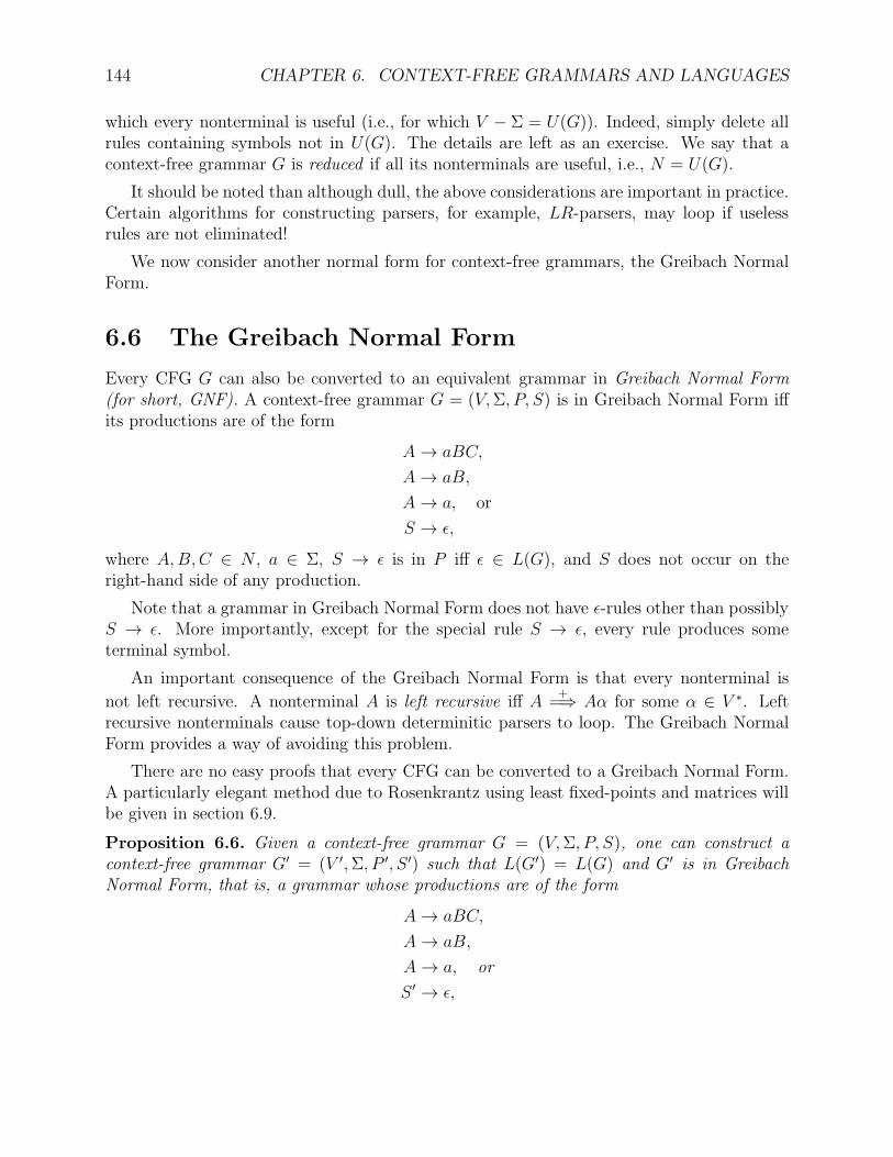
144 CHAPTER 6. CONTEXT-FREE GRAMMARS AND LANGUAGES
which every nonterminal is useful (i.e., for which V − Σ = U(G)). Indeed, simply delete allrules containing symbols not in U(G). The details are left as an exercise. We say that acontext-free grammar G is reduced if all its nonterminals are useful, i.e., N = U(G).
It should be noted than although dull, the above considerations are important in practice.Certain algorithms for constructing parsers, for example, LR-parsers, may loop if uselessrules are not eliminated!
We now consider another normal form for context-free grammars, the Greibach NormalForm.
6.6 The Greibach Normal Form
Every CFG G can also be converted to an equivalent grammar in Greibach Normal Form(for short, GNF). A context-free grammar G = (V,Σ, P, S) is in Greibach Normal Form iffits productions are of the form
A→ aBC,
A→ aB,
A→ a, or
S → ǫ,
where A,B,C ∈ N , a ∈ Σ, S → ǫ is in P iff ǫ ∈ L(G), and S does not occur on theright-hand side of any production.
Note that a grammar in Greibach Normal Form does not have ǫ-rules other than possiblyS → ǫ. More importantly, except for the special rule S → ǫ, every rule produces someterminal symbol.
An important consequence of the Greibach Normal Form is that every nonterminal is
not left recursive. A nonterminal A is left recursive iff A+
=⇒ Aα for some α ∈ V ∗. Leftrecursive nonterminals cause top-down determinitic parsers to loop. The Greibach NormalForm provides a way of avoiding this problem.
There are no easy proofs that every CFG can be converted to a Greibach Normal Form.A particularly elegant method due to Rosenkrantz using least fixed-points and matrices willbe given in section 6.9.
Proposition 6.6. Given a context-free grammar G = (V,Σ, P, S), one can construct acontext-free grammar G′ = (V ′,Σ, P ′, S ′) such that L(G′) = L(G) and G′ is in GreibachNormal Form, that is, a grammar whose productions are of the form
A→ aBC,
A→ aB,
A→ a, or
S ′ → ǫ,
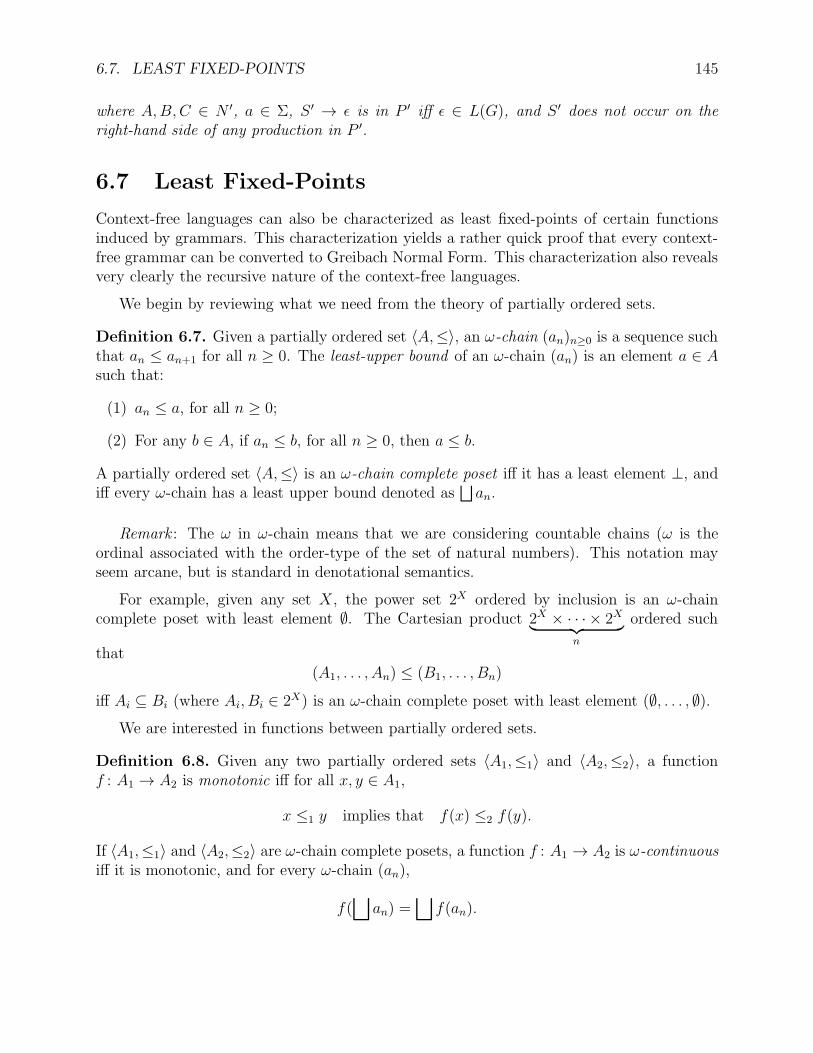
6.7. LEAST FIXED-POINTS 145
where A,B,C ∈ N ′, a ∈ Σ, S ′ → ǫ is in P ′ iff ǫ ∈ L(G), and S ′ does not occur on theright-hand side of any production in P ′.
6.7 Least Fixed-Points
Context-free languages can also be characterized as least fixed-points of certain functionsinduced by grammars. This characterization yields a rather quick proof that every context-free grammar can be converted to Greibach Normal Form. This characterization also revealsvery clearly the recursive nature of the context-free languages.
We begin by reviewing what we need from the theory of partially ordered sets.
Definition 6.7. Given a partially ordered set 〈A,≤〉, an ω-chain (an)n≥0 is a sequence suchthat an ≤ an+1 for all n ≥ 0. The least-upper bound of an ω-chain (an) is an element a ∈ Asuch that:
(1) an ≤ a, for all n ≥ 0;
(2) For any b ∈ A, if an ≤ b, for all n ≥ 0, then a ≤ b.
A partially ordered set 〈A,≤〉 is an ω-chain complete poset iff it has a least element ⊥, andiff every ω-chain has a least upper bound denoted as
⊔an.
Remark : The ω in ω-chain means that we are considering countable chains (ω is theordinal associated with the order-type of the set of natural numbers). This notation mayseem arcane, but is standard in denotational semantics.
For example, given any set X , the power set 2X ordered by inclusion is an ω-chaincomplete poset with least element ∅. The Cartesian product 2X × · · · × 2X︸ ︷︷ ︸
n
ordered such
that(A1, . . . , An) ≤ (B1, . . . , Bn)
iff Ai ⊆ Bi (where Ai, Bi ∈ 2X) is an ω-chain complete poset with least element (∅, . . . , ∅).We are interested in functions between partially ordered sets.
Definition 6.8. Given any two partially ordered sets 〈A1,≤1〉 and 〈A2,≤2〉, a functionf : A1 → A2 is monotonic iff for all x, y ∈ A1,
x ≤1 y implies that f(x) ≤2 f(y).
If 〈A1,≤1〉 and 〈A2,≤2〉 are ω-chain complete posets, a function f : A1 → A2 is ω-continuousiff it is monotonic, and for every ω-chain (an),
f(⊔
an) =⊔
f(an).
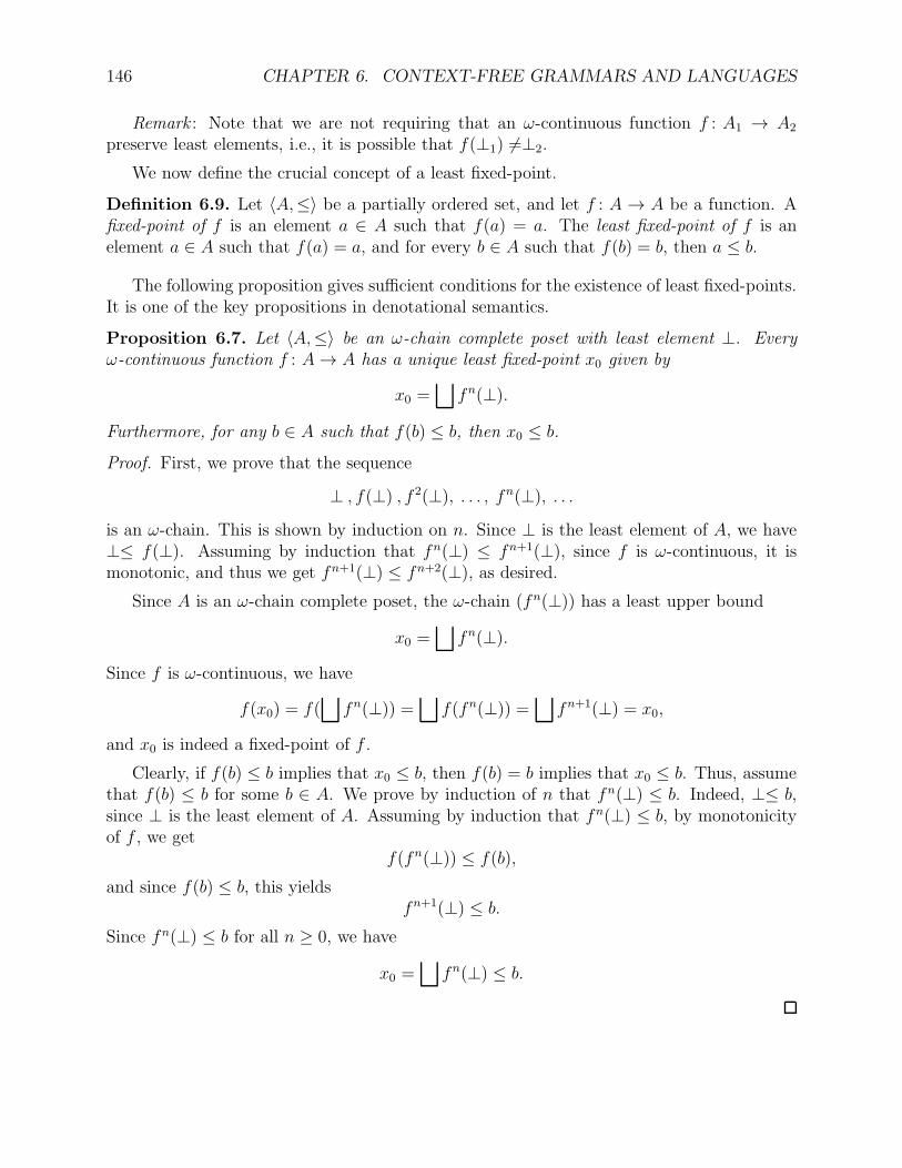
146 CHAPTER 6. CONTEXT-FREE GRAMMARS AND LANGUAGES
Remark : Note that we are not requiring that an ω-continuous function f : A1 → A2
preserve least elements, i.e., it is possible that f(⊥1) 6=⊥2.
We now define the crucial concept of a least fixed-point.
Definition 6.9. Let 〈A,≤〉 be a partially ordered set, and let f : A → A be a function. Afixed-point of f is an element a ∈ A such that f(a) = a. The least fixed-point of f is anelement a ∈ A such that f(a) = a, and for every b ∈ A such that f(b) = b, then a ≤ b.
The following proposition gives sufficient conditions for the existence of least fixed-points.It is one of the key propositions in denotational semantics.
Proposition 6.7. Let 〈A,≤〉 be an ω-chain complete poset with least element ⊥. Everyω-continuous function f : A→ A has a unique least fixed-point x0 given by
x0 =⊔
fn(⊥).
Furthermore, for any b ∈ A such that f(b) ≤ b, then x0 ≤ b.
Proof. First, we prove that the sequence
⊥ , f(⊥) , f 2(⊥), . . . , fn(⊥), . . .is an ω-chain. This is shown by induction on n. Since ⊥ is the least element of A, we have⊥≤ f(⊥). Assuming by induction that fn(⊥) ≤ fn+1(⊥), since f is ω-continuous, it ismonotonic, and thus we get fn+1(⊥) ≤ fn+2(⊥), as desired.
Since A is an ω-chain complete poset, the ω-chain (fn(⊥)) has a least upper bound
x0 =⊔
fn(⊥).
Since f is ω-continuous, we have
f(x0) = f(⊔
fn(⊥)) =⊔
f(fn(⊥)) =⊔
fn+1(⊥) = x0,
and x0 is indeed a fixed-point of f .
Clearly, if f(b) ≤ b implies that x0 ≤ b, then f(b) = b implies that x0 ≤ b. Thus, assumethat f(b) ≤ b for some b ∈ A. We prove by induction of n that fn(⊥) ≤ b. Indeed, ⊥≤ b,since ⊥ is the least element of A. Assuming by induction that fn(⊥) ≤ b, by monotonicityof f , we get
f(fn(⊥)) ≤ f(b),
and since f(b) ≤ b, this yieldsfn+1(⊥) ≤ b.
Since fn(⊥) ≤ b for all n ≥ 0, we have
x0 =⊔
fn(⊥) ≤ b.
6.8. CONTEXT-FREE LANGUAGES AS LEAST FIXED-POINTS 147
The second part of Proposition 6.7 is very useful to prove that functions have the sameleast fixed-point. For example, under the conditions of Proposition 6.7, if g : A → A isanother ω-chain continuous function, letting x0 be the least fixed-point of f and y0 be theleast fixed-point of g, if f(y0) ≤ y0 and g(x0) ≤ x0, we can deduce that x0 = y0. Indeed,since f(y0) ≤ y0 and x0 is the least fixed-point of f , we get x0 ≤ y0, and since g(x0) ≤ x0and y0 is the least fixed-point of g, we get y0 ≤ x0, and therefore x0 = y0.
Proposition 6.7 also shows that the least fixed-point x0 of f can be approximated asmuch as desired, using the sequence (fn(⊥)). We will now apply this fact to context-freegrammars. For this, we need to show how a context-free grammar G = (V,Σ, P, S) with mnonterminals induces an ω-continuous map
ΦG : 2Σ∗ × · · · × 2Σ
∗
︸ ︷︷ ︸m
→ 2Σ∗ × · · · × 2Σ
∗
︸ ︷︷ ︸m
.
6.8 Context-Free Languages as Least Fixed-Points
Given a context-free grammar G = (V,Σ, P, S) with m nonterminals A1, . . . Am, grouping allthe productions having the same left-hand side, the grammar G can be concisely written as
A1 → α1,1 + · · ·+ α1,n1,
· · · → · · ·Ai → αi,1 + · · ·+ αi,ni
,
· · · → · · ·Am → αm,1 + · · ·+ αm,nn
.
Given any set A, let Pfin(A) be the set of finite subsets of A.
Definition 6.10. Let G = (V,Σ, P, S) be a context-free grammar with m nonterminals A1,. . ., Am. For any m-tuple Λ = (L1, . . . , Lm) of languages Li ⊆ Σ∗, we define the function
Φ[Λ] : Pfin(V∗)→ 2Σ
∗
inductively as follows:
Φ[Λ](∅) = ∅,Φ[Λ](ǫ) = ǫ,Φ[Λ](a) = a, if a ∈ Σ,
Φ[Λ](Ai) = Li, if Ai ∈ N ,
Φ[Λ](αX) = Φ[Λ](α)Φ[Λ](X), if α ∈ V +, X ∈ V,Φ[Λ](Q ∪ α) = Φ[Λ](Q) ∪ Φ[Λ](α), if Q ∈ Pfin(V
∗), Q 6= ∅, α ∈ V ∗, α /∈ Q.
148 CHAPTER 6. CONTEXT-FREE GRAMMARS AND LANGUAGES
Then, writing the grammar G as
A1 → α1,1 + · · ·+ α1,n1,
· · · → · · ·Ai → αi,1 + · · ·+ αi,ni
,
· · · → · · ·Am → αm,1 + · · ·+ αm,nn
,
we define the mapΦG : 2Σ
∗ × · · · × 2Σ∗
︸ ︷︷ ︸m
→ 2Σ∗ × · · · × 2Σ
∗
︸ ︷︷ ︸m
such that
ΦG(L1, . . . Lm) = (Φ[Λ](α1,1, . . . , α1,n1), . . . ,Φ[Λ](αm,1, . . . , αm,nm))
for all Λ = (L1, . . . , Lm) ∈ 2Σ∗ × · · · × 2Σ
∗
︸ ︷︷ ︸m
.
One should verify that the map Φ[Λ] is well defined, but this is easy. The followingproposition is easily shown:
Proposition 6.8. Given a context-free grammar G = (V,Σ, P, S) with m nonterminals A1,. . ., Am, the map
ΦG : 2Σ∗ × · · · × 2Σ
∗
︸ ︷︷ ︸m
→ 2Σ∗ × · · · × 2Σ
∗
︸ ︷︷ ︸m
is ω-continuous.
Now, 2Σ∗ × · · · × 2Σ
∗
︸ ︷︷ ︸m
is an ω-chain complete poset, and the map ΦG is ω-continous. Thus,
by Proposition 6.7, the map ΦG has a least-fixed point. It turns out that the componentsof this least fixed-point are precisely the languages generated by the grammars (V,Σ, P, Ai).Before proving this fact, let us give an example illustrating it.
Example. Consider the grammar G = (A,B, a, b, a, b, P, A) defined by the rules
A→ BB + ab,
B → aBb+ ab.
The least fixed-point of ΦG is the least upper bound of the chain
(ΦnG(∅, ∅)) = ((Φn
G,A(∅, ∅),ΦnG,B(∅, ∅)),
whereΦ0
G,A(∅, ∅) = Φ0G,B(∅, ∅) = ∅,
6.8. CONTEXT-FREE LANGUAGES AS LEAST FIXED-POINTS 149
and
Φn+1G,A(∅, ∅) = Φn
G,B(∅, ∅)ΦnG,B(∅, ∅) ∪ ab,
Φn+1G,B(∅, ∅) = aΦn
G,B(∅, ∅)b ∪ ab.
It is easy to verify that
Φ1G,A(∅, ∅) = ab,
Φ1G,B(∅, ∅) = ab,
Φ2G,A(∅, ∅) = ab, abab,
Φ2G,B(∅, ∅) = ab, aabb,
Φ3G,A(∅, ∅) = ab, abab, abaabb, aabbab, aabbaabb,
Φ3G,B(∅, ∅) = ab, aabb, aaabbb.
By induction, we can easily prove that the two components of the least fixed-point arethe languages
LA = ambmanbn | m,n ≥ 1 ∪ ab and LB = anbn | n ≥ 1.
Letting GA = (A,B, a, b, a, b, P, A) and GB = (A,B, a, b, a, b, P, B), it is indeedtrue that LA = L(GA) and LB = L(GB) .
We have the following theorem due to Ginsburg and Rice:
Theorem 6.9. Given a context-free grammar G = (V,Σ, P, S) with m nonterminals A1, . . .,Am, the least fixed-point of the map ΦG is the m-tuple of languages
(L(GA1), . . . , L(GAm)),
where GAi= (V,Σ, P, Ai).
Proof. Writing G as
A1 → α1,1 + · · ·+ α1,n1,
· · · → · · ·Ai → αi,1 + · · ·+ αi,ni
,
· · · → · · ·Am → αm,1 + · · ·+ αm,nn
,
let M = max|αi,j| be the maximum length of right-hand sides of rules in P . Let
ΦnG(∅, . . . , ∅) = (Φn
G,1(∅, . . . , ∅), . . . ,ΦnG,m(∅, . . . , ∅)).
150 CHAPTER 6. CONTEXT-FREE GRAMMARS AND LANGUAGES
Then, for any w ∈ Σ∗, observe that
w ∈ Φ1G,i(∅, . . . , ∅)
iff there is some rule Ai → αi,j with w = αi,j, and that
w ∈ ΦnG,i(∅, . . . , ∅)
for some n ≥ 2 iff there is some rule Ai → αi,j with αi,j of the form
αi,j = u1Aj1u2 · · ·ukAjkuk+1,
where u1, . . . , uk+1 ∈ Σ∗, k ≥ 1, and some w1, . . . , wk ∈ Σ∗ such that
wh ∈ Φn−1G,jh
(∅, . . . , ∅),
and
w = u1w1u2 · · ·ukwkuk+1.
We prove the following two claims.
Claim 1: For every w ∈ Σ∗, if Ain
=⇒ w, then w ∈ ΦpG,i(∅, . . . , ∅), for some p ≥ 1.
Claim 2: For every w ∈ Σ∗, if w ∈ ΦnG,i(∅, . . . , ∅), with n ≥ 1, then Ai
p=⇒ w for some
p ≤ (M + 1)n−1.
Proof of Claim 1. We proceed by induction on n. If Ai1
=⇒ w, then w = αi,j for some ruleA→ αi,j, and by the remark just before the claim, w ∈ Φ1
G,i(∅, . . . , ∅).
If Ain+1=⇒ w with n ≥ 1, then
Ain
=⇒ αi,j =⇒ w
for some rule Ai → αi,j. If
αi,j = u1Aj1u2 · · ·ukAjkuk+1,
where u1, . . . , uk+1 ∈ Σ∗, k ≥ 1, then Ajh
nh=⇒ wh, where nh ≤ n, and
w = u1w1u2 · · ·ukwkuk+1
for some w1, . . . , wk ∈ Σ∗. By the induction hypothesis,
wh ∈ ΦphG,jh
(∅, . . . , ∅),
for some ph ≥ 1, for every h, 1 ≤ h ≤ k. Letting p = maxp1, . . . , pk, since each sequence(Φq
G,i(∅, . . . , ∅)) is an ω-chain, we have wh ∈ ΦpG,jh
(∅, . . . , ∅) for every h, 1 ≤ h ≤ k, and by
the remark just before the claim, w ∈ Φp+1G,i (∅, . . . , ∅).
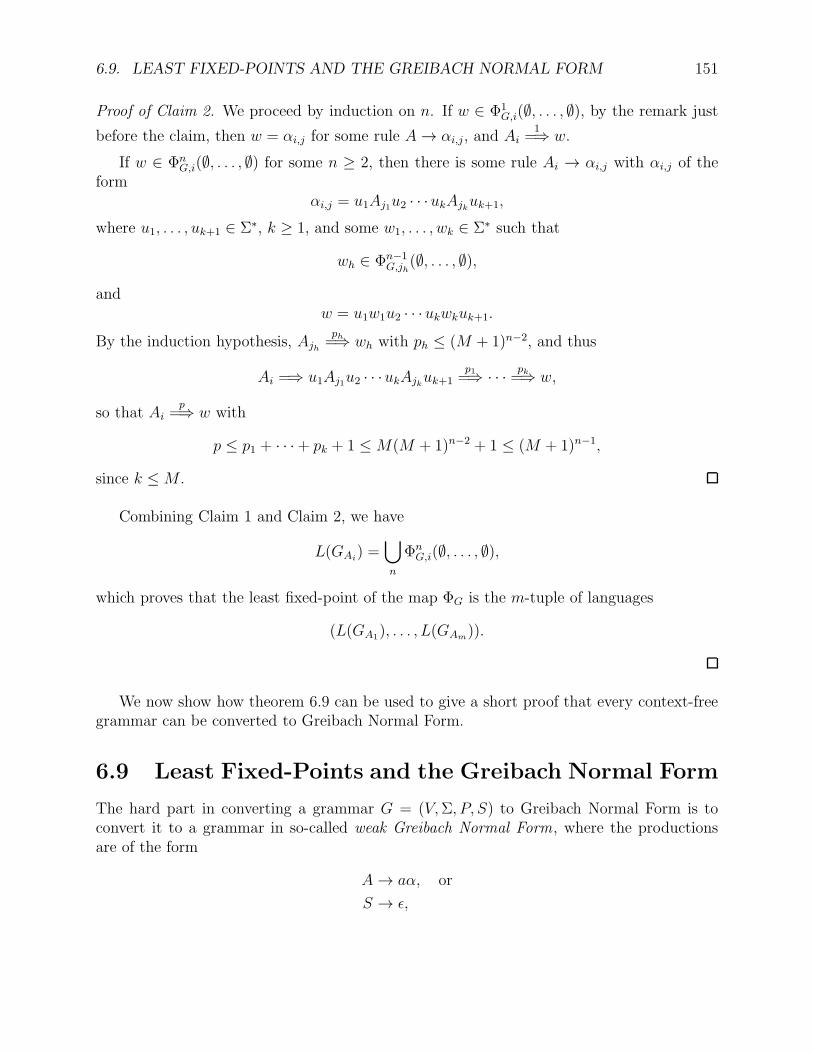
6.9. LEAST FIXED-POINTS AND THE GREIBACH NORMAL FORM 151
Proof of Claim 2. We proceed by induction on n. If w ∈ Φ1G,i(∅, . . . , ∅), by the remark just
before the claim, then w = αi,j for some rule A→ αi,j, and Ai1
=⇒ w.
If w ∈ ΦnG,i(∅, . . . , ∅) for some n ≥ 2, then there is some rule Ai → αi,j with αi,j of the
formαi,j = u1Aj1u2 · · ·ukAjkuk+1,
where u1, . . . , uk+1 ∈ Σ∗, k ≥ 1, and some w1, . . . , wk ∈ Σ∗ such that
wh ∈ Φn−1G,jh
(∅, . . . , ∅),
andw = u1w1u2 · · ·ukwkuk+1.
By the induction hypothesis, Ajh
ph=⇒ wh with ph ≤ (M + 1)n−2, and thus
Ai =⇒ u1Aj1u2 · · ·ukAjkuk+1p1=⇒ · · · pk=⇒ w,
so that Aip
=⇒ w with
p ≤ p1 + · · ·+ pk + 1 ≤ M(M + 1)n−2 + 1 ≤ (M + 1)n−1,
since k ≤M .
Combining Claim 1 and Claim 2, we have
L(GAi) =
⋃
n
ΦnG,i(∅, . . . , ∅),
which proves that the least fixed-point of the map ΦG is the m-tuple of languages
(L(GA1), . . . , L(GAm)).
We now show how theorem 6.9 can be used to give a short proof that every context-freegrammar can be converted to Greibach Normal Form.
6.9 Least Fixed-Points and the Greibach Normal Form
The hard part in converting a grammar G = (V,Σ, P, S) to Greibach Normal Form is toconvert it to a grammar in so-called weak Greibach Normal Form, where the productionsare of the form
A→ aα, or
S → ǫ,
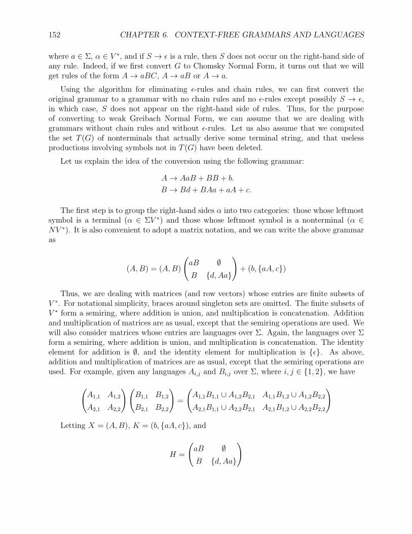
152 CHAPTER 6. CONTEXT-FREE GRAMMARS AND LANGUAGES
where a ∈ Σ, α ∈ V ∗, and if S → ǫ is a rule, then S does not occur on the right-hand side ofany rule. Indeed, if we first convert G to Chomsky Normal Form, it turns out that we willget rules of the form A→ aBC, A→ aB or A→ a.
Using the algorithm for eliminating ǫ-rules and chain rules, we can first convert theoriginal grammar to a grammar with no chain rules and no ǫ-rules except possibly S → ǫ,in which case, S does not appear on the right-hand side of rules. Thus, for the purposeof converting to weak Greibach Normal Form, we can assume that we are dealing withgrammars without chain rules and without ǫ-rules. Let us also assume that we computedthe set T (G) of nonterminals that actually derive some terminal string, and that uselessproductions involving symbols not in T (G) have been deleted.
Let us explain the idea of the conversion using the following grammar:
A→ AaB +BB + b.
B → Bd+BAa + aA + c.
The first step is to group the right-hand sides α into two categories: those whose leftmostsymbol is a terminal (α ∈ ΣV ∗) and those whose leftmost symbol is a nonterminal (α ∈NV ∗). It is also convenient to adopt a matrix notation, and we can write the above grammaras
(A,B) = (A,B)
(aB ∅B d, Aa
)+ (b, aA, c)
Thus, we are dealing with matrices (and row vectors) whose entries are finite subsets ofV ∗. For notational simplicity, braces around singleton sets are omitted. The finite subsets ofV ∗ form a semiring, where addition is union, and multiplication is concatenation. Additionand multiplication of matrices are as usual, except that the semiring operations are used. Wewill also consider matrices whose entries are languages over Σ. Again, the languages over Σform a semiring, where addition is union, and multiplication is concatenation. The identityelement for addition is ∅, and the identity element for multiplication is ǫ. As above,addition and multiplication of matrices are as usual, except that the semiring operations areused. For example, given any languages Ai,j and Bi,j over Σ, where i, j ∈ 1, 2, we have
(A1,1 A1,2
A2,1 A2,2
)(B1,1 B1,2
B2,1 B2,2
)=
(A1,1B1,1 ∪A1,2B2,1 A1,1B1,2 ∪ A1,2B2,2
A2,1B1,1 ∪A2,2B2,1 A2,1B1,2 ∪ A2,2B2,2
)
Letting X = (A,B), K = (b, aA, c), and
H =
(aB ∅B d, Aa
)

6.9. LEAST FIXED-POINTS AND THE GREIBACH NORMAL FORM 153
the above grammar can be concisely written as
X = XH +K.
More generally, given any context-free grammar G = (V,Σ, P, S) with m nonterminalsA1, . . ., Am, assuming that there are no chain rules, no ǫ-rules, and that every nonterminalbelongs to T (G), letting
X = (A1, . . . , Am),
we can write G asX = XH +K,
for some appropriate m×m matrix H in which every entry contains a set (possibly empty)of strings in V +, and some row vector K in which every entry contains a set (possibly empty)of strings α each beginning with a terminal (α ∈ ΣV ∗).
Given an m×m square matrix A = (Ai,j) of languages over Σ, we can define the matrixA∗ whose entry A∗
i,j is given by
A∗i,j =
⋃
n≥0
Ani,j,
where A0 = Idm, the identity matrix, and An is the n-th power of A. Similarly, we defineA+ where
A+i,j =
⋃
n≥1
Ani,j.
Given a matrix A where the entries are finite subset of V ∗, where N = A1, . . . , Am, forany m-tuple Λ = (L1, . . . , Lm) of languages over Σ, we let
Φ[Λ](A) = (Φ[Λ](Ai,j)).
Given a system X = XH +K where H is an m×m matrix and X,K are row matrices,if H and K do not contain any nonterminals, we claim that the least fixed-point of thegrammar G associated with X = XH + K is KH∗. This is easily seen by computing theapproximations Xn = Φn
G(∅, . . . , ∅). Indeed, X0 = K, and
Xn = KHn +KHn−1 + · · ·+KH +K = K(Hn +Hn−1 + · · ·+H + Im).
Similarly, if Y is an m × m matrix of nonterminals, the least fixed-point of the grammarassociated with Y = HY +H is H+ (provided that H does not contain any nonterminals).
Given any context-free grammar G = (V,Σ, P, S) with m nonterminals A1, . . ., Am,writing G as X = XH + K as explained earlier, we can form another grammar GH bycreating m2 new nonterminals Yi,j, where the rules of this new grammar are defined by thesystem of two matrix equations
X = KY +K,
Y = HY +H,
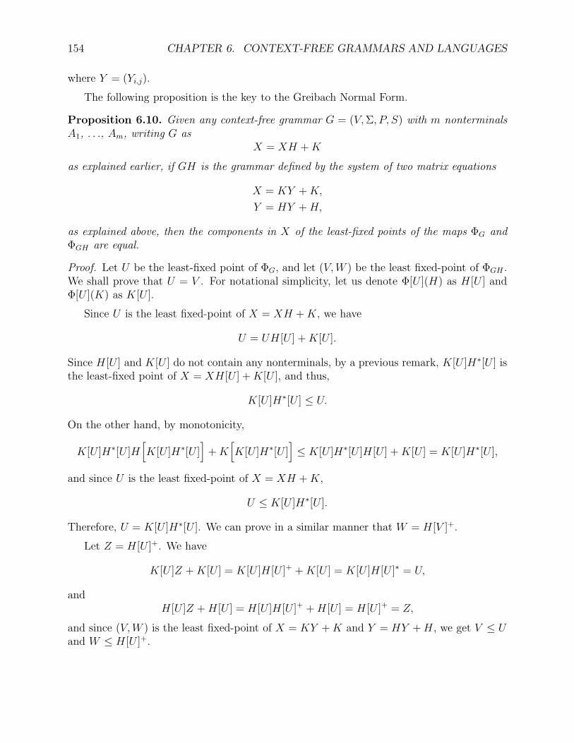
154 CHAPTER 6. CONTEXT-FREE GRAMMARS AND LANGUAGES
where Y = (Yi,j).
The following proposition is the key to the Greibach Normal Form.
Proposition 6.10. Given any context-free grammar G = (V,Σ, P, S) with m nonterminalsA1, . . ., Am, writing G as
X = XH +K
as explained earlier, if GH is the grammar defined by the system of two matrix equations
X = KY +K,
Y = HY +H,
as explained above, then the components in X of the least-fixed points of the maps ΦG andΦGH are equal.
Proof. Let U be the least-fixed point of ΦG, and let (V,W ) be the least fixed-point of ΦGH .We shall prove that U = V . For notational simplicity, let us denote Φ[U ](H) as H [U ] andΦ[U ](K) as K[U ].
Since U is the least fixed-point of X = XH +K, we have
U = UH [U ] +K[U ].
Since H [U ] and K[U ] do not contain any nonterminals, by a previous remark, K[U ]H∗[U ] isthe least-fixed point of X = XH [U ] +K[U ], and thus,
K[U ]H∗[U ] ≤ U.
On the other hand, by monotonicity,
K[U ]H∗[U ]H[K[U ]H∗[U ]
]+K
[K[U ]H∗[U ]
]≤ K[U ]H∗[U ]H [U ] +K[U ] = K[U ]H∗[U ],
and since U is the least fixed-point of X = XH +K,
U ≤ K[U ]H∗[U ].
Therefore, U = K[U ]H∗[U ]. We can prove in a similar manner that W = H [V ]+.
Let Z = H [U ]+. We have
K[U ]Z +K[U ] = K[U ]H [U ]+ +K[U ] = K[U ]H [U ]∗ = U,
andH [U ]Z +H [U ] = H [U ]H [U ]+ +H [U ] = H [U ]+ = Z,
and since (V,W ) is the least fixed-point of X = KY +K and Y = HY +H , we get V ≤ Uand W ≤ H [U ]+.
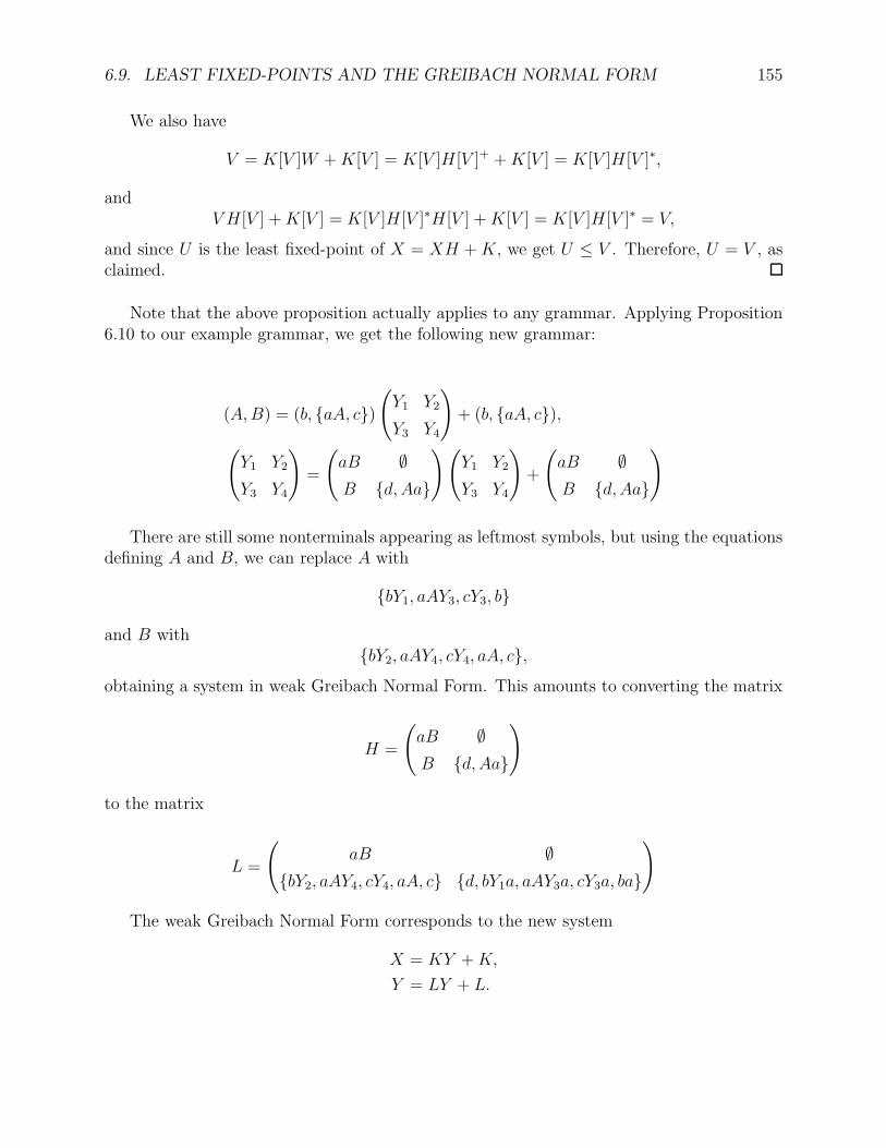
6.9. LEAST FIXED-POINTS AND THE GREIBACH NORMAL FORM 155
We also have
V = K[V ]W +K[V ] = K[V ]H [V ]+ +K[V ] = K[V ]H [V ]∗,
andV H [V ] +K[V ] = K[V ]H [V ]∗H [V ] +K[V ] = K[V ]H [V ]∗ = V,
and since U is the least fixed-point of X = XH +K, we get U ≤ V . Therefore, U = V , asclaimed.
Note that the above proposition actually applies to any grammar. Applying Proposition6.10 to our example grammar, we get the following new grammar:
(A,B) = (b, aA, c)(Y1 Y2
Y3 Y4
)+ (b, aA, c),
(Y1 Y2
Y3 Y4
)=
(aB ∅B d, Aa
)(Y1 Y2
Y3 Y4
)+
(aB ∅B d, Aa
)
There are still some nonterminals appearing as leftmost symbols, but using the equationsdefining A and B, we can replace A with
bY1, aAY3, cY3, b
and B withbY2, aAY4, cY4, aA, c,
obtaining a system in weak Greibach Normal Form. This amounts to converting the matrix
H =
(aB ∅B d, Aa
)
to the matrix
L =
(aB ∅
bY2, aAY4, cY4, aA, c d, bY1a, aAY3a, cY3a, ba
)
The weak Greibach Normal Form corresponds to the new system
X = KY +K,
Y = LY + L.
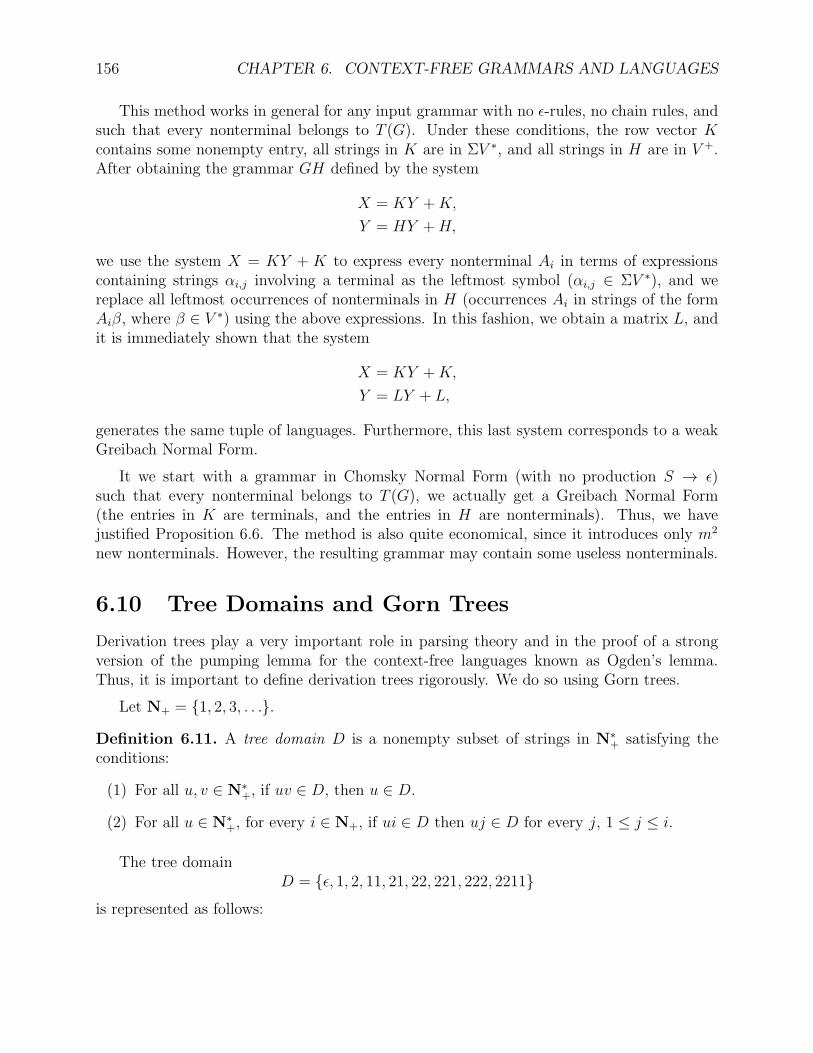
156 CHAPTER 6. CONTEXT-FREE GRAMMARS AND LANGUAGES
This method works in general for any input grammar with no ǫ-rules, no chain rules, andsuch that every nonterminal belongs to T (G). Under these conditions, the row vector Kcontains some nonempty entry, all strings in K are in ΣV ∗, and all strings in H are in V +.After obtaining the grammar GH defined by the system
X = KY +K,
Y = HY +H,
we use the system X = KY + K to express every nonterminal Ai in terms of expressionscontaining strings αi,j involving a terminal as the leftmost symbol (αi,j ∈ ΣV ∗), and wereplace all leftmost occurrences of nonterminals in H (occurrences Ai in strings of the formAiβ, where β ∈ V ∗) using the above expressions. In this fashion, we obtain a matrix L, andit is immediately shown that the system
X = KY +K,
Y = LY + L,
generates the same tuple of languages. Furthermore, this last system corresponds to a weakGreibach Normal Form.
It we start with a grammar in Chomsky Normal Form (with no production S → ǫ)such that every nonterminal belongs to T (G), we actually get a Greibach Normal Form(the entries in K are terminals, and the entries in H are nonterminals). Thus, we havejustified Proposition 6.6. The method is also quite economical, since it introduces only m2
new nonterminals. However, the resulting grammar may contain some useless nonterminals.
6.10 Tree Domains and Gorn Trees
Derivation trees play a very important role in parsing theory and in the proof of a strongversion of the pumping lemma for the context-free languages known as Ogden’s lemma.Thus, it is important to define derivation trees rigorously. We do so using Gorn trees.
Let N+ = 1, 2, 3, . . ..
Definition 6.11. A tree domain D is a nonempty subset of strings in N∗+ satisfying the
conditions:
(1) For all u, v ∈ N∗+, if uv ∈ D, then u ∈ D.
(2) For all u ∈ N∗+, for every i ∈ N+, if ui ∈ D then uj ∈ D for every j, 1 ≤ j ≤ i.
The tree domainD = ǫ, 1, 2, 11, 21, 22, 221, 222, 2211
is represented as follows:
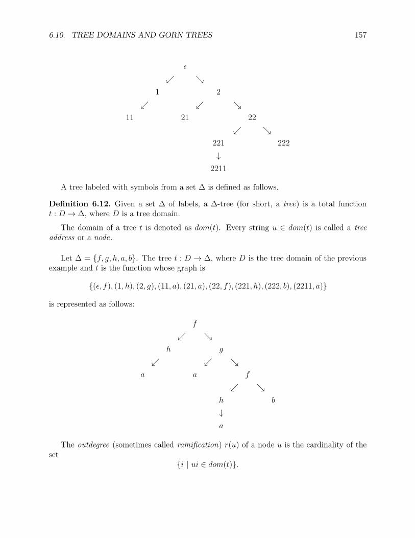
6.10. TREE DOMAINS AND GORN TREES 157
ǫ
ւ ց1 2
ւ ւ ց11 21 22
ւ ց221 222
↓2211
A tree labeled with symbols from a set ∆ is defined as follows.
Definition 6.12. Given a set ∆ of labels, a ∆-tree (for short, a tree) is a total functiont : D → ∆, where D is a tree domain.
The domain of a tree t is denoted as dom(t). Every string u ∈ dom(t) is called a treeaddress or a node.
Let ∆ = f, g, h, a, b. The tree t : D → ∆, where D is the tree domain of the previousexample and t is the function whose graph is
(ǫ, f), (1, h), (2, g), (11, a), (21, a), (22, f), (221, h), (222, b), (2211, a)
is represented as follows:
f
ւ ցh g
ւ ւ ցa a f
ւ ցh b
↓a
The outdegree (sometimes called ramification) r(u) of a node u is the cardinality of theset
i | ui ∈ dom(t).
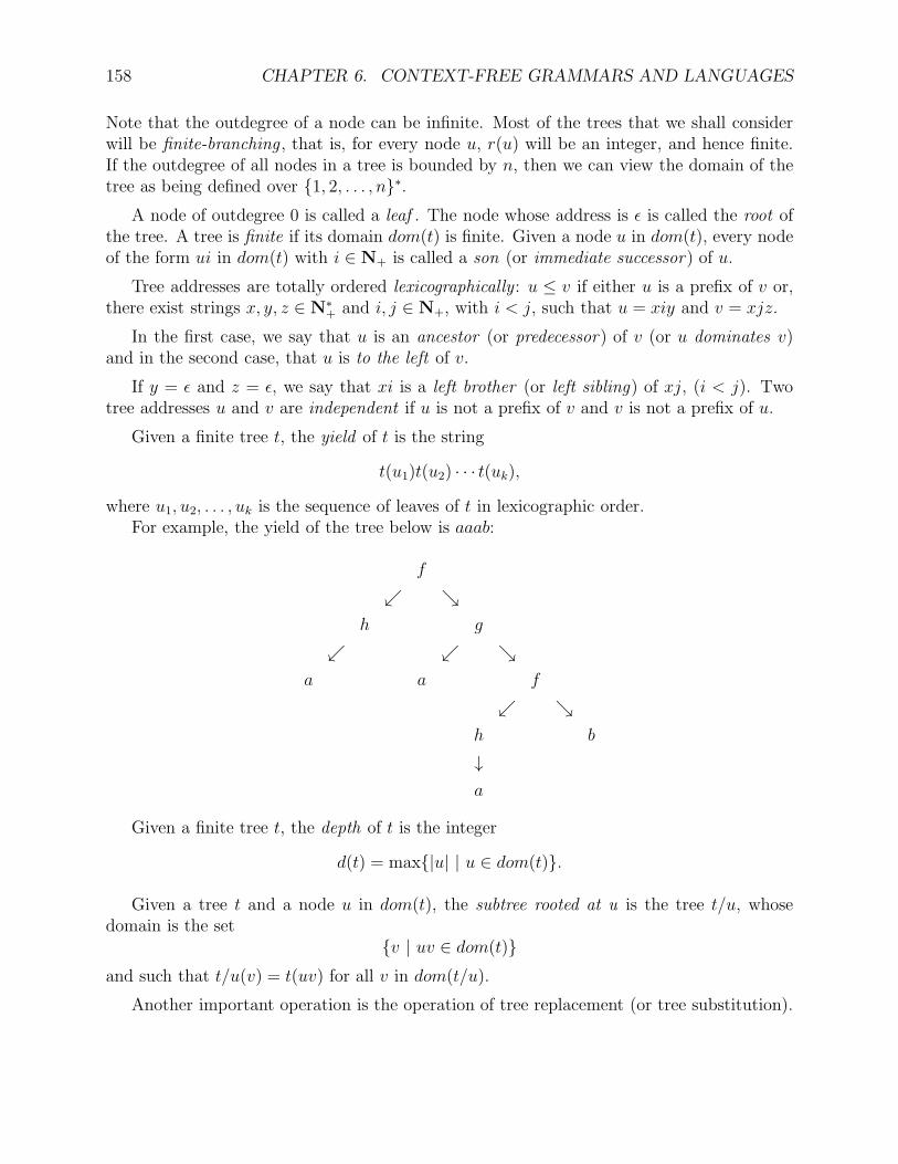
158 CHAPTER 6. CONTEXT-FREE GRAMMARS AND LANGUAGES
Note that the outdegree of a node can be infinite. Most of the trees that we shall considerwill be finite-branching , that is, for every node u, r(u) will be an integer, and hence finite.If the outdegree of all nodes in a tree is bounded by n, then we can view the domain of thetree as being defined over 1, 2, . . . , n∗.
A node of outdegree 0 is called a leaf . The node whose address is ǫ is called the root ofthe tree. A tree is finite if its domain dom(t) is finite. Given a node u in dom(t), every nodeof the form ui in dom(t) with i ∈ N+ is called a son (or immediate successor) of u.
Tree addresses are totally ordered lexicographically : u ≤ v if either u is a prefix of v or,there exist strings x, y, z ∈ N∗
+ and i, j ∈ N+, with i < j, such that u = xiy and v = xjz.
In the first case, we say that u is an ancestor (or predecessor) of v (or u dominates v)and in the second case, that u is to the left of v.
If y = ǫ and z = ǫ, we say that xi is a left brother (or left sibling) of xj, (i < j). Twotree addresses u and v are independent if u is not a prefix of v and v is not a prefix of u.
Given a finite tree t, the yield of t is the string
t(u1)t(u2) · · · t(uk),
where u1, u2, . . . , uk is the sequence of leaves of t in lexicographic order.For example, the yield of the tree below is aaab:
f
ւ ցh g
ւ ւ ցa a f
ւ ցh b
↓a
Given a finite tree t, the depth of t is the integer
d(t) = max|u| | u ∈ dom(t).
Given a tree t and a node u in dom(t), the subtree rooted at u is the tree t/u, whosedomain is the set
v | uv ∈ dom(t)and such that t/u(v) = t(uv) for all v in dom(t/u).
Another important operation is the operation of tree replacement (or tree substitution).
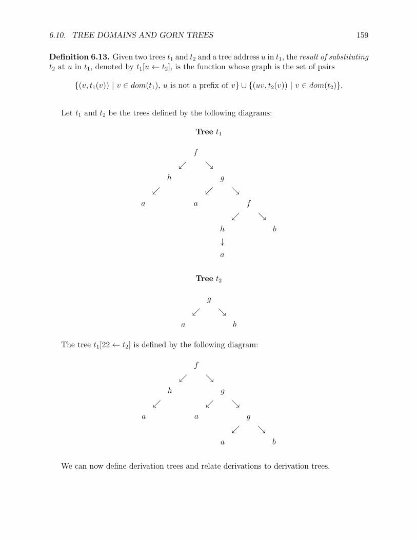
6.10. TREE DOMAINS AND GORN TREES 159
Definition 6.13. Given two trees t1 and t2 and a tree address u in t1, the result of substitutingt2 at u in t1, denoted by t1[u← t2], is the function whose graph is the set of pairs
(v, t1(v)) | v ∈ dom(t1), u is not a prefix of v ∪ (uv, t2(v)) | v ∈ dom(t2).
Let t1 and t2 be the trees defined by the following diagrams:
Tree t1
f
ւ ցh g
ւ ւ ցa a f
ւ ցh b
↓a
Tree t2
g
ւ ցa b
The tree t1[22← t2] is defined by the following diagram:
f
ւ ցh g
ւ ւ ցa a g
ւ ցa b
We can now define derivation trees and relate derivations to derivation trees.
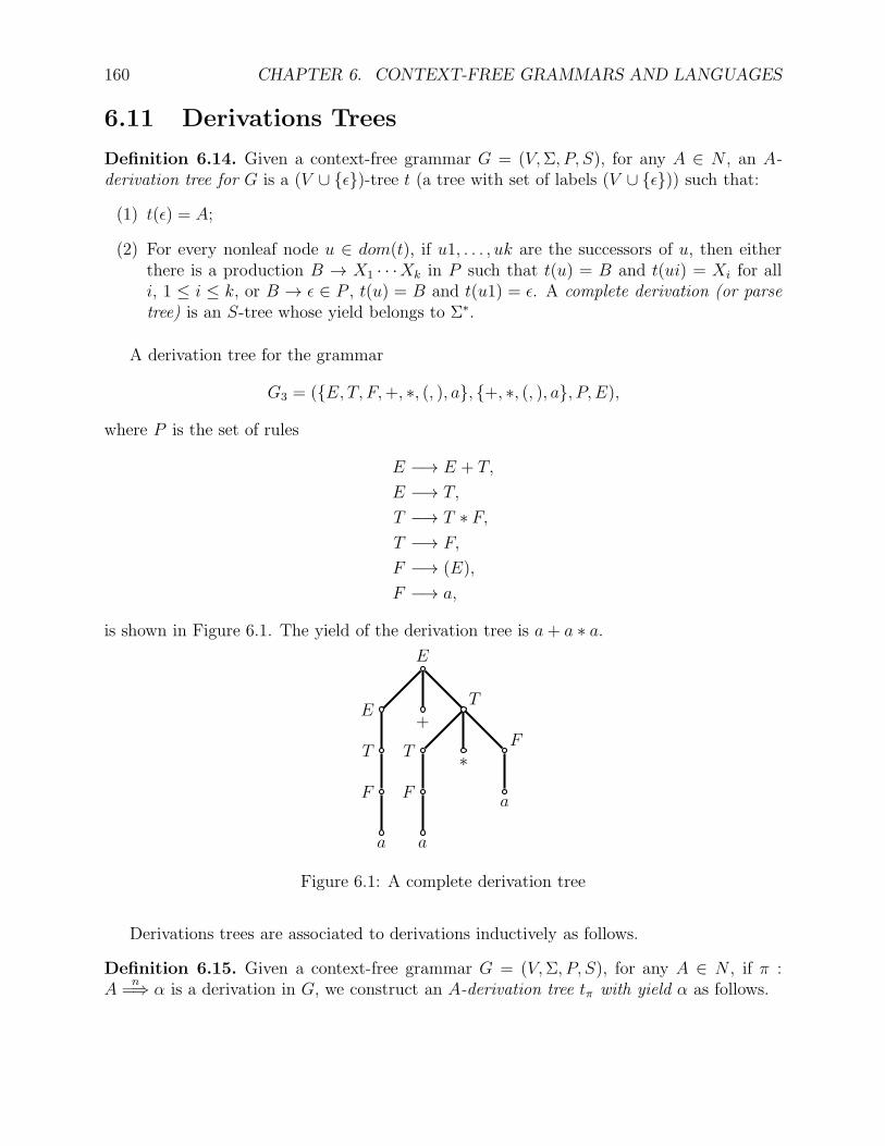
160 CHAPTER 6. CONTEXT-FREE GRAMMARS AND LANGUAGES
6.11 Derivations Trees
Definition 6.14. Given a context-free grammar G = (V,Σ, P, S), for any A ∈ N , an A-derivation tree for G is a (V ∪ ǫ)-tree t (a tree with set of labels (V ∪ ǫ)) such that:
(1) t(ǫ) = A;
(2) For every nonleaf node u ∈ dom(t), if u1, . . . , uk are the successors of u, then eitherthere is a production B → X1 · · ·Xk in P such that t(u) = B and t(ui) = Xi for alli, 1 ≤ i ≤ k, or B → ǫ ∈ P , t(u) = B and t(u1) = ǫ. A complete derivation (or parsetree) is an S-tree whose yield belongs to Σ∗.
A derivation tree for the grammar
G3 = (E, T, F,+, ∗, (, ), a, +, ∗, (, ), a, P, E),
where P is the set of rules
E −→ E + T,
E −→ T,
T −→ T ∗ F,T −→ F,
F −→ (E),
F −→ a,
is shown in Figure 6.1. The yield of the derivation tree is a+ a ∗ a.
a a
F
T
E
E
+
T
T ∗F
Fa
Figure 6.1: A complete derivation tree
Derivations trees are associated to derivations inductively as follows.
Definition 6.15. Given a context-free grammar G = (V,Σ, P, S), for any A ∈ N , if π :A
n=⇒ α is a derivation in G, we construct an A-derivation tree tπ with yield α as follows.
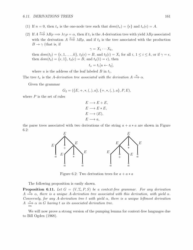
6.11. DERIVATIONS TREES 161
(1) If n = 0, then tπ is the one-node tree such that dom(tπ) = ǫ and tπ(ǫ) = A.
(2) If An−1=⇒ λBρ =⇒ λγρ = α, then if t1 is the A-derivation tree with yield λBρ associated
with the derivation An−1=⇒ λBρ, and if t2 is the tree associated with the production
B → γ (that is, ifγ = X1 · · ·Xk,
then dom(t2) = ǫ, 1, . . . , k, t2(ǫ) = B, and t2(i) = Xi for all i, 1 ≤ i ≤ k, or if γ = ǫ,then dom(t2) = ǫ, 1, t2(ǫ) = B, and t2(1) = ǫ), then
tπ = t1[u← t2],
where u is the address of the leaf labeled B in t1.
The tree tπ is the A-derivation tree associated with the derivation An
=⇒ α.
Given the grammar
G2 = (E,+, ∗, (, ), a, +, ∗, (, ), a, P, E),where P is the set of rules
E −→ E + E,
E −→ E ∗ E,E −→ (E),
E −→ a,
the parse trees associated with two derivations of the string a + a ∗ a are shown in Figure6.2:
a
a
E
E
+
E
E ∗E
a a a
EE
+
E
E∗
E
a
Figure 6.2: Two derivation trees for a + a ∗ a
The following proposition is easily shown.
Proposition 6.11. Let G = (V,Σ, P, S) be a context-free grammar. For any derivationA
n=⇒ α, there is a unique A-derivation tree associated with this derivation, with yield α.
Conversely, for any A-derivation tree t with yield α, there is a unique leftmost derivationA
∗=⇒lm
α in G having t as its associated derivation tree.
We will now prove a strong version of the pumping lemma for context-free languages dueto Bill Ogden (1968).
162 CHAPTER 6. CONTEXT-FREE GRAMMARS AND LANGUAGES
6.12 Ogden’s Lemma
Ogden’s lemma states some combinatorial properties of parse trees that are deep enough.The yield w of such a parse tree can be split into 5 substrings u, v, x, y, z such that
w = uvxyz,
where u, v, x, y, z satisfy certain conditions. It turns out that we get a more powerful versionof the lemma if we allow ourselves to mark certain occurrences of symbols in w beforeinvoking the lemma. We can imagine that marked occurrences in a nonempty string w areoccurrences of symbols in w in boldface, or red, or any given color (but one color only). Forexample, given w = aaababbbaa, we can mark the symbols of even index as follows:
aaababbbaa.
More rigorously, we can define a marking of a nonnull string w : 1, . . . , n → Σ as anyfunction m : 1, . . . , n → 0, 1. Then, a letter wi in w is a marked occurrence iff m(i) = 1,and an unmarked occurrence if m(i) = 0. The number of marked occurrences in w is equalto
n∑
i=1
m(i).
Ogden’s lemma only yields useful information for grammars G generating an infinitelanguage. We could make this hypothesis, but it seems more elegant to use the preconditionthat the lemma only applies to strings w ∈ L(D) such that w contains at least K markedoccurrences, for a constant K large enough. If K is large enough, L(G) will indeed beinfinite.
Proposition 6.12. For every context-free grammar G, there is some integer K > 1 suchthat, for every string w ∈ Σ+, for every marking of w, if w ∈ L(G) and w contains at leastK marked occurrences, then there exists some decomposition of w as w = uvxyz, and someA ∈ N , such that the following properties hold:
(1) There are derivations S+
=⇒ uAz, A+
=⇒ vAy, and A+
=⇒ x, so that
uvnxynz ∈ L(G)
for all n ≥ 0 (the pumping property);
(2) x contains some marked occurrence;
(3) Either (both u and v contain some marked occurrence), or (both y and z contain somemarked occurrence);
(4) vxy contains less than K marked occurrences.
6.12. OGDEN’S LEMMA 163
Proof. Let t be any parse tree for w. We call a leaf of t a marked leaf if its label is a markedoccurrence in the marked string w. The general idea is to make sure that K is large enoughso that parse trees with yield w contain enough repeated nonterminals along some path fromthe root to some marked leaf. Let r = |N |, and let
p = max2, max|α| | (A→ α) ∈ P.
We claim that K = p2r+3 does the job.
The key concept in the proof is the notion of a B-node. Given a parse tree t, a B-nodeis a node with at least two immediate successors u1, u2, such that for i = 1, 2, either ui isa marked leaf, or ui has some marked leaf as a descendant. We construct a path from theroot to some marked leaf, so that for every B-node, we pick the leftmost successor with themaximum number of marked leaves as descendants. Formally, define a path (s0, . . . , sn) fromthe root to some marked leaf, so that:
(i) Every node si has some marked leaf as a descendant, and s0 is the root of t;
(ii) If sj is in the path, sj is not a leaf, and sj has a single immediate descendant which iseither a marked leaf or has marked leaves as its descendants, let sj+1 be that uniqueimmediate descendant of si.
(iii) If sj is a B-node in the path, then let sj+1 be the leftmost immediate successors of sjwith the maximum number of marked leaves as descendants (assuming that if sj+1 isa marked leaf, then it is its own descendant).
(iv) If sj is a leaf, then it is a marked leaf and n = j.
We will show that the path (s0, . . . , sn) contains at least 2r + 3 B-nodes.
Claim: For every i, 0 ≤ i ≤ n, if the path (si, . . . , sn) contains b B-nodes, then si has atmost pb marked leaves as descendants.
Proof . We proceed by “backward induction”, i.e., by induction on n− i. For i = n, thereare no B-nodes, so that b = 0, and there is indeed p0 = 1 marked leaf sn. Assume that theclaim holds for the path (si+1, . . . , sn).
If si is not a B-node, then the number b of B-nodes in the path (si+1, . . . , sn) is the sameas the number of B-nodes in the path (si, . . . , sn), and si+1 is the only immediate successorof si having a marked leaf as descendant. By the induction hypothesis, si+1 has at most pb
marked leaves as descendants, and this is also an upper bound on the number of markedleaves which are descendants of si.
If si is a B-node, then if there are b B-nodes in the path (si+1, . . . , sn), there are b + 1B-nodes in the path (si, . . . , sn). By the induction hypothesis, si+1 has at most pb markedleaves as descendants. Since si is a B-node, si+1 was chosen to be the leftmost immediatesuccessor of si having the maximum number of marked leaves as descendants. Thus, since
164 CHAPTER 6. CONTEXT-FREE GRAMMARS AND LANGUAGES
the outdegree of si is at most p, and each of its immediate successors has at most pb markedleaves as descendants, the node si has at most ppd = pd+1 marked leaves as descendants, asdesired.
Applying the claim to s0, since w has at least K = p2r+3 marked occurrences, we havepb ≥ p2r+3, and since p ≥ 2, we have b ≥ 2r + 3, and the path (s0, . . . , sn) contains at least2r + 3 B-nodes (Note that this would not follow if we had p = 1).
Let us now select the lowest 2r + 3 B-nodes in the path, (s0, . . . , sn), and denote them(b1, . . . , b2r+3). Every B-node bi has at least two immediate successors ui < vi such that uior vi is on the path (s0, . . . , sn). If the path goes through ui, we say that bi is a right B-nodeand if the path goes through vi, we say that bi is a left B-node. Since 2r+3 = r+2+ r+1,either there are r+2 left B-nodes or there are r+2 right B-nodes in the path (b1, . . . , b2r+3).Let us assume that there are r + 2 left B-nodes, the other case being similar.
Let (d1, . . . , dr+2) be the lowest r + 2 left B-nodes in the path. Since there are r + 1B-nodes in the sequence (d2, . . . , dr+2), and there are only r distinct nonterminals, there aretwo nodes di and dj, with 2 ≤ i < j ≤ r + 2, such that t(di) = t(dj) = A, for some A ∈ N .We can assume that di is an ancestor of dj, and thus, dj = diα, for some α 6= ǫ.
If we prune out the subtree t/di rooted at di from t, we get an S-derivation tree having
a yield of the form uAz, and we have a derivation of the form S+
=⇒ uAz, since there areat least r + 2 left B-nodes on the path, and we are looking at the lowest r + 1 left B-nodes.Considering the subtree t/di, pruning out the subtree t/dj rooted at α in t/di, we get anA-derivation tree having a yield of the form vAy, and we have a derivation of the form
A+
=⇒ vAy. Finally, the subtree t/dj is an A-derivation tree with yield x, and we have a
derivation A+
=⇒ x. This proves (1) of the lemma.
Since sn is a marked leaf and a descendant of dj, x contains some marked occurrence,proving (2).
Since d1 is a left B-node, some left sibbling of the immediate successor of d1 on the pathhas some distinguished leaf in u as a descendant. Similarly, since di is a left B-node, someleft sibbling of the immediate successor of di on the path has some distinguished leaf in v asa descendant. This proves (3).
(dj, . . . , b2r+3) has at most 2r+1 B-nodes, and by the claim shown earlier, dj has at mostp2r+1 marked leaves as descendants. Since p2r+1 < p2r+3 = K, this proves (4).
Observe that condition (2) implies that x 6= ǫ, and condition (3) implies that eitheru 6= ǫ and v 6= ǫ, or y 6= ǫ and z 6= ǫ. Thus, the pumping condition (1) implies that the setuvnxynz | n ≥ 0 is an infinite subset of L(G), and L(G) is indeed infinite, as we mentionedearlier. Note that K ≥ 3, and in fact, K ≥ 32. The “standard pumping lemma” due toBar-Hillel, Perles, and Shamir, is obtained by letting all occurrences be marked in w ∈ L(G).
6.12. OGDEN’S LEMMA 165
Proposition 6.13. For every context-free grammar G (without ǫ-rules), there is some integerK > 1 such that, for every string w ∈ Σ+, if w ∈ L(G) and |w| ≥ K, then there exists somedecomposition of w as w = uvxyz, and some A ∈ N , such that the following properties hold:
(1) There are derivations S+
=⇒ uAz, A+
=⇒ vAy, and A+
=⇒ x, so that
uvnxynz ∈ L(G)
for all n ≥ 0 (the pumping property);
(2) x 6= ǫ;
(3) Either v 6= ǫ or y 6= ǫ;
(4) |vxy| ≤ K.
A stronger version could be stated, and we are just following tradition in stating thisstandard version of the pumping lemma.
Ogden’s lemma or the pumping lemma can be used to show that certain languages arenot context-free. The method is to proceed by contradiction, i.e., to assume (contrary towhat we wish to prove) that a language L is indeed context-free, and derive a contradictionof Ogden’s lemma (or of the pumping lemma). Thus, as in the case of the regular languages,it would be helpful to see what the negation of Ogden’s lemma is, and for this, we first stateOgden’s lemma as a logical formula.
For any nonnull string w : 1, . . . , n → Σ, for any marking m : 1, . . . , n → 0, 1 of w,for any substring y of w, where w = xyz, with |x| = h and k = |y|, the number of markedoccurrences in y, denoted as |m(y)|, is defined as
|m(y)| =i=h+k∑
i=h+1
m(i).
We will also use the following abbreviations:
nat = 0, 1, 2, . . .,nat32 = 32, 33, . . .,
A ≡ w = uvxyz,
B ≡ |m(x)| ≥ 1,
C ≡ (|m(u)| ≥ 1 ∧ |m(v)| ≥ 1) ∨ (|m(y)| ≥ 1 ∧ |m(z)| ≥ 1),
D ≡ |m(vxy)| < K,
P ≡ ∀n : nat (uvnxynz ∈ L(D)).
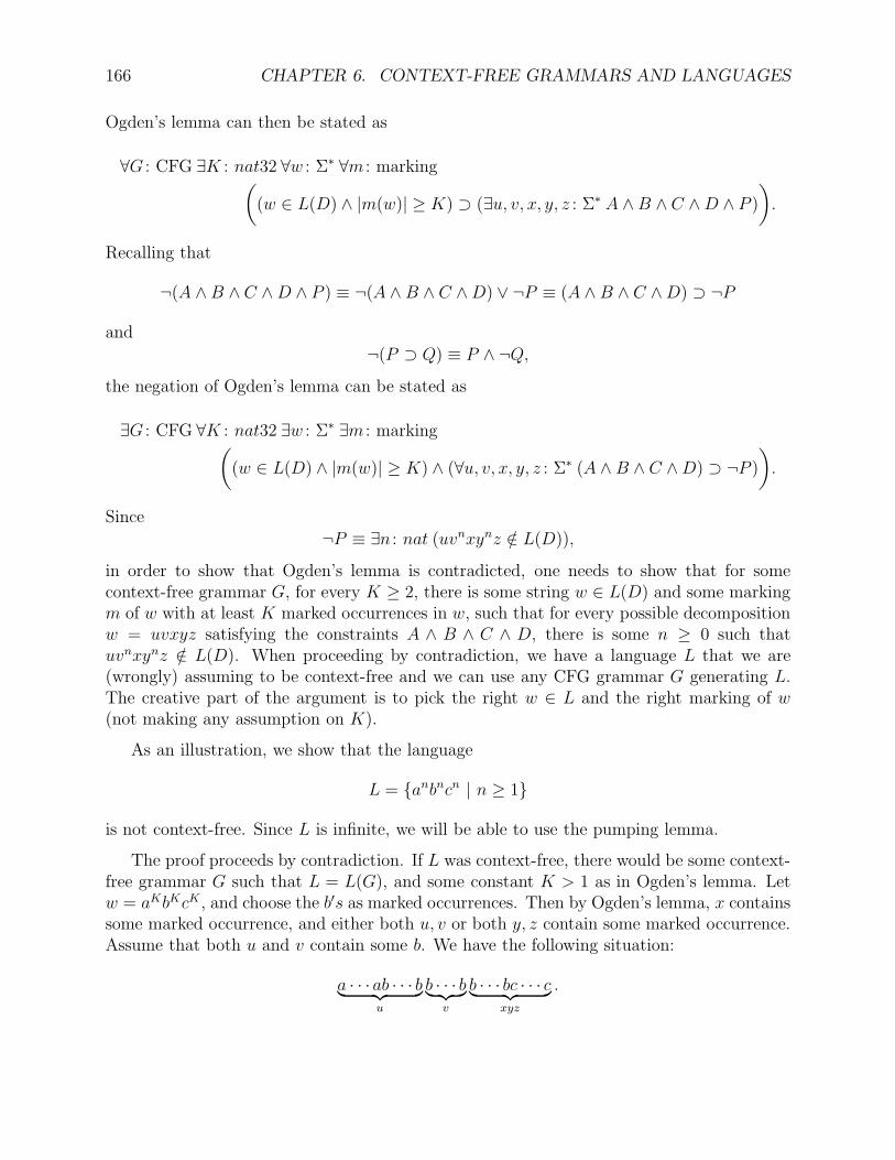
166 CHAPTER 6. CONTEXT-FREE GRAMMARS AND LANGUAGES
Ogden’s lemma can then be stated as
∀G : CFG ∃K : nat32 ∀w : Σ∗ ∀m : marking((w ∈ L(D) ∧ |m(w)| ≥ K) ⊃ (∃u, v, x, y, z : Σ∗ A ∧B ∧ C ∧D ∧ P )
).
Recalling that
¬(A ∧B ∧ C ∧D ∧ P ) ≡ ¬(A ∧ B ∧ C ∧D) ∨ ¬P ≡ (A ∧ B ∧ C ∧D) ⊃ ¬P
and
¬(P ⊃ Q) ≡ P ∧ ¬Q,the negation of Ogden’s lemma can be stated as
∃G : CFG ∀K : nat32 ∃w : Σ∗ ∃m : marking((w ∈ L(D) ∧ |m(w)| ≥ K) ∧ (∀u, v, x, y, z : Σ∗ (A ∧ B ∧ C ∧D) ⊃ ¬P )
).
Since
¬P ≡ ∃n : nat (uvnxynz /∈ L(D)),
in order to show that Ogden’s lemma is contradicted, one needs to show that for somecontext-free grammar G, for every K ≥ 2, there is some string w ∈ L(D) and some markingm of w with at least K marked occurrences in w, such that for every possible decompositionw = uvxyz satisfying the constraints A ∧ B ∧ C ∧ D, there is some n ≥ 0 such thatuvnxynz /∈ L(D). When proceeding by contradiction, we have a language L that we are(wrongly) assuming to be context-free and we can use any CFG grammar G generating L.The creative part of the argument is to pick the right w ∈ L and the right marking of w(not making any assumption on K).
As an illustration, we show that the language
L = anbncn | n ≥ 1
is not context-free. Since L is infinite, we will be able to use the pumping lemma.
The proof proceeds by contradiction. If L was context-free, there would be some context-free grammar G such that L = L(G), and some constant K > 1 as in Ogden’s lemma. Letw = aKbKcK , and choose the b′s as marked occurrences. Then by Ogden’s lemma, x containssome marked occurrence, and either both u, v or both y, z contain some marked occurrence.Assume that both u and v contain some b. We have the following situation:
a · · · ab · · · b︸ ︷︷ ︸u
b · · · b︸ ︷︷ ︸v
b · · · bc · · · c︸ ︷︷ ︸xyz
.
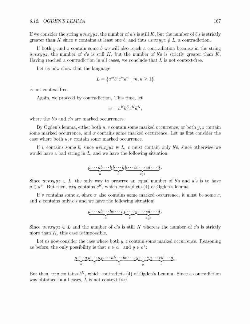
6.12. OGDEN’S LEMMA 167
If we consider the string uvvxyyz, the number of a’s is stillK, but the number of b’s is strictlygreater than K since v contains at least one b, and thus uvvxyyz /∈ L, a contradiction.
If both y and z contain some b we will also reach a contradiction because in the stringuvvxyyz, the number of c’s is still K, but the number of b’s is strictly greater than K.Having reached a contradiction in all cases, we conclude that L is not context-free.
Let us now show that the language
L = ambncmdn | m,n ≥ 1
is not context-free.
Again, we proceed by contradiction. This time, let
w = aKbKcKdK ,
where the b’s and c’s are marked occurrences.
By Ogden’s lemma, either both u, v contain some marked occurrence, or both y, z containsome marked occurrence, and x contains some marked occurrence. Let us first consider thecase where both u, v contain some marked occurrence.
If v contains some b, since uvvxyyz ∈ L, v must contain only b’s, since otherwise wewould have a bad string in L, and we have the following situation:
a · · · ab · · · b︸ ︷︷ ︸u
b · · · b︸ ︷︷ ︸v
b · · · bc · · · cd · · ·d︸ ︷︷ ︸xyz
.
Since uvvxyyz ∈ L, the only way to preserve an equal number of b’s and d’s is to havey ∈ d+. But then, vxy contains cK , which contradicts (4) of Ogden’s lemma.
If v contains some c, since x also contains some marked occurrence, it must be some c,and v contains only c’s and we have the following situation:
a · · · ab · · · bc · · · c︸ ︷︷ ︸u
c · · · c︸ ︷︷ ︸v
c · · · cd · · ·d︸ ︷︷ ︸xyz
.
Since uvvxyyz ∈ L and the number of a’s is still K whereas the number of c’s is strictlymore than K, this case is impossible.
Let us now consider the case where both y, z contain some marked occurrence. Reasoningas before, the only possibility is that v ∈ a+ and y ∈ c+:
a · · · a︸ ︷︷ ︸u
a · · · a︸ ︷︷ ︸v
a · · · ab · · · bc · · · c︸ ︷︷ ︸x
c · · · c︸ ︷︷ ︸y
c · · · cd · · ·d︸ ︷︷ ︸z
.
But then, vxy contains bK , which contradicts (4) of Ogden’s Lemma. Since a contradictionwas obtained in all cases, L is not context-free.
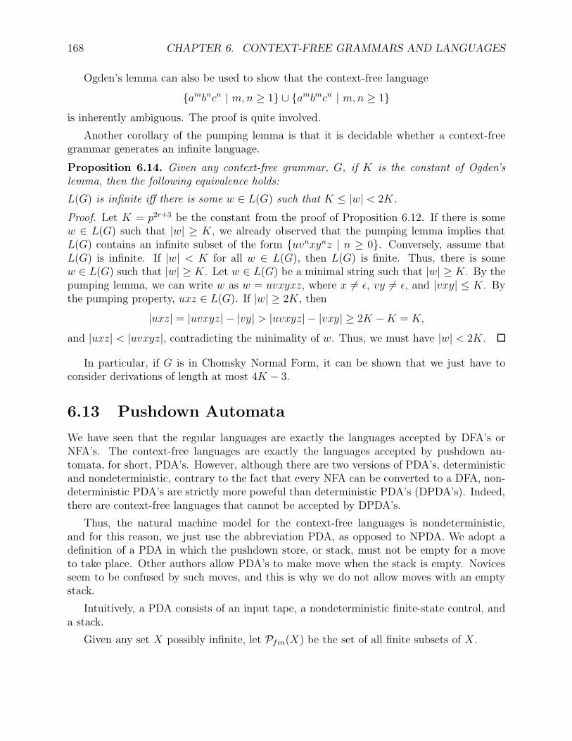
168 CHAPTER 6. CONTEXT-FREE GRAMMARS AND LANGUAGES
Ogden’s lemma can also be used to show that the context-free language
ambncn | m,n ≥ 1 ∪ ambmcn | m,n ≥ 1is inherently ambiguous. The proof is quite involved.
Another corollary of the pumping lemma is that it is decidable whether a context-freegrammar generates an infinite language.
Proposition 6.14. Given any context-free grammar, G, if K is the constant of Ogden’slemma, then the following equivalence holds:
L(G) is infinite iff there is some w ∈ L(G) such that K ≤ |w| < 2K.
Proof. Let K = p2r+3 be the constant from the proof of Proposition 6.12. If there is somew ∈ L(G) such that |w| ≥ K, we already observed that the pumping lemma implies thatL(G) contains an infinite subset of the form uvnxynz | n ≥ 0. Conversely, assume thatL(G) is infinite. If |w| < K for all w ∈ L(G), then L(G) is finite. Thus, there is somew ∈ L(G) such that |w| ≥ K. Let w ∈ L(G) be a minimal string such that |w| ≥ K. By thepumping lemma, we can write w as w = uvxyxz, where x 6= ǫ, vy 6= ǫ, and |vxy| ≤ K. Bythe pumping property, uxz ∈ L(G). If |w| ≥ 2K, then
|uxz| = |uvxyz| − |vy| > |uvxyz| − |vxy| ≥ 2K −K = K,
and |uxz| < |uvxyz|, contradicting the minimality of w. Thus, we must have |w| < 2K.
In particular, if G is in Chomsky Normal Form, it can be shown that we just have toconsider derivations of length at most 4K − 3.
6.13 Pushdown Automata
We have seen that the regular languages are exactly the languages accepted by DFA’s orNFA’s. The context-free languages are exactly the languages accepted by pushdown au-tomata, for short, PDA’s. However, although there are two versions of PDA’s, deterministicand nondeterministic, contrary to the fact that every NFA can be converted to a DFA, non-deterministic PDA’s are strictly more poweful than deterministic PDA’s (DPDA’s). Indeed,there are context-free languages that cannot be accepted by DPDA’s.
Thus, the natural machine model for the context-free languages is nondeterministic,and for this reason, we just use the abbreviation PDA, as opposed to NPDA. We adopt adefinition of a PDA in which the pushdown store, or stack, must not be empty for a moveto take place. Other authors allow PDA’s to make move when the stack is empty. Novicesseem to be confused by such moves, and this is why we do not allow moves with an emptystack.
Intuitively, a PDA consists of an input tape, a nondeterministic finite-state control, anda stack.
Given any set X possibly infinite, let Pfin(X) be the set of all finite subsets of X .
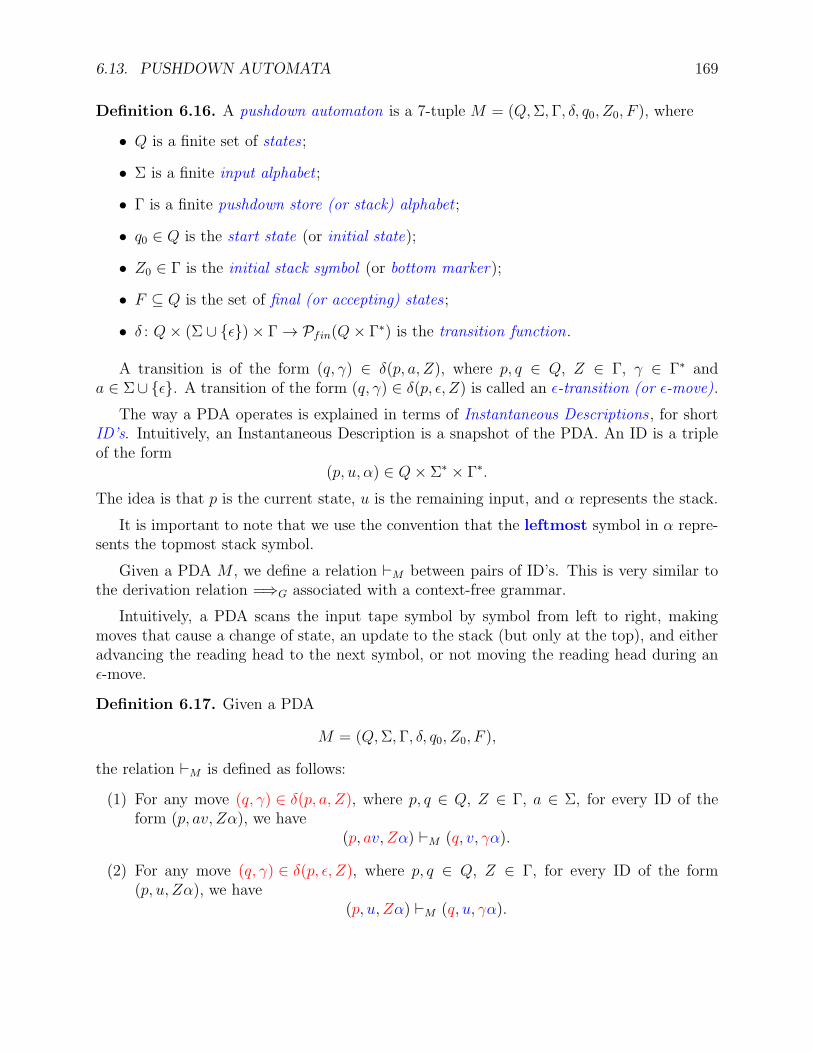
6.13. PUSHDOWN AUTOMATA 169
Definition 6.16. A pushdown automaton is a 7-tuple M = (Q,Σ,Γ, δ, q0, Z0, F ), where
• Q is a finite set of states ;
• Σ is a finite input alphabet ;
• Γ is a finite pushdown store (or stack) alphabet ;
• q0 ∈ Q is the start state (or initial state);
• Z0 ∈ Γ is the initial stack symbol (or bottom marker);
• F ⊆ Q is the set of final (or accepting) states ;
• δ : Q× (Σ ∪ ǫ)× Γ→ Pfin(Q× Γ∗) is the transition function.
A transition is of the form (q, γ) ∈ δ(p, a, Z), where p, q ∈ Q, Z ∈ Γ, γ ∈ Γ∗ anda ∈ Σ∪ ǫ. A transition of the form (q, γ) ∈ δ(p, ǫ, Z) is called an ǫ-transition (or ǫ-move).
The way a PDA operates is explained in terms of Instantaneous Descriptions , for shortID’s. Intuitively, an Instantaneous Description is a snapshot of the PDA. An ID is a tripleof the form
(p, u, α) ∈ Q× Σ∗ × Γ∗.
The idea is that p is the current state, u is the remaining input, and α represents the stack.
It is important to note that we use the convention that the leftmost symbol in α repre-sents the topmost stack symbol.
Given a PDA M , we define a relation ⊢M between pairs of ID’s. This is very similar tothe derivation relation =⇒G associated with a context-free grammar.
Intuitively, a PDA scans the input tape symbol by symbol from left to right, makingmoves that cause a change of state, an update to the stack (but only at the top), and eitheradvancing the reading head to the next symbol, or not moving the reading head during anǫ-move.
Definition 6.17. Given a PDA
M = (Q,Σ,Γ, δ, q0, Z0, F ),
the relation ⊢M is defined as follows:
(1) For any move (q, γ) ∈ δ(p, a, Z), where p, q ∈ Q, Z ∈ Γ, a ∈ Σ, for every ID of theform (p, av, Zα), we have
(p, av, Zα) ⊢M (q, v, γα).
(2) For any move (q, γ) ∈ δ(p, ǫ, Z), where p, q ∈ Q, Z ∈ Γ, for every ID of the form(p, u, Zα), we have
(p, u, Zα) ⊢M (q, u, γα).
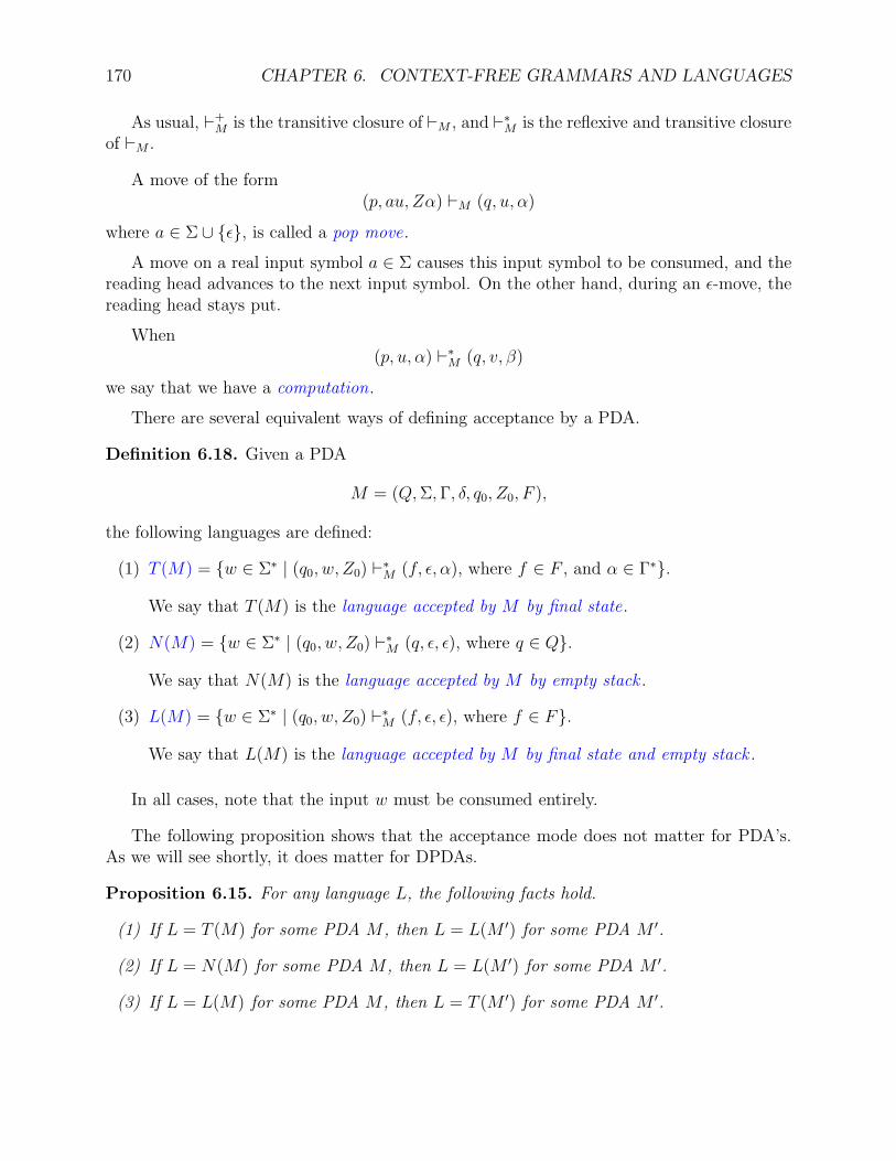
170 CHAPTER 6. CONTEXT-FREE GRAMMARS AND LANGUAGES
As usual, ⊢+M is the transitive closure of ⊢M , and ⊢∗M is the reflexive and transitive closureof ⊢M .
A move of the form(p, au, Zα) ⊢M (q, u, α)
where a ∈ Σ ∪ ǫ, is called a pop move.
A move on a real input symbol a ∈ Σ causes this input symbol to be consumed, and thereading head advances to the next input symbol. On the other hand, during an ǫ-move, thereading head stays put.
When(p, u, α) ⊢∗M (q, v, β)
we say that we have a computation.
There are several equivalent ways of defining acceptance by a PDA.
Definition 6.18. Given a PDA
M = (Q,Σ,Γ, δ, q0, Z0, F ),
the following languages are defined:
(1) T (M) = w ∈ Σ∗ | (q0, w, Z0) ⊢∗M (f, ǫ, α), where f ∈ F , and α ∈ Γ∗.
We say that T (M) is the language accepted by M by final state.
(2) N(M) = w ∈ Σ∗ | (q0, w, Z0) ⊢∗M (q, ǫ, ǫ), where q ∈ Q.
We say that N(M) is the language accepted by M by empty stack .
(3) L(M) = w ∈ Σ∗ | (q0, w, Z0) ⊢∗M (f, ǫ, ǫ), where f ∈ F.
We say that L(M) is the language accepted by M by final state and empty stack .
In all cases, note that the input w must be consumed entirely.
The following proposition shows that the acceptance mode does not matter for PDA’s.As we will see shortly, it does matter for DPDAs.
Proposition 6.15. For any language L, the following facts hold.
(1) If L = T (M) for some PDA M , then L = L(M ′) for some PDA M ′.
(2) If L = N(M) for some PDA M , then L = L(M ′) for some PDA M ′.
(3) If L = L(M) for some PDA M , then L = T (M ′) for some PDA M ′.
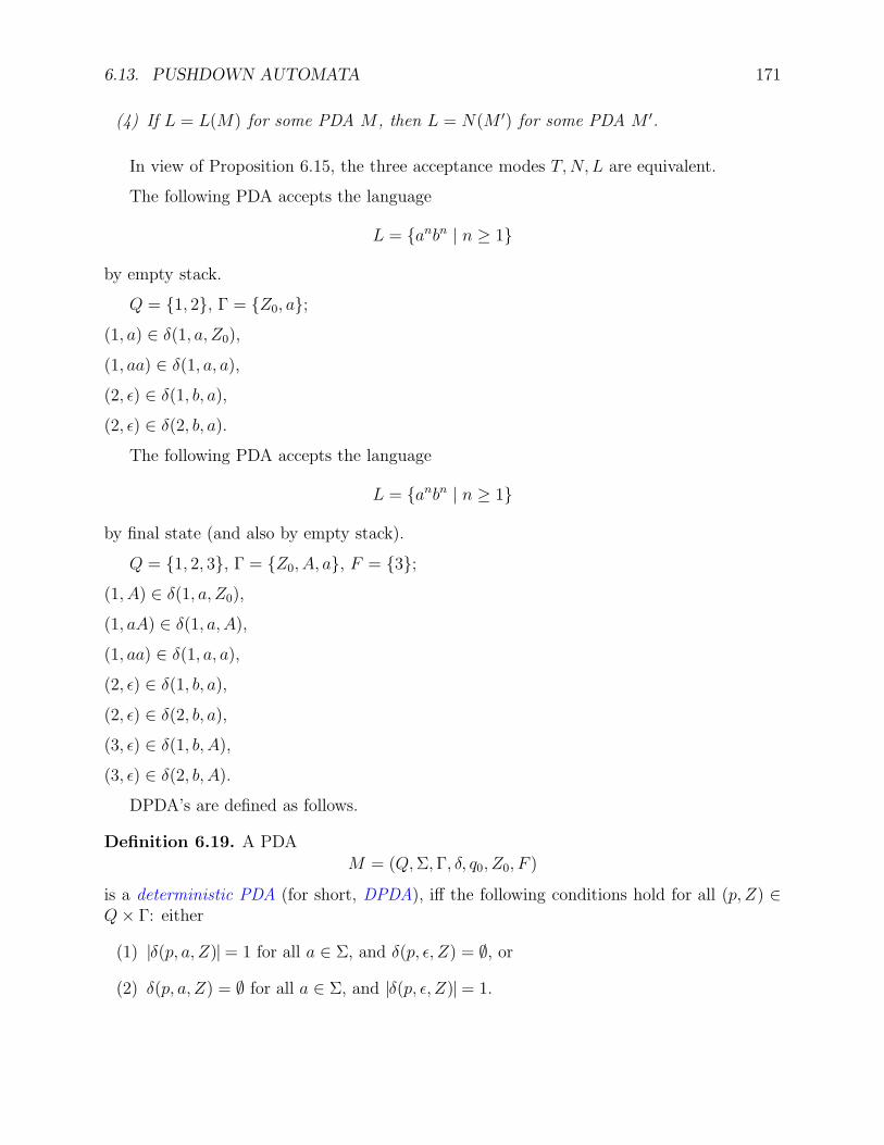
6.13. PUSHDOWN AUTOMATA 171
(4) If L = L(M) for some PDA M , then L = N(M ′) for some PDA M ′.
In view of Proposition 6.15, the three acceptance modes T,N, L are equivalent.
The following PDA accepts the language
L = anbn | n ≥ 1
by empty stack.
Q = 1, 2, Γ = Z0, a;(1, a) ∈ δ(1, a, Z0),
(1, aa) ∈ δ(1, a, a),(2, ǫ) ∈ δ(1, b, a),(2, ǫ) ∈ δ(2, b, a).
The following PDA accepts the language
L = anbn | n ≥ 1
by final state (and also by empty stack).
Q = 1, 2, 3, Γ = Z0, A, a, F = 3;(1, A) ∈ δ(1, a, Z0),
(1, aA) ∈ δ(1, a, A),(1, aa) ∈ δ(1, a, a),(2, ǫ) ∈ δ(1, b, a),(2, ǫ) ∈ δ(2, b, a),(3, ǫ) ∈ δ(1, b, A),(3, ǫ) ∈ δ(2, b, A).
DPDA’s are defined as follows.
Definition 6.19. A PDA
M = (Q,Σ,Γ, δ, q0, Z0, F )
is a deterministic PDA (for short, DPDA), iff the following conditions hold for all (p, Z) ∈Q× Γ: either
(1) |δ(p, a, Z)|= 1 for all a ∈ Σ, and δ(p, ǫ, Z) = ∅, or
(2) δ(p, a, Z) = ∅ for all a ∈ Σ, and |δ(p, ǫ, Z)|= 1.
172 CHAPTER 6. CONTEXT-FREE GRAMMARS AND LANGUAGES
A DPDA operates in realtime iff it has no ǫ-transitions.
It turns out that for DPDA’s the most general acceptance mode is by final state. Indeed,there are language that can only be accepted deterministically as T (M). The language
L = ambn | m ≥ n ≥ 1is such an example. The problem is that amb is a prefix of all strings ambn, with m ≥ n ≥ 2.
A language L is a deterministic context-free language iff L = T (M) for some DPDA M .
It is easily shown that if L = N(M) (or L = L(M)) for some DPDAM , then L = T (M ′)for some DPDA M ′ easily constructed from M .
A PDA is unambiguous iff for every w ∈ Σ∗, there is at most one computation
(q0, w, Z0) ⊢∗ IDn,
where IDn is an accepting ID.
There are context-free languages that are not accepted by any DPDA. For example, itcan be shown that the languages
L1 = anbn | n ≥ 1 ∪ anb2n | n ≥ 1,and
L2 = wwR | w ∈ a, b∗,are not accepted by any DPDA.
Also note that unambiguous grammars for these languages can be easily given.
We now show that every context-free language is accepted by a PDA.
6.14 From Context-Free Grammars To PDA’s
We show how a PDA can be easily constructed from a context-free grammar. Althoughsimple, the construction is not practical for parsing purposes, since the resulting PDA ishorribly nondeterministic.
Given a context-free grammar G = (V,Σ, P, S), we define a one-state PDA M as follows:
Q = q0; Γ = V ; Z0 = S; F = ∅;For every rule (A→ α) ∈ P , there is a transition
(q0, α) ∈ δ(q0, ǫ, A).
For every a ∈ Σ, there is a transition
(q0, ǫ) ∈ δ(q0, a, a).
The intuition is that a computation of M mimics a leftmost derivation in G. One mightsay that we have a “pop/expand” PDA.
6.15. FROM PDA’S TO CONTEXT-FREE GRAMMARS 173
Proposition 6.16. Given any context-free grammar G = (V,Σ, P, S), the PDA M justdescribed accepts L(G) by empty stack, i.e., L(G) = N(M).
Proof sketch. The following two claims are proved by induction.
Claim 1:
For all u, v ∈ Σ∗ and all α ∈ NV ∗ ∪ ǫ, if S ∗=⇒lm
uα, then
(q0, uv, S) ⊢∗ (q0, v, α).
Claim 2:
For all u, v ∈ Σ∗ and all α ∈ V ∗, if
(q0, uv, S) ⊢∗ (q0, v, α)
then S∗=⇒lm
uα.
We now show how a PDA can be converted to a context-free grammar
6.15 From PDA’s To Context-Free Grammars
The construction of a context-free grammar from a PDA is not really difficult, but it is quitemessy. The construction is simplified if we first convert a PDA to an equivalent PDA suchthat for every move (q, γ) ∈ δ(p, a, Z) (where a ∈ Σ ∪ ǫ), we have |γ| ≤ 2. In some sense,we form a kind of PDA in Chomsky Normal Form.
Proposition 6.17. Given any PDA
M = (Q,Σ,Γ, δ, q0, Z0, F ),
another PDA
M ′ = (Q′,Σ,Γ′, δ′, q′0, Z′0, F
′)
can be constructed, such that L(M) = L(M ′) and the following conditions hold:
(1) There is a one-to-one correspondence between accepting computations of M and M ′;
(2) If M has no ǫ-moves, then M ′ has no ǫ-moves; If M is unambiguous, then M ′ isunambiguous;
(3) For all p ∈ Q′, all a ∈ Σ ∪ ǫ, and all Z ∈ Γ′, if (q, γ) ∈ δ′(p, a, Z), then q 6= q′0 and|γ| ≤ 2.
174 CHAPTER 6. CONTEXT-FREE GRAMMARS AND LANGUAGES
The crucial point of the construction is that accepting computations of a PDA acceptingby empty stack and final state can be decomposed into subcomputations of the form
(p, uv, Zα) ⊢∗ (q, v, α),
where for every intermediate ID (s, w, β), we have β = γα for some γ 6= ǫ.
The nonterminals of the grammar constructed from the PDA M are triples of the form[p, Z, q] such that
(p, u, Z) ⊢+ (q, ǫ, ǫ)
for some u ∈ Σ∗.
Given a PDA
M = (Q,Σ,Γ, δ, q0, Z0, F )
satisfying the conditions of Proposition 6.17, we construct a context-free grammar G =(V,Σ, P, S) as follows:
V = [p, Z, q] | p, q ∈ Q,Z ∈ Γ ∪ Σ ∪ S,where S is a new symbol, and the productions are defined as follows: for all p, q ∈ Q, alla ∈ Σ ∪ ǫ, all X, Y, Z ∈ Γ, we have:
(1) S → ǫ ∈ P , if q0 ∈ F ;
(2) S → a ∈ P , if (f, ǫ) ∈ δ(q0, a, Z0), and f ∈ F ;
(3) S → a[p,X, f ] ∈ P , for every f ∈ F , if (p,X) ∈ δ(q0, a, Z0);
(4) S → a[p,X, s][s, Y, f ] ∈ P , for every f ∈ F , for every s ∈ Q, if (p,XY ) ∈ δ(q0, a, Z0);
(5) [p, Z, q]→ a ∈ P , if (q, ǫ) ∈ δ(p, a, Z) and p 6= q0;
(6) [p, Z, s]→ a[q,X, s] ∈ P , for every s ∈ Q, if (q,X) ∈ δ(p, a, Z) and p 6= q0;
(7) [p, Z, t]→ a[q,X, s][s, Y, t] ∈ P , for every s, t ∈ Q, if (q,XY ) ∈ δ(p, a, Z) and p 6= q0.
Proposition 6.18. Given any PDA
M = (Q,Σ,Γ, δ, q0, Z0, F )
satisfying the conditions of Proposition 6.17, the context-free grammar G = (V,Σ, P, S)constructed as above generates L(M), i.e., L(G) = L(M). Furthermore, G is unambiguousiff M is unambiguous.
6.16. THE CHOMSKY-SCHUTZENBERGER THEOREM 175
Proof skecth. We have to prove that
L(G) = w ∈ Σ+ | (q0, w, Z0) ⊢+ (f, ǫ, ǫ), f ∈ F∪ ǫ | q0 ∈ F.
For this, the following claim is proved by induction.
Claim:
For all p, q ∈ Q, all Z ∈ Γ, all k ≥ 1, and all w ∈ Σ∗,
[p, Z, q]k=⇒lm
w iff (p, w, Z) ⊢+ (q, ǫ, ǫ).
Using the claim, it is possible to prove that L(G) = L(M).
In view of Propositions 6.16 and 6.18, the family of context-free languages is exactly thefamily of languages accepted by PDA’s. It is harder to give a grammatical characterizationof the deterministic context-free languages. One method is to use Knuth LR(k)-grammars .
Another characterization can be given in terms of strict deterministic grammars due toHarrison and Havel.
6.16 The Chomsky-Schutzenberger Theorem
Unfortunately, there is no characterization of the context-free languages analogous to thecharacterization of the regular languages in terms of closure properties (R(Σ)).
However, there is a famous theorem due to Chomsky and Schutzenberger showing thatevery context-free language can be obtained from a special language, the Dyck set , in termsof homomorphisms, inverse homomorphisms and intersection with the regular languages.
Definition 6.20. Given the alphabet Σ2 = a, b, a, b, define the relation ≃ on Σ∗2 as follows:
For all u, v ∈ Σ∗2,
u ≃ v iff ∃x, y ∈ Σ∗2, u = xaay, v = xy or
u = xbby, v = xy.
Let ≃∗ be the reflexive and transitive closure of ≃, and let D2 = w ∈ Σ∗2 | w ≃∗ ǫ. This is
the Dyck set on two letters.
It is not hard to prove that D2 is context-free.
Theorem 6.19. (Chomsky-Schutzenberger) For every PDA, M = (Q,Σ,Γ, δ, q0, Z0, F ),there is a regular language R and two homomorphisms g, h such that
L(M) = h(g−1(D2) ∩ R).
176 CHAPTER 6. CONTEXT-FREE GRAMMARS AND LANGUAGES
Observe that Theorem 6.19 yields another proof of the fact that the language accepteda PDA is context-free.
Indeed, the context-free languages are closed under, homomorphisms, inverse homomor-phisms, intersection with the regular languages, and D2 is context-free.
From the characterization of a-transducers in terms of homomorphisms, inverse homo-morphisms, and intersection with regular languages, we deduce that every context-free lan-guage is the image of D2 under some a-transduction.
Chapter 7
A Survey of LR-Parsing Methods
In this chapter, we give a brief survey on LR-parsing methods. We begin with the definitionof characteristic strings and the construction of Knuth’s LR(0)-characteristic automaton.Next, we describe the shift/reduce algorithm. The need for lookahead sets is motivated bythe resolution of conflicts. A unified method for computing FIRST, FOLLOW and LALR(1)lookahead sets is presented. The method uses a same graph algorithm Traverse whichfinds all nodes reachable from a given node and computes the union of predefined setsassigned to these nodes. Hence, the only difference between the various algorithms forcomputing FIRST, FOLLOW and LALR(1) lookahead sets lies in the fact that the initialsets and the graphs are computed in different ways. The method can be viewed as anefficient way for solving a set of simultaneously recursive equations with set variables. Themethod is inspired by DeRemer and Pennello’s method for computing LALR(1) lookaheadsets. However, DeRemer and Pennello use a more sophisticated graph algorithm for findingstrongly connected components. We use a slightly less efficient but simpler algorithm (adepth-first search). We conclude with a brief presentation of LR(1) parsers.
7.1 LR(0)-Characteristic Automata
The purpose of LR-parsing , invented by D. Knuth in the mid sixties, is the following: Givena context-free grammar G, for any terminal string w ∈ Σ∗, find out whether w belongsto the language L(G) generated by G, and if so, construct a rightmost derivation of w, ina deterministic fashion. Of course, this is not possible for all context-free grammars, butonly for those that correspond to languages that can be recognized by a deterministic PDA(DPDA). Knuth’s major discovery was that for a certain type of grammars, the LR(k)-grammars, a certain kind of DPDA could be constructed from the grammar (shift/reduceparsers). The k in LR(k) refers to the amount of lookahead that is necessary in order toproceed deterministically. It turns out that k = 1 is sufficient, but even in this case, Knuthconstruction produces very large DPDA’s, and his original LR(1) method is not practical.Fortunately, around 1969, Frank DeRemer, in his MIT Ph.D. thesis, investigated a practicalrestriction of Knuth’s method, known as SLR(k), and soon after, the LALR(k) method was
177
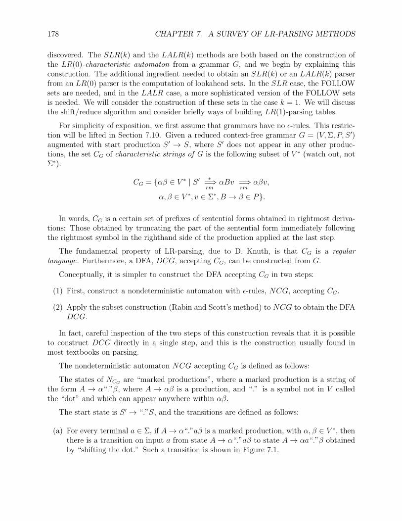
178 CHAPTER 7. A SURVEY OF LR-PARSING METHODS
discovered. The SLR(k) and the LALR(k) methods are both based on the construction ofthe LR(0)-characteristic automaton from a grammar G, and we begin by explaining thisconstruction. The additional ingredient needed to obtain an SLR(k) or an LALR(k) parserfrom an LR(0) parser is the computation of lookahead sets. In the SLR case, the FOLLOWsets are needed, and in the LALR case, a more sophisticated version of the FOLLOW setsis needed. We will consider the construction of these sets in the case k = 1. We will discussthe shift/reduce algorithm and consider briefly ways of building LR(1)-parsing tables.
For simplicity of exposition, we first assume that grammars have no ǫ-rules. This restric-tion will be lifted in Section 7.10. Given a reduced context-free grammar G = (V,Σ, P, S ′)augmented with start production S ′ → S, where S ′ does not appear in any other produc-tions, the set CG of characteristic strings of G is the following subset of V ∗ (watch out, notΣ∗):
CG = αβ ∈ V ∗ | S ′ ∗=⇒rm
αBv =⇒rm
αβv,
α, β ∈ V ∗, v ∈ Σ∗, B → β ∈ P.
In words, CG is a certain set of prefixes of sentential forms obtained in rightmost deriva-tions: Those obtained by truncating the part of the sentential form immediately followingthe rightmost symbol in the righthand side of the production applied at the last step.
The fundamental property of LR-parsing, due to D. Knuth, is that CG is a regularlanguage. Furthermore, a DFA, DCG, accepting CG, can be constructed from G.
Conceptually, it is simpler to construct the DFA accepting CG in two steps:
(1) First, construct a nondeterministic automaton with ǫ-rules, NCG, accepting CG.
(2) Apply the subset construction (Rabin and Scott’s method) to NCG to obtain the DFADCG.
In fact, careful inspection of the two steps of this construction reveals that it is possibleto construct DCG directly in a single step, and this is the construction usually found inmost textbooks on parsing.
The nondeterministic automaton NCG accepting CG is defined as follows:
The states of NCGare “marked productions”, where a marked production is a string of
the form A → α“.”β, where A → αβ is a production, and “.” is a symbol not in V calledthe “dot” and which can appear anywhere within αβ.
The start state is S ′ → “.”S, and the transitions are defined as follows:
(a) For every terminal a ∈ Σ, if A→ α“.”aβ is a marked production, with α, β ∈ V ∗, thenthere is a transition on input a from state A→ α“.”aβ to state A→ αa“.”β obtainedby “shifting the dot.” Such a transition is shown in Figure 7.1.
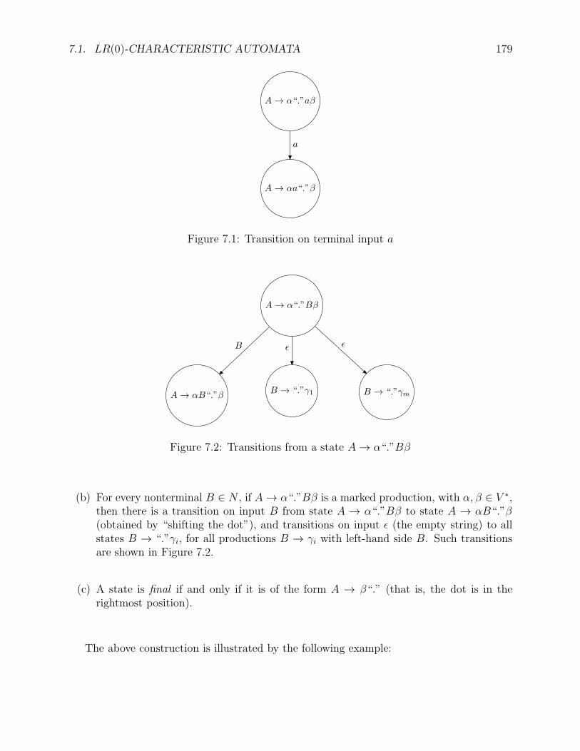
7.1. LR(0)-CHARACTERISTIC AUTOMATA 179
A→ α“.”aβ
A→ αa“.”β
a
Figure 7.1: Transition on terminal input a
A→ α“.”Bβ
B → “.”γ1A→ αB“.”β B → “.”γm
B ǫ ǫ
Figure 7.2: Transitions from a state A→ α“.”Bβ
(b) For every nonterminal B ∈ N , if A→ α“.”Bβ is a marked production, with α, β ∈ V ∗,then there is a transition on input B from state A → α“.”Bβ to state A → αB“.”β(obtained by “shifting the dot”), and transitions on input ǫ (the empty string) to allstates B → “.”γi, for all productions B → γi with left-hand side B. Such transitionsare shown in Figure 7.2.
(c) A state is final if and only if it is of the form A → β“.” (that is, the dot is in therightmost position).
The above construction is illustrated by the following example:
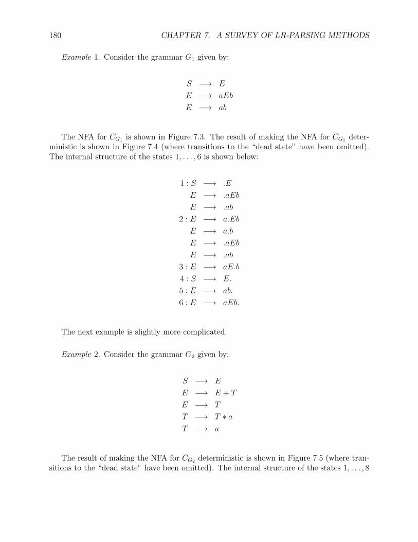
180 CHAPTER 7. A SURVEY OF LR-PARSING METHODS
Example 1. Consider the grammar G1 given by:
S −→ E
E −→ aEb
E −→ ab
The NFA for CG1 is shown in Figure 7.3. The result of making the NFA for CG1 deter-ministic is shown in Figure 7.4 (where transitions to the “dead state” have been omitted).The internal structure of the states 1, . . . , 6 is shown below:
1 : S −→ .E
E −→ .aEb
E −→ .ab
2 : E −→ a.Eb
E −→ a.b
E −→ .aEb
E −→ .ab
3 : E −→ aE.b
4 : S −→ E.
5 : E −→ ab.
6 : E −→ aEb.
The next example is slightly more complicated.
Example 2. Consider the grammar G2 given by:
S −→ E
E −→ E + T
E −→ T
T −→ T ∗ aT −→ a
The result of making the NFA for CG2 deterministic is shown in Figure 7.5 (where tran-sitions to the “dead state” have been omitted). The internal structure of the states 1, . . . , 8
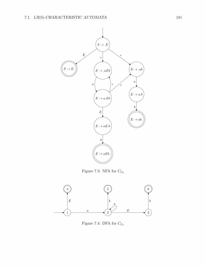
7.1. LR(0)-CHARACTERISTIC AUTOMATA 181
S → .E
E → .aEb
E → a.Eb
E → aE.b
E → aEb.
S → E. E → .ab
E → a.b
E → ab.
Eǫ
ǫ
E
b
a
b
ǫa ǫ
Figure 7.3: NFA for CG1
1 2 3
4 5 6
a E
E b ba
Figure 7.4: DFA for CG1
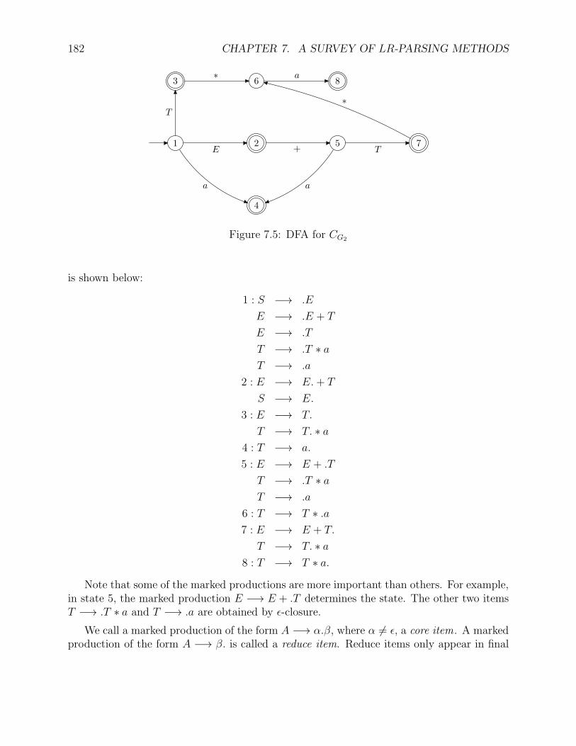
182 CHAPTER 7. A SURVEY OF LR-PARSING METHODS
1 2 5 7
3 6 8
4
E + T
∗ a
T
∗
a a
Figure 7.5: DFA for CG2
is shown below:
1 : S −→ .E
E −→ .E + T
E −→ .T
T −→ .T ∗ aT −→ .a
2 : E −→ E.+ T
S −→ E.
3 : E −→ T.
T −→ T. ∗ a4 : T −→ a.
5 : E −→ E + .T
T −→ .T ∗ aT −→ .a
6 : T −→ T ∗ .a7 : E −→ E + T.
T −→ T. ∗ a8 : T −→ T ∗ a.
Note that some of the marked productions are more important than others. For example,in state 5, the marked production E −→ E + .T determines the state. The other two itemsT −→ .T ∗ a and T −→ .a are obtained by ǫ-closure.
We call a marked production of the form A −→ α.β, where α 6= ǫ, a core item. A markedproduction of the form A −→ β. is called a reduce item. Reduce items only appear in final

7.1. LR(0)-CHARACTERISTIC AUTOMATA 183
states.
If we also call S ′ −→ .S a core item, we observe that every state is completely determinedby its subset of core items. The other items in the state are obtained via ǫ-closure. We cantake advantage of this fact to write a more efficient algorithm to construct in a single passthe LR(0)-automaton.
Also observe the so-called spelling property : All the transitions entering any given statehave the same label.
Given a state s, if s contains both a reduce item A −→ γ. and a shift item B −→ α.aβ,where a ∈ Σ, we say that there is a shift/reduce conflict in state s on input a. If s containstwo (distinct) reduce items A1 −→ γ1. and A2 −→ γ2., we say that there is a reduce/reduceconflict in state s.
A grammar is said to be LR(0) if the DFA DCG has no conflicts. This is the case forthe grammar G1. However, it should be emphasized that this is extremely rare in practice.The grammar G1 is just very nice, and a toy example. In fact, G2 is not LR(0).
To eliminate conflicts, one can either compute SLR(1)-lookahead sets, using FOLLOWsets (see Section 7.6), or sharper lookahead sets, the LALR(1) sets (see Section 7.9). Forexample, the computation of SLR(1)-lookahead sets for G2 will eliminate the conflicts.
We will describe methods for computing SLR(1)-lookahead sets and LALR(1)-lookaheadsets in Sections 7.6, 7.9, and 7.10. A more drastic measure is to compute the LR(1)-automaton, in which the states incoporate lookahead symbols (see Section 7.11). However,as we said before, this is not a practical methods for large grammars.
In order to motivate the construction of a shift/reduce parser from the DFA acceptingCG, let us consider a rightmost derivation for w = aaabbb in reverse order for the grammar
0: S −→ E
1: E −→ aEb
2: E −→ ab
aaabbb α1β1v1
aaEbb α1B1v1 E −→ ab
aaEbb α2β2v2
aEb α2B2v2 E −→ aEb
aEb α3β3v3 α3 = v3 = ǫ
E α3B3v3 α3 = v3 = ǫ E −→ aEb
E α4β4v4 α4 = v4 = ǫ
S α4B4v4 α4 = v4 = ǫ S −→ E
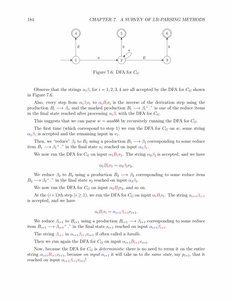
184 CHAPTER 7. A SURVEY OF LR-PARSING METHODS
1 2 3
4 5 6
a E
E b ba
Figure 7.6: DFA for CG
Observe that the strings αiβi for i = 1, 2, 3, 4 are all accepted by the DFA for CG shownin Figure 7.6.
Also, every step from αiβivi to αiBivi is the inverse of the derivation step using theproduction Bi −→ βi, and the marked production Bi −→ βi“ .” is one of the reduce itemsin the final state reached after processing αiβi with the DFA for CG.
This suggests that we can parse w = aaabbb by recursively running the DFA for CG.
The first time (which correspond to step 1) we run the DFA for CG on w, some stringα1β1 is accepted and the remaining input in v1.
Then, we “reduce” β1 to B1 using a production B1 −→ β1 corresponding to some reduceitem B1 −→ β1“ .” in the final state s1 reached on input α1β1.
We now run the DFA for CG on input α1B1v1. The string α2β2 is accepted, and we have
α1B1v1 = α2β2v2.
We reduce β2 to B2 using a production B2 −→ β2 corresponding to some reduce itemB2 −→ β2“ .” in the final state s2 reached on input α2β2.
We now run the DFA for CG on input α2B2v2, and so on.
At the (i+1)th step (i ≥ 1), we run the DFA for CG on input αiBivi. The string αi+1βi+1
is accepted, and we have
αiBivi = αi+1βi+1vi+1.
We reduce βi+1 to Bi+1 using a production Bi+1 −→ βi+1 corresponding to some reduceitem Bi+1 −→ βi+1“ .” in the final state si+1 reached on input αi+1βi+1.
The string βi+1 in αi+1βi+1vi+1 if often called a handle.
Then we run again the DFA for CG on input αi+1Bi+1vi+1.
Now, because the DFA for CG is deterministic there is no need to rerun it on the entirestring αi+1Bi+1vi+1, because on input αi+1 it will take us to the same state, say pi+1, that itreached on input αi+1βi+1vi+1!
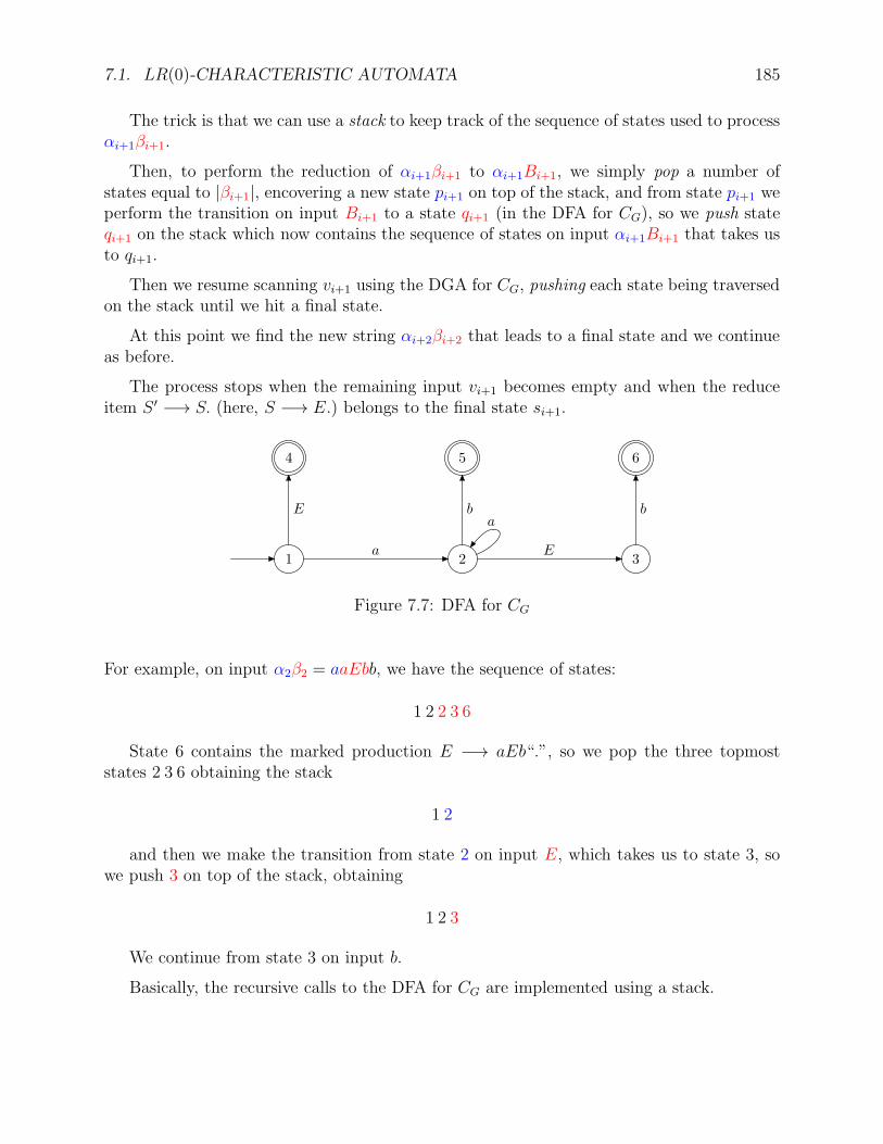
7.1. LR(0)-CHARACTERISTIC AUTOMATA 185
The trick is that we can use a stack to keep track of the sequence of states used to processαi+1βi+1.
Then, to perform the reduction of αi+1βi+1 to αi+1Bi+1, we simply pop a number ofstates equal to |βi+1|, encovering a new state pi+1 on top of the stack, and from state pi+1 weperform the transition on input Bi+1 to a state qi+1 (in the DFA for CG), so we push stateqi+1 on the stack which now contains the sequence of states on input αi+1Bi+1 that takes usto qi+1.
Then we resume scanning vi+1 using the DGA for CG, pushing each state being traversedon the stack until we hit a final state.
At this point we find the new string αi+2βi+2 that leads to a final state and we continueas before.
The process stops when the remaining input vi+1 becomes empty and when the reduceitem S ′ −→ S. (here, S −→ E.) belongs to the final state si+1.
1 2 3
4 5 6
a E
E b ba
Figure 7.7: DFA for CG
For example, on input α2β2 = aaEbb, we have the sequence of states:
1 2 2 3 6
State 6 contains the marked production E −→ aEb“.”, so we pop the three topmoststates 2 3 6 obtaining the stack
1 2
and then we make the transition from state 2 on input E, which takes us to state 3, sowe push 3 on top of the stack, obtaining
1 2 3
We continue from state 3 on input b.
Basically, the recursive calls to the DFA for CG are implemented using a stack.
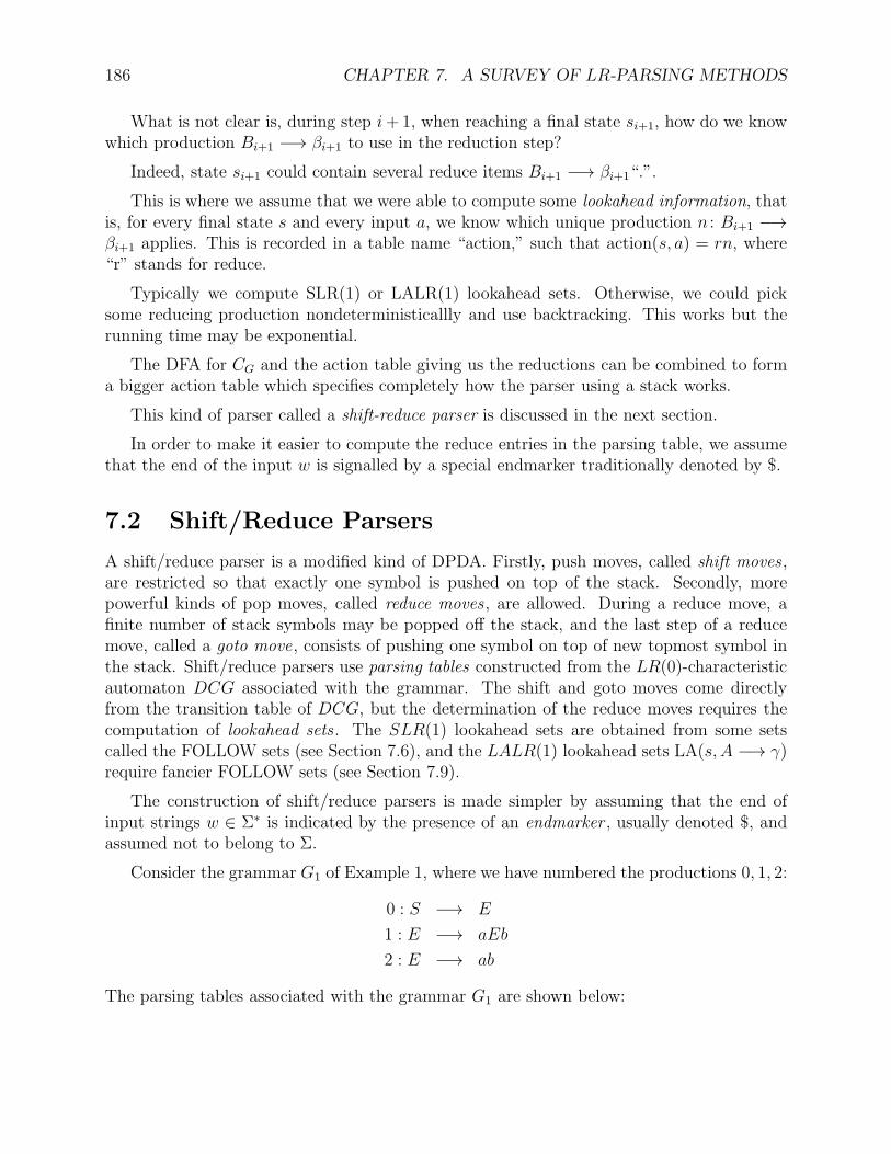
186 CHAPTER 7. A SURVEY OF LR-PARSING METHODS
What is not clear is, during step i+1, when reaching a final state si+1, how do we knowwhich production Bi+1 −→ βi+1 to use in the reduction step?
Indeed, state si+1 could contain several reduce items Bi+1 −→ βi+1“.”.
This is where we assume that we were able to compute some lookahead information, thatis, for every final state s and every input a, we know which unique production n : Bi+1 −→βi+1 applies. This is recorded in a table name “action,” such that action(s, a) = rn, where“r” stands for reduce.
Typically we compute SLR(1) or LALR(1) lookahead sets. Otherwise, we could picksome reducing production nondeterministicallly and use backtracking. This works but therunning time may be exponential.
The DFA for CG and the action table giving us the reductions can be combined to forma bigger action table which specifies completely how the parser using a stack works.
This kind of parser called a shift-reduce parser is discussed in the next section.
In order to make it easier to compute the reduce entries in the parsing table, we assumethat the end of the input w is signalled by a special endmarker traditionally denoted by $.
7.2 Shift/Reduce Parsers
A shift/reduce parser is a modified kind of DPDA. Firstly, push moves, called shift moves ,are restricted so that exactly one symbol is pushed on top of the stack. Secondly, morepowerful kinds of pop moves, called reduce moves , are allowed. During a reduce move, afinite number of stack symbols may be popped off the stack, and the last step of a reducemove, called a goto move, consists of pushing one symbol on top of new topmost symbol inthe stack. Shift/reduce parsers use parsing tables constructed from the LR(0)-characteristicautomaton DCG associated with the grammar. The shift and goto moves come directlyfrom the transition table of DCG, but the determination of the reduce moves requires thecomputation of lookahead sets . The SLR(1) lookahead sets are obtained from some setscalled the FOLLOW sets (see Section 7.6), and the LALR(1) lookahead sets LA(s, A −→ γ)require fancier FOLLOW sets (see Section 7.9).
The construction of shift/reduce parsers is made simpler by assuming that the end ofinput strings w ∈ Σ∗ is indicated by the presence of an endmarker , usually denoted $, andassumed not to belong to Σ.
Consider the grammar G1 of Example 1, where we have numbered the productions 0, 1, 2:
0 : S −→ E
1 : E −→ aEb
2 : E −→ ab
The parsing tables associated with the grammar G1 are shown below:
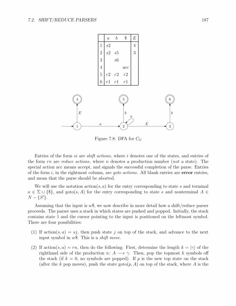
7.2. SHIFT/REDUCE PARSERS 187
a b $ E
1 s2 4
2 s2 s5 3
3 s6
4 acc
5 r2 r2 r2
6 r1 r1 r1
1 2 3
4 5 6
a E
E b ba
Figure 7.8: DFA for CG
Entries of the form si are shift actions , where i denotes one of the states, and entries ofthe form rn are reduce actions , where n denotes a production number (not a state). Thespecial action acc means accept, and signals the successful completion of the parse. Entriesof the form i, in the rightmost column, are goto actions . All blank entries are error entries,and mean that the parse should be aborted.
We will use the notation action(s, a) for the entry corresponding to state s and terminala ∈ Σ ∪ $, and goto(s, A) for the entry corresponding to state s and nonterminal A ∈N − S ′.
Assuming that the input is w$, we now describe in more detail how a shift/reduce parserproceeds. The parser uses a stack in which states are pushed and popped. Initially, the stackcontains state 1 and the cursor pointing to the input is positioned on the leftmost symbol.There are four possibilities:
(1) If action(s, a) = sj, then push state j on top of the stack, and advance to the nextinput symbol in w$. This is a shift move.
(2) If action(s, a) = rn, then do the following: First, determine the length k = |γ| of therighthand side of the production n : A −→ γ. Then, pop the topmost k symbols offthe stack (if k = 0, no symbols are popped). If p is the new top state on the stack(after the k pop moves), push the state goto(p, A) on top of the stack, where A is the
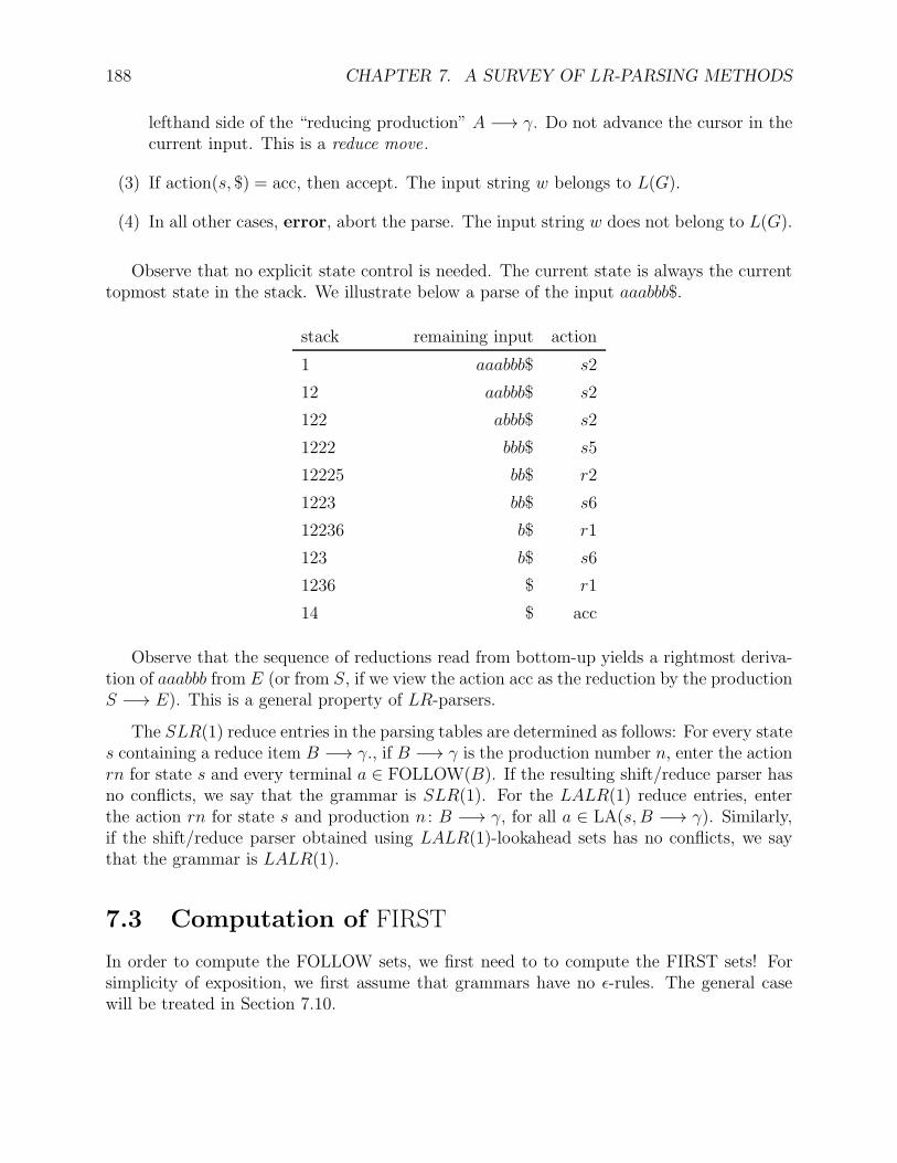
188 CHAPTER 7. A SURVEY OF LR-PARSING METHODS
lefthand side of the “reducing production” A −→ γ. Do not advance the cursor in thecurrent input. This is a reduce move.
(3) If action(s, $) = acc, then accept. The input string w belongs to L(G).
(4) In all other cases, error, abort the parse. The input string w does not belong to L(G).
Observe that no explicit state control is needed. The current state is always the currenttopmost state in the stack. We illustrate below a parse of the input aaabbb$.
stack remaining input action
1 aaabbb$ s2
12 aabbb$ s2
122 abbb$ s2
1222 bbb$ s5
12225 bb$ r2
1223 bb$ s6
12236 b$ r1
123 b$ s6
1236 $ r1
14 $ acc
Observe that the sequence of reductions read from bottom-up yields a rightmost deriva-tion of aaabbb from E (or from S, if we view the action acc as the reduction by the productionS −→ E). This is a general property of LR-parsers.
The SLR(1) reduce entries in the parsing tables are determined as follows: For every states containing a reduce item B −→ γ., if B −→ γ is the production number n, enter the actionrn for state s and every terminal a ∈ FOLLOW(B). If the resulting shift/reduce parser hasno conflicts, we say that the grammar is SLR(1). For the LALR(1) reduce entries, enterthe action rn for state s and production n : B −→ γ, for all a ∈ LA(s, B −→ γ). Similarly,if the shift/reduce parser obtained using LALR(1)-lookahead sets has no conflicts, we saythat the grammar is LALR(1).
7.3 Computation of FIRST
In order to compute the FOLLOW sets, we first need to to compute the FIRST sets! Forsimplicity of exposition, we first assume that grammars have no ǫ-rules. The general casewill be treated in Section 7.10.
7.4. THE INTUITION BEHIND THE SHIFT/REDUCE ALGORITHM 189
Given a context-free grammar G = (V,Σ, P, S ′) (augmented with a start productionS ′ −→ S), for every nonterminal A ∈ N = V − Σ, let
FIRST(A) = a | a ∈ Σ, A+
=⇒ aα, for some α ∈ V ∗.
For a terminal a ∈ Σ, let FIRST(a) = a. The key to the computation of FIRST(A) is thefollowing observation: a is in FIRST(A) if either a is in
INITFIRST(A) = a | a ∈ Σ, A −→ aα ∈ P, for some α ∈ V ∗,
or a is ina | a ∈ FIRST(B), A −→ Bα ∈ P, for some α ∈ V ∗, B 6= A.
Note that the second assertion is true because, if B+
=⇒ aδ, then A =⇒ Bα+
=⇒ aδα, andso, FIRST(B) ⊆ FIRST(A) whenever A −→ Bα ∈ P , with A 6= B. Hence, the FIRST setsare the least solution of the following set of recursive equations: For each nonterminal A,
FIRST(A) = INITFIRST(A) ∪⋃FIRST(B) | A −→ Bα ∈ P, A 6= B.
In order to explain the method for solving such systems, we will formulate the problem inmore general terms, but first, we describe a “naive” version of the shift/reduce algorithmthat hopefully demystifies the “‘optimized version” described in Section 7.2.
7.4 The Intuition Behind the Shift/Reduce Algorithm
Let DCG = (K, V, δ, q0, F ) be the DFA accepting the regular language CG, and let δ∗ be theextension of δ to K×V ∗. Let us assume that the grammar G is either SLR(1) or LALR(1),which implies that it has no shift/reduce or reduce/reduce conflicts. We can use the DFADCG accepting CG recursively to parse L(G). The function CG is defined as follows: Givenany string µ ∈ V ∗,
CG(µ) =
error if δ∗(q0, µ) = error;(δ∗(q0, θ), θ, v) if δ∗(q0, θ) ∈ F , µ = θv and θ is the
shortest prefix of µ s.t. δ∗(q0, θ) ∈ F .
The naive shift-reduce algorithm is shown below:
begin
accept := true;
stop := false;
µ := w$; input stringwhile ¬stop do
if CG(µ) = error then
190 CHAPTER 7. A SURVEY OF LR-PARSING METHODS
stop := true; accept := false
else
Let (q, θ, v) = CG(µ)
Let B → β be the production so that
action(q,FIRST(v)) = B → β and let θ = αβ
if B → β = S ′ → S then
stop := true
else
µ := αBv reductionendif
endif
endwhile
end
The idea is to recursively run the DFA DCG on the sentential form µ, until the first finalstate q is hit. Then, the sentential form µ must be of the form αβv, where v is a terminalstring ending in $, and the final state q contains a reduce item of the form B −→ β, withaction(q,FIRST(v)) = B −→ β. Thus, we can reduce µ = αβv to αBv, since we have founda rightmost derivation step, and repeat the process.
Note that the major inefficiency of the algorithm is that when a reduction is performed,the prefix α of µ is reparsed entirely by DCG. Since DCG is deterministic, the sequenceof states obtained on input α is uniquely determined. If we keep the sequence of statesproduced on input θ by DCG in a stack, then it is possible to avoid reparsing α. Indeed, allwe have to do is update the stack so that just before applying DCG to αAv, the sequenceof states in the stack is the sequence obtained after parsing α. This stack is obtained bypopping the |β| topmost states and performing an update which is just a goto move. Thisis the standard version of the shift/reduce algorithm!
7.5 The Graph Method for Computing Fixed Points
Let X be a finite set representing the domain of the problem (in Section 7.3 above, X = Σ),let F (1), . . . , F (N) be N sets to be computed and let I(1), . . . , I(N) be N given subsets ofX . The sets I(1), . . . , I(N) are the initial sets. We also have a directed graph G whoseset of nodes is 1, . . . , N and which represents relationships among the sets F (i), where1 ≤ i ≤ N . The graph G has no parallel edges and no loops, but it may have cycles. If thereis an edge from i to j, this is denoted by iGj (note that the absense of loops means thatiGi never holds). Also, the existence of a path from i to j is denoted by iG+j. The graphG represents a relation, and G+ is the graph of the transitive closure of this relation. Theexistence of a path from i to j, including the null path, is denoted by iG∗j. Hence, G∗ is the
7.5. THE GRAPH METHOD FOR COMPUTING FIXED POINTS 191
reflexive and transitive closure of G. We want to solve for the least solution of the systemof recursive equations:
F (i) = I(i) ∪ F (j) | iGj, i 6= j, 1 ≤ i ≤ N.
Since (2X)N is a complete lattice under the inclusion ordering (which means that ev-ery family of subsets has a least upper bound, namely, the union of this family), it is anω-complete poset, and since the function F : (2X)N → (2X)N induced by the system ofequations is easily seen to preserve least upper bounds of ω-chains, the least solution of thesystem can be computed by the standard fixed point technique (as explained in Section 3.7of the class notes). We simply compute the sequence of approximations (F k(1), . . . , F k(N)),where
F 0(i) = ∅, 1 ≤ i ≤ N,
andF k+1(i) = I(i) ∪
⋃F k(j) | iGj, i 6= j, 1 ≤ i ≤ N.
It is easily seen that we can stop at k = N − 1, and the least solution is given by
F (i) = F 1(i) ∪ F 2(i) ∪ · · · ∪ FN(i), 1 ≤ i ≤ N.
However, the above expression can be simplified to
F (i) =⋃I(j) | iG∗j, 1 ≤ i ≤ N.
This last expression shows that in order to compute F (i), it is necessary to compute theunion of all the initial sets I(j) reachable from i (including i). Hence, any transitive closurealgorithm or graph traversal algorithm will do. For simplicity and for pedagogical reasons,we use a depth-first search algorithm.
Going back to FIRST, we see that all we have to do is to compute the INITFIRST sets,the graph GFIRST, and then use the graph traversal algorithm. The graph GFIRST iscomputed as follows: The nodes are the nonterminals and there is an edge from A to B(A 6= B) if and only if there is a production of the form A −→ Bα, for some α ∈ V ∗.
Example 1. Computation of the FIRST sets for the grammar G1 given by the rules:
S −→ E$
E −→ E + T
E −→ T
T −→ T ∗ FT −→ F
F −→ (E)
F −→ −TF −→ a.
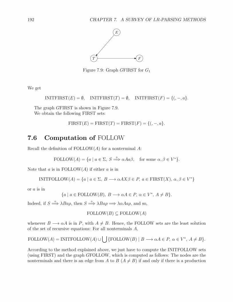
192 CHAPTER 7. A SURVEY OF LR-PARSING METHODS
E
T F
Figure 7.9: Graph GFIRST for G1
We get
INITFIRST(E) = ∅, INITFIRST(T ) = ∅, INITFIRST(F ) = (,−, a.
The graph GFIRST is shown in Figure 7.9.We obtain the following FIRST sets:
FIRST(E) = FIRST(T ) = FIRST(F ) = (,−, a.
7.6 Computation of FOLLOW
Recall the definition of FOLLOW(A) for a nonterminal A:
FOLLOW(A) = a | a ∈ Σ, S+
=⇒ αAaβ, for some α, β ∈ V ∗.
Note that a is in FOLLOW(A) if either a is in
INITFOLLOW(A) = a | a ∈ Σ, B −→ αAXβ ∈ P, a ∈ FIRST(X), α, β ∈ V ∗
or a is ina | a ∈ FOLLOW(B), B −→ αA ∈ P, α ∈ V ∗, A 6= B.
Indeed, if S+
=⇒ λBaρ, then S+
=⇒ λBaρ =⇒ λαAaρ, and so,
FOLLOW(B) ⊆ FOLLOW(A)
whenever B −→ αA is in P , with A 6= B. Hence, the FOLLOW sets are the least solutionof the set of recursive equations: For all nonterminals A,
FOLLOW(A) = INITFOLLOW(A) ∪⋃FOLLOW(B) | B −→ αA ∈ P, α ∈ V ∗, A 6= B.
According to the method explained above, we just have to compute the INITFOLLOW sets(using FIRST) and the graph GFOLLOW, which is computed as follows: The nodes are thenonterminals and there is an edge from A to B (A 6= B) if and only if there is a production
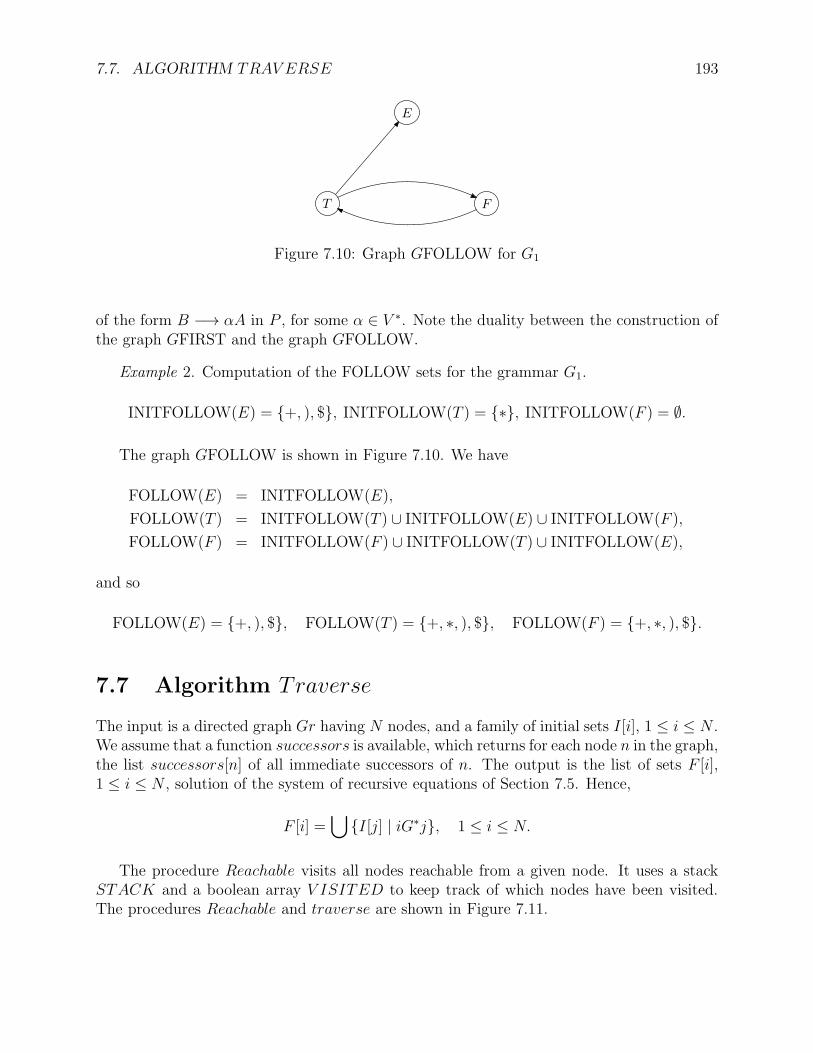
7.7. ALGORITHM TRAV ERSE 193
E
T F
Figure 7.10: Graph GFOLLOW for G1
of the form B −→ αA in P , for some α ∈ V ∗. Note the duality between the construction ofthe graph GFIRST and the graph GFOLLOW.
Example 2. Computation of the FOLLOW sets for the grammar G1.
INITFOLLOW(E) = +, ), $, INITFOLLOW(T ) = ∗, INITFOLLOW(F ) = ∅.
The graph GFOLLOW is shown in Figure 7.10. We have
FOLLOW(E) = INITFOLLOW(E),
FOLLOW(T ) = INITFOLLOW(T ) ∪ INITFOLLOW(E) ∪ INITFOLLOW(F ),
FOLLOW(F ) = INITFOLLOW(F ) ∪ INITFOLLOW(T ) ∪ INITFOLLOW(E),
and so
FOLLOW(E) = +, ), $, FOLLOW(T ) = +, ∗, ), $, FOLLOW(F ) = +, ∗, ), $.
7.7 Algorithm Traverse
The input is a directed graph Gr having N nodes, and a family of initial sets I[i], 1 ≤ i ≤ N .We assume that a function successors is available, which returns for each node n in the graph,the list successors[n] of all immediate successors of n. The output is the list of sets F [i],1 ≤ i ≤ N , solution of the system of recursive equations of Section 7.5. Hence,
F [i] =⋃I[j] | iG∗j, 1 ≤ i ≤ N.
The procedure Reachable visits all nodes reachable from a given node. It uses a stackSTACK and a boolean array V ISITED to keep track of which nodes have been visited.The procedures Reachable and traverse are shown in Figure 7.11.
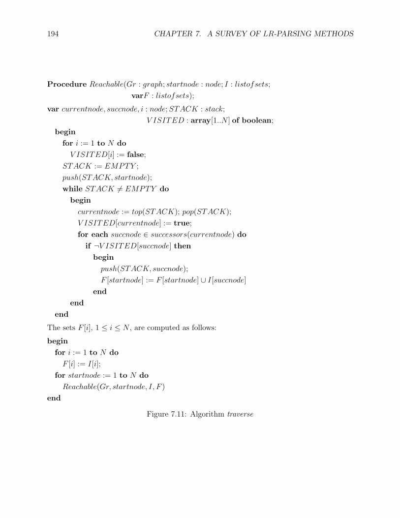
194 CHAPTER 7. A SURVEY OF LR-PARSING METHODS
Procedure Reachable(Gr : graph; startnode : node; I : listofsets;
varF : listofsets);
var currentnode, succnode, i : node;STACK : stack;
V ISITED : array[1..N ] of boolean;
begin
for i := 1 to N do
V ISITED[i] := false;
STACK := EMPTY ;
push(STACK, startnode);
while STACK 6= EMPTY do
begin
currentnode := top(STACK); pop(STACK);
V ISITED[currentnode] := true;
for each succnode ∈ successors(currentnode) doif ¬V ISITED[succnode] then
begin
push(STACK, succnode);
F [startnode] := F [startnode] ∪ I[succnode]end
end
end
The sets F [i], 1 ≤ i ≤ N , are computed as follows:
begin
for i := 1 to N do
F [i] := I[i];
for startnode := 1 to N do
Reachable(Gr, startnode, I, F )
end
Figure 7.11: Algorithm traverse
7.8. MORE ON LR(0)-CHARACTERISTIC AUTOMATA 195
7.8 More on LR(0)-Characteristic Automata
Let G = (V,Σ, P, S ′) be an augmented context-free grammar with augmented start produc-tion S ′ −→ S$ (where S ′ only occurs in the augmented production). The righmost derivationrelation is denoted by =⇒
rm.
Recall that the set CG of characteristic strings for the grammar G is defined by
CG = αβ ∈ V ∗ | S ′ ∗=⇒rm
αAv =⇒rm
αβv, αβ ∈ V ∗, v ∈ Σ∗.
The fundamental property of LR-parsing, due to D. Knuth, is stated in the followingtheorem:
Theorem 7.1. Let G be a context-free grammar and assume that every nonterminal derivessome terminal string. The language CG (over V ∗) is a regular language. Furthermore, adeterministic automaton DCG accepting CG can be constructed from G.
The construction ofDCG can be found in various places, including the book on Compilersby Aho, Sethi and Ullman. We explained this construction in Section 7.1. The proof that theNFA NCG constructed as indicated in Section 7.1 is correct, i.e., that it accepts precisely CG,is nontrivial, but not really hard either. This will be the object of a homework assignment!However, note a subtle point: The construction of NCG is only correct under the assumptionthat every nonterminal derives some terminal string. Otherwise, the construction could yieldan NFA NCG accepting strings not in CG.
Recall that the states of the characteristic automaton CGA are sets of items (or markedproductions), where an item is a production with a dot anywhere in its right-hand side.Note that in constructing CGA, it is not necessary to include the state S ′ −→ S$. (theendmarker $ is only needed to compute the lookahead sets). If a state p contains a markedproduction of the form A −→ β., where the dot is the rightmost symbol, state p is called areduce state and A −→ β is called a reducing production for p. Given any state q, we saythat a string β ∈ V ∗ accesses q if there is a path from some state p to the state q on inputβ in the automaton CGA. Given any two states p, q ∈ CGA, for any β ∈ V ∗, if there is asequence of transitions in CGA from p to q on input β, this is denoted by
pβ−→ q.
The initial state which is the closure of the item S ′ −→ .S$ is denoted by 1. The LALR(1)-lookahead sets are defined in the next section.
7.9 LALR(1)-Lookahead Sets
For any reduce state q and any reducing production A −→ β for q, let
LA(q, A −→ β) = a | a ∈ Σ, S ′ ∗=⇒rm
αAav =⇒rm
αβav, α, β ∈ V ∗, v ∈ Σ∗, αβ accesses q.
196 CHAPTER 7. A SURVEY OF LR-PARSING METHODS
In words, LA(q, A −→ β) consists of the terminal symbols for which the reduction byproduction A −→ β in state q is the correct action (that is, for which the parse will terminatesuccessfully). The LA sets can be computed using the FOLLOW sets defined below.
For any state p and any nonterminal A, let
FOLLOW(p, A) = a | a ∈ Σ, S ′ ∗=⇒rm
αAav, α ∈ V ∗, v ∈ Σ∗ and α accesses p.
Since for any derivation
S ′ ∗=⇒rm
αAav =⇒rm
αβav
where αβ accesses q, there is a state p such that pβ−→ q and α accesses p, it is easy to see
that the following result holds:
Proposition 7.2. For every reduce state q and any reducing production A −→ β for q, wehave
LA(q, A −→ β) =⋃FOLLOW(p, A) | p β−→ q.
Also, we let
LA(S ′ −→ S.$, S ′ −→ S$) = FOLLOW(1, S).
Intuitively, when the parser makes the reduction by production A −→ β in state q, eachstate p as above is a possible top of stack after the states corresponding to β are popped.Then the parser must read A in state p, and the next input symbol will be one of the symbolsin FOLLOW(p, A).
The computation of FOLLOW(p, A) is similar to that of FOLLOW(A). First, we computeINITFOLLOW(p, A), given by
INITFOLLOW(p, A) = a | a ∈ Σ, ∃q, r, p A−→ qa−→ r.
These are the terminals that can be read in CGA after the “goto transition” on nonterminalA has been performed from p. These sets can be easily computed from CGA.
Note that for the state p whose core item is S ′ −→ S.$, we have
INITFOLLOW(p, S) = $.
Next, observe that if B −→ αA is a production and if
S ′ ∗=⇒rm
λBav
where λ accesses p′, then
S ′ ∗=⇒rm
λBav =⇒rm
λαAav
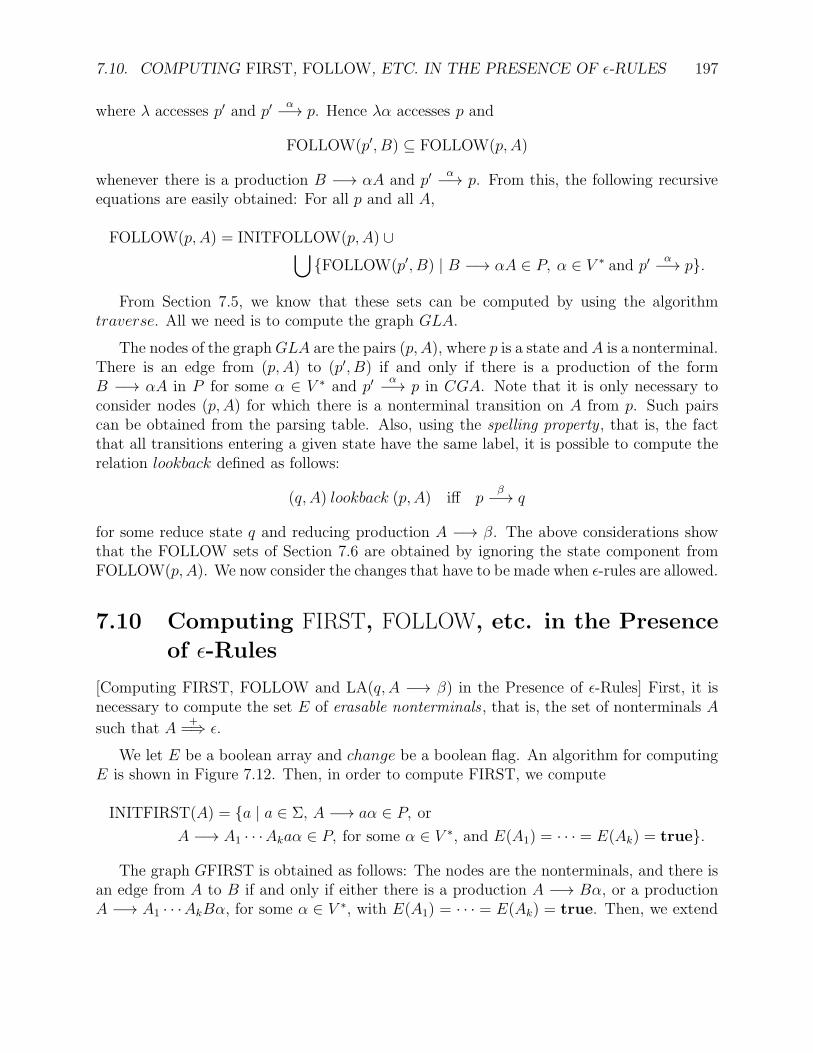
7.10. COMPUTING FIRST, FOLLOW, ETC. IN THE PRESENCE OF ǫ-RULES 197
where λ accesses p′ and p′α−→ p. Hence λα accesses p and
FOLLOW(p′, B) ⊆ FOLLOW(p, A)
whenever there is a production B −→ αA and p′α−→ p. From this, the following recursive
equations are easily obtained: For all p and all A,
FOLLOW(p, A) = INITFOLLOW(p, A) ∪⋃FOLLOW(p′, B) | B −→ αA ∈ P, α ∈ V ∗ and p′
α−→ p.
From Section 7.5, we know that these sets can be computed by using the algorithmtraverse. All we need is to compute the graph GLA.
The nodes of the graphGLA are the pairs (p, A), where p is a state andA is a nonterminal.There is an edge from (p, A) to (p′, B) if and only if there is a production of the formB −→ αA in P for some α ∈ V ∗ and p′
α−→ p in CGA. Note that it is only necessary toconsider nodes (p, A) for which there is a nonterminal transition on A from p. Such pairscan be obtained from the parsing table. Also, using the spelling property , that is, the factthat all transitions entering a given state have the same label, it is possible to compute therelation lookback defined as follows:
(q, A) lookback (p, A) iff pβ−→ q
for some reduce state q and reducing production A −→ β. The above considerations showthat the FOLLOW sets of Section 7.6 are obtained by ignoring the state component fromFOLLOW(p, A). We now consider the changes that have to be made when ǫ-rules are allowed.
7.10 Computing FIRST, FOLLOW, etc. in the Presence
of ǫ-Rules
[Computing FIRST, FOLLOW and LA(q, A −→ β) in the Presence of ǫ-Rules] First, it isnecessary to compute the set E of erasable nonterminals , that is, the set of nonterminals A
such that A+
=⇒ ǫ.
We let E be a boolean array and change be a boolean flag. An algorithm for computingE is shown in Figure 7.12. Then, in order to compute FIRST, we compute
INITFIRST(A) = a | a ∈ Σ, A −→ aα ∈ P, orA −→ A1 · · ·Akaα ∈ P, for some α ∈ V ∗, and E(A1) = · · · = E(Ak) = true.
The graph GFIRST is obtained as follows: The nodes are the nonterminals, and there isan edge from A to B if and only if either there is a production A −→ Bα, or a productionA −→ A1 · · ·AkBα, for some α ∈ V ∗, with E(A1) = · · · = E(Ak) = true. Then, we extend
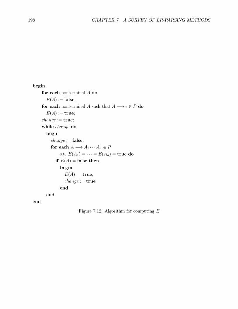
198 CHAPTER 7. A SURVEY OF LR-PARSING METHODS
begin
for each nonterminal A do
E(A) := false;
for each nonterminal A such that A −→ ǫ ∈ P do
E(A) := true;
change := true;
while change do
begin
change := false;
for each A −→ A1 · · ·An ∈ Ps.t. E(A1) = · · · = E(An) = true do
if E(A) = false then
begin
E(A) := true;
change := true
end
end
end
Figure 7.12: Algorithm for computing E

7.10. COMPUTING FIRST, FOLLOW, ETC. IN THE PRESENCE OF ǫ-RULES 199
FIRST to strings in V +, in the obvious way. Given any string α ∈ V +, if |α| = 1, thenβ = X for some X ∈ V , and
FIRST(β) = FIRST(X)
as before, else if β = X1 · · ·Xn with n ≥ 2 and Xi ∈ V , then
FIRST(β) = FIRST(X1) ∪ · · · ∪ FIRST(Xk),
where k, 1 ≤ k ≤ n, is the largest integer so that
E(X1) = · · · = E(Xk) = true.
To compute FOLLOW, we first compute
INITFOLLOW(A) = a | a ∈ Σ, B −→ αAβ ∈ P, α ∈ V ∗, β ∈ V +, and a ∈ FIRST(β).
The graph GFOLLOW is computed as follows: The nodes are the nonterminals. There is anedge from A to B if either there is a production of the form B −→ αA, or B −→ αAA1 · · ·Ak,for some α ∈ V ∗, and with E(A1) = · · · = E(Ak) = true.
The computation of the LALR(1) lookahead sets is also more complicated because an-other graph is needed in order to compute INITFOLLOW(p, A). First, the graph GLA isdefined in the following way: The nodes are still the pairs (p, A), as before, but there is anedge from (p, A) to (p′, B) if and only if either there is some production B −→ αA, for some
α ∈ V ∗ and p′α−→ p, or a production B −→ αAβ, for some α ∈ V ∗, β ∈ V +, β
+=⇒ ǫ, and
p′α−→ p. The sets INITFOLLOW(p, A) are computed in the following way: First, let
DR(p, A) = a | a ∈ Σ, ∃q, r, p A−→ qa−→ r.
The sets DR(p, A) are the direct read sets. Note that for the state p whose core item isS ′ −→ S.$, we have
DR(p, S) = $.Then,
INITFOLLOW(p, A) = DR(p,A) ∪⋃a | a ∈ Σ, S ′ ∗
=⇒rm
αAβav =⇒rm
αAav, α ∈ V ∗, β ∈ V +, β+
=⇒ ǫ, α accesses p.
The set INITFOLLOW(p, A) is the set of terminals that can be read before any handlecontaining A is reduced. The graph GREAD is defined as follows: The nodes are the pairs
(p, A), and there is an edge from (p, A) to (r, C) if and only if pA−→ r and r
C−→ s, for somes, with E(C) = true.
Then, it is not difficult to show that the INITFOLLOW sets are the least solution of theset of recursive equations:
INITFOLLOW(p, A) = DR(p, A) ∪⋃INITFOLLOW(r, C) | (p, A)GREAD (r, C).
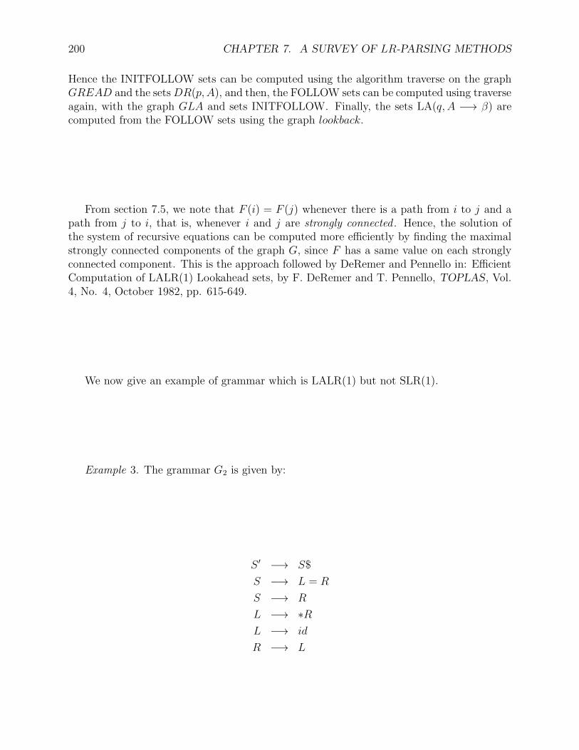
200 CHAPTER 7. A SURVEY OF LR-PARSING METHODS
Hence the INITFOLLOW sets can be computed using the algorithm traverse on the graphGREAD and the setsDR(p, A), and then, the FOLLOW sets can be computed using traverseagain, with the graph GLA and sets INITFOLLOW. Finally, the sets LA(q, A −→ β) arecomputed from the FOLLOW sets using the graph lookback.
From section 7.5, we note that F (i) = F (j) whenever there is a path from i to j and apath from j to i, that is, whenever i and j are strongly connected . Hence, the solution ofthe system of recursive equations can be computed more efficiently by finding the maximalstrongly connected components of the graph G, since F has a same value on each stronglyconnected component. This is the approach followed by DeRemer and Pennello in: EfficientComputation of LALR(1) Lookahead sets, by F. DeRemer and T. Pennello, TOPLAS, Vol.4, No. 4, October 1982, pp. 615-649.
We now give an example of grammar which is LALR(1) but not SLR(1).
Example 3. The grammar G2 is given by:
S ′ −→ S$
S −→ L = R
S −→ R
L −→ ∗RL −→ id
R −→ L
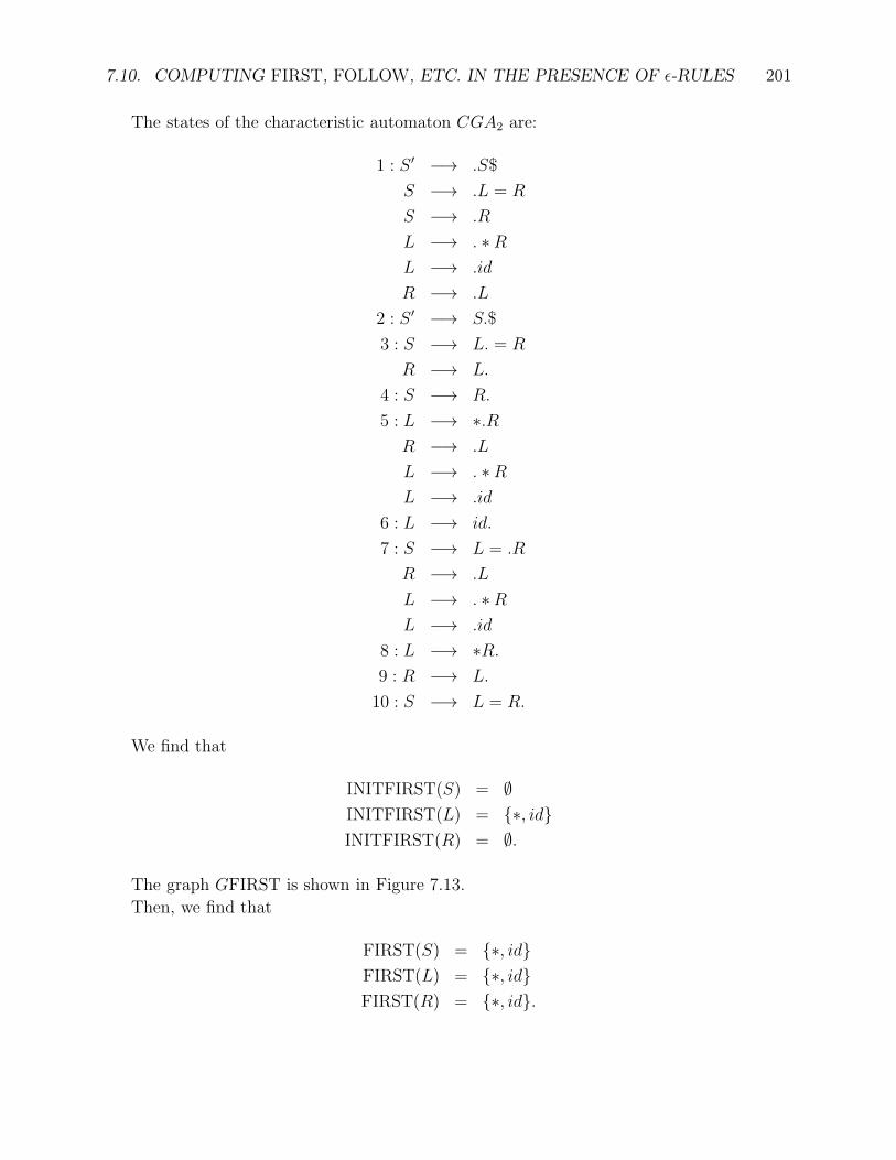
7.10. COMPUTING FIRST, FOLLOW, ETC. IN THE PRESENCE OF ǫ-RULES 201
The states of the characteristic automaton CGA2 are:
1 : S ′ −→ .S$
S −→ .L = R
S −→ .R
L −→ . ∗RL −→ .id
R −→ .L
2 : S ′ −→ S.$
3 : S −→ L. = R
R −→ L.
4 : S −→ R.
5 : L −→ ∗.RR −→ .L
L −→ . ∗RL −→ .id
6 : L −→ id.
7 : S −→ L = .R
R −→ .L
L −→ . ∗RL −→ .id
8 : L −→ ∗R.9 : R −→ L.
10 : S −→ L = R.
We find that
INITFIRST(S) = ∅INITFIRST(L) = ∗, idINITFIRST(R) = ∅.
The graph GFIRST is shown in Figure 7.13.
Then, we find that
FIRST(S) = ∗, idFIRST(L) = ∗, idFIRST(R) = ∗, id.
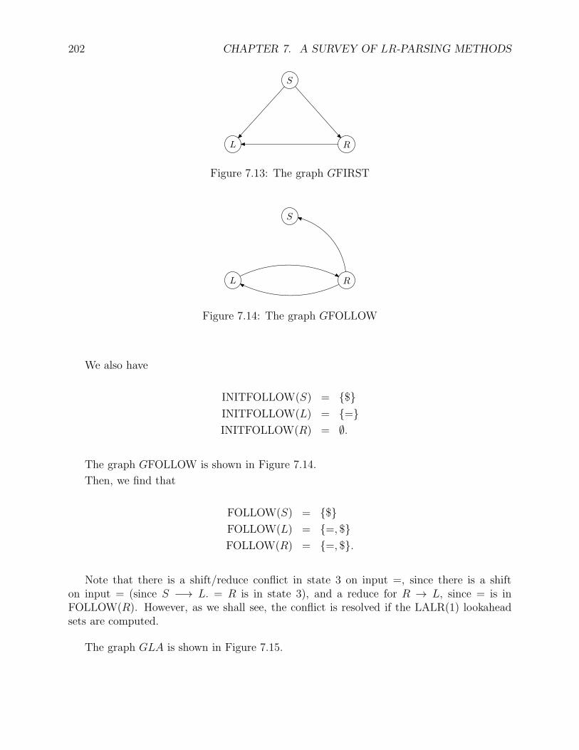
202 CHAPTER 7. A SURVEY OF LR-PARSING METHODS
S
RL
Figure 7.13: The graph GFIRST
S
RL
Figure 7.14: The graph GFOLLOW
We also have
INITFOLLOW(S) = $INITFOLLOW(L) = =INITFOLLOW(R) = ∅.
The graph GFOLLOW is shown in Figure 7.14.
Then, we find that
FOLLOW(S) = $FOLLOW(L) = =, $FOLLOW(R) = =, $.
Note that there is a shift/reduce conflict in state 3 on input =, since there is a shifton input = (since S −→ L. = R is in state 3), and a reduce for R → L, since = is inFOLLOW(R). However, as we shall see, the conflict is resolved if the LALR(1) lookaheadsets are computed.
The graph GLA is shown in Figure 7.15.
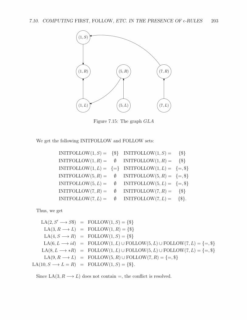
7.10. COMPUTING FIRST, FOLLOW, ETC. IN THE PRESENCE OF ǫ-RULES 203
(1, S)
(1, R)
(1, L)
(5, R)
(5, L)
(7, R)
(7, L)
Figure 7.15: The graph GLA
We get the following INITFOLLOW and FOLLOW sets:
INITFOLLOW(1, S) = $ INITFOLLOW(1, S) = $INITFOLLOW(1, R) = ∅ INITFOLLOW(1, R) = $INITFOLLOW(1, L) = = INITFOLLOW(1, L) = =, $INITFOLLOW(5, R) = ∅ INITFOLLOW(5, R) = =, $INITFOLLOW(5, L) = ∅ INITFOLLOW(5, L) = =, $INITFOLLOW(7, R) = ∅ INITFOLLOW(7, R) = $INITFOLLOW(7, L) = ∅ INITFOLLOW(7, L) = $.
Thus, we get
LA(2, S ′ −→ S$) = FOLLOW(1, S) = $LA(3, R −→ L) = FOLLOW(1, R) = $LA(4, S −→ R) = FOLLOW(1, S) = $LA(6, L −→ id) = FOLLOW(1, L) ∪ FOLLOW(5, L) ∪ FOLLOW(7, L) = =, $LA(8, L −→ ∗R) = FOLLOW(1, L) ∪ FOLLOW(5, L) ∪ FOLLOW(7, L) = =, $LA(9, R −→ L) = FOLLOW(5, R) ∪ FOLLOW(7, R) = =, $
LA(10, S −→ L = R) = FOLLOW(1, S) = $.
Since LA(3, R −→ L) does not contain =, the conflict is resolved.
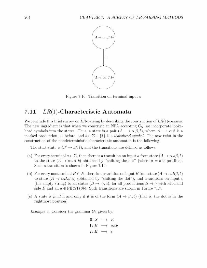
204 CHAPTER 7. A SURVEY OF LR-PARSING METHODS
(A→ α.aβ, b)
(A→ αa.β, b)
a
Figure 7.16: Transition on terminal input a
7.11 LR(1)-Characteristic Automata
We conclude this brief survey on LR-parsing by describing the construction of LR(1)-parsers.The new ingredient is that when we construct an NFA accepting CG, we incorporate looka-head symbols into the states. Thus, a state is a pair (A −→ α.β, b), where A −→ α.β is amarked production, as before, and b ∈ Σ ∪ $ is a lookahead symbol . The new twist in theconstruction of the nondeterministic characteristic automaton is the following:
The start state is (S ′ → .S, $), and the transitions are defined as follows:
(a) For every terminal a ∈ Σ, then there is a transition on input a from state (A→ α.aβ, b)to the state (A → αa.β, b) obtained by “shifting the dot” (where a = b is possible).Such a transition is shown in Figure 7.16.
(b) For every nonterminal B ∈ N , there is a transition on inputB from state (A→ α.Bβ, b)to state (A → αB.β, b) (obtained by “shifting the dot”), and transitions on input ǫ(the empty string) to all states (B → .γ, a), for all productions B → γ with left-handside B and all a ∈ FIRST(βb). Such transitions are shown in Figure 7.17.
(c) A state is final if and only if it is of the form (A → β., b) (that is, the dot is in therightmost position).
Example 3. Consider the grammar G3 given by:
0 : S −→ E
1: E −→ aEb
2: E −→ ǫ
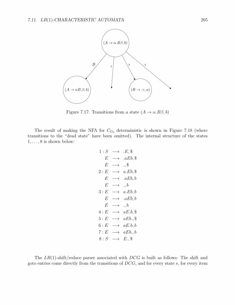
7.11. LR(1)-CHARACTERISTIC AUTOMATA 205
(A→ α.Bβ, b)
(A→ αB.β, b) (B → .γ, a)
B ǫ ǫ ǫ
Figure 7.17: Transitions from a state (A→ α.Bβ, b)
The result of making the NFA for CG3 deterministic is shown in Figure 7.18 (wheretransitions to the “dead state” have been omitted). The internal structure of the states1, . . . , 8 is shown below:
1 : S −→ .E, $
E −→ .aEb, $
E −→ ., $
2 : E −→ a.Eb, $
E −→ .aEb, b
E −→ ., b
3 : E −→ a.Eb, b
E −→ .aEb, b
E −→ ., b
4 : E −→ aE.b, $
5 : E −→ aEb., $
6 : E −→ aE.b, b
7 : E −→ aEb., b
8 : S −→ E., $
The LR(1)-shift/reduce parser associated with DCG is built as follows: The shift andgoto entries come directly from the transitions of DCG, and for every state s, for every item
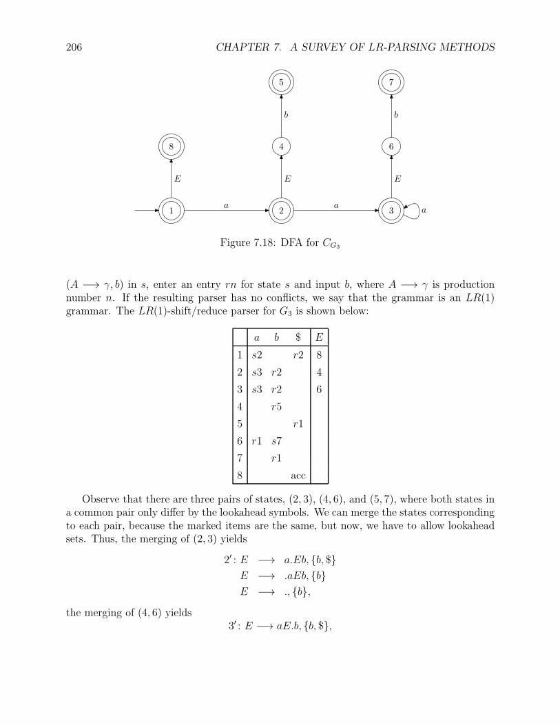
206 CHAPTER 7. A SURVEY OF LR-PARSING METHODS
1 2 3
4
5
6
7
8
a a
E E E
b b
a
Figure 7.18: DFA for CG3
(A −→ γ, b) in s, enter an entry rn for state s and input b, where A −→ γ is productionnumber n. If the resulting parser has no conflicts, we say that the grammar is an LR(1)grammar. The LR(1)-shift/reduce parser for G3 is shown below:
a b $ E
1 s2 r2 8
2 s3 r2 4
3 s3 r2 6
4 r5
5 r1
6 r1 s7
7 r1
8 acc
Observe that there are three pairs of states, (2, 3), (4, 6), and (5, 7), where both states ina common pair only differ by the lookahead symbols. We can merge the states correspondingto each pair, because the marked items are the same, but now, we have to allow lookaheadsets. Thus, the merging of (2, 3) yields
2′ : E −→ a.Eb, b, $E −→ .aEb, bE −→ ., b,
the merging of (4, 6) yields3′ : E −→ aE.b, b, $,
7.11. LR(1)-CHARACTERISTIC AUTOMATA 207
the merging of (5, 7) yields4′ : E −→ aEb., b, $.
We obtain a merged DFA with only five states, and the corresponding shift/reduce parser isgiven below:
a b $ E
1 s2′ r2 8
2′ s2′ r2 3′
3′ s4′
4′ r1 r1
8 acc
The reader should verify that this is the LALR(1)-parser. The reader should also checkthat that the SLR(1)-parser is given below:
a b $ E
1 s2 r2 r2 5
2 s2 r2 r2 3
3 s4
4 r1 r1
5 acc
The difference between the two parsing tables is that the LALR(1)-lookahead sets aresharper than the SLR(1)-lookahead sets. This is because the computation of the LALR(1)-lookahead sets uses a sharper version of FOLLOW sets. It can also be shown that if agrammar is LALR(1), then the merging of states of an LR(1)-parser always succeeds andyields the LALR(1) parser. Of course, this is a very inefficient way of producing LALR(1)parsers, and much better methods exist, such as the graph method described in these notes.However, there are cases where the merging fails. Sufficient conditions for successful merginghave been investigated, but there is still room for research in this area.
208 CHAPTER 7. A SURVEY OF LR-PARSING METHODS
Chapter 8
RAM Programs, Turing Machines,and the Partial Recursive Functions
See the scanned version of this chapter found in the web page for CIS511:
http://www.cis.upenn.edu/~jean/old511/html/tcbookpdf3a.pdf
8.1 Partial Functions and RAM Programs
We define an abstract machine model for computing functions
f : Σ∗ × · · · × Σ∗
︸ ︷︷ ︸n
→ Σ∗,
where Σ = a1, . . . , ak s some input alphabet.
Numerical functions f : Nn → N can be viewed as functions defined over the one-letteralphabet a1, using the bijection m 7→ am1 .
Let us recall the definition of a partial function.
Definition 8.1. A binary relation R ⊆ A × B between two sets A and B is functional iff,for all x ∈ A and y, z ∈ B,
(x, y) ∈ R and (x, z) ∈ R implies that y = z.
A partial function is a triple f = 〈A,G,B〉, where A and B are arbitrary sets (possiblyempty) and G is a functional relation (possibly empty) between A and B, called the graphof f .
209
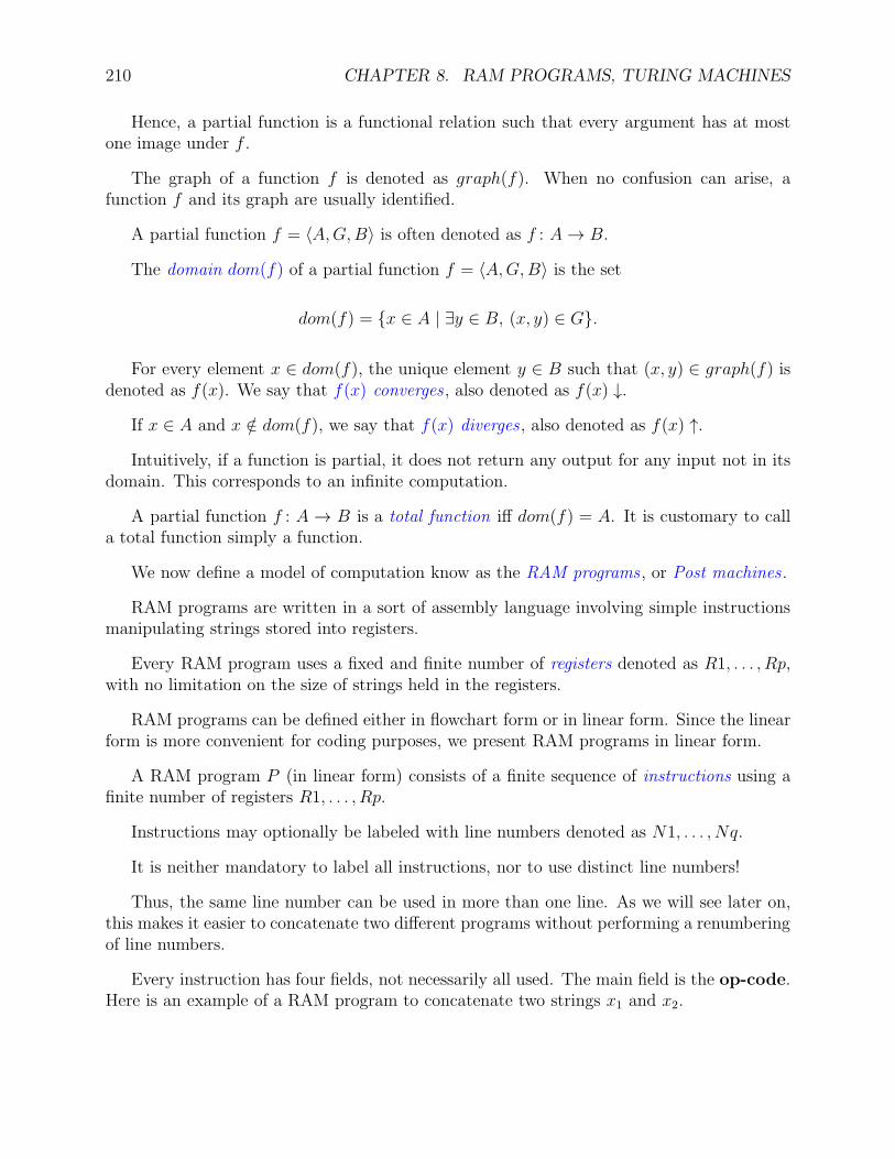
210 CHAPTER 8. RAM PROGRAMS, TURING MACHINES
Hence, a partial function is a functional relation such that every argument has at mostone image under f .
The graph of a function f is denoted as graph(f). When no confusion can arise, afunction f and its graph are usually identified.
A partial function f = 〈A,G,B〉 is often denoted as f : A→ B.
The domain dom(f) of a partial function f = 〈A,G,B〉 is the set
dom(f) = x ∈ A | ∃y ∈ B, (x, y) ∈ G.
For every element x ∈ dom(f), the unique element y ∈ B such that (x, y) ∈ graph(f) isdenoted as f(x). We say that f(x) converges , also denoted as f(x) ↓.
If x ∈ A and x /∈ dom(f), we say that f(x) diverges , also denoted as f(x) ↑.
Intuitively, if a function is partial, it does not return any output for any input not in itsdomain. This corresponds to an infinite computation.
A partial function f : A→ B is a total function iff dom(f) = A. It is customary to calla total function simply a function.
We now define a model of computation know as the RAM programs , or Post machines .
RAM programs are written in a sort of assembly language involving simple instructionsmanipulating strings stored into registers.
Every RAM program uses a fixed and finite number of registers denoted as R1, . . . , Rp,with no limitation on the size of strings held in the registers.
RAM programs can be defined either in flowchart form or in linear form. Since the linearform is more convenient for coding purposes, we present RAM programs in linear form.
A RAM program P (in linear form) consists of a finite sequence of instructions using afinite number of registers R1, . . . , Rp.
Instructions may optionally be labeled with line numbers denoted as N1, . . . , Nq.
It is neither mandatory to label all instructions, nor to use distinct line numbers!
Thus, the same line number can be used in more than one line. As we will see later on,this makes it easier to concatenate two different programs without performing a renumberingof line numbers.
Every instruction has four fields, not necessarily all used. The main field is the op-code.Here is an example of a RAM program to concatenate two strings x1 and x2.
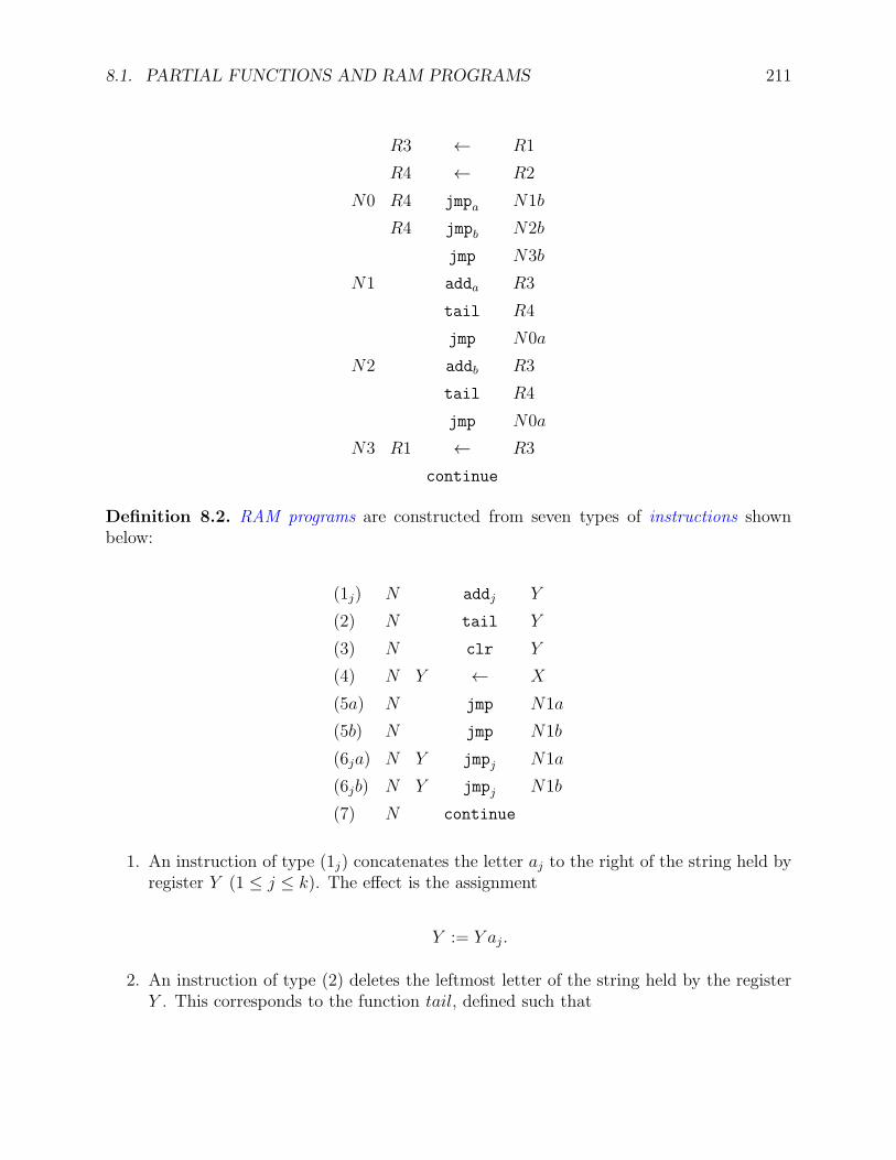
8.1. PARTIAL FUNCTIONS AND RAM PROGRAMS 211
R3 ← R1
R4 ← R2
N0 R4 jmpa N1b
R4 jmpb N2b
jmp N3b
N1 adda R3
tail R4
jmp N0a
N2 addb R3
tail R4
jmp N0a
N3 R1 ← R3
continue
Definition 8.2. RAM programs are constructed from seven types of instructions shownbelow:
(1j) N addj Y
(2) N tail Y
(3) N clr Y
(4) N Y ← X
(5a) N jmp N1a
(5b) N jmp N1b
(6ja) N Y jmpj N1a
(6jb) N Y jmpj N1b
(7) N continue
1. An instruction of type (1j) concatenates the letter aj to the right of the string held byregister Y (1 ≤ j ≤ k). The effect is the assignment
Y := Y aj .
2. An instruction of type (2) deletes the leftmost letter of the string held by the registerY . This corresponds to the function tail, defined such that
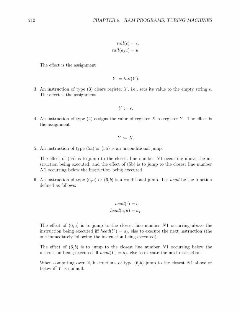
212 CHAPTER 8. RAM PROGRAMS, TURING MACHINES
tail(ǫ) = ǫ,
tail(aju) = u.
The effect is the assignment
Y := tail(Y ).
3. An instruction of type (3) clears register Y , i.e., sets its value to the empty string ǫ.The effect is the assignment
Y := ǫ.
4. An instruction of type (4) assigns the value of register X to register Y . The effect isthe assignment
Y := X.
5. An instruction of type (5a) or (5b) is an unconditional jump.
The effect of (5a) is to jump to the closest line number N1 occurring above the in-struction being executed, and the effect of (5b) is to jump to the closest line numberN1 occurring below the instruction being executed.
6. An instruction of type (6ja) or (6jb) is a conditional jump. Let head be the functiondefined as follows:
head(ǫ) = ǫ,
head(aju) = aj .
The effect of (6ja) is to jump to the closest line number N1 occurring above theinstruction being executed iff head(Y ) = aj , else to execute the next instruction (theone immediately following the instruction being executed).
The effect of (6jb) is to jump to the closest line number N1 occurring below theinstruction being executed iff head(Y ) = aj , else to execute the next instruction.
When computing over N, instructions of type (6jb) jump to the closest N1 above orbelow iff Y is nonnull.
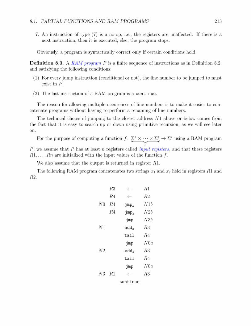
8.1. PARTIAL FUNCTIONS AND RAM PROGRAMS 213
7. An instruction of type (7) is a no-op, i.e., the registers are unaffected. If there is anext instruction, then it is executed, else, the program stops.
Obviously, a program is syntactically correct only if certain conditions hold.
Definition 8.3. A RAM program P is a finite sequence of instructions as in Definition 8.2,and satisfying the following conditions:
(1) For every jump instruction (conditional or not), the line number to be jumped to mustexist in P .
(2) The last instruction of a RAM program is a continue.
The reason for allowing multiple occurences of line numbers is to make it easier to con-catenate programs without having to perform a renaming of line numbers.
The technical choice of jumping to the closest address N1 above or below comes fromthe fact that it is easy to search up or down using primitive recursion, as we will see lateron.
For the purpose of computing a function f : Σ∗ × · · · × Σ∗
︸ ︷︷ ︸n
→ Σ∗ using a RAM program
P , we assume that P has at least n registers called input registers , and that these registersR1, . . . , Rn are initialized with the input values of the function f .
We also assume that the output is returned in register R1.
The following RAM program concatenates two strings x1 and x2 held in registers R1 andR2.
R3 ← R1
R4 ← R2
N0 R4 jmpa N1b
R4 jmpb N2b
jmp N3b
N1 adda R3
tail R4
jmp N0a
N2 addb R3
tail R4
jmp N0a
N3 R1 ← R3
continue
214 CHAPTER 8. RAM PROGRAMS, TURING MACHINES
Since Σ = a, b, for more clarity, we wrote jmpa instead of jmp1, jmpb instead of jmp2,adda instead of add1, and addb instead of add2.
Definition 8.4. A RAM program P computes the partial function ϕ : (Σ∗)n → Σ∗ if thefollowing conditions hold: For every input (x1, . . . , xn) ∈ (Σ∗)n, having initialized the inputregisters R1, . . . , Rn with x1, . . . , xn, the program eventually halts iff ϕ(x1, . . . , xn) converges,and if and when P halts, the value of R1 is equal to ϕ(x1, . . . , xn). A partial function ϕ isRAM-computable iff it is computed by some RAM program.
For example, the following program computes the erase function E defined such that
E(u) = ǫ
for all u ∈ Σ∗:
clr R1
continue
The following program computes the jth successor function Sj defined such that
Sj(u) = uaj
for all u ∈ Σ∗:
addj R1
continue
The following program (with n input variables) computes the projection function P ni
defined such that
P ni (u1, . . . , un) = ui,
where n ≥ 1, and 1 ≤ i ≤ n:
R1 ← Ri
continue
Note that P 11 is the identity function.
Having a programming language, we would like to know how powerful it is, that is, wewould like to know what kind of functions are RAM-computable.
At first glance, RAM programs don’t do much, but this is not so. Indeed, we will seeshortly that the class of RAM-computable functions is quite extensive.
8.2. DEFINITION OF A TURING MACHINE 215
One way of getting new programs from previous ones is via composition. Another one isby primitive recursion.
We will investigate these constructions after introducing another model of computation,Turing machines .
Remarkably, the classes of (partial) functions computed by RAM programs and by Turingmachines are identical.
This is the class of partial computable functions , also called partial recursive functions ,a term which is now considered old-fashion.
This class can be given several other definitions. We will present the definition of theso-called µ-recursive functions (due to Kleene).
The following proposition will be needed to simplify the encoding of RAM programs asnumbers.
Proposition 8.1. Every RAM program can be converted to an equivalent program only usingthe following type of instructions:
(1j) N addj Y
(2) N tail Y
(6ja) N Y jmpj N1a
(6jb) N Y jmpj N1b
(7) N continue
The proof is fairly simple. For example, instructions of the form
Ri← Rj
can be eliminated by transferring the contents of Rj into an auxiliary register Rk, and thenby transferring the contents of Rk into Ri and Rj.
8.2 Definition of a Turing Machine
We define a Turing machine model for computing functions
f : Σ∗ × · · · × Σ∗
︸ ︷︷ ︸n
→ Σ∗,
where Σ = a1, . . . , aN is some input alphabet. We only consider deterministic Turingmachines.
A Turing machine also uses a tape alphabet Γ such that Σ ⊆ Γ. The tape alphabetcontains some special symbol B /∈ Σ, the blank .
216 CHAPTER 8. RAM PROGRAMS, TURING MACHINES
In this model, a Turing machine uses a single tape. This tape can be viewed as a stringover Γ. The tape is both an input tape and a storage mechanism.
Symbols on the tape can be overwritten, and the tape can grow either on the left or onthe right. There is a read/write head pointing to some symbol on the tape.
Definition 8.5. A (deterministic) Turing machine (or TM ) M is a sextuple M = (K,Σ,Γ,L,R, δ, q0), where
• K is a finite set of states ;
• Σ is a finite input alphabet ;
• Γ is a finite tape alphabet , s.t. Σ ⊆ Γ, K ∩ Γ = ∅, and with blank B /∈ Σ;
• q0 ∈ K is the start state (or initial state);
• δ is the transition function, a (finite) set of quintuples
δ ⊆ K × Γ× Γ× L,R ×K,
such that for all (p, a) ∈ K × Γ, there is at most one triple (b,m, q) ∈ Γ× L,R ×Ksuch that (p, a, b,m, q) ∈ δ.
A quintuple (p, a, b,m, q) ∈ δ is called an instruction. It is also denoted as
p, a→ b,m, q.
The effect of an instruction is to switch from state p to state q, overwrite the symbolcurrently scanned a with b, and move the read/write head either left or right, according tom.
Here is an example of a Turing machine.
K = q0, q1, q2, q3;
Σ = a, b;
Γ = a, b, B;
The instructions in δ are:
8.3. COMPUTATIONS OF TURING MACHINES 217
q0, B → B,R, q3,
q0, a→ b, R, q1,
q0, b→ a, R, q1,
q1, a→ b, R, q1,
q1, b→ a, R, q1,
q1, B → B,L, q2,
q2, a→ a, L, q2,
q2, b→ b, L, q2,
q2, B → B,R, q3.
8.3 Computations of Turing Machines
To explain how a Turing machine works, we describe its action on Instantaneous descriptions .We take advantage of the fact that K ∩ Γ = ∅ to define instantaneous descriptions.
Definition 8.6. Given a Turing machine
M = (K,Σ,Γ, L,R, δ, q0),
an instantaneous description (for short an ID) is a (nonempty) string in Γ∗KΓ+, that is, astring of the form
upav,
where u, v ∈ Γ∗, p ∈ K, and a ∈ Γ.
The intuition is that an ID upav describes a snapshot of a TM in the current state p,whose tape contains the string uav, and with the read/write head pointing to the symbol a.
Thus, in upav, the state p is just to the left of the symbol presently scanned by theread/write head.
We explain how a TM works by showing how it acts on ID’s.
Definition 8.7. Given a Turing machine
M = (K,Σ,Γ, L,R, δ, q0),
the yield relation (or compute relation) ⊢ is a binary relation defined on the set of ID’s asfollows. For any two ID’s ID1 and ID2, we have ID1 ⊢ ID2 iff either
(1) (p, a, b, R, q) ∈ δ, and either
218 CHAPTER 8. RAM PROGRAMS, TURING MACHINES
(a) ID1 = upacv, c ∈ Γ, and ID2 = ubqcv, or
(b) ID1 = upa and ID2 = ubqB;
or
(2) (p, a, b, L, q) ∈ δ, and either
(a) ID1 = ucpav, c ∈ Γ, and ID2 = uqcbv, or
(b) ID1 = pav and ID2 = qBbv.
Note how the tape is extended by one blank after the rightmost symbol in case (1)(b),and by one blank before the leftmost symbol in case (2)(b).
As usual, we let ⊢+ denote the transitive closure of ⊢, and we let ⊢∗ denote the reflexiveand transitive closure of ⊢.
We can now explain how a Turing machine computes a partial function
f : Σ∗ × · · · × Σ∗
︸ ︷︷ ︸n
→ Σ∗.
Since we allow functions taking n ≥ 1 input strings, we assume that Γ contains thespecial delimiter , not in Σ, used to separate the various input strings.
It is convenient to assume that a Turing machine “cleans up” its tape when it halts,before returning its output. For this, we will define proper ID’s.
Definition 8.8. Given a Turing machine
M = (K,Σ,Γ, L,R, δ, q0),
where Γ contains some delimiter , not in Σ in addition to the blank B, a starting ID is ofthe form
q0w1,w2, . . . ,wn
where w1, . . . , wn ∈ Σ∗ and n ≥ 2, or q0w with w ∈ Σ+, or q0B.
A blocking (or halting) ID is an ID upav such that there are no instructions (p, a, b,m, q) ∈δ for any (b,m, q) ∈ Γ× L,R ×K.
A proper ID is a halting ID of the form
BkpwBl,
where w ∈ Σ∗, and k, l ≥ 0 (with l ≥ 1 when w = ǫ).
Computation sequences are defined as follows.
8.3. COMPUTATIONS OF TURING MACHINES 219
Definition 8.9. Given a Turing machine
M = (K,Σ,Γ, L,R, δ, q0),
a computation sequence (or computation) is a finite or infinite sequence of ID’s
ID0, ID1, . . . , IDi, IDi+1, . . . ,
such that IDi ⊢ IDi+1 for all i ≥ 0.
A computation sequence halts iff it is a finite sequence of ID’s, so that
ID0 ⊢∗ IDn,
and IDn is a halting ID.
A computation sequence diverges if it is an infinite sequence of ID’s.
We now explain how a Turing machine computes a partial function.
Definition 8.10. A Turing machine
M = (K,Σ,Γ, L,R, δ, q0)
computes the partial function
f : Σ∗ × · · · × Σ∗
︸ ︷︷ ︸n
→ Σ∗
iff the following conditions hold:
(1) For every w1, . . . , wn ∈ Σ∗, given the starting ID
ID0 = q0w1,w2, . . . ,wn
or q0w with w ∈ Σ+, or q0B, the computation sequence of M from ID0 halts in aproper IDiff f(w1, . . . , wn) is defined.
(2) If f(w1, . . . , wn) is defined, then M halts in a proper ID of the form
IDn = Bkpf(w1, . . . , wn)Bh,
which means that it computes the right value.
A function f (over Σ∗) is Turing computable iff it is computed by some Turing machineM .
220 CHAPTER 8. RAM PROGRAMS, TURING MACHINES
Note that by (1), the TM M may halt in an improper ID, in which case f(w1, . . . , wn)must be undefined. This corresponds to the fact that we only accept to retrieve the outputof a computation if the TM has cleaned up its tape, i.e., produced a proper ID. In particular,intermediate calculations have to be erased before halting.
Example.
K = q0, q1, q2, q3;Σ = a, b;Γ = a, b, B;The instructions in δ are:
q0, B → B,R, q3,
q0, a→ b, R, q1,
q0, b→ a, R, q1,
q1, a→ b, R, q1,
q1, b→ a, R, q1,
q1, B → B,L, q2,
q2, a→ a, L, q2,
q2, b→ b, L, q2,
q2, B → B,R, q3.
The reader can easily verify that this machine exchanges the a’s and b’s in a string. Forexample, on input w = aaababb, the output is bbbabaa.
8.4 RAM-computable functions are
Turing-computable
Turing machines can simulate RAM programs, and as a result, we have the following Theo-rem.
Theorem 8.2. Every RAM-computable function is Turing-computable. Furthermore, givena RAM program P , we can effectively construct a Turing machine M computing the samefunction.
The idea of the proof is to represent the contents of the registers R1, . . . Rp on the Turingmachine tape by the string
#r1#r2# · · ·#rp#,
8.5. TURING-COMPUTABLE FUNCTIONS ARE RAM-COMPUTABLE 221
Where # is a special marker and ri represents the string held by Ri, We also use Propo-sition 8.1 to reduce the number of instructions to be dealt with.
The Turing machine M is built of blocks, each block simulating the effect of some in-struction of the program P . The details are a bit tedious, and can be found in the notes orin Machtey and Young.
8.5 Turing-computable functions are
RAM-computable
RAM programs can also simulate Turing machines.
Theorem 8.3. Every Turing-computable function is RAM-computable. Furthermore, givena Turing machine M , one can effectively construct a RAM program P computing the samefunction.
The idea of the proof is to design a RAM program containing an encoding of the currentID of the Turing machine M in register R1, and to use other registers R2, R3 to simulatethe effect of executing an instruction of M by updating the ID of M in R1.
The details are tedious and can be found in the notes.
Another proof can be obtained by proving that the class of Turing computable functionscoincides with the class of partial computable functions (formerly called partial recursivefunctions).
Indeed, it turns out that both RAM programs and Turing machines compute preciselythe class of partial recursive functions. For this, we need to define the primitive recursivefunctions .
Informally, a primitive recursive function is a total recursive function that can be com-puted using only for loops, that is, loops in which the number of iterations is fixed (unlikea while loop).
A formal definition of the primitive functions is given in Section 8.7.
Definition 8.11. Let Σ = a1, . . . , aN. The class of partial computable functions also calledpartial recursive functions is the class of partial functions (over Σ∗) that can be computedby RAM programs (or equivalently by Turing machines).
The class of computable functions also called recursive functions is the subset of the classof partial computable functions consisting of functions defined for every input (i.e., totalfunctions).
We can also deal with languages.
222 CHAPTER 8. RAM PROGRAMS, TURING MACHINES
8.6 Computably Enumerable Languages and
Computable Languages
We define the computably enumerable languages, also called listable languages, and thecomputable languages.
The old-fashion terminology for computably enumerable languages is recursively enumer-able languages, and for computable languages is recursive languages.
We assume that the TM’s under consideration have a tape alphabet containing the specialsymbols 0 and 1.
Definition 8.12. Let Σ = a1, . . . , aN. A language L ⊆ Σ∗ is (Turing) computably enu-merable (for short, a c.e. set), or (Turing) listable (or recursively enumerable (for short, ar.e. set)) iff there is some TM M such that for every w ∈ L, M halts in a proper ID withthe output 1, and for every w /∈ L, either M halts in a proper ID with the output 0, or itruns forever.
A language L ⊆ Σ∗ is (Turing) computable (or recursive) iff there is some TM M suchthat for every w ∈ L, M halts in a proper ID with the output 1, and for every w /∈ L, Mhalts in a proper ID with the output 0.
Thus, given a computably enumerable language L, for some w /∈ L, it is possible that aTM accepting L runs forever on input w. On the other hand, for a computable (recursive)language L, a TM accepting L always halts in a proper ID.
When dealing with languages, it is often useful to consider nondeterministic Turing ma-chines . Such machines are defined just like deterministic Turing machines, except that theirtransition function δ is just a (finite) set of quintuples
δ ⊆ K × Γ× Γ× L,R ×K,
with no particular extra condition.
It can be shown that every nondeterministic Turing machine can be simulated by adeterministic Turing machine, and thus, nondeterministic Turing machines also accept theclass of c.e. sets.
It can be shown that a computably enumerable language is the range of some computable(recursive) function. It can also be shown that a language L is computable (recursive) iffboth L and its complement are computably enumerable. There are computably enumerablelanguages that are not computable (recursive).
Turing machines were invented by Turing around 1935. The primitive recursive functionswere known to Hilbert circa 1890. Godel formalized their definition in 1929. The partialrecursive functions were defined by Kleene around 1934.
8.7. THE PRIMITIVE RECURSIVE FUNCTIONS 223
Church also introduced the λ-calculus as a model of computation around 1934. Othermodels: Post systems, Markov systems. The equivalence of the various models of computa-tion was shown around 1935/36. RAM programs were only defined around 1963 (they are aslight generalization of Post system).
A further study of the partial recursive functions requires the notions of pairing functionsand of universal functions (or universal Turing machines).
8.7 The Primitive Recursive Functions
The class of primitive recursive functions is defined in terms of base functions and closureoperations.
Definition 8.13. Let Σ = a1, . . . , aN. The base functions over Σ are the following func-tions:
(1) The erase function E, defined such that E(w) = ǫ, for all w ∈ Σ∗;
(2) For every j, 1 ≤ j ≤ N , the j-successor function Sj , defined such that Sj(w) = waj,for all w ∈ Σ∗;
(3) The projection functions P ni , defined such that
P ni (w1, . . . , wn) = wi,
for every n ≥ 1, every i, 1 ≤ i ≤ n, and for all w1, . . . , wn ∈ Σ∗.
Note that P 11 is the identity function on Σ∗. Projection functions can be used to permute
the arguments of another function.
A crucial closure operation is (extended) composition.
Definition 8.14. Let Σ = a1, . . . , aN. For any function
g : Σ∗ × · · · × Σ∗
︸ ︷︷ ︸m
→ Σ∗,
and any m functionshi : Σ∗ × · · · × Σ∗
︸ ︷︷ ︸n
→ Σ∗,
the composition of g and the hi is the function
f : Σ∗ × · · · × Σ∗
︸ ︷︷ ︸n
→ Σ∗,
denoted as g (h1, . . . , hm), such that
f(w1, . . . , wn) = g(h1(w1, . . . , wn), . . . , hm(w1, . . . , wn)),
for all w1, . . . , wn ∈ Σ∗.
224 CHAPTER 8. RAM PROGRAMS, TURING MACHINES
As an example, f = g (P 22 , P
21 ) is such that
f(w1, w2) = g(P 22 (w1, w2), P
21 (w1, w2)) = g(w2, w1).
Another crucial closure operation is primitive recursion.
Definition 8.15. Let Σ = a1, . . . , aN. For any function
g : Σ∗ × · · · × Σ∗
︸ ︷︷ ︸m−1
→ Σ∗,
where m ≥ 2, and any N functions
hi : Σ∗ × · · · × Σ∗
︸ ︷︷ ︸m+1
→ Σ∗,
the functionf : Σ∗ × · · · × Σ∗
︸ ︷︷ ︸m
→ Σ∗,
is defined by primitive recursion from g and h1, . . . , hN , if
f(ǫ, w2, . . . , wm) = g(w2, . . . , wm),
f(ua1, w2, . . . , wm) = h1(u, f(u, w2, . . . , wm), w2, . . . , wm),
· · · = · · ·f(uaN , w2, . . . , wm) = hN (u, f(u, w2, . . . , wm), w2, . . . , wm),
for all u, w2, . . . , wm ∈ Σ∗.
When m = 1, for some fixed w ∈ Σ∗, we have
f(ǫ) = w,
f(ua1) = h1(u, f(u)),
· · · = · · ·f(uaN ) = hN(u, f(u)),
for all u ∈ Σ∗.
For numerical functions (i.e., when Σ = a1), the scheme of primitive recursion issimpler:
f(0, x2, . . . , xm) = g(x2, . . . , xm),
f(x+ 1, x2, . . . , xm) = h1(x, f(x, x2, . . . , xm), x2, . . . , xm),
8.7. THE PRIMITIVE RECURSIVE FUNCTIONS 225
for all x, x2, . . . , xm ∈ N.
The successor function S is the function
S(x) = x+ 1.
Addition, multiplication, exponentiation, and super-exponentiation, can be defined byprimitive recursion as follows (being a bit loose, we should use some projections ...):
add(0, n) = P 11 (n) = n,
add(m+ 1, n) = S P 32 (m, add(m,n), n)
= S(add(m,n))
mult(0, n) = E(n) = 0,
mult(m+ 1, n) = add (P 32 , P
33 )(m,mult(m,n), n)
= add(mult(m,n), n),
rexp(0, n) = S E(n) = 1,
rexp(m+ 1, n) = mult(rexp(m,n), n),
exp(m,n) = rexp (P 22 , P
21 )(m,n),
supexp(0, n) = 1,
supexp(m+ 1, n) = exp(n, supexp(m,n)).
We usually write m + n for add(m,n), m ∗ n or even mn for mult(m,n), and mn forexp(m,n).
There is a minus operation on N named monus. This operation denoted by.− is defined
by
m.− n =
m− n if m ≥ n
0 if m < n.
To show that it is primitive recursive, we define the function pred. Let pred be theprimitive recursive function given by
pred(0) = 0
pred(m+ 1) = P 21 (m, pred(m)) = m.
Then monus is defined by
monus(m, 0) = m
monus(m,n+ 1) = pred(monus(m,n)),
except that the above is not a legal primitive recursion. It is left as an exercise to give aproper primitive recursive definition of monus.
226 CHAPTER 8. RAM PROGRAMS, TURING MACHINES
As an example over a, b∗, the following functiong : Σ∗ × Σ∗ → Σ∗, is defined by primitive recursion:
g(ǫ, v) = P 11 (v),
g(uai, v) = Si P 32 (u, g(u, v), v),
where 1 ≤ i ≤ N . It is easily verified that g(u, v) = vu. Then,
f = g (P 22 , P
21 )
computes the concatenation function, i.e. f(u, v) = uv.
The following functions are also primitive recursive:
sg(n) =
1 if n > 0
0 if n = 0,
sg(n) =
0 if n > 0
1 if n = 0,
as well asabs(m,n) = |m−m| = m
.− n + n
.− m,
and
eq(m,n) =
1 if m = n
0 if m 6= n.
Indeed
sg(0) = 0
sg(n+ 1) = S E P 21 (n, sg(n)),
sg(n) = S(E(n)).− sg(n) = 1
.− sg(n),
andeq(m,n) = sg(|m− n|).
Finally, the function
cond(m,n, p, q) =
p if m = n
q if m 6= n,
is primitive recursive since
cond(m,n, p, q) = eq(m,n) ∗ p+ sg(eq(m,n)) ∗ q.
8.7. THE PRIMITIVE RECURSIVE FUNCTIONS 227
We can also design more general version of cond. For example, define compare≤ as
compare≤(m,n) =
1 if m ≤ n
0 if m > n,
which is given bycompare≤(m,n) = 1
.− sg(m
.− n).
Then we can define
cond≤(m,n, p, q) =
p if m ≤ n
q if m > n,
withcond≤(m,n, n, p) = compare≤(m,n) ∗ p+ sg(compare≤(m,n)) ∗ q.
The above allows to define functions by cases.
Definition 8.16. Let Σ = a1, . . . , aN. The class of primitive recursive functions is thesmallest class of functions (over Σ∗) which contains the base functions and is closed undercomposition and primitive recursion.
We leave as an exercise to show that every primitive recursive function is a total function.The class of primitive recursive functions may not seem very big, but it contains all the totalfunctions that we would ever want to compute.
Although it is rather tedious to prove, the following theorem can be shown.
Theorem 8.4. For an alphabet Σ = a1, . . . , aN, every primitive recursive function isTuring computable.
The best way to prove the above theorem is to use the computation model of RAMprograms. Indeed, it was shown in Theorem 8.2 that every RAM program can be convertedto a Turing machine.
It is also rather easy to show that the primitive recursive functions are RAM-computable.
In order to define new functions it is also useful to use predicates.
Definition 8.17. An n-ary predicate P (over Σ∗) is any subset of (Σ∗)n. We write thata tuple (x1, . . . , xn) satisfies P as (x1, . . . , xn) ∈ P or as P (x1, . . . , xn). The characteristicfunction of a predicate P is the function CP : (Σ
∗)n → a1∗ defined by
Cp(x1, . . . , xn) =
a1 iff P (x1, . . . , xn)ǫ iff not P (x1, . . . , xn).
A predicate P is primitive recursive iff its characteristic function CP is primitive recursive.
228 CHAPTER 8. RAM PROGRAMS, TURING MACHINES
We leave to the reader the obvious adaptation of the the notion of primitive recursivepredicate to functions defined over N. In this case, 0 plays the role of ǫ and 1 plays the roleof a1.
It is easily shown that if P and Q are primitive recursive predicates (over (Σ∗)n), thenP ∨Q, P ∧Q and ¬P are also primitive recursive.
As an exercise, the reader may want to prove that the predicate (defined over N):prime(n) iff n is a prime number, is a primitive recursive predicate.
For any fixed k ≥ 1, the function:ord(k, n) = exponent of the kth prime in the prime factorization of n, is a primitive recursivefunction.
We can also define functions by cases.
Proposition 8.5. If P1, . . . , Pn are pairwise disjoint primitive recursive predicates (whichmeans that Pi ∩ Pj = ∅ for all i 6= j) and f1, . . . , fn+1 are primitive recursive functions, thefunction g defined below is also primitive recursive:
g(x) =
f1(x) iff P1(x)...fn(x) iff Pn(x)fn+1(x) otherwise.
(writing x for (x1, . . . , xn).)
It is also useful to have bounded quantification and bounded minimization.
Definition 8.18. If P is an (n + 1)-ary predicate, then the bounded existential predicate∃y/xP (y, z) holds iff some prefix y of x makes P (y, z) true.
The bounded universal predicate ∀y/xP (y, z) holds iff every prefix y of x makes P (y, z)true.
Proposition 8.6. If P is an (n+1)-ary primitive recursive predicate, then ∃y/xP (y, z) and∀y/xP (y, z) are also primitive recursive predicates.
As an application, we can show that the equality predicate, u = v?, is primitive recursive.
Definition 8.19. If P is an (n + 1)-ary predicate, then the bounded minimization of P ,min y/xP (y, z), is the function defined such that min y/xP (y, z) is the shortest prefix of xsuch that P (y, z) if such a y exists, xa1 otherwise.
The bounded maximization of P , max y/xP (y, z), is the function defined such thatmax y/xP (y, z) is the longest prefix of x such that P (y, z) if such a y exists, xa1 other-wise.
8.8. THE PARTIAL COMPUTABLE FUNCTIONS 229
Proposition 8.7. If P is an (n+ 1)-ary primitive recursive predicate, then min y/xP (y, z)and max y/xP (y, z) are primitive recursive functions.
So far, the primitive recursive functions do not yield all the Turing-computable func-tions. In order to get a larger class of functions, we need the closure operation known asminimization.
8.8 The Partial Computable Functions
Minimization can be viewed as an abstract version of a while loop.
Let Σ = a1, . . . , aN. For any function
g : Σ∗ × · · · × Σ∗
︸ ︷︷ ︸m+1
→ Σ∗,
where m ≥ 0, for every j, 1 ≤ j ≤ N , the function
f : Σ∗ × · · · × Σ∗
︸ ︷︷ ︸m
→ Σ∗
looks for the shortest string u over a∗j (for a given j) such that
g(u, w1, . . . , wm) = ǫ :
u := ǫ;while g(u, w1, . . . , wm) 6= ǫ dou := uaj;endwhilelet f(w1, . . . , wm) = u
The operation of minimization (sometimes called minimalization) is defined as follows.
Definition 8.20. Let Σ = a1, . . . , aN. For any function
g : Σ∗ × · · · × Σ∗
︸ ︷︷ ︸m+1
→ Σ∗,
where m ≥ 0, for every j, 1 ≤ j ≤ N , the function
f : Σ∗ × · · · × Σ∗
︸ ︷︷ ︸m
→ Σ∗,
is defined by minimization over aj∗ from g, if the following conditions hold for all w1, . . .,wm ∈ Σ∗:
230 CHAPTER 8. RAM PROGRAMS, TURING MACHINES
(1) f(w1, . . . , wm) is defined iff there is some n ≥ 0 such that g(apj , w1, . . . , wm) is definedfor all p, 0 ≤ p ≤ n, and
g(anj , w1, . . . , wm) = ǫ.
(2) When f(w1, . . . , wm) is defined,
f(w1, . . . , wm) = anj ,
where n is such thatg(anj , w1, . . . , wm) = ǫ
andg(apj , w1, . . . , wm) 6= ǫ
for every p, 0 ≤ p ≤ n− 1.
We also writef(w1, . . . , wm) = minju[g(u, w1, . . . , wm) = ǫ].
Note: When f(w1, . . . , wm) is defined,
f(w1, . . . , wm) = anj ,
where n is the smallest integer such that condition (1) holds. It is very important to re-quire that all the values g(apj , w1, . . . , wm) be defined for all p, 0 ≤ p ≤ n, when definingf(w1, . . . , wm). Failure to do so allows non-computable functions.
Remark : Kleene used the µ-notation:
f(w1, . . . , wm) = µju[g(u, w1, . . . , wm) = ǫ],
actually, its numerical form:
f(x1, . . . , xm) = µx[g(x, x1, . . . , xm) = 0].
The class of partial computable functions is defined as follows.
Definition 8.21. Let Σ = a1, . . . , aN. The class of partial computable functions also calledpartial recursive functions is the smallest class of partial functions (over Σ∗) which containsthe base functions and is closed under composition, primitive recursion, and minimization.
The class of computable functions also called recursive functions is the subset of the classof partial computable functions consisting of functions defined for every input (i.e., totalfunctions).
One of the major results of computability theory is the following theorem.
8.8. THE PARTIAL COMPUTABLE FUNCTIONS 231
Theorem 8.8. For an alphabet Σ = a1, . . . , aN, every partial computable function (partialrecursive function) is Turing-computable. Conversely, every Turing-computable function isa partial computable function (partial recursive function). Similarly, the class of computablefunctions (recursive functions) is equal to the class of Turing-computable functions that haltin a proper ID for every input.
To prove that every partial computable function is indeed Turing-computable, since byTheorem 8.2, every RAM program can be converted to a Turing machine, the simplest thingto do is to show that every partial computable function is RAM-computable.
For the converse, one can show that given a Turing machine, there is a primitive recursivefunction describing how to go from one ID to the next. Then, minimization is used to guesswhether a computation halts. The proof shows that every partial computable function needsminimization at most once. The characterization of the computable functions in terms ofTM’s follows easily.
There are computable functions (recursive functions) that are not primitive recursive.Such an example is given by Ackermann’s function.
Ackermann’s function.
This is a function A : N× N→ N which is defined by the following recursive clauses:
A(0, y) = y + 1,
A(x+ 1, 0) = A(x, 1),
A(x+ 1, y + 1) = A(x, A(x+ 1, y)).
It turns out that A is a computable function which is not primitive recursive.
It can be shown that:
A(0, x) = x+ 1,
A(1, x) = x+ 2,
A(2, x) = 2x+ 3,
A(3, x) = 2x+3 − 3,
and
A(4, x) = 22···216x − 3,
with A(4, 0) = 16− 3 = 13.
For example
A(4, 1) = 216 − 3, A(4, 2) = 2216 − 3.
232 CHAPTER 8. RAM PROGRAMS, TURING MACHINES
Actually, it is not so obvious that A is a total function. This can be shown by induction,using the lexicographic ordering on N× N, which is defined as follows:
(m,n) (m′, n′) iff either
m = m′ and n = n′, or
m < m′, or
m = m′ and n < n′.
We write (m,n) ≺ (m′, n′) when (m,n) (m′, n′) and (m,n) 6= (m′, n′).
We prove that A(m,n) is defined for all (m,n) ∈ N× N by complete induction over thelexicographic ordering on N× N.
In the base case, (m,n) = (0, 0), and since A(0, n) = n + 1, we have A(0, 0) = 1, andA(0, 0) is defined.
For (m,n) 6= (0, 0), the induction hypothesis is that A(m′, n′) is defined for all (m′, n′) ≺(m,n). We need to conclude that A(m,n) is defined.
If m = 0, since A(0, n) = n+ 1, A(0, n) is defined.
If m 6= 0 and n = 0, since(m− 1, 1) ≺ (m, 0),
by the induction hypothesis, A(m − 1, 1) is defined, but A(m, 0) = A(m − 1, 1), and thusA(m, 0) is defined.
If m 6= 0 and n 6= 0, since(m,n− 1) ≺ (m,n),
by the induction hypothesis, A(m,n− 1) is defined. Since
(m− 1, A(m,n− 1)) ≺ (m,n),
by the induction hypothesis, A(m − 1, A(m,n − 1)) is defined. But A(m,n) = A(m −1, A(m,n− 1)), and thus A(m,n) is defined.
Thus, A(m,n) is defined for all (m,n) ∈ N×N. It is possible to show that A is a recursivefunction, although the quickest way to prove it requires some fancy machinery (the recursiontheorem).
Proving that A is not primitive recursive is harder.
The following proposition shows that restricting ourselves to total functions is too limit-ing.
Let F be any set of total functions that contains the base functions and is closed un-der composition and primitive recursion (and thus, F contains all the primitive recursivefunctions).
8.8. THE PARTIAL COMPUTABLE FUNCTIONS 233
Definition 8.22. We say that a function f : Σ∗×Σ∗ → Σ∗ is universal for the one-argumentfunctions in F iff for every function g : Σ∗ → Σ∗ in F , there is some n ∈ N such that
f(an1 , u) = g(u)
for all u ∈ Σ∗.
Proposition 8.9. For any countable set F of total functions containing the base functionsand closed under composition and primitive recursion, if f is a universal function for thefunctions g : Σ∗ → Σ∗ in F , then f /∈ F .
Proof. Assume that the universal function f is in F . Let g be the function such that
g(u) = f(a|u|1 , u)a1
for all u ∈ Σ∗. We claim that g ∈ F . It it enough to prove that the function h such that
h(u) = a|u|1
is primitive recursive, which is easily shown.
Then, because f is universal, there is some m such that
g(u) = f(am1 , u)
for all u ∈ Σ∗. Letting u = am1 , we get
g(am1 ) = f(am1 , am1 ) = f(am1 , a
m1 )a1,
a contradiction.
Thus, either a universal function for F is partial, or it is not in F .
234 CHAPTER 8. RAM PROGRAMS, TURING MACHINES
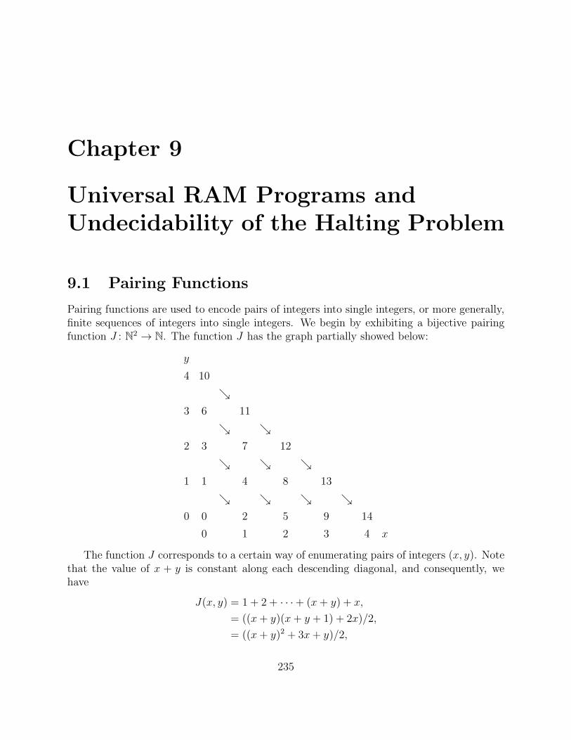
Chapter 9
Universal RAM Programs andUndecidability of the Halting Problem
9.1 Pairing Functions
Pairing functions are used to encode pairs of integers into single integers, or more generally,finite sequences of integers into single integers. We begin by exhibiting a bijective pairingfunction J : N2 → N. The function J has the graph partially showed below:
y
4 10
ց3 6 11
ց ց2 3 7 12
ց ց ց1 1 4 8 13
ց ց ց ց0 0 2 5 9 14
0 1 2 3 4 x
The function J corresponds to a certain way of enumerating pairs of integers (x, y). Notethat the value of x + y is constant along each descending diagonal, and consequently, wehave
J(x, y) = 1 + 2 + · · ·+ (x+ y) + x,
= ((x+ y)(x+ y + 1) + 2x)/2,
= ((x+ y)2 + 3x+ y)/2,
235
236 CHAPTER 9. UNIVERSAL RAM PROGRAMS AND THE HALTING PROBLEM
that is,J(x, y) = ((x+ y)2 + 3x+ y)/2.
For example, J(0, 3) = 6, J(1, 2) = 7, J(2, 2) = 12, J(3, 1) = 13, J(4, 0) = 14.
Let K : N → N and L : N → N be the projection functions onto the axes, that is, theunique functions such that
K(J(a, b)) = a and L(J(a, b)) = b,
for all a, b ∈ N. For example, K(11) = 1, and L(11) = 3; K(12) = 2, and L(12) = 2;K(13) = 3 and L(13) = 1.
The functions J,K, L are called Cantor’s pairing functions . They were used by Cantorto prove that the set Q of rational numbers is countable.
Clearly, J is primitive recursive, since it is given by a polynomial. It is not hard toprove that J is injective and surjective, and that it is strictly monotonic in each argument,which means that for all x, x′, y, y′ ∈ N, if x < x′ then J(x, y) < J(x′, y), and if y < y′ thenJ(x, y) < J(x, y′).
The projection functions can be computed explicitly, although this is a bit tricky. Weonly need to observe that by monotonicity of J ,
x ≤ J(x, y) and y ≤ J(x, y),
and thus,K(z) = min(x ≤ z)(∃y ≤ z)[J(x, y) = z],
andL(z) = min(y ≤ z)(∃x ≤ z)[J(x, y) = z].
Therefore, K and L are primitive recursive. It can be verified that J(K(z), L(z)) = z, forall z ∈ N.
More explicit formulae can be given for K and L. If we define
Q1(z) = ⌊(⌊√8z + 1⌋+ 1)/2⌋ − 1
Q2(z) = 2z − (Q1(z))2,
then it can be shown that
K(z) =1
2(Q2(z)−Q1(z))
L(z) = Q1(z)−1
2(Q2(z)−Q1(z)).
In the above formula, the function m 7→ ⌊√m⌋ yields the largest integer s such thats2 ≤ m. It can be computed by a RAM program.
9.1. PAIRING FUNCTIONS 237
The pairing function J(x, y) is also denoted as 〈x, y〉, and K and L are also denoted asΠ1 and Π2.
By induction, we can define bijections between Nn and N for all n ≥ 1. We let 〈z〉1 = z,
〈x1, x2〉2 = 〈x1, x2〉,
and〈x1, . . . , xn, xn+1〉n+1 = 〈x1, . . . , xn−1, 〈xn, xn+1〉〉n.
For example.
〈x1, x2, x3〉3 = 〈x1, 〈x2, x3〉〉2= 〈x1, 〈x2, x3〉〉
〈x1, x2, x3, x4〉4 = 〈x1, x2, 〈x3, x4〉〉3= 〈x1, 〈x2, 〈x3, x4〉〉〉
〈x1, x2, x3, x4, x5〉5 = 〈x1, x2, x3, 〈x4, x5〉〉4= 〈x1, 〈x2, 〈x3, 〈x4, x5〉〉〉〉.
It can be shown by induction on n that
〈x1, . . . , xn, xn+1〉n+1 = 〈x1, 〈x2, . . . , xn+1〉n〉.
The function 〈−, . . . ,−〉n : Nn → N is called an extended pairing function.
Observe that if z = 〈x1, . . . , xn〉n, then x1 = Π1(z), x2 = Π1(Π2(z)), x3 = Π1(Π2(Π2(z)),x4 = Π1(Π2(Π2(Π2(z)))), x5 = Π2(Π2(Π2(Π2(z)))).
We can also define a uniform projection function Π with the following property:if z = 〈x1, . . . , xn〉, with n ≥ 2, then
Π(i, n, z) = xi
for all i, where 1 ≤ i ≤ n. The idea is to view z as a n-tuple, and Π(i, n, z) as the i-thcomponent of that n-tuple. The function Π is defined by cases as follows:
Π(i, 0, z) = 0, for all i ≥ 0,
Π(i, 1, z) = z, for all i ≥ 0,
Π(i, 2, z) = Π1(z), if 0 ≤ i ≤ 1,
Π(i, 2, z) = Π2(z), for all i ≥ 2,
and for all n ≥ 2,
Π(i, n+ 1, z) =
Π(i, n, z) if 0 ≤ i < n,Π1(Π(n, n, z)) if i = n,Π2(Π(n, n, z)) if i > n.
238 CHAPTER 9. UNIVERSAL RAM PROGRAMS AND THE HALTING PROBLEM
By a previous exercise, this is a legitimate primitive recursive definition.
Some basic properties of Π are given as exercises. In particular, the following propertiesare easily shown:
(a) 〈0, . . . , 0〉n = 0, 〈x, 0〉 = 〈x, 0, . . . , 0〉n;(b) Π(0, n, z) = Π(1, n, z) and Π(i, n, z) = Π(n, n, z), for all i ≥ n and all n, z ∈ N;
(c) 〈Π(1, n, z), . . . ,Π(n, n, z)〉n = z, for all n ≥ 1 and all z ∈ N;
(d) Π(i, n, z) ≤ z, for all i, n, z ∈ N;
(e) There is a primitive recursive function Large, such that,
Π(i, n + 1,Large(n+ 1, z)) = z,
for i, n, z ∈ N.
As a first application, we observe that we need only consider partial computable functions(partial recursive functions)1 of a single argument. Indeed, let ϕ : Nn → N be a partialcomputable function of n ≥ 2 arguments. Let
ϕ(z) = ϕ(Π(1, n, z), . . . ,Π(n, n, z)),
for all z ∈ N. Then, ϕ is a partial computable function of a single argument, and ϕ can berecovered from ϕ, since
ϕ(x1, . . . , xn) = ϕ(〈x1, . . . , xn〉).Thus, using 〈−,−〉 and Π as coding and decoding functions, we can restrict our attentionto functions of a single argument.
Next, we show that there exist coding and decoding functions between Σ∗ and a1∗, andthat partial computable functions over Σ∗ can be recoded as partial computable functionsover a1∗. Since a1∗ is isomorphic to N, this shows that we can restrict out attention tofunctions defined over N.
9.2 Equivalence of Alphabets
Given an alphabet Σ = a1, . . . , ak, strings over Σ can be ordered by viewing strings asnumbers in a number system where the digits are a1, . . . , ak. In this number system, whichis almost the number system with base k, the string a1 corresponds to zero, and ak to k− 1.Hence, we have a kind of shifted number system in base k. For example, if Σ = a, b, c, alisting of Σ∗ in the ordering corresponding to the number system begins with
a, b, c, aa, ab, ac, ba, bb, bc, ca, cb, cc,
aaa, aab, aac, aba, abb, abc, . . . .
1The term partial recursive is now considered old-fashion. Many researchers have switched to the termpartial computable.
9.2. EQUIVALENCE OF ALPHABETS 239
Clearly, there is an ordering function from Σ∗ to N which is a bijection. Indeed, if u =ai1 · · ·ain , this function f : Σ∗ → N is given by
f(u) = i1kn−1 + i2k
n−2 + · · ·+ in−1k + in.
Since we also want a decoding function, we define the coding function Ck : Σ∗ → Σ∗ as
follows:
Ck(ǫ) = ǫ, and if u = ai1 · · · ain, then
Ck(u) = ai1kn−1+i2kn−2+···+in−1k+in1 .
The function Ck is primitive recursive, because
Ck(ǫ) = ǫ,
Ck(xai) = Ck(x)kai1.
The inverse of Ck is a function Dk : a1∗ → Σ∗. However, primitive recursive functions aretotal, and we need to extend Dk to Σ∗. This is easily done by letting
Dk(x) = Dk(a|x|1 )
for all x ∈ Σ∗. It remains to define Dk by primitive recursion over a1∗. For this, weintroduce three auxiliary functions p, q, r, defined as follows. Let
p(ǫ) = ǫ,
p(xai) = xai, if i 6= k,
p(xak) = p(x).
Note that p(x) is the result of deteting consecutive ak’s in the tail of x. Let
q(ǫ) = ǫ,
q(xai) = q(x)a1.
Note that q(x) = a|x|1 . Finally, let
r(ǫ) = a1,
r(xai) = xai+1, if i 6= k,
r(xak) = xak.
The function r is almost the successor function, for the ordering. Then, the trick is thatDk(xai) is the successor of Dk(x) in the ordering, and if
Dk(x) = yajank
240 CHAPTER 9. UNIVERSAL RAM PROGRAMS AND THE HALTING PROBLEM
with j 6= k, since the successor of yajank is yaj+1a
nk , we can use r. Thus, we have
Dk(ǫ) = ǫ,
Dk(xai) = r(p(Dk(x)))q(Dk(x)− p(Dk(x))).
Then, both Ck and Dk are primitive recursive, and Ck Dk = Dk Ck = id.
Let ϕ : Σ∗ → Σ∗ be a partial function over Σ∗, and let
ϕ+(x1, . . . , xn) = Ck(ϕ(Dk(x1), . . . , Dk(xn))).
The function ϕ+ is defined over a1∗. Also, for any partial function ψ over a1∗, let
ψ♯(x1, . . . , xn) = Dk(ψ(Ck(x1), . . . , Ck(xn))).
We claim that if ψ is a partial computable function over a1∗, then ψ♯ is partial computableover Σ∗, and that if ϕ is a partial computable function over Σ∗, then ϕ+ is partial computableover a1∗.
First, ψ can be extended to Σ∗ by letting
ψ(x) = ψ(a|x|1 )
for all x ∈ Σ∗, and so, if ψ is partial computable, then so is ψ♯ by composition. This seemsequally obvious for ϕ and ϕ+, but there is a difficulty. The problem is that ϕ+ is defined asa composition of functions over Σ∗. We have to show how ϕ+ can be defined directly overa1∗ without using any additional alphabet symbols. This is done in Machtey and Young[12], see Section 2.2, Lemma 2.2.3.
Pairing functions can also be used to prove that certain functions are primitive recursive,even though their definition is not a legal primitive recursive definition. For example, considerthe Fibonacci function defined as follows:
f(0) = 1,
f(1) = 1,
f(n+ 2) = f(n+ 1) + f(n),
for all n ∈ N. This is not a legal primitive recursive definition, since f(n+ 2) depends bothon f(n+1) and f(n). In a primitive recursive definition, g(y+1, x) is only allowed to dependupon g(y, x).
Definition 9.1. Given any function f : Nn → N, the function f : Nn+1 → N defined suchthat
f(y, x) = 〈f(0, x), . . . , f(y, x)〉y+1
is called the course-of-value function for f .
9.2. EQUIVALENCE OF ALPHABETS 241
The following lemma holds.
Proposition 9.1. Given any function f : Nn → N, if f is primitive recursive, then so is f .
Proof. First, it is necessary to define a function con such that if x = 〈x1, . . . , xm〉 andy = 〈y1, . . . , yn〉, where m,n ≥ 1, then
con(m, x, y) = 〈x1, . . . , xm, y1, . . . , yn〉.This fact is left as an exercise. Now, if f is primitive recursive, let
f(0, x) = f(0, x),
f(y + 1, x) = con(y + 1, f(y, x), f(y + 1, x)),
showing that f is primitive recursive. Conversely, if f is primitive recursive, then
f(y, x) = Π(y + 1, y + 1, f(y, x)),
and so, f is primitive recursive.
Remark : Why is it that
f(y + 1, x) = 〈f(y, x), f(y + 1, x)〉does not work?
We define course-of-value recursion as follows.
Definition 9.2. Given any two functions g : Nn → N and h : Nn+2 → N, the functionf : Nn+1 → N is defined by course-of-value recursion from g and h if
f(0, x) = g(x),
f(y + 1, x) = h(y, f(y, x), x).
The following lemma holds.
Proposition 9.2. If f : Nn+1 → N is defined by course-of-value recursion from g and h andg, h are primitive recursive, then f is primitive recursive.
Proof. We prove that f is primitive recursive. Then, by Proposition 9.1, f is also primitiverecursive. To prove that f is primitive recursive, observe that
f(0, x) = g(x),
f(y + 1, x) = con(y + 1, f(y, x), h(y, f(y, x), x)).
When we use Proposition 9.2 to prove that a function is primitive recursive, we rarelybother to construct a formal course-of-value recursion. Instead, we simply indicate how thevalue of f(y + 1, x) can be obtained in a primitive recursive manner from f(0, x) throughf(y, x). Thus, an informal use of Proposition 9.2 shows that the Fibonacci function isprimitive recursive. A rigorous proof of this fact is left as an exercise.
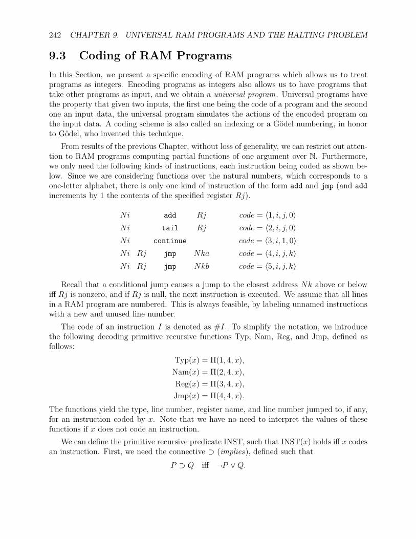
242 CHAPTER 9. UNIVERSAL RAM PROGRAMS AND THE HALTING PROBLEM
9.3 Coding of RAM Programs
In this Section, we present a specific encoding of RAM programs which allows us to treatprograms as integers. Encoding programs as integers also allows us to have programs thattake other programs as input, and we obtain a universal program. Universal programs havethe property that given two inputs, the first one being the code of a program and the secondone an input data, the universal program simulates the actions of the encoded program onthe input data. A coding scheme is also called an indexing or a Godel numbering, in honorto Godel, who invented this technique.
From results of the previous Chapter, without loss of generality, we can restrict out atten-tion to RAM programs computing partial functions of one argument over N. Furthermore,we only need the following kinds of instructions, each instruction being coded as shown be-low. Since we are considering functions over the natural numbers, which corresponds to aone-letter alphabet, there is only one kind of instruction of the form add and jmp (and add
increments by 1 the contents of the specified register Rj).
Ni add Rj code = 〈1, i, j, 0〉Ni tail Rj code = 〈2, i, j, 0〉Ni continue code = 〈3, i, 1, 0〉Ni Rj jmp Nka code = 〈4, i, j, k〉Ni Rj jmp Nkb code = 〈5, i, j, k〉
Recall that a conditional jump causes a jump to the closest address Nk above or belowiff Rj is nonzero, and if Rj is null, the next instruction is executed. We assume that all linesin a RAM program are numbered. This is always feasible, by labeling unnamed instructionswith a new and unused line number.
The code of an instruction I is denoted as #I. To simplify the notation, we introducethe following decoding primitive recursive functions Typ, Nam, Reg, and Jmp, defined asfollows:
Typ(x) = Π(1, 4, x),
Nam(x) = Π(2, 4, x),
Reg(x) = Π(3, 4, x),
Jmp(x) = Π(4, 4, x).
The functions yield the type, line number, register name, and line number jumped to, if any,for an instruction coded by x. Note that we have no need to interpret the values of thesefunctions if x does not code an instruction.
We can define the primitive recursive predicate INST, such that INST(x) holds iff x codesan instruction. First, we need the connective ⊃ (implies), defined such that
P ⊃ Q iff ¬P ∨Q.
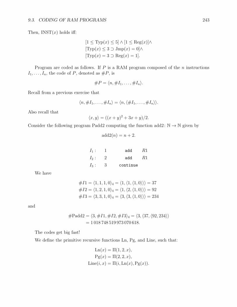
9.3. CODING OF RAM PROGRAMS 243
Then, INST(x) holds iff:
[1 ≤ Typ(x) ≤ 5] ∧ [1 ≤ Reg(x)]∧[Typ(x) ≤ 3 ⊃ Jmp(x) = 0]∧[Typ(x) = 3 ⊃ Reg(x) = 1].
Program are coded as follows. If P is a RAM program composed of the n instructionsI1, . . . , In, the code of P , denoted as #P , is
#P = 〈n,#I1, . . . ,#In〉.
Recall from a previous exercise that
〈n,#I1, . . . ,#In〉 = 〈n, 〈#I1, . . . ,#In〉〉.
Also recall that〈x, y〉 = ((x+ y)2 + 3x+ y)/2.
Consider the following program Padd2 computing the function add2: N→ N given by
add2(n) = n+ 2.
I1 : 1 add R1
I2 : 2 add R1
I3 : 3 continue
We have
#I1 = 〈1, 1, 1, 0〉4 = 〈1, 〈1, 〈1, 0〉〉〉 = 37
#I2 = 〈1, 2, 1, 0〉4 = 〈1, 〈2, 〈1, 0〉〉〉 = 92
#I3 = 〈3, 3, 1, 0〉4 = 〈3, 〈3, 〈1, 0〉〉〉 = 234
and
#Padd2 = 〈3,#I1,#I2,#I3〉4 = 〈3, 〈37, 〈92, 234〉〉= 1 018 748 519 973 070 618.
The codes get big fast!
We define the primitive recursive functions Ln, Pg, and Line, such that:
Ln(x) = Π(1, 2, x),
Pg(x) = Π(2, 2, x),
Line(i, x) = Π(i,Ln(x),Pg(x)).
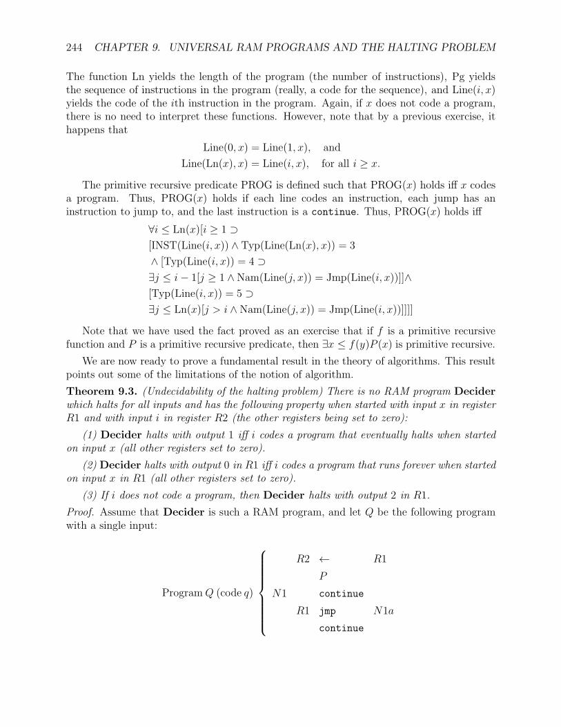
244 CHAPTER 9. UNIVERSAL RAM PROGRAMS AND THE HALTING PROBLEM
The function Ln yields the length of the program (the number of instructions), Pg yieldsthe sequence of instructions in the program (really, a code for the sequence), and Line(i, x)yields the code of the ith instruction in the program. Again, if x does not code a program,there is no need to interpret these functions. However, note that by a previous exercise, ithappens that
Line(0, x) = Line(1, x), and
Line(Ln(x), x) = Line(i, x), for all i ≥ x.
The primitive recursive predicate PROG is defined such that PROG(x) holds iff x codesa program. Thus, PROG(x) holds if each line codes an instruction, each jump has aninstruction to jump to, and the last instruction is a continue. Thus, PROG(x) holds iff
∀i ≤ Ln(x)[i ≥ 1 ⊃[INST(Line(i, x)) ∧ Typ(Line(Ln(x), x)) = 3
∧ [Typ(Line(i, x)) = 4 ⊃∃j ≤ i− 1[j ≥ 1 ∧Nam(Line(j, x)) = Jmp(Line(i, x))]]∧[Typ(Line(i, x)) = 5 ⊃∃j ≤ Ln(x)[j > i ∧ Nam(Line(j, x)) = Jmp(Line(i, x))]]]]
Note that we have used the fact proved as an exercise that if f is a primitive recursivefunction and P is a primitive recursive predicate, then ∃x ≤ f(y)P (x) is primitive recursive.
We are now ready to prove a fundamental result in the theory of algorithms. This resultpoints out some of the limitations of the notion of algorithm.
Theorem 9.3. (Undecidability of the halting problem) There is no RAM program Deciderwhich halts for all inputs and has the following property when started with input x in registerR1 and with input i in register R2 (the other registers being set to zero):
(1) Decider halts with output 1 iff i codes a program that eventually halts when startedon input x (all other registers set to zero).
(2) Decider halts with output 0 in R1 iff i codes a program that runs forever when startedon input x in R1 (all other registers set to zero).
(3) If i does not code a program, then Decider halts with output 2 in R1.
Proof. Assume that Decider is such a RAM program, and let Q be the following programwith a single input:
ProgramQ (code q)
R2 ← R1
P
N1 continue
R1 jmp N1a
continue
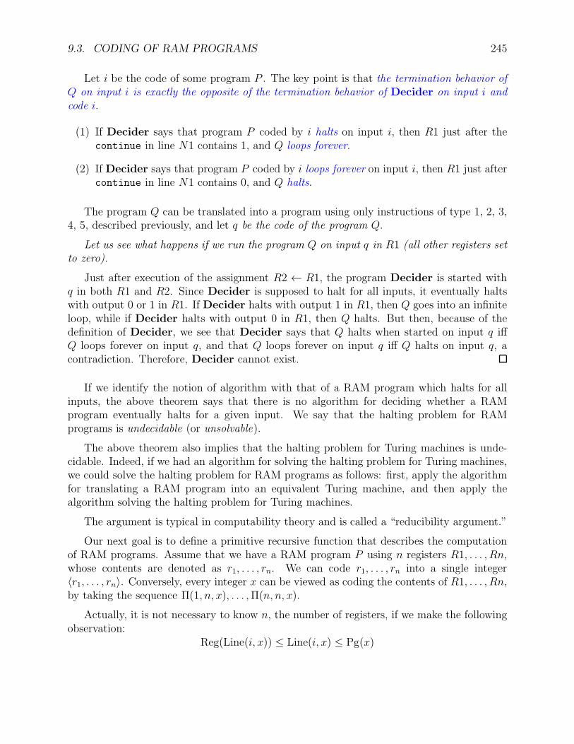
9.3. CODING OF RAM PROGRAMS 245
Let i be the code of some program P . The key point is that the termination behavior ofQ on input i is exactly the opposite of the termination behavior of Decider on input i andcode i.
(1) If Decider says that program P coded by i halts on input i, then R1 just after thecontinue in line N1 contains 1, and Q loops forever.
(2) If Decider says that program P coded by i loops forever on input i, then R1 just aftercontinue in line N1 contains 0, and Q halts.
The program Q can be translated into a program using only instructions of type 1, 2, 3,4, 5, described previously, and let q be the code of the program Q.
Let us see what happens if we run the program Q on input q in R1 (all other registers setto zero).
Just after execution of the assignment R2 ← R1, the program Decider is started withq in both R1 and R2. Since Decider is supposed to halt for all inputs, it eventually haltswith output 0 or 1 in R1. If Decider halts with output 1 in R1, then Q goes into an infiniteloop, while if Decider halts with output 0 in R1, then Q halts. But then, because of thedefinition of Decider, we see that Decider says that Q halts when started on input q iffQ loops forever on input q, and that Q loops forever on input q iff Q halts on input q, acontradiction. Therefore, Decider cannot exist.
If we identify the notion of algorithm with that of a RAM program which halts for allinputs, the above theorem says that there is no algorithm for deciding whether a RAMprogram eventually halts for a given input. We say that the halting problem for RAMprograms is undecidable (or unsolvable).
The above theorem also implies that the halting problem for Turing machines is unde-cidable. Indeed, if we had an algorithm for solving the halting problem for Turing machines,we could solve the halting problem for RAM programs as follows: first, apply the algorithmfor translating a RAM program into an equivalent Turing machine, and then apply thealgorithm solving the halting problem for Turing machines.
The argument is typical in computability theory and is called a “reducibility argument.”
Our next goal is to define a primitive recursive function that describes the computationof RAM programs. Assume that we have a RAM program P using n registers R1, . . . , Rn,whose contents are denoted as r1, . . . , rn. We can code r1, . . . , rn into a single integer〈r1, . . . , rn〉. Conversely, every integer x can be viewed as coding the contents of R1, . . . , Rn,by taking the sequence Π(1, n, x), . . . ,Π(n, n, x).
Actually, it is not necessary to know n, the number of registers, if we make the followingobservation:
Reg(Line(i, x)) ≤ Line(i, x) ≤ Pg(x)
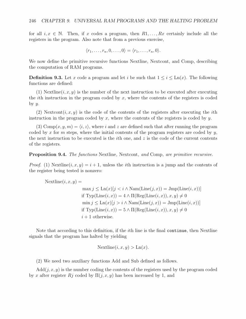
246 CHAPTER 9. UNIVERSAL RAM PROGRAMS AND THE HALTING PROBLEM
for all i, x ∈ N. Then, if x codes a program, then R1, . . . , Rx certainly include all theregisters in the program. Also note that from a previous exercise,
〈r1, . . . , rn, 0, . . . , 0〉 = 〈r1, . . . , rn, 0〉.
We now define the primitive recursive functions Nextline, Nextcont, and Comp, describingthe computation of RAM programs.
Definition 9.3. Let x code a program and let i be such that 1 ≤ i ≤ Ln(x). The followingfunctions are defined:
(1) Nextline(i, x, y) is the number of the next instruction to be executed after executingthe ith instruction in the program coded by x, where the contents of the registers is codedby y.
(2) Nextcont(i, x, y) is the code of the contents of the registers after executing the ithinstruction in the program coded by x, where the contents of the registers is coded by y.
(3) Comp(x, y,m) = 〈i, z〉, where i and z are defined such that after running the programcoded by x for m steps, where the initial contents of the program registers are coded by y,the next instruction to be executed is the ith one, and z is the code of the current contentsof the registers.
Proposition 9.4. The functions Nextline, Nextcont, and Comp, are primitive recursive.
Proof. (1) Nextline(i, x, y) = i + 1, unless the ith instruction is a jump and the contents ofthe register being tested is nonzero:
Nextline(i, x, y) =
max j ≤ Ln(x)[j < i ∧Nam(Line(j, x)) = Jmp(Line(i, x))]
if Typ(Line(i, x)) = 4 ∧Π(Reg(Line(i, x)), x, y) 6= 0
min j ≤ Ln(x)[j > i ∧Nam(Line(j, x)) = Jmp(Line(i, x))]
if Typ(Line(i, x)) = 5 ∧Π(Reg(Line(i, x)), x, y) 6= 0
i+ 1 otherwise.
Note that according to this definition, if the ith line is the final continue, then Nextlinesignals that the program has halted by yielding
Nextline(i, x, y) > Ln(x).
(2) We need two auxiliary functions Add and Sub defined as follows.
Add(j, x, y) is the number coding the contents of the registers used by the program codedby x after register Rj coded by Π(j, x, y) has been increased by 1, and
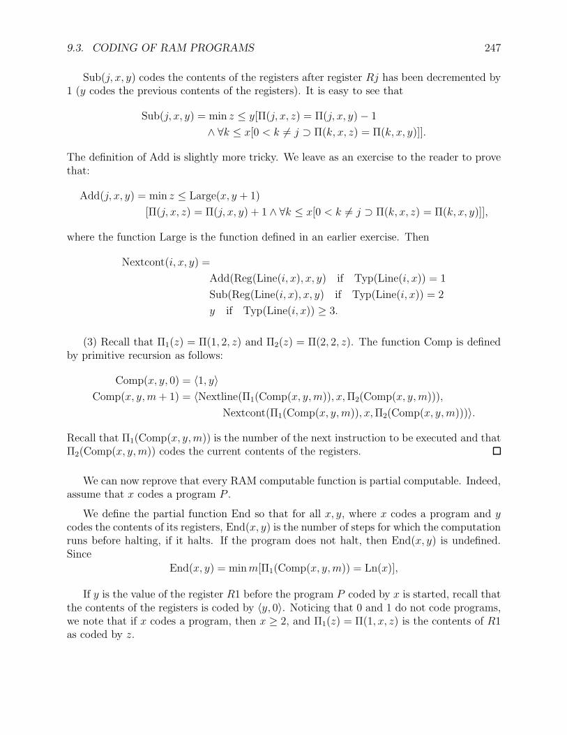
9.3. CODING OF RAM PROGRAMS 247
Sub(j, x, y) codes the contents of the registers after register Rj has been decremented by1 (y codes the previous contents of the registers). It is easy to see that
Sub(j, x, y) = min z ≤ y[Π(j, x, z) = Π(j, x, y)− 1
∧ ∀k ≤ x[0 < k 6= j ⊃ Π(k, x, z) = Π(k, x, y)]].
The definition of Add is slightly more tricky. We leave as an exercise to the reader to provethat:
Add(j, x, y) = min z ≤ Large(x, y + 1)
[Π(j, x, z) = Π(j, x, y) + 1 ∧ ∀k ≤ x[0 < k 6= j ⊃ Π(k, x, z) = Π(k, x, y)]],
where the function Large is the function defined in an earlier exercise. Then
Nextcont(i, x, y) =
Add(Reg(Line(i, x), x, y) if Typ(Line(i, x)) = 1
Sub(Reg(Line(i, x), x, y) if Typ(Line(i, x)) = 2
y if Typ(Line(i, x)) ≥ 3.
(3) Recall that Π1(z) = Π(1, 2, z) and Π2(z) = Π(2, 2, z). The function Comp is definedby primitive recursion as follows:
Comp(x, y, 0) = 〈1, y〉Comp(x, y,m+ 1) = 〈Nextline(Π1(Comp(x, y,m)), x,Π2(Comp(x, y,m))),
Nextcont(Π1(Comp(x, y,m)), x,Π2(Comp(x, y,m)))〉.
Recall that Π1(Comp(x, y,m)) is the number of the next instruction to be executed and thatΠ2(Comp(x, y,m)) codes the current contents of the registers.
We can now reprove that every RAM computable function is partial computable. Indeed,assume that x codes a program P .
We define the partial function End so that for all x, y, where x codes a program and ycodes the contents of its registers, End(x, y) is the number of steps for which the computationruns before halting, if it halts. If the program does not halt, then End(x, y) is undefined.Since
End(x, y) = minm[Π1(Comp(x, y,m)) = Ln(x)],
If y is the value of the register R1 before the program P coded by x is started, recall thatthe contents of the registers is coded by 〈y, 0〉. Noticing that 0 and 1 do not code programs,we note that if x codes a program, then x ≥ 2, and Π1(z) = Π(1, x, z) is the contents of R1as coded by z.
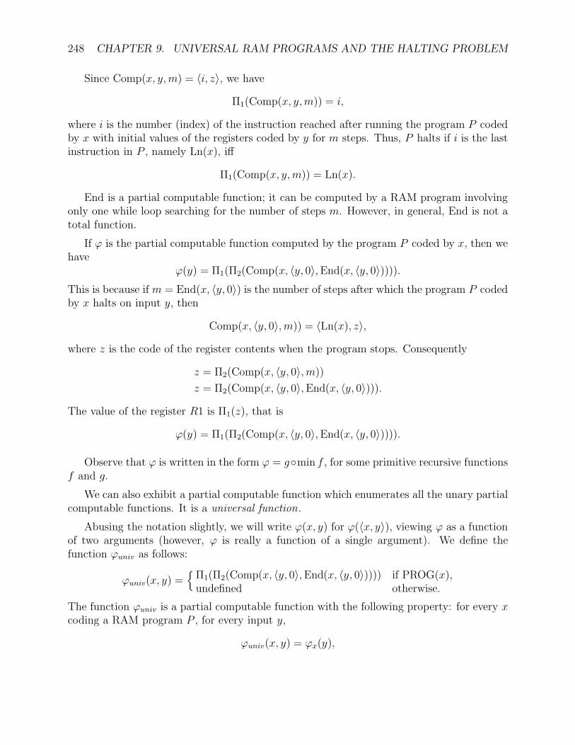
248 CHAPTER 9. UNIVERSAL RAM PROGRAMS AND THE HALTING PROBLEM
Since Comp(x, y,m) = 〈i, z〉, we have
Π1(Comp(x, y,m)) = i,
where i is the number (index) of the instruction reached after running the program P codedby x with initial values of the registers coded by y for m steps. Thus, P halts if i is the lastinstruction in P , namely Ln(x), iff
Π1(Comp(x, y,m)) = Ln(x).
End is a partial computable function; it can be computed by a RAM program involvingonly one while loop searching for the number of steps m. However, in general, End is not atotal function.
If ϕ is the partial computable function computed by the program P coded by x, then wehave
ϕ(y) = Π1(Π2(Comp(x, 〈y, 0〉,End(x, 〈y, 0〉)))).This is because if m = End(x, 〈y, 0〉) is the number of steps after which the program P codedby x halts on input y, then
Comp(x, 〈y, 0〉, m)) = 〈Ln(x), z〉,
where z is the code of the register contents when the program stops. Consequently
z = Π2(Comp(x, 〈y, 0〉, m))
z = Π2(Comp(x, 〈y, 0〉,End(x, 〈y, 0〉))).
The value of the register R1 is Π1(z), that is
ϕ(y) = Π1(Π2(Comp(x, 〈y, 0〉,End(x, 〈y, 0〉)))).
Observe that ϕ is written in the form ϕ = gmin f , for some primitive recursive functionsf and g.
We can also exhibit a partial computable function which enumerates all the unary partialcomputable functions. It is a universal function.
Abusing the notation slightly, we will write ϕ(x, y) for ϕ(〈x, y〉), viewing ϕ as a functionof two arguments (however, ϕ is really a function of a single argument). We define thefunction ϕuniv as follows:
ϕuniv(x, y) =Π1(Π2(Comp(x, 〈y, 0〉,End(x, 〈y, 0〉)))) if PROG(x),undefined otherwise.
The function ϕuniv is a partial computable function with the following property: for every xcoding a RAM program P , for every input y,
ϕuniv(x, y) = ϕx(y),
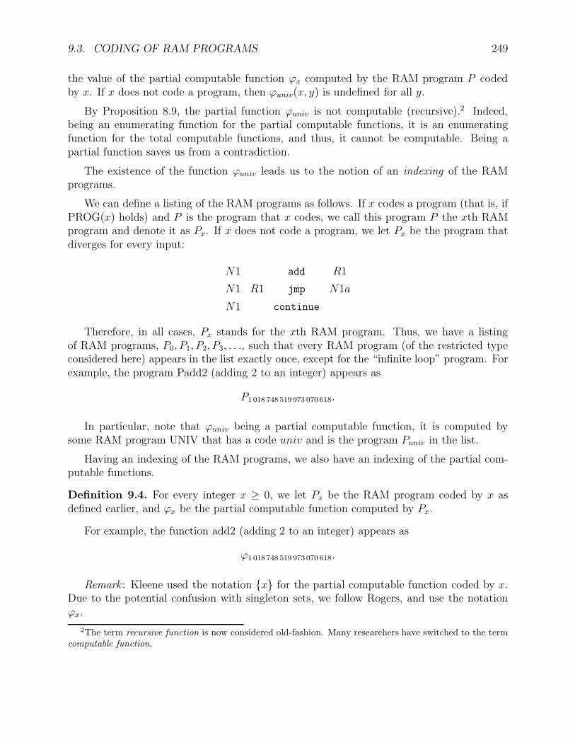
9.3. CODING OF RAM PROGRAMS 249
the value of the partial computable function ϕx computed by the RAM program P codedby x. If x does not code a program, then ϕuniv(x, y) is undefined for all y.
By Proposition 8.9, the partial function ϕuniv is not computable (recursive).2 Indeed,being an enumerating function for the partial computable functions, it is an enumeratingfunction for the total computable functions, and thus, it cannot be computable. Being apartial function saves us from a contradiction.
The existence of the function ϕuniv leads us to the notion of an indexing of the RAMprograms.
We can define a listing of the RAM programs as follows. If x codes a program (that is, ifPROG(x) holds) and P is the program that x codes, we call this program P the xth RAMprogram and denote it as Px. If x does not code a program, we let Px be the program thatdiverges for every input:
N1 add R1
N1 R1 jmp N1a
N1 continue
Therefore, in all cases, Px stands for the xth RAM program. Thus, we have a listingof RAM programs, P0, P1, P2, P3, . . ., such that every RAM program (of the restricted typeconsidered here) appears in the list exactly once, except for the “infinite loop” program. Forexample, the program Padd2 (adding 2 to an integer) appears as
P1 018 748 519 973 070 618.
In particular, note that ϕuniv being a partial computable function, it is computed bysome RAM program UNIV that has a code univ and is the program Puniv in the list.
Having an indexing of the RAM programs, we also have an indexing of the partial com-putable functions.
Definition 9.4. For every integer x ≥ 0, we let Px be the RAM program coded by x asdefined earlier, and ϕx be the partial computable function computed by Px.
For example, the function add2 (adding 2 to an integer) appears as
ϕ1 018 748 519 973 070 618.
Remark : Kleene used the notation x for the partial computable function coded by x.Due to the potential confusion with singleton sets, we follow Rogers, and use the notationϕx.
2The term recursive function is now considered old-fashion. Many researchers have switched to the termcomputable function.
250 CHAPTER 9. UNIVERSAL RAM PROGRAMS AND THE HALTING PROBLEM
It is important to observe that different programs Px and Py may compute the samefunction, that is, while Px 6= Py for all x 6= y, it is possible that ϕx = ϕy. In fact, it isundecidable whether ϕx = ϕy.
The existence of the universal function ϕuniv is sufficiently important to be recorded inthe following Lemma.
Proposition 9.5. For the indexing of RAM programs defined earlier, there is a universalpartial computable function ϕuniv such that, for all x, y ∈ N, if ϕx is the partial computablefunction computed by Px, then
ϕx(y) = ϕuniv(〈x, y〉).
The program UNIV computing ϕuniv can be viewed as an interpreter for RAM programs.By giving the universal program UNIV the “program” x and the “data” y, we get the resultof executing program Px on input y. We can view the RAM model as a stored programcomputer .
By Theorem 9.3 and Proposition 9.5, the halting problem for the single program UNIVis undecidable. Otherwise, the halting problem for RAM programs would be decidable, acontradiction. It should be noted that the program UNIV can actually be written (with acertain amount of pain).
The object of the next Section is to show the existence of Kleene’s T -predicate. Thiswill yield another important normal form. In addition, the T -predicate is a basic tool inrecursion theory.
9.4 Kleene’s T -Predicate
In Section 9.3, we have encoded programs. The idea of this Section is to also encode com-putations of RAM programs. Assume that x codes a program, that y is some input (not acode), and that z codes a computation of Px on input y. The predicate T (x, y, z) is definedas follows:
T (x, y, z) holds iff x codes a RAM program, y is an input, and z codes a halting compu-tation of Px on input y.
We will show that T is primitive recursive. First, we need to encode computations. Wesay that z codes a computation of length n ≥ 1 if
z = 〈n+ 2, 〈1, y0〉, 〈i1, y1〉, . . . , 〈in, yn〉〉,
where each ij is the physical location of the next instruction to be executed and each yjcodes the contents of the registers just before execution of the instruction at the locationij . Also, y0 codes the initial contents of the registers, that is, y0 = 〈y, 0〉, for some input y.We let Ln(z) = Π1(z). Note that ij denotes the physical location of the next instruction to
9.4. KLEENE’S T -PREDICATE 251
be executed in the sequence of instructions constituting the program coded by x, and notthe line number (label) of this instruction. Thus, the first instruction to be executed is inlocation 1, 1 ≤ ij ≤ Ln(x), and in−1 = Ln(x). Since the last instruction which is executed isthe last physical instruction in the program, namely, a continue, there is no next instructionto be executed after that, and in is irrelevant. Writing the definition of T is a little simplerif we let in = Ln(x) + 1.
Definition 9.5. The T -predicate is the primitive recursive predicate defined as follows:
T (x, y, z) iff PROG(x) and (Ln(z) ≥ 3) and
∀j ≤ Ln(z)− 3[0 ≤ j ⊃Nextline(Π1(Π(j + 2,Ln(z), z)), x,Π2(Π(j + 2,Ln(z), z))) = Π1(Π(j + 3,Ln(z), z)) and
Nextcont(Π1(Π(j + 2,Ln(z), z)), x,Π2(Π(j + 2,Ln(z), z))) = Π2(Π(j + 3,Ln(z), z)) and
Π1(Π(Ln(z)− 1,Ln(z), z)) = Ln(x) and
Π1(Π(2,Ln(z), z)) = 1 and
y = Π1(Π2(Π(2,Ln(z), z))) and Π2(Π2(Π(2,Ln(z), z))) = 0]
The reader can verify that T (x, y, z) holds iff x codes a RAM program, y is an input, andz codes a halting computation of Px on input y. In order to extract the output of Px fromz, we define the primitive recursive function Res as follows:
Res(z) = Π1(Π2(Π(Ln(z),Ln(z), z))).
The explanation for this formula is that Res(z) are the contents of register R1 when Px halts,that is, Π1(yLn(z)). Using the T -predicate, we get the so-called Kleene normal form.
Theorem 9.6. (Kleene Normal Form) Using the indexing of the partial computable functionsdefined earlier, we have
ϕx(y) = Res[min z(T (x, y, z))],
where T (x, y, z) and Res are primitive recursive.
Note that the universal function ϕuniv can be defined as
ϕuniv(x, y) = Res[min z(T (x, y, z))].
There is another important property of the partial computable functions, namely, thatcomposition is effective. We need two auxiliary primitive recursive functions. The functionConprogs creates the code of the program obtained by concatenating the programs Px andPy, and for i ≥ 2, Cumclr(i) is the code of the program which clears registers R2, . . . , Ri.To get Cumclr, we can use the function clr(i) such that clr(i) is the code of the program
N1 tail Ri
N1 Ri jmp N1a
N continue
252 CHAPTER 9. UNIVERSAL RAM PROGRAMS AND THE HALTING PROBLEM
We leave it as an exercise to prove that clr, Conprogs, and Cumclr, are primitive recursive.
Theorem 9.7. There is a primitive recursive function c such that
ϕc(x,y) = ϕx ϕy.
Proof. If both x and y code programs, then ϕx ϕy can be computed as follows: Run Py,clear all registers but R1, then run Px. Otherwise, let loop be the index of the infinite loopprogram:
c(x, y) =
Conprogs(y,Conprogs(Cumclr(y), x)) if PROG(x) and PROG(y)loop otherwise.
9.5 A Simple Function Not Known to be Computable
The “3n+ 1 problem” proposed by Collatz around 1937 is the following:
Given any positive integer n ≥ 1, construct the sequence ci(n) as follows starting withi = 1:
c1(n) = n
ci+1(n) =
ci(n)/2 if ci(n) is even
3ci(n) + 1 if ci(n) is odd.
Observe that for n = 1, we get the infinite periodic sequence
1 =⇒ 4 =⇒ 2 =⇒ 1 =⇒ 4 =⇒ 2 =⇒ 1 =⇒ · · · ,
so we may assume that we stop the first time that the sequence ci(n) reaches the value 1 (ifit actually does). Such an index i is called the stopping time of the sequence. And this isthe problem:
Conjecture (Collatz):
For any starting integer value n ≥ 1, the sequence (ci(n)) always reaches 1.
Starting with n = 3, we get the sequence
3 =⇒ 10 =⇒ 5 =⇒ 16 =⇒ 8 =⇒ 4 =⇒ 2 =⇒ 1.
Starting with n = 5, we get the sequence
5 =⇒ 16 =⇒ 8 =⇒ 4 =⇒ 2 =⇒ 1.
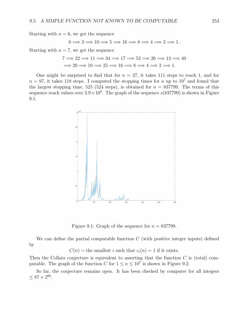
9.5. A SIMPLE FUNCTION NOT KNOWN TO BE COMPUTABLE 253
Starting with n = 6, we get the sequence
6 =⇒ 3 =⇒ 10 =⇒ 5 =⇒ 16 =⇒ 8 =⇒ 4 =⇒ 2 =⇒ 1.
Starting with n = 7, we get the sequence
7 =⇒ 22 =⇒ 11 =⇒ 34 =⇒ 17 =⇒ 52 =⇒ 26 =⇒ 13 =⇒ 40
=⇒ 20 =⇒ 10 =⇒ 25 =⇒ 16 =⇒ 8 =⇒ 4 =⇒ 2 =⇒ 1.
One might be surprised to find that for n = 27, it takes 111 steps to reach 1, and forn = 97, it takes 118 steps. I computed the stopping times for n up to 107 and found thatthe largest stopping time, 525 (524 steps), is obtained for n = 837799. The terms of thissequence reach values over 2.9×10⁹. The graph of the sequence s(837799) is shown in Figure9.1.
0 100 200 300 400 500 600
0
0.5
1
1.5
2
2.5
3×10
9
Figure 9.1: Graph of the sequence for n = 837799.
We can define the partial computable function C (with positive integer inputs) definedby
C(n) = the smallest i such that ci(n) = 1 if it exists.
Then the Collatz conjecture is equivalent to asserting that the function C is (total) com-putable. The graph of the function C for 1 ≤ n ≤ 107 is shown in Figure 9.2.
So far, the conjecture remains open. It has been checked by computer for all integers≤ 87× 260.
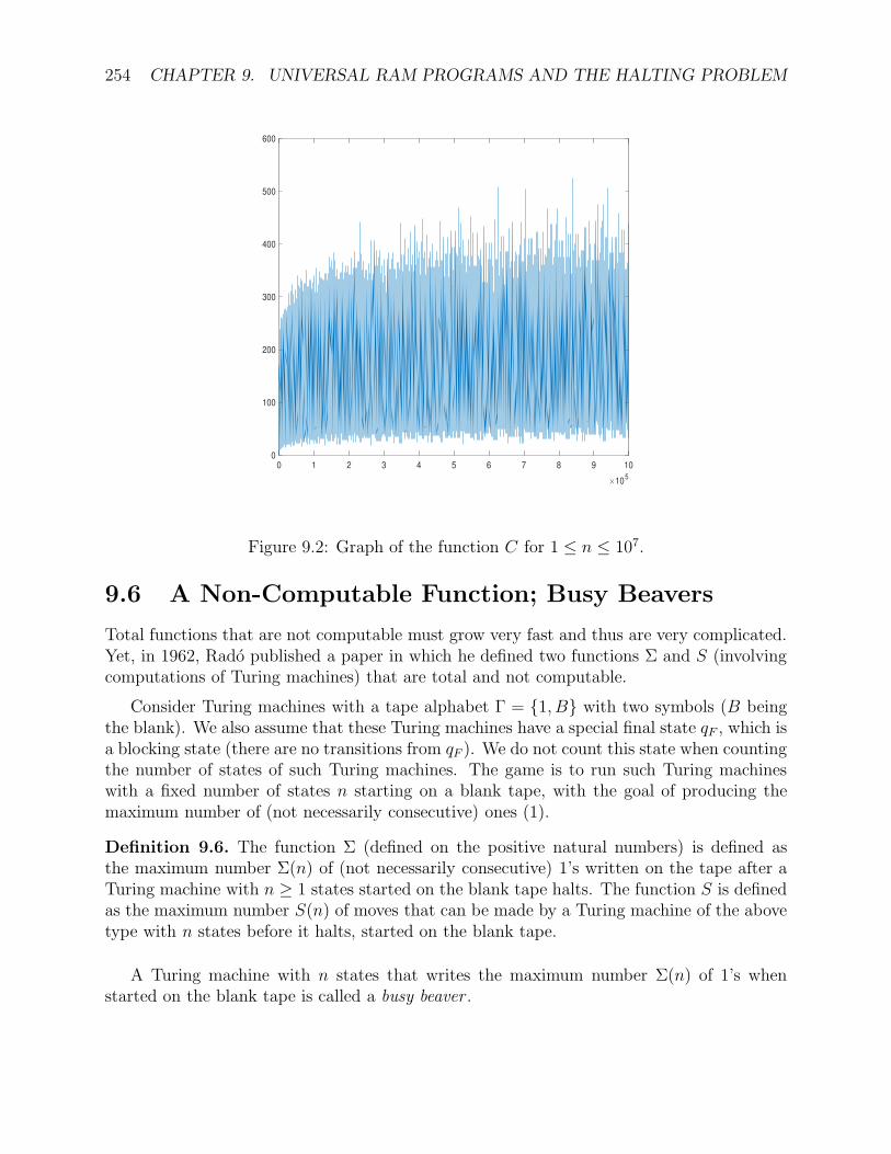
254 CHAPTER 9. UNIVERSAL RAM PROGRAMS AND THE HALTING PROBLEM
0 1 2 3 4 5 6 7 8 9 10
×105
0
100
200
300
400
500
600
Figure 9.2: Graph of the function C for 1 ≤ n ≤ 107.
9.6 A Non-Computable Function; Busy Beavers
Total functions that are not computable must grow very fast and thus are very complicated.Yet, in 1962, Rado published a paper in which he defined two functions Σ and S (involvingcomputations of Turing machines) that are total and not computable.
Consider Turing machines with a tape alphabet Γ = 1, B with two symbols (B beingthe blank). We also assume that these Turing machines have a special final state qF , which isa blocking state (there are no transitions from qF ). We do not count this state when countingthe number of states of such Turing machines. The game is to run such Turing machineswith a fixed number of states n starting on a blank tape, with the goal of producing themaximum number of (not necessarily consecutive) ones (1).
Definition 9.6. The function Σ (defined on the positive natural numbers) is defined asthe maximum number Σ(n) of (not necessarily consecutive) 1’s written on the tape after aTuring machine with n ≥ 1 states started on the blank tape halts. The function S is definedas the maximum number S(n) of moves that can be made by a Turing machine of the abovetype with n states before it halts, started on the blank tape.
A Turing machine with n states that writes the maximum number Σ(n) of 1’s whenstarted on the blank tape is called a busy beaver .
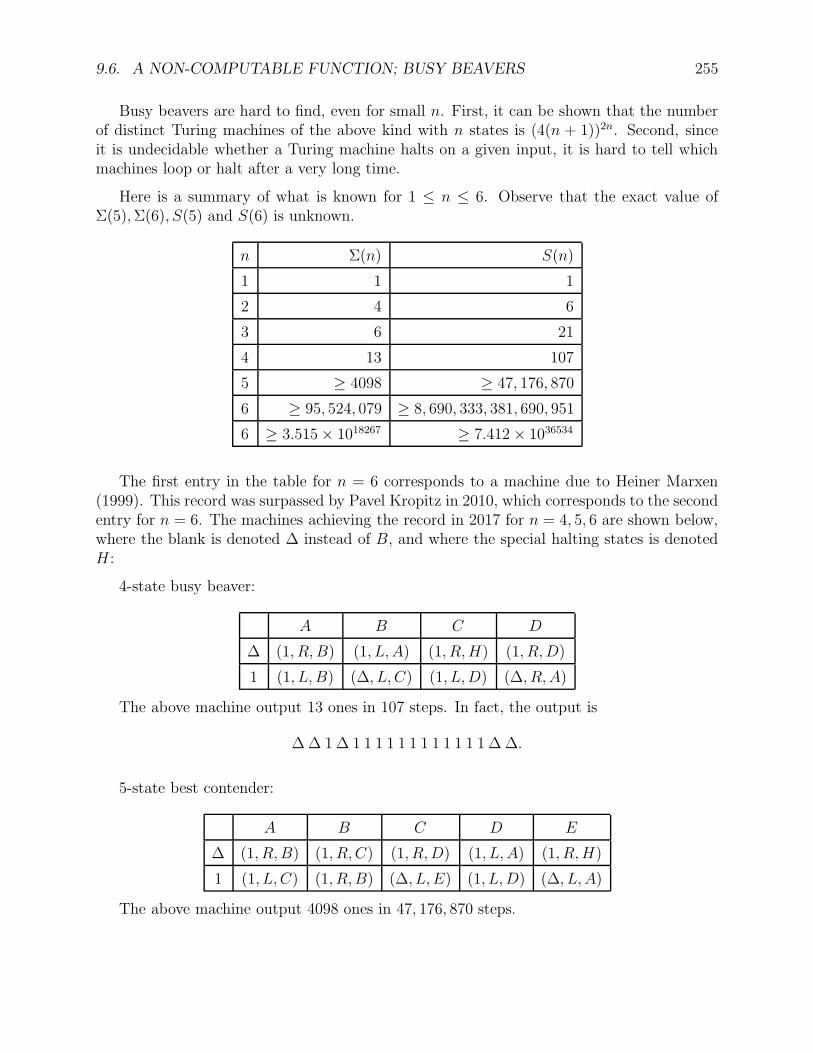
9.6. A NON-COMPUTABLE FUNCTION; BUSY BEAVERS 255
Busy beavers are hard to find, even for small n. First, it can be shown that the numberof distinct Turing machines of the above kind with n states is (4(n + 1))2n. Second, sinceit is undecidable whether a Turing machine halts on a given input, it is hard to tell whichmachines loop or halt after a very long time.
Here is a summary of what is known for 1 ≤ n ≤ 6. Observe that the exact value ofΣ(5),Σ(6), S(5) and S(6) is unknown.
n Σ(n) S(n)
1 1 1
2 4 6
3 6 21
4 13 107
5 ≥ 4098 ≥ 47, 176, 870
6 ≥ 95, 524, 079 ≥ 8, 690, 333, 381, 690, 951
6 ≥ 3.515× 1018267 ≥ 7.412× 1036534
The first entry in the table for n = 6 corresponds to a machine due to Heiner Marxen(1999). This record was surpassed by Pavel Kropitz in 2010, which corresponds to the secondentry for n = 6. The machines achieving the record in 2017 for n = 4, 5, 6 are shown below,where the blank is denoted ∆ instead of B, and where the special halting states is denotedH :
4-state busy beaver:
A B C D
∆ (1, R, B) (1, L, A) (1, R,H) (1, R,D)
1 (1, L, B) (∆, L, C) (1, L,D) (∆, R, A)
The above machine output 13 ones in 107 steps. In fact, the output is
∆ ∆ 1 ∆ 1 1 1 1 1 1 1 1 1 1 1 1 ∆ ∆.
5-state best contender:
A B C D E
∆ (1, R, B) (1, R, C) (1, R,D) (1, L, A) (1, R,H)
1 (1, L, C) (1, R, B) (∆, L, E) (1, L,D) (∆, L, A)
The above machine output 4098 ones in 47, 176, 870 steps.
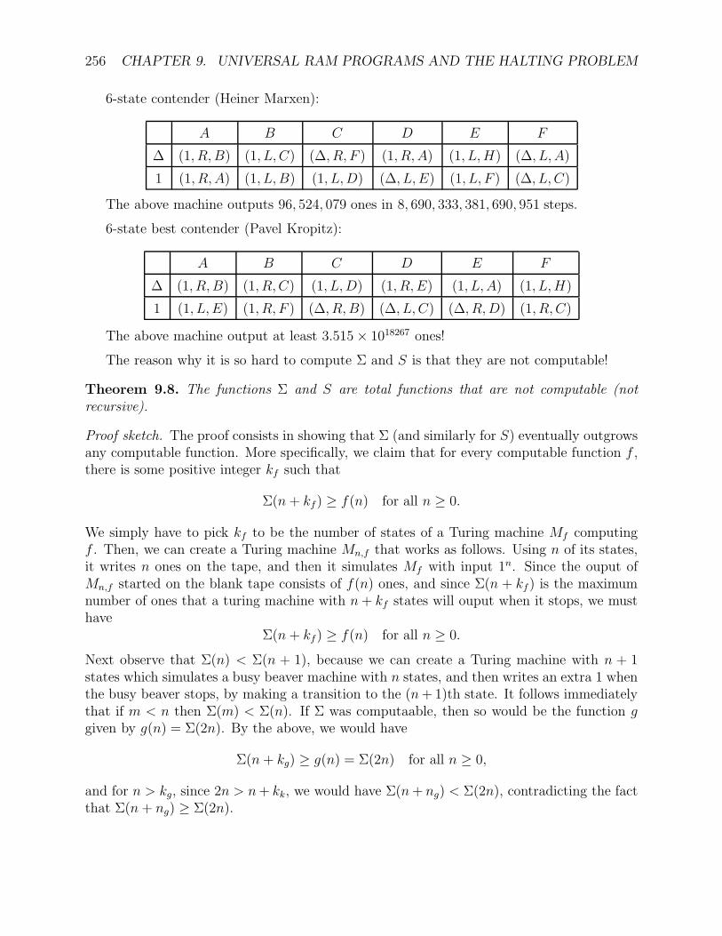
256 CHAPTER 9. UNIVERSAL RAM PROGRAMS AND THE HALTING PROBLEM
6-state contender (Heiner Marxen):
A B C D E F
∆ (1, R, B) (1, L, C) (∆, R, F ) (1, R, A) (1, L,H) (∆, L, A)
1 (1, R, A) (1, L, B) (1, L,D) (∆, L, E) (1, L, F ) (∆, L, C)
The above machine outputs 96, 524, 079 ones in 8, 690, 333, 381, 690, 951 steps.
6-state best contender (Pavel Kropitz):
A B C D E F
∆ (1, R, B) (1, R, C) (1, L,D) (1, R, E) (1, L, A) (1, L,H)
1 (1, L, E) (1, R, F ) (∆, R, B) (∆, L, C) (∆, R,D) (1, R, C)
The above machine output at least 3.515× 1018267 ones!
The reason why it is so hard to compute Σ and S is that they are not computable!
Theorem 9.8. The functions Σ and S are total functions that are not computable (notrecursive).
Proof sketch. The proof consists in showing that Σ (and similarly for S) eventually outgrowsany computable function. More specifically, we claim that for every computable function f ,there is some positive integer kf such that
Σ(n + kf) ≥ f(n) for all n ≥ 0.
We simply have to pick kf to be the number of states of a Turing machine Mf computingf . Then, we can create a Turing machine Mn,f that works as follows. Using n of its states,it writes n ones on the tape, and then it simulates Mf with input 1n. Since the ouput ofMn,f started on the blank tape consists of f(n) ones, and since Σ(n + kf) is the maximumnumber of ones that a turing machine with n+ kf states will ouput when it stops, we musthave
Σ(n + kf) ≥ f(n) for all n ≥ 0.
Next observe that Σ(n) < Σ(n + 1), because we can create a Turing machine with n + 1states which simulates a busy beaver machine with n states, and then writes an extra 1 whenthe busy beaver stops, by making a transition to the (n+1)th state. It follows immediatelythat if m < n then Σ(m) < Σ(n). If Σ was computaable, then so would be the function ggiven by g(n) = Σ(2n). By the above, we would have
Σ(n + kg) ≥ g(n) = Σ(2n) for all n ≥ 0,
and for n > kg, since 2n > n+ kk, we would have Σ(n+ ng) < Σ(2n), contradicting the factthat Σ(n + ng) ≥ Σ(2n).
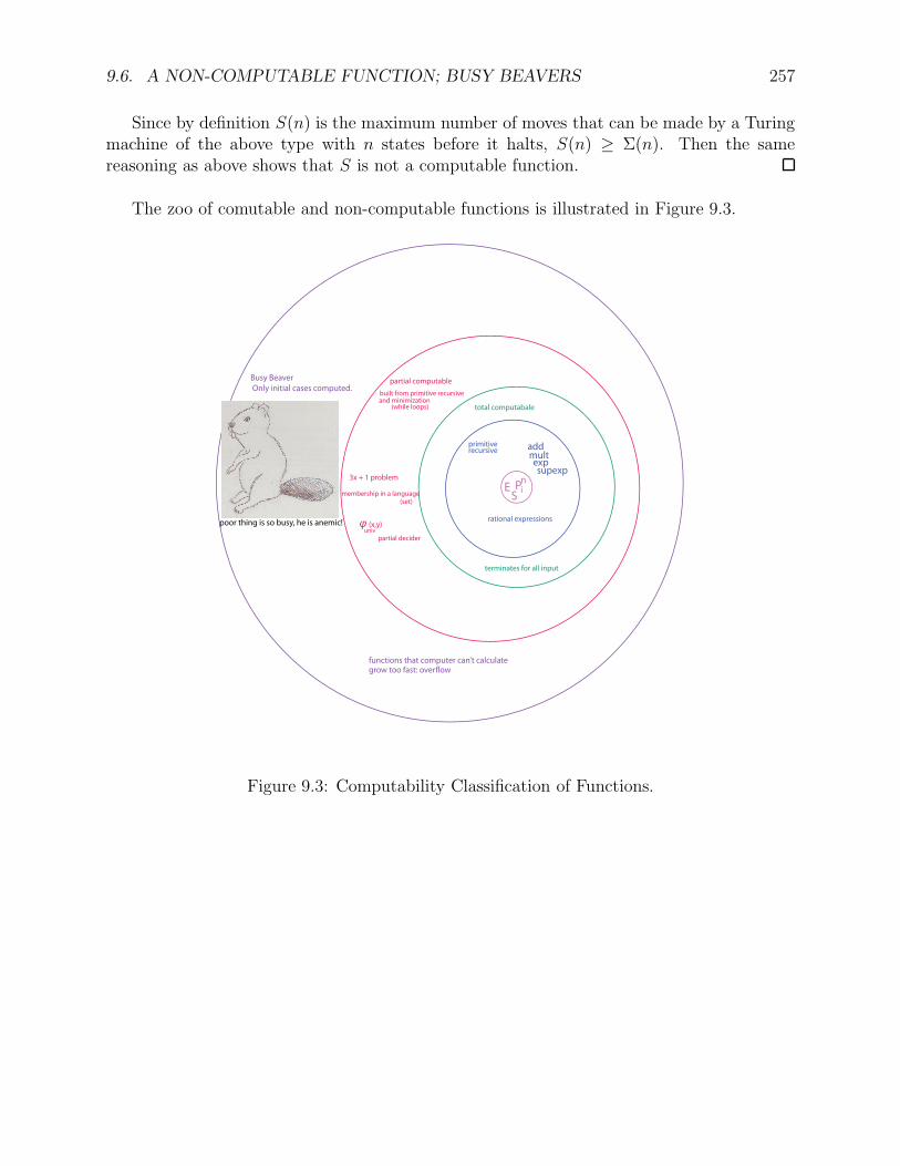
9.6. A NON-COMPUTABLE FUNCTION; BUSY BEAVERS 257
Since by definition S(n) is the maximum number of moves that can be made by a Turingmachine of the above type with n states before it halts, S(n) ≥ Σ(n). Then the samereasoning as above shows that S is not a computable function.
The zoo of comutable and non-computable functions is illustrated in Figure 9.3.
ESP
ni
primitiverecursive add
mult
supexp
rational expressions
total computabale
terminates for all input
partial computable
built from primitive recursiveand minimization
(while loops)
3x + 1 problem
membership in a language(set)
φuniv
(x,y)
partial decider
functions that computer can’t calculategrow too fast: overflow
Busy Beaver
Only initial cases computed.
poor thing is so busy, he is anemic!
exp
Figure 9.3: Computability Classification of Functions.
258 CHAPTER 9. UNIVERSAL RAM PROGRAMS AND THE HALTING PROBLEM
Chapter 10
Elementary Recursive FunctionTheory
10.1 Acceptable Indexings
In Chapter 9, we have exhibited a specific indexing of the partial computable functions byencoding the RAM programs. Using this indexing, we showed the existence of a universalfunction ϕuniv and of a computable function c, with the property that for all x, y ∈ N,
ϕc(x,y) = ϕx ϕy.
It is natural to wonder whether the same results hold if a different coding scheme is used orif a different model of computation is used, for example, Turing machines. In other words,we would like to know if our results depend on a specific coding scheme or not.
Our previous results showing the characterization of the partial computable functionsbeing independennt of the specific model used, suggests that it might be possible to pinpointcertain properties of coding schems which would allow an axiomatic development of recursivefunction theory. What we are aiming at is to find some simple properties of “nice” codingschemes that allow one to proceed without using explicit coding schemes, as long as theabove properties hold.
Remarkably, such properties exist. Furthermore, any two coding schemes having theseproperties are equivalent in a strong sense (effectively equivalent), and so, one can pickany such coding scheme without any risk of losing anything else because the wrong codingscheme was chosen. Such coding schemes, also called indexings, or Godel numberings, oreven programming systems, are called acceptable indexings .
Definition 10.1. An indexing of the partial computable functions is an infinite sequenceϕ0, ϕ1, . . . , of partial computable functions that includes all the partial computable func-tions of one argument (there might be repetitions, this is why we are not using the termenumeration). An indexing is universal if it contains the partial computable function ϕuniv
259
260 CHAPTER 10. ELEMENTARY RECURSIVE FUNCTION THEORY
such thatϕuniv(i, x) = ϕi(x)
for all i, x ∈ N. An indexing is acceptable if it is universal and if there is a total computablefunction c for composition, such that
ϕc(i,j) = ϕi ϕj
for all i, j ∈ N.
From Chapter 9, we know that the specific indexing of the partial computable functionsgiven for RAM programs is acceptable. Another characterization of acceptable indexings leftas an exercise is the following: an indexing ψ0, ψ1, ψ2, . . . of the partial computable functionsis acceptable iff there exists a total computable function f translating the RAM indexing ofSection 9.3 into the indexing ψ0, ψ1, ψ2, . . ., that is,
ϕi = ψf(i)
for all i ∈ N.
A very useful property of acceptable indexings is the so-called “s-m-n Theorem”. Usingthe slightly loose notation ϕ(x1, . . . , xn) for ϕ(〈x1, . . . , xn〉), the s-m-n theorem says thefollowing. Given a function ϕ considered as having m+ n arguments, if we fix the values ofthe first m arguments and we let the other n arguments vary, we obtain a function ψ of narguments. Then, the index of ψ depends in a computable fashion upon the index of ϕ andthe first m arguments x1, . . . , xm. We can “pull” the first m arguments of ϕ into the indexof ψ.
Theorem 10.1. (The “s-m-n Theorem”) For any acceptable indexing ϕ0, ϕ1, . . . , there is atotal computable function s, such that, for all i,m, n ≥ 1, for all x1, . . . , xm and all y1, . . . , yn,we have
ϕs(i,m,x1,...,xm)(y1, . . . , yn) = ϕi(x1, . . . , xm, y1, . . . , yn).
Proof. First, note that the above identity is really
ϕs(i,m,〈x1,...,xm〉)(〈y1, . . . , yn〉) = ϕi(〈x1, . . . , xm, y1, . . . , yn〉).
Recall that there is a primitive recursive function Con such that
Con(m, 〈x1, . . . , xm〉, 〈y1, . . . , yn〉) = 〈x1, . . . , xm, y1, . . . , yn〉
for all x1, . . . , xm, y1, . . . , yn ∈ N. Hence, a computable function s such that
ϕs(i,m,x)(y) = ϕi(Con(m, x, y))
will do. We define some auxiliary primitive recursive functions as follows:
P (y) = 〈0, y〉 and Q(〈x, y〉) = 〈x+ 1, y〉.
10.1. ACCEPTABLE INDEXINGS 261
Since we have an indexing of the partial computable functions, there are indices p and q suchthat P = ϕp and Q = ϕq. Let R be defined such that
R(0) = p,
R(x+ 1) = c(q, R(x)),
where c is the computable function for composition given by the indexing. We leave as anexercise to prove that
ϕR(x)(y) = 〈x, y〉for all x, y ∈ N. Also, recall that 〈x, y, z〉 = 〈x, 〈y, z〉〉, by definition of pairing. Then, wehave
ϕR(x) ϕR(y)(z) = ϕR(x)(〈y, z〉) = 〈x, y, z〉.Finally, let k be an index for the function Con, that is, let
ϕk(〈m, x, y〉) = Con(m, x, y).
Define s bys(i,m, x) = c(i, c(k, c(R(m), R(x)))).
Then, we have
ϕs(i,m,x)(y) = ϕi ϕk ϕR(m) ϕR(x)(y) = ϕi(Con(m, x, y)),
as desired. Notice that if the composition function c is primitive recursive, then s is alsoprimitive recursive. In particular, for the specific indexing of the RAM programs given inSection 9.3, the function s is primitive recursive.
As a first application of the s-m-n Theorem, we show that any two acceptable indexingsare effectively inter-translatable.
Theorem 10.2. Let ϕ0, ϕ1, . . . , be a universal indexing, and let ψ0, ψ1, . . . , be any indexingwith a total computable s-1-1 function, that is, a function s such that
ψs(i,1,x)(y) = ψi(x, y)
for all i, x, y ∈ N. Then, there is a total computable function t such that ϕi = ψt(i).
Proof. Let ϕuniv be a universal partial computable function for the indexing ϕ0, ϕ1, . . .. Sinceψ0, ψ1, . . . , is also an indexing, ϕuniv occurs somewhere in the second list, and thus, there issome k such that ϕuniv = ψk. Then, we have
ψs(k,1,i)(x) = ψk(i, x) = ϕuniv(i, x) = ϕi(x),
for all i, x ∈ N. Therefore, we can take the function t to be the function defined such that
t(i) = s(k, 1, i)
for all i ∈ N.
262 CHAPTER 10. ELEMENTARY RECURSIVE FUNCTION THEORY
Using Theorem 10.2, if we have two acceptable indexings ϕ0, ϕ1, . . . , and ψ0, ψ1, . . ., thereexist total computable functions t and u such that
ϕi = ψt(i) and ψi = ϕu(i)
for all i ∈ N. Also note that if the composition function c is primitive recursive, then anys-m-n function is primitive recursive, and the translation functions are primitive recursive.Actually, a stronger result can be shown. It can be shown that for any two acceptableindexings, there exist total computable injective and surjective translation functions. Inother words, any two acceptable indexings are recursively isomorphic (Roger’s isomorphismtheorem). Next, we turn to algorithmically unsolvable, or undecidable, problems.
10.2 Undecidable Problems
We saw in Section 9.3 that the halting problem for RAM programs is undecidable. In thissection, we take a slightly more general approach to study the undecidability of problems,and give some tools for resolving decidability questions.
First, we prove again the undecidability of the halting problem, but this time, for anyindexing of the partial computable functions.
Theorem 10.3. (Halting Problem, Abstract Version) Let ψ0, ψ1, . . . , be any indexing of thepartial computable functions. Then, the function f defined such that
f(x, y) =
1 if ψx(y) is defined,0 if ψx(y) is undefined,
is not computable.
Proof. Assume that f is computable, and let g be the function defined such that
g(x) = f(x, x)
for all x ∈ N. Then g is also computable. Let θ be the function defined such that
θ(x) =
0 if g(x) = 0,undefined if g(x) = 1.
We claim that θ is not even partial computable. Observe that θ is such that
θ(x) =
0 if ψx(x) is undefined,undefined if ψx(x) is defined.
If θ was partial computable, it would occur in the list as some ψi, and we would have
θ(i) = ψi(i) = 0 iff ψi(i) is undefined,
a contradiction. Therefore, f and g can’t be computable.
10.2. UNDECIDABLE PROBLEMS 263
Observe that the proof of Theorem 10.3 does not use the fact that the indexing is uni-versal or acceptable, and thus, the theorem holds for any indexing of the partial computablefunctions. The function g defined in the proof of Theorem 10.3 is the characteristic functionof a set denoted as K, where
K = x | ψx(x) is defined.
Given any set, X , for any subset, A ⊆ X , of X , recall that the characteristic function,CA (or χA), of A is the function, CA : X → 0, 1, defined so that, for all x ∈ X ,
CA(x) =1 if x ∈ A0 if x /∈ A.
The set K is an example of a set which is not computable (or not recursive). Since thisfact is quite important, we give the following definition:
Definition 10.2. A subset, A, of Σ∗ (or a subset, A, of N) is computable, or recursive,1 ordecidable iff its characteristic function, CA, is a total computable function.
Using Definition 10.2, Theorem 10.3 can be restated as follows.
Proposition 10.4. For any indexing ϕ0, ϕ1, . . . of the partial computable functions (over Σ∗
or N), the set K = x | ϕx(x) is defined is not computable (not recursive).
Computable (recursive) sets allow us to define the concept of a decidable (or undecidable)problem. The idea is to generalize the situation described in Section 9.3 and Section 9.4,where a set of objects, the RAM programs, is encoded into a set of natural numbers, usinga coding scheme.
Definition 10.3. Let C be a countable set of objects, and let P be a property of objects inC. We view P as the set
a ∈ C | P (a).A coding-scheme is an injective function #: C → N that assigns a unique code to each objectin C. The property P is decidable (relative to #) iff the set #(a) | a ∈ C and P (a) iscomputable (recursive). The property P is undecidable (relative to #) iff the set #(a) | a ∈C and P (a) is not computable (not recursive).
Observe that the decidability of a property P of objects in C depends upon the codingscheme #. Thus, if we are cheating in using a non-effective coding scheme, we may declarethat a property is decidabe even though it is not decidable in some reasonable coding scheme.Consequently, we require a coding scheme # to be effective in the following sense. Given any
1Since 1996, the term recursive has been considered old-fashioned by many researchers, and the termcomputable has been used instead.
264 CHAPTER 10. ELEMENTARY RECURSIVE FUNCTION THEORY
object a ∈ C, we can effectively (i.e.. algorithmically) determine its code #(a). Conversely,given any integer n ∈ N, we should be able to tell effectively if n is the code of some objectin C, and if so, to find this object. In practice, it is always possible to describe the objectsin C as strings over some (possibly complex) alphabet Σ (sets of trees, graphs, etc). In suchcases, the coding schemes are computable functions from Σ∗ to N = a1∗.
For example, let C = N×N, where the property P is the equality of the partial functionsϕx and ϕy. We can use the pairing function 〈−,−〉 as a coding function, and the problem isformally encoded as the computability (recursiveness) of the set
〈x, y〉 | x, y ∈ N, ϕx = ϕy.
In most cases, we don’t even bother to describe the coding scheme explicitly, knowingthat such a description is routine, although perhaps tedious.
We now show that most properties about programs (except the trivial ones) are undecid-able. First, we show that it is undecidable whether a RAM program halts for every input.In other words, it is undecidable whether a procedure is an algorithm. We actually prove amore general fact.
Proposition 10.5. For any acceptable indexing ϕ0, ϕ1, . . . of the partial computable func-tions, the set
TOTAL = x | ϕx is a total functionis not computable (not recursive).
Proof. The proof uses a technique known as reducibility. We try to reduce a set A knownto be noncomputable (nonrecursive) to TOTAL via a computable function f : A→ TOTAL,so that
x ∈ A iff f(x) ∈ TOTAL.
If TOTAL were computable (recursive), its characteristic function g would be computable,and thus, the function g f would be computable, a contradiction, since A is assumed to benoncomputable (nonrecursive. In the present case, we pick A = K. To find the computablefunction f : K → TOTAL, we use the s-m-n Theorem. Let θ be the function defined below:for all x, y ∈ N,
θ(x, y) =ϕx(x) if x ∈ K,undefined if x /∈ K.
Note that θ does not depend on y. The function θ is partial computable. Indeed, we have
θ(x, y) = ϕx(x) = ϕuniv(x, x).
Thus, θ has some index j, so that θ = ϕj , and by the s-m-n Theorem, we have
ϕs(j,1,x)(y) = ϕj(x, y) = θ(x, y).
10.2. UNDECIDABLE PROBLEMS 265
Let f be the computable function defined such that
f(x) = s(j, 1, x)
for all x ∈ N. Then, we have
ϕf(x)(y) =ϕx(x) if x ∈ K,undefined if x /∈ K
for all y ∈ N. Thus, observe that ϕf(x) is a total function iff x ∈ K, that is,
x ∈ K iff f(x) ∈ TOTAL,
where f is computable. As we explained earlier, this shows that TOTAL is not computable(not recursive).
The above argument can be generalized to yield a result known as Rice’s Theorem. Letϕ0, ϕ1, . . . be any indexing of the partial computable functions, and let C be any set of partialcomputable functions. We define the set PC as
PC = x ∈ N | ϕx ∈ C.
We can view C as a property of some of the partial computable functions. For example
C = all total computable functions.
We say that C is nontrivial if C is neither empty nor the set of all partial computablefunctions. Equivalently C is nontrivial iff PC 6= ∅ and PC 6= N. We may think of PC as theset of programs computing the functions in C.
Theorem 10.6. (Rice’s Theorem) For any acceptable indexing ϕ0, ϕ1, . . . of the partial com-putable functions, for any set C of partial computable functions, the set
PC = x ∈ N | ϕx ∈ C
is not computable (not recursive) unless C is trivial.
Proof. Assume that C is nontrivial. A set is computable (recursive) iff its complementis computable (recursive) (the proof is trivial). Hence, we may assume that the totallyundefined function is not in C, and since C 6= ∅, let ψ be some other function in C. Weproduce a computable function f such that
ϕf(x)(y) =
ψ(y) if x ∈ K,undefined if x /∈ K,
for all y ∈ N. We get f by using the s-m-n Theorem. Let ψ = ϕi, and define θ as follows:
θ(x, y) = ϕuniv(i, y) + (ϕuniv(x, x)− ϕuniv(x, x)),
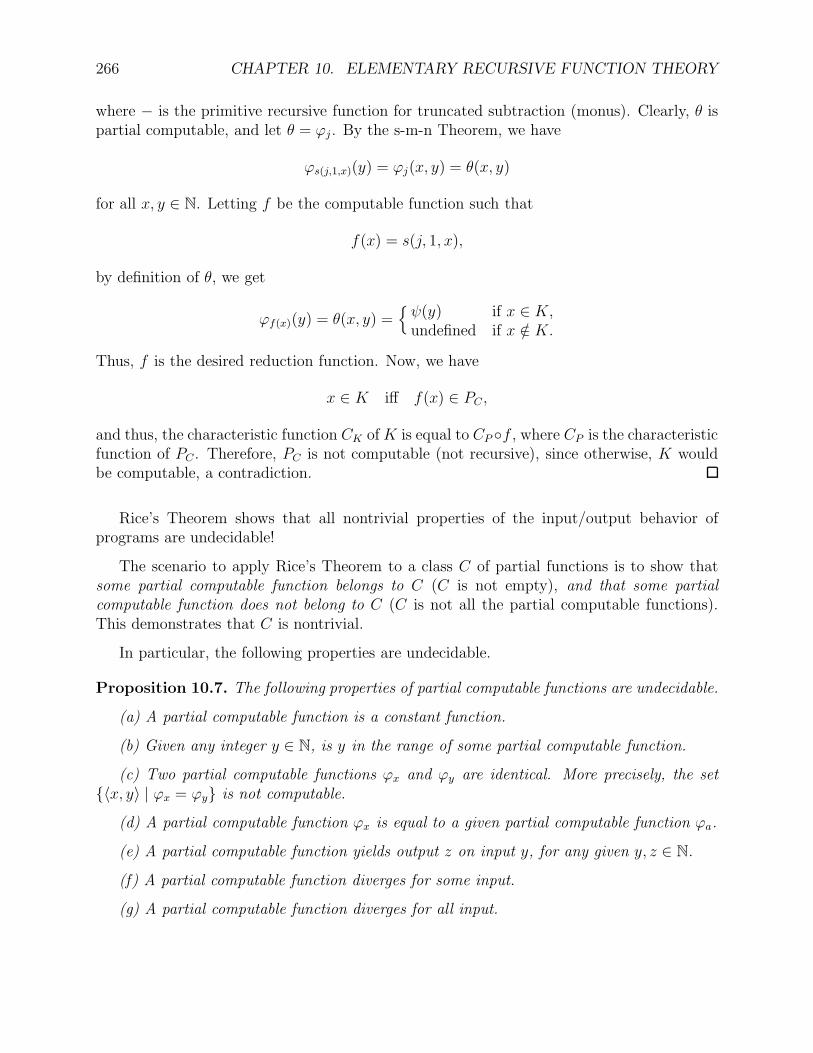
266 CHAPTER 10. ELEMENTARY RECURSIVE FUNCTION THEORY
where − is the primitive recursive function for truncated subtraction (monus). Clearly, θ ispartial computable, and let θ = ϕj . By the s-m-n Theorem, we have
ϕs(j,1,x)(y) = ϕj(x, y) = θ(x, y)
for all x, y ∈ N. Letting f be the computable function such that
f(x) = s(j, 1, x),
by definition of θ, we get
ϕf(x)(y) = θ(x, y) =ψ(y) if x ∈ K,undefined if x /∈ K.
Thus, f is the desired reduction function. Now, we have
x ∈ K iff f(x) ∈ PC ,
and thus, the characteristic function CK ofK is equal to CP f , where CP is the characteristicfunction of PC . Therefore, PC is not computable (not recursive), since otherwise, K wouldbe computable, a contradiction.
Rice’s Theorem shows that all nontrivial properties of the input/output behavior ofprograms are undecidable!
The scenario to apply Rice’s Theorem to a class C of partial functions is to show thatsome partial computable function belongs to C (C is not empty), and that some partialcomputable function does not belong to C (C is not all the partial computable functions).This demonstrates that C is nontrivial.
In particular, the following properties are undecidable.
Proposition 10.7. The following properties of partial computable functions are undecidable.
(a) A partial computable function is a constant function.
(b) Given any integer y ∈ N, is y in the range of some partial computable function.
(c) Two partial computable functions ϕx and ϕy are identical. More precisely, the set〈x, y〉 | ϕx = ϕy is not computable.
(d) A partial computable function ϕx is equal to a given partial computable function ϕa.
(e) A partial computable function yields output z on input y, for any given y, z ∈ N.
(f) A partial computable function diverges for some input.
(g) A partial computable function diverges for all input.
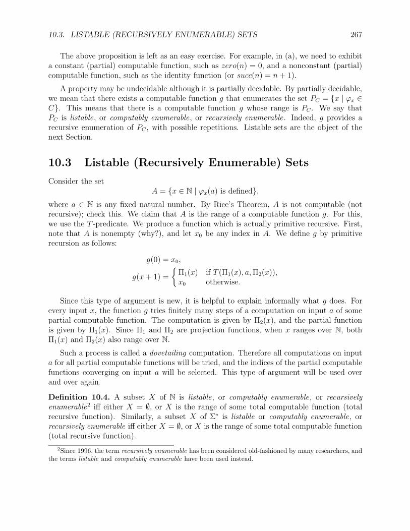
10.3. LISTABLE (RECURSIVELY ENUMERABLE) SETS 267
The above proposition is left as an easy exercise. For example, in (a), we need to exhibita constant (partial) computable function, such as zero(n) = 0, and a nonconstant (partial)computable function, such as the identity function (or succ(n) = n+ 1).
A property may be undecidable although it is partially decidable. By partially decidable,we mean that there exists a computable function g that enumerates the set PC = x | ϕx ∈C. This means that there is a computable function g whose range is PC . We say thatPC is listable, or computably enumerable, or recursively enumerable. Indeed, g provides arecursive enumeration of PC , with possible repetitions. Listable sets are the object of thenext Section.
10.3 Listable (Recursively Enumerable) Sets
Consider the setA = x ∈ N | ϕx(a) is defined,
where a ∈ N is any fixed natural number. By Rice’s Theorem, A is not computable (notrecursive); check this. We claim that A is the range of a computable function g. For this,we use the T -predicate. We produce a function which is actually primitive recursive. First,note that A is nonempty (why?), and let x0 be any index in A. We define g by primitiverecursion as follows:
g(0) = x0,
g(x+ 1) =
Π1(x) if T (Π1(x), a,Π2(x)),x0 otherwise.
Since this type of argument is new, it is helpful to explain informally what g does. Forevery input x, the function g tries finitely many steps of a computation on input a of somepartial computable function. The computation is given by Π2(x), and the partial functionis given by Π1(x). Since Π1 and Π2 are projection functions, when x ranges over N, bothΠ1(x) and Π2(x) also range over N.
Such a process is called a dovetailing computation. Therefore all computations on inputa for all partial computable functions will be tried, and the indices of the partial computablefunctions converging on input a will be selected. This type of argument will be used overand over again.
Definition 10.4. A subset X of N is listable, or computably enumerable, or recursivelyenumerable2 iff either X = ∅, or X is the range of some total computable function (totalrecursive function). Similarly, a subset X of Σ∗ is listable or computably enumerable, orrecursively enumerable iff either X = ∅, or X is the range of some total computable function(total recursive function).
2Since 1996, the term recursively enumerable has been considered old-fashioned by many researchers, andthe terms listable and computably enumerable have been used instead.
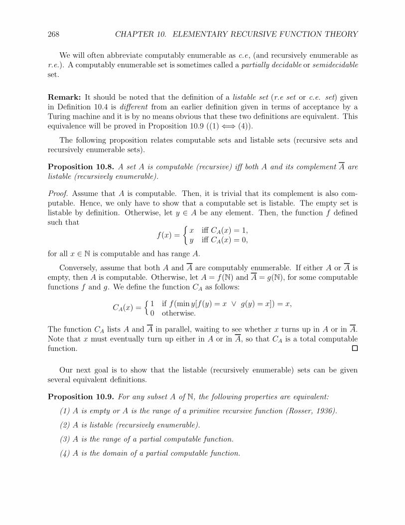
268 CHAPTER 10. ELEMENTARY RECURSIVE FUNCTION THEORY
We will often abbreviate computably enumerable as c.e, (and recursively enumerable asr.e.). A computably enumerable set is sometimes called a partially decidable or semidecidableset.
Remark: It should be noted that the definition of a listable set (r.e set or c.e. set) givenin Definition 10.4 is different from an earlier definition given in terms of acceptance by aTuring machine and it is by no means obvious that these two definitions are equivalent. Thisequivalence will be proved in Proposition 10.9 ((1)⇐⇒ (4)).
The following proposition relates computable sets and listable sets (recursive sets andrecursively enumerable sets).
Proposition 10.8. A set A is computable (recursive) iff both A and its complement A arelistable (recursively enumerable).
Proof. Assume that A is computable. Then, it is trivial that its complement is also com-putable. Hence, we only have to show that a computable set is listable. The empty set islistable by definition. Otherwise, let y ∈ A be any element. Then, the function f definedsuch that
f(x) =
x iff CA(x) = 1,y iff CA(x) = 0,
for all x ∈ N is computable and has range A.
Conversely, assume that both A and A are computably enumerable. If either A or A isempty, then A is computable. Otherwise, let A = f(N) and A = g(N), for some computablefunctions f and g. We define the function CA as follows:
CA(x) =1 if f(min y[f(y) = x ∨ g(y) = x]) = x,0 otherwise.
The function CA lists A and A in parallel, waiting to see whether x turns up in A or in A.Note that x must eventually turn up either in A or in A, so that CA is a total computablefunction.
Our next goal is to show that the listable (recursively enumerable) sets can be givenseveral equivalent definitions.
Proposition 10.9. For any subset A of N, the following properties are equivalent:
(1) A is empty or A is the range of a primitive recursive function (Rosser, 1936).
(2) A is listable (recursively enumerable).
(3) A is the range of a partial computable function.
(4) A is the domain of a partial computable function.
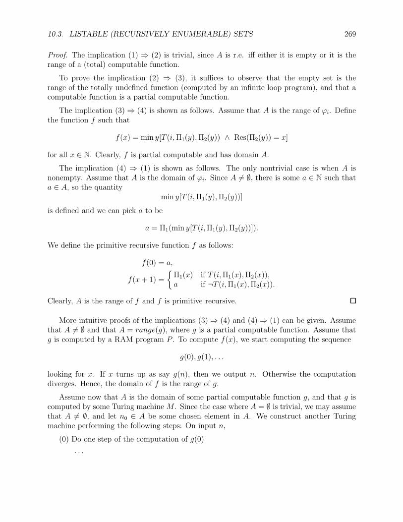
10.3. LISTABLE (RECURSIVELY ENUMERABLE) SETS 269
Proof. The implication (1) ⇒ (2) is trivial, since A is r.e. iff either it is empty or it is therange of a (total) computable function.
To prove the implication (2) ⇒ (3), it suffices to observe that the empty set is therange of the totally undefined function (computed by an infinite loop program), and that acomputable function is a partial computable function.
The implication (3)⇒ (4) is shown as follows. Assume that A is the range of ϕi. Definethe function f such that
f(x) = min y[T (i,Π1(y),Π2(y)) ∧ Res(Π2(y)) = x]
for all x ∈ N. Clearly, f is partial computable and has domain A.
The implication (4) ⇒ (1) is shown as follows. The only nontrivial case is when A isnonempty. Assume that A is the domain of ϕi. Since A 6= ∅, there is some a ∈ N such thata ∈ A, so the quantity
min y[T (i,Π1(y),Π2(y))]
is defined and we can pick a to be
a = Π1(min y[T (i,Π1(y),Π2(y))]).
We define the primitive recursive function f as follows:
f(0) = a,
f(x+ 1) =
Π1(x) if T (i,Π1(x),Π2(x)),a if ¬T (i,Π1(x),Π2(x)).
Clearly, A is the range of f and f is primitive recursive.
More intuitive proofs of the implications (3)⇒ (4) and (4)⇒ (1) can be given. Assumethat A 6= ∅ and that A = range(g), where g is a partial computable function. Assume thatg is computed by a RAM program P . To compute f(x), we start computing the sequence
g(0), g(1), . . .
looking for x. If x turns up as say g(n), then we output n. Otherwise the computationdiverges. Hence, the domain of f is the range of g.
Assume now that A is the domain of some partial computable function g, and that g iscomputed by some Turing machine M . Since the case where A = ∅ is trivial, we may assumethat A 6= ∅, and let n0 ∈ A be some chosen element in A. We construct another Turingmachine performing the following steps: On input n,
(0) Do one step of the computation of g(0)
. . .
270 CHAPTER 10. ELEMENTARY RECURSIVE FUNCTION THEORY
(n) Do n+ 1 steps of the computation of g(0)
Do n steps of the computation of g(1)
. . .
Do 2 steps of the computation of g(n− 1)
Do 1 step of the computation of g(n)
During this process, whenever the computation of g(m) halts for some m ≤ n, we outputm. Otherwise, we output n0.
In this fashion, we will enumerate the domain of g, and since we have constructed aTuring machine that halts for every input, we have a total computable function.
The following proposition can easily be shown using the proof technique of Proposition10.9.
Proposition 10.10. (1) There is a computable function h such that
range(ϕx) = dom(ϕh(x))
for all x ∈ N.
(2) There is a computable function k such that
dom(ϕx) = range(ϕk(x))
and ϕk(x) is total computable, for all x ∈ N such that dom(ϕx) 6= ∅.
The proof of Proposition 10.10 is left as an exercise. Using Proposition 10.9, we canprove that K is a listable set. Indeed, we have K = dom(f), where
f(x) = ϕuniv(x, x)
for all x ∈ N. The set
K0 = 〈x, y〉 | ϕx(y) convergesis also a listable set, since K0 = dom(g), where
g(z) = ϕuniv(Π1(z),Π2(z)),
which is partial computable. It worth recording these facts in the following lemma.
Proposition 10.11. The sets K and K0 are listable sets that are not computable (r.e. setsthat are not recursive).
We can now prove that there are sets that are not c.e. (r.e.).
10.3. LISTABLE (RECURSIVELY ENUMERABLE) SETS 271
Proposition 10.12. For any indexing of the partial computable functions, the complementK of the set
K = x ∈ N | ϕx(x) convergesis not listable (not recursively enumerable).
Proof. If K was listable, since K is also listable, by Proposition 10.8, the set K would becomputable, a contradiction.
The sets K and K0 are examples of sets that are not c.e. (r.e.). This shows that the c.e.sets (r.e. sets) are not closed under complementation. However, we leave it as an exercise toprove that the c.e. sets (r.e. sets) are closed under union and intersection.
We will prove later on that TOTAL is not c.e. (r.e.). This is rather unpleasant. Indeed,this means that there is no way of effectively listing all algorithms (all total computablefunctions). Hence, in a certain sense, the concept of partial computable function (procedure)is more natural than the concept of a (total) computable function (algorithm).
The next two propositions give other characterizations of the c.e. sets (r.e. sets) and ofthe computable sets (recursive sets). The proofs are left as an exercise.
Proposition 10.13. (1) A set A is c.e. (r.e.) iff either it is finite or it is the range of aninjective computable function.
(2) A set A is c.e. (r.e.) if either it is empty or it is the range of a monotonic partialcomputable function.
(3) A set A is c.e. (r.e.) iff there is a Turing machine M such that, for all x ∈ N, Mhalts on x iff x ∈ A.
Proposition 10.14. A set A is computable (recursive) iff either it is finite or it is the rangeof a strictly increasing computable function.
Another important result relating the concept of partial computable function and thatof a c.e. set (r.e. set) is given below.
Theorem 10.15. For every unary partial function f , the following properties are equivalent:
(1) f is partial computable.
(2) The set〈x, f(x)〉 | x ∈ dom(f)
is c.e. (r.e.).
Proof. Let g(x) = 〈x, f(x)〉. Clearly, g is partial computable, and
range(g) = 〈x, f(x)〉 | x ∈ dom(f).
272 CHAPTER 10. ELEMENTARY RECURSIVE FUNCTION THEORY
Conversely, assume that
range(g) = 〈x, f(x)〉 | x ∈ dom(f)
for some computable function g. Then, we have
f(x) = Π2(g(min y[Π1(g(y)) = x)]))
for all x ∈ N, so that f is partial computable.
Using our indexing of the partial computable functions and Proposition 10.9, we obtainan indexing of the c.e. sets. (r.e. sets).
Definition 10.5. For any acceptable indexing ϕ0, ϕ1, . . . of the partial computable functions,we define the enumeration W0,W1, . . . of the c.e. sets (r.e. sets) by setting
Wx = dom(ϕx).
We now describe a technique for showing that certain sets are c.e. (r.e.) but not com-putable (not recursive), or complements of c.e. sets (r.e. sets) that are not computable (notrecursive), or not c.e. (not r.e.), or neither c.e. (r.e.) nor the complement of a c.e. set (r.e.set). This technique is known as reducibility .
10.4 Reducibility and Complete Sets
We already used the notion of reducibility in the proof of Proposition 10.5 to show thatTOTAL is not computable (not recursive).
Definition 10.6. Let A and B be subsets of N (or Σ∗). We say that the set A is many-onereducible to the set B if there is a total computable function (or total recursive function)f : N→ N (or f : Σ∗ → Σ∗) such that
x ∈ A iff f(x) ∈ B for all x ∈ N.
We write A ≤ B, and for short, we say that A is reducible to B. Sometimes, the notationA ≤m B is used to stress that this is a many-to-one reduction (that is, f is not necessarilyinjective).
Intuitively, deciding membership in B is as hard as deciding membership in A. This isbecause any method for deciding membership in B can be converted to a method for decidingmembership in A by first applying f to the number (or string) to be tested.
The following simple proposition is left as an exercise to the reader.
10.4. REDUCIBILITY AND COMPLETE SETS 273
Proposition 10.16. Let A,B,C be subsets of N (or Σ∗). The following properties hold:
(1) If A ≤ B and B ≤ C, then A ≤ C.
(2) If A ≤ B then A ≤ B.
(3) If A ≤ B and B is c.e., then A is c.e.
(4) If A ≤ B and A is not c.e., then B is not c.e.
(5) If A ≤ B and B is computable, then A is computable.
(6) If A ≤ B and A is not computable, then B is not computable.
Another important concept is the concept of a complete set.
Definition 10.7. A c.e. set (r.e. set) A is complete w.r.t. many-one reducibility iff everyc.e. set (r.e. set) B is reducible to A, i.e., B ≤ A.
For simplicity, we will often say complete for complete w.r.t. many-one reducibility .Intuitively, a complete c.e. set (r.e. set) is a “hardest” c.e. set (r.e. set) as far as membershipis concerned.
Theorem 10.17. The following properties hold:
(1) If A is complete, B is c.e (r.e.), and A ≤ B, then B is complete.
(2) K0 is complete.
(3) K0 is reducible to K. Consequently, K is also complete.
Proof. (1) This is left as a simple exercise.
(2) Let Wx be any c.e. set. Then
y ∈ Wx iff 〈x, y〉 ∈ K0,
and the reduction function is the computable function f such that
f(y) = 〈x, y〉
for all y ∈ N.
(3) We use the s-m-n Theorem. First, we leave it as an exercise to prove that there is acomputable function f such that
ϕf(x)(y) =
1 if ϕΠ1(x)(Π2(x)) converges,undefined otherwise,
for all x, y ∈ N. Then, for every z ∈ N,
z ∈ K0 iff ϕΠ1(z)(Π2(z)) converges,
274 CHAPTER 10. ELEMENTARY RECURSIVE FUNCTION THEORY
iff ϕf(z)(y) = 1 for all y ∈ N. However,
ϕf(z)(y) = 1 iff ϕf(z)(f(z)) = 1,
since ϕf(z) is a constant function. This means that
z ∈ K0 iff f(z) ∈ K,
and f is the desired function.
As a corollary of Theorem 10.17, the set K is also complete.
Definition 10.8. Two sets A and B have the same degree of unsolvability or are equivalentiff A ≤ B and B ≤ A.
Since K and K0 are both complete, they have the same degree of unsolvability. We willnow investigate the reducibility and equivalence of various sets. Recall that
TOTAL = x ∈ N | ϕx is total.
We define EMPTY and FINITE, as follows:
EMPTY = x ∈ N | ϕx is undefined for all input,FINITE = x ∈ N | ϕx is defined only for finitely many input.
Obviously, EMPTY ⊂ FINITE, and since
FINITE = x ∈ N | ϕx has a finite domain,
we haveFINITE = x ∈ N | ϕx has an infinite domain,
and thus, TOTAL ⊂ FINITE.
Proposition 10.18. We have K0 ≤ EMPTY.
The proof of Proposition 10.18 follows from the proof of Theorem 10.17. We also havethe following proposition.
Proposition 10.19. The following properties hold:
(1) EMPTY is not c.e. (not r.e.).
(2) EMPTY is c.e. (r.e.).
(3) K and EMPTY are equivalent.
(4) EMPTY is complete.
10.4. REDUCIBILITY AND COMPLETE SETS 275
Proof. We prove (1) and (3), leaving (2) and (4) as an exercise (Actually, (2) and (4) followeasily from (3)). First, we show that K ≤ EMPTY. By the s-m-n Theorem, there exists acomputable function f such that
ϕf(x)(y) =
ϕx(x) if ϕx(x) converges,undefined if ϕx(x) diverges,
for all x, y ∈ N. Note that for all x ∈ N,
x ∈ K iff f(x) ∈ EMPTY,
and thus, K ≤ EMPTY. Since K is not c.e., EMPTY is not c.e.
By the s-m-n Theorem, there is a computable function g such that
ϕg(x)(y) = min z[T (x,Π1(z),Π2(z))],
for all x, y ∈ N. Note thatx ∈ EMPTY iff g(x) ∈ K
for all x ∈ N. Therefore, EMPTY ≤ K, and since we just showed that K ≤ EMPTY, thesets K and EMPTY are equivalent.
Proposition 10.20. The following properties hold:
(1) TOTAL and TOTAL are not c.e. (not r.e.).
(2) FINITE and FINITE are not c.e (not r.e.).
Proof. Checking the proof of Theorem 10.17, we note that K0 ≤ TOTAL and K0 ≤ FINITE.Hence, we get K0 ≤ TOTAL and K0 ≤ FINITE, and neither TOTAL nor FINITE is c.e.If TOTAL was c.e., then there would be a computable function f such that TOTAL =range(f). Define g as follows:
g(x) = ϕf(x)(x) + 1 = ϕuniv(f(x), x) + 1
for all x ∈ N. Since f is total and ϕf(x) is total for all x ∈ N, the function g is totalcomputable. Let e be an index such that
g = ϕf(e).
Since g is total, g(e) is defined. Then, we have
g(e) = ϕf(e)(e) + 1 = g(e) + 1,
a contradiction. Hence, TOTAL is not c.e. Finally, we show that TOTAL ≤ FINITE. Thisalso shows that FINITE is not c.e. By the s-m-n Theorem, there is a computable functionf such that
ϕf(x)(y) =
1 if ∀z ≤ y(ϕx(z) ↓),undefined otherwise,
276 CHAPTER 10. ELEMENTARY RECURSIVE FUNCTION THEORY
for all x, y ∈ N. It is easily seen that
x ∈ TOTAL iff f(x) ∈ FINITE
for all x ∈ N.
From Proposition 10.20, we have TOTAL ≤ FINITE. It turns out that FINITE ≤TOTAL, and TOTAL and FINITE are equivalent.
Proposition 10.21. The sets TOTAL and FINITE are equivalent.
Proof. We show that FINITE ≤ TOTAL. By the s-m-n Theorem, there is a computablefunction f such that
ϕf(x)(y) =
1 if ∃z ≥ y(ϕx(z) ↓),undefined if ∀z ≥ y(ϕx(z) ↑),
for all x, y ∈ N. It is easily seen that
x ∈ FINITE iff f(x) ∈ TOTAL
for all x ∈ N.
We now turn to the recursion Theorem.
10.5 The Recursion Theorem
The recursion Theorem, due to Kleene, is a fundamental result in recursion theory. Let fbe a total computable function. Then, it turns out that there is some n such that
ϕn = ϕf(n).
Theorem 10.22. (Recursion Theorem, Version 1) Let ϕ0, ϕ1, . . . be any acceptable indexingof the partial computable functions. For every total computable function f , there is some nsuch that
ϕn = ϕf(n).
Proof. Consider the function θ defined such that
θ(x, y) = ϕuniv(ϕuniv(x, x), y)
for all x, y ∈ N. The function θ is partial computable, and there is some index j such thatϕj = θ. By the s-m-n Theorem, there is a computable function g such that
ϕg(x)(y) = θ(x, y).
10.5. THE RECURSION THEOREM 277
Consider the function fg. Since it is computable, there is some indexm such that ϕm = fg.Let
n = g(m).
Since ϕm is total, ϕm(m) is defined, and we have
ϕn(y) = ϕg(m)(y) = θ(m, y) = ϕuniv(ϕuniv(m,m), y) = ϕϕuniv(m,m)(y)
= ϕϕm(m)(y) = ϕfg(m)(y) = ϕf(g(m))(y) = ϕf(n)(y),
for all y ∈ N. Therefore, ϕn = ϕf(n), as desired.
The recursion Theorem can be strengthened as follows.
Theorem 10.23. (Recursion Theorem, Version 2) Let ϕ0, ϕ1, . . . be any acceptable indexingof the partial computable functions. There is a total computable function h such that for allx ∈ N, if ϕx is total, then
ϕϕx(h(x)) = ϕh(x).
Proof. The computable function g obtained in the proof of Theorem 10.22 satisfies thecondition
ϕg(x) = ϕϕx(x),
and it has some index i such that ϕi = g. Recall that c is a computable composition functionsuch that
ϕc(x,y) = ϕx ϕy.
It is easily verified that the function h defined such that
h(x) = g(c(x, i))
for all x ∈ N does the job.
A third version of the recursion Theorem is given below.
Theorem 10.24. (Recursion Theorem, Version 3) For all n ≥ 1, there is a total computablefunction h of n + 1 arguments, such that for all x ∈ N, if ϕx is a total computable functionof n+ 1 arguments, then
ϕϕx(h(x,x1,...,xn),x1,...,xn) = ϕh(x,x1,...,xn),
for all x1, . . . , xn ∈ N.
Proof. Let θ be the function defined such that
θ(x, x1, . . . , xn, y) = ϕϕx(x,x1,...,xn)(y) = ϕuniv(ϕuniv(x, x, x1, . . . , xn), y)
278 CHAPTER 10. ELEMENTARY RECURSIVE FUNCTION THEORY
for all x, x1, . . . , xn, y ∈ N. By the s-m-n Theorem, there is a computable function g suchthat
ϕg(x,x1,...,xn) = ϕϕx(x,x1,...,xn).
It is easily shown that there is a computable function c such that
ϕc(i,j)(x, x1, . . . , xn) = ϕi(ϕj(x, x1, . . . , xn), x1, . . . , xn)
for any two partial computable functions ϕi and ϕj (viewed as functions of n+1 arguments)and all x, x1, . . . , xn ∈ N. Let ϕi = g, and define h such that
h(x, x1, . . . , xn) = g(c(x, i), x1, . . . , xn),
for all x, x1, . . . , xn ∈ N. We have
ϕh(x,x1,...,xn) = ϕg(c(x,i),x1,...,xn) = ϕϕc(x,i)(c(x,i),x1,...,xn),
and
ϕϕc(x,i)(c(x,i),x1,...,xn) = ϕϕx(ϕi(c(x,i),x1,...,xn),x1,...,xn),
= ϕϕx(g(c(x,i),x1,...,xn),x1,...,xn),
= ϕϕx(h(x,x1,...,xn),x1,...,xn).
As a first application of the recursion theorem, we can show that there is an index n suchthat ϕn is the constant function with output n. Loosely speaking, ϕn prints its own name.Let f be the computable function such that
f(x, y) = x
for all x, y ∈ N. By the s-m-n Theorem, there is a computable function g such that
ϕg(x)(y) = f(x, y) = x
for all x, y ∈ N. By the recursion Theorem 10.22, there is some n such that
ϕg(n) = ϕn,
the constant function with value n.
As a second application, we get a very short proof of Rice’s Theorem. Let C be suchthat PC 6= ∅ and PC 6= N, and let j ∈ PC and k ∈ N− PC . Define the function f as follows:
f(x) =
j if x /∈ PC ,k if x ∈ PC ,
10.5. THE RECURSION THEOREM 279
If PC is computable, then f is computable. By the recursion Theorem 10.22, there is somen such that
ϕf(n) = ϕn.
But then, we have
n ∈ PC iff f(n) /∈ PC
by definition of f , and thus,
ϕf(n) 6= ϕn,
a contradiction. Hence, PC is not computable.
As a third application, we prove the following proposition.
Proposition 10.25. Let C be a set of partial computable functions and let
A = x ∈ N | ϕx ∈ C.
The set A is not reducible to its complement A.
Proof. Assume that A ≤ A. Then, there is a computable function f such that
x ∈ A iff f(x) ∈ A
for all x ∈ N. By the recursion Theorem, there is some n such that
ϕf(n) = ϕn.
But then,
ϕn ∈ C iff n ∈ A iff f(n) ∈ A iff ϕf(n) ∈ C,contradicting the fact that
ϕf(n) = ϕn.
The recursion Theorem can also be used to show that functions defined by recursivedefinitions other than primitive recursion are partial computable. This is the case for thefunction known as Ackermann’s function, defined recursively as follows:
f(0, y) = y + 1,
f(x+ 1, 0) = f(x, 1),
f(x+ 1, y + 1) = f(x, f(x+ 1, y)).
It can be shown that this function is not primitive recursive. Intuitively, it outgrows allprimitive recursive functions. However, f is computable, but this is not so obvious. We can
280 CHAPTER 10. ELEMENTARY RECURSIVE FUNCTION THEORY
use the recursion Theorem to prove that f is computable. Consider the following definitionby cases:
g(n, 0, y) = y + 1,
g(n, x+ 1, 0) = ϕuniv(n, x, 1),
g(n, x+ 1, y + 1) = ϕuniv(n, x, ϕuniv(n, x+ 1, y)).
Clearly, g is partial computable. By the s-m-n Theorem, there is a computable function hsuch that
ϕh(n)(x, y) = g(n, x, y).
By the recursion Theorem, there is an m such that
ϕh(m) = ϕm.
Therefore, the partial computable function ϕm(x, y) satisfies the definition of Ackermann’sfunction. We showed in a previous Section that ϕm(x, y) is a total function, and thus,Ackermann’s function is a total computable function.
Hence, the recursion Theorem justifies the use of certain recursive definitions. How-ever, note that there are some recursive definitions that are only satisfied by the completelyundefined function.
In the next Section, we prove the extended Rice Theorem.
10.6 Extended Rice Theorem
The extended Rice Theorem characterizes the sets of partial computable functions C suchthat PC is c.e. (r.e.). First, we need to discuss a way of indexing the partial computablefunctions that have a finite domain. Using the uniform projection function Π, we define theprimitive recursive function F such that
F (x, y) = Π(y + 1,Π1(x) + 1,Π2(x)).
We also define the sequence of partial functions P0, P1, . . . as follows:
Px(y) =F (x, y)− 1 if 0 < F (x, y) and y < Π1(x) + 1,undefined otherwise.
Proposition 10.26. Every Px is a partial computable function with finite domain, and everypartial computable function with finite domain is equal to some Px.
The proof is left as an exercise. The easy part of the extended Rice Theorem is thefollowing lemma. Recall that given any two partial functions f : A→ B and g : A→ B, wesay that g extends f iff f ⊆ g, which means that g(x) is defined whenever f(x) is defined,and if so, g(x) = f(x).
10.6. EXTENDED RICE THEOREM 281
Proposition 10.27. Let C be a set of partial computable functions. If there is a c.e. set(r.e. set) A such that, ϕx ∈ C iff there is some y ∈ A such that ϕx extends Py, thenPC = x | ϕx ∈ C is c.e. (r.e.).
Proof. Proposition 10.27 can be restated as
PC = x | ∃y ∈ A, Py ⊆ ϕx
is c.e. If A is empty, so is PC , and PC is c.e. Otherwise, let f be a computable function suchthat
A = range(f).
Let ψ be the following partial computable function:
ψ(z) =Π1(z) if Pf(Π2(z)) ⊆ ϕΠ1(z),undefined otherwise.
It is clear thatPC = range(ψ).
To see that ψ is partial computable, write ψ(z) as follows:
ψ(z) =
Π1(z) if ∀w ≤ Π1(f(Π2(z)))[F (f(Π2(z)), w) > 0
⊃ ϕΠ1(z)(w) = F (f(Π2(z)), w)− 1],undefined otherwise.
To establish the converse of Proposition 10.27, we need two propositions.
Proposition 10.28. If PC is c.e. (r.e.) and ϕ ∈ C, then there is some Py ⊆ ϕ such thatPy ∈ C.
Proof. Assume that PC is c.e. and that ϕ ∈ C. By an s-m-n construction, there is acomputable function g such that
ϕg(x)(y) =
ϕ(y) if ∀z ≤ y[¬T (x, x, z)],undefined if ∃z ≤ y[T (x, x, z)],
for all x, y ∈ N. Observe that if x ∈ K, then ϕg(x) is a finite subfunction of ϕ, and if x ∈ K,then ϕg(x) = ϕ. Assume that no finite subfunction of ϕ is in C. Then,
x ∈ K iff g(x) ∈ PC
for all x ∈ N, that is, K ≤ PC . Since PC is c.e., K would also be c.e., a contradiction.
As a corollary of Proposition 10.28, we note that TOTAL is not c.e.
282 CHAPTER 10. ELEMENTARY RECURSIVE FUNCTION THEORY
Proposition 10.29. If PC is c.e. (r.e.), ϕ ∈ C, and ϕ ⊆ ψ, where ψ is a partial computablefunction, then ψ ∈ C.
Proof. Assume that PC is c.e. We claim that there is a computable function h such that
ϕh(x)(y) =
ψ(y) if x ∈ K,ϕ(y) if x ∈ K,
for all x, y ∈ N. Assume that ψ /∈ C. Then
x ∈ K iff h(x) ∈ PC
for all x ∈ N, that is, K ≤ PC , a contradiction, since PC is c.e. Therefore, ψ ∈ C. To findthe function h we proceed as follows: Let ϕ = ϕj and define Θ such that
Θ(x, y, z) =
ϕ(y) if T (j, y, z) ∧ ¬T (x, y, w), for 0 ≤ w < zψ(y) if T (x, x, z) ∧ ¬T (j, y, w), for 0 ≤ w < zundefined otherwise.
Observe that if x = y = j, then Θ(j, j, z) is multiply defined, but since ψ extends ϕ, weget the same value ψ(y) = ϕ(y), so Θ is a well defined partial function. Clearly, for all(m,n) ∈ N2, there is at most one z ∈ N so that Θ(x, y, z) is defined, so the function σdefined by
σ(x, y) =z if (x, y, z) ∈ dom(Θ)undefined otherwise
is a partial computable function. Finally, let
θ(x, y) = Θ(x, y, σ(x, y)),
a partial computable function. It is easy to check that
θ(x, y) =
ψ(y) if x ∈ K,ϕ(y) if x ∈ K,
for all x, y ∈ N. By the s-m-n Theorem, there is a computable function h such that
ϕh(x)(y) = θ(x, y)
for all x, y ∈ N.
Observe that Proposition 10.29 yields a new proof that TOTAL is not c.e. (not r.e.).Finally, we can prove the extended Rice Theorem.
Theorem 10.30. (Extended Rice Theorem) The set PC is c.e. (r.e.) iff there is a c.e. set(r.e. set) A such that
ϕx ∈ C iff ∃y ∈ A (Py ⊆ ϕx).
10.7. CREATIVE AND PRODUCTIVE SETS 283
Proof. Let PC = dom(ϕi). Using the s-m-n Theorem, there is a computable function k suchthat
ϕk(y) = Py
for all y ∈ N. Define the c.e. set A such that
A = dom(ϕi k).
Then,y ∈ A iff ϕi(k(y)) ↓ iff Py ∈ C.
Next, using Proposition 10.28 and Proposition 10.29, it is easy to see that
ϕx ∈ C iff ∃y ∈ A (Py ⊆ ϕx).
Indeed, if ϕx ∈ C, by Proposition 10.28, there is a finite subfunction Py ⊆ ϕx such thatPy ∈ C, but
Py ∈ C iff y ∈ A,as desired. On the other hand, if
Py ⊆ ϕx
for some y ∈ A, thenPy ∈ C,
and by Proposition 10.29, since ϕx extends Py, we get
ϕx ∈ C.
10.7 Creative and Productive Sets
In this section, we discuss some special sets that have important applications in logic: creativeand productive sets. The concepts to be described are illustrated by the following situation.Assume that
Wx ⊆ K
for some x ∈ N. We claim thatx ∈ K −Wx.
Indeed, if x ∈ Wx, then ϕx(x) is defined, and by definition of K, we get x /∈ K, a contradic-tion. Therefore, ϕx(x) must be undefined, that is,
x ∈ K −Wx.
The above situation can be generalized as follows.
284 CHAPTER 10. ELEMENTARY RECURSIVE FUNCTION THEORY
Definition 10.9. A set A is productive iff there is a total computable function f such that
if Wx ⊆ A then f(x) ∈ A−Wx
for all x ∈ N. The function f is called the productive function of A. A set A is creative if itis c.e (r.e.) and if its complement A is productive.
As we just showed, K is creative and K is productive. The following facts are immediateconequences of the definition.
(1) A productive set is not c.e. (r.e.).
(2) A creative set is not computable (not recursive).
Creative and productive sets arise in logic. The set of theorems of a logical theory isoften creative. For example, the set of theorems in Peano’s arithmetic is creative. Thisyields incompleteness results.
Proposition 10.31. If a set A is productive, then it has an infinite c.e. (r.e.) subset.
Proof. We first give an informal proof. let f be the computable productive function of A.We define a computable function g as follows: Let x0 be an index for the empty set, and let
g(0) = f(x0).
Assuming thatg(0), g(1), . . . , g(y)
is known, let xy+1 be an index for this finite set, and let
g(y + 1) = f(xy+1).
Since Wxy+1 ⊆ A, we have f(xy+1) ∈ A.For the formal proof, we use the following facts whose proof is left as an exercise:
(1) There is a computable function u such that
Wu(x,y) =Wx ∪Wy.
(2) There is a computable function t such that
Wt(x) = x.
Letting x0 be an index for the empty set, we define the function h as follows:
h(0) = x0,
h(y + 1) = u(t(f(y)), h(y)).
We define g such thatg = f h.
It is easily seen that g does the job.
10.7. CREATIVE AND PRODUCTIVE SETS 285
Another important property of productive sets is the following.
Proposition 10.32. If a set A is productive, then K ≤ A.
Proof. Let f be a productive function for A. Using the s-m-n Theorem, we can find acomputable function h such that
Wh(y,x) =
f(y) if x ∈ K,∅ if x ∈ K.
The above can be restated as follows:
ϕh(y,x)(z) =
1 if x ∈ K and z = f(y),undefined if x ∈ K,
for all x, y, z ∈ N. By the third version of the recursion Theorem (Theorem 10.24), there isa computable function g such that
Wg(x) =Wh(g(x),x)
for all x ∈ N. Letk = f g.
We claim thatx ∈ K iff k(x) ∈ A
for all x ∈ N. The verification of this fact is left as an exercise. Thus, K ≤ A.
Using Proposition 10.32, the following results can be shown.
Proposition 10.33. The following facts hold.
(1) If A is productive and A ≤ B, then B is productive.
(2) A is creative iff A is equivalent to K.
(3) A is creative iff A is complete,
286 CHAPTER 10. ELEMENTARY RECURSIVE FUNCTION THEORY
Chapter 11
Listable Sets and Diophantine Sets;Hilbert’s Tenth Problem
11.1 Diophantine Equations and Hilbert’s
Tenth Problem
There is a deep and a priori unexpected connection between the theory of computable andlistable sets and the solutions of polynomial equations involving polynomials in several vari-ables with integer coefficients. These are polynomials in n ≥ 1 variables x1, . . . , xn whichare finite sums of monomials of the form
axk11 · · ·xknn ,where k1, . . . , kn ∈ N are nonnegative integers, and a ∈ Z is an integer (possibly negative).The natural number k1 + · · ·+ kn is called the degree of the monomial axk11 · · ·xknn .
For example, if n = 3, then
1. 5, −7, are monomials of degree 0.
2. 3x1, −2x2, are monomials of degree 1.
3. x1x2, 2x21, 3x1x3, −5x22, are monomials of degree 2.
4. x1x2x3, x21x3, −x32, are monomials of degree 3.
5. x41, −x21x23, x1x22x3, are monomials of degree 4.
It is convenient to introduce multi-indices, where an n-dimensional multi-index is ann-tuple α = (k1, . . . , kn) with n ≥ 1 and ki ∈ N. Let |α| = k1 + · · ·+ kn. Then we can write
xα = xk11 · · ·xknn .For example, for n = 3,
x(1,2,1) = x1x22x3, x
(0,2,2) = x22x23.
287
288 CHAPTER 11. LISTABLE AND DIOPHANTINE SETS; HILBERT’S TENTH
Definition 11.1. A polynomial P (x1, . . . , xn) in the variables x1, . . . , xn with integer coef-ficients is a finite sum of monomials of the form
P (x1, . . . , xn) =∑
α
aαxα,
where the α’s are n-dimensional multi-indices, and with aα ∈ Z. The maximum of thedegrees |α| of the monomials aαx
α is called the total degree of the polynomial P (x1, . . . , xn).The set of all such polynomials is denoted by Z[x1, . . . , xn].
Sometimes, we write P instead of P (x1, . . . , xn). We also use variables x, y, z etc. insteadof x1, x2, x3, . . ..
For example, 2x− 3y − 1 is a polynomial of total degree 1, x2 + y2 − z2 is a polynomialof total degree 2, and x3 + y3 + z3 − 29 is a polynomial of total degree 3.
Mathematicians have been interested for a long time in the problem of solving equationsof the form
P (x1, . . . , xn) = 0,
with P ∈ Z[x1, . . . , xn], seeking only integer solutions for x1, . . . , xn.
Diophantus of Alexandria, a Greek mathematician of the 3rd century, was one of thefirst to investigate such equations. For this reason, seeking integer solutions of polynomialsin Z[x1, . . . , xn] is referred to as solving Diophantine equations .
This problem is not as simple as it looks. The equation
2x− 3y − 1 = 0
obviously has the solution x = 2, y = 1, and more generally x = −1 + 3a, y = −1 + 2a, forany integer a ∈ Z.
The equation
x2 + y2 − z2 = 0
has the solution x = 3, y = 4, z = 5, since 32 + 42 = 9 + 16 = 25 = 52. More generally, thereader should check that
x = t2 − 1, y = 2t, z = t2 + 1
is a solution for all t ∈ Z.
The equationx3 + y3 + z3 − 29 = 0
has the solution x = 3, y = 1, z = 1.
What about the equationx3 + y3 + z3 − 30 = 0?
11.1. DIOPHANTINE EQUATIONS; HILBERT’S TENTH PROBLEM 289
Amazingly, the only known integer solution is
(x, y, z) = (283059965, 2218888517, 2220422932),
discovered in 1999 by E. Pine, K. Yarbrough, W. Tarrant, and M. Beck, following an approachsuggested by N. Elkies.
And what about solutions of the equation
x3 + y3 + z3 − 33 = 0?
Well, nobody knows whether this equation is solvable in integers!
In 1900, at the International Congress of Mathematicians held in Paris, the famousmathematician David Hilbert presented a list of ten open mathematical problems. Soonafter, Hilbert published a list of 23 problems. The tenth problem is this:
Hilbert’s tenth problem (H10)
Find an algorithm that solves the following problem:
Given as input a polynomial P ∈ Z[x1, . . . , xn] with integer coefficients, return YES orNO, according to whether there exist integers a1, . . . , an ∈ Z so that P (a1, . . . , an) = 0; thatis, the Diophantine equation P (x1, . . . , xn) = 0 has a solution.
It is important to note that at the time Hilbert proposed his tenth problem, a rigorousmathematical definition of the notion of algorithm did not exist. In fact, the machineryneeded to even define the notion of algorithm did not exist. It is only around 1930 thatprecise definitions of the notion of computability due to Turing, Church, and Kleene, wereformulated, and soon after shown to be all equivalent.
So to be precise, the above statement of Hilbert’s tenth should say: find a RAM program(or equivalently a Turing machine) that solves the following problem: ...
In 1970, the following somewhat surprising resolution of Hilbert’s tenth problem wasreached:
Theorem (Davis-Putnam-Robinson-Matiyasevich)
Hilbert’s thenth problem is undecidable; that is, there is no algorithm for solving Hilbert’stenth problem.
In 1962, Davis, Putnam and Robinson had shown that if a fact known as Julia Robinsonhypothesis could be proved, then Hilbert’s tenth problem would be undecidable. At the time,the Julia Robinson hypothesis seemed implausible to many, so it was a surprise when in 1970Matiyasevich found a set satisfying the Julia Robinson hypothesis, thus completing the proofof the undecidability of Hilbert’s tenth problem. It is also a bit startling that Matiyasevich’set involves the Fibonacci numbers.
A detailed account of the history of the proof of the undecidability of Hilbert’s tenthproblem can be found in Martin Davis’ classical paper Davis [6].
290 CHAPTER 11. LISTABLE AND DIOPHANTINE SETS; HILBERT’S TENTH
Even though Hilbert’s tenth problem turned out to have a negative solution, the knowl-edge gained in developing the methods to prove this result is very significant. What wasrevealed is that polynomials have considerable expressive powers. This is what we discussin the next section.
11.2 Diophantine Sets and Listable Sets
We begin by showing that if we can prove that the version of Hilbert’s tenth problem withsolutions restricted to belong to N is undecidable, then Hilbert’s tenth problem (with solutionsin Z is undecidable).
Proposition 11.1. If we had an algorithm for solving Hilbert’s tenth problem (with solutionsin Z), then we would have an algorithm for solving Hilbert’s tenth problem with solutionsrestricted to belong to N (that is, nonnegative integers).
Proof. The above statement is not at all obvious, although its proof is short with the help ofsome number theory. Indeed, by a theorem of Lagrange (Lagrange’s four square theorem),every natural number m can be represented as the sum of four squares,
m = a20 + a21 + a22 + a23, a0, a1, a2, a3 ∈ Z.
We reduce Hilbert’s tenth problem restricted to solutions in N to Hilbert’s tenth problem(with solutions in Z). Given a Diophantine equation P (x1, . . . , xn) = 0, we can form thepolynomial
Q = P (u21 + v21 + y21 + z21 , . . . , u2n + v2n + y2n + z2n)
in the 4n variables ui, vi, yi, zi (1 ≤ i ≤ n) obtained by replacing xi by u2i + v2i + y2i + z2i for
i = 1, . . . , n. If Q = 0 has a solution (p1, q1, r1, s1, . . . , pn, qn, rn, sn, ) with pi, qi, ri, si ∈ Z,then if we set ai = p2i + q2i + r2i + s2i , obviously P (a1, . . . , an) = 0 with ai ∈ N. Conversely, ifP (a1, . . . , an) = 0 with ai ∈ N, then by Lagrange’s theorem there exist some pi, qi, ri, si ∈ Z
(in fact N) such that ai = p2i + q2i + r2i + s2i for i = 1, . . . , n, and the equation Q = 0 has thesolution (p1, q1, r1, s1, . . . , pn, qn, rn, sn, ) with pi, qi, ri, si ∈ Z. Therefore Q = 0 has a solution(p1, q1, r1, s1, . . . , pn, qn, rn, sn, ) with pi, qi, ri, si ∈ Z iff P = 0 has a solution (a!, . . . , an) withai ∈ N. If we had an algorithm to decide whether Q has a solution with its componentsin Z, then we would have an algorithm to decide whether P = 0 has a solution with itscomponents in N.
As consequence, the contrapositive of Proposition 11.1 shows that if the version ofHilbert’s tenth problem restricted to solutions in N is undecidable, so is Hilbert’s originalproblem (with solutions in Z).
In fact, the Davis-Putnam-Robinson-Matiyasevich theorem establishes the undecidabilityof the version of Hilbert’s tenth problem restricted to solutions in N. From now on, we restrictour attention to this version of Hilbert’s tenth problem.
11.2. DIOPHANTINE SETS AND LISTABLE SETS 291
A key idea is to use Diophantine equations with parameters, to define sets of numbers.
For example, consider the polynomial
P1(a, y, z) = (y + 2)(z + 2)− a.
For a ∈ N fixed, the equation (y + 2)(z + 2)− a = 0, equivalently
a = (y + 2)(z + 2),
has a solution with y, z ∈ N iff a is composite.
If we now consider the polynomial
P2(a, y, z) = y(2z + 3)− a,
for a ∈ N fixed, the equation y(2z + 3)− a = 0, equivalently
a = y(2z + 3),
has a solution with y, z ∈ N iff a is not a power of 2.
For a slightly more complicated example, consider the polynomial
P3(a, y) = 3y + 1− a2.
We leave it as an exercise to show that the natural numbers a that satisfy the equation3y + 1− a2 = 0, equivalently
a2 = 3y + 1,
or (a− 1)(a+ 1) = 3y, are of the form a = 3k + 1 or a = 3k + 2, for any k ∈ N.
In the first case, if we let S1 be the set of composite natural numbers, then we can write
S1 = a ∈ N | (∃y, z)((y + 2)(z + 2)− a = 0),
where it is understood that the existentially quantified variables y, z take their values in N.
In the second case, if we let S2 be the set of natural numbers that are not powers of 2,then we can write
S2 = a ∈ N | (∃y, z)(y(2z + 3)− a = 0).
In the third case, if we let S3 be the set of natural numbers that are congruent to 1 or 2modulo 3, then we can write
S3 = a ∈ N | (∃y)(3y + 1− a2 = 0).
A more explicit Diophantine definition for S3 is
S3 = a ∈ N | (∃y)((a− 3y − 1)(a− 3y − 2) = 0).
The natural generalization is as follows.
292 CHAPTER 11. LISTABLE AND DIOPHANTINE SETS; HILBERT’S TENTH
Definition 11.2. A set S ⊆ N of natural numbers is Diophantine (or Diophantine definable)if there is a polynomial P (a, x1, . . . , xn) ∈ Z[a, x1, . . . , xn], with n ≥ 01 such that
S = a ∈ N | (∃x1, . . . , xn)(P (a, x1, . . . , xn) = 0),
where it is understood that the existentially quantified variables x1, . . . , xn take their valuesin N. More generally, a relation R ⊆ Nm is Diophantine (m ≥ 2) if there is a polynomialP (a1, . . . , am, x1, . . . , xn) ∈ Z[a1, . . . , am, x1, . . . , xn], with n ≥ 0, such that
R = (a1, . . . , am) ∈ Nm | (∃x1, . . . , xn)(P (a1, . . . , am, x1, . . . , xn) = 0),
where it is understood that the existentially quantified variables x1, . . . , xn take their valuesin N.
For example, the strict order relation a1 < a2 is defined as follows:
a1 < a2 iff (∃x)(a1 + 1 + x− a2 = 0),
and the divisibility relation a1 | a2 (a1 divides a2) is defined as follows:
a1 | a2 iff (∃x)(a1x− a2 = 0).
What about the ternary relation R ⊆ N3 given by
(a1, a2, a3) ∈ R if a1 | a2 and a1 < a3?
At first glance it is not obvious how to “convert” a conjunction of Diophantine definitionsinto a single Diophantine definition, but we can do this using the following trick: given anyfinite number of Diophantine equations in the variables x1, . . . , xn,
P1 = 0, P2 = 0, . . . , Pm = 0, (∗)
observe that (∗) has a solution (a1, . . . , an), which means that Pi(a1, . . . , an) = 0 for i =1, . . . , m, iff the single equation
P 21 + P 2
2 + · · ·+ P 2m = 0 (∗∗)
also has the solution (a1, . . . , an). This is because, since P21 , P
22 , . . . , P
2m are all nonnegative,
their sum is equal to zero iff they are all equal to zero, that is P 2i = 0 for i = 1 . . . , m, which
is equivalent to Pi = 0 for i = 1 . . . , m.
Using this trick, we see that
(a1, a2, a3) ∈ R iff (∃u, v)((a1u− a2)2 + (a1 + 1 + v − a3)2 = 0).
We can also define the notion of Diophantine function.
1We have to allow n = 0. Otherwise singleton sets would not be Diophantine.
11.2. DIOPHANTINE SETS AND LISTABLE SETS 293
Definition 11.3. A function f : Nn → N is Diophantine iff its graph (a0, a1, . . . , an) ⊆Nn+1 | a0 = f(a1, . . . , an) is Diophantine.
For example, the pairing function J and the projection functions K,L due to Cantorintroduced in Section 9.1 are Diophantine, since
z = J(x, y) iff (x+ y − 1)(x+ y) + 2x− 2z = 0
x = K(z) iff (∃y)((x+ y − 1)(x+ y) + 2x− 2z = 0)
y = L(z) iff (∃x)((x+ y − 1)(x+ y) + 2x− 2z = 0).
How extensive is the family of Diophantine sets? The remarkable fact proved by Davis-Putnam-Robinson-Matiyasevich is that they coincide with the listable sets (the recursivelyenumerable sets). This is a highly nontrivial result.
The easy direction is the following result.
Proposition 11.2. Every Diophantine set is listable (recursively enumerable).
Proof sketch. Suppose S is given as
S = a ∈ N | (∃x1, . . . , xn)(P (a, x1, . . . , xn) = 0),
Using the extended pairing function 〈x1, . . . , xn〉n of Section 9.1, we enumerate all n-tuples(x1, . . . , xn) ∈ Nn, and during this process we compute P (a, x1, . . . , xn). If P (a, x1, . . . , xn)is zero, then we output a, else we go on. This way, S is the range of a computable function,and it is listable.
It is also easy to see that every Diophantine function is partial computable. The maintheorem of the theory of Diophantine sets is the following deep result.
Theorem 11.3. (Davis-Putnam-Robinson-Matiyasevich, 1970) Every listable subset of N isDiophantine. Every partial computable function is Diophantine.
Theorem 11.3 is often referred to as the DPRM theorem. A complete proof of Theorem11.3 is provided in Davis [6]. As noted by Davis, although the proof is certainly long andnontrivial, it only uses elementary facts of number theory, nothing more sophisticated thanthe Chinese remainder theorem. Nevetherless, the proof is a tour de force.
One of the most difficult steps is to show that the exponential function h(n, k) = nk
is Diophantine. This is done using the Pell equation. According to Martin Davis, theproof given in Davis [6] uses a combination of ideas from Matiyasevich and Julia Robinson.Matiyasevich’s proof used the Fibonacci numbers.
Using some results from the theory of computation it is now easy to deduce that Hilbert’stenth problem is undecidable. To achieve this, recall that there are listable sets that are not
294 CHAPTER 11. LISTABLE AND DIOPHANTINE SETS; HILBERT’S TENTH
computable. For example, it is shown in Lemma 10.11 that K = x ∈ N | ϕx(x) is definedis listable but not computable. Since K is listable, by Theorem 11.3, it is defined by someDiophantine equation
P (a, x1, . . . , xn) = 0,
which means that
K = a ∈ N | (∃x1 . . . , xn)(P (a, x1, . . . , xn) = 0).
We have the following strong form of the undecidability of Hilbert’s tenth problem, in thesense that it shows that Hilbert’s tenth problem is already undecidable for a fixed Diophan-tine equation in one parameter.
Theorem 11.4. There is no algorithm which takes as input the polynomial P (a, x1, . . . , xn)defining K and any natural number a ∈ N and decides whether
P (a, x1, . . . , xn) = 0.
Consequently, Hilbert’s tenth problem is undecidable.
Proof. If there was such an algorithm, then K would be decidable, a contradiction.
Any algorithm for solving Hilbert’s tenth problem could be used to decide whether ornot P (a, x1, . . . , xn) = 0, but we just showed that there is no such algorithm.
It is an open problem whether Hilbert’s tenth problem is undecidable if we allow rationalsolutions (that is, x1, . . . , xn ∈ Q).
Alexandra Shlapentokh proved that various extensions of Hilbert’s tenth problem areundecidable. These results deal with some algebraic number theory beyond the scope ofthese notes. Incidentally, Alexandra was an undegraduate at Penn and she worked on alogic project for me (finding a Gentzen system for a subset of temporal logic).
Having now settled once and for all the undecidability of Hilbert’s tenth problem, wenow briefly explore some interesting consequences of Theorem 11.3.
11.3 Some Applications of the DPRM Theorem
The first application of the DRPM theorem is a particularly striking way of defining thelistable subsets of N as the nonnegative ranges of polynomials with integer coefficients. Thisresult is due to Hilary Putnam.
Theorem 11.5. For every listable subset S of N, there is some polynomial Q(x, x1, . . . , xn)with integer coefficients such that
S = Q(a, b1, . . . , bn) | Q(a, b1, . . . , bn) ∈ N, a, b1, . . . , bn ∈ N.
11.3. SOME APPLICATIONS OF THE DPRM THEOREM 295
Proof. By the DPRM theorem (Theorem 11.3), there is some polynomial P (x, x1, . . . , xn)with integer coefficients such that
S = a ∈ N | (∃x1, . . . , xn)(P (a, x1, . . . , xn) = 0).
Let Q(x, x1, . . . , xn) be given by
Q(x, x1, . . . , xn) = (x+ 1)(1− P 2(x, x1, . . . , xn))− 1.
We claim that Q satisfies the statement of the theorem. If a ∈ S, then P (a, b1, . . . , bn) = 0for some b1, . . . , bn ∈ N, so
Q(a, b1, . . . , bn) = (a+ 1)(1− 0)− 1 = a.
This shows that all a ∈ S show up the the nonnegative range of Q. Conversely, assume thatQ(a, b1, . . . , bn) ≥ 0 for some a, b1, . . . , bn ∈ N. Then by definition of Q we must have
(a+ 1)(1− P 2(a, b1, . . . , bn))− 1 ≥ 0,
that is,(a+ 1)(1− P 2(a, b1, . . . , bn)) ≥ 1,
and since a ∈ N, this implies that P 2(a, b1, . . . , bn) < 1, but since P is a polynomial with in-teger coefficients and a, b1, . . . , bn ∈ N, the expression P 2(a, b1, . . . , bn) must be a nonnegativeinteger, so we must have
P (a, b1, . . . , bn) = 0,
which shows that a ∈ S.
Remark: It should be noted that in general, the polynomials Q arising in Theorem 11.5may take on negative integer values, and to obtain all listable sets, we must restrict ourselfto their nonnegative range.
As an example, the set S3 of natural numbers that are congruent to 1 or 2 modulo 3 isgiven by
S3 = a ∈ N | (∃y)(3y + 1− a2 = 0).so by Theorem 11.5, S3 is the nonnegative range of the polynomial
Q(x, y) = (x+ 1)(1− (3y + 1− x2)2))− 1
= −(x+ 1)((3y − x2)2 + 2(3y − x2)))− 1
= (x+ 1)(x2 − 3y)(2− (x2 − 3y))− 1.
Observe that Q(x, y) takes on negative values. For example, Q(0, 0) = −1. Also, in orderfor Q(x, y) to be nonnegative, (x2 − 3y)(2− (x2 − 3y)) must be positive, but this can onlyhappen if x2 − 3y = 1, that is, x2 = 3y + 1, which is the original equation defining S3.
296 CHAPTER 11. LISTABLE AND DIOPHANTINE SETS; HILBERT’S TENTH
There is no miracle. The nonnegativity of Q(x, x1, . . . , xn) must subsume the solvabilityof the equation P (x, x1, . . . , xn) = 0.
A particularly interesting listable set is the set of primes. By Theorem 11.5, in theory,the set of primes is the positive range of some polynomial with integer coefficients.
Remarkably, some explicit polynomials have been found. This is a nontrivial task. Inparticular, the process involves showing that the exponential function is definable, whichwas the stumbling block of the completion of the DPRM theorem for many years.
To give the reader an idea of how the proof begins, observe by the Bezout identity, ifp = s+ 1 and q = s!, then we can assert that p and q are relatively prime (gcd(p, q) = 1) asthe fact that the Diophantine equation
ap− bq = 1
is satisfied for some a, b ∈ N. Then, it is not hard to see that p ∈ N is prime iff the followingset of equations has a solution for a, b, s, r, q ∈ N:
p = s+ 1
p = r + 2
q = s!
ap− bq = 1.
The problem with the above is that the equation q = s! is not Diophantine. The next stepis to show that the factorial function is Diophantine, and this involves a lot of work. Oneway to proceed is to show that the above system is equivalent to a system allowing the useof the exponential function. The final step is to show that the exponential function can beeliminated in favor of polynomial equations.
We refer the interested reader to the remarkable expository paper by Davis, Matiyasevichand Robinson [7] for details. Here is a polynomial of total degree 25 in 26 variables (due toJ. Jones, D. Sato, H. Wada, D. Wiens) which produces the primes as its positive range:
(k + 2)[1− ([wz + h+ j − q]2 + [(gk + 2g + k + 1)(h+ j) + h− z]2
+ [16(k + 1)3(k + 2)(n + 1)2 + 1− f 2]2
+ [2n + p+ q + z − e]2 + [e3(e+ 2)(a+ 1)2 + 1− o2]2+ [(a2 − 1)y2 + 1− x2]2 + [16r2y4(a2 − 1) + 1− u2]2+ [((a + u2(u2 − a))2 − 1)(n+ 4dy)2 + 1− (x+ cu)2]2
+ [(a2 − 1)l2 + 1−m2]2 + [ai+ k + 1− l − i]2 + [n+ l + v − y]2+ [p + l(a− n− 1) + b(2an+ 2a− n2 − 2n− 2)−m]2
+ [q + y(a− p− 1) + s(2ap+ 2a− p2 − 2p− 2)− x]2
+ [z + pl(a− p) + t(2ap− p2 − 1)− pm]2)].
11.3. SOME APPLICATIONS OF THE DPRM THEOREM 297
Around 2004, Nachi Gupta, an undergraduate student at Penn, and I, tried to producethe prime 2 as one of the values of the positive range of the above polynomial. It turns outthat this leads to values of the variables that are so large that we never succeeded!
Other interesting applications of the DPRM theorem are the re-statements of famousopen problems, such as the Riemann hypothesis, as the unsolvability of certain Diophantineequations. One may also obtain a nice variant of Godel’s incompleteness theorem. For allthis, see Davis, Matiyasevich and Robinson [7].

298 CHAPTER 11. LISTABLE AND DIOPHANTINE SETS; HILBERT’S TENTH
Chapter 12
The Post Correspondence Problem;Applications to UndecidabilityResults
12.1 The Post Correspondence Problem
The Post correspondence problem (due to Emil Post) is another undecidable problem thatturns out to be a very helpful tool for proving problems in logic or in formal language theoryto be undecidable.
Let Σ be an alphabet with at least two letters. An instance of the Post Correspondenceproblem (for short, PCP) is given by two sequences U = (u1, . . . , um) and V = (v1, . . . , vm),of strings ui, vi ∈ Σ∗.
The problem is to find whether there is a (finite) sequence (i1, . . . , ip), with ij ∈ 1, . . . , mfor j = 1, . . . , p, so that
ui1ui2 · · ·uip = vi1vi2 · · · vip.
Equivalently, an instance of the PCP is a sequence of pairs
(u1, v1), . . . , (um, vm).
For example, consider the following problem:
(abab, ababaaa), (aaabbb, bb), (aab, baab), (ba, baa), (ab, ba), (aa, a).
There is a solution for the string 1234556:
abab aaabbb aab ba ab ab aa = ababaaa bb baab baa ba ba a.
We are beginning to suspect that this is a hard problem. Indeed, it is undecidable!
299
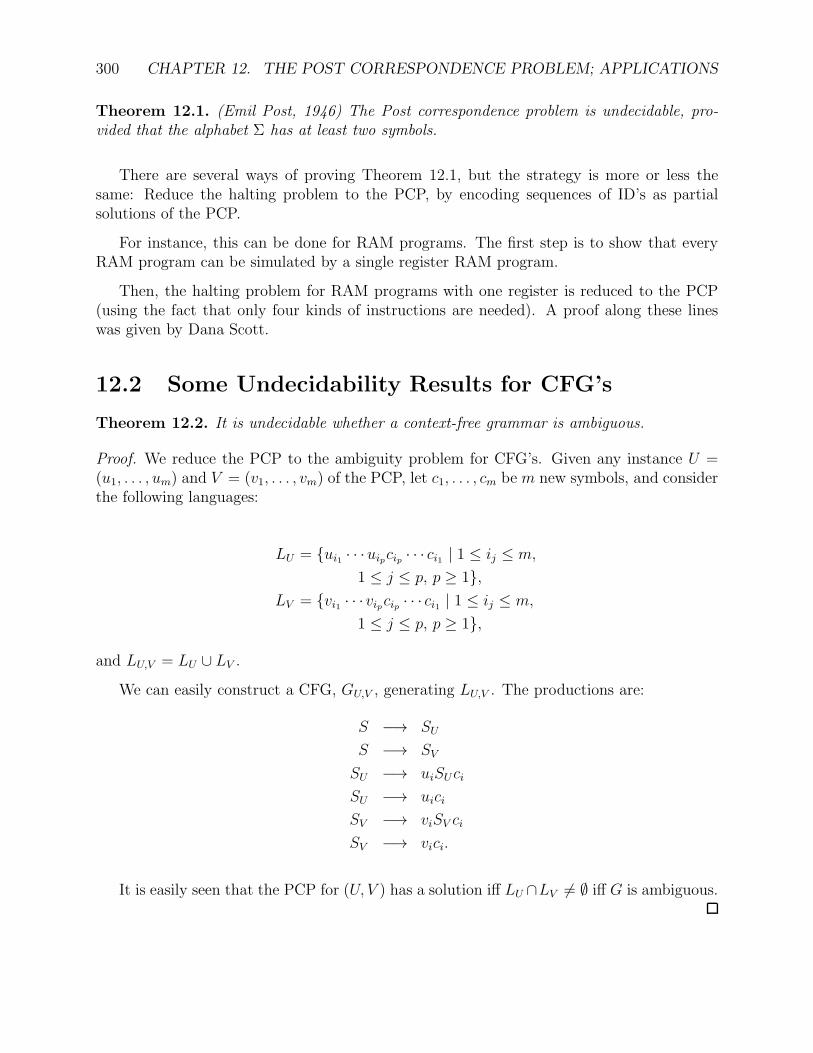
300 CHAPTER 12. THE POST CORRESPONDENCE PROBLEM; APPLICATIONS
Theorem 12.1. (Emil Post, 1946) The Post correspondence problem is undecidable, pro-vided that the alphabet Σ has at least two symbols.
There are several ways of proving Theorem 12.1, but the strategy is more or less thesame: Reduce the halting problem to the PCP, by encoding sequences of ID’s as partialsolutions of the PCP.
For instance, this can be done for RAM programs. The first step is to show that everyRAM program can be simulated by a single register RAM program.
Then, the halting problem for RAM programs with one register is reduced to the PCP(using the fact that only four kinds of instructions are needed). A proof along these lineswas given by Dana Scott.
12.2 Some Undecidability Results for CFG’s
Theorem 12.2. It is undecidable whether a context-free grammar is ambiguous.
Proof. We reduce the PCP to the ambiguity problem for CFG’s. Given any instance U =(u1, . . . , um) and V = (v1, . . . , vm) of the PCP, let c1, . . . , cm be m new symbols, and considerthe following languages:
LU = ui1 · · ·uipcip · · · ci1 | 1 ≤ ij ≤ m,
1 ≤ j ≤ p, p ≥ 1,LV = vi1 · · · vipcip · · · ci1 | 1 ≤ ij ≤ m,
1 ≤ j ≤ p, p ≥ 1,
and LU,V = LU ∪ LV .
We can easily construct a CFG, GU,V , generating LU,V . The productions are:
S −→ SU
S −→ SV
SU −→ uiSUci
SU −→ uici
SV −→ viSV ci
SV −→ vici.
It is easily seen that the PCP for (U, V ) has a solution iff LU ∩LV 6= ∅ iff G is ambiguous.
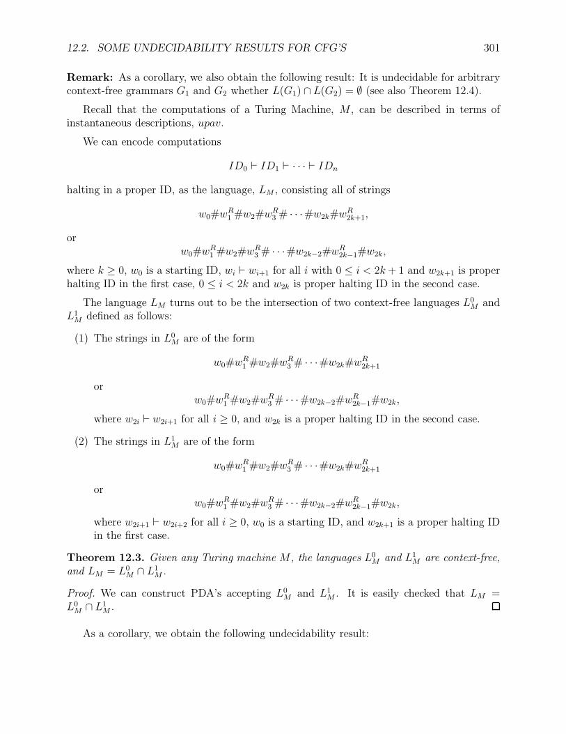
12.2. SOME UNDECIDABILITY RESULTS FOR CFG’S 301
Remark: As a corollary, we also obtain the following result: It is undecidable for arbitrarycontext-free grammars G1 and G2 whether L(G1) ∩ L(G2) = ∅ (see also Theorem 12.4).
Recall that the computations of a Turing Machine, M , can be described in terms ofinstantaneous descriptions, upav.
We can encode computations
ID0 ⊢ ID1 ⊢ · · · ⊢ IDn
halting in a proper ID, as the language, LM , consisting all of strings
w0#wR1 #w2#w
R3 # · · ·#w2k#w
R2k+1,
orw0#w
R1 #w2#w
R3 # · · ·#w2k−2#w
R2k−1#w2k,
where k ≥ 0, w0 is a starting ID, wi ⊢ wi+1 for all i with 0 ≤ i < 2k+ 1 and w2k+1 is properhalting ID in the first case, 0 ≤ i < 2k and w2k is proper halting ID in the second case.
The language LM turns out to be the intersection of two context-free languages L0M and
L1M defined as follows:
(1) The strings in L0M are of the form
w0#wR1 #w2#w
R3 # · · ·#w2k#w
R2k+1
orw0#w
R1 #w2#w
R3 # · · ·#w2k−2#w
R2k−1#w2k,
where w2i ⊢ w2i+1 for all i ≥ 0, and w2k is a proper halting ID in the second case.
(2) The strings in L1M are of the form
w0#wR1 #w2#w
R3 # · · ·#w2k#w
R2k+1
orw0#w
R1 #w2#w
R3 # · · ·#w2k−2#w
R2k−1#w2k,
where w2i+1 ⊢ w2i+2 for all i ≥ 0, w0 is a starting ID, and w2k+1 is a proper halting IDin the first case.
Theorem 12.3. Given any Turing machine M , the languages L0M and L1
M are context-free,and LM = L0
M ∩ L1M .
Proof. We can construct PDA’s accepting L0M and L1
M . It is easily checked that LM =L0M ∩ L1
M .
As a corollary, we obtain the following undecidability result:
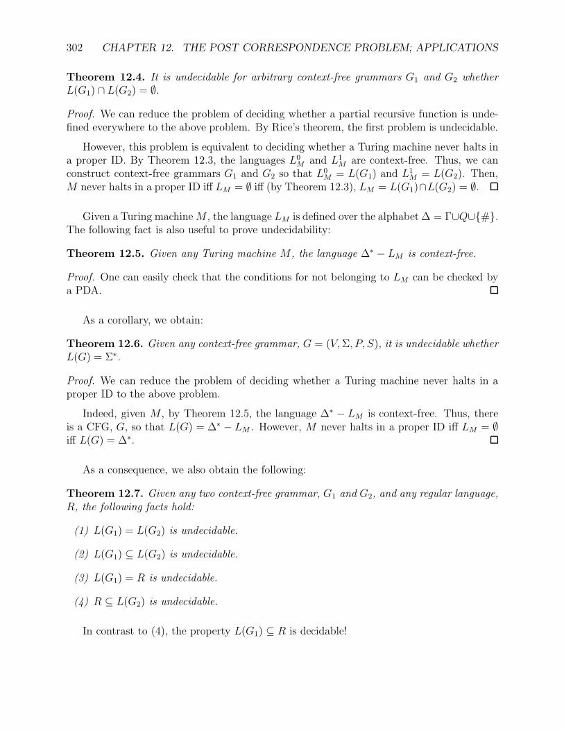
302 CHAPTER 12. THE POST CORRESPONDENCE PROBLEM; APPLICATIONS
Theorem 12.4. It is undecidable for arbitrary context-free grammars G1 and G2 whetherL(G1) ∩ L(G2) = ∅.
Proof. We can reduce the problem of deciding whether a partial recursive function is unde-fined everywhere to the above problem. By Rice’s theorem, the first problem is undecidable.
However, this problem is equivalent to deciding whether a Turing machine never halts ina proper ID. By Theorem 12.3, the languages L0
M and L1M are context-free. Thus, we can
construct context-free grammars G1 and G2 so that L0M = L(G1) and L
1M = L(G2). Then,
M never halts in a proper ID iff LM = ∅ iff (by Theorem 12.3), LM = L(G1)∩L(G2) = ∅.
Given a Turing machineM , the language LM is defined over the alphabet ∆ = Γ∪Q∪#.The following fact is also useful to prove undecidability:
Theorem 12.5. Given any Turing machine M , the language ∆∗ − LM is context-free.
Proof. One can easily check that the conditions for not belonging to LM can be checked bya PDA.
As a corollary, we obtain:
Theorem 12.6. Given any context-free grammar, G = (V,Σ, P, S), it is undecidable whetherL(G) = Σ∗.
Proof. We can reduce the problem of deciding whether a Turing machine never halts in aproper ID to the above problem.
Indeed, given M , by Theorem 12.5, the language ∆∗ − LM is context-free. Thus, thereis a CFG, G, so that L(G) = ∆∗ − LM . However, M never halts in a proper ID iff LM = ∅iff L(G) = ∆∗.
As a consequence, we also obtain the following:
Theorem 12.7. Given any two context-free grammar, G1 and G2, and any regular language,R, the following facts hold:
(1) L(G1) = L(G2) is undecidable.
(2) L(G1) ⊆ L(G2) is undecidable.
(3) L(G1) = R is undecidable.
(4) R ⊆ L(G2) is undecidable.
In contrast to (4), the property L(G1) ⊆ R is decidable!
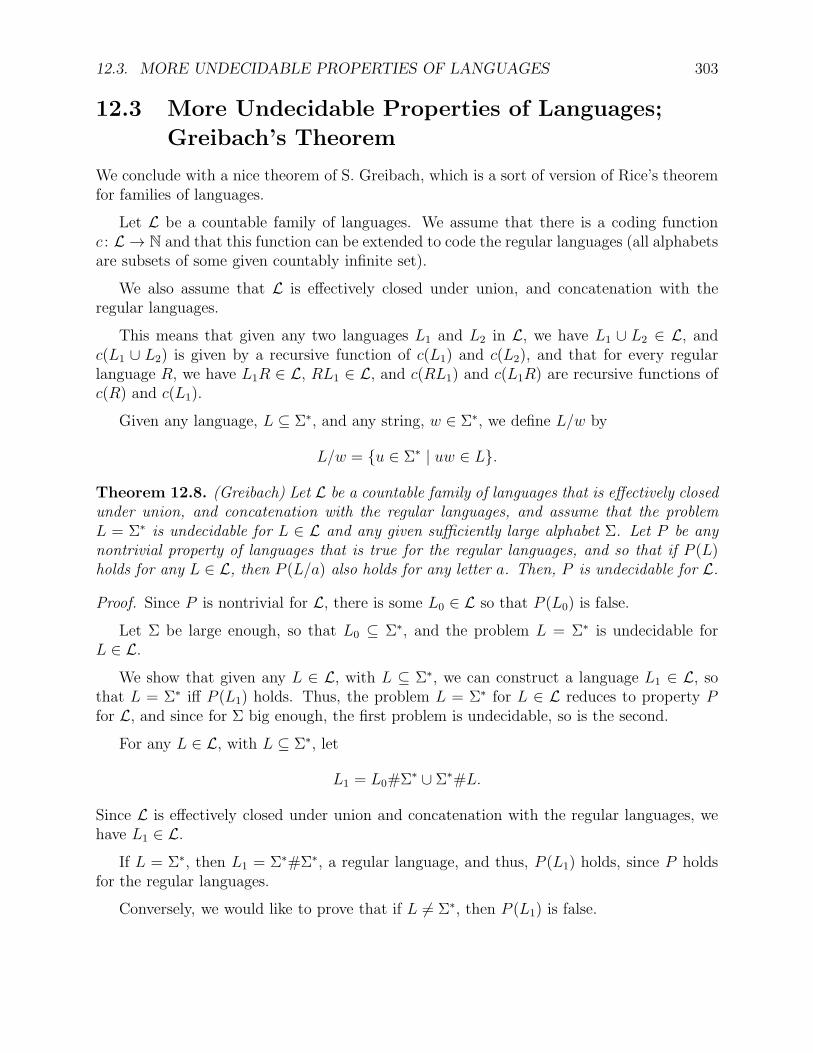
12.3. MORE UNDECIDABLE PROPERTIES OF LANGUAGES 303
12.3 More Undecidable Properties of Languages;
Greibach’s Theorem
We conclude with a nice theorem of S. Greibach, which is a sort of version of Rice’s theoremfor families of languages.
Let L be a countable family of languages. We assume that there is a coding functionc : L → N and that this function can be extended to code the regular languages (all alphabetsare subsets of some given countably infinite set).
We also assume that L is effectively closed under union, and concatenation with theregular languages.
This means that given any two languages L1 and L2 in L, we have L1 ∪ L2 ∈ L, andc(L1 ∪ L2) is given by a recursive function of c(L1) and c(L2), and that for every regularlanguage R, we have L1R ∈ L, RL1 ∈ L, and c(RL1) and c(L1R) are recursive functions ofc(R) and c(L1).
Given any language, L ⊆ Σ∗, and any string, w ∈ Σ∗, we define L/w by
L/w = u ∈ Σ∗ | uw ∈ L.
Theorem 12.8. (Greibach) Let L be a countable family of languages that is effectively closedunder union, and concatenation with the regular languages, and assume that the problemL = Σ∗ is undecidable for L ∈ L and any given sufficiently large alphabet Σ. Let P be anynontrivial property of languages that is true for the regular languages, and so that if P (L)holds for any L ∈ L, then P (L/a) also holds for any letter a. Then, P is undecidable for L.
Proof. Since P is nontrivial for L, there is some L0 ∈ L so that P (L0) is false.
Let Σ be large enough, so that L0 ⊆ Σ∗, and the problem L = Σ∗ is undecidable forL ∈ L.
We show that given any L ∈ L, with L ⊆ Σ∗, we can construct a language L1 ∈ L, sothat L = Σ∗ iff P (L1) holds. Thus, the problem L = Σ∗ for L ∈ L reduces to property Pfor L, and since for Σ big enough, the first problem is undecidable, so is the second.
For any L ∈ L, with L ⊆ Σ∗, let
L1 = L0#Σ∗ ∪ Σ∗#L.
Since L is effectively closed under union and concatenation with the regular languages, wehave L1 ∈ L.
If L = Σ∗, then L1 = Σ∗#Σ∗, a regular language, and thus, P (L1) holds, since P holdsfor the regular languages.
Conversely, we would like to prove that if L 6= Σ∗, then P (L1) is false.
304 CHAPTER 12. THE POST CORRESPONDENCE PROBLEM; APPLICATIONS
Since L 6= Σ∗, there is some w /∈ L. But then,
L1/#w = L0.
Since P is preserved under quotient by a single letter, by a trivial induction, if P (L1) holds,then P (L0) also holds. However, P (L0) is false, so P (L1) must be false.
Thus, we proved that L = Σ∗ iff P (L1) holds, as claimed.
Greibach’s theorem can be used to show that it is undecidable whether a context-freegrammar generates a regular language.
It can also be used to show that it is undecidable whether a context-free language isinherently ambiguous.
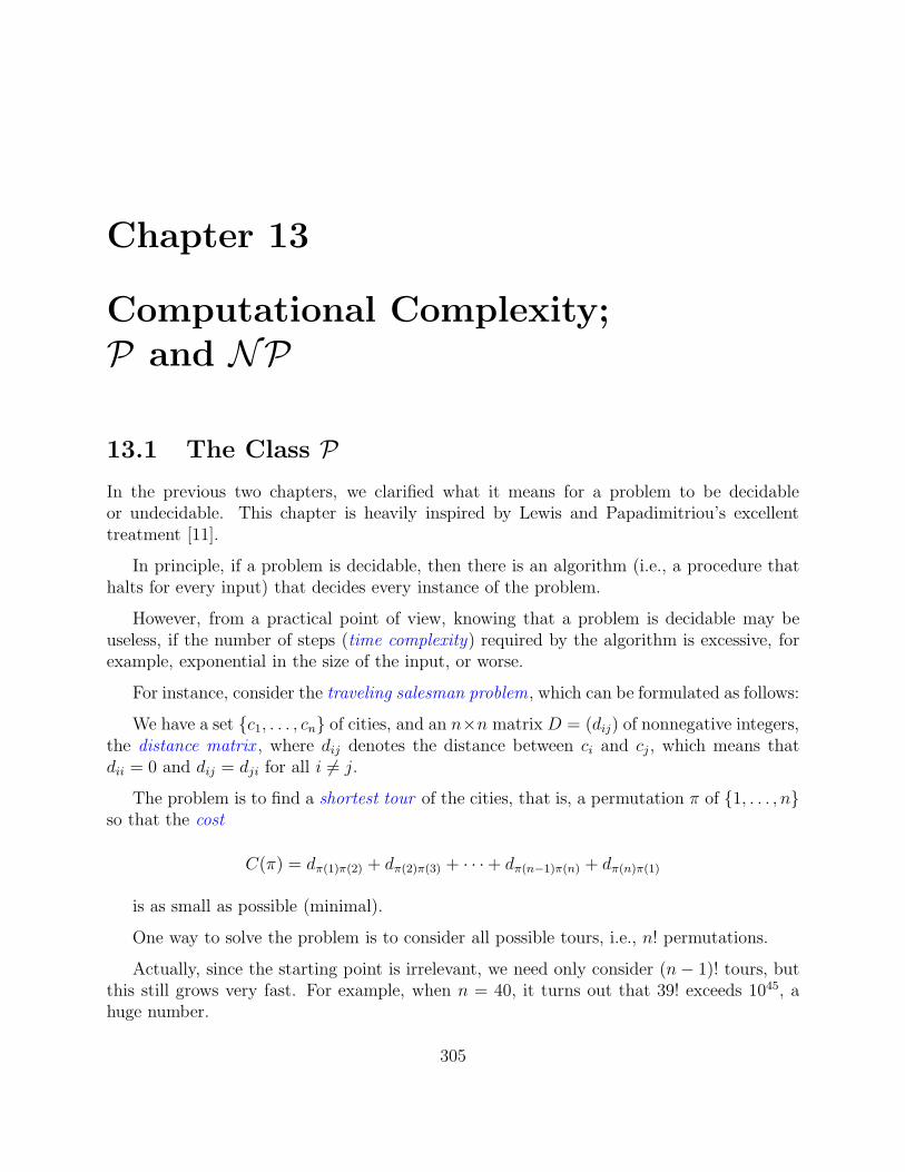
Chapter 13
Computational Complexity;P and NP
13.1 The Class PIn the previous two chapters, we clarified what it means for a problem to be decidableor undecidable. This chapter is heavily inspired by Lewis and Papadimitriou’s excellenttreatment [11].
In principle, if a problem is decidable, then there is an algorithm (i.e., a procedure thathalts for every input) that decides every instance of the problem.
However, from a practical point of view, knowing that a problem is decidable may beuseless, if the number of steps (time complexity) required by the algorithm is excessive, forexample, exponential in the size of the input, or worse.
For instance, consider the traveling salesman problem, which can be formulated as follows:
We have a set c1, . . . , cn of cities, and an n×n matrix D = (dij) of nonnegative integers,the distance matrix , where dij denotes the distance between ci and cj , which means thatdii = 0 and dij = dji for all i 6= j.
The problem is to find a shortest tour of the cities, that is, a permutation π of 1, . . . , nso that the cost
C(π) = dπ(1)π(2) + dπ(2)π(3) + · · ·+ dπ(n−1)π(n) + dπ(n)π(1)
is as small as possible (minimal).
One way to solve the problem is to consider all possible tours, i.e., n! permutations.
Actually, since the starting point is irrelevant, we need only consider (n− 1)! tours, butthis still grows very fast. For example, when n = 40, it turns out that 39! exceeds 1045, ahuge number.
305
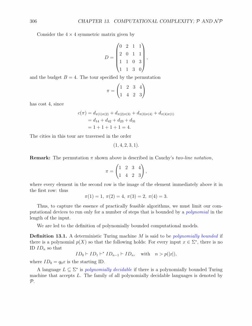
306 CHAPTER 13. COMPUTATIONAL COMPLEXITY; P AND NP
Consider the 4× 4 symmetric matrix given by
D =
0 2 1 1
2 0 1 1
1 1 0 3
1 1 3 0
,
and the budget B = 4. The tour specified by the permutation
π =
(1 2 3 4
1 4 2 3
)
has cost 4, since
c(π) = dπ(1)π(2) + dπ(2)π(3) + dπ(3)π(4) + dπ(4)π(1)
= d14 + d42 + d23 + d31
= 1 + 1 + 1 + 1 = 4.
The cities in this tour are traversed in the order
(1, 4, 2, 3, 1).
Remark: The permutation π shown above is described in Cauchy’s two-line notation,
π =
(1 2 3 4
1 4 2 3
),
where every element in the second row is the image of the element immediately above it inthe first row: thus
π(1) = 1, π(2) = 4, π(3) = 2, π(4) = 3.
Thus, to capture the essence of practically feasible algorithms, we must limit our com-putational devices to run only for a number of steps that is bounded by a polynomial in thelength of the input.
We are led to the definition of polynomially bounded computational models.
Definition 13.1. A deterministic Turing machine M is said to be polynomially bounded ifthere is a polynomial p(X) so that the following holds: For every input x ∈ Σ∗, there is noID IDn so that
ID0 ⊢ ID1 ⊢∗ IDn−1 ⊢ IDn, with n > p(|x|),where ID0 = q0x is the starting ID.
A language L ⊆ Σ∗ is polynomially decidable if there is a polynomially bounded Turingmachine that accepts L. The family of all polynomially decidable languages is denoted byP.
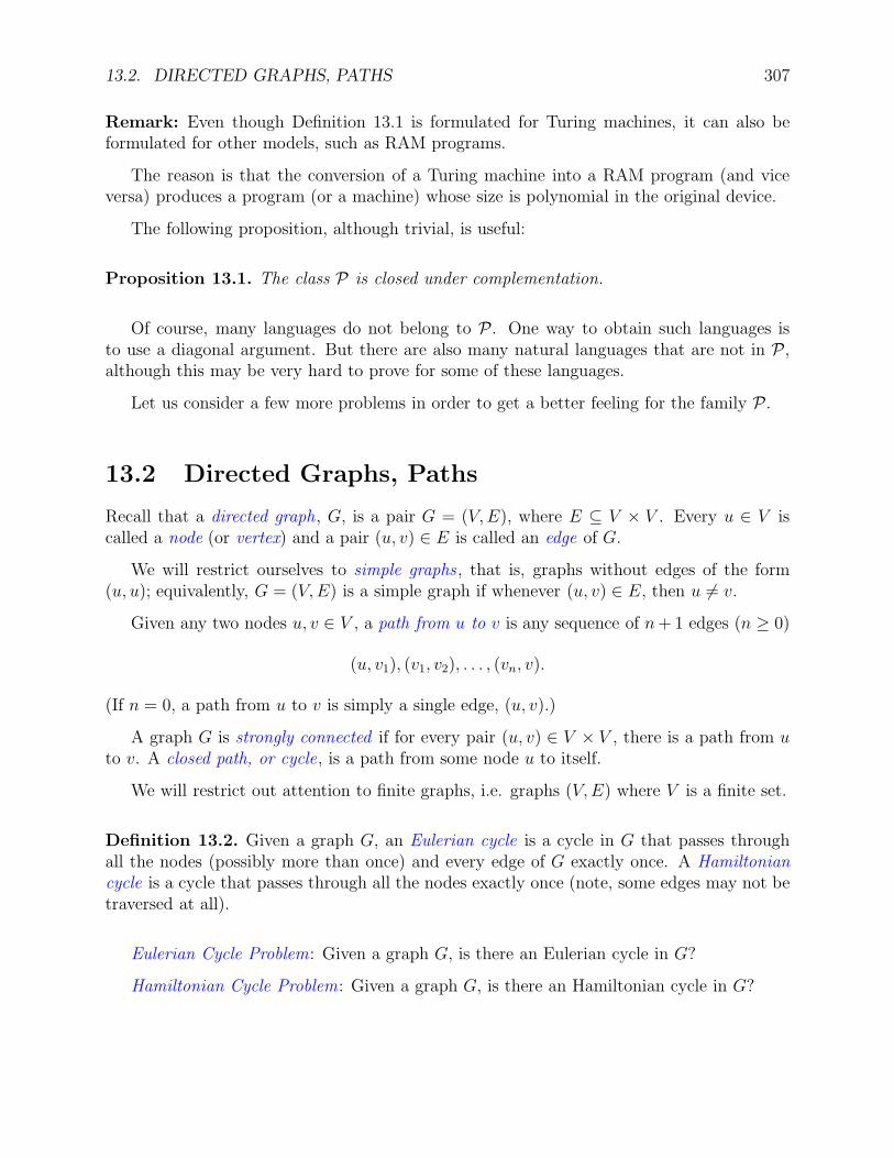
13.2. DIRECTED GRAPHS, PATHS 307
Remark: Even though Definition 13.1 is formulated for Turing machines, it can also beformulated for other models, such as RAM programs.
The reason is that the conversion of a Turing machine into a RAM program (and viceversa) produces a program (or a machine) whose size is polynomial in the original device.
The following proposition, although trivial, is useful:
Proposition 13.1. The class P is closed under complementation.
Of course, many languages do not belong to P. One way to obtain such languages isto use a diagonal argument. But there are also many natural languages that are not in P,although this may be very hard to prove for some of these languages.
Let us consider a few more problems in order to get a better feeling for the family P.
13.2 Directed Graphs, Paths
Recall that a directed graph, G, is a pair G = (V,E), where E ⊆ V × V . Every u ∈ V iscalled a node (or vertex) and a pair (u, v) ∈ E is called an edge of G.
We will restrict ourselves to simple graphs , that is, graphs without edges of the form(u, u); equivalently, G = (V,E) is a simple graph if whenever (u, v) ∈ E, then u 6= v.
Given any two nodes u, v ∈ V , a path from u to v is any sequence of n+ 1 edges (n ≥ 0)
(u, v1), (v1, v2), . . . , (vn, v).
(If n = 0, a path from u to v is simply a single edge, (u, v).)
A graph G is strongly connected if for every pair (u, v) ∈ V × V , there is a path from uto v. A closed path, or cycle, is a path from some node u to itself.
We will restrict out attention to finite graphs, i.e. graphs (V,E) where V is a finite set.
Definition 13.2. Given a graph G, an Eulerian cycle is a cycle in G that passes throughall the nodes (possibly more than once) and every edge of G exactly once. A Hamiltoniancycle is a cycle that passes through all the nodes exactly once (note, some edges may not betraversed at all).
Eulerian Cycle Problem: Given a graph G, is there an Eulerian cycle in G?
Hamiltonian Cycle Problem: Given a graph G, is there an Hamiltonian cycle in G?
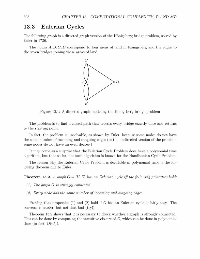
308 CHAPTER 13. COMPUTATIONAL COMPLEXITY; P AND NP
13.3 Eulerian Cycles
The following graph is a directed graph version of the Konigsberg bridge problem, solved byEuler in 1736.
The nodes A,B,C,D correspond to four areas of land in Konigsberg and the edges tothe seven bridges joining these areas of land.
B
A
C
D
Figure 13.1: A directed graph modeling the Konigsberg bridge problem
The problem is to find a closed path that crosses every bridge exactly once and returnsto the starting point.
In fact, the problem is unsolvable, as shown by Euler, because some nodes do not havethe same number of incoming and outgoing edges (in the undirected version of the problem,some nodes do not have an even degree.)
It may come as a surprise that the Eulerian Cycle Problem does have a polynomial timealgorithm, but that so far, not such algorithm is known for the Hamiltonian Cycle Problem.
The reason why the Eulerian Cycle Problem is decidable in polynomial time is the fol-lowing theorem due to Euler:
Theorem 13.2. A graph G = (V,E) has an Eulerian cycle iff the following properties hold:
(1) The graph G is strongly connected.
(2) Every node has the same number of incoming and outgoing edges.
Proving that properties (1) and (2) hold if G has an Eulerian cycle is fairly easy. Theconverse is harder, but not that bad (try!).
Theorem 13.2 shows that it is necessary to check whether a graph is strongly connected.This can be done by computing the transitive closure of E, which can be done in polynomialtime (in fact, O(n3)).
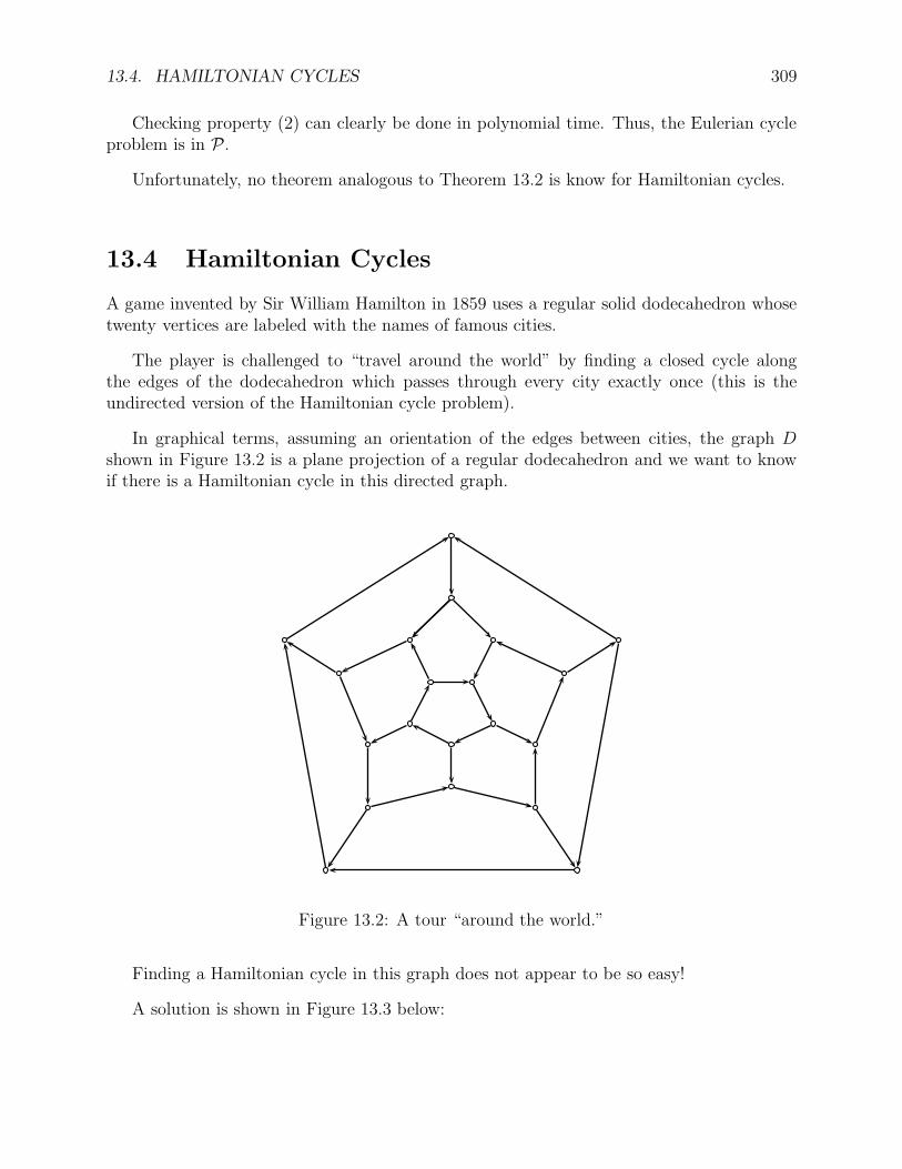
13.4. HAMILTONIAN CYCLES 309
Checking property (2) can clearly be done in polynomial time. Thus, the Eulerian cycleproblem is in P.
Unfortunately, no theorem analogous to Theorem 13.2 is know for Hamiltonian cycles.
13.4 Hamiltonian Cycles
A game invented by Sir William Hamilton in 1859 uses a regular solid dodecahedron whosetwenty vertices are labeled with the names of famous cities.
The player is challenged to “travel around the world” by finding a closed cycle alongthe edges of the dodecahedron which passes through every city exactly once (this is theundirected version of the Hamiltonian cycle problem).
In graphical terms, assuming an orientation of the edges between cities, the graph Dshown in Figure 13.2 is a plane projection of a regular dodecahedron and we want to knowif there is a Hamiltonian cycle in this directed graph.
Figure 13.2: A tour “around the world.”
Finding a Hamiltonian cycle in this graph does not appear to be so easy!
A solution is shown in Figure 13.3 below:
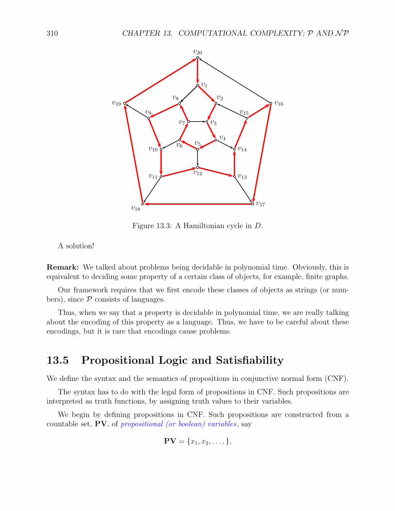
310 CHAPTER 13. COMPUTATIONAL COMPLEXITY; P AND NP
v18v17
v11v12 v13
v10v6 v5
v4
v14
v19v9
v8
v7 v3
v2
v15
v16
v1
v20
Figure 13.3: A Hamiltonian cycle in D.
A solution!
Remark: We talked about problems being decidable in polynomial time. Obviously, this isequivalent to deciding some property of a certain class of objects, for example, finite graphs.
Our framework requires that we first encode these classes of objects as strings (or num-bers), since P consists of languages.
Thus, when we say that a property is decidable in polynomial time, we are really talkingabout the encoding of this property as a language. Thus, we have to be careful about theseencodings, but it is rare that encodings cause problems.
13.5 Propositional Logic and Satisfiability
We define the syntax and the semantics of propositions in conjunctive normal form (CNF).
The syntax has to do with the legal form of propositions in CNF. Such propositions areinterpreted as truth functions, by assigning truth values to their variables.
We begin by defining propositions in CNF. Such propositions are constructed from acountable set, PV, of propositional (or boolean) variables , say
PV = x1, x2, . . . , ,
13.5. PROPOSITIONAL LOGIC AND SATISFIABILITY 311
using the connectives ∧ (and), ∨ (or) and ¬ (negation).
We define a literal (or atomic proposition), L, as L = x or L = ¬x, also denoted by x,where x ∈ PV.
A clause, C, is a disjunction of pairwise distinct literals,
C = (L1 ∨ L2 ∨ · · · ∨ Lm).
Thus, a clause may also be viewed as a nonempty set
C = L1, L2, . . . , Lm.
We also have a special clause, the empty clause, denoted ⊥ or (or ). It correspondsto the truth value false.
A proposition in CNF, or boolean formula, P , is a conjunction of pairwise distinct clauses
P = C1 ∧ C2 ∧ · · · ∧ Cn.
Thus, a boolean formula may also be viewed as a nonempty set
P = C1, . . . , Cn,
but this time, the comma is interpreted as conjunction. We also allow the proposition⊥, and sometimes the proposition ⊤ (corresponding to the truth value true).
For example, here is a boolean formula:
P = (x1 ∨ x2 ∨ x3), (x1 ∨ x2), (x2 ∨ x3), (x3 ∨ x1), (x1 ∨ x2 ∨ x3).
In order to interpret boolean formulae, we use truth assignments.
We let BOOL = F,T, the set of truth values, where F stands for false and T standsfor true.
A truth assignment (or valuation), v, is any function v : PV→ BOOL.
For example, the function vF : PV→ BOOL given by
vF (xi) = F for all i ≥ 1
is a truth assigmnent, and so is the function vT : PV→ BOOL given by
vT (xi) = T for all i ≥ 1.
312 CHAPTER 13. COMPUTATIONAL COMPLEXITY; P AND NP
The function v : PV→ BOOL given by
v(x1) = T
v(x2) = F
v(x3) = T
v(xi) = T for all i ≥ 4
is also a truth assignment.
Given a truth assignment v : PV → BOOL, we define the truth value v(X) of a literal,clause, and boolean formula, X , using the following recursive definition:
(1) v(⊥) = F, v(⊤) = T.
(2) v(x) = v(x), if x ∈ PV.
(3) v(x) = v(x), if x ∈ PV, where v(x) = F if v(x) = T and v(x) = T if v(x) = F.
(4) v(C) = F if C is a clause and iff v(Li) = F for all literals Li in C, otherwise T.
(5) v(P ) = T if P is a boolean formula and iff v(Cj) = T for all clauses Cj in P , otherwiseF.
Since a boolean formula P only contains a finite number of variables, say xi1 , . . . , xin,one should expect that its truth value v(P ) depends only on the truth values assigned bythe truth assignment v to the variables in the set xi1 , . . . , xin, and this is indeed the case.The following proposition is easily shown by induction on the depth of P (viewed as a tree).
Proposition 13.3. Let P be a boolean formula containing the set of variables xi1 , . . . , xin.If v1 : PV→ BOOL and v2 : PV→ BOOL are any truth assignments agreeing on the set ofvariables xi1 , . . . , xin, which means that
v1(xij ) = v2(xij ) for j = 1, . . . , n,
then v1(P ) = v2(P ).
In view of Proposition 13.3, given any boolean formula P , we only need to specify thevalues of a truth assignment v for the variables occurring on P . For example, given theboolean formula
P = (x1 ∨ x2 ∨ x3), (x1 ∨ x2), (x2 ∨ x3), (x3 ∨ x1), (x1 ∨ x2 ∨ x3),we only need to specify v(x1), v(x2), v(x3). Thus there are 2
3 = 8 distinct truth assignments:
F,F,F T,F,F
F,F,T T,F,T
F,T,F T,T,F
F,T,T T,T,T.
13.5. PROPOSITIONAL LOGIC AND SATISFIABILITY 313
In general, there are 2n distinct truth assignments to n distinct variables.
Here is an example showing the evaluation of the truth value v(P ) for the boolean formula
P = (x1 ∨ x2 ∨ x3) ∧ (x1 ∨ x2) ∧ (x2 ∨ x3) ∧ (x3 ∨ x1) ∧ (x1 ∨ x2 ∨ x3)= (x1 ∨ x2 ∨ x3), (x1 ∨ x2), (x2 ∨ x3), (x3 ∨ x1), (x1 ∨ x2 ∨ x3),
and the truth assignment
v(x1) = T, v(x2) = F, v(x3) = F.
For the literals, we have
v(x1) = T, v(x2) = F v(x3) = F, v(x1) = F, v(x2) = T v(x3) = T,
for the clauses
v(x1 ∨ x2 ∨ x3) = v(x1) ∨ v(x2) ∨ v(x3) = T ∨ F ∨ F = T,
v(x1 ∨ x2) = v(x1) ∨ v(x2) = F ∨ F = F,
v(x2 ∨ x3) = v(x2) ∨ v(x3) = T ∨ F = T,
v(x3 ∨ x1) = v(x3) ∨ v(x1) = T ∨T = T,
v(x1 ∨ x2 ∨ x3) = v(x1) ∨ v(x2) ∨ v(x3) = F ∨T ∨T = T,
and for the conjunction of the clauses,
v(P ) = v(x1 ∨ x2 ∨ x3) ∧ v(x1 ∨ x2) ∧ v(x2 ∨ x3) ∧ v(x3 ∨ x1) ∧ v(x1 ∨ x2 ∨ x3)= T ∧ F ∧T ∧T ∧T = F.
Therefore, v(P ) = F.
Definition 13.3. We say that a truth assignment v satisfies a boolean formula P , if v(P ) =T. In this case, we also write
v |= P.
A boolean formula P is satisfiable if v |= P for some truth assignment v, otherwise, it isunsatisfiable. A boolean formula P is valid (or a tautology) if v |= P for all truth assignmentsv, in which case we write
|= P.
One should check that the boolean formula
P = (x1 ∨ x2 ∨ x3), (x1 ∨ x2), (x2 ∨ x3), (x3 ∨ x1), (x1 ∨ x2 ∨ x3)
is unsatisfiable.
314 CHAPTER 13. COMPUTATIONAL COMPLEXITY; P AND NP
One may think that it is easy to test whether a proposition is satisfiable or not. Try it,it is not that easy!
As a matter of fact, the satisfiability problem, testing whether a boolean formula issatisfiable, also denoted SAT, is not known to be in P.
Moreover, it is an NP-complete problem. Most people believe that the satisfiabilityproblem is not in P, but a proof still eludes us!
Before we explain what is the class NP, let us remark that the satisfiability problem forclauses containing at most two literals (2-satisfiability , or 2-SAT) is solvable in polynomialtime.
The first step consists in observing that if every clause in P contains at most two literals,then we can reduce the problem to testing satisfiability when every clause has exactly twoliterals.
Indeed, if P contains some clause (x), then any valuation satisfying P must make x true.Then, all clauses containing x will be true, and we can delete them, whereas we can deletex from every clause containing it, since x is false.
Similarly, if P contains some clause (x), then any valuation satisfying P must make xfalse.
Thus, in a finite number of steps, either we get the empty clause, and P is unsatisfiable,or we get a set of clauses with exactly two literals.
The number of steps is clearly linear in the number of literals in P .
For the second step, we construct a directed graph from P . The nodes of this graph arethe literals in P , and edges are defined as follows:
(1) For every clause (x ∨ y), there is an edge from x to y and an edge from y to x.
(2) For every clause (x ∨ y), there is an edge from x to y and an edge from y to x
(3) For every clause (x ∨ y), there is an edge from x to y and an edge from y to x.
Then, it can be shown that P is unsatisfiable iff there is some x so that there is a cyclecontaining x and x.
As a consequence, 2-satisfiability is in P.
13.6 The Class NP, Polynomial Reducibility,
NP-Completeness
One will observe that the hard part in trying to solve either the Hamiltonian cycle problemor the satisfiability problem, SAT, is to find a solution, but that checking that a candidatesolution is indeed a solution can be done easily in polynomial time.
13.6. THE CLASS NP, NP-COMPLETENESS 315
This is the essence of problems that can be solved nondetermistically in polynomial time:A solution can be guessed and then checked in polynomial time.
Definition 13.4. A nondeterministic Turing machine M is said to be polynomially boundedif there is a polynomial p(X) so that the following holds: For every input x ∈ Σ∗, there isno ID IDn so that
ID0 ⊢ ID1 ⊢∗ IDn−1 ⊢ IDn, with n > p(|x|),
where ID0 = q0x is the starting ID.
A language L ⊆ Σ∗ is nondeterministic polynomially decidable if there is a polynomiallybounded nondeterministic Turing machine that accepts L. The family of all nondeterministicpolynomially decidable languages is denoted by NP.
Of course, we have the inclusionP ⊆ NP,
but whether or not we have equality is one of the most famous open problems of theoreticalcomputer science and mathematics.
In fact, the question P 6= NP is one of the open problems listed by the CLAY Institute,together with the Poincare conjecture and the Riemann hypothesis, among other problems,and for which one million dollar is offered as a reward!
It is easy to check that SAT is in NP, and so is the Hamiltonian cycle problem.
As we saw in recursion theory, where we introduced the notion of many-one reducibility,in order to compare the “degree of difficulty” of problems, it is useful to introduce the notionof reducibility and the notion of a complete set.
Definition 13.5. A function f : Σ∗ → Σ∗ is polynomial-time computable if there is a polyno-mial p(X) so that the following holds: There is a deterministic Turing machineM computingit so that for every input x ∈ Σ∗, there is no ID IDn so that
ID0 ⊢ ID1 ⊢∗ IDn−1 ⊢ IDn, with n > p(|x|),
where ID0 = q0x is the starting ID.
Given two languages L1, L2 ⊆ Σ∗, a polynomial-time reduction from L1 to L2 is apolynomial-time computable function f : Σ∗ → Σ∗ so that for all u ∈ Σ∗,
u ∈ L1 iff f(u) ∈ L2.
The notation L1 ≤P L2 is often used to denote the fact that there is polynomial-timereduction from L1 to L2. Sometimes, the notation L1 ≤P
m L2 is used to stress that this is amany-to-one reduction (that is, f is not necessarily injective). This type of reduction is alsoknown as a Karp reduction.
316 CHAPTER 13. COMPUTATIONAL COMPLEXITY; P AND NP
A polynomial reduction f : Σ∗ → Σ∗ from a language L1 to a language L2 is a methodthat converts in polynomial time every string u ∈ Σ∗ (viewed as an instance of a problemA encoded by language L1) to a string f(u) ∈ Σ∗ (viewed as an instance of a problem Bencoded by language L2) in such way that membership in L1, that is u ∈ L1, is equivalentto membership in L2, that is f(u) ∈ L2.
As a consequence, if we have a procedure to decide membership in L2 (to solve everyinstance of problem B), then we have a procedure for solving membership in L1 (to solve everyinstance of problem A), since given any u ∈ L1, we can first apply f to u to produce f(u),and then apply our procedure to decide whether f(u) ∈ L2; the defining property of f saysthat this is equivalent to deciding whether u ∈ L1. Furthermore, if the procedure for decidingmembership in L2 runs deterministically in polynomial time, since f runs deterministicallyin polynomial time, so does the procedure for deciding membership in L1, and similarly ifthe procedure for deciding membership in L2 runs non deterministically in polynomial time.
For the above reason, we see that membership in L2 can be considered at least as hardas membership in L1, since any method for deciding membership in L2 yields a methodfor deciding membership in L1. Thus, if we view L1 an encoding a problem A and L2 asencoding a problem B, then B is at least as hard as A.
The following version of Proposition 10.16 for polynomial-time reducibility is easy toprove.
Proposition 13.4. Let A,B,C be subsets of N (or Σ∗). The following properties hold:
(1) If A ≤P B and B ≤P C, then A ≤P C.
(2) If A ≤P B then A ≤P B.
(3) If A ≤P B and B ∈ NP, then A ∈ NP.(4) If A ≤P B and A /∈ NP, then B /∈ NP.(5) If A ≤P B and B ∈ P, then A ∈ P.(6) If A ≤P B and A /∈ P, then B /∈ P.
Intuitively, we see that if L1 is a hard problem and L1 can be reduced to L2 in polynomialtime, then L2 is also a hard problem.
For example, one can construct a polynomial reduction from the Hamiltonian cycle prob-lem to the satisfiability problem SAT. Given a directed graph G = (V,E) with n nodes, sayV = 1, . . . , n, we need to construct in polynomial time a set F = τ(G) of clauses such thatG has a Hamiltonian cycle iff τ(G) is satisfiable. We need to describe a permutation of thenodes that forms a Hamiltonian cycle. For this we introduce n2 boolean variables xij , withthe intended interpretation that xij is true iff node i is the jth node in a Hamiltonian cycle.
To express that at least one node must appear as the jth node in a Hamiltonian cycle,we have the n clauses
(x1j ∨ x2j ∨ · · · ∨ xnj), 1 ≤ j ≤ n. (1)
13.6. THE CLASS NP, NP-COMPLETENESS 317
The conjunction of these clauses is satisfied iff for every j = 1, . . . , n there is some node iwhich is the jth node in the cycle.
To express that only one node appears in the cycle, we have the clauses
(xij ∨ xkj), 1 ≤ i, j, k ≤ n, i 6= k. (2)
Since (xij ∨ xkj) is equivalent to (xij ∧ xkj), each such clause asserts that no two distinctnodes may appear as the jth node in the cycle. Let S1 be the set of all clauses of type (1)or (2).
The conjunction of the clauses in S1 assert that exactly one node appear at the jth nodein the Hamiltonian cycle. We still need to assert that each node i appears exactly once inthe cycle. For this, we have the clauses
(xi1 ∨ xi2 ∨ · · · ∨ xin), 1 ≤ i ≤ n, (3)
and
(xij ∨ xik), 1 ≤ i, j, k ≤ n, j 6= k. (4)
Let S2 be the set of all clauses of type (3) or (4).
The conjunction of the clauses in S1 ∪ S2 asserts that the xij represents a bijection of1, 2, . . . , n, in the sense that for any truth assigment v satisfying all these clauses, i 7→ jiff v(xij) = T defines a bijection of 1, 2, . . . , n.
It remains to assert that this permutation of the nodes is a Hamiltonian cycle, whichmeans that if xij and xkj+1 are both true then there there must be an edge (i, k). By
contrapositive, this equivalent to saying that if (i, k) is not an edge of G, then (xij ∧ xkj+1)is true, which as a clause is equivalent to (xij ∨ xkj+1).
Therefore, for all (i, k) such that (i, k) /∈ E (with i, k ∈ 1, 2, . . . , n), we have the clauses
(xij ∨ xk j+1 (mod n)), j = 1, . . . , n. (5)
Let S3 be the set of clauses of type (5). The conjunction of all the clauses in S1 ∪ S2 ∪ S3 isthe boolean formula F = τ(G).
We leave it as an exercise to prove that G has a Hamiltonian cycle iff F = τ(G) issatisfiable.
It is also possible to construct a reduction of the satisfiability problem to the Hamiltoniancycle problem but this is harder. It is easier to construct this reduction in two steps byintroducing an intermediate problem, the exact cover problem, and to provide a polynomialreduction from the satisfiability problem to the exact cover problem, and a polynomialreduction from the exact cover problem to the Hamiltonian cycle problem. These reductionsare carried out in Section 14.2.

318 CHAPTER 13. COMPUTATIONAL COMPLEXITY; P AND NP
The above construction of a set F = τ(G) of clauses from a graph G asserting that Ghas a Hamiltonian cycle iff F is satisfiable illustrates the expressive power of propositionallogic.
Remarkably, every language in NP can be reduced to SAT. Thus, SAT is a hardestproblem in NP (Since it is in NP).Definition 13.6. A language L is NP-hard if there is a polynomial reduction from everylanguage L1 ∈ NP to L. A language L is NP-complete if L ∈ NP and L is NP-hard.
Thus, an NP-hard language is as hard to decide as any language in NP.
Remark: There are NP-hard languages that do not belong to NP. Such problems arereally hard. Two standard examples are K0 and K, which encode the halting problem. SinceK0 and K are not computable, they can’t be in NP. Furthermore, since every languageL in NP is accepted nondeterminsticaly in polynomial time p(X), for some polynomialp(X), for every input w we can try all computations of length at most p(|w|) (there canbe exponentially many, but only a finite number), so every language in NP is computable.Finally, it is shown in Theorem 10.17 that K0 and K are complete with respect to many-onereducibility, so in particular they are NP-hard. An example of a computable NP-hardlanguage not in NP will be described after Theorem 13.6.
The importance of NP-complete problems stems from the following theorem which fol-lows immediately from Proposition 13.4.
Theorem 13.5. Let L be an NP-complete language. Then, P = NP iff L ∈ P.There are analogies between P and the class of computable sets, and NP and the class
of listable sets, but there are also important differences. One major difference is that thefamily of computable sets is properly contained in the family of listable sets, but it is an openproblem whether P is properly contained in NP. We also know that a set L is computableiff both L and L are listable, but it is also an open problem whether if both L ∈ NP andL ∈ NP, then L ∈ P. This suggests defining
coNP = L | L ∈ NP,that is, coNP consists of all complements of languages in NP. Since P ⊆ NP and P isclosed under complementation,
P ⊆ coNP,and thus
P ⊆ NP ∩ coNP,but nobody knows whether the inclusion is proper. There are problems in NP ∩ coNP notknown to be in P; see Section 14.3. It is unknown whether NP is closed under complemen-tation, that is, nobody knows whether NP = coNP. This is considered unlikely. We willcome back to coNP in Section 14.3.
Next, we prove a famous theorem of Steve Cook and Leonid Levin (proved independently):SAT is NP-complete.
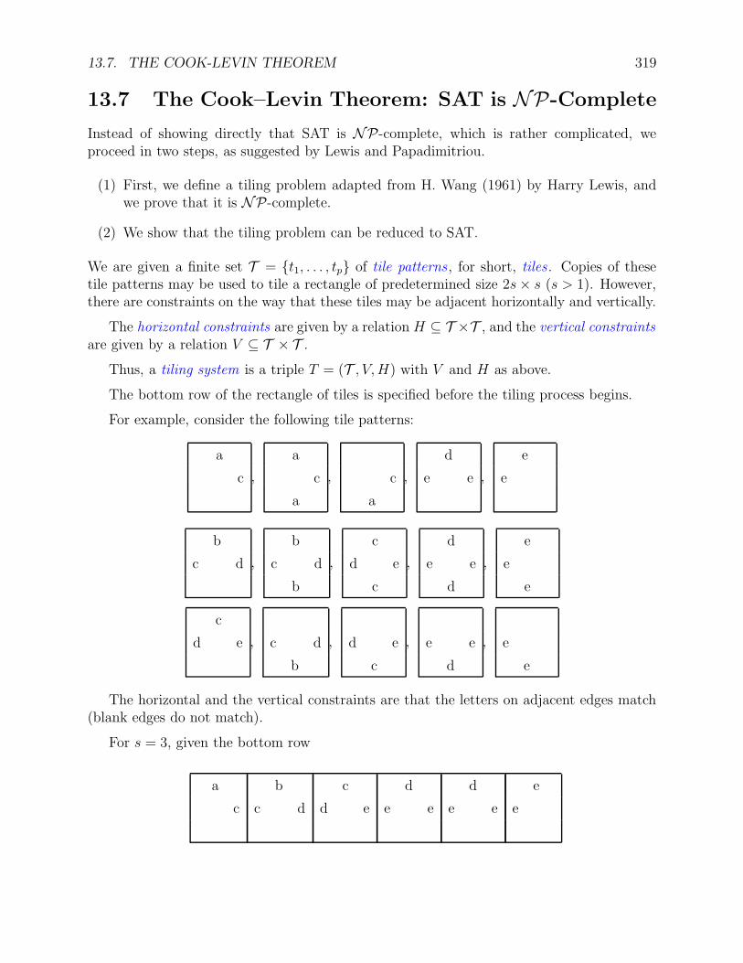
13.7. THE COOK-LEVIN THEOREM 319
13.7 The Cook–Levin Theorem: SAT is NP-Complete
Instead of showing directly that SAT is NP-complete, which is rather complicated, weproceed in two steps, as suggested by Lewis and Papadimitriou.
(1) First, we define a tiling problem adapted from H. Wang (1961) by Harry Lewis, andwe prove that it is NP-complete.
(2) We show that the tiling problem can be reduced to SAT.
We are given a finite set T = t1, . . . , tp of tile patterns , for short, tiles . Copies of thesetile patterns may be used to tile a rectangle of predetermined size 2s× s (s > 1). However,there are constraints on the way that these tiles may be adjacent horizontally and vertically.
The horizontal constraints are given by a relation H ⊆ T ×T , and the vertical constraintsare given by a relation V ⊆ T × T .
Thus, a tiling system is a triple T = (T , V,H) with V and H as above.
The bottom row of the rectangle of tiles is specified before the tiling process begins.
For example, consider the following tile patterns:
a
c ,
a
c
a
, c
a
,
d
e e ,
e
e
b
c d ,
b
c d
b
,
c
d e
c
,
d
e e
d
,
e
e
e
c
d e , c d
b
, d e
c
, e e
d
, e
e
The horizontal and the vertical constraints are that the letters on adjacent edges match(blank edges do not match).
For s = 3, given the bottom row
a
c
b
c d
c
d e
d
e e
d
e e
e
e
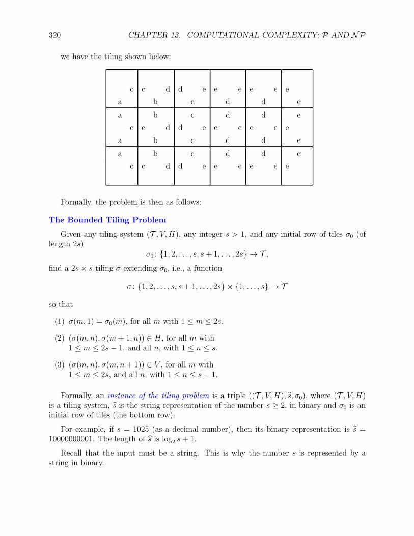
320 CHAPTER 13. COMPUTATIONAL COMPLEXITY; P AND NP
we have the tiling shown below:
c
a
c d
b
d e
c
e e
d
e e
d
e
e
a
c
a
b
c d
b
c
d e
c
d
e e
d
d
e e
d
e
e
e
a
c
b
c d
c
d e
d
e e
d
e e
e
e
Formally, the problem is then as follows:
The Bounded Tiling Problem
Given any tiling system (T , V,H), any integer s > 1, and any initial row of tiles σ0 (oflength 2s)
σ0 : 1, 2, . . . , s, s+ 1, . . . , 2s → T ,find a 2s× s-tiling σ extending σ0, i.e., a function
σ : 1, 2, . . . , s, s+ 1, . . . , 2s × 1, . . . , s → T
so that
(1) σ(m, 1) = σ0(m), for all m with 1 ≤ m ≤ 2s.
(2) (σ(m,n), σ(m+ 1, n)) ∈ H , for all m with1 ≤ m ≤ 2s− 1, and all n, with 1 ≤ n ≤ s.
(3) (σ(m,n), σ(m,n+ 1)) ∈ V , for all m with1 ≤ m ≤ 2s, and all n, with 1 ≤ n ≤ s− 1.
Formally, an instance of the tiling problem is a triple ((T , V,H), s, σ0), where (T , V,H)is a tiling system, s is the string representation of the number s ≥ 2, in binary and σ0 is aninitial row of tiles (the bottom row).
For example, if s = 1025 (as a decimal number), then its binary representation is s =10000000001. The length of s is log2 s+ 1.
Recall that the input must be a string. This is why the number s is represented by astring in binary.
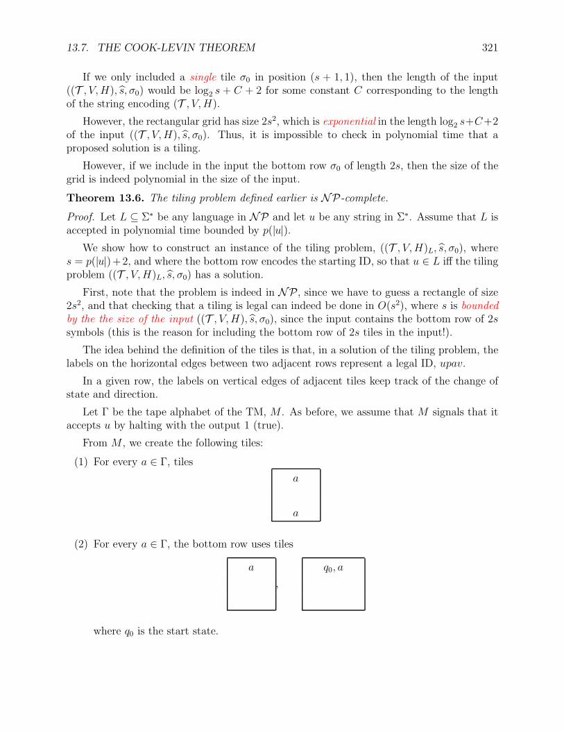
13.7. THE COOK-LEVIN THEOREM 321
If we only included a single tile σ0 in position (s + 1, 1), then the length of the input((T , V,H), s, σ0) would be log2 s + C + 2 for some constant C corresponding to the lengthof the string encoding (T , V,H).
However, the rectangular grid has size 2s2, which is exponential in the length log2 s+C+2of the input ((T , V,H), s, σ0). Thus, it is impossible to check in polynomial time that aproposed solution is a tiling.
However, if we include in the input the bottom row σ0 of length 2s, then the size of thegrid is indeed polynomial in the size of the input.
Theorem 13.6. The tiling problem defined earlier is NP-complete.
Proof. Let L ⊆ Σ∗ be any language in NP and let u be any string in Σ∗. Assume that L isaccepted in polynomial time bounded by p(|u|).
We show how to construct an instance of the tiling problem, ((T , V,H)L, s, σ0), wheres = p(|u|)+2, and where the bottom row encodes the starting ID, so that u ∈ L iff the tilingproblem ((T , V,H)L, s, σ0) has a solution.
First, note that the problem is indeed in NP, since we have to guess a rectangle of size2s2, and that checking that a tiling is legal can indeed be done in O(s2), where s is boundedby the the size of the input ((T , V,H), s, σ0), since the input contains the bottom row of 2ssymbols (this is the reason for including the bottom row of 2s tiles in the input!).
The idea behind the definition of the tiles is that, in a solution of the tiling problem, thelabels on the horizontal edges between two adjacent rows represent a legal ID, upav.
In a given row, the labels on vertical edges of adjacent tiles keep track of the change ofstate and direction.
Let Γ be the tape alphabet of the TM, M . As before, we assume that M signals that itaccepts u by halting with the output 1 (true).
From M , we create the following tiles:
(1) For every a ∈ Γ, tiles
a
a
(2) For every a ∈ Γ, the bottom row uses tiles
a
,
q0, a
where q0 is the start state.
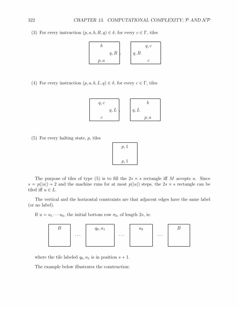
322 CHAPTER 13. COMPUTATIONAL COMPLEXITY; P AND NP
(3) For every instruction (p, a, b, R, q) ∈ δ, for every c ∈ Γ, tiles
b
q, R
p, a
,
q, c
q, R
c
(4) For every instruction (p, a, b, L, q) ∈ δ, for every c ∈ Γ, tiles
q, c
q, L
c
,
b
q, L
p, a
(5) For every halting state, p, tiles
p, 1
p, 1
The purpose of tiles of type (5) is to fill the 2s × s rectangle iff M accepts u. Sinces = p(|u|) + 2 and the machine runs for at most p(|u|) steps, the 2s × s rectangle can betiled iff u ∈ L.
The vertical and the horizontal constraints are that adjacent edges have the same label(or no label).
If u = u1 · · ·uk, the initial bottom row σ0, of length 2s, is:
B
· · ·q0, u1
· · ·uk
· · ·B
where the tile labeled q0, u1 is in position s+ 1.
The example below illustrates the construction:
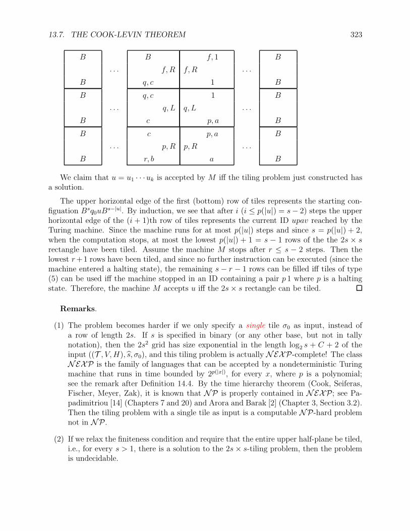
13.7. THE COOK-LEVIN THEOREM 323
B
B
. . .
B
f, R
q, c
f, 1
f, R
1
. . .
B
B
B
B
. . .
q, c
q, L
c
1
q, L
p, a
. . .
B
B
B
B
. . .
c
p, R
r, b
p, a
p, R
a
. . .
B
B
We claim that u = u1 · · ·uk is accepted by M iff the tiling problem just constructed hasa solution.
The upper horizontal edge of the first (bottom) row of tiles represents the starting con-figuation Bsq0uB
s−|u|. By induction, we see that after i (i ≤ p(|u|) = s− 2) steps the upperhorizontal edge of the (i + 1)th row of tiles represents the current ID upav reached by theTuring machine. Since the machine runs for at most p(|u|) steps and since s = p(|u|) + 2,when the computation stops, at most the lowest p(|u|) + 1 = s − 1 rows of the the 2s × srectangle have been tiled. Assume the machine M stops after r ≤ s − 2 steps. Then thelowest r+1 rows have been tiled, and since no further instruction can be executed (since themachine entered a halting state), the remaining s− r − 1 rows can be filled iff tiles of type(5) can be used iff the machine stopped in an ID containing a pair p 1 where p is a haltingstate. Therefore, the machine M accepts u iff the 2s× s rectangle can be tiled.
Remarks.
(1) The problem becomes harder if we only specify a single tile σ0 as input, instead ofa row of length 2s. If s is specified in binary (or any other base, but not in tallynotation), then the 2s2 grid has size exponential in the length log2 s + C + 2 of theinput ((T , V,H), s, σ0), and this tiling problem is actually NEXP-complete! The classNEXP is the family of languages that can be accepted by a nondeterministic Turingmachine that runs in time bounded by 2p(|x|), for every x, where p is a polynomial;see the remark after Definition 14.4. By the time hierarchy theorem (Cook, Seiferas,Fischer, Meyer, Zak), it is known that NP is properly contained in NEXP; see Pa-padimitriou [14] (Chapters 7 and 20) and Arora and Barak [2] (Chapter 3, Section 3.2).Then the tiling problem with a single tile as input is a computable NP-hard problemnot in NP.
(2) If we relax the finiteness condition and require that the entire upper half-plane be tiled,i.e., for every s > 1, there is a solution to the 2s× s-tiling problem, then the problemis undecidable.
324 CHAPTER 13. COMPUTATIONAL COMPLEXITY; P AND NP
In 1972, Richard Karp published a list of 21 NP-complete problems.
We finally prove the Cook-Levin theorem.
Theorem 13.7. (Cook, 1971, Levin, 1973) The satisfiability problem SAT is NP-complete.
Proof. We reduce the tiling problem to SAT. Given a tiling problem, ((T , V,H), s, σ0), weintroduce boolean variables
xmnt,
for all m with 1 ≤ m ≤ 2s, all n with 1 ≤ n ≤ s, and all tiles t ∈ T .The intuition is that xmnt = T iff tile t occurs in some tiling σ so that σ(m,n) = t.
We define the following clauses:
(1) For all m,n in the correct range, as above,
(xmnt1 ∨ xmnt2 ∨ · · · ∨ xmntp),
for all p tiles in T .
This clause states that every position in σ is tiled.
(2) For any two distinct tiles t 6= t′ ∈ T , for all m,n in the correct range, as above,
(xmnt ∨ xmnt′).
This clause states that a position may not be occupied by more than one tile.
(3) For every pair of tiles (t, t′) ∈ T × T −H , for all m with 1 ≤ m ≤ 2s− 1, and all n,with 1 ≤ n ≤ s,
(xmnt ∨ xm+1nt′).
This clause enforces the horizontal adjacency constraints.
(4) For every pair of tiles (t, t′) ∈ T × T − V , for all m with 1 ≤ m ≤ 2s, and all n, with1 ≤ n ≤ s− 1,
(xmnt ∨ xmn+1 t′).
This clause enforces the vertical adjacency constraints.
(5) For all m with 1 ≤ m ≤ 2s,(xm1σ0(m)).
This clause states that the bottom row is correctly tiled with σ0.
13.7. THE COOK-LEVIN THEOREM 325
It is easily checked that the tiling problem has a solution iff the conjunction of the clausesjust defined is satisfiable. Thus, SAT is NP-complete.
We sharpen Theorem 13.7 to prove that 3-SAT is also NP-complete. This is the satisfi-ability problem for clauses containing at most three literals.
We know that we can’t go further and retainNP-completeteness, since 2-SAT is in P.
Theorem 13.8. (Cook, 1971) The satisfiability problem 3-SAT is NP-complete.
Proof. We have to break “long clauses”
C = (L1 ∨ · · · ∨ Lk),
i.e., clauses containing k ≥ 4 literals, into clauses with at most three literals, in such away that satisfiability is preserved.
For example, consider the following clause with k = 6 literals:
C = (L1 ∨ L2 ∨ L3 ∨ L4 ∨ L5 ∨ L6).
We create 3 new boolean variables y1, y2, y3, and the 4 clauses
(L1 ∨ L2 ∨ y1), (y1 ∨ L3 ∨ y2), (y2 ∨ L4 ∨ y3), (y3 ∨ L5 ∨ L6).
Let C ′ be the conjunction of these clauses. We claim that C is satisfiable iff C ′ is.
Assume that C ′ is satisfiable but C is not. If so, in any truth assigment v, v(Li) = F,for i = 1, 2, . . . , 6. To satisfy the first clause, we must have v(y1) = T., Then to satisfy thesecond clause, we must have v(y2) = T, and similarly satisfy the third clause, we must havev(y3) = T. However, since v(L5) = F and v(L6) = F, the only way to satisfy the fourthclause is to have v(y3) = F, contradicting that v(y3) = T. Thus, C is indeed satisfiable.
Let us now assume that C is satisfiable. This means that there is a smallest index i suchthat Li is satisfied.
Say i = 1, so v(L1) = T. Then if we let v(y1) = v(y2) = v(y3) = F, we see that C ′ issatisfied.
Say i = 2, so v(L1) = F and v(L2) = T. Again if we let v(y1) = v(y2) = v(y3) = F, wesee that C ′ is satisfied.
Say i = 3, so v(L1) = F, v(L2) = F, and v(L3) = T. If we let v(y1) = T andv(y2) = v(y3) = F, we see that C ′ is satisfied.
Say i = 4, so v(L1) = F, v(L2) = F, v(L3) = F, and v(L4) = T. If we let v(y1) = T,v(y2) = T and v(y3) = F, we see that C ′ is satisfied.
326 CHAPTER 13. COMPUTATIONAL COMPLEXITY; P AND NP
Say i = 5, so v(L1) = F, v(L2) = F, v(L3) = F, v(L4) = F, and v(L5) = T. If we letv(y1) = T, v(y2) = T and v(y3) = T, we see that C ′ is satisfied.
Say i = 6, so v(L1) = F, v(L2) = F, v(L3) = F, v(L4) = F, v(L5) = F, and v(L6) = T.Again, if we let v(y1) = T, v(y2) = T and v(y3) = T, we see that C ′ is satisfied.
Therefore if C is satisfied, then C ′ is satisfied in all cases.
In general, for every long clause, create k − 3 new boolean variables y1, . . . yk−3, and thek − 2 clauses
(L1 ∨ L2 ∨ y1), (y1 ∨ L3 ∨ y2), (y2 ∨ L4 ∨ y3), · · · ,(yk−4 ∨ Lk−2 ∨ yk−3), (yk−3 ∨ Lk−1 ∨ Lk).
Let C ′ be the conjunction of these clauses. We claim that C is satisfiable iff C ′ is.
Assume that C ′ is satisfiable, but that C is not. Then, for every truth assignment v, wehave v(Li) = F, for i = 1, . . . , k.
However, C ′ is satisfied by some v, and the only way this can happen is that v(y1) = T,to satisfy the first clause. Then, v(y1) = F, and we must have v(y2) = T, to satisfy thesecond clause.
By induction, we must have v(yk−3) = T, to satisfy the next to the last clause. However,the last clause is now false, a contradiction.
Thus, if C ′ is satisfiable, then so is C.
Conversely, assume that C is satisfiable. If so, there is some truth assignment, v, so thatv(C) = T, and thus, there is a smallest index i, with 1 ≤ i ≤ k, so that v(Li) = T (and so,v(Lj) = F for all j < i).
Let v′ be the assignment extending v defined so that
v′(yj) = F if max1, i− 1 ≤ j ≤ k − 3,
and v′(yj) = T, otherwise.
It is easily checked that v′(C ′) = T.
Another version of 3-SAT can be considered, in which every clause has exactly threeliterals. We will call this the problem exact 3-SAT.
Theorem 13.9. (Cook, 1971) The satisfiability problem for exact 3-SAT is NP-complete.
Proof. A clause of the form (L) is satisfiable iff the following four clauses are satisfiable:
(L ∨ u ∨ v), (L ∨ u ∨ v), (L ∨ u ∨ v), (L ∨ u ∨ v).
13.7. THE COOK-LEVIN THEOREM 327
A clause of the form (L1 ∨ L2) is satisfiable iff the following two clauses are satisfiable:
(L1 ∨ L2 ∨ u), (L1 ∨ L2 ∨ u).
Thus, we have a reduction of 3-SAT to exact 3-SAT.
We now make some remarks on the conversion of propositions to CNF.
Recall that the set of propositions (over the connectives ∨, ∧, and ¬) is defined inductivelyas follows:
(1) Every propositional letter, x ∈ PV, is a proposition (an atomic proposition).
(2) If A is a proposition, then ¬A is a proposition.
(3) If A and B are propositions, then (A ∨B) is a proposition.
(4) If A and B are propositions, then (A ∧B) is a proposition.
Two propositions A and B are equivalent , denoted A ≡ B, if
v |= A iff v |= B
for all truth assignments, v.
It is easy to show that A ≡ B iff the proposition
(¬A ∨ B) ∧ (¬B ∨ A)
is valid.
Every proposition, A, is equivalent to a proposition, A′, in CNF.
There are several ways of proving this fact. One method is algebraic, and consists inusing the algebraic laws of boolean algebra.
First, one may convert a proposition to negation normal form, or nnf . A proposition isin nnf if occurrences of ¬ only appear in front of propositional variables, but not in front ofcompound propositions.
Any proposition can be converted to an equivalent one in nnf by using the de Morganlaws:
¬(A ∨B) ≡ (¬A ∧ ¬B)
¬(A ∧B) ≡ (¬A ∨ ¬B)
¬¬A ≡ A.
Then, a proposition in nnf can be converted to CNF, but the question of uniqueness ofthe CNF is a bit tricky.
328 CHAPTER 13. COMPUTATIONAL COMPLEXITY; P AND NP
For example, the proposition
A = (u ∧ (x ∨ y)) ∨ (¬u ∧ (x ∨ y))
has
A1 = (u ∨ x ∨ y) ∧ (¬u ∨ x ∨ y)A2 = (u ∨ ¬u) ∧ (x ∨ y)A3 = x ∨ y,
as equivalent propositions in CNF!
We can get a unique CNF equivalent to a given proposition if we do the following:
(1) Let Var(A) = x1, . . . , xm be the set of variables occurring in A.
(2) Define a maxterm w.r.t. Var(A) as any disjunction of m pairwise distinct literalsformed from Var(A), and not containing both some variable xi and its negation ¬xi.
(3) Then, it can be shown that for any proposition A that is not a tautology, there is aunique proposition in CNF equivalent to A, whose clauses consist of maxterms formedfrom Var(A).
The above definition can yield strange results. For instance, the CNF of any unsatisfiableproposition with m distinct variables is the conjunction of all of its 2m maxterms!
The above notion does not cope well with minimality.
For example, according to the above, the CNF of
A = (u ∧ (x ∨ y)) ∨ (¬u ∧ (x ∨ y))
should beA1 = (u ∨ x ∨ y) ∧ (¬u ∨ x ∨ y).
There are also propositions such that any equivalent proposition in CNF has size expo-nential in terms of the original proposition.
Here is such an example:
A = (x1 ∧ x2) ∨ (x3 ∧ x4) ∨ · · · ∨ (x2n−1 ∧ x2n).
Observe that it is in DNF.
We will prove a little later that any CNF for A contains 2n occurrences of variables.
A nice method to convert a proposition in nnf to CNF is to construct a tree whose nodesare labeled with sets of propositions using the following (Gentzen-style) rules :
13.7. THE COOK-LEVIN THEOREM 329
P,∆ Q,∆
(P ∧Q),∆and
P,Q,∆
(P ∨Q),∆
where ∆ stands for any set of propositions (even empty), and the comma stands forunion. Thus, it is assumed that (P ∧Q) /∈ ∆ in the first case, and that (P ∨Q) /∈ ∆ in thesecond case.
Since we interpret a set, Γ, of propositions as a disjunction, a valuation, v, satisfies Γ iffit satisfies some proposition in Γ.
Observe that a valuation v satisfies the conclusion of a rule iff it satisfies both premisesin the first case, and the single premise in the second case.
Using these rules, we can build a finite tree whose leaves are labeled with sets of literals.
By the above observation, a valuation v satisfies the proposition labeling the root of thetree iff it satisfies all the propositions labeling the leaves of the tree.
But then, a CNF for the original proposition A (in nnf, at the root of the tree) is theconjunction of the clauses appearing as the leaves of the tree.
We may exclude the clauses that are tautologies, and we may discover in the process thatA is a tautology (when all leaves are tautologies).
Going back to our “bad” proposition, A, by induction, we see that any tree for A has 2n
leaves.
However, it should be noted that for any proposition, A, we can construct in polynomialtime a formula, A′, in CNF, so that A is satisfiable iff A′ is satisfiable, by creating newvariables.
We proceed recursively. The trick is that we replace
(C1 ∧ · · · ∧ Cm) ∨ (D1 ∧ · · · ∧Dn)
by(C1 ∨ y) ∧ · · · ∧ (Cm ∨ y) ∧ (D1 ∨ y) ∧ · · · ∧ (Dn ∨ y),
where the Ci’s and the Dj’s are clauses, and y is a new variable.
It can be shown that the number of new variables required is at most quadratic in thesize of A.
Warning: In general, the proposition A′ is not equivalent to the proposition A.
Rules for dealing for ¬ can also be created. In this case, we work with pairs of sets ofpropositions,
330 CHAPTER 13. COMPUTATIONAL COMPLEXITY; P AND NP
Γ→ ∆,
where, the propositions in Γ are interpreted conjunctively, and the propositions in ∆ areinterpreted disjunctively.
We obtain a sound and complete proof system for propositional logic (a “Gentzen-style”proof system, see Gallier’s Logic for Computer Science).
Chapter 14
Some NP-Complete Problems
14.1 Statements of the Problems
In this chapter we will show that certain classical algorithmic problems are NP-complete.This chapter is heavily inspired by Lewis and Papadimitriou’s excellent treatment [11]. Inorder to study the complexity of these problems in terms of resource (time or space) boundedTuring machines (or RAM programs), it is crucial to be able to encode instances of a prob-lem P as strings in a language LP . Then an instance of a problem P is solvable iff thecorresponding string belongs to the language LP . This implies that our problems must havea yes–no answer, which is not always the usual formulation of optimization problems wherewhat is required is to find some optimal solution, that is, a solution minimizing or maximiz-ing so objective (cost) function F . For example the standard formulation of the travelingsalesman problem asks for a tour (of the cities) of minimal cost.
Fortunately, there is a trick to reformulate an optimization problem as a yes–no answerproblem, which is to explicitly incorporate a budget (or cost) term B into the problem, andinstead of asking whether some objective function F has a minimum or a maximum w, weask whether there is a solution w such that F (w) ≤ B in the case of a minimum solution,or F (w) ≥ B in the case of a maximum solution.
If we are looking for a minimum of F , we try to guess the minimum value B of F andthen we solve the problem of finding w such that F (w) ≤ B. If our guess for B is too small,then we fail. In this case, we try again with a larger value of B. Otherwise, if B was not toosmall we find some w such that F (w) ≤ B, but w may not correspond to a minimum of F ,so we try again with a smaller value of B, and so on. This yields an approximation methodto find a minimum of F .
Similarly, if we are looking for a maximum of F , we try to guess the maximum value Bof F and then we solve the problem of finding w such that F (w) ≥ B. If our guess for Bis too large, then we fail. In this case, we try again with a smaller value of B. Otherwise,if B was not too large we find some w such that F (w) ≥ B, but w may not correspondto a maximum of F , so we try again with a greater value of B, and so on. This yields an
331
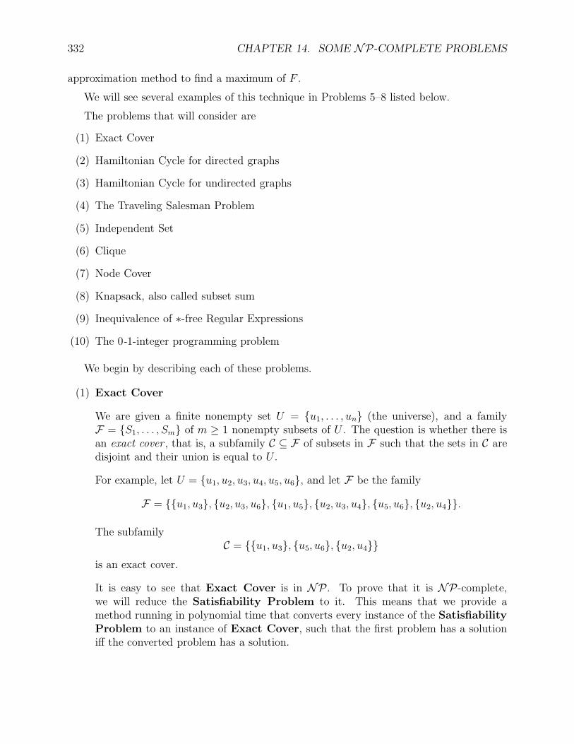
332 CHAPTER 14. SOME NP-COMPLETE PROBLEMS
approximation method to find a maximum of F .
We will see several examples of this technique in Problems 5–8 listed below.
The problems that will consider are
(1) Exact Cover
(2) Hamiltonian Cycle for directed graphs
(3) Hamiltonian Cycle for undirected graphs
(4) The Traveling Salesman Problem
(5) Independent Set
(6) Clique
(7) Node Cover
(8) Knapsack, also called subset sum
(9) Inequivalence of ∗-free Regular Expressions
(10) The 0-1-integer programming problem
We begin by describing each of these problems.
(1) Exact Cover
We are given a finite nonempty set U = u1, . . . , un (the universe), and a familyF = S1, . . . , Sm of m ≥ 1 nonempty subsets of U . The question is whether there isan exact cover , that is, a subfamily C ⊆ F of subsets in F such that the sets in C aredisjoint and their union is equal to U .
For example, let U = u1, u2, u3, u4, u5, u6, and let F be the family
F = u1, u3, u2, u3, u6, u1, u5, u2, u3, u4, u5, u6, u2, u4.
The subfamilyC = u1, u3, u5, u6, u2, u4
is an exact cover.
It is easy to see that Exact Cover is in NP. To prove that it is NP-complete,we will reduce the Satisfiability Problem to it. This means that we provide amethod running in polynomial time that converts every instance of the SatisfiabilityProblem to an instance of Exact Cover, such that the first problem has a solutioniff the converted problem has a solution.
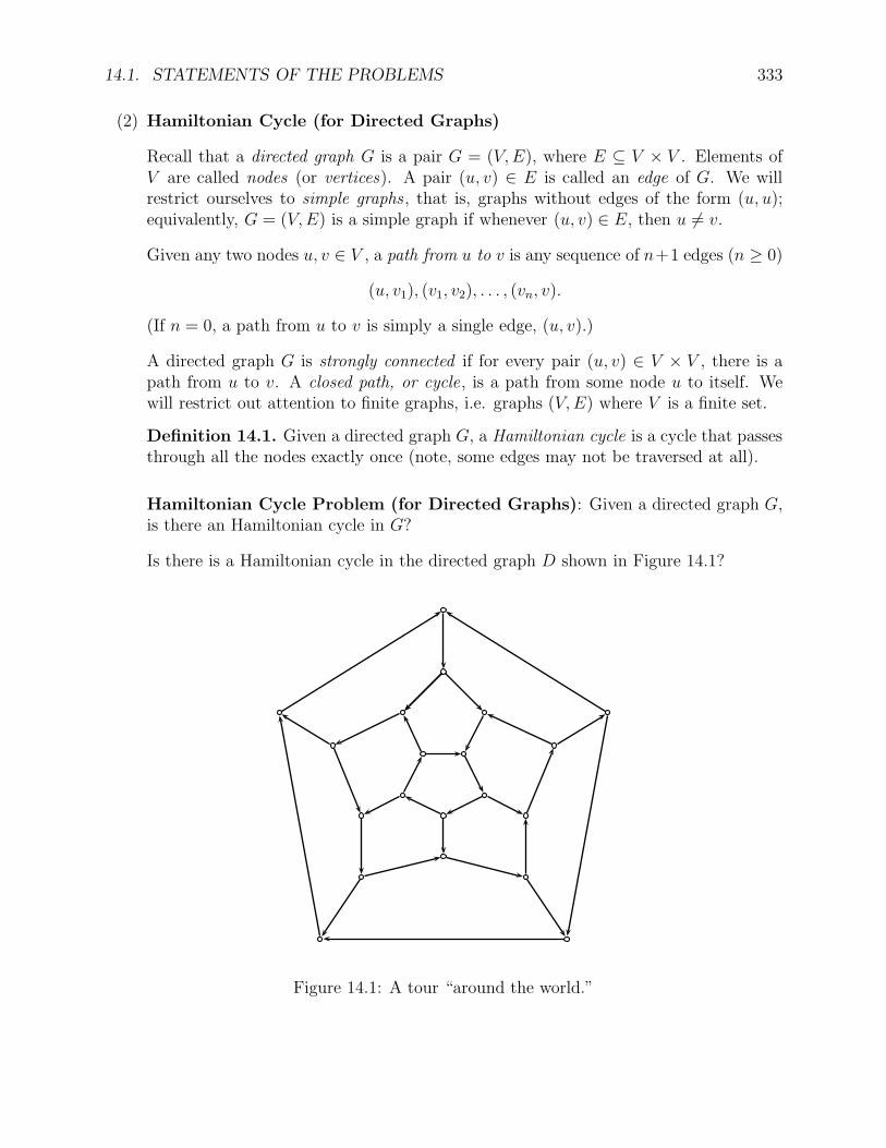
14.1. STATEMENTS OF THE PROBLEMS 333
(2) Hamiltonian Cycle (for Directed Graphs)
Recall that a directed graph G is a pair G = (V,E), where E ⊆ V × V . Elements ofV are called nodes (or vertices). A pair (u, v) ∈ E is called an edge of G. We willrestrict ourselves to simple graphs , that is, graphs without edges of the form (u, u);equivalently, G = (V,E) is a simple graph if whenever (u, v) ∈ E, then u 6= v.
Given any two nodes u, v ∈ V , a path from u to v is any sequence of n+1 edges (n ≥ 0)
(u, v1), (v1, v2), . . . , (vn, v).
(If n = 0, a path from u to v is simply a single edge, (u, v).)
A directed graph G is strongly connected if for every pair (u, v) ∈ V × V , there is apath from u to v. A closed path, or cycle, is a path from some node u to itself. Wewill restrict out attention to finite graphs, i.e. graphs (V,E) where V is a finite set.
Definition 14.1. Given a directed graph G, a Hamiltonian cycle is a cycle that passesthrough all the nodes exactly once (note, some edges may not be traversed at all).
Hamiltonian Cycle Problem (for Directed Graphs): Given a directed graph G,is there an Hamiltonian cycle in G?
Is there is a Hamiltonian cycle in the directed graph D shown in Figure 14.1?
Figure 14.1: A tour “around the world.”
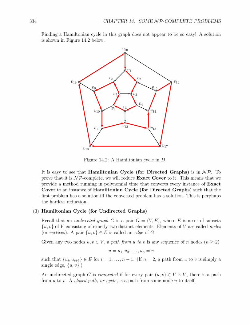
334 CHAPTER 14. SOME NP-COMPLETE PROBLEMS
Finding a Hamiltonian cycle in this graph does not appear to be so easy! A solutionis shown in Figure 14.2 below.
v18v17
v11v12 v13
v10v6 v5
v4
v14
v19v9
v8
v7 v3
v2
v15
v16
v1
v20
Figure 14.2: A Hamiltonian cycle in D.
It is easy to see that Hamiltonian Cycle (for Directed Graphs) is in NP. Toprove that it is NP-complete, we will reduce Exact Cover to it. This means that weprovide a method running in polynomial time that converts every instance of ExactCover to an instance of Hamiltonian Cycle (for Directed Graphs) such that thefirst problem has a solution iff the converted problem has a solution. This is perphapsthe hardest reduction.
(3) Hamiltonian Cycle (for Undirected Graphs)
Recall that an undirected graph G is a pair G = (V,E), where E is a set of subsetsu, v of V consisting of exactly two distinct elements. Elements of V are called nodes(or vertices). A pair u, v ∈ E is called an edge of G.
Given any two nodes u, v ∈ V , a path from u to v is any sequence of n nodes (n ≥ 2)
u = u1, u2, . . . , un = v
such that ui, ui+1 ∈ E for i = 1, . . . , n− 1. (If n = 2, a path from u to v is simply asingle edge, u, v.)An undirected graph G is connected if for every pair (u, v) ∈ V × V , there is a pathfrom u to v. A closed path, or cycle, is a path from some node u to itself.
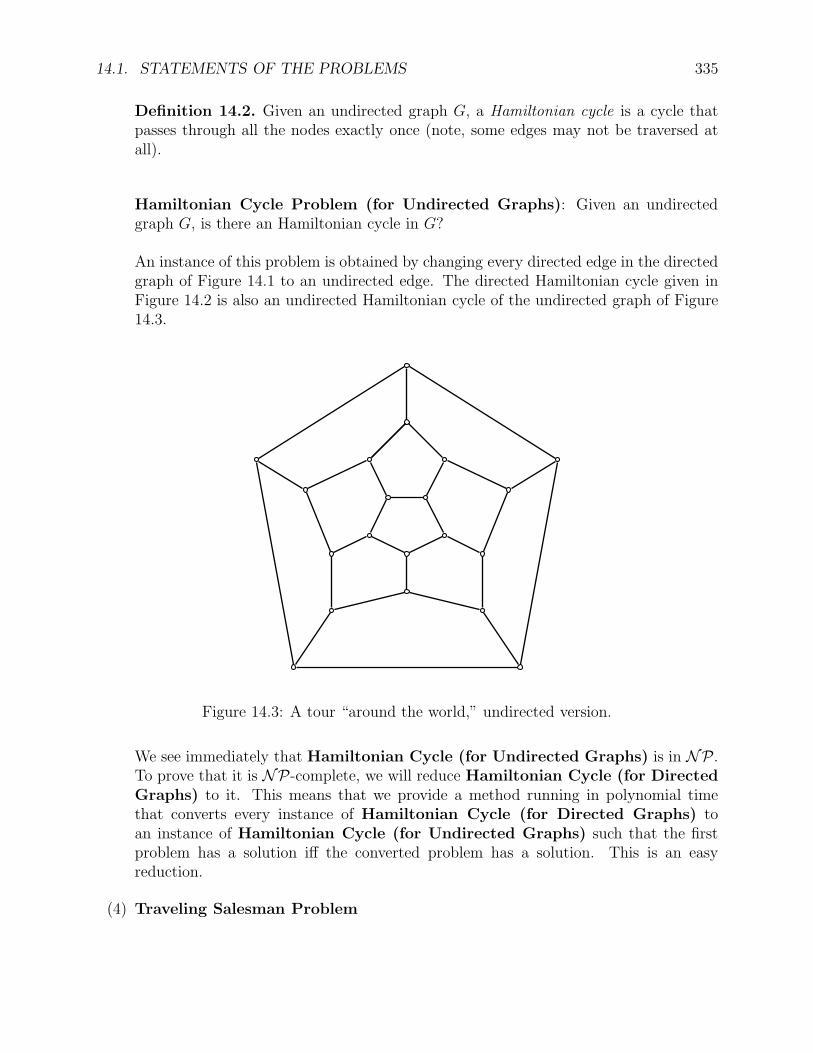
14.1. STATEMENTS OF THE PROBLEMS 335
Definition 14.2. Given an undirected graph G, a Hamiltonian cycle is a cycle thatpasses through all the nodes exactly once (note, some edges may not be traversed atall).
Hamiltonian Cycle Problem (for Undirected Graphs): Given an undirectedgraph G, is there an Hamiltonian cycle in G?
An instance of this problem is obtained by changing every directed edge in the directedgraph of Figure 14.1 to an undirected edge. The directed Hamiltonian cycle given inFigure 14.2 is also an undirected Hamiltonian cycle of the undirected graph of Figure14.3.
Figure 14.3: A tour “around the world,” undirected version.
We see immediately that Hamiltonian Cycle (for Undirected Graphs) is in NP.To prove that it is NP-complete, we will reduce Hamiltonian Cycle (for DirectedGraphs) to it. This means that we provide a method running in polynomial timethat converts every instance of Hamiltonian Cycle (for Directed Graphs) toan instance of Hamiltonian Cycle (for Undirected Graphs) such that the firstproblem has a solution iff the converted problem has a solution. This is an easyreduction.
(4) Traveling Salesman Problem
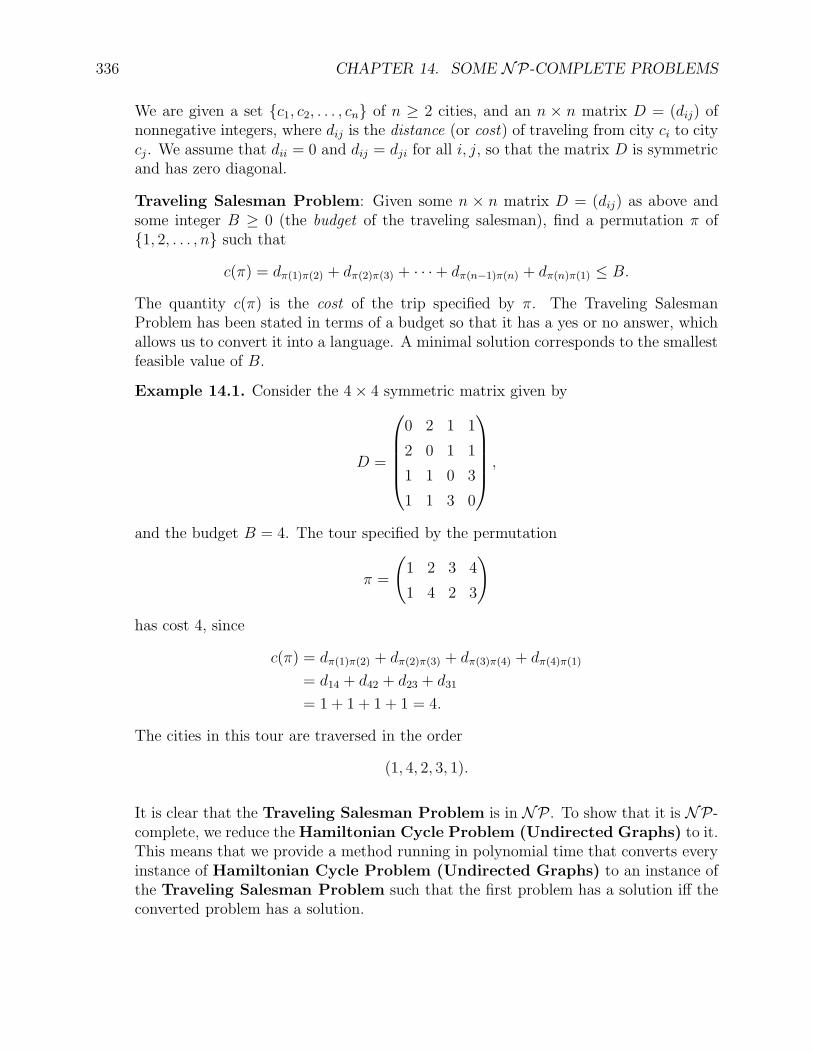
336 CHAPTER 14. SOME NP-COMPLETE PROBLEMS
We are given a set c1, c2, . . . , cn of n ≥ 2 cities, and an n × n matrix D = (dij) ofnonnegative integers, where dij is the distance (or cost) of traveling from city ci to citycj. We assume that dii = 0 and dij = dji for all i, j, so that the matrix D is symmetricand has zero diagonal.
Traveling Salesman Problem: Given some n × n matrix D = (dij) as above andsome integer B ≥ 0 (the budget of the traveling salesman), find a permutation π of1, 2, . . . , n such that
c(π) = dπ(1)π(2) + dπ(2)π(3) + · · ·+ dπ(n−1)π(n) + dπ(n)π(1) ≤ B.
The quantity c(π) is the cost of the trip specified by π. The Traveling SalesmanProblem has been stated in terms of a budget so that it has a yes or no answer, whichallows us to convert it into a language. A minimal solution corresponds to the smallestfeasible value of B.
Example 14.1. Consider the 4× 4 symmetric matrix given by
D =
0 2 1 1
2 0 1 1
1 1 0 3
1 1 3 0
,
and the budget B = 4. The tour specified by the permutation
π =
(1 2 3 4
1 4 2 3
)
has cost 4, since
c(π) = dπ(1)π(2) + dπ(2)π(3) + dπ(3)π(4) + dπ(4)π(1)
= d14 + d42 + d23 + d31
= 1 + 1 + 1 + 1 = 4.
The cities in this tour are traversed in the order
(1, 4, 2, 3, 1).
It is clear that the Traveling Salesman Problem is in NP. To show that it is NP-complete, we reduce theHamiltonian Cycle Problem (Undirected Graphs) to it.This means that we provide a method running in polynomial time that converts everyinstance of Hamiltonian Cycle Problem (Undirected Graphs) to an instance ofthe Traveling Salesman Problem such that the first problem has a solution iff theconverted problem has a solution.
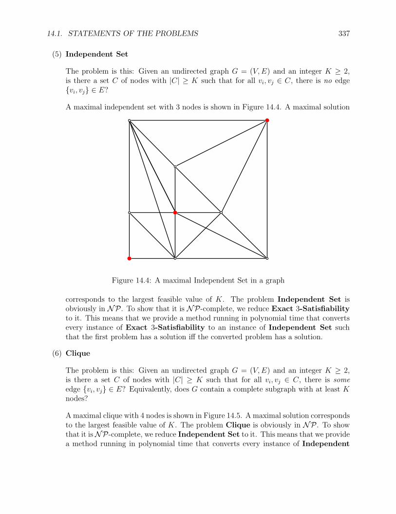
14.1. STATEMENTS OF THE PROBLEMS 337
(5) Independent Set
The problem is this: Given an undirected graph G = (V,E) and an integer K ≥ 2,is there a set C of nodes with |C| ≥ K such that for all vi, vj ∈ C, there is no edgevi, vj ∈ E?
A maximal independent set with 3 nodes is shown in Figure 14.4. A maximal solution
Figure 14.4: A maximal Independent Set in a graph
corresponds to the largest feasible value of K. The problem Independent Set isobviously in NP. To show that it is NP-complete, we reduce Exact 3-Satisfiabilityto it. This means that we provide a method running in polynomial time that convertsevery instance of Exact 3-Satisfiability to an instance of Independent Set suchthat the first problem has a solution iff the converted problem has a solution.
(6) Clique
The problem is this: Given an undirected graph G = (V,E) and an integer K ≥ 2,is there a set C of nodes with |C| ≥ K such that for all vi, vj ∈ C, there is someedge vi, vj ∈ E? Equivalently, does G contain a complete subgraph with at least Knodes?
A maximal clique with 4 nodes is shown in Figure 14.5. A maximal solution correspondsto the largest feasible value of K. The problem Clique is obviously in NP. To showthat it isNP-complete, we reduce Independent Set to it. This means that we providea method running in polynomial time that converts every instance of Independent
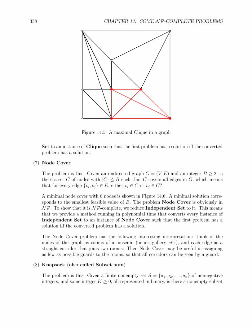
338 CHAPTER 14. SOME NP-COMPLETE PROBLEMS
Figure 14.5: A maximal Clique in a graph
Set to an instance ofClique such that the first problem has a solution iff the convertedproblem has a solution.
(7) Node Cover
The problem is this: Given an undirected graph G = (V,E) and an integer B ≥ 2, isthere a set C of nodes with |C| ≤ B such that C covers all edges in G, which meansthat for every edge vi, vj ∈ E, either vi ∈ C or vj ∈ C?
A minimal node cover with 6 nodes is shown in Figure 14.6. A minimal solution corre-sponds to the smallest feasible value of B. The problem Node Cover is obviously inNP. To show that it is NP-complete, we reduce Independent Set to it. This meansthat we provide a method running in polynomial time that converts every instance ofIndependent Set to an instance of Node Cover such that the first problem has asolution iff the converted problem has a solution.
The Node Cover problem has the following interesting interpretation: think of thenodes of the graph as rooms of a museum (or art gallery etc.), and each edge as astraight corridor that joins two rooms. Then Node Cover may be useful in assigningas few as possible guards to the rooms, so that all corridors can be seen by a guard.
(8) Knapsack (also called Subset sum)
The problem is this: Given a finite nonempty set S = a1, a2, . . . , an of nonnegativeintegers, and some integer K ≥ 0, all represented in binary, is there a nonempty subset
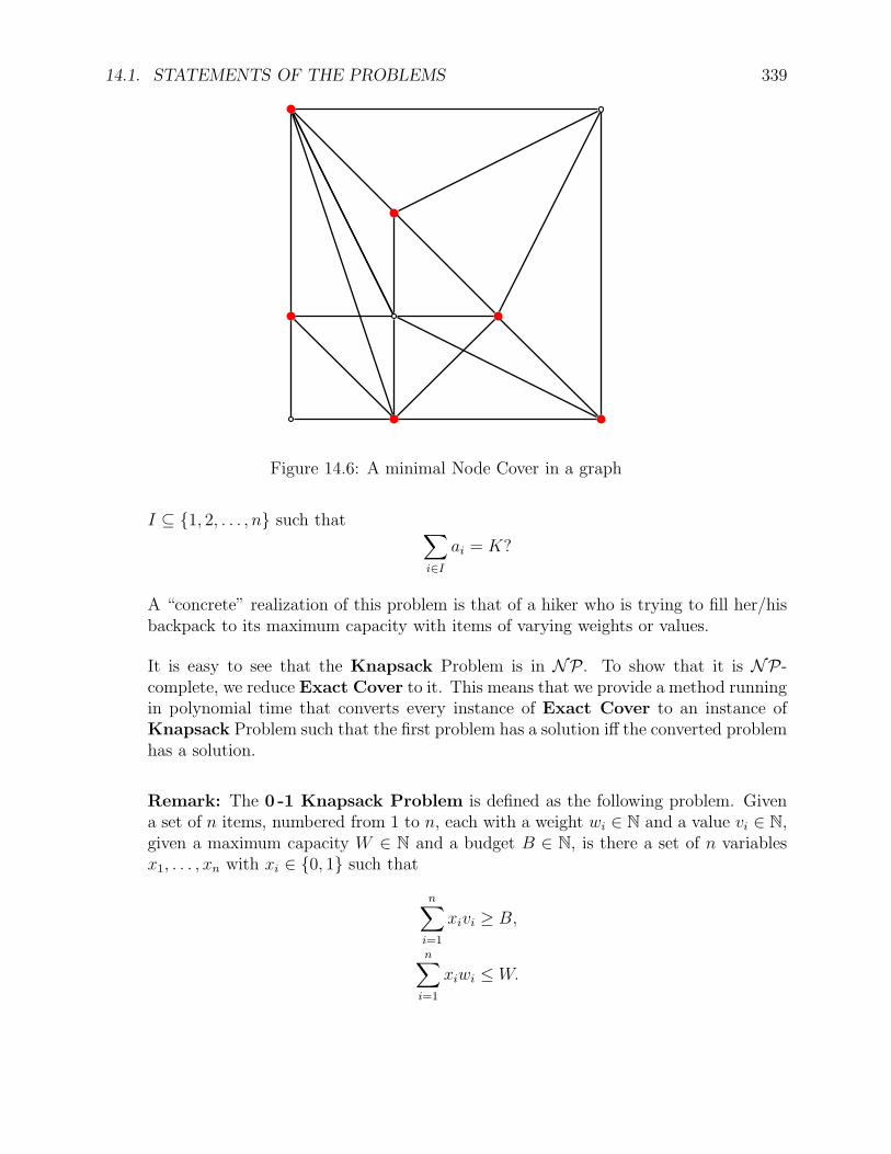
14.1. STATEMENTS OF THE PROBLEMS 339
Figure 14.6: A minimal Node Cover in a graph
I ⊆ 1, 2, . . . , n such that ∑
i∈I
ai = K?
A “concrete” realization of this problem is that of a hiker who is trying to fill her/hisbackpack to its maximum capacity with items of varying weights or values.
It is easy to see that the Knapsack Problem is in NP. To show that it is NP-complete, we reduce Exact Cover to it. This means that we provide a method runningin polynomial time that converts every instance of Exact Cover to an instance ofKnapsack Problem such that the first problem has a solution iff the converted problemhas a solution.
Remark: The 0 -1 Knapsack Problem is defined as the following problem. Givena set of n items, numbered from 1 to n, each with a weight wi ∈ N and a value vi ∈ N,given a maximum capacity W ∈ N and a budget B ∈ N, is there a set of n variablesx1, . . . , xn with xi ∈ 0, 1 such that
n∑
i=1
xivi ≥ B,
n∑
i=1
xiwi ≤W.
340 CHAPTER 14. SOME NP-COMPLETE PROBLEMS
Informally, the problem is to pick items to include in the knapsack so that the sumof the values exceeds a given minimum B (the goal is to maximize this sum), and thesum of the weights is less than or equal to the capacity W of the knapsack. A maximalsolution corresponds to the largest feasible value of B.
The Knapsack Problem as we defined it (which is how Lewis and Papadimitrioudefine it) is the special case where vi = wi = 1 for i = 1, . . . , n and W = B. For thisreason, it is also called the Subset Sum Problem. Clearly, the Knapsack (SubsetSum) Problem reduces to the 0 -1 Knapsack Problem, and thus the 0 -1 KnapsackProblem is also NP-complete.
(9) Inequivalence of ∗-free Regular Expressions
Recall that the problem of deciding the equivalence R1∼= R2 of two regular expressions
R1 and R2 is the problem of deciding whether R1 and R2 define the same language,that is, L[R1] = L[R2]. Is this problem in NP?
In order to show that the equivalence problem for regular expressions is in NP wewould have to be able to somehow check in polynomial time that two expressionsdefine the same language, but this is still an open problem.
What might be easier is to decide whether two regular expressions R1 and R2 areinequivalent . For this, we just have to find a string w such that either w ∈ L[R1]−L[R2]or w ∈ L[R2] − L[R1]. The problem is that if we can guess such a string w, we stillhave to check in polynomial time that w ∈ (L[R1]−L[R2])∪ (L[R2]−L[R1]), and thisimplies that there is a bound on the length of w which is polynomial in the sizes of R1
and R2. Again, this is an open problem.
To obtain a problem in NP we have to consider a restricted type of regular expressions,and it turns out that ∗-free regular expressions are the right candidate. A ∗-free regularexpression is a regular expression which is built up from the atomic expressions usingonly + and ·, but not ∗. For example,
R = ((a+ b)aa(a + b) + aba(a + b)b)
is such an expression.
It is easy to see that if R is a ∗-free regular expression, then for every string w ∈ L[R]we have |w| ≤ |R|. In particular, L[R] is finite. The above observation shows that ifR1 and R2 are ∗-free and if there is a string w ∈ (L[R1]−L[R2])∪(L[R2]−L[R1]), then|w| ≤ |R1|+ |R2|, so we can indeed check this in polynomial time. It follows that theinequivalence problem for ∗ -free regular expressions is in NP. To show that it is NP-complete, we reduce the Satisfiability Problem to it. This means that we providea method running in polynomial time that converts every instance of Satisfiability
14.1. STATEMENTS OF THE PROBLEMS 341
Problem to an instance of Inequivalence of Regular Expressions such that thefirst problem has a solution iff the converted problem has a solution.
Observe that both problems of Inequivalence of Regular Expressions and Equiv-alence of Regular Expressions are as hard as Inequivalence of ∗-free RegularExpressions, since if we could solve the first two problems in polynomial time, thenwe we could solve Inequivalence of ∗-free Regular Expressions in polynomialtime, but since this problem is NP-complete, we would have P = NP. This is veryunlikely, so the complexity of Equivalence of Regular Expressions remains open.
(10) 0-1 integer programming problem
Let A be any p× q matrix with integer coefficients and let b ∈ Zp be any vector withinteger coefficients. The 0-1 integer programming problem is to find whether asystem of p linear equations in q variables
a11x1 + · · ·+ a1qxq = b1...
...
ai1x1 + · · ·+ aiqxq = bi...
...
ap1x1 + · · ·+ apqxq = bp
with aij , bi ∈ Z has any solution x ∈ 0, 1q, that is, with xi ∈ 0, 1. In matrix form,if we let
A =
a11 · · · a1q...
. . ....
ap1 · · · apq
, b =
b1...
bp
, x =
x1...
xq
,
then we write the above system as
Ax = b.
It is immediate that 0-1 integer programming problem is in NP. To prove thatit is NP-complete we reduce the bounded tiling problem to it. This means thatwe provide a method running in polynomial time that converts every instance of thebounded tiling problem to an instance of the 0-1 integer programming problemsuch that the first problem has a solution iff the converted problem has a solution.
342 CHAPTER 14. SOME NP-COMPLETE PROBLEMS
14.2 Proofs of NP-Completeness
(1) Exact Cover
To prove that Exact Cover is NP-complete, we reduce the Satisfiability Problemto it:
Satisfiability Problem ≤P Exact Cover
Given a set F = C1, . . . , Cℓ of ℓ clauses constructed from n propositional variablesx1, . . . , xn, we must construct in polynomial time an instance τ(F ) = (U,F) of ExactCover such that F is satisfiable iff τ(F ) has a solution.
Example 14.2. If
F = C1 = (x1 ∨ x2), C2 = (x1 ∨ x2 ∨ x3), C3 = (x2), C4 = (x2 ∨ x3),
then the universe U is given by
U = x1, x2, x3, C1, C2, C3, C4, p11, p12, p21, p22, p23, p31, p41, p42,
and the family F consists of the subsets
p11, p12, p21, p22, p23, p31, p41, p42T1,F = x1, p11T1,T = x1, p21T2,F = x2, p22, p31T2,T = x2, p12, p41T3,F = x3, p23T3,T = x3, p42C1, p11, C1, p12, C2, p21, C2, p22, C2, p23,C3, p31, C4, p41, C4, p42.
It is easy to check that the set C consisting of the following subsets is an exact cover:
T1,T = x1, p21, T2,T = x2, p12, p41, T3,F = x3, p23,C1, p11, C2, p22, C3, p31, C4, p42.
The general method to construct (U,F) from F = C1, . . . , Cℓ proceeds as follows.Say
Cj = (Lj1 ∨ · · · ∨ Ljmj)
14.2. PROOFS OF NP-COMPLETENESS 343
is the jth clause in F , where Ljk denotes the kth literal in Cj andmj ≥ 1. The universeof τ(F ) is the set
U = xi | 1 ≤ i ≤ n ∪ Cj | 1 ≤ j ≤ ℓ ∪ pjk | 1 ≤ j ≤ ℓ, 1 ≤ k ≤ mj
where in the third set pjk corresponds to the kth literal in Cj.
The following subsets are included in F :
(a) There is a set pjk for every pjk.(b) For every boolean variable xi, the following two sets are in F :
Ti,T = xi ∪ pjk | Ljk = xi
which contains xi and all negative occurrences of xi, and
Ti,F = xi ∪ pjk | Ljk = xi
which contains xi and all its positive occurrences. Note carefully that Ti,T involvesnegative occurrences of xi whereas Ti,F involves positive occurrences of xi.
(c) For every clause Cj , the mj sets Cj , pjk are in F .
It remains to prove that F is satisfiable iff τ(F ) has a solution. We claim that if v isa truth assignement that satisfies F , then we can make an exact cover C as follows:
For each xi, we put the subset Ti,T in C iff v(xi) = T, else we we put the subset Ti,Fin C iff v(xi) = F. Also, for every clause Cj, we put some subset Cj, pjk in C for aliteral Ljk which is made true by v. By construction of Ti,T and Ti,F, this pjk is not inany set in C selected so far. Since by hypothesis F is satisfiable, such a literal exists forevery clause. Having covered all xi and Cj , we put a set pjk in C for every remainingpjk which has not yet been covered by the sets already in C.
Going back to Example 14.2, the truth assigment v(x1) = T, v(x2) = T, v(x3) = Fsatisfies F , so we put
T1,T = x1, p21, T2,T = x2, p12, p41, T3,F = x3, p23,C1, p11, C2, p22, C3, p31, C4, p42
in C.
We leave as an exercise to check that the above procedure works.
Conversely, if C is an exact cover of τ(F ), we define a truth assigment as follows:
For every xi, if Ti,T is in C, then we set v(xi) = T, else if Ti,F is in C, then we setv(xi) = F. We leave it as an exercise to check that this procedure works.
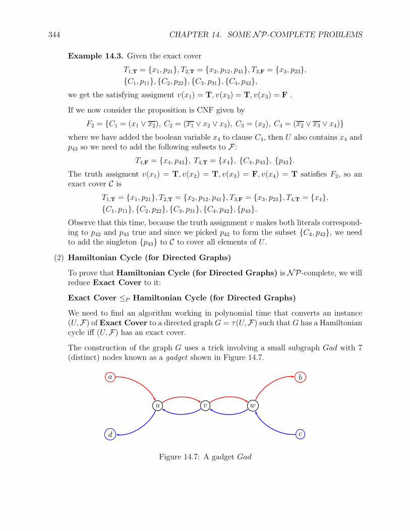
344 CHAPTER 14. SOME NP-COMPLETE PROBLEMS
Example 14.3. Given the exact cover
T1,T = x1, p21, T2,T = x2, p12, p41, T3,F = x3, p23,C1, p11, C2, p22, C3, p31, C4, p42,
we get the satisfying assigment v(x1) = T, v(x2) = T, v(x3) = F .
If we now consider the proposition is CNF given by
F2 = C1 = (x1 ∨ x2), C2 = (x1 ∨ x2 ∨ x3), C3 = (x2), C4 = (x2 ∨ x3 ∨ x4)where we have added the boolean variable x4 to clause C4, then U also contains x4 andp43 so we need to add the following subsets to F :
T4,F = x4, p43, T4,T = x4, C4, p43, p43.The truth assigment v(x1) = T, v(x2) = T, v(x3) = F, v(x4) = T satisfies F2, so anexact cover C is
T1,T = x1, p21, T2,T = x2, p12, p41, T3,F = x3, p23, T4,T = x4,C1, p11, C2, p22, C3, p31, C4, p42, p43.
Observe that this time, because the truth assignment v makes both literals correspond-ing to p42 and p43 true and since we picked p42 to form the subset C4, p42, we needto add the singleton p43 to C to cover all elements of U .
(2) Hamiltonian Cycle (for Directed Graphs)
To prove that Hamiltonian Cycle (for Directed Graphs) is NP-complete, we willreduce Exact Cover to it:
Exact Cover ≤P Hamiltonian Cycle (for Directed Graphs)
We need to find an algorithm working in polynomial time that converts an instance(U,F) of Exact Cover to a directed graph G = τ(U,F) such that G has a Hamiltoniancycle iff (U,F) has an exact cover.
The construction of the graph G uses a trick involving a small subgraph Gad with 7(distinct) nodes known as a gadget shown in Figure 14.7.
a
d
u v w
b
c
Figure 14.7: A gadget Gad
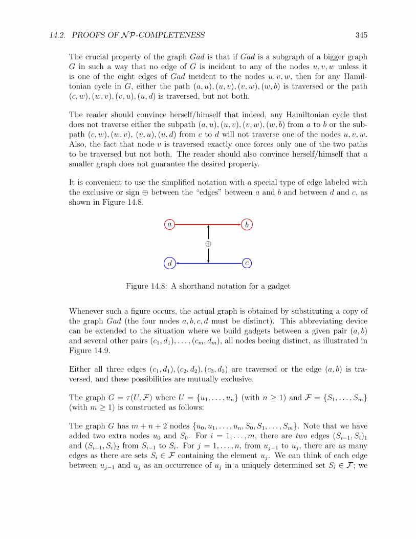
14.2. PROOFS OF NP-COMPLETENESS 345
The crucial property of the graph Gad is that if Gad is a subgraph of a bigger graphG in such a way that no edge of G is incident to any of the nodes u, v, w unless itis one of the eight edges of Gad incident to the nodes u, v, w, then for any Hamil-tonian cycle in G, either the path (a, u), (u, v), (v, w), (w, b) is traversed or the path(c, w), (w, v), (v, u), (u, d) is traversed, but not both.
The reader should convince herself/himself that indeed, any Hamiltonian cycle thatdoes not traverse either the subpath (a, u), (u, v), (v, w), (w, b) from a to b or the sub-path (c, w), (w, v), (v, u), (u, d) from c to d will not traverse one of the nodes u, v, w.Also, the fact that node v is traversed exactly once forces only one of the two pathsto be traversed but not both. The reader should also convince herself/himself that asmaller graph does not guarantee the desired property.
It is convenient to use the simplified notation with a special type of edge labeled withthe exclusive or sign ⊕ between the “edges” between a and b and between d and c, asshown in Figure 14.8.
a
d
b
c
⊕
Figure 14.8: A shorthand notation for a gadget
Whenever such a figure occurs, the actual graph is obtained by substituting a copy ofthe graph Gad (the four nodes a, b, c, d must be distinct). This abbreviating devicecan be extended to the situation where we build gadgets between a given pair (a, b)and several other pairs (c1, d1), . . . , (cm, dm), all nodes beeing distinct, as illustrated inFigure 14.9.
Either all three edges (c1, d1), (c2, d2), (c3, d3) are traversed or the edge (a, b) is tra-versed, and these possibilities are mutually exclusive.
The graph G = τ(U,F) where U = u1, . . . , un (with n ≥ 1) and F = S1, . . . , Sm(with m ≥ 1) is constructed as follows:
The graph G has m+ n + 2 nodes u0, u1, . . . , un, S0, S1, . . . , Sm. Note that we haveadded two extra nodes u0 and S0. For i = 1, . . . , m, there are two edges (Si−1, Si)1and (Si−1, Si)2 from Si−1 to Si. For j = 1, . . . , n, from uj−1 to uj, there are as manyedges as there are sets Si ∈ F containing the element uj. We can think of each edgebetween uj−1 and uj as an occurrence of uj in a uniquely determined set Si ∈ F ; we
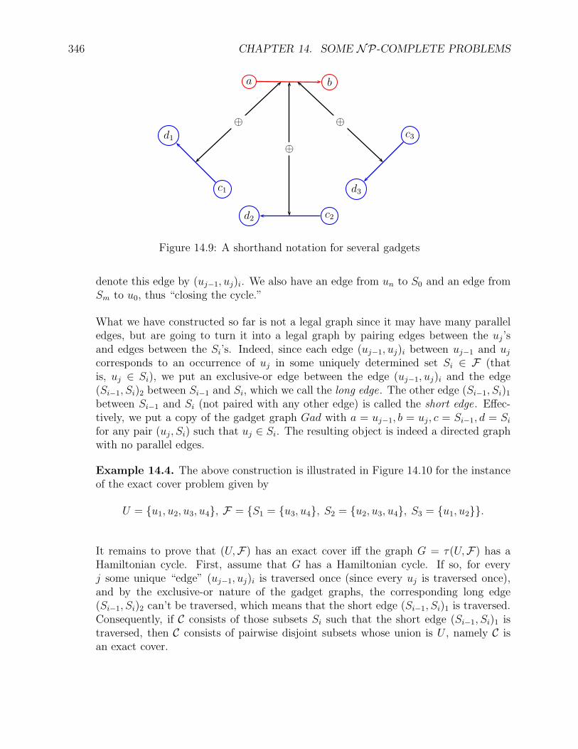
346 CHAPTER 14. SOME NP-COMPLETE PROBLEMS
a b
d2 c2
d1
c1 d3
c3⊕
⊕
⊕
Figure 14.9: A shorthand notation for several gadgets
denote this edge by (uj−1, uj)i. We also have an edge from un to S0 and an edge fromSm to u0, thus “closing the cycle.”
What we have constructed so far is not a legal graph since it may have many paralleledges, but are going to turn it into a legal graph by pairing edges between the uj’sand edges between the Si’s. Indeed, since each edge (uj−1, uj)i between uj−1 and ujcorresponds to an occurrence of uj in some uniquely determined set Si ∈ F (thatis, uj ∈ Si), we put an exclusive-or edge between the edge (uj−1, uj)i and the edge(Si−1, Si)2 between Si−1 and Si, which we call the long edge. The other edge (Si−1, Si)1between Si−1 and Si (not paired with any other edge) is called the short edge. Effec-tively, we put a copy of the gadget graph Gad with a = uj−1, b = uj, c = Si−1, d = Si
for any pair (uj, Si) such that uj ∈ Si. The resulting object is indeed a directed graphwith no parallel edges.
Example 14.4. The above construction is illustrated in Figure 14.10 for the instanceof the exact cover problem given by
U = u1, u2, u3, u4, F = S1 = u3, u4, S2 = u2, u3, u4, S3 = u1, u2.
It remains to prove that (U,F) has an exact cover iff the graph G = τ(U,F) has aHamiltonian cycle. First, assume that G has a Hamiltonian cycle. If so, for everyj some unique “edge” (uj−1, uj)i is traversed once (since every uj is traversed once),and by the exclusive-or nature of the gadget graphs, the corresponding long edge(Si−1, Si)2 can’t be traversed, which means that the short edge (Si−1, Si)1 is traversed.Consequently, if C consists of those subsets Si such that the short edge (Si−1, Si)1 istraversed, then C consists of pairwise disjoint subsets whose union is U , namely C isan exact cover.
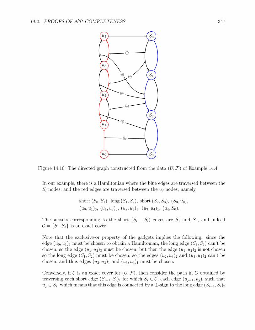
14.2. PROOFS OF NP-COMPLETENESS 347
u0
u1
u2
u3
u4 S0
S1
S2
S3
⊕
⊕ ⊕
⊕
⊕
⊕
⊕
Figure 14.10: The directed graph constructed from the data (U,F) of Example 14.4
In our example, there is a Hamiltonian where the blue edges are traversed between theSi nodes, and the red edges are traversed between the uj nodes, namely
short (S0, S1), long (S1, S2), short (S2, S3), (S3, u0),
(u0, u1)3, (u1, u2)3, (u2, u3)1, (u3, u4)1, (u4, S0).
The subsets corresponding to the short (Si−1, Si) edges are S1 and S3, and indeedC = S1, S3 is an exact cover.
Note that the exclusive-or property of the gadgets implies the following: since theedge (u0, u1)3 must be chosen to obtain a Hamiltonian, the long edge (S2, S3) can’t bechosen, so the edge (u1, u2)3 must be chosen, but then the edge (u1, u2)2 is not chosenso the long edge (S1, S2) must be chosen, so the edges (u2, u3)2 and (u3, u4)2 can’t bechosen, and thus edges (u2, u3)1 and (u3, u4)1 must be chosen.
Conversely, if C is an exact cover for (U,F), then consider the path in G obtained bytraversing each short edge (Si−1, Si)1 for which Si ∈ C, each edge (uj−1, uj)i such thatuj ∈ Si, which means that this edge is connected by a ⊕-sign to the long edge (Si−1, Si)2
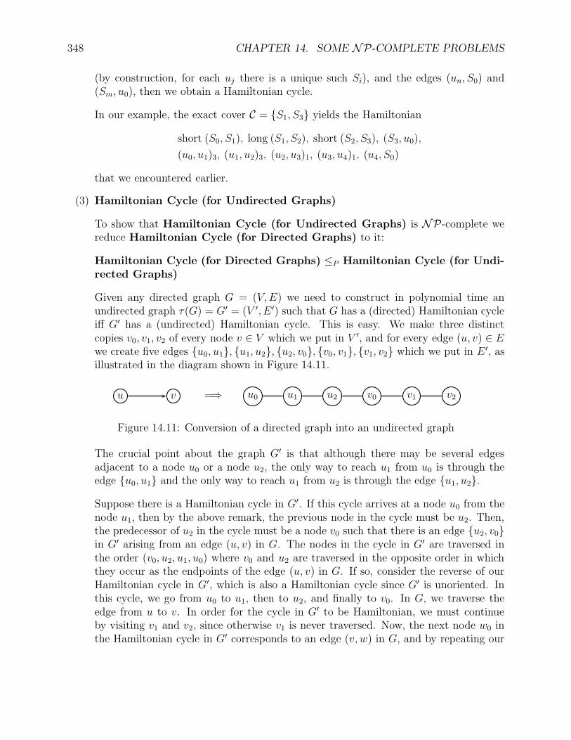
348 CHAPTER 14. SOME NP-COMPLETE PROBLEMS
(by construction, for each uj there is a unique such Si), and the edges (un, S0) and(Sm, u0), then we obtain a Hamiltonian cycle.
In our example, the exact cover C = S1, S3 yields the Hamiltonian
short (S0, S1), long (S1, S2), short (S2, S3), (S3, u0),
(u0, u1)3, (u1, u2)3, (u2, u3)1, (u3, u4)1, (u4, S0)
that we encountered earlier.
(3) Hamiltonian Cycle (for Undirected Graphs)
To show that Hamiltonian Cycle (for Undirected Graphs) is NP-complete wereduce Hamiltonian Cycle (for Directed Graphs) to it:
Hamiltonian Cycle (for Directed Graphs) ≤P Hamiltonian Cycle (for Undi-rected Graphs)
Given any directed graph G = (V,E) we need to construct in polynomial time anundirected graph τ(G) = G′ = (V ′, E ′) such that G has a (directed) Hamiltonian cycleiff G′ has a (undirected) Hamiltonian cycle. This is easy. We make three distinctcopies v0, v1, v2 of every node v ∈ V which we put in V ′, and for every edge (u, v) ∈ Ewe create five edges u0, u1, u1, u2, u2, v0, v0, v1, v1, v2 which we put in E ′, asillustrated in the diagram shown in Figure 14.11.
u v u0 u1 u2 v0 v1 v2=⇒
Figure 14.11: Conversion of a directed graph into an undirected graph
The crucial point about the graph G′ is that although there may be several edgesadjacent to a node u0 or a node u2, the only way to reach u1 from u0 is through theedge u0, u1 and the only way to reach u1 from u2 is through the edge u1, u2.
Suppose there is a Hamiltonian cycle in G′. If this cycle arrives at a node u0 from thenode u1, then by the above remark, the previous node in the cycle must be u2. Then,the predecessor of u2 in the cycle must be a node v0 such that there is an edge u2, v0in G′ arising from an edge (u, v) in G. The nodes in the cycle in G′ are traversed inthe order (v0, u2, u1, u0) where v0 and u2 are traversed in the opposite order in whichthey occur as the endpoints of the edge (u, v) in G. If so, consider the reverse of ourHamiltonian cycle in G′, which is also a Hamiltonian cycle since G′ is unoriented. Inthis cycle, we go from u0 to u1, then to u2, and finally to v0. In G, we traverse theedge from u to v. In order for the cycle in G′ to be Hamiltonian, we must continueby visiting v1 and v2, since otherwise v1 is never traversed. Now, the next node w0 inthe Hamiltonian cycle in G′ corresponds to an edge (v, w) in G, and by repeating our
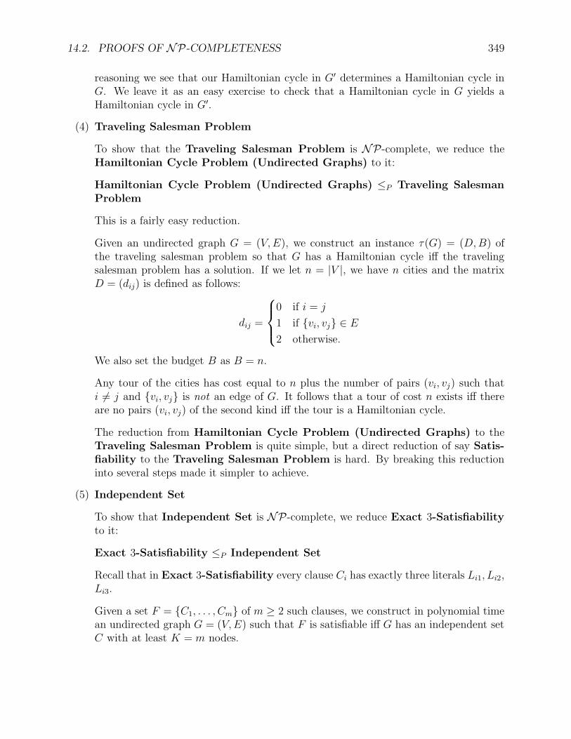
14.2. PROOFS OF NP-COMPLETENESS 349
reasoning we see that our Hamiltonian cycle in G′ determines a Hamiltonian cycle inG. We leave it as an easy exercise to check that a Hamiltonian cycle in G yields aHamiltonian cycle in G′.
(4) Traveling Salesman Problem
To show that the Traveling Salesman Problem is NP-complete, we reduce theHamiltonian Cycle Problem (Undirected Graphs) to it:
Hamiltonian Cycle Problem (Undirected Graphs) ≤P Traveling SalesmanProblem
This is a fairly easy reduction.
Given an undirected graph G = (V,E), we construct an instance τ(G) = (D,B) ofthe traveling salesman problem so that G has a Hamiltonian cycle iff the travelingsalesman problem has a solution. If we let n = |V |, we have n cities and the matrixD = (dij) is defined as follows:
dij =
0 if i = j
1 if vi, vj ∈ E2 otherwise.
We also set the budget B as B = n.
Any tour of the cities has cost equal to n plus the number of pairs (vi, vj) such thati 6= j and vi, vj is not an edge of G. It follows that a tour of cost n exists iff thereare no pairs (vi, vj) of the second kind iff the tour is a Hamiltonian cycle.
The reduction from Hamiltonian Cycle Problem (Undirected Graphs) to theTraveling Salesman Problem is quite simple, but a direct reduction of say Satis-fiability to the Traveling Salesman Problem is hard. By breaking this reductioninto several steps made it simpler to achieve.
(5) Independent Set
To show that Independent Set is NP-complete, we reduce Exact 3-Satisfiabilityto it:
Exact 3-Satisfiability ≤P Independent Set
Recall that in Exact 3-Satisfiability every clause Ci has exactly three literals Li1, Li2,Li3.
Given a set F = C1, . . . , Cm of m ≥ 2 such clauses, we construct in polynomial timean undirected graph G = (V,E) such that F is satisfiable iff G has an independent setC with at least K = m nodes.
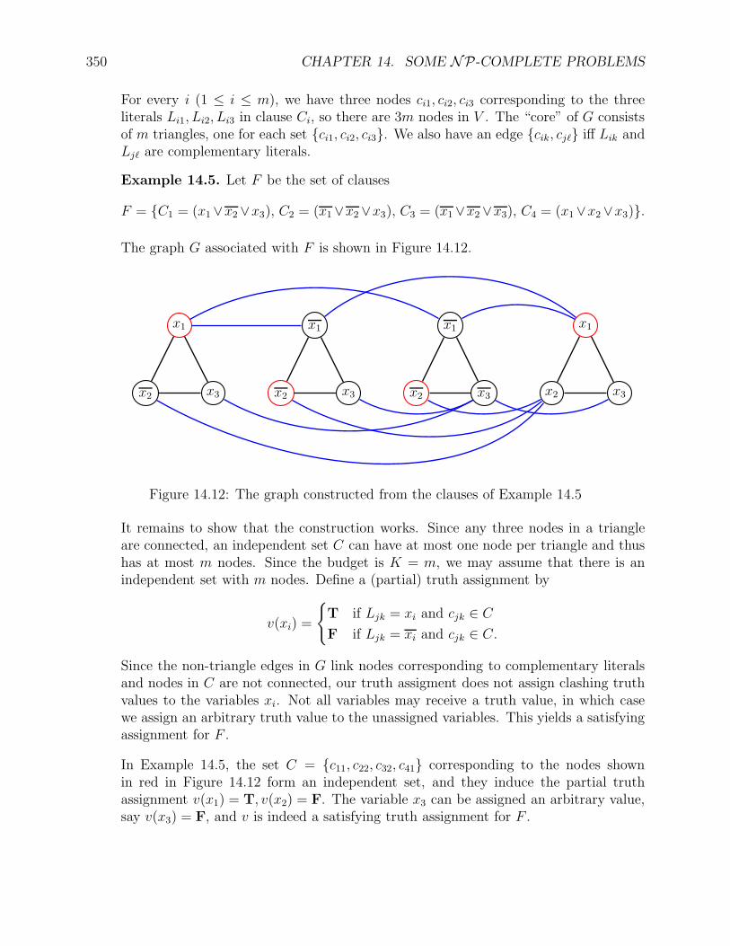
350 CHAPTER 14. SOME NP-COMPLETE PROBLEMS
For every i (1 ≤ i ≤ m), we have three nodes ci1, ci2, ci3 corresponding to the threeliterals Li1, Li2, Li3 in clause Ci, so there are 3m nodes in V . The “core” of G consistsof m triangles, one for each set ci1, ci2, ci3. We also have an edge cik, cjℓ iff Lik andLjℓ are complementary literals.
Example 14.5. Let F be the set of clauses
F = C1 = (x1∨x2∨x3), C2 = (x1∨x2∨x3), C3 = (x1∨x2∨x3), C4 = (x1∨x2∨x3).
The graph G associated with F is shown in Figure 14.12.
x2 x3
x1
x2 x3
x1
x2 x3
x1
x2 x3
x1
Figure 14.12: The graph constructed from the clauses of Example 14.5
It remains to show that the construction works. Since any three nodes in a triangleare connected, an independent set C can have at most one node per triangle and thushas at most m nodes. Since the budget is K = m, we may assume that there is anindependent set with m nodes. Define a (partial) truth assignment by
v(xi) =
T if Ljk = xi and cjk ∈ CF if Ljk = xi and cjk ∈ C.
Since the non-triangle edges in G link nodes corresponding to complementary literalsand nodes in C are not connected, our truth assigment does not assign clashing truthvalues to the variables xi. Not all variables may receive a truth value, in which casewe assign an arbitrary truth value to the unassigned variables. This yields a satisfyingassignment for F .
In Example 14.5, the set C = c11, c22, c32, c41 corresponding to the nodes shownin red in Figure 14.12 form an independent set, and they induce the partial truthassignment v(x1) = T, v(x2) = F. The variable x3 can be assigned an arbitrary value,say v(x3) = F, and v is indeed a satisfying truth assignment for F .
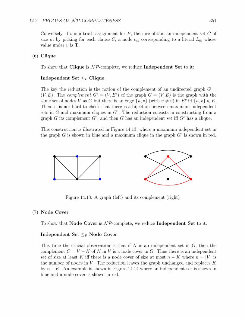
14.2. PROOFS OF NP-COMPLETENESS 351
Conversely, if v is a truth assignment for F , then we obtain an independent set C ofsize m by picking for each clause Ci a node cik corresponding to a literal Lik whosevalue under v is T.
(6) Clique
To show that Clique is NP-complete, we reduce Independent Set to it:
Independent Set ≤P Clique
The key the reduction is the notion of the complement of an undirected graph G =(V,E). The complement Gc = (V,Ec) of the graph G = (V,E) is the graph with thesame set of nodes V as G but there is an edge u, v (with u 6= v) in Ec iff u, v /∈ E.Then, it is not hard to check that there is a bijection between maximum independentsets in G and maximum cliques in Gc. The reduction consists in constructing from agraph G its complement Gc, and then G has an independent set iff Gc has a clique.
This construction is illustrated in Figure 14.13, where a maximum independent set inthe graph G is shown in blue and a maximum clique in the graph Gc is shown in red.
Figure 14.13: A graph (left) and its complement (right)
(7) Node Cover
To show that Node Cover is NP-complete, we reduce Independent Set to it:
Independent Set ≤P Node Cover
This time the crucial observation is that if N is an independent set in G, then thecomplement C = V −N of N in V is a node cover in G. Thus there is an independentset of size at least K iff there is a node cover of size at most n −K where n = |V | isthe number of nodes in V . The reduction leaves the graph unchanged and replaces Kby n−K. An example is shown in Figure 14.14 where an independent set is shown inblue and a node cover is shown in red.
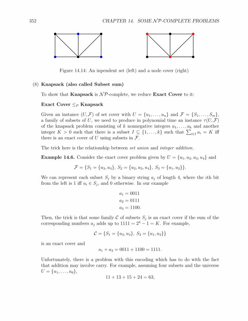
352 CHAPTER 14. SOME NP-COMPLETE PROBLEMS
Figure 14.14: An inpendent set (left) and a node cover (right)
(8) Knapsack (also called Subset sum)
To show that Knapsack is NP-complete, we reduce Exact Cover to it:
Exact Cover ≤P Knapsack
Given an instance (U,F) of set cover with U = u1, . . . , un and F = S1, . . . , Sm,a family of subsets of U , we need to produce in polynomial time an instance τ(U,F)of the knapsack problem consisting of k nonnegative integers a1, . . . , ak and anotherinteger K > 0 such that there is a subset I ⊆ 1, . . . , k such that
∑i∈I ai = K iff
there is an exact cover of U using subsets in F .
The trick here is the relationship between set union and integer addition.
Example 14.6. Consider the exact cover problem given by U = u1, u2, u3, u4 and
F = S1 = u3, u4, S2 = u2, u3, u4, S3 = u1, u2.
We can represent each subset Sj by a binary string aj of length 4, where the ith bitfrom the left is 1 iff ui ∈ Sj , and 0 otherwise. In our example
a1 = 0011
a2 = 0111
a3 = 1100.
Then, the trick is that some family C of subsets Sj is an exact cover if the sum of thecorresponding numbers aj adds up to 1111 = 24 − 1 = K. For example,
C = S1 = u3, u4, S3 = u1, u2
is an exact cover anda1 + a3 = 0011 + 1100 = 1111.
Unfortunately, there is a problem with this encoding which has to do with the factthat addition may involve carry. For example, assuming four subsets and the universeU = u1, . . . , u6,
11 + 13 + 15 + 24 = 63,
14.2. PROOFS OF NP-COMPLETENESS 353
in binary
001011 + 001101 + 001111 + 011000 = 111111,
but if we convert these binary strings to the corresponding subsets we get the subsets
S1 = u3, u5, u6S2 = u3, u4, u6S3 = u3, u4, u5, u6S4 = u2, u3,
which are not disjoint and do not cover U .
The fix is surprisingly simple: use base m (where m is the number of subsets in F)instead of base 2.
Example 14.7. Consider the exact cover problem given by U = u1, u2, u3, u4, u5, u6and F given by
S1 = u3, u5, u6S2 = u3, u4, u6S3 = u3, u4, u5, u6S4 = u2, u3,S5 = u1, u2, u4.
In base m = 5, the numbers corresponding to S1, . . . , S5 are
a1 = 001011
a2 = 001101
a3 = 001111
a4 = 011000
a5 = 110100.
This time,
a1 + a2 + a3 + a4 = 001011 + 001101 + 001111 + 011000 = 014223 6= 111111,
so S1, S2, S3, S4 is not a solution. However
a1 + a5 = 001011 + 110100 = 111111,
and C = S1, S5 is an exact cover.
354 CHAPTER 14. SOME NP-COMPLETE PROBLEMS
Thus, given an instance (U,F) of Exact Cover where U = u1, . . . , un and F =S1, . . . , Sm the reduction toKnapsack consists in forming them numbers a1, . . . , am(each of n bits) encoding the subsets Sj, namely aji = 1 iff ui ∈ Sj, else 0, and to letK = 1 +m2 + · · · +mn−1, which is represented in base m by the string 11 · · ·11︸ ︷︷ ︸
n
. In
testing whether∑
i∈I ai = K for some subset I ⊆ 1, . . . , m, we use arithmetic inbase m.
If a candidate solution C involves at most m− 1 subsets, then since the correspondingnumbers are added in base m, a carry can never happen. If the candidate solutioninvolves all m subsets, then a1+ · · ·+am = K iff F is a partition of U , since otherwisesome bit in the result of adding up these m numbers in base m is not equal to 1, evenif a carry occurs.
(9) Inequivalence of ∗-free Regular Expressions
To show that Inequivalence of ∗-free Regular Expressions is NP-complete, wereduce the Satisfiability Problem to it:
Satisfiability Problem ≤P Inequivalence of ∗-free Regular Expressions
We already argued that Inequivalence of ∗-free Regular Expressions is in NPbecause if R is a ∗-free regular expression, then for every string w ∈ L[R] we have|w| ≤ |R|. The above observation shows that if R1 and R2 are ∗-free and if there is astring w ∈ (L[R1]−L[R2])∪ (L[R2]−L[R1]), then |w| ≤ |R1|+ |R2|, so we can indeedcheck this in polynomial time. It follows that the inequivalence problem for ∗ -freeregular expressions is in NP.
We reduce the Satisfiability Problem to the Inequivalence of ∗-free RegularExpressions as follows. For any set of clauses P = C1 ∧ · · · ∧Cp, if the propositionalvariables occurring in P are x1, . . . , xn, we produce two ∗-free regular expressions R,S over Σ = 0, 1, such that P is satisfiable iff LR 6= LS. The expression S is actually
S = (0 + 1)(0 + 1) · · · (0 + 1)︸ ︷︷ ︸n
.
The expression R is of the form
R = R1 + · · ·+Rp,
where Ri is constructed from the clause Ci in such a way that LRicorresponds precisely
to the set of truth assignments that falsify Ci; see below.
Given any clause Ci, let Ri be the ∗-free regular expression defined such that, if xj andxj both belong to Ci (for some j), then Ri = ∅, else
Ri = R1i ·R2
i · · ·Rni ,
14.3. SUCCINCT CERTIFICATES, coNP, AND EXP 355
where Rji is defined by
Rji =
0 if xj is a literal of Ci
1 if xj is a literal of Ci
(0 + 1) if xj does not occur in Ci.
Clearly, all truth assignments that falsify Ci must assign F to xj if xj ∈ Ci or assignT to xj if xj ∈ Ci. Therefore, LRi
corresponds to the set of truth assignments thatfalsify Ci (where 1 stands for T and 0 stands for F) and thus, if we let
R = R1 + · · ·+Rp,
then LR corresponds to the set of truth assignments that falsify P = C1 ∧ · · · ∧ Cp.Since LS = 0, 1n (all binary strings of length n), we conclude that LR 6= LS iff P issatisfiable. Therefore, we have reduced the Satisfiability Problem to our problemand the reduction clearly runs in polynomial time. This proves that the problem ofdeciding whether LR 6= LS, for any two ∗-free regular expressions R and S is NP-complete.
(10) 0-1 integer programming problem
It is easy to check that the problem is in NP.
To prove that the is NP-complete we reduce the bounded-tiling problem to it:
bounded-tiling problem ≤P 0-1 integer programming problem
Given a tiling problem, ((T , V,H), s, σ0), we create a 0-1-valued variable xmnt, suchthat xmnt = 1 iff tile t occurs in position (m,n) in some tiling. Write equations orinequalities expressing that a tiling exists and then use “slack variables” to convertinequalities to equations. For example, to express the fact that every position is tiledby a single tile, use the equation
∑
t∈T
xmnt = 1,
for all m,n with 1 ≤ m ≤ 2s and 1 ≤ n ≤ s. We leave the rest as as exercise.
14.3 Succinct Certificates, coNP, and EXPAll the problems considered in Section 14.1 share a common feature, which is that for eachproblem, a solution is produced nondeterministically (an exact cover, a directed Hamiltoniancycle, a tour of cities, an independent set, a node cover, a clique etc.), and then this candidatesolution is checked deterministically and in polynomial time. The candidate solution is astring called a certificate (or witness).
It turns out that membership on NP can be defined in terms of certificates. To be acertificate, a string must satisfy two conditions:
356 CHAPTER 14. SOME NP-COMPLETE PROBLEMS
1. It must be polynomially succinct , which means that its length is at most a polynomialin the length of the input.
2. It must be checkable in polynomial time.
All “yes” inputs to a problem in NP must have at least one certificate, while all “no”inputs must have none.
The notion of certificate can be formalized using the notion of a polynomially balancedlanguage.
Definition 14.3. Let Σ be an alphabet, and let “;” be a symbol not in Σ. A languageL′ ⊆ Σ∗; Σ∗ is said to be polynomially balanced if there exists a polynomial p(X) such thatfor all x, y ∈ Σ∗, if x; y ∈ L′ then |y| ≤ p(|x|).
Suppose L′ is a polynomially balanced language and that L′ ∈ P. Then we can considerthe language
L = x ∈ Σ∗ | (∃y ∈ Σ∗)(x; y ∈ L′).The intuition is that for each x ∈ L, the set
y ∈ Σ∗ | x; y ∈ L′
is the set of certificates of x. For every x ∈ L, a Turing machine can nondeterministicallyguess one of its certificates y, and then use the deterministic Turing machine for L′ to check inpolynomial time that x; y ∈ L′. Note that, by definition, strings not in L have no certificate.It follows that L ∈ NP.
Conversely, if L ∈ NP and the alphabet Σ has at least two symbols, we can encode thepaths in the computation tree for every input x ∈ L, and we obtain a polynomially balancedlanguage L′ ⊆ Σ∗; Σ∗ in P such that
L = x ∈ Σ∗ | (∃y ∈ Σ∗)(x; y ∈ L′).
The details of this construction are left as an exercise. In summary, we obtain the followingtheorem.
Theorem 14.1. Let L ⊆ Σ∗ be a language over an alphabet Σ with at least two symbols, andlet “;” be a symbol not in Σ. Then L ∈ NP iff there is a polynomially balanced languageL′ ⊆ Σ∗; Σ∗ such that L′ ∈ P and
L = x ∈ Σ∗ | (∃y ∈ Σ∗)(x; y ∈ L′).
A striking illustration of the notion of succint certificate is illustrated by the set ofcomposite integers, namely those natural numbers n ∈ N that can be written as the productpq of two numbers p, q ≥ 2 with p, q ∈ N. For example, the number
4, 294, 967, 297
14.3. SUCCINCT CERTIFICATES, coNP, AND EXP 357
is a composite!
This is far from obvious, but if an oracle gives us the certificate 6, 700, 417, 641, it iseasy to carry out in polynomial time the multiplication of these two numbers and check thatit is equal to 4, 294, 967, 297. Finding a certificate is usually (very) hard, but checking thatit works is easy. This is the point of certificates.
We conclude this section with a brief discussion of the complexity classes coNP andEXP.
By definition,
coNP = L | L ∈ NP,that is, coNP consists of all complements of languages in NP. Since P ⊆ NP and P isclosed under complementation,
P ⊆ coNP,but nobody knows whether NP is closed under complementation, that is, nobody knowswhether NP = coNP.
What can be shown is that if NP 6= coNP then P 6= NP. However it is possible thatP 6= NP and yet NP = coNP, although this is considered unlikely.
Of course, P ⊆ NP ∩ coNP. There are problems in NP ∩ coNP not known to be in P.One of the most famous in the following problem:
Integer factorization problem:
Given an integer N ≥ 3, and another integer M (a budget) such that 1 < M < N , doesN have a factor d with 1 < d ≤M?
That Integer factorization is in NP is clear. To show that Integer factorization isin coNP, we can guess a factorization of N into distinct factors all greater than M , checkthat they are prime using the results of Chapter 15 showing that testing primality is in NP(even in P, but that’s much harder to prove), and then check that the product of thesefactors is N .
It is widely believed that Integer factorization does not belong to P, which is thetechnical justification for saying that this problem is hard. Most cryptographic algorithmsrely on this unproven fact. If Integer factorization was either NP-complete or coNP-complete, then we would have NP = coNP, which is considered very unlikely.
Remark: If√N ≤M < N , the above problem is equivalent to asking whether N is prime.
A natural instance of a problem in coNP is the unsatisfiability problem for propositionsUNSAT = ¬SAT, namely deciding that a proposition P has no satisfying assignmnent.
A proposition P (in CNF) is falsifiable if there is some truth assigment v such thatv(P ) = F. It is obvious that the set of falsifiable propositions is in NP. Since a proposition
358 CHAPTER 14. SOME NP-COMPLETE PROBLEMS
P is valid iff P is not falsifiable, the validity (or tautology) problem TAUT for propositionsis in coNP. In fact, TAUT is coNP-complete; see Papadimitriou [14].
This is easy to prove. Since SAT is NP-complete, for every language L ∈ NP, there isa polynomial-time computable function f : Σ∗ → Σ∗ such that x ∈ L iff f(x) ∈ SAT. Thenx /∈ L iff f(x) /∈ SAT, that is, x ∈ L iff f(x) ∈ ¬SAT, which means that every language L ∈coNP is polynomial-time reducible to ¬SAT = UNSAT. But TAUT = ¬P | P ∈ UNSAT,so we have the polynomial-time computable function g given by g(x) = ¬f(x) which givesus the reduction x ∈ L iff g(x) ∈ TAUT, which shows that TAUT is coNP-complete.
Despite the fact that this problem has been extensively studied, not much is known aboutits exact complexity.
The reasoning used to show that TAUT is coNP-complete can also be used to show thefollowing interesting result.
Proposition 14.2. If a language L is NP-complete, then its complement L is coNP-complete.
Proof. By definition, since L ∈ NP, we have L ∈ coNP. Since L is NP-complete, for everylanguage L2 ∈ NP, there is a polynomial-time computable function f : Σ∗ → Σ∗ such thatx ∈ L2 iff f(x) ∈ L. Then x /∈ L2 iff f(x) /∈ L, that is, x ∈ L2 iff f(x) ∈ L, which meansthat L is coNP-hard as well, thus coNP-complete.
The class EXP is defined as follows.
Definition 14.4. A deterministic Turing machine M is said to be exponentially bounded ifthere is a polynomial p(X) such that for every input x ∈ Σ∗, there is no ID IDn such that
ID0 ⊢ ID1 ⊢∗ IDn−1 ⊢ IDn, with n > 2p(|x|).
The class EXP is the class of all languages that are accepted by some exponentially boundeddeterministic Turing machine.
Remark: We can also define the class NEXP as in Definition 14.4, except that we allownondeterministic Turing machines.
One of the interesting features of EXP is that it contains NP.
Theorem 14.3. We have the inclusion NP ⊆ EXP.
Sketch of proof. LetM be some nondeterministic Turing machine accepting L in polynomialtime bounded by p(X). We can construct a deterministic Turing machine M ′ that operatesas follows: for every input x, M ′ simulates M on all computations of length 1, then onall possible computations of length 2, and so on, up to all possible computations of lengthp(|x|)+ 1. At this point, either an accepting computation has been discovered or all compu-tations have halted rejecting. We claim thatM ′ operates in time bounded by 2q(|x|) for some
14.3. SUCCINCT CERTIFICATES, coNP, AND EXP 359
poynomial q(X). First, let r be the degree of nondeterminism of M , that is, the maximumnumber of triples (b,m, q) such that a quintuple (p, q, b,m, q) is an instructions of M . Thento simulate a computation of M of length ℓ, M ′ needs O(ℓ) steps—to copy the input, toproduce a string c in 1, . . . , rℓ, and so simulate M according to the choices specified by c.It follows that M ′ can carry out the simulation of M on an input x in
p(|x|)+1∑
ℓ=1
rℓ ≤ (r + 1)p(|x|)+1
steps. Including the O(ℓ) extra steps for each ℓ, we obtain the bound (r + 2)p(|x|)+1. Then,we can pick a constant k such that 2k > r + 2, and with q(X) = k(p(X) + 1), we see thatM ′ operates in time bounded by 2q(|x|).
It is also immediate to see that EXP is closed under complementation. Furthermore thestrict inclusion P ⊂ EXP holds.
Theorem 14.4. We have the strict inclusion P ⊂ EXP.
Sketch of proof. We use a diagonalization argument to produce a language E such thatE /∈ P, yet E ∈ EXP. We need to code a Turing machine as a string, but this can certainlybe done using the techniques of Chapter 9. Let #(M) be the code of Turing machine M .Define E as
E = #(M)x |M accepts input x after at most 2|x| steps.
We claim that E /∈ P. We proceed by contradiction. If E ∈ P, then so is the languageE1 given by
E1 = #(M) |M accepts #(M) after at most 2|#(M)| steps.
Since P is closed under complementation, we also have E1 ∈ P. Let M∗ be a deterministicTuring machine accepting E1 in time p(X), for some polynomial p(X). Since p(X) is apolynomial, there is some n0 such that p(n) ≤ 2n for all all n ≥ n0. We may also assumethat |#(M∗)| ≥ n0, since if not we can add n0 “dead states” to M∗.
Now, what happens if we run M∗ on its own code #(M∗)?
It is easy to see that we get a contradiction, namely M∗ accepts #(M∗) iff M∗ rejects#(M∗). We leave this verification as an exercise.
In conclusion, E1 /∈ P, which in turn implies that E /∈ P.It remains to prove that E ∈ EXP. This is because we can construct a Turing machine
that can in exponential time simulate any Turing machine M on input x for 2|x| steps.
360 CHAPTER 14. SOME NP-COMPLETE PROBLEMS
In summary, we have the chain of inclusions
P ⊆ NP ⊆ EXP,
where the left inclusion and the right inclusion are both open problems, but we know thatat least one of these two inclusions is strict.
We also have the inclusions
P ⊆ NP ⊆ EXP ⊆ NEXP.
Nobody knows whether EXP = NEXP, but it can be shown that if EXP 6= NEXP, thenP 6= NP; see Papadimitriou [14].
Chapter 15
Primality Testing is in NP
15.1 Prime Numbers and Composite Numbers
Prime numbers have fascinated mathematicians and more generally curious minds for thou-sands of years. What is a prime number? Well, 2, 3, 5, 7, 11, 13, . . . , 9973 are prime numbers.
Definition 15.1. A positive integer p is prime if p ≥ 2 and if p is only divisible by 1 andp. Equivalently, p is prime if and only if p is a positive integer p ≥ 2 that is not divisible byany integer m such that 2 ≤ m < p. A positive integer n ≥ 2 which is not prime is calledcomposite.
Observe that the number 1 is considered neither a prime nor a composite. For example,6 = 2 · 3 is composite. Is 3 215 031 751 composite? Yes, because
3 215 031 751 = 151 · 751 · 28351.
Even though the definition of primality is very simple, the structure of the set of primenumbers is highly nontrivial. The prime numbers are the basic building blocks of the natu-ral numbers because of the following theorem bearing the impressive name of fundamentaltheorem of arithmetic.
Theorem 15.1. Every natural number n ≥ 2 has a unique factorization
n = pi11 pi22 · · · pikk ,
where the exponents i1, . . . , ik are positive integers and p1 < p2 < · · · < pk are primes.
Every book on number theory has a proof of Theorem 15.1. The proof is not difficultand uses induction. It has two parts. The first part shows the existence of a factorization.The second part shows its uniqueness. For example, see Apostol [1] (Chapter 1, Theorem1.10).
How many prime numbers are there? Many! In fact, infinitely many.
361
362 CHAPTER 15. PRIMALITY TESTING IS IN NP
Theorem 15.2. The set of prime numbers is infinite.
Proof. The following proof attributed to Hermite only use the fact that every integer greaterthan 1 has some prime divisor. We prove that for every natural number n ≥ 2, there issome prime p > n. Consider N = n! + 1. The number N must be divisible by some primep (p = N is possible). Any prime p dividing N is distinct from 2, 3, . . . , n, since otherwise pwould divide N − n! = 1, a contradiction.
The problem of determining whether a given integer is prime is one of the better knownand most easily understood problems of pure mathematics. This problem has caught theinterest of mathematicians again and again for centuries. However, it was not until the 20thcentury that questions about primality testing and factoring were recognized as problemsof practical importance, and a central part of applied mathematics. The advent of cryp-tographic systems that use large primes, such as RSA, was the main driving force for thedevelopment of fast and reliable methods for primality testing. Indeed, in order to createRSA keys, one needs to produce large prime numbers.
15.2 Methods for Primality Testing
The general strategy to test whether an integer n > 2 is prime or composite is to choosesome property, say A, implied by primality, and to search for a counterexample a to thisproperty for the number n, namely some a for which property A fails. We look for propertiesfor which checking that a candidate a is indeed a countexample can be done quickly.
Is simple property that is the basis of several primality testing algorithms is the Fermattest , namely
an−1 ≡ 1 (mod n),
which means that an−1 − 1 is divisible by n (see Definition 15.2 for the meaning of thenotation a ≡ b (mod n)). If n is prime, and if gcd(a, n) = 1, then the above test is indeedsatisfied; this is Fermat’s little theorem, Theorem 15.7.
Typically, together with the number n being tested for primality, some candidate coun-terexample a is supplied to an algorithm which runs a test to determine whether a is really acounterexample to property A for n. If the test says that a is a counterexample, also calleda witness , then we know for sure that n is composite.
For example, using the Fermat test, if n = 10 and a = 3, we check that
39 = 19683 = 10 · 1968 + 3,
so 39 − 1 is not divisible by 10, which means that
an−1 = 39 6≡ 1 (mod 10),
15.2. METHODS FOR PRIMALITY TESTING 363
and the Fermat test fails. This shows that 10 is not prime and that a = 3 is a witness ofthis fact.
If the algorithm reports that a is not a witness to the fact that n is composite, does thisimply that n is prime? Unfortunately, no. This is because, there may be some compositenumber n and some candidate counterexample a for which the test says that a is not acountexample. Such a number a is called a liar .
For example, using the Fermat test for n = 91 = 7 · 13 and a = 3, we can check that
an−1 = 390 ≡ 1 (mod 91),
so the Fermat test succeeds even though 91 is not prime. The number a = 3 is a liar.
The other reason is that we haven’t tested all the candidate counterexamples a for n. Inthe case where n = 91, it can be shown that 290 − 64 is divisible by 91, so the Fermat testfails for a = 2, which confirms that 91 is not prime, and a = 2 is a witness of this fact.
Unfortunately, the Fermat test has the property that it may succeed for all candidatecounterexamples, even though n is composite. The number n = 561 = 3 · 11 · 17 is such adevious number. It can be shown that for all a ∈ 2, . . . , 560 such that gcd(a, 561) = 1, wehave
a560 ≡ 1 (mod 561),
so all these a are liars.
Such composite numbers for which the Fermat test succeeds for all candidate counterex-amples are called Carmichael numbers , and unfortunately there are infinitely many of them.Thus the Fermat test is doomed. There are various ways of strengthening the Fermat test,but we will not discuss this here. We refer the interested reader to Crandall and Pomerance[5] and Gallier and Quaintance [8].
The remedy is to make sure that we pick a property A such that if n is composite, then atleast some candidate a is not a liar, and to test all potential countexamples a. The difficultyis that trying all candidate countexamples can be too expensive to be practical.
There are two classes of primality testing algorithms:
(1) Algorithms that try all possible countexamples, and for which the test does not lie.These algorithms give a definite answer: n is prime or n is composite. Until 2002,no algorithms running in polynomial time, were known. The situation changed in2002 when a paper with the title “PRIMES is in P,” by Agrawal, Kayal and Saxena,appeared on the website of the Indian Institute of Technology at Kanpur, India. Inthis paper, it was shown that testing for primality has a deterministic (nonrandomized)algorithm that runs in polynomial time.
We will not discuss algorithms of this type here, and instead refer the reader to Crandalland Pomerance [5] and Ribenboim [17].
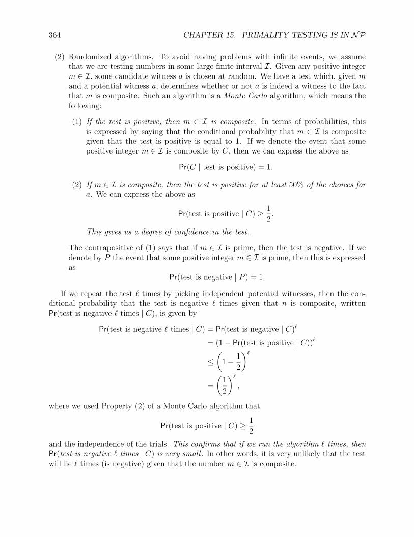
364 CHAPTER 15. PRIMALITY TESTING IS IN NP
(2) Randomized algorithms. To avoid having problems with infinite events, we assumethat we are testing numbers in some large finite interval I. Given any positive integerm ∈ I, some candidate witness a is chosen at random. We have a test which, given mand a potential witness a, determines whether or not a is indeed a witness to the factthat m is composite. Such an algorithm is a Monte Carlo algorithm, which means thefollowing:
(1) If the test is positive, then m ∈ I is composite. In terms of probabilities, thisis expressed by saying that the conditional probability that m ∈ I is compositegiven that the test is positive is equal to 1. If we denote the event that somepositive integer m ∈ I is composite by C, then we can express the above as
Pr(C | test is positive) = 1.
(2) If m ∈ I is composite, then the test is positive for at least 50% of the choices fora. We can express the above as
Pr(test is positive | C) ≥ 1
2.
This gives us a degree of confidence in the test .
The contrapositive of (1) says that if m ∈ I is prime, then the test is negative. If wedenote by P the event that some positive integer m ∈ I is prime, then this is expressedas
Pr(test is negative | P ) = 1.
If we repeat the test ℓ times by picking independent potential witnesses, then the con-ditional probability that the test is negative ℓ times given that n is composite, writtenPr(test is negative ℓ times | C), is given by
Pr(test is negative ℓ times | C) = Pr(test is negative | C)ℓ
= (1− Pr(test is positive | C))ℓ
≤(1− 1
2
)ℓ
=
(1
2
)ℓ
,
where we used Property (2) of a Monte Carlo algorithm that
Pr(test is positive | C) ≥ 1
2
and the independence of the trials. This confirms that if we run the algorithm ℓ times, thenPr(test is negative ℓ times | C) is very small . In other words, it is very unlikely that the testwill lie ℓ times (is negative) given that the number m ∈ I is composite.
15.3. MODULAR ARITHMETIC, THE GROUPS Z/nZ, (Z/nZ)∗ 365
If the probabilty Pr(P ) of the event P is known, which requires knowledge of the distri-bution of the primes in the interval I, then the conditional probability
Pr(P | test is negative ℓ times)
can be determined using Bayes’s rule.
A Monte Carlo algorithm does not give a definite answer. However, if ℓ is large enough(say ℓ = 100), then the conditional probability that the number n being tested is prime giventhat the test is negative ℓ times, is very close to 1.
Two of the best known randomized algorithms for primality testing are the Miller–Rabintest and the Solovay–Strassen test . We will not discuss these methods here, and we referthe reader to Gallier and Quaintance [8].
However, what we will discuss is a nondeterministic algorithm that checks that a numbern is prime by guessing a certain kind of tree that we call a Lucas tree (because this algorithmis based on a method due to E. Lucas), and then verifies in polynomial time (in the lentghlog2 n of the input given in binary) that this tree constitutes a ‘proof” that n is indeedprime. This shows that primality testing is in NP, a fact that is not obvious at all. Ofcourse, this is a much weaker result than the AKS algorithm, but the proof that the AKSworks in polynomial time (in log2 n) is much harder.
The Lucas test, and basically all of the primality-testing algorithms, use modular arith-metic and some elementary facts of number theory such as the Euler-Fermat theorem, so weproceed with a review of these concepts.
15.3 Modular Arithmetic, the Groups Z/nZ, (Z/nZ)∗
Recall the fundamental notion of congruence modulo n and its notation due to Gauss (circa1802).
Definition 15.2. For any a, b ∈ Z, we write a ≡ b (mod m) iff a− b = km, for some k ∈ Z
(in other words, a− b is divisible by m), and we say that a and b are congruent modulo m.
For example, 37 ≡ 1 (mod 9), since 37 − 1 = 36 = 4 · 9. It can also be shown that200250 ≡ 1 (mod 251), but this is impossible to do by brute force, so we will develop sometools to either avoid such computations, or to make them tractable.
It is easy to check that congruence is an equivalence relation but it also satisfies thefollowing properties.
Proposition 15.3. For any positive integer m, for all a1, a2, b1, b2 ∈ Z, the following prop-erties hold. If a1 ≡ b1 (modm) and a2 ≡ b2 (modm), then
(1) a1 + a2 ≡ b1 + b2 (modm).
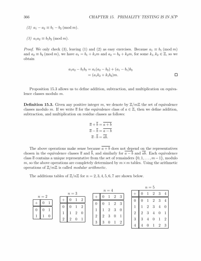
366 CHAPTER 15. PRIMALITY TESTING IS IN NP
(2) a1 − a2 ≡ b1 − b2 (modm).
(3) a1a2 ≡ b1b2 (modm).
Proof. We only check (3), leaving (1) and (2) as easy exercises. Because a1 ≡ b1 (mod m)and a2 ≡ b2 (modm), we have a1 = b1 + k1m and a2 = b2 + k2m, for some k1, k2 ∈ Z, so weobtain
a1a2 − b1b2 = a1(a2 − b2) + (a1 − b1)b2= (a1k2 + k1b2)m.
Proposition 15.3 allows us to define addition, subtraction, and multiplication on equiva-lence classes modulo m.
Definition 15.3. Given any positive integer m, we denote by Z/mZ the set of equivalenceclasses modulo m. If we write a for the equivalence class of a ∈ Z, then we define addition,subtraction, and multiplication on residue classes as follows:
a+ b = a+ b
a− b = a− ba · b = ab.
The above operations make sense because a + b does not depend on the representativeschosen in the equivalence classes a and b, and similarly for a− b and ab. Each equivalenceclass a contains a unique representative from the set of remainders 0, 1, . . . , m−1, modulom, so the above operations are completely determined by m×m tables. Using the arithmeticoperations of Z/mZ is called modular arithmetic.
The additions tables of Z/nZ for n = 2, 3, 4, 5, 6, 7 are shown below.
n = 2
+ 0 1
0 0 1
1 1 0
n = 3
+ 0 1 2
0 0 1 2
1 1 2 0
2 2 0 1
n = 4
+ 0 1 2 3
0 0 1 2 3
1 1 2 3 0
2 2 3 0 1
3 3 0 1 2
n = 5
+ 0 1 2 3 4
0 0 1 2 3 4
1 1 2 3 4 0
2 2 3 4 0 1
3 3 4 0 1 2
4 4 0 1 2 3
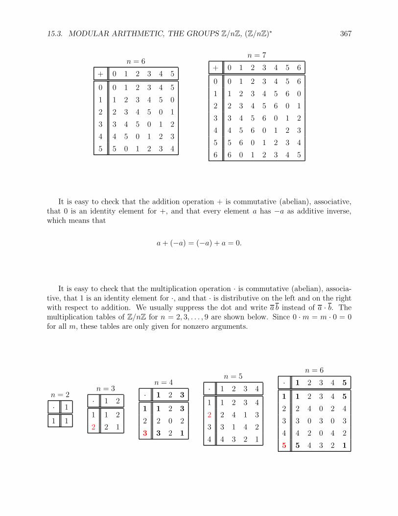
15.3. MODULAR ARITHMETIC, THE GROUPS Z/nZ, (Z/nZ)∗ 367
n = 6
+ 0 1 2 3 4 5
0 0 1 2 3 4 5
1 1 2 3 4 5 0
2 2 3 4 5 0 1
3 3 4 5 0 1 2
4 4 5 0 1 2 3
5 5 0 1 2 3 4
n = 7
+ 0 1 2 3 4 5 6
0 0 1 2 3 4 5 6
1 1 2 3 4 5 6 0
2 2 3 4 5 6 0 1
3 3 4 5 6 0 1 2
4 4 5 6 0 1 2 3
5 5 6 0 1 2 3 4
6 6 0 1 2 3 4 5
It is easy to check that the addition operation + is commutative (abelian), associative,that 0 is an identity element for +, and that every element a has −a as additive inverse,which means that
a+ (−a) = (−a) + a = 0.
It is easy to check that the multiplication operation · is commutative (abelian), associa-tive, that 1 is an identity element for ·, and that · is distributive on the left and on the rightwith respect to addition. We usually suppress the dot and write a b instead of a · b. Themultiplication tables of Z/nZ for n = 2, 3, . . . , 9 are shown below. Since 0 ·m = m · 0 = 0for all m, these tables are only given for nonzero arguments.
n = 2
· 1
1 1
n = 3
· 1 2
1 1 2
2 2 1
n = 4
· 1 2 3
1 1 2 3
2 2 0 2
3 3 2 1
n = 5
· 1 2 3 4
1 1 2 3 4
2 2 4 1 3
3 3 1 4 2
4 4 3 2 1
n = 6
· 1 2 3 4 5
1 1 2 3 4 5
2 2 4 0 2 4
3 3 0 3 0 3
4 4 2 0 4 2
5 5 4 3 2 1
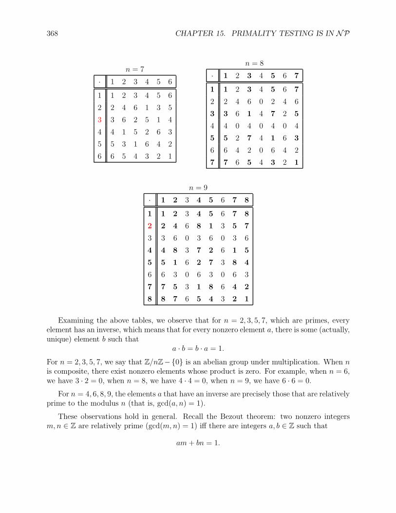
368 CHAPTER 15. PRIMALITY TESTING IS IN NP
n = 7
· 1 2 3 4 5 6
1 1 2 3 4 5 6
2 2 4 6 1 3 5
3 3 6 2 5 1 4
4 4 1 5 2 6 3
5 5 3 1 6 4 2
6 6 5 4 3 2 1
n = 8
· 1 2 3 4 5 6 7
1 1 2 3 4 5 6 7
2 2 4 6 0 2 4 6
3 3 6 1 4 7 2 5
4 4 0 4 0 4 0 4
5 5 2 7 4 1 6 3
6 6 4 2 0 6 4 2
7 7 6 5 4 3 2 1
n = 9
· 1 2 3 4 5 6 7 8
1 1 2 3 4 5 6 7 8
2 2 4 6 8 1 3 5 7
3 3 6 0 3 6 0 3 6
4 4 8 3 7 2 6 1 5
5 5 1 6 2 7 3 8 4
6 6 3 0 6 3 0 6 3
7 7 5 3 1 8 6 4 2
8 8 7 6 5 4 3 2 1
Examining the above tables, we observe that for n = 2, 3, 5, 7, which are primes, everyelement has an inverse, which means that for every nonzero element a, there is some (actually,unique) element b such that
a · b = b · a = 1.
For n = 2, 3, 5, 7, we say that Z/nZ−0 is an abelian group under multiplication. When nis composite, there exist nonzero elements whose product is zero. For example, when n = 6,we have 3 · 2 = 0, when n = 8, we have 4 · 4 = 0, when n = 9, we have 6 · 6 = 0.
For n = 4, 6, 8, 9, the elements a that have an inverse are precisely those that are relativelyprime to the modulus n (that is, gcd(a, n) = 1).
These observations hold in general. Recall the Bezout theorem: two nonzero integersm,n ∈ Z are relatively prime (gcd(m,n) = 1) iff there are integers a, b ∈ Z such that
am+ bn = 1.
15.3. MODULAR ARITHMETIC, THE GROUPS Z/nZ, (Z/nZ)∗ 369
Proposition 15.4. Given any integer n ≥ 1, for any a ∈ Z, the residue class a ∈ Z/nZ isinvertible with respect to multiplication iff gcd(a, n) = 1.
Proof. If a has inverse b in Z/nZ, then a b = 1, which means that
ab ≡ 1 (mod n),
that is ab = 1 + nk for some k ∈ Z, which is the Bezout identity
ab− nk = 1
and implies that gcd(a, n) = 1. Conversely, if gcd(a, n) = 1, then by Bezout’s identity thereexist u, v ∈ Z such that
au+ nv = 1,
so au = 1− nv, that is,au ≡ 1 (mod n),
which means that a u = 1, so a is invertible in Z/nZ.
We have alluded to the notion of a group. Here is the formal definition.
Definition 15.4. A group is a set G equipped with a binary operation · : G × G → Gthat associates an element a · b ∈ G to every pair of elements a, b ∈ G, and having thefollowing properties: · is associative, has an identity element e ∈ G, and every element in Gis invertible (w.r.t. ·). More explicitly, this means that the following equations hold for alla, b, c ∈ G:(G1) a · (b · c) = (a · b) · c. (associativity);
(G2) a · e = e · a = a. (identity);
(G3) For every a ∈ G, there is some a−1 ∈ G such that a · a−1 = a−1 · a = e. (inverse).
A group G is abelian (or commutative) if
a · b = b · a for all a, b ∈ G.
It is easy to show that the element e satisfying property (G2) is unique, and for anya ∈ G, the element a−1 ∈ G satisfying a · a−1 = a−1 · a = e required to exist by (G3) isactually unique. This element is called the inverse of a.
The set of integers Z with the addition operation is an abelian group with identityelement 0. The set Z/nZ of residues modulo m is an abelian group under addition withidentity element 0. In general, Z/nZ − 0 is not a group under multiplication, becausesome nonzero elements may not have an inverse.
The subset of elements, shown in boldface in the multiplication tables, forms an abeliangroup under multiplication.
370 CHAPTER 15. PRIMALITY TESTING IS IN NP
Definition 15.5. The group (under multiplication) of invertible elements of the ring Z/nZis denoted by (Z/nZ)∗. Note that this group is abelian and only defined if n ≥ 2.
The Euler ϕ-function plays an important role in the theory of the groups (Z/nZ)∗.
Definition 15.6. Given any positive integer n ≥ 1, the Euler ϕ-function (or Euler totientfunction) is defined such that ϕ(n) is the number of integers a, with 1 ≤ a ≤ n, which arerelatively prime to n; that is, with gcd(a, n) = 1.1
If p is prime, then by definition
ϕ(p) = p− 1.
We leave it as an exercise to show that if p is prime and if k ≥ 1, then
ϕ(pk) = pk−1(p− 1).
It can also be shown that if gcd(m,n) = 1, then
ϕ(mn) = ϕ(m)ϕ(n).
The above properties yield a method for computing ϕ(n), based on its prime factorization.If n = pi11 · · · pikk , then
ϕ(n) = pi1−11 · · · pik−1
k (p1 − 1) · · · (pk − 1).
For example, ϕ(17) = 16, ϕ(49) = 7 · 6 = 42,
ϕ(900) = ϕ(22 · 32 · 52) = 2 · 3 · 5 · 1 · 2 · 4 = 240.
Proposition 15.4 shows that (Z/nZ)∗ has ϕ(n) elements. It also shows that Z/nZ− 0is a group (under multiplication) iff n is prime.
Definition 15.7. If G is a finite group, the number of elements in G is called the the orderof G.
Given a group G with identity element e, and any element g ∈ G, we often need toconsider the powers of g defined as follows.
Definition 15.8. Given a group G with identity element e, for any nonnegative integer n,it is natural to define the power gn of g as follows:
g0 = e
gn+1 = g · gn.1We allow a = n to accomodate the special case n = 1.
15.3. MODULAR ARITHMETIC, THE GROUPS Z/nZ, (Z/nZ)∗ 371
Using induction, it is easy to show that
gmgn = gn+m
for all m,n ∈ N.
Since g has an inverse g−1, we can extend the definition of gn to negative powers. Forn ∈ Z, with n < 0, let
gn = (g−1)−n.
Then, it is easy to prove that
gi · gj = gi+j
(gi)−1 = g−i
gi · gj = gj · gi
for all i, j ∈ Z.
Given a finite group G of order n, for any element a ∈ G, it is natural to consider theset of powers e, a1, a2, . . . , ak, . . .. A crucial fact is that there is a smallest positive s ∈ N
such that as = e, and that s divides n.
Proposition 15.5. Let G be a finite group of order n. For every element a ∈ G, thefollowing facts hold:
(1) There is a smallest positive integer s ≤ n such that as = e.
(2) The set e, a, . . . , as−1 is an abelian group denoted 〈a〉.
(3) We have an = e, and the positive integer s divides n, More generally, for any positiveinteger m, if am = e, then s divides m.
Proof. (1) Consider the sequence of n+ 1 elements
(e, a1, a2, . . . , an).
Since G only has n distinct elements, by the pigeonhole principle, there exist i, j such that0 ≤ i < j ≤ n such that
ai = aj .
By multiplying both sides by (ai)−1 = a−i, we get
e = ai(ai)−1 = aj(ai)−1 = aja−i = aj−i.
Since 0 ≤ i < j ≤ n, we have 0 ≤ j − i ≤ n with aj−i = e. Thus there is some s with0 < s ≤ n such that as = e, and thus a smallest such s.
372 CHAPTER 15. PRIMALITY TESTING IS IN NP
(2) Since as = e, for any i, j ∈ 0, . . . , s−1 if we write i+ j = sq+ r with 0 ≤ r ≤ s−1,we have
aiaj = ai+j = asq+r = asqar = (as)qar = eqar = ar,
so 〈a〉 is closed under multiplication. We have e ∈ 〈a〉 and the inverse of ai is as−i, so 〈a〉 isa group. This group is obviously abelian.
(3) For any element g ∈ G, let g〈a〉 = gak | 0 ≤ k ≤ s− 1. Observe that for any i ∈ N,we have
ai〈a〉 = 〈a〉.
We claim that for any two elements g1, g2 ∈ G, if g1〈a〉 ∩ g2〈a〉 6= ∅, then g1〈a〉 = g2〈a〉.
Proof of the claim. If g ∈ g1〈a〉 ∩ g2〈a〉, then there exist i, j ∈ 0, . . . , s− 1 such that
g1ai = g2a
j .
Without loss of generality, we may assume that i ≥ j. By multipliying both sides by (aj)−1,we get
g2 = g1ai−j .
Consequentlyg2〈a〉 = g1a
i−j〈a〉 = g1〈a〉,as claimed.
It follows that the pairwise disjoint nonempty subsets of the form g〈a〉, for g ∈ G, form apartition of G. However, the map ϕg from 〈a〉 to g〈a〉 given by ϕg(a
i) = gai has for inversethe map ϕg−1 , so ϕg is a bijection, and thus the subsets g〈a〉 all have the same number ofelements, s. Since these subsets form a partition of G, we must have n = sq for some q ∈ N,which implies that an = e.
If gm = 1, then writing m = sq + r, with 0 ≤ r < s, we get
1 = gm = gsq+r = (gs)q · gr = gr,
so gr = 1 with 0 ≤ r < s, contradicting the minimality of s, so r = 0 and s divides m.
Definition 15.9. Given a finite group G of order n, for any a ∈ G, the smallest positiveinteger s ≤ n such that as = e in (1) of Proposition 15.5 is called the order of a.
For any integer n ≥ 2, let (Z/nZ)∗ be the group of invertible elements of the ring Z/nZ.This is a group of order ϕ(n). Then Proposition 15.5 yields the following result.
Theorem 15.6. (Euler) For any integer n ≥ 2 and any a ∈ 1, . . . , n − 1 such thatgcd(a, n) = 1, we have
aϕ(n) ≡ 1 (mod n).
15.3. MODULAR ARITHMETIC, THE GROUPS Z/nZ, (Z/nZ)∗ 373
In particular, if n is a prime, then ϕ(n) = n− 1, and we get Fermat’s little theorem.
Theorem 15.7. (Fermat’s little theorem) For any prime p and any a ∈ 1, . . . , p− 1, wehave
ap−1 ≡ 1 (mod p).
Since 251 is prime, and since gcd(200, 252) = 1, Fermat’s little theorem implies our earlierclaim that 200250 ≡ 1 (mod 251), without making any computations.
Proposition 15.5 suggests considering groups of the form 〈g〉.Definition 15.10. A finite group G is cyclic iff there is some element g ∈ G such thatG = 〈g〉. An element g ∈ G with this property is called a generator of G.
Even though, in principle, a finite cyclic group has a very simple structure, finding agenerator for a finite cyclic group is generally hard. For example, it turns out that themultiplicative group (Z/pZ)∗ is a cyclic group when p is prime, but no efficient method forfinding a generator for (Z/pZ)∗ is known (besides a brute-force search).
Examining the multiplication tables for (Z/nZ)∗ for n = 3, 4, . . . , 9, we can check thefollowing facts:
1. 2 is a generator for (Z/3Z)∗.
2. 3 is a generator for (Z/4Z)∗.
3. 2 is a generator for (Z/5Z)∗.
4. 5 is a generator for (Z/6Z)∗.
5. 3 is a generator for (Z/7Z)∗.
6. Every element of (Z/8Z)∗ satisfies the equation a2 = 1 (mod 8), thus (Z/8Z)∗ has nogenerators.
7. 2 is a generator for (Z/9Z)∗.
More generally, it can be shown that the multiplicative groups (Z/pkZ)∗ and (Z/2pkZ)∗
are cyclic groups when p is an odd prime and k ≥ 1.
Definition 15.11. A generator of the group (Z/nZ)∗ (when there is one), is called a primitiveroot modulo n.
As an exercise, the reader should check that the next value of n for which (Z/nZ)∗ hasno generator is n = 12.
The following theorem due to Gauss can be shown. For a proof, see Apostol [1] or Gallierand Quaintance [8].
Theorem 15.8. (Gauss) For every odd prime p, the group (Z/pZ)∗ is cyclic of order p− 1.It has ϕ(p− 1) generators.
The generators of (Z/pZ)∗ are the primitive roots modulo p.
374 CHAPTER 15. PRIMALITY TESTING IS IN NP
15.4 The Lucas Theorem; Lucas Trees
In this section we discuss an application of the existence of primitive roots in (Z/pZ)∗ wherep is an odd prime, known an the n− 1 test . This test due to E. Lucas determines whether apositive odd integer n is prime or not by examining the prime factors of n− 1 and checkingsome congruences.
The n− 1 test can be described as the construction of a certain kind of tree rooted withn, and it turns out that the number of nodes in this tree is bounded by 2 log2 n, and thatthe number of modular multiplications involved in checking the congruences is bounded by2 log22 n.
When we talk about the complexity of algorithms dealing with numbers, we assume thatall inputs (to a Turing machine) are strings representing these numbers, typically in base2. Since the length of the binary representation of a natural number n ≥ 1 is ⌊log2 n⌋ + 1(or ⌈log2(n+ 1)⌉, which allows n = 0), the complexity of algorithms dealing with (nonzero)numbers m,n, etc. is expressed in terms of log2m, log2 n, etc. Recall that for any realnumber x ∈ R, the floor of x is the greatest integer ⌊x⌋ that is less that or equal to x, andthe ceiling of x is the least integer ⌈x⌉ that is greater that or equal to x.
If we choose to represent numbers in base 10, since for any base b we have logb x =ln x/ ln b, we have
log2 x =ln 10
ln 2log10 x.
Since (ln 10)/(ln 2) ≈ 3.322 ≈ 10/3, we see that the number of decimal digits needed torepresent the integer n in base 10 is approximately 30% of the number of bits needed torepresent n in base 2.
Since the Lucas test yields a tree such that the number of modular multiplications in-volved in checking the congruences is bounded by 2 log22 n, it is not hard to show that testingwhether or not a positive integer n is prime, a problem denoted PRIMES, belongs to thecomplexity class NP. This result was shown by V. Pratt [15] (1975), but Peter Freyd toldme that it was “folklore.” Since 2002, thanks to the AKS algorithm, we know that PRIMESactually belongs to the class P, but this is a much harder result.
Here is Lehmer’s version of the Lucas result, from 1876.
Theorem 15.9. (Lucas theorem) Let n be a positive integer with n ≥ 2. Then n is primeiff there is some integer a ∈ 1, 2, . . . , n− 1 such that the following two conditions hold:
(1) an−1 ≡ 1 (mod n).
(2) If n > 2, then a(n−1)/q 6≡ 1 (mod n) for all prime divisors q of n− 1.
Proof. First, assume that Conditions (1) and (2) hold. If n = 2, since 2 is prime, we aredone. Thus assume that n ≥ 3, and let r be the order of a. We claim that r = n− 1. Thecondition an−1 ≡ 1 (mod n) implies that r divides n− 1. Suppose that r < n− 1, and let q
15.4. THE LUCAS THEOREM; LUCAS TREES 375
be a prime divisor of (n− 1)/r (so q divides n− 1). Since r is the order or a we have ar ≡ 1(mod n), so we get
a(n−1)/q ≡ ar(n−1)/(rq) ≡ (ar)(n−1)/(rq) ≡ 1(n−1)/(rq) ≡ 1 (mod n),
contradicting Condition (2). Therefore, r = n− 1, as claimed.
We now show that n must be prime. Now an−1 ≡ 1 (mod n) implies that a and n arerelatively prime so by Euler’s Theorem (Theorem 15.6),
aϕ(n) ≡ 1 (mod n).
Since the order of a is n− 1, we have n− 1 ≤ ϕ(n). If n ≥ 3 is not prime, then n has someprime divisor p, but n and p are integers in 1, 2, . . . , n that are not relatively prime to n,so by definition of ϕ(n), we have ϕ(n) ≤ n − 2, contradicting the fact that n − 1 ≤ ϕ(n).Therefore, n must be prime.
Conversely, assume that n is prime. If n = 2, then we set a = 1. Otherwise, pick a to beany primitive root modulo p.
Clearly, if n > 2 then we may assume that a ≥ 2. The main difficulty with the n − 1test is not so much guessing the primitive root a, but finding a complete prime factorizationof n − 1. However, as a nondeterministic algorithm, the n − 1 test yields a “proof” that anumber n is indeed prime which can be represented as a tree, and the number of operationsneeded to check the required conditions (the congruences) is bounded by c log22 n for somepositive constant c, and this implies that testing primality is in NP.
Before explaining the details of this method, we sharpen slightly Lucas theorem to dealonly with odd prime divisors.
Theorem 15.10. Let n be a positive odd integer with n ≥ 3. Then n is prime iff thereis some integer a ∈ 2, . . . , n − 1 (a guess for a primitive root modulo n) such that thefollowing two conditions hold:
(1b) a(n−1)/2 ≡ −1 (mod n).
(2b) If n− 1 is not a power of 2, then a(n−1)/2q 6≡ −1 (mod n) for all odd prime divisors qof n− 1.
Proof. Assume that Conditions (1b) and (2b) of Theorem 15.10 hold. Then we claim thatConditions (1) and (2) of Theorem 15.9 hold. By squaring the congruence a(n−1)/2 ≡ −1(mod n), we get an−1 ≡ 1 (mod n), which is Condition (1) of Theorem 15.9. Since a(n−1)/2 ≡−1 (mod n), Condition (2) of Theorem 15.9 holds for q = 2. Next, if q is an odd primedivisor of n− 1, let m = a(n−1)/2q. Condition (1b) means that
mq ≡ a(n−1)/2 ≡ −1 (mod n).
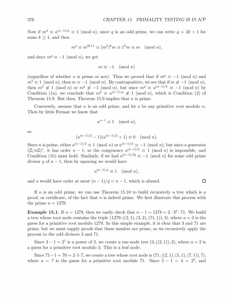
376 CHAPTER 15. PRIMALITY TESTING IS IN NP
Now if m2 ≡ a(n−1)/q ≡ 1 (mod n), since q is an odd prime, we can write q = 2k + 1 forsome k ≥ 1, and then
mq ≡ m2k+1 ≡ (m2)km ≡ 1km ≡ m (mod n),
and since mq ≡ −1 (mod n), we get
m ≡ −1 (mod n)
(regardless of whether n is prime or not). Thus we proved that if mq ≡ −1 (mod n) andm2 ≡ 1 (mod n), thenm ≡ −1 (mod n). By contrapositive, we see that ifm 6≡ −1 (mod n),then m2 6≡ 1 (mod n) or mq 6≡ −1 (mod n), but since mq ≡ a(n−1)/2 ≡ −1 (mod n) byCondition (1a), we conclude that m2 ≡ a(n−1)/q 6≡ 1 (mod n), which is Condition (2) ofTheorem 15.9. But then, Theorem 15.9 implies that n is prime.
Conversely, assume that n is an odd prime, and let a be any primitive root modulo n.Then by little Fermat we know that
an−1 ≡ 1 (mod n),
so(a(n−1)/2 − 1)(a(n−1)/2 + 1) ≡ 0 (mod n).
Since n is prime, either a(n−1)/2 ≡ 1 (mod n) or a(n−1)/2 ≡ −1 (mod n), but since a generates(Z/nZ)∗, it has order n − 1, so the congruence a(n−1)/2 ≡ 1 (mod n) is impossible, andCondition (1b) must hold. Similarly, if we had a(n−1)/2q ≡ −1 (mod n) for some odd primedivisor q of n− 1, then by squaring we would have
a(n−1)/q ≡ 1 (mod n),
and a would have order at most (n− 1)/q < n− 1, which is absurd.
If n is an odd prime, we can use Theorem 15.10 to build recursively a tree which is aproof, or certificate, of the fact that n is indeed prime. We first illustrate this process withthe prime n = 1279.
Example 15.1. If n = 1279, then we easily check that n− 1 = 1278 = 2 · 32 · 71. We builda tree whose root node contains the triple (1279, ((2, 1), (3, 2), (71, 1)), 3), where a = 3 is theguess for a primitive root modulo 1279. In this simple example, it is clear that 3 and 71 areprime, but we must supply proofs that these number are prime, so we recursively apply theprocess to the odd divisors 3 and 71.
Since 3− 1 = 21 is a power of 2, we create a one-node tree (3, ((2, 1)), 2), where a = 2 isa guess for a primitive root modulo 3. This is a leaf node.
Since 71−1 = 70 = 2·5·7, we create a tree whose root node is (71, ((2, 1), (5, 1), (7, 1)), 7),where a = 7 is the guess for a primitive root modulo 71. Since 5 − 1 = 4 = 22, and
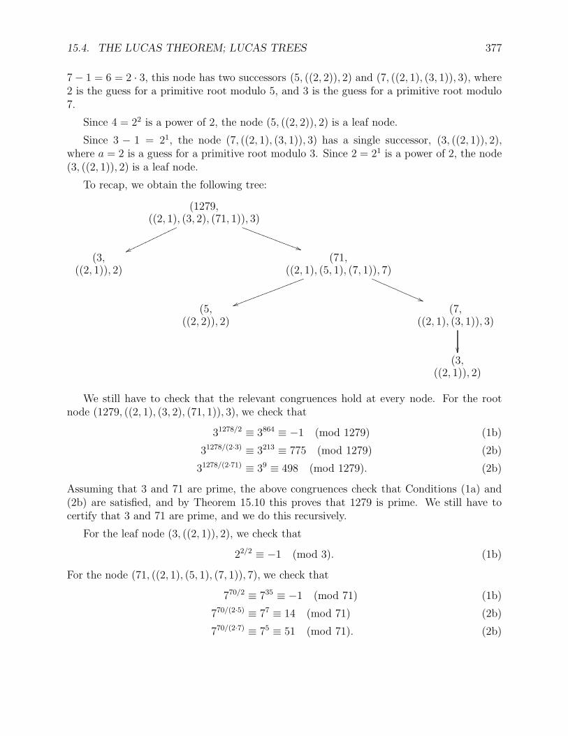
15.4. THE LUCAS THEOREM; LUCAS TREES 377
7− 1 = 6 = 2 · 3, this node has two successors (5, ((2, 2)), 2) and (7, ((2, 1), (3, 1)), 3), where2 is the guess for a primitive root modulo 5, and 3 is the guess for a primitive root modulo7.
Since 4 = 22 is a power of 2, the node (5, ((2, 2)), 2) is a leaf node.
Since 3 − 1 = 21, the node (7, ((2, 1), (3, 1)), 3) has a single successor, (3, ((2, 1)), 2),where a = 2 is a guess for a primitive root modulo 3. Since 2 = 21 is a power of 2, the node(3, ((2, 1)), 2) is a leaf node.
To recap, we obtain the following tree:
(1279,((2, 1), (3, 2), (71, 1)), 3)
ww♥♥♥♥♥♥♥♥♥♥♥♥♥
))
(3,((2, 1)), 2)
(71,((2, 1), (5, 1), (7, 1)), 7)
uu
((
(5,((2, 2)), 2)
(7,((2, 1), (3, 1)), 3)
(3,
((2, 1)), 2)
We still have to check that the relevant congruences hold at every node. For the rootnode (1279, ((2, 1), (3, 2), (71, 1)), 3), we check that
31278/2 ≡ 3864 ≡ −1 (mod 1279) (1b)
31278/(2·3) ≡ 3213 ≡ 775 (mod 1279) (2b)
31278/(2·71) ≡ 39 ≡ 498 (mod 1279). (2b)
Assuming that 3 and 71 are prime, the above congruences check that Conditions (1a) and(2b) are satisfied, and by Theorem 15.10 this proves that 1279 is prime. We still have tocertify that 3 and 71 are prime, and we do this recursively.
For the leaf node (3, ((2, 1)), 2), we check that
22/2 ≡ −1 (mod 3). (1b)
For the node (71, ((2, 1), (5, 1), (7, 1)), 7), we check that
770/2 ≡ 735 ≡ −1 (mod 71) (1b)
770/(2·5) ≡ 77 ≡ 14 (mod 71) (2b)
770/(2·7) ≡ 75 ≡ 51 (mod 71). (2b)
378 CHAPTER 15. PRIMALITY TESTING IS IN NP
Now, we certified that 3 and 71 are prime, assuming that 5 and 7 are prime, which we nowestablish.
For the leaf node (5, ((2, 2)), 2), we check that
24/2 ≡ 22 ≡ −1 (mod 5). (1b)
For the node (7, ((2, 1), (3, 1)), 3), we check that
36/2 ≡ 33 ≡ −1 (mod 7) (1b)
36/(2·3) ≡ 31 ≡ 3 (mod 7). (2b)
We have certified that 5 and 7 are prime, given that 3 is prime, which we finally verify.
At last, for the leaf node (3, ((2, 1)), 2), we check that
22/2 ≡ −1 (mod 3). (1b)
The above example suggests the following definition.
Definition 15.12. Given any odd integer n ≥ 3, a pre-Lucas tree for n is defined inductivelyas follows:
(1) It is a one-node tree labeled with (n, ((2, i0)), a), such that n− 1 = 2i0 , for some i0 ≥ 1and some a ∈ 2, . . . , n− 1.
(2) If L1, . . . , Lk are k pre-Lucas (with k ≥ 1), where the tree Lj is a pre-Lucas tree for someodd integer qj ≥ 3, then the tree L whose root is labeled with (n, ((2, i0), ((q1, i1), . . .,(qk, ik)), a) and whose jth subtree is Lj is a pre-Lucas tree for n if
n− 1 = 2i0qi11 · · · qikk ,
for some i0, i1, . . . , ik ≥ 1, and some a ∈ 2, . . . , n− 1.
Both in (1) and (2), the number a is a guess for a primitive root modulo n.
A pre-Lucas tree for n is a Lucas tree for n if the following conditions are satisfied:
(3) If L is a one-node tree labeled with (n, ((2, i0)), a), then
a(n−1)/2 ≡ −1 (mod n).
(4) If L is a pre-Lucas tree whose root is labeled with (n, ((2, i0), ((q1, i1), . . . , (qk, ik)), a),and whose jth subtree Lj is a pre-Lucas tree for qj , then Lj is a Lucas tree for qj forj = 1, . . . , k, and
(a) a(n−1)/2 ≡ −1 (mod n).
15.5. ALGORITHMS FOR COMPUTING POWERS MODULO m 379
(b) a(n−1)/2qj 6≡ −1 (mod n) for j = 1, . . . , k.
Since Conditions (3) and (4) of Definition 15.12 are Conditions (1b) and (2b) of Theorem,15.10, we see that Definition 15.12 has been designed in such a way that Theorem 15.10 yieldsthe following result.
Theorem 15.11. An odd integer n ≥ 3 is prime iff it has some Lucas tree.
The issue is now to see how long it takes to check that a pre-Lucas tree is a Lucas tree.For this, we need a method for computing xn mod n in polynomial time in log2 n. This isthe object of the next section.
15.5 Algorithms for Computing Powers Modulo m
Let us first consider computing the nth power xn of some positive integer. The idea is tolook at the parity of n and to proceed recursively. If n is even, say n = 2k, then
xn = x2k = (xk)2,
so, compute xk recursively and then square the result. If n is odd, say n = 2k + 1, then
xn = x2k+1 = (xk)2 · x,
so, compute xk recursively, square it, and multiply the result by x.
What this suggests is to write n ≥ 1 in binary, say
n = bℓ · 2ℓ + bℓ−1 · 2ℓ−1 + · · ·+ b1 · 21 + b0,
where bi ∈ 0, 1 with bℓ = 1 or, if we let J = j | bj = 1, as
n =∑
j∈J
2j.
Then we havexn ≡ x
∑j∈J 2j =
∏
j∈J
x2j
modm.
This suggests computing the residues rj such that
x2j ≡ rj (modm),
because then,
xn ≡∏
j∈J
rj (modm),
380 CHAPTER 15. PRIMALITY TESTING IS IN NP
where we can compute this latter product modulo m two terms at a time.
For example, say we want to compute 999179 mod 1763. First, we observe that
179 = 27 + 25 + 24 + 21 + 1,
and we compute the powers modulo 1763:
99921 ≡ 143 (mod 1763)
99922 ≡ 1432 ≡ 1056 (mod 1763)
99923 ≡ 10562 ≡ 920 (mod 1763)
99924 ≡ 9202 ≡ 160 (mod 1763)
99925 ≡ 1602 ≡ 918 (mod 1763)
99926 ≡ 9182 ≡ 10 (mod 1763)
99927 ≡ 102 ≡ 100 (mod 1763).
Consequently,
999179 ≡ 999 · 143 · 160 · 918 · 100 (mod 1763)
≡ 54 · 160 · 918 · 100 (mod 1763)
≡ 1588 · 918 · 100 (mod 1763)
≡ 1546 · 100 (mod 1763)
≡ 1219 (mod 1763),
and we find that999179 ≡ 1219 (mod 1763).
Of course, it would be impossible to exponentiate 999179 first and then reduce modulo 1763.As we can see, the number of multiplications needed is bounded by 2 log2 n, which is quitegood.
The above method can be implemented without actually converting n to base 2. If n iseven, say n = 2k, then n/2 = k and if n is odd, say n = 2k + 1, then (n− 1)/2 = k, so wehave a way of dropping the unit digit in the binary expansion of n and shifting the remainingdigits one place to the right without explicitly computing this binary expansion. Here is analgorithm for computing xn modm, with n ≥ 1, using the repeated squaring method.
An Algorithm to Compute xn modm Using Repeated Squaring
beginu := 1; a := x;
15.6. PRIMES IS IN NP 381
while n > 1 doif even(n) then e := 0 else e := 1;if e = 1 then u := a · u mod m;a := a2 mod m; n := (n− e)/2
endwhile;u := a · u mod m
end
The final value of u is the result. The reason why the algorithm is correct is that after jrounds through the while loop, a = x2
j
modm and
u =∏
i∈J | i<j
x2i
modm,
with this product interpreted as 1 when j = 0.
Observe that the while loop is only executed n − 1 times to avoid squaring once moreunnecessarily and the last multiplication a ·u is performed outside of the while loop. Also, ifwe delete the reductions modulo m, the above algorithm is a fast method for computing thenth power of an integer x and the time speed-up of not performing the last squaring step ismore significant. We leave the details of the proof that the above algorithm is correct as anexercise.
15.6 PRIMES is in NPExponentiation modulo n can performed by repeated squaring, as explained in Section 15.5.In that section, we observed that computing xm mod n requires at most 2 log2m modularmultiplications. Using this fact, we obtain the following result.
Proposition 15.12. If p is any odd prime, then any pre-Lucas tree L for p has at most log2 pnodes, and the number M(p) of modular multiplications required to check that the pre-Lucastree L is a Lucas tree is less than 2 log22 p.
Proof. Let N(p) be the number of nodes in a pre-Lucas tree for p. We proceed by completeinduction. If p = 3, then p− 1 = 21, any pre-Lucas tree has a single node, and 1 < log2 3.
Suppose the results holds for any odd prime less than p. If p − 1 = 2i0 , then any Lucastree has a single node, and 1 < log2 3 < log2 p. If p− 1 has the prime factorization
p− 1 = 2i0qi11 · · · qikk ,then by the induction hypothesis, each pre-Lucas tree Lj for qj has less than log2 qj nodes,so
N(p) = 1 +
k∑
j=1
N(qj) < 1 +
k∑
j=1
log2 qj = 1 + log2(q1 · · · qk) ≤ 1 + log2
(p− 1
2
)< log2 p,
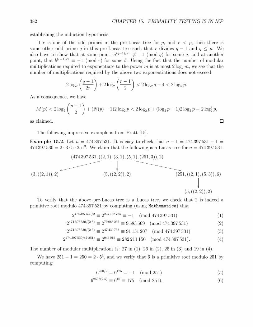
382 CHAPTER 15. PRIMALITY TESTING IS IN NP
establishing the induction hypothesis.
If r is one of the odd primes in the pre-Lucas tree for p, and r < p, then there issome other odd prime q in this pre-Lucas tree such that r divides q − 1 and q ≤ p. Wealso have to show that at some point, a(q−1)/2r 6≡ −1 (mod q) for some a, and at anotherpoint, that b(r−1)/2 ≡ −1 (mod r) for some b. Using the fact that the number of modularmultiplications required to exponentiate to the power m is at most 2 log2m, we see that thenumber of multiplications required by the above two exponentiations does not exceed
2 log2
(q − 1
2r
)+ 2 log2
(r − 1
2
)< 2 log2 q − 4 < 2 log2 p.
As a consequence, we have
M(p) < 2 log2
(p− 1
2
)+ (N(p)− 1)2 log2 p < 2 log2 p+ (log2 p− 1)2 log2 p = 2 log22 p,
as claimed.
The following impressive example is from Pratt [15].
Example 15.2. Let n = 474 397 531. It is easy to check that n − 1 = 474 397 531 − 1 =474 397 530 = 2 · 3 · 5 · 2513. We claim that the following is a Lucas tree for n = 474 397 531:
(474 397 531, ((2, 1), (3, 1), (5, 1), (251, 3)), 2)
ss
,,❳❳❳❳❳❳❳❳❳
❳❳❳❳❳❳❳❳
❳❳❳❳❳❳❳
(3, ((2, 1)), 2) (5, ((2, 2)), 2) (251, ((2, 1), (5, 3)), 6)
(5, ((2, 2)), 2)
To verify that the above pre-Lucas tree is a Lucas tree, we check that 2 is indeed aprimitive root modulo 474 397 531 by computing (using Mathematica) that
2474 397 530/2 ≡ 2237 198 765 ≡ −1 (mod 474 397 531) (1)
2474 397 530/(2·3) ≡ 279 066 255 ≡ 9 583 569 (mod 474 397 531) (2)
2474 397 530/(2·5) ≡ 247 439 753 ≡ 91 151 207 (mod 474 397 531) (3)
2474 397 530/(2·251) ≡ 2945 015 ≡ 282 211 150 (mod 474 397 531). (4)
The number of modular multiplications is: 27 in (1), 26 in (2), 25 in (3) and 19 in (4).
We have 251− 1 = 250 = 2 · 53, and we verify that 6 is a primitive root modulo 251 bycomputing:
6250/2 ≡ 6125 ≡ −1 (mod 251) (5)
6250/(2·5) ≡ 610 ≡ 175 (mod 251). (6)
15.6. PRIMES IS IN NP 383
The number of modular multiplications is: 6 in (5), and 3 in (6).
We have 5− 1 = 4 = 22, and 2 is a primitive root modulo 5, since
24/2 ≡ 22 ≡ −1 (mod 5). (7)
This takes one multiplication.We have 3− 1 = 2 = 21, and 2 is a primitive root modulo 3, since
22/2 ≡ 21 ≡ −1 (mod 3). (8)
This takes 0 multiplications.
Therefore, 474 397 531 is prime.
As nice as it is, Proposition 15.12 is deceiving, because finding a Lucas tree is hard.
Remark: Pratt [15] presents his method for finding a certificate of primality in terms ofa proof system. Although quite elegant, we feel that this method is not as transparent asthe method using Lucas trees, which we adapted from Crandall and Pomerance [5]. Pratt’sproofs can be represented as trees, as Pratt sketches in Section 3 of his paper. However,Pratt uses the basic version of Lucas’ theorem, Theorem 15.9, instead of the improvedversion, Theorem 15.10, so his proof trees have at least twice as many nodes as ours.
As nice as it is, Proposition 15.12 is deceiving, because finding a Lucas tree is hard.
The following nice result was first shown by V. Pratt in 1975 [15].
Theorem 15.13. The problem PRIMES (testing whether an integer is prime) is in NP.Proof. Since all even integers besides 2 are composite, we can restrict out attention to oddintegers n ≥ 3. By Theorem 15.11, an odd integer n ≥ 3 is prime iff it has a Lucas tree.Given any odd integer n ≥ 3, since all the numbers involved in the definition of a pre-Lucastree are less than n, there is a finite (very large) number of pre-Lucas trees for n. Given aguess of a Lucas tree for n, checking that this tree is a pre-Lucas tree can be performed inO(log2 n), and by Proposition 15.12, checking that it is a Lucas tree can be done in O(log22 n).Therefore PRIMES is in NP.
Of course, checking whether a number n is composite is in NP, since it suffices to guessto factors n1, n2 and to check that n = n1n2, which can be done in polynomial time in log2 n.Therefore, PRIMES ∈ NP ∩ coNP. As we said earlier, this was the situation until thediscovery of the AKS algorithm, which places PRIMES in P.
Remark: Altough finding a primitive root modulo p is hard, we know that the number ofprimitive roots modulo p is ϕ(ϕ(p)). If p is large enough, this number is actually quite large.According to Crandal and Pomerance [5] (Chapter 4, Section 4.1.1), if p is a prime and ifp > 200560490131, then p has more than p/(2 ln ln p) primitive roots.
384 CHAPTER 15. PRIMALITY TESTING IS IN NP
Bibliography
[1] Tom M. Apostol. Introduction to Analytic Number Theory. Undergraduate Texts inMathematics. Springer, first edition, 1976.
[2] Sanjeev Arora and Boaz Barak. Computational Complexity. A Modern Approach. Cam-bridge University Press, first edition, 2009.
[3] Pierre Bremaud. Markov Chains, Gibbs Fields, Monte Carlo Simulations, and Queues.TAM, Vol. 31. Springer Verlag, third edition, 2001.
[4] Erhan Cinlar. Introduction to Stochastic Processes. Dover, first edition, 2014.
[5] Richard Crandall and Carl Pomerance. Prime Numbers. A Computational Perspective.Springer, second edition, 2005.
[6] Martin Davis. Hilbert’s tenth problem is unsolvable. American Mathematical Monthly,80(3):233–269, 1973.
[7] Martin Davis, Yuri Matijasevich, and Julia Robinson. Hilbert’s tenth problem. diophan-tine equations: Positive aspects of a negative solution. In Mathematical DevelopmentsArising from Hilbert Problems, volume XXVIII, Part 2, pages 323–378. AMS, 1976.
[8] Jean Gallier and Jocelyn Quaintance. Notes on Primality Testing and Public Key Cryp-tography. Part I: Randomized Algorithms, Miller–Rabin and Solovay–Strassen Tests.Technical report, University of Pennsylvania, Levine Hall, Philadelphia, PA 19104, 2017.pdf file available from http://www.cis.upenn.edu/∼jean/RSA-primality-testing.pdf.
[9] Geoffrey Grimmett and David Stirzaker. Probability and Random Processes. OxfordUniversity Press, third edition, 2001.
[10] John G. Kemeny, Snell J. Laurie, and Anthony W. Knapp. Denumerable Markov Chains.GTM, Vol. No 40. Springer-Verlag, second edition, 1976.
[11] Harry R. Lewis and Christos H. Papadimitriou. Elements of the Theory of Computation.Prentice-Hall, second edition, 1997.
[12] Michael Machtey and Paul Young. An Introduction to the General Theory of Algorithms.Elsevier North-Holland, first edition, 1978.
385
386 BIBLIOGRAPHY
[13] Michael Mitzenmacher and Eli Upfal. Probability and Computing. Randomized Algo-rithms and Probabilistic Analysis. Cambridge University Press, first edition, 2005.
[14] Christos H. Papadimitriou. Computational Complexity. Pearson, first edition, 1993.
[15] Vaughan R. Pratt. Every prime has a succinct certificate. SIAM Journal on Computing,4(3):214–220, 1975.
[16] Lawrence R. Rabiner. A tutorial on hidden markov models and selected applications inspeech recognition. Proceedings of the IEEE, 77(2):257–286, 1989.
[17] Paulo Ribenboim. The Little Book of Bigger Primes. Springer-Verlag, second edition,2004.
[18] Elaine Rich. Automata, Computability, and Complexity. Theory and Applications. Pren-tice Hall, first edition, 2007.
[19] Mark Stamp. A revealing introduction to hidden markov models. Technical report, SanJose State University, Department of Computer Science, San Jose, California, 2015.
Related Documents


![Vita for Jean H. Gallier 1 Personal Data - University of ...jean/vita2.pdf4 Vita for Jean H. Gallier [15] Building Exact Computation Sequences. (With Alex Pelin). Theoretical Computer](https://static.cupdf.com/doc/110x72/5ad40abd7f8b9aff228b5c3e/vita-for-jean-h-gallier-1-personal-data-university-of-jeanvita2pdf4-vita.jpg)

