INTRODUCTION TO THE SPECIAL FUNCTIONS OF MATHEMATICAL PHYSICS with applications to the physical and applied sciences John Michael Finn April 13, 2005

Welcome message from author
This document is posted to help you gain knowledge. Please leave a comment to let me know what you think about it! Share it to your friends and learn new things together.
Transcript
INTRODUCTION TO THE SPECIAL FUNCTIONS
OF MATHEMATICAL PHYSICS
with applications to the
physical and applied sciences
John Michael Finn
April 13, 2005

CONTENTS
Contents iii
Preface xi
Dedication xvii
1. Infinite Series 1
1.1Convergence 1
1.2A cautionary tale 2
1.3Geometric series 6
Proof by mathematical induction 6
1.4Definition of an infinite series 7
Convergence of the chessboard problem 8
Distance traveled by A bouncing ball 9
1.5The remainder of a series 11
1.6Comments about series 12
1.7The Formal definition of convergence 13
1.8Alternating series 13
Alternating Harmonic Series 14
1.9Absolute Convergence 16
Distributive Law for scalar multiplication 18
Scalar multiplication 18
Addition of series 18
1.10Tests for convergence 19
iv Contents
Preliminary test 19
Comparison tests 19
The Ratio Test 20
The Integral Test 20
1.11Radius of convergence 21
Evaluation techniques 23
1.12Expansion of functions in power series 23
The binomial expansion 24
Repeated Products 25
1.13More properties of power series 26
1.14Numerical techniques 27
1.15Series solutions of differential equations 28
A simple first order linear differential equation 29
A simple second order linear differential equation 30
1.16Generalized power series 33
Fuchs's conditions 34
2. Analytic continuation 37
2.1The Fundamental Theorem of algebra 37
Conjugate pairs or roots. 38
Transcendental functions 38
2.2The Quadratic Formula 38
Definition of the square root 39
Definition of the square root of -1 40
The geometric interpretation of multiplication 41
2.3The complex plane 42
2.4Polar coordinates 44

Contents v
2.5Properties of complex numbers 45
2.6The roots of 1/ nz 47
2.7Complex infinite series 49
2.8Derivatives of complex functions 50
2.9The exponential function 53
2.10The natural logarithm 54
2.11The power function 55
2.12The under-damped harmonic oscillator 55
2.13Trigonometric and hyperbolic functions 58
2.14The hyperbolic functions 59
2.15The trigonometric functions 60
2.16Inverse trigonometric and hyperbolic functions 61
2.17The Cauchy Riemann conditions 63
2.18Solution to Laplace equation in two dimensions 64
3. Gamma and Beta Functions 67
3.1The Gamma function 67
Extension of the Factorial function 68
Gamma Functions for negative values of p 70
Evaluation of definite integrals 72
3.2The Beta Function 74
3.3The Error Function 76
3.4Asymptotic Series 78
Sterling’s formula 81
4. Elliptic Integrals 83
4.1Elliptic integral of the second kind 84
4.2Elliptic Integral of the first kind 88
vi Contents
4.3Jacobi Elliptic functions 92
4.4Elliptic integral of the third kind 96
5. Fourier Series 99
5.1Plucking a string 99
5.2The solution to a simple eigenvalue equation 100
Orthogonality 101
5.3Definition of Fourier series 103
Completeness of the series 104
Sine and cosine series 104
Complex form of Fourier series 105
5.4Other intervals 106
5.5Examples 106
The Full wave Rectifier 106
The Square wave 110
Gibbs Phenomena 112
Non-symmetric intervals and period doubling 114
5.6Integration and differentiation 119
Differentiation 119
Integration 120
5.7Parseval’s Theorem 123
Generalized Parseval’s Theorem 125
5.8Solutions to infinite series 125
6. Orthogonal function spaces 127
6.1Separation of variables 127
6.2Laplace’s equation in polar coordinates 127
6.3Helmholtz’s equation 130

Contents vii
6.4Sturm-Liouville theory 133
Linear self-adjoint differential operators 135
Orthogonality 137
Completeness of the function basis 139
Comparison to Fourier Series 139
Convergence of a Sturm-Liouville series 141
Vector space representation 142
7. Spherical Harmonics 145
7.1Legendre polynomials 146
Series expansion 148
Orthogonality and Normalization 151
A second solution 154
7.2Rodriquez’s formula 156
Leibniz’s rule for differentiating products 156
7.3Generating function 159
7.4Recursion relations 162
7.5Associated Legendre Polynomials 164
Normalization of Associated Legendre polynomials 168
Parity of the Associated Legendre polynomials 168
Recursion relations 169
7.6Spherical Harmonics 169
7.7Laplace equation in spherical coordinates 172
8. Bessel functions 175
8.1Series solution of Bessel’s equation 175
Neumann or Weber functions 178
8.2Cylindrical Bessel functions 180
viii Contents
Hankel functions 181
Zeroes of the Bessel functions 182
Orthogonality of Bessel functions 183
Orthogonal series of Bessel functions 183
Generating function 186
Recursion relations 186
8.3Modified Bessel functions 188
Modified Bessel functions of the second kind 190
Recursion formulas for modified Bessel functions 191
8.4Solutions to other differential equations 192
8.5Spherical Bessel functions 193
Definitions 194
Recursion relations 198
Orthogonal series of spherical Bessel functions 199
9. Laplace equation 205
9.1Origin of Laplace equation 205
9.2Laplace equation in Cartesian coordinates 207
Solving for the coefficients 210
9.3Laplace equation in polar coordinates 214
9.4Application to steady state temperature distribution 215
9.5The spherical capacitor, revisited 217
Charge distribution on a conducting surface 219
9.6Laplace equation with cylindrical boundary conditions 221
Solution for a clyindrical capacitor 225
10. Time dependent differential equations 227
10.1Classification of partial differential equations 227
Contents ix
10.2Diffusion equation 232
10.3Wave equation 236
Pressure waves: standing waves in a pipe 239
The struck string 240
The normal modes of a vibrating drum head 242
10.4Schrödinger equation 245
10.5Examples with spherical boundary conditions 246
Quantum mechanics in a spherical bag 246
Heat flow in a sphere 247
10.6Examples with cylindrical boundary conditions 250
Normal modes in a cylindrical cavity 250
Temperature distribution in a cylinder 250
11. Green’s functions and propagators 252
11.1The driven oscillator 253
11.2Frequency domain analysis 257
11.3Green’s function solution to Possion’s equation 259
11.4Multipole expansion of a charge distribution 260
11.5Method of images 262
Solution for a infinite grounded plane 263
Induced charge distribution on a grounded plane 265
Green’s function for a conducting sphere 266
11.6Green’s function solution to the Yakawa interaction 268

PREFACE
This text is based on a one semester advanced undergraduate
course that I have taught at the College of William and Mary. In
the spring semester of 2005, I decided to collect my notes and to
present them in a more formal manner. The course covers se-
lected topics on mathematical methods in the physical sciences
and is cross listed at the senior level in the physics and applied
sciences departments. The intended audience is junior and se-
nior science majors intending to continue their studies in the
pure and applied sciences at the graduate level. The course, as
taught at the College, is hugely successful. The most frequent
comment has been that students wished they had been intro-
duced to this material earlier in their studies.
Any course on mathematical methods necessarily involves a
choice from a venue of topics that could be covered. The empha-
sis on this course is to introduce students the special functions
of mathematical physics with emphasis on those techniques that
would be most useful in preparing a student to enter a program
of graduate studies in the sciences or the engineering discip-
lines. The students that I have taught at the College are the gen-
erally the best in their respective programs and have a solid
foundation in basic methods. Their mathematical preparation
xii Preface
includes, at a minimum, courses in ordinary differential equa-
tions, linear algebra, and multivariable calculus. The least expe-
rienced junior level students have taken at least two semesters
of Lagrangian mechanics, a semester of quantum mechanics,
and are enrolled in a course in electrodynamics, concurrently.
The senior level students have completed most of their required
course work and are well into their senior research projects. This
allows me to exclude a number of preliminary subjects, and to
concentrate on those topics that I think would be most helpful.
My classroom approach is highly interactive, with students pre-
senting several in-class presentations over the course of the
semester. In-class discussion is often lively and prolonged. It is a
pleasure to be teaching students that are genuinely interested
and engaged. I spend significant time in discussing the limita-
tion as well as the applicability of mathematical methods, draw-
ing from my own experience as a research scientist in particle
and nuclear physics. When I discuss computational algorithms,
I try to do so .from a programming language-neutral point of
view.
The course begins with review of infinite series and complex
analysis, then covers Gamma and Elliptic functions in some de-
tail, before turning to the main theme of the course: the unified
study of the most ubiquitous scalar partial differential equations
of physics, namely the wave, diffusion, Laplace, Poisson, and
Schrödinger equations. I show how the same mathematical me-
thods apply to a variety of physical phenomena, giving the stu-
Preface xiii
dents a global overview of the commonality of language and
techniques used in various subfields of study. As an interme-
diate step, Strum-Liouville theory is used to study the most
common orthogonal functions needed to separate variables in
Cartesian, cylindrical and spherical coordinate systems. Boun-
dary valued problems are then studied in detail, and integral
transforms are discussed, including the study of Green functions
and propagators.
The level of the presentation is a step below that of Mathemati-
cal Methods for Physicists by George B. Arfken and Hans J.
Weber, which is a great book at the graduate level, or as a desk-
top reference; and a step above that of Mathematical Methods
in the Physical Sciences, by Mary L. Boas, whose clear and sim-
ple presentation of basic concepts is more accessible to an un-
dergraduate audience. I have tried to improve on the rigor of her
presentation, drawing on material from Arfken, without over-
whelming the students, who are getting their first exposure to
much of this material.
Serious students of mathematical physics will find it useful to
invest in a good handbook of integrals and tables. My favorite is
the classic Handbook of Mathematical Functions, With Formu-
las, Graphs, and Mathematical Tables (AMS55), edited by Mil-
ton Abramowitz and Irene A. Stegun. This book is in the public
domain, and electronic versions are available for downloading
on the worldwide web. NIST is in the process of updating this
xiv Preface
work and plans to make an online version accessible in the near
future.
Such handbooks, although useful as references, are no longer
the primary means of accessing the special functions of mathe-
matical physics. A number of high level programs exist that are
better suited for this purpose, including Mathematica, Maple,
MATHLAB, and Mathcad. The College has site licenses for sev-
eral of these programs, and I let students use their program of
choice. These packages each have their strengths and weak-
nesses, and I have tried to avoid the temptation of relying too
heavily on proprietary technology that might be quickly out-
dated. My own pedagogical inclination is to have students work
out problems from first principles and to only use these pro-
grams to confirm their results and/or to assist in the presenta-
tion and visualization of data. I want to know what my students
know, not what some computer algorithm spits out for them.
The more computer savvy students might want to consider using
a high-level programming language, coupled with good numeric
and plotting libraries, to achieve the same results. For example,
the Ch scripting interpreter, from SoftIntegration, Inc, is availa-
ble for most computing platforms including Windows, Linux,
Mac OSX, Solaris, and HP-UX. It includes high level C99 scien-
tific math libraries and a decent plot package. It is a free down-
load for academic purposes. In my own work, I find the C# pro-
gramming language, within the Microsoft Visual Studio pro-
gramming environment, to be suitable for larger web-oriented
Preface xv
projects. The C# language is an international EMCA supported
specification. The .Net framework has been ported to other plat-
forms and is available under an open source license from the
MONO project.
These notes are intended to be used in a classroom, or other
academic settings, either as a standalone text or as supplemen-
tary material. I would appreciate feedback on ways this text can
be improved. I am deeply appreciative of the students who as-
sisted in this effort and to whom this text is dedicated.
Williamsburg, Virginia John Michael Finn
April, 2005 Professor of Physics


DEDICATION
For my students
at The College of
William and Mary
in Virginia

1. Infinite Series
The universe simply is.
Existence is not required to explain itself.
This is a task that mankind has chosen for himself,
and the reason that he invented mathematics.
1.1 Convergence
The ancient Greeks were fascinated by the concept of infinity.
They were aware that there was something transcendental
beyond the realm of rational numbers and the limits of finite al-
gebraic calculation, even if they did not fully comprehend how to
deal with it. Some of the most famous paradoxes of antiquity, at-
tributed to Zeno, wrestle with the question of convergence. If a
process takes an infinite number of steps to calculate, does that
necessarily imply that it takes an infinite amount of time? One
such paradox purportedly demonstrated that motion was im-
possible, a clear absurdity. Convergence was a concept that
mankind had to master before he was ready for Newton and his
calculus.
Physicists tend to take a cavalier attitude to convergence and
limits in general. To some extent, they can afford to. Physical
particles are different than mathematical points. They have a
2 Infinite Series
property, called inertia, which limits their response to external
force. In the context of special relativity, even their velocity re-
mains finite. Therefore, physical trajectories are necessarily
well-behaved, single-valued, continuous and differentiable func-
tions of time from the moment of their creation to the moment
of their annihilation. Mathematicians should be so fortunate.
Nevertheless, physicists, applied scientists, and engineering pro-
fessionals cannot afford to be too cavalier in their attitude. Un-
like the young, the innocent, and the unlucky, they need to be
aware of the pitfalls that can befall them. Mathematics is not re-
ality, but only a tool that we use to image reality. One needs to
be aware of its limitations and unspoken assumptions.
Infinite series and the theory of convergence are fundamental to
the calculus. They are taught as an introduction to most intro-
ductory analysis courses. Those who stayed awake in lecture
may even remember the proofs—Therefore, this chapter is in-
tended as a review of things previously learnt, but perhaps for-
gotten, or somehow neglected. We begin with a story.
1.2 A cautionary tale
The king of Persia had an astronomer that he wished to honor,
for just cause. Calling him into his presence, the king said that
he could ask whatever he willed, and, if it were within his power
to grant it, even if it were half his kingdom, he would.
Infinite Series 3
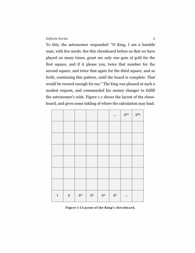
To this, the astronomer responded: “O King, I am a humble
man, with few needs. See this chessboard before us that we have
played on many times, grant me only one gain of gold for the
first square, and if it please you, twice that number for the
second square, and twice that again for the third square, and so
forth, continuing this pattern, until the board is complete. That
would be reward enough for me.” The king was pleased at such a
modest request, and commanded his money changer to fulfill
the astronomer’s wish. Figure 1-1 shows the layout of the chess-
board, and gives some inkling of where the calculation may lead.
… 262 263
1 2 22 23 24 25 …
Figure 1-1 Layout of the King’s chessboard.
4 Infinite Series
The total number grains of gold is a sequence whose sum is giv-
en by S=1+2+22+23+24+…, or more generally
63
02n
nS
=
=∑ . (1.1)
Note that mathematicians like to start counting at zero since 0 1x = is a good way to include a leading constant term in a pow-
er series. Many present day computer programs number their
arrays starting at zero for the first element as well.
The above is an example of a finite sequence of numbers to be
summed, a series of N terms, defined by an , which can be writ-
ten as
1
0
N
N nn
S a−
=
=∑ , (1.2)
where an denotes the thn element in the sum of a series of N
terms, expressed as NS . The algorithm or rule for defining the
constants in our chess problem is given by the prescription
0 11, and 2n na a a+= = . (1.3)
Note that a is used to compactly describe the progression. For
infinite series, where it is physically impossible to write down
every single term, the series must be defined by such a rule, of-
ten recursively derived, for constructing the nth term in the se-
ries.
Infinite Series 5
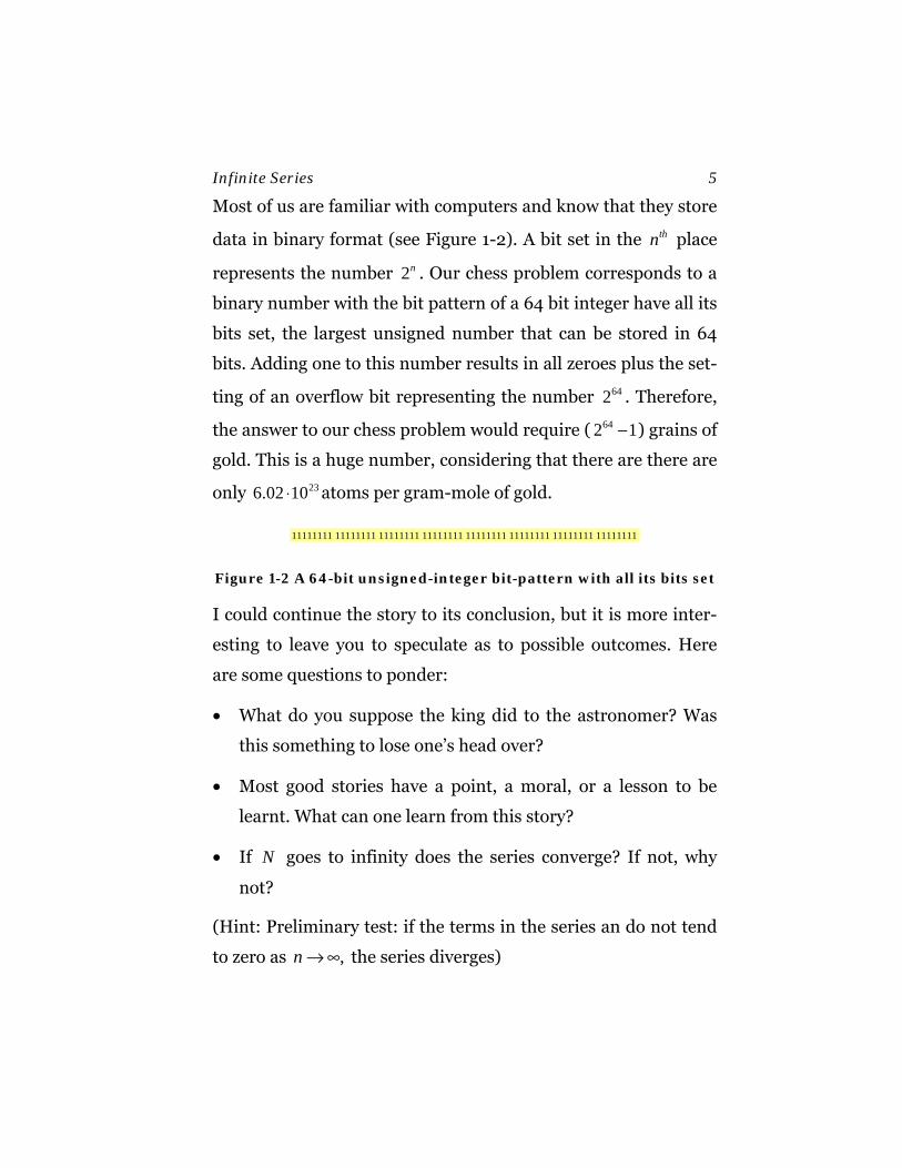
Most of us are familiar with computers and know that they store
data in binary format (see Figure 1-2). A bit set in the thn place
represents the number 2n . Our chess problem corresponds to a
binary number with the bit pattern of a 64 bit integer have all its
bits set, the largest unsigned number that can be stored in 64
bits. Adding one to this number results in all zeroes plus the set-
ting of an overflow bit representing the number 642 . Therefore,
the answer to our chess problem would require ( 642 1− ) grains of
gold. This is a huge number, considering that there are there are
only 236.02 10⋅ atoms per gram-mole of gold.
11111111 11111111 11111111 11111111 11111111 11111111 11111111 11111111
Figure 1-2 A 64-bit unsigned-integer bit-pattern with all its bits set
I could continue the story to its conclusion, but it is more inter-
esting to leave you to speculate as to possible outcomes. Here
are some questions to ponder:
• What do you suppose the king did to the astronomer? Was
this something to lose one’s head over?
• Most good stories have a point, a moral, or a lesson to be
learnt. What can one learn from this story?
• If N goes to infinity does the series converge? If not, why
not?
(Hint: Preliminary test: if the terms in the series an do not tend
to zero as ,n →∞ the series diverges)
6 Infinite Series
1.3 Geometric series
The chess board series is an example of a , one where successive
terms are multiplied by a constant ratio r. It represents one of
the oldest and best known of series. A geometric series can be
written in the general form as
( )1
,20 0 0
0, (1 ...)
Nn
NG a r a r r a r−
= + + + = ∑ . (1.4)
The initial term is 0 1a = and the ratio is 2r = for the chess
board problem. The sum of a geometric series can be evaluated
giving solution with a closed form:
1
0 0 00
1( , )1
nNn
NrG a r a r ar
− ⎛ ⎞−= = ⎜ ⎟−⎝ ⎠∑ . (1.5)
Proof by mathematical induction
There are a number of ways that the formula for the sum a geo-
metric series (1.5) can be verified. Perhaps the most useful for
future applications to other recursive problems is Induction in-
volves carrying out the following three logical steps.
• Verify that the expression is true for the initial case. Letting
0 1a = for simplicity, one gets
( )1
11 11
rG rr
⎛ ⎞−= =⎜ ⎟−⎝ ⎠. (1.6)
Infinite Series 7
• Assume that the expression is true for the thN case, i.e., as-
sume
( ) 11
N
NrG rr
⎛ ⎞−= ⎜ ⎟−⎝ ⎠. (1.7)
• Prove that it is true for the 1N + case:
1
1
1 1 1
1
1 ,1
1 1 1 ( 1) ,1 1 1
1 ) 1 1 .1 1 1
NN N
N N
N N NN
N
N N N N N
N
rG G r rr
r r r r rG rr r r
r r r r rGr r r
+
+
+ + +
+
⎛ ⎞−= + = +⎜ ⎟−⎝ ⎠⎛ ⎞− − − + −⎛ ⎞= + =⎜ ⎟ ⎜ ⎟− − −⎝ ⎠⎝ ⎠
⎛ ⎞ ⎛ ⎞− + − − −= = =⎜ ⎟ ⎜ ⎟− − −⎝ ⎠ ⎝ ⎠
(1.8)
1.4 Definition of an infinite series
The sum of an infinite series ( )S r can be defined as the sum of a
series of N terms ( )NS r in the limit as the number of terms N
goes to infinity. For the geometric series this becomes
( ) lim ( )NNG r G r
→∞= (1.9)
or
( ) 1( )1
rG r G rr
∞
∞⎛ ⎞−= = ⎜ ⎟−⎝ ⎠
, (1.10)
where

8 Infinite Series
0 1,1,
1 1 ... .
if rr f r
diverges
∞
<⎛⎜→ ∞ >⎜⎜ + +⎝
(1.11)
Therefore, for a general infinite geometric series,
0
000
1,( , ) 1
undefined for 1.
n
n
aa r for rG a r r
r
∞
=
⎧ = <⎪= −⎨⎪ ≥⎩
∑ (1.12)
Convergence of the chessboard problem
Let’s calculate how much gold we could obtain if we had a
chessboard of infinite size. First, let’s try plugging into the series
solution:
1
0
2 12 (1,2) ,2 1
1 1.1 2
NNn
N Nn
N N
S G
S
−
=
→∞
−= = =−
→ = −−
∑ (1.13)
This is clearly nonsense. One can not get a negative result by
adding a sequence that contains only positive terms. Note, how-
ever, that the series converges only if 1r < . This leads to our first
two major conclusions:
• The sum of a series is only meaningful if it converges.
• A function and the sum of the power series that it represents
are mathematically equivalent within, and only within, the
radius of convergence of the power series.

Infinite Series 9
Distance traveled by A bouncing ball
Here is an interesting variation on one of Zeno’s Paradoxes: If a
bouncing ball bounces an infinite number of times before com-
ing to rest, does this necessarily imply that it will bounce forev-
er? Answers to questions like this led to the development of the
formal theory of convergence. The detailed definition of the
problem to be solved is presented below.
Discussion Problem: A physics teacher drops a ball from rest
at a height 0h above a level floor. See Figure 1-3. The accelera-
tion of gravity g is constant. He neglects air resistance and as-
sumes that the collision, which is inelastic, takes negligible time
(using the impulse approximation). He finds that the height of
each succeeding bounce is reduced by a constant ratio r, so
1n nh rh −=
• Calculate the total distance traveled, as a Geometric series.
• Using Newton’s Laws of Motion, calculate the time nt needed
to drop from a height nh .
• Write down a series for the total time for N bounces. Does
this series converge? Why or why not?

10 Infinite Series
Figure 1-3 Height (m) vs. time (s) for a bouncing ball
Figure 1-3 shows a plot of the motion of a bouncing ball (h0=10
m, r=2/3, g=9.8 m/s2). The height of each bounce is reduced by
a constant ratio. A complication is that the total distance tra-
veled is to be calculated from the maximum of the first cycle, re-
quiring a correction to the first term in the series.
The series to be evaluated turn out to be geometric series. The
motion of the particle for the first cycle is given by
2
0
0 0
0 0 0
( ) ,2
2 ,
2 / 8 / ,
gty t v t
v gh
t v g h g
= −
=
Δ = =
(1.14)
where 0tΔ is the time for the first cycle, and
Infinite Series 11
00 0 0 0
0 0
0 0
22 2 ,1
8 / ,
.21
nn
n
hD h h h r h hr
t h r g t rt tT
r
= − = − = −−
Δ = = ΔΔ Δ= −−
∑ ∑ (1.15)
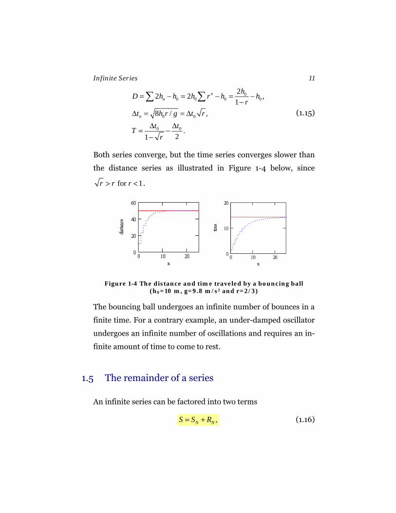
Both series converge, but the time series converges slower than
the distance series as illustrated in Figure 1-4 below, since
for 1r r r> < .
Figure 1-4 The distance and time traveled by a bouncing ball (h0=10 m, g=9.8 m/s2 and r=2/3)
The bouncing ball undergoes an infinite number of bounces in a
finite time. For a contrary example, an under-damped oscillator
undergoes an infinite number of oscillations and requires an in-
finite amount of time to come to rest.
1.5 The remainder of a series
An infinite series can be factored into two terms
,N NS S R= + (1.16)
12 Infinite Series
where
• 1
0
NN nn
S a−
==∑ is the , which has a finite sum of terms, and
• NR is the of the series, which has an infinite number of
terms
N nn N
R a∞
=
=∑ (1.17)
1.6 Comments about series
• NS denotes the partial sum of an infinite series S , the part
that is actually calculated. Since its computation involves a
finite number of algebraic operations (i.e., it is a finite algo-
rithm) computing it poses no conceptual challenge. In other
words, the rules of algebra apply, and a program can happily
be written to return the result.
• The remainder of a series S , denoted as NR , is an infinite se-
ries. This series may, or may not, converge.
• The convergence of NR is the same as the convergence of the
series S . The convergence of an infinite series is not affected
by the addition or subtraction of a finite number of leading
terms.
Infinite Series 13
• Computers (and humans too) can only calculate a finite
number of terms, therefore an estimate of NR is needed as a
measure of the error in the calculation.
• The most essential component of an infinite series is its re-
mainder—the part you don’t calculate. If one can’t estimate
or bound the error, the numerical value of the resulting ex-
pression is worthless.
Before using a series, one needs to know
• whether the series converges,
• how fast it converges, and
• what reasonable error bound one can place on the remainder
NR .
1.7 The Formal definition of convergence
A series converges if
for all ( ).N N
N N
S S RR S S N Nε ε
= += − < >
(1.18)
1.8 Alternating series
Definition: A series of terms with alternating terms is an
alternating series
Consider the alternating series A, given by
14 Infinite Series
( )1 nn
nA a= −∑ (1.19)
An alternating series converges if
1 0
0, as , and , for all N
n
n n
a na a n+
→ →∞< >
(1.20)
An oscillation of sign in a series can greatly improve its rate of
convergence. For a series of reducing terms, it is easy to define a
maximum error in a given approximation. The error in NS is
smaller that the first neglected term
N NR a< . (1.21)
Alternating Harmonic Series
An alternating harmonic series is defined as the series
( )
0
1 1 1 11 .1 2 3 4
n
n n
∞
=
−= − + − +
+∑ (1.22)
This is a decreasing alternating series which tends to zero and so
meets the preliminary test.
Example: Series expansion for the natural logarithm
In a book of math tables one can lookup the series expansion of
the natural logarithm, which is
( ) ( ) 1 2
0ln 1
1 2 3
n
n
x x xx xn
+∞
=
− −+ = = − +
+∑ (1.23)
Infinite Series 15
Setting 1,x = allows one to calculate the sum of an alternating
harmonic series in closed form
( ) ( )0
1ln(2) ln 1 1 0.6931471806
1
n
n n
∞
=
−= + = =
+∑ . (1.24)
Finding a functional representation of a series is a useful way of
expressing its sum in closed form.
What about ln(0) ?
( )
0
1 1 1ln 1 1 11 2 3
ln(0)n n
diverges
∞
=− = == + +
+= −∞
∑ (1.25)
So, to summarize:
( )
( )
11
11
n
n
S convergesn
but
S divergesn
⎛ ⎞−⎜ ⎟=⎜ ⎟+⎝ ⎠
−=
+
∑
∑
(1.26)
(1.27)
The series expansion for ln(1 )x+ can be summarized as
( )
1
0
( )ln 1 ,1
0 2.
n
n
xxn
for x
+∞
=
− −+ =+
< ≤
∑ (1.28)
This series is only conditionally convergent at its end points, de-
pending on the signs of the terms. What is going on here?
16 Infinite Series
Let’s rearrange the terms of the series so all the positive terms
come first (real numbers are commutative aren’t they?)
0
0
,1 ,
21 ,
2 1is undefined.
n
n
S S S
Sn
Sn
S
+ −
∞+
=
∞−
=
→ +
= →∞
= − → −∞+
= ∞ −∞
∑
∑ (1.29)
The problem is that a series is an algorithm, the first series di-
verges so one never gets around to calculating the terms of the
second series (remember we are limited to a finite number of
calculations, assuming we have only finite computer power
available to us)
• Note that infinity is not a real number!
1.9 Absolute Convergence
A series converges absolutely if the sum of the series generated
by taking the absolute value of all its terms converges. Let
nS a=∑ , then if the corresponding series of positive terms
nS a′ =∑ (1.30)
converges, the initial series S is said to be Otherwise if S is
convergent, but not absolutely convergent, it is said to be

Infinite Series 17
Discussion Problem: Show that a conditional convergent se-
ries S can be made to converge to any desired value.
Here is an outline of a possible proof: Separate S into two se-
ries, one of which contains only positive terms and the second
only negative terms. Since S is convergent, but not absolutely
convergent, each of these series is separately divergent. Now
borrow from the positive series until the sum is just greater than
the desired value (assuming it is positive). Next subtract from
the series just enough terms to bring it to just below the desired
value. Repeat the process. If one has a series of decreasing
terms, tending to zero, the results will oscillate about and even-
tually settle down to the desired value.
What is happening here is easy enough to understand: One can
always borrow from infinity and still have an infinite number in
reserve to draw upon:
na∞± = ∞ (1.31)
You can simply mortgage your future to get the desired result.
Some conclusions:
• Conditionally convergent series are dangerous, the commut-
ative law of addition does not apply (infinity is not a num-
ber).
• Absolutely convergent series always give the same answer no
matter how the terms are rearranged.
18 Infinite Series
• Absolute convergence is your friend. Don’t settle for any-
thing less than this. Absolutely convergent series can be
treated as if they represent real numbers in an algebraic ex-
pression (they do). They can be added, subtracted, multip-
lied and divided with impunity.
Distributive Law for scalar multiplication
A series can be multiplied term by term by a real number r
without affecting its convergence
Scalar multiplication
Scalar multiplication of a series by a real number r is given by
.n nr a ra=∑ ∑ (1.32)
Addition of series
Two absolutely convergent series can be added to each other
term by term; the resulting series converges within the common
interval of convergence of the original series.
( )
1 2 1 2
,
.n n nn
a b n n
a b a b
c S c S c a c b
± = ±
± = ±∑ ∑ ∑
∑ (1.33)
Infinite Series 19
1.10 Tests for convergence
Here is a summary of a few of the most useful tests for conver-
gence. Advanced references will list many more tests.
Preliminary test
A series NS diverges if its terms do not tend to zero as N goes to
infinity.
Comparison tests
Comparison tests involve comparing a series to a known series.
Comparison can be used to test for convergence or divergence of
a series:
• Given an absolutely convergent series a nS a=∑ the series
b nS b=∑ converges if
n nb a< (1.34)
for n N> .
• Given an absolutely divergent series ,a nS a=∑ the series
b nS b=∑ diverges if n nb a> for n N> .
• Given a absolutely convergent series ,a nS a=∑ the series
b nS b=∑ converges if
20 Infinite Series
1 1n n
n n
b ab a+ +< (1.35)
For n N> . (This test can also be used to test for divergence)
The Ratio Test
This is a variant of the comparison test where the ratio of terms
is compared to the geometric series: By comparison to a geome-
tric series, the series b nS b=∑ converges if the ratio of succeed-
ing terms decreases as n →∞ .
1define lim
1 the series converges,1 the series diverges,0 the test fails.
n
nn
brb
rif r
r
+
→∞=
<⎧⎪ >⎨⎪ =⎩
(1.36)
The Integral Test
The series b nS b=∑ converges if the upper limit of the integral
obtained by replacing 0 0
( )NN
nN N
b b n dn→∑ ∫ converges as N →∞ , and
it diverges if the integral diverges. The proof is demonstrated
graphically in Figure 1-5, which demonstrates that a sum of pos-
itive terms is bounded both above and below by its integral. The
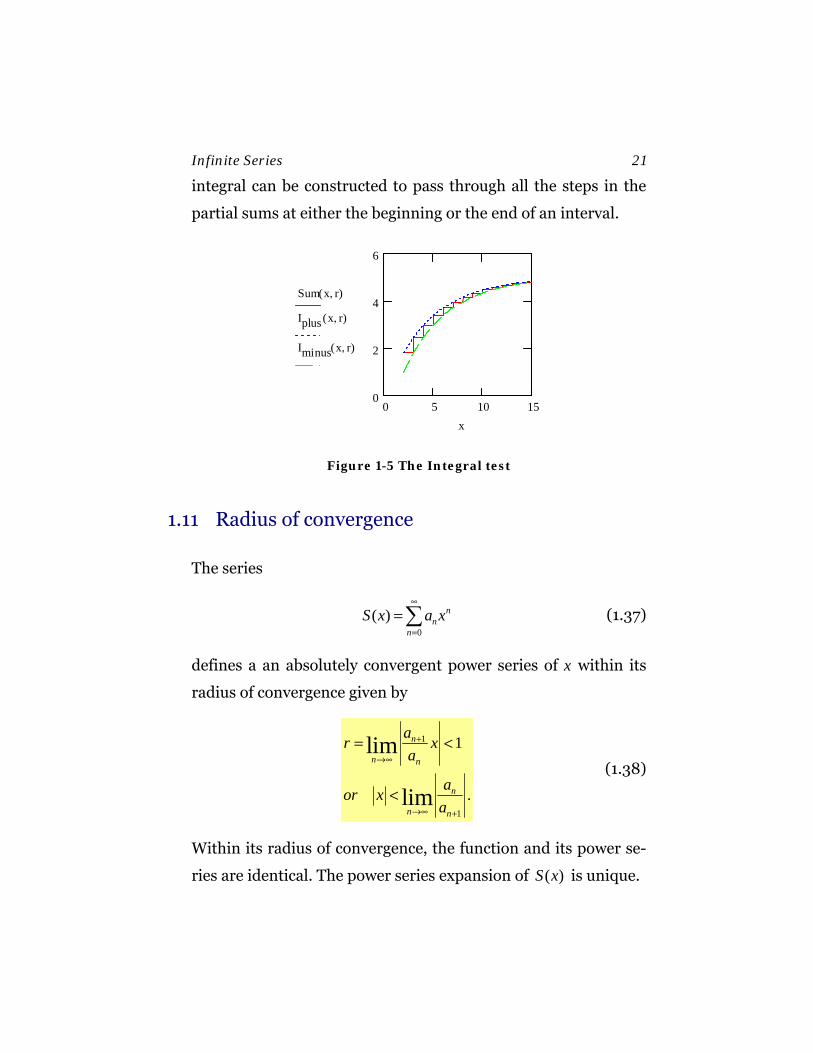
Infinite Series 21
integral can be constructed to pass through all the steps in the
partial sums at either the beginning or the end of an interval.
0 5 10 150
2
4
6
Sum x r,( )
Iplus x r,( )
Iminus x r,( )
x
Figure 1-5 The Integral test
1.11 Radius of convergence
The series
0
( ) nn
nS x a x
∞
=
=∑ (1.37)
defines a an absolutely convergent power series of x within its
radius of convergence given by
1
1
1
.
lim
lim
n
n n
n
n n
ar xa
aor xa
+
→∞
→∞ +
= <
<
(1.38)
Within its radius of convergence, the function and its power se-
ries are identical. The power series expansion of ( )S x is unique.
22 Infinite Series
Example: Definition of the exponential function.
The exponential function is defined as that function which is its
own derivative
( ) ( ).de x e x
dx= (1.39)
Let’s show that the series expansion for the exponential function
obeys this rule:
0
1
1
11
1 0
10 0
1 on the RHS
( 1)
( 1) .
x nn
nx
nn
n
n n xn n
n n
n nn n
n n
e a x
de na xdx
letting n n
na x n a x e
n a x a x
∞
=
∞−
=
∞ ∞′−
′+′= =
∞ ∞′
′+′= =
=
=
′→ +
′= + =
′ + =
∑
∑
∑ ∑
∑ ∑
(1.40)
Test for radius of convergence:
( ) ( )1 !
lim 1!
.
nx n
nx
+< = =
< ∞ (1.41)
(In practice, the useful range for computation is limited, de-
pending on the format and storage allocation of a real variable
in one’s calculator.)
Infinite Series 23
Evaluation techniques
• if 1x ≤ this series is converges rapidly
• if 1f x > use a b a be e e+ = to show
( )
0
1 ,
.!
xx
nx
n
ee
xe
n
−
∞−
=
=
−=∑
(1.42)
Alternating series converge faster, it is easy to estimate the er-
ror, and if the algorithm is written properly one shouldn’t get
overflow errors. Professional grade mathematical libraries
would use sophisticated algorithms to accurately evaluate a
function over its entire useful domain.
1.12 Expansion of functions in power series
The power series of a function is unique within its radius of cur-
vature. Since power series can be differentiated, we can use this
property to extract the coefficients of a power series. Let us ex-
pand a function of the real variable x about the origin:
24 Infinite Series
( )
( ) ( )
( )( )( )( )
0
( )
0
0
(1)1
(2)2
( )
;
0 ;
0 ,
0 ,
0 2 ,
0 ! .
nn
n
nn
nx
nn
f x a x
define
df f xdx
thenf a
f a
f a
f n a
∞
=
=
=
=
=
=
=
=
∑
(1.43)
This results in the famous Taylor series expansion:
( )( ) ( )
0
0.
!
nn
n
ff x x
n
∞
=
=∑ (1.44)
Substituting x x a→ − a, we get the generalization to a McLau-
ren Series
( )( ) ( ) ( )
0.
!
nn
n
f x af x x a
n
∞
=
−= −∑ (1.45)
Taylor’s expansion can be used to generate many well known se-
ries, such as the exponential function and the binomial expan-
sion.
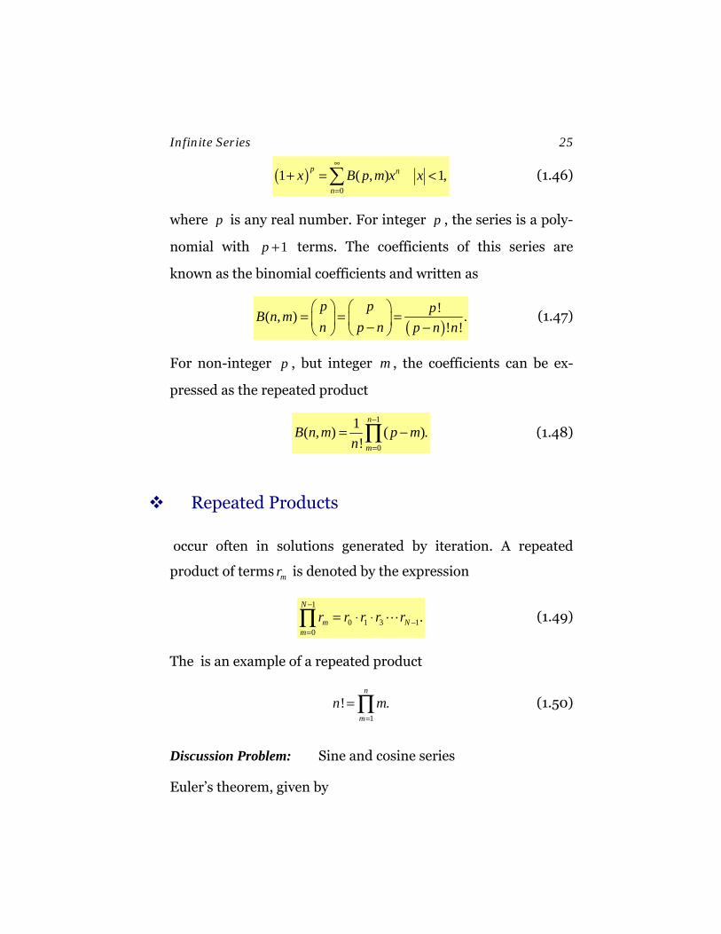
The binomial expansion
The binomial expansion is given by
Infinite Series 25
( )0
1 ( , ) 1,p n
nx B p m x x
∞
=
+ = <∑ (1.46)
where p is any real number. For integer p , the series is a poly-
nomial with 1p + terms. The coefficients of this series are
known as the binomial coefficients and written as
( )
!( , ) .! !
p p pB n mn p n p n n
⎛ ⎞ ⎛ ⎞= = =⎜ ⎟ ⎜ ⎟− −⎝ ⎠ ⎝ ⎠
(1.47)
For non-integer p , but integer m , the coefficients can be ex-
pressed as the repeated product
1
0
1( , ) ( ).!
n
m
B n m p mn
−
=
= −∏ (1.48)
Repeated Products
occur often in solutions generated by iteration. A repeated
product of terms mr is denoted by the expression
1
0 1 3 10
.N
m Nm
r r r r r−
−=
= ⋅ ⋅∏ (1.49)
The is an example of a repeated product
1
! .n
m
n m=
=∏ (1.50)
Discussion Problem: Sine and cosine series
Euler’s theorem, given by
26 Infinite Series
cos sin ,ie iθ θ θ= + (1.51)
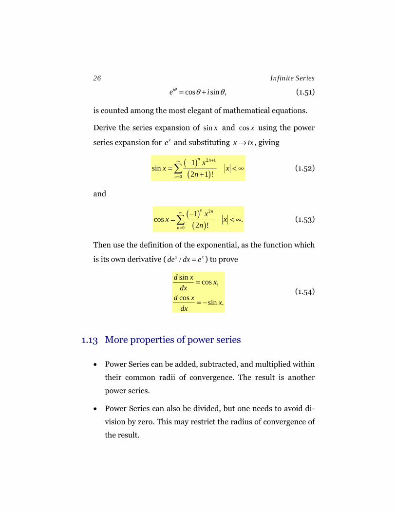
is counted among the most elegant of mathematical equations.
Derive the series expansion of sin x and cos x using the power
series expansion for xe and substituting x ix→ , giving
( )( )
2 1
0
1sin
2 1 !
n n
n
xx x
n
+∞
=
−= < ∞
+∑ (1.52)
and
( )( )
2
0
1cos .
2 !
n n
n
xx x
n
∞
=
−= < ∞∑ (1.53)
Then use the definition of the exponential, as the function which
is its own derivative ( /x xde dx e= ) to prove
sin cos ,
cos sin .
d x xdx
d x xdx
=
= − (1.54)
1.13 More properties of power series
• Power Series can be added, subtracted, and multiplied within
their common radii of convergence. The result is another
power series.
• Power Series can also be divided, but one needs to avoid di-
vision by zero. This may restrict the radius of convergence of
the result.
Infinite Series 27
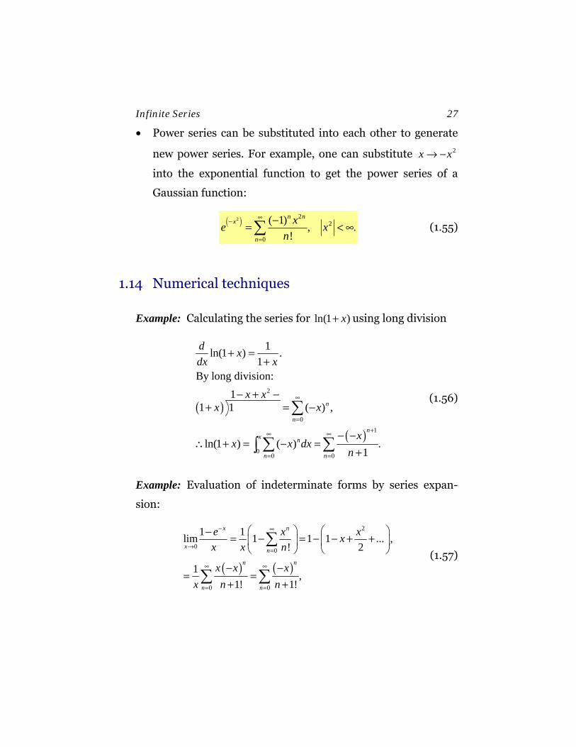
• Power series can be substituted into each other to generate
new power series. For example, one can substitute 2x x→ −
into the exponential function to get the power series of a
Gaussian function:
( )2 22
0
( 1) , .!
n nx
n
xe xn
∞−
=
−= < ∞∑ (1.55)
1.14 Numerical techniques
Example: Calculating the series for ln(1 )x+ using long division
( )
( )
2
01
00 0
1ln(1 ) .1
By long division:1
1 1 ( ) ,
ln(1 ) ( ) .1
n
nn
x n
n n
d xdx x
x xx x
xx x dx
n
∞
=
+∞ ∞
= =
+ =+
− + −+ = −
− −∴ + = − =
+
∑
∑ ∑∫
(1.56)
Example: Evaluation of indeterminate forms by series expan-
sion:
( ) ( )
2
0 0
0 0
1 1lim 1 1 1 ... ,! 2
1 ,1! 1!
x n
x n
n n
n n
e x xxx x n
x x xx n n
− ∞
→ =
∞ ∞
= =
⎛ ⎞ ⎛ ⎞− = − = − − + +⎜ ⎟ ⎜ ⎟⎝ ⎠ ⎝ ⎠
− −= =
+ +
∑
∑ ∑ (1.57)
28 Infinite Series
1.15 Series solutions of differential equations
The equation
( )0
( ) ( )iN
ii
dA x y x S xdx=
⎛ ⎞ =⎜ ⎟⎝ ⎠
∑ (1.58)
defines an thN order linear differential equation for ( )y x . If the
source term ( ) 0S x = , the equation is said to be homogeneous.
Otherwise, the equation is said to be inhomogeneous. We will
concern ourselves with solutions to homogeneous equations at
first. A linear homogenous equation has the general form
0
( ) ( ) 0iN
ii
dA x y xdx=
⎛ ⎞ =⎜ ⎟⎝ ⎠
∑ (1.59)
A thN order differential equation has N linearly-independent so-
lutions { }( )iy x , and by linearity, the general solution can be
written as
0
( ) ( )N
i ii
y x c y x=
=∑ (1.60)
If the coefficients ( )iA x can be expanded in a power series about
the point 0x = , one can attempt to solve for ( )iy x in terms of a
power series expansion of the form
0
( ) ni im
ny x a x
∞
=
=∑ (1.61)
Infinite Series 29
Since the function is linear in y , the resulting series expansion
will be linear in the coefficients ina , and the self-consistent solu-
tion will involve recursion relations between the coefficients of
various powers of m .
A simple first order linear differential equation
Consider the first order differential equation
( ) ( )dY x Y x
dx= − (1.62)
We already know the solution, it is given by
0( ) xY x Y e−= (1.63)
Since the equation is of first order, there is only one linearly in-
dependent solution so the above solution is complete. Let’s try
expanding this function in a power series
( )11
0 1 0( ) ; ( ) 1n n n
n n nn n n
Y x a x Y x na x n a x∞ ∞ ∞
′−′+
′= = =
′ ′= = = +∑ ∑ ∑ (1.64)
Where the last term involves making the change of va-
riables 1n n′= +
Substituting into equation (1.62) gives
( ) 10 0
1 n nn n
n nn a x a x
∞ ∞′
′+′= =
′ + = −∑ ∑ (1.65)
But n′ and n are dummy variables and we can compare similar
powers of x by setting n n′ = , giving the series solution
30 Infinite Series
( ) 10
1 0.nn n
nn a a x
∞
+′=
⎡ ⎤+ + =⎣ ⎦∑ (1.66)
The above expression can be true for arbitrary x only if term by
term the coefficients vanish:
( ) 11 0.n nn a a++ + = (1.67)
This gives rise to the recursive formula
( ) ( )1
1 ; or ,1
n nn n
a aa an n
−+ = − = −
+ (1.68)
with the solution
( ) ( )0
11 .
! !
nn o
naa Yn n
−= − = (1.69)
The series solution is given by
( )
0 00
1( ) .
!
nn x
nY x Y x Y e
n
∞−
=
−= =∑ (1.70)
A simple second order linear differential
equation
Here is a second order differential equation for which we al-
ready know the solution:
2
2( ) ( ) ( ).dY x Y x Y xdx
′′ = = − (1.71)
Infinite Series 31
In this case, there are two linearly independent solutions and
the general solution can be written as
( ) ( )0 1( ) cos sinY x a x a x= + (1.72)
However suppose we didn’t know the solution (or at least its se-
ries expansion which amounts to the same thing.) How would go
about finding two linearly independent solutions? Here symme-
try comes to our help. The operator 2 2/d dx is an even function
of x , so the even and odd parts of ( )y x are separately solutions
to equation (1.71). This suggests that we try to find series solu-
tions of the form
22
0( ) ; for 0,1n s
n sn
Y x a x s∞
++
=
= =∑ (1.73)
If 0s = we get an even function of x ; and if 1s = , an odd func-
tion of x . Substituting this series into equation (1.71) gives
( )( )
( )( )
2 22
2
22 2
0
22
0
( ) 2 2 1
2 2 2 1 (letting 2)
n sn s
n
n sn s
n
n sn s
n
Y x n s n s a x
n s n s a x n n
Y a x
∞+ −
+=
∞′+
′+ +′=
∞+
+=
′′ = + + −
′ ′ ′= + + + + = +
= − = −
∑
∑
∑
(1.74)
Comparing terms of the same power of x gives the recursion
formula
( )( ) 2 2 22 2 2 1 n s n sn s n s a a+ + ++ + + + = − (1.75)
with solution

32 Infinite Series
( ) ( )2
2 12 !
n sn s
aan s+ = −+
(1.76)
If 0,s = this gives a cosine series normalized to the value of 0a ;
and if 1s = , a sine series normalized to 1a , with the sum yielding
the general solution given by equation (1.72).
By making the substitution x mx→ , we get the differential equa-
tion
2( ) ( )Y x m Y x′′ = − (1.77)
with solutions
( ) ( )( ) cos sinm m mY x a mx b mx= + (1.78)
Some quick comments:
• In both of the above examples, we should have used the ratio
test to find the radius of convergence of the series solutions,
but we have already shown that the exponential, sine and co-
sine functions converge for all finite x .
• The power series expansion fails if the equation has a singu-
larity at the expansion point. Using the Method of Forbenius
in the next section, we will see how to extend the series tech-
nique to solve equations that have nonessential singularities
at their origin.
Infinite Series 33
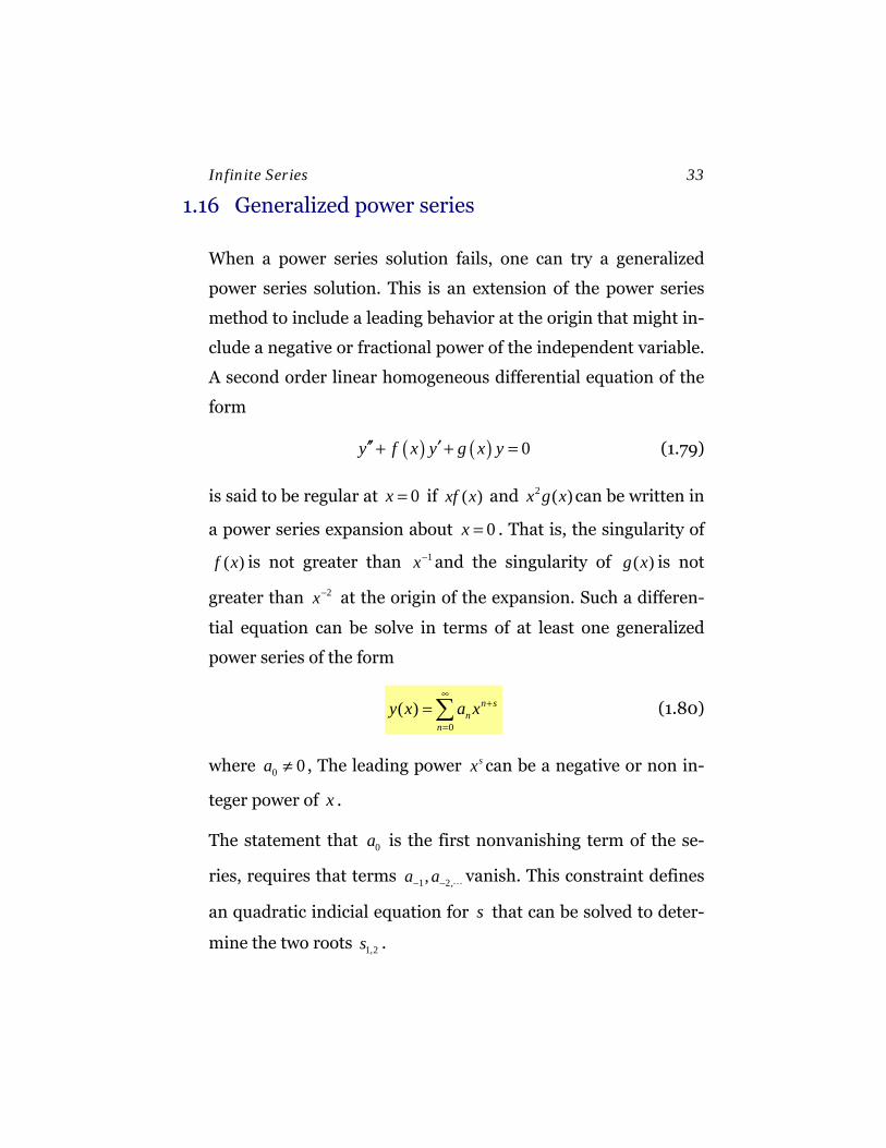
1.16 Generalized power series
When a power series solution fails, one can try a generalized
power series solution. This is an extension of the power series
method to include a leading behavior at the origin that might in-
clude a negative or fractional power of the independent variable.
A second order linear homogeneous differential equation of the
form
( ) ( ) 0y f x y g x y′′ ′+ + = (1.79)
is said to be regular at 0x = if ( )xf x and 2 ( )x g x can be written in
a power series expansion about 0x = . That is, the singularity of
( )f x is not greater than 1x− and the singularity of ( )g x is not
greater than 2x− at the origin of the expansion. Such a differen-
tial equation can be solve in terms of at least one generalized
power series of the form
0
( ) n sn
n
y x a x∞
+
=
=∑ (1.80)
where 0 0a ≠ , The leading power sx can be a negative or non in-
teger power of x .
The statement that 0a is the first nonvanishing term of the se-
ries, requires that terms 1 2,,a a− − vanish. This constraint defines
an quadratic indicial equation for s that can be solved to deter-
mine the two roots 1,2s .
34 Infinite Series
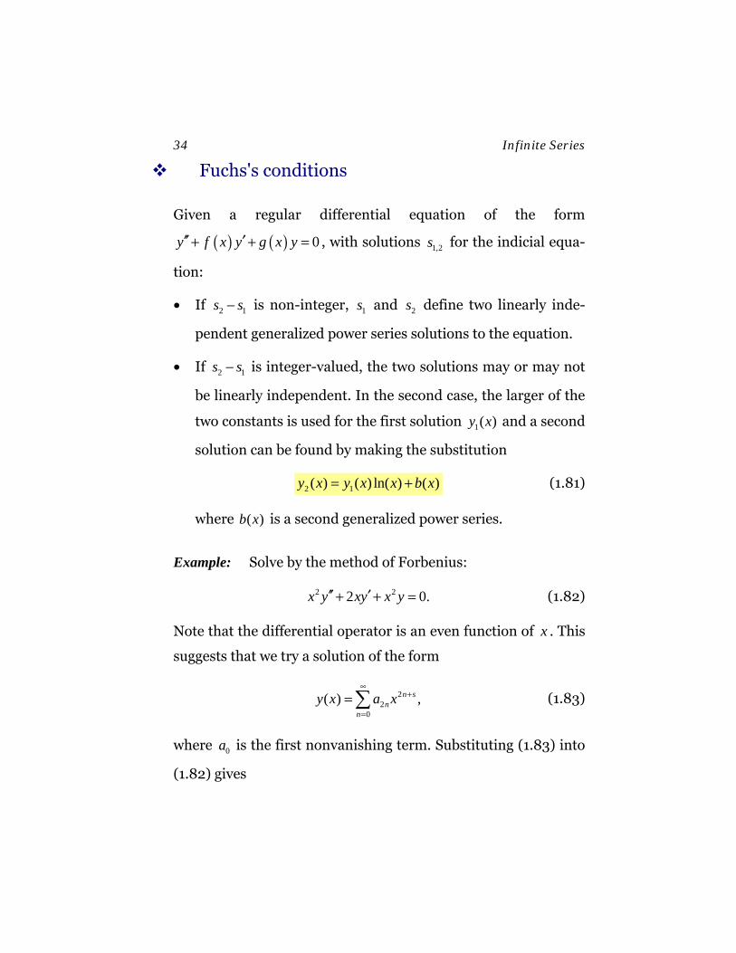
Fuchs's conditions
Given a regular differential equation of the form
( ) ( ) 0y f x y g x y′′ ′+ + = , with solutions 1,2s for the indicial equa-
tion:
• If 2 1s s− is non-integer, 1s and 2s define two linearly inde-
pendent generalized power series solutions to the equation.
• If 2 1s s− is integer-valued, the two solutions may or may not
be linearly independent. In the second case, the larger of the
two constants is used for the first solution 1( )y x and a second
solution can be found by making the substitution
2 1( ) ( ) ln( ) ( )y x y x x b x= + (1.81)
where ( )b x is a second generalized power series.
Example: Solve by the method of Forbenius:
2 22 0.x y xy x y′′ ′+ + = (1.82)
Note that the differential operator is an even function of x . This
suggests that we try a solution of the form
22
0( ) ,n s
nn
y x a x∞
+
=
=∑ (1.83)
where 0a is the first nonvanishing term. Substituting (1.83) into
(1.82) gives

Infinite Series 35
( )( ) ( )2 2
2 20 0
2 2 22 2 2
0 1
2 2 1 2 2
,
n s n sn n
n n
n s n sn n
n n
n s n s a x n s a x
a x a x
∞ ∞+ +
= =
∞ ∞+ + +
−= =−
+ + − + +
= − = −
∑ ∑
∑ ∑ (1.84)
which yields the recursion formula
( ) 2 2 22 (2 1) n nn s n s a a −+ + + = −⎡ ⎤⎣ ⎦ . (1.85)
Letting 0n = gives the indicial equation
( ) 0 2( 1) 0s s a a−+ = − =⎡ ⎤⎣ ⎦ (1.86)
or
0, 1s = − . (1.87)
Equation (1.85) can be rewritten as
( )
( )2 0
1,
2 1 !
n
na an s−
=+ +
(1.88)
giving the solutions
( )( )
20 0 0
0
1 sin( ) ,1 !
nn
n
xy x a x an x
∞
=
−= =
+∑ (1.89)
( )( )
2 11 0 0
0
1 cos( ) .!
nn
n
xy x a x an x
∞−
−=
−= =∑ (1.90)
The general solution is given by
sin cos( ) x xy x A B
x x= + (1.91)
36 Infinite Series
In this case, the solutions can be expressed in terms of elemen-
tary functions. A solution could have been found by substituting
( ) /y u x x= and solving for ( )u x to obtain ( ) sin cosu x A x B x= +
2. Analytic continuation
By venturing into the complex plane,
the geometric sense of multiplying by -1 can be replaced
from the operation of reflection, which is discrete,
to that of rotation, which is continuous.
The result is almost miraculous.
2.1 The Fundamental Theorem of algebra
Complex variables were introduced into algebra to solve a fun-
damental problem. Given a polynomial function of order N of a
real variable x, how do we find its roots (zero crossings)? The
equation to be solved can be written as
0
( ) 0N
nN n
nf x a x
=
= =∑ (2.1)
The problem may not have a real-valued solution, it may have a
unique solution, or it may have up to N distinct solutions, which
are called the N roots of ( )Nf x .
The problem can be reduced to the question of whether we can
fully factor the function into N linear products . That is, does an
algorithm exist that gives us uniquely
38 Analytic continuation
( )( )( ) ( )
( )0 1 2 1
0
( ) ...
0
N N N
N
N mm
f x a x x x x x x x x
a x x
−
=
= − − − −
= − =∏ (2.2)
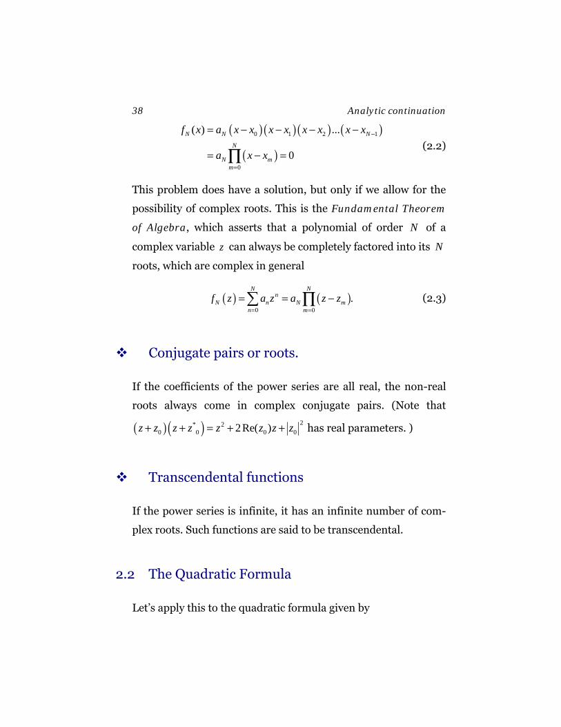
This problem does have a solution, but only if we allow for the
possibility of complex roots. This is the Fundamental Theorem
of Algebra, which asserts that a polynomial of order N of a
complex variable z can always be completely factored into its N
roots, which are complex in general
( ) ( )0 0
.NN
nN n N m
n m
f z a z a z z= =
= = −∑ ∏ (2.3)
Conjugate pairs or roots.
If the coefficients of the power series are all real, the non-real
roots always come in complex conjugate pairs. (Note that
( )( ) 2* 20 0 0 02Re( )z z z z z z z z+ + = + + has real parameters. )
Transcendental functions
If the power series is infinite, it has an infinite number of com-
plex roots. Such functions are said to be transcendental.
2.2 The Quadratic Formula
Let’s apply this to the quadratic formula given by

Analytic continuation 39
2
2
( )( ) 0
42
ax bx c a x x x xwhere
b b acxa
+ −
±
+ + = − − =
− ± −=
(2.4)
Here a, b, c are real coefficients. The roots x± are real if
( )2 4 0b ac− ≥ , and are complex if ( )2 4 0b ac− < . For the later case
we can rewrite the equation as
24 .
2b i ac bx
a±− ± −= (2.5)
Definition of the square root
Consider the plot of the quadratic function 2y x= shown in Fig-
ure 2-1.
3 1 1 33
1
1
3
5
7
9
y x( )
0
5
1−
x
40 Analytic continuation
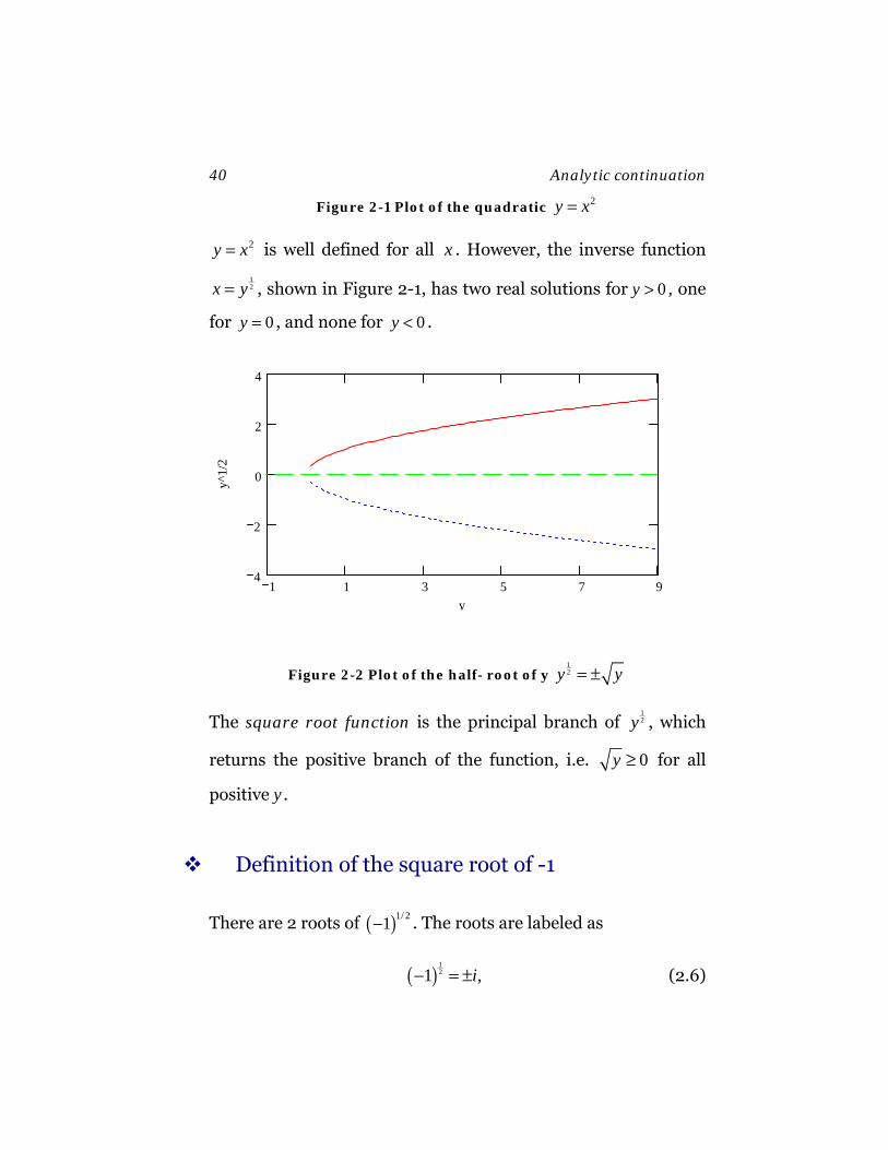
Figure 2-1 Plot of the quadratic 2y x=
2y x= is well defined for all x . However, the inverse function
12x y= , shown in Figure 2-1, has two real solutions for 0y > , one
for 0y = , and none for 0y < .
1 1 3 5 7 94
2
0
2
4
y
y^1/
2
Figure 2-2 Plot of the half- root of y 12y y= ±
The square root function is the principal branch of 12y , which
returns the positive branch of the function, i.e. 0y ≥ for all
positive y.
Definition of the square root of -1
There are 2 roots of ( )1/ 21− . The roots are labeled as
( )121 ,i− = ± (2.6)
Analytic continuation 41
where 1i = − is considered to be the primary branch of the
square root function. Since i is not a real number, it represents
a new dimension (degree of freedom). Just as one cannot add
meters and seconds, we can not add numbers on the real axis to
those along the imaginary axis i .To fully understand the mean-
ing of i , one first needs to appreciate the geometric interpreta-
tion of multiplication.
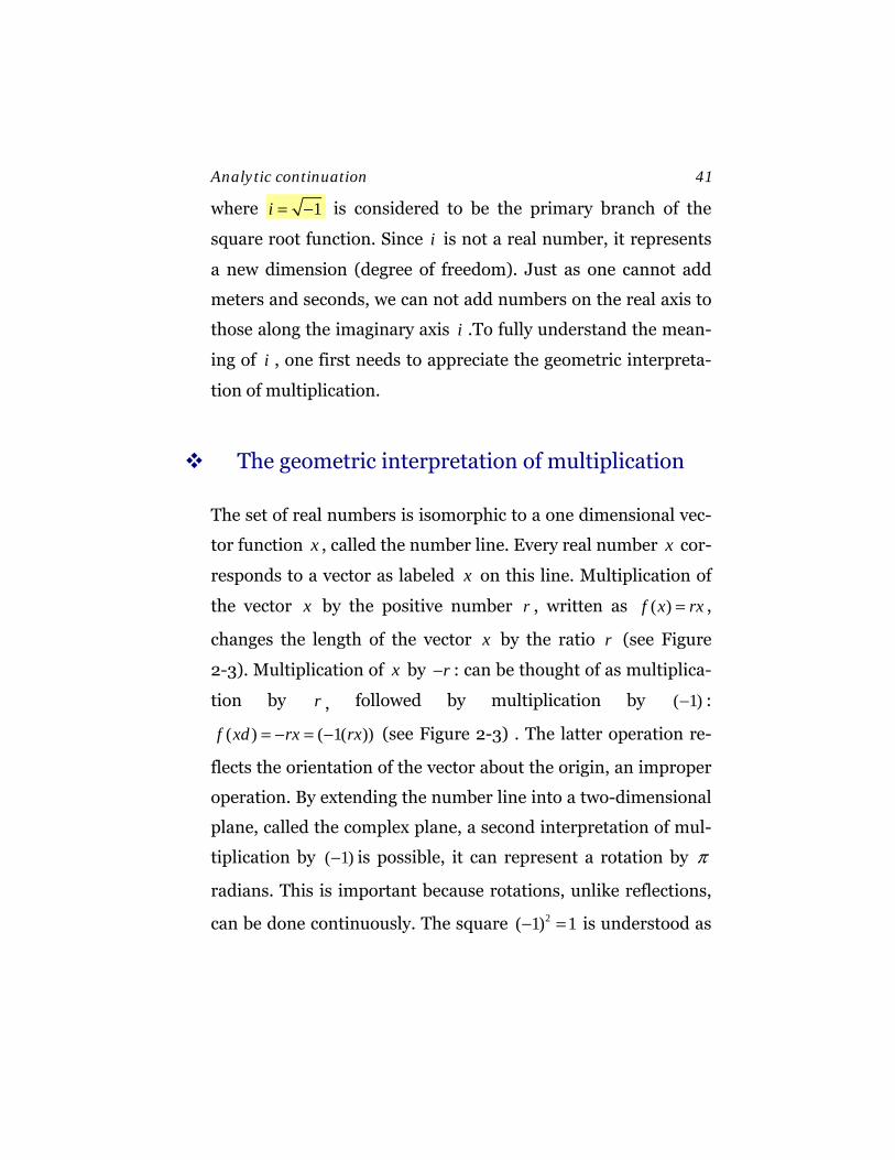
The geometric interpretation of multiplication
The set of real numbers is isomorphic to a one dimensional vec-
tor function x , called the number line. Every real number x cor-
responds to a vector as labeled x on this line. Multiplication of
the vector x by the positive number r , written as ( )f x rx= ,
changes the length of the vector x by the ratio r (see Figure
2-3). Multiplication of x by r− : can be thought of as multiplica-
tion by r , followed by multiplication by ( 1)− :
( ) ( 1( ))f xd rx rx= − = − (see Figure 2-3) . The latter operation re-
flects the orientation of the vector about the origin, an improper
operation. By extending the number line into a two-dimensional
plane, called the complex plane, a second interpretation of mul-
tiplication by ( 1)− is possible, it can represent a rotation by π
radians. This is important because rotations, unlike reflections,
can be done continuously. The square 2( 1) 1− = is understood as
42 Analytic continuation
two rotations by π , which brings us back to starting point.
( )r r− − = . And i can be written as the phase rotation 1ie π = − .
The geometric interpretation of ( )2 1i± = − is that i is the rota-
tion that when doubled produces a rotation by π radians. The
possible answers are / 2ie iπ± = ± , where / 2 1ii e π= = − , is the prin-
cipal branch of the square root function.
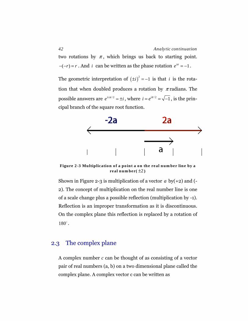
Figure 2-3 Multiplication of a point a on the real number line by a real number( 2± )
Shown in Figure 2-3 is multiplication of a vector a by(+2) and (-
2). The concept of multiplication on the real number line is one
of a scale change plus a possible reflection (multiplication by -1).
Reflection is an improper transformation as it is discontinuous.
On the complex plane this reflection is replaced by a rotation of
180 .
2.3 The complex plane
A complex number c can be thought of as consisting of a vector
pair of real numbers (a, b) on a two dimensional plane called the
complex plane. A complex vector c can be written as
Analytic continuation 43
.c a ib= + (2.7)
Addition of complex numbers is the same as addition of 2-
dimensional vectors on the plane. The plane represents all poss-
ible pairs of real numbers. Let x be an arbitrary number on the
real axis, and y be a arbitrary number along the imaginary axis,
then an arbitrary point on the complex plane can be referred to
as
.z x iy= + (2.8)
The complex plane can be quite “real” in that the properties of
“real” vectors constrained to a 2-dimensional plane can be quite
well represented as complex numbers in many applications. The
modulus z of a complex number z is its geometric length
2 2z x y= + . 2z z z∗= , where z∗ is the complex conjugate of z
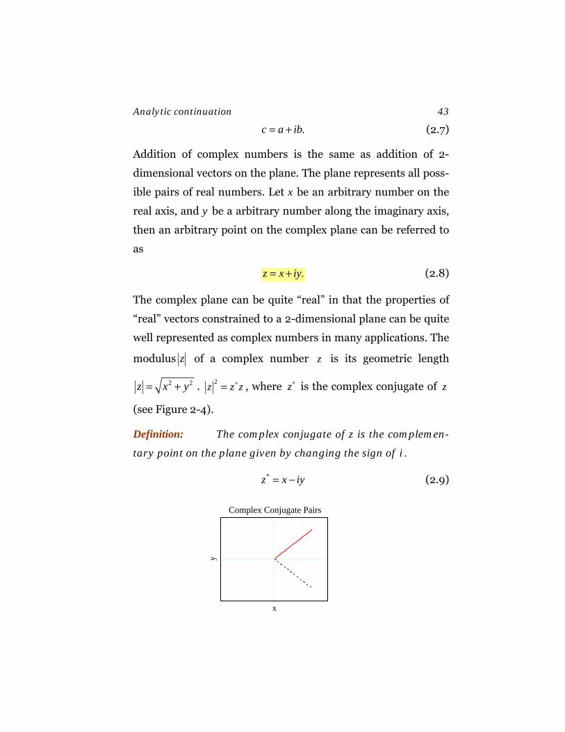
(see Figure 2-4).
Definition: The complex conjugate of z is the complemen-
tary point on the plane given by changing the sign of i .
*z x iy= − (2.9)
Complex Conjugate Pairs
x
y
44 Analytic continuation
Figure 2-4 Conjugate pairs of vectors in the complex plane x iy± .
2.4 Polar coordinates
Like any 2-dimensional vector pair, ( , )x y , the transformation of
a complex number into polar coordinates is given by the map-
ping
cos ,sin ,
x ry r
θθ
==
(2.10)
using
( )cos sin .iz r r iθ θ θ= = + (2.11)
Therefore, a complex number can be thought of as having a real
magnitude 0r > and an orientation θ wrt (with respect to) the
x axis. Note that the phase angle is cyclic, i.e. periodic, on inter-
val 2π
( 2 ) .i n ie eθ π θ+ = (2.12)
Example: Using
cos sin ,ixe x i x= + (2.13)
• Derive the series expansion of sin x and cos x using the pow-
er series expansion for xe and substituting x ix→ .
• Use the definition of the exponential, as the function which is
its own derivative ( /x xde dx e= ), to prove

Analytic continuation 45
sin cos ,
cos sin .
d x xdx
d x xdx
=
= − (2.14)
2.5 Properties of complex numbers
Complex numbers form a division algebra, an algebra with a
unique inverse for every non-zero element. Complex numbers
form commutative, associative groups under both the opera-
tions of addition and multiplication. The distributive law also
applies.
Definition: Addition and subtraction of complex numbers
Given
1 1 1 2 2 2and ,z x iy z x iy= + = + (2.15)
then,
( ) ( )3 1 2 1 2 1 2 .z z z x x i y y= ± = + ± + (2.16)
Definition: Multiplication of complex numbers
( )3 1 2 1 1 2 2 1 2 1 2 1 2 2 1( ) ( ) ( ),z z z x iy x iy x x y y i x y x y= ⋅ = + ⋅ + = − + + (2.17)
which in polar notation becomes
( )3 1 2 1 2( )3 3 1 2 1 2 .i i i iz r e re r e r r eθ θ θ θ θ+= = ⋅ = (2.18)
The geometric interpretation of complex multiplication is that it
represents a change of scale, scaling the length by 3 1 2r r r= , and a
46 Analytic continuation
rotation of one number by the phase of the other, with the final
orientation being the sum of the two phases 1 2θ θ+ .
Definition: Division is defined in terms of the inverse of a
complex number
( )
11 2 1 2
*1
*
1
/
in polar notation we get1i i
z z z z
zzz z
re er
θ θ
−
−
− −
= ⋅
=
=
(2.19)
Example: Calculate ( )2 /(1 )i i+ + .
*
21
2 2 4 1 5 / 21 1 1 1
ilet zi
i ithen z z zi i
+=+
− + += = ⋅ = =− + +
Example: Calculate 2 2z i=
First try it by brute force
( ) ( ) ( )22 2 2 2z x iy x y i xy= + = − +
This leads to two real equations
2 2 0,2 2.x yxy− ==
Substituting 1/y x= into the first equation, we get

Analytic continuation 47
14
22
4
1 0,
1 0,
Re 1 1,
1 1.
xx
x
x
yx
⎛ ⎞− =⎜ ⎟⎝ ⎠
− =
⎛ ⎞= = ±⎜ ⎟
⎝ ⎠
= = ±
Therefore
( )1 .z i= ± +
Of course, the easy way is to calculate ( )12
2i directly, the way to
do so will be made clear in the next section below
2.6 The roots of 1/ nz
The principal root of 1
1 1n = , since 1 1n = for the identity element.
Using polar notation, the thn distinct root of 1 is given by
( )
( )
11 2 2 /1 ,
with distinct roots for 0,1... 1 .
nn i m i m ne e
m n
π π= =
= − (2.20)
That is, the roots are unit vectors whose phase angles are equally
spaced from the identity element 1 in steps of 2 / nπ as shown in
Figure 2-5. This allows us to calculate the nth root of z
48 Analytic continuation
( )
11 1 / 2 /
,
0,1,...( 1).1 ,nn n n i m
i
i nz z r
let z rethen
for me
ne θ
θ
π
=⋅ =
−=
=
(2.21)
Definition: The principal root of 1/ nz is defined as
1/ /n i nn z r e φ= . All other roots are related by uniformly spaced
phase rotations of magnitude 2 / nπ
For example: 3 / 28 8 iz i e π= = has the solution
( ) ( ){ }/ 6 2 /3 / 6 4 /3/ 6
/ 6
2 , 2 ,2 ,
cos30 sin 30 .
i ii
i
z e e e
where e i
π π π ππ
π
+ +=
= +
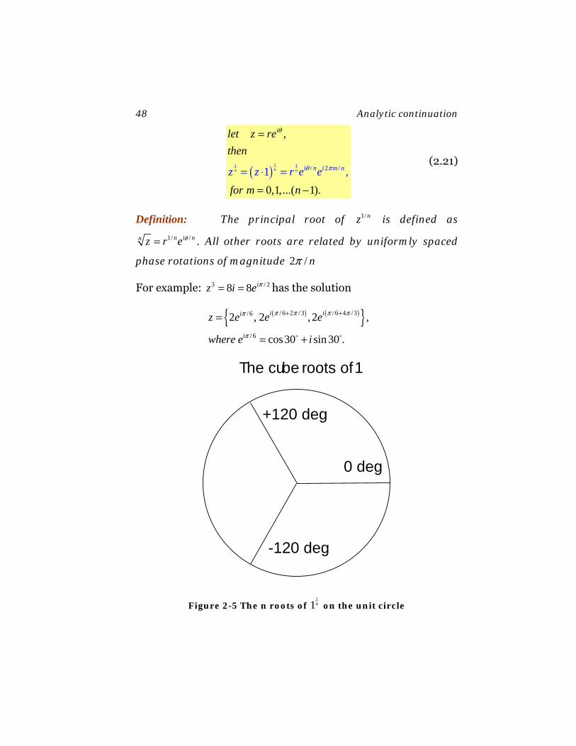
The cube roots of1
+120 deg
-120 deg
0 deg
Figure 2-5 The n roots of 1
1n on the unit circle
Analytic continuation 49
Shown in Figure 2-5 The n roots of 1
1n on the unit circle are the
cube roots of one. The concept of complex multiplication in-
volves a phase rotation plus a change of scale. The identity ele-
ment 1 is the principle root of 1
1n . The other 1n− roots are equal-
ly spaced vectors on the unit circle. The cube roots of 1 are those
phase vectors that, when applied 3 times, rotate themselves into
the real number 1.
2.7 Complex infinite series
A complex infinite series is the sum a real series and an imagi-
nary series. The complex series converges if both real series and
the imaginary series separately converge
( ) .c n n n n nS c a ib a i b= = + = +∑ ∑ ∑ ∑ (2.22)
A complex series converges absolutely if the series of real num-
bers given by n na ib+ absolutely converges.
Proof: Clearly, by the comparison test, n na c≤ and n nb c≤ ,
so if cS converges absolutely, then the component series aS and
bS converge absolutely.
The radius of convergence r of a complex power series nnc z∑ is
given by
1
lim .n
nn
cr zc→∞
+
= < (2.23)
50 Analytic continuation
Example: Find the radius of convergence of the exponential
function:
By analytic continuation ze is found by substituting z for x in
the power series representation of xe
0 !
nz
n
xen
∞
=
=∑ (2.24)
The radius of convergence is given by
1!lim lim 1 .11!
n n
nz n
n→∞ →∞
< = + = ∞
+
(2.25)
2.8 Derivatives of complex functions
To understand the meaning of a complex derivative, first let us
remind others of the definition of the derivative for a function
( )f x of a real variable x . The derivative /df dx of a real valued
function of x exits iff (if and only if) the limit
( )0
( ) ( )/ limx
f x f xdf x dx εε→
+ −= (2.26)
exists, and the limit is the same whether approaches zero from
below or above x .
Analytic continuation 51
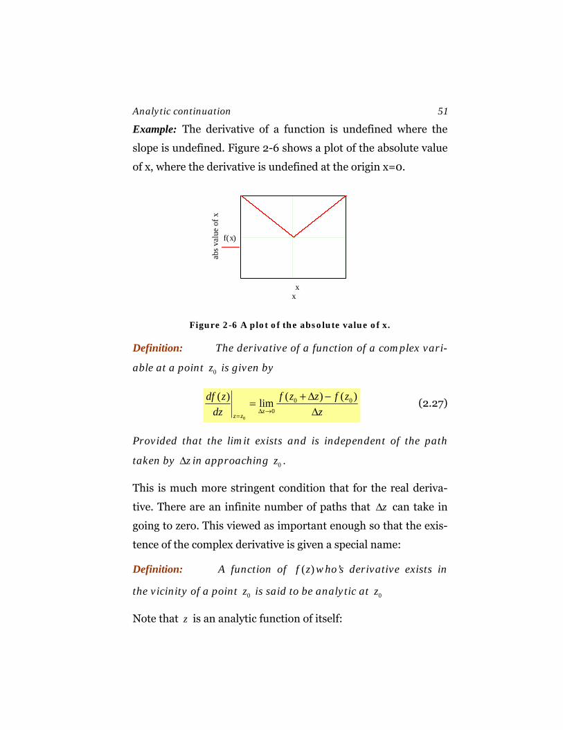
Example: The derivative of a function is undefined where the
slope is undefined. Figure 2-6 shows a plot of the absolute value
of x, where the derivative is undefined at the origin x=0.
x
abs v
alue
of x
f x( )
x
Figure 2-6 A plot of the absolute value of x.
Definition: The derivative of a function of a complex vari-
able at a point 0z is given by
0
0 0
0
( ) ( )( ) limz
z z
f z z f zdf zdz zΔ →
=
+ Δ −=Δ
(2.27)
Provided that the limit exists and is independent of the path
taken by zΔ in approaching 0z .
This is much more stringent condition that for the real deriva-
tive. There are an infinite number of paths that zΔ can take in
going to zero. This viewed as important enough so that the exis-
tence of the complex derivative is given a special name:
Definition: A function of ( )f z who’s derivative exists in
the vicinity of a point 0z is said to be analytic at 0z
Note that z is an analytic function of itself:
52 Analytic continuation
( )
0lim 1z
z z zzΔ →
+ Δ −=
Δ (2.28)
It follows (using the binomial expansion) that the derivative of
nz is also analytic:
( )
( )
1 2
0
11
0 0
( ),
lim lim .
nn n m m n n
m
n nn nn
z z
nz z z z z nz z O z
m
z z zdz nz z nzdz z z
− −
=
−−
Δ → Δ →
⎛ ⎞+ Δ = Δ = + Δ + Δ⎜ ⎟
⎝ ⎠
+ Δ − Δ= = =Δ Δ
∑ (2.29)
Clearly this means that all power series in z are analytic within
their radius of convergence. Note that
• Inverse powers z : nz− , are singular at the origin, so are not
analytic in the vicinity of 0z = .
• Inverse power series in z , can be thought of as power series
in ( )1/ z .
( )1
0.n
nn
f z c z∞
− −
=
=∑ (2.30)
By the ratio test such series converge for 1lim 1n
nn
cc z
+
→∞< , or for
1lim ,n
nn
cz rc+
→∞> = (2.31)
that is, they represent functions that are analytic outside of
some radius of convergence.
Analytic continuation 53
2.9 The exponential function
The exponential function is unusual in to it has a special syntax
( ) ze z e= ; some of its most important properties are listed below.
( )1 21 2
01
!2.718281828...
zz
z zz z
nz
n
de edz
e e eze zn
e e
+
∞
=
=
=
= < ∞
= =
∑ (2.32)
Proof: The first equation is simply the definition of the expo-
nential function as the function that is its own derivative. The
power series for ze comes from substituting the series into the
differential equation. We have already done this in the section
on infinite series, just substitute x z→ in the proof. The proof
that ( )1 21 2 z zz ze e e += can be derived by substituting the series for
the function in the expression, then rearranging the terms. An
outline of a proof follows:
( ) ( )
( ) ( )
1 2
1 2
2 21 2 1 1 2 2
0 0
2 21 2 1 1 2 2
21 2 1 2
1 2
0
1 ... 1 ...! ! 1 2 1 2
21 ...1 2
1 ... ...1 2
.!
n mz z
n m
nz z
n
z z z z z ze en m
z z z z z z
z z z z
z ze
n
∞ ∞
= =
∞+
=
⎛ ⎞⎛ ⎞= = + + + + + +⎜ ⎟⎜ ⎟
⎝ ⎠⎝ ⎠⎛ ⎞+ + += + + +⎜ ⎟⎝ ⎠⎛ ⎞+ +⎜ ⎟= + + + +⎜ ⎟⎝ ⎠
+= =
∑ ∑
∑
(2.33)
54 Analytic continuation
A more formal proof can be made using the binomial theorem.
From that it follows that
( )1
nnz z nz
n
e e e=
= =∏ (2.34)
Then, by extension, for any number c , we define
( )cz cze e= (2.35)
These properties, given in (2.33) and (2.35), are the justification
for using a power law representation for ( )e z .
2.10 The natural logarithm
The natural logarithm is the inverse of the exponential function.
Given zw e= ,
ln( ) .w z= (2.36)
Multiplying 1 2 1 2( )1 2
z z z zw w e e e += = gives
1 2 1 2 1 2ln( ) ln ln .w w z z w w= + = + (2.37)
ln( )z can easily be evaluated using polar notation. Let
( 2 )i i mz re reθ θ π+= = , then
( ) ( ) ( )( 2 ) ( 2 )ln ln ln .i m i mre r eθ π θ π+ += + (2.38)
Therefore, ln( )z is defined as
( )ln ln 2 for all m=0, 1,...z r i i mθ π= + + ± (2.39)
Analytic continuation 55
and the of the logarithm is defined as
( )ln ln , .z r iθ π θ π= + − < ≤ (2.40)
For example,
( ) ( )/ 2ln ln / 2 2 .ii e i i mπ π π= = + (2.41)
For all integer m . Therefore, the logarithm is a multivalued
function of a complex variable.
2.11 The power function
The power function is defined by analytic continuation as
( )ln( ) ln .ww z w zz e e= = (2.42)
For example,
( ) ( )2 / 2 2ln ln ( 2 2 ) .ii mi i i e i i mi e e e eπ π ππ π − ++= = = = (2.43)
Note that all the roots of ( )ii are real.
This definition results in the expected behavior for products of
powers:
( ) ( )1 2 1 21 1 2 lnln lnw w w z w www w z w zz z e e e z+ += = = (2.44)
2.12 The under-damped harmonic oscillator
The equation for the damped harmonic oscillator is given by
56 Analytic continuation
0,mx bx kx+ + = (2.45)
where 2 2/ and /x dx dt x d x dt= = . This equation can be thought of
as the projection onto the x axis of motion in a 2dimensional
space given by z x iy= +
0.mz bz kz+ + = (2.46)
Let’s try a solution of the form ( ) utz t e= . This leads to the qua-
dratic equation
2 0,mu bu k+ + = (2.47)
With solutions
2 4
2b b mku
m±− ± −= (2.48)
If 2 4 0,b mk− <
24
2b i mk bu
m±− ± −= (2.49)
The solution oscillates:
( ) ( )* / 2 / 2( ) 2 cos 2 sin .i t i t bt m bt mx t ce c e e t t eω ω α ω β ω− − −= + = + (2.50)
• The complex solutions are weighted sums of decaying spirals
one of which rotates clockwise and the other counter-
clockwise (Figure 2-7). This diagram could also represent a
2-dimensional phase space plot of position vs. momentum
p mv= for a 1-dimensional problem. In that case the point

Analytic continuation 57
that they decay into is the stable point of the equations of
motion ( 0x p= = ) which is often called the attractor.
Figure 2-7 Decaying spiral solutions to the damped oscillator in the complex plane.
The total solution for z(t) is the weighted sum of the 2 complex
solutions
( ) .u t u tz t c e c e+ −+ −= + (2.51)
The solution can be made real by taking the projection onto the
real axis
*
( ) .2
z zx t += (2.52)
This forces c± to be conjugate pairs, giving the solution
( ) ( )( ) cos sin .tz t a t b t e λω ω −⎡ ⎤= +⎣ ⎦ (2.53)
The equation of the under damped oscillator can be rewritten as
( )( ) cos ,tx t A t e λω ϕ −= + (2.54)
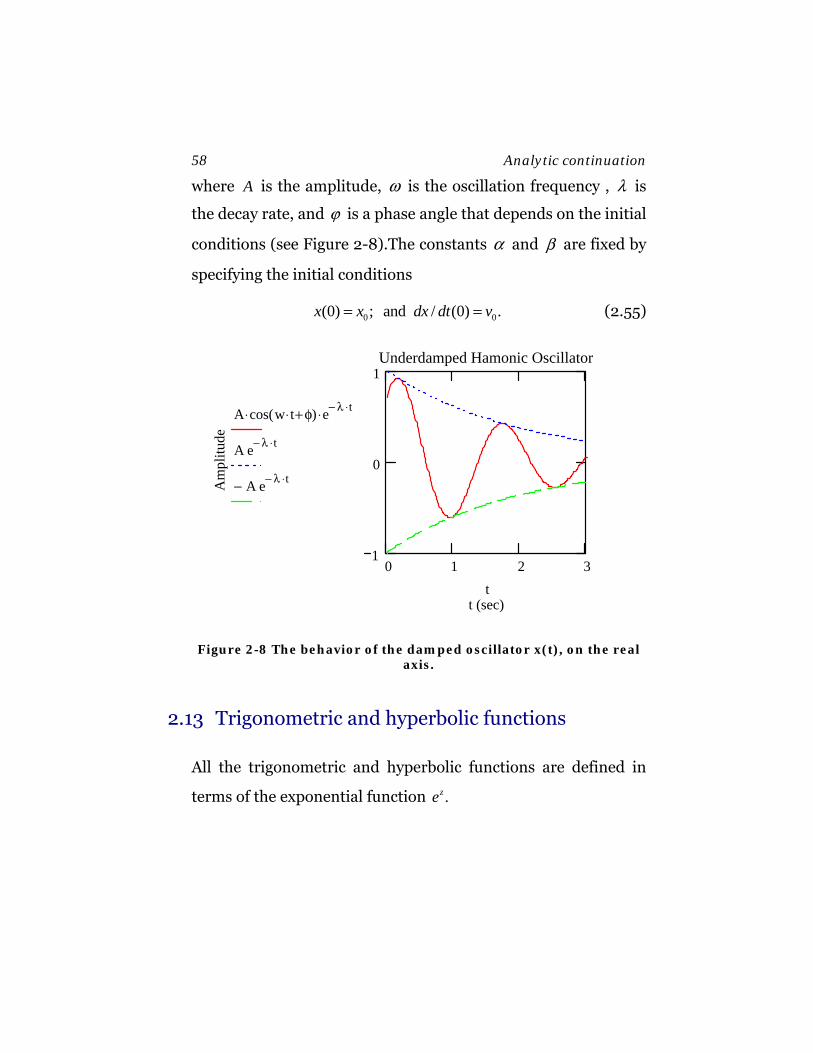
58 Analytic continuation
where A is the amplitude, ω is the oscillation frequency , λ is
the decay rate, and ϕ is a phase angle that depends on the initial
conditions (see Figure 2-8).The constants α and β are fixed by
specifying the initial conditions
0 0(0) ; and / (0) .x x dx dt v= = (2.55)
0 1 2 31
0
1Underdamped Hamonic Oscillator
t (sec)
Am
plitu
de
A cos w t⋅ φ+( )⋅ e λ− t⋅⋅
A e λ− t⋅
A− e λ− t⋅
t
Figure 2-8 The behavior of the damped oscillator x(t), on the real axis.
2.13 Trigonometric and hyperbolic functions
All the trigonometric and hyperbolic functions are defined in
terms of the exponential function .ze

Analytic continuation 59
2.14 The hyperbolic functions
cosh z and sinh z are defined as the even and odd parts of the
exponential function:
2
0
2 1
0
( ) ,2 2 !
( ) .2 2 1!
z z n
n
z z n
n
e e zcosh zn
e e zsinh zn
− ∞
=
− +∞
=
⎛ ⎞+= =⎜ ⎟⎝ ⎠⎛ ⎞−= =⎜ ⎟ +⎝ ⎠
∑
∑ (2.56)
A large number of identities have been tabulated for these func-
tions, let’s look at a few
2 2
2 2
( ) ( ) 1,( ) ( ),
( ) ( ),
(2 ) ( ) ( ),(2 ) 2 ( ) ( ).
cosh z sinh zd cosh z sinh z
dzd sinh z cosh z
dzcosh z cosh z sinh zsinh z cosh z sinh z
− =
=
=
= +=
(2.57)
The proofs all follow easily from the definitions of the functions.
Some selected proofs follow:
Example: Prove 2 2cosh sinh 1z z− = :
2 22 2
2 2 2 2
2 2
2 24 4
4 1.4
z z z z
z z z z z z z z
z z
e e e ecosh z sinh z
e e e e e e e e
e e
− −
− − − −
−
⎛ ⎞ ⎛ ⎞+ +− = −⎜ ⎟ ⎜ ⎟⎝ ⎠ ⎝ ⎠
+ + − += −
= =
(2.58)
60 Analytic continuation
Example: Prove that sinh / coshd z dz z= :
( ) ( ).
2 2
z z z zdsinh z d e e e e cosh zdz dx
− −⎛ ⎞ ⎛ ⎞− += = =⎜ ⎟ ⎜ ⎟⎝ ⎠ ⎝ ⎠
(2.59)
Example: Prove that sinh 2 2sinh coshz z z=
2 2
2 ( ) ( ) 2 (2 ).2 2 2
z z z z z ze e e e e esinh z cosh z sinh z− − −⎛ ⎞⎛ ⎞+ − −= = =⎜ ⎟⎜ ⎟
⎝ ⎠⎝ ⎠(2.60)
2.15 The trigonometric functions
The trigonometric functions are defined as the mapping z ize e→
giving
( )
( )
( )
02
02 1
0
cos( ) sin( ),!
cos( ) ( ) ,2 !
sin( ) ( ) .2 1!
niz
nn
nn
n
ize z i z
n
izz cosh iz
n
izz isinh iz i
n
∞
=
∞
=
+∞
=
= = +
= =
= − = −+
∑
∑
∑
(2.61)
Again a large number of identities have been derived for these
functions, and a few of these are
Analytic continuation 61
2 2
2 2
( ) ( ) 1,( ) ( ),
( ) ( ),
(2 ) ( ) ( ),(2 ) 2sin( ) cos( ).
cos z sin zdcos z sin z
dzdsin z cos z
dzcos z cos z sin zsin z z z
+ =
= −
=
= −=
(2.62)
The proofs are similar to the proofs for the hyperbolic functions.
Here is an example proof, made by direct substitution:
2 2 2 2 2
2 2
cosh ( ) sinh ( ) cos ( ) sin ( )
cos ( ) sin ( ) 1.
iz iz z i z
z z
⎡ ⎤ ⎡ ⎤− = −⎣ ⎦ ⎣ ⎦⎡ ⎤= + =⎣ ⎦
(2.63)
It is reassuring to know that all the familiar trigonometric iden-
tities, that we commonly use in real analysis, carry over essen-
tially unchanged into the complex plane.
2.16 Inverse trigonometric and hyperbolic functions
The inverse trigonometric and hyperbolic functions can be ex-
pressed in terms of the natural logarithm. However, it takes
some practice to get good at this.

62 Analytic continuation
Example: Find ( )arcsinh z:
( )
( )
( )
1
2
2
2 2
2
2
sinh( ) ,2 2
arcsinh ,
,2 1,
2 1 0,
1,
1,
ln 1 .
z z
z
z
e e u uw z
z w
u ewu u
u wu
u w w
u e w w
z w w
− −− += = =
=
== −
− − =
− = +
= = ± +
= ± +
(2.64)
Solving for z
( )1 2sinh ( ) ln 1z w w w−= = ± + (2.65)
but which of the signs is correct? That depends on the problem
to be solve. For example, one can find, in a book of math inte-
grals, the following formula:
1
20
sinh ( )1
x dx xx
−⎛ ⎞=⎜ ⎟
−⎝ ⎠∫ >0 for x>0, (2.66)
implying that the positive branch is the correct one for the case
x>0.
Analytic continuation 63
2.17 The Cauchy Riemann conditions
If a function ( , ) ( , ) ( , )f x y u x y iv x y= + is analytic in a region, the
real and imaginary parts of the function satisfy the following
constraints, called the Cauchy Riemann conditions:
;u v u vx y y x
∂ ∂ ∂ ∂= = −∂ ∂ ∂ ∂
(2.67)
By saying that ( , )f x y is analytic in a region we mean that the
derivative exists and is unique at each and every point in the re-
gion. The existence of the derivative implies, by the chain rule,
the existence of the partial derivatives with respect to x and y.
Let us consider ( ) /df z dz calculated two different ways, first by
holding y constant, then by holding x constant. In the first case
we get
( , ) .
y const
df x y f u vidz x x x=
∂ ∂ ∂= = +∂ ∂ ∂
(2.68)
Secondly, holding x constant gives
( , ) 1 .
x const
df x y f u v v ui idz i y i y y y y=
⎛ ⎞∂ ∂ ∂ ∂ ∂= = + = −⎜ ⎟∂ ∂ ∂ ∂ ∂⎝ ⎠ (2.69)
But the two expression are the same; therefore comparing the
real and imaginary parts, we get the Cauchy-Riemann condi-
tions. The Cauchy-Riemann conditions are both necessary and
sufficient conditions for a function to be analytic in a region.
Basically, the proof follows from rotational invariance: these

64 Analytic continuation
conditions have to be met on every straight line path chosen to
approach the limit. Any other well behaved path can be approx-
imated by a straight line over a small enough interval.
Example: Using the Cauchy Riemann conditions it is easy to
show that z x iy∗ = − is not an analytic function of z , applying
them we get
x yx y
∂ ∂≠ −∂ ∂
(2.70)
So z∗ is not an analytic function of z .
2.18 Solution to Laplace equation in two dimensions
The Laplace equation in 2dimensions can be written as
2 2
2 2 ( , ) 0.x yx y
⎛ ⎞∂ ∂+ Φ =⎜ ⎟∂ ∂⎝ ⎠ (2.71)
It is easy to show that, for real Φ the general solution take’s the
form
( , ) ( ) ( ).x y f x iy g x iyΦ = + + − (2.72)
Where
( )( ) ( )g z f z ∗∗ = (2.73)
Proof: By direct substitution, show that ( )f z is a solution:
Analytic continuation 65
2 2 2
2 2 2
2 2 22
2 2 2
2 2 2 2
2 2 2 2
( ) ( )
, ,
, ,
0.
f x iy f zf df z df f d f z d fx dz x dz x d z x d zf df z df f d f z d fi i iy dz y dz y d z y d z
f f d f d fx y d z d z
+ =
∂ ∂ ∂ ∂= = = =∂ ∂ ∂ ∂∂ ∂ ∂ ∂= = = =∂ ∂ ∂ ∂
∂ ∂∴ + = − =∂ ∂
(2.74)
The proof for ( )g z∗ , is similar, but, more directly, since the op-
erator is real, if ( )f z is a solution, then ( )( ) ( )f z g z∗ ∗′= must al-
so be a solution. If ( , )x yΦ represents a real potential, then the
solution takes the self-conjugate form
( )( , ) ( ) ( ) .x y f z f z ∗Φ = + (2.75)

3. Gamma and Beta Functions
A function that calls itself
is like a dog chasing its tail.
Where will this nonsense end?
3.1 The Gamma function
The coefficients of infinite power series are often given in terms
of recursive relations. For example the series solution
x nne a x=∑ to the differential equation for the exponential func-
tion /x xde dx e= leads to the following recursive formula:
11 ,n na an −= ⋅ (3.1)
with a solution
01 .!na a
n= (3.2)
Normalizing to 0 1a = gives
0
,!
nx
n
xen
∞
=
=∑ (3.3)
where
68 Gamma and Beta Functions
1
! .n
m
n m=
=∏ (3.4)
The factorial function occurs in the definition of Taylor’s Expan-
sion as well as in the definition of trigonometric and hyperbolic
functions. This particular combinatory formula is so useful that
it becomes desirable to extend its definition to non-integer val-
ues of n . The key property of the factorial is its :
( )! 1 !.n n n= ⋅ − (3.5)
It is this property that we wish to maintain as we extend it into
the domain of real numbers.
Extension of the Factorial function
The Gamma function represents the extension of the factorial
function. Its definition must satisfy two key requirements:
( 1) ! for integer 0,( 1) ( ) for all real . p p pp p p p
Γ + = >Γ + = Γ
(3.6)
It is sufficient to define ( )pΓ in the interval [ ]1,2p = as recur-
sion can be used to generate all other values. However, there ex-
ists a definite integral that has all the required properties and
which is valid for all positive p . This integral is what is used to
define ( )pΓ for 0p > . This integral is given by
1
0
( ) p tp t e dt∞
− −Γ = ∫ (3.7)
Gamma and Beta Functions 69
It is easy to demonstrate by integration by parts that
1
0 00 0
(2) 0 1t t t tt e dt te e dt e∞ ∞
∞ ∞− − − −Γ = = + = − =∫ ∫ =1! (3.8)
And, also by integration by parts,
1
00 0
( 1) ( ).p t p t p tp t e dt t e p t e dt p p∞ ∞
∞− − − −Γ + = = + = Γ∫ ∫ (3.9)
Therefore, by recursion, (3) 2 (2) 2!Γ = Γ = , etc. The integral (3.7)
meets all the necessary requirements to be the extension of the
factorial function (3.4). By explicit integration, we find
0
(1) 1 0!te dt∞
−Γ = = =∫ (3.10)
which defines 0!, and
1
0
(0) 1! .tt e dt∞
− −Γ = − = = ∞∫ (3.11)
In fact, , since by using ( ) ( 1) /p p pΓ = Γ +
1( 1) ( 1 1) (0) ,11 1 1( 2) ( 1) (0) , et etc.2 ( 2) ( 1)
Γ − = Γ − + = −Γ = −∞−
⋅Γ − = ⋅Γ − = ⋅Γ = ∞− − ⋅ −
(3.12)

70 Gamma and Beta Functions
Gamma Functions for negative values of p
Evaluation of the Gamma function for negative p is given by re-
peated applications of the relationship
( )1( ) 1 ,p pp
Γ = Γ + (3.13)
until ( )p nΓ + returns a positive number.
A plot of the Gamma function and its inverse is shown in Figure
3-1
4 0 420
0
20
Γ x( )
x
4 0 45
0
5
1
Γ x( )
x
Figure 3-1 Plot of the Gamma function and its inverse
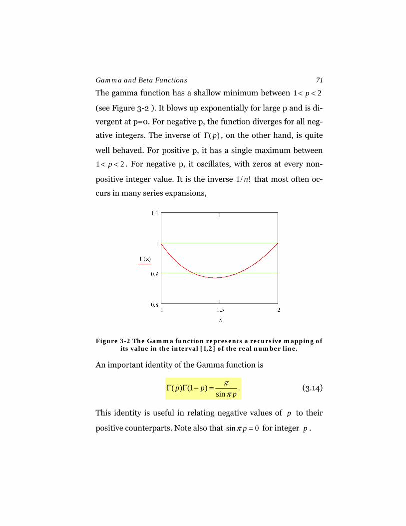
Gamma and Beta Functions 71
The gamma function has a shallow minimum between 1 2p< <
(see Figure 3-2 ). It blows up exponentially for large p and is di-
vergent at p=0. For negative p, the function diverges for all neg-
ative integers. The inverse of ( )pΓ , on the other hand, is quite
well behaved. For positive p, it has a single maximum between
1 2p< < . For negative p, it oscillates, with zeros at every non-
positive integer value. It is the inverse 1/ !n that most often oc-
curs in many series expansions,
Figure 3-2 The Gamma function represents a recursive mapping of its value in the interval [1,2] of the real number line.
An important identity of the Gamma function is
( ) (1 ) .sin
p pp
ππ
Γ Γ − = (3.14)
This identity is useful in relating negative values of p to their
positive counterparts. Note also that sin 0pπ = for integer p .

72 Gamma and Beta Functions
Example: Show that (1/ 2) .πΓ =
Use (3.14), letting 1/ 2p = ,
( ) ( ) ( ) ( )( )
21 1 12 2 2
12
1 ,sin / 2
.
π ππ
π
Γ Γ − = Γ = =
∴Γ = (3.15)
Example: Find ( 3 / 2).Γ −
Use the recursive property of the gamma function:
( ) ( )
( ) ( ) ( )3 1 12 2 23 3 1
2 2 2
1 / ,
1 1 1 4 .3
p p p
π
Γ = Γ +
⎛ ⎞⎛ ⎞Γ − = Γ − = Γ =⎜ ⎟⎜ ⎟− − −⎝ ⎠⎝ ⎠
(3.16)
Evaluation of definite integrals
An important use of Gamma functions is in the evaluation of de-
finite integrals. In fact, its definition for positive p can be
thought of as defining the normalization of a family of integrals.
By making a change of coordinates, the normalization of many
other useful integrals can be found.
Example: Transformation of coordinates 2.t x=
( ) 2
2
2 11
0 0
; 2 ;
( ) 2 .pp t x
t x x t dt xdx
p t e dt x e xdx∞ ∞
−− − −
= ⇒ = =
Γ = =∫ ∫ (3.17)
Gamma and Beta Functions 73
Therefore,
22 1
0
( ) 2 .p xp x e dx∞
− −Γ = ∫ (3.18)
Example: Find the normalization of a the Normal Gaussian Dis-
tribution
The Normal Distribution of a statistical measurement of a quan-
tity X , centered at a mean 0X and having a random rms error
spread σ , is given by
2 / 2( ) ,xy x Ne−= (3.19)
where ( )0 /x X X σ= − . This distribution is normalized such that
2 / 2( ) 1.xy x dx N e dx
∞ ∞−
−∞ −∞
= =∫ ∫ (3.20)
Since the integrand is symmetric we can rewrite this as
2 / 2
0
1 .2
xe dxN
∞− =∫ (3.21)
Let’s make the change of variable
2
1/ 2
/ 2 2 ,1 ,2
x x x x
dx xdx dx x dx−
′ ′= ⇒ =
′ ′ ′= ⇒ = (3.22)
Then, by substitution,
74 Gamma and Beta Functions
( )2 / 2 1/ 2 12
0 0
1 1 1 ,22 2
x xe dx x e dxN
∞ ∞′− − −′ ′= = Γ =∫ ∫ (3.23)
which leads to the following formula
( )12
2 1 1 .2 2
Nπ
= =Γ
(3.24)
Therefore, the “normalized” is given by
2 2/ 2 / 21 1( ) ; 1.
2 2x xy x e e dx
π π
∞− −
−∞
= =∫ (3.25)
3.2 The Beta Function
Another statistical combination that often reoccurs is
represented by the binomial coefficients, given by
( )
! .! !
n nm n m m⎛ ⎞
=⎜ ⎟ −⎝ ⎠ (3.26)
In probability theory, they denote the number of ways one can
arrange n objects taken m at a time. These coefficients have al-
ready been seen in the Binomial formula for integer powers of n,
( )0
.n
n n m m
m
nA B A B
m−
=
⎛ ⎞+ = ⎜ ⎟
⎝ ⎠∑ (3.27)
Again, one would like to extend this formula to the real number
domain. This is done by defining the Β (Greek capital beta)
function given by
Gamma and Beta Functions 75
( ) ( )( , ) .( )p q
p qp q
Γ ΓΒ =
Γ + (3.28)
Clearly, the Beta function is symmetric under interchange of in-
dices
( , ) ( , ),p q q pΒ = Β (3.29)
and, for integer values of p n= and q m= ,
!( )! 1 !( )!( 1, 1)
( 1)! 1 ( )!n m n mn m
n m n m n mΒ + + = =
+ + + + + (3.30)
( )1 .
1 ( 1, 1)n m
m n m n m+⎛ ⎞
=⎜ ⎟ + + Β + +⎝ ⎠ (3.31)
The Beta function is useful in the determining normalization of
many common integrals. Among them are the canonical forms
( ) ( ) ( )
( ) ( )
( )( )
2 1/ 2 2 1
0
11 1
01
0
for 0, 0 :
, 2 sin cos ,
, 1 ,
, .1
p q
p q
p
p q
p q
p q d
p q x x dx
yp q dxy
πθ θ θ
− −
− −
−∞
+
> >
Β =
Β = −
Β =+
∫
∫
∫
(3.32)
These three integral forms are related to one another by the
transformations
( )2sin / 1 .x y yθ= = + (3.33)
A number of other definite integrals that can be put into one of
these forms.
76 Gamma and Beta Functions
The following proof that the above functions are indeed equiva-
lent to the defining equation for the Beta function makes use of
the fact that the integration over the surface of a quadrant
0 ,0x y< < ∞ < < ∞ is integration over a quarter-circle. When we
change to polar coordinates the range of angles is 0 / 2θ π< < ,
giving
2 22 1 2 1
0 0
( ) ( ) 4 .p x q yp q x e dx y e dy∞ ∞
− − − −Γ Γ = ∫ ∫ (3.34)
( )
( ) ( ) 2/ 2
2 1 2 1 2( ) 1
0 0
cos , sin , :
4 cos sin ,p q p q r
Letting x r y r dxdy rdrd
d r e drπ
θ θ θ
θ θ θ∞
− − + − −
= = =
= ∫ ∫ (3.35)
and therefore,
( ) ( ) ( ) ( )2 1 2 1
0
2 ( ) cos sin ( ) ( , ).p qp q p q d p q B p qπ
θ θ θ− −Γ Γ = Γ + = Γ +∫ (3.36)
3.3 The Error Function
The Error function (Figure 3-3) can be considered as an incom-
plete integral over a gamma function or “”. are defined as the
partial integrals of the form
1
0
( , ) .t
p tt p t e dtγ − −= ∫ (3.37)
Often, it is desirable to use the normalized incomplete gamma
functions instead

Gamma and Beta Functions 77
1
0( , ) .( )
tp tt e dt
t pp
γ
− −
=Γ
∫ (3.38)
For example, the normalization of the Gaussian integral is given
by
2
0
(1/ 2) 2 .xe dx∞
−Γ = ∫ (3.39)
and the error function is defined as the normalized incomplete
integral
2
20
0
22( ) .
(1/ 2)
xx
xx
e dxErf x e dx
π
−
−= =Γ
∫∫ (3.40)
This integral can be expanded in a power series, giving
( ) 2 1
0
12( ) ,!(2 1)
nn
nErf x x
n nπ
∞+
=
−=
+∑ (3.41)
which is useful for small x.
The is defined as
( ) 1 ( ).erfc x erf x= − (3.42)
The Error function is closely related to the likelihood of error in
a measurement of normally distributed data. However, like
many standard mathematical functions, the normalization is
slightly different from how physicists would like to see it de-
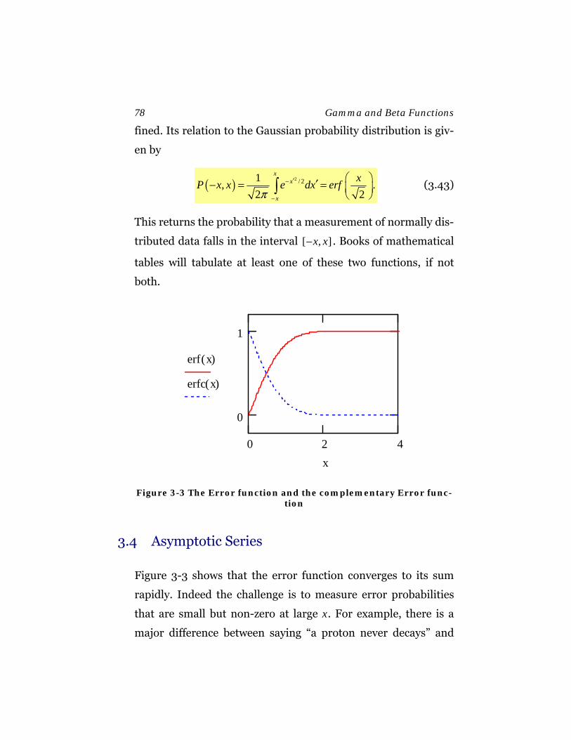
78 Gamma and Beta Functions
fined. Its relation to the Gaussian probability distribution is giv-
en by
( ) 2 / 21, .2 2
xx
x
xP x x e dx erfπ
′−
−
⎛ ⎞′− = = ⎜ ⎟⎝ ⎠∫ (3.43)
This returns the probability that a measurement of normally dis-
tributed data falls in the interval [ , ]x x− . Books of mathematical
tables will tabulate at least one of these two functions, if not
both.
0 2 4
0
1
erf x( )
erfc x( )
x
Figure 3-3 The Error function and the complementary Error func-tion
3.4 Asymptotic Series
Figure 3-3 shows that the error function converges to its sum
rapidly. Indeed the challenge is to measure error probabilities
that are small but non-zero at large x. For example, there is a
major difference between saying “a proton never decays” and
Gamma and Beta Functions 79
that of saying “a proton rarely decays”. Since the universe is still
around, the probability must be very, very small; but if we want
to quantify this probability, then we must be able to calculate
small deviations from zero.
Taylor’s expansion in terms of a convergent power series works
well for small x. But, at large x, it is convenient to expand the
function in inverse powers of x. However, in this case it turns
out that that expansion doesn’t converge. For problems like
these, the concept of an asymptotic series was created.
Let’s look at how we might calculate the complementary func-
tion from first principles. Define
22( ) 1 ( ) .t
x
erfc x erf x e dtπ
∞−= − = ∫ (3.44)
We can try to solve this by integrating by parts by making the
substitutions
( )2
2 2 2 221 1, ,2 2
tt t t ttee e dt e dt d e
t t t
−− − − −−= = = (3.45)
in
2 2 2
2 2
2
2
2 2 1 12 2
2 1 1 ,2 2
t t t
xx x
x t
x
e dt e e dtt t
e e dtx t
π π
π
∞∞ ∞− − −
∞− −
⎛ ⎞−= +⎜ ⎟⎜ ⎟⎝ ⎠⎛ ⎞
= +⎜ ⎟⎝ ⎠
∫ ∫
∫ (3.46)
where
80 Gamma and Beta Functions
2 2
2 2
1 1 .2 2
t t
x x
e dt e dtt x
∞ ∞− −<∫ ∫ (3.47)
Therefore, after the first integration by parts, the fractional error
in the remainder is less than 2
12x
. This is a small error if x is
large enough. We can repeat the process if we are not satisfied,
getting the asymptotic series
( ) ( )
2
2 32 2 2
1 1 3 1 3 5( ) 1 .2 2 2
xeerfc xxx x xπ
− ⎛ ⎞⋅ ⋅ ⋅⎜ ⎟− + − +⎜ ⎟⎝ ⎠
∼ (3.48)
For a number of iterations, integration by parts improves the er-
ror, but, after a while, the error begins to grow again (there is a
double factorial hiding in the numerator). Therefore, there are
an optimum number of integration by parts to make. The series,
with the partial sum NS taken to infinity, does not converge.
Nevertheless the error in the finite series (for fixed N ) goes to
zero as x →∞ . This is the difference between the definition of a
convergent series and an asymptotic series. A convergent series
is convergent for a given x, i.e., holding x constant, one takes the
limit N →∞ ; The asymptotic series holds N constant and takes
the limit x →∞ .
Definition: A series f(x) is said to be an asymptotic series
innx−, written as
0
( ) ,nn
n
af xx
∞
=∑∼ (3.49)
Gamma and Beta Functions 81
if the absolute value of the difference of the function and the
partial sum goes to zero faster than Nx− for fixed N as x →∞
0
lim ( ) 0.N
Nnnx n
af x xx→∞ =
− ⋅ →∑ (3.50)
It is possible for as series to be both convergent and asymptot-
ic—e.g., all power convergent series in x can be said to be
asymptotic as ( )0x → —but the non-convergent case is the most
interesting one.
Asymptotic series often occur in the solution of integrals of the
following kind:
1( ) ( )u
x
I x e f u du∞
−= ∫ (3.51)
Or of the type
2 ( ) ,u
x
uI x e f dux
∞− ⎛ ⎞= ⎜ ⎟
⎝ ⎠∫ (3.52)
where ( )/f u x is expanded in a power series in /u x .
Sterling’s formula
is a good example of a non-convergent asymptotic series. It is
given by
2 3
1 1 139( 1) 2 1 .12 288 51840
x xp x x ex x x
π − ⎧ ⎫Γ + ⋅ ⋅ + + − +⎨ ⎬⎩ ⎭
∼ (3.53)

82 Gamma and Beta Functions
If p is as small as 10, stopping after the second term gives an
error on the order of 50 ppm. For very large p ,
! 2 p pp p p eπ −⋅∼ (3.54)
is a good approximation to the factorial function, where the ∼
indicates that the ratio of the two sides approaches 1 as p →∞ .
Discussion Problem: The Exponential Integral
The integral
( )t
x
eEi x dtt
−∞= ∫ (3.55)
is called the Exponential Integral. Note that it diverges as 0x → .
• Find the asymptotic expansion for the exponential integral.
• Express 01/ ln(1/ )
xt dt∫ as an exponential integral.
4. Elliptic Integrals
When Kepler replaced the epicycles
of the ancients with ellipses,
he was onto something special.
Books of integral tables tabulate and catalog integrals in terms
of families with a certain generic behavior. For example, a large
number of integrals can be categorized as a rational function of
x times a radical of the form 2ax bx c+ + The solution of inte-
grals of this general form almost always can be expressed in
terms of elementary trigonometric functions or hyperbolic func-
tions. For example, substituting sinx θ= ,
( )2 2
212
sin 21 cos2 4
arcsin( ) 1 .
x dx d C
x x x C
θ θθ θ− = = + +
= + − +
∫ ∫ (4.1)
Or a similar example:
2
1 arcsin .1
dx xx
θ= =−∫ (4.2)
Elliptic functions were introduced to allow the solutions to the
large class of problems of the form
( ),R x y dx∫ (4.3)
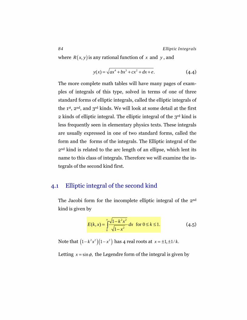
84 Elliptic Integrals
where ( ),R x y is any rational function of x and y , and
4 3 2( ) .y x ax bx cx dx e= + + + + (4.4)
The more complete math tables will have many pages of exam-
ples of integrals of this type, solved in terms of one of three
standard forms of elliptic integrals, called the elliptic integrals of
the 1st, 2nd, and 3rd kinds. We will look at some detail at the first
2 kinds of elliptic integral. The elliptic integral of the 3rd kind is
less frequently seen in elementary physics texts. These integrals
are usually expressed in one of two standard forms, called the
form and the forms of the integrals. The Elliptic integral of the
2nd kind is related to the arc length of an ellipse, which lent its
name to this class of integrals. Therefore we will examine the in-
tegrals of the second kind first.
4.1 Elliptic integral of the second kind
The Jacobi form for the incomplete elliptic integral of the 2nd
kind is given by
2 2
20
1( , ) for 0 1.1
x k xE k x dx kx
−= ≤ ≤−∫ (4.5)
Note that ( )( )2 2 21 1k x x− − has 4 real roots at 1, 1/ .x k= ± ±
Letting sin ,x φ= the Legendre form of the integral is given by

Elliptic Integrals 85
2 2
0
( , ) 1 sin for 0 1.E k k d kφ
φ φ φ= − ≤ ≤∫ (4.6)
A plot of the Legendre form, shown in Figure 4-1, is illustrative
of the general behavior. The integrand is periodic on interval
[ ]0,π , so the functions are sometimes said to be “doubly-
periodic” in φ . The integral is a repeating sum of the form
( , ) 2 ( ) ( , )E k n nE k E kφ π φ+ = + (4.7)
where ( )E k is the given by
1 / 22 2
2 2
20 0
1( ) ( , / 2) 1 sin .1
k xE k E k dx k dx
π
π φ φ−= = = −−∫ ∫ (4.8)
By symmetry about / 2π , it is only necessary to tabulate the
integral from [ ]0, / 2π .
( )( , / 2) 2 ( ) ( , ),
0 / 2 .E k E k E kφ π φ
φ π+ = −
≤ ≤ (4.9)
The integral over an even integrand is an odd function so
( ) ( ), , .E k E kφ φ= − (4.10)
Combining the above results gives
( ) ( ) ( ), 2 , for 0 / 2.E k n nE k E kπ φ φ φ π± = ± ≤ ≤ (4.11)
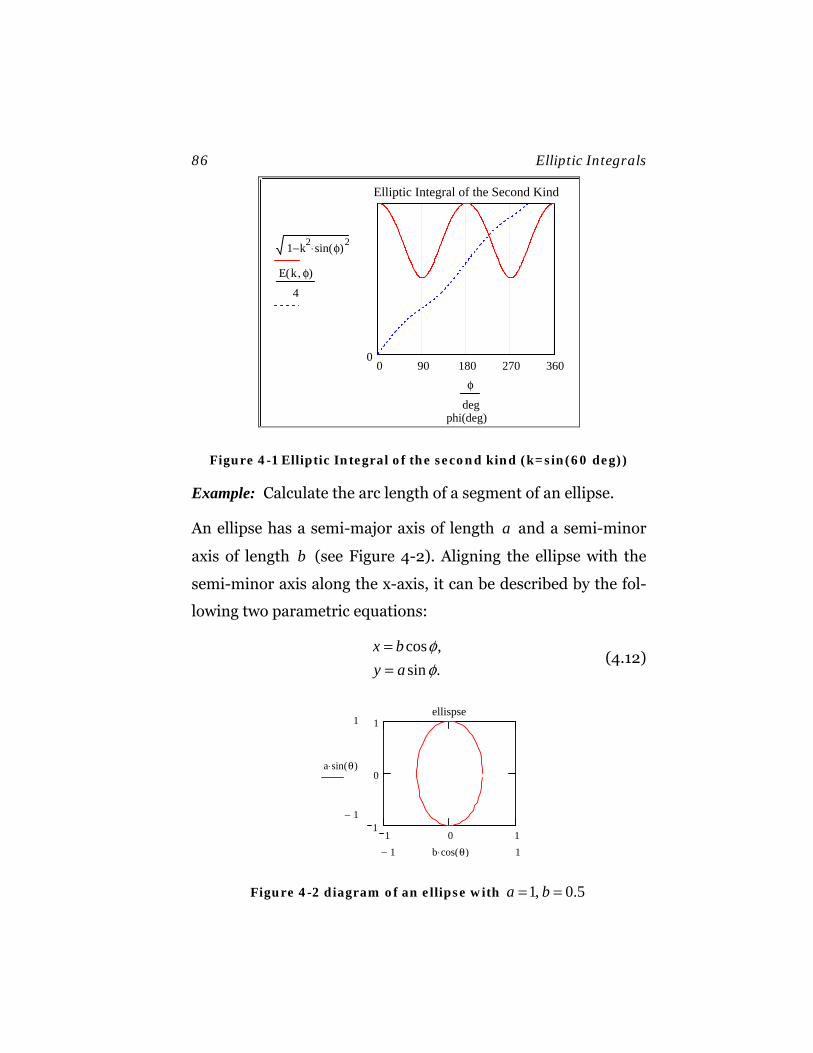
86 Elliptic Integrals
0 90 180 270 3600
Elliptic Integral of the Second Kind
phi(deg)
1 k2 sin φ( )2⋅−
E k φ,( )
4
φ
deg
Figure 4-1 Elliptic Integral of the second kind (k=sin(60 deg))
Example: Calculate the arc length of a segment of an ellipse.
An ellipse has a semi-major axis of length a and a semi-minor
axis of length b (see Figure 4-2). Aligning the ellipse with the
semi-minor axis along the x-axis, it can be described by the fol-
lowing two parametric equations:
cos ,sin .
x by a
φφ
==
(4.12)
1 0 11
0
1ellispse
1
1−
a sin θ( )⋅
11− b cos θ( )⋅
Figure 4-2 diagram of an ellipse with 1, 0.5a b= =
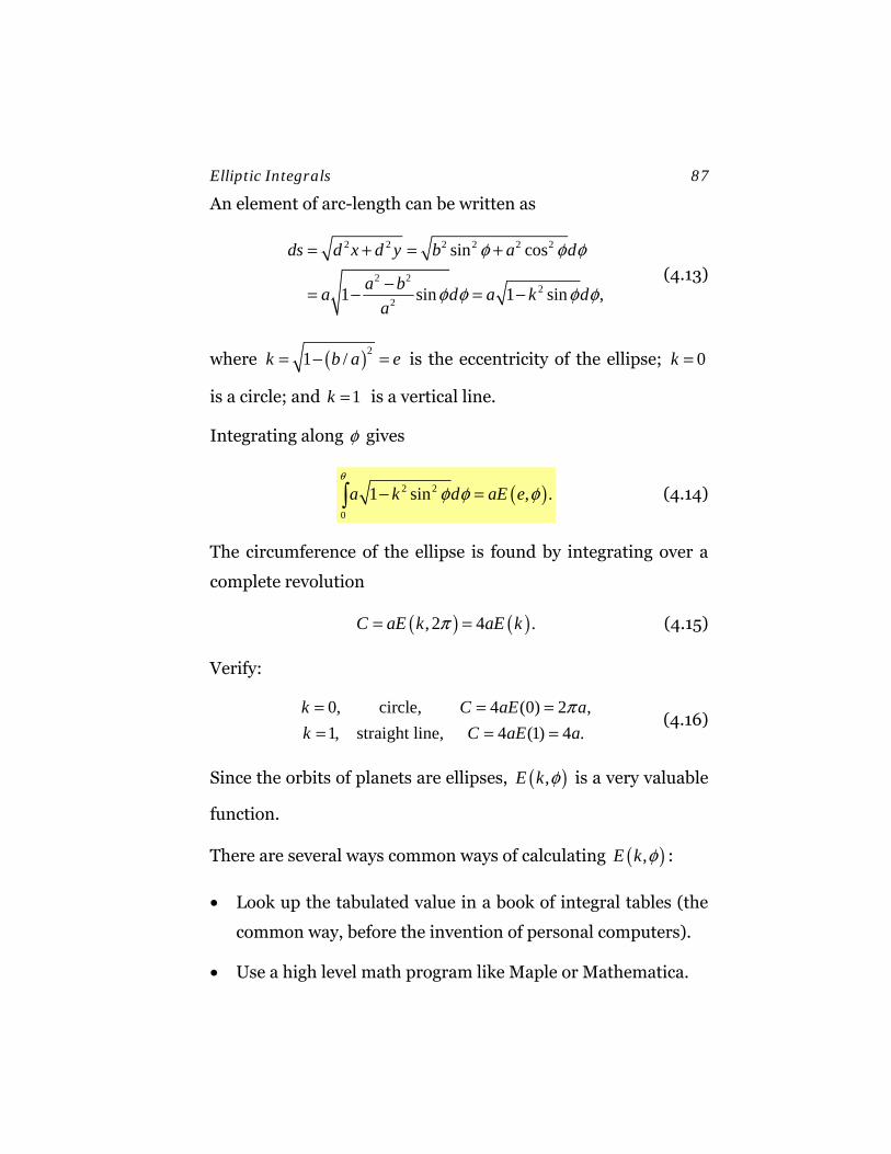
Elliptic Integrals 87
An element of arc-length can be written as
2 2 2 2 2 2
2 22
2
sin cos
1 sin 1 sin ,
ds d x d y b a d
a ba d a k da
φ φ φ
φ φ φ φ
= + = +
−= − = − (4.13)
where ( )21 /k b a e= − = is the eccentricity of the ellipse; 0k =
is a circle; and 1k = is a vertical line.
Integrating along φ gives
( )2 2
0
1 sin , .a k d aE eθ
φ φ φ− =∫ (4.14)
The circumference of the ellipse is found by integrating over a
complete revolution
( ) ( ), 2 4 .C aE k aE kπ= = (4.15)
Verify:
0, circle, 4 (0) 2 ,1, straight line, 4 (1) 4 .
k C aE ak C aE a
π= = == = =
(4.16)
Since the orbits of planets are ellipses, ( ),E k φ is a very valuable
function.
There are several ways common ways of calculating ( ),E k φ :
• Look up the tabulated value in a book of integral tables (the
common way, before the invention of personal computers).
• Use a high level math program like Maple or Mathematica.
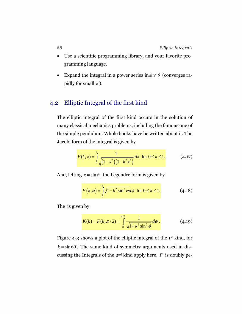
88 Elliptic Integrals
• Use a scientific programming library, and your favorite pro-
gramming language.
• Expand the integral in a power series in 2sin θ (converges ra-
pidly for small k ).
4.2 Elliptic Integral of the first kind
The elliptic integral of the first kind occurs in the solution of
many classical mechanics problems, including the famous one of
the simple pendulum. Whole books have be written about it. The
Jacobi form of the integral is given by
( )( )2 2 2
0
1( , ) for 0 1.1 1
x
F k x dx kx k x
= ≤ ≤− −
∫ (4.17)
And, letting sinx φ= , the Legendre form is given by
( ) 2 2
0
, 1 sin for 0 1.F k k d kθ
φ φ φ= − ≤ ≤∫ (4.18)
The is given by
/ 2
2 20
1( ) ( , / 2) .1 sin
K k F k dk
π
π φφ
= =−∫ (4.19)
Figure 4-3 shows a plot of the elliptic integral of the 1st kind, for
sin 60 .k = The same kind of symmetry arguments used in dis-
cussing the Integrals of the 2nd kind apply here, F is doubly pe-
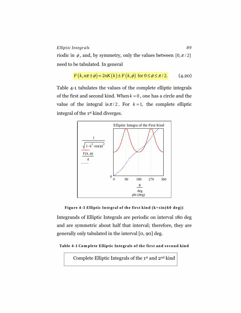
Elliptic Integrals 89
riodic in φ , and, by symmetry, only the values between [0, / 2]π
need to be tabulated. In general
( ) ( ) ( ), 2 , for 0 / 2.F k n nK k F kπ φ φ φ π± = ± ≤ ≤ (4.20)
Table 4-1 tabulates the values of the complete elliptic integrals
of the first and second kind. When 0k = , one has a circle and the
value of the integral is / 2π . For 1,k = the complete elliptic
integral of the 1st kind diverges.
0 90 180 270 3600
Ellipitic Integra of the First Kind
phi (deg)
1
1 k2 sin φ( )2⋅−
F k φ,( )
4
φ
deg
Figure 4-3 Elliptic Integral of the first kind (k=sin(60 deg))
Integrands of Elliptic Integrals are periodic on interval 180 deg
and are symmetric about half that interval; therefore, they are
generally only tabulated in the interval [0, 90] deg.
Table 4-1 Complete Elliptic Integrals of the first and second kind
Complete Elliptic Integrals of the 1st and 2nd kind
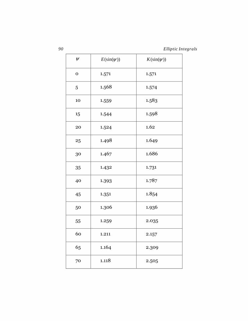
90 Elliptic Integrals
ψ (sin( ))E ψ (sin( ))K ψ
0 1.571 1.571
5 1.568 1.574
10 1.559 1.583
15 1.544 1.598
20 1.524 1.62
25 1.498 1.649
30 1.467 1.686
35 1.432 1.731
40 1.393 1.787
45 1.351 1.854
50 1.306 1.936
55 1.259 2.035
60 1.211 2.157
65 1.164 2.309
70 1.118 2.505
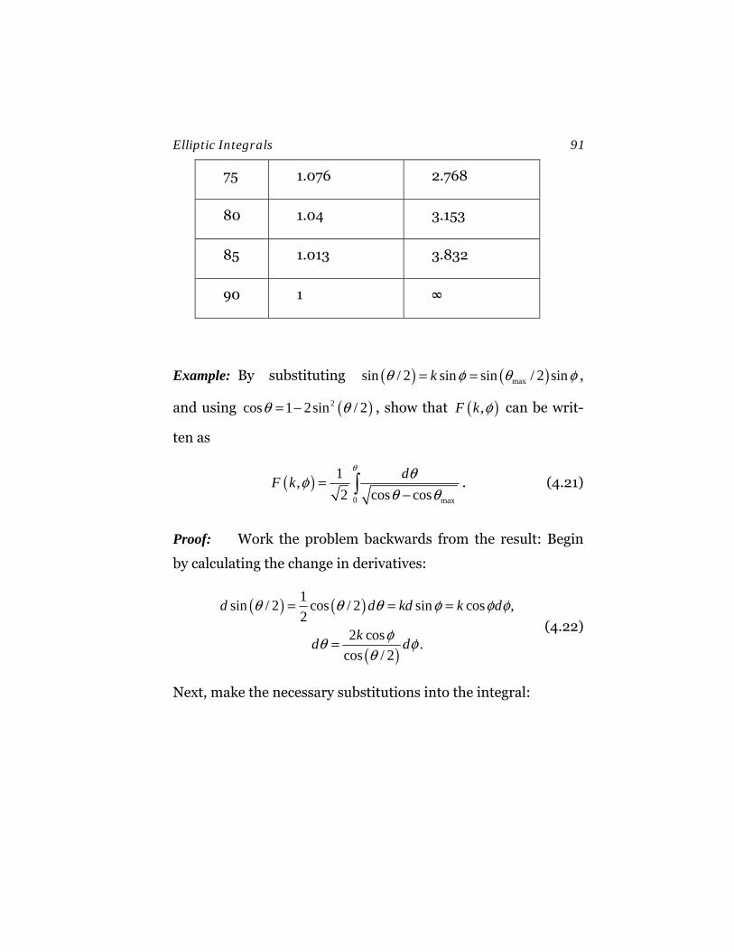
Elliptic Integrals 91
75 1.076 2.768
80 1.04 3.153
85 1.013 3.832
90 1 ∞
Example: By substituting ( ) ( )maxsin / 2 sin sin / 2 sinkθ φ θ φ= = ,
and using ( )2cos 1 2sin / 2θ θ= − , show that ( ),F k φ can be writ-
ten as
( )0 max
1,2 cos cos
dF kθ θφ
θ θ=
−∫ . (4.21)
Proof: Work the problem backwards from the result: Begin
by calculating the change in derivatives:
( ) ( )
( )
1sin / 2 cos / 2 sin cos ,2
2 cos .cos / 2
d d kd k d
kd d
θ θ θ φ φ φ
φθ φθ
= = =
= (4.22)
Next, make the necessary substitutions into the integral:
92 Elliptic Integrals
( )( ) ( )( )
( ) ( ) ( )
( )
( )
2 20 max
2 2 2 20 0max
2 2 20 0 0
2 2 20 0 0
1 ,2 1 2sin / 2 1 2sin / 2
1 1 ,2 2sin / 2 sin / 2 sin / 2
1 1 1 2 cos ,2 2 cos 2 cos cos / 2sin
.cos / 2 1 sin / 2 1 sin
dF
d dk
d d d kk kk k
d d dk
θ
θ θ
φθ θ
φ θ θ
θθ θ
θ θθ θ θ
θ θ φ φφ φ θφ
φ φ φθ θ ϕ
=− − −
= =− −
= = =−
= = =− −
∫
∫ ∫
∫ ∫ ∫
∫ ∫ ∫
(4.23)
4.3 Jacobi Elliptic functions
A rich literature has grown around the topic of the elliptic
integral of the 1st kind, with a specialized language and names
for functions. To see where this language comes from consider
the simpler circular integral which can be obtained by letting
0k = in the Jacobi form:
( )
( )2
0
10, arcsin ,1
sin .
x
u F x dx xx
sn u x
φ
φ
= = = =−
= =
∫ (4.24)
Now let’s generalize this terminology for 0k ≠ , in which case
u φ≠ . We call φ the amplitude of u
( )amp u φ= . (4.25)
and denote the inverse function 1F − by the special name so that
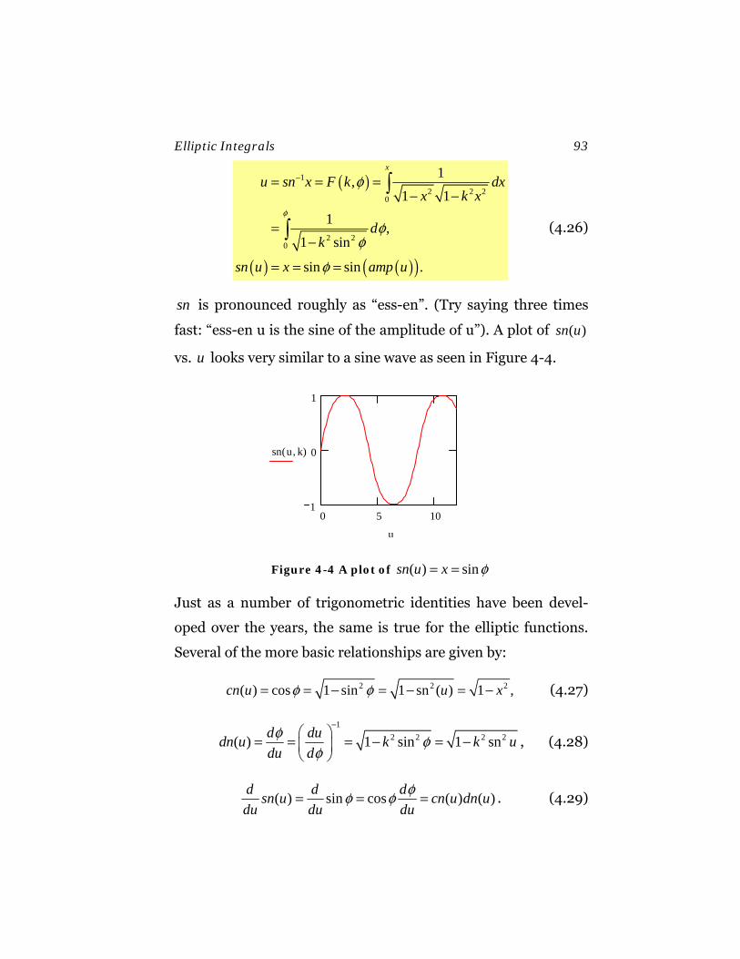
Elliptic Integrals 93
( )
( ) ( )( )
1
2 2 20
2 20
1,1 1
1 ,1 sin
sin sin .
x
u sn x F k dxx k x
dk
sn u x amp u
φ
φ
φφ
φ
−= = =− −
=−
= = =
∫
∫ (4.26)
sn is pronounced roughly as “ess-en”. (Try saying three times
fast: “ess-en u is the sine of the amplitude of u”). A plot of ( )sn u
vs. u looks very similar to a sine wave as seen in Figure 4-4.
0 5 101
0
1
sn u k,( )
u
Figure 4-4 A plot of ( ) sinsn u x φ= =
Just as a number of trigonometric identities have been devel-
oped over the years, the same is true for the elliptic functions.
Several of the more basic relationships are given by:
2 2 2( ) cos 1 sin 1 sn ( ) 1 ,cn u u xφ φ= = − = − = − (4.27)
1
2 2 2 2( ) 1 sin 1 snd dudn u k k udu dφ φ
φ
−⎛ ⎞= = = − = −⎜ ⎟⎝ ⎠
, (4.28)
( ) sin cos ( ) ( )d d dsn u cn u dn udu du du
φφ φ= = = . (4.29)

94 Elliptic Integrals
Example: The simple pendulum
Figure 4-5 Simple Pendulum
The simple pendulum (Figure 4-5) satisfies the conservation of
energy equation
( )2
maxcos cos 0,2
I mglθ θ θ+ − = (4.30)
where 2.I ml= Solving,
1
0 0max
1 / ,2 cos cos
d g ldtθ θ
θ θ=
−∫ ∫ (4.31)
Elliptic Integrals 95
( )
( )( )( )
00 max
max
0max
0
0
1 ( , ) ,2 cos cos
sin / 2 sin ,sin / 2,
sin / 2 ( ) , ,sin / 2
sin / 2 , ,
2arcsin , .
dt F k u
kk
x sn u sn t k
k sn t k
k sn t k
θ θω ϕθ θθ ϕ
θθ ω
θθ ω
θ ω
= = =−
==
= = =
=
=
∫
i
i
(4.32)
The depends on its amplitude and is given by
( )( ) ( )( )0 max maxsin / 2 ,2 4 sin / 2 .T F k Kω θ π θ= = = (4.33)
Let’s put in some numbers, choosing
20
max
max
1 kg,1 m,
/ 9.8 / s 3.13 rad/s,
60 ,
sin / 2 sin 30 1/ 2.
mL
g l
k
ωθ
θ
==
= = =
=
= = =
(4.34)
Then, the period of the pendulum is
( )
( )
( )
0
0
1/ 2,2 ,1 4 1/ 2 ,
1 4 1.686 2.15 s,3.13
T F k
T K
T
ω π
ω
= =
=
= =
(4.35)
Compare this to the small amplitude limit
00
2 2.01 s.smallOsc
T πω
= = (4.36)
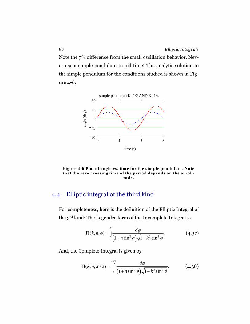
96 Elliptic Integrals
Note the 7% difference from the small oscillation behavior. Nev-
er use a simple pendulum to tell time! The analytic solution to
the simple pendulum for the conditions studied is shown in Fig-
ure 4-6.
0 1 2 390
45
0
45
90simple pendulum K=1/2 AND K=1/4
time (s)
angl
e (d
eg)
Figure 4-6 Plot of angle vs. time for the simple pendulum. Note that the zero crossing time of the period depends on the ampli-
tude.
4.4 Elliptic integral of the third kind
For completeness, here is the definition of the Elliptic Integral of
the 3rd kind: The Legendre form of the Incomplete Integral is
( )2 2 2
0
( , , ) .1 sin 1 sin
dk nn k
φ φφφ φ
Π =+ −∫ (4.37)
And, the Complete Integral is given by
( )
/ 2
2 2 20
( , , / 2) .1 sin 1 sin
dk nn k
π φπφ φ
Π =+ −∫ (4.38)

Elliptic Integrals 97

5. Fourier Series
Time is measured in cycles.
The earth rotates around the sun.
Atoms oscillate. Patterns repeat.
5.1 Plucking a string
What happens when one plucks a string on a stringed instru-
ment? The fundamental harmonic is given by the length of the
string, its mass density and its tension. Depending on where we
pluck the string, one can choose to emphasize different harmon-
ics. After this point, it starts to get complicated, as the shape and
nature of the sound board will further modify the sound. This
problem will be analyzed in some detail when we study the wave
equation. But in general, if one does a Fourier decomposition of
the wave form, only multiples of the fundamental frequency will
contribute. In the case of a plucked string, the boundary condi-
tions are due to the clamping of the string, which removes all
other frequencies. Is this effect real, or is it a mathematical con-
nivance? It is definitely real, one can hear it. The human ear is a
pretty good frequency analyzer. In this section we will explore
how to decompose a periodic function into its Fourier series
components. These components are a solution to an eigenvalue

100 Fourier Series
problem. The eigenfunctions represent the possible normal
modes of oscillation of a periodic function. In the case of the
plucked string, the motion is periodic in time. In other cases, we
might be dealing with a cyclic variable, say the rotation angle of
a planet as it makes its path around its sun. We begin with the
simplest of models: a one dimensional rotation angle. If one de-
fines a field on a circle, consistency requires that a rotation by
2π must give the same field.
5.2 The solution to a simple eigenvalue equation
In solutions to partial differential equations in cylindrical or
spherical coordinates, the technique of separation of variables
often leads to the following very simple equation for the azimul-
thal coordinate φ
( ) ( )
22
2
d fm f
dφ
φφ
= − (5.1)
where ( )f φ satisfies periodic boundary conditions
( ) ( )2f fφ π φ+ = (5.2)
The solutions of this equation are very well known —think “sim-
ple harmonic oscillator”— The exponential form of the solution
is
( ) , 0, 1, 2,imm mf c e mφφ = = ± ± (5.3)
Fourier Series 101
The requirement that ( )mf φ be periodic on interval 2π restricts
the eigenvalues to positive and negative integers. The case 0m =
is a special case in that 0m = ± represents the same eigenvalue.
Often it is convenient to solve the equation in terms of sine and
cosine functions. Using cos sinime m i mφ φ φ± = ± , we find the real
solutions to the eigenvalue equation to be
( )( ) ( )
0 m=02
cos sin m=1,2,3, m
m m
af
a m b mφ
φ φ
⎧⎪= ⎨⎪ +⎩ …
(5.4)
Here, the counting runs only over non-negative integers, since
sin( )mφ− and cos( )mφ− are not linearly independent from
sin( )mφ and cos( )mφ
Orthogonality
The eigenfunctions solutions of this equation are orthogonal to
each other when integrated over interval 2π . First, let us prove
this for the complex form of the series, normalizing the func-
tions by setting 1mc = :
( ) ( )
( )
*
2
0i m mim im i m m
m mi m m
m m
f f d e e d e d e m m
π π ππφφ φ φ
π π π φπ
π
φ φ φ′−′− ′−′
− − − ′−−
′=⎧⎪
= = = ⎨ ′= ≠⎪⎩
∫ ∫ ∫ (5.5)
The proof for sine and cosine series is slightly more complicated.
If m m′≠ , the sine and cosine functions can be re-expanded into
102 Fourier Series
terms involving ime φ± , and orthogonality follows from the above
equation:
( ) ( ) ( ) ( )
( ) ( )
sin sin sin cos
cos cos 0
m m d m m d
m m d m m
π π
π ππ
π
φ φ φ φ φ φ
φ φ φ
− −
−
′ ′=
′ ′= = ≠
∫ ∫
∫ (5.6)
For m m′= , one can use the fact that ( ) sin 2mφ is odd on interval
[ ],π π− to show
( ) ( ) ( )1 sin cos sin 2 02
m m d m dπ π
π π
φ φ φ φ φ− −
= =∫ ∫ (5.7)
Also, by symmetry, using the fact that sine and cosine functions
are the same up to a phase shift,
( ) ( )2 2
2 2
sin cos 1 2
2sin cos2
m m d d
m d m d
π π
π ππ π
π π
φ φ φ φ π
πφ φ φ φ π
− −
− −
+ = =
= = =
∫ ∫
∫ ∫ (5.8)
Finally, normalize the 0m = term to unity (1 cos(0)= ), giving
( ) ( )1sin 1cos 0
1 2
m d m d
d
π π
π ππ
π
φ φ φ φ
φ π
− −
−
′ ′= =
=
∫ ∫
∫ (5.9)
In quantum mechanics (QM), it is conventional to normalize the
square integrated eigenfunctions to unity. However, this is not
Fourier Series 103
often the case in classical physics. The special functions of ma-
thematical physics have a variety of sometimes bewildering
normalizations, all of which made sense to the people who first
studied them. The definition of Fourier series long predated
QM. The above normalization is standard in the literature.
5.3 Definition of Fourier series
A, , function ( )f x which is periodic over interval [ ],π π− , and
where the positive-definite integral ( ) 2f x dx
π
π−∫ is finite, can be
expanded in a series of sine and cosine functions having the
general form
( ) ( ) ( )0
1 1
cos sin2 n n
n n
af x a nx b nx∞ ∞
= =
= + +∑ ∑ (5.10)
The function has a finite number of maxima and minima
The function has a finite number of step-wise discrete disconti-
nuities
The coefficients of the series are given by
( )
( )
1 ( )cos for 0,1,2
1 ( )sin for 0,1,2
n
n
a f x nx dx m
b f x nx dx m
π
ππ
π
π
π
−
−
= =
= =
∫
∫
…
… (5.11)
104 Fourier Series
The infinite series converges to the function where it is conti-
nuous and to the midpoint of the discontinuity where it is step-
wise discontinuous.
Completeness of the series
In what sense can the function, which may be discontinuous af-
ter all, be said to be equal to a series consisting of only conti-
nuous functions? Note the limitation of the discontinuities to a
finite number of discrete points. These points have zero weight
when the function is integrated. The series and the function can
be said to be equivalent up to an interval of zero measure. That
is,
2lim ( ) ( ) 0NN
f x f x dxπ
π→∞
−
− =∫ (5.12)
where ( )Nf x is the partial sum of the infinite series.
Sine and cosine series
If a piece-wise continuous, periodic function f(x) is an even
function of x, it may be expanded in a Fourier Cosine series on
interval [ , ]π π− +
( ) ( )0
1
cos2c n
n
af x a nx∞
=
= +∑ (5.13)
Fourier Series 105
If a piece-wise continuous, periodic function f(x) is an odd func-
tion of x, it may be expanded in a Fourier Sine series on interval
[ , ]π π− +
( ) ( )1
sins nn
f x b nx∞
=
=∑ (5.14)
Complex form of Fourier series
A real-valued function can also be represented as a complex in-
finite series. Let ( ) / 2m m mc a b± = ∓ , then
( ) inxn
nf x c e
∞
=−∞
= ∑ (5.15)
With coefficients given by
1 ( )
2inx
nc e f x dxπ
ππ−
−
= ∫ (5.16)
Note for 0m ≠
2 2
2 2cos sin
imx imx imx imxm m m mm m
imx imx imx imx
m m
m m
a ib a ibc e c e e e
e e e ea bi
a mx b mx
− −−
− −
− +⎛ ⎞ ⎛ ⎞+ = +⎜ ⎟ ⎜ ⎟⎝ ⎠ ⎝ ⎠
⎛ ⎞ ⎛ ⎞+ −= +⎜ ⎟ ⎜ ⎟⎝ ⎠ ⎝ ⎠
= +
(5.17)
106 Fourier Series
5.4 Other intervals
Often the interval is of arbitrary length 2L rather than 2π .
Usually it is preferable to keep the interval symmetric over
[ ],L L− . This involves making a change of variable
( )/ /
/x x Ldx L dx
ππ
′ =′= (5.18)
Making these changes we find
( ) 0
1 1cos sin
2
1 ( )cos
1 ( )sin
n
n
n nn n
L
LL
L
a n x n xf x a bL L
n xa f x dxL L
n xb f x dxL L
π π
π
π
∞ ∞
= =
−
−
′ ′⎛ ⎞ ⎛ ⎞′ = + +⎜ ⎟ ⎜ ⎟⎝ ⎠ ⎝ ⎠′⎛ ⎞′ ′= ⎜ ⎟
⎝ ⎠
′⎛ ⎞′ ′= ⎜ ⎟⎝ ⎠
∑ ∑
∫
∫
(5.19)
5.5 Examples
The Full wave Rectifier
The full wave rectifier takes a sinusoidal wave at line frequency
and rectifies it using a bridge diode circuit. Figure 5-1 shows a
schematic of a full wave rectifier circuit. Positive and negative
parts of the line cycle take different paths through this diode
bridge circuit, but the current always flows through the resister
in a unidirectional manner, rectifying the signal. The result is
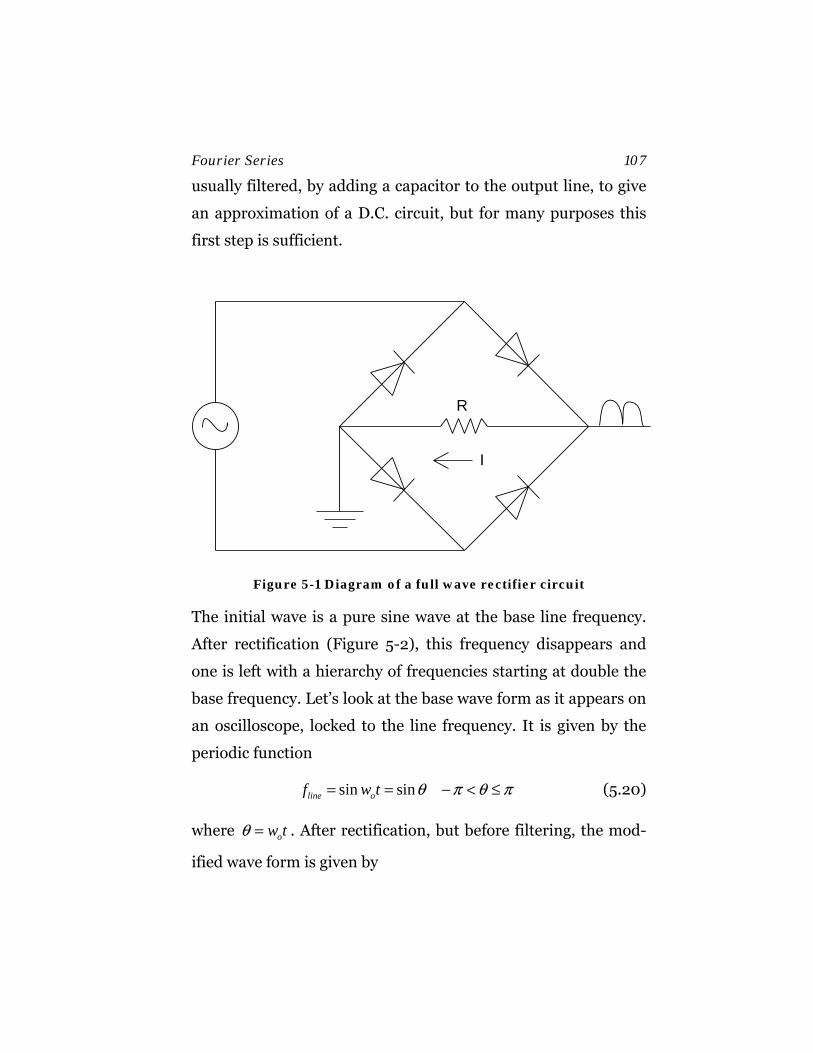
Fourier Series 107
usually filtered, by adding a capacitor to the output line, to give
an approximation of a D.C. circuit, but for many purposes this
first step is sufficient.
I
R
Figure 5-1 Diagram of a full wave rectifier circuit
The initial wave is a pure sine wave at the base line frequency.
After rectification (Figure 5-2), this frequency disappears and
one is left with a hierarchy of frequencies starting at double the
base frequency. Let’s look at the base wave form as it appears on
an oscilloscope, locked to the line frequency. It is given by the
periodic function
sin sinline of w t θ π θ π= = − < ≤ (5.20)
where ow tθ = . After rectification, but before filtering, the mod-
ified wave form is given by
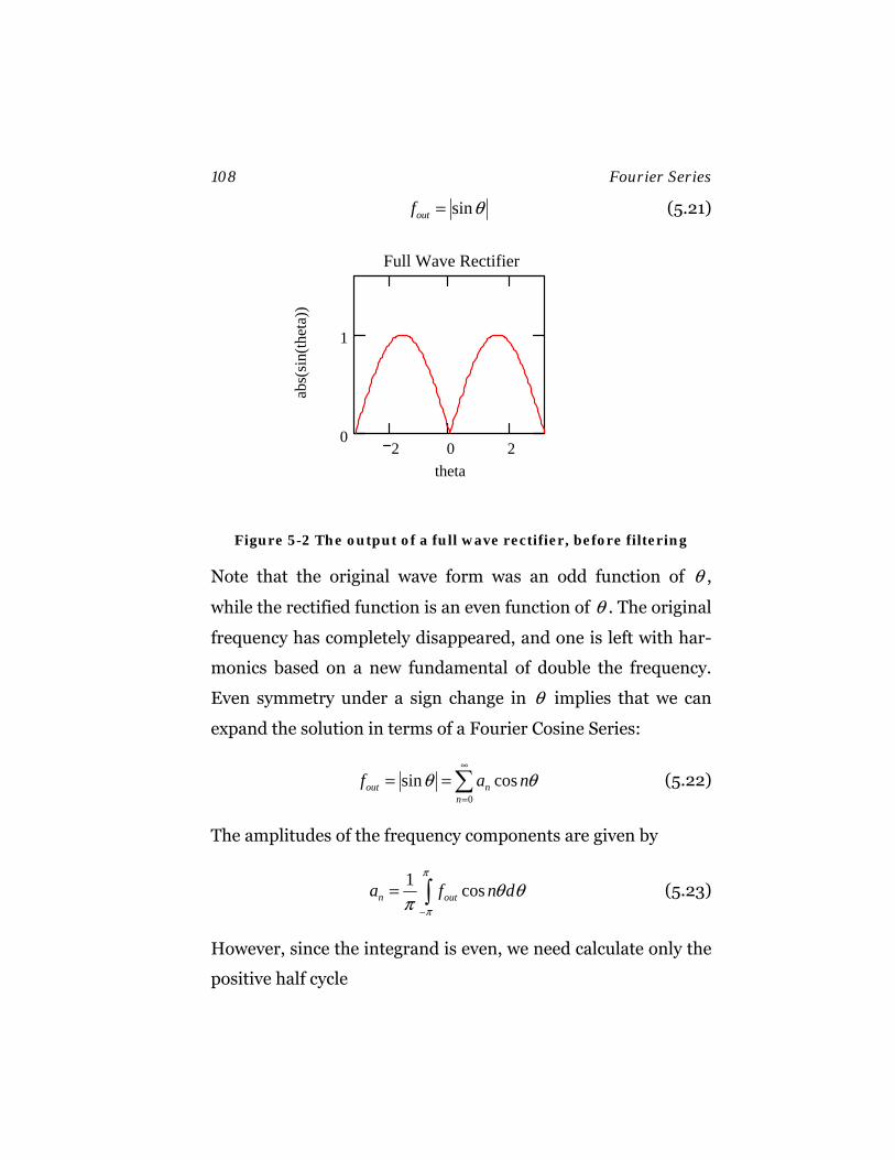
108 Fourier Series
sinoutf θ= (5.21)
2 0 20
1
Full Wave Rectifier
theta
abs(
sin(
thet
a))
Figure 5-2 The output of a full wave rectifier, before filtering
Note that the original wave form was an odd function of θ ,
while the rectified function is an even function of θ . The original
frequency has completely disappeared, and one is left with har-
monics based on a new fundamental of double the frequency.
Even symmetry under a sign change in θ implies that we can
expand the solution in terms of a Fourier Cosine Series:
0
sin cosout nn
f a nθ θ∞
=
= =∑ (5.22)
The amplitudes of the frequency components are given by
1 cosn outa f n d
π
π
θ θπ −
= ∫ (5.23)
However, since the integrand is even, we need calculate only the
positive half cycle

Fourier Series 109
0 0
2 2cos sin cosn outa f n d n dπ π
θ θ θ θ θπ π
= =∫ ∫ (5.24)
This integral can easily be solved by converting to exponential
notation
1
0
22 2
i i in in
ne e e ea d
i
θ θ θ θ
θπ
− −⎛ ⎞⎛ ⎞− += ⎜ ⎟⎜ ⎟⎝ ⎠⎝ ⎠∫ (5.25)
However, it is even easier to look up the answer in a book of
integral tables:
( ) ( )
0 0
cos (1 ) cos (1 )sin cos
2(1 ) 2(1 )n n
n dn n
ππ θ θθ θ θ
⎛ ⎞− += −⎜ ⎟− +⎝ ⎠
∫ (5.26)
The integral vanishes for odd n, and the result can be written as
2
1 even41
0 odd n
na n
nπ
⎧− ⎪= −⎨⎪⎩
(5.27)
The first term is positive and gives a DC offset
01 2 0.6372 2out out
af f dπ
π
θπ π−
= = = ≈∫ (5.28)
01( ) ( )2 2
L
L
af x f x dxL −
= =∫ (5.29)
The evaluated series can be written as
110 Fourier Series
( )
( )( )0
0 21
4cos 22sin( )2 1n
nw tw t
nπ π
∞
=
= −−
∑ (5.30)
And the allowed frequencies are
02w nw= (5.31)
Successively amplitudes fall off as ( )( )21/ 2 1n − , which means
that the energy stored in the frequency components falls off as
( )( )221/ 2 1n − .
Clearly, the series is convergent since by the integral test
2
4 / 1 04 1 ndnn n
ππ→∞⎯⎯⎯→ →
−∫ (5.32)
By adding a capacitor on the output side of the full wave rectifi-
er, one can short circuit the high frequency components to
ground. If the capacitor is large enough, the output of the circuit
is nearly D.C.
The Square wave
The square wave (shown in Figure 5-4) and its variants (i.e., the
step function, etc) are often found in digital circuits. The wave
form is given by
1 0
( )1 0
fθ π
θπ θ
+ < <⎧= ⎨− − < <⎩
(5.33)
Fourier Series 111
This function has stepwise singularities at { }0,θ π= ± . By the
Fourier Series Theorem the series will converge to the midpoint
of the discontinuity at those points. This function is an odd func-
tion of θ , so it can be expanded in a Fourier Sine series
( )1
sinSquareWave nn
f b nθ∞
=
=∑ (5.34)
Where
0 0
1 2 2sin sin sinn SW SWb f n d f n d n dπ π π
π
θ θ θ θ θ θπ π π−
= = =∫ ∫ ∫ (5.35)
The solution is
( )
0
42 cos( ) cos(0) n odd 2 cos0 n even
n
n
nb d n n
n n
π πθ π
π π
⎧− −− ⎪== = = ⎨⎪⎩
∫ (5.36)
The frequency decomposition of the square ware is shown in
Figure 5-3. The Fourier series expansion of this wave form is
given by
( ) ( )( )0
4 sin 2 12 1SW
nf n
nθ
π
∞
=
= ++∑ (5.37)
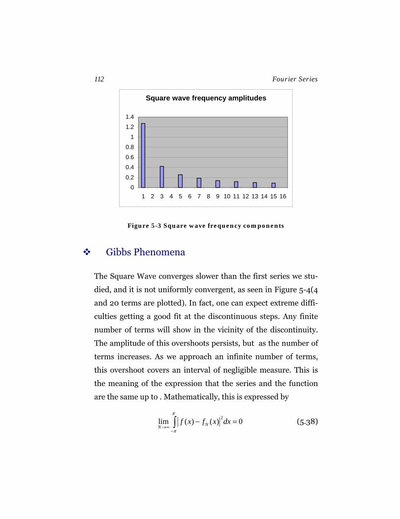
112 Fourier Series
Square wave frequency amplitudes
0
0.2
0.4
0.6
0.8
1
1.2
1.4
1 2 3 4 5 6 7 8 9 10 11 12 13 14 15 16
Figure 5-3 Square wave frequency components
Gibbs Phenomena
The Square Wave converges slower than the first series we stu-
died, and it is not uniformly convergent, as seen in Figure 5-4(4
and 20 terms are plotted). In fact, one can expect extreme diffi-
culties getting a good fit at the discontinuous steps. Any finite
number of terms will show in the vicinity of the discontinuity.
The amplitude of this overshoots persists, but as the number of
terms increases. As we approach an infinite number of terms,
this overshoot covers an interval of negligible measure. This is
the meaning of the expression that the series and the function
are the same up to . Mathematically, this is expressed by
2lim ( ) ( ) 0NN
f x f x dxπ
π→∞
−
− =∫ (5.38)
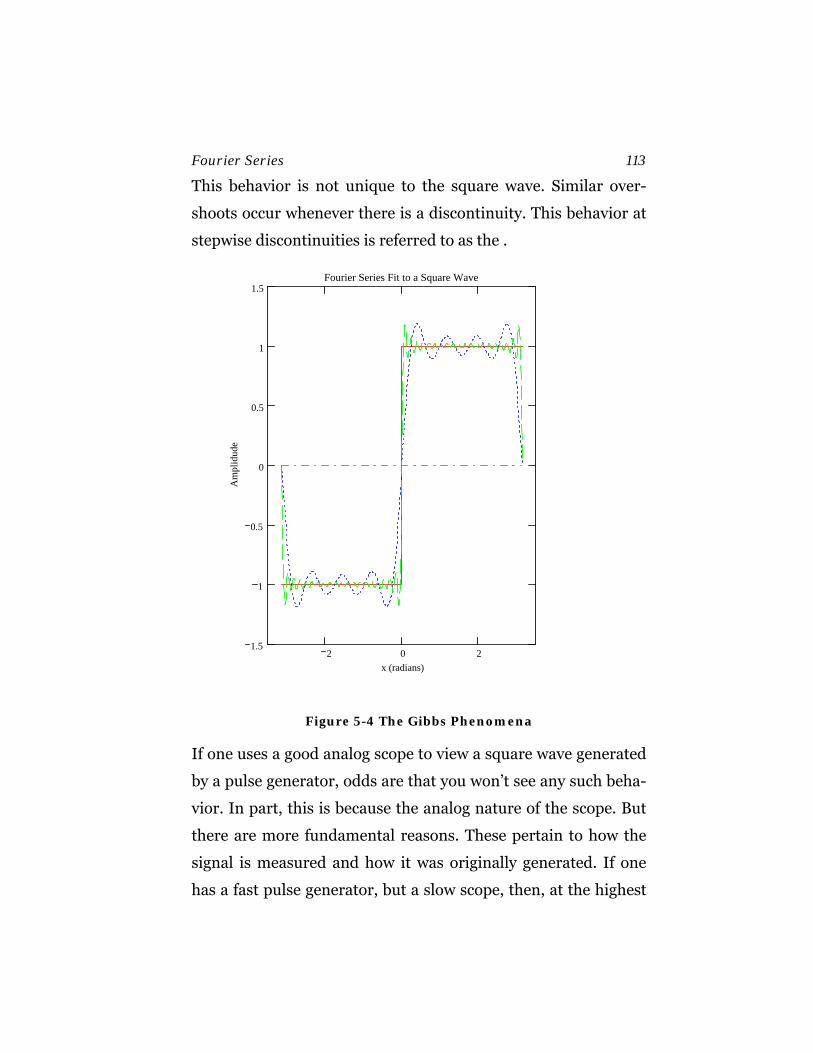
Fourier Series 113
This behavior is not unique to the square wave. Similar over-
shoots occur whenever there is a discontinuity. This behavior at
stepwise discontinuities is referred to as the .
2 0 21.5
1
0.5
0
0.5
1
1.5Fourier Series Fit to a Square Wave
x (radians)
Am
plid
ude
Figure 5-4 The Gibbs Phenomena
If one uses a good analog scope to view a square wave generated
by a pulse generator, odds are that you won’t see any such beha-
vior. In part, this is because the analog nature of the scope. But
there are more fundamental reasons. These pertain to how the
signal is measured and how it was originally generated. If one
has a fast pulse generator, but a slow scope, then, at the highest
114 Fourier Series
time resolutions, one sees a rise time in the signal due to the re-
sponse of the scope. If one has a fast scope, but a limited genera-
tor, one resolves the time structure of the source instead. Piece-
wise step functions are not physical. They are approximations
that allow us to ignore the messy details of exactly how a sudden
change happened. In time dependent problems, this is called the
impulse approximation.
For another example, consider a spherical capacitor, with one
conducting hemisphere at positive high voltage and the second
at negative high voltage. The step in voltage at the interface ig-
nores the necessary presence of a thin insulating barrier sepa-
rating the two regions. Such approximations are fine, as long as
one understands their limits of validity.
Find the Fourier series expansion to the step function given by
1 0
( )0 0
xf x
xπ
π< <⎧
= ⎨ − < <⎩ (5.39)
Hint: Note that it can be written as a sum of an even function
and an odd function.
Non-symmetric intervals and period doubling
Although the interval for fitting the period is often taken to be
symmetric, it need not be so. Consider the saw-tooth wave,
shown in Figure 5-5, initially defined on the interval[0, ]L .
( ) ; 0f x x x L= < < (5.40)

Fourier Series 115
Figure 5-5 A linear wave defined on interval[0,L]
One can double the period and fit it either as n even function
(Cosine Transform) or as and odd function (Sine Transform). If
we are interested only a fit within this region, there are several
ways of fitting this function. The most common technique is
called : The interval is doubled to the interval [ ],L L− and the
function is either symmetrized or anti-symmetrized on this
greater interval. The rate of convergence often depends on the
choice made.
• Symmetric option (Triangle wave)
The symmetrized function represents a triangle wave of the
form
116 Fourier Series
( ) for f x x L x L= − < < (5.41)
Fitting this with a Cosine Series, gives
0
1 2cos cosL L
nL
n x n xa x dx x dxL L L L
π π−
⎛ ⎞ ⎛ ⎞= =⎜ ⎟ ⎜ ⎟⎝ ⎠ ⎝ ⎠∫ ∫ (5.42)
Integrate by parts using ( )udv d uv vdu= −∫ ∫ ∫ or look up in
integral tables
2
cos sincos ax x axx axdxa a
= −∫ (5.43)
This gives the solution
2 20
(2 1)cos4( )
2 (2 1)n
n xL L Lf x x
n
π
π
∞
=
+⎛ ⎞⎜ ⎟⎝ ⎠= = −
+∑ (5.44)
Note that after the first term, which gives the average value of
the function, only terms odd in n contribute. Figure 5-6 shows
that after the addition of the first cosine term, the fit to a trian-
gle wave is already a fair approximation.
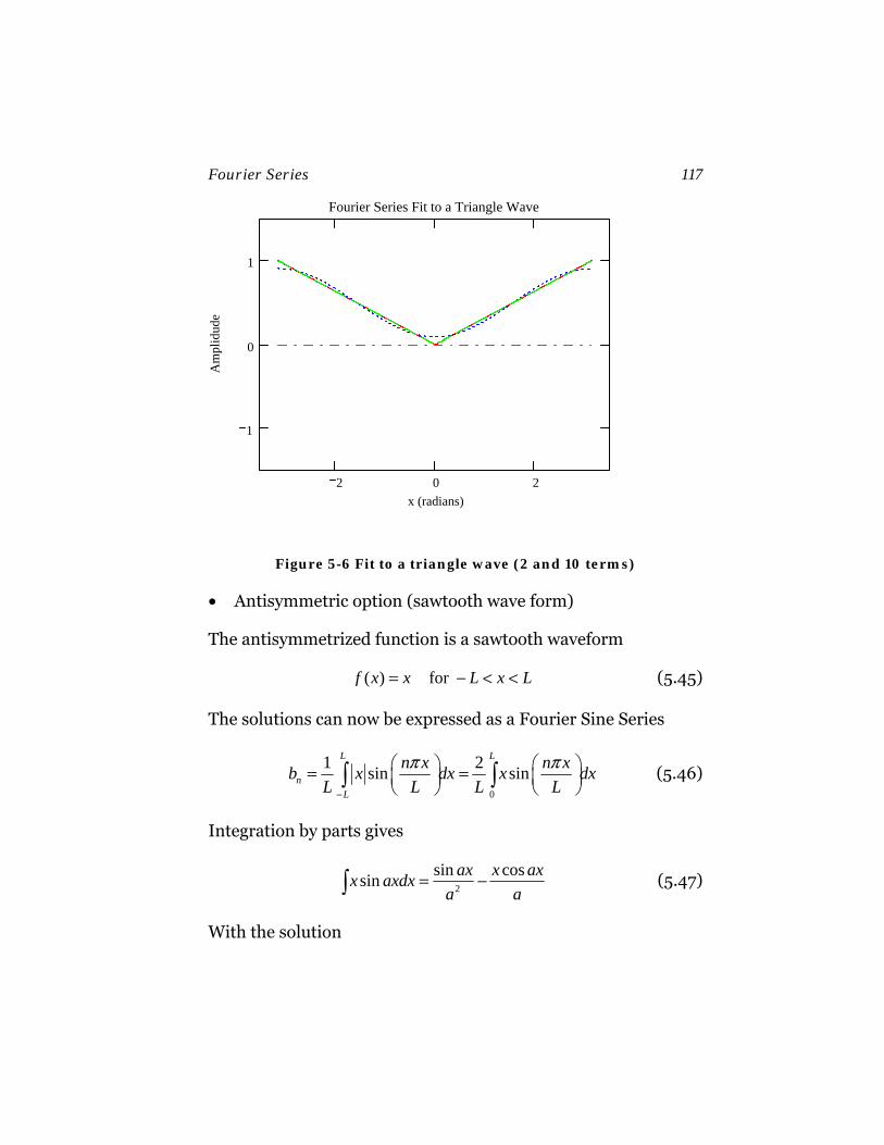
Fourier Series 117
2 0 2
1
0
1
Fourier Series Fit to a Triangle Wave
x (radians)
Am
plid
ude
Figure 5-6 Fit to a triangle wave (2 and 10 terms)
• Antisymmetric option (sawtooth wave form)
The antisymmetrized function is a sawtooth waveform
( ) for f x x L x L= − < < (5.45)
The solutions can now be expressed as a Fourier Sine Series
0
1 2sin sinL L
nL
n x n xb x dx x dxL L L L
π π−
⎛ ⎞ ⎛ ⎞= =⎜ ⎟ ⎜ ⎟⎝ ⎠ ⎝ ⎠∫ ∫ (5.46)
Integration by parts gives
2
sin cossin ax x axx axdxa a
= −∫ (5.47)
With the solution
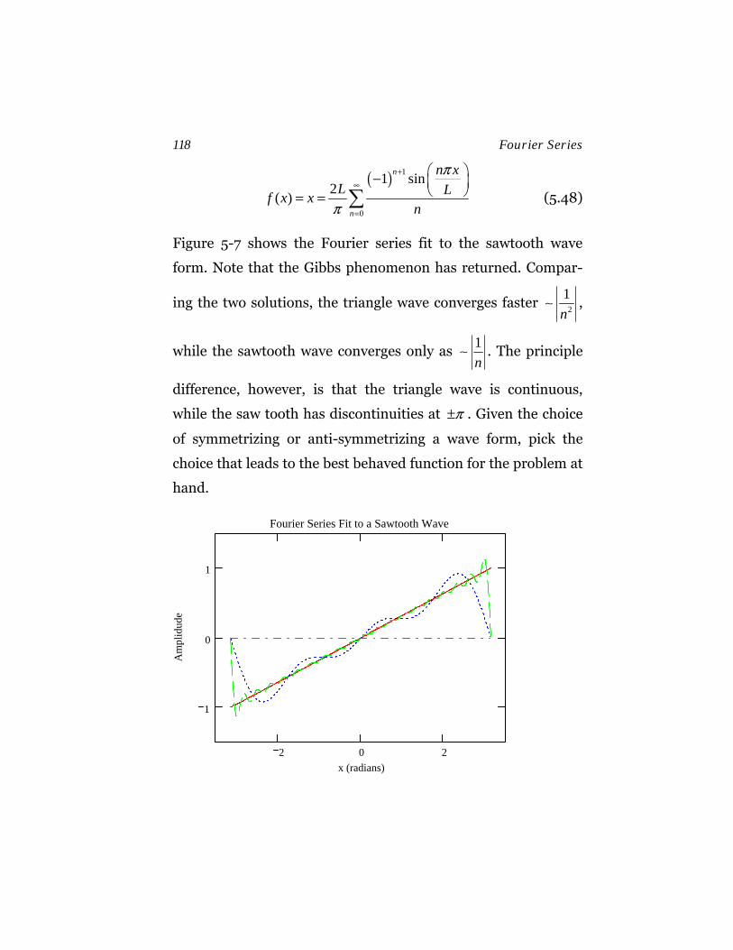
118 Fourier Series
( ) 1
0
1 sin2( )
n
n
n xL Lf x x
n
π
π
+∞
=
⎛ ⎞− ⎜ ⎟⎝ ⎠= = ∑ (5.48)
Figure 5-7 shows the Fourier series fit to the sawtooth wave
form. Note that the Gibbs phenomenon has returned. Compar-
ing the two solutions, the triangle wave converges faster 2
1n
∼ ,
while the sawtooth wave converges only as 1n
∼ . The principle
difference, however, is that the triangle wave is continuous,
while the saw tooth has discontinuities at π± . Given the choice
of symmetrizing or anti-symmetrizing a wave form, pick the
choice that leads to the best behaved function for the problem at
hand.
2 0 2
1
0
1
Fourier Series Fit to a Sawtooth Wave
x (radians)
Am
plid
ude
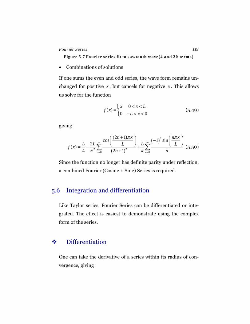
Fourier Series 119
Figure 5-7 Fourier series fit to sawtooth wave(4 and 20 terms)
• Combinations of solutions
If one sums the even and odd series, the wave form remains un-
changed for positive x , but cancels for negative x . This allows
us solve for the function
0
( )0 0x x L
f xL x< <⎧
= ⎨ − < <⎩ (5.49)
giving
( )
2 20 0
(2 1)cos 1 sin2( )
4 (2 1)
n
n n
n x n xL L LL Lf x
n n
π π
π π
∞ ∞
= =
+⎛ ⎞ ⎛ ⎞−⎜ ⎟ ⎜ ⎟⎝ ⎠ ⎝ ⎠= − +
+∑ ∑ (5.50)
Since the function no longer has definite parity under reflection,
a combined Fourier (Cosine + Sine) Series is required.
5.6 Integration and differentiation
Like Taylor series, Fourier Series can be differentiated or inte-
grated. The effect is easiest to demonstrate using the complex
form of the series.
Differentiation
One can take the derivative of a series within its radius of con-
vergence, giving
120 Fourier Series
( ) ( ) ( )inx inxn n
n n
d df x f x c e in c edx dx
∞ ∞
=−∞ =−∞
′ = = =∑ ∑ (5.51)
Because of the added factor of n in the numerator, ( )f x′ con-
verges slower than ( )f x .
Integration
One can integrate a series within its radius of convergence, giv-
ing
( )inx
inx nn
n n
c ef x dx c e dx constin
∞ ∞
=−∞ =−∞
= = +∑ ∑∫ ∫ (5.52)
Because of the added factor of n in the denominator ( )f x′ con-
verges faster than ( )f x .
The constant of integration can be tricky. it depends on where
the lower limit of integration is placed, as that affects the aver-
age value of the function. Often the integral is taken from the
origin 0x = , and the upper limit is either positive or negative x .
Fourier Series 121
Example: Evaluate the integral of the square wave
( ) ( ) ( )( )
( ) ( )( )
( )( )( )
( )( )( )
0
10 0
2 01
21
1 0 4 sin 2 11 0 2 1
4( ) sin 2 12 1
4 cos 2 12 1
4cos 2 1
2 1
SWn
x
n
n
n
xf n
x n
f d n dn
nn
nC
n
θ
θ
θ θπ
θ θ θ θ θπ
θπ
θ
π
∞
=
∞
=
∞
=
∞
=
+ >⎧ ⎫= = +⎨ ⎬− < +⎩ ⎭
= = ++
−= ++
− += +
+
∑
∑∫ ∫
∑
∑
(5.53)
But this integral must be the triangle wave previously defined
over the interval [ , ]π π− ,therefore the answer should be
( )
20
cos (2 1)4( )2 (2 1)sawtooth
n
nf x x
nθπ
π
∞
=
+= = −
+∑ (5.54)
Therefore, the constant of integration is
2
C π= (5.55)
If we didn’t know the answer ahead of time, one can fix the con-
stant by evaluation at a carefully chosen value of θ
( )( )
( )
21
21
40 02 1
422 1
n
n
f Cn
Cn
ππ
π
∞
=
∞
=
−= = ++
= =+
∑
∑ (5.56)
122 Fourier Series
Reversing the procedure, we see that the method allows us to
calculate the sum of a difficult looking series of constants in
closed form. This is a common use of Fourier Series.
Example: Find the value of the Zeta function ( )mς for m=2
The Zeta function is defined as the series of constants
( )1
1m
nm
nς
∞
=
=∑ (5.57)
Therefore
( )2
21
1 1 12 14 9 6n n
πς∞
=
= = + + + =∑ (5.58)
To prove this identity, the trick will be to find some Fourier se-
ries that gives this as a constant series for some value of its pa-
rameter. Let’s try
2( )f x x xπ π= − < < (5.59)
This the even series given by
( ) ( )
( ) ( )
( )
2 2
0
3 22
00 0
2
2 3
2
1 2
2 2 23 3
2 2 2cos sin
4 1
n
n
o
n
a x cos nx dx x cos nx dx
xa x dx
x xa nx nxn n n
n
π π
πππ
π
π π
ππ π
π
−
= =
= = =
⎛ ⎞⎛ ⎞= + −⎜ ⎟⎜ ⎟⎜ ⎟⎝ ⎠⎝ ⎠
= −
∫ ∫
∫ (5.60)
Fourier Series 123
or
( )2
2
1
2( ) 4 1 cos6
n
nf x x nxπ ∞
=
= = + −∑ (5.61)
Letting x π= , and using ( )cos 1 nnπ = − , we get
( ) ( )
( )
2 22
21
2 2
14 4 23 3
223 4 6
nf
nπ ππ π ς
π πς
∞
=
= = + = +
= =⋅
∑ (5.62)
5.7 Parseval’s Theorem
We have already defined the mean (expectation) value of a
Fourier series as
( ) 012 2
af f x dx xπ
π
π ππ −
= = − < <∫ (5.63)
Let’s now calculate the expectation value of 2f .using the com-
plex series notation
21 12 2
12
12
1 2 02
L
L
in imn m
n m
in imn m
n m
nm n m n nn m n
f f f dx f fdxL
c e c e dx
c e c e dx
c c c c
π
ππ
θ θ
π
πθ θ
π
π
π
π
πδπ
∗ ∗
− −
∞ ∞∗ −
=−∞ =−∞−
∞ ∞∗ −
=−∞ =−∞ −
∞ ∞ ∞∗ ∗
=−∞ =−∞ =−∞
= =
=
⎛ ⎞= ⎜ ⎟
⎝ ⎠
= = ≥
∫ ∫
∑ ∑∫
∑ ∑ ∫
∑ ∑ ∑
(5.64)
124 Fourier Series
This is Parseval’s Theorem. For classical waves, the wave’s ener-
gy density is proportional to the square of the amplitude of
wave. Therefore, Parseval’s Theorem can be interpreted as
meaning that the energy per cycle of a particular frequency is
proportional to the square of its amplitude integrated over a pe-
riod. In Quantum mechanics, the norm of a wave function is
usually normalized to unit probability. For this case, the theo-
rem is equivalent to saying that the partial probability of finding
a particle in a frequency eigenstate n is given by the square of its
amplitude.
Definition: Parseval’s Theorem
The expectation value of the square of the absolute value of a
function when averaged over its interval of periodicity is given
by
2 2* 1 1
2 2
L L
nnL L
f f f dx f fdx cL L
∞∗
=−∞− −
= = = ∑∫ ∫ (5.65)
If the function is real-valued, then the sum can be written as
( )2
2 2 20
12 n nn
af a b∞
=
= + +∑ (5.66)
2 0f ≥ so * 0f f > unless the function vanishes everywhere,
except possibly on an interval of null measure. This definition is
used to define the norm of a square-integrable function space.
The norm of a function is just the sum of the norms of its com-
ponent eigenfunctions.
Fourier Series 125
Generalized Parseval’s Theorem
Parseval’s theorem can be generalized by defining the as
1 12 2
in imn m
n m
n nn
f g f gdx f e g e dx
f g
π πθ θ
π ππ π
∞ ∞∗ ∗ ∗ −
=−∞ =−∞− −
∞∗
=−∞
= =
=
∑ ∑∫ ∫
∑ (5.67)
5.8 Solutions to infinite series
We have already seen one way to find the sum of a series and
have shown that ( )2
26πς = . Here is a second way, using Parsev-
al’s Identity. Note that
3 2
2 2 2
0 0
1 2 2 23 3xx x x x dx x dx
ππ π
π
ππ π π
∗
−
= = = = =∫ ∫ (5.68)
However x is just the functional form of a sawtooth wave, and
we have already solve that series. Letting the interval L π= , then
the Fourier Sine series normalizes to
( ) ( )0
1 2( ) sin ,
n
n nn
f x x b nx bn
∞
=
−= = =∑ (5.69)
Then, by Parseval’s Identity

126 Fourier Series
( )
( )
22 2
12
2 4 23
26
nn
x bπ ς
πς
∞
=
= = =
∴ =
∑ (5.70)
6. Orthogonal function spaces
The normal modes of the continuum
define an infinite Hilbert space.
6.1 Separation of variables
The solution of complicated mathematical problems is facili-
tated by breaking the problem down into simpler components.
By reducing the individual pieces into a standard form having a
known solution, the solution of the more complex problem can
be reconstructed. For example, partial differential equations are
often solvable by the technique of separation of variables. The
resulting are that can be solved by the general techniques that
we will explore in the following sections. The general solution to
the original partial differential equation of interest can then be
constructed from a summation over all product solutions to the
eigenvalue equations that meet certain specified boundary re-
quirements imposed by physical considerations.
6.2 Laplace’s equation in polar coordinates
An illuminating example is the solution to in two space dimen-
sions. The equation takes the form
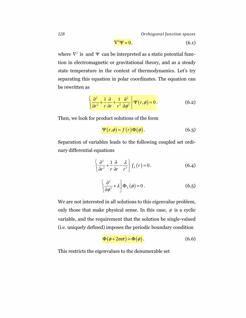
128 Orthogonal function spaces
2 0∇ Ψ = . (6.1)
where 2∇ is and Ψ can be interpreted as a static potential func-
tion in electromagnetic or gravitational theory, and as a steady
state temperature in the context of thermodynamics. Let’s try
separating this equation in polar coordinates. The equation can
be rewritten as
( )2 2
2 2 2
1 1 , 0rr r r r
φφ
⎧ ⎫∂ ∂ ∂+ + Ψ =⎨ ⎬∂ ∂ ∂⎩ ⎭. (6.2)
Then, we look for product solutions of the form
( ) ( ) ( ),r f rφ φΨ = Φ . (6.3)
Separation of variables leads to the following coupled set ordi-
nary differential equations
( )2
2 2
1 0f rr r r r λ
λ⎧ ⎫∂ ∂+ − =⎨ ⎬∂ ∂⎩ ⎭. (6.4)
( )2
2 0λλ φφ
⎧ ⎫∂ + Φ =⎨ ⎬∂⎩ ⎭. (6.5)
We are not interested in all solutions to this eigenvalue problem,
only those that make physical sense. In this case, φ is a cyclic
variable, and the requirement that the solution be single-valued
(i.e. uniquely defined) imposes the periodic boundary condition
( ) ( )2mφ π φΦ + = Φ . (6.6)
This restricts the eigenvalues to the denumerable set
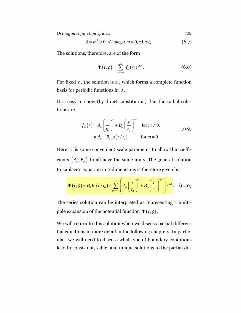
Orthogonal function spaces 129
2 0; integer 0, 1, 2,...m mλ = ≥ ∀ = ± ± . (6.7)
The solutions, therefore, are of the form
( ), ( ) imm
mr f r e φφ
∞
=−∞
Ψ = ∑ . (6.8)
For fixed r , the solution is a , which forms a complete function
basis for periodic functions in φ .
It is easy to show (by direct substitution) that the radial solu-
tions are
( )
( )0 0
0 0 0
for 0,
ln / for 0.
m m
m m mr rf r A B mr r
A B r r m
−⎛ ⎞ ⎛ ⎞
= + ≠⎜ ⎟ ⎜ ⎟⎝ ⎠ ⎝ ⎠
= + =
(6.9)
Here 0r is some convenient scale parameter to allow the coeffi-
cients { },m mA B to all have the same units. The general solution
to Laplace’s equation in 2-dimensions is therefore given by
( ) ( )0 00 0
, ln /m m
imm m
m
r rr B r r A B er r
φφ−∞
=−∞
⎛ ⎞⎛ ⎞ ⎛ ⎞⎜ ⎟Ψ = + +⎜ ⎟ ⎜ ⎟⎜ ⎟⎝ ⎠ ⎝ ⎠⎝ ⎠
∑ . (6.10)
The series solution can be interpreted as representing a multi-
pole expansion of the potential function ( ),r φΨ .
We will return to this solution when we discuss partial differen-
tial equations in more detail in the following chapters. In partic-
ular, we will need to discuss what type of boundary conditions
lead to consistent, sable, and unique solutions to the partial dif-

130 Orthogonal function spaces
ferential equation of interest. The product solutions, neverthe-
less, illustrates some general features of the separation of varia-
ble technique that are worth pointing out at this point:
• Separation of variables in partial differential equations natu-
rally leads to ordinary differential equations that are solu-
tions to an .
• The allowed eigenvalues are constrained by the imposed on
the equations.
• The function basis generated by the eigenvalue equations
forms a for the class of functions that satisfy the same boun-
dary conditions.
• The complete solution to the partial differential equation is a
to the eigenvalue equations where the coefficients are chosen
to match the physical .
6.3 Helmholtz’s equation
Let us next consider a class of second order partial differential
equations, which contains some of the most famous named sca-
lar equations in physics. These include
• Laplace’s equation
( )2 0.∇ Ψ =r (6.11)
• The wave equation
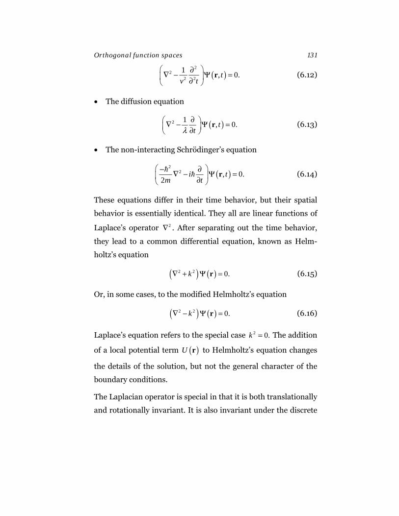
Orthogonal function spaces 131
( )2
22 2
1 , 0.tv t
⎛ ⎞∂∇ − Ψ =⎜ ⎟∂⎝ ⎠r (6.12)
• The diffusion equation
( )2 1 , 0.ttλ∂⎛ ⎞∇ − Ψ =⎜ ⎟∂⎝ ⎠
r (6.13)
• The non-interacting Schrödinger’s equation
( )2
2 , 0.2
i tm t
⎛ ⎞− ∂∇ − Ψ =⎜ ⎟∂⎝ ⎠r (6.14)
These equations differ in their time behavior, but their spatial
behavior is essentially identical. They all are linear functions of
Laplace’s operator 2∇ . After separating out the time behavior,
they lead to a common differential equation, known as Helm-
holtz’s equation
( ) ( )2 2 0.k∇ + Ψ =r (6.15)
Or, in some cases, to the modified Helmholtz’s equation
( ) ( )2 2 0.k∇ − Ψ =r (6.16)
Laplace’s equation refers to the special case 2 0.k = The addition
of a local potential term ( )U r to Helmholtz’s equation changes
the details of the solution, but not the general character of the
boundary conditions.
The Laplacian operator is special in that it is both translationally
and rotationally invariant. It is also invariant under the discrete
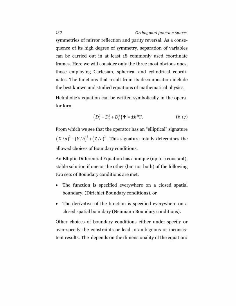
132 Orthogonal function spaces
symmetries of mirror reflection and parity reversal. As a conse-
quence of its high degree of symmetry, separation of variables
can be carried out in at least 18 commonly used coordinate
frames. Here we will consider only the three most obvious ones,
those employing Cartesian, spherical and cylindrical coordi-
nates. The functions that result from its decomposition include
the best known and studied equations of mathematical physics.
Helmholtz’s equation can be written symbolically in the opera-
tor form
( )2 2 2 2 .x y zD D D k+ + Ψ = ± Ψ (6.17)
From which we see that the operator has an “elliptical” signature
( ) ( ) ( )2 2 2/ / /X a Y b Z c+ + . This signature totally determines the
allowed choices of Boundary conditions.
An Elliptic Differential Equation has a unique (up to a constant),
stable solution if one or the other (but not both) of the following
two sets of Boundary conditions are met.
• The function is specified everywhere on a closed spatial
boundary. (Dirichlet Boundary conditions), or
• The derivative of the function is specified everywhere on a
closed spatial boundary (Neumann Boundary conditions).
Other choices of boundary conditions either under-specify or
over-specify the constraints or lead to ambiguous or inconsis-
tent results. The depends on the dimensionality of the equation:
Orthogonal function spaces 133
• In three-dimensions, the boundary is a closed surface;
• In two dimensions, it is an enclosing line;
• In one dimension, it is given by the two end points of the
line.
If the volume to be enclosed is infinite, the enclosing surface is
taken as the limit as the radius R →∞ of a very large boundary
envelope.
6.4 Sturm-Liouville theory
After separation of variables in the Helmholtz Equation, one is
left with a set of second order ordinary differential equations
having the following linear form:
( ){ } ( ) ( ) ( ) ( )
( ) ( )
2
2
.
d dL y x A x B x C x y xdx dx
W x y xλ
⎛ ⎞= + +⎜ ⎟⎝ ⎠
= (6.18)
L L∗= denotes a real-valued, linear second order differential op-
erator, , ,A B C are real-valued functions of the dependent varia-
ble x , λ is an eigenvalue, ( )W x is a weight function, and ( )y xλ
is the eigenfunction solution to the eigenvalue equation.
This equation is assumed to be valid on a closed inter-
val [ , ]x a b⊂ . The eigenvalue solutions of the above equation are
real if the linear operator can be written in the
134 Orthogonal function spaces
( ){ } ( ) ( ) ( ) ( ) ( )d dL y x A x C x y x W x y xdx dx
λ⎛ ⎞⎛ ⎞= + =⎜ ⎟⎜ ⎟⎝ ⎠⎝ ⎠
. (6.19)
This requires the constraint
( ) ( )B x A x′= . (6.20)
An equation that can be put in such a form is said to be a Sturm-
Liouville differential equation. If the equation is not in a self-
adjoint form, an integrating factor can often be found to put it
into such a form. In the standard notation for Sturm-Liouville
equations the functions A and C are referred to as the func-
tions P and Q respectively, so that the equation is often written
in the standard form
( ){ } ( ) ( ) ( ) ( ) ( )d dL y x P x Q x y x W x y xdx dx
λ⎛ ⎞⎛ ⎞= + =⎜ ⎟⎜ ⎟⎝ ⎠⎝ ⎠
. (6.21)
The ( )W x usually arises from the Jacobean of the transforma-
tion encountered in mapping from Cartesian coordinates to
some other coordinate system. This weight is required to be pos-
itive semi-definite. That is, it is except at a finite number of dis-
crete points on the interval [ , ]x a b⊂ where it may vanish. It de-
fines a norm for a function space such that
( ) 0b
a
N W x y ydx∗= ≥∫ . (6.22)
The class of functions that have a finite norm N are said to be
Orthogonal function spaces 135
Linear self-adjoint differential operators
A linear differential operator is said to be self-adjoint on interval
[ ],a b if it satisfies the following criteria
{ } { }*2 1 1 2
b b
a a
y L y dx y L y dx∗ =∫ ∫ (6.23)
with respect to any normalizable functions iy that meet certain
specified boundary conditions at the end points of the interval.
Sturm-Liouville differential operators are self-adjoint for Dirich-
let, Neumann, and periodic boundary conditions (B.C.). First
note that the term ( )Q x ( )mς where Q is a real-valued function
is automatically self-adjoint
2 1 1 2( ) ( ) ,b b
a a
y Q x y dx y Q x y dx∗ ∗=∫ ∫ (6.24)
since functions commute.
Next, integration by parts gives
2 1
2 12 1
( )
( ) ( ) .
b
ab b
a a
d dy P x y dxdx dx
dy dydy P x y P x dxdx dx dx
∗
∗∗
⎛ ⎞⎛ ⎞⎜ ⎟⎜ ⎟⎝ ⎠⎝ ⎠
⎛ ⎞= − ⎜ ⎟⎝ ⎠
∫
∫ (6.25)
Likewise,
136 Orthogonal function spaces
1 2
2 11 2
( )
( ) ( ) .
b
ab b
a a
d dy P x y dxdx dx
dy dydy P x y P x dxdx dx dx
∗
∗∗
⎛ ⎞⎛ ⎞⎜ ⎟⎜ ⎟⎝ ⎠⎝ ⎠
⎛ ⎞= − ⎜ ⎟⎝ ⎠
∫
∫ (6.26)
Subtracting (6.26) from (6.25) gives
{ } { }* 1 22 1 1 2 2 1 .
bbb b
aa a a
dy dyy L y dx y L y dx y P y Pdx dx
∗∗ ∗− = −∫ ∫ (6.27)
This clearly vanishes if the functions or their derivatives vanish
at the limits [ ],a b (i.e., for Dirichlet or Neumann B.C.). It also
vanishes if the upper and lower limits have the same value (i.e.,
for periodic B.C.) and also that
( ) ( ) 0.P a P b= = (6.28)
This latter case occurs for certain types of spherical functions,
such as the Legendre polynomials. An important theorem is that
the eigenvalues of a self-adjoint differential operator are real.
The proof follows from the use of the conjugate of a Sturm-
Liouville equation
( ){ } ( ) ( ) ( ) ( ) ( ).d dL y x P x Q x y x W x y xdx dx
λ∗ ∗ ∗ ∗⎛ ⎞⎛ ⎞= + =⎜ ⎟⎜ ⎟⎝ ⎠⎝ ⎠
(6.29)
(Note that the operator L and the weight function W are real).
Therefore,
{ } { } ( )*2 1 1 2 1 2 2 1 0.
b b b
a a a
y L y dx y L y dx Wy y dxλ λ∗ ∗ ∗− = − =∫ ∫ ∫ (6.30)

Orthogonal function spaces 137
Letting 1 2y y= gives
( )1 1 1 1 0,b
a
Wy y dxλ λ∗ ∗− =∫ (6.31)
but the norm 1 1 0b
a
Wy y dx∗∫ unless 1 0y ≡ ; therefore,
1 1 .λ λ∗= (6.32)
Orthogonality
The eigenfunctions of different non-degenerate eigenvalues are
orthogonal to each other with respect to weight W . The proof
follows, from (6.30)
( )1 2 2 1 0.b
a
Wy y dxλ λ ∗− =∫ (6.33)
If 1 2 ,λ λ≠ this implies that
2 1 0.b
a
Wy y dx∗ =∫ (6.34)
Given a set of linearly independent, but degenerate, eigenfunc-
tions nψ with the same eigenvalue, one can always construct a
“diagonal” basis of eigenfunctions nφ that are orthogonal to each
other with respect to weight .W One procedure, attributed to
Schmidt, is to construct the basis { }nφ from the sequence
138 Orthogonal function spaces
1 1
2 2 21 1
3 3 31 1 32 2
1
1
,,
,
.n
n n nm mm
cc c
c
φ ψφ ψ φφ ψ φ φ
φ ψ φ−
=
== −= − −
= −∑
(6.35)
The coefficients of the thn term is chosen such that nφ is ortho-
gonal to all previously orthogonalized eigenfunctions.
0 .b
m na
W dx m nφ φ∗ = ∀ <∫ (6.36)
For example,
( )1 2 1 2 21 1
1 2 21 1 1
1 2
21
1 1
0,
.
b b
a a
b b
a ab
ab
a
W dx W c dx
W dx c W dx
W dxc
W dx
φ φ φ ψ φ
φ ψ φ φ
φ ψ
φ φ
∗ ∗
∗ ∗
∗
∗
= −
= − =
=
∫ ∫
∫ ∫
∫
∫
(6.37)
When the functions are to be normalized as well as orthogona-
lized, this algorithm is referred to as the .
Orthogonal function spaces 139
Completeness of the function basis
Any piece-wise continuous function, with a finite number of
maxima and minima, that is normalizable on an interval [ ],a b
and which satisfies the same B.C. as the eigenfunctions of a self-
adjoint operator on that interval can be expanded in terms of a
complete basis of such eigenfunctions.
( ) ( )all
cn nf x y xλ
=∑ (6.38)
If the basis is an orthogonal one with normalizations given by
( )b
n n na
N W x y y dx∗= ∫ (6.39)
one can invert the problem to solve for the coefficients, giving
( )1 ( )b
n nn a
c W x f x y dxN
∗= ∫ (6.40)
The proof of inversion can be obtained by using the orthogonali-
ty condition
( )b
m n n nma
W x y y dx N δ∗ =∫ (6.41)
Comparison to Fourier Series
In retrospect, we see that our development of Fourier Series is a
direct application of Sturm-Liouville Theory. Letting
140 Orthogonal function spaces
2( ) ( ) 1; ( ) 0;P x W x Q x mλ= = = = − (6.42)
in the Sturm-Liouville equation and assuming periodic B.C. on
interval [ ],π π− gives
( )2
22 0mm φ
φ⎧ ⎫∂ + Φ =⎨ ⎬∂⎩ ⎭
(6.43)
having eigenfunctions
, for integer ime mφ (6.44)
in terms of which, we can expand any piece-wise continuous,
normalizable, periodic function as an infinite series
( ) imn
mf x c e φ
∞
=−∞
= ∑ (6.45)
By orthogonality, we can solve for the coefficients giving
( )12
imnc f e d
πφ
π
φ φπ
−
−
= ∫ (6.46)
This generalization would be a lot of work to go through just to
solve a single eigenvalue equation, but it saves time in the long
run. We no longer need to prove reality of the eigenvalues, or-
thogonality of the eigenfunctions, and completeness of the func-
tion basis in an ad-hoc manner for every eigenvalue equation
that we encounter.
Discussion Problem: Generalization of Parseval’s theorem
Show that Parseval’s theorem can be generalized to the form

Orthogonal function spaces 141
2 2( ) ( ) .
b
n nna
W x f x dx N c=∑∫ (6.47)
And that the average of the norm of 2( )f x with respect to
weight W can be written as
2
2( ) ( )
,( )
b
a nnb
n W
a
W x f x dxNf f cN
W x dx
∗ = =∫
∑∫
(6.48)
where
( ) .b
Wa
N W x dx= ∫ (6.49)
If / 1n WN N = , for all eigenfunctions, the eigenfunctions are said
to be normalized. The norm of a function can then be written as
2.n
nf f c∗ =∑ (6.50)
Convergence of a Sturm-Liouville series
Although we will not formally prove completeness here, it is use-
ful to define the sense in which we mean that the function and
its series expansion are equal. Partitioning the series into a finite
partial sum NS of N terms and an infinite remainder NR , then
the function and the series are the same in the sense that the
norm of the remainder tends to zero as N →∞
142 Orthogonal function spaces
( ) ( ) ( )2 2lim ( ) lim ( ) 0.
b b
N nN Na a
W x R x dx W x f x S x dx→∞ →∞
= − =∫ ∫ (6.51)
In plain English, this means that the series converges to the
function wherever the function is continuous and the Weight
function non-zero, and the function differs from the series only
at a finite number of discrete points (i.e., only on intervals of
null measure). This of course is essentially the same criteria that
we applied to the convergence of Fourier Series.
Vector space representation
Those familiar with quantum mechanics will recognize that a is
just a special case of a . Hermitian operators have real eigenva-
lues and form complete function spaces. By treating the basis
functions as representing independent degrees of freedom, one
can define an infinite-dimensional vector space with coeffi-
cients{ }nc . This is, in fact, the classical origins of Hilbert space,
which preceded the development of quantum mechanics. Let us
expand functions with respect to a normalized eigenfunction ba-
sis:
( ).
( )
b
n ma
n m nmb
a
W x dx
W x dx
φ φφ φ δ
∗
∗ = =∫
∫ (6.52)

Orthogonal function spaces 143
Each eigenfunction can be thought of as defining an indepen-
dent degree of freedom of the system, one which projects out an
orthogonal state with normalization
.nmn m δ= (6.53)
An arbitrary state in this infinite dimensional space can be writ-
ten as
( )
1
2
†1 2
,
... ,
nn
nn
cf c n c
f f n c c c∗ ∗ ∗
⎡ ⎤⎢ ⎥= = ⎢ ⎥⎢ ⎥⎣ ⎦
⎡ ⎤= = = ⎣ ⎦
∑
∑
(6.54)
where the basis vectors define projection operators for the am-
plitude coefficients
, ,n nn f c f n c∗= = (6.55)
and the norm of an arbitrary vector is given by
2.n
n
f f c=∑ (6.56)
The connection between the and the is given by relating the in-
ner product of the vector space with the weighted integral over
the overlap of two functions.
( ) ( ) ( ).
( )
b
an n b
n
a
W x A x B x dxA B a b A B
W x dx
∗
∗ ∗= = =∫
∑∫
(6.57)
144 Orthogonal function spaces
This last expression is recognizable as the extension of Parsev-
al’s theorem applied to an arbitrary set of normalized orthogon-
al functions.
The interpretation of the meaning of the norm of a Hilbert space
depends on the physical context. In quantum mechanics, the
normalization has a probabilistic interpretation, and the total
single particle wave function is normalized to unit probability.
In classical wave mechanics, the square of the wave amplitude
can be related to its energy density. Parseval’s theorem can then
be interpreted to state that normal (orthogonal) modes of oscil-
lation contribute independently to the energy integral. The total
energy of a wave is the incoherent sum of the energies of each
normal mode of oscillation.
7. Spherical Harmonics
Consider a spherical cow
—Introductory physics problem example
We live on the surface of a sphere. The stars and planets are ap-
proximate spheroids, as are atomic nuclei, at the other limit of
the size scale. The three-dimensional character of space, along
with the assumption that one is dealing with localized sources,
leads one naturally into considering using spherical coordinates.
Various irreducible classes of rotational symmetries arise out of
the rotational invariance of three-dimensional space. It is no
surprise, then, that the spherical functions are ubiquitous in ma-
thematical physics. Of these, the most important are the spheri-
cal harmonics ( ),lmY θ φ , which represent the angular eigenfunc-
tions of Laplace’s operator in a spherical basis. These, in turn,
are products of the Fourier series expansion ime φ for the cyclic
azimulthal angle dependence and the associated Legendre poly-
nomial eigenfunction expansion ( )coslmP θ for polar angle beha-
vior.
146 Spherical Harmonics
7.1 Legendre polynomials
The and their close cousins, the , arise in the solution for the po-
lar angle dependence in problems involving spherical coordi-
nates. The Legendre polynomials deal with the specific case
where the solution is azimuthally symmetric; the associated Le-
gendre polynomials deal with the general case. After separation
of variables in the Helmholtz equation, using spherical coordi-
nates ( ), ,r θ φ and assuming no φ dependence, one is left with
the following differential equation
( ) ( )21 ( ) 1 ( ).l ld dx y x l l y xdx dx
− = − + (7.1)
Here cosx θ= so the domain of the equation is the interval
1 1x− ≤ ≤ . We recognize this equation as being a Sturm-Liouville
equation with 2( ) 1P x x= − , ( ) 0Q x = , ( ) 1W x = , having real ei-
genvalues ( 1)l lλ = − + . Because ( 1) 0P ± = at the end points of
the interval, any piecewise-continuous, normalizable function
can be expanded in a Legendre’s series in the interval [ 1,1]− . By
substituting cosx θ= , Legendre’s equation can be written in the
form
( )1 sin 1 .sin l l
d d y l l yd d
θθ θ θ
= − + (7.2)
Spherical Harmonics 147
Discussion Problem: Origin of the spherical harmonics and
the associated Legendre equation:
Starting with Helmholtz’s equation in spherical coordinates (see
Figure 7-1 for a sketch of the coordinate system)
2 2
2 2 2 2
2
2 1 1 1sinsin sin
( , , )
d d d d ddr r dr r d d d
k r
θθ θ θ θ φ
θ φ
⎧ ⎫⎡ ⎤⎪ ⎪+ + +⎨ ⎬⎢ ⎥⎪ ⎪⎣ ⎦⎩ ⎭
= − Ψ
(7.3)
show that separation of variables leads to the angular equation
( ) ( )2
2 2
1 1sin , ( 1) , .sin sin
d d d Y l l Yd d d
θ θ φ θ φθ θ θ θ φ
⎧ ⎫+ = − +⎨ ⎬
⎩ ⎭ (7.4)
(You don’t need to solve the radial part to show this). Show by
further separation of variables that
( ), ( ) imlmY P x e φθ φ ∝ , (7.5)
where ( )lmP x are the Associated Legendre polynomials given by
( ) ( )2
221 ( ) ( ) 1 ( ).
1lm lm lmd d mx P x P x l l P xdx dx x
− − = − +−
(7.6)
The ordinary Legendre polynomials are related to the associated
Legendre polynomials by 0( ) ( )l lP x P x=
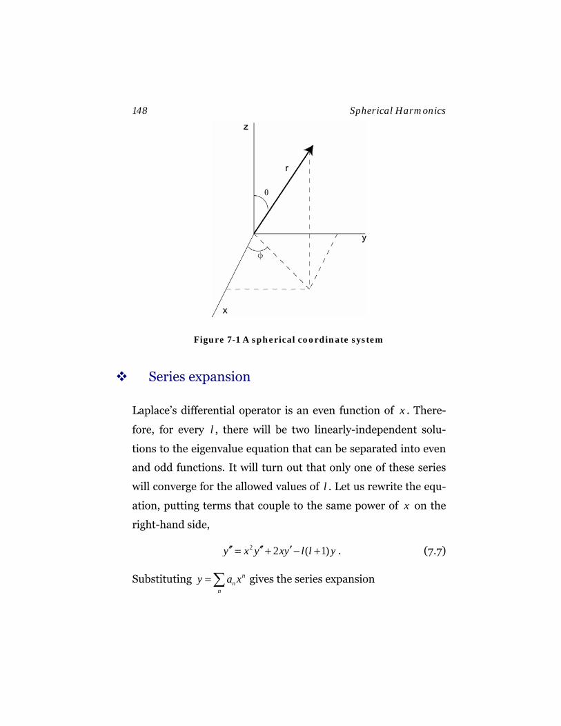
148 Spherical Harmonics
Figure 7-1 A spherical coordinate system
Series expansion
Laplace’s differential operator is an even function of x . There-
fore, for every l , there will be two linearly-independent solu-
tions to the eigenvalue equation that can be separated into even
and odd functions. It will turn out that only one of these series
will converge for the allowed values of l . Let us rewrite the equ-
ation, putting terms that couple to the same power of x on the
right-hand side,
2 2 ( 1)y x y xy l l y′′ ′′ ′= + − + . (7.7)
Substituting nn
ny a x=∑ gives the series expansion
Spherical Harmonics 149
2
2 0 0 0
( 1) ( 1) 2 ( 1)n n n nn n n n
n n n n
n n a x n n a x na x l l a x∞ ∞ ∞ ∞
−
= = = =
− = − + − +∑ ∑ ∑ ∑ (7.8)
or
( ) [ ]20 0
2 ( 1) ( 1) ( 1) ,n nn n
n n
n n a x n n l l a x∞ ∞
+= =
+ + = + − +∑ ∑ (7.9)
giving the recursion relation
[ ]
( )2
( 1) ( 1),
2 ( 1)n n
n n l la a
n n+
+ − +=
+ + (7.10)
which decouples even and odd powers of x .
We can test the series to determine its radius of convergence,
giving
( )
[ ]2
2
2 ( 1)lim lim 1
( 1) ( 1)n
n nn
n naxa n n l l→∞ →∞
+
+ +< = =
+ − + (7.11)
Therefore the range is the open interval ( 1, 1)− + . However, the
convergence of the series at the end points is still in doubt. A
more careful analysis shows that the ratio nr approaches 1 from
above for large n , and it turns out the series diverges at the end
points 1x = ± . This appears to be a disaster, if one fails to ob-
serve that the series terminates for integer values of l . More
specifically, the even series terminates for even l , and the odd
series terminates for odd l . When n l= , the coefficient 2na + and
all further terms in the series vanish, see Eq. (7.10). Therefore,
the boundary conditions at 2 1x = are satisfied by setting
150 Spherical Harmonics
0,1, 2l = . (7.12)
The solutions that converge at the end points of the interval are
finite polynomials of order l , called the Legendre polynomials,
which have an even or odd reflection symmetry given by
( )( ) 1 ( )ll lP x P x= − − (7.13)
For historic reasons they are normalized to 1 at 1x =
(1) 1lP = . (7.14)
Figure 7-2 shows a plot of the first six Legendre polynomials. By
direct substitution in the recursion relation (7.10) and using the
normalization constraint (7.14), the first few polynomials can be
written as
( )( )
0
1
212 2
313 2
1,,
3 1 ,
5 3 .
PP x
P x
P x x
==
= −
= −
(7.15)
You should verify these expressions for yourselves. Let’s calcu-
late 2 ( )P x as an example. There are two nonzero terms in the
expansion, 0 2&a a . They are related by
[ ]( )2 0 0 0
( 1) 6 3 .2 (1) 2l l
a a a a− + −= = = − (7.16)
Therefore,
Spherical Harmonics 151
( ) ( )( )( ) ( )
22 0
2 0
212 2
3 1 ,
1 1 2,
3 1 .
P x x a
P a
P x x
= − +
= ⇒ = −
∴ = −
(7.17)
Note that a Legendre polynomial of order n is a power series in
x of the same order n . The Legendre polynomials are bounded
by
( ) 1.lP x ≤ (7.18)
This can be useful in estimating errors in series expansion. A
useful formula is
( )( ) ( )/ 2
0 for odd 0 1 !!
1 for even !!
l l
lP l
ll
⎧⎪= −⎨
−⎪⎩
(7.19)
Orthogonality and Normalization
Since Legendre’s equation is a Sturm-Liouville equation, we
don’t have to prove orthogonality, it follows automatically. The
norm of the square-integral is given by
1
1
2 .2 1l l llPP dxl
δ′ ′−
=+∫ (7.20)
The proof will be left to a discussion problem.
A Legendre series is a series of Legendre polynomials given by

152 Spherical Harmonics
( ) ( )0
, 1.n nn
f x a P x x∞
=
= ≤∑ (7.21)
By orthogonality, the series can be inverted to extract the coeffi-
cients
1
1
2 1 ( ) ( ) .2n l
na f x P x dx−
+= ∫ (7.22)
A polynomial of order N can be expanded in a Legendre series
of order N :
0 0
( ).N N
mm n n
m nb x a P x
= =
=∑ ∑ (7.23)
The proof follows from the linear independence of the Legendre
polynomials. Since a Legendre series of order N is a polynomial
of order N , the above expression leads to 1N + linear equations
relating the na and mb coefficients. By linear independence, the
equations have a non-trivial solution. Since a Legendre series
expansion is unique, the solution obtained is the only possible
solution. Solving for na by brute force we get
1
01
2 1 .2
Nm
n n mm
na P b x dx=−
+= ∑∫ (7.24)

Spherical Harmonics 153
Example: Expand the quadratic equation 2ax bx c+ + in a Le-
gendre series:
( )2 21
0 1 2 2
22 1 0 2
3 1
3 1 .2 2
ax bx c a a x a x
a x a x a a
+ + = + + −
= + + − (7.25)
Therefore,
2 1 02 1, , and .3 3
a a a b a c a= = = + (7.26)
Discussion Problem: A spherical capacitor consists of two
conducting hemispheres of radius .r The top hemisphere is held
at positive voltage and the bottom hemisphere is held at nega-
tive voltage. The potential distribution is azimuthally symmetric
and is given by
( )0
for 1>x>0 for 0>x>-1
oVV x
V+⎧
= ⎨−⎩ (7.27)
Calculate the Legendre series for this potential distribution.

154 Spherical Harmonics
1 0.5 0 0.5 11
0.5
0
0.5
1
Leg 0 x,( )
Leg 1 x,( )
Leg 2 x,( )
Leg 3 x,( )
Leg 4 x,( )
Leg 5 x,( )
x
Figure 7-2 Legendre Polynomials
A second solution
The second solution to Legendre’s equation for integer l is an
infinite series that diverges on the z-axis, where cos 1x θ= = ±
(Figure 7-3). Although not as frequently seen, it is permitted for
problems with a line-charge distribution along the z-axis. The
solutions are labeled ( )lQ x and have the opposite symmetry to
the ( )lP x ,
( ) 1( ) 1 ( )ll lQ x Q x+= − − . (7.28)
A closed form solution for ( )lQ x can be found by substituting
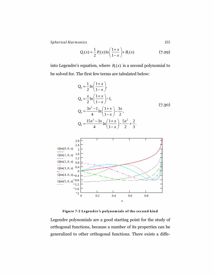
Spherical Harmonics 155
1 1( ) ( ) ln ( )2 1l l l
xQ x P x B xx
+⎛ ⎞= +⎜ ⎟−⎝ ⎠ (7.29)
into Legendre’s equation, where ( )lB x is a second polynomial to
be solved for. The first few terms are tabulated below:
0
0
2
0
3 2
0
1 1ln ,2 1
1ln 1,2 13 1 1 3ln ,
4 1 215 3 1 5 2ln .
4 1 2 3
xQx
x xQx
x x xQx
x x x xQx
+⎛ ⎞= ⎜ ⎟−⎝ ⎠+⎛ ⎞= −⎜ ⎟−⎝ ⎠
− +⎛ ⎞= −⎜ ⎟−⎝ ⎠− +⎛ ⎞= − +⎜ ⎟−⎝ ⎠
(7.30)
0 0.2 0.4 0.6 0.82
1.61.20.80.4
00.40.81.21.6
22.42.8
Qlm 0 0, x,( )
Qlm 1 0, x,( )
Qlm 2 0, x,( )
Qlm 3 0, x,( )
Qlm 4 0, x,( )
Qlm 5 0, x,( )
x
Figure 7-3 Legendre’s polynomials of the second kind
Legendre polynomials are a good starting point for the study of
orthogonal functions, because a number of its properties can be
generalized to other orthogonal functions. There exists a diffe-
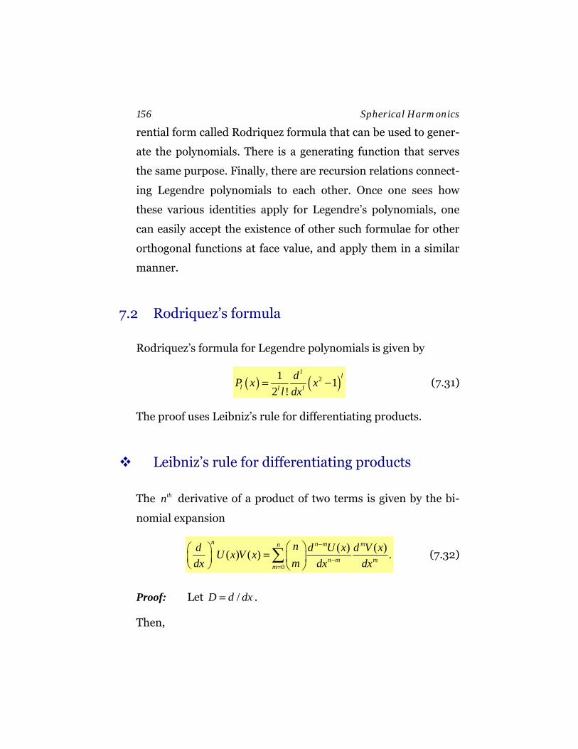
156 Spherical Harmonics
rential form called Rodriquez formula that can be used to gener-
ate the polynomials. There is a generating function that serves
the same purpose. Finally, there are recursion relations connect-
ing Legendre polynomials to each other. Once one sees how
these various identities apply for Legendre’s polynomials, one
can easily accept the existence of other such formulae for other
orthogonal functions at face value, and apply them in a similar
manner.
7.2 Rodriquez’s formula
Rodriquez’s formula for Legendre polynomials is given by
( ) ( )21 12 !
l l
l l l
dP x xl dx
= − (7.31)
The proof uses Leibniz’s rule for differentiating products.
Leibniz’s rule for differentiating products
The thn derivative of a product of two terms is given by the bi-
nomial expansion
0
( ) ( )( ) ( ) .n n m mn
n m mm
nd d U x d V xU x V xmdx dx dx
−
−=
⎛ ⎞⎛ ⎞ = ⎜ ⎟⎜ ⎟⎝ ⎠ ⎝ ⎠
∑ (7.32)
Proof: Let /D d dx= .
Then,
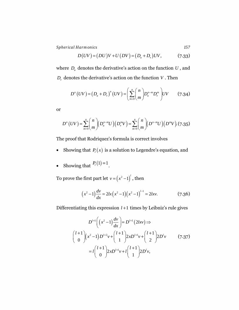
Spherical Harmonics 157
( ) ( ) ( ) ( ) ,u vD UV DU V U DV D D UV= + = + (7.33)
where uD denotes the derivative’s action on the function U , and
vD denotes the derivative’s action on the function V . Then
( ) ( ) ( )0
nnn n m m
u v u vm
nD UV D D UV D D UV
m−
=
⎛ ⎞⎛ ⎞= + = ⎜ ⎟⎜ ⎟
⎝ ⎠⎝ ⎠∑ (7.34)
or
( ) ( )( ) ( )( )0 0
.n n
n n m m n m mu v
m m
n nD UV D U D V D U D V
m m− −
= =
⎛ ⎞ ⎛ ⎞= =⎜ ⎟ ⎜ ⎟
⎝ ⎠ ⎝ ⎠∑ ∑ (7.35)
The proof that Rodriquez’s formula is correct involves
• Showing that ( )lP x is a solution to Legendre’s equation, and
• Showing that ( )1 1lP =.
To prove the first part let ( )2 1l
v x= − , then
( ) ( )( ) 12 2 21 2 1 1 2 .ldvx lx x x lxv
dx−
− = − − = (7.36)
Differentiating this expression 1l + times by Leibniz’s rule gives
( ) ( )
( )
1 2 1
2 2 1
1
1 2
1 1 11 2 2
0 1 2
1 12 2 ,
0 1
l l
l l l
l l
dvD x D lxvdx
l l lx D v xD v D v
l ll xD v l D v
+ +
+ +
+
⎛ ⎞− = ⇒⎜ ⎟⎝ ⎠
+ + +⎛ ⎞ ⎛ ⎞ ⎛ ⎞− + +⎜ ⎟ ⎜ ⎟ ⎜ ⎟
⎝ ⎠ ⎝ ⎠ ⎝ ⎠+ +⎛ ⎞ ⎛ ⎞
= +⎜ ⎟ ⎜ ⎟⎝ ⎠ ⎝ ⎠
(7.37)
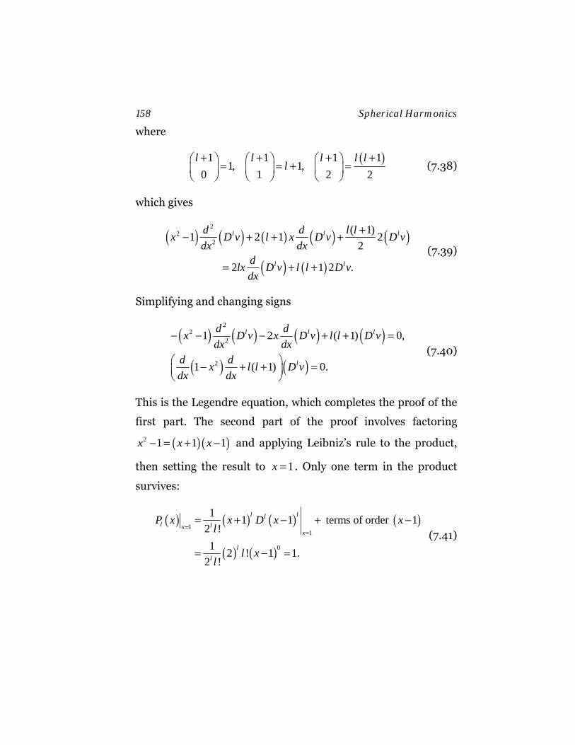
158 Spherical Harmonics
where
( )1 1 1 1
1, 1,0 1 2 2
l l l l ll
+ + + +⎛ ⎞ ⎛ ⎞ ⎛ ⎞= = + =⎜ ⎟ ⎜ ⎟ ⎜ ⎟
⎝ ⎠ ⎝ ⎠ ⎝ ⎠ (7.38)
which gives
( ) ( ) ( ) ( ) ( )
( ) ( )
22
2
( 1)1 2 1 22
2 1 2 .
l l l
l l
d d l lx D v l x D v D vdx dx
dlx D v l l D vdx
+− + + +
= + + (7.39)
Simplifying and changing signs
( ) ( ) ( ) ( )
( ) ( )
22
2
2
1 2 ( 1) 0,
1 ( 1) 0.
l l l
l
d dx D v x D v l l D vdx dx
d dx l l D vdx dx
− − − + + =
⎛ ⎞− + + =⎜ ⎟⎝ ⎠
(7.40)
This is the Legendre equation, which completes the proof of the
first part. The second part of the proof involves factoring
( )( )2 1 1 1x x x− = + − and applying Leibniz’s rule to the product,
then setting the result to 1x = . Only one term in the product
survives:
( ) ( ) ( ) ( )
( ) ( )
11
0
1 1 1 terms of order 12 !1 2 ! 1 1.
2 !
l lll lx
x
ll
P x x D x xl
l xl
==
= + − + −
= − = (7.41)

Spherical Harmonics 159
Example: Calculate 2 ( )P x from Rodriquez’s formula:
( ) ( ) ( )
( ) ( )
2 22 22 2 2
3 2
1 11 4 12 2! 81 1 3 1 .2 2
d dP x x x xdx dx
d x x xdx
⎡ ⎤= − = −⎣ ⎦
= − = − (7.42)
Example: Show that mx is orthogonal to lP if l m> :
Proof: One possible proof is to use Rodriquez’s formula and
integration by parts. Direct integration is easier. Expanding mx
in a Legendre series gives
1 1
' 01 1
0, m l
ml l m m
mPx dx P a P dx
<
′ ′−− −
= =∑∫ ∫ (7.43)
since ' 'm l m≠ ∀ .
7.3 Generating function
Legendre polynomials can also be obtained by a Taylor’s series
expansion of the generating function
( ) ( ) 1/ 22
0, 1 2 .ll
lx h xh h Ph
∞−
=
Φ = − + =∑ (7.44)
Note that, for 1x = , we get
( )0 0
11, (1) .1
l ll
l lh h P h
h
∞ ∞
= =
Φ = = =− ∑ ∑ (7.45)
160 Spherical Harmonics
This will turn out to be related to why the normalization (1) 1lP =
was originally chosen.
Before proving (7.44) it is useful to consider its physical origin.
Consider a unit charge located at a point 0r , as shown in Figure
7-1. Its electrostatic potential is given by
0 2 20 0 0
( , ) ,4 4 2
q qVr xrr rπ π
= =− − +
r rr r
(7.46)
where x is the cosine of the angle between r and 0r Let
( )( )
, ,
, ,
1.
o
o
r Greater r r
r Lesser r rrhr
>
<
<
>
=
=
= ≤
(7.47)
Then,
( )00
( , ) , ( ) .4 4
l
ll
rq qV r r x h P xr r rπ π
∞<
=> > >
⎛ ⎞= Φ = ⎜ ⎟
⎝ ⎠∑ (7.48)
At large distances 0r r ,The distribution approaches a pure
1/ r potential. The generating function is the multipole expan-
sion that arises from the fact that we didn’t think to place the
charge at the origin. The normalization of (1) 1lP = was used to
give all the angular moments equal weight at 1h = .
Now let’s turn to the proof of equation (7.44). Assume that the
RHS of this equation is the definition of Φ . We want to multiply
Φ by Legendre’s operator
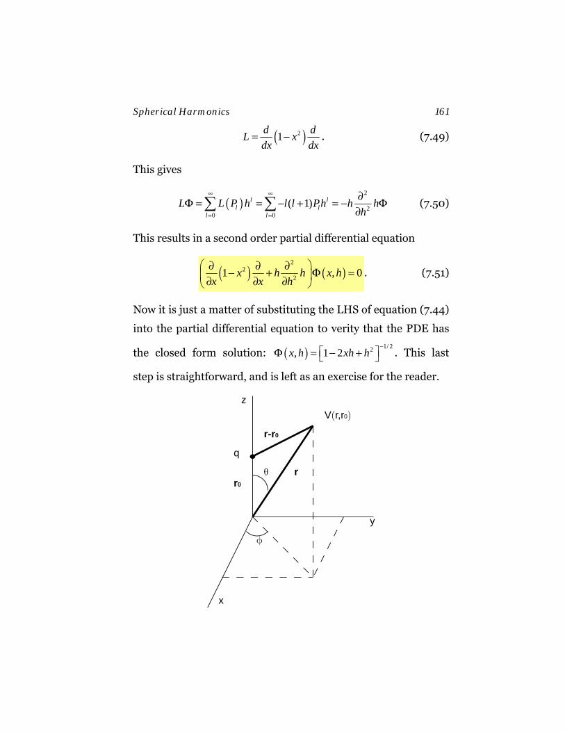
Spherical Harmonics 161
( )21d dL xdx dx
= − . (7.49)
This gives
( )2
20 0
( 1)l ll l
l lL L P h l l Ph h h
h
∞ ∞
= =
∂Φ = = − + = − Φ∂∑ ∑ (7.50)
This results in a second order partial differential equation
( ) ( )2
221 , 0x h h x h
x x h⎛ ⎞∂ ∂ ∂− + Φ =⎜ ⎟∂ ∂ ∂⎝ ⎠
. (7.51)
Now it is just a matter of substituting the LHS of equation (7.44)
into the partial differential equation to verity that the PDE has
the closed form solution: ( ) 1/ 22, 1 2x h xh h−
⎡ ⎤Φ = − +⎣ ⎦ . This last
step is straightforward, and is left as an exercise for the reader.
θ
φ
z
x
y
r0
r
r-r0
q
V(r,r0)
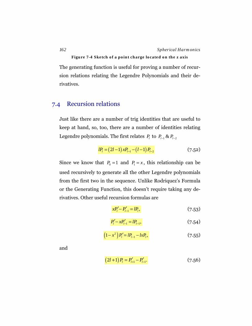
162 Spherical Harmonics
Figure 7-4 Sketch of a point charge located on the z axis
The generating function is useful for proving a number of recur-
sion relations relating the Legendre Polynomials and their de-
rivatives.
7.4 Recursion relations
Just like there are a number of trig identities that are useful to
keep at hand, so, too, there are a number of identities relating
Legendre polynomials. The first relates lP to 1 2&l lP P− −
( ) ( )1 22 1 1l l llP l xP l P− −= − − − (7.52)
Since we know that 0 1P = and 1P x= , this relationship can be
used recursively to generate all the other Legendre polynomials
from the first two in the sequence. Unlike Rodriquez’s Formula
or the Generating Function, this doesn’t require taking any de-
rivatives. Other useful recursion formulas are
1 ,l l lxP P lP−′ ′− = (7.53)
1 1,l l lP xP lP− −′ ′− = (7.54)
( )211 ,l l lx P lP lxP−′− = − (7.55)
and
( ) 1 12 1 .l l ll P P P+ −′ ′+ = − (7.56)
Spherical Harmonics 163
Given two recursion relations, the others follow by substitution,
so it is sufficient to prove the first two equations (7.52) and
(7.53) are valid identities.
The first relation Eq. (7.52) can be proven by taking partial de-
rivatives of the generating function. Taking the derivative with
respect to h gives
( )( ) ( )( ) ( )
13/ 22
2 1
2 1
1 1 1
,1 2
1 2 ,
1 2 ,
2 ,
ll
l
ll
l
l ll l
l l l l ll l l l l
x h lPhh xh h
x h xh h lPh
x h Ph l xh h Ph
xPh Ph lPh lxPh lPh
−
−
−
+ − +
∂ −Φ = =∂ − +
− Φ = − +
− = − +
− = − +
∑
∑
∑ ∑∑ ∑ ∑ ∑ ∑
(7.57)
Collecting terms of the same power of h , one gets the first recur-
sion formula (7.52):
( ) ( )( ) ( )( ) ( )
( ) ( )
1 1
1 1 11 2
11 2
1 2
2 1 1 0,
2 1 1 0,
2 1 1 0,
2 1 1 .
l l ll l l
l l ll l l
ll l l
l l l
l xPh l Ph lPh
l xP h l P h lPh
l xP l P lPh
lP l xP l P
+ −
− − −− −
−− −
− −
+ − + − =
− − − − =
⎡ ⎤− − − − =⎣ ⎦∴ = − − −
∑ ∑ ∑∑ ∑ ∑∑
(7.58)
In a similar manner, the solution for the second recursion rela-
tion, proceeds by taking the differential wrt x in the definition
of the generating function:
164 Spherical Harmonics
( )( )( )
3/ 22
2
1 2
1 2
,1 2
1 2 ,
1 2
2 .
ll
l
l ll l
l l ll l l
h h Px xh h
h xh h h
Ph xh h h P
Ph xPh Ph
+
+ +
∂ ′Φ = =∂ − +
Φ = − +
′= − +
′ ′ ′= − +
∑
∑∑ ∑
∑
(7.59)
Comparing coefficients of order 1lh + gives
1 12 .l l l lP P xP P+ −′ ′ ′= − + (7.60)
Now differentiate the first recursion relation to get
( ) ( ) ( )
( ) ( ) ( )1 1 2
1 1
2 1 2 1 1 or
1 2 1 2 1 .l l l l
l l l l
lP l P x l P l P
l P l P x l P lP− − −
+ −
′ ′ ′= − + − − −
′ ′ ′+ = + + + − (7.61)
Eliminating the 1lP+′ terms in equations (7.60) and (7.61) gives
the desired result for the second recursion formula (7.53):
1.l l llP xP P−′ ′= − (7.62)
Discussion Problem: Prove that 1 2
1
22 1lP dxl−
=+∫ . using the re-
cursion relation 1.l l llP xP P−′ ′= −
7.5 Associated Legendre Polynomials
Legendre polynomials represent the convergent solutions of the
special case 0m = of the associated Legendre Equation:
Spherical Harmonics 165
( ) ( )2
221 ( ) ( ) 1 ( ),
1lm lm lmd d mx P x P x l l P xdx dx x
− − = − +−
(7.63)
where
( ) ( )0 ,l lP x P x= (7.64)
From the symmetry of the equation one sees that the substitu-
tion m± leads to the same equation, therefore,
,lm l mP P−∝ (7.65)
Unfortunately, because of how these polynomials where origi-
nally defined, they turn out not to be simply equal to each other,
they differ in their norms. They also vary in sign conventions
from text to text.
Like the Legendre Polynomials, the associated Legendre func-
tions are solutions to an eigenvalue equation of the Sturm Liou-
ville form
( ){ } ( ) ( ) ( ) ( ) ( ) ,d dL y x P x Q x y x W x y xdx dx
λ⎛ ⎞⎛ ⎞= + =⎜ ⎟⎜ ⎟⎝ ⎠⎝ ⎠
(7.66)
which differs from the Legendre equation by the addition of a
function of x :
( )2
2 ,1
mQ xx
=−
(7.67)
Therefore, for fixed azimulthal index m , the lmP also represent
eigenvalue functions of ( 1)l l− + . For positive integer 0 m l≤ ≤
the solutions are given by
166 Spherical Harmonics
( ) / 22( ) 1 ( ),mm
lm lm
dP x x P xdx
= − (7.68)
which can be verified by direct substitution into the Associated
Legendre equation. Substituting Rodriguez’s formula for ( )lP x ,
gives the more general form,
( ) ( )/ 22 21( ) 1 1 .2 !
l mm l
lm l l m
dP x x xl dx
+
+= − − (7.69)
This is the generalized form of Rodriquez’s formula. In this
form, it can be applied to both positive and negative values of
m . This is in fact how the associated Legendre are defined, and
gives their normalization up to a sign convention of ( 1)m− em-
ployed in some textbooks. Using this formula as it stands, one
finds that the positive and negative m solutions are related by
( )( )
!( ) ( 1) ( ),
!m
l m lm
l mP x P x
l m−
⎛ ⎞−= − ⎜ ⎟⎜ ⎟+⎝ ⎠
(7.70)
and one sees that the solutions for negative m are simply pro-
portional to those of positive m . From formula (7.68) one finds
that the stretched configuration of llP is proportional to
( ) / 22( ) 1 sin .m l
llP x x θ∝ − = (7.71)
Example: Calculate the Legendre polynomials for 1l =
Use 1 10( ) ( )P x P x x= = , one needs to calculate only 1 1P± . Use equa-
tion (7.68) to calculate 11P
Spherical Harmonics 167
( ) ( )
( ) ( )
1/ 2 1/ 22 211 11
11/ 2 1/ 22 21
1 ( ) 1 ( )
1 1 sin .
lm
ll
d dP x P x x P xdx dxdx x xdx
θ
= − = −
= − = − = (7.72)
The negative values for m can be found from equation (7.70)
( )( )
( )( )
( )
1 1
111
1/ 22
!( ) ( 1) ( ),
!
1 1 !( 1) ( ),
1 1 !
1 11 sin ,2 2
mlm
l mP x P x
l m
P x
x θ
−
⎛ ⎞−= − ⎜ ⎟⎜ ⎟+⎝ ⎠⎛ ⎞−
= − ⎜ ⎟⎜ ⎟+⎝ ⎠− −= − =
(7.73)
There are ( )2 1l + m−states associated with a given value of l .
The solution for the 3 m−states of 1mP are
211
11
21 1
1 sin ,cos ,
1 11 sin .2 2
P xP x
P x
θθ
θ−
= − == =
− −= − =
(7.74)
This illustrates one of the problems with using the Associated
Legendre Polynomials. Because of the—too clever by far—
substitution into Rodriquez’s formula, the normalization of the
positive and negative m states differ. For this reason, it is better
to work with the spherical harmonics directly for cases where
0.m ≠
168 Spherical Harmonics
Normalization of Associated Legendre
polynomials
The normalization of the Associated Legendre Polynomials are
given by
( )( )
1
1
!2( ) ( ) .2 1 !lm l m ll
l mdxP x P x
l l mδ′ ′
−
+=
+ −∫ (7.75)
Therefore a series expansion of a function of x for fixed m takes
the form
( )( )
01
1
( ) ( ),
!2 1 ( ) ( ) .2 !
m lm lml
lm m lm
f x A P x
l mlA f x P x dxl m
∞
=
−
=
−+=+
∑
∫ (7.76)
Parity of the Associated Legendre polynomials
Knowing the parity of the Associated Legendre Polynomials is
useful. Reflection symmetry can often be used to identify terms
that identically vanish, reducing computational effort. The pari-
ty of a Legendre Polynomial of order ( ),l m is
( ) ( ) ( )1 .l mlm lmP x P x+− = − (7.77)
Another useful result is
( )1 0, for 0.lmP m± = ≠ (7.78)
Spherical Harmonics 169
Recursion relations
There are a significant number of recursion relations for the As-
sociated Legendre Polynomials. Here are a couple of examples:
• For fixed l :
( ) ( ), 2 , 1 ,2
2 1( 1) 0.
1l m l m l m
m xP P l m l m P
x+ +
+− + − + + =
− (7.79)
• For fixed m :
( ) 1, , 1,1 (2 1) ( ) 0.l m l m l ml m P l xP l m P+ −+ − − + + + = (7.80)
This latter relation reduces to equation (7.52) when 0.m =
7.6 Spherical Harmonics
Legendre Polynomials do not appear in isolation. They
represent the polar angle solutions to a spherical problem which
also has azimulthal dependence. In particular, they are the solu-
tions to the following angular equation which occurs when one
separates Laplace’s equation in spherical coordinates.
( ) ( )2 2
2 2 2
1 1sin 1 , 0.sin sin lml l Yθ θ φ
θ θ θ θ φ⎧ ⎫∂ ∂ ∂+ + + =⎨ ⎬∂ ∂ ∂⎩ ⎭
(7.81)
The operator is closely related to the square of the orbital angu-
lar momentum operator in quantum mechanics:
170 Spherical Harmonics
( ) ( )
( ) ( )
2 22 2
2 2 2
2
1 1, sin ,sin sin
1 , .
lm lm
lm
L Y Y
l l Y
θ φ θ θ φθ θ θ θ φ
θ φ
⎧ ⎫∂ ∂ ∂= − + +⎨ ⎬∂ ∂ ∂⎩ ⎭= +
(7.82)
When there is no azimulthal symmetry, ( 0m ≠ ), it is usually bet-
ter to work directly with the product solutions ( ),lmY θ φ , which
are called the spherical harmonics. The spherical harmonics are
products of the associated Legendre Polynomials and the com-
plex Fourier series expansion of the periodic azimulthal eigens-
tates. They have the advantages of having a simple normaliza-
tion:
( ) ( )*
1
1
, , ,
where 4 .
lm l m ll mmY Y d
d dx dπ
π
θ φ θ φ δ δ
φ π
′ ′ ′ ′
− −
Ω =
Ω = =
∫∫ ∫ ∫
(7.83)
The normalization of a complex Fourier series is given by
2 .im immmd e e
π φ φπ
φ πδ+ ′−
′−=∫ (7.84)
while the normalization of the associated Legendre polynomials
is given by equation (7.75). Putting the two together and one
finds
( ) ( ) ( )( ) ( )!2 1, 1 cos ,
4 !m im
lm lm
l mlY P el m
φθ φ θπ
−+= −+
(7.85)
where ( )1 m− is a commonly used phase convention. Because dif-
ferent phase conventions are in common use, one has to be care-
ful in using the spherical harmonics in a consistent manner.
Spherical Harmonics 171
This is true as well for the Associated Legendre Polynomials in
general.
Any piecewise continuous function defined on a sphere ( ),f θ φ
can be expressed as sums over the spherical harmonics
( ) ( )0
, , ,m l
lm lml m l
f C Yθ φ θ φ∞ =+
= =−
=∑∑ (7.86)
which, by orthogonality, gives
( ) ( ), , .lm lmC f Y dθ φ θ φ∗= Ω∫ (7.87)
If ( ),f θ φ is real, the spherical harmonics occur in complex con-
jugate pairs.
Calculating the spherical harmonics is not much more compli-
cated than calculating the associated Legendre Polynomials.
There are 2 1l + m -states for every irreducible spherical har-
monic tensor of rank l . For 0l = , this reduces to a single spheri-
cally symmetric state
001 .4
Yπ
= (7.88)
where it is easy to verify that
2
00 1.Y dΩ =∫ (7.89)
For 1l = , equation (7.85) reduces to
172 Spherical Harmonics
11
10
1 1
3 sin ,83 cos ,
43 sin .
8
i
i
Y e
Y
Y e
φ
φ
θπ
θπ
θπ
−−
= −
=
=
(7.90)
Some useful formulas are
( ), ,1 andml m l mY Y ∗− = − (7.91)
( ) 2
,2 1, .4
l
l mm l
lY θ φπ=−
+=∑ (7.92)
The completeness relation for spherical harmonics is given by
( ) ( )*, ,
0
, , (cos cos ) ( ),l
l m l ml m l
Y Yθ φ θ φ δ θ θ δ φ φ∞
= =−
′ ′ ′ ′= − −∑∑ (7.93)
and the multipole expansion of a point charge gives
( ) ( )*, ,1
0
1 4 , , .2 1
ll
l m l mll m l
r Y Yl rπ θ φ θ φ
∞<+
= =− >
′ ′=′− +∑∑r r
(7.94)
This latter equation is a generalization of the generating func-
tion (7.48) to the case where the point charge is not restricted to
be along the z-axis.
7.7 Laplace equation in spherical coordinates
Laplace’s equation in spherical coordinates can be written as
Spherical Harmonics 173
( ) ( )
22
22 2
2 2 2 2
1
1 1 1sinsin sin
0,
rr r r
rθ
θ θ θ θ φ
∂ ∂⎛ ⎞+⎜ ⎟∂ ∂⎜ ⎟∇ Ψ = Ψ⎛ ⎞∂ ∂ ∂⎜ ⎟+⎜ ⎟⎜ ⎟∂ ∂ ∂⎝ ⎠⎝ ⎠
=
r r (7.95)
which has product solutions of the form ( ) ( ) ( ), ,l l mf r Y θ φΨ =r ,
yielding the radial equation
22 2
2
1 ( 1) ( ) 0 or
( ) ( 1) ( ).
l
l l
d d l lr f rr dr dr r
d dr f r l l f rdr dr
+⎛ ⎞− =⎜ ⎟⎝ ⎠
= + (7.96)
Letting ( )lf r rλ= gives , ( 1)l lλ = − + leading to the solutions
( 1)
0 0
( )l l
l l lr rf r A Br r
− +⎛ ⎞ ⎛ ⎞
= +⎜ ⎟ ⎜ ⎟⎝ ⎠ ⎝ ⎠
, (7.97)
Where 0r is a scale parameter chosen such that the coefficients
A and B all have the same units. The general solution to Lap-
lace’s equation in spherical coordinates is then given by a sum
over all product solutions
( ) ( )( 1)
0
0 0
, .l ll
lm lm lml m l
rrA B Yr r
θ φ+∞
= =−
⎡ ⎤⎛ ⎞ ⎛ ⎞⎢ ⎥Ψ = +⎜ ⎟ ⎜ ⎟⎝ ⎠⎢ ⎥⎝ ⎠⎣ ⎦
∑ ∑r (7.98)
where the lmA coefficients are valid for the interior solution,
which includes the origin 0r → , and the lmB coefficients are va-
lid for the exterior solution, which includes the point at infinity
( r →∞ ).

174 Spherical Harmonics
8. Bessel functions
8.1 Series solution of Bessel’s equation
is a solution for the radial part of the Helmholtz equation in cy-
lindrical coordinates. The equation can be written as
( ) ( )2 2
22 2
1 , 0d d m y r k y r rdr r dr r
⎛ ⎞+ − = − ≤ ≤ ∞⎜ ⎟
⎝ ⎠. (8.1)
Letting 2 2k k→ − would give us the . m is an integer for cylin-
drical problems, but the equation is also useful for other cases so
we will replace m with the arbitrary real number p in what fol-
lows, and ( )y r with ( ) ( )p pJ x J kr= .
Like the sine and cosine functions in the expansion for Fourier
series, the eigenvalue k can be scaled away by setting x kr= ,
and the equation can be written in the standard form
( )2 2 0pd dx x p x J xdx dx
⎛ ⎞− + =⎜ ⎟⎝ ⎠
, (8.2)
which can be expressed in the explicitly self-adjoint form
2
0 0pd d px x J xdx dx x
⎛ ⎞− + = ≤ ≤ ∞⎜ ⎟
⎝ ⎠, (8.3)
where
176 Bessel functions
2
( ) ,( ) ,
( ) ;
1,
P x xW x x
pQ xx
λ
==
= −
=
(8.4)
This equation can be solved by the . Noting that the operator in
equation (8.2) is an even function of x . Let’s try a generalized
power series solution of the form
( )2
0 2
n s
p nn
xJ x a+∞
=
⎛ ⎞= ⎜ ⎟⎝ ⎠
∑ , (8.5)
where the factor of (2 )2 n s− + was arbitrarily inserted to simplify
the normalization of the final answer. oa is the first non-
vanishing term in the series. Regroup the equation to put terms
with the same power of x on the same side of the equation
( ) ( )2 2p p
d dx x p J x x J xdx dx
⎛ ⎞− = −⎜ ⎟⎝ ⎠
(8.6)
and substitute in the generalized power series
2 2
2 2
0 0
,2 2
n s n s
n nn n
d d x xx x p a x adx dx
+ +∞ ∞
= =
⎛ ⎞ ⎛ ⎞ ⎛ ⎞− = −⎜ ⎟ ⎜ ⎟ ⎜ ⎟⎝ ⎠ ⎝ ⎠ ⎝ ⎠
∑ ∑ (8.7)
where expansion gives
( )( )
2 2 22 2
0 0
2 '
1' 1
2 42 2
4 .2
n s n s
n nn n
n s
nn
x xn s p a a
xa
+ + +∞ ∞
= =
+∞
−=−
⎛ ⎞ ⎛ ⎞+ − = −⎜ ⎟ ⎜ ⎟⎝ ⎠ ⎝ ⎠
⎛ ⎞= − ⎜ ⎟⎝ ⎠
∑ ∑
∑ (8.8)

Bessel functions 177
Comparing coefficients of the same power of x yields the recur-
sion formula
( )( ) ( )2 2 2 2 212 4 4 4n n nn s p a n ns s p a a −
⎡ ⎤+ − = + + − = −⎣ ⎦ (8.9)
Subject to the constraint that the 1a− term must vanish
( )2 20 14s p a a−− = − . (8.10)
This gives the indicial equation
2 2s p= (8.11)
or
s p= ± . (8.12)
In this case 2s pΔ = , so if p is integer, or half-integer, there is a
possibility that the two series won’t be linearly independent.
(This in fact is what happens for integer p m= , but we are get-
ting ahead of ourselves.) Substituting into equation (8.9)
( ) 1n nn n p a a −± = − (8.13)
or
( )( ) 0
1.
! !
n
na an n p
−=
± (8.14)
For noninteger m , this can be written as
( )
( ) 0
1( 1) 1
n
na an n p
−=Γ + Γ ± +
. (8.15)
178 Bessel functions
So, if we choice to normalize to 0 1a = , we have the solutions
( )
( )
2
0
1( )
( 1) 1 2
n pn
pn
xJ xn n p
±∞
±=
− ⎛ ⎞= ⎜ ⎟Γ + Γ ± + ⎝ ⎠∑ (8.16)
This is the series solution for Bessel’s equation. In general, the
series expansion for Bessel functions converges on the open in-
terval ( )0, .∞
However, ( )1pΓ + is infinite for negative integers p , so that, for
integer p m= , the two series are not linearly independent.
( )( ) 1 ( )mm mJ x J x− = − . (8.17)
Neumann or Weber functions
In the case of Bessel’s equation, a special technique is used to
find a second linearly-independent solution. These are referred
to variously in the literature as pN or pY functions:
( ) ( ) ( ) ( )( )
cos( )
sinp p
p p
p J x J xN x Y x
pπ
π−−
= = . (8.18)
For noninteger p , pN and pJ are linearly independent since
pJ± are linearly independent. As intp m→ one has a nonvanish-
ing indefinite form to evaluate, which provides the second solu-
tion to Bessel’s equation for integer p m= . Using L’Hospital’s
rule, the Neumann functions for integer m can be written as
Bessel functions 179
( )
( ) 21
0
2( ) ln( / 2) ( )
1 !1! 2
m m
k mm
k
N x x J x
m k xk
γπ
π
−−
=
= +
− − ⎛ ⎞− ⎜ ⎟⎝ ⎠
∑ (8.19)
where 0.5772156...γ = is Euler’s constant. This second solution
is often used instead of pJ− even for noninteger p . The general
solution to Bessel’s equation is therefore given by
( ) ( ) ( )( ) ( ) ( )
for all 0
for 0,1,2,3...p p p
p p p
y kr AJ kr BN kr p
y kr AJ kr BJ kr p−
= + ≥
= + ≠, (8.20)
The main difference between the Bessel and Neumann functions
is that the Bessel Functions for 0p ≥ converge at the origin,
while the Neumann functions diverge at the origin. Their re-
spective leading order behavior for small kr is given by
( ) ( )
( ) ( )
( )
2
0
2
0
1lim ( )1 2
for 02lim ( )
2 ln( ) 1 for 0.
pp
px
pp
px
xJ x O xp
p x O x pN x
x O p
π
π
+
→
−−
→
⎛ ⎞= +⎜ ⎟Γ + ⎝ ⎠
⎧−Γ ⎛ ⎞ + >⎪ ⎜ ⎟⎪ ⎝ ⎠= ⎨⎪ + =⎪⎩
(8.21)
For large kr , the asymptotic expansions of two functions behave
like phase-shifted sine and cosine functions with a decay enve-
lop that falls of as 1/ 2( )kr − :
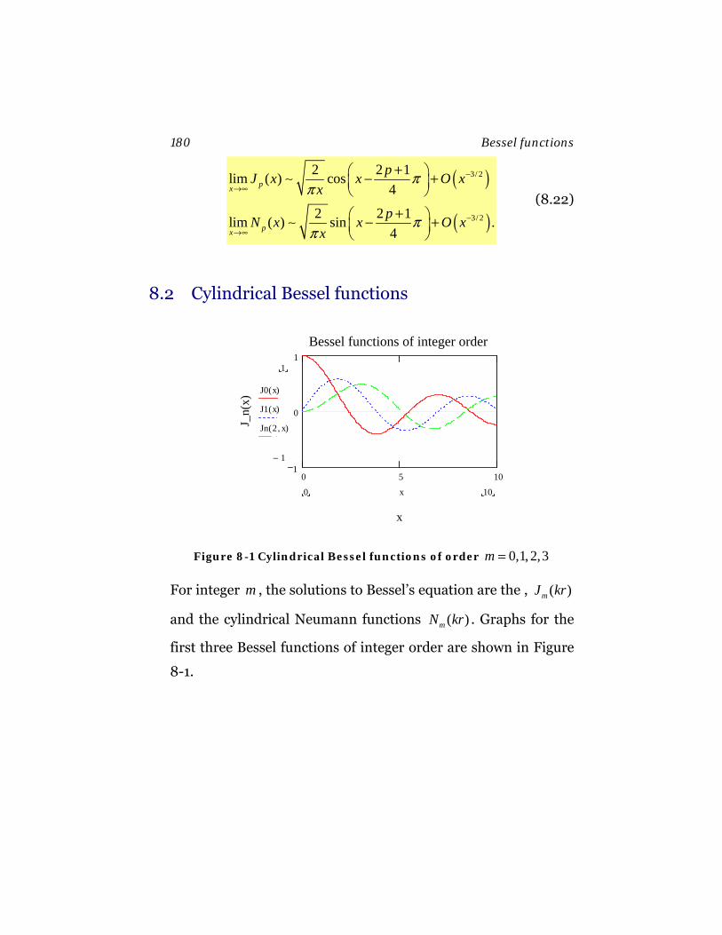
180 Bessel functions
( )
( )
3/ 2
3/ 2
2 2 1lim ( ) cos4
2 2 1lim ( ) sin .4
px
px
pJ x x O xx
pN x x O xx
ππ
ππ
−
→∞
−
→∞
+⎛ ⎞− +⎜ ⎟⎝ ⎠
+⎛ ⎞− +⎜ ⎟⎝ ⎠
∼
∼ (8.22)
8.2 Cylindrical Bessel functions
0 5 101
0
1Bessel functions of integer order
x
J_n(
x)
1
1−
J0 x( )
J1 x( )
Jn 2 x,( )
100 x
Figure 8-1 Cylindrical Bessel functions of order 0,1, 2,3m =
For integer m , the solutions to Bessel’s equation are the , ( )mJ kr
and the cylindrical Neumann functions ( )mN kr . Graphs for the
first three Bessel functions of integer order are shown in Figure
8-1.
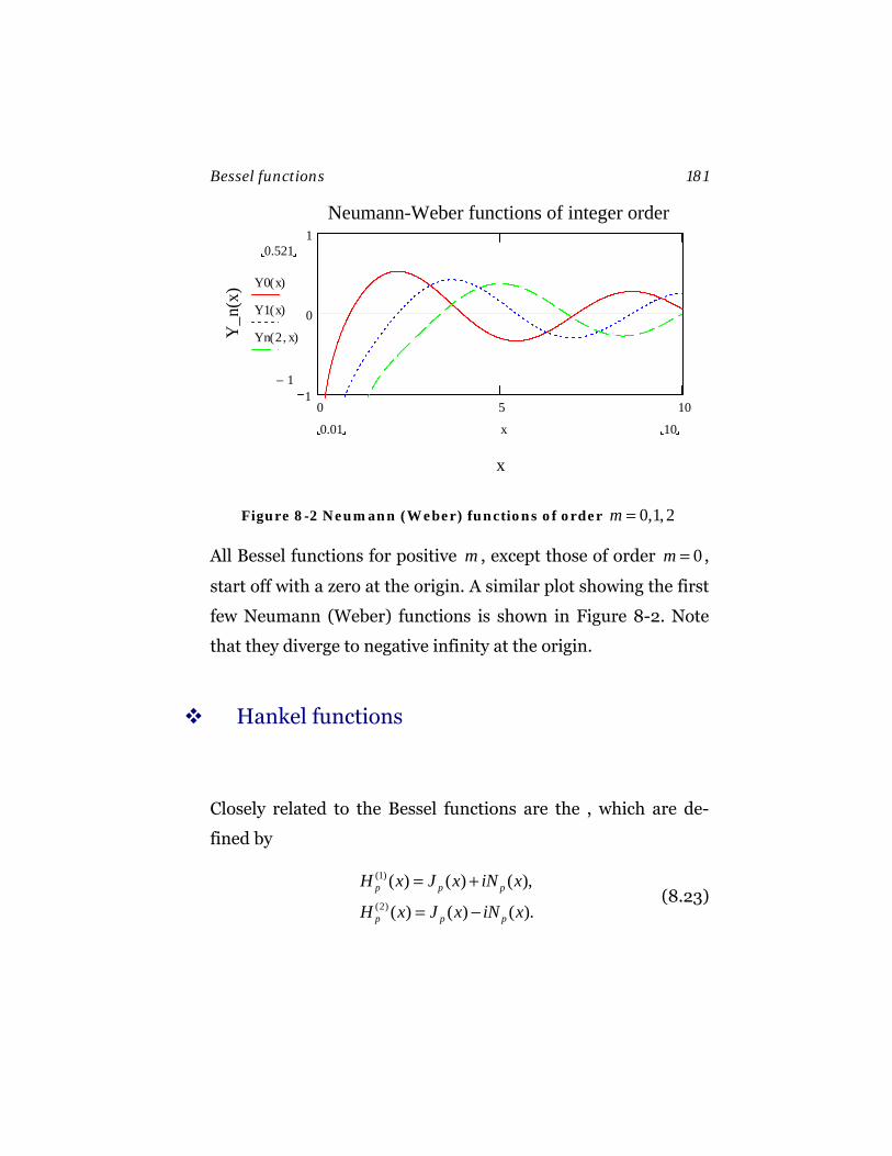
Bessel functions 181
0 5 101
0
1Neumann-Weber functions of integer order
x
Y_n
(x)
0.521
1−
Y0 x( )
Y1 x( )
Yn 2 x,( )
100.01 x
Figure 8-2 Neumann (Weber) functions of order 0,1, 2m =
All Bessel functions for positive m , except those of order 0m = ,
start off with a zero at the origin. A similar plot showing the first
few Neumann (Weber) functions is shown in Figure 8-2. Note
that they diverge to negative infinity at the origin.
Hankel functions
Closely related to the Bessel functions are the , which are de-
fined by
(1)
(2)
( ) ( ) ( ),
( ) ( ) ( ).p p p
p p p
H x J x iN x
H x J x iN x
= +
= − (8.23)
182 Bessel functions
Hankel functions are most often encountered in scattering prob-
lems where the boundary conditions specify incoming or out-
going cylindrical or spherical waves.
Zeroes of the Bessel functions
There are an infinite numbers of zeroes (zero-crossings) of the
Bessel functions. The zeroes of the Bessel functions are impor-
tant, since they provide the eigenvalues needed to find the inte-
rior solution to a cylindrical boundary value problem, where one
has either Dirichlet or Neumann boundary conditions. For Di-
richlet Boundary conditions, let 0/x kr ar r= = , where 0r is the
radius of a cylinder. Then
( ) ( ) ( )0lim / 0o
p p p pnr rJ ar r J a J x
→= = = , (8.24)
where pnx represent the thn zero of the thp Bessel function.
Therefore the eigenvalues of ( )pJ kr are restricted to
0
pnpn
xk
r= . (8.25)
For Neumann boundary conditions one has instead
( ) ( )0lim / 0o
p p pnr rJ ar r J x
→′ ′ ′= = , (8.26)
where pnx′ represent the thn zero of the derivative of the thp Bes-
sel function.
Bessel functions 183
Orthogonality of Bessel functions
Bessel’s equation is a self-adjoint differential equation. There-
fore, the solutions of the eigenvalue problem for Dirichlet or
Neumann boundary conditions are orthogonal to either other
with respect to the weight function x kr= . Like the Fourier se-
ries ( ) immf e φφ = , the eigenfunctions of Bessel’s equation for fixed
p are the same function ( )m nmJ k r stretched to have a zero at the
boundary.
Let ,a b be distinct zeroes of pJ , then the square-integral nor-
malization of a Bessel function is given by
( ) ( )1 2 210
1 .2p pxdx J ax J a+=∫ (8.27)
Substituting / ox r r=
( ) ( )02
2 20 10
/2
r op pn p pn
rrdrJ x r r J x+=∫ (8.28)
Orthogonal series of Bessel functions
Consider a piecewise continuous function ( )pf r that we want to
expand in a Bessel function series for the interval 0 or r≤ ≤ . Let
pnx denote the zeroes of 0( / )p pnJ x r r for or r= . Then, the series
expansion is given by

184 Bessel functions
( )01
( ) / ,p n p pnn
f r A J x r r∞
=
=∑ (8.29)
where the coefficients nA are given by
( ) ( )
( ) ( )0
1
2 01
02 2 00 1
2 ( )
2 ( ) /
pn p pnp pn
r
p pnp pn
A xdx f r J x xJ x
rdr f r J x r rr J x
+
+
=
=
∫
∫ (8.30)
and 0/x r r= .
Discussion Problem: Expand ( ) 1f r = in a 0 ( )J x Bessel func-
tion expansion inside a cylinder of radius a , assuming Dirichlet
boundary conditions.
Note: A first glance, this problem does not appear solvable as a
Bessel function series, since the function does not meet the re-
quired boundary conditions 0( ) 0f r = . But all this really means
is that we have a stepwise discontinuity at r a= . Orthogonal
functions are well suited to handle such discontinuities. (One
can expect to see some version of the Gibbs phenomena at the
discontinuous point however.) Since ( )f r is nonzero at 0r = , it
is appropriate to try an expansion in terms of 0 0( / )nJ x r a . (Ex-
pansions in ( )pJ x for 0p ≠ would not work.) The function to be
fitted can by rewritten as
( ) 1 for ,( ) 0 for .
f r r af r r a
= <= =
(8.31)
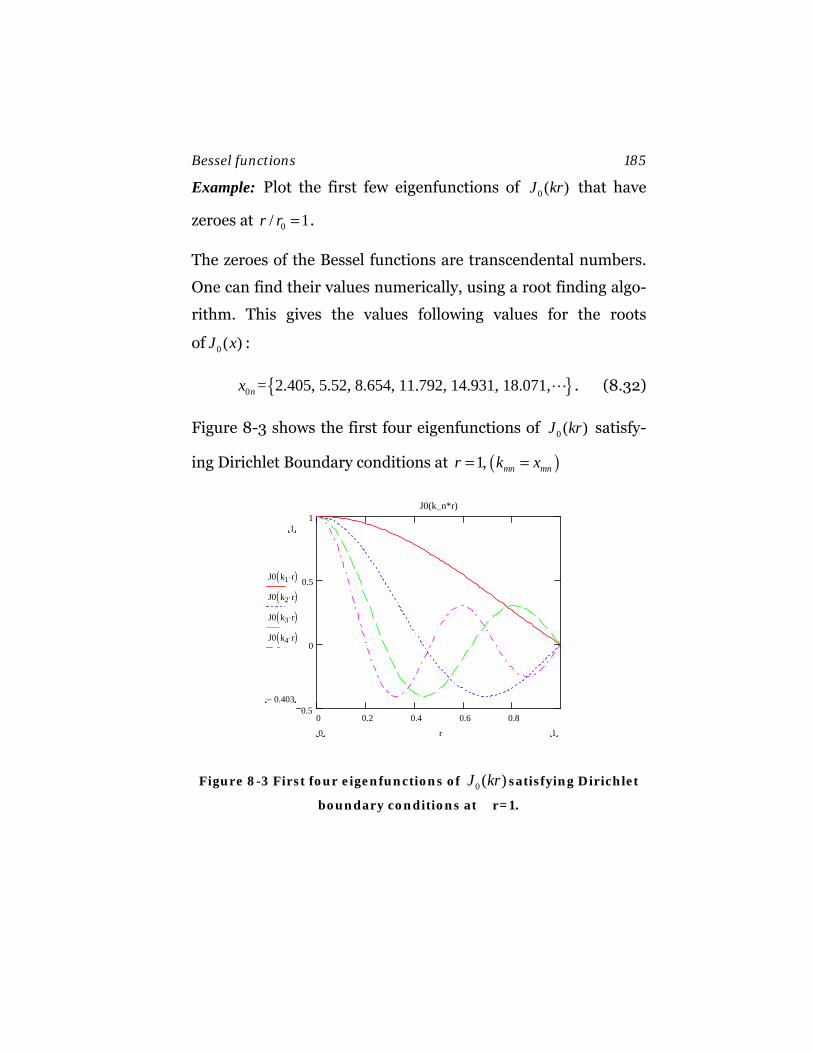
Bessel functions 185
Example: Plot the first few eigenfunctions of 0 ( )J kr that have
zeroes at 0/ 1r r = .
The zeroes of the Bessel functions are transcendental numbers.
One can find their values numerically, using a root finding algo-
rithm. This gives the values following values for the roots
of 0 ( )J x :
{ }0 = 2.405, 5.52, 8.654, 11.792, 14.931, 18.071,nx . (8.32)
Figure 8-3 shows the first four eigenfunctions of 0 ( )J kr satisfy-
ing Dirichlet Boundary conditions at ( )1, mn mnr k x= =
0 0.2 0.4 0.6 0.80.5
0
0.5
1J0(k_n*r)
1
0.403−
J0 k1 r⋅( )J0 k2 r⋅( )J0 k3 r⋅( )J0 k4 r⋅( )
10 r
Figure 8-3 First four eigenfunctions of 0 ( )J kr satisfying Dirichlet
boundary conditions at r=1.
186 Bessel functions
For fixed p , a function ( )pf r that is finite at the origin and va-
nishes at cylindrical boundary 0r r= () can be expanded as a
Bessel function series
( ) ( )( )
01
0
/ ,
0.
p pn p pnn
p
f r A J x r r
f r
∞
=
=
=
∑ (8.33)
If, instead, one were to use , one would use the expansion
( ) ( )( )
01
0
/ ,
0.
p pn p pnn
p
f r A J x r r
f r
∞
=
′=
′ =
∑ (8.34)
Generating function
The generating function for Bessel functions of integer order is
given by
( 1/ ) / 2 ( )m t t mme J x t
∞−
=−∞
=∑ . (8.35)
Recursion relations
Like Legendre Polynomials, there are a large number of useful
recursion formulas relating Bessel functions. Some of the more
useful identities are
1 12( ) ( ) ( )p p pJ x J x J xp+ −= − , (8.36)
Bessel functions 187
1 11( ) ( ) ( )2p p pJ x J x J x− +′ ⎡ ⎤= −⎣ ⎦ , (8.37)
and
1 1( ) ( ) ( ) ( ) ( )p p p p pp pJ x J x J x J x J xx x− +′ = − + = − . (8.38)
Of particular importance are the raising and lowering ladder op-
erators that relate a Bessel function to the next function on the
ladder:
1( ) ( )p pp p
d x J x x J xdx −⎡ ⎤ =⎣ ⎦ (8.39)
and
1( ) ( ).p pp p
d x J x x J xdx
− −+⎡ ⎤ =⎣ ⎦ (8.40)
The Neumann functions satisfy the same relations as (8.36)-
(8.40).
These recursion relations can most readily be proven by direct
substitution of the series expansion given by equation (8.16).
For example, the proof of equation (8.39) is given by
( ) ( )( )
( ) ( )( )
2 2
20
2 2 1
20
1( 1) 1 2
1 2 2.
( 1) 1 2
n n pp
p n pn
n n p
n pn
d d xx J xdx dx n n p
n p xn n p
+∞
+=
+ −∞
+=
− ⎛ ⎞⎡ ⎤ = ⎜ ⎟⎣ ⎦ Γ + Γ + + ⎝ ⎠
− + ⎛ ⎞= ⎜ ⎟Γ + Γ + + ⎝ ⎠
∑
∑ (8.41)
Using ( 1) ( ) ( )n p n p n pΓ + + = + Γ + gives
188 Bessel functions
( ) ( )( )
( )( )
2 2 1
2 10
2 1
2 10
1
1( 1) 2
1( 1) 2
.
n n pp
p n pn
n n pp
n pn
pp
d xx J xdx n n p
xxn n p
x J
+ −∞
+ −=
+ −∞
+ −=
−
− ⎛ ⎞⎡ ⎤ = ⎜ ⎟⎣ ⎦ Γ + Γ + ⎝ ⎠
− ⎛ ⎞= ⎜ ⎟Γ + Γ + ⎝ ⎠=
∑
∑ (8.42)
8.3 Modified Bessel functions
If one makes the replacement of k ik→ in Bessel’s equation
(8.1), one gets the modified Bessel equation.
( )2 2 0pd dx x p x I xdx dx
⎛ ⎞− − =⎜ ⎟⎝ ⎠
. (8.43)
where ( )pI x denote the modified Bessel functions of the first
kind. Their series solution is nearly identical to Bessel’s series
(8.16), except that the coefficients no longer alternate in sign
( )
2
0
1( )( 1) 1 2
n p
pn
xI xn n p
±∞
±=
⎛ ⎞= ⎜ ⎟Γ + Γ ± + ⎝ ⎠∑ . (8.44)
Noting that the substitution k ik→ is equivalent to the substitu-
tion x ix→ , so the solutions also can be written as
( ) ( )pp pI x i J ix= , (8.45)
where the factor pi is included so that the series expansion
(8.44) is a real-valued function.
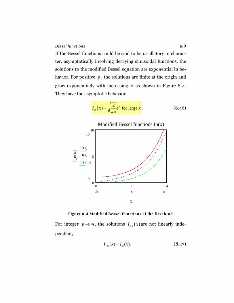
Bessel functions 189
If the Bessel functions could be said to be oscillatory in charac-
ter, asymptotically involving decaying sinusoidal functions, the
solutions to the modified Bessel equation are exponential in be-
havior. For positive p , the solutions are finite at the origin and
grow exponentially with increasing x as shown in Figure 8-4.
They have the asymptotic behavior
( ) 2 for large xpI x e x
xπ∼ . (8.46)
0 2 40
5
10Modified Bessel functions In(x)
x
I_n(
x)
10
0
I0 x( )
I1 x( )
In 2 x,( )
40 x
Figure 8-4 Modified Bessel Functions of the first kind
For integer p m→ , the solutions ( )pI x± are not linearly inde-
pendent,
( ) ( ).m mI x I x− = (8.47)
190 Bessel functions
Modified Bessel functions of the second kind
To obtain a second linearly-independent solution, valid for all
p , the linear combination
( ) ( ) ( )2sinp p pK x I x I x
pππ −⎡ ⎤= −⎣ ⎦ (8.48)
is used. The modified Bessel functions of the second kind ( )pK x
diverge at the origin. They exponentially decay for large values
of x , as shown in Figure 8-5, with the asymptotic behavior
( ) 1 for large .2
xpK x e x
xπ−∼ (8.49)
For integer p m= , the series expansion for ( )pK x , calculated
using L’Hospital’s rule, is given by
( ) ( ) ( ) ( ) ( ) ( )
( ) ( ) ( )
21
0
21
0
11 ln / 2 1 1 !2 2
1,
2 !( )! 2
k mmm k
m mk
m k mm
k
xK x x I x m k
k k m xk m k
γ−−
=
+−
=
⎛ ⎞= − + + − − −⎡ ⎤ ⎜ ⎟⎣ ⎦ ⎝ ⎠
− Φ +Φ + ⎛ ⎞+ ⎜ ⎟+ ⎝ ⎠
∑
∑(8.50)
where
( )
( )1
1 for 0,
0 0.
n
nn n
n′=
′Φ = ≠′
Φ =
∑ (8.51)
For small x , ( )pI x and ( )pK x have the leading order expan-
sions
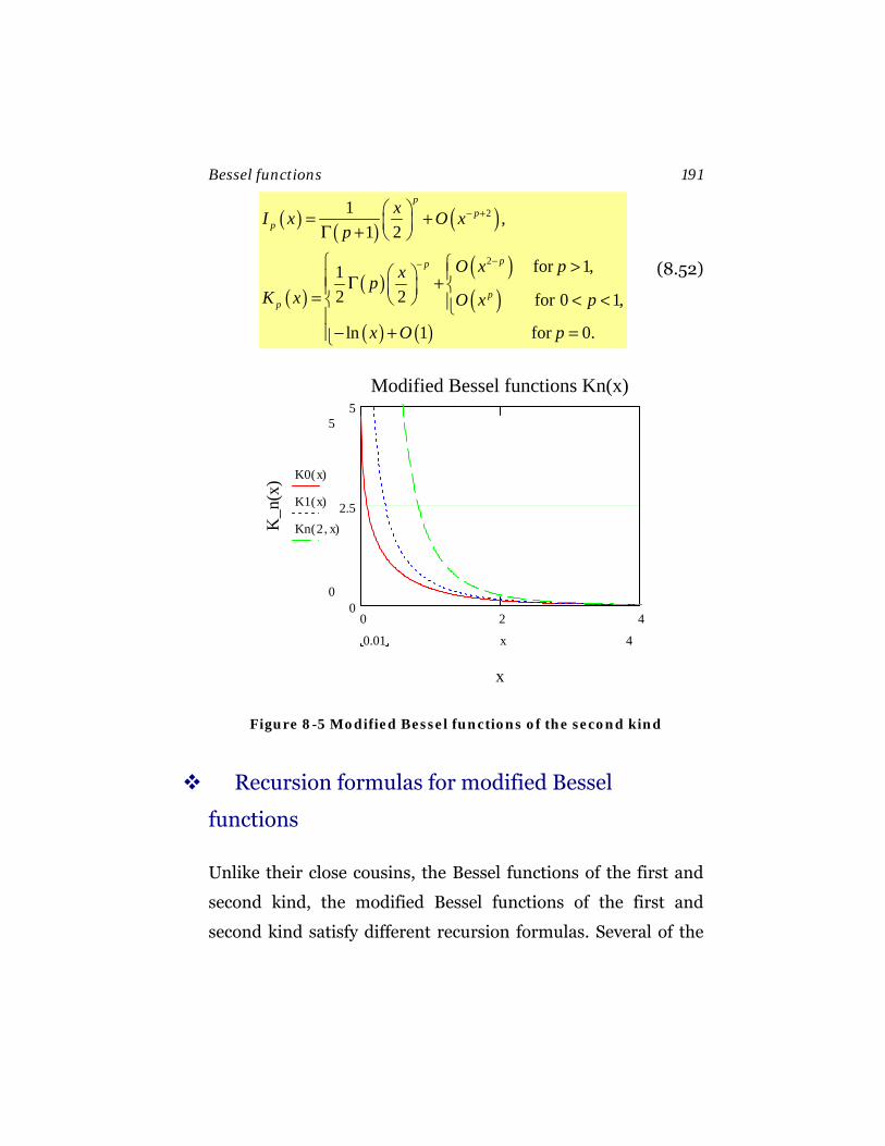
Bessel functions 191
( ) ( ) ( )
( ) ( )( )( )
( ) ( )
2
2
1 ,1 2
for 1,12 2 for 0 1,
ln 1 for 0.
pp
p
pp
pp
xI x O xp
O x pxpK x O x p
x O p
− +
−−
⎛ ⎞= +⎜ ⎟Γ + ⎝ ⎠
⎧ ⎧ >⎪⎛ ⎞⎪ Γ + ⎨⎪ ⎜ ⎟= ⎝ ⎠ < <⎨ ⎪⎩⎪− + =⎪⎩
(8.52)
0 2 40
2.5
5Modified Bessel functions Kn(x)
x
K_n
(x)
5
0
K0 x( )
K1 x( )
Kn 2 x,( )
40.01 x
Figure 8-5 Modified Bessel functions of the second kind
Recursion formulas for modified Bessel
functions
Unlike their close cousins, the Bessel functions of the first and
second kind, the modified Bessel functions of the first and
second kind satisfy different recursion formulas. Several of the
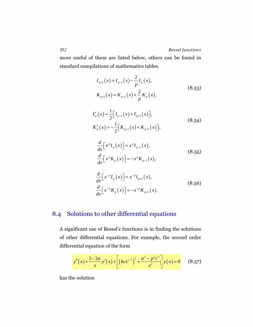
192 Bessel functions
more useful of these are listed below, others can be found in
standard compilations of mathematics tables.
( ) ( ) ( )
( ) ( ) ( )
1 1
1 1
2 ,
2 ,
p p p
p p p
I x I x I xp
K x K x K xp
+ −
+ −
= −
= + (8.53)
( ) ( ) ( )
( ) ( ) ( )
1 1
1 1
1 ,2
1 ,2
p p p
p p p
I x I x I x
K x K x K x
− +
− +
′ ⎡ ⎤= +⎣ ⎦
′ ⎡ ⎤= − +⎣ ⎦
(8.54)
( ) ( )
( ) ( )
1
1
,
,
p pp p
p pp p
d x I x x I xdxd x K x x K xdx
−
−
⎡ ⎤ =⎣ ⎦
⎡ ⎤ = −⎣ ⎦
(8.55)
( ) ( )
( ) ( )
1
1
,
.
p pp p
p pp p
d x I x x I xdxd x K x x K xdx
− −+
− −+
⎡ ⎤ =⎣ ⎦
⎡ ⎤ = −⎣ ⎦
(8.56)
8.4 Solutions to other differential equations
A significant use of Bessel’s functions is in finding the solutions
of other differential equations. For example, the second order
differential equation of the form
( ) ( ) ( ) ( )2 2 221
2
1 2 0ca a p cy x y x bcx y xx x
−⎡ ⎤− −′′ ′+ + + =⎢ ⎥⎣ ⎦
(8.57)
has the solution
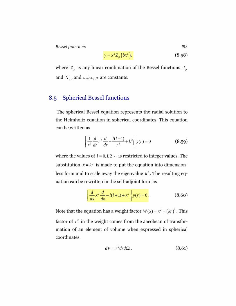
Bessel functions 193
( ) ,a cpy x Z bx= (8.58)
where pZ is any linear combination of the Bessel functions pJ
and pN , and , , ,a b c p are constants.
8.5 Spherical Bessel functions
The spherical Bessel equation represents the radial solution to
the Helmholtz equation in spherical coordinates. This equation
can be written as
2 22 2
1 ( 1) ( ) 0d d l lr k y rr dr dr r
+⎡ ⎤− + =⎢ ⎥⎣ ⎦ (8.59)
where the values of 0,1, 2l = is restricted to integer values. The
substitution x kr= is made to put the equation into dimension-
less form and to scale away the eigenvalue 2k . The resulting eq-
uation can be rewritten in the self-adjoint form as
2 2( 1) ( ) 0d dx l l x y rdx dx⎡ ⎤− + + =⎢ ⎥⎣ ⎦
. (8.60)
Note that the equation has a weight factor ( )22( )W x x kr= = . This
factor of 2r in the weight comes from the Jacobean of transfor-
mation of an element of volume when expressed in spherical
coordinates
2dV r drd= Ω . (8.61)
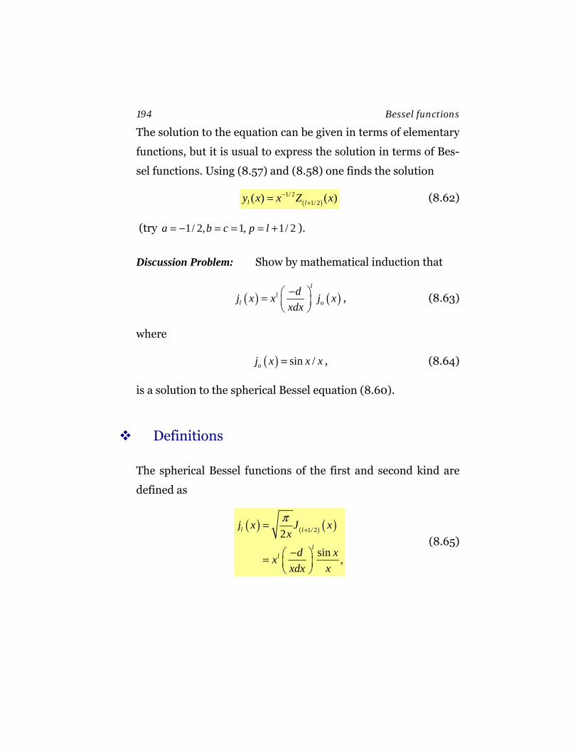
194 Bessel functions
The solution to the equation can be given in terms of elementary
functions, but it is usual to express the solution in terms of Bes-
sel functions. Using (8.57) and (8.58) one finds the solution
( )1/ 2
1/ 2( ) ( )l ly x x Z x−+= (8.62)
(try 1/ 2, 1, 1/ 2a b c p l= − = = = + ).
Discussion Problem: Show by mathematical induction that
( ) ( )l
ll o
dj x x j xxdx−⎛ ⎞= ⎜ ⎟
⎝ ⎠, (8.63)
where
( ) sin /oj x x x= , (8.64)
is a solution to the spherical Bessel equation (8.60).
Definitions
The spherical Bessel functions of the first and second kind are
defined as
( ) ( ) ( )1/ 22
sin ,
l l
ll
j x J xx
d xxxdx x
π+=
−⎛ ⎞= ⎜ ⎟⎝ ⎠
(8.65)

Bessel functions 195
( ) ( ) ( )1/ 22
cos .
l l
ll
n x N xx
d xxxdx x
π+=
− −⎛ ⎞= ⎜ ⎟⎝ ⎠
(8.66)
Like the cylindrical Bessel functions, the spherical Bessel func-
tions of the first (Figure 8-6) and second (Figure 8-7) kind are
oscillatory, with an infinite number of zero crossings. For large
x their decay envelope falls off as 1/ x .
0 5 101
0
1Spherical Bessel functions
x
j_l(x
)
1
1−
js 0 x,( )
js 1 x,( )
js 2 x,( )
100 x
Figure 8-6 Spherical Bessel functions
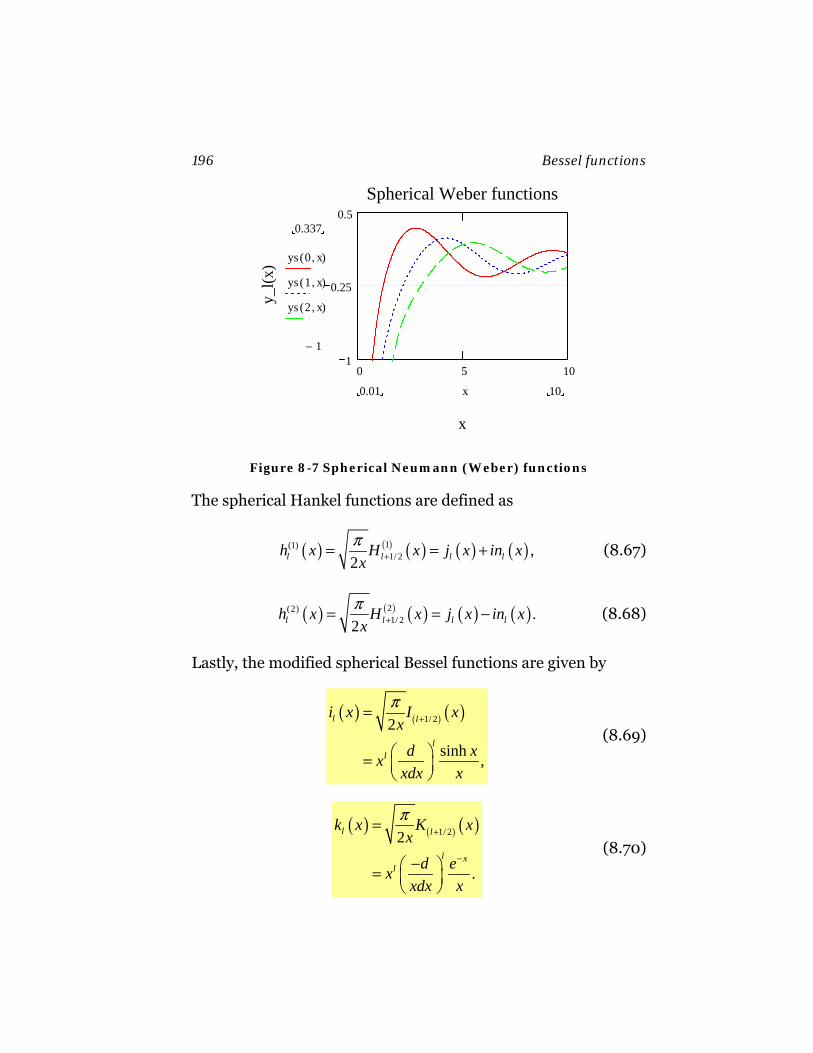
196 Bessel functions
0 5 101
0.25
0.5Spherical Weber functions
x
y_l(x
)
0.337
1−
ys 0 x,( )
ys 1 x,( )
ys 2 x,( )
100.01 x
Figure 8-7 Spherical Neumann (Weber) functions
The spherical Hankel functions are defined as
( ) ( ) ( ) ( ) ( )1(1)1/ 2 ,
2l l l lh x H x j x in xxπ
+= = + (8.67)
( ) ( ) ( ) ( ) ( )2(2)1/ 2 .
2l l l lh x H x j x in xxπ
+= = − (8.68)
Lastly, the modified spherical Bessel functions are given by
( ) ( ) ( )1/ 22
sinh ,
l l
ll
i x I xx
d xxxdx x
π+=
⎛ ⎞= ⎜ ⎟⎝ ⎠
(8.69)
( ) ( ) ( )1/ 22
.
l l
l xl
k x K xx
d exxdx x
π+
−
=
−⎛ ⎞= ⎜ ⎟⎝ ⎠
(8.70)

Bessel functions 197
Table 8-1 lists the first three l values of the most common
spherical Bessel functions. The limiting behavior of these func-
tions for small and large values of x are summarized in Table
8-2.
Table 8-1 Spherical Bessel functions of order 0, 1, and 2
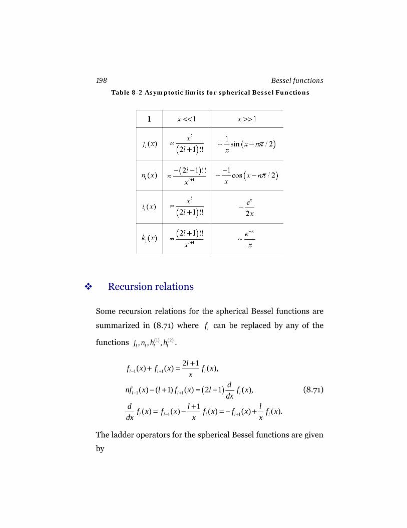
198 Bessel functions
Table 8-2 Asymptotic limits for spherical Bessel Functions
Recursion relations
Some recursion relations for the spherical Bessel functions are
summarized in (8.71) where lf can be replaced by any of the
functions (1) (2), , ,l l l lj n h h .
( )
1 1
1 1
1 1
2 1( ) ( ) ( ),
( ) ( 1) ( ) 2 1 ( ),
1( ) ( ) ( ) ( ) ( ).
l l l
l l l
l l l l l
lf x f x f xx
dnf x l f x l f xdx
d l lf x f x f x f x f xdx x x
− +
− +
− +
++ =
− + = +
+= − = − +
(8.71)
The ladder operators for the spherical Bessel functions are given
by
Bessel functions 199
1 11
1
( ) ( ),
( ) ( ).
l ll l
l ll l
d x f x x f xdxd x f x x f xdx
+ +−
− −+
⎡ ⎤ =⎣ ⎦
⎡ ⎤ = −⎣ ⎦
(8.72)
The equivalent recursion relations for the modified spherical
Bessel functions are summarized in (8.73) where lf can be re-
placed by 1 or (-1)ll li k+ .
( )
1 1
1 1
1 1
2 1( ) ( ) ( ),
( ) ( 1) ( ) 2 1 ( ),
1( ) ( ) ( ) ( ) ( ).
l l l
l l l
l l l l l
lf x f x f xx
dnf x l f x l f xdx
d l lf x f x f x f x f xdx x x
− +
− +
− +
+− =
+ + = +
+= − = +
(8.73)
The ladder operators for the modified spherical Bessel functions
are given by
1 11
1
( ) ( ),
( ) ( ).
l ll l
l ll l
d x f x x f xdxd x f x x f xdx
+ +−
− −+
⎡ ⎤ =⎣ ⎦
⎡ ⎤ =⎣ ⎦
(8.74)
Orthogonal series of spherical Bessel functions
Let 0/x r r= , where 0r is the surface of a sphere. Assuming Di-
richlet boundary conditions, the eigenfunctions of the spherical
Bessel functions that vanish on this surface are given by
( ), 0l l nj a = , (8.75)
200 Bessel functions
where ,l na denotes the thn zero of the thl spherical Bessel func-
tion. Suppose one has a function ( )lf r defined on the interior of
this sphere. Assume one wants to expand ( )lf r in a Bessel func-
tion series of order l . The expansion would take the form
( ), , 00
( ) /l l n l l nn
f r A j a r r∞
=
=∑ . (8.76)
(Figure 8-8 shows how the functions scale to fit in the nth zero
at the boundary) Since this is a series of orthogonal functions,
one can use the orthogonality relation, which is given by
( ) ( )21 2 1
0
( )2
ll l ab
j ax dxj ax j bx δ+=∫ , (8.77)
where ,a b denote two zeroes of the thl Bessel function. There-
fore, the coefficients ,l nA are given by
1 2, , 02 0
1
1 2, 02 3 0
1 0
2 ( ) ( / )( )2 ( ) ( / ).( )
l n l l l nl
l l l nl
A x dxf r j a r rj a
r drf r j a r rj a r
+
+
=
=
∫
∫ (8.78)
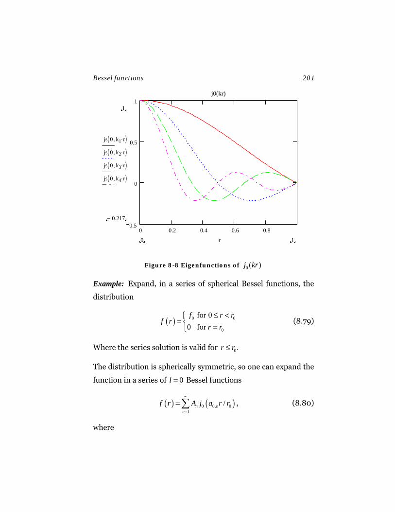
Bessel functions 201
0 0.2 0.4 0.6 0.80.5
0
0.5
1j0(kr)
1
0.217−
js 0 k1 r⋅,( )js 0 k2 r⋅,( )js 0 k3 r⋅,( )js 0 k4 r⋅,( )
10 r
Figure 8-8 Eigenfunctions of 0 ( )j kr
Example: Expand, in a series of spherical Bessel functions, the
distribution
( ) 0 0
0
for 00 for f r r
f rr r≤ <⎧
= ⎨ =⎩ (8.79)
Where the series solution is valid for 0.r r≤
The distribution is spherically symmetric, so one can expand the
function in a series of 0l = Bessel functions
( ) ( )0 0, 01
/n nn
f r A j a r r∞
=
=∑ , (8.80)
where
202 Bessel functions
1 20
0 0,2 01
2 ( )( )n n
n
fA x dxj a xj a
= ∫ . (8.81)
Using the ladder operators (8.72)
2 21 0( ) ( )d x j x x j x
dx⎡ ⎤ =⎣ ⎦ , (8.82)
the integral can be evaluated, giving
( )
0,
0,
1 2 20 030 0
0,
21 1 0,3 0
0, 0,
1( ) ( )
1 1( ) ,
n
n
a
nn
a
nn n
x dxj a x x dx j xa
x j x j aa a
′ ′ ′=
⎡ ⎤= =⎣ ⎦
∫ ∫ (8.83)
( )1 0,0 0
21 0, 0, 1
2 2( ) ( )
nn
n n n n
j af fAj a a a j a
= = , (8.84)
yielding the result
( ) ( )0 0, 00
1 0, 1 0,
/2
( )n
n n n
j a r rf r f
a j a
∞
=
= ∑ . (8.85)
The zeros of 0j are given by 0, =na nπ . The results of the series
approximation are shown in Figure 8-9. Because the distribu-
tion is discontinuous, the overshooting effect that is characteris-
tic of the Gibbs Phenomena is observed. The magnitude of the
overshoot persists even when increasing the number of terms,
but the area of the overshoot gets smaller. In the infinite series
limit, the series and the function would agree except on a inter-
val of null measure.
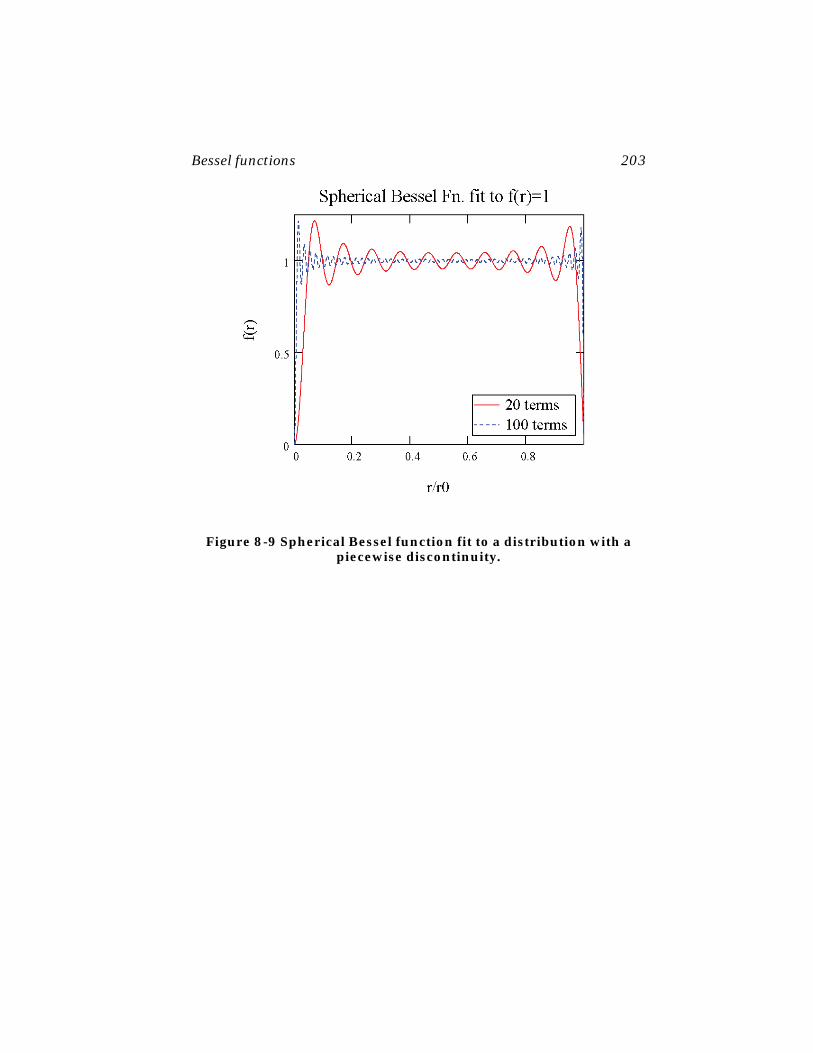
Bessel functions 203
Figure 8-9 Spherical Bessel function fit to a distribution with a piecewise discontinuity.

9. Laplace equation
9.1 Origin of Laplace equation
Laplace’s equation
( )2 0∇ Φ =r (9.1)
occurs as the steady-state (time-independent) limit of a number
of scalar second-order differential equations that span the range
of physics problems. In electrostatics or Newtonian gravitation
problems, the Φ field can be interpreted as defining a potential
function (electrostatic or gravitational, respectively) in a source
free region. The equation also occurs in thermodynamics, where
Φ can be interpreted as the local temperature of a system in a
steady state equilibrium.
To understand Laplace’s equation, let’s derive it in the context of
Gauss’s Law, which states that the net Electric flux crossing a
closed boundary surface is proportional to the charge enclosed
in the volume defined by the bounding surface:
0 0
1
V S
QdS dVρε ε⊂
⋅ = =∫ ∫E n (9.2)
206 Laplace equation
Where E is the electric field strength, n is a unit normal to the
surface S , and Q is the net charged enclosed in the region. The
differential form of Gauss’s law is given by Poisson’s Equation
0
ρε
∇ ⋅ =E (9.3)
where ρ is the charge density For a charge free region this re-
duces to
0∇⋅ =E (9.4)
For electrostatics, the electric field can be derived from a scalar
potential function = −∇ΦE , which leads to Laplace’s equation
(9.1). Figure 9-1 shows a region of space for which Laplace’s eq-
uation valid.
Figure 9-1. A closed region, in which Laplace’s equation is valid
Laplace’s equation has a unique (up to an overall constant value
of the potential) solution for either of the following two sets of
Boundary conditions:
• (Direchlet Boundary Conditions) The potential is defined
everywhere on the boundary surface
Laplace equation 207
( )S SΦ = Φ r (9.5)
OR
• (Neumann Boundary Conditions) The normal derivative of
the potential is defined everywhere on the bounding surface:
( )ˆ
n SSn S
E E∂ Φ = − = −∂
r (9.6)
9.2 Laplace equation in Cartesian coordinates
Laplace’s equation in Cartesian coordinates can be written as
( )2 2 2
2 2 2 , , 0x y zx y z
⎛ ⎞∂ ∂ ∂+ + Φ =⎜ ⎟∂ ∂ ∂⎝ ⎠ (9.7)
Solutions to this equation can be found by separation of va-
riables in terms of product solutions: ( ) ( ) ( )X x Y y Z z . The total
solution can be expressed as a superposition over all of these
“normal mode” solutions of the problem. For simplicity, lets
limit the problem to a 2-dimensional space. Then, Laplace’s eq-
uation reduces to
( )2 2
2 2 , 0x yx y
⎛ ⎞∂ ∂+ Φ =⎜ ⎟∂ ∂⎝ ⎠ (9.8)
By separation of variables the problem can be written in the
form
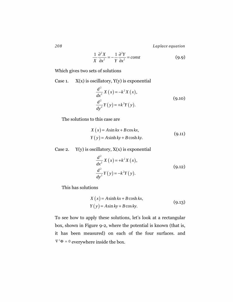
208 Laplace equation
2 2
2 2
1 1X Y constX x Y x
∂ ∂= − =∂ ∂
(9.9)
Which gives two sets of solutions
Case 1. X(x) is oscillatory, Y(y) is exponential
( ) ( )
( ) ( )
22
2
22
2
,
.
d X x k X xdxd Y y k Y ydy
= −
= + (9.10)
The solutions to this case are
( )( )
sin cos ,
sinh cosh .
X x A kx B kx
Y y A ky B ky
= +
= + (9.11)
Case 2. Y(y) is oscillatory, X(x) is exponential
( ) ( )
( ) ( )
22
2
22
2
,
.
d X x k X xdxd Y y k Y ydy
= +
= − (9.12)
This has solutions
( )( )
sinh cosh ,
sin cos .
X x A kx B kx
Y y A ky B ky
= +
= + (9.13)
To see how to apply these solutions, let’s look at a rectangular
box, shown in Figure 9-2, where the potential is known (that is,
it has been measured) on each of the four surfaces. and 2 0∇ Φ = everywhere inside the box.
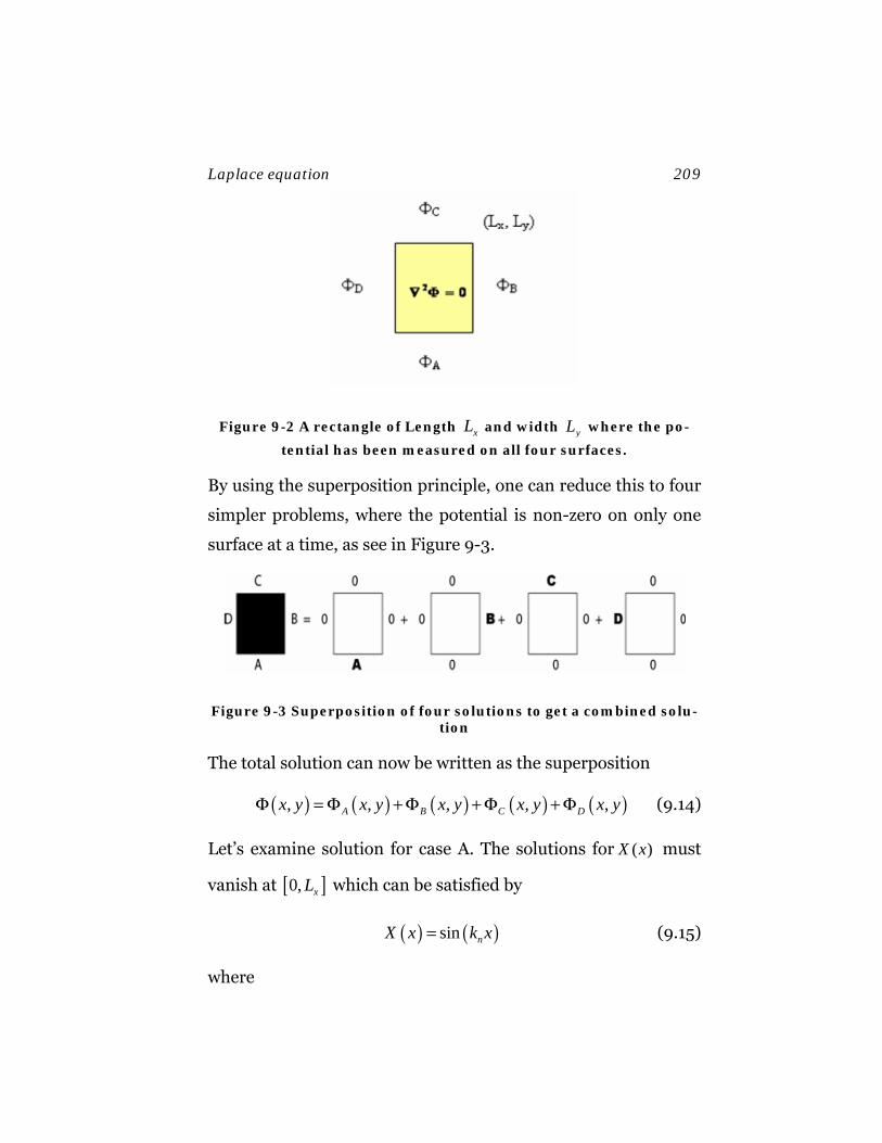
Laplace equation 209
Figure 9-2 A rectangle of Length xL and width yL where the po-
tential has been measured on all four surfaces.
By using the superposition principle, one can reduce this to four
simpler problems, where the potential is non-zero on only one
surface at a time, as see in Figure 9-3.
Figure 9-3 Superposition of four solutions to get a combined solu-tion
The total solution can now be written as the superposition
( ) ( ) ( ) ( ) ( ), , , , ,A B C Dx y x y x y x y x yΦ =Φ +Φ +Φ +Φ (9.14)
Let’s examine solution for case A. The solutions for ( )X x must
vanish at [ ]0, xL which can be satisfied by
( ) ( )sin nX x k x= (9.15)
where
210 Laplace equation
.mx
mkLπ= (9.16)
Therefore ( )Y y must be a sum of sinh and cosh functions. The
correct linear combination that vanishes at yy L= is given by
( ) ( )( )sinh n yY y k L y= − (9.17)
Therefore,
( ) ( )1
, sin sinh yA n
n x x
n L yn xx y AL L
ππ∞
=
−Φ =∑ (9.18)
By a similar analysis the solutions for the remaining three sur-
faces can be found:
( )1
, sin sinh ,C nn x x
n x n yx y CL Lπ π∞
=
Φ =∑ (9.19)
( ) ( )1
, sin sinh ,xB n
n y y
n L xn yx y BL L
ππ∞
=
−Φ =∑ (9.20)
( )1
, sin sinh .D nn y y
n y n xx y DL Lπ π∞
=
Φ =∑ (9.21)
Solving for the coefficients
The solution to
( ) ( )2
22
d X x k X xdx
= − (9.22)
Laplace equation 211
is a solution to a Sturm-Liouville differential equation, similar to
that for the Fourier series expansion. The main difference is that
the solution no longer satisfies periodic boundary conditions,
but rather, Direchlet (or Neumann) boundary conditions at the
end points of the interval [ ]0, xL The eigenfunctions are ortho-
gonal on this interval, and satisfy the normalization condition
0
sin sin .2
xLx
x x
Ln x m xdxL Lπ π =∫ (9.23)
Using this relationship, one can then solve for the coefficients of
the series expansion (9.18), giving
( )10 00
sin , sin sin sinh
sinh2
x xL Ly
A nnx x x xy
yxm
x
n Lm x m x n xdx x y AL L L L
m LLAL
ππ π π
π
∞
==
Φ =
=
∑∫ ∫(9.24)
or
( ) ( )
( )0
2 sin / ,0.
sinh /
xL
x A
nx y x
dx n x L xA
L n L L
π
π
Φ=∫
(9.25)
Similarly, the results for the other three surfaces are given by
( ) ( )
( )0
2 sin / ,,
sinh /
xL
y B x
nx x y
dx n x L L yB
L n L L
π
π
Φ=∫
(9.26)
212 Laplace equation
( ) ( )
( )0
2 sin / ,,
sinh /
xL
x C y
nx y x
dx n x L x LC
L n L L
π
π
Φ=∫
(9.27)
( ) ( )
( )0
2 sin / 0,.
sinh /
xL
y D
nx x y
dx n x L yD
L n L L
π
π
Φ=∫
(9.28)
Example: Consider a square 2-dimensional box of length L with
sides have constant potentials
0 .A c B DVΦ = Φ = = −Φ = −Φ (9.29)
Find the potential inside the box.
In this case x yL L L= = , and the geometry is symmetric for ref-
lections about the mid-plane wrt either the x or y directions. By
symmetry, only the odd n terms survive
( )
( )
( )
00
0 0
0
2 sin /
sinh
2 4sin for odd n,
xL
n n n n
n
V dx n x LA C B D
L n
V Vdx xn n
π
π
π
π π
= = − = − =
′ ′= =
∫
∫
(9.30)
( ) ( ) ( )
( ) ( )
0
0
0
0
( )sin sinh sinh4,
2 1 sinh
( )sin sinh sinh4 .
2 1 sinh
n
n
n x n y n L yV L L Lx y
n n
n y n x n L xV L L L
n n
π π π
π ππ π π
π π
∞
=
∞
=
−⎛ ⎞+⎜ ⎟⎝ ⎠Φ =
+
−⎛ ⎞+⎜ ⎟⎝ ⎠−
+
∑
∑
(9.31)
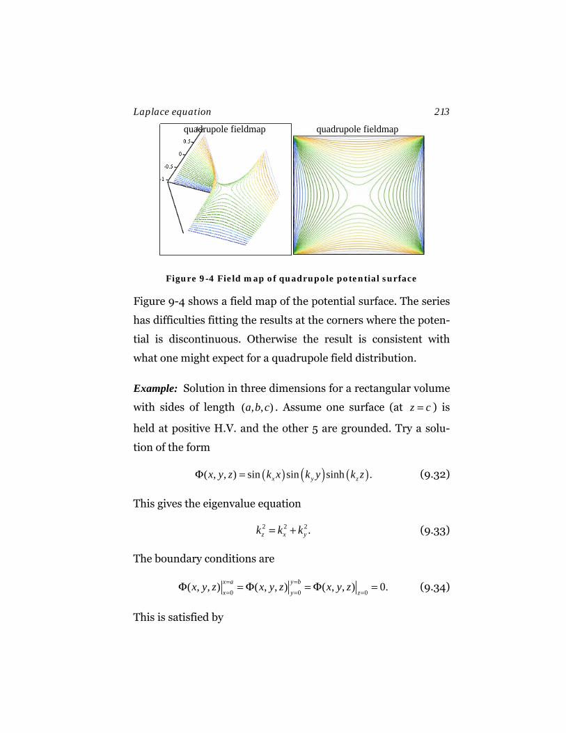
Laplace equation 213
quadrupole fieldmap quadrupole fieldmap
Figure 9-4 Field map of quadrupole potential surface
Figure 9-4 shows a field map of the potential surface. The series
has difficulties fitting the results at the corners where the poten-
tial is discontinuous. Otherwise the result is consistent with
what one might expect for a quadrupole field distribution.
Example: Solution in three dimensions for a rectangular volume
with sides of length ( , , )a b c . Assume one surface (at z c= ) is
held at positive H.V. and the other 5 are grounded. Try a solu-
tion of the form
( ) ( ) ( )( , , ) sin sin sinh .x y zx y z k x k y k zΦ = (9.32)
This gives the eigenvalue equation
2 2 2.z x yk k k= + (9.33)
The boundary conditions are
0 0 0
( , , ) ( , , ) ( , , ) 0.x a y b
x y zx y z x y z x y z= =
= = =Φ = Φ = Φ = (9.34)
This is satisfied by

214 Laplace equation
2 2
; ; .x y zm n m nk k ka b a bπ π π π⎛ ⎞ ⎛ ⎞= = = +⎜ ⎟ ⎜ ⎟
⎝ ⎠ ⎝ ⎠ (9.35)
The sum over a complete set of states satisfying the boundary
condition gives
( ) ( ) ( )1 1
, , sin / sin( / )sinh .nm mnm n
x y z A m x a n y b k zπ π∞ ∞
= =
Φ =∑∑ (9.36)
Solving for the coefficients gives
( ) ( )0 0
4 sin / sin / ( , ),sinh
a b
mn z cmn
A dx m x a dx m y b x yab k c
π π == Φ∫ ∫ (9.37)
where
2 2
mnk ,m na bπ π⎛ ⎞ ⎛ ⎞= +⎜ ⎟ ⎜ ⎟
⎝ ⎠ ⎝ ⎠ (9.38)
16 , for , odd,sinh
0, otherwise.mnmn
m nabmn k cA
⎧⎪= ⎨⎪⎩
(9.39)
9.3 Laplace equation in polar coordinates
Laplace’s equation in 2-dimensional polar coordinates is
( )2 2
2 2 2
2 1 , 0rr r r r
φφ
⎛ ⎞∂ ∂ ∂+ + Φ =⎜ ⎟∂ ∂ ∂⎝ ⎠ (9.40)
The azimulthal coordinate is cyclic ( ) ( ), 2 ,r n rφ π φΦ + = Φ . Try
a product solution of the form
Laplace equation 215
( ), ( ) ,immr f r e φφΦ = (9.41)
where 0, 1, 2,m = ± ± The radial equation becomes
( )2 2
2 2
2 0.md d m f rdr r dr r
⎛ ⎞+ − =⎜ ⎟
⎝ ⎠ (9.42)
The operator does not mix powers of r , so the solutions are
simple powers of r :
( ) .mmf r r±= (9.43)
However, for 0m = , this gives only one independent solution,
the second solution is ln( )r . The complete multipole series ex-
pansion can be written as
( ) ( )0 00 0
, ln / ,m mm
imm
m
r rr B r r A B er r
φφ−=∞
=−∞
⎛ ⎞⎛ ⎞ ⎛ ⎞⎜ ⎟Φ = + +⎜ ⎟ ⎜ ⎟⎜ ⎟⎝ ⎠ ⎝ ⎠⎝ ⎠
∑ (9.44)
where 0r is some convenient scale parameter, used so that all
the coefficients have the same dimensions.
9.4 Application to steady state temperature
distribution
For steady-state temperature distributions the temperature T is
a solution to Laplace’s equation
( )2 , 0T r φ∇ = . (9.45)

216 Laplace equation
Let us consider and infinitely long (OK, a very long) thick, cy-
lindrical pipe, with inside radius a and outer radius b. Super-
heated water at 205 C is flowing through the pipe which is bu-
ried underground at an ambient ground temperature of 55 C .
Calculate the temperature differential along the radius of the
pipe. Figure 9-5 shows a schematic cross section of the pipe.
T
Figure 9-5 Temperature contour map of a cross section of a cylin-drical pipe with superheated water flowing through it: The hotter
regions of the pipe are whiter. Heat flow is radial, from hot to cold.
In this case, we have cylindrical symmetry. Therefore, there can
not be any azimulthal dependence to the temperature distribu-
tion. The temperature can only depend on 0m = terms. It can be
written as
( ) ( )0 0 ln /T r A B r a= + (9.46)
Matching the temperature at the two boundaries gives
Laplace equation 217
( )( ) ( )
0
0 0
205 ,
55 ln / ,
T a C A
T b C A B b a
= =
= = + (9.47)
which gives
0 0205 and 150 / ln( / ).A C B C b a= = − (9.48)
9.5 The spherical capacitor, revisited
Consider a spherical capacitor, of radius 0r , consisting of two
conducting hemispheres, one a positive high voltage, the other
at negative high voltage. Pick the z-axis to be the symmetry axis.
The potential distribution at the surface is given by
( ) 00
0
for cos 0,, .
for cos 0V
r rV
θθ
θ+ >⎧
Φ = = ⎨− <⎩ (9.49)
The solution is azimuthally symmetric, so it can be expanded in
a Legendre series
0odd 0
( , ) (cos )l
in l ll
rr V a Pr
θ θ∞ ⎛ ⎞
Φ = ⎜ ⎟⎝ ⎠
∑ , (9.50)
for the interior solution, or
( 1)
00
odd ( , ) (cos )
l
out l ll
rr V b Pr
θ θ+∞ ⎛ ⎞Φ = ⎜ ⎟
⎝ ⎠∑ , (9.51)
for the exterior solution. The solution is odd under reflection
( )z z→ − ; therefore, only terms odd in l survive. Note that the
interior solution goes to zero at the origin, and the exterior solu-
218 Laplace equation
tion goes to zero as r →∞ . The potential must be continuous at
the boundary 0r r=
0 0( , ) ( , ),in outr rθ θΦ = Φ (9.52)
implying
.l la b= (9.53)
Solving for the coefficients of la gives
( )
( ) ( )
1
01
1
00
2 1 ( )2
2 1 ( ) for odd .
l l
l
laV V x P x dx
l V P x dx l
−
+=
= +
∫
∫ (9.54)
The integral can be evaluated by use of the recursion formula
( ) 1 12 1 ,l l ll P P P+ −′ ′+ = − (9.55)
giving
1 1(0) (0),l l la P P+ −= − (9.56)
where
( )( ) ( )/ 2
0 for odd ,0 1 !!
1 for even . !!
l l
lP l
ll
⎧⎪= −⎨
−⎪⎩
(9.57)
Figure 9-6 shows the resulting contour map for the spherical ca-
pacitor. At the surfaces the potential goes to 0V± .asymptotically
the distribution falls off as a dipole distribution
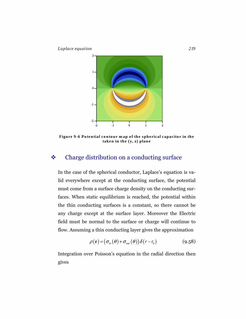
Laplace equation 219
Figure 9-6 Potential contour map of the spherical capacitor in the taken in the (y, z) plane
Charge distribution on a conducting surface
In the case of the spherical conductor, Laplace’s equation is va-
lid everywhere except at the conducting surface, the potential
must come from a surface charge density on the conducting sur-
faces. When static equilibrium is reached, the potential within
the thin conducting surfaces is a constant, so there cannot be
any charge except at the surface layer. Moreover the Electric
field must be normal to the surface or charge will continue to
flow. Assuming a thin conducting layer gives the approximation
( ) ( ) ( )( ) ( )0in out r rρ σ θ σ θ δ= + −r (9.58)
Integration over Poisson’s equation in the radial direction then
gives

220 Laplace equation
( ) ( )
( ) ( ) ( )( ) ( ) ( )
0 0
0 00
0
0 0 0
0 0
1 2
,
.
r rr
r r
r r r
out in total
E dr r r drr
E r E r E r
ε ε
ε εσ θ δ
εε ε θ
σ θ σ θ σ θε ε
+ +
− −
∂⎛ ⎞ = −⎜ ⎟∂⎝ ⎠+ − + = Δ
+= =
∫ ∫ (9.59)
where
0
0
00
0
0
( ) ,
( ) ,
in in inr r r
r r
out out outr r r
r r
Er
Er
σ θε
σ θε
==
==
∂Φ= − =∂
∂Φ= − =∂
(9.60)
This is a general result. For any conducting surface in static
equilibrium, the field component normal to the surface is
0
,nE σε
= (9.61)
which can easily be shown by constructing a infinitesimal Gaus-
sian pillbox near the surface, with one side in the conductor and
the other outside. The Electric field is discontinuous and points
out of the surface wherever the density is positive, and into the
surface, where it is negative. The surface charge density for the
interior surface is given by.
( ) ( )
( ) ( ) ( )
0
20 2 1
2 10 0 0
0 2 10 2 1
0 0
2 1cos ,
2 1cos .
llin
llr r
lin l
l
V a l r Pr r r
V a lP
r
θ
σ θ ε θ
∞+
+==
∞+
+=
+ ⎛ ⎞∂Φ− = − ⎜ ⎟∂ ⎝ ⎠+
= −
∑
∑ (9.62)
Likewise, for the outer surface,
Laplace equation 221
( ) ( ) ( )0 2 10 2 1
0 0
2 2cos .l
out ll
V a lP
rσ θ ε θ
∞+
+=
+= + ∑ (9.63)
9.6 Laplace equation with cylindrical boundary
conditions
Laplace’s equation in cylindrical coordinates is
( )2 2 2
2 2 2 2
1 1 , , 0.V r zr r r r z
φφ
⎛ ⎞∂ ∂ ∂ ∂+ + + =⎜ ⎟∂ ∂ ∂ ∂⎝ ⎠ (9.64)
Using separation of variables, one looks for product solutions of
the form ( ) ( ) ( ) ( ), ,V r z R r Z zφ φ= Φ . The function must satisfy
periodic boundary conditions in the azimulthal coordinate, sug-
gesting an expansion in Fourier series ( ) ime φφΦ ∼ should be
tried. This gives rise to the eigenvalue equation
2
22 for 0, 1, 2, .im ime m e mφ φ
φ∂ = − = ± ±∂
(9.65)
A similar expansion can be tried to separate the z dependence,
giving rive to two possible sets of solutions
Case I:
2 2 2
2 22 2 2 2
1, ( ) 0.kz ikz me k e k R rz r r r r φ
± ± ⎛ ⎞∂ ∂ ∂ ∂= + − + =⎜ ⎟∂ ∂ ∂ ∂⎝ ⎠ (9.66)
Case II:
222 Laplace equation
2 2 2
2 22 2 2 2
1, ( ) 0.ikz ikz me k e k R rz r r r r φ
± ± ⎛ ⎞∂ ∂ ∂ ∂= − + − − =⎜ ⎟∂ ∂ ∂ ∂⎝ ⎠ (9.67)
This gives rise to the Bessel equation in the first instance and to
the modified Bessel equation in the second instance. The com-
plete solutions are built from product solutions of the form
Case I: ( ) sinh( )
( , , )( ) cosh( )
m imI
m
J kr kzV r z e
N kr kzφφ ⎧ ⎫⎧ ⎫
⎨ ⎬⎨ ⎬⎩ ⎭⎩ ⎭
∼ (9.68)
and
Case II: ( ) sin( )
( , , ) .( ) cos( )
m imI
m
I kr kzV r z e
K kr kzφφ ⎧ ⎫⎧ ⎫
⎨ ⎬⎨ ⎬⎩ ⎭⎩ ⎭
∼ (9.69)
The choice of functions and allowed values of k are further re-
stricted by the boundary conditions. Let us consider the case
where one has Direchlet boundary conditions specified on the
surface of a can, defined to be a cylinder of height L and of ra-
dius R . If we are interested on solving Laplace’s equation in the
interior of the can, then only the ( )mJ kr and ( )mI kr Bessel func-
tions can be used. The other radial functions are divergent at the
origin. The solutions of Case I are appropriate if the potential is
zero on the surface of the cylinder. Then the allowed values of k
are restricted to fit the nodes of the Bessel function
( ) 0mJ kR = (9.70)
or
/ ,mn mmk x R= (9.71)
Laplace equation 223
where mmx are the zeros of the thm Bessel function. The general
solution to the first case is
( )1
sinh sinh ( )( , , ) ,sinh sinh
immn mnI mn mn m mn
n m mn mn
k z k L zV r z A B J k r ek L k L
φφ∞ ∞
= =−∞
⎛ ⎞−= +⎜ ⎟⎝ ⎠
∑ ∑ (9.72)
where the terms involving the A coefficients vanish on the sur-
face 0z = , and the terms involving the B coefficients vanish on
the surface z L= . Both terms vanish at the cylindrical surface
r R= . Notice that the z functions are pre-normalized to go to 1
on the non-vanishing surface. This is a common technique. Let
( , , )IAV r Lφ be the potential on the surface z L= .
Then, by integration,
( )
( ) ( )
( ) ( ) ( )
1
0
1
0
21 2
1
( , , ) /
/ /
22
imIA m mn
im immn m mn m m n
m n
m mnmn m mn mn
d xdxV r L J x r R e
A d xdxJ x r R J x r R e e
J xA J x A
π φπ
π φ φπ
φ φ
φ
π π
−
−
′−′ ′ ′−′ ′
++
=
⎛ ⎞= =⎜ ⎟
⎝ ⎠
∫ ∫∑ ∫ ∫ (9.73)
or
( ) ( )1
2 01
1 ( , , ) / .immn IA m mn
m mn
A d xdxV r L J x r R eJ x
π φπ
φ φπ
−
−+
= ∫ ∫ (9.74)
Likewise for the surface at 0z = :
( ) ( )1
2 01
1 ( , ,0) / .immn IB m mn
m mn
B d xdxV r J x r R eJ x
π φπ
φ φπ
−
−+
= ∫ ∫ (9.75)
224 Laplace equation
The remaining surface at r R= is a solution of the modified Bes-
sel equation, where the nodes of ( )Z z vanish at the end points of
the interval [ ]0, L :
( ) ( )( )
( , , ) sin ,m mn imII mn mn
m m mn
I k rV r z C k z e
I k Rφφ
∞
=−∞
= ∑ (9.76)
where
mnk L nπ= (9.77)
and 1
( , , ) sin .m
imII mn
m nm
n rIn z LV r z C e
n RL IL
φ
ππφ
π
∞ ∞
=−∞ =
⎛ ⎞⎜ ⎟⎛ ⎞ ⎝ ⎠= ⎜ ⎟ ⎛ ⎞⎝ ⎠⎜ ⎟⎝ ⎠
∑ ∑ (9.78)
Solving for the boundary conditions at surface C gives
1
( , , ) sin .imIIC mn
m n
n zV R z C eL
φπφ∞ ∞
=−∞ =
⎛ ⎞= ⎜ ⎟⎝ ⎠
∑ ∑ (9.79)
Integrating
( )1
( , , ) sin
sin sin
22
L imIICo
L im imm no
m n
mn mn
n zd dzV R z eL
n z n zd dzC e eL L
LC LC
π φπ
π φ φπ
πφ φ
π πφ
π π
−
−
∞ ∞′ −
′ ′−′ ′=−∞ =
⎛ ⎞⎜ ⎟⎝ ⎠′⎛ ⎞ ⎛ ⎞= ⎜ ⎟ ⎜ ⎟
⎝ ⎠ ⎝ ⎠⎛ ⎞= =⎜ ⎟⎝ ⎠
∫ ∫
∑ ∑∫ ∫ (9.80)
or
1 ( , , ) sin .
L immn IICo
n zC d dzV R z eL L
π φπ
πφ φπ
−
−
⎛ ⎞= ⎜ ⎟⎝ ⎠∫ ∫ (9.81)
Laplace equation 225
The total solution is a superposition of the above three solu-
tions:
( )1
1
( , , ) ( , , ) ( , , ) ( , , )
sinh sinh ( )sinh sinh
sin .
IA IB IIc
immn mnmn mn m mn
n m mn mn
mim
mnm n
m
V r z V r z V r z V r z
k z k L zA B J k r ek L k L
n rIn z LC e
n RL IL
φ
φ
φ φ φ φ
ππ
π
∞ ∞
= =−∞
∞ ∞
=−∞ =
= + +
⎛ ⎞−= +⎜ ⎟⎝ ⎠
⎛ ⎞⎜ ⎟⎛ ⎞ ⎝ ⎠+ ⎜ ⎟ ⎛ ⎞⎝ ⎠⎜ ⎟⎝ ⎠
∑ ∑
∑ ∑
(9.82)
Solution for a clyindrical capacitor
Consider a metal can with three metallic surfaces, held at three
different potentials. For simplicity, let the top and bottom sur-
faces be held at positive and negative high voltages 0V± , respec-
tively; Let the cylindrical side be grounded:
0 and 0IA IB IICV V V V= − = = (9.83)
By cylindrical symmetry, the sum over m vanishes, except for
0.m = The coefficients to be determined are
( ) ( )100 0 0 02 0
1 0
2 / .n n nn
VA B xdxJ x r RJ x
= − = ∫ (9.84)
where all the other coefficients vanish due to the boundary con-
ditions. This integral can be solved by use of the recursion for-
mula
226 Laplace equation
1( ) ( ).p pp p
d x J x x J xdx −⎡ ⎤ =⎣ ⎦ (9.85)
Letting 1p = gives
( ) ( )1 10 0 12 2 00 0
1 1( ) ( ) ,a a J a
xdx J ax x dx J x x J xa a a
′ ′ ′ ′ ′= = =∫ ∫ (9.86)
Leading to the result
( )0
0 00 1 0
2 .n nn n
VA Bx J x
= − = (9.87)
Putting it all together, the potential everywhere inside the can is
given by
( ) ( ) ( )0 0 00 0
1 0 1 0 0 0
2 sinh sinh ( ), ,sinh sinh
n nn
n n n n n
V k z k L zV r z J k rx J x k L k L
∞
=
⎛ ⎞−= −⎜ ⎟⎝ ⎠
∑ (9.88)
where 0 /on nk x R= .
10. Time dependent differential equations
Time changes all things. It is responsible for evolution at the
biological and cosmological scales. Time makes motion possible.
It is the apparent casual behavior of events that allows us to
make sense of our universe. Newton considered time to flow un-
iformly for all observers, a scalar parameter against which our
lives are played out. Special relativity showed that space and
time are geometrically related and transform like vectors in
Minkowski space. But there is an arrow of time, nonetheless.
There is no continuous Lorentz transform that takes a time-like
vector with a positive time direction and converts it to one with
a negative time sense. Thermodynamic processes are subject to
the laws of entropy, which may signal the eventual heat death of
our universe. More importantly for our purposes, the motions of
classical particles are well behaved single-valued functions of
time. Given a complete set of initial conditions and an adequate
theoretical framework, we can project the past into the future
and make useful predictions about outcomes. The solution of
the initial value problem forms the core of dynamics.
10.1 Classification of partial differential equations
Laplace’s equation
228 Time dependent differential equations
( )2 0∇ Ψ =r (10.1)
is an example of an elliptic differential equation, so-called be-
cause the differential operator takes on a elliptic form
2 2 2x y zD D D+ + . Such equations have solutions if the function or its
derivative is defined on a closed, bounding surface. Adding a po-
tential term to the operator does not change the character of the
solution. For example, the equation,
( )( ) ( )2 0K∇ + Ψ =r r (10.2)
is also classified as an elliptic differential equation, and the equ-
ation has a unique, stable solution if it satisfies Direchlet or
Neumann boundary conditions.
We are used to thinking of time as an additional dimension, but
it is a peculiar one. Solutions for time dependent problems are
defined in terms of specifying a set of initial conditions, If one
considers time as a fourth coordinate, then the initial value
problem is equivalent to a boundary value problem, where the
appropriate boundary conditions are to be specified over an
open hyper-surface, usually defined at a constant time, 0t t= .
Mathematically, the character of the differential operator differs
from the elliptic character of Laplace’s equation.
For example, the diffusion equation
( )22
1 , 0ttα∂⎛ ⎞∇ − Ψ =⎜ ⎟∂⎝ ⎠
r (10.3)
Time dependent differential equations 229
is linear in time and the differential operator has a parabolic
signature 2 2i ti
D Dα−−∑ . It is an example of a parabolic diffe-
rential equation. Analysis shows that stable unique solutions for
one direction in time can be found using either Direchlet or
Neumann boundary conditions on a open surface. The arrow of
time is forward, and thermodynamic systems flow in the direc-
tion of increasing entropy.
The wave equation
( )2
22 2
1 , 0tv t
⎛ ⎞∂∇ − Ψ =⎜ ⎟∂⎝ ⎠r (10.4)
is another common time-dependent partial differential equa-
tion. It is second order in time, but its time signature has the
opposite sign from the Laplacian operator: 2 2 2i ti
D c D−−∑ . This
is an example of a hyperbolic differential equation. The wave
equation has stable solutions in either time direction, but be-
cause it is second order in time, it satisfies Cauchy boundary
conditions on an open surface. Cauchy boundary conditions re-
quire that both the function and its normal derivative be speci-
fied at some initial or final time 0t t= . Finally, the Schrödinger
equation
( )2
2 , 02
i tm t
⎛ ⎞− ∂∇ − Ψ =⎜ ⎟∂⎝ ⎠r (10.5)
is first order in time. Like the diffusion equation, it satisfies Di-
rechlet or Neumann boundary conditions on an open surface.
230 Time dependent differential equations
Because of the imaginary i in the definition of the time opera-
tor, the operator is Hermitian, and the equation has sable solu-
tions in either time direction. Table 10-1 lists some common dif-
ferential equations and their boundary conditions.
Removal of the time dependence in any of the above equations
leads to the Helmholtz equation, which has an elliptic character.
Therefore, to solve these equations completely, one must specify
not only the functions and/or their derivatives throughout the
volume at some initial time, but also specify their behavior at
some bounding surface for all time. If, however, the behavior at
the boundary is static in character, then the problem can be se-
parated into two problems:
• the behavior at the static boundary can be fitted to a general
solution to the time-independent equation, ignoring the time
behavior of this part of the problem, (this usually results in
Laplace’s equation), and
• a particular solution to the time-dependent problem can be
added to this which satisfies the trivial boundary condition
that either the function or its normal derivative vanish at the
bounding surface.
The total solution is then
( ) ( ) ( ), ,static particulart tΨ =Ψ +Ψr r r, (10.6)
where ( )staticΨ r is given the job of satisfying any non-trivial, but
static, boundary conditions at the enclosing surface.

Time dependent differential equations 231
Table 10-1 A list of common partial differential equations and their allowed boundary conditions
Character Equation Boundary Conditions
Elliptic Laplace and
Helmholtz Equa-
tions
Direchlet or Neumann on a
closed surface.
Hyperbolic Wave Equation Cauchy on an open surface
Parabolic Diffusion Equa-
tion
Direchlet or Neumann on
an open surface. (stable in
one direction)
Complex
Parabolic
Schrödinger Eq-
uation
Direchlet or Neumann on
an open surface.
The usual procedure is to first solve for the steady state back-
ground term, and subtract its contribution from the initial con-
dition of the function in the interior volume. The remaining time
dependent problem can then be solved by separation of va-
riables, in terms of product solutions
( ) ( ) ( )( ) , ,particular k k kt T tΨ =Φr r (10.7)
where ( )kΦ r are the stationary normal nodes of the space prob-
lem. These normal modes are solutions to the Helmholtz equa-
tion

232 Time dependent differential equations
( ) ( )2 2 ,k∇ Φ = − Φr r (10.8)
in the absence of any complicating additional potential term.
10.2 Diffusion equation
The diffusion equation is often used to model stochastic heat
flow. It is valid where the thermal resistance is sufficient, and
time scales long enough, to allow definition of a local tempera-
ture in a thermodynamic medium. It can be derived from two
basic assumptions
• The gradient of the temperature T is proportional to the
heat flux T∝∇Q .
• the divergence of the heat flux is proportional to the rate of
change of temperature / .T t∇⋅ ∝ ∂ ∂Q
Colloquially, the first equation states that heat flows from hot to
cold, while the second states that temperature changes fastest
where the divergence is greatest. When the temperature reaches
a steady state condition one gets Laplace’s equation, which has
zero divergence:
20 0.T∇⋅ = ⇒∇ =Q (10.9)
In the general case, before steady state equilibrium has been
reached, the two assumptions give rise to the diffusion equation
22
1 ,TTtα
∂∇ =∂
(10.10)
Time dependent differential equations 233
where 2α is a property of the material that is proportional to the
thermal conductivity.
The time eigenstates of this equation are given by
( ) ( )2
.k tT t e α±= (10.11)
The negative sign is chosen, since one expects the system to re-
lax to a steady state temperature distribution, given sufficient
time. The terms with positive signs represent the time reversed
problem, which is unstable, since the terms exponentially di-
verge. The boundary values to the time independent Helmholtz
equation, (10.8), restrict the possible values of k , which in turn
restrict the 1/ e decay times of the normal modes
( )21/ .kt kα= (10.12)
The total solution can be written as
( ) ( ) ( ) /, .kt tsteadyState k kk
T t T A e−= + Φ∑r r r (10.13)
Note that the modes with larger values of k decay faster (since
they have smaller time constants), and that
( ) ( )lim , .steadyStatetT t T
→∞=r r (10.14)
Note as well that the initial value of the particular solution to the
time dependent problem is not given by ( ),0T r , but is given in-
stead by the difference
( ) ( ) ( ), , ,particular steadyStateT t T t T= −r r r (10.15)

234 Time dependent differential equations
evaluated in the limit as 0t → . The coefficients kA are deter-
mined by solving the initial value problem
( ) ( ) ( ) ( ),0 ,0 .particular steadyState k kkT T T A= − = Φ∑r r r r (10.16)
Example: Heat flow in a bar
Consider a long, thin iron bar that is insulated along its length,
but not at its ends. Originally the bar is in thermal equilibrium
at room temperature, 22 C , but at time 0t = , one end is inserted
into a vat of ice water at 00 C . Calculate the temperature distri-
bution in the bar as a function of time and find its final steady
state temperature distribution.
Since the bar is thin and its sides insulated, this can be treated
as a problem in one space dimension x .
The initial condition is given by the uniform temperature distri-
bution,
( ,0) 22 .T x C= (10.17)
The steady state condition, treating the room and the vat as infi-
nite heat sinks, gives the static boundary conditions,
(0, ) 22 and ( , ) 0.T t C T L t= = (10.18)
The steady state problem is a solution to Laplace’s equation in
one-dimension
2
2
( ) 0,d T xdx
= (10.19)

Time dependent differential equations 235
which has the solution
0( ) ,ssxT x T TL
= −Δ (10.20)
where 0 22T T C= Δ = . Therefore, the steady state limit corres-
ponds to a uniform temperature drop from the hot face to the
cold face of the bar.
The initial value problem for the particular time-dependent so-
lution is given by
( ) ( )0,0 .p ssxT x T T x TL
= − = Δ (10.21)
This excess temperature component decays in time, and the sys-
tem relaxes to its steady-state limit. The normal modes of the
time-dependent problem as sine functions that go to zero at the
end points of the interval [ ]0, L . Therefore the product solutions
take the form
( ) ( ) ( ) /sin ,kt tk kx T t kx e−Φ = (10.22)
where
( )2/ and / .kk n L t L nπ πα= = (10.23)
The solution to the initial value problem is
( ) 0,0 sin ,p nn
n xT x T ALπ= ∑ (10.24)
with coefficients given by
236 Time dependent differential equations
( )
00 0
,02 2sin sin .L L
pn
T x n x x n xA dx dxL T L L L L
π π= =∫ ∫ (10.25)
The total solution summing the steady state and time dependent
contributions is
( ) ( )2 2/0, 1 sin .n t L
nn
x n xT x t T A eL L
παπ −⎛ ⎞= − +⎜ ⎟⎝ ⎠
∑ (10.26)
The decay times fall as 2~ 1/ n , so after sufficient time has passed
only the first few modes are of importance. In the time-reversed
problem the opposite situation arises, the large n components
would grow exponentially as one goes further back into the past.
The solution of the time reverse problem depends sensitively on
the initial conditions, one must be able to bound very small high
frequency components to impossibly small constraints, and the
results are therefore unstable under small perturbations. The
diffusion equation can be reliably used only to predict the future
behavior of a thermodynamic system.
10.3 Wave equation
Material waves are time-dependent fluctuations in a medium
that transport energy and momentum to the boundaries of the
medium. They have a characteristic velocity of propagation that
is a property of the specific medium. Maxwell showed that a
self-consistent solution of the equations of electricity and mag-
netism, then though of as disparate, but interacting, fields re-
Time dependent differential equations 237
quired that the electric and magnetic fields simultaneously satis-
fy a wave equation where the wave velocity is determined by the
speed of light. From that he deduced that the origin of light is
fundamentally electromagnetic in character. Marconi later con-
firmed this hypothesis with the discovery of radio waves, in-
duced by the oscillation of electric charges in an antenna. Before
then, the Michelson-Morley experiment had already demon-
strated that the speed of light in free space was independent of
the properties of a underlying medium, referred to as the either.
Today we are comfortable with the notion that the electromag-
netic field is an intrinsic property of spacetime and does not re-
quire an underlying medium for its propagation.
Waves are classified as to whether the amplitude of oscillation is
along (longitudinal) or transverse to the direction of propaga-
tion. Vibrating strings and waves on the surface of a pond are
examples of transverse waves, while sound in a gaseous medium
is a purely longitudinal disturbance, since gases cannot support
a shear force. Waves in solids are more complex, having both
transverse and longitudinal modes, usually with different veloci-
ties of propagation. In most cases, the linear character of the
wave equation is the result a small amplitude approximation to
a more complex non-linear theory, one which includes dissipa-
tive and dispersive contributions.
In its simplest form, the wave equation relates the second-order
space and time derivatives of some fluctuation, to the wave ve-
locity v :
238 Time dependent differential equations
( )2
22 2
1 , 0.tv t
⎛ ⎞∂∇ − Ψ =⎜ ⎟∂⎝ ⎠r (10.27)
In the case of a string or a surface wave, this fluctuation is a
transverse displacement. In the case of sound vibrations in a
medium it represents the propagation of a pressure disturbance.
The stored energy density of the wave is proportional to the
square of this amplitude. Solution of the wave equation often in-
volves solving for the normal modes of oscillation in time via se-
paration of variables. This involves separating the wave into it
frequency components in the time domain:
( ) ( ) ( ) ( )/
, cos sin ,i tk k
k ct e A t B tω
ωω ω
ω ω±±
=Ψ = Φ = +∑ ∑r r r r (10.28)
where the wave number /k cω= is often restricted to discrete
values by the boundary conditions at the bounding surface of the
medium. For fixed frequency, the normal modes of oscillation,
which can be denoted as ( )kΦ r , are solutions to the time inde-
pendent Helmholtz equation (10.8). Note that there are two ini-
tial conditions that must be satisfied. At time 0t = , one must
specify both the initial function and its time derivative, i.e.,
( ) ( )/
, 0 coskk c
A tω
ω=
Ψ = ∑r r (10.29)
and
( ) ( )/
,0 sin ,kk c
B tω
ω ω=
′Ψ = ∑r r (10.30)
where

Time dependent differential equations 239
( ) ( )( ) 0, 0 , / .
tt t
=′Ψ = ∂Ψ ∂r r (10.31)
Pressure waves: standing waves in a pipe
Sound waves in a gaseous medium are longitudinal waves. At a
closed rigid boundary, the longitudinal displacement of the me-
dium goes to zero, and one has a displacement node that the
boundary. Correspondingly, the pressure at such a boundary is a
maximum or minimum and therefore the pressure has an anti-
node that the boundary. Stated in other terms, the pressure at a
closed boundary satisfies Neumann boundary conditions
closed boundary
( , ) 0.P x tt
∂ =∂
(10.32)
At an open surface, there is no impedance and the pressure dif-
ferential across the boundary drops to zero. Therefore a statio-
nary wave would satisfy Direchlet boundary conditions at an
open boundary.
open boundary
( , ) 0.P x t = (10.33)
If one applies this to an organ pipe of length L with a open end
at 0x = and a closed end at x L= , the allowed standing wave
nodes are
( )( , ) sin( ) cos ,P x t kx A tω φ∝ +⎡ ⎤⎣ ⎦ (10.34)

240 Time dependent differential equations
where φ is a phase angle given by the initial conditions, and
( , )P x t is a stationary solution to the wave equation
( )2 2
2 2 2
1 , 0.P x tx v t
⎛ ⎞∂ ∂− =⎜ ⎟∂ ∂⎝ ⎠ (10.35)
The wave velocity in a gas is given by /v Y ρ= where Y is
Young’s modulus (one-third of the bulk modulus) and ρ is the
density. The boundary conditions for a half-open pipe require
( )12 ,kL n π= + (10.36)
with an angular frequency given by
kvω = . (10.37)
Usually a organ pipe is sounded to emphasize a nearly pure
harmonic note at the fundamental frequency, corresponding to
0n = .
The struck string
The struck string on a string instrument satisfies Direchlet
boundary conditions at its end points
0
( , ) 0.x L
xy x t =
== (10.38)
where y is the transverse displacement of the string from its
equilibrium position. Its normal modes of motion are given by
Time dependent differential equations 241
( ) sin ,nn xxLπΦ = (10.39)
where / /k n L vπ ω= = . The wave velocity is given by /v T μ=
where T is the tension and μ is the mass per unit length. The
general solution can be written as
( )1
, cos sin sin .n nn
n vt n vt n xy x t A BL L Lπ π π∞
=
⎛ ⎞= +⎜ ⎟⎝ ⎠
∑ (10.40)
The string has a fundamental harmonic for / 2 / 2nv Lω π = with
a rich texture of harmonics depending on how the string is
struck. The actual sound produced by a stringed instrument is
significantly modified by its sound board, but let’s analyze the
response of the string in isolation. The initial conditions are giv-
en by
( )1
,0 sinnn
n xy x ALπ∞
=
=∑ (10.41)
and by
( )1
,0 sinn nn
n xy x BLπω
∞
=
′ =∑ (10.42)
where /n n v Lω π= .
The solution for the coefficients are given by
0
2 sin ( ,0)L
nn xA y x dx
L Lπ= ∫ (10.43)
and
242 Time dependent differential equations
0
2 sin ( ,0) .L
nn
n xB y x dxL L
πω
′= ∫ (10.44)
As an example, suppose the string is struck at its exact middle
by an impulsive force. Then the initial conditions can be ex-
pressed approximately by a delta-function contribution to the
instantaneous velocity distribution at the initial time 0t = :
0( ,0) 0; ( ,0) ( / 2)y x y x x Lλ δ′= = − (10.45)
Therefore, 0nA = and
0
2 2sin ( / 2) sin( / 2).L
nn
n x LB x L dx nL L n v
π δ πω π
= − =∫ (10.46)
Only terms odd in n contribute, with the time evolution of the
original delta function given by
( ) ( )( )
( ) ( )0
1 2 2 1 2 1, sin sin .
2 1
n
n
L n x n vty x t
n v L Lπ π
π
∞
=
⎛ ⎞− + += ⎜ ⎟
⎜ ⎟+⎝ ⎠∑ (10.47)
The normal modes of a vibrating drum head
A circular drum head can be approximated as a vibrating mem-
brane, clamped at its maximum radius 0r . The amplitude of
transverse motion in the z direction is a solution to the wave
equation
( )2
22 2
1 , 0Z tv t
⎛ ⎞∂∇ − =⎜ ⎟∂⎝ ⎠r (10.48)
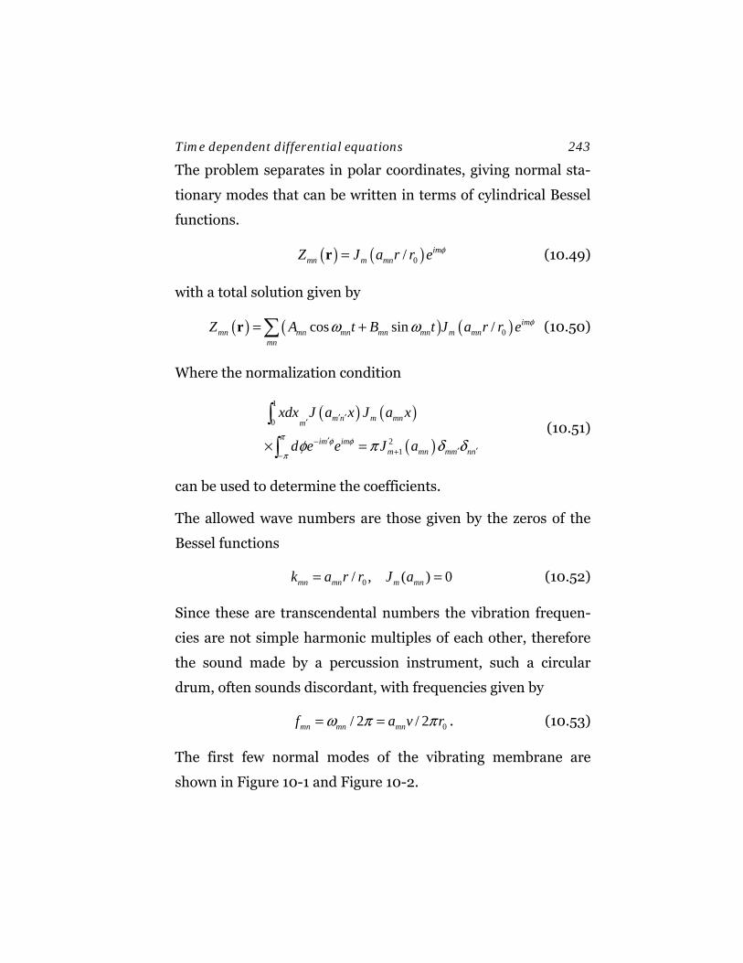
Time dependent differential equations 243
The problem separates in polar coordinates, giving normal sta-
tionary modes that can be written in terms of cylindrical Bessel
functions.
( ) ( )0/ immn m mnZ J a r r e φ=r (10.49)
with a total solution given by
( ) ( ) ( )0cos sin / immn mn mn mn mn m mn
mnZ A t B t J a r r e φω ω= +∑r (10.50)
Where the normalization condition
( ) ( )
( )
1
0
21
m n m mnm
im imm mn mm nn
xdx J a x J a x
d e e J aπ φ φ
πφ π δ δ
′ ′′
′−′ ′+−
× =
∫
∫ (10.51)
can be used to determine the coefficients.
The allowed wave numbers are those given by the zeros of the
Bessel functions
0/ , ( ) 0mn mn m mnk a r r J a= = (10.52)
Since these are transcendental numbers the vibration frequen-
cies are not simple harmonic multiples of each other, therefore
the sound made by a percussion instrument, such a circular
drum, often sounds discordant, with frequencies given by
0/ 2 / 2mn mn mnf a v rω π π= = . (10.53)
The first few normal modes of the vibrating membrane are
shown in Figure 10-1 and Figure 10-2.
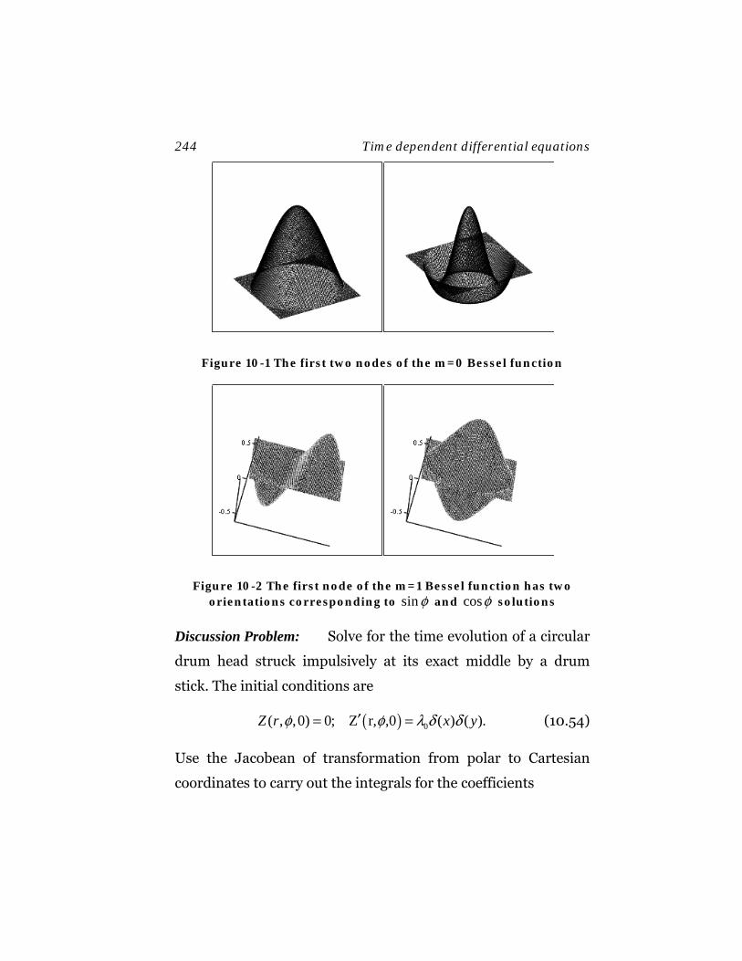
244 Time dependent differential equations
Figure 10-1 The first two nodes of the m=0 Bessel function
Figure 10-2 The first node of the m=1 Bessel function has two orientations corresponding to sinφ and cosφ solutions
Discussion Problem: Solve for the time evolution of a circular
drum head struck impulsively at its exact middle by a drum
stick. The initial conditions are
( ) 0( , ,0) 0; Z r, ,0 ( ) ( ).Z r x yφ φ λ δ δ′= = (10.54)
Use the Jacobean of transformation from polar to Cartesian
coordinates to carry out the integrals for the coefficients
Time dependent differential equations 245
( )( ) ( ) ( ) 2 (0).rdrd f dxdyf x y fφ δ δ π= =∫ ∫r r (10.55)
Note that only 0m = terms contribute to the result.
10.4 Schrödinger equation
The Schrödinger equation is given by
( , )( , ) ,tH t it
∂ΨΨ =∂rr (10.56)
where H is the Hamiltonian operator and 2( , )tΨ r represents
the probability density of finding a particle at a given location in
space. Therefore the equation represents the evolution of the
probability amplitude in time. If H is a Hermitian operator, the
probability is conserved and a single particle state is assigned a
total unit probability of being located somewhere in space
23 ( , ) 1.d r tΨ =∫ r (10.57)
The equation is first order in time, like the diffusion equation.
Unlike the diffusion equation the time behavior is oscillatory,
therefore the time evolutions is well-behaved for propagation in-
to past or future time. Separation of variables gives product so-
lutions of the form
( , ) ( ) ,i tk kt e ω−Ψ = Ψr r (10.58)
where
( ) ( ) ( ) ( )2 / 2k k k k kH E k mωΨ = Ψ = Ψ =r r r (10.59)
246 Time dependent differential equations
and k is a solution to the eigenvalue equation for the stationary
modes of motion.
10.5 Examples with spherical boundary conditions
Quantum mechanics in a spherical bag
The Time-Independent Schrödinger equation for a freely mov-
ing particle, in the absence of a potential, is given by
2 2
222 2
Hm m
= = − ∇p. (10.60)
This can be rewritten as the Helmholtz equation
2 2( ) ( )k∇ Ψ = − Ψr r , (10.61)
where ( )2
2k
Em
= .
If the particle is put into a infinite well of radius 0r r= , the wave
function vanishes at the spherical boundary. The product solu-
tions can then be written as
( ) ( ) ( ) ( ), , 03 20 1 ,
2 / , ,lm n l l n lml l n
j a r r Yr j a
θ φ+
Ψ =r (10.62)
where the normalization is chosen so that
( ) ( )0 2, ,0
1.r
lm n lm nr dr d ∗ΩΨ Ψ =∫ ∫ r r (10.63)
Time dependent differential equations 247
The allowed eigenvalues for the energies are constrained by the
boundary conditions to the discrete set
( )2
0/.
2ln
nl nl
a rE
mω= = (10.64)
The energy does not depend on the m state value, so the energies
are ( )2 1l + -fold degenerate for any given l value. In general the
total wave function need not be in an eigenstate of energy, so the
wave function at some initial time can be written as a sum over
all possible states
( ) ( ) ,nlm nlmnlm
cΨ = Ψ∑r r (10.65)
where 2
nlmc denotes the fractional probability that it is any given
state.
The time evolution of this wave packet is given by
( ) ( ), .nli tnlm nlm
nlmt c e ω−Ψ = Ψ∑r r (10.66)
If a particle where known to be localized at some point within
the sphere at a fixed time, the different time behaviors of normal
modes would cause its position probability to disperse in time.
Heat flow in a sphere
Consider a sphere heated to a uniform temperature 0T at some
initial time 0t , then immediately dropped into a quenching bath
248 Time dependent differential equations
at a temperature fT . Calculate it temperature distribution at lat-
er times.
The temperature distribution satisfies the initial condition
( )0 0,T t T=r (10.67)
and must satisfy the boundary condition
( )0
0, for .fr rT t T t t
== >r (10.68)
Therefore, it can be expanded in the series solution
( ) ( ) 0( ) /0
1, ( , ) / ,lmnt t t
f lmn lm l l nlm n
T t T A Y j a r r eθ φ∞
− −
=
= +∑ ∑r (10.69)
where fT is the steady-state solution. By spherical symmetry,
only 0l m= = terms contribute, and the time constants are given
by ( ) 2
0/lmn lnt a rα−
= . Therefore the solution can be written as
( ) ( ) 0( ) /0 0 0
1
, / ,lmnt t tf n n
n
T t T A j a r r e∞
− −
=
− =∑r (10.70)
where 004n nA Aπ= , and 0na nπ= , so that
( )2200 0 / .nt r nπα= (10.71)
The initial condition is given by
( )0 0 01
/ .f n l nn
T T T A j a r r∞
=
Δ = − =∑ (10.72)
Therefore, the solution is given by
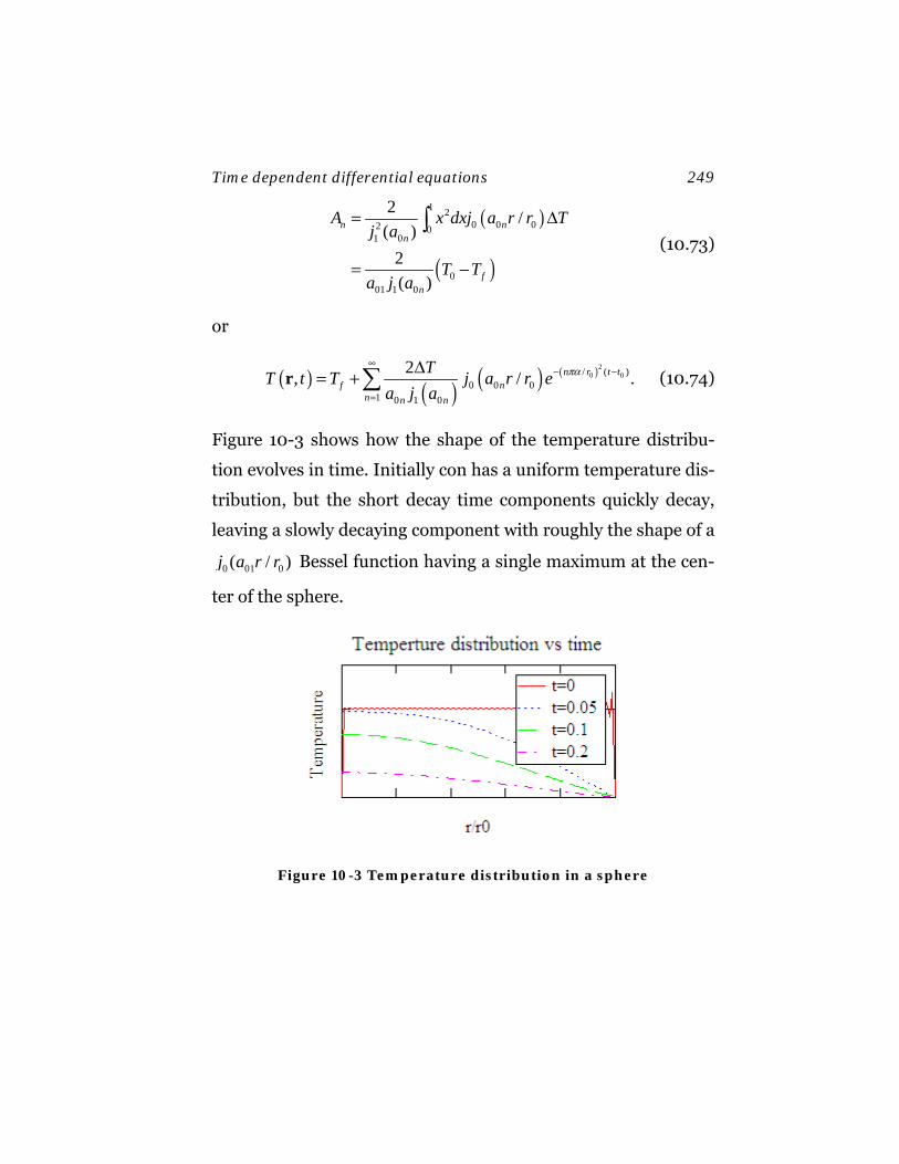
Time dependent differential equations 249
( )
( )
1 20 0 02 0
1 0
001 1 0
2 /( )
2( )
n nn
fn
A x dxj a r r Tj a
T Ta j a
= Δ
= −
∫ (10.73)
or
( ) ( ) ( ) ( )20 0/ ( )
0 0 01 0 1 0
2, / .n r t tf n
n n n
TT t T j a r r ea j a
πα∞
− −
=
Δ= +∑r (10.74)
Figure 10-3 shows how the shape of the temperature distribu-
tion evolves in time. Initially con has a uniform temperature dis-
tribution, but the short decay time components quickly decay,
leaving a slowly decaying component with roughly the shape of a
0 01 0( / )j a r r Bessel function having a single maximum at the cen-
ter of the sphere.
Figure 10-3 Temperature distribution in a sphere
250 Time dependent differential equations
10.6 Examples with cylindrical boundary conditions
Normal modes in a cylindrical cavity
The normal frequencies of oscillation in a cylindrical cavity dif-
fer depending on whether the time-dependent equation satisfies
Direchlet or Neumann boundary conditions. In either case, one
is dealing with the interior solutions to the Helmholtz equation
(10.8), therefore the solutions can be written in the general form
( ) cos /( ) .
sin /im
k m mn
n z LJ k r e
n z Lφ π
π⎧ ⎫
Φ = ⎨ ⎬⎩ ⎭
r (10.75)
For Direchlet Boundary conditions, the normal modes satisfy
( )
( )0
( ) sin /
and 0,
imk m mn
m mn
J k r e n z L
J k r
φ πΦ =
=
r (10.76)
while, in the Neumann case, one has
( )
( )0
( ) cos /
and 0.
imk m mn
m mn
J k r e n z L
J k r
φ πΦ =′ =
r (10.77)
Temperature distribution in a cylinder
For time-independent cylindrical boundary conditions, the
steady-state temperature ( )ssT r is calculated as a solution to
Laplace’s equation, and the result subtracted from the initial
temperature distribution within the cylindrical volume. The
Time dependent differential equations 251
time-dependent temperature profile for a cylinder of radius 0r
and height L is then given by
( ) ( )
( ) /0
1 1
,
/ sin ,lmn
ss
t timmnl m mn
m n l
T t T
l zA J a r r e eL
φ π∞ ∞ ∞−
=−∞ = =
−
= ∑ ∑∑
r r (10.78)
where mna are the zeroes of the Bessel functions and
2 2
2 2 2
0
1 ,mnmnl
mnl
a l kt r L
πα α⎛ ⎞⎛ ⎞ ⎛ ⎞⎜ ⎟= + =⎜ ⎟ ⎜ ⎟⎜ ⎟⎝ ⎠⎝ ⎠⎝ ⎠
(10.79)
Orthogonality can be used to determine the coefficients of the
time dependent part of the problem:
( ) ( )
( ) ( )
1
02 01
0
12
2 /
2 sin ,0 .
immnl
m mnm mn
L
ss
A e
xdxJ a r rJ a
l zdz T TL L
π φππ
π
−
−
−
=
×
× −⎡ ⎤⎣ ⎦
∫
∫
∫ r r
(10.80)
11. Green’s functions and propagators
When one exerts a force on a dynamic system, the response is a
disturbance of the system that propagates in time. Up to now we
have concentrated on the solution of linear homogeneous sys-
tems. But such systems do not start moving on their own. Ho-
mogeneous equations have the trivial solution that the field and
its derivates vanish everywhere. Their motion arises from flow
of energy and momentum into or out of the system, expressed in
terms of boundary conditions, and ultimately, to the action of
sources that are often inhomogeneous in origin. A complicated
force acting for an extended period of time, or over an extended
volume of space, can be decomposed into point-like impulses. If
the equation is linear, the net effect can be expressed as a super-
position of these influences. This is the essence of the Green’s
function technique for solving inhomogeneous differential equa-
tions. A Green’s function represents the potential due to a point-
like source meeting certain particular boundary conditions. If
the equation is time dependent, the Green’s function is often re-
ferred to as a propagator. The positive time propagator propa-
gates a signal into future times, and the negative time propaga-
tor propagates a signal backwards in time.

Green’s functions and propagators 253
11.1 The driven oscillator
Consider a driven oscillator that might, for example, be an ap-
proximation to a swing with a child on it. When one pushes the
swing, it begins to move. If one pushes in phase with a existing
motion, the amplitude grows. Before and after the introduction
of the time dependent force, assuming that the amplitude re-
mains small, the motion of the swing is a solution to a linear
homogeneous differential equation with a characteristic angular
frequency of oscillation oω . It behaves like a driven oscillator.
The differential equation of motion for the driven oscillator can
be written as
2
202
( ) 0,( )
0 0,f t td y t
tdtω
>⎛ ⎞ ⎧+ = ⎨⎜ ⎟ ≤⎩⎝ ⎠
(11.1)
where ( )f t is a generalized force that begins acting at some time
0t > . The initial state of the system is a solution to the homoge-
neous equation
2
202 ( ) 0,h
d y tdt
ω⎛ ⎞+ =⎜ ⎟
⎝ ⎠ (11.2)
with a solution
0 0( ) cos sin ,hy t A t B tω ω= + (11.3)
where the coefficients A and B can be determined from the ini-
tial conditions
0(0) , (0) .h hy A y Bω′= = (11.4)
254 Green’s functions and propagators
The complete solution to the inhomogeneous problem is a sup-
position of this homogeneous solution with a particular solution
to the inhomogeneous problem that has the swing initially at
rest.
( ) ( ) ( ),h py t y t y t= + (11.5)
where
2
202
( ) 0( )
0 0p
f t td y ttdt
ω>⎛ ⎞ ⎧
+ = ⎨⎜ ⎟ ≤⎩⎝ ⎠ (11.6)
and
( ) ( ) 0 for 0p py t y t t′= = ≤ (11.7)
The solution to the driven oscillator problem can be expressed
as a convolution over a simpler problem involving the response
of the system to an impulsive force of unit magnitude acting at
an instance of time 0t′ > :
2
202 ( , ) ( ), 0d g t t t t t
dtω δ+
⎛ ⎞ ′ ′ ′+ = − >⎜ ⎟⎝ ⎠
(11.8)
satisfying the boundary condition
( , ) 0g t t t t+ ′ ′= < (11.9)
( , )g t t+ ′ is the positive time propagator that will propagate the
solution forward in time. The general solution to the problem
can then be written as
0
( ) ( ) ( ) ( , ) .t
hy t y t f t g t t dt′ ′ ′= + ∫ (11.10)

Green’s functions and propagators 255
The proof is straightforward:
2 22 20 02 2
2202 0
22020
0
( ) ( )
( ) ( , )
0 ( ) ( , )
( ) ( ) ( ).
h
t
t
t
d dy t y tdt dt
d f t g t t dtdt
df t g t t dtdt
f t t t dt f t
ω ω
ω
ω
δ
⎛ ⎞ ⎛ ⎞+ = +⎜ ⎟ ⎜ ⎟
⎝ ⎠ ⎝ ⎠⎛ ⎞ ′ ′ ′+ +⎜ ⎟⎝ ⎠
⎛ ⎞′ ′ ′= + +⎜ ⎟⎝ ⎠
′ ′ ′= − =
∫
∫
∫
(11.11)
In another way of looking at the problem, the Green’s function is
a solution to the homogeneous equation for t t′≠ . Because of the
delta function source term, it has a discontinuity in its derivative
at t t′= :
( )0 0
lim ( ) lim 1.t t
tty t t t dt
ε ε
εε εεδ
′+ ′+
′−→ →′−′ ′ ′= − =∫ (11.12)
Therefore, the solution can be written as
( ) 0
0
0 , sin ,
t tg t t t t tω
ω+
′<⎧⎪′ = ⎨ ′>⎪⎩
(11.13)
or more compactly as
( ) ( )0
0
sin, tg t t t tωω+ ′ ′= Θ − (11.14)
where ( )t t′Θ − is the step function distribution given by
( ) 0 ,1 .
t tt t
t t′<⎧′Θ − = ⎨ ′>⎩
(11.15)
256 Green’s functions and propagators
The step function satisfies the differential equation
( ) ( ) ,d t t t tdt
δ′ ′Θ − = − (11.16)
which can be demonstrated by direct integration of the equa-
tion.
Suppose the swing were initially at rest, and that the force acts
for a finite time max0 t t′< < . The asymptotic state of the system
can then be written as
( )
max max 00 0
0
0 0 0 max
sin ( )( ) ( ) ( , ) ( )
sin for ,
t t
t
t ty t f t g t t dt f t dt
y t t t
ωω
ω φ
′>
′−′ ′ ′ ′ ′= =
= + >
∫ ∫ (11.17)
where the solution for large times is a solution for the homoge-
neous equation with an amplitude and phase determined by the
convolution of the green’s function with the time dependent
force over the period for which it was active.
It is unrealistic to expect a swing to oscillate forever, so let’s in-
troduce a subcritical damping force with a damping coefficient
γ . The modified equation of motion is
2
202
( ) 0( )
0 0,f t td d y t
tdt dtγ ω
>⎛ ⎞ ⎧+ + = ⎨⎜ ⎟ ≤⎩⎝ ⎠
(11.18)
which has the homogeneous solution
( )/ 2( ) sin ,thy t Ae tγ ω φ− ′= + (11.19)
where
Green’s functions and propagators 257
2
20 .
4γω ω′ = + (11.20)
The Green’s function solution to the equation of motion is given
by
( ) ( ) ( )/ 2 sin( , ) .t t t t
g t t e t tγ ωω
′− −+
′ ′−′ ′= Θ −
′ (11.21)
It is straight forward to show that
( , ) 0g t t t t+ ′ ′= < (11.22)
and
0
lim ( , ) 1 .t t
t tg t t
ε
ε ε
′= +
+→ ′= −′ ′ = (11.23)
11.2 Frequency domain analysis
Another approach to this problem is to resolve the time spectra
of the force into its frequency components. This leads to a
Fourier transformation. Given an equation of the form
2
202 ( ) ( )d d y t f t
dt dtγ ω⎛ ⎞
+ + =⎜ ⎟⎝ ⎠
(11.24)
one can resolve the force into frequency components
( )( ) .i tf t f e dωω ω∞ −
−∞= ∫ (11.25)
Similarly, the response can be written as

258 Green’s functions and propagators
( )( ) .i ty t y e dωω ω∞ −
−∞= ∫ (11.26)
Leading to the Fourier transform equation of motion
( ) ( ) ( )2 20 ,i y w fω γω ω ω− − + = (11.27)
which has the solution
( ) ( )( ) ( )02 2
0
( , ) .R
fy f
iω
ω ω ω ωω γω ω
= = Γ− − +
(11.28)
The response at a given frequency has a typical resonance line
shape, as seen in Figure 11-1, where the norm-square of RΓ .is
plotted By making the inverse transform, one gets the particular
solution
( )1( ) .2
i tpy t y e dωω ω
π∞
−∞= ∫ (11.29)
The boundary conditions can be satisfied by adding an appro-
priate homogeneous term to this solution.
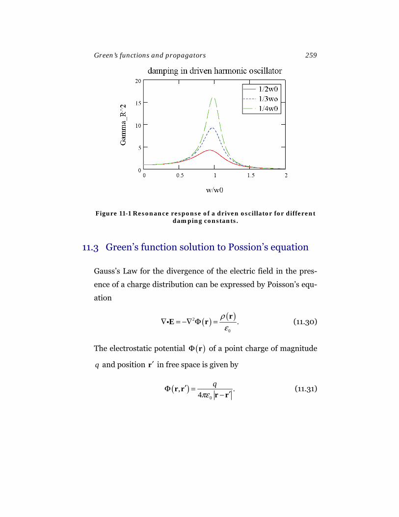
Green’s functions and propagators 259
Figure 11-1 Resonance response of a driven oscillator for different damping constants.
11.3 Green’s function solution to Possion’s equation
Gauss’s Law for the divergence of the electric field in the pres-
ence of a charge distribution can be expressed by Poisson’s equ-
ation
( ) ( )2
0
.ρε
∇ = −∇ Φ =r
E ri (11.30)
The electrostatic potential ( )Φ r of a point charge of magnitude
q and position ′r in free space is given by
( )0
, .4
qπε
′Φ =′−
r rr r
(11.31)
260 Green’s functions and propagators
The potential due to a distribution of charge with density ( )ρ ′r
can be written as a integral over the pointlike potential contribu-
tions for infinitesimal elements of charge ( ) 3dq d rρ ′ ′= r , giving
( ) ( )3
0
.4
d rρ
πε′
′Φ =′−∫
rr
r r (11.32)
From this we deduce that the free space Green’s function for
Poisson’s equation is given by
( )0
1, ,4
Gπε
′ =′−
r rr r
(11.33)
where
( ) ( )2
0
1,G δε
′ ′−∇ = −r r r r (11.34)
and
( ) ( ) ( )3 , .d r G ρ′ ′ ′Φ = ∫r r r r (11.35)
11.4 Multipole expansion of a charge distribution
Using the series expansion
( ) ( )*, ,1
0
1 4 , , ,2 1
ll
l m l mll m l
r Y Yl rπ θ φ θ φ
∞<+
= =− >
′ ′=′− +∑∑r r
(11.36)
one can make a multipole expansion of an arbitrary charge dis-
tribution, assuming that the charge distribution is localized
Green’s functions and propagators 261
within a volume of radius or . We are interested in finding the
potential only in the exterior region or r r′> > . Then equation
(11.36) can be written as
( ) ( )*, ,1
0
1 4 , , .2 1
ll
l m l mll m l
r Y Yl rπ θ φ θ φ
∞
+= =−
′ ′ ′=′− +∑∑r r
(11.37)
Substituting into equation (11.32) gives
( ) ( ) ( ) ( )
( )
( ) ( )
, 3 *,1
0 01
,00
3 *,
,1 ,2 1
1 1 , , implying44 , ,
2 1
ll m l
l mll m l
ll
lm l ml m l
llm l m
Yd r r Y
l r
B Yr
B d r Yl
θ φ ρθ φ
ε
θ φπεπ ρ θ φ
∞
+= =−
+∞
= =−
′′ ′ ′ ′Φ =
+
⎛ ⎞= ⎜ ⎟⎝ ⎠
′ ′ ′ ′=+
∑∑ ∫
∑∑
∫
rr
r
(11.38)
where the lmB represent the multipole moments of the distribu-
tion.
As an example, consider the following line charge distribution
along the z-axis
( ) ( ) ( )2/ for z .qz a x y aρ δ δ′ = <r (11.39)
We are interested in obtaining the multipole expansion of this
distribution for a>r . By azimulthal symmetry, only the 0m =
terms will contribute.
262 Green’s functions and propagators
( ) ( )
( ) ( ) ( )
3 *0 ,0
*,02
21
01 12 0
4 ,2 1
4 ,2 1
4 / 2 1 ( / )2 1 4
4 ,2 1
ll l
a lla
a lla
a l l
a
B d r r Yl
qzdz dx dy r x y Yl a
q a ldz z P z zl
q dz z dz zl a
π ρ θ φ
π δ δ θ φ
ππ
π
−
+
−
+ +
−
′ ′ ′ ′ ′=+
′⎛ ⎞′ ′ ′ ′ ′ ′ ′ ′= ⎜ ⎟+ ⎝ ⎠
+′ ′=+
⎡ ⎤′ ′ ′ ′= −⎢ ⎥⎣ ⎦+
∫
∫ ∫∫
∫
∫ ∫
r
(11.40)
or
0
0 for even ,
4 2 for odd ,2 1 ( 2)
ll
lB qa l
l lπ
⎧⎪= ⎨⎪ + +⎩
(11.41)
Therefore,
( ) ( )1
even 0
2 cos for .4 2
l
ll
q aP aa l r
θπε
+∞ ⎛ ⎞Φ = >⎜ ⎟+ ⎝ ⎠∑r r (11.42)
For large r , the leading order behavior of the distribution ap-
proaches that of a dipole charge distribution
( ) 20
cos .6qa
rθ
πεΦ =r (11.43)
11.5 Method of images
The Free space Green’s function is a solution to Poisson’s equa-
tion for a unit point charge, subject to the boundary conditions
( )lim , 0.FreerG
→∞′ =r r (11.44)
Green’s functions and propagators 263
To find a similar Green’s function for a unit point charge within
a closed surface, subject to Direchlet Boundary conditions at the
surface, this Green’s function must be modified to vanish at the
boundary. This can be accomplished by adding a solution of the
homogeneous equation, valid within the boundary, to the free
space Green’s function:
( ) ( ) ( ), , ,Direchlet Free hG G′ ′= +Φr r r r r (11.45)
Subject to the constraint
( ), 0.Direchlet BoundaryG ′ =r r (11.46)
The general solution to Poisson’s equation within the boundary
region is given by
( ) ( ) ( ) ( )3h , .DirechletV d r G ρ′ ′ ′Φ = + ∫r r r r r (11.47)
Where ( )hV r is another solution to the homogeneous Laplace
equation satisfying the actual Direchlet boundary on the boun-
dary surface:
( ) ( )hboundary boundaryVΦ =r r (11.48)
Solution for a infinite grounded plane
Calculating Green’s functions of a complicated surface is non
trivial, but for simple surface, one can use symmetry arguments
to generate an appropriate Green’s function. For example, sup-
264 Green’s functions and propagators
pose the boundary is a grounded infinite plane at 0,z = and we
were interested in obtaining the Green’s function for the positive
half plane 0.z ≥ The surface of the plane is an equipotential sur-
face, therefore the Electric field would have to be normal to the
surface (if the field has a component in the plane, charge would
flow, which would contradict the assumption that the system
has reached static equilibrium).
The grounded plane problem for the positive half plane would
be equivalent to removing the plane and adding a mirror charge
of opposite sign in the negative half plane. In fact for any distri-
bution of charge ( , , )x y zρ in the positive half plane, the mirror
distribution ( , , )x y zρ− − would lead to a zero-valued, equipoten-
tial surface at 0z = . In the case of a point charge at
( ), ,x y z′ ′ ′ ′=r , where 0z′ ≥ , one can place an image charge of
opposite sign at ( ), ,x y z′′ ′ ′ ′= −r to construct the Green’s function
( )
( ) ( ) ( )
( ) ( ) ( )
0 0
2 2 20
2 2 20
1 1,4 4
1
4
1 .4
G
x x y y z z
x x y y z z
πε πε
πε
πε
′ = −′ ′′− −
=′ ′ ′− + − + −
−′ ′ ′− + − + +
r rr r r r
(11.49)
Note
( ) ( )2
0
1, for 0G zδε
′ ′−∇ = − >r r r r (11.50)
Green’s functions and propagators 265
and
( )0
, 0.z
G=
′ =r r (11.51)
Induced charge distribution on a grounded
plane
The induced charge density on the conducting plane is given by
( )
00 0
,( )z z
z
x yE
zσ
ε==
∂Φ= − =∂
r (11.52)
Therefore, a point particle of magnitude q located at ′r induces
a surface charge density given by
( ) ( )0
0
,, ,
z
Gx y q
zσ ε
=
′∂= −
∂r r
(11.53)
( )( ) ( ) ( )( )3/ 22 2 2
2, .4
qzx yx x y y z
σπ
′−=′ ′ ′− + − +
(11.54)
Integrating the induced charge density over the surface gives
( )( )
2
3/ 20 0 2 2
2, .4
qzdxdy x y d d qz
πσ ρ ρ φ
π ρ
∞ ∞ ∞
−∞ −∞
′−= = −′+
∫ ∫ ∫ ∫ (11.55)
A point charge induces a net charge of equal magnitude and op-
posite sign on the conducting surface. This is illustrated in Fig-
ure 11-1,which shows how a positive charge attracts a negative
charge density of equivalent magnitude to the surface region

266 Green’s functions and propagators
closest to it. The sharpness of the induced charge distribution
depends on how close the point charge is to the plane.
11-2 Induced surface charge density on a grounded plane due to a nearby point charge.
Green’s function for a conducting sphere
The above technique is called the method of images. It can be
extended to find the Green’s function for a grounded spherical
cavity. Let the radius of the sphere be a and let ′r be the posi-
tion of a point charge inside the cavity. Then one can construct
an image charge of magnitude q′′ and position λ′′ ′=r r where λ
is some scale factor to give the Green’s function solution
( )0 0
1, ,4 4sphere
qGπε πε
′′′ = −′ ′′− −
r rr r r r
(11.56)
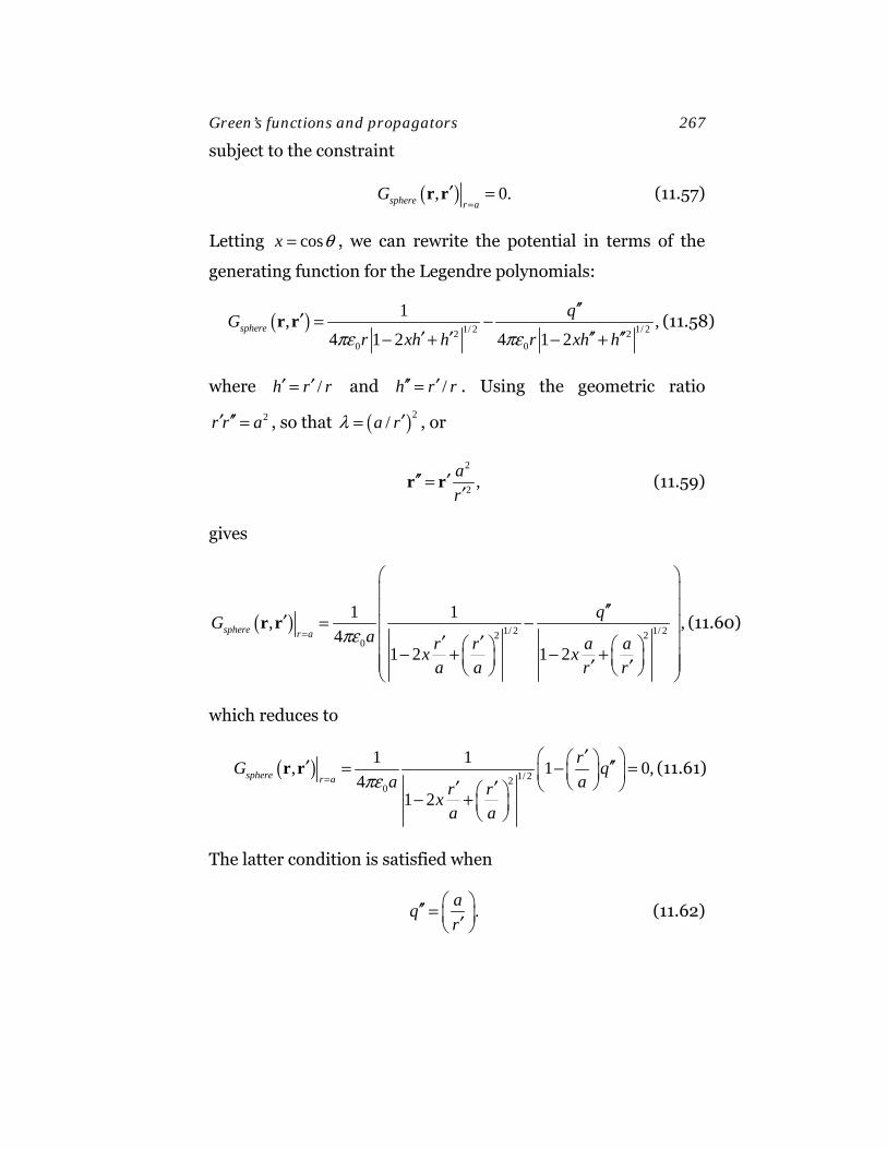
Green’s functions and propagators 267
subject to the constraint
( ), 0.sphere r aG
=′ =r r (11.57)
Letting cosx θ= , we can rewrite the potential in terms of the
generating function for the Legendre polynomials:
( ) 1/ 2 1/ 22 20 0
1, ,4 1 2 4 1 2
sphereqG
r xh h r xh hπε πε
′′′ = −′ ′ ′′ ′′− + − +
r r (11.58)
where /h r r′ ′= and /h r r′′ ′= . Using the geometric ratio
2r r a′ ′′ = , so that ( )2/a rλ ′= , or
2
2 ,ar
′′ ′=′
r r (11.59)
gives
( ) 1/ 2 1/ 22 20
1 1, ,4
1 2 1 2sphere r a
qGa r r a ax x
a a r r
πε=
⎛ ⎞⎜ ⎟⎜ ⎟′′′ = −⎜ ⎟⎜ ⎟′ ′⎛ ⎞ ⎛ ⎞− + − +⎜ ⎟⎜ ⎟ ⎜ ⎟⎜ ⎟′ ′⎝ ⎠ ⎝ ⎠⎝ ⎠
r r (11.60)
which reduces to
( ) 1/ 220
1 1, 1 0,4
1 2sphere r a
rG qa ar rx
a a
πε=
′⎛ ⎞⎛ ⎞′ ′′= − =⎜ ⎟⎜ ⎟⎝ ⎠⎝ ⎠′ ′⎛ ⎞− + ⎜ ⎟⎝ ⎠
r r (11.61)
The latter condition is satisfied when
.aqr
⎛ ⎞′′ = ⎜ ⎟′⎝ ⎠ (11.62)

268 Green’s functions and propagators
Therefore,
( ) 20
0
1, .4
4sphere
arG
ar
πεπε
⎛ ⎞⎜ ⎟′⎝ ⎠′ = −
′− ⎛ ⎞ ′− ⎜ ⎟′⎝ ⎠
r rr r
r r (11.63)
11.6 Green’s function solution to the Yakawa
interaction
The strong nuclear force, unlike the electromagnetic force, is
short ranged. This short range character is due to a massive bo-
son interaction. To model this, in the static limit, we add a mass
term to the Laplace equation, giving rise to a Yukawa interac-
tion,
( ) ( ) ( )2 2 .m ρ− ∇ − Φ =r r (11.64)
The factor m results in a exponential damping of the potential,
giving it a short range character. This becomes apparent when
one solves for the Green’s function
( ) ( ) ( )2 2 , , ,m G δ′ ′− ∇ − =r r r r (11.65)
which results in the free space Green’s function
( ), .4
meGπ
′− −
′ =′−
r r
r rr r
(11.66)
Green’s functions and propagators 269
Letting 0m → recovers the Coulomb result in units of 0 1ε = .
Therefore, the long range character of the electromagnetic force
is due to the photon being massless.
Related Documents