Introduction to the Discrete Fourier Transform TU Delft TU Delft

1

Introduction to theDiscrete Fourier Transform

Lucas J. van Vlietwww.ph.tn.tudelft.nl/~lucas

TU DelftTNW: Faculty of Applied SciencesIST: Imaging Science and technologyPH: Pattern Recognition Group

Discrete Fourier Transform 2

TU DelftPattern Recognition Group

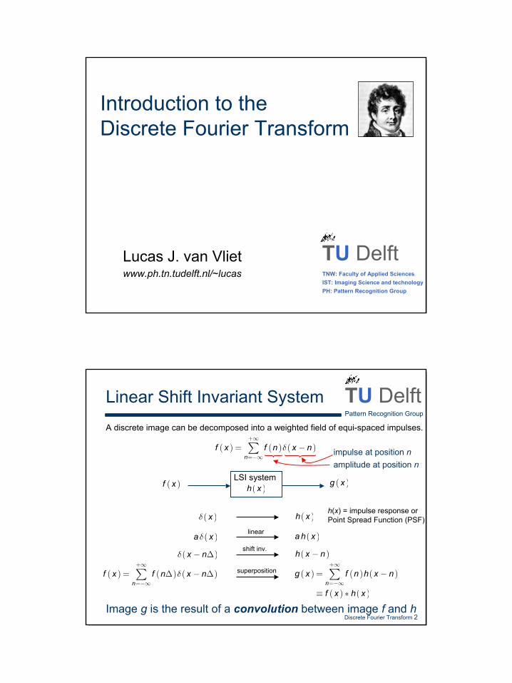
Linear Shift Invariant SystemA discrete image can be decomposed into a weighted field of equi-spaced impulses.

( )f x ( )g xLSI system( )h x

( ) ( ) ( )n

f x f n x nδ+∞

=−∞= −∑

( )a xδ ( )a h xlinear

( )x nδ − ∆ ( )h x n−shift inv.

( ) ( ) ( )n

f x f n x nδ+∞

=−∞= ∆ − ∆∑ ( ) ( ) ( )

( ) ( )n

g x f n h x n

f x h x

+∞

=−∞= −

≡ ∗

∑superposition

( )xδ ( )h xh(x) = impulse response or Point Spread Function (PSF)

Image g is the result of a convolution between image f and h

impulse at position namplitude at position n

2



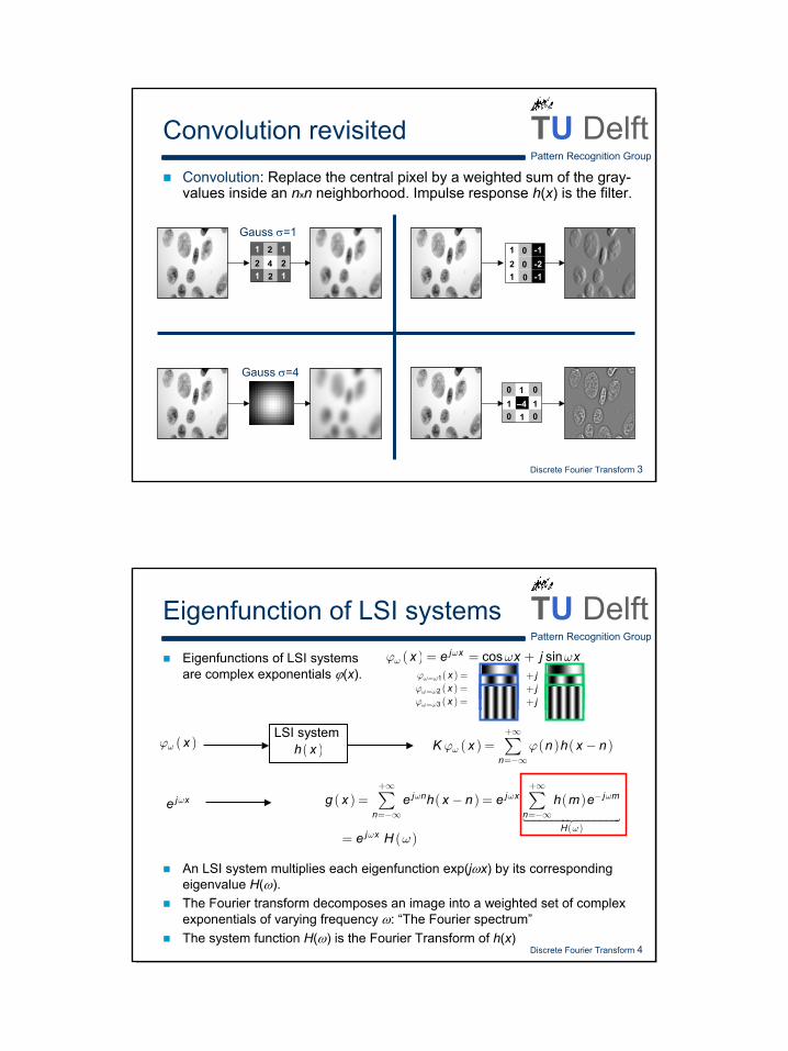
Convolution revisitedConvolution: Replace the central pixel by a weighted sum of the gray-values inside an nxn neighborhood. Impulse response h(x) is the filter.

Gauss σ=11 1

1 142

2 22

1 -1

1 -100

2 -20

0 0

0 0–41

1 11

Gauss σ=4



Eigenfunction of LSI systemsEigenfunctions of LSI systems are complex exponentials ϕ(x).

( )xωϕ ( ) ( ) ( )n

K x n h x nωϕ ϕ+∞

=−∞= −∑

LSI system( )h x

( ) cos sinj xx e x j xωωϕ ω ω= = +

An LSI system multiplies each eigenfunction exp(jωx) by its corresponding eigenvalue H(ω).The Fourier transform decomposes an image into a weighted set of complex exponentials of varying frequency ω: “The Fourier spectrum”The system function H(ω) is the Fourier Transform of h(x)

( ) ( ) ( )

( )

j n j x j m

n nH

g x e h x n e h m eω ω ω

ω

+∞ +∞−

=−∞ =−∞= − =∑ ∑j xe ω

( )j xe Hω ω=

( )1 xω ωϕ = = j+( )2 xω ωϕ = = j+( )3 xω ωϕ = = j+

3



Convolution property

A convolution between an image f(x) and an impulse response h(x) in space, corresponds to a multiplication of the Fourier spectra F(ω) and H(ω) in the Fourier domain.

LSI system( )h x( )f x ( ) ( ) ( ) ( )

nf x h x f n h x n

+∞

=−∞∗ = ∆ − ∆∑

( ) ( ){ } ( ) ( )

( )

( )

( )

( )

( ) ( )

j x

x n

j n j m

n xF H

F f x h x f n h x n e

f n e h m e

F H

ω

ω ω

ω ω

ω ω

+∞ +∞−

=−∞ =−∞

+∞ +∞− −

=−∞ =−∞

∗ = −

=

=

∑ ∑

∑ ∑



Gaussian derivativesHow to compute a derivative in digital space?

Introduce (Gaussian) scale

Derivative at scale σ is computed by convolution of the discrete image f[x,y] with discrete Gaussian derivative

Note that the Gaussian function is known analytically, compute the derivative(s), and then sample to produce a discrete filter. Thesampling of the Gaussian should be high enough, i.e. σ > 0.9 pixels

( ) [ ] ( ) [ ] ( ) [ ]( ) [ ] ( ) [ ] ( ) [ ]

0

5 3 4

, , ,

, , ,

f x y f x y g x y

f x y f x y g x y

σ σ

σ σ σ= = =

= ⊗

= ⊗

[ ] [ ], , ?xf x y f x yx∂ =∂

( ) [ ] ( ) [ ] ( ) [ ]0, , ,x xf x y f x y g x yσ σ= ⊗

4



Fourier filters: Gaussian

F

|G| |G| |G|

|FG| |FG| |FG||F|

f f*g f*g f*g

g g g



Gaussian derivative filtersIn continuous space: the derivative operator corresponds to multiplication of the Fourier spectrum with jω

( ) ( )

( ) ( )

( ) ( )2

22

F

F

F

f x F

d f x j Fdxd f x Fdx

ω

ω ω

ω ω

←→

←→

←→ −

In discrete space: combine the derivative operator with Gaussian smoothing

( ) ( ) ( ) ( )

( ) ( ) ( ) ( )

( ) ( ) ( ) ( )

( )

( )

2( ) 2

2

F

F

F

g x f x G F

d g x f x j G Fdxd g x f x G Fdx

σ

σ

σ

ω ω

ω ω ω

ω ω ω

∗ ←→

∗ ←→

∗ ←→ −

σ=1 σ=2 σ=4 σ=1 σ=2 σ=4

5



Fourier: Gaussian derivative

F

Im{Gx} Im{Gx} Im{Gx}

|FGx| |FGx| |FGx||F|

f f*gx f*gx f*gx

gx gx gx



Fourier: Laplace & sharpening

F

|F|

f

Re{Gxx+Gyy}

|F(Gxx+Gyy)|

f*(gxx+gyy)

g xx+

g yy

Re{Gxx+Gyy}

|F(Gxx+Gyy)|

f*(gxx+gyy)

g xx+

g yy

f–2f*(gxx+gyy) f–2f*(gxx+gyy)

6



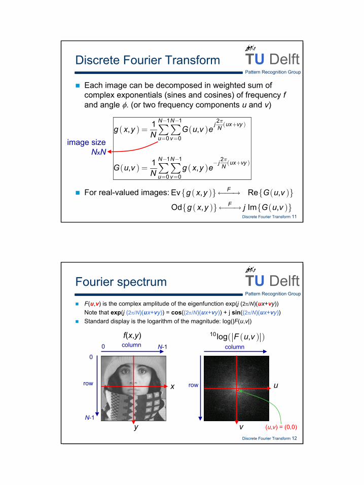
Discrete Fourier Transform

Each image can be decomposed in weighted sum of complex exponentials (sines and cosines) of frequency fand angle φ. (or two frequency components u and v)

( ) ( )( )

( ) ( )( )

1 1 2

0 0

1 1 2

0 0

1, ,

1, ,

N N j ux vyN

u v

N N j ux vyN

u v

g x y G u v eN

G u v g x y eN

π

π

− − +

= =

− − − +

= =

=

=

∑∑

∑∑

For real-valued images: ( ){ } ( ){ }

( ){ } ( ){ }

Ev , Re ,

Od , Im ,

F

F

g x y G u v

g x y j G u v

←→

←→

image sizeNxN



Fourier spectrumF(u,v) is the complex amplitude of the eigenfunction exp(j (2π/N)(ux+vy))Note that exp(j (2π/N)(ux+vy)) = cos((2π/N)(ux+vy)) + j sin((2π/N)(ux+vy))Standard display is the logarithm of the magnitude: log(|F(u,v|)

u

v

x

y

column

row

column

row

0

0N-1

N-1(u,v) = (0,0)

f(x,y) ( )( )10log ,F u v

7



Getting used to Fourier (2)

An image is a weighted sum of cos (even) and sin (odd) images.

a+jba−jb

Fourier domain with complex amplitude: a+jb



Eigenfunctions: Even & Odd

( )0 0

0

2 2

21 cos

1 2

j u x j u xN N

u xN

e eπ π

π

−

+ =

++( )0 0

0

2 2

2sin

2

j u x j u xN N

u xN

e ej

π π

π

−

=

−

( )( )

( )

1 102

102

,,

,N

u vu u v

u u v

δδ

δ

+ − + +

( )

( )

1021

102

,

,N

u u vj

u u v

δ

δ

− − + +

Real & even Real & odd

Real & even Imag & odd

F F

8



Orientation & frequency

F F F



Getting used to Fourier (1)

Graphite surface by Scanning Tunneling MicroscopyAtomic structure of graphite shows a hexagonal surface

column

row

0

0N-1

N-1

(c,r) = (½N,½N)(u,v) = (0,0)

x

y

u

v

(c,r) = (0,0)(u,v) = (-½N,-½N)

(c,r) = (N-1,N-1)(u,v) = (½N-1, ½N-1)

9



SuperpositionFourier spectrum

= + + +

= + + +

F F F F F



Fourier transforms

F

F

magnitude phase

10



Magnitude & phase

F –1

F –1

( ),F u v

( ) ( )( )

, ,,

j F u v F u veF u v

=

?

?



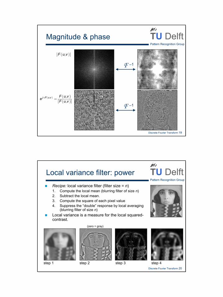
Local variance filter: powerRecipe: local variance filter (filter size = n)1. Compute the local mean (blurring filter of size n)2. Subtract the local mean.3. Compute the square of each pixel value4. Suppress the “double” response by local averaging

(blurring filter of size n)Local variance is a measure for the local squared-contrast.

step 1 step 2 step 3 step 4

(zero = gray)

11



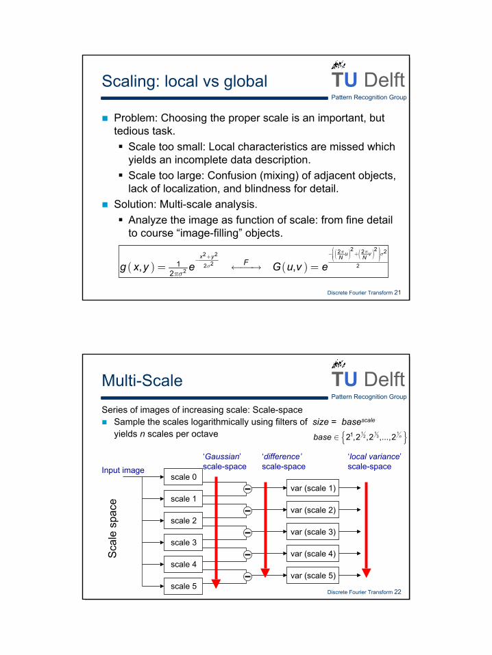
Scaling: local vs global

Problem: Choosing the proper scale is an important, but tedious task.

Scale too small: Local characteristics are missed which yields an incomplete data description.Scale too large: Confusion (mixing) of adjacent objects, lack of localization, and blindness for detail.

Solution: Multi-scale analysis.Analyze the image as function of scale: from fine detail to course “image-filling” objects.

( ) ( )( ) ( )2 22 2 22 2

22 22

12

, ,u vx y N N

Fg x y e G u v eπ π σ

σπσ

− + + −= ←→ =



Multi-ScaleSeries of images of increasing scale: Scale-space

Sample the scales logarithmically using filters of size = basescale

yields n scales per octave

Input imagescale 0

scale 1

scale 2

scale 3

scale 4

scale 5

var (scale 1)

var (scale 2)

var (scale 3)

var (scale 4)

var (scale 5)

‘local variance’ scale-space

{ }11 13212 ,2 ,2 ,...,2 nbase ∈

‘difference’scale-space

Scal

e sp

ace

‘Gaussian’scale-space

12



1

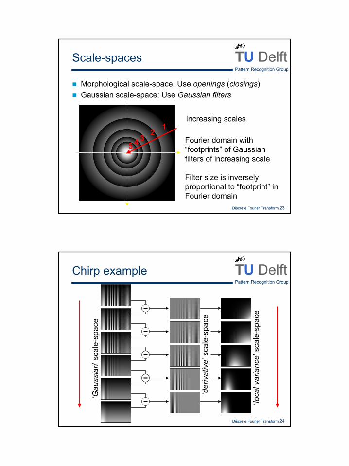
Scale-spaces

Morphological scale-space: Use openings (closings)Gaussian scale-space: Use Gaussian filters

Increasing scales

Fourier domain with “footprints” of Gaussian filters of increasing scale

Filter size is inversely proportional to “footprint” in Fourier domain

2345



Chirp example

‘der

ivat

ive’

sca

le-s

pace

‘loca

l var

ianc

e’ s

cale

-spa

ce

‘Gau

ssia

n’sc

ale-

spac

e

13



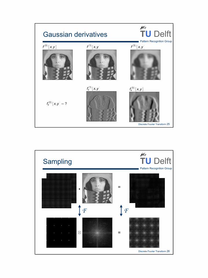
Gaussian derivatives

( ) [ ]0 , ?xf x y =

( ) [ ]1 ,xf x y ( ) [ ]5 ,xf x y

( ) [ ]1 ,f x y ( ) [ ]5 ,f x y( ) [ ]0 ,f x y



Sampling

=

=⊗

i

F F

14



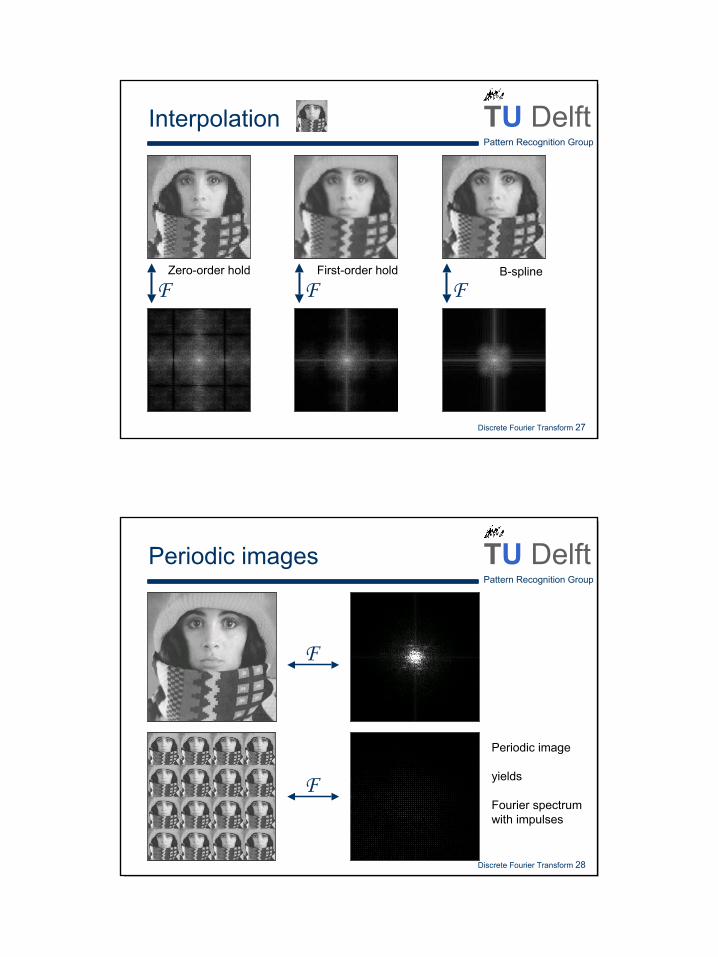
Interpolation

Zero-order hold First-order hold B-spline

F F F



Periodic images

F

F

Periodic image

yields

Fourier spectrumwith impulses

Introduction to the Discrete Fourier Transform TU Delft TU Delft

Documents