Introduction to STATA - University of Notre Damewevans1/econ30331/Introduction to STATA.pdf · 1 Introduction to STATA ECONOMICS 30331 Bill Evans Spring 2016 This handout provides

1

Introduction to STATA

ECONOMICS 30331

Bill Evans

Spring 2016

This handout provides a very brief introduction to STATA, a convenient and versatile econometrics package. In the

past 20 years, STATA has become one of the leading statistical programs used by economic researchers. STATA

was written by economists so it is more intuitive for researchers in our field. It is fast and relatively easy to use.

STATA’s speed advantage comes from the fact that all data is loaded into RAM. Subsequently, the amount of high

memory restricts the size of the problem. Given the size of the data sets we will use in class and the available

memory on typical machines, this will not prove to be a constraint.

All the STATA data files, sample programs, this handout, etc., will be available for download from the course web

page, http://www.nd.edu/~wevans1/econ30331.htm. In the lower right hand side of the page is a link to “STATA

programs and data files”.

This outline demonstrates those STATA procedures necessary for the course. However, this handout only scratches

the surface of STATA’s capabilities. The text is written so that you should be able to follow along on a computer

with STATA and gradually build up to the point where you can generate simple statistics. My suggestion is that you

print out this tutorial, find a computer with STATA, enter the program, then follow along with the tutorial.

Some places on the web where you can learn more about STATA include

STATA faq’s http://www.stata.com/support/faqs/

The STATA listserv http://www.stata.com/statalist/

UCLA’s resources for learning STATA http://www.ats.ucla.edu/stat/stata/

STATA Availability STATA is available in all Windows-based machines in computer clusters and classrooms on campus. STATA is not

available on the MAC machines in the clusters. If you want your own copy of STATA, a one-year site license for

STATA 13/IC can be purchased through the STATA Grad Purchase plan. The web site is

http://www.stata.com/order/new/edu/gradplans/student-pricing/ and the cost is $125 for a one-year license or $75 for

a six-month license. This version of STATA is available for either Windows or MAC platforms. This is not

required for class but is available if you want STATA on you own machine.

Once you are into STATA Click on the STATA icon and the program will open.

When you first enter STATA, the screen will look like Figure 1 below. You will notice that there are five boxes on

the screen. I want to focus on four at this time.

Area A is called the command line. This is where you will type executable statements.

Area B is the variable list. Once you load a data set into STATA, all the variables available to you will be

listed in the box.

Area C is the review box and it will contain a history of all the commands executed during this STATA

session.

Area D is where any results will be reported.

2

Figure 1

The command line is the active area of the screen where you will be typing all your commands. The contents of the

other boxes will be determined by what you type here. Once in STATA, the cursor should be blinking in the

command line indicating to you that the program is waiting to accept input. Commands are executed by hitting

return after you have typed the command.

Throughout this tutorial, anything written in COURIER FONT is a command that should be executed through the

command line.

There are two ways to produce statistics in STATA. First, you can write executable statements, line by line from the

command line, and execute the codes. Alternatively, you can write an entire program that contains a group of

executable statements, then submit the program from the command line. In the text below, we will indicate the ‘line-

by-line’ interactive approach but in Appendix 1, I provide a STATA program, cps87.do, that generates all the results

in this tutorial. At the end of the handout, I also outline how to execute the batch program. The results from this

single program are reported in Appendix 2. Please refer to these results when you want to see the output from any

particular line-by-line statement in the tutorial below.

From the command line, you can ask for help at any point. Suppose you wanted some information about how to

describe the contents of data sets. From the command line, you would type

help describe

then hit return. A pop-up box appears that outlines the syntax for the ‘describe’ command. Notice also that the

command you executed is now in the Review box C. If at any time you want to re-use a command that has already

C

D

A

B

3

been executed, using the mouse, click once on the command and the text appears in the command line.

In any software package, in order to generate statistical results, you must do three things:

1. Read in raw data from another format and store in a form usable to the statistical package

2. Manipulate the data (delete observations, create new variables) as needed

3. Perform statistical operations

As you will quickly learn, the bulk of your time will be spent on task 2. Generating results in most software

packages is trivial; getting the data in a form that is usable is what takes time. Over the next few sections, I will

illustrate some ways that STATA handles each of the tasks above.

For this class, we will skip step 1 – I will provide you data that is already in STATA format. Later in the semester

we will consider how to read data from Excel into STATA.

STATA assumes that all external files (data and programs) are stored on the default subdirectory (folder). What that

default directory is depends on how your particular machine is set up. What I recommend is that you construct a

folder on a thumb drive for your STATA work and once in STATA, change where STATA is looking for. So for

example, suppose that you have constructed a folder c:\bill\econ30331 for your STATA work. From the command

line, you would type

cd c:\bill\econ30331

and hit return. Now STATA will look in this folder for all data sets and write all results to this folder as well.

When you are working interactively, you may want to save a ‘log’ of your activity – a list of all the commands and

results from your current STATA session that are posted in the results section (area D in Figure 1). You can

construct a log by typing the following command.

log using stata_log_1.log,replace

and hitting return. The log will be written to the file ‘stata_log_1.log’ and the replace option tells the program to

overwrite an existing file with that name. At the end of your session, you will type

log close

and hit return to close the log file. Please note that STATA commands, data set names, and variable names are case

sensitive.

Reading in STATA Data Sets Most data sets come to the researcher in some easily transportable format, such as ASCII, comma delimited, or

Excel. These data are not directly usable by STATA because they are not in the proper format. Programmers must

first load data from other programs into STATA and store the data in STATA format in order to use the data the

program. Once the data is stored in STATA format, it can be easily accessed.

For almost all classroom projects, you will have access to a data file that is already in STATA format and ready for

use by the program. STATA data files always have a .dta extension and loading them into STATA is

straightforward.

4

On the class web page is a STATA data set cps87.dta. Please download that into the folder you have set up for this

class. Once this is done, to load the data into STATA, simply type

use cps87

and hit return. The variables in the data set are now available for use in STATA. One the data set is in memory you

can construct new variables, delete particular observations, and generate statistics.

A data set contains a collection of variables that describe different units. Think of the data set as a matrix having

columns and rows. The rows are separate observations (people, companies, cities, time periods) while each column

is a different variable that describes a specific characteristic of the observations in the sample. The data for this

example contains 7 variables for 19,906 respondents to the 1987 Current Population Survey. The data file reports

information for males, aged 21-64 who were working full time (>30 hours per week) at the time of the survey. The

variables in the data set are described in Table 1 below. The 7 variables measure the respondent’s : age, race, years

of educ, union status, the type of area they live (smsa_size), their region of the country and their usual weekly

earnings.

Table 1: Detailed Variable Definitions for cps87.dta

Variable Definition

AGE Age in years

RACE =1 if white, non-Hispanic, =2 if black, non-Hispanic, =3 if Hispanic

EDUC Years of completed education, maximum is 18.

UNIONM =1 if a union member, =2 otherwise

SMSA =1 if live in one of 19 largest Standard metropolitan Statistical Areas (SMSA),

=2 if live in other SMSA, =3 if live in non-SMSA

REGION =1 if live in Northeast, =2 if live in Midwest, =3 if live in South, =4 if live in

West

EARNWKE Usual weekly earnings, nominal 1987 dollars, maximum is $999

A matrix representation of the data is best represented by considering what the data might look like in Excel. In

Figure 2 below is a data set that has first 31 lines of data from cps87.xls. Notice that each row is a different person

and each column provides difference pieces of information about that person.

What all statistical software packages are designed to manipulate are the columns in the matrix or the different

variables. So you may want to know average earnings across the respondents in your sample or what fraction of

people voted in the last election or the correlation between income and years of education for people.

5

Figure 2 Contents of cps87.xls

After you have constructed new variables, you can save the revised data set by saving the data under a new name

save cps87_update

6

and hit return. Alternatively, you can save the new data set under the old name by typing

save cps87, replace

and hit return. If you no longer need the data set, you can clear it out of memory by typing

clear

and hit return. Before going on in this tutorial, please clear this data out of memory.

At any time, you can get a list of all of the variables in your data set by typing

describe

and hit return. A description of the variables data set so far is printed in below and in block A of the results in

Appendix 2.

Contents of DESCRIBE procedure

Contains data from cps87.dta

obs: 19,906

vars: 7 12 Aug 2008 13:05

size: 159,248

--------------------------------------------------------------------------------------------------

storage display value

variable name type format label variable label

--------------------------------------------------------------------------------------------------

age byte %8.0g age in years

race byte %8.0g =1 if white non-Hisp, =2 if black non-Hisp, =3 if Hispanic

years_educ byte %8.0g years of competed education

union_status byte %8.0g =1 if in union, =2 otherwise

smsa_size byte %8.0g =1 if largest 19 smsa, =2 if other smsa, =3 not in smsa

region byte %8.0g =1 if northeast, =2 if midwest, =3 if south, =4 if west

weekly_earn int %8.0g usual weekly earnings, up to $999

--------------------------------------------------------------------------------------------------

When using variables in STATA you refer to them by their name: age for age in years, weekly_earn for usual

weekly earnings, etc. Variables names can be up to 32 characters in length, contain letters, numbers and the

underscore ( _ ) but no blanks. Variable names are case sensitive. For example, in this data set you can have three

different variables: “age” “AGE” and “Age”. Variable names can begin with a letter or an underscore but NOT a

number.

Notice that after each variable name is a “label.” This is a short description of what the variable is measuring and it

is user-supplied. The text for the label should mirror the text that describes the data in documents like Table 1.

Everyone is different but I find it easier to work with variable names that reflect what the variable is measuring: age

for years of age, years_educ for years of education. In some cases, people name variables v1 through v7 – which

never makes sense to me.

If you are interested in knowing how to read data from Excel (spreadsheet) format into STATA, please see

Appendices C and D of this handout.

Generating new variables in STATA

Once you have loaded data into STATA, you can take the original variables and transform them into new variables.

7

These new variables can easily be created with the “gen” command. The syntax for “gen” is

gen new variable name=mathematic expression

The new variable is the name of the newly created variable and it must follow STATA naming conventions outlined

above.

Below are six examples of the gen statement that construct new variables from the data set we just loaded into

memory.

gen age2=age*age

gen ln_weekly_earn=ln(weekly_earn)

gen union=union_status==1

gen nonwhite=((race==2)|(race==3))

gen big_northeast_city=((region==1)&(smsa==1))

The first two lines use standard mathematical operators to construct new variables. Here, we construct age squared

and the natural log of usual weekly earnings. We construct age squared because earnings rise sharply as a person

ages, then the wage changes become less pronounced over time. We can capture this with a quadratic function in

age. We usually analyze ln(earnings) rather than earnings because the latter is a ‘skewed’ variable while the former

is in most cases normally distributed.

One of the most common variables in applied work is a “dummy variable” that equals 1 or 0, separating people into

two groups (male or female, black or white, etc). These variables are easy to construct with the use of “logical

operators.” Logical operators are of the form

gen varname=logical statement

that constructs a new variable names “varname” that equals 1 when the logical statement is true

and zero otherwise.

The last three variables listed above demonstrate how to use logical operators. The variable union constructs a

variable that equals 1 for union members and zero otherwise. Notice that two equal signs must be used when exact

equality is indicated in a logical statement. Combinations of logical statements can be used to construct dummy

variables. The vertical line | represents “or” and the & sign represent “and” The variable nonwhite equals 1 if races

equals 1 OR 2, and big_ne equals 1 if a respondent comes from a big SMSA from the Northeast census region.

After the variables are constructed, I add a set of variable LABELs. The syntax for labels is illustrated in the next

six lines.

label var age2 "age squared"

label var ln_weekly_earn "ln usual earnings per week"

label var union "1=in union, 0 otherwise"

label var nonwhite "1=nonwhite, 0=white"

label var big_ne "1= live in big smsa from northeast,

0=otherwsie"

It is good programming practice to label your variables.

8

Getting descriptive statistics Once you have the correct collection of variables in your STATA data file, you may want to construct some simple

descriptive statistics. Summary statistics (mean, min, max and standard deviation) are produced with the “sum”

command. So the command

sum

gets descriptive statistics for all variables. If you only want information for a subset of variables, like age and

education, then add the variables after the sum command

sum age years_educ

and hit return.

If you want more detailed information on a particular variable (quantiles, medians, skewness, kurtosis, etc.), use the

“sum” command, list the variables, and ask for detailed calculations.

sum weekly_earn age, detail

generates detailed statistics for only two variables. Results from these three exercises are reported in blocks B, C

and D respectively in Appendix 2. In Block B, note that the average age is 37.97 years and 23% of workers are in

unions. In Box D, note that median weekly earnings are $449 dollars but average earnings are higher at $488.26.

Summary statistics for subsamples of the population are easily calculated as well. For example, suppose one wanted

to look at average weekly earnings across different racial and ethnic groups. First, you would sort the data by race

sort race

then ask to have the means calculated for the racial subgroups

by race: sum weekly_earn

The by variable: option must be ended with a colon (:) and the data must be sorted in order for this option to work.

The by option can be used with virtually all of STATA’s commands. Results from this exercise are reported in Box

E of Appendix 2. Note that average earnings for whites, black and Hispanics are $506, $383, and $369.

Suppose instead that one needed sample means for those with at least a high school education. In this case, the “if’

statement can be used as an option and he sample restricted to those people where the if statement is correct. So for

example

sum weekly_earn if years_educ>=12

will only generate sample means for those people with 12 or more years of education. The observations with

years_educ<12 have not been deleted from the sample, but rather, they were simply not used in the previous

9

command. These results are in Box F in Appendix 2 and note that average earnings increase to $509.62 when lower

educated workers are excluded.

You can obtain complete distributions for discrete variables by using the TABULATE command. For example if

you want to know the fraction of people by racial/ethnic group, you would type

tab race

and hit return. These results are reported in block G in Appendix 2 and 85.9 percent of the sample is white, non-

Hispanic, 8.25 are Black, non-Hispanic while 5.83% are Hispanic.

You can construct two-way contingency tables by listing the two variables in the TABULATE command. For

example, in the line

tab region smsa, row column

and hit return. STATA will count the number of observations for all 12 unique groups of region and SMSA. The

row and column options to the command tell STATA to produce row and column totals. The results from this

exercise are reported in Block H of Appendix 2. Notice in this case that 2906 observations have region=1

(northeast) and smsa=1 (one of the 19 largest smsa) while 1133 observations have region=4 (west) and smsa=3 (non-

SMSA).

Testing whether means in two subsamples are the same The simplest statistical test than can be performed is to examine whether the means from two different groups are the

same. In this case, we will examine weekly earnings for union and non-unions workers. The difference in means

across samples is tested with a t-test and the syntax is

ttest weekly_earn, by(union)

The results from this exercise are reported in section I of the results. In this case, notice that the mean earnings

among unions workers is $515.28 while the mean earnings for non-union workers is $480.15 and therefore the

difference across the two groups (non-union minus union) is -$35.13. The t-statistic on this difference is -27.35. The

95% critical value of a t-test with 19,904 degrees of freedom is 1.96 so we can easily reject the null hypothesis that

the means across the two subsamples are the same, which is indicated by the low p-value on the t-test.

Running a simple OLS regression The most-often estimated model in labor economics is the human capital earnings function. Log weekly wages has

been shown to be roughly linear in education and quadratic in age. In the next few lines, we run a simple OLS

regression. Basic regressions are generated by the reg command and the syntax is simple where the first variable

after reg is the dependent variable and all other variables are independent variables. In this example, there are five

covariates: age, age2, years_educ, union and non-white. STATA automatically adds a constant to every model

unless otherwise specified. The regression statement in the sample program is as follows.

reg ln_weekly_earn age age2 years_educ nonwhite union

10

The results from this example are reported in Block J of Appendix 2. We will not interpret these results at this time.

In many empirical models, observations can be grouped into discrete categories. Sometimes, the number of

categories is small (e.g., race and sex) Sometimes the categories are numerous (states and countries). In a sample

with people from 50 states, to add state dummy variables requires the construction of 49 variables. STATA has an

automated procedure that will construct the discrete variables and add them to a model. Before the REG command

is invoked, the XI option signals to STATA that the variables defined by i.name.

Clearing and closing Once you are done with your interactive STATA session, you can close the log file by typing

log close

and hitting return. Also, in order to exit, you must clear the data out of memory which can be done by typing

clear

You can clear the data out of memory at this point.

Running *.do programs The text above describes an interactive STATA session where lines of code are typed in the command line and

submitted one at a time. An interactive session is excellent way to learn STATA: you see the errors right away and

you adjust as you go along.

However, as you get more proficient in your programming, you will turn want to write STATA programs and submit

them as a ‘batch’ job. STATA programs can be written in any ASCII editor such as Wordpad or Notepad and the

files must have a .do extension.

All of the lines of code discussed above have been collected in a STATA .do program called cps87.do and a copy of

this program is contained in Appendix 1 below. The program is also available for download from the class web

page. Please download this file to the default folder you are using for this class.

STATA reads each line of this program as a separate executable statement. Note that between the executable

statements there are lines that begin with *’s. These stars indicate that the line is a comment and is not an executable

command. It is good programming practice to include comments in your programs. This helps you when you go

back to a program after a long delay and detailed comments helps anyone else who reads your program understand

what you are up to.

A few lines into the program you will notice the line

set more off

When you execute a program, STATA will fill up one screen’s worth of text, then wait for the operator to hit return

in order to proceed. The command above turns this feature off.

11

If you have a copy of the comma-delimited data set cps87.csv and a copy of the STATA program cps87.do on your

default folder, you can execute the STATA batch program by typing the following

do cps87

and hit return. The command do will look for the cps87.do file and execute the commands line by line. The results

from this program should be identical to that in Appendix 2.

Handling errors If your program has errors, enter any ASCII editor, call up the program, then edit and save the program. You will

need to close any open log from the command line by typing ‘log close’ and ‘clear’ any active variables in memory.

You are then ready to re-run your program.

If you hit the “page up” key, you will notice that previously-entered commands appear in the command line. This is

a quick way of recalling lines of code.

Exiting STATA To exit STATA, please do to the command line, type CLEAR and hit return which clears all variables from memory,

then type EXIT and hit return.

Appendix A

cps87.do

* set it such that the computer does not

* need the operator to hit the return key

* to continue

set more off

* write results to a log file

log using cps87.log,replace

* read in stata data set cps87.dta

use cps87

* describe what is in the data set

describe

* generate new variables

* lines 1-2 illustrate basic math functoins

* line 3 line illustrates a logical operator

* line 4 illustrate the OR statement

* line 5 illustrates the AND statement

gen age2=age*age

gen ln_weekly_earn=ln(weekly_earn)

12

gen union=union_status==1

gen nonwhite=((race==2)|(race==3))

gen big_ne=((region==1)&(smsa==1))

label var age2 "age squared"

label var ln_weekly_earn "log earnings per week"

label var union "1=in union, 0 otherwise"

label var nonwhite "1=nonwhite, 0=white"

label var big_ne "1= live in big smsa from northeast, 0=otherwsie"

* get descriptive statistics for all variables

sum

* get statistics for only a subset of variables

sum age years_educ

* get detailed descriptics for a subset of variables

sum weekly_earn age, detail

* to get means across different subgroups in the

* sample, first sort the data, then generate

* summary statistics by subgroup

sort race

by race: sum weekly_earn

* get weekly earnings for only those with a

* high school education

sum weekly_earn if years_educ>=12

* get frequencies of discrete variables

tabulate race

* get two-way table of frequencies

tabulate region smsa, row column

* test whether means are the same across two subsamples

ttest weekly_earn, by(union)

*run simple regression

reg ln_weekly_earn age age2 years_educ nonwhite union

* run regression adding smsa, region and race fixed-effects

xi: reg ln_weekly_earn age age2 years_educ union i.race i.region i.smsa

* close log file

log close

* see ya

13

Appendix B: Results

cps87.log

------------------------------------------------------------------------------------

name: <unnamed>

log: C:\Users\wevans1\Dropbox\public\fall_2013\econometrics\cps87.log

log type: text

opened on: 19 Aug 2013, 21:44:02

.

. * read in stata data set cps87.dta

. use cps87

. * describe what is in the data set

. describe

Contains data

obs: 19,906

vars: 7

size: 318,496 (88.6% of memory free)

-------------------------------------------------------------------------------

storage display value

variable name type format label variable label

-------------------------------------------------------------------------------

age byte %8.0g age in years

race byte %8.0g =1 if white non-Hisp, =2 if

black non-Hisp, =3 if Hispanic

years_educ byte %8.0g years of competed education

union_status byte %8.0g =1 if in union, =2 otherwise

smsa_size byte %8.0g =1 if largest 19 smsa, =2 if

other smsa, =3 not in smsa

region byte %8.0g =1 if northeast, =2 if midwest,

=3 if south, =4 if west

weekly_earn int %8.0g usual weekly earnings, up to

$999

-------------------------------------------------------------------------------

Sorted by:

Note: dataset has changed since last saved

.

. * generate new variables

. * lines 1-2 illustrate basic math functoins

. * line 3 line illustrates a logical operator

. * line 4 illustrate the OR statement

. * line 5 illustrates the AND statement

.

. gen age2=age*age

. gen ln_weekly_earn=ln(weekly_earn)

. gen union=union_status==1

. gen nonwhite=((race==2)|(race==3))

. gen big_ne=((region==1)&(smsa==1))

. label var age2 "age squared"

. label var ln_weekly_earn "log earnings per week"

Box

A

14

. label var union "1=in union, 0 otherwise"

. label var nonwhite "1=nonwhite, 0=white"

. label var big_ne "1= live in big smsa from northeast, 0=otherwsie"

.

. * get descriptive statistics for all variables

. sum

Variable | Obs Mean Std. Dev. Min Max

-------------+--------------------------------------------------------

age | 19906 37.96619 11.15348 21 64

race | 19906 1.199136 .525493 1 3

years_educ | 19906 13.16126 2.795234 0 18

union_status | 19906 1.769065 .4214418 1 2

smsa_size | 19906 1.908369 .7955814 1 3

-------------+--------------------------------------------------------

region | 19906 2.462373 1.079514 1 4

weekly_earn | 19906 488.264 236.4713 60 999

age2 | 19906 1565.826 912.4383 441 4096

ln_weekly_~n | 19906 6.067307 .513047 4.094345 6.906755

union | 19906 .2309354 .4214418 0 1

-------------+--------------------------------------------------------

nonwhite | 19906 .1408118 .3478361 0 1

big_ne | 19906 .1409625 .3479916 0 1

.

. * get statistics for only a subset of variables

. sum age years_educ

Variable | Obs Mean Std. Dev. Min Max

-------------+--------------------------------------------------------

age | 19906 37.96619 11.15348 21 64

years_educ | 19906 13.16126 2.795234 0 18

.

. * get detailed descriptics for a subset of variables

. sum weekly_earn age, detail

usual weekly earnings, up to $999

-------------------------------------------------------------

Percentiles Smallest

1% 128 60

5% 178 60

10% 210 60 Obs 19906

25% 300 63 Sum of Wgt. 19906

50% 449 Mean 488.264

Largest Std. Dev. 236.4713

75% 615 999

90% 865 999 Variance 55918.7

95% 999 999 Skewness .668646

99% 999 999 Kurtosis 2.632356

age in years

-------------------------------------------------------------

Percentiles Smallest

1% 21 21

5% 23 21

Box

B

Box

C

Box

D

15

10% 24 21 Obs 19906

25% 29 21 Sum of Wgt. 19906

50% 36 Mean 37.96619

Largest Std. Dev. 11.15348

75% 46 64

90% 55 64 Variance 124.4001

95% 59 64 Skewness .4571929

99% 63 64 Kurtosis 2.224794

.

. * to get means across different subgroups in the

. * sample, first sort the data, then generate

. * summary statistics by subgroup

.

. sort race

. by race: sum weekly_earn

-------------------------------------------------------------------------------

-> race = 1

Variable | Obs Mean Std. Dev. Min Max

-------------+--------------------------------------------------------

weekly_earn | 17103 506.4874 237.2567 60 999

-------------------------------------------------------------------------------

-> race = 2

Variable | Obs Mean Std. Dev. Min Max

-------------+--------------------------------------------------------

weekly_earn | 1642 383.095 196.2224 90 999

-------------------------------------------------------------------------------

-> race = 3

Variable | Obs Mean Std. Dev. Min Max

-------------+--------------------------------------------------------

weekly_earn | 1161 368.5512 200.6758 66 999

.

. * get weekly earnings for only those with a

. * high school education

. sum weekly_earn if years_educ>=12

Variable | Obs Mean Std. Dev. Min Max

-------------+--------------------------------------------------------

weekly_earn | 17129 509.6206 238.1675 60 999

.

. * get frequencies of discrete variables

. tabulate race

=1 if white |

non-Hisp, |

=2 if black |

non-Hisp, |

=3 if |

Box

E

Box

G

Box

F

16

Hispanic | Freq. Percent Cum.

------------+-----------------------------------

1 | 17,103 85.92 85.92

2 | 1,642 8.25 94.17

3 | 1,161 5.83 100.00

------------+-----------------------------------

Total | 19,906 100.00

.

. * get two-way table of frequencies

. tabulate region smsa, row column

+-------------------+

| Key |

|-------------------|

| frequency |

| row percentage |

| column percentage |

+-------------------+

=1 if |

northeast, |

=2 if |

midwest, |

=3 if | =1 if largest 19 smsa, =2 if

south, =4 | other smsa, =3 not in smsa

if west | 1 2 3 | Total

-----------+---------------------------------+----------

1 | 2,806 1,349 842 | 4,997

| 56.15 27.00 16.85 | 100.00

| 38.46 18.89 15.39 | 25.10

-----------+---------------------------------+----------

2 | 1,501 1,742 1,592 | 4,835

| 31.04 36.03 32.93 | 100.00

| 20.58 24.40 29.10 | 24.29

-----------+---------------------------------+----------

3 | 1,501 2,542 1,904 | 5,947

| 25.24 42.74 32.02 | 100.00

| 20.58 35.60 34.80 | 29.88

-----------+---------------------------------+----------

4 | 1,487 1,507 1,133 | 4,127

| 36.03 36.52 27.45 | 100.00

| 20.38 21.11 20.71 | 20.73

-----------+---------------------------------+----------

Total | 7,295 7,140 5,471 | 19,906

| 36.65 35.87 27.48 | 100.00

| 100.00 100.00 100.00 | 100.00

.

. * test whether means are the same across two subsamples

. ttest weekly_earn, by(union)

Two-sample t test with equal variances

------------------------------------------------------------------------------

Group | Obs Mean Std. Err. Std. Dev. [95% Conf. Interval]

---------+--------------------------------------------------------------------

0 | 15309 480.1503 2.017734 249.6532 476.1953 484.1053

1 | 4597 515.2845 2.705061 183.4063 509.9813 520.5878

---------+--------------------------------------------------------------------

Box

H

Box

I

17

combined | 19906 488.264 1.676048 236.4713 484.9788 491.5492

---------+--------------------------------------------------------------------

diff | -35.13423 3.969334 -42.91446 -27.354

------------------------------------------------------------------------------

diff = mean(0) - mean(1) t = -8.8514

Ho: diff = 0 degrees of freedom = 19904

Ha: diff < 0 Ha: diff != 0 Ha: diff > 0

Pr(T < t) = 0.0000 Pr(|T| > |t|) = 0.0000 Pr(T > t) = 1.0000

.

. *run simple regression

. reg ln_weekly_earn age age2 years_educ nonwhite union

Source | SS df MS Number of obs = 19906

-------------+------------------------------ F( 5, 19900) = 1775.70

Model | 1616.39963 5 323.279927 Prob > F = 0.0000

Residual | 3622.93905 19900 .182057239 R-squared = 0.3085

-------------+------------------------------ Adj R-squared = 0.3083

Total | 5239.33869 19905 .263217216 Root MSE = .42668

------------------------------------------------------------------------------

ln_weekly_~n | Coef. Std. Err. t P>|t| [95% Conf. Interval]

-------------+----------------------------------------------------------------

age | .0679808 .0020033 33.93 0.000 .0640542 .0719075

age2 | -.0006778 .0000245 -27.69 0.000 -.0007258 -.0006299

years_educ | .069219 .0011256 61.50 0.000 .0670127 .0714252

nonwhite | -.1716133 .0089118 -19.26 0.000 -.1890812 -.1541453

union | .1301547 .0072923 17.85 0.000 .1158612 .1444481

_cons | 3.630805 .0394126 92.12 0.000 3.553553 3.708057

------------------------------------------------------------------------------

.

. * run regression adding smsa, region and race fixed-effects

. xi: reg ln_weekly_earn age age2 years_educ union i.race i.region i.smsa

i.race _Irace_1-3 (naturally coded; _Irace_1 omitted)

i.region _Iregion_1-4 (naturally coded; _Iregion_1 omitted)

i.smsa_size _Ismsa_size_1-3 (naturally coded; _Ismsa_size_1 omitted)

Source | SS df MS Number of obs = 19906

-------------+------------------------------ F( 11, 19894) = 920.86

Model | 1767.66908 11 160.697189 Prob > F = 0.0000

Residual | 3471.66961 19894 .174508375 R-squared = 0.3374

-------------+------------------------------ Adj R-squared = 0.3370

Total | 5239.33869 19905 .263217216 Root MSE = .41774

------------------------------------------------------------------------------

ln_weekly_~n | Coef. Std. Err. t P>|t| [95% Conf. Interval]

-------------+----------------------------------------------------------------

age | .070194 .0019645 35.73 0.000 .0663435 .0740446

age2 | -.0007052 .000024 -29.37 0.000 -.0007522 -.0006581

years_educ | .0643064 .0011285 56.98 0.000 .0620944 .0665184

union | .1131485 .007257 15.59 0.000 .0989241 .1273729

_Irace_2 | -.2329794 .0110958 -21.00 0.000 -.254728 -.2112308

_Irace_3 | -.1795253 .0134073 -13.39 0.000 -.2058047 -.1532458

_Iregion_2 | -.0088962 .0085926 -1.04 0.301 -.0257383 .007946

_Iregion_3 | -.0281747 .008443 -3.34 0.001 -.0447238 -.0116257

_Iregion_4 | .0318053 .0089802 3.54 0.000 .0142034 .0494071

_Ismsa_siz~2 | -.1225607 .0072078 -17.00 0.000 -.1366886 -.1084328

_Ismsa_siz~3 | -.2054124 .0078651 -26.12 0.000 -.2208287 -.1899961

Box

K

Box

J

18

_cons | 3.76812 .0391241 96.31 0.000 3.691434 3.844807

------------------------------------------------------------------------------

.

. * close log file

. log close

log: d:\bill\stata\cps87.log

log type: text

closed on: 12 Aug 2008, 12:22:06

-------------------------------------------------------------------------------

19

Appendix C

Reading Data from Excel to STATA

Many times the data you want to use in STATA is stored as a matrix in Excel format. It is relatively to move data

from Excel format into STATA. First, please look back at Figure 2 which contains a picture of the first 32 line of

cps87.xls, an Excel version of the STATA data set cps87.dta. Notice that each row is a different person and each

column represents a different variable – something that differentiates one person from the next. Notice also that the

1st row of the matrix has the names of the columns which will be our variable names. To read data in this format into

STATA, all you need to do is “import” the data using the command

import excel using cps87.xls, firstrow

This text reads the excel spreadsheet cps87.xls and you are letting the program now the first row (line) of the matrix

contains the variables names. After this point, you will want to label the variables. Some examples are below

label var age "age in years"

label var years_educ "years of competed education"

label var union_status "=1 if in union, =2 otherwise"

A *.do program that reads the data into STATA is names read_in_excel_version_cps87.do.

20

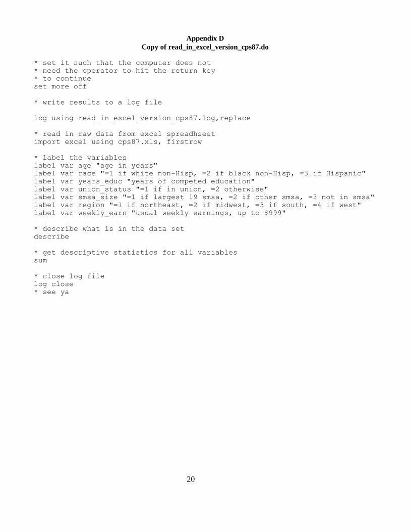
Appendix D

Copy of read_in_excel_version_cps87.do

* set it such that the computer does not

* need the operator to hit the return key

* to continue

set more off

* write results to a log file

log using read_in_excel_version_cps87.log,replace

* read in raw data from excel spreadhseet

import excel using cps87.xls, firstrow

* label the variables

label var age "age in years"

label var race "=1 if white non-Hisp, =2 if black non-Hisp, =3 if Hispanic"

label var years_educ "years of competed education"

label var union_status "=1 if in union, =2 otherwise"

label var smsa_size "=1 if largest 19 smsa, =2 if other smsa, =3 not in smsa"

label var region "=1 if northeast, =2 if midwest, =3 if south, =4 if west"

label var weekly_earn "usual weekly earnings, up to $999"

* describe what is in the data set

describe

* get descriptive statistics for all variables

sum

* close log file

log close

* see ya