Introduction to SPSS Workshop

http://csass.ucsc.edu/short%20courses/index.html

SPSS WORKSHOP!What: Part 1 Handout for “Introduction to SPSS” Workshop Part 1 Topics: Data entry, including transforming and computing variables Frequency tables and descriptive statistics Simple graphs Contingency Table Analysis (lambda, gamma, chi-square, etc.) Part 2 Topics: T Tests ANOVA Correlation Regression Questions? Please email Yvonne Y. Kwan at [email protected]

Written and presented by Yvonne Y. Kwan, UCSC CSASS Statistics Consultant

mailto:[email protected]


http://csass.ucsc.edu/short%20courses/index.html

Introduction to SPSS - UCSC CSASS Workshop

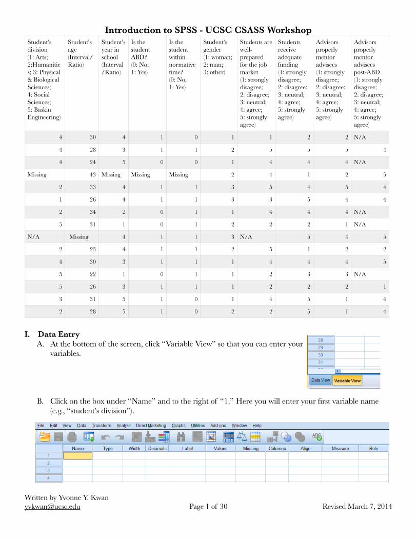
I. Data Entry

A. At the bottom of the screen, click “Variable View” so that you can enter your variables. !!!!

B. Click on the box under “Name” and to the right of “1.” Here you will enter your first variable name (e.g., “student’s division”).

Revised March 7, 2014Page ! of !1 30Written by Yvonne Y. Kwan [email protected]

Student’s division (1: Arts; 2:Humanities; 3: Physical & Biological Sciences; 4: Social Sciences; 5: Baskin Engineering)

Student’s age (Interval/Ratio)

Student’s year in school (Interval/Ratio)

Is the student ABD? (0: No; 1: Yes)

Is the student within normative time? (0: No, 1: Yes)

Student’s gender (1: woman; 2: man; 3: other)

Students are well-prepared for the job market (1: strongly disagree; 2: disagree; 3: neutral; 4: agree; 5: strongly agree)

Students receive adequate funding (1: strongly disagree; 2: disagree; 3: neutral; 4: agree; 5: strongly agree)

Advisors properly mentor advisees (1: strongly disagree; 2: disagree; 3: neutral; 4: agree; 5: strongly agree)

Advisors properly mentor advisees post-ABD (1: strongly disagree; 2: disagree; 3: neutral; 4: agree; 5: strongly agree)

4 30 4 1 0 1 1 2 2 N/A

4 28 3 1 1 2 5 5 5 4

4 24 5 0 0 1 4 4 4 N/A

Missing 43 Missing Missing Missing 2 4 1 2 5

2 33 4 1 1 3 5 4 5 4

1 26 4 1 1 3 3 5 4 4

2 34 2 0 1 1 4 4 4 N/A

5 31 1 0 1 2 2 2 1 N/A

N/A Missing 4 1 1 3 N/A 5 4 5

2 23 4 1 1 2 5 1 2 2

4 30 3 1 1 1 4 4 4 5

5 22 1 0 1 1 2 3 3 N/A

5 26 3 1 1 1 2 2 2 1

3 31 5 1 0 1 4 5 1 4

2 28 5 1 0 2 2 5 1 4


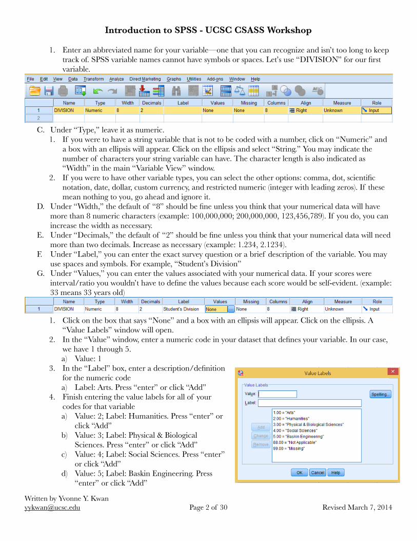
Introduction to SPSS - UCSC CSASS Workshop!1. Enter an abbreviated name for your variable—one that you can recognize and isn’t too long to keep

track of. SPSS variable names cannot have symbols or spaces. Let’s use “DIVISION” for our first variable.

! C. Under “Type,” leave it as numeric.

1. If you were to have a string variable that is not to be coded with a number, click on “Numeric” and a box with an ellipsis will appear. Click on the ellipsis and select “String.” You may indicate the number of characters your string variable can have. The character length is also indicated as “Width” in the main “Variable View” window.

2. If you were to have other variable types, you can select the other options: comma, dot, scientific notation, date, dollar, custom currency, and restricted numeric (integer with leading zeros). If these mean nothing to you, go ahead and ignore it.

D. Under “Width,” the default of “8” should be fine unless you think that your numerical data will have more than 8 numeric characters (example: 100,000,000; 200,000,000, 123,456,789). If you do, you can increase the width as necessary.

E. Under “Decimals,” the default of “2” should be fine unless you think that your numerical data will need more than two decimals. Increase as necessary (example: 1.234, 2.1234).

F. Under “Label,” you can enter the exact survey question or a brief description of the variable. You may use spaces and symbols. For example, “Student’s Division”

G. Under “Values,” you can enter the values associated with your numerical data. If your scores were interval/ratio you wouldn’t have to define the values because each score would be self-evident. (example: 33 means 33 years old)

! 1. Click on the box that says “None” and a box with an ellipsis will appear. Click on the ellipsis. A

“Value Labels” window will open. 2. In the “Value” window, enter a numeric code in your dataset that defines your variable. In our case,

we have 1 through 5. a) Value: 1

3. In the “Label” box, enter a description/definition for the numeric code a) Label: Arts. Press “enter” or click “Add”

4. Finish entering the value labels for all of your codes for that variable a) Value: 2; Label: Humanities. Press “enter” or

click “Add” b) Value: 3; Label: Physical & Biological

Sciences. Press “enter” or click “Add” c) Value: 4; Label: Social Sciences. Press “enter”

or click “Add” d) Value: 5; Label: Baskin Engineering. Press

“enter” or click “Add”


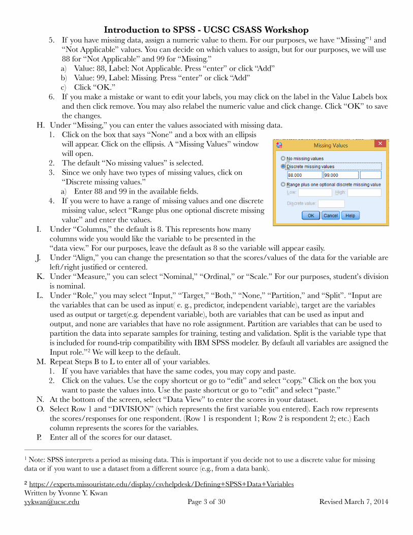
Introduction to SPSS - UCSC CSASS Workshop5. If you have missing data, assign a numeric value to them. For our purposes, we have “Missing” and 1

“Not Applicable” values. You can decide on which values to assign, but for our purposes, we will use 88 for “Not Applicable” and 99 for “Missing.” a) Value: 88, Label: Not Applicable. Press “enter” or click “Add” b) Value: 99, Label: Missing. Press “enter” or click “Add” c) Click “OK.”

6. If you make a mistake or want to edit your labels, you may click on the label in the Value Labels box and then click remove. You may also relabel the numeric value and click change. Click “OK” to save the changes.

H. Under “Missing,” you can enter the values associated with missing data. 1. Click on the box that says “None” and a box with an ellipsis

will appear. Click on the ellipsis. A “Missing Values” window will open.

2. The default “No missing values” is selected. 3. Since we only have two types of missing values, click on

“Discrete missing values.” a) Enter 88 and 99 in the available fields.

4. If you were to have a range of missing values and one discrete missing value, select “Range plus one optional discrete missing value” and enter the values.

I. Under “Columns,” the default is 8. This represents how many columns wide you would like the variable to be presented in the “data view.” For our purposes, leave the default as 8 so the variable will appear easily.

J. Under “Align,” you can change the presentation so that the scores/values of the data for the variable are left/right justified or centered.

K. Under “Measure,” you can select “Nominal,” “Ordinal,” or “Scale.” For our purposes, student’s division is nominal.

L. Under “Role,” you may select “Input,” “Target,” “Both,” “None,” “Partition,” and “Split”. “Input are the variables that can be used as input( e. g., predictor, independent variable), target are the variables used as output or target(e.g. dependent variable), both are variables that can be used as input and output, and none are variables that have no role assignment. Partition are variables that can be used to partition the data into separate samples for training, testing and validation. Split is the variable type that is included for round-trip compatibility with IBM SPSS modeler. By default all variables are assigned the Input role.” We will keep to the default. 2

M. Repeat Steps B to L to enter all of your variables. 1. If you have variables that have the same codes, you may copy and paste. 2. Click on the values. Use the copy shortcut or go to “edit” and select “copy.” Click on the box you

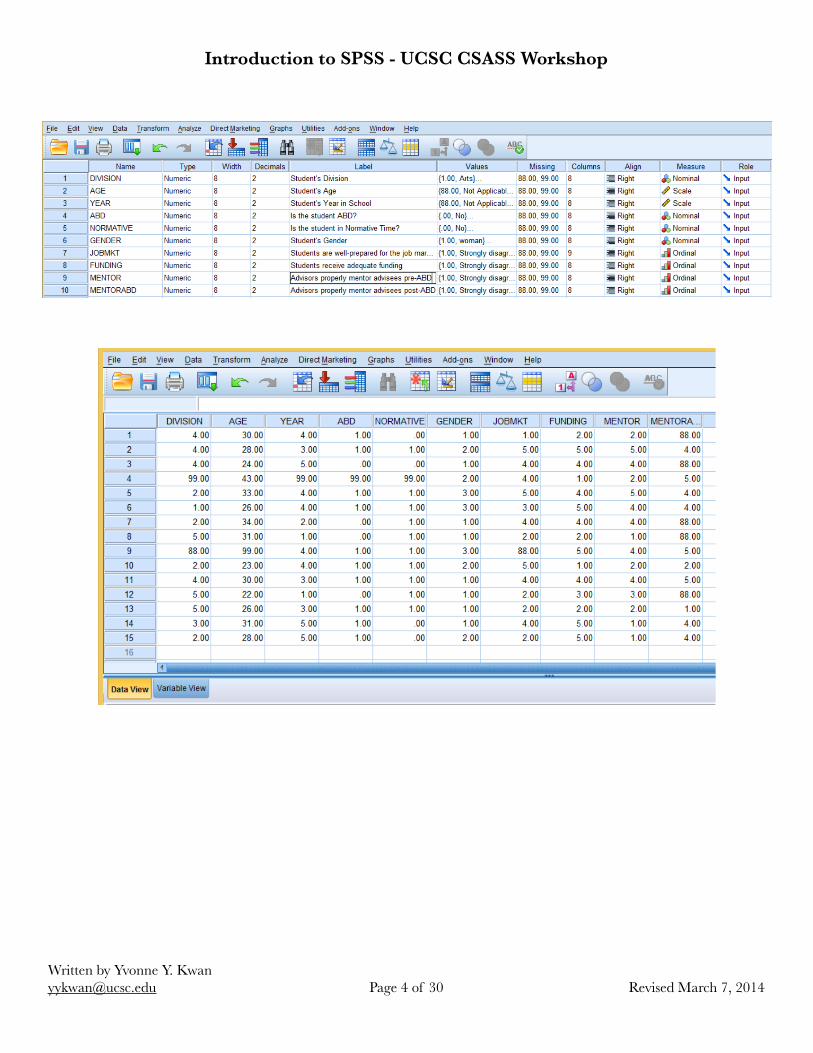
want to paste the values into. Use the paste shortcut or go to “edit” and select “paste.” N. At the bottom of the screen, select “Data View” to enter the scores in your dataset. O. Select Row 1 and “DIVISION” (which represents the first variable you entered). Each row represents

the scores/responses for one respondent. (Row 1 is respondent 1; Row 2 is respondent 2; etc.) Each column represents the scores for the variables.

P. Enter all of the scores for our dataset.


! Note: SPSS interprets a period as missing data. This is important if you decide not to use a discrete value for missing 1

data or if you want to use a dataset from a different source (e.g., from a data bank).

� https://experts.missouristate.edu/display/csvhelpdesk/Defining+SPSS+Data+Variables2



Introduction to SPSS - UCSC CSASS WorkshopII. Transforming Variables 3

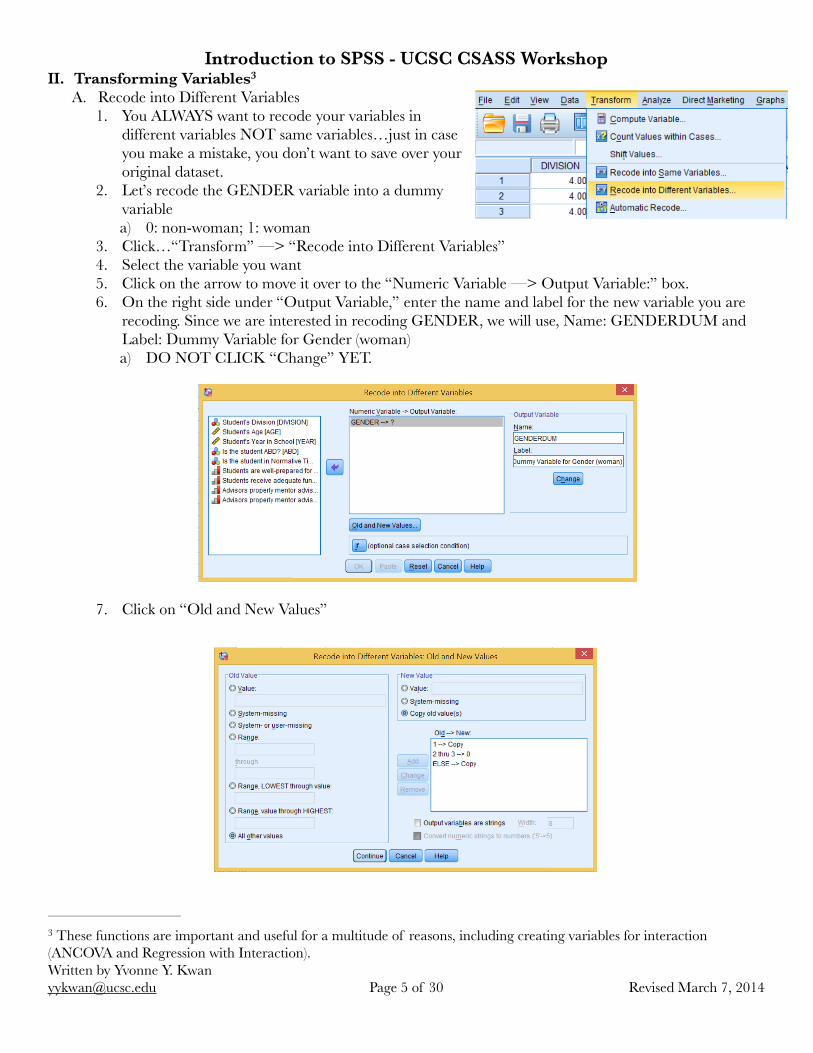
A. Recode into Different Variables 1. You ALWAYS want to recode your variables in

different variables NOT same variables…just in case you make a mistake, you don’t want to save over your original dataset.

2. Let’s recode the GENDER variable into a dummy variable a) 0: non-woman; 1: woman

3. Click…“Transform” —> “Recode into Different Variables” 4. Select the variable you want 5. Click on the arrow to move it over to the “Numeric Variable —> Output Variable:” box. 6. On the right side under “Output Variable,” enter the name and label for the new variable you are

recoding. Since we are interested in recoding GENDER, we will use, Name: GENDERDUM and Label: Dummy Variable for Gender (woman) a) DO NOT CLICK “Change” YET.

7. Click on “Old and New Values”


! These functions are important and useful for a multitude of reasons, including creating variables for interaction 3

(ANCOVA and Regression with Interaction).

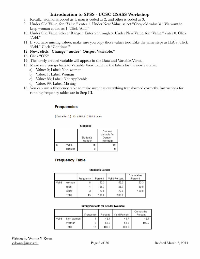
Introduction to SPSS - UCSC CSASS Workshop8. Recall…woman is coded as 1, man is coded as 2, and other is coded as 3. 9. Under Old Value, for “Value,” enter 1. Under New Value, select “Copy old value(s)”. We want to

keep woman coded as 1. Click “Add.” 10. Under Old Value, select “Range.” Enter 2 through 3. Under New Value, for “Value,” enter 0. Click

“Add.” 11. If you have missing values, make sure you copy those values too. Take the same steps as II.A.9. Click

“Add.” Click “Continue.” 12. Now, click “Change” under “Output Variable.” 13. Click “OK” 14. The newly created variable will appear in the Data and Variable Views. 15. Make sure you go back to Variable View to define the labels for the new variable.

a) Value: 0; Label: Non-woman b) Value: 1; Label: Woman c) Value: 88; Label: Not Applicable d) Value: 99; Label: Missing

16. You can run a frequency table to make sure that everything transformed correctly. Instructions for running frequency tables are in Step III.


Introduction to SPSS - UCSC CSASS WorkshopB. Compute a Variable Using Transformations or Computations

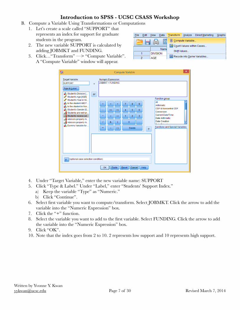
1. Let’s create a scale called “SUPPORT” that represents an index for support for graduate students in the program.

2. The new variable SUPPORT is calculated by adding JOBMKT and FUNDING.

3. Click…“Transform” —> “Compute Variable”. A “Compute Variable” window will appear.

4. Under “Target Variable,” enter the new variable name: SUPPORT 5. Click “Type & Label.” Under “Label,” enter “Students’ Support Index.”

a) Keep the variable “Type” as “Numeric.” b) Click “Continue”.

6. Select first variable you want to compute/transform. Select JOBMKT. Click the arrow to add the variable into the “Numeric Expression” box.

7. Click the “+” function. 8. Select the variable you want to add to the first variable. Select FUNDING. Click the arrow to add

the variable into the “Numeric Expression” box. 9. Click “OK”. 10. Note that the index goes from 2 to 10. 2 represents low support and 10 represents high support.


Introduction to SPSS - UCSC CSASS WorkshopC. Compute a Variable Using Conditions

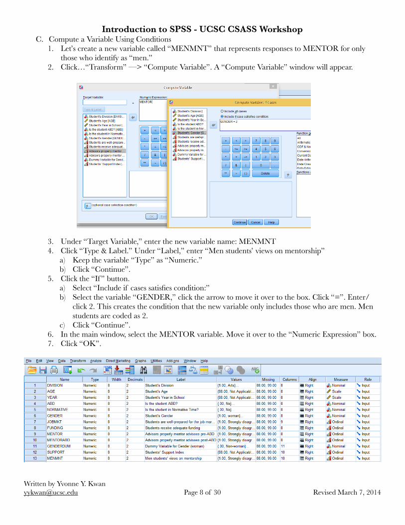
1. Let’s create a new variable called “MENMNT” that represents responses to MENTOR for only those who identify as “men.”

2. Click…“Transform” —> “Compute Variable”. A “Compute Variable” window will appear.

3. Under “Target Variable,” enter the new variable name: MENMNT 4. Click “Type & Label.” Under “Label,” enter “Men students’ views on mentorship”

a) Keep the variable “Type” as “Numeric.” b) Click “Continue”.

5. Click the “If ” button. a) Select “Include if cases satisfies condition:” b) Select the variable “GENDER,” click the arrow to move it over to the box. Click “=”. Enter/

click 2. This creates the condition that the new variable only includes those who are men. Men students are coded as 2.

c) Click “Continue”. 6. In the main window, select the MENTOR variable. Move it over to the “Numeric Expression” box. 7. Click “OK”. !

!


Introduction to SPSS - UCSC CSASS WorkshopIII. Descriptive Statistics

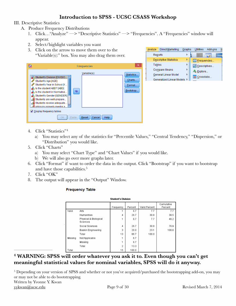
A. Produce Frequency Distributions 1. Click…“Analyze” —> “Descriptive Statistics” —> “Frequencies”. A “Frequencies” window will

appear. 2. Select/highlight variables you want 3. Click on the arrow to move them over to the

“Variable(s):” box. You may also drag them over.

4. Click “Statistics” 4

a) You may select any of the statistics for “Percentile Values,” “Central Tendency,” “Dispersion,” or “Distribution” you would like.

5. Click “Charts” a) You may select “Chart Type” and “Chart Values” if you would like. b) We will also go over more graphs later.

6. Click “Format” if want to order the data in the output. Click “Bootstrap” if you want to bootstrap and have those capabilities. 5

7. Click “OK” 8. The output will appear in the “Output” Window.


! WARNING: SPSS will order whatever you ask it to. Even though you can’t get 4

meaningful statistical values for nominal variables, SPSS will do it anyway.! Depending on your version of SPSS and whether or not you’ve acquired/purchased the bootstrapping add-on, you may 5

or may not be able to do bootstrapping.

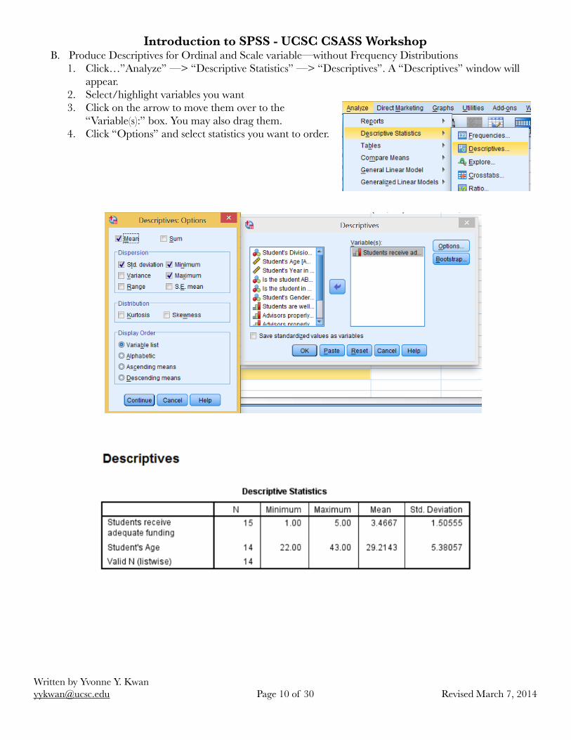
Introduction to SPSS - UCSC CSASS WorkshopB. Produce Descriptives for Ordinal and Scale variable—without Frequency Distributions

1. Click…”Analyze” —> “Descriptive Statistics” —> “Descriptives”. A “Descriptives” window will appear.

2. Select/highlight variables you want 3. Click on the arrow to move them over to the

“Variable(s):” box. You may also drag them. 4. Click “Options” and select statistics you want to order. !


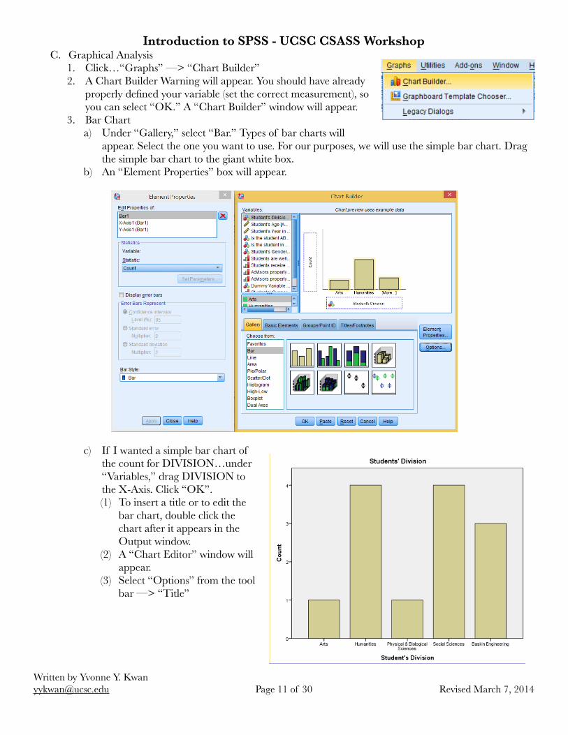
Introduction to SPSS - UCSC CSASS WorkshopC. Graphical Analysis

1. Click…“Graphs” —> “Chart Builder” 2. A Chart Builder Warning will appear. You should have already

properly defined your variable (set the correct measurement), so you can select “OK.” A “Chart Builder” window will appear.

3. Bar Chart a) Under “Gallery,” select “Bar.” Types of bar charts will

appear. Select the one you want to use. For our purposes, we will use the simple bar chart. Drag the simple bar chart to the giant white box.

b) An “Element Properties” box will appear.

c) If I wanted a simple bar chart of the count for DIVISION…under “Variables,” drag DIVISION to the X-Axis. Click “OK”. (1) To insert a title or to edit the

bar chart, double click the chart after it appears in the Output window.

(2) A “Chart Editor” window will appear.

(3) Select “Options” from the tool bar —> “Title” !


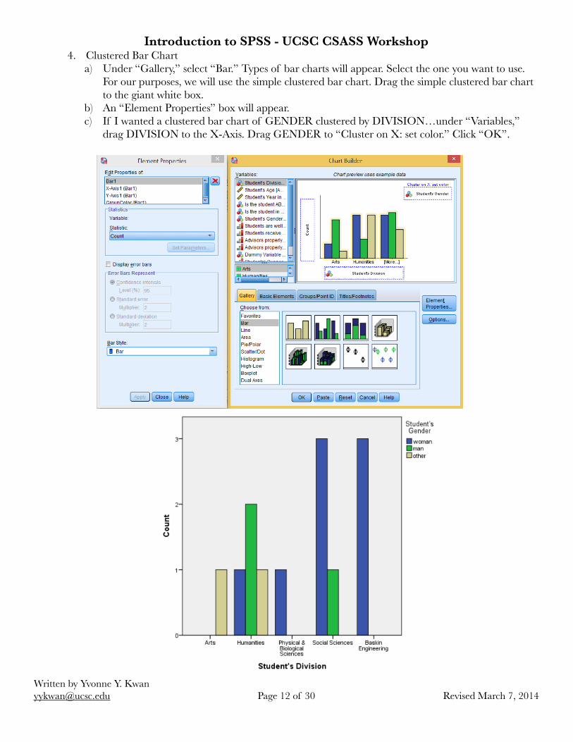
Introduction to SPSS - UCSC CSASS Workshop4. Clustered Bar Chart

a) Under “Gallery,” select “Bar.” Types of bar charts will appear. Select the one you want to use. For our purposes, we will use the simple clustered bar chart. Drag the simple clustered bar chart to the giant white box.

b) An “Element Properties” box will appear. c) If I wanted a clustered bar chart of GENDER clustered by DIVISION…under “Variables,”

drag DIVISION to the X-Axis. Drag GENDER to “Cluster on X: set color.” Click “OK”.


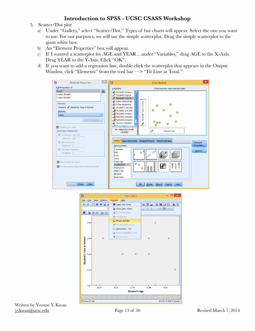
Introduction to SPSS - UCSC CSASS Workshop5. Scatter/Dot plot

a) Under “Gallery,” select “Scatter/Dot.” Types of bar charts will appear. Select the one you want to use. For our purposes, we will use the simple scatterplot. Drag the simple scatterplot to the giant white box.

b) An “Element Properties” box will appear. c) If I wanted a scatterplot for AGE and YEAR…under “Variables,” drag AGE to the X-Axis.

Drag YEAR to the Y-Axis. Click “OK”. d) If you want to add a regression line, double click the scatterplot that appears in the Output

Window, click “Elements” from the tool bar —> “Fit Line at Total.”


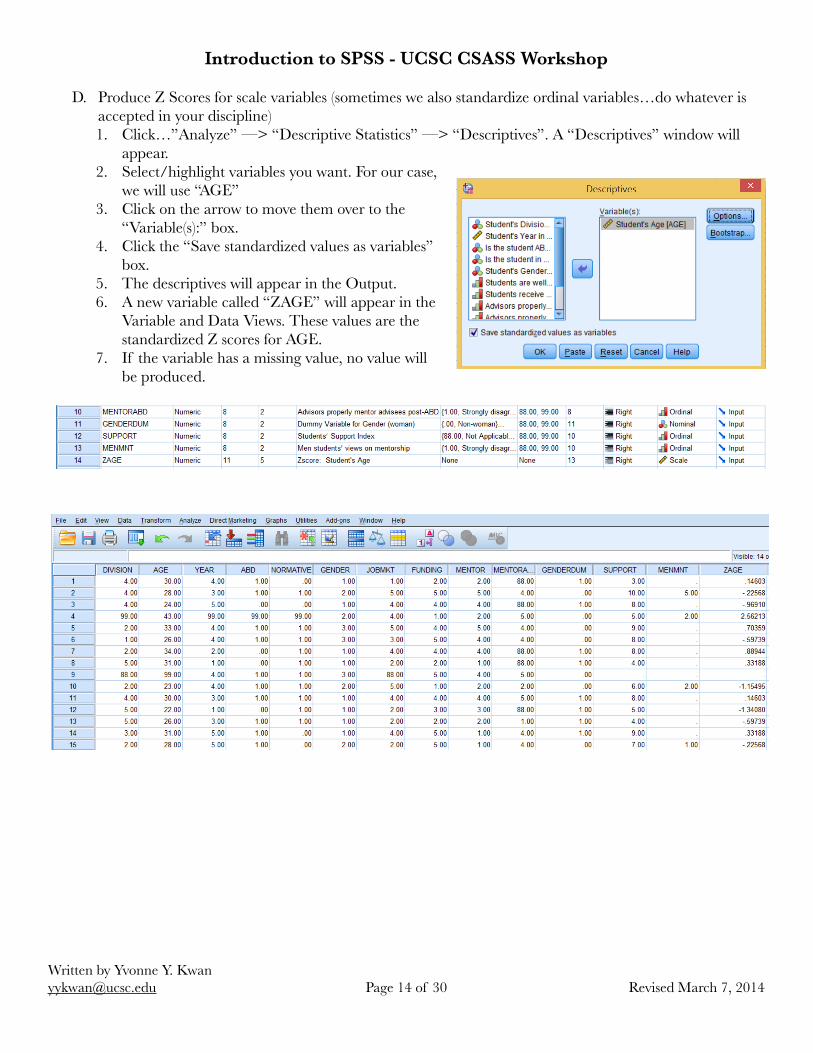
Introduction to SPSS - UCSC CSASS Workshop!D. Produce Z Scores for scale variables (sometimes we also standardize ordinal variables…do whatever is

accepted in your discipline) 1. Click…”Analyze” —> “Descriptive Statistics” —> “Descriptives”. A “Descriptives” window will

appear. 2. Select/highlight variables you want. For our case,

we will use “AGE” 3. Click on the arrow to move them over to the

“Variable(s):” box. 4. Click the “Save standardized values as variables”

box. 5. The descriptives will appear in the Output. 6. A new variable called “ZAGE” will appear in the

Variable and Data Views. These values are the standardized Z scores for AGE.

7. If the variable has a missing value, no value will be produced.

!


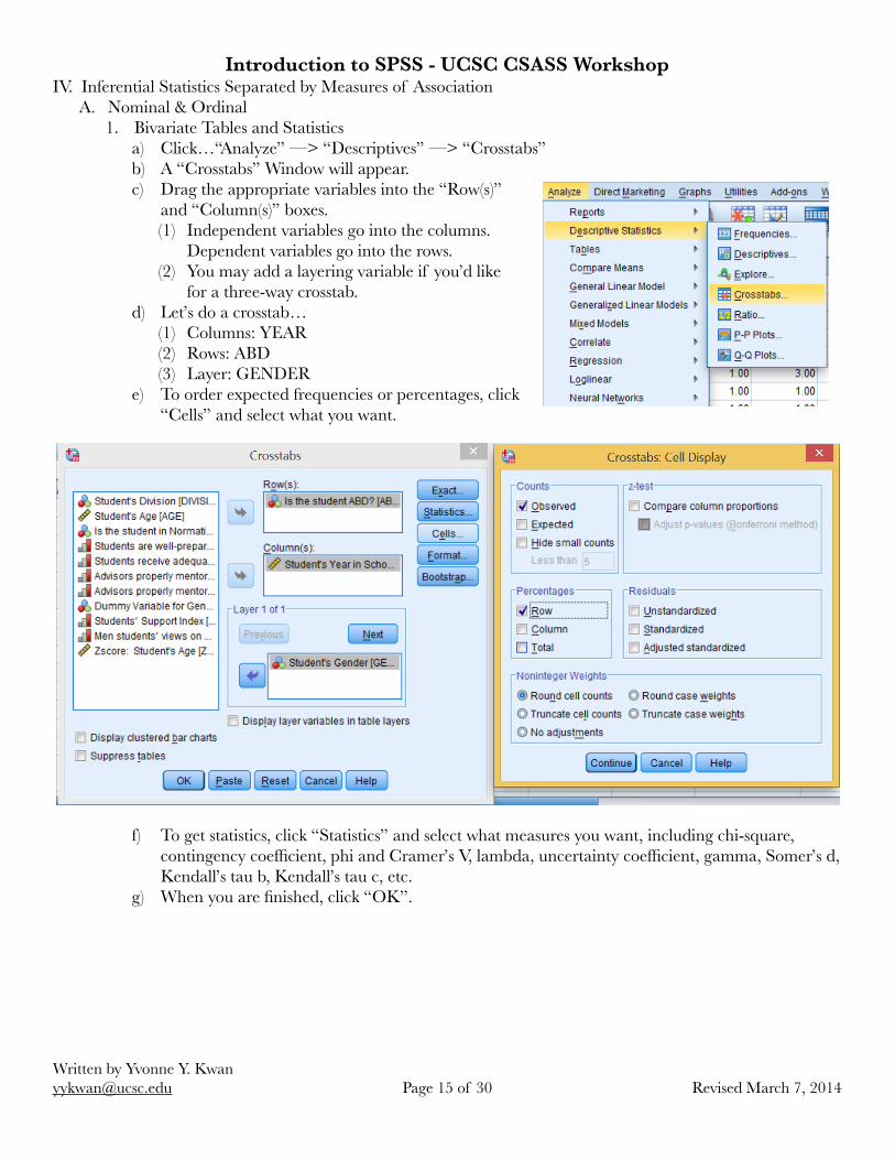
Introduction to SPSS - UCSC CSASS WorkshopIV. Inferential Statistics Separated by Measures of Association

A. Nominal & Ordinal 1. Bivariate Tables and Statistics

a) Click…“Analyze” —> “Descriptives” —> “Crosstabs” b) A “Crosstabs” Window will appear. c) Drag the appropriate variables into the “Row(s)”

and “Column(s)” boxes. (1) Independent variables go into the columns.

Dependent variables go into the rows. (2) You may add a layering variable if you’d like

for a three-way crosstab. d) Let’s do a crosstab…

(1) Columns: YEAR (2) Rows: ABD (3) Layer: GENDER

e) To order expected frequencies or percentages, click “Cells” and select what you want.

f) To get statistics, click “Statistics” and select what measures you want, including chi-square, contingency coefficient, phi and Cramer’s V, lambda, uncertainty coefficient, gamma, Somer’s d, Kendall’s tau b, Kendall’s tau c, etc.

g) When you are finished, click “OK”. !




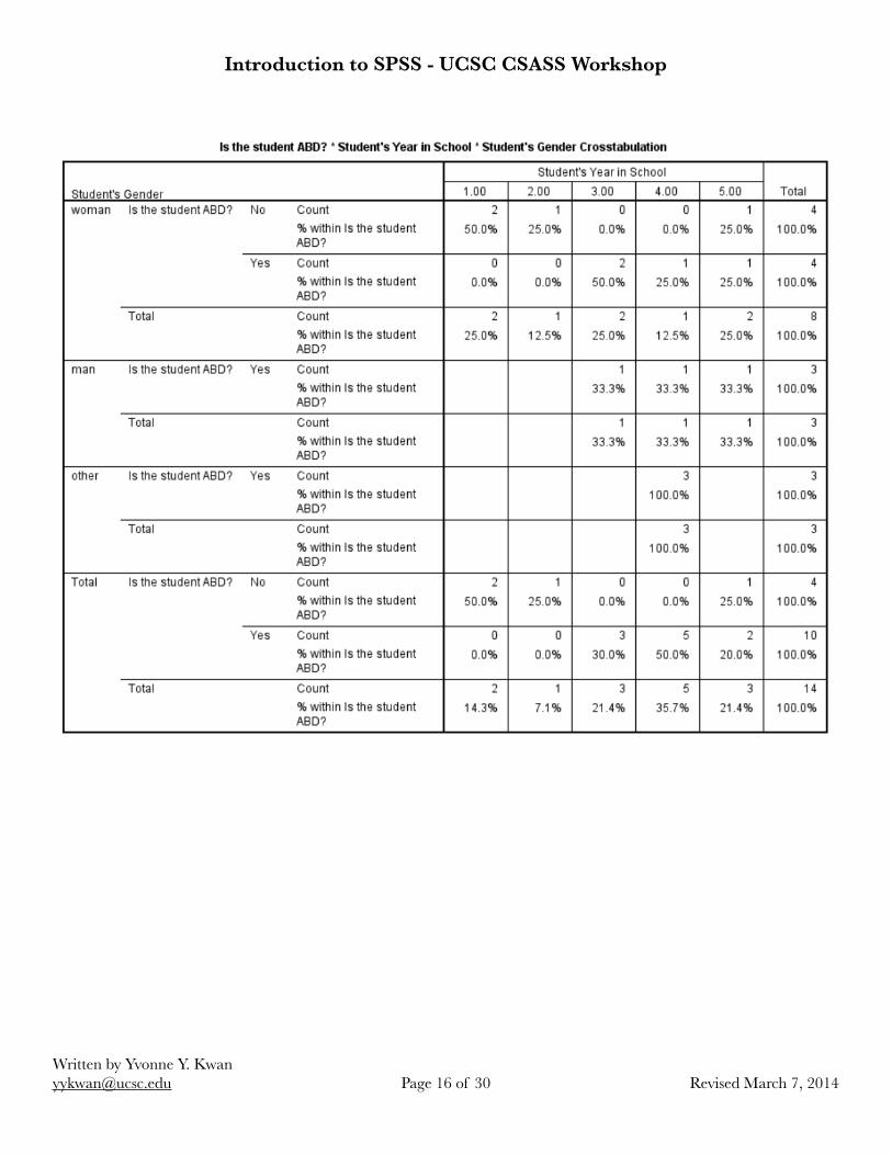
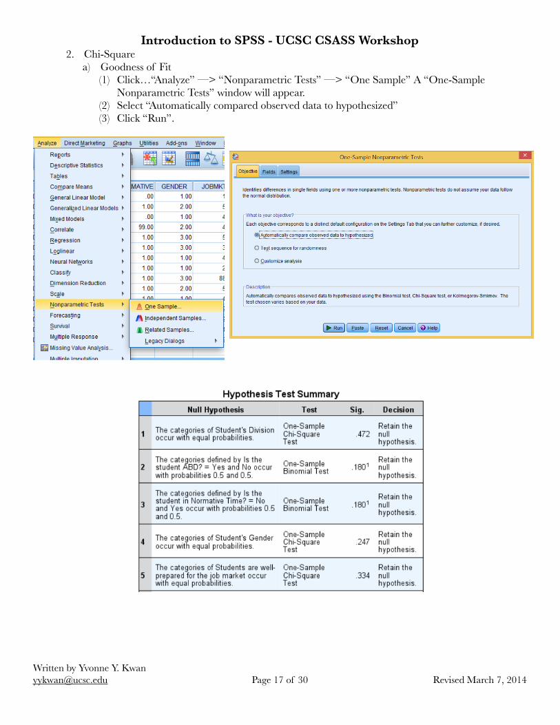
Introduction to SPSS - UCSC CSASS Workshop2. Chi-Square

a) Goodness of Fit (1) Click…“Analyze” —> “Nonparametric Tests” —> “One Sample” A “One-Sample

Nonparametric Tests” window will appear. (2) Select “Automatically compared observed data to hypothesized” (3) Click “Run”.


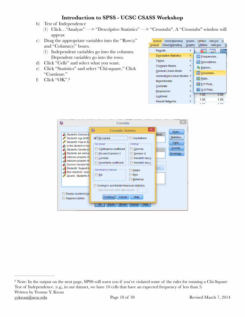
Introduction to SPSS - UCSC CSASS Workshopb) Test of Independence

(1) Click…“Analyze” —> “Descriptive Statistics” —> “Crosstabs". A “Crosstabs" window will appear.

c) Drag the appropriate variables into the “Row(s)” and “Column(s)” boxes. (1) Independent variables go into the columns.

Dependent variables go into the rows. d) Click “Cells” and select what you want. e) Click “Statistics” and select “Chi-square.” Click

“Continue.” f) Click “OK”. 6


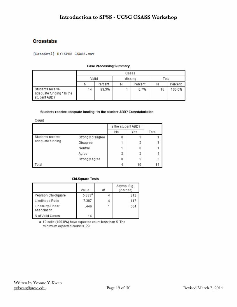
! Note: In the output on the next page, SPSS will warn you if you’ve violated some of the rules for running a Chi-Square 6

Test of Independence. (e.g., in our dataset, we have 10 cells that have an expected frequency of less than 5)

Introduction to SPSS - UCSC CSASS Workshop!


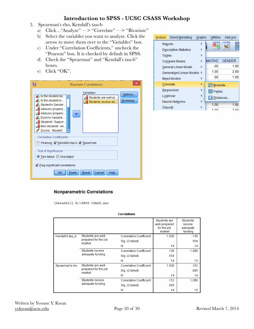
Introduction to SPSS - UCSC CSASS Workshop3. Spearman’s rho, Kendall’s tau-b

a) Click…“Analyze” —> “Correlate” —> “Bivariate” b) Select the variables you want to analyze. Click the

arrow to move them over to the “Variables” box. c) Under “Correlation Coefficients,” uncheck the

“Pearson” box. It is checked by default in SPSS. d) Check the “Spearman” and “Kendall’s tau-b”

boxes. e) Click “OK”.


Introduction to SPSS - UCSC CSASS Workshop!B. Interval/Ratio

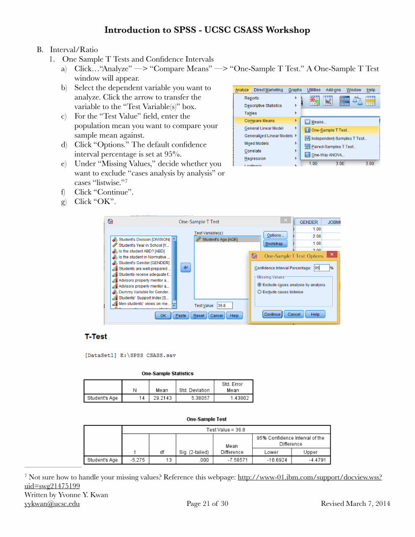
1. One Sample T Tests and Confidence Intervals a) Click…“Analyze” —> “Compare Means” —> “One-Sample T Test.” A One-Sample T Test

window will appear. b) Select the dependent variable you want to

analyze. Click the arrow to transfer the variable to the “Test Variable(s)” box.

c) For the “Test Value” field, enter the population mean you want to compare your sample mean against.

d) Click “Options.” The default confidence interval percentage is set at 95%.

e) Under “Missing Values,” decide whether you want to exclude “cases analysis by analysis” or cases “listwise.” 7

f) Click “Continue”. g) Click “OK”.

!


! Not sure how to handle your missing values? Reference this webpage: http://www-01.ibm.com/support/docview.wss?7

uid=swg21475199

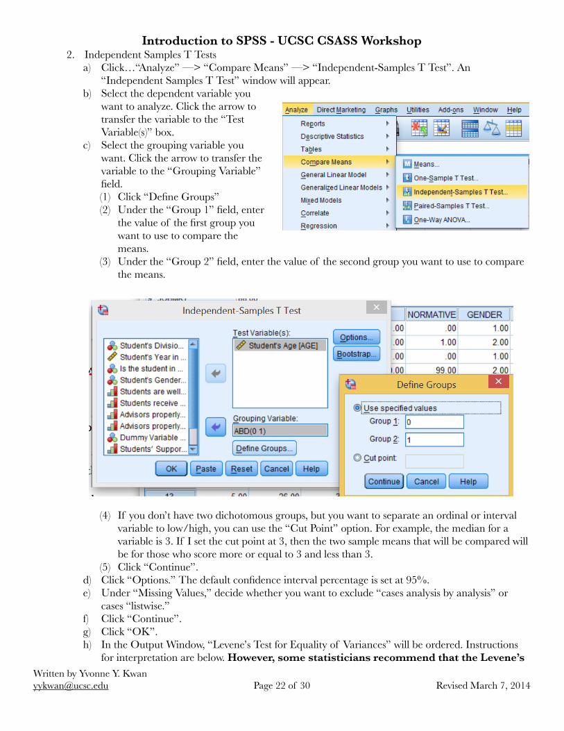
Introduction to SPSS - UCSC CSASS Workshop2. Independent Samples T Tests

a) Click…“Analyze” —> “Compare Means” —> “Independent-Samples T Test”. An “Independent Samples T Test” window will appear.

b) Select the dependent variable you want to analyze. Click the arrow to transfer the variable to the “Test Variable(s)” box.

c) Select the grouping variable you want. Click the arrow to transfer the variable to the “Grouping Variable” field. (1) Click “Define Groups” (2) Under the “Group 1” field, enter

the value of the first group you want to use to compare the means.

(3) Under the “Group 2” field, enter the value of the second group you want to use to compare the means.

(4) If you don’t have two dichotomous groups, but you want to separate an ordinal or interval variable to low/high, you can use the “Cut Point” option. For example, the median for a variable is 3. If I set the cut point at 3, then the two sample means that will be compared will be for those who score more or equal to 3 and less than 3.

(5) Click “Continue”. d) Click “Options.” The default confidence interval percentage is set at 95%. e) Under “Missing Values,” decide whether you want to exclude “cases analysis by analysis” or

cases “listwise.” f) Click “Continue”. g) Click “OK”. h) In the Output Window, “Levene’s Test for Equality of Variances” will be ordered. Instructions

for interpretation are below. However, some statisticians recommend that the Levene’s


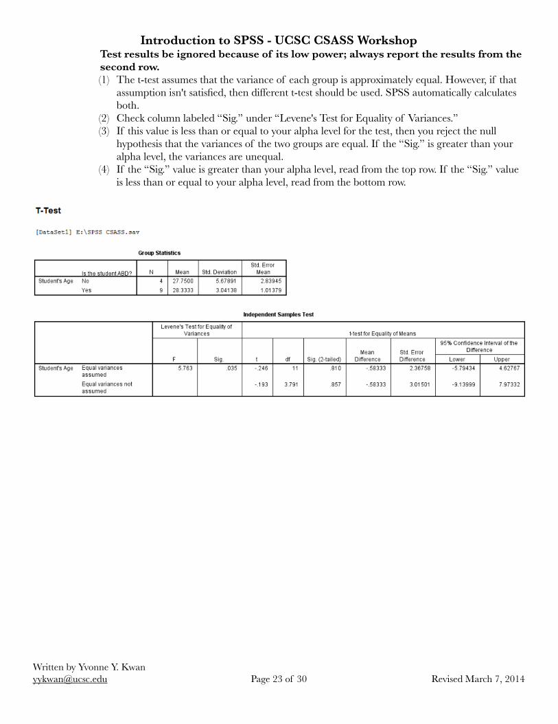
Introduction to SPSS - UCSC CSASS WorkshopTest results be ignored because of its low power; always report the results from the second row. (1) The t-test assumes that the variance of each group is approximately equal. However, if that

assumption isn't satisfied, then different t-test should be used. SPSS automatically calculates both.

(2) Check column labeled “Sig.” under “Levene's Test for Equality of Variances.” (3) If this value is less than or equal to your alpha level for the test, then you reject the null

hypothesis that the variances of the two groups are equal. If the “Sig.” is greater than your alpha level, the variances are unequal.

(4) If the “Sig.” value is greater than your alpha level, read from the top row. If the “Sig.” value is less than or equal to your alpha level, read from the bottom row.

!


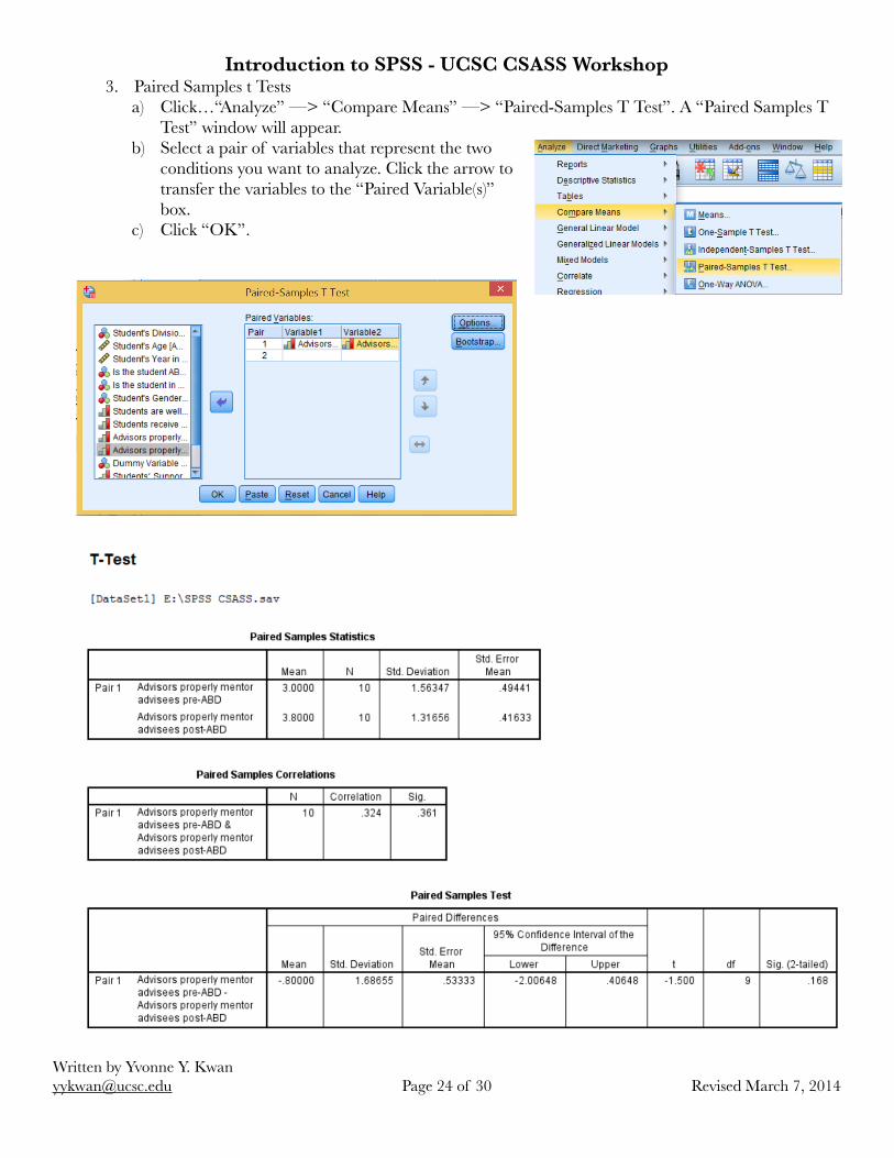
Introduction to SPSS - UCSC CSASS Workshop3. Paired Samples t Tests

a) Click…“Analyze” —> “Compare Means” —> “Paired-Samples T Test”. A “Paired Samples T Test” window will appear.

b) Select a pair of variables that represent the two conditions you want to analyze. Click the arrow to transfer the variables to the “Paired Variable(s)” box.

c) Click “OK”.


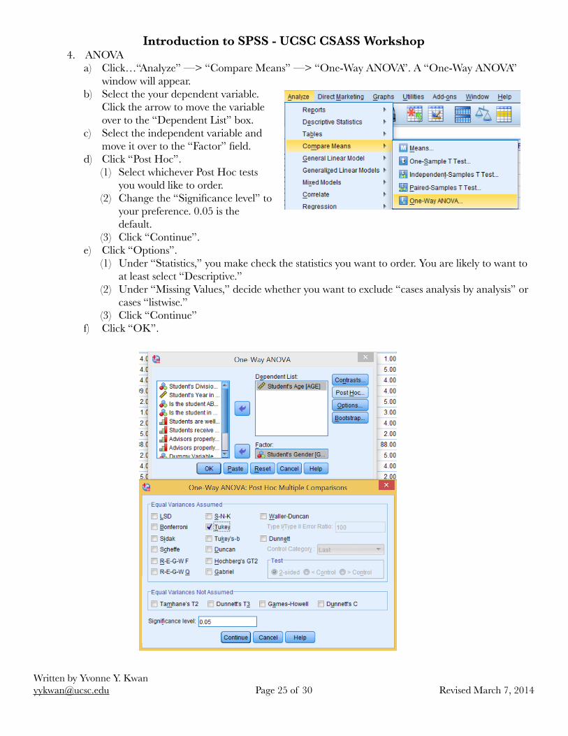
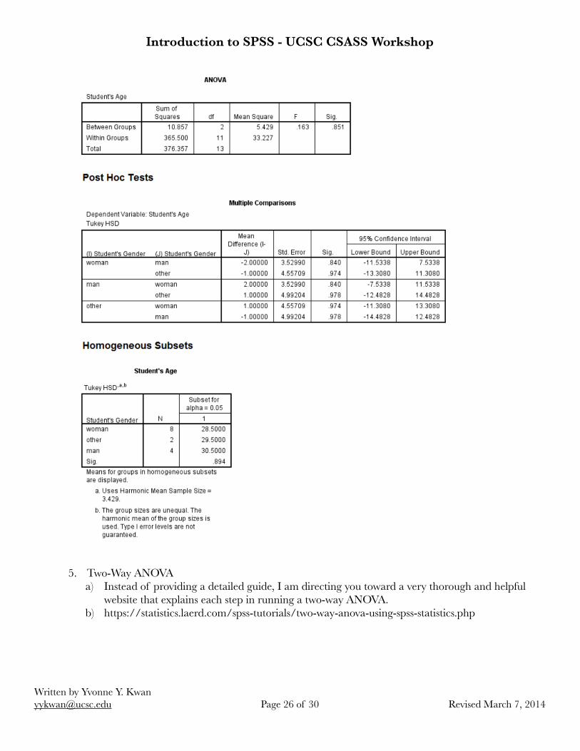
Introduction to SPSS - UCSC CSASS Workshop4. ANOVA

a) Click…“Analyze” —> “Compare Means” —> “One-Way ANOVA”. A “One-Way ANOVA” window will appear.

b) Select the your dependent variable. Click the arrow to move the variable over to the “Dependent List” box.

c) Select the independent variable and move it over to the “Factor” field.

d) Click “Post Hoc”. (1) Select whichever Post Hoc tests

you would like to order. (2) Change the “Significance level” to

your preference. 0.05 is the default.

(3) Click “Continue”. e) Click “Options”.

(1) Under “Statistics,” you make check the statistics you want to order. You are likely to want to at least select “Descriptive.”

(2) Under “Missing Values,” decide whether you want to exclude “cases analysis by analysis” or cases “listwise.”

(3) Click “Continue” f) Click “OK”. !



!5. Two-Way ANOVA

a) Instead of providing a detailed guide, I am directing you toward a very thorough and helpful website that explains each step in running a two-way ANOVA.

b) https://statistics.laerd.com/spss-tutorials/two-way-anova-using-spss-statistics.php


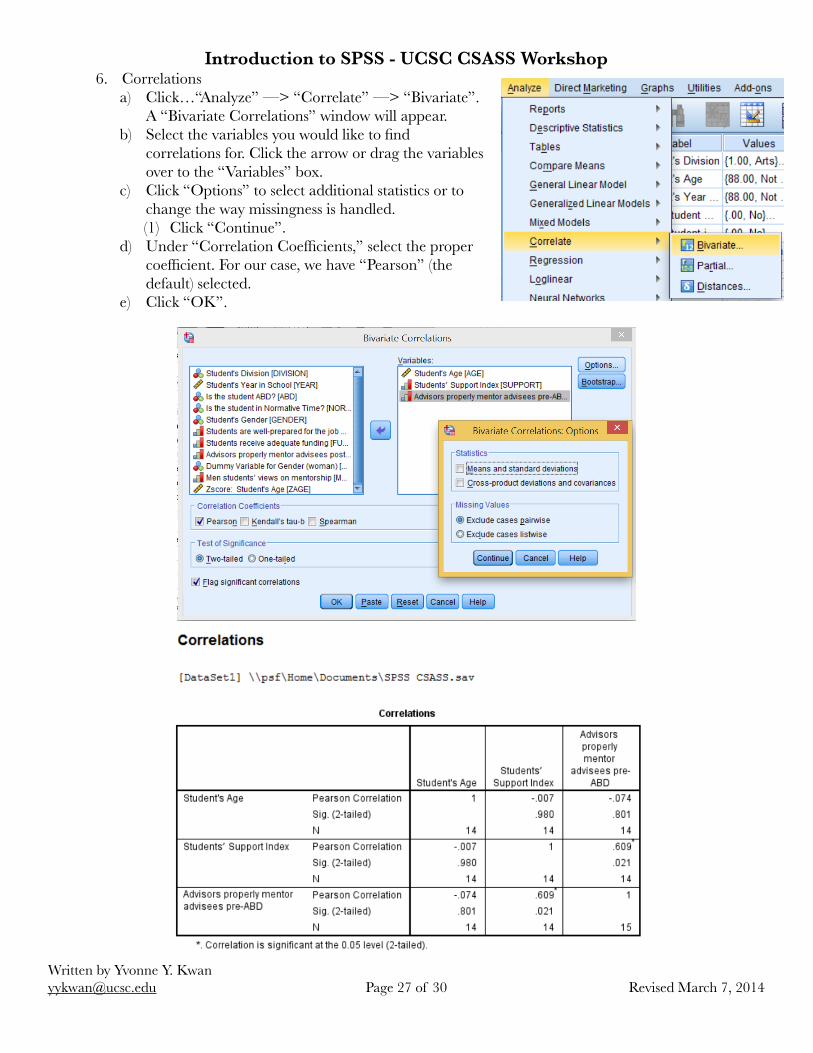
Introduction to SPSS - UCSC CSASS Workshop6. Correlations

a) Click…“Analyze” —> “Correlate” —> “Bivariate”. A “Bivariate Correlations” window will appear.

b) Select the variables you would like to find correlations for. Click the arrow or drag the variables over to the “Variables” box.

c) Click “Options” to select additional statistics or to change the way missingness is handled. (1) Click “Continue”.

d) Under “Correlation Coefficients,” select the proper coefficient. For our case, we have “Pearson” (the default) selected.

e) Click “OK”.


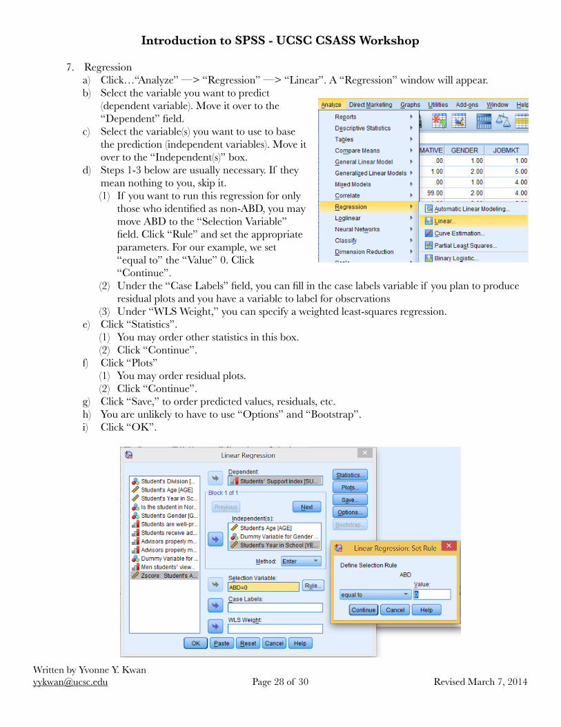
Introduction to SPSS - UCSC CSASS Workshop!7. Regression

a) Click…“Analyze” —> “Regression” —> “Linear”. A “Regression” window will appear. b) Select the variable you want to predict

(dependent variable). Move it over to the “Dependent” field.

c) Select the variable(s) you want to use to base the prediction (independent variables). Move it over to the “Independent(s)” box.

d) Steps 1-3 below are usually necessary. If they mean nothing to you, skip it. (1) If you want to run this regression for only

those who identified as non-ABD, you may move ABD to the “Selection Variable” field. Click “Rule” and set the appropriate parameters. For our example, we set “equal to” the “Value” 0. Click “Continue”.

(2) Under the “Case Labels” field, you can fill in the case labels variable if you plan to produce residual plots and you have a variable to label for observations

(3) Under “WLS Weight,” you can specify a weighted least-squares regression. e) Click “Statistics”.

(1) You may order other statistics in this box. (2) Click “Continue”.

f) Click “Plots” (1) You may order residual plots. (2) Click “Continue”.

g) Click “Save,” to order predicted values, residuals, etc. h) You are unlikely to have to use “Options” and “Bootstrap”. i) Click “OK”.


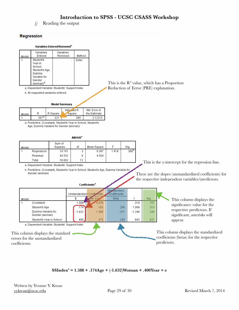
Introduction to SPSS - UCSC CSASS Workshopj) Reading the output

!


This is the R2 value, which has a Proportion Reduction of Error (PRE) explanation.

This is the y-intercept for the regression line.

These are the slopes (unstandardized coefficients) for the respective independent variables/predictors.

This column displays the standard errors for the unstandardized coefficients.

This column displays the standardized coefficients (betas) for the respective predictors.

This column displays the significance value for the respective predictors. If significant, asterisks will appear.

SSIndex’ = 1.588 + .174Age + (-1.632)Woman + .400Year + e

Introduction to SPSS - UCSC CSASS WorkshopFor the following, I will provide instructions as to how to run a simple logistic regression. However, since this is an introductory workshop, I will not review how to read the output. Please see the sources I’ve listed below for thorough and detailed explanations for reading/analyzing the outputs. !

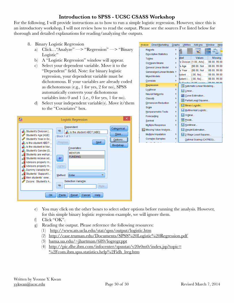
8. Binary Logistic Regression a) Click…“Analyze” —> “Regression” —> “Binary

Logistic” b) A “Logistic Regression” window will appear. c) Select your dependent variable. Move it to the

“Dependent” field. Note: for binary logistic regression, your dependent variable must be dichotomous. If your variables are already coded as dichotomous (e.g., 1 for yes, 2 for no), SPSS automatically converts your dichotomous variables into 0 and 1 (i.e., 0 for yes, 1 for no).

d) Select your independent variable(s). Move it/them to the “Covariates” box.

e) You may click on the other boxes to select other options before running the analysis. However, for this simple binary logistic regression example, we will ignore them.

f) Click “OK”. g) Reading the output. Please reference the following resources:

(1) http://www.ats.ucla.edu/stat/spss/output/logistic.htm (2) http://case.truman.edu/Documents/SPSS%20Logistic%20Regression.pdf (3) bama.ua.edu/~jhartman/689/logregr.ppt (4) http://pic.dhe.ibm.com/infocenter/spssstat/v20r0m0/index.jsp?topic=

%2Fcom.ibm.spss.statistics.help%2Fidh_lreg.htm
