Introduction to Signal Estimation. 94/10/142 Outline

Introduction to Signal Estimation

94/10/1494/10/14 22

Outline

94/10/1494/10/14 33

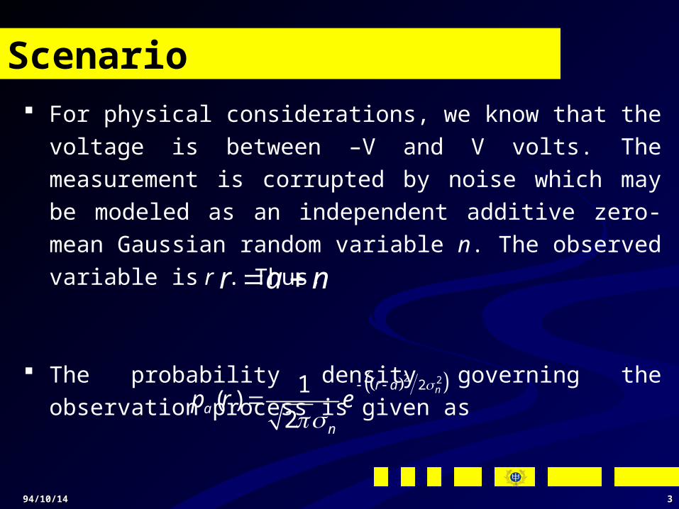
Scenario For physical considerations, we know that the voltage is

between –V and V volts. The measurement is corrupted by

noise which may be modeled as an independent additive

zero-mean Gaussian random variable n. The observed

variable is r . Thus,

The probability density governing the observation process is

given as 2 221( )

2

nr a

a

n

p r e

r a n

94/10/1494/10/14 44

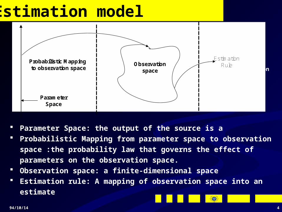
Estimation model

Parameter Space: the output of the source is a Probabilistic Mapping from parameter space to observation

space :the probability law that governs the effect of parameters on

the observation space. Observation space: a finite-dimensional space Estimation rule: A mapping of observation space into an estimate

Probabilistic Mapping to observation space

Observationspace

Decision ruleDecision

H0

H1

Parameter Space

Estimation Rule

94/10/1494/10/14 55

Parameter Estimation Problem In the composite hypothesis-testing problem ， a family of di

stributions on the observation space, indexed by a paramete

r or set of parameters, a binary decision is wanted to make

about the parameter 。 In the estimation problem, values of parameters want to be

determined as accurately as possible from the observation e

nbodied 。 Estimation design philosophies are different due to

o the amount of prior information known about the parameter o the performance criteria applied 。 .

94/10/1494/10/14 66

Basic approaches to the parameter estimation Bayesian estimation:

o assuming that parameters under estimation are to be a random

quantity related statistically to the observation。 Nonrandom parameter estimation:

o the parameters under estimation are assumed to be unknown but

without being endowed with any probabilistic structure。

94/10/1494/10/14 77

Bayesian Parameter Estimation

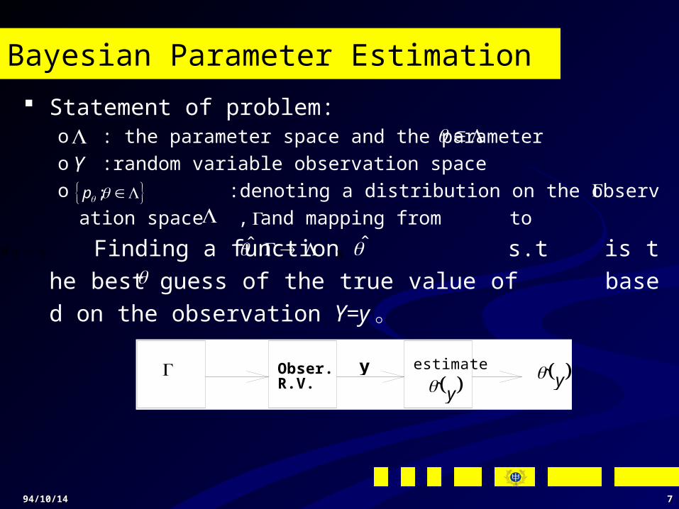
Statement of problem:o : the parameter space and the parametero :random variable observation spaceo :denoting a distribution on the observation space , and map

ping from to

Finding a function s.t is the best guess of the true v

alue of based on the observation Y=y 。

Y ;p

: ˆ :

Obser.R.V.

y estimate

y y

94/10/1494/10/14 88

Bayesian Parameter Estimation

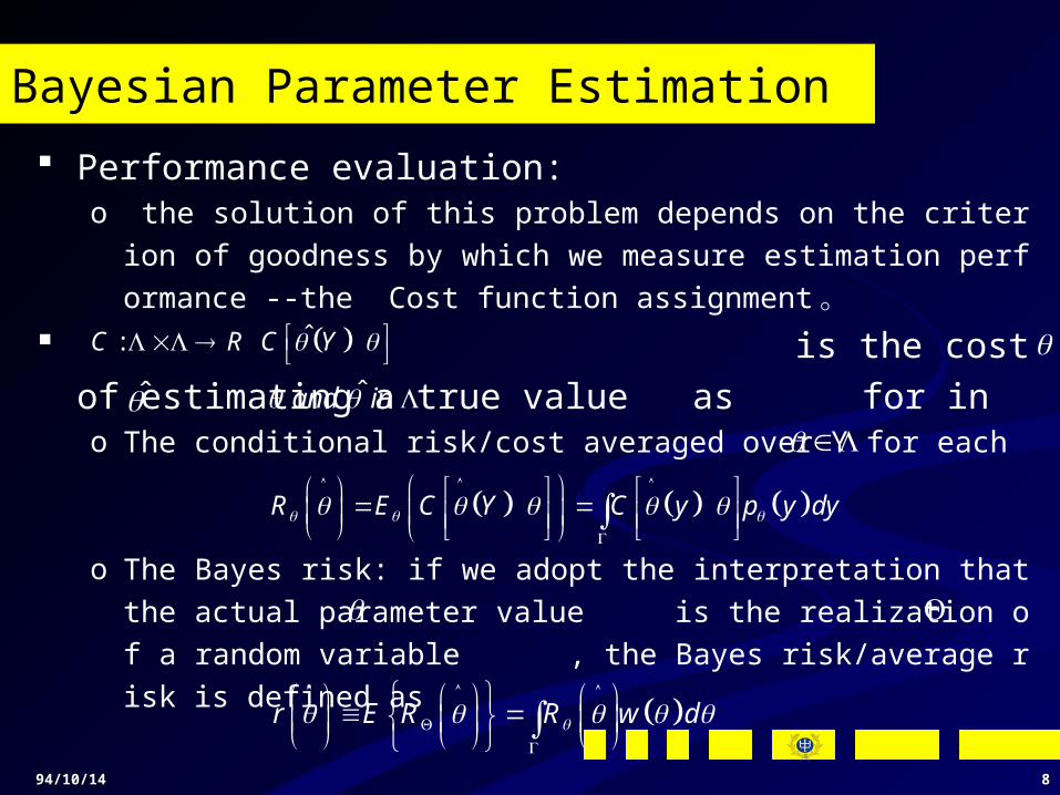
Performance evaluation:o the solution of this problem depends on the criterion of goodness by

which we measure estimation performance --the Cost function assig

nment 。 is the cost of estimating a true value a

s for in o The conditional risk/cost averaged over Y for each

o The Bayes risk: if we adopt the interpretation that the actual paramet

er value is the realization of a random variable , the Bayes risk/

average risk is defined as

ˆ:C R C Y

ˆand in

R E C Y C y p y dy

r E R R w d

94/10/1494/10/14 99

Bayesian Parameter Estimation

o where is the prior for random variable 。 the appropriate design

goal is to find an estimator minimizing ， and the estimator is kno

wn as a Bayes estimate of o Actually ， the conditional risk can be rewritten as

o the Bayes risk can be formulated as

o the Bayes risk can also be written as

w

ˆr

R E C Y E C Y

r E R E E C Y E C Y

r E R E C Y E E C Y Y E C Y Y y p y dy

94/10/1494/10/14 1010

Bayesian Parameter Estimation

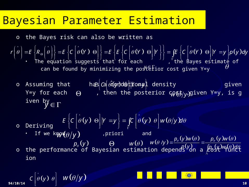
o the Bayes risk can also be written as

• The equation suggests that for each , the Bayes estimate of can be f

ound by minimizing the posterior cost given Y=y

o Assuming that has a conditional density given Y=y for each

, then the posterior cost ,given Y=y, is given by

o Deriving• If we know ,priori and

o the performance of Bayesian estimation depends on a cost function

w

r E R E C Y E E C Y Y E C Y Y y p y dy

y

ˆE C y Y y w y

y

E C y Y y C y w y d

w y

p y

/p y w p y w

w yp y p y w d

C y

w y

94/10/1494/10/14 1111

(MMSE) Minimum-Mean-Squared-Error Estimation

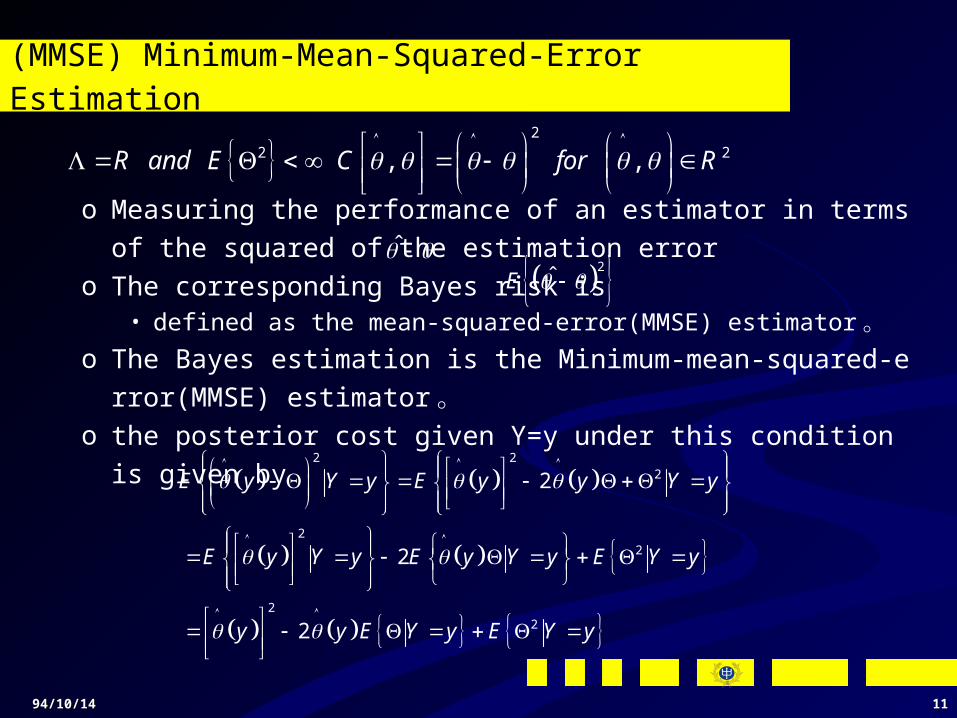
o Measuring the performance of an estimator in terms of the squared o

f the estimation erroro The corresponding Bayes risk is

• defined as the mean-squared-error(MMSE) estimator 。o The Bayes estimation is the Minimum-mean-squared-error(MMSE) e

stimator 。

o the posterior cost given Y=y under this condition is given by

2

2 2, ,R and E C for R

2ˆE

2 22

22

22

2

2

2

E y Y y E y y Y y

E y Y y E y Y y E Y y

y y E Y y E Y y

94/10/1494/10/14 1212

(MMSE) Minimum-Mean-Squared-Error Estimation

o the cost function is a quadratic form of ,and is a convex function 。

o Therefore, it achieves its unique minimum at the point where its deriv

ative with respective to is zero 。

o the conditional mean of given Y=y 。 The estimator is also sometim

es termed the conditional mean estimator-CME 。

000 DH 111 DH 000 DH 111 DH

y

y

2ˆˆ2 2 0

ˆ

E y Y yy E Y y

y

MMSE y E Y y w y d

94/10/1494/10/14 1313

(MMSE) Minimum-Mean-Squared-Error Estimation

Another derivation:

2 2

E y Y y y w y d

2ˆˆ2 0

ˆ

ˆ

E y Y yy w y d

y

y w y d w y d

ˆ y w y d E Y y

94/10/1494/10/14 1414

(MMAE) : Minimum-Mean-Absolute-Error Estimation

Measuring the performance of an estimator in terms of the a

bsolute value of the estimation error,

The corresponding Bayes risk is ， which is defined as

the mean-absolute-error (MMAE) 。 The Bayes estimation is the Minimum-mean-absolute-error

(MMAE) estimator 。

2ˆ, ,R and E C for R

ˆE

94/10/1494/10/14 1515

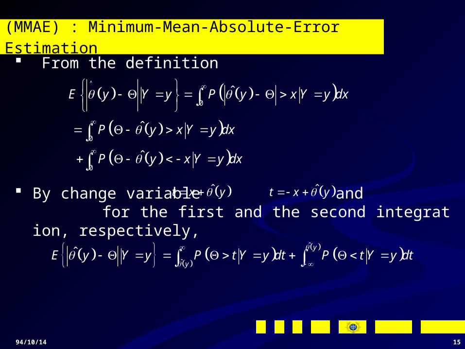
(MMAE) : Minimum-Mean-Absolute-Error Estimation From the definition

By change variable and for the first and the second integration, respectively,

0

0

0

ˆ

ˆ

ˆ

E y Y y P y x Y y dx

P y x Y y dx

P y x Y y dx

ˆt x y ˆt x y

ˆ

ˆˆ y

yE y Y y P t Y y dt P t Y y dt

94/10/1494/10/14 1616

(MMAE) : Minimum-Mean-Absolute-Error Estimation

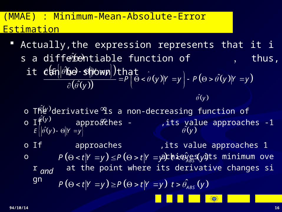
Actually,the expression represents that it is a differentiable f

unction of ， thus, it can be shown that

o The derivative is a non-decreasing function ofo If approaches - ,its value approaches -1 o If approaches ,its value approaches 1o achieves its minimum over at the point where its d

erivative changes sign

ˆ y

ˆˆ

ˆ

E y Y yP y Y y P y Y y

y

ˆ y

ˆ y ˆ y ˆE y Y y ˆ y

ˆ

ˆ

ABS

ABS

P t Y y P t Y y t y

and

P t Y y P t Y y t y

94/10/1494/10/14 1717

(MMAE) : Minimum-Mean-Absolute-Error Estimation the cost function can be also expressed as

o the minimum-mean-absolute-error estimator is to estimate the median of the co

nditional density function of ,Y=y 。o the MMAE is also termed as condition median estimator o For a given density function of , if its mean and median are the same, then,MM

SE and MMAE coincide each other,i.e. they have the same performance based

on different criterion adopted 。

ˆ

ˆˆy

yE y Y y w y d w y d

ˆ

ˆ

ˆ0

ˆ

y

y

E y Y yw y d w y d

y

ˆ

ˆ

1

2

y

yw y d w y d

94/10/1494/10/14 1818

MAP Maximum A posterior Probability Estimation

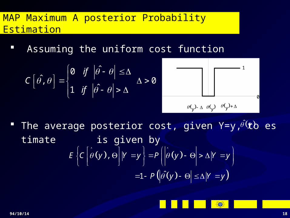
Assuming the uniform cost function

The average posterior cost, given Y=y, to estimate is giv

en by

ˆ0, 0

ˆ1

ifC

if

y y y

0

1

ˆ y

,

ˆ1

E C y Y y P y Y y

P y Y y

94/10/1494/10/14 1919

MAP Maximum A posterior Probability Estimation

Consideration I:o Assuming is a discrete random variable taking values in a finite set

and with the average posterior

cost is given as

which suggests that to minimize the average posterior cost,

The Bayes estimate in this case is given for each by any value

of which can maximizes the posterior probability over ，i.e. the Bayes estimate is the value of that has the maximum a po

sterior probability of occurring given Y=y

0 1M i j for i j

ˆ, 1

ˆ1

E C y Y y P Y y

w y

y

w y

94/10/1494/10/14 2020

MAP Maximum A posterior Probability Estimation

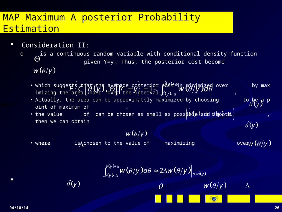
Consideration II: o is a continuous random variable with conditional density function

given Y=y 。 Thus, the posterior cost become

• which suggests that the average posterior cost is minimized over by maximizing the area

under over the interval 。 • Actually, the area can be approximately maximized by choosing to be a point of maximum

of 。 • the value of can be chosen as small as possible and smooth , then we can obtain

• where is chosen to the value of maximizing over 。

w y

ˆ

ˆˆ , 1

y

yE C y Y y w y d

ˆ y y y

ˆ y w y

w y

ˆ

ˆˆ2

y

yyw y d w y

y yw

ˆ y w y

94/10/1494/10/14 2121

MAP Maximum A posterior Probability Estimation

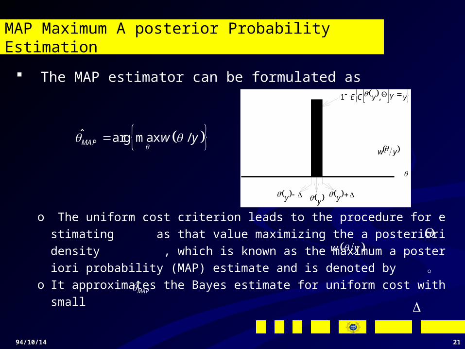
The MAP estimator can be formulated as

o The uniform cost criterion leads to the procedure for estimating a

s that value maximizing the a posteriori density , which is know

n as the maximum a posteriori probability (MAP) estimate and is den

oted by 。 o It approximates the Bayes estimate for uniform cost with small

ˆ arg max /MAP w y

yw

y y y

yYyCE ,ˆ1

w y

MAP

94/10/1494/10/14 2222

MAP Maximum A posterior Probability Estimation

The MAP estimates are often easier to compute than MMSE 、 MMAE ， or other estimates 。

A density achieves its maximum value is termed a mode of t

he corresponding probability 。 Therefore, the MMSE 、 M

MAE 、 and MAP estimates are the mean 、 median 、 and

mode of the corresponding distribution, respectively 。

94/10/1494/10/14 2323

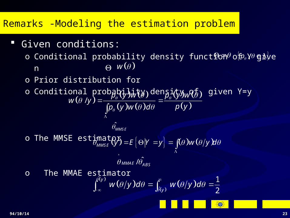
Remarks -Modeling the estimation problem

Given conditions: o Conditional probability density function of Y giveno Prior distribution foro Conditional probability density of given Y=y

o The MMSE estimator

o The MMAE estimator

,p

w

/p y w p y w

w yp yp y w d

MMSE y E Y y w y d

MMSE

ˆ/MMAE ABS

ˆ

ˆ

1

2

y

yw y d w y d

94/10/1494/10/14 2424

Remarks -Modeling the estimation problem

The MAP estimator

o For MAP estimator, it is not necessary to calculate because the

unconditional probability density of y does not affect the maximizatio

n over 。 o can be found by maximizing over . o For the logarithm is an increasing function, therefore, also maxim

izes over 。o If is a continuous random variable given Y=y ， then for sufficie

nt smooth and ,a necessary condition for MAP is given by

MAP equation

MAP

ˆ arg max /MAP w y

p y

MAP p y w

MAP

log logp y w

p y w

log logMAP MAPy y

p y w

94/10/1494/10/14 2525

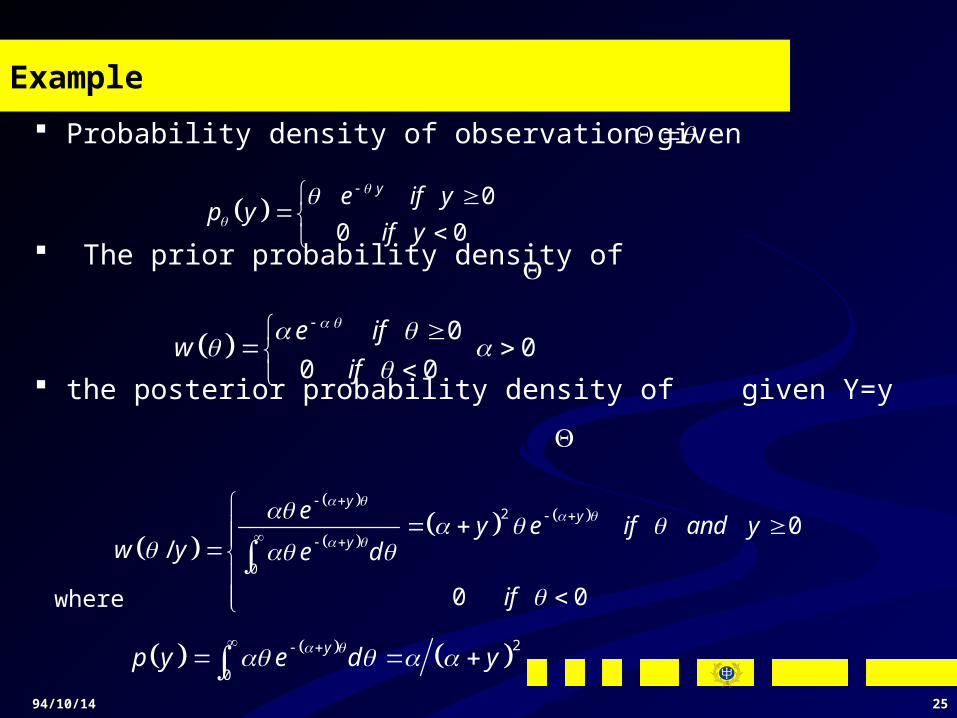
Example

Probability density of observation given

The prior probability density of

the posterior probability density of given Y=y

where

0

0 0

ye if yp y

if y

00

0 0

e ifw

if

2

0

0/

0 0

yy

y

ey e if and y

w y e d

if

2

0

yp y e d y

94/10/1494/10/14 2626

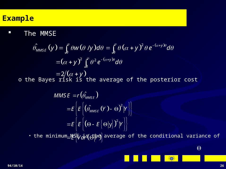
Example

The MMSE

o the Bayes risk is the average of the posterior cost

• the minimum MSE is the average of the conditional variance of

2

0 0

2 2

0

ˆ /

2

yMMSE

y

y w y d y e d

y e d

y

2

2

ˆ

ˆ

y

MMSE

MMSE

MMSE r

E E Y Y

E E E Y

E Var Y

94/10/1494/10/14 2727

Example

• the conditional variance given Y=y is shown as

• MMSE

2 2Var y E Y y E Y y

22

0

2 23

0

2

ˆ

4

2

MMSEVar y w y d y

y w y d y

y

0

2 2

0

2

2

2 3

MMSE E Var Y Var y p y dy

y y dy

94/10/1494/10/14 2828

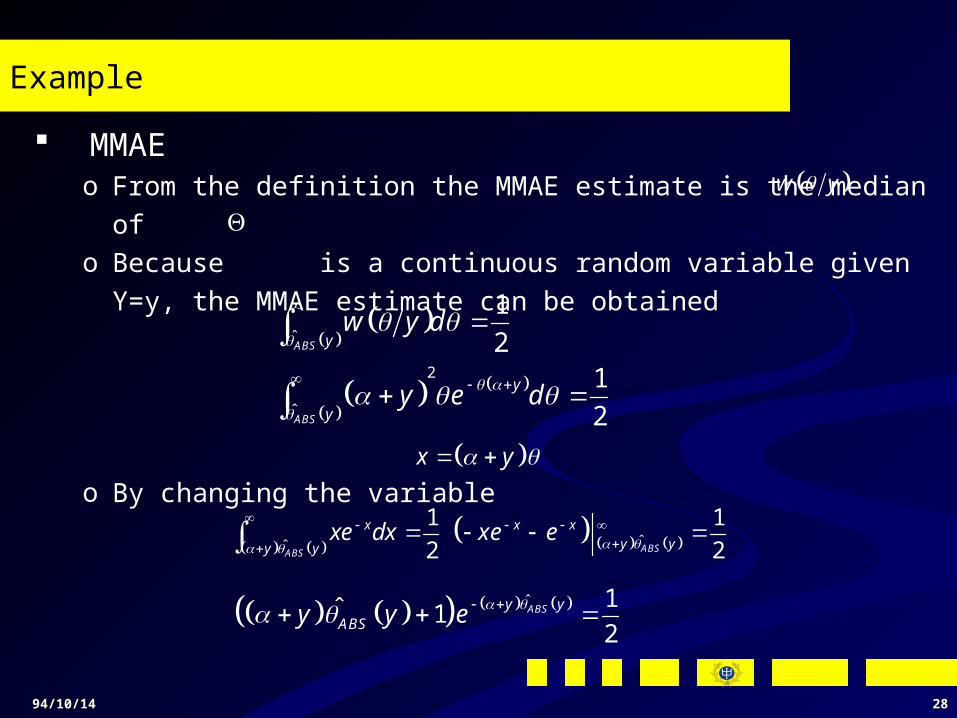
Example

MMAE o From the definition the MMAE estimate is the median ofo Because is a continuous random variable given Y=y, the MMAE e

stimate can be obtained

o By changing the variable

w y

ˆ

2

ˆ

1

21

2

ABS

ABS

y

y

y

w y d

y e d

x y

ˆˆ

1 1

2 2ABSABS

x x xy yy y

xe dx xe e

ˆ 1ˆ 12

ABSy yABSy y e

94/10/1494/10/14 2929

Example

o the solution is

• where T is the solution for ¸ and T~1.68.

The MAP

o

ABS

Ty

y

1 1 2TT e

max w y 2=max yy e

max ye

ˆ 0MAP

y ye y e

1

y

94/10/1494/10/14 3030

Example

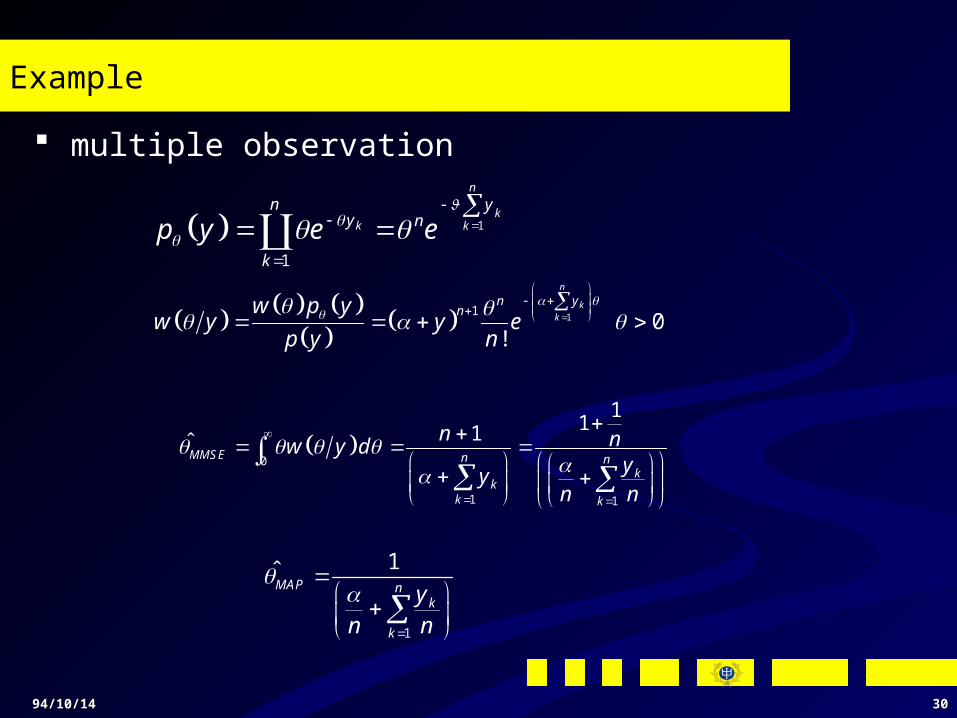
multiple observation

1

1

n

kk k

n yy n

k

p y e e

1

10

!

n

kk

ynnw p y

w y y ep y n

0

1 1

111

MMSE n nk

kk k

n nw y dyy

n n

1

1MAP n

k

k

yn n

94/10/1494/10/14 3131

Nonrandom parameter(real) estimation

A problem in which we have a parameter indexing the class

of observation statistics, that is not modeled as a random var

iable but nevertheless is unknown. Don’t have enough prior information about the parameter to

assign a prior probability distribution to it. Treat the estimation of such parameters in an organized ma

nner.

94/10/1494/10/14 3232

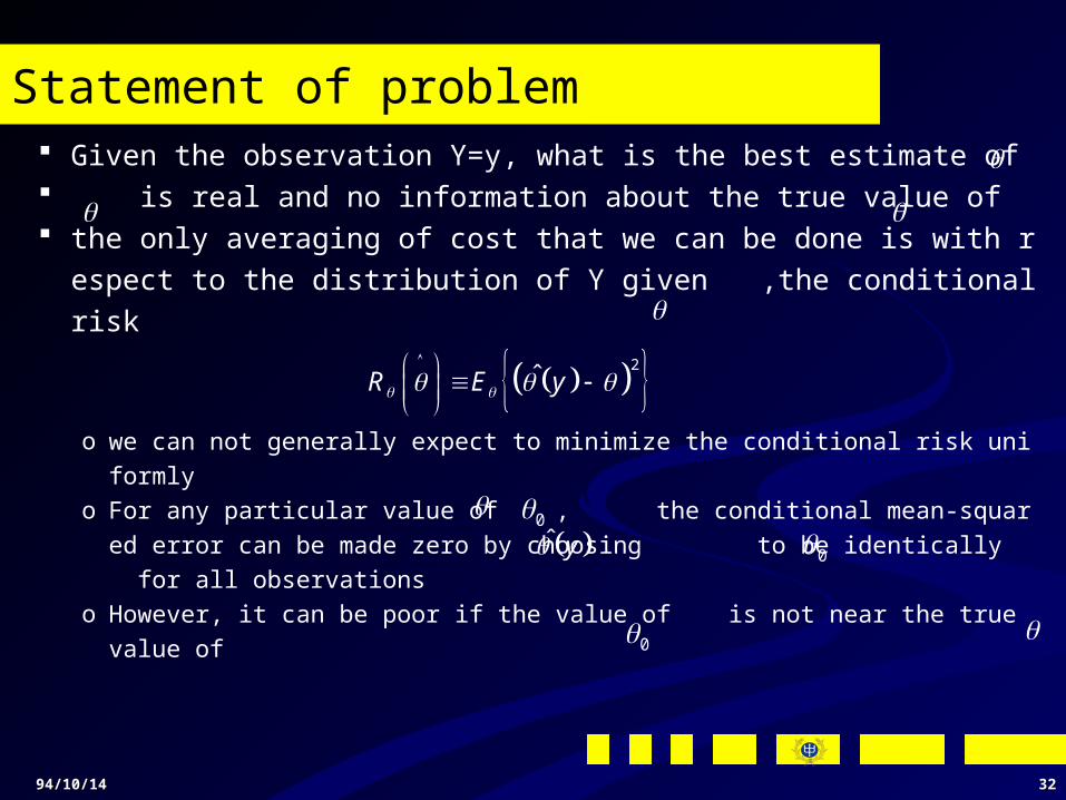
Statement of problem Given the observation Y=y, what is the best estimate of is real and no information about the true value of the only averaging of cost that we can be done is with respe

ct to the distribution of Y given ,the conditional risk

o we can not generally expect to minimize the conditional risk uniformlyo For any particular value of , the conditional mean-squared error

can be made zero by choosing to be identically for all observat

ions o However, it can be poor if the value of is not near the true value of

2ˆR E y

0 ˆ y 0

0

94/10/1494/10/14 3333

Statement of problem

o Unless o it is not a good estimator due to not with minimum conditional mean-

squared-error。

the conditional mean o if we say that the estimate is unbiasedo in general we have biased estimateo variance of estimatoro

2

0

2

0

2 2

0 0

ˆ

ˆ

ˆ ˆ2

E y

E y

E y E E y

0 2 2

0ˆ ˆE y E y

ˆ ˆE y y p y dy ˆE y

ˆ 0b E y b

2ˆ ˆvar E y E y

94/10/1494/10/14 3434

MVUE

2

22

22

22

ˆvar

ˆ ˆ2

ˆ ˆ2

ˆ

E y b

E y b E b y

E y b b E y

E y b

0b p for the unbias estimator ,and the variance is the cond

itional mean-squared error under

The best we can hope for is minimum variance unbiased es

timator-MVUE

0b

p

2ˆvar E y

94/10/1494/10/14 3535

Q & A