1/ 26 Introduction to Scheduling Theory Arnaud Legrand Laboratoire Informatique et Distribution IMAG CNRS, France [email protected] November 9, 2004

Welcome message from author
This document is posted to help you gain knowledge. Please leave a comment to let me know what you think about it! Share it to your friends and learn new things together.
Transcript

1/ 26
Introduction to Scheduling Theory
Arnaud Legrand
Laboratoire Informatique et DistributionIMAG CNRS, France
November 9, 2004

2/ 26
Outline
1 Task graphs from outer space
2 Scheduling definitions and notions
3 Platform models and scheduling problems
3/ 26
Outline
1 Task graphs from outer space
2 Scheduling definitions and notions
3 Platform models and scheduling problems

4/ 26
Analyzing a simple code
Solving A.x = B where A is lower triangular matrix
1: for i = 1 to n do2: Task Ti,i: x(i)← b(i)/a(i, i)3: for j = i + 1 to n do4: Task Ti,j : b(j)← b(j)−a(j, i)×x(i)
For a given value 1 6 i 6 n, all tasks Ti,∗ are computations doneduring the ith iteration of the outer loop.
<seq is the sequential order :
T1,1 <seq T1,2 <seq T1,3 <seq . . .<seq T1,n <seq T2,2 <seq T2,3 <seq
. . .<seq Tn,n .

5/ 26
Independence
However, some independent tasks could be executed in parallel.Independent tasks are the ones whose execution order can be changedwithout modifying the result of the program.Two independent tasks may read the value but never write to thesame memory location.
For a given task T , In(T ) denotes the set of input variables andOut(T ) the set of output variables.In the previous example, we have :{In(Ti,i) = {b(i), a(i, i)}Out(Ti,i) = {x(i)} and{In(Ti,j) = {b(j), a(j, i), x(i)}Out(Ti,j) = {b(j)} for j > i.
for i = 1 to N doTask Ti,i: x(i)← b(i)/a(i, i)for j = i + 1 to N do
Task Ti,j : b(j)← b(j)−a(j, i)×x(i)

6/ 26
Bernstein conditions
Definition.
Two tasks T and T ′ are not independent ( T⊥T ′) whenever theyshare a written variable:
T⊥T ′ ⇔
In(T ) ∩Out(T ′) 6= ∅
or Out(T ) ∩ In(T ′) 6= ∅or Out(T ) ∩Out(T ′) 6= ∅
.
Those conditions are known as Bernstein’s conditions [Ber66].
We can check that:
I Out(T1,1)∩In(T1,2) = {x(1)}; T1,1⊥T1,2.
I Out(T1,3) ∩Out(T2,3) = {b(3)}; T1,3⊥T2,3.
for i = 1 to N doTask Ti,i: x(i)← b(i)/a(i, i)
for j = i + 1 to N do
Task Ti,j : b(j)← b(j)− a(j, i)× x(i)

7/ 26
Precedence
If T⊥T ′, then they should be ordered with the sequential executionorder. T ≺ T ′ if T⊥T ′ and T <seq T ′.More precisely ≺ is defined as the transitive closure of (<seq ∩ ⊥).
for i = 1 to N doTask Ti,i: x(i)← b(i)/a(i, i)
for j = i + 1 to N do
Task Ti,j : b(j)← b(j)− a(j, i)× x(i)
A dependence graph G is used.
(e : T → T ′) ∈ G means that T ′ canstart only if T has already been finished.T is a predecessor of T ′.
Transitivity arc are generally omitted.
T1,2 T1,3 T1,4 T1,5 T1,6
T6,6
T2,3 T2,4 T2,6T2,5
T3,3
T4,5
T3,4 T3,5 T3,6
T5,6
T2,2
T4,4
T5,5
T4,6
T1,1

8/ 26
Coarse-grain task graph
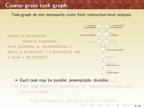
Task-graph do not necessarily come from instruction-level analysis.
select p.proteinID,
blast(p.sequence)
from proteins p, proteinTerms t
where p.proteinID = t.proteinID and
t.term = GO:0008372
scan(proteinTerms t)
(termGO:0008372)
project
(t.proteinID)
exchange
join
(p.proteinID=t.proteinID)
project
(p.proteinID,blast)
operation call
(blast(p.sequence))
exchange
scan(proteins p)
(termGO:0008372)
project
(p.proteinID,p.sequence)
exchange
I Each task may be parallel, preemptable, divisible, . . .
I Each edge depicts a dependency i.e. most of the times somedata to transfer.
In the following, we will focus on simple models.
8/ 26
Coarse-grain task graph
Task-graph do not necessarily come from instruction-level analysis.
select p.proteinID,
blast(p.sequence)
from proteins p, proteinTerms t
where p.proteinID = t.proteinID and
t.term = GO:0008372
scan(proteinTerms t)
(termGO:0008372)
project
(t.proteinID)
exchange
join
(p.proteinID=t.proteinID)
project
(p.proteinID,blast)
operation call
(blast(p.sequence))
exchange
scan(proteins p)
(termGO:0008372)
project
(p.proteinID,p.sequence)
exchange
I Each task may be parallel, preemptable, divisible, . . .
I Each edge depicts a dependency i.e. most of the times somedata to transfer.
In the following, we will focus on simple models.

9/ 26
Outline
1 Task graphs from outer space
2 Scheduling definitions and notions
3 Platform models and scheduling problems

10/ 26
Task system
Definition (Task system).
A task system is an directed graph G = (V,E, w) where :
I V is the set of tasks (V is finite)
I E represent the dependence constraints:
e = (u, v) ∈ E iff u ≺ v
I w : V → N∗ is a time function that give the weight (or dura-tion) of each task.
We could set w(Ti,j) = 1 but also decidethat performing a division is more expen-sive than a multiplication followed by anaddition.
T1,2 T1,3 T1,4 T1,5 T1,6
T6,6
T2,3 T2,4 T2,6T2,5
T3,3
T4,5
T3,4 T3,5 T3,6
T5,6
T2,2
T4,4
T5,5
T4,6
T1,1

11/ 26
Schedule and Allocation
Definition (Schedule).
A schedule of a task system G = (V,E, w) is a time function σ :V → N∗ such that:
∀(u, v) ∈ E, σ(u) + w(u) 6 σ(v)
Let us denote by P = {P1, . . . , Pp} the set of processors.
Definition (Allocation).
An allocation of a task system G = (V,E, w) is a function π : V →P such that:
π(T ) = π(T ′)⇔
{σ(T ) + w(T ) 6 σ(T ′) or
σ(T ′) + w(T ′) 6 σ(T )
Depending on the application and platform model, much more com-plex definitions can be proposed.

12/ 26
Gantt-chart
Manipulating functions is generally not very convenient. That iswhy Gantt-chart are used to depict schedules and allocations.
P1
P2
P3
Processors
Time
T1
T2
T5
T3 T4
T6 T7
T8

13/ 26
Basic feasibility condition
Theorem.
Let G = (V,E, w) be a task system. There exists a valid scheduleof G iff G has no cycle.
Sketch of the proof.
⇒ Assume that G has a cycle v1 → v2 → . . . → vk → v1. Thenv1 ≺ v1 and a valid schedule σ should hold σ(v1) + w(v1) 6σ(v1) true, which is impossible because w(v1) > 0.
⇐ If G is acyclic, then some tasks have no predecessor. They canbe scheduled first.More precisely, we sort topologically the vertexes and schedulethem one after the other on the same processor. Dependencesare then fulfilled.
Therefore all task systems we will be considering in the following areDirected Acyclic Graphs.

14/ 26
Makespan
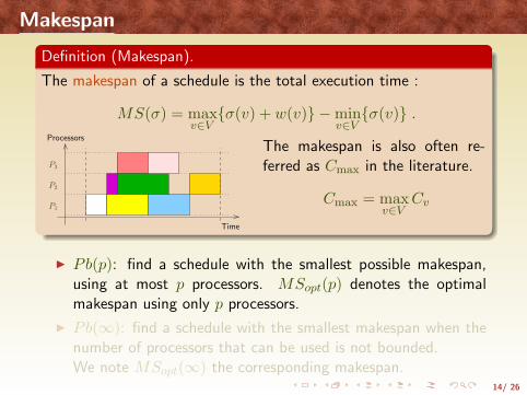
Definition (Makespan).
The makespan of a schedule is the total execution time :
MS(σ) = maxv∈V{σ(v) + w(v)} −min
v∈V{σ(v)} .
P1
P2
P3
Processors
Time
The makespan is also often re-ferred as Cmax in the literature.
Cmax = maxv∈V
Cv
I Pb(p): find a schedule with the smallest possible makespan,using at most p processors. MSopt(p) denotes the optimalmakespan using only p processors.
I Pb(∞): find a schedule with the smallest makespan when thenumber of processors that can be used is not bounded.We note MSopt(∞) the corresponding makespan.
14/ 26
Makespan
Definition (Makespan).
The makespan of a schedule is the total execution time :
MS(σ) = maxv∈V{σ(v) + w(v)} −min
v∈V{σ(v)} .
P1
P2
P3
Processors
Time
The makespan is also often re-ferred as Cmax in the literature.
Cmax = maxv∈V
Cv
I Pb(p): find a schedule with the smallest possible makespan,using at most p processors. MSopt(p) denotes the optimalmakespan using only p processors.
I Pb(∞): find a schedule with the smallest makespan when thenumber of processors that can be used is not bounded.We note MSopt(∞) the corresponding makespan.

15/ 26
Critical path
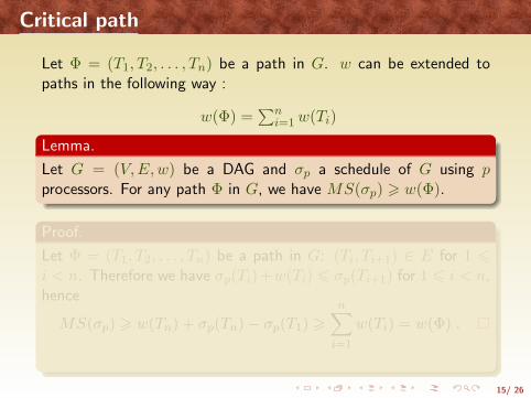
Let Φ = (T1, T2, . . . , Tn) be a path in G. w can be extended topaths in the following way :
w(Φ) =∑n
i=1 w(Ti)
Lemma.
Let G = (V,E, w) be a DAG and σp a schedule of G using pprocessors. For any path Φ in G, we have MS(σp) > w(Φ).
Proof.
Let Φ = (T1, T2, . . . , Tn) be a path in G: (Ti, Ti+1) ∈ E for 1 6i < n. Therefore we have σp(Ti)+w(Ti) 6 σp(Ti+1) for 1 6 i < n,hence
MS(σp) > w(Tn) + σp(Tn)− σp(T1) >n∑
i=1
w(Ti) = w(Φ) .
15/ 26
Critical path
Let Φ = (T1, T2, . . . , Tn) be a path in G. w can be extended topaths in the following way :
w(Φ) =∑n
i=1 w(Ti)
Lemma.
Let G = (V,E, w) be a DAG and σp a schedule of G using pprocessors. For any path Φ in G, we have MS(σp) > w(Φ).
Proof.
Let Φ = (T1, T2, . . . , Tn) be a path in G: (Ti, Ti+1) ∈ E for 1 6i < n. Therefore we have σp(Ti)+w(Ti) 6 σp(Ti+1) for 1 6 i < n,hence
MS(σp) > w(Tn) + σp(Tn)− σp(T1) >n∑
i=1
w(Ti) = w(Φ) .

16/ 26
Speed-up and Efficiency
Definition.
Let G = (V,E, w) be a DAG and σp a schedule of G using only p processors:
I Speed-up: s(σp) =Seq
MS(σp), where Seq = MSopt(1) =
∑v∈V
w(v).
I Efficiency: e(σp) =s(σp)
p=
Seq
p×MS(σp).
Theorem.
Let G = (V,E, w) be a DAG. For any schedule σp using p processors:
0 6 e(σp) 6 1 .
17/ 26
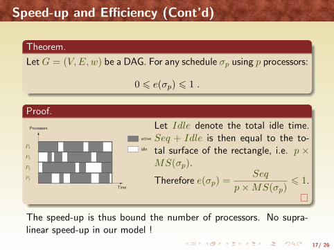
Speed-up and Efficiency (Cont’d)
Theorem.
Let G = (V,E, w) be a DAG. For any schedule σp using p processors:
0 6 e(σp) 6 1 .
Proof.
P4
P3
P2
P1
Processors
Time
idle
active
Let Idle denote the total idle time.Seq + Idle is then equal to the to-tal surface of the rectangle, i.e. p ×MS(σp).
Therefore e(σp) =Seq
p×MS(σp)6 1.
The speed-up is thus bound the number of processors. No supra-linear speed-up in our model !

18/ 26
A trivial result
Theorem.
Let G = (V,E, w) be a DAG. We have
Seq = MSopt(1) > . . . > MSopt(p) > MSopt(p+1) > . . . > MSopt(∞) .
Allowing to use more processors cannot hurt.
However, using more processors may hurt, especially in a modelwhere communications are taken into account.
If we define MS′(p) as the smallest makespan of schedules usingexactly p processors, we may have MS′(p) > MS′(p′) with p < p′.

19/ 26
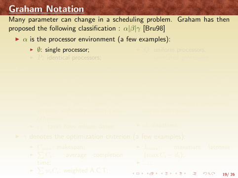
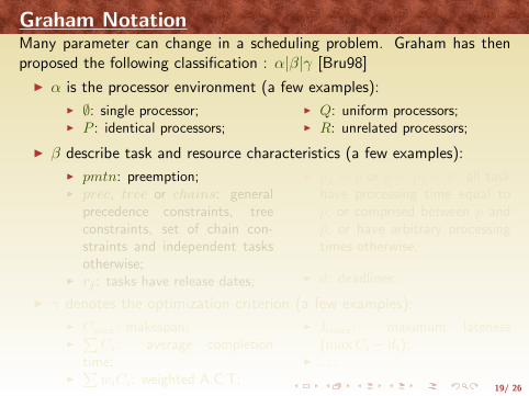
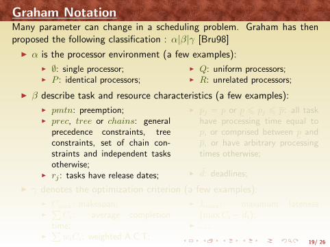
Graham NotationMany parameter can change in a scheduling problem. Graham has thenproposed the following classification : α|β|γ [Bru98]
I α is the processor environment (a few examples):
I ∅: single processor;I P : identical processors;
I Q: uniform processors;I R: unrelated processors;
I β describe task and resource characteristics (a few examples):
I pmtn: preemption;I prec, tree or chains: general
precedence constraints, treeconstraints, set of chain con-straints and independent tasksotherwise;
I rj : tasks have release dates;
I pj = p or p 6 pj 6 p: all taskhave processing time equal top, or comprised between p andp, or have arbitrary processingtimes otherwise;
I d̃: deadlines;
I γ denotes the optimization criterion (a few examples):
I Cmax: makespan;I
∑Ci: average completion
time;I
∑wiCi: weighted A.C.T;
I Lmax: maximum lateness(max Ci − di);
I . . .

19/ 26
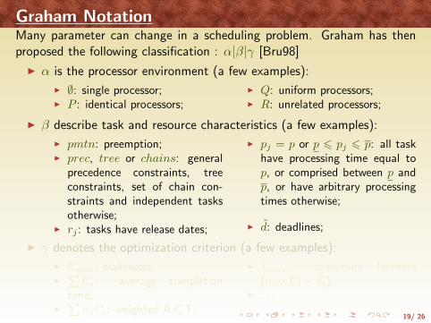
Graham NotationMany parameter can change in a scheduling problem. Graham has thenproposed the following classification : α|β|γ [Bru98]
I α is the processor environment (a few examples):
I ∅: single processor;I P : identical processors;
I Q: uniform processors;I R: unrelated processors;
I β describe task and resource characteristics (a few examples):
I pmtn: preemption;I prec, tree or chains: general
precedence constraints, treeconstraints, set of chain con-straints and independent tasksotherwise;
I rj : tasks have release dates;
I pj = p or p 6 pj 6 p: all taskhave processing time equal top, or comprised between p andp, or have arbitrary processingtimes otherwise;
I d̃: deadlines;
I γ denotes the optimization criterion (a few examples):
I Cmax: makespan;I
∑Ci: average completion
time;I
∑wiCi: weighted A.C.T;
I Lmax: maximum lateness(max Ci − di);
I . . .
19/ 26
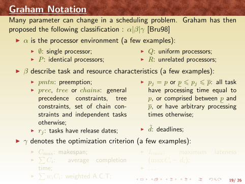
Graham NotationMany parameter can change in a scheduling problem. Graham has thenproposed the following classification : α|β|γ [Bru98]
I α is the processor environment (a few examples):
I ∅: single processor;I P : identical processors;
I Q: uniform processors;I R: unrelated processors;
I β describe task and resource characteristics (a few examples):
I pmtn: preemption;I prec, tree or chains: general
precedence constraints, treeconstraints, set of chain con-straints and independent tasksotherwise;
I rj : tasks have release dates;
I pj = p or p 6 pj 6 p: all taskhave processing time equal top, or comprised between p andp, or have arbitrary processingtimes otherwise;
I d̃: deadlines;
I γ denotes the optimization criterion (a few examples):
I Cmax: makespan;I
∑Ci: average completion
time;I
∑wiCi: weighted A.C.T;
I Lmax: maximum lateness(max Ci − di);
I . . .

19/ 26
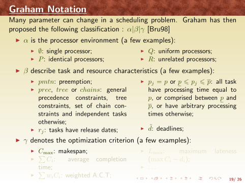
Graham NotationMany parameter can change in a scheduling problem. Graham has thenproposed the following classification : α|β|γ [Bru98]
I α is the processor environment (a few examples):
I ∅: single processor;I P : identical processors;
I Q: uniform processors;I R: unrelated processors;
I β describe task and resource characteristics (a few examples):
I pmtn: preemption;I prec, tree or chains: general
precedence constraints, treeconstraints, set of chain con-straints and independent tasksotherwise;
I rj : tasks have release dates;
I pj = p or p 6 pj 6 p: all taskhave processing time equal top, or comprised between p andp, or have arbitrary processingtimes otherwise;
I d̃: deadlines;
I γ denotes the optimization criterion (a few examples):
I Cmax: makespan;I
∑Ci: average completion
time;I
∑wiCi: weighted A.C.T;
I Lmax: maximum lateness(max Ci − di);
I . . .

19/ 26
Graham NotationMany parameter can change in a scheduling problem. Graham has thenproposed the following classification : α|β|γ [Bru98]
I α is the processor environment (a few examples):
I ∅: single processor;I P : identical processors;
I Q: uniform processors;I R: unrelated processors;
I β describe task and resource characteristics (a few examples):
I pmtn: preemption;I prec, tree or chains: general
precedence constraints, treeconstraints, set of chain con-straints and independent tasksotherwise;
I rj : tasks have release dates;
I pj = p or p 6 pj 6 p: all taskhave processing time equal top, or comprised between p andp, or have arbitrary processingtimes otherwise;
I d̃: deadlines;
I γ denotes the optimization criterion (a few examples):
I Cmax: makespan;I
∑Ci: average completion
time;I
∑wiCi: weighted A.C.T;
I Lmax: maximum lateness(max Ci − di);
I . . .
20/ 26
Outline
1 Task graphs from outer space
2 Scheduling definitions and notions
3 Platform models and scheduling problems

21/ 26
Complexity results
If we have an infinite number of processors, the “as-soon-as-possible”schedule is optimal. MSopt(∞) = max
Φ path in Gw(Φ).
I P, 2||Cmax is weakly NP-complete (2-Partition);
Proof.
By reduction to 2-Partition: can A = {a1, . . . , an} be partitionedinto two sets A1, A2 such
∑a∈A1
a =∑
a∈A2a?
p = 2, G = (V,E, w) with V = {v1, . . . , vn}, E = ∅ and w(vi) =ai,∀1 6 i 6 n.Finding a schedule of makespan smaller or equal to 1
2
∑i ai is equiv-
alent to solve the instance of 2-Partition.
I P, 3|prec|Cmax is strongly NP-complete (3DM);
I P |prec, pj = 1|Cmax is strongly NP-complete (max-clique);
I P, p > 3|prec, pj = 1|Cmax is open;
I P, 2|prec, 1 6 pj 6 2|Cmax is strongly NP-complete;

22/ 26
List scheduling
When simple problems are hard, we should try to find good approx-imation heuristics.Natural idea: using greedy strategy like trying to allocate the mostpossible task at a given time-step. However at some point we mayface a choice (when there is more ready tasks than available proces-sors).Any strategy that does not let on purpose a processor idle is effi-cient [Cof76]. Such a schedule is called list-schedule.
Theorem (Coffman).
Let G = (V,E, w) be a DAG, p the number of processors, and σp alist-schedule of G.
MS(σp) 6(2− 1
p
)MSopt(p) .
One can actually prove that this bound cannot be improved.
Most of the time, list-heuristics are based on the critical path.

23/ 26
Taking communications into accountA very simple model (things are already complicated enough): themacro-data flow model. If there is some data-dependence betweenT and T ′, the communication cost is
c(T, T ′) =
{0 if alloc(T ) = alloc(T ′)c(T, T ′) otherwise
Definition.
A DAG with communication cost (say cDAG) is a directed acyclicgraph G = (V,E, w, c) where vertexes represent tasks and edgesrepresent dependence constraints. w : V → N∗ is the computationtime function and c : E → N∗ is the communication time function.Any valid schedule has to respect the dependence constraints.
∀e = (v, v′) ∈ E,{σ(v) + w(v) 6 σ(v′) if alloc(v) = alloc(v′)σ(v) + w(v) + c(v; v′) 6 σ(v′) otherwise.

24/ 26
Taking communications into account (cont’d)
Even Pb(∞) is NP-complete !!!
You constantly have to figure out whether you should use moreprocessor (but then pay more fore communications) or not. Findingthe good trade-off is a real challenge.4/3-approximation if all communication times are smaller than com-putation times.Finding guaranteed approximations for other settings is really hard,but really useful.
That must be the reason why there is so much research about it !

25/ 26
Conclusion
Most of the time, the only thing we can done is to compare heuris-tics. There are three ways of doing that:
I Theory: being able to guarantee your heuristic;
I Experiment: Generating random graphs and/or typical applica-tion graphs along with platform graphs to compare your heuris-tics.
I Smart: proving that your heuristic is optimal for a particularclass of graphs (fork, join, fork-join, bounded degree, . . . ).
However, remember that the first thing to do is to look whether yourproblem is NP-complete or not. Who knows? You may be lucky...

26/ 26
Bibliography
A.J. Bernstein.Analysis of programs for parallel processing.IEEE Transactions on Electronic Computers, 15:757–762, October 1966.
Peter Brucker.Scheduling Algorithms.Springer, Heidelberg, 2 edition, 1998.
E. G. Coffman.Computer and job-shop scheduling theory.John Wiley & Sons, 1976.
Related Documents


