Introduction to SAS BIO 226 – Spring 2009. 2 Outline Windows and common rules Getting the data –The PRINT and CONTENT Procedures Manipulating the data.

Introduction to SAS

BIO 226 – Spring 2009

2

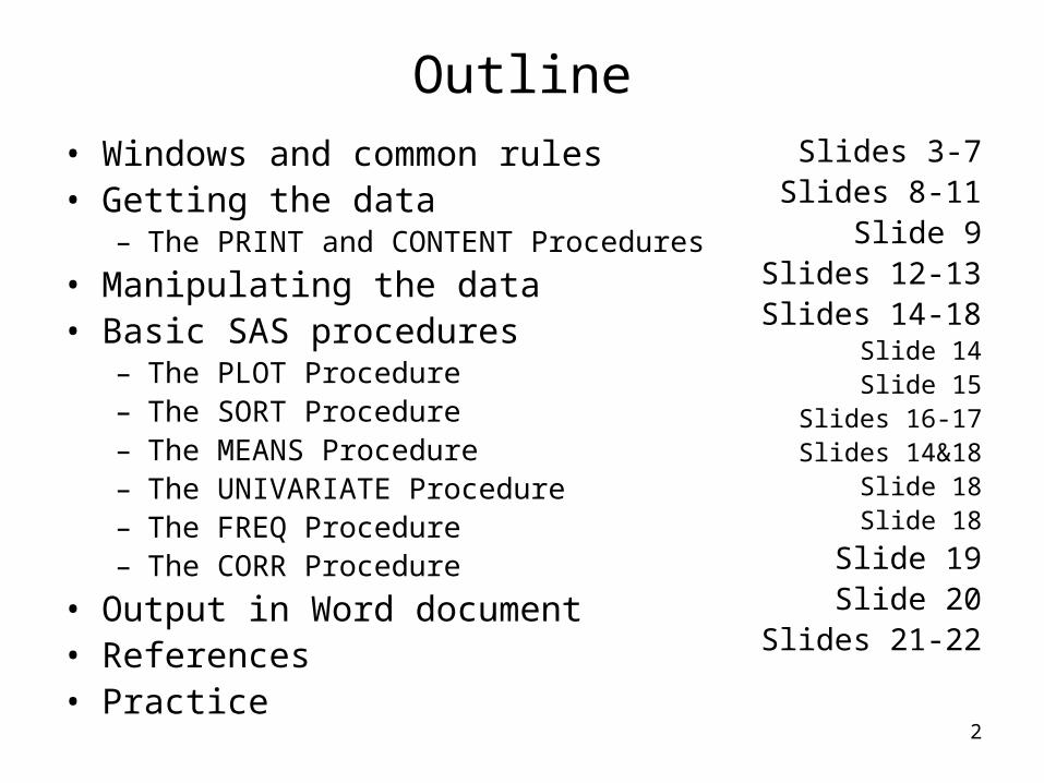
Outline• Windows and common rules• Getting the data

– The PRINT and CONTENT Procedures

• Manipulating the data• Basic SAS procedures

– The PLOT Procedure– The SORT Procedure– The MEANS Procedure– The UNIVARIATE Procedure– The FREQ Procedure– The CORR Procedure

• Output in Word document• References• Practice

Slides 3-7Slides 8-11

Slide 9Slides 12-13 Slides 14-18

Slide 14Slide 15

Slides 16-17Slides 14&18

Slide 18Slide 18

Slide 19Slide 20

Slides 21-22

3

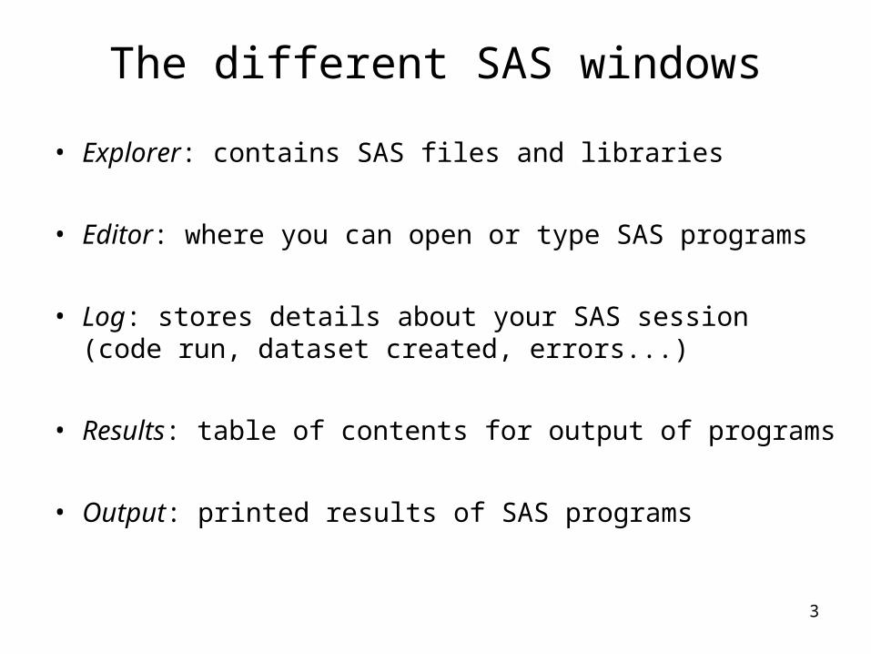
The different SAS windows

• Explorer: contains SAS files and libraries

• Editor: where you can open or type SAS programs

• Log: stores details about your SAS session (code run, dataset created, errors...)

• Results: table of contents for output of programs

• Output: printed results of SAS programs

4

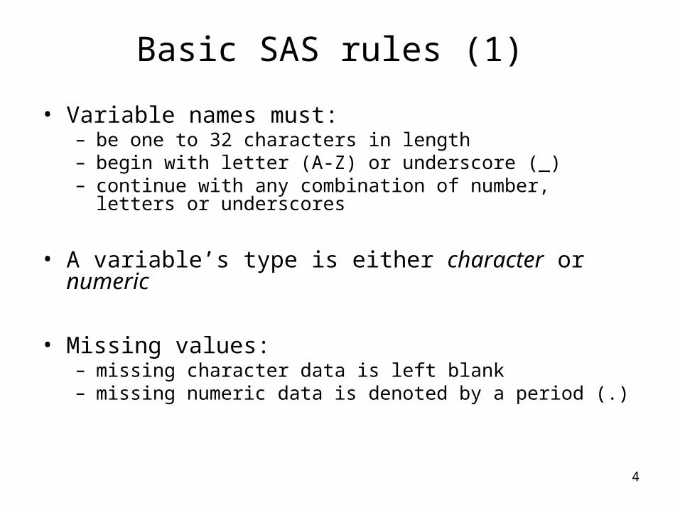
Basic SAS rules (1)

• Variable names must:– be one to 32 characters in length– begin with letter (A-Z) or underscore (_)– continue with any combination of number, letters or underscores

• A variable’s type is either character or numeric

• Missing values: – missing character data is left blank– missing numeric data is denoted by a period (.)

5

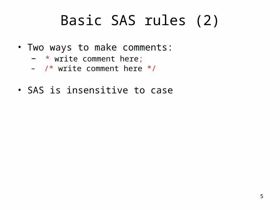
Basic SAS rules (2)

• Two ways to make comments: – * write comment here;– /* write comment here */

• SAS is insensitive to case

6

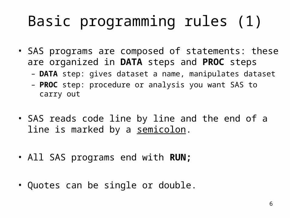
Basic programming rules (1)

• SAS programs are composed of statements: these are organized in DATA steps and PROC steps– DATA step: gives dataset a name, manipulates dataset– PROC step: procedure or analysis you want SAS to carry out

• SAS reads code line by line and the end of a line is marked by a semicolon.

• All SAS programs end with RUN;

• Quotes can be single or double.

7

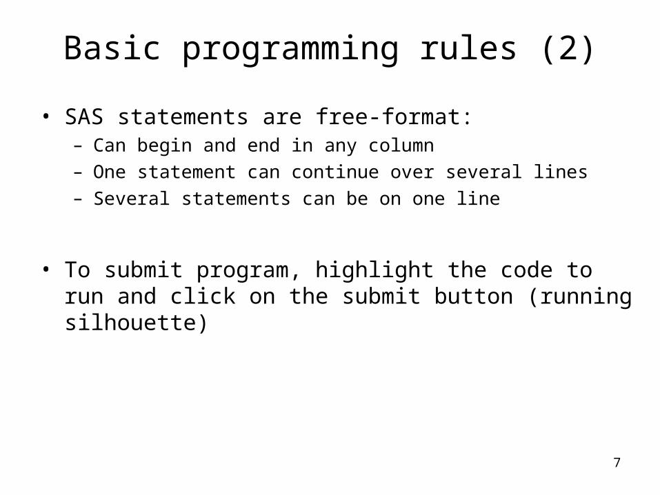
Basic programming rules (2)

• SAS statements are free-format:– Can begin and end in any column– One statement can continue over several lines– Several statements can be on one line

• To submit program, highlight the code to run and click on the submit button (running silhouette)

8

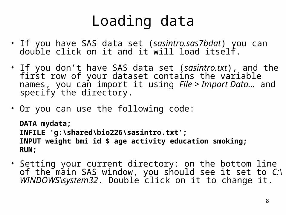
Loading data• If you have SAS data set (sasintro.sas7bdat) you can double

click on it and it will load itself.

• If you don’t have SAS data set (sasintro.txt), and the first row of your dataset contains the variable names, you can import it using File > Import Data… and specify the directory.

• Or you can use the following code:

DATA mydata;INFILE ‘g:\shared\bio226\sasintro.txt’;INPUT weight bmi id $ age activity education smoking;RUN;

• Setting your current directory: on the bottom line of the main SAS window, you should see it set to C:\WINDOWS\system32. Double click on it to change it.

9

How to view the loaded data?

• Go in the Explorer window, double click on Libraries, then Work and sasintro.sas7bdat

• Use the PRINT procedure to view the first 10 records:

PROC PRINT DATA=mydata (OBS=10);RUN;

• To view general information about the data set, like variables’ name and type:

PROC CONTENTS DATA=mydata;RUN;

10

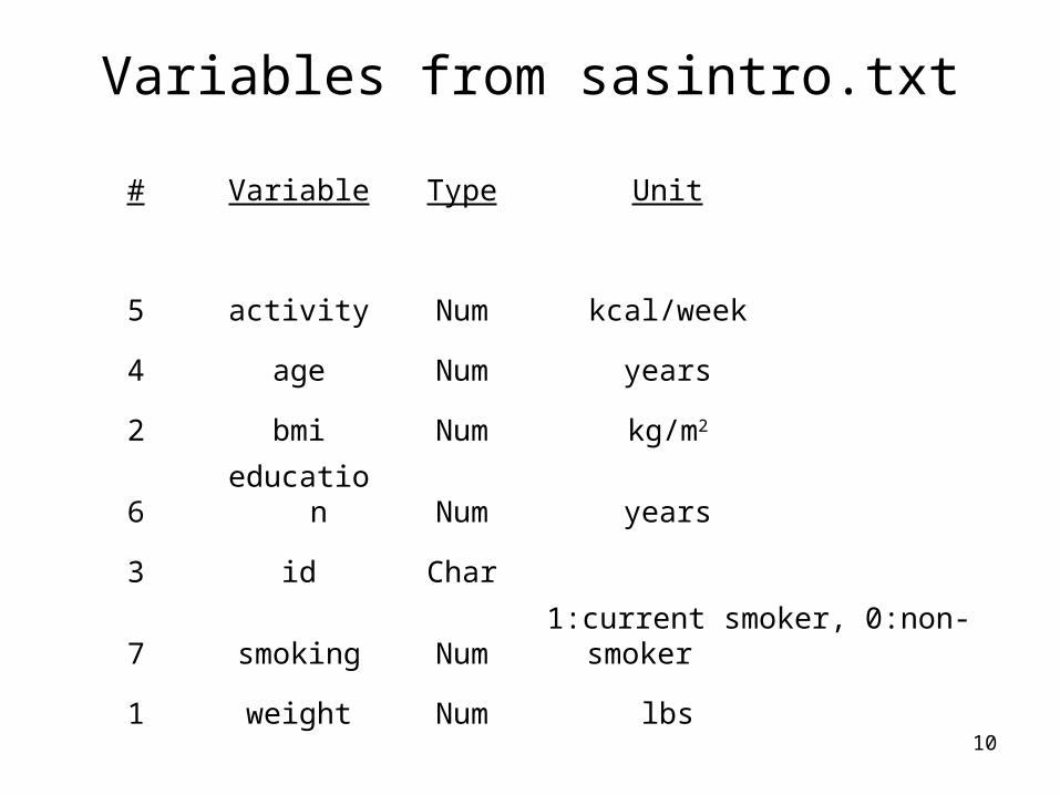
Variables from sasintro.txt

# Variable Type Unit

5 activity Num kcal/week

4 age Num years

2 bmi Num kg/m2

6 education Num years

3 id Char

7 smoking Num 1:current smoker, 0:non-smoker

1 weight Num lbs

11

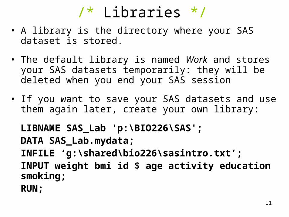
/* Libraries */• A library is the directory where your SAS dataset is stored.

• The default library is named Work and stores your SAS datasets temporarily: they will be deleted when you end your SAS session

• If you want to save your SAS datasets and use them again later, create your own library:

LIBNAME SAS_Lab 'p:\BIO226\SAS';DATA SAS_Lab.mydata;INFILE ‘g:\shared\bio226\sasintro.txt’;INPUT weight bmi id $ age activity education smoking;RUN;

12

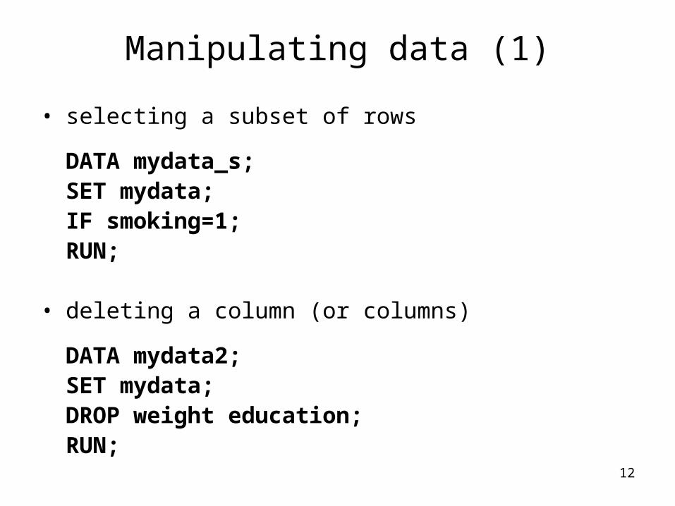
Manipulating data (1)

• selecting a subset of rows

DATA mydata_s;SET mydata;IF smoking=1;RUN;

• deleting a column (or columns)

DATA mydata2;SET mydata;DROP weight education;RUN;

13

Manipulating data (2)

• adding a column (or columns)

DATA mydata3;SET mydata;weight_kg=weight*0.453;IF age <= 60 THEN agegroup=1;ELSE IF age<=70 THEN agegroup=2;ELSE agegroup=3;/*drop age;*/RUN;

14

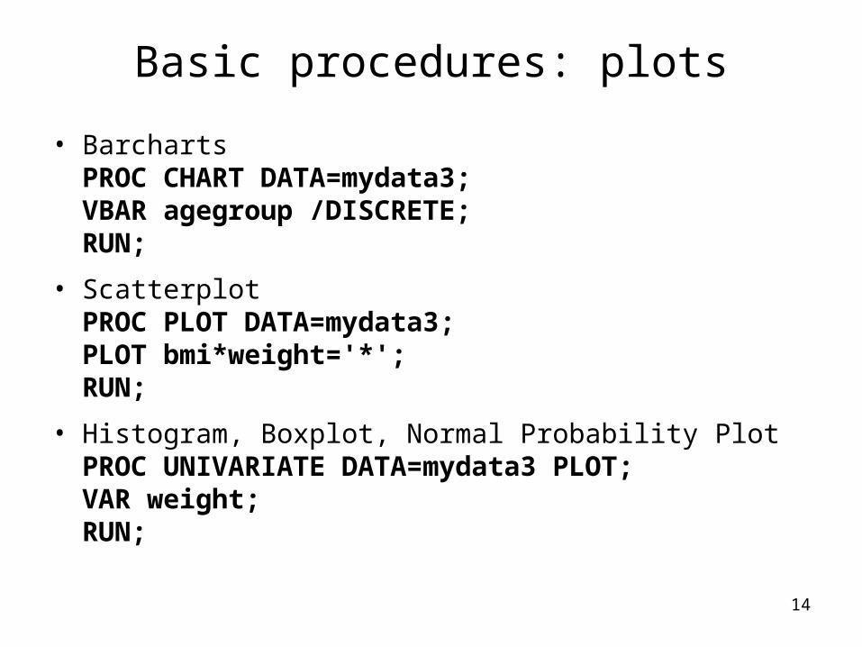
Basic procedures: plots

• BarchartsPROC CHART DATA=mydata3;VBAR agegroup /DISCRETE;RUN;

• ScatterplotPROC PLOT DATA=mydata3;PLOT bmi*weight='*';RUN;

• Histogram, Boxplot, Normal Probability PlotPROC UNIVARIATE DATA=mydata3 PLOT;VAR weight;RUN;

15

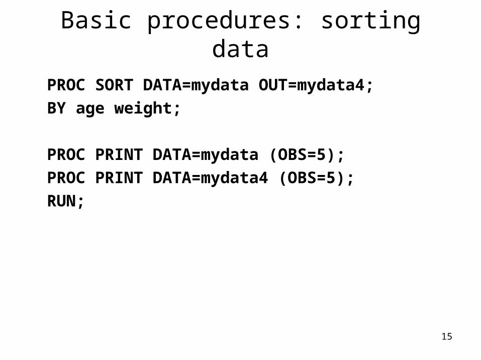
Basic procedures: sorting data

PROC SORT DATA=mydata OUT=mydata4;BY age weight;

PROC PRINT DATA=mydata (OBS=5);PROC PRINT DATA=mydata4 (OBS=5);RUN;

16

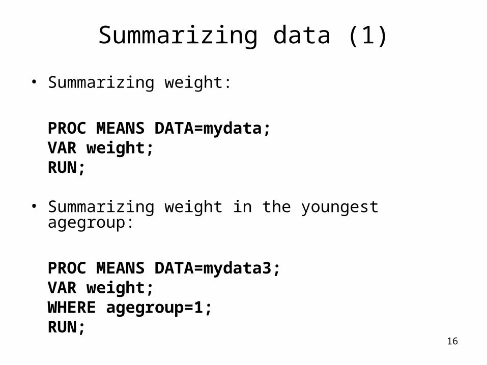
Summarizing data (1)

• Summarizing weight:

PROC MEANS DATA=mydata;VAR weight;RUN;

• Summarizing weight in the youngest agegroup:

PROC MEANS DATA=mydata3;VAR weight;WHERE agegroup=1;RUN;

17

Summarizing data (2)

• Summarizing weight by smoking status (two possible codes):

PROC SORT DATA=mydata OUT=mydata5;BY smoking;PROC MEANS DATA=mydata5;VAR weight;BY smoking;RUN;

PROC MEANS DATA=mydata;CLASS smoking;VAR weight;RUN;

• All these summarizing measures can be obtained with PROC UNIVARIATE also.

18

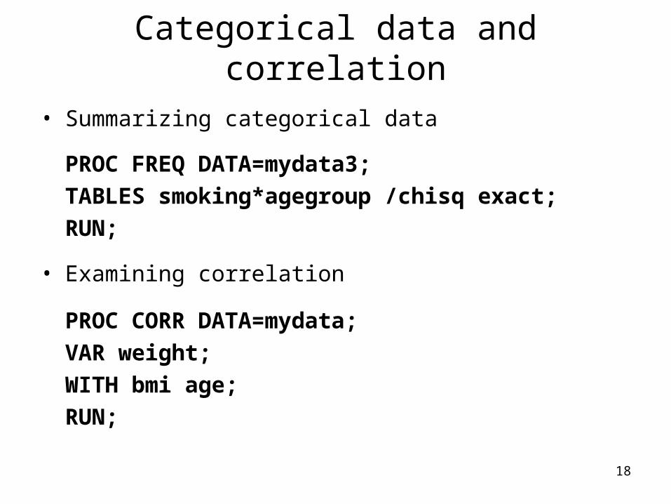
Categorical data and correlation

• Summarizing categorical data

PROC FREQ DATA=mydata3;TABLES smoking*agegroup /chisq exact;RUN;

• Examining correlation

PROC CORR DATA=mydata;VAR weight;WITH bmi age;RUN;

19

SAS output and Word

• To send you SAS output to a Word document:

ODS RTF FILE=‘p:output.RTF’ style=minimal;PROC CORR DATA =mydata;

VAR weight;WITH bmi age;RUN;

ODS RTF CLOSE;

• Other styles: Journal, Analysis, Statistical

20

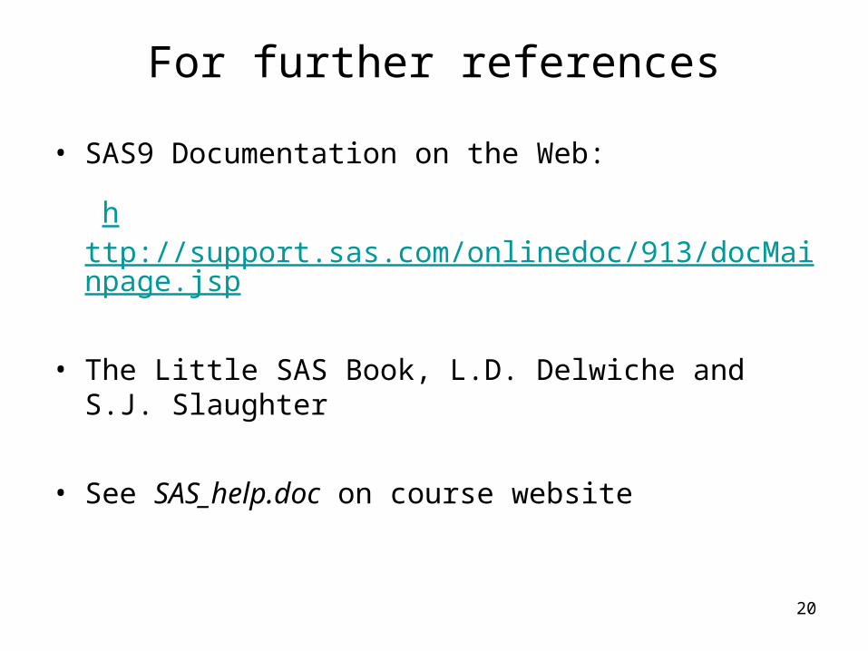
For further references

• SAS9 Documentation on the Web:

http://support.sas.com/onlinedoc/913/docMainpage.jsp

• The Little SAS Book, L.D. Delwiche and S.J. Slaughter

• See SAS_help.doc on course website

21

Try your own

• Find the summary statistics (mean, mode, standard deviation,…) for education with PROC UNIVARIATE, as well as a histogram for years of education.

• Create a new variable educ_group which breaks years of education into four groups (0-10, 10-15,15-18,18-25). Put this new variable in a new data set and drop the education variable, as well as weight, bmi and age.

• Find the number of smokers per education group.

• Find the mean physical activity in each education group.

22

Data name Description

mydata original imported data

mydata_s only smokers

mydata2 dropped weight, education

mydata3 added weight_kg, agegroup, dropped age

mydata4 sorted original data by age and weight

mydata5 sorted original data by smoking status

Recap of different datasets created