Introduction to Riemannian and Sub-Riemannian geometry From Hamiltonian viewpoint andrei agrachev davide barilari ugo boscain This version: June 12, 2016 Preprint SISSA 09/2012/M

Welcome message from author
This document is posted to help you gain knowledge. Please leave a comment to let me know what you think about it! Share it to your friends and learn new things together.
Transcript
Introduction to Riemannian and
Sub-Riemannian geometry
From Hamiltonian viewpoint
andrei agrachev
davide barilari
ugo boscain
This version: June 12, 2016
Preprint SISSA 09/2012/M

2
Contents
Introduction 9
1 Geometry of surfaces in R3 17
1.1 Geodesics and optimality . . . . . . . . . . . . . . . . . . . . . . . . . . . . . . . . . 17
1.1.1 Existence and minimizing properties of geodesics . . . . . . . . . . . . . . . . 21
1.1.2 Absolutely continuous curves . . . . . . . . . . . . . . . . . . . . . . . . . . . 23
1.2 Parallel transport . . . . . . . . . . . . . . . . . . . . . . . . . . . . . . . . . . . . . . 23
1.3 Gauss-Bonnet Theorems . . . . . . . . . . . . . . . . . . . . . . . . . . . . . . . . . . 26
1.3.1 Gauss-Bonnet theorem: local version . . . . . . . . . . . . . . . . . . . . . . . 27
1.3.2 Gauss-Bonnet theorem: global version . . . . . . . . . . . . . . . . . . . . . . 30
1.3.3 Consequences of the Gauss-Bonnet Theorems . . . . . . . . . . . . . . . . . . 33
1.3.4 The Gauss map . . . . . . . . . . . . . . . . . . . . . . . . . . . . . . . . . . . 34
1.4 Surfaces in R3 with the Minkowski inner product . . . . . . . . . . . . . . . . . . . . 37
1.5 Model spaces of constant curvature . . . . . . . . . . . . . . . . . . . . . . . . . . . . 40
1.5.1 Zero curvature: the Euclidean plane . . . . . . . . . . . . . . . . . . . . . . . 40
1.5.2 Positive curvature: spheres . . . . . . . . . . . . . . . . . . . . . . . . . . . . 40
1.5.3 Negative curvature: the hyperbolic plane . . . . . . . . . . . . . . . . . . . . 42
2 Vector fields and vector bundles 45
2.1 Differential equations on smooth manifolds . . . . . . . . . . . . . . . . . . . . . . . 45
2.1.1 Tangent vectors and vector fields . . . . . . . . . . . . . . . . . . . . . . . . . 45
2.1.2 Flow of a vector field . . . . . . . . . . . . . . . . . . . . . . . . . . . . . . . . 47
2.1.3 Vector fields as operators on functions . . . . . . . . . . . . . . . . . . . . . . 47
2.1.4 Nonautonomous vector fields . . . . . . . . . . . . . . . . . . . . . . . . . . . 48
2.2 Differential of a smooth map . . . . . . . . . . . . . . . . . . . . . . . . . . . . . . . 50
2.3 Lie brackets . . . . . . . . . . . . . . . . . . . . . . . . . . . . . . . . . . . . . . . . . 51
2.4 Cotangent space . . . . . . . . . . . . . . . . . . . . . . . . . . . . . . . . . . . . . . 54
2.5 Vector bundles . . . . . . . . . . . . . . . . . . . . . . . . . . . . . . . . . . . . . . . 55
2.6 Submersions and level sets of smooth maps . . . . . . . . . . . . . . . . . . . . . . . 58
3 Sub-Riemannian structures 61
3.1 Basic definitions . . . . . . . . . . . . . . . . . . . . . . . . . . . . . . . . . . . . . . 61
3.1.1 The minimal control and the length of an admissible curve . . . . . . . . . . 63
3.1.2 Equivalence of sub-Riemannian structures . . . . . . . . . . . . . . . . . . . . 67
3.1.3 Examples . . . . . . . . . . . . . . . . . . . . . . . . . . . . . . . . . . . . . . 68
3
3.1.4 Every sub-Riemannian structure is equivalent to a free one . . . . . . . . . . 69
3.1.5 Proto sub-Riemannian structures . . . . . . . . . . . . . . . . . . . . . . . . . 71
3.2 Sub-Riemannian distance and Chow-Rashevskii Theorem . . . . . . . . . . . . . . . 71
3.2.1 Proof of Chow-Raschevskii Theorem . . . . . . . . . . . . . . . . . . . . . . . 72
3.3 Existence of length-minimizers . . . . . . . . . . . . . . . . . . . . . . . . . . . . . . 76
3.4 Pontryagin extremals . . . . . . . . . . . . . . . . . . . . . . . . . . . . . . . . . . . . 79
3.4.1 The energy functional . . . . . . . . . . . . . . . . . . . . . . . . . . . . . . . 80
3.4.2 Proof of Theorem 3.44 . . . . . . . . . . . . . . . . . . . . . . . . . . . . . . . 81
3.A Measurability of the minimal control . . . . . . . . . . . . . . . . . . . . . . . . . . . 84
3.A.1 Main lemma . . . . . . . . . . . . . . . . . . . . . . . . . . . . . . . . . . . . 84
3.A.2 Proof of Lemma 3.11 . . . . . . . . . . . . . . . . . . . . . . . . . . . . . . . . 86
3.B Lipschitz vs Absolutely continuous admissible curves . . . . . . . . . . . . . . . . . . 86
4 Characterization and local minimality of Pontryagin extremals 89
4.1 Geometric characterization of Pontryagin extremals . . . . . . . . . . . . . . . . . . . 89
4.1.1 Lifting a vector field from M to T ∗M . . . . . . . . . . . . . . . . . . . . . . 90
4.1.2 The Poisson bracket . . . . . . . . . . . . . . . . . . . . . . . . . . . . . . . . 91
4.1.3 Hamiltonian vector fields . . . . . . . . . . . . . . . . . . . . . . . . . . . . . 93
4.2 The symplectic structure . . . . . . . . . . . . . . . . . . . . . . . . . . . . . . . . . . 94
4.2.1 The symplectic form vs the Poisson bracket . . . . . . . . . . . . . . . . . . . 95
4.3 Characterization of normal and abnormal extremals . . . . . . . . . . . . . . . . . . 97
4.3.1 Normal extremals . . . . . . . . . . . . . . . . . . . . . . . . . . . . . . . . . 97
4.3.2 Abnormal extremals . . . . . . . . . . . . . . . . . . . . . . . . . . . . . . . . 100
4.3.3 Example: codimension one distribution and contact distributions . . . . . . . 102
4.4 Examples . . . . . . . . . . . . . . . . . . . . . . . . . . . . . . . . . . . . . . . . . . 103
4.4.1 2D Riemannian Geometry . . . . . . . . . . . . . . . . . . . . . . . . . . . . . 103
4.4.2 Isoperimetric problem . . . . . . . . . . . . . . . . . . . . . . . . . . . . . . . 105
4.4.3 Heisenberg group . . . . . . . . . . . . . . . . . . . . . . . . . . . . . . . . . . 108
4.5 Lie derivative . . . . . . . . . . . . . . . . . . . . . . . . . . . . . . . . . . . . . . . . 109
4.6 Symplectic geometry . . . . . . . . . . . . . . . . . . . . . . . . . . . . . . . . . . . . 110
4.7 Local minimality of normal trajectories . . . . . . . . . . . . . . . . . . . . . . . . . 112
4.7.1 The Poincare-Cartan one form . . . . . . . . . . . . . . . . . . . . . . . . . . 113
4.7.2 Normal trajectories are geodesics . . . . . . . . . . . . . . . . . . . . . . . . . 115
5 Integrable Systems 119
5.1 Completely integrable systems . . . . . . . . . . . . . . . . . . . . . . . . . . . . . . 119
5.2 Arnold-Liouville theorem . . . . . . . . . . . . . . . . . . . . . . . . . . . . . . . . . 121
5.3 Integrable geodesic flows . . . . . . . . . . . . . . . . . . . . . . . . . . . . . . . . . . 124
5.3.1 Geodesic flow . . . . . . . . . . . . . . . . . . . . . . . . . . . . . . . . . . . . 125
5.4 Geodesic flow on ellipsoids . . . . . . . . . . . . . . . . . . . . . . . . . . . . . . . . . 128
6 Chronological calculus 131
6.1 Duality . . . . . . . . . . . . . . . . . . . . . . . . . . . . . . . . . . . . . . . . . . . 131
6.2 Operator ODE and Volterra expansion . . . . . . . . . . . . . . . . . . . . . . . . . . 132
6.2.1 Volterra expansion . . . . . . . . . . . . . . . . . . . . . . . . . . . . . . . . . 133
6.2.2 Adjoint representation . . . . . . . . . . . . . . . . . . . . . . . . . . . . . . . 135
4
6.3 Variations Formulae . . . . . . . . . . . . . . . . . . . . . . . . . . . . . . . . . . . . 137
6.4 Whitney topology on smooth functions . . . . . . . . . . . . . . . . . . . . . . . . . . 138
6.5 Estimates of the Volterra series . . . . . . . . . . . . . . . . . . . . . . . . . . . . . . 139
7 Lie groups and left-invariant sub-Riemannian structures 143
7.1 Lie groups and Lie algebras . . . . . . . . . . . . . . . . . . . . . . . . . . . . . . . . 143
7.2 Left-invariant structures . . . . . . . . . . . . . . . . . . . . . . . . . . . . . . . . . . 143
7.3 Pontryagin extremals for left invariant structures . . . . . . . . . . . . . . . . . . . . 143
7.4 Bi-invariant metrics . . . . . . . . . . . . . . . . . . . . . . . . . . . . . . . . . . . . 143
7.5 Geodesics . . . . . . . . . . . . . . . . . . . . . . . . . . . . . . . . . . . . . . . . . . 143
8 End-point and Exponential map 145
8.1 The end-point map and its differential . . . . . . . . . . . . . . . . . . . . . . . . . . 145
8.2 Lagrange multipliers rule . . . . . . . . . . . . . . . . . . . . . . . . . . . . . . . . . 148
8.3 Pontryagin extremals via Lagrange multipliers . . . . . . . . . . . . . . . . . . . . . . 148
8.4 Critical points and second order conditions . . . . . . . . . . . . . . . . . . . . . . . 149
8.4.1 The manifold of Lagrange multipliers . . . . . . . . . . . . . . . . . . . . . . . 152
8.5 Sub-Riemannian case . . . . . . . . . . . . . . . . . . . . . . . . . . . . . . . . . . . . 156
8.5.1 Free initial point problem . . . . . . . . . . . . . . . . . . . . . . . . . . . . . 159
8.6 Exponential map . . . . . . . . . . . . . . . . . . . . . . . . . . . . . . . . . . . . . . 160
8.7 Conjugate points and minimality of extremal trajectories . . . . . . . . . . . . . . . 162
8.7.1 Local minimality of normal extremal trajectories in the uniform topology . . 165
8.8 Global minimizers . . . . . . . . . . . . . . . . . . . . . . . . . . . . . . . . . . . . . 167
8.9 An example: the first conjugate locus on perturbed sphere . . . . . . . . . . . . . . . 169
9 2D-Almost-Riemannian Structures 173
9.1 Basic Definitions and properties . . . . . . . . . . . . . . . . . . . . . . . . . . . . . . 173
9.1.1 How big is the singular set? . . . . . . . . . . . . . . . . . . . . . . . . . . . . 178
9.1.2 Genuinely 2D-almost-Riemannian structures have always infinite area . . . . 179
9.1.3 Geodesics . . . . . . . . . . . . . . . . . . . . . . . . . . . . . . . . . . . . . . 180
9.2 The Grushin plane . . . . . . . . . . . . . . . . . . . . . . . . . . . . . . . . . . . . . 181
9.2.1 Geodesics of the Grushin plane . . . . . . . . . . . . . . . . . . . . . . . . . . 181
9.3 Riemannian, Grushin and Martinet points . . . . . . . . . . . . . . . . . . . . . . . . 183
9.4 Generic 2D-almost-Riemannian structures . . . . . . . . . . . . . . . . . . . . . . . . 187
9.4.1 Proof of the genericity result . . . . . . . . . . . . . . . . . . . . . . . . . . . 187
9.5 A Gauss-Bonnet theorem . . . . . . . . . . . . . . . . . . . . . . . . . . . . . . . . . 189
9.5.1 Proof of Theorem 9.43 . . . . . . . . . . . . . . . . . . . . . . . . . . . . . . . 192
9.5.2 Construction of trivializable 2-ARSs with no tangency points . . . . . . . . . 195
10 Nonholonomic tangent space 197
10.1 Jet spaces . . . . . . . . . . . . . . . . . . . . . . . . . . . . . . . . . . . . . . . . . . 197
10.2 Admissible variations . . . . . . . . . . . . . . . . . . . . . . . . . . . . . . . . . . . . 200
10.3 Nilpotent approximation and privileged coordinates . . . . . . . . . . . . . . . . . . 203
10.3.1 Existence of privileged coordinates . . . . . . . . . . . . . . . . . . . . . . . . 212
10.4 Geometric meaning . . . . . . . . . . . . . . . . . . . . . . . . . . . . . . . . . . . . . 216
10.5 Algebraic meaning . . . . . . . . . . . . . . . . . . . . . . . . . . . . . . . . . . . . . 221
5
11 Regularity of the sub-Riemannian distance 223
11.1 General properties of the distance function . . . . . . . . . . . . . . . . . . . . . . . 223
11.2 Regularity of the squared distance . . . . . . . . . . . . . . . . . . . . . . . . . . . . 225
11.3 Locally Lipschitz functions and maps . . . . . . . . . . . . . . . . . . . . . . . . . . . 232
11.3.1 Locally Lipschitz map and Lipschitz submanifolds . . . . . . . . . . . . . . . 235
11.3.2 A non-smooth version of Sard Lemma . . . . . . . . . . . . . . . . . . . . . . 238
11.4 Geodesic completeness and Hopf-Rinow theorem . . . . . . . . . . . . . . . . . . . . 243
12 Abnormal extremals and second variation 245
12.1 Second variation . . . . . . . . . . . . . . . . . . . . . . . . . . . . . . . . . . . . . . 245
12.2 Abnormal extremals and regularity of the distance . . . . . . . . . . . . . . . . . . . 246
12.3 Goh and generalized Legendre conditions . . . . . . . . . . . . . . . . . . . . . . . . 251
12.3.1 Proof of Goh condition - (i) of Theorem 12.13 . . . . . . . . . . . . . . . . . . 253
12.3.2 Proof of generalized Legendre condition - (ii) of Theorem 12.13 . . . . . . . . 259
12.3.3 More on Goh and generalized Legendre conditions . . . . . . . . . . . . . . . 260
12.4 Rank 2 distributions and nice abnormal extremals . . . . . . . . . . . . . . . . . . . 261
12.5 Optimality of nice abnormal in rank 2 structures . . . . . . . . . . . . . . . . . . . . 264
12.6 Conjugate points along abnormals . . . . . . . . . . . . . . . . . . . . . . . . . . . . 270
12.6.1 Abnormals in dimension 3 . . . . . . . . . . . . . . . . . . . . . . . . . . . . . 273
12.6.2 Higher dimension . . . . . . . . . . . . . . . . . . . . . . . . . . . . . . . . . . 274
12.7 Equivalence of local minimality . . . . . . . . . . . . . . . . . . . . . . . . . . . . . . 276
13 Some model spaces 279
13.1 Carnot groups of step 2 . . . . . . . . . . . . . . . . . . . . . . . . . . . . . . . . . . 279
13.1.1 Heisenberg . . . . . . . . . . . . . . . . . . . . . . . . . . . . . . . . . . . . . 279
13.1.2 (3, 6) . . . . . . . . . . . . . . . . . . . . . . . . . . . . . . . . . . . . . . . . . 279
13.1.3 (k, k(k + 1)/2) . . . . . . . . . . . . . . . . . . . . . . . . . . . . . . . . . . . 279
13.2 Other nilpotent structures . . . . . . . . . . . . . . . . . . . . . . . . . . . . . . . . . 279
13.2.1 Grushin . . . . . . . . . . . . . . . . . . . . . . . . . . . . . . . . . . . . . . . 279
13.2.2 Martinet . . . . . . . . . . . . . . . . . . . . . . . . . . . . . . . . . . . . . . . 279
13.3 Left invariant structures . . . . . . . . . . . . . . . . . . . . . . . . . . . . . . . . . . 279
13.3.1 SU(2), SO(3), SL(2) . . . . . . . . . . . . . . . . . . . . . . . . . . . . . . . . 279
13.3.2 SE(2) . . . . . . . . . . . . . . . . . . . . . . . . . . . . . . . . . . . . . . . . 279
13.3.3 (3, 5) - Rolling sphere with twist . . . . . . . . . . . . . . . . . . . . . . . . . 279
14 Curves in the Lagrange Grassmannian 281
14.1 The geometry of the Lagrange Grassmannian . . . . . . . . . . . . . . . . . . . . . . 281
14.1.1 The Lagrange Grassmannian . . . . . . . . . . . . . . . . . . . . . . . . . . . 284
14.2 Regular curves in Lagrange Grassmannian . . . . . . . . . . . . . . . . . . . . . . . . 286
14.3 Curvature of a regular curve . . . . . . . . . . . . . . . . . . . . . . . . . . . . . . . . 289
14.4 Reduction of non-regular curves in Lagrange Grassmannian . . . . . . . . . . . . . . 292
14.5 Ample curves . . . . . . . . . . . . . . . . . . . . . . . . . . . . . . . . . . . . . . . . 293
14.6 From ample to regular . . . . . . . . . . . . . . . . . . . . . . . . . . . . . . . . . . . 295
14.7 Conjugate points in L(Σ) . . . . . . . . . . . . . . . . . . . . . . . . . . . . . . . . . 299
14.8 Comparison theorems for regular curves . . . . . . . . . . . . . . . . . . . . . . . . . 300
6
15 Jacobi curves 303
15.1 From Jacobi fields to Jacobi curves . . . . . . . . . . . . . . . . . . . . . . . . . . . . 30315.1.1 Jacobi curves . . . . . . . . . . . . . . . . . . . . . . . . . . . . . . . . . . . . 304
15.2 Conjugate points and optimality . . . . . . . . . . . . . . . . . . . . . . . . . . . . . 306
15.3 Reduction of the Jacobi curves by homogeneity . . . . . . . . . . . . . . . . . . . . . 307
16 Riemannian curvature 311
16.1 Ehresmann connection . . . . . . . . . . . . . . . . . . . . . . . . . . . . . . . . . . . 31116.1.1 Curvature of an Ehresmann connection . . . . . . . . . . . . . . . . . . . . . 31216.1.2 Linear Ehresmann connections . . . . . . . . . . . . . . . . . . . . . . . . . . 313
16.1.3 Covariant derivative and torsion for linear connections . . . . . . . . . . . . . 31416.2 Riemannian connection . . . . . . . . . . . . . . . . . . . . . . . . . . . . . . . . . . 31616.3 Relation with Hamiltonian curvature . . . . . . . . . . . . . . . . . . . . . . . . . . . 320
16.4 Locally flat spaces . . . . . . . . . . . . . . . . . . . . . . . . . . . . . . . . . . . . . 32116.5 Example: curvature of the 2D Riemannian case . . . . . . . . . . . . . . . . . . . . . 323
17 Curvature in 3D contact sub-Riemannian geometry 32717.1 3D contact sub-Riemannian manifolds . . . . . . . . . . . . . . . . . . . . . . . . . . 327
17.1.1 Curvature of a 3D contact structure . . . . . . . . . . . . . . . . . . . . . . . 329
18 Asymptotic expansion of the 3D contact exponential map 33518.1 Nilpotent case . . . . . . . . . . . . . . . . . . . . . . . . . . . . . . . . . . . . . . . . 336
18.2 General case: second order asymptotic expansion . . . . . . . . . . . . . . . . . . . . 33718.3 General case: higher order asymptotic expansion . . . . . . . . . . . . . . . . . . . . 341
18.3.1 Proof of Theorem 18.6: asymptotics of the exponential map . . . . . . . . . . 343
18.3.2 Asymptotics of the conjugate locus . . . . . . . . . . . . . . . . . . . . . . . . 34718.3.3 Asymptotics of the conjugate length . . . . . . . . . . . . . . . . . . . . . . . 34918.3.4 Stability of the conjugate locus . . . . . . . . . . . . . . . . . . . . . . . . . . 350
19 The volume in sub-Riemannian geometry 35319.1 The Popp volume . . . . . . . . . . . . . . . . . . . . . . . . . . . . . . . . . . . . . . 353
19.2 Popp volume for equiregular sub-Riemannian manifolds . . . . . . . . . . . . . . . . 35319.3 A formula for Popp volume . . . . . . . . . . . . . . . . . . . . . . . . . . . . . . . . 35519.4 Popp volume and isometries . . . . . . . . . . . . . . . . . . . . . . . . . . . . . . . . 358
20 The sub-Riemannian heat equation 36120.1 The heat equation . . . . . . . . . . . . . . . . . . . . . . . . . . . . . . . . . . . . . 361
20.1.1 The heat equation in the Riemannian context . . . . . . . . . . . . . . . . . . 361
20.1.2 The heat equation in the sub-Riemannian context . . . . . . . . . . . . . . . 36420.1.3 Few properties of the sub-Riemannian Laplacian: the Hormander theorem
and the existence of the heat kernel . . . . . . . . . . . . . . . . . . . . . . . 36620.1.4 The heat equation in the non-Lie-bracket generating case . . . . . . . . . . . 368
20.2 The heat-kernel on the Heisenberg group . . . . . . . . . . . . . . . . . . . . . . . . . 36820.2.1 The Heisenberg group as a group of matrices . . . . . . . . . . . . . . . . . . 36820.2.2 The heat equation on the Heisenberg group . . . . . . . . . . . . . . . . . . . 369
A Hermite polynomials 375
7
B Elliptic functions 377
C Structural equations for curves in Lagrange Grassmannian 379
8
Introduction
This book concerns a fresh development of the eternal idea of the distance as the length of a shortestpath. In Euclidean geometry, shortest paths are segments of straight lines that satisfy all classicalaxioms. In the Riemannian world, Euclidean geometry is just one of a huge amount of possibilities.However, each of these possibilities is well approximated by Euclidean geometry at very small scale.In other words, Euclidean geometry is treated as geometry of initial velocities of the paths startingfrom a fixed point of the Riemannian space rather than the geometry of the space itself.
The Riemannian construction was based on the previous study of smooth surfaces in the Eu-clidean space undertaken by Gauss. The distance between two points on the surface is the lengthof a shortest path on the surface connecting the points. Initial velocities of smooth curves startingfrom a fixed point on the surface form a tangent plane to the surface, that is an Euclidean plane.Tangent planes at two different points are isometric, but neighborhoods of the points on the surfaceare not locally isometric in general; certainly not if the Gaussian curvature of the surface is differentat the two points.
Riemann generalized Gauss’ construction to higher dimensions and realized that it can bedone in an intrinsic way; you do not need an ambient Euclidean space to measure the length ofcurves. Indeed, to measure the length of a curve it is sufficient to know the Euclidean lengthof its velocities. A Riemannian space is a smooth manifold whose tangent spaces are endowedwith Euclidean structures; each tangent space is equipped with its own Euclidean structure thatsmoothly depends on the point where the tangent space is attached.
For a habitant sitting at a point of the Riemannian space, tangent vectors give directions whereto move or, more generally, to send and receive information. He measures lengths of vectors, andangles between vectors attached at the same point, according to the Euclidean rules, and this isessentially all what he can do. The point is that our habitant can, in principle, completely recoverthe geometry of the space by performing these simple measurements along different curves.
In the sub-Riemannian space we cannot move, receive and send information in all directions.There are restictions (imposed by the God, the moral imperative, the government, or simply aphysical law). A sub-Riemannian space is a smooth manifold with a fixed admissible subspace inany tangent space where admissible subspaces are equipped with Euclidean structures. Admissiblepaths are those curves whose velocities are admissible. The distance between two points is theinfimum of the length of admissible paths connecting the points. It is assumed that any pair ofpoints in the same connected component of the manifold can be connected by at least an admissiblepath. The last assumption might look strange at a first glance, but it is not. The admissiblesubspace depends on the point where it is attached, and our assumption is satisfied for a more orless general smooth dependence on the point; better to say that it is not satisfied only for veryspecial families of admissible subspaces.
Let us describe a simple model. Let our manifold be R3 with coordinates x, y, z. We consider
9
the differential 1-form ω = dz + 12 (xdy − ydx). Then dω = dx ∧ dy is the pullback on R
3 of thearea form on the xy-plane. In this model the subspace of admissible velocities at the point (x, y, z)is assumed to be the kernel of the form ω. In other words, a curve t 7→ (x(t), y(t), z(t)) is anadmissible path if and only if z(t) = 1
2 (y(t)x(t)− x(t)y(t)).The length of an admissible tangent vector (x, y, z) is defined to be (x2+ y2)
12 , that is the length
of the projection of the vector to the xy-plane. We see that any smooth planar curve (x(t), y(t))has a unique admissible lift (x(t), y(t), z(t)) in R
3, where:
z(t) =1
2
∫ t
0x(s)y(s)− x(s)y(s) ds.
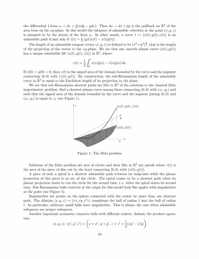
If x(0) = y(0) = 0, then z(t) is the signed area of the domain bounded by the curve and the segmentconnecting (0, 0) with (x(t), y(t)). By construction, the sub-Riemannian length of the admissiblecurve in R
3 is equal to the Euclidean length of its projection to the plane.We see that sub-Riemannian shortest paths are lifts to R
3 of the solutions to the classical Didoisoperimetric problem: find a shortest planar curve among those connecting (0, 0) with (x1, y1) andsuch that the signed area of the domain bounded by the curve and the segment joining (0, 0) and(x1, y1) is equal to z1 (see Figure 1).
y
z (x(t), y(t), z(t))
(x(t), y(t))
x
Figure 1: The Dido problem
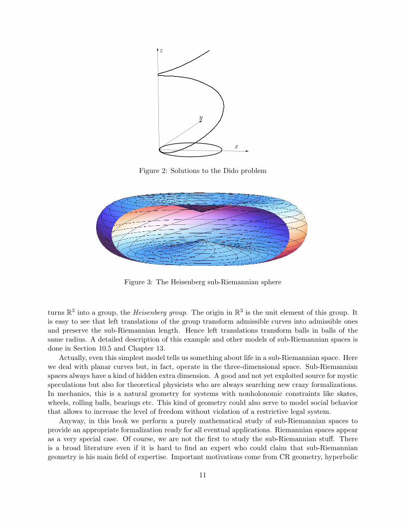
Solutions of the Dido problem are arcs of circles and their lifts to R3 are spirals where z(t) is
the area of the piece of disc cut by the hord connecting (0, 0) with (x(t), y(t)).A piece of such a spiral is a shortest admissible path between its endpoints while the planar
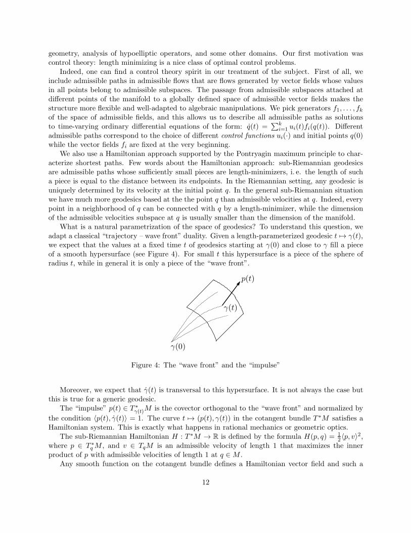
projection of this piece is an arc of the circle. The spiral ceases to be a shortest path when itsplanar projection starts to run the circle for the second time, i. e. when the spiral starts its secondturn. Sub-Riemannian balls centered at the origin for this model look like apples with singularitiesat the poles (see Figure 3).
Singularities are points on the sphere connected with the center by more than one shortestpath. The dilation (x, y, z) 7→ (rx, ry, r2z) transforms the ball of radius 1 into the ball of radiusr. In particular, arbitrary small balls have singularities. This is always the case when admissiblesubspaces are proper subspaces.
Another important symmetry connects balls with different centers. Indeed, the product opera-tion
(x, y, z) · (x′, y′, z′) .=(x+ x′, y + y′, z + z′ +
1
2(xy′ − x′y)
)
10
z
x
y
Figure 2: Solutions to the Dido problem
Figure 3: The Heisenberg sub-Riemannian sphere
turns R3 into a group, the Heisenberg group. The origin in R3 is the unit element of this group. It
is easy to see that left translations of the group transform admissible curves into admissible onesand preserve the sub-Riemannian length. Hence left translations transform balls in balls of thesame radius. A detailed description of this example and other models of sub-Riemannian spaces isdone in Section 10.5 and Chapter 13.
Actually, even this simplest model tells us something about life in a sub-Riemannian space. Herewe deal with planar curves but, in fact, operate in the three-dimensional space. Sub-Riemannianspaces always have a kind of hidden extra dimension. A good and not yet exploited source for mysticspeculations but also for theoretical physicists who are always searching new crazy formalizations.In mechanics, this is a natural geometry for systems with nonholonomic constraints like skates,wheels, rolling balls, bearings etc. This kind of geometry could also serve to model social behaviorthat allows to increase the level of freedom without violation of a restrictive legal system.
Anyway, in this book we perform a purely mathematical study of sub-Riemannian spaces toprovide an appropriate formalization ready for all eventual applications. Riemannian spaces appearas a very special case. Of course, we are not the first to study the sub-Riemannian stuff. Thereis a broad literature even if it is hard to find an expert who could claim that sub-Riemanniangeometry is his main field of expertise. Important motivations come from CR geometry, hyperbolic
11
geometry, analysis of hypoelliptic operators, and some other domains. Our first motivation wascontrol theory: length minimizing is a nice class of optimal control problems.
Indeed, one can find a control theory spirit in our treatment of the subject. First of all, weinclude admissible paths in admissible flows that are flows generated by vector fields whose valuesin all points belong to admissible subspaces. The passage from admissible subspaces attached atdifferent points of the manifold to a globally defined space of admissible vector fields makes thestructure more flexible and well-adapted to algebraic manipulations. We pick generators f1, . . . , fkof the space of admissible fields, and this allows us to describe all admissible paths as solutionsto time-varying ordinary differential equations of the form: q(t) =
∑ki=1 ui(t)fi(q(t)). Different
admissible paths correspond to the choice of different control functions ui(·) and initial points q(0)while the vector fields fi are fixed at the very beginning.
We also use a Hamiltonian approach supported by the Pontryagin maximum principle to char-acterize shortest paths. Few words about the Hamiltonian approach: sub-Riemannian geodesicsare admissible paths whose sufficiently small pieces are length-minimizers, i. e. the length of sucha piece is equal to the distance between its endpoints. In the Riemannian setting, any geodesic isuniquely determined by its velocity at the initial point q. In the general sub-Riemannian situationwe have much more geodesics based at the the point q than admissible velocities at q. Indeed, everypoint in a neighborhood of q can be connected with q by a length-minimizer, while the dimensionof the admissible velocities subspace at q is usually smaller than the dimension of the manifold.
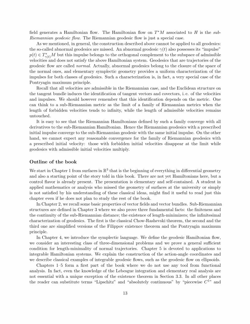
What is a natural parametrization of the space of geodesics? To understand this question, weadapt a classical “trajectory – wave front” duality. Given a length-parameterized geodesic t 7→ γ(t),we expect that the values at a fixed time t of geodesics starting at γ(0) and close to γ fill a pieceof a smooth hypersurface (see Figure 4). For small t this hypersurface is a piece of the sphere ofradius t, while in general it is only a piece of the “wave front”.
γ(0)
p(t)
γ(t)
Figure 4: The “wave front” and the “impulse”
Moreover, we expect that γ(t) is transversal to this hypersurface. It is not always the case butthis is true for a generic geodesic.
The “impulse” p(t) ∈ T ∗γ(t)M is the covector orthogonal to the “wave front” and normalized by
the condition 〈p(t), γ(t)〉 = 1. The curve t 7→ (p(t), γ(t)) in the cotangent bundle T ∗M satisfies aHamiltonian system. This is exactly what happens in rational mechanics or geometric optics.
The sub-Riemannian Hamiltonian H : T ∗M → R is defined by the formula H(p, q) = 12〈p, v〉2,
where p ∈ T ∗qM , and v ∈ TqM is an admissible velocity of length 1 that maximizes the inner
product of p with admissible velocities of length 1 at q ∈M .Any smooth function on the cotangent bundle defines a Hamiltonian vector field and such a
12
field generates a Hamiltonian flow. The Hamiltonian flow on T ∗M associated to H is the sub-Riemannian geodesic flow. The Riemannian geodesic flow is just a special case.
As we mentioned, in general, the construction described above cannot be applied to all geodesics:the so-called abnormal geodesics are missed. An abnormal geodesic γ(t) also possesses its “impulse”p(t) ∈ T ∗
γ(t)M but this impulse belongs to the orthogonal complement to the subspace of admissiblevelocities and does not satisfy the above Hamiltonian system. Geodesics that are trajectories of thegeodesic flow are called normal. Actually, abnormal geodesics belong to the closure of the space ofthe normal ones, and elementary symplectic geometry provides a uniform characterization of theimpulses for both classes of geodesics. Such a characterization is, in fact, a very special case of thePontryagin maximum principle.
Recall that all velocities are admissible in the Riemannian case, and the Euclidean structure onthe tangent bundle induces the identification of tangent vectors and covectors, i. e. of the velocitiesand impulses. We should however remember that this identification depends on the metric. Onecan think to a sub-Riemannian metric as the limit of a family of Riemannian metrics when thelength of forbidden velocities tends to infinity, while the length of admissible velocities remainsuntouched.
It is easy to see that the Riemannian Hamiltonians defined by such a family converge with allderivatives to the sub-Riemannian Hamiltonian. Hence the Riemannian geodesics with a prescribedinitial impulse converge to the sub-Riemannian geodesic with the same initial impulse. On the otherhand, we cannot expect any reasonable convergence for the family of Riemannian geodesics witha prescribed initial velocity: those with forbidden initial velocities disappear at the limit whilegeodesics with admissible initial velocities multiply.
Outline of the book
We start in Chapter 1 from surfaces in R3 that is the beginning of everything in differential geometry
and also a starting point of the story told in this book. There are not yet Hamiltonians here, but acontrol flavor is already present. The presentation is elementary and self-contained. A student inapplied mathematics or analysis who missed the geometry of surfaces at the university or simplyis not satisfied by his understanding of these classical ideas, might find it useful to read just thischapter even if he does not plan to study the rest of the book.
In Chapter 2, we recall some basic properties of vector fields and vector bundles. Sub-Riemannianstructures are defined in Chapter 3 where we also prove three fundamental facts: the finiteness andthe continuity of the sub-Riemannian distance; the existence of length-minimizers; the infinitesimalcharacterization of geodesics. The first is the classical Chow-Rashevski theorem, the second and thethird one are simplified versions of the Filippov existence theorem and the Pontryagin maximumprinciple.
In Chapter 4, we introduce the symplectic language. We define the geodesic Hamiltonian flow,we consider an interesting class of three-dimensional problems and we prove a general sufficientcondition for length-minimality of normal trajectories. Chapter 5 is devoted to applications tointegrable Hamiltonian systems. We explain the construction of the action-angle coordinates andwe describe classical examples of integrable geodesic flows, such as the geodesic flow on ellipsoids.
Chapters 1–5 form a first part of the book where we do not use any tool from functionalanalysis. In fact, even the knowledge of the Lebesgue integration and elementary real analysis arenot essential with a unique exception of the existence theorem in Section 3.3. In all other placesthe reader can substitute terms “Lipschitz” and “absolutely continuous” by “piecewise C1” and
13
“measurable” by “piecewise continuous” without a loss for the understanding.
We start to use some basic functional analysis in Chapter 6. In this chapter, we give elementsof an operator calculus that simplifies and clarifies calculations with non-stationary flows, theirvariations and compositions. In Chapter 7, we use this calculus for a fast introduction to the Liegroup theory.
In Chapter 8, we interpret the “impulses” as Lagrange multipliers for constrained optimizationproblems and apply this point of view to the sub-Riemannian case. We also introduce the sub-Riemannian exponential map and we study conjugate points.
In Chapter 10, we construct the nonholonomic tangent space at a point q of the manifold: afirst quasi-homogeneous approximation of the space if you observe and exploit it from q by meansof admissible paths. In general, such a tangent space is a homogeneous space of a nilpotent Liegroup equipped with an invariant vector distribution; its structure may depend on the point wherethe tangent space is attached. At generic points, this is a nilpotent Lie group endowed with aleft-invariant vector distribution. The construction of the nonholonomic tangent space does notneed a metric; if we take into account the metric, we obtain the Gromov–Hausdorff tangent to thesub-Riemannian metric space. Useful “ball-box” estimates of small balls follow automatically.
Chapter 13 is devoted to the explicit calculation of the sub-Riemannian distance for modelspaces. In Chapter 11, we study general analytic properties of the sub-Riemannian distance as afunction of points of the manifold. It is shown that the distance is smooth on an open dense subsetand is semi-concave out of the points connected by abnormal length-minimizers. Moreover, genericsphere is a Lipschitz submanifold if we remove these bad points.
In Chapter 12, we turn to abnormal geodesics, which provide the deepest singularities of thedistance. Abnormal geodesics are critical points of the endpoint map defined on the space ofadmissible paths, and the main tool for their study is the Hessian of the endpoint map.
This is the end of the second part of the book; next few chapters are devoted to the curvatureand its applications. Let Φt : T ∗M → T ∗M , for t ∈ R, be a sub-Riemannian geodesic flow.Submanifolds Φt(T ∗
qM), q ∈ M, form a fibration of T ∗M . Given λ ∈ T ∗M , let Jλ(t) ⊂ Tλ(T∗M)
be the tangent space to the leaf of this fibration.
Recall that Φt is a Hamiltonian flow and T ∗qM are Lagrangian submanifolds; hence the leaves
of our fibrations are Lagrangian submanifolds and Jλ(t) is a Lagrangian subspace of the symplecticspace Tλ(T
∗M).
In other words, Jλ(t) belongs to the Lagrangian Grassmannian of Tλ(T∗M), and t 7→ Jλ(t) is
a curve in the Lagrangian Grassmannian, a Jacobi curve of the sub-Riemannian structure. Thecurvature of the sub-Riemannian space at λ is simply the “curvature” of this curve in the LagrangianGrassmannian.
Chapter 14 is devoted to the elementary differential geometry of curves in the LagrangianGrassmannian; in Chapter 15 we apply this geometry to Jacobi curves.
The language of Jacobi curves is translated to the traditional language in the Riemanniancase in Chapter 16. We recover the Levi Civita connection and the Riemannian curvature anddemonstrate their symplectic meaning. In Chapter 17, we explicitly compute the sub-Riemanniancurvature for contact three-dimensional spaces. In the next Chapter 18 we study the small distanceasymptotics of the expowhree-dimensional contact case and see how the structure of the conjugatelocus is encoded in the curvature.
In Chapter ??, we consider two-dimensional sub-Riemannian metrics; such a metric differs froma Riemannian one only along a one-dimensional submanifold. In the last Chapter 20 we define the
14
sub-Riemannian Laplace operator, the canonical volume form, and compute the density of thesub-Riemannian Hausdorff measure. We conclude with a discussion of the sub-Riemannian heatequation and an explicit formula for the heat kernel in the three-dimensional Heisenberg case.
We finish here this introduction into the Introduction. . .We hope that the reader won’t bebored; comments to the chapters contain suggestions for further reading.1
1This research has been supported by the European Research Council, ERC StG 2009 “GeCoMethods”, contractnumber 239748 and by the ANR project SRGI “Sub-Riemannian Geometry and Interactions”, contract numberANR-15-CE40-0018.
15

16
Chapter 1
Geometry of surfaces in R3
In this preliminary chapter we study the geometry of smooth two dimensional surfaces in R3 as a
“heating problem” and we recover some classical results.In the fist part of the chapter we consider surfaces in R
3 endowed with the standard Euclideanproduct, which we denote by 〈· | ·〉. In the second part we study surfaces in the Minskowski space,that is R3 endowed with a sign-indefinite inner product, which we denote by 〈· | ·〉hDefinition 1.1. A surface of R3 is a subset M ⊂ R
3 such that for every q ∈ M there exists aneighborhood U ⊂ R
3 of q and a smooth function a : U → R such that U ∩M = a−1(0) and ∇a 6= 0on U ∩M .
1.1 Geodesics and optimality
Let M ⊂ R3 be a surface and γ : [0, T ]→M be a smooth curve in M . The length of γ is defined as
ℓ(γ) :=
∫ T
0‖γ(t)‖dt. (1.1)
where ‖v‖ =√〈v | v〉 denotes the norm of a vector in R
3.
Remark 1.2. Notice that the definition of length in (1.1) is invariant by reparametrizations of thecurve. Indeed let ϕ : [0, T ′] → [0, T ] be a monotone smooth function. Define γϕ : [0, T ′] → M byγϕ := γ ϕ. Using the change of variables t = ϕ(s), one gets
ℓ(γϕ) =
∫ T ′
0‖γϕ(s)‖ds =
∫ T ′
0‖γ(ϕ(s))‖|ϕ(s)|ds =
∫ T
0‖γ(t)‖dt = ℓ(γ).
The definition of length can be extended to piecewise smooth curves on M , by adding the lengthof every smooth piece of γ.
When the curve γ is parametrized in such a way that ‖γ(t)‖ ≡ c for some c > 0 we say that γhas constant speed. If moreover c = 1 we say that γ is parametrized by length.
The distance between two points p, q ∈M is the infimum of length of curves that join p to q
d(p, q) = infℓ(γ), γ : [0, T ]→M piecewise smooth, γ(0) = p, γ(T ) = q. (1.2)
Now we focus on length-minimizers, i.e., piece-wise smooth curves that realize the distance betweentheir endpoints: ℓ(γ) = d(γ(0), γ(T )).
17
γ(t)γ(t)
M
Tγ(t)M
γ(t)
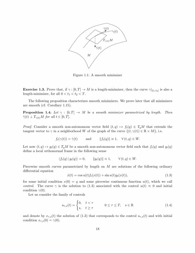
Figure 1.1: A smooth minimizer
Exercise 1.3. Prove that, if γ : [0, T ]→M is a length-minimizer, then the curve γ|[t1,t2] is also alength-minimizer, for all 0 < t1 < t2 < T .
The following proposition characterizes smooth minimizers. We prove later that all minimizersare smooth (cf. Corollary 1.15).
Proposition 1.4. Let γ : [0, T ] → M be a smooth minimizer parametrized by length. Thenγ(t) ⊥ Tγ(t)M for all t ∈ [0, T ].
Proof. Consider a smooth non-autonomous vector field (t, q) 7→ ft(q) ∈ TqM that extends thetangent vector to γ in a neighborhood W of the graph of the curve (t, γ(t)) ∈ R×M, i.e.
ft(γ(t)) = γ(t) and ‖ft(q)‖ ≡ 1, ∀ (t, q) ∈W.
Let now (t, q) 7→ gt(q) ∈ TqM be a smooth non-autonomous vector field such that ft(q) and gt(q)define a local orthonormal frame in the following sense
〈ft(q) | gt(q)〉 = 0, ‖gt(q)‖ ≡ 1, ∀ (t, q) ∈W.
Piecewise smooth curves parametrized by length on M are solutions of the following ordinarydifferential equation
x(t) = cos u(t)ft(x(t)) + sinu(t)gt(x(t)), (1.3)
for some initial condition x(0) = q and some piecewise continuous function u(t), which we callcontrol. The curve γ is the solution to (1.3) associated with the control u(t) ≡ 0 and initialcondition γ(0).
Let us consider the family of controls
uτ,s(t) =
0, t < τ
s, t ≥ τ0 ≤ τ ≤ T, s ∈ R (1.4)
and denote by xτ,s(t) the solution of (1.3) that corresponds to the control uτ,s(t) and with initialcondition xτ,s(0) = γ(0).
18
Lemma 1.5. For every τ1, τ2, t ∈ [0, T ] the following vectors are linearly dependent
∂
∂s
∣∣∣∣s=0
xτ1,s(t)∂
∂s
∣∣∣∣s=0
xτ2,s(t) (1.5)
Proof. By Exercice 1.3 is not restrictive to assume t = T . Fix 0 ≤ τ1 ≤ τ2 ≤ T and consider thefamily of curves φ(t;h1, h2) solutions of (1.3) associated with controls
vh1,h2(t) =
0, t ∈ [0, τ1[,
h1, t ∈ [τ1, τ2[,
h1 + h2, t ∈ [τ2, T + ε[,
where h1, h2 belong to a neighborhood of 0 and ε is small enough (to guarantee the existence ofthe trajectory). Notice that φ is smooth in a neighborhood of (t, h1, h2) = (T, 0, 0) and
∂φ
∂hi
∣∣∣∣(h1,h2)=0
=∂
∂s
∣∣∣∣s=0
xτi,s(T ), i = 1, 2.
By contradiction assume that the vectors in (1.5) are linearly independent. Then ∂φ∂h is invertible
and the classical implicit function theorem applied to the map (t, h1, h2) 7→ φ(t;h1, h2) at the point(T, 0, 0) implies that there exists δ > 0 such that
∀ t ∈ ]T − δ, T + δ[, ∃h1, h2, s.t. φ(t;h1, h2) = γ(T ),
In particular there exists a curve with unit speed joining γ(0) and γ(T ) in time t < T , which givesa contradiction, since γ is a minimizer.
Lemma 1.6. For every τ, t ∈ [0, T ] the following identity holds⟨∂
∂s
∣∣∣∣s=0
xτ,s(t)
∣∣∣∣ γ(t)⟩
= 0. (1.6)
Proof. If t ≤ τ , then by construction (cf. (1.4)) the first vector is zero since there is no variationw.r.t. s and the conclusion follows. Let us now assume that t > τ . Again, by Remark 1.3, it issufficient to prove the statement at t = T . Let us write the Taylor expansion of ψ(t) = ∂
∂s
∣∣s=0
xτ,s(t)in a right neighborhood of t = τ . Observe that, for t ≥ τ
xτ,s = cos(s)ft(xτ,s) + sin(s)gt(xτ,s).
Hence
ψ(τ) =∂
∂s
∣∣∣∣s=0
xτ,s(τ) = 0, ψ(τ) =∂
∂s
∣∣∣∣s=0
xτ,s(τ) = gτ (xτ,s(τ)).
Then, for t ≥ τ , we haveψ(t) = (t− τ)gτ (xτ,s(τ)) +O((t− τ)2). (1.7)
For τ sufficiently close to T , one can take t = T in (1.7). Passing to the limit for τ → T one gets
1
T − τ∂
∂s
∣∣∣∣s=0
xτ,s(T ) −→τ→T
gT (γ(T )).
Now, by Lemma 1.5 all vectors in left hand side are parallel among them, hence they are parallelto gT (γ(T )). The lemma is proved since γ(T ) = fT (γ(T )) and fT and gT are orthogonal.
19
Now we end the proposition by showing that γ(t) ⊥ Tγ(t)M . Notice that this is equivalent toshow
〈γ(t) | ft(γ(t))〉 = 〈γ(t) | gt(γ(t))〉 = 0. (1.8)
Recall that 〈γ(t) | γ(t)〉 = 1. Differentiating this identity one gets
0 =d
dt〈γ(t) | γ(t)〉 = 2 〈γ(t) | γ(t)〉 ,
which shows that γ(t) is orthogonal to ft(γ(t)). Next, differentiating (1.6) with respect to t, wehave1 for t 6= τ ⟨
∂
∂s
∣∣∣∣s=0
xτ,s(t)
∣∣∣∣ γ(t)⟩+
⟨∂
∂s
∣∣∣∣s=0
xτ,s(t)
∣∣∣∣ γ(t)⟩
= 0. (1.9)
Now, from 〈xτ,s(t) | xτ,s(t)〉 = 1 one gets⟨∂
∂sxτ,s(t)
∣∣∣∣ xτ,s(t)⟩
= 0, for t 6= τ.
Evaluating at s = 0, using that xτ,0(t) = γ(t), one has⟨∂
∂s
∣∣∣∣s=0
xτ,s(t)
∣∣∣∣ γ(t)⟩
= 0, for t 6= τ.
Hence, by (1.9), it follows that ⟨∂
∂s
∣∣∣∣s=0
xτ,s(t)
∣∣∣∣ γ(t)⟩
= 0,
which, by continuity, holds for every t ∈ [0, T ]. Using that ∂∂s
∣∣s=0
xτ,s(t) is parallel to gt(γ(t)) (seeproof of Lemma 1.6), it follows that 〈gt(γ(t)) | γ(t)〉 = 0.
Definition 1.7. A smooth curve γ : [0, T ]→M parametrized with constant speed is called geodesicif it satisfies
γ(t) ⊥ Tγ(t)M, ∀ t ∈ [0, T ]. (1.10)
Proposition 1.4 says that a smooth curve that minimizes the length is a geodesic.
Now we get an explicit characterization of geodesics when the manifold M is globally definedas the zero level of a smooth function. In other words there exists a smooth function a : R3 → R
such thatM = a−1(0), and ∇a 6= 0 on M. (1.11)
Remark 1.8. Recall that for all q ∈M it holds ∇qa ⊥ TqM . Indeed, for every q ∈M and v ∈ TqM ,let γ : [0, T ] → M be a smooth curve on M such that γ(0) = q and γ(0) = v. By definition of Mone has a(γ(t)) = 0. Differentiating this identity with respect to t at t = 0 one gets 〈∇qa | v〉 = 0.
Proposition 1.9. A smooth curve γ : [0, T ]→M is a geodesic if and only if it satisfies, in matrixnotation:
γ(t) = −γ(t)T (∇2
γ(t)a)γ(t)
‖∇γ(t)a‖2∇γ(t)a, ∀ t ∈ [0, T ], (1.12)
where ∇2γ(t)a is the Hessian matrix of a.
1notice that xτ,s is smooth on the set [0, T ] \ τ.
20
Proof. Differentiating the equality⟨∇γ(t)a
∣∣ γ(t)⟩= 0 we get, in matrix notation:
γ(t)T (∇2γ(t)a)γ(t) + γ(t)T∇γ(t)a = 0.
By definition of geodesic there exists a function b(t) such that
γ(t) = b(t)∇γ(t)a.
Hence we getγ(t)T (∇2
γ(t)a)γ(t) + b(t)‖∇γ(t)a‖2 = 0,
from which (1.12) follows.
Remark 1.10. Notice that formula (1.12) is always true locally since, by definition of surface, theassumptions (1.11) are always satisfied locally.
1.1.1 Existence and minimizing properties of geodesics
As a direct consequence of Proposition 1.9 one gets the following existence and uniqueness theoremfor geodesics.
Corollary 1.11. Let q ∈M and v ∈ TqM . There exists a unique geodesic γ : [0, ε] →M , for ε > 0small enough, such that γ(0) = q and γ(0) = v.
Proof. By Proposition 1.9, geodesics satisfy a second order ODE, hence they are smooth curves,characterized by ther initial position and velocity.
To end this section we show that small pieces of geodesics are always global minimizers.
Theorem 1.12. Let γ : [0, T ]→M be a geodesic. For every τ ∈ [0, T [ there exists ε > 0 such that
(i) γ|[τ,τ+ε] is a minimizer, i.e. d(γ(τ), γ(τ + ε)) = ℓ(γ|[τ,τ+ε]),
(ii) γ|[τ,τ+ε] is the unique minimizers joining γ(τ) and γ(τ + ε) in the class of piecewise smoothcurves, up to reparametrization.
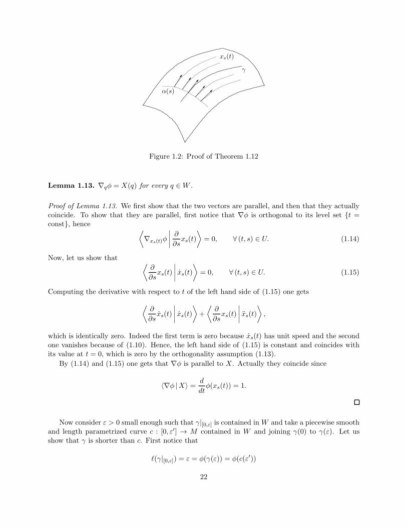
Proof. Without loss of generality let us assume that τ = 0 and that γ is length parametrized.Consider a length-parametrized curve α on M such that α(0) = γ(0) and α(0) ⊥ γ(0) and denoteby (t, s) 7→ xs(t) the smooth variation of geodesics such that x0(t) = γ(t) and (see also Figure 1.2)
xs(0) = α(s), xs(0) ⊥ α(s). (1.13)
The map ψ : (t, s) 7→ xs(t) is a local diffeomorphism near (0, 0). Indeed the partial derivatives
∂ψ
∂t
∣∣∣t=s=0
=∂
∂t
∣∣∣∣t=0
x0(t) = γ(0),∂ψ
∂s
∣∣∣t=s=0
=∂
∂s
∣∣∣∣s=0
xs(0) = α(0),
are linearly independent. Thus ψ maps a neighborhood U of (0, 0) on a neighborhood W of γ(0).We now consider the function φ and the vector field X defined on W
φ : xs(t) 7→ t,
X : xs(t) 7→ xs(t).
21
γ
α(s)
xs(t)
Figure 1.2: Proof of Theorem 1.12
Lemma 1.13. ∇qφ = X(q) for every q ∈W .
Proof of Lemma 1.13. We first show that the two vectors are parallel, and then that they actuallycoincide. To show that they are parallel, first notice that ∇φ is orthogonal to its level set t =const, hence ⟨
∇xs(t)φ∣∣∣∣∂
∂sxs(t)
⟩= 0, ∀ (t, s) ∈ U. (1.14)
Now, let us show that ⟨∂
∂sxs(t)
∣∣∣∣ xs(t)⟩
= 0, ∀ (t, s) ∈ U. (1.15)
Computing the derivative with respect to t of the left hand side of (1.15) one gets
⟨∂
∂sxs(t)
∣∣∣∣ xs(t)⟩+
⟨∂
∂sxs(t)
∣∣∣∣ xs(t)⟩,
which is identically zero. Indeed the first term is zero because xs(t) has unit speed and the secondone vanishes because of (1.10). Hence, the left hand side of (1.15) is constant and coincides withits value at t = 0, which is zero by the orthogonality assumption (1.13).
By (1.14) and (1.15) one gets that ∇φ is parallel to X. Actually they coincide since
〈∇φ |X〉 = d
dtφ(xs(t)) = 1.
Now consider ε > 0 small enough such that γ|[0,ε] is contained inW and take a piecewise smoothand length parametrized curve c : [0, ε′] → M contained in W and joining γ(0) to γ(ε). Let usshow that γ is shorter than c. First notice that
ℓ(γ|[0,ε]) = ε = φ(γ(ε)) = φ(c(ε′))
22
Using that φ(c(0)) = φ(γ(0)) = 0 and that ℓ(c) = ε′ we have that
ℓ(γ|[0,ε]) = φ(c(ε′))− φ(c(0)) =∫ ε′
0
d
dtφ(c(t))dt (1.16)
=
∫ ε′
0〈∇φ(c(t)) | c(t)〉 dt
=
∫ ε′
0〈X(c(t)) | c(t)〉 dt ≤ ε′ = ℓ(c), (1.17)
The last inequality follows from the Cauchy-Schwartz inequality
〈X(c(t)) | c(t)〉 ≤ ‖X(c(t))‖‖c(t)‖ = 1 (1.18)
which holds at every smooth point of c(t). In addition, equality in (1.18) holds if and only ifc(t) = X(c(t)) (at the smooth points of c). Hence we get that ℓ(c) = ℓ(γ|[0,ε]) if and only if ccoincides with γ|[0,ε].
Now let us show that there exists ε ≤ ε such that γ|[0,ε] is a global minimizer among all piecewisesmooth curves joining γ(0) to γ(ε). It is enough to take ε < dist(γ(0), ∂W ). Every curve that escapefrom W has length greater than ε.
From Theorem 1.12 it follows
Corollary 1.14. Any minimizer of the distance (in the class of piecewise smooth curves) is ageodesic, and hence smooth.
1.1.2 Absolutely continuous curves
Notice that formula (1.1) defines the length of a curve even in the class of absolutely continuousones, if one understands the integral in the Lebesgue sense.
In this setting, in the proof of Theorem 1.12, one can assume that the curve c is actuallyabsolutely continuous. This proves that small pieces of geodesics are minimizers also in the classof absolutely continuous curves on M . Morever, this proves the following.
Corollary 1.15. Any minimizer of the distance (in the class of absolutely continuous curves) is ageodesic, and hence smooth.
1.2 Parallel transport
In this section we want to introduce the notion of parallel transport, which let us to define themain geometric invariant of a surface: the Gaussian curvature.
Let us consider a curve γ : [0, T ] → M and a vector ξ ∈ Tγ(0)M . We want to define theparallel transport of ξ along γ. Heuristically, it is a curve ξ(t) ∈ Tγ(t)M such that the vectorsξ(t), t ∈ [0, T ] are all “parallel”.
Remark 1.16. If M = R2 ⊂ R
3 is the set z = 0 we can canonically identify every tangent spaceTγ(t)M with R
2 so that every tangent vector ξ(t) belong to the same vector space.2 In this case,
parallel simply means ξ(t) = 0 as an element of R3. This is not the case if M is a manifold becausetangent spaces at different points are different.
2The canonical isomorphism R2 ≃ TxR
2 is written explicitly as follows: y 7→ ddt
∣∣t=0
x+ ty.
23
Definition 1.17. Let γ : [0, T ] → M be a smooth curve. A smooth curve of tangent vectorsξ(t) ∈ Tγ(t)M is said to be parallel if ξ(t) ⊥ Tγ(t)M .
Assume now that M is the zero level of a smooth function a : R3 → R as in (1.11). We havethe following description:
Proposition 1.18. A smooth curve of tangent vectors ξ(t) defined along γ : [0, T ]→M is parallelif and only if it satisfies
ξ(t) = −γ(t)T (∇2
γ(t)a)ξ(t)
‖∇γ(t)a‖2∇γ(t)a, ∀ t ∈ [0, T ]. (1.19)
Proof. As in Remark 1.8, ξ(t) ∈ Tγ(t)M implies⟨∇γ(t)a, ξ(t)
⟩= 0. Moreover, by assumption
ξ(t) = α(t)∇γ(t)a for some smooth function α. With analogous computations as in the proof ofProposition 1.9 we get that
γ(t)T (∇2γ(t)a)ξ(t) + α(t)‖∇γ(t)a‖2 = 0,
from which the statement follows.
Remark 1.19. Notice that, since (1.53) is a first order linear ODE with respect to ξ, for a givencurve γ : [0, T ] → M and initial datum v ∈ Tγ(0)M , there is a unique parallel curve of tangentvectors ξ(t) ∈ Tγ(t)M along γ such that ξ(0) = v. Since (1.53) is a linear ODE, the operator thatassociates with every initial condition ξ(0) the final vector ξ(t) is a linear operator, which is calledparallel transport.
Next we state a key property of the parallel transport.
Proposition 1.20. The parallel transport preserves the inner product. In other words, if ξ(t), η(t)are two parallel curves of tangent vectors along γ, then we have
d
dt〈ξ(t) | η(t)〉 = 0, ∀ t ∈ [0, T ]. (1.20)
Proof. From the fact that ξ(t), η(t) ∈ Tγ(t)M and ξ(t), η(t) ⊥ Tγ(t)M one immediately gets
d
dt〈ξ(t) | η(t)〉 = 〈ξ(t)|η(t)〉 + 〈ξ(t) | η(t)〉 = 0.
The notion of parallel transport permits to give a new characterization of geodesics. Indeed, bydefinition
Corollary 1.21. A smooth curve γ : [0, T ]→M is a geodesic if and only if γ is parallel along γ.
In the following we assume that M is oriented.
Definition 1.22. The spherical bundle SM on M is the disjoint union of all unit tangent vectorsto M :
SM =⊔
q∈MSqM, SqM = v ∈ TqM, ‖v‖ = 1. (1.21)
24
SM is a smooth manifold of dimension 3. Moreover it has the structure of fiber bundle withbase manifold M , typical fiber S1, and canonical projection
π : SM →M, π(v) = q if v ∈ TqM.
Remark 1.23. Since every vector in the fiber SqM has norm one, we can parametrize every v ∈SqM by an angular coordinate θ ∈ S1 through an orthonormal frame e1(q), e2(q) for SqM , i.e.v = cos(θ)e1(q) + sin(θ)e2(q).
The choice of a positively oriented orthonormal frame e1(q), e2(q) corresponds to fix theelement in the fiber corresponding to θ = 0. Hence, the choice of such an orthonormal frame atevery point q induces coordinates on SM of the form (q, θ + ϕ(q)), where ϕ ∈ C∞(M).
Given an element ξ ∈ SqM we can complete it to an orthonormal frame (ξ, η, ν) of R3 in thefollowing unique way:
(i) η ∈ TqM is orthogonal to ξ and (ξ, η) is positively oriented (w.r.t. the orientation of M),
(ii) ν ⊥ TqM and (ξ, η, ν) is positively oriented (w.r.t. the orientation of R3).
Let t 7→ ξ(t) ∈ Sγ(t)M be a smooth curve of unit tangent vectors along γ : [0, T ] → M . Define
η(t), ν(t) ∈ Tγ(t)M as above. Since t 7→ ξ(t) has constant speed, one has ξ(t) ⊥ ξ(t) and we canwrite
ξ(t) = uξ(t)η(t) + vξ(t)ν(t).
In particular this shows that every element of TξSM , written in the basis (ξ, η, ν), has zero com-ponent along ξ.
Definition 1.24. The Levi-Civita connection on M is the 1-form ω ∈ Λ1(SM) defined by
ωξ : TξSM → R, ωξ(z) = uz, (1.22)
where z = uzη + vzν and (ξ, η, ν) is the orthonormal frame defined above.
Notice that ω change sign if we change the orientation of M .
Lemma 1.25. A curve of unit tangent vectors ξ(t) is parallel if and only if ωξ(t)(ξ(t)) = 0.
Proof. By definition ξ(t) is parallel if and only if ξ(t) is orthogonal to Tγ(t)M , i.e., collinear toν(t).
In particular, a curve parametrized by length γ : [0, T ]→M is a geodesic if and only if
ωγ(t)(γ(t)) = 0, ∀ t ∈ [0, T ]. (1.23)
Proposition 1.26. The Levi-Civita connection ω ∈ Λ1(SM) satisfies:
(i) there exist two smooth functions a1, a2 :M → R such that
ω = dθ + a1(x1, x2)dx1 + a2(x1, x2)dx2, (1.24)
where (x1, x2, θ) is a system of coordinates on SM .
25
(ii) dω = π∗Ω, where Ω is a 2-form defined on M and π : SM →M is the canonical projection.
Proof. (i) Fix a system of coordinates (x1, x2, θ) on SM and consider the vector field ∂/∂θ on SM .Let us show that
ω
(∂
∂θ
)= 1.
Indeed consider a curve t 7→ ξ(t) of unit tangent vector at a fixed point which describes a rotationin a single fibre. As a curve on SM , the velocity of this curve is exactly its orthogonal vector, i.e.ξ(t) = η(t) and the equality above follows from the definition of ω. By construction, ω is invariantby rotations, hence the coefficients ai = ω(∂/∂xi) do not depend on the variable θ.
(ii) Follows directly from expression (1.24) noticing that dω depends only on x1, x2.
Remark 1.27. Notice that the functions a1, a2 in (1.24) are not invariant by change of coordinateson the fiber. Indeed the transformation θ → θ+ϕ(x1, x2) induces dθ → dθ+(∂x1ϕ)dx1+(∂x2ϕ)dx2which gives ai → ai + ∂xiϕ for i = 1, 2.
By definition ω is an intrinsic 1-form on SM . Its differential, by property (ii) of Proposition1.55, is the pull-back of an intrinsic 2-form on M , that in general is not exact.
Definition 1.28. The area form dV on a surface M is the differential two form that on everytangent space to the manifold agrees with the volume induced by the inner product. In otherwords, for every positively oriented orthonormal frame e1, e2 of TqM , one has dV (e1, e2) = 1.
Given a set Γ ⊂M its area is the quantity |Γ| =∫Γ dV .
Since any 2-form on M is proportional to the area form dV , it makes sense to give the followingdefinition:
Definition 1.29. The Gaussian curvature of M is the function κ :M → R defined by the equality
Ω = −κdV. (1.25)
Note that κ does not depend on the orientation ofM , since both Ω and dV change sign if we reversethe orientation. Moreover the area 2-form dV on the surface depends only on the metric structureon the surface.
1.3 Gauss-Bonnet Theorems
In this section we will prove both the local and the global version of the Gauss-Bonnet theorem. Astrong consequence of these results is the celebrated Gauss’ Theorema Egregium which says thatthe Gaussian curvature of a surface is independent on its embedding in R
3.
Definition 1.30. Let γ : [0, T ] → M be a smooth curve parametrized by length. The geodesiccurvature of γ is defined as
ργ(t) = ωγ(t)(γ(t)). (1.26)
Notice that if γ is a geodesic, then ργ(t) = 0 for every t ∈ [0, T ]. The geodesic curvaturemeasures how much a curve is far from being a geodesic.
Remark 1.31. The geodesic curvature changes sign if we move along the curve in the oppositedirection. Moreover, if M = R
2, it coincides with the usual notion of curvature of a planar curve.
26
1.3.1 Gauss-Bonnet theorem: local version
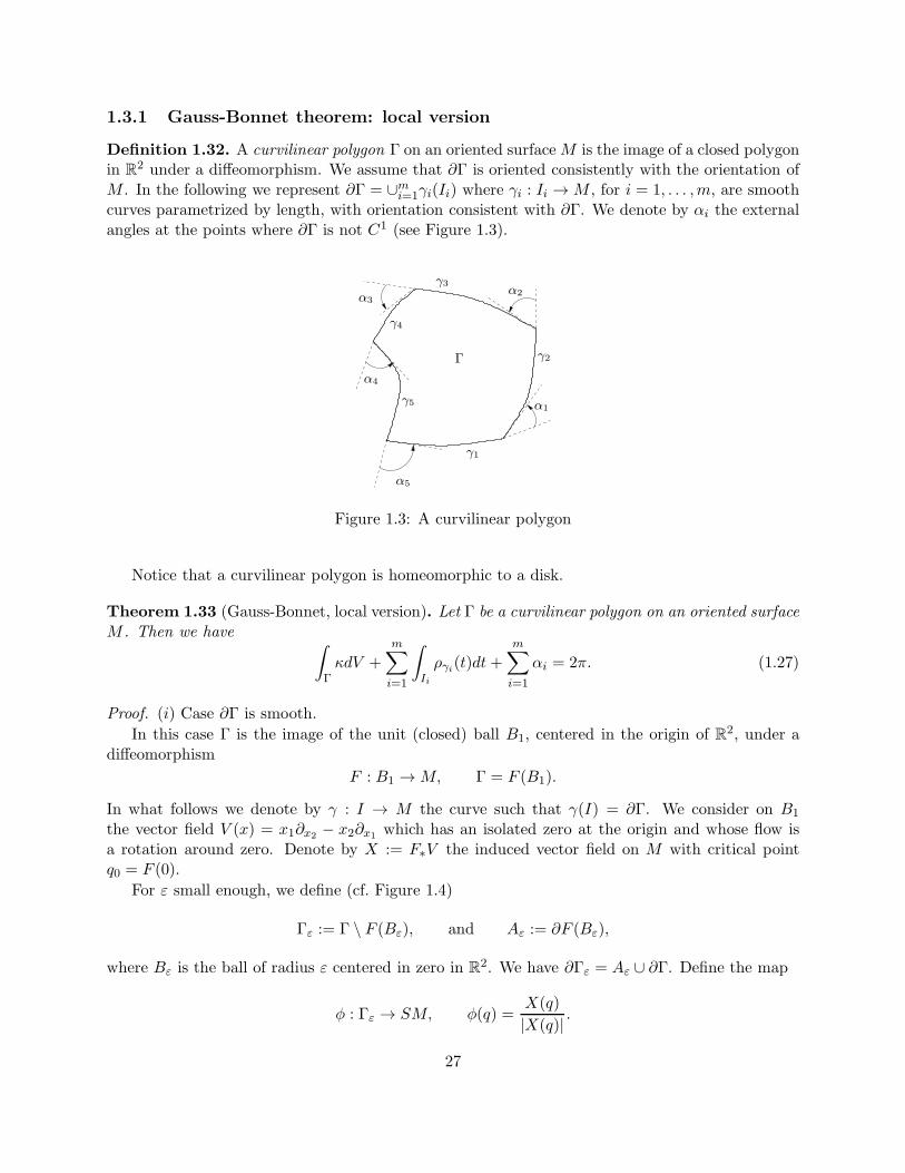
Definition 1.32. A curvilinear polygon Γ on an oriented surfaceM is the image of a closed polygonin R
2 under a diffeomorphism. We assume that ∂Γ is oriented consistently with the orientation ofM . In the following we represent ∂Γ = ∪mi=1γi(Ii) where γi : Ii →M , for i = 1, . . . ,m, are smoothcurves parametrized by length, with orientation consistent with ∂Γ. We denote by αi the externalangles at the points where ∂Γ is not C1 (see Figure 1.3).
Γ
γ1
γ2
γ5
γ3
γ4
α1
α2α3
α4
α5
Figure 1.3: A curvilinear polygon
Notice that a curvilinear polygon is homeomorphic to a disk.
Theorem 1.33 (Gauss-Bonnet, local version). Let Γ be a curvilinear polygon on an oriented surfaceM . Then we have ∫
ΓκdV +
m∑
i=1
∫
Ii
ργi(t)dt+
m∑
i=1
αi = 2π. (1.27)
Proof. (i) Case ∂Γ is smooth.
In this case Γ is the image of the unit (closed) ball B1, centered in the origin of R2, under adiffeomorphism
F : B1 →M, Γ = F (B1).
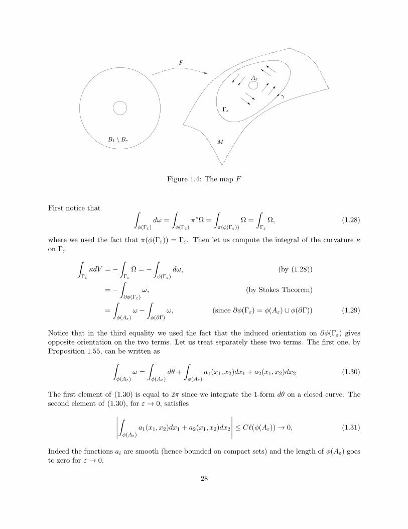
In what follows we denote by γ : I → M the curve such that γ(I) = ∂Γ. We consider on B1
the vector field V (x) = x1∂x2 − x2∂x1 which has an isolated zero at the origin and whose flow isa rotation around zero. Denote by X := F∗V the induced vector field on M with critical pointq0 = F (0).
For ε small enough, we define (cf. Figure 1.4)
Γε := Γ \ F (Bε), and Aε := ∂F (Bε),
where Bε is the ball of radius ε centered in zero in R2. We have ∂Γε = Aε ∪ ∂Γ. Define the map
φ : Γε → SM, φ(q) =X(q)
|X(q)| .
27
Γε
F
Aε
γ
MB1 \Bε
Figure 1.4: The map F
First notice that ∫
φ(Γε)dω =
∫
φ(Γε)π∗Ω =
∫
π(φ(Γε))Ω =
∫
Γε
Ω, (1.28)
where we used the fact that π(φ(Γε)) = Γε. Then let us compute the integral of the curvature κon Γε
∫
Γε
κdV = −∫
Γε
Ω = −∫
φ(Γε)dω, (by (1.28))
= −∫
∂φ(Γε)ω, (by Stokes Theorem)
=
∫
φ(Aε)ω −
∫
φ(∂Γ)ω, (since ∂φ(Γε) = φ(Aε) ∪ φ(∂Γ)) (1.29)
Notice that in the third equality we used the fact that the induced orientation on ∂φ(Γε) givesopposite orientation on the two terms. Let us treat separately these two terms. The first one, byProposition 1.55, can be written as
∫
φ(Aε)ω =
∫
φ(Aε)dθ +
∫
φ(Aε)a1(x1, x2)dx1 + a2(x1, x2)dx2 (1.30)
The first element of (1.30) is equal to 2π since we integrate the 1-form dθ on a closed curve. Thesecond element of (1.30), for ε→ 0, satisfies
∣∣∣∣∣
∫
φ(Aε)a1(x1, x2)dx1 + a2(x1, x2)dx2
∣∣∣∣∣ ≤ Cℓ(φ(Aε))→ 0, (1.31)
Indeed the functions ai are smooth (hence bounded on compact sets) and the length of φ(Aε) goesto zero for ε→ 0.
28
Let us now consider the second term of (1.29). Since φ(∂Γ) is parametrized by the curvet 7→ γ(t) (as a curve on SM), we have
∫
φ(∂Γ)ω =
∫
Iωγ(t)(γ(t))dt =
∫
Iργ(t)dt.
Concluding we have from (1.29)∫
ΓκdV = lim
ε→0
∫
Γε
κdV = 2π −∫
Iργ(t)dt,
that is (1.27) in the smooth case (i.e. when αi = 0 for all i).(ii) Case ∂Γ non smooth.
We reduce to the previous case with a sequence of polygons Γn such that ∂Γn is smooth and Γnapproximates Γ in a “smooth” way. In particular, we assume that ∂Γn coincides with ∂Γ exceptsin neighborhoods Ui, for i = 1, . . . ,m, of each point qi where ∂Γ is not smooth, in such a way that
the curve σ(n)i that parametrize (∂Γn \ ∂Γ) ∩ Ui satisfies ℓ(σni ) ≤ 1/n.
If we apply the statement of the Theorem for the smooth case to Γn we have∫
Γn
κdV +
∫ργ(n)(t)dt = 2π,
where γ(n) is the curve that parametrizes ∂Γn. Since Γn tends to Γ as n→∞, then
limn→∞
∫
Γn
κdV =
∫
ΓκdV.
We are left to prove that
limn→∞
∫ργ(n)(t)dt =
m∑
i=1
∫
Ii
ργi(t)dt+
m∑
i=1
αi. (1.32)
For every n, let us split the curve γ(n) as the union of the smooth curves σ(n)i and γ
(n)i as in Figure
??. Then ∫ργ(n)(t)dt =
m∑
i=1
∫ργ(n)i
(t)dt+m∑
i=1
∫ρσ(n)i
(t)dt.
Since the curve γ(n)i tends to γi for n→∞ one has
limn→∞
∫ργ(n)i
(t)dt =
∫ργi(t)dt.
Moreover, with analogous computations of part (i) of the proof∫ρσ(n)i
(t)dt =
∫
φ(σ(n)i )
ω =
∫
φ(σ(n)i )
dθ + a1(x1, x2)dx1 + a2(x1, x2)dx2
and one has, using that ℓ(φ(σ(n)i ))→ 0
∫
φ(σ(n)i )
dθ −→n→∞
αi,
∫
φ(σ(n)i )
a1(x1, x2)dx1 + a2(x1, x2)dx2 −→n→∞
0.
Then (1.32) follows.
29
An important corollary is obtained by applying the Gauss-Bonnet Theorem to geodesic triangles.A geodesic triangle T is a curvilinear polygon with m = 3 edges and such that every smooth pieceof boundary γi is a geodesic. For a geodesic triangle T we denote by Ai := π−αi its internal angles.Corollary 1.34. Let T be a geodesic triangle and Ai(T ) its internal angles. Then
κ(q) = lim|T |→0
∑iAi(T )− π|T |
Proof. Fix a geodesic triangle T . Using that the geodesic curvature of γi vanishes, the local versionof Gauss-Bonnet Theorem (1.27) can be rewritten as
3∑
i=1
Ai = π +
∫
ΓκdV. (1.33)
Dividing for |T | and passing to the limit for |T | → 0 in the class of geodesic triangles containing qone obtains
κ(q) = lim|T |→0
1
|T |
∫
TκdV = lim
|T |→0
∑iAi(T )− π|T |
1.3.2 Gauss-Bonnet theorem: global version
Now we state the global version of the Gauss-Bonnet theorem. In other words we want to generalize(1.27) to the case when Γ is a region ofM not necessarily homeomorphic to the disk, see for instanceFigure 1.5. As we will see that the result depends on the Euler characteristic χ(Γ) of this region.
In what follows, by a triangulation ofM we mean a decomposition ofM into curvilinear polygons(see Definition 1.32). Notice that every compact surface admits a triangulation.3
Definition 1.35. Let M ⊂ R3 be a compact oriented surface with boundary ∂M (possibly with
angles). Consider a triangulation of M . We define the Euler characteristic of M as
χ(M) := n2 − n1 + n0, (1.34)
where ni is the number of i-dimensional faces in the triangulation.
The Euler characteristic can be defined for every region Γ of M in the same way. Here, by aregion Γ on a surfaceM , we mean a closed domain of the manifold with piecewise smooth boundary.
Remark 1.36. The Euler characteristic is well-defined. Indeed one can show that the quantity(1.34) is invariant for refinement of a triangulation, since every at every step of the refinementthe alternating sum does not change. Moreover, given two different triangulations of the sameregion, there always exists a triangulation that is a refinement of both of them. This shows thatthe quantity (1.34) is independent on the triangulation.
Example 1.37. For a compact connected orientable surface Mg of genus g (i.e., a surface thattopologically is a sphere with g handles) one has χ(Mg) = 2− 2g. For instance one has χ(S2) = 2,χ(T2) = 0, where T
2 is the torus. Notice also that χ(B1) = 1, where B1 is the closed unit disk inR2.3Formally, a triangulation of a topological space M is a simplicial complex K, homeomorphic to M , together with
a homeomorphism h : K → M .
30
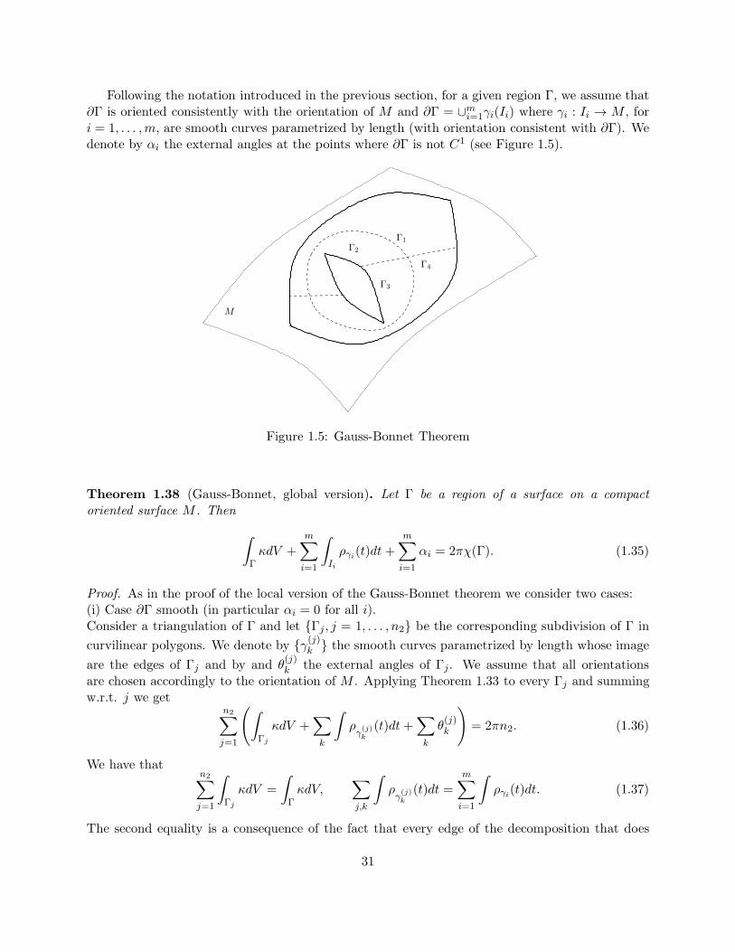
Following the notation introduced in the previous section, for a given region Γ, we assume that∂Γ is oriented consistently with the orientation of M and ∂Γ = ∪mi=1γi(Ii) where γi : Ii → M , fori = 1, . . . ,m, are smooth curves parametrized by length (with orientation consistent with ∂Γ). Wedenote by αi the external angles at the points where ∂Γ is not C1 (see Figure 1.5).
M
Γ3
Γ1
Γ4
Γ2
Figure 1.5: Gauss-Bonnet Theorem
Theorem 1.38 (Gauss-Bonnet, global version). Let Γ be a region of a surface on a compactoriented surface M . Then
∫
ΓκdV +
m∑
i=1
∫
Ii
ργi(t)dt+
m∑
i=1
αi = 2πχ(Γ). (1.35)
Proof. As in the proof of the local version of the Gauss-Bonnet theorem we consider two cases:(i) Case ∂Γ smooth (in particular αi = 0 for all i).Consider a triangulation of Γ and let Γj , j = 1, . . . , n2 be the corresponding subdivision of Γ in
curvilinear polygons. We denote by γ(j)k the smooth curves parametrized by length whose image
are the edges of Γj and by and θ(j)k the external angles of Γj. We assume that all orientations
are chosen accordingly to the orientation of M . Applying Theorem 1.33 to every Γj and summingw.r.t. j we get
n2∑
j=1
(∫
Γj
κdV +∑
k
∫ργ(j)k
(t)dt+∑
k
θ(j)k
)= 2πn2. (1.36)
We have thatn2∑
j=1
∫
Γj
κdV =
∫
ΓκdV,
∑
j,k
∫ργ(j)k
(t)dt =m∑
i=1
∫ργi(t)dt. (1.37)
The second equality is a consequence of the fact that every edge of the decomposition that does
31
not belong to ∂Γ appears twice in the sum, with opposite sign. It remains to check that
∑
j,k
θ(j)k = 2π(n1 − n0), (1.38)
Let us denote by N the total number of angles in the sum of the left hand side of (1.38). Afterreindexing we have to check that
N∑
ν=1
θν = 2π(n1 − n0). (1.39)
Denote by n∂0 the number of vertexes that belong to ∂Γ and with nI0 := n0 − n∂0 . Similarly wedefine n∂1 and nI1. We have the following relations:
(i) N = 2nI1 + n∂1 ,
(ii) n∂0 = n∂1 ,
Claim (i) follows from the fact that every curvilinear polygon with n edges has n angles, butthe internal edges are counted twice since each of them appears in two polygons. Claim (ii) is aconsequence of the fact that ∂Γ is the union of closed curves. If we denote by Ak := π − θk theinternal angles, we have
N∑
ν=1
θν = Nπ −N∑
ν=1
Aν . (1.40)
Moreover the sum of the internal angles is equal to π for a boundary vertex, and to 2π for aninternal one. Hence one gets
N∑
ν=1
Aν = 2πnI0 + πn∂0 , (1.41)
Combining (1.40), (1.41) and (i) one has
ν∑
i=1
θν = (2nI1 + n∂1)π − (2nI0 + n∂0)π
Using (ii) one finally gets (1.39).(ii) Case ∂Γ non-smooth.
We consider a decomposition of Γ into curvilinear polygons whose edges intersect the boundary inthe smooth part (this is always possible). The proof is identical to the smooth case up to formula(1.37). Now, instead of (1.39), we have to check that
N∑
ν=1
θν =
m∑
i=1
αi + 2π(n1 − n0), (1.42)
Now (1.42) can be rewritten as ∑
ν /∈Aθν = 2π(n1 − n0),
where A is the set of indices whose corresponding angles are non smooth points of ∂Γ.
32
Consider now a new region Γ, obtained by smoothing the edges of Γ, together with the decom-position induced by Γ (see Figure 1.5). Denote by n1 and n0 the number of edges and vertexes ofthe decomposition of Γ. Notice that θν , ν /∈ A is exactly the set of all angles of the decompositionof Γ. Moreover n1 − n0 = n1 − n0, since n0 = n0 +m and n1 = n1 +m, where m is the number ofnon-smooth points. Hence, by part (i) of the proof:
∑
ν /∈Aθν = 2π(n1 − n0) = 2π(n1 − n0).
Corollary 1.39. Let M be a compact oriented surface without boundary. Then
∫
MκdV = 2πχ(M). (1.43)
1.3.3 Consequences of the Gauss-Bonnet Theorems
Definition 1.40. Let M,M ′ be two surfaces in R3. A smooth map φ : R3 → R
3 is called anisometry between M and M ′ if φ(M) =M ′ and for every q ∈M it satisfies
〈v |w〉 = 〈Dqφ(v) |Dqφ(w)〉 , ∀ v,w ∈ TqM. (1.44)
If the property (1.44) is satisfied by a map defined locally in a neighborhood of every point q ofM , then it is called a local isometry.
Two surfaces M and M ′ are said to be isometric (resp. locally isometric) if there exists anisometry (resp. local isometry) between M and M ′. Notice that the restriction φ of a globalisometry Φ of R3 to a surface M ⊂ R
3 always defines an isometry between M and M ′ = φ(M).
From (1.44) it follows that an isometry preserves the angles between vectors and, a fortiori, thelength of a curve and the distance between two points.
Corollary 1.34, and the fact that the angles and the volumes are preserved by isometries, oneobtains that the Gaussian curvature is invariant by local isometries, in the following sense.
Corollary 1.41 (Gauss’s Theorema Egregium). Assume φ is a local isometry between M and M ′,then for every q ∈M one has κ(q) = κ′(φ(q)), where κ (resp. κ′) is the Gaussian curvature of M(resp. M ′).
This Theorem says that the Gaussian curvature κ depends only on the metric structure on Mand not on the specific fact that the surface is embedded in R
3 with the induced inner product.
Corollary 1.42. Let M be surface and q ∈ M . If κ(q) 6= 0 then M is not locally isometric to R2
in a neighborhood of q.
Exercise 1.43. Prove that a surface M is locally isometric to the Euclidean plane R2 around a
point q ∈M if and only if there exists a coordinate system (x1, x2) in a neighborhood U of q ∈Msuch that the vectors ∂x1 and ∂x2 have unit length and are everywhere orthonormal.
As a converse of Corollary 1.42 we have the following.
33
Theorem 1.44. Assume that κ ≡ 0 in a neighborhood of a point q ∈ M . Then M is locallyEuclidean (i.e., locally isometric to R
2) around q.
Proof. From our assumptions we have, in a neighborhood U of q:
Ω = κdV = 0.
Hence dω = π∗Ω = 0. From its explicit expression
ω = dθ + a1(x1, x2)dx1 + a2(x1, x2)dx2,
it follows that the 1-form a1dx1 + a2dx2 is locally exact, i.e. there exists a neighborhood W of q,W ⊂ U , and a function φ : W → R such that a1(x1, x2)dx1 + a2(x1, x2)dx2 = dφ. Hence
ω = d(θ + φ(x1, x2)).
Thus we can define a new angular coordinate on SM , which we still denote by θ, in such a waythat (see also Remark 1.27)
ω = dθ. (1.45)
Now, let γ be a length parametrized geodesic, i.e. ωγ(t)(γ(t)) = 0. Using the the angular coordinateθ just defined on the fibers of SM , the curve t 7→ γ(t) ∈ Sγ(t)M is written as t 7→ θ(t). Using(1.45), we have then
0 = ωγ(t)(γ(t)) = dθ(γ(t)) = θ(t).
In other words the angular coordinate of a geodesic γ is constant.
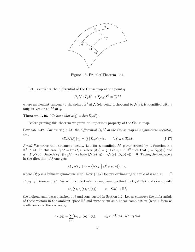
We want to construct Cartesian coordinates in a neighborhood U of q. Consider the two lengthparametrized geodesics γ1 and γ2 starting from q and such that θ1(0) = 0, θ2(0) = π/2. Definethem to be the x1-axes and x2-axes of our coordinate system, respectively.
Then, for each point q′ ∈ U consider the two geodesics starting from q′ and satisfying θ1(0) = 0and θ2(0) = π/2. We assign coordinates (x1, x2) to each point q′ in U by considering the lengthparameter of the geodesic projection of q′ on γ1 and γ2 (See Figure 1.6). Notice that the family ofgeodesics constructed in this way, and parametrized by q′ ∈ U , are mutually orthogonal at everypoint.
By construction, in this coordinate system the vectors ∂x1 and ∂x2 have length one (being thetangent vectors to length parametrized geodesics) and are everywhere mutually orthogonal. Hencethe theorem follows from Exercise 1.43.
1.3.4 The Gauss map
We end this section with a geometric characterization of the Gaussian curvature of a manifold M ,using the Gauss map.
Definition 1.45. Let M be an oriented surface. We define the Gauss map associated to M as
N :M → S2, q 7→ νq, (1.46)
where νq ∈ S2 ⊂ R3 denotes the external unit normal vector to M at q.
34
q
q′
γ2
γ1
x1
x2
Figure 1.6: Proof of Theorem 1.44.
Let us consider the differential of the Gauss map at the point q
DqN : TqM → TN (q)S2 ≃ TqM
where an element tangent to the sphere S2 at N (q), being orthogonal to N (q), is identified with atangent vector to M at q.
Theorem 1.46. We have that κ(q) = det(DqN ).
Before proving this theorem we prove an important property of the Gauss map.
Lemma 1.47. For every q ∈M , the differential DqN of the Gauss map is a symmetric operator,i.e.,
〈DqN (ξ) | η〉 = 〈ξ |DqN (η)〉 , ∀ ξ, η ∈ TqM. (1.47)
Proof. We prove the statement locally, i.e., for a manifold M parametrized by a function φ :R2 → M . In this case TqM = ImDuφ, where φ(u) = q. Let v,w ∈ R
2 such that ξ = Duφ(v) andη = Duφ(w). Since N (q) ∈ TqM⊥ we have 〈N (q) | η〉 = 〈N (q) |Duφ(w)〉 = 0. Taking the derivativein the direction of ξ one gets
〈DqN (ξ) | η〉+⟨N (q)
∣∣D2uφ(v,w)
⟩= 0,
where D2uφ is a bilinear symmetric map. Now (1.47) follows exchanging the role of v and w.
Proof of Theorem 1.46. We will use Cartan’s moving frame method. Let ξ ∈ SM and denote with
(e1(ξ), e2(ξ), e3(ξ)), ei : SM → R3,
the orthonormal basis attached at ξ and constructed in Section 1.2. Let us compute the differentialsof these vectors in the ambient space R
3 and write them as a linear combination (with 1-form ascoefficients) of the vectors ei
dξei(η) =
3∑
j=1
(ωξ)ij(η) ej(ξ), ωij ∈ Λ1SM, η ∈ TξSM.
35
Dropping ξ and η from the notation one gets the relation
dei =
3∑
j=1
ωij ej , ωij ∈ Λ1SM.
Since for each ξ the basis (e1(ξ), e2(ξ), e3(ξ)) is orthonormal (hence can be seen as an element ofSO(3)) its derivative is expressed through a skew-symmentric matrix (i.e., ωij = −ωji) and onegets the equations
de1 = ω12e2 + ω13e3,
de2 = −ω12e1 + ω23e3, (1.48)
de3 = −ω13e1 − ω23e2.
Let us now prove the following identity
ω13 ∧ ω23 = dω12. (1.49)
Indeed, differentiating the first equation in (1.48) one gets, using that d2 = 0,
0 = d2e1 = dω12e2 + ω12 ∧ de2 + dω13e3 + ω13 ∧ de3= (dω12 − ω13 ∧ ω23)e2 + (dω13 − ω12 ∧ ω23)e3,
which implies in particular (1.49).
The statement of the theorem can be rewritten as an identity between 2-forms as follows
det(DqN )dV = κdV.
Applying π∗ to both sides one gets
π∗(det(DqN )dV ) = π∗κdV = dω (1.50)
where ω is the Levi-Civita connection. Let us show that (1.50) is equivalent to (1.49).
Indeed by construction ω12 computes the coefficient of the derivative of the first vector of theorthonormal basis along the second one, hence ω12 = ω (see also Definition 1.54). It remains toshow that
ω13 ∧ ω23 = π∗(det(DqN )dV ) = det(Dπ(ξ)N )π∗dV
Since e3 = N π, where π : SM →M is the canonical projection, one has
DqN π∗ = de3 = −ω13e1 − ω23e2
The proof is completed by the following
Exercise 1.48. Let V be a 2-dimensional Euclidean vector space and e1, e2 an orthonormal basis.Let F : V → V a linear map and write F = F1e1 + F2e2, where Fi : V → R are linear functionals.Prove that F1 ∧ F2 = (detF )dV , where dV is the area form induced by the inner product.
36

Remark 1.49. Lemma 1.47 allows us to define the principal curvatures of M at the point q as thetwo real eigenvalues k1(q), k2(q) of the map DqN . In particular
κ(q) = k1(q)k2(q), q ∈M.
The principal curvatures can be geometrically interpreted as the maximum and the minimum ofcurvature of sections of M with orthogonal planes.
Notice moreover that, using the Gauss-Bonnet theorem, one can relate then degree of the mapN with the Euler characteristic of M as follows
degN :=1
Area(S2)
∫
M(detDqN )dV =
1
4π
∫
MκdV =
1
2χ(M).
1.4 Surfaces in R3 with the Minkowski inner product
The theory and the results obtained in this chapter can be adapted to the case when M ⊂ R3 is
a surface in the Minkowski 3-space, that is R3 endowed with the hyperbolic (or Minkowski-type)
inner product〈q1, q2〉h = x1x2 + y1y2 − z1z2. (1.51)
Here qi = (xi, yi, zi) for i = 1, 2, are two points in R3. When 〈q, q〉h ≥ 0, we denote by ‖q‖h =
〈q, q〉1/2h the norm induced by the inner product (1.51).For the metric structure to be defined onM , we require that the restriction of the inner product
(1.51) to the tangent space to M is positive definite at every point. Indeed, under this assumption,the inner product (1.51) can be used to define the length of a tangent vector to the surface (whichis non-negative). Thus one can introduce the length of (piecewise) smooth curves on M and itsdistance by the same formulas as in Section 1.1. These surfaces are also called space-like surfacesin the Minkovski space.
The structure of the inner product impose some condition on the structure of space-like surfaces,as the following exercice shows.
Exercise 1.50. Let M be a space-like surface in R3 endowed with the inner product (1.51).
(i) Show that if v ∈ TqM is a non zero vector that is orthogonal to TqM , then 〈v, v〉h < 0.
(ii) Prove that, if M is compact, then ∂M 6= ∅.
(iii) Show that restriction to M of the projection π(x, y, z) = (x, y) onto the xy-plane is a localdiffeomorphism.
(iv) Show that M is locally a graph on the plane z = 0.
The results obtained in the previous sections for surfaces embedded in R3 can be recovered for
space-like surfaces by simply adapting all formulas to their “hyperbolic” counterpart. For instance,geodesics are defined as curves of unit speed whose second derivative is orthogonal, with respect to〈· | ·〉h, to the tangent space to M .
For a smooth function a : R3 → R, its hyperbolic gradient ∇hqa is defined as
∇hqa =
(∂a
∂x,∂a
∂y,−∂a
∂z
)
37
If we assume that M = a−1(0) is a regular level set of a smooth function a : R3 → R. If γ(t) is acurve contained in M , i.e. a(γ(t)) = 0, one has the identity
0 =⟨∇hγ(t)a
∣∣∣ γ(t)⟩h.
The same computation shows that ∇hγ(t)a is orthogonal to the level sets of a, where orthogo-
nal always means with respect to 〈· | ·〉h. In particular, if M = a−1(0) is space-like, one has〈∇qa,∇qa〉h < 0.
Exercise 1.51. Let γ be a geodesic on M = a−1(0). Show that γ satisfies the equation (in matrixnotation)
γ(t) = −γ(t)T (∇2
γ(t)a)γ(t)
‖∇hγ(t)a‖2h∇hγ(t)a, ∀ t ∈ [0, T ]. (1.52)
where ∇2γ(t)a is the (classical) matrix of second derivatives of a.4
Given a smooth curve γ : [0, T ] → M on a surface M , a smooth curve of tangent vectorsξ(t) ∈ Tγ(t)M is said to be parallel if ξ(t) ⊥ Tγ(t)M , with respect to the hyperbolic inner product.It is then straightforward to check that, if M is the zero level of a smooth function a : R3 → R,then ξ(t) is parallel along γ if and only if it satisfies
ξ(t) = −γ(t)T (∇2
γ(t)a)ξ(t)
‖∇hγ(t)a‖2h∇hγ(t)a, ∀ t ∈ [0, T ]. (1.53)
By definition a smooth curve γ : [0, T ]→M is a geodesic if and only if γ is parallel along γ.
Remark 1.52. As for surfaces in the Euclidean space, given curve γ : [0, T ]→M and initial datumv ∈ Tγ(0)M , there is a unique parallel curve of tangent vectors ξ(t) ∈ Tγ(t)M along γ such thatξ(0) = v. Moreover the operator ξ(0) 7→ ξ(t) is a linear operator, which the parallel transport of valong γ.
Exercise 1.53. Show that if ξ(t), η(t) are two parallel curves of tangent vectors along γ, then wehave
d
dt〈ξ(t) | η(t)〉h = 0, ∀ t ∈ [0, T ]. (1.54)
Assume that M is oriented. Given an element ξ ∈ SqM we can complete it to an orthonormalframe (ξ, η, ν) of R3 in the following unique way:
(i) η ∈ TqM is orthogonal to ξ with respect to 〈· | ·〉h and (ξ, η) is positively oriented (w.r.t. theorientation of M),
(ii) ν ⊥ TqM with respect to 〈· | ·〉h and (ξ, η, ν) is positively oriented (w.r.t. the orientation ofR3).
For a smooth curve of unit tangent vectors ξ(t) ∈ Sγ(t)M along a curve γ : [0, T ] → M we defineη(t), ν(t) ∈ Tγ(t)M and we can write
ξ(t) = uξ(t)η(t) + vξ(t)ν(t).
4otherwise one can write the numerator of (1.52) as⟨
∇2,hγ(t)γ(t)
∣∣∣ γ(t)
⟩
h, where ∇2,h
γ(t) is the hyperbolic Hessian.
38
Definition 1.54. The hyperbolic Levi-Civita connection on M is the 1-form ω ∈ Λ1(SM) definedby
ωξ : TξSM → R, ωξ(z) = uz, (1.55)
where z = uzη + vzν and (ξ, η, ν) is the orthonormal frame defined above.
It is again easy to check that a curve of unit tangent vectors ξ(t) is parallel if and only ifωξ(t)(ξ(t)) = 0 and a curve parametrized by length γ : [0, T ]→M is a geodesic if and only if
ωγ(t)(γ(t)) = 0, ∀ t ∈ [0, T ]. (1.56)
Exercise 1.55. Prove that the hyperbolic Levi Civita connection ω ∈ Λ1(SM) satisfies:
(i) there exist two smooth functions a1, a2 :M → R such that
ω = dθ + a1(x1, x2)dx1 + a2(x1, x2)dx2, (1.57)
where (x1, x2, θ) is a system of coordinates on SM .
(ii) dω = π∗Ω, where Ω is a 2-form defined on M and π : SM →M is the canonical projection.
Again one can introduce the area form dV on M induced by the inner product and it makessense to give the following definition:
Definition 1.56. The Gaussian curvature of a surfaceM in the Minkowski 3-space is the functionκ :M → R defined by the equality
Ω = −κdV. (1.58)
By reasoning as in the Euclidean case, one can define the geodesic curvature of a curve andprove the analogue of the Gauss-Bonnet theorem in this context. As a consequence one gets thatthe Gaussian curvature is again invariant under isometries of M and hence is an intrinsic quantitythat depends only on the metric properties of the surface and not on the fact that its metric isobtained as the restriction of some metric defined in the ambient space.
Finally one can define the hyperbolic Gauss map
Definition 1.57. Let M be an oriented surface. We define the Gauss map
N :M → H2, q 7→ νq, (1.59)
where νq ∈ H2 ⊂ R3 denotes the external unit normal vector to M at q, with respect to the
Minkovsky inner product.
Let us now consider the differential of the Gauss map at the point q:
DqN : TqM → TN (q)H2 ≃ TqM
where an element tangent to the hyperbolic plane H2 at N (q), being orthogonal to N (q), is iden-tified with a tangent vector to M at q.
Theorem 1.58. The differential of the Gauss map DqN is symmetric, and κ(q) = det(DqN ).
39
1.5 Model spaces of constant curvature
In this section we briefly discuss surfaces embedded in R3 (with Euclidean or Lorentzian inner
product) that have constant Gaussian curvature, playing the role of model spaces. For each modelwe are interested in describing geodesics and, more generally, curves of constant geodesic curvature.These results will be useful in the study of sub-Riemannian model spaces in dimension three (cf.Chapter ??).
Assume that the surface M has constant Gaussian curvature κ ∈ R. We already know that κis a metric invariant of the surface, i.e., it does not depend on the embedding of the surface in R
3.We will distinguish the following three cases:
(i) κ = 0: this is the flat model of the classical Euclidean plane,
(ii) κ > 0: these corresponds to the case of the sphere,
(iii) κ < 0: these corresponds to the hyperbolic plane.
We will briefly discuss the cases (i), since it is trivial, and study in some more detail the cases (ii)and (iii) of spherical and hyperbolic geometry.
1.5.1 Zero curvature: the Euclidean plane
The Euclidean plane can be realized as the surface of R3 defined by the zero level set of the function
a : R3 → R, a(x, y, z) = z.
It is an easy exercise, applying the results of the previous sections, to show that the curvatureof this surface is zero (the Gauss map is constant) and to characterize geodesics and curves withconstant curvature.
Exercise 1.59. Prove that geodesics on the Euclidean plane are lines. Moreover, show that curveswith constant curvature c 6= 0 are circles of radius 1/c.
1.5.2 Positive curvature: spheres
Let us consider the sphere S2r of radius r as the surface of R3 defined as the zero level set of the
functionS2r = a−1(0), a(x, y, z) = x2 + y2 + z2 − r2. (1.60)
If we denote, as usual, with 〈· | ·〉 the Euclidean inner product in R3, S2
r can be viewed also as theset of points q = (x, y, z) whose Euclidean norm is constant
S2r = q ∈ R
3 | 〈q | q〉 = r2.
The Gauss map associated with this surface can be easily computed since its is explicitly given by
N : S2r → S2, N (q) =
1
rq, (1.61)
It follows immediately by (1.69) that the Gaussian curvature of the sphere is κ = 1/r2 at everypoint q ∈ S2
r . Let us now recover the structure of geodesics and constant geodesic curvature curveson the sphere.
40
Proposition 1.60. Let γ : [0, T ]→ S2r be a curve with constant geodesic curvature equal to c ∈ R.
For every vector w ∈ R3 the function α(t) = 〈γ(t) |w〉 is a solution of the differential equation
α(t) +
(c2 +
1
r2
)α(t) = 0
Proof. Without loss of generality, we can assume that γ is parametrized by unit speed. Differen-tiating twice the equality a(γ(t)) = 0, where a is the function defined in (1.68), we get (in matrixnotation):
γ(t)T (∇2γ(t)a)γ(t) + γ(t)T∇γ(t)a = 0.
Moreover, since ‖γ(t)‖ is constant and γ has constant geodesic curvature equal to c, there exists afunction b(t) such that
γ(t) = b(t)∇γ(t)a+ cη(t) (1.62)
where c is the geodesic curvature of the curve and η(t) = γ(t)⊥ is the vector orthogonal to γ(t) inTγ(t)S
2r (defined in such a way that γ(t) and η(t) is a positively oriented frame). Reasoning as in
the proof of Proposition 1.9 and noticing that ∇γ(t)a is proportional to the vector γ(t), one cancompute b(t) and obtains that γ satisfies the differential equation
γ(t) = − 1
r2γ(t) + cη(t). (1.63)
Lemma 1.61. η(t) = −cγ(t)
Proof of Lemma 1.61. The curve η(t) has constant norm, hence η(t) is orthogonal to η(t). Recallthat the triple (γ(t), γ(t), η(t)) defines an orthogonal frame at every point. Differentiating theidentity 〈η(t) | γ(t)〉 = 0 with respect to t one has
0 = 〈η(t) | γ(t)〉+ 〈η(t) | γ(t)〉 = 〈η(t) | γ(t)〉 .
Hence η(t) has nonvanishing component only along γ(t). Differentiating the identity 〈η(t) | γ(t)〉 = 0one obtains
0 = 〈η(t) | γ(t)〉+ 〈η(t) | γ(t)〉 = 〈η(t) | γ(t)〉+ c
where we used (1.63). Hence η(t) = 〈η(t) | γ(t)〉 γ(t) = −cγ(t).
Next we compute the derivatives of the function α as follows
α(t) = 〈γ(t) |w〉 = − 1
r2〈γ(t) |w〉+ c 〈η(t) |w〉 . (1.64)
Using Lemma 1.61, we have
α(t) = − 1
r2〈γ(t) |w〉+ c 〈η(t) |w〉 (1.65)
= − 1
r2〈γ(t) |w〉 − c2 〈γ(t) |w〉 = −
(1
r2+ c2
)α(t). (1.66)
which ends the proof of the Proposition 1.60.
41
Corollary 1.62. Constant geodesic curvature curves are contained in the intersection of S2r with
an affine plane of R3. In particular, geodesics are contained in the intersection of S2r with planes
passing through the origin, i.e., great circles.
Proof. Let us fix a vector w ∈ R3 that is orthogonal to γ(0) and γ(0). Let us then prove that
α(t) := 〈γ(t) |w〉 = 0 for all t ∈ [0, T ]. By Proposition 1.60, the function α(t) is a solution of theCauchy problem
α(t) + ( 1r2
+ c2)α(t) = 0
α(0) = α(0) = 0(1.67)
Since (1.67) admits the unique solution α(t) = 0 for all t.If the curve is a geodesic, then c = 0 and the geodesic equation is written as γ(t) = −γ(t).
Then consider the function Γ(t) := 〈γ(t) |w〉, where w is chosen as before. Γ(t) is constant sinceΓ(t) = α(t) = 0. In fact Γ(t) is identically zero since Γ(0) = 〈γ(0) |w〉 = −〈γ(0) |w〉 = 0, bythe assumption on w. This proves that the curve γ is contained in a plane passing through theorigin.
Remark 1.63. Curves with constant geodesic curvatures on the spheres are circles obtained as theintersection of the sphere with an affine plane. Moreover all these curves can be also characterizedin the following two ways:
(i) curves that have constant distance from a geodesic (equidistant curves),
(ii) boundary of metric balls (spheres).
1.5.3 Negative curvature: the hyperbolic plane
The negative constant curvature model is the hyperbolic plane H2r obtained as the surface of R3,
endowed with the hyperbolic metric, defined as the zero level set of the function
a(x, y, z) = x2 + y2 − z2 + r2. (1.68)
Indeed this surface is a two-fold hyperboloid, so we restrict our attention to the set of pointsH2r = a−1(0) ∩ z > 0.In analogy with the positive constant curvature model (which is the set of points in R
3 whoseeuclidean norm is constant) the negative constant curvature can be seen as the set of points whosehyperbolic norm is constant in R
3. In other words
H2r = q = (x, y, z) ∈ R
3 | ‖q‖2h = −r2 ∩ z > 0.
The hyperbolic Gauss map associated with this surface can be easily computed since its is explicitlygiven by
N : H2r → H2, N (q) =
1
r∇qa, (1.69)
Exercise 1.64. Prove that the Gaussian curvature of H2r is κ = −1/r2 at every point q ∈ H2
r .
We can now discuss the structure of geodesics and constant geodesic curvature curves on thehyperbolic space. With start with a result than can be proved in an analogous way to Proposition1.60.
42
Proposition 1.65. Let γ : [0, T ]→ H2r be a curve with constant geodesic curvature equal to c ∈ R.
For every vector w ∈ R3 the function α(t) = 〈γ(t) |w〉h is a solution of the differential equation
α(t) +
(c2 − 1
r2
)α(t) = 0. (1.70)
As for the sphere, this result implies immediately the following corollary.
Corollary 1.66. Constant geodesic curvature curves on H2r are contained in the intersection of
H2r with affine planes of R3. In particular, geodesics are contained in the intersection of H2
r withplanes passing through the origin.
Exercise 1.67. Prove Proposition 1.65 and Corollary 1.66.
Geodesics on H2r are hyperbolas, obtained as intersections of the hyperboloid with plane passing
through the origin. The classification of constant geodesic curvature curves is in fact more rich. Thesections of the hyperboloid with affine planes can have different shapes depending on the Euclideanorthogonal vector to the plane: they are circles when it has negative hyperbolic length, hyperbolaswhen it has positive hyperbolic length or parabolas when it has length zero (that is it belong tothe x2 + y2 − z2 = 0).
These distinctions reflects in the value of the geodesic curvature. Indeed, as the form of (1.70)also suggest, the value c = 1
r is a threshold and we have the following situation:
(i) if 0 ≤ c < 1/r, then the curve is an hyperbola,
(ii) if c = 1/r, then the curve is a parabola,
(iii) if c > 1/r, then the curve is a circle.
This is not the only interesting feature of this classification. Indeed curves of type (i) are equidistantcurves while curves of type (iii) are boundary of balls, i.e., spheres, in the hyperbolic plane. Finally,curves of type (ii) are also called horocycles (cf. Remark 1.63 for the difference with respect to thecase of the positive constant curvature model).
43

44
Chapter 2
Vector fields and vector bundles
In this chapter we collect some basic definitions of differential geometry, in order to recall someuseful results and to fix the notation. We assume the reader to be familiar with the definitions ofsmooth manifold and smooth map between manifolds.
2.1 Differential equations on smooth manifolds
In what follows I denotes an interval of R containing 0 in its interior.
2.1.1 Tangent vectors and vector fields
Let M be a smooth n-dimensional manifold and γ1, γ2 : I → M two smooth curves based atq = γ1(0) = γ2(0) ∈ M . We say that γ1 and γ2 are equivalent if they have the same 1-st orderTaylor polynomial in some (or, equivalently, in every) coordinate chart. This defines an equivalencerelation on the space of smooth curves based at q.
Definition 2.1. Let M be a smooth n-dimensional manifold and let γ : I →M be a smooth curvesuch that γ(0) = q ∈M . Its tangent vector at q = γ(0), denoted by
d
dt
∣∣∣∣t=0
γ(t), or γ(0), (2.1)
is the equivalence class in the space of all smooth curves in M such that γ(0) = q.
It is easy to check, using the chain rule, that this definition is well-posed (i.e., it does not dependon the representative curve).
Definition 2.2. Let M be a smooth n-dimensional manifold. The tangent space to M at a pointq ∈M is the set
TqM :=
d
dt
∣∣∣∣t=0
γ(t) , γ : I →M smooth, γ(0) = q
.
It is a standard fact that TqM has a natural structure of n-dimensional vector space, where n =dimM .
45
Definition 2.3. A smooth vector field on a smooth manifold M is a smooth map
X : q 7→ X(q) ∈ TqM,
that associates to every point q inM a tangent vector at q. We denote by Vec(M) the set of smoothvector fields on M .
In coordinates we can writeX =∑n
i=1Xi(x) ∂
∂xi, and the vector field is smooth if its components
Xi(x) are smooth functions. The value of a vector field X at a point q is denoted in what followsboth with X(q) and X
∣∣q.
Definition 2.4. Let M be a smooth manifold and X ∈ Vec(M). The equation
q = X(q), q ∈M, (2.2)
is called an ordinary differential equation (or ODE ) on M . A solution of (2.2) is a smooth curveγ : J →M , where J ⊂ R is an interval, such that
γ(t) = X(γ(t)), ∀ t ∈ J. (2.3)
We also say that γ is an integral curve of the vector field X.
A standard theorem on ODE ensures that, for every initial condition, there exists a uniqueintegral curve of a smooth vector field, defined on some interval.
Theorem 2.5. Let X ∈ Vec(M) and consider the Cauchy problem
q(t) = X(q(t))
q(0) = q0(2.4)
For any point q0 ∈ M there exists δ > 0 and a solution γ : (−δ, δ) → M of (2.4), denoted byγ(t; q0). Moreover the map (t, q) 7→ γ(t; q) is smooth on a neighborhood of (0, q0).
The solution is unique in the following sense: if there exists two solutions γ1 : I1 → M andγ2 : I2 →M of (2.4) defined on two different intervals I1, I2 containing zero, then γ1(t) = γ2(t) forevery t ∈ I1 ∩ I2. This permits to introduce the notion of maximal solution of (2.4), that is theunique solution of (2.4) that is not extendable to a larger interval J containing I.
If the maximal solution of (2.4) is defined on a bounded interval I = (a, b), then the solutionleaves every compact K of M in a finite time tK < b.
A vector field X ∈ Vec(M) is called complete if, for every q0 ∈M , the maximal solution γ(t; q0)of the equation (2.2) is defined on I = R.
Remark 2.6. The classical theory of ODE ensure completeness of the vector field X ∈ Vec(M) inthe following cases:
(i) M is a compact manifold (or more generally X has compact support in M),
(ii) M = Rn and X is sub-linear, i.e. there exists C1, C2 > 0 such that
|X(x)| ≤ C1|x|+C2, ∀x ∈ Rn.
where | · | denotes the Euclidean norm in Rn.
46
When we are interested in the behavior of the trajectories of a vector field X ∈ Vec(M) in acompact subset K of M , the assumption of completeness is not restrictive.
Indeed consider an open neighborhood OK of a compact K with compact closure OK in M .There exists a smooth cut-off function a :M → R that is identically 1 on K, and that vanishes outof OK . Then the vector field aX is complete, since it has compact support in M . Moreover, thevector fields X and aX coincide on K, hence their integral curves coincide too.
2.1.2 Flow of a vector field
Given a complete vector field X ∈ Vec(M) we can consider the family of maps
φt : M →M, φt(q) = γ(t; q), t ∈ R. (2.5)
where γ(t; q) is the integral curve of X starting at q when t = 0. By Theorem 2.5 it follows thatthe map
φ : R×M →M, φ(t, q) = φt(q),
is smooth in both variables and the family φt, t ∈ R is a one parametric subgroup of Diff(M),namely, it satisfies the following identities:
φ0 = Id,
φt φs = φs φt = φt+s, ∀ t, s ∈ R, (2.6)
(φt)−1 = φ−t, ∀ t ∈ R,
Moreover, by construction, we have
∂φt(q)
∂t= X(φt(q)), φ0(q) = q, ∀ q ∈M. (2.7)
The family of maps φt defined by (2.5) is called the flow generated by X. For the flow φt of avector field X it is convenient to use the exponential notation φt := etX , for every t ∈ R. Usingthis notation, the group properties (2.6) take the form:
e0X = Id, etX esX = esX etX = e(t+s)X , (etX )−1 = e−tX , (2.8)
d
dtetX(q) = X(etX (q)), ∀ q ∈M. (2.9)
Remark 2.7. When X(x) = Ax is a linear vector field on Rn, where A is a n × n matrix, the
corresponding flow φt is the matrix exponential φt(x) = etAx.
2.1.3 Vector fields as operators on functions
A vector field X ∈ Vec(M) induces an action on the algebra C∞(M) of the smooth functions onM , defined as follows
X : C∞(M)→ C∞(M), a 7→ Xa, a ∈ C∞(M), (2.10)
where
(Xa)(q) =d
dt
∣∣∣∣t=0
a(etX(q)), q ∈M. (2.11)
In other words X differentiates the function a along its integral curves.
47
Remark 2.8. Let us denote at := aetX . The map t 7→ at is smooth and from (2.11) it immediatelyfollows that Xa represents the first order term in the expansion of at with respect to t:
at = a+ tXa+O(t2).
Exercise 2.9. Let a ∈ C∞(M) and X ∈ Vec(M), and denote at = a etX . Prove the followingformulas
d
dtat = Xat, (2.12)
at = a+ tXa+t2
2!X2a+
t3
3!X3a+ . . .+
tk
k!Xka+O(tk+1). (2.13)
It is easy to see also that the following Leibnitz rule is satisfied
X(ab) = (Xa)b+ a(Xb), ∀ a, b ∈ C∞(M), (2.14)
that means that X, as an operator on functions, is a derivation of the algebra C∞(M).
Remark 2.10. Notice that, in coordinates, if a ∈ C∞(M) and X =∑
iXi(x)∂∂xi
then Xa =∑iXi(x)
∂a∂xi
. In particular, when X is applied to the coordinate functions ai(x) = xi thenXai = Xi, which shows that a vector field is completely characterized by its action on functions.
Exercise 2.11. Let f1, . . . , fk ∈ C∞(M) and assume that N = f1 = . . . = fk = 0 ⊂ M is asmooth submanifold. Show that X ∈ Vec(M) is tangent to N , i.e., X(q) ∈ TqN for all q ∈ N , ifand only if Xfi = 0 for every i = 1, . . . , k.
2.1.4 Nonautonomous vector fields
Definition 2.12. A nonautonomous vector field is family of vector fields Xtt∈R such that themap X(t, q) = Xt(q) satisfies the following properties
(C1) X(·, q) is measurable for every fixed q ∈M ,
(C2) X(t, ·) is smooth for every fixed t ∈ R,
(C3) for every system of coordinates defined in an open set Ω ⊂M and every compact K ⊂ Ω andcompact interval I ⊂ R there exists L∞ functions c(t), k(t) such that
‖X(t, x)‖ ≤ c(t), ‖X(t, x) −X(t, y)‖ ≤ k(t)‖x− y‖, ∀ (t, x), (t, y) ∈ I ×K
Notice that conditions (C1) and (C2) are equivalent to require that for every smooth functiona ∈ C∞(M) the real function Xta|q defined on R×M is measurable in t and smooth in q.
Remark 2.13. In these lecture notes we are mainly interested in nonautonomous vector fields of thefollowing form
Xt(q) =
m∑
i=1
ui(t)fi(q) (2.15)
48
where ui are L∞ functions and fi are smooth vector fields on M . For this class of nonautonomous
vector fields assumptions (C1)-(C2) are trivially satisfied. For what concerns (C3), by the smooth-ness of fi for every compact set K ⊂ Ω we can find two positive constants CK , LK such that for alli = 1, . . . ,m and j = 1, . . . , n we have
‖fi(x)‖ ≤ CK ,∥∥∥∥∂fi∂xj
∥∥∥∥ ≤ LK , ∀x ∈ K,
and one gets for all (t, x), (t, y) ∈ I ×K
‖X(t, x)‖ ≤ CKm∑
i=1
|ui(t)|, ‖X(t, x) −X(t, y)‖ ≤ LKm∑
i=1
|ui(t)| · ‖x− y‖. (2.16)
The existence and uniqueness of integral curves of a nonautonomous vector field is guaranteedby the following theorem (see [9]).
Theorem 2.14 (Caratheodory theorem). Assume that the nonautonomous vector field Xtt∈Rsatisfies (C1)-(C3). Then the Cauchy problem
q(t) = X(t, q(t))
q(t0) = q0(2.17)
has a unique solution γ(t; t0, q0) defined on an open interval I containing t0 such that (2.17) issatisfied for almost every t ∈ I and γ(t0; t0, q0) = q0. Moreover the map (t, q0) 7→ γ(t; t0, q0) isLipschitz with respect to t and smooth with respect to q0.
Let us assume now that the equation (2.14) is complete, i.e., for all t0 ∈ R and q0 ∈ M thesolution γ(t; t0, q0) is defined on I = R. Let us denote Pt0,t(q) = γ(t; t0, q). The family of mapsPt0,t :M →M is the (nonautonomous) flow generated by Xt. It satisfies
∂
∂t
∂Pt0,t∂q
(q) =∂X
∂q(t, Pt0,t(q0))Pt0,t(q)
Moreover the following algebraic identities are satisfied
Pt,t = Id,
Pt2,t3 Pt1,t2 = Pt1,t3 , ∀ t1, t2, t3 ∈ R, (2.18)
(Pt1,t2)−1 = Pt2,t1 , ∀ t1, t2 ∈ R,
Conversely, with every family of smooth diffeomorphism Pt,s : M → M satisfying the relations(2.18), that is called a flow on M , one can associate its infinitesimal generator Xt as follows:
Xt(q) =d
ds
∣∣∣∣s=0
Pt,t+s(q), ∀ q ∈M. (2.19)
The following lemma characterizes flows whose infinitesimal generator is autonomous.
Lemma 2.15. Let Pt,st,s∈R be a family of smooth diffeomorphisms satisfying (2.18). Its infinites-imal generator is an autonomous vector field if and only if
P0,t P0,s = P0,t+s, ∀ t, s ∈ R.
49
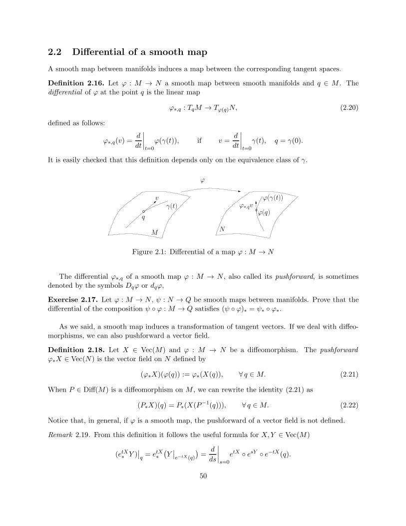
2.2 Differential of a smooth map
A smooth map between manifolds induces a map between the corresponding tangent spaces.
Definition 2.16. Let ϕ : M → N a smooth map between smooth manifolds and q ∈ M . Thedifferential of ϕ at the point q is the linear map
ϕ∗,q : TqM → Tϕ(q)N, (2.20)
defined as follows:
ϕ∗,q(v) =d
dt
∣∣∣∣t=0
ϕ(γ(t)), if v =d
dt
∣∣∣∣t=0
γ(t), q = γ(0).
It is easily checked that this definition depends only on the equivalence class of γ.
N
q
γ(t)
ϕ
ϕ(q)ϕ∗,qv
v ϕ(γ(t))
M
Figure 2.1: Differential of a map ϕ :M → N
The differential ϕ∗,q of a smooth map ϕ : M → N , also called its pushforward, is sometimesdenoted by the symbols Dqϕ or dqϕ,
Exercise 2.17. Let ϕ : M → N , ψ : N → Q be smooth maps between manifolds. Prove that thedifferential of the composition ψ ϕ :M → Q satisfies (ψ ϕ)∗ = ψ∗ ϕ∗.
As we said, a smooth map induces a transformation of tangent vectors. If we deal with diffeo-morphisms, we can also pushforward a vector field.
Definition 2.18. Let X ∈ Vec(M) and ϕ : M → N be a diffeomorphism. The pushforwardϕ∗X ∈ Vec(N) is the vector field on N defined by
(ϕ∗X)(ϕ(q)) := ϕ∗(X(q)), ∀ q ∈M. (2.21)
When P ∈ Diff(M) is a diffeomorphism on M , we can rewrite the identity (2.21) as
(P∗X)(q) = P∗(X(P−1(q))), ∀ q ∈M. (2.22)
Notice that, in general, if ϕ is a smooth map, the pushforward of a vector field is not defined.
Remark 2.19. From this definition it follows the useful formula for X,Y ∈ Vec(M)
(etX∗ Y )∣∣q= etX∗
(Y∣∣e−tX(q)
)=
d
ds
∣∣∣∣s=0
etX esY e−tX(q).
50
If P ∈ Diff(M) and X ∈ Vec(M), then P∗X is, by construction, the vector field whose integralcurves are the image under P of integral curves of X. The following lemma shows how it acts asoperator on functions.
Lemma 2.20. Let P ∈ Diff(M), X ∈ Vec(M) and a ∈ C∞(M) then
etP∗X = P etX P−1, (2.23)
(P∗X)a = (X(a P )) P−1. (2.24)
Proof. From the formula
d
dt
∣∣∣∣t=0
P etX P−1(q) = P∗(X(P−1(q))) = (P∗X)(q),
it follows that t 7→ P etX P−1(q) is an integral curve of P∗X, from which (2.23) follows. Toprove (2.24) let us compute
(P∗X)a∣∣q=
d
dt
∣∣∣∣t=0
a(etP∗X(q)).
Using (2.23) this is equal to
d
dt
∣∣∣∣t=0
a(P (etX (P−1(q))) =d
dt
∣∣∣∣t=0
(a P )(etX (P−1(q))) = (X(a P )) P−1.
As a consequence of Lemma 2.20 one gets the following formula: for every X,Y ∈ Vec(M)
(etX∗ Y )a = Y (a etX ) e−tX . (2.25)
2.3 Lie brackets
In this section we introduce a fundamental notion for sub-Riemannian geometry, the Lie bracket oftwo vector fieldsX and Y . Geometrically it is defined as the infinitesimal version of the pushforwardof the second vector field along the flow of the first one. As expalined below, it measures how muchY is modified by the flow of X.
Definition 2.21. Let X,Y ∈ Vec(M). We define their Lie bracket as the vector field
[X,Y ] :=∂
∂t
∣∣∣∣t=0
e−tX∗ Y. (2.26)
Remark 2.22. The geometric meaning of the Lie bracket can be understood by writing explicitly
[X,Y ]∣∣q=
∂
∂t
∣∣∣∣t=0
e−tX∗ Y∣∣q=
∂
∂t
∣∣∣∣t=0
e−tX∗ (Y∣∣etX(q)
) =∂
∂s∂t
∣∣∣∣t=s=0
e−tX esY etX(q). (2.27)
Proposition 2.23. As derivations on functions, one has the identity
[X,Y ] = XY − Y X. (2.28)
51
Proof. By definition of Lie bracket we have [X,Y ]a = ∂∂t
∣∣t=0
(e−tX∗ Y )a. Hence we have to computethe first order term in the expansion, with respect to t, of the map
t 7→ (e−tX∗ Y )a.
Using formula (2.25) we have
(e−tX∗ Y )a = Y (a e−tX) etX .By Remark 2.8 we have a e−tX = a− tXa+O(t2), hence
(e−tX∗ Y )a = Y (a− tXa+O(t2)) etX
= (Y a− t Y Xa+O(t2)) etX .Denoting b = Y a− t Y Xa+O(t2), bt = b etX , and using again the expansion above we get
(e−tX∗ Y )a = (Y a− t Y Xa+O(t2)) + tX(Y a− t Y Xa+O(t2)) +O(t2)
= Y a+ t(XY − Y X)a+O(t2).
that proves that the first order term with respect to t in the expansion is (XY − Y X)a.
Proposition 2.23 shows that (Vec(M), [·, ·]) is a Lie algebra.
Exercise 2.24. Prove the coordinate expression of the Lie bracket: let
X =n∑
i=1
Xi∂
∂xi, Y =
n∑
j=1
Yj∂
∂xj,
be two vector fields in Rn. Show that
[X,Y ] =
n∑
i,j=1
(Xi∂Yj∂xi− Yi
∂Xj
∂xi
)∂
∂xj.
Next we prove that every diffeomorphism induces a Lie algebra homomorphism on Vec(M).
Proposition 2.25. Let P ∈ Diff(M). Then P∗ is a Lie algebra homomorphism of Vec(M), i.e.,
P∗[X,Y ] = [P∗X,P∗Y ], ∀X,Y ∈ Vec(M).
Proof. We show that the two terms are equal as derivations on functions. Let a ∈ C∞(M), prelim-inarly we see, using (2.24), that
P∗X(P∗Y a) = P∗X(Y (a P ) P−1)
= X(Y (a P ) P−1 P ) P−1
= X(Y (a P )) P−1,
and using twice this property and (2.28)
[P∗X,P∗Y ]a = P∗X(P∗Y a)− P∗Y (P∗Xa)
= XY (a P ) P−1 − Y X(a P ) P−1
= (XY − Y X)(a P ) P−1
= P∗[X,Y ]a.
52
To end this section, we show that the Lie bracket of two vector fields is zero (i.e., they commuteas operator on functions) if and only if their flows commute.
Proposition 2.26. Let X,Y ∈ Vec(M). The following properties are equivalent:
(i) [X,Y ] = 0,
(ii) etX esY = esY etX , ∀ t, s ∈ R.
Proof. We start the proof with the following claim
[X,Y ] = 0 =⇒ e−tX∗ Y = Y, ∀ t ∈ R. (2.29)
To prove (2.29) let us show that [X,Y ] = ddt
∣∣t=0
e−tX∗ Y = 0 implies that ddte
−tX∗ Y = 0 for all t ∈ R.
Indeed we have
d
dte−tX∗ Y =
d
dε
∣∣∣∣ε=0
e−(t+ε)X∗ Y =
d
dε
∣∣∣∣ε=0
e−tX∗ e−εX∗ Y
= e−tX∗d
dε
∣∣∣∣ε=0
e−εX∗ Y = e−tX∗ [X,Y ] = 0,
which proves (2.29).
(i)⇒(ii). Fix t ∈ R. Let us show that φs := e−tX esY etX is the flow generated by Y . Indeedwe have
∂
∂sφs =
∂
∂ε
∣∣∣∣ε=0
e−tX e(s+ε)Y etX
=∂
∂ε
∣∣∣∣ε=0
e−tX eεY etX e−tX esY etX︸ ︷︷ ︸φs
= e−tX∗ Y φs = Y φs.
where in the last equality we used the Claim. Using uniqueness of the flow generated by a vectorfield we get
e−tX esY etX = esY , ∀ t, s ∈ R,
which is equivalent to (ii).
(ii)⇒(i). For every function a ∈ C∞ we have
XY a =∂2
∂t∂s
∣∣∣t=s=0
a esY etX =∂2
∂s∂t
∣∣∣t=s=0
a etX esY = Y Xa.
Then (i) follows from (2.28).
Exercise 2.27. Let X,Y ∈ Vec(M) and q ∈M . Consider the curve on M
γ(t) = e−tY e−tX etY etX(q).
Prove that the tangent vector to the curve t 7→ γ(√t) at t = 0 is [X,Y ](q).
53
Exercise 2.28. Let X,Y ∈ Vec(M). Using the semigroup property of the flow, prove the followingexpansion
e−tX∗ Y =
∞∑
n=0
tn
n!(adX)nY
= Y + t[X,Y ] +t2
2[X, [X,Y ]] +
t3
6[X, [X, [X,Y ]]] + . . .
Exercise 2.29. Let X,Y ∈ Vec(M) and a ∈ C∞(M). Prove the following Leibnitz rule for the Liebracket:
[X, aY ] = a[X,Y ] + (Xa)Y.
Exercise 2.30. Let X,Y,Z ∈ Vec(M). Prove that the Lie bracket satisfies the Jacobi identity :
[X, [Y,Z]] + [Y, [Z,X]] + [Z, [X,Y ]] = 0. (2.30)
Hint: Differentiate the identity etX∗ [Y,Z] = [etX∗ Y, etX∗ Z].
2.4 Cotangent space
In this section we introduce tangent covectors, that are linear functionals on the tangent space.The space of all covectors at a point q ∈ M , called cotangent space is, in algebraic terms, simplythe dual space to the tangent space.
Definition 2.31. Let M be a n-dimensional smooth manifold. The cotangent space at a pointq ∈M is the set
T ∗qM := (TqM)∗ = λ : TqM → R, λ linear.
If λ ∈ T ∗qM and v ∈ TqM , we will denote by 〈λ, v〉 := λ(v) the action of the covector λ on the
vector v.
As we have seen, a smooth map yields a linear map between tangent spaces. Dualizing thismap, we get a linear map on cotangent spaces.
Definition 2.32. Let ϕ :M → N be a smooth map and q ∈M . The pullback of ϕ at point ϕ(q),where q ∈M , is the map
ϕ∗ : T ∗ϕ(q)N → T ∗
qM, λ 7→ ϕ∗λ,
defined by duality in the following way
〈ϕ∗λ, v〉 := 〈λ, ϕ∗v〉 , ∀ v ∈ TqM, ∀λ ∈ T ∗ϕ(q)M.
Example 2.33. Let a : M → R be a smooth function and q ∈ M . The differential dqa of thefunction a at the point q ∈M , defined through the formula
〈dqa, v〉 :=d
dt
∣∣∣∣t=0
a(γ(t)), v ∈ TqM, (2.31)
where γ is any smooth curve such that γ(0) = q and γ(0) = v, is an element of T ∗qM , since (2.31)
is linear with respect to v.
54
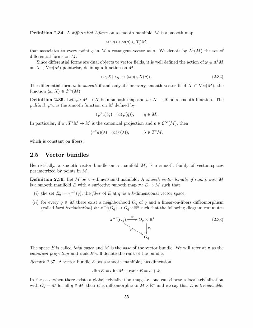
Definition 2.34. A differential 1-form on a smooth manifold M is a smooth map
ω : q 7→ ω(q) ∈ T ∗qM,
that associates to every point q in M a cotangent vector at q. We denote by Λ1(M) the set ofdifferential forms on M .
Since differential forms are dual objects to vector fields, it is well defined the action of ω ∈ Λ1Mon X ∈ Vec(M) pointwise, defining a function on M .
〈ω,X〉 : q 7→ 〈ω(q),X(q)〉 . (2.32)
The differential form ω is smooth if and only if, for every smooth vector field X ∈ Vec(M), thefunction 〈ω,X〉 ∈ C∞(M)
Definition 2.35. Let ϕ : M → N be a smooth map and a : N → R be a smooth function. Thepullback ϕ∗a is the smooth function on M defined by
(ϕ∗a)(q) = a(ϕ(q)), q ∈M.
In particular, if π : T ∗M →M is the canonical projection and a ∈ C∞(M), then
(π∗a)(λ) = a(π(λ)), λ ∈ T ∗M,
which is constant on fibers.
2.5 Vector bundles
Heuristically, a smooth vector bundle on a manifold M , is a smooth family of vector spacesparametrized by points in M .
Definition 2.36. Let M be a n-dimensional manifold. A smooth vector bundle of rank k over Mis a smooth manifold E with a surjective smooth map π : E →M such that
(i) the set Eq := π−1(q), the fiber of E at q, is a k-dimensional vector space,
(ii) for every q ∈ M there exist a neighborhood Oq of q and a linear-on-fibers diffeomorphism(called local trivialization) ψ : π−1(Oq)→ Oq×R
k such that the following diagram commutes
π−1(Oq)
π%%
ψ// Oq × R
k
π1
Oq
(2.33)
The space E is called total space and M is the base of the vector bundle. We will refer at π as thecanonical projection and rank E will denote the rank of the bundle.
Remark 2.37. A vector bundle E, as a smooth manifold, has dimension
dimE = dimM + rank E = n+ k.
In the case when there exists a global trivialization map, i.e. one can choose a local trivializationwith Oq =M for all q ∈M , then E is diffeomorphic to M ×R
k and we say that E is trivializable.
55
Example 2.38. For any smooth n-dimensional manifold M , the tangent bundle TM , defined asthe disjoint union of the tangent spaces at all points of M ,
TM =⋃
q∈MTqM,
has a natural structure of 2n-dimensional smooth manifold, equipped with the vector bundle struc-ture (of rank n) induced by the canonical projection map
π : TM →M, π(v) = q if v ∈ TqM.
In the same way one can consider the cotangent bundle T ∗M , defined as
T ∗M =⋃
q∈MT ∗qM.
Again, it is a 2n-dimensional manifold, and the canonical projection map
π : T ∗M →M, π(λ) = q if λ ∈ T ∗qM,
endows T ∗M with a structure of rank n vector bundle.
Let O ⊂M be a coordinate neighborhood and denote by
φ : O → Rn, φ(q) = (x1, . . . , xn),
a local coordinate system. The differentials of the coordinate functions
dxi∣∣q, i = 1, . . . , n, q ∈ O,
form a basis of the cotangent space T ∗qM . The dual basis in the tangent space TqM is defined by
the vectors
∂
∂xi
∣∣∣∣q
∈ TqM, i = 1, . . . , n, q ∈ O, (2.34)
⟨dxi,
∂
∂xj
⟩= δij , i, j = 1, . . . , n. (2.35)
Thus any tangent vector v ∈ TqM and any covector λ ∈ T ∗qM can be decomposed in these basis
v =
n∑
i=1
vi∂
∂xi
∣∣∣∣q
, λ =
n∑
i=1
pidxi∣∣q,
and the maps
ψ : v 7→ (x1, . . . , xn, v1, . . . , vn), ψ : λ 7→ (x1, . . . , xn, p1, . . . , pn), (2.36)
define local coordinates on TM and T ∗M respectively, which we call canonical coordinates inducedby the coordinates ψ on M .
56
Definition 2.39. A morphism f : E → E′ between two vector bundles E,E′ on the base M (alsocalled a bundle map) is a smooth map such that the following diagram is commutative
E
π
f// E′
π′
M
(2.37)
where f is linear on fibers. Here π and π′ denote the canonical projections.
Definition 2.40. Let π : E → M be a smooth vector bundle over M . A local section of E is asmooth map1 σ : A ⊂M → E satisfying π σ = IdA, where A is an open set of M . In other wordsσ(q) belongs to Eq for each q ∈ A, smoothly with respect to q. If σ is defined on all M it is said tobe a global section.
Example 2.41. Let π : E →M be a smooth vector bundle over M . The zero section of E is theglobal section
ζ :M → E, ζ(q) = 0 ∈ Eq, ∀ q ∈M.
We will denote by M0 := ζ(M) ⊂ E.
Remark 2.42. Notice that smooth vector fields and smooth differential forms are, by definition,sections of the vector bundles TM and T ∗M respectively.
We end this section with some classical construction on vector bundles.
Definition 2.43. Let ϕ :M → N be a smooth map between smooth manifolds and E be a vectorbundle on N , with fibers Eq′ , q′ ∈ N. The induced bundle (or pullback bundle) ϕ∗E is a vectorbundle on the base M defined by
ϕ∗E := (q, v) | q ∈M,v ∈ Eϕ(q) ⊂M × E.
Notice that rankϕ∗E = rankE, hence dimϕ∗E = dimM + rankE.
Example 2.44. (i). Let M be a smooth manifold and TM its tangent bundle, endowed with anEuclidean structure. The spherical bundle SM is the vector subbundle of TM defined as follows
SM =⋃
q∈MSqM, SqM = v ∈ TqM | |v| = 1.
(ii). Let E,E′ be two vector bundles over a smooth manifold M . The direct sum E ⊕ E′ is thevector bundle over M defined by
(E ⊕ E′)q := Eq ⊕ E′q.
1hetre smooth means as a map between manifolds.
57
2.6 Submersions and level sets of smooth maps
If ϕ :M → N is a smooth map, we define the rank of ϕ at q ∈M to be the rank of the linear mapϕ∗,q : TqM → Tϕ(q)N . It is of course just the rank of the matrix of partial derivatives of ϕ in anycoordinate chart, or the dimension of Im (ϕ∗,q) ⊂ Tϕ(q)N . If ϕ has the same rank k at every point,we say ϕ has constant rank, and write rankϕ = k.
An immersion is a smooth map ϕ :M → N with the property that ϕ∗ is injective at each point(or equivalently rankϕ = dimM). Similarly, a submersion is a smooth map ϕ :M → N such thatϕ∗ is surjective at each point (equivalently, rankϕ = dimN).
Theorem 2.45 (Rank Theorem). Suppose M and N are smooth manifolds of dimensions m andn, respectively, and ϕ :M → N is a smooth map with constant rank k in a neighborhood of q ∈M .Then there exist coordinates (x1, . . . , xm) centered at q and (y1, . . . , yn) centered at ϕ(q) in whichϕ has the following coordinate representation:
ϕ(x1, . . . , xm) = (x1, . . . , xk, 0, . . . , 0). (2.38)
Remark 2.46. The previous theorem can be rephrased in the following way. Let ϕ : M → N be asmooth map between two smooth manifolds. Then the following are equivalent:
(i) ϕ has constant rank in a neighborhood of q ∈M .
(ii) There exist coordinates near q ∈M and ϕ(q) ∈ N in which the coordinate representation ofϕ is linear.
In the case of a submersion, from Theorem 2.45 one can deduce the following result.
Corollary 2.47. Assume ϕ : M → N is a smooth submersion at q. Then ϕ admits a local rightinverse at ϕ(q). Moreover ϕ is open at q. More precisely it exist ε > 0 and C > 0 such that
Bϕ(q)(C−1r) ⊂ ϕ(Bq(r)), ∀ r ∈ [0, ε[. (2.39)
Remark 2.48. The constant C appearing in (2.39) is the norm of the differential of the local rightinverse. When ϕ is a diffeomorphism, C is a bound on the norm of the differential of the inverse ofϕ. This recover the classical quantitative statement of the inverse function theorem.
Using these results, one can give some very general criteria for level sets of smooth maps (orsmooth functions) to be submanifolds.
Theorem 2.49 (Constant Rank Level Set Theorem). Let M and N be smooth manifolds, and letϕ : M → N be a smooth map with constant rank k. Each level set ϕ−1(y), for y ∈ N is a closedembedded submanifold of codimension k in M .
Remark 2.50. It is worth to specify the following two important sub cases of Theorem 2.49:
(a) If ϕ : M → N is a submersion at every q ∈ ϕ−1(y) for some y ∈ N , then ϕ−1(y) is a closedembedded submanifold whose codimension is equal to the dimension of N .
(b) If a :M → R is a smooth function such that dqa 6= 0 for every q ∈ a−1(c), where c ∈ R, thenthe level set a−1(c) is a smooth hypersurface of M
Exercise 2.51. Let a : M → R be a smooth function. Assume that c ∈ R is a regular value ofa, i.e., dqa 6= 0 for every q ∈ a−1(c). Then Nc = a−1(c) = q ∈ M | a(q) = c ⊂ M is a smoothsubmanifold. Prove that for every q ∈ Nc
TqNc = ker dqa = v ∈ TqM | 〈dqa, v〉 = 0.
58
Bibliographical notes
The material presented in this chapter is classical and covered by many textbook in differentialgeometry, as for instance in [6, 24, 14, 32].
Theorem 2.14 is a well-known theorem in ODE. The statement presented here can be deducedfrom [10, Theorem 2.1.1, Exercice 2.4]. The functions c(t), k(t) appearing in (C3) are assumed tobe L∞, that is stronger than L1 (on compact intervals). This stronger assumptions implies thatthe solution is not only absolutely continuous with respect to t, but also locally Lipschitz.
59

60
Chapter 3
Sub-Riemannian structures
3.1 Basic definitions
In this section we introduce a definition of sub-Riemannian structure which is quite general. In-deed, this definition includes all the classical notions of Riemannian structure, constant-rank sub-Riemannian structure, rank-varying sub-Riemannian structure, almost-Riemannian structure etc.
Definition 3.1. Let M be a smooth manifold and let F ⊂ Vec(M) be a family of smooth vectorfields. The Lie algebra generated by F is the smallest sub-algebra of Vec(M) containing F , namely
LieF := span[X1, . . . , [Xj−1,Xj ]],Xi ∈ F , j ∈ N. (3.1)
We will say that F is bracket-generating (or that satisfies the Hormander condition) if
LieqF := X(q),X ∈ LieF = TqM, ∀ q ∈M.
Moreover, for s ∈ N, we define
LiesF := span[X1, . . . , [Xj−1,Xj ]],Xi ∈ F , j ≤ s. (3.2)
We say that the family F is of step s at q if m is the minimal integer satisfying
LiesqF := X(q),X ∈ LiesF = TqM,
Notice that, in general, the step may depend on the point on M and s = s(q) can be unboundedon M even for bracket-generating structure.
Definition 3.2. Let M be a connected smooth manifold. A sub-Riemannian structure on M is apair (U, f) where:
(i) U is an Euclidean bundle with base M and Euclidean fiber Uq, i.e., for every q ∈M , Uq is avector space equipped with a scalar product (· | ·)q , smooth with respect to q. For u ∈ Uq wedenote the norm of u as |u|2 = (u |u)q.
(ii) f : U → TM is a smooth map that is a morphism of vector bundles, i.e. the followingdiagram is commutative (here πU : U→M and π : TM →M are the canonical projections)
U
πU ""
f// TM
πM
(3.3)
61
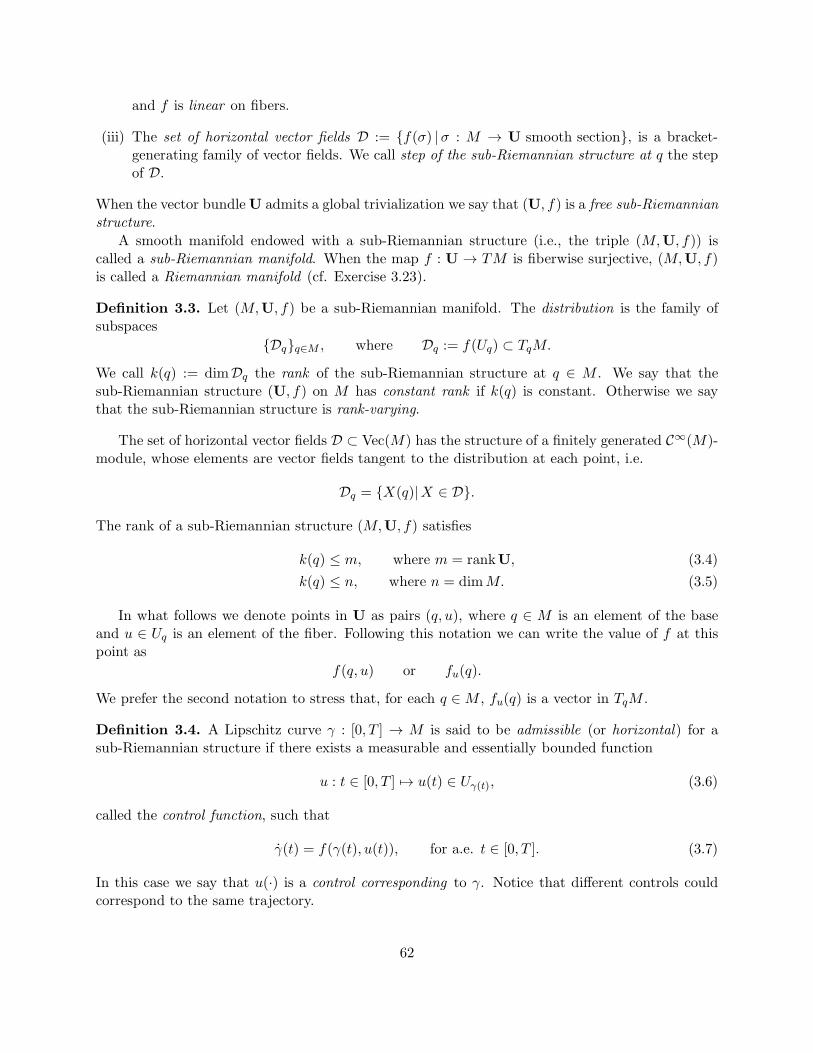
and f is linear on fibers.
(iii) The set of horizontal vector fields D := f(σ) |σ : M → U smooth section, is a bracket-generating family of vector fields. We call step of the sub-Riemannian structure at q the stepof D.
When the vector bundleU admits a global trivialization we say that (U, f) is a free sub-Riemannianstructure.
A smooth manifold endowed with a sub-Riemannian structure (i.e., the triple (M,U, f)) iscalled a sub-Riemannian manifold. When the map f : U → TM is fiberwise surjective, (M,U, f)is called a Riemannian manifold (cf. Exercise 3.23).
Definition 3.3. Let (M,U, f) be a sub-Riemannian manifold. The distribution is the family ofsubspaces
Dqq∈M , where Dq := f(Uq) ⊂ TqM.
We call k(q) := dimDq the rank of the sub-Riemannian structure at q ∈ M . We say that thesub-Riemannian structure (U, f) on M has constant rank if k(q) is constant. Otherwise we saythat the sub-Riemannian structure is rank-varying.
The set of horizontal vector fields D ⊂ Vec(M) has the structure of a finitely generated C∞(M)-module, whose elements are vector fields tangent to the distribution at each point, i.e.
Dq = X(q)|X ∈ D.
The rank of a sub-Riemannian structure (M,U, f) satisfies
k(q) ≤ m, where m = rankU, (3.4)
k(q) ≤ n, where n = dimM. (3.5)
In what follows we denote points in U as pairs (q, u), where q ∈ M is an element of the baseand u ∈ Uq is an element of the fiber. Following this notation we can write the value of f at thispoint as
f(q, u) or fu(q).
We prefer the second notation to stress that, for each q ∈M , fu(q) is a vector in TqM .
Definition 3.4. A Lipschitz curve γ : [0, T ] → M is said to be admissible (or horizontal) for asub-Riemannian structure if there exists a measurable and essentially bounded function
u : t ∈ [0, T ] 7→ u(t) ∈ Uγ(t), (3.6)
called the control function, such that
γ(t) = f(γ(t), u(t)), for a.e. t ∈ [0, T ]. (3.7)
In this case we say that u(·) is a control corresponding to γ. Notice that different controls couldcorrespond to the same trajectory.
62
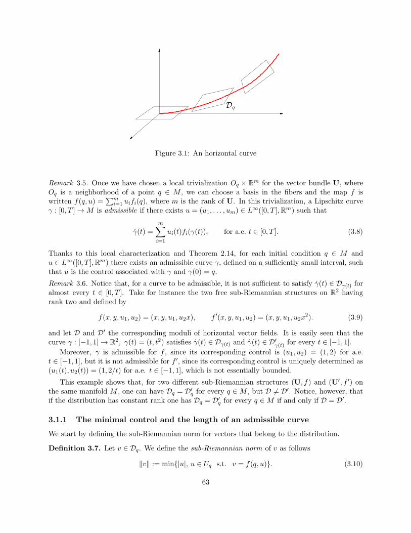
Dq
Figure 3.1: An horizontal curve
Remark 3.5. Once we have chosen a local trivialization Oq × Rm for the vector bundle U, where
Oq is a neighborhood of a point q ∈ M , we can choose a basis in the fibers and the map f iswritten f(q, u) =
∑mi=1 uifi(q), where m is the rank of U. In this trivialization, a Lipschitz curve
γ : [0, T ]→M is admissible if there exists u = (u1, . . . , um) ∈ L∞([0, T ],Rm) such that
γ(t) =m∑
i=1
ui(t)fi(γ(t)), for a.e. t ∈ [0, T ]. (3.8)
Thanks to this local characterization and Theorem 2.14, for each initial condition q ∈ M andu ∈ L∞([0, T ],Rm) there exists an admissible curve γ, defined on a sufficiently small interval, suchthat u is the control associated with γ and γ(0) = q.
Remark 3.6. Notice that, for a curve to be admissible, it is not sufficient to satisfy γ(t) ∈ Dγ(t) foralmost every t ∈ [0, T ]. Take for instance the two free sub-Riemannian structures on R
2 havingrank two and defined by
f(x, y, u1, u2) = (x, y, u1, u2x), f ′(x, y, u1, u2) = (x, y, u1, u2x2). (3.9)
and let D and D′ the corresponding moduli of horizontal vector fields. It is easily seen that thecurve γ : [−1, 1]→ R
2, γ(t) = (t, t2) satisfies γ(t) ∈ Dγ(t) and γ(t) ∈ D′γ(t) for every t ∈ [−1, 1].
Moreover, γ is admissible for f , since its corresponding control is (u1, u2) = (1, 2) for a.e.t ∈ [−1, 1], but it is not admissible for f ′, since its corresponding control is uniquely determined as(u1(t), u2(t)) = (1, 2/t) for a.e. t ∈ [−1, 1], which is not essentially bounded.
This example shows that, for two different sub-Riemannian structures (U, f) and (U′, f ′) onthe same manifold M , one can have Dq = D′
q for every q ∈M , but D 6= D′. Notice, however, thatif the distribution has constant rank one has Dq = D′
q for every q ∈M if and only if D = D′.
3.1.1 The minimal control and the length of an admissible curve
We start by defining the sub-Riemannian norm for vectors that belong to the distribution.
Definition 3.7. Let v ∈ Dq. We define the sub-Riemannian norm of v as follows
‖v‖ := min|u|, u ∈ Uq s.t. v = f(q, u). (3.10)
63
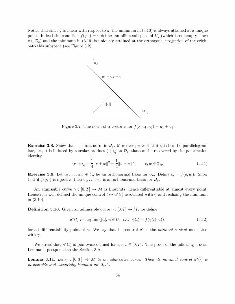
Notice that since f is linear with respect to u, the minimum in (3.10) is always attained at a uniquepoint. Indeed the condition f(q, ·) = v defines an affine subspace of Uq (which is nonempty sincev ∈ Dq) and the minimum in (3.10) is uniquely attained at the orthogonal projection of the originonto this subspace (see Figure 3.2).
u1 + u2 = v
u1
u2
‖v‖
Figure 3.2: The norm of a vector v for f(x, u1, u2) = u1 + u2
Exercise 3.8. Show that ‖ · ‖ is a norm in Dq. Moreover prove that it satisfies the parallelogramlaw, i.e., it is induced by a scalar product 〈· | ·〉q on Dq, that can be recovered by the polarizationidentity
〈v |w〉q =1
4‖v + w‖2 − 1
4‖v − w‖2, v, w ∈ Dq. (3.11)
Exercise 3.9. Let u1, . . . , um ∈ Uq be an orthonormal basis for Uq. Define vi = f(q, ui). Showthat if f(q, ·) is injective then v1, . . . , vm is an orthonormal basis for Dq.
An admissible curve γ : [0, T ] → M is Lipschitz, hence differentiable at almost every point.Hence it is well defined the unique control t 7→ u∗(t) associated with γ and realizing the minimumin (3.10).
Definition 3.10. Given an admissible curve γ : [0, T ]→M , we define
u∗(t) := argmin |u|, u ∈ Uq s.t. γ(t) = f(γ(t), u). (3.12)
for all differentiability point of γ. We say that the control u∗ is the minimal control associatedwith γ.
We stress that u∗(t) is pointwise defined for a.e. t ∈ [0, T ]. The proof of the following crucialLemma is postponed to the Section 3.A.
Lemma 3.11. Let γ : [0, T ] → M be an admissible curve. Then its minimal control u∗(·) ismeasurable and essentially bounded on [0, T ].
64
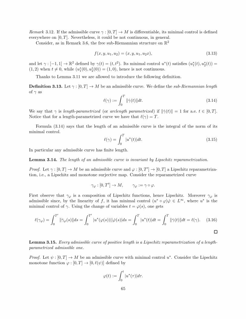
Remark 3.12. If the admissible curve γ : [0, T ]→M is differentiable, its minimal control is definedeverywhere on [0, T ]. Nevertheless, it could be not continuous, in general.
Consider, as in Remark 3.6, the free sub-Riemannian structure on R2
f(x, y, u1, u2) = (x, y, u1, u2x), (3.13)
and let γ : [−1, 1]→ R2 defined by γ(t) = (t, t2). Its minimal control u∗(t) satisfies (u∗1(t), u
∗2(t)) =
(1, 2) when t 6= 0, while (u∗1(0), u∗2(0)) = (1, 0), hence is not continuous.
Thanks to Lemma 3.11 we are allowed to introduce the following definition.
Definition 3.13. Let γ : [0, T ]→M be an admissible curve. We define the sub-Riemannian lengthof γ as
ℓ(γ) :=
∫ T
0‖γ(t)‖dt. (3.14)
We say that γ is length-parametrized (or arclength parametrized) if ‖γ(t)‖ = 1 for a.e. t ∈ [0, T ].Notice that for a length-parametrized curve we have that ℓ(γ) = T .
Formula (3.14) says that the length of an admissible curve is the integral of the norm of itsminimal control.
ℓ(γ) =
∫ T
0|u∗(t)|dt. (3.15)
In particular any admissible curve has finite length.
Lemma 3.14. The length of an admissible curve is invariant by Lipschitz reparametrization.
Proof. Let γ : [0, T ]→M be an admissible curve and ϕ : [0, T ′]→ [0, T ] a Lipschitz reparametriza-tion, i.e., a Lipschitz and monotone surjective map. Consider the reparametrized curve
γϕ : [0, T ′]→M, γϕ := γ ϕ.
First observe that γϕ is a composition of Lipschitz functions, hence Lipschitz. Moreover γϕ isadmissible since, by the linearity of f , it has minimal control (u∗ ϕ)ϕ ∈ L∞, where u∗ is theminimal control of γ. Using the change of variables t = ϕ(s), one gets
ℓ(γϕ) =
∫ T ′
0‖γϕ(s)‖ds =
∫ T ′
0|u∗(ϕ(s))||ϕ(s)|ds =
∫ T
0|u∗(t)|dt =
∫ T
0‖γ(t)‖dt = ℓ(γ). (3.16)
Lemma 3.15. Every admissible curve of positive length is a Lipschitz reparametrization of a length-parametrized admissible one.
Proof. Let ψ : [0, T ]→M be an admissible curve with minimal control u∗. Consider the Lipschitzmonotone function ϕ : [0, T ]→ [0, ℓ(ψ)] defined by
ϕ(t) :=
∫ t
0|u∗(τ)|dτ.
65
Notice that if ϕ(t1) = ϕ(t2), the monotonicity of ϕ ensures ψ(t1) = ψ(t2). Hence we are allowed todefine γ : [0, ℓ(ψ)] →M by
γ(s) := ψ(t), if s = ϕ(t) for some t ∈ [0, T ].
In other words, it holds ψ = γ ϕ. To show that γ is Lipschitz let us first show that there existsa constant C > 0 such that, for every t0, t1 ∈ [0, T ] one has, in some local coordinates (where | · |denotes the Euclidean norm in coordinates)
|ψ(t1)− ψ(t0)| ≤ C∫ t1
t0
|u∗(τ)|dτ.
Indeed fix K ⊂M a compact set such that ψ([0, T ]) ⊂ K and C := maxx∈K
(m∑
i=1
|fi(x)|2)1/2
. Then
|ψ(t1)− ψ(t0)| ≤∫ t1
t0
m∑
i=1
|u∗i (t)fi(ψ(t))| dt
≤∫ t1
t0
√√√√m∑
i=1
|u∗i (t)|2√√√√
m∑
i=1
|fi(ψ(t))|2dt
≤ C∫ t1
t0
|u∗(t)|dt,
Hence if s1 = ϕ(t1) and s0 = ϕ(t0) one has
|γ(s1)− γ(s0)| = |ψ(t1)− ψ(t0)| ≤ C∫ t1
t0
|u∗(τ)|dτ = C|s1 − s0|,
which proves that γ is Lipschitz. It particular γ(s) exists for a.e. s ∈ [0, ℓ(ψ)].
We are going to prove that γ is admissible and its minimal control has norm one. Define forevery s such that s = ϕ(t), ϕ(t) exists and ϕ(t) 6= 0, the control
v(s) :=u∗(t)ϕ(t)
=u∗(t)|u∗(t)| .
By Exercise 3.16 the control v is defined for a.e. s. Moreover, by construction, |v(s)| = 1 for a.e. sand v is the minimal control associated with γ.
Exercise 3.16. Show that for a Lipschitz and monotone function ϕ : [0, T ] → R, the Lebesguemeasure of the set s ∈ R | s = ϕ(t), ϕ(t) exists, ϕ(t) = 0 is zero.
By the previous discussion, in what follows, it will be often convenient to assume that admissiblecurves are length-parametrized (or parametrized such that ‖γ(t)‖ is constant).
66
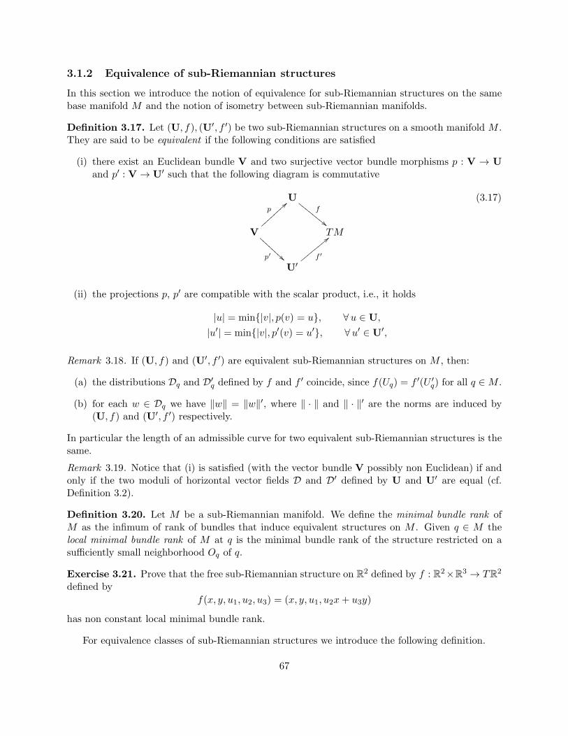
3.1.2 Equivalence of sub-Riemannian structures
In this section we introduce the notion of equivalence for sub-Riemannian structures on the samebase manifold M and the notion of isometry between sub-Riemannian manifolds.
Definition 3.17. Let (U, f), (U′, f ′) be two sub-Riemannian structures on a smooth manifold M .They are said to be equivalent if the following conditions are satisfied
(i) there exist an Euclidean bundle V and two surjective vector bundle morphisms p : V → Uand p′ : V→ U′ such that the following diagram is commutative
Uf
""
V
p′
p>>⑤⑤⑤⑤⑤⑤⑤⑤
TM
U′f ′
<<②②②②②②②②
(3.17)
(ii) the projections p, p′ are compatible with the scalar product, i.e., it holds
|u| = min|v|, p(v) = u, ∀u ∈ U,
|u′| = min|v|, p′(v) = u′, ∀u′ ∈ U′,
Remark 3.18. If (U, f) and (U′, f ′) are equivalent sub-Riemannian structures on M , then:
(a) the distributions Dq and D′q defined by f and f ′ coincide, since f(Uq) = f ′(U ′
q) for all q ∈M .
(b) for each w ∈ Dq we have ‖w‖ = ‖w‖′, where ‖ · ‖ and ‖ · ‖′ are the norms are induced by(U, f) and (U′, f ′) respectively.
In particular the length of an admissible curve for two equivalent sub-Riemannian structures is thesame.
Remark 3.19. Notice that (i) is satisfied (with the vector bundle V possibly non Euclidean) if andonly if the two moduli of horizontal vector fields D and D′ defined by U and U′ are equal (cf.Definition 3.2).
Definition 3.20. Let M be a sub-Riemannian manifold. We define the minimal bundle rank ofM as the infimum of rank of bundles that induce equivalent structures on M . Given q ∈ M thelocal minimal bundle rank of M at q is the minimal bundle rank of the structure restricted on asufficiently small neighborhood Oq of q.
Exercise 3.21. Prove that the free sub-Riemannian structure on R2 defined by f : R2×R
3 → TR2
defined by
f(x, y, u1, u2, u3) = (x, y, u1, u2x+ u3y)
has non constant local minimal bundle rank.
For equivalence classes of sub-Riemannian structures we introduce the following definition.
67
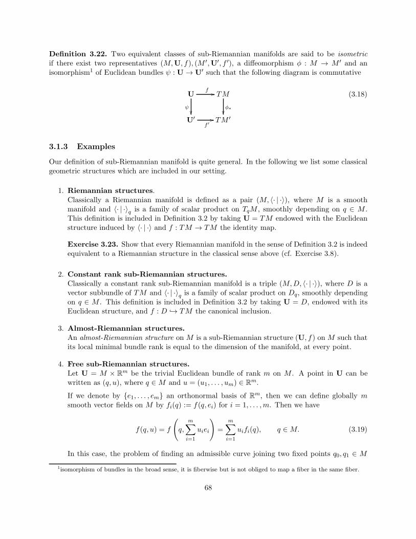
Definition 3.22. Two equivalent classes of sub-Riemannian manifolds are said to be isometricif there exist two representatives (M,U, f), (M ′,U′, f ′), a diffeomorphism φ : M → M ′ and anisomorphism1 of Euclidean bundles ψ : U→ U′ such that the following diagram is commutative
U
ψ
f// TM
φ∗
U′f ′
// TM ′
(3.18)
3.1.3 Examples
Our definition of sub-Riemannian manifold is quite general. In the following we list some classicalgeometric structures which are included in our setting.
1. Riemannian structures.Classically a Riemannian manifold is defined as a pair (M, 〈· | ·〉), where M is a smoothmanifold and 〈· | ·〉q is a family of scalar product on TqM , smoothly depending on q ∈ M .This definition is included in Definition 3.2 by taking U = TM endowed with the Euclideanstructure induced by 〈· | ·〉 and f : TM → TM the identity map.
Exercise 3.23. Show that every Riemannian manifold in the sense of Definition 3.2 is indeedequivalent to a Riemannian structure in the classical sense above (cf. Exercise 3.8).
2. Constant rank sub-Riemannian structures.Classically a constant rank sub-Riemannian manifold is a triple (M,D, 〈· | ·〉), where D is avector subbundle of TM and 〈· | ·〉q is a family of scalar product on Dq, smoothly dependingon q ∈ M . This definition is included in Definition 3.2 by taking U = D, endowed with itsEuclidean structure, and f : D → TM the canonical inclusion.
3. Almost-Riemannian structures.An almost-Riemannian structure on M is a sub-Riemannian structure (U, f) on M such thatits local minimal bundle rank is equal to the dimension of the manifold, at every point.
4. Free sub-Riemannian structures.Let U = M × R
m be the trivial Euclidean bundle of rank m on M . A point in U can bewritten as (q, u), where q ∈M and u = (u1, . . . , um) ∈ R
m.
If we denote by e1, . . . , em an orthonormal basis of Rm, then we can define globally m
smooth vector fields on M by fi(q) := f(q, ei) for i = 1, . . . ,m. Then we have
f(q, u) = f
(q,
m∑
i=1
uiei
)=
m∑
i=1
uifi(q), q ∈M. (3.19)
In this case, the problem of finding an admissible curve joining two fixed points q0, q1 ∈ M1isomorphism of bundles in the broad sense, it is fiberwise but is not obliged to map a fiber in the same fiber.
68
and with minimal length is rewritten as the optimal control problem
γ(t) =
m∑
i=1
ui(t)fi(γ(t))
∫ T
0|u(t)|dt→ min
γ(0) = q0, γ(T ) = q1
(3.20)
For a free sub-Riemannian structure, the set of vector fields f1, . . . , fm build as above is calleda generating family. Notice that, in general, a generating family is not orthonormal when fis not injective.
5. Surfaces in R3 as free sub-Riemannian structures
Due to topological constraints, in general it not possible to regard a surface as a free sub-Riemannian structure of rank 2, i.e., defined by a pair of globally defined orthonormal vectorfields. However, it is always possible to regard it as a free sub-Riemannian structure of rank3.
Indeed, for an embedded surfaceM in R3, consider the trivial Euclidean bundle U =M×R
3,where points are denoted as usual (q, u), with u ∈ R
3, q ∈M , and the map
f : U→ TM, f(q, u) = π⊥q (u) ∈ TqM. (3.21)
where π⊥q : R3 → TqM ⊂ R3 is the orthogonal projection.
Notice that f is a surjective bundle map and the set of vector fields π⊥q (∂x), π⊥q (∂y), π⊥q (∂z)is a generating family for this structure.
Exercise 3.24. Show that (U, f) defined in (3.21) is equivalent to the Riemannian structureon M induced by the embedding in R
3.
3.1.4 Every sub-Riemannian structure is equivalent to a free one
The purpose of this section is to show that every sub-Riemannian structure (U, f) on M is equiva-lent to a sub-Riemannian structure (U′, f ′) where U′ is a trivial bundle with sufficiently big rank.
Lemma 3.25. Let M be a n-dimensional smooth manifold and π : E →M a smooth vector bundleof rank m. Then, there exists a vector bundle π0 : E0 → M with rankE0 ≤ 2n + m such thatE ⊕E0 is a trivial vector bundle.
Proof. Remember that E, as a smooth manifold, has dimension
dim E = dim M + rank E = n+m.
Consider the map i : M → E which embeds M into the vector bundle E as the zero sectionM0 = i(M). If we denote with TME := i∗(TE) the pullback vector bundle, i.e., the restriction ofTE to the section M0, we have the isomorphism (as vector bundles on M)
TME ≃ E ⊕ TM. (3.22)
69
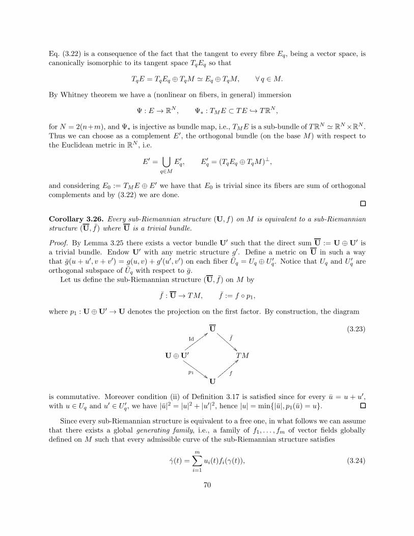
Eq. (3.22) is a consequence of the fact that the tangent to every fibre Eq, being a vector space, iscanonically isomorphic to its tangent space TqEq so that
TqE = TqEq ⊕ TqM ≃ Eq ⊕ TqM, ∀ q ∈M.
By Whitney theorem we have a (nonlinear on fibers, in general) immersion
Ψ : E → RN , Ψ∗ : TME ⊂ TE → TRN ,
for N = 2(n+m), and Ψ∗ is injective as bundle map, i.e., TME is a sub-bundle of TRN ≃ RN×RN .
Thus we can choose as a complement E′, the orthogonal bundle (on the base M) with respect tothe Euclidean metric in R
N , i.e.
E′ =⋃
q∈ME′q, E′
q = (TqEq ⊕ TqM)⊥,
and considering E0 := TME ⊕ E′ we have that E0 is trivial since its fibers are sum of orthogonalcomplements and by (3.22) we are done.
Corollary 3.26. Every sub-Riemannian structure (U, f) on M is equivalent to a sub-Riemannianstructure (U, f) where U is a trivial bundle.
Proof. By Lemma 3.25 there exists a vector bundle U′ such that the direct sum U := U ⊕U′ isa trivial bundle. Endow U′ with any metric structure g′. Define a metric on U in such a waythat g(u + u′, v + v′) = g(u, v) + g′(u′, v′) on each fiber Uq = Uq ⊕ U ′
q. Notice that Uq and U ′q are
orthogonal subspace of Uq with respect to g.Let us define the sub-Riemannian structure (U, f) on M by
f : U→ TM, f := f p1,
where p1 : U⊕U′ → U denotes the projection on the first factor. By construction, the diagram
Uf
!!
U⊕U′
p1##
Id
;;TM
Uf
==④④④④④④④④④
(3.23)
is commutative. Moreover condition (ii) of Definition 3.17 is satisfied since for every u = u + u′,with u ∈ Uq and u′ ∈ U ′
q, we have |u|2 = |u|2 + |u′|2, hence |u| = min|u|, p1(u) = u.
Since every sub-Riemannian structure is equivalent to a free one, in what follows we can assumethat there exists a global generating family, i.e., a family of f1, . . . , fm of vector fields globallydefined on M such that every admissible curve of the sub-Riemannian structure satisfies
γ(t) =
m∑
i=1
ui(t)fi(γ(t)), (3.24)
70
Moreover, by the classical Gram-Schmidt procedure, we can assume that fi are the image of anorthonormal frame defined on the fiber. (cf. Example 4 of Section 3.1.3)
Under these assumptions the length of an admissible curve γ is given by
ℓ(γ) =
∫ T
0|u∗(t)|dt =
∫ T
0
√√√√m∑
i=1
u∗i (t)2dt,
where u∗(t) is the minimal control associated with γ.
Notice that Corollary 3.26 implies that the modulus of horizontal vector fields D is globallygenerated by f1, . . . , fm.
Remark 3.27. The integral curve γ(t) = etfi , defined on [0, T ], of an element fi of a generatingfamily F = f1, . . . , fm is admissible and ℓ(γ) ≤ T . If F = f1, . . . , fm are linearly independentthen they are an orthonormal frame and ℓ(γ) = T .
Exercise 3.28. Consider a sub-Riemannian structure (U, f) over M . Let m = rank(U) andhmax = maxh(q) : q ∈ M ≤ m where h(q) is the local minimal bundle rank at q. Prove thatthere exists a sub-Riemannian structure (U, f) equivalent to (U, f) such that rank(U) = hmax.
3.1.5 Proto sub-Riemannian structures
Sometimes can be useful to consider structures that satisfy only property (i) and (ii) of Definition3.2, but that are not bracket generating. In what follows we call these structures proto sub-Riemannian structures.
The typical example is the one of a Riemannian foliation, that is obtained when the family ofhorizontal vector fields D satisfies
(i) [D,D] ⊂ D,
(ii) dimDq does not depend on q ∈M .
In this case the manifold M is foliated by integral manifolds of the distribution, and each of themis endowed with a Riemannian structure.
3.2 Sub-Riemannian distance and Chow-Rashevskii Theorem
In this section we introduce the sub-Riemannian distance between two points as the infimum ofthe length of admissible curves joining them.
Recall that, in the definition of sub-Riemannian manifold, M is assumed to be connected.Moreover, thanks to the construction of Section 3.1.4, in what follows we can assume that the sub-Riemannian structure is free, with generating family F = f1, . . . , fm. Notice that, by definition,F is assumed to be bracket generating.
Definition 3.29. Let M be a sub-Riemannian manifold and q0, q1 ∈ M . The sub-Riemanniandistance (or Carnot-Caratheodory distance) between q0 and q1 is
d(q0, q1) = infℓ(γ) | γ : [0, T ]→M admissible, γ(0) = q0, γ(T ) = q1, (3.25)
71
One of the purpose of this section is to show that, thanks to the bracket generating condition,(9.1) is well-defined, namely for every q0, q1 ∈M , there exists an admissible curve that joins q0 toq1, hence d(q0, q1) < +∞.
Theorem 3.30 (Chow-Raschevskii). Let M be a sub-Riemannian manifold. Then
(i) (M,d) is a metric space,
(ii) the topology induced by (M,d) is equivalent to the manifold topology.
In particular, d :M ×M → R is continuous.
In what follows B(q, r) (sometimes denoted also Br(q)) is the (open) sub-Riemannian ball ofradius r and center q
B(q, r) := q′ ∈M | d(q, q′) < r.The rest of this section is devoted to the proof of Theorem 3.30. To prove it, we have to show thatd is actually a distance, i.e.,
(a) 0 ≤ d(q0, q1) < +∞ for all q0, q1 ∈M ,
(b) d(q0, q1) = 0 if and only if q0 = q1,
(c) d(q0, q1) = d(q1, q0) and d(q0, q2) ≤ d(q0, q1) + d(q1, q2) for all q0, q1, q2 ∈M ,
and the equivalence between the metric and the manifold topology: for every q0 ∈M we have
(d) for every ε > 0 there exists a neighborhood Oq0 of q0 such that Oq0 ⊂ B(q0, ε),
(e) for every neighborhood Oq0 of q0 there exists δ > 0 such that B(q0, δ) ⊂ Oq0 .
3.2.1 Proof of Chow-Raschevskii Theorem
The symmetry of d is a direct consequence of the fact that if γ : [0, T ] → M is admissible,then the curve γ : [0, T ] → M defined by γ(t) = γ(T − t) is admissible and ℓ(γ) = ℓ(γ). Thetriangular inequality follows from the fact that, given two admissible curves γ1 : [0, T1] → M andγ2 : [0, T2]→M such that γ1(T1) = γ2(0), their concatenation
γ : [0, T1 + T2]→M, γ(t) =
γ1(t), t ∈ [0, T1],
γ2(t− T1), t ∈ [T1, T1 + T2].(3.26)
is still admissible. These two arguments prove item (c).We divide the rest of the proof of the Theorem in the following steps.
S1. We prove that, for every q0 ∈ M , there exists a neighborhood Oq0 of q0 such that d(q0, ·) isfinite and continuous in Oq0 . This proves (d).
S2. We prove that d is finite on M ×M . This proves (a).
S3. We prove (b) and (e).
To prove Step 1 we first need the following lemmas:
72
Lemma 3.31. Let N ⊂M be a submanifold and F ⊂ Vec(M) be a family of vector fields tangentto N , i.e., X(q) ∈ TqN , for every q ∈ N and X ∈ F . Then for all q ∈ N we have LieqF ⊂ TqN .In particular dimLieqF ≤ dimN .
Proof. Let X ∈ F . As a consequence of the local existence and uniqueness of the two Cauchyproblems
q = X(q), q ∈M,
q(0) = q0, q0 ∈ N.and
q = X
∣∣N(q), q ∈ N,
q(0) = q0, q0 ∈ N.
it follows that etX(q) ∈ N for every q ∈ N and t small enough. This property, together with thedefinition of Lie bracket (see formula (2.27)) implies that, if X,Y are tangent to N , the vector field[X,Y ] is tangent to N as well. Iterating this argument we get that LieqF ⊂ TqN for every q ∈ N ,from which the conclusion follows.
Lemma 3.32. Let M be an n-dimensional sub-Riemannian manifold with generating family F =f1, . . . , fm. For every q0 ∈ M and every neighborhood V of the origin in R
n there exist s =(s1, . . . , sn) ∈ V , and a choice of n vector fields fi1 , . . . , fin ∈ F , such that s is a regular point ofthe map
ψ : Rn →M, ψ(s1, . . . , sn) = esnfin · · · es1fi1 (q0).
Remark 3.33. Notice that, if Dq0 6= Tq0M , then s = 0 cannot be a regular point of the map ψ.Indeed, for s = 0, the image of the differential of ψ at 0 is spanq0fij , j = 1, . . . , n ⊂ Dq0 and thedifferential of ψ cannot be surjective.
We stress that, in the choice of fi1 , . . . , fin ∈ F , a vector field can appear more than once, asfor instance in the case m < n.
Proof of Lemma 3.32. We prove the lemma by steps.
1. There exists a vector field fi1 ∈ F such that fi1(q0) 6= 0, otherwise all vector fields in F vanishat q0 and dimLieq0F = 0, which contradicts the bracket generating condition. Then, for |s|small enough, the map
φ1 : s1 7→ es1fi1 (q0),
is a local diffeomorphism onto its image Σ1. If dimM = 1 the Lemma is proved.
2. Assume dimM ≥ 2. Then there exist t11 ∈ R, with |t11| small enough, and fi2 ∈ F such that,
if we denote by q1 = et11fi1 (q0), the vector fi2(q1) is not tangent to Σ1. Otherwise, by Lemma
3.31, dim LieqF = 1, which contradicts the bracket generating condition. Then the map
φ2 : (s1, s2) 7→ es2fi2 es1fi1 (q0),
is a local diffeomorphism near (t11, 0) onto its image Σ2. Indeed the vectors
∂φ2∂s1
∣∣∣∣(t11,0)
∈ Tq1Σ1,∂φ2∂s2
∣∣∣∣(t11,0)
= fi2(q1),
are linearly independent by construction. If dimM = 2 the Lemma is proved.
73
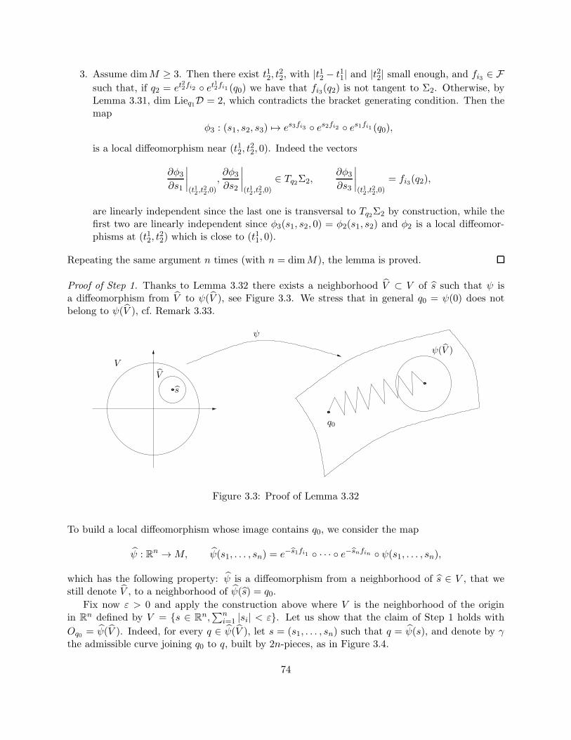
3. Assume dimM ≥ 3. Then there exist t12, t22, with |t12 − t11| and |t22| small enough, and fi3 ∈ F
such that, if q2 = et22fi2 et12fi1 (q0) we have that fi3(q2) is not tangent to Σ2. Otherwise, by
Lemma 3.31, dim Lieq1D = 2, which contradicts the bracket generating condition. Then themap
φ3 : (s1, s2, s3) 7→ es3fi3 es2fi2 es1fi1 (q0),
is a local diffeomorphism near (t12, t22, 0). Indeed the vectors
∂φ3∂s1
∣∣∣∣(t12,t
22,0)
,∂φ3∂s2
∣∣∣∣(t12,t
22,0)
∈ Tq2Σ2,∂φ3∂s3
∣∣∣∣(t12,t
22,0)
= fi3(q2),
are linearly independent since the last one is transversal to Tq2Σ2 by construction, while thefirst two are linearly independent since φ3(s1, s2, 0) = φ2(s1, s2) and φ2 is a local diffeomor-phisms at (t12, t
22) which is close to (t11, 0).
Repeating the same argument n times (with n = dimM), the lemma is proved.
Proof of Step 1. Thanks to Lemma 3.32 there exists a neighborhood V ⊂ V of s such that ψ isa diffeomorphism from V to ψ(V ), see Figure 3.3. We stress that in general q0 = ψ(0) does notbelong to ψ(V ), cf. Remark 3.33.
ψ(V )
V
V
s
ψ
q0
Figure 3.3: Proof of Lemma 3.32
To build a local diffeomorphism whose image contains q0, we consider the map
ψ : Rn →M, ψ(s1, . . . , sn) = e−s1fi1 · · · e−snfin ψ(s1, . . . , sn),
which has the following property: ψ is a diffeomorphism from a neighborhood of s ∈ V , that westill denote V , to a neighborhood of ψ(s) = q0.
Fix now ε > 0 and apply the construction above where V is the neighborhood of the originin R
n defined by V = s ∈ Rn,∑n
i=1 |si| < ε. Let us show that the claim of Step 1 holds with
Oq0 = ψ(V ). Indeed, for every q ∈ ψ(V ), let s = (s1, . . . , sn) such that q = ψ(s), and denote by γthe admissible curve joining q0 to q, built by 2n-pieces, as in Figure 3.4.
74
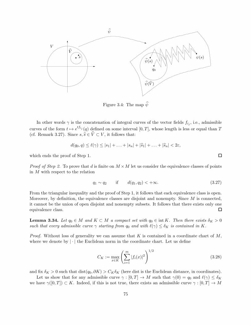
s
V
V
ψ
ψ(s)
q0
ψ(s)
ψ(V )
Figure 3.4: The map ψ
In other words γ is the concatenation of integral curves of the vector fields fij , i.e., admissible
curves of the form t 7→ etfij (q) defined on some interval [0, T ], whose length is less or equal than T(cf. Remark 3.27). Since s, s ∈ V ⊂ V , it follows that:
d(q0, q) ≤ ℓ(γ) ≤ |s1|+ . . .+ |sn|+ |s1|+ . . .+ |sn| < 2ε,
which ends the proof of Step 1.
Proof of Step 2. To prove that d is finite on M×M let us consider the equivalence classes of pointsin M with respect to the relation
q1 ∼ q2 if d(q1, q2) < +∞. (3.27)
From the triangular inequality and the proof of Step 1, it follows that each equivalence class is open.Moreover, by definition, the equivalence classes are disjoint and nonempty. Since M is connected,it cannot be the union of open disjoint and nonempty subsets. It follows that there exists only oneequivalence class.
Lemma 3.34. Let q0 ∈ M and K ⊂ M a compact set with q0 ∈ intK. Then there exists δK > 0such that every admissible curve γ starting from q0 and with ℓ(γ) ≤ δK is contained in K.
Proof. Without loss of generality we can assume that K is contained in a coordinate chart of M ,where we denote by | · | the Euclidean norm in the coordinate chart. Let us define
CK := maxx∈K
(m∑
i=1
|fi(x)|2)1/2
(3.28)
and fix δK > 0 such that dist(q0, ∂K) > CKδK (here dist is the Euclidean distance, in coordinates).
Let us show that for any admissible curve γ : [0, T ] → M such that γ(0) = q0 and ℓ(γ) ≤ δKwe have γ([0, T ]) ⊂ K. Indeed, if this is not true, there exists an admissible curve γ : [0, T ] → M
75
with ℓ(γ) ≤ δK and t∗ := supt ∈ [0, T ], γ([0, t]) ⊂ K, with t∗ < T . Then
|γ(t∗)− γ(0)| ≤∫ t∗
0|γ(t)|dt =
∫ t∗
0
m∑
i=1
|u∗i (t)fi(γ(t))| dt (3.29)
≤∫ t∗
0
√√√√m∑
i=0
|fi(γ(t))|2√√√√
m∑
i=0
u∗i (t)2 dt (3.30)
≤ CK∫ t∗
0
√√√√m∑
i=0
u∗i (t)2 dt ≤ CKℓ(γ) (3.31)
≤ CKδK < dist(q0, ∂K). (3.32)
which contradicts the fact that, at t∗, the curve γ leaves the compact K. Thus t∗ = T .
Proof of Step 3. Let us prove that Lemma 3.34 implies property (b). Indeed the only nontrivialimplication is that d(q0, q1) > 0 whenever q0 6= q1. To prove this, fix a compact neighborhood K ofq0 such that q1 /∈ K. By Lemma 3.34, each admissible curve joining q0 and q1 has length greaterthan δK , hence d(q0, q1) ≥ δK > 0.
Let us now prove property (e). Fix ε > 0 and a compact neighborhood K of q0. Define CKand δK as in Lemma 3.34, and set δ := minδK , ε/CK. Let us show that |q − q0| < ε wheneverd(q0, q) < δ, where again | · | is the Euclidean norm in a coordinate chart.
Consider a minimizing sequence γn : [0, T ]→M of admissible trajectories joining q0 and q suchthat ℓ(γn) → d(q0, q) for n →∞. Without loss of generality, we can assume that ℓ(γn) ≤ δ for alln. By Lemma 3.34, γn([0, T ]) ⊂ K for all n.
We can repeat estimates (3.29)-(3.31) proving that |q − q0| = |γn(T )− γn(0)| ≤ CKℓ(γn) for alln. Passing to the limit for n→∞, one gets
|q − q0| ≤ CKd(q0, q) ≤ CKδ < ε. (3.33)
Corollary 3.35. The metric space (M,d) is locally compact, i.e., for any q ∈M there exists ε > 0such that the closed sub-Riemannian ball B(q, r) is compact for all 0 ≤ r ≤ ε.
Proof. By the continuity of d, the set B(q, r) = d(q, ·) ≤ r is closed for all q ∈ M and r ≥ 0.Moreover the sub-Riemannian metric d induces the manifold topology onM . Hence, for radius smallenough, the sub-Riemannian ball is bounded. Thus small sub-Riemannian balls are compact.
3.3 Existence of length-minimizers
In this section we want to discuss the existence of length-minimizers.
Definition 3.36. Let γ : [0, T ]→M be an admissible curve. We say that γ is a length-minimizerif it minimizes the length among admissible curves with same endpoints, i.e., ℓ(γ) = d(γ(0), γ(T )).
76
Remark 3.37. Notice that the existence length-minimizers between two points is not guaranteedin general, as it happens for two points in M = R
2 \ 0 (endowed with the Euclidean distance)that are symmetric with respect to the origin. On the other hand, when length-minimizers existbetween two fixed points, they may not be unique, as it happens for two antipodal points on thesphere S2.
We now show a general semicontinuity property of the length functional.
Theorem 3.38. Let γn : [0, T ] → M be a sequence of admissible curves on M such that γn → γuniformly on [0, T ]. Then
ℓ(γ) ≤ lim infn→∞
ℓ(γn). (3.34)
If moreover lim infn→∞ ℓ(γn) < +∞, then γ is also admissible.
Proof. Without loss of generality we assume that γn and γ are parametrized with constant speedon the interval [0, 1]. Moreover, denote L := lim inf ℓ(γn) and choose a subsequence, which we stilldenote by the same symbol, such that ℓ(γn)→ L. If L = +∞ the inequality (3.34) is clearly true,thus assume L < +∞.
Fix δ > 0. By uniform convergence, it is not restrictive to assume that, for n large enough,ℓ(γn) ≤ L+ δ and that the image of γn are all contained in a common compact set K. Since γn isparametrized by constant speed on [0, 1] we have that γn(t) ∈ Vγn(t) where
Vq = fu(q), |u| ≤ L+ δ ⊂ TqM, fu(q) =
m∑
i=1
uifi(q).
Notice that Vq is convex for every q ∈M , thanks to the linearity of f in u. Let us prove that γ isadmissible and satisfies ℓ(γ) ≤ L+ δ. Since δ is arbitrary, this implies ℓ(γ) ≤ L, that is (3.34).
In local coordinates, we have for every ε > 0
1
ε(γn(t+ ε)− γn(t)) =
1
ε
∫ t+ε
tfun(τ)(γn(τ))dτ ∈ convVγn(τ), τ ∈ [t, t+ ε]. (3.35)
Next we want to estimate the right hand side of (3.35) uniformly. For n ≥ n0 sufficiently large,we have |γn(t) − γ(t)| < ε (by uniform convergence) and an estimate similar to (3.31) gives forτ ∈ [t, t+ ε]
|γn(t)− γn(τ)| ≤∫ τ
t|γn(s)|ds ≤ CK(L+ δ)ε. (3.36)
where CK is the constant (3.28) defined by the compact K. Hence we deduce for every τ ∈ [t, t+ ε]and every n ≥ n0
|γn(τ)− γ(t)| ≤ |γn(t)− γn(τ)|+ |γn(t)− γ(t)| ≤ C ′ε, (3.37)
where C ′ is independent on n and ε. From the estimate (3.37) and the equivalence of the manifoldand metric topology we have that, for all τ ∈ [t, t+ ε] and n ≥ n0, γn(τ) ∈ Bγ(t)(rε), with rε → 0when ε→ 0. In particular
convVγn(τ), τ ∈ [t, t+ ε] ⊂ convVq, q ∈ Bγ(t)(rε). (3.38)
Plugging (3.38) in (3.35) and passing to the limit for n→∞ we get finally to
1
ε(γ(t+ ε)− γ(t)) ∈ convVq, q ∈ Bγ(t)(rε). (3.39)
77
Assume now that t ∈ [0, 1] is a differentiability point of γ. Then the limit of the left hand side in(3.39) for ε → 0 exists and gives γ(t) ∈ conv Vγ(t) = Vγ(t). For every differentiability point t wecan thus define the unique u∗(t) satisfying γ(t) = f(γ(t), u∗(t)) and |u∗(t)| = ‖γ(t)‖. Using theargument contained in Appendix 3.A it follows that u∗(t) is measurable in t. Moreover |u∗(t)| isessentially bounded since, by construction, |u∗(t)| ≤ L+ δ for a.e. t ∈ [0, T ]. Hence γ is admissible.Moreover ℓ(γ) ≤ L+ δ since γ is length-parametrized on the interval [0, 1].
Corollary 3.39. Let γn be a sequence of length-minimizers on M such that γn → γ uniformly.Then γ is a length-minimizer.
Proof. Since the length is invariant under reparametrization, it is not restrictive to assume thatall curves γn and γ are parametrized on [0, 1]. Since γn is a length-minimizer one has ℓ(γn) =d(γn(0), γn(1)). By uniform convergence γn(t) → γ(t) for every t ∈ [0, 1] and, by continuity of thedistance and semicontinuity of the length
ℓ(γ) ≤ lim infn→∞
ℓ(γn) = lim infn→∞
d(γn(0), γn(1)) = d(γ(0), γ(1)),
that implies that ℓ(γ) = d(γ(0), γ(1)), i.e., γ is a length-minimizer.
The semicontinuity of the length implies the existence of minimizers, under a natural compact-ness assumption on the space.
Theorem 3.40 (Existence of minimizers). Let M be a sub-Riemannian manifold and q0 ∈ M .Assume that the ball Bq0(r) is compact, for some r > 0. Then for all q1 ∈ Bq0(r) there exists alength minimizer joining q0 and q1, i.e., we have
d(q0, q1) = minℓ(γ) | γ : [0, T ]→M admissible , γ(0) = q0, γ(T ) = q1.Proof. Fix q1 ∈ Bq0(r) and consider a minimizing sequence γn : [0, 1] → M of admissible trajecto-ries, parametrized with constant speed, joining q0 and q1 and such that ℓ(γn)→ d(q0, q1).
Since d(q0, q1) < r, we have ℓ(γn) ≤ r for all n ≥ n0 large enough, hence we can assume withoutloss of generality that the image of γn is contained in the common compact K = Bq0(r) for all n.In particular, the same argument leading to (3.36) shows that for all n ≥ n0
|γn(t)− γn(τ)| ≤∫ t
τ|γn(s)|ds ≤ CKr|t− τ |, ∀ t, τ ∈ [0, 1]. (3.40)
where CK depends only on K. In other words, all trajectories in the sequence γnn∈N are Lipschitzwith the same Lipschitz constant. Thus the sequence is equicontinuous and uniformly bounded.
By the classical Ascoli-Arzela Theorem there exist a subsequence of γn, which we still denote bythe same symbol, and a Lipschitz curve γ : [0, T ] → M such that γn → γ uniformly. By Theorem3.38, the curve γ satisfies ℓ(γ) ≤ lim inf ℓ(γn) = d(q0, q1), that implies ℓ(γ) = d(q0, q1).
Remark 3.41. Assume that B(q, r0) is compact for some r0 > 0. Then for every 0 < r ≤ r0 wehave that B(q, r) is compact also, being a closed subset of a compact set B(q, r0).
Corollary 3.42. Let q0 ∈M . Under the hypothesis of Corollary 3.40 there exists ε > 0 such thatfor all r ≤ ε and q1 ∈ Bq0(r) there exists a minimizing curve joining q0 and q1.
Proof. It is a direct consequence of Theorem 3.40 and Corollary 3.35.
Remark 3.43. It is well known that a length space is complete if and only if all closed balls arecompact, see [11, Ch. 2]. In particular, if (M,d) is complete with respect to the sub-Riemanniandistance, then for every q0, q1 ∈M there exists a length minimizer joining q0 and q1.
78
3.4 Pontryagin extremals
In this section we want to give necessary conditions to characterize length-minimizer trajectories.To begin with, we would like to motivate our Hamiltonian approach that we develop in the sequel.
In classical Riemannian geometry length-minimizer trajectories satisfy a necessary conditiongiven by a second order differential equation inM , which can be reduced to a first-order differentialequation in TM . Hence the set of all length-minimizers is contained in the set of extremals, i.e.,trajectories that satisfy the necessary condition, that are be parametrized by initial position andvelocity.
In our setting (which includes Riemannian and sub-Riemannian geometry) we cannot use theinitial velocity to parametrize length-minimizer trajectories. This can be easily understood by adimensional argument. If the rank of the sub-Riemannian structure is smaller than the dimensionof the manifold, the initial velocity γ(0) of an admissible curve γ(t) starting from q0, belongs to theproper subspace Dq0 of the tangent space Tq0M . Hence the set of admissible velocities form a setwhose dimension is smaller than the dimension of M , even if, by the Chow and Filippov theorems,length-minimizer trajectories starting from a point q0 cover a full neighborhood of q0.
The right approach is to parametrize length-minimizers by their initial point and an initialcovector λ0 ∈ T ∗
q0M , which can be thought as the linear form annihilating the “front”, i.e., the setγq0(ε) | γq0 is a length-minimizer starting from q0 on the corresponding length-minimizer trajec-tory for ε→ 0.
The next theorem gives the necessary condition satisfied by length-minimizers in sub-Riemanniangeometry. Curves satisfying this condition are called Pontryagin extremals. The proof the followingtheorem is given in the next section.
Theorem 3.44 (Characterization of Pontryagin extremals). Let γ : [0, T ] → M be an admissiblecurve which is a length-minimizer, parametrized by constant speed. Let u(·) be the correspondingminimal control, i.e., for a.e. t ∈ [0, T ]
γ(t) =
m∑
i=1
ui(t)fi(γ(t)), ℓ(γ) =
∫ T
0|u(t)|dt = d(γ(0), γ(T )),
with |u(t)| constant a.e. on [0, T ]. Denote with P0,t the flow2 of the nonautonomous vector field
fu(t) =∑k
i=1 ui(t)fi. Then there exists λ0 ∈ T ∗γ(0)M such that defining
λ(t) := (P−10,t )
∗λ0, λ(t) ∈ T ∗γ(t)M, (3.41)
we have that one of the following conditions is satisfied:
(N) ui(t) ≡ 〈λ(t), fi(γ(t))〉 , ∀ i = 1, . . . ,m,
(A) 0 ≡ 〈λ(t), fi(γ(t))〉 , ∀ i = 1, . . . ,m.
Moreover in case (A) one has λ0 6= 0.
Notice that, by definition, the curve λ(t) is Lipschitz continuous. Moreover the conditions (N)and (A) are mutually exclusive, unless u(t) = 0 for a.e. t ∈ [0, T ], i.e., γ is the trivial trajectory.
2P0,t(x) is defined for t ∈ [0, T ] and x in a neighborhood of γ(0)
79
Definition 3.45. Let γ : [0, T ]→M be an admissible curve with minimal control u ∈ L∞([0, T ],Rm).Fix λ0 ∈ T ∗
γ(0)M \ 0, and define λ(t) by (3.41).
- If λ(t) satisfies (N) then it is called normal extremal (and γ(t) a normal extremal trajectory).
- If λ(t) satisfies (A) then it is called abnormal extremal (and γ(t) a abnormal extremal trajec-tory).
Remark 3.46. In the Riemannian case there are no abnormal extremals. Indeed, since the map fis fiberwise surjective, we can always find m vector fields f1, . . . , fm on M such that
spanq0f1, . . . , fm = Tq0M,
and (A) would imply that 〈λ0, v〉 = 0, for all v ∈ Tq0M , that gives the contradiction λ0 = 0.
Remark 3.47. If the sub-Riemannian structure is not Riemannian at q0, namely if
Dq0 = spanq0f1, . . . , fm 6= Tq0M,
then the trivial trajectory, corresponding to u(t) ≡ 0, is always normal and abnormal.Notice that even a nontrivial admissible trajectory γ can be both normal and abnormal, since
there may exist two different lifts λ(t), λ′(t) ∈ T ∗γ(t)M , such that λ(t) satisfies (N) and λ′(t) satisfies
(A).
Exercise 3.48. Prove that condition (N) of Theorem 3.41 implies that the minimal control u(t)is smooth. In particular normal extremals are smooth.
At this level it seems not obvious how to use Theorem 3.44 to find the explicit expression ofextremals for a given problem. In the next chapter we provide another formulation of Theorem3.44 which gives Pontryagin extremals as solutions of a Hamiltonian system.
The rest of this section is devoted to the proof of Theorem 3.44.
3.4.1 The energy functional
Let γ : [0, T ] → M be an admissible curve. We define the energy functional J on the space ofLipschitz curves on M as follows
J(γ) =1
2
∫ T
0‖γ(t)‖2dt.
Notice that J(γ) < +∞ for every admissible curve γ.
Remark 3.49. While ℓ is invariant by reparametrization (see Remark 3.14), J is not. Indeedconsider, for every α > 0, the reparametrized curve
γα : [0, T/α]→M, γα(t) = γ(αt).
Using that γα(t) = α γ(αt), we have
J(γα) =1
2
∫ T/α
0‖γα(t)‖2dt =
1
2
∫ T/α
0α2‖γ(αt)‖2dt = αJ(γ).
Thus, if the final time is not fixed, the infimum of J , among admissible curves joining two fixedpoints, is always zero.
80
The following lemma relates minimizers of J with fixed final time with minimizers of ℓ.
Lemma 3.50. Fix T > 0 and let Ωq0,q1 be the set of admissible curves joining q0, q1 ∈ M . Anadmissible curve γ : [0, T ] → M is a minimizer of J on Ωq0,q1 if and only if it is a minimizer of ℓon Ωq0,q1 and has constant speed.
Proof. Applying the Cauchy-Schwarz inequality
(∫ T
0f(t)g(t)dt
)2
≤∫ T
0f(t)2dt
∫ T
0g(t)2dt, (3.42)
with f(t) = ‖γ(t)‖ and g(t) = 1 we get
ℓ(γ)2 ≤ 2J(γ)T. (3.43)
Moreover in (3.42) equality holds if and only if f is proportional to g, i.e., ‖γ(t)‖ = const. in (3.43).Since, by Lemma 3.15, every curve is a Lipschitz reparametrization of a length-parametrized one,the minima of J are attained at admissible curves with constant speed, and the statement follows.
3.4.2 Proof of Theorem 3.44
By Lemma 3.50 we can assume that γ is a minimizer of the functional J among admissible curvesjoining q0 = γ(0) and q1 = γ(T ) in fixed time T > 0. In particular, if we define the functional
J(u(·)) := 1
2
∫ T
0|u(t)|2dt, (3.44)
on the space of controls u(·) ∈ L∞([0, T ],Rm), the minimal control u(·) of γ is a minimizer for theenergy functional J
J(u(·)) ≤ J(u(·)), ∀u ∈ L∞([0, T ],Rm),
where trajectories corresponding to u(·) join q0, q1 ∈M . In the following we denote the functionalJ by J .
Consider now a variation u(·) = u(·)+v(·) of the control u(·), and its associated trajectory q(t),solution of the equation
q(t) = fu(t)(q(t)), q(0) = q0, (3.45)
Recall that P0,t denotes the local flow associated with the optimal control u(·) and that γ(t) =P0,t(q0) is the optimal admissible curve. We stress that in general, for q different from q0, the curvet 7→ P0,t(q) is not optimal. Let us introduce the curve x(t) defined by the identity
q(t) = P0,t(x(t)). (3.46)
In other words x(t) = P−10,t (q(t)) is obtained by applying the inverse of the flow of u(·) to the solution
associated with the new control u(·) (see Figure 3.5). Notice that if v(·) = 0, then x(t) ≡ q0.The next step is to write the ODE satisfied by x(t). Differentiating (3.46) we get
q(t) = fu(t)(q(t)) + (P0,t)∗(x(t)) (3.47)
= fu(t)(P0,t(x(t))) + (P0,t)∗(x(t)) (3.48)
81
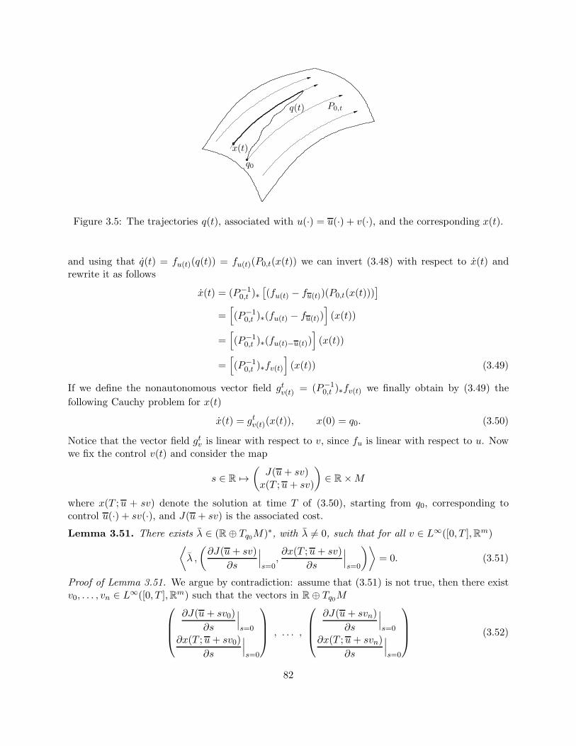
x(t)
q(t) P0,t
q0
Figure 3.5: The trajectories q(t), associated with u(·) = u(·) + v(·), and the corresponding x(t).
and using that q(t) = fu(t)(q(t)) = fu(t)(P0,t(x(t)) we can invert (3.48) with respect to x(t) andrewrite it as follows
x(t) = (P−10,t )∗
[(fu(t) − fu(t))(P0,t(x(t)))
]
=[(P−1
0,t )∗(fu(t) − fu(t))](x(t))
=[(P−1
0,t )∗(fu(t)−u(t))](x(t))
=[(P−1
0,t )∗fv(t)](x(t)) (3.49)
If we define the nonautonomous vector field gtv(t) = (P−10,t )∗fv(t) we finally obtain by (3.49) the
following Cauchy problem for x(t)
x(t) = gtv(t)(x(t)), x(0) = q0. (3.50)
Notice that the vector field gtv is linear with respect to v, since fu is linear with respect to u. Nowwe fix the control v(t) and consider the map
s ∈ R 7→(J(u+ sv)x(T ;u+ sv)
)∈ R×M
where x(T ;u + sv) denote the solution at time T of (3.50), starting from q0, corresponding tocontrol u(·) + sv(·), and J(u+ sv) is the associated cost.
Lemma 3.51. There exists λ ∈ (R⊕ Tq0M)∗, with λ 6= 0, such that for all v ∈ L∞([0, T ],Rm)⟨λ ,
(∂J(u+ sv)
∂s
∣∣∣s=0
,∂x(T ;u+ sv)
∂s
∣∣∣s=0
)⟩= 0. (3.51)
Proof of Lemma 3.51. We argue by contradiction: assume that (3.51) is not true, then there existv0, . . . , vn ∈ L∞([0, T ],Rm) such that the vectors in R⊕ Tq0M
∂J(u+ sv0)
∂s
∣∣∣s=0
∂x(T ;u+ sv0)
∂s
∣∣∣s=0
, . . . ,
∂J(u+ svn)
∂s
∣∣∣s=0
∂x(T ;u+ svn)
∂s
∣∣∣s=0
(3.52)
82
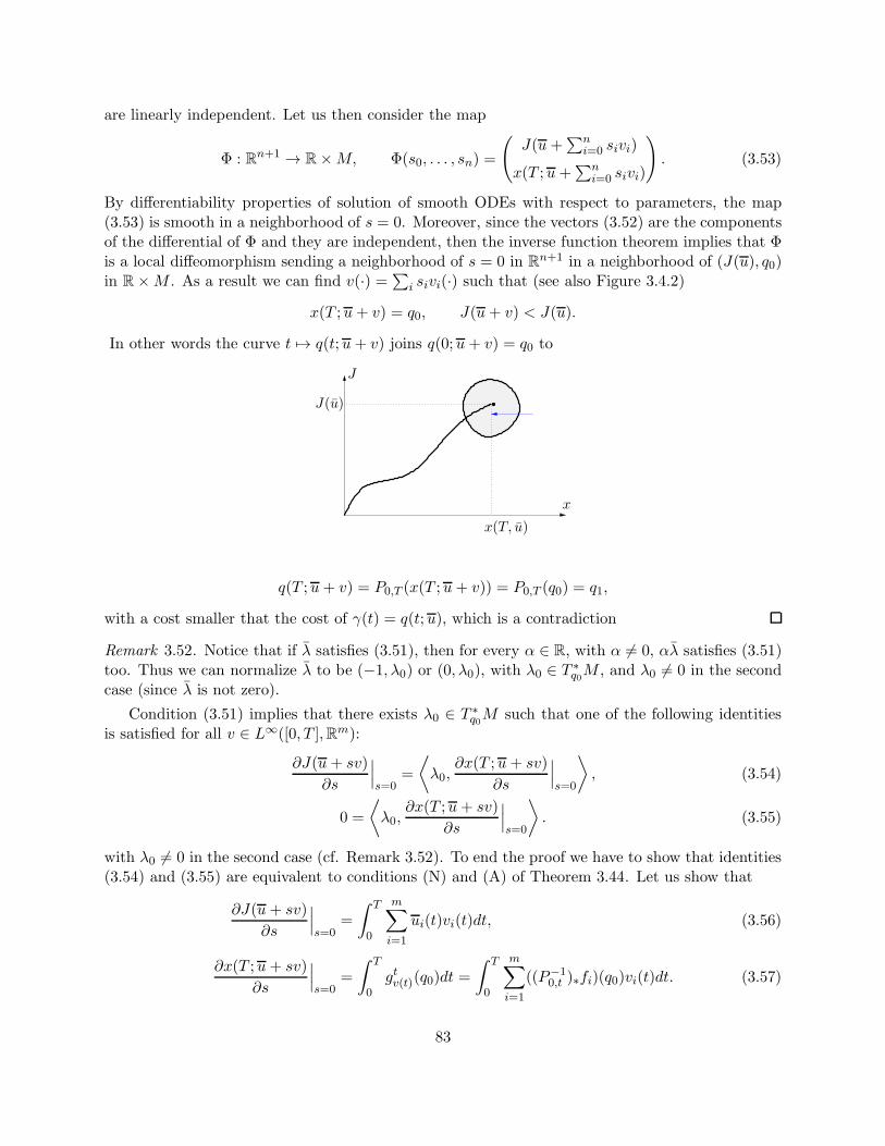
are linearly independent. Let us then consider the map
Φ : Rn+1 → R×M, Φ(s0, . . . , sn) =
(J(u+
∑ni=0 sivi)
x(T ;u+∑n
i=0 sivi)
). (3.53)
By differentiability properties of solution of smooth ODEs with respect to parameters, the map(3.53) is smooth in a neighborhood of s = 0. Moreover, since the vectors (3.52) are the componentsof the differential of Φ and they are independent, then the inverse function theorem implies that Φis a local diffeomorphism sending a neighborhood of s = 0 in R
n+1 in a neighborhood of (J(u), q0)in R×M . As a result we can find v(·) =∑i sivi(·) such that (see also Figure 3.4.2)
x(T ;u+ v) = q0, J(u+ v) < J(u).
In other words the curve t 7→ q(t;u+ v) joins q(0;u+ v) = q0 to
x(T, u)
J(u)
J
x
q(T ;u+ v) = P0,T (x(T ;u+ v)) = P0,T (q0) = q1,
with a cost smaller that the cost of γ(t) = q(t;u), which is a contradiction
Remark 3.52. Notice that if λ satisfies (3.51), then for every α ∈ R, with α 6= 0, αλ satisfies (3.51)too. Thus we can normalize λ to be (−1, λ0) or (0, λ0), with λ0 ∈ T ∗
q0M , and λ0 6= 0 in the secondcase (since λ is not zero).
Condition (3.51) implies that there exists λ0 ∈ T ∗q0M such that one of the following identities
is satisfied for all v ∈ L∞([0, T ],Rm):
∂J(u+ sv)
∂s
∣∣∣s=0
=
⟨λ0,
∂x(T ;u+ sv)
∂s
∣∣∣s=0
⟩, (3.54)
0 =
⟨λ0,
∂x(T ;u+ sv)
∂s
∣∣∣s=0
⟩. (3.55)
with λ0 6= 0 in the second case (cf. Remark 3.52). To end the proof we have to show that identities(3.54) and (3.55) are equivalent to conditions (N) and (A) of Theorem 3.44. Let us show that
∂J(u+ sv)
∂s
∣∣∣s=0
=
∫ T
0
m∑
i=1
ui(t)vi(t)dt, (3.56)
∂x(T ;u+ sv)
∂s
∣∣∣s=0
=
∫ T
0gtv(t)(q0)dt =
∫ T
0
m∑
i=1
((P−10,t )∗fi)(q0)vi(t)dt. (3.57)
83
The identity (3.56) follows from the definition of J
J(u+ sv) =1
2
∫ T
0|u+ sv|2dt. (3.58)
Eq. (3.57) can be proved in coordinates. Indeed by (3.50) and the linearity of gv with respect to vwe have
x(T ;u+ sv) = q0 + s
∫ T
0gtv(t)(x(t;u+ sv))dt,
and differentiating with respect to s at s = 0 one gets (3.57).
Let us show that (3.54) is equivalent to (N) of Theorem 3.44. Similarly, one gets that (3.55) isequivalent to (A). Using (3.56) and (3.57), equation (3.54) is rewritten as
∫ T
0
m∑
i=1
ui(t)vi(t)dt =
∫ T
0
m∑
i=1
⟨λ0, ((P
−10,t )∗fi)(q0)
⟩vi(t)dt
=
∫ T
0
m∑
i=1
〈λ(t), fi(γ(t))〉 vi(t)dt, (3.59)
where we used, for every i = 1, . . . ,m, the identities
⟨λ0, ((P
−10,t )∗fi)(q0)
⟩=⟨λ0, (P
−10,t )∗fi(γ(t))
⟩=⟨(P−1
0,t )∗λ0, fi(γ(t))
⟩= 〈λ(t), fi(γ(t))〉 .
Since vi(·) ∈ L∞([0, T ],Rm) are arbitrary, we get ui(t) = 〈λ(t), fi(γ(t))〉 for a.e. t ∈ [0, T ].
3.A Measurability of the minimal control
In this appendix we prove a technical lemma about measurability of solutions to a class of mini-mization problems. This lemma when specified to the sub-Riemannian context, implies that theminimal control associated with an admissible curve is measurable.
3.A.1 Main lemma
Let us fix an interval I = [a, b] ⊂ R and a compact set U ⊂ Rm. Consider two functions g : I×U →
Rn, v : I → R
n such that
(M1) g(·, u) is measurable in t for every fixed u ∈ U ,
(M2) g(t, ·) is continuous in u for every fixed t ∈ I,
(M3) v(t) is measurable with respect to t.
Moreover we assume that
(M4) for every fixed t ∈ I, the problem min|u| : g(t, u) = v(t), u ∈ U has a unique solution.
Let us denote by u∗(t) the solution of (M4) for a fixed t ∈ I.
84
Lemma 3.53. Under assumptions (M1)-(M4), the function t 7→ |u∗(t)| is measurable on I.
Proof. Denote ϕ(t) := |u∗(t)|. To prove the lemma we show that for every fixed r > 0 the set
A = t ∈ I : ϕ(t) ≤ r
is measurable in R. By our assumptions
A = t ∈ I : ∃u ∈ U s.t. |u| ≤ r, g(t, u) = v(t)
Let us fix r > 0 and a countable dense set uii∈N in the ball of radius r in U . Let show that
A =⋂
n∈NAn =
⋂
n∈N
⋃
i∈NAi,n
︸ ︷︷ ︸:=An
(3.60)
whereAi,n := t ∈ I : |g(t, ui)− v(t)| < 1/n
Notice that the set Ai,n is measurable by construction and if (3.60) is true, A is also measurable.
⊂ inclusion. Let t ∈ A. This means that there exists u ∈ U such that |u| ≤ r and g(t, u) = v(t).Since g is continuous with respect to u and uii∈N is a dense, for each n we can find uin such that|g(t, uin)− v(t)| < 1/n, that is t ∈ An for all n.
⊃ inclusion. Assume t ∈ ⋂n∈N An. Then for every n there exists in such that the correspondinguin satisfies |g(t, uin) − v(t)| < 1/n. From the sequence uin , by compactness, it is possible toextract a convergent susequence uin → u. By continuity of g with respect to u one easily gets thatg(t, u) = v(t). That is t ∈ A.
Next we exploit the fact that the function ϕ(t) := |u∗(t)| is measurable to show that the vectorfunction u∗(t) is measurable.
Lemma 3.54. Under assumptions (M1)-(M4), the vector function t 7→ u∗(t) is measurable on I.
Proof. It is sufficient to prove that, for every closed ball O in Rn the set
B := t ∈ I : u∗(t) ∈ O
is measurable. Since the minimum in (M4) is uniquely determined, this is equivalent to
B = t ∈ I : ∃u ∈ O s.t. |u| = ϕ(t), g(t, u) = v(t)
Let us fix the ball O and a countable dense set uii∈N in O. Let show that
B =⋂
n∈NBn =
⋂
n∈N
⋃
i∈NBi,n
︸ ︷︷ ︸:=Bn
(3.61)
whereBi,n := t ∈ I : |ui| < ϕ(t) + 1/n, |g(t, ui)− v(t)| < 1/n;
85
Notice that the set Bi,n is measurable by construction and if (3.61) is true, B is also measurable.
⊂ inclusion. Let t ∈ B. This means that there exists u ∈ O such that |u| = ϕ(t) andg(t, u) = v(t). Since g is continuous with respect to u and uii∈N is a dense in O, for each n wecan find uin such that |g(t, uin)− v(t)| < 1/n and |uin | < ϕ(t) + 1/n, that is t ∈ Bn for all n.
⊃ inclusion. Assume t ∈ ⋂n∈N Bn. Then for every n it is possible to find in such that thecorresponding uin satisfies |g(t, uin )− v(t)| < 1/n and |uin | < ϕ(t) + 1/n. From the sequence uin ,by compactness of the closed ball O, it is possible to extract a convergent susequence uin → u. Bycontinuity of f in u one easily gets that g(t, u) = v(t). Moreover |u| ≤ ϕ(t). Hence |u| = ϕ(t).That is t ∈ B.
3.A.2 Proof of Lemma 3.11
Consider an admissible curve γ : [0, T ] → M . Since measurability is a local property it is notrestrictive to assume M = R
n. Moreover, by Lemma 3.15, we can assume that γ is length-parametrized so that its minimal control belong to the compact set U = |u| ≤ 1. Define g :[0, T ]× U → R
n and v : [0, T ]→ Rn by
g(t, u) = f(γ(t), u), v(t) = γ(t).
Assumptions (M1)-(M4) are satisfied. Indeed (M1)-(M3) follow from the fact that g(t, u) is linearwith respect to u and measurable in t. Moreover (M4) is also satisfied by linearity with respect tou of f . Applying Lemma 3.54 one gets that the minimal control u∗(t) is measurable in t.
3.B Lipschitz vs Absolutely continuous admissible curves
In these lecture notes sub-Riemannian geometry is developed in the framework of Lipschitz admissi-ble curves (that correspond to the choice of L∞ controls). However, the theory can be equivalentlydeveloped in the framework of H1 admissible curves (corresponding to L2 controls) or in the frame-work of absolutely continuous admissible curves (corresponding to L1 controls).
Definition 3.55. An absolutely continuous curve γ : [0, T ] → M is said to be AC-admissible ifthere exists an L1 function u : t ∈ [0, T ] 7→ u(t) ∈ Uγ(t) such that γ(t) = f(γ(t), u(t)), for a.e.t ∈ [0, T ]. We define H1-admissible curves similarly.
Being the set of absolutely continuous curve bigger than the set of Lipschitz ones, one couldexpect that the sub-Riemannian distance between two points is smaller when computed among allabsolutely continuous admissible curves. However this is not the case thanks to the invariance byreparametrization. Indeed Lemmas 3.14 and 3.15 can be rewritten in the absolutely continuousframework in the following form.
Lemma 3.56. The length of an AC-admissible curve is invariant by AC reparametrization.
Lemma 3.57. Any AC-admissible curve of positive length is a AC reparametrization of a length-parametrized admissible one.
86
The proof of Lemma 3.56 differs from the one of Lemma 3.14 only by the fact that, if u∗ ∈ L1
is the minimal control of γ then (u∗ ϕ)ϕ is the minimal control associated with γ ϕ. Moreover(u∗ ϕ)ϕ ∈ L1, using the monotonicity of ϕ. Under these assumptions the change of variablesformula (3.16) still holds.
The proof of Lemma 3.57 is unchanged. Notice that the statement of Exercise 3.16 remains trueif we replace Lipschitz with absolutely continuous. We stress that the curve γ built in the proof isLipschitz (since it is length-parametrized).
As a consequence of these results, if we define
dAC(q0, q1) = infℓ(γ) | γ : [0, T ]→M AC -admissible, γ(0) = q0, γ(T ) = q1, (3.62)
we have the following proposition.
Proposition 3.58. dAC(q0, q1) = d(q0, q1)
Since L2([0, T ]) ⊂ L1([0, T ]), Lemmas 3.56, 3.57 and Proposition 3.58 are valid also in theframework of admissible curves associated with L2 controls.
Bibliographical notes
Sub-Riemannian manifolds have been introduced, even if with different terminology, in severalcontexts starting from the end of 60s, see for instance [23, 20, 15, 21, 16]. However, some pioneeringideas were already present in the work of Caratheodory and Cartan. The name sub-Riemanniangeometry first appeared in [33].
Classical general references for sub-Riemannian geometry are [27, 4, 26, 17, 35]. Recent mono-graphs [22, 31].
The definition of sub-Riemannian manifold using the language of bundles dates back to [2, 4].For the original proof of the Raschevski-Chow theorem see [29, 12]. The proof of existence of sub-Riemannian length minimizer presented here is an adaptation of the proof of Filippov theorem inoptimal control. The fact that in sub-Riemannian geometry there exist abnormal length minimizersis due to Montgomery [25, 27]. The fact that the theory can be equivalently developed for Lipschitzor absolutely continuous curves is well known, a discussion can be found in [4].
The definition of the length by using the minimal control is, up to our best knowledge, original.The problem of the measurability of the minimal control can be seen as a problem of differentialinclusion [10]. The characterization of Pontryagin extremals given in Theorem 3.44 is a simplifiedversion of the Pontryagin Maximum Priciple (PMP) [28]. The proof presented here is originaland adapted to this setting. For more general versions of PMP see [3, 5]. The fact that everysub-Riemannian structure is equivalent to a free one (cf. Section 3.1.4) is a consequence of classicalresults on fiber bundles. A different proof in the case of classical (constant rank) distribution wasalso considered in [31, 36].
87

88
Chapter 4
Characterization and local minimalityof Pontryagin extremals
This chapter is devoted to the study of geometric properties of Pontryagin extremals. To thispurpose we first rewrite Theorem 3.44 in a more geometric setting, which permits to write adifferential equation in T ∗M satisfied by Pontryagin extremals and to show that they do notdepend on the choice of a generating family. Finally we prove that small pieces of normal extremaltrajectories are length-minimizers.
To this aim, all along this chapter we develop the language of symplectic geometry, starting bythe key concept of Poisson bracket.
4.1 Geometric characterization of Pontryagin extremals
In the previous chapter we proved that if γ : [0, T ]→M is a length minimizer on a sub-Riemannianmanifold, associated with a control u(·), then there exists λ0 ∈ T ∗
γ(0)M such that defining
λ(t) = (P−10,t )
∗λ0, λ(t) ∈ T ∗γ(t)M, (4.1)
one of the following conditions is satisfied:
(N) ui(t) ≡ 〈λ(t), fi(γ(t))〉 , ∀ i = 1, . . . ,m,
(A) 0 ≡ 〈λ(t), fi(γ(t))〉 , ∀ i = 1, . . . ,m, λ0 6= 0.
Here P0,t denotes the flow associated with the nonautonomous vector field fu(t) =∑m
i=1 ui(t)fi and
(P−10,t )
∗ : T ∗qM → T ∗
P0,t(q)M. (4.2)
is the induced flow on the cotangent space.
The goal of this section is to characterize the curve (4.1) as the integral curve of a suitable(non-autonomous) vector field on T ∗M . To this purpose, we start by showing that a vector fieldon T ∗M is completely characterized by its action on functions that are affine on fibers. To fix theideas, we first focus on the case in which P0,t :M →M is the flow associated with an autonomousvector field X ∈ Vec(M), namely P0,t = etX .
89
4.1.1 Lifting a vector field from M to T ∗M
We start by some preliminary considerations on the algebraic structure of smooth functions onT ∗M . As usual π : T ∗M →M denotes the canonical projection.
Functions in C∞(M) are in a one-to-one correspondence with functions in C∞(T ∗M) that areconstant on fibers via the map α 7→ π∗α = α π. In other words we have the isomorphism ofalgebras
C∞(M) ≃ C∞cst(T ∗M) := π∗α |α ∈ C∞(M) ⊂ C∞(T ∗M). (4.3)
In what follows, with abuse of notation, we often identify the function π∗α ∈ C∞(T ∗M) with thefunction α ∈ C∞(M).
In a similar way smooth vector fields onM are in a one-to-one correspondence with functions inC∞(T ∗M) that are linear on fibers via the map Y 7→ aY , where aY (λ) := 〈λ, Y (q)〉 and q = π(λ).
Vec(M) ≃ C∞lin(T ∗M) := aY |Y ∈ Vec(M) ⊂ C∞(T ∗M). (4.4)
Notice that this is an isomorphism as modules over C∞(M). Indeed, as Vec(M) is a module overC∞(M), we have that C∞lin(T ∗M) is a module over C∞(M) as well. For any α ∈ C∞(M) andaX ∈ C∞lin(T ∗M) their product is defined as αaX := (π∗α)aX = aαX ∈ C∞lin(T ∗M).
Definition 4.1. We say that a function a ∈ C∞(T ∗M) is affine on fibers if there exist two functionsα ∈ C∞cst(T ∗M) and aX ∈ C∞lin(T ∗M) such that a = α+ aX . In other words
a(λ) = α(q) + 〈λ,X(q)〉 , q = π(λ).
We denote by C∞aff(T ∗M) the set of affine function on fibers.
Remark 4.2. Linear and affine functions on T ∗M are particularly important since they reflects thelinear structure of the cotangent bundle. In particular every vector field on T ∗M , as a derivationof C∞(T ∗M), is completely characterized by its action on affine functions,
Indeed for a vector field V ∈ Vec(T ∗M) and f ∈ C∞(T ∗M), one has that
(V f)(λ) =d
dt
∣∣∣∣t=0
f(etV (λ)) = 〈dλf, V (λ)〉 , λ ∈ T ∗M. (4.5)
which depends only on the differential of f at the point λ. Hence, for each fixed λ ∈ T ∗M ,to compute (4.5) one can replace the function f with any affine function whose differential at λcoincide with dλf . Notice that such a function is not unique.
Let us now consider the infinitesimal generator of the flow (P−10,t )
∗ = (e−tX )∗. Since it satisfiesthe group law
(e−tX)∗ (e−sX)∗ = (e−(t+s)X )∗ ∀ t, s ∈ R,
by Lemma 2.15 its infinitesimal generator is an autonomous vector field VX on T ∗M . In otherwords we have (e−tX )∗ = etVX for all t.
Let us then compute the right hand side of (4.5) when V = VX and f is either a functionconstant on fibers or a function linear on fibers.
The action of VX on functions that are constant on fibers, of the form β π with β ∈ C∞(M),coincides with the action of X. Indeed we have for all λ ∈ T ∗M
d
dt
∣∣∣∣t=0
β π((e−tX )∗λ)) =d
dt
∣∣∣∣t=0
β(etX (q)) = (Xβ)(q), q = π(λ). (4.6)
90
For what concerns the action of VX on functions that are linear on fibers, of the form aY (λ) =〈λ, Y (q)〉, we have for all λ ∈ T ∗M
d
dt
∣∣∣∣t=0
aY ((e−tX )∗λ) =
d
dt
∣∣∣∣t=0
⟨(e−tX )∗λ, Y (etX(q))
⟩
=d
dt
∣∣∣∣t=0
⟨λ, (e−tX∗ Y )(q)
⟩= 〈λ, [X,Y ](q)〉 (4.7)
= a[X,Y ](λ).
Hence, by linearity, one gets that the action of VX on functions of C∞aff(T ∗M) is given by
VX(β + aY ) = Xβ + a[X,Y ]. (4.8)
As explained in Remark 4.2, formula (4.8) characterizes completely the generator VX of (P−10,t )
∗.To find its explicit form we introduce the notion of Poisson bracket.
4.1.2 The Poisson bracket
The purpose of this section is to introduce an operation ·, · on C∞(T ∗M), called Poisson bracket.First we introduce it in C∞lin(T ∗M), where it reflects the Lie bracket of vector fields in Vec(M), seenas elements of C∞lin(T ∗M). Then it is uniquely extended to C∞aff(T ∗M) and C∞(T ∗M) by requiringthat it is a derivation of the algebra C∞(T ∗M) in each argument.
More precisely we start by the following definition.
Definition 4.3. Let aX , aY ∈ C∞lin(T ∗M) be associated with vector fields X,Y ∈ Vec(M). TheirPoisson bracket is defined by
aX , aY := a[X,Y ], (4.9)
where a[X,Y ] is the function in C∞lin(T ∗M) associated with the vector field [X,Y ].
Remark 4.4. Recall that the Lie bracket is a bilinear, skew-symmetric map defined on Vec(M),that satisfies the Leibnitz rule for X,Y ∈ Vec(M):
[X,αY ] = α[X,Y ] + (Xα)Y, ∀α ∈ C∞(M). (4.10)
As a consequence, the Poisson bracket is bilinear, skew-symmetric and satisfies the following relation
aX , α aY = aX , aαY = a[X,αY ] = αa[X,Y ] + (Xα) aY , ∀α ∈ C∞(M). (4.11)
Notice that this relation makes sense since the product between α ∈ C∞cst(T ∗M) and aX ∈ C∞lin(T ∗M)belong to C∞lin(T ∗M), namely αaX = aαX .
Next, we extend this definition on the whole C∞(T ∗M).
Proposition 4.5. There exists a unique bilinear and skew-simmetric map
·, · : C∞(T ∗M)× C∞(T ∗M)→ C∞(T ∗M)
that extends (4.9) on C∞(T ∗M), and that is a derivation in each argument, i.e. it satisfies
a, bc = a, bc + a, cb, ∀ a, b, c ∈ C∞(T ∗M). (4.12)
We call this operation the Poisson bracket on C∞(T ∗M).
91
Proof. We start by proving that, as a consequence of the requirement that ·, · is a derivation ineach argument, it is uniquely extended to C∞aff(T ∗M).
By linearity and skew-symmetry we are reduced to compute Poisson brackets of kind aX , αand α, β, where aX ∈ C∞lin(T ∗M) and α, β ∈ C∞cst(T ∗M). Using that aαY = αaY and (4.12) onegets
aX , aαY = aX , α aY = αaX , aY + aX , αaY . (4.13)
Comparing (4.11) and (4.13) one gets
aX , α = Xα (4.14)
Next, using (4.12) and (4.14), one has
aαY , β = α aY , β = αaY , β + α, βaY (4.15)
= αY β + α, βaY . (4.16)
Using again (4.14) one also has aαY , β = αY β, hence α, β = 0.
Combining the previous formulas one obtains the following expression for the Poisson bracketbetween two affine functions on T ∗M
aX + α, aY + β := a[X,Y ] +Xβ − Y α. (4.17)
From the explicit formula (4.17) it is easy to see that the Poisson bracket computed at a fixedλ ∈ T ∗M depends only on the differential of the two functions aX + α and aY + β at λ.
Next we extend this definition to C∞(T ∗M) in such a way that it is still a derivation. Forf, g ∈ C∞(T ∗M) we define
f, g|λ := af,λ, ag,λ|λ (4.18)
where af,λ and ag,λ are two functions in C∞aff(T ∗M) such that dλf = dλ(af,λ) and dλg = dλ(ag,λ).
Remark 4.6. The definition (4.18) is well posed, since if we take two different affine functions af,λand a′f,λ their difference satisfy dλ(af,λ − a′f,λ) = dλ(af,λ) − dλ(a′f,λ) = 0, hence by bilinearity ofthe Poisson bracket
af,λ, ag,λ|λ = a′f,λ, ag,λ|λ.
Let us now compute the coordinate expression of the Poisson bracket. In canonical coordinates(p, x) in T ∗M , if
X =n∑
i=1
Xi(x)∂
∂xi, Y =
n∑
i=1
Yi(x)∂
∂xi,
we have
aX(p, x) =
n∑
i=1
piXi(x), aY (p, x) =
n∑
i=1
piYi(x).
92
and, denoting f = aX + α, g = aY + β we have
f, g = a[X,Y ] +Xβ − Y α
=n∑
i,j=1
pj
(Xi∂Yj∂xi− Yi
∂Xj
∂xi
)+Xi
∂β
∂pi− Yi
∂α
∂pi
=
n∑
i,j=1
Xi
(pj∂Yj∂xi
+∂β
∂pi
)− Yi
(pj∂Xj
∂xi+∂α
∂pi
)
=
n∑
i=1
∂f
∂pi
∂g
∂xi− ∂f
∂xi
∂g
∂pi.
From these computations we get the formula for Poisson brackets of two functions a, b ∈ C∞(T ∗M)
a, b =n∑
i=1
∂a
∂pi
∂b
∂xi− ∂a
∂xi
∂b
∂pi, a, b ∈ C∞(T ∗M). (4.19)
The explicit formula (4.19) shows that the extension of the Poisson bracket to C∞(T ∗M) is still aderivation.
Remark 4.7. We stress that the value a, b|λ at a point λ ∈ T ∗M depends only on dλa and dλb.Hence the Poisson bracket computed at the point λ ∈ T ∗M can be seen as a skew-symmetric andnondegenerate bilinear form
·, ·λ : T ∗λ (T
∗M)× T ∗λ (T
∗M)→ R.
4.1.3 Hamiltonian vector fields
By construction, the linear operator defined by
~a : C∞(T ∗M)→ C∞(T ∗M) ~a(b) := a, b (4.20)
is a derivation of the algebra C∞(T ∗M), therefore can be identified with an element of Vec(T ∗M).
Definition 4.8. The vector field ~a on T ∗M defined by (4.20) is called the Hamiltonian vector fieldassociated with the smooth function a ∈ C∞(T ∗M).
From (4.19) we can easily write the coordinate expression of ~a for any arbitrary function a ∈C∞(T ∗M)
~a =
n∑
i=1
∂a
∂pi
∂
∂xi− ∂a
∂xi
∂
∂pi. (4.21)
The following proposition gives the explicit form of the vector field V on T ∗M generating the flow(P−1
0,t )∗.
Proposition 4.9. Let X ∈ Vec(M) be complete and let P0,t = etX . The flow on T ∗M defined by(P−1
0,t )∗ = (e−tX)∗ is generated by the Hamiltonian vector field ~aX , where aX(λ) = 〈λ,X(q)〉 and
q = π(λ).
93
Proof. To prove that the generator V of (P−10,t )
∗ coincides with the vector field ~aX it is sufficient toshow that their action is the same. Indeed, by definition of Hamiltonian vector field, we have
~aX(α) = aX , α = Xα
~aX(aY ) = aX , aY = a[X,Y ].
Hence this action coincides with the action of V as in (4.6) and (4.7).
Remark 4.10. In coordinates (p, x) if the vector field X is written X =∑n
i=1Xi∂∂xi
then aX(p, x) =∑ni=1 piXi and the Hamitonian vector field ~aX is written as follows
~aX =
n∑
i=1
Xi∂
∂xi−
n∑
i,j=1
pi∂Xi
∂xj
∂
∂pj. (4.22)
Notice that the projection of ~aX onto M coincides with X itself, i.e., π∗(~aX) = X.
This construction can be extended to the case of nonautonomous vector fields.
Proposition 4.11. Let Xt be a nonautonomous vector field and denote by P0,t the flow of Xt onM . Then the nonautonomous vector field on T ∗M
Vt :=−→aXt , aXt(λ) = 〈λ,Xt(q)〉 ,
is the generator of the flow (P−10,t )
∗.
4.2 The symplectic structure
In this section we introduce the symplectic structure of T ∗M following the classical construction. Insubsection 4.2.1 we show that the symplectic form can be interpreted as the “dual” of the Poissonbracket, in a suitable sense.
Definition 4.12. The tautological (or Liouville) 1-form s ∈ Λ1(T ∗M) is defined as follows:
s : λ 7→ sλ ∈ T ∗λ (T
∗M), 〈sλ, w〉 := 〈λ, π∗w〉 , ∀λ ∈ T ∗M, w ∈ Tλ(T ∗M),
where π : T ∗M →M denotes the canonical projection.
The name “tautological” comes from its expression in coordinates. Recall that, given a systemof coordinates x = (x1, . . . , xn) on M , canonical coordinates (p, x) on T ∗M are coordinates forwhich every element λ ∈ T ∗M is written as follows
λ =n∑
i=1
pidxi.
For every w ∈ Tλ(T ∗M) we have the following
w =
n∑
i=1
αi∂
∂pi+ βi
∂
∂xi=⇒ π∗w =
n∑
i=1
βi∂
∂xi,
94
hence we get
〈sλ, w〉 = 〈λ, π∗w〉 =n∑
i=1
piβi =
n∑
i=1
pi 〈dxi, w〉 =⟨
n∑
i=1
pidxi, w
⟩.
In other words the coordinate expression of the Liouville form s at the point λ coincides with theone of λ itself, namely
sλ =n∑
i=1
pidxi. (4.23)
Exercise 4.13. Let s ∈ Λ1(T ∗M) be the tautological form. Prove that
ω∗s = ω, ∀ω ∈ Λ1(M).
(Recall that a 1-form ω is a section of T ∗M , i.e. a map ω :M → T ∗M such that π ω = idM ).
Definition 4.14. The differential of the tautological 1-form σ := ds ∈ Λ2(T ∗M) is called thecanonical symplectic structure on T ∗M .
By construction σ is a closed 2-form on T ∗M . Moreover its expression in canonical coordinates(p, x) shows immediately that is a nondegenerate two form
σ =n∑
i=1
dpi ∧ dxi. (4.24)
Remark 4.15 (The symplectic form in non-canonical coordinates). Given a basis of 1-forms ω1, . . . , ωnin Λ1(M), one can build coordinates on the fibers of T ∗M as follows.
Every λ ∈ T ∗M can be written uniquely as λ =∑n
i=1 hiωi. Thus hi become coordinates on thefibers. Notice that these coordinates are not related to any choice of coordinates on the manifold,as the p were. By definition, in these coordinates, we have
s =
n∑
i=1
hiωi, σ = ds =
n∑
i=1
dhi ∧ ωi + hidωi. (4.25)
Notice that, with respect to (4.24) in the expression of σ an extra term appears since, in general,the 1-forms ωi are not closed.
4.2.1 The symplectic form vs the Poisson bracket
Let V be a finite dimensional vector space and V ∗ denotes its dual (i.e. the space of linear formson V ). By classical linear algebra arguments one has the following identifications
non degenerate
bilinear forms on V
≃linear invertible maps
V → V ∗
≃
non degeneratebilinear forms on V ∗
. (4.26)
Indeed to every bilinear form B : V × V → R we can associate a linear map L : V → V ∗ definedby L(v) = B(v, ·). On the other hand, given a linear map L : V → V ∗, we can associate with ita bilinear map B : V × V → R defined by B(v,w) = 〈L(v), w〉, where 〈·, ·〉 denotes as usual the
95
pairing between a vector space and its dual. Moreover B is non-degenerate if and only if the mapB(v, ·) is an isomorphism for every v ∈ V , that is if and only if L is invertible.
The previous argument shows how to identify a bilinear form on B on V with an invertiblelinear map L from V to V ∗. Applying the same reasoning to the linear map L−1 one obtain abilinear map on V ∗.
Exercise 4.16. (a). Let h ∈ C∞(T ∗M). Prove that the Hamiltonian vector field ~h ∈ Vec(T ∗M)satisfies the following identity
σ(·,~h(λ)) = dλh, ∀λ ∈ T ∗M.
(b). Prove that, for every λ ∈ T ∗M the bilinear forms σλ on Tλ(T∗M) and ·, ·λ on T ∗
λ (T∗M) (cf.
Remark 4.7) are dual under the identification (4.26). In particular show that
a, b = ~a(b) = 〈db,~a〉 = σ(~a,~b), ∀ a, b ∈ C∞(T ∗M). (4.27)
Remark 4.17. Notice that σ is nondegenerate, which means that the map w 7→ σλ(·, w) defines alinear isomorphism between the vector spaces Tλ(T
∗M) and T ∗λ (T
∗M). Hence ~h is the vector field
canonically associated by the symplectic structure with the differential dh. For this reason ~h is alsocalled symplectic gradient of h.
From formula (4.24) we have that in canonical coordinates (p, x) the Hamiltonian vector filedassociated with h is expressed as follows
~h =n∑
i=1
∂h
∂pi
∂
∂xi− ∂h
∂xi
∂
∂pi,
and the Hamiltonian system λ = ~h(λ) is rewritten as
xi =∂h
∂pi
pi = −∂h
∂xi
, i = 1, . . . , n.
We conclude this section with two classical but rather important results:
Proposition 4.18. A function a ∈ C∞(T ∗M) is a constant of the motion of the Hamiltoniansystem associated with h ∈ C∞(T ∗M) if and only if h, a = 0.
Proof. Let us consider a solution λ(t) = et~h(λ0) of the Hamiltonian system associated with ~h, with
λ0 ∈ T ∗M . Let us prove the following formula for the derivative of the function a along the solution
d
dta(λ(t)) = h, a(λ(t)). (4.28)
By (4.28) it is easy to see that, if h, a = 0, then the derivative of the function a along theflow vanishes for all t and then a is constant. Conversely, if a is constant along the flow then itsderivative vanishes and the Poisson bracket is zero.
The skew-simmetry of the Poisson brackets immediately implies the following corollary.
Corollary 4.19. A function h ∈ C∞(T ∗M) is a constant of the motion of the Hamiltonian systemdefined by ~h.
96
4.3 Characterization of normal and abnormal extremals
Now we can rewrite Theorem 3.44 using the symplectic language developed in the last section.Given a sub-Riemannian structure on M with generating family f1, . . . , fm, and define the
fiberwise linear functions on T ∗M associated with these vector fields
hi : T∗M → R, hi(λ) := 〈λ, fi(q)〉 , i = 1, . . . ,m.
Theorem 4.20 (PMP). Let γ : [0, T ] → M be an admissible curve which is a length-minimizer,parametrized by constant speed. Let u(·) be the corresponding minimal control. Then there exists aLipschitz curve λ(t) ∈ T ∗
γ(t)M such that
λ(t) =
m∑
i=1
ui(t)~hi(λ(t)), a.e. t ∈ [0, T ], (4.29)
and one of the following conditions is satisfied:
(N) hi(λ(t)) ≡ ui(t), i = 1, . . . ,m, ∀ t,
(A) hi(λ(t)) ≡ 0, i = 1, . . . ,m, ∀ t.Moreover in case (A) one has λ(t) 6= 0 for all t ∈ [0, T ].
Proof. The statement is a rephrasing of Theorem 3.44, obtained by combining Proposition 4.9 andExercise 4.11.
Notice that Theorem 4.20 says that normal and abnormal extremals appear as solution of anHamiltonian system. Nevertheless, this Hamiltonian system is non autonomous and depends onthe trajectory itself by the presence of the control u(t) associated with the extremal trajectory.
Moreover, the actual formulation of Theorem 4.20 for the necessary condition for optimalitystill does not clarify if the extremals depend on the generating family f1, . . . , fm for the sub-Riemannian structure. The rest of the section is devoted to the geometric intrinsic description ofnormal and abnormal extremals.
4.3.1 Normal extremals
In this section we show that normal extremals are characterized as solutions of a smooth au-tonomous Hamiltonian system on T ∗M , where the Hamiltonian H is a function that encodes allthe informations on the sub-Riemannian structure.
Definition 4.21. Let M be a sub-Riemannian manifold. The sub-Riemannian Hamiltonian is thefunction on T ∗M defined as follows
H : T ∗M → R, H(λ) = maxu∈Uq
(〈λ, fu(q)〉 −
1
2|u|2), q = π(λ). (4.30)
Proposition 4.22. The sub-Riemannian Hamiltonian H is smooth and quadratic on fibers. More-over, for every generating family f1, . . . , fm of the sub-Riemannian structure, the sub-RiemannianHamiltonian H is written as follows
H(λ) =1
2
m∑
i=1
〈λ, fi(q)〉2 , λ ∈ T ∗qM, q = π(λ). (4.31)
97
Proof. In terms of a generating family f1, . . . , fm, the sub-Riemannian Hamiltonian (4.30) iswritten as follows
H(λ) = maxu∈Rm
(m∑
i=1
ui 〈λ, fi(q)〉 −1
2
m∑
i=1
u2i
). (4.32)
Differentiating (4.32) with respect to ui, one gets that the maximum in the r.h.s. is attained atui = 〈λ, fi(q)〉, from which formula (4.31) follows. The fact that H is smooth and quadratic onfibers then easily follows from (4.31).
Exercise 4.23. Prove that two equivalent sub-Riemannian structures (U, f) and (U′, f ′) on amanifold M define the same Hamiltonian.
Theorem 4.24. Every normal extremal is a solution of the Hamiltonian system λ(t) = ~H(λ(t)).In particular, every normal extremal trajectory is smooth.
Proof. Denoting, as usual, hi(λ) = 〈λ, fi(q)〉 for i = 1, . . . ,m, the functions linear on fibers associ-
ated with a generating family and using the identity−→h2i = 2hi~hi (see (4.12)), it follows that
~H =1
2
−−−→m∑
i=1
h2i =m∑
i=1
hi~hi.
In particular, since along a normal extremal hi(λ(t)) = ui(t) by condition (N) of Theorem 4.20,one gets
~H(λ(t)) =
m∑
i=1
hi(λ(t))~hi(λ(t)) =
m∑
i=1
ui(t)~hi(λ(t)).
Remark 4.25. In canonical coordinates λ = (p, x) in T ∗M , H is quadratic with respect to p and
H(p, x) =1
2
m∑
i=1
〈p, fi(x)〉2 .
The Hamiltonian system associated with H, in these coordinates, is written as follows
x =∂H
∂p=∑m
i=1 〈p, fi(x)〉 fi(x)
p = −∂H∂x
= −∑mi=1 〈p, fi(x)〉 〈p,Dxfi(x)〉
(4.33)
From here it is easy to see that if λ(t) = (p(t), x(t)) is a solution of (4.33) then also the rescaledextremal αλ(αt) = (α p(αt), x(αt)) is a solution of the same Hamiltonian system, for every α > 0.
Lemma 4.26. Let λ(t) be a normal extremal and γ(t) = π(λ(t)) be the corresponding normalextremal trajectory. Then for all t ∈ [0, T ] one has
1
2‖γ(t)‖2 = H(λ(t)).
98
Proof. For every normal extremal λ(t) associated with the (minimal) control u(·) we have
1
2‖γ(t)‖2 = 1
2|u(t)|2 =
1
2
k∑
i=1
ui(t)2 = H(λ(t)) (4.34)
where we used the fact that, along a normal extremal, we have the relations for all t ∈ [0, T ]
ui(t) = 〈λ(t), fi(γ(t))〉 .
Corollary 4.27. A normal extremal trajectory is parametrized by constant speed. In particular itis length parametrized if and only if its extremal lift is contained in the level set H−1(1/2).
Proof. The fact that H is constant along λ(t), easily implies by (4.34) that ‖γ(t)‖2 is constant.Moreover one easily gets that ‖γ(t)‖ = 1 if and only if H(λ(t)) = 1/2.
Finally, by Remark 4.25, all normal extremal trajectories are reparametrization of lengthparametrized ones.
Let λ(t) be a normal extremal such that λ(0) = λ0 ∈ T ∗q0M . The corresponding normal extremal
trajectory γ(t) = π(λ(t)) can be written in the exponential notation
γ(t) = π et ~H(λ0).
By Corollary 4.27, length-parametrized normal extremal trajectories corresponds to the choice ofλ0 ∈ H−1(1/2).
We end this section by characterizing normal extremal trajectory as characteristic curves of thecanonical symplectic form contained in the level sets of H.
Definition 4.28. Let M be a smooth manifold and Ω ∈ ΛkM a 2-form. A Lipschitz curveγ : [0, T ]→M is a characteristic curve for Ω if for almost every t ∈ [0, T ] it holds
γ(t) ∈ KerΩγ(t), (i.e. Ωγ(t)(γ(t), ·) = 0) (4.35)
Notice that this notion is independent on the parametrization of the curve.
Proposition 4.29. Let H be the sub-Riemannian Hamiltonian and assume that c > 0 is a regularvalue of H. Then a Lipschitz curve γ is a characteristic curve for σ|H−1(c) if and only if it is thereparametrization of a normal extremal on H−1(c).
Proof. Recall that if c is a regular value of H, then the set H−1(c) is a smooth (2n−1)-dimensionalmanifold in T ∗M (notice that by Sard Theorem almost every c > 0 is regular value for H).
For every λ ∈ H−1(c) let us denote by Eλ = TλH−1(c) its tangent space at this point. Notice
that, by construction, Eλ is an hyperplane (i.e., dimEλ = 2n−1) and dλH∣∣Eλ
= 0. The restriction
σ|H−1(c) is computed by σλ|Eλ, for each λ ∈ H−1(c).
One one hand kerσλ|Eλis non trivial since the dimension of Eλ is odd. On the other hand the
symplectic 2-form σ is nondegenerate on T ∗M , hence the dimension of ker σλ|Eλcannot be greater
than one. It follows that dimkerσλ|Eλ= 1.
We are left to show that ker σλ|Eλ= ~H(λ). Assume that ker σλ|Eλ
= Rξ, for some ξ ∈ Tλ(T ∗M).By construction, Eλ coincides with the skew-orthogonal to ξ, namely
Eλ = ξ∠ = w ∈ Tλ(T ∗M)) |σλ(ξ, w) = 0.
99
Since, by skew-symmetry, σλ(ξ, ξ) = 0, it follows that ξ ∈ Eλ. Moreover, by definition of Hamilto-nian vector field σ(·, ~H) = dH, hence for the restriction to Eλ one has
σλ(·, ~H(λ))∣∣Eλ
= dλH∣∣Eλ
= 0.
Exercise 4.30. Prove that if two smooth Hamiltonians h1, h2 : T ∗M → R define the same levelset, i.e. E = h1 = c1 = h2 = c2 for some c1, c2 ∈ R, then their Hamiltonian flow ~h1,~h2 coincideon E, up to reparametrization.
Exercise 4.31. The sub-Riemannian Hamiltonian H encodes all the information about the sub-Riemannian structure.
(a) Prove that a vector v ∈ TqM is sub-unit, i.e., it satisfies v ∈ Dq and ‖v‖ ≤ 1 if and only if
1
2|〈λ, v〉|2 ≤ H(λ), ∀λ ∈ T ∗
qM.
(b) Show that this implies the following characterization for the sub-Riemannian Hamiltonian
H(λ) =1
2‖λ‖2, ‖λ‖ = sup
v∈Dq ,|v|=1|〈λ, v〉|.
When the structure is Riemannian, H is the “inverse” norm defined on the cotangent space.
4.3.2 Abnormal extremals
In this section we provide a geometric characterization of abnormal extremals. Even if for abnor-mal extremals it is not possible to determine a priori their regularity, we show that they can becharacterized as characteristic curves of the symplectic form. This gives an unified point of view ofboth class of extremals.
We recall that an abnormal extremal is a non zero solution of the following equations
λ(t) =
m∑
i=1
ui(t)~hi(λ(t)), hi(λ(t)) = 0, i = 1, . . . ,m.
where f1, . . . , fm is a generating family for the sub-Riemannian structure and h1, . . . , hm arethe corresponding functions on T ∗M linear on fibers. In particular every abnormal extremal iscontained in the set
H−1(0) = λ ∈ T ∗M | 〈λ, fi(q)〉 = 0, i = 1, . . . ,m, q = π(λ). (4.36)
where H denotes the sub-Riemannian Hamiltonian (4.31).
Proposition 4.32. Let H be the sub-Riemannian Hamiltonian and assume that H−1(0) is a smoothmanifold. Then a Lipschitz curve γ is a characteristic curve for σ|H−1(0) if and only if it is thereparametrization of a abnormal extremal on H−1(0).
100
Proof. In this proof we denote for simplicity N := H−1(0) ⊂ T ∗M . For every λ ∈ N we have theidentity
Kerσλ|N = TλN∠ = span~hi(λ) | i = 1, . . . ,m. (4.37)
Indeed, from the definition of N , it follows that
TλN = w ∈ Tλ(T ∗M) | 〈dλhi, w〉 = 0, i = 1, . . . ,m= w ∈ Tλ(T ∗M) |σ(w,~hi(λ)) = 0, i = 1, . . . ,m= span~hi(λ) | i = 1, . . . ,m∠.
and (4.37) follows by taking the skew-orthogonal on both sides. Thus w ∈ TλH−1(0) if and only ifw is a linear combination of the vectors ~hi(λ). This implies that λ(t) is a characteristic curve forσ|H−1(0) if and only if there exists controls ui(·) for i = 1, . . . ,m such that
λ(t) =m∑
i=1
ui(t)~hi(λ(t)). (4.38)
Notice that 0 is never a regular value of H. Nevertheless, the following exercise shows that theassumption of Proposition 4.32 is always satisfied in the case of a regular sub-Riemannian structure.
Exercise 4.33. Assume that the sub-Riemannian structure is regular , namely the following as-sumption holds
dimDq = dim spanqf1, . . . , fm = const. (4.39)
Then prove that the set H−1(0) defined by (4.36) is a smooth submanifold of T ∗M .
Remark 4.34. From Proposition 4.32 it follows that abnormal extremals do not depend on thesub-Riemannian metric, but only on the distribution. Indeed the set H−1(0) is characterized asthe annihilator D⊥ of the distribution
H−1(0) = λ ∈ T ∗M | 〈λ, v〉 = 0, ∀ v ∈ Dπ(λ) = D⊥ ⊂ T ∗M.
Here the orthogonal is meant in the duality sense.
Under the regularity assumption (4.39) we can select (at least locally) a basis of 1-formsω1, . . . , ωm for the dual of the distribution
D⊥q = spanωi(q) | i = 1, . . . ,m, (4.40)
Let us complete this set of 1-forms to a basis ω1, . . . , ωn of T∗M and consider the induced coordinates
h1, . . . , hn as defined in Remark 4.15. In these coordinates the restriction of the symplectic structureD⊥ to is expressed as follows
σ|D⊥ = d(s|D⊥) =
m∑
i=1
dhi ∧ ωi + hidωi, (4.41)
We stress that the restriction σ|D⊥ can be written only in terms of the elements ω1, . . . , ωm (andnot of a full basis of 1-forms) since the differential d commutes with the restriction.
101
4.3.3 Example: codimension one distribution and contact distributions
Let M be a n-dimensional manifold endowed with a constant rank distribution D of codimensionone, i.e., dimDq = n− 1 for every q ∈M . In this case D and D⊥ are sub-bundles of TM and T ∗Mrespectively and their dimension, as smooth manifolds, are
dim D = dimM + rankD = 2n− 1,
dim D⊥ = dimM + rankD⊥ = n+ 1.
Since the symplectic form σ is skew-symmetric, a dimensional argument implies that for n even,the restriction σ|D⊥ has always a nontrivial kernel. Hence there always exist characteristic curvesof σ|D⊥ , that correspond to reparametrized abnormal extremals by Proposition 4.32.
Let us consider in more detail the case n = 3. Assume that there exists a one form ω ∈ Λ1(M)such that D = kerω (this is not restrictive for a local description). Consider a basis of one formsω0, ω1, ω2 such that ω0 := ω and the coordinates h0, h1, h2 associated to these forms (see Remark4.15). By (4.41)
σ|D⊥ = dh0 ∧ ω + h0 dω, (4.42)
and we can easily compute (recall that D⊥ is 4-dimensional)
σ ∧ σ|D⊥ = 2h0 dh0 ∧ ω ∧ dω. (4.43)
Lemma 4.35. Let N be a smooth 2k-dimensional manifold and Ω ∈ Λ2M . Then Ω is nondegen-erate on N if and only if ∧kΩ 6= 0.1
Definition 4.36. LetM be a three dimensional manifold. We say that a constant rank distributionD = kerω on M of corank one is a contact distribution if ω ∧ dω 6= 0.
For a three dimensional manifold M endowed with a distribution D = kerω we define theMartinet set as
M = q ∈M | (ω ∧ dω)|q = 0 ⊂M.
Corollary 4.37. Under the previous assumptions all nontrivial abnormal extremal trajectories arecontained in the Martinet set M. In particular, if the structure is contact, there are no nontrivialabnormal extremal trajectories.
Proof. By Proposition 4.32 any abnormal extremal λ(t) is a characteristic curve of σ|D⊥ . By Lemma4.35 σ|D⊥ is degenerate if and only if σ ∧ σ|D⊥ = 0, which is in turn equivalent to ω ∧ dω = 0thanks to (4.43) (notice that dh0 and ω ∧ dω are independent since they depend on coordinates onthe fibers and on the manifold, respectively).
This shows that, if γ(t) is an abnormal trajectory and λ(t) is the associated abnormal extremal,then λ(t) is a characteristic curve of σ|D⊥ if and only if (ω ∧ dω)|γ(t) = 0, that is γ(t) ∈ M. Bydefinition of M it follows that, if D is contact, then M is empty.
Remark 4.38. Since M is three dimensional, we can write ω ∧ dω = adV where a ∈ C∞(M) anddV is some smooth volume form on M , i.e., a never vanishing 3-form on M .
1Here ∧kΩ = Ω ∧ . . . ∧ Ω︸ ︷︷ ︸
k
.
102
In particular the Martinet set is M = a−1(0) and the distribution is contact if and only ifthe function a is never vanishing. When 0 is a regular value of a, the set a−1(0) defines a twodimensional surface on M , called the Martinet surface. Notice that this condition is satisfied for ageneric choice of the (one form defining the) distribution.
Abnormal extremal trajectories are the horizontal curves that are contained in the Martinetsurface. When M is smooth, the intersection of the tangent bundle to the surface M and the2-dimensional distribution of admissible velocities defines, generically, a line field on M. Abnormalextremal trajectories coincide with the integral curves of this line field, up to a reparametrization.
4.4 Examples
4.4.1 2D Riemannian Geometry
LetM be a 2-dimensional manifold and f1, f2 ∈ Vec(M) a local orthonormal frame for the Rieman-nian structure. The problem of finding length-minimizers on M could be described as the optimalcontrol problem
q(t) = u1(t)f1(q(t)) + u2(t)f2(q(t)),
where length and energy are expressed as
ℓ(q(·)) =∫ T
0
√u1(t)2 + u2(t)2 dt, J(q(·)) = 1
2
∫ T
0
(u1(t)
2 + u2(t)2)dt.
Geodesics are projections of integral curves of the sub-Riemannian Hamiltonian in T ∗M
H(λ) =1
2(h1(λ)
2 + h2(λ)2), hi(λ) = 〈λ, fi(q)〉 , i = 1, 2.
Since the vector fields f1 and f2 are linearly independent, the functions (h1, h2) defines a system ofcoordinates on fibers of T ∗M . In what follows it is convenient to use (q, h1, h2) as coordinates onT ∗M (even if coordinates on the manifold are not necessarily fixed).
Let us start by showing that there are no abnormal extremals. Indeed if λ(t) is an abnormalextremal and γ(t) is the associated abnormal trajectory we have
〈λ(t), f1(γ(t))〉 = 〈λ(t), f2(γ(t))〉 = 0, ∀ t ∈ [0, T ], (4.44)
that implies that λ(t) = 0 for all t ∈ [0, T ] since f1, f2 is a basis of the tangent space at everypoint. This is a contradiction since λ(t) 6= 0 by Theorem 3.44.
Suppose now that λ(t) is a normal extremal. Then ui(t) = hi(λ(t)) and the equation on thebase is
q = h1f1(q) + h2f2(q). (4.45)
For the equation on the fiber we have (remember that along solutions a = H, a)h1 = H,h1 = −h1, h2h2h2 = H,h2 = h1, h2h1.
(4.46)
From here one can see directly that H is constant along solutions. Indeed
H = h1h1 + h2h2 = 0.
103
If we require that extremals are parametrized by arclength u1(t)2 + u2(t)
2 = 1 for a.e. t ∈ [0, T ],we have
H(λ(t)) =1
2⇐⇒ h21(λ(t)) + h22(λ(t)) = 1.
It is then convenient to restrict to the spherical cotangent bundle S∗M (see Example 2.44) ofcoordinates (q, θ), by setting
h1 = cos θ, h2 = sin θ.
Let a1, a2 ∈ C∞(M) be such that
[f1, f2] = a1f1 + a2f2. (4.47)
Since h1, h2(λ) = 〈λ, [f1, f2]〉, we have h1, h2 = a1h1 + a2h2 and equations (4.53) and (4.54)are rewritten in (θ, q) coordinates
θ = a1(q) cos θ + a2(q) sin θ
q = cos θf1(q) + sin θf2(q)(4.48)
In other words we are saying that an arc-length parametrized curve on M (i.e. a curve whichsatisfies the second equation) is a geodesic if and only if it satisfies the first. Heuristically thissuggests that the quantity
θ − a1(q) cos θ − a2(q) sin θ,
has some relation with the geodesic curvature on M .
Let µ1, µ2 the dual frame of f1, f2 (so that dV = µ1 ∧ µ2) and consider the Hamiltonian field inthese coordinates
~H = cos θf1 + sin θf2 + (a1 cos θ + a2 sin θ)∂θ. (4.49)
The Levi-Civita connection on M is expressed by some coefficients (see Chapter ??)
ω = dθ + b1µ1 + b2µ2,
where bi = bi(q). On the other hand geodesics are projections of integral curves of ~H so that
〈ω, ~H〉 = 0 =⇒ b1 = −a1, b2 = −a2.
In particular if we apply ω = dθ − a1µ1 − a2µ2 to a generic curve (not necessarily a geodesic)
λ = cos θf1 + sin θf2 + θ ∂θ,
which projects on γ we find geodesic curvature
κg(γ) = θ − a1(q) cos θ − a2(q) sin θ,
as we infer above. To end this section we prove a useful formula for the Gaussian curvature of M
Corollary 4.39. If κ denotes the Gaussian curvature of M we have
κ = f1(a2)− f2(a1)− a21 − a22.
104
Proof. From (1.58) we have dω = −κdV where dV = µ1 ∧ µ2 is the Riemannian volume form. Onthe other hand, using the following identities
dµi = −aiµ1 ∧ µ2, dai = f1(ai)µ1 + f2(ai)µ2, i = 1, 2.
we can compute
dω = −da1 ∧ µ1 − da2 ∧ µ2 − a1dµ1 − a2dµ2= −(f1(a2)− f2(a1)− a21 − a22)µ1 ∧ µ2.
4.4.2 Isoperimetric problem
LetM be a 2-dimensional orientable Riemannian manifold and ν its Riemannian volume form. Fixa smooth one-form A ∈ Λ1M and c ∈ R.
Problem 1. Fix c ∈ R and q0, q1 ∈M . Find, whenever it exists, the solution to
min
ℓ(γ) : γ(0) = q0, γ(T ) = q1,
∫
γA = c
. (4.50)
Remark 4.40. Minimizers depend only on dA, i.e., if we add an exact term to A we will find sameminima for the problem (with a different value of c).
Problem 1 can be reformulated as a sub-Riemannian problem on the extended manifold
M =M × R,
in the sense that solutions of the problem (12.76) turns to be length minimizers for a suitablesub-Riemannian structure on M , that we are going to construct.
To every curve γ on M satisfying γ(0) = q0 and γ(T ) = q1 we can associate the function
z(t) =
∫
γ|[0,t]A =
∫ t
0A(γ(s))ds.
The curve ξ(t) = (γ(t), z(t)) defined on M satisfies ω(ξ(t)) = 0 where ω = dz −A is a one form onM , since
ω(ξ(t)) = z(t)−A(γ(t)) = 0.
Equivalently, ξ(t) ∈ Dξ(t) where D = kerω. We define a metric on D by defining the norm of
a vector v ∈ D as the Riemannian norm of its projection π∗v on M , where π : M → M is thecanonical projection on the first factor. This endows M with a sub-Riemannian structure.
If we fix a local orthonormal frame f1, f2 for M , the pair (γ(t), z(t)) satisfies
(γz
)= u1
(f1〈A, f1〉
)+ u2
(f2〈A, f2〉
). (4.51)
Hence the two vector fields on M
F1 = f1 + 〈A, f1〉 ∂z, F2 = f2 + 〈A, f2〉 ∂z,
105
defines an orthonormal frame for the metric defined above on D = span(F1, F2).Problem 1 is then equivalent to the following:
Problem 2. Fix c ∈ R and q0, q1 ∈M . Find, whenever it exists, the solution to
minℓ(ξ) : ξ(0) = (q0, 0), ξ(T ) = (q1, c), ξ(t) ∈ Dξ(t)
. (4.52)
Notice that, by construction, D is a distribution of constant rank (equal to 2) but is notnecessarily bracket-generating. Let us now compute normal and abnormal extremals associatedto the sub-Riemannian structure just introduced on M . In what follows we denote with hi(λ) =〈λ, Fi(q)〉 the Hamiltonians linear on fibers of T ∗M .
Normal extremals
Equations of normal extremals are projections of integral curves of the sub-Riemannian Hamiltonianin T ∗M
H(λ) =1
2(h21(λ) + h22(λ)), hi(λ) = 〈λ, fi(q)〉 , i = 1, 2.
Let us introduce F0 = ∂z and h0(λ) = 〈λ, F0(q)〉. Since F1, F2 and F0 are linearly independent,then (h1, h2, h0) defines a system of coordinates on fibers of T ∗M . In what follows it is convenientto use (q, h1, h2, h0) as coordinates on T
∗M .For a normal extremal we have ui(t) = hi(λ(t)) for i = 1, 2 and the equation on the base is
ξ = h1F1(ξ) + h2F2(ξ). (4.53)
For the equation on the fibers we have (remember that along solutions a = H, a)
h1 = H,h1 = −h1, h2h2h2 = H,h2 = h1, h2h1.h0 = H,h0 = 0
(4.54)
If we require that extremals are parametrized by arclength we can restrict to the cylinder of thecotangent bundle T ∗M defined by
h1 = cos θ, h2 = sin θ.
Let a1, a2 ∈ C∞(M) be such that[f1, f2] = a1f1 + a2f2. (4.55)
Then
[F1, F2] = [f1 + 〈A, f1〉 ∂z, f2 + 〈A, f2〉 ∂z]= [f1, f2] + (f1 〈A, f2〉 − f2 〈A, f1〉)∂z
(by (4.55)) = a1(F1 − 〈A, f1〉) + a2(F2 − 〈A, f2〉) + f1 〈A, f2〉 − f2 〈A, f1〉)∂z= a1F1 + a2F2 + dA(f1, f2)∂z.
where in the last equality we use Cartan formula (cf. (4.74) for a proof). Let µ1, µ2 be the dualforms to f1 and f2. Then ν = µ1 ∧ µ2 and we can write dA = bµ1 ∧ µ2, for a suitable functionb ∈ C∞(M). In this case
[F1, F2] = a1F1 + a2F2 + b∂z.
106
andh1, h2 = 〈λ, [F1, F2]〉 = a1h1 + a2h2 + bh0. (4.56)
With computations analogous to the 2D case we obtain the Hamiltonian system associated to Hin the (q, θ, h0) coordinates
ξ = cos θF1(ξ) + sin θF2(ξ)
θ = a1 cos θ + a2 sin θ + bh0
h0 = 0
(4.57)
In other words if q(t) = π(ξ(t)) is the projection of a normal extremal path onM (here π :M →M),its geodesic curvature
κg(q(t)) = θ(t)− a1(q(t)) cos θ(t)− a2(q(t)) sin θ(t) (4.58)
satisfiesκg(q(t)) = b(q(t))h0. (4.59)
Namely, projections onM of normal extremal paths are curves with geodesic curvature proportionalto the function b at every point. The case b equal to constant is treated in the example of Section4.4.3.
Abnormal extremals
We prove the following characterization of abnormal extremal
Lemma 4.41. Abnormal extremal trajectories are contained in the Martinet set M = b = 0.
Proof. Assume that λ(t) is an abnormal extremal whose projection is a curve ξ(t) = π(λ(t)) thatis not reduced to a point. Then we have
h1(λ(t)) = 〈λ(t), F1(ξ(t))〉 = 0, h2(λ(t)) = 〈λ(t), F2(ξ(t))〉 = 0, ∀ t ∈ [0, T ], (4.60)
We can differentiate the two equalities with respect to t ∈ [0, T ] and we get
d
dth1(λ(t)) = u2(t)h1, h2|λ(t) = 0
d
dth2(λ(t)) = −u1(t)h1, h2|λ(t) = 0
Since the pair (u1(t), u2(t)) 6= (0, 0) we have that h1, h2|λ(t) = 0 that implies
0 = 〈λ(t), [F1, F2](ξ(t))〉 = b(ξ(t))h0, (4.61)
where in the last equality we used (4.56) and the fact that h1(λ(t)) = h2(λ(t)) = 0. Recall thath0 6= 0 otherwise the covector is identically zero (that is not possible for abnormals), then b(ξ(t)) = 0for all t ∈ [0, T ].
The last result shows that abnormal extremal trajectories are forced to live in connected com-ponents of b−1(0).
Exercise 4.42. Prove that the set b−1(0) is independent on the Riemannian metric chosen on M(and the corresponding sub-Riemannian metric defined on D).
107
4.4.3 Heisenberg group
The Heisenberg group is a basic example in sub-Riemannian geometry. It is the sub-Riemannianstructure defined by the isoperimetric problem in M = R
2 = (x, y) endowed with its Euclideanscalar product and the 1-form (cf. previous section)
A =1
2(xdy − ydx).
Notice that dA = dx ∧ dy defines the area form on R2, hence b ≡ 1 in this case. On the extended
manifold M = R3 = (x, y, z) the one-form ω is written as
ω = dz − 1
2(xdy − ydx)
Following the notation of the previous paragraph we can choose as an orthonormal frame for R2
the frame f1 = ∂x and f2 = ∂y. This induced the choice
F1 = ∂x −y
2∂z, F2 = ∂y +
x
2∂z.
for the orthonormal frame on D = kerω. Notice that [F1, F2] = ∂z, that implies that D is bracket-generating at every point. Defining F0 = ∂z and hi = 〈λ, Fi(q)〉 for i = 0, 1, 2, the Hamiltonianslinear on fibers of T ∗M , we have
h1, h2 = h0,
hence the equation (4.57) for normal extremals become
q = cos θF1(q) + sin θF2(q)
θ = h0
h0 = 0
(4.62)
It follows that the two last equation can be immediately solved
θ(t) = θ0 + h0t
h0(t) = h0(4.63)
Moreover h1(t) = cos(θ0 + h0t)
h2(t) = sin(θ0 + h0t)(4.64)
From these formulas and the explicit expression of F1 and F2 it is immediate to recover the normalextremal trajectories starting from the origin (x0 = y0 = z0 = 0) in the case h0 6= 0
x(t) =1
h0(sin(θ0 + h0t)− sin(θ0)) y(t) =
1
h0(cos(θ0 + h0t)− cos(θ0)) (4.65)
and the vertical coordinate z is computed as the integral
z(t) =1
2
∫ t
0x(t)y′(t)− y(t)x′(t)dt = 1
2h20(h0t− sin(h0t))
108
When h0 = 0 the curve is simply a straight line
x(t) = sin(θ0)t y(t) = cos(θ0)t z(t) = 0 (4.66)
Notice that, as we know from the results of the previous paragraph, normal extremal trajectoriesare curves whose projection on R
2 = (x, y) has constant geodesic curvature, i.e., straight linesor circles on R
2 (that correspond to horizontal lines and helix on M). There are no non trivialabnormal geodesics since b = 1.
4.5 Lie derivative
In this section we extend the notion of Lie derivative, already introduced for vector fields in Section3.2, to differential forms. Recall that if X,Y ∈ Vec(M) are two vector fields we define
LXY = [X,Y ] =d
dt
∣∣∣∣t=0
e−tX∗ Y.
If P : M →M is a diffeomorphism we can consider the pullback P ∗ : T ∗P (q)M → T ∗
qM and extend
its action to k-forms. Let ω ∈ ΛkM , we define P ∗ω ∈ ΛkM in the following way:
(P ∗ω)q(ξ1, . . . , ξk) := ωP (q)(P∗ξ1, . . . , P∗ξk), q ∈M, ξi ∈ TqM. (4.67)
It is an easy check that this operation is linear and satisfies the two following properties
P ∗(ω1 ∧ ω2) = P ∗ω1 ∧ P ∗ω2, (4.68)
P ∗ d = d P ∗. (4.69)
Definition 4.43. Let X ∈ Vec(M) and ω ∈ ΛkM , where k ≥ 0. We define the Lie derivative of ωwith respect to X as
LX : ΛkM → ΛkM, LXω =d
dt
∣∣∣∣t=0
(etX)∗ω. (4.70)
When k = 0 this definition recovers the Lie derivative of smooth functions LXf = Xf , forf ∈ C∞(M). From (4.68) and (4.69), we easily deduce the following properties of the Lie derivative:
(i) LX(ω1 ∧ ω2) = (LXω1) ∧ ω2 + ω1 ∧ (LXω2),
(ii) LX d = d LX .
The first of these properties can be also expressed by saying that LX is a derivation of the exterioralgebra of k-forms.
The Lie derivative combines together a k-form and a vector field defining a new k-form. A secondway of combining these two object is to define their inner product, by defining a (k − 1)-form.
Definition 4.44. Let X ∈ Vec(M) and ω ∈ ΛkM , with k ≥ 1. We define the inner product of ωand X as the operator iX : ΛkM → Λk−1M , where we set
(iXω)(Y1, . . . , Yk−1) := ω(X,Y1, . . . , Yk−1), Yi ∈ Vec(M). (4.71)
109
One can show that the operator iX is an anti-derivation, in the following sense:
iX(ω1 ∧ ω2) = (iXω1) ∧ ω2 + (−1)k1ω1 ∧ (iXω2), ωi ∈ ΛkiM, i = 1, 2. (4.72)
We end this section proving two classical formulas linking together these notions, and usuallyreferred as Cartan’s formulas.
Proposition 4.45 (Cartan’s formula). The following identity holds true
LX = iX d+ d iX . (4.73)
Proof. Define DX := iX d+ d iX . It is easy to check that DX is a derivation on the algebra ofk-forms, since iX and d are anti-derivations. Let us show that DX commutes with d. Indeed, usingthat d2 = 0, one gets
d DX = d iX d = DX d.Since any k-form can be expressed in coordinates as ω =
∑ωi1...ikdxi1 . . . dxik , it is sufficient to
prove that LX coincide with DX on functions. This last property is easily checked by
DXf = iX(df) + d(iXf)︸ ︷︷ ︸=0
= 〈df,X〉 = Xf = LXf.
Corollary 4.46. Let X,Y ∈ Vec(M) and ω ∈ Λ1M , then
dω(X,Y ) = X 〈ω, Y 〉 − Y 〈ω,X〉 − 〈ω, [X,Y ]〉 . (4.74)
Proof. On one hand Definition 4.43 implies, by Leibnitz rule
〈LXω, Y 〉q =d
dt
∣∣∣∣t=0
⟨(etX )∗ω, Y
⟩q
=d
dt
∣∣∣∣t=0
⟨ω, etX∗ Y
⟩etX(q)
= X 〈ω, Y 〉 − 〈ω, [X,Y ]〉 .
On the other hand, Cartan’s formula (4.73) gives
〈LXω, Y 〉 = 〈iX(dω), Y 〉+ 〈d(iXω), Y 〉= dω(X,Y ) + Y 〈ω,X〉 .
Comparing the two identities one gets (4.74).
4.6 Symplectic geometry
In this section we generalize some of the constructions we considered on the cotangent bundle T ∗Mto the case of a general symplectic manifold.
Definition 4.47. A symplectic manifold (N,σ) is a smooth manifold N endowed with a closed,non degenerate 2-form σ ∈ Λ2(N). A symplectomorphism of N is a diffeomorphism φ : N → Nsuch that φ∗σ = σ.
110
Notice that a symplectic manifold N is necessarily even-dimensional. We stress that, in general,the symplectic form σ is not exact, as in the case of N = T ∗M .
The symplectic structure on a symplectic manifold N permits us to define the Hamiltonianvector field ~h ∈ Vec(N) associated with a function h ∈ C∞(N) by the formula i~hσ = −dh, orequivalently σ(·,~h) = dh.
Proposition 4.48. A diffeomorphism φ : N → N is a symplectomorphism if and only if for everyh ∈ C∞(N):
(φ−1∗ )~h =
−−−→h φ. (4.75)
Proof. Assume that φ is a symplectomorphism, namely φ∗σ = σ. More precisely, this means thatfor every λ ∈ N and every v,w ∈ TλN one has
σλ(v,w) = (φ∗σ)λ(v,w) = σφ(λ)(φ∗v, φ∗w),
where the second equality is the definition of φ∗σ. If we apply the above equality at w = φ−1∗ ~h one
gets, for every λ ∈ N and v ∈ TλN
σλ(v, φ−1∗ ~h) = (φ∗σ)λ(v, φ
−1∗ ~h) = σφ(λ)(φ∗v,~h)
=⟨dφ(λ)h, φ∗v
⟩=⟨φ∗dφ(λ)h, v
⟩.
= 〈d(h φ), v〉
This shows that σλ(·, φ−1∗ ~h) = d(hφ), that is (4.75). The converse implication follows analogously.
Next we want to characterize those vector fields whose flow generates a one-parametric familyof symplectomorphisms.
Lemma 4.49. Let X ∈ Vec(N) be a complete vector field on a symplectic manifold (N,σ). Thefollowing properties are equivalent
(i) (etX )∗σ = σ for every t ∈ R,
(ii) LXσ = 0,
(iii) iXσ is a closed 1-form on N .
Proof. By the group property e(t+s)X = etX esX one has the following identity for every t ∈ R:
d
dt(etX )∗σ =
d
ds
∣∣∣∣s=0
(etX)∗(esX)∗σ = (etX )∗LXσ.
This proves the equivalence between (i) and (ii), since the map (etX )∗ is invertible for every t ∈ R.Recall now that the symplectic form σ is, by definition, a closed form. Then dσ = 0 and
Cartan’s formula (4.73) reads as follows
LXσ = d(iXσ) + iX(dσ) = d(iXσ),
which proves the the equivalence between (ii) and (iii).
111
Corollary 4.50. The flow of a Hamiltonian vector field defines a flow of symplectomorphisms.
Proof. This is a direct consequence of the fact that, for an Hamitonian vector field ~h, one hasi~hσ = −dh. Hence i~hσ is a cloded form (actually exact) and property (iii) of Lemma 4.49 holds.
Notice that the converse of Corollary 4.50 is true when N is simply connected, since in this caseevery closed form is exact.
Definition 4.51. Let (N,σ) be a symplectic manifold and a, b ∈ C∞(N). The Poisson bracketbetween a and b is defined as a, b = σ(~a,~b).
We end this section by collecting some properties of the Poisson bracket that follow from theprevious results.
Proposition 4.52. The Poisson bracket satisfies the identities
(i) a, b φ = a φ, b φ, ∀ a, b ∈ C∞(N),∀φ ∈ Sympl(N),
(ii) a, b, c + c, a, b + b, c, a = 0, ∀ a, b, c ∈ C∞(N).
Proof. Property (i) follows from (4.75). Property (ii) follows by considering φ = et~c in (i), for somec ∈ C∞(N),. and computing the derivative with respect to t at t = 0.
Corollary 4.53. For every a, b ∈ C∞(N) we have
−−−→a, b = [~a,~b]. (4.76)
Proof. Property (ii) of Proposition 4.52 can be rewritten, by skew-symmetry of the Poisson bracket,as follows
a, b, c = a, b, c − b, a, c. (4.77)
Using that a, b = σ(~a,~b) = ~ab one rewrite (4.77) as
−−−→a, bc = ~a(~bc)−~b(~ac) = [~a,~b]c.
Remark 4.54. Property (ii) of Proposition 4.52 says that a, · is a derivation of the algebra C∞(N).Moreover, the space C∞(N) endowed with ·, · as a product is a Lie algebra isomorphic to a sub-algebra of Vec(N). Indeed, by (4.76), the correspondence a 7→ ~a is a Lie algebra homomorphismbetween C∞(N) and Vec(N).
4.7 Local minimality of normal trajectories
In this section we prove a fundamental result about local optimality of normal trajectories. Moreprecisely we show small pieces of a normal trajectory are length minimizers.
112
4.7.1 The Poincare-Cartan one form
Fix a smooth function a ∈ C∞(M) and consider the smooth submanifold of T ∗M defined by thegraph of its differential
L0 = dqa | q ∈M ⊂ T ∗M. (4.78)
Notice that the restriction of the canonical projection π : T ∗M →M to L0 defines a diffeomorphismbetween L0 and M , hence dimL0 = n. Assume that the Hamiltonian flow is complete and considerthe image of L0 under the Hamiltonian flow
Lt := et~H(L0), t ∈ [0, T ]. (4.79)
Define the (n+ 1)-dimensional manifold with boundary in R× T ∗M as follows
L = (t, λ) ∈ R× T ∗M |λ ∈ Lt, 0 ≤ t ≤ T (4.80)
= (t, et ~Hλ0) ∈ R× T ∗M |λ0 ∈ L0, 0 ≤ t ≤ T. (4.81)
Finally, let us introduce the Poincare-Cartan 1-form on T ∗M × R ≃ T ∗(M × R) defined by
s−Hdt ∈ Λ1(T ∗M × R)
where s ∈ Λ1(T ∗M) denotes, as usual, the tautological 1-form of T ∗M . We start by proving apreliminary lemma.
Lemma 4.55. s|L0 = d(a π)|L0
Proof. By definition of tautological 1-form sλ(w) = 〈λ, π∗w〉, for every w ∈ Tλ(T ∗M). If λ ∈ L0then λ = dqa, where q = π(λ). Hence for every w ∈ Tλ(T ∗M)
sλ(w) = 〈λ, π∗w〉 = 〈dqa, π∗w〉 = 〈π∗dqa,w〉 = 〈dq(a π), w〉 .
Proposition 4.56. The 1-form (s−Hdt)|L is exact.
Proof. We divide the proof in two steps: (i) we show that the restriction of the Poincare-Cartan1-form (s−Hdt)|L is closed and (ii) that it is exact.
(i). To prove that the 1-form is closed we need to show that the differential
d(s −Hdt) = σ − dH ∧ dt, (4.82)
vanishes when applied to every pair of tangent vectors to L. Since, for each t ∈ [0, T ], the set Lthas codimension 1 in L, there are only two possibilities for the choice of the two tangent vectors:
(a) both vectors are tangent to Lt, for some t ∈ [0, T ].
(b) one vector is tangent to Lt while the second one is transversal.
Case (a). Since both tangent vectors are tangent to Lt, it is enough to show that the restriction ofthe one form σ− dH ∧ dt to Lt is zero. First let us notice that dt vanishes when applied to tangent
vectors to Lt, thus σ − dH ∧ dt|Lt = σ|Lt . Moreover, since by definition Lt = et~H(L0) one has
σ|Lt = σ|et ~H (L0)
= (et~H )∗σ|L0 = σ|L0 = ds|L0 = d2(a π)|L0 = 0.
113
where in the last line we used Lemma 4.55 and the fact that (et~H)∗σ = σ, since et
~H is an Hamiltonianflow and thus preserves the symplectic form.Case (b). The manifold L is, by construction, the image of the smooth mapping
Ψ : [0, T ]× L0 → [0, T ]× T ∗M, Ψ(t, λ) 7→ (t, et~Hλ),
Thus a tangent vector to L that is transversal to Lt can be obtained by differentiating the map Ψwith respect to t:
∂Ψ
∂t(t, λ) =
∂
∂t+ ~H(λ) ∈ T(t,λ)L. (4.83)
It is then sufficient to show that the vector (4.83) is in the kernel of the two form σ − dH ∧ dt. Inother words we have to prove
i∂t+ ~H(σ − dH ∧ dt) = 0. (4.84)
The last equality is a consequence of the following identities
i ~Hσ = σ( ~H, ·) = −dH, i∂tσ = 0,
i ~H(dH ∧ dt) = (i ~HdH︸ ︷︷ ︸=0
) ∧ dt− dH ∧ (i ~Hdt︸︷︷︸=0
) = 0,
i∂t(dH ∧ dt) = (i∂tdH︸ ︷︷ ︸=0
) ∧ dt− dH ∧ (i∂tdt︸︷︷︸=1
) = −dH.
where we used that i ~HdH = dH( ~H) = H,H = 0.(ii). Next we show that the form s − Hdt|L is exact. To this aim we have to prove that, for
every closed curve Γ in L one has ∫
Γs−Hdt = 0. (4.85)
Every curve Γ in L can be written as follows
Γ : [0, T ]→ L, Γ(s) = (t(s), et(s)~Hλ(s)), where λ(s) ∈ L0.
Moreover, it is easy to see that the continuous map defined by
K : [0, T ] ×L → L, K(τ, (t, et~Hλ0)) = (t− τ, e(t−τ) ~Hλ0)
defines an homotopy of L such that K(0, (t, et~Hλ0)) = (t, et
~Hλ0) and K(t, (t, et~Hλ0)) = (0, λ0).
Then the curve Γ is homotopic to the curve Γ0(s) = (0, λ(s)). Since the 1-form s−Hdt is closed,the integral is invariant under homotopy, namely
∫
Γs−Hdt =
∫
Γ0
s−Hdt.
Moreover, the integral over Γ0 is computed as follows (recall that Γ0 ⊂ L0 and dt = 0 on L0):∫
Γ0
s−Hdt =∫
Γ0
s =
∫
Γ0
d(a π) = 0,
where we used Lemma 4.55 and the fact that the integral of an exact form over a closed curve iszero. Then (4.85) follows.
114
4.7.2 Normal trajectories are geodesics
Now we are ready to prove a sufficient condition that ensures the optimality of small pieces of normaltrajectories. As a corollary we will get that small pieces of normal trajectories are geodesics.
Recall that normal trajectories for the problem
q = fu(q) =
m∑
i=1
uifi(q), (4.86)
where f1, . . . , fm is a generating family for the sub-Riemannian structure are projections of integralcurves of the Hamiltonian vector fields associated with the sub-Riemannian Hamiltonian
λ(t) = ~H(λ(t)), (i.e. λ(t) = et~H(λ0)), (4.87)
γ(t) = π(λ(t)), t ∈ [0, T ]. (4.88)
where
H(λ) = maxu∈Uq
〈λ, fu(q)〉 −
1
2|u|2
=1
2
m∑
i=1
〈λ, fi(q)〉2 . (4.89)
Recall that, given a smooth function a ∈ C∞(M), we can consider the image of its differentialL0 and its evolution Lt under the Hamiltonian flow associated to H as is (4.78) and (4.79).
Theorem 4.57. Assume that there exists a ∈ C∞(M) such that the restriction of the projectionπ|Lt is a diffeomorphism for every t ∈ [0, T ]. Then for any λ0 ∈ L0 the normal geodesic
γ(t) = π et ~H(λ0), t ∈ [0, T ], (4.90)
is a strict length-minimizer among all admissible curves γ with the same boundary conditions.
Proof. Let γ(t) be an admissible trajectory, different from γ(t), associated with the control u(t)and such that γ(0) = γ(0) and γ(T ) = γ(T ). We denote by u(t) the control associated with thecurve γ(t).
By assumption, for every t ∈ [0, T ] the map π|Lt : Lt → M is a local diffeomorphism, thus thetrajectory γ(t) can be uniquely lifted to a smooth curve λ(t) ∈ Lt. Notice that the correspondingcurves Γ and Γ in L defined by
Γ(t) = (t, λ(t)), Γ(t) = (t, λ(t)) (4.91)
have the same boundary conditions, since for t = 0 and t = T they project to the same base pointon M and their lift is uniquely determined by the diffeomorphisms π|L0 and π|LT
, respectively.Recall now that, by definition of the sub-Riemannian Hamiltonian, we have
H(λ(t)) ≤⟨λ(t), fu(t)(γ(t))
⟩− 1
2|u(t)|2, γ(t) = π(λ(t)), (4.92)
where λ(t) is a lift of the trajectory γ(t) associated with a control u(t). Moreover, the equalityholds in (4.92) if and only if λ(t) is a solution of the Hamiltonian system λ(t) = H(λ(t)). For thisreason we have the relations
H(λ(t)) <⟨λ(t), fu(t)(γ(t))
⟩− 1
2|u(t)|2, (4.93)
H(λ(t)) =⟨λ(t), fu(t)(γ(t))
⟩− 1
2|u(t)|2. (4.94)
115
since λ(t) is a solution of the Hamiltonian equation by assumptions, while λ(t) is not. Indeedλ(t) and λ(t) have the same initial condition, hence, by uniqueness of the solution of the Cauchyproblem, it follows that λ(t) = H(λ(t)) if and only if λ(t) = λ(t), that implies that γ(t) = γ(t).
Let us then show that the energy associated with the curve γ is bigger than the one of the curveγ. Actually we prove the following chain of (in)equalities
1
2
∫ T
0|u(t)|2dt =
∫
Γs−Hdt =
∫
Γs−Hdt < 1
2
∫ T
0|u(t)|2dt, (4.95)
where Γ and Γ are the curves in L defined in (4.91).By Lemma 4.56, the 1-form s − Hdt is exact. Then the integral over the closed curve Γ ∪ Γ
vanishes, and one gets ∫
Γs−Hdt =
∫
Γs−Hdt.
The last inequality in (4.95) can be proved as follows
∫
Γs−Hdt =
∫ T
0〈λ(t), γ(t)〉 −H(λ(t))dt
=
∫ T
0
⟨λ(t), fu(t)(γ(t))
⟩−H(λ(t))dt
<
∫ T
0
⟨λ(t), fu(t)(γ(t))
⟩−(⟨λ(t), fu(t)(γ(t))
⟩− 1
2|u(t)|2
)dt (4.96)
=1
2
∫ T
0|u(t)|2dt.
where we used (4.93). A similar computation gives computation, using (4.94), gives
∫
Γs−Hdt = 1
2
∫ T
0|u(t)|2dt, (4.97)
that ends the proof of (4.95).
As a corollary we state a local version of the same theorem, that can be proved by adaptingthe above technique.
Corollary 4.58. Assume that there exists a ∈ C∞(M) and neighborhoods Ωt of γ(t), such that
π et ~H da|Ω0 : Ω0 → Ωt is a diffeomorphism for every t ∈ [0, T ]. Then (4.90) is a strictlength-minimizer among all admissible trajectories γ with same boundary conditions and such thatγ(t) ∈ Ωt for all t ∈ [0, T ].
We are in position to prove that small pieces of normal trajectories are global length minimizers.
Theorem 4.59. Let γ : [0, T ] → M be a sub-Riemannian normal trajectory. Then for everyτ ∈ [0, T [ there exists ε > 0 such that
(i) γ|[τ,τ+ε] is a length minimizer, i.e., d(γ(τ), γ(τ + ε)) = ℓ(γ|[τ,τ+ε]).
(ii) γ|[τ,τ+ε] is the unique length minimizer joining γ(τ) and γ(τ + ε), up to reparametrization.
116
Proof. Without loss of generality we can assume that the curve is parametrized by length and prove
the theorem for τ = 0. Let γ(t) be a normal extremal trajectory, such that γ(t) = π(et~H (λ0)), for
t ∈ [0, T ]. Consider a smooth function a ∈ C∞(M) such that dqa = λ0 and let Lt be the family ofsubmanifold of T ∗M associated with this function by (4.78) and (4.79). By construction, for the
extremal lift associated with γ one has λ(t) = et~H(λ0) ∈ Lt for all t. Moreover the projection π
∣∣L0
is a diffeomorphism, since L0 is a section of T ∗M .Hence, for every fixed compact K ⊂ M containing the curve γ, by continuity there exists
t0 = t0(K) such that the restriction onK of the map π∣∣Lt
is also a diffeomorphism, for all 0 ≤ t < t0.Let us now denote δK the positive constant defined in Lemma 3.34 such that every curve startingfrom γ(0) and leaving K is necessary longer than δK .
Then, defining ε = ε(K) := minδK , t0(K) we have that the curve γ|[0,ε] is contained in K andis shorter than any other curve contained in K with the same boundary condition by Corollary 4.58(applied to Ωt = K for all t ∈ [0, T ]). Moreover ℓ(γ|[0,ε]) = ε since γ is length parametrized, henceit is shorter than any admissible curve that is not contained in K. Thus γ|[0,ε] is a global minimizer.Moreover it is unique up to reparametrization by uniqueness of the solution of the Hamiltonianequation (see proof of Theorem 4.57).
Remark 4.60. When Dq0 = Tq0M , as it is the case for a Riemannian structure, the level set of theHamiltonian
H = 1/2 = λ ∈ T ∗q0M |H(λ) = 1/2,
is diffeomorphic to an ellipsoid, hence compact. Under this assumption, for each λ0 ∈ H = 1/2,the corresponding geodesic γ(t) = π(et
~H(λ0)) is optimal up to a time ε = ε(λ0), with λ0 belongingto a compact set. It follows that it is possible to find a common ε > 0 (depending only on q0) suchthat each normal trajectory with base point q0 is optimal on the interval [0, ε].
It can be proved that this is false as soon as Dq0 6= Tq0M . Indeed in this case, for every ε > 0there exists a normal extremal path that lose optimality in time ε, see Theorem 12.17.
Bibliographical notes
The Hamiltonian approach to sub-Riemannian geometry is nowadays classical. However the con-struction of the symplectic structure, obtained by extending the Poisson bracket from the space ofaffine functions, is not standard and is inspired by [?].
Historically, in the setting of PDE, the sub-Riemannian distance (also called Carnot-Caratheodorydistance) is introduced by means of sub-unit curves, see for instance [13] and references therein.The link between the two definition is clarified in Exercice 4.31
The proof that normal extremal are geodesics is an adaptation of a more general condition foroptimality given in [3] for a more general class of problems. This is inspired by the classical ideaof “fields of extremals” in classical Calculus of Variation.
117

118
Chapter 5
Integrable Systems
In this chapter we present some applications of the Hamiltonian formalism developed in the previouschapter. In particular we give a proof the well-known Arnold-Liouville’s Theorem and, as anapplication, we study the complete integrability of the geodesic flow on a special class of Riemannianmanifolds.
5.1 Completely integrable systems
Let M be an n-dimensional smooth manifold and assume that there exist n independent Hamilto-nians in involution in T ∗M , i.e. a set of n smooth functions
hi : T∗M → R, i = 1, . . . , n,
hi, hj = 0, ∀ i, j = 1, . . . , n. (5.1)
such that the differentials dλh1, . . . , dλhn of the functions are independent at every point λ ∈ T ∗M .
Definition 5.1. Under the assumptions (5.1), the Hamiltonian system defined by one of the Hamil-tonian hi, i = 1, . . . , n, is said to be completely integrable.
Let us consider the vector valued map, called moment map, defined by
h : T ∗M → Rn, h = (h1, . . . , hn),
and let c = (c1, . . . , cn) ∈ Rn be a regular value of the map h.
Lemma 5.2. The set h−1(c) is a n-dimensional submanifold in T ∗M and we have
Tλh−1(c) = span~h1(λ), . . . ,~hn(λ), ∀λ ∈ h−1(c). (5.2)
Proof. Since c is a regular value of h, by Remark 2.51 the set h−1(c) is a submanifold of dimensionn in T ∗M . In particular dimTλh
−1(c) = n. Moreover, by Exercise 2.11, each vector field ~hi istangent to h−1(c), since ~hihj = hi, hj = 0 by assumption. To prove (5.2) it is then enough toshow that these vector fields are linearly independent.
Recall that the differentials of the functions hi are linearly independent on h−1(c), namely
dλh1 ∧ . . . ∧ dλhn 6= 0, ∀λ ∈ h−1(c). (5.3)
119
Moreover the symplectic form σ on T ∗M induces for all λ an isomorphism Tλ(T∗M)→ T ∗
λ (T∗M)
defined by w 7→ σλ(·, w). By nondegeneracy of the symplectic form, this implies that the vectors~h1(λ), . . . ,~hn(λ) are linearly independent, hence they form a basis for Tλh
−1(c).
Remark 5.3. Notice that the symplectic form vanishes on Tλh−1(c). Indeed this is a consequence
of the fact that σ(~hi,~hj) = hi, hj = 0 for all i, j = 1, . . . , n.
In what follows we denote by Nc = h−1(c) the level set of h. If h−1(c) is not connected, Nc willdenote a connected component of h−1(c).
Proposition 5.4. Assume that the vector fields ~hi are complete and define the map
Ψ : Rn → Diff(Nc), Ψ(s1, . . . , sn) := es1~h1 . . . esn~hn
∣∣∣Nc
. (5.4)
The map Ψ defines a transitive action of Rn onto Nc. In particular Nc is diffeomorphic to T k×Rn−kfor some 0 ≤ k ≤ n, where T k denotes the k-dimensional torus.
Proof. The complete integrability assumption together with Corollary 4.53 implies that the flowsof ~hi and ~hj commute for every i, j = 1, . . . , n since
[~hi,~hj ] =−−−−−→hi, hj = 0.
By Proposition 2.26, this is equivalent to
et~hi eτ~hj = eτ
~hj et~hi , ∀ t, τ ∈ R. (5.5)
Since the vector fields are complete by assumption, we can compute for every s, s′ ∈ Rn
Ψ(s+ s′) = e(s1+s′1)~h1 . . . e(sn+s′n)~hn
= es1~h1 es′1~h1 . . . esn~hn es′n~hn
= es1~h1 . . . esn~hn es′1~h1 . . . es′n~hn (by (5.5))
= Ψ(s) Ψ(s′),
which proves that Ψ is a group action. Moreover, for every point λ ∈ Nc, we can consider its orbitunder the action of Ψ, namely
Ωλ = Ψ(s)λ| s ∈ Rn.
Notice that, for every λ, this defines a smooth local diffeomorphism between Rn and Ωλ. Indeed
the partial derivatives∂Ψ
∂si(Ψ(s)λ) = ~hi(Ψ(s)λ), i = 1, . . . , n,
are linearly independent on the level set Nc. As a consequence the stabilizer Sλ of the point λ, i.e.the set
Sλ = s ∈ Rn|Ψ(s)λ = λ,
is a discrete subgroup of Rn. Then the proof of Proposition 5.4 is completed by the next lemma.
120
Lemma 5.5. Let G be a non trivial discrete subgroup of Rn. Then there exist k ∈ N with 1 ≤ k ≤ nand e1, . . . , ek ∈ R
n such that
G =
k∑
i=1
miei, mi ∈ Z
.
Proof. We prove the claim by induction on the dimension n of the ambient space Rn.
(i). Let n = 1. Since G is a discrete subgroup of R, then there exists an element e1 6= 0 closestto the origin 0 ∈ R. We claim that G = Ze1 = me1, m ∈ Z. By contradiction assume that thereexists an element f ∈ G such that me1 < f < (m + 1)e1 for some m ∈ Z. Then f := f −me1belong to G and is closer to the origin with respect to e1, that is a contradiction.
(ii). Assume the statement is true for n − 1 and let us prove it for n. The discreteness of Gguarantees the existence of an element e1 ∈ G, closest to the origin. Moreover one can prove thatG1 := G ∩ Re1 is a subgroup and, as in part (i) of the proof, that
G1 := G ∩ Re1 = Ze1.
If G = G1 then the theorem is proved with k = 1. Otherwise one can consider the quotient G/G1.
Exercise 5.6. (i). Prove that there exists a nonzero element e2 ∈ G/G1 that minimize the distanceto the line ℓ = Re1 in R
n.(ii). Show that there exists a neighborhood of the line ℓ that does not contain elements of G/G1.
By Exercise 5.6 the quotient group G/G1 is a discrete subgroup in Rn/ℓ ≃ R
n−1. Hence, by theinduction step there exists e2, . . . , ek such that
G/G1 =
k∑
i=2
miei, mi ∈ Z
.
From Proposition 5.4 and the fact that T k ×Rn−k is compact if and only if k = n we have the
following corollary.
Corollary 5.7. If Nc is compact, then Nc ≃ T n.
Remark 5.8. On any level set λ ∈ Nc the map Ψλ : Rn → Nc defined by Ψλ(s) = Ψ(s)λ definescoordinates (s1, . . . , sn) in a neighborhood of the point λ. In these coordinate set (defined on Nc)the Hamiltonian vector fields ~hi are constant.
5.2 Arnold-Liouville theorem
In this section we consider the moment map of a completely integrable system
h : T ∗M → Rn, h = (h1, . . . , hn),
and we assume that for all values of c ∈ R the level set h−1(c) is a smooth compact and connectedmanifold. In particular Nc ≃ T n for all c ∈ R by Corollary 5.7
Fix c ∈ R and a point λc ∈ Nc. Let us consider the basis e1, . . . , en in Rn given by Lemma 5.5
and denote by (θ1, . . . , θn) the coordinates defined in Rn by the choice of this basis.
121
Since θ1, . . . , θn are obtained by (s1, . . . , sn) by a linear change of coordinates on each level set,the vector fields ~hi are constant in these coordinates (see Remark 5.8) and the basis ∂θ1 , . . . , ∂θncan be expressed as follows
∂θi =n∑
j=1
bij(c)~hj , (5.6)
where the coefficients bij depend only on c, i.e., are constant on each level Nc.
Remark 5.9. Notice that the coordinate set (θ1, . . . , θn) are not uniquely defined. Indeed everytransformation of the kind θi 7→ θi + ψi(c) still defines a set of angular coordinates on each levelset. The choice of the functions ψi(c) corresponds to the choice of the initial value of θi at a point(for every choice of c).
Notice that the vector fields ∂θi are well defined and independent on this choice.
Let us now introduce the diffeomorphism
Fc : Tn → Nc, Fc(θ1, . . . , θn) = Ψ(θ1 + 2πZ, . . . , θn + 2πZ)(λc).
Next we want to analyze the dependence of this construction with respect to c. Fix c ∈ Rn and
consider a neighborhood O of the submanifold Nc in the cotangent space T ∗M . Being Nc compact,in O we have a foliation of invariant tori Nc, for c close to c. In other words we have a well definedcoordinate set (c1, . . . , cn, θ1, . . . , θn).
Theorem 5.10 (Arnold-Liouville). Let us consider a moment map h : T ∗M → Rn associated with
a completely integrable system such that every level set Nc is compact and connected. Then forevery c ∈ R there exists a neighborhood O of Nc and a change of coordinates
(c1, . . . , cn, θ1, . . . , θn) 7→ (I1, . . . , In, ϕ1, . . . , ϕn) (5.7)
such that
(i) I = Φ h, where Φ : h(O)→ Rn is a diffeomorphism,
(ii) σ =∑n
j=1 dIj ∧ dϕj .
Definition 5.11. The coordinates (I, ϕ) defined in Theorem 5.10 are called action-angle coordi-nates.
Remark 5.12. This proves that there exists a regular foliation of the phase space by invariantmanifolds, that are actually tori, such that the Hamiltonian vector fields associated to the invariantsof the foliation span the tangent distribution.
There then exist, as mentioned above, special sets of canonical coordinates on the phase spacesuch that the invariant tori are the level sets of the action variables, and the angle variables are thenatural periodic coordinates on the torus. The motion on the invariant tori, expressed in terms ofthese canonical coordinates, is linear in the angle variables.
Indeed, since the hj are functions on I variables only, we have
~hj =
n∑
i=1
∂hj∂Ii
∂ϕi .
122
In other words, the Hamiltonian system in the angle-action coordinate (I, ϕ) is written as follows
Ii = −∂hj∂ϕi
= 0, ϕi =∂hj∂Ii
(I). (5.8)
This explains also why this property is called complete integrability.
Proof of Theorem 5.10. In this proof we will use the following notation:
- if c = (c1, . . . , cn) ∈ Rn we set cj,ε = (c1, . . . , cj + ε, . . . , cn),
- γi(c) is the closed curve in the torus Nc parametrized by the i-th angular coordinate θi,namely
γi(c) = Fc(θ1, . . . , θi + τ, . . . , θn) ∈ Nc | τ ∈ [0, 2π].
- Cj,εi denotes the cylinder defined by the union of curves γi(cj,τ ), for 0 ≤ τ ≤ ε.
Let us first define the coordinates Ii = Ii(c1, . . . , cn) by the formula
Ii(c) =1
2π
∫
γi(c)s,
where s is the tautological 1-form on T ∗M . Being σ|Nc ≡ 0, by Stokes Theorem the variable Iidepends only on the homotopy class of γi.
1
Let us compute the Jacobian of the change of variables.
∂Ii∂cj
(c) =1
2π
∂
∂ε
∣∣∣∣ε=0
(∫
γi(cj,ε)s−
∫
γi(c)s
)
=1
2π
∂
∂ε
∣∣∣∣ε=0
∫
∂Cj,εi
s
=1
2π
∂
∂ε
∣∣∣∣ε=0
∫
Cj,εi
σ (where σ = ds)
=1
2π
∂
∂ε
∣∣∣∣ε=0
∫ cj+ε
cj
∫
γi(cj,τ )σ(∂cj , ∂θi)dθidτ
=1
2π
∫
γi(c)σ(∂cj , ∂θi)dθi.
Using that ∂θi =∑n
j=1 bij(c)~hj (see (5.6)) one gets
σ(·, ∂θi) =n∑
j=1
bij(c)dhj . (5.9)
1Hence, in principle, we are free to choose any basis γ1, . . . , γn for the first homotopy group of Tn.
123
Moreover dhi = dci since they define the same coordinate set. Hence
∂Ii∂cj
(c) =1
2π
∫
γi(c)
⟨n∑
k=1
bikdck, ∂ci
⟩dθi
=1
2π
∫
γi(c)bij(c)dθi
= bij(c)
Combining the last identity with (5.9) one gets
σ(·, ∂θi) = dIi
In particular this implies that the symplectic form has the following expression in the coordinates(I, θ)
σ =∑
ij
aij(I)dIi ∧ dIj +∑
i
dIi ∧ dθi. (5.10)
where the smooth functions aij depends only on the action variables, since the symplectic form σand the term
∑i dIi ∧ dθi are closed form. Moreover it is easy to see that the first term of (5.10)
can be rewritten asn∑
i,j=1
aij(I)dIi ∧ dIj = d
(n∑
i=1
βi(I)
)∧ dIi
and σ can be rewritten as
σ =
n∑
i=1
dIi ∧ d(θi − βi(I))
The proof is completed by defining ϕi := θi − βi(I).
Remark 5.13. The notion of complete integrability introduced here is the classical one given byLiouville and Arnold. Sometimes, complete integrability of a dynamical system is also referred tosystems whose solution can be reduced to a sequence of quadratures. Notice that by Theorem 5.10complete integrability implies integrability by quadratures (see also Remark 5.12).
5.3 Integrable geodesic flows
In this section we want to discuss whether it is possible to apply the Arnold-Lioville’s Theorem tothe case of a geodesic flow on a Riemannian (or sub-Riemannian) manifold.
Recall that on a sub-Riemannian manifold, we denote by H the sub-Riemannian Hamiltonian.
Definition 5.14. We say that a complete smooth vector field X ∈ Vec(M) is a Killing vector fieldif it generates a one parametric flow of isometries, i.e. etX :M →M is an isometry for all t ∈ R.
Recall that, for every X ∈ Vec(M), we can define the function hX ∈ C∞(T ∗M) linear on fibersassociated with X by hX(λ) = 〈λ,X(q)〉, where q = π(λ).
The following lemma shows that, if X is a Killing vector field, i.e. a vector field on M whoseflow generates isometries, then the Hamiltonian associated with it is in involution with the sub-Riemannian Hamiltonian.
124
Lemma 5.15. Let M be a sub- Riemannian manifold and H the sub-Riemannian Hamiltonian.For a vector field X ∈ Vec(M) is a Killing vector field if and only if H,hX = 0.
Proof. A vector field X generates isometries if and only if, by definition, the differential of itsflow etX∗ : TqM → TetX(q)M preserves the sub-Riemannian distribution and the norm on it, i.e.
etX∗ v ∈ DetX(q) for every v ∈ Dq and ‖etX∗ v‖ = ‖v‖. By definition of H, this is equivalent to theidentity
H(etX∗λ) = H(λ), ∀λ ∈ T ∗M.
On the other hand Proposition 4.9 implies that (etX )∗ = et~hX , where hX is the hamiltonian linear
on fibers related to X. Hence differentiating with respect to t we find the equivalence
H etX∗ = H ⇔ ~hXH = 0 ⇔ H,hX = 0.
In other words to every 1-parametric group of isometries of M we can associate an Hamiltonianin involution with H. Let us show the complete integrability of the geodesic flow in some verysymmetric cases.
Example 5.16 (Revolution surfaces in R3). Let M be a 2-dimensional revolution surface in R
3.Since the rotation around the revolution axis preserves the Riemannian structure, by definition,we have that the Hamiltonian generated by this flow and the Riemannian Hamiltonian H are ininvolution. As a consequence the geodesic flow is completely integrable.
Example 5.17 (Isoperimetric sub-Riemannian problem). Let us consider a sub-Riemannian struc-ture associated with an isoperimetric problem defined on a 2-dimensional revolution surfaceM (seeSection 4.4.2). The sub-Riemannian structure on M ×R is determined by the function b ∈ C∞(M)satisfying dA = bdV , where A ∈ Λ1(M) is the 1-form defining the isoperimetric problem and dV isthe volume form on M .
(i) If both M and b are rotational invariant we find a first integral of the geodesic flow as in theprevious example
(ii) By construction the problem is invariant by translation along the z-axis
Hence there exists three Hamitonian in involution and the geodesic flow is completely integrable.
5.3.1 Geodesic flow
Let us consider now a smooth function a : Rn → R and consider the family of hypersurfaces definedby the level sets of a
Mc := a−1(c) ⊂ Rn, c is a regular value of a,
endowed with the Riemannian structure induced by the ambient space Rn. By Sard’s Lemma
for almost every c ∈ R, c is a regular value for a (in particular, Mc is a smooth submanifold ofcodimension one in R
n).Adapting the arguments of Proposition 1.4 in Chapter 1, one can prove the following charac-
terization of geodesics on a hypersurface M .
125
Proposition 5.18. Let γ : [0, 1] → M a lenght-parametrized curve on M . Then γ is a geodesic ifand only if γ(t) ⊥ Tγ(t)M .
For a large class of functions a, we will find an Hamiltonian, defined on the ambient space T ∗Rn,
whose (reparametrized) flow generates the geodesic flow when restricted to each level set Mc.
Consider the standard symplectic structure on T ∗Rn
T ∗Rn = R
n × Rn = (x, p), x, p ∈ R
n, σ =n∑
i=1
dpi ∧ dxi,
For x, p ∈ Rn we will denote by x+ Rp the line of Rn x+ tp, t ∈ R.
Assumptions. In what follows we assume that the function a : Rn → R satisfies the followingassumptions:
(i) the restriction of a : Rn → R to every line is strictly convex,
(ii) a(x)→ +∞ when |x| → +∞.
Under these assumptions the restriction of the function a to each affine line in Rn always attains a
minimum and we can define the function
h(x, p) = mint∈R
a(x+ tp). (5.11)
Remark 5.19. Given x, p ∈ Rn the line x+Rp is tangent to the level set a−1(c) (with c = a(x+ tp))
at the point ξ = x+ tp ∈ Rn at which the minimum in (5.11) is attained. Indeed
0 =d
dt
∣∣∣∣t=t
a(x+ tp) = 〈dξa, p〉 .
It is clear from the definition of h that actually it is a well-defined function on the space ofaffine lines in Rn. This is formally proved in the following lemma.
Lemma 5.20. The Hamiltonian b(x, p) = 12 |p|2 satisfies h, b = 0, i.e. h it is constant along the
flow of ~b.
Proof. The Hamiltonian system for~b is easily solved for every initial condition (x(0), p(0)) = (x0, p0)
x = ∂b
∂p = p
p = − ∂b∂x = 0
⇒x = x0 + tp0
p = p0(5.12)
and it is easy to see that, by its very definition, h is constant under this flow.
Remark 5.21. Notice that to restrict to a level set of b is equivalent to restrict the function h tothe space of affine lines in R
n since
(x, p) ∈ T ∗Rn, b(x, p) = 1/2 = (x, p) ∈ T ∗
Rn, |p| = 1.
126
Now we introduce the following function
ξ : Rn × Rn → R
n, ξ(x, p) = x+ s(x, p)p, (5.13)
where s(x, p) = t is the point at which the function f(t) = a(x+ tp) attains its minimum.The following proposition says that if we follow the flow of ~h, as a flow on the space of lines,
then the line is always tangent to the same quadric and actually describes a geodesic on it.
Proposition 5.22. Let (x(t), p(t)) be a trajectory of the Hamiltonian vector field ~h associated to(5.11). Then the function
t 7→ ξ(t) := ξ(x(t), p(t)) ∈ Rn, (5.14)
(i) is contained in a level set Mc = a−1(c), for some c ∈ R,
(ii) is a geodesic on Mc,
Proof. Property (i) is a simple consequence of Corollary 4.19, since every function is constantalong the flow of its Hamiltonian vector field. Indeed, writing h(x, p) = a(ξ(x, p)) and denoting by(x(t), p(t)) the Hamiltonian flow, we get
a(ξ(t)) = a(ξ(x(t), p(t))) = h(x(t), p(t)) = const,
i.e. the curve ξ(t) is contained on a level set of a. Moreover by definition s(x, p) denotes on theline x+ Rp where a attains its minimum, hence
⟨∇ξ(t)a, p(t)
⟩= 0, ∀ t. (5.15)
The Hamiltonian system associated with h readsx = s∇ξap = −∇ξa
(5.16)
that immediately implies x+ sp = 0. Computing the derivative
ξ = x+ sp+ sp = sp,
it follows that ξ is parallel to p, and actually p(t) is the velocity of the curve ξ(t), when reparametrizedwith the parameter s, since |p| = 1 implies |ξ| = s.
Finally, the second derivative of the reparametrized of ξ is p and, since p ∧ ∇ξa = 0 from theHamiltonian system, the second derivative of ξ(t) (when reparametrized by the length) is orthogonalto the level set, i.e. ξ(t) is a geodesic.
Notice also that s is a well defined parameter. Computing the derivative with respect to t in(5.15) we have that
s〈∇2ξa p, p〉 − |∇ξa|2 = 0.
and the strict convexity of a implies 〈∇2ξa p, p〉 6= 0.
Remark 5.23. Thus we can visualize the solutions of ~h as a motion of lines: the lines move insuch a way to be tangent to one and the same geodesic. The tangency point x on the line movesperpendicular to this line in this process. We will also refer to this flow as the “line flow” associatedwith a.
127
Consider now two functions a, b : Rn → R that satisfies our assumptions (i), (ii). Following ournotation, we set
h(x, p) = a(ξ(x, p)), ξ(x, p) = x+ s(x, p)p
g(x, p) = b(η(x, p)), η(x, p) = x+ t(x, p)p
where s(x, p) and t(x, p) are defined as above, and ξ, η denote the tangency point of the line x+Rpwith the level set of a and b respectively. The following proposition computes the Poisson bracketof these Hamiltonian functions
Proposition 5.24. Under the previous assumptions
h, g = (s− t) 〈∇ξa,∇ηb〉 . (5.17)
Proof. From the very definition of Poisson bracket
h, g = 〈∇ph,∇xg〉 − 〈∇xh,∇pg〉= (s− t) 〈∇ξa,∇ηb〉 .
where we used equations (5.16) for both h and g.
5.4 Geodesic flow on ellipsoids
It was Jacobi who first established that the geodesic flow on an ellipsoid is completely integrable,using the separation of variables method. Here we give a different derivation, essentially due toMoser, as an application of the theory developed in the previous section. More precisely we considerthe particular case when the function a is a quadratic polynomial, i.e. every level set of our functionis a quadric in R
n.
Definition 5.25. Let A be an n×n non degenerate symmetrix matrix. The quadric Q associatedto A is the set
Q = x ∈ Rn, 〈A−1x, x〉 = 1. (5.18)
For simplicity we consider the case when A has simple distinct eigenvalues α1 < . . . < αn.Define, for every λ that is not an eigenvalue of A,
aλ(x) = 〈(A− λI)−1x, x〉, Qλ = x ∈ Rn, aλ(x) = 1.
If A = diag(α1, . . . , αn) is a diagonal matrix then (5.18) reads
Q = x ∈ Rn,
n∑
i=1
x2iαi
= 1,
and Qλ represents the family quadrics that are confocal to Q
Qλ = x ∈ Rn,
n∑
i=1
x2iαi − λ
= 1, ∀λ ∈ R \ Λ,
where Λ = α1, . . . , αn denotes the set of eigenvalues of A. Note that Qλ = ∅ when λ > αn.
Note. In what follows by a “generic” point x for A we mean a point x that does not belong toany proper invariant subspace of A. In the diagonal case it is equivalent to say that x = (x1, . . . , xn),with xi 6= 0 for every i.
128
Exercise 5.26. Denote by Aλ := (A− λI)−1. Prove the two following formulas:
(i) ddλAλ = A2
λ,
(ii) Aλ −Aµ = (µ− λ)AλAµ.Lemma 5.27. Let x ∈ R
n be a generic point for A and let Qλλ∈Λ be the family of confocalquadrics. Then there exists exactly n distinct real numbers λ1, . . . , λn in R \ Λ such that x ∈ Qλifor every i = 1, . . . , n, and the quadrics Qλi are pairwise orthoghonal at the point x.
Proof. For a fixed x, the function λ 7→ aλ(x) = 〈Aλx, x〉 satisfies in R \ Λ∂aλ∂λ
(x) =⟨A2λx, x
⟩= |Aλx|2 ≥ 0, where Aλ := (A− λI)−1,
as follows from part (i) of Exercise 5.26 and the fact that A (hence Aλ) is self-adjoint. Thus aλ(x) ismonotone increasing as a function of λ, and takes values from −∞ to +∞ in each interval ]αi, αi+1[contained between two eigenvalues of A. This implies that, for a fixed x, there exist exactly n valuesλ1, . . . , λn such that aλi(x) = 1 (that means x ∈ Qλi). Next, using part (ii) of Exercise 5.26 (alsoknown as resolvent formula) we can compute, for two distinct values λi 6= λj and x ∈ Qλi ∩ Qλj :
⟨∇xaλi ,∇xaλj
⟩= 4
⟨Aλix,Aλjx
⟩
= 4⟨AλiAλjx, x
⟩
=4
λj − λi(〈Aλix, x〉 −
⟨Aλjx, x
⟩) = 0,
where again we used the fact that Aλ is selfadjoint and 〈Aλx, x〉 = 1 for all λ.
Now we define the family of Hamiltonians associated with the family of confocal quadrics
hλ(x, p) = mintaλ(x+ tp) = aλ(ξλ(x, p)), (5.19)
Now we prove another interesting “orthogonality” property of the family. We show that if twoconfocal quadrics are tangent to the same line, then their gradient are orthogonal at the tangencypoints.
Proposition 5.28. Assume that two confocal quadrics are tangent to a given line, i.e. there existx, y ∈ R
n such that
aλ(ξλ) = aµ(ξµ), where ξλ = x+ tλp, ξµ = x+ tµp.
Then 〈∇ξλaλ,∇ξµaµ〉 = 0. In particular hλ, hµ = 0.
Proof. The condition that the quadric Qλ is tangent to the line x + Ry at ξλ is expressed by thefollowing two equality
〈Aλξλ, y〉 = 0, 〈Aλξλ, ξλ〉 = 1 (5.20)
and an analogue relations is valid for Qµ. Notice than from (5.20) one also gets 〈Aλξλ, ξµ〉 =〈Aµξµ, ξλ〉 = 1. Then,with the same computation as before using (5.26)
⟨∇ξλaλ,∇ξµaµ
⟩= 4 〈Aλξλ, Aµξµ〉= 4 〈AλAµξλ, ξµ〉
=4
µ− λ(〈Aλξλ, ξµ〉 − 〈Aµξµ, ξλ〉) = 0,
The last claim follows from Proposition (5.24).
129

Proposition 5.29. A generic line in Rn is tangent to n− 1 quadrics of a confocal family.
Proof. Consider the projection along the fixed line x + Rp of the quadrics of the confocal familyonto an orthogonal hyperplane. The following exercise shows that this projection defines a confocalfamily of quadrics on the reduced space.
Exercise 5.30. (i). Show that the map x 7→ apλ(x) := 〈Aλ(x+ tλp), x+ tλp〉 is a quadratic formand that p ∈ Ker apλ. In particular this implies that apλ is well defined on the quotient Rn/Rp.(ii). Prove that apλλ is a family of confocal quadric on the factor space (in n− 1 variables).
Applying then Lemma 5.27 to the family apλλ we get that, for a generic choice of x, thereexists n − 1 quadrics passing through the point on the plane where the line is projected, i.e. theline x+ Rp is tangent to n− 1 confocal quadrics of the family aλλ.
Remark 5.31. Notice that this proves that every generic line in Rn is associated with an orthonormal
frame of Rn, being all the normal vectors to the n− 1 quadrics given by Proposition 5.29 mutuallyorthogonal and orthogonal to the line itself.
Theorem 5.32. The geodesic flow on an ellipsoid is completely integrable. In particular, thetangents of any geodesics on an ellipsoid are tangent to the same set of its confocal quadrics, i.e.independently on the point on the geodesic.
Proof. We want to show that the functions λ1(x, p), . . . , λn−1(x, p) (as functions defined on the setof lines in R
n) that assign to each line x + Rp in Rn the n − 1 values of λ such that the line is
tangent to Qλ are independent and in involution.First notice that each level set λi(x, p) = c coincide with the level set hc = 1. Hence, by Exercise
4.30, the two functions defines the same Hamiltonian flow on this level set (up to reparametrization).We are then reduced to prove that the functions hc1 , . . . , hcn−1 are independent and in involution,which is a consequence of Proposition 5.28.
Since the lines that are tangent to a geodesic on the ellipsoid Qλ form an integral curve ofthe Hamiltoian flow of the associated function hλ, and all the Poisson brackets with the otherHamiltonians are zero, it follows that the line remains tangent to the same set of n−1 quadrics.
130
Chapter 6
Chronological calculus
In this chapter we develop some tools from chronological caluculs that will allow us to manage ina very efficient way with flows of nonautonomous vector fields.
The main idea is to replace a nonlinear object defined on the manifold M with its linearcounterpart, when interpreted as an operator on the space C∞(M) of smooth functions on M .
6.1 Duality
We recall that the set C∞(M) of smooth functions on M is an R-algebra with the usual operationof pointwise addition and multiplication
(a+ b)(q) = a(q) + b(q),
(λa)(q) = λa(q), a, b ∈ C∞(M), λ ∈ R,
(a · b)(q) = a(q)b(q).
Any point q ∈M can be interpreted as the linear functional
q : C∞(M)→ R, q(a) := a(q).
For every q ∈M , the functional q is a homomorphism of algebras, i.e. it satisfies
q(a · b) = q(a)q(b).
A diffeomorphism P ∈ Diff(M) can be thought as the linear “change of variables” operator
P : C∞(M)→ C∞(M), P (a) := a(P (q)).
which is an automorphism of the algebra C∞(M).
Remark 6.1. Notice that every nontrivial homomorphism of algebras ϕ : C∞(M)→ R is representedby some point, i.e., ϕ = q for some q ∈ M . Moreover for every automorphism of algebras Φ :C∞(M) → C∞(M) there exists a diffeomorphism P ∈ Diff(M) such that P = Φ. For a proof ofthese facts one can see [3, Appendix A].
131
Next we want to characterize tangent vectors as functionals on C∞(M). As explained in Chapter2, a tangent vector v ∈ TqM defines in a natural way the derivation in the direction of v, i.e. thefunctional
v : C∞(M)→ R, v(a) = 〈dqa, v〉 ,that satisfies the Leibnitz rule
v(a · b) = v(a)b(q) + a(q)v(b), ∀ a, b ∈ C∞(M).
If v ∈ TqM is the tangent vector of a curve q(t) such that q(0) = q, it is also natural to checkthe identity as operators
v =d
dt
∣∣∣∣t=0
q(t) : C∞(M)→ R. (6.1)
Indeed, it is sufficient to differentiate at t = 0 the following identity
q(t)(a · b) = q(t)a · q(t)b.
In the same spirit, a vector field X ∈ Vec(M) is characterized, as a derivation of C∞(M) (cf. alsothe discussion in Chapter 2), as the infinitesimal version of a flow (i.e., family of diffeomorphisms)Pt ∈ Diff(M). Indeed if we set
X =d
dt
∣∣∣∣t=0
Pt : C∞(M)→ C∞(M),
we find that X satisfies (see (2.14))
X(ab) = X(a)b+ aX(b), ∀ a, b ∈ C∞(M).
Remark 6.2. It is possible to define on C∞(M) the Whitney topology and define regularity prop-erties of family of functionals in a weak sense: we say that a family of operators At is continuos(differentiable, etc.) if the map t 7→ Ata has the same property for every a ∈ C∞(M). For instance,if Xt denotes some locally integrable family of vector fields we denote
∫ t
0Xs ds : a 7→
∫ t
0Xsa ds
For a more detailed presentation1 see [3].
6.2 Operator ODE and Volterra expansion
Consider a nonautonomous vector field Xt and the corresponding nonautonomous ODE
d
dtq(t) = Xt(q(t)), q ∈M. (6.2)
1With this interpretation it makes sense to consider, for instance, the sum of a point q and a vector v
q + v : a 7→ a(q) + 〈dqa, v〉
132
Using the notation introduced in the previous section we can rewrite (6.2) in the following way
d
dtq(t) = q(t) Xt. (6.3)
Indeed assume that q(t) satisfies (6.2) and let a ∈ C∞(M). We compute
(d
dtq(t)
)a =
d
dtq(t)a =
d
dta(q(t))
=⟨dq(t)a,Xt(q(t))
⟩= (Xta)(q(t)) (6.4)
= (q(t) Xt)a
As discussed in Chapter 2, the solution to the nonautonomous ODE (6.2) defines a flow, i.e.,family of diffeomorphisms, Ps,t. We call Ps,t the right chronological exponential and use the notation
Ps,t :=−→exp
∫ t
sXτdτ. (6.5)
Sometimes it is useful to set the initial time s = 0. In this case we use the short notation Pt := P0,t.
Lemma 6.3. The flow Pt defined by (6.5) satisfies the differential equation
d
dtPt = Pt Xt, P0 = Id. (6.6)
Proof. Fix a point q0 ∈M and denote by q(t) the solution of the Cauchy problem (6.2) with initialcondition q(0) = q0. By the very definition of Pt we have that q(t) = Pt(q0), which easily impliesq(t) = q0 Pt.
Remark 6.4. In the following we will identify any object with its dual interpretation as operatoron functions and stop to use a different notation for the same object when acting on the space ofsmooth functions. The meaning of the notation will be clear from the context. Notice that there isno risk of confusion since, when using operatorial notation, composition works in the opposite side.
6.2.1 Volterra expansion
The operator differential equation Pt = Pt Xt
P0 = Id(6.7)
can be rewritten as an integral equation as follows
Pt = Id +
∫ t
0Ps Xsds (6.8)
133
Substituting into (6.8), and iterating we have
Pt = Id +
∫ t
0
(Id +
∫ s1
0Ps2 Xs2ds2
)Xs1ds1
= Id +
∫ t
0Xsds +
∫∫
0≤s2≤s1≤t
Ps2 Xs2 Xs1ds1ds2
= . . .
= Id +
N∑
k=1
∫· · ·∫
0≤sk≤...≤s1≤t
Xsk · · · Xs1dks+RN
where
RN =
∫· · ·∫
0≤sN≤...≤s1≤t
PsN XsN · · · Xs1dNs
Formally, letting N →∞ and assuming that RN → 0, we can write the chronological series
−→exp∫ t
0Xsds = Id +
∞∑
k=1
∫· · ·∫
Sk(t)
Xsk · · · Xs1dks (6.9)
where Sk(t) = (s1, . . . , sk) ∈ Rk| 0 ≤ sk ≤ . . . ≤ s1 ≤ t denotes the k-dimensional symplex.
A detailed discussion about the convergence of the series is contained in Section 6.5.
Remark 6.5. If we write expansion (6.9) when Xt = X is an autonomous vector field, we find thatthe chronological exponential coincides with the exponential of the vector field
−→exp∫ t
0Xds = Id +
∞∑
k=1
∫· · ·∫
Sk(t)
X · · · X︸ ︷︷ ︸k
dks
=
∞∑
k=0
vol(Sk(t))
k!Xk =
∞∑
k=0
tk
k!Xk = etX ,
since vol(Sk(t)) = tk/k!. In the nonautonomous case for different time Xs1 and Xs2 might notcommute, hence the order in which the vector fields appears in the composition is very important.The arrow in the notation recalls in which “direction” the parameters are increasing.
Exercise 6.6. Prove that in general, for a nonautonomous vector field Xt, one has
−→exp∫ t
0Xsds 6= e
∫ t0 Xsds. (6.10)
Prove that if [Xt,Xτ ] = 0 for all t, τ ∈ R then the equality holds in (6.10)
Assume now that Pt satisfies (6.8) and consider the inverse flow Qt := P−1t . Let us characterize
the differential equation satisfied by Qt. First, by differentiating the identity
Pt Qt = Id, (6.11)
134
and using the Leibnitz rule one gets to
Pt Qt + Pt Qt = 0.
Using (6.7) then we getPt Xt Qt + Pt Qt = 0
hence we get, multiplying Qt on the right both sides, that Qt satisfies the equation
Qt = −Xt Qt,Q0 = Id.
(6.12)
The solution to the problem (6.12) will be denoted by the left chronological exponential
Qt :=←−exp
∫ t
0(−Xs)ds. (6.13)
Repeating analogous reasoning, we find the formal expansion
←−exp∫ t
0(−Xs)ds = Id +
∞∑
k=1
∫· · ·∫
0≤sk≤...≤s1≤t
(−Xs1) · · · (−Xsk)dks.
The difference with respect to the right chronological exponential is in the order of composition.In particular the arrow over the exp says in which direction the time increases.
We can summarize properties of the chronological exponential into the following
d
dt−→exp
∫ t
0Xsds =
−→exp∫ t
0Xsds Xt, (6.14)
d
dt←−exp
∫ t
0Xsds = Xt ←−exp
∫ t
0Xsds, (6.15)
(−→exp
∫ t
0Xsds
)−1
=←−exp∫ t
0(−Xs)ds. (6.16)
6.2.2 Adjoint representation
Now we can study the action of diffeomorphisms on vectors and vector fields. Let v ∈ TqM andP ∈ Diff(M). We claim that, as functionals on C∞(M), we have
P∗v = v P.
Indeed consider a curve q(t) such that q(0) = v and compute
(P∗v)a =d
dt
∣∣∣∣t=0
a(P (q(t))) =
(d
dt
∣∣∣∣t=0
q(t)
) Pa = v Pa
Recall that, if X ∈ Vec(M) is a vector field we have P∗X∣∣q= P∗(X
∣∣P−1(q)
). In a similar way we
will find an expression for P∗X as derivation of C∞(M)
P∗X = P−1 X P. (6.17)
135
Remark 6.7. We can reinterpret the pushforward of a vector field in a totally algebraic way in thespace of linear operator on C∞(M). Indeed
P∗X = (AdP−1)X,
whereAdP : X 7→ P X P−1, ∀X ∈ Vec(M)
is the adjoint action of P on the space of vector fields2.
Assume now that Pt =−→exp
∫ t0 Xsds. We try to characterize the flow AdPt by looking for the
ODE it satisfies. Applying to a vector field Y we have
(d
dtAdPt
)Y =
d
dt(AdPt)Y =
d
dt(Pt Y P−1
t )
= Pt Xt Y P−1t + Pt Y (−Xt) P−1
t
= Pt (Xt Y − Y Xt) P−1t
= (AdPt)[Xt, Y ]
= (AdPt)(adXt)Y
whereadX : Y 7→ [X,Y ],
is the adjoint action on the Lie algebra of vector fields.In other words we proved that AdPt is a solution to the differential equation
At = At adXt, A0 = Id.
Thus it can be expressed as chronological exponential and we have the identity
Ad
(−→exp
∫ t
0Xsds
)= −→exp
∫ t
0adXsds. (6.18)
Exercise 6.8. Prove that, if [Xt, Y ] = 0 for all t, then (AdPt)Y = Y .
Remark 6.9. More explicitly we can write the following formula
(AdPt)Y = Y +
∞∑
k=1
∫· · ·∫
0≤sk≤...≤s1≤t
[Xsn , . . . , [Xs2 , [Xs1 , Y ]]dks, (6.19)
which generalizes the formula (??). Indeed if Pt = etX is the flow associated to an autonomousvector field we get
(Ad etX )Y = e−tX∗ Y = Y +
∞∑
k=1
tk
k![X, . . . , [X,Y ]]
= Y + t[X,Y ] +t2
2[X, [X,Y ]] + o(t2)
2this is the differential of the conjugation Q 7→ P Q P−1, Q ∈ Diff(M)
136
Exercise 6.10. Prove the following using operator notation:
1. Show that ad is the infinitesimal version of the operator Ad , i.e. if Pt is a flow generated by thevector field X ∈ Vec(M) then
adX =d
dt
∣∣∣∣t=0
AdPt.
2. Show that, if P ∈ Diff(M), then P∗ preserves Lie brackets, i.e. P∗[X,Y ] = [P∗X,P∗Y ].
3. Show that the Jacobi identity in Vec(M) is the infinitesimal version of the identity proved in 2.(Hint. use Pt = etZ)
Exercise 6.11. Prove the following change of variables formula for a nonautonomous flow
P −→exp∫ t
0Xsds P−1 = −→exp
∫ t
0(AdP )Xsds. (6.20)
Notice that for an autonomous vector field this identity reduces to (2.23).
6.3 Variations Formulae
Consider the following ODEq = Xt(q) + Yt(q) (6.21)
where Yt is thought as a perturbation of our original equation (6.2). We want to describe thesolution to the perturbed equation (6.21) as the perturbation of the solution of the original one.
Proposition 6.12. Let Xt, Yt be two nonautonomous vector fields. Then
−→exp∫ t
0(Xs + Ys)ds =
−→exp∫ t
0
(−→exp
∫ s
0adXτdτ
)Ysds −→exp
∫ t
0Xsds (6.22)
= −→exp∫ t
0(AdPs)Ysds Pt (6.23)
where Pt =−→exp
∫ t0 Xsds denotes the flow of the original vector field.
Proof. Our goal is to find a flow Rt such that
Qt :=−→exp
∫ t
0(Xs + Ys)ds = Rt Pt (6.24)
By definition of right chronological exponential we have
Qt = Qt (Xt + Yt) (6.25)
On the other hand, from (6.24), we also have
Qt = Rt Pt +Rt Pt= Rt Pt +Rt Pt Xt
= Rt Pt +Qt Xt (6.26)
137
Comparing (6.25) and (6.26), one gets
Qt Yt = Rt Pt
and the ODE satisfied by Rt is
Rt = Qt Yt P−1t
= Rt (AdPt)Yt
Since R0 = Id we find that Rt is a chronological exponential and
−→exp∫ t
0(Xs + Ys)ds =
−→exp∫ t
0(AdPs)Ysds Pt
which is (6.23). Plugging (6.18) in (6.23) one gets (6.22).
Exercise 6.13. Prove the following versions of the variation formula:
(i) For every non autonomous vector fields Xt, Yt on M
−→exp∫ t
0(Xs + Ys)ds =
−→exp∫ t
0Xsds −→exp
∫ t
0
(−→exp
∫ s
tadXτdτ
)Ysds (6.27)
(ii) For every autonomous vector fields X,Y ∈ Vec(M) prove that
et(X+Y ) = −→exp∫ t
0es adXY ds etX = −→exp
∫ t
0e−sX∗ Y ds etX (6.28)
= etX −→exp∫ t
0e(s−t) adXY ds (6.29)
6.4 Whitney topology on smooth functions
We introduce the Whitney topology on the space C∞(M). Denote by X1, . . . ,XN a family of vectorfields such that
spanX1, . . . ,XN|q = TqM, ∀ q ∈M.
For s ∈ N and K ⊂M compact, define the following seminorm of a function f ∈ C∞(M)
‖f‖s,K = supq∈K,|(Xiℓ · · · Xi1f)(q)| : 1 ≤ ij ≤ N, 0 ≤ ℓ ≤ s
The family of seminorms ‖ · ‖s,K induces a topology on C∞(M) as follows: take a family ofcompact sets Knn∈N such that Kn ⊂ Kn+1 ⊂ M for every n ∈ N and M = ∪n∈NKn. For everyf ∈ C∞(M), a local base of neighborhood of f in this topology is given by
Uf,n :=
g ∈ C∞(M) : ‖f − g‖n,Kn ≤
1
n
, n ∈ N.
Example 6.14. Prove that the topology does not depend on the family of vector fields X1, . . . ,XN
generating the tangent space to M and on the family of compact sets Knn∈N invading M .
138
This topology turns C∞(M) into a Frechet space, i.e., a complete, metrizable, locally convextopological vector space. More details about this topology, and the topology of the space Ck(M,N)of Ck maps among two smooth manifolds M and N , can be found, for instance, in [19].
Example 6.15. Prove that, given a diffeomorphism P ∈ Diff(M) and s ∈ N, there exists a constantCs,P > 0 such that for all f ∈ C∞(M) one has
‖Pf‖s,K ≤ Cs,P‖f‖s,P (K), ∀K ⊂M.
In other words the diffeomorphism P , when interpreted as a linear operator on C∞(M), is contin-uous in the Whitnhey topology.
Given a vector field X on M , we define its seminorms as follows
‖X‖s,K = sup‖Xf‖s,K : ‖f‖s+1,K ≤ 1, ∀K ⊂M.
Convergence of functions, norm of vector fields and diffeo.
6.5 Estimates of the Volterra series
In this section we discuss the convergence of the Volterra series
Id +∞∑
k=1
∫· · ·∫
Sk(t)
Xsk · · · Xs1dks (6.30)
where Sk(t) = (s1, . . . , sk) ∈ Rk| 0 ≤ sk ≤ . . . ≤ s1 ≤ t denotes the k-dimensional symplex.
Recall that if Xs = X is autonomous then the series (6.30) simplifies in
∞∑
k=0
tk
k!Xk (6.31)
We prove the following result, saying that in general, if the vector field is not zero, the chronologicalexponential is never convergent on the whole space C∞(M).
Proposition 6.16. Let X be a nonzero smooth vector field. Then there exists a ∈ C∞(M) suchthat the Volterra series ∞∑
k=0
tk
k!Xka (6.32)
is not convergent at some point q ∈M .
Proof. Fix a point q ∈M such that X(q) 6= 0 and consider a smooth coordinate chart around q suchthat X is rectified in this chart. We are then reduced to study the case when X = ∂x1 in R
n. Fixa sequence (cn)n∈N and let f : I → R defined in a neighborhood I of 0 such that f (n)(0) = cn, forevery n ∈ N. The existence of such a function is guaranteed by Lemma . Then define a(x) = f(x1),where x = (x1, x
′) ∈ Rn. In this case Xka(q) = ∂kx1f(0) = ck and
∞∑
k=0
tk
k!Xka|q =
∞∑
k=0
tk
k!ck (6.33)
which is not convergent for a suitable choice of the sequence (an).
139
Lemma 6.17 (Borel lemma). Let (cn)n∈N be a sequence of real numbers. Then there exist a C∞
function f : I → R defined in a neighborhood I of 0 such that f (n)(0) = cn, for every n ∈ N.
Proof. Fix a C∞ function φ : R→ R with compact support and such that φ(0) = 1 and φj(0) = 0for every j ≥ 1. Then set
gk(x) :=ckk!xkφ
(x
εk
)(6.34)
Notice that g(j)k (0) = δjkck, where δjk is the Kronecker symbol, and |g(j)k (x)| ≤ Cj,kε
k−jk for every
x ∈ R, for some constant Cj,k > 0. Then choose εk > 0 in such a way that
|g(j)k (x)| ≤ 2−j, ∀ j ≤ k − 1,∀x ∈ R, (6.35)
and define the function
f(x) :=∞∑
k=0
gk(x).
The series converges uniformly with all the derivatives by (6.35) and, by differentiating under thesum one obtains
f (j)(x) :=
∞∑
k=0
g(j)k (x), f (j)(0) :=
∞∑
k=0
g(j)k (0) = aj
Even if in general the series is not convergent, it gives a good approximation of the chronologicalexponential. More precisely, if we denote by
SN (t) = Id +N∑
k=1
∫· · ·∫
Sk(t)
Xsk · · · Xs1dks
we have the following estimate.
Theorem 6.18. For every a ∈ C∞(M), s ∈ N, K ⊂M compact, we have
∥∥∥∥(−→exp
∫ t
0Xsds− Sm(t)
)a
∥∥∥∥s,K
≤ C
m+ 1!eC
∫ t0 ‖Xs‖s,K′ds
(∫ t
0‖Xs‖s+m,K ′ds
)m+1
‖a‖s+m+1,K ′
(6.36)for some K ′ compact set containing K and some positive constant C > 0.
Proof.
Let us specify this estimate for a non autonomous vector field of the form
Xt =m∑
i=1
ui(t)Xi
where X1, . . . ,Xm are smooth vector fields on M and u ∈ L2([0, T ],Rm).
140
Theorem 6.19. For every a ∈ C∞(M), s ∈ N, K ⊂M compact, we have
∥∥∥∥∥
(−→exp
∫ t
0
m∑
i=1
ui(t)Xi − Sm(t))a
∥∥∥∥∥s,K
≤ C
(m+ 1)!eC‖u‖2‖u‖m+1
2 ‖a‖s+m+1,K ′ (6.37)
for some K ′ compact set containing K and some positive constant C = Cs,m,K ′ > 0.
Proof.
To complete the discussion, let us describe one special case when the whole Volterra series isconvergent. One can prove, for instance, the following convergence result.
Proposition 6.20. Let Xt be a nonautonomous vector field, locally bounded w.r.t. t. Assume thatthere exists a normed subspace (L, ‖ · ‖) ⊂ C∞(M) such that
(a) Xta ∈ L for all a ∈ L and all t ∈ I
(b) sup‖Xta‖ : a ∈ L, ‖a‖ ≤ 1, t ∈ I <∞
Then the Volterra series (6.30) converges on L for every t ∈ I.
Proof. We can bound the general term of the sum with respect to the norm ‖ · ‖ of L∥∥∥∥∥∥∥
∫· · ·∫
Sk(t)
Xsk · · · Xs1a dks
∥∥∥∥∥∥∥≤∫· · ·∫
Sk(t)
‖Xsk‖ · · · ‖Xs1‖dks ‖a‖ (6.38)
=1
n!
(∫ t
0‖Xs‖ds
)n‖a‖ (6.39)
then the norm of the n-th term of the Volterra series is bounded above by the exponential series,and the Volterra series converges on L uniformly.
Remark 6.21. The assumption in the theorem is satisfied in particular for a linear vector field Xon M = R
n and L ⊂ C∞(Rn) the set of linear functions.
A statement about analytic vector fields and [?].
141

142
Chapter 7
Lie groups and left-invariantsub-Riemannian structures
7.1 Lie groups and Lie algebras
7.2 Left-invariant structures
7.3 Pontryagin extremals for left invariant structures
7.4 Bi-invariant metrics
7.5 Geodesics
143

144
Chapter 8
End-point and Exponential map
In Chapter 4 we started to study necessary conditions for an horizontal trajectory to be a minimizerof the sub-Riemannian length between two fixed points. By applying first order variations we foundtwo different class of candidates, namely normal and abnormal extremals. We also proved thatnormal extremal trajectories are geodesics, i.e., short arcs realize the sub-Riemannian distance.
In this chapter we go further and we study second order conditions. To this purpose, we intro-duce the end-point map Eq0 that associates to a control u the final point Eq0(u) of the admissibletrajectory associated to u and starting from q0. Then we treat the problem of minimizing the en-ergy J of curves joining two fixed points q0, q1 ∈M as the problem of minimization with constraint
min J |E−1q0
(q1), q1 ∈M. (8.1)
It is then natural to introduce Lagrange multipliers. First order conditions recover Pontryaginextremals, while second order conditions give new information. This viewpoint permits to interpretabnormal extremals as candidates for optimality that are critical points of the map Eq0 definingthe constraint.
In this chapter we take advantage of the invariance by reparametrization to assume all thetrajectories to be defined on the same interval [0, 1]. Also, since the energy of a curve coincideswith the L2-norm of the corresponding control, it is natural to take L2([0, 1],Rm) as class ofadmissible controls (cf. Section 3.B). This is useful since L2([0, 1],Rm) has a natural structure ofHilbert space.
8.1 The end-point map and its differential
Recall that every sub-Riemannian manifold (M,U, f) is equivalent to a free one (cf. Chapter3). In this chapter we always assume that the sub-Riemannian structure is free of rank m, i.e.,U =M × R
m. In the following f1, . . . , fm denotes a generating frame.
Fix q0 ∈ M . Recall that, for every control u ∈ L2([0, 1],Rm), the corresponding trajectory γuis the unique solution of the Cauchy problem
γ(t) =
m∑
i=1
ui(t)fi(γ(t)), γ(0) = q0. (8.2)
145

q0
γu(t)
fv(t)
(Put,1)∗
(Put,1)∗fv(t)
γu(1)
Tγu(1)M
Figure 8.1: Differential of the end-point map
Definition 8.1. Let (M,U, f) be a free sub-Riemannian manifold of rank m and fix q0 ∈ M .Define Uq0 ⊂ L2([0, 1],Rm) the set of controls u such that the corresponding trajectory γu startingat q0 is defined on [0, 1]. The end-point map based at q0 is the map
Eq0 : Uq0 →M, Eq0(u) = γu(1). (8.3)
Exercise 8.2. Prove that Uq0 is an open subset of L2([0, 1],Rm).
In what follows we employ the usual notation fu(q) =∑m
i=1 uifi(q).
Remark 8.3. With the notation of Chapter 6 the end-point map is rewritten as the chronologicalexponential
Eq0(u) = q0 −→exp∫ 1
0fu(t) dt. (8.4)
Now we prove that the end-point map is differentiable and we compute its (Frechet) differential.
Proposition 8.4. The end-point map Eq0 is smooth on Uq0 and for every u ∈ Uq0 we have
DuEq0 : L2([0, 1],Rm)→ Tγu(1)M, DuEq0(v) =
∫ 1
0(P ut,1)∗fv(t)
∣∣γu(1)
dt. (8.5)
for every v ∈ L2([0, 1],Rm). Here P ut,s is the flow generated by u.
From the geometric viewpoint, the differential DuEq0(v) computes the integral mean of thevector field fv(t) defined by v along the trajectory γu defined by u, where all the vectors are pushedforward in the same tangent space Tγu(1) with P
ut,1 (see Figure 8.1). We stress that, since Uq0 is an
open set of L2([0, 1],Rm), the differential is defined on the whole tangent space (identified with)L2([0, 1],Rm).
Proof of Proposition 8.4. The end-point map from q0 can be rewritten as the chronological expo-nential (8.4). Let us first consider the smoothness near the control u ≡ 0.
E(v(·)) = Sm(v) +Rm(v) (8.6)
where
Sm(v) = Id +
m∑
k=1
∫· · ·∫
Sk(1)
fv(tk) · · · fv(t1)dks
146
Rm(v) =
∫· · ·∫
Sm(1)
P v0,tm fv(tm) · · · fv(t1)dks
By estimate (??)
‖Rm(v)a‖s,K ≤C
m!eC‖v‖2‖v‖m2 ‖a‖s+m,K ′ (8.7)
that proves that the end-point map is differentiable at u = 0 (indeed m-times differentiable, forevery m ∈ N) and the previous inequality for m = 1 gives that
∥∥∥∥(E(v(·)) −
∫ 1
0fv(t)dt
)a
∥∥∥∥s,K
≤ CeC‖v‖2‖v‖2‖a‖s+1,K ′ (8.8)
To compute the differential at a point u ∈ U , have to consider the expansion near 0 of the map
v(·) 7→ F (u(·) + v(·)) = q0 −→exp∫ 1
0f(u+v)(t)dt.
We reproduce the argument used in the proof of Proposition ??, i.e. we write
E(u+ v) = P u0,1 Gu(v)
where Gu is the map defined as follows
Gu(v) =−→exp
∫ 1
0(P u0,t)
−1∗ fv(t)dt
Indeed this is easily seen by using the variation formula (6.22) (compare also with the proof ofProposition 3.44)
−→exp∫ 1
0f(u+v)(t)dt =
−→exp∫ 1
0fu(t) + fv(t)dt
= −→exp∫ 1
0
(−→exp
∫ t
0ad fu(s)ds
)fv(t)dt −→exp
∫ 1
0fu(t)dt
= −→exp∫ 1
0(P u0,t)
−1∗ fv(t)dt P u0,1
Then, the expansion of v 7→ Gu(v) near v = 0 is obtained again by estimate (??) and one obtains
D0Gu =
∫ 1
0(P u0,t)
−1∗ fv(t)dt (8.9)
from which we get, denoting q1 = E(u)
DuE(v) = (P0,1)∗
∫ 1
0(P u0,t)
−1∗ fv(t)(q0)dt =
∫ 1
0(P ut,1)∗fv(t)(q1)dt.
147
8.2 Lagrange multipliers rule
Let U be an open set of an Hilbert space H, and let M be a smooth n-dimensional manifold.Consider two smooth maps
ϕ : U → R, F : U →M. (8.10)
In this section we discuss the Lagrange multipliers rule for the minimization of the function ϕ underthe constraint defined by F . More precisely, we want to write necessary conditions for the solutionsof the problem
min ϕ∣∣F−1(q)
, q ∈M. (8.11)
Theorem 8.5. Assume u ∈ U is solution of the minimization problem (8.11). Then there exists acovector (λ, ν) ∈ T ∗
qM × R such that (λ, ν) 6= (0, 0) and
λDuF + νDuϕ = 0. (8.12)
Remark 8.6. Formula (8.18) means that for every v ∈ TqM one has
〈λ,DuF (v)〉+ νDuϕ(v) = 0.
Proof. Let us prove that if u ∈ U is solution of the minimization problem (8.11), then u is a criticalpoint for the extended map Ψ : U →M ×R defined by Ψ(v) = (F (v), ϕ(v)).
Indeed, if u is not a critical point for Ψ, then DuΨ is surjective. By implicit function theorem,this implies that Ψ is locally surjective at u. In particular, for every neighborhood V of u it existsv ∈ V such that F (v) = F (u) = q and ϕ(v) < ϕ(u), that contradicts that u is a constrainedminimum.
Hence DuΨ = (DuF,Duϕ) is not surjective and there exists a non zero covector (λ, ν) such thatλDuF + νDuϕ = 0.
8.3 Pontryagin extremals via Lagrange multipliers
Applying the previous result to the case when F = Eq0 is the end-point map and ϕ = J is thesub-Riemannian energy, one obtains the following result.
Corollary 8.7. Assume that a control u ∈ U is a solution of the minimization problem (8.1), thenthere exists (λ, ν) ∈ T ∗
qM × R such that (λ, ν) 6= (0, 0) and
λDuEq0 + νDuJ = 0. (8.13)
Let us now prove that these necessary conditions are equivalent to those obtained in Chapter4. Recall that, since J(u) = 1
2‖u‖2L2 , then DuJ(v) = (u, v)L2 and, identifying L2([0, 1],Rm) withits dual, we have DuJ = u.
Proposition 8.8. We have the following:
(N) (u(t), λ(t)) is a normal extremal if and only if there exists λ1 ∈ T ∗q1M , where q1 = Eq0(u),
such that λ(t) = (P ut,1)∗λ1 and u satisfies (8.13) with (λ, ν) = (λ1,−1), namely
λ1DuEq0 = u. (8.14)
148
(A) (u(t), λ(t)) is an abnormal extremal if and only if there exists λ1 ∈ T ∗q1M , where q1 = Eq0(u),
such that λ(t) = (P ut,1)∗λ1 and u satisfies (8.13) with (λ, ν) = (λ1, 0), namely
λ1DuEq0 = 0. (8.15)
where in (8.14) we identify u ∈ L2 with the element (u, ·)L2 ∈ (L2)′
Proof. Let us prove (N). The proof of (A) is similar.Recall that the pair (u(t), λ(t)) is a normal extremal if the curve λ(t) satisfies λ(t) = (P ut,1)
∗λ(1)(that is equivalent to say that λ(t) is a solution of the Hamiltonian system, cf. Chapter 4) and〈λ(t), fi(γ(t))〉 = ui(t) for every i = 1, . . . ,m, where γ(t) = π(λ(t)).
Assume that u satisfies (8.14) for some λ1, let us prove that the curve defined by λ(t) := (P ut,1)∗λ1
is a normal extremal. Condition (8.14) means that for every v ∈ L2([0, T ],Rm) we have
〈λ1,DuEq0(v)〉 = (u, v)L2 (8.16)
Using (8.5), the left hand side is rewritten as follows
〈λ1,DuEq0(v)〉 =∫ 1
0
⟨λ1, (P
ut,1)∗fv(t)(q1)
⟩dt =
∫ 1
0
⟨(P ut,1)
∗λ1, fv(t)(γ(t))⟩dt
=
∫ 1
0
⟨λ(t), fv(t)(γ(t))
⟩dt =
∫ 1
0
m∑
i=1
〈λ(t), fi(γ(t))〉 vi(t)dt,
where we used that γ(t) = P−1t,1 (q1). Then (8.16) becomes
∫ 1
0
m∑
i=1
〈λ(t), fi(γ(t))〉 vi(t)dt =∫ 1
0
m∑
i=1
ui(t)vi(t)dt. (8.17)
and since v(t) is arbitrary, this implies 〈λ(t), fi(γ(t))〉 = ui(t) for every i = 1, . . . ,m. Following thesame computations in the oppposite direction we have that if (u(t), λ(t)) is a normal extremal thenthe identity (8.14) is satisfied.
8.4 Critical points and second order conditions
In this chapter, we develop second order conditions for constrained critical points in the case inwhich the constrained is regular. When applied to the sub-Riemannian case (cf. Section 8.5), thisgives second order conditions for normal extremals.
In the following H always denote an Hilbert space. Recall that a smooth submanifold of H isa subset V ⊂ H such that for every point v ∈ V there is an open neighborhood Y of v in H and asmooth diffeomorphism φ : V → W to an open subset W ⊂ H such that φ(V ∩ Y ) =W ∩ U for Ua closed linear subspace of H.
We now recall the implicit function theorem in our setting.
Proposition 8.9 (Implicit function theorem). Let F : H →M be a smooth map and fix q ∈M . IfF is a submersion at every u ∈ F−1(q), i.e., the Frechet differential DuF : H → TqM is surjectivefor every u ∈ F−1(q), then F−1(q) is a smooth submanifold whose codimension is equal to thedimension of M . Moreover TuF
−1(q) = kerDuF .
149
We now define critical points.
Definition 8.10. Let ϕ : H → R be a smooth function and N ⊂ H be a smooth submanifold.Then u ∈ N is called a critical point of ϕ
∣∣N
if Duϕ∣∣TuN
= 0.
We start with a geometric version of the Lagrange multipliers rule, which characterize con-strained critical points (not just minima). This construction is then used to develop a second orderanalysis.
Proposition 8.11 (Lagrange multipliers rule). Let U be an open subset of H and assume thatu ∈ U is a regular point of F : U → M . Let q = F (u), then u is a critical point of ϕ
∣∣F−1(q)
if and
only if it exists λ ∈ T ∗qM such that
λDuF = Duϕ. (8.18)
Proof. Recall that the differential of F is a well-defined map
DuF : TuU → TqM, q = F (u).
Since u is a regular point, DuF is surjective and, by implicit function theorem, the level set Vq :=F−1(q) is a smooth submanifold (of codimension n = dimM), with u ∈ Vq and TuVq = KerDuF .Since u is a critical point of ϕ
∣∣Vq, by definition Duϕ
∣∣TuVq
= Duϕ∣∣KerDuF
= 0, i.e.,
KerDuF ⊂ KerDuϕ. (8.19)
Now consider the following diagram
TuU
duϕ##
DuF // TqM
?R
(8.20)
From (8.19), using Exercice 8.12, it follows that there exists a linear map λ : TqM → R (that meansλ ∈ T ∗
qM) that makes the diagram (8.20) commutative.
Exercise 8.12. Let V be a separable Hilbert spaces and W be a finite-dimensional vector space.Let G : V → W and φ : V → R two linear maps such that kerG ⊂ ker φ. Then show that thereexists a linear map λ :W → R such that λ G = φ.
Now we want to consider second order information at critical points. Recall that, for a functionϕ : U → R defined on an open set U of an Hilbert space H, the first and second differential aredefined in the following way,
Duϕ(v) =d
ds
∣∣∣∣s=0
ϕ(u+ sv), D2uϕ(v) =
d2
ds2
∣∣∣∣s=0
ϕ(u+ sv)
For a function F : U →M whose target space is a manifold its first differential DuF : H → TF (u)Mis still well defined while the second differential D2
uF is meaningful only if we fix a set of coordinatesin the target space.
If V is a submanifold in H, the first differential of a smooth function ψ : V → R at a pointu ∈ V is defined as
Duψ : TuV → R, Duψ(v) =d
ds
∣∣∣∣s=0
ψ(w(s)),
150
where w : (−ε, ε)→ V is a curve that satisfies w(0) = u, w(0) = v. If ψ = ϕ|V is the restriction ofa function ϕ : H → R defined globally on H, then Duψ = Duφ|TuV coincides with the restriction ofthe differential defined on the ambient space H. For the second differential things are more delicate.Indeed the formula
v ∈ TuV 7→d2
ds2
∣∣∣∣s=0
ψ(w(s)) (8.21)
where w : (−ε, ε) → V is a curve that satisfies w(0) = u, w(0) = v, is a well-defined object (i.e.,the right hand side depends only on v) only if u is a critical point of ψ. Indeed, if this is not thecase, the quantity (8.21) depends also on the second derivative of w, as it is easily checked.
If u is a critical point of ψ : V → R (i.e., Duψ = 0) the second order differential (8.21) is awell-defined quadratic form TuV, that is called the Hessian of ψ at u:
Hessu ψ : TuV → R, v 7→ d2
ds2
∣∣∣∣s=0
ψ(w(s)) (8.22)
We stress that if ψ = ϕ|V is the restriction of a function ϕ : H → R defined globally on H, then theHessian of ψ at a critical point u does not coincide, in general, with the restriction of the seconddifferential of ϕ to the tangent space TuV.
Let us compute the Hessian of the restriction in the case when V = F−1(q) is a smooth sub-manifold of H, and ψ = ϕ
∣∣F−1(q)
. Using that TuF−1(q) = KerDuF , the Hessian is a well-defined
quadratic formHessu ϕ
∣∣F−1(q)
: KerDuF → R
that is computed in terms of the second differentials of ϕ and F as follows.
Proposition 8.13. For all v ∈ KerDuF we have
Hessu ϕ∣∣F−1(q)
(v) = D2uϕ(v) − λD2
uF (v). (8.23)
where λ is satisfies the identity λDuF = Duϕ.
Remark 8.14. We stress again that in (8.23), while the left hand side is a well defined object, inthe right hand side D2
uϕ is well-defined thanks to the linear structure of H, while D2uF needs also
a choice of coordinates in the manifold M .
Proof of Proposition 8.13. By assumption F−1(q) ⊂ U is a smooth submanifold in a Hilbert space.Fix u ∈ F−1(q) and consider a smooth path w(s) in U such that w(0) = u and w(s) ∈ F−1(q) forall s. Differentiating twice with respect to u, with respect to some local coordinates on M , we have
DuF (u) = 0, 〈D2uF (u), u〉+DuF (u) = 0. (8.24)
where we denoted by u = u(0) and u = u(0). Analogous computations for ϕ gives
Hessu ϕ∣∣F−1(q)
(u) =d2
ds2
∣∣∣∣s=0
ϕ(w(s))
= 〈D2uϕ(u), u〉+Duϕ(u)
= 〈D2uϕ(u), u〉+ λDuF (u) (by λDuF = Duϕ)
= 〈D2uϕ(u), u〉 − λ〈D2
uF (u), u〉 (by (8.24))
151
8.4.1 The manifold of Lagrange multipliers
As above, let us consider the two smooth maps ϕ : U → R and F : U →M defined on an open setU of an Hilbert space H.
Definition 8.15. We say that a pair (u, λ), with u ∈ U and λ ∈ T ∗M , is a Lagrange point for thepair (F,ϕ) if λ ∈ T ∗
F (u)M and Duϕ = λDuF . We denote the set of all Lagrange points by CF,ϕ.More precisely
CF,ϕ = (u, λ) ∈ U × T ∗M | F (u) = π(λ), Duϕ = λDuF. (8.25)
The set CF,ϕ is a well-defined subset of the vector bundle F ∗(T ∗M), that we recall is defined as(see also Definition 2.43)
F ∗(T ∗M) = (u, λ) ∈ U × T ∗M | F (u) = π(λ). (8.26)
We now study the structure of the set CF,ϕ. It turns to be a smooth manifold under someregularity conditions on the maps (F,ϕ).
Definition 8.16. The pair (F,ϕ) is said to be a Morse pair (or a Morse problem) if 0 is not acritical value for the smooth map
θ : F ∗(T ∗M)→ U∗ ≃ U , (u, λ) 7→ Duϕ− λDuF. (8.27)
Remark 8.17. Notice that, if M is a single point, then F is the trivial map and with this definitionwe have that (F,ϕ) is a Morse pair if and only if ϕ is a Morse function. Indeed in this case DuF = 0,and 0 is a critical value for θ if, by definition, the second differential D2
uϕ is non-degenerate.
Proposition 8.18. If (F,ϕ) define a Morse problem, then CF,ϕ is a smooth manifold in F ∗(T ∗M).
Proof. To prove that CF,ϕ is a smooth manifold it is sufficient to notice that CF,ϕ = θ−1(0) and,by definition of Morse pair, 0 is a regular value of θ. The result follows from the version of theimplicit function theorem stated in Lemma 8.19
Lemma 8.19. Let N be a smooth manifold and H a Hilbert space. Consider a smooth mapf :M → H and assume that 0 is a regular value of f . Then f−1(0) is a smooth submanifold of N .
If the dimension of U , the target space of θ, were finite, a simple dimensional argument wouldpermit to compute the dimension of CF,ϕ = θ−1(0) (as in Proposition 8.9). In this case, since thedifferential of θ is surjective we would have that
dim F ∗(T ∗M)− dim CF,ϕ = dim U
so we could compute the dimension of CF,ϕ
dim CF,ϕ = dim F ∗(T ∗M)− dim U= (dim U + rankT ∗M)− dim U= rankT ∗M = n
However, in the case dim U = +∞ the above argument is no more valid, and we need the explicitexpression of the differential of θ.
152
Proposition 8.20. Under the assumption of Proposition 8.18, then dimCF,ϕ = dimM = n.
Proof. To prove the statement, let us choose a set of coordinates λ = (ξ, x) in T ∗M and describethe set CF,ϕ ⊂ F ∗(T ∗M) as follows
Duϕ− ξDuF = 0
F (u) = x(8.28)
where here ξ is thought as a row vector. To compute dimCF,ϕ, it will be enough to compute thedimension of its tangent space T(u,ξ,x)CF,ϕ at a every (u, ξ, x). The tangent space T(u,ξ,x)CF,ϕ isdescribed in coordinates by the set of points (u′, ξ′, x′) satisfying the equations1
D2uϕ(u
′, ·)− ξD2uF (u
′, ·)− ξ′DuF (·) = 0
DuF (u′) = x′
(8.29)
Let us denote the linear map Q : U → U∗ ≃ U defined by
Q(u′) = D2uϕ(u
′, ·)− ξD2uF (u
′, ·).
Since Q is defined by second derivatives of the maps F and ϕ, it is a symmetric operator. on theHilbert space U .
The definition of Morse problem is immediately rewritten as follows: the pair (F,ϕ) defines aMorse problem if and only if the following map is surjective.
Θ : U × Rn∗ → U∗ ≃ U , Θ(u′, ξ′) = Q(u′)−B(ξ′). (8.30)
where we denoted with B : Rn∗ → U∗ ≃ U the map
B(ξ′) = ξ′DuF (·).
Indeed the map Θ is exactly the first equation in (8.29). The dimension of CF,ϕ coincides with thedimension of ker Θ. Indeed for each element (u′, ξ′) ∈ KerΘ by setting x′ = DuF (u
′) we find aunique (x′, u′, ξ′) ∈ CF,ϕ. Since Q is self-adjoint, we have
U = KerQ⊕ ImQ, dimKerQ = codim ImQ.
Using that Θ is surjective and dim(ImB) ≤ n we get that
dimkerQ = codim ImQ ≤ dim ImB ≤ n,
is finite dimensional (in particular ImQ is closed and U = KerQ⊕ ImQ).If we denote with πKer : U → KerQ and πIm : U → ImQ the orthogonal projection onto the
two subspaces, it is easy to see that
Θ(u′, ξ′) = 0 ⇐⇒πKerBξ
′ = 0
πImBξ′ = Qu′
1If a manifold C is described as the set z : Ψ(z) = 0, then its tangent space TzC at a point z ∈ C is describedby the linear equation z′ : DzΨ(z′) = 0.
153
Moreover πKerB : Rn → KerQ is a surjective map between finite-dimensional spaces (the surjec-tivity is a consequence of the fact that Θ is surjective). In particular we have dimKer (πKerB) =n− dimKerQ. Then we get the identity
dimKerΘ = dimKerQ+ dimKer (πKerB) = dimKerQ+ (n− dimKerQ) = n
since πKerB : Rn → KerQ is a surjective map
The last characterization of Morse problem leads to a convenient criterion to check whether apair (F,ϕ) defines a Morse problem.
Lemma 8.21. The pair (F,ϕ) defines a Morse problem if and only if
(i) ImQ is closed,
(ii) KerQ ∩KerDuF = 0.
Proof. Assume that (F,ϕ) is a Morse problem. Then, following the lines of the proof of Proposition8.20, ImQ has finite codimension, hence is closed, and (i) is proved. Moreover, since the problemis Morse, then the image of the differential of the map (8.27) is surjective, i.e. if there exists w ∈ Uthat is orthogonal to ImΘ, namely
〈Q(u′), w〉 − 〈ξ′DuF (·), w〉 = 0, ∀ (ξ′, u′),
then w = 0. Using that Q is self-adjoint we can rewrite the previous identity as
〈u′, Q(w)〉 − 〈ξ′DuF (·), w〉 = 0, ∀ (ξ′, u′),
that is equivalent, since ξ′, u′ are arbitrary, to
Q(w) = 0 and DuF (w) = 0.
This proves (ii). The converse implications are proved in a similar way.
Definition 8.22. Let N be a n-dimensional submanifold. An immersion F : N → T ∗M is said tobe a Lagrange immersion if F ∗σ = 0, where σ denotes the standard symplectic form on T ∗M .
Let us consider now the projection map Fc : CF,ϕ −→ T ∗M defined by :
Fc(u, λ) = λ.
Proposition 8.23. If the pair (F,ϕ) defines a Morse problem, then Fc is a Lagrange immersion.
Proof. First we prove that Fc is an immersion and then that F ∗c σ = 0.
(i). Recall that Fc : CF,ϕ → T ∗M where
CF,ϕ = (u, ξ, x) | equations (8.28) holds
The differential D(u,λ)Fc : T(u,λ)CF,ϕ → TλT∗M is defined by the linearization of equations (8.28)
T(u,λ)CF,ϕ = (u′, ξ′, x′) | equations (8.29) holds
154
whereD(u,λ)Fc(u
′, ξ′, x′) = (ξ′, x′)
Now looking at (8.29) it easily seen that
D(u,λ)Fc(u′, ξ′, x′) = 0 iff Q(u′) = DuF (u
′) = 0.
Since (F,ϕ) defines a Morse problem we have by Lemma 8.21 that such a u′ does not exists. Hencethe differential is never zero and Fc is an immersion.
(ii). We now show that F ∗c σ = 0. Since σ = ds is the differential of the tautological form s, and
F ∗c σ = dF ∗
c s since the pullback commutes with the differential, it is sufficient to show that F ∗c s is
closed. Let us show the identityF ∗c s = D(ϕ πU)
∣∣CF,ϕ
.
By definition of the map Fc, the following diagram is commutative:
CF,ϕ
πU
Fc // T ∗M
πM
UF
//M
(8.31)
Moreover, notice that if φ : M → N is smooth and ω ∈ Λ1(N), by definition of pull-back we have(φ∗ω)q = ωφ(q) Dqφ. Hence
(F ∗c s)(u,λ) = sλ D(u,λ)Fc
= λ πM∗ D(u,λ)Fc (by definition sλ = λ πM∗)
= λ DuF πU∗ (by (8.31))
= Du(ϕ πU ) (by (8.18))
Definition 8.24. The set LF,ϕ ⊂ T ∗M of Lagrange multipliers associated with the pair (F,ϕ) isthe image of CF,ϕ under the map Fc.
From Proposition 8.23 it follows that, if LF,ϕ is a smooth manifold, then it is a Lagrangiansubmanifold of T ∗M , i.e., σ|LF,ϕ
= 0.Collecting the results obtained above, we have the following proposition.
Proposition 8.25. Let (F,ϕ) be a Morse pair and assume (u, λ) is a Lagrange point such that uis a regular point for F , where F (u) = q = π(λ). The following properties are equivalent:
(i) Hessu ϕ∣∣F−1(q)
is degenerate,
(ii) (u, λ) is a critical point for the map π Fc = F∣∣CF,ϕ
: CF,ϕ →M ,
Moreover, if LF,ϕ is a submanifold, then (i) and (ii) are equivalent to
(iii) λ is a critical point for the map π∣∣LF,ϕ
: LF,ϕ →M .
155
Proof. In coordinates we have the following expression for the Hessian
Hessuϕ∣∣F−1(q)
(v) = 〈Q(v), v〉, ∀ v ∈ KerDuF.
and Q is the linear operator associated to the bilinear form. Assume that Hessu ϕ∣∣F−1(q)
is degen-
erate, i.e. there exists u′ ∈ KerDuF such that
〈Qu′, v〉 = 0, ∀ v ∈ KerDuF.
In other words Q(u′) ⊥ KerDuF that is equivalent to say that Q(u′) is a linear combination of therow of the Jacobian matrix of F
∃ ξ′ such that Q(u′) = ξ′DuF (·).From equations (8.29) it follows immediately that (i) is equivalent to (ii). The fact that (ii) isequivalent to (iii) is obvious.
8.5 Sub-Riemannian case
In this section we want to specify all the theory that we developed in the previous ones to thecase of sub-Riemannian normal extremal. Hence, we will consider the functional J defined byJ(u) = 1
2
∫ 10 |u(t)|2dt and we consider its critical points constrained to a regular level set of the
end-point map E, that means that we fix the final point of our trajectory (as usual we assume thatthe starting point q0 is fixed by the very beginning).
We already characterized critical points by means of Lagrange multipliers, now we want toconsider second order informations. We start by computing the Hessian of J
∣∣E−1(q1)
.
Lemma 8.26. Let q1 ∈M and (u, λ) be a critical point of J∣∣E−1(q1)
. Then for every v ∈ KerDuF
HessuJ∣∣E−1(q1)
(v) = ‖v‖2L2 −⟨λ,D2
uE(v)⟩
(8.32)
where
D2uE(v, v) = 2 q1
∫∫
0≤s≤t≤1
[(Ps,1)∗fv(s), (Pt,1)∗fv(t)]dsdt. (8.33)
and Pt,s is the nonautonomous flow defined by the control u.
Proof. By Proposition 8.13 we have
HessuJ∣∣E−1(q1)
(v) = D2uJ − λD2
uE.
It is easy to compute derivatives of J . Indeed we can rewrite it as J(u) = 12(u, u)L2 , hence
DuJ(v) = (u, v)L2 , D2uJ(v) = (v, v)L2 = ‖v‖2L2 , ∀ v ∈ KerDuE
It remains to compute the second derivative of the end-point map. From the Volterra expansion(8.9) we get
D2uE(v, v) = 2 q1
∫∫
0≤s≤t≤1
(Ps,1)∗fv(s) (Pt,1)∗fv(t)dsdt (8.34)
To end the proof we use the following lemma on chronological calculus, which we will use tosymmetrize the second derivative.
156
Lemma 8.27. Let Xt be a nonautonomous vector field on M . Then∫∫
0≤s≤t≤1
Xs Xtdsdt =1
2
∫ 1
0Xsds
∫ 1
0Xtdt+
1
2
∫∫
0≤s≤t≤1
[Xs,Xt]dsdt. (8.35)
Proof of the Lemma. We have
2
∫∫
0≤s≤t≤1
Xs Xtdsdt =
∫∫
0≤s≤t≤1
Xs Xtdsdt+
∫∫
0≤s≤t≤1
Xs Xtdsdt
−∫∫
0≤s≤t≤1
Xt Xsdsdt+
∫∫
0≤s≤t≤1
Xt Xsdsdt
=
∫∫
0≤s≤t≤1
Xs Xtdsdt+
∫∫
0≤s≤t≤1
[Xs,Xt]dsdt+
∫∫
0≤s≤t≤1
Xt Xsdsdt
=
∫ 1
0
∫ 1
0Xs Xtdsdt+
∫∫
0≤s≤t≤1
[Xs,Xt]dsdt
=
∫ 1
0Xsds
∫ 1
0Xtdt+
∫∫
0≤s≤t≤1
[Xs,Xt]dsdt.
Using Lemma 8.27 we obtain from (8.34)
D2uE(v, v) = 2q1
∫∫
0≤s≤t≤1
[(Ps,1)∗fv(s), (Pt,1)∗fv(t)]dsdt (8.36)
where we used that∫ 10 (Pt,1)∗fv(t)dt = 0 since v ∈ kerDuE.
Proposition 8.28. The sub-Riemannian problem (E, J) is a Morse pair.
Proof. We use the characterization of Lemma 8.21. We have to show that
Im(Id− λD2
uE)is closed, Ker
(Id− λD2
uE)∩Ker (DuE) = 0. (8.37)
Using the previous notation and defining gtv := (Pt,1)∗fv, we can write
DuE(v) = q1 ∫ 1
0gtv(t)dt
Moreover we have
⟨λD2
uE(v), v⟩= 2
∫∫
0≤s≤t≤1
gsv(s) gtv(t)dsdt a (8.38)
=
∫∫
0≤s≤t≤1
gsv(s) gtv(t)dsdt a+∫∫
0≤t≤s≤1
gtv(t) gsv(s)dsdt a (8.39)
=
∫ 1
0
∫ t
0gsv(s) gtv(t)dsdt a+
∫ 1
0
∫ 1
tgtv(t) gsv(s)dsdt a (8.40)
157
where a is a smooth function such that dq1a = λ.The kernel of the bilinear form is the kernel of the symmetric linear operator associated to it,
the unique symmetric operator Q satisfying
⟨λD2
uE(v), v⟩= (Qv, v)L2 =
∫ 1
0(Av)(t)v(t)dt.
Then it follows
(Qv)(t) =
(∫ t
0gsv(s)ds gt + gt
∫ 1
tgsv(s)ds
) a (8.41)
Since (8.41) is a compact integral operator, then I−Q is Fredholm, and the closedness of Im (I−Q)follows from the fact that it is of finite codimension. On the other hand, for every control v ∈KerDuE we can compute (see (8.5))
q1 ∫ t
0gsv(s)ds = −q1
∫ 1
tgsv(s)ds
Hence we have that v belong to the intersection (8.37) if and only if it satisfies
(I − λD2
uE)v(·)(t) = v(t) + λ
∫ t
0
[gsv(s), g
tv(t)
](q1)ds
which has trivial kernel as it follows from the next lemma.
Lemma 8.29. Let us consider the linear operator A : L2([0, T ],Rm)→ L2([0, T ],Rm) defined by
(Av)(t) = v(t)−∫ t
0K(t, s)v(s)ds (8.42)
where K(t, s) is a function in L2([0, T ]2,Rm). Then
(i) A = I −Q, where Q is a compact operator,
(ii) kerA = 0.Moreover, if K(t, s) = K(s, t) for all t, s, then A is a symmetric operator.
Proof. The fact that the integral operator Q : L2([0, T ],Rm)→ L2([0, T ],Rm) defined by
(Qv)(t) =
∫ t
0K(t, s)v(s)ds (8.43)
is compact is classical (see for instance [18, Chapter 6]). We then prove statement (ii) in two steps.a) we prove it for small T . b) we prove it for arbitrary T .
(a). Fix T > 0 and consider a solution in L2([0, T ],Rm) to the equation
v(t) =
∫ t
0K(t, s)v(s)ds, t ∈ [0, T ]. (8.44)
We multiply (8.44) by v(t) and integrate on [0, T ], obtaining
∫ T
0v(t)2dt =
∫ T
0
∫ t
0K(t, s)v(s)v(t)dsdt
158
By applying twice the Cauchy-Schwartz identity, one obtains
∫ T
0v(t)2dt ≤
(∫ T
0
∫ T
0|K(t, s)|2dtds
)1/2 ∫ T
0v(t)2dt.
or, equivalently‖v‖2L2 ≤ ‖K‖L2‖v‖2L2 .
Since for T → 0 we have ‖K‖L2([0,T ]2,Rm) → 0, this implies that v = 0 on [0, T ].(b). Consider a solution of the identity (8.44) and define T ∗ = supτ > 0 | v(t) = 0, t ∈ [0, τ ].
By part (a) one has T ∗ > 0. Since the set v ∈ L2([0, T ],Rm) | v(t) = 0 a.e. on [0, T ∗] is preservedby A then again by part (a) one obtains that v indeed vanishes on [0, T ∗ + ε], for some ε > 0,contradicting the fact that that T ∗ is the supremum.
Combining the last result with Proposition 8.23 we obtain the following corollary.
Corollary 8.30. The manifold of Lagrange multilpliers of the sub-Riemannian problem (E, J)
L(E,J) := λ1 ∈ T ∗M |λ1 = e~H(λ0), λ0 ∈ T ∗
q0M
is a smooth n-dimensional submanifold of T ∗M .
8.5.1 Free initial point problem
Let us consider the free initial point problem, i.e., consider the map
E :M × U →M, (q, u) 7→ Eq(u),
where Eq(u) is the end-point map based at q. Notice that E is a submersion and
E∣∣q0×U = Eq0 , E
∣∣M×u = P u0,1
where P ut,s is the nonautonomous flow associated with u. Since the initial point is not fixed, theminimization problem
minE−1(q1)
J (8.45)
has only the trivial solution. We can try to look for solutions of the problem
minE−1(q1)
J(u) + a(q) (8.46)
where a ∈∈ C∞(M) is a suitable smooth function.Critical points of this constrained minimization problem can be found with the Lagrange mul-
tiplier rule studied in the previous sections with
F = E, ϕ = J + a.
Fix a point (q0, u) ∈ M × U . Notice that every level set E−1(q1) is regular since the map E is a
submersion. Then the equation (8.18) is written as
λD(q0,u)E = D(q0,u)(J + a) (8.47)
159
SinceD(q0,u)E = (DuEq0 , (P
u0,1)∗), D(q0,u)(J + a) = (DuJ, dq0a)
the equation (8.47) splits into λDuF = DuJ = u,
λ(P u0,1)∗ = dq0a
In other words, to every critical point of the problem (8.46) we can associate a normal extremal
λ(t) = (P−10,t )
∗λ,
where the initial condition is defined by the function a by λ = dq0a.
Exercise 8.31. Fix q0 ∈M and a ∈ C∞(M). Prove that to every critical point of the free endpointproblem
minu
J(u)− a(Eq0(u)), (8.48)
we can associate a normal extremal satisfying
λDuF = u, λ = dF (u)a.
In other words now we do not restrict to the sublevel F−1(q1) (we do not fix the final point ofthe trajectory) but we consider a penalty in the functional we want to minimize.
8.6 Exponential map
A key object in sub-Riemannian geometry is the exponential map, that parametrize normal ex-tremals by their initial covectors.
Definition 8.32. Let q0 ∈M . The sub-Riemannian exponential map (based at q0) is the map
Eq0 : Dq0 ⊂ T ∗q0M →M, Eq0(λ0) = π e ~H(λ0). (8.49)
where the domain Dq0 is the set of covectors such that the corresponding solution of the Hamiltoniansystem is defined on [0, 1].
When there is no confusion on the point where the exponential map is based at, we omit it inthe notation, writing E .
The homogeneity of the sub-Riemannian Hamiltonian H yields to the following homogeneityproperty of the flow of ~H.
Lemma 8.33. Let H be the sub-Riemannian Hamiltonian. Then, for every λ ∈ T ∗M
et~H(αλ) = αeαt
~H (λ), (8.50)
for every α > 0 and t > 0 such that both sides are defined.
Proof. By Remark 4.25 we know that if λ(t) = et~H(λ0) is a solution of the Hamiltonian system,
then also λα(t) := αλ(αt) is a solution. The result follows from the uniqueness of the solution andthe identity λα(0) = αλ(0).
160
The homogeneity property (8.50) permits to recover the whole extremal trajectory as the imageof the ray that join 0 to λ0 in the fiber T ∗
q0M .
Corollary 8.34. Let λ(t), t ∈ [0, T ], be the normal extremal that satisfies the initial condition
λ(0) = λ0 ∈ T ∗q0M.
Then the normal extremal path γ(t) = π(λ(t)) satisfies
γ(t) = Eq0(tλ0), t ∈ [0, T ]
Proof. Using (8.50) we get
Eq0(tλ0) = π(e~H(tλ0)) = π(et
~H (λ0)) = π(λ(t)) = γ(t).
Remark 8.35. Due to the homogeneity property we can consider the following map
R+ × Cq0 →M, (t, λ0) 7→ Eq0(tλ0)
where Cq0 is the hypercylinder of normalized covectors
Cq0 = λ ∈ T ∗q0M | H(λ) = 1/2
With an abuse of notation in what follows we define
Eq0(t, λ0) := Eq0(tλ0),whenever the right hand side is defined. In other words we restrict to length parametrized extremalpaths, considering the time as an extra variable.
Proposition 8.36. If (M, d) is complete, then Dq0 = T ∗q0M . Moreover, if there are no strictly
abnormal minimizers, the exponential map is surjective.
Proof. To prove that Dq0 = T ∗q0M , it is enough to show that any normal extremal λ(t) starting
from λ0 ∈ T ∗q0M with H(λ0) = 1/2 is defined for all t ∈ R. Assume that the extremal λ(t) is defined
on [0, T [, and assume that it is extendable to any interval [0, T + ε[. The projection γ(t) = π(λ(t))defined on [0, T [ is a curve with unit speed hence for any sequence tj → T the sequence γ(tj) is aCauchy sequence on M since
d(γ(ti), γ(tj)) ≤ |ti − tj |hence convergent to a point q1 by completeness of M . Let us now consider coordinates around thepoint q1 and show that, in coordinates λ(t) = (p(t), x(t)), also p(t) is uniformly bounded. This willgive a contradiction to the fact that λ(t) is not extendable. By Hamilton equations (4.33)
p(t) = −∂H∂x
(p(t), x(t)) = −m∑
i=1
〈p(t), fi(γ(t))〉 〈p(t),Dxfi(γ(t))〉
Since H(λ(t)) = 12
∑mi=1 〈p(t), fi(γ(t))〉2 = 1/2 then | 〈p(t), fi(γ(t))〉 | ≤ 1. Moreover by smoothness
of fi, the derivatives |Dxfi| ≤ C are locally bounded in the neighborhood and one get the inequality
|p(t)| ≤ C|p(t)|which by Gronwall’s lemma implies that |p(t)| is uniformly bounded. The second part of thestatement follows from the existence of minimizers.
161
We end this section by the Hamiltonian version of the Gauss’ Lemma
Proposition 8.37 (Gauss’ Lemma). Let λ0 ∈ Cq0 and let λ(t) = et~H(λ0) for t ∈ [0, 1] be a normal
extremal. Assume that the sub-Riemannian front Eq0(Cq0) is smooth at Eq0(λ(0)). Then the covectorλ(1) annihilates the tangent space to Eq0(Cq0).
Proof. It is enough to show that for every smooth variation ηs ∈ T ∗q0M ∩ H−1(1/2) of initial
covectors such that η0 = λ(0) we have
⟨λ(1),
d
ds
∣∣∣∣s=0
Eq0(ηs)⟩
= 0.
Let us consider the family of associated controls us(·) defined by the identities
usi (t) = 〈ηs(t), fi(γs(t))〉 , ‖us‖L2 = 1
where ηs(t) is the solution of the Hamiltonian equation with initial value ηs and γs(t) is thecorresponding trajectory. For these controls one has Eq0(ηs) = Eq0(u
s) hence
d
ds
∣∣∣∣s=0
Eq0(ηs) =d
ds
∣∣∣∣s=0
Eq0(us) = DuEq0(v), v :=
d
ds
∣∣∣∣s=0
us (8.51)
Notice that v is orthogonal to u since ‖us‖ = const. Thus by the normal equation (8.14) and (8.51)
⟨λ(1),
d
ds
∣∣∣∣s=0
Eq0(ηs)⟩
= 〈λ(1),DuEq0(v)〉 = (u, v)L2 = 0. (8.52)
Proposition 8.38. The sub-Riemannian exponential map Eq0 : T ∗q0M →M is a local diffemorphism
at 0 if and only if Dq0 = Tq0M .
Proof. It follows from D0E(λ0) = γλ0(0) that imD0E = Dq0 .
8.7 Conjugate points and minimality of extremal trajectories
Consider now an extremal pair (u(t), λ(t)), t ∈ [0, 1], such that the corresponding extremal pathγ(t) is strictly normal. Recall that by Corollary 4.59, the curve γ is a geodesic. Moreover, γ|[0,s] isa geodesic too, for every s > 0. If we define γs(t) := γ(st), with t ∈ [0, 1], then γs corresponds tothe control us(t) = su(st). Notice that γs is the curve γ|[0,s] reparametrized with constant speedon [0, 1].
Definition 8.39. An extremal trajectory γ : [0, T ] → M is said to be strongly normal, if γ|[0,s] isstricly normal ∀ s > 0.
Proposition 8.40. Let γ be a strongly normal extremal trajectory. The following are equivalent:
(i) HessuJ∣∣E−1(γ(1))
is positive definite,
(ii) HessusJ∣∣E−1(γs(1))
is non degenerate for all s > 0.
162
Proof. Recall that every operator A on L2([0, T ],Rm) can be associated with the quadratic formQ(v) = (Av, v)L2 and viceversa. The quadratic form
HessusJ∣∣E−1(γs(1))
(v) = ‖v‖2L2 − 〈λ(s) ,D2usE(v, v)〉, (8.53)
defined for v ∈ kerDusE, is written as (·, ·)L2 −Qs, with
Qs(v) = 〈λ(s) ,D2usE(v, v)〉
that is associated with a compact operator, thanks to Lemma 8.29. Then define the function
α(s) : = inf‖v‖=1
‖v‖2L2 − 〈λ(s) ,D2
usE(v, v)〉
= 1− sup‖v‖=1
⟨λ(s),D2
usE(v, v)⟩
(8.54)
Let us prove the folllowing properties
(a) α(0) = 1
(b) α(s) = 0 implies that HessusJ∣∣E−1(γs(1))
is degenerate
(c) α(s) is a continuous and monotone decreasing function
To prove (a), let us notice that
DusE(v) =
∫ s
0P 1t∗fv(t)dt, D2
usE(v, v) =
∫∫
0≤τ≤t≤s
[P 1τ∗fv(τ), P
1t∗fv(t)]dτdt. (8.55)
A change of variables in the integral gives
DusE(v) = s
∫ 1
0P 1st∗fv(st)dt, D2
usE(v, v) = s2∫∫
0≤τ≤t≤1
[P 1sτ∗fv(sτ), P
1st∗fv(st)]dτdt. (8.56)
Hence for s = 0 we have D2usE(v, v) = 0 and α(0) = 1.
To prove (b), notice that α(s) = 0 means that the quadratic form (·, ·)L2 − Qs is nonnegativeand has infimum zero. Hence there exists a sequence of vj such that ‖vj‖2 = 1 and
‖vj‖2 −Q(vj)→ 0. (8.57)
Since the unit ball in L2 is weakly compact we can extract a convergent subsequence, that we stilldenote by the same symbol, vj v. By compactness of Qs we have
‖vj‖2 −Q(vj) = 1−Q(vj)→ 1−Q(v). (8.58)
Comparing (8.57) and (8.58) we get
HessusJ∣∣E−1(γs(1))
(v) = 0
Thanks to Exercise 8.41, the quadratic form HessusJ∣∣E−1(γs(1))
is degenerate.
163
Exercise 8.41. Let V be a vector space and Q : V ×V → R be a quadratic form on V . Recall thatQ is degenerate if there exists v ∈ V such that Q(v, ·) = 0. Prove that a non negative quadraticform is degenerate if and only if there exists v such that Q(v, v) = 0.
Finally to prove (c), let us write the second differential applied to functions v ∈ L2([0, 1],Rm)
D2usE(v, v) = s2
∫∫
0≤τ≤t≤1
[P 1sτ∗fv(τ), P
1st∗fv(t)]dτdt. (8.59)
consider 0 ≤ s ≤ s′ ≤ 1 and v ∈ KerDusE and define the control
v(t) =
√s′
sv
(s′
st
), 0 ≤ t ≤ s
s′,
0,s
s′< t ≤ 1.
Then ‖v‖ = ‖v‖, v ∈ KerDus′E and D2usE(v, v) = D2
us′E(v, v), hence α(s) ≥ α(s′).
To prove that α is continuous we need that both the integrand in the expression of DusE andthe kernel KerDusE of these quadratic form is continuous with respect to s. This follows from ourmain assumption on γ. Indeed, since every restriction γ|[0,s] is strictly normal we have that rankof DusE is always equal to n, and the kernel continuously depend on s.
Remark 8.42. Notice that (i) implies only that u is local minimizer in the L2-topology. We willdiscuss more stronger minimality conditions in next sections.
Definition 8.43. Let q0 ∈ M and Eq0 be the exponential map based at q0. We say that q isconjugate to q0 along γ(t) = Eq0(tλ) if q = γ(s) and sλ is a critical point of the exponentialmap Eq0 . We say that q is the first conjugate point to q0 along γ(t) = Eq0(tλ) if q = γ(s) ands = infτ > 0 | τλ is a critical point of Eq0.
We denote by Conq0 the set of all first conjugate points to q0 along some normal extremaltrajectory starting from q0.
Proposition 8.44. Let γ : [0, T ] → M be a strongly normal extremal trajectory and s ∈]0, T ].Then γ(s) is conjugate to γ(0) along γ if and only if Hessus J
∣∣E−1(γs)
is degenerate.
Proof. We apply Proposition 8.25. Indeed γ(s) is a conjugate point if and only if us is a criticalpoint of the exponential map, that is equivalent to the fact that Hessus J
∣∣E−1(γs)
is degenerate.
Corollary 8.45. Let γ : [0, T ]→M be a strongly normal extremal trajectory and assume that γ(t)is not conjugate to γ(0) along γ for every t > 0. Then HessuJ
∣∣E−1(q1)
> 0. In particular γ(t) is a
local minimizer in the L2-topology for controls.
Proof. Since γ contains no conjugate points, by Proposition 8.44 it follows that Hessus J∣∣E−1(γs)
is
non degenerate for every s ∈ [0, 1], hence Hessuc∣∣F−1(q1)
> 0 by Proposition 8.40.
Corollary 8.46. Let γ : [0, T ]→M be a strongly normal extremal trajectory. Then the set
s > 0 | γ(s) is conjugate to γ(0)is isolated from 0.
Proof. It follows from the fact that small pieces of a normal extremal trajectory are minimizersand Proposition 8.44.
164
8.7.1 Local minimality of normal extremal trajectories in the uniform topology
In the previous section we proved that a normal extremal trajectory that contains no conjugatepoints, is a local minimizer for the length in the space of admissible trajectories with fixed endpoints,endowed with the H1-topology, i.e., the L2-topology for controls.
In this section we prove that, in absence of conjugate points, a normal extremal trajectory is alocal minimizer with respect to the stronger uniform (i.e., C0) topology in the space of admissibletrajectories with fixed endpoints.
Proposition 8.47. Let γ : [0, T ] → M be a strongly normal extremal trajectory. If γ(s) is notconjugate to γ(0) for every s > 0, then γ is a local miminum for the length in the C0-topology inthe space of admissible trajectories with the same endpoints.
Proof. Assume that
γ(t) = π et ~H(λ0), λ0 ∈ T ∗qM
We want to show that hypothesis of Theorem 4.57 are satisfied. We will use the following lemma,which we prove at the end of the proposition.
Lemma 8.48. There exists a ∈ C∞(M) such that
λ0 = dq0a, Hess(q0,u)J + a∣∣∣E−1(γs)
> 0,
In this case (E, J + a) is a Morse problem and
L(E,J+a) = e~H(dqa), q ∈M
From this Lemma it follows that sλ0 is a regular point of the map π e ~H∣∣L0, where as usual
L0 = dqa, q ∈ M denotes the graph of the differential. Using the homogeneity property (8.50)we can rewrite this saying that
π es ~H∣∣L0
is an immersion at λ0, ∀ s ∈ [0, 1],
In particular it is a local diffeomorphism. Hence we can apply the local version of Theorem 4.57.
Proof of Lemma 8.48. First we notice that
KerD(q0,u)E ⊂ Tq0M ⊕U, U Hilbert
In particularKerD(q0,u)E ∩ (0⊕U) = KerDuE
Since there are no conjugate points, it follows that
Hess(q0,u)J + a∣∣∣0⊕KerDuE
= HessuJ > 0 (8.60)
Then it is sufficient to show that there exists a choice of the function a ∈ C∞(M) such that theHessian is positive definite also in the complement. We define
Ws := ξ ⊕ v ∈ KerD(q0,us)E|Hess(J + a)(ξ ⊕ v, 0⊕KerDusE) = 0
165
Notice from (8.60) that, if there is some ξ ⊕ v ∈Ws, then ξ 6= 0. Now we prove that there exists amap
Bs : TqM → U, Ws = ξ ⊕Bsξ, ξ ∈ TqMThen we will have
KerD(q0,us)E = (0⊕KerDusF ) +Ws
and we get
Hess(J + a)(ξ ⊕Bsξ + 0⊕ v, ξ ⊕Bsξ + 0⊕ v) == HessJ(v, v) + Hess(J + a)(ξ ⊕Bsξ, ξ ⊕Bsξ)= HessJ(v, v) + d2a(ξ, ξ) +Q(ξ)
where we used that mixed terms give no contribution and denote with Q(ξ) a quadratic form thatdoes not depend on second derivatives of a. In particular, since the first term is positive, we canchoose a in such a way that it remains positive.
Up to now we proved a sufficient condition for a strictly normal extremal trajectory to be astrong minimum of the sub-Riemannian distance. Indeed Proposition 8.47 says that, if γ containsno conjugate points, then it is optimal with respect to sufficiently C0-closed curves.
On the other hand, if we consider a control u such that the corresponding trajectory
γ(t) = q0 −→exp∫ t
0fu(s)ds
is strictly normal, that means u is not a critical point of the end-point map E, then it is well definedthe Hessian of J
∣∣E−1(q1)
, where q1 = E(u) at the point u. Moreover, if γ is locally optimal, also in
a very weak sense, then necessarily we have
Hessu J∣∣E−1(q1)
≥ 0
Indeed if the Hessian is sign-indefinite, then the map is locally open around the point u and wehave that small perturbations give rise to a smaller cost.
As in the proof of Proposition 8.40 we consider the family of rescaled controls (and correspondingtrajectories)
us(t) = su(st), γs(t) = γ(st), s, t ∈ [0, 1],
and we define the function
α(s) = min‖v‖=1
Hessus J∣∣E−1(γs(1))
that is well defined, continuous and non-increasing, under the assumption that γs is strictly normalfor every s ∈ [0, 1]. Notice that α(s) = 0 if and only if γ(s) is a conjugate point. Since α(0) = 1 wehave only three cases
(a) α(1) > 0. By monotonicity this implies α(s) > 0 for all s and we have no conjugate points.Hence, by Proposition 8.47, γ is a minimum in the strong topology.
(b) α(1) < 0. Then the Hessian at u is sign indefinite and γ is not a minimum, also in the weaktopology.
166
(c) α(1) = 0. In this case the Hessian is semi-definite and we cannot conclude anything on theminimality of γ.
Notice that in cases (b) and (c) also a segment of conjugate point can appear. To analyzein details case (c) and to understand better the properties of a segment of conjugate point weintroduce the notion of Jacobi curves, which is some sense generalize the notion of Jacobi fields inRiemannanian geometry. (see Chapter 15)
8.8 Global minimizers
Before going to the analysis of global minimality of extremal trajectories, let us resume in thefollowing Theorem our results about local minimality.
Theorem 8.49. Let M be complete and γ(s) with γ|[0,s] and γ|[s,1] strictly normal 0 ≤ s ≤ 1.
(i) if γ has no conjugate point then its a minimizer in the C0-topology for the trajectories,
(ii) if γ has at least a conjugate point then its not minimizer in the L2-topology for controls.
Remark 8.50. The assumption that the curve γ is strictly normal is essential in what we proved.Indeed if a curve γ is both normal and abnormal we have that there exists two covectors λ1, ν1 6= 0that satisfy
λ1DuF = u, ν1DuF = 0,
that implies
(λ1 + sν1)DuF = u, ∀ s ∈ R
and the whole one parameter family of covectors projects on the same extremal trajectory, and γwould be a critical point of the projection. In this case the definition of conjugate point should bechanged.
Remark 8.51. Notice that the hypotheses of the above theorem imply that in the case (ii) it notpossible to have ha segment of full conjugate point up to t = 1.
Definition 8.52. We say that a point q is in the cut locus of q0 if there exists two length minimizersjoining q0 and q.
Our previous analysis of conjugate points let us to state the following result.
Theorem 8.53. Let M be a complete sub-Riemannian manifold and γ : [0, 1] → M be a normalextremal path. Then
(i) assume that γ|[0,s] is strictly normal for all s > 0 and that γ is not a minimizer. Then thereexists τ ∈]0, 1] such that γ(τ) is either cut or conjugate to γ(0),
(ii) assume that γ|[s,1] is strictly normal for all s > 0 and that there exists τ ∈]0, 1] such that γ(s)is either cut or conjugate to γ(0). Then γ not a minimizer.
In particular if γ is strongly normal then we have that γ is not a minimizer if and only if thereexists a cut or a conjugate point along γ.
167
Proof. (i). Let us assume that γ is not a minimizer and that there are no conjugate points alongγ. We prove that this implies the presence of a cut point. Define
t∗ := supt ∈ [0, 1] | γ|[0,t] is minimizing
Let us show that 0 < t∗ < 1. Indeed t∗ > 0 since small pieces of a normal extremal path areminimizers. Moreover, since γ|[0,1] is not a minimizer, by continuity of the distance also t∗ < 1 andℓ(γ|[0,t∗]) = d(γ(0), γ(t∗)).
Fix now a sequence tn → t∗ such that tn > t∗ for all n and denote by γn(·) a minimizer joiningγ(0) to γ(tn) such that ℓ(γn) = d(γ(0), γ(tn)) (the existence of such a minimizers follows from thecompleteness assumption).
By compactness of minimizers (up to considering a subsequence) there exists a limit minimizerγn → γ joining γ(0) to γ(t∗). In particular ℓ(γ|[0,t∗]) = d(γ(0), γ(t∗)) = ℓ(γ|[0,t∗]).
On the other hand, since the segment γ|[0,t∗] contains no conjugate points (by definition oft∗), the curve γ|[0,t∗] is a minimizer in the strict C0-topology. Thus γ cannot be contained in aneighborhood γ. From this it follows that γ(t∗) is a cut point.
(ii). Assume that there exists a conjugate point γ(τ) in the segment [0, 1]. Then γ is not a local(hence global) minimizer, as proved in Theorem 8.49. It remains to show that the same remainstrue if γ(τ) is a cut point. Indeed in this case we have a minimizer γ such that γ(τ) = γ(τ).From this it follows that the curve built with γ|[0,τ ] and γ|[τ,1] is also a minimizer and the pieceγ[τ,1], by uniqueness of the covector, would be associated with two different normal covectors, henceabnormal, that contradicts our assumptions.
Theorem 8.54. Let γ : [0, 1]→M be a strictly normal extremal path. Assume that for some s > 0
(i) γ|[0,s] is a global minimizer,
(ii) at each point in a neighborhood of γ(s) there exists a unique minimizer joining γ(0) to γ(s),that is not abnormal.
Then there exists ε > 0 such that γ|[0,s+ε] is a global minimizer.
Proof. Let us consider a neighborhood O of γ(s) and, for each q ∈ O, let us denote by uq (resp.γq) the minimizing control (resp. trajectory) joining γ(0) to q.
The map q 7→ uq is continuous in the L2 topology. Hence we can consider the family λq1 ofcovectors such that
λq1DuqF = uq, ∀ q ∈ O.
By the smoothness of F and the continuity of the map q 7→ DuqF we have that the map q 7→ λq1is continuous. Indeed since the trajectory associated with uq is not abnormal by assumptions, onehas DuqF is onto. Thus its adjoint (DuqF )
∗ is injective and satisfies λq1 = (DuqF )∗uq. Thus the
map q 7→ λq0 is continuous too, being the composition of the previous one with (P ∗0,1)
−1.
Moreover, the map q 7→ λq0 is also injective. Indeed it is an inverse of the exponential map. Bythe invariance of domain theorem we have that O′ = λq0, q ∈ O is open in T ∗
qM .
Thus (1 + ε)λγ(s)0 ∈ O′ for |ε| small enough. Since (1 + ε)λ
γ(s)0 = λ
γ((1+ε)s)0 , this means that γ
is minimizer on the interval [0, (1 + ε)s[. Hence γ(s) is not a conjugate point.
168
Corollary 8.55. If we assume in Theorem 8.54 that γ is strongly normal, then γ(s) is not aconjugate point.
Corollary 8.56. Assume that the sub-Riemannian structures admits no abnormal minimizer. Letγ : [0, 1] → M be a length minimizer such that γ(1) is conjugate to γ(0). Then any neighborhoodof γ(1) contains a cut point.
8.9 An example: the first conjugate locus on perturbed sphere
In this section we prove that a C∞ small perturbation of the standard metric on S2 has a firstconjugate locus with at least 4 cusps. See Figure ??. Recall that geodesics for the standard metricon S2 are great circles, and the first conjugate locus from a point q0 coincides with its antipodalpoint q0. Indeed all geodesics starting from q0 meet and lose their local and global optimality atq0.
Denote H0 the Hamiltonian associated with the standard metric on the sphere and let H be anHamiltonian associated with a Riemannian metric on S2 such that H is sufficiently close to H0,with respect to the C∞ topology for smooth functions in T ∗M .
Fix a point q0 ∈ S2. Normal extremal trajectories starting from q0 and parametrized bylength (with respect to the Hamiltonian H) can be parametrized by covectors λ ∈ T ∗
q0M such thatH(λ) = 1/2. The set H−1(1/2) is diffeomorphic to a circle S1 and can be parametrized by an angleθ. For a fixed initial condition λ0 = (q0, θ), where q0 ∈M and θ ∈ S1 we write
λ(t) = et~H(λ0) = (p(t, θ), γ(t, θ)),
and we denote by E = Eq0 the exponential map based at q0
Eq0(t, λ0) = π et ~H(λ0) = γ(t, θ)
For every initial condition θ ∈ S1 denote by tc(θ) the first conjugate time along γ(·, θ), i.e. tc(θ) =infτ > 0 | γ(τ, θ) is conjugate to q0 along γ(·, θ).
Proposition 8.57. The first conjugate time tc(θ) is characterized as follows
tc(θ) = inf
t > 0
∣∣∣∣∂E∂θ
(t, θ) = 0
. (8.61)
Proof. Conjugate points correspond to critical points of the exponential map, i.e., points E(t, θ)such that
rank
∂E∂t
(t, θ),∂E∂θ
(t, θ)
= 1. (8.62)
Notice that ∂E∂t (t, θ) = γ(t, θ) 6= 0. Let us show that condition (8.62) occurs only if ∂E
∂θ (t, θ) = 0.Indeed, by Proposition 8.37, one has that
⟨p,∂E∂t
(t, θ)
⟩= 1,
⟨p,∂E∂θ
(t, θ)
⟩= 0,
thus, whenever ∂E∂θ (t, θ) 6= 0, the two vectors appearing in (8.62) are always linearly independent.
169
Lemma 8.58. The function θ 7→ tc(θ) is C1.
Proof. By Proposition 8.57, tc(θ) is a solution to the equation (with respect to t)
∂E∂θ
(t, θ) = 0. (8.63)
Let us first remark that, for the exponential map E0 associated with the Hamitonian H0 we have
∂E0∂θ
(t0c(θ), θ) = 0,∂2E0∂t∂θ
(t0c(θ), θ) 6= 0 (8.64)
where t0c(θ) is the first conjugate time with respect to the metric induced by H0, as it is easilychecked.
Since H is close to H0 in the C∞ topology, by continuity with respect to the data of solution ofODEs, we have that E is close to E0 in the C∞ topology too. Moreover the condition (8.64) ensuresthe existence of a solution tc(θ) of (8.63) that is close to t0c(θ). Hence we have that
∂2E∂t∂θ
(tc(θ), θ) 6= 0 (8.65)
By the implicit function the function θ 7→ tc(θ) is C1.
Let us introduce the function β : S1 → M defined by β(θ) = E(tc(θ), θ). The first conjugatelocus, by definition, is the image of the map β. The cuspidal point of the conjugate locus areby definition those points where the function θ 7→ t′c(θ) change sign. By continuity (cf. proof ofLemma 8.58) the map β takes value in a neighborhood of the point q0 antipodal to q0. Let us takestereographic coordinates around this point and consider β as a function from S1 to R
2. By thechain rule and (8.63), we have
β′(θ) = t′c(θ)∂E∂t
(tc(θ), θ) +∂E∂θ
(tc(θ), θ)︸ ︷︷ ︸
=0
(8.66)
Let us define g, g0 : S1 → R2 by g(θ) := ∂E
∂t (tc(θ), θ) and g0(θ) :=∂E0∂t (t
0c(θ), θ). The set
C0 = ρg0(θ) | θ ∈ S1, ρ ∈ [0, 1]
is convex, since
g0(θ) =
(cos θsin θ
)
By assumption the perturbation of the metric is small in the C∞-topology, hence
C = ρg(θ) | θ ∈ S1, ρ ∈ [0, 1], (8.67)
remains convex.
Theorem 8.59. The conjugate locus of the perturbed sphere has at least 4 cuspidal points.
170
Proof. Notice that the function θ 7→ t′c(θ) can change sign only an even number of times onS1 = [0, 2π]/ ∼. Moreover ∫ 2π
0t′c(θ)dθ = tc(2π)− tc(0) = 0. (8.68)
A function with zero integral mean on [0, 2π] which is not identically zero has to change sign atleast twice on the interval. Notice also that
∫ 2π
0t′c(θ)g(θ)dθ =
∫ 2π
0β′(θ)dθ = β(2π) − β(0) = 0. (8.69)
Let us now assume by contradiction that the function θ 7→ t′c(θ) changes sign exactly twice atθ1, θ2 ∈ S1. Then, by convexity of C, there exists a covector η ∈ (R2)∗ such that 〈η, g(θi)〉 = 0 fori = 1, 2 and such that t′c(θ) 〈η, g(θ)〉 > 0 if θ 6= θi for i = 1, 2. This implies in particular
⟨η,
∫ 2π
0t′c(θ)g(θ)dθ
⟩=
∫ 2π
0t′c(θ) 〈η, g(θ)〉 dθ 6= 0
which contradicts (8.69).
Remark 8.60. A careful analysis of the proof shows that the statement remains true if one considersa small perturbation of the Hamiltonian (or equivalently, the metric) in the C4 topology. Indeedthe key point is that g is close to g0 in the C2 topology, to preserve the convexity of the set Cdefined by (8.67).
The same argument can be applied for every arbitrary small C∞ (and actually C4) perturbationH of the Riemannian Hamiltonian H0 associated with the standard Riemannian structure on S2,without requiring that H comes from a Riemannian metric.
171

172
Chapter 9
2D-Almost-Riemannian Structures
Almost-Riemannian structures are examples of sub-Riemannian strucures such that the local min-imum bundle rank (cf. Definition 3.20) is equal to the dimension of the manifold at each point (cf.Section 3.1.3). They are the prototype of rank-varying sub-Riemannian structures. In this chapterwe study the 2-dimensional case, that is very simple since it is Riemannian almost everywhere (seeTheorem 9.19), but presents already some interesting phenomena as for instance the presence ofsets of finite diameter but infinite area and the presence of conjugate points even when the curva-ture is always negative (where it is defined). Also the Gauss-Bonnet theorem has a surprising formin this context.
9.1 Basic Definitions and properties
Thanks to Exercise 3.28, given a structure having constant local minimum bundle rank m one canfind an equivalent one having bundle rank m. In dimension 2, due to the Lie bracket generatingassumption, also the opposite holds true in the following sense: a structure having bundle rank 2has local minimal bundle rank 2. Hence we can define a 2D-almost-Riemannian structure in thefollowing simpler way.
Definition 9.1. Let M be a 2-D connected smooth manifold. A 2D-almost-Riemannian structureon M is a pair (U, f) where
• U is an Euclidean bundle over M of rank 2. We denote each fiber by Uq, the scalar producton Uq by (· | ·)q and the norm of u ∈ Uq as |u| =
√(u |u)q.
• f : U→ TM is a smooth map that is a morphism of vector bundles i.e. f(Uq) ⊆ TqM and fis linear on fibers.
• D = f(σ) | σ :M → U smooth section, is a bracket-generating family of vector fields.
As for a general sub-Riemannian structure, we define:
• the distribution as D(q) = X(q) | X ∈ D = f(Uq) ⊆ TqM ,
• the norm of a vector v ∈ Dq as ‖v‖ := min|u|, u ∈ Uq s.t. v = f(q, u).
173
• admissible curve as a Lipschitz curve γ : [0, T ] → M such that there exists a measurableand essentially bounded function u : t ∈ [0, T ] 7→ u(t) ∈ Uγ(t), called control function, suchthat γ(t) = f(γ(t), u(t)), for a.e. t ∈ [0, T ]. Recall that there may be more than one controlcorresponding to the same admissible curve.
• minimal control of an admissible curve γ as u∗(t) := argmin|u|, u ∈ Uγ(t) s.t. γ(t) =f(γ(t), u) (for all differentiability point of γ). Recall that the minimal control is measurable(cf. Section 3.A)
• (almost-Riemannian) length of an admissible curve γ : [0, T ] → M as ℓ(γ) :=∫ T0 ‖γ(t)‖dt =∫ T
0 |u∗(t)|dt.
• distance between two points q0, q1 ∈M as
d(q0, q1) = infℓ(γ) | γ : [0, T ]→M admissible, γ(0) = q0, γ(T ) = q1. (9.1)
Recall that thanks to the Lie-bracket generating condition, the Chow-Rashevskii Theorem3.30 guarantees that (M,d) is a metric space and that the topology induced by (M,d) isequivalent to the manifold topology.
Definition 9.2. If (σ1, σ2) is an orthonormal frame for (· | ·)q on a local trivialization Ω × R2 of
U, an orthonormal frame for the 2D-almost-Riemannian structure on Ω is the pair of vector fields(F1, F2) := (f σ1, f σ2). In Ω × R
2 the map f can be written as f(q, u) = u1F1(q) + u2F2(q).When this can be done globally, we say that the 2D-almost-Riemannian structure is free.
In this chapter we do not work with an equivalent structure of higher bundle rank that is free.Technically such a structure fits Definition 3.20 (i.e., that local minimum bundle rank is equal tothe dimension of the manifold at each point) but not Definition 9.1. We rather work with localorthonormal frames that, as explained below, are orthonormal in the standard sense out of thesingular set.
This point of view permits to understand how global properties of U (as its orientability, itstopology) are transferred in properties of the almost-Riemannian structure.
Definition 9.3. A 2D-almost-Riemannian structure (U, f) over a 2D manifold M is said to beorientable if U is orientable. It is said to be fully orientable if both U and M are orientable.
Remark 9.4. Free 2D almost-Riemannian structures are always orientable.
On an orientable 2D almost-Riemannian structure if F1, F2 and G1, G2 are two positiveoriented orthonormal frames defined respectively on two open subsets Ω and Ξ then on Ω∩Ξ thereexists a smooth function θ :M → S1 such that
(G1(q)G2(q)
)=
(cos(θ(q)) sin(θ(q))− sin(θ(q)) cos(θ(q))
)(F1(q)F2(q)
).
As shown by the following examples, one can construct orientable 2D-almost-Riemannian structureson non-orientable manifolds and viceversa.
An orientable 2D almost-Riemannian structure on the Klein bottle. Let M be the Kleinbottle seen as the square [−π, π] × [−π, π] with the identifications (x,−π) ∼ (x, π), (−π, y) ∼(π,−y).
174
Let U = M × R2 with the standard Euclidean metric and consider the morphism of vector
bundles given by
f : U→ TM, f(x1, x2, u1, u2) = (x1, x2, u1, u2 sin(2x1))
This structure is Lie bracket generating and the two vector fields
F1(x1, x2) = f(x1, x2, 1, 0) = (x1, x2, 1, 0), F2(x1, x2) = (x1, x2, 0, sin(2x1)),
which are well defined on M , provide a global orthonormal frame. This structure is orientable sinceU is trivial.
Exercise 9.5. Construct a non orientable almost-Riemannian structure on the 2D torus.
We now define Euler number of U that measures how far the vector bundle U is from the trivialone.
Definition 9.6. Consider a 2D-almost-Riemannian structure (U, f) on a 2D manifold M . TheEuler number ofU, denoted by e(U) is the self-intersection number ofM inU, whereM is identifiedwith the zero section. To compute e(U), consider a smooth section σ : M → U transverse to thezero section. Then, by definition,
e(U) =∑
p|σ(p)=0
i(p, σ),
where i(p, σ) = 1, respectively −1, if dpσ : TpM → Tσ(p)U preserves, respectively reverses, theorientation. Notice that if we reverse the orientation on M or on U then e(U) changes sign.Hence, the Euler number of an orientable vector bundle E is defined up to a sign, dependingon the orientations of both U and M . Since reversing the orientation on M also reverses theorientation of TM , the Euler number of TM is defined unambiguously and is equal to χ(M), theEuler characteristic of M .
Remark 9.7. Assume that σ ∈ Γ(E) has only isolated zeros, i.e. the set p | σ(p) = 0 is finite.Since U is endowed with a smooth scalar product (· | ·)q we can define σ :M \p | σ(p) = 0 → SU
by σ(q) = σ(q)√(σ |σ)q
(here SU denotes the spherical bundle of U). Then if σ(p) = 0, i(p, σ) = i(p, σ)
is equal to the degree of the map ∂B → S1 that associate with each q ∈ ∂B the value σ(q), whereB is a neighborhood of p diffeomorphic to an open ball in R
n that does not contain any other zeroof σ.
Notice that if i(p, σ) 6= 0, the limit limq→p σ(q) does not exist.
Remark 9.8. Notice that U is trivial if and only if e(U) = 0.
Remark 9.9. Consider a 2D-almost-Riemannian structure (U, f) on a 2D manifold M . Let σ be asection of U and zσ the set of its zeros. As in Remark 9.7, define onM \zσ the normalization σ of σand let σ⊥ (still defined onM \zσ) its orthogonal with respect to (· | ·)q . Then the original structureis free when restricted to M \ zσ and σ, σ⊥ is a global orthonormal frame for (· | ·)q . The globalorthonormal frame for the corresponding 2D-almost-Riemannian structure is then (f σ, f σ⊥).
Exercise 9.10. Consider a 2D-almost-Riemannian structure (U, f) on a 2D manifold M . Provethat (U, f) is free when restricted to M \ q0 where q0 is any point on M .
175

Definition 9.11. The singular set Z of a 2D-almost-Riemannian structure (U, f) over a 2D man-ifold M is the set of points q of M such that f is not fiberwise surjective, i.e., such that the rankof the distribution k(q) :=dim(Dq) is less than 2.
Notice if q ∈ Z then k(q) = 1. Indeed at q we have k(q) = 0 then the structure could not bebracket generated at q.
Since outside the singular set Z, f is fiberwise surjective, we have the following
Proposition 9.12. A 2D-almost-Riemannian strucutre is Riemannian strucutre on M \ Z.On Riemannian points, the Riemannian metric g is reconstructed with the polarization identity
(see Exercice 3.8). We have that if v = v1F1(q)+v2F2(q) ∈ TqM and w = w1F1(q)+w2F2(q) ∈ TqMthen
gq(v,w) = v1w1 + v2w2.
By construction, at Riemannian points, F1, F2 is an orthonormal frame in the usual sense
gq(Fi(q), Fj(q)) = δij , i, j = 1, 2.
Exercise 9.13. Assume that in a local system of coordinates an orthonormal frame is given by
F1 =
(F 11
F 21
), F2 =
(F 12
F 22
)and let F = (F ji )i,j=1,2 =
(F 11 F 1
2
F 21 F 2
2
).
Prove that at Riemannian points the Riemannian metric is represented by the matrix g = t(F−1)F−1.
The following Proposition is very useful to study local properties of 2D-almost-Riemannianstructures
Proposition 9.14. For every point q0 of M there exists a neighborhood Ω of this point and asystem of coordinates (x1, x2) in Ω such that an orthonormal frame for the 2D-almost-Riemannianstructure can be written in Ω as:
F1(q) =
(10
), F2 =
(0
f(x1, x2)
), (9.2)
where f : Ω→ R is a smooth function. Moreover
(i) the integral curves of F1 are geodesics;
(ii) if the step of the structure at q is equal to s, we have ∂rx1f = 0 for r = 1, 2, . . . , s − 2 and∂s−1x1 f 6= 0;
Remark 9.15. Notice that using the system of coordinates and the orthonormal frame given byProposition 9.14, we have that Z ∩ Ω = (x1, x2) ∈ Ω | f(x1, x2) = 0.
Before proving Proposition 9.14, let us prove the following Lemma
Lemma 9.16. Consider a 2D-almost-Riemannian structure and let W be a smooth embedded one-dimensional submanifold of M . Assume that W is transversal to the distribution D, i.e., such thatD(q) + TqW = TqM for every q ∈W . Then, for every q ∈W there exists an open neighborhood Uof q such that for every ε > 0 small enough, the set
q′ ∈ U | d(q′,W ) = ε (9.3)
is a smooth embedded one-dimensional submanifold of U .
176
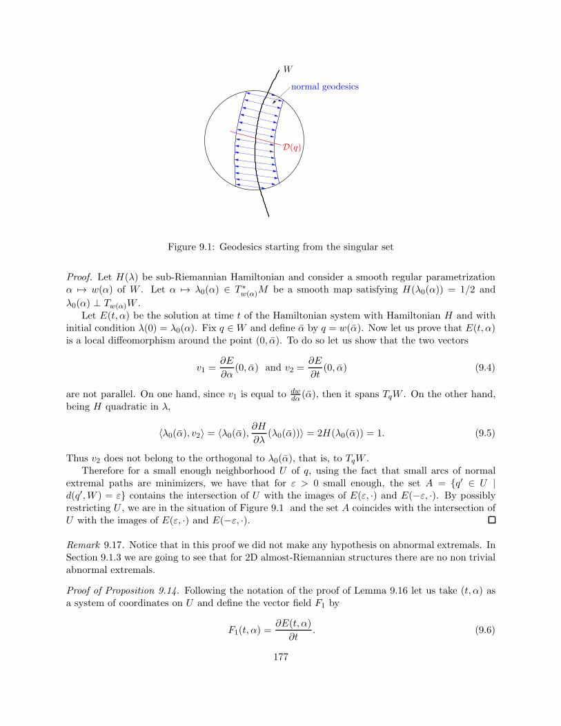
normal geodesics
W
D(q)
Figure 9.1: Geodesics starting from the singular set
Proof. Let H(λ) be sub-Riemannian Hamiltonian and consider a smooth regular parametrizationα 7→ w(α) of W . Let α 7→ λ0(α) ∈ T ∗
w(α)M be a smooth map satisfying H(λ0(α)) = 1/2 and
λ0(α) ⊥ Tw(α)W .Let E(t, α) be the solution at time t of the Hamiltonian system with Hamiltonian H and with
initial condition λ(0) = λ0(α). Fix q ∈W and define α by q = w(α). Now let us prove that E(t, α)is a local diffeomorphism around the point (0, α). To do so let us show that the two vectors
v1 =∂E
∂α(0, α) and v2 =
∂E
∂t(0, α) (9.4)
are not parallel. On one hand, since v1 is equal to dwdα (α), then it spans TqW . On the other hand,
being H quadratic in λ,
〈λ0(α), v2〉 = 〈λ0(α),∂H
∂λ(λ0(α))〉 = 2H(λ0(α)) = 1. (9.5)
Thus v2 does not belong to the orthogonal to λ0(α), that is, to TqW .Therefore for a small enough neighborhood U of q, using the fact that small arcs of normal
extremal paths are minimizers, we have that for ε > 0 small enough, the set A = q′ ∈ U |d(q′,W ) = ε contains the intersection of U with the images of E(ε, ·) and E(−ε, ·). By possiblyrestricting U , we are in the situation of Figure 9.1 and the set A coincides with the intersection ofU with the images of E(ε, ·) and E(−ε, ·).
Remark 9.17. Notice that in this proof we did not make any hypothesis on abnormal extremals. InSection 9.1.3 we are going to see that for 2D almost-Riemannian structures there are no non trivialabnormal extremals.
Proof of Proposition 9.14. Following the notation of the proof of Lemma 9.16 let us take (t, α) asa system of coordinates on U and define the vector field F1 by
F1(t, α) =∂E(t, α)
∂t. (9.6)
177
Notice that, by construction, for every q′ ∈ U the vector X(q′) belongs to D(q′) and ‖F1(q′)‖ = 1. In
the coordinates (t, α) we have F1 = (1, 0) and by construction its integral curves are geodesics. LetF2 be a vector field on U such that (F1, F2) is an orthonormal frame for the 2D almost-Riemannianstructure in U .
We claim that the first component of F2 is identically equal to zero. Indeed, were this not thecase, the norm of F1 would not be equal to one.
We are left to prove B. We have
F3 := [F1, F2] =
(0
∂x1f(x1, x2)
)(9.7)
and beside (9.7), the only brackets among F1, F2 and F3 that could be different from zero are ofthe form
[F3, . . . , [F3, F1], F1]︸ ︷︷ ︸r times
=
(0
∂rx1f(x1, x2)
).
Hence if the structure has step s at q we have ∂rx1f = 0 for r = 1, 2, . . . , s − 2 and ∂s−1x1 f 6= 0.
The form (9.2) is very useful to express the Riemannian quantities on M \ Z. Indeed one has
Lemma 9.18. Assume that on an open set Ω ⊂M a system of coordinates (x1, x2) is fixed and anorthonormal frame for the 2D-almost-Riemannian is given in the form (9.2). Then on Ω∩ (M \Z)the Riemannian metric, the element of Riemannian area and the Gaussian curvatures are given by
g(x1,x2) =
(1 00 1
f(x1,x2)2
), (9.8)
dA(x1,x2) =1
|f(x1, x2)|dx1 dx2, (9.9)
K(x1, x2) =f(x1, x2)∂
2x1f(x1, x2)− 2 (∂x1f(x1, x2))
2
f(x1, x2)2. (9.10)
Proof. Formula (9.8) is a direct consequence of (9.1). Formula (9.9) comes from the definition ofthe Riemannian area dA(F1, F2) = 1 where F1, F2 is a local orthonormal frame. Formula (9.10)comes from the formula
K(q) = −α21 − α2
2 + F1α2 − F2α1
where α1 and α2 are the two functions defined by [F1, F2] = α1F1 + α2F2 (see Corollary 4.39).
Hence in a 2D-almost-Riemannian structure all Riemannian quantities explodes while approach-ing to Z.
9.1.1 How big is the singular set?
A natural question is how big could be the singular set. The answer is given by the followingLemma.
Theorem 9.19. Consider a system of coordinates (x1, x2) defined on an open set Ω and let dx1 dx2be the corresponding Lebesgue measure. Then Z ∩ Ω has zero dx1 dx2-measure.
178
Proof. Without loss of generality we can assume that Ω has the following properties:
• it is the product of two non-empty intervals:
Ω = (xA1 , xB1 )× (xA2 , x
B2 ),
• on Ω we have an orthonormal frame of the form
F1(q) =
(10
), F2 =
(0
f(x1, x2)
), (9.11)
• on Ω the step of the structure is s ∈ N.
If some of the properties above are not satisfied, one can prove the theorem on a countable unionof sets where the properties above hold.
Let 1Z : Ω→ 0, 1 be the characteristic function of Z. Using Fubini theorem,
∫
Z∩Ωdx1dx2 =
∫
Ω1Z(x1, x2) dx1dx2 =
∫ xB2
xA2
(∫ xB1
xA1
1Z(x1, x2)dx1
)dx2.
We now prove that for every fixed x2 ∈ (xA2 , xB2 ), we have
∫ xB1xA1
1Z(x1, x2)dx1 = 0 from which the
conclusion of the theorem follows.Indeed B. of Proposition 9.14 guarantees that there exists r ≤ s− 1 such that ∂rx1f(x1, x2) 6= 0
for every x1 ∈ (xA1 , xB1 ). Hence f(·, x2) has only isolated zeros and
∫ xB1xA1
1Z(x1, x2)dx1 = 0.
Exercise 9.20. Show that from the proof of Theorem 9.19 it follows that the singular set is locallythe countable union of zero- and one-dimensional manifolds and hence that it is rectifiable.
9.1.2 Genuinely 2D-almost-Riemannian structures have always infinite area
Theorem 9.21. Let Ω be a bounded open set such that Ω ∩ Z 6= ∅. Then
diam(Ω) ≤ ∞ and
∫
Ω\ZdA =∞
where diam(Ω) is the diameter of Ω computed with respect to the almost-Riemannian distance anddA is the Riemannian area associated to the almost-Riemannian structure on Ω \ Z.
Proof. Take a a point q0 ∈ Ω \ Z and a system of coordinates (x1, x2) on a neighborhood Ω0 ⊂ Ωof q0. Expanding f in Taylor series, we have
f(x1, x2) = a1x1 + a2x2 +O(x21 + x22). (9.12)
According to (9.9), the (almost-Riemannian) area of Ω0 is∫
Ω0
1
|f(x1, x2)|dx1 dx2.
But the inverse of a function of the form (9.12) is never integrable around the origin in the plane.
179
9.1.3 Geodesics
Since 2D almost Riemannian structures are particular cases of sub-Riemannian structures, thereare two kind of candidate optimal trajectories: normal and abnormal extremals. Normal extremalsare geodesics while abnormal extremals could or could not be geodesics. An important fact is thefollowing.
Theorem 9.22. For a 2D-almost-Riemannian strucutre, all abnormal extremal are trivial. More-over a trivial trajectory γ : [a, b] → M , γ(t) = q0 is the projection of an abnormal extremal if andonly if q0 ∈ Z.
Proof. It is immediate to verify that if γ(t) = q0 ∈ Z for every t ∈ [a, b] then γ admits an abnormallift.
Let γ : [a, b] → M , (a < b) be the projection of an abnormal extremal and let us prove thatγ([a, b]) = q0 for some q0 ∈ Z.
Let us first prove that γ([a, b]) ⊂ Z. By contradiction assume that there exists t ∈]a, b[ such thatγ(t) /∈ Z. By continuity there exists a non trivial interval [c, d] ⊂]a, b[ such that γ([c, d]) ∩ Z = ∅.Then γ[c,d] is a Riemannian geodesic and hence cannot be abnormal. Recall that if an arc of ageodesic is not abnormal, then the geodesic if not abnormal too, hence it follows that γ is notabnormal. This contradicts the hypothesis that γ is the projection of an abnormal extremal.
Let us fix a local system of coordinates such that an orthonormal frame is given in the form(9.2). If this is not possible globally on a neighborhood of γ([a, b]), one can repeat the proof ondifferent coordinate charts.
Let us write in coordinates γ(t) = (γ1(t), γ2(t)). We have different cases.
• If (γ1(t), γ2(t)) = (c1, c2) for every t ∈ [a, b] we already know that γ admits an abnormal lift.
• If γ1 is not constant and γ2 = c in [a, b], then γ2 = 0 in [a, b] and Z contains a set of the type
Z = (x1, c) | x1 ∈ [xA1 , xB1 ] with xA1 < xB1 .
Hence f = 0 on Z . It follows that ∂rx1f = 0 on Z for every r = 1, 2, . . .. As in the proofof Theorem 9.19 it follows that all brackets between F1 and F2 are zero on Z and that thebracket generating condition is violated. Hence this case is not possible.
• There exists t ∈]a, b[ such that γ2(t) is defined and γ2(t) 6= 0. Now since
γ(t) =
(v1
v2f(γ(t))
),
for some v1, v2 ∈ R, we have f(γ(t)) 6= 0 and hence γ(t) /∈ Z violating the condition γ([a, b]) ⊂Z for an abnormal extremal. Hence also this case is not possible.
Hence all non-trivial geodesics are normal and are projection on M of the solution of theHamiltonian system whose Hamiltonian is (cf. (4.30))
H : T ∗M → R, H(λ) = maxu∈Uq
(〈λ, f(q, u)〉 − 1
2|u|2), q = π(λ). (9.13)
180
Locally, if an orthonormal frame F1, F2 is assigned, we have
H(λ) =1
2
(〈λ, F1(q)〉2 + 〈λ, F2(q)〉2
).
For a system of coordinates and a choice of an orthonormal frame as those of Proposition 9.14, wehave
H(x1, x2, p1, p2) =1
2
(p21 + p22 f(x1, x2)
2). (9.14)
As a consequence of the fact that all geodesics are projections of solutions of a smooth Hamiltoniansystem and that our structure is Riemannian on M \ Z, we have
Proposition 9.23. In 2D almost-Riemannian geometry all geodesics are smooth and they coincidewith Riemannian geodesics on M \ Z.
The only particular property of geodesics in almost-Riemannian geometry is that on the singularset their velocity is constrained to belong to the distribution (otherwise their length could not befinite). All this is illustrated in the next section for the Grushin plane.
9.2 The Grushin plane
The Grushin plane is the simplest example of genuinely almost-Riemannian structure. It is the freealmost-Riemannain structure on R
2 for which a global orthonormal frame is given by
F1 =
(10
), F2 =
(0x1
)
In the sense of Definition 9.1, it can be seen as the pair (U, f) where U = R2 × R
2 andf((x1, x2), (u1, u2)) = ((x1, x2), (u1, u2x1)).
Here the singular set Z is the x2 axis and on R2 \ Z the Riemannian metric, the Riemannian
area and the Gaussian curvature are given respectively by:
g =
(1 00 1
x21
), dA =
1
|x1|dx1 dx2, K = − 2
x21. (9.15)
Notice that the (almost-Riemannian) area of an open set intersecting the x2 axis is always infinite.
9.2.1 Geodesics of the Grushin plane
In this section we recall how to compute the geodesics for the Grushin plane, with the purpose ofstressing that they can cross the singular set with no singularities.
In this case the Hamiltonian (9.14) is given by
H(x1, x2, p1, p2) =1
2(p21 + x21p
22) (9.16)
and the corresponding Hamiltonian equations are:
x1 = p1, p1 = −x1p22x2 = x21p2, p2 = 0 (9.17)
181
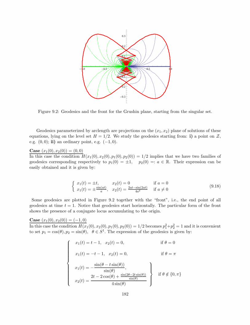
-1.0 -0.5 0.5 1.0
-0.3
-0.2
-0.1
0.1
0.2
0.3
Figure 9.2: Geodesics and the front for the Grushin plane, starting from the singular set.
Geodesics parameterized by arclength are projections on the (x1, x2) plane of solutions of theseequations, lying on the level set H = 1/2. We study the geodesics starting from: i) a point on Z,e.g. (0, 0); ii) an ordinary point, e.g. (−1, 0).
Case (x1(0), x2(0)) = (0, 0)In this case the condition H(x1(0), x2(0), p1(0), p2(0)) = 1/2 implies that we have two families ofgeodesics corresponding respectively to p1(0) = ±1, p2(0) =: a ∈ R. Their expression can beeasily obtained and it is given by:
x1(t) = ±t, x2(t) = 0 if a = 0
x1(t) = ± sin(at)a , x2(t) =
2at−sin(2at)4a2
if a 6= 0(9.18)
Some geodesics are plotted in Figure 9.2 together with the “front”, i.e., the end point of allgeodesics at time t = 1. Notice that geodesics start horizontally. The particular form of the frontshows the presence of a conjugate locus accumulating to the origin.
Case (x1(0), x2(0)) = (−1, 0)In this case the conditionH(x1(0), x2(0), p1(0), p2(0)) = 1/2 becomes p21+p
22 = 1 and it is convenient
to set p1 = cos(θ), p2 = sin(θ), θ ∈ S1. The expression of the geodesics is given by:
x1(t) = t− 1, x2(t) = 0, if θ = 0
x1(t) = −t− 1, x2(t) = 0, if θ = π
x1(t) = −sin(θ − t sin(θ))
sin(θ),
x2(t) =2t− 2 cos(θ) + sin(2θ−2t sin(θ))
sin(θ)
4 sin(θ)
if θ /∈ 0, π
182
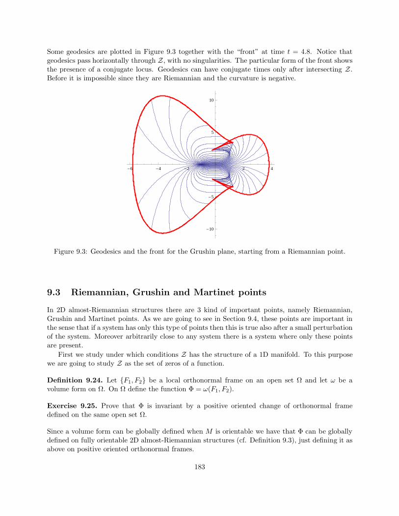
Some geodesics are plotted in Figure 9.3 together with the “front” at time t = 4.8. Notice thatgeodesics pass horizontally through Z, with no singularities. The particular form of the front showsthe presence of a conjugate locus. Geodesics can have conjugate times only after intersecting Z.Before it is impossible since they are Riemannian and the curvature is negative.
-6 -4 -2 2 4
-10
-5
5
10
Figure 9.3: Geodesics and the front for the Grushin plane, starting from a Riemannian point.
9.3 Riemannian, Grushin and Martinet points
In 2D almost-Riemannian structures there are 3 kind of important points, namely Riemannian,Grushin and Martinet points. As we are going to see in Section 9.4, these points are important inthe sense that if a system has only this type of points then this is true also after a small perturbationof the system. Moreover arbitrarily close to any system there is a system where only these pointsare present.
First we study under which conditions Z has the structure of a 1D manifold. To this purposewe are going to study Z as the set of zeros of a function.
Definition 9.24. Let F1, F2 be a local orthonormal frame on an open set Ω and let ω be avolume form on Ω. On Ω define the function Φ = ω(F1, F2).
Exercise 9.25. Prove that Φ is invariant by a positive oriented change of orthonormal framedefined on the same open set Ω.
Since a volume form can be globally defined when M is orientable we have that Φ can be globallydefined on fully orientable 2D almost-Riemannian structures (cf. Definition 9.3), just defining it asabove on positive oriented orthonormal frames.
183
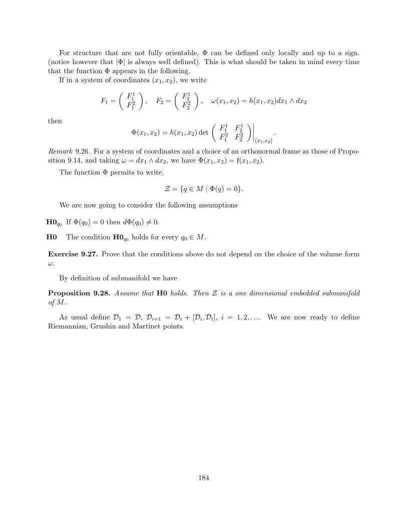
For structure that are not fully orientable, Φ can be defined only locally and up to a sign.(notice however that |Φ| is always well defined). This is what should be taken in mind every timethat the function Φ appears in the following.
If in a system of coordinates (x1, x2), we write
F1 =
(F 11
F 21
), F2 =
(F 12
F 22
), ω(x1, x2) = h(x1, x2)dx1 ∧ dx2
then
Φ(x1, x2) = h(x1, x2) det
(F 11 F 1
2
F 21 F 2
2
)∣∣∣∣(x1,x2)
.
Remark 9.26. For a system of coordinates and a choice of an orthonormal frame as those of Propo-sition 9.14, and taking ω = dx1 ∧ dx2, we have Φ(x1, x2) = f(x1, x2).
The function Φ permits to write,
Z = q ∈M | Φ(q) = 0.
We are now going to consider the following assumptions
H0q0 If Φ(q0) = 0 then dΦ(q0) 6= 0.
H0 The condition H0q0 holds for every q0 ∈M .
Exercise 9.27. Prove that the conditions above do not depend on the choice of the volume formω.
By definition of submanifold we have
Proposition 9.28. Assume that H0 holds. Then Z is a one dimensional embedded submanifoldof M .
As usual define D1 = D, Di+1 = Di + [Di,Di], i = 1, 2, . . .. We are now ready to defineRiemannian, Grushin and Martinet points.
184
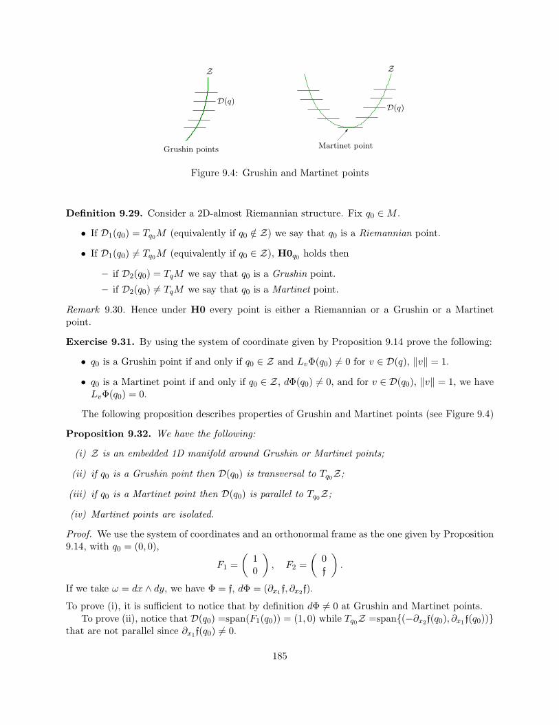
ZZ
D(q)
Grushin points Martinet point
D(q)
Figure 9.4: Grushin and Martinet points
Definition 9.29. Consider a 2D-almost Riemannian structure. Fix q0 ∈M .
• If D1(q0) = Tq0M (equivalently if q0 /∈ Z) we say that q0 is a Riemannian point.
• If D1(q0) 6= Tq0M (equivalently if q0 ∈ Z), H0q0 holds then
– if D2(q0) = TqM we say that q0 is a Grushin point.
– if D2(q0) 6= TqM we say that q0 is a Martinet point.
Remark 9.30. Hence under H0 every point is either a Riemannian or a Grushin or a Martinetpoint.
Exercise 9.31. By using the system of coordinate given by Proposition 9.14 prove the following:
• q0 is a Grushin point if and only if q0 ∈ Z and LvΦ(q0) 6= 0 for v ∈ D(q), ‖v‖ = 1.
• q0 is a Martinet point if and only if q0 ∈ Z, dΦ(q0) 6= 0, and for v ∈ D(q0), ‖v‖ = 1, we haveLvΦ(q0) = 0.
The following proposition describes properties of Grushin and Martinet points (see Figure 9.4)
Proposition 9.32. We have the following:
(i) Z is an embedded 1D manifold around Grushin or Martinet points;
(ii) if q0 is a Grushin point then D(q0) is transversal to Tq0Z;
(iii) if q0 is a Martinet point then D(q0) is parallel to Tq0Z;
(iv) Martinet points are isolated.
Proof. We use the system of coordinates and an orthonormal frame as the one given by Proposition9.14, with q0 = (0, 0),
F1 =
(10
), F2 =
(0f
).
If we take ω = dx ∧ dy, we have Φ = f, dΦ = (∂x1 f, ∂x2f).
To prove (i), it is sufficient to notice that by definition dΦ 6= 0 at Grushin and Martinet points.To prove (ii), notice that D(q0) =span(F1(q0)) = (1, 0) while Tq0Z =span(−∂x2f(q0), ∂x1 f(q0))
that are not parallel since ∂x1f(q0) 6= 0.
185
To prove (iii), notice that D(q0) =span(F1(q0)) = (1, 0) while Tq0Z =span(−∂x2f, 0) since thecondition D2(q0) 6= Tq0M implies ∂x1f(q0) = 0.
To prove (iv), simply observe that if Martinet points were accumulating at q0 then at that pointwe cold not have ∂s−1
x1 f 6= 0, where s is the step of the structure at q0.
Examples
• All points on the x2 axis for the Grushin plane are Grushin points.
• The origin the following structure is the simplest example of Martinet point
F1 =
(10
), F2 =
(0
x2 − x21
).
• The origin for the following example
F1 =
(10
)and F2 =
(0
x22 − x21
),
is not a Martinet point since the condition dΦ(0, 0) 6= 0 is not satisfied. Outside the originall points are either Riemannian or Grushin points, but at the origin Z is not a manifold.
• The x2 axis of the following example
F1 =
(10
)and F2 =
(0x21
),
is not made by Grushin points since D2((0, x2)) 6= T(0,x2)M and it is not made by Martinetpoints since dΦ(0, x2) 6= 0 is not satisfied (althugh in this case Z is a manifold). In this caseD(0, x2)) is transversal to Z.
Proposition 9.33. Let q0 be a Riemannian, Grushin or a Martinet point. There exists a neigh-borhood Ω of q0 and a system of coordinates (x1, x2) in Ω such that an orthonormal frame for the2D-almost-Riemannian structure can be written in Ω as:
(NF1) if q0 is a Riemannian point, then
F1(x1, x2) = (1, 0), F2(x1, x2) = (0, eφ(x1,x2)),
(NF2) if q0 is a Grushin point, then
F1(x1, x2) = (1, 0), F2(x1, x2) = (0, xeφ(x1,x2))
(NF3) if q0 is a Martinet point, then
F1(x1, x2) = (1, 0), F2(x1, x2) = (0, (x2 − xs−11 ψ(x))eξ(x1,x2)),
where φ, ξ and ψ are smooth real-valued functions such that φ(0, x2) = 0 and ψ(0) 6= 0. Moreovers ≥ 2 is an integer, that is the step of the structure at the Martinet point.
186
9.4 Generic 2D-almost-Riemannian structures
Recall hypothesis H0q0 and H0:
H0q0 If Φ(q0) = 0 then dΦ(q0) 6= 0.
H0 The condition H0q0 holds for every q0 ∈M .
Recall the H0 is independent from the volume form used to define the function Φ. We haveseen (cf. Remark 9.30) that under hypothesis H0 every point is either a Riemannian or a Grushinor a Martinet point.
In this section we are going to prove that hypothesis H0 holds for most of the systems. Moreprecisely we are going to prove that hypothesis H0 is generic in the following sense.
Definition 9.34. Fix a rank 2 Euclidean bundle U over a 2D compact manifold M . Let F be theset of all morphism of bundle from U to TM such that (U, f), f ∈ F is a 2D almost-Riemannianstructure. Endowed F with the C1 norm. We say that a subset of F is generic if it is open anddense in F.
Theorem 9.35. Under the same hypothesis of Definition 9.34, let F ⊂ F the subset of morphismssatisfying H0. Then F is generic.
Remark 9.36. In Theorem 9.35 we have assumed that M is compact. A similar result holds alsoin the case in which M is not compact. However, in the non compact case, one gets that F isa countable union of open and dense subsets of F and one should use a suitable topology (theWhitney one). In this book we have decided not to enter inside transversality theory and we haveprovided a statement that can be proved easily via the Sard lemma.
9.4.1 Proof of the genericity result
Since the map that to f : U→ TM associate Φ :M → R is continuous in the C1 topology, a smallperturbation of f will provocate a small perturbation of Φ. Fixed q0, condition H0q0 is clearlyopen in the set of maps from M to R for the C1 topology. As a consequence, since the manifold iscompact, condition H0 is open as well.
We are now going to prove that H0 is dense. To this purpose we consider an almost Riemannianstructure (U, f) over M with the corresponding function Φ and we construct an arbitrarily smallperturbation (in the C1 norm) of f for which H0 is satisfied.
Fix a finite number of points points q1, . . . , qr in such a way that
• the structure is Riemannian in a neighborhood Ω of q1, . . . , qr;
• if we consider another open set Ω0 compacly contained in Ω, the structure (U, f) when
restricted toM := int(M \Ω0) is free (cf. Remark 9.9 and Exercise 9.10); In the following we
call (U, f)| M
this structure.
For every ε ∈ R with |ε| small enough, consider a perturbation fε of f such that:
• ‖f − fε‖C1 ≤ Cε (for some C > 0 independent from ε);
• the corresponding function Φε satisfies:
187
(A) onM we have Φε = Φ+ ε;
(B) on Ω0, where the structure is Riemannian, we do not add any non-Riemannian point.
The difficult point is to realize (A). This can be done thanks to Lemma 9.37 below. Once thatthis is done, (B) can be easily realized since the perturbation fε is small in the C1 norm and theproperty of having only Riemannian points is open.
Let now apply the Sard Lemma to the C∞ function Φ| M. We have that the set
c ∈ R such that there exists q ∈M such that Φ(q) = c and dΦ(q) = 0
has measure zero. As a consequence, since Φε = Φ+ ε, we have that the set
ε ∈ R such that there exists q ∈M such that Φε(q) = 0 and dΦε(q) = 0
has measure zero. It follows that for almost every ε condition H0 is realized for fε.
To conclude the proof we have to show that (A) can be realized. This can be done thanks tothe following Lemma.
Lemma 9.37. For every ε ∈ R with |ε| small enough there exists a perturbation fε of f such that
‖f − fε‖C1 ≤ Cε (for some C > 0 independent from ε) and onM we have Φε = Φ+ ε;
Proof. Let σ be a never vanishing section of (U, f) restricted toM of unitary norm.
Let σ⊥ the orthogonal section to σ i.e. satisfying (σ |σ⊥)q = 0 and (σ⊥ |σ⊥)q = 1. A globalorthonormal frame for the structure is (F,F⊥) := (f σ, f σ⊥).
Let us first assume that F is never vanishing.
CoverM with a finite number of coordinate neighborhood Ui, i = 1 . . . N , and in each Ui,
construct coordinates (xi1, xi2) in such a way that F is represented by:
Fi(xi1, x
i2) =
(10
). (9.19)
In other words we use coordinates where F is rectified. In these coordinates
F⊥i (xi1, x
i2) =
(ai(x
i1, x
i2)
bi(xi1, x
i2)
).
Notice that to have that (9.19) holds in every coordinate chart, the only admitted change ofcoordinates have the form
xj1 = xi1 + αji(xi2), (9.20)
xj2 = βji(xi2). (9.21)
The Jacobian of each change of coordinates has then the form
(1 α′
ji
0 β′ji
).
188

In each coordinate chart we have that ω is represented by
hi(xi1, x
i2)dx
i1 ∧ dxi2.
Hence Φ = ω(F,F⊥) is represented by
hi(xi1, x
i2)bi(x
i1, x
i2)
Consider now a perturbation F⊥ε of F⊥ that in each coordinate chart is
F⊥εi (xi1, x
i2) =
(ai(x
i1, x
i2)
bi(xi1, x
i2) +
εhi(xi1,x
i2)
). (9.22)
Notice that equation (9.22) defines F⊥ε globally. Indeed for a change of coordinates of the type(9.20), (9.21) we have that
bj = β′jibi, and hj = β′−1ji hi.
It follows that in each coordinate chart ω(F,F⊥ε) is represented by
hi(xi1, x
i2)
(bi(x
i1, x
i2) +
ε
hi(xi1, x
i2)
)= hi(x
i1, x
i2)bi(x
i1, x
i2) + ε
Since this is true in each coordinate chart, we have that
Φε = ω(F,F⊥ε) = Φ+ ε.
Notice that by construction F⊥ε is close to F⊥ in the C1 norm and hence this is true also for f andfε.
In the case in which F has some zeros .........
9.5 A Gauss-Bonnet theorem
For an compact orientable 2D-Riemannian manifold, the Gauss-Bonnet theorem asserts that theintegral of the curvature is a topological invariant that is the Euler characteristic of the manifold(see Section 1.3).
This theorem admit an interesting generalization in the context of 2D almost-Riemannian struc-tures that are fully orientable. This generalization is not trivial since one needs to integrate theGaussian curvature (that in general is diverging while approaching to the singular set) on themanifold (that has always infinite volume).
This generalization holds under certain natural assumptions on the 2D almost-Riemannianstructure, namely we will assume
HG : The base manifold M is compact. The 2D almost-Riemannian structure is fully orientable,H0 holds and every point of Z is a Grushin point.
The hypotheses that the structure is fully orientable is crucial and it is the almost-Riemannianversion of the classical orientability hypothesis that one need in Riemannian geometry. Thehypothesis H0 is the basic hypothesis to have a reasonable description of the asymptotics of K ina neighborhood of Z. The hypotesis that every point is a Grushin point is a technical hypothesis.A version of a Gauss Bonnet Theorem in presence of Martinet points can also be written, but ismore technical and outside the purpose of this book.
With an argument similar to the one of the beginning of Section 9.4.1, one get
189
Theorem 9.38. Hypothesis HG is open in the set of smooth map f : U→ TM endowed with C1topology:
Clearly hypothesis HG is not dense since Martinet points do not disappear for small C1 per-turbations of the system.
It is important to notice that HG is not empty. Indeed we have
Lemma 9.39. Every oriented compact surface can be endowed with an oriented almost-Riemannianstructure satisfying the requirement that there are no Martinet points.
We are going to prove Lemma 9.39 in Section 9.5.2.
Definition 9.40. Consider a 2D almost-Riemannian structure (U, f) over a 2D manifold M andassume that HG holds.
Let ν a volume form for the Euclidean structure on U, i.e. a never vanishing 2-form s.t.ν(σ1, σ2) = 1 on every positive oriented local orthonormal frame for (· | ·)q . Let Ξ be an orientationon M . We define:
• The signed area form dAs on M as the two-form on M \ Z given by the pushforward of νalong f . Notice that the Riemannian area dA on M \ Z is the density associated to thevolume form dAs.
• M+ = q ∈M \ Z, s.t. the orientation given by dAsq and Ξq are the same .1
• M− = q ∈M \ Z, s.t. the orientation given by dAsq and Ξq are opposite .
Notice that given a measurable function h : Ω ⊂M± \ Z → R, we have
∫
Ωh dAs = ±
∫
Ωh dA (if it exists). (9.23)
Definition 9.41. Under the same hypotheses of Definition 9.40, define
• Mε = q ∈M | d(q,Z) > ε where d(·, ·) is the 2D-almost-Riemannian structure on M .
• M±ε =Mε ∩M±
• Given a measurable function h :M \ Z → R, we say that it is AR-integrable if
limε→0
∫
Mε
h dAs (9.24)
exists and is finite. In this case we denote such a limit by∫hdAs.
Remark 9.42. Notice that (9.24) is equivalent to
limε→0
(∫
M+ε
h dA−∫
M−ε
h dA
)
1i.e. dAsq(F1, F2) = αΞ(F1, F2) with α > 0
190
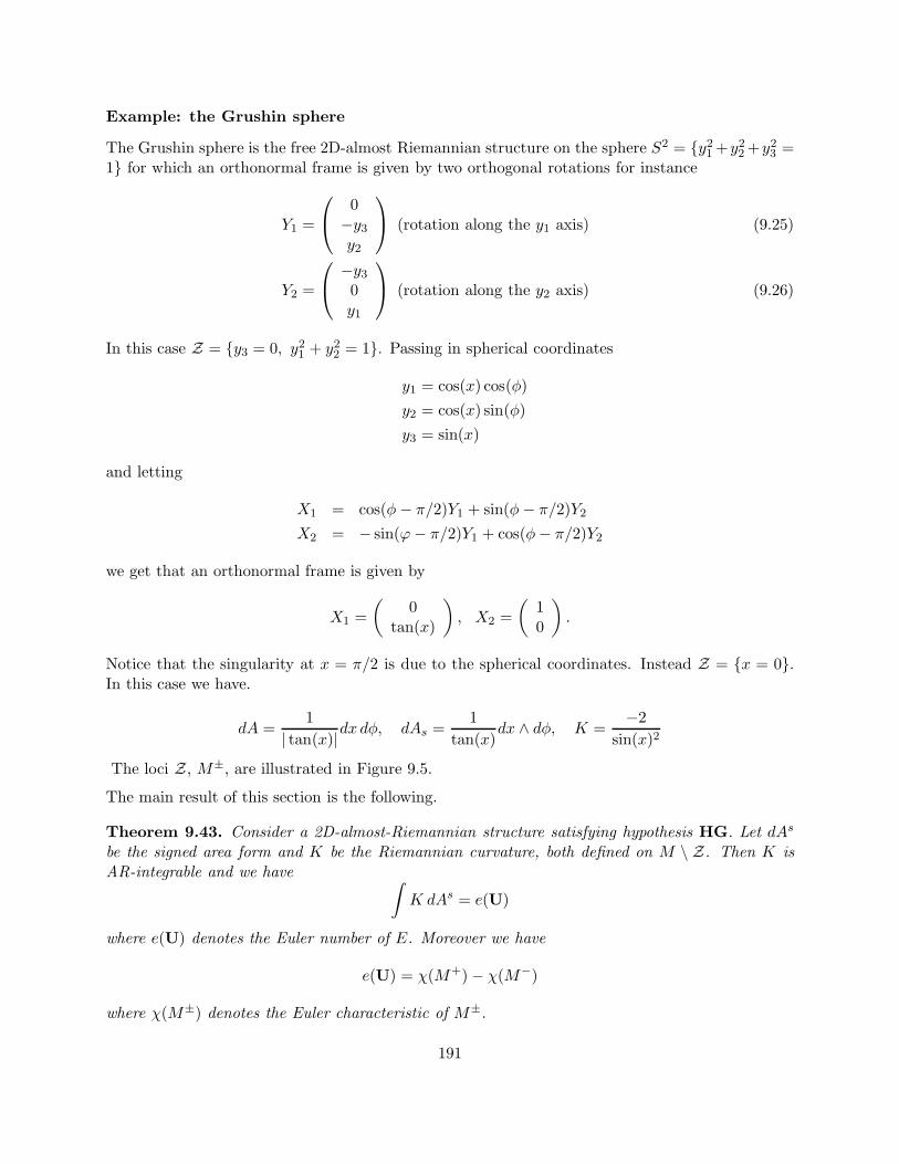
Example: the Grushin sphere
The Grushin sphere is the free 2D-almost Riemannian structure on the sphere S2 = y21+y22+y23 =1 for which an orthonormal frame is given by two orthogonal rotations for instance
Y1 =
0−y3y2
(rotation along the y1 axis) (9.25)
Y2 =
−y30y1
(rotation along the y2 axis) (9.26)
In this case Z = y3 = 0, y21 + y22 = 1. Passing in spherical coordinates
y1 = cos(x) cos(φ)
y2 = cos(x) sin(φ)
y3 = sin(x)
and letting
X1 = cos(φ− π/2)Y1 + sin(φ− π/2)Y2X2 = − sin(ϕ− π/2)Y1 + cos(φ− π/2)Y2
we get that an orthonormal frame is given by
X1 =
(0
tan(x)
), X2 =
(10
).
Notice that the singularity at x = π/2 is due to the spherical coordinates. Instead Z = x = 0.In this case we have.
dA =1
| tan(x)|dx dφ, dAs =1
tan(x)dx ∧ dφ, K =
−2sin(x)2
The loci Z, M±, are illustrated in Figure 9.5.
The main result of this section is the following.
Theorem 9.43. Consider a 2D-almost-Riemannian structure satisfying hypothesis HG. Let dAs
be the signed area form and K be the Riemannian curvature, both defined on M \ Z. Then K isAR-integrable and we have ∫
K dAs = e(U)
where e(U) denotes the Euler number of E. Moreover we have
e(U) = χ(M+)− χ(M−)
where χ(M±) denotes the Euler characteristic of M±.
191
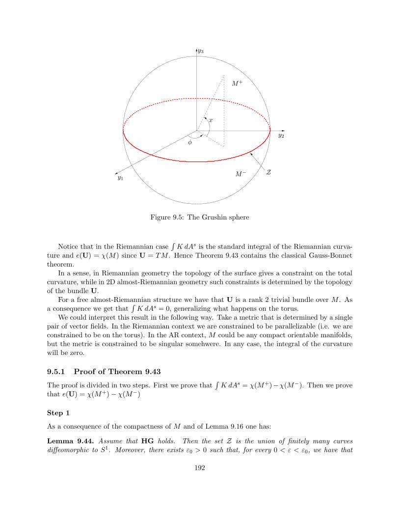
M−
y3
y2
y1Z
φ
x
M+
Figure 9.5: The Grushin sphere
Notice that in the Riemannian case∫K dAs is the standard integral of the Riemannian curva-
ture and e(U) = χ(M) since U = TM . Hence Theorem 9.43 contains the classical Gauss-Bonnettheorem.
In a sense, in Riemannian geometry the topology of the surface gives a constraint on the totalcurvature, while in 2D almost-Riemannian geometry such constraints is determined by the topologyof the bundle U.
For a free almost-Riemannian structure we have that U is a rank 2 trivial bundle over M . Asa consequence we get that
∫K dAs = 0, generalizing what happens on the torus.
We could interpret this result in the following way. Take a metric that is determined by a singlepair of vector fields. In the Riemannian context we are constrained to be parallelizable (i.e. we areconstrained to be on the torus). In the AR context, M could be any compact orientable manifolds,but the metric is constrained to be singular somehwere. In any case, the integral of the curvaturewill be zero.
9.5.1 Proof of Theorem 9.43
The proof is divided in two steps. First we prove that∫K dAs = χ(M+)−χ(M−). Then we prove
that e(U) = χ(M+)− χ(M−)
Step 1
As a consequence of the compactness of M and of Lemma 9.16 one has:
Lemma 9.44. Assume that HG holds. Then the set Z is the union of finitely many curvesdiffeomorphic to S1. Moreover, there exists ε0 > 0 such that, for every 0 < ε < ε0, we have that
192
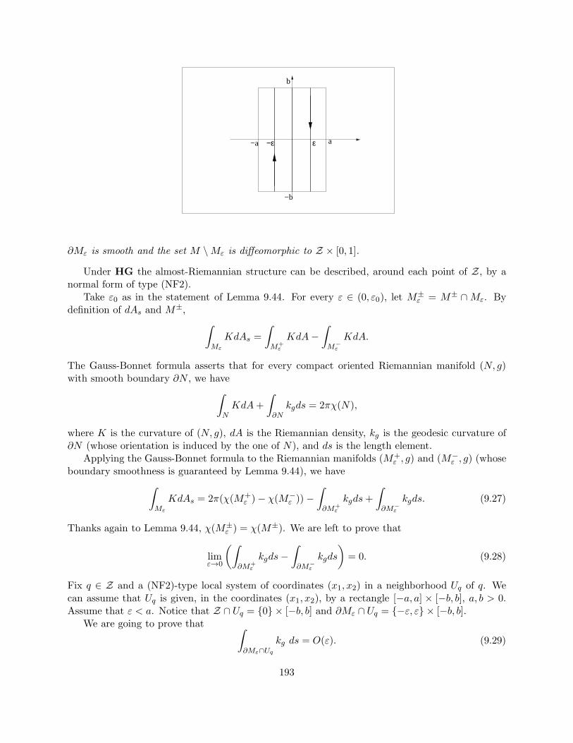
−b
b
ε a−ε−a
∂Mε is smooth and the set M \Mε is diffeomorphic to Z × [0, 1].
Under HG the almost-Riemannian structure can be described, around each point of Z, by anormal form of type (NF2).
Take ε0 as in the statement of Lemma 9.44. For every ε ∈ (0, ε0), let M±ε = M± ∩Mε. By
definition of dAs and M±,
∫
Mε
KdAs =
∫
M+ε
KdA−∫
M−ε
KdA.
The Gauss-Bonnet formula asserts that for every compact oriented Riemannian manifold (N, g)with smooth boundary ∂N , we have
∫
NKdA+
∫
∂Nkgds = 2πχ(N),
where K is the curvature of (N, g), dA is the Riemannian density, kg is the geodesic curvature of∂N (whose orientation is induced by the one of N), and ds is the length element.
Applying the Gauss-Bonnet formula to the Riemannian manifolds (M+ε , g) and (M−
ε , g) (whoseboundary smoothness is guaranteed by Lemma 9.44), we have
∫
Mε
KdAs = 2π(χ(M+ε )− χ(M−
ε ))−∫
∂M+ε
kgds+
∫
∂M−ε
kgds. (9.27)
Thanks again to Lemma 9.44, χ(M±ε ) = χ(M±). We are left to prove that
limε→0
(∫
∂M+ε
kgds−∫
∂M−ε
kgds
)= 0. (9.28)
Fix q ∈ Z and a (NF2)-type local system of coordinates (x1, x2) in a neighborhood Uq of q. Wecan assume that Uq is given, in the coordinates (x1, x2), by a rectangle [−a, a] × [−b, b], a, b > 0.Assume that ε < a. Notice that Z ∩ Uq = 0 × [−b, b] and ∂Mε ∩ Uq = −ε, ε × [−b, b].
We are going to prove that ∫
∂Mε∩Uq
kg ds = O(ε). (9.29)
193
Then (9.28) follows from the compactness of Z. (Indeed, −ε × [−b, b] and ε × [−b, b], thehorizontal edges of ∂Uq, are geodesics minimizing the length from Z. Therefore, Z can be coveredby a finite number of neighborhoods of type Uq whose pairwise intersections have empty interior.)
Without loss of generality, we can assume thatM+∩Uq = (0, a]×[−b, b]. Therefore,M+ε induces
on ∂M+ε = ε× [−b, b] a downwards orientation (see Figure 9.5.1). The curve s 7→ c(s) = (ε, x2(s))
satisfyingc(s) = −F2(c(s)) , c(0) = (ε, 0) ,
is an oriented parametrization by arclength of ∂M+ε , making a constant angle with F1. Let (θ1, θ2)
be the dual basis to (F1, F2) on Uq ∩M+, i.e., θ1 = dx1 and θ2 = x−11 e−φ(x1,x2)dx2. According to
[?, Corollary 3, p. 389, Vol. III], the geodesic curvature of ∂M+ε at c(s) is equal to λ(c(s)), where
λ ∈ Λ1(Uq) is the unique one-form satisfying
dθ1 = λ ∧ θ2 , dθ2 = −λ ∧ θ1 .
A trivial computation shows that
λ = ∂x1(x−11 e−φ(x1,x2))dx2 .
Thus,
kg(c(s)) = −∂x1(x−11 e−φ(c(s))) (dx2(F2))(c(s)) =
1
ε+ ∂x1φ(ε, x2(s)) .
Denote by L1 and L2 the lengths of, respectively, ε × [0, b] and ε × [−b, 0]. Then,∫
∂M+ε ∩Uq
kgds =
∫ L2
−L1
kg(c(s))ds
=
∫ L2
−L1
(1
ε+ ∂x1φ(ε, (s))
)ds
=
∫ b
−b
(1
ε+ ∂x1φ(ε, x2)
)1
εeφ(ε,x2)dx2 ,
where the last equality is obtained taking x2 = x2(−s) as the new variable of integration.We reason similarly on ∂M−
ε ∩Uq, on whichM−ε induces the upwards orientation. An orthonor-
mal frame on M− ∩ Uq, oriented consistently with M , is given by (F1,−F2), whose dual basis is(θ1,−θ2). The same computations as above lead to
∫
∂M−ε ∩Uq
kgds =
∫ b
−b
(1
ε− ∂x1φ(−ε, x2)
)1
εeφ(−ε,x2)dx2 .
DefineF (ε, x2) = (1 + ε∂x1φ(ε, x2))e
−φ(ε,x2). (9.30)
Then ∫
∂M+ε ∩Uq
kgds−∫
∂M−ε ∩Uq
kgds =1
ε2
∫ b
−b(F (ε, x2)− F (−ε, x2)) dx2.
By Taylor expansion with respect to ε we get
F (ε, x2)− F (−ε, x2) = 2∂εF (0, x2)ε+O(ε3) = O(ε3)
194
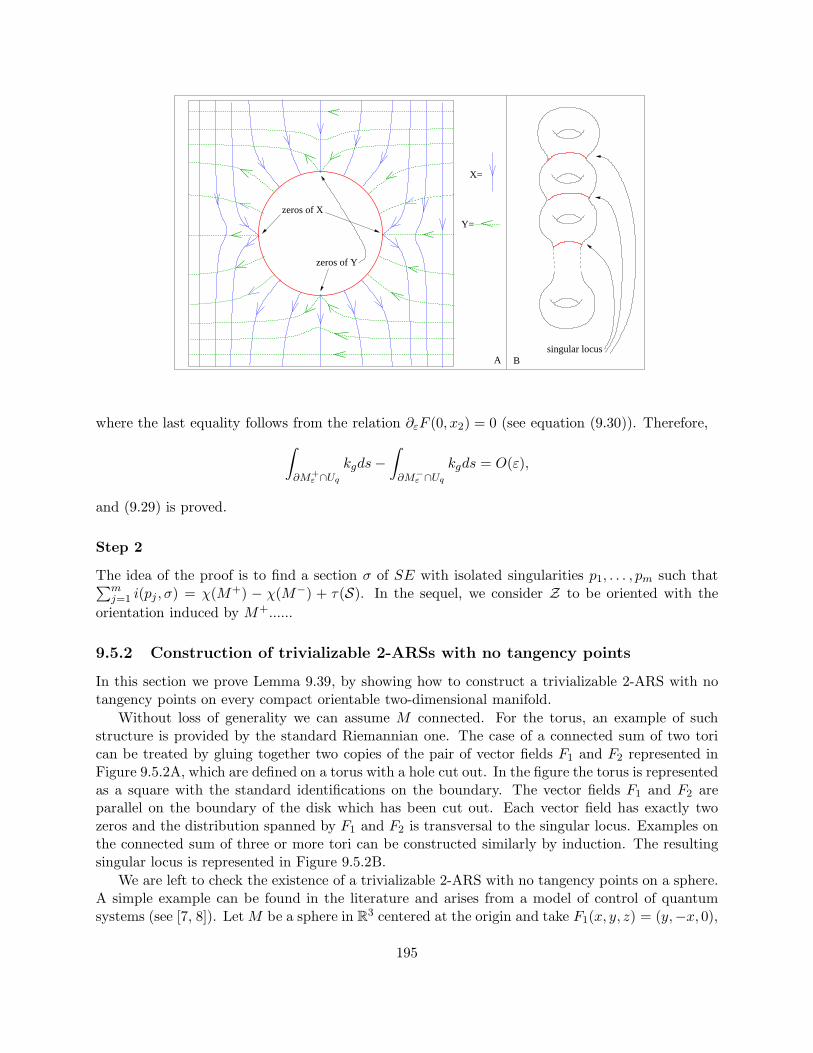
X=
zeros of X
zeros of Y
Y=
singular locusBA
where the last equality follows from the relation ∂εF (0, x2) = 0 (see equation (9.30)). Therefore,
∫
∂M+ε ∩Uq
kgds−∫
∂M−ε ∩Uq
kgds = O(ε),
and (9.29) is proved.
Step 2
The idea of the proof is to find a section σ of SE with isolated singularities p1, . . . , pm such that∑mj=1 i(pj , σ) = χ(M+) − χ(M−) + τ(S). In the sequel, we consider Z to be oriented with the
orientation induced by M+......
9.5.2 Construction of trivializable 2-ARSs with no tangency points
In this section we prove Lemma 9.39, by showing how to construct a trivializable 2-ARS with notangency points on every compact orientable two-dimensional manifold.
Without loss of generality we can assume M connected. For the torus, an example of suchstructure is provided by the standard Riemannian one. The case of a connected sum of two torican be treated by gluing together two copies of the pair of vector fields F1 and F2 represented inFigure 9.5.2A, which are defined on a torus with a hole cut out. In the figure the torus is representedas a square with the standard identifications on the boundary. The vector fields F1 and F2 areparallel on the boundary of the disk which has been cut out. Each vector field has exactly twozeros and the distribution spanned by F1 and F2 is transversal to the singular locus. Examples onthe connected sum of three or more tori can be constructed similarly by induction. The resultingsingular locus is represented in Figure 9.5.2B.
We are left to check the existence of a trivializable 2-ARS with no tangency points on a sphere.A simple example can be found in the literature and arises from a model of control of quantumsystems (see [7, 8]). LetM be a sphere in R
3 centered at the origin and take F1(x, y, z) = (y,−x, 0),
195
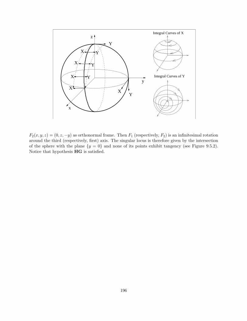
Integral Curves of X
Integral Curves of Y
z
x
y
Y
XY
Y
Y
Y
X
X
X
X
F2(x, y, z) = (0, z,−y) as orthonormal frame. Then F1 (respectively, F2) is an infinitesimal rotationaround the third (respectively, first) axis. The singular locus is therefore given by the intersectionof the sphere with the plane y = 0 and none of its points exhibit tangency (see Figure 9.5.2).Notice that hypothesis HG is satisfied.
196
Chapter 10
Nonholonomic tangent space
In this chapter, for a point q ∈ M , the symbol Ωq denotes the set of smooth curves γ on M thatare based at q, that is γ(0) = q.
10.1 Jet spaces
Fix q in M and a curve γ ∈ Ωq. In every coordinate chart it is meaningful to write the Taylorexpansion
γ(t) = q + γ(0)t +O(t2) (10.1)
The tangent vector v ∈ TqM to γ at t = 0 is by definition the equivalence class of curves in Ωq suchthat, in some coordinate chart, they have the same 1-st order Taylor polynomial. (This requirementindeed implies that the same is true for every coordinate chart, by the chain rule.)
In the same spirit we can consider, given a smooth curve such that γ(0) = q, its m-th orderTaylor polynomial at q
γ(t) = q + γ(0)t+ γ(0)t2
2+ . . .+ γ(m)(0)
tm
m!+O(tm+1) (10.2)
Exercise 10.1. Let γ, γ′ ∈ Ωq. We say that γ is (m-)equivalent to γ′ at q, and we write γ ∼q,m γ′,if their Taylor polynomial at q of order m in some coordinate chart coincide. Prove that ∼q,m is awell-defined equivalence relation on the set of curves based at q.
Definition 10.2. Let m > 0 be an integer and q ∈M . We define the set of m-th jets of curves atpoint q ∈M as the equivalence classes of curves based at q with respect to ∼q,m. We denote withJmq γ the equivalence class of a curve γ and with
Jmq := Jmq γ : γ ∈ ΩqRemark 10.3. From coordinates representation (10.2), one can prove that Jmq is a smooth manifoldand dimJmq = mn. Indeed the m-th order Taylor polynomial is characterized by the n-dimensional
vectors γ(i)(0) for i=1,. . . ,m (cf. (10.2)).
In the following we always assume that q ∈M is fixed together with a coordinate chart aroundq, where q = 0. The Taylor expansion of a curve γ ∈ Ωq is then written as follows
Jmq γ =
m∑
i=1
γ(i)(0)ti
i!.
197
To better understand the structure of Jmq as a smooth manifold we consider the map which “forgetabout” the m-th derivative
Πmm−1 : Jmq −→ Jm−1q
m∑
i=1
γ(i)(0)ti
i!7→
m−1∑
i=1
γ(i)(0)ti
i!
Proposition 10.4. Jmq is an affine bundle over Jm−1q with projection Πmm−1, whose fibers are affine
spaces over TqM .
Proof. Fix an element j ∈ Jm−1q , then the fiber (Πmm−1)
−1(j) is the set of all mth-jets with fixed
(m− 1)th jet equal to j. To show that it is an affine space over TqM we should define the sum ofa tangent vector and an mth-jet, with (m − 1)th-jet fixed, having as a result another mth-jet withthe same (m− 1)th-jet.
Let j = Jmq γ be the mth-jet of a smooth curve in M and let v ∈ TqM . Consider a smoothvector field V ∈ Vec(M) such that V (q) = v and define the sum
Jmq γ + v := Jmq (γv), γv(t) = etmV (γ(t)) (10.3)
It is easy to see that, due to the presence of the power tm, the (m − 1)th Taylor polynomial of γand γv coincide. Indeed
Jmq (etmV (γ(t))) = Jmq γ + tmV (q)
Hence the sum (10.3) gives to (Πmm−1)−1(j) the structure of affine space over TqM . Indeed it is
enough to check that the definition does not depend on the reoresentative.
The geometric meaning of the fact that Jmq is an affine bundle (and not an vector bundle) is
that we cannot complete in a canonic way a (m− 1)th-jet to a mth-jet, i.e. we cannot fix an originin the fiber. On the other hand there exists a sort of “global” origin on Jmq , that is the jet of theconstant curve equal to q.
Now we want to define dilations on jet spaces, analogously to homothety in Euclidean spaces.Since we have no vector space structure we have to find an appropriate notion
Definition 10.5. Let α ∈ R and define γα(t) := γ(αt) for every t ∈ R. Define the dilation of factorα on Jmq as
δα : Jmq → Jmq , δα(Jmq γ) = Jmq (γα)
One can check that this definition does not depend on the representative and, in coordinates,it is written as a quasi-homogeneous multiplication
δα
(m∑
i=1
tiξi
)=
m∑
i=1
tiαiξi
Next we extend the notion of jets also for vector fields. To start with we consider flows on themanifold.
Definition 10.6. A flow on M is a smooth family of diffeomorphisms
P = Pt ∈ Diff(M), t ∈ R, P0 = Id
198
Notice that we do not reuire the family to be a one parametric group (i.e., the group lawPt Ps = Pt+s is not satisfied) and this in general is carachterized as the flow of the nonautonomousvector field
Xt :=d
dε
∣∣∣∣ε=0
Pt+ε P−1t .
The set of all flows on M is a group with the point-wise product, i.e. the product of the flowsP = Pt and Q = Qt is given by
(P Q)t := Pt Qt
Clearly we can act with a flow on a smooth curve on M as follows: (Pγ)(t) = Pt(γ(t)). Moreover,since P0 = Id, every flow defines a map on Ωq.
This action is well-behaved with respect to equivalence relations ∼m,q, i.e., it defines a map onJmq . Indeed if γ ∈ Ωq, then Pγ ∈ Ωq and from the chain rule it follws that Jmq (Pγ) depends onlyon first m derivatives of γ at q, i.e., on Jmq γ.
Definition 10.7. Let P be a smooth flow on M . The action of P on Jmq is defined by
Pj := Jmq (Pγ), if j = Jmq γ.
It can be easily checked that the definition is well-posed and (P Q)j = P (Qj) for every j ∈ Jmq .
Jets of vector fields
Given a vector field V ∈ Vec(M) we want to define its mth-jet Jmq V which should be naturally anelement of Vec(Jmq ).
Let us denote with PV = etV the 1-parametric group defined by the flow of V . As we explainedwe can act on jets
PV : j 7→ e·V (j)
To act on a family of curves we need a family of flows, then let us consider the 1-parametric groupof flows P sV = estV
Definition 10.8. For every V ∈ Vec(M) we define the vector field Jmq V ∈ Vec(Jmq ) is the sectionJmq V : Jmq → TJmq defined as follows
(Jmq V )(Jmq γ) :=∂
∂s
∣∣∣∣s=0
P sV (Jmq γ) =
∂
∂s
∣∣∣∣s=0
Jmq (etsV (γ(t))) (10.4)
Exercise 10.9. Prove the following formula for every V ∈ Vec(M)
(Jmq V )(Jmq γ) =
m∑
i=1
ti
i!
di
dti
∣∣∣t=0
(tV (γ(t)))
where V is identified with a vector function V : Rn → Rn in coordinates.
To end this section we study the interplay between dilations and jets of vector fields. Since δα isa map on Jmq its differential (δα)∗ acts on elements of Vec(Jmq ), and in particular on jets of vectorfields on M . Surprisingly, its action on these fields is linear with respect to α.
199
Proposition 10.10. For every α ∈ R and V ∈ Vec(M) one has
(δα)∗(Jmq V ) = Jmq (αV ) = αJmq V.
Proof. From the very definition of the differential of a map (see also Chapter 2) we have
((δα)∗Jmq V ))(Jmq γ) =∂
∂s
∣∣∣∣s=0
Jmq (δα etsV δ1/α(γ(t)))
=∂
∂s
∣∣∣∣s=0
Jmq (δα etsV (γ(t/α)))
=∂
∂s
∣∣∣∣s=0
Jmq (eαtsV (γ(t)))
= Jmq (αV ) = αJmq V
10.2 Admissible variations
In this section we define the appropriate notion of tangent vector to a sub-Riemannian manifold.Our goal is to define the “tangent structure” to a sub-Riemannian one.
As usual, we assume that the sub-Riemannian structure is defined by the generating familyf1, . . . , fm. Admissible curves on M are maps γ : [0, T ] → M such that there exists a controlfunction u ∈ L∞ such that
γ(t) = fu(t)(γ(t)) =
m∑
i=1
ui(t)fi(γ(t)).
To have a good definition of tangent vector we could not restrict to family of admissible curves,because in this way we lose all the information about directions that are not in the distribution.Indeed we want the tangent space to be a first order approximation of the structure, containinginformations about all directions.
We need a proper definition of tangent vector, that means a proper definition of “variation of apoint”, in order to give a precise meaning to its “principal term”, that is going to be the tangentvector.
We now introduce the notion of smooth admissible variation.
Definition 10.11. A curve γ : [0, T ] → M in Ωq is said a smooth admissible variation if thereexists a family of controls u(t, s)s∈[0,τ ] such that
(i) u(t, ·) is measurable and essentially bounded for all t ∈ [0, T ],
(ii) u(·, s) is smooth with bounded derivatives, for all s ∈ [0, τ ],
(iii) u(0, s) = 0 for all s ∈ [0, τ ],
(iv) γ(t) = q −→exp∫ τ
0fu(t,s)ds
200
In other words γ is a smooth admissible variation (or shortly, admissible variation) it can beparametrized as the final point of a smooth family of admissible curves. We stress that an admissiblevariation is not an admissible curve, in general.
Remark 10.12. Recall that two distributions are said to be equivalent (see also Definition 3.3 and3.17) if and only if the corresponding modulus of horizontal vector fields are isomorphic D ≃ D′,where
D = spanf(σ), σ smooth section of U.
is finitely generated by a basis f1, . . . , fm.
Let us show that the definition of admissible variation does not depend on the frame f1, . . . , fm.By definition any admissible variation γ(t) is associated with a family q(t, s), for s ∈ [0, τ ] solutionof
∂
∂sq(t, s) =
m∑
i=1
ui(t, s)fi(q(t, s)), (10.5)
such that γ(t) = q(t, τ). Assume that f1, . . . , fm is another set of local generators of the modulus.Then there exist functions aij ∈ C∞(M) such that
fi(q) =m∑
j=1
aij(q)fj(q), ∀ q ∈M, ∀ i = 1, . . . ,m. (10.6)
and assume that γ is an admissible variation with respect to u(t, s), i.e., it satisfies (10.6).
Now we prove that there exist a family u(t, s) of controls such that γ is an admissible variationin the new frame. From (10.6) we get
m∑
i=1
ui(t, s)fi(q) =m∑
i,j=1
ui(t, s)aij(q)fj(q)
Then we could define, using the solution q(t, s) of (10.5), the new family of controls
uj(t, s) =m∑
i=1
ui(t, s)aij(q(t, s))
and we see from identities above that
∂
∂sq(t, s) =
m∑
i=1
uj(t, s)fj(q(t, s)), s ∈ [0, τ ] (10.7)
Assumption. From now on, we assume that the sub-Riemannian structure is bracket gener-ating at q with step m, i.e. Dmq = TqM .
Definition 10.13. Let (M,U, f) be a sub-Riemannian structure. The set of admissible jets withrespect to the sub-Riemannian structure is
Jfq := Jmq γ, γ ∈ Ωq is an admissible variation
201
Example 10.14. Consider two vector fields X,Y ∈ Vec(M) and the curve
γ : [0, T ]→M, γ(t) = e−tY e−tX etY etX(q)
It is easily seen that γ is an admissible variation if we set
γ(t) = −→exp∫ 4
0ftv(s)(q)ds
where
v(s) =
(1, 0), if s ∈ [0, 1],
(0, 1), if s ∈ [1, 2],
(−1, 0), if s ∈ [2, 3],
(0,−1), if s ∈ [3, 4].
In coordinates we have expansion γ(t) = q + t2[X,Y ](q) + o(t2).
Now we want to introduce the nonholonomic tangent space in a coordinate-free way. In thenext section we will see how it can be described in some special set of coordinates.
Definition 10.15. The group of flows of admissible variations is
Pf :=
−→exp
∫ τ
0fu(t,s)ds, u(t, s) smooth variation
Any admissible variation is given by γ(t) = Pt(q) for some P ∈ Pf , where we identify q with theconstant curve.
Remark 10.16. Pf is a group, indeed the following equality holds
−→exp∫ τ1
0fu(t,s)ds −→exp
∫ τ2
0fv(t,s)ds =
−→exp∫ τ1+τ2
0fw(t,s)ds
where
w(t, s) =
u(t, s), 0 ≤ s ≤ τ1,v(t, s − τ1), τ1 ≤ s ≤ τ1 + τ2.
is the concatenation of controls. Then we have that
Jfq = Jmq (P (q)), P ∈ Pf
is exactly the orbit of q under the action of the group Pf .The nonholonomic tangent space is the quotient of Pf with respect to the action of the subgroup
of “slow” flows. Heuristically, a flow is slow if the first nonzero jet J iqγ of its associated trajectoryγ belongs to a subspace Dj , with j < i.
Definition 10.17. Let Q ∈ Pf . Q is said to be a slow flow if it is associated to a smooth variation
u(t, s) such that satisfies u(0, s) =∂u
∂t(0, s) = 0.
The subgroup of slow flows is the normal subgroup Pf0 of Pf generated by slow flows, i.e.
Pf0 :=(Pt)
−1 Qt Pt : P ∈ Pf , Q slow flow
202
Remark 10.18. Notice that, by definition of slow flow and the linearity of f , a slow flow is associatedwith a family of control that can be written in the form u(t, s) = tv(t, s), where v(0, s) = 0.Moreover we have
Pt =−→exp
∫ τ
0fu(t,s)ds =
−→exp∫ τ
0ftv(t,s)ds =
−→exp∫ τ
0tfv(t,s)ds = t−→exp
∫ τ
0fv(t,s)ds,
In other words a slow flow Q ∈ Pf0 is of the form Qt = tPt for some P ∈ Pf .
Exercise 10.19. Let j = Jmq γ and j′ = Jmq γ′ for some γ, γ′ ∈ Ωq. Prove that
Jmq γ ∼ Jmq γ′, if γ′(t) = Pt(γ(t)) (10.8)
for some P ∈ Pf0 is a well defined equivalence relation on Jfq .
Definition 10.20. The nonholonomic tangent space T fq is defined as
T fq := Jfq / ∼
where ∼ is the equivalence relation (10.8).
Proposition 10.21. Let X ∈ D be an horizontal vector field for the sub-Riemannian structure onM . The action of the one parametric group etX on Jfq defined by (10.4) passes to the quotient withrespect to the equivalence classes with respect to ∼.
Proof. From the very definition of Jfq it is easy to see that if Jmq γ is the jet of an admissible variationthen the right hand side of (10.4) is an admissible variation for every s. We are left to show that if
γ(t) ∼ γ′(t) =⇒ etXγ(t) ∼ etXγ′(t).
From our assumption we get γ′(t) = γ(t) Qt for a slow flow Q ∈ Pf0 . It follows that
γ′(t) etX = γ(t) Qt etX
= γ(t) etX e−tX Qt etX
= (γ(t) etX) Qt
where Qt := e−tX Qt etX is also a slow flow. This shows that etX is independent on therepresentative and its action is well defined on the quotient.
10.3 Nilpotent approximation and privileged coordinates
In this section we want to introduce some coordinates in which we have a good description of thenonholonomic tangent space.
Consider some non negative integers k1, . . . , km such that n = k1 + . . .+ km and the splitting
Rn = R
k1 ⊕ . . .⊕ Rkm, x = (x1, . . . , xm)
where every xi = (x1i , . . . , xkii ) ∈ R
ki .
203
The space Der(Rn) of all differential operators in Rn with smooth coefficients form an associative
algebra with composition of operators as multiplication. The differential operators with polynomialcoefficients form a subalgebra of this algebra with generators 1, xji ,
∂
∂xji, where i = 1, . . . ,m; j =
1, . . . , ki. We define weights of generators as
ν(1) = 0, ν(xji ) = i, ν
(∂
∂xji
)= −i.
Then for any monomial
ν
(y1 · · · yα
∂β
∂z1 · · · ∂zβ
)=
α∑
i=1
ν(yi)−β∑
j=1
ν(zj).
We say that a polynomial differential operator D is homogeneous if it is a sum of monomial termsall of same weight. We stress that this definition depends on the coordinate set and the choice ofthe weights.
Lemma 10.22. Let D1,D2 be two homogeneous differential operators. Then D1 D2 is homoge-neous and
ν(D1 D2) = ν(D1) + ν(D2) (10.9)
Proof. It is sufficent to check formula (10.9) for monomials of kind D1 =∂
∂xj1i1
and D2 = xj2i2 . This
follows from the identity
∂
∂xj1i1
xj2i2 = xj2i2∂
∂xj1i1
+∂xj2i2
∂xj1i1
A special case is when we consider, as differential operators, vector fields.
Corollary 10.23. If V1, V2 ∈ Vec(Rn) are homogeneous vector fields then [V1, V2] is homogeneousand ν([V1, V2]) = ν(V1) + ν(V2).
With these properties we can define a filtration in the space of all smooth differential operatorsIndeed we can write (in multiindex notation)
D =∑
α
ϕα(x)∂|α|
∂xα
Considering the Taylor expansion at 0 of every coefficient we can splitD as a sum of its homogeneouscomponents
D ≈∞∑
i=−∞D(i)
and define the filtration
D(h) = D ∈ Der(Rn) : D(i) = 0,∀ i < h, h ∈ Z
204
It is easy to see that it is a decreasing filtration, i.e. D(h) ⊂ D(h−1) for every h, and if we restrictour attention to vector fields we get
V ∈ Vec(Rn) ⇒ V (i) = 0, ∀ i < −m
Indeed every monomial of a N th-order differential operator has weight not smaller than −mN). Inother words we have
(i) Vec(Rn) ⊂ D(−m),
(ii) V ∈ Vec(Rn) ∩D(0) implies V (0) = 0.
and every vector field that is not zero at the origin is at least in D(−1). This motivates the followingdefinition
Definition 10.24. A system of coordinates near the point q is said linearly adapted to the flagD1q ⊂ D2
q ⊂ . . . ⊂ Dmq if
Diq = Rk1 ⊕ . . . ⊕R
ki , ∀ i = 1, . . . ,m. (10.10)
A system of coordinates near the point q is said privileged if it is linearly adapted to the flag andf ∈ D(−1) for every f ∈ D.
Notice that condition (i) can always be satisfied after a suitable linear change of coordinates.Condition (ii) says that each horizontal vector field has no homogeneous component of degree lessthan −1.
Example 10.25. We analyze the meaning of privileged coordinates in the basic cases m = 1, 2and then for m = 3 we show that in general not all system of linearly adapted coordinates areprivileged.
(1) If m = 1 all sets of coordinates are privileged because Vec(M) ⊂ D(−1) since ν(∂xi) = −1 forall i.
(2) If m = 2 then all systems of coordinates that are linearly adapted to the flag are privileged.Indeed, since ν(∂
xj1) = −1 and ν(∂
xj2) = −2, a vector field belonging to D(−2) \ D(−1) must
contain a monomial vector field of the kind ∂xj2, with constant coefficients. On the other hand a
vector field f ∈ D cannot contain such a monomial since, by our assumption f(0) ∈ D10 = R
k1 .
(3) Let us consider the following set of vector fields in R3 = R⊕ R⊕ R
f1 = ∂x1 + x1∂x3 , f2 = x1∂x2 , f3 = x2∂x3
and set ν(xi) = i for i = 1, 2, 3. The nontrivial commutators between these vector fields are
[f1, f2] = ∂x2 , [f2, f3] = x1∂x3 , [[f1, f2], f3] = ∂x3 .
Then the flag (computed at x = 0) is given by
D10 = span∂x1, D2
0 = span∂x1 , ∂x2, D30 = span∂x1 , ∂x2 , ∂x3.
These coordinates are then linearly adapted to the flag but they are not privileged sinceν(x1∂x3) = −2 and f1 ∈ D(−2) \ D(−1).
205
Theorem 10.26. Let M be a sub-Riemannian manifold and q ∈M . There always exists a systemof privileged coordinates around q.
We postpone the proof of this theorem to the end of this section, after having analyzed in moredetail the structure of privileged coordinates.
Theorem 10.27. Let M be a sub-Riemannian manifold and q ∈ M . In privileged coordinates wehave the following
(i) Jfq = ∑mi=1 t
iξi, ξi ∈ Diq and dim Jfq = mk1 + (m− 1)k2 + . . .+ km.
(ii) Let j1, j2 ∈ Jfq . Then j1 ∼ j2 if and only if j1 − j2 =∑m
i=1 tiηi, where ηi ∈ Di−1
q .
First part of proof of Theorem 10.27. We start by proving the inclusion Jfq ⊂ ∑m
i=1 tiξi, ξi ∈ Diq.
For any smooth variation γ(t) we can write
γ(t) = q −→exp∫ τ
0fu(t,s)ds
Taylor expansion leads to
γ(t) = q +i∑
j=1
∫· · ·∫
0≤sj≤...≤s1≤s
q fu(t,s1) . . . fu(t,sj) ds1 . . . dsj +O(ti+1)
Indeed using the fact that f is linear in u, we can factor out t from every term since u(0, s) = 0. Ifwe want compute our curve in privileged coordinates (to compute weights) it is sufficient to applyall to the coordinate function. In particular, since by definition of privileged coordinates fu ∈ D(−1)
for each u, we have thatfu(t,s1) . . . fu(t,sj) ∈ D(−j)
and applying to a coordinate function xβα, where α = 1, . . . ,m and β = 1, . . . , kα we have
fu(t,s1) . . . fu(t,sj)xβα ∈ D(−j+α)
because ν(xβα) = α. Then, if α > i we have that this function has positive weight. Thus, whenevaluated at x = 0 it is zero.
In other words we proved that, for every i = 1, . . . ,m, up to the ith-term we can find onlyelement in Diq.
To prove the converse inclusion we have to show that, given some elements ξi ∈ Diq we can finda smooth variation that has these vectors as elements of its jet. We start with some preliminarylemmas.
Lemma 10.28. Let m,n be two integers. Assume that we have two flows such that
Pt = Id + V tn +O(tn+1)
Qt = Id +Wtm +O(tm+1)
in the operator sense. Then PtQtP−1t Q−1
t = Id + [V,W ]tn+m +O(tn+m+1).
206
Exercise 10.29. Assume that the flow Pt satisfies Pt = Id + V tn + O(tn+1). Show that thenonautonomous vector field Vt associated to Pt satisfies Vt = ntn−1V +O(tn).
Proof. Define R(t, s) := PtQsP−1t Q−1
s . Since P0 = Q0 = Id we have that R satisfies R(0, s) =R(t, 0) = Id for every t, s ∈ R. Hence the only derivative that enter in our expansion, that coincidewith F (t) = R(t, t), are mixed derivatives. This remark let us to expand the product PtQsP
−1t Q−1
s
and keep only terms with mixed power of t and s in the expansion. Using that for the inverse flowwe have the expansions
P−1t = Id− tnV +O(tn+1), Q−1
t = Id− tmW +O(tm+1).
one gets
(Id + tnV +O(tn+1))(Id + smW+O(sm+1))(Id − tnV +O(tn+1))(Id − smW +O(sm+1)) =
= Id + tnsm(V W −WV ) +O(tn+m+1)
= Id + tnsm[V,W ] +O(tn+m+1)
and the lemma is proved.
Lemma 10.30. For all l ≥ h and ∀ i1, . . . , ih ∈ 1, . . . , k, there exists an admissible variationu(t, s) such that
q −→exp∫ τ
0fu(t,s)ds = q + tl[fi1 , . . . , [fih−1
, fih ]](q) +O(tl+1). (10.11)
Proof. We prove the lemma by induction on h
- ∀ l ≥ 1 and ∀ i = 1, . . . , k we have to show that there exists an admissible variation u(t, s)such that
q −→exp∫ τ
0fu(t,s)ds = q + tlfi(q) +O(tl+1)
To this aim, it is sufficient to consider a control u = (u1, . . . , uk) where ui = tl and uj = 0 forall j 6= i.
- ∀ l ≥ 2 and ∀ i, j = 1, . . . , k, we have to show that there exists an admissible variation u(t, s)such that
q −→exp∫ τ
0fu(t,s)ds = q + tl[fi, fj](q) +O(tl+1)
To this aim, it is sufficient to use the previous lemma where Pt and Qt are flows respectivelyof nonautonomous vector fields Vt = tl−1fi1 and Wt = tfi2 .
With analogous arguments we can prove by induction the lemma.
In other words we proved that every bracket monomial of degree i can be presented as the i-thterm of a jet of some admissible variation. Now we prove that we can do the same for any linearcombination of such monomials (recall that Di is the linear span of all i-th order brackets).
Remark 10.31. The previous construction of u(t, s) does not depend on the sub-Riemannian struc-ture but only on the structure of the Lie bracket.
207
Lemma 10.32. Let π = π(f1, . . . , fk) a bracket polynomial of degree deg π ≤ l. There exists anadmissible variation u(t, s) such that
q −→exp∫ τ
0fu(t,s)ds = q + tlπ(f1, . . . , fk)(q) +O(tl+1)
Proof. Let π(f1, . . . , fk) =∑N
j=1 Vj(f1, . . . , fk) where Vj are monomials. By our previous argument
we can find uj(t, s), s ∈ [0, τj ] such that
q −→exp∫ τ
0fuj(t,s)ds = q + tlVj(f1, . . . , fk)(q) +O(tl+1)
Now consider the concatenation of controls u(t, s), where s ∈ [0, τ ] and τ =∑N
j=1 τj defined asfollows
u(t, s) = uj
(t, s −
j∑
i=1
τi
), if
j∑
i=1
τi ≤ s <j+1∑
i=1
τi, 1 ≤ j ≤ N.
Exercise 10.33. Complete the previous proof by showing that the flow associated with u hasas main term in the Taylor expansion
∑j Vj at order l. Then prove, by using a time rescaling
argument, that also any monomial of type αV for α ∈ R can be presented in this way.
Second part of Theorem 10.27. Now we can complete the proof of the first statemet of Theorem10.27 proving the following inclusion ∑m
i=1 tiξi, ξi ∈ Diq ⊂ Jfq .
Let us consider a m-th jet j =∑m
i=1 tiξi, ξi ∈ Diq. We prove the statement by steps: at i-th step
we built an admissible variation whose i-th Taylor polynomial coincide with the one of j.
- From Lemma ?? there exists a smooth admissible variation γ(t) such that
γ(t) = q −→exp∫ τ
0fu(t,s)ds, γ(t) = ξ1
Then we will have γ(t) = tξ1 + t2η2 + O(t3) where η2 ∈ D2 from first part of the proof. Inthe second step we correct the second order term.
- From Lemma ?? there exists a smooth admissible variation γ1(t) such that
γ1(t) = q −→exp∫ τ
0fv(t,s)ds, γ1(t) = t2(ξ2 − η2) +O(t3)
Defining γ2(t) := γ1(t) γ(t) we have
γ2(t) ≃ tξ1 + t2η2 + t2(ξ2 − η2) + t3η3
≃ tξ1 + t2ξ2 + t3η3
where η3 ∈ D3.
At every step we can correct the right term of the jet and after m steps we have the inclusion.
208
(ii) We have to prove that
j ∼ j′ ⇐⇒ j − j′ =m∑
i=1
tiηi, ηi ∈ Di−1q .
(⇒). Assume that j ∼ j′, where j = Jmq γ =∑tiξi and j
′ = Jmq γ′ =
∑tiξ′i. Then γ′ = γ Qt for
some slow flow Qt ∈ Pf0 of the form
Qt = Q1t · · · Qht
Qit = P it −→exp∫ τ
0ftvi(t,s)ds (P it )−1
for some P i ∈ Pf , i = 1, . . . , h. For simplicity we prove only the case h = 1. By formula (6.20) wehave that
Qt = Pt −→exp∫ τ
0ftv(t,s)ds P−1
t = −→exp∫ τ
0Pt ftv(t,s) P−1
t ds
then by linearity of f we have
Qt =−→exp
∫ τ
0tAdPt fv(t,s)ds
Now recall that Pt =−→exp
∫ τ0 fw(t,θ)dθ for some admissible variation w(t, θ) and from (6.18) we get
Qt =−→exp
∫ τ
0t −→exp
∫ s
0adfw(t,θ)dθ fv(t,s)ds
Finally, if γ(t) = q −→exp∫ τ0 fu(t,s)ds we can write
γ′(t) = q −→exp∫ τ
0fu(t,s)ds −→exp
∫ τ
0t −→exp
∫ s
0adfw(t,θ)dθ fv(t,s)ds
Expanding with respect to t we have Qt ≃ (Id + t∑tiVi) = Id +
∑ti+1Vi where Vi is a bracket
polynomial of degree ≤ i. Due to the presence of t it is easy to see that in the expansion of γ′ wewill find the same terms of γ plus something that belong to Di−1.
(⇐). Assume now that j = Jmq γ =∑tiξi and j
′ = Jmq γ′ =
∑tiξ′i, with
j − j′ =m∑
i=1
tiηi, ηi ∈ Di−1q .
We need to find a slow flow Qt such that γ′ = γ Qt. In other words it is sufficient to prove that wecan realize with a slow flow every jet of type
∑mi=1 t
iηi, ηi ∈ Di−1q . To this purpose we can repeat
arguments of proof of part (i), using the following
Lemma 10.34. Let Pt, Qt be two flows with Pt ∈ Pf and Qt ∈ Pf0 (or Pt ∈ Pf0 and Qt ∈ Pf ).Then PtQtP
−1t Q−1
t ∈ Pf0 .
Proof. If Qt ∈ Pf0 then Q−1t ∈ Pf0 . Moreover from the definition of Pf0 we have that PtQtP
−1t ∈ Pf0 .
Hence also their composition is in Pf0 .
209
We have the following corollary of Theorem 10.27, part (i).
Corollary 10.35. In privileged coordinates (x1, . . . , xm) defined by the splitting Rn = R
k1 ⊕ . . .⊕Rkm we have
Jfq =
tx1 +O(t2)t2x2 +O(t3)
...tmxm
: xi ∈ R
ki , i = 1, . . . ,m
Proof. Indeed we know that Di = Rk1 ⊕ . . .⊕ R
ki and writing
ξi = xi,1 + . . .+ xi,i, xi,j ∈ Rkj
we have, expanding and collecting terms
∑tiξi = tξ1 + t2ξ2 + . . .+ tmξm
= tx1,1 + t2(x2,1 + x2,2) + . . .+ tm(xm,1 + . . . + xm,m)
= (tx1,1 + t2x2,1 + . . .+ tmxm,1, t2x2,2 + . . .+ tmxm,2, t
mxm,m)
Corollary 10.36. The nonholonomic tangent space T fq is a smooth manifold of dimension dimT fq =∑m(q)i=1 ki(q). In privileged coordinates we can write
T fq =
tx1t2x2...
tmxm
: xi ∈ R
ki , i = 1, . . . ,m
and dilations δα acts on T fq in a quasi-homogeneous way as follows
δα(tx1, . . . , tmxm) = (αtx1, . . . , α
mtmxm), α > 0.
Proof. It follows directly from the representation of the equivalence relation. Indeed two elementsj and j′ can be written in coordinates as
j = (tx1 +O(t2), t2x2 +O(t3), . . . , tmxm)
j′ = (ty1 +O(t2), t2y2 +O(t3), . . . , tmym)
and j ∼ j′ if and only if xi = yi for all i = 1, . . . ,m.
Remark 10.37. Notice that a polynomial differential operator homogeneous with respect to ν (i.e.whose monomials are all of same weight) is homogeneous with respect to dilations δt : R
n → Rn
defined by
δt(x1, . . . , xm) = (tx1, t2x2, . . . , t
mxm), t > 0. (10.12)
In particular for a homogeneous vector field X of weight h it holds δ∗X = t−hX.
210
Now we can improve Proposition 10.21 and see that actually the jet of a horizontal vector fieldis a vector field on the tangent space and belongs to D(−1) (in privileged coordinates).
Lemma 10.38. Fix a set of privileged coordinate. Let V ∈ D(−1), then the jet Jmq V is tangent
to the submanifold Jfq . Moreover it is well defined as vector field V on the nonhonolomic tangent
space. In other words V ∈ Vec(T fq ) and we have
V =
v1(x)v2(x)...
vm(x)
=⇒ V =
v1(x)v2(x)...
vm(x)
(10.13)
where vi is the term of order i− 1 of vi.
Proof. Let V ∈ D(−1) and γ(t) be an admissible variation. When expressed in coordinates we have
V =
v1(x)v2(x)...
vm(x)
, γ(t) =
tx1 +O(t2)t2x2 +O(t3)
...tmxm
We know that (Jmq V )(Jmq γ) is expressed as the m-th jet of tV (γ(t)) by Exercise 10.9. Hence wecompute
(Jmq V )(Jmq γ) =
tv1(tx1 +O(t2), . . . , tmxm)tv2(tx1 +O(t2), . . . , tmxm)
...tvm(tx1 +O(t2), . . . , tmxm)
(10.14)
Notice that V ∈ D(−1) means exactly that
V =
m∑
i=1
vi(x)∂
∂xi=∑
vji (x)∂
∂xji, ν
(∂
∂xji
)= −i
and vi is a function of order at least i − 1. Let we denote with vi the homogeneous part of vi oforder i− 1. To compute the value of V then we have to restrict its action on admissible variationsfrom T fq , then evaluate and neglect the higher order part (that corresponds to the projection onthe factor space) in order to have
vi(tx1, . . . , tmxm) = ti−1vi(x1, . . . , xm) +O(ti)
and using equality we have
(Jmq V )∣∣∣T fq
=
tv1(tx1, . . . , tmxm)
tv2(tx1, . . . , tmxm)
...tvm(tx1, . . . , t
mxm)
=
tv1 +O(t2)t2v2 +O(t3)
...tmvm +O(tm+1)
(10.15)
Then (10.13) follows.
211
Remark 10.39. Notice that, since vi is a homogeneous function of weight i − 1, it depends onlyon variables x1, . . . , xi−1 of weight equal of smaller than its weight. Hence V has the followingtriangular form
V (x) =
v1v2(x1)
...vm(x1, . . . , xm−1)
(10.16)
Moreover the flow of a vector field of this kind can be easily computed by a step by step substitution.
10.3.1 Existence of privileged coordinates
Now we prove existence of privileged coordinates
Proof of Theorem 10.26. Consider our sub-Riemannian structure onM defined by the orthonormalframe f1, . . . , fk and its flag D1
q ⊂ D2q ⊂ . . . ⊂ Dmq = TqM , with
nj := dimDjq (nj = k1 + . . .+ kj)
Let we consider a basis V1, . . . , Vn of the tangent space adapted to the flag, i.e.
Vi = πi(f1, . . . , fk)
πi bracket polynomial, deg πi ≤ j if i ≤ njDjq = spanV1(q), . . . , Vnj (q), j = 1, . . . ,m
In particular V1, . . . , Vn1 are selected in fi, i = 1, . . . , k, Vn1+1, . . . , Vn2 are selected from [fi, fj], i, j =1, . . . , k and so on.
Define the map
Ψ : (s1, . . . , sn) 7→ q es1V1 . . . esnVn (10.17)
We want to show that Ψ−1 defines privileged coordinates around q. It is easy to show that (10.17)is a local diffeomorphism since
∂Ψ
∂si
∣∣∣s=0
= Ψ∗∂
∂si
∣∣∣s=0
= Vi(q), i = 1, . . . , n (10.18)
Hence it remains to show that
(i) Ψ−1∗ (Diq) = span ∂
∂s1, . . . ,
∂
∂sni
,
(ii) Ψ−1∗ fi ∈ D(−1) for every i = 1, . . . , k
Part (i) easily follows from our choice of adapted frame to the flag and (10.18). On the other handthe second part is not trivial since we need to compute differential of Ψ at every point and not onlyat s = 0.
212
Remark 10.40. In what follows we consider on TqM the weight defined by coordinates (y1, . . . , yn)induced by the flag. In other words we consider the basis V1(q), . . . , Vn(q) in TqM and write
v = (y1, . . . , yn) =∑
yiVi(q), where ν(yi) := wi = j if nj−1 < i ≤ njMoreover we can think at v ∈ TqM as the constant vector field on TqM identically equal to v. Inthis way it makes sense to consider the value of a polynomial bracket at π(f1, . . . , fk) at the pointq and consider its weight ν(π).
We prove the following auxiliary
Lemma 10.41. Let X = π(f1, . . . , fk)(q) ∈ Vec(TqM), ν(X) ≤ d. Consider now the polynomialvector field on TqM
Y (y) =∑
yil · · · yi1(ad Vil · · · adVi1X)(q) (10.19)
=∑
pi(y)Vi(q)
for some polynomial pi. Then pi ∈ D(wi−d).
Proof of Lemma. It easily follows from definition of weights that
adVil · · · adVi1(X) ∈ D(−∑wij
−d)
hence every summand of (10.19) belong to D(−d). Then if we rewrite the sum in terms of the basisVi(q), i = 1, . . . , k we have that every coefficient pi(y) must belong to D(wi−d), since ν(Vi(q)) =wi.
Now we prove the following claim: for every bracket polynomial X = π(f1, . . . , fk) we haveΨ−1
∗ X ∈ D(−d). In particular part (ii) will follow when d = 1. Clearly we can write in coordinates
Ψ−1∗ X =
n∑
i=1
ai(s)∂
∂si(10.20)
and our claim is equivalent to show that ai ∈ D(wi−d). First we notice that
Ψ∗∂
∂si=
∂
∂ε
∣∣∣∣ε=0
q es1V1 · · · e(si+ε)Vi · · · esnVn
= q es1V1 · · · esiVi Vi esi+1Vi+1 · · · esnVn
= q es1V1 · · · esnVn︸ ︷︷ ︸Ψ(s)
e−snVn · · · e−si+1Vi+1 Vi esi+1Vi+1 · · · esnVn
In geometric notation we can write
Ψ∗∂
∂si= esnVn∗ · · · esi+1Vi+1
∗ Vi
∣∣∣Ψ(s)
(10.21)
Remember that, as operator on functions, etY∗ = e−t ad Y . This implies that in (10.21) we have aseries of bracket polynomials. Apply Ψ∗ to (10.20) we get
X∣∣∣Ψ(s)
=
n∑
i=1
ai(s)esnVn∗ · · · esi+1Vi+1
∗ Vi
∣∣∣Ψ(s)
213
Now we apply e−s1V1∗ · · · e−snVn∗ to both sides to compute the vector field at the point q
e−s1V1∗ · · · e−snVn∗ X∣∣∣q=
n∑
i=1
ai(s)e−s1V1∗ · · · e−si−1Vi−1
∗ Vi
∣∣∣q
(10.22)
Rewriting this identity in coordinates∑
i
bi(s)Vi(q) =∑
i,j
ai(s)(ϕij(s)Vj(q) + Vi(q)) (10.23)
where ϕij(0) = 0. Indeed we split the zero order term since we know that for s = 0 the pushforwardof the vector fields is exactly Vi. Using Lemma above with X and Vi, i = 1, . . . , n we have
bi ∈ Dwi−d, ϕij ∈ Dwj−wi
On the other hand we can rewrite relation between coefficients as follows
B(s) = A(s)(Φ(s) + I)
where we denote B(s) = (b1(s), . . . , bn(s)), A(s) = (a1(s), . . . , an(s)) and Φ(s) = (ϕij)ij Thus weget
A(s) = B(s)(I +Φ(s))−1
= B(s)(I − Φ(s) + Φ(s)2 − . . .)= B(s)− (BΦ)(s) + (BΦ2)(s)− . . .
and we can finish the proof noticing that
(B)i = bi ∈ Dwi−d
(BΦ)i =∑
bjϕji ∈ Dwj−d+(wi−wj) = Dwi−d
...
and so on. Hence we get ai ∈ Dwi−d.
Remark 10.42. One can repeat all calculation in chronological notation and recover the proof in apurely algebraic way. In the above computations nothing change if we consider any permutationσ = (i1, . . . , in) of (1, . . . , n) and the coordinate map
Ψσ : (s1, . . . , sn) 7→ q esinVin . . . esi1Vi1In particular we can consider the coordinate map
Φ : (x1, . . . , xn) 7→ q exnVn . . . ex1V1
and it is easy to see that it satisfies
Φ−1∗ V1 = ∂x1
Φ−1∗ V2
∣∣∣x1=0
= ∂x2
... (10.24)
Φ−1∗ Vi
∣∣∣x1=...=xi−1=0
= ∂xi
for i = 1, . . . , n1, the set of vector fields among f1, . . . , fk that generates Dq.
214
In Riemannian geometry the tangent space depends only on the dimension of the manifold(i.e. all tangent spaces to a n-dimensional manifold are isometric). Now we can prove that insub-Riemannian geometry this is not true. Indeed we see that, even in dimension 3, we can havenon isometric tangent space, depending on the growth vector (n1, . . . , nm).
In bigger dimension it is also possible to prove that, for a fixed growth vector, we have nonisometric tangent space depending on the point on the manifold.
Example 10.43. (Heisenberg)Assume n = 3 and that growth vector is (2, 3). Then we consider coordinates (x1, x2, x3) andweights (w1, w2, w3) = (1, 1, 2). We can assume that
V1 = f1, V2 = f2, V3 = [f1, f2]
From last Remark we have that, in privileged coordinates we can assume
f1 = ∂x1 , f2 = ∂x2 + αx1∂x3 , α ∈ R (10.25)
because fi = ∂xi+ something that has weight −1 and depend only on ∂xj , j > n1. On the otherhand from (10.24) we have
[f1, f2]∣∣∣0= ∂x3 =⇒ α = 1
and we get the Heisenberg algebra
f1 = ∂x1 , f2 = ∂x2 + x1∂x3 , f3 = ∂x3 (10.26)
Example 10.44. (Martinet)Assume n = 3 and that growth vector is (2, 2, 3). Then we consider coordinates (x1, x2, x3) andweights (w1, w2, w3) = (1, 1, 3). We can assume, up to change indices, that
V1 = f1, V2 = f2, V3 = [f1, [f1, f2]]
From last Remark we have that, in privileged coordinates we can write
f1 = ∂x1 , f2 = ∂x2 + (αx21 + βx1x2)∂x3 , α, β ∈ R (10.27)
since we assume f2|x1=0 = ∂x2 that implies f2 = ∂x2 + x1a(x)∂x3 , but ν(f2) = −1 and so (10.27)follows.
From V3|x=0 = ∂x3 we have
[f1, [f1, f2]] = 2α∂x3 =⇒ α = 1/2.
Moreover, since we are interested to normalize sub-Riemannian structure and not only the pair ofvector fields, we consider rotations of the orthonormal frame.
Remark 10.45. Notice that
f1 = cos θf1 − sin θf2f2 = sin θf1 + cos θf2
=⇒ [f1, f2] = [f1, f2].
215
Thus, denoting as usual
fu = u1f1 + u2f2
we can consider the linear map
ϕ : u 7→ [fu, [f1, f2]]/D
which vanish on some line on the plane D = spanf1, f2. Up to a rotation of the frame we canassume that f2 ∈ kerϕ so that [f2, [f1, f2]] = 0, hence β = 0.
f1 = ∂x1 , f2 = ∂x2 +1
2x21∂x3 , f3 = ∂x3 (10.28)
10.4 Geometric meaning
In the previous section we very clearly found how V is analitically recovered from V . It is nothingelse but the principal part of V in privileged coordinates. But now we want to discuss in whichsense V is an approximation of V . It turns out that in this nonholonomic setting it plays the samerole that linearization of a vector filed does in the Euclidean case.
Lemma 10.46. Let V a vector field. In privileged coordinates we have equality
εδ 1ε∗V = V + εWε, where Wε is smooth
Proof. Write V = V +W and applying the dilation we find
δ 1ε∗V = δ 1
ε∗V + δ 1
ε∗W
Since V is homogeneous of degree −1 we have δ 1ε∗V = 1
ε V and settingWε = εδ 1ε∗W we are done.
Remark 10.47. Geometrically this procedure means that we consider a small neighborhood of thepoint q and we make a dilation. Then we properly rescale in order to catch the principal term.This is a blow-up procedure. Notice that we are blowing-up in a nonisotropic way and it containsinformation about local structure of the bracket .
Now we can give a very precise meaning of the fact that nilpotent approximation is the principalpart of the sub-Riemannian structure, which knows local geometry near the point q. Let us considerthe end point map
E : U →M, u(·) 7→ q −→exp∫ 1
0fu(t)dt
where U = Lk2(0, 1) = L2([0, 1],Rk) is the set of admissible controls. Let we denote by ρ thesub-Riemannian distance from the fixed point
ρ(x) := d(x, q) = inf‖u‖, E(u) = x (10.29)
From Lemma 10.46 we can write for ε > 0
f εu := εδ 1ε∗fu = fu + εW ε
u
216
Denote now with f ε and f respectively the sub-Riemannian structures on Rn and by dε and d the
associated sub-Riemannian distance. Notice that, from the very definition of dε we have
dε(x, y) =1
εd(δε(x), δε(y))
that says dε is d when we look infinitesimally near the point q and rescale.
Let ρε, ρ and Eε, E have analogous meaning. We start from an auxiliary proposition.
Proposition 10.48. Eε → E uniformly on balls in Lk2(0, 1) (actually in C∞ sense).
Proof. Consider the solution xε(t) and x(t) of the two systems based atq = 0
˙x(t) = fu(t)(x(t)), xε(t) = f εu(t)(xε(t))
Using Lemma 10.46 we rewrite the second equation as
xε(t) = fu(t)(xε(t)) + εW ε
t (xε(t))
and standard estimates from ODE theory prove that xε → x.
Notice that, since nilpotent vector fields are complete, the solution x(t) is defined for all t ∈R.
Lemma 10.49. ρεε>0 is an equicontinuous family.
Proof. We will prove the following: for every compact K ⊂ Rn there exists ε0, C > 0, depending
on K, such that
dε(x, y) ≤ C|x− y|1/m, ∀ ε < ε0,∀x, y ∈ K. (10.30)
where m is the degree of nonholonomy. Notice that from (10.30) we get, using triangle inequality
|ρε(x)− ρε(y)| = |dε(0, x) − dε(0, y)| ≤ dε(x, y) ≤ C|x− y|1/m
which proves the lemma. We are then reduced to prove (10.30). Idea is to cover a fixed neighborhoodof the origin using controls with bounded norms, uniformly in ε.
Let V1, . . . , Vn an adapted basis of the nilpotent system f , such that Vi = πi(f1, . . . , fk) forsome bracket polynomials πi, i = 1, . . . , n. From the very definition we have
V1(0) ∧ . . . ∧ Vn(0) 6= 0
On the other hand, by continuity, this implies that they are linearly independent also in a smallneighborhood of the origin and by quasi-homogeneity we get
V1(x) ∧ . . . ∧ Vn(x) 6= 0, ∀x ∈ Rn.
Let V εi = πi(f
ε1 , . . . , f
εk) denote vector fields defined by the same bracket polynomials but in terms
of the vector fields of the approximating system. For every K ⊂ Rn there exists ε0 = ε0(K) such
that
V ε1 (x) ∧ . . . ∧ V ε
n (x) 6= 0, ∀x ∈ K,∀ ε ≤ ε0.
217
Recall that by Lemma 10.32, given a bracket polynomial πi(g1, . . . , gk),deg πi = wi there existsan admissible variation ui(t, s), depending only on πi, such that
−→exp∫ 1
0gui(t,s)ds = Id + twiπi(g1, . . . , gk) +O(twi+1)
If we apply this lemma for gi = f εi we find ui(t, s) such that
−→exp∫ 1
0f εui(t,s)ds = Id + twiV ε
i +O(twi+1), ∀ ε > 0
where wi = deg Vi = degV εi . Now consider the map
Φε(t1, . . . , tn, x) = x −→exp∫ 1
0f εu1(t
1/w11 ,s)
ds . . . −→exp∫ 1
0f εun(t
1/wnn ,s)
ds (10.31)
Remark 10.50. We have the expansion
x −→exp∫ 1
0f εui(t
1/wii ,s)
ds = x+ tiVεi (x) +O(t
wi+1
wii )
In particular this is a C1 map with respect to t. Notice that it is not C2 if wi > 1 for some i (i.e. a“real” subriemannian problem).
From this remark it follows that Φε ∈ C1 as a function of t, being a composition of C1 maps.Moreover we get the expansion
Φε(t1, . . . , tn, x) = x+
n∑
i=1
tiVεi (x) +O(|t|) =⇒ ∂Φε
∂ti
∣∣∣t=0
= V εi (x)
Hence the map Φε is a local diffeomorphism near the origin t = (t1, . . . , tn) = 0 and by ImplicitFunction Theorem there exists a constant c > 0 such that
x+ cνB ⊂ Φε(νB, x), B = B(0, 1) ⊂ Rn, x ∈ K, (10.32)
where c is independent of ε and ν is small enough.
Let us denote now with Ex the end-point map based at the point x ∈ Rn (with analogous
meaning for Eεx, Ex), and with BL2 the unit ball in Lk2 [0, 1].We claim that (10.32) implies that there exists a constant c′ such that
x+ c′νB ⊂ Eεx(ν1mBL2), ∀ ν, ε > 0 (10.33)
Since t 7→ ui(t, ·) is a smooth map for every i, and ui(0, ·) = 0 we have that there exist aconstant ci such that
t ∈ νB ⇒ ui(t, ·) ∈ ciνBL2 , (10.34)
⇒ ui(t1/wi , ·) ∈ ciν1/wiBL2 , (10.35)
for all ν > 0 small enough.
218
For such ν we have by inclusion (10.33) that
|x− y| ≤ cν =⇒ dε(x, y) ≤ ν1/m
where we used the fact that dε is the infimum of norm of u such that Eεx(u) = y. From this easilyfollows
dε(x, y) ≤ c− 1m |x− y| 1m (10.36)
Remark 10.51. All estimates are valid also for ε → 0, i.e. for the nilpotent approximation. Inparticular, using homogeneity
d(x, y) ≤ C|x− y| 1m , ∀x, y ∈ Rn (10.37)
Indeed from the proof of Lemma 10.49 it follows that the estimate (10.37) holds in a compact Kcontaining the origin. Consider two arbitrary points x, y ∈ R
n and ε > 0 such that δεx, δεy ∈ K.By the homogeneity of the distance
d(δεx, δεy) = ε d(x, y).
Moreover since the estimate (10.37) holds in K
d(δεx, δεy) ≤ C|δεx− δεy|1/m
≤ Cε|x− y|1/m
We can state now the main result
Theorem 10.52. ρε → ρ uniformly on compacts in Rn.
Proof. By Lemma 10.49 it is sufficient to prove pointwise convergence. We prove the followinginequalities
lim supε→0+
ρε(x) ≤ ρ(x) ≤ lim infε→0+
ρε(x) (10.38)
(i) Fix a point x and a control u such that
E(u) = x, ‖u‖ = ρ(x),
i.e. such that the corresponding trajectory is a minimizer for the system f . Now consider xε :=Eε(u). From Proposition 10.48 we get xε → x for ε → 0. Moreover, from the definition of ρε wehave ρε(xε) ≤ ρ(x). Hence
ρε(x) = ρε(xε) + ρε(x)− ρε(xε)≤ ρ(x) + |ρε(x)− ρε(xε)|
Using that ρε is an equicontinuous family and that xε → x we have the left inequality in (10.38).
219
(ii) Let now uε be a control such that
Eε(uε) = x, ‖uε‖ = ρε(x)
and define xε := E(uε). As before we have ρ(xε) ≤ ρε(x). Then
ρ(x) = ρ(xε) + ρ(x)− ρ(xε)≤ ρε(x) + |ρ(x)− ρ(xε)|
and now it is sufficient to notice that xε = Eε(uε) → E(uε) = x since Eε → E uniformly on ballsof L2 and uε bounded since ρε are equicontinuous..
In privileged coordinates x = (x1, . . . , xm) ∈ Rk1 ⊕ . . .⊕ R
km = Rn we set
Πε = x ∈ Rn, |xi| ≤ εi, i = 1, . . . ,m
Corollary 10.53 (Ball-Box Theorem). There exists constants c1, c2 > 0 such that
c1Πε ⊂ B(x, ε) ⊂ c2Πεwhere B(x, ε) is the subriemannian ball in privileged coordinates.
Notice that this is a weaker statement with respect to Theorem 10.52.
Exercise 10.54. Prove Corollary 10.53.
Definition 10.55. Let f and f be two sub-Riemannian structures on the same manifold M . Wesay that the structures are locally Lipschitz equivalent if, for any compact K ⊂ M there existc1, c2 > 0 such that
c1d(x, y) ≤ d(x, y) ≤ c2d(x, y)where µ and µ are respectively the sub-Riemannian distances induced by f and f .
From the Ball-Box Theorem we easily get a characterization of locally Lipschitz equivalentstructures in term of the distribution.
Corollary 10.56. Two sub-Riemannian structures are locally Lipschitz equivalent if and only ifthe two flags are equal at al points, i.e.
Diq = Diq, ∀ q ∈M, ∀ i ≥ 1.
Corollary 10.57. Two regular sub-Riemannian structures are locally Lipschitz equivalent if andonly if their distributions are equal at al points, i.e.
Dq = Dq, ∀ q ∈M.
In other words, in the regular case, the distribution define the metric up to locally Lipschitz equiv-alence.
Remark 10.58. In the proof of Theorem 10.52 we showed that, in some coordinates, the sub-Riemannian metric has an holder estimate with respect to the Euclidean one. The fact that themetric is Lipschitz equivalent to the Euclidean one characterize exactly Riemannian structures onM .
Moreover we notice that this is only local property since we do not study the behaviour of theconstants c1, c2 when K become big.
220
10.5 Algebraic meaning
In the last section we proved in which sense the sub-Riemannian tangent space approximate thesub-Riemannian structure on the manifold. Now we also show that, at least in the regular case, thenilpotent approximation has a structure of Lie group, endowed with a left-invariant sub-Riemannianstructure.
Recall that given an orthonormal frame f1, . . . , fk for the sub-Riemannian structure, byProposition 10.21 the vector field Jmq fi, jet of a vector field on M , is a well defined vector field on
the quotient T fq := Jfq / ∼, which we denote fi.
Proposition 10.59. The Lie algebra Lief1, . . . , fk is a nilpotent Lie algebra of step m, where mis the nonholonomic degree of f at q.
Proof. Consider privileged coordinates around the point q. Then fi has weight −1 and is homoge-neous with respect to the dilation δλ. Moreover for any bracket monomial we have
ν([fi1 , . . . , [fij−1 , fij ]]) = −j
Since every vector field V , when written in privileged coordinates, satisfies ν(V ) ≥ −m, then everybracket of m vector fileds is necessarily zero.
Consider now the group generated by the flows of these vector fields
G = Gretf1 , . . . , etfk
which acts on T fq on the right, and is by definition a nilpotent Lie group.1 Moreover in the proofof Theorem 10.27 we showed that this action is also transitive (i.e. we can realize every element of
T fq with this action)Collecting together all these results we have
Corollary 10.60. The nilpotent approximation T fq is a homogeneous space, diffeomorphic to the
quotient G/G0, where G0 is the isotropy group of the trivial element of T fq .
Before interpreting this contruction at the level of Lie algebras, we recall some definitions.The free associative algebra on k generators x1, . . . , xk is the associative algebra Ak of linear
combinations of words of its generators, where the product of two element is defined by juxtaposi-tion. The free Lie algebra on k generators, denoted Lk, is the algebra of Lie elements of Ak wherethe product of two elements x, y is defined by the commutator [x, y] = xy − yx.
The nilpotent step m free Lie algebra on k generators x1, . . . , xk, is the quotient of the free Liealgebra by the ideal Im+1 generated as follows: I1 = L, and Ij = [Ij−1,L].
Let LiemX1, . . . ,Xk be the nilpotent step m free Lie algebra generated by the vector fieldsX1, . . . ,Xk and consider the subalgebra
C := π ∈ LiemX1, . . . ,Xk |π(f1, . . . , fk)(0) = 0
of all polynomial bracket such that if we replace Xi with fi are zero when evaluated at zero. Then
LieT fq ≃ LiemX1, . . . ,Xk/C1A Lie group G is nilpotent if its Lie algebra g is nilpotent. The fact that G acts on the right is because right
action satisfies Rhg = RgRh (i.e. x · (hg) = (x · h) · g).
221
Remark 10.61. To discuss regularity properties of T fq with respect to q, we can restate this char-acterization in such a way that does not depend on the nilpotent approximation:
LieT fq ≃ LiemX1, . . . ,Xk/Cq
where Cq is the core subalgebra
Cq := π ∈ LiemX1, . . . ,Xk |π(f1, . . . , fk)(q) ∈ Ddeg π−1q (10.39)
Lemma 10.62. Assume that the sub-Riemannian structure has constant growth vector, i.e. thatni(q) = dimDiq does not depend on q. Then Cq is an ideal.
In particular T fq is a Lie group.
Proof. It is sufficent to prove that
X ∈ Cq =⇒ [fi,X] ∈ Cq, ∀ i = 1, . . . , k
Since the structure has constant growth vector, we can consider an adapted basis V1, . . . , Vn, welldefined in a neighborhood Oq of q. In particular if X = π(f1, . . . , fk) is a bracket polynomial ofdegree deg π = d we can write
X(q′) =∑
i:wi≤dai(q
′)Vi(q′), ∀ q′ ∈ Oq
where ai are suitable smooth functions. From (10.39) we have that X ∈ Cq if and only if it belongsto Dd−1
q , i.e. ai(q) = 0, ∀ i s.t. wi = d. On the other hand
[fi,X] = [fi,∑
wj≤dajVj ]
=∑
wj≤daj [fi, Vj ] + fi(aj)Vj (10.40)
From this equality it is easy to check that every coefficient of degree d+ 1 in this sum is null at q,since they can appear only in the first summand of (10.40).
Corollary 10.63. Under previuos assumptions f1, . . . , fk are a basis of left-invariant vector fieldson T fq .
Proof. All relies on the fact that if we consider a left invariant vector field X on a Lie group G, andwe consider the right action of a normal subgroup H on it, then X is a well defined left-invariantvector field on the quotient G/H, which is still a Lie group.
Examples
Heisenberg
Martinet
Grushin
222
Chapter 11
Regularity of the sub-Riemanniandistance
In this chapter we focus our attention on the analytical properties of the sub-Riemannian squareddistance from a fixed point. In particular we want to answer to the following questions:
(i) Which is the (minimal) regularity of d2 that one can expect?
(ii) Is the sub-Riemannian distance d2 smooth? If not, can we characterize smooth points?
11.1 General properties of the distance function
In this section we recall and collect some general properties of the sub-Riemannian distance andresults related to it, some of which we already proved in the previous chapters.
Let us consider a free sub-Riemannian structure (M,U, f) where the vector fields f1, . . . , fmdefine a generating family, i.e.
f : U→ TM, f(u, q) =m∑
i=1
uifi(q)
Here U is a trivial Euclidean bundle on M of rank m.
Definition 11.1. Fix a point q ∈ M . The flag of the sub-Riemannian structure at the point q isthe sequence of subspaces Diqi∈N defined by
Diq := span[fj1 , . . . , [fjl−1, fjl ]](q), ∀ l ≤ i
Notice that D1q = Dq is the set of admissible directions. Moreover, by construction, Diq ⊂ Di+1
q forall i ≥ 1.
The bracket generating assumptions implies that
∀ q ∈M, ∃m(q) > 0 s.t. Dm(q)q = TqM
and m(q) is called the step of the sub-Riemannian structure at q.
223
Exercise 11.2. 1. Prove that the filtration defined by the subspaces Diq, for i ≥ 1, is independenton the choice of a generating family (i.e., on the trivialization of U).
2. Show that m(q) does not depend on the generating frame. Prove that the map q 7→ m(q) isupper semicontinuous.
In Chapter 10 we already proved that the sub-Riemannian distance is Holder continuous. Forthe reader’s convenience, we recall here the statement.
Proposition 11.3. For every q ∈ M there exists a neighborhood Oq such that ∀ q0, q1 ∈ Oq andfor every coordinate map φ : Oq → R
n
d(q0, q1) ≤ C|φ(q0)− φ(q1)|1/m
where m = m(q) is the step of the sub-Riemannian structure at q.
In what follows we fix a point q0 ∈M to be fixed and r0 > 0 such that B = Bq0(r0) is a closedcompact ball centered in q0.
Let us denote by E = Eq0 : U → M the end-point map based at q0 ∈ M , i.e., the map thatassociates to every control u(·) ∈ U ⊂ L2 the end-point qu(1) of the solution associated to thecontrol u (we recall that U is the open set of L2 such that the corresponding solution qu(·) isdefined on [0, 1]). Denote with B the ball of radius r0 in L2 (where r0 is chosen in such a way thatthe closure of Bq0(r0) is compact). Notice that since B is compact then B ⊂ U .
Proposition 11.4. F∣∣B : B →M is continuous in the weak topology. In other words if un u in
the weak-L2 topology then F (un)→ F (u).
Proof. Consider the solution of the problem
γ(t) = fu(t)(γ(t)), γ(0) = q0, u ∈ B.
Since the ball B is compact, all trajectories are Lipschitzian with the same Lipchitz constant. Inparticular this set has compact closure in the C0 topology.
Assume now that un u and consider the family of curves γn(t) associated to un, that satisfy
γn(t) = q0 +
∫ t
0fun(τ)(γn(τ))dτ.
By compactness there exists a subsequence, which we still denote γn, such that γn → γ uniformly,for some curve γ, in particular their endpoints converge. It remains to show that γ is the trajectoryassociated to u.
Since un u we have that fun(t)(γn(t)) → fu(t)(γ(t)) being the product between strong andweak convergent sequences.1 taking the limit we find
γ(t) = q0 +
∫ t
0fu(τ)(γ(τ))dτ,
i.e. γ is the trajectory associated to u.
1one can write the coordinate expression∑
uikfi(qk(t))
224
Remark 11.5. Actually we prove that all trajectories converge uniformly and not only their end-points.
The previous proposition given another proof of the existence of minimizers
Corollary 11.6 (Existence of minimizers). For any q ∈ Bq0(r) there exists u (with ‖u‖ ≤ r) thatjoin q0 and q and is a minimizer. i.e. ‖u‖ = d(q0, q).
Proof. Consider a point q in the compact ball B. Then take a minimizing sequence un such thatF (un) = q and ‖un‖ → d(q0, q). The sequence (‖un‖)n is bounded, hence by weak compactnessof balls in L2 there exists a subsequence, that we still call un such that un u for some u. Bycontinuity F (u) = q. Moreover the semicontinuity of the L2 norm proves that u corresponds to aminimizer joining q0 to q since
‖u‖ ≤ lim infn→∞
‖un‖ = d(q0, q).
Definition 11.7. A control u is called a minimizer if it satisfies J(u) = 12d
2(q0, F (u)). Notice thatin this case we have ‖u‖ = d(q0, F (u)).
We denote byM⊂ L2 the set of all minimizing controls.
Theorem 11.8 (Compactness). Let K ⊂M be compact. The set of all minimal controls associatedwith trajectories reaching K
MK = u ∈ M|F (u) ∈ K,is compact in the strong L2 topology.
Proof. Consider a sequence un ∈ MK . Since K is compact, the sequence ‖un‖ is bounded. Sincebounded sets in L2 are weakly compact, we can assume that un u . Let us show that we alsohave ‖un‖ → ‖u‖.
From Proposition 11.4 it follows that F (un) → F (u) in M and the continuity of the distanceimplies d(q0, F (un))→ d(q0, F (u)). Moreover since un ∈ M we have that ‖un‖ = d(q0, F (un)) andby weak semicontinuity of the L2 norm we get
‖u‖ ≤ lim infn→∞
‖un‖ = lim infn→∞
d(q0, F (un)) = d(q0, F (u)).
Hence un → u strongly in L2 and u ∈ M.
11.2 Regularity of the squared distance
In this section we fix once for all a point q0 ∈ M and a closed ball B = Bq0(r0) such that B iscompact. In particular for each q ∈ B there exists a minimizer joining q0 and q (see Corollary11.6). In what follows we denote by f the squared distance from q0
f(·) = 1
2d2(q0, ·). (11.1)
The main result of this chapter is the following.
225
Theorem 11.9. The function f∣∣B: B → R is smooth on a open dense subset of B.
In the case of complete sub-Riemannian structures, since balls are compact for all radii, we haveimmediately the following corollary
Corollary 11.10. Assume that M is a complete sub-Riemannian manifold and q0 ∈M . Then f issmooth on an open and dense subset of M .
We start by looking for necessary conditions for f to be C∞ around a point.
Proposition 11.11. Let q ∈ B and assume that f is C∞ at q. Then
(i) there exists a unique length minimizer γ joining q0 with q. Moreover γ is not abnormal andnot conjugate.
(ii) dqf = λ1, where λ1 is the final covector of the normal lift of γ.
Proof. Under the above assumptions the functional
Ψ : v 7→ J(v)− f(F (v)), v ∈ L∞([0, T ],Rk), (11.2)
is smooth and non negative. For every optimal trajectory γ, associated with the control u, thatconnects q0 with q in time 1, one has
0 = duΨ = duJ − dqf DuF. (11.3)
Thus, γ is a normal extremal trajectory, with Lagrange multiplier λ1 = dqf. By Theorem 4.24,
we can recover γ by the formula γ(t) = π e(t−1) ~H (λ1). Then, γ is the unique minimizer of Jconnecting its endpoints, and is normal.
Next we show that γ is not abnormal and not conjugate. For y in a neighbourhood Oq of q, letus consider the map
Φ : Oq 7→ T ∗q0M, Φ(y) = e−
~H(dyf). (11.4)
The map Φ, by construction, is a smooth right inverse for the exponential map, since
E(Φ(y)) = π e ~H(e− ~H(dyf)) = π(dyf) = y. (11.5)
This implies that q is a regular value for the exponential map. Since q is a regular value for theexponential map and, a fortiori, u is a regular point for the end-point map. This proves that ucorresponds to a trajectory that is at the same time strictly normal and not conjugate.
Remark 11.12. Notice that from the proof it follows that if we only assume that f is differentiableat q, we can still conclude that there exists a unique minimizer γ joining q0 to q, and it is normal.
Before going further in the study of the smoothness property of the distance function, we arealready able to prove an important corollary of this result.
226
Denote, for r > 0, Sr := f−1( r2
2 ) the sub-Riemannian sphere of radius r centered at q0
Corollary 11.13. Assume that Dq0 6= Tq0M . For every r ≤ r0, the sphere Sr contains a nonsmooth point of the function f.
Proof. Since r ≤ r0, the sphere Sr is non empty and contained in a compact ball. Assume, bycontradiction, that f is smooth at every point of Sr. Then Sr is a level set defined by f anddqf 6= 0 for every q ∈ Sr (since dqf is the nonzero covector attached at the final point of a geodesic,see Proposition 11.11). It follows that Sr is a smooth submanifold of dimension n − 1, withoutboundary. Moreover, being the level set of a continuous function, Sr is closed, hence compact.
Let us consider the map
Φ : Sr → T ∗q0M, Φ(q) = e−
~H(dqf),
By assumption f is smooth, hence Φ is a smooth right inverse of the exponential map (see also(11.5)). In particular the differential of Φ is injective at every point. Moreover H(Φ(q)) = r sincef(q) = H(λ) = r for every q ∈ Sr. It follows that actually Φ defines a smooth immersion
Φ : Sr → H−1(r) ∩ T ∗q0M (11.6)
of the sphere Sr into the set
Cr := H−1(r) ∩ T ∗q0M =
λ ∈ T ∗
q0M :1
2
k∑
i=1
〈λ, fi(q0)〉2 = r
.
Notice that Cr is a smooth connected and non compact n− 1 dimensional submanifold of the fiberT ∗q0M , indeed diffeomorphic to the cylinder Sk−1 × R
n−k (here k = dimDq0 < n is the rank ofthe structure at the point q0). By continuity of Φ, the image Φ(Sr) is closed in Cr . Moreover,since every immersion is a local submersion and dimSr = dimCr, the set Φ(Sr) is also open in Cr.Hence it is connected. Since Φ(Sr) has no boundary, it is a connected component of Cr, namelyΦ(Sr) = Cr. This is a contradiction since, by continuity, Φ(Sr) is compact, while Cr is not.
Next we go back to the proof of the main result. Recall that q0 ∈M is fixed and f is the one halfof the distance squared from q0. After Proposition 11.11, it is natural to introduce the followingdefinition.
Definition 11.14. Fix a point q0 ∈ M . The set of smooth point from q0 is the set Σ ⊂ M ofq ∈M such that there exists a unique lenght-minimizer γ joining q0 to q, that it is strictly normal,and not conjugate.
From the proof of Proposition 11.11 (see also Remark 11.12) it follows that if the squareddistance f from q0, is smooth at q then q ∈ Σ. The name smooth point of f is justified by thefollowing theorem.
Theorem 11.15. The set Σ is open and dense in B. Moreover f is smooth at every point of Σ.
Proof. We divide the proof into three parts: (a) the set Σ is open, (b) the function f is smooth ina neighborhood of every point of Σ, (c) the set Σ is dense in B.
227
(a). To prove that Σ is open we have to show that for every q ∈ Σ there exists a neighborhoodOq of q such that every q′ ∈ Oq is also in Σ.
Let us start by proving the following claim: there exists a neighborhood of q in B such thatevery point in this neighborhood is reached by exactly one minimizer.
By contradiction, if this property is not true, there exists a sequence qn of points in B convergingto q such that (at least) two minimizers γn and γ′n joining q0 and qn. Let us denote by un and vnthe corresponding minimizing controls.
By Proposition 11.8, the set of controls associated with minimizers whose endpoint is in thecompact ball B is compact in L2 (w.r.t. the strong topology). Then there exist, up to consideringa subsequence, two controls u, v such that un → u and vn → v. Moreovers the limits u and v areboth minimizers and join q0 with q. Since by assumption there is a unique minimizer γ joining q0with q, it follows that u = v is the corresponding control.
By smoothness of the end point map both DunF and DvnF tends to DuF , which has has fullrank (u is strictly normal, hence is not a critical point for F ). Hence, for n big enough, both DunFand DvnF are surjective, i.e., un and vn are strictly normal, and we can build the sequence λn1 andξn1 of corresponding final covectors in T ∗
qnM satisfying
λn1DunF = un, ξn1DvnF = vn.
These relations can be rewritten in terms of the adjoint linear maps
(DunF )∗λn1 = un, (DvnF )
∗ξn1 = vn.
Since both (DunF )∗ and (DvnF )
∗ are a family of injective linear maps converging to (DuF )∗ and
un, vn → u, it follows that the corresponding (unique) solutions λn1 and ξn1 also converge to thesolution of the limit problem (DuF )
∗λ1 = u, i.e, both converge to the final covector λ1 correspondingto γ. By using the flow defined by the corresponding controls we can deduce the convergence of thesequences λn0 and ξn0 of the initial covectors associated to un and vn to the unique initial covectorλ0 corresponding to γ.
Finally, since λ0 by assumption is a regular point of the exponential map, i.e., the uniqueminimizer γ joining q0 to q is not conjugate, it follows that the exponential map is invertible in aneighborhood Vλ0 of λ0 onto its image Oq := E(Vλ0), that is a neighborhood of q. In particular thisproves our initial claim.
More precisely we have proved that for every point q′ ∈ Oq there exists a unique minimizerjoining q0 to q′, whose initial covector λ′ ∈ Vλ is a regular point of the exponential map. Thisimplies that every q′ ∈ Oq is a smooth point, and Σ is open.
(b). Now we prove that f is smooth in a neighborhood of each point q ∈ Σ. From the part (a)of the proof it follows that if q ∈ Σ there exists a neighborhood Vλ0 of λ0 and Oq of q such thatE|Vλ0 : Vλ0 → Oq is a smooth invertible map. Denote by Φ : Oq → Vλ0 its smooth inverse. Since forevery q′ ∈ Oq there is only one minimizer joining q0 to q′ with initial covector Φ(q′) it follows that,
f(q′) =1
2d2(q0, q
′) = H(Φ(q′)),
that is a composition of smooth functions, hence smooth.
(c). Our next goal is to show that Σ is a dense set in B. We start by a preliminary definition.
228
Definition 11.16. A point q ∈ B is said to be
(i) a fair point if there exists a unique minimizer joining q0 to q, that is normal.
(ii) a good point if it is a fair point and the unique minimizer joining q0 to q is strictly normal.
We denote by Σf and Σg the set of fair and good points, respectively.
We stress that a fair point can be reached by a unique minimizer that is both normal andabnormal. From the definition it is immediate that Σ ⊂ Σg ⊂ Σf . The proof of (c) relies on thefollowing four steps:
(c1) Σf is a dense set in B,
(c2) Σg is a dense set in B,
(c3) f is Lipschitz in a neighborhood of every point of Σg,
(c4) Σ is a dense set in B.
(c1). Fix an open set O ⊂ B and let us show that Σf ∩ O 6= ∅. Consider a smooth functiona : O → R such that a−1([s,+∞[) is compact for every s ∈ R. Then consider the function
ψ : O → R, ψ(q) = f(q)− a(q)
The function ψ is continuous on O and, since f is nonnegative, the set ψ−1(]−∞, s[) are compactfor every s ∈ R due to the assumption on a. It follows that ψ attains its minimum at some pointq1 ∈ O. Define a control u1 associated with a minimizer γ joining q0 and F (u1) = q1.
Since J(u) ≥ f(F (u)) for every u, it is easy to see that the map
Φ : U → R, Φ(u) = J(u)− a(F (u))
attains its minimum at u1. In particular it holds
0 = Du1Φ = u1 − (dq1a)Du1F.
The last identity implies that u1 is normal and λ1 = dq1a is the final covector associated with thetrajectory. By Theorem 4.24, the corresponding trajectory γ is uniquely recovered by the formula
γ(t) = πe(t−1) ~H (dq1a). In particular γ is the unique minimizer joining q0 to q1 ∈ O, and is normal,i.e. q1 ∈ Σf ∩O.
Remark 11.17. In the Riemannian case Σf = Σg since there are no abnormal extremal.
(c2). As in the proof of (c1), we shall prove that Σg ∩O 6= ∅ for any open O ⊂ B. By (c1) theset Σf ∩ O is nonempty. For any q ∈ Σf ∩ O we can define rank q := rankDuF , where u is thecontrol associated to the unique minimizer γ joining q0 to q. To prove (c2) it is sufficient to provethat there exists a point q′ ∈ Σf ∩O such that rank q′ = n (i.e., Du′F is surjective, where u′ is thecontrol associated to the unique minimizer joining q0 and q′). Assume by contradiction that
kO := maxq∈Σf∩O
rank q < n,
and consider a point q where the maximum is attained, i.e., such that rank q = kO.
229
We claim that all points of Σf ∩O that are sufficiently close to q have the same rank (we stressthat the existence of points in Σf ∩O arbitrary close to q is also guaranteed by (c1)).
Assume that the claim is not true, i.e., there exist a sequence of points qn ∈ Σf ∩O such thatqn → q and rank qn ≤ kO−1. Reasoning as in the proof of (a), using uniqueness and compactness ofthe minimizers, one can prove that the sequence of controls un associated to the unique minimizersjoining q0 to qn satisfies un → u strongly in L2, where u is the control associated to the uniqueminimizer joining q0 with q. By smoothness of the end-point map F it follows that DunF → DuFwhich, by semicontinuity of the rank, implies the contradiction
rank q = rankDuF ≤ lim infn→∞
rankDunF ≤ kO − 1.
Thus, without loss of generality, we can assume that rank q = kO < n for every q ∈ Σf ∩ O(maybe by restricting our neighborhood O). We introduce the following set
Πq = e−~Hξ ∈ T ∗
qM | ξDuF = λ1DuF ⊂ T ∗q0M.
The set Πq is the set of initial covector λ0 ∈ T ∗q0M whose image via the exponential map is the
point q.
Lemma 11.18. Πq is an affine subset of T ∗q0M such that dimΠq = n − kO. Moreover the map
q 7→ Πq is continuous.
Proof. It is easy to check that the set Πq = ξ ∈ T ∗qM | ξDuF = λ1DuF is an affine subspace of
T ∗q0M . Indeed ξ ∈ Πq if and only if (DuF )
∗(ξ − λ1) = 0, that is
Πq = ξ ∈ T ∗qM | ξDuF = λ1DuF = λ1 +Ker (DuF )
∗,
Moreover dimKer (DuF )∗ = n − dim ImDuF = n − kO. Since all elements ξ ∈ Πq are associated
with the same control u, we have that Πq = e− ~H(Πq) = P ∗0,t(Πq), hence Πq is an affine subspace of
T ∗q0M .Let us now show that the map q 7→ Πq is continuous on Σf ∩O. Consider a sequence of points
qn in Σf ∩O such that qn → q ∈ Σf ∩O. Let un (resp. u) be the unique control associated with theminimizing trajectory joining q0 and qn (resp. q). By the uniqueness-compactness argument alreadyused in the previous part of the proof we have that un → u strongly and moreover DunF → DuF .Since rank DunF is constant, it follows that Ker (DunF )
∗ → Ker (DuF )∗, as subspaces.
Consider now A ⊂ T ∗q0M a kO-dimensional ball that contains λ0 = e− ~H(λ1) and is transversal to
Πq. By continuity A is transversal also to Πq′ , for q′ ∈ Σf ∩O close to q. In particular Πq′ ∩A 6= ∅.
Since E(Πq) = q, this implies that Σf ∩ O ⊂ E(A). By (c1), Σf ∩O is a dense set, hence E(A)is also dense in O. On the other hand, since E is a smooth map and A is a compact ball of positivecodimension (kO < n), by Sard Lemma it follows that E(A) is a closed dense set of O that hasmeasure zero, that is a contradiction.
(c3) The proof of this claim relies on the following result, which is of independent interest.
Theorem 11.19. Let K ⊂ B a compact in our ball such that any minimizer connecting q0 toq ∈ K is strictly normal. Then f is Lipschitz on K.
230
Proof of Theorem 11.19. Let us first notice that, since K is compact, it is sufficient to show that fis locally Lipschitz on K.
Fix a point q ∈ K and some control u associated with a minimizer joining q0 and q (it may benot unique). By our assumptions DuF is surjective, since u is strictly normal. Thus, by inversefunction theorem, there exist neighborhoods V of u in U and Oq of q in K, together with a smoothmap Φ : Oq → V that is a local right inverse for the end-point map, namey F (Φ(q′)) = q′ for allq′ ∈ Oq (see also Theorem 2.47).
Fix then local coordinates around q. Since Φ is smooth, there exists R > 0 and C0 > 0 suchthat
Bq(C0r) ⊂ F (Bu(r)), ∀ 0 ≤ r < R, (11.7)
where Bu(r) is the ball of radius r in L2 and Bq(r) is the ball of radius r in coordinates on M . Letus also observe that, since J is smooth on, there exists C1 > 0 such that for every u, u′ ∈ Bu(R)one has
J(u′)− J(u) ≤ C1‖u′ − u‖2Pick then any point q′ ∈ K such that |q′ − q| = C0r, with 0 ≤ r ≤ R. By (11.7), there existsu′ ∈ Bu(R) with ‖u′ − u‖2 ≤ r such that F (u′) = q′. Using that f(q′) ≤ J(u′) and f(q) = J(u),since u is a minimizer, we have
f(q′)− f(q) ≤ J(u′)− J(u) ≤ C1‖u′ − u‖2 ≤ C ′|q′ − q|,
where C ′ = C1/C0. Notice that the above inequality is true for all q′ such that |q′ − q| ≤ C0R.Since K is compact, and the set of control u associated with minimizers that reach the compact
set K is also compact, the constants R > 0 and C0, C1 can be chosen uniformly with respect toq ∈ K. Hence we can exchange the role of q′ and q in the above reasoning and get
|f(q′)− f(q)| ≤ C ′|q′ − q|,
for every pair of points q, q′ such that |q′ − q| ≤ C0R.
To end the proof of (c3) it is sufficient to show that if q ∈ Σg there exists a (compact) neigh-borhood Oq of q such that every point in Oq is reached by only strictly normal minimizers (westress that no uniqueness is required here). By contradiction, assume that the claim is not true.Then there exists a sequence of points qn converging to q and a choice of controls un, such thatthe corresponding minimizers are abnormal. By compacness of minimizers there exists u such thatun → u and by uniqueness of the limit u is abnormal for the point q, that is a contradiction.
(c4). We have to prove that Σ ∩O is non empty for every open neighborhood O in B. By (c3)we can choose q′ ∈ Σg ∩ O and fix O′ ⊂ O neighborhood of q such that f is Lipschitz on O′. It isthen sufficient to show that Σ ∩O′ 6= ∅.
By Proposition 11.11 (see also Remark 11.12) every differentiability point of f is reached by aunique minimizer that is normal, hence is a fair point. Since we know that f is Lipschitz on O′,it follows by Rademacher Theorem that almost every point of O′ is fair, namely meas(Σf ∩O′) =meas(O′).
Let us also notice that the set Σf ∩O′ of fair points of O′ is also contained in the image of theexponential map. Thanks to the Sard Lemma, the set of regular values of the exponential map in
231
O′ is also a set of full measure in O′. Since by definition a point in Σf that is a regular value forthe exponential map is in Σ, this implies that meas(Σ ∩O′) = meas(Σf ∩O′) = meas(O′). This inparticular proves that Σ ∩O′ is not empty.
As a corollary of this result we can prove that if there are no abnormal minimizers, then theset of smooth points has full measure
Corollary 11.20. Assume that M is a complete sub-Riemannian structure and that there are noabnormal minimizers. Then meas(M \ Σ) = 0.
This result is not known in general, and it is indeed a main open problem of sub-Riemanniangeometry to establish whether Corollary 11.20 remains true in presence of abnormal minimizers.
We stress that the assumptions of the theorem are satisfied in the case of Riemannian structure.Indeed in this case, following the same arguments of the proof, we have the following result.
Proposition 11.21. Let M be a sub-Riemannian structure that is Riemannian at q0,i.e., such thatdimDq0 = dimM . Then there exists a neighborhood Oq0 of q0 such that f is smooth on Oq0 .
11.3 Locally Lipschitz functions and maps
If S is a subset of a vector space V , we denote by conv(S) the convex hull of S, that is the smallestconvex set containing S. It is characterized as the set of v ∈ V such that there exists a finitenumber of elements v0, . . . , vℓ ∈ S such that
v =
ℓ∑
i=0
λivi, λi ≥ 0,
n∑
i=0
λi = 1.
If ϕ :M → R is a function defined on a smooth manifold M , we say that ϕ is locally Lipschitzis ϕ is locally Lipschitz in any coordinate chart, as a function defined on R
n.The classical Rademacher theorem implies that a locally Lipschitz function ϕ : M → R is
differentiable almost everywhere. Still we can introduce a weak notion of differential that is definedat every point.
If ϕ : M → R is locally Lipschitz, any point q ∈ M is the limit of differentiability points. Inwhat follows, whenever we write dqϕ, it is implicitly understood that q ∈ M is a differentiabilitypoint of ϕ.
Definition 11.22. Let ϕ : M → R be a locally Lipschitz function. The (Clarke) generalizeddifferential of ϕ at the point q ∈M is the set
∂qϕ := convξ ∈ T ∗qM | ξ = lim
qn→qdqnϕ (11.8)
Notice that, by definition, ∂qϕ is a subset of T ∗qM . It is closed by definition and bounded since the
function is locally Lipschitz, hence compact.
Exercise 11.23. (i). Show that the mapping q 7→ ∂qϕ is upper semicontinuous in the followingsense: if qn → q in M and ξn → ξ in T ∗M where ξn ∈ ∂qnϕ, then ξ ∈ ∂qϕ.
(ii). We say that q is regular for ϕ if 0 /∈ ∂qϕ. Prove that the set of regular point for ϕ is openin M .
232
From the very definition of generalized differential we have the following result.
Lemma 11.24. Let ϕ : M → R be a locally Lipschitz function and q ∈ M . The following areequivalent:
(i) ∂qϕ = ξ is a singleton,
(ii) dqϕ = ξ and the map x 7→ dxϕ is continuous at q, i.e., for every sequence of differentiabilitypoint qn → q we have dqnϕ→ dqϕ.
Remark 11.25. Let A be a subset of Rn of measure zero and consider the set of half-lines Lv =q + tv, t ≥ 0 emanating from q and parametrized by v ∈ Sn−1. It follows from Fubini’s theoremthat for almost every v ∈ Sn−1 the one-dimensional measure of the intersection A ∩ Lv is zero.
If we apply this fact to the case when A is the set at which a locally Lipschitz function ϕ : Rn →R fails to be differentiable, we deduce that for almost all v ∈ Sn−1, the function t 7→ ϕ(q + tv) isdifferentiable for a.e. t ≥ 0.
Example 11.26. Let ϕ : R→ R defined by
(i) ϕ(x) = |x|. Then ∂0ϕ = [−1, 1],
(ii) ϕ(x) = x, if x < 0 and ϕ(x) = 2x, if x ≥ 0. In this case ∂0ϕ = [1, 2].
In particular in the first example 0 is a minimum for ϕ and 0 ∈ ∂0ϕ. In the second case the functionis locally invertible near the origin and ∂0ϕ is separated from zero. In what follows we will provethat these fact corresponds to general results (cf. Proposition 11.30 and Theorem 11.34).
The following is a classical hyperplane separation theorem for closed convex sets in Rn.
Lemma 11.27. Let K and C be two disjoint, closed, convex sets in Rn, and suppose that K is
compact. Then there exists ε > 0 and a vector v ∈ Sn−1 such that
〈x, v〉 > 〈y, v〉+ ε, ∀x ∈ K, ∀ y ∈ C. (11.9)
We also recall here another useful result from convex analysis.
Lemma 11.28 (Caratheodory). Let S ⊂ Rn and x ∈ conv(S). Then there exists x0, . . . , xn ∈ S
such that x ∈ convx0, . . . , xn.
The notion of generalized gradient permits to extend some classical properties of critical pointsof smooth functions.
Proposition 11.29. Let ϕ : M → R be locally Lipschitz and q be a local minimum for ϕ. Then0 ∈ ∂qϕ.
Proof. Since the claim is a local property we can assume without loss of generality thatM = Rn. As
usual we will identify vectors and covectors with elements of Rn and the duality covectors-vectorsis given by the Euclidean scalar product, that we still denote 〈·, ·〉.
Assume by contradiction that 0 /∈ ∂qϕ and let us show that q cannot be a minimum for ϕ. Tothis aim, we prove that there exists a direction w in Sn−1 such that the scalar map t 7→ ϕ(q + tw)has no minimum at t = 0.
233
The set ∂qϕ is a compact convex set that does not contain the origin, hence by Lemma 11.27,there exist ε > 0 and v ∈ Sn−1 such that
〈ξ, v〉 < −ε, ∀ ξ ∈ ∂qϕ.
By definition of generalized differential, one can find open neighborhoods Oq of q in Rn and Vv of
v in Sn−1 such that for all differentiability point q′ ∈ Oq of ϕ one has
⟨dq′ϕ, v
′⟩ ≤ −ε/2, ∀ v′ ∈ Vv.
Fix q′ ∈ Oq where ϕ is differentiable and a vector w ∈ Vv such that the set of differentiable pointswith the line q + tw has full measure (cf. Remark 11.25). Then we can compute for t > 0
ϕ(q + tw)− ϕ(q) =∫ t
0〈dq+swϕ,w〉 ds ≤ −εt/2.
Thus ϕ cannot have a minimum at q.
The following proposition gives an estimate for the generalized differential of some special classof function.
Proposition 11.30. Let ϕω : M → R be a family of C1 functions, with ω ∈ Ω a compact set.Assume that the following maps are continuous:
(ω, q) 7→ ϕω(q), (ω, q) 7→ dqϕω
Then the function a(q) := minω∈Ω
ϕω(q) is locally Lipschitz on M and
∂qa ⊂ convdqϕω| ∀ω ∈ Ω s.t. ϕω(q) = a(q). (11.10)
Proof. As in the proof of Proposition 11.29 we can assume that M = Rn. Notice that, if we denote
by Ωq = ω ∈ Ω, ϕω(q) = a(q) we have by compactness of Ω that Ωq is non empy for every q ∈Mand we can rewrite the claim as follows
∂qa ⊂ convdqϕω|ω ∈ Ωq. (11.11)
We divide the proof into two steps. In step (i) we prove that a is locally Lipschitz and then in (ii)we show the estimate (11.11).
(i). Fix a compact K ⊂M . Since every ϕω is Lipschitz on K and Ω is compact, there exists acommon Lipschitz constant CK > 0, i.e. the following inequality holds
ϕω(q)− ϕω(q′) ≤ CK |q − q′|, ∀ q, q′ ∈ K, ω ∈ Ω,
Clearly we have
minω∈Ω
ϕω(q)− ϕω(q′) ≤ CK |q − q′|, ∀ q, q′ ∈ K, ω ∈ Ω,
and since the last inequality holds for all ω ∈ Ω we can pass to the min with respect to ω in theleft hand side and
a(q)− a(q′) ≤ CK |q − q′|, ∀ q, q′ ∈ K.
234
Since the constant CK depends only on the compact setK we can exchange in the previous reasoningthe role of q and q′, that gives
|a(q)− a(q′)| ≤ CK |q − q′|, ∀ q, q′ ∈ K.(ii). Define Dq := convdqϕω| ∀ω ∈ Ωq. Let us first prove prove that dqa ∈ Dq for every
differentiability point q of a.Fix any ξ /∈ Dq. By Lemma 11.27 applied to the pair Dq and ξ, there exist ε > 0 and
v ∈ Sn−1 such that〈dqϕω, v〉 > 〈ξ, v〉 + ε, ∀ω ∈ Ωq,
By continuity of the map (ω, q) 7→ dqϕω, there exists a neighborhood Oq of q and V neighborhoodof Ωq such that ⟨
dq′ϕω′ , v⟩> 〈ξ, v〉 + ε/2, ∀ q′ ∈ Oq, ∀ω′ ∈ V,
An integration argument let us to prove that there exists δ > 0 such that for ω ∈ V1
t(ϕω(q + tv)− ϕω(q)) > 〈ξ, v〉+ ε/4, ∀ 0 < t < δ.
Clearly we have1
t(ϕω(q + tv)− a(q)) ≥ 〈ξ, v〉+ ε/4, ∀ 0 < t < δ.
and since the minimum in a(q+ tv) = minω∈Ω ϕω(q+ tv) is attained for ω in Ωq+tv ⊂ V for t smallenough, we can pass to the minimum w.r.t. ω ∈ V in the left hand side, proving that there existst0 > 0 such that
1
t(a(q + tv)− a(q)) ≥ 〈ξ, v〉 + ε/4, ∀ 0 < t < t0.
Passing to the limit for t→ 0 we get
〈dqa, v〉 ≥ 〈ξ, v〉 + ε/4 (11.12)
If dqa /∈ Dq we can choose ξ = dqa in the above reasoning and (11.12) gives the contradiction〈dqa, v〉 ≥ 〈dqa, v〉+ ε/4. Hence dqa ∈ D for every differentiability point q of a.
Now suppose that one has a sequence qn → q, where qn are differentiability points of a. Thendqna ∈ Dqn for all n from the first part of the proof. We want to show that, whenever the limitξ = limn→∞ dqna exists, then ξ ∈ Dq. This is a consequence of the fact that the map (ω, q) 7→ dqϕωis continuous (in particular upper semicontinuous in the sense of Exercise 11.23) and the fact thatΩ is compact.
Exercise 11.31. Complete the second part of the proof of Proposition 11.30. Hint: use Caratheodorylemma.
11.3.1 Locally Lipschitz map and Lipschitz submanifolds
As for scalar functions, a map f :M → N between smooth manifolds is said to be locally Lipschitz iffor any coordinate chart inM and N the corresponding function from R
n to Rn is locally Lipschitz.
For a locally Lipschitz map between manifolds f :M → N the (Clarke) generalized differentialis defined as follows
∂qf := convL ∈ Hom(TqM,Tf(q)N)|L = limqn→q
Dqnf, qn diff. point of f,
The following lemma shows how the standard chain rule extends to the Lipschitz case.
235
Lemma 11.32. Let M be a smooth manifold and f :M → N be a locally Lipschitz map.
(a) If φ :M →M is a diffeomorphism and q ∈M we have
∂q(f φ) = ∂ϕ(q)f ·Dqφ. (11.13)
(b) If ϕ : N →W is a C1 map, and q ∈M we have
∂q(ϕ f) = Df(q)ϕ · ∂qf. (11.14)
Moreover the generalized differential, as a set, is upper semicontinuous. More precisely for everyneighborhood Ω ∈ Hom(TqM,Tf(q)N) of ∂qf there exists a neighborhood Oq of q such that ∂q′f ∈ Ω,for every q′ ∈ Oq.
Sketch of the proof. For a detailed proof of this result see ??. Here we only give the main ideas.
(a). Since φ is a diffeomorphism, it sends every differentiability point q of f φ to a differen-tiability point φ(q) for f . Then (11.13) is true at differentiability point and passing to the limitit is also valid for sub-differential (one proves both inclusions using φ and φ−1). Part (b) can beproved along the same lines. The semicontinuity can be proved by using the hyperplane separationtheorem and the Caratheodory Lemma.
Definition 11.33. Let f : M → N be a locally Lipschitz map. A point q ∈ M is said critical forf if ∂qf contains a non-surjective map. If q ∈M is not critical it is said regular.
Notice that by the semicountinuity property of Lemma 11.32, it follows that the set of regularpoint of a locally Lipschitz map f is open.
Theorem 11.34. Let f : Rn → Rn be a locally Lipschitz map and q ∈ M be a regular point.
Then there exists neighborhood Of(q) and a locally Lipschitz map g : Of(q) ⊂ Rn → R
n such thatf g = g f = Id.
Remark 11.35. The classical C1 version of the inverse function theorem (cf. Theorem ??) can beproved from Theorem 11.34 and the chain rule (Lemma 11.32). Indeed Theorem 11.34 impliesthat there exists a locally Lipschitz inverse g and using the chain rule it is easy to show that thesub-differential of g contains only one element (this implies that it is differentiable at that point)and the differential of g is the inverse of the differential of f .
Before proving Theorem 11.34 we need the following technical lemma.
Lemma 11.36. Let f : Rn → Rn be a locally Lipschitz map and q ∈ M be a regular point. Then
there exists a neighborhood Oq of q and ε > 0 such that
∀ v ∈ Sn−1, ∃ ξv ∈ Sn−1 s.t. 〈ξv, ∂xf(v)〉 > ε, ∀x ∈ Oq. (11.15)
Moreover |f(x)− f(y)| ≥ ε|x− y|, for all x, y ∈ Oq.
We stress that (11.15) means that the inequality 〈ξv, L(v)〉 > ε holds for every x ∈ Oq and everyelement L ∈ ∂xf .
236
Proof. Notice that, since q is a regular point, the set ∂qf contains only invertible linear maps. Forevery v ∈ Sn−1, the set ∂qf(v) is compact and convex, and does not contain the zero linear map. Bythe hyperplane separation theorem we can find ξv such that 〈ξv, ∂qf(v)〉 > ε(v). The map x 7→ ∂xfis upper semicontinuous, hence there exists a neighborhood Oq of q such that 〈ξv, ∂xf(v)〉 > ε(v)for all x ∈ Oq. Since Sn−1 is compact, there exists a uniform ε = minε(v), v ∈ Sn−1 that satisfies(11.15).
To prove the second statement of the Lemma, write y = x+sv, where s = |x−y| and v ∈ Sn−1.Consider a vector v′ ∈ Sn−1 close to v such that almost every point in the direction of v′ is a pointof differentiability (cf. Remark 11.25), and set y′ = x + sv′ and ξv′ the vector associated to v′
defined by (11.15). Then we can write
f(y′)− f(x) =∫ s
0(Dx+tv′f)v
′dt.
and we have the inequality
|f(y′)− f(x)| ≥⟨ξv′ , f(y
′)− f(x)⟩
=
∫ s
0
⟨ξv′ , (Dx+tv′f)v
′⟩ dt
≥ ε|y′ − x|
Since ε does not depend on v, we can pass to the limit for v′ → v in the above inequality (inparticular y′ → y) and the Lemma is proved.
Proof of Theorem 11.34. The inequality proved in Lemma 11.36 implies that f is injective in theneighborhood Oq of the point q. If we show that f(Oq) covers a neighborhood Of(q) of the pointf(q), then the inverse function g : Of(q) → R
n is well defined and locally Lipschitz.
Without loss of generality, up to restricting the neighborhood Oq, we can assume that everypoint in Oq is regular for f and moreover that the estimate of the Lemma 11.36 holds also on thetopological boundary ∂Oq. Lemma 11.36 also implies that
dist(f(q), ∂f(Oq)) ≥ εdist(q, ∂Oq) > 0,
where dist(x,A) = infy∈A |x−y| denotes the Euclidean distance from x to the set A. Then considera neighborhood W ⊂ f(Oq) of f(q) such that |y − f(q)| < dist(y, ∂f(Oq)), for every y ∈ W . Fixan arbitrary y ∈W and let us show that the equation f(x) = y has a solution. Define the function
ψ : Oq → R, ψ(x) = |f(x)− y|2
By construction ψ(q) < ψ(z), for all z ∈ ∂Oq, hence by continuity ψ attains the minimum on somepoint x ∈ Oq. By Proposition 11.29, we have 0 ∈ ∂xψ. Moreover, using the chain rule
∂xψ = (f(x)− y)T · ∂xf
Since x is a regular point of f , the linear map ∂xf is invertible. Thus 0 ∈ ∂xψ implies f(x) = y.
We say that c ∈ R is a regular value of a locally Lipschitz function ϕ : M → R if ϕ−1(c) 6= ∅and every x ∈ ϕ−1(c) is a regular point.
237
Corollary 11.37. Let ϕ :M → R be locally Lipschitz and assume that c ∈ R is a regular value forϕ. Then ϕ−1(c) is a Lipschitz submanifold of M of codimension 1.
Proof. We show that in any small neighborhood Ox of every x ∈ ϕ−1(c) the set Ox ∩ ϕ−1(c) canbe described as the zero locus of a locally Lipschitz function. Since ∂xϕ does not contain 0, by thehyperplane separation theorem there exists v1 ∈ Sn−1, such that 〈∂xϕ, v1〉 > 0 for every x in thecompact neighborhood Ox ∩ ϕ−1(y).
Let us complete v1 to an orthonormal basis v1, v2, . . . , vn of Rn and consider the map
f : Ox → Rn, f(x′) =
ϕ(x′)− c〈v2, x′〉
...〈vn, x′〉
By construction f is locally Lipschitz and x is a regular point of f . Hence there exists, by Theorem11.34 a Lipschitz inverse g of f . In particular the inverse map is a Lipschitz function that transformsthe hyperplane y1 = 0 into ϕ−1(c). Hence the level set ϕ−1(c) is a Lipschitz submanifold.
11.3.2 A non-smooth version of Sard Lemma
In this section we prove a Sard-type result for the special class of Lipschitz functions we consideredin the previous section.
We first recall the statement of the classical Sard lemma. We denote by Cf the critical pointof a smooth map f : M → N , i.e. the set of points x in M at which the differential of f is notsurjective.
Theorem 11.38 (Sard lemma). Let f : Rn → Rm be a Ck function, with k ≥ maxn−m+ 1, 1.
Then the set f(Cf ) of critical values of f has measure zero in Rm.
Notice that the classical Sard Lemma does not apply to C1 functions ϕ : Rn → R, whenevern ≥ 1.
Theorem 11.39. Let M be a smooth manifold and ϕω : M → R a family of smooth functions,with ω ∈ Ω. Assume that
(i) Ω =⋃i∈NNi is the union of smooth submanifold, and is compact,
(ii) the maps (ω, q) 7→ ϕω(q) and (ω, q) 7→ dqϕω are continuous on Ω×M ,
(iii) the maps ψi : Ni ×M → R, (ω, q) 7→ ϕω(q) are smooth.
Then the set of critical values of the function a(q) = minω∈Ω
ϕω(q) has measure zero in R.
Proof. We are going to define a countable set of smooth functions Φα indexed by α = (α0, . . . , αn) ∈Nn+1, where n = dimM , such that to every critical point q of a there corresponds a critical point
zq of some Φα. Moreover we have Φα(zq) = a(q).
238
Denote by Λn = (λ0, . . . , λn)|λi ≥ 0,∑λi = 1. For every α = (α0, . . . , αn) ∈ N
n+1 let usconsider the map
Φα : Nα0 × . . .×Nαn × Λn ×M → R
Φα(ω0, . . . , ωn, λ0, . . . , λn, q) =n∑
i=0
λiϕωi(q). (11.16)
By computing partial derivatives, it is easy to see that a point z = (ω0, . . . , ωn, λ0, . . . , λn, q) iscritical for Φα id and only if it satisfies the following relations:
∑ni=0 λi
∂ψαi
∂ω(ωi, q) = 0, i = 0, . . . , n,
∑ni=0 λidqϕωi = 0 i = 0, . . . , n,
ϕω0(q) = . . . = ϕωn(q)
(11.17)
Recall that ψi is simply the restriction of the map (ω, q) 7→ ϕω(q) for ω ∈ Ni.
Let us now show that every critical point q of a can be associated to a critical point zq of someΦα. By Proposition 11.30, the function a is locally Lipschitz. Assume that q is a critical point ofa, then we have
0 ∈ ∂qa ⊂ convdqϕω| ∀ω ∈ Ω s.t. ϕω(q) = a(q).By Caratheodory lemma there exist n+ 1 element ω0, . . . , ωn and n+ 1 scalars λ0, . . . , λn such
that λi ≥ 0,∑n
i=0 λi = 1 and
0 =
n∑
i=0
λidqϕωi , ϕωi(q) = a(q), ∀ i = 0, . . . , n.
Moreover, let us choose for every i = 0, . . . , n an index αi ∈ N such that ωi ∈ Nαi . Since ϕωi(q) =a(q) = minΩ ϕω(q), ωi is critical for the map ψαi , namely we have
∂ψαi
∂ω(ωi, q) = 0.
This implies that zq = (ω0, . . . , ωn, λ0, . . . , λn, q) satisfies the relations (11.17) for the function Φα,with α = (α0, . . . , αn). Moreover it is easy to check that Φα(zq) = a(q) since
Φα(zq) =
n∑
i=0
λiϕωi(q) =
(n∑
i=0
λi
)a(q) = a(q).
Then if Ca denotes the set of critical points of a and Cα the set of critical point of Φα we have
meas(a(Ca)) ≤ meas
⋃
α∈Nn+1
Φα(Cα)
≤
∑
α∈Nn+1
meas(Φα(Cα)) = 0,
since meas(Φα(Cα)) = 0 for all α by classical Sard lemma.
239
We want to apply the previous result in the case of functions that are infimum of smoothfunctions on level sets of a submersion.
Theorem 11.40. Let F : N → M be a smooth map between finite dimensional manifolds andϕ : N → R be a smooth function. Assume that
(i) F is a submersion
(ii) for all q ∈M the set Nq = x ∈ N, ϕ(x) = miny∈F−1(q)
ϕ(y) is a non empty compact set.
Then the set of critical values of the function a(q) = minx∈F−1(q)
ϕ(x) has measure zero in R.
Proof. Denote by Ca the set of critical points of a and a(Ca) is the set of its critical values. Letus first show that for every point q ∈ M there exist an open neighborhood Oq of q such thatmeas(a(Ca) ∩Oqn) = 0.
From assumption (i), it follows that for every q ∈ M the set F−1(q) is a smooth submanifoldin N . Let us now consider an auxiliary non negative function ψ : N → R such that
(A0) Aα := ψ−1([0, α]) is compact for every α > 0.
and select moreover a constant c > 0 such that the following assumptions are satisfied:
(A1) Nq ⊂ intAc,
(A2) c is a regular level of ψ∣∣F−1(q)
.
The existence of such a c > 0 is guaranteed by the fact that (A1) is satisfied for all c big enoughsince Nq is compact and Ac contains any compact as c→ +∞. Moreover, by classical Sard lemma(cf. Theorem 11.38), almost every c is a regular value for the smooth function ψ
∣∣F−1(q)
.
By continuity, there exists a neighborhood Oq of the point q such that assumptions (A0)-(A2)are satisfied for every q′ ∈ Oq, for c > 0 and ψ fixed. We observe that (A2) is equivalent to requirethat level set of F are transversal to level of ψ. We can infer that F−1(Oq)∩Ac is a smooth manifoldwith boundary that has the structure of locally trivial bundle. Maybe restricting the neighborhoodof q then we can assume
F−1(q) ∩Ac = Ω, F−1(Oq) ∩Ac ≃ Oq × Ω,
where Ω is a smooth manifold with boundary. In this neighborhood we can split variables in N asfollows x = (ω, q) with ω ∈ Ω and q ∈M and the restriction a|Oq is written as
a|Oq : Oq → R, a(q) = minω∈Ω
ϕ(ω, q).
Notice that Ω is compact and is the union of its interior and its boundary, which are smooth byassumptions (A0)-(A2). We can then apply the Theorem 11.39 to a|Oq , that gives meas(a(Ca∩Oq) =0 for every q ∈M .
We have built a covering of M =⋃q∈M Oq. Since M is a smooth manifold, from every covering
it is possible to extract a countable covering, i.e. there exists a sequence qn of points in M suchthat
M =⋃
n∈NOqn
240
In particular this implies that
meas(a(Ca)) ≤∑
n∈Nmeas(a(Ca) ∩Oqn) = 0
since meas(a(Ca ∩Oq) = 0 for every q.
Remark 11.41. Notice that we do not assume that N is compact. In that case the proof is easiersince every submersion F : N →M with N compact automatically endows N with a locally trivialbundle structure.
We end this section by applying the previous theory to get information about the regularity ofsub-Riemannian spheres. Before proving the main result we need two lemmas.
Lemma 11.42. Fix q0 ∈ M and let K ⊂ T ∗q0M \ (H−1(0) ∩ T ∗
q0M) be a compact set such that allnormal extremals associated with λ0 ∈ K are not abnormal. Then there exists ε = ε(K) such thattλ0 is a regular point for the Eq0 for all 0 < t ≤ ε.
Proof. By Corollary 8.46 for every strongly normal extremal γ(t) = E(tλ0), with λ0 ∈ T ∗q0M , there
exists ε = ε(λ0) > 0 such that γ|]0,ε] does not contain points conjugate to q0, or equivalently, tλ0is a regular point for the Eq0 for all 0 < t ≤ ε. Since K is compact, it follows that there existsε = ε(K) such that the above property holds uniformly on K.
Lemma 11.43. Let q0 ∈ M and K ⊂ M be a compact set such that every point of K is reachedfrom q0 by only strictly normal minimizers. Define the set
C = λ0 ∈ T ∗q0M | λ0 minimizer, E(λ0) ∈ K.
Then C is compact.
Proof. It is enough to show that C is bounded. Assume by contradiction that there exists asequence λn ∈ C of covectors (and the associate sequence of minimizing trajectories γn, associatedwith controls un) such that |λn| → +∞, where | · | is some norm in T ∗
q0M . Since these minimizersare normal they satisfy the relation
λnDunF = un, ∀n ∈ N. (11.18)
and dividing by |λn| one obtain the identity
λn|λn|
DunF =un|λn|
, ∀n ∈ N. (11.19)
Using compactness of minimizers whose endpoints stay in a compact region, we can assume thatun → u. Morever the sequence λn/|λn| is bounded and we can assume that λn/|λn| → λ for somefinal covector λ. Using that DunF → DuF and the fact that |λn| → +∞, passing to the limitfor n → ∞ in (11.19) we obtain λDuF = 0. This implies in particular that the minimizers γnconverge to a minimizer γ (associated to λ) that is abnormal and reaches a point of K that is acontradiction.
241
Theorem 11.44. Let M be a sub-Riemannian manifold, q0 ∈M and r0 > 0 such that every pointdifferent from q0 in the compact ball Bq0(r0) is not reached by abnormal minimizers. Then thesphere Sq0(r) is a Lipschitz submanifold of M for almost every r ≤ r0.Proof. Let us fix δ > 0 and consider the annulus Aδ = Br0(q0) \Bδ(q0). Define the set
C = λ0 ∈ T ∗q0M | λ0 minimizer, E(λ0) ∈ Aδ
By Lemma 11.43 the set C0 := C is compact. Moreover define
C1 := λ0 ∈ C0 ∩H−1([0, ε0]),
for some ε0 > 0 that is chosen later. Notice that C1 is compact. For every λ0 ∈ T ∗M let us considerthe control u associated with γ(t) = E(tλ0) and denote by
Φλ0 := (P−10,t )∗ : T
∗q0M → T ∗
Eq0 (λ0)M,
the pullback of the flow defined by the control u, computed at q0.For a fixed λ0 ∈ C0, using that C1 is compact, let us choose ε = ε(λ0) satisfying the following
property: for every λ1 ∈ C1, the covector Φλ0(λ1) ∈ T ∗Eq0 (λ0)
M , is a regular point of EEq0 (λ0). BeingC0 also compact, we can define ε0 = minε(λ0), λ0 ∈ C0. Define the map
Ψ : C0 × C1 → Dδ ⊂M, Ψ(λ0, λ1) = EEq0 (λ0)(Φλ0(λ1)).
By construction Ψ is a submersion. We want to apply Theorem 11.40 to the submersion Ψ andthe scalar function
H : C0 × C1 → R, H(λ0, λ1) = H(λ0) +H(λ1).
Let us show that the assumption of Theorem 11.40 are satisfied. Indeed we have to show that theset
Nq = (λ0, λ1) ∈ C0 × C1 |H(λ0, λ1) = minΨ(λ0,λ1)=q
H(λ0, λ1), ∀ q ∈ Aδ,
is non empty and compact. Let us first notice that
Ψ(λ0, sλ0) = Eq0((1 + s)λ0), H(λ0, sλ0) = (1 + s2)H(λ0).
By definition of C0, for each q ∈ Aδ there exists λ0 ∈ C0 such that Eq0(λ0) = q and such that thecorresponding trajectory is a minimizer. Moreover we can always write this unique minimizer asthe union of two minimizers. It follows that
minΨ(λ0,λ1)=q
H(λ0, λ1) = minEq0 (λ0)=q
H(λ0) = f(q), ∀ q ∈ Aδ.
This implies that Nq is non empty for every q. Moreover one can show that Nq is compact. Byapplying Theorem 11.40 one gets that the function
a(q) = minΨ(λ0,λ1)=q
H(λ0, λ1) = f(q),
is locally Lipschitz in Aδ and the set of its critical values has measure zero in Aδ. Since δ > 0 isarbitrary we let δ → 0 and we have that f is locally Lipschitz in Bq0(r0) \ q0 and the set of itscritical values has measure zero. In particular almost every r ≤ r0 is a regular value for f. Then,applying Corollary 11.37, the sphere f−1(r2/2) is a Lipschitz submanifold for almost every r ≤ r0.
242
11.4 Geodesic completeness and Hopf-Rinow theorem
We start by proving a technical lemma that is needed later.
Lemma 11.45. For every ε > 0 and x ∈M we have
B(x, r + ε) =⋃
y∈B(x,r)
B(y, ε). (11.20)
Proof. The inclusion ⊇ is a direct consequence of the triangle inequality. Let us prove the converseinclusion ⊆.
Let y ∈ B(x, r+ε)\B(x, ε). Then there exists a length-parameterized curve γ connecting x withy such that ℓ(γ) = t+ ε where 0 ≤ t < r. Let t′ ∈]t, r[; then γ(t′) ∈ B(x, r) and y ∈ B(γ(t′), ε).
Theorem 11.46. Let M be a sub-Riemannian manifold. Then (M, d) is complete if and only ifall sub-Riemannian closed balls are compact.
Proof. (i). Assume that all closed balls are compact and let xj be a Cauchy sequence in M . Wehave to prove that xj admits a convergent subsequence. By assumption, if we fix ε > 0 thereexists n0 ∈ N such that d(xj , xk) < ε for all j, k ≥ n0. Let us define R := maxj≤n0 d(xj, xn0)+ε > 0.By construction xj ∈ B(xn0 , R) for every j, and B(xn0 , R) has compact closure by assumption.Hence the sequence admits a converging sub-sequence.
(ii). Assume now that (M, d) is complete. Fix x ∈M and define
A := r > 0 |B(x, r) is compact , R := supA. (11.21)
Since the topology of (M, d) is locally compact then A 6= ∅ and R > 0. First we prove that A isopen and then we prove that R = +∞. Notice in particular that this proves that A =]0,+∞[ since,by Remark 3.41, r ∈ A implies ]0, r[⊂ A.
(ii.a) It is enough to show that, if r ∈ A, then there exists δ > 0 such that r + δ ∈ A. For eachy ∈ B(x, r) there exists r(y) < ε small enough such that B(y, r(y)) is compact. We have
B(x, r) ⊂⋃
y∈B(x,r)
B(y, r(y)).
By compactness of B(x, r) there exists a finite number of points yiNi=1 in B(x, r) such that (denoteri := r(yi))
B(x, r) ⊂N⋃
i=1
B(yi, ri).
Moreover, there exists δ > 0 such that the set of points B(x, r+δ) = y ∈M |dist(y,B(x, r)) ≤ δ,where the equality is given by Lemma 11.45, satisfies
B(x, r + δ) ⊂N⋃
i=1
B(yi, ri).
This proves that r + δ ∈ A, since a finite union of compact sets is compact.
243
(ii.b) Assume by contradiction that R < +∞ and let us prove that B := B(x,R) is compact.Since B is a closed set, it is enough to show that it is totally bounded, i.e. it admits an ε-net2 forevery ε > 0. Fix ε > 0 and consider an (ε/3)-net S for the ball B′ = B(x,R − ε/3), that exists bycompactness. By Lemma 11.45 one has for every y ∈ B that dist(y,B′) < ε/3. Then it is easy toshow that
dist(y, S) < dist(y,B′) + ε/3 < ε,
that is S is an ε-net for B and B is compact.This shows that if R < +∞, then R ∈ A. Hence (ii.a) implies that R + δ ∈ A for some δ > 0,
contradicting the fact that R is a sup. Hence R = +∞.
The next result implies that the geodesic completeness ofM , i.e. the completeness of ~H, impliesthe completeness of M as a metric space.
Theorem 11.47 (sub-Riemannian Hopf-Rinow). Let M be a sub-Riemannian manifold that doesnot admit abnormal length minimizers. If there exists a point x ∈M such that the exponential mapEx is defined on the whole T ∗
xM , then M is complete with respect to the sub-Riemannian distance.
Proof. For the fixed x ∈M , let us consider
A = r > 0 |B(x, r) is compact , R := supA.
As in the proof of Theorem 11.46, one can show that A 6= ∅ and that A is open (by using the localcompactness of the topology and repeating the proof of (ii.a)). Assume now that R < +∞ and letus show that R ∈ A. By openness of A this will give a contradiction and A =]0,+∞[.
We have to show that B(x,R) is compact, i.e., for every sequence yi in B(x,R) we can extracta convergent subsequence. Define ri := d(yi, x). It is not restrictive to assume that ri → R (if it isnot the case, the sequence stays in a compact ball and the existence of a convergent subsequenceis clear). Since the ball B(x, ri) is compact, by Theorem 3.40 there exists a length minimizingtrajectory γi : [0, ri]→M joining x and yi, parametrized by unit speed.
Due to the completeness of the vector field ~H, we can extend each curve γi, parametrized bylength, to the common interval [0, R]. By construction this sequence of trajectory is normal
γi(t) = E(tλi) = π et ~H(λi),for some λi ∈ TxM , and is contained in the compact set B(x,R). Since there is no abnormalminimizer, by Lemma 11.43 the sequence λi is bounded in T ∗
xM , thus there exists a subsequenceλin converging to λ. Then rinλin → Rλ and by continuity of E we have that yi has a convergentsubsequence
yin = γin(rin) = E(rinλin)→ E(Rλ) =: y
To end the proof, one should just notice that an arbitrary Cauchy sequence in M is bounded,hence contained in a suitable ball centered at x, which is compact since R = +∞. Thus it admitsa convergent subsequence.
As an immediate corollary we have the following version of geodesic completeness theorem.
Corollary 11.48. Let M be a sub-Riemannian manifold that does not admit abnormal lengthminimizers. If the vector field ~H is complete on T ∗M , then M is complete with respect to thesub-Riemannian distance.
2an ε-net S for a set B in a metric space is a finite set of points S = ziNi=1 such that for every y ∈ B one has
dist(y, S) < ε (or, equivalently, for every y ∈ B there exists i such that d(y, zi) < ε).
244
Chapter 12
Abnormal extremals and secondvariation
In this chapter we are going to discuss in more details abnormal extremals and how the regularityof the sub-Riemannian distance is affected by the presence of these extremals.
12.1 Second variation
We want to introduce the notion of Hessian (and second derivative) for smooth maps betweenmanifolds. We first discuss the case of the second differential of a map between linear spaces.
Let F : V →M be a smooth map from a linear space V on a smooth manifold M . As we know,the first differential of F at a point x ∈ V
DxF : V → TF (x)M, DxF (v) =d
dt
∣∣∣∣t=0
F (x+ tv), v ∈ V,
and is a well defined linear map independent on the linear structure on V . This is not the case forthe second differential. Indeed it is easy to see that the second order derivative
D2xF (v) =
d2
dt2
∣∣∣∣t=0
F (x+ tv) (12.1)
has not invariant meaning if DxF (v) 6= 0. Indeed in this case the curve γ : t 7→ F (x + tv) isa smooth curve in M with nonzero tangent vector. Then there exists some local coordinates onM such that the curve γ is a straight line. Hence the second derivative D2
xF (v) vanish in thesecoordinates.
In general, the linear structure on V let us to define the second differential of F as a quadraticmap
D2xF : KerDxF → TF (x)M (12.2)
On the other hand the map (12.2) is not independent on the choice of the linear structure onV and this construction cannot be used if the source of F is a smooth manifold.
Assume now that F : N → M is a map between smooth manifolds. The first differential is alinear map between the tangent spaces
DxF : TxN → TF (x)M, x ∈ N.
245
and the definition of second order derivative should be modified using smooth curves with fixedtangent vector (that belong to the kernel of DxF ):
D2xF (v) =
d2
dt2
∣∣∣∣t=0
F (γ(t)), γ(0) = x, γ(0) = v ∈ KerDxF, (12.3)
Computing in coordinates we find that
d2
dt2
∣∣∣∣t=0
F (γ(t)) =d2F
dx2(γ(0), γ(0)) +
dF
dxγ(0) (12.4)
that shows that term (12.4) is defined only up to ImDxF .Thus is intrinsically defined only a certain part of the second differential, which is called the
Hessian of F, i.e. the quadratic map
HessxF : KerDxF → TF (x)M/ ImDxF
12.2 Abnormal extremals and regularity of the distance
In the previuos chapter we proved that if we have abnormal minimizer that reach some point q,then the sub-Riemannian distance is not smooth at q. If we also have that no normal minimizersreach q we can say that it is not even Lipschitz.
Proposition 12.1. Assume that there are no normal minimizers that join q0 to q. Then f is notLipschitz in a neighborhood of q. Moreover
limq→qq∈Σ
|dqf| = +∞. (12.5)
In the previous theorem | · | is an arbitrary norm of the fibers of T ∗M .
Proof. Consider a sequence of smooth points qn ∈ Σ such that qn → q. Since qn are smooth weknow that there exists unique controls un and covectors λn such that
λnDunF = un, λn = dqnf.
Assume by contradiction that |dqnf| ≤ M then, using compactness we find that un → u, λn → λwith λDuF = u, that means that the associate geodesic reach q. In other words, there exists anormal minimizer that goes at q, that is a contradiction.
Let us now consider the end-point map F : U → M . As we explained in the previous section,its Hessian at a point u ∈ U is the quadratic vector function
HessuF : KerDuF → CokerDuF = TF (u)M/ImDuF.
Remark 12.2. Recall that λDuF = 0 if and only if λ ∈ (ImDuF )⊥. In other words, for every
abnormal extremal there is a well defined scalar quadratic form
λHessuF : KerDuF → R
Notice that the dimension of the space ImDuF⊥ of such covectors coincide with dimCokerDuF .
246
Definition 12.3. Let Q : V → R be a quadratic form defined on a vector space V . The index ofQ is the maximal dimension of a negative subspace of Q:
ind−Q = supdimW | Q∣∣W\0 < 0. (12.6)
Recall that in the finite-dimensional case this number coincide with the number of negative eigen-values in the diagonal form of Q.
The following notion of index of the map F will be also useful:
Definition 12.4. Let F : U →M and u ∈ U be a critical point for F . The index of F at u is
InduF = minλ∈ImDuF⊥
λ 6=0
ind−(λHessuF )− codim ImDuF
Remark 12.5. If codim ImDuF = 1, then there exists a unique (up to scalar multiplication) nonzero λ ⊥ ImDuF , hence InduF = ind−(λHessuF )− 1.
Theorem 12.6. If InduF ≥ 1, then u is not a strictly abnormal minimizer.
We state without proof the following result (see Lemma 20.8 of [3])
Lemma 12.7. Let Q : RN → Rn be a vector valued quadratic form. Assume that Ind0Q ≥ 0. Then
there exists a regular point x ∈ Rn of Q such that Q(x) = 0.
Definition 12.8. Let Φ : E → Rn be a smooth map defined on a linear space E and r > 0. We
say that Φ is r-solid at a point x ∈ E if there exists a constant C > 0, ε > 0 and a neighborhoodU of x such that for all ε < ε there exists δ(ε) > 0 satisfying
BΦ(x)(Cεr) ⊂ Φ(Bx(ε)), (12.7)
for all maps Φ ∈ C0(E,Rn) such that ‖Φ− Φ‖C0(U,Rn) < δ.
Exercise 12.9. Prove that if x is a regular point of Φ, then Φ is 1-solid at x.(Hint: Use implicit function theorem to prove that Φ satisfies (12.7) and Brower theorem to showthat the same holds for some small perturbation)
Proposition 12.10. Assume that IndxΦ ≥ 0. Then Φ is 2-solid at x.
Proof. We can assume that x = 0 and that Φ(0) = 0. We divide the proof in two steps: firstwe prove that there exists a finite dimensional subspace E′ ⊂ E such that the restriction Φ
∣∣E′
satisfies the assumptions of the theorem. Then we prove the proposition under the assumptionthat dimE < +∞.
(i). Denote k := dimCokerD0Φ and consider the Hessian
Hess0Φ : KerD0Φ→ CokerD0Φ
We can rewrite the assumption on the index of Φ as follows
ind−λHess0Φ ≥ k, ∀λ ∈ ImD0Φ⊥ \ 0. (12.8)
247
Since property (12.8) is invariant by multiplication of the covector by a positive scalar we arereduced to the sphere
λ ∈ Sk−1 = λ ∈ ImD0Φ⊥, |λ| = 1.
By definition of index, for every λ ∈ Sk−1, there exists a subspace Eλ ⊂ E, dimEλ = k such that
λHessuΦ∣∣Eλ\0 < 0
By the continuity of the form with respect to λ, there exists a neighborhood Oλ of λ such thatEλ′ = Eλ for every λ′ ∈ Oλ.
By compactness we can choose a finite covering of Sk−1 made by open subsets
Sk−1 = Oλ1 ∪ . . . ∪OλNThen it is sufficient to consider the finitedimensional subspace
E′ =N⊕
j=1
Eλj
(ii). Assume dimE <∞ and split
E = E1 ⊕ E2 E2 := KerD0Φ
The Hessian is a mapHess0Φ : E2 → R
n/D0Φ(E1)
According to Lemma 12.7 there exists e2 ∈ E2, regular point of Hess0Φ, such that
Hess0Φ(e2) = 0 =⇒ D20Φ(e2) = D0Φ(e1), for some e1 ∈ E1.
Define the map Q : E → Rn by the formula
Q(v1 + v2) := D0Φ(v1) +1
2D2
0Φ(v2), v = v1 + v2 ∈ E = E1 ⊕ E2.
and the vector e := −e1/2+ e2. From our assumptions it follows that e is a regular point of Q andQ(e) = 0. In particular there exists c > 0 such that
B0(c) ⊂ Q(B0(1))
and the same holds for some perturbation of the map Q (see Exercice 12.9). Consider then themap
Φε : v1 + v2 7→1
ε2Φ(ε2v1 + εv2) (12.9)
Using that v2 ∈ KerD0Φ we compute the Taylor expansion with respect to ε
Φε(v1 + v2) = Q(v1 + v2) +O(ε) (12.10)
hence for small ε the image of Φε contain a ball around 0 from which it follows that
Bφ(0)(cε2) ⊂ Φ(B0(ε)) (12.11)
Moreover as soon as ε is fixed we can perturb the map Φ and still the estimate (12.11) holds.
248
Actually we proved the following statement, that is stronger than 2-solideness of Φ:
Lemma 12.11. Under the assumptions of the Theorem 12.10, there exists C > 0 such that forevery ε small enough
BΦ(0)(Cε2) ⊂ Φ(B′
0(ε2)×B′′
0 (ε)) (12.12)
where B′ and B′′ denotes the balls in E1 and E2 respectively.
The key point is that, in the subspace where the differential of Φ vanish, the ball of radius ε ismapped into a ball of radius ε2, while the restriction on the other subspace “preserves” the order,as the estimates (12.9) and (12.10) show. 1
Proof of Theorem 12.6. We prove that if InduF ≥ 1, where u is a strictly abnormal geodesic, thenu cannot be a minimizer. It is sufficient to show that the “extended” endpoint map
Φ : U → R×M, Φ(u) =
(J(u)F (u)
),
is locally open at u. Recall that duJ = λDuF , for some λ ∈ TF (u)M , if and only if duJ∣∣KerDuF
= 0(see also Proposition 8.11). Since u is strictly abnormal, it follows that
duJ∣∣KerDuF
6= 0. (12.13)
Moreover from the definition of Φ and (12.13) one has
KerDuΦ = Ker duJ ∩KerDuF, dim Im duJ = 1.
Moreover, a covector λ = (α, λ) in R × T ∗F (u)M annihilates the image of DuΦ if and only if α = 0
and λ ∈ ImDuF⊥, indeed if
0 = λDuΦ = αduJ + λDuF
with α 6= 0, this would imply that u is also normal. In other words we proved the equality
ImDuΦ⊥ = (0, λ) ∈ R× T ∗
F (u)M |λ ∈ ImDuF⊥ (12.14)
Combining (12.13) and (12.14) one obtains for every λ = (0, λ) ∈ ImDuΦ⊥
λHessuΦ = λHessuF∣∣Ker duJ∩KerDuF
(12.15)
Moreover codim ImDuΦ = codim ImDuF since dim ImDuΦ = dim ImDuF+1 by (12.13) and DuΦtakes values in R× TF (u)M . Then for every λ = (0, λ) ∈ ImDuΦ
⊥
ind−(λHessuΦ)− codim ImDuΦ = ind−(λHessuF∣∣Ker duJ∩KerDuF
)− codim ImDuF
≥ ind−(λHessuF )− 1− codim ImDuF
and passing to the infimum with respect to λ we get
InduΦ ≥ InduF − 1 ≥ 0.
By Proposition 12.10 this implies that Φ is locally open at u. Hence u cannot be a minimizer.
1B0(c) ⊂ Φε(B(1)) ⇔ B0(cε2) ⊂ Φ(ε2v1 + εv2), vi ∈ Bi(1) ⇔ B0(cε
2) ⊂ Φ(B′ε2 ×B′′
ε )
249
Now we prove that, under the same assumptions on the index of the endpoint map given inTheorem 12.6, the sub-Riemannian is Lipschitz even if some abnormal minimizers are present.
Theorem 12.12. Let K ⊂ Bq0(r0) be a compact and assume that InduF ≥ 1 for every abnormalminimizer u such that F (u) ∈ K. Then f is Lipschitz on K.
Proof. Recall that if there are no abnormal minimizers reaching K, Theorem 11.44 ensures that fis Lipschitz on K. Then, using compactness of the set of all minimizers, it is sufficient to prove theestimate in neighborhood of a point q = F (u), where u is abnormal.
Since InduF ≥ 1 by assumption, Theorem 12.6 implies that every abnormal minimizer u is notstrictly abnormal, i.e., has also a normal lift. We have
HessuF : KerDuF → CokerDuF, with InduF ≥ 1.
and, since u is also normal, it follows that duJ = λDuF for some λ ∈ T ∗F (u)M , hence KerDuF ⊂
Ker duJ . The assumption of Lemma 12.11 are satisfied, hence splitting the the space of controls
L2k([0, 1]) = E1 ⊕E2, E2 := KerDuF
we have that there exists C0 > 0 and R > 0 such that for 0 ≤ ε < R we have
Bq(C0ε2) ⊂ F (Bε), Bε := B′u(ε2)× B′′u(ε), q = F (u), (12.16)
where B′u(r) and B′′u(r) are the ball of radius r in E1 and E2 respectively, and Bq(r) is the ball ofradius r in coordinates on M .
Let us also observe that, since J is smooth on B′u(ε2)× B′′u(ε), with duJ = 0 on E2, by Taylorexpansion we can find constants C1, C2 > 0 such that for every u′ = (u′1, u
′2) ∈ Bε one has (we write
u = (u1, u2))
J(u′)− J(u) ≤ C1‖u′1 − u1‖+ C2‖u′2 − u2‖2
Pick then any point q′ ∈ K such that |q′ − q| = C0ε2, with 0 ≤ ε < R. Then (12.16) implies
that there exists u′ = (u′1, u′2) ∈ Bε such that F (u′) = q′. Using that f(q′) ≤ J(u′) and f(q) = J(u),
since u is a minimizer, we have
f(q′)− f(q) ≤ J(u′)− J(u) ≤ C1‖u′1 − u1‖+ C2‖u′2 − u2‖2 (12.17)
≤ Cε2 = C ′|q′ − q| (12.18)
where we can choose C = maxC1, C2 and C ′ = C/C0.
Since K is compact, and the set of control u associated with minimizers that reach the compactset K is also compact, the constants R > 0 and C0, C1, C2 can be chosen uniformly with respect toq ∈ K. Hence we can exchange the role of q′ and q in the above reasoning and get
|f(q′)− f(q)| ≤ C ′|q′ − q|,
for every pair of points q, q′ such that |q′ − q| ≤ C0R2.
250
12.3 Goh and generalized Legendre conditions
In this section we present some necessary conditions for the index of the quadratic form along anabnormal extremal to be finite.
Theorem 12.13. Let u be an abnormal minimizer and let λ1 ∈ T ∗F (u)M satisfy λ1DuF = 0.
Assume that ind−λ1HessuF < +∞. Then the following condition are satisfied :
(i) 〈λ(t), [fi, fj](γ(t))〉 ≡ 0, for a.e. t, ∀ i, j = 1, . . . , k, (Goh condition)
(ii)⟨λ(t), [[fu(t), fv], fv](γ(t))
⟩≥ 0, for a.e. t, ∀ v ∈ R
k, (Generalized Legendre condition)
where λ(t) and γ(t) = π(λ(t)) are respectively the extremal and the trajectory associated to λ1.
Remark 12.14. Notice that, in the statement of the previous theorem, if λ1 satisfies the assump-tion λ1DuF = 0, then also −λ1 satisfies the same assumptions. Since ind−(−λ1HessuF ) =ind+λ1HessuF this implies that the statement holds under the assumption ind+λ1HessuF < +∞.Indeed the proof shows that as soon as the Goh condition is not satisfied, both the positive andthe negative index of this form are infinity.
Notice that these condition are related to the properties of the distribution of the sub-Rieman-nian structure and not to the metric. Indeed recall that the extremal λ(t) is abnormal if and onlyif it satisfies
λ(t) =k∑
i=1
ui(t)~hi(λ(t)), 〈λ(t), fi(γ(t))〉 = 0, ∀ i = 1, . . . , k,
i.e. λ(t) satifies the Hamiltonian equation and belongs to D⊥γ(t). Goh condition are equivalent to
require that λ(t) ∈ (D2γ(t))
⊥.
Corollary 12.15. Assume that the sub-Riemannian structure is 2-generating, i.e. D2q = TqM for
all q ∈ M . Then there are no strictly abnormal minimizers. In particular f is locally Lipschitz onM .
Proof. Since D2q = TqM implies (D2
γ(t))⊥ = 0 for every q ∈M , no abnormal extremal can satisfy the
Goh condition. Hence by Theorem 12.13 it follows that InduF = +∞, for any abnormal minimizeru. In particular, from Theorem 12.6 it follows that the minimizer cannot be strictly abnormalHence f is globally Lipschitz by Theorem 12.12.
Remark 12.16. Notice that f is locally Lipschitz onM if and only if the sub-Riemannian structure is2-generating. Indeed if the structure is not 2-generating at a point q, then from Ball-Box Theorem(Corollary 10.53) it follows that the squared distance f is not Lipschitz at the base point q0.
On the other hand, on the set where f is positive, we have that f is Lipschitz if and only if thesub-Riemannian distance d(q0, ·) is.
Before going into the proof of the Goh conditions (Theorem 12.13) we discuss an importantcorollary.
251
Theorem 12.17. Assume that Dq0 6= D2q0 . Then for every ε > 0 there exists a normal extremal
path γ starting from q0 such that ℓ(γ) = ε and γ is not a length-minimizer.
Before the proof, this is the idea: fix an element ξ ∈ D⊥q0 \ (D2
q0)⊥ which is non empty by
assumptions. We want to build an abnormal minimizing trajectory that has ξ as initial covectorand that is the limit of a sequence of stricly normal lenth-minimizers. In this way this abnormalwill have finite index (the abnormal quadratic form will be the limit of positive ones) and then byGoh condition ξ · D2
q0 = 0, which is a contradiction.
Proof. Assume by contradiction that there exists T > 0 such that all normal extremal paths γλassociated with initial covector λ ∈ H−1(1/2)∩T ∗
q0M minimize on the segment [0, T ]. Since restric-tion of length-minimizers are still length-minimizers, by suitably reducing T > 0, we can assume,thanks to Lemma 3.34, that there exists2 a compact set K such that γλ(T ) |λ ∈ H−1(1/2) ⊂ K.
Fix an element ξ ∈ D⊥q0 \ (D2
q0)⊥, which is non empty by assumptions. Then consider, given any
λ0 ∈ H−1(1/2)∩T ∗q0M , the family of normal extremal paths (and corresponding normal trajectories)
λs(t) = et~H(λ0 + sξ), γs(t) = π(λs(t)), t ∈ [0, T ].
and let us be the control associated with γs, and defined on [0, T ]. Due to Theorem 11.9, there existsa positive sequence sn → +∞ such that qn := γsn(T ) is a smooth point for the squared distancefrom q0, for every n ∈ N. By compactness of minimizers reaching K, there exists a subsequence ofsn, that we still denote by the same symbol, and a minimizing control u such that usn → u, whenn→∞. In particular γsn is a strictly normal length-minimizer for every n ∈ N.
Denote Φnt = Pusn0,t the non autonomous flow generated by the control usn . The family λsn(t)
satisfiesλsn(t) = et
~H(λ0 + snξ) = (Φnt )∗(λ0 + snξ).
Moreover, by continuity of the flow with respect to convergence of controls, we have that Φnt → Φtfor n → ∞, where Φt denotes the flow associated with the control u. Hence we have that therescaled family
1
snλsn(t) = (Φnt )
∗(
1
snλ0 + ξ
)
converges for n → ∞ to the limit extremal λ(t) = Φ∗t ξ. Notice that λ(t) is, by construction, an
abnormal extremal associated to the minimizing control u, and with initial covector ξ.The fact that usn is a strictly normal minimizer says that the Hessian of the energy J restricted
to the level set F−1(qn) is non negative. Recall that
HessuJ |F−1(q) = I − λ1D2uF,
where λ1 ∈ TF (u)M is the final covector of the extremal lift. In particular we have for every n ∈ N
and every control v the following inequality
‖v‖2 − λsn(T )D2usn
F (v, v) ≥ 0.
This immediately implies1
sn‖v‖2 − 1
snλsn(T )D
2usn
F (v, v) ≥ 0,
2indeed it is enough to fix an arbitrary compact K with q0 ∈ int(K) such that the corresponding δK defined byLemma 3.34 is smaller than T .
252
and passing to the limit for n→∞ one gets
−λ(T )D2uF (v, v) ≥ 0.
In particular one has that
ind+λ(T )HessuF = ind−(−λ(T )D2uF ) = 0.
Hence the abnormal extremal has finite (positive) index and we can apply Goh conditions (seeTheorem 12.13 and Remark 12.14). Thus ξ is orthogonal to D2
q0 , which is a contradiction since
ξ ∈ D⊥q0 \ (D2
q0)⊥.
Remark 12.18 (About the assumptions of Theorem 12.17). Assume that the sub-Riemannian struc-ture is bracket-generating and is not Riemannian in an open set O ⊂M , i.e., Dq0 6= Tq0M for everyq ∈ O. Then there exists a dense set D ⊂ O such that Dq0 6= D2
q0 for every q ∈ D.Indeed assume that Dq 6= D2
q for all q in an open set A, then it is easy to see that Diq = Dq 6= TqMfor all q ∈ A, since the structure is not Riemannian. Hence the structure is not bracket-generatingin A, which gives a contradiction.
12.3.1 Proof of Goh condition - (i) of Theorem 12.13
Proof of Theorem 12.13. Denote by u the abnormal control and by Pt =−→exp
∫ t0 fu(s)ds the nonau-
tonomous flow generated by u. Following the argument used in the proof of Proposition 8.4 we canwrite the end-point map as the composition
E(u+ v) = P1(G(v)), DuE = P1∗D0G,
and reduced the problem to the expansion of G, which is easier. Indeed denoting gti := P−1t∗ fi, the
map G can be interpreted as the end-point map for the system
q(t) = gtv(t)(q(t)) =k∑
i=1
vi(t)gti(q(t))
and the Hessian of F can be computed easily starting from the Hessian of G at v = 0
HessuF = P1∗Hess0G
from which we get, using that λ0 = P ∗1 λ1,
λ1HessuF = λ1P1∗Hess0G = λ0Hess0G
Moreover computing
〈λ(t), [fi, fj](γ(t))〉 =⟨λ0, P
−1t∗ [fi, fj ](γ(t))
⟩
=⟨λ0, [g
ti , g
tj ](γ(0))
⟩
the Goh and generalized Legendre conditions can also be rewritten as
⟨λ0, [g
ti , g
tj ]γ(0)
⟩≡ 0, for a.e. t ∈ [0, 1], ∀ i, j = 1, . . . , k, (G.1)
〈λ0, [[gtu(t), gti ], gti ]](γ(0))〉 ≥ 0, for a.e. t ∈ [0, 1], ∀ i = 1, . . . , k. (L.1)
253
Now we want to compute the Hessian of the map G. Using the Volterra expansion computedin Chapter 6 we have
G(v(·)) ≃ q0
Id +
∫ 1
0gtv(t)dt+
∫∫
0≤τ≤t≤1
gτv(τ) gtv(t)dτdt
+O(‖v‖3)
where we used that gtv is linear with respect to v to estimate the remainder.This expansion let us to recover immediately the linear part, i.e. the expressions for the first
differential, which can be interpreted geometrically as the integral mean
D0G(v) =
∫ 1
0gtv(t)(q0)dt,
On the other hand the expression for the quadratic part, i.e. the second differential
D20G(v) = 2 q0
∫∫
0≤τ≤t≤1
gτv(τ) gtv(t)dτdt.
has not an immediate geometrical interpretation. Recall that the second differential D20G is defined
on the set
KerD0G = v ∈ L2k[0, 1],
∫ 1
0gtv(t)(q0)dt = 0 (12.19)
and, for such a v, D20G(v) belong to the tangent space Tq0M . Indeed, using Lemma 8.27, and that
v belong to the set (12.19), we can symmetrize the second derivative, getting the formula
D20G(v) =
∫∫
0≤τ≤t≤1
[gτv(τ), gtv(t)](q0)dτdt,
which shows that the second differential is computed by the integral mean of the commutator ofthe vector field gtv(t) for different times.
Now consider an element λ0 ∈ ImD0G⊥, i.e. that satisfies
⟨λ0, g
tv(q0)
⟩= 0, for a.e. t ∈ [0, 1],∀ v ∈ R
k.
Then we can compute the Hessian
λ0Hess0G(v) =
∫∫
0≤τ≤t≤1
〈λ0, [gτv(τ), gtv(t)](q0)〉dτdt (12.20)
Remark 12.19. Denoting by K the bilinear form
K(τ, t)(v,w) =⟨λ0, [g
τv , g
tw](q0)
⟩,
the Goh and generalized Legendre conditions are rewritten as follows
K(t, t)(v,w) = 0, ∀ v,w ∈ Rk, for a.e. t ∈ [0, 1], (G.2)
∂K
∂τ(τ, t)
∣∣∣∣τ=t
(v, v) ≥ 0, ∀ v ∈ Rk, for a.e. t ∈ [0, 1]. (L.2)
254
Indeed, the first one easily follows from (G.1). Moreover recall that gtv = P−1t∗ fv, hence the map
t 7→ gtv is Lipschitz for every fixed v. By definition of Pt =−→exp
∫ t0 fu(t)dt it follows that
∂
∂tgtv = [gtu(t), g
tv]
which shows that (L.2) is equivalent to (L.1).
Finally we want to express the Hessian of G in Hamiltonian terms. To this end, consider thefamily of functions on T ∗M which are linear on fibers, associated to the vector fields gtv :
htv(λ) :=⟨λ, gtv(q)
⟩, λ ∈ T ∗M, q = π(λ).
and define, for a fixed element λ0 ∈ ImD0G⊥:
ηtv :=~htv(λ0) ∈ Tλ0T ∗M (12.21)
Using the identities
σλ(~htv ,~htw) = htv, htw(λ) =
⟨λ, [gtv , g
tw](q)
⟩, q = π(λ)
and computing at the point λ0 ∈ T ∗q0M we find
σλ0(ηtv, η
tw) =
⟨λ0, [g
tv , g
tw](q0)
⟩
and we get the final expression for the Hessian
λ0Hess0G(v(·)) =∫∫
0≤τ≤t≤1
σλ0(ητv(τ), η
tv(t))dtdτ. (12.22)
where the control v ∈ KerD0G satisfies the relation (notice that π∗ηtv = gtv(q0))
π∗
∫ 1
0ηtv(t)dt =
∫ 1
0π∗η
tv(t)dt = 0
Moreover the “Hamiltonian” version of Goh and Legendre conditions is expressed as follows:
σλ0(ηtv, η
tw) = 0, ∀ v,w ∈ R
k, for a.e. t ∈ [0, 1], (G.3)
σλ0(ηtv, η
tv) ≥ 0, ∀ v ∈ R
k, for a.e. t ∈ [0, 1]. (L.3)
We are reduced to prove, under the assumption ind−λ0Hess0G < +∞, that (G.3) and (L.3) hold.Actually we will prove that Goh and generalized Legendre conditions are necessary conditions forthe restriction of the quadratic form to the subspace of controls in KerD0G that are concentratedon small segments [t, t+ s].
In what follows we fix once for all t ∈ [0, 1[. Consider an arbitrary vector control functionv : [0, 1]→ R
k with compact support in [0, 1] and build, for s > 0 small enough, the control
vs(τ) = v
(τ − ts
), supp vs ⊂ [t, t+ s]. (12.23)
255
The idea is to apply the Hessian to this particular control functions and then compute the asymp-totics for s→ 0.
indice finito allora e finito anche qui sopra.Actually, since the index of a quadratic form is finite if and only if the same holds for the
restriction of the quadratic form to a subspace of finite codimension, it is not restrictive to restrictalso to the subspace of zero average controls
Es := vs ∈ KerD0G, vs defined by (12.23),
∫ 1
0v(τ)dτ = 0.
Notice that this space depend on the choice of t, while codimEs does not depend on s.
Remark 12.20. We will use the following identity (writing σ for σλ0), which holds for arbitrarycontrol functions v,w : [0, 1]→ R
k
∫∫
α≤τ≤t≤β
σ(ητv(τ), ηtw(t))dtdτ =
∫ β
ασ(
∫ t
αητv(τ)dτ, η
tw(t))dt =
∫ β
ασ(ητv(τ),
∫ β
τηtw(t)dt)dτ. (12.24)
For the specific choice w(t) =∫ t0 v(τ)dτ we have also the integration by parts formula
∫ β
αηtv(t)dt = ηβw(β) − η
αw(α) −
∫ β
αηtw(t)dt. (12.25)
Combining (12.22) and (12.24), we rewrite the Hessian applied to vs as follows
λ0Hess0G(vs(·)) =∫ t+s
tσ(
∫ τ
tηθvs(θ)dθ, η
τvs(τ)
)dτ. (12.26)
Notice that the control vs is concentrated on the segment [t, t + s], thus we have restricted theextrema of the integral. The integration by parts formula (12.25), using our boundary conditions,gives ∫ τ
tηθvs(θ)dθ = ητws(τ)
−∫ τ
tηθws(θ)
dθ. (12.27)
where we defined
ws(θ) =
∫ θ
tvs(τ)dτ, θ ∈ [t, t+ s].
Combining (12.26) and (12.27) one has
λ0Hess0G(vs(·)) =∫ t+s
tσ(ητws(τ)
, ητvs(τ))dτ −∫ t+s
tσ(
∫ τ
tηθws(θ)
dθ, ητvs(τ))dτ
=
∫ t+s
tσ(ητws(τ)
, ητvs(τ))dτ −∫ t+s
tσ(ητws(τ)
,
∫ t+s
τηθvs(θ)dθ)dτ (12.28)
where the second equality uses (12.24).Next consider the second term in (12.28) and apply again the integration by part formula (recall
that ws(t+ s) = 0)∫ t+s
tσ(ητws(τ)
,
∫ t+s
τηθvs(θ)dθ)dτ = −
∫ t+s
tσ(ητws(τ)
, ητws(τ))dτ
−∫ t+s
tσ(ητws(τ)
,
∫ t+s
τηθws(θ)
dθ)dτ.
256
Collecting together all these results one obtains
λ0Hess0G(vs(·)) =∫ t+s
tσ(ητws(τ)
,ητvs(τ))dτ
+
∫ t+s
tσ(ητws(τ)
, ητws(τ))dτ
+
∫ t+s
tσ(ητws(τ)
,
∫ t+s
τηθws(θ)
dθ)dτ
This is indeed a homogeneous decomposition of λ0Hess0G(vs(·)) with respect to s, in the followingsense. Since
ws(θ) = sw
(θ − ts
),
we can perform the change of variable
ζ =τ − ts
, τ ∈ [t, t+ s],
and obtain the following expression for the Hessian:
λ0Hess0G(vs(·)) = s2∫ 1
0σ(ηt+sθw(θ) ,η
t+sθv(θ) )dθ
+s3∫ 1
0σ(ηt+sθw(θ) , η
t+sθw(θ) )dθ (12.29)
+ s4∫ 1
0σ(ηt+sθw(θ) ,
∫ 1
θηt+sζw(ζ)dζ)dθ
We recall that here vs is defined through a control v compactly supported in [0, 1] by (12.23) andw is the primitive of v, that is also compactly supported on [0, 1].
In particular we can write
λ0Hess0G(vs(·)) = s2∫ 1
0σ(ηtw(θ), η
tv(θ))dθ +O(s3). (12.30)
By assumption ind−λ0Hess0G < +∞. This implies that the quadratic form given by its principalpart
w(·) 7→∫ 1
0σ(ηtw(θ), η
tw(θ))dθ, (12.31)
has also finite index. Indeed, assume that (12.31) has infinite negative index. Then by continuityevery sufficiently small perturbation of (12.31) would have infinite index too. Hence, for s smallenough, the quadratic form λ0Hess0G would also have infinite index, contradicting our assumptionon (12.30).
To prove Goh condition, it is then sufficient to show that if (12.31) has finite index then theintegrand is zero, which is guaranteed by the following
Lemma 12.21. Let A : Rk × Rk → R be a skew-symmetric bilinear form and define the qudratic
form
Q : U → R, Q(w(·)) =∫ 1
0A(w(t), w(t))dt,
where U := w(·) ∈ Lip[0, 1], w(0) = w(1) = 0. Then ind−Q < +∞ if and only if A ≡ 0.
257
Proof. Clearly if A = 0, then Q = 0 and ind−Q = 0. Assume then that A 6= 0 and we prove thatind−Q = +∞. We divide the proof into steps
(i). The bilinear form B : U × U → R defined by
B(w1(·), w2(·)) =∫ 1
0A(w1(t), w2(t))dt
is symmetric. Indeed, integrating by parts and using the boundary conditions we get
B(w1, w2) =
∫ 1
0A(w1(t), w2(t))dt
= −∫ 1
0A(w1(t), w2(t))dt
=
∫ 1
0A(w2(t), w1(t))dt = B(w2, w1)
(ii). Q is not identically zero. Since Q is the quadratic form associated to B and from thepolarization formula
B(w1, w2) =1
4(Q(w1 + w2)−Q(w1 − w2))
it easily follows that Q ≡ 0 if and only if B ≡ 0. Then it is sufficient to prove that B is not zero.
Assume that there exists x, y ∈ Rk such that A(x, y) 6= 0, and consider a smooth nonconstant
function
α : R→ R, s.t. α(0) = α(1) = α(0) = α(1) = 0.
Then α(t)z, α(t)z ∈ U for every z ∈ Rk and we can compute
B(α(·)x, α(·)y) =∫ 1
0A(α(t)x, α(t)y)dt
= A(x, y)
∫ 1
0α(t)2dt 6= 0.
(iii). Q has the same number of positive and negative eigenvalues. Indeed it is easy to see thatQ satisfies the identity
Q(w(1− ·)) = −Q(w(·))from which (iii) follows.
(iv). Q is non zero on a infinite dimensional subspace.
Consider some w ∈ U such that Q(w) = α 6= 0. For every x = (x1, . . . , xN ) ∈ RN one can built
the function
wx(t) = xi w(Nt− i), t ∈ [i
N,i+ 1
N], i = 1, . . . , N.
An easy computations shows that
Q(wx) = α
N∑
i=1
x2i
In particular there exists a subspace of arbitrary large dimension where Q is nondegenerate.
258
12.3.2 Proof of generalized Legendre condition - (ii) of Theorem 12.13
Applying Lemma 12.21 for any t we prove that the s2 order term in (12.29) vanish and we get to
λ0Hess0G(v(·)) = s3∫ 1
0σ(ηt+sθw(θ) , η
t+sθw(θ) )dθ +O(s4)
= s3∫ 1
0σ(ηt+sθw(θ) , η
tw(θ))dθ +O(s4)
where the last equalily follows from the fact that ηtv is Lipschitz with respect to t (see also (12.21)),i.e.
ηt+sθv = ηtv +O(s)
On the other hand ηtv is only measurable bounded, but the Lebesgue points of u are the same of η.In particular if t is a Lebesgue point of η, the quantity ηtw(·) is well defined and we can write
λ0Hess0G(v(·)) = s3∫ 1
0σ(ηtw(θ), η
tw(θ))dθ
− s3(∫ 1
0σ(ηt+sθw(θ) , η
tw(θ))− σ(ηtw(θ), ηtw(θ))dθ
)+O(s4)
Using the linearity of σ and the boundedness of the vector fields we can estimate
∣∣∣∣∫ 1
0σ(ηt+sθw(θ) , η
tw(θ))− σ(ηtw(θ), ηtw(θ))dθ
∣∣∣∣ ≤ C∫ 1
0|ηt+sθw(θ) − ηtw(θ)|dθ
≤ C sup|v|≤1
1
s
∫ s
0|ηt+τv − ηtv |dτ −→
s→00
where the last term tends to zero by definition of Lebesgue point. Hence we come to
λ0Hess0G(v(·)) = s3∫ 1
0σ(ηtw(θ), η
tw(θ))dθ + o(s3) (12.32)
To prove the generalized Legendre condition we have to prove that the integrand is a nonnegative quadratic form. This follows from the following Lemma, which can be proved similarly toLemma 12.21.
Lemma 12.22. Let Q : Rk → R be a quadratic form on Rk and
U := w(·) ∈ Lip[0, 1], w(0) = w(1) = 0.
The quadratic form
Q : U → R, Q(w(·)) =∫ 1
0Q(w(t))dt
has finite index if and only if Q is non negative.
259
12.3.3 More on Goh and generalized Legendre conditions
If Goh condition is satisfied, the generalized Legendre condition can also be characterized as anintrinsic property of the module. Indeed one can see that the quadratic map
Uγ(t) → R, v 7→⟨λ(t), [[fu(t), fv], fv](γ(t))
⟩
is well defined and does not depend on the extension of fv to a vector field fv(t) on U.
Notice that, using the notation hv(λ) = 〈λ, fv(q)〉 an abnormal extremal satisfies
hv(λt) ≡ 0, ∀ v ∈ Rk
Recalling that the Poisson bracket between linear functions on T ∗M is computed by the Lie bracket
hv, hw(λ) = 〈λ, [fv, fw](q)〉
we can rewrite the Goh condition as follows
hv , hw(λ(t)) ≡ 0, ∀ v,w ∈ Rk (12.33)
while strong Legendre conditions reads
hu(t), hv, hv ≥ 0, ∀ v ∈ Rk (12.34)
Taking derivative of (12.33) with respect to t we find
hu(t), hv , hw(λ(t)) ≡ 0, ∀ v,w ∈ Rk
and using Jacobi identity of the Poisson bracket we get that the bilinear form
(v,w) 7→ hu(t), hv, hw(λ) (12.35)
is symmetric. Hence the generalized Legendre condition says that the quadratic form associated to(12.35) is nonnegative.
Now we want to characterize the trajectories that satisfy these conditions. Recall that, if λ(t)is an abnormal geodesic, we have
λ(t) = ~hu(t)(λ(t)), hi(λ(t)) ≡ 0, 0 ≤ t ≤ 1. (12.36)
where ~hu(t) =∑k
i=1 ui(t)~hi(t). Moreover for any smooth function a : T ∗M → R
d
dta(λ(t)) = hu(t), a(λ(t)) =
k∑
i=1
ui(t)hi, a(λ(t))
Notation. We will denote the iterated Poisson brackets
hi1...ik(λ) = hi1 , . . . , hik−1, hik(λ) (12.37)
=⟨λ, [fi1 , . . . , [fik−1
, fik ]](q)⟩, q = π(λ) (12.38)
260
Differentiating the identities in (12.36), using (12.37), we get
hi(λ(t)) = 0 ⇒k∑
j=1
uj(t)hji(λ(t)) = 0, ∀ t. (12.39)
If k is odd we always have a nontrivial solution of the system, if k is even is possible only forthose λ that satisfy dethij(λ) = 0. But we want to characterize only those controls that satisfyGoh conditions, i.e. such that
hij(λ(t)) ≡ 0. (12.40)
Hence you cannot recover the control u from the linear system (12.39). We differentiate againequations (12.40) and we find
k∑
l=1
ul(t)hlij(λ(t)) ≡ 0. (12.41)
For every fixed t, these are k(k − 1)/2 equations in k variables u1, . . . , uk. Hence
(i) If k = 2, we have 1 equation in 2 variables and we can recover the control u1, u2 up to a scalarmutilplier, if at least one of the coefficients does not vanish. Since we can always deal withlengh-parametrized curve this uniquely determine the control u.
(ii) If k ≥ 3, we have that the system is overdetermined.
Remark 12.23. For generic systems it is proved that, when k ≥ 3, Goh conditions are not satisfied.On the other hand, in the case of Carnot groups, for big codimension of the distribution, abnormalminimizers always appear.
12.4 Rank 2 distributions and nice abnormal extremals
Consider a rank 2 distribution generated by a local frame f1, f2 and let h1, h2 be the associatedlinear Hamiltonian. An abnormal extremal λ(t) associated with a control u(t) satisfies the systemof equations
λ(t) = u1(t)~h1(λ(t)) + u2(t)~h2(λ(t)),
h1(λ(t)) = h2(λ(t)) = 0. (12.42)
Define the linear Hamiltonian associated with the h12(λ(t)) = 〈λ, [f1, f2](q)〉. Notice that in thisspecial framework the Goh condition is rewritten as h12(λ(t)) = 0 for a.e. t.
Equivalently, every abnormal extremal satisfies Goh conditions if and only if
λ(t) ∈ (D2)⊥.
Lemma 12.24. Every nontrivial abnormal extremal on a rank 2 sub-Riemannian structure satisfiesthe Goh condition.
Proof. Indeed differentiating the identity (12.42) one gets (we omit t in the notation for simplicity)
u2h2, h1 = u2h21(λ) = 0,
u1h1, h2 = −u1h21(λ) = 0,
Since at least one among u1 and u2 is not identically zero, we have that h12(λ(t)) ≡ 0, that is Gohcondition.
261
From now on we focus on a special class of abnormal extremals.
Definition 12.25. An abnormal extremal λ(t) is called nice abnormal if, for every t ∈ [0, 1], itsatisfies
λ(t) ∈ (D2)⊥ \ (D3)⊥.
Remark 12.26. Assume that λ(t) is a nice abnormal extremal. The system (12.41) obtained bydifferentiating twice the equations (12.42) reads
u1h112(λ) = u2h221(λ). (12.43)
Under our assumption, at least one coefficient in (12.43) is nonzero and we can uniquely recoverthe control u = (u1, u2) up to a scalar as follows
u1(t) = h221(λ(t)), u2(t) = h112(λ(t)). (12.44)
If we plug this control into the original equation we find that λ(t) is a solution of
λ = h221(λ)~h1(λ) + h112(λ)~h2(λ). (12.45)
Let us now introduce the quadratic Hamitonian
H0 = h221h1 + h112h2. (12.46)
Theorem 12.27. Any abnormal extremal belong to (D2)⊥. Moreover we have that λ(t) ∈ (D2)⊥ \(D3)⊥ for all t ∈ [0, 1] if and only if λ(t) satisfies
λ(t) = ~H0(λ(t)) (12.47)
with initial condition λ0 ∈ (D2q )
⊥ \ (D3q )
⊥.
Remark 12.28. Notice that, as soon as n > 3, the set (D2q)
⊥ \ (D3q )
⊥ is nonempty for an open denseset of q ∈ M . Indeed assume that we have D2
q = D3q for any q in a open neighborhood Oq0 of a
point q0 in M . Then it follows that
D2q0 = D3
q0 = D4q0 = . . .
and the structure cannot be bracket generating, since dimDiq0 < dimM for every i > 1. The casen = 3 will be treated separately.
Proof. Using that any abnormal extremal belong to the subset h1(λ(t)) = h2(λ(t)) = 0, it is easyto show that an abnormal extremal λ(t) satisfies (12.45) if and only if it is an integral curve of theHamiltonian vector field ~H0.
It remains to prove that a solution of the system
λ(t) = ~H(λ(t)), λ0 ∈ (D2)⊥ \ (D3)⊥, (12.48)
satisfies λ(t) ∈ (D2)⊥ \ (D3)⊥ for every t. First notice that the solution cannot intersect the set(D3)⊥ since these are equilibrium points of the system (12.48) (since at these points the Hamiltonianhas a root of order two).
262
We are reduced to prove that (D2)⊥ is an invariant subset for ~H. Hence we prove that thefunctions h1, h2, h12 are constantly zero when computed on the extremal.
To do this we find the differential equation satisfied by these Hamiltonians. Recall that, for any
smooth function a : T ∗M → R and any solution of the Hamiltonian system λ(t) = et~Hλ0, we have
a = H, a. Hence we get
h12 = h221h1 + h112h2, h12= h221, h12h1 + h112, h12h2 + h112h221 + h212h112︸ ︷︷ ︸
=0= c1h1 + c2h2
for some smooth coefficients c1 and c2. We see that there exists smooth functions a1, a2, a12 andb1, b2, b12 such that
h1 = a1h1 + a2h2 + a12h12
h2 = b1h1 + b2h2 + b12h12
h12 = c1h1 + c2h2
(12.49)
If we plug the solution λ(t) into the equation of (12.48), i.e. if we consider it as a system of differen-tial equations for the scalar functions hi(t) := hi(λ(t)), with variable coefficients ai(λ(t)), bi(λ(t)),ci(λ(t)), we find that h1(t), h2(t), h12(t) satisfy a nonautonomous homogeneous linear system ofdifferential equation with zero initial condition, since λ0 ∈ (D2)⊥, i.e.
h1(λ0) = h2(λ0) = h12(λ0) = 0. (12.50)
Hence
h1(λ(t)) = h2(λ(t)) = h12(λ(t)) = 0, ∀ t.
We also can prove easily that nice abnormals satisfy the generalized Legendre condition. Recallthat if λ(t) is an abnormal extremal, then −λ(t) is also an abnormal extremal.
Lemma 12.29. Let λ(t) be a nice abnormal. Then λ(t) or −λ(t) satisfy the generalized Legendrecondition.
Proof. Let u(t) be the control associated with the extremal λ(t). It is sufficient to prove that thequadratic form
Qt : v 7→⟨λ(t), [[fu(t), fv], fv]
⟩, v ∈ R
2 (12.51)
is non negative definite. We already proved (cf. ??) that the bilinear form
Bt : (v,w) 7→⟨λ(t), [[fu(t), fv], fw]
⟩, v, w ∈ R
2 (12.52)
is symmetric. From (12.52) it is easy to see that u(t) ∈ KerBt for every t. Hence Qt is degeneratefor every t. On the other hand if the quadratic form is identically zero we have λ(t) ∈ (D3)⊥, whichis a contradiction.
Hence the quadratic form has rank 1 and is semi-definite and we can choose ±λ0 in such a waythat (12.51) is positive at t = 0. Since the sign of the quadratic form does not change along thecurve (it is continuous and it cannot vanish) we have that it is positive for all t.
263
12.5 Optimality of nice abnormal in rank 2 structures
Up to now we proved that every nice abnormal extremal in a rank 2 sub-Riemannian structureautomatically satisfies the necessary condition for optimality. Now we prove that actually they arestrict local minimizers.
Theorem 12.30. Let λ(t) be a nice abnormal extremal and let γ(t) be corresponding abnormaltrajectory. Then there exists s > 0 such that γ|[0,s] is a strict local length minimizer in the L2-topology for the controls (equivalently the H1-topology for trajectories).
Remark 12.31. Notice that this property of γ does not depend on the metric but only on thedistribution. In particular the value of s will be independent on the metric structure defined onthe distribution.
It follows that, as soon as the metric is fixed, small pieces of nice abnormal are also globalminimizers.
Before proving Theorem 12.30 we prove the following technical result.
Lemma 12.32. Let Φ : E → Rn be a smooth map defined on a Hilbert space E such that Φ(0) = 0,
where 0 is a critical point for Φ
λD0Φ = 0, λ ∈ Rn∗, λ 6= 0.
Assume that λHess0φ is a positive definite quadratic form. Then for every v such that 〈λ, v〉 < 0,there exists a neighborhood of zero O ⊂ E such that
Φ(x) /∈ R+v, ∀x ∈ O,x 6= 0, R
+ = α ∈ R, α > 0.
In particular the map Φ is not locally open and x = 0 is an isolated point on its level set.
Proof. In the first part of the proof we build some particular set of coordinates that simplifies theproof, exploiting the fact that the Hessian is well defined independently on the coordinates.
Split the domain and the range of the map as follows
E = E1 ⊕ E2, E2 = KerD0Φ, (12.53)
Rn = R
k1 ⊕ Rk2 , R
k1 = ImD0Φ, (12.54)
where we select the complement Rk2 in such a way that v ∈ R
k2 (notice that by our assumptionv /∈ R
k1). Accordingly to the notation introduced, let us write
Φ(x1, x2) = (Φ1(x1, x2),Φ2(x1, x2)), xi ∈ Ei, i = 1, 2.
Since Φ1 is a submersion by construction, the Implicit function theorem implies that by a smoothchange of coordinates we can linearize Φ1 and assume that Φ has the form
Φ(x1, x2) = (D0Φ(x1),Φ2(x1, x2)),
since x2 ∈ E2 = KerD0Φ. Notice that, by construction of the coordinate set, the function x2 7→Φ2(0, x2) coincides with the restriction of Φ to the kernel of its differential, modulo its image.
264
Hence for every scalar function a : Rk2 → R such that d0a = λ we have the equality
λHess0Φ = Hess0(a Φ2(0, ·)) > 0
In particular the function a Φ2(0, y) is non negative in a neighborhood of 0.Assume now that Φ(x1, x2) = sv for some s ≥ 0. Since v ∈ R
k2 it follows that
D0Φ(x1) = 0 =⇒ x1 = 0, and Φ2(0, x2) = sv.
In particular we have
d
ds
∣∣∣∣s=0
a(Φ2(0, x2)) =d
ds
∣∣∣∣s=0
a(sv) = 〈λ, v〉 ≤ 0 ⇒ a(sv) ≤ 0 for s ≥ 0
which is a contradiction.
Let λ(t) be an abnormal extremal and let γ(t) be corresponding abnormal trajectory.
γ = u1f1(γ) + u2f2(γ). (12.55)
In what follows we always assume that γ.= γ(t) : t ∈ [0, 1] is a smooth one-dimensional
submanifold of M , with or without border. Then either the curve γ has no self-intersection or γ isdiffeomorfic to S1. In both cases we can chose a basis f1, f2 in a neighborhood of γ in such a waythat γ is the integral curve of f1
γ = f1(γ)
Then γ is the solution of (12.55) with associated control u = (1, 0). Notice that a change of theframe on M corresponds to a smooth change of coordinates on the end-point map. With analogousreasoning as in the previous section, we describe the end point map
F : (u1, u2) 7→ γ(1)
as the compositionF = ef1 G
where G is the end point map for the system
q = (u1 − 1)e−tf1∗ f1 + u2e−tf1∗ f2. (12.56)
Since e−tf1∗ f1 = f1, denoting gt := e−tf1∗ f2 and defining the primitives
w(t) =
∫ t
0(1− u1(τ))dτ, v(t) =
∫ t
0u2(τ)dτ, (12.57)
we can rewrite the system, whose endpoint map is G, as follows
q = −wf1(q) + vgt(q).
The Hessian of G is computed
λ0Hess0G(u1, v) =
∫ 1
0〈λ0, [
∫ t
0−w(τ)f1 + v(τ)gτdτ,−w(t)f1 + v(t)gt](q0)〉dt. (12.58)
265
Recall that
D0G(u1, v) =
∫ 1
0−w(t)f1(q0) + v(t)gt(q0)dt
= −w(1)f1(q0) +∫ 1
0v(t)gt(q0)dt
and the condition λ0 ∈ ImD0G⊥ is rewritten as
〈λ0, f1(q0)〉 = 〈λ0, gt(q0)〉 = 0, ∀ t. (12.59)
Notice that since equality (12.59) is valid for all t then we have that
〈λ0, gt(q0)〉 = 〈λ0, [f1, gt](q0)〉 = 0, (12.60)
Then we can rewrite our quadratic form only as a function of v, since all terms containing wdisappear
λ0Hess0G(v) =
∫ 1
0〈λ0, [
∫ t
0v(τ)gτdτ, v(t)gt](q0)〉dt (12.61)
with the extra condition ∫ 1
0v(t)gt(q0)dt = w(1)f1(q0). (12.62)
Now we rearrange these formulas, using integration by parts, rewriting the Hessian as a quadraticform on the space of primitives
v(t) =
∫ t
0v(τ)dτ
Using the equality ∫ t
0v(τ)gτdτ = v(t)gt −
∫ t
0v(τ)gτdτ (12.63)
we have
λ0Hess0G(v) =
∫ 1
0〈λ0, [v(t)gt, v(t)gt](q0)〉dt
−∫ 1
0〈λ0, [
∫ t
0v(τ)gτdτ, v(t)gt](q0)〉dt
The first addend is zero since [gt, gt] = 0. Exchanging the order of integration in the second term
∫ 1
0〈λ0, [
∫ t
0v(τ)gτdτ, v(t)gt](q0)〉dt =
∫ 1
0〈λ0, [v(t)gt,
∫ 1
tv(τ)gτdτ ](q0)〉dt
and then integrating by parts
∫ 1
tv(τ)gτdτ = v(1)g1 − v(t)gt −
∫ 1
tv(τ)gτdτ
266
we get to
λHess0G(v) =
∫ 1
0〈λ0, [gt, gt](q0)〉v(t)2dt
+
∫ 1
0〈λ0, [
∫ t
0v(τ)gτ , v(t)gt − v(1)g1](q0)〉dt (12.64)
which can also be rewritten as follows
λHess0G(v) =
∫ 1
0〈λ0, [gt, gt](q0)〉v(t)2 dt
+
∫ 1
0〈λ0, [
∫ t
1v(τ)gτ dτ + v(1)g1, v(t)gt](q0) dt. (12.65)
Moreover, again integrating by parts the extra condition (12.62), we find
∫ 1
0v(t)gt(q0)dt = −w(1)f1(q0) + v(1)g1(q0) (12.66)
Remark 12.33. Notice that we cannot plug in the expression (12.66) directly into the formula sincethis equality is valid only at the point q0, while in (12.64) we have to compute the bracket.
Notice that the vectors f1(q1) and f2(q1) are linearly independent, then also
f1(q0) = e−f1∗ (f1(q1)), and g1(q0) = e−f1∗ (f2(q1)),
are linearly independent. From (12.66) it follows that for every pair (w, v) in the kernel the followingestimates are valid
|w(1)| ≤ C‖v‖L2 , |v(1)| ≤ C‖v‖L2 . (12.67)
Theorem 12.34. Let γ : [0, 1]→M be an abnormal trajectory and assume that the quadratic form(12.64) satisfies
λ0Hess0G(v) ≥ α‖v‖2L2 . (12.68)
Then the curve is locally minimizer in the L2 topology of controls.
Remark 12.35. Notice that the estimate (12.68) depends only on v, while the map G is a smoothmap of v and w. Hence Lemma 12.32 does not apply.
Moreover, the statement of Lemma 12.32 violates for the endpoint map, since it is locally openas soon as the bracket generating condition is satisfied (this is equivalent to the Chow-RashevskyTheorem). Moreover the final point of the trajectory is never isolated in the level set.
What we are going to use is part of the proof of this Lemma, to show that the statements holdsfor the restriction of the endpoint map to some subset of controls
Proof of Theorem 12.34. Our goal is to prove that there are no curves shorter than γ that join q0to q1 = γ(1).
To this extent we consider the restriction of the endpoint map to the set of curves that areshorter or have the same lenght than the original curve. Hence we need to fix some sub-Riemannianstructure on M .
267
We can then assume the orthonormal frame f1, f2 to be fixed and that the length of our curveis exactly 1 (we can always dilate all the distances on our manifold and the local optimality of thecurve is not affected).
The set of curves of length less or equal than 1 can be parametrized, using Lemma 3.15, by theset
(u1, u2)|u21 + u22 ≤ 1Following the notation (12.57), notice that
(u1, u2)|u21 + u22 ≤ 1 ⊂ (w, v)| w ≥ 0.
We want to show that, for some function a ∈ C∞(M) such that dqa = λ ∈ ImD0F⊥, we have
a F∣∣D(w, v) = λHess0F (w, v) +R(w, v), where
R(w, v)
‖v‖2 −→‖(w,v)‖→0
0 (12.69)
in the domainD = (w, v) ∈ KerD0F, w ≥ 0
Indeed if we prove (12.69) we have that the point (w, v) = (0, 0) is locally optimal for F . Thismeans that the curve γ, i.e. the curve associated to controls u1 = 1, u2 = 0, is also locally optimal.
Using the identity
−→exp∫ t
0v(τ)f2dτ = ev(t)f2
and applying the variations formula (6.22) to the endpoint map F we get
F (w, v) = q0 −→exp∫ 1
0(1− w(t))f1 + v(t)f2 dt
= q0 −→exp∫ 1
0(1− w(t))e−v(t)f2∗ f1 dt ev(1)f2
Hence we can express the endpoint map as a smooth function of the pair (w, v).Now, to compute (12.69), we can assume that the function a is constant on the trajectories of
f2 (since we only fix its differential at one point) so that
ev(1)f2 a = a
which simplifies our estimates:
a F (w, v) = q0 −→exp∫ 1
0(1− w(t))e−v(t)f2∗ f1 dt a
Writing
(1− w(t))e−v(t)f2∗ f1 = f1 +X0(v(t)) + w(t)X1(v(t)) (12.70)
and using the variation formula (6.23), setting Y it = e
(t−1)f1∗ Xi for i = 0, 1, we get (recall that
q1 = q0 ef1(q0))
a F (w, v) = q1 −→exp∫ 1
0Y 0t (v(t)) + w(t)Y 1
t (v(t))dt a, Y 0t (0) = Y 1
t (0) = 0,
Expanding the chronological exponential we find that
268
(a) the zero order term vanish since Y 0t (0) = Y 1
t (0) = 0,
(b) all first order terms vanish since the vector fields f1 and [f1, f2] spans the image of thedifferential (hence are orthogonal to λ = dqa)
(c) the second order terms are in the Hessian, since our domain D is contained in the kernel ofthe differential
In other words it remains to show that every term in v,w of order greater or equal than 3 in theexpansion can be estimated with o(‖v‖2).3
Let us prove first the claim for monomial of order three:
∫ 1
0w(t)v2(t)dt = o(‖v‖2),
∫ 1
0w(t)
∫ t
0w(τ)v(τ)dτdt = o(‖v‖2)
∫ 1
0w(t)
∫ t
0w(τ)
∫ τ
0w(s)dsdτdt = o(‖v‖2)
Using that w ≥ 0, which is the key assumption, and the fact that (w, v) ∈ KerD0F , which givesthe estimates (12.67), we compute
∣∣∣∣∫ 1
0w(t)v2(t)dt
∣∣∣∣ ≤∫ 1
0|w(t)|v2(t)dt
=
∫ 1
0w(t)v2(t)dt
= w(1)v2(1)−∫ 1
0w(t)v(t)v(t)dt
≤ ‖v‖3 + ε‖v‖2,
where we estimate for the second term follows from∣∣∣∣∫ 1
0w(t)v(t)v(t)dt
∣∣∣∣ ≤ maxw(t)
∣∣∣∣∫ 1
0v(t)v(t)dt
∣∣∣∣≤ w(1)‖v‖‖v‖≤ C‖v‖‖v‖2
The second integral can be rewritten
∫ 1
0w(t)
∫ t
0w(τ)v(τ)dτdt = w(1)
∫ 1
0w(t)v(t)dt −
∫ 1
0w(t)v(t)w(t)dt
and then we estimate∣∣∣∣∫ 1
0w(t)
∫ t
0w(τ)v(τ)dτdt
∣∣∣∣ ≤ 2|w(1)|∫ 1
0v(t)w(t)dt
≤ C‖w‖‖v‖2
3where o(‖v‖2) have the same meaning as in (12.69).
269
Finally, the last integral is very easy to estimate using the equality
∫ 1
0w(t)
∫ t
0w(τ)
∫ τ
0w(s)dsdτdt =
1
6
∫ 1
0w(t)3dt
≤ C‖w‖‖v‖2
Starting from these estimate it is easy to show that any mixed monomial of order greater that threesatisfies these estimates as well.
Applying these results to a small piece of abnormal trajectory we can prove that small piecesof nice abnormals are minimizers
Proof of Theorem 12.30 . If we apply the arguments above to a small piece γs = γ|[0,s] of the curveγ it is easy to see that the Hessian rescale as follows,
λ0Hess0Gs(v) =
∫ s
0〈λ0, [gt, gt](q0)〉v(t)2dt
+
∫ s
0〈λ0, [
∫ t
0v(τ)gτdτ, v(t)gt − v(s)gs](q0)〉dt
Since the generalized Legendre condition ensures4 that (see also Lemma 12.29)
〈λ0, [gt, gt](q0)〉 ≥ C > 0
then the norm
‖v‖g =(∫ s
0〈λ0, [gt, gt](q0)〉v(t)2dt
)1/2
(12.71)
is equivalent to the standard L2-norm. Hence the Hessian can be rewritten as
λHess0Gs(v) = ‖v‖g + 〈Tv, v〉 (12.72)
where T is a compact operator in L2 of the form
(Tv)(t) =
∫ s
0K(t, τ)v(τ)dτ
Since ‖T‖2 = ‖K‖2L2 → 0 for s → 0, it follows that the Hessian is positive definite for smalls > 0.
12.6 Conjugate points along abnormals
In this section, we give an effective way to check the inequality (12.68) that implies local minimalityof the nice abnormal geodesic according to Theorem 12.34.
4it is semidefinite and we already know that f1 is in the kernel
270
We define Q1(v) := λHess0G(v). Quadratic form Q1 is continuous in the topology defined bythe norm ‖v‖L2 . The closure of the domain of Q1 in this topology is the space
D(Q1) =
v ∈ L2[0, 1] :
∫ 1
0v(t)gt(q0) dt ∈ spanf1(q0), g1(q0)
.
The extension of Q1 to this closure is denoted by the same symbol Q1. We set:
l(t) = 〈λ0, [gt, gt](q0)〉, Xt = v1g1 +
∫ t
1v(τ)gτ dτ
and we rewrite the form Q1 in these more compact notations:
Q1(v) =
∫ 1
0l(t)v(t)2 dt+
∫ 1
0〈λ0, [Xt, Xt](q0)〉 dt,
Xt = v(t)gt, X1 ∧ g1 = 0, X0(q0) ∧ f1(q0) = 0. (1)
Moreover, we introduce the family of quadratic forms Qs, for 0 < s ≤ 1, as follows
Qs(v) :=
∫ s
0l(t)v(t)2 dt+
∫ s
0〈λ0, [Xt, Xt](q0)〉 dt,
Xt = v(t)gt, Xs ∧ gs = 0, X0(q0) ∧ f1(q0) = 0. (1)
Recall that l(t) is a strictly positive continuous function. In particular,∫ 10 l(t)v(t)
2 dt is thesquare of a norm of v that is equivalent to the standard L2-norm. Next statement is proved by thesame arguments as Proposition 8.40. We leave details to the reader.
Proposition 12.36. The form Q1 is positive definite if and only if kerQs = 0, ∀s ∈ (0, 1].
Definition 12.37. A time moment s ∈ (0, 1] is called conjugate to 0 for the abnormal geodesic γif kerQs 6= 0.
We are going to characterize conjugate times in terms of an appropriate “Jacobi equation”.
Let ξ1 ∈ Tλ0(T ∗M) and ζt ∈ Tλ0(T ∗M) be the values at λ0 of the Hamiltonian lifts of the vectorfields f1 and gt. Recall that the Hamiltonian lift of a field f ∈ VecM is the Hamiltonian vectorfield associated to the Hamiltonian function λ 7→ 〈λ, f(q)〉, λ ∈ T ∗
qM, q ∈M . We have:
Qs(v) =
∫ s
0l(t)v(t)2 dt+
∫ s
0σ(x(t), x(t)) dt,
x(t) = v(t)ζt, x(s) ∧ ζs = 0, π∗x(0) ∧ π∗ξ1 = 0, (2)
where σ is the standard symplectic product on Tλ0(T∗M) and π : T ∗M → M is the standard
projection. Moreover
l(t) = σ(ζt, ζt), 0 ≤ t ≤ 1. (12.73)
Let E = spanξ1, ζt, 0 ≤ t ≤ 1. We use only the restriction of σ to E in the expression of Qsand we are going to get rid of unnecessary variables. Namely, we set: Σ
.= E/(ker σ|E).
271
Lemma 12.38. dimΣ ≤ 2 (dim spanf1(q0), gt(q0), 0 ≤ t ≤ 1 − 1).
Proof. Dimension of Σ is equal to twice the codimension of a maximal isotropic subspace of σ|E .We have: σ(ξ1, ζt) = 〈λ0, [f1, gt](q0)]〉 = 0, ∀t ∈ [0, 1], hence ξ1 ∈ ker σ|E . Moreover, π∗(E) =spanf1(q0), gt(q0), 0 ≤ t ≤ 1 and E ∩ ker π∗ is an isotropic subspace of σ|E .
We denote by ζt∈ Σ the projection of ζt to Σ and by Π ⊂ Σ the projection of E ∩ kerπ∗. Note
that the projection of ξ1 to Σ is 0; moreover, equality (12.73) implies that ζt6= 0, ∀t ∈ [0, 1]. The
final expression of Qs is as follows:
Qs(v) =
∫ s
0l(t)v(t)2 dt+
∫ s
0σ(x(t), x(t)) dt,
x(t) = v(t)ζt, x(s) ∧ ζ
s= 0, x(0) ∈ Π. (4)
We have: v ∈ kerQs if and only if∫ s
0
(l(t)v(t) + σ(x(t), ζ
t))w(t) dt = 0,
for any w(·) such that ∫ s
0ζtw(t) dt ∈ Π+ Rζ
s. (5)
We obtain that v ∈ kerQs if and only if there exists ν ∈ Π∠ ∩ ζ∠ssuch that
l(t)v(t) + σ(x(t), ζt) = σ(ν, ζ
t), 0 ≤ t ≤ s.
We set y(t) = x(t)− ν and obtain the following:
Theorem 12.39. A time moment s ∈ (0, 1] is conjugate to 0 if and only if there exists a nontrivialsolution of the equation
l(t)y = σ(ζt, y)ζ
t(12.74)
that satisfy the following boundary conditions:
∃ ν ∈ Π∠ ∩ ζ∠s
such that (y(s) + ν) ∧ ζs= 0, (y(0) + ν) ∈ Π. (12.75)
Remark 12.40. Notice that identity (12.73) implies that y(t) = ζtfor t ∈ [0, 1] is a solution to the
equation (12.74). However this solution may violate the boundary conditions.
Let us consider the special case: dim spanf1(q0), gt(q0), 0 ≤ t ≤ 1 = 2; this is what weautomatically have for abnormal geodesics in a 3-dimensional sub-Riemannian manifold. In thiscase, dimE = 2, dimΠ = 1; hence Π∠ = Π, ζ∠
s= Rζ
sand Π∠ ∩ ζ∠
s= 0. Then ν in the boundary
conditions (12.75) must be 0 and y(s) = cζs, where c is a nonzero constant. Hence y(t) = cζ
tfor
0 ≤ t ≤ 1 and y(0) = cζ0/∈ Π. We obtain:
Corollary 12.41. If dim spanf1(q0), gt(q0), 0 ≤ t ≤ 1 = 2, then the segment [0, 1] does notcontain conjugate time moments and assumption of Theorem 12.34 is satisfied.
We can apply this corollary to the isoperimetric problem studied in Section 4.4.2. Abnormalgeodesics correspond to connected components of the zero locus of the function b (see notations inSec. 4.4.2). All these abnormal geodesics are nice if and only if zero is a regular value of b. Take acompact connected component of b−1(0); this is a smooth closed curve. Our corollary together withTheorem 12.34 implies that this closed curve passed once, twice, three times or arbitrary numberof times is a locally optimal solution of the isoperimetric problem. Moreover, this is true for anyRiemannian metric on the surface M !
272
12.6.1 Abnormals in dimension 3
Nice abnormals for the isoperimetric problem on surfaces
Recall the isoperimetric problem: given two points x0, x1 on a 2-dimensional Riemannian manifoldN , a 1-form ν ∈ Λ1N and c ∈ R, we have to find (if it exists) the minimum:
minℓ(γ), γ(0) = x0, γ(T ) = x1,
∫
γν = c (12.76)
As shown in Section 4.4.2, this problem can be reformulated as a sub-Riemannian problem on theextended manifold
M = N × R = (x, y), x ∈ N, y ∈ R,where the sub-Riemannian structure is defined by the contact form
D = Ker (dy − ν)
and the sub-Riemannian length of a curve coincides with the Riemannian length of its projectionon N . If we write dν = b dV , where b is a smooth function and dV denote the Riemannian volumeon N , we have that the Martinet surface is defined by the cilynder
M = R× b−1(0),
where, generically, the set b−1(0) is a regular level of b.
Since the distribution is well behaved with the projection on N by construction, it followsthat the distribution is always transversal to the Martinet surface and all abnormal are nice, sinceD3q = TqM for all q.
Thus the projection of abnormal geodesics on N are the connected components of the set b−1(0)and we can recover the whole abnormal extremal integrating the 1-form ν to find the missingcomponent. In other words the abnormal extremals are spirals onM with step equal to
∫A dν, (if
dν is the volume form on N , it coincide with the area of the region A inside the curve defined onN by the connected component of b−1(0)).
Corollary 12.42. Let M be a sub-Riemannian manifold, dimM = 3, and let γ : [0, 1] → M bea nice abnormal geodesic. Then γ is a strict local minimizer for the L2 control topology, for anymetric.
Remark 12.43. Notice that we do not require that the curve does not self-intersect since in the 3Dcase this is automatically guaranteed by the fact that nice abnormal are integral curves of a smoothvector fields on M .
A non nice abnormal extremal
In this section we give an example of non nice (and indeed not smooth) abnormal extremal.
Consider the isoperimetric problem on R2 = (x1, x2), xi ∈ R defined by the 1-form ν such
that
dν = x1x2dx1dx2.
273
Here b(x1, x2) = x1x2 and the set b−1(0) consists of the union of the two axes, with moreoverdb|0 = 0.
Let us fix x1, x2 > 0 and consider the curve joining (0, x2) and (x1, 0) that is the union of twosegment contained in the coordinate axes
γ : [−x2, x1]→ R2, γ(t) =
(0,−t), t ∈ [−x2, 0],(t, 0), t ∈ [0, x1].
Proposition 12.44. The curve γ is a projection of an abnormal extremal that is not a lengthminimizer.
Proof of Proposition 12.44. Let us built a family of “variations” γε,δ of the curve γ defined as inFigure 12.1. Namely in γε,δ we cut a corner of size ε at the origin and we turn around a small circleof radius δ before reaching the endpoint. Denoting by Dε and Dδ the two region enclosed by thecurve it is easy to see that the isoperimetric condition rewrites as follows
0 =
∫
γε,δ
ν =
∫
Dε
dν −∫
Dδ
dν
It is then easy using that dν = x1x2dx1dx2 to show that there exists c1, c2 > 0 such that
∫
Dε
dν = c1ε4,
∫
Dδ
dν = c2δ3
while
ℓ(γε,δ)− ℓ(γ) = 2πδ − (2−√2)ε (12.77)
Choosing ε in such a way that c1ε4 = c2δ
3 it is an easy exercise to show that the quantity (12.77)is negative when δ > 0 is very small.
Remark 12.45. If you consider some plane curve γ that is a projection of a normal extremal havingthe same endpoint γ and contained in the set (x1, x2) ∈ R
2, x1 > 0, x2 > 0, then γ must have selfintersections. Indeed it is easy to see that if it is not the case then the isoperimetric condition
∫
γν = 0
cannot be satisfied.
It is still an open problem to find which is the length minimizer joining these two points. Weknow that it should be a projection of a normal extremal (hence smooth) but for instance we donot know how many self-intersection it has.
12.6.2 Higher dimension
Now consider another important special case that is typical if dimension of the ambient manifoldis greater than 3. Namely, assume that, for some k ≥ 2, the vector fields
f1, f2, (adf1)f2, . . . , (adf1)k−1f2 (12.78)
274
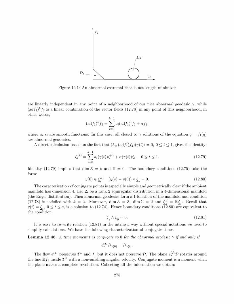
Dε
Dδ
x2
x1
Figure 12.1: An abnormal extremal that is not length minimizer
are linearly independent in any point of a neighborhood of our nice abnormal geodesic γ, while(adf1)
kf2 is a linear combination of the vector fields (12.78) in any point of this neighborhood; inother words,
(adf1)kf2 =
k−1∑
i=0
ai(adf1)if2 + αf1,
where ai, α are smooth functions. In this case, all closed to γ solutions of the equation q = f1(q)are abnormal geodesics.
A direct calculation based on the fact that 〈λt, (adf i1)f2)(γ(t)〉 = 0, 0 ≤ t ≤ 1, gives the identity:
ζ(k)t =
k−1∑
i=0
ai(γ(t))ζ(i) + α(γ(t))ξ1. 0 ≤ t ≤ 1. (12.79)
Identity (12.79) implies that dimE = k and Π = 0. The boundary conditions (12.75) take theform:
y(0) ∈ ζ∠s, (y(s)− y(0)) ∧ ζ
s= 0. (12.80)
The caracterization of conjugate points is especially simple and geometrically clear if the ambientmanifold has dimension 4. Let ∆ be a rank 2 equiregular distribution in a 4-dimensional manifold(the Engel distribution). Then abnormal geodesics form a 1-foliation of the manifold and condition(12.78) is satisfied with k = 2. Moreover, dimE = 3, dimΣ = 2 and ζ∠
s= Rζ
s. Recall that
y(t) = ζt, 0 ≤ t ≤ s, is a solution to (12.74). Hence boundary conditions (12.80) are equivalent to
the conditionζs∧ ζ
0= 0. (12.81)
It is easy to re-write relation (12.81) in the intrinsic way without special notations we used tosimplify calculations. We have the following characterization of conjugate times.
Lemma 12.46. A time moment t is conjugate to 0 for the abnormal geodesic γ if and only if
etf1∗ Dγ(0) = Dγ(t).
The flow etf1 preserves D2 and f1 but it does not preserve D. The plane etf1∗ D rotates aroundthe line Rf1 inside D2 with a nonvanishing angular velocity. Conjugate moment is a moment whenthe plane makes a complete revolution. Collecting all the information we obtain:
275
Theorem 12.47. Let D be the Engel distribution, f1 be a horizontal vector field such that [f1,D2] =D2 and γ = f1(γ). Then γ is an abnormal geodesic. Moreover
(i) if etf1∗ Dγ(0) 6= Dγ(t), ∀t ∈ (0, 1], then γ is a local length minimizer for any sub-Riemannianstructure on D
(ii) If etf1∗ Dγ(0) = Dγ(t) for some t ∈ (0, 1) and γ is not a normal geodesic, then γ is not a locallength minimizer.
12.7 Equivalence of local minimality
Now we prove that, under the assumption that our trajectory is smooth, it is equivalent to belocally optimal in the H1-topology or in the uniform topology for the trajectories.
Recall that a curve γ is called a C0-local length-minimizer if ℓ(γ) ≤ ℓ(γ) for every curve γthat is C0-close to γ satisfying the same boundary conditions, while it is called a H1-local length-minimizer if ℓ(γ) ≤ ℓ(γ) for every curve γ such that the control u corresponding to γ is close inthe L2 topology to the control u associated with γ and γ satisfies the same boundary conditions.
Any C0-local minimizer is automatically a H1-local minimizer. Indeed it is possible to showthat for every v,w in a neighborhood of a fixed control u there exists a constant C > 0 such that
|γv(t)− γw(t)| ≤ C‖u− v‖L2 , ∀ t ∈ [0, T ],
where γv and γw are the trajectories associated to controls v,w respectively.
Theorem 12.48. LetM be a sub-Riemannian structure that is the restriction to D of a Riemannianstructure (M,g). Assume γ is of class C1 and has no self intersections. If γ is a (strict) localminimizer in the L2 topology for the controls then γ is also a (strict) local minimizer in the C0topology for the trajectories.
Proof. Since γ has no self intersections, we can look for a preferred system of coordinates on anopen neighborhood Ω in M of the set V = γ(t) : t ∈ [0, 1]. For every ε > 0, define the cylinderin R
n = (x, y) : x ∈ R, y ∈ Rn−1 as follows
Iε ×Bn−1ε = (x, y) ∈ R
n : x ∈]− ε, 1 + ε[, y ∈ Rn−1, |y| < ε, (12.82)
We need the following technical lemma.
Lemma 12.49. There exists ε > 0 and a coordinate map Φ : Iε × Bn−1ε → Ω such that for all
t ∈ [0, 1]
(a) Φ(t, 0) = γ(t),
(b) the Riemannian metric Φ∗g is the identity matrix at (t, 0),i.e., along γ.
Proof of the Lemma. As in the proof of Theorem ??, for every ε > 0 we can find coordinates inthe cylinder Iε×Bn−1
ε such that, in these coordinates, our curve γ is rectified γ(t) = (t, 0) and haslength one.
Our normalization of the curve γ implies that for the matrix representing the Riemannian metricΦ∗g in these coordinates satisfies
Φ∗g =
(G11 G12
G21 G22
), with G11(x, 0) = 1
276
where Gij , for i, j = 1, 2, are the blocks of Φ∗g corresponding to the splitting Rn = R × R
n−1
defined in (12.82). For every point (x, 0) let us consider the orthogonal complement T (x, 0) of thetangent vector e1 = ∂x to γ with respect to G. It can be written as follows (in this proof 〈·, ·〉 isthe Euclidean product in R
n)
T (x, 0) =(〈vx, y〉 , y) , y ∈ R
n−1
for some family5 of vectors vx ∈ Rn−1, depending smoothly with respect to x. Let us consider now
the smooth change of coordinates
Ψ : Rn → Rn, Ψ(x, y) = (x− 〈vx, y〉 , y)
Fix ε > 0 small enough such that the restriction of Ψ to Iε × Bn−1ε is invertible. Notice that this
is possible since
detDΨ(x, y) = 1−⟨∂vx∂x
, y
⟩.
It is not difficult to check that, in the new variables (that we still denote by the same symbol), onehas
G(x, 0) =
(1 00 M(x, 0)
),
where M(x, 0) is a positive definite matrix for all x ∈ Iε. With a linear change of cooordinates inthe y space
(x, y) 7→ (x,M(x, 0)1/2y)
we can finally normalize the matrix in such a way that G(x, 0) = Id for all x ∈ Iε.
We are now ready to prove the theorem. We check the equivalence between the two notions oflocal minimality in the coordinate set, denoted (x, y), defined by the previous lemma. Notice thatthe notion of local minimality is independent on the coordinates.
Given an admissible curve γ(t) = (x(t), y(t)) contained in the cylinder Iε×Bn−1ε and satisfying
γ(0) = (0, 0) and γ(1) = (1, 0) and denoting the reference trajectory γ(t) = (t, 0) we have that
‖γ − γ‖2H1 =
∫ 1
0|x(t)− 1|2 + |y(t)|2dt
=
∫ 1
0|x(t)|2 + |y(t)|2dt− 2
∫ 1
0x(t)dt+ 1
=
∫ 1
0|x(t)|2 + |y(t)|2dt− 1
where we used that x(0) = 0 and x(1) = 1 since γ satisfies the boundary conditions. If we denoteby
J(γ) =
∫ 1
0〈G(γ(t))γ(t), γ(t)〉 dt, Je(γ) =
∫ 1
0|x(t)|2 + |y(t)|2dt (12.83)
respectively the energy of γ and the “Euclidean” energy, we have ‖γ − γ‖2H1 = Je(γ) − 1 and theH1-local minimality can be rewritten as follows:
5Indeed it is easily checked that vx = −G121(x, 0), where G1
21 denotes the first column of the (n − 1) × (n − 1)matrix G21.
277
(∗) there exists ε > 0 such that for every γ admissible and Je(γ) ≤ 1 + ε one has J(γ) ≥ 1.
Next we build the following neighborhood of γ: for every δ > 0 define Aδ as the set of admissiblecurves γ(t) = (x(t), y(t)) in Iε × Bn−1
ε such that the dilated curve γδ(t) = (x(t), 1δy(t)) is stillcontained in the cylinder. This implies that in particular that γ is contained in Iε ×Bn−1
δε . Noticethat Aδ ⊂ Aδ′ whenever δ < δ′. Moreover, every curve that is εδ close to γ in the C0-topology iscontained in Aδ.
It is then sufficient to prove that, for δ > 0 small enough, for every γ ∈ Aδ one has ℓ(γ) ≥ ℓ(γ).Indeed it is enough to check that J(γ) ≥ J(γ). Let us consider two cases
(i) γ ∈ Aδ and Je(γ) ≤ 1 + ε. In this case (∗) implies that J(γ) ≥ 1.
(ii) γ ∈ Aδ and Je(γ) > 1 + ε. In this case we have G(x, 0) = Id and, by smoothness of G, wecan write for (x, y) ∈ Iε ×Bn−1
δε and δ → 0
〈G(x, y)v, v〉 = (1 +O(δ)) 〈v, v〉 ,
where O(δ) is uniform with respect to (x, y). Since γ ∈ Aδ implies that γ is contained inIε ×Bn−1
δε we can deduce for δ → 0
J(γ) = Je(γ)(1 +O(δ)) ≥ (1 + ε)(1 +O(δ))
and one can choose δ > 0 small enough such that the last quantity is strictly bigger than one.
This proves that there exists δ > 0 such every admissible curve γ ∈ Aδ is longer than γ.
Remark 12.50. Notice that this result implies in particular Theorem 4.57, since normal extremalsare always smooth. Nevertheless, the argument of Theorem 4.57 can be adapted for more generalcoercive functional (see [3]), while this proof use specific estimates that hold only for our explicitcost (i.e., the distance).
We proved in Theorem 12.27 that nice abnormals are smooth and cannot have self-intersections,being solution of a smooth Hamiltonian system. Thus we can combine Theorem 12.30 and 12.48and obtain the following result.
Corollary 12.51. Let γ(t) be a nice abnormal trajectory. Then there exists s > 0 such that γ|[0,s]is a strict local length minimizer in the C0-topology.
278
Chapter 13
Some model spaces
13.1 Carnot groups of step 2
13.1.1 Heisenberg
13.1.2 (3, 6)
13.1.3 (k, k(k + 1)/2)
13.2 Other nilpotent structures
13.2.1 Grushin
13.2.2 Martinet
13.3 Left invariant structures
13.3.1 SU(2), SO(3), SL(2)
13.3.2 SE(2)
13.3.3 (3, 5) - Rolling sphere with twist
279

280
Chapter 14
Curves in the Lagrange Grassmannian
In this chapter we introduce the manifold of Lagrangian subspaces of a symplectic vector space.After a description of its geometric properties, we discuss how to define the curvature for regularcurves in the Lagrange Grassmannian, that are curves with non-degenerate derivative. Then wediscuss the non-regular case, where a reduction procedure let us to reduce to a regular curve in areduced symplectic space.
14.1 The geometry of the Lagrange Grassmannian
In this section we recall some basic facts about Grassmanians of k-dimensional subspaces of ann-dimensional vector space and then we consider, for a vector space endowed with a symplecticstructure, the submanifold of its Lagrangian subspaces.
Definition 14.1. Let V be an n-dimensional vector space. The Grassmanian of k-planes on V isthe set
Gk(V ) := W | W ⊂ V is a subspace, dim(W ) = k.
It is a standard fact that Gk(V ) is a compact manifold of dimension k(n − k).
Now we describe the tangent space to this manifold.
Proposition 14.2. Let W ∈ Gk(V ). We have a canonical isomorphism
TWGk(V ) ≃ Hom(W,V/W ).
Proof. Consider a smooth curve on Gk(V ) which starts from W , i.e. a smooth family of k-dimensional subspaces defined by a moving frame
W (t) = spane1(t), . . . , ek(t), W (0) =W.
We want to associate in a canonical way with the tangent vector W (0) a linear operator from Wto the quotient V/W . Fix w ∈W and consider any smooth extension w(t) ∈W (t), with w(0) = w.Then define the map
W → V/W, w 7→ w(0) (mod W ). (14.1)
281
We are left to prove that the map (14.1) is well defined, i.e. independent on the choices of rep-resentatives. Indeed if we consider another extension w1(t) of w satisfying w1(t) ∈ W (t) we canwrite
w1(t) = w(t) +
k∑
i=1
αi(t)ei(t),
for some smooth coefficients αi(t) such that αi(0) = 0 for every i. It follows that
w1(t) = w(t) +k∑
i=1
αi(t)ei(t) +k∑
i=1
αi(t)ei(t), (14.2)
and evaluating (14.2) at t = 0 one has
w1(0) = w(0) +
k∑
i=1
αi(0)ei(0).
This shows that w1(0) = w(0) (mod W ), hence the map (14.1) is well defined. In the same way onecan prove that the map does not depend on the moving frame defining W (t).
Finally, it is easy to show that the map that associates the tangent vector to the curve W (t)with the linear operator W → V/W is surjective, hence it is an isomorphism since the two spacehave the same dimension.
Let us now consider a symplectic vector space (Σ, σ), i.e. a 2n-dimensional vector space Σendowed with a non degenerate symplectic form σ ∈ Λ2(Σ).
Definition 14.3. A vector subspace Π ⊂ Σ of a symplectic space is called
(i) symplectic if σ|Π is nondegenerate,
(ii) isotropic if σ|Π ≡ 0,
(iii) Lagrangian if σ|Π ≡ 0 and dimΠ = n.
Notice that in general for every subspace Π ⊂ Σ, by nondegeneracy of the symplectic form σ, onehas
dimΠ+ dimΠ∠ = dimΣ. (14.3)
where as usual we denote the symplectic orthogonal by Π∠ = x ∈ Σ |σ(x, y) = 0, ∀ y ∈ Π.
Exercise 14.4. Prove the following properties for a vector subspace Π ⊂ Σ:
(i) Π is symplectic iff Π ∩Π∠ = 0,
(ii) Π is isotropic iff Π ⊂ Π∠,
(iii) Π is Lagrangian iff Π = Π∠.
Exercise 14.5. Prove that, given two subspaces A,B ⊂ Σ, one has the identities (A + B)∠ =A∠ ∩B∠ and (A ∩B)∠ = A∠ +B∠.
282
Example 14.6. Any symplectic vector space admits Lagrangian subspaces. Indeed fix any non-zero element e1 := e 6= 0 in Σ. Choose iteratively
ei ∈ spane1, . . . , ei−1∠ \ spane1, . . . , ei−1, i = 2, . . . , n. (14.4)
Then Π := spane1, . . . , en is a Lagrangian subspace by construction. Notice that the choice (14.4)is possible by (14.3)
Lemma 14.7. Let Π = spane1, . . . , en be a Lagrangian subspace of Σ. Then there exists vectorsf1, . . . , fn ∈ Σ such that
(i) Σ = Π⊕∆, ∆ := spanf1, . . . , fn,
(ii) σ(ei, fj) = δij , σ(ei, ej) = σ(fi, fj) = 0, ∀ i, j = 1, . . . , n.
Proof. We prove the lemma by induction. By nondegeneracy of σ there exists a non-zero x ∈ Σsuch that σ(en, x) 6= 0. Then we define the vector
fn :=x
σ(en, x), =⇒ σ(en, fn) = 1.
The last equality implies that σ restricted to spanen, fn is nondegerate, hence by (a) of Exercise14.4
spanen, fn ∩ spanen, fn∠ = 0, (14.5)
And we can apply induction on the 2(n − 1) subspace Σ′ := spanen, fn∠. Notice that (14.5)implies that σ is non degenerate also on Σ′.
Remark 14.8. In particular the complementary subspace ∆ = spanf1, . . . , fn defined in Lemma14.7 is Lagrangian and transversal to Π
Σ = Π⊕∆.
Considering coordinates induced from the basis chosen for this splitting we can write Σ = Rn∗⊕Rn,
(denoting Rn∗ denotes the set of row vectors). More precisely x = (ζ, z) if
x =
n∑
i=1
ζ iei + zifi, ζ =(ζ1 · · · ζn
), z =
z1
...zn
,
and using canonical form of σ on our basis (see Lemma 14.7) we find that in coordinates, ifx1 = (ζ1, z1), x2 = (ζ2, z2) we get
σ(x1, x2) = ζ1z2 − ζ2z1, (14.6)
where we denote with ζz the standard rows by columns product.
Lemma 14.7 shows that the group of symplectomorphisms acts transitively on pairs of transver-sal Lagrangian subspaces. The next exercise, whose proof is an adaptation of the previous one,describes all the orbits of the action of the group of symplectomorphisms on pairs of subspaces ofa symplectic vector spaces.
Exercise 14.9. Let Λ1,Λ2 be two subspaces in a symplectic vector space Σ, and assume thatdimΛ1 ∩ Λ2 = k. Show that there exists Darboux coordinates (p, q) in Σ such that
Λ1 = (p, 0), Λ2 = ((p1, . . . , pk, 0, . . . , 0), (0, . . . , 0, qk+1, . . . , qn).
283
14.1.1 The Lagrange Grassmannian
Definition 14.10. The Lagrange Grassmannian L(Σ) of a symplectic vector space Σ is the set ofits n-dimensional Lagrangian subspaces.
Proposition 14.11. L(Σ) is a compact submanifold of the Grassmannian Gn(Σ) of n-dimensionalsubspaces. Moreover
dimL(Σ) =n(n+ 1)
2. (14.7)
Proof. Recall that Gn(Σ) is a n2-dimensional compact manifold. Clearly L(Σ) ⊂ Gn(Σ) as a subset.
Consider the set of all Lagrangian subspaces that are transversal to a given one
∆⋔ = Λ ∈ L(Σ) : Λ ∩∆ = 0.
Clearly ∆⋔ ⊂ L(Σ) is an open subset and since by Lemma 14.7 every Lagrangian subspace admitsa Lagrangian complement
L(Σ) =⋃
∆∈L(Σ)
∆⋔.
It is then sufficient to find some coordinates on these open subsets. Every n-dimensional subspaceΛ ⊂ Σ which is transversal to ∆ is the graph of a linear map from Π to ∆. More precisely thereexists a matrix SΛ such that
Λ ∩∆ = 0⇔ Λ = (zT , SΛz), z ∈ Rn.
(Here we used the coordinates induced by the splitting Σ = Π⊕∆.) Moreover it is easily seen that
Λ ∈ L(Σ)⇔ SΛ = (SΛ)T .
Indeed we have that Λ ∈ L(Σ) if and only if σ|Λ = 0 and using (14.6) this is rewritten as
σ((zT1 , SΛz1), (zT2 , SΛz2)) = zT1 SΛz2 − zT2 SΛz1 = 0,
which means exactly SΛ symmetric. Hence the open set of all subspaces that are transversal to Λis parametrized by the set of symmetric matrices, that gives coordinates in this open set. This alsoproves that the dimension of L(Σ) coincide with the dimension of the space of symmetric matrices,hence (14.7). Notice also that, being L(Σ) a closed set in a compact manifold, it is compact.
Now we describe the tangent space to the Lagrange Grassmannian.
Proposition 14.12. Let Λ ∈ L(Σ). Then we have a canonical isomorphism
TΛL(Σ) ≃ Q(Λ),
where Q(Λ) denote the set of quadratic forms on Λ.
Proof. Consider a smooth curve Λ(t) in L(Σ) such that Λ(0) = Λ and Λ(0) ∈ TΛL(Σ) its tangentvector. As before consider a point x ∈ Λ and a smooth extension x(t) ∈ Λ(t) and denote withx := x(0). We define the map
Λ : x 7→ σ(x, x), (14.8)
284
that is nothing else but the quadratic map associated to the self adjoint map x 7→ x by thesymplectic structure. We show that in coordinates Λ is a well defined quadratic map, independenton all choices. Indeed
Λ(t) = (zT , SΛ(t)z), z ∈ Rn,
and the curve x(t) can be written
x(t) = (z(t)T , SΛ(t)z(t)), x = x(0) = (zT , SΛz),
for some curve z(t) where z = z(0). Taking derivative we get
x(t) = (z(t)T , SΛ(t)z(t) + SΛ(t)z(t)),
and evaluating at t = 0 (we simply omit t when we evaluate at t = 0) we have
x = (zT , SΛz), x = (zT , SΛz + SΛz),
and finally get, using the simmetry of SΛ, that
σ(x, x) = zT (SΛz + SΛz)− zTSΛz= zT SΛz + zTSΛz − zTSΛz= zT SΛz. (14.9)
Exercise 14.13. Let Λ(t) ∈ L(Σ) such that Λ = Λ(0) and σ be the symplectic form. Prove thatthe map S : Λ × Λ → R defined by S(x, y) = σ(x, y), where y = y(0) is the tangent vector to asmooth extension y(t) ∈ Λ(t) of y, is a symmetric bilinear map.
Remark 14.14. We have the following natural interpretation of this result: since L(Σ) is a subman-ifold of the Grassmanian Gn(Σ), its tangent space TΛL(Σ) is naturally identified by the inclusionwith a subspace of the Grassmannian
i : L(Σ) → Gn(Σ), i∗ : TΛL(Σ) → TΛGn(Σ) ≃ Hom(Λ,Σ/Λ),
where the last isomorphism is Proposition 14.2. Being Λ a Lagrangian subspace of Σ, the symplecticstructure identifies in a canonical way the factor space Σ/Λ with the dual space Λ∗ defining
Σ/Λ ≃ Λ∗, 〈[z]Λ, x〉 = σ(z, x). (14.10)
Hence the tangent space to the Lagrange Grassmanian consist of those linear maps in the spaceHom(Λ,Λ∗) that are self-adjoint, which are naturally identified with quadratic forms on Λ itself. 1
Remark 14.15. Given a curve Λ(t) in L(Σ), the above procedure associates to the tangent vectorΛ(t) a family of quadratic forms Λ(t), for every t.
We end this section by computing the tangent vector to a special class of curves that will playa major role in the sequel, i.e. the curve on L(Σ) induced by the action on Λ by the flow of thelinear Hamiltonian vector field ~h associated with a quadratic Hamiltonian h ∈ C∞(Σ). (Recall thata Hamiltonian vector field transform Lagrangian subspaces into Lagrangian subspaces.)
1any quadratic form on a vector space q ∈ Q(V ) can be identified with a self-adjoint linear map L : V → V ∗,L(v) = B(v, ·) where B is the symmetric bilinear map such that q(v) = B(v, v).
285
Proposition 14.16. Let Λ ∈ L(Σ) and define Λ(t) = et~h(Λ). Then Λ = 2h|Λ.
Proof. Consider x ∈ Λ and the smooth extension x(t) = et~h(x). Then x = ~h(x) and by definition
of Hamiltonian vector field we find
σ(x, x) = σ(x,~h(x))
= 〈dxh, x〉= 2h(x),
where in the last equality we used that h is quadratic on fibers.
14.2 Regular curves in Lagrange Grassmannian
The isomorphism between tangent vector to the Lagrange Grassmannian with quadratic formsmakes sense to the following definition (we denote by Λ the tangent vector to the curve at the pointΛ as a quadratic map)
Definition 14.17. Let Λ(t) ∈ L(Σ) be a smooth curve in the Lagrange Grassmannian. We saythat the curve is
(i) monotone increasing (descreasing) if Λ(t) ≥ 0 (Λ(t) ≤ 0).
(ii) strictly monotone increasing (decreasing) if the inequality in (i) is strict.
(iii) regular if its derivative Λ(t) is a non degenerate quadratic form.
Remark 14.18. Notice that if Λ(t) = (p, S(t)p), p ∈ Rn in some coordinate set, then it follows
from the proof of Proposition 14.12 that the quadratic form Λ(t) is represented by the matrix SΛ(t)(see also (14.9)). In particular the curve is regular if and only if det SΛ(t) 6= 0.
The main goal of this section is the construction of a canonical Lagrangian complement. (i.e.another curve Λ(t) in the Lagrange Grassmannian defined by Λ(t) and such that Σ = Λ(t)⊕Λ(t).)
Consider an arbitrary Lagrangian splitting Σ = Λ(0) ⊕∆ defined by a complement ∆ to Λ(0)(see Lemma 14.7) and fix coordinates in such a way that that
Σ = (p, q), p, q ∈ Rn, Λ(0) = (p, 0), p ∈ R
n, ∆ = (0, q), q ∈ Rn.
In these coordinates our regular curve is described by a one parametric family of symmetric matricesS(t)
Λ(t) = (p, S(t)p), p ∈ Rn,
such that S(0) = 0 and S(0) is invertible. All Lagrangian complement to Λ(0) are parametrized bya symmetrix matrix B as follows
∆B = (Bq, q), q ∈ Rn, B = BT .
The following lemma shows how the coordinate expression of our curve Λ(t) change in the newcoordinate set defined by the splitting Σ = Λ(0) ⊕∆B .
286
Lemma 14.19. Let SB(t) the one parametric family of symmetric matrices defining Λ(t) in coor-dinates w.r.t. the splitting Λ(0)⊕∆B. Then the following identity holds
SB(t) = (S(t)−1 −B)−1. (14.11)
Proof. It is easy to show that, if (p, q) and (p′, q′) denotes coordinates with respect to the splittingdefined by the subspaces ∆ and ∆B we have
p′ = p−Bqq′ = q
(14.12)
The matrix SB(t) by definition is the matrix that satisfies the identity q′ = SB(t)p′. Using that
q = S(t)p by definition of Λ(t), from (14.12) we find
q′ = q = S(t)p = S(t)(p′ +Bq′),
and with straightforward computations we finally get
SB(t) = (I − S(t)B)−1S(t) = (S(t)−1 −B)−1.
Since S(t) represents the tangent vectors to the regular curve Λ(t), its properties are invariantwith respect to change of coordinates. Hence it is natural to look for a change of coordinates (i.e.a choice of the matrix B) that simplifies the second derivative our curve.
Corollary 14.20. There exists a unique symmetric matrix B such that SB(0) = 0.
Proof. Recall that for a one parametric family of matrices X(t) we have
d
dtX(t)−1 = −X(t)−1X(t)X(t)−1.
Applying twice this identity to (14.11) (we omit t to denote the value at t = 0) we get
d
dt
∣∣∣∣t=0
SB(t) = −(S−1 −B)−1
(d
dt
∣∣∣∣t=0
S−1(t)
)(S−1 −B)−1
= (S−1 −B)−1S−1SS−1(S−1 −B)−1
= (I − SB)−1S(I −BS)−1.
Hence for the second derivative evaluated at t = 0 (remember that in our coordinates S(0) = 0)one gets
SB = S + 2SBS,
and using that S is non degerate, we can choose B = −12 S
−1SS−1.
We set Λ(0) := ∆B, where B is determined by (14.13). Notice that by construction Λ(0) isa Lagrangian subspace and it is transversal to Λ(0). The same argument can be applied to defineΛ(t) for every t.
287
Definition 14.21. Let Λ(t) be a regular curve, the curve Λ(t) defined by the condition above iscalled derivative curve of Λ(t).
Exercise 14.22. Prove that, if Λ(t) = (p, S(t)p), p ∈ Rn (without the condition S(0) = 0), then
the derivative curve Λ(t) = (p, S(t)p), p ∈ Rn, satisfies
S(t) = B(t)−1 + S(t), where B(t) := −1
2S(t)−1S(t)S(t)−1, (14.13)
provided Λ(t) is transversal to the subspace ∆ = (0, q), q ∈ Rn. (Actually this condition is
equivalent to the invertibility of B(t).) Notice that if S(0) = 0 then S(0) = B(0)−1.
Remark 14.23. The set Λtr of all n-dimensional spaces transversal to a fixed subspace Λ is an affinespace over Hom(Σ/Λ,Λ). Indeed given two elements ∆1,∆2 ∈ Λtr we can associate with theirdifference the operator
∆2 −∆1 7→ A ∈ Hom(Σ/Λ,Λ), A([z]Λ) = z2 − z1 ∈ Λ, (14.14)
where zi ∈ ∆i ∩ [z]Λ are uniquely identified.If Λ is Lagrangian, we have identification Σ/Λ ≃ Λ∗ given by the symplectic structure (see
(14.10)) that Λ⋔, that coincide by definition with the intersection Λtr ∩L(Σ) is an affine space overHomS(Λ∗,Λ), the space of selfadjoint maps between Λ∗ and Λ, that it isomorphic to Q(Λ∗).
Notice that if we fix a distinguished complement of Λ, i.e. Σ = Λ ⊕∆, then we have also theidentification Σ/Λ ≃ ∆ and Λ⋔ ≃ Q(Λ∗) ≃ Q(∆).
Exercise 14.24. Prove that the operator A defined by (14.14), in the case when Λ is Lagrangian,is a self-adjoint operator.
Remark 14.25. Assume that the splitting Σ = Λ⊕∆ is fixed. Then our curve Λ(t) in L(Σ), such thatΛ(0) = Λ, is characterized by a family of symmetric matrices S(t) satisfying Λ(t) = (p, S(t)p), p ∈Rn, with S(0) = 0.By regularity of the curve, Λ(t) ∈ Λ⋔ for t > 0 small enough, hence we can consider its
coordinate presentation in the affine space on the vector space of quadratic forms defined on ∆ (seeRemark 14.23) that is given by S−1(t) and write the Laurent expansion of this curve in the affinespace
S(t)−1 =
(tS +
t2
2S +O(t3)
)−1
=1
tS−1
(I +
t
2SS−1 +O(t2)
)−1
=1
tS−1−1
2S−1SS−1
︸ ︷︷ ︸B
+O(t).
It is not occasional that the matrix B coincides with the free term of this expansion. Indeed theformula (14.11) for the change of coordinates can be rewritten as follows
SB(t)−1 = S−1(t)−B, (14.15)
and the choice of B corresponds exactly to the choice of a coordinate set where the curve Λ(t) hasno free term in this expansion (i.e. SB(t)
−1 has no term of order zero). This is equivalent to saythat a regular curve let us to choose a privileged origin in the affine space of Lagrangian subspacesthat are transversal to the curve itself.
288
14.3 Curvature of a regular curve
Now we want to define the curvature of a regular curve in the Lagrange Grassmannian. Let Λ(t)be a regular curve and consider its derivative curve Λ(t).
The tangent vectors to Λ(t) and Λ(t), as explained in Section 14.1, can be interpreted in a acanonical way as a quadratic form on the space Λ(t) and Λ(t) respectively
Λ(t) ∈ Q(Λ(t)), Λ(t) ∈ Q(Λ(t)).
Being Λ(t) a canonical Lagrangian complement to Λ(t) we have the identifications through thesymplectic form2
Λ(t)∗ ≃ Λ(t), Λ(t)∗ ≃ Λ(t),
and the quadratic forms Λ(t), Λ(t) can be treated as (self-adjoint) mappings:
Λ(t) : Λ(t)→ Λ(t), Λ(t) : Λ(t)→ Λ(t). (14.16)
Definition 14.26. The operator RΛ(t) := Λ(t)Λ(t) : Λ(t)→ Λ(t) is called the curvature operator
of the regular curve Λ(t).
Remark 14.27. In the monotonic case, when |Λ(t)| defines a scalar product on Λ(t), the operatorR(t) is, by definition, symmetric with respect to this scalar product. Moreover R(t), as quadraticform, has the same signature and rank as Λ
(t) sign(Λ
(t)).
Definition 14.28. Let Λ1,Λ2 be two transversal Lagrangian subspaces of Σ. We denote
πΛ1Λ2 : Σ→ Λ2, (14.17)
the projection on Λ2 parallel to Λ1, i.e. the linear operator such that
πΛ1Λ2 |Λ1 = 0 πΛ1Λ2 |Λ2 = Id.
Exercise 14.29. Assume Λ1 and Λ2 be two Lagrangian subspaces in Σ and assume that, in somecoordinate set, Λi = (x, Six),∈ R
n for i = 1, 2 . Prove that Σ = Λ1 ⊕ Λ2 if and only ifker(S1 − S2) = 0. In this case show that the following matrix expression for πΛ1Λ2 :
πΛ1Λ2 =
(S−112 S1 −S−1
12
S2S−112 S1 −S2S−1
12
), S12 := S1 − S2. (14.18)
From the very definition of the derivative of our curve we can get the following geometriccharacterization of the curvature of a curve.
Proposition 14.30. Let Λ(t) a regular curve in L(Σ) and Λ(t) its derivative curve. Then
Λ(t)(xt) = πΛ(t)Λ(t)(xt), Λ(t)(xt) = −πΛ(t)Λ(t)(xt).
In particular the curvature is the composition RΛ(t) = Λ(t) Λ(t).
2if Σ = Λ⊕∆ is a splitting of a vector space then Σ/Λ ≃ ∆. If moreover the splitting is Lagrangian in a symplecticspace, the symplectic form identifies Σ/Λ ≃ Λ∗, hence Λ∗ ≃ ∆.
289
Proof. Recall that, by definition, the linear operator Λ : Λ → Σ/Λ associated with the quadraticform is the map x 7→ x (mod Λ). Hence to build the map Λ → Λ it is enough to compute theprojection of x onto the complement Λ, that is exactly πΛΛ(x). Notice that the minus sign inequation (14.30) is a consequence of the skew symmetry of the symplectic product. More precisely,the sign in the identification Λ ≃ Λ∗ depends on the position of the argument.
The curvature RΛ(t) of the curve Λ(t) is a kind of relative velocity between the two curves Λ(t)and Λ(t). In particular notice that if the two curves moves in the same direction we have RΛ(t) > 0.
Now we compute the expression of the curvature RΛ(t) in coordinates.
Proposition 14.31. Assume that Λ(t) = (p, S(t)p) is a regular curve in L(Σ). Then we havethe following coordinate expression for the curvature of Λ (we omit t in the formula)
RΛ = ((2S)−1S)− ((2S)−1S)2 (14.19)
=1
2S−1...
S − 3
4(S−1S)2. (14.20)
Proof. Assume that both Λ(t) and Λ(t) are contained in the same coordinate chart with
Λ(t) = (p, S(t)p), Λ(t) = (p, S(t)p).
We start the proof by computing the expression of the linear operator associated with the derivativeΛ : Λ → Λ (we omit t when we compute at t = 0). For each element (p, Sp) ∈ Λ and anyextension (p(t), S(t)p(t)) one can apply the matrix representing the operator πΛΛ (see (14.18)) tothe derivative at t = 0 and find
πΛΛ(p, Sp) = (p′, Sp′), p′ = −(S − S)−1Sp.
Exchanging the role of Λ and Λ, and taking into account of the minus sign one finds that thecoordinate representation of R is given by
R = (S − S)−1S(S − S)−1S. (14.21)
We prove formula (14.20) under the extra assumption that S(0) = 0. Notice that this isequivalent to the choice of a particular coordinate set in L(Σ) and, being the expression of Rcoordinate independent by construction, this is not restrictive.
Under this extra assumption, it follows from (14.13) that
Λ(t) = (p, S(t)p), Λ(t) = (p, S(t)p),
where S(t) = B(t)−1 + S(t) and we denote by B(t) := −12 S(t)
−1S(t)S(t)−1.Hence we have, assuming S(0) = 0 and omitting t when t = 0
R = (S − S)−1S(S − S)−1S
= B
(d
dt
∣∣∣∣t=0
B(t)−1 + S(t)
)BS
= (BS)2 − BS.
Plugging B = −12 S
−1SS−1 into the last formula, after some computations one gets to (14.20).
290
Remark 14.32. The formula for the curvature RΛ(t) of a curve Λ(t) in L(Σ) takes a very simpleform in a particular coordinate set given by the splitting Σ = Λ(0)⊕ Λ(0), i.e. such that
Λ(0) = (p, 0), p ∈ Rn, Λ(0) = (0, q), q ∈ R
n.
Indeed using a symplectic change of coordinates in Σ that preserves both Λ and Λ (i.e. of the kindp′ = Ap, q′ = (A−1)∗q) we can choose the matrix A in such a way that S(0) = I. Moreover weknow from Proposition that the fact that Λ = (0, q), q ∈ R
n is equivalent to S(0) = 0. Henceone finds from (14.20) that
R =1
2
...S
When the curve Λ(t) is strictly monotone, the curvature R represents a well defined operator onΛ(0), naturally endowed with the sign definite quadratic form Λ(0). Hence in these coordinates theeigenvalues of
...S (and not only the trace and the determinant) are invariants of the curve.
Exercise 14.33. Let f : R→ R be a smooth function. The Schwartzian derivative of f is definedas
Sf :=
(f ′′
2f ′
)′−(f ′′
2f ′
)2
(14.22)
Prove that Sf = 0 if and only if f(t) =at+ b
ct+ dfor some a, b, c, d ∈ R.
Remark 14.34. The previous proposition says that the curvature R is the matrix version of theSchwartzian derivative of the matrix S (cfr. (14.19) and (14.22)).
Example 14.35. Let Σ be a 2-dimensional symplectic space. In this case L(Σ) ≃ P1(R) is the real
projective line. Let us compute the curvature of a curve in L(Σ) with constant (angular) velocityα > 0. We have
Λ(t) = (p, S(t)p), p ∈ R, S(t) = tan(αt) ∈ R.
From the explicit expression it easy to find the relation
S(t) = α(1 + S2(t)), ⇒ S(t)
2S(t)= αS(t),
from which one gets that R(t) = αS(t)− α2S2(t) = α2, i.e. the curve has constant curvature.
We end this section with a useful formula on the curvature of a reparametrized curve.
Proposition 14.36. Let ϕ : R→ R a diffeomorphism and define the curve Λϕ(t) := Λ(ϕ(t)). Then
RΛϕ(t) = ϕ2(t)RΛ(ϕ(t)) +Rϕ(t)Id. (14.23)
Proof. It is a simple check that the Schwartzian derivative of the composition of two function fand g satisfies
S(f g) = (Sf g)(g′)2 + Sg.Notice that Rϕ(t) makes sense as the curvature of the regular curve ϕ : R→ R ⊂ P
1 in the LagrangeGrassmannian L(R2).
291
Exercise 14.37. (Another formula for the curvature). Let Λ0,Λ1 ∈ L(Σ) be such that Σ = Λ0⊕Λ1
and fix two tangent vectors ξ0 ∈ TΛ0L(Σ) and ξ1 ∈ TΛ1L(Σ). As in (14.16) we can treat each tangentvector as a linear operator
ξ0 : Λ0 → Λ1, ξ1 : Λ1 → Λ0, (14.24)
and define the cross-ratio [ξ1, ξ0] = −ξ1 ξ0. If in some coordinates Λi = (p, Sip) for i = 0, 1 wehave3
[ξ1, ξ0] = (S1 − S0)−1S1(S1 − S0)−1S0.
Let now Λ(t) a regular curve in L(Σ). By regularity Σ = Λ(0)⊕Λ(t) for all t > 0 small enough,hence the cross ratio
[Λ(t), Λ(0)] : Λ(0)→ Λ(0),
is well defined. Prove the following expansion for t→ 0
[Λ(t), Λ(0)] ≃ 1
t2Id+
1
3RΛ(0) +O(t). (14.25)
14.4 Reduction of non-regular curves in Lagrange Grassmannian
In this section we want to extend the notion of curvature to non-regular curves. As we will seein the next chapter, it is always possible to associate with an extremal a family of Lagrangiansubspaces in a symplectic space, i.e. a curve in a Lagrangian Grassmannian. This curve turnsout to be regular if and only if the extremal is an extremal of a Riemannian structure. Hence, ifwe want to apply this theory for a genuine sub-Riemannian case we need some tools to deal withnon-regular curves in the Lagrangian Grassmannian.
Let (Σ, σ) be a symplectic vector space and L(Σ) denote the Lagrange Grassmannian. We startby describing a natural subspace of L(Σ) associated with an isotropic subspace Γ of Σ. This willallow us to define a reduction procedure for a non regular curve.
Let Γ be a k-dimensional isotropic subspace of Σ, i.e. σ∣∣Γ= 0. This means that Γ ⊂ Γ∠. In
particular Γ∠/Γ is a 2(n − k) dimensional symplectic space with the restriction of σ.
Lemma 14.38. There is a natural identification of L(Γ∠/Γ) as a subspace of L(Σ):
L(Γ∠/Γ) ≃ Λ ∈ L(Σ),Γ ⊂ Λ ⊂ L(Σ). (14.26)
Moroever we have a natural projection
πΓ : L(Σ)→ L(Γ∠/Γ), Λ 7→ ΛΓ,
where ΛΓ := (Λ ∩ Γ∠) + Γ = (Λ + Γ) ∩ Γ∠.
Proof. Assume that Λ ∈ L(Σ) and Γ ⊂ Λ. Then, since Λ is Lagrangian, Λ = Λ∠ ⊂ Γ∠, hence theidentification (14.26).
Assume now that Λ ∈ L(Γ∠/Γ) and let us show that πΓ(Λ) = Λ, i.e. πΓ is a projection. Indeedfrom the inclusions Γ ⊂ Λ ⊂ Γ∠ one has πΓ(Λ) = ΛΓ = (Λ ∩ Γ∠) + Γ = Λ+ Γ = Λ.
3here Si denotes the matrix associated with ξi.
292
We are left to check that ΛΓ is Lagrangian, i.e. (ΛΓ)∠ = ΛΓ.
(ΛΓ)∠ = ((Λ ∩ Γ∠) + Γ)∠
= (Λ ∩ Γ∠)∠ ∩ Γ∠
= (Λ + Γ) ∩ Γ∠ = ΛΓ,
where we repeatedly used Exercise 14.5. (The identity (Λ ∩ Γ∠) + Γ = (Λ + Γ) ∩ Γ∠ is also aconsequence of the same exercise.)
Remark 14.39. Let Γ⋔ = Λ ∈ L(Σ),Λ ∩ Γ = 0. The restriction πΓ∣∣Γ⋔ is smooth. Indeed it can
be shown that πΓ is defined by a rational function, since it is expressed via the solution of a linearsystem.
The following example shows that the projection πΓ is not globally continous on L(Σ).
Example 14.40. Consider the symplectic structure σ on R4, with Darboux basis e1, e2, f1, f2,
i.e. σ(ei, fj) = δij . Let Γ = spane1 be a one dimensional isotropic subspace and define
Λε = spane1 + εf2, e2 + εf1, ∀ ε > 0.
It is easy to see that Λε is Lagrangian for every ε and that
ΛΓε = spane1, f2, ∀ ε > 0, (14.27)
ΛΓ0 = spane1, e2.
Indeed f2 ∈ e∠1 , that implies e1 + εf2 ∈ Λε ∩ Γ∠, therefore f2 ∈ Λε ∩ Γ∠. By definition of reducedcurve f2 ∈ ΛΓ
ε and (14.27) holds. The case ε = 0 is trivial.
14.5 Ample curves
In this section we introduce ample curves.
Definition 14.41. Let Λ(t) ∈ L(Σ) be a smooth curve in the Lagrange Grassmannian. The curveΛ(t) is ample at t = t0 if there exists N ∈ N such that
Σ = spanλ(i)(t0)| λ(t) ∈ Λ(t), λ(t) smooth, 0 ≤ i ≤ N. (14.28)
In other words we require that all derivatives up to order N of all smooth sections of our curve inL(Σ) span all the possible directions.
As usual, we can choose coordinates in such a way that, for some family of symmetric matricesS(t), one has
Σ = (p, q)| p, q ∈ Rn, Λ(t) = (p, S(t)p)| p ∈ R
n.Exercise 14.42. Assume that Λ(t) = (p, S(t)p), p ∈ R
n with S(0) = 0. Prove that the curve isample at t = 0 if and only if there exists N ∈ N such that all the columns of the derivative of S(t)up to order N (and computed at t = 0) span a maximal subspace:
rankS(0), S(0), . . . , S(N)(0) = n. (14.29)
In particular, a curve Λ(t) is regular at t0 if and only if is ample at t0 with N = 1.
293
An important property of ample and monotone curves is described in the following lemma.
Lemma 14.43. Let Λ(t) ∈ L(Σ) a monotone, ample curve at t0. Then, there exists ε > 0 suchthat Λ(t) ∩ Λ(t0) = 0 for 0 < |t− t0| < ε.
Proof. Without loss of generality, assume t0 = 0. Choose a Lagrangian splitting Σ = Λ⊕ Π, withΛ = J(0). For |t| < ε, the curve is contained in the chart defined by such a splitting. In coordinates,Λ(t) = (p, S(t)p)| p ∈ R
n, with S(t) symmetric and S(0) = 0. The curve is monotone, then S(t)is a semidefinite symmetric matrix. It follows that S(t) is semidefinite too.
Suppose that, for some t, Λ(t) ∩ Λ(0) 6= 0 (assume t > 0). This means that ∃ v ∈ Rn such
that S(t)v = 0. Indeed also v∗S(t)v = 0. The function τ 7→ v∗S(τ)v is monotone, vanishing atτ = 0 and τ = t. Therefore v∗S(τ)v = 0 for all 0 ≤ τ ≤ t. Being a semidefinite, symmetric matrix,v∗S(τ)v = 0 if and only if S(τ)v = 0. Therefore, we conclude that v ∈ kerS(τ) for 0 ≤ τ ≤ t. Thisimplies that, for any i ∈ N, v ∈ kerS(i)(0), which is a contradiction, since the curve is ample at0.
Exercise 14.44. Prove that a monotone curve Λ(t) is ample at t0 if and only if one of the equivalentconditions is satisfied
(i) the family of matrices S(t) − S(t0) is nondegenerate for t 6= t0 close enough, and the sameremains true if we replace S(t) by its N -th Taylor polynomial, for some N in N.
(ii) the map t 7→ det(S(t)− S(t0)) has a finite order root at t = t0.
Let us now consider an analytic monotone curve on L(Σ). Without loss of generality we canassume the curve to be non increasing, i.e. Λ(t) ≥ 0. By monotonicity
Λ(0) ∩ Λ(t) =⋂
0≤τ≤tΛ(τ) =: Υt
Clearly Υt is a decreasing family of subspaces, i.e. Υt ⊂ Υτ if τ ≤ t. Hence the family Υt for t→ 0stabilizes and the limit subspace Υ is well defined
Υ := limt→0
Υt
The symplectic reduction of the curve by the isotropic subspace Υ defines a new curve Λ(t) :=Λ(t)Υ ∈ L(Υ∠/Υ).
Proposition 14.45. If Λ(t) is analytic and monotone in L(Σ), then Λ(t) is ample L(Υ∠/Υ).
Proof. By construction, in the reduced space Υ∠/Υ we removed the intersection of Λ(t) with Λ(0).Hence
Λ(0) ∩ Λ(t) = 0, in L(Υ∠/Υ) (14.30)
In particular, if S(t) denotes the symmetric matrix representing Λ(t) such that S(0) = Λ(t0), itfollows that S(t) is non degenerate for 0 < |t| < ε. The analyticity of the curve guarantees thatthe Taylor polynomial (of a suitable order N) is also non degenerate.
294
14.6 From ample to regular
In this section we prove the main result of this chapter, i.e. that any ample monotone curve canbe reduced to a regular one.
Theorem 14.46. Let Λ(t) be a smooth ample monotone curve and set Γ := Ker Λ(0). Then the
reduced curve t 7→ ΛΓ(t) is a smooth regular curve. In particular ΛΓ(0) > 0.
Before proving Theorem 14.46, let us discuss two useful lemmas.
Lemma 14.47. Let v1(t), . . . , vk(t) ∈ Rn and define V (t) as the n × k matrix whose columns are
the vectors vi(t). Define the matrix S(t) :=∫ t0 V (τ)V (τ)∗dτ . Then the following are equivalent:
(i) S(t) is invertible (and positive definite),
(ii) spanvi(τ)| i = 1, . . . , k; τ ∈ [0, t] = Rn.
Proof. Fix t > 0 and let us assume S(t) is not invertible. Since S(t) is non negative then thereexists a nonzero x ∈ R
n such that 〈S(t)x, x〉 = 0. On the other hand
〈S(t)x, x〉 =∫ t
0〈V (τ)V (τ)∗x, x〉 dτ =
∫ t
0‖V (τ)∗x‖2dτ
This implies that V (τ)∗x = 0 (or equivalently x∗V (τ) = 0) for τ ∈ [0, t], i.e. the nonzero vector x∗
is orthogonal to Im τ∈[0,t]V (τ) = spanvi(τ)| i = 1, . . . , k, τ ∈ [0, t] = Rn, that is a contradiction.
The converse is similar.
Lemma 14.48. Let A,B two positive and symmetric matrices such that 0 < A < B. Then wehave also 0 < B−1 < A−1.
Proof. Assume first that A and B commute. Then A and B can be simultaneously diagonalizedand the statement is trivial for diagonal matrices.
In the general case, since A is symmetric and positive, we can consider its square root A1/2,which is also symmetric and positive. We can write
0 < 〈Av, v〉 < 〈Bv, v〉
By setting w = A1/2v in the above inequality and using 〈Av, v〉 =⟨A1/2v,A1/2v
⟩one gets
0 < 〈w,w〉 <⟨A−1/2BA−1/2w,w
⟩,
which is equivalent to I < A−1/2BA−1/2. Since the identity matrix commutes with every othermatrix, we obtain
0 < A1/2B−1A1/2 = (A−1/2BA−1/2)−1 < I
which is equivalent to 0 < B−1 < A−1 reasoning as before.
Proof of Theorem 14.46. By assumption the curve t 7→ Λ(t) is ample, hence Λ(t) ∩ Γ = 0 andt 7→ ΛΓ(t) is smooth for t > 0 small enough. We divide the proof into three parts: (i) we computethe coordinate presentation of the reduced curve. (ii) we show that the reduced curve, extendedby continuity at t = 0, is smooth. (iii) we prove that the reduced curve is regular.
295
(i). Let us consider Darboux coordinates in the symplectic space Σ such that
Σ = (p, q) : p, q ∈ Rn, Λ(t) = (p, S(t)p)| p ∈ R
n, S(0) = 0.
Morover we can assume also Rn = R
k ⊕ Rn−k, where Γ = 0 ⊕ R
n−k. According to this splittingwe have the decomposition p = (p1, p2) and q = (q1, q2). The subspaces Γ and Γ∠ are described bythe equations
Γ = (p, q) : p1 = 0, q = 0, Γ∠ = (p, q) : q2 = 0and (p1, q1) are natural coordinates for the reduced space Γ∠/Γ. Up to a symplectic change ofcoordinates preserving the splitting R
n = Rk ⊕ R
n−k we can assume that
S(t) =
(S11(t) S12(t)S∗12(t) S22(t)
), with S(0) =
(Ik 00 0
). (14.31)
where Ik is the k × k identity matrix. Finally, from the fact that S is monotone and ample, thatimplies S(t) > 0 for each t > 0, it follows
S11(t) > 0, S22(t) > 0, ∀ t > 0. (14.32)
Then we can compute the coordinate expression of the reduced curve, i.e. the matrix SΓ(t) suchthat
ΛΓ(t) = (p1, SΓ(t)p1), p1 ∈ Rk.
From the identity
Λ(t) ∩ Γ∠ = (p, S(t)p), S(t)p ∈ Rk =
(S−1(t)
(q10
),
(q10
)), q1 ∈ R
k
(14.33)
one gets the key relation SΓ(t)−1 = (S(t)−1)11.Thus the matrix expression of the reduced curve ΛΓ(t) in L(Γ∠/Γ) is recovered simply by
considering it as a map of (p1, q1) only, i.e.
S(t)p =
(S11 S12S∗12 S22
)(p1p2
)=
(S11p1 + S12p2S∗12p1 + S22p2
)
from which we get S(t)p ∈ Rk if and only if S∗
12(t)p1 + S22(t)p2 = 0. Then
ΛΓ(t) = (p1, S11p1 + S12p2) : S∗12(t)p1 + S22(t)p2 = 0
= (p1, (S11 − S12S−122 S
∗12)p1)
that meansSΓ = S11 − S12S−1
22 S∗12. (14.34)
(ii). By the coordinate presentation of SΓ(t) the only term that can give rise to singularities isthe inverse matrix S−1
22 (t). In particular, since by assumption t 7→ detS22(t) has a finite order zeroat t = 0, the a priori singularity can be only a finite order pole.
To prove that the curve is smooth it is enough the to show that SΓ(t) → 0 for t → 0, i.e. thecurve remains bounded. This follows from the following
Claim I. As quadratic forms on Rk, we have the inequality 0 ≤ SΓ(t) ≤ S11(t).
296
Indeed S(t) symmetric and positive one has that its inverse S(t)−1 is symmetric and positive also.This implies that SΓ(t)−1 = (S(t)−1)11 > 0 and so is SΓ(t). This proves the left inequality of theClaim I.
Moreover using (14.34) and the fact that S22 is positive definite (and so S−122 ) one gets
⟨(S11 − SΓ)p1, p1
⟩=⟨S12S
−122 S
∗12p1, p1
⟩=⟨S−122 (S
∗12p1), (S
∗12p1)
⟩≥ 0.
Since S(t)→ 0 for t→ 0, clearly S11(t)→ 0 when t→ 0, that proves that SΓ(t)→ 0 also.(iii). We are reduced to show that the derivative of t 7→ SΓ(t) at 0 is non degenerate matrix,
which is equivalent to show that t 7→ SΓ(t)−1 has a simple pole at t = 0.We need the following lemma, whose proof is postponed at the end of the proof of Theorem
14.46.
Lemma 14.49. Let A(t) be a smooth family of symmetric nonnegative n × n matrices. If thecondition rank(A, A, . . . , A(N))|t=0 = n is satisfied for some N , then there exists ε0 > 0 such thatεtA(0) <
∫ t0 A(τ)dτ for all ε < ε0 and t > 0 small enough.
Applying the Lemma to the family A(t) = S(t) one obtains (see also (14.31))
〈S(t)p, p〉 > εt|p1|2
for all 0 < ε < ε0, any p ∈ Rn and any small time t > 0.
Now let p1 ∈ Rk be arbitrary and extend it to a vector p = (p1, p2) ∈ R
n such that (p, S(t)p) ∈Λ(t) ∩ Γ∠ (i.e. S(t)p = (q1 0)T or equivalently S(t)−1(q1, 0) = (p1, p2)). This implies in particularthat SΓ(t)p1 = q1 and ⟨
SΓ(t)p1, p1⟩= 〈S(t)p, p〉 ≥ εt|p1|2,
This identity can be rewritten as SΓ(t) > εt Ik > 0 and implies by Lemma 14.48
0 < SΓ(t)−1 <1
εtIk
which completes the proof.
Proof of Lemma 14.49. We reduce the proof of the Lemma to the following statement:
Claim II. There exists c, N > 0 such that for any sufficiently small ε, t > 0
det
(∫ t
0A(τ) − εA(0) dτ
)> c tN .
Moreover c, N depends only on the 2N -th Taylor polynomial of A(t).
Indeed fix t0 > 0. Since A(t) ≥ 0 and A(t) is not the zero family, then∫ t00 A(τ)dτ > 0. Hence, for
a fixed t0, there exists ε small enough such that∫ t00 A(τ) − εA(0) dτ > 0. Assume now that the
matrix St =∫ t0 A(τ) − εA(0) dτ > 0 is not strictly positive for some 0 < t < t0, then detS(τ) = 0
for some τ ∈ [t, t0], that is a contradiction.
We now prove Claim II. We may assume that t 7→ A(t) is analytic. Indeed, by continuityof the determinant, the statement remains true if we substitute A(t) by its Taylor polynomial ofsufficiently big order.
297
An analytic one parameter family of symmetric matrices t 7→ A(t) can be simultaneously di-agonalized (see ??), in the sense that there exists an analytic (with respect to t) family of vectorsvi(t), with i = 1, . . . , n, such that
〈A(t)x, x〉 =n∑
i=1
〈vi(t), x〉2 .
In other words A(t) = V (t)V (t)∗, where V (t) is the n × n matrix whose columns are the vectorsvi(t). (Notice that some of these vector can vanish at 0 or even vanish identically.)
Let us now consider the flag E1 ⊂ E2 ⊂ . . . ⊂ EN = Rn defined as follows
Ei = spanv(l)j , 1 ≤ j ≤ n, 0 ≤ l ≤ i.Notice that this flag is finite by our assumption on the rank of the consecutive derivatives of A(t)and N is the same as in the statement of the Lemma. We then choose coordinates in R
n adaptedto this flag (i.e. the spaces Ei are coordinate subspaces) and define the following integers (heree1, . . . , en is the standard basis of Rn)
mi = minj : ei ∈ Ej, i = 1, . . . , n.
In other words, when written in this new coordinate set, mi is the order of the first nonzero term inthe Taylor expansion of the i-th row of the matrix V (t). Then we introduce a quasi-homogeneousfamily of matrices V (t): the i-th row of V (t) is the mi-homogeneous part of the i-the row of V (t).Then we define A(t) := V (t)V (t)∗. The columns of the matrix A(t) satisfies the assumption ofLemma 14.47, then
∫ t0 A(τ)dτ > 0 for every t > 0.
If we denote the entries A(t) = aij(t)ni,j=1 and A(t) = aij(t)ni,j=1 we obtain
aij(t) = cijtmi+mj , aij(t) = aij(t) +O(tmi+mj+1),
for suitable constants cij (some of them may be zero).Then we let Aε(t) := A(t)− εA(0) = aεij(t)ni,j=1. Of course aεij(t) = cεijt
mi+mj +O(tmi+mj+1)where
cεij =
(1− ε)cij , if mi +mj = 0,
cij , if mi +mj > 0.
From the equality ∫ t
0aεij(τ)dτ = tmi+mj+1
(cεij
mi +mj + 1+O(t)
)
one gets
det
(∫ t
0Aε(τ)dτ
)= tn+2
∑Ni=1mi
(det
(cεij
mi +mj + 1
)+O(t)
)
On the other hand
det
(∫ t
0A(τ)dτ
)= tn+2
∑Ni=1mi
(det
(cij
mi +mj + 1
)+O(t)
)> 0
hence det(
cεijmi+mj+1
)> 0 for small ε. The proof is completed by setting
c := det
(cij
mi +mj + 1
), N := n+ 2
N∑
i=1
mi
298
14.7 Conjugate points in L(Σ)
In this section we introduce the notion of conjugate point for a curve in the Lagrange Grassmannian.In the next chapter we explain why this notion coincide with the one given for extremal paths insub-Riemannian geometry.
Definition 14.50. Let Λ(t) be a monotone curve in L(Σ). We say that Λ(t) is conjugate to Λ(0)if Λ(t) ∩ Λ(0) 6= 0.
As a consequence of Lemma 14.43, we have the following immediate corollary.
Corollary 14.51. Conjugate points on a monotone and ample curve in L(Σ) are isolated.
The following two results describe general properties of conjugate points
Theorem 14.52. Let Λ(t),∆(t) two ample monotone curves in L(Σ) defined on R such that
(i) Σ = Λ(t)⊕∆(t) for every t ≥ 0,
(ii) Λ(t) ≤ 0, ∆(t) ≥ 0, as quadratic forms.
Then there exists no τ > 0 such that Λ(τ) is conjugate to Λ(0). Moreover ∃ limt→+∞Λ(t) = Λ(∞).
Proof. Fix coordinates induced by some Lagrangian splitting of Σ in such a way that SΛ(0) = 0 andS∆(0) = I. The monotonicity assumption implies that t 7→ SΛ(t) (resp. t 7→ S∆(t)) is a monotoneincreasing (resp. decreasing) curve in the space of symmetric matrices. Moreover the tranversalityof Λ(t) and ∆(t) implies that S∆(t)− SΛ(t) is a non degenerate matrix for all t. Hence
0 < SΛ(t) < S∆(t) < I, for all t > 0.
In particular Λ(t) never leaves the coordinate neighborhood under consideration, the subspace Λ(t)is always traversal to Λ(0) for t > 0 and has a limit Λ(∞) whose coordinate representation isSΛ(∞) = limt→+∞ SΛ(t).
Theorem 14.53. Let Λs(t), for t, s ∈ [0, 1] be an homotopy of curves in L(Σ) such that Λs(0) = Λfor s ∈ [0, 1]. Assume that
(i) Λs(·) is monotone and ample for every s ∈ [0, 1],
(ii) Λ0(·),Λ1(·) and Λs(1), for s ∈ [0, 1], contains no conjugate points to Λ.
Then no curve t 7→ Λs(t) contains conjugate points to Λ.
Proof. Let us consider the open chart Λ⋔ defined by all the Lagrangian subspaces traversal to Λ.The statement is equivalent to prove that Λs(t) ∈ Λ⋔ for all t > 0 and s ∈ [0, 1]. Let us fixcoordinates induced by some Lagrangian splitting Σ = Λ⊕∆ in such a way that Λ = (p, 0) and
Λs(t) = (Bs(t)q, q)
for all s and t > 0 (at least for t small enough, indeed by ampleness Λs(t) ∈ Λ⋔ for t small).Moreover we can assume that Bs(t) is a monotone increasing family of symmetric matrices.
299
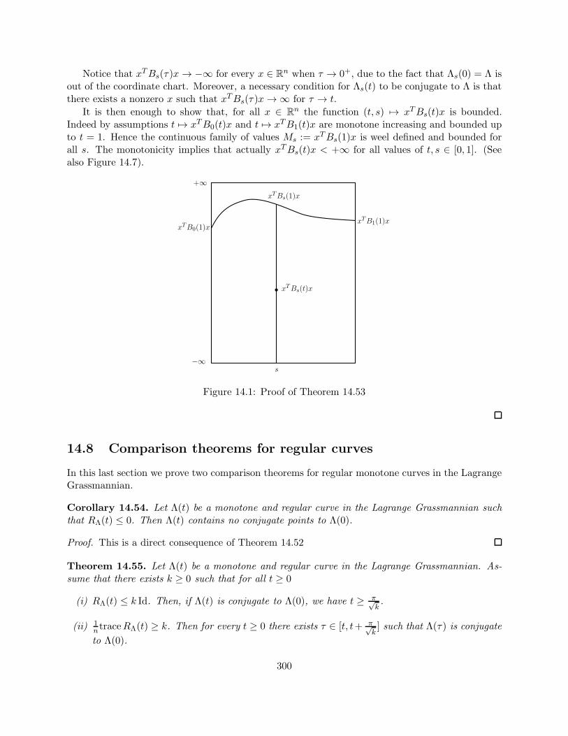
Notice that xTBs(τ)x→ −∞ for every x ∈ Rn when τ → 0+, due to the fact that Λs(0) = Λ is
out of the coordinate chart. Moreover, a necessary condition for Λs(t) to be conjugate to Λ is thatthere exists a nonzero x such that xTBs(τ)x→∞ for τ → t.
It is then enough to show that, for all x ∈ Rn the function (t, s) 7→ xTBs(t)x is bounded.
Indeed by assumptions t 7→ xTB0(t)x and t 7→ xTB1(t)x are monotone increasing and bounded upto t = 1. Hence the continuous family of values Ms := xTBs(1)x is weel defined and bounded forall s. The monotonicity implies that actually xTBs(t)x < +∞ for all values of t, s ∈ [0, 1]. (Seealso Figure 14.7).
−∞
+∞
xTB0(1)xxTB1(1)x
xTBs(1)x
xTBs(t)x
s
b
Figure 14.1: Proof of Theorem 14.53
14.8 Comparison theorems for regular curves
In this last section we prove two comparison theorems for regular monotone curves in the LagrangeGrassmannian.
Corollary 14.54. Let Λ(t) be a monotone and regular curve in the Lagrange Grassmannian suchthat RΛ(t) ≤ 0. Then Λ(t) contains no conjugate points to Λ(0).
Proof. This is a direct consequence of Theorem 14.52
Theorem 14.55. Let Λ(t) be a monotone and regular curve in the Lagrange Grassmannian. As-sume that there exists k ≥ 0 such that for all t ≥ 0
(i) RΛ(t) ≤ k Id. Then, if Λ(t) is conjugate to Λ(0), we have t ≥ π√k.
(ii) 1ntraceRΛ(t) ≥ k. Then for every t ≥ 0 there exists τ ∈ [t, t+ π√
k] such that Λ(τ) is conjugate
to Λ(0).
300
We stress that assumption (i) means that all the eigenvalues of RΛ(t) are smaller or equal thank, while (ii) requires only that the average of the eigenvalues is bigger or equal than k.
Remark 14.56. Notice that the estimates of Theorem 14.55 are sharp, as it is immediately seen byconsidering the example of a 1-dimensional curve of constant velocity (see Example 14.35).
Proof. (i). Consider the real function
ϕ : R→]0,π√k[, ϕ(t) =
1√k(arctan
√kt+
π
2)
Using that ϕ(t) = (1 + kt2)−1 it is easy to show that the Schwarzian derivative of ϕ is
Rϕ(t) = −k
(1 + kt2)2.
Thus using ϕ as a reparametrization we find, by Proposition 14.36
RΛϕ(t) = ϕ2RΛ(ϕ(t)) +Rϕ(t)Id
=1
(1 + kt2)2(RΛ(ϕ(t)) − kId) ≤ 0.
By Corollary 14.54 the curve Λ ϕ has no conjugate points, i.e. Λ has no conjugate points in theinterval ]0, π√
k[.
(ii). We prove the claim by showing that the curve Λ(t), on every interval of length π/√k has
non trivial intersection with every subspace (hence in particular with Λ(0)). This is equivalent toprove that Λ(t) is not contained in a single coordinate chart for a whole interval of length π/
√k.
Assume by contradiction that Λ(t) is contained in one coordinate chart. Then there existscoordinates such that Λ(t) = (p, S(t)p) and we can write the coordinate expression for thecurvature:
RΛ(t) = B(t)−B(t)2, where B(t) = (2S(t))−1S(t).
Let now b(t) := traceB(t). Computing the trace in both sides of equality
B(t) = B2(t) +RΛ(t),
we getb(t) = trace(B2(t)) + traceRΛ(t). (14.35)
Lemma 14.57. For every n× n symmetric matrix S the following inequality holds true
trace(S2) ≥ 1
n(traceS)2. (14.36)
Proof. For every symmetric matrix S there exists a matrix M such that MSM = D is diagonal.Since trace(MAM−1) = trace(A) for every matrix A, it is enough to prove the inequality (14.36)for a diagonal matrix D = diag(λ1, . . . , λn). In this case (14.36) reduces to the Cauchy-Schwartzinequality
n∑
i=1
λ2i ≥1
n
(n∑
i=1
λi
)2
.
301
Applying Lemma 14.57 to (14.35) and using the assumption (ii) one gets
b(t) ≥ 1
nb2(t) + nk, (14.37)
By standard results in ODE theory we have b(t) ≥ ϕ(t) , where ϕ(t) is the solution of the differentialequation
ϕ(t) =1
nϕ2(t) + nk (14.38)
The solution for (14.38), with initial datum ϕ(t0) = 0, is explicit and given by
ϕ(t) = n√k tan(
√k(t− t0)).
This solution is defined on an interval of measure π/√k. Thus the inequality b(t) ≥ ϕ(t) completes
the proof.
302
Chapter 15
Jacobi curves
Now we are ready to introduce the main object of this part of the book, i.e. the Jacobi curveassociated with a normal extremal. Heuristically, we would like to extract geometric properties ofthe sub-Riemannian structure by studying the symplectic invariants of its geodesic flow, that is theflow of ~H. The simplest idea is to look for invariants in its linearization.
As we explain in the next sections, this object is naturally related to geodesic variations, andgeneralizes the notion of Jacobi fields in Riemannian geometry to more general geometric structures.
In this chapter we consider a sub-Riemannian structure (M,U, f) on a smooth n-dimensionalmanifold M and we denote as usual by H : T ∗M → R its sub-Riemannian Hamiltonian.
15.1 From Jacobi fields to Jacobi curves
Fix a covector λ ∈ T ∗M , with π(λ) = q, and consider the normal extremal starting from q andassociated with λ, i.e.
λ(t) = et~H(λ), γ(t) = π(λ(t)). (i.e. λ(t) ∈ T ∗
γ(t)M.)
For any ξ ∈ Tλ(T ∗M) we can define a vector field along the extremal λ(t) as follows
X(t) := et~H
∗ ξ ∈ Tλ(t)(T ∗M)
The set of vector fields obtained in this way is a 2n-dimensional vector space which is the space ofJacobi fields along the extremal. For an Hamiltonian H corresponding to a Riemannian structure,the projection π∗ gives an isomorphisms between the space of Jacobi fields along the extremal andthe classical space of Jacobi fields along the geodesic γ(t) = π(λ(t)).
Notice that this definition, equivalent to the standard one in Riemannian geometry, doesnot need curvature or connection, and can be extended naturally for any strongly normal sub-Riemannian geodesic.
In Riemannian geometry, the study of one half of this vector space, namely the subspace ofclassical Jacobi fields vanishing at zero, carries informations about conjugate points along thegiven geodesic. By the aforementioned isomorphism, this corresponds to the subspace of Jacobifields along the extremal such that π∗X(0) = 0. This motivates the following construction: For
303
any λ ∈ T ∗M , we denote Vλ := kerπ∗|λ the vertical subspace. We could study the whole family of(classical) Jacobi fields (vanishing at zero) by means of the family of subspaces along the extremal
L(t) := et~H
∗ Vλ ⊂ Tλ(t)(T ∗M).
Notice that actually, being et~H
∗ a symplectic transformation and Vλ a Lagrangian subspace, thesubspace L(t) is a Lagrangian subspace of Tλ(t)(T
∗M).
15.1.1 Jacobi curves
The theory of curves in the Lagrange Grassmannian developed in Chapter ?? is an efficient toolto study family of Lagrangian subspaces contained in a single symplectic vector space. It is thenconvenient to modify the construction of the previous section in order to collect the informationsabout the linearization of the Hamiltonian flow into a family of Lagrangian subspaces at a fixedtangent space.
By definition, the pushforward of the flow of ~H maps the tangent space to T ∗M at the pointλ(t) back to the tangent space to T ∗M at λ:
e−t~H
∗ : Tλ(t)(T∗M)→ Tλ(T
∗M).
If we then restrict the action of the pushforward e−t ~H∗ to the vertical subspace at λ(t), i.e. thetangent space Tλ(t)(T
∗γ(t)M) at the point λ(t) to the fiber T ∗
γ(t)M , we define a one parameter family
of n-dimensional subspaces in the 2n-dimensional vector space Tλ(T∗M). This family of subspaces
is a curve in the Lagrangian Grassmannian L(Tλ(T∗M)).
Notation. In the following we use the notation Vλ := Tλ(T∗qM) for the vertical subspace at
the point λ ∈ T ∗M , i.e. the tangent space at λ to the fiber T ∗qM , where q = π(λ). Being the
tangent space to a vector space, sometimes it will be useful to identify the vertical space Vλ withthe vector space itself, namely Vλ ≃ T ∗
qM .
Definition 15.1. Let λ ∈ T ∗M . The Jacobi curve at the point λ is defined as follows
Jλ(t) := e−t~H
∗ Vλ(t), (15.1)
where λ(t) := et~H(λ) and γ(t) = π(λ(t)). Notice that Jλ(t) ⊂ Tλ(T ∗M) and Jλ(0) = Vλ = Tλ(T
∗qM)
is vertical.
As discussed in Chapter 14, the tangent vector to a curve in the Lagrange Gassmannian can beinterpreted as a quadratic form. In the case of a Jacobi curve Jλ(t) its tangent vector is a quadraticform Jλ(t) : Jλ(t)→ R.
Proposition 15.2. The Jacobi curve Jλ(t) satisfies the following properties:
(i) Jλ(t+ s) = e−t ~H∗ Jλ(t)(s), for all t, s ≥ 0,
(ii) Jλ(0) = −2H|T ∗qM as quadratic forms on Vλ ≃ T ∗
qM .
(iii) rank Jλ(t) = rankH|T ∗γ(t)
M
304
Proof. Claim (i) is a consequence of the semigroup property of the family e−t ~H∗ t≥0.
To prove (ii), introduce canonical coordinates (p, x) in the cotangent bundle. Fix ξ ∈ Vλ. The
smooth family of vectors defined by ξ(t) = e−t ~H∗ ξ (considering ξ as a constant vertical vector field)is a smooth extension of ξ, i.e. it satisfies ξ(0) = ξ and ξ(t) ∈ Jλ(t). Therefore, by (14.8)
Jλ(0)ξ = σ(ξ, ξ) = σ
(ξ,d
dt
∣∣∣∣t=0
e−t~H
∗ ξ
)= σ(ξ, [ ~H, ξ]). (15.2)
To compute the last quantity we use the following elementary, although very useful, property ofthe symplectic form σ.
Lemma 15.3. Let ξ ∈ Vλ a vertical vector. Then, for any η ∈ Tλ(T ∗M)
σ(ξ, η) = 〈ξ, π∗η〉, (15.3)
where we used the canonical identification Vλ = T ∗qM .
Proof. In any Darboux basis induced by canonical local coordinates (p, x) on T ∗M , we have σ =∑ni=1 dpi ∧ dxi and ξ =
∑ni=1 ξ
i∂pi . The result follows immediately.
To complete the proof of point (ii) it is enough to compute in coordinates
π∗[ ~H, ξ] = π∗
[∂H
∂p
∂
∂x− ∂H
∂x
∂
∂p, ξ∂
∂p
]= −∂
2H
∂p2ξ∂
∂x,
Hence by Lemma 15.3 and the fact that H is quadratic on fibers one gets
σ(ξ, [ ~H, ξ]) = −⟨ξ,∂2H
∂p2ξ
⟩= −2H(ξ).
(iii). The statement for t = 0 is a direct consequence of (ii). Using property (i) it is easily seen thatthe quadratic forms associated with the derivatives at different times are related by the formula
Jλ(t) et~H
∗ = Jλ(t)(0). (15.4)
Since e−t ~H∗ is a symplectic transformation, it preserves the sign and the rank of the quadratic form.1
Remark 15.4. Notice that claim (iii) of Proposition 15.2 implies that rank of the derivative of theJacobi curve is equal to the rank of the sub-Riemannian structure. Hence the curve is regular if andonly if it is associated with a Riemannian structure. In this case of course it is strictly monotone,namely Jλ(t) < 0 for all t.
Corollary 15.5. The Jacobi curve Jλ(t) associated with a sub-Riemannian extremal is monotonenonincreasing for every λ ∈ T ∗M .
1Notice that Jλ(t), Jλ(t)(0) are defined on Jλ(t), Jλ(t)(0) respectively, and Jλ(t) = e−t ~H∗ Jλ(t)(0).
305
15.2 Conjugate points and optimality
At this stage we have two possible definition for conjugate points along normal geodesics. On onehand we have singular points of the exponential map along the extremal path, on the other handwe can consider conjugate points of the associated Jacobi curve. The next result show that actuallythe two definition coincide.
Proposition 15.6. Let γ(t) = Eq(tλ) be a normal geodesic starting from q with initial covector λ.Denote by Jλ(t) its Jacobi curve. Then for s > 0
γ(s) is conjugate to γ(0) ⇐⇒ Jλ(s) is conjugate to Jλ(0).
Proof. By Definition 8.43, γ(s) is conjugate to γ(0) if sλ is a critical point of the exponentialmap Eq. This is equivalent to say that the differential of the map from T ∗
qM to M defined by
λ 7→ π es ~H (λ) is not surjective at the point λ, i.e. the image of the differential es~H
∗ has a nontrivialintersection with the kernel of the projection π∗
es~H
∗ Jλ(0) ∩ Tλ(s)T ∗γ(s)M 6= 0. (15.5)
Applying the linear invertible transformation e−s ~H∗ to both subspaces one gets that (15.5) is equiv-alent to
Jλ(0) ∩ Jλ(s) 6= 0
which means by definition that Jλ(s) is conjugate to Jλ(0).
The next result shows that, as soon as we have a segment of points that are conjugate to theinitial one, the segment is also abnormal.
Theorem 15.7. Let γ : [0, 1]→M be a normal extremal path such that γ|[0,s] is not abnormal forall 0 < s ≤ 1. Assume γ|[t0,t1] is a curve of conjugate points to γ(0). Then the restriction γ|[t0,t1]is also abnormal.
Remark 15.8. Recall that if a curve γ : [0, T ] → M is a strictly normal trajectory, it can happenthat a piece of it is abnormal as well. If the trajectory is strongly normal, then if t0, t1 satisfy theassumptions of Theorem 15.7 necessarily t0 > 0.
Proof. Let us denote by Jλ(t) the Jacobi curve associated with γ(t). From Proposition 15.6 itfollows that Jλ(t) ∩ Jλ(0) 6= 0 for each t ∈ [t0, t1]. We now show that actually this implies
Jλ(0) ∩⋂
t∈[t0,t1]Jλ(t) 6= 0. (15.6)
We can assume that the whole piece of the Jacobi curve Jλ(t), with t0 ≤ t ≤ t1, is contained in asingle coordinate chart. Otherwise we can cover [t0, t1] with such intervals and repeat the argumenton each of them. Let us fix coordinates given by a Lagrangian splitting in such a way that
Jλ(t) = (p, S(t)p), p ∈ Rn, Jλ(0) = (p, 0), p ∈ R
n
306
Moreover we can assume that S(t) ≤ 0 for every t0 ≤ t ≤ t1, i.e. is non positive definite andmonotone decreasing, 2 In particular Jλ(t1) ∩ Jλ(0) 6= 0 if and only if there exists a vector vsuch that S(t1)v = 0. Since the map t 7→ vTS(t)v is nonpositive and decreasing this means thatS(t)v = 0 for all t ∈ [t0, t1], thus
Jλ(0) ∩ Jλ(t1) ⊂ Jλ(0) ∩⋂
t∈[t0,t1]Jλ(t) (15.7)
that implies that actually we have the equality in (15.7).We are left to show that if a Jacobi curve Jλ(t) is such that every t is a conjugate point for
0 ≤ τ ≤ τ , then the corresponding extremal is also abnormal. Indeed let us fix an element ξ 6= 0such that
ξ ∈⋂
t∈[0,τ ]Jλ(t)
which is non-empty by the above discussion. Then we consider the vertical vector field
ξ(t) = et~H
∗ ξ ∈ Tλ(t)(T ∗γ(t)M), 0 ≤ t ≤ τ.
By construction, the vector field ξ is preserved by the Hamiltonian field, i.e. et~H
∗ ξ = ξ, that implies[ ~H, ξ](λ(t)) = 0. Then the statement is proved by the following
Exercise 15.9. Define η(t) = ξ(λ(t)) ∈ T ∗γ(t)M (by canonical identification Tλ(T
∗qM) ≃ T ∗
qM).
Show that the identity [ ~H, ξ](λ(t)) = 0 rewrites in coordinates as follows
k∑
i=1
hi(η(t))2 = 0, η(t) =
k∑
i=1
hi(λ(t))~hi(η(t)). (15.8)
Exercise 15.9 shows that η(t) is a family of covectors associated with the extremal path corre-sponding to controls ui(t) = hi(λ(t)) and such that hi(η(t)) = 0, that means that it is abnormal.
Corollary 15.10. Let Jλ(t) be the Jacobi curve associated with λ ∈ T ∗M and γ(t) = π(λ(t)) theassociated sub-Riemannian extremal path. Then γ|[0,τ ] is not abnormal for all 0 ≤ τ ≤ t if and onlyif Jλ(τ) ∩ Jλ(0) = 0 for all 0 ≤ τ ≤ t.
15.3 Reduction of the Jacobi curves by homogeneity
The Jacobi curve at point λ ∈ T ∗M parametrizes all the possible geodesic variations of the geodesicassociated with an initial covector λ. Since the variations in the direction of the motion are alwaystrivial, i.e. the trajectory remains the same up to parametrizations, one can reduce the space ofvariation to an (n− 1)-dimensional one.
This idea is formalized by considering a reduction of the Jacobi curve in a smaller symplecticspace. As we show in the next section, this is a natural consequence of the homogeneity of thesub-Riemannian Hamiltonian.
2Indeed it is proved that the only invariant of a pair of two Lagrangian subspaces in a symplectic space is thedimension of the intersection, i.e. the rank of the difference rank(S(t)− S(0)). Add exercise
307
Remark 15.11. This procedure was already exploited in Section 8.9, obtained by a direct argumentvia Proposition 8.37. Indeed one can recognize that the procedure that reduced the equation forconjugate points of one dimension corresponds exactly to the reduction by homogeneity of theJacobi curve associated to the problem.
We start with a technical lemma, whose proof is left as an exercise.
Lemma 15.12. Let Σ = Σ1 ⊕ Σ2 be a splitting of the symplectic space, with σ = σ1 ⊕ σ2. LetΛi ∈ L(Σi) and define the curve Λ(t) := Λ1(t)⊕ Λ2(t) ∈ L(Σ). Then one has the splittings:
Λ(t) = Λ1(t)⊕ Λ2(t),
RΛ(t) = RΛ1(t)⊕RΛ2(t).
Consider now a Jacobi curve associated with λ ∈ T ∗M :
Jλ(t) = e−t~H
∗ Vλ(t), Vλ = Tλ(T∗π(λ)M).
Denote by δα : T ∗M → T ∗M the fiberwise dilation δα(λ) = αλ, where α > 0 .
Definition 15.13. The Euler vector field ~E ∈ Vec(T ∗M) is the vertical vector field defined by
~E(λ) =d
ds
∣∣∣∣s=1
δs(λ), λ ∈ T ∗M.
It is easy to see that in canonical coordinates (x, ξ) it satisfies ~E =∑n
i=1 ξi∂∂ξi
and the followingidentity holds
et~Eλ = etλ, i.e. et
~E(ξ, x) = (etξ, x).
Exercise 15.14. Prove that the Euler vector field is characterized by the identity
i ~E σ = s, s = Liouville 1-form in T ∗M.
Lemma 15.15. We have the identity e−t ~H∗ ~E = ~E − t ~H. In particular [ ~H, ~E] = − ~H.
Proof. The homogeneity property (8.50) of the Hamiltonian can be rewritten as follows
et~H(δsλ) = δs(e
st ~H(λ)), ∀ s, t > 0.
Applying δ−s to both sides and changing t into −t one gets the identity
δ−s e−t ~H δs = e−st~H . (15.9)
Computing the 2nd order mixed partial derivative at (t, s) = (0, 1) in (15.9) one gets, by (2.27),
that [ ~H, ~E] = − ~H. Thus, by (??) we have e−t ~H∗ ~E = ~E − t ~H, since every higher order commutatorvanishes.
Proposition 15.16. The subspace Σ = span~E, ~H is invariant under the action of the Hamilto-nian flow. Moreover ~E, ~H is a Darboux basis on Σ ∩H−1(1/2).
308
Proof. The fact that Σ is an invariant subspace is a consequence of the identities
e−t~H
∗ ~E = ~E − t ~H, e−t~H
∗ ~H = 0.
Moreover, on the level set H−1(1/2), we have by homogeneity of H w.r.t. p:
σ( ~E, ~H) = ~E(H) =d
dt
∣∣∣∣t=0
H(et~E(p, x)) = p
∂H
∂p= 2H = 1. (15.10)
It follows that ~E, ~H is a Darboux basis for Σ.
In particular we can consider the the symplectic splitting Σ = Σ⊕ Σ∠.
Exercise 15.17. Prove the following intrinsic characterization of the skew-orthogonal to Σ:
Σ∠ = ξ ∈ T ∗λ (T
∗M) : 〈dλH, ξ〉 = 〈sλ, ξ〉 = 0.
The assumptions of Lemma 15.12 are satisfied and we could split our Jacobi curve.
Definition 15.18. The reduced Jacobi curve is defined as follows
Jλ(t) := Jλ(t) ∩ Σ∠. (15.11)
Notice that, if we put Vλ := Vλ ∩ TλH−1(1/2), we get
Jλ(0) = Vλ, Jλ(t) = e−t~H
∗ Vλ.
Moreover we have the splitting
Jλ(t) = Jλ(t)⊕ R( ~E − t ~H).
We stress again that Jλ(t) is a curve of (n−1)-dimensional Lagrangian subspaces in the (2n−2)-dimensional vector space Σ∠.
Exercise 15.19. With the notation above
(i) Show that the curvature of the curve Jλ(t) ∩ Σ in Σ is always zero.
(ii) Prove that Jλ(0) ∩ Jλ(s) 6= 0 if and only if Jλ(0) ∩ Jλ(s) 6= 0.
309

310
Chapter 16
Riemannian curvature
On a manifold, in general there is no canonical method for identifying tangent spaces at differentpoints, (or more generally fibers of a vector bundle at different points). Thus, we have to expectthat a notion of derivative for vector fields (or sections of a vector bundle), has to depend on certainchoices.
In our presentation we introduce the general notion of Ehresmann connection and we then wediscuss how this notion is related with the notion of parallel transport and covariant derivativeusually introduced in classical Riemannian geometry.
16.1 Ehresmann connection
Given a smooth fiber bundle E, with base M and canonical projection π : E → M , we denote byEq = π−1(q) the fiber at the point q ∈ M . The vertical distribution is by definition the collectionof subspaces in TE that are tangent to the fibers
V = Vzz∈E , Vz := kerπ∗,z = TzEπ(z) ⊂ TzE.
Definition 16.1. Let E be a smooth fiber bundle. An Ehresmann connection on E is a smoothvector distribution H in E satisfying
H = Hzz∈E , TzE = Vz ⊕Hz.
Notice that V, being the kernel of the pushforward π∗, is canonically associated with the fibrebundle. Defining a connection means exactly to define a canonical complement to this distribution.For this reason H is also called horizontal distribution.
Definition 16.2. Let X ∈ Vec(M). The horizontal lift of X is the unique vector field∇X ∈ Vec(E)such that
∇X(z) ∈ Hz, π∗∇X = X, ∀ z ∈ E. (16.1)
The uniqueness follows from the fact that π∗,z : TzE → Tπ(z)M is an isomorphism when restrictedto Hz. Indeed π∗,z is a surjective linear map with ker π∗,z = Vz.
Notation. In the following we will refer also at ∇ as the connection on E.
311
Given a smooth curve γ : [0, T ] → M on the manifold M , the connection let us to definethe parallel transport along γ, i.e. a way to identify tangent vectors belonging to tangent spacesat different points of the curve. Let Xt be a nonautonomous smooth vector field defined on aneighborhood of γ, that is an extension of the velocity vector field of the curve1, i.e. such that
γ(t) = Xt(γ(t)), ∀ t ∈ [0, T ].
Then consider the non autonomous vector field ∇Xt ∈ Vec(E) obtained by its lift.
Definition 16.3. Let γ : [0, T ]→M be a smooth curve. The parallel transport along γ is the mapΦ defined by the flow of ∇Xt
Φt0,t1 := −→exp∫ t1
t0
∇Xsds : Eγ(t0) → Eγ(t1), for 0 < t0 < t1 < T. (16.2)
In the general case we need some extra assumptions on the vector field to ensure that (16.2)exists (even for small time t > 0) since the existence time of a solution also depend on the pointon the fiber. For instance if we the fibers are compact, then it is possible to find such t > 0.
Exercise 16.4. Show that the parallel transport map sends fibers to fibers and does not dependon the extension of the vector field Xt. (Hint: consider two extensions and use the existence anduniqueness of the flow.)
16.1.1 Curvature of an Ehresmann connection
Assume that π : E → M is a smooth fiber bundle and let ∇ be a connection on E, defining thesplitting E = V ⊕H. Given an element z ∈ E we will also denote by zhor (resp. zver) its projectionon the horizontal (resp. vertical) subspace at that point.
The commutator of two vertical vector field is always vertical. The curvature operator associatedwith the connection computes if the same holds true for two horizontal vector fields.
Definition 16.5. Let E be a smooth fiber bundle and ∇ a connection on E. Let X,Y ∈ Vec(M)and define
R(X,Y ) := [∇X ,∇Y ]ver (16.3)
The operator R is called the curvature of the connection.
Notice that, given a vector field on E, its horizontal part coincide, by definition, with the liftof its projection. In particular
[∇X ,∇Y ]hor = ∇[X,Y ], (i.e. π∗[∇X ,∇Y ] = [X,Y ])
Hence R(X,Y ) computes the nontrivial part of the bracket between the lift of X and Y and R ≡ 0if and only if the horizontal distribution H is involutive.
The curvature R(X,Y ) is also rewritten in the following more classical way
R(X,Y ) = [∇X ,∇Y ]−∇[X,Y ].
= ∇X∇Y −∇X∇Y −∇[X,Y ].
Next we show that R is actually a tensor on TqM , i.e. the value of R(X,Y ) at q depends onlyon the value of X and Y at the point q.
1this is always possible with a (maybe non autonomous) vector field.
312
Proposition 16.6. R is a skew symmetric tensor on M .
Proof. The skew-symmetry is immediate. To prove that the value of R(X,Y ) at q depends onlyon the value of X and Y at the point q, it is sufficient to prove that R is linear on functions. Byskew-symmetry, we are reduced to prove that R is linear in the first argument, namely
R(aX, Y ) = aR(X,Y ), where a ∈ C∞(M).
Notice that the symbol a in the right hand side stands for the function π∗a = a π in C∞(E), thatis constant on fibers.
By definition of lift of a vector field it is easy to prove the identities ∇aX = a∇X and ∇Xa = Xafor every a ∈ C∞(M). Applying the definition of ∇ and the Leibnitz rule for the Lie bracket onegets
R(aX, Y ) = [∇aX ,∇Y ]−∇[aX,Y ]
= a[∇X ,∇Y ]− (∇Y a)∇X −∇a[X,Y ]−(Y a)X
= a[∇X ,∇Y ]− (Y a)∇X − a∇[X,Y ] + (Y a)∇X= aR(X,Y ).
16.1.2 Linear Ehresmann connections
Assume now that E is a vector bundle on M (i.e. each fiber Eq = π−1(q) has a natural structureof vector space). In this case it is natural to introduce a notion of linear Ehresmann connection ∇on E.
Given a vector bundle π : E →M , we denote by C∞L (E) the set of smooth functions on E thatare linear on fibers.
Remark 16.7. For a vector bundle π : E → M , the base manifold M can be considered immersedin E as the zero section (see also Example 2.41). The “dual” version of this identification is theinclusion i : C∞(M)→ C∞(E). Indeed any function in C∞(M) can be considered as a functions inC∞(E) which is constant on fibers, i.e. more precisely a ∈ C∞(M) 7→ π∗a ∈ C∞(E).
Exercise 16.8. Show that a vector field on E is the lift of a vector field on M if and only if, as adifferential operator on C∞(E), it maps the subspace C∞(M) into itself.
After this discussion it is natural to give the following definition.
Definition 16.9. A linear connection on a vector bundle E on the base M is an Ehresmannconnection ∇ such that the lift ∇X of a vector field X ∈ Vec(M) satisfies the following property:for every a ∈ C∞L (E) it holds ∇Xa ∈ C∞L (E).
Remark 16.10. Given a local basis of vector fields X1, . . . ,Xn on M we can build dual coordinates(u1, . . . , un) on the fibers of E defining the functions ui(z) = 〈z,Xi(q)〉 where q = π(z). In this way
E = (u, q), q ∈M,u ∈ Rn,
313
and the tangent space to E is splitted in TzE ≃ TqM ⊕ TzEq. A connection on E is determined bythe lift of the vector fields Xi, i = 1, . . . , n on the base manifold (recall that π∗∇Xi = Xi)
∇Xi = Xi +
n∑
j=1
aij(u, q)∂uj , i = 1, . . . , n, (16.4)
where aij ∈ C∞(E) are suitable smooth functions. Then ∇ is linear if and only if for every i, j thefunction aij(u, q) =
∑nk=1 Γ
kij(q)uk is linear with respect to u .
The smooth functions Γkij are also called the Christoffel symbols of the linear connection.
Exercise 16.11. Let γ be a smooth curve on the manifold such that γ(t) =∑n
i=1 vi(t)Xi(γ(t)).Show that the differential equation ξ(t) = ∇γ(t)ξ(t) for the parallel transport along γ are written
as uj =∑
i,k Γkijviuk where (u1, . . . , un) are the vertical coordinates of ξ.
Notice that, for a linear connection, the parallel transport is defined by a first order linear(nonautonomous) ODE. The existence of the flow is then guaranteed from stantard results formODE theory. Moreover, when it exists, the map Φt0,t1 is a linear transformation between fibers.
16.1.3 Covariant derivative and torsion for linear connections
Once a connection on a linear vector bundle E is given, we have a well defined linear paralleltransport map
Φt0,t1 := −→exp∫ t1
t0
∇Xsds : Eγ(t0) → Eγ(t1), for 0 < t0 < t1 < T. (16.5)
If we consider the dual map of the parallel transport one can naturally introduce a non autonomouslinear flow on the dual bundle (notice the exchange of t0, t1 in the integral)
Φ∗t0,t1 :=
(−→exp
∫ t0
t1
∇Xsds
)∗: E∗
γ(t0)→ E∗
γ(t1), for 0 < t0 < t1 < T. (16.6)
The infinitesimal generator of this “adjoint” flow defines a linear parallel transport, hence a linearconnection, on the dual bundle E∗.
In what follows we will restrict our attention to the case of the vector bundle E = T ∗M andwe assume that a linear connection ∇ on T ∗M is given. Notice that, by the above discussion, allthe constructions can be equivalently performed on the dual bundle E∗ = TM .
For every vector field Y ∈ Vec(M) let us denote with Y ∗ ∈ C∞(T ∗M) the function
Y ∗(λ) = 〈λ, Y (q)〉 , q = π(z),
namely the smooth function on E associated with Y that is linear on fibers. This identificationbetween vector fields onM and linear functions on T ∗M permits us to define the covariant derivativeof vector fields.
Definition 16.12. Let X,Y ∈ Vec(M). We define ∇XY = Z if and only if ∇XY ∗ = Z∗ withZ ∈ Vec(M).
314
Notice that the definition is well-posed since ∇ is linear, hence ∇XY ∗ is a linear function andthere exists Z ∈ Vec(M) such that ∇XY ∗ = Z∗.2
Lemma 16.13. Let X1, . . . ,Xn be a local frame on M . Then ∇XiXj = ΓkijXk, where Γkij arethe Christoffel symbols of the connection ∇.
Proof. Let us prove this in the coordinates dual to our frame. In these coordinates, the linearconnection is specified by the lifts
∇Xi = Xi + Γkijuk∂uj , where uj(λ) = 〈λ,Xj〉 .
Moreover X∗j = uj . Hence it is immediate to show ∇XiX
∗j = ΓkijX
∗k , and the lemma is proved.
We now introduce the torsion tensor of a linear connection on T ∗M . As usual, σ denotes thecanonical symplectic structure on T ∗M .
Definition 16.14. The torsion of a linear connection ∇ is the map T : Vec(M)2 → Vec(M) definedby the identity
T (X,Y )∗ := σ(∇X ,∇Y ), ∀X,Y ∈ Vec(M). (16.7)
It is easy to check that T is actually a tensor, i.e. the value of T (X,Y ) at a point q depends onlyon the values of X,Y at the point. The torsion computes how much the horizontal distribution His far from being Lagrangian. In particular H is Lagrangian if and only if T ≡ 0.
The classical formula for the torsion tensor, in terms of the covariant derivative, is recovered inthe following lemma.
Lemma 16.15. The torsion tensor satisfies the identity
T (X,Y ) = ∇XY −∇YX − [X,Y ]. (16.8)
Proof. We have to prove that T (X,Y )∗ = ∇XY ∗ −∇YX∗ − [X,Y ]∗. Notice that by definition ofthe Liouville 1-form s ∈ Λ1(T ∗M), sλ = λ π∗ we have X∗(λ) = 〈λ,X〉 = 〈sλ,∇X〉. Then we have,using that σ = ds and the Cartan formula (4.74)
T (X,Y )∗ = ds(∇X ,∇Y )= ∇X 〈s,∇Y 〉 − ∇Y 〈s,∇X〉 − 〈s, [∇X ,∇Y ]〉= ∇X 〈s,∇Y 〉 − ∇Y 〈s,∇X〉 −
⟨s,∇[X,Y ]
⟩
= ∇XY ∗ −∇YX∗ − [X,Y ]∗,
where in the second equality we used that 〈s, [∇X ,∇Y ]〉 = 〈s, [∇X ,∇Y ]hor〉 =⟨s,∇[X,Y ]
⟩since the
Liouville form by definition depends only on the horizontal part of the vector.
Exercise 16.16. Show that a linear connection ∇ on a vector bundle E satisfies the followingLeibnitz rule
∇X(aY ) = a∇XY + (Xa)Y, for each a ∈ C∞(M).
2There is no confusion in the notation above since, by definition, ∇X it is well defined when applied to smoothfunctions on T ∗M . Whenever it is applied to a vector field we follow the aforementioned convention.
315
16.2 Riemannian connection
In this section we want to introduce the Levi-Civita connection on a Riemannian manifold M bydefining an Ehresmann connection on T ∗M via the Jacobi curve approach.
Recall that every Jacobi curve associated with a trajectory on a Riemannian manifold is regular.Moreover, as showed in Chapter 14, every regular curve in the Lagrangian Grassmannian admitsa derivative curve, which defines a canonical complement to the curve itself. Hence, followingthis approach, it is natural to introduce the Riemannian connection at λ ∈ T ∗M as the canonicalcomplement to the Jacobi curve defined at λ.
Definition 16.17. The Levi-Civita connection on T ∗M is the Ehresmann connection H is definedby
Hλ = Jλ(0), λ ∈ T ∗M,
where as usual Jλ(t) denotes the Jacobi curve defined at the point λ ∈ T ∗M and Jλ denotes its
derivative curve.
The next proposition characterizes the Levi-Civita connection as the unique linear connectionon T ∗M that is linear, metric preserving and torsion free.
Proposition 16.18. The Levi-Civita connection satisfies the following properties:
(i) is a linear connection,
(ii) is torsion free,
(iii) is metric preserving, i.e. ∇XH = 0 for each vector field X ∈ Vec(M).
Proof. (i). It is enough to prove that the connection Hλ is 1-homogeneous, i.e.
Hcλ = δc∗Hλ, ∀ c > 0. (16.9)
Indeed in this case the functions aij ∈ C∞(T ∗M) defining the connection (see (16.4)) are 1-homogeneous, hence linear as a consequence of Exercise 16.19.
Let us prove (16.9). The differential of the dilation on the fibers δc : T∗M → T ∗M satisfies the
property δc∗(Tλ(T ∗qM)) = Tcλ(T
∗qM). From this identity and differentiating the identity
et~H δc = δc ect ~H , ∀ c > 0, (16.10)
one easily gets that
Jcλ(t) = δc∗Jλ(ct), ∀ t ≥ 0, λ ∈ T ∗M. (16.11)
Indeed one has the following chain of identities
Jcλ(t) = e−t~H
∗ (Tcλ(T∗qM))
= e−t~H
∗ δc∗(Tλ(T ∗qM)) (by (16.10))
= δc∗ e−ct ~H∗ (Tλ(T∗qM))
= δc∗Jλ(ct).
316
Now we show that the same relation holds true also for the derivative curve, i.e.
Jcλ(t) = δc∗J
λ(ct), ∀ t ≥ 0, λ ∈ T ∗M. (16.12)
Indeed one can check in coordinates (we denote as usual Jλ(t) = (p, Sλ(t)p), p ∈ Rn) that the
identity (16.11) is written as Scλ(t) =1cSλ(ct) thus Scλ(t)
−1 = cSλ(ct)−1. From here3 one also gets
Bcλ(t) = cBλ(ct) and (16.12) follows from the identity S(t) = B−1(t) + S(t). (See also Exercise14.22). In particular at t = 0 the identity (16.12) says that Hcλ = δc∗Hλ.
(ii). It is a direct consequence of the fact that Jλ(0) is a Lagrangian subspace of Tλ(T
∗M) forevery λ ∈ T ∗M , hence the symplectic form vanishes when applied to two horizontal vectors.
(iii). Again, for every X ∈ Vec(M), both ∇X and ~H are horizontal vector field. Since thehorizontal space is Lagrangian
∇XH = σ(∇X , ~H) = 0.
Exercise 16.19. Let f : Rn → R be a smooth function that satisfies f(αx) = αf(x) for everyx ∈ R
n and α ≥ 0. Then f is linear.
The following theorem says that a connection satisfying the three properties above is unique.Then it characterize the Levi-Civita connection in terms of the structure constants of the Lie algebradefined by an orthonormal frame.
Theorem 16.20. There is a unique Ehresmann connection ∇ satisfying the properties (i), (ii), and(iii) of Proposition 16.18, that is the Levi-Civita connection. Its Christoffel symbols are computedby
Γkij =1
2(ckij − cijk + cjki), (16.13)
where ckij are the smooth functions defined by the identity [Xi,Xj ] =∑n
k=1 ckijXk.
Proof. Let X1, . . . ,Xn be a local orthonormal frame for the Riemannian structure and let us con-sider coordinates (q, u) in T ∗M , where the fiberwise coordinates u = (u1, . . . , un) are dual to theorthonormal frame. From the linearity of the connection it follows that there exist smooth functionsΓkij :M → R (depending on q only) such that
∇Xi = Xi +n∑
j=1
Γkijuk∂uj , i = 1, . . . , n.
In particular ∇XiXj = ΓkijXk. In these coordinates the Hamiltonian vector field associated with
the Riemannian Hamiltonian H = 12
∑ni=1 u
2i reads (see also Exercise ??)
~H =
n∑
i,j,k=1
uiXi + ckijuiuk∂uj ,
while the symplectic form σ is written (ν1, . . . , νn denotes the dual basis to X1, . . . ,Xn)
σ =
n∑
i,j,k=1
duk ∧ νk − ckijukνi ∧ νk.
3recall that B is the zero order term of the expansion of S−1.
317
Since the horizontal space is Lagrangian, one has the relations
0 = σ(∇Xi ,∇Xj ) =n∑
k=1
(Γkij − Γkji − ckij)uk, ∀ i, j = 1, . . . , n,
hence ckij = Γkij − Γkji for all i, j, k. Moreover the connection is metric, i.e. it satisfies
0 = ∇XiH =n∑
j,k=1
Γkijukuj , ∀ i = 1, . . . , n.
The last identity implies that Γkij is skew-symmetric with respect to the pair (j, k), i.e. Γkij = −Γjik.Thus combining the two identities one gets
ckij − cijk + cjki = (Γkij − Γkji)− (Γijk + Γikj) + (Γjki − Γjik)
= Γkij − Γjik = 2Γkij .
Remark 16.21. Notice that in the classical approach one can recover formula (16.13) from thefollowing particular case of the Koszul formula
Γkij = g(∇XiXj ,Xk) =1
2(g([Xi,Xj ],Xk)− g([Xj ,Xk],Xi) + g([Xk,Xi],Xj)) ,
that holds for every orthonormal basis X1, . . . ,Xn. Notice also that the Hamiltonian vector field iswritten in coordinates ~H =
∑ni=1 ui∇Xi , which gives another proof of the fact that it is horizontal.
Let X,Y,Z,W ∈ Vec(M). We define R(X,Y )Z =W if R(X,Y )Z∗ =W ∗.
Proposition 16.22 (Bianchi identity). For every X,Y,Z ∈ Vec(M) the following identity holds
R(X,Y )Z +R(Y,Z)X +R(Z,X)Y = 0. (16.14)
Proof. We will show that (16.14) is a consequence of the Jacobi identity (2.30). Using that ∇ is atorsion free connection we can write
[X, [Y,Z]] = ∇X [Y,Z]−∇[Y,Z]X
= ∇X∇Y Z −∇X∇ZY −∇[Y,Z]X,
[Z, [X,Y ]] = ∇Z∇XY −∇Z∇YX −∇[X,Y ]Z,
[Y, [Z,X]] = ∇Y∇ZX −∇Y∇XZ −∇[Z,X]Y,
Then
0 = [X, [Y,Z]] + [Y, [Z,X]] + [Z, [X,Y ]]
= ∇X∇Y Z −∇X∇ZY −∇[Y,Z]X
+∇Z∇XY −∇Z∇YX −∇[X,Y ]Z
+∇Y∇ZX −∇Y∇XZ −∇[Z,X]Y
= R(X,Y )Z +R(Y,Z)X +R(Z,X)Y.
318
Exercise 16.23. Prove the second Bianchi identity
(∇XR)(Y,Z,W ) + (∇YR)(Z,X,W ) + (∇ZR)(X,Y,W ) = 0, ∀X,Y,Z,W ∈ Vec(M).
(Hint: Expand the identity ∇[X,[Y,Z]]+[Y,[Z,X]]+[Z,[X,Y ]]W = 0 .)
Let us denote (X,Y,Z,W ) := 〈R(X,Y )Z,W 〉. Following this notation, the first Bianchi identitycan be rewritten as follows:
(X,Y,Z,W ) + (Z,X, Y,W ) + (Y,Z,X,W ) = 0, ∀X,Y,Z,W ∈ Vec(M). (16.15)
Remark 16.24. The property of the Riemann tensor can be reformulated as follows
(X,Y,Z,W ) = −(Y,X,Z,W ), (X,Y,Z,W ) = −(X,Y,W,Z). (16.16)
Proposition 16.25. For every X,Y,Z,W ∈ Vec(M) we have (X,Y,Z,W ) = (Z,W,X, Y ).
Proof. Using (16.15) four times we can write the identities
(X,Y,Z,W ) + (Z,X, Y,W ) + (Y,Z,X,W ) = 0,
(Y,Z,W,X) + (W,Y,Z,X) + (Z,W, Y,X) = 0,
(Z,W,X, Y ) + (X,Z,W, Y ) + (W,X,Z, Y ) = 0,
(W,X, Y,Z) + (Y,W,X,Z) + (X,Y,W,Z) = 0.
Summing all together and using the skew symmetry (16.16), one gets (X,Z,W, Y ) = (W,Y,X,Z).
Proposition 16.26. Assume that (X,Y,X,W ) = 0 for every X,Y,W ∈ Vec(M). Then
(X,Y,Z,W ) = 0 ∀X,Y,Z,W ∈ Vec(M).
Proof. By assumptions and the skew-simmetry properties (16.16) of the Riemann tensor we havethat (X,Y,Z,W ) = 0 whenever any two of the vector fields coincide. In particular
0 = (X,Y +W,Z, Y +W ) = (X,Y,Z,W ) + (X,W,Z, Y ). (16.17)
since the two extra terms that should appear in the expansion vanish by assumptions. Then (16.17)can be rewritten as
(X,Y,Z,W ) = (Z,X, Y,W ),
i.e. the quantity (X,Y,Z,W ) is invariant by ciclic permutations of X,Y,Z. But the cyclic sum ofterms is zero by (16.15), hence (X,Y,Z,W ) = 0.
We end this section by summarizing the symmetry property of the Riemann curvature as follows
Corollary 16.27. There is a well defined map
R : ∧2TqM → ∧2TqM, R(X ∧ Y ) := R(X,Y ).
Moreover R is skew-adjoint with respect to the induced scalar product on ∧2TqM , that means
⟨R(X ∧ Y ), Z ∧W
⟩=⟨X ∧ Y,R(Z ∧W )
⟩.
319
16.3 Relation with Hamiltonian curvature
In this section we compute the curvature of the Jacobi curve associated with a Riemannian geodesicand we describe the relation with the Riemann curvature discussed in the previous section. As weshow, the curvature associated to a geodesic is a kind of sectional curvature operator in the directionof the geodesic itself.
Definition 16.28. The Hamiltonian curvature tensor at λ ∈ T ∗M is the operator
Rλ := RJλ(0) : Vλ → Vλ.
In other words Rλ is the curvature of the Jacobi curve associated with λ at t = 0.
Proposition 16.29. Let ξ ∈ Vλ and V be a smooth vertical vector field extending ξ. Then
Rλ(ξ) = −[ ~H, [ ~H, V ]hor]ver(λ)
Proof. This is a direct consequence of Proposition 14.30. Indeed recall that the curvature of theJacobi curve is expressed through the composition
Rλ = Jλ(0) Jλ(0).
Moreover, being Jλ(0) = Vλ and Jλ(0) = Hλ we have that
πJ(0)J(0)(ξ) = ξhor, πJ(0)J(0)(η) = ηver.
FInally we can extend vectors in Jλ(0) (resp. Jλ(0)) by applying the Hamiltonian vector field
since Jλ(t) = et~H
∗ Jλ(0) (resp. Jλ(t) = et
~H∗ J
λ(0)). From these remarks we obtain the followingformulas
Jλ(0)ξ = [ ~H, V ]hor, Jλ(0)η = −[ ~H,W ]ver
for some V vertical (resp. W horizontal) extension of the vector ξ ∈ Vλ (reps. η ∈ Hλ).
Another immediate property of the curvature tensor is the homogeneity with respect to therescaling of the covector (that corresponds to reparametrization of the trajectory). Indeed bychoosing ϕ(t) = ct, with c > 0, in Proposition 14.36 one gets
Corollary 16.30. For every c > 0 we have Rcλ = c2Rλ.
If we use the Riemannian product to identify the tangent and the cotangent space at a point,we recognize that Rλ is nothing but the sectional curvature operator where one entry is the tangentvector γ of the geodesic.
Let us denote by I : TM → T ∗M the isomorphism defined by the Riemannian scalar product〈·|·〉. In particular I(v) = λ for λ ∈ T ∗
qM and v ∈ TqM if 〈λ,w〉 = 〈v|w〉 for all w ∈ TqM .Let denote Hq = H|T ∗
qM . Recall that the differential of Hq can be interpreted as a linear mapDHq : T ∗
qM → TqM that sends λ ∈ T ∗qM into DλHq seen as a linear functional on T ∗
qM , i.e. atangent vector. This map is actually the inverse of the isomorphism I.
Lemma 16.31. DλHq = I−1(λ).
Proof. It is a simple consequence of the formula H(λ) = 12
⟨λ, I−1(λ)
⟩.
320
Corollary 16.32. Assume I(v) = λ, then ~H(λ) = ∇v.
Proof. Indeed, since ~H is an horizontal vector field, it is sufficient to show that π∗ ~H(λ) = v, whichis a consequence of Lemma 16.31. Indeed for every vertical vector ξ ∈ Tλ(T ∗
qM) one has
〈ξ, v〉 =⟨ξ, I−1(λ)
⟩= DλH(ξ) = σ(ξ, ~H(λ)) =
⟨ξ, π∗ ~H(λ)
⟩.
By arbitrary of ξ ∈ Tλ(T ∗qM) one has the equality v = π∗ ~H(λ).
Theorem 16.33. We have the following identity
RI(X)(I(Y )) = R(X,Y )X, ∀X,Y ∈ TqM. (16.18)
Proof. We have to compute the quantity
RI(X)(I(Y )) = −[ ~H, [ ~H, IY ]hor]ver(I(X))
First notice that π∗[ ~H, I(Y )] = −Y hence [ ~H, I(Y )]hor = −∇Y . Then
−[ ~H, [ ~H, I(Y )]hor]ver(I(X)) = [∇X ,∇Y ]ver(I(X)) = R(X,Y )(X).
Definition 16.34. The Ricci tensor at λ is defined as the trace of the curvature operator at λ,Ric(λ) := trace Rλ.
Exercise 16.35. Prove the following expression for the Ricci tensor, where X1, . . . ,Xn is a localorthonormal frame and γ(0) = v = I−1(λ) is the tangent vector to the geodesic:
Ric(λ) =
n∑
i=1
〈R(v,Xi)v|Xi〉
=
n∑
i=1
σλ([ ~H,∇Xi ],∇Xi).
This shows that Ric(λ) = Ric(v) coincide with the classical Riemannian Ricci tensor.
16.4 Locally flat spaces
In this section we want to show that the Riemannian curvature is the only obstruction for a Rie-mannian manifold to be locally Euclidean. Finally we show that the Riemannian curvature is alsocompletely recovered by the Hamiltonian curvature Rλ.
A Riemannian manifold M is called flat if R(X,Y ) = 0 for every X,Y ∈ Vec(M).
Theorem 16.36. M is flat if and only if M is locally isometric to Rn.
321
Proof. If M is locally isometric to Rn, then its curvature tensor at every point in a neighborhood
is identically zero.
Then let us assume that the Riemann tensor R vanishes identically and prove that M is locallyEuclidean. We will do that by showing that there exists coordinate such that the Hamiltonian, inthese set of coordinates, is written as the Hamiltonian of the Euclidean R
n.
Since R is identically zero the horizontal distribution (defined by the Levi Civita connection)is involutive. Hence, by Frobenius theorem, there exists a horizontal Lagrangian foliation of T ∗M ,i.e. for each λ ∈ T ∗M , there exists a leaf Lλ of the foliation passing through this point that istangent to the horizontal space Hλ. In particular each leaf is transversal to the fiber T ∗
qM , whereq = π(λ).
Fix a point q0 ∈M and a neighborhood Oq0 where R is identically zero. Define the map
Ψ : π−1(Oq0)→ T ∗q0M, λ ∈ π−1(Oq0) 7→ Lλ ∩ T ∗
q0M
that assigns to each λ the intersection of the leaf passing through this point and T ∗q0M .
Exercise 16.37. Show that Ψ is a linear, orthogonal transformation, i.e. H(Ψ(λ)) = H(λ) for allλ ∈ π−1(Oq0). (Hint: use the linearity of the connection and the fact that ~H is horizontal).
Fix now a basis ν1, . . . , νn in T ∗q0M that is orthonormal (with respect to the dual metric).
Being Ψ linear on fibers, we can write
Ψ(λ) =n∑
i=1
ψi(λ)νi, where ψi(λ) = 〈λ,Xi(q)〉
for a suitable basis of vector fields X1, . . . ,Xn in the neighborhood Oq0 . Moreover X1, . . . ,Xn isan orthonormal basis since Ψ is an orthogonal map.
We want to show that X1, . . . ,Xn is an orthonormal basis of vector fields that commuteseverywhere.
Let us show that the fact that the foliation is Lagrangian implies [Xi,Xj ] = 0 for all i, j =1, . . . , n.
Indeed the tautological 1-form is written in these coordinates as s =∑n
i=1 ψi νi and
σ = ds =
n∑
i=1
dψi ∧ νi + ψidνi. (16.19)
Since on each leaf the function ψi is constant by definition (hence dψi|L = 0), we have thatσ|L =
∑i ψi dνi. In particular each leaf is Lagrangian if and only if dνi = 0 for i = 1, . . . , n. Then,
from the Cartan formula, one gets
0 = dνi(Xj ,Xk) = −νi([Xj ,Xk]), ∀ i, j, k.
This proves that [Xi,Xj ] = 0 for each i, j = 1, . . . , n. Hence, in the coordinate set (ψ, q), we haveH(ψ, q) = 1
2 |ψ|2.
The next result shows that the Hamiltonian curvature can detect if a manifold is flat or not.
Corollary 16.38. M is flat if and only if Rλ = 0 for every λ ∈ T ∗M .
322
Proof. Assume that M is flat. Then R is identically zero and a fortiori Rλ = 0 from (16.18).
Let us prove the converse. Recall that Rλ = 0 implies, again by (16.18), that
(X,Y,X,W ) = 0, ∀X,Y,W ∈ Vec(M).
Then the statement is a consequence of Proposition 16.26.
Exercise 16.39. Prove that actually the Riemann tensor R is completely determined by R.
16.5 Example: curvature of the 2D Riemannian case
In this section we apply the definition of curvature discussed in this chapter to a two dimensionalRiemannian surface. As we explain, we recover that the Riemannian curvature tensor is determinedby the Gauss curvature of the manifold.
Let M be a 2-dimensional surface and f1, f2 ∈ Vec(M) be a local orthonormal frame for theRiemannian metric. The Riemannian Hamiltonian H is written as follows (we use canonical coor-dinates λ = (p, x) on T ∗M)
H(p, x) =1
2(〈p, f1(x)〉2 + 〈p, f2(x)〉2) (16.20)
Here, for a covector λ = (p, x) ∈ T ∗M , the symplectic vector space Σλ = Tλ(T∗M) is 4-dimensional.
Recall that, being M 2-dimensional, the level set H−1(1/2)∩T ∗qM is a circle. Hence, there is a
well defined vector field that produces rotation on the reduced fiber. Let us define the angle θ onthe level H−1(1/2) ∩ T ∗
xM by setting
〈p, f1(x)〉 = cos θ, 〈p, f2(x)〉 = sin θ,
in such a way that θ = 0 corresponds to the direction of f1. Denote by ∂θ the rotation in the fiberof the unit tangent bundle and by ~E, the Euler vector field. Denote finally by ~H ′ := [∂θ, ~H ].
Notice that Σλ = Vλ ⊕Hλ where Vλ = span~E, ∂θ and Hλ = span ~H, ~H ′.
Lemma 16.40. The vector fields ~E, ∂θ, ~H, ~H ′ at λ form a Darboux basis for Σλ.
Proof. We want to compute the following symplectic products of the vector fields:
σ(∂θ, ~E) = 0, σ(∂θ, ~H) = 0, σ( ~E, ~H) = 1. (16.21)
σ(∂θ, ~H′) = 1, σ( ~E, ~H ′) = 0, σ( ~H, ~H ′) = 0. (16.22)
Indeed, let us prove first (16.21). The first equality follows from the fact that both vectors belongto the vertical subspace, that is Lagrangian. The second one is a consequence of the fact that, byconstruction, ∂θ is tangent to the level set of H, i.e. σ(∂θ, ~H) = ∂θ( ~H) = 〈dH, ∂θ〉 = 0. The lastidentity is (15.10).
As a preliminary step for the proof of (16.22) notice that, if s = i ~Eσ denotes the tautologicalLiouville form, one has
〈s, ~H〉 = 1, 〈s, ~H ′〉 = 0. (16.23)
323
These two identities follows from
〈s, ~H〉 = σ( ~E, ~H) = 1, (16.24)
〈s, ~H ′〉 = 〈s, [∂θ, ~H]〉 = ds(∂θ, ~H) = σ(∂θ, ~H) = 0, (16.25)
where in the second line we used the Cartan formula (4.74) and the fact that ∂θ is vertical.Let us now prove (16.22). Being [∂θ, ~H
′] = [∂θ, [∂θ, ~H ]] = − ~H, we have again by Cartan formulaand (16.23)
σ(∂θ, ~H′) = ds(∂θ, ~H
′) = −〈s, [∂θ, ~H ′]〉 = 〈s, ~H〉 = σ( ~E, ~H) = 1
Moreover by (16.23)
σ( ~E, ~H ′) = 〈s, ~H ′〉 = 0.
The last computation is similar. Let us write
σ( ~H, ~H ′) = 〈dH, ~H ′〉 = 〈dH, [∂θ, ~H ]〉,
and apply the Cartan formula to the last term (with dH as 1-form).
dH([∂θ, ~H ]) = d2H(∂θ, ~H)− ∂θ〈dH, ~H〉+ ~H 〈dH, ∂θ〉 = 0
since the three terms are all equal to zero.
Now we compute the curvature via the Jacobi curve, reduced by homogeneity. Notice thatby Lemma 16.40 we can remove the symplectic space spanned by ~E, ~H and, being ~E, ~H∠ =∂θ, ~H ′, we have
Jλ(t) = spane−t ~H∗ ∂θ.Then we define the generator of the Jacobi curve
Vt = e−t~H
∗ ∂θ, Vt = e−t~H
∗ [ ~H, ∂θ] = −e−t ~H∗ ~H ′
Notice that
σ(Vt, Vt) = −1, for every t ≥ 0. (16.26)
Indeed it is true for t = 0 and the equality is valid for all t since the transformation et~H
∗ is symplectic.To compute the curvature of the Jacobi curve let us write
Vt = α(t)V0 − β(t)V0 (16.27)
We claim that the matrix S(t) representing the 1-dimensional Jacobi curve (that actually is ascalar), is given in these coordinates by
S(t) =β(t)
α(t)=σ(V0, Vt)
σ(V0, Vt).
Indeed the identity
Vt = α(t)V0 − β(t)V0 = α(t)
(V0 −
β(t)
α(t)V0
), (16.28)
324
tells us that the matrix representing the vector space spanned by Vt is the graph of the linear mapV0 7→ −β(t)
α(t) V0. Moreover, using that V0 and V0 is a Darboux basis, it is easy to compute
σ(V0, Vt) = α(t)σ(V0, V0)︸ ︷︷ ︸=0
−β(t)σ(V0, V0)︸ ︷︷ ︸=−1
= β(t), (16.29)
σ(V0, Vt) = α(t)σ(V0, V0)︸ ︷︷ ︸=1
−β(t)σ(V0, V0)︸ ︷︷ ︸=0
= α(t). (16.30)
Differentiating the identity (16.26) with respect to t one gets the relations
σ(Vt, Vt) = 0, σ(Vt, V(3)t ) = −σ(Vt, Vt)
Notice that these quantities are constant with respect to t. Collecting the above results one cancompute the asymptotic expansion of S(t) with respect to t
S(t) =−t+ t3
6σ(V0,
...V 0) +O(t5)
1 +t2
2σ(V0, V0) +O(t4)
(16.31)
=
(−t+ t3
6σ(V0,
...V 0) +O(t5)
)(1− t2
2σ(V0, V0) +O(t4)
)(16.32)
and one gets for the derivative of S(t) at t = 0
S(0) = −1, S(0) = 0,...S (0) = 2σ(V0, V0).
The formula for the curvature R is finally computed in terms of S(t) as follows:
R = −1
2
...S (0) = σ(V0, V0) (16.33)
Using that Vt = e−t ~H∗ ∂θ we can expand Vt as follows
Vt = ∂θ + t[ ~H, ∂θ] +t2
2[ ~H, [ ~H, ∂θ]] +O(t3)
hence (16.33) is rewritten as
R = σ([ ~H, [ ~H, ∂θ]], [ ~H, ∂θ]) (16.34)
= σ([ ~H, ~H ′], ~H ′) (16.35)
To end this section, we compute the curvature R with respect to the orthonormal frame f1, f2.Denote the Hamiltonians
hi(p, x) = 〈p, fi(x)〉 , i = 1, 2.
The PMP reads
x = h1f1(x) + h2f2(x)
h1 = H,h1 = h2, h1h2h2 = H,h2 = −h2, h1h1
(16.36)
325
Moreover h2, h1(p, x) = 〈p, [f2, f1](x)〉. Assume that
[f1, f2] = a1f1 + a2f2, ai ∈ C∞(M).
Thenh2, h1 = −a1h1 − a2h2.
If we restrict to h1 = cos θ and h2 = sin θ equations (16.36) become
x = cos θf1 + sin θf2
θ = a1 cos θ + a2 sin θ
and it is easy to compute the following expression for ~H and commutators4
~H = h1f1 + h2f2 + (a1h1 + a2h2)∂θ,
~H ′ = −h2f1 + h1f2 + (−a1h2 + a2h1)∂θ,
[ ~H, ~H ′] = (f1a2 − f2a1 − a21 − a22)∂θ.
Recall thatκ = f1a2 − f2a1 − a21 − a22,
is the Gaussian curvature of the surface M (see also Chapter 4). Since σ(∂θ, ~H′) = 1 one gets
R = σ([ ~H, ~H ′], ~H ′) = σ(κ∂θ, ~H′) = κ.
Exercise 16.41. In this exercise we recover the previous computations introducing dual coordinatesto our frame. Let ν1, ν2 be the dual basis to f1, f2 and set
fθ := h1f1 + h2f2, νθ := h1ν1 + h2ν2.
Define the smooth function b := a1h1 + a2h2 on T ∗M . In these notation
~H = fθ + b∂θ, ~H ′ = fθ′ + b′∂θ,
where ′ denotes the derivative with respect to θ. Then, using that in these coordinates the tauto-logical form is s = νθ, show that the symplectic form is written as
σ = ds = dθ ∧ νθ′ − b ν1 ∧ ν2,
and compute the following expressions
i ~H′σ = (b′ − b)νθ′ − dθ,[ ~H, ~H ′] = (fθb
′ − fθ′b− b2 − b′2)∂θ,
showing that this gives an alternative proof of the above computation of the curvature.
4here we still use the notation h1, h2 as functions of θ satisfying ∂θh1 = −h2, ∂θh2 = h1
326
Chapter 17
Curvature in 3D contactsub-Riemannian geometry
The main goal of this chapter is to compute the curvature of the three dimensional contact sub-Riemannian case. Then we will discuss some general features of the curvature in sub-Riemanniangeometry.
17.1 3D contact sub-Riemannian manifolds
In this section we consider a sub-Riemannian manifold M of dimension 3 whose distribution isdefined as the kernel of a contact 1-form ω ∈ Λ1(M), i.e. Dq = kerωq for all q ∈M . Let us also fixa local orthonormal frame f1, f2 such that
Dq = kerωq = spanf1(q), f2(q)
Recall that the 1-form ω ∈ Λ1(M) defines a contact distribution if and only if ω ∧ dω 6= 0 is nevervanishing.
Exercise 17.1. Let M be a 3D manifold, ω ∈ Λ1M and D = kerω. The following are equivalent:
(i) ω is a contact 1-form,
(ii) dω∣∣D 6= 0,
(iii) ∀ f1, f2 ∈ D linearly independent, then [f1, f2] /∈ D.Remark 17.2. The contact form ω is defined up to a smooth function, i.e. if ω is a contact form,aω is a contact form for every a ∈ C∞(M). This let us to normalize the contact form by requiringthat
dω∣∣D = ν1 ∧ ν2, (i.e. dω(f1, f2) = 1.)
where ν1, ν2 is the dual basis to f1, f2. This is equivalent to say that dω is equal to the area forminduced on the distribution by the sub-Riemannian scalar product.
Definition 17.3. The Reeb vector field of the contact structure is the unique vector field f0 ∈Vec(M) that satisfies
dω(f0, ·) = 0, ω(f0) = 1
327
In particular f0 is transversal to the distribution and the triple f0, f1, f2 defines a basis ofTqM at every point q ∈M . Notice that ω, ν1, ν2 is the dual basis to this frame.
Remark 17.4. The flow generated by the Reeb vector field etf0 : M → M is a group of diffeomor-phisms that satisfy (etf0)∗ω = ω. Indeed
Lf0ω = d(if0ω) + if0dω = 0
since if0ω = ω(f0) = 1 is constant and if0dω = dω(f0, ·) = 0.
In what follows, to simplify the notation, we will replace the contact form ω by ν0, as the dualelement to the vector field f0. We can write the structure equations of this basis of 1-forms
dν0 = ν1 ∧ ν2dν1 = c101ν0 ∧ ν1 + c102ν0 ∧ ν2 + c112ν1 ∧ ν2dν2 = c201ν0 ∧ ν1 + c202ν0 ∧ ν2 + c212ν1 ∧ ν2
(17.1)
The structure constants ckij are smooth functions on the manifold. Recall that the equation
dνk =2∑
i,j=0
ckijνi ∧ νj if and only if [fj , fi] =2∑
k=0
ckijfk.
Introduce the coordinates (h0, h1, h2) in each fiber of T ∗M induced by the dual frame
λ = h0ν0 + h1ν1 + h2ν2
where hi(λ) = 〈λ, fi(q)〉 are the Hamiltonians linear on fibers associated to fi, for i = 0, 1, 2. Thesub-Riemannian Hamiltonian is written as follows
H =1
2(h21 + h22).
We now compute the Poisson bracket H,h0, denoting with H,h0q its restriction to the fiberT ∗qM .
Proposition 17.5. The Poisson bracket H,h0q is a quadratic form. Moreover we have
H,h0 = c101h21 + (c201 + c102)h1h2 + c202h
22, (17.2)
c101 + c202 = 0. (17.3)
Notice that ∆⊥q ⊂ ker H,h0q and H,h0q can be treated as a quadratic form on T ∗
qM/∆⊥q = ∆∗
q.
Proof. Using the equality hi, hj(λ) = 〈λ, [fi, fj ](q)〉 we get
H,h0 =1
2h21 + h22, h0 = h1h1, h0+ h2h2, h0
= h1(c101h1 + c201h2) + h2(c
102h1 + c202h2)
= c101h21 + (c201 + c102)h1h2 + c202h
22.
328
Differentiating the first equation in (17.1) one gets:
0 = d2ν0 = dν1 ∧ ν2 − ν1 ∧ ν2= (c101ν0 ∧ ν1) ∧ ν2 − ν1 ∧ (c202ν0 ∧ ν2)= (c101 + c202)ν0 ∧ ν1 ∧ ν2
which proves (17.3).
Remark 17.6. Being H,h0q a quadratic form on the Euclidean plane Dq (using the canonicalidentification of the vector space Dq with its dual D∗
q given by the scalar product), it can beinterpreted as a symmetric operator on the plane itself. In particular its determinant and its traceare well defined. From (17.3) we get
trace H,h0q = c101 + c202 = 0.
This identity is a consequence of the fact that the flow defined by the normalized Reeb f0 preservesnot only the distribution but also the area form on it.
It is natural then to define our first invariant as the positive eigenvalue of this operator, namely:
χ(q) =√−detH,h0q. (17.4)
Notice that the function χ measures an intrinsic quantity since both H and h0 are defined onlyby the sub-Riemannian structure and are independent by the choice of the orthonormal frame.Indeed the quantity H,h0 compute the derivative of H along the flow of ~h0, i.e. the obstructionto the fact that the flow of the Reeb field f0 (which preserves the distribution and the volume formon it) to preserve the metric. Notice that, by definition χ ≥ 0.
Corollary 17.7. Assume that the vector field f0 is complete. Then etf0t∈R is a group of sub-Riemannian isometries if and only if χ ≡ 0.
In the case when χ ≡ 0 one can consider (locally) the quotient of M with respect to the actionof this group, i.e. the space of trajectories described by f0. The two dimensional surface definedby the quotient strucure is endowed with a well defined Riemannian metric.
The sub-Riemannian structure on M coincide with the isoperimetric Dido problem constructedon this surface. The Heisenberg case corresponds with the case when the surface has zero Gaussiancurvature.
17.1.1 Curvature of a 3D contact structure
In this section we compute the sub-Riemannian curvature of a 3D contact structure with a techniquesimilar to that used in Section 16.5 for the 2D Riemannian case. Let us consider the level setH = 1/2 = h21 + h22 = 1 and define the coordinate θ in such a way that
h1 = cos θ, h2 = sin θ.
On the bundle T ∗M ∩ H−1(1/2) we introduce coordinates (x, θ, h0). Notice that each fiber istopologically a cylinder S1 × R.
329
The sub-Riemannian Hamiltonian equation written in these coordinates are
x = h1f1(x) + h2f2(x)
h1 = H,h1 = h2, h1h2h2 = H,h2 = −h2, h1h1h0 = H,h0
(17.5)
Computing the Poisson bracket h2, h1 = h0 + c112h1 + c212h2 and introducing the two functionsa, b : T ∗M → R given by
a = H,h0 =2∑
i,j=1
cj0ihihj , b := c112h1 + c212h2.
we can rewrite the system, when restricted to H−1(1/2), as follows
x = cos θf1 + sin θf2
θ = −h0 − bh0 = a
(17.6)
Notice that, while a is intrinsic, the function b depends on the choice of the orthonormal frame.In particular we have for the Hamiltonian vector field in the coordinates (q, θ, h0) (where we
use h1, h2 as a shorthand for cos θ and sin θ):
~H = h1f1 + h2f2 − (h0 + b)∂θ + a∂h0 (17.7)
[∂θ, ~H ] = ~H ′ = −h2f1 + h1f2 + a′∂h0 − b′∂θ (17.8)
where we denoted by ′ the derivative with respect to θ, e.g. h′1 = −h2 and h′2 = h1.Now consider the symplectic vector space Σλ = Tλ(T
∗M). The vertical subspace Vλ is generatedby the vectors ∂θ, ∂h0 ,
~E. Hence the Jacobi curve is
Jλ(t) = spane−t ~H∗ ∂θ, e−t ~H∗ ∂h0 , e
−t ~H∗ ~E
The first reduction, by homogeneity, let us to split the space Σλ = span~E, ~H⊕ span~E, ~H∠ andconsider the reduced Jacobi curve Λ(t) := Jλ(t) in the 4-dimensional symplectic space
Λ(t) := e−t~H
∗ Vλ/R ~H = spane−t ~H∗ ∂θ, e−t ~H∗ ∂h0/R ~H
Next we describe the second reduction of the Jacobi curve, the one related with the fact thatthe curve is non-regular. Indeed notice that the rank of Jλ(t) is 1. To find the new reduced curve,we need to compute the kernel of the derivative of the curve at t = 0
Γ := Ker Λ(0)
From the definition of Λ := Λ(0) it follows that
Λ(∂θ) = π∗[ ~H, ∂θ] = h2f1 − h1f2Λ(∂h0) = π∗[ ~H, ∂h0 ] = π∗(∂θ) = 0
Hence Γ = R∂h0 and Γ∠ is 3-dimensional in Vλ/R ~H.
330
Proposition 17.8. We have the following characterizations:
(i) Γ∠ = span∂h0 , ∂θ, ~H ′ in Vλ/R ~H,
(ii) ∂θ, ~H ′ is a Darboux basis for Γ∠/Γ.
Proof. Since ∂h0 and ∂θ are vertical to prove (i) it is enough to show that ~H ′ is skew-orthongonalto ∂h0 . It is easy to compute, by Cartan formula
σ(∂h0 ,~H ′) = ∂h0〈s, ~H ′〉 − ~H ′ 〈s, ∂h0〉 − 〈s, [∂h0 , ~H ′]〉 = 0,
since all the three terms vanish. Indeed 〈s, ~H ′〉 = σ( ~E, ~H ′) = 0 and 〈s, ∂h0〉 = 〈s, [∂h0 , ~H ′]〉 = 0since ∂h0 and [∂h0 ,
~H ′] are both vertical, as can be computed from (17.8).
To complete the proof of (ii) it is enough to show, using [∂θ, ~H′] = − ~H, that
σ(∂θ, ~H′) = ∂θ〈s, ~H ′〉 − ~H ′ 〈s, ∂θ〉 − 〈s, [∂θ, ~H ′]〉 = 〈s, ~H〉 = 1.
Next we compute the curvature in terms of the Hamiltonian vector field and its commutators.For a vector field W we use the notations
W := [ ~H,W ], W ′ := [∂θ,W ].
Let us consider the vector field Vt = e−t ~H∗ ∂h0 . Notice that
V0 = ∂θ, V0 = − ~H ′.
The fact that ∂θ and ∂h0 are vertical implies that
σ(Vt, Vt) = 0, ∀ t ≥ 0
Differentiating the above identity at t = 0 we get (from now on, we omit t when we evaluate att = 0)
σ(V , V ) + σ(V, V ) = 0 =⇒ σ(V, V ) = 0.
Differentiating once more the last identity and using σ(V , V ) = −σ(∂θ, ~H ′) = −1 one gets
σ(V , V ) + σ(V, V (3)) = 0 =⇒ σ(V, V (3)) = 1.
With similar computations one can show that σ(V , V (3)) = σ(V, V (4)) = 0. Evaluating all deriva-tives of order 4 one can see that
r := σ(V , V (3)) = −σ(V , V (4)) = σ(V, V (5)).
Proposition 17.9. The sub-Riemannian curvature is
R =1
10σ([ ~H, ~H ′], ~H ′) = − r
10
331
Proof. The second equality follows from the definition of r and the fact that V = − ~H ′ and V (3) =[ ~H, ~H ′].
To prove the first identity we have to compute the Schwartzian derivative of the bi-reducedcurve, in the symplectic basis (V ,−V ) of the space Γ∠/Γ (notice the minus sign).
Recall that Λ(t) = spanVt, Vt. To compute the 1-dimensional reduced curve ΛΓ(t) in thesymplectic space Γ∠/Γ we need to compute the intersection of Λ(t) with Γ∠ (for all t). In otherwords we look for x(t) such that
σ(Vt + x(t)Vt, V0) = 0 =⇒ x(t) = −σ(Vt, V0)σ(Vt, V0)
. (17.9)
Then we write this vector as a linear combination of the Darboux basis (cf. (16.28) for the 2DRiemannian case)
Vt + x(t)Vt = α(t)V0 − β(t)V0 + ξ(t)V0 (17.10)
To see it as a curve in the space Γ/Γ∠ we simply ignore the coefficient along V0. In these coordinatesthe matrix S(t), which is a scalar, representing the curve is
S(t) =β(t)
α(t)(17.11)
Notice that this is a one-dimensional non-degenerate curve. These coefficients are computed by thesymplectic products
α(t) = −σ(Vt + x(t)Vt, V0) (17.12)
β(t) = −σ(Vt + x(t)Vt, V0) (17.13)
Combining (17.12),(17.13) with (17.11) and (17.9) one gets
S(t) =σ(Vt, V0)σ(Vt, V0)− σ(Vt, V0)σ(Vt, V0)σ(Vt, V0)σ(Vt, V0)− σ(Vt, V0)σ(Vt, V0)
(17.14)
After some computations, by Taylor expansion one gets
S(t) =t
4− t3
120r +O(t4) (17.15)
Since S0 = 0 the curvature is computer by
R =
...S 0
2S0= − r
10
We end this section by computing the expression of the curvature in terms of the orthonormalframe for the distribution and the Reeb vector filed. As usual we restrict to the level set H−1(1/2)where
h21 + h22 = 1, h1 = cos θ, h2 = sin θ.
In the following we use the notation
fθ = h1f1 + h2f2, νθ = h1ν1 + h2ν2.
332
If h = (h1, h2) = (cos θ, sin θ) we denote by h′ = (−h2, h1) = (− sin θ, cos θ) its derivative withrespect to θ and, more in general, we denote F ′ := ∂θF for a smooth function F on T ∗M .
To express the quantity r = σ([ ~H, ~H ′], ~H ′) we start by computing the commutator [ ~H, ~H ′].From (17.7) and (17.8) one gets
[ ~H, ~H ′] = −f0 + h0fθ + (f2c112 − f1c212 − (h0 + b)b− (b′)2 + a′)∂θ.
Next we write, following this notation, the symplectic form σ = ds. The Liouville form s isexpressed, in the dual basis ν0, ν1, ν2 to the basis of vector fields f1, f2, f0 as follows
s = h0ν0 + νθ
hence the symplectic form σ is written as follows
σ = dh0 ∧ ν0 + h0 νθ ∧ νθ′ + dθ ∧ νθ′ + dνθ
where we used that dν0 = ν1 ∧ ν2 = νθ ∧ νθ′ . Computing the symplectic product then one finds thevalue of
10R = h20 +3
2a′ + κ
where
κ = f2c112 − f1c212 − (c112)
2 − (c212)2 +
c201 − c1022
(17.16)
By homogeneity, the function R is defined on the whole T ∗M , and not only for λ ∈ H−1(1/2).For every λ = (h0, h1, h2) ∈ T ∗
xM
10R = h20 +3
2a′ + κ(h21 + h22)
Remark 17.10. The restriction of R to the 1-dimensional subspace λ ∈ D⊥ (that corresponds toλ = (h0, 0, 0)), is a strictly positive quadratic form. Moreover it is equal to 1/10 when evaluated onthe Reeb vector field. Hence the curvatureR encodes both the contact form ω and its normalization.
On the orthogonal complement (with respect to R) h0 = 0 we have that R is treated as aquadratic form
R =3
2a′ + κ(h21 + h22).
Remark 17.11. (i). If a 6= 0 there always exists a frame such that
a = 2χh1h2
and in this frame we can express R as a quadratic form on the whole T ∗M
R = h20 + (κ+ 3χ)h21 + (κ− 3χ)h22.
It is easily seen from this formulas that we can recover the two invariants χ, κ considering
trace(10R∣∣h0=0
) = 2κ, discr(10R∣∣h0=0
) = 36χ.
(ii). When a = 0 the eigenvalues of R coincide and χ = 0. In this case κ represents the Riemanniancurvature of the surface defined by the quotient of M with respect to the flow of the Reeb vectorfield.
333
Indeed the flow etf0∗ preserves the metric and it is easy to see that the identities
etf0∗ fi = fi, i = 1, 2.
implies [f0, f1] = [f0, f2] = 0. Hence c201, c102 = 0 and the expression of κ reduces to the Riemannian
curvature of a surface whose orthonormal frame is f1, f2.
Exercise 17.12. Let f1, f2 be an orthonormal frame forM and denote by f1, f2 the frame obtainedrotating f1, f2 by an angle θ = θ(q). Show that the structure constants ckijof rotated frame satisfies
c112 = cos θ(c112 − f1(θ))− sin θ(c212 − f2(θ)),c212 = sin θ(c112 − f1(θ)) + cos θ(c212 − f2(θ)).
Exercise 17.13. Show that the expression (17.16) for κ does not depend on the choice of anorthonormal frame f1, f2 for the sub-Riemannian structure.
334
Chapter 18
Asymptotic expansion of the 3Dcontact exponential map
In this chapter we study the small time asymptotics of the exponential map in the three-dimensionalcontact case and see how the structure of the cut and the conjugate locus is encoded in the curvature.
Let us consider the sub-Riemannian Hamiltonian of a 3D contact structure (cf. Section 17.1.1)
~H = h1f1 + h2f2 − (h0 + b)∂θ + a∂h0 (18.1)
written in the dual coordinates (h0, h1, h2) of a local frame f0, f1, f2, where ν0 is the normalizedcontact form, f0 is the Reeb vector field and f1, f2 is a local orthonormal frame for the sub-Riemannian structure. As usual the coordinate θ on the level set H−1(1/2) is defined such a waythat h1 = cos θ and h2 = sin θ.
In this chapter it will be convenient to introduce the notation ρ := −h0 for the function linearon fibers of T ∗M associated with the opposite of the Reeb vector field. The Hamiltonian system(18.1) on the level set H−1(1/2) is rewritten in the following form:
q = cos θf1 + sin θf2
θ = ρ− bρ = −a
(18.2)
The exponential map starting from the initial point q0 ∈M is the map that to each time t > 0and every initial covector (θ0, ρ0) ∈ T ∗
q0M ∩H−1(1/2) assigns the first component of the solutionat time t of the system (18.2), denoted by Eq0(t, θ0, ρ0), or simply E(t, θ0, ρ0).
Conjugate points are points where the differential of the exponential map is not surjective, i.e.solutions to the equation
∂E∂θ0∧ ∂E∂ρ0∧ ∂E∂t
= 0. (18.3)
The variation of the exponential map along time is always nonzero and independent with respectto variations of the covectors in the set H−1(1/2) (see also Section 8.9 and Proposition 8.37). Thisimplies that (18.3) is equivalent to
∂E∂θ0∧ ∂E∂ρ0
= 0. (18.4)
335
18.1 Nilpotent case
The nilpotent case, i.e. the Heisenberg group, corresponds to the case when the functions a and bvanish identically, i.e. the system
q = cos θf1 + sin θf2
θ = ρ
ρ = 0
(18.5)
Let us first recover, in this notation, the conjugate locus in the case of the Heisenberg group.Let us denote coordinates on the manifold R
3 as follows
q = (x, y), x = (x1, x2) ∈ R2, y ∈ R. (18.6)
Notice moreover that in this case the Reeb vector field is proportional to ∂y and its dual coordinateρ is constant along trajectories. There are two possible cases:
(i) ρ = 0. Then the solution is a straight line contained in the plane y = 0 and is optimal for alltime.
(ii) ρ 6= 0. In this case we claim that the equation (18.4) is equivalent to the following
∂x
∂θ0∧ ∂x
∂ρ0= 0. (18.7)
By the Gauss’ Lemma (Proposition 8.37) the covector p = (px, ρ) at the final point annihilatesthe differential of the exponential map restricted to the level set, i.e.
⟨p,∂E∂θ0
⟩=
⟨px,
∂x
∂θ0
⟩+ ρ
∂y
∂θ0= 0 (18.8)
⟨p,∂E∂ρ0
⟩=
⟨px,
∂x
∂ρ0
⟩+ ρ
∂y
∂ρ0= 0 (18.9)
and since ρ 6= 0 it follows that among the three vectors
∂x1∂θ0
∂x1∂ρ0
∂x2∂θ0
∂x2∂ρ0
∂y
∂θ0
∂y
∂ρ0
(18.10)
the third one is always a linear combination of the first two.
Proposition 18.1. The first conjugate time is tc(θ0, ρ0) = 2π/|ρ0|.Proof. In the standard coordinates (x1, x2, y) the two vector fields f1 and f2 defining the orthonor-mal frame are
f1 = ∂x1 −x22∂y, f2 = ∂x2 +
x12∂y
Thus, the first two coordinates of the horizontal part of the Hamiltonian system satisfyx1 = cos θ
x2 = sin θ(18.11)
336
It is then easy to integrate the x-part of the exponential map being θ(t) = θ0 + ρt (recall thatρ ≡ ρ0 and, without loss of generality we can assume ρ > 0)
x(t; θ0, ρ0) =
∫ t
0
(cos(θ0 + ρs)sin(θ0 + ρs)
)ds =
∫ θ0+t
θ0
(cos ρssin ρs
)ds (18.12)
Due to the symmetry of the Heisenberg group, the determinant of the Jacobian map will notdepend on θ0. Hence to compute the determinant of the Jacobian it is enough to compute partialderivatives at θ0 = 0
∂x
∂θ0=
(cos ρt− 1sin ρt
)
∂x
∂ρ0= − 1
ρ2
(sin ρt
1− cos ρt
)+t
ρ
(cos ρtsin ρt
)
and denoting by τ := ρt one can compute
∂x
∂θ0∧ ∂x
∂ρ0=
1
ρ2det
(cos τ − 1 τ cos τ − sin τsin τ −1 + τ sin τ + cos τ
),
=1
ρ2(τ sin τ + 2cos τ − 2).
The fact that tc = 2π/|ρ| follows from Exercise 18.2.
Exercise 18.2. Prove that τc = 2π is the first positive root of the equation τ sin τ +2cos τ −2 = 0.Moreover show that τc is a simple root.
18.2 General case: second order asymptotic expansion
Let us consider the Hamiltonian system for the general 3D contact case
q = fθ := cos θf1 + sin θf2
θ = ρ− bρ = −a
(18.13)
We are going to study the asymptotic expansion for our system for the initial parameter ρ0 → ±∞.To this aim, it is convenient to introduce the change of variables r := 1/ρ and denote by ν :=r(0) = 1/ρ0 its initial value. Notice that ρ is no more constant in the general case and ρ0 → ∞implies ν → 0.
The main result of this section says that the conjugate time for the perturbed system is aperturbation of the conjugate time of the nilpotent case, where the perturbation has no term oforder 2.
Proposition 18.3. The conjugate time tc(θ0, ν) is a smooth function of the parameter ν for ν > 0.Moreover for ν → 0
tc(θ0, ν) = 2π|ν|+O(|ν|3).
337
Proof. Let us introduce a new time variable τ such that dtdτ = r. If we now denote by F the
derivative of a function F with respect to the new time τ , the system (18.13) is rewritten in thenew coordinate system (q, θ, r) (where we recall r = 1/ρ), as follows
q = rfθ
θ = 1− rbr = r3a
t = r
(18.14)
To compute the asymptotics of the conjugate time, it is also convenient to consider a system ofcoordinates, depending on a parameter ε, corresponding to the quasi-homogeneous blow up of thesub-Riemannian structure at q0 and converging to the nilpotent approximation. In other words weconsider the change of coordinates Φε such that fθ 7→ 1
εfεθ where
f εθ = f + εf (0) + ε2f (1) + . . .
Accordingly to this change of coordinates we have the equalities
fi =1
εf εi , f0 =
1
ε2f ε0 , b =
1
εbε, a =
1
ε2aε
where f ε0 is the Reeb vector field defined by the orthonormal frame f ε1 , fε2 (and analogously for
aε, bε).Let us now define, for fixed ε, the variable w such that r = εw. The system (18.14) is finally
rewritten in the following form
q = wf εθθ = 1− wbεw = εw3aε
t = εw
(18.15)
Notice that the dynamical system is written in a coordinate system that depends on ε. Moreoverthe initial asymptotic for ρ0 → ∞, corresponding to r → 0, is now reduced to fix an initial valuew(0) = 1 and send ε→ 0.
Consider some linearly adapted coordinates (x, y), with x ∈ R2 and y ∈ R (cf. Definition 10.24).
If we denote by qε = (xε, yε) the solution of the horizontal part of the ε-system (18.15), conjugatepoints are solutions of the equation
∂qε
∂θ0∧ ∂qε
∂w0
∣∣∣∣w0=1
= 0.
As in Section 18.1, one can check that this condition is equivalent to
∂xε
∂θ0∧ ∂xε
∂w0
∣∣∣∣w0=1
= 0.
Notice that the original parameters (t, θ0, ρ0) parametrizing the trajectories in the exponential mapcorrespond to a conjugate point if the corresponding parameters (τ, θ0, ε) satisfy
ϕ(τ, ε, θ0) :=∂xε
∂θ0∧ ∂xε
∂w0
∣∣∣∣w0=1
= 0 (18.16)
338
For ε = 0, i.e. the nilpotent approximation, the first conjugate time is τc = 2π, and moreover it isa simple root. Thus one gets
ϕ(2π, 0, θ0) = 0,∂ϕ
∂τ(2π, 0, θ0) 6= 0. (18.17)
Hence the implicit function theorem guarantees that there exists a smooth function τc(ε, θ0) suchthat τc(0, θ0) = 2π and
ϕ(τc(ε, θ0), ε, θ0) = 0. (18.18)
In other words τc(ε, θ0) computes the conjugate time τ associated with parameters ε, θ0. By smooth-ness of τc one immediately has the expansion for ε→ 0
τc(ε, θ0) = 2π +O(ε).
Now the statement of the proposition is rewritten in terms of the function τc as follows
τc(ε, θ0) = 2π +O(ε2). (18.19)
Differentiating the identity (18.18) with respect to ε one has
∂ϕ
∂τ
∂τc∂ε
+∂ϕ
∂ε= 0,
hence, thanks to (18.17), the expansion (18.19) holds if and only if∂ϕ
∂ε(2π, 0, θ0) = 0.
Moreover differentiating the expression (18.16) with respect to ε one has
∂ϕ
∂ε(2π, 0, θ0) =
∂2xε
∂ε∂θ0∧ ∂xε
∂w0− ∂2xε
∂ε∂w0∧ ∂x
ε
∂θ0
∣∣∣∣w0=1,ε=0,τ=2π
The second one vanishes since at ε = 0 is the Heisenberg case, whose horizontal part at τ = 2πdoes not depend on θ0. Hence we are reduced to prove that
∂2xε
∂ε∂θ0
∣∣∣∣ε=0,τ=2π
= 0. (18.20)
which is a consequence of the following lemma.
Lemma 18.4. The quantity∂xε
∂ε
∣∣∣∣ε=0,τ=2π
does not depend on θ0.
Proof of Lemma. To prove the lemma it will be enough to find the first order expansion in ε of thesolution of the system (18.15).
Recall that when ε = 0 the system corresponds to the Heisenberg case, i.e. we have aε|ε=0 =0, bε|ε=0 = 0. This gives the expansion of w (recall that w(0) = w0 = 1)
w(t) = w(0) +
∫ t
0εaε(τ)w3(τ)dτ ⇒ w = 1 +O(ε2)
Analogously we have bε = ε 〈β, u〉+O(ε2), where 〈β, u〉 = β1u1+β2u2 and β denotes the (constant)coefficient of weight zero in the expansion of b with respect to ε.
339
Denoting u(θ) = (cos θ, sin θ), the equation for θ then is reduced to
θ = 1− ε 〈β, u(θ)〉+O(ε2), θ(0) = θ0.
This equation can be integrated and one gets
∂θ
∂ε
∣∣∣∣ε=0
= −∫ t
0〈β, u(θ(τ))〉 dτ =
⟨β, u′(θ0 + t)− u′(θ0)
⟩(18.21)
where u′(θ) = (− sin θ, cos θ).
Next we are going to use (18.21) to compute the derivative of xε wrt ε. The equation for thehorizontal part of (18.15) can be expanded in ε as follows
xε = u(θ) + εf(0)u(θ)(x) +O(ε2)
where the first term is Heisenberg, and f(0)u(θ) is the term of weight zero of fu, which is linear with
respect to x1 and x2 because of the weight.1 To compute the derivative of the solution with respect
to parameter we use the following general fact
Lemma 18.5. Let φ(ε, t) denote the solution of the differential equation y = F (ε, y) with fixedinitial condition y(0) = y0. Then the derivative ∂φ
∂ε satisfies the following linear ODE
d
dt
∂φ
∂ε(ε, t) =
∂F
∂y(ε, φ(ε, t))
∂φ
∂ε(ε, t) +
∂F
∂ε(ε, φ(ε, t))
We apply the above lemma when y = (x, θ) and F = (F x, F θ) and we compute at ε = 0. Inparticular we need the solution of the original system at ε = 0
φ(0, t) = (x(t), θ(t)), θ(t) = θ0 + t, x(t) = u′(θ0)− u′(θ0 + t).
Then by Lemma 18.5 we have
d
dt
∂x
∂ε=∂F x
∂x
∂x
∂ε+∂F x
∂θ
∂θ
∂ε+∂F x
∂ε
Computing the derivatives at ε = 0 gives
∂F x
∂x
∣∣∣∣ε=0
= 0,∂F x
∂θ
∣∣∣∣ε=0
= u′(θ(t)),∂F x
∂ε
∣∣∣∣ε=0
= f(0)
u(θ(t))(x(t))
and we obtain the equation for ∂x∂ε
d
dt
∂x
∂ε
∣∣∣∣ε=0
=∂θ
∂ε
∣∣∣∣ε=0
u′(θ0 + t) + f(0)u(θ0+t)
(u′(θ0)− u′(θ0 + t))
1Recall that this is the zero order part of the vector field fu along ∂x, hence only x variables appear and haveorder 1.
340
If we set s = θ0 + t we can rewrite this equation
d
ds
∂x
∂ε
∣∣∣∣ε=0
=∂θ
∂εu′(s) + f
(0)u(s)(u
′(θ0)− u′(s))
and integrating one has
∂x
∂ε
∣∣∣∣(2π,0)
=
∫ θ0+2π
θ0
⟨β, u′(s)− u′(θ0)
⟩u′(s)ds
+
∫ θ0+2π
θ0
f(0)u(s)(u
′(θ0)− u′(s))ds
In the last expression it is easy to see that all terms where θ0 appears are zero, while the othersvanish since we compute integrals of periodic functions over a period (which does not dep on θ0).This finishes the proof of Lemma 18.4, hence the proof of the Proposition 18.3.
18.3 General case: higher order asymptotic expansion
Next we continue our analysis about the structure of the conjugate locus for a 3D contact structureby studying the higher order asymptotic. In this section we determine the coefficient of order 3 inthe asymptotic expansion of the conjugate locus. Namely we have the following result, whose proofis postponed to Section 18.3.1.
Theorem 18.6. In a system of local coordinates around q0 ∈M one has the expansion
Conq0(θ0, ν) = q0 ± πf0|ν|2 ± π(a′fθ0 − afθ′0)|ν|3 +O(|ν|4), ν → 0±. (18.22)
If we choose coordinates such that a = 2χh1h2 one gets
Conq0(θ0, ν) = q0 ± πf0|ν|2 ± 2πχ(q0)(cos3 θf2 − sin3 θf1)|ν|3 +O(|ν|4), ν → 0±. (18.23)
Moreover for the conjugate length we have the expansion
ℓc(θ0, ν) = 2π|ν| − πκ|ν|3 +O(|ν|4), ν → 0±. (18.24)
Analogous formulas can be obtained for the asymptotics of the cut locus at a point q0 wherethe invariant χ is non vanishing.
Theorem 18.7. Assume χ(q0) 6= 0. In a system of local coordinates around q0 ∈ M such thata = 2χu1u2 one gets
Cutq0(θ, ν) = q0 ± πν2f0(q0)± 2πχ(q0) cos θf1(q0)ν3 +O(ν4), ν → 0±
Moreover the cut length satisfies
ℓcut(θ, ν) = 2π|ν| − π(κ+ 2χ sin2 θ)|ν|3 +O(ν4), ν → 0± (18.25)
341
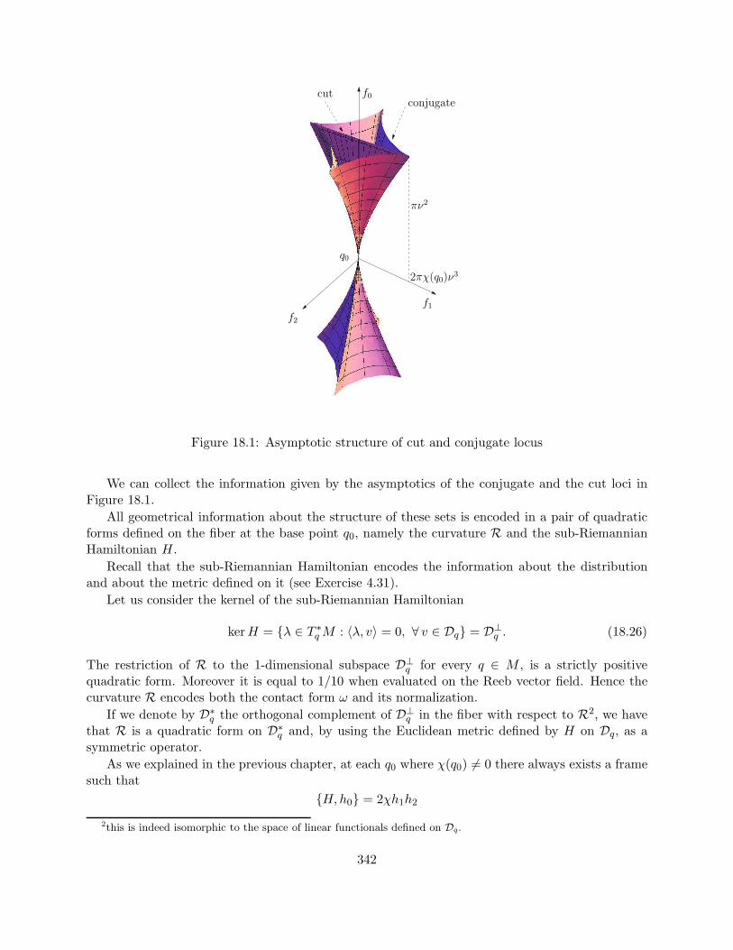
f2
f1
f0
πν2
2πχ(q0)ν3
q0
cutconjugate
Figure 18.1: Asymptotic structure of cut and conjugate locus
We can collect the information given by the asymptotics of the conjugate and the cut loci inFigure 18.1.
All geometrical information about the structure of these sets is encoded in a pair of quadraticforms defined on the fiber at the base point q0, namely the curvature R and the sub-RiemannianHamiltonian H.
Recall that the sub-Riemannian Hamiltonian encodes the information about the distributionand about the metric defined on it (see Exercise 4.31).
Let us consider the kernel of the sub-Riemannian Hamiltonian
kerH = λ ∈ T ∗qM : 〈λ, v〉 = 0, ∀ v ∈ Dq = D⊥
q . (18.26)
The restriction of R to the 1-dimensional subspace D⊥q for every q ∈ M , is a strictly positive
quadratic form. Moreover it is equal to 1/10 when evaluated on the Reeb vector field. Hence thecurvature R encodes both the contact form ω and its normalization.
If we denote by D∗q the orthogonal complement of D⊥
q in the fiber with respect to R2, we havethat R is a quadratic form on D∗
q and, by using the Euclidean metric defined by H on Dq, as asymmetric operator.
As we explained in the previous chapter, at each q0 where χ(q0) 6= 0 there always exists a framesuch that
H,h0 = 2χh1h2
2this is indeed isomorphic to the space of linear functionals defined on Dq.
342
and in this frame we can express the restriction of R to D∗q (corresponding to the set h0 = 0) on
this subspace as follows (see Section 17.1.1)
10R = (κ+ 3χ)h21 + (κ− 3χ)h22.
From this formulae it is easy to recover the two invariants χ, κ considering
trace(10R∣∣h0=0
) = 2κ, discr(10R∣∣h0=0
) = 36χ2,
where the discriminant of an operatorQ, defined on a two-dimensional space, is defined as the squareof the difference of its eigenvalues, and can be compute by the formula discr(Q) = trace2(Q) −4 det(Q).
The cubic term of the conjugate locus (for a fixed value of ν) parametrizes an astroid. Thecuspidal directions of the astroid are given by the eigenvectors of R, and the cut locus intersect theconjugate locus exactly at the cuspidal points in the direction of the eigenvector of R correspondingto the larger eigenvalue.
Finally the “size” of the cut locus increases for bigger values of χ, while κ is involved in thelength of curves arriving at cut/conjugate locus
Remark 18.8. The expression of the cut locus given in Theorem 18.7 gives the truncation up toorder 3 of the asymptotics of the cut locus of the exponential map. It is possible to show that thisis actually the exact cut locus corresponding to the truncated exponential map at order 3, whichis the object of the next sections (see Section 18.3.4).
18.3.1 Proof of Theorem 18.6: asymptotics of the exponential map
The proof of Theorem 18.6 requires a careful analysis of the asymptotic of the exponential map.Let us consider again our Hamiltonian system in the form (18.14)
q = rfθ
θ = 1− rbr = r3a
t = r
(18.27)
where we recall that equations are written with respect to the time τ . In particular, since we restricton the level set H−1(1/2), the trajectories are parametrized by length and the time t coincides withthe length of the curve. Thus in what follows we replace the variable t by ℓ.
Next, we consider a last change of the time variable. Namely we parametrize trajectories bythe coordinate θ. In other words we rewrite again the equations in such a way that θ = 1 and thedot will denote derivative with respect to θ. The equations are rewritten in the following form:
q =r
1− rbfθθ = 1
r =r3
1− rbaℓ =
r
1− rb
(18.28)
343
where we recall that fθ = cos θf1 + sin θf2. Moreover we define F (t; θ0, ν) := q(t+ θ0; θ0, ν), whereq(θ0; θ0, ν) = q0. This means that the curve that corresponds to initial parameter θ0 start from q0at time equal to θ0.
Notice that in (18.28) we can solve the equation for r = r(τ) and substitute it in the firstequation. In this way we can write the trajectory as an integral curve of the nonautonomous vectorfield
F (t; θ0, ν) = q0 Qθ0,νt , Qθ0,νt = −→exp∫ θ0+t
θ0
r(τ)
1− r(τ)b(τ)fτdτ.
To simplify the notation in what follows we denote the flow Qθ0,νt simply by Qt and by Vt the nonautonomous vector field defined by this flow
Qt =−→exp
∫ θ0+t
θ0
Vτdτ, Vτ :=r(τ)
1− r(τ)b(τ)fτ . (18.29)
We start by analyzing the asymptotics of the end point map after time t = 2π.
Lemma 18.9. F (2π; θ0, ν) = q0 − πf0(q0)ν2 +O(ν3)
Proof. From (18.28), recalling that r(0) = ν, it is easy to see that r satisfies the identity
r(t) = ν + r(t)ν3 = ν +O(ν3)
for some smooth function r(t). Thus, to find the second order term in ν of the endpoint mapF (2π; θ, ν), we can then assume that r is constantly equal to ν = r(0).
Using the Volterra expansion (cf. (6.9))
−→exp∫ θ0+2π
θ0
Vτdτ =
Id +
∫ θ0+2π
θ0
Vτdτ +
∫∫
θ0≤τ2≤τ1≤θ0+2π
Vτ2 Vτ1dτ1dτ2 + . . .
(18.30)
and substituting r(τ) ≡ ν we have the following expansion for the first term in (18.30):
∫ θ0+2π
θ0
Vτdτ =
∫ θ0+2π
θ0
ν
1− νb(τ)fτdτ =
∫ θ0+2π
θ0
ν(1 + νb(τ) +O(ν2))fτ dτ,
= ν
∫ θ0+2π
θ0
fτdτ + ν2∫ θ0+2π
θ0
b(τ)fτdτ +O(ν3)
= ν2∫ θ0+2π
θ0
b(τ)fτdτ +O(ν3)
Notice that the first order term in ν vanishes since we integrate over a period and∫ θ0+2πθ0
fτdτ = 0.
344
The second term in (18.30) can be rewritten using Lemma 8.27
∫∫
0≤τ2≤τ1≤t
Vτ2 Vτ1dτ1dτ2 =1
2
∫ θ0+2π
θ0
Vτdτ ∫ θ0+2π
θ0
Vτdτ +
∫∫
θ0≤τ2≤τ1≤θ0+2π
[Vτ2 , Vτ1 ]dτ1dτ2
=ν2
2
∫ θ0+2π
θ0
fτdτ ∫ θ0+2π
θ0
fτdτ +
∫∫
θ0≤τ2≤τ1≤θ0+2π
[fτ2 , fτ1 ]dτ1dτ2
=ν2
2
∫∫
θ0≤τ2≤τ1≤θ0+2π
[fτ2 , fτ1 ]dτ1dτ2
where we used again∫ θ0+2πθ0
fτdτ = 0. Notice that higher order terms in the Volterra expansions
are O(ν3). Collecting together the two expansions and recalling that
[f2, f1] = f0 + α1f1 + α2f2
one easily obtains
F (2π; θ0, ν) = q0 + ν2(∫ θ0+2π
θ0
b(t)ft dt+1
2
[∫ t
θ0
fτdτ, ft
]dt
)+O(ν3)
= q0 − πν2f0(q0) +O(ν3) (18.31)
Notice that the factor π in (18.31) comes out from the evaluation of integrals of kind∫ θ0+2πθ0
cos2 τdτ
and∫ θ0+2πθ0
sin2 τdτ .
Next we prove a symmetry of the exponential map
Lemma 18.10. F (t; θ0, ν) = F (t; θ0 + π,−ν)
Proof. It is a direct consequence of our geodesic equation. Recall that F (t; θ0, ν) = q(t+ θ0; θ0, ν),is the solution of the system, with initial condition q(θ0; θ0, ν) = q0.
Applying the transformation t 7→ t + π and ν → −ν we see that the right hand side of q in(18.28) is preserved while the right hand side of r change sign (we use that ui(t + π) = −ui(t),hence a(t + π) = a(t) and b(t + π) = −b(t)). Then, if (q(t), r(t)) is a solution of the system then(q(t+ π),−r(t+ π)) is also a solution. The lemma follows.
The symmetry property just proved permits to characterize all odd terms in the expansion inν of the exponential map at t = 2π, as follows.
Corollary 18.11. Consider the expansion
F (2π; θ, ν) ≃∞∑
n=0
qn(θ)νn.
We have the following identities
(i) qn(θ + π) = (−1)nqn(θ),
345
(ii) q2n+1(θ) = −1
2
∫ θ+π
θ
dq2n+1
dθ(τ)dτ .
Proof. This is an immediate consequence of Lemma 18.10 and the identity
2q2n+1(θ) = q2n+1(θ)− q2n+1(θ + π) = −∫ θ+π
θ
dq2n+1
dθ(τ)dτ.
We already computed the terms q1(θ) and q2(θ). To find q3(θ) we start by computing thederivative of the map F with respect to θ.
Lemma 18.12.∂F
∂θ0(2π; θ0, ν) = −π[f0, fθ0 ]q0ν3 +O(ν4)
Proof. We stress that, since we are now interested to third order term in ν, we can no more assumethat r(τ) is constant. Differentiating (3.59) with respect to θ gives two terms as follows:
∂F
∂θ0=
∂
∂θ0(q0 Qt) = q0
∂
∂θ0
(−→exp
∫ θ+2π
θVτdτ
)
= q0 (Q2π Vθ0+2π − Vθ0 Q2π) (18.32)
Next let us rewrite
Q2π Vθ0+2π = Q2π Vθ0+2π Q−12π Q2π
= AdQ2π Vθ0+2π
so that (18.32) can be rewritten as
∂F
∂θ0= q0 (AdQ2π Vθ0+2π − Vθ0) Q2π (18.33)
Thanks to Lemma 18.9 we can write
Q2π = Id− πν2f0 +O(ν3) (18.34)
that implies the following asymptotics for the action of its adjoint by (6.18)
AdQ2π = Id− πν2ad f0 +O(ν3)
We are left to compute the asymptotic expansion of (18.33). To this goal, recall that r = r(τ)satisfies
r =r3
1− rba = r3a+O(r4)
hence we can compute its term of order 3 with respect to ν
r(t) = ν + ν3∫ t
θ0
a(τ)dτ +O(ν4) (18.35)
This in particular implies that r(θ0 + 2π) = ν +O(ν4) since∫ θ0+2πθ0
a(t)dt = 0.
346
This allows us to replace r(·) with ν in the term Vθ0+2π since r(θ+ 2π) = ν +O(ν4). Moreoverusing that b(θ0 + 2π) = b(θ0) and fθ0+2π = fθ0 we get
AdQ2π Vθ0+2π − Vθ0 = (Id− πν2ad f0 +O(ν3))
(ν
1− νbfθ0)−(
ν
1− νbfθ0)+O(ν4)
= −πν2ad f0(νfθ0) +O(ν4) (18.36)
and finally plugging (18.34) and (18.36) into (18.33) one obtains
∂F
∂θ= q0
(−πν2ad f0(νfθ0) +O(ν4)
) (Id +O(ν))
= q0 (−πν3[f0, fθ0 ] +O(ν4))
18.3.2 Asymptotics of the conjugate locus
In this section we finally prove Theorem 18.6, by computing the expansion of the conjugate timetc(θ0, ν). We know from Proposition 18.3 that
τc(θ0, ν) = 2π + ν2s(θ0) +O(ν3)
By definition of conjugate point, the function s = s(θ0) is characterized as the solution of theequation
∂F
∂s∧ ∂F∂θ∧ ∂F∂ν
∣∣∣∣(2π+ν2s,θ,ν)
= 0, (18.37)
where s is considered as a parameter. Notice that the derivative with respect to s is computed by
∂F
∂s=∂F
∂t
∂t
∂s= (νfθ +O(ν2))ν2 ≃ ν3fθ +O(ν4)
Moreover, from the expansion of F with respect to ν one has
∂F
∂ν= −2πνf0 +O(ν2)
ThusF (2π + ν2s; θ, ν) = F (2π, θ, ν) + ν3sfθ +O(ν4)
and differentiation with respect to θ0 together with Lemma 18.12 gives
∂F
∂θ(2π + ν2s; θ, ν) = ν3(π[fθ, f0] + sfθ′) +O(ν4)
where as usual fθ′ denotes the derivative with respect to θ.Then, collecting together all these computations, the equation for conjugate points (18.37) can
be rewritten asfθ ∧ (sfθ′ + π[fθ, f0]) ∧ f0 = O(ν) (18.38)
Since fθ, fθ′ are an orthonormal frame on D and f0 is transversal to the distribution, (18.38) isequivalent to
fθ ∧ (sfθ′ + π[fθ, f0]) = O(ν)
347
that implies
s(θ) = π 〈[f0, fθ], fθ′〉+O(ν)
where 〈·, ·〉 denotes the the scalar product on the distribution. Hence
tc(θ, ν) = 2π + πν2 〈[f0, fθ], fθ′〉q0 +O(ν3)
To find the expression of conjugate locus, we evaluate the ecponential map at time tc(θ, ν).
We first consider the asymptotic of the conjugate locus. Using again that the first order termwith respect to ν of ∂tF is νfθ we have
F (2π + ν2s(θ0), θ0, ν) = F (2π; θ0, ν) + ν3s(θ0)fθ0 +O(ν4)
Hence, by Corollary 18.11 and Lemma 18.9 one gets
Conq0(θ0, ν) = q0 − πν2f0(q0)−ν3
2
∫ θ0+π
θ0
dq3dτ
dτ + ν3s(θ0)fθ0 +O(ν4)
Moreover, since∂F
∂θ0(2π, ν, θ0) = ν3[fθ0 , f0] +O(ν4)
we have by definition that q3(θ) = [fθ, f0] and
Conq0(θ0, ν) = q0 − ν2f0(q0)−ν3
2
∫ θ0+π
θ0
π[fθ0 , f0]dτ + ν3s(θ0)fθ0
= q0 − ν2f0(q0)−ν3
2
∫ θ0+π
θ0
π[fθ0 , f0] + s′(t)fθ0 + s(t)fθ′0dt (18.39)
where the last identify follows by writing fθ′′ = −fθ and integrating by parts. Using that
s(θ) = π 〈[f0, fθ], fθ′〉s′(θ) = π 〈[f0, fθ′ ], fθ′〉 − π 〈[f0, fθ], fθ〉 = 2πa
we can rewrite (18.39) as follows
π[fθ0 , f0] + s′(t)fθ0 + s(t)fθ′0 = π[fθ0 , f0] + 2πafθ0 + π⟨[f0, fθ0 ], fθ′0
⟩fθ′0
= π 〈[fθ0 , f0], fθ0〉 fθ0 + 2πafθ0
= 3πafθ0
Finally
Conq0(θ0, ν) = q0 − ν2f0(q0)−3ν3
2π
∫ θ0+π
θ0
a(τ)fτdτ +O(ν4)
= q0 − ν2f0(q0) + ν3π(a′fθ0 − afθ′0) +O(ν4)
348
18.3.3 Asymptotics of the conjugate length
Similarly, we consider conjugate length. Recall that
ℓc(θ0, ν) =
∫ θ0+tc(θ0,ν)
θ0
r(t)
1− r(t)Qθ0,νt b(t)dt
where we replaced b(t) by its value along the flow Qθ0,νt b(t).
As a first step, notice that we can reduce to an integral over a period, up to higher order termswith respect to ν. Namely
ℓc(θ0, ν) =
∫ θ0+2π
θ0
r(t)
1− r(t)Qθ0,νt b(t)dt+ ν3s(θ0) +O(ν4) (18.40)
Indeed tc(θ0, ν) = 2π+ν2s(θ)+O(ν3) and the first order term w.r.t. ν in the integrand is exactly ν
by (18.35). In what follows we use again the notation Qt := Qθ0,νt , and we compute the expansionin ν of the integral appearing in (18.40).
First notice that
r(t)
1− r(t)Qtb(t)= r(t)
(1 + r(t)Qtb(t) + r2(t)[Qtb(t) Qtb(t)] +O(r(t)3)
)
Using that r(t) = ν +O(ν3) and Qtb(t) = b(t) +O(ν) we have that
r(t)
1− r(t)Qtb(t)= r(t) + r2(t)Qtb(t) + r3(t)b(t)2 +O(ν4)
Now each addend of the sum expands as follows
r(t) = ν + ν3∫ t
0a(t)dt+O(ν4) (18.41)
r2(t)Qt(ν)b(t) = (ν2 +O(ν4))
(Id + ν
∫ t
0fτdτ +O(ν)
)b(t) (18.42)
= ν2b(t) + ν3∫ t
0fτdτb(t) +O(ν4) (18.43)
r3(t)b(t)2 = ν3b(t)2 +O(ν4) (18.44)
Integrating the sum over the interval [θ0, θ0 +2π] and considering terms only up to O(ν4) we have
ℓc(θ0, ν) = 2πν +
(∫ θ0+2π
θ0
[∫ t
0a(τ)dτ +
∫ t
0fτdτ
]b(t) + b2(t)dt
)ν3 +O(ν4)
where the coefficient in ν2 vanishes since∫ θ0+2πθ0
b(τ)dτ = 0. A straightforward computation of theintegrals ends the proof of the theorem.
349
18.3.4 Stability of the conjugate locus
In this section we want to prove that the third order Taylor polynomial of the exponential mapcorresponds to a stable map in the sense of singularity theory. More precisely it can be treatedas a one parameter family of maps between 2-dimensional manifolds that has only singular pointsof “cusp” and “fold” type. As a consequence the original exponential map can be treated as aperturbation of the (truncated) stable one.
The classic Whitney theorem on the stability of maps between 2-dimensional manifolds thenimplies that the structure of their singularity will be the same, and actually the singular set of theperturbed one is the image under an homeomorphism of the singular set of the truncated map.
Fix some local coordinates (x0, x1, x2) around the point q0 such that
q0 = (0, 0, 0), fi(q0) = ∂xi , ∀ i = 0, 1, 2.
Lemma 18.13. In these coordinates we have
1
πF (2π + πη2τ, θ, ν) = (x0(τ, θ, ν), x1(τ, θ, ν), x2(τ, θ, ν))
= (−ν2, (τ − c102) cos(θ)ν3, (τ + c201) sin(θ)ν3) +O(ν4) (18.45)
Let us define the new variable ζ =√−x0(τ, θ, ν) =
√ν2 +O(ν4) = ν + O(ν3) and apply the
smooth change of variables (τ, θ, ν) 7→ (τ, θ, ζ). The map (18.45) is rewritten as follows
1
πF (2π + πη2τ, θ, ν) = (−ζ2, (τ − c102) cos(θ)ζ3 +O(ζ4), (τ + c201) sin(θ)ζ
3 +O(ζ4)) (18.46)
Notice that the first coordinate function of this map is constant in the new variables, when ζ isconstant. The map (18.46) can be interpreted as a family of maps, parametrized by ζ, dependingon two variables
1
πF (2π + πη2τ, θ, ν) = (−ζ2, ζ3Φζ(τ, θ)) (18.47)
where we have defined
Φζ(τ, θ) = ((τ − c102) cos(θ), (τ + c201) sin(θ)) +O(ζ) (18.48)
The critical set of the map Φ0(τ, θ) is a smooth closed curve in R× S1 defined by the equation
τ = c102 sin2(θ)− c201 cos2(θ). (18.49)
The critical values of this map, that is the image under the map Φ0 of the set defined by (18.49),is the astroid
A0 = 2χ(− sin3(θ), cos3(θ)), θ ∈ S1 (18.50)
The restriction to Φ0 to the set A0 is a one-to-one map. Moreover every critical point of Φ0 is a foldor a cusp. This implies that Φ0 is a Whitney map. Hence it is stable, in the sense of Thom-Mathertheory, see [?, ?].
In other words, for any compact K ⊂ R × S1 big enough, there exists ε > 0 such that for allζ ∈]0, ε[, the map Φζ |K is equivalent to Φ0|K , under a smooth family of change of coordinates inthe source and in the image. Moreover, this family can be chosen to be smooth with respect to theparameter ζ.
Collecting these results, we have proved that the shape of the conjugate locus described inFigure 18.1 obtained via third order approximation of the end-point map is indeed a picture of thetrue shape.
350
Theorem 18.14. Suppose M is a 3D contact sub-Riemannian structure and χ(q0) 6= 0. Thenthere exists ε > 0 such that for every closed ball B = B(q0, r) with r ≤ ε there exists an open setU ⊂ B \ q0 and a diffeomorphism Ψ : U → R
3 × ±1 such that B ∩ Conq0 ⊂ U and
Ψ(B ∩Conq0) = (ζ2, cos3(θ)ζ3,− sin3(θ)ζ3) : ζ > 0, θ ∈ S1 × ±1.
In particular, each of the two connected components of B ∩ Conq0 contains 4 cuspidal edges.
A similar statement concerning the stability of the cut locus can be found in [1].
351

352
Chapter 19
The volume in sub-Riemanniangeometry
19.1 The Popp volume
For an equiregular sub-Riemannian manifold M , Popp’s volume is a smooth volume which iscanonically associated with the sub-Riemannian structure, and it is a natural generalization ofthe Riemannian one. In this chapter we define the Popp volume and we prove a general formulafor its expression, written in terms of a frame adapted to the sub-Riemannian distribution.
As a first application of this result, we prove an explicit formula for the canonical sub-Laplacian,namely the one associated with Popp’s volume. Finally, we discuss sub-Riemannian isometries, andwe prove that they preserve Popp’s volume.
19.2 Popp volume for equiregular sub-Riemannian manifolds
Recall that a distribution D is equiregular if the growth vector is constant, i.e. for each i =1, 2, . . . ,m, ki(q) = dim(Diq) does not depend on q ∈M . In this case the subspaces Diq are fibres ofthe higher order distributions Di ⊂ TM .
For equiregular distributions we will simply talk about growth vector and step of the distribu-tion, without any reference to the point q.
Next, we introduce the nilpotentization of the distribution at the point q, which is fundamentalfor the definition of Popp’s volume.
Definition 19.1. Let D be an equiregular distribution of step m. The nilpotentization of D at thepoint q ∈M is the graded vector space
grq(D) = Dq ⊕D2q/Dq ⊕ . . .⊕Dmq /Dm−1
q .
The vector space grq(D) can be endowed with a Lie algebra structure, which respects thegrading. Then, there is a unique connected, simply connected group, Grq(D), such that its Liealgebra is grq(D). The global, left-invariant vector fields obtained by the group action on anyorthonormal basis of Dq ⊂ grq(D) define a sub-Riemannian structure on Grq(D), which is calledthe nilpotent approximation of the sub-Riemannian structure at the point q.
In what follows, we provide the definition of Popp’s volume. Our presentation follows closelythe one that can be found in [?]. (See also [27]). The definition rests on the following lemmas.
353
Lemma 19.2. Let E be an inner product space and V a vector space. Let π : E → V be a surjectivelinear map. Then π induces an inner product on V such that the norm of v ∈ V is
‖v‖V = min‖e‖E s.t. π(e) = v . (19.1)
Proof. It is easy to check that Eq. (19.1) defines a norm on V . Moreover, since ‖ · ‖E is inducedby an inner product, i.e. it satisfies the parallelogram identity, it follows that ‖ · ‖V satisfies theparallelogram identity too. Notice that this is equivalent to consider the inner product on V definedby the linear isomorphism π : (ker π)⊥ → V . Indeed the norm of v ∈ V is the norm of the shortestelement e ∈ π−1(v).
Lemma 19.3. Let E be a vector space of dimension n with a flag of linear subspaces 0 = F 0 ⊂F 1 ⊂ F 2 ⊂ . . . ⊂ Fm = E. Let gr(F ) = F 1 ⊕ F 2/F 1 ⊕ . . . ⊕ Fm/Fm−1 be the associated gradedvector space. Then there is a canonical isomorphism θ : ∧nE → ∧ngr(F ).
Proof. We only give a sketch of the proof. For 0 ≤ i ≤ m, let ki := dimF i. Let X1, . . . ,Xn be aadapted basis for E, i.e. X1, . . . ,Xki is a basis for F i. We define the linear map θ : E → gr(F )which, for 0 ≤ j ≤ m−1, takes Xkj+1, . . . ,Xkj+1
to the corresponding equivalence class in F j+1/F j .This map is indeed a non-canonical isomorphism, which depends on the choice of the adapted basis.In turn, θ induces a map θ : ∧nE → ∧ngr(F ), which sends X1 ∧ . . . ∧Xn to θ(X1) ∧ . . . ∧ θ(Xn).The proof that θ does not depend on the choice of the adapted basis is “dual” to the proof of [27,Lemma 10.4].
The idea behind Popp’s volume is to define an inner product on each Diq/Di−1q which, in turn,
induces an inner product on the orthogonal direct sum grq(D). The latter has a natural volumeform, which is the canonical volume of an inner product space obtained by wedging the elements anorthonormal dual basis. Then, we employ Lemma 19.3 to define an element of (∧nTqM)∗ ≃ ∧nT ∗
qM ,which is Popp’s volume form computed at q.
Fix q ∈ M . Then, let v,w ∈ Dq, and let V,W be any horizontal extensions of v,w. Namely,V,W ∈ Γ(D) and V (q) = v, W (q) = w. The linear map π : Dq ⊗Dq → D2
q/Dq
π(v ⊗ w) := [V,W ]q mod Dq , (19.2)
is well defined, and does not depend on the choice the horizontal extensions. Indeed let V andW be two different horizontal extensions of v and w respectively. Then, in terms of a local frameX1, . . . ,Xk of D
V = V +
k∑
i=1
fiXi , W =W +
k∑
i=1
giXi , (19.3)
where, for 1 ≤ i ≤ k, fi, gi ∈ C∞(M) and fi(q) = gi(q) = 0. Therefore
[V , W ] = [V,W ] +k∑
i=1
(V (gi)−W (fi))Xi +k∑
i,j=1
figj [Xi,Xj ] . (19.4)
Thus, evaluating at q, [V , W ]q = [V,W ]q mod Dq, as claimed. Similarly, let 1 ≤ i ≤ m. The linearmaps πi : ⊗iDq → Diq/Di−1
q
πi(v1 ⊗ · · · ⊗ vi) = [V1, [V2, . . . , [Vi−1, Vi]]]q mod Di−1q , (19.5)
354
are well defined and do not depend on the choice of the horizontal extensions V1, . . . , Vi of v1, . . . , vi.
By the bracket-generating condition, πi are surjective and, by Lemma 19.2, they induce aninner product space structure on Diq/Di−1
q . Therefore, the nilpotentization of the distribution at q,namely
grq(D) = Dq ⊕D2q/Dq ⊕ . . .⊕Dmq /Dm−1
q , (19.6)
is an inner product space, as the orthogonal direct sum of a finite number of inner product spaces.As such, it is endowed with a canonical volume (defined up to a sign) µq ∈ ∧ngrq(D)∗, which is thevolume form obtained by wedging the elements of an orthonormal dual basis.
Finally, Popp’s volume (computed at the point q) is obtained by transporting the volume ofgrq(D) to TqM through the map θq : ∧nTqM → ∧ngrq(D) defined in Lemma 19.3. Namely
Pq = θ∗q(µq) = µq θq , (19.7)
where θ∗q denotes the dual map and we employ the canonical identification (∧nTqM)∗ ≃ ∧nT ∗qM .
Eq. (19.7) is defined only in the domain of the chosen local frame. Since M is orientable, witha standard argument, these n-forms can be glued together to obtain Popp’s volume P ∈ Ωn(M).The smoothness of P follows directly from Theorem 19.5.
Remark 19.4. The definition of Popp’s volume can be restated as follows. Let (M,D) be an orientedsub-Riemannian manifold. Popp’s volume is the unique volume P such that, for all q ∈ M , thefollowing diagram is commutative:
(M,D) P−−−−→ (∧nTqM)∗
grq
yyθ∗q
grq(D) −−−−→µ (∧ngrq(D))∗
where µ associates the inner product space grq(D) with its canonical volume µq, and θ∗q is the dual
of the map defined in Lemma 19.3.
19.3 A formula for Popp volume
In this section we prove an explicit formula for the Popp volume.
We say that a local frame X1, . . . ,Xn is adapted if X1, . . . ,Xki is a local frame for Di, whereki := dimDi, and X1, . . . ,Xk are orthonormal. It is useful to define the functions clij ∈ C∞(M) by
[Xi,Xj ] =
n∑
l=1
clijXl . (19.8)
With a standard abuse of notation we call them structure constants. For j = 2, . . . ,m we definethe adapted structure constants bli1... ij ∈ C∞(M) as follows:
[Xi1 , [Xi2 , . . . , [Xij−1 ,Xij ]]] =
kj∑
l=kj−1+1
bli1i2... ijXl mod Dj−1 , (19.9)
355

where 1 ≤ i1, . . . , ij ≤ k. These are a generalization of the clij , with an important difference: thestructure constants of Eq. (19.8) are obtained by considering the Lie bracket of all the fields ofthe local frame, namely 1 ≤ i, j, l ≤ n. On the other hand, the adapted structure constants ofEq. (19.9) are obtained by taking the iterated Lie brackets of the first k elements of the adaptedframe only (i.e. the local orthonormal frame for D), and considering the appropriate equivalenceclass. For j = 2, the adapted structure constants can be directly compared to the standard ones.Namely blij = clij when both are defined, that is for 1 ≤ i, j ≤ k, l ≥ k + 1.
Then, we define the kj − kj−1 dimensional square matrix Bj as follows:
[Bj]hl =
k∑
i1,i2,...,ij=1
bhi1i2...ijbli1i2...ij , j = 1, . . . ,m , (19.10)
with the understanding that B1 is the k × k identity matrix. It turns out that each Bj is positivedefinite.
Theorem 19.5. Let X1, . . . ,Xn be a local adapted frame, and let ν1, . . . , νn be the dual frame.Then Popp’s volume P satisfies
P =1√∏j detBj
ν1 ∧ . . . ∧ νn , (19.11)
where Bj is defined by (19.10) in terms of the adapted structure constants (19.9).
To clarify the geometric meaning of Eq. (19.11), let us consider more closely the case m = 2.If D is a step 2 distribution, we can build a local adapted frame X1, . . . ,Xk,Xk+1, . . . ,Xn bycompleting any local orthonormal frame X1, . . . ,Xk of the distribution to a local frame of thewhole tangent bundle. Even though it may not be evident, it turns out that B−1
2 (q) is the Grammatrix of the vectors Xk+1, . . . ,Xn, seen as elements of TqM/Dq. The latter has a natural structureof inner product space, induced by the surjective linear map [ , ] : Dq ⊗ Dq → TqM/Dq (seeLemma 19.2). Therefore, the function appearing at the beginning of Eq. (19.11) is the volumeof the parallelotope whose edges are X1, . . . ,Xn, seen as elements of the orthogonal direct sumgrq(D) = Dq ⊕ TqM/Dq.
Proof of Theorem 19.5
We are now ready to prove Theorem 19.5. For convenience, we first prove it for a distribution of stepm = 2. Then, we discuss the general case. In the following subsections, everything is understoodto be computed at a fixed point q ∈ M . Namely, by gr(D) we mean the nilpotentization of D atthe point q, and by Di we mean the fibre Diq of the appropriate higher order distribution.
Step 2 distribution
If D is a step 2 distribution, then D2 = TM . The growth vector is G = (k, n). We choose n − kindependent vector fields Ylnl=k+1 such that X1, . . . ,Xk, Yk+1, . . . , Yn is a local adapted frame forTM . Then
[Xi,Xj ] =n∑
l=k+1
blijYl mod D . (19.12)
356
For each l = k + 1, . . . , n, we can think to blij as the components of an Euclidean vector in Rk2 ,
which we denote by the symbol bl. According to the general construction of Popp’s volume, weneed first to compute the inner product on the orthogonal direct sum gr(D) = D ⊕ D2/D. ByLemma 19.2, the norm on D2/D is induced by the linear map π : ⊗2D → D2/D
π(Xi ⊗Xj) = [Xi,Xj ] mod D . (19.13)
The vector space ⊗2D inherits an inner product from the one on D, namely ∀X,Y,Z,W ∈ D,〈X ⊗ Y,Z ⊗W 〉 = 〈X,Z〉〈Y,W 〉. π is surjective, then we identify the range D2/D with ker π⊥ ⊂⊗2D, and define an inner product on D2/D by this identification. In order to compute explicitlythe norm on D2/D (and then, by polarization, the inner product), let Y ∈ D2/D. Then
‖D2/D‖Y = min‖ ⊗2 D‖Z s.t. π(Z) = Y . (19.14)
Let Y =∑n
l=k+1 clYl and Z =
∑ki,j=1 aijXi ⊗Xj ∈ ⊗2D. We can think to aij as the components
of a vector a ∈ Rk2 . Then, Eq. (19.14) writes
‖D2/D‖Y = min|a| s.t. a · bl = cl, l = k + 1, . . . , n , (19.15)
where |a| is the Euclidean norm of a, and the dot denotes the Euclidean inner product. Indeed,‖D2/D‖Y is the Euclidean distance of the origin from the affine subspace of Rk
2defined by the
equations a · bl = cl for l = k + 1, . . . , n. In order to find an explicit expression for ‖D2/D‖2Y interms of the bl, we employ the Lagrange multipliers technique. Then, we look for extremals of
L(a, bk+1, . . . , bn, λk+1, . . . , λn) = |a|2 − 2n∑
l=k+1
λl(a · bl − cl) . (19.16)
We obtain the following system
n∑
l=k+1
λl · bl − a = 0,
n∑
l=k+1
λlbl · br = cr , r = k + 1, . . . , n.
(19.17)
Let us define the n − k square matrix B, with components Bhl = bh · bl. B is a Gram matrix,which is positive definite iff the bl are n − k linearly independent vectors. These vectors areexactly the rows of the representative matrix of the linear map π : ⊗2D → D2/D, which has rankn − k. Therefore B is symmetric and positive definite, hence invertible. It is now easy to writethe solution of system (19.17) by employing the matrix B−1, which has components B−1
hl . Indeeda straightforward computation leads to
‖D2/D‖2csYs = chB−1hl c
l . (19.18)
By polarization, the inner product on D2/D is defined, in the basis Yl, by
〈Yl, Yh〉D2/D = B−1lh . (19.19)
Observe that B−1 is the Gram matrix of the vectors Yk+1, . . . , Yn seen as elements of D2/D. Then,by the definition of Popp’s volume, if ν1, . . . , νk, µk+1, . . . , µn is the dual basis associated withX1, . . . ,Xk, Yk+1, . . . , Yn, the following formula holds true
P =1√
detBν1 ∧ · · · ∧ νk ∧ µk+1 ∧ · · · ∧ µn . (19.20)
357
General case
In the general case, the procedure above can be carried out with no difficulty. Let X1, . . . ,Xn
be a local adapted frame for the flag D0 ⊂ D ⊂ D2 ⊂ · · · ⊂ Dm. As usual ki = dim(Di). Forj = 2, . . . ,m we define the adapted structure constants bli1... ij ∈ C∞(M) by
[Xi1 , [Xi2 , . . . , [Xij−1 ,Xij ]]] =
kj∑
l=kj−1+1
bli1i2... ijXl mod Dj−1 , (19.21)
where 1 ≤ i1, . . . , ij ≤ k. Again, bli1...ij can be seen as the components of a vector bl ∈ Rkj .
Recall that for each j we defined the surjective linear map πj : ⊗jD → Dj/Dj−1
πj(Xi1 ⊗Xi2 ⊗ · · · ⊗Xij ) = [Xi1 , [Xi2 , . . . , [Xij−1 ,Xij ]]] mod Dj−1 . (19.22)
Then, we compute the norm of an element of Dj/Dj−1 exactly as in the previous case. It isconvenient to define, for each 1 ≤ j ≤ m, the kj−kj−1 dimensional square matrix Bj, of components
[Bj]hl =
k∑
i1,i2,...,ij=1
bhi1i2...ijbli1i2...ij . (19.23)
with the understanding that B1 is the k×k identity matrix. Each one of these matrices is symmetricand positive definite, hence invertible, due to the surjectivity of πj. The same computation of theprevious case, applied to each Dj/Dj−1 shows that the matrices B−1
j are precisely the Gram matrices
of the vectors Xkj−1+1, . . . ,Xkj ∈ Dj/Dj−1, in other words
〈Xkj−1+l,Xkj−1+h〉Dj/Dj−1 = B−1lh . (19.24)
Therefore, if ν1, . . . , νn is the dual frame associated with X1, . . . ,Xn, Popp’s volume is
P =1√∏m
j=1 detBjν1 ∧ . . . ∧ νn . (19.25)
19.4 Popp volume and isometries
In the last part of the paper we discuss the conditions under which a local isometry preserves Popp’svolume. In the Riemannian setting, an isometry is a diffeomorphism such that its differential is anisometry for the Riemannian metric. The concept is easily generalized to the sub-Riemannian case.
Definition 19.6. A (local) diffeomorphism φ : M → M is a (local) isometry if its differentialφ∗ : TM → TM preserves the sub-Riemannian structure (D, 〈· | ·〉), namely
i) φ∗(Dq) = Dφ(q) for all q ∈M ,
ii) 〈φ∗X |φ∗Y 〉φ(q) = 〈X |Y 〉q for all q ∈M , X,Y ∈ Dq .
Remark 19.7. Condition i), which is trivial in the Riemannian case, is necessary to define isometriesin the sub-Riemannian case. Actually, it also implies that all the higher order distributions arepreserved by φ∗, i.e. φ∗(Diq) = Diφ(q), for 1 ≤ i ≤ m.
358
Definition 19.8. Let M be a manifold equipped with a volume form µ ∈ Ωn(M). We say that a(local) diffeomorphism φ :M →M is a (local) volume preserving transformation if φ∗µ = µ.
In the Riemannian case, local isometries are also volume preserving transformations for theRiemannian volume. Then, it is natural to ask whether this is true also in the sub-Riemanniansetting, for some choice of the volume. The next proposition states that the answer is positive ifwe choose Popp’s volume.
Proposition 19.9. Sub-Riemannian (local) isometries are volume preserving transformations forPopp’s volume.
Proposition 19.9 may be false for volumes different than Popp’s one. We have the following.
Proposition 19.10. Let Iso(M) be the group of isometries of the sub-Riemannian manifold M . IfIso(M) acts transitively on M , then Popp’s volume is the unique volume (up to multiplication byscalar constant) such that Proposition 19.9 holds true.
Definition 19.11. LetM be a Lie group. A sub-Riemannian structure (M,D, 〈· | ·〉) is left invariantif ∀g ∈M , the left action Lg :M →M is an isometry.
As a trivial consequence of Proposition 19.9 we recover a well-known result (see again [27]).
Corollary 19.12. Let (M,D, 〈· | ·〉) be a left-invariant sub-Riemannian structure. Then Popp’svolume is left invariant, i.e. L∗
gP = P for every g ∈M .
This section is devoted to the proof of Propositions 19.9 and 19.10.
Proof of Proposition 19.9
Let φ ∈ Iso(M) be a (local) isometry, and 1 ≤ i ≤ m. The differential φ∗ induces a linear map
φ∗ : ⊗iDq → ⊗iDφ(q) . (19.26)
Moreover φ∗ preserves the flag D ⊂ . . . ⊂ Dm. Therefore, it induces a linear map
φ∗ : Diq/Di−1q → Diφ(q)/Di−1
φ(q) . (19.27)
The key to the proof of Proposition 19.9 is the following lemma.
Lemma 19.13. φ∗ and φ∗ are isometries of inner product spaces.
Proof. The proof for φ∗ is trivial. The proof for φ∗ is as follows. Remember that the inner producton Di/Di−1 is induced by the surjective maps πi : ⊗iD → Di/Di−1 defined by Eq. (19.5). Namely,let Y ∈ Diq/Di−1
q . Then
‖Y ‖Diq/Di−1
q= min‖Z‖⊗Dq s.t. πi(Z) = Y . (19.28)
As a consequence of the properties of the Lie brackets, πi φ∗ = φ∗ πi. Therefore
‖Y ‖Diq/Di−1
q= min‖φ∗Z‖⊗Dφ(q)
s.t. πi(φ∗Z) = φ∗Y = ‖φ∗Y ‖Diφ(q)
/Di−1φ(q)
. (19.29)
By polarization, φ∗ is an isometry.
359
Since grq(D) = ⊕mi=1Diq/Di−1q is an orthogonal direct sum, φ∗ : grq(D) → grφ(q)(D) is also an
isometry of inner product spaces.Finally, Popp’s volume is the canonical volume of grq(D) when the latter is identified with TqM
through any choice of a local adapted frame. Since φ∗ is equal to φ∗ under such an identification,and the latter is an isometry of inner product spaces, the result follows.
Proof of Proposition 19.10
Let µ be a volume form such that φ∗µ = µ for any isometry φ ∈ Iso(M). There exists f ∈ C∞(M),f 6= 0 such that P = fµ. It follows that, for any φ ∈ Iso(M)
fµ = P = φ∗P = (f φ)φ∗µ = (f φ)µ , (19.30)
where we used the Iso(M)-invariance of Popp’s volume. Then also f is Iso(M)-invariant, namelyφ∗f = f for any φ ∈ Iso(M). By hypothesis, the action of Iso(M) is transitive, then f is constant.
Hausdorff dimension and Hausdorff volume
Density of the Hausdorff volume with respect to a smooth volume
Bibliographical notes
family
360
Chapter 20
The sub-Riemannian heat equation
In this chapter we derive the sub-Riemannian heat equation and we discuss the strictly relatedquestion of how to define an intrinsic volume in sub-Riemannian geometry.
20.1 The heat equation
To write the heat equation in a sub-Riemannian manifold, let us recall how to write it in the Rie-mannian context and let us see which mathematical structures are missing in the sub-Riemannianone.
20.1.1 The heat equation in the Riemannian context
Let (M,g) be an oriented Riemannian manifold of dimension n and let ω the Riemannian volumedefined by
ω(X1, . . . ,Xn) = 1, where X1, . . . ,Xn is a local orthonormal frame.
In coordinates if g is represented by a matrix (gij), we have
ω =√
det(gij) dx1 ∧ . . . ∧ dxn.
Let φ be a quantity (depending on the position q and the time t) subjects to a diffusion processe.g. the temperature of a body, the concentration of a chemical product, the noise etc..... Let F bea time dependent vector field representing the flux of the quantity φ, i.e., how much of φ is flowingthrough the unity of surface in unitary time.
Our purpose is to get a partial differential equation describing the evolution of φ. The Rieman-nian heat equation is obtained by postulating the following two facts:
(R1) the flux is proportional to minus the gradient of φ i.e., normalizing the proportionality con-stant to one, we assume that
F = −grad(φ); (20.1)
361
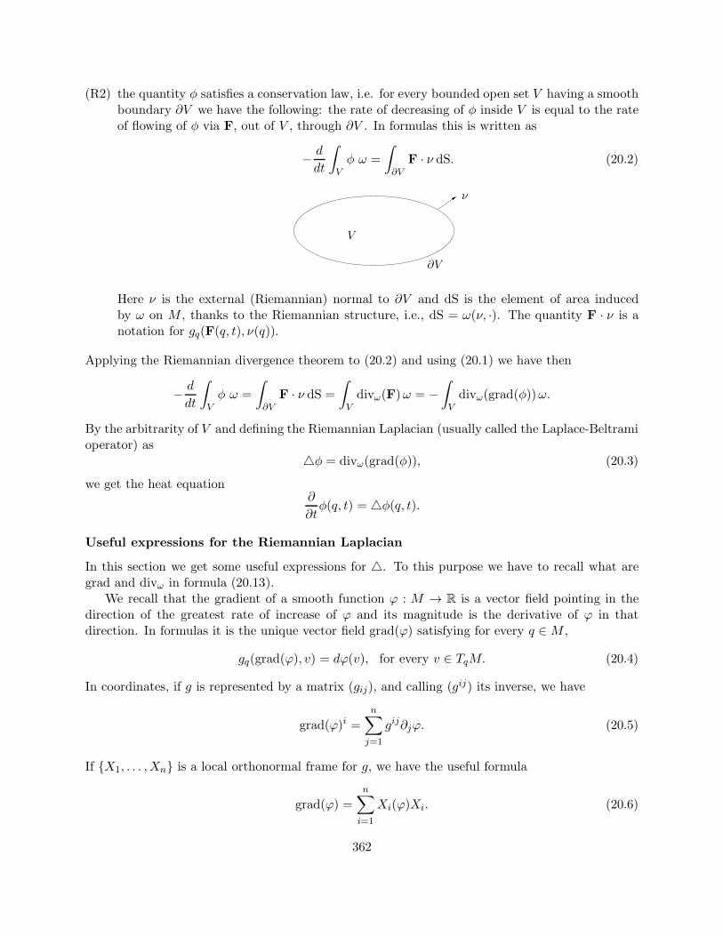
(R2) the quantity φ satisfies a conservation law, i.e. for every bounded open set V having a smoothboundary ∂V we have the following: the rate of decreasing of φ inside V is equal to the rateof flowing of φ via F, out of V , through ∂V . In formulas this is written as
− d
dt
∫
Vφ ω =
∫
∂VF · ν dS. (20.2)
ν
∂V
V
Here ν is the external (Riemannian) normal to ∂V and dS is the element of area inducedby ω on M , thanks to the Riemannian structure, i.e., dS = ω(ν, ·). The quantity F · ν is anotation for gq(F(q, t), ν(q)).
Applying the Riemannian divergence theorem to (20.2) and using (20.1) we have then
− d
dt
∫
Vφ ω =
∫
∂VF · ν dS =
∫
Vdivω(F)ω = −
∫
Vdivω(grad(φ))ω.
By the arbitrarity of V and defining the Riemannian Laplacian (usually called the Laplace-Beltramioperator) as
φ = divω(grad(φ)), (20.3)
we get the heat equation∂
∂tφ(q, t) = φ(q, t).
Useful expressions for the Riemannian Laplacian
In this section we get some useful expressions for . To this purpose we have to recall what aregrad and divω in formula (20.13).
We recall that the gradient of a smooth function ϕ : M → R is a vector field pointing in thedirection of the greatest rate of increase of ϕ and its magnitude is the derivative of ϕ in thatdirection. In formulas it is the unique vector field grad(ϕ) satisfying for every q ∈M ,
gq(grad(ϕ), v) = dϕ(v), for every v ∈ TqM. (20.4)
In coordinates, if g is represented by a matrix (gij), and calling (gij) its inverse, we have
grad(ϕ)i =
n∑
j=1
gij∂jϕ. (20.5)
If X1, . . . ,Xn is a local orthonormal frame for g, we have the useful formula
grad(ϕ) =
n∑
i=1
Xi(ϕ)Xi. (20.6)
362
Exercise 20.1. Prove that if the Riemannian metric is defined globally via a generating familyX1, . . . ,Xm with m ≥ n, in the sense of Chapter 3, then grad(ϕ) =
∑mi=1Xi(ϕ)Xi.
Recall that the divergence of a smooth vector field X says how much the flow of X is increasingor decreasing the volume. It is defined in the following way. The Lie derivative in the directionof X of the volume form is still a n-form and hence point-wise proportional to the volume formitself. The “point-wise” constant of proportionality is a smooth function that by definition is thedivergence of X. In formulas
LXω = divω(X)ω.
Now using dω = 0 and the Cartan formula we have that LXω = iXdω + d(iXω) = d(iXω). Hencethe divergence of a vector field X can be defined by
d(iXω) = divω(X)ω. (20.7)
In coordinates, if ω = h(x)dx1 ∧ . . . dxn we have
divω(X) =1
h(x)
n∑
i=1
∂i(h(x)Xi). (20.8)
Remark 20.2. Notice that to define the divergence of a vector field it is not necessary a Riemannianstructure, but only a volume form.
If we put together formula 20.5 and formula 20.8, with X = grad(ϕ) we get the well knownexpression
(ϕ) = divω(grad(ϕ)) =1
h(x)
n∑
i,j=1
∂i(h(x)gij∂jϕ). (20.9)
Combining formula 20.6 with the property div(aX) = adiv(X) +X(a) where X is a vector fieldand a a function, we get
(ϕ) =n∑
i=1
(X2i ϕ+ divω(Xi)Xi(ϕ)
)where X1, . . . Xn is a local orthonormal frame. (20.10)
Similarly, defining the Riemannian structure via a generating family we get
(ϕ) =
m∑
i=1
(X2i ϕ+ divω(Xi)Xi(ϕ)
)where X1, . . . Xm, m ≥ n, is a generating family (20.11)
Remark 20.3. Notice that the choice of the volume form does not affect the second order terms,but only the first order ones.
When is built with respect to the Riemannian volume form, it is called the Laplace-Beltramioperator.
363
20.1.2 The heat equation in the sub-Riemannian context
Let M be a sub-Riemannian manifold of dimension n. Let D be the associated set of horizontalvector fields and gq the corresponding metric on the distribution Dq.
As in the Riemannian case, we assume by simplicity that M is oriented and we assume thata volume form ω has been assigned on M . In Chapter 19 we have seen that, in the equiregularcase, the sub-Riemannian structure induces, canonically, a volume form on M . For the moment weassume that the volume form is assigned independently of the sub-Riemannian structure.
As in the previous section, we denote by φ the quantity subject to the diffusion process, by Fthe corresponding flux, and we postulate that:
(SR1) the heat flows in the direction where φ is varying more but only among horizontal directions;
(SR2) the quantity φ satisfies a conservation law, i.e. for every bounded open set V having a smoothand orientable boundary ∂V we have the following: the rate of decreasing of φ inside V isequal to the rate of flowing of φ via F, out of V , through ∂V .
To derive the heat equation in the Riemannian case, we have used the following ingredients thatare not directly available in the sub-Riemannian context:
• the Riemannian gradient;
• the Riemannian normal to ∂V , and the inner product to define the conservation 20.2;
• the Riemannian divergence theorem.
Hence the standard Riemannian construction fails in the sub-Riemannian context and we have toreason in a different way to derive the heat equation. Let us analyse one by one the ingredientsabove and let us see how to generalise them in sub-Riemannian geometry.
The horizontal gradient
In sub-Riemannian geometry the gradient of a smooth function ϕ : M → R is a horizontal vectorfield (called horizontal gradient) pointing in the horizontal direction of the greatest rate of increaseof ϕ and its magnitude is the derivative of ϕ in that direction. In formulas it is the unique vectorfield gradH(ϕ) satisfying for every q ∈M ,
〈gradH(ϕ) | v〉q = dϕ(v), for every v ∈ DqM. (20.12)
Here 〈· | ·〉q is the scalar product induced by the sub-Riemannian structure on Dq (see Exercise 3.8).If X1, . . . ,Xm is a generating family then
gradH(ϕ) =m∑
i=1
Xi(ϕ)Xi.
The postulate (SR1) is then written as
F = −gradH(φ).
364
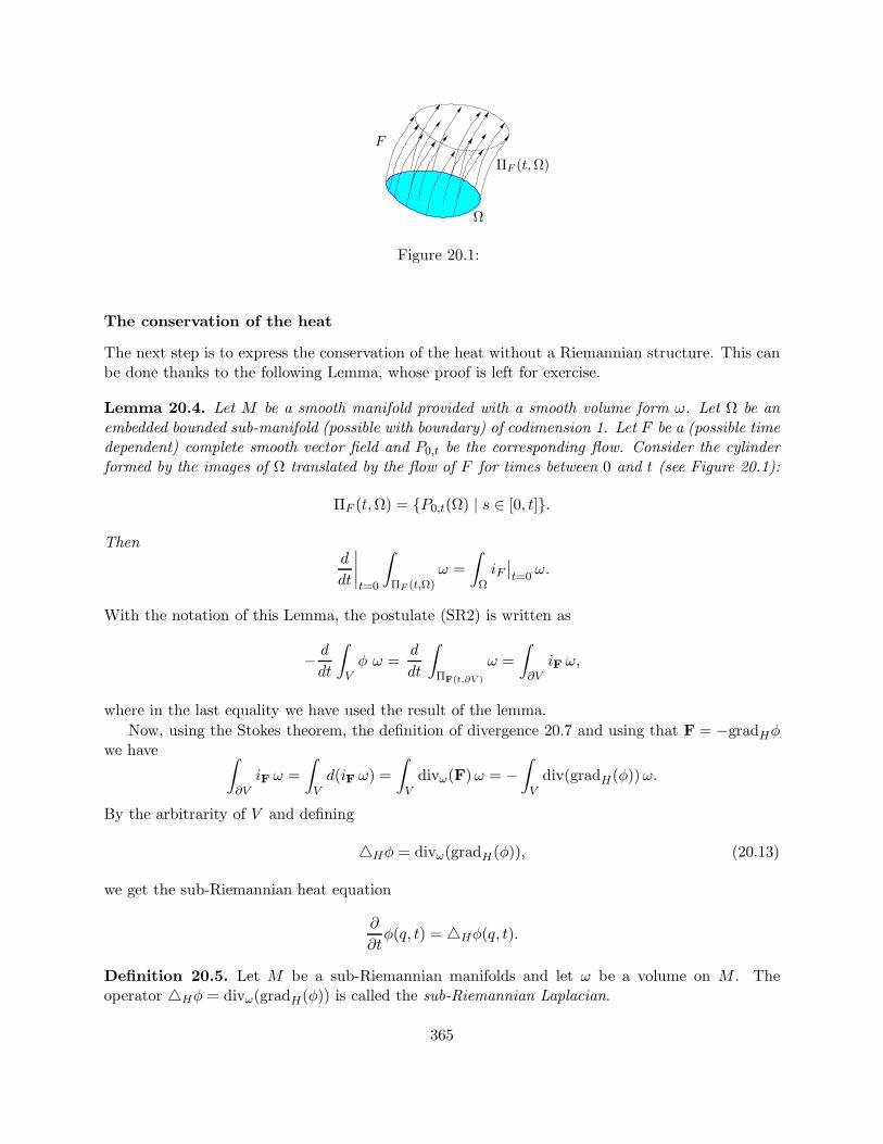
Ω
ΠF (t,Ω)
F
Figure 20.1:
The conservation of the heat
The next step is to express the conservation of the heat without a Riemannian structure. This canbe done thanks to the following Lemma, whose proof is left for exercise.
Lemma 20.4. Let M be a smooth manifold provided with a smooth volume form ω. Let Ω be anembedded bounded sub-manifold (possible with boundary) of codimension 1. Let F be a (possible timedependent) complete smooth vector field and P0,t be the corresponding flow. Consider the cylinderformed by the images of Ω translated by the flow of F for times between 0 and t (see Figure 20.1):
ΠF (t,Ω) = P0,t(Ω) | s ∈ [0, t].
Thend
dt
∣∣∣∣t=0
∫
ΠF (t,Ω)ω =
∫
ΩiF∣∣t=0
ω.
With the notation of this Lemma, the postulate (SR2) is written as
− d
dt
∫
Vφ ω =
d
dt
∫
ΠF(t,∂V )
ω =
∫
∂ViF ω,
where in the last equality we have used the result of the lemma.
Now, using the Stokes theorem, the definition of divergence 20.7 and using that F = −gradHφwe have ∫
∂ViF ω =
∫
Vd(iF ω) =
∫
Vdivω(F)ω = −
∫
Vdiv(gradH(φ))ω.
By the arbitrarity of V and defining
Hφ = divω(gradH(φ)), (20.13)
we get the sub-Riemannian heat equation
∂
∂tφ(q, t) = Hφ(q, t).
Definition 20.5. Let M be a sub-Riemannian manifolds and let ω be a volume on M . Theoperator Hφ = divω(gradH(φ)) is called the sub-Riemannian Laplacian.
365
When it is possible to construct a volume from the sub-Riemannian structure, then the cor-responding sub-Riemannian Laplacian is called the intrinsic sub-Laplacian. The construction of acanonical volume form in an equiregular sub-Riemannian manifold has been done in Chapter 19and it is called the Popp volume. Here let us just remark that in the case of left-invariant structureson Lie groups, the Popp volume is proportional to the left Haar volume (that is a canonical volumethat can be built on any Lie group).
Remark 20.6. Notice that the expression of the sub-Riemannian Laplacian does not change if wemultiply the volume by a (non zero) constant.
20.1.3 Few properties of the sub-Riemannian Laplacian: the Hormander theo-rem and the existence of the heat kernel
The same computation of the Riemannian case provides the following expression for the sub-Riemannian Laplacian,
H(φ) =m∑
i=1
(X2i φ+ divω(Xi)Xi(φ)
)where X1, . . . Xm, is a generating family. (20.14)
In the Riemannian case, the operator ∆H is elliptic, i.e., in coordinates it has the expression
H =
n∑
i,j=0
aij(x)∂i∂j + first order terms,
where the matrix (aij) is symmetric and positive definite for every x.
In the sub-Riemannian (and not-Riemannian) case, ∆H it is not elliptic since the matrix (aij)can have several zero eigenvalues. However, a theorem of Hormander says that thanks to the Liebracket generating condition ∆H is hypoelliptic. More precisely we have the following.
Theorem 20.7 (Hormander). Let Y0, Y1 . . . Yk be a set of Lie bracket generating vector fields on asmooth manifold M . Then the operator L = Y0 +
∑ki=1 Y
2i is hypoellptic which means that if ϕ is
a distribution defined on an open set Ω ⊂M , such that Lϕ is C∞, then ϕ is C∞ in Ω.
Notice that:
• Elliptic operators with C∞ coefficients are hypoelliptic.
• The heat operator−∂t, where is the Laplace-Beltrami operator on a Riemannian manifoldM is not elliptic (since the matrix of coefficients of the second order derivatives in R ×Mhas one zero eigenvalue), but it is hypoelliptic since if X1 . . . Xn is an orthonormal frame,then Y0 =
∑ni=1 divω(Xi)Xi(φ) − ∂t and Y1 := X1, . . .Yn := Xn are Lie Bracket generating
in R×M .
• The sub-Riemannian heat operatorH−∂t is hypoelliptic since if X1 . . . Xm is a generatingfamily, then Y0 =
∑mi=1 divω(Xi)Xi(φ) − ∂t and Y1 := X1, . . .Ym := Xm are Lie Bracket
generating in R × M . (The hypoellipticity of H alone is consequence of the fact thatX1 . . . Xm are Lie Bracket generating on M .)
366
One of the most important consequences of the Hormander theorem is that the heat evolutionsmooths out immediately every initial condition. Indeed if one can guarantee that a solution of(∆H − ∂t)ϕ = 0 exists in distributional sense in an open set Ω of R ×M , then, being 0 ∈ C∞, itfollows that ϕ is C∞ in Ω.
A standard result for the existence of a solution in L2(M,ω) is given by the following theorem.See for instance [30, 37].
Theorem 20.8 (Stone). Let M be a smooth manifold and ω a volume on M . If ∆ is a non negativeand essentially self-adjoint operator on L2(M,ω), then, there exists a unique solution to the Cauchyproblem
(∂t −)φ = 0φ(q, 0) = φ0(q) ∈ L2(M,ω),
(20.15)
on [0,∞[×M . Moreover for each t ∈ [0,∞[ this solution belongs to L2(M,ω).
It is immediate to prove that ∆H is non-negative and symmetric on L2(M,ω). If in additionone can prove that ∆H is essentially self-adjoint, then thanks to the Hormander theorem, one hasthat the solution of (20.15) is indeed C∞ in ]0,∞[×M .
The discussion of the theory of self-adjoint operators is out of the purpose of this book. How-ever the essential self-adjointness of ∆H is guaranteed by the completeness of the sub-Riemannianmanifold as metric space.
Theorem 20.9 (Strichartz, [33, 34]). Consider a sub-Riemannian manifold that is complete asmetric space. Let ω be a volume on M . Then ∆H defined on C∞c (M) is essentially self-adjoint inL2(M,ω).
Typical cases in which the sub-Riemannian manifold is complete are let-invariant structure onLie groups, sub-Riemannian manifold obtained as restriction of complete Riemannian manifolds,sub-Riemannian structures defined in R
n having as generating family a set of sub-linear vectorfields.
When the manifold is not complete as metric space (as for instance the standard Euclideanstructure on the unitary disc in R
2), then to study the Cauchy problem (20.15) one need to specifymore the problem (e.g., boundary conditions).
As a consequence of the hypoellipticity of H − ∂t, of Therem 20.8 and of Theorem 20.9, wehave
Corollary 20.10. Consider a sub-Riemannian manifold that is complete as metric space. Let ωbe a volume on M . There exists a unique solution to the Cauchy problem (20.15), that is C∞ in]0,∞[×M .
Indeed under the hypothesis of competeness of the manifold one can also guarantee the existenceof a convolution kernel .
Theorem 20.11 (Strichartz, [33, 34]). Consider a sub-Riemannian manifold that is complete asmetric space. Let ω be a volume on M . Then the unique solution to the Cauchy problem(20.15) on[0,∞[×M can be written as
φ(q, t) =
∫
Mφ0(q)Kt(q, q)ω(q)
where Kt(q, q) is a positive function defined on ]0,∞[×M ×M which is smooth, symmetric for theexchange of q and q and such that for every fixed t, q, we have Kt(q, ·) ∈ L2(M,ω).
367
20.1.4 The heat equation in the non-Lie-bracket generating case
If the sub-Riemannian structure is not Lie-bracket generated, i.e., when we are dealing with aproto-sub-Riemannian structure in the sense of Section 3.1.5 then the operator H can be definedas above, but in general it is not hypoelliptic and the heat evolution does not smooth the initialcondition.
Consider for example the the proto-sub-Riemannian structure on R3 for which an orthonormal
frame is given by ∂x, ∂y. Take as volume the Lebesgue volume on R3. Then H = ∂2x+∂2y on R3.
This operator is not obtained from Lie-bracket generating vector fields. Consider the correspondingheat operator ∆H − ∂t on ]0,∞[×R3. Since the z direction is not appearing in this operator, anydiscontinuity in the z variable is not smoothed by the evolution. For instance if ψ(x, y, t) is asolution of the heat equation ∆H−∂t = 0 on [0,∞[×R2, then ψ(x, y, t)θ(z) is a solution of the heatequation in ]0,∞[×R3, where θ is the Heaviside function.
20.2 The heat-kernel on the Heisenberg group
In this section we construct the heat kernel on the Heisenberg sub-Riemannian structure. To thispurpose it is convenient to see this structure as a left-invariant structure on a matrix representationof the Heisenberg group. This point of view is useful to build in a canonical way a volume form andhence the sub-Riemannian Laplacian. Moreover this point of view permits to look for a simplifiedversion of the heat kernel using the group law.
20.2.1 The Heisenberg group as a group of matrices
The Heisenberg group H2 can be seen as the 3-dimensional group of matrices
H2 =
1 x z + 12xy
0 1 y0 0 1
| x, y, z ∈ R
endowed with the standard matrix product. H2 is indeed R3, endowed with the group law
(x1, y1, z1) · (x2, y2, z2) =(x1 + x2, y1 + y2, z1 + z2 +
1
2(x1y2 − x2y1)
).
This group law comes from the matrix product after making the identification
(x, y, z) ∼
1 x z + 12xy
0 1 y0 0 1
.
The identity of the group is the element (0, 0, 0) and the inverse element is given by the formula
(x, y, z)−1 = (−x,−y,−z)
A basis of its Lie algebra of H2 is p1, p2, k where
p1 =
0 1 00 0 00 0 0
p2 =
0 0 00 0 10 0 0
k =
0 0 10 0 00 0 0
. (20.16)
368
They satisfy the following commutation rules: [p1, p2] = k, [p1, k] = [p2, k] = 0, hence H2 is a 2-stepnilpotent group.
Remark 20.12. Notice that if one write an element of the algebra as xp1 + yp2 + zk, one has that
exp(xp1 + yp2 + zk) =
1 x z + 12xy
0 1 y0 0 1
. (20.17)
Hence the coordinates (x, y, z) are the coordinates on the Lie algebra related to the basis p1, p2, k,transported on the group via the exponential map. They are called coordinates of the “first type”.As we will see later, coordinate x, y, w = z + 1
2xy, that are more adapted to the group, are alsouseful.
The standard sub-Riemannian structure on H2 is the one having as generating family:
X1(g) = gp1, X2(g) = gp2.
With a straightforward computation one get the following coordinate expression for the generatingfamily:
X1 = ∂x −y
2∂z, X2 = ∂y +
x
2∂z,
that we already met several times in the previous chapters.
Let Lg (reap. Rg) be the left (resp. right) multiplication on H2:
Lg : H2 ∋ h 7→ gh (resp. Rg : H2 ∋ h 7→ hg).
Exercise Prove that, up to a multiplicative constant, there exist one and only one 3-form dhLon H2 which is left-invariant, i.e. such that L∗
gdh = dh and that in coordinates coincide (up toa constant) with the Lebesgue measure dx ∧ dy ∧ dz. Prove the same for a right-invariant 3-formdhR,
The left- and right-invariant forms built in the exercise above are called the left and right Haarmeasures. Since they coincide up to a constant the Heisenberg group is said to be “unimodular”.In the following we normalise the left and right Haar measures on the sub-Riemannian structurein such a way that
dhL(X1,X2, [X1,X2]) = dhR(X1,X2, [X1,X2]) = 1. (20.18)
The 3-form obtained in this way coincide with the Lebesgue measure and in the following we callit simply the “Haar measure”
dh = dx ∧ dy ∧ dz.Exercise Prove that the two conditions (20.18) are invariant by change of the orthonormal frame.
20.2.2 The heat equation on the Heisenberg group
Given a volume form ω on R3, the sub-Riemannian Laplacian for the Heisenberg sub-Riemannian
structure is given by the formula,
H(φ) =(X2
1 +X22 + divω(X1)X1 + divω(X2)X2
)φ. (20.19)
369
If we take as volume the Haar volume dh, and using the fact that X1 and X2 are divergence freewith respect to dh, we get for the sub-Riemannian Laplacian
H(φ) = (X1)2 + (X2)
2 = (∂x −y
2∂z)
2 + (∂y +x
2∂z)
2. (20.20)
The heat equation on the Heisenberg group is then
∂tφ(x, y, z, t) = H(φ) =((∂x −
y
2∂z)
2 + (∂y +x
2∂z)
2)φ(x, y, z, t)
For this equation, we are looking for the heat kernel, namely a function Kt(q, q) such that thesolution to the Cauchy problem
(H − ∂t)φ = 0φ(q, 0) = φ0(q) ∈ L2(R3, dh)
(20.21)
can be expressed as
φ(q, t) =
∫
R3
Kt(q, q)φ0(q)dh(q). (20.22)
The existence of a heat kernel that is smooth, positive and symmetric is guaranteed by Theorem20.9 since the Heisenberg group (as sub-Riemannian structure) is complete.
The construction of the explicit expression of the heat kernel on the Heisenberg group was animportant achievement of the end of the seventies [16, 21]. Here we propose an elementary directmethod. divided in the following step:
STEP 1. We look for a special form for Kt(q, q) using the group law.
STEP 2. We make a change of variables in such a way that the coefficients of the heat equation dependonly on one variable instead than two.
STEP 3. By using the Fourier transform in two variables, we transform the heat equation (that wasa PDE in 3 variable plus the time) in a heat equation with an harmonic potential in onevariable plus the time.
STEP 4. We find the kernel for the heat equation with the harmonic potential, thanks to the Mehlerformula for Hermite polynomials.
STEP 5. We come back to the original variables.
Let us make these steps one by one.
STEP 1 Due to invariance under the group law, we have that for Kt(q, q) = Kt(p ·q, p · q) for everyp ∈ H2. Taking p = q−1 we have that Kt(q, q) = Kt(0, q
−1q) hence we can write
Kt(q, q) = pt(q−1 · q) = pt(x− x, y − y, z − z) = pt(x− x, y − y, z − z),
for a suitable function pt(·) called the fundamental solution. In the last equality we have used thesymmetry of the heat kernel.
370
STEP 2 Let us make the change the variable z → w, where
w = z +1
2xy
(cf. Remark 20.12). In the new variables we have that the Haar measure is dh = dx ∧ dy ∧ dw.The generating family and the sub-Riemannian Laplacian become
X1 =
100
= ∂x (20.23)
X2 =
01x
= ∂y + x∂w (20.24)
H(φ) = (X1)2 + (X2)
2 = ∂2x + (∂y + x∂w)2. (20.25)
The new coordinates are very useful since now the coefficients of the different terms in H dependonly on one variable. We are then looking for the solution to the Cauchy problem
∂tϕ(x, y, w, t) = H(ϕ(x, y, w, t)) =
(∂2x + (∂y + x∂w)
2)ϕ(x, y, w, t)
ϕ(x, y, w, 0) = ϕ0(x, y, w) ∈ L2(R3, dh)(20.26)
where ϕ(x, y, w, t) = φ(x, y, w − 12xy).
STEP 3 By making the Fourier transform in y and w, we have ∂y → iµ, ∂w → iν and the Cauchyproblem become
∂tϕ(x, µ, ν, t) =(∂2x − (µ + νx)2
)ϕ(x, µ, ν, t)
ϕ(x, µ, ν, 0) = ϕ0(x, µ, ν).(20.27)
By making the change of variable x→ θ, where µ+ νx = νθ, i.e., θ = x+ µν we get:
∂tϕ
µ,ν(θ, t) =(∂2θ − ν2θ2
)ϕµ,ν(θ, t)
ϕµ,ν(θ, 0) = ϕµ,ν0 (θ),(20.28)
where we set ϕµ,ν(θ, t) := ϕ(θ − µν , µ, ν, t), and ϕ
µ,ν0 (θ) = ϕ0(θ − µ
ν , µ, ν).
STEP 4. We have the following
Theorem 20.13. The solution of the Cauchy problem for the evolution of the heat in an harmonicpotential, i.e.
∂tψ(θ, t) =(∂2θ − ν2θ2
)ψ(θ, t)
ψ(θ, 0) = ψ0(θ) ∈ L2(R, dθ)(20.29)
can be written in the form of a convolution kernel
ψ(θ, t) =
∫
R
Qνt (θ, θ)ψ0(θ)dθ.
where
Qνt (θ, θ) :=
√ν
2π sinh(2νt)exp
(−1
2
ν cosh(2νt)
sinh(2νt)(θ2 + θ2) +
νθθ
sinh(2νt)
). (20.30)
371
Remark 20.14. In the case ν = 0 we interpret Q0t (θ, θ) as
limν→0Qνt (θ, θ) =
1√4πt
exp[−(θ − θ)24t
]. (20.31)
Proof. For ν = 0, equation (20.29) is the standard heat equation on R and the heat kernel is givenby formula (20.31). See for instance [?]. In the following we assume ν 6= 0. The eigenvalues andthe eigenfunctions of the operator ∂2θ − ν2θ2 on R are (see Appendix ??)
Ej = −2ν(j + 1/2)
ϕνj (θ) =1√2jj!
(νπ
) 14exp(−νθ
2
2)Hj(
√ν θ) (20.32)
where Hj are the Hermite polynomials
Hj(θ) = (−1)j exp(θ2) dj
dθjexp(−θ2).
Being ϕνj j∈N an orthonormal frame of L2(R), we can write
ψ(θ, t) =∑
j
Cj(t)ϕνj (θ).
Using equation (20.29), we obtain that
Cj(t) = Cj(0) exp(tEj)
where Cj(0) =∫Rϕνj (θ)ψ0(θ) dθ. Hence
ψ(θ, t) =
∫
R
Qνt (θ, θ)ψ0(θ) dθ
whereQνt (θ, θ) =
∑
j
ϕνj (θ)ϕνj (θ) exp(tEj).
After some algebraic manipulations and using the Mehler formula for Hermite polynomials
∑
j
Hj(θ)Hj(θ)
2jj!(w)j = (1− w2)−
12 exp
(2θθw − (θ2 + θ2)w2
1− w2
), ∀ w ∈ R
with θ → √νθ, θ → √νθ, w → exp(−2νt), one get formula (20.30).
Using Theorem 20.13 we can write the solution to 20.29 as
ϕµ,ν(θ, t) =
∫
R
Qνt (θ, θ)ϕµ,ν0 (θ)dθ.
STEP 5 We now come back to the original variables step by step. We have
ϕ(x, µ, ν, t) = ϕµ,ν(x+µ
ν, t) =
∫
R
Qνt (x+µ
ν, θ)ϕµ,ν0 (θ)dθ =
∫
R
Qνt (x+µ
ν, x+
µ
ν)ϕ0(x, µ, ν)dx.
372
In the last equality we made the change of integration variable θ → x with θ = x+ µν and we used
the fact that ϕµ,ν0 (x+ µν ) = ϕ0(x, µ, ν).
Now, using the fact that ϕ0(x, µ, ν) is the Fourier transform of the initial condition, i.e.
ϕ0(x, µ, ν) =
∫
R
∫
R
ϕ0(x, y, w)e−iµye−iνwdy dw,
and making the inverse Fourier transform we get
ϕ(x, y, w, t) =1
(2π)2
∫
R
∫
R
ϕ(x, µ, ν, t)eiµyeiνwdµ dν
=
∫
R3
(1
(2π)2
∫
R
∫
R
Qνt (x+µ
ν, x+
µ
ν)eiµ(y−y)eiν(w−w)dµ dν
)ϕ0(x, y, w)dx dy dw.
Coming back to the variable x, y, z, we have
φ(x, y, z, t) = ϕ(x, y, z +1
2xy) =
∫
R3
Kt(x, y, z, x, y, z)φ0(x, y, z)dx dy dz.
where
Kt(x, y, z, x, y, z) =1
(2π)2
∫
R
∫
R
Qνt (x+µ
ν, x+
µ
ν)eiµ(y−y)eiν(z−z+
12(xy−xy))dµ dν.
Setting x, y, z to zero and after some algebraic manipulations we get for the fundamental solution
pt(x, y, z) =1
(2πt)2
∫
R
2τ
sinh(2τ)exp
(− τ(x
2 + y2)
2t tanh(2τ)
)cos(2
zτ
t)dτ. (20.33)
The integral representation (20.33) can be computed explicitly on the origin and on the z axis.Indeed we have
Kt(0, 0, 0; 0, 0, 0) = pt(0, 0, 0) =1
16t2(20.34)
Kt(0, 0, 0; 0, 0, z) = pt(0, 0, z) =1
8t2(1 + cosh
(πzt
)) =1
4t2exp
(−d
2(0, 0, 0; 0, 0, z)
4t
)f(t) (20.35)
In the last equality we have used the fact that for the Heisenberg group d(0, 0, 0; 0, 0, z) =√4πz.
Here f(t) is a smooth function of t such that f(0) = 1 (here z 6= 0 is fixed). A more detailedanalysis permits to get for every fixed (x, y, z) such that x2 + y2 6= 0
Kt(0, 0, 0;x, y, z) = pt(x, y, z) =C +O(t)
t3/2exp
(−d
2(0, 0, 0;x, y, z)
4t
). (20.36)
Notice that the asymptotics (20.34), (20.35), (20.36) are deeply different with respect to thosein the Euclidean case. Indeed the heat kernel for the standard heat equation in R
n is given by theformula
Kt(0, 0, 0;x, y, z) =1
(4πt)n/2exp
(−x
2 + y2 + z2
4t
). (20.37)
373
Comparing (20.37) with (20.34), (20.35), (20.36), one has the impression that the heat diffusionon the Heisenberg group at the origin and on the points on the z axis, is similar to the one inan Euclidean space of dimension 4. While on all the other points it is similar to to the one inan Euclidean space of dimension 3. Indeed the difference of asymptotics between the Heisenbergand the Euclidean case at the origin is related to the fact that the Hausdorff dimension of theHeisenberg group is 4, while its topological dimension is 3 (See Chapter ??). While the differenceof asymptotics on the z axis (without the origin) is related to the fact that these are points reacheda one parameter family of optimal geodesics starting from the origin and hence they are at thesame time cut and conjugate points. For more details see [?]. It is interesting to remark that on aRiemannian manifold of dimension n the asymptotics are similar to the Euclidean ones for points
close enough. Indeed for every q close enough to q we have Kt(q, q) =1+O(t)
(4πt)n/2 exp(−d2(q,q)
4t
).
374
Appendix A
Hermite polynomials
375

376
Appendix B
Elliptic functions
377

378
Appendix C
Structural equations for curves inLagrange Grassmannian
379
Index
2D Riemannian problem, 103
abnormal extremals, 246
AC admissible curve, 86admissible curve, 62
bracket-generating, 61
bundle map, 57
Carnot-Caratheodory distance, 71Cartan’s formula, 110
characteristic curve, 99chronological
calculus, 131
exponentialleft, 135right, 133
conjugate point, 164contact
form, 102
sub-Riemannian structrure, 102cotangent
bundle, 56
cotangent bundlecanonical coordinates, 56
cotangent space, 54
critical poinrconstrained, 150
differential form, 55
differential of a map, 50distribution, 62
dual, 101
end-point map, 145differential, 146
energy functional, 80
Euler vector field, 308exponential map, 160
extremalabnormal, 80, 100normal, 80, 97path, 80
flag, 223flow, 47free
sub-Riemannian structure, 68fundamental solution of the Heisenberg group,
370
Gauss’s Theorema Egregium, 33Gauss-Bonnet, 26
global version, 31local version, 27
HamiltonianODE, 96sub-Riemannian, 97system, 96vector field, 93
Heisenberg groupheat kernel, 368
Hessian, 151
indexof a map, 247of a quadratic form, 247
induced bundle, 57integral curve, 46intrinsic sub-Laplacian, 366isoperimetric problem, 105
Jacobi curve, 304reduced, 309
Lagrangemultiplier, 148, 150multipliers rule, 148, 150
380
point, 152
Lie bracket, 51Lie derivative, 109Liouville form, 94
Morseproblem, 152
ODE, 46
nonautonomous, 132
PMP, 79Poisson bracket, 91
pullback, 54pushforward, 50
reduced Jacobi curve, 309
Sr structureflag, 223
sub-Laplacian, 365sub-Riemannian
distance, 71
extremalabnormal, 148normal, 148
geodesic, 116Hamiltonian, 97
isometry, 68length, 65local rank, 67
manifold, 61, 173rank, 67
structure, 61, 173equivalent, 67free, 68
rank-varying, 62regular, 101
symplectic
manifold, 110symplectic structure, 95
symplettomorphism, 110
Table of contents, 8tangent
bundle, 56space, 45
vector, 45tautological form, 94theorem
Caratheodory, 49Chow-Raschevskii, 72existence of minimizers, 78
trivializablevector bundle, 55
unimodular, 369
variations formula, 137vector bundle, 55
canonical projection, 55local trivialization, 55morphism, 57rank, 55section, 57
vector field, 46bracket-generating family, 61complete, 46flow, 47Hamiltonian, 93nonautonomous, 48
381

382
Bibliography
[1] A. A. Agrachev. Exponential mappings for contact sub-Riemannian structures. J. Dynam.Control Systems, 2(3):321–358, 1996.
[2] A. A. Agrachev and R. V. Gamkrelidze. Feedback-invariant optimal control theory and differ-ential geometry. I. Regular extremals. J. Dynam. Control Systems, 3(3):343–389, 1997.
[3] A. A. Agrachev and Y. L. Sachkov. Control theory from the geometric viewpoint, volume 87 ofEncyclopaedia of Mathematical Sciences. Springer-Verlag, Berlin, 2004. Control Theory andOptimization, II.
[4] A. Bellaıche. The tangent space in sub-Riemannian geometry. In Sub-Riemannian geometry,volume 144 of Progr. Math., pages 1–78. Birkhauser, Basel, 1996.
[5] B. Bonnard and M. Chyba. Singular trajectories and their role in control theory, volume 40of Mathematiques & Applications (Berlin) [Mathematics & Applications]. Springer-Verlag,Berlin, 2003.
[6] W. M. Boothby. An introduction to differentiable manifolds and Riemannian geometry, volume120 of Pure and Applied Mathematics. Academic Press, Inc., Orlando, FL, second edition, 1986.
[7] U. Boscain, T. Chambrion, and G. Charlot. Nonisotropic 3-level quantum systems: com-plete solutions for minimum time and minimum energy. Discrete Contin. Dyn. Syst. Ser. B,5(4):957–990 (electronic), 2005.
[8] U. Boscain, G. Charlot, J.-P. Gauthier, S. Guerin, and H.-R. Jauslin. Optimal control inlaser-induced population transfer for two- and three-level quantum systems. J. Math. Phys.,43(5):2107–2132, 2002.
[9] A. Bressan and B. Piccoli. Introduction to the mathematical theory of control, volume 2 ofAIMS Series on Applied Mathematics. American Institute of Mathematical Sciences (AIMS),Springfield, MO, 2007.
[10] A. Bressan and B. Piccoli. Introduction to the mathematical theory of control, volume 2 ofAIMS Series on Applied Mathematics. American Institute of Mathematical Sciences (AIMS),Springfield, MO, 2007.
[11] D. Burago, Y. Burago, and S. Ivanov. A course in metric geometry, volume 33 of GraduateStudies in Mathematics. American Mathematical Society, Providence, RI, 2001.
383
[12] W.-L. Chow. Uber Systeme von linearen partiellen Differentialgleichungen erster Ordnung.Math. Ann., 117:98–105, 1939.
[13] D. Danielli, N. Garofalo, and D. M. Nhieu. Sub-Riemannian calculus on hypersurfaces inCarnot groups. Adv. Math., 215(1):292–378, 2007.
[14] M. P. do Carmo. Riemannian geometry. Mathematics: Theory & Applications. BirkhauserBoston, Inc., Boston, MA, 1992. Translated from the second Portuguese edition by FrancisFlaherty.
[15] G. B. Folland. A fundamental solution for a subelliptic operator. Bull. Amer. Math. Soc.,79:373–376, 1973.
[16] B. Gaveau. Principe de moindre action, propagation de la chaleur et estimees sous elliptiquessur certains groupes nilpotents. Acta Math., 139(1-2):95–153, 1977.
[17] M. Gromov. Carnot-Caratheodory spaces seen from within. In Sub-Riemannian geometry,volume 144 of Progr. Math., pages 79–323. Birkhauser, Basel, 1996.
[18] F. Hirsch and G. Lacombe. Elements of functional analysis, volume 192 of Graduate Texts inMathematics. Springer-Verlag, New York, 1999. Translated from the 1997 French original bySilvio Levy.
[19] M. W. Hirsch. Differential topology. Springer-Verlag, New York-Heidelberg, 1976. GraduateTexts in Mathematics, No. 33.
[20] L. Hormander. Hypoelliptic second order differential equations. Acta Math., 119:147–171,1967.
[21] A. Hulanicki. The distribution of energy in the Brownian motion in the Gaussian field andanalytic-hypoellipticity of certain subelliptic operators on the Heisenberg group. Studia Math.,56(2):165–173, 1976.
[22] F. Jean. Control of Nonholonomic Systems: from Sub-Riemannian Geometry to Motion Plan-ning. Springerbriefs in Mathematics, 2014.
[23] D. Jerison and A. Sanchez-Calle. Subelliptic, second order differential operators. In Complexanalysis, III (College Park, Md., 1985–86), volume 1277 of Lecture Notes in Math., pages46–77. Springer, Berlin, 1987.
[24] J. M. Lee. Introduction to smooth manifolds, volume 218 of Graduate Texts in Mathematics.Springer, New York, second edition, 2013.
[25] R. Montgomery. Abnormal minimizers. SIAM J. Control Optim., 32(6):1605–1620, 1994.
[26] R. Montgomery. Survey of singular geodesics. In Sub-Riemannian geometry, volume 144 ofProgr. Math., pages 325–339. Birkhauser, Basel, 1996.
[27] R. Montgomery. A tour of subriemannian geometries, their geodesics and applications, vol-ume 91 of Mathematical Surveys and Monographs. American Mathematical Society, Provi-dence, RI, 2002.
384
[28] L. S. Pontryagin, V. G. Boltyanskii, R. V. Gamkrelidze, and E. F. Mishchenko. The mathe-matical theory of optimal processes. Translated from the Russian by K. N. Trirogoff; edited byL. W. Neustadt. Interscience Publishers John Wiley & Sons, Inc. New York-London, 1962.
[29] P. Rashevsky. Any two points of a totally nonholonomic space may be connected by anadmissible line. Uch. Zap. Ped Inst. im. Liebknechta, 2:83–84, 1938.
[30] M. Reed and B. Simon. Methods of modern mathematical physics. II. Fourier analysis, self-adjointness. Academic Press [Harcourt Brace Jovanovich Publishers], New York, 1975.
[31] L. Rifford. Sub-Riemannian geometry and Optimal Transport. Springerbriefs in Mathematics,2014.
[32] M. Spivak. A comprehensive introduction to differential geometry. Vol. I. Publish or Perish,Inc., Wilmington, Del., second edition, 1979.
[33] R. S. Strichartz. Sub-Riemannian geometry. J. Differential Geom., 24(2):221–263, 1986.
[34] R. S. Strichartz. Corrections to: “Sub-Riemannian geometry” [J. Differential Geom. 24 (1986),no. 2, 221–263; MR0862049 (88b:53055)]. J. Differential Geom., 30(2):595–596, 1989.
[35] H. J. Sussmann. A cornucopia of four-dimensional abnormal sub-Riemannian minimizers. InSub-Riemannian geometry, volume 144 of Progr. Math., pages 341–364. Birkhauser, Basel,1996.
[36] H. J. Sussmann. Smooth distributions are globally finitely spanned. In Analysis and design ofnonlinear control systems, pages 3–8. Springer, Berlin, 2008.
[37] K. Yosida. Functional analysis. Classics in Mathematics. Springer-Verlag, Berlin, 1995. Reprintof the sixth (1980) edition.
385
Related Documents


![SUB-RIEMANNIAN INTERPOLATION INEQUALITIES - arXiv · 2018-11-30 · SUB-RIEMANNIAN INTERPOLATION INEQUALITIES DAVIDEBARILARI[ANDLUCARIZZI] Abstract. We prove that ideal sub-Riemannian](https://static.cupdf.com/doc/110x72/5f08d5737e708231d423f1fd/sub-riemannian-interpolation-inequalities-arxiv-2018-11-30-sub-riemannian-interpolation.jpg)
